The effects of background music and sound ineconomic decision making: Evidence from a

laboratory experiment

Takemi Fujikawa∗ Yohei Kobayashi†

June 14, 2010

Abstract

This paper experimentally studies the effectsof background music and sound on the pref-erence of the decision makers for rewards inpairwise intertemporal choice tasks and lot-tery choice tasks. The participants took partin the current experiment, involving four treat-ments: (1) the familiar music treatment; (2)the unfamiliar music treatment; (3) the noisetreatment and (4) the no music treatment. Theexperimental results confirm that backgroundnoise affects human performance in decisionmaking under risk and intertemporal decisionmaking, though the results do not indicate thesignificant familiarity effect that is a change ofthe preference in the presence of familiar back-ground music and sound.

Keywords: Allais-type preferences; choice un-der risk; intertemporal choice; the familiarityeffect

1 Introduction

This paper shall experimentally investigatethe relation between the background mu-sic/sound and behavioural preference (i.e.,risk and time preference). For investigat-ing risk preference, this paper elicits decision-making preferences in “choice under risk”,that is, choices under the followings: (1) low-and high-money payoffs (e.g., a choice be-tween a 80% chance of winning 400 yen and

∗Graduate School of Business, Universiti SainsMalaysia. Email: takemi@usm.my.

†Advanced Medical and Dental Institute, UniversitiSains Malaysia. Email: kobapie@gmail.com.

sure 300 yen; a choice between a 80% chanceof winning 4000 yen and sure 3000 yen) and;(2) low- and high-probability payoffs (e.g., achoice between a 80% chance of winning 4000yen and sure 3000 yen; a choice between a20% chance of winning 4000 yen and a 25%chance of winning 3000 yen). On the otherhand, for investigating time preference, thispaper elicits decision-making preferences inintertemporal choice, that is, choices underthe followings: (1) smaller-sooner and smaller-later money payoffs (e.g., a choice between800 yen in 7 days and 880 yen in 30 days;a choice between 700 yen in 7 days and 770yen in 30 days); (2) larger-sooner and larger-later money payoffs (e.g., a choice betweenpresent 5000 yen and 5500 yen in 30 days; achoice between present 5000 yen and 5005 yenin 7 days) and; (3) smaller-sooner and larger-longer money payoffs (e.g., a choice between800 yen in 7 days and 1600 yen in 14 days; achoice between 900 yen in 7 days and 1800 in14 days).

The goal of the present study is to see if fa-miliar and unfamiliar background music andthe white noise sound could affect the be-haviour of the participants, who were askedto make decisions in choice under risk and in-tertemporal choices. The current experimentwas conducted to examine the effects of thebackground music and sound presented to theparticipants during their choice tasks, involv-ing choice under uncertainty and intertempo-ral choice. We used three forms of backgroundmusic and sound (i.e., familiar music, unfamil-iar music and noise). We shall show an exten-sive analysis that was made to answer centralquestions:

1

• Do familiar and unfamiliar backgroundmusic and the white noise sound affecthuman behaviour? Do people changetheir behaviour in the presence of thesebackground music and sound?

• Do people behave exhibiting the increasedor attenuated familiarity effect in the pres-ence of familiar background music? Doesfamiliar background music facilitate ordetract the familiarity effect when peopleengage in decision making?

The organisation of this paper is as follows:Section 2 provides a sketchy description ofchoice under risk and intertemporal choice.Section 3 is devoted to review literature on ef-fects of background music in decision making.In Section 4, we discuss details of the currentexperiment. Section 5 contains a general dis-cussion of the experimental results. Finally, weconclude.

2 Decision Making underRisk and with Intertempo-ral Choice

Economists have been analysing, both theoret-ically and experimentally, “choice under risk”and “intertemporal choice”, as the analysis hasmuch to contribute to the study of economicson rationality. As we shall show below, this pa-per aims to investigate behavioural tendencieswhen people engage in decision making un-der risk and decision making with intertempo-ral choice in the presence of particular back-ground music and sound. Our aim is worth-while, as there should be much discussion onthe effect of background music and sound inour daily decision making (e.g., consumer be-haviour).

On the one hand, much attention has beenfocused on choice under risk and its related“Allais-type” behaviour (Allais, 1953) to ex-emplify deviations from rationality. SinceAllais (1953), there have been a number ofexperiment-based studies, investigating anddemonstrating human behaviour in decisionmaking under risk. One of the most elegantstudies is Kahneman and Tversky (1979). Theyperformed a choice experiment, where theyasked the participants to choose between: (H1)

a 80% chance to win $4 and (L1) a sure gainof $3. The results revealed that many of theparticipants preferred a safe option (L1). Thispreference for a certain payoff is termed as thecertainty effect. In another experiment, Kahne-man and Tversky (1979) asked the participantsto choose between (H2) a 20% chance to win $4and (L2) a 25% chance to win $3. Many of theparticipants preferred (H2). This participants’response is well known as Allais paradox.

On the other hand, preferences in intertem-poral consumption choice under certaintywere in previous studies (e.g. Green, Fristoeand Myerson, 1994; Kirby and Herrenstein,1995; Millar and Navarick, 1984; Solnick, Kan-nenberg, Eckerman and Waller, 1980). Fred-erick and Loewenstein (2002) introduced anexample, where people make choice between:(H3) a sure gain of $101 in 101 days and (L3) asure gain of $100 in 100 days. Many would pre-fer (H3). By decreasing day length, this choiceproblem could be reduced to the choice prob-lem between: (H4) a sure gain of $101 tomor-row and (L4) a sure gain of $100 today. Manypeople would prefer (L4), though it has a lowerobjective value. This behavioural tendency isconsistent with the existing body of literature(McKerchar, Green, Myerson, Pickford, Hilland Stout, 2009) which supports the assertionthat people often choose an option that yieldssooner reward even if it has a lower rewardwhen they make a choice between two rewardsthat differ in delay. Furthermore, Takahashi(2009) demonstrated that subjects often prefersmall-sooner rewards to larger-later rewards.

The aforementioned preference reversalphenomena raise an issue relevant to economictheory. It has been examined and reportedin the tradition of Samuelson’s (Samuelson,1937) model of discounted utility that ex-plains patterns of intertemporal choice, andVon Neumann-Morganstern expected utilitytheory (von Neumann and Morgenstern, 1944)that is a rational choice model in economics.Despite these elegant models, recent and pre-vious studies have provided robust evidencefor a number of “anomalies” and “violations”in intertemporal choice and decision makingunder risk. Frederick and Loewenstein (2002)provide historical origins of the discountedutility model and a convincing discussion onthe model. We note here that the results andfindings are inconsistent, despite many lab-

2

oratory experiments conducted by researchersacross countries.

3 Effects of Background Mu-sic in Decision Making

Music is a most specialised, peculiar hu-man cultural artefact (Andrade, 2004; Bea-ment, 2001) and powerful stimulus to our be-haviour and decision making. One raises aquestion: Can background music affect our be-haviour? There has been much of the con-troversy pertaining to this question (Brayfieldand Crockett, 1955; Jacob, 1968; McGehee andGardner, 1949; Milliman, 1982; Smith, 1947;Uhrbrock, 1961). Hilliard and Tolin (1979)showed that performance in the presence of fa-miliar background music is higher than thatin the presence of unfamiliar music. Corhanand Gounard (1976) premised that vigorousrock music should be associated with betterperformance than easy-listening music. Mu-sic is employed in the background of officesand retail stores to produce certain desiredbehaviours and decision making among em-ployees and/or customers (Milliman, 1982).Bruner (1990) presumed that music affects hu-man beings in various ways as long as theyplay music. Having accepted this presump-tion, previous researchers presented study onbehavioural effects on music in decision mak-ing.

There exists literature pertinent to the ef-fects of music on behaviour and decision mak-ing. Iwanaga and Ito (2002) examined the dis-turbance effect of music on human behaviourin memory tasks. They conducted an ex-periment in which the participants performedchoice tasks in the presence of vocal music,instrumental music, a natural sound and nomusic. We here note that vocal music con-tains more verbal information than instrumen-tal music (Iwanaga and Ito, 2002). Iwanagaand Ito (2002) reported that highest distur-bance was observed under the vocal musiccondition. Sundstrom and Sundstrom (1986)showed that music was effective in maintain-ing both arousal and motivation when the de-cision makers (DMs) were performing easydecision-making tasks. Wolf and Weiner (1972)asked undergraduates to perform a mentalarithmetic task with having them listen to rock

music, and showed that their performance inthe task was neither decreased nor increased.Hence, the effects of background music in de-cision making are inconsistent. The kinds ofbackground music varied: classical (Hilliardand Tolin, 1979), folk (Mowsesian and Heyer,1973), hard rock (Wolf and Weiner, 1972), vo-cal and instrumental (Salame and Baddeley,1982), pop (Iwanaga and Ito, 2002). All ofbackground music in these studies consistedof existing songs (e.g., Mozart, well-knownJapanese pop songs, and so on).

3.1 The Familiarity Effect

It must be noted at the outset that, in previousexperiments, the “familiarity effect” was likelyto be idiosyncratic among individual partic-ipants. The familiarity effect is a change ofpreference in the presence of familiar back-ground music/sound. The previous authorsconducted experiments in which the partici-pants were asked to perform the tasks in thepresence of background music that was chosen— either biasedly or unbiasedly — from thelist of existing songs (e.g., Mozart in Rauscher,Shaw and Ky (1993)).

Thus, the previous experiments were con-ducted with the setting where the songs usedas background music during the experimentshad been accessible (i.e., purchasable anddownloadable). This setting is inadequatesince it leads to all sorts of difficulties with ex-perimental controls, in such a way that impres-sion towards particular songs was idiosyn-cratic among the participants. For example,some of the participants had or had not beenfamiliar with the songs; they had or had nothad prior personal images or preconceivedopinions of the songs. If (some of) the partic-ipants had had prior personal images or pre-conceived opinions of the songs used as back-ground music during the experiment, it wouldmore or less affect their behaviour. Lack ofcontrol with respect to how familiar the songsare may produce results that cannot be inter-preted clearly, as different participants may ac-tivate different mechanisms to the “same” mu-sical stimulus, with resulting differences in be-haviour (Juslin and Vastfjall, 2008). Thus, pre-vious results more or less were biased by thefamiliarity effect.

The familiarity effect is concerned with

3

episodic memory that refers to a processwhereby an emotion is induced in a listener,as the music evokes a memory of a partic-ular event in the listener’s life (Juslin andVastfjall, 2008). Music often evokes memories(Gabrielsson, 2001; Juslin, Laukka, Liljestrom,Vastfjall and Lundqvist, L.-O., submitted; Slo-boda, 1992), and the emotion is associated withthe memories. Such a emotion can be ratherintense (Juslin and Vastfjall, 2008). Baum-gartner (1992) showed that episodic memoriesevoked by music tend to involve not only so-cial relationships (e.g., past or current roman-tic partners) but private relationships (e.g., thedeath of grandfather). Episodic memory canbe one of the most frequent and subjectivelyimportant sources of emotion in music (Juslinand Liljestrom, in press; Sloboda and O’Neill,2001). Thus, the familiarity effect and its re-lated effect of the episodic memory cannot beneglected.

In the current experiment, the song wasused which had not been available to the pub-lic before the experiment. The coauthor ofthe current paper, who is a composer of mu-sic, developed and composed the song usedas background music for the current experi-ment that was neither downloadable nor pur-chasable. Thus, the current experiment wascarried out with the setting, where none of theparticipants had had an opportunity in listen-ing to and knowing the song before the ex-periment. This setting conforms to the behav-ior of the DMs, who have no personal imagesand/or preconceived opinions of the song.

4 Experiment

The current experiment was conducted atthe Kyoto Experimental Economics Laboratory(KEEL) in Japan. On arrival at the KEEL,each participant was assigned a workstationthat displayed an experimental screen, anddistributed a written instruction that was readaloud. In the instructions, the participantswere told that they could have a right to leavethe laboratory before the experiment started,if they did not wish to participate in the ex-periment. The participants were also told thatthey were given an opportunity to ask ques-tions individually before and during the ex-periment. At the conclusion of the experiment,

they were paid individually and privately ac-cording to their response to choice problems,the detailed procedures of which shall be de-scribed below. The participants received noinitial (showing up) fee. Decision task comple-tion took no longer 90 minutes, and an averagepayoff was 3735 yen (about 40 US dollars at thetime of the experiment) per participant.

4.1 Participants

The participants in the current experimentwere 42 undergraduates from various facultiesat Kyoto Sangyo University, of whom were 6women and 36 men. These participants hada mean age of 20.73 years (SD = 2.8, range=18 − 34 years).

4.2 Apparatus

The experiment included four treatments:

• Treatment 1 in which the participantsmade decisions in the presence of familiarbackground music;

• Treatment 2 in which the participantsmade decisions in the presence of unfamil-iar background music;

• Treatment 3 in which the participantsmade decisions in the presence of noise(white noise);

• Treatment 4 in which the participantsmade decisions without the presence ofany background music/sound.

The background music/sound was playedin each treatment through personal head-phones that were connected with each work-station. As the order of the four treatmentswas randomised, each participant took part inthe four treatments in a different order. For ex-ample, the order of the treatments performedby some participants was Treatment 2, 1, 3 and4; while the order by the other participantswas Treatment 3, 4, 1 and 2. She/he startedwith the first treatment and participated inthe second treatment. On completion of thefirst treatment, she/he was advised by theautomatically-generated message on the com-puter screen that the first treatment had beencompleted, and a 10-minutes break was givenbefore starting the second treatment. During

4

the 10-minutes break, she/he participated in aquestionnaire shown on the computer screenand used a mouse to respond to a set of ques-tions. During the break, she/he was allowedto remove the headphone.

In each treatment, each participant wasasked to respond to 30 random samples ofpairwise choice problems taken by a computerprogramme from 120 choice problems, consist-ing of the following three types:

• Type A: Choice under risk (i.e., a choicebetween a p1 chance of winning x1 yen to-day and a p2 chance of winning x2 yen to-day (p1, p2 ∈ (0, 1], p1x1 > p2x2);

• Type B: Intertemporal choice (i.e., a choicebetween sure y1 yen in t1 days and sure y2yen in t2 days (y1 > y2 > 0 and t1 > t2 ≥0);

• Type C: Self-evident choice (i.e., a choicebetween a q1 chance of winning z1 yen to-day and a q2 chance of winning z2 yen to-day (q1, q2 ∈ [0, 1), q1 ≤ q2, 0 < z1 ≤ z2); achoice between sure z3 yen today and surez4 yen today (z3 > z4 > 0))

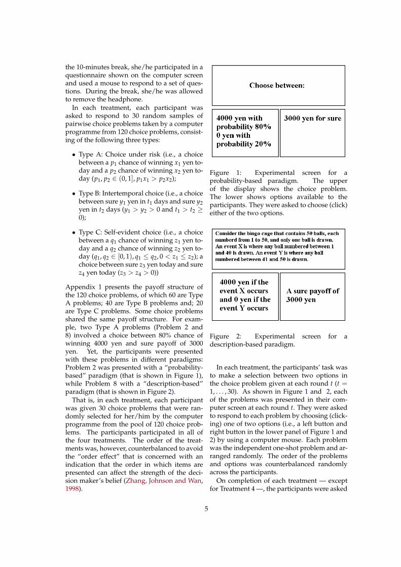
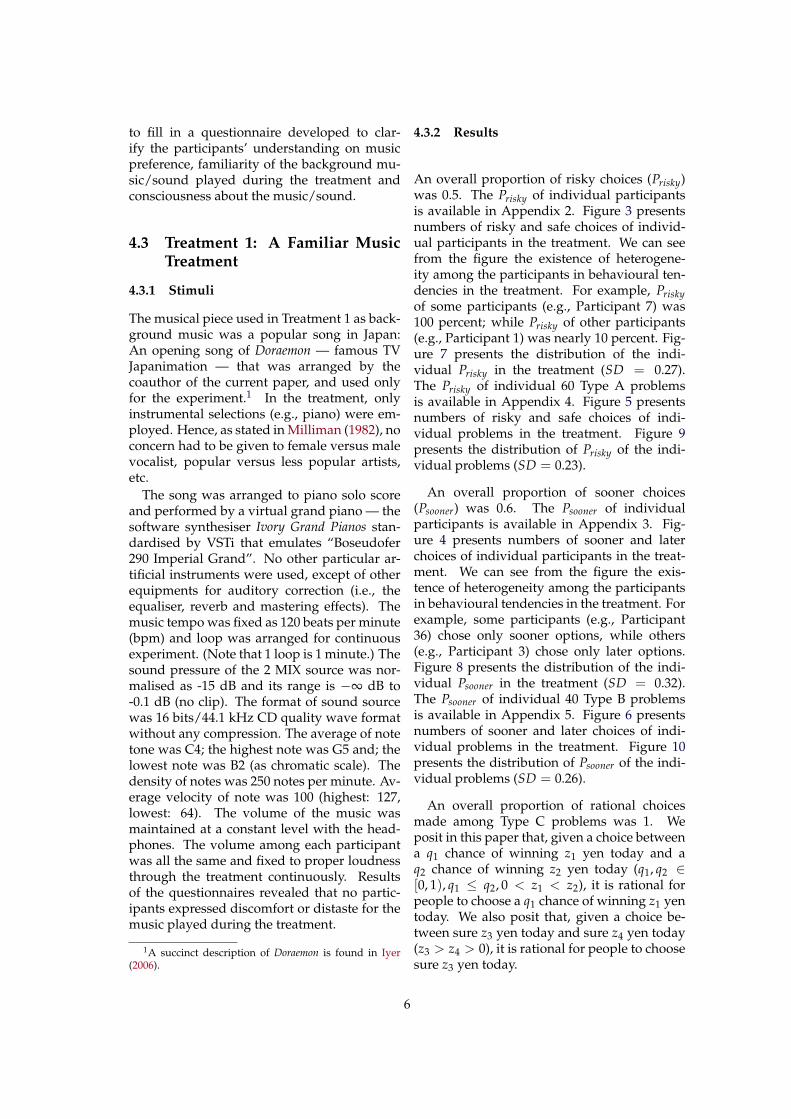
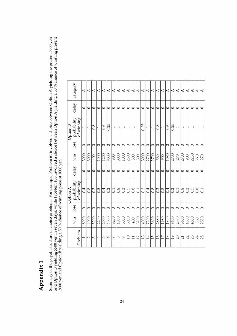
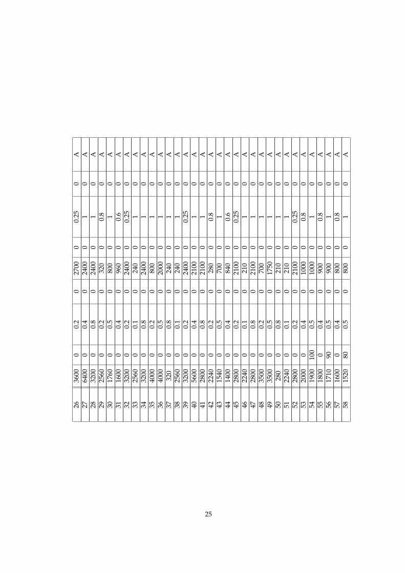
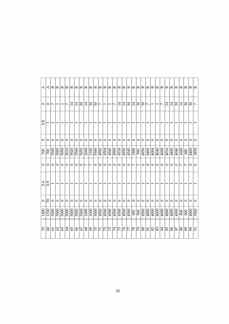
Appendix 1 presents the payoff structure ofthe 120 choice problems, of which 60 are TypeA problems; 40 are Type B problems and; 20are Type C problems. Some choice problemsshared the same payoff structure. For exam-ple, two Type A problems (Problem 2 and8) involved a choice between 80% chance ofwinning 4000 yen and sure payoff of 3000yen. Yet, the participants were presentedwith these problems in different paradigms:Problem 2 was presented with a “probability-based” paradigm (that is shown in Figure 1),while Problem 8 with a “description-based”paradigm (that is shown in Figure 2).

That is, in each treatment, each participantwas given 30 choice problems that were ran-domly selected for her/him by the computerprogramme from the pool of 120 choice prob-lems. The participants participated in all ofthe four treatments. The order of the treat-ments was, however, counterbalanced to avoidthe “order effect” that is concerned with anindication that the order in which items arepresented can affect the strength of the deci-sion maker’s belief (Zhang, Johnson and Wan,1998).

Figure 1: Experimental screen for aprobability-based paradigm. The upperof the display shows the choice problem.The lower shows options available to theparticipants. They were asked to choose (click)either of the two options.

Figure 2: Experimental screen for adescription-based paradigm.

In each treatment, the participants’ task wasto make a selection between two options inthe choice problem given at each round t (t =1, . . . , 30). As shown in Figure 1 and 2, eachof the problems was presented in their com-puter screen at each round t. They were askedto respond to each problem by choosing (click-ing) one of two options (i.e., a left button andright button in the lower panel of Figure 1 and2) by using a computer mouse. Each problemwas the independent one-shot problem and ar-ranged randomly. The order of the problemsand options was counterbalanced randomlyacross the participants.

On completion of each treatment — exceptfor Treatment 4 —, the participants were asked

5

to fill in a questionnaire developed to clar-ify the participants’ understanding on musicpreference, familiarity of the background mu-sic/sound played during the treatment andconsciousness about the music/sound.

4.3 Treatment 1: A Familiar MusicTreatment

4.3.1 Stimuli

The musical piece used in Treatment 1 as back-ground music was a popular song in Japan:An opening song of Doraemon — famous TVJapanimation — that was arranged by thecoauthor of the current paper, and used onlyfor the experiment.1 In the treatment, onlyinstrumental selections (e.g., piano) were em-ployed. Hence, as stated in Milliman (1982), noconcern had to be given to female versus malevocalist, popular versus less popular artists,etc.

The song was arranged to piano solo scoreand performed by a virtual grand piano — thesoftware synthesiser Ivory Grand Pianos stan-dardised by VSTi that emulates “Boseudofer290 Imperial Grand”. No other particular ar-tificial instruments were used, except of otherequipments for auditory correction (i.e., theequaliser, reverb and mastering effects). Themusic tempo was fixed as 120 beats per minute(bpm) and loop was arranged for continuousexperiment. (Note that 1 loop is 1 minute.) Thesound pressure of the 2 MIX source was nor-malised as -15 dB and its range is −∞ dB to-0.1 dB (no clip). The format of sound sourcewas 16 bits/44.1 kHz CD quality wave formatwithout any compression. The average of notetone was C4; the highest note was G5 and; thelowest note was B2 (as chromatic scale). Thedensity of notes was 250 notes per minute. Av-erage velocity of note was 100 (highest: 127,lowest: 64). The volume of the music wasmaintained at a constant level with the head-phones. The volume among each participantwas all the same and fixed to proper loudnessthrough the treatment continuously. Resultsof the questionnaires revealed that no partic-ipants expressed discomfort or distaste for themusic played during the treatment.

1A succinct description of Doraemon is found in Iyer(2006).

4.3.2 Results

An overall proportion of risky choices (Prisky)was 0.5. The Prisky of individual participantsis available in Appendix 2. Figure 3 presentsnumbers of risky and safe choices of individ-ual participants in the treatment. We can seefrom the figure the existence of heterogene-ity among the participants in behavioural ten-dencies in the treatment. For example, Priskyof some participants (e.g., Participant 7) was100 percent; while Prisky of other participants(e.g., Participant 1) was nearly 10 percent. Fig-ure 7 presents the distribution of the indi-vidual Prisky in the treatment (SD = 0.27).The Prisky of individual 60 Type A problemsis available in Appendix 4. Figure 5 presentsnumbers of risky and safe choices of indi-vidual problems in the treatment. Figure 9presents the distribution of Prisky of the indi-vidual problems (SD = 0.23).

An overall proportion of sooner choices(Psooner) was 0.6. The Psooner of individualparticipants is available in Appendix 3. Fig-ure 4 presents numbers of sooner and laterchoices of individual participants in the treat-ment. We can see from the figure the exis-tence of heterogeneity among the participantsin behavioural tendencies in the treatment. Forexample, some participants (e.g., Participant36) chose only sooner options, while others(e.g., Participant 3) chose only later options.Figure 8 presents the distribution of the indi-vidual Psooner in the treatment (SD = 0.32).The Psooner of individual 40 Type B problemsis available in Appendix 5. Figure 6 presentsnumbers of sooner and later choices of indi-vidual problems in the treatment. Figure 10presents the distribution of Psooner of the indi-vidual problems (SD = 0.26).

An overall proportion of rational choicesmade among Type C problems was 1. Weposit in this paper that, given a choice betweena q1 chance of winning z1 yen today and aq2 chance of winning z2 yen today (q1, q2 ∈[0, 1), q1 ≤ q2, 0 < z1 < z2), it is rational forpeople to choose a q1 chance of winning z1 yentoday. We also posit that, given a choice be-tween sure z3 yen today and sure z4 yen today(z3 > z4 > 0), it is rational for people to choosesure z3 yen today.

6

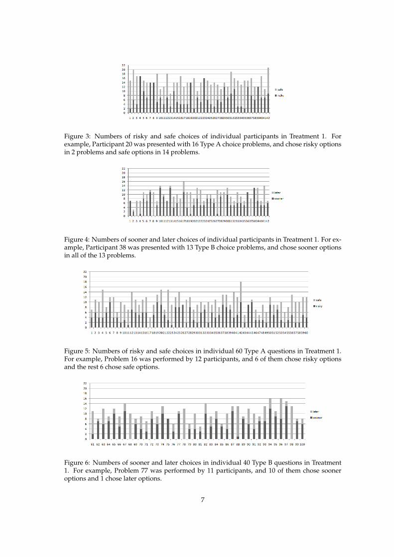
Figure 3: Numbers of risky and safe choices of individual participants in Treatment 1. Forexample, Participant 20 was presented with 16 Type A choice problems, and chose risky optionsin 2 problems and safe options in 14 problems.

Figure 4: Numbers of sooner and later choices of individual participants in Treatment 1. For ex-ample, Participant 38 was presented with 13 Type B choice problems, and chose sooner optionsin all of the 13 problems.

Figure 5: Numbers of risky and safe choices in individual 60 Type A questions in Treatment 1.For example, Problem 16 was performed by 12 participants, and 6 of them chose risky optionsand the rest 6 chose safe options.

Figure 6: Numbers of sooner and later choices in individual 40 Type B questions in Treatment1. For example, Problem 77 was performed by 11 participants, and 10 of them chose sooneroptions and 1 chose later options.

7

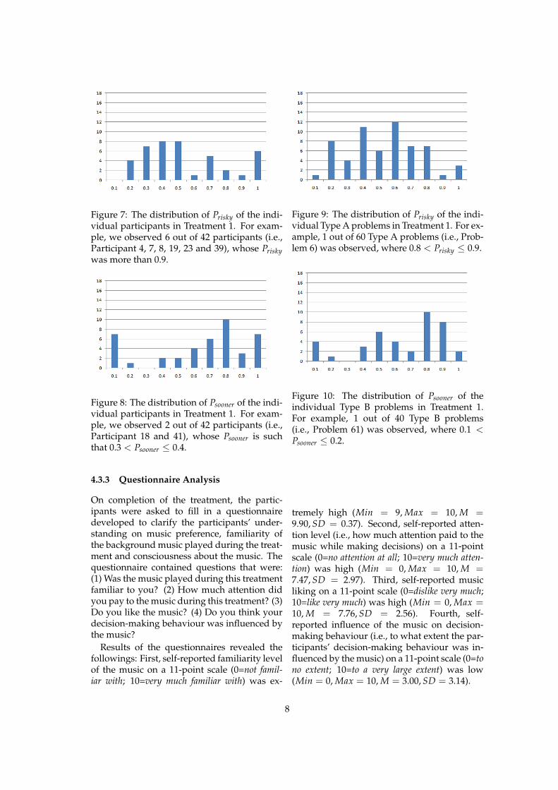
Figure 7: The distribution of Prisky of the indi-vidual participants in Treatment 1. For exam-ple, we observed 6 out of 42 participants (i.e.,Participant 4, 7, 8, 19, 23 and 39), whose Priskywas more than 0.9.

Figure 8: The distribution of Psooner of the indi-vidual participants in Treatment 1. For exam-ple, we observed 2 out of 42 participants (i.e.,Participant 18 and 41), whose Psooner is suchthat 0.3 < Psooner ≤ 0.4.

4.3.3 Questionnaire Analysis

On completion of the treatment, the partic-ipants were asked to fill in a questionnairedeveloped to clarify the participants’ under-standing on music preference, familiarity ofthe background music played during the treat-ment and consciousness about the music. Thequestionnaire contained questions that were:(1) Was the music played during this treatmentfamiliar to you? (2) How much attention didyou pay to the music during this treatment? (3)Do you like the music? (4) Do you think yourdecision-making behaviour was influenced bythe music?

Results of the questionnaires revealed thefollowings: First, self-reported familiarity levelof the music on a 11-point scale (0=not famil-iar with; 10=very much familiar with) was ex-

Figure 9: The distribution of Prisky of the indi-vidual Type A problems in Treatment 1. For ex-ample, 1 out of 60 Type A problems (i.e., Prob-lem 6) was observed, where 0.8 < Prisky ≤ 0.9.

Figure 10: The distribution of Psooner of theindividual Type B problems in Treatment 1.For example, 1 out of 40 Type B problems(i.e., Problem 61) was observed, where 0.1 <Psooner ≤ 0.2.

tremely high (Min = 9, Max = 10, M =9.90, SD = 0.37). Second, self-reported atten-tion level (i.e., how much attention paid to themusic while making decisions) on a 11-pointscale (0=no attention at all; 10=very much atten-tion) was high (Min = 0, Max = 10, M =7.47, SD = 2.97). Third, self-reported musicliking on a 11-point scale (0=dislike very much;10=like very much) was high (Min = 0, Max =10, M = 7.76, SD = 2.56). Fourth, self-reported influence of the music on decision-making behaviour (i.e., to what extent the par-ticipants’ decision-making behaviour was in-fluenced by the music) on a 11-point scale (0=tono extent; 10=to a very large extent) was low(Min = 0, Max = 10, M = 3.00, SD = 3.14).

8

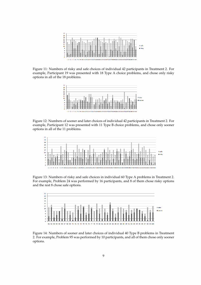
Figure 11: Numbers of risky and safe choices of individual 42 participants in Treatment 2. Forexample, Participant 19 was presented with 18 Type A choice problems, and chose only riskyoptions in all of the 18 problems.

Figure 12: Numbers of sooner and later choices of individual 42 participants in Treatment 2. Forexample, Participant 12 was presented with 11 Type B choice problems, and chose only sooneroptions in all of the 11 problems.

Figure 13: Numbers of risky and safe choices in individual 60 Type A problems in Treatment 2.For example, Problem 24 was performed by 16 participants, and 8 of them chose risky optionsand the rest 8 chose safe options.

Figure 14: Numbers of sooner and later choices of individual 40 Type B problems in Treatment2. For example, Problem 95 was performed by 10 participants, and all of them chose only sooneroptions.

9

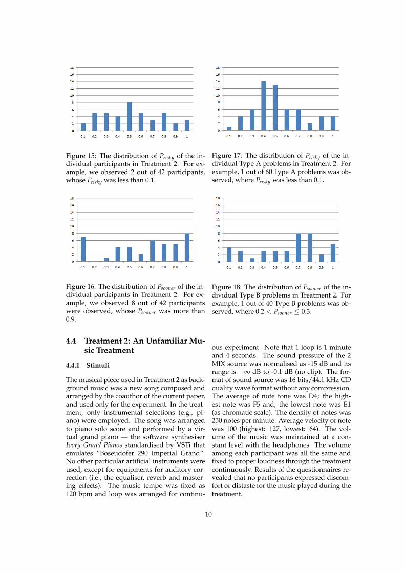
Figure 15: The distribution of Prisky of the in-dividual participants in Treatment 2. For ex-ample, we observed 2 out of 42 participants,whose Prisky was less than 0.1.

Figure 16: The distribution of Psooner of the in-dividual participants in Treatment 2. For ex-ample, we observed 8 out of 42 participantswere observed, whose Psooner was more than0.9.

4.4 Treatment 2: An Unfamiliar Mu-sic Treatment

4.4.1 Stimuli

The musical piece used in Treatment 2 as back-ground music was a new song composed andarranged by the coauthor of the current paper,and used only for the experiment. In the treat-ment, only instrumental selections (e.g., pi-ano) were employed. The song was arrangedto piano solo score and performed by a vir-tual grand piano — the software synthesiserIvory Grand Pianos standardised by VSTi thatemulates “Boseudofer 290 Imperial Grand”.No other particular artificial instruments wereused, except for equipments for auditory cor-rection (i.e., the equaliser, reverb and master-ing effects). The music tempo was fixed as120 bpm and loop was arranged for continu-

Figure 17: The distribution of Prisky of the in-dividual Type A problems in Treatment 2. Forexample, 1 out of 60 Type A problems was ob-served, where Prisky was less than 0.1.

Figure 18: The distribution of Psooner of the in-dividual Type B problems in Treatment 2. Forexample, 1 out of 40 Type B problems was ob-served, where 0.2 < Psooner ≤ 0.3.

ous experiment. Note that 1 loop is 1 minuteand 4 seconds. The sound pressure of the 2MIX source was normalised as -15 dB and itsrange is −∞ dB to -0.1 dB (no clip). The for-mat of sound source was 16 bits/44.1 kHz CDquality wave format without any compression.The average of note tone was D4; the high-est note was F5 and; the lowest note was E1(as chromatic scale). The density of notes was250 notes per minute. Average velocity of notewas 100 (highest: 127, lowest: 64). The vol-ume of the music was maintained at a con-stant level with the headphones. The volumeamong each participant was all the same andfixed to proper loudness through the treatmentcontinuously. Results of the questionnaires re-vealed that no participants expressed discom-fort or distaste for the music played during thetreatment.

10

4.4.2 Results

An overall Prisky was 0.49. The Prisky of indi-vidual participants is available in Appendix 2.Figure 11 presents numbers of risky and safechoices of individual participants in the treat-ment. We can see from the figure the existenceof heterogeneity among the participants in be-havioural tendencies in the treatment. For ex-ample, Prisky of some participants (e.g., Partic-ipant 19) was 100 percent; while Prisky of otherparticipants (e.g., Participant 26) was less than10 percent. Figure 15 presents the distribu-tion of the individual Prisky in the treatment(SD = 0.26). The Prisky of individual 60 Type Aproblems is available in Appendix 4. Figure 13presents numbers of risky and safe choices ofindividual problems in the treatment. Fig-ure 17 presents the distribution of Prisky of theindividual problems (SD = 0.23).

An overall Psooner was 0.57. The Psooner of in-dividual participants is available in Appendix3. Figure 12 presents numbers of sooner andlater choices of individual participants in thetreatment. We can see from the figure the exis-tence of heterogeneity among the participantsin behavioural tendencies in the treatment. Forexample, some participants (e.g., Participant 1)chose only sooner options, while others (e.g.,Participant 16) chose only later options. Fig-ure 16 presents the distribution of the indi-vidual Psooner in the treatment (SD = 0.34).The Psooner of individual 40 Type B problemsis available in Appendix 5. Figure 14 presentsnumbers of sooner and later choices of indi-vidual problems in the treatment. Figure 18presents the distribution of Psooner of the indi-vidual problems (SD = 0.29). An overall pro-portion of rational choices made among TypeC problems was 1.

4.4.3 Questionnaire Analysis

On completion of the treatment, the partici-pants were asked to fill in a questionnaire thatcontained the same set of questions as Treat-ment 1.

Results of the questionnaire revealed the fol-lowings: First, self-reported familiarity levelof the music on a 11-point scale (0=not fa-miliar with; 10=very much familiar with) wasextremely low (Min = 0, Max = 6, M =0.88, SD = 1.46). Second, self-reported at-

tention level on a 11-point scale (0=no atten-tion at all; 10=very much attention) was mod-erate (Min = 0, Max = 10, M = 5.79, SD =3.03). Third, self-reported music liking on a11-point scale (0=dislike very much; 10=like verymuch) was high (Min = 1, Max = 10, M =7.40, SD = 1.79). Fourth, self-reported in-fluence of the music on decision-making be-haviour on a 11-point scale (0=to no extent;10=to a very large extent) was low (Min =0, Max = 10, M = 2.98, SD = 3.09).

4.5 Treatment 3: Noise Treatment

4.5.1 Stimuli

The background sound used in Treatment 3was “Gaussian white noise”. The format ofsound source was 16bits/44.1kHz CD qualitywave format without any compression, thusthe power of spectrum pattern was evenly atthe range from 0 Hz to 22.1 kHz. The soundpressure was normalised as -20 dB, thus thewave form was slightly different from idealwave form. An amplitude over bit range wascut off. The sound pressure was lower thanthe other music treatments. This is becausethe perception of this stimulus was higher thanother musical stimulus and we feel more loud-ness under the same sound pressure. To avoidthe participants’ uncomfortableness, the levelof the sound pressure of this stimulus was de-creased, so that the participants would feel thestimulus was as loud as the stimulus used inthe other two treatments. The sound patternwas evenly static across the treatment. No mu-sical pieces were used in the treatment exceptwhite noise. The volume among each partic-ipant was all the same and fixed to properloudness across the treatment. Results of thequestionnaires revealed that no participantsexpressed discomfort or distaste for the noiseplayed during the treatment.

4.5.2 Results

An overall Prisky was 0.54. The Prisky of indi-vidual participants is available in Appendix 2.Figure 19 presents numbers of risky and safechoices of individual participants in the treat-ment. We can see from the figure the existenceof heterogeneity among the participants in be-havioural tendencies in the treatment. For ex-

11

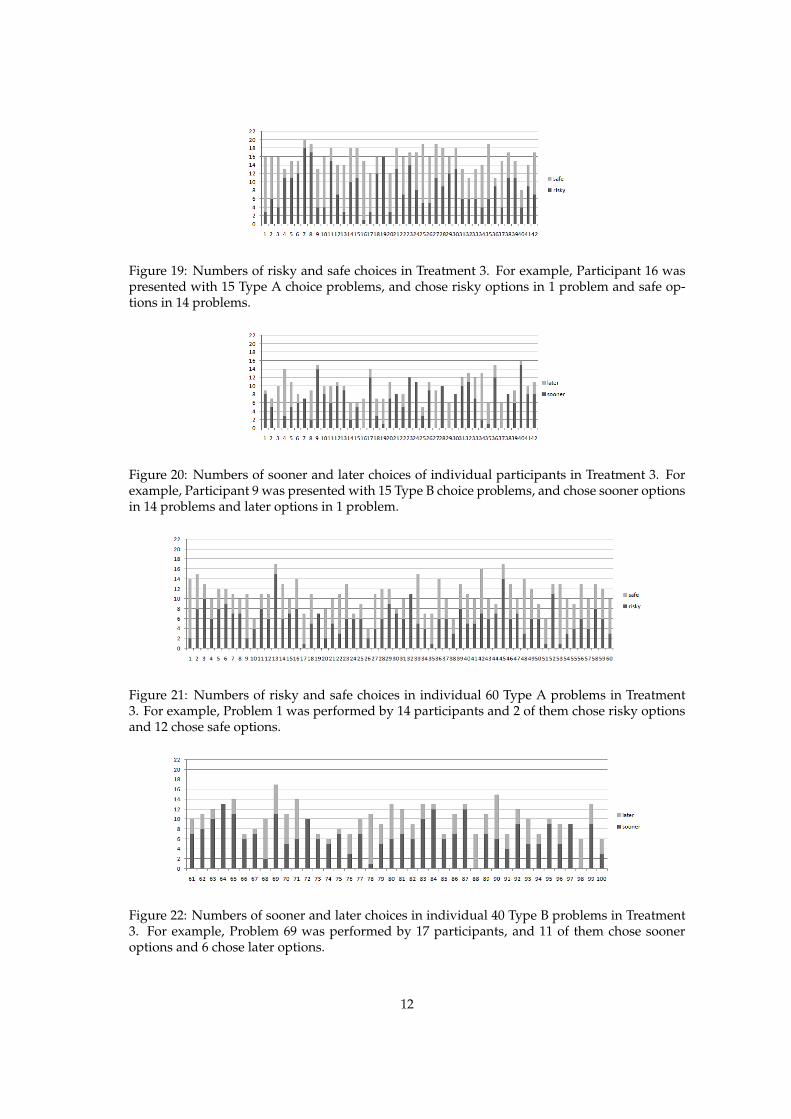
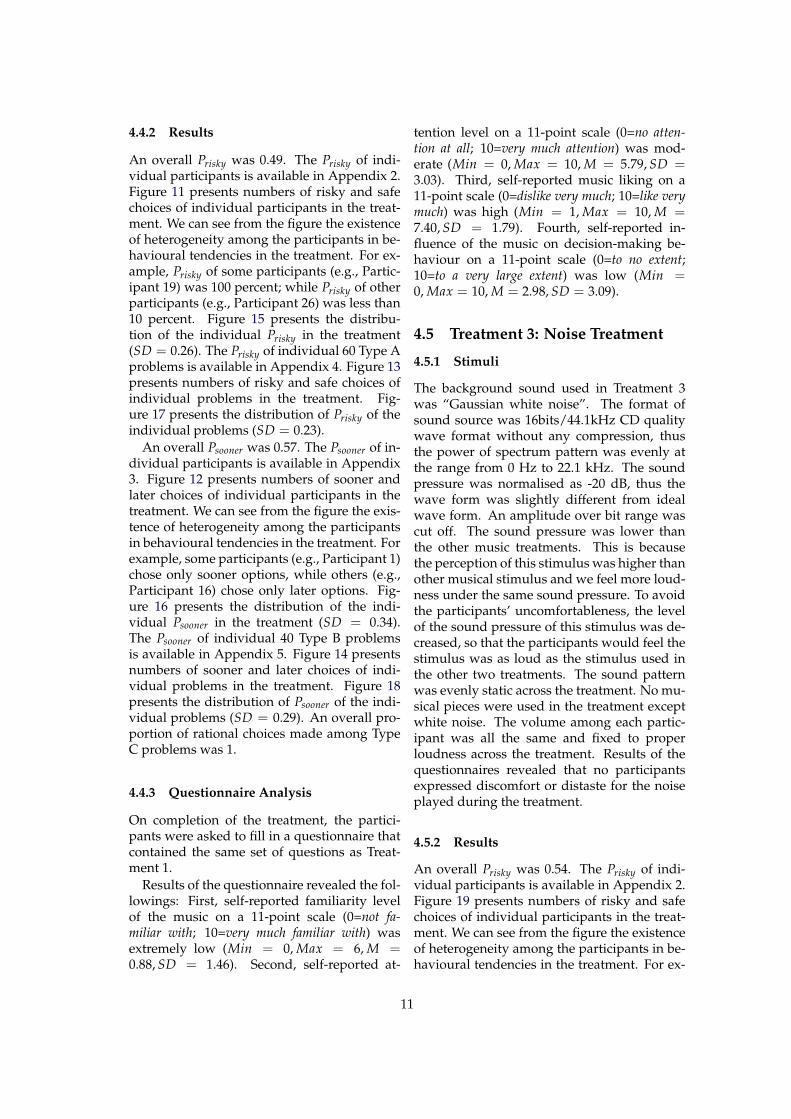
Figure 19: Numbers of risky and safe choices in Treatment 3. For example, Participant 16 waspresented with 15 Type A choice problems, and chose risky options in 1 problem and safe op-tions in 14 problems.

Figure 20: Numbers of sooner and later choices of individual participants in Treatment 3. Forexample, Participant 9 was presented with 15 Type B choice problems, and chose sooner optionsin 14 problems and later options in 1 problem.

Figure 21: Numbers of risky and safe choices in individual 60 Type A problems in Treatment3. For example, Problem 1 was performed by 14 participants and 2 of them chose risky optionsand 12 chose safe options.

Figure 22: Numbers of sooner and later choices in individual 40 Type B problems in Treatment3. For example, Problem 69 was performed by 17 participants, and 11 of them chose sooneroptions and 6 chose later options.

12

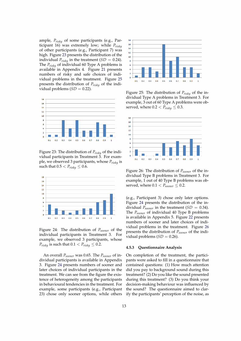
ample, Prisky of some participants (e.g., Par-ticipant 16) was extremely low; while Priskyof other participants (e.g., Participant 7) washigh. Figure 23 presents the distribution of theindividual Prisky in the treatment (SD = 0.24).The Prisky of individual 60 Type A problems isavailable in Appendix 4. Figure 21 presentsnumbers of risky and safe choices of indi-vidual problems in the treatment. Figure 25presents the distribution of Prisky of the indi-vidual problems (SD = 0.22).

Figure 23: The distribution of Prisky of the indi-vidual participants in Treatment 3. For exam-ple, we observed 3 participants, whose Prisky issuch that 0.5 < Prisky ≤ 0.6.

Figure 24: The distribution of Psooner of theindividual participants in Treatment 3. Forexample, we observed 3 participants, whosePrisky is such that 0.1 < Prisky ≤ 0.2.

An overall Psooner was 0.65. The Psooner of in-dividual participants is available in Appendix3. Figure 24 presents numbers of sooner andlater choices of individual participants in thetreatment. We can see from the figure the exis-tence of heterogeneity among the participantsin behavioural tendencies in the treatment. Forexample, some participants (e.g., Participant23) chose only sooner options, while others

Figure 25: The distribution of Prisky of the in-dividual Type A problems in Treatment 3. Forexample, 3 out of 60 Type A problems were ob-served, where 0.2 < Prisky ≤ 0.3.

Figure 26: The distribution of Psooner of the in-dividual Type B problems in Treatment 3. Forexample, 1 out of 40 Type B problems was ob-served, where 0.1 < Psooner ≤ 0.2.

(e.g., Participant 3) chose only later options.Figure 24 presents the distribution of the in-dividual Psooner in the treatment (SD = 0.34).The Psooner of individual 40 Type B problemsis available in Appendix 5. Figure 22 presentsnumbers of sooner and later choices of indi-vidual problems in the treatment. Figure 26presents the distribution of Psooner of the indi-vidual problems (SD = 0.26).

4.5.3 Questionnaire Analysis

On completion of the treatment, the partici-pants were asked to fill in a questionnaire thatcontained questions: (1) How much attentiondid you pay to background sound during thistreatment? (2) Do you like the sound presentedduring this treatment? (3) Do you think yourdecision-making behaviour was influenced bythe sound? The questionnaire aimed to clar-ify the participants’ perception of the noise, as

13

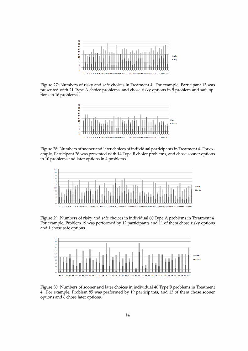
Figure 27: Numbers of risky and safe choices in Treatment 4. For example, Participant 13 waspresented with 21 Type A choice problems, and chose risky options in 5 problem and safe op-tions in 16 problems.

Figure 28: Numbers of sooner and later choices of individual participants in Treatment 4. For ex-ample, Participant 26 was presented with 14 Type B choice problems, and chose sooner optionsin 10 problems and later options in 4 problems.

Figure 29: Numbers of risky and safe choices in individual 60 Type A problems in Treatment 4.For example, Problem 19 was performed by 12 participants and 11 of them chose risky optionsand 1 chose safe options.

Figure 30: Numbers of sooner and later choices in individual 40 Type B problems in Treatment4. For example, Problem 85 was performed by 19 participants, and 13 of them chose sooneroptions and 6 chose later options.

14

compared to perception of background musicin Treatment 1 and 2.

Results of the questionnaire revealed thefollowings: First, self-reported attention levelon a 11-point scale (0=no attention at all;10=very much attention) was moderate (Min =0, Max = 10, M = 6.21, SD = 3.77). Sec-ond, self-reported sound liking on a 11-pointscale (0=dislike very much; 10=like very much)was extremely low (Min = 0, Max = 8, M =1.88, SD = 2.01). Third, self-reported influenceof the sound on decision-making behaviouron a 11-point scale (0=to no extent; 10=to avery large extent) was low (Min = 0, Max =10, M = 2.85, SD = 3.18).

4.6 Treatment 4: No Music Treat-ment

4.6.1 Stimuli

No background music/sound was used inTreatment 4. The participants were asked toengage in choice tasks in the presence neither ofbackground music nor of background sound.

4.6.2 Results

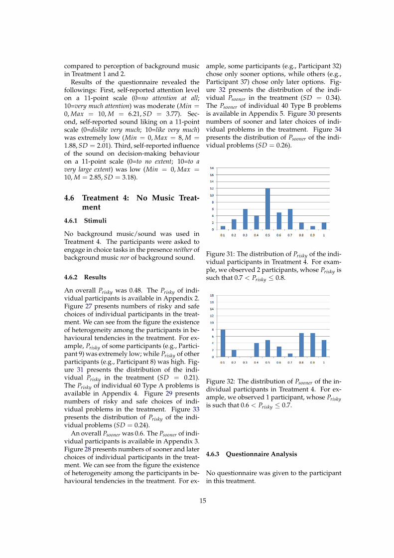
An overall Prisky was 0.48. The Prisky of indi-vidual participants is available in Appendix 2.Figure 27 presents numbers of risky and safechoices of individual participants in the treat-ment. We can see from the figure the existenceof heterogeneity among the participants in be-havioural tendencies in the treatment. For ex-ample, Prisky of some participants (e.g., Partici-pant 9) was extremely low; while Prisky of otherparticipants (e.g., Participant 8) was high. Fig-ure 31 presents the distribution of the indi-vidual Prisky in the treatment (SD = 0.21).The Prisky of individual 60 Type A problems isavailable in Appendix 4. Figure 29 presentsnumbers of risky and safe choices of indi-vidual problems in the treatment. Figure 33presents the distribution of Prisky of the indi-vidual problems (SD = 0.24).

An overall Psooner was 0.6. The Psooner of indi-vidual participants is available in Appendix 3.Figure 28 presents numbers of sooner and laterchoices of individual participants in the treat-ment. We can see from the figure the existenceof heterogeneity among the participants in be-havioural tendencies in the treatment. For ex-

ample, some participants (e.g., Participant 32)chose only sooner options, while others (e.g.,Participant 37) chose only later options. Fig-ure 32 presents the distribution of the indi-vidual Psooner in the treatment (SD = 0.34).The Psooner of individual 40 Type B problemsis available in Appendix 5. Figure 30 presentsnumbers of sooner and later choices of indi-vidual problems in the treatment. Figure 34presents the distribution of Psooner of the indi-vidual problems (SD = 0.26).

Figure 31: The distribution of Prisky of the indi-vidual participants in Treatment 4. For exam-ple, we observed 2 participants, whose Prisky issuch that 0.7 < Prisky ≤ 0.8.

Figure 32: The distribution of Psooner of the in-dividual participants in Treatment 4. For ex-ample, we observed 1 participant, whose Priskyis such that 0.6 < Prisky ≤ 0.7.

4.6.3 Questionnaire Analysis

No questionnaire was given to the participantin this treatment.

15

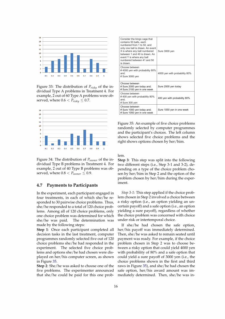
Figure 33: The distribution of Prisky of the in-dividual Type A problems in Treatment 4. Forexample, 2 out of 60 Type A problems were ob-served, where 0.6 < Prisky ≤ 0.7.

Figure 34: The distribution of Psooner of the in-dividual Type B problems in Treatment 4. Forexample, 2 out of 40 Type B problems was ob-served, where 0.8 < Psooner ≤ 0.9.

4.7 Payments to Participants

In the experiment, each participant engaged infour treatments, in each of which she/he re-sponded to 30 pairwise choice problems. Thus,she/he responded to a total of 120 choice prob-lems. Among all of 120 choice problems, onlyone choice problem was determined for whichshe/he was paid. The determination wasmade by the following steps:Step 1: Once each participant completed alldecision tasks in the last treatment, computerprogrammes randomly selected five out of 120choice problems she/he had responded in theexperiment. The selected five choice prob-lems and options she/he had chosen were dis-played on her/his computer screen, as shownin Figure 35.Step 2: She/he was asked to choose one of thefive problems. The experimenter announcedthat she/he could be paid for this one prob-

Consider the bingo cage that

contains 50 balls, each numbered from 1 to 50, and

only one ball is drawn. An event X is where any ball numbered

between 1 and 40 is drawn. An

event Y is where any ball numbered between 41 and 50

is drawn.

Sure 3000 yen

Choose between

# 4000 yen with probability 80% and;

# Sure 3000 yen

4000 yen with probability 80%

Choose between

# Sure 2000 yen today and; # Sure 2100 yen in one week

Sure 2000 yen today

Choose between

# 400 yen with probability 80% and;

# Sure 300 yen

400 yen with probability 80%

Choose between

# Sure 1000 yen today and; # Sure 1050 yen in one week

Sure 1050 yen in one week

Figure 35: An example of five choice problemsrandomly selected by computer programmesand the participant’s choices. The left columnshows selected five choice problems and theright shows options chosen by her/him.

lem.Step 3: This step was split into the followingtwo different steps (i.e., Step 3-1 and 3-2), de-pending on a type of the choice problem cho-sen by her/him in Step 2 and the option of theproblem chosen by her/him during the exper-iment.

Step 3-1: This step applied if the choice prob-lem chosen in Step 2 involved a choice betweena risky option (i.e., an option yielding an un-certain payoff) and a safe option (i.e., an optionyielding a sure payoff), regardless of whetherthe choice problem was concerned with choiceunder risk or intertemporal choice.

If she/he had chosen the safe option,her/his payoff was immediately determined.Then, she/he was asked to remain seated untilpayment was ready. For example, if the choiceproblem chosen in Step 2 was to choose be-tween a risky option that could yield 4000 yenwith probability of 80% and a safe option thatcould yield a sure payoff of 3000 yen (i.e., thechoice problems shown in the first and thirdraws in Figure 35), and she/he had chosen thesafe option, her/his award amount was im-mediately determined. Then, she/he was in-

16

formed that she/he could be given 3000 yenshortly.

On the other hand, if she/he had chosenthe risky option, she/he was presented withan empty bingo cage and a set of numberedballs. Then, she/he was asked to put thesenumbered balls into the empty bingo cage, anddraw one ball from the bingo cage. An out-come of the risky option was determined, ac-cording to the ball drawn. The composition ofthe bingo cage varied, depending on the choiceproblem and option she/he had chosen. Thepreparation of the bingo cage and balls wasdone in view of her/him, staff at KEEL andother participants.

For example, if she/he had chosen the riskyoption in the abovementioned choice problem,the experimenter prepared the empty bingocage and balls numbered 1 through 50, andasked her/him to put these 50 balls into theempty bingo cage. Then, she/he was askedto choose and write down any ten numbersfrom 1 to 50 on a blackboard at the laboratory.Before asking her/him to draw one ball fromthe bingo cage, containing 50 balls, the exper-imenter informed her/him that she/he couldbe given 4000 yen if any of the balls that car-ried numbers you chose and wrote down onthe blackboard was not drawn, and no money,otherwise.

Step 3-2: This step applied if the choice prob-lem she/he chose in Step 2 involved an in-centive scheme that payments could be madein the future (e.g., one week after the experi-ment). We employed Japanese practice of us-ing “registered mail for cash” to send her/hima cash payoff, if she/he was to receive deferredpayments. Postage costs were borne by the ex-perimenter. For example, if the choice problemwas to choose between “a sure payoff of 1000yen today” and “a sure payoff of 1050 yen inone week”, and her/his choice was the latter,then 1050 yen was received by registered mailone week after the experiment.

5 General Discussion

5.1 Behavioural Tendencies in thePresence of Background Noise

A perusal of previous studies renders towhat extent background noise affects the de-

cision makers’ performance. Some (e.g., Eller-meier and Hellbruck, 1998; Jones, Miles andPage, 1990; Abikoff, Courtney, Szeibel andKoplewicz, 1996; Salame and Baddeley, 1987)showed that background noise does not af-fect cognitive performance. Others, however,provided an account for noise-induced im-provement (e.g., Usher and Feingold, 2000;Soderlund and Smart, 2007; Baker and Hold-ing, 1993; Zentall and Shaw, 1980) and noise-induced deterioration in cognitive perfor-mance (e.g., Schlittmeier and Hellbruck, 2009;Cassidy and MacDonald, 2007; Hygge, Evansand Bullinger, 2002; Ylias and Heaven, 2003).

The results of the current experiment con-firm that background noise affects perfor-mance in decision making under risk and in-tertemporal decision making.

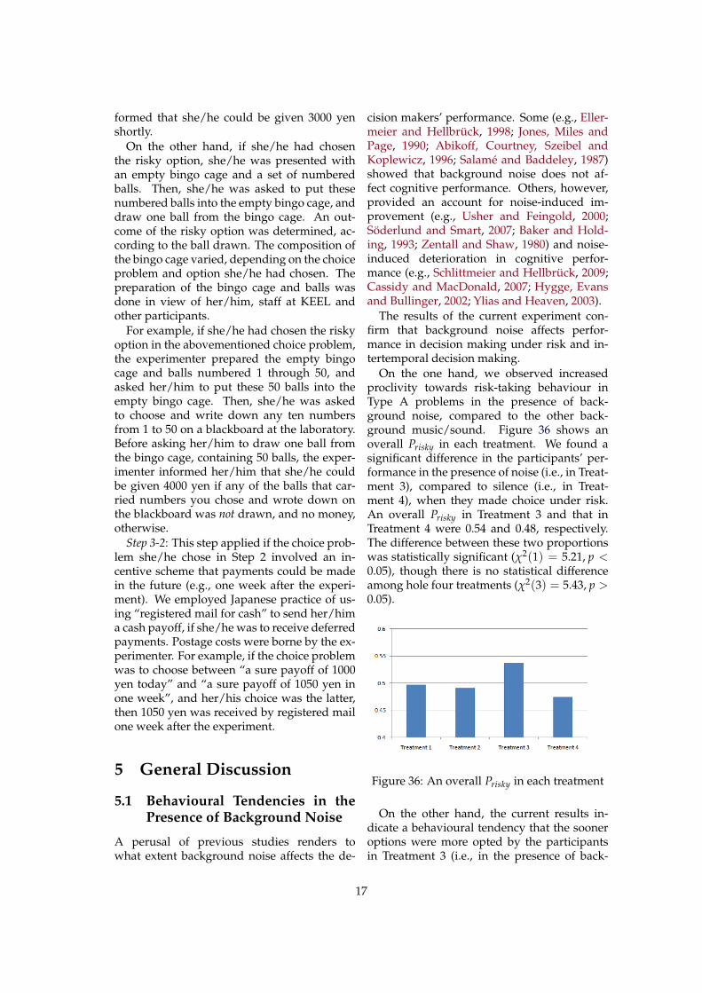
On the one hand, we observed increasedproclivity towards risk-taking behaviour inType A problems in the presence of back-ground noise, compared to the other back-ground music/sound. Figure 36 shows anoverall Prisky in each treatment. We found asignificant difference in the participants’ per-formance in the presence of noise (i.e., in Treat-ment 3), compared to silence (i.e., in Treat-ment 4), when they made choice under risk.An overall Prisky in Treatment 3 and that inTreatment 4 were 0.54 and 0.48, respectively.The difference between these two proportionswas statistically significant (χ2(1) = 5.21, p <0.05), though there is no statistical differenceamong hole four treatments (χ2(3) = 5.43, p >0.05).

Figure 36: An overall Prisky in each treatment

On the other hand, the current results in-dicate a behavioural tendency that the sooneroptions were more opted by the participantsin Treatment 3 (i.e., in the presence of back-

17

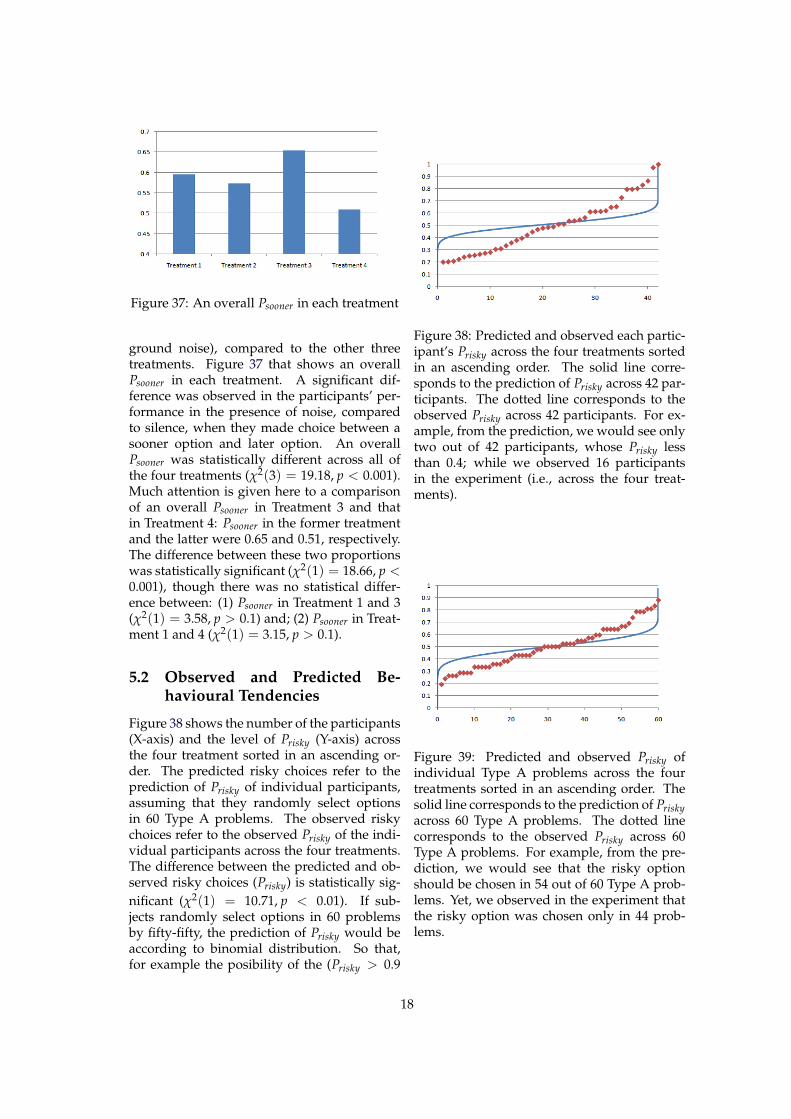
Figure 37: An overall Psooner in each treatment

ground noise), compared to the other threetreatments. Figure 37 that shows an overallPsooner in each treatment. A significant dif-ference was observed in the participants’ per-formance in the presence of noise, comparedto silence, when they made choice between asooner option and later option. An overallPsooner was statistically different across all ofthe four treatments (χ2(3) = 19.18, p < 0.001).Much attention is given here to a comparisonof an overall Psooner in Treatment 3 and thatin Treatment 4: Psooner in the former treatmentand the latter were 0.65 and 0.51, respectively.The difference between these two proportionswas statistically significant (χ2(1) = 18.66, p <0.001), though there was no statistical differ-ence between: (1) Psooner in Treatment 1 and 3(χ2(1) = 3.58, p > 0.1) and; (2) Psooner in Treat-ment 1 and 4 (χ2(1) = 3.15, p > 0.1).

5.2 Observed and Predicted Be-havioural Tendencies

Figure 38 shows the number of the participants(X-axis) and the level of Prisky (Y-axis) acrossthe four treatment sorted in an ascending or-der. The predicted risky choices refer to theprediction of Prisky of individual participants,assuming that they randomly select optionsin 60 Type A problems. The observed riskychoices refer to the observed Prisky of the indi-vidual participants across the four treatments.The difference between the predicted and ob-served risky choices (Prisky) is statistically sig-nificant (χ2(1) = 10.71, p < 0.01). If sub-jects randomly select options in 60 problemsby fifty-fifty, the prediction of Prisky would beaccording to binomial distribution. So that,for example the posibility of the (Prisky > 0.9

Figure 38: Predicted and observed each partic-ipant’s Prisky across the four treatments sortedin an ascending order. The solid line corre-sponds to the prediction of Prisky across 42 par-ticipants. The dotted line corresponds to theobserved Prisky across 42 participants. For ex-ample, from the prediction, we would see onlytwo out of 42 participants, whose Prisky lessthan 0.4; while we observed 16 participantsin the experiment (i.e., across the four treat-ments).

Figure 39: Predicted and observed Prisky ofindividual Type A problems across the fourtreatments sorted in an ascending order. Thesolid line corresponds to the prediction of Priskyacross 60 Type A problems. The dotted linecorresponds to the observed Prisky across 60Type A problems. For example, from the pre-diction, we would see that the risky optionshould be chosen in 54 out of 60 Type A prob-lems. Yet, we observed in the experiment thatthe risky option was chosen only in 44 prob-lems.

18

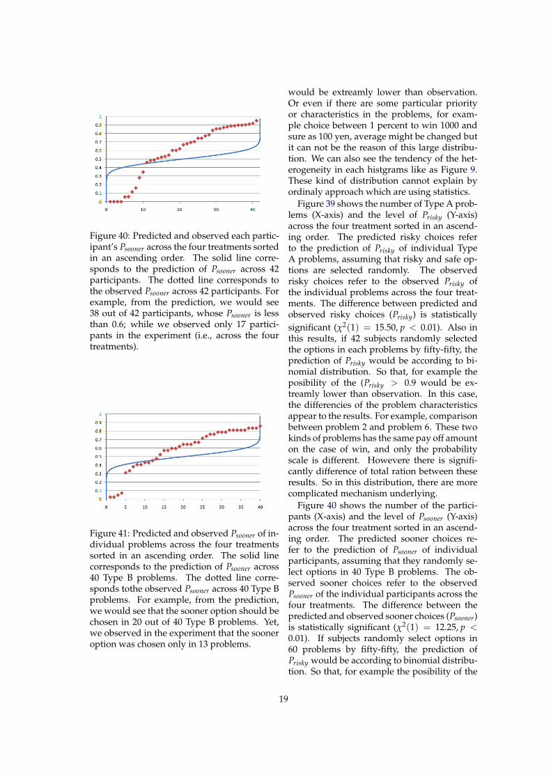
Figure 40: Predicted and observed each partic-ipant’s Psooner across the four treatments sortedin an ascending order. The solid line corre-sponds to the prediction of Psooner across 42participants. The dotted line corresponds tothe observed Psooner across 42 participants. Forexample, from the prediction, we would see38 out of 42 participants, whose Psooner is lessthan 0.6; while we observed only 17 partici-pants in the experiment (i.e., across the fourtreatments).

Figure 41: Predicted and observed Psooner of in-dividual problems across the four treatmentssorted in an ascending order. The solid linecorresponds to the prediction of Psooner across40 Type B problems. The dotted line corre-sponds tothe observed Psooner across 40 Type Bproblems. For example, from the prediction,we would see that the sooner option should bechosen in 20 out of 40 Type B problems. Yet,we observed in the experiment that the sooneroption was chosen only in 13 problems.

would be extreamly lower than observation.Or even if there are some particular priorityor characteristics in the problems, for exam-ple choice between 1 percent to win 1000 andsure as 100 yen, average might be changed butit can not be the reason of this large distribu-tion. We can also see the tendency of the het-erogeneity in each histgrams like as Figure 9.These kind of distribution cannot explain byordinaly approach which are using statistics.

Figure 39 shows the number of Type A prob-lems (X-axis) and the level of Prisky (Y-axis)across the four treatment sorted in an ascend-ing order. The predicted risky choices referto the prediction of Prisky of individual TypeA problems, assuming that risky and safe op-tions are selected randomly. The observedrisky choices refer to the observed Prisky ofthe individual problems across the four treat-ments. The difference between predicted andobserved risky choices (Prisky) is statisticallysignificant (χ2(1) = 15.50, p < 0.01). Also inthis results, if 42 subjects randomly selectedthe options in each problems by fifty-fifty, theprediction of Prisky would be according to bi-nomial distribution. So that, for example theposibility of the (Prisky > 0.9 would be ex-treamly lower than observation. In this case,the differencies of the problem characteristicsappear to the results. For example, comparisonbetween problem 2 and problem 6. These twokinds of problems has the same pay off amounton the case of win, and only the probabilityscale is different. Howevere there is signifi-cantly difference of total ration between theseresults. So in this distribution, there are morecomplicated mechanism underlying.

Figure 40 shows the number of the partici-pants (X-axis) and the level of Psooner (Y-axis)across the four treatment sorted in an ascend-ing order. The predicted sooner choices re-fer to the prediction of Psooner of individualparticipants, assuming that they randomly se-lect options in 40 Type B problems. The ob-served sooner choices refer to the observedPsooner of the individual participants across thefour treatments. The difference between thepredicted and observed sooner choices (Psooner)is statistically significant (χ2(1) = 12.25, p <0.01). If subjects randomly select options in60 problems by fifty-fifty, the prediction ofPrisky would be according to binomial distribu-tion. So that, for example the posibility of the

19

(Prisky > 0.9 would be extreamly lower thanobservation. These results are all about type Bproblems, so its mechanism would be differentfrom results of type A problem. However inthese results, the tendency of the heterogeneitycould be observed in wide range. Some partic-ipants selected only later choice and some par-ticipants selected only sooner choice, thoughthere are 0.1 percent to more than 1 percent in-terest per day.

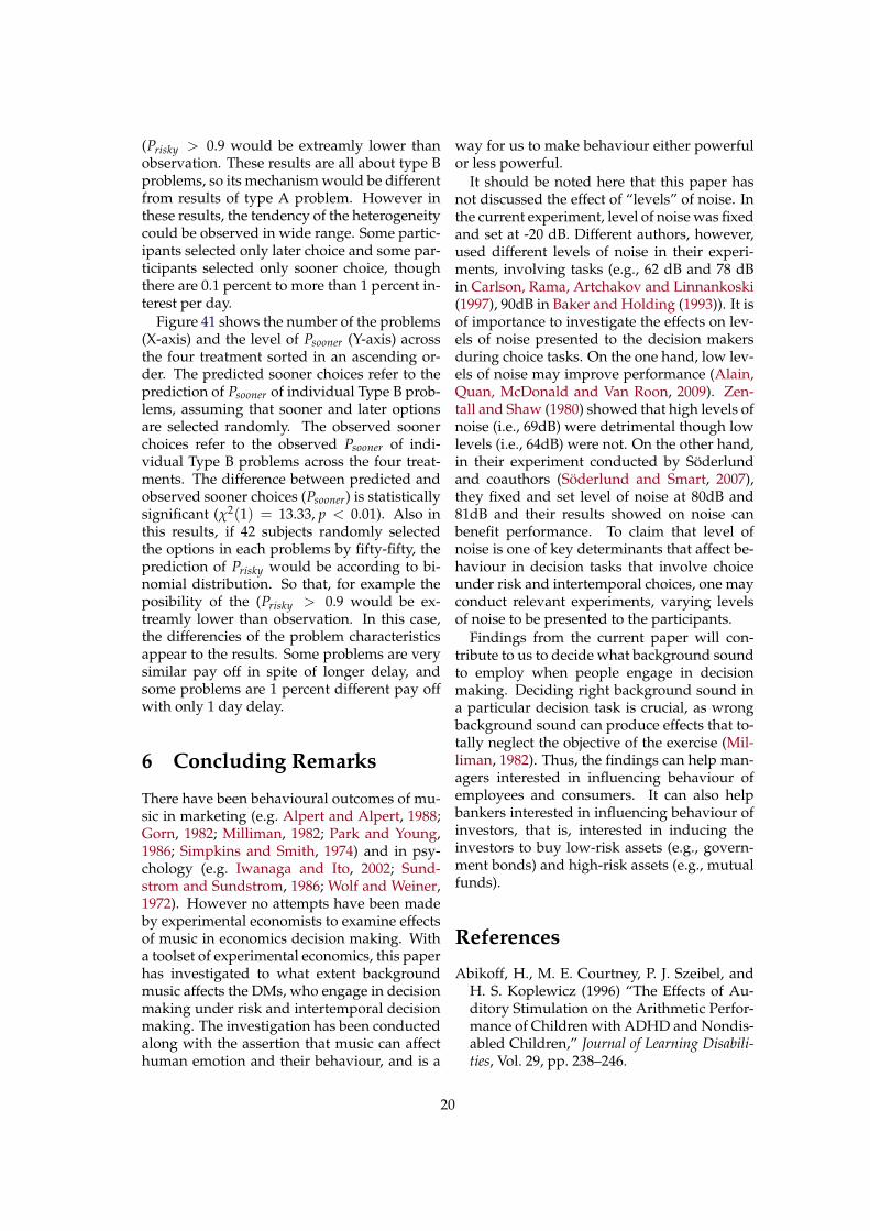
Figure 41 shows the number of the problems(X-axis) and the level of Psooner (Y-axis) acrossthe four treatment sorted in an ascending or-der. The predicted sooner choices refer to theprediction of Psooner of individual Type B prob-lems, assuming that sooner and later optionsare selected randomly. The observed soonerchoices refer to the observed Psooner of indi-vidual Type B problems across the four treat-ments. The difference between predicted andobserved sooner choices (Psooner) is statisticallysignificant (χ2(1) = 13.33, p < 0.01). Also inthis results, if 42 subjects randomly selectedthe options in each problems by fifty-fifty, theprediction of Prisky would be according to bi-nomial distribution. So that, for example theposibility of the (Prisky > 0.9 would be ex-treamly lower than observation. In this case,the differencies of the problem characteristicsappear to the results. Some problems are verysimilar pay off in spite of longer delay, andsome problems are 1 percent different pay offwith only 1 day delay.

6 Concluding Remarks

There have been behavioural outcomes of mu-sic in marketing (e.g. Alpert and Alpert, 1988;Gorn, 1982; Milliman, 1982; Park and Young,1986; Simpkins and Smith, 1974) and in psy-chology (e.g. Iwanaga and Ito, 2002; Sund-strom and Sundstrom, 1986; Wolf and Weiner,1972). However no attempts have been madeby experimental economists to examine effectsof music in economics decision making. Witha toolset of experimental economics, this paperhas investigated to what extent backgroundmusic affects the DMs, who engage in decisionmaking under risk and intertemporal decisionmaking. The investigation has been conductedalong with the assertion that music can affecthuman emotion and their behaviour, and is a

way for us to make behaviour either powerfulor less powerful.

It should be noted here that this paper hasnot discussed the effect of “levels” of noise. Inthe current experiment, level of noise was fixedand set at -20 dB. Different authors, however,used different levels of noise in their experi-ments, involving tasks (e.g., 62 dB and 78 dBin Carlson, Rama, Artchakov and Linnankoski(1997), 90dB in Baker and Holding (1993)). It isof importance to investigate the effects on lev-els of noise presented to the decision makersduring choice tasks. On the one hand, low lev-els of noise may improve performance (Alain,Quan, McDonald and Van Roon, 2009). Zen-tall and Shaw (1980) showed that high levels ofnoise (i.e., 69dB) were detrimental though lowlevels (i.e., 64dB) were not. On the other hand,in their experiment conducted by Soderlundand coauthors (Soderlund and Smart, 2007),they fixed and set level of noise at 80dB and81dB and their results showed on noise canbenefit performance. To claim that level ofnoise is one of key determinants that affect be-haviour in decision tasks that involve choiceunder risk and intertemporal choices, one mayconduct relevant experiments, varying levelsof noise to be presented to the participants.

Findings from the current paper will con-tribute to us to decide what background soundto employ when people engage in decisionmaking. Deciding right background sound ina particular decision task is crucial, as wrongbackground sound can produce effects that to-tally neglect the objective of the exercise (Mil-liman, 1982). Thus, the findings can help man-agers interested in influencing behaviour ofemployees and consumers. It can also helpbankers interested in influencing behaviour ofinvestors, that is, interested in inducing theinvestors to buy low-risk assets (e.g., govern-ment bonds) and high-risk assets (e.g., mutualfunds).

References

Abikoff, H., M. E. Courtney, P. J. Szeibel, andH. S. Koplewicz (1996) “The Effects of Au-ditory Stimulation on the Arithmetic Perfor-mance of Children with ADHD and Nondis-abled Children,” Journal of Learning Disabili-ties, Vol. 29, pp. 238–246.

20

Alain, C., J. Quan, K. McDonald, andP. Van Roon (2009) “Noise-induced Increasein Human Auditory Evoked NeuromagneticFields,” European Journal of Neuroscience, Vol.30, pp. 132–142.

Allais, M. (1953) “Le Comportement del’Homme Rationnel devant le Risque: Cri-tique des Postulats et Axiomes de l’EcoleAmericaine,” Econometrica, Vol. 21, pp. 503–546.

Alpert, J. I. and M. I. Alpert (1988) “Back-ground Music as an Influence in ConsumerMood and Advertising Responses,” in T. K.Scrull ed. Advances in Consumer Research,Honolulu: Association for Consumer Re-search, pp. 485–491.

Andrade, P. E. (2004) “Uma abordagem evolu-tionaria e neuroscientifıca da musica (Evolu-tionary and neuroscientific approach to mu-sic),” Neurosciencias, Vol. 1, pp. 24–33.

Baker, M. A. and D. H. Holding (1993) “The Ef-fects of Noise and Speech on Cognitive TaskPerformance,” Journal of General Psychology,Vol. 120, pp. 339–355.

Baumgartner, H. (1992) “Remembrance ofthings past: Music, autobiographical mem-ory, and emotion,” Advances in Consumer Re-search, Vol. 19, pp. 613–620.

Beament, J. (2001) How we hear music: The rela-tionship between music and the hearing mecha-nism, Woodbridge, UK: Boydell and Brewer.

Brayfield, A. H. and W. H. Crockett (1955)“Employee Attitudes and Employee Perfor-mance,” Psychological Bulletin, Vol. 52, pp.396–424.

Bruner, II, Gordon C. (1990) “Music, Mood,and Marketing,” Journal of Marketing, Vol. 54,pp. 94–104.

Carlson, S., P. Rama, D. Artchakov, and I. Lin-nankoski (1997) “Effects of Music and WhiteNoise on Working Memory Performance inMonkeys,” Neuroreport, Vol. 8, pp. 2853–2856.

Cassidy, G. and R. A. R. MacDonald (2007)“The Effect of Background Music and Back-ground Noise on the Task Performance of In-troverts and Extraverts,” Psychology of Music,Vol. 35, pp. 517–537.

Corhan, C. M. and B. R. Gounard (1976) “Typesof Music, Schedules of Background Stimula-tion, and Visual Vigilance Performance,” Pe-ceptual and Motor Skills, Vol. 42, p. 662.

Ellermeier, W. and J. Hellbruck (1998) “Is LevelIrrelevant in ‘Irrelevant Speech’? Effects ofLoudness, Signal-to-noise Ratio, and Binau-ral Unmasking,” Journal of Experimental Psy-chology: Human Perception and Performance,Vol. 24, pp. 1406–1414.

Frederick, S. and G. Loewenstein (2002) “TimeDiscounting and Time Preference: A CriticalReview,” Journal of Economic Literature, Vol.40, pp. 351–401.

Gabrielsson, A. (2001) “Emotions in strong ex-periences with music,” in P. N. Juslin andJ. A. Sloboda eds. Music and emotion: The-ory and research, Oxford: Oxford UniversityPress, pp. 431–449.

Gorn, G. J. (1982) “The Effects of Music inAdvertising on Choice Behavior: A lassicalConditioning Approach,” Journal of Market-ing, Vol. 46, pp. 94–101.

Green, L., N. Fristoe, and J. Myerson (1994)“Temporal Discounting and Preference Re-versals in Choice Between Delayed Out-comes,” Psychonomic Bulletin and Review, Vol.1, pp. 383–389.

Hilliard, O. M. and Philip Tolin (1979) “Ef-fects of Familiarity with Background Mu-sic on Performance of Simple and DifficultReading Comprehension Tasks,” Perceptualand Motor Skills, Vol. 49, pp. 713–714.

Hygge, S., G. W. Evans, and M. Bullinger(2002) “A Prospective Study of Some Effectsof Aircraft Noise on Cognitive Performancein Schoolchildren,” Psychological Science, Vol.13, pp. 469–474.

Iwanaga, M. and T. Ito (2002) “Disturbance ef-fect of music on processing of verbal andspatial memories,” Perceptual Motor Skills,Vol. 94, pp. 1251–1258.

Iyer, P. (2006) “The Cuddliest Hero inAsia,” Retrieved from Time (Asia) on 4April, 2010, http://www.time.com/time/asia/features/heroes/doraemon.html.

21

Jacob, J. (1968) “Work Music and Morale: ANeglected but Important Relationship,” Per-sonnel Journal, Vol. 47, pp. 882–886.

Jones, D. M., C. Miles, and J. Page (1990)“Disruption of Proofreading by IrrelevantSpeech: Effects of Attention, Arousal orMemory?” Applied Cognitive Psychology, Vol.4, pp. 89–108.

Juslin, P. N. and S. Liljestrom (in press) “Howdoes music evoke emotions? Exploring theunderlying mechanisms,” in P. N. Juslin andJ. A. Sloboda eds. Handbook of music and emo-tion: Theory, research, applications, Oxford:Oxford University Press.

Juslin, P. N. and D. Vastfjall (2008) “Emo-tional responses to music: The need to con-sider underlying mechanisms,” Behavioraland Brain Sciences, Vol. 31, pp. 559–621.

Juslin, P. N., P. Laukka, S. Liljestrom,D. Vastfjall, and Lundqvist, L.-O. (submit-ted) “A representative survey study of emo-tional reactions to music.”

Kahneman, Daniel and Amos Tversky (1979)“Prospect Theory: An Analysis of Decisionunder Risk,” Econometrica, Vol. 47, pp. 23–53.

Kirby, K. N. and R. J. Herrenstein (1995) “Pref-erence Reversals due to Myopic Discount-ing of Delayed Reward,” Psychological Sci-ence, Vol. 6, pp. 83–89.

McGehee, W. and J. Gardner (1949) “Music ina Complex Indutrial Job,” Personnel Psychol-ogy, Vol. 2, pp. 405–417.

McKerchar, T. L, L. Green, J. Myerson, T. S.Pickford, J. C. Hill, and S. C. Stout (2009) “AComparison of Four Models of Delay Dis-counting in Humans,” Behavioural Processes,Vol. 81, pp. 256–259.

Millar, A. and D. Navarick (1984) “Self-Controland Choice in Humans: Effects of VideoGame Playing as a Positive Reinforcer,”Learning and Motivation, Vol. 15, pp. 203–218.

Milliman, R. E. (1982) “The Influence of Back-ground Music on the Behavior of RestaurantPatrons,” Journal of Consumer Research, Vol.13, pp. 286–289.

Mowsesian, R. and M. Heyer (1973) “The ef-fect of music as a distraction on test-takingperformance,” Measurement and Evaluation inGuidance, Vol. 6, pp. 104–110.

Park, C. W. and S. M. Young (1986) “Con-sumer Response to Television Commercials:The Impact of Involvement and BackgroundMusic on Brand Attitude Formation,” Jour-nal of Marketing Research, Vol. 23.

Rauscher, F. H., G. L. Shaw, and K. N. Ky (1993)“Music and Spatial Task-performance,” Na-ture, Vol. 365, p. 611.

Salame, P. and A. D. Baddeley (1982) “Disrup-tion of Short-term Memory by UnattendedSpeech: Implications for the structure ofWorking Memory,” Journal of Verbal Learningand Berbal Behavior, Vol. 21, pp. 150–164.

(1987) “Noise, Unattended Speechand Short-term Memory,” Ergonomics, Vol.30, pp. 1185–1194.

Samuelson, P. A. (1937) “A Note on Measure-ment of Utility,” Review of Economic Studies,Vol. 4, pp. 155–161.

Schlittmeier, S. J. and J. Hellbruck (2009)“Background Music as Noise Abatement inOpen-Plan Of?ces: A Laboratory Study onPerformance Effects and Subjective Prefer-ences,” Applied Cognitive Psychology, Vol. 23,pp. 684–697.

Simpkins, J. D. and J. A. Smith (1974) “Effectsof Music on Source Evaluations,” Journal ofBroadcasting, Vol. 18, pp. 361–367.

Sloboda, J. A. (1992) “Empirical studies ofemotional response to music,” in M. Riess-Jones and S. Holleran eds. Cognitive bases ofmusical communication, New York: Ameri-carn Psychological Association, pp. 33–46.

Sloboda, J. A. and S. A. O’Neill (2001) “Emo-tions in everyday listening to music,” in P. N.Juslin and J. A. Sloboda eds. Music and emo-tion: Theory and research, Oxford: OxfordUniversity Press, pp. 415–429.

Smith, H. C. (1947) “Mucis in Relation toEmployee Attitudes, Piecework, Productionand industrial Accidents,” Applied Psychol-ogy Monographs, Vol. 14, p. 55.

22

Soderlund, S., G.and Sikstrom and A. Smart(2007) “Listen to the Noise: Noise is Bene-ficial for Cognitive Performance in ADHD,”Journal of Child Psychology and Psychiatry, Vol.48, pp. 840–847.

Solnick, J., C. Kannenberg, D. Eckerman, andW. Waller (1980) “An Experimental Analysisof Impulsivity and Impulse Control in Hu-mans,” Learning and Motivation, Vol. 11, pp.61–77.

Sundstrom, E. and M. G. Sundstrom (1986)Work places: the psychology of the physical en-vironment in office and factories, New York:Cambridge University Press.

Takahashi, T. (2009) “Theoretical Frame-works for Neuroeconomics of IntertemporalChoice,” Journal of Neuroscience, Psychology,and Economics, Vol. 2, pp. 75–90.

Uhrbrock, R. S. (1961) “Music on the Job: Its In-fluence on Worker Morale and Production,”Personell Psychology, Vol. 14, pp. 9–38.

Usher, M. and M. Feingold (2000) “Stochas-tic Resonance in the Speed of Memory Re-trieval,” Biological Cybernetics, Vol. 83, pp.L11–16.

von Neumann, John and Oskar Morgenstern(1944) Theory of Games and Economic Behavior,New Jersey: Princeton University Press.

Wolf, R. H. and F. F. Weiner (1972) “Effects offour noise conditions on arithmetic perfor-mance,” Perceptual and Motor Skills, Vol. 35,pp. 928–930.

Ylias, G. and P. C. L. Heaven (2003) “The Influ-ence of Distraction on Reading Comprehen-sion: A Big Five Analysis,” Personality andIndividual Differences, Vol. 34, pp. 1069–1079.

Zentall, S. S. and J. H. Shaw (1980) “Effects ofClassroom Noise on Performance and Activ-ity of Second-grade Hyperactive and Con-trol Children,” Journal of Educational Psychol-ogy, Vol. 72, pp. 830–840.

Zhang, Jiajie, Todd R. Johnson, and HongbinWan (1998) “The Relation Between Order Ef-fects and Frequency Learning in Tactical De-cision Making,” Thinking and Reasoning, Vol.4, pp. 123–145.

23

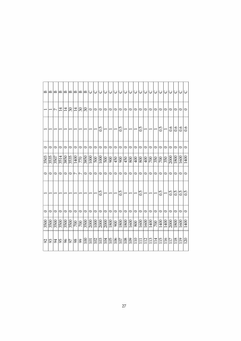
App

endi

x1

Sum

mar

yof

the

payo

ffst

ruct

ure

ofch

oice

prob

lem

s.Fo

rex

ampl

e,Pr

oble

m61

invo

lved

ach

oice

betw

een

Opt

ion

Ayi

eldi

ngth

epr

esen

t500

0ye

nan

dO

ptio

nB

yiel

ding

5500

yen

inse

ven

days

;whi

lePr

oble

m10

3in

volv

eda

choi

cebe

twee

nO

ptio

nA

yiel

ding

a50

%ch

ance

ofw

inni

ngpr

esen

t20

00ye

nan

dO

ptio

nB

yiel

ding

a50

%ch

ance

ofw

inni

ngpr

esen

t100

0ye

n.

Opt

ion

AO

ptio

nB

win

lose

prob

abili

tyde

lay

win

lose

prob

abili

tyde

lay

cate

gory

Prob

lem

ofw

inni

ngof

win

ning

180

000

0.4

030

000

10

A2

4000

00.

80

3000

01

0A

332

000

0.2

040

00

0.8

0A

422

000

0.5

010

000

10

A5

2000

00.

40

1200

00.

60

A6

4000

00.

20

3000

00.

250

A7

3200

00.

10

300

01

0A

840

000

0.8

030

000

10

A9

5000

00.

20

1000

01

0A

1050

000

0.5

025

000

10

A11

400

00.

80

300

01

0A

1232

000

0.1

030

00

10

A13

4000

00.

20

3000

00.

250

A14

7200

00.

40

2700

01

0A

1536

000

0.8

027

000

10

A16

2880

00.

20

360

00.

80

A17

1980

00.

50

900

01

0A

1818

000

0.4

010

800

0.6

0A

1936

000

0.2

027

000

0.25

0A

2028

800

0.1

027

00

10

A21

3600

00.

80

2700

01

0A

2245

000

0.2

090

00

10

A23

4500

00.

50

2250

01

0A

2436

00

0.8

027

00

10

A25

2880

00.

10

270

01

0A

24

2636

000

0.2

027

000

0.25

0A

2764

000

0.4

024

000

10

A28

3200

00.

80

2400

01

0A

2925

600

0.2

032

00

0.8

0A

3017

600

0.5

080

00

10

A31

1600

00.

40

960

00.

60

A32

3200

00.

20

2400

00.

250

A33

2560

00.

10

240

01

0A

3432

000

0.8

024

000

10

A35

4000

00.

20

800

01

0A

3640

000

0.5

020

000

10

A37

320

00.

80

240

01

0A

3825

600

0.1

024

00

10

A39

3200

00.

20

2400

00.

250

A40

5600

00.

40

2100

01

0A

4128

000

0.8

021

000

10

A42

2240

00.

20

280

00.

80

A43

1540

00.

50

700

01

0A

4414

000

0.4

084

00

0.6

0A

4528

000

0.2

021

000

0.25

0A

4622

400

0.1

021

00

10

A47

2800

00.

80

2100

01

0A

4835

000

0.2

070

00

10

A49

3500

00.

50

1750

01

0A

5028

00

0.8

021

00

10

A51

2240

00.

10

210

01

0A

5228

000

0.2

021

000

0.25

0A

5320

000

0.4

010

000

0.8

0A

5419

0010

00.

50

1000

01

0A

5518

000

0.4

090

00

0.8

0A

5617

1090

0.5

090

00

10

A57

1600

00.

40

800

00.

80

A58

1520

800.

50

800

01

0A

25

5914

000

0.4

070

00

0.8

0A

6013

3070

0.5

070

00

10

A61

5000

01

055

000

17

B62

5000

01

050

050

11

B63

5000

01

050

500

11

B64

5000

01

050

100

17

B65

5000

01

050

200

114

B66

5000

01

055

000

114

B67

5000

01

050

500

130

B68

1000

01

720

000

114

B69

1000

01

711

000

130

B70

5000

01

055

000

130

B71

4500

01

049

500

17

B72

4500

01

045

040

11

B73

4500

01

045

450

11

B74

4500

01

045

090

17

B75

4500

01

045

180

114

B76

4500

01

049

500

114

B77

4500

01

045

450

130

B78

900

01

718

000

114

B79

900

01

799

00

130

B80

4500

01

049

500

130

B81

4000

01

044

000

17

B82

4000

01

040

040

11

B83

4000

01

040

400

11

B84

4000

01

040

080

17

B85

4000

01

040

160

114

B86

4000

01

044

000

114

B87

4000

01

040

400

130

B88

800

01

716

000

114

B89

800

01

788

00

130

B90

4000

01

044

000

130

B91

3500

01

038

500

17

B

26

9235

000

10

3503

01

1B

9335

000

10

3535

01

1B

9435

000

10

3507

01

7B

9535

000

10

3514

01

14B

9635

000

10

3850

01

14B

9735

000

10

3535

01

30B

9870

00

17

1400

01

14B

9970

00

17

770

01

30B

100

3500

01

038

500

130

B10

120

000

10

1000

01

0C

102

1000

01

050

00

10

C10

320

000

0.5

010

000

0.5

0C

104

2000

01

050

00

10

C10

518

000

10

900

01

0C

106

900

01

045

00

10

C10

718

000

0.5

090

00

0.5

0C

108

1800

01

045

00

10

C10

916

000

10

800

01

0C

110

800

01

040

00

10

C11

116

000

0.5

080

00

0.5

0C

112

1600

01

040

00

10

C11

314

000

10

700

01

0C

114

700

01

035

00

10

C11

514

000

0.5

070

00

0.5

0C

116

1400

01

035

00

10

C11

720

000

0.5

020

000

0.6

0C

118

1800

00.

50

1800

00.

60

C11

916

000

0.5

016

000

0.6

0C

120

1400

00.

50

1400

00.

60

C

27

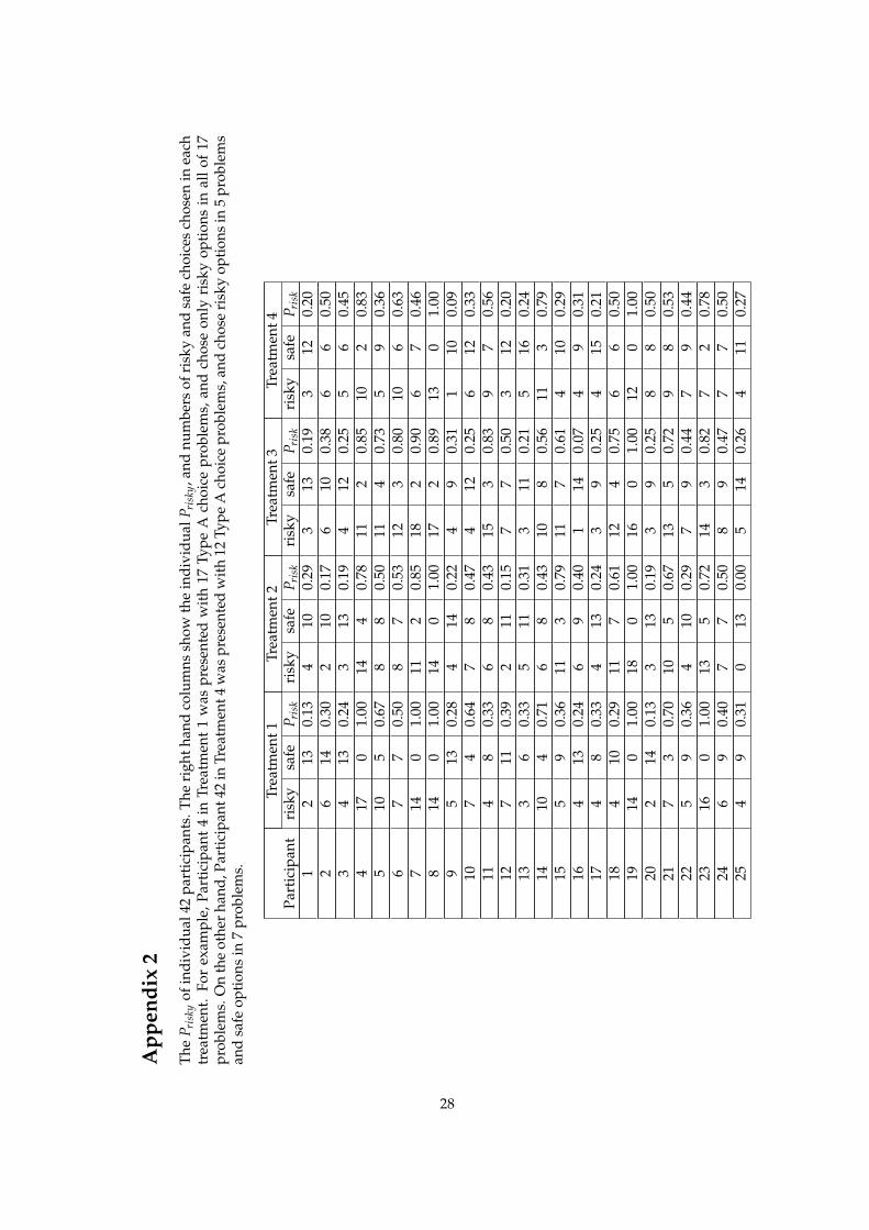
App

endi

x2

The

P ris

kyof

indi

vidu

al42

part

icip

ants

.The

righ

than

dco

lum

nssh

owth

ein

divi

dual

P ris

ky,a

ndnu

mbe

rsof

risk

yan

dsa

fech

oice

sch

osen

inea

chtr

eatm

ent.

For

exam

ple,

Part

icip

ant

4in

Trea

tmen

t1

was

pres

ente

dw

ith

17Ty

peA

choi

cepr

oble

ms,

and

chos

eon

lyri

sky

opti

ons

inal

lof

17pr

oble

ms.

On

the

othe

rha

nd,P

arti

cipa

nt42

inTr

eatm

ent4

was

pres

ente

dw

ith

12Ty

peA

choi

cepr

oble

ms,

and

chos

eri

sky

opti

ons

in5

prob

lem

san

dsa

feop

tion

sin

7pr

oble

ms.

Trea

tmen

t1Tr

eatm

ent2

Trea

tmen

t3Tr

eatm

ent4

Part

icip

ant

risk

ysa

feP r

isk

risk

ysa

feP r

isk

risk

ysa

feP r

isk

risk

ysa

feP r

isk

12

130.

134

100.

293

130.

193

120.

202

614

0.30

210

0.17

610

0.38

66

0.50

34

130.

243

130.

194

120.

255

60.

454

170

1.00

144

0.78

112

0.85

102

0.83

510

50.

678

80.

5011

40.

735

90.

366

77

0.50

87

0.53

123

0.80

106

0.63

714

01.

0011

20.

8518

20.

906

70.

468

140

1.00

140

1.00

172

0.89

130

1.00

95

130.

284

140.

224

90.

311

100.

0910

74

0.64

78

0.47

412

0.25

612

0.33

114

80.

336

80.

4315

30.

839

70.

5612

711

0.39

211

0.15

77

0.50

312

0.20

133

60.

335

110.

313

110.

215

160.

2414

104

0.71

68

0.43

108

0.56

113

0.79

155

90.

3611

30.

7911

70.

614

100.

2916

413

0.24

69

0.40

114

0.07

49

0.31

174

80.

334

130.

243

90.

254

150.

2118

410

0.29

117

0.61

124

0.75

66

0.50

1914

01.

0018

01.

0016

01.

0012

01.

0020

214

0.13

313

0.19

39

0.25

88

0.50

217

30.

7010

50.

6713

50.

729

80.

5322

59

0.36

410

0.29

79

0.44

79

0.44

2316

01.

0013

50.

7214

30.

827

20.

7824

69

0.40

77

0.50

89

0.47

77

0.50

254

90.

310

130.

005

140.

264

110.

27

28

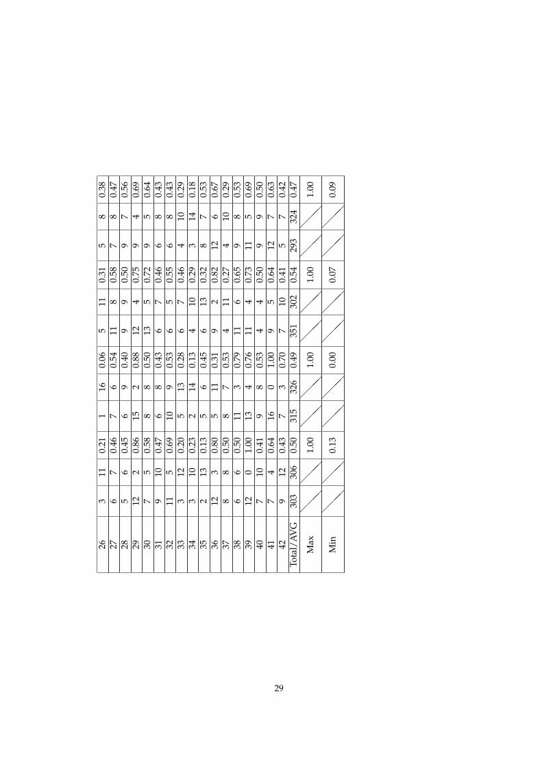
263

110.

211

160.

065

110.

315

80.

3827

67

0.46

76

0.54

118

0.58

78

0.47

285

60.

456

90.

409

90.

509

70.

5629

122

0.86

152

0.88

124

0.75

94

0.69

307

50.

588

80.

5013

50.

729

50.

6431

910

0.47

68

0.43

67

0.46

68

0.43

3211

50.

6910

90.

536

50.

556

80.

4333

312

0.20

513

0.28

67

0.46

410

0.29

343

100.

232

140.

134

100.

293

140.

1835

213

0.13

56

0.45

613

0.32

87

0.53

3612

30.

805

110.

319

20.

8212

60.

6737

88

0.50

87

0.53

411

0.27

410

0.29

386

60.

5011

30.

7911

60.

659

80.

5339

120

1.00

134

0.76

114

0.73

115

0.69

407

100.

419

80.

534

40.

509

90.

5041

74

0.64

160

1.00

95

0.64

127

0.63

429

120.

437

30.

707

100.

415

70.

42To

tal/

AV

G30

330

60.

5031

532

60.

4935

130

20.

5429

332

40.

47

Max

@@ @

@@ @

1.00

@@ @

@@ @

1.00

@@ @

@@ @

1.00

@@ @

@@ @

1.00

Min

@@ @

@@ @

0.13

@@ @

@@ @

0.00

@@ @

@@ @

0.07

@@ @

@@ @

0.09

29

App

endi

x3

The

P soo

ner

ofin

divi

dual

42pa

rtic

ipan

ts.

The

righ

tha

ndco

lum

nssh

owth

ein

divi

dual

P soo

ner,

and

num

bers

ofso

oner

opti

ons

and

late

opti

ons

chos

enin

each

trea

tmen

t.Fo

rex

ampl

e,Pa

rtic

ipan

t17

inTr

eatm

ent

1w

aspr

esen

ted

wit

h16

Type

Bch

oice

prob

lem

s,an

dch

ose

soon

erop

tion

sin

11pr

oble

ms

and

late

rop

tion

sin

5pr

oble

ms.

On

the

othe

rha

nd,P

arti

cipa

nt34

inTr

eatm

ent3

was

pres

ente

dw

ith

13Ty

peB

choi

cepr

oble

ms,

and

chos

eso

oner

opti

ons

only

in2

prob

lem

s.

Trea

tmen

t1Tr

eatm

ent2

Trea

tmen

t3Tr

eatm

ent4

Part

icip

ant

soon

erla

ter

P soo

ner

soon

erla

ter

P soo

ner

soon

erla

ter

P soo

ner

soon

erla

ter

P soo

ner

17

01.

0013

01.

008

10.

8910

10.

912

21

0.67

96

0.60

52

0.71

123

0.80

30

70.

000

80.

000

100.

000

150.

004

16

0.14

25

0.29

311

0.21

012

0.00

58

30.

735

30.

635

60.

456

40.

606

73

0.70

46

0.40

62

0.75

48

0.33

711

10.

926

20.

757

01.

0011

20.

858

011

0.00

09

0.00

27

0.22

011

0.00

95

20.

718

10.

8914

10.

938

10.

8910

131

0.93

80

1.00

82

0.80

62

0.75

119

10.

908

40.

676

40.

604

40.

5012

70

1.00

110

1.00

101

0.91

83

0.73

1313

10.

937

01.

009

10.

907

20.

7814

45

0.44

68

0.43

24

0.33

29

0.18

156

40.

6011

30.

795

10.

836

40.

6016

08

0.00

011

0.00

07

0.00

014

0.00

1711

50.

694

10.

8012

20.

865

01.

0018

47

0.36

63

0.67

34

0.43

58

0.38

191

100.

090

90.

001

60.

140

130.

0020

53

0.63

46

0.40

74

0.64

92

0.82

218

50.

626

30.

678

01.

008

20.

8022

57

0.42

57

0.42

53

0.63

44

0.50

235

20.

718

01.

0012

01.

0011

20.

8524

82

0.80

91

0.90

110

1.00

81

0.89

258

20.

805

90.

363

20.

604

70.

36

30

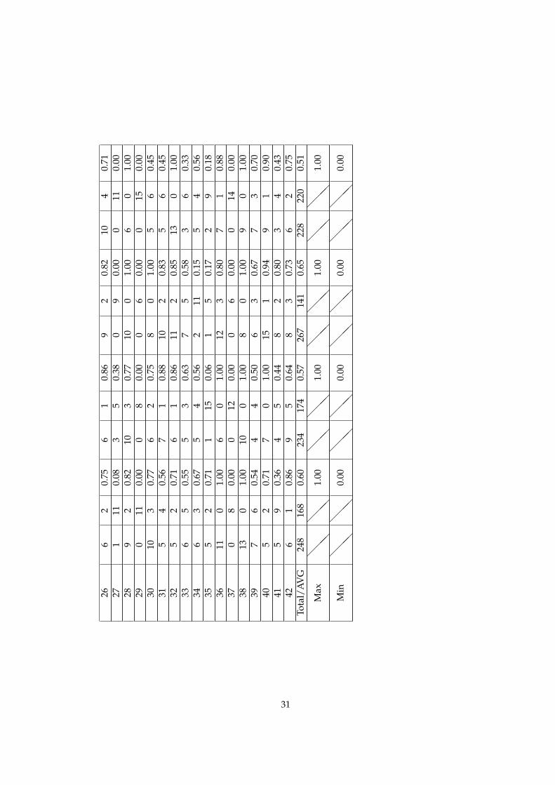
266

20.

756

10.

869

20.

8210

40.

7127

111

0.08

35

0.38

09

0.00

011

0.00

289

20.

8210

30.

7710

01.

006

01.

0029

011

0.00

08

0.00

06

0.00

015

0.00

3010

30.

776

20.

758

01.

005

60.

4531

54

0.56

71

0.88

102

0.83

56

0.45

325

20.

716

10.

8611

20.

8513

01.

0033

65

0.55

53

0.63

75

0.58

36

0.33

346

30.

675

40.

562

110.

155

40.

5635

52

0.71

115

0.06

15

0.17

29

0.18

3611

01.

006

01.

0012

30.

807

10.

8837

08

0.00

012

0.00

06

0.00

014

0.00

3813

01.

0010

01.

008

01.

009

01.

0039

76

0.54

44

0.50

63

0.67

73

0.70

405

20.

717

01.

0015

10.

949

10.

9041

59

0.36

45

0.44

82

0.80

34

0.43

426

10.

869

50.

648

30.

736

20.

75To

tal/

AV

G24

816

80.

6023

417

40.

5726

714

10.

6522

822

00.

51

Max

@@ @

@@ @

1.00

@@ @

@@ @

1.00

@@ @

@@ @

1.00

@@ @

@@ @

1.00

Min

@@ @

@@ @

0.00

@@ @

@@ @

0.00

@@ @

@@ @

0.00

@@ @

@@ @

0.00

31

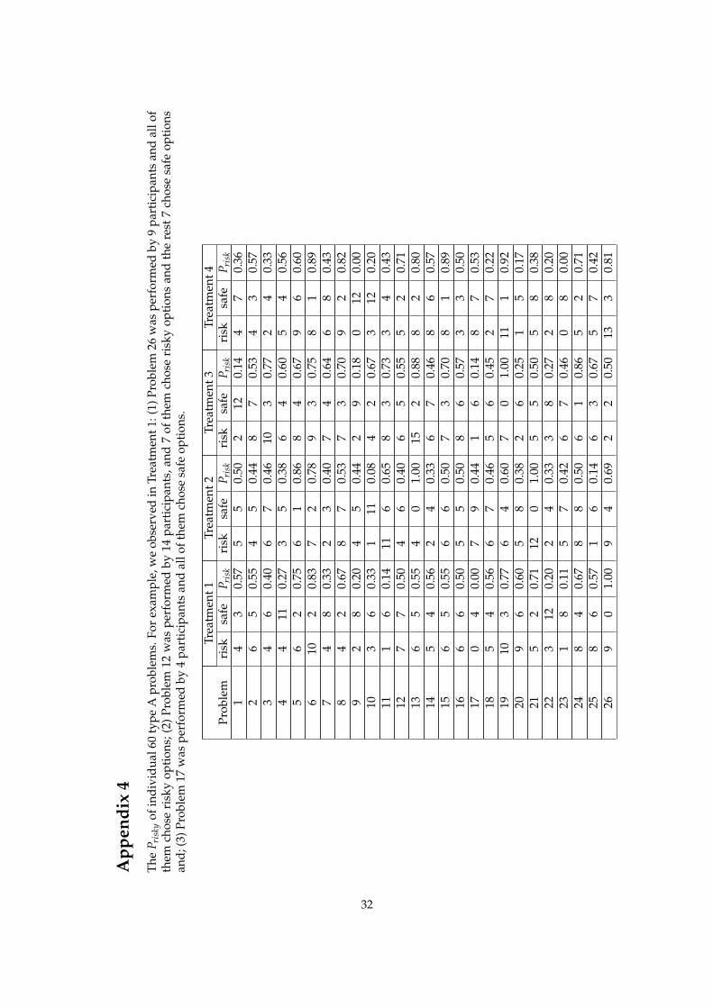
App

endi

x4

The

P ris

kyof

indi

vidu

al60

type

Apr

oble

ms.

For

exam

ple,

we

obse

rved

inTr

eatm

ent1

:(1)

Prob

lem

26w

aspe

rfor

med

by9

part

icip

ants

and

allo

fth

emch

ose

risk

yop

tion

s;(2

)Pr

oble

m12

was

perf

orm

edby

14pa

rtic

ipan

ts,a

nd7

ofth

emch

ose

risk

yop

tion

san

dth

ere

st7

chos

esa

feop

tion

san

d;(3

)Pro

blem

17w

aspe

rfor

med

by4

part

icip

ants

and

allo

fthe

mch

ose

safe

opti

ons.

Trea

tmen

t1Tr

eatm

ent2

Trea

tmen

t3Tr

eatm

ent4

Prob

lem

risk

safe

P ris

kri

sksa

feP r

isk

risk

safe

P ris

kri

sksa

feP r

isk

14

30.

575

50.

502

120.

144

70.

362

65

0.55

45

0.44

87

0.53

43

0.57

34

60.

406

70.

4610

30.

772

40.

334

411

0.27

35

0.38

64

0.60

54

0.56

56

20.

756

10.

868

40.

679

60.

606

102

0.83

72

0.78

93

0.75

81

0.89

74

80.

332

30.

407

40.

646

80.

438

42

0.67

87

0.53

73

0.70

92

0.82

92

80.

204

50.

442

90.

180

120.

0010

36

0.33

111

0.08

42

0.67

312

0.20

111

60.

1411

60.

658

30.

733

40.

4312

77

0.50

46

0.40

65

0.55

52

0.71

136

50.

554

01.

0015

20.

888

20.

8014

54

0.56

24

0.33

67

0.46

86

0.57

156

50.

556

60.

507

30.

708

10.

8916

66

0.50

55

0.50

86

0.57

33

0.50

170

40.

007

90.

441

60.

148

70.

5318

54

0.56

67

0.46

56

0.45

27

0.22

1910

30.

776

40.

607

01.

0011

10.

9220

96

0.60

58

0.38

26

0.25

15

0.17

215

20.

7112

01.

005

50.

505

80.

3822

312

0.20

24

0.33

38

0.27

28

0.20

231

80.

115

70.

426

70.

460

80.

0024

84

0.67

88

0.50

61

0.86

52

0.71

258

60.

571

60.

146

30.

675

70.

4226

90

1.00

94

0.69

22

0.50

133

0.81

32

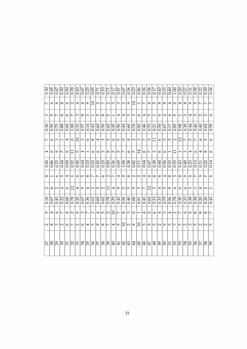
272

90.

182

80.

204

70.

363

70.

3028

84

0.67

61

0.86

66

0.50

56

0.45

293

40.

432

60.

259

30.

757

80.

4730

27

0.22

45

0.44

71

0.88

88

0.50

316

40.

606

40.

606

40.

606

60.

5032

72

0.78

121

0.92

110

1.00

72

0.78

332

80.

204

60.

405

100.

333

40.

4334

63

0.67

95

0.64

43

0.57

84

0.67

354

70.

364

80.

331

60.

143

90.

2536

53

0.63

27

0.22

68

0.43

110

0.09

379

40.

695

70.

426

40.

605

20.

7138

85

0.62

26

0.25

33

0.50

87

0.53

397

20.

7811

20.

858

50.

625

20.

7140

410

0.29

47

0.36

56

0.45

15

0.17

415

70.

429

40.

695

50.

504

30.

5742

108

0.56

20

1.00

79

0.44

42

0.67

432

30.

405

80.

386

40.

605

90.

3644

90

1.00

92

0.82

72

0.78

310

0.23

4510

10.

915

20.

7114

30.

826

10.

8646

34

0.43

74

0.64

67

0.46

47

0.36

473

20.

6012

60.

677

30.

705

40.

5648

36

0.33

58

0.38

311

0.21

15

0.17

492

40.

334

60.

406

60.

506

80.

4350

93

0.75

54

0.56

63

0.67

48

0.33

515

40.

569

80.

531

50.

176

40.

6052

72

0.78

65

0.55

112

0.85

90

1.00

533

70.

306

80.

431

120.

081

40.

2054

24

0.33

69

0.40

37

0.30

38

0.27

553

50.

383

90.

254

50.

444

90.

3156

58

0.38

17

0.13

67

0.46

35

0.38

572

80.

204

90.

314

60.

402

70.

2258

28

0.20

27

0.22

85

0.62

37

0.30

595

70.

421

60.

146

60.

504

70.

36

33

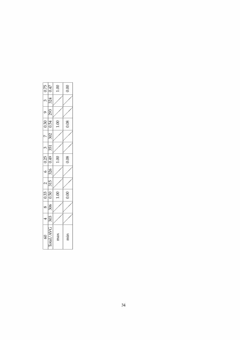
604

80.

332

60.

253

70.

309

30.

75To

tal/

AV

G30

330

60.

5031

532

60.

4935

130

20.

5429

332

40.

47

max

@@ @

@@ @

1.00

@@ @

@@ @

1.00

@@ @

@@ @

1.00

@@ @

@@ @

1.00

min

@@ @

@@ @

0.00

@@ @

@@ @

0.08

@@ @

@@ @

0.08

@@ @

@@ @

0.00

34

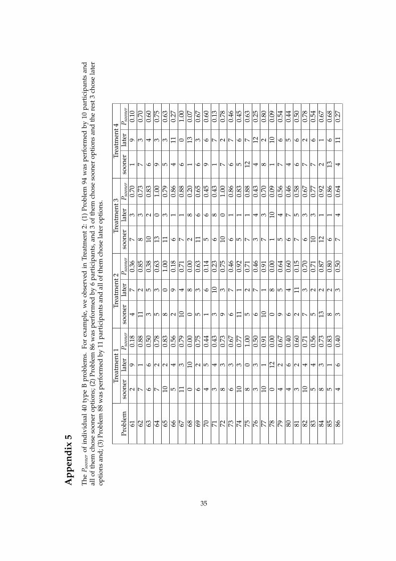
App

endi

x5

The

P soo

ner

ofin

divi

dual

40ty

peB

prob

lem

s.Fo

rex

ampl

e,w

eob

serv

edin

Trea

tmen

t2:

(1)

Prob

lem

94w

aspe

rfor

med

by10

part

icip

ants

and

allo

fthe

mch

ose

soon

erop

tion

s;(2

)Pro

blem

86w

aspe

rfor

med

by6

part

icip

ants

,and

3of

them

chos

eso

oner

opti

ons

and

the

rest

3ch

ose

late

rop

tion

san

d;(3

)Pro

blem

88w

aspe

rfor

med

by11

part

icip

ants

and

allo

fthe

mch

ose

late

rop

tion

s.

Trea

tmen

t1Tr

eatm

ent2

Trea

tmen

t3Tr

eatm

ent4

Prob

lem

soon

erla

ter

P soo

ner

soon

erla

ter

P soo

ner

soon

erla

ter

P soo

ner

soon

erla

ter

P soo

ner

612

90.

184

70.

367

30.

701

90.

1062

71

0.88

112

0.85

83

0.73

73

0.70

636

60.

503

50.

3810

20.

836

40.

6064

72

0.78

53

0.63

130

1.00

93

0.75

6510

20.

838

01.

0011

30.

795

30.

6366

54

0.56

29

0.18

61

0.86

411

0.27

6711

30.

7910

40.

717

10.

886

01.

0068

010

0.00

08

0.00

28

0.20

113

0.07

696

20.

755

30.

6311

60.

656

30.

6770

45

0.44

16

0.14

56

0.45

96

0.60

713

40.

433

100.

236

80.

431

70.

1372

83

0.73

93

0.75

100

1.00

72

0.78

736

30.

676

70.

466

10.

866

70.

4674

103

0.77

111

0.92

51

0.83

56

0.45

758

01.

005

20.

717

10.

8812

70.

6376

33

0.50

67

0.46

34

0.43

412

0.25

7710

10.

9110

10.

917

30.

708

20.

8078

012

0.00

08

0.00

110

0.09

110

0.09

794

20.

679

50.

645

40.

567

60.

5480

46

0.40

64

0.60

67

0.46

45

0.44

813

20.

602

110.

157

50.

586

60.

5082

104

0.71

73

0.70

63

0.67

72

0.78

835

40.

565

20.

7110

30.

777

60.

5484

83

0.73

132

0.87

121

0.92

21

0.67

855

10.

838

20.

806

10.

8613

60.

6886

46

0.40

33

0.50

74

0.64

411

0.27

35

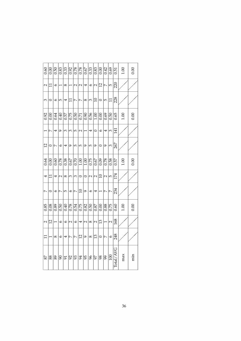
8711

20.

857

40.

6412

10.

923

20.

6088

112

0.08

011

0.00

07

0.00

011

0.00

898

10.

896

40.

607

40.

646

60.

5090

66

0.50

72

0.78

69

0.40

51

0.83

914

60.

405

80.

384

30.

574

80.

3392

72

0.78

63

0.67

93

0.75

111

0.92

937

60.

547

30.

705

50.

507

20.

7894

124

0.75

100

1.00

52

0.71

72

0.78

959

20.

829

01.

009

10.

908

40.

6796

88

0.50

62

0.75

54

0.56

36

0.33

9713

20.

874

20.

679

01.

0010

20.

8398

013

0.00

110

0.09

06

0.00

012

0.00

997

10.

887

20.

789

40.

695

70.

4210

06

20.

757

50.

583

30.

5011

50.

69To

tal/

AV

G24

816

80.

6023

417

40.

5726

714

10.

6522

822

00.

51

max

@@ @

@@ @

1.00

@@ @

@@ @

1.00

@@ @

@@ @

1.00

@@ @

@@ @

1.00

min

@@ @

@@ @

0.00

@@ @

@@ @

0.00

@@ @

@@ @

0.00

@@ @

@@ @

0.00

36