Musical Sound Effects: Analog and Digital Sound Processing
365
-
Upload
khangminh22 -
Category
Documents
-
view
0 -
download
0
Transcript of Musical Sound Effects: Analog and Digital Sound Processing


Musical Sound Effects

Musical Sound Effects
Analog and Digital Sound Processing
Jean-Michel Réveillac

First published 2018 in Great Britain and the United States by ISTE Ltd and John Wiley & Sons, Inc.
Apart from any fair dealing for the purposes of research or private study, or criticism or review, as permitted under the Copyright, Designs and Patents Act 1988, this publication may only be reproduced, stored or transmitted, in any form or by any means, with the prior permission in writing of the publishers, or in the case of reprographic reproduction in accordance with the terms and licenses issued by the CLA. Enquiries concerning reproduction outside these terms should be sent to the publishers at the undermentioned address:
ISTE Ltd John Wiley & Sons, Inc. 27-37 St George’s Road 111 River Street London SW19 4EU Hoboken, NJ 07030 UK USA
www.iste.co.uk www.wiley.com
© ISTE Ltd 2018 The rights of Jean-Michel Réveillac to be identified as the author of this work have been asserted by him in accordance with the Copyright, Designs and Patents Act 1988.
Library of Congress Control Number: 2017954678 British Library Cataloguing-in-Publication Data A CIP record for this book is available from the British Library ISBN 978-1-78630-131-4
Contents
Foreword . . . . . . . . . . . . . . . . . . . . . . . . . . . . . . . . . . . . . . . . . xi
About this Book . . . . . . . . . . . . . . . . . . . . . . . . . . . . . . . . . . . . xiii
Introduction . . . . . . . . . . . . . . . . . . . . . . . . . . . . . . . . . . . . . . . xvii
Chapter 1. Notes on the Theory of Sound . . . . . . . . . . . . . . . . . . 1 1.1. Basic concepts . . . . . . . . . . . . . . . . . . . . . . . . . . . . . . . . . . 1
1.1.1. What is sound? . . . . . . . . . . . . . . . . . . . . . . . . . . . . . . . 1 1.1.2. Intensity . . . . . . . . . . . . . . . . . . . . . . . . . . . . . . . . . . . 4 1.1.3. Sound pitch . . . . . . . . . . . . . . . . . . . . . . . . . . . . . . . . . 7 1.1.4. Approaching the concept of timbre . . . . . . . . . . . . . . . . . . . 8
1.2. The ears . . . . . . . . . . . . . . . . . . . . . . . . . . . . . . . . . . . . . . 9 1.2.1. How our ears work . . . . . . . . . . . . . . . . . . . . . . . . . . . . . 9 1.2.2. Fletcher–Munson curves . . . . . . . . . . . . . . . . . . . . . . . . . . 14 1.2.3. Auditory spatial awareness . . . . . . . . . . . . . . . . . . . . . . . . 15
1.3. The typology of sounds . . . . . . . . . . . . . . . . . . . . . . . . . . . . . 21 1.3.1. Sounds and periods . . . . . . . . . . . . . . . . . . . . . . . . . . . . . 21 1.3.2. Simple sounds and complex sounds . . . . . . . . . . . . . . . . . . . 22
1.4. Spectral analysis . . . . . . . . . . . . . . . . . . . . . . . . . . . . . . . . . 24 1.4.1. The sound spectrum . . . . . . . . . . . . . . . . . . . . . . . . . . . . 24 1.4.2. Sonogram and spectrogram . . . . . . . . . . . . . . . . . . . . . . . . 26
1.5. Timbre . . . . . . . . . . . . . . . . . . . . . . . . . . . . . . . . . . . . . . . 27 1.5.1. Transient phenomena . . . . . . . . . . . . . . . . . . . . . . . . . . . 27 1.5.2. Range . . . . . . . . . . . . . . . . . . . . . . . . . . . . . . . . . . . . . 28 1.5.3. Mass of musical objects . . . . . . . . . . . . . . . . . . . . . . . . . . 30 1.5.4. Classification of sounds . . . . . . . . . . . . . . . . . . . . . . . . . . 31
1.6. Sound propagation . . . . . . . . . . . . . . . . . . . . . . . . . . . . . . . . 32 1.6.1. Dispersion . . . . . . . . . . . . . . . . . . . . . . . . . . . . . . . . . . 32

vi Musical Sound Effects
1.6.2. Interference . . . . . . . . . . . . . . . . . . . . . . . . . . . . . . . . . 33 1.6.3. Diffraction . . . . . . . . . . . . . . . . . . . . . . . . . . . . . . . . . . 35 1.6.4. Reflection . . . . . . . . . . . . . . . . . . . . . . . . . . . . . . . . . . 37 1.6.5. Reverberation (reverb) . . . . . . . . . . . . . . . . . . . . . . . . . . . 39 1.6.6. Absorption . . . . . . . . . . . . . . . . . . . . . . . . . . . . . . . . . . 39 1.6.7. Refraction . . . . . . . . . . . . . . . . . . . . . . . . . . . . . . . . . . 39 1.6.8. The Doppler effect . . . . . . . . . . . . . . . . . . . . . . . . . . . . . 40 1.6.9. Beats . . . . . . . . . . . . . . . . . . . . . . . . . . . . . . . . . . . . . 40
1.7. Conclusion . . . . . . . . . . . . . . . . . . . . . . . . . . . . . . . . . . . . 41
Chapter 2. Audio Playback . . . . . . . . . . . . . . . . . . . . . . . . . . . . . 43 2.1. History . . . . . . . . . . . . . . . . . . . . . . . . . . . . . . . . . . . . . . . 44 2.2. Dolby playback standards and specifications . . . . . . . . . . . . . . . . 48
2.2.1. Dolby Surround encoding and decoding . . . . . . . . . . . . . . . . 48 2.2.2. Dolby Stereo . . . . . . . . . . . . . . . . . . . . . . . . . . . . . . . . . 49 2.2.3. Dolby Surround . . . . . . . . . . . . . . . . . . . . . . . . . . . . . . . 50 2.2.4. Dolby Surround Pro-Logic . . . . . . . . . . . . . . . . . . . . . . . . 50 2.2.5. Dolby DIGITAL AC-3 . . . . . . . . . . . . . . . . . . . . . . . . . . . 51 2.2.6. Dolby Surround EX . . . . . . . . . . . . . . . . . . . . . . . . . . . . 52 2.2.7. Dolby Surround Pro-Logic II . . . . . . . . . . . . . . . . . . . . . . . 52 2.2.8. Dolby Digital Plus . . . . . . . . . . . . . . . . . . . . . . . . . . . . . 54 2.2.9. Dolby TrueHD . . . . . . . . . . . . . . . . . . . . . . . . . . . . . . . 54 2.2.10. Dolby Atmos . . . . . . . . . . . . . . . . . . . . . . . . . . . . . . . . 55
2.3. DTS encodings . . . . . . . . . . . . . . . . . . . . . . . . . . . . . . . . . . 55 2.3.1. DTS . . . . . . . . . . . . . . . . . . . . . . . . . . . . . . . . . . . . . . 56 2.3.2. DTS Neo 6 . . . . . . . . . . . . . . . . . . . . . . . . . . . . . . . . . . 56 2.3.3. DTS ES 6.1 . . . . . . . . . . . . . . . . . . . . . . . . . . . . . . . . . 57 2.3.4. DTS 96/24 . . . . . . . . . . . . . . . . . . . . . . . . . . . . . . . . . . 57 2.3.5. DTS HD Master Audio . . . . . . . . . . . . . . . . . . . . . . . . . . 57 2.3.6. DTS X . . . . . . . . . . . . . . . . . . . . . . . . . . . . . . . . . . . . 58
2.4. Special encodings . . . . . . . . . . . . . . . . . . . . . . . . . . . . . . . . 58 2.5. SDDS . . . . . . . . . . . . . . . . . . . . . . . . . . . . . . . . . . . . . . . 59 2.6. THX certification . . . . . . . . . . . . . . . . . . . . . . . . . . . . . . . . 59
2.6.1. THX select and ultracertification . . . . . . . . . . . . . . . . . . . . . 61 2.6.2. THX Ultra 2 certification . . . . . . . . . . . . . . . . . . . . . . . . . 61
2.7. Multichannel audio recording . . . . . . . . . . . . . . . . . . . . . . . . . 62 2.8. Postproduction and encoding . . . . . . . . . . . . . . . . . . . . . . . . . 63 2.9. Multichannel music media: DVD-Audio and SACD . . . . . . . . . . . 65
2.9.1. DVD-Audio . . . . . . . . . . . . . . . . . . . . . . . . . . . . . . . . . 65 2.9.2. Super Audio CD . . . . . . . . . . . . . . . . . . . . . . . . . . . . . . 67 2.9.3. Comparison of CDs, SACDs and DVD-Audios . . . . . . . . . . . . 69
2.10. Conclusion . . . . . . . . . . . . . . . . . . . . . . . . . . . . . . . . . . . 69

Contents vii
Chapter 3. Types of Effect . . . . . . . . . . . . . . . . . . . . . . . . . . . . . 71 3.1. Physical appearance . . . . . . . . . . . . . . . . . . . . . . . . . . . . . . . 71
3.1.1. Racks . . . . . . . . . . . . . . . . . . . . . . . . . . . . . . . . . . . . . 72 3.1.2. Pedals . . . . . . . . . . . . . . . . . . . . . . . . . . . . . . . . . . . . . 74 3.1.3. Software plugins . . . . . . . . . . . . . . . . . . . . . . . . . . . . . . 77
3.2. Audio processing . . . . . . . . . . . . . . . . . . . . . . . . . . . . . . . . 78 3.3. Conclusion . . . . . . . . . . . . . . . . . . . . . . . . . . . . . . . . . . . . 80
Chapter 4. Filtering Effects . . . . . . . . . . . . . . . . . . . . . . . . . . . . 81 4.1. Families of filtering effects . . . . . . . . . . . . . . . . . . . . . . . . . . 81 4.2. Equalization . . . . . . . . . . . . . . . . . . . . . . . . . . . . . . . . . . . 84
4.2.1. Frequency bands and ranges . . . . . . . . . . . . . . . . . . . . . . . 84 4.2.2. Types of equalizer . . . . . . . . . . . . . . . . . . . . . . . . . . . . . 86 4.2.3. Examples of equalizers . . . . . . . . . . . . . . . . . . . . . . . . . . 91 4.2.4. Tips for equalizing a mix . . . . . . . . . . . . . . . . . . . . . . . . . 94
4.3. Wah-wah . . . . . . . . . . . . . . . . . . . . . . . . . . . . . . . . . . . . . 97 4.3.1. History . . . . . . . . . . . . . . . . . . . . . . . . . . . . . . . . . . . . 97 4.3.2. Theory . . . . . . . . . . . . . . . . . . . . . . . . . . . . . . . . . . . . 99 4.3.3. Auto-wah . . . . . . . . . . . . . . . . . . . . . . . . . . . . . . . . . . . 100 4.3.4. Examples of wah-wah pedals . . . . . . . . . . . . . . . . . . . . . . . 101
4.4. Crossover . . . . . . . . . . . . . . . . . . . . . . . . . . . . . . . . . . . . . 102 4.5. Conclusion . . . . . . . . . . . . . . . . . . . . . . . . . . . . . . . . . . . . 104
Chapter 5. Modulation Effects . . . . . . . . . . . . . . . . . . . . . . . . . . 105 5.1. Flanger . . . . . . . . . . . . . . . . . . . . . . . . . . . . . . . . . . . . . . 105
5.1.1. History . . . . . . . . . . . . . . . . . . . . . . . . . . . . . . . . . . . . 105 5.1.2. Theory and parameters . . . . . . . . . . . . . . . . . . . . . . . . . . . 107 5.1.3. Models of flanger . . . . . . . . . . . . . . . . . . . . . . . . . . . . . . 110
5.2. Phaser . . . . . . . . . . . . . . . . . . . . . . . . . . . . . . . . . . . . . . . 111 5.2.1. Examples of phasers . . . . . . . . . . . . . . . . . . . . . . . . . . . . 113
5.3. Chorus . . . . . . . . . . . . . . . . . . . . . . . . . . . . . . . . . . . . . . . 115 5.3.1. Examples of chorus . . . . . . . . . . . . . . . . . . . . . . . . . . . . . 116
5.4. Rotary, univibe or rotovibe. . . . . . . . . . . . . . . . . . . . . . . . . . . 117 5.4.1. History . . . . . . . . . . . . . . . . . . . . . . . . . . . . . . . . . . . . 118 5.4.2. Theoretical principles . . . . . . . . . . . . . . . . . . . . . . . . . . . 120 5.4.3. Leslie speakers . . . . . . . . . . . . . . . . . . . . . . . . . . . . . . . 122 5.4.4. Examples of rotary or univibe pedals . . . . . . . . . . . . . . . . . . 123 5.4.5. Leslie speakers and sound recording . . . . . . . . . . . . . . . . . . 125
5.5. Ring modulation . . . . . . . . . . . . . . . . . . . . . . . . . . . . . . . . . 127 5.5.1. Theoretical principles . . . . . . . . . . . . . . . . . . . . . . . . . . . 127 5.5.2. Examples of ring modulators . . . . . . . . . . . . . . . . . . . . . . . 129
5.6. Final remarks . . . . . . . . . . . . . . . . . . . . . . . . . . . . . . . . . . . 130

viii Musical Sound Effects
Chapter 6. Frequency Effects . . . . . . . . . . . . . . . . . . . . . . . . . . . 131 6.1. Vibrato . . . . . . . . . . . . . . . . . . . . . . . . . . . . . . . . . . . . . . 131
6.1.1. Theoretical principles . . . . . . . . . . . . . . . . . . . . . . . . . . . 132 6.1.2. Settings . . . . . . . . . . . . . . . . . . . . . . . . . . . . . . . . . . . . 132 6.1.3. Examples of vibrato . . . . . . . . . . . . . . . . . . . . . . . . . . . . 133
6.2. Transposers . . . . . . . . . . . . . . . . . . . . . . . . . . . . . . . . . . . . 135 6.2.1. Octaver . . . . . . . . . . . . . . . . . . . . . . . . . . . . . . . . . . . . 135 6.2.2. Pitch shifter . . . . . . . . . . . . . . . . . . . . . . . . . . . . . . . . . 137 6.2.3. Harmonizer . . . . . . . . . . . . . . . . . . . . . . . . . . . . . . . . . 139 6.2.4. Auto-Tune . . . . . . . . . . . . . . . . . . . . . . . . . . . . . . . . . . 142
6.3. Conclusion . . . . . . . . . . . . . . . . . . . . . . . . . . . . . . . . . . . . 154
Chapter 7. Dynamic Effects . . . . . . . . . . . . . . . . . . . . . . . . . . . . 155 7.1. Compression . . . . . . . . . . . . . . . . . . . . . . . . . . . . . . . . . . . 156
7.1.1. History . . . . . . . . . . . . . . . . . . . . . . . . . . . . . . . . . . . . 156 7.1.2. Parameters of compression . . . . . . . . . . . . . . . . . . . . . . . . 156 7.1.3. Examples of compressors . . . . . . . . . . . . . . . . . . . . . . . . . 163 7.1.4. Multiband compressors . . . . . . . . . . . . . . . . . . . . . . . . . . 166 7.1.5. Guidelines for configuring a compressor . . . . . . . . . . . . . . . . 169 7.1.6. Parallel compression . . . . . . . . . . . . . . . . . . . . . . . . . . . . 170 7.1.7. Serial compression . . . . . . . . . . . . . . . . . . . . . . . . . . . . . 171 7.1.8. Compression with a sidechain . . . . . . . . . . . . . . . . . . . . . . 171 7.1.9. Some basic compression settings . . . . . . . . . . . . . . . . . . . . . 172 7.1.10. Synchronizing the compressor . . . . . . . . . . . . . . . . . . . . . 175 7.1.11. Using a compressor as a limiter . . . . . . . . . . . . . . . . . . . . . 175
7.2. Expanders . . . . . . . . . . . . . . . . . . . . . . . . . . . . . . . . . . . . . 178 7.2.1. Parameters . . . . . . . . . . . . . . . . . . . . . . . . . . . . . . . . . . 178 7.2.2. Examples of software expanders . . . . . . . . . . . . . . . . . . . . . 179
7.3. Noise gates . . . . . . . . . . . . . . . . . . . . . . . . . . . . . . . . . . . . 180 7.3.1. Parameters . . . . . . . . . . . . . . . . . . . . . . . . . . . . . . . . . . 180 7.3.2. Examples of noise gates . . . . . . . . . . . . . . . . . . . . . . . . . . 182 7.3.3. Configuring noise gates . . . . . . . . . . . . . . . . . . . . . . . . . . 184
7.4. De-essers . . . . . . . . . . . . . . . . . . . . . . . . . . . . . . . . . . . . . 184 7.4.1. Principle of a de-esser . . . . . . . . . . . . . . . . . . . . . . . . . . . 184 7.4.2. Examples of de-essers . . . . . . . . . . . . . . . . . . . . . . . . . . . 185 7.4.3. Replacing a de-esser with an equalizer and a compressor . . . . . . 186 7.4.4. Configuring a de-esser . . . . . . . . . . . . . . . . . . . . . . . . . . . 186
7.5. Saturation . . . . . . . . . . . . . . . . . . . . . . . . . . . . . . . . . . . . . 187 7.5.1. Fuzz . . . . . . . . . . . . . . . . . . . . . . . . . . . . . . . . . . . . . 187 7.5.2. Overdrive. . . . . . . . . . . . . . . . . . . . . . . . . . . . . . . . . . . 188 7.5.3. Distortion. . . . . . . . . . . . . . . . . . . . . . . . . . . . . . . . . . . 188 7.5.4. Examples of equipment dedicated to creating saturation . . . . . . . 189
Contents ix
7.6. Exciters and enhancers . . . . . . . . . . . . . . . . . . . . . . . . . . . . . 192 7.6.1. Examples of exciters . . . . . . . . . . . . . . . . . . . . . . . . . . . . 193 7.6.2. Using a sound enhancer . . . . . . . . . . . . . . . . . . . . . . . . . . 195
7.7. Conclusion . . . . . . . . . . . . . . . . . . . . . . . . . . . . . . . . . . . . 195
Chapter 8. Time Effects . . . . . . . . . . . . . . . . . . . . . . . . . . . . . . . 197 8.1. Reverb . . . . . . . . . . . . . . . . . . . . . . . . . . . . . . . . . . . . . . . 197
8.1.1. Theoretical principles . . . . . . . . . . . . . . . . . . . . . . . . . . . 197 8.1.2. History . . . . . . . . . . . . . . . . . . . . . . . . . . . . . . . . . . . . 200 8.1.3. Principles . . . . . . . . . . . . . . . . . . . . . . . . . . . . . . . . . . . 208 8.1.4. Reverb configuration . . . . . . . . . . . . . . . . . . . . . . . . . . . . 219 8.1.5. Recording the IR and deconvolution . . . . . . . . . . . . . . . . . . 227 8.1.6. Studio mixing and reverb . . . . . . . . . . . . . . . . . . . . . . . . . 240
8.2. Delay . . . . . . . . . . . . . . . . . . . . . . . . . . . . . . . . . . . . . . . 243 8.2.1. History . . . . . . . . . . . . . . . . . . . . . . . . . . . . . . . . . . . . 243 8.2.2. Types of delay . . . . . . . . . . . . . . . . . . . . . . . . . . . . . . . . 244 8.2.3. Tips for using delays in the studio . . . . . . . . . . . . . . . . . . . . 251
8.3. Conclusion . . . . . . . . . . . . . . . . . . . . . . . . . . . . . . . . . . . . 255
Chapter 9. Unclassifiables . . . . . . . . . . . . . . . . . . . . . . . . . . . . . 257 9.1. Combined effects . . . . . . . . . . . . . . . . . . . . . . . . . . . . . . . . 257
9.1.1. Fuzzwha . . . . . . . . . . . . . . . . . . . . . . . . . . . . . . . . . . . 257 9.1.2. Octafuzz . . . . . . . . . . . . . . . . . . . . . . . . . . . . . . . . . . . 258 9.1.3. Shimmer . . . . . . . . . . . . . . . . . . . . . . . . . . . . . . . . . . . 259
9.2. Tremolo . . . . . . . . . . . . . . . . . . . . . . . . . . . . . . . . . . . . . . 262 9.2.1. History . . . . . . . . . . . . . . . . . . . . . . . . . . . . . . . . . . . . 262 9.2.2. Examples of tremolos . . . . . . . . . . . . . . . . . . . . . . . . . . . 264
9.3. Sound restoration tools . . . . . . . . . . . . . . . . . . . . . . . . . . . . . 266 9.3.1. Declickers . . . . . . . . . . . . . . . . . . . . . . . . . . . . . . . . . . 266 9.3.2. Decracklers . . . . . . . . . . . . . . . . . . . . . . . . . . . . . . . . . 267 9.3.3. Denoisers . . . . . . . . . . . . . . . . . . . . . . . . . . . . . . . . . . . 267 9.3.4. Declippers . . . . . . . . . . . . . . . . . . . . . . . . . . . . . . . . . . 267 9.3.5. Debuzzers . . . . . . . . . . . . . . . . . . . . . . . . . . . . . . . . . . 268 9.3.6. Examples of restoration tools . . . . . . . . . . . . . . . . . . . . . . . 268 9.3.7. Final remarks on sound restoration . . . . . . . . . . . . . . . . . . . 271
9.4. Loopers . . . . . . . . . . . . . . . . . . . . . . . . . . . . . . . . . . . . . . 271 9.4.1. Looper connections . . . . . . . . . . . . . . . . . . . . . . . . . . . . . 272 9.4.2. Examples of looper pedals . . . . . . . . . . . . . . . . . . . . . . . . 274
9.5. Time stretching. . . . . . . . . . . . . . . . . . . . . . . . . . . . . . . . . . 275 9.6. Resampling . . . . . . . . . . . . . . . . . . . . . . . . . . . . . . . . . . . . 276 9.7. Spatialization effects . . . . . . . . . . . . . . . . . . . . . . . . . . . . . . 277 9.8. Conclusion . . . . . . . . . . . . . . . . . . . . . . . . . . . . . . . . . . . . 278

x Musical Sound Effects
Conclusion . . . . . . . . . . . . . . . . . . . . . . . . . . . . . . . . . . . . . . . . 279
Appendices . . . . . . . . . . . . . . . . . . . . . . . . . . . . . . . . . . . . . . . 283
Appendix 1 . . . . . . . . . . . . . . . . . . . . . . . . . . . . . . . . . . . . . . . . 285
Appendix 2 . . . . . . . . . . . . . . . . . . . . . . . . . . . . . . . . . . . . . . . . 295
Appendix 3 . . . . . . . . . . . . . . . . . . . . . . . . . . . . . . . . . . . . . . . . 299
Appendix 4 . . . . . . . . . . . . . . . . . . . . . . . . . . . . . . . . . . . . . . . . 313
Glossary . . . . . . . . . . . . . . . . . . . . . . . . . . . . . . . . . . . . . . . . . 319
Bibliography . . . . . . . . . . . . . . . . . . . . . . . . . . . . . . . . . . . . . . 327
Index . . . . . . . . . . . . . . . . . . . . . . . . . . . . . . . . . . . . . . . . . . . . 337

Foreword
What will music look like in the future?
If you are wondering about the building blocks of the music of tomorrow, or if you wish to understand them, this book will prove a valuable “toolbox”. Jean Michel Réveillac introduces us to the myriad of sounds effects of the world of music. He weaves implicit threads between the art of sound and the history of science, allowing us to appreciate how digital effects influence the typology and morphology of physical waves.
The materials that will be used by the sound architects of our future are playback images, colors, matter and expressions. The possibilities of sound effect processing afford a glimpse into a universe of infinite and unsuspected dimensions of human hearing. By chronologically and thematically exploring these physical phenomena, Jean Michel Réveillac not only reveals the path, but delicately retraces the resources and techniques of the scientific, philosophical and sociological tradition in which the history of these technologies is steeped. The transmitted codes of electronic music have made space for sound objects, creating a certain anatomy of sound, and many other musical movements have also drawn inspiration from various applied effects.
The breakthrough transition to a fully digital world is uprooting the traditions of analog processing. The increasing capabilities of DAWs1 and 5.1 multichannel mixing are challenging the old trades and customs of applied effects. Music itself is a canvas for composers to shape according to their desires of expression by sound narration, and digital audio tools are a palette for virtual modeling. Today, sound occupies a permanent place within our environment. Jean Michel Réveillac revisits the original historical approaches enriched with the knowledge of digital audio 1 Digital Audio Workstations.
xii Musical Sound Effects
processing. By broadening its field of investigation, the history of sound effects has carved its role in how we understand the challenges of modern sound. This book upholds the quality of its scientific roots and the relevance of its forays into audio research. After exploring the wealth of knowledge on musical processing present in this book, we are left with no doubt that a summary of modern research into the history of sound effects was sorely needed.
As if set in stone, the chosen approach conveys the timelessness of mixing techniques and colors, forging an eternal record of the methodology of recent years. Leaving us with the feeling that this was just the beginning of a journey to the heart of a perpetually expanding culture. Many of the sound effects presented in this book are currently extremely popular, with multiple areas of application. Chapter by chapter, the singular vision of a constantly evolving landscape of audio effects gradually emerges. With great passion, the author retraces the greatest events in the history of sound effects and the key theoretical ideas that accompanied them, and offers his own thoughts on the origin of this universe that has drawn him ever deeper, as well as the impact and future of technological advancements that will allow everyone to leave their own mark on the evolution of sound.
Léo PAOLETTI “Leo Virgile”
Composer and audio designer

About this Book
If you are wondering whether this book is for you, how it is put together and organized, what it contains and which conventions we will use, you are in the right place. Everything will be explained here.
Target audience
This book is intended for anybody who is passionate about sound – amateurs or professionals who love sound recording, mixing or playback, and, of course, musicians, performers and composers.
The topics discussed in a few sections require some basic knowledge of the principles of general computing and digital audio.
You need to be familiar with operating systems (paths, folders and directories, files, filenames, file extensions, copying, dragging, etc.) and you need to know how to use a digital audio editor like Adobe Audition, Steinberg Wavelab, Magix Sound Forge, Audacity, etc., or a DAW (Digital Audio Workstation) such as Avid Pro Tools, Magix Samplitude, Sonar Cakewalk, Apple Logic Pro and so on.
Organization and contents
This book has nine chapters:
– Notes on the Theory of Sound;
– Audio Playback;
– Types of Effects;

xiv Musical Sound Effects
– Filtering Effects;
– Modulation Effects;
– Frequency Effects;
– Dynamic Effects;
– Time Effects;
– Unclassifiables.
Each of these chapters can be read separately. Some concepts depend on concepts from other chapters, but references are given wherever they are needed. The first chapter, dedicated to the theory of sound, is slightly different. It provides the basic foundations needed to understand each of the other chapters.
If you are new to the scene, I highly recommend reading the first chapter. The rest of the book will be easier to understand.
Even if you are not, it might still surprise you with a few new ideas.
The conclusion, unsurprisingly, attempts to give an overview of the current state of the world of sound effects, and how they might continue to develop in future.
Appendices 1–4 discuss a few extra ideas and reminders in the following order:
– Distortion;
– Classes of Amplifiers;
– Basics with Max/MSP;
– Multieffect Racks.
A bibliography and a list of Internet links can be found at the end of the book.
There is also a glossary explaining some of the logos, acronyms and terminology specific to sound effects, sound recording, mixing and playback.
Conventions
The following formatting conventions are used throughout the book:
– italics: indicates the first time that an important term is used. For example, this could be one of the words explained in the glossary at the end of the book, mathematical terms, comments, equations, formulas or variables;

About this Book xv
– (italics): terms written in languages other than English;
– CAPS: names of windows, icons, buttons, folders or directories, menus or submenus. This also includes elements, options or controls in the windows of a software program.
Additional remarks are identified by the keyword.
REMARK.– These comments supplement the explanations given in the main body of the text.
All figures and tables have explanatory captions.
Vocabulary and definitions
Like all specialized techniques, audio sound effects have their own vocabulary. Some of the words, acronyms, abbreviations, logos and proper nouns may not be familiar to all readers. The glossary mentioned earlier should help with these terms.
Acknowledgments
I would especially like to thank the team at ISTE and my editor, Chantal Ménascé, for placing their trust in me. I am greatly indebted to the composer and musician Léo Paoletti, known by his stage name “Leo Virgile,” for the time, attention and interest he has granted me, as well as for writing the foreword to this book.
Finally, I would like to thank my wife, Vanna, for never ceasing to support me as I wrote these pages.
Introduction
Sound effects have always fascinated me. I remember my amazement and disbelief as a child when I heard the sound of my voice echoing for the first time when hiking on a mountain in the Alps. How is this possible?
My father, who was with me at the time, tried to give me a simple explanation of the phenomenon, but I could not really understand what he meant, and for years it remained a mystery to me.
Maybe this was what triggered my passion for listening, observing and understanding how sounds drift and wander within their natural environments, later leading to my interest in how these sounds can be artificially processed.
Today, sound effects are most commonly used for shows, movies and musical production. With the proliferation of microcomputers and electronics, creating sound effects has never been easier. New tools and software can do things that we would have struggled to imagine just a few years ago.
The idea of this book arises from the many questions that people have asked me when they visit my studio, over the course of my university lectures, conferences and my frequent chaotic discussions with family and friends.
While wandering though environments focused on sound and real-time 3D for more than 30 years, I have encountered (and still encounter) a great many problems for which I have had to devise various solutions, some of which are better than others.
Before we begin, we should take a moment to review the modern state of the industry with a few definitions, observations and important historical facts.
xviii Musical Sound Effects
What is a sound effect?
Agreeing upon a definition is not easy, since the concept of sound effect can have several meanings. The first concepts that spring to mind are the very popular sound effects used in radio and movies to associate a certain motion, image, action, dialogue or commentary with a specific sound: an opening door, a galloping horse, the waves of the ocean, rain, a steam locomotive entering the station, car tires screeching on tarmac and so on.
This is the most common meaning of the term. Next, many people think of natural phenomena: echoes, the Doppler effect1, the rumbling of thunder, sound masking2, etc.
Third, it is music. Classically, we have the notion of tempo (adagio, allegro, vivace, etc.), as well as effects created by specific instrumental techniques (glissando, tremolo, vibrato, trills, etc.).
Finally, we have the idea on which this book is based. Namely, the analog and digital musical sound effects used in studio and live environments. The following definition is in my opinion the most insightful:
Generic term describing a modification of the sound parameters of a signal. It refers to techniques widely used in modern music (jazz, blues, rock, pop, etc.) to modify the original sound of an electrical or electronic instrument. The most common effects are: reverb, echo (delay), phasing, distortion, flanger, compression. Most modern recordings use the possibilities of sound effects in some form, either by means of expanders and multi-effect pedals, or by using an array of independent pedals. (www.musicmot.com)
If we had formulated the question more precisely and specifically, like: “What is an audio effect?”, we might have arrived at a different answer. Consider for instance the following two quotes:
Audio effects are analog or digital devices that are used to intentionally alter how a musical instrument or other audio source sounds. Effects can be subtle or extreme, and they can be used in live or recording situations. (blog.dubspot.com3)
1 The Doppler effect is a frequency shift phenomenon that occurs with mechanical waves (see section 5.4.2). 2 The practice of playing a sound, usually neutral or soft, to cover up unwanted noises and improve the feel of the sound quality in a location. 3 Music production and DJ school based in New York, Los Angeles, and online.

Introduction xix
Sound effects (or audio effects) are artificially created or enhanced sounds, or
sound processes used to emphasize artistic or other content of films, television shows, live performance, animation, video games, music, or other media. (Wikipedia)
With this definition of sound effects, one aspect is often important. Natural sound phenomena always unfold in real time, and of course the same is true for live performances. However, in studios, during postproduction, the notion of time suddenly becomes completely relative. Recorded audio signals do not fade over time.
The constraints are completely different, and real-time effects no longer have to play by the same rules.
When you are playing live music, you cannot go backwards in time; what is done is done. But in a studio, although listening and editing in real time can be more comfortable, you can always start again. Recorded tracks are not volatile, and even while you are still recording you can repeat anything you need to.
Let us now take a different approach, and consider the evolution of sound effects through history.
Our tale begins at the turn of the 20th Century4.
Of course, there had been plenty of interest in sound effects around the world before then, but this had been largely restricted to musical instruments and singing (percussion, xylophones, flutes, church organs, etc.) without any connection to advanced technology based on electricity, electromechanics or electronics, which did not yet exist.
As we mentioned earlier, the first sound effects were widely used on the radio to provide an acoustic background for serial programs, which were very popular in the early 1920s.
Once movies progressed from silent pictures to pictures with sound, the movie industry also started to play an important role in sound effects.
By the early 1930s, most studios could mix manual sound effects and prerecorded sounds.
4 Author’s note: The various effects mentioned here will be revisited, presented and explained in more detail in the chapters of this book.

xx Musical Sound Effects
The first magnetic recorder (called the Telegraphone) was invented by V. Poulsen5, who used a wire and later a steel ribbon. F. Pfleumer6 improved the design in 1928 by introducing a much more reliable recording medium, magnetic tape (paper tape or acetate and iron oxide), which gained prominence in the 1940s. This marked the beginning of the first usable recording devices.
Figure I.1. A replica of the “Telegraphone”, 1915–1918 (Gaylor Ewing collection) (source: museumofmagneticsoundrecording.org)
One of the first effects used in musical recordings was reverb, which was used as early as 1930, followed by the appearance of the tremolo effect, based on an invention by D. Leslie7, the creator of the famous speaker bearing his name.
The advent of analog electronics, first in the form of electronic tubes, then transistors, shook the musical world to its foundations, and sound effects began to take early recording studios by storm.
5 Valdemar Poulsen, 1869–1942, Danish engineer, inventor of the first magnetic recording device. 6 Fritz Pfleumer, 1848–1934, Austrian engineer, inventor of magnetic tape for sound recordings. 7 Donald Leslie, 1911–2004, inventor of the Leslie speaker, a mechanical and electronic amplification device originally designed for Hammond organs that creates a sound playback environment based on the Doppler effect.

Introduction xxi
The invention of magnetic tape recorders at around the same period created
significant added value, opening new doors and new horizons for technicians and musicians, notably including electronic music and concrete music.
One easily overlooked sound effect is signal fading (with a potentiometer/fader), and mixing with other signals. Mixing also began to be used by radio stations around the early 1930s.
Once the first amplification systems began to hit the stage, mixing consoles were no longer limited to simply fading and mixing signals, but could now amplify them too.
In the mid-1940s, in his studio workshop in Hollywood, Les Paul8 invented the delay and flanger9 effects. His next project was to modify one of the first Ampex10 tape recorders by adding extra recording heads, turning it into a multitrack recorder.
Figure I.2. Brochure presenting the first Ampex tape recorders
In the early 1950s, the first tone control circuits and filters began to appear. The well-known Baxandall tone control system, named after its inventor, P. Baxandall11, could correct two or three bands (bass, mid and treble). It was soon followed by the first equalizer, marketed in 1951 by Pultec.
8 Lester William Polsfuss (“Les Paul”), 1915–2009, American guitarist and inventor. 9 This effect can be heard in the 1945 track “Mamie’s Boogie”. 10 American company, manufacturer of electronic products including the first studio tape recorders. Ampex is an acronym for Alexander M. Poniatoff Excellence. A. M. Poniatoff was the founder of the company. 11 Peter Baxandall, 1921–1995, British engineer and audio electronics specialist.

xxii Musical Sound Effects
Figure I.3. View of a mixing console in the 1960s
Subsequent advancements introduced dynamic signal processing: compression, limitation and expansion.
As early as 1959, B. Putnam12 came up with the idea of a modular mixing console with filters on each track.
During the same period, the distortion effect made its first appearance in amplifiers based on mechanisms ranging from holes in the membrane of the (electroacoustic) speaker to saturation of the amplifiers themselves.
Phasing would not be embraced by the music industry until 1975, despite having been known since 1940. Pitch-shifting was created at around the same time.
By 1977, the first digital audio workstations13 had begun to arrive on the market. At this point, they were still extremely primitive, due to the low processing
12 Bill Putnam, 1920–1989, American engineer and audio specialist, composer, producer and entrepreneur. He is often described as “the father of modern recording”. 13 The American company Soundstream was one of the first companies to market a DAW. It was based on a DEC PDP-11/60 mini computer.
Introduction xxiii
capabilities of contemporary computers, but they have never stopped improving ever since.
Our story ends here, in the early 1980s. By this time, most sound effects had arguably already been invented, with the exception of autotune in 1997. Since then, the only real change has been recent integration in the form of software components (plugins) since the beginning of the 21st Century.
In conclusion, note that many of the sound effects presented throughout this book are currently extremely popular and have multiple areas of application. No doubt many of the audio enthusiasts reading this book will have already worked with some sound effects, and, if so, I hope that I will be able to provide some insight. For those of you who have not experienced this, I hope that you will enjoy discovering new ideas. Use them wisely, to enhance your sound recordings, mixes, your instrumental technique or even just your musical knowledge.
One final remark is that the many tables provided in the chapters of this book that group effects together by type do not attempt to establish an exhaustive index of everything that you might possibly encounter in the world of musical effects. New equipment is released every day, just as older models are gradually discontinued by their manufacturers and distributors over time. Electronic hardware and software also evolve at a breakneck pace, rendering them highly volatile and quickly obsolete.

1
Notes on the Theory of Sound
This chapter presents concepts that are indispensable to understanding and studying the phenomena associated with sound. In this study, readers can find the details required to discuss the variety of ways that exist to process sounds.
Mathematical equations are deliberately presented in their simplest and purest forms, without going into detail and avoiding any mathematical proofs. However, the standards of scientific rigor to which all physical sciences are committed have not been lost.
1.1. Basic concepts
We shall begin by describing the nature of a sound, followed by a few of its characteristics, before turning to the question of how our ears work. This leads into an analysis of the typology of sounds, spectral analysis and timbre.
To conclude, we will present the fundamental aspects of the propagation of sound, and we will consider a few common phenomena to be explored in more detail in subsequent chapters.
1.1.1. What is sound?
Although this question might seem simple, the answer is by no means easy. There are two ways to approach this topic: from a purely scientific perspective,
Musical Sound Effects: Analog and Digital Sound Processing, First Edition. Jean-Michel Réveillac.© ISTE Ltd 2018. Published by ISTE Ltd and John Wiley & Sons, Inc.

2 Musical Sound Effects
working from the laws of physics, or alternatively by thinking about how our senses allow us to perceive sound.
Physicists view sound as a mechanical wave that propagates as a perturbation within an elastic medium or object. In other words, they view sound as the forward-and-backward motion (mechanical oscillation) of particles around their resting position. Electromagnetic waves, on the other hand, propagate as energy in the form of an electric field coupled to a magnetic field.
Figure 1.1. A simple example of a mechanical wave. Here, the wave is created on the surface of the water after a stone is thrown in
Many people will find it easier to define sounds as auditory sensations.
Sounds are produced by vibrating objects. These objects are sources, and the environment in which the sound is emitted carries the sound to our ears. When a sound reaches our ears, our brains allow us to perceive it, become aware of it and interpret it.

Notes on the Theory of Sound 3
Most of the objects around us can produce sounds when they interact with
shocks, friction, airflows or deformations. Who has not entertained themselves by twanging a plastic ruler at the edge of a table?
Figure 1.2. Vibrating ruler at the edge of a table
Sound cannot propagate in a vacuum, since there is no medium to convey the vibration.
Like all physical phenomena, sounds can be characterized. We can use parameters such as the intensity, the pitch and the timbre to define and distinguish different sounds. Other parameters are possible too – people interpret sounds as they hear them. This involves subjective phenomena, so-called psychoacoustic phenomena, which depend on the physiology, culture and ethnicity of the individuals receiving the sound message. This approach to decrypting the process of sound characterization is highly complex. We will quickly encounter questions to which science has not yet been able to provide comprehensive answers.
Over the centuries, philosophers have often wondered: does a sound exist if no one is there to hear it?
The field of science that studies the physics of sound phenomena is known as acoustics. Some of its goals include characterizing the audibility of sounds, defining
4 Musical Sound Effects
the means of transportation and transformation of sounds and determining the deformations that a given sound can undergo. It is often an extremely theoretical field. Acoustics provides working foundations, but quickly reaches its limits when sounds come together to form music. Music is not a science, and appeals to many parameters that are not necessarily measurable, and which are intricately intertwined in extremely complex ways.
Before we continue, we shall review a few concepts that are required to understand the foundations and the nature of sound.
1.1.2. Intensity
This parameter characterizes the strength of a sound, determining whether the sound seems loud or quiet. The term loudness is also used.
When a sound is emitted, the sound waves deform the fluid medium (usually air). This deformation creates a change or local perturbation in the pressure around the source of the sound. This perturbation travels through the surrounding material(s) at a speed (speed of sound or celerity) that depends on the nature of the elements in the medium, as well as their states and thermodynamic properties. The materials through which the perturbation travels – fluids or alternatively flexible or rigid bodies – each have a certain elasticity, which usually allows them to recover their original states once the sound wave(s) have passed through them. Permanent deformation or destruction can occur if the sound pressure generated by the wave is greater than the elastic limits of these materials. This scenario is uncommon, since the stresses involved in sound propagation are relatively low.
The pressure variation mentioned above, usually observed in air, is known as the instantaneous acoustic pressure, measured in pascals. This acoustic pressure induces an acoustic energy. These two parameters are both described by the term acoustic sound pressure level, also simply called the sound level.
The sound pressure ranges over many different scales. Its units are pascals (1 Pa = 1 N/m2), denoted by the symbol Pa. The normal atmospheric pressure at sea level is defined as 1.013 × 10⁵ or 1,013 hPa (1 hPa = 100 Pa). When working with the scale of the acoustic sound pressure, we normalize by a reference pressure value close to the average absolute intensity threshold of the human auditory system between 1,000 and 4,000 Hz (hertz1), namely 2 × 10⁻⁵ Pa. This corresponds to a
1 Unit measuring the frequency of a phenomenon that has a period of 1 s, see section 1.1.3 of this chapter.
Notes on the Theory of Sound 5
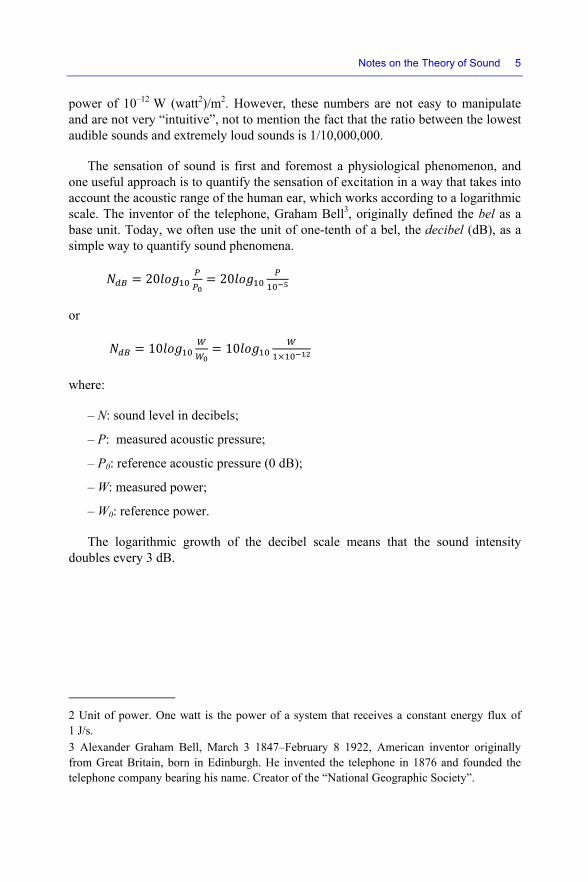
power of 10–12 W (watt2)/m2. However, these numbers are not easy to manipulate and are not very “intuitive”, not to mention the fact that the ratio between the lowest audible sounds and extremely loud sounds is 1/10,000,000.
The sensation of sound is first and foremost a physiological phenomenon, and one useful approach is to quantify the sensation of excitation in a way that takes into account the acoustic range of the human ear, which works according to a logarithmic scale. The inventor of the telephone, Graham Bell3, originally defined the bel as a base unit. Today, we often use the unit of one-tenth of a bel, the decibel (dB), as a simple way to quantify sound phenomena. = 20 = 20
or = 10 = 10 ×
where:
– N: sound level in decibels;
– P: measured acoustic pressure;
– P0: reference acoustic pressure (0 dB);
– W: measured power;
– W0: reference power.
The logarithmic growth of the decibel scale means that the sound intensity doubles every 3 dB.
2 Unit of power. One watt is the power of a system that receives a constant energy flux of 1 J/s. 3 Alexander Graham Bell, March 3 1847–February 8 1922, American inventor originally from Great Britain, born in Edinburgh. He invented the telephone in 1876 and founded the telephone company bearing his name. Creator of the “National Geographic Society”.

6 Musical Sound Effects
Type of audio signal Effects Sound level (dBA)
Rocket take-off 180 Turbojet engine, airplane take-off 140 Rifle shot, engine on a test bench 130 Formula 1, jackhammer Pain threshold 120 Rock band, metal workshop 110 Train passing by, circular saw, night club 100 Portable music player at maximum volume, sander, shouting Hearing risk threshold 90
Radio at maximum volume, machine tools 80 Noisy restaurant, office with typewriters Office work 70 Lively conversation, street, public place 60
Quiet conversation, large quiet office Intellectual work requiring high concentration 50
Quiet apartment, quiet office 40 Walk through the forest 30 Peaceful countryside, whispering 20 Recording studio 10 Silence Audibility threshold 0
Table 1.1. Table of sound intensities
When measuring the sound level with a sonometer, our unit of choice is the decibel A or dB(A). As we will see in section 1.2.2, the sensitivity of the human ear varies as a function of the frequency of the sound signal. To compensate for this physiological behavior of our ears, the sound levels of each frequency component of a sound wave are weighted and summed to give an overall measurement. The units of dB(A) are adjusted to reflect this weighting.
Figure 1.3. Psophometric curve (weighted curve) db(A)

Notes on the Theory of Sound 7
1.1.3. Sound pitch
The pitch of a sound is characterized by its frequency, i.e. the number of oscillations per second of the molecules in the traversed medium (usually air) around their resting position when a sound wave passes through them.
The frequency is measured in units of hertz, denoted by the symbol Hz, and its multiples: kilohertz (kHz), megahertz (MHz), etc. The range of audible frequencies for humans is 20–20,000 Hz (20 kHz). This range varies from individual to individual, and also changes with age.
The speed at which a sound wave travels, also known as its celerity, is 343 m/s through air at a temperature of 20 °C. This value changes depending on the nature of the object or the medium through which the wave is traveling, as well as the pressure and the temperature. For instance, it is equal to 331 m/s through air at 0 °C. The speed of sound is higher in liquid and solid objects (~1,400 m/s in water and ~5,000 m/s in steel).
Having defined the frequency, we should take the opportunity to define a few other parameters: the wavelength, the period and the amplitude.
The wavelength is the distance between two consecutive maxima of a sound wave. This defines the separation between two consecutive periods of a periodic wave (see Figure 1.4), and so is also equal to the distance traveled by the wave during one period.
The period is the time in seconds taken to complete one full oscillation (one cycle). It is the inverse of the frequency and vice versa: = =
where:
– T: period in seconds;
– f: frequency in hertz.
A frequency of 1,000 Hz (1 kHz) corresponds to a period of 0.001 s or 1 ms.

8 Musical Sound Effects
The amplitude defines the sound intensity. As we saw above, this characterizes the variation in pressure.
The wavelength, the period, the frequency and the speed of sound satisfy the relation: = =
where:
– λ: wavelength in meters;
– c: speed of sound in m/s;
– T: period in seconds;
– f: frequency in hertz.
Figure 1.4. Representation of a sound wave and its parameters over time
1.1.4. Approaching the concept of timbre
Timbre is what allows our ears to distinguish and recognize different sounds, whether everyday noises, musical instrument or people’s voices.
It is closely related to the shape of the sound wave. Timbre is a complex notion that we still struggle to fully explain today, since it involves concepts relating to the act of hearing, our ability to judge sounds, our auditory memory and perception.

Notes on the Theory of Sound 9
Before we can begin to discuss the notion of timbre more precisely, we will need
to study several other sound-related parameters, including the physiological mechanisms of our ears, the typology of sounds, the spectrum, transient phenomena and the nature of sound-emitting source(s).
Claude Elwood Shannon4, a renowned mathematician, once stated: “Timbre is what makes sounds sing to our ears”.
1.2. The ears
Hearing is the second of our five senses. It relies in part on our auditory system, whose primary external organ is our ears.
In this chapter, we will find out precisely how our ears work, what makes them interesting and we will analyze how they operate within sound-based environments.
1.2.1. How our ears work
The ear can be divided into three parts: the outer ear, the middle ear and the inner ear.
The outer ear is the part of the system that captures sounds. This system serves the roles of amplification and protection. It is separated from the middle ear by a thin, flexible membrane, the eardrum, which deforms under the effect of sound waves.
The outer ear consists of the auricle and the ear canal, the latter of which is approximately 2.5 cm long. The ear canal carries sound vibrations to the eardrum, amplifying frequencies between 1,500 and 7,000 Hz by 10–15 dB. These are the most useful frequencies to us, notably including speech.
The auricle also plays a role in locating the source of sounds in space for frequencies between 2,000 and 7,000 Hz.
4 Claude Elwood Shannon, 1916–2001, American electrical engineer, mathematician and cryptographer, known as the father of the digital transmission of information. He created the field of “mathematical information theory”.

10 Musical Sound Effects
Figure 1.5. The outer, middle and inner ear
The middle ear is a cavity filled with air. It is connected to the pharynx by the eustachian tube, which opens when we swallow in order to equalize the pressure on either side of the eardrum. This cavity also contains a series of ossicles (small bones): the malleus, attached to the eardrum, the incus and the stapes. The stapes acts as an interface between the air-filled medium of the middle ear and the liquid medium of the inner ear. It rests against the oval window, which acts as the boundary to the inner ear.
Together, the ossicles form a lever that increases the pressure and thus the amplitude of sound waves. The surface area of the eardrum is around 15 times larger than the oval window, which creates an increase of 20 dB. The middle ear acts as a pressure amplifier.
When excessive sounds louder than 80 dB are detected, the stapedius (stapes muscle) contracts to reduce the vibration of the ossicles (acoustic reflex), attenuating the transmission of sound waves to the inner ear. This protection mechanism reduces the sound signal by 40 dB.
It should be noted that the stapedius develops fatigue over time, and so cannot provide long-term protection. Additionally, it only activates at low frequencies of less than 1 kHz, and the contraction occurs too slowly to protect from sudden noises like explosions, since the “reflex latency” (physiological reaction time associated with the information processing sequence of humans) is around 30 ms.

Notes on the Theory of Sound 11
Figure 1.6. Detailed diagram of the middle ear
The inner ear consists of two sensory organs: the vestibule, a balance organ, and the cochlea, a hearing organ.
Figure 1.7. The inner ear
12 Musical Sound Effects
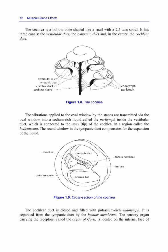
The cochlea is a hollow bone shaped like a snail with a 2.5-turn spiral. It has three canals: the vestibular duct, the tympanic duct and, in the center, the cochlear duct.
Figure 1.8. The cochlea
The vibrations applied to the oval window by the stapes are transmitted via the oval window into a sodium-rich liquid called the perilymph inside the vestibular duct, which is connected to the apex (tip) of the cochlea, in a region called the helicotrema. The round window in the tympanic duct compensates for the expansion of the liquid.
Figure 1.9. Cross-section of the cochlea
The cochlear duct is closed and filled with potassium-rich endolymph. It is separated from the tympanic duct by the basilar membrane. The sensory organ carrying the receptors, called the organ of Corti, is located on the internal face of

Notes on the Theory of Sound 13
this membrane. The receptors are hair cells. The inner hair cells are arranged in a single row, and the outer cells are arranged in three rows. The tips of the hairs (or stereocilia) of the outer cells are anchored to the tectorial membrane. Both inner and outer cells are connected to the fibers of the auditory nerve. The motion of the liquids contained in the ducts induces deformations in the basilar membrane, which tilts and twists the hairs connected to the tectorial membrane, which itself remains fixed. This tilting and twisting encodes the sound vibrations into ionic motion that polarizes or depolarizes the membrane of each cell.
Figure 1.10. Detailed diagram of the organ of Corti
The outer hair cells are in fact selective amplifiers, and the inner cells are the actual sensory cells. A tonotopy (representation of the auditory spectrum) is arranged along the cochlear duct. In other words, a characteristic resonance frequency can be determined at each point along the duct. The low-frequency resonators (low-pitched) are located near the apex, and the high-frequency resonators (high-pitched) are located at the base of the duct.
Figure 1.11. Tonotopy of the cochlear duct and frequency distribution

14 Musical Sound Effects
As well as being channeled through the air, sound vibrations are transmitted by means of another mechanism, known as bone conduction. Sound messages are directed to the inner ear via the bones in the skull. A much larger quantity of energy is required to produce a given stimulus via this path than is needed to propagate sound through the air. Indeed, the relative attenuation between the two paths has been measured as 30–60 dB, depending on the frequency.
1.2.2. Fletcher–Munson curves
The sensitivity of our ears is not linear with respect to the sound pressure. In other words, the perceived volume of a sound with a given intensity can seem higher or lower depending on the frequency of the signal. The Fletcher–Munson curves demonstrate this phenomenon. Below a certain frequency-dependent power threshold, sounds are imperceptible. This defines our threshold of hearing. The same is true for high-power sound messages, which become unbearable after a certain point, defining the threshold of pain. Fletcher established the curve relating the frequency on the x-axis to the power (sound pressure) on the y-axis. When listening binaurally (with both ears), the curves show which sounds create identical sensations. This work was standardized in 1961 to define so-called loudness contours (isosonic curves).
Figure 1.12. Fletcher–Munson curves (isosonic curves)

Notes on the Theory of Sound 15
1.2.3. Auditory spatial awareness
Our ears are capable of pinpointing the source of a sound fairly accurately. This ability is based on several parameters.
In 1907, Lord Rayleigh5 demonstrated the principles of interaural level differences and interaural time differences for the first time.
The interaural time difference (ITD) is a construction characterizing the time difference between the arrival of a sound wave at each of the two ears of a person. If the sound is coming from the front, this difference is zero.
Figure 1.13. Principle of sound localization by ITD
The ITD can be approximated with the equation:
Δ = ( + sin )
5 John William Strutt Rayleigh, British physicist born at Langford Grove (Essex), 1842–1919. He was awarded the Nobel prize in physics in 1904 for the discovery of inert argon gas together with William Ramsay, and conducted extensive research into wave-related phenomena.

16 Musical Sound Effects
where:
– Δt: ITD in seconds;
– R: radius of the head in meters (8.75 cm by default);
– α: angle of incidence in radians;
– c: speed of sound (340 m/s).
For example, if a sound source is located at 30°, we find that:
Δ = 0.0875(0.523 + 0.5)340 = 2.63 × 10 s = 263
The sound will reach the person’s ears with a time difference of 263 μs. This difference can be thought of as a phase shift that is analyzed and interpreted by our brain in order to locate the position of the source. The maximum ITD is around 673 μs.
Figure 1.14. ITD calculation chart
This phenomenon is particularly distinctive at low frequencies below 1,500 Hz. At higher frequencies, the interaural level difference (ILD), the interaural intensity difference (IID) or the interaural pressure difference (IPD) is used instead.

Notes on the Theory of Sound 17
If a sound is emitted by a source that is closer to one ear than the other, there will
be difference in the sound intensity or acoustic pressure. Our auditory system uses this difference to locate the sound source.
Gary S. Kendall and C.A. Puddie Rodgers proposed a simple equation to calculate the ILD:
Δ = 1 + 1,000 . ×
where:
– Δl: ILD;
– f: frequency in kHz;
– α: angle of incidence in radians.
But the ITD and ILD alone are not the only factors that allow us to discriminate between the positions of different sources. In some cases, the ITD and the ILD may be identical, even though the sources are located at different positions, as shown in Figure 1.15.
Figure 1.15. Angular localization error in the horizontal and vertical directions. The
sources S1 and S2 (vertical plane) have exactly the same ITD and ILD values as the sources S3 and S4 (horizontal plane)

18 Musical Sound Effects
Another parameter is also used as a factor to locate the source of sounds based on diffraction caused by the morphology of the head. This eliminates the ambiguity created by the localization errors presented previously. Today, this factor is thought to be the most important factor, and is currently the subject of extensive research. The head-related transfer functions (HRTF) method represents the result of this work.
To understand how HRTF localization works, suppose that a source is placed directly to the right of an individual. His or her right eardrum will receive the sound message along a straight path. However, the sound waves that reach the left ear will need to follow a much more complex path around the head before ultimately hitting the left eardrum after multiple reflections and diffractions within the auricle and the ear canal.
Figure 1.16. Implementation of HTRF. The source is placed in front of
the observer, and its elevation is varied from 0 to 30° relative to the horizontal plane through the observer’s ears
As it travels, the timbre of the sound wave, and therefore its spectrum, is modified. These modifications depend on the location of the source within three-dimensional space and are interpreted by the brain in order to determine this location. Note that HRTF localization is capable of determining vertical position, unlike the ITD and ILD.

Notes on the Theory of Sound 19
Figure 1.17. The HRTF can distinguish between different heights, unlike
the ITD and ILD methods. The curves change as a function of the height of the source relative to the ears of the observer
The angular localization errors6 are shown in Figure 1.18, determined by all of the above methods (ITD, ILD and HRTF).
Figure 1.18. Values of the angular perception errors in the horizontal and vertical directions
6 Based on the measurements and experiments performed by Blauert.

20 Musical Sound Effects
It should be noted that the localization functions studied previously (ITD, ILD and HRTF) are based on binaural hearing (with both ears), but localization is also possible with monaural hearing. The auricle of the outer ear filters sound by means of reflections that depend on the angle of incidence of the source. These reflections introduce delays and timbre deformations, which can be used to determine the origin of the emitted sound.
Certain effects can impede or enhance the process of locating sounds in space. Two effects are particularly significant: the “cocktail party” effect, and the precedence effect, also known as the Haas effect.
The “cocktail party” effect occurs in noisy environments. We are capable of locating the source of a sound if we know where it is.
The Haas effect7 reveals how we perceive reflected sounds compared to direct sounds. Our ears cannot distinguish between direct sounds and reflected (or reemitted) sounds if they are separated by less than 50 ms, even if the reflected source is louder8 than the direct source by several dB. If the separation is longer, our ears no longer perceive the sources together, but instead as an echo. This phenomenon implies that our auditory system interprets the direction of an acoustic phenomenon as the direction of the first source that it perceives. This effect is also known as the law of the first wavefront.
Figure 1.19. Demonstration of the precedence effect or Haas effect. If the
difference between the sources S1 and S2 is less than 50 ms, the observer cannot perceive a difference between them (no echo)
7 According to a study conducted by Helmut Haas in 1951. 8 Depending on the separation (0 to 50 ms), this value ranges up to a maximum of 10 dB.
Notes on the Theory of Sound 21
1.3. The typology of sounds
Like everything that surrounds us, sounds can be organized into a typology based on characteristics distinguishable by physics or hearing.
1.3.1. Sounds and periods
Pure sounds and constant frequencies rarely exist in our natural environment, except in certain circumstances. The sounds around us are typically complex. We can define a typology of sounds to distinguish them. The first thing to consider is the property of periodicity.
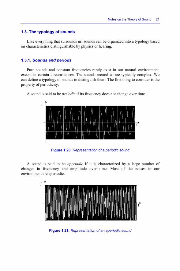
A sound is said to be periodic if its frequency does not change over time.
Figure 1.20. Representation of a periodic sound
A sound is said to be aperiodic if it is characterized by a large number of changes in frequency and amplitude over time. Most of the noises in our environment are aperiodic.
Figure 1.21. Representation of an aperiodic sound

22 Musical Sound Effects
White noise is an extreme example of an aperiodic sound. It uses the entire spectrum of audible frequencies.
Figure 1.22. Representation of white noise
A sound with extremely short duration is called an impulse, whereas longer sounds are described as continuous.
Figure 1.23. Representations of impulses and a continuous sound
1.3.2. Simple sounds and complex sounds
Sounds with sinusoidal waveforms are called simple sounds. All other sounds are complex sounds. Complex sounds are composed of two or more sinusoidal waves. Thus, complex sounds are combinations of multiple simple sounds.

Notes on the Theory of Sound 23
Figure 1.24. Combination of multiple simple sounds
To determine the simple waves that compose a complex sound, we can use a mathematical tool called a Fourier transform9.
Fourier transforms allow us to decompose complex sounds into a series of simple sounds (sinusoidal waves). Complex sounds in the real world can contain dozens of sinusoidal components.
The amplitude of a complex sound at any given moment in time is given by the sum of the amplitudes of the simple sounds from which it is composed.
The frequency of a complex sound is equal to the lowest of the frequencies of the simple sounds from which it is made up of.
The frequency of a complex sound is called the fundamental frequency (F0). If a sound is not periodic, it implicitly does not have a fundamental frequency. Instead, we think of it as a noise.
9 Jean Baptiste Joseph Fourier, March 21 1768–May 16 1830, French mathematician and physicist.

24 Musical Sound Effects
1.4. Spectral analysis
Spectral sound analysis combines several analytical techniques for determining the characteristics of an audio signal. The results of spectral analysis are often presented graphically.
1.4.1. The sound spectrum
The spectrum of a sound is a representation of its amplitudes and frequencies. The representations that we used earlier always described each sound by a variation in amplitude along the vertical axis and a horizontal axis representing time.
The spectrum of a sound wave does not contain any information about time.
Figure 1.25. Spectrum of a periodic complex sound
The spectrum is often represented as a vertical bar graph (or line graph). Each bar shows the amplitude of a certain frequency. The lowest frequency is the fundamental frequency.

Notes on the Theory of Sound 25
Figure 1.26. Line spectrum of the sound in Figure 1.22 (intensity in dB)
This type of graph is excellent for periodic sounds, since they contain a limited number of frequencies. We say that such sounds have a discontinuous spectrum, line spectrum or comb spectrum.
The other frequencies are called harmonics and are multiples of the fundamental frequency.
Designation Symbol Frequency Fundamental frequency or first harmonic F0 440 Hz
Second harmonic F1 2 × F0 = 2 × 440 = 880 Hz
Third harmonic F2 3 × F0 = 3 × 440 = 1,320 Hz
Fourth harmonic F3 4 × F0 = 4 × 440 = 1,760 Hz
Fifth harmonic F4 5 × F0 = 5 × 440 = 2,200 Hz
Sixth harmonic F5 6 × F0 = 6 × 440 = 2,640 Hz
Seventh harmonic F6 7 × F0 = 7 × 440 = 3,080 Hz
Table 1.2. The harmonics of (440 Hz)
Sometimes we need to visualize the frequency distribution of the spectrum, in which case we use a graph showing the spectral envelope of the sound instead of a bar graph.
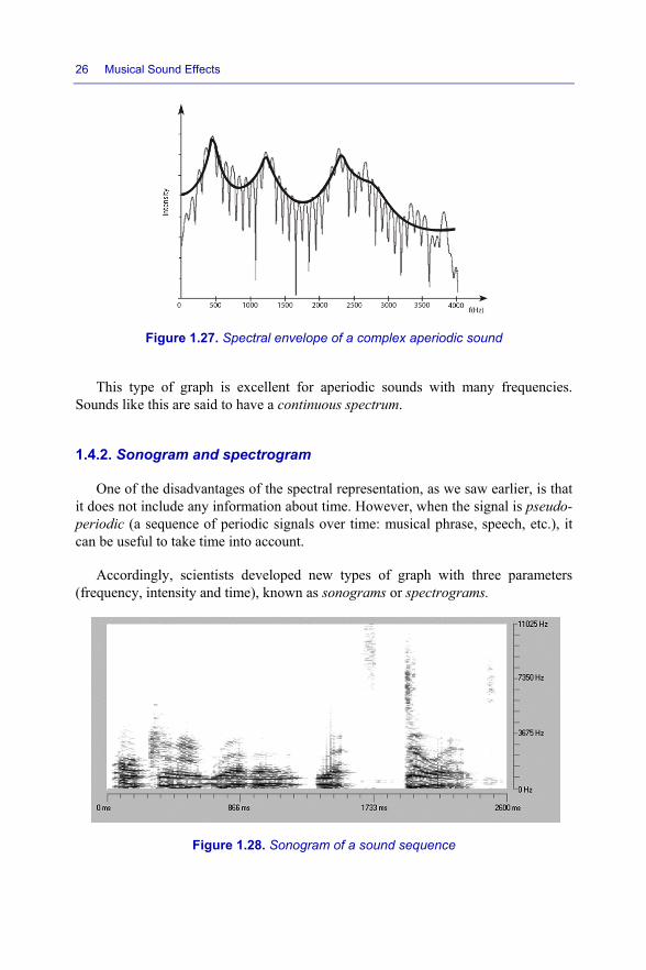
26 Musical Sound Effects
Figure 1.27. Spectral envelope of a complex aperiodic sound
This type of graph is excellent for aperiodic sounds with many frequencies. Sounds like this are said to have a continuous spectrum.
1.4.2. Sonogram and spectrogram
One of the disadvantages of the spectral representation, as we saw earlier, is that it does not include any information about time. However, when the signal is pseudo-periodic (a sequence of periodic signals over time: musical phrase, speech, etc.), it can be useful to take time into account.
Accordingly, scientists developed new types of graph with three parameters (frequency, intensity and time), known as sonograms or spectrograms.
Figure 1.28. Sonogram of a sound sequence

Notes on the Theory of Sound 27
A sonogram is a 2D graph where the sound intensity is defined by a scale of
colors or shades of gray. A spectrogram is usually a 3D graph with time and frequency on the x- and z-axes, and the sound intensity on the y-axis.
Figure 1.29. Spectrogram of a sound sequence
1.5. Timbre
The notion of timbre is too difficult to describe in terms of the fundamental frequency, the harmonics or the loudness (sound intensity). Timbre is a complex psychoacoustic concept. Sounds can be strident, dull, dry, warm and many more things.
1.5.1. Transient phenomena
Sound perception exists within a wider context. Each sound begins, stabilizes and then fades. Each single moment in the act of hearing a sound is a transient phenomenon. There are several types: attack transients and release transients, which describe the beginning and the end of sound phenomena. We can add other parameters to this list, which, like vibrato and tremolo, can either occur in a single phase (often when the sound has stabilized), or in every phase.

28 Musical Sound Effects
Figure 1.30. The transients of the sound of a pipe organ
The attack transient gives the sound its unique signature. For example, the attack transient is what allows us to distinguish between the sound of a clarinet and the sound of a flute. Its duration varies, typically ranging from 1 to 100 ms. It is thought that the human ear needs 40–50 ms to distinguish and recognize a sound. This type of transient is often complex. As well as its duration, we need to consider its slope, its instability, its spectral composition, the number of components and the order in which they occur, as well as many other factors.
The stabilization phase (or sustain) is often steady, although it can be influenced by the environment or the musician’s technique.
The release transients often depend on environmental parameters (echo, reverb, damping, etc.) and technique-related parameters for musical instruments. It can range from very short to very long (sound accessories or natural or artificial echo phenomena), from 1 to 5,000 ms.
Together, the transient phenomena: attack, sustain and release are often called the envelope of the sound.
1.5.2. Range
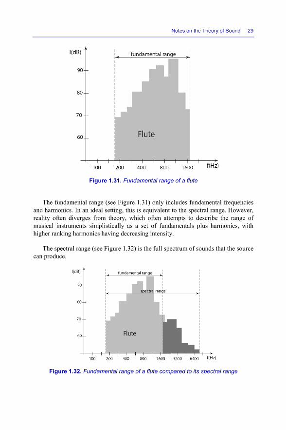
Each sound source, especially musical instruments and voices, can emit sound over a certain range of frequencies. This range is also known as the tessitura. However, we must be careful to distinguish between two concepts: the fundamental range and the spectral range
Notes on the Theory of Sound 29
Figure 1.31. Fundamental range of a flute
The fundamental range (see Figure 1.31) only includes fundamental frequencies and harmonics. In an ideal setting, this is equivalent to the spectral range. However, reality often diverges from theory, which often attempts to describe the range of musical instruments simplistically as a set of fundamentals plus harmonics, with higher ranking harmonics having decreasing intensity.
The spectral range (see Figure 1.32) is the full spectrum of sounds that the source can produce.
Figure 1.32. Fundamental range of a flute compared to its spectral range

30 Musical Sound Effects
1.5.3. Mass of musical objects10
This notion of mass was introduced by Pierre Schaeffer11, who discussed it in his “Treatise on Musical Objects”, which remains an important reference to this day. On the subject of concrete sounds, i.e. sounds that are not affiliated with any musical instrument that is culturally recognizable to a given observer, he writes:
But when we consider an arbitrary concrete sound (for example, produced by a membrane, a metal sheet, a rod...), we see that, unlike traditional sounds that have a clearly identifiable pitch, it has a certain mass located somewhere within its range, approximately characterizable by the intervals that it occupies, which are relatively easy to decipher. For example, it might contain several sounds with slowly changing pitch, which are dominated or surrounded by an aggregate of partials that are also gradually changing, the entirety of which can be approximately localized within a certain pitch interval. Our ears can quickly identify the most salient features and components, with some practice; these sounds then become as familiar to us as traditional harmonic sounds: they have a characteristic mass.
His comments reveal the extent of the complexity involved in attempts to define the timbre. The concept of timbre extends far beyond the physics of the phenomenon into the realm of psychoacoustics. Schaeffer continues:
At this point, we should stop to note that, since musicians care about things like: a note with good timbre, good or poor timbre, etc., they are distinguishing between two separate notions of timbre: one that relates to the instrument, indicating the provenance of the sound by the simple act of hearing, and another relating to each of the objects created by the instrument, involving an appreciation of the musical
10 The concept of object was particularly important to Pierre Schaeffer: “A sound object refers to the studied signal, viewed within the context of perception. Instead of hearing events via sounds, we hear sounds as events.” 11 Pierre Schaeffer, 1910–1995, founder of the research department of the ORTF (Office de Radiodiffusion-Télévision Française), researcher in the fields of audiovisual communication and music. The inventor of musique concrète (concrete music), he created the GRM (Groupe de Recherche Musicale) in 1951, as well as being a composer (Variations sur une flûte mexicaine, Suite pour 14 instruments, Symphonie pour un homme seule, Toute la Lyre, Orphée 51, Masquerage, and others), and author of the monumental and prophetic work “Traité des Objets Musicaux” (“Treatise on Musical Objects”).

Notes on the Theory of Sound 31
effects contained in the objects themselves, which are desirable in the context of musical interpretation and musical activities. We can go even further by speaking of the timbre of one single component of the object: the timbre of the attack, which is distinct from its stiffness.
However, given this definition, the timbre of an object is nothing other than the form and substance of its sound, its complete specification among the range of sounds that a given instrument can create, up to any admissible artistic variation. Associating the concept of timbre with the object therefore cannot help us describe the object itself any further, since it simply postpones the analysis of the subtleties of our qualified perceptions of the sound.
1.5.4. Classification of sounds
Based on the observations relating to the concept of timbre presented above, we can define a classification of different types of sound message.
Category Composition Spectrum Example
Pure sound Tonal sound without harmonics Filiform
Sinusoidal sound (BC generator, synth VCO, etc.)
Tonal sound Sound with an identifiable pitch A band
Note played by an instrument (piano, harpsichord, violin, etc.)
Tonal group Group of multiple tonal sounds Multiple bands
Chord played by an instrument (piano, harpsichord, organ chord, etc.)
Nodal group Aggregate sound without an identifiable pitch Multiple bands
Set of percussions (multiple cymbals together)
Nodal sound Set of multiple nodal groups A band Percussive sound
(cymbal)
White noise Group containing every pitch Full spectrum White noise generator
Complex sound
Mixed group containing tonal sounds, tonal groups, nodal sounds, nodal groups.
Complex shape Natural sound (bell, gong, metal sheet, etc.)
Table 1.3. Classification of sounds

32 Musical Sound Effects
1.6. Sound propagation
Sound waves propagate through their surrounding media by means of specific phenomena that result in specific behaviors. We will study the most important principles.
1.6.1. Dispersion
A sound wave emitted by a point source disperses as a set of concentric spheres.
Figure 1.33. Spherical dispersion of a wave from a point source. The
sound pressure level decreases by 6 dB whenever the distance doubles
Sound propagates through gaseous media like air, which is the most common transporting medium, in the form of alternating compressed and dilated layers. The set of wavefronts vibrate in phase (with each other).
In order to describe certain phenomena, scientists introduced the abstract notion of plane waves, which do not actually exist in reality. Plane waves are just sections of spherical waves. When the source is sufficiently far away from the point of audition, spherical waves have a large radius of curvature, and so may be approximated by plane waves.

Notes on the Theory of Sound 33
1.6.2. Interference
Figure 1.34. Interference between two waves on the surface of a liquid
When two sound waves meet, they overlap, and their intersection creates constructive or destructive interference.
Figure 1.35. Interference between two identical waves (same frequency and amplitude). The sources S1 and S2 emit sound waves that overlap, creating
interference (nodes and antinodes)
If you strike a tuning fork it and then rotate it near your ear, you will notice that it sounds louder or softer depending on the angle of rotation. This simple experiment demonstrates the creation of constructive and destructive interference.
34 Musical Sound Effects
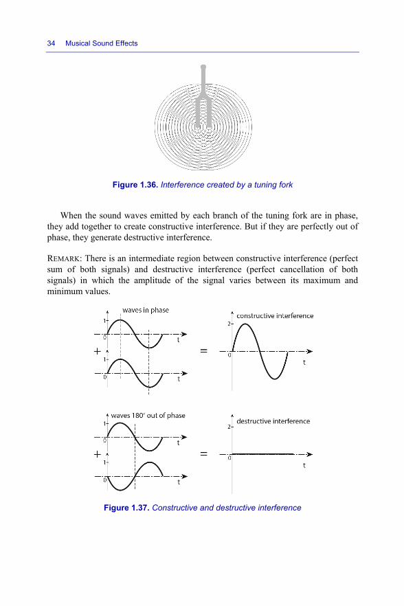
Figure 1.36. Interference created by a tuning fork
When the sound waves emitted by each branch of the tuning fork are in phase, they add together to create constructive interference. But if they are perfectly out of phase, they generate destructive interference.
REMARK: There is an intermediate region between constructive interference (perfect sum of both signals) and destructive interference (perfect cancellation of both signals) in which the amplitude of the signal varies between its maximum and minimum values.
Figure 1.37. Constructive and destructive interference

Notes on the Theory of Sound 35
Constructive and destructive interference12
With two identical sound waves, the shape of the interference pattern is easy to determine. In the case of non-identical waves, it can be determined by the principle of superposition: when two sound waves occupy the same space at the same time, the total perturbation is simply the sum of each of the two individual perturbations at each point in space and time.
1.6.3. Diffraction
When a sound wave encounters an obstacle, it goes around it. The edge of the obstacle becomes the center of a new wave, called a secondary wave or a diffracted wave.
Figure 1.38. Diffraction of a wave through an opening. The
opening in a) is small relative to the wavelength λ, so a new point source is created. The opening in b) is larger than λ, so there is practically no diffraction
12 We will return to the concepts of interference, phase and antiphase in section 4.1 when discussing equalization and filtering effects.

36 Musical Sound Effects
Diffraction is what allows us to hear sounds emitted by sources located behind obstacles.
Waves do not propagate in straight lines. Once a wave has moved past the obstacle, it again propagates in every direction. This phenomenon was demonstrated by the physicist C. Huygens13, who also gave us Huygens’ principle.
“Each point on a wavefront may be viewed as the point source of a wave propagating in the same direction as the original wave. The next wave front may be obtained by summing all of these new waves”.
In simpler terms, a wave can be thought of as a sum of elementary waves vibrating in phase that are moving in the same direction as the original wave.
When the obstacle placed in front of the sound-emitting source is smaller than the wavelength, it does not exist from the perspective of the wave – the sound wave propagates around it as if it were “invisible”. The greater the wavelength-to-width ratio of the obstacle (λ/l), the greater the effect of diffraction. When the ratio is large, an observer located behind the obstacle does not perceive any difference compared to when the obstacle is removed.
Figure 1.39. Circumventing an obstacle smaller than the wavelength
13 Christian Huygens, born at La Haye, Holland, April 14 1629–July 8 1695, mathematician, physicist and astronomer, author of “De ratiociniis in ludo aleae” in 1657 and “Horologium oscillatorium” in 1673. He discovered Saturn’s ring, the rotation of Mars and the Orion nebula. He researched and published many papers on the wave theory of light, which enabled him to explain reflection and refraction, among other things.

Notes on the Theory of Sound 37
If the width of the obstacle is large, part of the sound wave is reflected, and the
edges of the obstacle become secondary sources of propagation.
Figure 1.40. Emission of secondary waves at the edges of an obstacle
1.6.4. Reflection
When a sound wave encounters an obstacle that it cannot circumvent because the width of the obstacle is greater than the wavelength of the wave, the wave is reflected. The reflection of sound waves follows the appropriately named law of reflection (Descartes’ law14). This law states that the new direction of the sound wave after hitting a point on the surface is equal to the angle of the wave with the normal at this point at the moment of impact; in other words, the angle of incidence is equal to the angle of reflection.
Figure 1.41. Angles of incidence and reflection of a sound wave (α = β)
14 René Descartes, born in France, Touraine, 1596–1650, philosopher, physicist and mathematician, author of the famous “Discours de la méthode”, as well as his “Traité du Monde et de la Lumière”, “la Dioptrique”, “Météores” and so on.

38 Musical Sound Effects
Note that the reflected waves can interfere with the incident waves to create constructive or destructive interference. Within a thin layer very close to the surface hit by the wave, the sound intensity is increased by the sum of the incident wave and the reflected wave. In this layer, the acoustic sound pressure is doubled, which increases the intensity by around 6 dB.
Figure 1.42. Reflection of a sound wave on a flat surface and a concave surface
If the obstacle reflecting the wave has a concave shape, a focusing phenomenon occurs. In the opposite case, when the obstacle has a convex shape, a scattering phenomenon occurs.
Wavefronts hitting a wall created reflected waves that act as if they were generated by an “image” of the sound source located the same distance on the other side of the wall.
Figure 1.43. Reflection of a sound wave on a wall and image of its source

Notes on the Theory of Sound 39
When a sound wave strikes a hard surface, there is no phase change in the
reflected wave. We say that the surface has an acoustic impedance greater than air. But when a sound wave encounters an obstacle with a lower impedance, there is a phase inversion (for example when a sound transmitted by a solid meets the air).
1.6.5. Reverberation (reverb)
This phenomenon will be discussed at great detail in Chapter 8, which presents time effects.
1.6.6. Absorption
When a sound wave hits an obstacle, it is reflected, but loses some of its energy. This energy is absorbed by the material. The ability of a material to capture or absorb sound energy is described by its absorption coefficient, often denoted as α. = 1 − | |
where:
– α: absorption coefficient (recall that α = 1: perfectly absorbent, α = 0: perfectly reflective);
– r: reflection factor.
Hard materials such as marble, cement and plaster have absorption coefficients ranging from 0.01 to 0.05, whereas porous or fibrous materials such as carpet, felt or glass wool have coefficients between 0.2 and 0.4 (see the table of absorption coefficients established by Sabine in section 8.1.1).
1.6.7. Refraction
When a sound wave passes from one environment to a different environment, it changes speed (discontinuous celerity) and direction. This generates both a reflected wave and a refracted wave (especially in the case of thin materials) with a lower energy than the original incident wave.
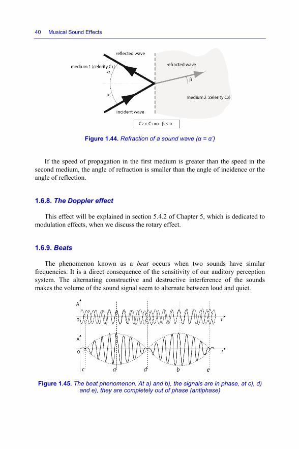
40 Musical Sound Effects
Figure 1.44. Refraction of a sound wave (α = α’)
If the speed of propagation in the first medium is greater than the speed in the second medium, the angle of refraction is smaller than the angle of incidence or the angle of reflection.
1.6.8. The Doppler effect
This effect will be explained in section 5.4.2 of Chapter 5, which is dedicated to modulation effects, when we discuss the rotary effect.
1.6.9. Beats
The phenomenon known as a beat occurs when two sounds have similar frequencies. It is a direct consequence of the sensitivity of our auditory perception system. The alternating constructive and destructive interference of the sounds makes the volume of the sound signal seem to alternate between loud and quiet.
Figure 1.45. The beat phenomenon. At a) and b), the signals are in phase, at c), d)
and e), they are completely out of phase (antiphase)

Notes on the Theory of Sound 41
The frequency of the beat is equal to the absolute value of the difference of the
two frequencies of each sound wave. = | − |
If the frequency of the beat is greater than 50 Hz, our brain is able to distinguish between the two sound sources. If not (<50 Hz), our brain detects a sound with an intermediate pitch (often called: the subjective tone or combination tone) with an intensity that appears to vary at the rate of the beat frequency.
1.7. Conclusion
Now that we have taken a brief tour around the notions of sound and acoustics, readers will have gained the foundations needed to understand the various sound effects that we shall discuss throughout the rest of the book.
We have not even nearly mentioned everything there is to know about sound. Interested readers can explore further using the web links and bibliography given at the end of this book, but you should now be able to continue reading without any difficulties, if you prefer.

2
Audio Playback
Multichannel sound, audio playback and audio media are important enough to have a dedicated chapter in this book. They often inspire many questions, many of which deserve to be answered.
The next few sections only give a simple description. They are not enough to fully understand the key ideas of multichannel processing, but offer a gentle introduction to the vocabulary, conventions and standards of audio.
Between 1964 and today, the world has gone through a variety of different media:
– the K7 audio cassette, invented by Philips in 1964;
– the laserdisc, or video disc, invented by David Paul Gregg in 1958, and introduced to the general public in 1972 by Philips and MCA (Music Corporation of America);
– the audio CD (compact disc), also invented by Philips in collaboration with the Japanese company Sony in 1979, based on laserdisc technology;
– the DVD (digital versatile disc), the result of collaboration between a large panel of companies specializing in audio (Philips, Toshiba, Time Warner, Matsushita Electric, Hitachi, Mitsubishi Electric, Pioneer, Thomson, etc.), launched in 1995;
– the Blu-ray disc (BD) and its competitor, the HD DVD1, introduced in 2006, both specifically designed to support HD video.
1 The HD DVD (high-density DVD) standard, originally created by Toshiba, was discontinued in March 2008.
Musical Sound Effects: Analog and Digital Sound Processing, First Edition. Jean-Michel Réveillac.© ISTE Ltd 2018. Published by ISTE Ltd and John Wiley & Sons, Inc.

44 Musical Sound Effects
The most recent of these media are also capable of storing multichannel music,
notably including DVDs and Blu-rays, despite being primarily designed for video.
Even so, multichannel playback can still prove difficult. Multichannel systems require large setups with several speakers, which are often expensive, and ensuring that a given setup is compatible with the constantly expanding set of existing standards can be challenging. All in pursuit of perfect sound quality.
2.1. History
Before we begin to review the list of modern audio playback standards and techniques, it will be enlightening to start with a brief history of sound recording and reproduction.
In 1877, Edison2 recorded the human voice for the first time on a sheet of tinfoil using a cylinder phonograph built by his best mechanic, John Kreusi3. He patented this invention on February 19, 1878, with patent number 200521.
Figure 2.1. Edison’s phonograph
Thus, begins the history of sound recording. Chichester Bell and Charles Tainter, Charles Cros, Emile Berliner, Eldridge Johnson, Levi Montross, Gianni Bettini, Henri Lioret, François Dussaud and many others will help to perfect the invention.
2 Thomas Edison was born on February 11, 1847 in Milan, Ohio, and died on October 18, 1931 in West Orange, New Jersey. An American inventor and entrepreneur, he has 1,093 patents to his name. 3 John Kruesi, May 15 1843–February 22 1899, Swiss mechanic and engineer who worked closely with Edison to perfect a number of inventions.

Audio Playback 45
The cylinder was superseded by flat discs made from shellac, then from celluloid a few years later. The first motorized phonographs were offered for sale in 1900.
In 1898, Poulsen4 filed a patent in Denmark for a device that he named the “telegraphone”. This device was the first magnetic recorder, and was based on the same principle as the phonograph, but used a steel wire instead of a cylinder, and a small electromagnet instead of a needle. The steel wire is the medium. After displaying his device at the Exposition Universelle in Paris in 1900, he was awarded American patent number 661619 for his invention.
Figure 2.2. Poulsen’s “telegraphone” based on a steel wire
The first so-called “high-fidelity” (or hi-fi) discs were born in 1924, operating in the frequency band between 100 and 5,000 Hz.
As technology kept improving, the microphones used to pick up sound became more and more sensitive. In 1927, G. Neumann5 allowed the whole industry to make a giant leap forward by inventing a completely new, highly sensitive microphone capable of perfectly reproducing the spectrum and range of recorded voices and instruments.
4 Valdemar Poulsen, November 23 1869–July 23 1942, Danish engineer and inventor. 5 Georg Neumann, 1898–1976, German inventor who founded the company Georg Neumann & Co. together with Erich Rickmann.
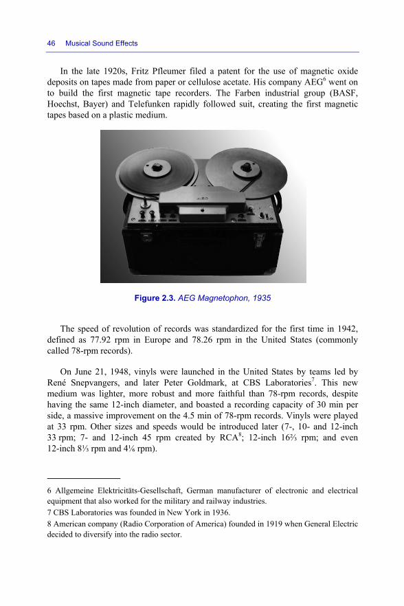
46 Musical Sound Effects
In the late 1920s, Fritz Pfleumer filed a patent for the use of magnetic oxide
deposits on tapes made from paper or cellulose acetate. His company AEG6 went on to build the first magnetic tape recorders. The Farben industrial group (BASF, Hoechst, Bayer) and Telefunken rapidly followed suit, creating the first magnetic tapes based on a plastic medium.
Figure 2.3. AEG Magnetophon, 1935
The speed of revolution of records was standardized for the first time in 1942, defined as 77.92 rpm in Europe and 78.26 rpm in the United States (commonly called 78-rpm records).
On June 21, 1948, vinyls were launched in the United States by teams led by René Snepvangers, and later Peter Goldmark, at CBS Laboratories7. This new medium was lighter, more robust and more faithful than 78-rpm records, despite having the same 12-inch diameter, and boasted a recording capacity of 30 min per side, a massive improvement on the 4.5 min of 78-rpm records. Vinyls were played at 33 rpm. Other sizes and speeds would be introduced later (7-, 10- and 12-inch 33 rpm; 7- and 12-inch 45 rpm created by RCA8; 12-inch 16⅔ rpm; and even 12-inch 8⅓ rpm and 4⅙ rpm).
6 Allgemeine Elektricitäts-Gesellschaft, German manufacturer of electronic and electrical equipment that also worked for the military and railway industries. 7 CBS Laboratories was founded in New York in 1936. 8 American company (Radio Corporation of America) founded in 1919 when General Electric decided to diversify into the radio sector.
Audio Playback 47
By 1945, the quality of tape recorders had significantly improved, and they
began to be more widely used.
However, we should bear in mind that sound playback systems were still monophonic at this point, although they had now advanced from a simple horn attached to a needle without any form of amplification in the first phonographs to an electronic audio system with amplifiers and loudspeakers. The latter were first developed by Siemens9, who patented a moving-coil loudspeaker system on December 14, 1877. For a long time, his invention would be exclusively used for historical telephones, before being significantly improved and adapted for audio playback.
In the 1940s, the main concern was to achieve maximum gain, and people did not worry about distortion or bandwidth. Audio playback systems based on horns were supplanted by acoustic loudspeakers in the 1950s, but the latter still distorted the sound signal. The first speakers were large, cumbersome and often relatively ugly. Miniaturization would not be achieved until 1970s, when small speakers with moving elements and high displacement were introduced, finally capable of correctly reproducing low frequencies.
Stereophony was born in a series of experiments by Harvey Fletcher and most notably Alan Blumlein, who worked for EMI10 in the United Kingdom. He realized that reproducing a wavefront was impossible, so he decided to try to build an audio playback system with two sound sources. He placed an observer at one of the vertices of an equilateral triangle, and sources at the other two vertices. During recording, he used the technique of coincident microphones. Stereo sound would require more than a decade to become popular, and the golden age of “high-fidelity” (hi-fi) would only begin in the early 1960s. However, movie theaters began using multiple channels and loudspeakers at the beginning of the 1950s. In 1959, radio took its first steps toward stereo broadcasting, but stereo television would not see the light of day until 1978, in Japan.
Stereo and hi-fi reached their peak at the turn of the 1970s, and the industry began to search for new ideas, ultimately leading to quadriphonic sound. Recording was simple enough, but reproducing the sound was another story: how can you fit four channels onto a vinyl that is already struggling to store just two? A number of solutions based on complex matrix decoding systems were attempted, but the results
9 Ernst Werner von Siemens, December 13 1816–December 06 1892, German inventor and industrialist, founder of the company bearing his name. 10 EMI (Electrical and Musical Industries), a major record company, was founded in 1931 by merging Columbia Records and HMV (His Master’s Voice).
48 Musical Sound Effects
were ultimately disappointing, and the general public remained unimpressed by the expensive and highly fragile equipment.
In 1971, Stanley Kubrick used a new noise reduction technique named “Dolby11 A” for the first time in his film “A Clockwork Orange”.
In 1978, Dolby Laboratories announced its Dolby Stereo system. This system, specially designed for movies, condensed four separate audio channels (left, center, right and surround) onto just two channels using a matrix decoding system. It also incorporated a noise reduction system that improves the dynamics of the sound. For the first time, viewers could feel immersed in space while listening, even though this system seems archaic to us today. In 1982, it was made available to the general public in the form of Dolby Surround, followed by an improved version, Dolby Surround Pro-Logic (DPL), in 1987. From this point onward, multichannel systems flourished, especially in movie theaters and private homes, with the rise in popularity of home theaters. Digital audio proved immensely popular, with Dolby Digital 5.1 in 1992, the Digital Theater System (DTS) in 1992, 6.1-channel standards in 1999 and so on. Today, a niche market has developed for DVD-Audio and Super Audio CD (SACD), specifically dedicated to music recordings, although audio CDs continue to dominate.
2.2. Dolby playback standards and specifications
The Dolby Stereo, Dolby Surround and DPL formats refer to specific decoding techniques. The signal is encoded as Dolby Surround in each case, also known as Dolby MP Matrix (MP for Motion Picture).
2.2.1. Dolby Surround encoding and decoding
The objective of this type of encoding is to deliver four sound channels, two for the front left and right, one for the front center and one for the rear.
The center channel is attenuated by 3 dB, then added to the left and right channels. If the signal is only in the center, the left and right channels are identical.
11 Named after its inventor, Ray Dolby, born in Portland, Oregon, an American engineer and physicist who invented a noise reduction system in the 1960s to improve the audio quality of magnetic recordings.

Audio Playback 49
The rear channel is also attenuated by 3 dB, then the signal is filtered to only
include frequencies between 100 Hz and 7 kHz. After filtering, the Dolby B noise reduction system is applied to a specific frequency range.
Figure 2.4. Flowchart of a Dolby Surround encoder
Decoding is executed passively. The decoder applies the inverse operation to the encoder. However, a delay is added when decoding the rear channel, typically between 10 and 30 ms. Because of the Haas effect (see section 1.2.3), this reduces the listener’s awareness of the residual left and right components that still remain in the surround channel. A 7-kHz low-pass filter is also applied to this channel to only retain high frequencies, which are easier to identify for our ears.
2.2.2. Dolby Stereo
Figure 2.5. The Dolby Stereo logo
Dolby Stereo was developed in the 1970s and is primarily designed for the movie industry. It delivers four audio channels. As well as the two front channels, which recreate a stereo signal, there is an additional center channel and a rear channel. This rear channel is typically reserved for ambient sounds and sound effects.

50 Musical Sound Effects
2.2.3. Dolby Surround
Figure 2.6. The Dolby Surround logo
Dolby Surround (home theater version) and Dolby SR (Spectral Recording –movie theater version) provides four channels with a greater depth of field than Dolby Stereo: two front left and right channels (stereo), a third center channel and a fourth rear channel. Music and sound effects are played through the stereo front channels, which are placed on either side of the screen. The center channel is reserved for dialogue. It is typically placed behind the screen. The rear channel, filtered to the frequency band 100 Hz–7 kHz, reinforces the sensation of spatial depth by playing ambient sounds and sound effects. This analog system, released in 1982, is still used today in some movie theaters. Even if the playback system does not have a Dolby SR decoder, the stereo signal can simply be played directly. This format is described as 4.0, i.e. four sound channels without a dedicated channel for low frequencies.
Figure 2.7. The Dolby Surround playback symbol
2.2.4. Dolby Surround Pro-Logic
Figure 2.8. The Dolby Surround Pro-Logic logo
DPL, introduced in 1987, is a special method for decoding Dolby Surround. All monophonic signals are sent to the center speaker, and all signals in antiphase are sent to the rear channel. The center and rear signals are subtracted from the front left

Audio Playback 51
and right channels. A 120-Hz filter is applied to redirect low frequencies to a dedicated speaker.
2.2.5. Dolby DIGITAL AC-3
Figure 2.9. The Dolby Digital logo
This format was very widely used until around 2010. It was developed in 1991, and was made available to the general public in 1995 on NSTC laserdiscs. It was the first fully digital multichannel sound format. It could be found in many movie theaters and was also widely used by DVDs.
The Dolby Digital encoding scheme is known as AC-3 (Audio Coding 3). This process only encodes frequencies that are audible to the human ear, which minimizes the volume of sound data that needs to be stored. Dolby Digital supports three different sampling rates, 32, 44.1 and 48 kHz, with transfer rates ranging from 32 to 640 kbps (kilobits per second).
This type of encoding is called 5.1, with five sound channels plus one extra channel dedicated to low frequencies. All of these channels are independent of the others:
– two front channels for music and sound effects (20 Hz–20 kHz);
– one front center channel for dialogue (20 Hz–20 kHz);
– two rear left and right channels for ambient sounds and effects (20 Hz–20 kHz);
– one so-called low-frequency effects (LFE) channel to reinforce low sounds (typically between 3 and 120 Hz). This channel is usually played through a special speaker known as a “subwoofer”.
All six channels are independent, unlike previous Dolby systems encoded on two tracks.
Dolby Digital also supports mono, for example when storing old film that has been converted.

52 Musical Sound Effects
Dolby SR-D is the digital version of Dolby SR, reserved for movie theaters, and
is equivalent to Dolby AC3 for home theaters.
Figure 2.10. The Dolby Digital playback symbol
2.2.6. Dolby Surround EX
Figure 2.11. The Dolby Digital logo
The EX (Extended) format was launched in 1999, and extends the specifications of Dolby Digital by adding an additional rear center channel. It was developed by a collaboration between Dolby Laboratories and Lucasfilm THX.
Figure 2.12. The Dolby Digital EX playback symbol
2.2.7. Dolby Surround Pro-Logic II
Figure 2.13. The three logos of Dolby Surround Pro-Logic II

Audio Playback 53
Launched in 2000, this format replaces DPL, achieving better sound quality than
its predecessor by decoding five channels from a stereoencoded signal: front left, front right, center, rear left and rear right. Another advantage is that it can process any stereo signal, whether encoded in Dolby Surround or not. This allows a multichannel signal to be derived from any audio source, allowing end users to make the most of their home theater. The matrix decoding process of the original signal was also improved, providing excellent separation between channels, and increasing the bandwidth to 20 Hz–20 kHz on the rear channels.
This format has two modes: Movie mode and Music mode, adapted to each type of media.
In Movie mode, the source needs to have been encoded in Dolby Surround. The rear surround channels are stereo, and the bandwidth is said to be “full”, meaning that it is not limited to 7 kHz like DPL.
The Music mode can process any stereo music source, whether encoded in Dolby Surround or not. This mode can be configured with three criteria:
– the center width, i.e. the balance of left and right that is sent to the center channel;
– the dimension, which adjusts the front-to-rear balance;
– the panorama, which creates identical sound on the front and rear channels.
This encoding could be used with VHS sources, although it was primarily designed for movies.
REMARKS.– There are two other version of Dolby Surround Pro-Logic II, x and z.
Pro-Logic IIx retains the same characteristics, with the additional option of playing 6.1 or 7.1 from a stereo or 5.1 source. It has three playback modes, “movie”, “music” and “game”, to optimize sounds effects depending on their nature.
Pro-Logic IIz adds an extra spatial dimension, allowing two surround speakers to be placed above the front speakers. This introduces a new vertical component that was absent from other encodings when this format was launched (for example sound can now come from the roof, the sky, the attic, etc.).

54 Musical Sound Effects
Figure 2.14. The Dolby Pro Logic IIx and IIz playback symbols
2.2.8. Dolby Digital Plus
This encoding was designed for consumer HD applications. The quality was improved, and the number of available channels was increased. This is the standard used by all HD DVDs, and is often used for Blu-rays. It works in 7.1 and delivers sufficiently high transmission rates to support television and streaming at 6 Mbps (megabits per second).
Figure 2.15. The Dolby Digital Plus playback symbol
2.2.9. Dolby TrueHD
It is one of the latest forms of multichannel encoding, developed for HD. This standard uses lossless technology, with a bitrate of 18 Mbps. Dolby TrueHD supports 14 channels at a resolution of 24 bits and 96 kHz.
Many Blu-ray films are encoded in this format.
Figure 2.16. The Dolby TrueHD playback symbol
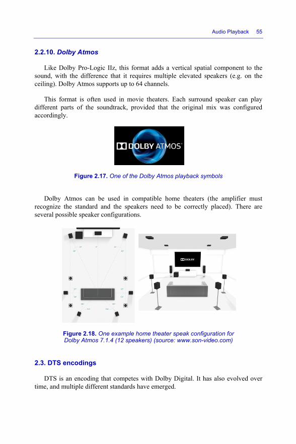
Audio Playback 55
2.2.10. Dolby Atmos
Like Dolby Pro-Logic IIz, this format adds a vertical spatial component to the sound, with the difference that it requires multiple elevated speakers (e.g. on the ceiling). Dolby Atmos supports up to 64 channels.
This format is often used in movie theaters. Each surround speaker can play different parts of the soundtrack, provided that the original mix was configured accordingly.
Figure 2.17. One of the Dolby Atmos playback symbols
Dolby Atmos can be used in compatible home theaters (the amplifier must recognize the standard and the speakers need to be correctly placed). There are several possible speaker configurations.
Figure 2.18. One example home theater speak configuration for Dolby Atmos 7.1.4 (12 speakers) (source: www.son-video.com)
2.3. DTS encodings
DTS is an encoding that competes with Dolby Digital. It has also evolved over time, and multiple different standards have emerged.

56 Musical Sound Effects
2.3.1. DTS
Figure 2.19. The DTS logo
DTS was released in 1999, and encodes six channels, like Dolby Digital (5 + 1 LFE). However, DTS has a lower compression rate than Dolby Digital and therefore offers better quality. In movie theaters, this system uses time codes to synchronize the audio, which is recorded on a separate CD-ROM, and the image on the film. Many movie theaters around the world still support this format, which has been available since 1993.
DTS supports multiple sampling rates ranging from 8 to 192 kHz. The transfer rate varies from 32 to 4,096 kbps.
Figure 2.20. The DTS playback symbol
2.3.2. DTS Neo 6
Figure 2.21. The DTS Neo 6 logo
Released in July 2000, this format has two modes, Movie and Music. It was developed by DTS as a direct competitor for DPL II.

Audio Playback 57
2.3.3. DTS ES 6.1
Figure 2.22. The DTS ES logo
This configuration of DTS has an extra channel, designed to be placed at the center rear. It is a director competitor of Dolby Digital Surround EX.
2.3.4. DTS 96/24
The goal of this standard is to improve the quality of the signal by using a 96-kHz, 24-bit encoding on six channels, with the option of outputting the digital stream via S/PDIF12.
Figure 2.23. The DTS 96/24 logo
2.3.5. DTS HD Master Audio
This is a lossless format that uses a variable bitrate technique to produce high-quality signals. It supports two encoding frequencies, 96 kHz for eight audio channels (7.1), and 192 kHz for six channels (5.1).
The bitrate of this type of DTS ranges from 1 to 24.5 Mbps.
Figure 2.24. DTS HD Master Audio logo
12 Sony/Philips Digital Interface (S/PDIF) is a format for digital audio data transmission, defined in 1989.

58 Musical Sound Effects
REMARK.– There is an intermediate standard called DTS HD High-Resolution Audio that delivers 7.1 at 96 kHz, with bitrates ranging from 2 to 6 Mbps.
Figure 2.25. The DTS High-Resolution Audio logo
2.3.6. DTS X
DTS X supports up to 32 speakers, but it is usually used with 11.2-channel systems. It has a sampling rate of 96 kHz.
The goal of this standard is to faithfully recreate a 3D audio space by introducing the notion of independent sound objects that can move and occupy positions throughout this space.
Figure 2.26. The DTS X logo
DTS X is built around DTS HD Master Audio. In the most general case, this standard adds two or four additional speakers to 5.1, 7.1 or 9.1 configurations. These extra speakers are placed above the front speakers and rear surround speakers.
Of course, like all of the more modern standards, DTS X requires a compatible playback system.
2.4. Special encodings
As well as the Dolby and DTS standards listed above, both have other, more specific encodings:
– Dolby Headphone: introduced in 2000, this standard allows surround environments to be recreated within a conventional stereo headset;

Audio Playback 59
– Dolby Virtual Speaker: introduced in 2000, this standard creates the illusion of
surround sound using a single pair of frontal speakers;
– DTS Headphone: X: launched in 2013 to compete with Dolby Headphone, this standard simulates surround sound with headsets;
– DTS Interactive: This a version of DTS designed for video games.
REMARK.– Even the long list of Dolby and DTS standards presented above is not exhaustive. There are other variants designed for specific environments and hardware, and even other experimental standards.
2.5. SDDS
Figure 2.27. Logo of the SDDS format
Dating back to 1994, the SDDS (Sony Dynamic Digital Sound) format is exclusively reserved for movie theaters. It was developed by Sony and Columbia. It is usually arranged in 5.1 or 7.1 configurations. It uses a proprietary data compression algorithm developed by Sony for the Sony MiniDisc, called ATRAC (Adaptative TRansform Acoustic Coding).
2.6. THX certification
Figure 2.28. The logo of THX (Tom Holman eXperiment)

60 Musical Sound Effects
The acronym THX comes from the name of one of the engineers at Lucasfilm,
Tomlinson Holman, who wrote specifications for reproducing movie soundtracks according to a set of very strict quality criteria in response to a request by George Lucas. The name is also a reference to George Lucas’s first film, “THX 1138”, which was released in 1971. The first film shown in theaters under this standard was “The Return of the Jedi” from the Star Wars saga.
THX recommendations are now also available in a form suitable for home theater.
The main areas considered by THX quality certification are:
– sound balance;
– sound power;
– high dynamic range;
– low background noise;
– realistic sound space;
– immersive surround sound;
– realistic distribution of sound perspectives;
– clarity and intelligibility of dialogue.
The surround speakers of THX systems are bidirectional (dipole speakers), and the frequency band between 80 and 20 kHz is covered by five speakers, reserving low frequencies for subwoofers (from 1 to 3 for THX Home Cinema systems) on the LFE channel.
The standard also includes other specifications relating to the theater venues themselves, such as room reverb, acoustic insulation, viewing angles for spectators and projection type.
The hardware requirements are very strict for both commercial and home theaters, placing requirements on the media (LD, DVD, etc.), as well as the connection cables and materials used by the sound system.
REMARK.– There is also a separate THX I/S Plus standard designed for small home theaters.

Audio Playback 61
2.6.1. THX select and ultracertification
Figure 2.29. The logos of THX Select and Ultra
THX Select applies to lower range sound systems, namely systems with power below 100 W per channel, which is a minimum requirement of regular THX. To differentiate between the two more clearly, Lucasfilm rebranded THX-certified systems as THX Ultra when THX Select was launched.
2.6.2. THX Ultra 2 certification
Figure 2.30. The logo of THX Ultra 2
THX has of course evolved over time to keep up with the introduction of new standards. In 1995, THX 4.0 was replaced by THX 5.1. With the arrival of 6.1 standards, THX Surround EX and THX Select Surround EX were born. THX Select/Ultra 7.1 was developed after the introduction of 7.1.

62 Musical Sound Effects
However, THX Ultra 2 is a particularly noteworthy step forward, introducing
support for DVD-Audio and SACD, which are specially designed for listening to music.
2.7. Multichannel audio recording
To properly understand this type of audio recording, we need to revisit some of the principles of stereophonic audio. The challenge is to record a homogeneous audio signal by accounting for the acoustic properties of the recording environment.
We will not go into extensive detail here – we are moving away from the central theme of this book, and I do not specialize in this type of recording. If you are interested, you can explore the internet links and bibliography at the end of the book to find out more.
However, a few things are worth mentioning.
Sound recording techniques can be based on three, four or five microphones, or sometimes even more.
One key principle is that there is one essential recording axis along which the primary audio image of the scene is concentrated. This axis defines the global spatial configuration of the sources by perfectly balancing the direct sound field and the secondary sound field reverberated by the environment. It establishes the foundation for the timbre and determines the rendering of the recording by providing the spatial localization of each source.
In addition to this primary audio image, there is a secondary, less concentrated image containing ambient sounds without any direct sources. This image represents the atmosphere and soundscape of the audio scene, and is usually constructed from the primary image.
The primary and secondary images are supplemented by the front audio, as well as any very close sounds surrounding the listener.
Multichannel recording is based on two main factors, localization and spatialization. The goal is to combine both of these factors to cover a 360° space without any gaps, while keeping cross-talk at acceptably low levels.

Audio Playback 63
Many recording setups meet these requirements: the Decca tree, the MMAD
(Multiphonic Microphone Array Design), Double ORTF, the Hamasaki square, OCT (Optimized Cardioid Triangle) Surround, Soundfield, the IRT cross, the holophone H2, etc.
Figure 2.31. An IRT cross recording setup
These systems are of varying effectiveness and produce very different sound renderings. Thus, there is no single universal solution to the problem of multichannel recording, but rather multiple solutions depending on the location and the desired levels of ambient sound, as well as the desired sensitivity and approach chosen by the sound technician.
2.8. Postproduction and encoding
Postproduction mixing, encoding, decoding, measuring and control of multichannel formats requires highly specialized tools, typically integrated into a DAW. A wide variety of tools are also available as racks developed for studios that specialize in this type of mixing/encoding/mastering.
Table 2.1 provides a simple list of plugins for manipulating and processing multichannel audio. Many of these plugins were designed to be integrated into the Avid Protools software. The others have various other formats (VST, VST2, VST3, AU, etc.) and can be used with various DAWs and digital audio editing suites. More information about the specifications of each of these tools is easy to find online.
If you wish to find out more about audio processing systems like Dolby, DTS, etc., a few useful references are listed in the web links and bibliography sections of this book.

64 Musical Sound Effects
Editor Name Remarks
Avid Dolby Surround Tools Surround encoding and decoding
Waves 360° Surround Tools
Toolbox for 5.1 surround production: compressor, quantizer, limiter, low-pass filter, reverb, imager, mixer, VU meters, etc.
Waves DTS Neural Surround Collection
Set of three tools for encoding 5.1/7.1 DST
Auro Technologies
Auro-3D Authoring Tools Surround encoder
New Audio Technology
Spatial Audio Designer 5.1/7.1 surround encoder
Dolby Atmos Mastering Suite
Dolby Atmos surround encoder
Dolby Atmos Production Suite
Toolbox for Dolby Atmos surround production
Dolby Media Emulator Metadata simulator for 5.1 Dolby playback – Dolby E preencoder
Dolby Surround tools Surround encoder/decoder Cycling’74 UpMix Toolbox for 5.1 surround encoding Neyrinckl SoundCode for
DTS Surround encoder/decoder
DTS Neural Upmix UpMix – stereo to 5.1 – 5.1–7.1 Sonnox Fraunhofer Pro
codec 5.1 encoder
Sonic Anomaly
Surround Pan Freeware – DTS encoder
Minnetonka audio
SurCode DTS DTS encoder/decoder
Minnetonka audio
SurCode Dolby Dolby encoder/decoder
Dolby LM100 Software version of a loudness measuring tool Neyrinck Mix 51 5.1 mixing tool Neyrinck V-Mon 10 inputs to 5.1 measuring tool – 7.1 output
control Neyrinck Soundcode LtRt LtRt Dolby Pro-Logic I and II encoder TC Electronic
LM5D Tool for measuring and loudness control
Table 2.1. Examples of tools for mixing, encoding, decoding, controlling and measuring multichannel 5.1/7.1 Dolby or DTS audio

Audio Playback 65
2.9. Multichannel music media: DVD-Audio and SACD
DVD-Audio and SACD were specifically designed to support 5.1 multichannel music playback. Although the idea might seem extremely promising, these media struggled to conquer the market and sales have stagnated. However, these two formats are, nonetheless, worth bearing in mind. They can be used to take advantage of audio with spatial depth in home theater systems whenever a compatible media player is available.
2.9.1. DVD-Audio
In 1996, manufacturers and a group of experts from the DVD Forum began to draft specifications and develop a new DVD-based musical media format. In May 1998, the DVD-Audio standard (usually referred to as DVD-A) was unveiled. It was finalized in February 1999. This standard introduces a new lossless compression process for audio data called MLP (Meridian Lossless Packing) that can achieve up to 45% reduction in space and which supports real-time decompression.
Figure 2.32. The DVD-Audio logo
DVD-Audios have the same physical dimensions as audio CDs and use the same encoding technique, namely Pulse Code Modulation (PCM).
The main difference lies in the sampling rate. CDs have a fixed sampling frequency of 44.1 kHz at 16 bits, whereas DVD-A offers the choice between 44.1, 88.2, 96, 176.4 and 192 kHz at 16–24 bits.
Table 2.2 shows the supported combinations of channels and sampling frequencies.
The bandwidth can thus range up to 96 kHz (192 kHz for 24 bits), which is much higher than the 20 kHz offered by CDs. The signal-to-noise ratio is 144 dB.

66 Musical Sound Effects
Number of channels Sampling frequency at 16, 20 or 24 bits
44.1 kHz 48 kHz 88.2 kHz 96 kHz 176.4 kHz 192 kHz
1.0 (mono)
OK OK OK OK OK OK
2.0 (stereo)
OK OK OK OK OK OK
2.1 (stereo)
OK OK OK OK – –
3.0/3.1 (stereo + mono surround)
OK OK OK OK – –
3.0/3.1 (3-stereo)
OK OK OK OK – –
4.0/4.1 (3-stereo + mono surround)
OK OK OK OK
5.0/5.1 (surround)
OK OK OK OK
Table 2.2. Supported sampling frequencies and channels
Depending on the sampling frequency, the number of channels can be modulated. For example, 5.1 playback can be achieved by three 96-kHz 24-bit channels and two 48-kHz 20-bit channels (see Table 2.2).
DVD-Audios can also store other types of information than just soundtracks, such as text or images. Each DVD-A can be divided into nine groups of 99 tracks, each of which can have 99 indexes. Depending on the type of DVD, audio recordings can last up to 7 h of 16-bit 44.1-kHz stereo, or 74 min of six 24-bit 96-kHz channels (DVD-513). Type-9 DVDs and above have even higher storage capacity. Mixed audio and video DVDs are also possible.
DVD-Audios require a compatible DVD player.
13 There are several types of DVDs: DVD 5 – 4.7 GB – single-sided/single-layer, DVD-9 – 8.54 GB – single-sided/double-layer, DVD-10 – 9.4 GB – double-sided/single-layer, DVD-14 – 13.24 GB – (DVD-5 + DVD-9) side 1: single-layer/side 2: double-layer, DVD-18 – 17 GB – double-sided/double-layer.
Audio Playback 67
2.9.2. Super Audio CD
In 1998, Philips and Sony announced a new medium with the same physical dimensions as CDs, termed as SACD. This new medium supports high-quality music recordings with multichannel spatial sound.
Figure 2.33. The SACD logo
This type of media can be played by dedicated SACD players (which are also compatible with CDs), SACD-compatible DVD players and Direct Stream Digital (DSD) players.
The technology on which SACDs are based does not use the same PCM process as DVD-Audios and CDs. The audio sampling frequency is 2,822.4 kHz, which is 64 times the sampling frequency of audio CDs (44.1 kHz).
However, audio CDs are encoded with 16-bit samples, whereas SACDs have a single bit, which explains the extremely high frequency. The 16 bits of audio CDs are used to define 65,536 different values that characterize frequencies between 20 Hz and 20 kHz. With only 1 bit, the only possible values are 0 and 1, and so a different method is required. The value 1 is interpreted as a frequency increase, and the value 0 is interpreted as a frequency decrease. This is repeated 2,822,000 times per second (sampling frequency of SACDs). This technique is advantageous because consecutively sampled frequencies have very similar values, resulting in a loss in the sampled signal that is extremely low relative to the original signal. This technique is called DSD.
SACDs have much higher bandwidth than audio CDs, ranging from 1 Hz to 100 kHz, i.e. much wider than the spectrum perceived by the human ear. However, we should bear in mind that some frequencies can influence the sound even though they are inaudible. For example, infrasounds can be physically felt by the body. The signal-to-noise ratio of SACDs can range up to 120 dB.

68 Musical Sound Effects
Figure 2.34. Three types of SACDs
There are three types of SACDs:
– single-layer high density (HD), which can only be read by SACD players;
– double-layer HD, which can also only be read by SACD players;
– hybrid double layer with two different layers. One of the tracks is reserved for SACD players, and the other is reserved for conventional CD players.
Figure 2.35. A hybrid double-layer SACD. The laser beam on the right, with a wavelength of 780 nm, passes through the HD layer, which is transparent to it. The
laser beam on the left, with a wavelength of 650 nm, can read the HD layer

Audio Playback 69
2.9.3. Comparison of CDs, SACDs and DVD-Audios
Table 2.3 summarizes the most important features of these three media.
Type CD SACD DVD-A
Diameter (cm) 12 12 12
Sampling rate 44.1 kHz 16 bits
2,822.4 kHz 1 bit
44.1–192 kHz 16–24 bits
Bandwidth 20 Hz–20 kHz 100 kHz 96 kHz
Signal-to-noise ratio 96 dB 120 dB 144 dB
Channels 2 (stereo) 5.1 5.1
Notes – One audio CD track for the hybrid double-layer version
Can store text or images
Storage capacity 700 MB 4.7 GB 4.7 GB
Table 2.3. Comparison of CDs, SACDs and DVD-As
REMARK.– There are also next-generation versions of these standards, most notably of the SACD, with the SHM SACD (Super High Material Compact Disc) created in 2010, and the DSD–CD.
Figure 2.36. Logos of the SHM SACD and the DSD–CD
2.10. Conclusion
As we can see, there are a large number of existing standards for multichannel encoding. New additions are constantly being made over time as media and playback technology changes. It is easy to get lost, even before considering the options for certifying and configuring audio spaces (large and small theater venues, home theater setups, etc.).

70 Musical Sound Effects
The DVD-A and SACD standards are still current, although the market for these
media remains very limited. Today, they are almost exclusively used by audio enthusiasts who are passionate about classical music.
Properly encoding audio and complying with the subtleties of each standard can represent a significant challenge for recording studios. Acquiring the proper equipment for encoding and playback can quickly present substantial technical and financial challenges.
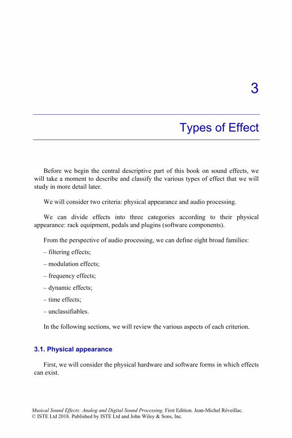
3
Types of Effect
Before we begin the central descriptive part of this book on sound effects, we will take a moment to describe and classify the various types of effect that we will study in more detail later.
We will consider two criteria: physical appearance and audio processing.
We can divide effects into three categories according to their physical appearance: rack equipment, pedals and plugins (software components).
From the perspective of audio processing, we can define eight broad families:
– filtering effects;
– modulation effects;
– frequency effects;
– dynamic effects;
– time effects;
– unclassifiables.
In the following sections, we will review the various aspects of each criterion.
3.1. Physical appearance
First, we will consider the physical hardware and software forms in which effects can exist.
Musical Sound Effects: Analog and Digital Sound Processing, First Edition. Jean-Michel Réveillac.© ISTE Ltd 2018. Published by ISTE Ltd and John Wiley & Sons, Inc.

72 Musical Sound Effects
3.1.1. Racks
Rack effects are primarily used for sound recording in studio environments, mixing, mastering and sound reinforcement, typically in connection with a mixing desk.
Audio racks are analog or digital effects integrated into compact box-shaped units that can be vertically stacked inside a cabinet with standardized shelves designed specially to accommodate them.
Strictly speaking, the rack refers to the cabinet itself, which stores “rack-mountable” effects units. However, over time, the effects themselves have come to be known as racks.
3.1.1.1. Standards and dimensions of racks
Racks (storage shelves in cabinets) can be mounted on wheels in a road case ready for live applications, or permanently installed in a recording studio. Their dimensions are regulated by the standards IEC 602971 and EIA 310-D2.
By default, professional audio racks have a width of 19 inches (482.60 mm). They have two vertical metal rails, each 0.625 inches (15.875 mm) wide, with 17.75 inches (450.85 mm) of space in between.
Figure 3.1. Example of a 19-inch audio rack cabinet
Holes are drilled in the rails, with 18 and 5/16 inches (465.14 mm) of horizontal space and 0.625 inches (15.875 mm) of vertical space between holes.
1 International Electrotechnical Commission. This standard was formerly DIN 41 494 (see web links at the end of the book). 2 Electronic Industries Association.

Types of Effect 73
The holes are often square-shaped, designed for captive nuts (also known as
caged nuts). Some rails have prethreaded holes. Two types of thread are used: 10–32 and 12–24. The nut diameter is typically 6 mm.
Figure 3.2. Captive nuts (or caged nuts) and screws
Figure 3.3. Standard dimensions of a 19-inch rack

74 Musical Sound Effects
The height of rack-mountable modules is measured in units of U, which is
simply short for unit. One U is equal to 1.75 inches (44.45 mm).
The height of a module is typically given in multiples of U, e.g. 1U, 2U, 3U, 4U or more (Eurocard system).
To ensure that modules can be easily mounted, a clearance of 1/32nd of an inch (0.79 mm) is left between modules, resulting in a face height of 43.66 mm for each module.
3.1.1.2. Effects units
Let us now move on to the actual contents of the rack, which for us means the musical audio effects themselves. Effects units are usually reasonably compact, rarely exceeding 3U in size.
Figure 3.4. Three examples of (19’’) rack-mountable effects with different heights: “PCM92” reverb by Lexicon (1U), “PE-1C” parametric equalizer by Tube-Tech (2U)
and the “Profiler” multieffects processor by Kemper Amps (3U)
The audio inputs/outputs (Jack, XLR, S/PDIF, optical, etc.), other connections (USB, MIDI, RS422, etc.) and power cables are typically located at the back of the unit. Extra connectors are sometimes placed on the front, such as headphone jacks, remote control interfaces and microphone inputs. These front connectors can, for example, be redundant duplicates of the ones on the back.
3.1.2. Pedals
Pedal effects take the form of a physical pedal, sometimes in combination with other equipment like a rack.

Types of Effect 75
3.1.2.1. Amplifier pedals
Some effects are integrated directly into an amplifier and are operated using a convenient pedal that connects to a dedicated input on the amp.
Figure 3.5. Fender amp, 65 Deluxe Reverb model (top left), with its effects pedal (top right) for controlling the vibrato and reverb effects. The jack
socket for connecting the pedal is visible in the bottom image (“foot switch”)
Usually, with the occasional exception, these pedals have limited functionality, and are simply used to toggle tremolo, vibrato or reverb effects that must be preconfigured using the controls directly on the amp.
3.1.2.2. Dedicated effects pedals
Since the first electronic guitar effects began to appear in the mid-1970s, engineers and sound technicians have invented control designs that can be easily operated while standing or sitting. Pedals are a perfect example of this.
REMARK.– Effects pedals were inspired by the earlier pedals used to control the volume of electronic organs.
Before the introduction of these pedals, effects such as distortion or overdrive needed to be configured via the controls on the amplifier, which was highly impractical on stage.
Effects pedals are connected between the instrument and the amplifier, and can be chained together to allow multiple pedals to be combined or used independently.
Some musicians also use pedalboards, which make it easier to manage audio connections and power supplies with multiple pedals.
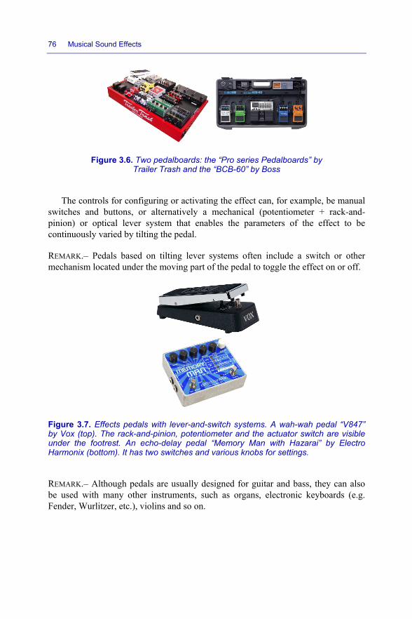
76 Musical Sound Effects
Figure 3.6. Two pedalboards: the “Pro series Pedalboards” by Trailer Trash and the “BCB-60” by Boss
The controls for configuring or activating the effect can, for example, be manual switches and buttons, or alternatively a mechanical (potentiometer + rack-and-pinion) or optical lever system that enables the parameters of the effect to be continuously varied by tilting the pedal.
REMARK.– Pedals based on tilting lever systems often include a switch or other mechanism located under the moving part of the pedal to toggle the effect on or off.
Figure 3.7. Effects pedals with lever-and-switch systems. A wah-wah pedal “V847” by Vox (top). The rack-and-pinion, potentiometer and the actuator switch are visible under the footrest. An echo-delay pedal “Memory Man with Hazarai” by Electro Harmonix (bottom). It has two switches and various knobs for settings.
REMARK.– Although pedals are usually designed for guitar and bass, they can also be used with many other instruments, such as organs, electronic keyboards (e.g. Fender, Wurlitzer, etc.), violins and so on.

Types of Effect 77
3.1.2.3. Racks with pedals
Racks are often more powerful and flexible for musicians. In some cases, they can be placed on top of the amplifier and controlled via foot pedal. Most are capable of saving presets in their memory. These presets can then, for example, be selected by scrolling through them.
Figure 3.8. Example of a multieffects rack designed for guitar, with a control pedal. This model is the G-sharp by TC Electronic
Many effects racks behave like emulators, recreating specific amplifiers or certain popular effects that can be found on the market. These racks are often suitable for studio usage.
Figure 3.9. A rack for emulating amplifiers and effects, the “Eleven” model by Avid. It can be used either in the studio or live directly with guitars or other instruments. Below it is a control pedal compatible with the MIDI standard, the “Ground Control Pro” by Voodoo Lab.
3.1.3. Software plugins
Plugins are software components recognized by a Digital Audio Workstation (DAW) such as Avid Pro Tools, Magix Samplitude Pro X, Cakewalk Sonar, Presonus Studio One, Apple Logic Pro, Ableton Live, and many more, or alternatively by digital audio processing software such as Adobe Audition, Magix Sound Forge, Steinberg Wavelab, Audacity and so on. This list is far from exhaustive.

78 Musical Sound Effects
The format of plugins varies depending on the operating system and the
software.
Table 3.1 lists the characteristics of each plugin format. Users can see the format of a plugin by looking at its file extension.
File extension Editor Software–hardware compatibility VST (Virtual Studio Technology)
Steinberg 1996 DAW–Audio processing software–PC/Mac
VST2 Steinberg DAW–Audio processing software–Improved version of VST–PC/Mac
VST3 Steinberg DAW–Audio processing software–Improved version of VST2–PC/Mac
AU (AudioUnits) Apple DAW–Audio processing software–Mac–OSX
and Mac OS AAX (Avid Audio eXtension) Avid Pro Tools 64 bits–PC/Mac
MAS (MOTU Audio System)
MOTU (Mark of The Unicorn)
Digital Performer–Mac
AS (Audiosuite) Digidesign Pro Tools–PC/Mac
EASI (Enhanced Audio Streaming Interface)
Apple Logic Audio–Mac
RTAS (Real-Time Audio Suite)
Digidesign Pro Tools 10 minimum–PC/Mac
TDM (Time Division Multiplexing)
Digidesign Cartes HD Core or HD Accel Digidesign–PC/Mac
DX (Direct X) Microsoft PC
Table 3.1. Plugins by file extension
Many plugins exist in multiple versions to provide compatibility with multiple types of software or hardware.
3.2. Audio processing
As we mentioned at the beginning of the chapter, there are eight families of audio processing effects that we can use as a classification. Chapters 4–9 describe the effects that belong to each of these families.
Table 3.2 gives a list of effects by family.

Types of Effect 79
Family Effect
Filtering Graphic equalization Parametric equalization Semiparametric equalization Band-stop equalization Linear phase equalization Dynamic equalization Wah-wah Auto-wah Crossover
Modulation Flanger Phaser Chorus Rotary, univibe, rotovibe Ring modulation
Frequency Vibrato Transposer Octave up/down Pitch shifter Harmonizer Autotune
Dynamic Compressor Limiter Expander Noise gate De-esser Saturation Fuzz Overdrive Distortion Exciter, enhancer, embellisher
Time Analog reverb Digital reverb Convolution reverb Delay Slapback Doubler Pan delay Echo
Unclassifiables Fuzzwha Octafuzz Shimmer Tremolo Declicker Decrackler Denoiser Declipper Debuzzer Looper Time stretching Resampling Spatialization
Table 3.2. Families of effects

80 Musical Sound Effects
3.3. Conclusion
This brief introduction to the various existing types of effect will make the following chapters easier to understand. We will examine most of the sound effects that we might find in a studio, on stage and on live sets.
The order in which we will study these effects has a certain logic that will allow us to discuss the connections and combinations between effects, but any readers who are interested in a specific effect are welcome to skip directly to the relevant section. References and hints are given wherever they are helpful.

4
Filtering Effects
Filters can be used to cut, eliminate, boost or modify regions or frequency bands of arbitrary width in an audio signal. Some filters are extremely selective, only targeting very narrow frequency components, e.g. based on a gain threshold.
4.1. Families of filtering effects
There are four large families of filtering effects:
– high-pass filters: these filters only allow through frequencies above a certain frequency threshold, called the cut-off frequency. They are used to reduce low frequencies;
– low-pass filters: these filters are the reverse of high-pass filters. They only keep frequencies below the cut-off frequency;
– band-pass filters: only the frequency band between an upper threshold and a lower threshold is allowed through. These filters are often used to isolate a certain part of the audio signal;
– band-stop filters or band-rejection filters: other names include band limit filters, bell filters, band-elimination filters and T-notch filters. Unlike the types of filter listed above, these filters reduce a certain frequency band to eliminate undesirable parts of the original signal, such as noise, crackling, etc.
A signal frequency is usually said to be filtered if it is attenuated by 3 dB or more. To distinguish between different types of filters, we can compare their “bandforms”. This divides filters into each of the families listed above. Different filters can also have different “orders”. Without going into too much technical detail, the order of a filter is determined by the slope rate of its attenuation. A first-order filter has a slope of 20 dB/decade, i.e. 6 dB per octave, a second-order filter has a slope of 40 dB/decade, a third-order filter has a slope of 60 dB/decade, and so on.
Musical Sound Effects: Analog and Digital Sound Processing, First Edition. Jean-Michel Réveillac.© ISTE Ltd 2018. Published by ISTE Ltd and John Wiley & Sons, Inc.
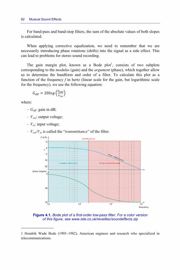
82 Musical Sound Effects
For band-pass and band-stop filters, the sum of the absolute values of both slopes is calculated.
When applying corrective equalization, we need to remember that we are necessarily introducing phase rotations (shifts) into the signal as a side effect. This can lead to problems for stereo sound recording.
The gain margin plot, known as a Bode plot1, consists of two subplots corresponding to the modulus (gain) and the argument (phase), which together allow us to determine the bandform and order of a filter. To calculate this plot as a function of the frequency f in hertz (linear scale for the gain, but logarithmic scale for the frequency), we use the following equation: = 20
where:
– GdB: gain in dB;
– Vout: output voltage;
– Vin: input voltage;
– Vout/Vin is called the “transmittance” of the filter.
Figure 4.1. Bode plot of a first-order low-pass filter. For a color version of this figure, see www.iste.co.uk/reveillac/soundeffects.zip
1 Hendrik Wade Bode (1905–1982), American engineer and research who specialized in telecommunications.

Filtering Effects 83
By analyzing the eliminated frequencies (the frequencies for which GdB is less than –3 dB), we can determine the bandform of the filter, and by considering the slope, we can find its order.
Equalizers are often used in tandem with spectrum analyzers, which allows the corrections to be more precisely visualized in real time.
Today, digital and software equalizers have become much more precise, and analyzers are easier to find, often integrated directly into Digital Audio Workstations and other audio processing software.
REMARKS.– You might also come across bell filters or Baxandall2 filters. Bell filters act on a specific target frequency. Their name comes from the shape of their attenuation curve, which looks like a bell. Baxandall filters are named after their inventor. They are precursors of pitch correctors that were used long before the first equalizers were invented. They can be used to correct bass and treble frequencies, and generally operate at around 1 kHz. They are characterized by the fact that they preserve certain ratios between harmonics. Some sources on equalization also mention the concept of “Q factor”. This simply refers to the width of the frequency band on which the filter acts.
Figure 4.2. Equalization curves of a bell correction and a Baxandall correction. For a color version of this figure, see www.iste.co.uk/reveillac/soundeffects.zip
2 Peter J. Baxandall (1921–1995) British electronics and sound engineer. In 1952, he invented the pitch correction filter that bears his name. The first Baxandall filters were built from electronic tubes.

84 Musical Sound Effects
4.2. Equalization
The purpose of equalization is to correct the timbre of a sound by boosting or cutting one or more frequency bands in the audio signal.
This type of audio processing is widely used during recording, production and in sound reinforcement systems. It can be implemented using various technological tools, known as equalizers or EQs, which work in a variety of different ways.
Over time, equalization has become vital to sound engineers, who need it to achieve the right frequency balance in the signal. This allows them to properly separate and showcase each instrument in the mix. For example, the sound of a bass guitar needs to be clearly audible, and should not be allowed to conflict with the bass drum.
We can use different frequency scales to describe the frequencies specific to each type of instrument.
4.2.1. Frequency bands and ranges
Frequencies can be divided into six families according to their frequency band:
– treble: from 4 to 20 kHz;
– high-midrange: from 2 to 4 kHz;
– midrange: 500 Hz–2 kHz:
– low-midrange: 250–500 Hz;
– bass: 63–250 Hz;
– sub-bass: 20–63 Hz.
Each octave (in the musical sense of the term) can be associated with one of these frequency bands. Table 4.1 shows their distribution.
The “register” row in Table 4.1 lists a few technical terms often used to describe the subjective impression created by the sounds in each band.

Filtering Effects 85
Octave C0 C1 C2 C3 C4 C5 C6 C7 C8 C9 C10*
Frequency (Hz)
from C to B
16.3 to 30.8
32.7 to 62
65 to 123
131 to 247
262 to 494
523 to 988
1,046.5 to 1,975
2,093 to 3,951
4,186 to
7,902
8,372 to 15,804
16,744 to 19,912
Register Rumble Body Warmth Low mids
High mids Presence or attack
Brilliance or clarity
Air
Table 4.1. Equivalence between octaves and frequencies (* from C to E)
Figure 4.3 displays the approximate range (frequency spreads) of a few common instruments compared to a standard keyboard.
Figure 4.3. Range of instruments as a function of frequency (top) compared to the notes on a keyboard (bottom) (source: IRN3 (www.independentrecording.net)). For a
color version of this figure, see www.iste.co.uk/reveillac/soundeffects.zip
3 We can find an interactive version of this table with plenty of extra information at: www. independentrecording.net/irn/resources/freqchart/main_display.htm.

86 Musical Sound Effects
Having an idea of the range of each instrument will help you to identify the frequency band of the sound you are trying to equalize or modify.
But bear in mind that range is not the only factor. The sound of each instrument has a rich spectrum of harmonics that also need to be taken into consideration.
4.2.2. Types of equalizer
There are several kinds of equalizer:
– graphic equalizers;
– parametric equalizers;
– semiparametric equalizers;
– band-stop equalizers or notch equalizers;
– linear phase equalizers;
– dynamic equalizers.
4.2.2.1. Graphic equalizers
These equalizers are named after their physical design. They are arranged as a series of linear potentiometers (sliders) that cover the entire audible sound spectrum, one for each frequency band, positioned in increasing order from left to right.
One major advantage of graphic equalizers is that they make it very easy to visualize the currently applicable corrections to the incoming signal. The gain/attenuation on each band ranges between ± 18 dB.
Over the years, and as technology has progressed, the number of bands has increased from 5 to 31 (1/3 octave), and in some cases even 64.
Figure 4.4. Opal FCS-966, a 31-band graphic equalizer by BSS Audio

Filtering Effects 87
4.2.2.2. Parametric equalizers
Parametric equalizers allow the user to specify the type of filter, cut-off frequency or center frequency, bandwidth and gain.
They are more precise than graphic equalizers, but are more delicate to operate.
Figure 4.5. Orban 622B, a 2 × 4-band parametric equalizer
This type of equalizer only acts on a single frequency band at a time, which means that multiple equalizers are required for more elaborate corrections. Most manufacturers offer parametric equalizers with two or four bands.
You can also find so-called passive parametric equalizers, which only reduce the gain, and cannot boost it. A separate active circuit can be used to restore the gain level of the output. The advantage of this type of equalizer is that the signal is largely left unaltered, since the unpowered passive components only create very slight losses.
Figure 4.6. The well-known passive equalizer EQP-1A by Pultec

88 Musical Sound Effects
4.2.2.3. Semiparametric equalizers
Semiparametric equalizers combine some of the characteristics of graphic and parametric equalizers.
They typically consist of three (treble, mid and bass) or four frequency bands on which central cut-off frequencies can be defined and the gain can be specified.
Figure 4.7. The Aphex EQF-2 equalizer and a more recent modernized version, the Aphex EQF-500 model
4.2.2.4. Band-stop equalizers
Band-stop equalizers are not strictly speaking a separate class of equalizer, but rather a specific feature offered by many equalizers, especially software equalizers.
Band-stop equalization is the reverse of band-pass filtering used to eliminate very narrow frequency bands. For example, a hum at 50 Hz can be eliminated without affecting the surrounding frequencies.
This type of equalizer can be found on some mixing desks and is often used to avoid feedback effects.

Filtering Effects 89
Figure 4.8. An example of a band-stop (notch) filter on a sound reinforcement system
The filters used by these equalizers are also known as notch filters or rejection filters.
4.2.2.5. Linear phase equalizers
As their name suggests, linear phase equalizers are specially designed to avoid introducing phase shift during processing.
This is an important advantage for the sound engineers responsible for mastering. These equalizers allow phase rotation issues to be avoided during equalization, regardless of the amplification or attenuation of each processed frequency.
Figure 4.9. “Linear Phase EQ”, a linear phase software equalizer by Waves
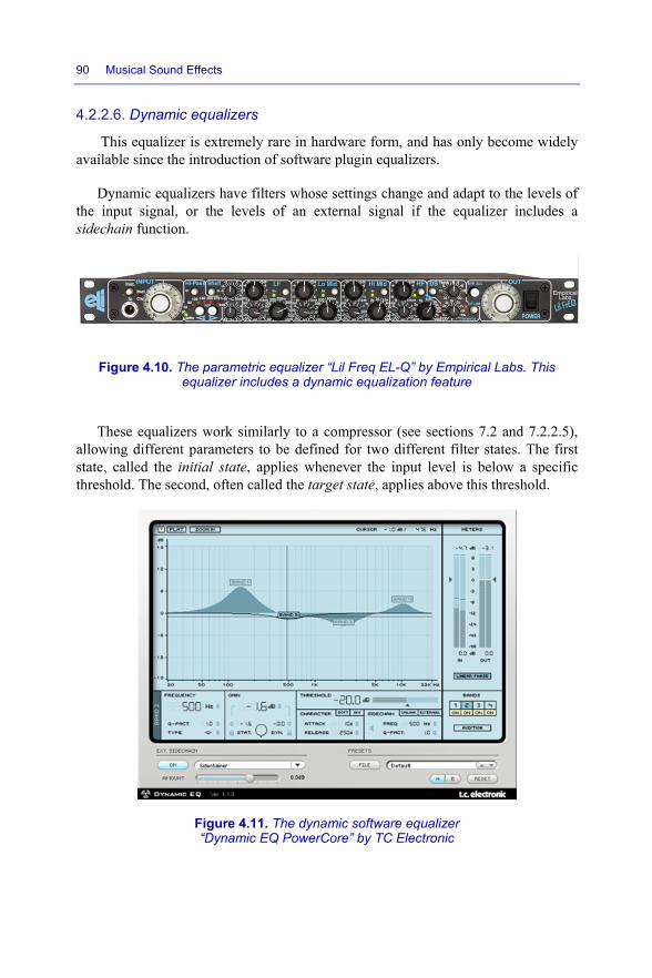
90 Musical Sound Effects
4.2.2.6. Dynamic equalizers
This equalizer is extremely rare in hardware form, and has only become widely available since the introduction of software plugin equalizers.
Dynamic equalizers have filters whose settings change and adapt to the levels of the input signal, or the levels of an external signal if the equalizer includes a sidechain function.
Figure 4.10. The parametric equalizer “Lil Freq EL-Q” by Empirical Labs. This equalizer includes a dynamic equalization feature
These equalizers work similarly to a compressor (see sections 7.2 and 7.2.2.5), allowing different parameters to be defined for two different filter states. The first state, called the initial state, applies whenever the input level is below a specific threshold. The second, often called the target state, applies above this threshold.
Figure 4.11. The dynamic software equalizer “Dynamic EQ PowerCore” by TC Electronic

Filtering Effects 91
4.2.3. Examples of equalizers
Table 4.2 lists a few examples of equalizers by type: pedals, racks and software.
Figure 4.12. Seven-band, 2-channel digital studio equalizer, EQ1 model by Weiss
A vast number (hundreds) of equalizer plugins are available on the market. Many software publishers have developed software clones of the most popular studio equalizers.
Type Manufacturer or publisher Name or model Remarks
Pedal
Boss GE-7 Graphic – 7 bands
Carl Martin 3 bands – Parametric Pre-Amp
Parametric – 3 bands
Electro Harmonix Attack Equalizer 2 bands + mixer Electro Harmonix Knockout Graphic – 2 bands Ibanez GE9 Graphic – 6 bands
Maxon GE601 Graphic – 6 bands
MXR M109 Graphic – 6 bands MXR M124 Graphic – 2 × 15 bands TC Electronic Dual Parametric EQ Parametric – 2 bands
Rack
Apex Audio DBQ Zero Graphic – 2 × 30 bands – ± 15 dB
Avalon AD 2055 Parametric – 3 bands – 2 channels
Boss GE-215 Graphic – 2 × 15 bands – ± 15 dB BSS Audio FCS-966 Opal Graphic – 2 × 30 bands – ± 15 dB DBX 2231 Graphic – 2 × 31 bands – ± 15 dB
D.W. Fearn VT-4 Parametric – 1 channel – Electronic tubes
Empirical Labs Lil FreQ EL-Q Parametric – 4 bands – 2 Baxandall

92 Musical Sound Effects
GML Model 8200 Parametric – 5 bands – 2 channels
Gyraf Audio Gyratec XIV Parametric – 5 bands – Passive – Electronic tubes
Manley Massive Passive EQ Parametric – Passive – Electronic tubes – 4 bands – 2 channels
Moog Music 10 Band Graphic EQ Graphic – 10 bands Moog 3 Band Parametric EQ Parametric – 3 bands Orban 672A Parametric – 8 bands
Pultec MEQ5-SS Parametric – Electronic tube – 2 boosting bands and 2 cutting bands – 300–5,000 Hz
Rupert Neve Designs Portico 5033 Parametric – 3 bands + 2 shelf
bands4 Samson technologies E62i Graphic – 2 × 31 bands – ± 12 dB
Urei/JBL 527A Graphic – 27 bands – ± 10 dB
Summit EQP-200B Parametric – 2 bands + 1 low shelf band – Electronic tubes
Tube-Tech EQ 1AM Parametric – 3 band – ± 20 dB – Electronic tubes
Tube-Tech PE1C Parametric – 2 bands – Passive, with electronic tubes
Weiss EQ1 Parametric – Digital – 7 bands – 2 channels
Software
Abbey Road TG Mastering Pack Parametric – 4 bands + filters Windows: VST OSX: VST; AU
Analog Obsession EAQ
Emulation of EAR 825Q Parametric Windows: VST2 OSX: VST2; AU; AAX
Bomb Factory Pultec Bundle
Emulation of Pultec EQP-1A, EQH-2, and MEQ-5 Windows: TDM; RTAS OSX: TDM; RTAS; AU
4 A shelf is a filter that extends from one end of the audible frequency spectrum (or the frequency spectrum modified by the equalizer) up/down to some specific frequency. There are two shelves, high and low, one at each end of the spectrum.

Filtering Effects 93
FabFilter Pro-Q2
24 bands + various filters + (rejection filters, shelves, etc.) Windows: VST OSX: VST; AU
IK Multimedia T-Racks Classic Equalizer Parametric – 6 bands + filters Windows: VST; RTAS; AAX OSX: VST; RTAS; AAX
MeldaProduction MEqualizerLinearPhase
3 equalization algorithms – 9 filters Windows: VST; VST3; AAX OSX: VST; VST3; AAX
Overtone DSP EQ4000 Parametric Windows: VST; VST3; AAX OSX: VST; VST3; AAX; AU
PSP Audioware Retro Q
Parametric – 3 bands – Vintage EQ emulation Windows: VST; AAX OSX: VST; AAX; AU
RJProjects Aqualizer Freeware – Graphic – 32 bands – ± 12 dB Windows – OSX: VST
Rob Papen RP-EQ 8 bands + filters + spectrogram Windows: VST; AAX OSX: VST; AAX; AU
Softube Tube-tech ME1B Emulation of Tube-Tech ME-1B based on Pultec MEQ-5
Softube Tube-Tech PE1C Emulation of Tube-Tech PE-1C
Sonnox Oxford EQ Parametric – 5 bands Windows: TDM; RTAS; AAX OSX: TDM; RTAS; AAX
SPL Free Ranger Freeware – Graphic – 4 bands Windows: VST; VST3; AAX OSX: VST; VST3; AAX; AU
TC Electronic Assimilator
Based on curves – Presets – Limiter Windows: VST OSX: VST; MAS
Universal Audio Pultec Passive EQ Collection
Emulation of Pultec EQP-1A, HLF-3C, and MEQ-5
Universal Audio NEVE 1073 EQ NEVE 1073 emulation

94 Musical Sound Effects
Voxengo HarmoniEQ
Parametric – Stereo and 5.1 surround mastering equalizer – Dynamic equalization – Spectrum analyzer Windows: VST; VST3 OSX: VST; VST3; AU
Voxengo GlissEQ 3
Parametric – Stereo and 5.1 surround equalizer – Spectrum analyzer – Dynamic equalization Windows: VST; VST3 OSX: VST; VST3; AU
Waves Linear Phase
Mastering equalizer – 9 types of filter Windows: VST; VST3; AAX OSX: VST; VST3; AAX; AU
Waves Q10 Paragraphic – 10 bands Windows: VST; VST3; AAX OSX: VST; VST3; AAX; AU
Waves H-EQ
Hybrid (parametric + curves) – 7 types of filter Windows: VST; VST3; AAX OSX: VST; VST3; AAX; AU
Waves RS56 Passive EQ
Passive parametric – 3 bands – 6 types of filter Windows: VST; VST3; AAX OSX: VST; VST3; AAX; AU
Waves V-EQ4
Parametric – 4 bands – Emulation of NEVE 1081 console Windows: VST; VST3; AAX OSX: VST; VST3; AAX; AU
Table 4.2. Examples of each of the three types of equalizer
4.2.4. Tips for equalizing a mix
Many modern mixing desks already have an integrated four-band parametric equalizer, often with a low-cut filter. These tools will probably be sufficient for most things, although they of course cannot compare with the level of sophistication offered by one or several external equalizers.

Filtering Effects 95
Figure 4.13. Integrated parametric filters on a mixing desk
The first question is where the equalizer should be placed in the audio processing chain: before or after the compressor (see Chapter 7 – Dynamic effects)? In fact, there is no single answer to this. As a rule of thumb, if you are cutting frequencies, put the compressor first, and if you are boosting frequencies, put the equalizer first.
Be wary of equalizers that add color (non-transparent equalizers) when you boost certain frequencies. This can affect the style of the mix, which may be undesirable. For initial separation and rough filtering, use an equalizer that is as neutral as possible.
In my personal opinion, the best approach is to start by cutting certain frequencies to clean the mix before boosting anything. Work surgically and carefully on narrow bands. You usually will not need to modify the gain by more than ± 3 dB, which is already a lot.
The basic rules described in the following can be useful. Keep in mind which frequency bands are occupied by each of the instruments in your mix.

96 Musical Sound Effects
If your mix is too aggressive, cut the band between 1.2 and 3 kHz. This will soften the sound a little. You can muffle the sound by pushing the gain toward the negatives. However, bear in mind that some instruments and vocals can be affected by this and might lose clarity. To compensate, you can boost the higher part of this band, between 2 and 3 kHz.
If the lower frequencies lack space or air, you can cut the 80–100 Hz region of the mix. Since this is the bottom of the spectrum, you can use a shelf to cut frequencies below 100 Hz. But be careful not to squash the bass. You can make it more distinctive by boosting its specific tone.
If your mix seems cluttered and confused, you can carefully cut the mid band from 100 to 300 Hz.
High frequencies are often the most difficult to equalize, since too much gain will create an imbalance that can disrupt the whole mix, resulting in a sound that quickly becomes uncomfortable.
If you are having problems with excessive sibilance, you will get better results with a de-esser (see section 7.5) than an equalizer.
If you think that your mix has too much air, you can configure a shelf at the top of the spectrum above 15 kHz and cut slightly. Make sure that you keep some presence.
Note that we tend to cut frequencies rather than boost them. You will get the feel for this over time. The most important thing is to keep listening to your mix, constantly playing with the bypass to get a clearer picture of the difference with and without your adjustments. Take your time, and allow your ears to rest whenever they need to. Equalization can be very tricky, so do not hesitate to revert any changes that do not work. Do not forget that a single change can affect the entire mix.
Accentuation can be used to shape the sound space of the mix or add color. If you are lacking in color, you can choose an instrument to accentuate using a separate equalizer from the one used to make the adjustments described above, perhaps a more stylized model that specifically fits the musical style of your mix. Working on narrow bands will allow you to increase the presence or brilliance of an instrument, whereas working with wider bands can enhance an ensemble. Remember that the wider the band, the smaller the required gain, usually less than 2 dB.
The sound space can be managed according to a simple principle that reflects how things work physically in reality: the trebles should be less present when the

Filtering Effects 97
source is further away and vice versa. Play with the gain in small increments of 0.25 dB in both directions until you find the right location for each sound. The higher the frequency (>10 kHz), the lower the required corrections. If you want to expand or broaden the space with respect to one or multiple instruments, one possible solution is to use a shelf to create slight accentuation above 5 or 6 kHz.
If you are using a shelf for the bass frequencies (<300 Hz) of an instrument, you should move it to the edge of the sound field.
These instructions might seem vague, but equalizing mixes is difficult and very subjective. If you are working on a specific instrument, listen carefully, first to the effect of the changes on the instrument itself, and then to their effect on similar instruments, and finally to the effect on the whole mix.
I use this three-step approach myself for my work, it works very well for me. It is one way of doing things, but everyone needs to forge their own path. There are no hard-and-fast rules, and the only things that you need to answer to – it is impossible to emphasize this enough – are your ears.
4.3. Wah-wah
Some people might find it strange to include the wah-wah in this chapter. But from the perspective of physics, wah-wah is definitely a filtering effect, so it fully deserves its place here.
Wah-wah is an effect that alters a musical passage to sound like a human voice. Musicians use it as a way of playing more expressively. It can be used with most instruments, but is most popular with brass instruments and electric guitar.
REMARK.– Wah-wah is pronounced like it is written. You might also come across the alternative spellings “wha-wha” or “wa-wa”.
4.3.1. History
Wah-wah was invented in the mid-1960s. The effect imitates the crying sound that can be made with the human voice. The electronic wah-wah pedal was invented by the engineer Brad Plunkett. He discovered the effect when he was modifying a Vox amplifier in an attempt to make it cheaper to manufacture without sacrificing any sound quality.
The original Vox amplifier had a switch known as an MRB (Mid-Range Boost) that increased the presence of the sound by boosting the central part of its spectrum

98 Musical Sound Effects
(300–500 Hz). Plunkett replaced this switch with a potentiometer, which at the time was much less expensive.
Figure 4.14. The three-position MRB EFFECTS switch (right) used in the first Vox amplifiers
He later realized that varying the potentiometer while a guitarist was playing through the amp created this wah-wah effect. He therefore decided to mount this system into a Vox Continental organ pedal so that it could be operated by foot. Thus, the wah-wah pedal came into existence.
In 1967, Vox placed the pedal on the market with two different names: “Cry-Baby”, because it sounds like a crying baby, and “Vox Wah-Wah”. The electronics in both pedals were identical.
Figure 4.15. Two versions of the Vox wah-wah pedal, the “Vox Wah-Wah” and the “Cry-Baby”
The wah-wah effect was already familiar to trumpeters, who had been using it since the 1920s by inserting a mute, known as the “wah-wah”, into the bell of the trumpet.

Filtering Effects 99
Figure 4.16. A “wah-wah” mute designed for a trumpet
This mute simply consisted of a sliding tube and a cup. By sliding the tube back and forth, the trumpeter can modify the sound. By varying how much the tube is blocked while playing, the trumpeter controls the wah-wah effect.
REMARK.– By pressing a regular toilet plunger against the bell of the trumpet and varying the gap, jazz trumpeters can simulate the wah-wah effect.
4.3.2. Theory
The wah-wah pedal is based on a selective amplification system (affecting only certain parts of the sound spectrum) whose central frequency is modulated.
When the musician tilts the pedal, the boosted and filtered regions of the spectrum slide up or down.
Figure 4.17. Frequency response of a classic wah-wah pedal. The three curves (red, blue and green) represent the filtering and amplification of each region of the sound spectrum depending on the position of the pedal, from the up position to the down position. The spectrum slides from left to right as the pedal is lowered. For a color version of this figure, see www.iste.co.uk/reveillac/soundeffects.zip

100 Musical Sound Effects
Electronically, there are several ways of creating this effect. Without going into any detail, we can quote:
– the oldest, used from 1960 to 1975, involved an array of transistors plus a resonant filter;
– from 1975 to 1990, operational amplifiers plus a resonant filter were used;
– digital filters have been used since the 1990s.
There are also systems controlled by Pulse Width Modulation that can be used to program the wah-wah effect, allowing extra dimensions (stereo rebound, periodic sound variation, acceleration, deceleration, rotation, etc.) to be added.
4.3.3. Auto-wah
This type of pedal, also known as T-wah, Q-wah or an envelope filter, is most commonly used with guitars, much like its close relative, the wah-wah pedal, although it can of course also be used with other instruments.
The fundamental difference with a wah-wah pedal is that the auto-wah effect is controlled by the volume or attack dynamics of the input signal. Some variants use a low-frequency oscillator with a configurable frequency to trigger the effect.
One of the most famous models of auto-wah is the Mu-Tron III created by Mike Beigel5.
Figure 4.18. The famous Mu-Tron III auto-wah pedal, an early model from the 1970s
5 One of the founders of Musitronics Corporation in the 1970s, together with Aaron Newman. Musitronics Corporation was an American company based in New Jersey that specialized in audio filters and sound effects. In 2013, Mike Beigel founded the Californian company Mu-FX.

Filtering Effects 101
4.3.4. Examples of wah-wah pedals
Table 4.3 lists a few examples of wah-wah pedals, including the best-known models (Vox, Dunlop, Morley, etc.), and a few auto-wah pedals.
Manufacturer Name or model Remarks
Boss AW-3 Wah-wah – Auto-wah – Humanizer
Carl Martin 2 Wah Wah-wah pedal
Digitech Synth Wah Auto-wah + filters + effects
Dunlop DCR 2SR Cry Baby Rack – Wah-wah – 6-band equalizer – Various settings – External control pedal
Dunlop GCB95 Wah-wah pedal
Dunlop Cry Baby Wah-wah pedal
Dunlop JH1 Jimi Hendrix Wah-wah pedal
Electro Harmonix Doctor Q Auto-wah
Electro Harmonix Mini Q-Tron Auto-wah
Electro Harmonix Doctor Q Nano Auto-wah
Electro Harmonix Wailer Wah Wah-wah pedal
Electro Harmonix GE9 Graphic – 6 bands
Mooer Funky Monkey Auto-wah – 3 modes
Morley Power Wah Wah-wah pedal
Morley Steve Vai Bad Horsie Wah Wah-wah pedal
Morley Pro Series Wah Wah-wah pedal
Mu-Fx Tru-Tron 3X Auto-wah – Based on the Mu-Tron filter
MXR M120 Auto Q Auto-wah – Various filter settings
MXR M124 Graphic – 2 × 15 bands
Vox V847 Wah-wah pedal
Vox King Wah Wah-wah pedal
WMD Super Fatman Auto-wah – 12 filters – Various settings
Table 4.3. Examples of auto-wah and wah-wah pedals

102 Musical Sound Effects
4.4. Crossover
There is one final effect that I want to mention in this chapter. Crossover is an effect that is mostly used in studios, although it is also used for sound reinforcement.
Crossover is a filter that divides an audio signal into two or more frequency ranges. Crossover filters are often passively integrated into speakers with two or three tracks, enabling the speakers to cover the full spectrum (bass, mid, treble).
Figure 4.19. The three typical curves of a 3-way crossover (blue: bass; green: mid; red: treble), showing the gain as a function of the frequency. For a
color version of this figure, see www.iste.co.uk/reveillac/soundeffects.zip
You can also find them in systems with subwoofers, such as home theater sound systems. Finally, they are used by some specialist sound processing studios.
Figure 4.20. Front (top) and rear (bottom) of an active 2- or 3-way crossover, the AC 23S by Rane. At the rear, we can see one
input and three outputs for each of the two channels

Filtering Effects 103
When the crossover is turned on, it splits the audio signal before the final amplification stage. Crossover is often combined with a delay, an equalizer, or a limiter (surround systems).
Many racks have integrated active crossovers, but crossovers can also be found in the form of preprocessing plugins. Table 4.4 lists a few examples.
Type Brand or publisher
Name or model Remarks
Rack
ART 311 Active – 2-way stereo + mono sub
Behringer CX-2310 Active – 2-way stereo – 3-way mono
Behringer CX-3400 Active – 2- or 3-way stereo – 4-way mono – Limiter
DBX 234XS Active – 3-way stereo – 4-way mono – Phase inverter
Lab Audio AXC-23 XL Active – 2- or 3-way stereo
LD Systems X223 Active – 2-way stereo – 3-way mono
Peavey PW350XO Active – 2- or 3-way stereo – 4- or 5-way mono
Phonic PCR2213 Active – 2-way stereo – 3-way mono – Delay (0-4 ms)
Rane MX 22 Active – Stereo – 2 tracks
Rane AC 23S Active – 2- or 3-way stereo – 4- or 5-way mono – Delay
Samson S-3 Active – 2- or 3-way stereo – 4-way mono + sub – Delay – Limiter
Software
Hornet 3xOver 3 bands Windows – OSX: VST2; VST3
RS-Met CrossOver Freeware – 4 bands Windows – OSX: VST
Table 4.4. Examples of crossovers

104 Musical Sound Effects
4.5. Conclusion
As you can see, there is a vast diversity in the nature and applications of filtering effects, which are used for purposes ranging from audio signal equalization to guitar effects and sound reproduction.
Equalization is an essential part of mixing or mastering, and is one of the key factors in sound quality and rendering. However, it can be a difficult skill to perfect.
The wah-wah effect is now part of the standard repertoire of every guitarist. Others also use it with bass guitar, electric pianos or keyboards, or even clavinet6 electric clavichords.
Crossover filters are primarily used within multichannel systems, as well as for certain specialized types of audio processing.
6 Widely used electric clavichord manufactured by Hohner.
5
Modulation Effects
Modulation effects introduce a slight delay into the audio signal, then readd the signal thus obtained to the original signal.
The main types of effect in this category are:
– flanger;
– phaser;
– chorus;
– rotary, univibe or rotovibe;
– ring modulation.
5.1. Flanger
Flanger is the oldest and also the simplest from a technical point of view, so we shall discuss it first. In a certain sense, the other modulation effects, phaser and chorus are just more or less sophisticated derivatives of the flanger effect.
Flanger creates a sound like a jet engine. Although it can be applied to any audio signal, it is most commonly used with guitars and electric keyboards, giving them a very specific and recognizable color.
5.1.1. History
It is not completely clear where flanger came from, but there are a few major milestones that we can quote:
Musical Sound Effects: Analog and Digital Sound Processing, First Edition. Jean-Michel Réveillac.© ISTE Ltd 2018. Published by ISTE Ltd and John Wiley & Sons, Inc.

106 Musical Sound Effects
– Les Paul1 may have discovered it in the 1940s while tinkering with the machines in his studio;
– David S. Gold and Stan Ross from Gold Star Studios in Hollywood claim to have used it in their 1959 release of the song “The Big Hurt” by Toni Fisher;
– in 1966, Ken Townsend, a sound engineer at Abbey Road Studios (formerly EMI), is probably the person who played the largest part in popularizing the effect. In order to be able to overlay duplicates of John Lennon’s voice without having to record it twice, he invented a technique known as “Artificial Double Tracking (ADT)”. His technique worked, but also created a rotational effect whenever the scrolling speed of one of the recorders was accidentally changed, causing flanging2 (buckling) in the tape;
– George Chkiantz, a sound engineer at Olympic Studios, used it for the 1967 recording “Itchycoo Park” by Small Faces;
– the first stereo version of the flanger may have been created by the producer and sound engineer Eddie Kramer for the song “Bold as Love” by Jimi Hendrix, released in 1967;
– in 1968, the producer and studio director Warren Kendrick invented a reliable way of controlling the effect by using two Ampex recorders and a screwdriver placed between them.
Figure 5.1. The method invented by W. Kendrick for creating the flanger effect. The position of the screwdriver controls the extent of the flanging (buckling) of the tape, allowing the recording on one track to be shifted relative to the other. In the high position, the two recordings are further apart; in the low position, they are closer together. For a color version of this figure, see www.iste.co.uk/reveillac/ soundeffects.zip 1 Full name Lester William Polsfuss, 1915–2009, American guitarist and inventor. 2 Lateral deformation of a long component under normal compression.

Modulation Effects 107
The first analog flangers appeared in the 1970s, as musical electronics began to become available, because of new components such as integrated circuits.
They would soon be followed by digital flangers based on dedicated digital signal processors.
Today, a variety of flanger software plugins are also available.
5.1.2. Theory and parameters
A very short delay, between 5 and 50 ms, is added to the audio signal. The delayed signal thus obtained is then rerouted to the input via a connection called the feedback. The delay time is determined by a low-frequency oscillator (LFO). A mixer then combines the original (dry) signal with the processed (wet) signal.
Figure 5.2. Flowchart of the flanger effect
The physics of the effect can be described as shown in Figure 5.3.
For example, if a signal with a frequency of 1 kHz is added to another signal of same frequency with a delay of 1 ms (a multiple of this frequency), the periods of the signals line up (two signals are in phase) and the amplitude increases.
However, if the delay is 1 ms and the frequency is 500 Hz, the periods of both signals cancel (the two signals are out of phase by 180°).
In reality, sounds are much more complex and contain many signals with different frequencies. Different parts of the sound will therefore be modified

108 Musical Sound Effects
differently. Some frequencies will be boosted, some will be cut and some will cancel out completely. The same is true for the harmonics.
Figure 5.3. The influence of the delay time as a function of the frequency when summing sine waves. For a color version of this figure, see
www.iste.co.uk/reveillac/soundeffects.zip
By referring to Figure 5.2, we can identify each of the parameters that you might encounter when configuring a flanger.
The most important parameters are:
– the delay time: this defines the time difference between the original signal and the processed signal. Usually expressed in ms;
– the speed (or rate): this parameter defines the modulation speed. Usually expressed in Hz;
– the mix (dry/wet): the mix is the ratio of original signal to processed signal;

Modulation Effects 109
REMARK.– The mix is often called the depth or width, especially on some models of pedal. This is a separate concept from the depth parameter defined below.
– the feedback (or regen): this parameter controls the quantity of processed signal returned to the input. Usually expressed as a percentage between 0 and 100%.
Figure 5.4. Three flanger pedals: “BF-3” by Boss, “Vortex” by TC Electronic and “Micro Flanger” by MXR
Some flangers also include the following additional parameters (the list is far from exhaustive):
– the depth (occasionally width): the depth defines the extent of the effect and is usually expressed as a percentage between 0 and 100%. At 0%, the delay is a fixed constant value; at 50%, the delay varies over a time interval equal to half of its value; at 100%, the delay varies over its full value. For example, if the delay is 5 ms, then 0% depth gives a fixed delay of 5 ms; 50% depth gives a delay varying between 0 and 2.5 ms; and 100% gives a delay varying between 0 and 5 ms;
– the waveform: this defines the modulation shape, which can be a sine wave, a triangle wave, etc.;
– the stereo offset: this distributes the flanging effect over the two channels of a stereo signal and is usually expressed in degrees between 0 and 180°. At 0°, the effect is in phase on both channels; at 180°, the flanging effect is minimal on the left channel and maximal on the right channel; and so on;

110 Musical Sound Effects
– the output level (gain): this parameter defines the overall output volume (original signal + processed signal) and usually expressed in dB;
– the filter: this defines a threshold between two frequency bands: low and high. It is usually expressed in Hz or kHz.
Figure 5.5. The “MetaFlanger” plugin by Waves, with its various settings
5.1.3. Models of flanger
In Table 5.1, you can find a few examples of flanger pedals, racks and plugins.
Some plugins are part of a larger bundle of effects.
Type Manufacturer Name or model Remarks
Pedal
Alexander Pedals F.13 Three types of flanger
Boss BF-3 Flanger – Guitar or bass input – Tap tempo – Mono or stereo output
Electro Harmonix Electric Mistress Multieffects: Flanger – Filter matrix
Moog MF Flanger Analog – 2 types of flanger
MXR M117R Flanger for any instrument
MXR M152 Micro Flanger Analog flanger
TC Electronic Vortex Analog flanger – Stereo inputs/outputs
Rack
Avid Eleven Rack Multieffects – Guitar amp simulators
Digitech GSP1101 Multieffects – Guitar amp simulators
Ibanez AD-220 Analog – Delay and flanger (vintage 1970)

Modulation Effects 111
Lexicon MX Series MPX Series
Digital multieffects Digital multieffects
Line 6 Pod Pro Multieffects – Guitar amp simulators
MXR Model 126 Flanger and doubler (vintage)
TC-Electronic D-Two M Series
Digital multieffects – Multitap Digital multieffects
Plugins
Auddifex STA Flanger Windows: VST; VST3; RTAS OSX: VST; VST3; AU; RTAS
Blue Cat Audio Flanger (freeware) – Windows: VST; AAX; RTAS; DX OSX: VST; AAX; RTAS; AU
Blue Cat Audio Stereo Flanger (freeware) – Windows: VST; AAX; RTAS OSX: VST; AAX; RTAS; AU
Eventide Instant flanger Windows: VST; AAX OSX: VST; AU; AAX
Kjaerhus Audio Golden modulator – GMO-1 Multieffects – Windows: VST
Nomad factory Blue Tube – Analog chorus/flanger
Windows – OSX: VST; RTAS
Softube Fix flanger Windows: VST; VST3; AAX; OSX: VST; VST3; AU; AAX
Waves MetaFlanger Windows: VST; VST3; AAX; RTAS OSX: VST; VST3; AAX; AU; RTAS
Table 5.1. Examples of flangers
5.2. Phaser
Phaser is a slightly more complex effect derived from the flanger. The input signal is divided into several frequency bands using multiple band-pass filters. Then, a delay is applied to each of them, as shown in Figure 5.6.

112 Musical Sound Effects
Figure 5.6. Flowchart of the phaser effect
The number of bands is not fixed, but there are usually at least four. Like the flanger, the delay on each band is very short (<20 ms).
Phasers can be viewed as a combination of multiple flangers.
Figure 5.7. Three phaser pedals: Moog MF-103, Boss PH-1 and MXR Phase 100

Modulation Effects 113
Modern phasers can have over a dozen3 filters and frequency bands. Some have special features that only act on certain parts of the sound spectrum.
Figure 5.8. The “Blue Cat’s Phaser” plugin
5.2.1. Examples of phasers
The rack section of Table 5.2 overlaps with the list of flangers cited earlier, since racks often offer multiple effects.
Some plugins are part of a larger bundle of effects.
Type Manufacturer Name or model Remarks
Pedal
Boss PH-1 Vintage: 1977-1981 – Analog 4- stage Boss PH-2 Vintage: 1988-2001 – Analog 12-stage Electro Harmonix Bad stone 2015 – 6-stage Ibanez PT9 Vintage, 1980s Moog MF-103 Analog – 6- or 12-stage Morley Pro phaser Phaser + Expression pedal
MXR M101 – Phase 90 From 1970 to today (reissue) – One of the classics – Analog
MXR M107 – Phase 100
From 1970 to today (reissue) – Analog – Modified version of the Phase 90
MXR M290 Combines the Phase 45 and the Phase 90
TC Electronic Blood moon phaser Vintage – 3 settings: rate, depth, feedback
TC Electronic TonePrint Helix Phaser
Four settings: speed, depth, feedback, mix
T-Rex engineering Tremonti phaser Four- or 8-stage – four settings: bite,
level, depth, rate
3 The number of filters is commonly called the number of stages: 4-stage, 12-stage, etc.
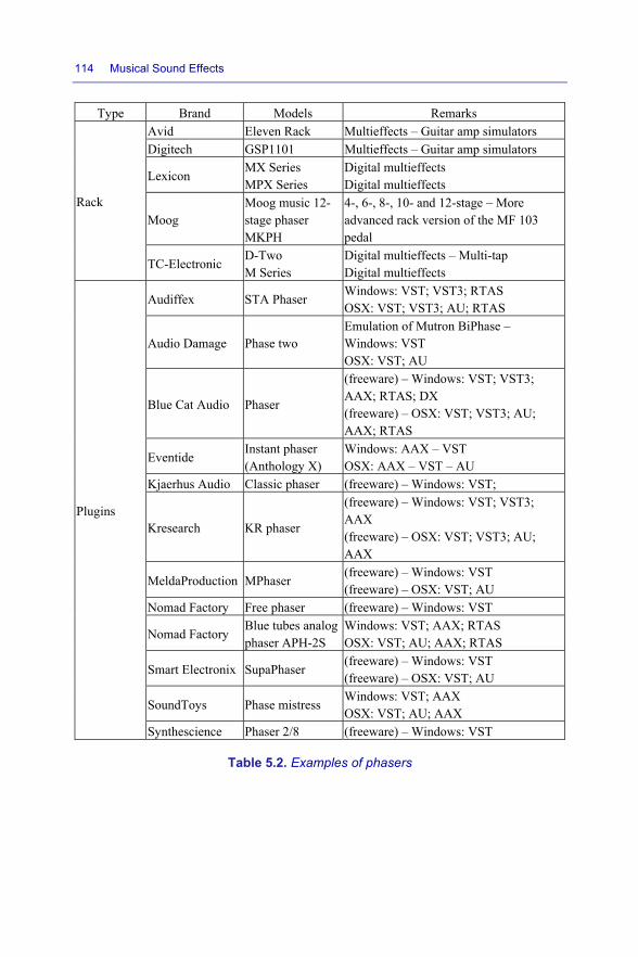
114 Musical Sound Effects
Type Brand Models Remarks
Rack
Avid Eleven Rack Multieffects – Guitar amp simulators Digitech GSP1101 Multieffects – Guitar amp simulators
Lexicon MX Series MPX Series
Digital multieffects Digital multieffects
Moog Moog music 12-stage phaser MKPH
4-, 6-, 8-, 10- and 12-stage – More advanced rack version of the MF 103 pedal
TC-Electronic D-Two M Series
Digital multieffects – Multi-tap Digital multieffects
Plugins
Audiffex STA Phaser Windows: VST; VST3; RTAS OSX: VST; VST3; AU; RTAS
Audio Damage Phase two Emulation of Mutron BiPhase – Windows: VST OSX: VST; AU
Blue Cat Audio Phaser
(freeware) – Windows: VST; VST3; AAX; RTAS; DX (freeware) – OSX: VST; VST3; AU; AAX; RTAS
Eventide Instant phaser (Anthology X)
Windows: AAX – VST OSX: AAX – VST – AU
Kjaerhus Audio Classic phaser (freeware) – Windows: VST;
Kresearch KR phaser
(freeware) – Windows: VST; VST3; AAX (freeware) – OSX: VST; VST3; AU; AAX
MeldaProduction MPhaser (freeware) – Windows: VST (freeware) – OSX: VST; AU
Nomad Factory Free phaser (freeware) – Windows: VST
Nomad Factory Blue tubes analog phaser APH-2S
Windows: VST; AAX; RTAS OSX: VST; AU; AAX; RTAS
Smart Electronix SupaPhaser (freeware) – Windows: VST (freeware) – OSX: VST; AU
SoundToys Phase mistress Windows: VST; AAX OSX: VST; AU; AAX
Synthescience Phaser 2/8 (freeware) – Windows: VST
Table 5.2. Examples of phasers

Modulation Effects 115
5.3. Chorus
Chorus works according to a similar principle to the flanger and phaser effects. The fundamental difference is that chorus uses higher delays of between 20 and 80 ms.
The goal is to create the impression of multiple instruments or voices. In reality, whenever several people play together, there are small differences between each of them – they are never perfectly synchronized. The chorus recreates this effect.
Figure 5.9. Flowchart of the chorus effect
A slight pitch (tuning) difference can be applied to each filter to simulate the fact that multiple instruments are always very slightly out of tune with each other.
Figure 5.10. Three chorus pedals: “Small Clone” by Electro Harmonix, “Stereo Chorus” by MXR and “Corona Chorus” by TC Electronic

116 Musical Sound Effects
Not every instrument has exactly the same range, so filtering affects different instruments differently. Thus, by varying the volume of each filter, we can create the impression of differentiation between instruments by simulating their distance from the sound recording equipment.
5.3.1. Examples of chorus
Again, the rack section of Table 5.3 overlaps with the flanger, since each rack can have multiple effects.
Some plugins are part of a larger bundle of effects.
Type Manufacturer or publisher
Model Remarks
Pedal
Boss CE-20 Released in 2001 – 6 types of chorus – 4 presets – Various settings
Boss CH-1 Available since 1989 – Analog until 2001 – Digital today
Boss CE-5 chorus ensemble
Available since 1991 – Analog until 2001 – Digital today – 2 filters
Electro Harmonix Small clone MK2 Analog – Reissue from the 1990s
Electro Harmonix Neo clone Released in 2010 – Analog – Simple settings
Ibanez TC10 Released in 1986 – Analog – 2 types of chorus
Korg NuVibe Chorus and vibrato – Reissue of the famous “Uni-vibe” – Allows the waveform to be configured
Moog MF Chorus Analog – 3 types of chorus
Providence ADC-4 Amandine chorus
Analog – 3 types of chorus
MXR M234 Analog – 2 filters

Modulation Effects 117
MXR M134 Various settings – Bass filter
TC Electronic Corona chorus Three types of chorus – Toneprint – USB port
TC Electronic Corona mini Simple settings – Toneprint – USB port
Strymon Ola Three types of chorus – 3 types of dynamics – Various settings
Rack
Avid Eleven Rack Multieffects – Guitar amp simulators
Digitech GSP1101 Multieffects – Guitar amp simulators
Lexicon MX Series
MPX Series
Digital multieffects
Digital multieffects
Moog Moog music 12-stage phaser MKPH
4-, 6-, 8-, 10- and 12-stage – More advanced rack version of the MF 103 pedal
TC-Electronic D-Two
M Series
Digital multieffects – Multi-tap
Digital multieffects
Plugins Kjaerhus Audio Classic phaser (freeware) – Windows: VST
Audiffex STA chorus Windows: AAX; RTAS; VST2; VST3
OSX: AAX; AU; RTAS; VST2; VST3
Table 5.3. Examples of chorus
REMARK.– The “CE-1” model by Boss, released in 1976, was one of the first ever chorus pedals. But it was actually designed to recreate an effect from a legendary amp, the “JC-120” by Roland4, which stands for “Jazz Chorus 120”. As its name suggests, the amp had an integrated chorus effect.
5.4. Rotary, univibe or rotovibe
This effect simulates the sound of Leslie rotating speakers, an amplification system specifically designed for electronic organs including Hammond organs.
4 Boss is a division of the Japanese company Roland.

118 Musical Sound Effects
Figure 5.11. Exterior and interior view of a Leslie speaker, 122 model
These speakers are named after their inventor, Donald Leslie5.
5.4.1. History
After acquiring a Hammond organ together with a so-called “tone cabinet” amplification system in the 1930s, Donald Leslie began to look for an alternative system, finding that the sound was flat and lacked warmth. He wanted to recreate the sound effects of a pipe organ, resulting in the development and creation of his first rotating speaker in 1937.
He presented his invention to Laurens Hammond, but Hammond was not pleased, anticipating that it would compete with his own amplification system.
Spurred on by Hammond’s rejection, D. Leslie created his own company, Electro Music Inc., which marketed its first Leslie speaker in 1940 under the name “Vibratone – 30A model”.
These speakers were then improved over time. In some models, the tube amps (20–50 W) were replaced by more powerful transistor amps (90 W and above). In 1963, in addition to the standard speed of rotation, which was called “tremolo”, they
5 Donald James Leslie, 1911–2004, American inventor. Member of the American Music Conference Hall of Fame, alongside Laurens Hammond (who invented the Hammond organ) and Leo Fender (who founded Fender).

Modulation Effects 119
were fitted with a second, slower speed, called “chorale”. Spring reverb was added to some models (Hammond – see section 8.1.2).
Figure 5.12. Two generations of Leslie speakers: The first model – 30 A (1940) with tubes, and the 760 model with transistors (solid-state – 1970s)
Special control panels and preamplifier pedals, known as “combo pedals”, were invented to connect the speakers to any type of organ, or even other instruments such as guitars.
Figure 5.13. A “Combo” preamplifier pedal manufactured by Leslie

120 Musical Sound Effects
In the 1990s, Electro Music Inc. was acquired by Hammond-Suzuki.
Leslie speakers still exist today, and new speakers are still available on the market, manufactured and distributed by Hammond-Suzuki.
5.4.2. Theoretical principles
The idea is to send the low frequencies of an amplified sound signal to a rotating drum with an inclined, rounded plane, and to send the high frequencies to a rotating horn, as shown in Figure 5.14.
Figure 5.14. Diagram of a Leslie speaker
The rotation varies the sound modulation, making it seem to move back and forth.
This phenomenon is caused by the Doppler effect, which was discovered by the physicist Christian Doppler6 in 1845. The Doppler effect arises from the receiver’s perception of the offset between the emitted wave and the received wave whenever the emitter and the receiver are moving relative to each other.
6 Johann Christian Doppler, Austrian physicist, 1803–1853.

Modulation Effects 121
I am sure you have noted the sound made by a passing car when you are standing at the edge of the road. The sound is higher pitched when the car is moving closer, and lower pitched when it is moving away.
Whenever a sound source moves toward an observer, the sound waves are compressed, reducing the wavelength λ2 and increasing the frequency of the sound. The perceived sound is therefore higher. Whenever the source moves away from the observer, the opposite phenomenon occurs. The sound waves dilate, the wavelength λ1 increases and the frequency decreases, making the sound appear lower.
Figure 5.15. The Doppler effect
= + = −
where:
– c: speed of sound (340 m/s);
– λ1: wavelength 1 (m);
– λ2: wavelength 2 (m);
– Vm: speed of the moving object (m/s);
– T: period (s).

122 Musical Sound Effects
One simple way to visualize the Doppler effect is to imagine yourself standing in the water at the seaside. Suppose that the waves hit your feet every 5 s. If you run further into the sea, the waves will hit you more often as you run, and so their frequency is higher (compression). If you turn around and run back to shore, the waves will hit you less often as you run, and so their frequency is lower (dilation). Note however that moving around in the water does not change the total number of waves.
5.4.3. Leslie speakers
Many brands, such as Elka, Sharma, Dynacord, Echolette, Fender, Solton and others, have created their own copies of Leslie speakers.
Figure 5.16. Leslie speaker clones: Sharma, Echolette, Dynacord and Elka

Modulation Effects 123
Table 5.4 lists a few models of speaker that are still available today.
Manufacturer Model Remarks Motion Sound KBR-3D 100 W + 45 W (12AX7 pre-amp tubes)
for the rotary channel – Stereo – Equalizer
Motion Sound PRO 145 130 W bass and 70 W treble (12AX7 pre-amp tubes)
Motion Sound 1771 – 1771W 200 W + 2 rotors Motion Sound PRO-3X 45 W – Equalizer – Very compact Hammond Leslie 122XB 40 W with tubes – 2 rotating systems –
Reissue of the 122 Leslie model Hammond Leslie 3300 220 W bass + 80 W treble – Pre-amp
with tubes – Solid-state amp – 2 rotating systems
Hammond Leslie 2101 50W rotating horn – 4 fixed 75 W speakers – Overdrive with tubes
Table 5.4. Modern speakers available for purchase7
5.4.4. Examples of rotary or univibe pedals
Figure 5.17. Four rotary effects pedals: “Rototron” by Pigtronix, “Leslie Digital” and “RT-20” by Boss, and “Lex” by Strymon
7 These speakers are currently available for purchase at the time of writing.

124 Musical Sound Effects
As mentioned before, you may recognize some of the racks listed in Table 5.5, since many of these products include multiple effects.
Type Manufacturer or publisher Model Remarks
Pedal
Boss RT-20 Four different sounds – Overdrive for guitar or keyboard
Digitech Ventura Vibe Rotary or vibrato effect – 4 settings – 2 inputs – 2 outputs
Dunlop Rotovibe Expression pedal and rotary – Vibrato and chorus mode
Dunlop UV-1 Uni-Vibe Three settings – Chorus/vibrato mode
Electro Harmonix Lester G For guitar – Overdrive emulation – 8 settings – Stereo/mono output
Fulltone Deja’Vibe CS-MDV-1
Two settings – Vibrato/chorus and modern/vintage modes
Hughes Kettner Rotosphere 12AX7 pre-amp tubes – Stereo/mono
Leslie Leslie digital pedal Four types of speaker and amp (122, 147, 18V, PR40)
Leslie–Hammond G Pedal Leslie Three types of speaker (122, 147, preset)
Line 6 Roto-machine Three types of speaker (122, 145, L16) – Configurable transition time
Neo Instruments Ventilator II For organ, guitar and keyboard – Overdrive – 2 inputs – 2 outputs
Pigtronix RSS Rototron Analog – For guitar – 4 settings – 2 inputs – 2 outputs
Tech 21 RotoChoir Six settings – Overdrive – Stereo output
Strymon Lex Four settings – Boost function – Stereo output

Modulation Effects 125
Rack
Alesis Nanoverb Multieffects
Avid Eleven Rack Multieffects – Guitar amp simulators
Dynacord CLS 222 Dedicated to the Leslie effect
Lexicon MX Series MPX Series
Digital multieffects Digital multieffects
TC Electronic M-One Multieffects
Zoom Studio 1201 Multieffects
Software
GSI MrDonald (freeware) Windows: VST
Nubi3 Spinner LE (freeware) Windows: VST
PSP Audioware PSP L’otary2 Windows: VST; AAX; RTAS OSX: VST; AAX; RTAS; AU
MeldaProduction MVintageRotary Windows: VST; VST3; AAX OSX: VST; VST3; AAX; AU
Mda Leslie Windows: VST OSX: VST; AU
BetaBugsAudio Spinbug (freeware) Windows: VST
Xils-Labs LX122 Windows: VST
Table 5.5. Models of rotary effects
5.4.5. Leslie speakers and sound recording
One way of recording a Leslie speaker is to use two static wide-band cardioid pickups on either side of the speaker to capture the trebles emitted by the horn.
Importantly, these pickups should not be placed facing each other, but at a slight angle. This avoids any problems due to antiphase phenomena8 that might eliminate certain frequencies.
To record the rotating drum, which is dedicated to low frequencies, we can place a third microphone in front of the lower vents, angled downwards, carefully ensuring that it cannot cross phases with the top microphones.
8 Some DAWs (Digital Audio Workstations) offer integrated plugins (SurroundScope, Voxengo PHA-979, etc.) and tools for managing the phase.

126 Musical Sound Effects
Figure 5.18. Positioning of microphones to record a Leslie speaker
Be careful – in “tremolo” mode, the rapid rotation of the drum or horns can generate a hiss that disrupts the microphone recordings. Pop filters can help if you are encountering this issue.
Finally, when the musician stops the rotation of the speakers, there is no reason to expect that the microphones will be in the right place relative to the horns or rotor. An extra dynamic microphone can be placed very close or even inside the speakers (by removing one of the panels, for example the rear panel) to record the inner reflections of the speaker and improve the dynamics.
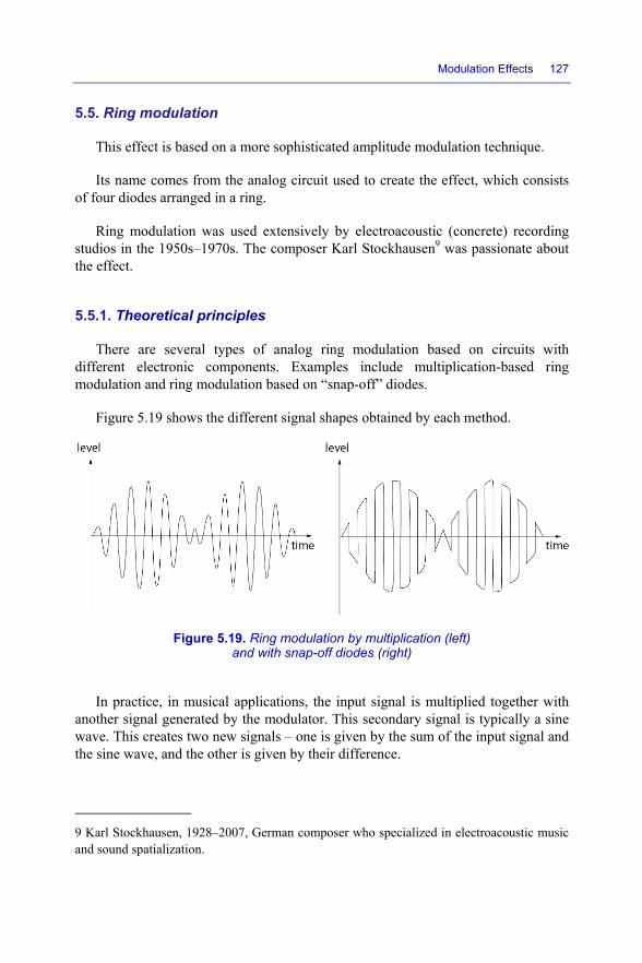
Modulation Effects 127
5.5. Ring modulation
This effect is based on a more sophisticated amplitude modulation technique.
Its name comes from the analog circuit used to create the effect, which consists of four diodes arranged in a ring.
Ring modulation was used extensively by electroacoustic (concrete) recording studios in the 1950s–1970s. The composer Karl Stockhausen9 was passionate about the effect.
5.5.1. Theoretical principles
There are several types of analog ring modulation based on circuits with different electronic components. Examples include multiplication-based ring modulation and ring modulation based on “snap-off” diodes.
Figure 5.19 shows the different signal shapes obtained by each method.
Figure 5.19. Ring modulation by multiplication (left) and with snap-off diodes (right)
In practice, in musical applications, the input signal is multiplied together with another signal generated by the modulator. This secondary signal is typically a sine wave. This creates two new signals – one is given by the sum of the input signal and the sine wave, and the other is given by their difference.
9 Karl Stockhausen, 1928–2007, German composer who specialized in electroacoustic music and sound spatialization.

128 Musical Sound Effects
For example, if the input signal is a 600-Hz triangle wave and the modulation is a 200-Hz sine wave, the outputs are two signals with frequencies of 400 Hz and 800 Hz (600 – 200 Hz and 600 + 200 Hz), as shown in Figure 5.20.
Figure 5.20. Principle of a ring modulator. The top spectrum analyzer shows a 600-Hz triangle wave. The bottom one shows the output of the ring modulator after combining with a 200-Hz sine wave. The middle panel shows the ring modulator and the spectrum analyzer (in Ableton Live). For a color version of this figure, see www.iste.co.uk/reveillac/soundeffects.zip
Note that if the modulation frequency is lower than 20 Hz, the modulator is similar to a LFO. In this case, the resulting effect is relatively similar to a tremolo effect.

Modulation Effects 129
Most pedals and plugins dedicated to ring modulation are tricky to master. Their settings typically include:
– the choice of modulation waveform;
– the modulation frequency;
– the amplitude of the modulation (width or depth);
– the frequency of the LFO, if applicable;
– the mix between the original signal and the processed signal (dry/wet).
5.5.2. Examples of ring modulators
In Table 5.6, you can find a few examples of ring modulators, pedals and plugins.
Type Brand or publisher Model Remarks
Pedal
Way Huge WHE606 RingWorm Digital – 5 settings – Input for an expression pedal
Moog MF-102 Ring Modulator
Oscillator from 2 Hz to 4 kHz – Waveform: sine and square – Integrated LFO
Electro Harmonix Ring Thing Nine presets – Various settings options
Moog MF Ring Analog – 3 settings
Digitek DOD FX13 Gonkulator 1993 – Includes distortion
Plugin
Wok Ring-O (freeware) – Windows: VST
Ndc Plugs The modulator 2 (freeware) – Windows: VST
MeldaProduction MRingModulator (freeware) – Windows: VST; VST3; AAX OSX: VST; VST3; AAX; AU
SonicXTC Ring modulator 101 (freeware) – Windows: VST
Physical Audio PA2 Little ringer (freeware) – OSX
Table 5.6. Models of ring modulators

130 Musical Sound Effects
5.6. Final remarks
Where should modulation effects be placed in the audio flow? They are usually placed after distortion, wah-wah, dynamic effects, but before time effects.
Chorus is the most popular and widely used effect, as it is easy to use. Guitarists are very fond of using it to give their sound a rich and thick quality.
Chorus can of course be applied to any type of sound, but it is most effective on signals that are rich in harmonics, which explains why guitarists love it so much.
Phaser and flanger are closely related, although the latter is more precise and subtle. Flanger tends to enlarge the space, whereas phaser tends to fill it. Either way, both effects very quickly create a very specific color when applied overly generously.
Due caution is required – although they make the sound warmer, phaser and flanger tend to sacrifice clarity and impact. You need to find the right compromise between purity, depth of shimmer and dynamics.
Rotary is usually designed for electronic organs, but guitarists were also quick to add it to their repertoire. Although it can be used without moderation with organs, as we have become completely accustomed to how it sounds, some judgment is required with guitar. Rotary does not necessarily suit every style of music.
Finally, ring modulation is a truly unique effect, capable of the best but also the worst. It can create a very synthetic sound rendering, especially with guitar, bass, percussion or piano. There is a good reason it is used by so many synthesizers.

6
Frequency Effects
As their name suggests, frequency effects act upon the frequency of the audio signal, for example by modifying it or varying it. Some of the first effects used by musicians were frequency effects, in the earliest generations of analog and later digital electronics.
The processes and techniques on which these effects are based are often complex. More recent software versions have allowed remarkable advancements to be achieved and highly sophisticated audio processing techniques to be developed.
6.1. Vibrato
The vibrato effect is a cyclic variation of the pitch and hence fundamental frequency of the signal.
Most musicians achieve this effect by directly manipulating the instrument itself, by executing a certain playing technique, usually for very short durations (a few notes or at most a few bars).
It is worth noting that in some cases, especially for vocals and wind instruments, vibrato affects the intensity more than the pitch.
On some electric guitars, vibrato is achieved with a device mounted near the bridge that modifies the tension of the strings to vary the frequency of each note.
Musical Sound Effects: Analog and Digital Sound Processing, First Edition. Jean-Michel Réveillac.© ISTE Ltd 2018. Published by ISTE Ltd and John Wiley & Sons, Inc.

132 Musical Sound Effects
Electronic or digital versions of the vibrato effect instead tend to be used over
longer periods to create a certain color, style or atmosphere. Vibrato was one of the first effects to be implemented electronically.
6.1.1. Theoretical principles
A low-frequency oscillator is used to cyclically vary the frequency of the audio signal up and down, as shown in Figure 6.1.
Figure 6.1. Principle of the vibrato
The difference between the lowest and highest frequencies determines the depth of the vibrato.
6.1.2. Settings
Vibrato can have several user-configurable parameters. Pedals usually only have a few configurable parameters, but software vibratos (plugins) can have many.
Here is a non-exhaustive list of the most common settings:
– the depth: determines the intensity of the vibrato;
– the speed (or rate): determines the frequency of the vibrato;
– the rise time: defines the time required for the vibrato to reach the chosen maximum intensity (depth);
– the tone: shifts the effect toward lower or higher frequencies;
– the shape of the variation signal: defines the waveform of the vibrato, usually ranging from a sine wave to a triangle wave.

Frequency Effects 133
Figure 6.2. The “MVibrato” plugin by MeldaProduction
6.1.3. Examples of vibrato
Figure 6.3. Three models of vibrato pedal: “Viper” by T-Rex, “VB-2w” by Boss and “NuVibe” by Korg
Some manufacturers combine the vibrato and tremolo effects into a single pedal.
REMARK.– People often fail to properly distinguish between the vibrato and tremolo effects. This confusion has been perpetuated by some pedal manufacturers, who frequently misuse the two terms. Many instrument amps also list vibrato on their controls for effects that are in fact tremolos.
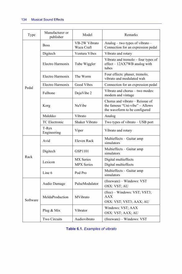
134 Musical Sound Effects
Type Manufacturer or
publisher Model Remarks
Pedal
Boss VB-2W Vibrato Waza Craft
Analog – two types of vibrato – Connection for an expression pedal
Digitech Ventura Vibes Vibrato and rotary
Electro Harmonix Tube Wiggler Vibrato and tremolo – four types of effect – 12AX7WB analog with tubes
Electro Harmonix The Worm Four effects: phaser, tremolo, vibrato and modulated wah
Electro Harmonix Good Vibes Connection for an expression pedal
Fulltone DejaVibe 2 Vibrato and chorus – two modes: modern and vintage
Korg NuVibe Chorus and vibrato – Reissue of the famous “Uni-vibe” – Allows the waveform to be configured
Malekko Vibrato Analog TC Electronic Shaker Vibrato Two types of vibrato – USB port T-Rex Engineering Viper Vibrato and rotary
Rack
Avid Eleven Rack Multieffects – Guitar amp simulators
Digitech GSP1101 Multieffects – Guitar amp simulators
Lexicon MX Series MPX Series
Digital multieffects Digital multieffects
Line 6 Pod Pro Multieffects – Guitar amp simulators
Software
Audio Damage PulseModulator (freeware) – Windows: VST OSX: VST; AU
MeldaProduction MVibrato (free) – Windows: VST; VST3; AAX OSX: VST; VST3; AAX; AU
Plug & Mix Vibrator Windows: VST; AAX OSX: VST; AAX; AU
Two Circuits Audiovibrato (freeware) – Windows: VST
Table 6.1. Examples of vibrato

Frequency Effects 135
6.2. Transposers
These effects modify the tone of the sound. There are several variations, including:
– octaver;
– pitch shifter;
– harmonizer;
– autotune.
Although these effects can be applied to any instrument, the first three are most commonly used by guitar players. They were invented with the goal of enriching the harmonics of a sound passage, similar to musical arrangements that overlay the same musical phrase at different pitches (octave, fifth, third, etc.).
REMARK.– These effects are also often confused, and consequently different models of transposer work differently. The pitch shifter effect can be viewed as a harmonizer, and so can the octaver. Digital technology has muddied the waters even further, providing an even more extensive range of sound processing options.
6.2.1. Octaver
This effect divides the frequency of the input signal by two. Musically, this lowers the sound by one octave. By applying the same operation twice, we can reduce by two octaves.
Figure 6.4. The pedal “Octavia” by Tycobrahe, a commercial version of the pedal used by Jimi Hendrix, marketed in the 1970s
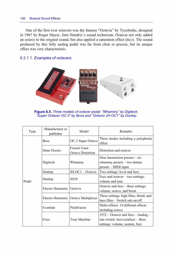
136 Musical Sound Effects
One of the first ever octavers was the famous “Octavia” by Tycobrahe, designed
in 1967 by Roger Mayer, Jimi Hendrix’s sound technician. Octavia not only added an octave to the original sound, but also applied a saturation effect (fuzz). The sound produced by this fully analog pedal was far from clear or precise, but its unique effect was very characteristic.
6.2.1.1. Examples of octavers
Figure 6.5. Three models of octaver pedal: “Whammy” by Digitech, “Super Octaver OC-3” by Boss and “Octavio JH-OC1” by Dunlop
Type Manufacturer or publisher Model Remarks
Pedal
Boss OC-3 Super Octave Three modes including a polyphonic effect
Dane Electro French Toast Octave Distortion Distortion and octaver
Digitech Whammy Nine harmonizer presets – six whammy presets – two detune presets – MIDI input
Dunlop JH-OC1 – Octavio Two settings: level and fuzz
Dunlop JH3S Fuzz and octaver – two settings: volume and tone
Electro Harmonix Octavix Octaver and fuzz – three settings: volume, octave, and boost
Electro Harmonix Octave Multiplexer Three settings: high filter, blend, and bass filter – Switch sub on/off
Eventide PitchFactor Multi-effects: 10 different effects including octave
Foxx Tone Machine 1972 – Octaver and fuzz – Analog – one switch: fuzz/octafuzz – three settings: volume, sustain, fuzz

Frequency Effects 137
Fulltone Octafuzz OF-2 Copy of the famous “Octavia” by Tycobrahe – two settings: volume and boost
Fulltone Ultimate Octave Fuzz and octaver – Switch: octave-up – three settings: volume, tone, and fuzz
Joyo JF-12 Voodoo Octave
Octaver and fuzz – three settings: fuzz, tone, and volume – two switches: fuzz and octave
Movall Octopuzz Two settings: level and tone
MXR Custom Shop Machine Fuzz
Fuzz and octaver – Analog – four settings: volume, tone, fuzz, sub
Roger Mayer Octavia Classic Reissue from the 1960s
TC Electronic Sub ’N’ Up Octaver
PitchShifter, Octaver, Harmonizer – USB port
Tycobrahe Octavia 1970 – Analog – The gold standard – Hard to find
Voodoo Lab Proctavia Fuzz and octaver – two settings: volume and boost
Rack
Avid Eleven Rack Multieffects – Guitar amp simulators Digitech GSP1101 Multieffects – Guitar amp simulators
Lexicon MX Series MPX Series
Digital multieffects Digital multieffects
Line 6 Pod Pro Multieffects – Guitar amp simulators
Software
Antares Harmony Engine EVO
Pitch shifter and time stretcher Windows: VST; AAX; RTAS OSX: VST; AAX; RTAS; AU MIDI features
Audiowish Octave Shifter 2 (freeware) OSX: AU Chris Hooker Octaver OC-D2 (freeware) Windows: VST TbT Octaver 12B (freeware) Windows: VST
Waves UltraPitch Windows: VST; VST3; AAX; RTAS OSX: VST; VST3; AAX; RTAS; AU
Table 6.2. Examples of octavers
6.2.2. Pitch shifter
This effect modifies the pitch of a sound signal while keeping its duration constant. By convention (and in most cases), pitch shifters change the pitch by a constant number of semitones over one or more octaves.

138 Musical Sound Effects
Analog pitch shifters do not work well with polyphonic sound sources. This
effect is primarily designed for mono signals.
This is no longer a problem with digital models. Virtually all digital models support polyphonic sound.
Figure 6.6. Three pitch-shifter pedals: “Pitch Fork” by Electro Harmonix, “PS-5” by Boss and “Particle” by Red Panda
Type Manufacturer or publisher Model Remarks
Pedal
Boss PS-2 1987–1994 – Pitch shifter and delay (2 s max) – six different modes
Boss PS-3 1994–1999 – Pitch shifter (–2 oct to +2 oct) and delay (2 s max) – 11 different modes
Boss PS-5 Super Shifter1999–2011– Digital – Polyphonic – Thirds, fourths, fifths, sevenths, one octave, two octaves
Eventide PitchFactor Pitch shifter and delay (1.5 s max) – four diatonic pitch-shifting tracks – 10 different modes – 100 presets
Electro Harmonix Pitch Fork 2014 – Digital – Polyphonic – ±3 octaves – three modes
Red Panda Particle Pitch shifter and granular delay (900 ms max) – eight different modes
Rack Boss RPS-10 Two settings: level and fuzz
Digitech Intelligent Pitch-Shifter
1987 – Pitch shifter (–1 oct to +1 oct) and delay (800 ms max)
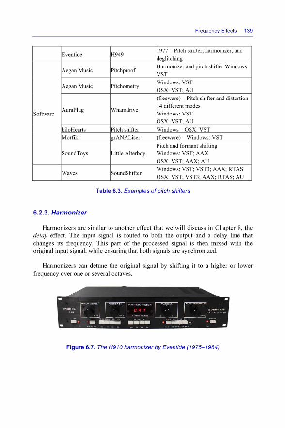
Frequency Effects 139
Eventide H949 1977 – Pitch shifter, harmonizer, and
deglitching
Software
Aegan Music Pitchproof Harmonizer and pitch shifter Windows: VST
Aegan Music Pitchometry Windows: VST OSX: VST; AU
AuraPlug Whamdrive
(freeware) – Pitch shifter and distortion 14 different modes Windows: VST OSX: VST; AU
kiloHearts Pitch shifter Windows – OSX: VST Morfiki grANALiser (freeware) – Windows: VST
SoundToys Little Alterboy Pitch and formant shifting Windows: VST; AAX OSX: VST; AAX; AU
Waves SoundShifter Windows: VST; VST3; AAX; RTAS OSX: VST; VST3; AAX; RTAS; AU
Table 6.3. Examples of pitch shifters
6.2.3. Harmonizer
Harmonizers are similar to another effect that we will discuss in Chapter 8, the delay effect. The input signal is routed to both the output and a delay line that changes its frequency. This part of the processed signal is then mixed with the original input signal, while ensuring that both signals are synchronized.
Harmonizers can detune the original signal by shifting it to a higher or lower frequency over one or several octaves.
Figure 6.7. The H910 harmonizer by Eventide (1975–1984)

140 Musical Sound Effects
Unlike pitch shifters, harmonizers take into account the key in which the notes
are being played by adjusting the number of semitones in the shift to be consistent with the key and the choice of interval (thirds, fifths, octaves, etc.).
For example, in C major, if the harmonizer is set to thirds, it will apply the following shifts, as presented in Table 6.4.
Original note
Note generated by the
harmonizer
No. of semitones
Original note
Note generated
by the harmonizer
No. of semitones
C E 4 F# A 3
C# E 3 G B 4
D F 3 G# B 3
D# F# 3 A C 3
E G 3 A# C# 3
F A 4 B D 3
Table 6.4. The notes generated by the harmonizer to create a third in the same key. The number of semitones depends on the note
REMARK.– Some pitch shifters have harmonizer functions and vice versa.
Figure 6.8. Three harmonizer pedals: “AHAR-3” by Tom’s Line Engineering, “Harmonist PS-6” by Boss and “Harmony” by Hotone Audio

Frequency Effects 141
Type Manufacturer
or publisher Model Remarks
Pedal
Digitech HarmonyMan Harmonizer – Whammy octaver (pitch shift)
DOD Meatbox 2015 Harmonizer – Whammy octaver (pitch shift)
Eventide H9 Harmonizer Multi-effects: ModFactor, Pitchfactor, TimeFactor – USB port – iOS app
Hotone Audio Harmony Harmonizer – Whammy octaver (pitch
shift) – 24 semitones
Morpheus Bomber Harmonizer – Octaver – Whammy (pitch shift)
Tom’s Line Engineering
AHAR-3 Harmonizer Harmonizer and pitch shifter
Rack
AMS Neve DMX 15-80S 1978 – Delay and digital harmonizer
Eventide H910 1975–1984 – First digital harmonizer – four delays – CV input
Eventide H3000 Ultra Harmonizer
Multi-effects – 21 algorithms – 600 presets
Eventide H7600 Ultra Harmonizer
Multi-effects – 1,000 algorithms – 230 effects blocks – Windows and OSX interface
Software
Aegan Music Pitchproof Harmonizer and pitch shifter – Windows: VST
Eventide H3000 Digital emulation of the H3000 Windows: VST; AAX; RTAS OSX: VST; AAX; RTAS; AU
Eventide H910 Digital emulation of the famous H910 Windows: VST; AAX; RTAS OSX: VST; AAX; RTAS; AU
Martin Eastwood Duet (freeware) – Windows: VST
Waves UltraPitch Windows: VST; VST3; AAX; RTAS OSX: VST; VST3; AAX; RTAS; AU
Waves Doubler Pitch detune, chorus, delay Windows: VST; VST3; AAX; RTAS OSX: VST; VST3; AAX; RTAS; AU
Table 6.5. Examples of harmonizers

142 Musical Sound Effects
6.2.4. Auto-Tune
Auto-Tune was originally designed to correct out-of-tune vocals. It was created in 1997 and has since also become popular as a fully fledged vocal synthesis instrument, inspiring the development of new tools that can be classified as voice processors.
Figure 6.9. Antares Auto-Tune Version 3 for DirectX, Windows. For a color version of this figure, see www.iste.co.uk/reveillac/soundeffects.zip
6.2.4.1. History
Auto-Tune was created by Harold (Andy) Hildebrand, whose field of expertise amusingly had nothing to do with music. He worked for the petroleum industry, and specialized in determining the feasibility and viability of exploiting oil deposits.
As part of his work, he developed a method based on autocorrelation1 that allows acoustic waves to be transmitted underground. After perfecting his method, he sold it to the oil company Exxon, and retired.
Some time later, at a dinner party – as he tells the story – somebody challenged him to develop an application that makes you always sing in tune. Using exactly the same autocorrelation technique that he had used for his work, he developed the software program “Auto-Tune” in 1996.
1 Autocorrelation is a mathematical tool used for signal processing that allows patterns in a signal to be detected, among other things.

Frequency Effects 143
Precursory tools had long been available, such as the “Voder”, invented in 1937
by the engineer Homer Dudley2, which modified the voice of singers, and the “Sonovox”, which was created in 1940. The Sonovox can be seen in the movie “You’ll Find Out” starring Kay Kyser.
Figure 6.10. The “Voder” invented by Homer Dudley
But it was the German physicist Werner Meyer-Eppler, founder of the Cologne Studio for Electronic Music, who was truly responsible for propelling voice effects onto the musical scene in the late 1950s.
In 1968, because of technological advancements, the famous synthesizer manufacturer Moog released their first “vocoder” for sale. This effect can be heard in many musical tracks from this period, including “Autobahn” by Kraftwerk.
2 Homer Dudley, 1896–1987, American engineer, creator of the first speech synthesizer at Bell Labs, which was used to encrypt voice communications during World War II. He also invented the “Vocoder” in 1939.

144 Musical Sound Effects
Figure 6.11. Sixteen-channel vocoder by Moog
Even though they use similar technology, the “vocoder” and “Auto-Tune” are not the same. The former generates sounds using a keyboard to create vocal harmonies, and the latter processes vocals using dedicated software.
The first commercial version of Auto-Tune was developed in 1997 by Audio Antares Technologies, a company founded by H. Hildebrand.
One of the first hits to use the effect was “Believe”, performed by the singer Cher in 1998. Although Auto-Tune was originally intended as a tool for singing in tune, this song used it as a musical effect in its own right. Many other tracks would later follow suit.
Today, Auto-Tune is no longer just a tool for cleaning up vocals, but has become an entirely new form of instrument.
Figure 6.12. Version 8 of the Auto-Tune plugin by Antares. For a color version of this figure, see www.iste.co.uk/reveillac/soundeffects.zip

Frequency Effects 145
6.2.4.2. Autotune effects and voice processors
Table 6.6 contains a list combining autotune effects, vocoders and voice processors. The “other” category consists of “desktop” processors that can be placed on a table or attached to a microphone stand. They are usually specifically designed for vocals.
Figure 6.13. Four voice processors: “Perform-V” by TC-Helicon, “SVC-350” by Roland, “TA-1VP” by Tascam and “VE-2” by Boss
Type Manufacturer or publisher Model Remarks
Pedal
Boss VE-2 Voice processor – three presets – 24 types of harmonization
Boss VE-8 Voice processor for singers accompanied by acoustic guitar
Electro Harmonix Voice Box Harmonizer and vocoder – nine modes
Mooer VEM Box Voice processor – 54 types of effect
TC-Helicon Harmony singer Voice processor for voice + guitar – USB – Detection of guitar key
TC-Helicon VoiceLive3 Extreme
Voice processor – Various modes for voice and guitar
TC-Helicon VoiceTone Correct XT
Voice processor – Automatic pitch correction, de-esser, equalizer
Rack
Roland VP-70 Voice processor and harmonizer
Roland SVC-350 Vocoder
Voice processor and vocoder – Inputs for microphone, guitar, synthesizer
Tascam TA-1VP Voice processor – Includes Antares Auto-Tune – Microphone modeling – MIDI
TC-Helicon VoiceWorks Voice processor – Harmonizer – Various features – MIDI

146 Musical Sound Effects
Software
Antares Auto-Tune Live
The live version of the Antares Auto-Tune effect Windows: VST; AAX OSX: VST; AAX; AU
Antares Auto-Tune 8
The latest version3 of Antares Auto-Tune Windows: VST; AAX OSX: VST; AAX; AU MIDI features
Antares Auto-Tune EFX 3
Simplified version of Auto-Tune – Limited corrections and settings Windows: VST; AAX OSX: VST; AAX; AU
g200kg Kerovee 1.61 (freeware) – Windows: VST
GVST Gsnap Pitch corrector (freeware) – Windows: VST
Oli Larkin Autotalent (freeware) – Windows: VST
SoundToys Little AlterBoy
Hard-tune – Pitch shifter – Harmonizer – Various other effects Windows: VST; AAX OSX: VST; AAX; AU
Waves SoundShifter Voice processor Windows: VST; AAX OSX: VST; AAX; AU
Other
Roland VT-3 Voice processor Desktop or microphone stand controller
TC-Helicon Perform-V Voice processor Mounted on a microphone stand
TC-Helicon VoiceLive Touch 2
Voice processor Desktop or microphone stand controller
Table 6.6. Examples of voice processors, vocoders and autotuned effects
6.2.4.3. Why do we need autotune?
You might be wondering: what is the point of using autotune?
3 Version 8 is the latest version at the time of writing this chapter (February 2017).

Frequency Effects 147
Autotune has been widely criticized by the media, but it is used by 90% of all
professional recording studios. Here are four arguments in favor of autotune that I personally find convincing:
– when used in moderation, autotune unquestionably improves the quality of vocals without distorting them;
– voice modification represents a simple way of enhancing or deliberately distorting vocals for stylistic effect, but does not just make anybody into a good singer;
– autotune saves time when processing renderings of vocals;
– it can be used as a replacement for vocoder, allowing vocals to be “robotized”, giving them a strongly artificial quality.
Opinions vary, but auto-tune is here to stay. Like many new technologies, progress is difficult to stop, no matter which side you are on. Try it out, and decide for yourself!
6.2.4.4. How to use Antares Auto-Tune
The next few sections give a brief introduction to Antares Auto-Tune and some of its parameters.
After installing Antares Auto-Tune in your favorite DAW (Digital Audio Workstation), load the voice segment that you want to process onto a new track. You can also open a multitrack project with one or several dedicated voice tracks.
Figure 6.14. The opening window of the Antares Auto-Tune 8 plugin. For a color version of this figure, see www.iste.co.uk/reveillac/soundeffects.zip

148 Musical Sound Effects
On this track, load the Antares Auto-Tune effect, which might be in a VST, AU
or AAX format.
A plugin window will open, displaying various settings, as shown in Figure 6.14.
Before processing our voice track, let us take a moment to explore this interface, starting with the top ribbon.
The drop-down list INPUT TYPE allows you to select the register that best matches the voice track. SOPRANO is the default option.
– SOPRANO: soprano voice;
– ALTO/TENOR: alto or tenor voice;
– LOW MALE: bass voice;
– INSTRUMENT: for instrumental tracks (Auto-Tune also works on instruments, but this is less popular), such as a guitar;
– BASS INSTRUMENT: for instruments with lower registers, for example a bass guitar.
Next, the TRACKING control ranges from RELAXED to CHOOSY, allowing us to specify whether the voice contours are clean and isolated (recording studio), or whether there is ambient background noise (live recording).
For studio environments, we will tend to use RELAXED, whereas in live environments we will tend to prefer CHOOSY, since we will need to be more selective. A good default for conventional sound recording is simply 50%.
Figure 6.15. Top ribbon of Auto-Tune 8
The PITCH REF switch specifies which channel should be used to differentiate between the notes of the melody for stereo signals. If the voice is equally balanced across both channels, we do not need to specify a preference for left (L) or right (R).
The LOW LATENCY button activates a mode that reduces the latency time to unnoticeable levels (for live applications), at the cost of the processing quality. Do not use this option for postproduction (studio processing).

Frequency Effects 149
The KEY, SCALE and SCALE DETUNE block are used to define the key and
scale of the voice track.
KEY specifies the key, from C to B, and SCALE allows the scale or mode to be selected, either CHROMATIC, MAJOR or MINOR. The SCALE DETUNE button is used to define the primary chord with fundamental note A. By default, this is 440 Hz, but it can be adjusted by –1 to +1 semitone (100% = 1 semitone).
The next block has the TRANSPOSE, THROAT LENGTH and FORMANT buttons:
– the TRANSPOSE function modifies the overall tuning (pitch) of the melody over an interval of ± 1 octave;
– the THROAT LENGTH function controls the timbre of the vocals, e.g. switching between a child’s voice to a woman’s or a man’s. This function only works when FORMANT is turned off;
– the FORMANT button attempts to preserve the characteristics of the formant4 of the singer’s voice, independently of all other settings.
The final block consists of the CORRECTION MODE switch and the OPTIONS button:
– the CORRECTION MODE function switches between automatic voice correction mode (AUTO) and graphical editing mode (GRAPH);
– the OPTIONS button opens a dialog window with general Auto-Tune settings: buffer size, number of undos, button mode, etc.
Figure 6.16. PITCH CORRECTION CONTROL settings 4 The spectral envelope that characterizes an acoustic signal like a person’s voice along their vocal tract, including resonance. The formant is specific to each individual.

150 Musical Sound Effects
Next, let us look at the subblock for PITCH CORRECTION CONTROL, which
controls the overall pitch of the voice using five controls:
– RETUNE SPEED: defines the reactivity of the pitch correction in milliseconds. The lower this value, the more natural the voice will seem, and vice versa;
– CORRECTION STYLE: restricts Auto-Tune’s corrections to allow the vocalist to retain as much expression as possible (FLEX-TUNE). The NONE position means that no corrections are made, and the CLASSIC position allows Auto-Tune to operate normally;
– HUMANIZE: this function differentiates between short notes and long or sustained notes by slowing down the retune speed on longer notes, which “humanizes” the voice, making it seem more natural;
– NATURAL VIBRATO: defines the degree to which Auto-Tune corrects notes in the vocals with vibrato (notes that oscillate around the correct pitch);
– TARGETING IGNORE VIBRATO: instructs Auto-Tune to disregard vibrato in the vocals.
REMARK.– When TARGETING IGNORE VIBRATO is turned off, Auto-Tune tends to make the melody sound out of tune if the vocals include strong vibrato effects.
Next, we will examine the central group, which by default contains buttons corresponding to each of the 12 notes of the chromatic scale, from C to B, and other buttons for configuring the scale or musical mode.
Figure 6.17. Group for selecting notes and modes
By clicking on the buttons in the REMOVE column lined up with each note, you can remove them from pitch correction in the chosen key.

Frequency Effects 151
By clicking on one of the BYPASS buttons, you remove pitch correction from
that note regardless of the chosen key. Auto-Tune acts as if these notes do not exist:
– the SET MAJOR button sets the scale to major mode;
– the SET MINOR button sets the scale to minor mode;
– the SET ALL button adds every note in the chosen scale to pitch correction;
– the BYPASS ALL button excludes every note from pitch correction;
– the REMOVE ALL button removes every note from the chosen scale from pitch correction.
Now that we have been introduced to some of the commands, we can process our first audio sequence:
– first, select the primary register of the voice in INPUT TYPE. This is usually SOPRANO for female voices or children and ALTO/TENOR for male voices;
– next, set the TRACKING to 50 (middle position) and make sure that LOW LATENCY is switched on (blue);
– choose the key and scale of the melody, e.g. C major, G minor, etc. from the KEY and SCALE drop-down lists. If you do not know the key or scale of your track, simply choose C and CHROMATIC;
– if necessary, adjust the SCALE DETUNE overall tuning. In the United States, musicians usually tune A to 440 Hz, with some exceptions. For example, you can sometimes find instruments and orchestras with A tuned to 442 Hz;
– start playing the track with Auto-Tune, and listen carefully so that you can configure the reactivity (RETUNE SPEED). You need to make sure that as many notes as possible are captured by the correction space without causing the voice to seem unnatural;
– adjust the HUMANIZE setting to fine-tune the quality of sustained notes;
– you can also adjust the inflections of the vocals to improve their spontaneity with the CORRECTION STYLE parameter, although simply setting it approximately to FLEX-TUNE will usually be your best bet;
– if necessary, you can polish the final rendering by adjusting any vibrato with the NATURAL VIBRATO button.

152 Musical Sound Effects
REMARK.– If you chose CHROMATIC because you are not sure which key the vocals are in, you can deselect specific notes in the middle panel in the REMOVE column to prevent them from being processed.
Auto-Tune works by always correcting to the closest note in the specified scale.
For example, if the melody is written as A, but the singer is very out of tune and sings closer to G, Auto-Tune will replace this A by G if G is in the scale (center panel). To avoid this problem, you can remove G from the scale.
REMARK.– You usually will not be able to correct an entire voice track in a single operation. I recommend working on short sequences of a few notes or a few dozen notes at most. This will allow you to make corrections that are imperceptible in the final mix. Auto-Tune is a powerful tool, but requires plenty of patience and attention to achieve good vocal renderings.
Auto-Tune also has a graphical voice editing mode that can be accessed by setting CORRECTION MODE to GRAPH. The graphical editor enables you to correct each phoneme or syllable in the voice melody. This approach is used by professionals to achieve pitch-perfect vocals that sound as natural as possible. The vocals are often split into several tracks in the DAW and recombined later. Auto-Tune can work separately with both channels of a stereo signal.
Figure 6.18. Auto-Tune’s graphical editing mode for making extremely fine adjustments to vocals. For a color
version of this figure, see www.iste.co.uk/reveillac/soundeffects.zip

Frequency Effects 153
The full functionality of the graphical editor goes well beyond the scope of this
book. You can find out more from the web links and bibliography at the end of the book.
6.2.4.5. Synthetic voices with Auto-Tune
Today, Auto-Tune has become a very fashionable way of deforming vocals to give them a synthetic feel. As we mentioned earlier, Cher was the first singer to do this, in her song “Believe”. Since then, many other artists have taken advantage of this technique, most notably rappers.
To recreate this effect, repeat the steps as in section 6.2.4.4, but set SCALE DETUNE to a value between 445 and 460, RETUNE SPEED to FAST and optionally set PITCH AMOUNT in the CREATE VIBRATO block to a value between 20 and 30.
REMARK.– These values are only guidelines. You will need to fine-tune the settings to achieve fluid results with a high-quality artificial and synthetic rendering.
6.2.4.6. For fun: autotune effects on smartphones and tablets
Although they really are not much more than gadgets, Auto-Tune’s popularity inspired the development of several fun little apps:
– MicDroid for Android: autotune effect (freeware);
– Songify by Smule for Android and iOS: turns your lyrics into songs (commercial);
– Auto-Tune Mobile for iOS: Antares Auto-Tune for iPad and iPhone (commercial);
Figure 6.19. Apps: Auto-Tune by Antares (left) and Voice Synth by Qneo (right) for iOS. For a color version of this
figure, see www.iste.co.uk/reveillac/soundeffects.zip

154 Musical Sound Effects
– I’m T-Pain by Smule for iOS: autotune to sing like T-Pain (commercial);
– Voloco by Resonant Cavity LLC: Auto Voice Tune: harmonizer and karaoke (freeware);
– Voice Synth Free by Qneo: autotune and vocoder (freeware);
– Voice Synth Free by Qneo: more advanced autotune and vocoder (commercial);
6.3. Conclusion
Frequency effects are always capable of achieving a fantastic rendering, but they need to be used in some moderation to avoid stifling the music.
Excessive usage quickly leads to chaos.
However, pitch correction effects have more recently become extremely popular for vocals. Professionals and consumers alike have become accustomed to hearing them everywhere. Personally, I think that it is a bit of a shame. The proliferation of autotune has created a tendency to standardize sounds and depersonalize the individual performance of vocalists.
The “robot voice” autotune trend has been everywhere these past few years. It should hopefully die off soon, given widespread criticism by music critics, the media and professional musicians, all of whom have had enough. Too much is too much!

7
Dynamic Effects
This family of effects acts on the relative level of maximum loudness of the sound signal. Dynamics are described by the dynamic range, which is a dimensionless quantity expressed in decibels. The dynamic range characterizes the level of sound as perceived by an observer, and can be influenced by variations in the acoustics and timbre, which often characterize our perception of the power of the sound. Physically, dynamic effects nuance the sound by modifying the spectral composition of the signal.
Each musical instrument has its own dynamic range, defined by the peak sound level that this instrument is able to generate.
In the context of a recording medium, things work slightly differently. The dynamic range is instead defined by the difference between the zero-signal level and the maximum (peak) level supported by the medium. Above the peak level of the medium, the signal becomes saturated due to the limitations of the medium itself, unrelated to the properties of the original signal.
REMARK.– In a recording medium, the zero-signal level is the minimum level of background noise. For example, with magnetic tape, the zero-signal level is the background noise of the tape itself (always present). Any signal that is weaker than this background noise is physically impossible to record.
Dynamic effects take many forms, e.g. pedals, racks and software components, either directly integrated into a Digital Audio Workstation (DAW) or available as specialized plugins.
Musical Sound Effects: Analog and Digital Sound Processing, First Edition. Jean-Michel Réveillac.© ISTE Ltd 2018. Published by ISTE Ltd and John Wiley & Sons, Inc.

156 Musical Sound Effects
7.1. Compression
Compression is widely used by professional recording and sound technicians. The idea is simple. Compression automatically adjusts the level of the sound signal to certain predefined values in order to manage variations in volume.
Compression changes both the quality and our perception of the signal. This is mostly because it strongly affects the attack and release.
Compression is used at virtually every stage of musical production, whether recording, mixing, reproduction or publishing.
7.1.1. History
Before compressors were invented, sound engineers and technicians needed to manually vary the volume to compensate for the fluctuations in the incoming sound signal.
The first compressors were not introduced until the 1950s. They were initially developed for radio. Limiters had been invented earlier, in the 1930s, shortly after vacuum tubes were discovered.
But the widespread adoption of compressors by recording studios would have to wait until the 1960s.
7.1.2. Parameters of compression
Usually, compression is only triggered above a certain sound level, called the threshold, and expressed in decibels. Below this threshold, the compressor is inactive, leaving the sound completely intact.
Figure 7.1. Drawmer 1973 studio compressor

Dynamic Effects 157
When the threshold is exceeded, dynamic range compression is activated. Its
action is governed by the following parameters:
– the input and output levels (gains);
– the compression ratio;
– the attack;
– the release;
– the make-up gain.
Figure 7.2. The software compressor “Ozone 7 Vintage Compressor” by Izotrope. For a color version of this figure, see www.iste.co.uk/reveillac/soundeffects.zip
7.1.2.1. The compression ratio
This parameter describes the proportion by which the sound will be compressed. The higher the compression ratio, the greater the compression.
Suppose that n denotes the number of decibels above the threshold. Whenever n increases by x dB, the compressed signal only increases by y dB (beginning at the threshold).
x:y is the compression ratio.
The following equation describes the output level of the compressor: = ( ) +
where:
– no: output level in dB;
– ni: input level in dB;
–s: threshold in dB;
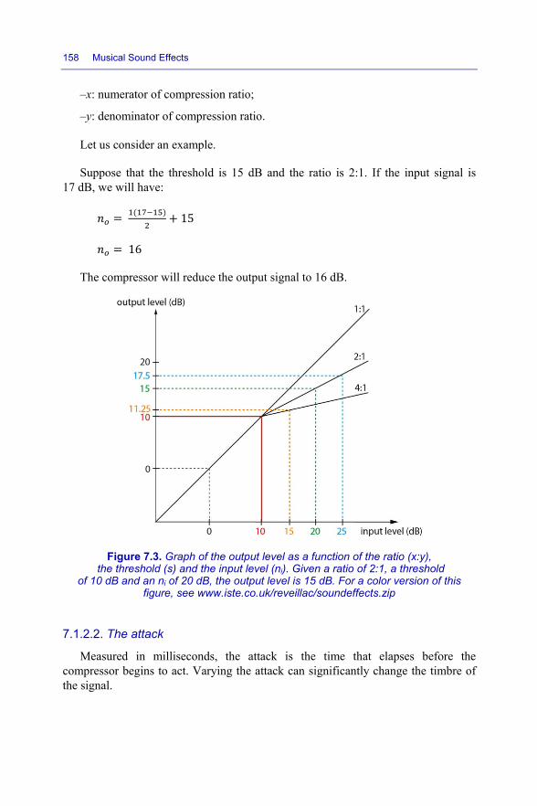
158 Musical Sound Effects
–x: numerator of compression ratio;
–y: denominator of compression ratio.
Let us consider an example.
Suppose that the threshold is 15 dB and the ratio is 2:1. If the input signal is 17 dB, we will have: = ( ) + 15 = 16
The compressor will reduce the output signal to 16 dB.
Figure 7.3. Graph of the output level as a function of the ratio (x:y), the threshold (s) and the input level (ni). Given a ratio of 2:1, a threshold
of 10 dB and an ni of 20 dB, the output level is 15 dB. For a color version of this figure, see www.iste.co.uk/reveillac/soundeffects.zip
7.1.2.2. The attack
Measured in milliseconds, the attack is the time that elapses before the compressor begins to act. Varying the attack can significantly change the timbre of the signal.

Dynamic Effects 159
If the attack is too long, the compressor will struggle to stabilize, which
negatively affects the signal quality. The attack duration needs to be chosen in such a way as to retain and preserve the transients, i.e. the earliest information in the sound wave, namely the initial amplitude of the wave.
Some sounds, like those made by percussion instruments, have extremely obvious and pronounced transients. Other instruments, such as strings, create much softer transients.
If the attack is too short, the signal will be flattened and the percussive components of the signal will be lost.
Figure 7.4. Attack and release during compression. For a color version of this figure, see www.iste.co.uk/reveillac/soundeffects.zip
7.1.2.3. The release
The release is also measured in milliseconds, like the attack. It represents the time that elapses between the moment when the sound passes back below the

160 Musical Sound Effects
threshold and the moment when the compressor turns off. The release also strongly influences the timbre of the sound.
Many compressors have an automatic release mode. In this mode, the compressor intelligently adapts to the type of input signal.
Figure 7.5. Example of compression illustrating its parameters. For a color version of this figure, see www.iste.co.uk/reveillac/soundeffects.zip
7.1.2.4. The make-up gain
This parameter specifies how to compensate any loss in the signal gain caused by compression. It therefore determines the final gain.
7.1.2.5. Other functions
The knee: this determines whether the compressor should turn on gradually, which is known as soft knee, or abruptly, which is known as hard knee;
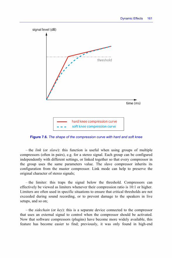
Dynamic Effects 161
Figure 7.6. The shape of the compression curve with hard and soft knee
– the link (or slave): this function is useful when using groups of multiple compressors (often in pairs), e.g. for a stereo signal. Each group can be configured independently with different settings, or linked together so that every compressor in the group uses the same parameters value. The slave compressor inherits its configuration from the master compressor. Link mode can help to preserve the original character of stereo signals;
– the limiter: this traps the signal below the threshold. Compressors can effectively be viewed as limiters whenever their compression ratio is 10:1 or higher. Limiters are often used in specific situations to ensure that critical thresholds are not exceeded during sound recording, or to prevent damage to the speakers in live setups, and so on;
– the sidechain (or key): this is a separate device connected to the compressor that uses an external signal to control when the compressor should be activated. Now that software compressors (plugins) have become more widely available, this feature has become easier to find; previously, it was only found in high-end

162 Musical Sound Effects
compressors. Sidechains can also include other (internal) processing operations, such as low-pass filters to eliminate pumping1, switching to an insert such as an equalizer (see section 4.2) or a de-esser (see below, section 7.4). One of its very first applications was to lower the volume of music when an announcement is made on the microphone, as is still common practice today;
– the mix: this determines the ratio of original audio input signal to compressed signal in the output of the compressor;
– the low-cut comp: this function, included in some compressors, eliminates low frequencies in the sidechain control signal;
– rotation point compressor: this function, when available, creates a rotation at the point where the audio signal and the threshold intersect. This amplifies the signal below the threshold and compresses the signal above it.
Figure 7.7. The effect of the rotation point. For a color version of this figure, see www.iste.co.uk/reveillac/soundeffects.zip
1 If the compressor releases too quickly, you can sometimes hear the increase in the sound level after the compressor stops cutting the peaks. This phenomenon is called “pumping”.

Dynamic Effects 163
7.1.3. Examples of compressors
Table 7.1 gives a non-exhaustive list of a few compressors, available as pedals, racks or plugins.
Type Manufacturer or publisher Model Remarks
Pedal
Biyang CO-10 Compress X
Compressor/sustainer for guitar
BOSS CP-1X Multiband compressor for guitar Carl Martin Classic opto
compressor Optical compressor* for guitar
Diamond Pedals Compressor Optical compressor* Fender Micro-
compressor Compressor for guitar
Marshall ED-1 The compressor
Compressor for guitar
MXR M132 Super comp
Compressor for guitar
MXR M76 Studio Compressor for guitar Providence Velvet VLC-1 Compressor/sustainer for guitar Rocktron Reaction
compressor Compressor/sustainer for guitar
Taurus TUX MK2 Compressor/sustainer for guitar T-Rex Engineering
Tonebug sustainer
Compressor/sustainer for guitar
Way Huge Electroniucs
Saffron squeeze
Compressor/sustainer for guitar
Rack
Alesis 3632 Compressor/limiter/expander/gate – 2 channels
Aphex CX-500 Compressor/noise gate – 1 channel ART PRO VLA II Optical tube compressor* – 2 channels Avalon AD 2044 Optical compressor* – 2 channels Behringer MDX2200 Compressor/limiter/gate – 2 channels Chandler Limited
RS124 Tube compressor – 1 channel
Chandler Limited
Germanium compressor
Compressor – 1 channel
DBX 160VU Compressor – 1 channel DBX 266XL Compressor/limiter/gate – 2 channels DBX 166XS Compressor/limiter/gate – 2 channels Drawner 1968 MKII Tube compressor – 2 channels

164 Musical Sound Effects
Manley Variable MU Mastering
Compressor/limiter – Tubes – 2 channels
Fairchild 670 Compressor/limiter – Tubes – 2 channels NEVE 33609J/D Compressor/limiter – 2 channels –
Vintage Rupert Neve Designs
Portico 5043 Compressor/limiter – 2 channels
Samson S-Com plus Compressor/limiter/expander/gate/ de-esser – 2 channels
SSL G Comp Stereo compressor – API 500 Rackmount Tornade music systems
E-Series stereo bus compressor
Compressor – 2 channels – VCA**
Universal Audio LA2A Optical compressor – 1 channel Urei JBL 1176LN Compressor – 1 channel
Vertigo Sound VSC-2 Compressor – 2 channels – 4 VCA** Vintech Audio 609CA Compressor/limiter – 2 channels Warm Audio WA-2A Tube compressor – 1 channel Weiss Engineering
Gambit DS1 Dynamic compressor/limiter – Wideband, multiband, and parallel – AES/EBU only
Software
Audiocation Compressor AC-1
Freeware – Compressor Windows: VST
Eventide Omnipressor Compressor/limiter/expander Windows: VST; RTAS; AAX OSX: AU; VST; RTAS; AAX
IK Multimedia Classic T-RackS Compressor
Compressor Windows: VST; RTAS; AAX OSX: AU; VST; RTAS; AAX
MeldaProduction Audio Technologies
MCompressor Freeware – Compressor/limiter Windows: VST; VST3; AAX OSX: AU; VST; VST3; AAX
PSP Audioware MasterComp Compressor Windows: VST; RTAS; AAX OSX: AU; VST; RTAS; AAX
Softube Valley People Dyna-mite
Compressor/limiter/expander/de-esser/gate Windows: VST; VST3; RTAS; AAX OSX: AU; VST; VST3; RTAS; AAX
URS 1975 Classic Compressor/limiter Windows: VST; RTAS; AAX OSX: AU; VST; RTAS

Dynamic Effects 165
Waves H-Comp Compressor
Windows: VST; VST3; AAX; RTAS OSX: AU; VST; VST3; AAX; RTAS
Waves PuigChild 670 Compressor – Emulation of the Fairchild 660 and 670 Windows: VST; VST3; AAX; RTAS OSX: AU; VST; VST3; AAX; RTAS
Waves API 2500 Compressor Windows: VST; VST3; AAX; RTAS OSX: AU; VST; VST3; AAX; RTAS
Waves SSL G-Master Buss Compressor
Compressor – Emulation of the G-Comp by SSL Windows: VST; VST3; AAX; RTAS OSX: AU; VST; VST3; AAX; RTAS
Waves VComp Compressor/limiter/de-esser – Emulation of the 2254 by Neve Windows: VST; VST3; AAX; RTAS OSX: AU; VST; VST3; AAX; RTAS
Waves CLA-3A Compressor/limiter – Emulation of the LA-3A by Universal Audio Windows: VST; VST3; AAX; RTAS OSX: AU; VST; VST3; AAX; RTAS
Waves C1 Compressor
Compressor/expander/gate/equalizer Windows: VST; VST3; AAX; RTAS OSX: AU; VST; VST3; AAX; RTAS
Waves Renaissance Compressor
Compressor Windows: VST; VST3; AAX; RTAS OSX: AU; VST; VST3; AAX; RTAS
* Optical compressors have a light source whose intensity varies according to the amount of signal passing through it and a photoelectric cell that reacts to the luminosity of the light source. These types of compressor can be either highly colored or very neutral. They provide an “organic” dimension to the sound. **The VCA (voltage-controlled amplifier) is a transistor chip that monitors the level of the incoming signal to determine how much reduction needs to be applied. VCA compressors provide rapid and precise compression.
Table 7.1. Examples of compression pedals, racks (studio) and plugins
Studio compressors and pedals are based on several different technologies: optical compressors, field effect transistor (FET) compressors, tube compressors, voltage-controlled amplifier (VCA) compressors, operational transconductance amplifier compressors and many others. Each technology has its own pros and cons,

166 Musical Sound Effects
and their performance in terms of sound rendering varies. To decide between them, you need to listen to how they sound within a given musical context. Most studios have multiple compressors to allow their sound engineers to add customized color or transparency to each mix.
Figure 7.8. Four well-known studio compressors (from top to bottom): LA-2A by Universal Audio (optical compressor), 609CA by Vintech and 1176 by Urei/JBL (FET
compressors) and a Manley tube compressor
There are a staggering number of software compressors – hundreds of them. They offer a broad spectrum of possibilities, as well as rich and very sophisticated settings. Many software compressors are clones of studio compressors.
7.1.4. Multiband compressors
This type of compressor separates the input signal into multiple bands (three or more) using an array of filters. Each band is then processed with a different compressor, before recombining the processed signals into a single output.

Dynamic Effects 167
Figure 7.9. Diagram of the principle of a multiband compressor. For a color version of this figure, see www.iste.co.uk/reveillac/soundeffects.zip
These compressors can correct frequency imbalance in the original audio signal.
Figure 7.10. The high-end digital dynamic studio rack compressor/limiter “Gambit DS1-MK2” by Weiis. This compressor is wideband, multiband and parallel (see
section 7.1.6)
Increasing the number of bands makes the compressor more complex. These types of processor are extremely delicate to operate, and dividing the signal into frequency bands is especially tricky.
Figure 7.11. The multiband software compressor (3) Drawner 1973 by Softube

168 Musical Sound Effects
Table 7.2 lists a few examples of multiband software compressors. There are many of them, so this list is far from exhaustive.
Publisher Name Remarks
Audio Damage Rough Rider Freeware – Multiband compressor Windows: VST OSX: AU; VST
Blue Cat Audio MB-5 Dynamix Multiband compressor Windows: VST; RTAS; AAX OSX: AU; VST; RTAS; AAX
Izotope Ozone 7 – Vintage compressor
Multiband compressor Windows: RTAS; VST2; VST3; AAX OSX: RTAS; AU; VST2; VST3; AAX
Avid Pro Tools Multiband compressor Windows: AAX OSX: AAX
Nomad Factory Essential Multiband Compressor
Multi-band compressor Windows: RTAS; VST OSX: RTAS; AU; VST
Nomad Factory AMT Multi Max
Multiband compressor Windows: RTAS; VST OSX: RTAS; AU; VST
Softube Drawner 1973 Multiband
Multiband compressor – Emulation of the Drawner 1973 compressor Windows: VST; VST3; AAX OSX: AU; VST; VST3; AAX
FabFilter Pro-MB Multiband compressor Windows: VST; VST3; AAX; RTAS OSX: AU; VST; VST3; AAX; RTAS
Waves C6 Multiband Compressor
Multiband compressor Windows: VST; VST3; AAX; RTAS OSX: AU; VST; VST3; AAX; RTAS
Cakewalk Sonitus Multiband compressor Compatible with Sonar 4 Producer Edition and Sonar Studio Edition
Table 7.2. Examples of multiband software compressors

Dynamic Effects 169
7.1.5. Guidelines for configuring a compressor
Properly configuring a compressor is extremely difficult. It is possibly one of the most complex tasks that you will encounter in mixing, and requires an enormous amount of subtlety and finesse. There is no magic recipe. It is a bit like cooking – even if you have the right ingredients, instructions and temperatures, you still need skill and experience to manage the vast number of unpredictable, incalculable or unknowable factors.
In the following, a sketch of the outlines of a simple method for studio applications is provided. As you gain experience, you can make your own refinements.
The objective is to stabilize the position of the sound signal relative to the position of the observer. We need to eliminate any sensation of back-and-forth motion:
1) Set the compression (threshold) to 0 dB;
2) Set the compression ratio to its maximum value;
3) Set the attack to its minimum value;
4) Set the release to its minimum value;
5) Begin playing the track;
6) Lower the threshold until the compressor is not constantly active;
7) Lower the compression ratio until the hypercompression caused by setting everything to max has been eliminated. At this point, you are looking to make the sound rendering more organic;
8) Increase the attack and listen to the effect on the transients; the perceived thickness of the sound should change;
9) Increase the release until any pumping is eliminated, letting the signal breathe. Look for the slowest possible setting that creates a groove and that you are happy with;
10) Adjust the knee until you find the right color and punch;
11) These settings should make the gain indicator dance around.

170 Musical Sound Effects
Remember, each parameter influences the others. You need to be tweaking and adjusting everything continuously, while listening carefully.
If you close your eyes, it should feel like the sound source has a stable position in space, with a characteristic groove and a natural quality.
If you lost gain during the processing, you can compensate by adjusting the increase/decrease setting. Some compressors have an automatic make-up gain function.
It is difficult to describe the sensations created by a compressor in writing. It truly is something that only your ears can fully appreciate. Do not hesitate to keep repeating your tests as many times as you need with your headset or via monitoring.
7.1.6. Parallel compression
Parallel compression is also known as “invisible compression” or “New York compression”. It is a technique that makes sounds feel bigger without changing their dynamics.
It is often used for drums, but also works with other instruments, such as bass guitar or brass ensembles. It is not recommended for vocals.
The idea is to duplicate the track (for drums, first create a group that combines all percussions onto a single track). One of the new tracks is a copy of the original signal (optionally very slightly compressed), preserving the dynamics of the sound. The other track is compressed to obtain the sound matter.
Both tracks are then mixed into a single, definitive output signal.
Figure 7.12. Principle of parallel compression. For a color version of this figure, see www.iste.co.uk/reveillac/soundeffects.zip
Be careful. It is very easy to end up with a sound that is confused and ugly. The key is to find the perfect balance, which in some cases can be extremely difficult.
Dynamic Effects 171
One simple approach is to configure the compressor as follows: minimum
threshold, maximum compression ratio, very quick attack, very short release and very hard knee.
Then play with the mix of original and compressed signals until you find a good compromise.
7.1.7. Serial compression
Just like electrical circuits, compression can be arranged in series as well as in parallel. With serial compression, the signal passes through two connected compressors consecutively. The goal is to obtain a powerful sound with lots of matter. These two objectives are contradictory with a single compressor.
The solution is to place multiple compressors in a certain predefined order. First, we process the sound matter and consistency, and then we give it power and muscle separately.
Each compressor has its own compression ratio. The overall compression ratio is obtained by multiplying the two individual ratios together, unlike the attack, release and knee, which are added together. This means that the sound rendering can become unnatural very quickly.
Serial compression is complex to implement. Much like parallel compression, it is very sensitive to its configuration. The right balance between the two compressors must be found in order to avoid an awful noisy mess.
7.1.8. Compression with a sidechain
We introduced the concept of sidechain in section 7.1.2.4. We now have a chance to go into a little more detail.
One of the possible applications of this technique is to prevent the instruments in a sound mix from masking each other. Instead of applying standard compression to the signal level, the compression is controlled by an external signal. For example, to clarify the sound rendering of a bass guitar, we can use the bass drum as an external source. Another example is to use the snare drum as an external source for vocals.
Sidechains are also extremely useful for synth pads. Due to their synthetic nature, synth pads often lack in dynamics. By using a strong, rhythmic component like the kick drum as a sidechain, we can give the synth pads more energy by varying their level with the rhythm.

172 Musical Sound Effects
This technique is called an “external sidechain”, as opposed to an “internal sidechain”, which we discussed previously.
We can also use the original signal itself as a trigger by compressing it and applying a high-pass or low-pass filter, allowing the compressor to target specific regions of the frequency spectrum. For drums, the lower end of the spectrum is often filtered to prevent the signal of the bass drum from being excessively compressed, which can drag the rest of the drums down with it, e.g. snare drum, tom-toms, etc. Doing this provides the sound rendering of the drums more clarity and transparency while still allowing compression to be achieved.
7.1.9. Some basic compression settings
This section gives guidelines for creating some of the various sounds that can be achieved with compressors, either for studio mixing or live sound reinforcement. However, there are no universal rules or methods. The following sections guide us in the right direction for good results.
7.1.9.1. Improving sound cohesion
Sometimes, a collection of multiple audio tracks requires extra coherence. Today, mixes can have many wildly different components, distributed over multiple distinct tracks, but which need to be linked to each other. Examples of such components might include recorded instruments, samples, electronic sounds, virtual instruments and so on. We can use a compressor to forge connections between components, either in combination with other methods or separately.
You will need the following settings:
– compressor with a well-defined color rather than a very transparent compressor. Vintage compressors or emulators should therefore be preferred;
– long attack time;
– suitable release time. If your compressor has an automatic mode, this is a good opportunity to use it;
– very soft knee;
– low compression ratio, between 1.1:1 and 2.0:1;
– threshold that reduces the signal by –0.5 to –1.5 dB.
Dynamic Effects 173
7.1.9.2. Increasing sound thickness
Often, your sound recording or sequence will seem very or excessively clear, pure or discrete. You can reinforce it to occupy more space without losing its natural feel by increasing its thickness or consistency.
We need the following settings:
– long attack time for percussion instruments or any other rhythmic instruments, and short attack time for all other components;
– release time appropriate for the rhythm of the music. Automatic mode can be a good compromise, but is not always suitable; you will need to try it and see;
– knee as soft as possible;
– filtered bass frequencies to soften the compression;
– compression ratio as finely tuned as possible to retain the natural feel of the recording;
– threshold that grips (captures) each peak.
7.1.9.3. Smoothening the sound
Sometimes, you will want to create a very soft, fluid sound, with long attacks and little aggressiveness, without compromising on presence, naturalness or energy. This is often the case for the background of a mix, which supports the main sound sequence, or might for example be desirable for vocals in a slow part of a song.
You will need the following settings:
– very short attack time;
– rapid release;
– knee either soft or hard on a case-by-case basis. You will have to listen carefully to decide;
– high compression ratio, between 5:1 and 10:1;
– threshold that grips each peak;
– make-up gain to restore the signal to satisfactory levels. If your compressor has an automatic mode, you should use it, but it will not always be enough.
7.1.9.4. Creating a powerful sound
This technique places a sound at the front of the overall mix. It will seem more aggressive and present, closer to the audience and more detached from the other

174 Musical Sound Effects
sounds. It will also seem less flattened and masked by other tracks that might cover parts of its frequency spectrum.
You will need the following settings:
– attack time long enough to preserve the natural timbre and feel of the signal;
– release time long enough to preserve the envelope without affecting the next group of transient frequencies;
– hard knee to ensure that the sound remains aggressive;
– high compression ratio to make the sound feel percussive without completely flattening it;
– threshold chosen to catch the most important peaks in the signal, namely those that carry and make up the dynamics;
– optionally, a make-up gain if you judge that the losses created by these settings need to be compensated.
7.1.9.5. Examples of standard settings
Table 7.3 lists a few standard settings that can be applied to individual tracks, either for recording or mixing.
Instrument Compression ratio
Threshold
Attack
Release
Knee Notes
Powerful drums 20:1 to max:1 5– 10 dB 0.1–2 ms 40–100 ms Hard
Usually applied to the bass drum
Drums 5:1 2– 5 dB 1–10 ms 100–400 ms Soft
Bass guitar 4:1 to 10:1 3– 6 dB 2–25 ms 250–350 ms Hard Longer attack for slap bass (harmonics)
Brass 4:1 5– 8 dB for peaks Auto Auto
Electric guitar 4:1 to 6:1
Depending on style of music, from 5– 10 dB
5–30 ms 200–300 ms
Relatively hard, depending on style of music
Auto mode often works for attack and release
Acoustic guitar 3:1 to 4:1 3–5 dB 20–50 ms 200–300 ms Soft
Try to preserve the natural sound of the instrument

Dynamic Effects 175
Synthesizer No compression, synth sound is usually already compressed enough
Wind instruments 3:1
Relatively high, depending on instrument
5–10 ms 50–200 ms Soft
Adjust depending on whether instrument plays solo
Studio vocals 2:1 to 6:1 5–12 dB for
peaks 10–50 ms 100–400 ms Soft For rock music, reduce attack and sustain
Live vocals 2:1 to 4:1 5–10 dB for peaks 10–30 ms 100–300 ms Soft
Auto release can be good for live sets
Solo voice 1.5:1 to 2:1 Max 10 ms 200 ms Soft
Try to preserve the natural feel and grain of the voice
Table 7.3. Examples of standard compression settings for specific instruments
7.1.10. Synchronizing the compressor
If your compressor has a sidechain function with an external key input, there is an intriguing opportunity that you might like to explore.
You can plug a metronome or a track with the musical rhythm, like the hi-hat from the drums, into the key input.
Your compressor will synchronize with the external signal. This will enhance any instruments with weaker dynamics, like strings or synth pads.
In this way, you can create very special and original effects.
There is no hard-and-fast rule. You just need to play around, listen and then accept or reject the results depending on what you are looking for.
7.1.11. Using a compressor as a limiter
Theoretically, any compressor can act as a limiter if it allows the compression ratio to be set higher than 20:1, up to ∞:1 (which corresponds to a perfect limiter).
“Brickwall” limiters allow us to define a level or volume that will never be exceeded no matter what. This prevents clipping during mastering or on tracks with large differences in sound level.

176 Musical Sound Effects
Limiters tend not to have many configurable parameters. One parameter is the threshold, which defines the height of the limit, and another is the output level (or ceiling).
Some limiters also have a configurable release time, which defines the time taken by the limiter to stop acting on the signal, and thus the speed at which it does so.
Figure 7.13. The software limiter L1 by Waves with its straightforward features (threshold, ceiling, release)
Some software limiters have a few additional parameters.
Figure 7.14. The software limiter LM-662 by Nomad Factory, a tool with more sophisticated parameters

Dynamic Effects 177
Limiters are often placed at the end of the processing chain in the mix (main
bus), which is why software versions often include features for configuring the sampling depth (dither or dithering), which ranges from 8 to 24 bits.
Personally, I do not use limiters during mixing, because I find them too restrictive. But that is just me – some people do like to use them.
To use a limiter for mastering, you need to set the output level to around –0.5 to –0.2 dB. The threshold should only affect peaks, and its reduction level should never reach 0.
Table 7.4 lists a few examples of software limiters.
Publisher Name or model Remarks Abbey Road TG 12413
Limiter Emulation of the EMI Abbey Road 1960 limiter – Limiter/compressor Windows: VST; RTAS OSX: AU; VST; RTAS
Blue Cat Audio Blue Cat’s Protector
“Brickwall” limiter Windows: VST; VST3; RTAS; AAX; DX OSX: AU; VST; VST3; RTAS; AAX
dB Audioware dB-L Mastering Limiter 1.00
Freeware – Limiter Windows: DX
FabFilter Pro-L Multi-band compressor Windows: VST; VST3; RTAS; AAX OSX: AU; VST; VST3; RTAS; AAX
Kjaerhus Audio Classic Master Limiter
Freeware – “Brickwall” limiter Windows: VST
MeldaProduction MDynamics Limiter
Limiter Windows: VST; VST3; AAX OSX: AU; VST; VST3; AAX
Nomad Factory BT Brickwall BW-2S
“Brickwall” limiter/compressor Windows: VST; RTAS OSX: VST; RTAS; AU
Nomad Factory LM-662 Limiter
Emulation of the Fairchild 670 limiter Windows: VST; RTAS OSX: VST; RTAS; AU

178 Musical Sound Effects
Sonnox Oxford Limiter V2
Limiter with variable knee Windows: VST2; AAX; RTAS OSX: VST2; RTAS; AU; AAX
Waves L1 Limiter Limiter Windows: VST; VST3; RTAS; AAX OSX: AU; VST; VST3; RTAS; AAX
Table 7.4. Examples of software limiters
7.2. Expanders
This section briefly presents dynamic range expanders, which are included with most compressors and DAWs.
The purpose of an expander is to increase the dynamic range of an audio signal. Therefore, it operates like a reverse audio compressor.
7.2.1. Parameters
Above a certain threshold, the expander does nothing. Below this threshold, it applies a predefined expansion ratio.
This ratio takes values ranging from 1:2 and 1:4 up to 1:10, at which point the expander essentially behaves like a gate.
Figure 7.15. Principle of an expander. For a color version of this figure, see www.iste.co.uk/reveillac/soundeffects.zip

Dynamic Effects 179
Just like a compressor, expanders have time parameters, including attack,
release, knee and a hold function that defines the behavior of the expander after the signal exceeds the threshold, but before the release time begins.
Some expanders also have a sidechain mode, like most dynamics processing tools. Many compression plugins and studio compressors include an expander function.
7.2.2. Examples of software expanders
Table 7.5 lists a few expanders that are found in combination with noise gates (see below, section 7.3), compressors (see Table 7.1) and limiters (see section 7.1.11).
Type Manufacturer or publisher Model or name Remarks
Rack
Behringer Multigate Pro XR4400
Expander/gate – 4 channels
Behringer Multicom Pro-XL MDX4600
Expander/gate/compressor/limiter – 4 channels
DBX 1074 QuadGate Expander/gate – 4 channels Drawmer DS101 Expander/gate – Rack unit, model
500 Samson Technologies
S-Com plus Compressor/gate/expander/de-esser/limiter
Software
Audio Damage AD022 BigSeq-2 Noise gate/expander Windows: VST OSX: VST; AU
FabFilter Pro-G Noise gate/expander Windows: VST; VST3; AAX; RTAS OSX: VST; VST3; AU; AAX; RTAS
Kjaerhus Audio GAG-1 Noise gate/expander Windows: VST OSX: VST; AU
MeldaProduction MStereoSpread Noise gate/expander Windows: VST; VST3; AAX OSX: VST; VST3; AU; AAX

180 Musical Sound Effects
Nomad Factory AS Gate Expander
Noise gate/expander Windows: VST; AAX OSX: VST; AAX
Waves Primary Source Expander
Noise gate/expander Windows: VST; VST3; AAX; RTAS OSX: VST; VST3; AU; AAX; RTAS
Table 7.5. Examples of expanders
7.3. Noise gates
As you may have guessed from their name, noise gates either block a sound signal or allow it to pass. They are used to eliminate any hiss or background noise on a track in a mix or from instruments, usually analog ones. An ideal noise gate does not modify the rendering or the color of the sound in any way.
Figure 7.16. The DBX 1074, a studio noise gate
This technique appeared in the late 1960s and was later adopted by high-end recording equipment in the 1980s for real-time applications.
7.3.1. Parameters
The parameters of noise gates are largely equivalent to those of compressors. Noise gates continuously analyze the signal, comparing it to a user-defined threshold. Whenever the overall level passes below this threshold, the noise gate closes, blocking the signal. The gate opens again once the level goes back over the threshold.
The attack and release parameters define the time taken by the gate to open and close whenever the signal crosses the threshold. The gate opens gradually during the attack to allow the audio signal to pass, and closes during the release until the signal is fully blocked.

Dynamic Effects 181
Figure 7.17. Principle of the noise gate. For a color version of this figure, see www.iste.co.uk/reveillac/soundeffects.zip
There can also be a hold parameter, which configures how long the gate should remain open after the signal falls below the threshold. The hold time elapses before the release begins (Figure 7.16).
Figure 7.18. Principle of a noise gate with a hold parameter. For a color version of this figure, see www.iste.co.uk/reveillac/soundeffects.zip
The concept of hysteresis is often mentioned in connection with noise gates. The idea is to define two thresholds, the open threshold and the close threshold. The

182 Musical Sound Effects
hysteresis is the difference between these values, which are measured in dB (Figure 7.17).
Figure 7.19. Hysteresis in the context of an audio signal (input level) using a noise gate (top, without hysteresis; bottom, with hysteresis) (source: Wikipedia). For a color
version of this figure, see www.iste.co.uk/reveillac/soundeffects.zip
Some noise gates include an audio filtering system that only activates the gate on a certain frequency band.
Sidechains can also be used to control when the gate opens using an external signal. This can significantly improve the accuracy of the noise gate.
7.3.2. Examples of noise gates
Some examples of available software and hardware noise gates can be found in Table 7.5 and sections 7.1.3 and 7.2.2. Noise gates are often included with expanders or other dynamics processing equipment.
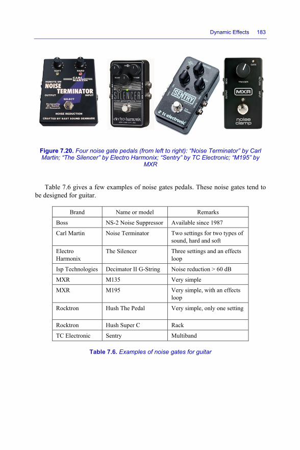
Dynamic Effects 183
Figure 7.20. Four noise gate pedals (from left to right): “Noise Terminator” by Carl Martin; “The Silencer” by Electro Harmonix; “Sentry” by TC Electronic; “M195” by
MXR
Table 7.6 gives a few examples of noise gates pedals. These noise gates tend to be designed for guitar.
Brand Name or model Remarks
Boss NS-2 Noise Suppressor Available since 1987
Carl Martin Noise Terminator Two settings for two types of sound, hard and soft
Electro Harmonix
The Silencer Three settings and an effects loop
Isp Technologies Decimator II G-String Noise reduction > 60 dB
MXR M135 Very simple
MXR M195 Very simple, with an effects loop
Rocktron Hush The Pedal Very simple, only one setting
Rocktron Hush Super C Rack
TC Electronic Sentry Multiband
Table 7.6. Examples of noise gates for guitar
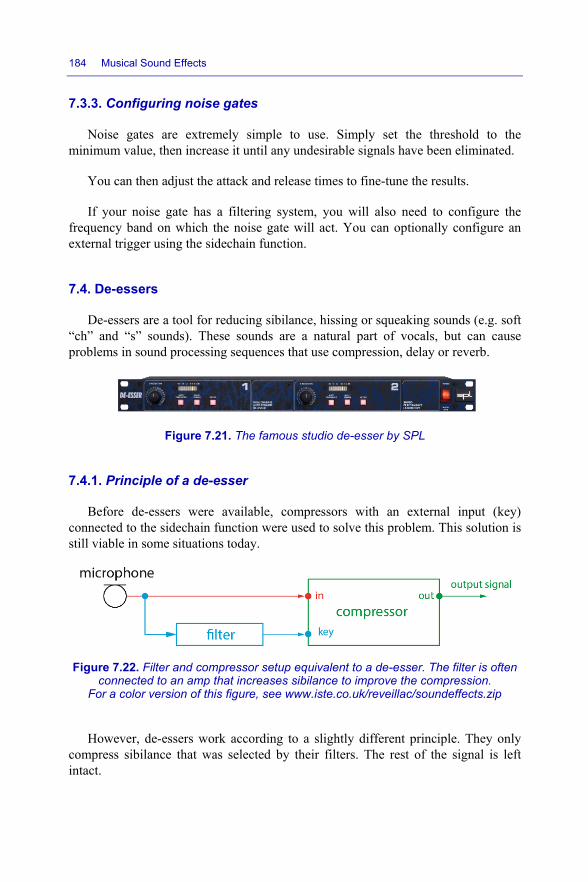
184 Musical Sound Effects
7.3.3. Configuring noise gates
Noise gates are extremely simple to use. Simply set the threshold to the minimum value, then increase it until any undesirable signals have been eliminated.
You can then adjust the attack and release times to fine-tune the results.
If your noise gate has a filtering system, you will also need to configure the frequency band on which the noise gate will act. You can optionally configure an external trigger using the sidechain function.
7.4. De-essers
De-essers are a tool for reducing sibilance, hissing or squeaking sounds (e.g. soft “ch” and “s” sounds). These sounds are a natural part of vocals, but can cause problems in sound processing sequences that use compression, delay or reverb.
Figure 7.21. The famous studio de-esser by SPL
7.4.1. Principle of a de-esser
Before de-essers were available, compressors with an external input (key) connected to the sidechain function were used to solve this problem. This solution is still viable in some situations today.
Figure 7.22. Filter and compressor setup equivalent to a de-esser. The filter is often connected to an amp that increases sibilance to improve the compression.
For a color version of this figure, see www.iste.co.uk/reveillac/soundeffects.zip
However, de-essers work according to a slightly different principle. They only compress sibilance that was selected by their filters. The rest of the signal is left intact.
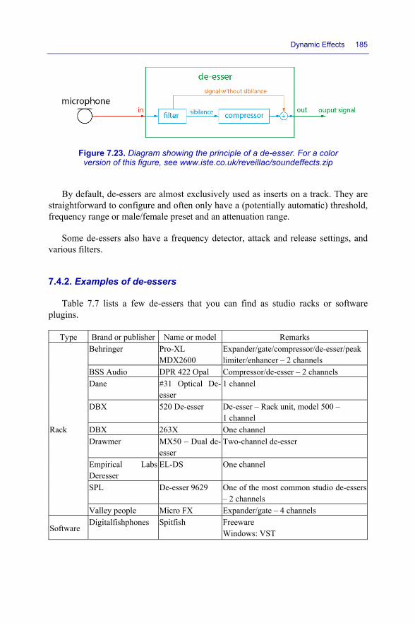
Dynamic Effects 185
Figure 7.23. Diagram showing the principle of a de-esser. For a color version of this figure, see www.iste.co.uk/reveillac/soundeffects.zip
By default, de-essers are almost exclusively used as inserts on a track. They are straightforward to configure and often only have a (potentially automatic) threshold, frequency range or male/female preset and an attenuation range.
Some de-essers also have a frequency detector, attack and release settings, and various filters.
7.4.2. Examples of de-essers
Table 7.7 lists a few de-essers that you can find as studio racks or software plugins.
Type Brand or publisher Name or model Remarks
Rack
Behringer Pro-XL MDX2600
Expander/gate/compressor/de-esser/peak limiter/enhancer – 2 channels
BSS Audio DPR 422 Opal Compressor/de-esser – 2 channels Dane #31 Optical De-
esser 1 channel
DBX 520 De-esser De-esser – Rack unit, model 500 – 1 channel
DBX 263X One channel Drawmer MX50 – Dual de-
esser Two-channel de-esser
Empirical Labs Deresser
EL-DS One channel
SPL De-esser 9629 One of the most common studio de-essers – 2 channels
Valley people Micro FX Expander/gate – 4 channels
Software Digitalfishphones Spitfish Freeware
Windows: VST

186 Musical Sound Effects
Eiosis E2deesser Windows: VST2; VST3; AAX OSX: VST2; VST3; AU; AAX
FabFilter Pro-DS Windows: VST; VST3; AAX; RTAS OSX: VST; VST3; AU; AAX; RTAS
Nomad Factory BT Deesser DS-2S
Windows: VST; RTAS OSX: VST; AU; RTAS
Sonnox Oxford SuprEsser Windows: VST; RTAS OSX: VST; AU; RTAS
Waves DeEsser Windows: VST; VST3; AAX; RTAS OSX: VST; VST3; AU; AAX; RTAS
Waves Renaissance DeEsser
Windows: VST; VST3; AAX; RTAS OSX: VST; VST3; AU; AAX; RTAS
Table 7.7. Examples of de-esser racks and plugins
7.4.3. Replacing a de-esser with an equalizer and a compressor
In the following, we explain a simple method for de-essing a vocals track with a studio mixing desk:
– send the vocals track that you want to process onto two channels of the desk;
– on the first channel, use the equalizer on the mixing desk to isolate the vocals as much as possible and amplify any sibilance;
– on the second channel, send the signal to a compressor;
– send the equalized signal to the key of the compressor’s sidechain to eliminate the sibilance.
You can use the fader on the first channel to vary how much sibilance is eliminated, and the compressor on the second channel to control the de-essing rate.
7.4.4. Configuring a de-esser
Every de-esser is different, but you can adapt these basic settings to any model.
First, you need to determine the frequency at which your de-esser will be working. This is usually between 6 and 9 kHz (upper region of the spectrum). You need to narrow this down to reflect the vocal range of the singers: male, female, child, etc.

Dynamic Effects 187
Next, configure the attenuation. This should usually be less than 8 dB to ensure
that the sibilance is significantly reduced but that the dynamics of the signal are not flattened and that no gaps are created.
7.5. Saturation
Saturation in an analog audio circuit means that the strength of the processed signal cannot be increased no matter how much the input level is raised. Saturated signals exhibit clipping, a phenomenon that deforms the signal, also known as distortion.
Figure 7.24. Effect of saturation on an audio signal, with slight and heavy clipping. For a color version of this figure, see www.iste.co.uk/reveillac/soundeffects.zip
In practice, clipping begins well below maximum amplification. Various types of intermediate effects can therefore be achieved, including fuzz, overdrive and crunch.
These effects strongly depend on the underlying technology: vacuum tubes, transistors, pre-amp equipment and any analog, digital or software systems.
This section presents some of the various types of saturation.
7.5.1. Fuzz
This effect creates a bold sound that is very rich in harmonics. It was one of the characteristic sounds of the 1960s and 1970s. This type of saturation has the most clipping, which tends to increase the sustain, i.e. the duration of each played note.

188 Musical Sound Effects
The effect depends strongly on the equipment (amps) and instruments. Many musicians have made it their own, and still use it to this day: Jimi Hendrix (“Purple Haze”), Carlos Santana, The Rolling Stones, Pink Floyd and many more. Legend has it that Johnny Burnette was one of the first to use it in 1957. Link Wray popularized the effect in 1958 with instrumental tracks like “Rumble” and, of course, “The Fuzz”.
7.5.2. Overdrive
This effect imitates the sound of a tube amp pushed to maximum power, creating a very warm distortion that is highly popular with blues and rock guitarists (Chuck Berry, Ritchie Blackmore, Gary Moore, Steven Morse, Eddie Van Halen, etc.). Some organists have also used it, most notably with Hammond organs (Deep Purple, ELP, Pink Floyd, etc.).
Figure 7.25. The model MA100H Marshall amp with overdrive settings (in the center of the control panel – magnified below)
Some tube amps have an overdrive channel or setting that increases the signal gain of the instrument in the pre-amp phase, creating a saturated sound that is very rich in harmonics.
The overdrive effect is often also called “crunch” or “crunchy”.
7.5.3. Distortion
Distortion is more aggressive than overdrive, offering a less natural and more clipped sound. Much like its close relatives, fuzz and overdrive, the sound of distortion strongly depends on the underlying equipment, and the various models

Dynamic Effects 189
that simulate it vary wildly from one another. Distortion can be aggressive, melodic, smooth, rich, soft, irregular, hard, creamy and much more.
REMARK.– Distortion, the effect used by musicians, is not quite the same as the more general concept of distortion, which is used in acoustics to describe audio signals. In the general sense, distortion refers to any alteration experienced by an audio signal as it travels through the processing and amplification chain including the final sound reproduction and playback system, e.g. speakers or headphones. In acoustics, distortion is characterized by several factors: the level, the frequency response, the harmonic distortion, the cross-talk and the signal-to-noise ratio. Appendix 1 explains this in more detail.
7.5.4. Examples of equipment dedicated to creating saturation
Pedals for generating fuzz, overdrive or distortion effects have proliferated since the 1970s. They simplify the process of configuring instruments and amplifiers, which is highly inconvenient on stage. The electronic components in the circuits used by saturation pedals have evolved over time, from germanium transistors with highly flawed stability and linearity to today’s integrated circuits and software plugins.
Figure 7.26. Three different types of pedal: “Big Muff” by Electro Harmonix (fuzz), “Tube Screamer” by Ibanez (overdrive) and “Distortion DS-1” by Boss (distortion)
Table 7.8 lists a collection of pedals and other equipment (effects racks, software plugins) for creating and manipulating saturation effects. Most of these effects are designed for guitars, but they can also be used with other instruments.
A vast number of saturation pedals have been specifically designed for guitar – hundreds of them – and so this table only presents a very limited selection. The same is true for plugins.

190 Musical Sound Effects
Type Brand or publisher Model or name Remarks
Pedals
Akai Fuzz Fuzz BBE 427 Distortion Boss FZ-3 Fuzz Boss ML-2 Distortion Boss DS1-X Distortion Distortion – Improved digital
version of the DS-1 Boss DS-1 Distortion Distortion Boss BD-2 Overdrive Carl Martin Classic DC Drive Overdrive Carl Martin Crush Zone Vintage Distortion Digitech Death Metal Distortion Dunlop JHF1 Fuzz Electro Harmonix Big Muff Fuzz Electro Harmonix Micro metal Muff Distortion Electro Harmonix Bass Blogger Distortion/overdrive/fuzz Fender Blender Reissue Fuzz Fender Distortion Distortion Fulltone Octafuzz Fuzz Ibanez TS808 Tube Screamer Overdrive Ibanez DS7 Distortion Distortion Line 6 Dr. Distorto Distortion Maestro MFZ-1 Fuzz Marshall Shred Master Distortion Mojo France Bass Fuzz Fuzz Mooer Blues Grab Overdrive Mooer Fog Distortion/overdrive/fuzz for bass
guitar Morley Distortion One Distortion MXR M236 Fuzz MXR M75 Super Badass
Distortion Distortion
MXR M115 Distortion 3 Distortion MXR M89 Distortion/overdrive/fuzz for bass
guitar Rocktron Rampage Distortion Rocktron Reaction Distortion 1 Distortion TC Electronic MojoMojo Overdrive TC Electronic Vintage Distortion Distortion TC Electronic Dark Matter
Distortion Distortion

Dynamic Effects 191
T-Rex Engineering Nitros Distortion
Software
Audio Damage FuzzPlus3 Freeware – Distortion/amplifier simulation Windows: VST2; VST3 OSX: AU; VST2; VST3
AuraPlug EddieVsHeaven Freeware – Windows: VST OSX: AU; VST
Blue Cat Audio Destructor Distortion/compression/amplifier simulation Windows: VST; VST3; AAX; RTAS OSX: VST; VST3; AAX; AU; RTAS
BBE Green Screamer Distortion – Emulation of Ibanez Tube Screamer Windows: VST OSX: AU; VST
FabFilter Saturn Distortion – Multiple styles – 150 presets Windows: VST; VST3; AAX; RTAS OSX: VST; VST3; AAX; AU; RTAS
Izotope Trash 2 Distortion – Multiband – Convolution and delay module – 300 presets Windows: VST; VST3; AAX; RTAS; DirectX OSX: VST; VST3; AAX; AU; RTAS
MeldaProduction MPolySaturator Distortion – Choice of saturation spectrum Windows: VST; VST3; AAX OSX: VST; VST3; AAX; AU
Softube Acoustic feedback Distortion/guitar feedback Windows: VST; VST3; AAX OSX: VST; VST3; AAX; AU
SoundSpot Halcyon Distortion/overdrive Windows: VST; VST3; AAX OSX: VST; VST3; AAX; AU
SoundToys Decapitator Distortion/overdrive – 5 presets

192 Musical Sound Effects
Windows: VST; AAX OSX: VST; AAX; AU
SSL X-Saturator Distortion – Emulation of tube and transistor amps Windows: VST; VST3; RTAS; DirectX OSX: VST; VST3; AU; RTAS
Waves OneKnob Driver Overdrive Windows: VST; VST3; AAX; RTAS; DirectX OSX: VST; VST3; AAX; AU; RTAS
Wave Arts Tube Saturator 2 Overdrive Windows: VST2; VST3; AAX OSX: AU; VST2; VST3; AAX
Table 7.8. Examples of dedicated saturation effects
7.6. Exciters and enhancers
Exciters, also called aural exciters, harmonic exciters and enhancers by some manufacturers, are devices that modify the audio signal by applying dynamic equalization, usually to the higher frequencies of the sound spectrum. Exciters can also be used to increase the harmonics of a sound with the goal of improving its contrast and therefore making it more intelligible.
Exciters can be difficult and sensitive to operate. They have the unfortunate tendency of caricaturizing sounds, especially vocals.
The original introduction of the famous “Aural Exciter” by Aphex in 1975 was met with fervent enthusiasm by many studios, who eagerly adopted it and immediately applied it to a vast number of their productions. Its popularity did not last. Exciters have a questionable effect on the quality, and sound technicians soon realized that it could easily be replaced with good equalization.
Figure 7.27. The famous “Aural Exciter” by Aphex

Dynamic Effects 193
Since then, many other exciters have been created, some as racks, but most
commonly as plugins. It is not easy to judge their appeal and benefits. Some users love them, others dislike them. You will need to try them out and listen to decide for yourself.
Figure 7.28. Two modern rack enhancers: the “Sonic Maximizer 882i” by BBE and the “Exciter” model by Aphex
You can also find exciter effects pedals, usually for guitar.
7.6.1. Examples of exciters
Table 7.9 gives a list of exciter pedals, studio racks and software plugins.
Type Brand or publisher Model or name Remarks
Pedals
BBE Sonic Stomp - TC Electronic Bodyrez - Boss EH-2 -
Aphex 1401 Transistor pre-amp Aphex Xciter - Behringer SE200 Spectrum
Enhancer -
Rack
Aphex The Exciter Two channels – XLR and jack inputs/outputs
Aphex 204 Aural Exciter Two channels – XLR and jack inputs/outputs
Aphex 103A Aural Exciter Two channels – Jack inputs/outputs Aphex 204 Aural Exciter Two channels – XLR and jack
inputs/outputs BBE Sonic Maximizer
882i Two channels – XLR and jack inputs/outputs – Input VU-meter with

194 Musical Sound Effects
LEDs and peak display
Behringer Ultrafex II EX3100 Two channels – XLR and jack inputs/outputs – Surround
Behringer Ultrafex Pro EX3200
Two channels – XLR and jack inputs/outputs – Surround
Rocktron RX20 Designed for guitar Rocktron RX1 Designed for guitar SPL Tube Vitalizer Two channels – XLR and jack
inputs/outputs – High-end exciter SPL Spectralizer 99 presets – AES/EBU – S/P-DIF –
RS422 – MIDI in/thru SPL Vitalizer SX2 pro Two channels – XLR and jack
inputs/outputs
SPL Vitalizer Mk2-T Two channels – XLR and jack inputs/outputs
Software
BBE Sonic Sweet Suite of several plugins: D82, H82, and L82 Windows: VST; RTAS OSX: VST; AU; RTAS
Crysonic Spectralive NXT-3 Windows: VST OSX: VST; AU
MeldaProduction MStereoProcessor Windows: VST2; VST3; AAX OSX: VST2; VST3; AU; AAX
Nomad Factory AS-Exciter Windows: VST; AAX; RTAS OSX: VST; AAX; RTAS
SPL Vitalizer MK2-T Windows: VST2; VST3; AAX OSX: VST2; VST3; AU; AAX
Voxengo Warmifier Windows: VST; VST3 OSX: VST; VST3; AU
Waves Renaissance Bass Windows: VST; VST3; AAX; RTAS OSX: VST; VST3; AU; AAX; RTAS
Waves Maserati B72 Windows: VST; VST3; AAX; RTAS OSX: VST; VST3; AU; AAX; RTAS
Waves Vitamin Windows: VST; VST3; AAX; RTAS OSX: VST; VST3; AU; AAX; RTAS
Table 7.9. Examples of exciters

Dynamic Effects 195
7.6.2. Using a sound enhancer
Exciters might seem like impressive tools that enhance the substance of a sound message by creating a richer, warmer signal with increased presence.
However, you need to be careful and apply them sparingly. They create harmonic distortion, which can quickly become uncomfortable for the audience.
Try to avoid processing the full bandwidth of the signal. Only process the bands of the spectrum that really need it, based on any issues that you noticed by listening.
You need to bear in mind that your ear will quickly get used to the extra sound information added by the enhancer. You need to be very careful and make adjustments in small increments.
Take frequent rests from your work, allowing a few hours for your hearing to settle so that your ear can recover its selectiveness and regain the ability to discriminate sufficiently well between signals.
7.7. Conclusion
Dynamic effects can really improve sounds, but they are extremely subtle. Experience is required to achieve a good rendering, which can all too easily spiral into an awful mess that is unpleasant to listen to.
We need to remain alert. Always listen, then listen again before doing something, and do not hesitate to revert any changes that do not work. Remember that it is often better to use as few effects as possible to preserve the substance of the original sound recording, assuming that the recording was properly executed in favorable conditions.
The same advice applies to sound reinforcement and live sets. Keep things simple and relaxed – just a little is often enough, and too much is too much.

8
Time Effects
The category of effects studied in this chapter revolves around time, which is one of the most important parameters for reverb and delay. Although the speed of sound (around 340 m/s1) might seem high at first glance, humans are actually capable of perceiving and interpreting tiny and subtle time variations in sound messages when they listen carefully.
Time-based effects are sometimes also called spatialization effects, since they perfectly characterize the sound space of a room or hall.
8.1. Reverb
Reverb is without a doubt one of the most commonly encountered effects in modern recordings. Since reverb arises naturally in some environments but can also be created artificially, it attracts a great deal of controversy. Purists claim that artificial reverb is quite simply wrong. Many others view reverb as a highly relevant and fully configurable creative tool that offers an infinite range of possibilities to musicians and sound engineers, allowing them to redefine and remodel the ambience of their sound palette.
8.1.1. Theoretical principles
As sound waves propagate through the air, they are reflected by any obstacles, walls, ground, ceiling or other objects that they encounter. A single wave can be reflected multiple times, causing it to follow longer and longer paths. As it does so, its energy gradually decreases, absorbed by the reflecting materials.
1 Rate of propagation of sound in air with normal temperature and pressure conditions.
Musical Sound Effects: Analog and Digital Sound Processing, First Edition. Jean-Michel Réveillac.© ISTE Ltd 2018. Published by ISTE Ltd and John Wiley & Sons, Inc.
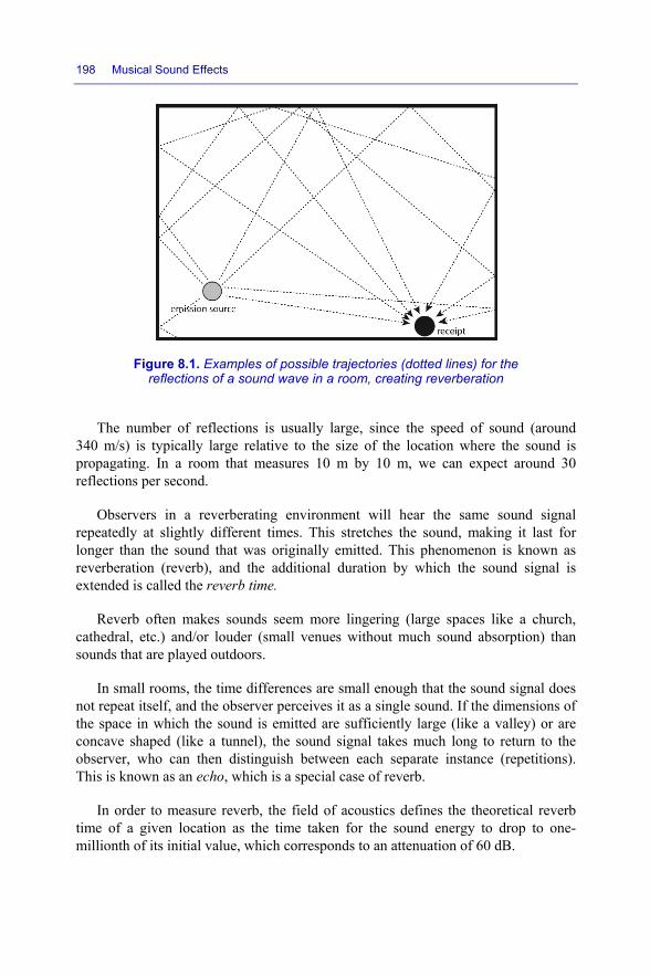
198 Musical Sound Effects
Figure 8.1. Examples of possible trajectories (dotted lines) for the reflections of a sound wave in a room, creating reverberation
The number of reflections is usually large, since the speed of sound (around 340 m/s) is typically large relative to the size of the location where the sound is propagating. In a room that measures 10 m by 10 m, we can expect around 30 reflections per second.
Observers in a reverberating environment will hear the same sound signal repeatedly at slightly different times. This stretches the sound, making it last for longer than the sound that was originally emitted. This phenomenon is known as reverberation (reverb), and the additional duration by which the sound signal is extended is called the reverb time.
Reverb often makes sounds seem more lingering (large spaces like a church, cathedral, etc.) and/or louder (small venues without much sound absorption) than sounds that are played outdoors.
In small rooms, the time differences are small enough that the sound signal does not repeat itself, and the observer perceives it as a single sound. If the dimensions of the space in which the sound is emitted are sufficiently large (like a valley) or are concave shaped (like a tunnel), the sound signal takes much long to return to the observer, who can then distinguish between each separate instance (repetitions). This is known as an echo, which is a special case of reverb.
In order to measure reverb, the field of acoustics defines the theoretical reverb time of a given location as the time taken for the sound energy to drop to one-millionth of its initial value, which corresponds to an attenuation of 60 dB.

Time Effects 199
Architects often analyze the reverb time when designing buildings. Sabine’s equation2 can be used to calculate the theoretical reverb time. = . ×
where:
– 0.163: constant in s/m;
– T: reverb time in s;
– V: volume of the room in m3;
– A: absorption surface area in m2 (sum of the product of the area of each surface Sn in m2 and its Sabine absorption coefficient αn). = × + × +⋯
Table 8.1 gives a few examples of Sabine absorption coefficients as a function of the sound wave frequency.
Material 125 Hz 250 Hz 500 Hz 1 kHz 2 kHz 5 kHz
Wood 0.09 0.11 0.1 0.08 0.08 0.1
Cement coating 0.01 0.01 0.02 0.02 0.02 0.03
Wallpaper 0.01 0.02 0.04 0.1 0.2 0.3
Carpet 0.12 0.2 0.25 0.45 0.4 0.35
4-cm-thick rock wool 0.3 0.7 0.88 0.85 0.65 0.6
Exposed plaster 0.04 0.03 0.03 0.04 0.05 0.08
Painted plaster 0.01 0.01 0.02 0.03 0.04 0.05
Exposed concrete 0.01 0.01 0.01 0.02 0.05 0.07
5 mm plywood + 5 cm air 0.47 0.34 0.3 0.11 0.08 0.08
Tiles 0.01 0.015 0.02 0.025 0.03 0.04
Ordinary glazing 0.3 0.22 0.17 0.14 0.1 0.02
Table 8.1. Sabine absorption coefficients of various materials at different frequencies
2 Wallace Clement Sabine, born in Colombus, OH, USA, 1868–1919. Acoustic engineer and Harvard graduate.
200 Musical Sound Effects
As αn tends to 1, the wall absorbs an increasing proportion of the sound energy. If no energy is reflected, the material is said to be perfectly absorbent. As αn tends to 0, the material becomes increasingly reverberant.
Sabine also showed (Sabine’s laws):
– the curves describing the build-up and decay of a sound are essentially exponential, and are complementary, meaning that the increase in sound energy over a given period is equal to the decrease over the same period;
– the effect of an absorbent material does not depend on its position;
– the release period of a sound is approximately the same at every point in the sound space;
– the reverb is independent of the position of the sound source within the space.
However, these laws need to be nuanced in some cases. For example, reverb works slightly different in the presence of obstacles, people and convex or concave walls.
8.1.2. History
Reverberation was integrated into early recordings by physically performing the recording in a sound space with natural reverb.
In the early 1920s, the first record companies actively hunted for good locations and venues for recording reverb. Their sound engineers devised various ingenuous strategies for arranging their microphones to create specific effects.
The engineer Bill Fine was one of the first to use natural reverb in sound recordings. He simply used a single microphone to capture the ambient sound of the room. His recordings were produced and published by Mercury Records on a disc in their “Living Presence” series.
The music industry later began to design and build dedicated acoustic reverb chambers. These chambers were typically closed spaces whose walls had non-parallel surfaces and shapes, coated with shellac to make them highly reflective. These shapes, often called diffusors, were designed to break up the reflections and return them chaotically. A speaker and one or several microphones were arranged around the room to record the reflections of the original sound.

Time Effects 201
Figure 8.2. One of the reverb chambers at Abbey Road Studios. You can see the cylindrical diffusors at the back of the room. The speaker that
plays the sound can be seen in the foreground (source: CBS Interactive)
Improvements in recording techniques, microphones and the invention of “high-fidelity3” after the war caused reverb to gain in popularity. Today, it has become one of the most classic effects.
Figure 8.3. Acoustics Research Society Dresden, reverb chamber with multiple diffusors (source: wikiwand)
3 Also known as “hi-fi”. This term is used to describe audio equipment that is of higher quality than conventional equipment. The goal is to achieve sound reproduction that recreates the original sound as closely as possible for audiophiles.

202 Musical Sound Effects
One of the first creative applications of reverb was proposed by Bill Putnam4, the founder of the first independent recording studio, Universal Recording, Chicago, USA, in 1947. He incorporated the natural reverb of his studio bathroom into the recording of the song “Peg O’ My Heart5” by the Harmonicats. The result was hugely successful.
Figure 8.4. “Peg O’ My Heart” by the “Harmonicats”
Over the next few years, like many other large studios, he would commission the construction of dedicated rooms of various sizes to create beautiful reverb effects. At the time, this was the only way of obtaining artificial reverb. It would continue to be widely used by recording studios during the 1960s.
REMARK.– Many reverb chambers still exist today, often for research purposes.
By changing how the recording microphone(s), the speaker and the diffusors are arranged, sound engineers can create very different reverb effects within the same chamber.
4 American sound engineer, author, publisher, producer, 1920–1989. He is viewed as the father of modern sound recording. 5 You can listen to this song on YouTube at the following address: https://youtu.be/ 9BIuX7IsdE8.

Time Effects 203
Although reverb chambers are highly effective, it was difficult to achieve long reverb times similar to those found in a cathedral, as this requires enormous spaces.
Because of technological progress, one of the first solutions to this problem was developed in 1957 by the German company EMT6 (ElektroMessTecknik). They made a truly innovative contribution by developing and marketing a plate reverberation unit, the EMT 140, developed in collaboration with the Nuremberg Technical Broadcasting Institute and the Hamburg Institute of Radio Engineering, the workplace of Walter Kuhl, the engineer who invented it.
The EMT 140 is excellent at creating reverb, and is still used today in many studios. However, it has a major disadvantage: its bulky size of 2.30 × 1.25 × 0.31 m and its weight of more than 170 kg.
Figure 8.5. The service manual of the EMT 140 (left) and several operational EMT 140 units (right) (Source: Basta Music)
In 1959, another less cumbersome solution was invented by Laurens Hammond, the inventor of the famous organ bearing his name. Since 1935, Hammond organ
6 Today, EMT is considered the oldest and most popular manufacturer of reverb solutions. They have made constant improvements to their products over the years.

204 Musical Sound Effects
owners had been eager to recreate the sound of the pipe organs found in churches and theaters. However, this had proven impossible so far, since this kind of reverb requires very particular architecture.
Hammond, like any good inventor and businessman, was interested in meeting this demand for reverb equipment. After studying the work conducted by Bell Laboratories, he discovered that they had invented a spring-based electromechanical device that was capable of simulating delays, which they were currently using for long-distance telephone calls. By modifying this device, Hammond developed a satisfactory artificial reverb system. The first version of this system was around 1.20 m in height.
Hammond’s system was then improved by the three engineers Alan Young, Herbert Canfield and Bert Meinema, who developed so-called “necklace” reverb. The name is inspired by the way that the springs in the device hang like a necklace (see Figure 8.6). It was much smaller than the original system: about 35 cm wide, 2.5 cm thick and 36 cm tall.
Figure 8.6. A reverb “necklace” placed inside the amplification cabinet of a Hammond organ
This reverb system was further improved and made smaller in the early 1960s (Figure 8.7).

Time Effects 205
Figure 8.7. The famous Hammond spring reverb, Accutronics type 4 model. This system became an industry standard
It is still widely manufactured and used today, especially inside various instrument amps by brands such as Fender, Marshall, Peavey, Ampeg and many others.
In 1976, at the AES convention in Zurich, Karl Otto Bäder, the technical director of EMT, revolutionized the reverb industry by unveiling the first ever digital reverb, the EMT 250 (Figure 8.8). This represented a huge step forwards, reinvigorating reverb with an impressive range of possibilities given the technology of the time. However, it was prohibitively expensive, costing almost $15,000. Even today, the EMT 250 arguably still fully holds its own against the latest generations of reverb hardware.
Figure 8.8. The famous EMT 250 digital reverb
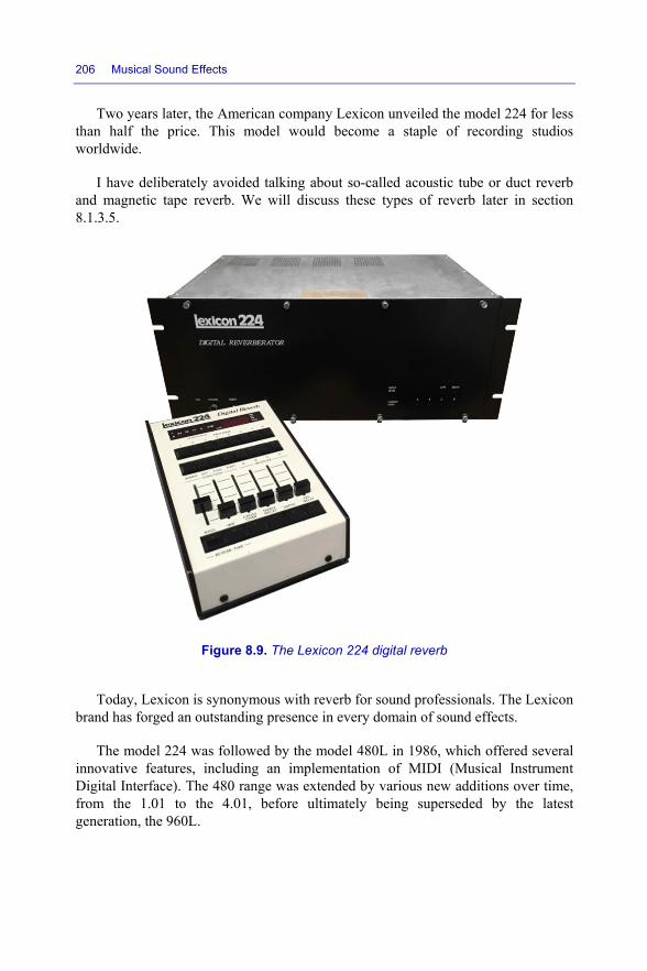
206 Musical Sound Effects
Two years later, the American company Lexicon unveiled the model 224 for less than half the price. This model would become a staple of recording studios worldwide.
I have deliberately avoided talking about so-called acoustic tube or duct reverb and magnetic tape reverb. We will discuss these types of reverb later in section 8.1.3.5.
Figure 8.9. The Lexicon 224 digital reverb
Today, Lexicon is synonymous with reverb for sound professionals. The Lexicon brand has forged an outstanding presence in every domain of sound effects.
The model 224 was followed by the model 480L in 1986, which offered several innovative features, including an implementation of MIDI (Musical Instrument Digital Interface). The 480 range was extended by various new additions over time, from the 1.01 to the 4.01, before ultimately being superseded by the latest generation, the 960L.

Time Effects 207
Figure 8.10. The 480L reverb unit by Lexicon
In 1999, Sony introduced a real-time convolution reverb processor named the DRE S777. This was another massive technical advancement that heralded another round of improvements to reverb systems.
Figure 8.11. The SONY DRE-S777 reverb effects processor
Since the early 2000s, many distributors and manufacturers have marketed reverb equipment (or reverb processors) of various calibers and price brackets: Lexicon, TC Electronic, Alesis and many more.
In parallel, software reverb began to emerge in the form of plugins. One of the earliest and the best-known plugins is the famous Altiverb (convolution reverb) developed by the Dutch company Audio Ease. It would be followed by many others.

208 Musical Sound Effects
Figure 8.12. The Altiverb reverb plugin by Audio Ease
REMARK.– Software reverb has not rendered other types of reverb obsolete.
8.1.3. Principles
In this section, we will discuss the main types of reverb technology that we encountered in section 8.1.2. We will discover how each of them works.
We will study them in the following order:
– analog plate reverb;
– analog spring reverb;
– digital reverb based on algorithms;
– digital convolution reverb;
– other types of reverb.
8.1.3.1. Analog plate reverberation
This type of reverb is based on a metal plate, usually a steel sheet (the EMT 240 model uses gold leaf and was a lot smaller than its competitor, the EMT 140, but this meant that it was extremely fragile – see Figure 8.13).
This plate (1 × 2 m sheet 0.5 mm thick in the case of the EMT 140) is stretched taut over a metal frame mounted in a wooden box to protect it from the outside environment. After amplification, a transducer in the center of the plate transmits the sound by vibrating the sheet, transforming the original signal into a mechanical

Time Effects 209
signal (wave) that travels through the plate and is partially reflected. A sensor (or two sensors for stereo) placed at one (or both) end(s) records the reverberated sound.
Figure 8.13. The EMT 240 (produced in 1972), whose plate includes a 30 × 30 cm gold sheet that is 0.018 mm thick. Its outer
dimensions are 64 × 30 × 62.5 cm, and it weighs 67 kg
Figure 8.14. Principle of plate reverberation. For a color version of this figure, see www.iste.co.uk/reveillac/soundeffects.zip
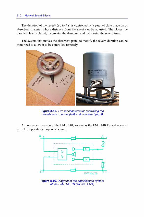
210 Musical Sound Effects
The duration of the reverb (up to 5 s) is controlled by a parallel plate made up of absorbent material whose distance from the sheet can be adjusted. The closer the parallel plate is placed, the greater the damping, and the shorter the reverb time.
The system that moves the absorbent panel to modify the reverb duration can be motorized to allow it to be controlled remotely.
Figure 8.15. Two mechanisms for controlling the reverb time: manual (left) and motorized (right)
A more recent version of the EMT 140, known as the EMT 140 TS and released in 1971, supports stereophonic sound.
Figure 8.16. Diagram of the amplification system of the EMT 140 TS (source: EMT)
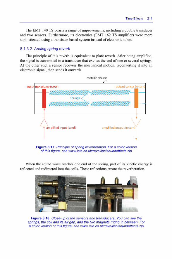
Time Effects 211
The EMT 140 TS boasts a range of improvements, including a double transducer and two sensors. Furthermore, its electronics (EMT 162 TS amplifier) were more sophisticated using a transistor-based system instead of electronic tubes.
8.1.3.2. Analog spring reverb
The principle of this reverb is equivalent to plate reverb. After being amplified, the signal is transmitted to a transducer that excites the end of one or several springs. At the other end, a sensor recovers the mechanical motion, reconverting it into an electronic signal, then sends it onwards.
Figure 8.17. Principle of spring reverberation. For a color version of this figure, see www.iste.co.uk/reveillac/soundeffects.zip
When the sound wave reaches one end of the spring, part of its kinetic energy is reflected and redirected into the coils. These reflections create the reverberation.
Figure 8.18. Close-up of the sensors and transducers. You can see the springs, the coil and its air gap, and the two magnets (right) in between. For a color version of this figure, see www.iste.co.uk/reveillac/soundeffects.zip

212 Musical Sound Effects
The springs, the transducer and the sensor are usually mounted in an open metal case fixed to the amplifier or other system.
Figure 8.19. The electronics of the “Vibraverb” amplifier by Fender. This was one of the first amps (1963) to incorporate spring reverb (bottom image)
8.1.3.3. Algorithm-based digital reverb
This type of reverb is also described as synthetic reverb. It uses algorithms to model sounds by simulating a space with specific shape, size and other properties (damping, surface type, materials, etc.).
One helpful analogy to describe the way that algorithmic reverb generates effects is to think about how synthesizers create the musical sound of instruments (flute, oboe, organ, piano, violin, etc.).
Algorithmic reverb uses delay lines based on specialized circuits dedicated to DSP (digital signal processing). These circuits apply special algorithms such as circular buffering7.
After being attenuated, the delayed signals are mixed with the original signal to achieve the desired effect. The number of delayed signals can be relatively high. The
7 The circular buffering algorithm uses dedicated DSP registers called DAGs (Data Address Generators).

Time Effects 213
first signals represent the primary reflections of the sound, the next represent reflections of reflections and so on. This creates a densification phenomenon in the sound message, which becomes more diffuse. This diffusion represents and characterizes the intrinsic nature of the reverb effect.
This explanation is very simplistic. In reality, things are much more complex, since reverb behaves differently depending on the nature of the sound signal: pulses, continuous, sequential; and its frequency: treble, mid or bass.
Effects developers and manufacturers need to balance all of these factors in order to create high-quality reverb that is as faithful as possible, depending on what their users want.
To find out more about signal processing and the complexity of audio processing algorithms, you can visit the relevant entries in the bibliography and the web links at the end of this book.
Synthetic reverb can be found in the form of hardware, such as pedals or studio processors, sometimes combined with other effects, or in the form of software plugins. It would be very difficult to list all of them. Table 8.2 gives a non-exhaustive list8 of synthetic reverb effects classified by category and manufacturer.
Type Manufacturer or publisher Name or model Remarks
Pedal
Boss RV-5 Six types of reverb – Stereo RV-6 Eight types of reverb – Stereo
Electro Harmonix
Holy Grail Three types of reverb Cathedral Eight types of reverb – Stereo
Eventide TimeFactor Multieffects – 10 types of effect (echo, reverb, delays, etc.) – Stereo
MXR M300 Six types of reverb TC Electronic
Alter Ego V2 Multieffects – 9 types of effect Arena reverb Multieffects – 10 types of effect
Rack Alesis
MicroVerb 3 Sixteen types of effect – Stereo effects (reverb, delay)
MicroVerb 4 Multieffects (reverb, delay, chorus, etc.) – 100 presets – 100 user programs
NanoVerb 2 Multieffects (reverb, delay, chorus, etc.) – 16 presets – Stereo
Eventide Reverb 2016 High-end reverb – 99 user presets – Stereo
8 For more information on the characteristics of each model of reverb, including sales price, manufacturing date, etc., and to find more models, you can visit the corresponding section of the web links at the end of the book.

214 Musical Sound Effects
Lexicon
PCM 81 High-end multieffects – 300 presets – Stereo PCM 96 High-end reverb – 300 presets – Stereo MX 200 Reverb – 99 presets – 99 user programs – Stereo MX 500 Reverb – 99 presets – 99 user programs – Stereo
MPX- 1 Multieffects – 200 presets – 50 user programs – Stereo
MPX 550 Multieffects – 240 presets – 64 user programs – Stereo
TC Electronic
M3000 High-end multieffects – 250 simple presets + 50 combined presets – 250 user presets + 50 combined presets
Mastering 6000
Very high end multichannel reverb and mastering processor
Software
Waves H-Reverb Windows: AAX; VST; VST3 OSX: AAX; AU; VST; VST3
UVI Sparkverb Windows: AAX; VST OSX: AU; AAX; VST
Lexicon MPX/PCM/LXP Windows: RTAS; VST OSX: RTAS; AU; VST
LiquidSonics Seventh Heaven Windows: VST2; VST3; AAX OSX: VST2; VST3; AAX; AU
PSP AudioWare Nexcellence Windows: RTAS; VST2; VST3; AAX
OSX: RTAS; AAX; AU; VST2; VST3
Rob Papen RP-Verb 2 Windows: VST; AAX OSX: VST; AAX; AU
Eventide UltraReverb/TVerb
Windows: AAX; VST OSX: AU; AAX; VST
Universal Audio EMT 140
Windows: RTAS; VST; AAX OSX: RTAS; AAX; AU; VST UAD-1 and UAD-2 cards
Valhalla DSP ValhallaRoom ValhallaPlate
Windows: RTAS; VST; AAX OSX: RTAS; AAX; AU; VST
Sinusweb FreeverbToo Freeware – Windows: VST; DX
Kresearch KR-Reverb FSQFreeware Windows: VST; AAX OSX: VST; AAX; AU
Rhythm Lab Mo’Verb Freeware – Windows: VST
TC Electronic
M30/ClassicVerb/DVR2 powercore
Windows: VST OSX: VST; AU
TC Electronic VSS3 Windows: VST2.4; VST3; AAX
OSX: VST2.4; VST3; AAX; AU
Table 8.2. Examples of algorithmic reverb effects by type

Time Effects 215
8.1.3.4. Digital convolution reverb
This is the most modern type of reverb. Convolution reverb works by sampling the sound of a room. The system records the reflections, then analyzes them to build an accurate model of the room that includes a description of its shape and its properties.
As an analogy, you can think of a musical sampler, which records samples of the sound created by a musical instrument in order to be able to recreate that instrument.
In the following few sections, I will give a simplified presentation of the concept of convolution in the context of sound processing. For more details, and for discussions on this subject from a deeper mathematical perspective, you can visit the bibliography and web links at the end of the book.
Convolution is a mathematical operation on two functions. These functions are often denoted x(t) and h(t). The first defines the input signal, and the second defines the impulse response (IR).
What is the IR? It is an acoustic signature that characterizes a given location. The IR is determined by recording a sound message using one of two possible methods: the free-field method, also known as the “transients” method, and the “sine sweep” method.
The first method typically records a very short signal that contains every audible frequency with no echo, such as a balloon bursting, gunfire, etc.
The second method records a “sweeping” sound, which is simply a sine wave that ranges over every frequency within a relatively short period of time (a few seconds).
Once the recording is complete, deconvolution9 is performed, which subtracts the original known signal to isolate the IR.
The function y(t) is the convolution product, i.e. the result of the convolution x(t) × h(t). This is the output signal obtained by applying the IR to the sound message, which adds reverb to it.
In summary, we calculate the sound signature of a location, and then we process any sound sequence that we like in order to endow it with the characteristics of the reverb encoded in this signature.
9 Deconvolution is not required for the signals used by the free-field method, since these signals are a very close approximation of a Dirac pulse. A Dirac pulse is a signal with zero duration and infinite amplitude. This type of source signal is used in the mathematical theory of convolutions.

216 Musical Sound Effects
Convolution reverb effects are very faithful, convincing and high quality, but are limited by the rigidity of their implementation (based on a static recording). They provide very limited options for configuring the sound rendering. However, significant progress has been made more recently, and the latest generations allow attenuation, equalization and spatialization to be configured, as well as offering a “reverse” mode.
Table 8.3 lists a few examples of convolution reverb10. They are all software based (plugins). This effect no longer exists in the form of studio processors (racks).
Publisher Name Remarks Acustica Audio Nebula HS Reverb – Windows: VST – (freeware)
Audio Ease Altiverb 6 XL – Windows: AAX; VST; RTAS – OSX: AAX; AU; MAS; VST; RTAS; TDM
Audio Ease Altiverb 7 – Windows: AAX; VST – OSX: AAX; AU; MAS; VST; RTAS
Audio Ease Altiverb 7 XL – Windows: AAX; VST; RTAS – OSX: AAX; AU; MAS; VST; RTAS; TDM
Native instrument Reflektor – Windows – OSX Thomas Resch Tconvolution – OSX (freeware): VST; AU; RTAS
VSL Vienna MIR – Windows: VST; AAX; RTAS – OSX: VST; AAX; RTAS; AU
VSL Vienna MIR Pro – Windows: VST; AAX; RTAS – OSX: VST; AAX; RTAS; AU
Waves IR360 – Windows: VST; AAX; RTAS – OSX: VST; AAX; RTAS; AU
Table 8.3. Examples of convolution reverb
8.1.3.5. Other types of reverb
As promised earlier, we will now discuss the so-called acoustic tube or duct reverb, as well as magnetic tape and magnetic plate reverb.
The latter types of reverb are actually more similar to echo chambers or delay effects, although they can sometimes also create the illusion of reverberation.
10 For more information on the characteristics of each model of reverb, including sales price, manufacturing date, etc., and to find more models, you can visit the corresponding section of the web links at the end of this book.
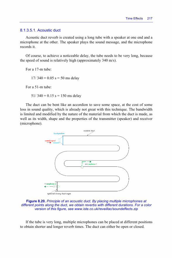
Time Effects 217
8.1.3.5.1. Acoustic duct
Acoustic duct reverb is created using a long tube with a speaker at one end and a microphone at the other. The speaker plays the sound message, and the microphone records it.
Of course, to achieve a noticeable delay, the tube needs to be very long, because the speed of sound is relatively high (approximately 340 m/s).
For a 17-m tube:
17/ 340 = 0.05 s = 50 ms delay
For a 51-m tube:
51/ 340 = 0.15 s = 150 ms delay
The duct can be bent like an accordion to save some space, at the cost of some loss in sound quality, which is already not great with this technique. The bandwidth is limited and modified by the nature of the material from which the duct is made, as well as its width, shape and the properties of the transmitter (speaker) and receiver (microphone).
Figure 8.20. Principle of an acoustic duct. By placing multiple microphones at different points along the duct, we obtain reverbs with different durations. For a color
version of this figure, see www.iste.co.uk/reveillac/soundeffects.zip
If the tube is very long, multiple microphones can be placed at different positions to obtain shorter and longer reverb times. The duct can either be open or closed.

218 Musical Sound Effects
8.1.3.5.2. Magnetic tapes or plates
This type of reverb is created using either a magnetic tape loop or a circular magnetic plate.
It works as follows:
– the audio signal input is recorded on the tape or plate by a write head placed at a certain position;
– a read head is placed after the write head in the direction of scrolling/rotation. This second head reads the signal, then simultaneously sends it to the output while also feeding it back to the write head;
– one or multiple other read heads can similarly be placed at various distances behind the first.
If the write head and the read head are positioned close together, or if the tape/plate is scrolling/rotating quickly, the repetitions will overlap, and will be indistinguishable to the naked ear.
Conversely, if the scrolling/rotation speed is slow and/or the heads are far apart, the reverb becomes an echo or a delay. We will revisit these concepts later in section 8.2.
Figure 8.21. The famous Roland echo chamber “Space Echo RE-201” manufactured between 1974 and 1990. Its looping magnetic tape system is visible in the bottom left image, and its write head and four read heads can be seen in the bottom right image

Time Effects 219
REMARK.– The part of the signal that is fed back to the write head needs to be weaker than the original signal, otherwise the system becomes saturated. One characteristic property of tape and plate systems is that the signal becomes weaker every time it is fed back through the system. This imitates physical reality, where the power of an audio signal gradually fades and the trebles are quickly absorbed as they are reflected by reflective surfaces (walls, partitions, arches, pillars, etc.).
Figure 8.22. The electronic tube echo chamber “Echorec” (1962) by Binson. You can see the plate surrounded by multiple heads, with a rubber drive wheel (in the center).
In the middle of the controls, you can see a magic green eye. This controls the volume of the audio signal
These systems were popularized by manufacturers such as Binson (Italy), Dynacord (Germany), Echoplex (USA), Fender (USA), Meazzi (Italy), Roland (Japan), Selmer TrueVoice (UK), WEM (UK) and many others, from the 1960s until today (Fulltone – USA).
8.1.4. Reverb configuration
Now that we have presented the theory, history, principles and technology of the various types of reverb that you can find on the market, we can finally begin to discuss their settings and parameters.

220 Musical Sound Effects
8.1.4.1. Main settings
The reverb time or RT60
– This is the duration for which the sound signal can still be perceived after the original signal has disappeared. Formally, it is defined as the time required for the signal to decrease by 60 dB (which explains the acronym RT60 – Reverb Time 60 dB) relative to the original signal (direct sound).
The predelay
– This is the time that elapses before the first reflections, known as the early reflections, are created in the audio signal. In physical contexts, this parameter depends on the physical dimensions of the room and any obstacles that it contains. The closer the nearest obstacle or surface, the shorter the predelay time. The higher the predelay time, the larger the size of the virtually simulated room. In a certain sense, this parameter “airs” out the signal by separating the dry sound from the wet reverb.
Figure 8.23. Three main components of reverb. For a color version of this figure, see www.iste.co.uk/reveillac/soundeffects.zip

Time Effects 221
The early reflections or initial level:
– These are the initial reflections, the responses from when the audio signal first encounters reflective obstacles. If the room or location is massive (like a valley or a tunnel), these reflections are echoes, but in most conventional venues (empty room, church, cathedral, etc.) they will be perceived as normal reverb. This parameter is directly related to the decay level of the reverb. If the first reflections are very weak, you are essentially simulating movement between the back and the center of the sound space from the perspective of the observer.
The decay (or decay time) or attenuation:
– This parameter plays a role in the secondary reflections, i.e. the reflections of reflections, creating a diffusion phenomenon among the sound waves. As the number of reflections increases, the intensity decreases until it vanishes completely as the waves are absorbed by the sound space. Decay is one of the fundamental parameters of reverb.
8.1.4.2. Specific parameters
Since audio processing is never more than an imitation of physical reality, convolution and algorithm-based reverb processors and plugins use an array of other parameters to describe the desired nature and texture of the effect more accurately.
We will see a few of these parameters in the following, but the list is far from exhaustive. Manufacturers and software publishers are constantly innovating and outdoing each other to offer ever more sophisticated, powerful, user-friendly and accurate products based on state-of-the-art scientific advancements.
The parameters presented in the following are listed in alphabetical order.
Crossover frequency
– This defines a threshold between high and low frequencies. This value of this parameter affects the other parameters.
Damping
– This characterizes the reflections in terms of the underlying materials that create them. For example, a hard surface will have a greater dynamic range and will be more favorable for high frequencies. A softer, gentler surface on the other hand will absorb these higher frequencies, creating a warmer sound. Adjusting the damping modifies the texture of the reverb, ranging from an artificial-sounding effect to a more natural one.

222 Musical Sound Effects
Figure 8.24. Example configuration of a reverb plugin, the “Renaissance Reverberator” by Waves. This plugin includes most of the parameters listed in this section: damping, predelay, time, size, diffusion, decay, early reflections, mix (wet/dry), with various curves, equalization, reverb damping and the overall shape of the reverb (in the center). For a color version of this figure, see www.iste.co.uk/ reveillac/soundeffects.zip
Density
– This parameter increases or decreases the time interval between the first group of reflections and the next group. The nature of the sound signal is critical when configuring this parameter. Typically, drier sounds (very short attack) need higher densities and vice versa. Density can be viewed as the thickness of the reverb, and as such is a relatively similar concept to the diffusion.
Diffusion
– This parameter modifies the overall effect, and plays a key role in defining the rendering of the reverb. When the diffusion is increased, the early reflections are more tightly bunched together, which increases the mass of the sound signal. This makes echoes more difficult to distinguish individually. The best setting for this parameter therefore heavily depends on the nature of the sound. For pulse signals (percussion instruments), the diffusion typically needs to be high, whereas lower tends to be better for longer, sustained signals.

Time Effects 223
Figure 8.25. Another example of reverb settings, this time the “LexRoom” by Lexicon. This plugin also includes many of the most common parameters. For
a color version of this figure, see www.iste.co.uk/reveillac/soundeffects.zip
Frequency decay (or frequency attenuation/frequency level)
– This parameter is often split into two or more distinct frequency bands (bass, mids, treble, etc.). In physically realistic sounds, higher frequencies are more strongly affected by the decay. However, there is no reason you cannot choose other configurations to create more unreal sounds. The frequency decay is proportional to the elapsed time. It play an important role in the overall sound of the effect.
Gate
– This defines a threshold for the signal level below which the reverb is inactive.
Gate decay
– This determines how long it takes for the reverb to fade once the signal passes below the threshold defined by the gate.
Mix
– This parameter determines the ratio of original signal (dry) to reverb (wet).

224 Musical Sound Effects
Figure 8.26. A third example of the configuration of a plugin. This time, “VintageVerb” by Valhalla. For a color version of this figure, see
www.iste.co.uk/reveillac/soundeffects.zip
Preset (algorithm)
– The choice of reverb algorithm defines the IR. Each algorithm typically attempts to simulate a certain class of realistic acoustics, or in some cases virtual acoustics (acoustics that do not exist in reality). In digital reverb processors, pedals and plugins, the algorithms are usually saved as presets. Table 8.4 lists the most common types of reverb algorithm.
Type Description Representation
FLAT
The amplitude curve of the early reflections is flat. This simulates a small room. In fact, this approximately recreates the results of EMT-type plate reverb (see section 8.1.3.1).
ROOM
The amplitude curve of the early reflections decreases according to a regular trend, more or less linearly. This simulates a relatively large room, like a small events hall or concert hall.
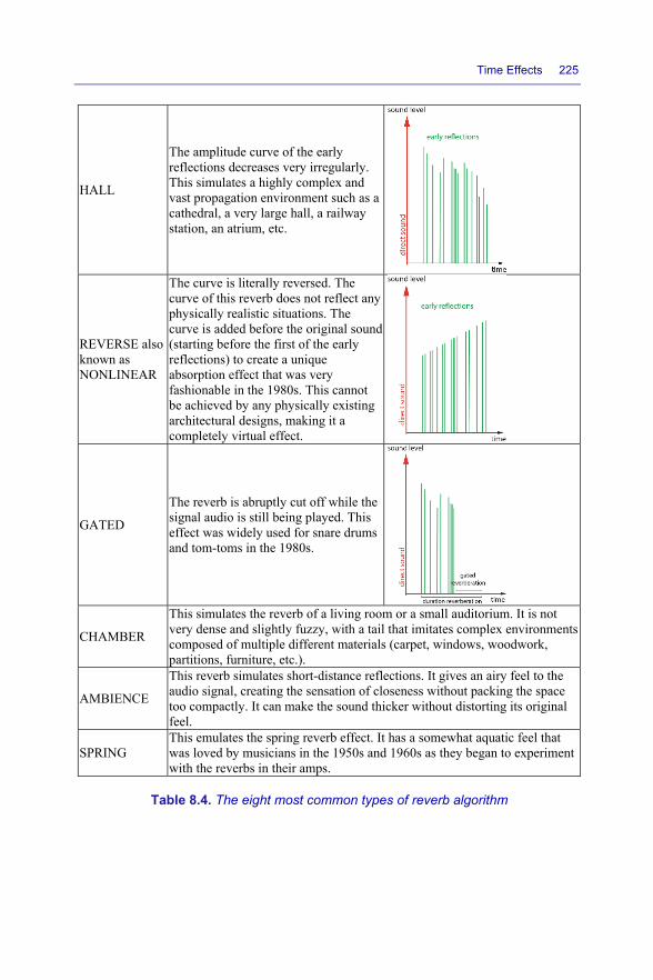
Time Effects 225
HALL
The amplitude curve of the early reflections decreases very irregularly. This simulates a highly complex and vast propagation environment such as a cathedral, a very large hall, a railway station, an atrium, etc.
REVERSE also known as NONLINEAR
The curve is literally reversed. The curve of this reverb does not reflect any physically realistic situations. The curve is added before the original sound (starting before the first of the early reflections) to create a unique absorption effect that was very fashionable in the 1980s. This cannot be achieved by any physically existing architectural designs, making it a completely virtual effect.
GATED
The reverb is abruptly cut off while the signal audio is still being played. This effect was widely used for snare drums and tom-toms in the 1980s.
CHAMBER
This simulates the reverb of a living room or a small auditorium. It is not very dense and slightly fuzzy, with a tail that imitates complex environments composed of multiple different materials (carpet, windows, woodwork, partitions, furniture, etc.).
AMBIENCE
This reverb simulates short-distance reflections. It gives an airy feel to the audio signal, creating the sensation of closeness without packing the space too compactly. It can make the sound thicker without distorting its original feel.
SPRING This emulates the spring reverb effect. It has a somewhat aquatic feel that was loved by musicians in the 1950s and 1960s as they began to experiment with the reverbs in their amps.
Table 8.4. The eight most common types of reverb algorithm

226 Musical Sound Effects
Room size (or just size)
– This adjusts the reverb time to reflect the size of the virtual room that is being simulated. In larger rooms, the sound waves travel for longer before being reflected by an obstacle (wall or partition).
Spread
– This parameter widens or reduces the stereo image of the reverb tail11. When the spread is set to minimum, the sound is distributed monophonically. At maximum spread, the sound is distributed across a very wide stereo field.
Figure 8.27. Another plugin by LEXICON, “Plate” reverb in LXP Native
Width
– This increases or decreases the width of the stereo image.
REMARK.– As noted above, convolution reverb effects tend to be less flexible, with fewer configurable parameters. You can see an example of this in Figure 8.28.
11 The reverb tail (or “diffuse reverb”) is the type of reverb obtained when there are so many reflections that they seem to blend together in time, creating a homogeneous sound with a diffuse and highly dense feel.

Time Effects 227
Figure 8.28. The “Altiverb 7 XL” plugin by Audio Ease for convolution reverb. There are few parameters, but the most common parameters are still present:
time, damping, predelay, mix, etc. For a color version of this figure, see www.iste.co.uk/reveillac/soundeffects.zip
8.1.5. Recording the IR and deconvolution
As explained in section 8.1.3.4, there are two possible methods of determining the IR.
The “transients” method is difficult to implement. It can be very delicate to record a signal like a gunshot or a balloon bursting without distortion, since these sounds are very loud and have very strong transient components. Furthermore, this process yields little information about the lower (bass) and upper (treble) frequency bands, since they are not strongly represented, which limits the width of the usable range of reverb.
The “sine sweep” method is therefore preferable. This method covers the entirety of the audible frequency spectrum. Unlike the gunshot, we do not reuse the recorded sound signal directly. Instead, we first apply deconvolution to the recorded signal to extract information about the reflections of the space from it. This recorded signal is not a single impulse, but a continuous signal that sweeps over the entire spectrum.
We should stop for a second to clarify one important point. The recording process involves various pieces of equipment, including speakers, amplifiers, preamplifiers, microphones and analog-to-digital converters. The performance of each device influences the quality of the recorded sound, and so the quality of the IR necessarily depends on every piece of equipment involved in recording it.

228 Musical Sound Effects
8.1.5.1. Configuring the sine sweep recording
First, we need one sound source for each channel. For example, if we plan to apply the reverb to mono signals, we only need one speaker. For stereo signals, we need two speakers12 and so on.
The recording can be implemented in several ways, but the simplest approach is to have one microphone for each source. This avoids the need for multiple recordings.
There are too many possible ways to position the sources and microphones for us to list them all. The ideal positioning depends on the desired results, the configuration, and location in which you are recording (size, materials, obstacles, etc.). Experience and experimentation will determine the rendering that you ultimately manage to achieve.
Here are some examples (the arrows denote the possible positions and orientations of the sources, in blue, and the microphones, in red):
– mono signal (Figure 8.29) – one speaker and one microphone;
Figure 8.29. Four example setups for recording a mono signal (there are many others): one speaker and one microphone facing each other; one speaker and one microphone facing away from each other; one speaker and one microphone facing in the same direction; one speaker and one microphone facing in the other direction. For a color version of this figure, see www.iste.co.uk/reveillac/soundeffects.zip
12 If the IR is calculated using the “transients” method, no speakers are required. Instead, you use a balloon or a starter pistol as the sound source.

Time Effects 229
– stereo signal (Figure 8.30) – two speakers and two microphones;
Figure 8.30. Four example setups for recording a stereo signal (many others are possible): two speakers and two microphones facing each other (stage – audience); two speakers and two microphones facing away from each other; two speakers and two microphones facing in the same directions; two speakers and two microphones facing in the other directions. For a color version of this figure, see www.iste.co.uk/ reveillac/soundeffects.zip
– five-channel surround sound (Figure 8.31) – five speakers and five microphones.
Figure 8.31. Two examples setups for recording five-channel surround: five speakers and five microphones facing each other and five speakers and
five microphones facing in the same directions. For a color version of this figure, see www.iste.co.uk/reveillac/soundeffects.zip

230 Musical Sound Effects
Pointing the microphones toward the speakers creates a setup that imitates an orchestra or stage musician facing an audience. This is one of the most classic recording setups. When the speakers are oriented away from the microphones, there are no direct paths between them. This means that the recording will pick up many more reflections, and so the character of the location will be much more pronounced in the recording.
You can find download free “sine sweep” files from the following websites13 for your own recordings:
– the Waves Ltd website (www.waves.com) under “Downloads” – “Free downloads”: “IR convolution reverb sweep file for self-capture”;
– the Audiocheck website (www.audiocheck.net), under “Test tones”: “Full sine sweep”;
– the Freesound website (www.freesound.org), under “Sounds”: “Utility sounds: Sine Sweep 20 Hz to 20 kHz 10 seconds.wav”;
– and many others that are easy to find with a search engine.
8.1.5.2. Processing the IR
Once you have completed the sine sweep recording, you will need a software program to perform deconvolution.
Figure 8.32. The waveforms are two impulse response files from a stereo recording. The top and bottom are the left and right channels, respectively.
For a color version of this figure, see www.iste.co.uk/reveillac/soundeffects.zip
13 These websites were live at the time of writing.

Time Effects 231
For example, the following programs can do this:
– CATT GratisVolver – Microsoft Windows – freeware;
– Voxengo Deconvolver – Microsoft Windows – shareware;
– Christian Deconvolver – Microsoft Windows – freeware;
– Waves IR-1 – OS-X and Microsoft Windows;
– Audio Ease Altiverb – OS-X and Microsoft Windows.
8.1.5.3. Example of deconvolution with Waves IR-1
For our first demonstration of processing an audio file with the IR, we will use the multitrack audio editor Adobe Audition CC with the IR-1 plugin by Waves:
– after starting up Adobe Audition, open the file to which you want to add reverb;
Figure 8.33. Stereo audio file opened with Adobe Audition CC ready to add reverb. For a color version of this figure, see www.iste.co.uk/reveillac/soundeffects.zip
– now, start up the Waves IR-1 plugin, and select the type of audio file (mono, stereo, live, etc.). This will open a settings window (Figure 8.34);
– in the example shown in the figures, the file is stereo, which means that two IR files are required, one for each of the left and right channels;
– next, create a new subfolder under “IR1Impulses V2” in the root folder “Waves”, and copy your two IR files into it;

232 Musical Sound Effects
Figure 8.34. IR-1 plugin window (in this example, the type is mono/stereo). For a color version of this figure, see www.iste.co.uk/reveillac/soundeffects.zip
– click the LOAD button in the top right and select IMPORT SWEEP RESPONSE FROM FILE;
– a prompt will allow you to select the two sine sweep recording files;
Figure 8.35. The prompt for selecting the sine sweep recordings. In the example, you can see the two files “SSL.wav” and “SSR.wav” in the
newly created “IR Sine Sweep” folder. For a color version of this figure, see www.iste.co.uk/reveillac/soundeffects.zip
– after a brief deconvolution calculation period, a new curve will appear in the center of the window of the IR-1, showing the IR of your reverb;
– you can now save your IR by clicking the SAVE button and selecting SAVE TO NEW FILE;

Time Effects 233
– enter a filename, and click SAVE (Figure 8.36);
Figure 8.36. Saving the file (.xps) containing the preset for your new reverb effect (in this example, the file has been given the name “My Office IR.xps”).
For a color version of this figure, see www.iste.co.uk/reveillac/soundeffects.zip
– another dialog box will open, this time asking you to choose a name for the preset. The name you choose will be added to the list of options in IR-1. After clicking OK, your new preset will now be available at any time.
Figure 8.37. Saving the new preset, here “Office reverb”. For a color version of this figure, see www.iste.co.uk/reveillac/soundeffects.zip
REMARK.– You might notice that a .wir file has been created in the folder containing your IRs. This is the deconvolution file generated by Waves IR-1.
If you restart IR-1, you will see your new preset as an option in the LOAD list.

234 Musical Sound Effects
Figure 8.38. The new preset “Office reverb” in the folder “IR Sine Sweep” that was created in an earlier step. For a color
version of this figure, see www.iste.co.uk/reveillac/soundeffects.zip
8.1.5.4. All-in-one with Apple Logic Pro X
The software program Apple Logic Pro X includes an “Impulse Response Utility”. This application offers multitrack audio recording, deconvolution and can generate the IR using the reverb module “Space designer”:
– start up Logic Pro X, create an EMPTY PROJECT, then choose to record an audio signal (Figure 8.39);
REMARK.– Choose the most appropriate digital audio input/output interface (M-Audio, MOTU, PreSonus, Apogee, FocusRite, etc.) that is available to you.
Figure 8.39. Creating an audio project in Logic Pro X

Time Effects 235
– display the mixing desk: press the X key or click VIEW then SHOW MIXER in the menu, or alternatively press the sixth icon from the left in the top ribbon;
– click AUDIO FX for input 1 on the mixing desk, select REVERB, SPACE DESIGNER, then MONO/STEREO;
– a dialog box will open for the convolution reverb plugin “Space designer”. Scroll down the IR SAMPLE list and select OPEN IR UTILITY (Figure 8.40);
Figure 8.40. Opening the “Impulse Response Utility”
– this opens the “Impulse Response Utility”;
– configure the number of tracks that you wish to record: mono, stereo, true stereo, pro-logic, etc., then click OK;
– now you can generate and record the audio signal of the sine sweep, which yields the IR;
Figure 8.41. The Impulse Response Utility

236 Musical Sound Effects
REMARK.– The top toolbar of the utility allows you to configure the audio input and output devices. The sampling frequency displayed to the right of the audio output is for information only. You cannot configure it here, as it is determined by the choice of digital audio interface.
– connect the microphone(s) to your digital audio interface, one for mono or several for stereo or higher, and hook up a sound reproduction system to the outputs;
– arrange the equipment (microphones and speakers) around the room to capture the IR;
– in the SWEEP section, choose the CHANNEL, and select a TEST TONE of 1 kHz. Check the ON checkbox and adjust the LEVEL between –60 and 0 dB until the intensity is at the right level (no saturation on the level monitors, below the red region);
– check the intensity at other frequencies (100 Hz, 5 kHz, 10 kHz), adjusting the level if necessary;
– repeat for each channel;
Figure 8.42. Testing the level (–12.9 dB) at a frequency of 10 kHz on channel 1. The level monitors (green and yellow) of both channels are shown. For a color version of this figure, see www.iste.co.uk/reveillac/soundeffects.zip
– uncheck the ON checkbox to end the test tone;
– click the R icon in the RECORD column of each channel. The background of the letter R will turn red;
– click the SWEEP button and wait for 10 s14. The sound signal will play, and you will see the waveform being plotted in the top window;
REMARK.– Make sure to turn off the monitor output to prevent feedback during recording. To do this, click MUTE.
14 Silence is of course required for this step, otherwise you risk distorting the recorded signal.

Time Effects 237
– after sound playback is complete, a dialog box will open, asking you to choose a filename for the IR. Note that the channels are automatically locked (green padlock in the LOCK column) in the table if you take additional recordings in order to keep the same settings for the sine sweep generator.
Figure 8.43. The waveform of the recorded sine sweep and the dialog box for saving it. Track 1 is locked in the table. For a color version of this figure, see
www.iste.co.uk/reveillac/soundeffects.zip
– click on DECONVOLVE to begin deconvolution, which calculates the IR of your new reverb.
Figure 8.44. The impulse response (IR) obtained by deconvolution

238 Musical Sound Effects
To check whether your IR is good enough, you can use the listening tool, which allows you to apply convolution to test files and listen to the results.
– click on AUDITION IR to open the testing window;
– click on one of the four buttons SNARE, WOODBLOCK, MALE SHOUT or FEMALE SHOUT to test the rendering of your reverb;
– the MIX slider adjusts the balance between the test sound (source) and the sound after applying reverb. This equivalent to the “dry/wet” setting commonly found with reverb effects;
– the MONITOR slider adjusts the playback volume;
Figure 8.45. Audio test window
– to exit the audio test window, click DONE.
You can load one to five custom audio files by clicking the OPEN buttons. You can then listen to them by pressing PLAY.
You can save your IR by generating a .sdir file and a .pst file:
– click on CREATE SETTING..., choose a name for your file, then click OK;

Time Effects 239
– a dialog box will confirm that you have created the two files, and will display the path to their locations;
Figure 8.46. Saving the IR, here with filename “MySWP”
– click OK to confirm.
REMARK.– The “Impulse Response Utility” has various features that we have not discussed here, including IR editing, B-format surround encoding, the method of “transients” (using a “gunshot” instead of deconvolution), etc.
You can exit the “Impulse Response Utility” application by closing the window, clicking the IMPULSE RESPONSE UTILITY menu, then selecting QUIT IMPULSE RESPONSE UTILITY, or by pressing the keyboard shortcut CMD Q. A dialog box will ask whether you wish to save your project:
– click DON’T SAVE or SAVE accordingly.
Exiting the “Impulse Response Utility” returns you to the “Space designer” effects plugin. To use the newly generated reverb, we need to load the IR file:
– scroll down the IR SAMPLE list and select LOAD IR;
– in the dialog box that opens, select your .SDIR file, then click OPEN;
– your IR will be displayed, and you can now use it however you wish by configuring it and applying it to one or multiple audio tracks in Logic Pro X.

240 Musical Sound Effects
Figure 8.47. Our newly created reverb, given the name “MySWP” in this example, viewed in “Space designer” within Apple Logic Pro X
8.1.6. Studio mixing and reverb
Managing reverb when mixing a recording is a complicated task that requires precision, experience and finesse. The primary objective is to give each instrument its own position within the sound space.
In the following, we give a few guidelines that should help you to understand the basic ideas of reverb management.
First, we shall consider the effect of the predelay parameter, which allows the position of an instrument to be defined.
There is a simple rule for this:
– shorter predelay times (between 10 and 20 ms) make the instrument seem further away from the observer. This places the instrument at the back of the mix;
– longer predelay times (>20 ms) make the instrument seem closer to the observer. This places the instrument at the front of the mix.
Do not set the predelay too high. If you do, it turns into a delay, which creates a noticeable duplicate signal, especially for very short sounds (percussions). The predelay is expressed in milliseconds.

Time Effects 241
Another important parameter is the diffusion. In simplified terms, the diffusion controls the mass of the reverb. At its lowest setting, there are few reflections. This creates the impression that the sound signal is being played in a highly absorbent room. Choosing the highest setting creates the impression of an extremely reflective room. The diffusion is often expressed as a value between 0 and 100.
The damping also gives the reverb a very particular color. Note that this setting is not available on every model of reverb. The damping allows you to configure the reverb time on one or multiple frequency bands.
Figure 8.48. The “TrueVerb” plugin by Waves. The bottom graph shows the frequency response curve of the damping. In this example, the damping is configured to increase the reverb time by 1.40× (140%) at 400 Hz (bass frequencies) and reduce the reverb time by 0.42× (42%) at 6,800 Hz (treble frequencies). For a color version of this figure, see www.iste.co.uk/reveillac/soundeffects.zip
The size (or room size) is a very subjective parameter. The person managing the mix needs to rely on their own judgment to create the right atmosphere, depending on whether they want a large sound space or a narrower one.

242 Musical Sound Effects
In mixes that already have reverb on one or more tracks, you will need to implement any additional reverb as a postfader effect on the corresponding auxiliary track.
Finally, Table 8.5 gives a few examples of reverb configurations, drawing from my own personal preferences and experience (sound recordings taken in my studio: rectangular surface area: 40 m2 – height: 2.90 m – floor: wood + carpet – walls: concrete + acoustic panels – ceiling: acoustic tiles).
Remember that the primary purpose of reverb is to define regions within the sound space and improve the presence and color of the sound source. Use it sparingly – too much reverb degrades the clarity and precision of the mix.
Be careful when adding reverb to sounds that already have reverb. It can be done, but you need to dose it carefully, or you might create resonance, phase variations, saturation and many other undesirable side effects.
Source Style Type Predelay (ms) Diffusion
Electric guitar Solo rock Hall 60–80 max
Rhythmic rock Room 40–60 max
Bass guitar rock Room 30–40 max
Electric guitar Solo blues Flat 60–70 max
Rhythmic blues Flat 40–60 max
Bass guitar blues Room 25–35 max
Acoustic guitar Solo blues Flat 40–50 max
Drums Snare Room 0–10 max
Bass drum Ambiance 0–10 3/4-max
Cymbal Chamber 0–10 3/4-max
Tom-toms Room 0–10 max
Vocals Rock Flat-hall 30–50 1/2
Blues Flat-chamber 20–40 max
Table 8.5. Example configurations for a selection of sources and styles
It is advisable to use as little reverb as possible when recording, to the extent that your recording location allows you to. It is much easier to add reverb later than remove it.

Time Effects 243
8.2. Delay
In section 8.1.3.5.2, we talked about echo chambers based on tapes or plates. These echo chambers are sometimes used for reverb by using high scrolling speeds and positioning the write and read head(s) very closely together. But these chambers are in fact perfect for creating delays; it is what they do best.
Delay recreates the everyday phenomenon of echoes. An echo is when a sound repeats several times, fading over time. If you could write an echo in words, it might look something like this:
– you shout ECHO…
– …and a few tenths of a second later, your surroundings answer you back:
– ECHO... ECHO... ECHO... echo... ech... ec...
This repetition is caused by the sound returning to you after being reflected somewhere far away. The sound is quieter when it comes back because part of its energy was absorbed when it collided with the reflecting material. Once the reflected sound reaches you, the process starts all over again. The sound is reflected back and forth several times until the volume fades completely.
The difference between reverb and an echo or delay is that you can distinguish each repetition with echoes. With reverb, the repetitions merge together and are indistinguishable.
REMARK.– There is a technical distinction between a delay and an echo. A delay can have infinitely many repetitions, whereas an echo cannot. However, in everyday language, the terms “echo” and “delay” are often used interchangeably.
8.2.1. History
The first echo effect to be used in a recording is often misattributed to Sam Phillips, the CEO of Sun Records. In fact, Les Paul and Mary Ford had used echoes before that in 1951 for their track “How High The Moon”.
In 1954, Sam Phillips used two tape recorders (Ampex 350), modifying one of them to allow that the write and read heads to be activated simultaneously. Doing this led him to invent a form of tape delay known as “slapback”.

244 Musical Sound Effects
Slapback delay works as follows:
– the write head of the first tape recorder records the local signal picked up by the microphone;
– a read head is placed slightly behind the write head on the tape. The read head plays the newly recorded signal with a slight offset (a few centimeters). This creates a delay or echo (the delay time depends on the scrolling speed of the tape – at the time, the speed was most likely 7.5 inches per second, or around 19 cm/s);
Figure 8.49. The famous Ampex 350 recorder
– the mixing desk sends these two signals (the original signal from the microphone and the delayed signal from the first tape recorder) to the second tape recorder, which records them together. Of course, this delay effect was only capable of creating a single repetition.
Over the course of the 1970s, many musicians began to experiment with tape delays. Some of their solutions used highly unusual techniques (Frank Zappa, Pink Floyd, Robert Fripp, etc.).
8.2.2. Types of delay
There are four broad categories of delay:
– tape or plate delay;
– analog delay;

Time Effects 245
– digital delay;
– software delay (plugins).
We talked about tape and plate delays earlier.
The next category, analog delays, was invented in the 1970s because of the progress that had been made in musical electronics. The delay time of these effects was limited, usually 500 ms at most.
Some configurable settings were already available, e.g. the mix, which defines the ratio of direct and processed sound (wet/dry), and the feedback, which specifies the number of repetitions.
One major problem with these delay effects is that they introduce a certain color in the sound, often combined with slight distortion.
They are often integrated into effects pedals.
Figure 8.50. The famous “Memory Man” pedal by Electro Harmonix, one of the first ever analog delay pedals (delay time: max 300 ms)
The first digital delays began to appear in the early 1980s. Many of them are still available today from various manufacturers. They offer great sound quality and dynamics in the form of effects pedals or studio racks. They have much more sophisticated settings, with delay times ranging up to several seconds.

246 Musical Sound Effects
Figure 8.51. The digital delay DM1000 by Ibanez, released in the early 1980s. It has a maximum delay of 900 ms
These settings can include:
– a sample or hold function, which saves repetitions in memory;
– a filter to attenuate specific frequency bands;
– a low-frequency oscillator (LFO) with configurable depth and modulation speed to modulate the repetitions;
– a “tap” or “tap-tempo” function to specify the time between repetitions (allowing the delay to be synchronized with the beat) via a tap button;
– and many more.
Figure 8.52. A modern digital delay pedal, the DD-500 by Boss. This pedal has a very wide range of possibilities. It can even emulate digital delays from the 1980s
Today, digital delay effects have become extremely sophisticated, with delay times of up to 10 s. They often have integrated looping features, and can store patches with factory or user presets. Some include USB and/or MIDI ports in addition to the usual audio inputs/outputs.

Time Effects 247
Most multieffects racks available on the market include some form of delay, with varying degrees of sophistication.
Table 8.6 lists some widely used examples of analog and digital delays. The list is far from exhaustive, as the range of available models is simply too vast. Delays can be divided into two broad categories: studio delays in the form of racks15 and delays in the form of pedals designed for musicians, most notably for guitarists.
Category Manufacturer Model Year Main features
Rack
Ibanez DM1000 1983 Digital – Delay time: 1.75–900 ms Ibanez DM2000 1983 Digital – Delay time: 0–1,023 ms Korg SDD3000 1982 Digital – Delay time: 0–1,023 ms Lexicon PCM-42 1981-82 Digital – Delay time: 400–4,800 ms
Lexicon MPX-1 1990s Digital multieffects – Delay time: 0–2,000 ms
Lexicon MPX-550 2003 Digital multieffects – Delay time: 0–5.5 ms for mono, or 2.7 ms for stereo
Lexicon PCM-92 2009 Digital – Reverb + delay + modulation effects
Lexicon Prime Time II 1979-80 Reissued in 1995
Digital – integrated LFO – Delay time: 1.92 s max.–7.68 s max. with additional memory
Mu-tron 1173 1980s Digital – Delay time: 2.5–160 ms
Roland SDE-3000 1983 Digital
Pedal
Boss DM-1 1978 Analog – Delay time: 500 ms max.
Boss DM-2
1981 Analog – Delay time: 20–300 ms
Boss DSD-2 1985 Digital – Includes a sampler function
Boss DD-3 1983 Digital – Delay time: 20–300 ms
Boss RV-2 1987 Digital – Includes a panning function (“ping-pong”)
Boss RV-3 1994 Digital – Delay time: 2 ms max.
Boss DD-6 2002 Digital – Delay time: 5.2 ms max. Boss DD-7 2008 Digital – Delay time: 6.4 s max.
Boss DD-500 2015 Digital – Various highly advanced functions
Electro Deluxe 2010 Analog – Delay time: 30–550 ms –
15 This list does not include tape or plate delays, which are presented in section 8.1.3.5.2.

248 Musical Sound Effects
Harmonix Memory Boy Includes a tap function
Electro Harmonix Memory Man
1976-1978 – Multiple reissues in 1990 and after
Analog – Includes chorus and vibrato – Very colorful sound
Electro Harmonix
Memory Man XO 2009 Analog – Delay time: 700 ms max. –
Includes chorus and vibrato Electro Harmonix
Memory Man with Hazarai 2008 Analog – Delay time: 3 s max. –
Loop, reverse, multitap functions Ibanez AD9 1982 Analog – Delay time: 20–300 ms
Korg SDD3000 pedal 2014 Digital – Emulates the analog
SDD3000 and many others
Moog MF-104 2000 Analog – Delay time: 40–800 ms – Integrated LFO
MXR M169 Carbon copy 2008 Analog – Delay time: 20–600 ms
TC Electronic Flashback 2014 Digital – Delay time: 20–7,000 ms – Many features
Vox Time machine 2008 Digital emulation of analog delay – Delay time: 0–1 s
Table 8.6. Examples of delay racks and pedals
Next, let us talk about plugins. Just like reverb, there are countless software-based delay effects. Many of them are virtual recreations of hardware delays available on the market.
Figure 8.53. The plugins PSP 42 and PSP 84 by AudioWare, inspired by the famous PCM 42 delay by Lexicon
There are many things that you can do with these plugins. Most of them offer plenty of settings for configuring the standard delay parameters. For example:
– a panning (or “ping-pong”) effect;
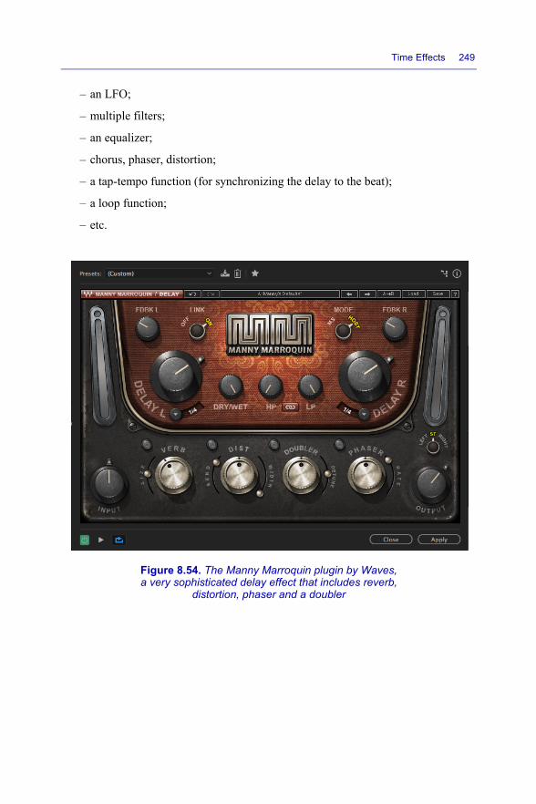
Time Effects 249
– an LFO;
– multiple filters;
– an equalizer;
– chorus, phaser, distortion;
– a tap-tempo function (for synchronizing the delay to the beat);
– a loop function;
– etc.
Figure 8.54. The Manny Marroquin plugin by Waves, a very sophisticated delay effect that includes reverb,
distortion, phaser and a doubler

250 Musical Sound Effects
Table 8.7 lists a few examples of popular delay plugins.
Publisher Name Operating system and format
Arne Scheffler Multi Delay OSX: VST (freeware)
Audio Damage DubStation Windows: VST OSX: AU/VST
AudioWare PSP 85 Windows: VST; RTAS; AAX OSX: VST; RTAS; AAX; AU
Avid Line6 Echo Farm Windows – OSX: TDM
Big Tick Hexaline Windows: VST (freeware)
D16 Sigmund Windows: VST; AAX OSX: VST; AAX; AU
FabFilter Timeless 2 Windows – OSX: VST 2/3
Kjaerhus Audio Classic Delay Windows: VST (freeware)
MaxProject T.Rex Delay Windows: VST (freeware)
Ohm Force OhmBoyz Windows: VST; VST3; RTAS; AAX OSX: VST; RTAS; AAX
Rob Papen RP Delay Windows: VST; AAX OSX: VST; AAX; AU
Smartelectronix Analog Delay Windows: VST (freeware) OSX: VST (freeware)
SoundToys EchoBoy Windows: VST; AAX OSX: VST; AAX; AU
Universal Audio Roland RE-201 Space Echo
Windows: RTAS; VST; AAX OSX: RTAS; VST; AAX; UA
Waves H-Delay Windows: VST; VST3; AAX; RTAS OSX: VST; VST3; AAX; RTAS; AU
Waves Manny Marroquin Windows: VST; VST3; AAX; RTAS OSX: VST; VST3; AAX; RTAS; AU
Waves SuperTap Windows: VST; VST3; AAX; RTAS OSX: VST; VST3; AAX; RTAS; AU
Table 8.7. Examples of delay plugins

Time Effects 251
8.2.3. Tips for using delays in the studio
8.2.3.1. Slapback
We mentioned this effect earlier in section 8.2.1. To generate slapback delay, select a delay time between 50 and 120 ms, and set the feedback to zero so that there is one single repetition very close to the source signal.
Additionally, we need to reduce the signal bandwidth acted upon by the effect, otherwise the repeated signal will sound exactly like the original, creating an extremely unpleasant duplication effect.
To restrict the bandwidth, equalize the top and bottom of the spectrum by setting up appropriate filters.
Slapback delay is usually reserved for electric guitars and vocals. It endows them with a vintage quality.
8.2.3.2. Doubling
Doubling is a way of making the sound feel bigger.
Choose a very short delay time between 5 and 50 ms, set the feedback to 0 and adjust the dry/wet mix until you can only just hear the effect.
Above this limit, increasing the presence of the effect (making it wetter) will make the sound seem less natural. Conversely, decreasing the presence (making it drier) will make your sound seem more natural and occupy more space.
Beware of unpleasant filtering effects in the mix if you set the delay time too low.
Similar to slapback delay, you will typically need to equalize the delayed portion of the signal.
To make your sound seem even bigger, you can use stereo delay with slightly different delay times on each channel, or even apply a slight modulation.
Doubling is especially convincing with analog delays, as this trick was originally designed for analog systems.

252 Musical Sound Effects
8.2.3.3. Pan-delay
Also known as “ping-pong delay”. With this delay, the reverb swings back and forth between left and right. If the delay time is very short, less than 70 ms, the effect becomes diffuse, creating a reverberating space.
Setting the delay time higher, above 120 ms, gives an artificial quality to the sound.
Figure 8.55. The H-Delay plugin by Waves with filters, LFO, and a ping-pong delay function (top center)
Pan-delay is included in many modern pedals and plugins.
8.2.3.4. Delay and tempo
If you synchronize the delay time with the tempo of the sound, you can add depth to the mix without the delay itself being noticeable. Many sound engineers use this method to stylize their sound environments, endowing them with a very natural ambient reverb that smoothly blends into the overall structure of the recording in the final mix.
Most reverbs have tap-tempo features. If your reverb does not include this feature, there are also dedicated apps (including ones that you can run on your

Time Effects 253
smartphone) to find the right delay time for a given musical passage. Here is a list of examples16:
– Tap/Tempo by Benjamin Jaeger for iOS;
– BPM Tap Tempo by Audiolog for iOS (free);
– BPM Tap by Erik Byström for Android (free);
– Tap Tempo for Windows (free);
– Delay Genie by Bobby Owinski for iOS (free);
– Tap BPM by DrumBot for Windows and OSX (free);
– Tap Tempo and Metronome for Android (free).
8.2.3.5. Delay/echo with an analog multitrack tape recorder
This section will explain how to use a multitrack tape recorder to create a delay or echo effect.
Why use such outdated equipment today? I know for a fact that many audio enthusiasts and recording professionals still have tape recorders stashed away somewhere in a closet or a corner. This will give you the opportunity to dust them off and use them to create a vintage warmth and color that is currently very trendy.
You will need a multitrack tape recorder (2, 4, 8, 16 or more tracks) with separate read and write heads, e.g. a Revox A77 or B77.
Figure 8.56. The stereo Revox A77 MkIV recorder, manufactured from 1974 to 1977
16 These apps are still available at the time of writing. You may need to check if they are still accessible.

254 Musical Sound Effects
The idea is as follows. During recording, the signal is picked up by the read head and sent to the write head, which re-records the signal, delayed by a time interval determined by the distance traveled by the tape between the two heads.
This time interval and hence the delay time depend on the speed of the tape. For example, for a Revox A77:
– 1 ⅞ inch/s (4.75 cm/s): 700 ms;
– 3 ¾ inch/s (9.5 cm/s): 350 ms;
– 7 ½ inch/s (19 cm/s): 175 ms;
– 15 inch/s (38 cm/s): 87 ms.
Some models of recorder have a speed regulator. If yours does, you can use it to vary the delay/echo linearly over a certain range of speeds.
Figure 8.57. A speed regulator made by Revox for the B77 model recorder
In the following, we will describe the procedure for a Revox A77 or B77. They can easily be adapted to other models of equipment;
– connect the source to input II (mic input on the front or aux on the back);
– select this source by switching the channel dial II to MIC LO, MIC HI or AUX;
– the LEVEL II dial controls the level of the recorded sound signal. This should be set as high as possible, but saturation and excessive modulation should be avoided, as they will combine with the delayed signal;
– turn the dial for input I to I > II in order to send track I to track II;
– press REC CHI to confirm the recording channel, leaving REC CHII pushed out;

Time Effects 255
Figure 8.58. The various controls of the Revox A77. From left to right on the bottom row: volume and mono/stereo dial, balance and MONITOR dial, recording track 1 and the dial for selecting its source, and recording track 2 with the dial for selecting its source. In the top right, you can also see the REC CHI and REC CHII recording buttons on either side of the two VU level meters.
– the intensity of the delay effect is controlled by the LEVEL I dial. By turning this dial, you can pass from a short and weak delay to a long and powerful delay, and internal feedback;
– set the MONITOR switch to NAB and the mono/stereo dial to channel I;
– to begin recording, you can now simply press PLAY and REC together.
REMARK.– If you decide to record from channel I, you need to choose the opposite settings for the input dial (II > I). In this case, the source is controlled by the LEVEL I button, and the delay is controlled by the LEVEL II button. You also need to reverse the states of the recording buttons, and the dial specifying the mode needs to be set to II.
8.3. Conclusion
Reverb plays an extremely important role in sound, and our relationship with it is rather special. We constantly encounter reverb in every sound space of our everyday lives. Our brains analyze the tiniest of details contained in this reverb in order to deduce information about our surroundings.
Artificial reverb can help us build sounds that are more relevant, more catchy, warmer and easier to understand, but can also render sounds incoherent, artificial or inaudible.
Learning to master reverb is a difficult and complex process. There are many settings to manage, and it is crucial to dose every one of them accurately. The entire structure of a recording mix relies on the foundation provided by its reverb. Reverb is a fundamental component and significantly affects the final rendering.

256 Musical Sound Effects
We encounter delays and echoes less frequently in reality, which may explain why they are so very delicate to manipulate.
You will need to rely on your own personal judgment and ear to decide whether a given delay or reverb sounds good or bad. Determining precisely the right amount of reverb and delay will add presence to your sound and make it feel natural, as if you are standing in the room, the audience, at the concert, or even directly among the musicians on stage, depending on the rendering that you are trying to achieve.
Listen closely, close your eyes and imagine the scene. Your brain needs to be able to retrace the balance of the sound and the path that it takes. The path must be clear and easy to understand. This clarity is key in determining the flavor, character and charm of your mix.
9
Unclassifiables
This chapter attempts to group together the effects that do not fit into any of the six other categories, for example, because they act upon more than one of the fundamental characteristics of the audio signal: frequency, modulation, amplitude, dynamics, phase, tempo, etc.
This chapter also discusses specialized processing techniques used for tasks such as audio restoration, synchronization, sample editing and other activities that you might encounter while managing sound effects.
9.1. Combined effects
In this section, we will discuss three combined effects, i.e. effects obtained by combining several different techniques from the previous chapters. These three combined effects are called fuzzwha, octafuzz and shimmer.
As discussed before, we will begin by presenting the theoretical principles on which these effects are based, and then we will list a few hardware and software models.
9.1.1. Fuzzwha
This effect is a combination of wah-wah (see section 4.3) and fuzz (see section 7.6.1). It was very popular in music from the 1970s.
Most fuzzwha pedals allow you to select just wah-wah or just fuzz, but can of course also mix both effects. Fuzzwha is very rich in harmonics, with a somewhat distorted sound.
Musical Sound Effects: Analog and Digital Sound Processing, First Edition. Jean-Michel Réveillac.© ISTE Ltd 2018. Published by ISTE Ltd and John Wiley & Sons, Inc.

258 Musical Sound Effects
Below are a few examples of fuzzwha pedals. There are many others as follows:
– Fender: “Fuzz-Wah Pedal Reissue” model;
– Colorsound: “Wah-Fuzz” model (vintage);
– Aria Diamond: “Wah-Fuzz” model (vintage);
– Morley: “Power Wah Fuzz” model (vintage);
– Boss: “PW-10” model;
– Mooer: “FuWah” model;
– Morley: “M2 Cliff Burton Fuzz Wah” model;
– Electro Harmonix: “Cock Fight” model;
– Vox: “Stereo Fuzz-Wah Model 9-3700” model.
Figure 9.1. Three fuzzwha pedals: (from left to right) “Fuzzwha” by Colorsound, “M2 Cliff Burton” by Morley and “FuWah” by Mooer
9.1.2. Octafuzz
Also known as “Octavia”, this is a fuzz pedal (see section 7.6.1) that also adds an extra harmonic one octave higher or lower (see section 6.2.1).
There are only a few models of this pedal. Examples include:
– MXR: “SF01 Slash Octave Fuzz” model;
– Catalinbread: “Octapussy” model;
– Fulltone: “Octafuzz” model;

Unclassifiables 259
– NIG Music: “Octa Fuzz POC” model;
– Joyo: “JF-12 Voodoo Octave” model;
– Fulltone: “Ultimate Octave” model;
– Home Brew Electronics: “UFO (Ultimate Fuzz Octave)” model.
Figure 9.2. Three octafuzz pedals (from left to right): “Octafuzz” by Fulltone, “Octapussy” by Catalinbread and “SF01 Slash Octave Fuzz” by MXR
9.1.3. Shimmer
This effect combines reverb (see Chapter 8) with an octaver (see section 6.2.4) to create a sound similar to synth pads.
It is very difficult to describe this effect in words. Its sound varies wildly from instrument to instrument and depending on musical technique (see the web links at the end of the book). The word “shimmer” comes fairly close to capturing its essence.
This effect is not usually created with a single device. Many guitarists create shimmer by coupling together multiple effects pedals or in some cases by combining effects pedals and software programs such as “IK Multimedia Amplitube” and “Native Instruments Guitar Rig”. Some multieffects audio racks include shimmer directly as a preset.
9.1.3.1. Creating shimmer
Here are a few examples of combinations that you can use to construct the famous shimmer effect:

260 Musical Sound Effects
– Solution 1: Delay pedal (Boss DD7, MXR M169 Carbon Copy, Boss DD20, Electro Harmonix Canyon, etc.) coupled to a pitch shifter with a second delay effect added using AmpliTube (solution first proposed by Guitar Douche).
Figure 9.3. First solution for creating shimmer. For a color version of this figure, see www.iste.co.uk/reveillac/soundeffects.zip
– Solution 2: This solution was developed by Bill Rupert. It uses multiple Electro Harmonix pedals coupled together. The final sound rendering is unbelievable.
Figure 9.4. The famous “Crystal Shimmer” by Bill Ruppert, using only pedals manufactured by Electro Harmonix. For a color version of this figure, see
www.iste.co.uk/reveillac/soundeffects.zip
– Solution 3: The third solution was proposed by Justin Gomez. It uses the “Guitar Rig” amp simulator in Native Instruments. The following modules are chained together in Guitar Rig: Volume–Compressor–Octaver–Pitch Pedal–Delay Man–Octaverb (see Figure 9.5).

Unclassifiables 261
Figure 9.5. Shimmer created with “Guitar Rig”. For a color version of this figure, see www.iste.co.uk/reveillac/soundeffects.zip
9.1.3.2. Examples of dedicated pedals
Below is a non-exhaustive list of dedicated shimmer pedals and other pedals with a shimmer mode.
Shimmer pedals are much more difficult to compare than pedals for other effects, such as wah-wah, distortion, reverb and so on, since every version of shimmer produces a very different sound rendering. The only way to truly compare any two pedals is to try them both:
– Neunaber Technology, “Seraphim Mono Shimmer” model;
– Neunaber Technology, “Wet Stereo Reverb” model;
– Strymon, “blueSky Reverberator” model;
– Eventide, “Space Reverb” model;
– Boss, “RV6” model;
– MAK Crazy Sound Technology, “Space Reverb” model;
– Walrus Audio, “Descent” model;
– Mugig, “Reverburg” model.

262 Musical Sound Effects
Figure 9.6. Four pedals with shimmer effects (from left to right): “Reverburg” by Mugig, “blueSky” by Strymon, “Space Reverb” by MAK Crazy Sound Technology
and “Seraphim Mono Shimmer” by Neunaber Technology
9.2. Tremolo
The tremolo effect is a variation in the amplitude of the sound created by means of an electromechanical or electronic system, as if you were manually turning the volume button up and down according to a certain rhythm.
Tremolo is often confused with the vibrato effect, but vibrato is in fact completely different (see section 6.1).
9.2.1. History
Tremolo is very old. Mechanical systems for producing this effect were probably invented in the 16th Century. One of the first known examples was a pipe organ in the San Martino Maggiore church in Bologna, Italy, dating from 1555. The way that the system was designed (by varying the air pressure in the pipes) created both tremolo and vibrato simultaneously, since the pressure affected both the volume and the pitch.
This may explain why there is still so much confusion between the two effects.
Over the next few centuries, various inventors filed patents for devices for tremolo only, vibrato only or both together, but their documents often failed to discriminate between the terms vibrato and tremolo, perpetuating the misuse of terminology.
Much more recently, in 1941, the company DeArmond1 is thought to have invented the first ever electromechanical tremolo. Their device consisted of a small
1 Named after Harry DeArmond, 1906–1999, American musician and inventor. In the mid-1930s, he invented the first ever commercial guitar microphone.

Unclassifiables 263
motor that worked by shaking a cylindrical container filled with an electrolytic liquid. Inside this (partly metal) cylinder, there was an electrode that intermittently became conductive whenever it was splashed by the liquid. To increase the agitation speed of the liquid, the device had a button for adjusting the position of a wheel along a conical axis, which changed the agitation speed of the cam to which the cylinder was fixed.
Figure 9.7. The DeArmond tremolo (model 601) manufactured by ROWE Industries from 1946 onwards. On the right, part of the internal mechanism, showing the conical axis of the motor, the wheel and the cylindrical container filled with electrolytic liquid
The first tremolos manufactured by DeArmond were designed to be mounted under the keyboard of Storytone2 electric pianos, which were unveiled in 1939 at the New York World Fair a few years before the mechanism was marketed to guitarists.
Figure 9.8. The Storytone piano
2 Storytone pianos were the fruit of a partnership between Story and Clark and RCA. The instrument was designed by John Vassos, a renowned American industrial designer.
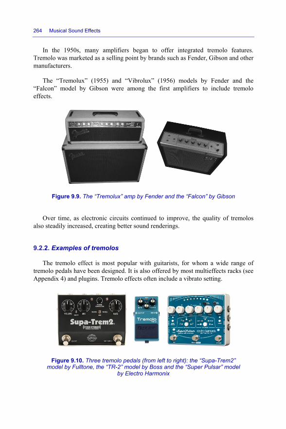
264 Musical Sound Effects
In the 1950s, many amplifiers began to offer integrated tremolo features. Tremolo was marketed as a selling point by brands such as Fender, Gibson and other manufacturers.
The “Tremolux” (1955) and “Vibrolux” (1956) models by Fender and the “Falcon” model by Gibson were among the first amplifiers to include tremolo effects.
Figure 9.9. The “Tremolux” amp by Fender and the “Falcon” by Gibson
Over time, as electronic circuits continued to improve, the quality of tremolos also steadily increased, creating better sound renderings.
9.2.2. Examples of tremolos
The tremolo effect is most popular with guitarists, for whom a wide range of tremolo pedals have been designed. It is also offered by most multieffects racks (see Appendix 4) and plugins. Tremolo effects often include a vibrato setting.
Figure 9.10. Three tremolo pedals (from left to right): the “Supa-Trem2” model by Fulltone, the “TR-2” model by Boss and the “Super Pulsar” model
by Electro Harmonix
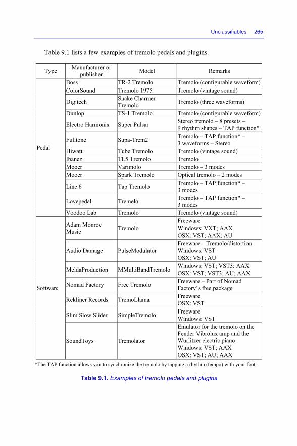
Unclassifiables 265
Table 9.1 lists a few examples of tremolo pedals and plugins.
Type Manufacturer or publisher Model Remarks
Pedal
Boss TR-2 Tremolo Tremolo (configurable waveform) ColorSound Tremolo 1975 Tremolo (vintage sound)
Digitech Snake Charmer Tremolo Tremolo (three waveforms)
Dunlop TS-1 Tremolo Tremolo (configurable waveform)
Electro Harmonix Super Pulsar Stereo tremolo – 8 presets – 9 rhythm shapes – TAP function*
Fulltone Supa-Trem2 Tremolo – TAP function* – 3 waveforms – Stereo
Hiwatt Tube Tremolo Tremolo (vintage sound) Ibanez TL5 Tremolo Tremolo Mooer Varimolo Tremolo – 3 modes Mooer Spark Tremolo Optical tremolo – 2 modes
Line 6 Tap Tremolo Tremolo – TAP function* – 3 modes
Lovepedal Tremelo Tremolo – TAP function* – 3 modes
Voodoo Lab Tremolo Tremolo (vintage sound)
Software
Adam Monroe Music Tremolo
Freeware Windows: VXT; AAX OSX: VST; AAX; AU
Audio Damage PulseModulator Freeware – Tremolo/distortion Windows: VST OSX: VST; AU
MeldaProduction MMultiBandTremolo Windows: VST; VST3; AAX OSX: VST; VST3; AU; AAX
Nomad Factory Free Tremolo Freeware – Part of Nomad Factory’s free package
Rekliner Records TremoLlama Freeware OSX: VST
Slim Slow Slider SimpleTremolo Freeware Windows: VST
SoundToys Tremolator
Emulator for the tremolo on the Fender Vibrolux amp and the Wurlitzer electric piano Windows: VST; AAX OSX: VST; AU; AAX
*The TAP function allows you to synchronize the tremolo by tapping a rhythm (tempo) with your foot.
Table 9.1. Examples of tremolo pedals and plugins
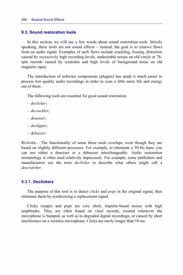
266 Musical Sound Effects
9.3. Sound restoration tools
In this section, we will say a few words about sound restoration tools. Strictly speaking, these tools are not sound effects – instead, the goal is to remove flaws from an audio signal. Examples of such flaws include crackling, hissing, distortion caused by excessively high recording levels, undesirable noises on old vinyls or 78-rpm records caused by scratches and high levels of background noise on old magnetic tapes.
The introduction of software components (plugins) has made it much easier to process low-quality audio recordings in order to coax a little more life and energy out of them.
The following tools are essential for good sound restoration:
– declicker;
– decrackler;
– denoiser;
– declipper;
– debuzzer.
REMARK.– The functionality of some these tools overlaps, even though they are based on slightly different processes. For example, to eliminate a 50-Hz hum, you can use either a denoiser or a debuzzer interchangeably. Audio restoration terminology is often used relatively imprecisely. For example, some publishers and manufacturers use the term declicker to describe what others might call a descratcher.
9.3.1. Declickers
The purpose of this tool is to detect clicks and pops in the original signal, then eliminate them by synthesizing a replacement signal.
Clicks (snaps) and pops are very short, impulse-based noises with high amplitudes. They are often found on vinyl records, created whenever the microphone is bumped, as well as in degraded digital recordings, or caused by short interference on a wireless microphone. Clicks are rarely longer than 10 ms.
Unclassifiables 267
Figure 9.11. The results of applying a declicker: the clicks in the shaded region are detected, eliminated and replaced by a synthesized signal (in green). For
a color version of this figure, see www.iste.co.uk/reveillac/soundeffects.zip
9.3.2. Decracklers
Much like declickers, decracklers identify crackling (static noise), and then mix it with the signals immediately before and after the crackling to significantly attenuate any undesirable noise.
Crackling has lower amplitude than clicks and lasts for longer. Conceptually, it is more of an irregularity in the continuous flow of the audio signal – a component that does not fit with the surrounding audio and music.
9.3.3. Denoisers
Denoisers are used to eliminate background noise, which usually consists of white noise. It is impossible to fully eliminate background noise due to its extremely wide spectrum. To remove all of it, you would have to delete the entire signal.
Instead, denoisers target the most prominent components, such as whistling, buzzing, camera motor noise and much more. These parts of the signal are attenuated while preserving as much of the rest of the signal as possible.
Denoisers usually work by learning. You need to provide a representative sample of the noise that needs to be eliminated as an input, from which the denoiser generates a sound profile. This profile is then used to target and attenuate noise in the rest of the audio signal. There is often also a second smoothing phase to reduce any artifacts that may have been introduced by the first phase.
9.3.4. Declippers
Declippers fix clipping issues caused by saturation in the recording or overly ambitious analog-to-digital conversion.

268 Musical Sound Effects
The clipped waveforms are replaced with new synthesized and recalculated audio data in order to remove any flat regions in the waveform of the saturated signal.
Figure 9.12. Top, a clipped audio signal. Bottom, the same signal after processing with a declipper
9.3.5. Debuzzers
Debuzzers are more specific and targeted versions of denoisers designed to eliminate hissing and buzzing. They usually target the fundamental frequency of the unwanted noise, and then attempt to predict which harmonics might also need to be deleted.
REMARK.– This tool is sometimes called a dehummer.
9.3.6. Examples of restoration tools
Table 9.2 lists a few restoration tools. Today, most restoration tools on the market are software based, often sold as suites with multiple features.
Sound restoration racks are uncommon, but some manufacturers do offer a few highly effective models.

Unclassifiables 269
Figure 9.13. Sound restoration racks (from top to bottom): three racks by Cedar, the “DNA-1” model by Weiss and a very popular model, the “SNR2000” denoiser by Behringer
Type Manufacturer or publisher Model Remarks
Rack
Behringer SNR2000 Denoiser – Stereo Behringer SNR202 Denoiser – 2 channels Behringer SNR208 Denoiser – 8 channels Cedar CRX Decrackler Decrackler Cedar DCX Declicker Declicker Cedar BRX Debuzzer Debuzzer ELP Declicker Vinyl declicker (HiFi) – Stereo
Weiss DNA1 Denoiser/declicker/decrackler – Ambient sound processor – M/S encoder/decoder
Software
Accusonus Era-D Denoiser and reverb suppressor Windows: VST2; VST3; AAX OSX: VST2; VST3; AU; AAX
Acon Dgital Media
Restoration Suite
Denoiser/declicker/declipper/dehummer Windows: VST; VST3; AAX OSX: VST; VST3; AU; AAX
Cedar Cedar Studio Declicker/debuzzer/decrackler and more Windows: VST; RTAS OSX: VST; RTAS; AU
Izotope RX6 Advanced Windows: VST2; VST3; AAX; RTAS OSX: VST; VST3; AU; AAX; RTAS; DPM Standalone version available

270 Musical Sound Effects
Izotope RX6 Standard Windows: VST2; VST3; AAX; RTAS OSX: VST2; VST3; AU; AAX; RTAS; DPM Standalone version available
Magix SOS Vinyl and K7 Audio
Software solution for digitizing vinyls and K7s with integrated restoration features Microsoft Windows Version
Sonic Solutions NoNoise3
Denoiser/dehummer/debuzzer and more Windows: VST OSX: VST; AU
Sonic Studio
Legendary Audio I.C.E. (In Case of Emergency)
Audio restoration for very low quality recordings Windows: VST; AAX OSX: VST; AAX; AU
Sonnox Restore Denoiser/debuzzer/declicker Windows: VST2; AAX; RTAS OSX: VST2; AAX; AU; RTAS
Sonnox Oxford Declicker Native
Declicker Windows: VST2; AAX; RTAS OSX: VST2; AAX; AU; RTAS
Sonnox Oxford Debuzzer Native
Debuzzer Windows: VST2; AAX; RTAS OSX: VST2; AAX; AU; RTAS
Sonnox Oxford Denoiser Native
Denoiser Windows: VST2; AAX; RTAS OSX: VST2; AAX; AU; RTAS
TC Electronic
Restoration Suite
Denoiser/declicker/descratcher/decrackler/dethumper3 Windows: VST; AAX; RTAS OSX: VST; AU; RTAS
Wave Arts Master Restoration Suite
Denoiser/declicker/dehummer and more Windows: VST; AAX; RTAS OSX: VST; AU; RTAS
Waves X-Click Part of the “Restoration” suite
Waves Z-Noise Part of the “Restoration” suite
Waves X-Hum Part of the “Restoration” suite
Waves X-Noise Part of the “Restoration” suite
Waves X-Crackle Part of the “Restoration” suite
Waves Restoration Declicker/denoiser/decrackler/dehummer Windows: VST2; VST3; AAX OSX: VST; VST3; AU; AAXFF
Table 9.2. Examples of audio restoration tools
3 Elimination of low-frequency pulses.

Unclassifiables 271
9.3.7. Final remarks on sound restoration
The tools presented in this section are not the only tools that you might need in order to properly restore sound. There are a host of other problems that you might encounter, such as poor dynamics, loss of treble frequencies, low-quality stereo and so on.
To solve these issues, you will need to use tools such as compressors (see section 7.2), equalizers (see section 4.2), enhancers (see section 7.3) and many others. The objective is to fully reconstruct the original sound message in order to achieve a high-quality and natural sound rendering that is true to the original source.
All of these tools are presented in the previous chapters. Do not hesitate to flip back and forth as much as you need.
9.4. Loopers
Loopers can be used to repeat a certain musical passage ad infinitem, but also have other applications.
This effect has been around for a long time. The first implementations used tape recorders, later followed by samplers, and finally by microcomputers, which are still used today. However, loopers in the form of pedals are much more convenient and user-friendly for practical situations.
Although loopers are most commonly employed by guitarists, they can be used with any instrument, and even microphones are (sometimes) compatible with this type of pedal.
Figure 9.14. Three looper pedals (from left to right): The “JamMan Looper” model by Digitech, the “Ditto Looper” model
by TC Electronic and the “22500” model by Electro Harmonix

272 Musical Sound Effects
The duration of each loop depends on the size of the internal memory of the pedal, as well as the quality of the recording. They usually allow large or sometimes unlimited numbers of loops (overdubs or re-recordings) to be layered on top of each other.
The latest generations of loopers offer a variety of features, including effects (reverse, delay, etc.), integrated rhythms, metronomes, presets, etc.
9.4.1. Looper connections
There are several possible ways to connect a looper in the audio flow. Unlike some other effects, loopers apply a very specific processing operation, and so their position is critical.
The simplest solution is to place the looper between the instrument and the amp, like most other effects.
But if you need to chain multiple effects together, you will need to decide whether to place your looper before, after or between the other pedals.
9.4.1.1. Before other effect(s)
If you place other effects after the looper, you need to remember that any effects that are active when the looper is used will be present in the loop. This might not necessarily be desirable. For example, if you are using a fuzz pedal, your loop will quickly become chaotic.
Figure 9.15. A looper pedal placed before a fuzz pedal
9.4.1.2. After other effect(s)
If we switch the order of the two pedals, only the sound of the guitar is processed when the fuzz pedal is turned on. The loop remains neutral and clear.

Unclassifiables 273
Of course, this assumes that the loop was previously recorded with the fuzz pedal turned off.
Figure 9.16. A looper pedal placed after a fuzz pedal
This example clearly shows the importance of the order of the looper and fuzz pedals. However, in other cases, for example with slight reverb, it might be preferable to keep the effects pedal after the looper pedal.
9.4.1.3. Between effects
As you might have guessed, placing a looper between two or more other effects requires some thought. Any effects placed after the looper will always be applied to the prerecorded loop, whereas the effects placed before it can be used independently from it.
Figure 9.17. A looper pedal placed between several other effects
9.4.1.4. In an effects loop
Some amplifiers include a so-called effects loop, similar to those found on mixing desks. The effects loop allows something else to be placed between the pre-amp and the power amp.
The loop usually has two connections called “SEND” and “RETURN”.

274 Musical Sound Effects
Figure 9.18. Connecting an instrument and a looper pedal to an amp with an effects loop
The SEND on the amp needs to be connected to the input (IN) of the looper pedal with one cable, and the output (OUT) of the looper pedal needs to be connected to RETURN on the amp using a second cable, as shown in Figure 9.18.
This setup has several advantages. Any modifications applied to the pre-amp, such as overdrive, channel settings and internal effects (tremolo, reverb, etc.) will be ignored by the looper, which simply reproduces the originally recorded loop.
9.4.2. Examples of looper pedals
Manufacturer Model Remarks
Boss RC-505 Loop Station Five stereo tracks – 99 memory slots – MIDI controls – effects – live or studio – advanced features
Boss RC-30 Dual Track Looper
Two stereo tracks – 99 memory slots – 3 h of stereo recording
Boss RC-1 Stereo – 12 min of recording – Very simple
Digitech JanMan Stereo Stereo – 35 minutes of recording – 16 h of recording to SD card – 99 memory slots – advanced features
Electro Harmonix
22500 Dual Stereo Looper
Stereo – 12 h of recording (SHDC card) – 100 loops per card – 16 integrated percussions loops – effects – advanced features
Electro Harmonix
2880 Super Multi-Track Looper
Two stereo tracks or 4 mono tracks – Compact flash card – 31 min of recording with a 1-GB card – MIDI – simple to use

Unclassifiables 275
Electro Harmonix Nano Looper 360 Six minutes of recording – 11 memory slots –
unlimited overdubs*
Line 6 JM-4 Looper Stereo – integrated tuner – presets – effects – equalizer – 100 tracks – Mic input – memory card – advanced features
Mooer Micro Looper 30 min of recording – unlimited overdubs* – very simple
TC Electronic Ditto Looper Very simple – 5 min of 24-bit recording – one track – unlimited overdubs*
TC Electronic Ditto X2 Looper Five minutes of 24-bit recording – unlimited overdubs* – loop imports and exports – effects
TC-Helicon Ditto Mic Looper Loop pedal for microphone – 5 minutes of 24-bit recording – XLR input/output – phantom power
*Re-recordings.
Table 9.3. Examples of looper pedals
9.5. Time stretching
This effect modifies the tempo and thus the duration of a recording by making it longer or shorter in order to synchronize it with another audio signal without changing the pitch.
Figure 9.19. An audio signal with a duration of 2.1 s (top) after applying 1.5× time stretching, resulting in a duration of 3.15 s (bottom). The red and blue boxes show the equivalence between time scales: 2.0 s -> 3.0 s (in yellow) (the editor is Adobe Audition CC). For a color version of this figure, see www.iste.co.uk/reveillac/ soundeffects.zip

276 Musical Sound Effects
Most time stretching effects use one of three main techniques called “phase vocoder”, “spectral sine modeling” and SOLA (Synchronous OverLap and Add), which we will not discuss in detail here (see the web links at the end of the book).
Many audio editors and DAWs offer at least one of these three techniques.
REMARK.– Features like “pitch scaling” are often associated with time stretching, allowing an audio signal to be transposed without changing its duration (constant speed). Some harmonizers (see section 6.2.3) also include these features.
9.6. Resampling
Resampling is strictly speaking more of a processing operation than an effect. It modifies the bit depth or sampling frequency of a digital audio signal to make it compatible with a different medium, for example converting from 24-bit sound in a DAW to a 16-bit signal for CD, or converting from a 44.1-kHz CD to a 48-kHz K7 DAT.
Figure 9.20. Resampling a 48-kHz 24-bit audio file with the software editor Sound Forge Pro. For a color
version of this figure, see www.iste.co.uk/reveillac/soundeffects.zip

Unclassifiables 277
9.7. Spatialization effects
To expand on sections 2.6 and 2.7 of this book, we will now list a few examples of spatializers with relatively specialized features. However, in my personal opinion, fully mastering effects such as compression, reverb, delay, equalization and filtering is the most important step toward properly understanding spatialization, especially for the production of conventional mixes.
Figure 9.21. IRCAM SPAT 3, a very powerful spatializer. For a color version of this figure, see www.iste.co.uk/reveillac/soundeffects.zip
These tools can be useful to simulate the sound environments of specific locations, or even artificial sound environments, for example in the context of video games.
Publisher Name Remarks
Auburn Sound Advanced Binaural Panner Freeware Windows: VST OSX: VST; AU
Taucher interact MNTN The Sound of the Mountain Windows: VST; VST3 OSX: VST; VST3; AU
Longcat Binaural Spatializer Windows: VST
Flux Ircam SPAT V3 Windows: VST; AAX OSX: VST; AAX; AU
Tokyo Dawn Records Proximity Freeware Windows: VST OSX: VST; AU
Table 9.4. Examples of dedicated spatializer plugins
278 Musical Sound Effects
9.8. Conclusion
The effects and processes assembled in this final chapter are those that seem most important to me personally, but there are many more that we do not have the time or space to mention. To find out more, interested readers can visit the websites of each publisher and product brand. Downloading user manuals and instructions, often available free of cost, is another great way to find more information.
Conclusion
After nine chapters and four appendices, we have finally reached the end of this book. I hope that reading through these chapters and appendices has allowed you to discover, explore and understand the fascinating universe of digital sound effects.
No doubt there is much left to say. Many effects other than those mentioned here would arguably have deserved a place within these pages, but my own knowledge is far from perfect. I can only talk about effects with which I am personally familiar – the ones that I have encountered and used myself over the course of my professional career.
I work with some of these effects every day in my studio, but even after all these years, I still discover new settings, approaches, combinations and configurations every single day. These discoveries allow me to build ever more striking and attractive sounds.
Working at my mixing desk and workstation is never a chore. Nothing gives my eyes and especially my ears more pleasure than listening, relistening, tweaking and perfecting the musical passages that have been entrusted to me. In my work, I always try to satisfy the needs of the people for whom the sounds are ultimately intended – whether for live performances, radio, sound reinforcement, artistic creativity, digital art or even just family.
I also love to trade stories with performers, composers, sound professionals and anyone else who shares my passion and eagerness for working with sound.
Since the late 1990s, it has become increasingly rare for completely new effects to be invented. But the digital age was nonetheless an earth-shattering revolution for the world of audio. The sophistication of DAWs and audio editors has exploded.
Musical Sound Effects: Analog and Digital Sound Processing, First Edition. Jean-Michel Réveillac.© ISTE Ltd 2018. Published by ISTE Ltd and John Wiley & Sons, Inc.

280 Musical Sound Effects
Audio software programs have forged increasingly close connections with their users, taking advantage of the rapid expansion of computing power from year to year.
Internet and networking technology has taken root, improving discussions, simplifying cabling problems and standardizing the various components of audio systems as much as realistically could have been possible.
Today, there is software for almost everything. Even the oldest effects, created in the 1960s, have been republished, and in some cases improved and reinvented.
My personal opinion is that you do not need dozens of different plugins. Instead, choose the characteristics of the plugin carefully to reflect what you are trying to achieve. Do not hesitate to download trial versions to try out any products that you find on the market so that you can form your own opinion.
Similarly, I believe that digital solutions are not always the answer, though they are unquestionably capable of amazing things. Personally – and many others share my views on this – nothing can beat a good old studio rack or hardware versions of classic effects, even if they are dinosaurs in terms of bulk and usability. If you are not already convinced, see if you can find an opportunity to listen to a Fairchild 670 compressor, a Binson echo chamber, a Pultec EQP-1A equalizer, an MXR 100 phaser, Leslie speakers or any other equipment of similar pedigree. The experience is well worth your while. By placing any of these hardware effects at the right position in the audio flow, you can create wonders – these effects give you the physical sensation of shaping the audio signal with your own hands, your own body. The virtual perception of digital effects simply cannot compare with this.
Of course, the flip side is that hardware equipment is often prohibitively expensive. This is the price of perfection in sound rendering.
However, it is often said that no man is a prophet in his own country, and I do not doubt that this nugget of wisdom applies to me. I consider myself lucky to have started working with sound decades ago, but I will undoubtedly have settled into routines and habits over the years, both good and bad.
What might the future look like? We can expect our equipment to improve even further. Network bandwidth and transfer speeds will continue to increase, more advanced software will be developed. Real-time sound processing will also continue to mature. These things are hardly difficult to foresee. But who knows what surprises might lurk around the corner?

Conclusion 281
One domain that might experience significant change in the not-too-distant
future is the reproduction and playback of new virtualized musical formats. Even though the multichannel systems available today are extremely advanced, our ears can still distinguish between real and virtual sound environments. This is one aspect of sound rendering that potentially still offers some room for improvement.
Finally, it seems that a slight vintage breeze has begun to blow throughout the small world of sound recording. Vinyls are making an unexpected comeback. Old analog effects seem to be regaining some momentum. Is this just a passing trend, or does it perhaps represent a more lasting shift in preferences? Time will tell.

Appendices

Appendix 1
Distortion
A1.1. Introduction
Distortion is often denounced as the public enemy number one of sound reproduction. But some musicians create distortion deliberately to create certain colors for the sound of their instruments. What does this mean, and what is the true nature of distortion?
A1.2. Measuring distortion
To quantify the quality of sound production equipment, we often measure the distortion that it generates. When doing so, it is important to take account of the most relevant type of distortion – there are several.
Distortion is more than just a single isolated concept. There are various types of distortion described in terms of six parameters that we can measure independently:
– the level;
– the frequency response;
– the signal-to-noise ratio (SNR);
– the harmonic distortion;
– the cross-talk;
– the phase.
Musical Sound Effects: Analog and Digital Sound Processing, First Edition. Jean-Michel Réveillac.© ISTE Ltd 2018. Published by ISTE Ltd and John Wiley & Sons, Inc.

286 Musical Sound Effects
A1.2.1. The level
This parameter describes the level of the output signal relative to the input signal. The difference between the two is the distortion. This might seem like an unusual definition at first, but distortion is conceptually an alteration of the original signal, and so variation in the volume may be viewed as a form of distortion.
A sound source is said to be distortion free if the reproduced sound level is equivalent to the original volume of the sound when it was emitted.
But in practice, we are perfectly used to recreating sounds much louder than their original input volume, and so this does not seem unnatural to us.
When a signal is amplified, an enormous amount of energy is lost by the equipment (cables, pre-amp, amp, speakers, etc.). Most of this is due to the Joule effect (the resistance of the components creates losses in the form of heat, among other factors).
When an amplification system is used to increase the volume of a sound, the system defines a nominal level for 0 dB. If this value is exceeded, the capacity of the equipment is overwhelmed, and the sound is altered, often in the form of saturation.
The exact nature of this saturation varies according to the technology on which the equipment is based: tube amps, transistors, integrated circuits or hybrid amps, with classes A, AB, B, D, H, etc.1
To measure the level, we apply an audio signal input with suitable characteristics, then increase the volume up to the nominal value before taking a measurement.
The result is a sound pressure reading expressed in either dB SPL (sound pressure level) or pascal (Pa).
94 dB SPL is equivalent to a sound pressure of 1 Pa. = 20 × in dB
1 See Appendix 2.
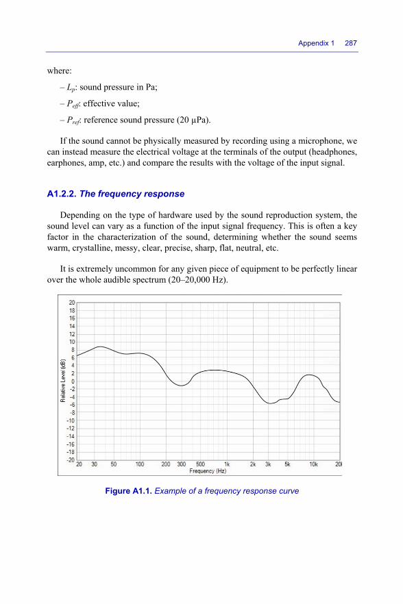
Appendix 1 287
where:
– Lp: sound pressure in Pa;
– Peff: effective value;
– Pref: reference sound pressure (20 µPa).
If the sound cannot be physically measured by recording using a microphone, we can instead measure the electrical voltage at the terminals of the output (headphones, earphones, amp, etc.) and compare the results with the voltage of the input signal.
A1.2.2. The frequency response
Depending on the type of hardware used by the sound reproduction system, the sound level can vary as a function of the input signal frequency. This is often a key factor in the characterization of the sound, determining whether the sound seems warm, crystalline, messy, clear, precise, sharp, flat, neutral, etc.
It is extremely uncommon for any given piece of equipment to be perfectly linear over the whole audible spectrum (20–20,000 Hz).
Figure A1.1. Example of a frequency response curve

288 Musical Sound Effects
Measuring the frequency response can be tricky, since it depends on many different parameters.
To measure the frequency response of a speaker, the usual approach is to record with a microphone. But this microphone is itself never perfectly linear, and the location in which the measurement is being executed can also affect the results (reflections, damping, etc.). Another factor is the distance between the microphone and the source – there are many others.
By contrast, the frequency response of amplifiers is measured by examining their output signal when a load is applied (typically 4, 8 and 16 Ω). The load is chosen to imitate reality as best as possible.
One often-quoted property is the global bandwidth of the system, for example 30–18,500 Hz. The usual definition of the global bandwidth is the frequency band on which all sound signals have a level of at least 3 dB2.
A1.2.3. The signal-to-noise ratio
The SNR is an extremely important factor when evaluating the quality of a sound system.
Many auxiliary signals can potentially interfere with the sound reproduction system. The choice and nature of the electronic components in the system, the shielding of the power supply, the quality of the cables and many other factors all affect the results to some degree or another.
Each of these factors can interfere with and distort the outgoing audio signal by introducing background noise.
This background noise often takes the form of a permanent hissing that attaches itself to the sound content. Unwanted noise can obscure some of the information contained by the original input.
Electronics defines five types of noise that can make up undesirable hissing: thermal noise (resistance noise or Johnson noise), shot noise (or Poisson noise or Schottky noise), flicker noise (or low-frequency noise or excess noise), avalanche noise and burst noise (random telegraph signal (RTS) noise or popcorn noise or impulse noise):
– thermal noise is caused by thermal agitation of electrons;
2 Other definitions of values are sometimes used.

Appendix 1 289
– shot noise is caused by the fact that the electric current is not continuous, but instead consists of individual electrons carrying elementary charges;
– flicker noise is linked to electronic components and is always present whenever they are used. It is often caused by impurities in the constituent materials;
– avalanche noise arises from semiconductors and is caused by the electric field, which accelerates certain electrons;
– burst noise is caused by the creation of voltage peaks of a few microvolts, especially in operational amps3.
Figure A1.2. Illustration of how an input signal acquires noise
3 Electronic amplifiers that boost the electrical voltage of its input(s).

290 Musical Sound Effects
To understand the concept of SNR, we need to introduce the notion of dynamic range, which is defined as the ratio between the strongest and weakest sounds that can be emitted by the sound reproduction system.
If the SNR is larger than the dynamic range, everything is fine. If not, things do not look quite so good – low-intensity information is degraded, or even destroyed and lost, drowned out by noise.
The SNR therefore needs to be as high as possible to provide a good listening experience.
Measuring the SNR of a system is straightforward. A perfectly known input signal (S) described in terms of the frequency and intensity is applied to the system, and then compared to the output in order to isolate any additions or changes (N). The difference between the input and the output gives the SNR (S/NdB).
Figure A1.3. Representation of a signal S partially obscured by noise N. For a color version of this figure, see www.iste.co.uk/reveillac/soundeffects.zip
A1.2.4. Harmonic distortion
Harmonic distortion is also known as the Total Harmonic Distortion (THD). To explain this concept, we first require a definition of the concept of harmonics.
A harmonic is a component of a periodic sound whose frequency is an integer multiple of the fundamental frequency of the signal. Harmonics can be classified into even harmonics (multiples of 2) and odd harmonics.
Harmonic distortion is said to arise within a sound reproduction system whenever a non-negligible quantity of harmonics that were not present in the original input signal are generated by the system. These harmonics represent a distortion of the original sound.

Appendix 1 291
Harmonic distortion is very low in most modern equipment, often completely covered by the background noise measured in terms of the SNR. Therefore, with modern equipment, a parameter called the THD + noise (THD-N) is defined in order to determine whether the harmonic distortion is stronger than the background noise, and, if so, by how much.
The THD is calculated using the following equation: = (1 ℎ . ) + (2 ℎ . ) + ⋯ + ( ℎ . )
For example, with the following input signal, where F denotes the fundamental frequency:
Figure A1.4. Input signal
and the following output signal:
Figure A1.5. Output signal with distortion (in red)

292 Musical Sound Effects
the THD is:
= (52% − 50%) + (5%) + (33% − 30%) ≈ 0.501 (i.e. 5.01%)
The THD can also be expressed in dB using the following transformation formula: = 20log %
In our example, this gives: = 20 log . ≈ −26.003
The value of –26 dB means that the intensity of the THD is 26 dB lower than that of the fundamental frequency F.
A1.2.5. Cross-talk
Cross-talk measures the tendency of parts of the signal from the x-channel to bleed over into the y-channel when both channels are processed by the same equipment (often the case for stereo sound). This usually arises from phenomena related to insufficient shielding, components placed too closely together on the same circuit, capacitance effects and so on.
High cross-talk means that the signals on multiple channels merge together, resulting in more of a mono signal, losing the stereo or multichannel depth of the original signal.
To measure cross-talk, we apply an input signal to one of the channels, for example the left channel of a stereo system, and then observe whether there is any output on the right channel. In multichannel systems, this procedure is repeated for each channel.
A1.2.6. Phase
There are several phase interaction phenomena that can occur whenever you have more than one signal (see section 1.6.2). These phenomena have the unfortunate tendency of destroying parts of each signal.
For example, if you send the same 1-kHz sine wave to both channels of a stereo playback system, you should ideally ultimately obtain two signals that are fully

Appendix 1 293
aligned (in phase), which combine to give the same signal with a higher amplitude (the sine waves add together).
But if there is a delay on one of the channels, the crests and troughs of the sine waves will be shifted relative to each other. The resulting sound will still have the same frequency, but will not be so loud. We say that partial phase cancellation has occurred.
If one of the channels is delayed so much that the troughs of one wave align with the crests of the other (and vice versa), the two waveforms cancel fully, resulting in no sound at all. The two signals are in antiphase, and we say that total phase cancellation has occurred. Alternatively, we say that the signals are “180° out of phase”.
This cancellation process also occurs if the polarity of one of the channels is inverted. Because of this, people often conflate the two separate phenomena of polarity inversion and phase inversion. They are not the same.
Figure A1.6. Transformation of a signal composed of two complex out-of-phase waveforms (red and green). For a color version of this figure, see
www.iste.co.uk/reveillac/soundeffects.zip
In practice, the problems created by phase issues are much more complex. Imagine for example that you are recording a guitar passage on two channels. Any delay on one of the channels will in fact change the pitch of the mixed signal instead of its level. Indeed, for a given delay time, the phase relations between the various

294 Musical Sound Effects
sine waves4 on the first and second channels depend on the frequency of each of the wave components in the signal generated by the guitar. If the delay is 0.5 ms, any 1-kHz waves will be in antiphase (1-kHz sine waves have a period of 1 ms). But if the sound of the guitar also includes any components with frequencies of 2 kHz, these components will have a period of 0.5 ms, and so will remain perfectly in phase.
As a result, the intensity of each signal component present in the signal increases as its frequency ranges from 1 to 2 kHz. This is an example of partial phase cancellation, and the sound intensity is highest at the frequency that experiences phase alignment, namely 2 kHz.
This phenomenon is repeated at every higher frequency. The signal will also partially cancel at some higher frequencies, leaving only signal components that are in phase.
With this explanation, you can easily imagine the kinds of problems that can arise from distortion caused by phase shift in sound reproduction systems.
A1.3. Conclusion
There is still much more that could be said about the various types of distortion and the phenomena associated with them. You can find out more by visiting the bibliography and web links at the end of the book.
4 Always bear in mind that any audio passage, no matter what kind, is in fact a more or less complex combination of a potentially infinite set of sine waves (as shown by the French mathematician Joseph Fourier, 1768–1830).

Appendix 2
Amplifier Classes
A2.1. Introduction
There is a classification for electronic amplifiers that allows us to characterize them, with one letter for each category of amplifier.
There are 10 major classes: A, AB, B, C, D, E, F, G, H and S. There are also other smaller classes, e.g. the T class, which are usually variants of the major classes.
The first generation of amplifiers was divided into four classes, A, B, AB and C, according to the polarization of their electronic tubes. This same principle was used for the next generation of transistor amps. As new technologies were developed, additional classes were added to the list.
Some classes of amplifier are not relevant to studio work or sound reproduction and playback. These applications are only interested in amplifying signals located in the frequency band from 20 and 20,000 Hz.
Therefore, only classes A, AB, B, D and H fall within the scope of this book.
A2.2. Class A
Most specialists view A as the most faithful and musical class of amplifiers.
High-end hi-fi amplification systems are often based on class A technology, providing great dynamics and excellent musical rendering.
Musical Sound Effects: Analog and Digital Sound Processing, First Edition. Jean-Michel Réveillac.© ISTE Ltd 2018. Published by ISTE Ltd and John Wiley & Sons, Inc.

296 Musical Sound Effects
Class A amplification components are 100% active even when there is no signal
(at rest). This requires electronic systems capable of dissipating large quantities of heat (radiators, fans and other cooling mechanisms).
Although they run very hot, class A amplifiers are highly stable, with very low distortion rates. The price of these qualities is mediocre energy efficiency; these amplifiers require large power supplies and consume a lot of energy.
Without going into any further detail, there are various subcategories within class A, including “pure class A”, A1, A2 and so on.
A2.3. Class B
The amplification components in this class operate at 50% when the amp is at rest. This is more efficient than class A amplifiers, but is slightly less faithful, resulting in more distortion. Today, very few manufacturers offer amplifiers from this class, even though they are less expensive to produce, largely because their power supply does not need to be as robust as class A amplifiers.
A2.4. Class AB
This class is a combination of classes A and B. At rest, the system operates at a level somewhere between 50% (class B) and 100% (class A). When active, the amp gradually transitions from class B to class A as the current increases. Many amplifiers, especially those used by sound reinforcement systems, are based on this technology, which is more efficient than class A, although slightly less responsive.
The power supplies of class AB amplifiers are more reasonably sized than those of class A amplifiers, offering a good compromise.
A2.5. Class D
You might be forgiven for guessing (and indeed some sources mistakenly claim) that the letter D standards for “digital”. But class D amps are in fact also analog, not digital.
Class D amplifiers are based on sophisticated technology with maximum efficiency and very low power dissipation. This technology is most suitable for small amplifiers and is perfect for mobile or portable devices.

Appendix 2 297
In the past, these amps were criticized for having poor musicality, but a lot of
progress has been made over the last few generations. Many home theater and hi-fi systems now use class D amplifiers.
Class D is also used by many subwoofers and wireless speakers.
A2.6. Class H
To improve the efficiency of a class B or AB amplifier, one idea is to vary the voltage as a function of the audio signal. Without going into too much detail, this is how class H systems work.
The main advantage is significant improvements in energy efficiency, which means that a much smaller power supply is required. Sadly, this requires a sacrifice in audio quality. This technology creates distortion in some usage conditions, especially in intermediate volume regions, where the power supply voltage can be expected to vary a lot.
Class H amplifiers achieve excellent energy efficiency and can also be made very compact, since they only require a small power supply.
A2.7. Conclusion
This appendix has hopefully helped to clarify the meaning of the various classes of amplifier. I deliberately did not attempt to go into extensive detail or approach the topic of digital amplifiers (binary switching amplifiers). If you are interested in a more in-depth discussion of the electronics, design, measurements and performance of amplifiers, you can visit the bibliography and the web links at the end of the book.
Appendix 3
Introduction to Max/MSP
A3.1. Introduction
Throughout this book, we have discussed a wide range of ideas about audio signal processing, mostly from a theoretical perspective. Putting these ideas into practice and listening to how they work in practice is an instructive exercise.
Max/MSP by Cycling’74 is an ideal example of a software tool that allows you to do this, although there are plenty of others, both freeware and commercial, that are also perfectly suitable.
Max1 is my first choice because I have now been using it for more than 30 years. At the time, it was truly revolutionary. We were working on the first generations of Apple computers (Mac Plus, Mac II, Mac SE30, etc.). Since then, Max has changed a lot, but has never lost sight of its guiding principles, which are still perfectly recognizable in the latest versions (Max 7).
REMARK.– “Max for Live” is a version of Max designed to be compatible with Ableton Live 9.
The concepts presented here are easy to adapt to other software tools (Pure Data, SuperCollider, jMax, etc.). You will find everything you need at the end of the book in the bibliography and web links (textbooks, download links, publishers’ websites, forums, tutorials, etc.).
1 Music software for synthesizing sound, controlling instruments, recording, performing audio analysis and more. Max was developed in France by IRCAM (Institute for Research and Coordination in Acoustics/Music) in the 1980s.
Musical Sound Effects: Analog and Digital Sound Processing, First Edition. Jean-Michel Réveillac.© ISTE Ltd 2018. Published by ISTE Ltd and John Wiley & Sons, Inc.

300 Musical Sound Effects
This appendix simply introduces a few basic examples with Max/MSP that will allow you to start experimenting for yourself. If you are interested, you can then keep exploring further on your own.
If you asked me the question: “What can you do with Max/MSP?”, my answer would be: anything, or almost anything that you could possibly imagine for audio or possibly even video. Max/MSP is a vast toolbox, almost like a more user-friendly version of a programming language. It has a completely open structure and supports connections with many other software programs, robots, electronic instruments, smartphones, etc.
A3.2. How Max works
Max works almost exclusively with graphical interfaces. Blocks (boxes or elements) are placed into a window and connected together. Each block has its own role, with inputs and/or outputs, and an array of configurable parameters that can be defined and edited.
Each set of connected blocks is placed in a window called a “patcher”.
A3.3. Getting started: sine wave oscillator
For our first project, we will construct a small sine wave generator that can be manually varied from 20 Hz to 20 kHz.
Open Max, go to the FILE menu, and select NEW PATCHER. The window that opens is now your main window.
Figure A3.1. The main window of MAX (version 7)

Appendix 3 301
The top toolbar allows you to select blocks. They are listed separated or grouped
into families. From left to right: objects, message, comment, toggle, buttons, numbers, sliders, Max for Live objects and add object.
Figure A3.2. The horizontal toolbar
REMARK.– The 100% dropdown in the top left is for adjusting the scale (zoom ±).
When you click on OBJECT, a block is created in the center of the window. You can move this block by dragging it.
An object is a box whose function has not yet been configured. When a name is entered in the box, the object gains a function.
The blinking text cursor indicates that the software is waiting for you to type the name of a primitive. For our example, we will choose: “cycle”. Immediately after starting to type, autocomplete pops up, allowing you to select “cycle˜” (sinusoidal oscillator), as shown in Figure A3.3.
This creates a sine wave oscillator.
Figure A3.3. An OBJECT block with the “cycle˜” function, i.e. a sinusoidal oscillator
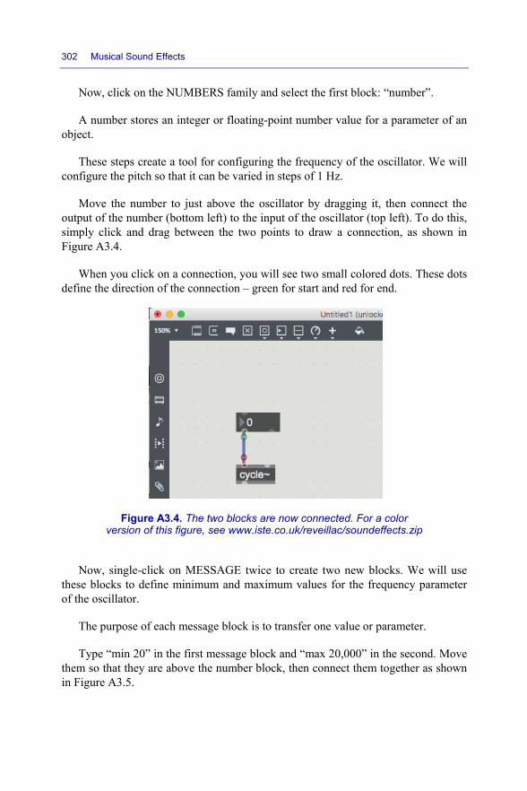
302 Musical Sound Effects
Now, click on the NUMBERS family and select the first block: “number”.
A number stores an integer or floating-point number value for a parameter of an object.
These steps create a tool for configuring the frequency of the oscillator. We will configure the pitch so that it can be varied in steps of 1 Hz.
Move the number to just above the oscillator by dragging it, then connect the output of the number (bottom left) to the input of the oscillator (top left). To do this, simply click and drag between the two points to draw a connection, as shown in Figure A3.4.
When you click on a connection, you will see two small colored dots. These dots define the direction of the connection – green for start and red for end.
Figure A3.4. The two blocks are now connected. For a color version of this figure, see www.iste.co.uk/reveillac/soundeffects.zip
Now, single-click on MESSAGE twice to create two new blocks. We will use these blocks to define minimum and maximum values for the frequency parameter of the oscillator.
The purpose of each message block is to transfer one value or parameter.
Type “min 20” in the first message block and “max 20,000” in the second. Move them so that they are above the number block, then connect them together as shown in Figure A3.5.

Appendix 3 303
Figure A3.5. After moving the MESSAGE blocks into position
Next, click on the ADD OBJECT family, select the AUDIO subfamily and choose the block that is shaped like a speaker (ezdac˜). This block creates an amplified audio signal output, which is usually sent to the sound card and speakers of your computer.
Connect this block to the oscillator (see Figure A3.5). We need two connections in order to support a stereo signal on both channels, left and right.
Figure A3.6. The audio output block is now connected
Next, open the FILE menu, choose SAVE, type a name for your file, select a file location and finally click SAVE.
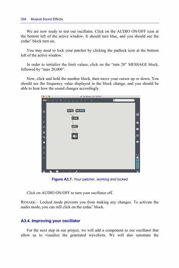
304 Musical Sound Effects
We are now ready to test our oscillator. Click on the AUDIO ON/OFF icon at the bottom left of the active window. It should turn blue, and you should see the ezdac˜ block turn on.
You may need to lock your patcher by clicking the padlock icon at the bottom left of the active window.
In order to initialize the limit values, click on the “min 20” MESSAGE block, followed by “max 20,000”.
Now, click and hold the number block, then move your cursor up or down. You should see the frequency value displayed in the block change, and you should be able to hear how the sound changes accordingly.
Figure A3.7. Your patcher, working and locked
Click on AUDIO ON/OFF to turn your oscillator off.
REMARK.– Locked mode prevents you from making any changes. To activate the audio mode, you can still click on the ezdac˜ block.
A3.4. Improving your oscillator
For the next step in our project, we will add a component to our oscillator that allow us to visualize the generated waveform. We will also automate the

Appendix 3 305
configuration of the number block. This avoids the need to initialize the min (20) and max (20,000) values manually and ensures that the working range of the oscillator is bounded.
Click on the ADD OBJECT icon, choose the AUDIO subfamily, then select a scope˜ block.
Drag the edges of this block slightly so that it becomes a rectangle, then connect a number block and the output of the cycle˜ object to its input, as shown in Figure A3.8.
Figure A3.8. The oscillator with an added graph (oscilloscope) for visualization
The number block connected to the scope˜ block allows us to manage the size of the signal display buffer. Changing the value of the number block will extend or reduce the length of the curve. This parameter is essentially equivalent to the horizontal “Time/Div” setting on physical oscilloscopes.
To automatically configure the working range of the oscillator whenever it is turned on, we simply need to connect a loadbang input to the two message blocks.
Open the FILE menu, select SAVE, then click the SAVE button to save your changes.

306 Musical Sound Effects
Figure A3.9. Our oscillator, now with a loadbang object (top left)
A3.5. Tremolo, vibrato, reverb and chorus
After mastering the simple example presented above, you can start playing around with more interesting patchers.
REMARK.–:You can access the help function by right-clicking on any block. This displays one or several working examples of prebuilt, modifiable patchers using this block.
Figures A3.10–A3.13 show four ready-made patches for building, experimenting and listening to tremolo, vibrato, reverb and chorus effects.
REMARK.– In sections A3.5.1–A3.5.4, comments explaining the functionality of each of the implemented blocks and objects are written in italics.

Appendix 3 307
A3.5.1. Tremolo
Figure A3.10. Example of a tremolo
Tremolo can be constructed using the following blocks:
– three flonum blocks – NUMBERS family – displays and generates a decimal value;
– one number block – NUMBERS family – displays and generates an integer value;
– two cycle˜ objects – creates a sinusoidal oscillator;
– 2 *˜ objects – multiplies two signals together;
– one ezdac˜ block – ADD OBJECT family – AUDIO subfamily – Audio output (on/off);
– one scope˜ block – ADD OBJECT family – AUDIO subfamily – visualizes an audio signal.
REMARK.– You can use “comment” blocks to add text to your patcher.

308 Musical Sound Effects
A3.5.2. Vibrato
Figure A3.11. Example of a vibrato
Vibrato can be constructed using the following blocks:
– three flonum blocks – NUMBERS family – displays and generates a decimal value;
– one number block – NUMBERS family – displays and generates an integer value;
– two cycle˜ objects – creates a sinusoidal oscillator;
– one *˜ object – multiplies two signals together;
– one +˜ object – adds two signals together, or adds a compensation value to a signal;
– one gain˜ block – SLIDERS family – controls the gain;
– one ezdac˜ block – ADD OBJECT family – AUDIO subfamily – audio output (on/off);
– one scope˜ block – ADD OBJECT family – AUDIO subfamily – visualizes an audio signal.

Appendix 3 309
A3.5.3. Reverb
Figure A3.12. Reverb effect. This effect records the sound of your voice using your computer’s microphone (by default)
Reverb can be constructed using the following blocks:
– two flonum blocks – NUMBERS family – displays and generates a decimal value;
– two number blocks – NUMBERS family – displays and generates an integer value;
– two *˜ objects – multiplies two signals together;
– two +˜ objects – adds two signals together, or adds a compensation value to a signal;
– one gain˜ block – SLIDERS family – controls the gain;
– one tapin˜ object – generates a delay time on the input signal;

310 Musical Sound Effects
– one tapout˜ object – generates an output signal with a delay;
– one ezadc˜ block – ADD OBJECT family – AUDIO subfamily – audio input (microphone by default, on/off);
– one ezdac˜ block – ADD OBJECT family – AUDIO subfamily – audio output (on/off);
– one scope˜ block – ADD OBJECT family – AUDIO subfamily – visualizes an audio signal.
A3.5.4. Chorus
By removing one number block and adding a few extra elements to the previous patcher (section 3.5.3), we can transform reverb into chorus.
Figure A3.13. Chorus based on the previous patcher. The chorus records the sound of your voice using your computer’s microphone (by default)
We need to add the following blocks:
– three flonum blocks – NUMBERS family – displays and generates a decimal value;
– two *˜ objects – multiplies two signals together;

Appendix 3 311
– one +˜ object – adds two signals together, or adds a compensation value to a
signal;
– one rand˜ object – generates a random signal between –1 and 1 of an input frequency.
A3.6. Going further
As mentioned earlier, this appendix is just an extremely basic introduction to Max/MSP. If you would like to build other patchers, you can do so by exploring the documentation available on the Cycling’74 website in the “Max” section, as well as the web links given at the end of the book.

Appendix 4
Multieffects Racks
A4.1. Introduction
This appendix presents Tables A4.1 and A4.2 with a collection of multieffects racks, also known as effects processors, including both historical (vintage) models and more modern examples. Some of these are specifically intended for guitar or bass.
The advantage of these racks is that they combine several dozens of effects into the same device. Some models allow multiple effects to be chained together.
However, the controls of this equipment are not always user-friendly. Managing the settings and sound quality can be tricky. Therefore, you should definitely take the opportunity to try them out if you can, and consider some of the many reviews, tests and demonstration videos that can be found online (YouTube, Daily Motion, Vimeo, etc.) to form your own opinions.
You can also find more information on the manufacturer’s website of each model (see Bibliography).
A4.2. Vintage racks
I have done my best to give an approximate release date for each model in this list. Racks are sorted alphabetically by name of manufacturer.
Musical Sound Effects: Analog and Digital Sound Processing, First Edition. Jean-Michel Réveillac.© ISTE Ltd 2018. Published by ISTE Ltd and John Wiley & Sons, Inc.

314 Musical Sound Effects
Manufacturer Model Release year Remarks
Alesis Midiverb Early 1980s
Twelve bits – 63 presets – Reverb, reverse, echo, MIDI
Alesis Midiverb II Early 1980s
Sixteen bits – 99 presets – Reverb, delay, echo, chorus, etc. – MIDI
Alesis Midiverb 4 1985 Eighteen bits – 128 presets – 128 user programs – Reverb, delay, chorus, flanger, pitch, etc. – MIDI
Alesis Quadraverb Early 1990s
Sixteen bits – 100 presets (90 in ROM) – Equalizer, pitch, delay, reverb – MIDI
Boss SE-50 1990 Twenty-eight presets – 100 user slots – Reverb, chorus, flanger, phase, equalizer, etc. – MIDI
Ensoniq DP4 Early 1990s
Twenty-four bits – 400 presets including 200 user slots – Reverb, chorus, flanger, delay, distortion, pitch, etc.
Eventide Eclipse studio 2001
Twenty-four bits – 11 reverbs, delay, chorus, pitch shift, loop – AES/EBU – S/PDIF – MIDI –XLR
Ibanez UE405 Mid 1980s
Vintage – Analog delay, equalizer, chorus, compressor, limiter
Kawai RV4 Late 1980s
Fifty presets – 50 user slots – Reverb, delay, chorus, vibrato, tremolo, etc. – MIDI – AES/EBU
Korg A3 1990 Vintage – For guitar – Compression, distortion, delay, modulation, reverb
Lexicon LXP15 II Early 2000s
128 presets – 128 user slots – Reverb, chorus, delay, pitch, etc. – MIDI
Lexicon MPX-1 1996 Eighteen bits – 200 presets – Reverb, chorus, pitch, equalizer, modulation, delay – MIDI

Appendix 4 315
Lexicon PCM41 1980 Reverb, delay, vibrato, flanger, vocoder, etc.
Roland
SDX-330 1994 Sixteen bits – 100 presets – 200 user programs – Chorus, flanger, phaser, delay, pitch, rotary, etc. – MIDI
Sony DPS-V55 1998 Twenty bits – 200 presets – 200 user programs – 45 effects – MIDI
TC Electronic M-One XL 1999 Twenty-four bits – 200 presets – 100 user slots – Reverb, delay, chorus, flanger, compressor, noise gate, etc.
TC Electronic M2000 1995
Twenty-four bits – 250 presets – 128 user slots – Reverb, delay, pitch, equalizer, etc. – AES/EBU – S/PDIF – MIDI
TC Electronic FireworX studio 1998
Twenty-four bits – 400 presets – Vocoder, filter, phaser, special effects, etc. – SLR – MIDI – ADAT S/PDIF
Yamaha SPX90 1985 Sixteen bits – 30 presets – 60 additional effects – MIDI
Yamaha SPX900 Late 1990s
Sixteen bits – 50 presets – 49 user slots – Reverb, flanger, chorus, phaser, tremolo, pitch, compressor, distortion, etc. – MIDI
Yamaha EMP100 1991 Sixteen bits – 100 presets – Reverb, chorus, flanger, delay, pitch – MIDI
Yamaha SPX990 1993 Twenty bits – 80 presets – Reverb, delay, chorus, flanger, phaser, pitch, etc. – MIDI
Yamaha FX500B 1990
Sixteen bits – Specially designed for bass – 30 presets – 30 user slots – Compressor, overdrive, equalizer, modulation, reverb, delay – MIDI
Yamaha EMP700 1994
Sixteen bits – 90 presets – 50 user slots – Equalizer, compressor, limiter, reverb, delay, enhancer, distortion, pitch shift, wah-wah, phaser, modulation, etc.

316 Musical Sound Effects
Yamaha SPX2000 2003 Twenty-four bits – 80 presets – Reverb, delay, pitch, modulation, gate, etc. – AES/EBU – XLR – MIDI
Zoom RFX-2000 Early 2000s
Twenty bits – 616 presets – 100 memory slots – Reverb, delay, phaser, pitch, chorus, etc. – MIDI – S/PDIF
Table A4.1. Examples of vintage multieffects racks
A4.3. Modern multieffects racks
Table A4.2 gives a list of more recent racks. Most of these are still available for sale at the time of writing. As before, they are sorted alphabetically by name of manufacturer.
Manufacturer Model Remarks
Eventide H8000FW Twenty-four bits – Multichannel multieffects – 1,600 presets – AES – ADAT – S/PDIF
Behringer FX2000 Twenty-four bits – 3D effects – Amplifier emulation – Psychoacoustic effects – MIDI
Lexicon MX300 Twenty-four bits – 16 reverbs, compressor, de-esser, etc. – VST plugin – USB port – MIDI
Lexicon MX400 Twenty-four bits – 17 reverbs, delay, compressor, etc. – VST plugin – USB port – MIDI
Lexicon MX200 Twenty-four bits – 16 reverbs, compressor, de-esser, etc. – VST plugin – USB port – MIDI
Lexicon MX550 Twenty-four bits – 240 presets – Reverb, flanger, chorus, pitch, delay, echo, etc.
Line 6 Helix rack guitar processor
Twenty-four bits – For guitar – Amplifier + effect simulation – S/PDIF – AES/EBU – VDI – USB

Appendix 4 317
Line 6 POD HD Pro X
For guitar – 512 presets – 128 user programs – 22 amp simulations, 19 delays, 23 modulation effects, 17 distortion effects, 12 compressors, 26 filters, 12 reverbs – USB – MIDI – S/PDIF – AES/EBU
Peavey Dual Deltafex
Twenty-four bits – 200 presets including 100 user presets – Delay, reverb, modulation, distortion, rotary, chorus, etc.
Rocktron Xpression
Twenty-four bits – For guitar and bass – 128 presets – Reverb, pitch shifting, compressor, delay, chorus, flanger, rotary, phaser, etc.
TC Electronic M3000 Twenty-four bits – Reverb + effects – Numerous presets – S/PDIF – AES/EBU – ADAT – MIDI
TC Electronic M350
Twenty-four bits – 256 presets – 99 user slots – 15 reverbs + 15 types of effect – VST plugin – MIDI – S/PDIF
Table A4.2. Examples of modern multieffects racks

Glossary
A
Autotune: Tone correction software developed by Antares Audio Technologies.
Auxiliary: On a mixing desk, each input channel has one or more outputs labeled “auxiliary”. These can usually be toggled between “postfader” and “prefader” modes (see the corresponding entries later in the glossary) to choose whether the signal should be taken from before or after the fader. The fader controls the output volume of each input channel (track).
B
Bus: Temporary processing channel that allows several channels or inputs to be combined on a mixing desk.
Bus master: Combines all output channels of a mixing desk. In the studio, a copy of the bus master is typically sent to the monitor to allow the person managing the mix to listen in.
Bypass: Bypass mode allows an audio signal to pass through processing equipment without altering its sound characteristics.
C
Cardioid: Term that describes the directionality of certain types of microphone. Cardioid microphones are highly sensitive to sound from the front, but much less sensitive to sound from the rear. They are used to isolate sounds from unwanted
Musical Sound Effects: Analog and Digital Sound Processing, First Edition. Jean-Michel Réveillac.© ISTE Ltd 2018. Published by ISTE Ltd and John Wiley & Sons, Inc.

320 Musical Sound Effects
ambient noise, which makes them extremely valuable for recording in noisy environments.
Coincident microphones: Pair of cardioid microphones of same type coupled together for sound recording. The sensors (capsules) of the microphones are placed as close as possible (less than 40 cm) at a relative angle between 90° and 135°, pointing toward the sound source.
Compressor: Hardware or software that applies dynamic range compression.
Crosstalk: Interference between two audio signals.
D
DAW (Digital Audio Workstation): Workstation (on a computer or tablet) for recording, editing, mixing, manipulating, creating, processing and reading audio content. Examples of DAWs include Avid Pro Tools, MOTU Digital Performer, Magix Samplitude, Cakewalk Sonar, Apple Logic Pro, PreSonus Studio One and many others.
Decibel (dB): Unit used in acoustics and electronics, defined as 10 times the base-ten logarithm of the ratio of two powers.
De-esser: Tool for reducing whistles and occlusives (stops) in a sound.
Distortion: Undesirable alteration of an audio signal.
Dithering: Technique for improving digital sound data.
Doppler effect: Frequency shift in a sound wave caused by a variation in the distance from the source of emission over time.
DSD (Direct Stream Digital): Protocol for storing and recording audio signals on a digital medium, for example used by Super Audio CDs (SACDs).
DSP (Digital Signal Processing): Processor dedicated to and optimized for executing signal processing tasks (filtering, extraction, conversion, encoding, decoding, compression, etc.).
Dynamic range compression: Audio technique that reduces the difference in level between the loudest and quietest sounds of a signal.

Glossary 321
E
Enhancer: Hardware or software tool for improving the sound rendering.
Equalizer: Hardware or software system for correcting the timbre of a sound. Equalizers can filter, boost and cut specific frequency bands of the audio signal. They are commonly used for sound recording, mixing and sound reinforcement.
Exciter: see enhancer.
Expander: Hardware or software tool for increasing (expanding) the dynamic range of an audio signal.
F
Fuzz: Sound effect that creates saturation in the sound signal by means of heavy clipping.
H
Harmonizer: Hardware or software tool that enhances vocals by duplicating them at higher or lower musical intervals (third, fifth, etc.), creating chords.
I
Insert: Integrated access point on the mixing console or desk that allows users to add new devices (peripherals) into the audio flow between the pre-amp and the mixing bus.
L
Leslie: Common name for an amplification cabinet with one or more rotating speakers designed to create a Doppler effect in the sound signal, usually a signal originating from an electronic organ. Named after their inventor, Donald Leslie, these speakers can also be used with instruments other than organs. Effects that simulate the sound of Leslie speakers are often called Leslie effects, “rotovibe,” “rotary” or “univibe”.
Leslie speakers: see Leslie.

322 Musical Sound Effects
LFO (Low-Frequency Oscillator): Oscillator specially designed for low-frequency variations, often used for tremolo and vibrato effects.
Limiter: Tool for processing the dynamics of an audio signal. Limiters allow us to optimize the overall volume of a sound message, perfectly complementing the possibilities offered by a compressor.
Loudness: Digital quantity representing the volume as a sound as perceived by a human observer. Loudness is a complex psychoacoustic concept that depends on a large number of parameters.
M
Main bus: Primary output bus from a mixing desk. Usually stereo.
Mastering: Final stage of audio postproduction during which the sound rendering of a mix is optimized and calibrated in order to be transferred (for example to a medium like a CD), used or played.
Matrixing: Another term for mastering (see above).
Max/MSP: Music software for synthesizing sound, controlling instruments, recording, performing audio analysis and so on. It was developed in France by IRCAM (Institute for Research and Coordination in Acoustics/Music) in the 1980s.
MIDI (Musical Instrument Digital Interface): Protocol, communication standard and file format (MIDIfile) created for electronic musical instruments, officially released in 1983. MIDI connections are based on three 5-pin DIN connectors: input (MIDI in), output (MIDI out) and forwarding (MIDI Thru). Two cables are required for two-way communication between each device in the musical sequence.
Mixing: During postproduction in a recording studio, mixing is the operation that combines multiple sound sources together to construct a single cohesive overall sound. Mixing is also performed in real time and on-site for live events such as concerts.
N
Noise gate: Processing operation that filters unwanted sounds before amplification.

Glossary 323
O
Overdrive: Sound effect used to modify the sound of an instrument by increasing the gain of the amplifier to create controlled distortion.
P
PCM (Pulse Code Modulation): Processing operation for digitizing an electrical signal or analog audio. After sampling, each sample is quantified and transformed into a digital code.
Phoneme: Smallest distinguishable element when dividing a spoken message into segments. This term is used in the field of linguistics, most notably in phonology.
Pitch shifter: Hardware or software tool for applying a sound effect that modifies the pitch of a sound signal while keeping the same tempo (without modifying the duration of the sound).
Postfader: On a mixing desk, the auxiliary “postfader” output is usually a dial that copies part of the signal after it has passed through the fader (linear potentiometer) of the corresponding channel (track). The position of the fader modifies the level of the signal sent to the “postfader”.
Prefader: On a mixing desk, the “prefader” output copies part of the signal before it passes through the fader (linear potentiometer) of the corresponding channel (track). The level of this auxiliary output is not affected by the position of the fader.
Presence: System for adding trebles and sharpness to a sound. This is usually done directly at the power stage of the amp via a feedback system (part of the input signal received by the amp is fed back into it).
Q
Quadriphonic sound: Also known as “tetraphonic sound”. Procedure designed to create a spatialized sound signal by using four independent channels: front right, front left, back right, back left.
R
Re-recording: Technique that involves recording sound messages by adding them to and mixing them with other prerecorded sounds.
324 Musical Sound Effects
Rotary: See Leslie.
Rotovibe: See Leslie.
RS422: Digital transmission standard based on a serial communication protocol.
S
SACD (Super Audio Compact Disc): Optical digital medium that allows music to be stored in very high quality, created by Sony and Philips and first marketed in 1999.
Saturation: Saturation occurs in an electronic circuit whenever the output level does not increase any further when the input level is increased. Saturation is therefore an alteration or deformation of the sound signal, which is said to be distorted (saturation generates distortion).
Sibilance: Whistling caused by strongly accentuated “sq”, “sh”, soft “ch”, “z” and “j” sounds in speech. Also called the “sibilants” or “occlusives” of a sound.
Sidechain: Feature that varies the sound parameters (usually but not always the gain) as a function of an input signal, typically an external input.
S/PDIF (Sony/Philips Digital Interface): Digital interface for transferring digital audio data, also known as IEC 958. This standard was designed by Sony and Philips in 1989. It competes directly with the professional standard AES/EBU (Audio Engineering Society/European Broadcasting Union).
T
Timbre: The set of sound parameters that characterize instruments and voices and which enable us to identify them.
Tremolo: Periodic variation in the volume (and/or pitch) of a sound signal, usually created by a low-frequency oscillator (LFO).
U
Univibe: See Leslie.

Glossary 325
USB (Universal Serial Bus): Standard for serial transmission connecting multiple devices to a computer or any other compatible host. USB was designed in the mid-1990s to replace various other communication devices, such as parallel ports, serial ports, SCSI ports, etc. It requires a specific type of cable and has evolved and improved over time. The latest version, USB 3.1, released in 2014, can theoretically achieve 10 Gbits/s.
V
Vacuum tubes: Also called “electronic tubes”. Active electronic component usually used for signal amplification, later replaced by semiconductors (transistors, diodes, etc.). Vacuum tubes were invented by Lee De Forest in 1907 (triode).
Vibrato: Periodic variation in the frequency of a sound signal, usually created by a low-frequency oscillator (LFO).
W
Wah-wah: Musical effect used by trumpeters, trombonists and guitarists based on the principle of shifting the sound spectrum. It can be generated mechanically, with a mute, or electronically, usually with a pedal. Sometimes written “wha-wha” or “wa-wa”.
Wurlitzer: Brand of a famous electric piano with 64 keys, based on a mechanism with hammers that strike metal blades. It has a very distinctive and unique sound. Many musicians have used it in the past and still (occasionally) do to this day, especially for rock and jazz. It was invented by Ben F. Meissner in the early 1950s, and peaked in popularity from 1960 to 1975. This piano was a serious competitor of the Fender Rhodes piano, although much less widely used.
X
XLR: Type of connector with a circular cross-section used for connecting professional audio and lighting equipment. It can have three to seven pins. The three-pin version is much more commonly used.

Bibliography
[BAY 13] BAYLE J., Le guide ultime et zen de Max for Live, Leanpub, 2013.
[CAP 13] CAPLAIN R., Technique de prise de son, 6th ed., Dunod, Paris, 2013.
[CAS 07] CASE A., SoundFX: unlocking the creative potential of recording studio effects, Focal Press, 2007.
[ERN 15] ERNOULD F., Le grand livre du home studio – Tout pour enregistrer et mixer de la musique chez soi, Dunod, Paris, 2015.
[FLE 95] FLEURY P., MATHIEU J.P., Vibrations mécaniques acoustiques, Eyrolles, Paris, 1995.
[FOR 86] FORTIER D., Le mini studio, théorie et pratique, Editions Fréquences, 1986.
[GIB 97] GIBSON D., The Art of Mixing, Mix Books, 1997.
[JOU 99] JOUHANNEAU J., Notions élémentaires d’acoustique, Editions Tec & Doc, 1999.
[HUB 13] HUBER D.M., RUNSTEIN R.E., Modern Recording Techniques, Focal Press, 2013.
[HUG 05] HUGONNET C., WALDER P., Théorie et pratique de la prise de son, Eyrolles, Paris, 2005.
[HUN 14] HUNTER D., Guitar Amps and Effect for Dummies, For Dummies, Wiley, 2014.
[IZH 11] IZHAKI R., Mixing Audio: Concepts, Practices and Tools, Focal Press, 2011.
[KAT 14] KATZ B., Mastering audio: The Art and the Science, 3rd ed., Focal Press, Wiley, 2014.
[KIN 99] KINSLER E.L., FREY R.F, COPPENS A.B. et al., Fundamentals of Acoustics, Wiley, 1999.
[LAN 11] LAGRANGE M., Modélisation sinusoïdale des sons polyphoniques, PhD thesis, University of Bordeaux, 2011.
[LYO 12] LYON E., Designing Audio Objects for Max/MSP, A-R Editions, 2012.
Musical Sound Effects: Analog and Digital Sound Processing, First Edition. Jean-Michel Réveillac.© ISTE Ltd 2018. Published by ISTE Ltd and John Wiley & Sons, Inc.

328 Musical Sound Effects
[MAN 16] MANZO V.J., Max/MSP/Jitter for Music: A Practical Guide to Developing
Interactive Music Systems for Education and More, 2nd ed., OUP USA, 2016.
[MAT 69] MATRAS J.J., L’acoustique appliquée, Presses Universitaires de France, Paris, 1969.
[MER 13] MERCIER D., Le livre des techniques du son – Tome 3: L’exploitation, 4th ed., Dunod, Paris, 2013.
[MER 15] MERCIER D., BOURCET P., CALMET M. et al., Le livre des techniques du son – Tome 1: Notions fondamentales, 5th ed., Dunod, 2015.
[OWI 13] OWINSKI B., The Mixing Engineer’s Handbook, Delmar Cengage Learning, 2013.
[PAR 96] PARKER D.J., STARETT R.A., CD Recordable Handbook, Pemberton Press, 1996.
[PER 15] PERIAUX B., OHL J.L., THÉVENOT P., Le son multicanal – De la production à la diffusion du son 5.1, 3D et binaural, Dunod, 2015.
[PER 14] PERRINE J., Sound Design, Mixing, and Mastering with Ableton 9, Hal Leonard Corporation, Milwaukee, 2014.
[PIE 84] PIERCE J.R., Le son musical, Belin, Paris, 1984.
[REI 14] REISS J.D., MCPHERSON A., Audio Effects: Theory, Implementation and Application, CRC Press, 2014.
[ROA 16] ROADS C., L’audionumérique – Musique et informatique, 3rd ed., Dunod, Paris, 2016.
[ROB 14] ROBISON K., Ableton Live 9: Create, Produce, Perform, Focal Press, 2014.
[ROT 95] ROTHSTEIN J., MIDI: A Comprehensive Introduction, vol. 7, A-R Editions, 1995.
[RUM 02] RUMSEY F., MCCORMICK T., Son et enregistrement, Eyrolles, Paris, 2002.
[SCH 73] SCHAEFFER P., La musique concrète, Presses universitaires de France, Paris, 1973.
[SCH 77] SCHAEFFER P., Traité des objets musicaux, Le Seuil, Paris, 1977.
[SER 11] SENIOR M., Mixing secrets for the small studio, Focal Press, 2011.
[TUR 15] TURRIER C., Le son – Théorie et technologie, Ellipses, Paris, 2015.
[VIE 14] VIERS R., EDERY T., Le guide ultime du sound designer: Comment créer et enregistrer des effets sonores pour le cinéma et la télévision, Editions Dixit, Paris, 2014.
[WHI 93] WHITE P., L’isolation, la correction acoustique et le monitoring, ACME, 1993.
[WHI 93] WHITE P., Effets et processeurs, vols 1–2, ACME, 1993.
[WYN 00] WYNER J., Audio Mastering: Essential Practices, Berklee Press Publications, Boston, 2000.

Bibliography 329
Web links
By their very nature, Internet links are unreliable. Resources can be moved to new locations, or sometimes removed completely. All of these links were valid when this book was written. If you find that a link no longer works, you may be able to find an alternative location by using Google or your preferred search engine.
Miscellaneous
Audio restoration: http://www.audio-maniac.com/?page_id=190
Audio restoration: http://www.clickrepair.net/
Amplifier classes: http://www.electronics-tutorials.ws/amplifier/amplifier-classes.html
Audio amplifier classes: http://www.audioholics.com/audio-amplifier/amplifier-classes
Digital amplification, analog: http://www.sonopourtous.fr/fr/article/12-amplification-numerique-analogique-qu-est-ce-que-c-est-
How a digital amplifier works: http://www.axiomaudio.com/blog/digital_amplifier
What types of modification can you find in a distorted signal?: http://www.tpe-distorsion2. sitew.com/2_Les_types_de_distorsions.D.htm#2_Les_types_de_distorsions.D
Audio distortion measurements: http://www.bksv.com/media/doc/BO0385.pdf
The phase vocoder, a tutorial: https://www.eumus.edu.uy/eme/ensenanza/ electivas/dsp/presentaciones/PhaseVocoderTutorial.pdf
Introduction to computer music: Phase vocoding: http://iub.edu/~emusic/etext/synthesis/ chapter4_pv.shtml
Download links for the “sine sweep”: http://www.audiocheck.net/testtones_sinesweep20-20k.php
Software publishers
3R Audio : www.3raudio.com
Ableton: www.ableton.com
Acon Digital Media: acondigital.com
Audacity: audacity.fr/
Audio Damage: www.audiodamage.com

330 Musical Sound Effects
Audio Ease: www.audioease.com
Avid: www.avid.com
Brainworx: www.brainworx-music.de
Cycling’74: www.cycling74.com
D16 Group: d16.pl
Digidesign: www.avid.com
Eventide: www.eventideaudio.com
FabFilter: www.fabfilter.com
Flux: www.fluxhome.com
Focusrite: focusrite.com
IK Multimedia: www.ikmultimedia.com
Izotope: www.izotope.com
Kjaerhus Audio: www.vst4free.com/index.php?dev=Kjaerhus_Audio or www.kvraudio.com/developer/kjaerhus-audio
Lexicon: www.lexicon.com
Magix: www.magix.com
Max for Cats: maxforcats.com
MeldaProduction: www.meldaproduction.com
MOTU: www.motu.com
Nomad Factory: www.nomadfactory.com
PSP Audioware: www.pspaudioware.com
Rob Papen: www.robpapen.com
Softube: www.softube.com
Sonic Timeworks: www.sonictimeworks.com
Sonar: www.cakewalk.com
Sonnox: www.sonnox.com
SoundToys: www.soundtoys.com
Spectrasonics: www.spectrasonics.net
Steinberg: www.steinberg.net
TC Electronic: www.tcelectronic.com
Universal Audio: www.uaudio.com

Bibliography 331
Valhalla: valhalladsp.com
Voxengo: www.voxengo.com
Waves: www.waves.com
Wave Arts: wavearts.com
Sound effects
Vintage Digital website dedicated to vintage sound effects: http://www.vintagedigital. com.au/
Distortions: The challenges of sound reproduction: http://www.lesnumeriques.com/labo-son-test-audio-se-passe-comment-a1166/les-distorsions-eternel-probleme-de-la-reproduction-sonore-ap793.html
Noise distortion and total harmonic distortion: http://www.audiosonica.com/fr/cours/ post/204/Bruit-Distorsion_et_distorsion_harmonique_totale_THD
The invention of wah-wah pedal: http://priceonomics.com/the-invention-of-the-wah-wah-pedal/
Acoustics of rooms: http://physique.unice.fr/sem6/2012-2013/PagesWeb/PT/ Reverberation/page1.html
History of reverb: http://www.rts.ch/couleur3/8498599-l-histoire-de-la-reverberation-du-son-.html
What is reverb? http://www.mediacollege.com/audio/reverb/intro.html
The ultimate guide to effects, reverb: http://www.musicradar.com/tuition/tech/the-ultimate-guide-to-effects-reverb-461487
Reverb in audio and music production: http://www.sonible.com/blog/reverb-audio-production/
Convolution reverb: http://www.sounddesigners.org/articles/theorie/item/14-la-r%C3%A9 verb%C3%A9ration-par-convolution.html
Convolution reverb explained: http://www.bhphotovideo.com/find/newsLetter/Convolution-Reverb.jsp/
How to use convolution reverb and effects: http://music.tutsplus.com/tutorials/how-to-use-convolution-for-reverb-effects--audio-1089
Reverberation time: www.bksv.com/media/doc/BO0228.pdf
Echo and reverberation: http://personal.ee.surrey.ac.uk/Personal/P.Jackson/ ee1.lab/D3_echo/D3_EchoAndReverberationExpt.pdf
Make your guitar sound “shimmer”: http://www.soundonsound.com/techniques/make-your-guitar-sound-shimmer

332 Musical Sound Effects
Building a shimmer reverb with Reason: http://www.propellerheads.se/blog/building-shimmer-reverb
Pedal tricks: The shimmer effect: http://pedals.thedelimagazine.com/pedal-tricks-the-shimmer-effect/
How to use convolution for reverb and effects: http://music.tutsplus.com/tutorials/how-to-use-convolution-for-reverb-effects--audio-1089
Convolution reverb explained: http://www.bhphotovideo.com/find/newsLetter/Convolution-Reverb.jsp/
Autotune by Antares: http://www.antarestech.com/
Hardware manufacturers
Alesis: www.alesis.com
Behringer: www.music-group.com/brand/behringer/home
Boss: www.boss.info
Cedar: www.cedar-audio.com
Dunlop: www.jimdunlop.com
Electro Harmonix: www.ehx.com
Fender: www.fender.com
Gibson: www.gibson.com
Hammond: www.hammondorganco.com
Ibanez: www.ibanez.com
Leslie: www.hammondorganco.com/products/leslie/
Lexicon: www.lexiconpro.com
Line 6: www.line6.com
Mooer: www.mooeraudio.com
Moog: www.moogmusic.com
MXR: www.jimdunlop.com
Musitronics Mu-Tron: www.mu-tron.org
Pultec: www.pulsetechniques.com
Rocktron: www.rocktron.com
Vox: www.voxamps.com

Bibliography 333
Weiss: www.weiss.ch
Yamaha: www.yamaha.com
Audio filtering
Audio filters: http://www.sonelec-musique.com/electronique_bases_filtre_audio.html
Audio filters: http://www2.ece.ohio-state.edu/~anderson/Outreachfiles/ AudioEqualizerPresentation.pdf
Sound synthesis and modeling software
Website of the publisher of Max/MSP: http://cycling74.com/products/max/
CodeLab forums Section dedicated to Max/MSP: http://codelab.fr/max-msp
CodeLab forums – Section dedicated to PureData: http://codelab.fr/pure-data
CodeLab forums – Section dedicated to SuperCollider: http://codelab.fr/supercollider
List of Max objects: http://maxobjects.com/
Max/MSP patches by Florian Gourio: http://www.floriangourio.fr/patches-max-msp/
The Pure Data community (downloads and more): http://puredata.info/
Programming with Pure Data: http://www.flossmanualsfr.net/puredata/
Website for downloading jMax: http://sourceforge.net/projects/jmax/
SuperCollider website: http://supercollider.github.io/
Native Instruments and its Reaktor software website: http://www.native-instruments.com/fr/products/komplete/synths/reaktor-6/
General-purpose websites
Activstudio: http://www.activstudio.fr/mixage-audio/
Attack magazine, a magazine dedicated to music and digital audio: https://www. attackmagazine.com/
Audiofanzine, website dedicated to musical audio hardware: http://www.audiofanzine.com
Canford, seller audio and video products: http://www.canford.fr/
Training and resources for sound enthusiasts: http://deveniringeson.com/

334 Musical Sound Effects
Harmony Central, one of the best websites dedicated to musical audio: www. harmonycentral.com
Keyboard magazine: http://www.keyboardmag.com/
KR Home studio, the magazine for musical creation: https://www.kr-homestudio.fr/
KVR, a website for free audio plugins, among others: https://www.kvraudio.com/
Setting up a Home Studio: http://www.monter-son-home-studio.fr/
Mastering addict: http://mastering-addict.com/#sthash.yun06RU3.dpbs
Music Store Professional, hardware seller: http://www.musicstore.de/en_OE/EUR
MusicTech, website dedicated to sound engineers and music production: http://www. musictech.net/
Musiker Board, a website for musical audio (in German): www.musiker-board.de
Pro Audio Review magazine: http://www.prosoundnetwork.com/article.aspx?articleid=39995
ProSound: http://www.prosoundnetwork.com/
SoundClick, website dedicated to musical audio: www.soundclick.com
Synthmuseum, website dedicated to old synthesizers: http://www.synthmuseum.com/
Synthtopia, a museum of old synthesizers: http://www.synthtopia.com/
Tape Op magazine : http://tapeop.com/
Thomann, online sales platform for musical products: http://www.thomann.de/fr/index.html
Website dedicated to vintage synthesizers: http://www.vintagesynth.com/
VST4free, website for free VST plugins: http://www.vst4free.com/index.php?plug-ins=Synthesizers
Woodbrass, online sales platform for musical products: http://www.woodbrass.com/
Zikinf, general purpose website for music and audio: http://www.zikinf.com/
Multichannel sound
Dolby digital 5.1: http://www.dolby.com/us/en/technologies/dolby-digital.html
Dolby Surround 7.1: http://www.dolby.com/us/en/technologies/dolby-surround-7-1.html
DTS : http://dts.com/
News about multichannel audio: http://www.lesonmulticanal.com/
Recording multichannel sound: http://multiphonie.free.fr/docs/multicanal_jm_lhotel.pdf
Bibliography 335
Thoughts about 5.1 multichannel sound recording and postproduction: http://www. conservatoiredeparis.fr/fileadmin/user_upload/Recherche/Le_service_audiovisuel/post-prod-multicanal5-1.pdf
Multichannel recording: http://wiki.audacityteam.org/wiki/Multichannel_Recording
Multichannel sound recording: http://microphone-data.com/media/filestore/articles/MMAD-10.pdf
Surround sound by Dolby: http://www.dolby.com/us/en/technologies/surround-sound.html
DTS, DTS-HD Master audio: http://www.hdfever.fr/2009/03/09/digital-theater-system-dts-hd-master-audio/
The DTS website: http://dts.com/
Theory of sound
Physics theory of sound and perception: http://www.sonorisation-spectacle.org/physique/son.html
Long term sinusoidal modeling of speech: http://tel.archives-ouvertes.fr/tel-00211294/document
Understanding Pitch-Synchronous Overlap-Add (PSOLA): http://dafx.org/understanding-pitch-synchronous-overlap-add-psola/
Time scaling (OLA – SOLA – PSOLA): ftp://ftp.esat.kuleuven.be/sista/jszurley/peno/timescaling.pdf
Fourier transforms and theirapplications: http://www.techniques-ingenieur.fr/base-documentaire/sciences-fondamentales-th8/applications-des-mathematiques-42102210/la-transformee-de-fourier-et-ses-applications-partie-1-af1440/
Constructing and analyzing a signal by Fourier analysis: http://www.tangentex.com/AnalyseFourier.htm
Sine sweep vibration testing for modal response primer: http://www.noar.technion.ac.il/ images/attachments/Scitech/Eric_Sauther_Sine_Sweep_Tutorial.pdf
Video tutorials about audio
Elephorm: http://www.elephorm.com/audio-mao.html
Mj tutoriels: http://www.mjtutoriels.com/18-techniques-audio
Tutorom: http://www.tutorom.fr/categories-de-tutoriels/fr/audio
Virtual Production School (VPS): http://www.tutoriels-mao.com/les-tutoriels/mix-et-master-de-a-%C3%A0-z-avec-des-plugins-gratuits-detail

336 Musical Sound Effects
Learning to mix with Ableton: http://le-son-ableton.fr/apprendre-le-mixage-avec-ableton/
Anto’s tutorials: http://www.tutodanto.com/c/voir-tous-les-tutos-mao
Tuto.com: http://fr.tuto.com/tuto/audio-mao/
Home studios for beginners: http://www.home-studio-debutant.com/

Index
33 rpm, 46 45 rpm, 46 78 rpm, 46 78 rpm, 46
A absorption, 39
coefficient, 39 AC-3, 51 accentuation, 96, 97 acoustic
duct, 206, 216, 217 impedance, 39 pressure, 14 sound pressure level, 4
acoustic reflex, 272 acoustics, 3 activation, 76 Adaptative Transform Acoustic
Coding (ATRAC), 59 Adobe Audition CC, 231 algorithm, 208, 212 Allgemeine Elektricitäts-Gesellschaft
(AEG), 46 Altiverb, 207 ambience, 62, 197, 225 Ampex, 106 amplitude, 7, 23, 24, 129, 159. 262
modulation, 127
analog digital conversion, 267 multitrack tape recorder, 253
angle of incidence, 37, 40 reflection, 37, 40
antiphase, 125 aperiodic, 21 apex, 12 argument, 82 Artificial Double Tracking (ADT),
106 attack, 100, 156–158, 169, 171–174,
179, 180, 184, 185 attenuation, 81, 216
range, 185 audibility, 3 audio
Antares Technologies, 144 CD, 43 filtering, 182 flow, 130 processing chain, 95
audiocheck, 230 auditory
nerve, 13 spatial awareness, 15
aural exciter, 192 auricle, 9
Musical Sound Effects: Analog and Digital Sound Processing, First Edition. Jean-Michel Réveillac.© ISTE Ltd 2018. Published by ISTE Ltd and John Wiley & Sons, Inc.

338 Musical Sound Effects auto-tune, 135, 142, 145, 146 auto-wah, 100 Avid Protools, 63
B background noise, 180, 267 Bäder, Karl Otto, 205 balance, 129, 171 band-stop, 81 bandwidth, 47, 83, 217, 251 basilar membrane, 12 bass, 84 Baxandall, 83 bel, 5 bell, 44, 83 Berliner, 44 Berry, Chuck, 188 binaural, 14 Blackmore, Ritchie, 188 Blu-ray, 43, 54 Bode plot, 82 bone conduction, 14 brickwall, 175 bundle, 110, 113, 116 Burnette, Johnny, 188 bypass, 96
C cardioid, 125 CD, 276 ceiling, 176 celerity, 4, 121 center width, 53 chamber, 225 chorus, 105, 115, 116, 130, 249 clavinet, 104 clicks, 266 clipping, 175, 187, 267 close threshold, 181 cochlea, 11, 12 cocktail party, 20 coincident microphones, 47 combo, 119
complex sound, 31 component, 28 compression, 122, 156, 184, 277
dynamic range, 157 invisible, 170 serial, 171 with a sidechain 171
compressors, 156, 158, 179, 186 field effect transistor (FET), 165 multiband, 166 operational transconductance
amplifier, 165 optical, 165 tube, 165 voltage controlled amplifier
(VCA), 165 cry-baby, 98
cut-off, 223 concave, 38 constructive interference, 33, 34 continuous, 22 convexe, 38 convolution, 208, 215 Cros, Charles, 44 cross-talk, 62, 189 crossover, 102, 221 crunch, 187, 188 cut-off release, 223
D damping, 28, 210, 221, 241 dB(A), 5, 6 de-esser, 96, 184 DeArmond, 262 debuzzer, 266, 268 decay, 221, 223
level, 221 time, 221
Decca tree, 63 decibel, 5, 6 declicker, 266 declipper, 266, 267

Index 339
deconvolution, 215, 227, 230, 232–234, 237
decrackler, 266, 267 Deep Purple, 188 dehummer, 268 delay, 103, 108, 139, 184, 197, 216,
218, 243, 252, 256, 272, 277 analog, 244 lines, 212 stereo, 251 tape, 244
denoiser, 266–268 densification, 213 density, 222 depth, 109, 129, 132 Descartes’ law, 37 destratcher, 266 destructive, 33
interference, 34 diffraction, 35, 36 diffuse reverb, 15, 226 diffusion, 38, 213, 221, 222, 241 diffusor, 200, 201 digital, 245
signal processing, 212 signal processor, 107 theater system, 48, 55
Digital Audio Tape (DAT), 276 Digital Audio Workstation (DAW),
63, 77, 147, 152, 155, 178 dilation, 122 dimension, 53 direct sound, 20 Direct Stream Digital (DSD), 67
DSD-CD, 69 dispersion, 32 distortion, 187 dither, 177 dithering, 177 Dolby, 63
A, 48 Atmos, 55 Digital 5.1, 48 Digital AC-3, 51
Digital Plus, 54 Headphone, 58 SR, 50 SR-D, 52 Stereo, 49 Surround, 48, 50, 53 Surround EX, 52 Surround Pro-Logic, 48, 50 Surround Pro Logic II, 52 TrueHD, 54 Virtual Speaker, 59
Doppler, 120 double ORTF, 63 doubling, 251 dry, 107, 220, 223 dry/wet, 238, 251 DSD, 67 DSP, 107, 212 DTS, 48, 55, 63
96/24, 57 ES 6.1, 57 HD High Resolution Audio, 58 HD Master Audio, 57 Headphone, 59 Interactive, 59 Neo 6, 56 X, 58
Dudley, Homer, 143 Dussaud, Francois, 44 DVD, 43, 51
A, 65, 70 Audio, 48, 62, 65 HD DVD, 43, 54
dynamic equalization, 192 dynamics, 79, 126, 155, 170, 187
E ear, 9
canal, 18 inner, 10 middle, 10 outer, 20
early reflections, 221

340 Musical Sound Effects echo, 28, 198, 218, 243, 256
chamber, 216, 243 Edison, Thomas, 44 effect(s), 245
Doppler, 40, 120 dynamic, 71, 155 filtering, 71, 81 frequency, 71, 131 fuzz, 187 Haas, 20 modulation, 105 precendence, 20 rotary, 40 time, 71, 197
elastic limit, 4 elasticity, 4 electric
field, 2 piano, 263
electronic tubes, 211 ElektroMessTecknik (EMT), 203 ELP, 188 Emulator, 77 Endolymph, 12 enhancer, 192, 271 envelope, 28, 174 EQ, 84 equalization, 82, 84, 96, 104, 216,
251, 277 equalizer (EQ), 83, 84, 91, 103, 249,
271, 186 band-stop, 86, 88 dynamic, 86, 90 graphic, 86 linear phase, 86, 89 parametric, 86, 87, 94 semi-parametric, 86, 88
eustachian tube, 10 exciter, 192, 193 expander, 178 external
input, 175, 184 signal, 182
F Falcon, 264 feedback, 107, 109, 245, 251 Fender, 76, 264 filter, 110, 113, 166, 246
band-pass, 81, 88, 111 high-pass, 81, 172 low-cut comp, 162 low-pass, 81, 162 resonant, 100
band-stop, 81 digital, 100 Fine, Bill, 200 flanger, 105, 106, 130 flanging, 106, 109 Fletcher-Munson, 14 focusing, 38 Ford, Mary, 243 Formant, 149 Fourier transform, 23 free-field, 215 Freesound, 230 frequency, 7, 23, 213
attenuation, 223 bands, 46, 84, 111 beat, 41 central, 99 cut-off, 88 decay, 223 detector, 185 distribution, 13, 25 fundamental, 23, 24, 27, 29 range, 185 response, 189 sampling, 236
Fripp, Robert, 244 fuzz, 187, 257, 258, 272 fuzzwha, 257
G gain, 82, 88, 95, 110, 157, 170 gate, 178, 223
Index 341
decay, 223 gated, 225 germanium transistor, 189 Gibson, 264 graphic, 24
H hair cells, 13 hall, 225 Hamasaki square, 63 Hammond, 117, 188 Hammond, Laurens, 118, 203 Hammond-Suzuki, 120 harmonic
distortion, 189, 195 exciter, 192
harmonics, 108 harmonizer, 135 Head Related Transfer Functions
(HRTF), 18 headset, 170 Hendrix, Jimi, 106, 136, 188 Hertz (Hz), 7 hi-fi, 45, 201 high-fidelity, 45, 47, 201 high-midrange, 84 Hildebrand, 142 hissing, 184 hold, 179, 181, 246 Holman, 60 holophone H2, 63 home-cinema, 102 Huygens, Christian, 36 Huygens’ principle, 36 hysteresis, 181
I, J I’m T-Pain, 154 impulse response (IR), 215, 227, 230,
232, 234, 237 Utility, 234, 239
Incus, 10 initial state, 90
insert, 185 intensity, 3, 41 interaural level, 15 Interaural Level Difference (ILD), 18 Interaural Time Difference (ITD), 15,
18 interference, 38, 40 intial level, 221 isosonic curves, 14 ITD, 15, 18 Johnson, Eldridge, 44
K K7 audio, 43 Kendrick, Warren, 106 Key, 175, 184, 186 kinetic energy, 211 knee, 160, 169, 171–174, 179
soft, 160 hard, 160
Kraftwerk, 143 Kruesi, John, 44 Kuhl, Walter, 203
L laserdisc, 43, 51 law of
reflection, 37 the first wavefront, 20
Les Paul, 106, 243 Leslie, 117
speaker, 117, 122 Lexicon, 206 limiter, 103, 161, 175, 179 link, 161 Lioret, Henri, 44 loop, 246, 249
effect, 273 loopers, 271 loudness, 4, 27, 155
contour, 14 low-midrange, 84 low-pass, 172

342 Musical Sound Effects low frequency
effect, 51, 56, 60, 162 oscillator, 100, 107, 128, 132, 246,
249 Lucasfilm, 52, 60
M magnetic
field, 2 plate, 216 tape, 216 tape recorders, 46, 243
major mode, 151 make-up gain, 157, 160, 170, 173,
174 malleus, 10 masking, 171 mass, 30 mastering, 63, 89, 104, 175, 177 maxima, 63 Mercury Records, 200 Meridian Lossless Packing (MLP),
65 metronome, 272 Meyer-Eppler, Werner, 143 MicDroid, 153 microcomputers , 271 MIDI, 74, 246 mids, 84 mini-disc, 59 mix, 108, 162, 223, 245 mixing, 72, 104, 166, 169, 173, 177,
180 modulation speed, 108 modulator, 127 module, 82 monitoring, 170 monophony, 138 Moore, Gary, 188 morphology, 18 Morse, Steve, 188 Movie, 53, 56 MP-Matrix, 48
Multiphonic Microphone Array Design (MMAD), 63
Music, 53, 56 mute, 98 Mu-Tron III, 100
N necklace, 204 Neumann, Georg, 45 New York compression, 170 Newton, 4 nodal
group, 31 sound, 31
noise, 23 gate, 180
nonlinear, 225 notch, 81, 86, 89
O Octafuzz, 257, 258 Octave, 84, 135, 137 Octaver, 135 Octavia, 136, 258 open threshold, 181 operational amplifiers, 100 Optimized Cardioid Triangle (OCT),
63 order, 81 organ of Corti, 12 organists, 188 output level, 110, 176, 177 oval window, 10, 12 overdrive, 75, 187, 188, 274 overdubs, 272
P Pa, 4 pan-delay, 252 panning, 248 panorama, 53 parallel, 170

Index 343
pascals, 4 pedal, 71, 74, 247, 261 pedalboards, 75 perilymph, 12 periodic, 21 periodicity, 21 Pfleumer, Fritz, 4 pharynx, 10 phase, 32, 34, 36, 82
inversion, 39 rotation, 89 shift, 89 variation, 242 vocoder, 276
phaser, 105, 111, 130, 249 Philipps, Sam, 243 phoneme, 152 phonograph, 47 piano, 85 ping-pong delay, 252 Pink Floyd, 188, 244 pipe, 216 pitch, 3, 7, 115, 131
correction, 150 scaling, 276
pitch-shifter, 135, 137, 140 plate, 208, 224 plugin, 63, 71, 77, 107, 155, 161,
207, 213, 221, 245, 248, 239 point of
audition, 32 rotation, 162
Polsfuss, Lester William, 106 polyphonic, 138 pop, 26
filter, 126 post-production, 63, 148 Poulsen, Valdemar, 45 pre-delay, 220, 240 presence, 96 preset, 224 principle of superposition, 35 pseudo-periodic, 26 psophometric, 6
psychoacoustic, 3, 27, 30 Pulse
Code Modulation (PCM), 65 Width Modulation (PWM), 100
pumping, 169 pure sound, 31 Putnam, Bill, 202
Q, R quadriphonic, 47 Q-wah, 100 rack, 72, 247 range, 28, 84, 85, 116
fundamental, 28 spectral, 28 vocal, 186
rate, 132 ratio, 157, 161, 169, 171–175 re-recording, 276 read, 169 read head, 254 recording, 62, 72
head, 254 reflex latency, 10 reflections, 37, 39, 211, 221, 227
primary, 220, 221 secondary, 221
refraction, 39 regen, 109 rejection filter, 81, 89 relâchement, 156, 157, 159, 169,
171–174, 176, 179, 180, 184, 185 release, 157, 159 resampling, 276 resonance, 242 reverb, 28, 39, 75, 184, 197, 255, 274, 277
algorithmic, 212 analog, 208 artificial, 202, 204 chamber, 200, 202 convolution, 207 digital, 205, 208, 215

344 Musical Sound Effects magnetic tape, 206 plate, 203 processors, 207 software, 207 spring, 119 synthetic, 212, 213 tail, 226 time, 198, 220, 226
reverse, 216, 225, 272 ring modulation, 105, 127, 130 rise time, 132 room size, 226, 241 rotary, 105, 117, 123, 130 rotating
drum, 120 horn, 120
rotation point compressor, 162
rotovibe, 105, 117 RS422, 74 RT60, 220
S S/PDIF, 57, 74 Sabine, 39, 199 Sabine’s laws, 200 sample, 246 samplers, 271 sampling depth, 177 Santana, Carlos, 188 saturation, 187, 189, 242, 267 Schaeffer, Pierre, 30 semitone, 137, 140 send, 273 sensors, 12, 209
and transducers, 211 Shannon, Claude Elwood, 9 shape, 132 shelf, 92, 96 shimmer, 257, 259 sibilance, 96, 184, 186, 187 sidechain, 161, 162, 171, 175, 179,
182, 184, 186
external, 172 internal, 172
signal -to-noise ratio, 189 impulse, 222 processing, 107
sine sweep, 215, 227, 228, 230, 235,
237 wave, 108, 109, 127, 128, 132, 215,
292, 293, 294 slapback, 243, 251 slave, 161 slope, 28, 81
rate, 81 smoothening the sound, 173 software component, 71 SOLA, 276 Songify, 153 Sonogram, 26 Sonovox, 143 Sony Dynamic Digital Sound
(SDDS), 59 Sound, 99, 113
cohesion, 172 intensity, 38 level, 4 propagation, 37 reinforcement, 72 restoration, 266 signature, 215 spectrum, 24 thickness, 173
Soundfield, 63 Space designer, 234, 239 spatial localization, 62 spatialization, 277 spatializers, 197, 216,
277 spectral
analysis, 1, 24 envelope, 25 recording, 50 sine modeling, 276

Index 345
spectrogram, 26 spectrum, 18, 102, 186
analyzer, 83 comb, 25 continuous, 26 discontinuous, 25 line, 25
speed, 132 of sound, 4
spread, 226 spring, 208, 211, 225 stapes, 10
muscle, 10 static noise, 267 stereo
image, 226 offset, 109
stereocilia, 13 Stockhausen, Karl, 127 Storytone, 263 sub-bass, 84 subwoofer, 51 Super
Audio CD (SACD), 48, 62, 67, 70 High Material (SHM) SACD, 69
surround, 49, 60, 103 sustain, 187, 222 syllable, 152 Synchronous OverLap and Add, 276 synthesizer, 130, 259
T Tainter, Charles, 44 tap-tempo, 246, 249, 252 tape recorder, 271 target state, 90 tectorial membrane, 13 telegraphone, 45 tempo, 252 The Rolling Stones, 188 threshold, 90, 156, 157, 160, 161,
169, 171–174, 176–178, 180, 185
THX, 52, 60 certification, 59 I/S Plus, 60 select, 61 ultra 2, 61
timbre, 1, 3, 8, 18, 27, 84, 158, 160 time
code, 56 interval, 222 stretching, 275
tonal group, 31 tone, 132
cabinet, 118 tonotopy, 13 transducer, 208, 211, 212 transient phenomena, 27 transients, 215, 227, 239
attack, 17 release, 27, 28
transmittance, 82 transposers, 135 treble, 84 tremolo, 276 Tremolux, 264 triangle wave, 109, 128, 132 tuning, 115 T-wah, 100 tympanic duct, 12
U, V univibe, 105, 117, 123 USB, 74, 246 vacuum tubes, 156, 187 Van Halen, Eddie, 188 variation signal, 132 vestibular duct, 12 vestibule, 11 VHS, 53 vibrato, 27, 75, 131, 150, 151, 262,
264 Vibrolux, 264 video disc, 43 vinyl, 46

346 Musical Sound Effects vocal
processors, 142, 145 synthesis, 142
vocoder, 143, 147 voder, 143 voice contours, 148 voloco, 154 voltage-controlled amplifier (VCA),
165 volume, 262 Vox
Continental, 98 Wah-wah, 98
W, Z wah-wah, 97, 99, 104, 257 wave, 209
diffracted , 35 form, 109
incident , 38 mechanical, 2 plane, 32 refracted, 38, 39 secondary, 35 spherical, 32
wavefronts, 32, 38 wavelength, 7, 8, 36, 121 Waves IR-1, 231 wet/dry, 245 white noise, 22, 31, 267 width, 109, 129, 226 Wray, Link, 188 Zappa, Frank, 244

Other titles from
in
Waves
2017 DAHOO Pierre-Richard, LAKHLIFI Azzedine Infrared Spectroscopy of Diatomics for Space Observation (Infrared Spectroscopy Set – Volume 1)
PARET Dominique, HUON Jean-Paul Secure Connected Objects
PARET Dominque, SIBONY Serge Musical Techniques: Frequencies and Harmony
STAEBLER Patrick Human Exposure to Electromagnetic Fields
2016 ANSELMET Fabien, MATTEI Pierre-Olivier Acoustics, Aeroacoustics and Vibrations
BAUDRAND Henri, TITAOUINE Mohammed, RAVEU Nathalie The Wave Concept in Electromagnetism and Circuits: Theory and Applications

PARET Dominique Antennas Designs for NFC Devices
PARET Dominique Design Constraints for NFC Devices
WIART Joe Radio-Frequency Human Exposure Assessment
2015 PICART Pascal New Techniques in Digital Holography
2014 APPRIOU Alain Uncertainty Theories and Multisensor Data Fusion
JARRY Pierre, BENEAT Jacques N. RF and Microwave Electromagnetism
LAHEURTE Jean-Marc UHF RFID Technologies for Identification and Traceability
SAVAUX Vincent, LOUËT Yves MMSE-based Algorithm for Joint Signal Detection, Channel and Noise Variance Estimation for OFDM Systems
THOMAS Jean-Hugh, YAAKOUBI Nourdin New Sensors and Processing Chain
TING Michael Molecular Imaging in Nano MRI
VALIÈRE Jean-Christophe Acoustic Particle Velocity Measurements using Laser: Principles, Signal Processing and Applications
VANBÉSIEN Olivier, CENTENO Emmanuel Dispersion Engineering for Integrated Nanophotonics

2013 BENMAMMAR Badr, AMRAOUI Asma Radio Resource Allocation and Dynamic Spectrum Access
BOURLIER Christophe, PINEL Nicolas, KUBICKÉ Gildas Method of Moments for 2D Scattering Problems: Basic Concepts and Applications
GOURE Jean-Pierre Optics in Instruments: Applications in Biology and Medicine
LAZAROV Andon, KOSTADINOV Todor Pavlov Bistatic SAR/GISAR/FISAR Theory Algorithms and Program Implementation
LHEURETTE Eric Metamaterials and Wave Control
PINEL Nicolas, BOURLIER Christophe Electromagnetic Wave Scattering from Random Rough Surfaces: Asymptotic Models
SHINOHARA Naoki Wireless Power Transfer via Radiowaves
TERRE Michel, PISCHELLA Mylène, VIVIER Emmanuelle Wireless Telecommunication Systems
2012 LALAUZE René Chemical Sensors and Biosensors
LE MENN Marc Instrumentation and Metrology in Oceanography
LI Jun-chang, PICART Pascal Digital Holography

2011 BECHERRAWY Tamer Mechanical and Electromagnetic Vibrations and Waves
GOURE Jean-Pierre Optics in Instruments
GROUS Ammar Applied Metrology for Manufacturing Engineering
LE CHEVALIER François, LESSELIER Dominique, STARAJ Robert Non-standard Antennas
2010 BEGAUD Xavier Ultra Wide Band Antennas
MARAGE Jean-Paul, MORI Yvon Sonar and Underwater Acoustics
2009 BOUDRIOUA Azzedine Photonic Waveguides
BRUNEAU Michel, POTEL Catherine Materials and Acoustics Handbook
DE FORNEL Frederique, FAVENNEC Pierre-Noël Measurements using Optic and RF Waves
FRENCH COLLEGE OF METROLOGY Transverse Disciplines in Metrology
2008 FILIPPI Paul J.T. Vibrations and Acoustic Radiation of Thin Structures

LALAUZE René Physical Chemistry of Solid-Gas Interfaces
2007 KUNDU Tribikram Advanced Ultrasonic Methods for Material and Structure Inspection
PLACKO Dominique Fundamentals of Instrumentation and Measurement
RIPKA Pavel, TIPEK Alois Modern Sensors Handbook
2006 BALAGEAS Daniel et al. Structural Health Monitoring
BOUCHET Olivier et al. Free-Space Optics
BRUNEAU Michel, SCELO Thomas Fundamentals of Acoustics
FRENCH COLLEGE OF METROLOGY Metrology in Industry
GUILLAUME Philippe Music and Acoustics
GUYADER Jean-Louis Vibration in Continuous Media