arX

iv:c

hao-

dyn/

9601

012v

1 1

7 Ja

n 19

96

The effect of small-scale forcing on large-scale structures

in two-dimensional flows

Alexei Chekhlov and Steven A. Orszag

Fluid Dynamics Research Center, Princeton University, Princeton, NJ

08544-0710

Semion Sukoriansky

Department of Mechanical Engineering, Ben-Gurion University of the Negev,

Beer-Sheva 84105, Israel

Boris Galperin

Department of Marine Science, University of South Florida,

St. Petersburg, FL 33701

Ilya Staroselsky

Cambridge Hydrodynamics, Inc., P.O. Box 1403, Princeton, NJ 08542

The effect of small scale forcing on large scale structures in β-plane two-dimensional (2D) turbulence is studied using long-term direct numericalsimulations (DNS). We find that nonlinear effects remain strong at alltimes and for all scales and establish an inverse energy cascade that ex-tends to the largest scales available in the system. The large scale flowdevelops strong spectral anisotropy: k−5/3 Kolmogorov scaling holds foralmost all φ, φ = arctan(ky/kx), except in the small vicinity of kx = 0,where Rhines’s k−5 scaling prevails. Due to the k−5 scaling, the spectralevolution of β-plane turbulence becomes extremely slow which, perhaps,explains why this scaling law has never before been observed in DNS. Sim-ulations with different values of β indicate that the β-effect diminishes atsmall scales where the flow is nearly isotropic. Thus, for simulations ofβ-plane turbulence forced at small scales sufficiently removed from thescales where β-effect is strong, large eddy simulation (LES) can be used.A subgrid scale (SGS) parameterization for such LES must account forthe small scale forcing that is not explicitly resolved and correctly accom-modate two inviscid conservation laws, viz. energy and enstrophy. Thisrequirement gives rise to a new anisotropic stabilized negative viscosity(SNV) SGS representation which is discussed in the context of LES ofisotropic 2D turbulence.

Preprint submitted to Elsevier Preprint 5 February 2008

1 Introduction

Turbulent flows subjected to differential rotation develop spectral anisotropy.Understanding and modeling such flows present a major theoretical and exper-imental challenge, mainly due to their geophysical, astrophysical and plasmaphysics importance. The simplest two-dimensional system of this kind de-scribes the flow of a thin layer of homogeneous fluid on the surface of a ro-tating sphere. Such flows are governed by the barotropic vorticity equation inthe β-plane approximation in which the fluid moves in tangential planes [1],

∂ζ

∂t+

∂ (∇−2ζ, ζ)

∂(x, y)+ β

∂

∂x

(

∇−2ζ)

= νo∇2ζ + ξ. (1)

Here, ζ is the fluid vorticity, νo is the molecular viscosity, and ξ is the forcing;x and y are directed eastward and northward, respectively.

The constant β is the background vorticity gradient describing the latitudinalvariation of the normal component of the Coriolis parameter, f = f0 + βy.Considering the energy transfer subrange typical of classical isotropic two-dimensional turbulence [2,3], we assume that the forcing ξ is concentratedaround some high wave number kξ and is random, zero-mean, Gaussian andwhite noise in time with the correlation function

〈ξ(k, t) ξ(k′, t′)〉 = 8π η δ(k2 − k2ξ) δ(k + k′) δ(t − t′), (2)

where 〈. . .〉 denotes ensemble average. Thus defined, the forcing ξ suppliesthe system (1) with energy and enstrophy at rates

∫ 〈|ξ(k, t)|2〉/k2 dk/(2π)2 =ǫ = η/k2

ξ and∫ 〈|ξ(k, t)|2〉 dk/(2π)2 = η, respectively. In the inviscid limit, the

corresponding total energy and enstrophy vary in time as in the isotropic case,according to E(t) = E(0) + ǫ t and Ω(t) = Ω(0) + η t; the β-term does notenter these evolution laws explicitly.

In the linear limit with no forcing, Eq. (1) describes propagation of planetary,or Rossby waves with the dispersion relation

ωk = −βkx/k2, (3)

while in the nonlinear limit without the β-term, this equation represents clas-sical isotropic 2D turbulence. Thus, Eq. (1) describes the interaction of 2Dturbulence and Rossby waves and is important for understanding of planetaryscale geophysical processes.

The relative simplicity of Eq. (1) has placed it at the focal point of theoreti-cal geophysical fluid dynamics, and much has been learned from this model.

2

However, the large scale behavior of its solutions still remains controversial;their spectral evolution laws have not been well established, while the spec-tral anisotropy and the importance of nonlinearity have received insufficientattention in the existing literature. Here, using DNS, we address the prob-lems of scaling laws and spectral anisotropy of β-plane turbulence governedby (1) and forced at small scales. In the next section, evolution and scalinglaws of β-plane turbulence will be discussed. On relatively small scales theβ-effect is small and the flow is nearly isotropic. On larger scales, the effect ofthe β-term becomes progressively stronger, and spectral anisotropy develops.Along with that, spectral evolution slows down considerably, compared to theisotropic case. As a result, prohibitively long integration time is required forlow wavenumber modes to become excited even for relatively moderate reso-lution. To address this problem, LES of β-plane turbulence can be sought. Insection 3, an eddy viscosity for such LES is calculated. This SGS representa-tion includes negative Laplacian term that accounts for the unresolved smallscale forcing and inverse cascade. Thus, this SGS representation gives rise toa stabilized negative viscosity (SNV) SGS parameterization [4]. In section 4,some results of the application of this SNV representation to isotropic 2D flowsare presented. Finally, in section 5, we summarize our results and conclusions.

2 Evolution and Scaling Laws of β-Plane Turbulence

Preliminary asymptotic analysis of Eq. (1) reveals that as k → ∞, the ampli-tude of the β-term decays as k−1 cos φ [φ = arctan(ky/kx)], so that for largek, the β-effect is expected to be small and the system should behave mostlyas isotropic 2D turbulence in the energy transfer subrange [2,3,5]. The energyspectrum defined as E(k, t) = 2π 〈|ζ(k, t)|2〉/k, with

∫

dk∫

2π0 E(k, t)dφ/(2π) =

E(t) being the total energy, is nearly isotropic, E(k, t) ≈ E(k, t), and Kolmo-gorov-like, i.e.

EK(k) = CK ǫ2/3 k−5/3, (4)

where CK is the Kolmogorov constant. On the other hand, Rossby waves dom-inate as k → 0. Assuming that the energy spectrum in this limit is determinedby β and k only, one finds, using dimensional considerations [6]

ER(k) = CR β2 k−5, (5)

where CR, by analogy to the Kolmogorov constant, can be referred to as theRhines constant. For isotropic 2D turbulence, the estimate of the Kolmogorovconstant CK from DNS and analytical theories of turbulence is about 6. Onthe other hand, the Rhines spectrum (5) has not been observed in DNS so far

3

so that not only no estimate of CR is available, but even the very existence ofthe spectrum (5) has been in doubt.

Turbulence and waves have comparable effects when the eddy turnover timeof isotropic 2D turbulence approaches the Rossby wave period, which occursat a transitional wave number, kt(φ),

kt(φ) = kβ cos3/5 φ, kβ = (β3/ǫ)1/5. (6)

The contour (6) in wavevector space has been termed “the dumb-bell shape”by Vallis and Maltrud [7]; earlier, a similar contour was called “lazy 8” byHolloway [8] in the context of β-plane flow predictability studies. According to[6], as k → kβ, the inverse energy cascade slows down, and increasing spectralanisotropy facilitates preferential energy transfer into large scale structureswith kx → 0, or zonal jets. This conceptual picture was further developed inlater publications. In particular, Vallis and Maltrud [7] found that as k → kβ,the dumb-bell shape becomes a barrier for turbulence energy. However, sincethe dumb-bell shape excludes the axis kx = 0, the inverse cascade can continuein the vicinity of kx = 0 facilitating the funneling of the energy into coherentstructures corresponding to zonal flows. Rhines [6], Vallis and Maltrud [7],and Holloway [9] note that the spectral anisotropy induced by the β-term canbe associated with the mechanism of generation and maintenance of zonalflows. Zonal structures are robust features of the simulations by Rhines [6],Vallis and Maltrud [7] and Panetta [10], as well as of the large scale Earthand planetary circulations. On the other hand, for k < kβ one would expectthat nonlinear transfer becomes relatively ineffective, and the flow regimesinside the dumb-bell shape are more prone to linear dynamics [11]. Althoughthis assumption underlines some theories, it has not been thoroughly tested inDNS so far. Generally, processes at k < kβ were avoided in the previous DNSof β-plane turbulence. Thus, not only could these processes not be properlyresolved (kβ usually did not exceed 20 or so), but the whole region k < kβ

was treated rather as an area of large scale energy dissipation due to linear(Ekman) drag or other factors.

In the present DNS, the processes at scales of the order of k−1β and larger

are of primary interest. These DNS employ a fully-dealiased pseudospectralFourier method to solve Eq. (1) in a box x, y ∈ [0, 2π]× [0, 2π] with doublyperiodic boundary conditions and zero initial data. The spatial resolution is5122 and the 2/3 dealiasing rule is used. The time discretization is the sameas in [12]. A hyperviscous term of the form νS (−1)p+1 ∆pζ + νL (−1)q+1 ∆−qζwith p = 8 and q = 5 is introduced in (1) to ensure sharp energy removalfrom both small and large wave number modes. The forcing ξ is representedby ξ(k, t) = Aξσk(t)/

√δt for k ∈ [100, 105] and is zero otherwise; here, δt

is the time step, and σk(t) is a discrete and uncorrelated in time, Gaussian,random number with unit variance. Parameter setting for DNS reported here

4

is: δt = 1.0, νL = 20.0, νS = 1.0 × 10−36, and Aξ = 0.1 which results in anenergy injection rate of ǫ ≈ 2.7 × 10−13. Results of three DNS, with β = 0,0.053, and 0.3, corresponding to kβ = 0, 56, and 158, respectively, are reportedhere and shown in Figs. 1–5. These cases will be referred to as Case 1, 2, and3, respectively. All simulations were terminated when the energy reached thelargest scales available in the computational box and condensation startedaffecting flow behavior at smaller scales [13,14].

In Figure 1, we plot the evolution of total energy and enstrophy normalized bythe corresponding values, E0 and Ω0, of the steady state, isotropic (β = 0) case.A striking feature is that increasing in β causes increasing in computationaltime necessary for the effects of condensation to appear. For example, forβ=0.3, the effect of large scale energy saturation becomes significant at aboutt/τtu ≈ 50, where τtu = 2π/

√2E0 is the large scale eddy turnover time of

the steady state in the isotropic case. For comparison, in the correspondingisotropic DNS, the large scale energy condensate forms after only about 4τtu. Infact, the dramatic increase in computational time necessary for the energy toreach the lowest active modes in the system is the major factor hampering DNSof β-plane turbulence; the problem is exacerbated with increasing resolution.The reason why such a long integration time is required will be explainedlater.

The results plotted in Figure 1 show that in agreement with the conservationlaw, E(t) exhibits linear in time growth. The analysis of mode-wise energy dis-tribution (not shown here) indicates that increasingly longer time is requiredfor saturation of the lower modes.

In Figures 2–4 we plot k-dependent energy spectra averaged over small sectors±π/12 around φ = 0 and φ = π/2. For Case 1, as expected, the spectrum isisotropic and Kolmogorov-like. When β 6= 0, spectral anisotropy develops. AsFigs. 3 and 4 indicate, this anisotropy becomes more and more pronouncedwith increasing β. Although, as mentioned earlier, spectral evolution slowsdown with β 6= 0, spectral anisotropy develops relatively fast. In Figure 3we show that for Case 2 with kξ ∈ [100, 105] and kβ = 56, anisotropizationbegins at t ≈ τtu, while for Case 3 with kβ = 158, anisotropization startsimmediately. Long term integration indicates that in the direction φ = 0, orky = 0, the Kolmogorov scaling (4) develops, while for the directions φ =±π/2, a scaling similar to that of Rhines (5), k−5

y , prevails. Compared to Fig.3, Fig. 4 presents results of DNS with larger β, or larger kβ, leading to betterresolution of the region k < kβ and a more pronounced k−5

y spectrum. InFigure 5, we compare the compensated spectrum E(k)β−2k5 along φ = ±π/2at the end of integration for Cases 2 and 3, i.e., for t/τtu = 16.25 and 30.12,respectively. An important conclusion that can be drawn from this comparisonis that along φ = ±π/2, the energy spectrum scales with β2. Combined withdimensional considerations, this result reaffirms the validity of the scaling (5)

5

along φ = ±π/2. More detailed analysis of the anisotropic spectra revealsthat the Kolmogorov k−5/3 scaling holds for almost all directions φ exceptfor the small vicinity of φ = ±π/2. It is important to emphasize that theinverse energy transfer does not cease for any direction and any k ≤ kβ andeventually extends to the largest scales available in the system. Rather thanbeing a barrier, or even a soft barrier for the inverse energy cascade, kβ onlyappears to be a threshold of spectral anisotropy. After the energy front reacheskβ, some readjustment of CK is observed; its value decreases from 6 to about 3.This points to the active energy exchange between the Kolmogorov and Rhinesscaling regions facilitated by nonlinear interactions and to intensification ofthe Rhines’s flow regime at the expense of its Kolmogorov counterpart.

Generally, since the k−5y spectrum is much steeper than the k−5/3 spectrum,

most of energy resides in sectors closely adjacent to φ = ±π/2, so that theangular-averaged energy spectrum also obeys Rhines’s k−5 scaling (5). There-fore, the present DNS confirms Rhines’s arguments in [6]. Indeed, this is thefirst time that the k−5 spectrum is observed in DNS. Our results also showwhy meaningful DNS of β-plane turbulence requires much longer integrationtimes than the corresponding isotropic DNS. Indeed, from the total energyevolution law for both isotropic and β-plane turbulence, E(t) ∝ ǫt, one es-timates that the time required for the energy front to reach wave number kis t ∝ E(t)/ǫ. For the same ǫ, the ratio of these characteristic time scales,tR/tK , for Rhines and Kolmogorov spectra can be estimated from (4) and (5)by angular averaging and integrating corresponding energy spectra between∞ and k giving tR/tK ∝ (kβ/k)10/3. For Cases 2 and 3 and k = 15, one findsthat tR/tK is of the order of 80 and 2500, respectively.

Here, further discussion of the physical meaning of kβ given by (6) would berelevant. Other definitions of kβ have been used in the literature interchang-ingly with (6) (see, for instance, [7]). One of those definitions is due to Rhines[6], kβ = (β/2U)1/2, and another one is due to Holloway and Hendershott [15],kβ = β/ζ . Here, U is a characteristic velocity which can be identified withthe square root of the total energy of the system, while ζ is a characteristicvorticity that can be identified with the square root of the total enstrophy ofthe system. For the k−5 spectrum, it can be shown that, within numerical co-efficients, both Rhines’s and Holloway and Hendershott’s definitions providekβ = k, where k is the smallest wavenumber attained by the energy front.Furthermore, taking into account the evolution law of β-plane turbulence, onecan show that thus defined kβ is time dependent, kβ ∼ t−1/4. Therefore, defi-nitions (6) and those suggested by Rhines [6] and Holloway and Hendershott[15] characterize different processes in β-plane turbulence. While the formerprovides the stationary threshold separating the regions of nearly isotropic andstrongly anisotropic, Rossby wave dominated turbulence, the latter pertain tothe largest scales available in the system at any given time.

6

To better understand the anisotropy of the energy (or enstrophy) spectrumof β-plane turbulence, let us consider the enstrophy transfer function TΩ(k, t)derived from the enstrophy equation

[

∂

∂t+ 2νok

2

]

Ω(k, t) = TΩ(k, t). (7)

Here, Ω(k, t) is vorticity correlation function, and TΩ(k, t) is given by

TΩ(k, t) = 2πk∫

p+q=k

p × q

p2〈ζ(p, t)ζ(q, t)ζ(−k, t)〉dp dq

(2π)2. (8)

Let us introduce a cutoff wavenumber kc separating explicit (k < kc) andimplicit, or SGS (k > kc) modes and consider enstrophy exchange between allimplicit modes and a given explicit mode k in the limit t → ∞. Following [16],this exchange is denoted by TΩ(k|kc) and is obtained from (8) by extendingintegration only over all such triangles (k, p, q) that p and/or q are greaterthan kc.

In Figure 6, we plot the anisotropic energy transfer TE(k|kc) derived from thecorresponding enstrophy transfer TΩ(k|kc) for Case 3 with kc = 50. Obviously,TE(k|kc) describes energy transfer from all SGS modes with k > kc to anexplicit mode with the wavenumber k, k < kc. As in [12], this energy transferfunction was calculated here directly from DNS results. Consistently with theisotropic case [12], TE(k|kc) develops a cusp at k → kc. As k → 0, stronganisotropy prevails, and most of the energy is funneled into the sectors adja-cent to φ = ±π/2. On the one hand, the modes with small kx carry most of theenergy; on the other, they allow for weak x-dependency of the flow field, thusmaintaining nontrivial nonlinearity which in turn sustains anisotropic transfer.Thus, the modes with small kx correspond to nearly one-dimensional, zonalstructures, or jets. Such structures are clearly seen in an instantaneous snap-shot of the vorticity field in physical space at t = 39.6τtu for Case 3 as plottedin Fig. 7; these jets have also been a robust feature of earlier simulations [7,10].The observation that can be made based upon the present DNS is that thenumber of jets is very close to the minimal excited wavenumber in the energyspectrum; there is no obvious linkage between the number of jets and kβ.

The zonally-averaged velocity component U(y, t) is plotted in Fig. 8 for Case 3.Initially, the jets were nearly symmetric with respect to the reflection y → −y.By t = 39.6τtu, the zonal jets develop strong asymmetry; as also observed in [7],eastward jets are sharp and narrow while westward jets are smooth and wide.It is important to know whether or not these jets are stable with respect toperturbations with nonzero kx. Although the velocity field is time-dependent,the meridional motions are rather slow compared to zonal flows. In this case,

7

the Rayleigh–Kuo inviscid stability criterion generalized for β 6= 0 requiresthat the profile U(y, t) − β y2/2 has no inflection points for the flow to belinearly stable. Examination of the second derivative Uyy(y, t) shown in Fig.8 demonstrates that the Rayleigh–Kuo criterion Uyy(y, t) − β 6= 0 does hold,which also agrees with the results in [7]. Furthermore, as time advances, theprofile of Uyy(y, t) develops large negative peaks thus ensuring linear stabilityat later times. As long as the effect of the large scale drag remains small,excitation of progressively smaller wavenumber modes leads to a diminishingnumber of jets, in agreement with other simulations [10]. It is interesting tonote that in models of barotropic flows on a β-plane with externally imposedmean flow U , the difference βe = β−Uyy may decrease to zero or even becomenegative. The sign of βe is related to interaction between the critical layerand Rossby waves and may point to absorption (βe > 0), perfect reflection(βe = 0), or over-reflection (βe < 0) of Rossby waves by the critical layer(for more details, see [17–21]). In the present DNS, as well as in the previousstudies by Vallis and Maltrud [7], the mean flow U is generated and sustainedby small scale random forcing, while βe is always positive.

In summary, it is useful to highlight the peculiarities caused by the nonlinearterms in barotropic vorticity equation on a β-plane. Although the β-term doesnot enter the energy and enstrophy equations explicitly, it has a profound effecton the energy spectrum and spectral transfer. This effect is solely due to thenonlinearity of Eq. (1) which facilitates interaction between Rossby wavesand vorticity modes. As a result, the energy spectrum and transfer developstrong anisotropy for k < kβ while the inverse energy cascade extends toever smaller k. Furthermore, inside the dumb-bell shape (6), where, by simplescaling considerations, the β-effect is expected to prevail, the energy spectrumis determined not by β but by the presumably irrelevant parameter ǫ. On theother hand, in the small sectors around φ = ±π/2 outside the dumb-bellshape naive considerations show that the β-term is vanishing [β∂x∇−2ζ →iβkxk

−2ζ → 0 as kx → 0 in (1)] and the mechanism of anisotropic inversetransfer funnels energy into zonal jets. In the present DNS we find that thezonal jets do indeed form, but the effect of the β-term does not diminish byany means: the spectrum of energy in the regions φ → ±π/2 is determined byβ.

The possibility of energy transfer from Rossby waves to zonal flows has longbeen discussed in the literature and by no means is a trivial matter. Straight-forward generalization of the Fjortoft theorem [22] shows that a resonant triadof wavevectors one of which is aligned with the axis y does not allow for directenergy transfer into zonal flows. However, the vector with kx = 0 facilitatesenergy exchange between the other two vectors - members of the triad. Thisfact was proved in [23] in much more general way; it was shown that the cou-pling coefficient is zero for any such triad that kx = 0 for one of the vectors.Later, Newell [24] showed that Rossby waves can transfer energy into zonal

8

flows through a sideband resonance mechanism or through a quartet reso-nance. Reinforcing this result, the present DNS indicate that not only energytransfer into zonal flows due to nonlinear interaction is possible, but in fact itis the dominant mechanism of β-plane turbulence on large scales.

3 Parameterization of Eddy Viscosity for LES of β-Plane Turbu-

lence

Since DNS of β-plane turbulence in the energy transfer subrange demands ex-cessive computational resources even for relatively moderate resolution, LEScould be a viable alternative. For such LES, however, a SGS representationis crucial since not only should it accommodate inverse energy transfer butalso it should account for the small scale energy forcing excluded in the ex-plicit modes. Following [4], an SGS representation for high wavenumber forcedβ-plane turbulence can be given by an anisotropic two-parametric viscosity,ν(k|kc), defined by

ν(k|kc) = −TΩ(k|kc)

2k2Ω(k). (9)

This two-parametric viscosity was calculated analytically using the renormal-ization group (RG) theory of turbulence [25]; it is shown in Fig. 9 for the setof parameters corresponding to Case 2 of DNS. The behavior of the theoret-ically derived ν(k|kc) is quite similar to that obtained from DNS as shownin Fig. 10 also for Case 2. For large k, the β-effect is weak, and ν(k|kc) be-haves similarly to the isotropic case [25,12]; there is a sharp positive cusp andthen ν(k|kc) becomes negative. As k → 0, the effect of the β-term becomesstronger; ν(k|kc) remains negative in the vicinity of φ = ±π/2 but increasesto zero in other directions. The negativity of ν(k|kc) along φ = ±π/2 is con-sistent with the strong energy flux into zonal jets as discussed in the previoussection. It is important to mention that when the DNS integration was ter-minated, the low wavenumber end of the spectrum was not yet fully energysaturated. This fact explains the sharp increase in DNS-derived ν(k|kc) atsmall k evident in Fig. 10. The sign-changing structure of ν(k|kc) is indicativeof a physical space SGS representation which combines a negative Laplacianand a positive (dissipative) hyperviscosity thus presenting an anisotropic ver-sion of the Kuramoto–Sivashinsky equation or SNV SGS representation [4].The main ideas of the SNV formulation are discussed in the next section asapplied to LES of more simple isotropic 2D turbulence. The isotropic SNVSGS representation can be useful for LES of β-plane turbulence with kβ < kc

since deviation from isotropy is expected only for k < kβ where, due to thefactor of k2 on the right hand side of (10) below, the SGS contribution is small.

9

4 SNV SGS Representation for Isotropic 2D Turbulence

Specific difficulties of LES of 2D turbulence in the energy transfer subrangeare that the SGS representation must simultaneously be consistent with theconservation laws for both energy and enstrophy (or potential enstrophy) [4].In addition, in LES of the inverse energy cascade, the wavenumber modesof the energy source lie in the subgrid scales so that the SGS representationmust assume the function of the forcing. The SGS schemes being used to datein both 3D and quasi-2D flows usually employ Laplacian or higher order hy-perviscosities that ensure SGS energy dissipation but not forcing. While suchSGS are consistent with the dynamics of 3D turbulence where energy is di-rectly cascaded from large to small scales where it dissipates, they cannot beexpected to work well in quasi-2D flows where energy cascades from smallto large scales while the enstrophy is transferred in the opposite direction. Apossible resolution to this problem can involve the replacement of the SGSforcing by force located in the explicitly resolved region near kc. However,this solution is not only quite cumbersome but also significantly distorts theexplicit scales near kc. In addition, this approach is difficult for implementa-tion in physical space, particularly for bounded systems and/or systems withspatially nonuniform energy sources.

An alternative approach is offered by the SNV representation developed in[4] for isotropic 2D turbulence. In this approach, Eq. (1) (with β = 0) thatincludes small scale forcing ξ is replaced by LES equation

∂ζ(k)

∂t+

∫

|p|,|k−p|<kc

p × k

p2ζ(p)ζ(k− p)

dp

(2π)2= −ν(k|kc)k

2ζ(k), (10)

0 < k < kc.

Here, eddy viscosity is identified with the two-parametric viscosity ν(k|kc)defined by (9) (where, due to isotropy of the flow, the angular dependence isomitted). In [4] it was found that this eddy viscosity is given by

ν(k|kc) =ǫ

0.8Ω(t)N(k/kc), (11)

where Ω(t) is the total enstrophy of the system and N(k/kc) ≡ ν(k|kc)/|ν(0|kc)|is plotted in Fig. 11. This formulation is designed to provide constant energytransfer with the rate ǫ. Consistent with the eddy viscosity approach, the SGSrepresentation (11) is a function of the flow. In a statistical steady state, Eq.(11) coincides with the two-parametric viscosity derived from the RG theory[4].

10

In a series of LES that employ the formulation (11) together with a speciallydesigned large scale drag that effectively removes energy that reaches thelargest computational scales, it was found that simulations can be carried outnearly indefinitely (being terminated after about 200 turnover times), while avery robust Kolmogorov k−5/3 energy spectrum was established.

The formulation (11) can be simplified to make it more easily adaptable forsimulations of quasi-2D flows in physical space. First, a two-term power seriesexpansion in powers of k/kc that satisfies all necessary conservation laws canbe derived from (11) [4],

ν(k|kc) =25

18

ǫ

Ω(t)

−1 +8

5

(

k

kc

)2

. (12)

Here, the negative term in the square brackets accounts for the effect of thesmall scale forcing and inverse energy cascade. The second term describes dis-sipative processes and is equivalent to a biharmonic viscosity in physical space.Then, (12) can be further simplified if Ω in its dissipative term is replaced bythe value obtained from the Kolmogorov spectrum (4). Finally, the resultingSGS representation for 2D turbulence in the energy transfer subrange takesthe form

ν(k|kc) = −25

18

ǫ

Ω(t)+ 0.511ǫ1/3k−10/3

c k2. (13)

In Figs 12 and 13, we plot the results of LES of 2D turbulence with the SGSrepresentation (13). One can see that the total energy and enstrophy oscillateslightly around their steady state values while a robust Kolmogorov energyspectrum is established.

The corresponding physical space representation of the SGS operator for quasi-2D flows in the energy subrange is obtained using the inverse Fourier transformof (13),

− ∂

∂xi

(

A2

∂

∂xi

)

− A4

∂4

∂x2i ∂x2

j

, (14)

where

A2 =25

18

ǫ

Ω(x), (15)

A4 = 0.511ǫ1/3(∆/2π)10/3, (16)

11

and where Ω(x) denotes the enstrophy averaged over an area adjacent tothe grid cell, ∆ is the grid resolution, the Laplacian term in (14) is written inthe conservative form. Since (14) includes two terms, a negative Laplacian andpositive (in the sense of dissipation) biharmonic, it is referred to as a stabilized

negative viscosity (SNV) formulation. Generally, SNV equations are far morecomplicated than equations of the Kuramoto–Sivashinsky type [26,27] becausein the former, the coefficients are not constant but, as in the classical eddyviscosity approach, are functions of the flow.

5 Conclusions

In this paper, we describe results of direct numerical simulations of β-planeturbulence forced at small scales. As for isotropic 2D turbulence, nonlinearinteractions play a crucial role in the evolution and dynamics of β-plane tur-bulence on all scales and at all times. The effect of the small scale forcingpropagates to ever larger scales due to the inverse energy cascade. On rel-atively small scales, k > kβ, the flow is nearly isotropic and behaves likeclassical 2D turbulence. For modes with eddy turnover times comparable withthe Rossby wave period, the turbulence energy spectrum begins to developanisotropy that increases for k → 0. It is found that for almost all φ exceptfor the small vicinity of φ = ±π/2, the spectrum of turbulence is Kolmogorov-like, E(k) ∼ k−5/3. Around φ = ±π/2, or |kx| → 0, the two-parametric en-ergy transfer function TE(k|kc) attains a sharp maximum, which indicatesthat there is a strongly anisotropic energy transfer into quasi-one-dimensional(zonal) structures. These zonal flows are generated and sustained by nonlinearprocesses, particularly, anisotropic inverse energy cascade. For φ → ±π/2, theenergy spectrum becomes very steep, E(k) ∼ k−5, as was first suggested byRhines [6]. The steepening of the spectrum slows down flow evolution, to theextent that DNS even with relatively moderate resolution becomes computa-tionally prohibitive. This difficulty can be resolved through LES of β-planeturbulence. For such LES, an SGS representation has been designed basedupon a two-parametric viscosity. We have applied this approach for an exam-ple of isotropic 2D turbulence for which case the SGS representation is givenby the SNV parameterization.

A.C. acknowledges fruitful discussions with V. Yakhot. This work has beensupported by ARPA/ONR under Contract N00014-92-J-1796, ONR underContract N00014-92-J-1363, NASA under Contract NASS-32804, and the Perl-stone Center for Aeronautical Engineering Studies. The computations wereperformed on Cray Y-MP of NAVOCEANO Supercomputer Center, StennisSpace Center, Mississippi.

12

References

[1] J. Pedlosky, Geophysical Fluid Dynamics (Second Edition. Springer-Verlag, Inc.,1987).

[2] R. Kraichnan, Inertial ranges in two-dimensional turbulence, Phys. Fluids 10

(1967) 1417–1423.

[3] R. Kraichnan, Inertial-range transfer in two- and three-dimensional turbulence,J. Fluid Mech. 47 (1971) 525–535.

[4] S. Sukoriansky, A. Chekhlov, B. Galperin, and S. Orszag, Large eddy simulationof isotropic two-dimensional turbulence in the energy subrange, J. Sci. Comput.

(1995) in press.

[5] R. Kraichnan and D. Montgomery, Two-dimensional turbulence, Rep. Prog.

Phys. 43 (1980) 547–619.

[6] P. Rhines, Waves and turbulence on a β-plane, J. Fluid Mech. 69 (1975) 417–443.

[7] G. Vallis and M. Maltrud, Generation of mean flows and jets on beta plane andover topography, J. Phys. Oceanogr. 23 (1993) 1346–1362.

[8] G. Holloway, Contrary roles of planetary wave propagation in atmosphericpredictability, in: G. Holloway and B.J. West, eds., Predictability of Fluid

Motions (American Institute of Physics, New York, 1984) 593–599.

[9] G. Holloway, Eddies, waves, circulation, and mixing: Statistical geofluidmechanics, Ann. Rev. Fluid Mech. 18 (1986) 91–147.

[10] R. Panetta, Zonal jets in wide baroclinically unstable regions: persistence andscale selection, J. Atmos. Sci. 50 (1993) 2073–2106.

[11] J. Whitaker and A. Barcilon, Low-frequency variability and wavenumberselection in models with zonally symmetric forcing, J. Atmos. Sci. 52 (1995)491–503.

[12] A. Chekhlov, S. A. Orszag, S. Sukoriansky, B. Galperin and I. Staroselsky,Direct numerical simulation tests of eddy viscosity in two dimensions, Phys.

Fluids 6 (1994) 2548–2550.

[13] L. Smith and V. Yakhot, Bose condensation and small-scale structure generationin a random force driven 2D turbulence, Phys. Rev. Lett. 71 (1993) 352–355.

[14] L. Smith and V. Yakhot, Fine-size effects in forced two-dimensional turbulence,J. Fluid Mech. 274 (1994) 115–138.

[15] G. Holloway and M. Hendershott, Stochastic closure for nonlinear Rossby waves,J. Fluid Mech. 82 (1977) 747–765.

[16] R. Kraichnan, Eddy viscosity in two and three dimensions, J. Atmos. Sci. 33

(1976) 1521–1536.

13

[17] R. Dickinson, Development of a Rossby wave critical level, J. Atmos. Sci. 27

(1970) 627–633.

[18] J. Geisler and R. Dickinson, Numerical study of an interacting Rossby waveand barotropic zonal flow near a critical level, J. Atmos. Sci. 31 (1974) 946–955.

[19] P. Haynes, The effect of barotropic instability on the nonlinear evolution of aRossby wave critical layer, J. Fluid Mech. 207 (1989) 231–266.

[20] P. Haynes, and M. McIntyre, On the representation of Rossby wave criticallayers and wave breaking in zonally truncated models, J. Atmos. Sci. 44 (1987)2359–2382.

[21] P. Killworth and M. McIntyre, Do Rossby wave critical layers absorb, reflect,or over-reflect? J. Fluid Mech. 161 (1985) 449–492.

[22] M. Lesieur, Turbulence in Fluids (Second Revised Edition. Kluwer AcademicPublishers, 1990).

[23] M. Longuet-Higgins and A. Gill, Resonant interactions between planetarywaves, Proc. Roy. Soc. A299 (1967) 120–140.

[24] A. Newell, Rossby wave packet interactions, J. Fluid Mech. 35 (1969) 255–271.

[25] S. Sukoriansky, B. Galperin, and I. Staroselsky, Large-scale dynamics of two-dimensional turbulence with Rossby waves, in: H. Branover and Y. Unger, eds.,Progress in Turbulence Research 162, (American Institute of Astronautics andAeronautics, Washington, DC) 108–120.

[26] S. Gama, U. Frisch, and H. Scholl, The two-dimensional Navier-Stokes equationswith a large-scale instability of the Kuramoto-Sivashinsky type: Numericalexploration on the connection machine, J. Sci. Comput. 6 (1991) 425–452.

[27] S. Gama, M. Vergassola, and U. Frisch, Negative eddy viscosity in isotropicallyforced two-dimensional flow: linear and nonlinear dynamics, J. Fluid Mech. 260

(1994) 95–125.

14

Fig. 1. Evolution of total energy E(t) (top) and enstrophy Ω(t) (bottom) for Cases1, 2 and 3 (solid, dotted, and dashed lines, respectively).

15

0.5 1 1.5 2-14

-12

-10

-8

-6

Fig. 2. Energy spectra for φ = 0 (dotted line) and φ = π/2 (dashed line) averaged intime and over a small surrounding sector ±π/12 for t/τtu = 0.63, 1.19, and 8.32 forβ = 0 (Case 1) (due to the central symmetry, only these two directions are shown).Long dashed lines depict slopes of −5 and −5/3.

16

0.5 1 1.5 2-14

-12

-10

-8

-6

Fig. 3. Same as in Fig. 2 but for t/τtu = 0.63, 1.19, and 16.25 and β=0.053 (Case2).

17

0.5 1 1.5 2-14

-12

-10

-8

-6

Fig. 4. Same as in Fig. 2 but for t/τtu = 0.63, 1.19, and 30.12 and β=0.3 (Case 3).

18

0.5 1 1.5 2

0

0.5

1

1.5

Fig. 5. Compensated energy spectrum for Cases 2 (dashed line) and 3 (solid line)for t/τtu = 16.25 and 30.12, respectively.

19

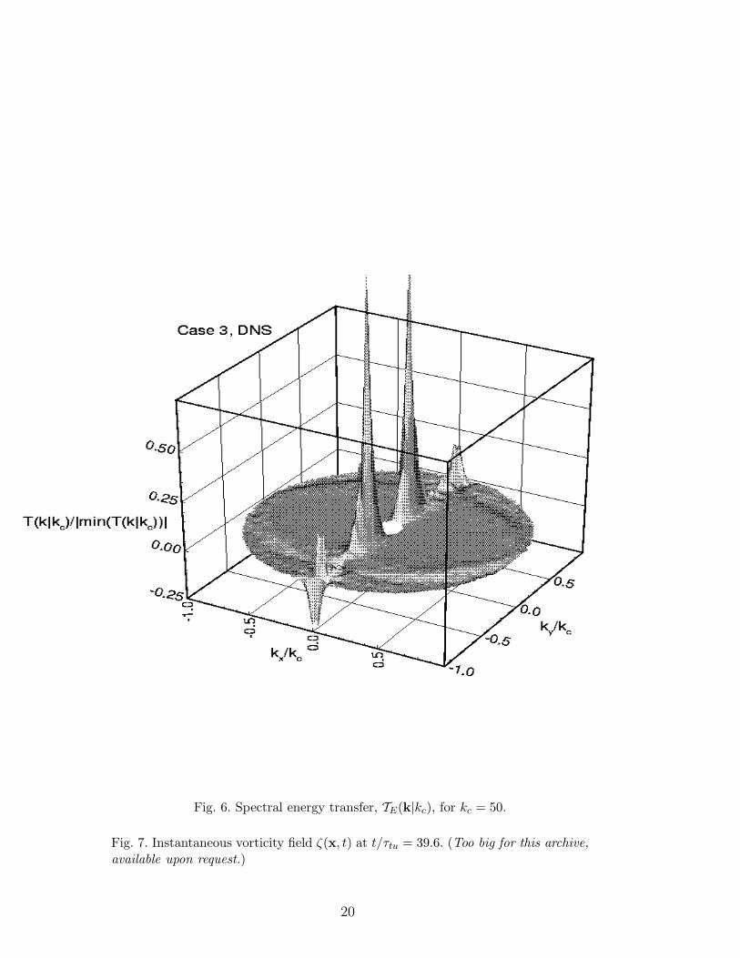
Fig. 6. Spectral energy transfer, TE(k|kc), for kc = 50.

Fig. 7. Instantaneous vorticity field ζ(x, t) at t/τtu = 39.6. (Too big for this archive,

available upon request.)

20

-5 0 5

0

2

4

6

-5 0 5

0

2

4

6

-5 0 5

0

2

4

6

-3.00004 -3.00002 -3

0

2

4

6

-3.00004 -3.00002 -3

0

2

4

6

-3.00004 -3.00002 -3

0

2

4

6

Fig. 8. Zonally-averaged velocity profile U(y, t) (left column) and its second deriva-tive Uyy(y, t) (right column) for Case 3 at (from top to bottom) t/τtu= 21.8, 39.6,and 59.4.

21

-2.0

-1.0

0.0

1.0

-1.0

-0.5

0.0

0.5

-1.0

-0.5

0.0

0.5

-1.0

-0.5

0.0

0.5

-1.0

-0.5

0.0

0.5

-2.0

-1.0

0.0

1.0

ky/kc

kx/kc

ν(k|kc)/|min(ν(k|kc))|

Case 2, theory

Fig. 9. RG-derived two-parametric viscosity normalized by the absolute value of itsminimum for β-plane turbulence. Parameter setting corresponds to Case 2 DNS.

22

Fig. 10. DNS-based two-parametric viscosity normalized by the absolute value ofits minimum for Case 2 of β-plane turbulence.

23

Fig. 11. Function N(k/kc) obtained from DNS (dots), TFM (dashed line) and RG(solid line) (from [12]).

24

Fig. 12. Evolution of the total energy E(t) (a) and enstrophy Ω(t) (b) in LES ofisotropic 2D turbulence. In (a) we also plot the evolution of E(t) with the energyof the 4th, 5th, 6th and 7th modes removed.

25

Fig. 13. Time averaged energy spectrum for LES of isotropic 2D turbulence. Thesolid line depicts the Kolmogorov −5/3 slope.

26