The effect of landscape-scale environmental drivers on the vegetation composition of British...

BIOLOGICAL

CONSERVATION

Biological Conservation 120 (2004) 491–505

www.elsevier.com/locate/biocon

The effect of landscape-scale environmental drivers on thevegetation composition of British woodlands

P.M. Corney a,*, M.G. Le Duc a, S.M. Smart b, K.J. Kirby c, R.G.H. Bunce b,1,R.H. Marrs a

a Applied Vegetation Dynamics Laboratory, School of Biological Sciences, University of Liverpool, P.O. Box 147, Liverpool L69 3GS, UKb Merlewood Research Station, Centre for Ecology and Hydrology, Grange-over-sands, Cumbria LA11 6JU, UK

c English Nature, Northminster House, Peterborough PE1 1UA, UK

Received 4 September 2003; received in revised form 16 March 2004; accepted 26 March 2004

Abstract

Assessment of factors influencing woodland vegetation composition across Britain was made using multivariate techniques to

analyse data gathered during the 1971 National Woodland Survey. Indirect gradient analysis (unconstrained ordination using

detrended correspondence analysis) suggested a gradient strongly associated with nutrient availability and pH. Direct gradient

analysis (constrained ordination using canonical correspondence analysis) and variation partitioning were used with over 250

ecophysiologically relevant variables, including climatic, geographical, soil and herbivore data, to model the response of woodland

vegetation. Although there was a high degree of multicollinearity between environmental variables, analysis revealed the vegetation

composition of surveyed woodlands to be primarily structured by geographical, climatic and soil gradients, in particular rainfall, soil

pH and accumulated temperature. The woods have recently been resurveyed. The results of this analysis therefore provide a baseline

against which species dynamics can be assessed under a series of conservation threats, such as land use and climate change.

� 2004 Elsevier Ltd. All rights reserved.

Keywords: National Woodland Survey; Environmental factors; Vegetation analysis; Canonical correspondence analysis; Variation partitioning

1. Introduction

Successful implementation of local and nationalwoodland conservation management goals requires an

understanding of the way in which key environmental

factors influence the ability of species to persist. Extant

classifications for woodlands in Britain (e.g. Bunce,

1982, 1989; Rodwell et al., 1991; Peterken, 1993;

Rackham, 2003) provide useful information regarding

species composition, history and management, while

* Corresponding author. Tel.: +44-151-794-4775; fax: +44-151-794-

4940.

E-mail address: [email protected] (P.M. Corney).1 Present address: Alterra, Landscape and Spatial Planning Section,

P.O. Box 47, 6700AA Wageningen, The Netherlands.

0006-3207/$ - see front matter � 2004 Elsevier Ltd. All rights reserved.

doi:10.1016/j.biocon.2004.03.022

Bunce and Shaw (1975) and Bunce (1981) assess the

principal gradients behind woodland vegetation in

Britain. However, little has been done to quantify therelative contribution of key environmental variables to

the determination of woodland species composition. In

this paper, we explore the relative impact of climate (e.g.

temperature, precipitation, atmospheric pollution), site

factors (e.g. altitude, edaphic factors) and land use on

woodland composition, using vegetation data collected

in 1971. We thus provide a baseline against which to

assess changes under a series of conservation threats,such as land use change, global warming and exotic

species invasion.

In fragmented landscapes, woodlands may act as

refugia, harbouring rare woodland plant communities,

which can act as a source of propagules for estab-

lishment of new communities in the wider landscape.

Since both persistence of species and dispersal ability

mail to: [email protected]

492 P.M. Corney et al. / Biological Conservation 120 (2004) 491–505

are significantly affected by environmental conditions,

it is important for the purposes of conservation sci-

ence that the effects of biotic and abiotic factors be

quantified.

Current factors affecting woodland composition anddistribution are diverse and their interactions complex.

They range from factors such as climate (Cannell,

2002; Williams et al., 2002) and topography (Mod-

rzynski and Eriksson, 2002), soil parent material and

time of soil development (Jenny, 1980), to management

(Brunet et al., 1996) and grazing by native ungulates,

such as deer (Kirby, 2001). Moreover, it is becoming

apparent that anthropogenic activity leading to climatechange (e.g. Bakkenes et al., 2002; Houghton et al.,

2001; Lasch et al., 2002; Mitchell and Karoly, 2001),

nitrogen deposition and acidification (Bobbink et al.,

1998; Brunet et al., 1998; Hofmeister et al., 2002) may

alter plant distribution, as species climatic envelopes

begin to shift geographically. Modification of local

climatic optima has particular significance for conser-

vation of woodland habitats in Britain, as it has beensuggested that a large proportion (30%) of woodland

plant species may be unable to colonise suitable target

habitats in fragmented areas after a period of 30–40

years (Honnay et al., 2002).

Thus, although management can profoundly effect

woodland vegetation distribution, assessing the true

impact of such can be problematic, as continental, re-

gional, countrywide and local scale environmental fac-tors also exert a considerable influence on the

performance of both higher and lower plants (Furness

and Grime, 1982; Redfern and Hendry, 2002; Yeo and

Blackstock, 2002). Accordingly, this paper reports a

study which aimed to partition the range of variation

within a sample of semi-natural woodlands in Britain in

terms of factors that operate at a range of scales (site to

countrywide) and through a variety of mechanisms(natural to anthropogenic, direct to diffuse), and are

likely to be important in driving the distribution and

composition of native woodlands.

The analysis presented here is based upon data col-

lected during the National Woodland Survey (NWS),

carried out by the Nature Conservancy of Britain in the

summer of 1971 using a standardised methodology

(Bunce and Shaw, 1973; Smart et al., 2001). Whilst thisproject was primarily about classification, the objectives

written in 1969 also specified examining principal un-

derlying environmental factors. Environmental data not

collected during the original survey but likely to be

important in controlling woodland species composition

were obtained from a variety of sources at the site scale.

Multivariate analyses were used to describe variation in

the dataset in relation to selected significant environ-mental variables and relative contribution of selected

groups of environmental variables was assessed using

variation partitioning.

2. Methods

2.1. National Woodland Survey site selection

In order to cover the range of variation within semi-natural woodlands, selection of sites in 1971 was made

from a survey of 2463 woodland sites (>4.05 ha) car-

ried out for the Nature Conservation Review (Ratcliffe,

1977). This site series represented approximately a 10%

sample of the population of semi-natural woodlands in

Britain (Bunce and Shaw, 1972, 1973). Full historical

background is given by Sheail and Bunce (2003). As-

sociation analysis (Williams and Lambert, 1959) per-formed on this dataset divided the 2463 sites into 103

groups defined by their similarity of plant species

composition (Hill et al., 1975). Numerical analysis of

topographical and climatic data was then used to select

a representative site from each group (Bunce and

Shaw, 1973). These 103 sites were surveyed for NWS

1971. Site locations are shown in Fig. 1, grouped into

Countryside Vegetation System (CVS) classes (Barret al., 1993; Bunce et al., 1999) generated from site

species data using the Modular Analysis of Vegetation

Information System (MAVIS) Plot Analyser, version

1.0 (Smart, 2000).

2.2. NWS methodology

For each of the 103 sites, a sample size of 16 pointswas fixed and marked on 1:25,000 Ordnance Survey

(OS) site maps prior to survey within the delin-

eated woodland area, representing the location of sur-

vey plots (Bunce and Shaw, 1973). Survey of all 1648

14.14� 14.14 m (200 m2) plots was carried out between

June and October 1971 by separate teams of trained

surveyors (Bunce and Shaw, 1973; Hill et al., 1975).

Estimates of cover (5% classes) were made across each200 m2 plot, for individual ground flora species, along

with six additional ground cover categories; bryophyte

cover, litter, dead wood material, rock, bare ground and

standing water (Smart et al., 2001). Woody species

(trees, saplings and shrubs) and bryophyte species

present within each plot were also assessed. Plot slope

and aspect were recorded, along with plot- and site-scale

descriptions, including signs of seven groups of herbiv-orous mammals (sheep, red deer, other deer species,

cattle, horses/ponies, rabbits, squirrels) and boundary

types such as intact walls, ditches and derelict fences. A

single soil sample was taken from each plot for assess-

ment of pH and loss-on-ignition. Diagnostic soil profile

details were recorded in the field (Bunce and Shaw,

1973) and soil subgroup classes were assigned to each

soil sample using Avery’s (1980) classification system.For further description of NWS methods, see Bunce and

Shaw (1973). Table 1 gives a breakdown of those vari-

ables available for, and used in, the present analysis.

Fig. 1. Distribution of sites surveyed in the 1971 National Woodland Survey of Britain. Sites are illustrated according to Countryside Vegetation

System (Barr et al., 1993; Bunce et al., 1999) classes.

P.M. Corney et al. / Biological Conservation 120 (2004) 491–505 493

2.3. Use of NWS botanical data

To facilitate examination of between-site variation,

within-site variation was explicitly omitted by aggre-

gating botanical data for all 16 plots per site. Although

cover data were available for field layer species, data for

the complete vegetation complement (bryophytes, field,

sapling, shrub and tree layer species) were only availableas presence/absence. Analysis therefore proceeded on

the basis of full botanical complement of species present

within each site as present or absent only.

2.4. Potential environmental drivers of woodland compo-

sition

One hundred eighty six additional environmental

variables likely to affect woodland species composi-tion were assembled and amalgamated into groups

Table 1

Description of the nature and transformation of variable sets obtained from National Woodland Survey 1971 data and used in the analysis presented

here

Variable set Description of original data T Description of data used in analysis V No.

Animals Plot level presence or absence

(sight, signs, sounds) of seven

herbivorous mammal species

s Intensity of herbivore grazing pressure by site d 7

Site boundary type Site level presence or absence of different

boundary types

u Site level presence or absence of different

boundary types

b 17

Date Month during which woodland was

surveyed

u Month surveyed. Used as five dummy

variables.

b 1 (5)

Edaphic Plot level soil pH; LOI (%); depth to each soil

horizon (A00, litter layer; A0, organic layer;

A1, mixed mineral/organic layer; A2, leached or

eluviated layer; B, weathered mineral layer)

present (cm)

a Site level soil pH; c 7

g, t Site level LOI;

a Site level cumulative depth to the

bottom of five soil horizons (cm)

Geographic,

regionality

National Grid easting and northing (km)

of site datum

u Easting and northing (km) of site datum c 2

Geographic,

micro-climatic

Plot level slope, the steepest gradient passing

through plot centre (deg) and aspect (deg)

a Average slope of site (deg); c 3

g Transformation (s) of aspect (a, degrees,the site-wise mean), s ¼ sinða� p=180Þ=2,giving a site level southerly aspect;

g Transformation (w) of aspect (a, degrees,the site-wise mean),

w ¼ j sinðða� p=180Þ � p=2Þ=2Þj, giving a site

level westerly aspect

Ground cover

categories

Plot level cover (%) of ground cover estimated

within 14.14� 14.14 m quadrats

g, t Site level estimate of six ground cover types

(bryophyte cover, litter, dead wood material,

rock, bare ground and standing water)

c 6

Soil classification Soil sub groups present in each plot.

Where more than one subgroup occurred

in each plot, the mosaic was assumed

to comprise equal amounts of each constituent

subgroup

a, t Arithmetic average of proportion of

subgroups present in plots, giving the

proportion of 26 soil groups present

within each site;

c 33

a, t As above, giving the proportion of seven

major soil groups present within each site

T – transformation used: a, arithmetic average of plot data by site; g, geometric average of plot data by site; s, sum of plot data by site; t, arcsine

transformation of data (Sokal and Rohlf, 1995); u, untransformed site level data.

V– variable type: b, binary; c, continuous; d, discrete.

No. – number of variables per set used in this analysis.


containing landscape, spatial, anthropogenic and cli-

matic variables. Data for 33 variables, the Centre for

Ecology and Hydrology (CEH) satellite Land Cover

Map 2000 (LCM 2000) classes, woodland spatial vari-

ables, nitrogenous deposition data and distance to the

sea, were only available at the site level. However for

other variables (e.g. altitude), plot level data were ob-

tained using plot OS grid references generated using thesoftware package ERDAS IMAGINE version 8.5

(ERDAS, 2001). These results were then aggregated for

each site, to produce an appropriate mean site value for

each variable. Using a full series of 103 digital site map

images, ERDAS IMAGINE was also employed to cal-

culate length of delineated woodland perimeter and

area. These measures of woodland perimeter (Pw) (km)

and area (Aw) (ha) were then used to generate twowoodland shape indices, a perimeter index, after Hinsley

et al. (1995), and an area index. The perimeter index was

calculated as PwPc, where Pc was the perimeter of a hy-

pothetical circular site of the same area. Thus the pe-

rimeter index of a wood is high for woods with scalloped

or jagged edges. The area index was described using an

index calculated as Aw=Pw. This second index contrasts

circular woodlands with those that tend towards a more

ellipsoidal shape. Presence and effect of possible spatial

autocorrelation was assessed using seven terms of qua-dratic and cubic trend surface, derived from site geo-

graphical co-ordinates (e.g. Yeo and Blackstock, 2002).

Distance to the sea, calculated as the minimum dis-

tance from site OS datum point to the nearest coast was

computed with MINDIST2, a FORTRAN77 program

using a set of digitised UK coastal co-ordinates, com-

prising 1550 points (Le Duc et al., 2000).

Plot altitude was extracted from Land-Form PAN-ORAMA Digital Terrain Model contour maps held on

the OS DIGIMAP service (EDINA, 2002), using OS


plot co-ordinates generated as outlined above, MAP

MANAGER version 6.2 (ESRI, 2001), ARCVIEW GIS

version 3.2a (ESRI, 2000), and the Avenue Script

GETGRIDVALUE (Elmquist and Davies, 1999).

Climatic data were drawn from two sources: theMeteorological Office and the Forestry Commission.

Monthly and yearly Meteorological Office 5 km� 5 km

grid baseline data were acquired for generated plot co-

ordinates from long term average (LTA) datasets for the

period 1961 to 1990 and 1961 to 2000, respectively,

produced in association with the UK Climate Impacts

Programme, UKCIP (Meteorological Office, 2003). This

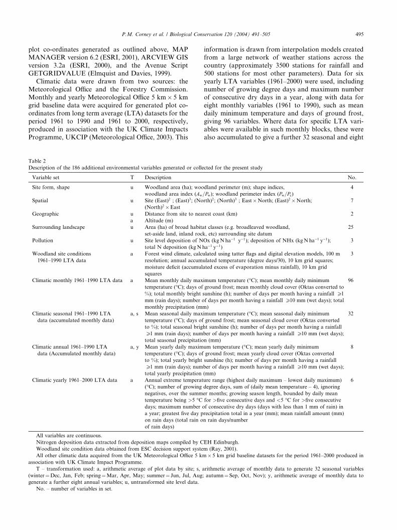
Table 2

Description of the 186 additional environmental variables generated or colle

Variable set T Description

Site form, shape u Woodland area (ha); woo

woodland area index (Aw

Spatial u Site (East)2 ; (East)3; (No

(North)2 �East

Geographic u Distance from site to nea

a Altitude (m)

Surrounding landscape u Area (ha) of broad habita

set-aside land, inland roc

Pollution u Site level deposition of N

total N deposition (kgNh

Woodland site conditions

1961–1990 LTA data

a Forest wind climate, calc

resolution; annual accum

moisture deficit (accumul

squares

Climatic monthly 1961–1990 LTA data a Mean monthly daily max

temperature (�C); days of%); total monthly bright

mm (rain days); number o

monthly precipitation (m

Climatic seasonal 1961–1990 LTA

data (accumulated monthly data)

a, s Mean seasonal daily max

temperature (�C); days ofto %); total seasonal brig

P1 mm (rain days); num

total seasonal precipitatio

Climatic annual 1961–1990 LTA

data (Accumulated monthly data)

a, y Mean yearly daily maxim

temperature (�C); days ofto %); total yearly bright

P1 mm (rain days); num

total yearly precipitation

Climatic yearly 1961–2000 LTA data a Annual extreme temperat

(�C); number of growing

negatives, over the summ

temperature being >5 �Cdays; maximum number o

a year; greatest five day p

on rain days (total rain o

of rain days)

All variables are continuous.

Nitrogen deposition data extracted from deposition maps compiled by C

Woodland site condition data obtained from ESC decision support syste

All other climatic data acquired from the UK Meteorological Office 5 km

association with UK Climate Impact Programme.

T – transformation used: a, arithmetic average of plot data by site; s, a

(winter¼Dec, Jan, Feb; spring¼Mar, Apr, May; summer¼ Jun, Jul, Aug

generate a further eight annual variables; u, untransformed site level data.

No. – number of variables in set.

information is drawn from interpolation models created

from a large network of weather stations across the

country (approximately 3500 stations for rainfall and

500 stations for most other parameters). Data for six

yearly LTA variables (1961–2000) were used, includingnumber of growing degree days and maximum number

of consecutive dry days in a year, along with data for

eight monthly variables (1961 to 1990), such as mean

daily minimum temperature and days of ground frost,

giving 96 variables. Where data for specific LTA vari-

ables were available in such monthly blocks, these were

also accumulated to give a further 32 seasonal and eight

cted for the present study

No.

dland perimeter (m); shape indices,

=Pw); woodland perimeter index (Pw=Pc)4

rth)2; (North)3 ; East�North; (East)2 �North; 7

rest coast (km) 2

t classes (e.g. broadleaved woodland,

k, etc) surrounding site datum

25

Ox (kgNha�1 y�1); deposition of NHx (kgNha�1 y�1);

a�1 y�1)

3

ulated using tatter flags and digital elevation models, 100 m

ulated temperature (degree days/30), 10 km grid squares;

ated excess of evaporation minus rainfall), 10 km grid

3

imum temperature (�C); mean monthly daily minimum

ground frost; mean monthly cloud cover (Oktas converted to

sunshine (h); number of days per month having a rainfall P1

f days per month having a rainfall P10 mm (wet days); total

m)

96

imum temperature (�C); mean seasonal daily minimum

ground frost; mean seasonal cloud cover (Oktas converted

ht sunshine (h); number of days per month having a rainfall

ber of days per month having a rainfall P10 mm (wet days);

n (mm)

32

um temperature (�C); mean yearly daily minimum

ground frost; mean yearly cloud cover (Oktas converted

sunshine (h); number of days per month having a rainfall

ber of days per month having a rainfall P10 mm (wet days);

(mm)

8

ure range (highest daily maximum – lowest daily maximum)

degree days, sum of (daily mean temperature – 4), ignoring

er months; growing season length, bounded by daily mean

for >five consecutive days and <5 �C for >five consecutive

f consecutive dry days (days with less than 1 mm of rain) in

recipitation total in a year (mm); mean rainfall amount (mm)

n rain days/number

6

EH Edinburgh.

m (Ray, 2001).

� 5 km grid baseline datasets for the period 1961–2000 produced in

rithmetic average of monthly data to generate 32 seasonal variables

; autumn¼ Sep, Oct, Nov); y, arithmetic average of monthly data to


annual values. Woodland site condition data were ob-

tained from the Ecological Site Classification (ESC)

decision support system published by the Forestry

Commission (Ray, 2001), comprising a windiness score,

accumulated temperature and moisture deficit data forthe 30-year period 1961–1990.

Oxidised (NOx) and reduced (NHx) nitrogen (N)

deposition data (sum of wet, dry and cloud deposition)

for surveyed woodlands were extracted from 5� 5 km

resolution national deposition maps (1995–1997) com-

piled by CEH Edinburgh and derived using methods

described in NEGTAP (2001). NOx and NHx were

summed to generate total N deposition entered as athird pollutant variable in analyses. Although a measure

of total N deposition generated in this way is unlikely to

be independent of its constituent parts, this facilitated

an examination of possible responses to total N load.

Current landscape-scale habitat data constructed

from satellite images were obtained from CEH LCM

2000 (Fuller et al., 2002). LCM subclass level-two hab-

itats found within a circular area of radius of 1500 msurrounding each site OS datum were selected. Table 2

gives a summary of additional environmental variables

used.

2.5. Statistical analyses

All statistical analyses were carried out using CA-

NOCO for Windows version 4.5 (Ter Braak and �Smil-auer, 2002), using default settings and untransformed

species data, unless otherwise specified.

Detrended Correspondence Analysis (DCA) was used

to obtain estimates of gradient lengths in standard de-

viation (SD) units of species turnover (Ter Braak and�Smilauer, 2002), thereby assisting in the decision of

whether to use a linear or unimodal approach to the

data.Principle Components Analysis (PCA) was employed

with both original survey variables (Table 1) and addi-

tional variables (Table 2) for preliminary exploration of

environmental factors only.

The full range of variables was then used, either as

environmental variables or covariables, in different

combinations, along with botanical data, to assess the

influence of environmental factors on vegetation varia-tion, using the CANOCO Canonical Correspondence

Analysis (CCA) forward selection procedure. Forward

selection was used to select significant variables, the

Monte Carlo test being used to assess significance, with

499 permutations for exploratory analyses and 9999 for

final results (Legendre and Legendre, 1998). In all per-

mutation tests, an unrestricted permutation structure

was used. This process was combined with an exami-nation of inflation values, to remove those variables that

were highly multicollinear. If an inflation factor is large,

the variable is likely to be strongly correlated with other

variables (Ter Braak and �Smilauer, 2002). As a result,

the effects of different environmental variables on com-

munity composition cannot be separated out and con-

sequently, canonical coefficients are unstable and do not

merit interpretation (Ter Braak, 1986). Therefore, vari-ables exhibiting high inflation values coupled with low

or non-significance were removed and analysis re-run,

until a set of significant variables was obtained, with

inflation factors of <15. The final model contained 20

variables.

Significant variables selected were divided into three

clearly defined and ecologically meaningful sets; biotic

factors, soil properties and geographical with climatic(geo-climatic) variables. Variation partitioning was

carried out using a standardised procedure (e.g. Borcard

et al., 1992; Marrs and Le Duc, 2000; Yeo and Black-

stock, 2002), variance in the data being partitioned be-

tween these sets and expressed as a percentage of the

total variation explained.

3. Results

3.1. Description of survey sites

Site summary data are presented in Table 3 according

to CVS vegetation classes (Barr et al., 1993; Bunce et al.,

1999; Smart, 2000). The sites covered an extremely wide

geographic range (Fig. 1) and showed considerablephysiographic variability (Table 3), while the wide

range of vegetation types encountered reflects the high

b-diversity within the dataset.

3.2. Range of variation in native semi-natural woodland

communities

Preliminary DCA produced an ordination with a firstaxis gradient length of 3.266 SD units, demonstrating

high b-diversity and suggesting that a unimodal model

such as CCA would adequately describe the relationship

between species and environmental variables (Ter Braak

and Prentice, 1988; Ter Braak and �Smilauer, 2002).

Nevertheless, initial CCA results described using

CANODRAW (Ter Braak and �Smilauer, 2002) revealed

an apparent distortion. Subsequent data explorationrevealed the distortion to be due to a large number (151)

of species, each of which occurred only once within the

dataset (25% of all species recorded) and one outlying

site. As CCA is sensitive to deviant sites when they are

outliers with regard to both species composition and

environment, the 151 species were made supplementary

in further analysis, as recommended by Ter Braak and

Prentice (1988). Species made passive in this way do notinfluence ordination axes, but are added to ordination

diagrams so that their relationship to other species can

be examined. Rare species were also down-weighted,

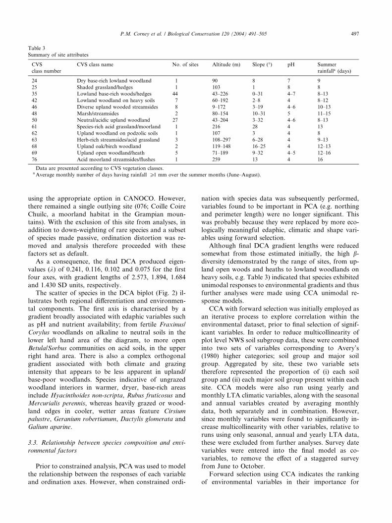
Table 3

Summary of site attributes

CVS

class number

CVS class name No. of sites Altitude (m) Slope (�) pH Summer

rainfalla (days)

24 Dry base-rich lowland woodland 1 90 8 7 9

25 Shaded grassland/hedges 1 103 1 8 8

35 Lowland base-rich woods/hedges 44 43–226 0–31 4–7 8–13

42 Lowland woodland on heavy soils 7 60–192 2–8 4 8–12

46 Diverse upland wooded streamsides 8 9–172 3–19 4–6 10–13

48 Marsh/streamsides 2 80–154 10–31 5 11–15

50 Neutral/acidic upland woodland 27 43–204 3–32 4–6 8–13

61 Species-rich acid grassland/moorland 1 216 28 4 13

62 Upland woodland on podzolic soils 1 107 3 4 8

63 Herb-rich streamsides/acid grassland 3 108–297 6–28 4 9–13

68 Upland oak/birch woodland 2 119–148 16–25 4 12–13

69 Upland open woodland/heath 5 71–189 9–32 4–5 12–16

76 Acid moorland streamsides/flushes 1 259 13 4 16

Data are presented according to CVS vegetation classes.aAverage monthly number of days having rainfall P1 mm over the summer months (June–August).


using the appropriate option in CANOCO. However,

there remained a single outlying site (076; Coille Coire

Chuilc, a moorland habitat in the Grampian moun-

tains). With the exclusion of this site from analyses, inaddition to down-weighting of rare species and a subset

of species made passive, ordination distortion was re-

moved and analysis therefore proceeded with these

factors set as default.

As a consequence, the final DCA produced eigen-

values (k) of 0.241, 0.116, 0.102 and 0.075 for the first

four axes, with gradient lengths of 2.573, 1.894, 1.684

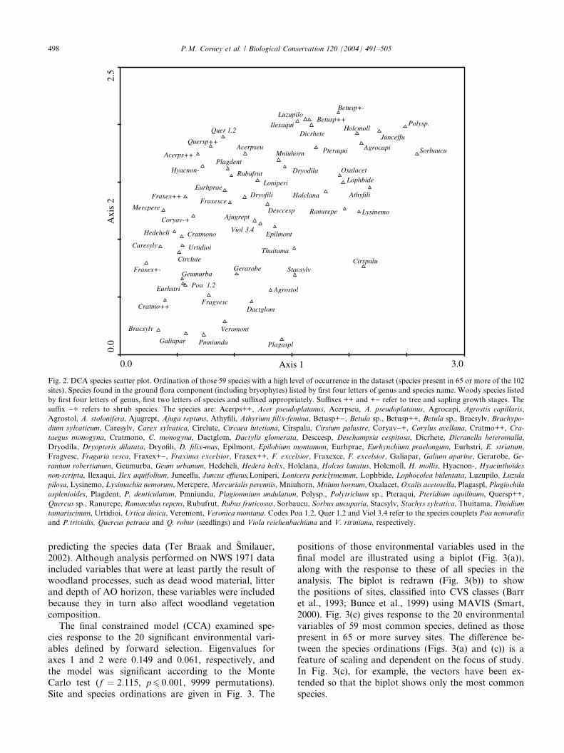
and 1.430 SD units, respectively.The scatter of species in the DCA biplot (Fig. 2) il-

lustrates both regional differentiation and environmen-

tal components. The first axis is characterised by a

gradient broadly associated with edaphic variables such

as pH and nutrient availability; from fertile Fraxinus/

Corylus woodlands on alkaline to neutral soils in the

lower left hand area of the diagram, to more open

Betula/Sorbus communities on acid soils, in the upperright hand area. There is also a complex orthogonal

gradient associated with both climate and grazing

intensity that appears to be less apparent in upland/

base-poor woodlands. Species indicative of ungrazed

woodland interiors in warmer, dryer, base-rich areas

include Hyacinthoides non-scripta, Rubus fruticosus and

Mercurialis perennis, whereas heavily grazed or wood-

land edges in cooler, wetter areas feature Cirsium

palustre, Geranium robertianum, Dactylis glomerata and

Galium aparine.

3.3. Relationship between species composition and envi-

ronmental factors

Prior to constrained analysis, PCA was used to model

the relationship between the responses of each variableand ordination axes. However, when constrained ordi-

nation with species data was subsequently performed,

variables found to be important in PCA (e.g. northing

and perimeter length) were no longer significant. This

was probably because they were replaced by more eco-logically meaningful edaphic, climatic and shape vari-

ables using forward selection.

Although final DCA gradient lengths were reduced

somewhat from those estimated initially, the high b-diversity (demonstrated by the range of sites, from up-

land open woods and heaths to lowland woodlands on

heavy soils, e.g. Table 3) indicated that species exhibited

unimodal responses to environmental gradients and thusfurther analyses were made using CCA unimodal re-

sponse models.

CCA with forward selection was initially employed as

an iterative process to explore correlation within the

environmental dataset, prior to final selection of signif-

icant variables. In order to reduce multicollinearity of

plot level NWS soil subgroup data, these were combined

into two sets of variables corresponding to Avery’s(1980) higher categories; soil group and major soil

group. Aggregated by site, these two variable sets

therefore represented the proportion of (i) each soil

group and (ii) each major soil group present within each

site. CCA models were also run using yearly and

monthly LTA climatic variables, along with the seasonal

and annual variables created by averaging monthly

data, both separately and in combination. However,since monthly variables were found to significantly in-

crease multicollinearity with other variables, relative to

runs using only seasonal, annual and yearly LTA data,

these were excluded from further analyses. Survey date

variables were entered into the final model as co-

variables, to remove the effect of a staggered survey

from June to October.

Forward selection using CCA indicates the rankingof environmental variables in their importance for

0.0 3.0

0.0

2.5

Acerpseu

Agrostol

Agrocapi

Ajugrept

Athyfili

Bracsylv

Caresylv

Circlute Cirspalu

Cratmono

Dactglom

Desccesp

Dryodila

Dryofili

Hyacnon-

Epilmont

Fragvesc

Fraxexce

Galiapar

GerarobeGeumurba

Hedeheli

Holclana

HolcmollIlexaqui

Junceffu

Loniperi

Luzupilo

LysinemoMercpere

Oxalacet

Pteraqui

Ranurepe

Rubufrut

Sorbaucu

Stacsylv

Urtidioi

Veromont

Poa 1.2

Quer 1.2

Viol 3.4

Dicrhete

Eurhprae

Eurhstri

Lophbide

Mniuhorn

Plagaspl

Plagdent

Pmniundu

Polysp.

Thuitama

Acerps++

Betusp++

Cratmo++

Fraxex++

Quersp++

Betusp+-

Fraxex+-

Coryav-+

Axis 1

Axi

s 2

Fig. 2. DCA species scatter plot. Ordination of those 59 species with a high level of occurrence in the dataset (species present in 65 or more of the 102

sites). Species found in the ground flora component (including bryophytes) listed by first four letters of genus and species name. Woody species listed

by first four letters of genus, first two letters of species and suffixed appropriately. Suffixes ++ and +) refer to tree and sapling growth stages. The

suffix )+ refers to shrub species. The species are: Acerps++, Acer pseudoplatanus, Acerpseu, A. pseudoplatanus, Agrocapi, Agrostis capillaris,

Agrostol, A. stolonifera, Ajugrept, Ajuga reptans, Athyfili, Athyrium filix-femina, Betusp+), Betula sp., Betusp++, Betula sp., Bracsylv, Brachypo-

dium sylvaticum, Caresylv, Carex sylvatica, Circlute, Circaea lutetiana, Cirspalu, Cirsium palustre, Coryav)+, Corylus avellana, Cratmo++, Cra-

taegus monogyna, Cratmono, C. monogyna, Dactglom, Dactylis glomerata, Desccesp, Deschampsia cespitosa, Dicrhete, Dicranella heteromalla,

Dryodila, Dryopteris dilatata, Dryofili, D. filix-mas, Epilmont, Epilobium montanum, Eurhprae, Eurhynchium praelongum, Eurhstri, E. striatum,

Fragvesc, Fragaria vesca, Fraxex+), Fraxinus excelsior, Fraxex++, F. excelsior, Fraxexce, F. excelsior, Galiapar, Galium aparine, Gerarobe, Ge-

ranium robertianum, Geumurba, Geum urbanum, Hedeheli, Hedera helix, Holclana, Holcus lanatus, Holcmoll, H. mollis, Hyacnon-, Hyacinthoides

non-scripta, Ilexaqui, Ilex aquifolium, Junceffu, Juncus effusus,Loniperi, Lonicera periclymenum, Lophbide, Lophocolea bidentata, Luzupilo, Luzula

pilosa, Lysinemo, Lysimachia nemorum, Mercpere,Mercurialis perennis, Mniuhorn,Mnium hornum, Oxalacet, Oxalis acetosella, Plagaspl, Plagiochila

asplenioides, Plagdent, P. denticulatum, Pmniundu, Plagiomnium undulatum, Polysp., Polytrichum sp., Pteraqui, Pteridium aquilinum, Quersp++,

Quercus sp., Ranurepe, Ranunculus repens, Rubufrut, Rubus fruticosus, Sorbaucu, Sorbus aucuparia, Stacsylv, Stachys sylvatica, Thuitama, Thuidium

tamariscinum, Urtidioi, Urtica dioica, Veromont, Veronica montana. Codes Poa 1.2, Quer 1.2 and Viol 3.4 refer to the species couplets Poa nemoralis

and P.trivialis, Quercus petraea and Q. robur (seedlings) and Viola reichenbachiana and V. riviniana, respectively.


predicting the species data (Ter Braak and �Smilauer,

2002). Although analysis performed on NWS 1971 dataincluded variables that were at least partly the result of

woodland processes, such as dead wood material, litter

and depth of AO horizon, these variables were included

because they in turn also affect woodland vegetation

composition.

The final constrained model (CCA) examined spe-

cies response to the 20 significant environmental vari-

ables defined by forward selection. Eigenvalues foraxes 1 and 2 were 0.149 and 0.061, respectively, and

the model was significant according to the Monte

Carlo test (f ¼ 2:115, p6 0:001, 9999 permutations).

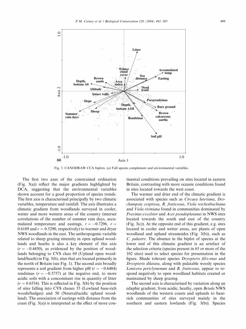
Site and species ordinations are given in Fig. 3. The

positions of those environmental variables used in the

final model are illustrated using a biplot (Fig. 3(a)),along with the response to these of all species in the

analysis. The biplot is redrawn (Fig. 3(b)) to show

the positions of sites, classified into CVS classes (Barr

et al., 1993; Bunce et al., 1999) using MAVIS (Smart,

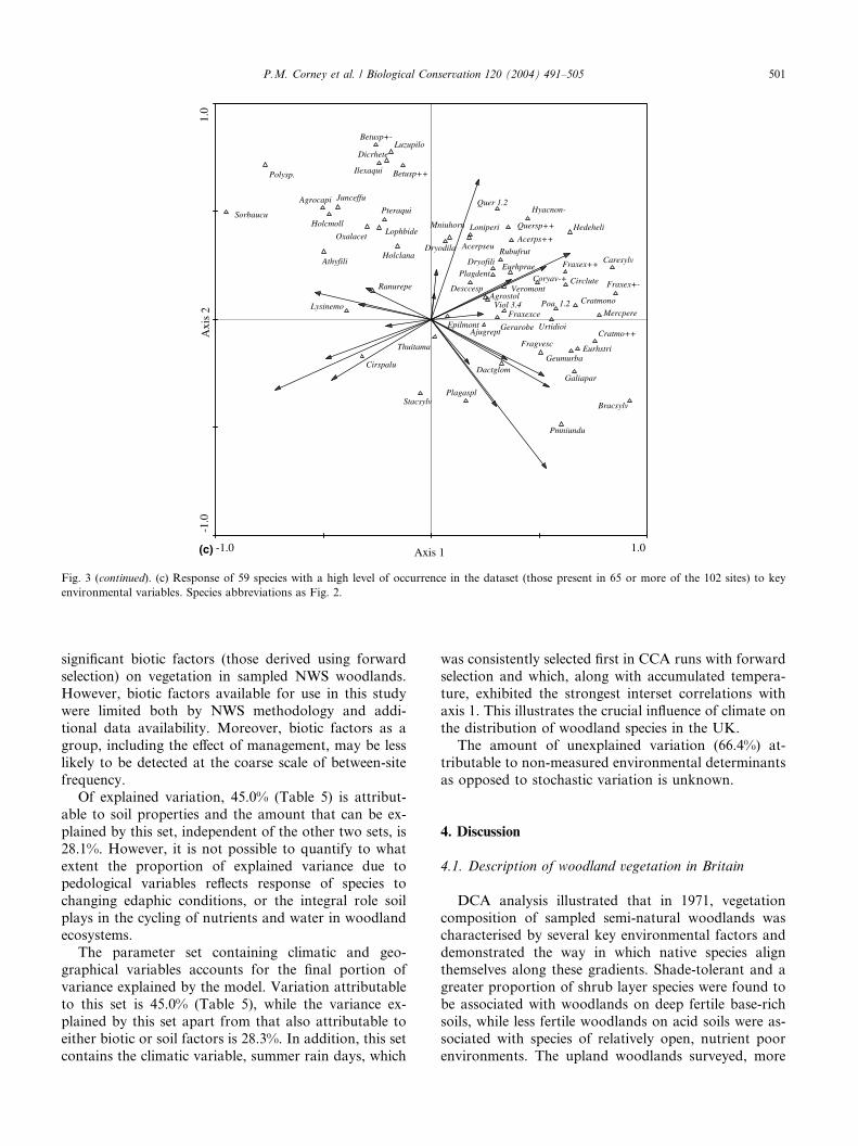
2000). Fig. 3(c) gives response to the 20 environmental

variables of 59 most common species, defined as those

present in 65 or more survey sites. The difference be-

tween the species ordinations (Figs. 3(a) and (c)) is afeature of scaling and dependent on the focus of study.

In Fig. 3(c), for example, the vectors have been ex-

tended so that the biplot shows only the most common

species.

-1.0 1.0

-1.0

1.0

Sheep

Intact walls

Soil pH

Depth,

Depth,

AreaEasting

Sea

Altitude

Slope

Litter

Dead

Bare ground

Rendzinas

Pararendzinas

Brown

Brown

Winter

Summer

Accumulated

Axis 1

Axi

s 2

temp

distance

wood

calcareous

bottom A1H

rain days

bottom A0 index

cloudcover

earths

sands

(a)

Fig. 3. CANODRAW CCA biplots. (a) Full species complement and environmental variables.


The first two axes of the constrained ordination

(Fig. 3(a)) reflect the major gradients highlighted by

DCA, suggesting that the environmental variables

shown account for a good proportion of species trends.

The first axis is characterised principally by two climatic

variables, temperature and rainfall. The axis illustrates a

climatic gradient from woodlands surveyed in cooler,

wetter and more western areas of the country (intersetcorrelations of the number of summer rain days, accu-

mulated temperature and eastings, r ¼ �0:7296, r ¼0:6189 and r ¼ 0:5290, respectively) to warmer and dryer

NWS woodlands in the east. The anthropogenic variable

related to sheep grazing intensity in open upland wood-

lands and heaths is also a key element of this axis

(r ¼ �0:4450), as evidenced by the position of wood-

lands belonging to CVS class 69 (Upland open wood-land/heath) in Fig. 3(b), sites that are located primarily in

the north of Britain (see Fig. 1). The second axis broadly

represents a soil gradient from higher pH (r ¼ �0:6484)rendzinas (r ¼ �0:3757) at the negative end, to more

acidic soils with a concomitant rise in quantity of litter

(r ¼ 0:6554). This is reflected in Fig. 3(b) by the position

of sites falling into CVS classes 35 (Lowland base-rich

woods/hedges) and 50 (Neutral/acidic upland wood-land). The association of eastings with distance from the

coast (Fig. 3(a)) is interpreted as the effect of more con-

tinental conditions prevailing on sites located in eastern

Britain, contrasting with more oceanic conditions found

in sites located towards the west coast.

The warmer and drier end of the climatic gradient is

associated with species such as Circaea lutetiana, Des-

champsia cespitosa, R. fruticosus, Viola reichenbachiana

and Viola riviniana found in communities dominated by

Fraxinus excelsior and Acer pseudoplatanus in NWS siteslocated towards the south and east of the country

(Fig. 3(c)). At the opposite end of this gradient, e.g. sites

located in cooler and wetter areas, are plants of open

woodland and upland streamsides (Fig. 3(b)), such as

C. palustre. The absence in the biplot of species at the

lower end of this climatic gradient is an artefact of

the selection criteria (species present in 65 or more of the

102 sites) used to select species for presentation in thefigure. Shade tolerant species Dryopteris filix-mas and

Dryopteris dilatata, along with palatable woody species

Lonicera periclymenum and R. fruticosus, appear to re-

spond negatively to open woodland habitats created or

maintained by sheep grazing.

The second axis is characterised by variation along an

edaphic gradient, from acidic, heathy, open Betula NWS

woodlands of the western coasts and uplands to base-rich communities of sites surveyed mainly in the

southern and eastern lowlands (Fig. 3(b)). Species

-1.0 1.0

-1.0

1.0

Axis 1

Axi

s 2

(b)

Fig. 3 (continued). (b) Environmental variables and sites, given in CVS classes. CVS class symbols: 61 Species-rich acid grassland/moorland, ; 25

Shaded grassland/hedges, ; 63 Herb-rich streamsides/acid grassland, ; 46 Diverse upland wooded streamsides, N; 48 Marsh/streamsides, ; 68

Upland oak/birch woodland,j; 62 Upland woodland on podzolic soils, ; 69 Upland open woodland/heath, ; 50 Neutral/acidic upland woodland,

�; 24 Dry base-rich lowland woodland, s; 42 Lowland woodland on heavy soils, d; 35 Lowland base-rich woodland/hedges, .


typical of more shallow, acid or lighter soils at the

negative end of this gradient (Fig. 3(c)) include Poly-

trichum sp., often found on wet heaths, moorland and

streamsides in woodland, along with Luzula pilosa,

common among heather, leaf-litter, or moss-dominated

sites, and under Sorbus aucuparia. These communities

are also often found at higher altitudes and exhibit a

more open character associated with higher field layerspecies diversity. In contrast, at the positive end of this

gradient are Geum urbanum, M. perennis, Ajuga reptans

and Plagiomnium undulatum, species found in woodland

on deep, fertile, neutral to base-rich soils which are more

common in the lowlands where dense stands and pro-

nounced shrub layers are associated with greater

amounts of bare ground. The Quercus species, Pteridium

aquilinum and D. dilatata, all species that contributesignificantly to woodland litter production, are found to

be strongly associated with this variable (Fig. 3(c)).

3.4. Assessing the relative contribution of environmental

factors to species composition

The 20 significant environmental variables were di-

vided into three sets (biotic factors, geo-climatic vari-

ables and soil properties), each with similar numbers of

variables (Table 4).

Total inertia was 1.748, estimated total variation

explained (Borcard et al., 1992) was 0.587 and total

variation in the data explained by all three variable

sets was 33.6%. At this level, the variables selected can

be considered to be strongly associated with the

structure of the woodland communities sampled, withregard to between-site species coincidence. The results

of variation partitioning indicating the relative im-

portance of sets of variables in determining broad-

scale woodland vegetation patterns are illustrated

(Fig. 4). There was very little overlap in the variation

accounted for by each of the sets in this model, sug-

gesting only modest interaction between the variable

groups used.Of the total variation in the dataset explained,

36.6% (Table 5) can be attributed to biotic factors on

their own, of which anthropogenic influences are a

part. When soil and geo-climatic sets are included,

20.6% is attributable to biotic variables, the remainder

being as likely to be explained by the other variable

sets, because of their inter-correlation. Variation par-

titioning therefore suggests a moderate impact of

-1.0 1.0

-1.0

1.0

Acerpseu

Agrostol

Agrocapi

Ajugrept

Athyfili

Bracsylv

Caresylv

Circlute

Cirspalu

Cratmono

Dactglom

Desccesp

Dryodila

Dryofili

Hyacnon-

Epilmont

Fragvesc

Fraxexce

Galiapar

Gerarobe

Geumurba

Hedeheli

Holclana

Holcmoll

Ilexaqui

Junceffu

Loniperi

Luzupilo

LysinemoMercpere

Oxalacet

Pteraqui

Ranurepe

Rubufrut

Sorbaucu

Stacsylv

Urtidioi

Veromont

Poa 1.2

Quer 1.2

Viol 3.4

Dicrhete

Eurhprae

Eurhstri

LophbideMniuhorn

Plagaspl

Plagdent

Pmniundu

Polysp.

Thuitama

Acerps++

Betusp++

Cratmo++

Fraxex++

Quersp++

Betusp+-

Fraxex+-Coryav-+

Axis 1

Axi

s 2

(c)

Fig. 3 (continued). (c) Response of 59 species with a high level of occurrence in the dataset (those present in 65 or more of the 102 sites) to key

environmental variables. Species abbreviations as Fig. 2.


significant biotic factors (those derived using forward

selection) on vegetation in sampled NWS woodlands.

However, biotic factors available for use in this study

were limited both by NWS methodology and addi-

tional data availability. Moreover, biotic factors as a

group, including the effect of management, may be less

likely to be detected at the coarse scale of between-site

frequency.Of explained variation, 45.0% (Table 5) is attribut-

able to soil properties and the amount that can be ex-

plained by this set, independent of the other two sets, is

28.1%. However, it is not possible to quantify to what

extent the proportion of explained variance due to

pedological variables reflects response of species to

changing edaphic conditions, or the integral role soil

plays in the cycling of nutrients and water in woodlandecosystems.

The parameter set containing climatic and geo-

graphical variables accounts for the final portion of

variance explained by the model. Variation attributable

to this set is 45.0% (Table 5), while the variance ex-

plained by this set apart from that also attributable to

either biotic or soil factors is 28.3%. In addition, this set

contains the climatic variable, summer rain days, which

was consistently selected first in CCA runs with forward

selection and which, along with accumulated tempera-

ture, exhibited the strongest interset correlations with

axis 1. This illustrates the crucial influence of climate on

the distribution of woodland species in the UK.

The amount of unexplained variation (66.4%) at-

tributable to non-measured environmental determinants

as opposed to stochastic variation is unknown.

4. Discussion

4.1. Description of woodland vegetation in Britain

DCA analysis illustrated that in 1971, vegetation

composition of sampled semi-natural woodlands wascharacterised by several key environmental factors and

demonstrated the way in which native species align

themselves along these gradients. Shade-tolerant and a

greater proportion of shrub layer species were found to

be associated with woodlands on deep fertile base-rich

soils, while less fertile woodlands on acid soils were as-

sociated with species of relatively open, nutrient poor

environments. The upland woodlands surveyed, more

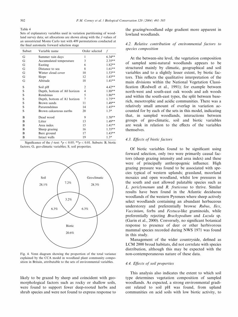
Table 4

Sets of explanatory variables used in variation partitioning of wood-

land survey data; set allocations are shown along with the f -values ofan unrestricted Monte Carlo test with 499 permutations conducted at

the final automatic forward selection stage

Subset Variable name Order selected f

G Summer rain days 1 6.34**

G Accumulated temperature 3 2.35**

G Easting 6 1.82**

G Distance to sea 8 1.61**

G Winter cloud cover 10 1.53**

G Slope 12 1.43**

G Altitude 18 1.41**

S Soil pH 2 4.42**

S Depth, bottom of A0 horizon 4 1.88**

S Rendzinas 5 1.86**

S Depth, bottom of A1 horizon 7 1.75**

S Brown sands 11 1.49**

S Pararendzinas 14 1.45**

S Brown calcareous earths 20 1.3*

B Dead wood 9 1.58**

B Litter 13 1.49**

B Area index 15 1.41**

B Sheep grazing 16 1.35**

B Bare ground 17 1.43**

B Intact walls 19 1.3*

Significance of the f -test: *p < 0:05; **p < 0:01. Subsets: B, biotic

factors; G, geo-climatic variables; S, soil properties.

Biotic

20.6%

Soil

28.1%

Geo-climatic

28.3%

6.3%6.3%

3.2%

7.2%

Fig. 4. Venn diagram showing the proportion of the total variance

explained by the CCA model in woodland plant community compo-

sition in Britain, attributable to the sets of environmental variables.


likely to be grazed by sheep and coincident with geo-

morphological factors such as rocky or shallow soils,were found to support fewer deep-rooted herbs and

shrub species and were not found to express response to

the grazing/woodland edge gradient more apparent in

lowland woodlands.

4.2. Relative contribution of environmental factors to

species composition

At the between-site level, the vegetation composition

of sampled semi-natural woodlands appears to be

structured mainly by climatic, geographical and soil

variables and to a slightly lesser extent, by biotic fac-

tors. This reflects the qualitative interpretation of the

main divisions within the National Vegetation Classi-

fication (Rodwell et al., 1991); for example betweennorth-west and south-east oak woods and ash woods

and within the south-east types, the split between base-

rich, mesotrophic and acidic communities. There was a

relatively small amount of overlap in variation ac-

counted for by each of the sets in this model, indicating

that, in sampled woodlands, interactions between

groups of geo-climatic, soil and biotic variables

are weak in relation to the effects of the variablesthemselves.

4.3. Effects of biotic factors

Of biotic variables found to be significant using

forward selection, only two were primarily causal fac-

tors (sheep grazing intensity and area index) and these

were of principally anthropogenic influence. Highgrazing pressure was found to be associated with spe-

cies typical of western uplands; grassland, moorland

mosaics and open woodland, whilst low pressures in

the south and east allowed palatable species such as

L. periclymenum and R. fruticosus to thrive. Similar

results have been found in the Atlantic deciduous

woodlands of the western Pyrenees where sheep actively

select woodlands containing an abundant herbaceousunderstorey and preferentially browse Rubus, Ilex,

Vaccinium, forbs and Festuca-like graminoids, while

preferentially rejecting Brachypodium and Luzula sp.

(Garin et al., 2000). Conversely, no significant botanical

response to presence of deer or other herbivorous

mammal species recorded during NWS 1971 was found

in this study.

Management of the wider countryside, defined asLCM 2000 broad habitats, did not correlate with species

distribution, although this may be expected with the

non-contemporaneous nature of these data.

4.4. Effects of soil properties

This analysis also indicates the extent to which soil

type determines vegetation composition of sampledwoodlands. As expected, a strong environmental gradi-

ent related to soil pH was found, from upland

communities on acid soils with low biotic activity, to

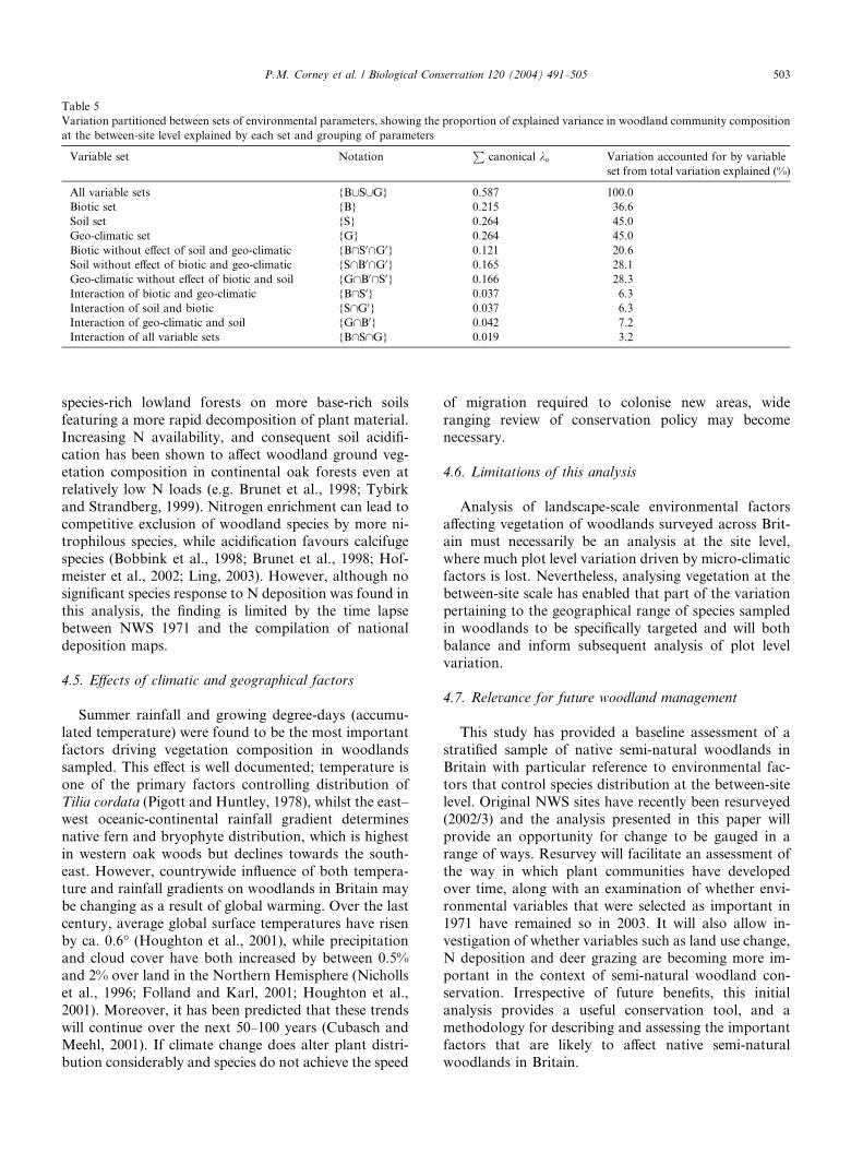
Table 5

Variation partitioned between sets of environmental parameters, showing the proportion of explained variance in woodland community composition

at the between-site level explained by each set and grouping of parameters

Variable set NotationP

canonical kn Variation accounted for by variable

set from total variation explained (%)

All variable sets {B[S[G} 0.587 100.0

Biotic set {B} 0.215 36.6

Soil set {S} 0.264 45.0

Geo-climatic set {G} 0.264 45.0

Biotic without effect of soil and geo-climatic {B\S0\G0} 0.121 20.6

Soil without effect of biotic and geo-climatic {S\B0\G0} 0.165 28.1

Geo-climatic without effect of biotic and soil {G\B0\S0} 0.166 28.3

Interaction of biotic and geo-climatic {B\S0} 0.037 6.3

Interaction of soil and biotic {S\G0} 0.037 6.3

Interaction of geo-climatic and soil {G\B0} 0.042 7.2

Interaction of all variable sets {B\S\G} 0.019 3.2


species-rich lowland forests on more base-rich soils

featuring a more rapid decomposition of plant material.

Increasing N availability, and consequent soil acidifi-

cation has been shown to affect woodland ground veg-

etation composition in continental oak forests even at

relatively low N loads (e.g. Brunet et al., 1998; Tybirk

and Strandberg, 1999). Nitrogen enrichment can lead to

competitive exclusion of woodland species by more ni-trophilous species, while acidification favours calcifuge

species (Bobbink et al., 1998; Brunet et al., 1998; Hof-

meister et al., 2002; Ling, 2003). However, although no

significant species response to N deposition was found in

this analysis, the finding is limited by the time lapse

between NWS 1971 and the compilation of national

deposition maps.

4.5. Effects of climatic and geographical factors

Summer rainfall and growing degree-days (accumu-

lated temperature) were found to be the most important

factors driving vegetation composition in woodlands

sampled. This effect is well documented; temperature is

one of the primary factors controlling distribution of

Tilia cordata (Pigott and Huntley, 1978), whilst the east–west oceanic-continental rainfall gradient determines

native fern and bryophyte distribution, which is highest

in western oak woods but declines towards the south-

east. However, countrywide influence of both tempera-

ture and rainfall gradients on woodlands in Britain may

be changing as a result of global warming. Over the last

century, average global surface temperatures have risen

by ca. 0.6� (Houghton et al., 2001), while precipitationand cloud cover have both increased by between 0.5%

and 2% over land in the Northern Hemisphere (Nicholls

et al., 1996; Folland and Karl, 2001; Houghton et al.,

2001). Moreover, it has been predicted that these trends

will continue over the next 50–100 years (Cubasch and

Meehl, 2001). If climate change does alter plant distri-

bution considerably and species do not achieve the speed

of migration required to colonise new areas, wide

ranging review of conservation policy may become

necessary.

4.6. Limitations of this analysis

Analysis of landscape-scale environmental factors

affecting vegetation of woodlands surveyed across Brit-ain must necessarily be an analysis at the site level,

where much plot level variation driven by micro-climatic

factors is lost. Nevertheless, analysing vegetation at the

between-site scale has enabled that part of the variation

pertaining to the geographical range of species sampled

in woodlands to be specifically targeted and will both

balance and inform subsequent analysis of plot level

variation.

4.7. Relevance for future woodland management

This study has provided a baseline assessment of a

stratified sample of native semi-natural woodlands in

Britain with particular reference to environmental fac-

tors that control species distribution at the between-site

level. Original NWS sites have recently been resurveyed(2002/3) and the analysis presented in this paper will

provide an opportunity for change to be gauged in a

range of ways. Resurvey will facilitate an assessment of

the way in which plant communities have developed

over time, along with an examination of whether envi-

ronmental variables that were selected as important in

1971 have remained so in 2003. It will also allow in-

vestigation of whether variables such as land use change,N deposition and deer grazing are becoming more im-

portant in the context of semi-natural woodland con-

servation. Irrespective of future benefits, this initial

analysis provides a useful conservation tool, and a

methodology for describing and assessing the important

factors that are likely to affect native semi-natural

woodlands in Britain.


Acknowledgements

The authors thank Jane Hall (CEH Monks Wood),

Dr. David Howard (CEH Merlewood), Duncan Ray

(Forest Research), Mary Thorp and Dr. Hugh McAll-ister (University of Liverpool) for technical support.

Financial support for Philip Corney was provided by

EN and CEH in the form of a CASE research stu-

dentship. We are grateful to all who read previous drafts

and supplied useful comments, in particular the valuable

reviews of two anonymous referees which were greatly

appreciated in the final preparation of this manuscript.

References

Avery, B.W., 1980. Soil classification for England and Wales [Higher

categories]. Soil Survey Technical Monograph No.14, Rothamsted

Experimental Station, Harpenden.

Bakkenes, M., Alkemade, J.R.M., Ihle, F., Leemans, R., Latour, J.B.,

2002. Assessing effects of forecasted climate change on the diversity

and distribution of European higher plants for 2050. Global

Change Biology 8, 390–407.

Barr, C.J., Bunce, R.G.H., Clarke, R.T., Fuller, R.M., Furse, M.T.,

Gillespie, M.K., Groom, G.B., Hallam, C.J., Hornung, M.,

Howard, D.C., Ness, M., 1993. Countryside Survey 1990: main

report. Department of the Environment, London.

Bobbink, R., Hornung, M., Roelofs, J.G.M., 1998. The effects of air-

borne nitrogen pollutants on species diversity in natural and semi-

natural European vegetation. Journal of Ecology 86, 717–738.

Borcard, D., Legendre, P., Drapeau, P., 1992. Partialling out the

spatial component of ecological variation. Ecology 73, 1045–1055.

Brunet, J., Diekmann, M., Falkengren-Grerup, U., 1998. Effects of

nitrogen deposition on field layer vegetation in south Swedish oak

forests. Environmental Pollution 102, 35–40.

Brunet, J., FalkengrenGrerup, U., Tyler, G., 1996. Herb layer

vegetation of south Swedish beech and oak forests – effects of

management and soil acidity during one decade. Forest Ecology

and Management 88, 259–272.

Bunce, R.G.H., 1981. British woodlands in an European context. In:

Last, F.T., Gardiner, A.S. (Eds.), Institute of Terrestrial Ecology

Symposium No. 8. Nature of Tree and Woodland Resources.

Natural Environment Research Council.

Bunce, R.G.H., 1982. A Field Key for Classifying British Woodland

Vegetation. Part 1. Institute of Terrestrial Ecology, Cambridge.

Bunce, R.G.H., 1989. A Field Key for Classifying British Woodland

Vegetation. Part 2. Institute of Terrestrial Ecology, Cambridge.

Bunce, R.G.H., Barr, C.J., Gillespie, M.K., Howard, D.C., Scott,

W.A., Smart, S.M., van de Poll, H.M., Watkins, J.W., 1999.

Vegetation of the British countryside – the Countryside Vegetation

System. ECOFACT Volume 1. Department of Environment,

Transport and the Regions, London.

Bunce, R.G.H., Shaw, M.W., 1972. Classifying woodland for conser-

vation. Forestry and Home Grown Timber 1, 23–25.

Bunce, R.G.H., Shaw, M.W., 1973. A standardized procedure for

ecological survey. Journal of Environmental Management 1, 239–

258.

Bunce, R.G.H., Shaw, M.W., 1975. Classification of semi-natural

woodlands in Britain. Institute of Terrestrial Ecology Annual

Report 1974. Natural Environmental Research Council, p. 43.

Cannell, M., 2002. Impacts of climate change on forest growth. In:

Broadmeadow, M. (Ed.), Climate Change: Impacts on UK forests.

Forestry Commission, Edinburgh, pp. 141–149.

Cubasch, U., Meehl, G.A., 2001. Projections of future climate change.

In: Houghton, J.T., Ding, Y., Griggs, D.J., Noguer, M., van der

Linden, P.J., Dai, X., Maskell, K., Johnson, C.A. (Eds.), Climate

Change 2001; The Scientific Basis. Cambridge University Press,

Cambridge, pp. 525–582.

EDINA, 2002. Digimap online mapping service (http://edina.ac.uk/

digimap). � Crown Copyright. An EDINA Digimap/JISC supplied

service.

Elmquist, M., Davies, J., 1999. Getgridvalue ArcView Avenue Script.

ERDAS, 2001. ERDAS IMAGINE, version 8.5. ERDAS, Inc.,

Atlanta, GA.

ESRI, 2000. ArcView GIS, version 3.2a. Environmental Systems

Research Institute, Redlands, CA.

ESRI, 2001. Map Manager version 6.2. ESRI, Redlands, CA.

Folland, C.K., Karl, T.R., 2001. Observed climate variability and

change. In: Houghton, J.T., Ding, Y., Griggs, D.J., Noguer, M.,

van der Linden, P.J., Dai, X., Maskell, K., Johnson, C.A. (Eds.),

Climate Change 2001; The Scientific Basis. Cambridge University

Press, Cambridge, pp. 99–181.

Fuller, R.M., Smith, G.M., Sanderson, R.A., Hill, R.A., Thomson,

A.G., 2002. The UK Land Cover Map 2000: Construction of a

parcel-based vector map from satellite images. Cartographic

Journal 39, 15–25.

Furness, S.B., Grime, J.P., 1982. Growth rate and temperature

responses in bryophytes. II. A comparative study of species of

contrasted ecology. Journal of Ecology 70, 525–536.

Garin, I., Aldezabal, A., Herrero, J., Garcia-Serrano, A., 2000.

Understorey foraging and habitat selection by sheep in mixed

Atlantic woodland. Journal of Vegetation Science 11, 863–870.

Hill, M.O., Bunce, R.G.H., Shaw, M.W., 1975. Indicator species

analysis, a divisive polythetic method of classification and its

application to a survey of native pinewoods in Scotland. Journal of

Ecology 63, 597–613.

Hinsley, S.A., Bellamy, P.E., Newton, I., 1995. Bird species turnover

and stochastic extinction in woodland fragments. Ecography 18,

41–50.

Hofmeister, J., Mihaljevic, M., Hosek, J., Sadlo, J., 2002. Eutrophi-

cation of deciduous forests in the Bohemian Karst (Czech

Republic): the role of nitrogen and phosphorus. Forest Ecology

and Management 169, 213–230.

Honnay, O., Verheyen, K., Butaye, J., Jacquemyn, H., Bossuyt, B.,

Hermy, M., 2002. Possible effects of habitat fragmentation and

climate change on the range of forest plant species. Ecology Letters

5, 525–530.

Houghton, J.T., Ding, Y., Griggs, D.J., Noguer, M., van der Linden,

P.J., Dai, X., Maskell, K., Johnson, C.A., 2001. Climate Change

2001; The Scientific Basis. Contribution of Working Group I to the

Third assessment Report of the Intergovernmental Panel on

Climate Change. Cambridge University Press, Cambridge.

Jenny, H., 1980. The Soil Resource. Springer, Berlin.

Kirby, K.J., 2001. The impact of deer on the ground flora of British

broadleaved woodland. Forestry 74, 219–229.

Lasch, P., Lindner, M., Erhard, M., Suckow, F., Wenzel, A., 2002.

Regional impact assessment on forest structure and functions

under climate change – the Brandenburg case study. Forest

Ecology and Management 162, 73–86.

Le Duc, M.G., Pakeman, R.J., Marrs, R.H., 2000. Vegetation

development on upland and marginal land treated with herbicide,

for bracken (Pteridium aquilinum) control, in Great Britain. Journal

of Environmental Management 58, 147–160.

Legendre, P., Legendre, L., 1998. Numerical Ecology. Elsevier,

Amsterdam.

Ling, K.A., 2003. Using environmental and growth characteristics of

plants to detect long-term changes in response to atmospheric

pollution: some examples from British beech woods. Science of the

Total Environment 310, 203–210.

http://edina.ac.uk/digimap

http://edina.ac.uk/digimap


Marrs, R.H., Le Duc, M.G., 2000. Factors controlling vegetation

change in long-term experiments designed to restore heathland in

Breckland, UK. Applied Vegetation Science 3, 135–146.

Meteorological Office, 2003. UK 5 km� 5 km grid baseline datasets

for the period 1961 to 2000. Available from: (http://www.metof-

fice.com/index.html).

Mitchell, J.F.B., Karoly, D.J., 2001. Detection of climate change and

attribution of causes. In: Houghton, J.T., Ding, Y., Griggs, D.J.,

Noguer, M., van der Linden, P.J., Dai, X., Maskell, K., Johnson,

C.A. (Eds.), Climate Change 2001; The Scientific Basis. Cambridge

University Press, Cambridge, pp. 695–738.

Modrzynski, J., Eriksson, G., 2002. Response of Picea abies popula-

tions from elevational transects in the Polish Sudety and Carpa-

thian mountains to simulated drought stress. Forest Ecology and

Management 165, 105–116.

NEGTAP (National Expert Group on Transboundary Air Pollution),

2001. Transboundary Air Pollution: Acidification, Eutrophication

and Ground-Level Ozone in the UK. Report of the National

Expert Group on Transboundary Air Pollution (NEGTAP) for the

UK Department for Environment, Food and Rural Affairs,

Scottish Executive, The National Assembly for Wales/Cynulliad

Cenedlaethol Cymru and the Department of the Environment for

Northern Ireland. CEH, Edinburgh.

Nicholls, N., Gruza, G.V., Jouzel, J., Karl, T.R., Ogallo, L.A.,

Parker, D.E., 1996. Observed climate variability and change. In:

Houghton, J.T., Meira Filho, L.G., Callander, B.A., Harris, N.,

Kattenberg, A., Maskell, K. (Eds.), Climate Change 1995; The

Science of Climate Change. Contribution of Working Group I to

the Second Assessment Report of the Intergovernmental Panel on

Climate Change. Cambridge University Press, Cambridge, pp.

133–192.

Peterken, G.F., 1993. Woodland Conservation and Management.

Chapman & Hall, London.

Pigott, C.D., Huntley, J.P., 1978. Factors controlling the distribution

of Tilia cordata at the northern limits of its geographical range.

New Phytologist 81, 429–441.

Rackham, O., 2003. Ancient Woodland, New ed. Castlepoint Press,

Dalbeattie.

Ratcliffe, D.A., 1977. A nature conservation review: the selection of

biological sites of national importance to nature conservation in

Britain. Cambridge University Press, Cambridge.

Ray, D., 2001. Ecological Site Classification, version 1.7 A PC-based

Decision Support System for British Forests. Forestry Commis-

sion, Edinburgh.

Redfern, D., Hendry, S., 2002. Climate change and damage to trees

caused by extremes of temperature. In: Broadmeadow, M. (Ed.),

Climate Change: Impacts on UK forests. Forestry Commission,

Edinburgh, pp. 29–39.

Rodwell, J., Pigott, C.D., Ratcliffe, D.A., Malloch, A.J.C., Birks,

H.J.B., Proctor, M.C.F., Shimwell, D.W., Huntley, J.P., Radford,

E., Wigginton, M.J., Wilkins, P., 1991. British Plant Communities,

vol. 1. Woodlands and Scrub. Cambridge University Press,

Cambridge.

Sheail, J., Bunce, R.G.H., 2003. The development and scientific

principles of an environmental classification for strategic ecological

survey in the united Kingdom. Environmental Conservation 30,

147–159.

Smart, S.M., 2000. Modular Analysis of Vegetation Information

System (MAVIS) Plot Analyser, version 1.00. CEH, Merlewood,

Cumbria.

Smart, S.M., Bunce, R.G.H., Black, H.I.J., Ray, N., Bunce, F., Kirby,

K.J., Watson, R., Singleton, D., 2001. Measuring long term change

in Biodiversity in British woodlands (1971–2000) – a pilot re-survey

of 14 sites from the 1971 Nature Conservancy ‘Bunce’ woodland

survey and two from the 1971 Native Pinewood Survey. Centre for

Ecology and Hydrology, Merlewood, Cumbria.

Sokal, R.R., Rohlf, F.J., 1995. Biometry, third ed. Freeman, New

York.

Ter Braak, C.J.F., 1986. Canonical correspondence analysis: a new

eigenvector technique for multivariate direct gradient analysis.

Ecology 67, 1167–1179.

Ter Braak, C.J.F., Prentice, C.I., 1988. A theory of gradient analysis.

Advances in Ecological Research 18, 271–313.

Ter Braak, C.J.F., �Smilauer, P., 2002. CANOCO Reference Manual

and CANODRAW for Windows User’s Guide version 4.5.

Microcomputer Power, Ithaca, NY.

Tybirk, K., Strandberg, B., 1999. Oak forest development as a result of

historical land-use patterns and present nitrogen deposition. Forest

Ecology and Management 114, 97–106.

Williams, J.W., Post, D.M., Cwynar, L.C., Lotter, A.F., Levesque,

A.J., 2002. Rapid and widespread vegetation responses to past

climate change in the North Atlantic region. Geology 30, 971–974.

Williams, W.T., Lambert, J.M., 1959. Multivariate methods in plant

ecology. Association analysis in plant communities. Journal of

Ecology 47, 83.

Yeo, M.J.M., Blackstock, T.H., 2002. A vegetation analysis of the

pastoral landscapes of upland Wales, UK. Journal of Vegetation

Science 13, 803–816.

http://www.metoffice.com/index.html

http://www.metoffice.com/index.html

The effect of landscape-scale environmental drivers on the vegetation composition of British...

Documents

Transcript of The effect of landscape-scale environmental drivers on the vegetation composition of British...