CCGGEEHH WWoorrkkiinngg PPaappeerr SSeerriieess

The development of inequality and poverty in Indonesia, 1932-1999

Bas van Leeuwen, Utrecht University

Peter Foldvari, Debrecen University

January 2012

Working paper no. 26

http://www.cgeh.nl/working-paper-series/

© 2011 by Authors. All rights reserved. Short sections of text, not to exceed two paragraphs, may be quoted without explicit permission provided that full credit, including © notice, is given to the source.

The development of inequality and poverty in Indonesia, 1932-1999

Bas van Leeuwen, Utrecht University

Peter Foldvari, Debrecen University

Abstract In this paper we estimate inequality in Indonesia between 1932 and 1999. There was an increase in inequality at the start of this period but then a sharp decline from the 1960s. A shift from domestic to export agriculture over the period up to the Great Depression accounts for the increase in inequality. During the 1930s, as the price of export crops declined, the income of rich farmers suffered a blow. Yet, this was counterbalanced by increasing gap between expenditure in the urban and rural sectors, causing an over-all rise in inequality. As for the second half of the century, we find that the employment shift towards manufacturing and services, combined with an increase in labour productivity in agriculture, accounts for the decline in inequality. These inequality trends had an effect on poverty as well, but prior to the 1940s the negative impact of the rise in inequality was offset by an increase in per capita GDP. Between 1950 and 1980 a decline in inequality, combined with increased per capita GDP rapidly raised a large portion of the population above the poverty line.

Keywords: Indonesia, inequality, poverty, economic development JEL Codes: D63, I32, N15, Corresponding author: Bas van Leeuwen: bas.vanleeuwen1@googlemail.com

Acknowledgements:

INTRODUCTION

While income inequality has received considerable attention over the past few decades, most long-

run studies focus on Western countries and Western offshoots1 (e.g. Piketty 2003; Saez and Veall

2005; Piketty and Saez 2006), and few use comparable data to address the issue of long-run

inequality and poverty trends in less-developed countries (e.g. Banerjee and Piketty 2005; Bértola et

al. 2009; Van Zanden et al. 2009; Leigh and Van der Eng 2010).

While there is a large body of literature on inequality and poverty in Indonesia, no

consensus has yet been achieved regarding the magnitude of these two variables or their pattern of

change over time (Booth and Sundrum 1981). The introduction of the Indonesian household survey

(Susenas) in 1963/64 generated a large amount of data on expenditures, triggering many studies of

inequality and poverty. Unfortunately, frequent changes in the definition of poverty have

complicated the challenge of making comparisons over time. In addition, the reliability of the

Susenas data has been questioned (Booth 1993: 55). Sudjana and Mishra (2004) argue that

relatively wealthy households are underrepresented in these data, creating a significant bias, and

one that increases over time. This under-representation goes far to account for the fact total private

household expenditures estimated on the basis of Susenas in the 1980s and 1990s turn out to be

much lower than what is reported in the national income accounts (Van der Eng 2001). The

income-inequality estimates, however, suffer from even worse defects: so much worse, in fact, that

at first they were not even reported in official publications. Income-tax data represent less than 5%

of all income earners, and the Susenas data include no information on income prior to 1979. These

shortcomings oblige us to rely on expenditure data for any long-run analysis of inequality in

Indonesia. Table 1 presents the results of one such analysis (WIID2b 2007), which, unlike our

findings in this paper, suggests a roughly constant level of inequality from 1960 on. If one accepts

this conclusion, however, it remains to be explained why three decades of New Order policies and

the 1970s oil boom, both of which caused significant structural change within the economy, had no

1 For instance, settler destinations such as the USA and Australia.

significant impact on inequality. Our aim in this paper is to offer a more reliable picture of

expenditure inequality in Indonesia during the 20th century.

In the remainder of this paper we construct new historical series of inequality and poverty,

extending back to 1932, which makes it possible to discern trends in inequality and poverty over the

entire twentieth century, which in turn allows us to make several valuable, if tentative, observations

regarding the underlying causes of these trends.

INEQUALITY MEASURES

Most estimates of inequality in Indonesia (e.g. Booth and Sundrum 1981; Hughes and Islam 1981;

Alatas and Bourguignon 2000; Cameron 2002; Frankema and Marks 2009; 2010; Van der Eng

2009) are based on expenditure rather than income data, not only because they are available in

greater quantity but also because they constitute a more reliable indicator of the actual welfare

(consumption) of the population.2 Moreover, they allow one to circumvent the problem, inherent in

income-based estimates, of overestimation at the top of the distribution and underestimation at the

bottom, and hence an overestimation of income inequality. Factors such as progressive taxation

(reducing the expenditure of the wealthy more than proportionately) and saving rates dependent on

income (Dynan et al 2004) contribute to a deviation between the two pictures generated by the two

types of data. Likewise, by-employment (that is, part-time employment in addition to the

individual's main job), which is relatively widespread in the rural sector (where average income is

relatively low), further biases the picture one can obtain on income inequality based on expenditure

data (Van der Eng 2002: 147). This is because income is calculated from a person’s main

occupation. Since in the relatively low productivity sectors by-employment is higher, this means

that income based inequality measures that do not take account of by-employment will overestimate

inequality. Likewise, rates of by-employment are especially high among the poor. Indeed, in the

2 François and Rojas-Romagosa (2005: 17) argue that expenditure measures are subject to biases caused by

borrowing and lending. However, since in the long run the tendency is that these are equal, the impact is insignificant.

1984-96 WIID income-inequality estimates for Indonesia (WIID2b 2007), the Gini coefficients3

derived from expenditure data are 8–23% lower than those estimated from income data (Table 1).

Table 1 Gini coefficient of inequality, 1964-1999a

Expenditure Income Differenceb

%

1964 0.33 1970 0.31 1976 0.32 1978 0.35 1980 0.32 1981 0.31 1984 0.31 0.40 22.5

1990 0.32 0.39 17.9 1993 0.34 0.42 19.0

1996 0.37 0.40 7.5

1999 0.31c

Notes: a Unit of analysis: household. b Percentage difference is relative to income inequality. c The expenditure Gini for 1999 is inexplicably low (WIID2b 2007).

Source: WIID2b (2007)

The fact that income inequality is greater than expenditure inequality is not the only problem to

complicate poverty analysis. If we were to follow the income approach we would find a level of

inequality between 1984 and 1996 even more stable than the level indicated by the expenditure

approach (Table 1) — a somewhat surprising finding, given the many significant economic and

social developments that Indonesia experienced during the New Order period (1966–98). Our

primary purpose in this paper, therefore, is to construct an alternative series for expenditure

inequality that, if not perfect, provides a more accurate picture of change in inequality over the long

run.

3 The Gini coeffiicent is a commonly used measure of inequality in the distribution of income or

expenditure, ranging in value from 0 (complete equality), to 1 (maximal inequality).

Our starting point is Van Leeuwen (2007),4 who provides data on expenditure and

population shares for six urban and four rural household categories for several benchmark years

between 1932 and 1999. Since the data and their construction are well described in Van Leeuwen

(2007), we will only give a brief description here, and then move on to the estimation of

expenditure Ginis.

For the period after 1975, data on the share of each household category in total income were

obtained from the social-accounting matrices provided by BPS (six volumes of Sistem neraca social

ekonomi Indonesia, for the years 1975, 1980, 1985, 1990, 1993 and 1999). Since the data provided

therein on all income, expenditure and production streams within the Indonesian economy are

consistent, they can be regarded as more reliable than the Susenas data. Since our data on each

household category are limited to income and number of people in that category, our estimates are

equivalent to what is referred to in the literature as “social tables” (e.g. Lindert and Williamson

1982).

For the pre-1975 period, we have no direct observations on either the share of household

categories in the total population or their expenditure share. Backcasting using a logarithmic trend

for each household category on the post-1975 data, we found that the change in the share of each

household class in the total population diminished on average prior to the 1960s, indicating that

before 1960 the share of each household class in the total population remained quite constant.

Indeed, given that the shifts in household-category shares generally start slowly and do not speed up

until after urbanisation and industrialisation takes flight, we expect that the population shift from

rural to urban household categories must have been slow prior to 1960. We find that, whereas in

1920 roughly 76% of the labour force was employed in agriculture (and, needless to say, lived in

rural areas), by 1960 that figure had declined to 67% (Van der Eng 1996). This finding supports the

plausibility that the 1960 household population shares can be combined with the income shares for

the previous periods resulting in our social table (Table 4) .

4 These data are available at <http://www.iisg.nl/indonesianeconomy/humancapital/>.

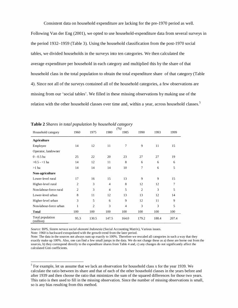
Consistent data on household expenditure are lacking for the pre-1970 period as well.

Following Van der Eng (2001), we opted to use household-expenditure data from several surveys in

the period 1932–1959 (Table 3). Using the household classification from the post-1970 social

tables, we divided households in the surveys into ten categories. We then calculated the

average expenditure per household in each category and multiplied this by the share of that

household class in the total population to obtain the total expenditure share of that category (Table

4). Since not all of the surveys contained all of the household categories, a few observations are

missing from our ‘social tables’. We filled in these missing observations by making use of the

relation with the other household classes over time and, within a year, across household classes.5

Table 2 Shares in total population by household category (%)

Household category 1960 1975 1980 1985 1990 1993 1999

Agriculture

Employee 14 12 11 7 9 11 15 Operator, landowner 0 - 0.5 ha 25 22 20 23 27 27 19 >0.5 - <1 ha 14 12 11 8 6 6 6

>1 ha 14 14 14 10 7 6 5

Non-agriculture

Lower-level rural 17 16 15 13 9 9 15 Higher-level rural 2 3 4 8 12 12 7

Non-labour-force rural 2 3 4 5 2 3 5 Lower-level urban 8 11 12 13 13 12 14

Higher-level urban 3 5 6 9 12 11 9 Non-labour-force urban 1 2 3 4 3 3 5

Total 100 100 100 100 100 100 100

Total population (million)

95.3 130.5 147.5 164.0 179.2 188.4 207.4

Source: BPS, Sistem neraca social ekonomi Indonesia (Social Accounting Matrix), Various issues. Note: 1960 is backward extrapolated with the growth trend from the later period. Note: The data in the sources not always sum up exactly to 100%. Therefore we rescaled all categories in such a way that they exactly make up 100%. Also, one can find a few small jumps in the data. We do not change these as a) these are borne out from the sources, b) they correspond directly to the expenditure shares from Table 4 and, c) any changes do not significantly affect the calculated Gini coefficients.

5 For example, let us assume that we lack an observation for household class x for the year 1939. We calculate the ratio between its share and that of each of the other household classes in the years before and after 1939 and then choose the ratio that minimizes the sum of the squared differences for those two years. This ratio is then used to fill in the missing observation. Since the number of missing observations is small, so is any bias resulting from this method.

Table 3 Overview of main household expenditure surveys in Java/Indonesia, 1927-1962 Source Sample households Region Year(s)

Number Type

Boeke (1927) 29 rural Java (various parts) 1924-25

CKS (1928) 314 urban Indonesia 1925

Rohrman (1932) 18 rural Kraksaän (Probolinggo) 1932

CKS (1939) 95 labourers Jakarta 1937

Huizenga (1958) 1,945 rural labourers Java 1939-40

Sato (1994: 96) 421 farm Tasikmadu (Malang, E. Java) 1942

Sato (1994: 102-3) 345 farm Tumut (Bantul, C. Java) 1942

ILO (1967)* 2,639 urban Jakarta 1957

ILO (1967)* 2,180 urban Surabaya 1958

Sukamto (1962) 503 urban Yogyakarta 1958-9

*Obtained from the Ministry of Labour, Indonesia.

Table 4 Shares in total consumption expenditure by household category (%)

Household category 1932 1942 1953 1960 1975 1980 1985 1990 1993 1999

Agriculture

Employee 5 8 5 4 6 5 4 4 4 6

Operator, landowner 0 - 0.5 ha 8 1 4 6 13 14 14 18 16 9

>0.5 - <1 ha 5 6 9 11 10 7 6 5 5 5

>1 ha 48 38 31 27 16 15 13 8 7 5

Non-agriculture Lower-level rural 8 8 9 9 12 14 10 7 6 12

Higher-level rural 5 5 5 5 6 7 11 16 19 13

Non-lab.-force rural 12 14 12 10 3 3 4 2 2 5

Lower-level urban 1 5 8 10 15 17 16 12 10 19 Higher-level urban 6 13 15 16 17 15 17 25 28 21

Non-lab.-force urban 2 2 2 2 2 3 5 3 3 5

Total 100 100 100 100 100 100 100 100 100 100

Source: See text and Table 2; BPS, Sistem neraca social ekonomi Indonesia (Social Accounting Matrix), Various issues. Note: The data in the sources not always sum up exactly to 100%. Therefore we rescaled all categories in such a way that they exactly make up 100%. Also, one can find a few small jumps in the data. We do not change these as a) these are borne out from the sources, b) they correspond directly to the population shares from Table 3 and, c) any changes do not significantly affect the calculated Gini coefficients.

The resulting social tables are consistent over time, with a steady increase in non-agricultural

household expenditure shares. Moreover, Van Leeuwen (2007, Appendix 4) shows that the results

are also consistent with existing current-price GDP estimates. More importantly, by applying the

trapezoid approximation method employed in Milanovic et al. (2007), we can use these tables to

estimate the Gini measure of inequality. First we calculate the cumulative share of expenditure

class6 i in the population and in total income, denoted by p and L(p), respectively; together they can

be used to estimate the Lorenz curve. In this case, since we order households according to

expenditure level, from the highest to the lowest, the Lorenz curve is above the 45-degree line. If

we have k classes in the population, we can estimate the Gini as follows:

퐺 = (푝 − 푝 ) (퐿(푝 ) − 푝 + 퐿(푝 ) − 푝 )

where

0 ( ) 0( ) 1

o

k k

p L pp L p

It can be seen in Figure 1 (based on Table 5) that the trend of our estimates of inequality for

rural and urban areas combined (i.e. ‘total’) compare quite well with those based on data, drawn

from Leigh and Van der Eng (2010), on the income share of the upper quantiles of the population

(to which we refer subsequently as ‘income share inequality’). Whether we assume a Pareto or a

log-normal distribution for converting data on the Lorenz curve into Gini coefficients (see appendix

1 for a description), we consistently find that inequality peaks in the 1930s. Gini coefficients for

the rural and urban sectors, derived from the household categories sub-division and reported in the

second and third columns, follow a similar trend.

The results of our inequality estimates in Table 5 are in accordance with expectations: an

increase in inequality during the economic crises of the 1930s and 1990s and a decline in the

1940s–70s. The estimated Gini for 1980 and 1985 is low (0.24) but not implausible, because this is

in line with estimates elsewhere: 0.18 in China in 1995, 0.25 in Egypt in 1965, and 0.16 in

Luxemburg in 1986(WIID2b 2007). In addition, several authors have stressed the low level of

expenditure inequality in Indonesia (e.g. Van der Eng 2009: 7). Furthermore, in Table 5, for the pre-

1960 period the trend in the income share Ginis resembles that of our expenditure Ginis—especially

between 1925 and 1932, a period in which both series are distinguished by a sharp increase in 6 The sum of the shares of all classes up to and including class i.

inequality. Even if we assume, as we do in the notes to Table 5, that the estimate by Booth is too

low and that a Gini of 0.45 in 1925 would be more appropriate, there must have been a considerable

increase in inequality between 1925 and 1932. For the post-1960 period the newly estimated

expenditure Ginis move in the same direction as the Ginis based on the income quantiles, albeit at

different rates (see also Figure 1 in the Appendix).7 To summarise, for the post-war period we find a

decreasing trend up until the early 1980s and an increase in inequality from about the early 1990s.

The overall pattern that emerges from Table 5 is one of increasing inequality in the 1920s–

30s and decreasing inequality in the second half of the century. This is consistent with the

hypothesis of Lindert and Williamson (2003): since land rents were largely owned by the rich and

wages by the poor, the increased use of abundant land resources for export production prior to the

1930s, increased land rents relative to wages, contributing to a growth in income inequality in

Indonesia. Pursuing this line of reasoning, Leigh and Van der Eng (2010) argue that the rapidly

expanding use of labour for export-oriented production since the 1970s should have contributed to a

reduction in inequality, and therefore that the maximum level of inequality must have been reached

in the 1960s.

Alternatively, the transition from a rural to an industrial economy in developing countries,

which has been modelled by Lewis (1954) and Kuznets (1955), should lead to a general increase in

the income share of the modern sector, with inequality increasing to the point at which the majority

of the workforce is employed in the high-productivity modern sector. According to Lindert and

Williamson, it was a shift in agriculture's market orientation, from domestic to export, and not (as

argued by Kuznets) a shift from agriculture to manufacturing and services, that caused an increase

in inequality prior to the 1930s. While both hypotheses predict an initial increase in inequality, that

of Lindert and Williamson implies that the gap between rural and urban inequality continues to

widen as the increase in the urban sector's income outpaces the rural sector's, whereas the Kuznets

7 For us this is not a problem, since we are more interested in the pattern than the level. However, if one wants to construct a consistent series based on income inequality, it is advisable to extend our pre-1960 expenditure series with either the income Ginis or the average Gini estimated from the income shares benchmarked on the income Ginis.

hypothesis maintains that the migration of labour from the lower-productivity agricultural to the

higher-productivity urban sector causes the gap to narrow. Thus according to Lindert and

Williamson we should expect a decrease in wages in agriculture relative to other sectors, whereas

according to Kuznets we should expect a relative increase. Indeed, our dataset permits us to

estimate that between rural-urban inequality8 increased in the 1930s from 0.009 to 0.14 suggesting

that expenditure in the urban sector increased versus that in the rural sector.9 In addition, Van der

Eng (1996, Table A.3) shows that rural employment constituted 76% of the total in 1900 and 74%

in 1940, undermining the argument based on a shift from agricultural to manufacturing and

services employment which again seems to confirm the Lindert-Williamson argument. . Finally,

between 1900 and 1930 average labour productivity in agriculture (the contribution of the

agricultural sector to GDP divided by the share of the agricultural workforce) declined, relative to

the corresponding measure for services and manufacturing, from 25.2% to 18.3% (Van der Eng

2002).10 This suggests that there was a redistribution of income in favour of the urban sector,

caused by an increase in the production of export crops which profited primarily the urban sector.11

Indeed, between 1932 and 1939 private expenditure in the urban sector grew from 34% to 43% of

the total, while the share of estate crops (mostly for export) in total agricultural GDP increased

from 11.5% in 1900 to 24% in 1930 (Van der Eng 1996, 260–62). This relative increase in non-

rural incomes again seems to confirm the Lindert-Williamson argument.

This trend of an intensification of agricultural exports as identified by Lindert and

Williamson came to an end during the Great Depression of the 1930s. Not only was the Ethical

8 The between Gini reflects the difference between the average income in rural and urban sectors. On a detailed note on the decomposition of the Gini, see footnote 10. 9 This estimate is based on three separate Gini estimates – within, between and overlap — as suggested by Pyatt (1976). The overlap Gini takes into account the fact that an individual's wealth is relative to the various categories to which he or she belongs; for instance, a street-sweeper might be among the poorest 10% urban workers but at the same time among the wealthiest 10% of rural workers. It is also important to note that since these are expenditure Ginis they do not take account of the urban-rural difference in price levels. On the other hand, Asra (1999: 58) found that these price differences are in fact much smaller than official publications indicate. 10 We have to be careful in interpreting these figures, since the deflation rate in agriculture may differ from that in services or manufacturing, although probably not significantly so. 11 The earnings to labour remained in the rural sector.

Policy abandoned (Timmer 2005: 20) but there was a drop in prices of the most important export

commodities as well. The current price value of exports of seven major crops expressed in guilders

fell by 75% between 1929 and 1933, while the quantity exported decreased by 42% (Creutzberg

1975: Table 1), causing the share of agricultural households in total household consumption to

decline from 66% in 1932 to 53% in 1942—largely as a result of a decline in the income share of

richer household, enjoying income from export-oriented production. Because the income share of

the richer agricultural households declined, inequality in the rural sector declined relative to that in

the urban sector. Yet, it increased the expenditure gap between the urban and rural sector, thus

increasing the between rural-urban Gini (see footnote 10). The increasing between Gini combined

with a decrease in the rural Gini resulted in an over-all increase in the national Gini in 1939 as can

be seen in Table 5. This trend of increasing inequality is not uncommon though. A recent study

based on tax data indicate that between 1928 and 1938 Hungary, a country with a rural economy

then comparable in size relative to GDP to that of Indonesia, experienced an increase in the Gini

coefficient of 0.018 points (Földvári 2009).

The next decade, however, is marked by a reversal of the pattern, with inequality decreasing

between 1939 and 1953, from 0.60 to 0.51. Whether this is an example of the effect of war on

inequality, an effect attested by several studies (e.g. Van Zanden 1995: 646; Piketty and Saez 2006:

203), remains unsubstantiated, due to the lack of evidence. Likewise, it may be possible that the

decline in inequality is partly attributable to a decline in racial inequality because of the withdrawal

of Netherlands from its position of both political and economic domination. Van Zanden (2003)12

estimated the 1880 income Gini for Indonesians to be 0.32, versus 0.63 and 0.61 for Chinese and

Europeans respectively in 1880. Forty-five years later, in 1925, the pattern remained little changed,

with inequality among Indonesian taxpayers of 0.37, among Chinese taxpayers of 0.53, and among

European taxpayers of 0.51 (Booth 1988: 326). It thus seems likely, even though again

unsubstantiated, that the removal of the Europeans from their positions after World War II resulted

12 These Gini estimates are updated at the Global Price and Income History Group website: <http://gpih.ucdavis.edu/Distribution.htm>.

in a decline in inequality. However, notwithstanding above suggestions, all that we can state with

any certainty is that during the period 1942–53 changes in the income share of agricultural

households were relatively significant, primarily because the income share of small landowners

increased while that of larger ones declined (Table 4). The same applies to the urban Gini, which

declined only slightly, largely because of a relative decline in urban wages, hence the decline in

overall inequality.

Table 5 Gini coefficients on inequality

This study WIID2b Leigh and Van der Enga

Rural Urban Total Rural Urban Total Pareto

distribution

Log-normal

distribution

1880 0.39b

1920 0.23 0.42

1925 0.32c 0.34 0.56

1930 0.38 0.60 1932 0.52 0.57 0.56 0.44 0.70

1939d 0.60

1942 0.60 0.53 0.59 0.42 0.64

1953 0.51 0.50 0.54 1959 0.46 0.40 0.51 1964 0.39 1970 0.35 1975 0.17 0.32 0.29 1976 0.31 0.35 0.34 1978 0.34 0.38 0.37 1980 0.14 0.19 0.24 0.31 0.36 0.34 1981 0.29 0.33 0.33 1982 0.27 0.47

1984 0.28 0.32 0.33 1985 0.19 0.20 0.24 1987 0.26 0.32 0.32 0.28 0.50 1990 0.15 0.20 0.25 0.25 0.34 0.32 0.29 0.49

1993 0.16 0.22 0.30 0.26 0.33 0.34 0.32 0.53

1996 0.27 0.36 0.36 0.32 0.53

1999 0.17 0.11 0.32 0.24 0.32 0.31 0.38 0.61

2002 0.34 0.56 a “Pareto distribution” and “log-normal distribution” are estimated using the income shares of the x% richest persons under the alternative assumptions of Pareto or log-normal probability distributions, respectively (Appendix A.2). b Van Zanden (2003) c Calculated on the basis of Booth (1988, Table 7). This figure seems to be too low compared with the previous and subsequent estimates and does not accord with the observations made by Lindert and Williamson (2003). A Gini coefficient of 0.45, derived from data in Leigh and Van der Eng (2010), which are benchmarked on the expenditure Gini of 1932, therefore seems more appropriate. d 1939 (using the 1934 ratio to correct for the omission of the income share of the wealthiest 10%)

This decline in overall inequality that began in the 1940s continued for the next three decades; what

distinguished the decline during the 1960s and 1970s was the fact that now it was rural inequality

that became lower than its urban counterpart. This can be explained by several factors: most notably

public expenditure on agriculture translated into an increase in the wages of rural labourers. In

addition, the Green Revolution largely benefited one element in particular of the rural sector, rice

farmers (Van der Eng 2009: 5–6) hence increasing the relative expenditure of the small scale rice

farmers. At the same time we can see a decline in the expenditure shares of agricultural households

with medium-size and large land holdings, a development also reported by Van der Eng (2009: 13–

14), who noted a significant decrease, especially in the Outer Provinces – part of a 1963-93 trend

towards increasing equality which was accompanied by a Gini decrease that brought it close to

Java's levels.

The trend of declining inequality in the Indonesian economy continued until the mid-1980s.

For example, Timmer (2004) convincingly demonstrates that thanks to the pro-poor growth policy

of the Soeharto government during this period the poorest 20% of the population experienced the

same expenditure growth as did those moderately well off. If the growth-incidence curve for the

period prior to 1990 was similar to that for 1996–99 (Timmer 2004), this would have contributed to

the decline in inequality, as did the oil-price shocks, because they prompted the government to

increase spending on development. Moreover, these shocks and the resulting Dutch disease13 may

have hurt the poor in Indonesia less than the poor in other oil-exporting countries not only because

the government chose to invest in development but also because it adopted a policy that combined a

policy of balanced-budget expenditure with an orientation toward export and trade liberalization

(Temple 2003).

All this changed, however, with the oil glut of 1986, when an overvalued currency (Booth

1986) in combination with reduced income from oil exports hit the economy. It is probably no

coincidence that in the mid-1980s inequality started to rise again; and as if that was not enough, the

13 The Dutch disease, often paired with an increase in income from raw materials, such as oil, results in an overvaluation of the currency, which in turn causes exports to decline and thus unemployment to rise.

country was hit by the Asian financial crisis in 1997. A study based on household surveys suggests

that the rapid rise in the price of rice during this crisis caused a rapid rise in poverty, inducing

households to increase the share of basic foodstuffs in their budget (Frankenberg et al. 1999).

Indeed, Timmer (2005) reports that the annual increase in rice prices between 1996 and 1999 was

19.2% (compared with an increase in the CPI which was about 10 percentage points lower), higher

than any increase recorded during the previous three decades. These troubles translated into an

increase in rural inequality, both in absolute terms and relative to urban inequality.

But what did this pattern of initially decreasing and, after the mid-1980s increasing,

inequality have on the actual standard of living in the population? To answer this question, we will

look at income growth and poverty in the next Section.

POVERTY

While Indonesia has proved to be fertile ground for studies establishing the impact of inequality on

poverty, most of these studies treat a short time span (e.g. Booth 1993). In the previous section we

found a long-run pattern of increasing inequality up to the 1940s and decreasing inequality

thereafter (with the exception of an increase of limited duration, coinciding with the 1990s

economic crisis). This finding prompts the question, How does poverty's pattern compare?

To answer this question, we begin with an estimate of the population share below a poverty

line of $2/day in 1990 prices.14 The definition of extreme poverty used in much of the literature

(e.g. Van Zanden et al. 2009) is $1/day, but this figure is based on consumption and inequality data

drawn from household surveys. Following Sala-i-Martin (2002a, b) and López and Servén (2006),

we combine this sort of data with per capita GDP using $2/day as the poverty line. Chen and

Ravallion (2004) and Ravallion (2004) have shown that the two methods generate similar results.

Our method permits us to make a direct estimate of the population share below the poverty

line, on the basis of the Gini coefficients calculated in the previous section. López and Servén 14 The World Bank currently uses a definition of extreme poverty of 1.25 dollars a day in 2005 PPP in order to correct for the price level difference between 1990 and 2005. Since we use 1990 international dollar, as most studies do in this field, , also for the sake of comparability, we use the old definitions.

(2006) found that income distribution is consistent with log - normality, in which case to make a

poverty estimate all one needs are the poverty line, average income and the Gini coefficient. The

share of population below the poverty line (the poverty headcount, P0) can thus be calculated as:

푃 = 훷 푙표푔 /휎 + 휎/2 ,

where 훷 is the cumulative normal distribution, given by

휎 = √2훷 (1 + 퐺)/2 ,

v is per capita income (proxied here by per capita GDP), z is the poverty line (in our case $2/day), 휎

is the standard deviation of the distribution and G is the Gini coefficient. The expression for P0

implies that both decreases in inequality (reduction in Gini-coefficient) and increases in per capita

GDP cause decreases in poverty.

The estimates are presented in Table 6. Whether we use the World Bank's old $1/day

poverty line, its alternative $2/day poverty line, or the two poverty lines presented in Booth (1993)

-- one relying on the official BPS poverty line and the other relying on a poverty line suggested by

Esmara (1986) -- we see the same trend. Furthermore, our series matches Booth’s quite well: in

both series the percentage of those below the poverty line in drops from around 25% in 1980 to

16% in 1990. Indeed, both Booth's series and ours indicate that during the 1960s and 1970s poverty

declined sharply. Table 6 reports the magnitude of poverty before the 1960s as well.15 We find that

the percentage constituted by the poor remained virtually unchanged until the 1950s,16 at which

15 We argued in the previous section that in the prewar period expenditure smoothing is less of an issue and therefore that income and expenditure inequality converge during that period. Using a poverty limit of $2/day for the prewar period therefore possibly overestimates poverty. When $1per day is used the figures are 1942: 58.4%; 1932: 55.3%; 1925: 32.1% (assumed Gini 0.32)/46.01% (assumed Gini 0.45); 1880: 50.1%. Although the percentage of the poor in the prewar period is lower when these figures are used, the overall pattern of development of poverty does not change. 16 An exception could be the period 1880–1932, when the percentage poor decreased slightly. However, the 1930s economic crisis caused another increase, this time to more than 60%. However, as we pointed out in the notes to Table 2, we think that the Gini of 0.32, based on Booth's data (1988, Table 7), is too low. In fact, Booth herself acknowledges this inaccuracy, and presents an alternative Gini estimate of around 0.67, based on tax data, but this seems to be highly unlikely, given the estimates for the prior and subsequent periods. A Gini close to 0.45, based on the data of Leigh and Van der Eng (2007), is more plausible (see Table 2), and accords with the thesis of Lindert and Williamson (2003). In this case, the share of the poor in 1925, at 60.1%, is almost equal to the levels in 1888 and 1932 (Table 3).

point it began to decline, only to rise again in 1999 (third column of Table 6).

Table 6 Share of population below poverty line

(%)

This study $2/day World Bank (2007) $1/day Booth (1993)

Indonesia (million pers.) Indonesia East Asia and

the Pacific (average)

BPS poverty line Esmara poverty line

1880a 66.3 21.8

1925b 52.0 29.7 1925c 60.1 34.3 1932 65.8 41.1 1942 68.1 49.3 1953 66.2 55.4 1959 63.7 59.6 1970 47.4 1975 36.9 48.0 1976 40.1 45.2 1980 23.2 34.1 28.2 28.6 41.9 1981 57.7 1984 39.0 21.6 37.3 1985 21.6 35.3 1987 28.2 17.4 34.4 1990 16.6 29.6 29.8 15.1 1993 19.8 37.2 17.4 25.2 1996 14.1 16.1 1999 21.2 43.2 15.5

a Gini - coefficient based on Van Zanden (2003) for Java. b Gini coefficient based on Booth (1988) for Java. c Alternative estimates for 1925 based on a Gini of 0.45 (see notes to Table 2) .

It is interesting to see that until 1993 poverty levels in Indonesia were lower not just than in Asia

but than in the entire Pacific area. This changes, however, in the mid 1980s, when, as we have

shown, the inequality trend in Indonesia reversed course, indicating that inequality has a significant

impact on poverty in Indonesia. Table 7, based on the decomposition suggested by Datt and

Ravallion (1992), shows the contributions of changing inequality and increasing per capita income

to the observed changes in the level of poverty. Poverty increased during the late 1920s and 1930s,

despite increasing GDP per capita, because inequality rose in the 1930s. The poverty rate increased

somewhat between 1942 and 1953, but this time it was attributable to GDP per capita, severely

damaged by the war and the ensuing two “police actions” of 1947 and 1948/49, during which the

Dutch tried to regain control of the country. Inequality decreased during this period, but not enough

to offset declining GDP.

Table 7 Annual contribution of growth and distributional changes to poverty (%)

Note: Changes in poverty calculated on the basis of the Ginis from Table 5.

It is only between 1953 and 1980 that a decline in inequality combined with an increase in

GDP per capita cause the poverty share to shrink. According to Timmer (2005), this is roughly the

period in which the incomes of the poorest 20% grew in line with per capita GDP, thereby reducing

absolute poverty. After 1985, however, economic growth along with other, unidentified factors

included in the residual, account entirely for further such reductions.

change in poverty distribution effect growth effect residual

1880-1925 -0.18 0.08 -0.21 -0.04

1925-1932 0.82 0.86 -0.03 -0.01

1932-1942 -0.06 0.18 -0.22 -0.02

1942-1953 0.09 -0.23 0.37 -0.05

1953-1959 -0.47 -0.27 -0.22 0.02

1959-1975 -1.68 -1.23 -0.85 0.40

1975-1980 -2.76 -1.42 -1.47 0.13

1980-1985 -0.32 0.00 -0.32 0.00

1985-1990 -1.32 0.29 -1.30 -0.31

1990-1993 -1.16 2.29 -1.36 -2.09

1993-1999 -0.42 0.45 -0.18 -0.82

CONCLUSION

Inequality in Indonesia is a much-researched topic, but the measurement difficulties cause estimates

to differ by as much as 30–40%. In addition, the most frequently used series – based on expenditure

data – show relatively little change in inequality between 1964 and 1999, despite the fact that

during this period Indonesia experienced phases of rapid economic growth, the oil boom and the

Asian financial crisis. Furthermore, research efforts are hampered by an insufficiency of data

regarding patterns of inequality prior to the 1960s. We therefore constructed a long-run dataset on

inequality that has the advantage of comparability over time, and used expenditure data, relatively

easy to obtain, to calculate the Gini coefficient. Another advantage of expenditure data, in addition

to their availability, is that they provide a more accurate reflection of living standards than do

income data, and are therefore more useful for poverty analysis.

The remarkable finding is that expenditure and income-inequality estimates for the pre-1950

period describe comparable patterns, while after the 1950s expenditure inequality decreases much

faster than income inequality. Even though we cannot pinpoint the cause or causes of this

phenomenon, the literature quoted in this paper attributes it to factors such as progressive taxation

and an increase in the savings rate of those in the upper tax brackets. The inequality development in

the first half of the century seems to have been driven by a shift in income generation from the rural

to the urban sector. As the share of rural labour in the total workforce remained roughly constant,

this shift also reduced the productivity of rural labour relative to that of urban labour, thus

increasing the ratio of rural to urban inequality. In addition, the effects of the Great Depression were

felt. In the 1930s the abandonment of the ‘ethical policy’ and decreases in small farmers’ income

increased rural inequality. Within agriculture this increase was partly offset by a decrease in large

farmers’ export incomes, but overall inequality increased nonetheless.

In the second half of the twentieth century we found a steep decline in inequality, driven, not

surprisingly, by several factors. The share of services and manufacturing in total employment

increased at the expense of agriculture, causing (for a variety of interconnected reasons related to

production technology) an increase in labour productivity in agriculture, and thus a decrease in

urban-rural inequality. This also implies that the more productive, urban, sector accounted for

nearly 50% of the workforce, contributing to a decline in overall inequality. In addition, as in many

other countries, the war reduced racial inequality, contributing, if only slightly, to a reduction in

inequality. Finally, other, Indonesia-specific factors, such as the Green Revolution, had an impact.

Until the 1990s Indonesia's inequality level declined until it was lower than that of the Asia-Pacific

region generally, but in the 1990s it reversed course; two possible culprits are the 1986 oil glut and

the Asia crisis.

All of these changes in inequality had a profound impact on the poverty rate. During the

prewar period, because inequality and per capita GDP were rising in tandem, the poverty rate

remained virtually unchanged, whereas the decline in inequality and the increase in per capita GDP

during the postwar period caused the poverty share to decrease. Although inequality increased again

after 1985, the poverty-reducing effect of GDP per capita growth was sufficiently strong to keep

this increase from soaring to new heights. Even though this decline in poverty rate over the

twentieth century can be witnessed in other developing economies as well, it was especially strong

in Indonesia. Whether this was due to factors common to all developing economies or that it was

due to Indonesia-specific factors such as the availability of oil and the pro-poor growth policy

remains for further research.

References

Aabergé, R. (2005) ‘Gini's nuclear family’, International Conference to Honor Two Eminent Social Scientists, accessed at 23 June 2010 <http://www.unisi.it/eventi/GiniLorenz05/25%20may%20paper/PAPER_Aaberge.pdf>

Aitchison, J. and Brown, J. (1966) The Lognormal Distribution, Cambridge University Press, Cambridge.

Alatas, V. and Bourguignon, F. (2000) The evolution of the distribution of income during Indonesia fast growth: 1980-1996, Unpublished paper, Research Project on Microeconomics of Income Distribution Dynamics, Inter-American

Development Bank and the World Bank 2000, Washington, D.C. Asra, A. (1999) ‘Urban-rural differences in cost of living and their impact on poverty measures’,

Bulletin of Indonesian Economic Studies 35 (3): 51-69. Banerjee, A. and Piketty, T. (2005) ‘Top Indian incomes, 1922-2000’, The World Bank

Economic Review 19 (1): 1-20. Bértola, L., Castelnovo, C., Rodríguez, J. and Willebald, H. (2009) Between the colonial heritage

and the first globalization boom: on income inequality in the Southern Cone, Paper presented to the World Economic History Congress, Utrecht.

Biro (Badan) Pusat Statistik, Sistem neraca social ekonomi Indonesia (Social Accounting Matrix Indonesia), Jakarta: Biro Pusat Statistik 1975, 1980, 1985, 1990, 1993, 1999.

Boeke, J. H. (1926) ‘Inlandse budgetten’, Koloniale Studiën 10: 229-334. Booth, A. (1993) ‘Counting the poor in Indonesia’, Bulletin of Indonesian Economic Studies 29 (1):

53-83. Booth, A. and Sundrum, R. M. (1981) ‘Income distribution’, in The Indonesian Economy During

the Soeharto Era, ed. A. Booth and P. McCawley, Oxford University Press, Kuala Lumpur: 181-217.

Booth, A. (1988) ‘Living Standards and the Distribution of Income in Colonial Indonesia’, Journal of Southeast Asia Studies 19 (2): 310- 34.

Booth, A. (2000) ‘Poverty and inequality in the Soeharto era: an assessment’, Bulletin of Indonesian Economic Studies 36 (1): 73-104. Booth, A. (1986) ‘Survey of recent developments’, Bulletin of Indonesian Economic Studies 22 (3):

1-26. Cameron, L. (2002) ‘Growth with or without equity? the distributional impact of Indonesian development’, Asian-Pacific Economic Literature 16 (2): 1-17. Chen, S. and Ravallion, M. (2004) ‘How have the world's poorest fared since the early 1980s?’,

The World Bank Research Observer , 19 (2): 141-69. CKS (1939) ‘Een onderzoek naar de levenswijze der Gemeentekoelies te Batavia in 1937’,

Mededeelingen van het Centraal Kantoor voor de Statistiek, No. 177, Cyclostyle Centrale: Batavia.

CKS (1928) ‘Onderzoek naar Gezinsuitgaven in Nederlandsch-Indië Gedurende Augustus 1925 en het Jaar 1926’, Mededeelingen van het Centraal Kantoor van de Statistiek, No. 60, Albrecht: Weltevreden.

Creutzberg, P. (1975) Changing Economy in Indonesia, Vol. 1, Indonesia’s export crops, 1816-1940, Martinus Nijhoff, The Hague.

Datt, G. and Ravallion, M. (1992) ‘Growth and redistribution components of changes in poverty measures: a decomposition with applications to Brazil and India in the 1980s’, Journal of Development Economics 38 (2): 275-95.

Deininger, K. and Squire, L. (1996) ‘A new data set measuring income inequality’, The World Bank Economic Review 10 (3): 565-91.

De Gregorio, J. and Lee, J.-W. (1999) ‘Education and income distribution: new evidence from cross-country data’, Serie Economia No. 55, Centro de Economia Applicada, Universidad de Chile. Dynan, K. E., Skinner, J. and Zeldes, S. P. (2004) Do the Rich Save More? Journal of Political

Economy 112 (21): 397-444. Esmara, H. (1986) Perencaman dan Pembangunan di Indonesia, Gramedia, Jakarta. Földvári, P. (2009) ‘Estimating income inequality from tax data with a priori assumed income

distributions in Hungary, 1928–41’, Historical Methods 42 (3): 111-15. François, J. F. and Rojas-Romagosa, H. (2005) ‘The construction and interpretation of combined cross section and time-series inequality datasets’,World Bank Policy Research Working Paper 3748.

Frankema, E. and Marks, D. (2009) ‘Was it really “Growth with Equity” under Soeharto? a Theil analysis of Indonesian income inequality, 1961-2002’, Economics and Finance Indonesia 57 (1): 47-80. Frankema, E. and Marks, D. (2010) ‘Growth, Stability, but what about Equity? Reassessing

Indonesian Income Inequality from a Comparative Perspective,’ Economic History of Developing Regions 25 (1): 75-104.

Frankenberg, E., Duncan, Th. and Beegle, K. (1999) ‘The real costs of Indonesia’s economic crises: preliminary findings from the Indonesia Family Life Surveys’, RAND, Labor and Population Program Working Paper Series 99-04.

Hughes, G. A. and Islam, I. (1981) ‘Inequality in Indonesia: a decomposition analysis’, Bulletin of Indonesian Economic Studies 17 (2), 42-71.

Huizenga, L. H. (1958), Het Koeliebudgetonderzoek op Java in 1939-40, PhD dissertation, University of Wageningen, Wageningen.

International Labour Office (ILO) (1967) ‘Household income and expenditure statistics No. 1, 1950-1964’, International Labour Office, Geneva.

Kuznets, S. (1955) ‘Economic growth and income inequality’, American Economic Review 45 (1): 1-28.

Leigh, A. (2007) ‘How closely do top income shares track other measures of inequality?’, The Economic Journal 117 (524), F589-F603.

Leigh, A. and Van der Eng, P. (2010) ‘Top incomes in Indonesia, 1920-2004’, in Top Incomes Over the Twentieth Century. Vol. 2, A Global Perspective, ed. A. B. Atkinson and T. Piketty, Oxford University Press, Oxford: 171-219.

Lewis, W. A. (1954) ‘Economic development with unlimited supplies of labor’, The Manchester School of Economic and Social Studies 22 (2): 139-91.

Lindert, P. H. and Williamson, J. G. (1982) ‘Revising England's social tables 1688-1812’, Explorations in Economic History 19 (4): 385-408.

Lindert, P. H. and Williamson, J. G. (2003) ‘Does globalization make the world more unequal?’, in Globalization in Historical Perspective, ed. M. D. Bordo, A. M. Taylor and J. G. Williamson, University of Chicago Press, Chicago: 227-70.

López, J. H. and Sérven, L. (2006) ‘A normal relationship? Poverty, growth, and inequality’, World Bank Policy Research Working Paper 3814.

Milanovic, B., Lindert, P. and Williamson, J. (2007) ‘Measuring ancient inequality’, NBER Working Paper No. 13550. Piketty, T. (2003) ‘Income inequality in France, 1901-1998’, Journal of Political Economy

111 (5): 1004-42. Piketty, T. and Saez, E. (2003) ‘Income inequality in the United States, 1913-1998’, Quarterly

Journal of Economics , 118 (1): 1-39. Updated Excel file, October 2007, Table A1 (Top fractiles income shares (excluding capital gains) in the U.S., 1913-2005).

Piketty, T. and Saez, E. (2006) ‘The evolution of top incomes: a historical and international perspective’, The American Economic Review 96 (2): 200-205.

Pyatt, G. (1976) ‘On the interpretation and disaggregation of Gini coefficients’, Economics Journal 86 (342): 243-55.

Ravallion, M. (2004) ‘Pessimistic on poverty?’, The Economist 371, 10 April. Rohrman, Th. G. C. (1932) ‘Beschrijving van een aantal gezinnen in het Regentschap Kraksaän’,

Volkscredietwezen 20, 694-736. Saez, E. and Veall, M. R. (2005) ‘The evolution of high incomes in northern America: lessons from

Canadian evidence’, American Economic Review 95 (3): 831- 49. Sala-i-Martin, X. (2002a) ‘The disturbing 'rise' in global income inequality’, NBER Working Paper

8904. Sala-i-Martin, X. (2002b) ‘The world distribution of income (estimated from individual country distributions)’, NBER Working Paper 8933.

Sato, S. (1994) War, Nationalism, and Peasants. Java Under the Japanese Occupation 1942-1945, M. E. Sharpe, New York.

Sudjana, B. G. and Mishra, S. (2004) ‘Growth and inequality in Indonesia today: implication for future development policy’, United Nations Support Facility for Indonesia Recovery (UNSFIR) Working Paper, Jakarta.

Sukamto (1962) Laporan Penjelidikan Biaja Hidup untuk Daerah Istimewa Jogjakarta 1954-1960 in Laporan Kongres Ilmu Pengetahuan Nasional Kedua, Djilid Kesembilan Seksi E-3 (Ekonomi), MIPI, : Djakarta: 331-78.

Temple, J. (2003) ‘Growing into trouble: Indonesia after 1966’, in In Search of Prosperity: Analytic Narratives on Economic Growth, ed. D. Rodrik, Princeton University Press, Princeton: 152-83.

Timmer, C. P. (2005) ‘Operationalizing pro-poor growth’, Country study for the World Bank Indonesia.

Timmer, C. P. (2004) ‘The road to pro-poor growth: the Indonesian experience in regional perspective’, Bulletin of Indonesian Economic Studies 40 (2): 173-203.

Thorbecke, E. (1991) ‘Adjustment, growth and income distribution in Indonesia’, World Development 19 (11): 1595-1614.

Van der Eng, P. (1996) , Agricultural Growth in Indonesia: Productivity Change and Policy Impact since 1880, Macmillan, London.

Van der Eng, P. (2009) ‘Growth and inequality: the case of Indonesia. 1960-1997’, MPRA Paper No. 12725, posted 14 January 2009 (http://mpra.ub.uni-muenchen.de/12725/).

Van der Eng, P. (2002) ‘Indonesia’s growth performance in the twentieth century’, in The Asian Economies in the Twentieth Century, ed. A. Maddison, D. S. Prasada Rao and William F. Shepherd, Edward Elgar, Cheltenham: 143-79.

Van der Eng, P. (2001) Long-term trends in gross domestic expenditure in Indonesia and its usage to estimating the ‘Colonial Drain’, Paper presented to the International Workshop on Modern Economic Growth and Distribution in Asia, Latin America and the European Periphery: A Historical National Accounts Approach, Hitotsubashi University, Tokyo, 16-18 March 2001. Van Leeuwen, B. (2007) ‘Human capital and economic growth in India, Indonesia, and Japan: a

quantitative analysis, 1890-2000’, PhD dissertation, Utrecht University. (http://www.iisg.nl/indonesianeconomy/humancapital/).

Van Zanden, J. L., Baten, J., Foldvari, P. and Van Leeuwen, B. (2009: second draft) World income inequality1820-2000, Paper presented to the World Economic History Congress, Utrecht.

Van Zanden, J. L. (2003) ‘Rich and Poor before the Industrial Revolution: a comparison between Java and the Netherlands at the beginning of the 19th century’, Explorations in Economic History 40 (1): 1-23. (updated Gini coefficients from The Global Price and Income History Group: http://gpih.ucdavis.edu/Distribution.htm)

Van Zanden, J. L. (1995) ‘Tracing the beginning of the Kuznets curve: Western Europe during the early modern period’, Economic History Review 48 (4): 643-64. World Bank (2007) World Development Indicators (WDI) December 2007, ESDS International ,

(MIMAS), University of Manchester, December 2007. World Income Inequality Database V 2.0b May 2007 (http://www.wider.unu.edu/wiid/wiid.htm).

Appendix: converting income shares to Gini coefficients

The method that we have presented for estimating the expenditure Ginis does not exploit all of the

data available for Indonesia. For example, beginning in the 1960s there are sporadic estimates of the

household income and expenditure Ginis from WIID2b, as presented in Table 1. The most

comprehensive dataset, however, is that of Leigh and Van der Eng (2010), who provide the shares

in total income of the wealthiest Indonesians, composing a pyramid of six categories, from the top

10% to the top 0.001%, by way of the top 5%, 1%, 0.5%, and 0.01%. In order to compare them

with other estimates of income inequality we need to convert these data into Gini coefficients.

Leigh and Van der Eng provide a set of six points along the Lorenz curve to represent the

six income levels of the six wealthiest-Indonesians categories described above. If one assumes that

income follows some two parameter probability distribution (i.e. log-normal or Pareto), Gini

coefficients can be estimated in a straightforward way. We begin with a log-normal distribution.

Lopez and Servén (2006) argued, on the basis of Aitchison and Brown (1966), that under the

assumption of log-normality the Lorenz curve can be expressed as:

퐿(푝) = 훷(훷 (푝) − 1)

where p denotes the pth quantile of the population, and σ is the standard deviation of log income and

Φ(.) denotes the cumulative normal distribution. can be calculated as:

-1 1+ Gσ = 2Φ2

where G is the Gini coefficient.

To calculate the Gini coefficient on the assumption of a Pareto distribution, we have to take

an extra step. We start with the Cumulative Distribution Function (CDF) of the Pareto probability

distribution:

퐹(푥) = 푃(푋 ≤ 푥) = 1 −푥푥

where Xm > 0 is the minimum value of x, and the positive parameter k is called the Pareto index.

The Lorenz curve can be derived as follows by assuming a Pareto distribution:

where L(F) is the share of the Fth quantile of the population in total income. For example, if the

richest 0.1% account for 1% of the total income, we should write: L(F) = 0.99, F = 0.999. From this

we can calculate k, which, as derived by Aabergé (2005), can be used to estimate the Gini

coefficient:

퐺 =1

2푘 − 1

The results for our expenditure Gini, the income Ginis and the Ginis based on assumed

lognormal and Pareto distributions are presented in Figure A.1. The fact that the income, Pareto and

log-normal Ginis all move in the same direction is not surprising, since both the log-normal and the

Pareto estimates are based on tax data and hence resemble the income approach. (The levels are not

comparable since they are estimated under different assumptions on the size distribution of

income.) More interesting is that the expenditure Gini seems to follow the same pattern as the Ginis

estimated from income shares (on the assumption of either a lognormal or a Pareto distribution) and

the income Ginis estimated from surveys, before about 1960 and after about 1980; in the

intervening two decades the expenditure Gini declines much faster than the other measures. Indeed,

this is confirmed by Leigh (2007), who found that during the late twentieth century income shares

had a strong positive association with the Gini coefficient. Since all of the factors that made the

expenditure Gini trend deviate from the income Gini trend are located in the period from about

1960 to 1980, it follows that toward the end of the twentieth century income, income share and

expenditure Ginis were positively correlated.

As we explain in the paper, the literature suggest a significant flattening of the expenditure

distribution after 1960 accounts for the sharp decline in the expenditure Gini relative to the income

Gini between about 1960 and 1980. Taxation, an increase of the unrecorded economy and, more

importantly, economic growth inducing the wealthy to increase their savings rate caused the income

Gini to be higher than the expenditure Gini. These factors became especially prevalent between

about 1960 and 1980, causing the expenditure Gini to decrease relative to the other Ginis, which

were less sensitive to these factors.

This implies that before 1960 the income Ginis, income shares and expenditure Ginis must

come back into correlation. This contrasts with Milanovic (2007), who finds that income and

income share Ginis have no significant association. However, our argument was that the trends, not

the levels, moved in the same direction. Since Milanovic relies on observations at a single point in

time, differences in the levels of the income share Ginis across countries make it difficult to

interpret his regression. Indeed, the fact that country-specific effects are significant is underscored

by Leigh (2007), who finds that including country-specific effects increases the R2 of his

regressions from 0.2 to 0.76, while inclusion of year effects (the trend) results in nothing more than

a small increase in the R2. Hence one can conclude that a difference in the two studies' data

structures accounts for the differences in their results: Milanovic tests whether the top income

shares and the income Ginis have a similar level – which, of course, is rejected –whereas Leigh tests

also for a similar trend -- which is not. Our results are consistent with the latter finding. In addition,

drawing on a large sample of countries, Van Zanden et al. (2009) find that indeed the relationship

between income and expenditure Ginis changes between about 1960 and 1980.