The Design and Analysis of an Efficient Local Algorithm for Coverage and Exploration Based on Sensor...

IEEE TRANSACTIONS ON ROBOTICS, VOL. 23, NO. 4, AUGUST 2007 661

The Design and Analysis of an Efficient LocalAlgorithm for Coverage and Exploration

Based on Sensor Network DeploymentMaxim A. Batalin, Member, IEEE, and Gaurav S. Sukhatme, Senior Member, IEEE

Abstract—We present the design and theoretical analysis ofa novel algorithm termed least recently visited (LRV). LRVefficiently and simultaneously solves the problems of coverage,exploration, and sensor network deployment. The basic premisebehind the algorithm is that a robot carries network nodes as apayload, and in the process of moving around, emplaces the nodesinto the environment based on certain local criteria. In turn, thenodes emit navigation directions for the robot as it goes by. Nodesrecommend directions least recently visited by the robot, hence,the name LRV. We formally establish the following two properties:1) LRV is complete on graphs and 2) LRV is optimal on trees. Wepresent experimental conjectures for LRV on regular square andcube lattice graphs and compare its performance empirically toother graph exploration algorithms. We study the effects of theorder of the exploration and show on a square lattice that withan appropriately chosen order, LRV performs optimally. Finally,we discuss the implementation of LRV in simulation and in realhardware.

Index Terms—Coverage, deployment, exploration, mobilerobots, sensor network.

I. INTRODUCTION

THE COVERAGE problem has been defined [3] as themaximization of the total area covered by robot’s sensors.

The static coverage problem is addressed by algorithms [4]–[6]which are designed to deploy robot(s) in a static configuration,such that every point in the environment is under the robots’sensor shadow (i.e., covered) at every instant of time. Forcomplete static coverage of an environment, the robot groupshould be larger than a critical size (depending on environmentsize, complexity, and robot sensor ranges). Determining thecritical number is difficult or impossible if the environmentis unknown a priori. Dynamic coverage, on the other hand,is addressed by algorithms which explore and hence “cover”the environment with constant motion and neither settle toa particular configuration [7], nor necessarily to a particularpattern of traversal.

Manuscript received December 14, 2005; revised October 6, 2006. Thispaper was recommended for publication by Associate Editor J. Wen and EditorF. Park upon evaluation of the reviewers’ comments. This work was supportedin part by the National Science Foundation under Grant ANI-0082498, GrantIIS-0133947, Grant EIA-0121141, and Grant CCR-0120778. Portions of thispaper have appeared previously in [1] and [2].

The authors are with the University of California, Los Angeles, CA 90095USA (e-mail: [email protected]) and the University of Southern Cali-fornia, Los Angeles, CA 90089 USA (e-mail: [email protected]).

Color versions of one or more of the figures in this paper are available onlineat http://ieeexplore.ieee.org.

Digital Object Identifier 10.1109/TRO.2007.903809

This paper simultaneously addresses the problems of cov-erage, exploration, and sensor network deployment via a singlealgorithm called least recently visited (LRV). LRV is based ona robot which can carry network nodes as payload. As the robotmoves, it deposits nodes into the environment based on certainlocal criteria. These nodes, once placed in the environment, emitnavigation directions for the robot as it goes by. Nodes recom-mend directions least recently visited by the robot, hence thename LRV. In this paper, two formal properties of LRV areestablished: completeness on graphs and optimality on trees.Experimental conjectures for LRV on regular square and cubelattice graphs are given. We also empirically compare the per-formance of LRV to other graph exploration algorithms. The ef-fects of the order of the exploration are studied. LRV is shownto perform optimally on a square lattice with an appropriatelychosen order. Finally, we discuss the design and implementa-tion of LRV in simulation and in real hardware.

II. RELATED WORK AND ASSUMPTIONS

In this paper, we consider a single robot in a bounded envi-ronment whose layout is unknown. The environment is assumedto be large enough, so that complete static coverage of the en-vironment is not possible with one robot. The robot must thuscontinually move in order to observe all points in the environ-ment frequently. In other words, we address the dynamic cov-erage problem with a single robot.

A recent survey of coverage algorithms is provided by Choset[8]. This survey distinguishes between online algorithms, inwhich the map of the environment is not available a priori,and offline algorithms, in which the map is available (hence,an optimal assignment is possible). Choset [8] further distin-guishes between the algorithms based on approximate cellulardecomposition, where the free space is approximated by a gridof equally spaced cells, and exact decomposition, where thefree space is exactly partitioned.

Exploration, a problem closely related to coverage, has beenextensively studied [9], [10]. The frontier-based approach [9]concerns itself with incrementally constructing a global occu-pancy map of the environment. The map is analyzed to locate the“frontiers” between the free and unknown space. Explorationproceeds in the direction of the closest “frontier.” The multi-robot version of the same problem was addressed in [11].

Our algorithm differs from these approaches in a number ofways. We use neither a map, nor localization in a shared frameof reference. Our algorithm is based on the deployment of static,communication-enabled, sensor nodes into the environment by

1552-3098/$25.00 © 2007 IEEE

662 IEEE TRANSACTIONS ON ROBOTICS, VOL. 23, NO. 4, AUGUST 2007

the robot. For purposes of analysis, we treat this collection ofsensor nodes as the vertices of a graph even though no explicitadjacency lists are maintained at each node. The graph is thuspurely an aid to our analysis of the coverage and explorationalgorithm, not an entity used by the algorithm itself.

qThe problem of exploration using passive nodes (READ-onlydevices) was considered from the graph theoretic viewpoint in[12] and [13]. In both cases the authors studied the problem ofdynamic single robot coverage on a graph world. The key resultwas that the ability to tag a limited number of vertices (in somecases, only one vertex) with unique passive nodes dramaticallyimproved the cover time. We note that [12] and [13] considerthe coverage problem, but in the process, also create a topolog-ical map of the graph being explored. References [12] and [13]also show that in certain environments exploration is impossiblewithout tagging. There are four key differences between our al-gorithm and the work reported in [12] and [13].

1) We do not assume the robot can navigate from one node toanother in any reliable fashion. The robot does not localizeitself, nor has a map of the environment (the structure ofthe graph corresponding to the environment is not knownto the robot, nor does it construct it on the fly).

2) We assume the number of sensor nodes available fordropoff is unlimited; in [12] and [13], a limited number ofnodes are used.

3) We assume that each node being dropped off is capableof simple computation and communication—the nodes areactive; in [12] and [13], the nodes are passive—they neithercompute nor communicate.

4) We do not assume that nodes need to be retrieved; in[12] and [13], retrieval and reuse of nodes by the robot isimplied.

Our paper is closely related to the ant robots literature[14]–[20], where the idea of a node with decaying intensity(a semi-active node) is used. The robots sense the change inintensity and are able to change the direction of exploration tocover environment efficiently. Our algorithm differs from theseapproaches—we assume that each deployed node is capable ofsensing, simple computation and communication. We exploitthe computation and communication capabilities of the nodesto address problems beyond coverage and exploration.

The nodes we use, act as a support infrastructure which themobile robot uses to solve the coverage problem efficiently. Therobot explores the environment, and based on certain local cri-teria, drops a node into the environment, from time to time. Eachnode is equipped with sensing, a small processor, and a radio oflimited range. The ensemble of nodes forms a sensor network.Our algorithm performs the coverage task successfully usingonly local sensing and local interactions between the robot andthe sensor network.

The problem of coverage and deployment in the sensor net-work community was considered from a different perspective.For example, [21] considers quality of service of the deployednetwork, [22] discusses algorithms to achieve low energy de-ployment. Collaborative target tracking and surveillance is con-sidered in [23] and [24].

Algorithm 1 Least Recently Visited (LRV) Algorithm—RobotLoop

—current node and suggested direction;—set containing data received from nodes in robot’s

vicinity (node id, signal strength, suggested direction);SHORT—communication range threshold used todetermine when to deploy new nodes;

—function returning direction oppositeto

receive NODE_INFO messages from nodes in vicinityif out of SHORT communication range with then

node and corresponding direction inwithlargest signal strength}

if thenSend(UPDATE_DIR, , )Send(UPDATE_DIR, , Opposite( ))

elsedeploy sensor node with suggested direction

if no obstacles detected in direction

elseSend(UPDATE_DIR, , )Wait for response, repeat the check

if moving and obstacle detectedOBSTACLE_AVOIDANCE_RANGE then

if obstacle is large and no nodes in vicinitydeploy sensor node with suggested direction

if obstacles detected in direction thenSend(UPDATE_DIR, , )Wait for response, repeat the check

elseavoid the obstacle

if thenMove in direction

Algorithm 2 LRV Algorithm—Sensor Node Loop

—set of directions incident to node ; —numberof times direction traversed from this node;

—function returns member of setaccording to arbitrary rule

Repeat:if received UPDATE_DIR message from robot withdirection then

Send(NODE_INFO, , )

III. LRV ALGORITHM

In this section, we present the LRV algorithm for sensor net-work deployment and maintenance, coverage, and exploration.

BATALIN AND SUKHATME: DESIGN AND ANALYSIS OF AN EFFICIENT LOCAL ALGORITHM 663

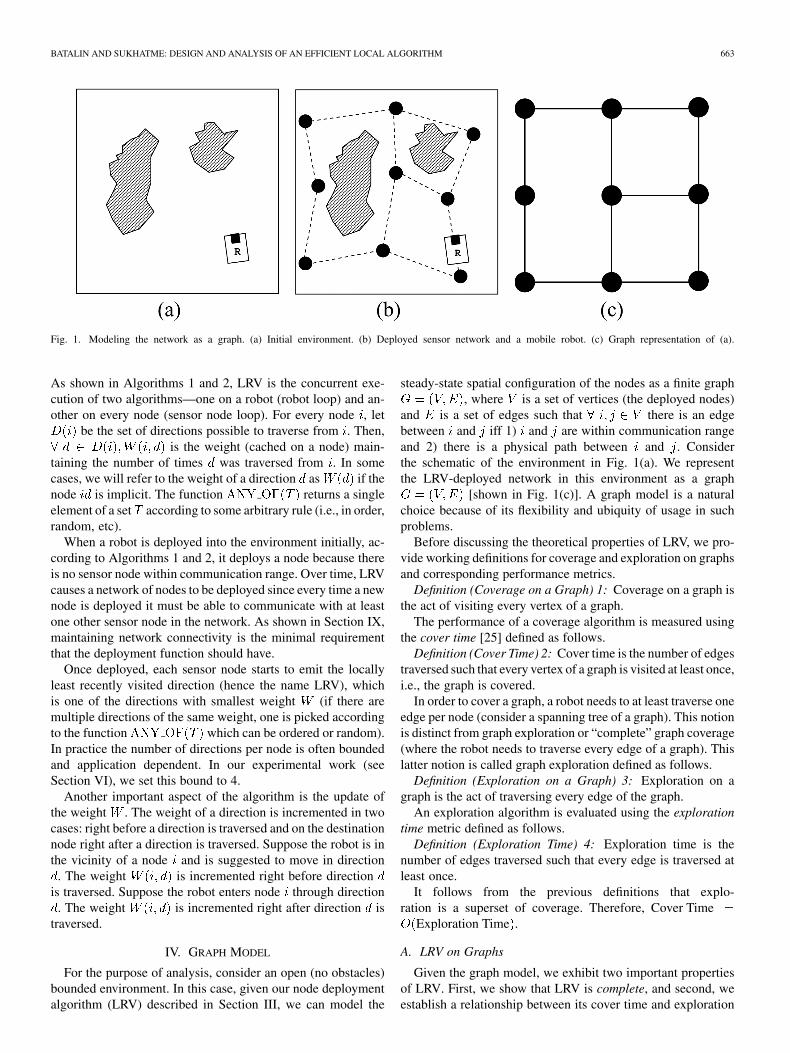
Fig. 1. Modeling the network as a graph. (a) Initial environment. (b) Deployed sensor network and a mobile robot. (c) Graph representation of (a).

As shown in Algorithms 1 and 2, LRV is the concurrent exe-cution of two algorithms—one on a robot (robot loop) and an-other on every node (sensor node loop). For every node , let

be the set of directions possible to traverse from . Then,is the weight (cached on a node) main-

taining the number of times was traversed from . In somecases, we will refer to the weight of a direction as if thenode is implicit. The function returns a singleelement of a set according to some arbitrary rule (i.e., in order,random, etc).

When a robot is deployed into the environment initially, ac-cording to Algorithms 1 and 2, it deploys a node because thereis no sensor node within communication range. Over time, LRVcauses a network of nodes to be deployed since every time a newnode is deployed it must be able to communicate with at leastone other sensor node in the network. As shown in Section IX,maintaining network connectivity is the minimal requirementthat the deployment function should have.

Once deployed, each sensor node starts to emit the locallyleast recently visited direction (hence the name LRV), whichis one of the directions with smallest weight (if there aremultiple directions of the same weight, one is picked accordingto the function which can be ordered or random).In practice the number of directions per node is often boundedand application dependent. In our experimental work (seeSection VI), we set this bound to 4.

Another important aspect of the algorithm is the update ofthe weight . The weight of a direction is incremented in twocases: right before a direction is traversed and on the destinationnode right after a direction is traversed. Suppose the robot is inthe vicinity of a node and is suggested to move in direction

. The weight is incremented right before directionis traversed. Suppose the robot enters node through direction

. The weight is incremented right after direction istraversed.

IV. GRAPH MODEL

For the purpose of analysis, consider an open (no obstacles)bounded environment. In this case, given our node deploymentalgorithm (LRV) described in Section III, we can model the

steady-state spatial configuration of the nodes as a finite graph, where is a set of vertices (the deployed nodes)

and is a set of edges such that there is an edgebetween and iff 1) and are within communication rangeand 2) there is a physical path between and . Considerthe schematic of the environment in Fig. 1(a). We representthe LRV-deployed network in this environment as a graph

[shown in Fig. 1(c)]. A graph model is a naturalchoice because of its flexibility and ubiquity of usage in suchproblems.

Before discussing the theoretical properties of LRV, we pro-vide working definitions for coverage and exploration on graphsand corresponding performance metrics.

Definition (Coverage on a Graph) 1: Coverage on a graph isthe act of visiting every vertex of a graph.

The performance of a coverage algorithm is measured usingthe cover time [25] defined as follows.

Definition (Cover Time) 2: Cover time is the number of edgestraversed such that every vertex of a graph is visited at least once,i.e., the graph is covered.

In order to cover a graph, a robot needs to at least traverse oneedge per node (consider a spanning tree of a graph). This notionis distinct from graph exploration or “complete” graph coverage(where the robot needs to traverse every edge of a graph). Thislatter notion is called graph exploration defined as follows.

Definition (Exploration on a Graph) 3: Exploration on agraph is the act of traversing every edge of the graph.

An exploration algorithm is evaluated using the explorationtime metric defined as follows.

Definition (Exploration Time) 4: Exploration time is thenumber of edges traversed such that every edge is traversed atleast once.

It follows from the previous definitions that explo-ration is a superset of coverage. Therefore, Cover Time

Exploration Time .

A. LRV on Graphs

Given the graph model, we exhibit two important propertiesof LRV. First, we show that LRV is complete, and second, weestablish a relationship between its cover time and exploration


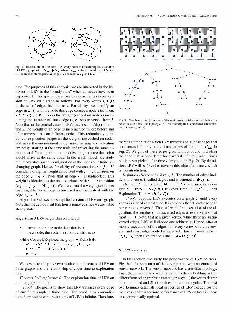
Fig. 2. Illustration for Theorem 1. At every point in time during the executionof LRV a graph G = G + G , where G is the explored part of G andG is an unexplored part. An edge e connects G and G .

time. For purposes of this analysis, we are interested in the be-havior of LRV in the “steady state” when all nodes have beendeployed. In this special case, one can consider a simple ver-sion of LRV on a graph as follows. For every vertex ,is the set of edges incident to . For clarity, we identify anedge in with the node this edge connects node to. Then,

is the weight (cached on node ) main-taining the number of times edge was traversed from .Note that in the general case of LRV, described in Algorithms 1and 2, the weight of an edge is incremented twice: before andafter traversal, but on different nodes. This redundancy is re-quired for practical purposes: the weights are cached on nodesand since the environment is dynamic, sensing and actuationare noisy, starting at the same node and traversing the same di-rection at different points in time does not guarantee that robotwould arrive at the same node. In the graph model, we studythe steady-state spatial configuration of the nodes on a finite un-changing graph. Hence, for clarity of presentation,consider storing the weight associated with transition onthe edge . Note that an edge is undirected. Thisweight is identical to the one associated with transition(e.g., ). We increment the weight just in onecase: right before an edge is traversed and associate it with theedge .

Algorithm 3 shows this simplified version of LRV on a graph.Note that the deployment function is removed since we are in thesteady state.

Algorithm 3 LRV Algorithm on a Graph

—current node; the node the robot is at—next node; the node the robot transitions to

while Covered/Explored the graph FALSE do

We now state and prove two results: completeness of LRV onfinite graphs and the relationship of cover time to explorationtime.

Theorem 1 (Completeness): The exploration time of LRV ona finite graph is finite.

Proof: The goal is to show that LRV traverses every edgeof any finite graph in finite time. The proof is by contradic-tion. Suppose the exploration time of LRV is infinite. Therefore,

Fig. 3. Graph as a tree. (a) A map of the environment with an embedded sensornetwork with a tree-like topology. (b) Tree isomorphic to embedded sensor net-work topology of (a).

there is a time after which LRV traverses only those edges thatit traverses infinitely many times (edges of the graph inFig. 2). Weights of these edges grow without bound, includingthe edge that is considered for traversal infinitely many timesbut is never picked after time (edge in Fig. 2). By defini-tion, LRV will be forced to traverse this edge after time , whichis a contradiction.

Definition (Degree of a Vertex) 5: The number of edges inci-dent to a vertex is called degree and is denoted as .

Theorem 2: For a graph with maximum de-gree , if Cover Time , thenExploration Time .

Proof: Suppose LRV executes on a graph until everyvertex is visited at least once. It is obvious that at least one edgeper vertex is traversed. Thus, after the first execution of the al-gorithm, the number of untraversed edges at every vertex is atmost . Note, that at a given vertex, while there are untra-versed edges, LRV will choose one arbitrarily. Hence, after atmost executions of the algorithm every vertex would be cov-ered and every edge would be traversed. Thus, if Cover Time

, then Exploration Time .

B. LRV on a Tree

In this section, we study the performance of LRV on trees.Fig. 3(a) shows a map of the environment with an embeddedsensor network. The sensor network has a tree-like topology.Fig. 3(b) shows the tree which represents the embedding. A treediffers from other graphs in two major ways: 1) the vertex degreeis not bounded and 2) a tree does not contain cycles. The nexttwo Lemmas establish local properties of LRV needed for themain result of this section: performance of LRV on trees is linearor asymptotically optimal.


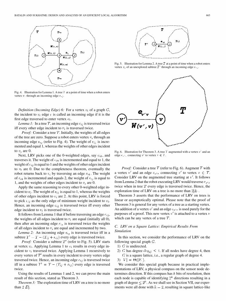
Fig. 4. Illustration for Lemma 1. A tree T at a point of time when a robot entersvertex v through an incoming edge e .

Definition (Incoming Edge) 6: For a vertex of a graph ,the incident to edge is called an incoming edge if it is thefirst edge traversed to enter vertex .

Lemma 1: In a tree , an incoming edge is traversed twiceiff every other edge incident to is traversed twice.

Proof: Consider a tree . Initially, the weights of all edgesof the tree are zero. Suppose a robot enters vertex through anincoming edge (refer to Fig. 4). The weight of is incre-mented and equal 1, whereas the weights of other edges incidentto are 0.

Next, LRV picks one of the 0-weighted edges, say , andtraverses it. The weight of is incremented and equal to 1, theweight of is equal to 1 and the weights of other edges incidentto are 0. Due to the completeness theorem, eventually therobot returns back to by traversing an edge . The weightof is incremented and equals 2, the weight of is equal to1, and the weights of other edges incident to are 0.

Apply the same reasoning to every other 0-weighted edge in-cident to . The weight of is equal to 1, whereas the weightsof other edges incident to are 2. At this point, LRV is forcedto pick as the only edge of minimum weight incident to .Hence, an incoming edge is traversed twice iff every otheredge incident to is traversed twice.

It follows from Lemma 1 that if before traversing an edge ,the weights of all edges incident to are equal (initially all 0),then after an incoming edge is traversed twice the weightsof all edges incident to are equal and incremented by two.

Lemma 2: An incoming edge is traversed twice iff in asubtree every edge is traversed twice.

Proof: Consider a subtree (refer to Fig. 5). LRV startsat vertex . Applying Lemma 1 to results in every edge in-cident to traversed twice. Applying Lemma 1 recursively toevery vertex of results in every incident to every vertex edgetraversed twice. Hence, an incoming edge is traversed twiceiff in a subtree every edge is traversedtwice.

Using the results of Lemmas 1 and 2, we can prove the mainresult of this section, stated as Theorem 3.

Theorem 3: The exploration time of LRV on a tree is no morethan .

Fig. 5. Illustration for Lemma 2. A tree T at a point of time when a robot entersvertex v of an unexplored subtree T through an incoming edge e .

Fig. 6. Illustration for Theorem 3. A tree T augmented with a vertex v and anedge e connecting v to vertex v 2 T .

Proof: Consider a tree (refer to Fig. 6). Augment witha vertex and an edge connecting to vertex .Consider LRV on the augmented tree starting at . It followsfrom Lemma 2 that the robot executing LRV would traversetwice when in tree every edge is traversed twice. Hence, theexploration time of LRV on a tree is no more than .

Theorem 3 asserts that the performance of LRV on trees islinear or asymptotically optimal. Please note that the proof ofTheorem 3 is general for any vertex of a tree as a starting vertex.An addition of a vertex and an edge is used purely for thepurposes of a proof. This new vertex is attached to a vertexwhich can be any vertex of a tree .

C. LRV on a Square Lattice: Empirical Results FromSimulation

In this section, we consider the performance of LRV on thefollowing special graph .

1) is undirected.2) has degree . If all nodes have degree 4, then

is a square lattice, i.e., a regular graph of degree 4.3) .We consider this special graph because in practical imple-

mentations of LRV, a physical compass on the sensor node de-termines direction. If this compass has bits of resolution, theneach node is capable of identifying directions resulting in agraph of degree . As we shall see in Section VII, our exper-iments were all done with , resulting in square lattice-like


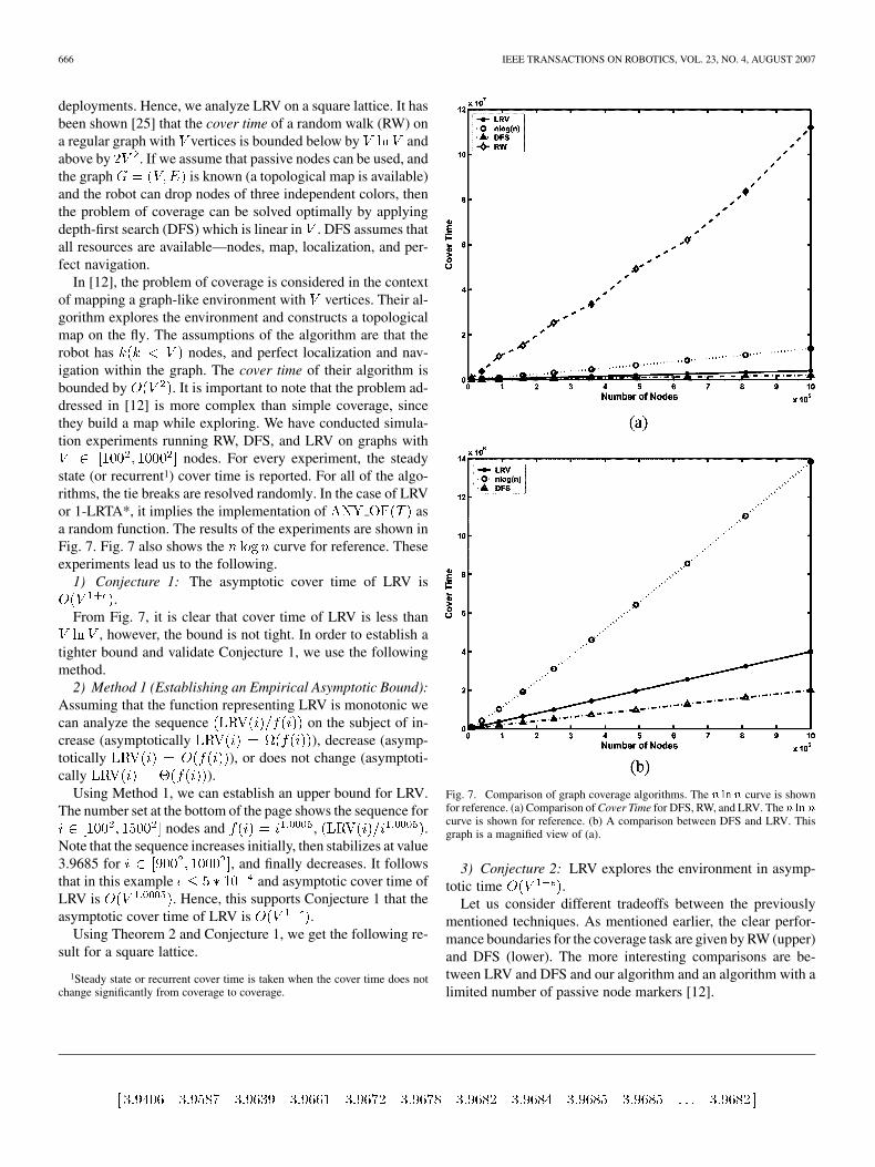
deployments. Hence, we analyze LRV on a square lattice. It hasbeen shown [25] that the cover time of a random walk (RW) ona regular graph with vertices is bounded below by andabove by . If we assume that passive nodes can be used, andthe graph is known (a topological map is available)and the robot can drop nodes of three independent colors, thenthe problem of coverage can be solved optimally by applyingdepth-first search (DFS) which is linear in . DFS assumes thatall resources are available—nodes, map, localization, and per-fect navigation.

In [12], the problem of coverage is considered in the contextof mapping a graph-like environment with vertices. Their al-gorithm explores the environment and constructs a topologicalmap on the fly. The assumptions of the algorithm are that therobot has nodes, and perfect localization and nav-igation within the graph. The cover time of their algorithm isbounded by . It is important to note that the problem ad-dressed in [12] is more complex than simple coverage, sincethey build a map while exploring. We have conducted simula-tion experiments running RW, DFS, and LRV on graphs with

nodes. For every experiment, the steadystate (or recurrent1) cover time is reported. For all of the algo-rithms, the tie breaks are resolved randomly. In the case of LRVor 1-LRTA*, it implies the implementation of asa random function. The results of the experiments are shown inFig. 7. Fig. 7 also shows the curve for reference. Theseexperiments lead us to the following.

1) Conjecture 1: The asymptotic cover time of LRV is.

From Fig. 7, it is clear that cover time of LRV is less than, however, the bound is not tight. In order to establish a

tighter bound and validate Conjecture 1, we use the followingmethod.

2) Method 1 (Establishing an Empirical Asymptotic Bound):Assuming that the function representing LRV is monotonic wecan analyze the sequence on the subject of in-crease (asymptotically ), decrease (asymp-totically ), or does not change (asymptoti-cally ).

Using Method 1, we can establish an upper bound for LRV.The number set at the bottom of the page shows the sequence for

nodes and , .Note that the sequence increases initially, then stabilizes at value3.9685 for , and finally decreases. It followsthat in this example and asymptotic cover time ofLRV is . Hence, this supports Conjecture 1 that theasymptotic cover time of LRV is .

Using Theorem 2 and Conjecture 1, we get the following re-sult for a square lattice.

1Steady state or recurrent cover time is taken when the cover time does notchange significantly from coverage to coverage.

Fig. 7. Comparison of graph coverage algorithms. The n lnn curve is shownfor reference. (a) Comparison of Cover Time for DFS, RW, and LRV. Then lnn

curve is shown for reference. (b) A comparison between DFS and LRV. Thisgraph is a magnified view of (a).

3) Conjecture 2: LRV explores the environment in asymp-totic time .

Let us consider different tradeoffs between the previouslymentioned techniques. As mentioned earlier, the clear perfor-mance boundaries for the coverage task are given by RW (upper)and DFS (lower). The more interesting comparisons are be-tween LRV and DFS and our algorithm and an algorithm with alimited number of passive node markers [12].


Fig. 7(b) shows that the asymptotic performance of our al-gorithm is similar to DFS. Note that in order to determine theidentity of neighboring vertices and to navigate perfectly fromnode to node, DFS assumes that a map of the environment isavailable and that the robot is perfectly localized. Our algorithm,on the other hand, does not have access to global informationand the robot does not localize itself. The nodes used in our al-gorithm are more complicated than those used in DFS and thecover times are asymptotically somewhat larger than the covertimes of DFS.

In [12], the algorithm builds a topological map of the environ-ment and assumes perfect navigation (and thus, localization) onthe graph. The node markers are very simple (the only functionis to mark the vertex) and the robot cannot differentiate betweenthem. In addition, the algorithm assumes that there exists a localenumeration of edges. The cover time of this algorithm, how-ever, is bounded by . Our algorithm, on the other hand,does not have a map and the robot does not localize itself. An-other important difference is that we assume that the number ofnodes available to us is equal to the number of vertices. In ad-dition, the nodes used in our algorithm are more complex, sincethey keep a certain state per direction and are uniquely iden-tifiable. The cover time of our algorithm, however, is conjec-tured to be less than . Thus, the apparent tradeoff is usinga large number of “smart” nodes (and no global informationor localization) versus a limited number of simple nodes (withmapping and partial localization within the graph). The covertime achieved by our algorithm is clearly better. However, if thenodes are a precious resource, the algorithm described in [12]would be preferred.

Another algorithm we compare LRV to is 1-LRTA* [26].1-LRTA* is a well known graph search algorithm that can beapplied to graph coverage. Algorithm 4 shows the details of1-LRTA*. In 1-LRTA*, a weight is associated with a node. Theedge to traverse is chosen based on weights of neighboringnodes. The weight of a node is incremented with the weight ofa node the robot transitions to. Hence, 1-LRTA* requires nodesto communicate.

Algorithm 4 1-LRTA* Algorithm on a Graph

—current node; the node the robot is at—next node; the node the robot transitions to

while Covered/Explored the graph FALSE do

Fig. 8 shows that generally 1-LRTA* outperforms LRV.However, it should be noted that LRV is a deployment andexploration algorithm, whereas 1-LRTA* is a graph explo-ration algorithm which assumes the graph is given. Moreover,1-LRTA* uses information obtained from the neighbors viacommunication, whereas LRV is purely local.

Finally, lets examine how fast LRV, 1-LTRA*, and RW con-verge to a full coverage. Fig. 9 shows a comparison of the con-vergence speed for LRV, 1-LRTA*, and RW on a regular

Fig. 8. Comparison of Cover time of DFS, 1-LRTA*, and LRV.

square lattice. In other words, Fig. 9 shows the percentage ofthe whole graph covered as the algorithms progress (i.e., visitmore and more nodes or as more actions are taken). Fig. 9 (top)shows a linear convergence of LRV and 1-LRTA*, whereas,RW on the interval of 50%–100% of complete coverage [seeFig. 9 (bottom)] exhibits a nonlinear increase in running time.The curve for DFS is not included, since the convergence factoris optimal and the cover time is at most twice the number ofnodes.

D. LRV on a Cube Lattice or LRV in 3-D

In Section IV-C, we considered an application of LRV to theproblem of coverage and exploration on a plane. In the planarcase, the graph representing the network embedding is a squarelattice. In this section, we extend discussion of LRV perfor-mance to a general 3-D case. In 3-D case, the graph representa-tion of the deployed sensor network is a graph .

1) is undirected.2) has degree . If all nodes have degree 6, then

is a cube lattice, i.e., a regular graph of degree 6.3) .Fig. 10 shows an example of a cube lattice which represents

possible network embedding in a real 3-D environment. Notethat in comparison with a square lattice representation in theplanar case, a general cube lattice has two more edges incident toevery node. At the same time, we will show that the performanceof LRV scales similarly with the size of the graph.

We have conducted simulation experiments running LRV and1-LRTA* on graphs with nodes. For every ex-periment the steady state (or recurrent) cover time is reported.The tie breaks are resolved randomly (e.g., is arandom function). The results of the experiments are shown inFig. 11. As shown on Fig. 11, 1-LRTA* outperforms LRV (as isthe case in the planar case), however, it is also more sensitive tothe initial conditions (various starting points).


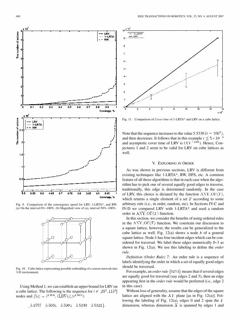
Fig. 9. Comparison of the convergence speed for LRV, 1-LRTA*, and RW.(a) On the interval 0%–100%. (b) Magnified view of (a), interval 50%–100%.

Fig. 10. Cube lattice representing possible embedding of a sensor network into3-D environment.

Using Method 1, we can establish an upper bound for LRV ona cube lattice. The following is the sequence fornodes and , :

Fig. 11. Comparison of Cover time of 1-LRTA* and LRV on a cube lattice.

Note that the sequence increases to the value 5.5330 ,and then decreases. It follows that in this exampleand asymptotic cover time of LRV is . Hence, Con-jectures 1 and 2 seem to be valid for LRV on cube lattices aswell.

V. EXPLORING IN ORDER

As was shown in previous sections, LRV is different fromexisting techniques like 1-LRTA*, RW, DFS, etc. A commonfeature of all these algorithms is that in each case when the algo-rithm has to pick one of several equally good edges to traverse,traditionally, this edge is determined randomly. In the caseof LRV, this choice is dictated by the function ,which returns a single element of a set according to somearbitrary rule (i.e., in order, random, etc). In Sections IV-C andIV-D we compared LRV with 1-LRTA* and used a randomorder in function.

In this section, we consider the benefits of using ordered rulesin the function. We constrain our discussion toa square lattice, however, the results can be generalized to thecube lattice as well. Fig. 12(a) shows a node of a generalsquare lattice. Node has four incident edges which can be con-sidered for traversal. We label these edges numerically 0–3 asshown in Fig. 12(a). We use this labeling to define the orderrule.

Definition (Order Rule) 7: An order rule is a sequence oflabels identifying the order in which a set of equally good edgesshould be traversed.

For example, an order rule means that if several edgesare equally good for traversal (say edges 2 and 3), then an edgeappearing first in the order rule would be preferred (i.e., edge 2in this case).

Without loss of generality, assume that the edges of the squarelattice are aligned with the plane [as in Fig. 12(a)]. Fol-lowing the labeling of Fig. 12(a), edges 0 and 2 span thedimension, whereas dimension is spanned by edges 1 and


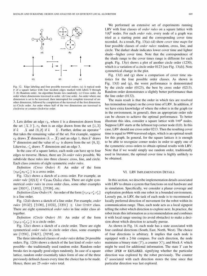
Fig. 12. Edge labeling and four possible traversal orders. (a) A typical nodek of a square lattice with four incident edges marked with labels 0 through3. (b) Random order. An algorithm breaks ties randomly. (c) Cross order. Anorder where dimensions traversed in order. (d) Line order. An order where onedimension is set to be traversed, then interrupted for complete traversal of an-other dimension, followed by completion of the traversal of the first dimension.(e) Circle order. An order where half of the two dimensions are traversed inclockwise or counter-clockwise order.

3. Lets define an edge , where is a dimension drawn fromthe set , then is an edge drawn from the setif and if . Further, define an operatorthat takes the remaining value of the set. For example, suppose

draws dimension and an edge 1, then drawsdimension and the value of is drawn from the set .

Likewise, draws dimension and an edge 3.In the case of a square lattice, each node can have up to four

edges to traverse. Hence, there are 24 order rules possible. Wesubdivide these rules into three classes: cross, line, and circle.Each class consists of eight symmetric order rules.

Definition (Cross Order) 8: An order of the formis a cross order.

Fig. 12(c) shows a sketch of a cross order. For example, anorder rule class. There are eight sym-metrical order rules in cross order class, some other examplesare , , , etc.

Definition (Line Order) 9: An order of the formis a line order.

Fig. 12(d) shows a sketch of a line order. For example, orderrules class.There are eight symmetrical order rules in line order class al-together.

Definition (Circle Order) 10: An order of the formis a circle order.

Fig. 12(e) shows a sketch of a circle order. There are eightsymmetrical order rules in circle order class, some examplesare , , , etc.

The three introduced classes of order rules define 24 possibleorders. Fig. 12(b) shows a sketch of the last kind of order rulespossible—the traditionally used random order. Random orderbreaks ties in equally good edges randomly. In case of a squarelattice, random order essentially takes form of one of the threepreviously defined classes every time the choice has to be made.Hence, there are 25 order rules total.

We performed an extensive set of experiments runningLRV with four classes of order rules on a square lattice with

nodes. For each order rule, every node of a graph wastried as a starting point and the corresponding cover timerecorded. As a result, Fig. 13(a)–(d) show cover time maps forfour possible classes of order rules: random, cross, line, andcircle. The darker shade indicates lower cover time and lightershade—higher cover time. Note that the correspondence ofthe shade range to the cover times range is different for eachgraph. Fig. 13(e) shows a plot of another circle order (1230),which is a variation of a circle order 0123 [see Fig. 13(d)]. Notesymmetrical change in the plot.

Fig. 13(f) and (g) show a comparison of cover time sta-tistics for the four possible order classes. As shown inFig. 13(f) and (g), the worst performance is demonstratedby the circle order (0123), the best by cross order (0213).Random order demonstrates a slightly better performance thanthe line order (0132).

The main result is that the order in which ties are resolvedhas tremendous impact on the cover time of LRV. In addition, ifwe have extra knowledge of where the robot is in the graph (orin the environment, in general), then an appropriate order rulecan be chosen to achieve the optimal performance. To betterillustrate this idea, consider a square lattice with nodes.Suppose LRV starts at the leftmost top corner node (0,0). In thiscase, LRV should use cross order 0213. Then the resulting covertime is equal to 9999 traversed edges, which is an optimal resultfor this graph. In general, for the square lattices it is enoughto be able to recognize corner nodes in order to apply one ofthe symmetric cross orders to obtain optimal results with LRV.Note that if we would simply use random order, traditionallyused in literature, the optimal cover time is highly unlikely tobe obtained.

VI. LRV IMPLEMENTATION DETAILS

In this section, we describe implementation details associatedwith LRV to obtain a system that functions on real hardware andin simulation. Specifically, we consider a planar coverage andexploration problem with one robot in a bounded environment.Loosely put, in LRV, the task of each node is to recommend alocally preferred direction of movement for the robot within itscommunication range. Thus, each node acts as a local signposttelling the robot which direction to explore next. In practice, therobot treats this information as a recommendation and combinesit with local range sensing (to avoid obstacles) to make a deci-sion about which direction to actually pursue.

As shown in Fig. 14, each node has a state associated withfour cardinal directions (South, East, North, West). The choiceof four directions is arbitrary. It implies that each node isequipped with a 2-bit compass. For each direction, the nodemaintains a binary state , a counter , and block whichmight be used for additional information. The state can beeither or , signifying whether the particulardirection was explored by the robot previously. The counter

associated with each direction stores the time since thatparticular direction was last explored.


Fig. 13. Possible orders and their effect on cover time. (a)–(d) Four distinctive types of orders possible in the case of a square lattice. Plots show the cover timesof running LRV with representative order on a square lattice with 100 nodes. Every node tried as a starting point. Grayscale pixels in each plot represent a covertime of LRV using a node at corresponding XY location as a starting node. The darker shade indicates lower cover time and the lighter shade indicates highercover time. Note that the correspondence of the color range to the cover times range is different for each graph. (e) Circle order 1230 is a variation of a circle order0123. Note symmetrical change in the plot. (f)–(g) Comparison of cover times statistic for the four different possible orders presented in (a)–(d). (a) Random order.(b) Cross (0213) order. (c) Line (0132) order. (d) Circle (0123) order. (e) Circle (1230) order. (f) Comparison of cover times. (g) Magnified view of f).

Fig. 14. Node architecture.

When deployed, a node emits two data packets with differentsignal strengths. The packet with the lower signal strengthis called the MIN-packet and the one with the higher signalstrength is called the MAX-packet. The MAX-packet is used fordata propagation within the deployed network. The MIN-packetcontains information about the suggested direction the robotshould take for coverage/exploration. This implies that therobot’s compass and the node’s compass agree locally on theirmeasurement of direction. Given the coarse coding of directionwe have chosen, this is not a problem in realistic settings. Thepolicy used by the nodes to compute the suggested direction forexploration/coverage to recommend the least recently visited

Fig. 15. System architecture showing robot behaviors.

directions preferentially. All directions are recommendedfirst (in order from South to West), followed by thedirections with least last update value (least value of C). Notethat this algorithm does not use inter-node communication.

The robot is programmed using a behavior-based approach[27] with arbitration [28] for behavior coordination. Prioritiesare assigned to every behavior a priori. As shown in Fig. 15, therobot executes four behaviors: ObstacleAvoidance, AtBeacon,DeployBeacon, and SearchBeacon. In addition to priority, everybehavior has an activation level, which decides, given the sen-sory input, whether the behavior should be in an active or pas-sive state (1 or 0, respectively). Each behavior computes theproduct of its activation level and corresponding priority and


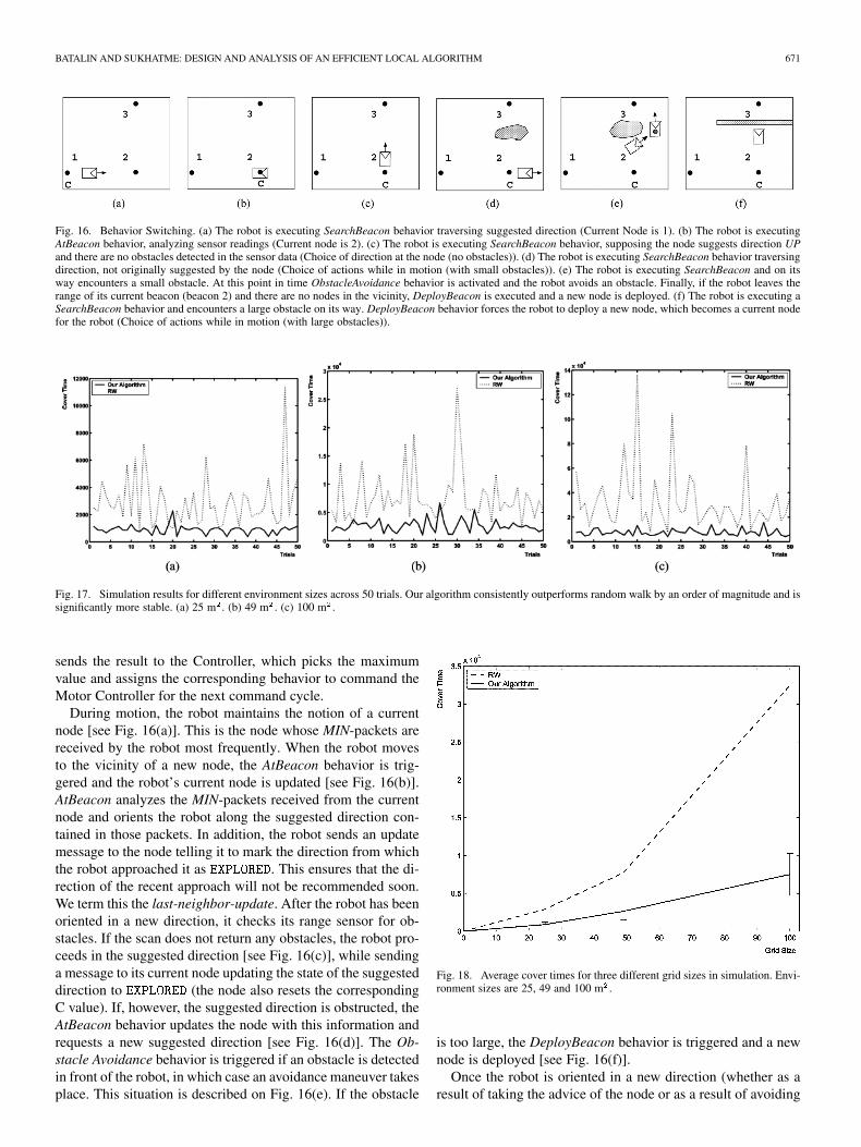
Fig. 16. Behavior Switching. (a) The robot is executing SearchBeacon behavior traversing suggested direction (Current Node is 1). (b) The robot is executingAtBeacon behavior, analyzing sensor readings (Current node is 2). (c) The robot is executing SearchBeacon behavior, supposing the node suggests direction UPand there are no obstacles detected in the sensor data (Choice of direction at the node (no obstacles)). (d) The robot is executing SearchBeacon behavior traversingdirection, not originally suggested by the node (Choice of actions while in motion (with small obstacles)). (e) The robot is executing SearchBeacon and on itsway encounters a small obstacle. At this point in time ObstacleAvoidance behavior is activated and the robot avoids an obstacle. Finally, if the robot leaves therange of its current beacon (beacon 2) and there are no nodes in the vicinity, DeployBeacon is executed and a new node is deployed. (f) The robot is executing aSearchBeacon behavior and encounters a large obstacle on its way. DeployBeacon behavior forces the robot to deploy a new node, which becomes a current nodefor the robot (Choice of actions while in motion (with large obstacles)).

Fig. 17. Simulation results for different environment sizes across 50 trials. Our algorithm consistently outperforms random walk by an order of magnitude and issignificantly more stable. (a) 25 m . (b) 49 m . (c) 100 m .

sends the result to the Controller, which picks the maximumvalue and assigns the corresponding behavior to command theMotor Controller for the next command cycle.

During motion, the robot maintains the notion of a currentnode [see Fig. 16(a)]. This is the node whose MIN-packets arereceived by the robot most frequently. When the robot movesto the vicinity of a new node, the AtBeacon behavior is trig-gered and the robot’s current node is updated [see Fig. 16(b)].AtBeacon analyzes the MIN-packets received from the currentnode and orients the robot along the suggested direction con-tained in those packets. In addition, the robot sends an updatemessage to the node telling it to mark the direction from whichthe robot approached it as . This ensures that the di-rection of the recent approach will not be recommended soon.We term this the last-neighbor-update. After the robot has beenoriented in a new direction, it checks its range sensor for ob-stacles. If the scan does not return any obstacles, the robot pro-ceeds in the suggested direction [see Fig. 16(c)], while sendinga message to its current node updating the state of the suggesteddirection to (the node also resets the correspondingC value). If, however, the suggested direction is obstructed, theAtBeacon behavior updates the node with this information andrequests a new suggested direction [see Fig. 16(d)]. The Ob-stacle Avoidance behavior is triggered if an obstacle is detectedin front of the robot, in which case an avoidance maneuver takesplace. This situation is described on Fig. 16(e). If the obstacle

Fig. 18. Average cover times for three different grid sizes in simulation. Envi-ronment sizes are 25, 49 and 100 m .

is too large, the DeployBeacon behavior is triggered and a newnode is deployed [see Fig. 16(f)].

Once the robot is oriented in a new direction (whether as aresult of taking the advice of the node or as a result of avoiding


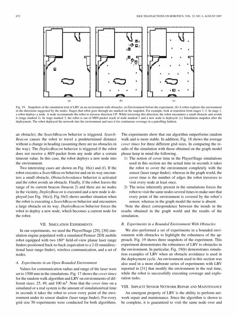
Fig. 19. Snapshots of the simulation trial of LRV on an environment with obstacles. (a) Environment before the experiment. (b) A robot explores the environmentin the directions suggested by the nodes. Stages that robot goes through are marked on the snapshot. For example, look at transition from stages 1–3. In stage 1,a robot deploys a node. A node recommends the robot to traverse direction UP. While traversing this direction, the robot encounters a small obstacle and avoidsit (stage marked 2). In stage marked 3, the robot is out of MIN-packet reach of node marked 1 and a new node is deployed. (c) Simulation snapshot after thedeployment. The robot deployed the network into the environment and uses it for continuous coverage in a patrolling fashion.

an obstacle), the SearchBeacon behavior is triggered. Search-Beacon causes the robot to travel a predetermined distancewithout a change in heading (assuming there are no obstacles inthe way). The DeployBeacon behavior is triggered if the robotdoes not receive a MIN-packet from any node after a certaintimeout value. In this case, the robot deploys a new node intothe environment.

Two interesting cases are shown on Fig. 16(e) and (f). If therobot executes a SearchBeacon behavior and on its way encoun-ters a small obstacle, ObstacleAvoidance behavior is activatedand the robot avoids an obstacle. Finally, if the robot leaves therange of its current beacon (beacon 2) and there are no nodesin the vicinity, DeployBeacon is executed and a new node is de-ployed [see Fig. 16(e)]. Fig 16(f) shows another situation whenthe robot is executing a SearchBeacon behavior and encountersa large obstacle on its way. DeployBeacon behavior forces therobot to deploy a new node, which becomes a current node forthe robot.

VII. SIMULATION EXPERIMENTS

In our experiments, we used the Player/Stage [29], [30] sim-ulation engine populated with a simulated Pioneer 2DX mobilerobot equipped with two 180 field-of-view planar laser rangefinders positioned back-to-back (equivalent to a 2-D omnidirec-tional laser range finder), wireless communication, and a set ofnodes.

A. Experiments in an Open Bounded Environment

Values for communication radius and range of the laser wereset to 1500 mm in the simulations. Fig. 17 shows the cover timesfor the random walk algorithm and LRV on environments of dif-ferent sizes: 25, 49, and 100 m . Note that the cover time on asimulated or a real system is the amount of simulation/real timein seconds it takes the robot to cover every point of the envi-ronment under its sensor shadow (laser range finder). For everygrid size 50 experiments were conducted for both algorithms.

The experiments show that our algorithm outperforms randomwalk and is more stable. In addition, Fig. 18 shows the averagecover times for three different grid sizes. In comparing the re-sults of the simulation with those obtained on the graph modelplease keep in mind the following.

1) The notion of cover time in the Player/Stage simulationsused in this section are the actual time in seconds it takesthe robot to cover the environment completely with thesensor (laser range finder), whereas in the graph world, thecover time is the number of edges the robot traverses tovisit every node at least once.

2) The noise inherently present in the simulations forces therobot to visit the same nodes several times to make sure thatevery point of the environment is covered by the robot’ssensor, whereas in the graph model the noise is absent.

Note the direct correspondence between the trends in theresults obtained in the graph world and the results of thesimulation.

B. Experiments in a Bounded Environment With Obstacles

We also performed a set of experiments in a bounded envi-ronment with obstacles to highlight the robustness of the ap-proach. Fig. 19 shows three snapshots of the experiment. Thisexperiment demonstrates the robustness of LRV to obstacles inthe environment. In particular, Fig. 19(b) demonstrates simula-tion examples of LRV when an obstacle avoidance is used inthe deployment cycle. An environment used in this section wasalso used in a more elaborate series of experiments with LRVreported in [31] that modify the environment in the real time,while the robot is successfully executing coverage and explo-ration tasks.

VIII. IMPLICIT SENSOR NETWORK REPAIR AND MAINTENANCE

An emergent property of LRV is the ability to perform net-work repair and maintenance. Since the algorithm is shown tobe complete, it is guaranteed to visit the same node over and


over again. Suppose that one of the nodes, say node , ran out ofpower or was damaged. Further consider a moment in time justbefore the robot traverses direction towards the damaged node.Now, the robot is moving along direction towards node . Ac-cording to the deployment function that is used, there should bea communication/sensing gap in the deployed sensor network(unless the network was over deployed and does not require re-pair). Hence, while facing the same deployment situation andusing the same deployment function at the location where node

was deployed, the robot simply deploys a new node, therebysolving the problem of sensor network repair and maintenanceimplicitly. Note that if the robot can recognize the nodes then itcan attempt repairing the node first (or retrieving for later repairat the base) before deploying the new node.

IX. REMARKS ON GENERALIZATION

In this paper, we have presented an algorithm based on thepolicy of choosing the least recently visited directions preferen-tially. At the same time, depending on the application require-ments, other policies might be better. It is possible to extendother search/coverage algorithms using physical network em-bedding to function in unknown, unstructured, dynamic envi-ronments. The basic idea is to augment a coverage algorithmwith an ability to deploy and maintain physical network infra-structure, while simultaneously using the network to aid in cov-erage and exploration. Thus, what we want to highlight is the un-derlying philosophy of network deployment as an integral partof coverage and exploration.

Sensor network deployment is one of the building blocks ofthis paper. A robot decides when to deploy a node based on adeployment condition, or more generally, deployment function.A deployment function should be designed based on the appli-cation. However, there are two main characteristics that everydeployment function should have: 1) the deployed sensor net-work is connected (i.e., between any two nodes there should bea communication path) and 2) deployed static network configu-ration should be such that static coverage is maximized. In theproposed implementation of LRV, both characteristics are cap-tured. The deployment is based on communication range thresh-olding. Hence, the two consecutive nodes are guaranteed to beconnected (thus, the deployed sensor network is connected) andwe adjusted communication range threshold so that if everysensor node is equipped with high fidelity sensor, static cov-erage is maximized. Note that in a general case when the dy-namic coverage problem is considered, a complete coverage isachieved by LRV when the deployment distance is less than orequal to twice the sensing range, which is trivial to visualizegeometrically.

Other deployment functions could also encode such parame-ters as desired topology (i.e., by specifying the number of nodesdeployed in different directions, etc.), desired boundary, phe-nomenon density (deploy more nodes in places with high phe-nomenon density), deploy where landmarks detected, etc.

X. CONCLUSION

In this paper, we have presented an efficient, robust, and scal-able algorithm to embed an active infrastructure (sensing, com-

munication, and computation) into the environment while si-multaneously using this infrastructure for coverage and explo-ration. The algorithm (LRV) is based on visiting the LRV direc-tions preferentially and is decentralized, scalable, robust, faulttolerant, and can be used on simple robots. LRV is based onthe idea of deploying sensor nodes from time to time. Once de-ployed, every node acts like a signpost recording which direc-tions the robot has explored recently. When a robot is in thevicinity of a node, it recommends to the robot a direction thathas been least recently visited (hence, the name LRV).

We analyzed the characteristics of LRV theoretically, mod-eling the static steady state of the deployed sensor network asa finite graph . We proved that LRV is complete on (i.e.,the exploration time of LRV on a finite graph is finite). For agraph with maximum degree , if Cover Time

, then Exploration Time . We provedthat exploration time is (twice the number of edges, orasymptotically optimal) for the special case, when is a tree.For another special case, when is a square lattice, we em-pirically conjectured that both cover and exploration times areasymptotically . The special case of a square lattice isalso interesting from practical perspective, because in our LRVimplementation and experiments we chose to maintain at mostfour directions, which results in a static steady state of the de-ployed sensor network resembling a square lattice.

We examined the tradeoffs that should be considered inchoosing one exploration algorithm over another to solve thisproblem. The bounds for the coverage task are given by randomwalk (the robot has no information and explores randomly) anddepth first search (a map of the environment is available in theform of a graph) which solves the problem optimally.

The data shown in Fig. 7, suggests strongly that our algorithmasymptotically outperforms the node algorithm presented in[12].

In addition, it is shown in [12] that if the number of avail-able nodes reduces, the cover time increases rapidly. Therefore,in dynamic environments the performance of the algorithm de-creases drastically even if one node is destroyed. Whereas in ouralgorithm, such a problem does not exist, since a new node willbe deployed in place of the destroyed one automatically.

We compared LRV to 1-LRTA* [26]. 1-LRTA* is a wellknown graph search algorithm that can be applied to graphcoverage. In 1-LRTA*, a weight is associated with a node. Theedge to traverse is chosen based on weights of neighboringnodes. The weight of a node is incremented with the weightof a node the robot transitions to. Hence, 1-LRTA* requiresnodes to communicate. Fig. 8 shows that generally 1-LRTA*outperforms LRV. However, in reality LRV deploys the net-work in addition to exploring, whereas 1-LRTA* requires thegraph to operate on. An important result of this chapter isthat it is possible to extend other search/coverage algorithmsusing physical network embedding to function in unknown,unstructured, dynamic environments.

We have extended an analysis of LRV to a cube lattice graphthat represents network embedding in 3-D case. For this specialcase, when is a cube lattice, we empirically conjectured thatboth cover and exploration times are asymptotically as in squarelattice case and is bounded by .


Fig. 20. Deployment of nodes in a representative simulation trial. Note that dueto noise added in simulation, the deployed nodes do not form a perfectly squarelattice.

We also studied the benefits of using ordered rules in tie breakresolution (choosing one of equally good edges). In the case ofa square lattice, each node can have up to four edges to traverse.Hence, there are 24 order rules possible. We proposed classi-fication of these rules into three classes: cross, line, and circle.Each class consists of eight symmetric order rules. We have per-formed extensive experimental trials that showed cross ordersperform better than traditionally used random order. Further-more, in general, for square lattices it is enough to be able torecognize corner nodes in order to apply one of the symmetriccross orders to obtain optimal results with LRV. Note that if wewould simply use random order, traditionally used in literature,the optimal cover time is highly unlikely to obtain.

We verified the performance of LRV and its asymptotic be-havior in simulation. There exists a direct correspondence be-tween the results obtained from the theoretical analysis (cov-erage on the graph) and the data from simulation experiments.Note also, that even though the lattice grid was considered as agraph environment for the theoretical analysis, in practice, thenetwork of deployed nodes is not required to be a perfect grid.Fig. 20 shows a series of screen shots taken from one of the trialsof the simulation in the 49 m environment. Note also that theperformance of our algorithm is not affected, since it does notrely on localization or mapping.

The theoretical analysis on graphs and verification in simu-lation shows that tradeoffs in the assumptions can affect covertime significantly. Simple algorithms like RW or DFS can beused for coverage, but only in the extreme cases as describedpreviously. In the case where mapping and localization are notavailable but the number of available nodes is unlimited, our al-gorithm appears to outperform others.

The algorithm that we propose and analyze in this paper(LRV) allows us to deploy and maintain a sensor network, while

covering and exploring the environment. In our paper, we useLRV as a fundamental system [32] for enabling network-me-diated robot navigation [33], network-mediated multi-robottask allocation [34], and the general problem of spatiotemporalmonitoring [35].

REFERENCES

[1] M. A. Batalin and G. S. Sukhatme, “Efficient exploration without lo-calization,” in Proc. IEEE Int. Conf. Robot. Autom. (ICRA), 2003, pp.2714–2719.

[2] M. A. Batalin and G. S. Sukhatme, “The analysis of an efficient al-gorithm for robot coverage and exploration based on sensor networkdeployment,” in Proc. IEEE Int. Conf. Robot. Autom. (ICRA), 2005,pp. 3489–3496.

[3] D. W. Gage, “Command control for many-robot systems,” in Proc. 19thAnnu. AUVS Techn. Symp., 1992, pp. 22–24.

[4] J. O’Rourke, Art Gallery Theorems and Algorithms. New York: Ox-ford Univ. Press, 1987.

[5] A. Howard, M. J. Mataric, and G. S. Sukhatme, “Mobile sensor net-work deployment using potential fields: A distributed, scalable solu-tion to the area coverage problem,” in Proc. 6th Int. Symp. Distrib. Au-tonomous Robot. Syst., 2002, pp. 299–308.

[6] M. A. Batalin and G. S. Sukhatme, “Spreading out: A local approachto multi-robot coverage,” in Proc. 6th Int. Symp. Distrib. AutonomousRobot. Syst., 2002, pp. 373–382.

[7] M. A. Batalin and G. S. Sukhatme, “Sensor coverage using mobilerobots and stationary nodes,” in Proc. SPIE, 2002, pp. 269–276.

[8] H. Choset, “Coverage for robotics—A survey of recent results,” AnnalsMath. Artif. Intell., vol. 31, pp. 113–126, 2001.

[9] B. Yamauchi, “Frontier-based approach for autonomous exploration,”in Proc. IEEE Int. Symp. Comput. Intell., Robot. Autom., 1997, pp.146–151.

[10] A. Zelinsky, “A mobile robot exploration algorithm,” IEEE Trans.Robot. Autom., vol. 8, no. 6, pp. 707–717, Dec. 1992.

[11] W. Burgard, D. Fox, M. Moors, R. Simmons, and S. Thrun, “Collabo-rative multirobot exploration,” in Proc. IEEE Int. Conf. Robot. Autom.(ICRA), 2000, pp. 476–481.

[12] G. Dudek, M. Jenkin, E. Milios, and D. Wilkes, “Robotic explorationas graph construction,” IEEE Trans. Robot. Autom., vol. 7, no. 6, pp.859–865, Dec. 1991.

[13] M. A. Bender, A. Fernandez, D. Ron, A. Sahai, and S. Vadhan, “Thepower of a pebble: Exploring and mapping directed graphs,” in Proc.Annu. ACM Symp. Theory Comput. (STOC), 1998, pp. 269–278.

[14] R. T. Vaughan, K. Stoy, G. S. Sukhatme, and M. J. Mataric, “Whistlingin the dark: Cooperative trail following in uncertain localization space,”in Proc. Autonomous Agents Multi-Agent Syst., 2000, pp. 187–194.

[15] R. T. Vaughan, K. Stoy, G. S. Sukhatme, and M. J. Mataric, “Lost:Localization-space trails for robot teams,” IEEE Trans. Robot. Autom.,Special Issue Multi-Robot Syst., vol. 18, no. 5, pp. 796–812, Oct. 2002.

[16] S. Koenig, B. Szymanski, and Y. Liu, “Efficient and inefficient ant cov-erage methods,” Annals Math. Artif. Intell., vol. 41, no. 76, pp. 31–31,2001.

[17] J. Svennebring and S. Koenig, “Trail-laying robots for robust terraincoverage,” in Proc. IEEE Int. Conf. Robot. Autom. (ICRA), 2003, pp.75–82.

[18] I. Wagner, M. Lindenbaum, and A. Bruckstein, “Distributed coveringby ant-robots using evaporating traces,” IEEE Trans. Robot. Autom.,vol. 15, no. 5, pp. 918–933, Oct. 1999.

[19] I. Wagner, M. Lindenbaum, and A. Bruckstein, “Efficiently searching adynamic graph by a smell-oriented vertex process,” Annals Math. Artif.Intell., vol. 24, pp. 211–223, 1998.

[20] I. Wagner, M. Lindenbaum, and A. Bruckstein, “Mac vs. pc: Deter-minism and randomness as complementary approaches to robotic ex-ploration of continuous unknown domains,” Int. J. Robot. Res., vol. 19,no. 1, pp. 12–31, 2000.

[21] S. Meguerdichian, F. Koushanfar, M. Potkonjak, and M. B. Srivas-tava, “Coverage problems in wireless ad-hoc sensor networks,” in Proc.IEEE INFOCOM, 2001, pp. 1380–1387.

[22] M. McGlynn and S. Borbash, “Birthday protocols for low energy de-ployment and flexible neighbor discovery in ad hoc wireless networks,”in Proc. MobiHoc, 2001, pp. 137–145.

[23] T. Clouqueur, V. Phipatanasuphorn, P. Ramanathan, and K. K. Saluja,“Sensor deployment strategy for target detection,” in Proc. 1st ACMInt. Workshop Wireless Sensor Netw. Appl., 2002, pp. 42–48.


[24] S. S. Dhillon and K. Chakrabarty, “Sensor placement for effective cov-erage and surveillance in distributed sensor networks,” in Proc. IEEEWireless Commun. Netw. Conf., 2003, pp. 1609–1614.

[25] L. Lovasz, “Random Walks on Graphs: A Survey,” Bolyai Soc. Math.Study, Combinatorics, vol. 2, pp. 1–46, 1993.

[26] S. Koenig and R. Simmons, “Easy and hard testbeds for real-timesearch algorithms,” in Proc. Nat. Conf. Artif. Intell., 1996, pp.279–285.

[27] M. J. Mataric, “Behavior-based control: Examples from navigation,learning, and group behavior,” J. Experimental Theoretical Artif.Intell., Special Issue Softw. Arch. Phys. Agents, vol. 9, no. 2-3, pp.323–336, 1997.

[28] P. Pirjanian, “Behavior coordination mechanisms—state-of-the-art,”Inst. Robot. Intell. Syst., Univ. Southern California, Los Angeles,Tech. Rep. IRIS-99-375, 1999.

[29] B. P. Gerkey, R. Vaughan, K. Stoy, A. Howard, G. Sukhatme, and M.Mataric, “Most valuable player: A robot device server for distributedcontrol,” in Proc. IEEE/RSJ Int. Conf. Intell. Robot. Syst. (IROS), 2001,pp. 1226–1231.

[30] R. Vaughan, “Stage: A multiple robot simulator,” Inst. Robot. Intell.Syst., Univ. Southern California, Los Angeles, Tech. Rep. IRIS-00-393, 2000.

[31] M. A. Batalin and G. Sukhatme, “Coverage, exploration and deploy-ment by a mobile robot and communication network,” Telecommun.Syst. J., Special Issue Wireless Sensor Netw., vol. 26, no. 2, pp.181–196, 2004.

[32] M. Batalin, “Symbiosis: Cooperative algorithms for mobile robotsand a sensor network,” Ph.D. dissertation, Comput. Sci. Dept., Univ.Southern California, Los Angeles, 2005.

[33] M. Batalin, G. Sukhatme, and M. Hattig, “Mobile robot navigationusing a sensor network,” in Proc. IEEE Int. Conf. Robot. Autom., 2004,pp. 636–642.

[34] M. Batalin and G. Sukhatme, “Sensor network-mediated multi-robottask allocation,” in Proc. 3rd Int. Naval Res. Lab. Multi-Robot Syst.Workshop, 2005, pp. 27–42.

[35] M. Batalin, M. Rahimi, Y. Yu, S. Liu, A. Kansal, G. Sukhatme, W.Kaiser, M. Hansen, G. Pottie, M. Srivastava, and D. Estrin, “Call andresponse: Experiments in sampling the environment,” in Proc. ACMSENSYS, 2004, pp. 25–38.

Maxim A. Batalin (M’05) received the M.S. andPh.D. degrees in computer science from the Univer-sity of Southern California (USC), Los Angeles, andthe B.S. degree in mathematics, computer sciencefrom the University of Oregon, Eugene, OR, in 2001,and the M.S. degree in management from TavriyaNational University, Simferopol, Ukraine, in 2002.

He is a Researcher with the Center for EmbeddedNetworked Sensing, University of California, LosAngeles (UCLA). His primary research interestsare in mobile robotics, sensor networking, and

biomedical systems. He has published over 20 technical papers.Dr. Batalin is a member of Sigma Xi.

Gaurav S. Sukhatme (M’05) received the M.S. andPh.D. degrees in computer science from Universityof Southern California (USC), Los Angeles.

He is an Associate Professor of Computer Science(joint appointment in Electrical Engineering) withUSC. He is the Codirector of the USC RoboticsResearch Laboratory and the Director of the USCRobotic Embedded Systems Laboratory, which hefounded in 2000. His research interests includemultirobot systems, sensor/actuator networks, androbotic sensor networks. He has published exten-

sively in these and related areas.Prof. Sukhatme was a recipient of the NSF CAREER Award and the Okawa

Foundation Research Award. He has served as PI on several NSF, DARPA, andNASA grants. He is a Co-PI on the Center for Embedded Networked Sensing(CENS), an NSF Science and Technology Center. He is a member of AAAIand the ACM. and is one of the founders of the Robotics: Science and Systemsconference. He is program chair of the 2008 IEEE International Conference onRobotics and Automation and the Editor-in-Chief of Autonomous Robots. Hehas served as an Associate Editor of the IEEE TRANSACTIONS ON ROBOTICS

AND AUTOMATION, the IEEE TRANSACTIONS ON MOBILE COMPUTING, and onthe editorial board of IEEE Pervasive Computing.

The Design and Analysis of an Efficient Local Algorithm for Coverage and Exploration Based on Sensor...

Documents

Transcript of The Design and Analysis of an Efficient Local Algorithm for Coverage and Exploration Based on Sensor...