The accretion history of dark matter halos II: The connections with the mass power spectrum and the...

arX

iv:1

501.

0438

2v1

[as

tro-

ph.C

O]

19

Jan

2015

Mon. Not. R. Astron. Soc. 000, 1–?? (2013) Printed 20 January 2015 (MN LaTEX style file v2.2)

The accretion history of dark matter halos II:

The connections with the mass power spectrum and the

density profile

Camila A. Correa1⋆, J. Stuart B. Wyithe1, Joop Schaye2 and Alan R. Duffy1,31 School of Physics, University of Melbourne, Parkville, Victoria 3010, Australia2 Leiden Observatory, Leiden University, P.O. Box 9513, 2300 RA Leiden, The Netherlands3 Centre for Astrophysics and Supercomputing, Swinburne University of Technology, Melbourne, Victoria 3122, Australia

20 January 2015

ABSTRACT

We explore the relation between the structure and mass accretion histories of darkmatter halos using a suite of cosmological simulations. We confirm that the formationtime, defined as the time when the virial mass of the main progenitor equals the massenclosed within the scale radius, correlates strongly with concentration. We provide asemi-analytic model for halo mass history that combines analytic relations with fitsto simulations. This model has the functional form, M(z) = M0(1 + z)αeβz, wherethe parameters α and β are directly correlated with concentration. We then combinethis model for the halo mass history with the analytic relations between α, β andthe linear power spectrum derived by Correa et al. (2014) to establish the physicallink between halo concentration and the initial density perturbation field. Finally, weprovide fitting formulas for the halo mass history as well as numerical routines†, wederive the accretion rate as a function of halo mass, and we demonstrate how the halomass history depends on cosmology and the adopted definition of halo mass.

Key words: cosmology: theory - galaxies: halos - methods: numerical.

1 INTRODUCTION

Dark matter halos provide the potential wells inside whichgalaxies form. As a result, understanding their basic proper-ties, including their formation history and internal structure,is an important step for understanding galaxy evolution. Itis generally believed that the halo mass accretion historydetermines dark matter halo properties, such as their ‘uni-versal’ density profile (Navarro et al. 1996). The argumentis as follows. During hierarchical growth, halos form throughmergers with smaller structures and accretion from the in-tergalactic medium. Most mergers are minor (with smallersatellite halos) and do not alter the structure of the innerhalo. Major mergers (mergers between halos of comparablemass) can bring material to the centre, but they are foundnot to play a pivotal role in modifying the internal mass dis-tribution (Wang & White 2009). Halo formation can there-fore be described as an ‘inside out’ process, where a stronglybound core collapses, followed by the gradual addition ofmaterial at the cosmological accretion rate. Through thisprocess, halos acquire a nearly universal density profile that

⋆ E-mail: [email protected]† Available at http://www.ph.unimelb.edu.au/∼correac/

can be described by a simple formula known as the ‘NFWprofile’ (Navarro et al. 1996, hereafter NFW).

The origin of this universal density profile is not fullyunderstood. One possibility is that the NFW profile re-sults from a relaxation mechanism that produces equilib-rium and is largely independent of the initial conditionsand merger history (Navarro et al. 1997). However, anotherpopular explanation, originally proposed by Syer & White(1998), is that the NFW profile is determined by the halomass history, and it is then expected that halos should alsofollow a universal mass history profile (Dekel et al. 2003;Manrique et al. 2003; Sheth & Tormen 2004; Dalal et al.2010; Salvador-Sole et al. 2012; Giocoli et al. 2012). Thisuniversal accretion history was recently illustrated byLudlow et al. (2013), who showed that the halo mass histo-ries, if scaled to certain values, follow the NFW profile. Thiswas done by comparing the mass accretion history, expressedin terms of the critical density of the Universe, M(ρcrit(z)),with the NFW density profile, expressed in units of enclosedmass and mean density within r, M(〈ρ〉(< r)) at z = 0, ina mass-density plane.

In this work we aim to provide a model that links thehalo mass history with the halo concentration, a parameterthat fully describes the internal structure of dark matter

c© 2013 RAS

http://de.arxiv.org/abs/1501.04382v1

http://www.ph.unimelb.edu.au/~correac/

2 C.A. Correa, J.S.B. Wyithe, J. Schaye and A.R. Duffy

halos. By doing so, we will gain insight into the origin of theNFW profile and its connection with the halo mass history.We also aim to find a physical explanation for the knowncorrelation between the linear rms fluctuation of the densityfield, σ, and halo concentration.

This paper is organized as follows. We briefly introduceour simulations in Section 2, where we explain how we calcu-lated the merger history trees and discuss the necessary nu-merical convergence conditions. Then we provide a model forthe halo mass history, which we refer to as the semi-analytic

model. This semi-analytic model is described in Section 3,along with an analysis of the formation time definition. Forthis model we use the empirical McBride et al. (2009) for-mula. This functional form was motivated by EPS theory ina companion paper (Correa et al. 2014; hereafter Paper I),and we calibrate the correlation between its 2-parameters (αand β) using numerical simulations. As a result, the semi-analytic model combines analytic relations with fits to sim-ulations, to relate halo structure to the mass accretion his-tory. In Section 3.6 we show how the semi-analytic modelfor the halo mass history depends on cosmology and theadopted definition for halo mass. In Section 4 we providea detailed comparison between the semi-analytic halo masshistory model provided in this work, and the analytic modelpresented in Paper I. The parameters in this analytic modeldepend on the linear power spectrum and halo mass, whereasin the semi-analytic model the parameters depend on con-centration and halo mass. We therefore combine the twomodels to establish the physical relation between the linearpower spectrum and halo concentration. We will expand onthis in a forthcoming paper (Correa et al. 2015 in prepara-tion, hereafter Paper III), where we predict the evolutionof the concentration-mass relation and its dependence oncosmology. Finally, we provide a summary of formulae anddiscuss our main findings in Section 5.

2 SIMULATIONS

In this work we use the set of cosmological hydrodynam-ical simulations (the REF model) along with a set ofdark matter only (DMONLY) simulations from the OWLSproject (Schaye et al. 2010). These simulations were runwith a significantly extended version of the N-Body Tree-PM, smoothed particle hydrodynamics (SPH) code Gadget3(last described in Springel 2005). In order to assess the ef-fects of the finite resolution and box size on our results,most simulations were run using the same physical model(DMONLY or REF) but different box sizes (ranging from25 h−1Mpc to 400 h−1Mpc) and particle numbers (rangingfrom 1283 to 5123). The main numerical parameters of theruns are listed in Table 1. The simulation names containstrings of the form LxxxNyyy, where xxx is the simulationbox size in comoving h−1Mpc, and yyy is the cube rootof the number of particles per species (dark matter or bary-onic). For more details on the simulations we refer the readerto Appendix A.

Our DMONLY simulations assume the WMAP5 cos-mology, whereas the REF simulations assume WMAP3. Toinvestigate the dependence on the adopted cosmological pa-rameters, we include an extra set of five dark matter onlysimulations (100 h−1Mpc box size and 5123 dark matter par-

Table 2. Cosmological parameters.

Simulation Ωm ΩΛ h σ8 ns

DMONLY−WMAP1 0.25 0.75 0.73 0.90 1.000DMONLY−WMAP3 0.238 0.762 0.73 0.74 0.951DMONLY−WMAP5 0.258 0.742 0.72 0.796 0.963DMONLY−WMAP9 0.282 0.718 0.70 0.817 0.964DMONLY−Planck1 0.317 0.683 0.67 0.834 0.962

ticles) which assume values for the cosmological parametersderived from the different releases of Wilkinson MicrowaveAnisotropy Probe (WMAP) and the Planck mission. Table2 lists the sets of cosmological parameters adopted in thedifferent simulations.

Halo mass histories are obtained from the simulationoutputs by building halo merger trees. We define the halomass history as the mass of the most massive halo (mainprogenitor) along the main branch of the merger tree. Themethod used to create the merger trees is described in de-tail in Appendix A1. While analysing the merger trees fromthe simulations, we look for a numerical resolution criterionunder which mass accretion histories converge numerically.We begin by investigating the minimum number of particleshalos must contain so that the merger trees lead to accu-rate numerical convergence. We find a necessary minimumlimit of 300 dark matter particles, that corresponds to a min-imum dark matter halo mass of Mhalo ∼ 2.3×1011M⊙ in the100 h−1Mpc box, Mhalo ∼ 2.6 × 1010M⊙ in the 50h−1Mpcbox, and Mhalo ∼ 3.4× 109M⊙ in the 25h−1Mpc box.

In a merger tree, when a progenitor halo contains lessthan 300 dark matter particles, it is considered unresolvedand discarded from the analysis. As a result, the number ofhalos in the sample that contribute to the median value ofthe mass history decreases with increasing redshift. Remov-ing unresolved halos from the merger tree can introduce abias. When the number of halos that are discarded dropsto more than 50% of the original sample, a spurious upturnin the median mass history occurs. To avoid this bias, themedian mass history curve is only built out to the redshiftat which less than 50% of the original number of halos con-tributes to the median mass value.

Fig. 1 shows the effects of changing the resolution forthe dark matter only and reference simulations. We first varythe box size while keeping the number of particles fixed (leftpanel). Then we vary the number of particles while keep-ing the box size fixed (right panel). The left panel (rightpanel) of Fig. 1 shows the mass history as a function of red-shift for halos in eleven (seven) different mass bins for theDMONLY (REF) simulation. All halo masses are binned inequally spaced logarithmic bins of size ∆ log10 M = 0.5. Themass histories are computed by calculating the median valueof the halo masses from the merger tree at a given outputredshift, the error bars correspond to 1σ confidence inter-vals. The different coloured lines indicate the different sim-ulations from which the halo mass histories were calculated.The horizontal dashed dotted lines in the panels show the300 ×mdm limit for the simulation that matches the color.Halos in the simulation with masses lower than this valueare unresolved, and hence their mass histories are not consid-ered. The mass histories from halos whose main progenitors

c© 2013 RAS, MNRAS 000, 1–??

The accretion history of dark halos II 3

Table 1. List of simulations. From left-to-right the columns show: simulation identifier; comoving box size; number of dark matterparticles (there are equally many baryonic particles); initial baryonic particle mass; dark matter particle mass; comoving (Plummer-equivalent) gravitational softening; maximum physical softening; final redshift.

Simulation L N mb mdm ǫcom ǫprop zend(h−1Mpc) (h−1M⊙) (h−1M⊙) (h−1kpc) (h−1kpc)

REF−L100N512 100 5123 8.7× 107 4.1× 108 7.81 2.00 0REF−L100N256 100 2563 6.9× 108 3.2× 109 15.62 4.00 0REF−L100N128 100 1283 5.5× 109 2.6× 1010 31.25 8.00 0REF−L050N512 50 5123 1.1× 107 5.1× 107 3.91 1.00 0REF−L025N512 25 5123 1.4× 106 6.3× 106 1.95 0.50 2REF−L025N256 25 2563 1.1× 107 5.1× 107 3.91 1.00 2REF−L025N128 25 1283 8.7× 107 4.1× 108 7.81 2.00 2DMONLY−WMAP5−L400N512 400 5123 − 3.4× 1010 31.25 8.00 0DMONLY−WMAP5−L200N512 200 5123 − 3.2× 109 15.62 4.00 0DMONLY−WMAP5−L100N512 100 5123 − 5.3× 108 7.81 2.00 0DMONLY−WMAP5−L050N512 50 5123 − 6.1× 107 3.91 1.00 0DMONLY−WMAP5−L025N512 25 5123 − 8.3× 106 2.00 0.50 0

Figure 1. Median halo mass history as a function of redshift from simulations DMONLY (left panel) and REF (right panel) for halos ineleven and seven different mass bins, respectively. The curves show the median value, and the 1σ error bars are determined by bootstrapresampling the halos from the merger tree at a given output redshift. The different colour lines show the mass histories of halos fromdifferent simulations. We find that a necessary condition for a halo to be defined, and mass histories to converge, is that halos should havea minimum of 300 dark matter particles. The horizontal dashed dotted lines show the 300 ×mdm limit for the simulation that matchesthe color, where mdm is the respective dark matter particle mass. When following a merger tree from a given halo sample, some halosare discarded when unresolved. This introduces a bias and so an upturn in the median mass history. Therefore, mass history curves arestopped once fewer than 50% of the original sample of halos are considered. Simulations in the REF model with 25h−1Mpc comovingbox size have a final redshift of z = 2, therefore the halos mass histories begin at this redshift.

c© 2013 RAS, MNRAS 000, 1–??


have masses lower than 1012M⊙ at z = 0 were computedfrom simulations with 50 h−1Mpc and 25 h−1Mpc comovingbox sizes. In the right panel, where the mass histories fromthe REF model are shown, all mass history curves obtainedfrom the REF simulation with a 25h−1Mpc comoving boxsize have a final redshift of z = 2. Therefore, these halo masshistories begin at this redshift.

3 SEMI-ANALYTIC MODEL FOR THE HALO

MASS HISTORY

In the following subsections we study dark matter halo prop-erties and provide a semi-analytic model that relates halostructure to the mass accretion history. We begin with theNFW density profile and derive an analytic expression forthe mean inner density, 〈ρ〉(< r−2), within the scale radius,r−2. We then define the formation redshift, and use the sim-ulations to find the relation between 〈ρ〉(< r−2) and thecritical density of the universe at the formation redshift. Wediscuss the universality of the mass history curve and showhow we can obtain an semi-analytic model for the mass his-tory that depends on only one parameter (as expected fromour EPS analysis presented in a companion paper). We thencalibrate this single parameter fit using our numerical sim-ulations. Finally, we show how the semi-analytic model forhalo mass history depends on cosmology and halo mass def-inition.

3.1 Density profile

An important property of a population of halos is theirspherically averaged density profile. Based on N-body simu-lations, Navarro et al. (1997) found that the density profilesof CDM halos can be approximated by a two parameter pro-file,

ρ(r) =ρcritδc

(r/r−2)(1 + r/r−2)2, (1)

where r is the radius, r−2 is the characteristic radiusat which the logarithmic density slope is −2, ρcrit(z) =3H2(z)/8πG is the critical density of the universe and δcis a dimensionless parameter related to the concentration cby

δc =200

3

c3

[ln(1 + c) − c/(1 + c)],

which applies at fixed virial mass and where c is definedas c = r200/r−2, and r200 is the virial radius. A halo isoften defined so that the mean density 〈ρ〉(< r) within thehalo virial radius r∆ is a factor ∆ times the critical densityof the universe at redshift z. Unfortunately, not all authorsadopt the same definition, and readers should be aware of thedifference in halo formation history and internal structurewhen different mass definitions are adopted (see Duffy et al.2008; Diemer et al. 2013). We explore this in section 3.6.2 towhich the reader is referred for further details. Throughoutthis work we use ∆ = 200. We denote Mz ≡ M200(z) as thehalo mass as a function of redshift, Mr ≡ M(< r) as thehalo mass profile within radius r at z = 0, r200 as the virialradius at z = 0 and c as the concentration at z = 0. Note

Table 3. Notation reference. Unless specified otherwise, quanti-ties are evaluated at z = 0.

Notation Definition

M200 Mr(r200), total halo massr200 Virial radius

r−2 NFW scale radiusc NFW concentrationMz M(z), total halo mass at redshift zMr(r) M(< r), mass enclosed within rx r/r200〈ρ〉(< r−2) Mean density within r−2

Mr(r−2) M(< r−2), enclosed mass within r−2

z−2 Formation redshift, when Mz equals Mr(r−2)ρcrit,0 Critical densityρcrit(z) Critical density at redshift zρm(z) Mean background density at redshift z

that the halo mass is defined as all matter within the radiusr200. See Table 3 for reference.

The NFW profile is characterised by a logarithmicslope that steepens gradually from the center outwards,and can be fully specified by the concentration param-eter and halo mass. Simulations have shown that thesetwo parameters are correlated, with the average concentra-tion of a halo being a weakly decreasing function of mass(e.g. NFW; Bullock et al. 2001; Eke et al. 2001; Shaw et al.2006; Neto et al. 2007; Duffy et al. 2008; Maccio et al. 2008;Dutton & Maccio 2014; Diemer & Kravtsov 2014a). There-fore, the NFW density profile can be described by a singlefree parameter, the concentration, which can be related tovirial mass. The following relation was found by Duffy et al.(2008) from a large set of N−body simulations with theWMAP5 cosmology,

c = 6.67(M200/2× 1012h−1M⊙)−0.092, (2)

for halos in equilibrium (relaxed).The NFW profile can be expressed in terms of the mean

internal density

〈ρ〉(< r) =Mr(r)

(4π/3)r3=

200

x3

Y (cx)

Y (c)ρcrit, (3)

where x is defined as x = r/r200 and Y (u) = ln(1 + u) −u/(1 + u). From this last equation we can verify that atr = r200, x = 1 and 〈ρ〉(< r200) = 200ρcrit.

Evaluating 〈ρ〉(< r) at r = r−2, we obtain

〈ρ〉(< r−2) =Mr(r−2)

(4π/3)r3−2

= 200c3Y (1)

Y (c)ρcrit. (4)

From this last expression we see that for a fixed redshift themean inner density 〈ρ〉(< r−2) can be written in terms of c.By substituting eq. (2) into (4), we can obtain 〈ρ〉(< r−2) asa function of virial mass. Finally, we can compute the massenclosed within r−2. From eq. (4) we obtain

Mr(r−2) = M200Y (1)

Y (c), (5)

where we used M200 = (4π/3)r3200200ρcrit.Although the NFW profile is widely used and gen-

erally describes halo density profiles with high accuracy,it is worth noting that high resolution numerical simu-lations have shown that the spherically averaged density

c© 2013 RAS, MNRAS 000, 1–??


Figure 2. Relation between the mean density within the NFWscale radius at z = 0 and the critical density of the universe at thehalo formation redshift, z−2, for DMONLY simulations from theOWLS project. The simulations assume the WMAP-5 cosmolog-ical parameters and have box sizes of 400h−1Mpc, 200h−1Mpc,100h−1Mpc, 50h−1Mpc and 25h−1Mpc. The black solid line in-dicates the relation shown in eq. (6), which only depends on cos-mology through the mass-concentration relation. The black (red)star symbols show the mean values of the complete (relaxed) sam-ple in logarithmic mass bins of width δ log10 M = 0.2. The blackdashed and solid lines show the relations found by fitting the dataof the complete and relaxed samples, respectively. The filled cir-cles correspond to values of individual halos and are coloured bymass according to the colour bar at the top of the plot.

profiles of dark matter halos have small but systematicdeviations from the NFW form (e.g. Navarro et al. 2004;Hayashi & White 2008; Navarro et al. 2010; Ludlow et al.2010; Diemer & Kravtsov 2014b). While there is no clear un-derstanding of what breaks the structural similarity amonghalos, an alternative parametrization is sometimes used (theEinasto profile), which assumes the logarithmic slope to be asimple power law of radius, d ln ρ/d ln r ∝ (r/r−2)

α (Einasto1965). Recently, Ludlow et al. (2013) investigated the rela-tion between the accretion history and mass profile of colddark matter halos. They found that halos whose mass pro-files deviate from NFW and are better approximated byEinasto profiles also have accretion histories that deviatefrom the NFW shape in a similar way. However, they foundthe residuals from the systematic deviations from the NFWshape to be smaller than 10%. We therefore only considerthe NFW halo density profile in this work.

3.2 Formation redshift

Navarro et al. (1997) showed that the characteristic over-density (δc) is closely related to formation time (zf), whichthey defined as the time when half the mass of the main pro-genitor was first contained in progenitors larger than somefraction f of the mass of the halo at z = 0. They foundthat the ‘natural’ relation δc ∝ Ωm(1 + zf)

3 describes how

the overdensity of halos varies with their formation redshift.Subsequent investigations have used N-body simulations andempirical models to explore the relation between concentra-tion and formation history in more detail (Wechsler et al.2002; Zhao et al. 2003, 2009). A good definition of forma-tion time that relates concentration to halo mass historywas found to be the time when the main progenitor switchesfrom a period of fast growth to one of slow growth. This isbased on the observation that halos that have experienced arecent major merger typically have relatively low concentra-tions, while halos that have experienced a longer phase of rel-atively quiescent growth have larger concentrations. More-over, Zhao et al. (2009) argue that halo concentration canbe very well determined at the time the main progenitor ofthe halo has 4% of its final mass.

The various formation time definitions each provide ac-curate fits to the simulations on which they are based and,at a given halo mass, show reasonably small scatter. How-ever, our goal is to adopt a formation time definition thathas a natural justification without invoking arbitrary massfractions. To this end, we go back to the idea that halos areformed ‘inside out’, and consider the formation time to bedefined as the time when the initial bound core forms. Wefollow Ludlow et al. (2013) and define the formation redshiftas the time at which the mass of the main progenitor equalsthe mass enclosed within the scale radius at z = 0, yielding

z−2 = z[Mz = Mr(r−2)].

From now on we denote the formation redshift by z−2.Interestingly, Ludlow et al. (2013) found that at this for-mation redshift, the critical density of the universe is di-rectly proportional to the mean density within the scaleradius of halos at z = 0 : ρcrit(z−2) ∝ 〈ρ〉(< r−2). Apossible interpretation of this relation is that the centralstructure of a dark matter halo (contained within r−2) isestablished through collapse followed by violent relaxation(Syer & White 1996; Salvador-Sole et al. 1998). Later accre-tion and mergers increase the mass and size of the halo with-out adding much material to its inner regions, thus increas-ing the halo virial radius while leaving the scale radius andits inner density (〈ρ〉(< r−2)) almost unchanged (Huss et al.1999; Wang & White 2009).

3.3 Relation between halo formation time and

concentration from numerical simulations

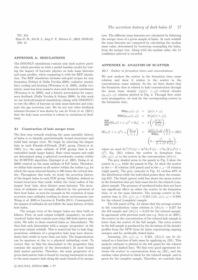
We now study the relation between ρcrit(z−2) and 〈ρ〉(< r−2)using a set of DMONLY cosmological simulations from theOWLS project that adopt the WMAP-5 cosmology. We be-gin by considering two samples of halos. Our complete sam-ple contains all halos that satisfy our resolution criteria whileour ‘relaxed’ sample retains only those halos for which theseparation between the most bound particle and the cen-tre of mass of the Friends-of-Friends halo is smaller than0.07Rvir, where Rvir is the radius for which the mean inter-nal density is ∆ (as given by Bryan & Norman 1998) timesthe critical density. Neto et al. (2007) found that this sim-ple criterion resulted in the removal of the vast majority ofunrelaxed halos and as such we do not use their additionalcriteria. At z = 0, our complete sample contains 2831 halos,while our relaxed sample is reduced to 2387 (84%).

c© 2013 RAS, MNRAS 000, 1–??


Figure 3. Relation between formation redshift, z−2, and halo concentration, c (left panel), and between formation redshift and z = 0halo mass, M200 (right panel). The different symbols correspond to the median values of the relaxed sample and the error bars to 1σconfidence limits. The solid line in the left panel is not a fit but a prediction of the z−2 − c relation for relaxed halos given by eq. (7).Similarly, the dashed line is the prediction for the complete sample of halos, assuming a constant of proportionality between 〈ρ〉(< r−2)and ρcrit of 854, rather than the value of 900 used for the relaxed sample. The grey area shows the scatter in z−2 plotted in Fig. A1 (rightpanel). Similarly, the solid line in the right panel is a prediction of the z−2 − M200 relation given by eqs. (7) and (2). The dashed linealso shows the z−2 −M200 relation assuming 〈ρ〉(< r−2) = 854ρcrit and the concentration-mass relation calculated using the completesample.

To compute the mean inner density within the scale ra-dius, 〈ρ〉(< r−2), we need to fit the NFW density profileto each individual halo. We begin by fitting NFW profilesto all halos at z = 0 that contain at least 104 dark matterparticles within the virial radius. For each halo, all particlesin the range −1.25 6 log10(r/r200) 6 0, where r200 is thevirial radius, are binned radially in equally spaced logarith-mic bins of size ∆ log10 r = 0.078. The density profile is thenfit to these bins by performing a least square minimizationof the difference between the logarithmic densities of themodel and the data, using equal weighting. The correspond-ing mean enclosed mass, Mr(r−2), and mean inner densityat r−2, 〈ρ〉(< r−2), are found by interpolating along the cu-mulative mass and density profiles (measured while fittingthe NFW profile) from r = 0 to r−2 = r200/c, where c is theconcentration from the NFW fit. Then we follow the masshistory of these halos through the snapshots, and interpolateto determine the redshift z−2 at which Mz = Mr(r−2).

We perform a least-square minimization of the quan-tity ∆2 = 1

N

∑N

i=1[〈ρi〉(ρcrit,i) − f(ρcrit,i, A)], to obtain

the constant of proportionality, A. We find 〈ρ〉(< r−2) =(900±50)ρcrit(z−2) for the relaxed sample, and 〈ρ〉(< r−2) =(854 ± 47)ρcrit(z−2) for the complete sample. The 1σ er-ror was obtained from the least squares fit. For comparison,Ludlow et al. (2014) found a constant value of 853 for theirrelaxed sample of halos and the WMAP-1 cosmology. Fig. 2shows the relation between the mean inner density at z = 0and the critical density of the universe at redshift z−2 forvarious DMONLY simulations. Each dot in this panel cor-

responds to an individual halo from the complete samplein the DMONLY−WMAP5 simulations that have box sizesof 400 h−1Mpc, 200 h−1Mpc, 100h−1Mpc, 50h−1Mpc and25h−1Mpc. The 〈ρ〉(< r−2)-ρcrit(z−2) values are colouredby mass according to the colour bar at the top of the plot.The black (red) star symbols show the mean values of thecomplete (relaxed) sample in logarithmic mass bins of widthδ log10 M = 0.2. As expected when unrelaxed halos are dis-carded (e.g. Duffy et al. 2008), the relaxed sample containson average slightly higher concentrations (by a factor of 1.16)and so higher formation times (by a factor of 1.1).

In Fig. 2 the best-fit to the data points from the relaxedsample is shown by the solid line, while the dashed line isthe fit to the complete sample. The ρcrit(z−2)− 〈ρ〉(< r−2)correlation clearly shows that halos that collapsed earlierhave denser cores at z = 0. Using the mean inner density-critical density relation for the relaxed sample,

〈ρ〉(< r−2) = (900± 50)ρcrit(z−2). (6)

We replace 〈ρ〉(< r−2) by eq. (4) and calculate the depen-dence of formation redshift on concentration,

(1 + z−2)3 =

200

900

c3

Ωm

Y (1)

Y (c)−

ΩΛ

Ωm. (7)

This last expression is tested in Fig. 3 (left panel) where weplot the median formation redshift as a function of concen-

c© 2013 RAS, MNRAS 000, 1–??


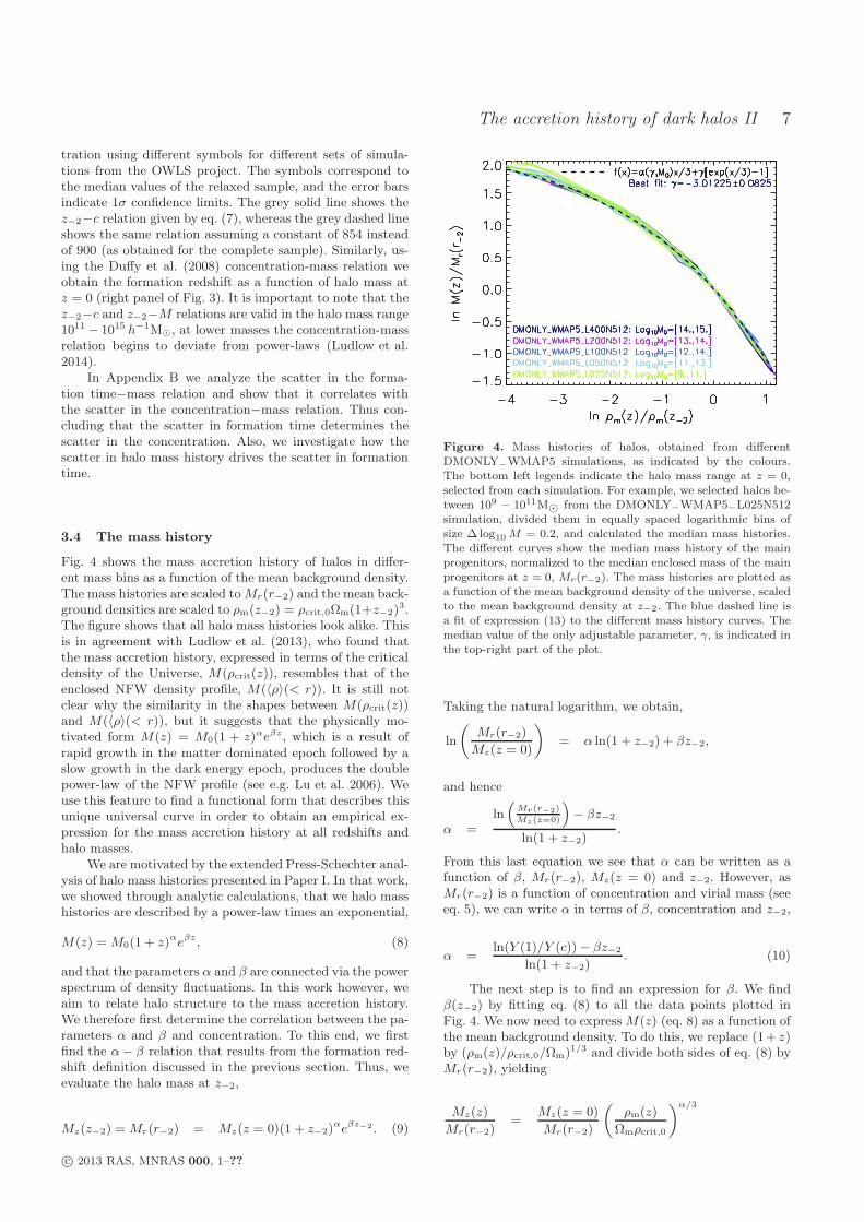
tration using different symbols for different sets of simula-tions from the OWLS project. The symbols correspond tothe median values of the relaxed sample, and the error barsindicate 1σ confidence limits. The grey solid line shows thez−2−c relation given by eq. (7), whereas the grey dashed lineshows the same relation assuming a constant of 854 insteadof 900 (as obtained for the complete sample). Similarly, us-ing the Duffy et al. (2008) concentration-mass relation weobtain the formation redshift as a function of halo mass atz = 0 (right panel of Fig. 3). It is important to note that thez−2−c and z−2−M relations are valid in the halo mass range1011 − 1015 h−1M⊙, at lower masses the concentration-massrelation begins to deviate from power-laws (Ludlow et al.2014).

In Appendix B we analyze the scatter in the forma-tion time−mass relation and show that it correlates withthe scatter in the concentration−mass relation. Thus con-cluding that the scatter in formation time determines thescatter in the concentration. Also, we investigate how thescatter in halo mass history drives the scatter in formationtime.

3.4 The mass history

Fig. 4 shows the mass accretion history of halos in differ-ent mass bins as a function of the mean background density.The mass histories are scaled toMr(r−2) and the mean back-ground densities are scaled to ρm(z−2) = ρcrit,0Ωm(1+z−2)

3.The figure shows that all halo mass histories look alike. Thisis in agreement with Ludlow et al. (2013), who found thatthe mass accretion history, expressed in terms of the criticaldensity of the Universe, M(ρcrit(z)), resembles that of theenclosed NFW density profile, M(〈ρ〉(< r)). It is still notclear why the similarity in the shapes between M(ρcrit(z))and M(〈ρ〉(< r)), but it suggests that the physically mo-tivated form M(z) = M0(1 + z)αeβz, which is a result ofrapid growth in the matter dominated epoch followed by aslow growth in the dark energy epoch, produces the doublepower-law of the NFW profile (see e.g. Lu et al. 2006). Weuse this feature to find a functional form that describes thisunique universal curve in order to obtain an empirical ex-pression for the mass accretion history at all redshifts andhalo masses.

We are motivated by the extended Press-Schechter anal-ysis of halo mass histories presented in Paper I. In that work,we showed through analytic calculations, that we halo masshistories are described by a power-law times an exponential,

M(z) = M0(1 + z)αeβz, (8)

and that the parameters α and β are connected via the powerspectrum of density fluctuations. In this work however, weaim to relate halo structure to the mass accretion history.We therefore first determine the correlation between the pa-rameters α and β and concentration. To this end, we firstfind the α− β relation that results from the formation red-shift definition discussed in the previous section. Thus, weevaluate the halo mass at z−2,

Mz(z−2) = Mr(r−2) = Mz(z = 0)(1 + z−2)αeβz

−2 . (9)

Figure 4. Mass histories of halos, obtained from differentDMONLY−WMAP5 simulations, as indicated by the colours.The bottom left legends indicate the halo mass range at z = 0,selected from each simulation. For example, we selected halos be-tween 109 − 1011M⊙ from the DMONLY−WMAP5−L025N512simulation, divided them in equally spaced logarithmic bins ofsize ∆ log10 M = 0.2, and calculated the median mass histories.The different curves show the median mass history of the mainprogenitors, normalized to the median enclosed mass of the mainprogenitors at z = 0, Mr(r−2). The mass histories are plotted asa function of the mean background density of the universe, scaledto the mean background density at z−2. The blue dashed line isa fit of expression (13) to the different mass history curves. Themedian value of the only adjustable parameter, γ, is indicated inthe top-right part of the plot.

Taking the natural logarithm, we obtain,

ln

(

Mr(r−2)

Mz(z = 0)

)

= α ln(1 + z−2) + βz−2,

and hence

α =ln(

Mr(r−2)

Mz(z=0)

)

− βz−2

ln(1 + z−2).

From this last equation we see that α can be written as afunction of β, Mr(r−2), Mz(z = 0) and z−2. However, asMr(r−2) is a function of concentration and virial mass (seeeq. 5), we can write α in terms of β, concentration and z−2,

α =ln(Y (1)/Y (c))− βz−2

ln(1 + z−2). (10)

The next step is to find an expression for β. We findβ(z−2) by fitting eq. (8) to all the data points plotted inFig. 4. We now need to express M(z) (eq. 8) as a function ofthe mean background density. To do this, we replace (1+ z)by (ρm(z)/ρcrit,0/Ωm)1/3 and divide both sides of eq. (8) byMr(r−2), yielding

Mz(z)

Mr(r−2)=

Mz(z = 0)

Mr(r−2)

(

ρm(z)

Ωmρcrit,0

)α/3

c© 2013 RAS, MNRAS 000, 1–??


× exp

(

β

[

(

ρm(z)

Ωmρcrit,0

)1/3

− 1

])

.

Multiplying both denominators and numerators by ρm(z−2),we get, after rearranging,

Mz(z)

Mr(r−2)=

Mz(z = 0)

Mr(r−2)

(

ρm(z−2)

Ωmρcrit,0

)α/3(

ρm(z)

ρm(z−2)

)α/3

× exp

(

β

[

(

ρm(z−2)

Ωmρcrit,0

)1/3

− 1

])

× exp

(

γ

[

(

ρm(z)

ρm(z−2)

)1/3

− 1

])

, (11)

where, we have defined γ ≡β(ρm(z−2)/Ωm/ρcrit,0)

1/3 = β(1 + z−2). The term

Mz(z=0)Mr(r−2)

(

ρm(z−2)

Ωmρcrit,0

)α/3

exp

(

β

[

(

ρm(z−2)

Ωmρcrit,0

)1/3

− 1

])

in eq. (11) is equal to unity, which can be seen by replacingρm(z−2)/Ωmρcrit,0 = (1+ z−2)

3 and comparing with eq. (9).Hence eq. (11) becomes

Mz(z)

Mr(r−2)=

(

ρm(z)

ρm(z−2)

)α/3

× exp

(

γ

[

(

ρm(z)

ρm(z−2)

)1/3

− 1

])

. (12)

Thus, based on eq. (12), the functional form to fit themass accretion histories from the simulations can be written

f(z, γ) = α(z−2, c, γ)z/3 + γ(ez/3 − 1), (13)

where f(z, γ) = ln(

Mz(z)Mr(r−2)

)

and z = ln[

ρm(z)ρm(z

−2)

]

. From

eq. (10) we see that the parameter α is a function of z−2, cand γ,

α =ln(Y (1)/Y (c))− γz−2/(1 + z−2)

ln(1 + z−2). (14)

Therefore, γ is now the only adjustable parameter. We per-form a χ2-like minimization of the quantity

∆2 =1

N

N∑

i=1,N

[log10(Mz(zi)/Mr(r−2))− f(zi, γ)]2,

and find the value of γ that best fits all halo accretion his-tories. The sum in the χ2-like minimization is over the Navailable simulation output redshifts at zi(i = 1, N), with

zi = ln[

ρcrit,0Ωm(1+zi)3

ρm(z−2)

]

.

Fig. 4 shows halo mass histories (with Mz(z) scaled toMr(r−2)) for our complete halo sample as a function of themean background density (ρm(z) scaled to ρm(z−2)). Theblue dashed line is the fit of expression (13) to all the masshistory curves included in the figure. Here, the only ad-justable parameter is γ. We obtained γ = −3.01 ± 0.08,

yielding

β = −3(ρm(z−2)/Ωm/ρcrit,0)−1/3 = −3/(1 + z−2). (15)

Fig. 4 shows that the halo mass histories have a char-acteristic shape consisting of a rapid growth at early times,followed by a slower growth at late times. The change fromrapid to slow accretion corresponds to the transition be-tween the mass and dark energy dominated eras (see Pa-per I), and depends on the parameter β in the exponential(as can be seen from eq. 8). The dependence of β on theformation redshift is given in eq. (15), which shows that amore recent formation time, and hence a larger halo mass,results in a larger value of β, and so a steeper halo masshistory curve. This last point can be seen in Fig. 5 fromthe mass histories of halos in different mass bins (colouredlines shown in the panels). The panel on the left shows themass history curves from the DMONLY simulation outputs(coloured lines in the background), and the mass historiespredicted by eqs. (8), (10) and (15) (red dashed lines). Fromthese panels we see that, i) the mass history formula worksremarkably well when compared with the simulation, and ii)the larger the mass of a halo at z = 0, the steeper the masshistory curve at early times. In contrast, the mass history oflow-mass halos is essentially governed by the power law atlate times.

The halo mass histories plotted in Fig. 5 come from thecomplete sample of halos (relaxed and unrelaxed). We foundno significant difference in mass growth when only relaxedhalos are considered. We therefore conclude that the factthat a halo is unrelaxed at a particular redshift does not af-fect its halo mass history, provided the concentration−massrelation fit from the relaxed halo sample is used. This is aninteresting result because while deriving the semi-analyticmodel of halo mass history, we assumed that the halo densityprofile is described by the NFW profile at all times. There-fore while the NFW is not a good fit for the density profile ofunrelaxed halos (Neto et al. 2007), our semi-analytic model(based on NFW profiles) is a good fit all halos (relaxed andunrelaxed).

The right panel of Fig. 5 shows halo mass histories fromthe REF hydrodynamical simulations. We compute the halomass as the total mass (gas and dark matter) within thevirial radius (r200). We find that the inclusion of baryonssteepens the mass histories at high redshift, therefore thebest description of M(z) is given by eqs. (8), (10), (15), andthe concentration-mass relation from the complete sampleof halos, c = 5.74(M/2 × 1012h−1M⊙)−0.097.

3.5 The mass accretion rate

The accretion of gas and dark matter from the intergalac-tic medium is a fundamental driver of both, the evolution ofdark matter halos and the formation of galaxies within them.For that reason, developing a theoretical model for the massaccretion rate is the basis for analytic and semi-analyticmodels that study galaxy formation and evolution. In thissection we look for a suitable expression for the mean accre-tion rate of dark matter halos. To achieve this, we take thederivative of the semi-analytic mass history model, M(z),given by eq. (8) with respect to time and replace dz/dt by−H0[Ωm(1 + z)5 + ΩΛ(1 + z)2]1/2, yielding

c© 2013 RAS, MNRAS 000, 1–??


Figure 5. Mass histories of all halos from simulations DMONLY−WMAP5 (left panel) and REF (right panel). Halo masses are binnedin equally spaced logarithmic bins of size ∆ log10 M = 0.5. The mass histories are computed by calculating the median value of the halomasses from the merger tree at a given output redshift, the error bars correspond to 1σ. The different colour lines show the mass historiesof halos from different simulations as indicated in the legends, while the red dashed curves correspond to the mass histories predicted byeqs. (8), (14) and (15).

dM

dt= 71.6M⊙yr−1M12h0.7[−α− β(1 + z)]× (16)

[Ωm(1 + z)3 + ΩΛ]1/2,

where h0.7 = h/0.7, M12 = M/1012M⊙ and α and β aregiven by eqs. (10) and (15), respectively. As shown in theprevious section, the parameters α and β depend on halomass (through the formation time dependence). We findthat this mass dependence is crucial for obtaining an ac-curate description for the mass history (as shown in Fig. 5).However, the factor of 2 (3) change for α (β) between halomasses of 108 − 1014M⊙ is not significant when calculatingthe accretion rate. Therefore, we provide an approximationfor the mean mass accretion rate as a function of redshiftand halo mass, by averaging α and β over halo mass, yield-ing 〈α〉=0.24, 〈β〉=-0.75, and

〈dM

dt〉 = 71.6M⊙yr−1M12h0.7 × (17)

[−0.24 + 0.75(1 + z)][Ωm(1 + z)3 + ΩΛ]1/2.

Fig. 6 (top panel) compares the median dark matteraccretion rate for different halo masses as a function of red-shift (solid lines) to the mean accretion rate given by eq. (17)(grey dashed lines). From the merger trees of the main halos,we compute the mass growth rate of a halo of a given mass.We do this by following the main branch of the tree and

computing dM/dt = (M(z1) − M(z2))/∆t, where z1 < z2,M(z1) is the descendant halo mass at time t and M(z2) isthe most massive progenitor at time t − ∆t. The medianvalue of dM/dt for the complete set of resolved halos is thenplotted for different constant halo masses. We find very goodagreement between the simulation outputs and the analyticestimate given by eq. (17). As expected, the larger the halomass, the larger the dark matter accretion rate.

3.5.1 Baryonic accretion

Next, we estimate the gas accretion rate and compareour model with similar fitting formulae proposed byFakhouri et al. (2010) and Dekel & Krumholz (2013). Thebottom panel of Fig. 6 shows the gas accretion rate as afunction redshift for a range of halo masses (log10 M/M⊙ =11.2 − 12.8). The grey circles correspond to the gas ac-cretion rate measured in REF−L100N512. In this case wecompute the total mass growth (M = Mgas + MDM) fromthe merger trees, and then estimate the gas accretion rateby multiplying the total accretion rate by the universalbaryon fraction fb = Ωb/Ωm. The green solid line corre-sponds to our gas accretion rate model (given by Ωb/Ωm

times eq. 17). The blue dot-dashed line is the gas accre-tion rate proposed by Dekel & Krumholz (2013) (dMb/dt =30M⊙yr−1fbM12(1 + z)5/2), who derived the baryonic in-flow onto a halo dMb/dt from the averaged growth rate ofhalo mass through mergers and smooth accretion based on

c© 2013 RAS, MNRAS 000, 1–??


Figure 6. Mean accretion rate of dark matter (top panel) andgas (bottom panel) as a function of redshift for different halomasses. Top panel: the accretion rate obtained from the simula-tion outputs up to the redshift where the halo mass histories areconverged. Grey dashed lines show the accretion rate estimatedusing eq. (17). Bottom panel: Gas accretion rate obtained fromthe REF−L100N512 simulation (grey circles), from Ωb/Ωm timeseq. (17) (green solid line), and from various fitting formulae takenfrom the literature.

the EPS theory of gravitational clustering (Neistein et al.2006; Neistein & Dekel 2008). Lastly, we compare our modelwith the accretion rate formula from Fakhouri et al. (2010)(dMb/dt = 46.1M⊙yr−1fbM

1.112 (1 + 1.11z)(Ωm(1 + z)3 +

ΩΛ)1/2), plotted as the purple dashed line. Fakhouri et al.

(2010) constructed merger trees of dark matter halos andquantified their merger rates and mass growth rate usingthe Millennium and Millennium II simulations. They de-fined the halo mass as the sum of the masses of all subhaloswithin a FoF halo. We see that our accretion rate model is inexcellent agreement with the formulae from Fakhouri et al.(2010) and Dekel & Krumholz (2013). We find that theFakhouri et al. (2010) formula generally overpredicts the gasaccretion rate in the low-redshift regime (e.g. it overpredictsit by a factor of 1.4 at z = 0 for a 1012M⊙ mass halo).

The Dekel & Krumholz (2013) formula underpredicts (over-predicts) the gas accretion rate in the low- (high-) redshiftregime for halos with masses larger (lower) than 1012M⊙.

3.6 Dependence on cosmology and mass definition

We have developed a semi-analytic model that relates theinner structure of a halo at redshift zero to its mass history.The model adopts the NFW profile, computes the mean in-ner density within the scale radius, and relates this to thecritical density of the universe at the redshift where the halovirial mass equals the mass enclosed within r−2. This rela-tion enables us to find the formation redshift - halo massdependence and to derive a one parameter model for thehalo mass history. In this section we consider the effects ofcosmology and mass definition on the semi-analytic model.

3.6.1 Cosmology dependence

The adopted cosmological parameters affect the mean in-ner halo densities, concentrations, formation redshifts andhalo mass histories. To investigate the dependence of halomass histories on cosmology, we have run a set of darkmatter only simulations with different cosmologies. Ta-ble 2 lists the sets of cosmological parameters adoptedby the different simulations. Specifically, we assume val-ues for the cosmological parameters derived from measure-ments of the cosmic microwave background by the Wilkin-son Microwave Anisotropy Probe (WMAP) and the Planck

missions (Spergel et al. 2003, 2007; Komatsu et al. 2009;Hinshaw et al. 2013; Planck Collaboration et al. 2013).

It has been shown that halos that formed earlier aremore concentrated (Navarro et al. 1997; Bullock et al. 2001;Eke et al. 2001; Kuhlen et al. 2005; Maccio et al. 2007;Neto et al. 2007). Maccio et al. (2008) explored the depen-dence of halo concentration on the adopted cosmologicalmodel for field galaxies. They found that dwarf-scale fieldhalos are more concentrated by a factor of 1.55 in WMAP1compared to WMAP3, and by factor of 1.29 for cluster-sizehalos. This reflects the fact that halos of a fixed z = 0 massassemble earlier in a universe with higher Ωm, higher σ8

and/or higher ns.The halo formation redshift can be related to the

power at the corresponding mass scale, and thereforedepends on both σ8 and ns. The parameter σ8 setsthe power at a scale of 8h−1Mpc, which correspondsto a mass of about 1.53 × 1014h−1M⊙(Ωm/Ωm,WMAP5),and a wave number of k8. This last quantity is givenby the relation M = (4πρm/3)(2π/k)3. For a power-lawspectrum P (k) ∝ kn, the variance can be written asσ2(k)/σ2

8 = (k/k8)n+3. Therefore, the change in σ between

WMAP5 and WMAP1 for a given halo mass that corre-sponds to a wave number k is

σWMAP1(k)

σWMAP5(k)=

σ8,WMAP1

σ8,WMAP5

(

k

k8

)(ns,WMAP1−ns,WMAP5)/2

.

A halo mass of 1012M⊙ corresponds to a wave number ofk1.3 ∼ 6k8. The total change in the mean power spectrum atthis mass scale is σWMAP1(k1.3)

σWMAP5(k1.3)= 1.27. This is proportional

to the change of the formation redshift,

c© 2013 RAS, MNRAS 000, 1–??


(1 + zf,WMAP1) = 1.27(1 + zf,WMAP5).

Next, we test how this change affects the halo masshistory. We showed that the mass history profile is welldescribed by the expression M(z) = Mz(z = 0)(1 + z)αeβz,where α and β both depend on the formation redshift. Inthe mass history model presented in Section 4 there are twobest-fit parameters that can be cosmology dependent. Oneis the constant value A = 900 in eq. (6) that relates themean inner density to the critical density at z−2, and theother is the constant value γ = −3 in eq. (15) that definesthe β parameter.

To investigate the cosmology dependence of A, we an-alyze the 〈ρ〉(< r−2)− ρcrit(z−2) relation in the simulationswith different cosmologies We do the same as in Section 4.3.First we fit the NFW profile to dark matter halos to obtainc and r−2, and calculate the cumulative mass, M−2, anddensity, 〈ρ〉(< r−2), from r = 0 to r = r−2. Then we followthe halo mass histories through the snapshots and interpo-late to calculate z−2, the redshift for which M(z) is equal toM−2. Finally, we obtain the best-fit 〈ρ〉(< r−2)− ρcrit(z−2)relation. We find that the parameter Acosmo, where cosmo isWMAP1, WMAP3, WMAP5, WMAP9 or Planck, changeswith cosmology. We show this in the top panel of Fig. 8.We find AWMAP1 = 787 ± 52.25, AWMAP3 = 850 ± 39.60,AWMAP5 = 903 ± 48.63, AWMAP9 = 820 ± 51.03 andAPlanck = 798 ± 43.73. We do not find good agreementwith Ludlow et al. (2013), who found AWMAP1 = 853 forWMAP1 cosmology. This is due to the fact that we are onlyanalyzing the 〈ρ〉(< r−2) − ρcrit(z−2) relation in the high-mass regime (M = 1012.8−1013.8M⊙), due to the limitationsof the box size (L = 100 h−1Mpc). With a more completehalo population, we may obtain better agreement. We con-clude that the Acosmo parameter depends on cosmology, atleast for the halo mass ranges we are considering.

Next, we analyze how the change of the formation red-shift due to cosmology affects β, defined as β = −3/(1 + zf).We find from Fig. 7 that the constant value, −3, is insensi-tive to cosmology. Fig. 7 shows the same analysis as Fig. 4,but for halo mass histories obtained from simulations withtheWMAP1 andWMAP5 cosmology as indicated in the leg-ends. We fit expression (13) to the mass history curves fromdifferent cosmologies and obtained the same adjustable pa-rameter γ. We therefore conclude that γ = −3 is insensitiveto cosmology.

If we then consider that the change in β betweenWMAP1 and WMAP5 is βWMAP1 = −3/(1 + zf,WMAP1) =−3/1.27/(1+zf,WMAP5) = βWMAP5/1.27, the change in thehalo mass history between the WMAP5 and WMAP1 cos-mologies, for a halo mass of 1012M⊙ at z = 0, correspondsto

log10M(z)WMAP1

M(z)WMAP5= log10 e

(βWMAP1−βWMAP5)z

≈ −0.12βWMAP1z,

≈ 0.1z.

In the last step we replaced βWMAP1 by−3/(1 + zf,WMAP1) = −0.75 for a 1012M⊙ halo. Weobtained zf,WMAP1 from the 〈ρ〉(< r−2)− ρcrit(z−2) rela-

Figure 7. Mass histories of halos, obtained from simulationswith the WMAP1 cosmology (DMONLY−WMAP1−L100N512,blue solid lines) and the WMAP5 cosmology(DMONLY−WMAP5−L100N512, green solid lines). Thecurves show the median mass history of the main progenitors,normalized to the median enclosed mass, Mr(r−2), of the mainprogenitors at z = 0. The mass histories are plotted as a functionof the mean background density of the universe, scaled to themean background density at z−2. The blue dashed line is afit of expression (13) to the different mass history curves. Themedian value of the only adjustable parameter, γ, is indicatedin the top-right part of the plot. We find that γ is insensitive tocosmology.

tion suitable for the WMAP1 cosmology (see top panel ofFig. 8) and the concentration-mass relation from Neto et al.(2007).

Next, we test the change in halo mass history. For ex-ample, if a halo had a mass of 1011.4M⊙ at z = 2 in theWMAP5 cosmology, it would have had a mass of 1011.6M⊙in the WMAP1 cosmology. The value of σ8 has a particu-larly large effect at high redshift, because structure forma-tion proceeds faster in the WMAP1 cosmology, as shown bythe above expression. This last point can also be seen in thetwo panels of Fig. 8. The top panel is the same as the rightpanel of Fig. 3, and shows the formation redshift, z−2, as afunction of halo mass (obtained from simulations with dif-ferent cosmologies). We see that there are large differencesbetween the WMAP5 and WMAP1 cosmologies due to thechanges in σ8 and ns. Interestingly, there is only a small dif-ference between the Planck and WMAP1 cosmologies (inagreement with Ludlow et al. 2014 and Dutton & Maccio2014), and also between the Planck and WMAP9 cosmolo-gies for which we found (1+zf)Planck = 1.01(1+zf)WMAP9 fora 1012M⊙ halo. The bottom panel of Fig. 8 shows the masshistory of 1012M⊙ halos at z = 0 from DMONLY simula-tions with different cosmologies. As predicted, the changein mass history between the WMAP5 and WMAP1 cos-mologies is log10

M(z)WMAP1

M(z)WMAP5∼ 0.1z. While little difference is

found between the WMAP9 and Planck (∆M(z) ∼ 10−3z).We found that as long as a suitable concentration-mass

relation and value for the A parameter are assumed for thecosmology being considered, eqs. (24), (25) and (26) pro-

c© 2013 RAS, MNRAS 000, 1–??


vide a good estimate of the mass history curve. This canseen in the bottom panel of Fig. 8 by comparing the differenthalo mass histories. For the WMAP5 and WMAP3 cosmolo-gies we assumed the concentration-mass relation found byDuffy et al. (2008), whereas we used the relation from Netoet al. (2007) for the other cosmologies. For a step-by-stepdescription of how to use the mass history models (analyticand semi-analytic) that were presented in Sections 2 and 4.4,respectively, see Appendix C.

3.6.2 Mass definition dependence

So far our calculations have been based on a halo mass de-fined as the mass of all matter within the radius r200 at whichthe mean internal density 〈ρ〉(< r200) is a factor of ∆ = 200times the critical density of the universe, ρcrit (from nowon we denote this halo mass by M200). In the literature anumber of values have been used for ∆. Some authors optto use ∆ = 200 (e.g., Jenkins et al. 2001) or ∆ = 200Ωm(z)(e.g. NFW), while others (e.g., Bullock et al. 2001) choose∆ = ∆vir according to the spherical virialization criterion ofBryan & Norman (1998). These definitions can lead to size-able differences in c for a given halo and, as discussed, thedifferences are also cosmology-dependent.

In this section we study how the structural proper-ties and mass accretion histories depend on the adoptedmass definition. We analyse halo mass histories of relaxedhalos using three different halo mass definitions. First, weuse M200. Second, we use Mmean, which is the mass withinthe radius rmean for which the mean internal density is200 times the mean background density. Finally, Mvir isthe mass within the radius rvir for which the mean in-ternal density is ∆vir times the critical density as deter-mined by Bryan & Norman (1998). Note that halo massesand radii are determined using a spherical overdensity rou-tine within the SUBFIND algorithm (Springel et al. 2001)centred on the main subhalo of the Friends-of-Friends (FoF)halos (Davis et al. 1985). We perform all calculations for thethree different halo definitions, taking the halo centre to bethe location of the particle in the FoF group for which thegravitational potential is minimum.

Eq. (6) shows that the formation redshift is directlyproportional to the mean density within the scale radius((1 + z−2)

3 ∝ 〈ρ〉(< r−2)), but the constant of proportion-ality depends on the mass definition that is adopted. There-fore, a change in the mass definition changes the formationtime as

(1 + zf )∆1

(1 + zf )∆2

≈

(

〈ρ〉(< r−2)∆1

〈ρ〉(< r−2)∆2

)1/3

, (18)

where ∆1,2 refer to different overdensity criteria. That is,from eq. (4), 〈ρ〉(< r−2) changes according to the massdefinition as 〈ρ〉(< r−2)∆ = ∆×ρcrit,0c

3∆Y (1)/Y (c∆). Then

〈ρ〉(< r−2)∆1=200 refers to the mean internal density withinr−2, obtained by defining the mean internal density atthe virial radius to be 200ρcrit,0. If we consider ∆1 = 200and ∆2 = mean = 200Ωm, and that there is a factorof 0.55 difference between the concentrations c200 andcmean for a 1012M⊙ halo, then we obtain (using eq. 18)

the relation (1 + zf)200 ≈ (0.255Ω−1m )1/3(1 + zf)mean,

where we have used the fact that

Figure 8. Top panel: Relation between formation redshift (z−2)and halo mass at z = 0 (M0). The different symbols correspondto median values, the error bars to 1σ confidence limits and thegrey area to the scatter. These were computed from the dark

matter only simulations that assumed a WMAP3 (light blue line),WMAP5 (blue line), WMAP1 (green line), WMAP9 (purple line)and Planck cosmology (dark blue line). The solid lines are notfits, but predictions of the z−2 −Mhalo relation given by eq. (7).We also indicated the different values of the constant of propor-tionality A obtained by fitting the 〈ρ−2〉 − ρcrit(z−2) relation.Bottom panel: halo mass history of a halo of 1012M⊙ at z = 0from DMONLY simulations with different cosmologies. The greycurves show that as long as a suitable concentration-mass relationis assumed for the cosmology under consideration, eqs. (24), (25)and (26) give a good estimate of the mass history curve.

〈ρ〉(< r−2)mean ∼ (Ωm/0.255)〈ρ〉(< r−2)2001. This im-

plies that the change in the halo mass history due todifferent halo mass definitions is

1 In this last step we used the approximation that 〈ρ〉(< r−2)∆ =∆× c3Y (1)/Y (c)ρcrit,0 ≈ ∆× 0.643c2.28ρcrit,0

c© 2013 RAS, MNRAS 000, 1–??


Figure 9. Mass history of a 1012M⊙ halo as a function of red-shift. The different coloured lines show the change in the masshistory when different halo mass definitions are used. The greenline shows the mass history of a halo of M200 = 1012M⊙ atz = 0, whereas the dark blue (purple) line shows the mass historyof a halo of Mmean = 1012M⊙ (Mvir = 1012M⊙) at z = 0. Thedashed lines show the mass history predicted by eqs. (24), (25)and (26). The difference lies in the formation redshift definitionwhich is affected by the change in the mean inner density (seeeq. 6). The value of 〈ρ〉(< r−2) changes with the value of ∆ weused in the definition of halo mass. The c−M relation correspondto the mass definition under consideration.

log10M(z)200M(z)mean

= log10(1 + z)α200−αmean

+ log10 e(β200−βmean)z

≈ 0.956α200 log10(1 + z) (19)

+[1− (0.255/Ωm)1/3] log10(e)β200z

≈ 0.0543z, (20)

where in step (19) we replaced α200 − αmean ≈ 0.956α200 ,which is valid for a 1012M⊙ halo, and α200 = 0.2501 andβ200 = −0.8147.

The difference in mass history given by eq. (20) canbe seen in Fig. 9, which shows how the halo mass his-tory is affected by the halo mass definition. The greenline in Fig. 9 shows the mass history assuming the M200

mass definition. The purple line shows the Mvir defini-tion, and the dark blue line shows the Mmean definition.The different dashed lines correspond to the mass historiesM(z) = M(z = 0)(1 + z)αeβz, where the difference liesin the mass definition that changes the mean inner densityand the concentration-mass relation (for a relaxed halo sam-ple). Duffy et al. (2008) studied how the halo mass definitionchanges the concentration-mass relation, and provided theparameters of the different c−M relations. They found thatthe concentration of a relaxed Mmean halo is 80% larger thanthe concentration of a relaxed M200 halo. We adopt thosefits in our calculations of the M(z) estimate and concludethat, as long as we use a concentration−mass relation thatis consistent with the adopted halo mass definition, the ex-

pressions (24), (25) and (26) accurately reproduce the halomass history.

The analytic estimate given by eq. (20) predicts thatthe difference in mass history due to the change in the massdefinition (M200 versus Mmean) is ∆ log10 M(z) ≈ 0.0543z.This can be seen in Fig. 9, where ∆ log10 M(z) = 0.1086at z = 2 (Mmean(z = 2) = 1011.3035M⊙ andM200(z = 2) = 1011.4117M⊙).

4 COMPARISON BETWEEN SEMI-ANALYTIC

AND ANALYTIC MODELS

In this section we compare the semi-analytic model derivedin Section 3.4, with the analytic model for halo mass historyderived in Paper I. Note that while the semi-analytic modelis obtained through fits to simulations, the analytic modelwas based on the extended Press-Schechter (EPS) theorywithout calibration against simulations.

Fig. 10 shows a comparison between the models for var-ious halo masses (log10[M0/M⊙] = 5− 15). As can be seenfrom the figure, the models mostly agree on the mass his-tories of halos with final masses between 1010 − 1014M⊙.However, there are a few factors of difference in the masshistories of larger and smaller halos, and the difference in-creases towards high redshift. We find that in the analyticmodel the halo mass decreases quite abruptly at high red-shift for halos with final masses > 1014M⊙. For instance,there is up to a factor of 2 difference at z = 8 between themodels for a 1015M⊙ halo . This difference is probably dueto the progenitor definition. In the analytic model, the pro-genitor is defined as the halo with mass a factor of q lower(q ∼ 4 for M0 > 1014M⊙) at redshift zf (zf ∼ 0.9). Whereasin the semi-analytic model, the progenitor is the halo thatcontain most of the 25 most bound dark matter particles inthe following snapshot.

Fig. 10 also shows that the semi-analytic model overpre-dicts the mass histories of halos with final masses < 109M⊙.This is expected because the parameters α and β in the semi-analytic model depend on the concentration-mass relationadopted. In this case we are using Duffy et al. (2008) rela-tion, which is calibrated in the mass range 1010 − 1014M⊙,for lower masses the concentration-mass relation deviatesfrom a simple power-law (Ludlow et al. 2014).

In Paper I we developed an analytic model of halo masshistory, based on EPS theory, that only depends on thepower spectrum of the primordial density perturbations. Inthis work we have developed a semi-analytic model that usesthe functional form for the mass history motivated by EPStheory, and linked the mass history to halo structure throughempirical relations obtained from simulations.

We now combine these two models (semi-analytic andanalytic) to establish the physical link between a halo con-centration and the linear rms fluctuation of the primordialdensity field. From Fig. 10 we have found that there are afew factors of difference between the models. We now focuson the mass range 1011 − 1015M⊙, where the factor of dif-ference is less than 1.5. We set the mass history curve to bethe same in the two models, that is

M(z)Analytic = M(z)Semi−analytic

c© 2013 RAS, MNRAS 000, 1–??


Figure 10. Comparison between the semi-analytic and the an-alytic model for halo mass history. The different coloured linescorrespond to the ratio of the models for various halo masses(log10[M0/M⊙] = 5− 15).

for all redshifts. We then evaluate this equality at redshift 1and obtain,

f(M0)(

0.92dD

dz|z=0 − 0.3

)

= αS(c) ln(2) + βS(c). (21)

In this last equation, αS(c) and βS(c) are given by eqs. (14)and (15), respectively, and depend on concentration, D isthe linear growth factor and f(M0) depends on the rmsof the primordial density field, σ. We approximate variousterms in eq. (21), including f(M0) ∼ 1.155(σ(M0)

2)0.277 andY (1)/Y (c) ∼ 0.643c−0.71 , and obtain

c = 3σ0.946 + 2.3, (22)

which is suitable for a WMAP5 cosmology. Note thateq. (22) is not a fit to any simulation data, it has beenderived from eq. (21). Fig. 11 shows the c − σ relation atz = 0. In this figure we compare the predicted relation (solidline), as given by eq. (22) (obtained by equaling the ana-lytic and semi-analytic models), with the simulation outputs(coloured symbols). The different symbols correspond to themedian values of the relaxed sample of halos and the errorbars to 1σ confidence limits. The good agreement betweenthe analytic prediction and the simulation outputs clearlyshows that the halo mass accretion history is the physicalconnection in the c− σ correlation.

5 SUMMARY AND CONCLUSION

In this work we have demonstrated that there is an intrinsicrelation between halo assembly history and inner halo struc-ture, and that the mass history is the physical connectionbetween the inner halo structure and the power spectrum ofinitial density fluctuations.

We examined the density profiles and mass growthhistories of a large sample of halos and their progenitors

Figure 11. Comparison between the σ − c relation at z = 0predicted by the combination of the mass history models (solidline), and the simulation outputs (coloured symbols).

within the OWLS simulations. We separated our halo sam-ple into a ‘relaxed’ sample, and a ‘complete’ sample thatincludes both relaxed and unrelaxed halos. We confirmedthe finding of Ludlow et al. (2013) that for relaxed halos themean enclosed density within the NFW scale radius (r−2),〈ρ〉(< r−2), is directly proportional to the critical density ofthe Universe at the formation redshift, z−2, defined as thetime at which the mass of the main progenitor equals themass enclosed within the scale radius at z = 0,

〈ρ〉(< r−2) = 900ρcrit(z−2). (23)

In the above relation, the value, 900±50 is obtained throughfits to the simulation data (suitable for WMAP5 cosmology).We showed in Section 3.6.1 that expression (23) provides astraightforward relation between formation time and con-centration,

(1 + z−2) = [(200/900)c3Y (1)/Y (c)− ΩΛ]1/3Ω−1/3

m ,

where Y (c) = ln(1 + c) − c/(1 + c). The overall trend ofdecreasing formation redshift with decreasing concentrationis evident for the main branches of the descendant halos.This implies that halos which assemble earlier have a higherconcentration, because the density of the Universe at theformation time was larger. To relate the formation time tohalo mass, we used the following concentration mass relationfor relaxed halos

c = 6.67(M/2 × 1012h−1M⊙)−0.092,

obtained by Duffy et al. (2008) by fitting to the simulationdata and suitable for the WMAP5 cosmology. We found thaton average, halo concentrations differ by a factor of 1.16between the relaxed and complete samples. The lower in-dividual concentrations of unrelaxed halos (due to spurioussubhalos or ongoing mergers that do not result in an accu-rate fit for an NFW density profile) produces incorrect en-closed halo masses and therefore lower formation times (by

c© 2013 RAS, MNRAS 000, 1–??


a factor of 1.1). However, on average, the formation time-concentration relation does not change, thus indicating thatthe halo mass history is not affected by the fact that a halois out of equilibrium at a particular redshift. We used thesefindings to show that scatter in the halo mass history leadsto scatter in the formation time (δz−2), and hence to scatterin the concentration−mass relation (δc).

We found that formation time decreases with increasingmass (at a non-linear rate). This means that high-mass halosare still accreting mass rapidly in the present epoch, whilelow-mass halos typically accreted their mass early. Thus, theformation time−concentration relation provides the physicallink between the halo mass history and internal structure.This result led us to provide a semi-analytic model for thehalo mass history, which uses a direct, analytic correlationbetween the parameters α and β in the mass history (eq. 24)and concentration,

M(z) = M0(1 + z)αeβz, (24)

α = [ln(Y (1)/Y (c))− βz−2]/ ln(1 + z−2), (25)

β = −3/(1 + z−2), (26)

where we obtained the constant value, −3.01 ± 0.08, in thelast relation (eq. 26) by fitting the halo mass history model(eq. 24) to the simulation data. Then we obtained a semi-analytic model for the mass accretion history, that adoptsthe functional form, eq. (24), and the parameters α and βare now given by analytic relations that include numbers ob-tained from fits to simulation results. It is important to notethat the semi-analytic model was derived assuming that thedensity profile of all halos is NFW. Interestingly, we foundthat the semi-analytic model describes with high-accuracythe mass histories of both relaxed and unrelaxed halo sam-ple, even though the NFW profile is not a good fit to thedensity profile of unrelaxed halos.

We investigated how cosmology affects the semi-analytic model. We found that as long as a suitableconcentration-mass relation and the value for the best-fit pa-rameter in the 〈ρ〉(< r−2)− ρcrit(z−2) relation are assumedfor the cosmology being considered, the semi-analytic mod-els describes the mass histories with high accuracy. In addi-tion, we investigated how different mass definitions changethe halo mass histories and we found that as long as weuse a concentration-mass relation that is consistent with theadopted halo mass definition, the semi-analytic model accu-rately reproduces the halo mass history.

In Paper I, we presented an analytic model for the halomass history, based on extended Press-Schechter theory andnot calibrated against simulations data. We compared theanalytic model of Paper I with the semi-analytic model pre-sented here and found very good agreement in the massrange 109 − 1014M⊙. However, we found that the analyticmodel predicts larger masses at high redshift for halos withfinal masses > 1014M⊙, whereas the semi-analytic modeloverpredicts the mass history of low-mass halos (halos withfinal masses < 109M⊙). This is expected because the semi-analytic model depends on the adopted concentration-massrelation, which deviates from the assumed power-law at lowmasses. The reader may find a step-by-step guide on how to

implement the semi-analytic model in Appendix C, as wellas numerical routines online2.

Interestingly, by combining these two models (semi-analytic and analytic) we established the physical link be-tween a halo concentration and the initial density perturba-tion field, that explains the correlation between concentra-tion and rms fluctuation of the primordial density field, σ(Fig. 11).

Finally, by differentiating eq. (24) we obtained the darkmatter accretion rate,

dM

dt= 71.6M⊙yr−1M12h0.7 ×

[−α− β(1 + z)][Ωm(1 + z)3 + ΩΛ]1/2.

As the change in the α and β parameters over halo masses isnot significant when calculating accretion rates, we providedamean accretion rate, obtained by averaging the parametersα and β over halo mass,

〈dM

dt〉 = 71.6M⊙yr−1M12h0.7 ×

[−0.24 + 0.75(1 + z)][Ωm(1 + z)3 + ΩΛ]1/2.

We then concluded that in order to predict halo massgrowth, the concentration-mass relation from a relaxed sam-ple should be used.

Putting the pieces together, we addressed the questionof how the structure of halos depends on the primordialdensity perturbation field. We found that concentration isthe link between the halo mass profile and the halo masshistory (and that one can be determined from the other).We also found that the ‘shape’ of the halo mass history isgiven by the linear growth factor and linear power spectrumof density fluctuations. Therefore, we concluded that haloconcentrations are directly connected to the initial densityperturbation field.

In a forthcoming paper (Paper III) we will combine theanalytic model presented in Paper I and semi-analytic modelpresented here to predict the concentration-mass relation.We will investigate its evolution, we will show that extrapo-lations to low masses of power-law fits to simulations resultsare highly inadequate, and we will investigate whether lin-ear 〈ρ〉(< r−2)− ρcrit(z−2) relation holds at redshifts otherthan 0.

ACKNOWLEDGEMENTS

We are grateful to the referee Aaron Ludlow for fruitful com-ments that substantially improved the original manuscript.CAC acknowledges the support of the 2013 John Hodg-son Scholarship and the hospitality of Leiden Observatory.JSBW is supported by an Australian Research Council Lau-reate Fellowship. JS acknowledges support by the Euro-pean Research Council under the European Union’s Sev-enth Framework Programme (FP7/2007-2013)/ERC Grantagreement 278594-GasAroundGalaxies. We are grateful tothe OWLS team for their help with the simulations.

2 Available at http://www.ph.unimelb.edu.au/∼correac/.

c© 2013 RAS, MNRAS 000, 1–??

http://www.ph.unimelb.edu.au/~correac/


REFERENCES

Bryan G. L., Norman M. L., 1998, ApJ, 495, 80Bullock J. S., Kolatt T. S., Sigad Y., Somerville R. S.,Kravtsov A. V., Klypin A. A., Primack J. R., Dekel A.,2001, MNRAS, 321, 559

Correa C. A., Wyithe J. S. B., Schaye J., Duffy A. R., 2014,ArXiv e-prints (Paper I)

Correa C. A., Wyithe J. S. B., Schaye J., Duffy A. R., 2015,To be submitted to MNRAS (Paper III)

Dalal N., Lithwick Y., Kuhlen M., 2010, ArXiv e-prints

Dalla Vecchia C., Schaye J., 2008, MNRAS, 387, 1431Davis M., Efstathiou G., Frenk C. S., White S. D. M., 1985,ApJ, 292, 371

Dekel A., Devor J., Hetzroni G., 2003, MNRAS, 341, 326Dekel A., Krumholz M. R., 2013, MNRAS, 432, 455

Diemer B., Kravtsov A. V., 2014a, ArXiv e-printsDiemer B., Kravtsov A. V., 2014b, ApJ, 789, 1Diemer B., More S., Kravtsov A. V., 2013, ApJ, 766, 25Dolag K., Borgani S., Murante G., Springel V., 2009, MN-RAS, 399, 497

Duffy A. R., Schaye J., Kay S. T., Dalla Vecchia C., 2008,MNRAS, 390, L64

Dutton A. A., Maccio A. V., 2014, MNRAS, 441, 3359Einasto J., 1965, Trudy Astrofizicheskogo Instituta Alma-Ata, 5, 87

Eke V. R., Navarro J. F., Steinmetz M., 2001, ApJ, 554,114

Fakhouri O., Ma C.-P., Boylan-Kolchin M., 2010, MNRAS,406, 2267

Giocoli C., Tormen G., Sheth R. K., 2012, MNRAS, 422,185

Hayashi E., White S. D. M., 2008, MNRAS, 388, 2Hinshaw G., Larson D., Komatsu E., Spergel D. N., Ben-nett C. L., Dunkley J., Nolta M. R., Halpern M., HillR. S., Odegard N., et al. 2013, ApJS, 208, 19

Huss A., Jain B., Steinmetz M., 1999, ApJ, 517, 64Jenkins A., Frenk C. S., White S. D. M., Colberg J. M.,Cole S., Evrard A. E., Couchman H. M. P., Yoshida N.,2001, MNRAS, 321, 372

Klypin A. A., Trujillo-Gomez S., Primack J., 2011, ApJ,740, 102

Komatsu E., Dunkley J., Nolta M. R., Bennett C. L., GoldB., Hinshaw G., Jarosik N., Larson D., Limon M., PageL., et al. 2009, ApJS, 180, 330

Kuhlen M., Strigari L. E., Zentner A. R., Bullock J. S.,Primack J. R., 2005, MNRAS, 357, 387

Lacerna I., Padilla N., 2011, MNRAS, 412, 1283

Lu Y., Mo H. J., Katz N., Weinberg M. D., 2006, MNRAS,368, 1931

Ludlow A. D., Navarro J. F., Angulo R. E., Boylan-KolchinM., Springel V., Frenk C., White S. D. M., 2014, MNRAS,441, 378

Ludlow A. D., Navarro J. F., Boylan-Kolchin M., BettP. E., Angulo R. E., Li M., White S. D. M., Frenk C.,Springel V., 2013, MNRAS

Ludlow A. D., Navarro J. F., Li M., Angulo R. E., Boylan-Kolchin M., Bett P. E., 2012, MNRAS, 427, 1322

Ludlow A. D., Navarro J. F., Springel V., Vogelsberger M.,Wang J., White S. D. M., Jenkins A., Frenk C. S., 2010,MNRAS, 406, 137

Maccio A. V., Dutton A. A., van den Bosch F. C., 2008,

MNRAS, 391, 1940Maccio A. V., Dutton A. A., van den Bosch F. C., MooreB., Potter D., Stadel J., 2007, MNRAS, 378, 55

Manrique A., Raig A., Salvador-Sole E., Sanchis T., SolanesJ. M., 2003, ApJ, 593, 26

McBride J., Fakhouri O., Ma C.-P., 2009, MNRAS, 398,1858

Navarro J. F., Frenk C. S., White S. D. M., 1996, ApJ, 462,563

Navarro J. F., Frenk C. S., White S. D. M., 1997, ApJ, 490,493

Navarro J. F., Hayashi E., Power C., Jenkins A. R., FrenkC. S., White S. D. M., Springel V., Stadel J., Quinn T. R.,2004, MNRAS, 349, 1039

Navarro J. F., Ludlow A., Springel V., Wang J., Vogels-berger M., White S. D. M., Jenkins A., Frenk C. S., HelmiA., 2010, MNRAS, 402, 21

Neistein E., Dekel A., 2008, MNRAS, 388, 1792Neistein E., van den Bosch F. C., Dekel A., 2006, MNRAS,372, 933

Neto A. F., Gao L., Bett P., Cole S., Navarro J. F., FrenkC. S., White S. D. M., Springel V., Jenkins A., 2007, MN-RAS, 381, 1450

Planck Collaboration Ade P. A. R., Aghanim N., Armitage-Caplan C., Arnaud M., Ashdown M., Atrio-Barandela F.,Aumont J., Baccigalupi C., Banday A. J., et al. 2013,ArXiv e-prints

Prada F., Klypin A. A., Cuesta A. J., Betancort-Rijo J. E.,Primack J., 2012, MNRAS, 423, 3018

Salvador-Sole E., Solanes J. M., Manrique A., 1998, ApJ,499, 542

Salvador-Sole E., Vinas J., Manrique A., Serra S., 2012,MNRAS, 423, 2190

Schaye J., Dalla Vecchia C., 2008, MNRAS, 383, 1210Schaye J., Dalla Vecchia C., Booth C. M., WiersmaR. P. C., Theuns T., Haas M. R., Bertone S., Duffy A. R.,McCarthy I. G., van de Voort F., 2010, MNRAS, 402,1536

Shaw L. D., Weller J., Ostriker J. P., Bode P., 2006, ApJ,646, 815

Sheth R. K., Tormen G., 2004, MNRAS, 349, 1464Spergel D. N., Bean R., Dore O., Nolta M. R., BennettC. L., Dunkley J., Hinshaw G., Jarosik N., Komatsu E.,Page L., et al. 2007, ApJS, 170, 377

Spergel D. N., Verde L., Peiris H. V., Komatsu E., NoltaM. R., Bennett C. L., Halpern M., Hinshaw G., JarosikN., Kogut A., et al. 2003, ApJS, 148, 175

Springel V., 2005, MNRAS, 364, 1105Springel V., White M., Hernquist L., 2001, ApJ, 549, 681Syer D., White S. D. M., 1996, ArXiv Astrophysics e-printsSyer D., White S. D. M., 1998, MNRAS, 293, 337van de Voort F., Schaye J., Booth C. M., Haas M. R., DallaVecchia C., 2011, MNRAS, 414, 2458

Wang H., Mo H. J., Jing Y. P., 2009, MNRAS, 396, 2249Wang J., White S. D. M., 2009, MNRAS, 396, 709Wechsler R. H., Bullock J. S., Primack J. R., KravtsovA. V., Dekel A., 2002, ApJ, 568, 52

Wiersma R. P. C., Schaye J., Smith B. D., 2009, MNRAS,393, 99

Wiersma R. P. C., Schaye J., Theuns T., Dalla Vecchia C.,Tornatore L., 2009, MNRAS, 399, 574

Zhao D. H., Jing Y. P., Mo H. J., Borner G., 2009, ApJ,

c© 2013 RAS, MNRAS 000, 1–??


707, 354Zhao D. H., Mo H. J., Jing Y. P., Borner G., 2003, MNRAS,339, 12

APPENDIX A: SIMULATIONS

The DMONLY simulations contain only dark matter parti-cles, which provides us with a useful baseline model for test-ing the impact of baryonic physics on halo mass historiesand mass profiles, when comparing it with the REF simula-tion. The REF simulation includes sub-grid recipes for starformation (Schaye & Dalla Vecchia 2008), radiative (metal-line) cooling and heating (Wiersma et al. 2009), stellar evo-lution, mass loss form massive stars and chemical enrichment(Wiersma et al. 2009), and a kinetic prescription for super-nova feedback (Dalla Vecchia & Schaye 2008). In this workwe use hydrodynamical simulations (along with DMONLY)to test the effect of baryons on halo mass histories and com-pute the gas accretion rate. We do not test other feedbackschemes because it was shown by van de Voort et al. (2011)that the halo mass accretion is robust to variations in feed-back.

A1 Construction of halo merger trees

The first step towards studying the mass assembly historyof halos is to identify gravitationally bound structures andbuild halo merger trees. We begin by selecting the largesthalo in each Friends-of-Friends (FoF) group (Davis et al.1985) (i.e. the main subhalo of FOF groups that is notembedded inside larger halos). Halo virial masses and radiiare determined using a spherical overdensity routine withinthe SUBFIND algorithm (Springel et al. 2001; Dolag et al.2009) centred on the main subhalo of FoF halos. Therefore,we define halo masses as all matter within the radius r200 forwhich the mean internal density is 200 times the critical den-sity. Throughout this work, we study the accretion historyof the largest halos in each FOF group. Subhalos, defined asbound structures that reside within the virial radius of thelargest ‘host’ halo, show distinct mass histories. The struc-tures of subhalos are strongly affected by the potential oftheir host halos, as seen for example in the cessation of massaccretion onto subhalos residing in dense environments (seeWang et al. 2009 or Lacerna & Padilla 2011). Consequently,the masses of subhalos do not follow the mass history of theirhost halos.

The merger trees of the largest halos are then built asfollows. First, at each output redshift (snapshot), we select‘resolved’ halos that contain more than 300 dark matter par-ticles. We refer to these resolved halos as ‘descendants’. Wethen link each descendant with a unique ‘progenitor’ at theprevious output redshift. This is nontrivial due to halo frag-mentation: subhalos of a progenitor halo may have descen-dants that reside in more than one halo. The fragmentationcan be spurious or due to a physical unbinding event. Tocorrect this, we link the descendant to the progenitor thatcontains the majority of the descendant’s 25 most bounddark matter particles. Therefore, the main progenitor of agiven dark matter halo is found by tracing backwards in timeto the most massive halo along the main branch of its merger

tree. The different mass histories are calculated by followingthe merger trees of a given sample of halos. At each redshiftthe mass histories are computed by calculating the medianmass value, determined by bootstrap resampling the halos,from the merger tree. Along with the median value, the 1σconfidence interval is recorded.

APPENDIX B: ANALYSIS OF SCATTER

B0.1 Scatter in formation times and concentrations

We now analyse the scatter in the formation time−massrelation and show it relates to the scatter in theconcentration−mass relation. So far, we have shown thatthe formation time is related to halo concentration throughthe mean inner density (〈ρ〉(< r−2))−critical density(ρcrit(z−2)) relation plotted in Fig. 2. Through first ordererror propagation, we look for the corresponding scatter inthe formation time,

900ρcrit(z−2) = 〈ρ〉(< r−2),

900δ(ρcrit(z−2)) = δ(〈ρ〉(< r−2)),

900

200δ[Ωm(1 + z−2)

3 + ΩΛ] = δ

(

c3Y (1)

Y (c)

)

,

3Ωm(1 + z−2)2z−2

(

δz−2

z−2

)

=〈ρ〉(< r−2)

900ρ0

(

δc

c

)

× (B1)

(

3−c2

(1 + c)21

Y (c)

)

,

where we used δ(c3/Y (c)) = 3c2δc/Y (c) − c4δc/[Y (c)2(1 +c)2]. Eq. (B1) relates the scatter in formation time(|δz−2|/z−2) to the scatter in the concentration (|δc|/c).

The grey shaded areas in the panels in Fig. 3 show thescatter in z−2, while the panels in Fig. A1 show the scatterin the c−M relation (left panel) and in the z−2−M relation(right panel). The grey contours in Fig. A1 enclose 68% ofthe distribution while the individual points show the remain-ing 32%. The black (green) solid line shows the mean scatterin the formation time per halo mass bin for the relaxed (com-plete) sample. The presence of unrelaxed halos does not haveany significant effect on either the scatter in the formationtime, or on the mass histories. The average scatter in for-mation time is 〈|δz−2|/z−2〉 = 0.324 (〈|δz−2|/z−2〉 = 0.356)for the relaxed (complete) sample.

The left panel of Fig. A1 shows that the average scatterin the concentration−mass relation is 〈|δc|/c〉 = 0.257 forthe full sample and 〈|δc|/c〉 = 0.218 for the relaxed sample.In agreement with previous work (see e.g. Neto et al. 2007),the scatter in the concentration of the relaxed halo sample islower than the scatter of the full sample. The extra scatterin the full sample is produced by the deviation of the densityprofiles from the NFW form for halos experiencing ongoingmergers and for artificially linked halos.

Assuming 〈|δz−2|/z−2〉 = 0.324, 〈|δc|/c〉 can be ob-tained as a function of halo mass by applying eq. (B1). Thisanalytic estimate is plotted in the left panel for the relaxedsample (red dashed line). We find very good agreement be-tween the scatter in concentration from eq. (B1), and themedian value plotted in black for the relaxed sample, and ingreen for the complete sample. Therefore, we conclude that

c© 2013 RAS, MNRAS 000, 1–??


Figure A1. Scatter in the concentration−mass relation (left panel) and the formation redshift−mass relation (right panel). Left panel:Y-axis shows the difference between the concentration predicted by Duffy et al. (2008) (see eq. 2) and the actual concentration fromthe simulation output. This difference is divided by the concentration from the simulation output and plotted against virial halo mass.The different colours of the points indicate that the concentration outputs were obtained from DMONLY−WMAP5 simulations withdifferent box sizes. The grey contours enclose 68% of the distribution while the individual points show the remaining 32%. The black(green) solid line shows the mean relative scatter in the concentration-mass relation per halo mass bin of the relaxed (complete) sample.The red dashed line is an analytic estimate of the scatter obtained by propagating the scatter in the formation redshift−mass relationto the concentration−mass relation (eq. B1). Right panel: same as the left panel but the scatter is obtained from the difference in the

formation redshift predicted from eq. (7) and the simulation output. The black (green) solid line shows the median value in the scatteras a function of mass of the relaxed (complete) sample.

the scatter in formation time determines the scatter in theconcentration. However, at higher masses and redshifts thefraction of relaxed halos decreases (e.g. Ludlow et al. 2012)and it has been found that the concentration-mass relationof the complete halo sample exhibits a strong flattening andupturn (Klypin et al. 2011; Prada et al. 2012). As a result,at high masses and redshifts the scatter in the concentrationwill probably depend on other variables besides the scatterin formation time.

In the following subsection we find that the scatter inthe accretion history determines the scatter in the formationtime.

B0.2 Scatter in halo mass histories

In this subsection we analyse the scatter found when com-puting mass histories from the simulation outputs. We an-alytically estimate the scatter in the mass history due toboth the scatter in the concentration and formation times(estimated in previous Section B0.1). We then compare thisto the scatter obtained from the simulation outputs.

To compute the scatter in the mass history we performa first order error propagation in M(z) (eq. 8),

δM(z)/M(z) = δα ln(1 + z) + zδβ, (B2)

where δα (δβ) is the scatter in α (β) due to the scatter inc and z−2. From eq. (10) we first compute δα due to thescatter in z−2,

δα = δ(−βz−2/ ln(1 + z−2))

=−z−2δβ − βδz−2

ln(1 + z−2)− βz−2δ[ln(1 + z−2)]

−1

= −z−2β(1 + z−2 ln(1 + z−2))

(1 + z−2) ln(1 + z−2)

(

δz−2

z−2

)

, (B3)

where in the last line we used δβ =−βz

−2

(1+z−2)

(

δz−2

z−2

)

, which

follows from eq. (15). Similarly, we calculate the scatter inα due to the scatter in c,

δα = δ(ln(Y (1)/Y (c))/ ln(1 + z−2)

= −δY (c)

Y (c)

1

ln(1 + z−2)

= −c2

(1 + c)2Y (c) ln(1 + z−2)

(

δc

c

)

, (B4)

where in the last step we used δY (c) = c2

(1+c)2

(

δcc

)

. Fi-

nally, we substitute δβ =−βz

−2

(1+z−2)

(

δz−2

z−2

)

and eqs. (B3) and

(B4) into eq. (B2). From Section B0.1 we adopt the av-erage scatter in z−2 and c for the complete sample, thatis 〈|δc|/c〉 = 0.25 and 〈δz−2/z−2〉 = 0.35, and compute〈|δM(z)/M(z)|〉 as a function of redshift. Fig. B1 showsthe scatter measured from the simulation outputs (colouredlines) and from the analytic estimates (grey dashed lines).The different coloured lines correspond to the median val-ues of the scatter from simulations with different box sizes.We calculate these by averaging the difference between themass history predicted by eqs. (8), (10) and (15) (for a givenhalo with mass M200 at z = 0), and each M(z) given by themerger trees from the complete halo sample. We find very

c© 2013 RAS, MNRAS 000, 1–??


Figure B1.Mean scatter in the halo mass history against redshiftfor different halo masses M200. The y-axis shows the mean valueof the difference between the mass history (Mfit) predicted byeqs. (8), (10) and (15), and the mass history (Msim) from thesimulation output. The difference is divided by the Msim fromthe simulation output. The different coloured lines correspond tothe different DMONLY−WMAP5 simulations as indicated in thelegends. The grey lines show the analytic estimates of the masshistory curves given by eqs. (B2), (B3) and (B4).

good agreement indicating that the scatter in the concen-tration comes from the scatter in the formation time, whichin turn comes from the scatter in the halo mass history.

APPENDIX C: STEP-BY-STEP GUIDE TO

COMPUTE HALO MASS HISTORIES

C0.3 Semi-analytical model

This appendix provides a step-by-step procedure that out-lines how to calculate the halo mass histories using the nu-merical model presented in Section 4.4:

(i) First assume a cosmology and choose a concentration-mass relation from the literature. For instance, the Duffyet al. (2008) relation, c = 6.67(M0/2× 1012h−1M⊙)−0.092,is suitable for the WMAP5 cosmology, whereas Neto et al.(2007) is suitable for WMAP1.

(ii) Calculate the formation time,

z−2 =

(

200

Acosmo

c(M0)3Y (1)

ΩmY (c(M0))−

ΩΛ

Ωm

)1/3

− 1. (C1)

Note that the value of Acosmo in the above equation iscosmology dependent. AWMAP5 = 900 is suitable for theWMAP5 cosmology. In this work we obtained AWMAP1 =787, AWMAP3 = 850, AWMAP9 = 820 and APlanck = 798.

(iii) Calculate the parameters α and β,

α = [ln(Y (1)/Y (c))− βz−2]/ ln(1 + z−2), (C2)

β = −3/(1 + z−2). (C3)

(iv) Finally, the mass history can be calculated as follows,

M(z) = M0(1 + z)αeβz. (C4)

The above model is suitable for any cosmology (as longas the concentration-mass relation and the value of Acosmo

correspond to the desire cosmology) and is valid over thehalo mass range for which the concentration-mass and thez−2−M0 relations, obtained from simulations, are valid (e.g.1010 − 1014M⊙ for Duffy et al. 2008).

c© 2013 RAS, MNRAS 000, 1–??

The accretion history of dark matter halos II: The connections with the mass power spectrum and the...

Documents

Transcript of The accretion history of dark matter halos II: The connections with the mass power spectrum and the...