arX

iv:a

stro

-ph/

0508

497v

1 2

4 A

ug 2

005

Mon. Not. R. Astron. Soc. 000, 000–000 (0000) Printed 5 February 2008 (MN LATEX style file v2.2)

The Shape of Dark Matter Halos: Dependence on Mass,

Redshift, Radius, and Formation

Brandon Allgood1, Ricardo A. Flores2, Joel R. Primack1, Andrey V. Kravtsov3,

Risa H. Wechsler3,4, Andreas Faltenbacher5, and James S. Bullock6

1Physics Department, University of California, Santa Cruz, CA 95064; allgood@physics.ucsc.edu, joel@scipp.ucsc.edu2Department of Physics and Astronomy, University of Missouri – St. Louis, St. Louis, MO 63121; ricardo.flores@umsl.edu3Dept. of Astronomy and Astrophysics, Kavli Institute for Cosmological Physics, and The Enrico Fermi Institute,

The University of Chicago, Chicago, IL 60637; andrey@oddjob.uchicago.edu, risa@cfcp.uchicago.edu4Hubble Fellow, Enrico Fermi Fellow5Lick Observatory, University of California, Santa Cruz, CA 95064; fal@ucolick.org6Center for Cosmology, Department of Physics and Astronomy, University of California, Irvine, CA 92697; bullock@uci.edu

5 February 2008

ABSTRACT

Using six high resolution dissipationless simulations with a varying box size in a flatLCDM universe, we study the mass and redshift dependence of dark matter haloshapes for Mvir = 9.0 × 1011 − 2.0 × 1014, over the redshift range z = 0 − 3, and fortwo values of σ8 = 0.75 and 0.9. Remarkably, we find that the redshift, mass, andσ8 dependence of the mean smallest-to-largest axis ratio of halos is well described bythe simple power-law relation 〈s〉 = (0.54 ± 0.02)(Mvir/M∗)

−0.050±0.003, where s ismeasured at 0.3Rvir and the z and σ8 dependences are governed by the characteristicnonlinear mass, M∗ = M∗(z, σ8). We find that the scatter about the mean s is welldescribed by a Gaussian with σ ∼ 0.1, for all masses and redshifts. We compare ourresults to a variety of previous works on halo shapes and find that reported differencesbetween studies are primarily explained by differences in their methodologies. Weaddress the evolutionary aspects of individual halo shapes by following the shapes ofthe halos through ∼ 100 snapshots in time. We determine the formation scalefactor ac

as defined by Wechsler et al. (2002) and find that it can be related to the halo shapeat z = 0 and its evolution over time.

Key words: cosmology: theory — galaxies: formation — galaxies: halos — large-scalestructure of universe

1 INTRODUCTION

A generic prediction of cold dark matter (CDM) theory isthe process of bottom up halo formation, where large halosform from the mergers of smaller halos, which are in turnformed from even smaller halos. This is a violent processand it violates most of the assumptions that go into thespherical top-hat collapse model of halo formation which isoften used to describe halos. Since mass accretion onto halosis often directional and tends to be clumpy, one would notexpect halos to be spherical if the relaxation time of thehalos were longer than the time between mergers and/or ifthe in-falling halos came along a preferential direction (suchas along a filament). In both theoretical modelling of CDMand observations, halos are found to be very non-spherical.In fact, spherical halos are rare. Therefore, the analysis of

halo shapes can give us another clue to the nature of thedark matter and the process of halo and galaxy formation.

One way of quantifying the shape of a halo is to goone step beyond the spherical approximation and approx-imate halos by ellipsoids. Ellipsoids are characterised bythree axes, a, b, c, with a ≥ b ≥ c, which are normally de-scribed in terms of ratios, s ≡ c/a, q ≡ b/a, and p ≡ c/b. El-lipsoids can also be described in terms of three classes, whichhave corresponding ratio ranges: prolate (sausage shaped)ellipsoids have a > b ≈ c leading to axial ratios of s ≈ q < p,oblate (pancake shaped) ellipsoids have a ≈ b > c leadingto axial ratios of s ≈ p < q, and triaxial ellipsoids are in be-tween prolate and oblate with a > b > c. Additionally, whentalking about purely oblate ellipsoids, a = b, it is commonto use just q, since s and q are degenerate.

There have been many theoretical papers pub-lished over the years which examined the subject

2 Allgood et al.

of halo shapes. The early work on the subject in-cludes Barnes & Efstathiou (1987); Dubinski & Carlberg(1991); Katz (1991); Warren et al. (1992); Dubinski (1994);Jing et al. (1995); Tormen (1997); Thomas et al. (1998). Allof these works agreed that halos are ellipsoidal, but oth-erwise differ in several details. Dubinski & Carlberg (1991)found that halos have axial ratios of s ∼ 0.5 in the interiorand become more spherical at larger radii, while Frenk et al.(1988) found that halos are slightly more spherical in thecentres. Thomas et al. (1998) claimed that larger mass ha-los have a slight tendency to be more spherical, where morerecent simulation results find the opposite. Despite these dis-agreements many of the early authors give us clues into thenature of halos shapes. Warren et al. (1992) and Tormen(1997) showed that the angular momentum axis of a halois well correlated with the smallest axis, c, although, asmost of these authors pointed out, halos are not rotation-ally supported. This therefore has led many to conclude thatthe shapes are supported by anisotropic velocity dispersion.Tormen (1997) took it one step further and found that thevelocity anisotropy was in turn correlated with the infallanisotropy of merging satellites. Most authors found thatthe axial ratios of halos are ∼ 0.5 ± 0.1 and that halos tendto be prolate as opposed to oblate in shape. The most likelysource of the disagreement in these works and in the morerecent works we describe below is the different methods usedoften coupled with inadequate resolution.

More recent studies of halos’ shape were per-formed by Bullock (2002); Jing & Suto (2002);Springel, White & Hernquist (2004); Bailin & Steinmetz(2005); Kasun & Evrard (2004); Hopkins et al. (2005). Theresults of these authors differ, in some cases, considerably.One of the goals of this paper is to carefully examine thedifferences in the findings presented by the above authors.

All of the aforementioned publications (exceptSpringel et al. 2004) analyse simulations with either nobaryons or with adiabatic hydrodynamics. This is both dueto the cost associated with performing self consistent hy-drodynamical simulations of large volumes with high massresolution and due to the fact that very few cosmologicalsimulations yet produce realistic galaxies. Nonetheless, weknow that the presence of baryons should have an effecton the shapes of halos due to their collisional behaviour.Three recent papers have attempted to examine the effectof baryons (Springel et al. 2004; Kazantzidis et al. 2004;Bailin et al. 2005). In Springel et al. (2004) the same simu-lations were done using no baryons, adiabatic baryons andbaryons with cooling and star formation. In the first twocases there was very little difference, but with the presenceof cooling and star formation the halos became morespherical. The radial dependence of shape also changes suchthat the halo is more spherical in the centre. At R > 0.3Rvir

the axial ratio s increases by ≤ 0.09, but in the interior theincrease ∆s is as much as 0.2. In an independent study,Kazantzidis et al. (2004) found an even larger effect dueto baryonic cooling in a set of 11 high resolution clusters.At R = 0.3Rvir the authors found that s can increase by0.2 − 0.3 in the presence of gas cooling. The extent of theover-cooling problem plaguing these simulations is stilluncertain. This amount of change in the shape should beviewed as an upper limit. The most recent work on thesubject is Bailin et al. (2005), who concentrate more on the

relative orientation of the galaxy formed at the centre ofeight high resolution halos than on the relative sphericityof the halos. Despite this, from Figure 1 of Bailin et al.(2005) it seems that they would also predict an increaseof ∼ 0.2 for s. It is still useful to study shapes of haloswithout baryonic cooling. Cooling and star formation insimulations is still a very open question, making the effectof the cooling uncertain. We show in Paper II that oursimulations without cooling match shapes of X-ray clusters.

Measurements of the shapes of both cluster andgalaxy mass halos through varied observational tech-niques are increasingly becoming available. Therehave been many studies of the X-ray morpholo-gies of clusters (see McMillan, Kowalski & Ulmer1989; Mohr, Evrard, Fabricant & Geller 1995;Kolokotronis, Basilakos, Plionis & Georgantopoulos 2001)which can be directly related to the shape of the inner partof the cluster halo (Lee & Suto 2003; Buote & Xu 1997).For a review of X-ray cluster shapes and the latest results,see Flores et al. (2005), hereafter referred to as Paper II.

There has also been important new information on theshape of galaxy mass halos, in particular our own Milky Wayhalo. Olling & Merrifield (2000) concluded that the hosthalo around the Galactic disk is oblate with a short-to-longaxial ratio of 0.7 < q < 0.9. Investigations of Sagittarius’tidal streams have led to the conclusion that the Milky Wayhalo is oblate and nearly spherical with q & 0.8 (Ibata et al.2001; Majewski et al. 2003; Martınez-Delgado et al. 2004).However, by inspecting M giants within the leading streamHelmi (2004) and Law, Johnston & Majewski (2005) founda best fit prolate halo with s = 0.6. Merrifield (2004) sum-marises the currently reliable observations for galaxy hosthalo shapes using multiple techniques and find that the ob-servations vary a lot.

Another method for studying shapes of halos athigher redshift is galaxy-galaxy weak lensing studies.Analysing data taken with the Canada-France-Hawaii tele-scope, Hoekstra, Yee & Gladders (2004) find a signal at a99.5% confidence level for halo asphericity. They detect anaverage projected ellipticity of 〈ǫ〉 ≡ 〈1 − q2D〉 = 0.20+0.04

−0.05 ,corresponding to s = 0.66+0.07

−0.06 , for halos with an averagemass of 8 × 1011h−1 M⊙. Ongoing studies of galaxy-galaxyweak lensing promise rapidly improving statistics from largescale surveys like the Canada-France Legacy survey.

This paper is organised as follows: In Section 2 we de-scribe the simulations, halo finding method, and halo prop-erty determination methods used in this study. In Section3 we discuss the method used to determine the shapes ofhalos. In Section 4 we examine the mean axial ratios fromour simulations and their dependence on mass, redshift andσ8. We then examine the dispersion of the axial ratio ver-sus mass relation. We briefly discuss the shape of halos asa function of radius and then examine the relationship ofthe angular momentum and velocity anisotropy to the haloshape. In Section 5 we examine the relationship between theformation history of halos and their present day shapes. InSection 6 we compare our results to those of previous au-thors and explain the sources of the differences. In section7 we examine the observational tests and implications ofour findings. Finally, Section 8 is devoted to summary andconclusions.

The Shape of Dark Matter Halos 3

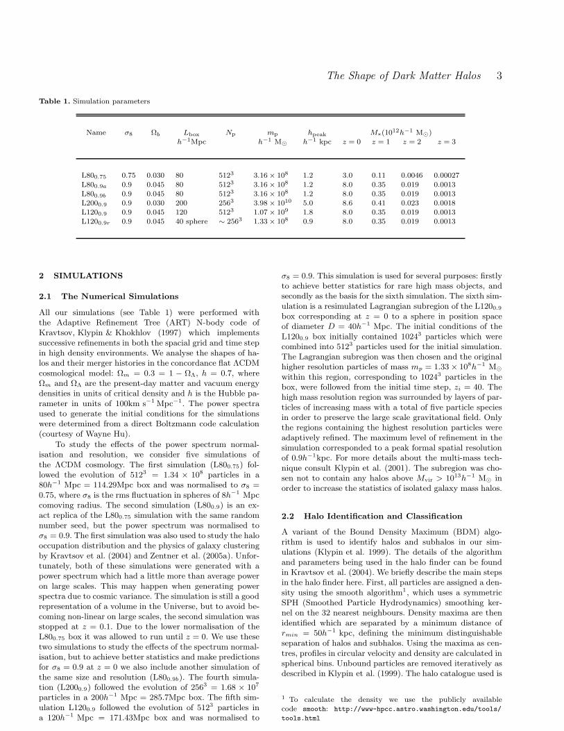
Table 1. Simulation parameters

Name σ8 Ωb Lbox Np mp hpeak M∗(1012h−1 M⊙)h−1Mpc h−1 M⊙ h−1 kpc z = 0 z = 1 z = 2 z = 3

L800.75 0.75 0.030 80 5123 3.16 × 108 1.2 3.0 0.11 0.0046 0.00027

L800.9a 0.9 0.045 80 5123 3.16 × 108 1.2 8.0 0.35 0.019 0.0013L800.9b 0.9 0.045 80 5123 3.16 × 108 1.2 8.0 0.35 0.019 0.0013L2000.9 0.9 0.030 200 2563 3.98 × 1010 5.0 8.6 0.41 0.023 0.0018L1200.9 0.9 0.045 120 5123 1.07 × 109 1.8 8.0 0.35 0.019 0.0013L1200.9r 0.9 0.045 40 sphere ∼ 2563 1.33 × 108 0.9 8.0 0.35 0.019 0.0013

2 SIMULATIONS

2.1 The Numerical Simulations

All our simulations (see Table 1) were performed withthe Adaptive Refinement Tree (ART) N-body code ofKravtsov, Klypin & Khokhlov (1997) which implementssuccessive refinements in both the spacial grid and time stepin high density environments. We analyse the shapes of ha-los and their merger histories in the concordance flat ΛCDMcosmological model: Ωm = 0.3 = 1 − ΩΛ, h = 0.7, whereΩm and ΩΛ are the present-day matter and vacuum energydensities in units of critical density and h is the Hubble pa-rameter in units of 100km s−1 Mpc−1. The power spectraused to generate the initial conditions for the simulationswere determined from a direct Boltzmann code calculation(courtesy of Wayne Hu).

To study the effects of the power spectrum normal-isation and resolution, we consider five simulations ofthe ΛCDM cosmology. The first simulation (L800.75) fol-lowed the evolution of 5123 = 1.34 × 108 particles in a80h−1 Mpc = 114.29Mpc box and was normalised to σ8 =0.75, where σ8 is the rms fluctuation in spheres of 8h−1 Mpccomoving radius. The second simulation (L800.9) is an ex-act replica of the L800.75 simulation with the same randomnumber seed, but the power spectrum was normalised toσ8 = 0.9. The first simulation was also used to study the halooccupation distribution and the physics of galaxy clusteringby Kravtsov et al. (2004) and Zentner et al. (2005a). Unfor-tunately, both of these simulations were generated with apower spectrum which had a little more than average poweron large scales. This may happen when generating powerspectra due to cosmic variance. The simulation is still a goodrepresentation of a volume in the Universe, but to avoid be-coming non-linear on large scales, the second simulation wasstopped at z = 0.1. Due to the lower normalisation of theL800.75 box it was allowed to run until z = 0. We use thesetwo simulations to study the effects of the spectrum normal-isation, but to achieve better statistics and make predictionsfor σ8 = 0.9 at z = 0 we also include another simulation ofthe same size and resolution (L800.9b). The fourth simula-tion (L2000.9) followed the evolution of 2563 = 1.68 × 107

particles in a 200h−1 Mpc = 285.7Mpc box. The fifth sim-ulation L1200.9 followed the evolution of 5123 particles ina 120h−1 Mpc = 171.43Mpc box and was normalised to

σ8 = 0.9. This simulation is used for several purposes: firstlyto achieve better statistics for rare high mass objects, andsecondly as the basis for the sixth simulation. The sixth sim-ulation is a resimulated Lagrangian subregion of the L1200.9

box corresponding at z = 0 to a sphere in position spaceof diameter D = 40h−1 Mpc. The initial conditions of theL1200.9 box initially contained 10243 particles which werecombined into 5123 particles used for the initial simulation.The Lagrangian subregion was then chosen and the originalhigher resolution particles of mass mp = 1.33 × 108h−1 M⊙within this region, corresponding to 10243 particles in thebox, were followed from the initial time step, zi = 40. Thehigh mass resolution region was surrounded by layers of par-ticles of increasing mass with a total of five particle speciesin order to preserve the large scale gravitational field. Onlythe regions containing the highest resolution particles wereadaptively refined. The maximum level of refinement in thesimulation corresponded to a peak formal spatial resolutionof 0.9h−1kpc. For more details about the multi-mass tech-nique consult Klypin et al. (2001). The subregion was cho-sen not to contain any halos above Mvir > 1013h−1 M⊙ inorder to increase the statistics of isolated galaxy mass halos.

2.2 Halo Identification and Classification

A variant of the Bound Density Maximum (BDM) algo-rithm is used to identify halos and subhalos in our sim-ulations (Klypin et al. 1999). The details of the algorithmand parameters being used in the halo finder can be foundin Kravtsov et al. (2004). We briefly describe the main stepsin the halo finder here. First, all particles are assigned a den-sity using the smooth algorithm1, which uses a symmetricSPH (Smoothed Particle Hydrodynamics) smoothing ker-nel on the 32 nearest neighbours. Density maxima are thenidentified which are separated by a minimum distance ofrmin = 50h−1 kpc, defining the minimum distinguishableseparation of halos and subhalos. Using the maxima as cen-tres, profiles in circular velocity and density are calculated inspherical bins. Unbound particles are removed iteratively asdescribed in Klypin et al. (1999). The halo catalogue used is

1 To calculate the density we use the publicly availablecode smooth: http://www-hpcc.astro.washington.edu/tools/

tools.html

4 Allgood et al.

complete for halos with & 50 particles. This corresponds toa mass below which the cumulative mass and velocity func-tions begin to flatten (see Kravtsov et al. (2004) for details).

The halo density profiles are constructed using onlybound particles and they are fit by an NFW profile(Navarro et al. 1996):

ρNF W (r) =ρs

(r/rs)(1 + r/rs)2, (1)

where rs is the radius at which the log density profile hasa slope of −2 and the density is ρs/4. One of the pa-rameters, rs or ρs, can be replaced by a virial parameter(Rvir,Mvir, or Vvir) defined such that the mean density in-side the virial radius is ∆vir times the mean universal densityρo(z) = Ωm(z)ρc(z) at that redshift:

Mvir =4π

3∆virρoR

3vir (2)

where ρc(z) is the critical density, and

∆vir(z) =18π2 + 82(Ωm(z) − 1) − 39(Ωm(z) − 1)2

Ωm(z)(3)

from Bryan & Norman (1998) with ∆vir(0) ≈ 337 for theΛCDM cosmology assumed here. The NFW density profilefitting is performed using a χ2 minimisation algorithm. Theprofiles are binned logarithmically from twice the resolutionlength (see Table 1) out to R500, the radius within whichthe average density is equal to 500 times the critical densityof the universe. The choice of this outer radius is motivatedby Tasitsiomi et al. (2004) who showed that halos are wellrelaxed within this radius. The binning begins with 10 ra-dial bins. The number of bins is then reduced if any bincontains fewer than 10 particles or is radially smaller thanthe resolution length. This reduction of bins is continued un-til both criteria are met. Fits using this method have beencompared to fits determined using different merit functions,such as the maximum deviation from the fit as described inTasitsiomi et al. (2004) and it was found that they give verysimilar results for individual halos. After fitting the halos thehost halo and subhalo relationship is determined very sim-ply. If a halo’s centre is contained within the virial radiusof a more massive halo, that halo is considered a subhaloof the larger halo. All halo properties reported here are forhalos which are determined to be isolated or host halos (i.e.,not subhalos).

3 METHODS OF DETERMINING SHAPES

There are many different methods to determine shapes ofhalos. All methods model halos as ellipsoidal with the eigen-vectors of some form of the inertia tensor corresponding tothe axes c ≤ b ≤ a (s ≡ c/a and q ≡ b/a). The two forms ofthe inertia tensor used in the literature to determine shapeare the unweighted,

Iij ≡∑

n

xi,nxj,n (4)

and the weighted (or reduced),

Iij ≡∑

n

xi,nxj,n

r2n

(5)

where

rn =√

x2n + y2

n/q2 + z2n/s2, (6)

is the elliptical distance in the eigenvector coordinate systemfrom the centre to the nth particle. In both cases the eigen-values (λa ≤ λb ≤ λc) determine the axial ratios describedat the beginning of Section 1 with (a, b, c) =

√λa, λb, λc. The

orientation of the halo is determined by the correspondingeigenvectors.

One would like to recover the shape of an isodensity sur-face. The method used here begins by determining I withs = 1 and q = 1, including all particles within some radius.Subsequently, new values for s and q are determined andthe volume of analysis is deformed along the eigenvectorsin proportion to the eigenvalues. There are two options tochoose from when deforming the volume. The volume withinthe ellipsoid can be kept constant, or one of the eigenvectorscan be kept equal to the original radius of the spherical vol-ume. In our analysis of shapes, the longest axis is kept equalto the original spherical radius. After the deformation of theoriginal spherical region, I is calculated once again, but nowusing the newly determined s and q and only including theparticles found in the new ellipsoidal region. The iterativeprocess is repeated until convergence is achieved. Conver-gence is achieved when the variance in both axial ratios, sand q, is less than a given tolerance.

The analysis presented here begins with a sphere of R =0.3Rvir, and keeps the largest axis fixed at this radius unlessotherwise stated. For determining halo shapes accurately welimit our analysis to isolated halos with Np ≥ 7000 withinRvir. This corresponds to Mvir ≥ 2.21 × 1012h−1 M⊙ forthe 80h−1Mpc box simulations, Mvir ≥ 7.49 × 1012h−1 M⊙for the 120h−1Mpc box simulation, and Mvir ≥ 9.3 ×1011h−1 M⊙ in the resimulated region of the 120h−1Mpcbox. For a discussion of our resolution tests, see AppendixA.

4 SHAPES AS A FUNCTION OF HALO MASS

The simulations analysed here enable us to analyse halosspanning a mass range from galaxy to cluster sized objects.These data provide an opportunity to study the variationof shape and its intrinsic scatter with halo mass. Variousstatistics are used to derive robust estimates of the depen-dence of shape on halo-centric radius. Combining the de-tailed spatial and dynamical information from the simula-tions we can relate quantities like angular momentum orvelocity anisotropy tensor to the shape and the orientationof the halo. In this section we aim to present a comprehen-sive analysis of the properties of halos at all redshifts. Insection 5 we will address evolutionary aspects of individualhalo shapes.

4.1 Median Relationships for Distinct Halos

We begin by fitting the mass dependence of halo shape andfind that the mean value of the axial ratio s ≡ c/a decreasesmonotonically with increasing halo mass as illustrated inFigure 1. In other words, less massive halos have a morespherical mean shape than more massive halos. Since we usefour different simulations (L800.9b, L1200.9, L1200.9r , and

The Shape of Dark Matter Halos 5

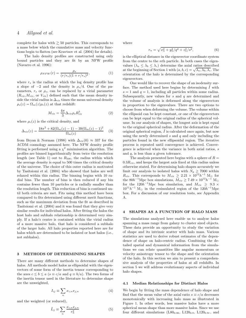
Figure 1. Mean axial ratios s = c/a for four simulations ofdifferent mass resolution are presented with a fit (solid blacklines) given by Equation (7) and dispersion of 0.1. The trian-gles, squares, solid circles and × symbols are the average s fora given mass bin. The solid circles have been shifted by 0.05 inlog for clarity. The open circles and error bars are the best fitKolmogorov-Smirnov mean and 68% confidence level assuming aGaussian parent distribution. The dashed lines connect the rawdispersion for each point and the coloured solid lines are the bestfit (KS test) dispersion. (See the electronic edition for colour ver-sion of the figure)

L2000.9) with varying mass and length scales we are able todetermine 〈s〉(Mvir) over a wide mass range. We find thatover the accessible mass range the variation of shape withhalo mass is well described by

〈s〉(Mvir, z = 0) = α

(

Mvir

M∗

)β

(7)

with best fit values

α = 0.54 ± 0.03, β = −0.050 ± 0.003. (8)

The parameters, α and β were determined by weighted χ2

minimisation on the best fit mean data points determinedvia Kolmogorov-Smirnov (KS) analysis assuming a Gaussiandistribution within a given mass bin (see section 4.4). M∗(z)is the characteristic nonlinear mass at z such that the rmstop-hat smoothed overdensity at scale σ(M∗, z) is δc = 1.68.The M∗ for z = 0 is 8.0 × 1012h−1 M⊙ for the simulationswith Ωb = 0.045 and 8.6 × 1012 for the simulations withΩb = 0.03. Only bins containing halos above our previouslystated lower bound resolution limit were used and only massbins with at least 20 halos were included in the fit. Thiswork extends the mass range of the similar relationshipsfound by previous authors (Jing & Suto 2002; Bullock 2002;Springel et al. 2004; Kasun & Evrard 2004); we compare ourresults with these previous works in Section 6.

Figure 2. 〈s〉(M) for z = 0.0, 1.0, 2.0, 3.0. The binning is thesame as in Figure 1, but now for many different redshifts. Thesolid line is the power-law relation set out in Equation (7).The L1200.9 points are shifted by 0.05 in log for clarity. TheSpringel data agrees quite well with our data and model forz = 0.0, 1.0, 2.0.

4.2 Shapes of Halos at Higher Redshifts

The use of M∗ in the Equation (7) alludes to the evolutionof the 〈s〉(Mvir) relation. After examining the 〈s〉(Mvir) re-lation at higher redshifts, we find that the relation between〈s〉 and Mvir is successfully described by Equation (7) withthe appropriate M∗(z). The M∗ for z = 1.0, 2.0, and 3.0are 3.5× 1011 , 1.8× 1010 , and 1.3× 109h−1 M⊙ respectivelyfor the simulations with Ωb = 0.045. We present our resultsfor various redshifts in Figure 2 from the L1200.9r , L800.9,L1200.9 and L2000.9 simulations. We have also included datapoints provided to us by Springel (private communication)in Figure 2 for comparison, which from a more completesample than the data presented in Springel et al. (2004) andare for shapes measured at 0.4Rvir.

4.3 Dependence on σ8

Of the parameters in the ΛCDM cosmological model the pa-rameter which is the least constrained and the most uncer-tain is the normalisation of the fluctuation spectrum, usuallyspecified by σ8. Therefore, it is of interest to understandthe dependence of the 〈s〉(Mvir) relation on σ8. Since M∗is dependent on σ8 the scaling with M∗ in Equation (7)may already be sufficient to account for the σ8 dependence.As stated in Section 2, L800.75 and L800.9a were producedwith the same Gaussian random field but different valuesfor the normalisation. Therefore the differences between thetwo simulations can only be a result of the different values

6 Allgood et al.

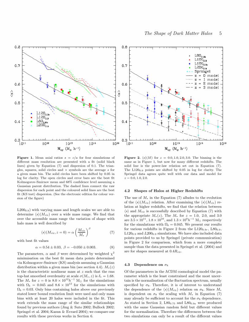
Figure 3. 〈s〉 vs M with different values of σ8. Different values ofσ8 predict different values for the 〈s〉 vs M relationship. Here onecan see that a universe with a lower σ8 produces halos which aremore elongated, although the power-law relationship (Equation(7)) remains valid, as shown by the agreement between the pointsand the lines representing this prediction.

for σ8. As Figure 3 illustrates, the two simulations do indeedproduce different relations. We find that the M∗ dependencein Equation (7) is sufficient to describe the differences be-tween simulations of different σ8. One should expect thisfrom the result of the previous subsection, that the redshiftevolution was also well described by the M∗ dependence.The values of M∗ for z = 0.1 are 5.99 × 1012 for σ8 = 0.9and 2.22×1012 for σ8 = 0.75. The value of M∗ for σ8 = 0.75at z = 1 and 2 are 1.09 × 1011 and 4.57 × 109 respectively.A simple fit to the redshift dependence of M∗ in these cos-mologies is log(M∗) = A − Blog(1 + z) − C(log(1 + z))2,with A(B, C) = 12.9(2.68, 5.96) for σ8 = 0.9 and A(B,C) =12.5(2.94, 6.28) for σ8 = 0.75, and accurate to within 1.6%and 3.1%, respectively, for z ≤ 3.

4.4 Mean - Dispersion Relationship

In the previous subsections we used the best KS test fitmean, assuming a Gaussian parent distribution, as an esti-mate of the true mean of axial ratios within a given massbin. In this subsection we examine the validity of this as-sumption, and test whether the dispersion has the mass de-pendence suggested by Jing & Suto (2002). In Figure 4 wepresent the distribution of s in the six bins from Figure 1 forL1200.9. In each of the plots we have also included the KSbest fit Gaussian, from which the mean was used to deter-mine the best fit power-law in Equation (7). The error-barson the mean indicated in Figure 1 are the 68% confidencelimits of the KS probability. The limits are determined by

Figure 4. The distribution of s in the L1200.9b simulation in themass ranges indicated. The number of halos in each bin is alsoindicated. The Gaussian fit shown for each graph is the best fit,based on a KS test analysis.

varying the mean of the parent distribution until the KSprobability drops below 16% for greater and less than thebest fit value for the dispersion in each mass bin. The valuesfrom this analysis corresponding to the distributions in Fig-ure 4 can be found in Table 2. In Figure 4 the lowest massbin, which also contains the most halos, is well fit by a Gaus-sian. This is seen in Table 2 not only by the best fit KS prob-ability, but also by the small range of the confidence limits.The higher mass bins are consistent with having Gaussianparent distributions though the parent distributions’ valuesfor the mean and dispersion are not as well constrained.There is no indication of a structured tail to lower values ofs, but Table 3 indicates that the distributions have negativeskewness. This arises from a small number of halos with verylow values of s, which are always determined to be ongoingmajor mergers with very close cores.

Jing & Suto (2002) found that the distribution of swithin a given mass bin is Gaussian. They found no indi-cation of a tail or any low values of s. This is most likelydue to their treatment of halos with multiple cores (see sec-tion 6). Bullock (2002) found a large tail to low values of susing R = Rvir. After repeating our analysis at R = Rvir wefind the exact opposite. We find even less indication of a tailthan in the distributions shown in Figure 4. The differenceis most likely due to the centres of halos determined by thedifferent halo finders used. Bailin & Steinmetz (2005) finda more subtle but significant tail to lower values of s. Thisis most likely just a side effect of combining all mass binsinto one histogram. If the histogram were divided into binsover smaller ranges in mass, this tail would be seen as a con-sequence of the combination of Gaussian distributions with

The Shape of Dark Matter Halos 7

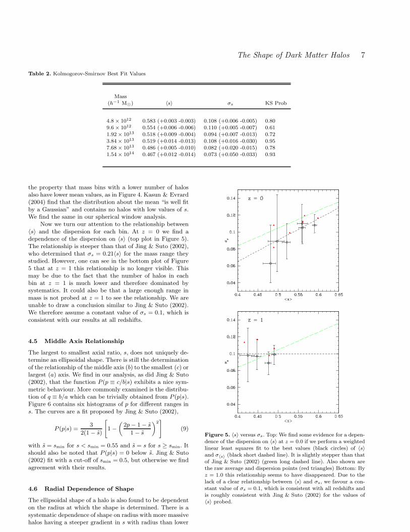
Table 2. Kolmogorov-Smirnov Best Fit Values

Mass(h−1 M⊙) 〈s〉 σs KS Prob

4.8 × 1012 0.583 (+0.003 -0.003) 0.108 (+0.006 -0.005) 0.809.6 × 1012 0.554 (+0.006 -0.006) 0.110 (+0.005 -0.007) 0.61

1.92 × 1013 0.518 (+0.009 -0.004) 0.094 (+0.007 -0.013) 0.723.84 × 1013 0.519 (+0.014 -0.013) 0.108 (+0.016 -0.030) 0.957.68 × 1013 0.486 (+0.005 -0.010) 0.082 (+0.020 -0.015) 0.781.54 × 1014 0.467 (+0.012 -0.014) 0.073 (+0.050 -0.033) 0.93

the property that mass bins with a lower number of halosalso have lower mean values, as in Figure 4. Kasun & Evrard(2004) find that the distribution about the mean “is well fitby a Gaussian” and contains no halos with low values of s.We find the same in our spherical window analysis.

Now we turn our attention to the relationship between〈s〉 and the dispersion for each bin. At z = 0 we find adependence of the dispersion on 〈s〉 (top plot in Figure 5).The relationship is steeper than that of Jing & Suto (2002),who determined that σs = 0.21〈s〉 for the mass range theystudied. However, one can see in the bottom plot of Figure5 that at z = 1 this relationship is no longer visible. Thismay be due to the fact that the number of halos in eachbin at z = 1 is much lower and therefore dominated bysystematics. It could also be that a large enough range inmass is not probed at z = 1 to see the relationship. We areunable to draw a conclusion similar to Jing & Suto (2002).We therefore assume a constant value of σs = 0.1, which isconsistent with our results at all redshifts.

4.5 Middle Axis Relationship

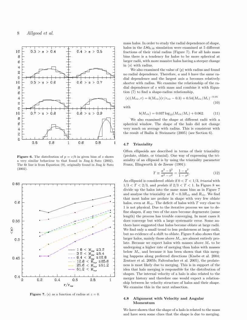
The largest to smallest axial ratio, s, does not uniquely de-termine an ellipsoidal shape. There is still the determinationof the relationship of the middle axis (b) to the smallest (c) orlargest (a) axis. We find in our analysis, as did Jing & Suto(2002), that the function P (p ≡ c/b|s) exhibits a nice sym-metric behaviour. More commonly examined is the distribu-tion of q ≡ b/a which can be trivially obtained from P (p|s).Figure 6 contains six histograms of p for different ranges ins. The curves are a fit proposed by Jing & Suto (2002),

P (p|s) =3

2(1 − s)

[

1 −(

2p − 1 − s

1 − s

)2]

(9)

with s = smin for s < smin = 0.55 and s = s for s ≥ smin. Itshould also be noted that P (p|s) = 0 below s. Jing & Suto(2002) fit with a cut-off of smin = 0.5, but otherwise we findagreement with their results.

4.6 Radial Dependence of Shape

The ellipsoidal shape of a halo is also found to be dependenton the radius at which the shape is determined. There is asystematic dependence of shape on radius with more massivehalos having a steeper gradient in s with radius than lower

Figure 5. 〈s〉 versus σs. Top: We find some evidence for a depen-dence of the dispersion on 〈s〉 at z = 0.0 if we perform a weightedlinear least squares fit to the best values (black circles) of 〈s〉and σ〈s〉 (black short dashed line). It is slightly stepper than thatof Jing & Suto (2002) (green long dashed line). Also shown arethe raw average and dispersion points (red triangles) Bottom: Byz = 1.0 this relationship seems to have disappeared. Due to thelack of a clear relationship between 〈s〉 and σs, we favour a con-stant value of σs = 0.1, which is consistent with all redshifts andis roughly consistent with Jing & Suto (2002) for the values of〈s〉 probed.

8 Allgood et al.

Figure 6. The distribution of p = c/b in given bins of s showsa very similar behaviour to that found in Jing & Suto (2002).The fit line is from Equation (9), originally found in Jing & Suto(2002).

Figure 7. 〈s〉 as a function of radius at z = 0.

mass halos. In order to study the radial dependence of shape,halos in the L800.9b simulation were examined at 5 differentfractions of their virial radius (Figure 7). For all halo massbins there is a tendency for halos to be more spherical atlarger radii, with more massive halos having a steeper changein 〈s〉 with radius.

We also examined the value of 〈p〉 with radius and foundno radial dependence. Therefore, a and b have the same ra-dial dependence and the largest axis a becomes relativelyshorter with radius. We examine the relationship of the ra-dial dependence of s with mass and combine it with Equa-tion (7) to find a shape-radius relationship,

〈s〉(Mvir, r) = b(Mvir)(r/rvir − 0.3) + 0.54(Mvir/M∗)−0.05

(10)with

b(Mvir) = 0.037 log10(Mvir/M∗) + 0.062. (11)

We also examined the shape at different radii with aspherical window. The shape of the halo did not changevery much on average with radius. This is consistent withthe result of Bailin & Steinmetz (2005) (see Section 6).

4.7 Triaxiality

Often ellipsoids are described in terms of their triaxiality(prolate, oblate, or triaxial). One way of expressing the tri-axiality of an ellipsoid is by using the triaxiality parameterFranx, Illingworth & de Zeeuw (1991):

T ≡ a2 − b2

a2 − c2=

1 − q2

1 − s2. (12)

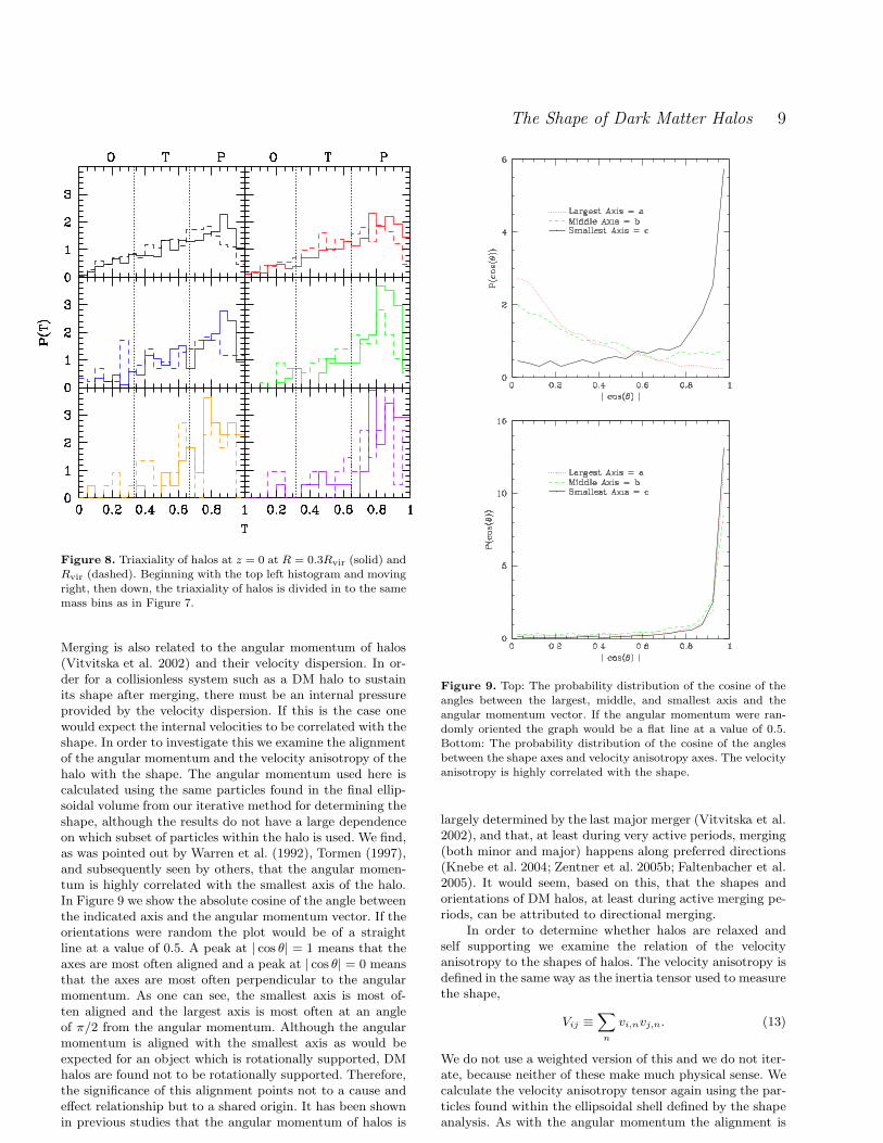
An ellipsoid is considered oblate if 0 < T < 1/3, triaxial with1/3 < T < 2/3, and prolate if 2/3 < T < 1. In Figure 8 wedivide up the halos into the same mass bins as in Figure 7and analyse the triaxiality at R = 0.3Rvir and Rvir. We findthat most halos are prolate in shape with very few oblatehalos, even at Rvir. The deficit of halos with T very close to1 is not physical. Due to the iterative process we use to de-fine shapes, if any two of the axes become degenerate (samelength) the process has trouble converging. In most cases itdoes converge but with a large systematic error. Some au-thors have suggested that halos become oblate at large radii.We find only a small trend to less prolateness at large radii,but no evidence of a shift to oblate. Figure 8 also shows thatlarger halos, mainly those above M∗, are almost entirely pro-late. Because we expect halos with masses above M∗ to beundergoing a higher rate of merging than halos with massesbelow M∗, and because it has been shown that this merg-ing happens along preferred directions (Knebe et al. 2004;Zentner et al. 2005b; Faltenbacher et al. 2005), the prolate-ness is most likely due to merging. This is in support of theidea that halo merging is responsible for the distribution ofshapes. The internal velocity of a halo is also related to themerger history and therefore one would expect a relation-ship between he velocity structure of halos and their shape.We examine this in the next subsection.

4.8 Alignment with Velocity and Angular

Momentum

We have shown that the shape of a halo is related to the massand have seen some clues that the shape is due to merging.

The Shape of Dark Matter Halos 9

Figure 8. Triaxiality of halos at z = 0 at R = 0.3Rvir (solid) andRvir (dashed). Beginning with the top left histogram and movingright, then down, the triaxiality of halos is divided in to the samemass bins as in Figure 7.

Merging is also related to the angular momentum of halos(Vitvitska et al. 2002) and their velocity dispersion. In or-der for a collisionless system such as a DM halo to sustainits shape after merging, there must be an internal pressureprovided by the velocity dispersion. If this is the case onewould expect the internal velocities to be correlated with theshape. In order to investigate this we examine the alignmentof the angular momentum and the velocity anisotropy of thehalo with the shape. The angular momentum used here iscalculated using the same particles found in the final ellip-soidal volume from our iterative method for determining theshape, although the results do not have a large dependenceon which subset of particles within the halo is used. We find,as was pointed out by Warren et al. (1992), Tormen (1997),and subsequently seen by others, that the angular momen-tum is highly correlated with the smallest axis of the halo.In Figure 9 we show the absolute cosine of the angle betweenthe indicated axis and the angular momentum vector. If theorientations were random the plot would be of a straightline at a value of 0.5. A peak at | cos θ| = 1 means that theaxes are most often aligned and a peak at | cos θ| = 0 meansthat the axes are most often perpendicular to the angularmomentum. As one can see, the smallest axis is most of-ten aligned and the largest axis is most often at an angleof π/2 from the angular momentum. Although the angularmomentum is aligned with the smallest axis as would beexpected for an object which is rotationally supported, DMhalos are found not to be rotationally supported. Therefore,the significance of this alignment points not to a cause andeffect relationship but to a shared origin. It has been shownin previous studies that the angular momentum of halos is

Figure 9. Top: The probability distribution of the cosine of theangles between the largest, middle, and smallest axis and theangular momentum vector. If the angular momentum were ran-domly oriented the graph would be a flat line at a value of 0.5.Bottom: The probability distribution of the cosine of the anglesbetween the shape axes and velocity anisotropy axes. The velocityanisotropy is highly correlated with the shape.

largely determined by the last major merger (Vitvitska et al.2002), and that, at least during very active periods, merging(both minor and major) happens along preferred directions(Knebe et al. 2004; Zentner et al. 2005b; Faltenbacher et al.2005). It would seem, based on this, that the shapes andorientations of DM halos, at least during active merging pe-riods, can be attributed to directional merging.

In order to determine whether halos are relaxed andself supporting we examine the relation of the velocityanisotropy to the shapes of halos. The velocity anisotropy isdefined in the same way as the inertia tensor used to measurethe shape,

Vij ≡∑

n

vi,nvj,n. (13)

We do not use a weighted version of this and we do not iter-ate, because neither of these make much physical sense. Wecalculate the velocity anisotropy tensor again using the par-ticles found within the ellipsoidal shell defined by the shapeanalysis. As with the angular momentum the alignment is

10 Allgood et al.

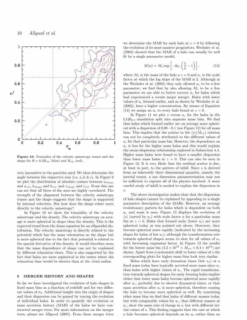
Figure 10. Triaxiality of the velocity anisotropy tensor and theshape for R = 0.3Rvir (blue) and Rvir (red).

very insensitive to the particles used. We then determine theangle between the respective axis (i.e. a, b, & c). In Figure 9we plot the distribution of absolute cosines between ashape

and avel, bshape and bvel, and cshape and cvel. From this onecan see that all three of the axes are highly correlated. Thestrength of the alignment between the velocity anisotropytensor and the shape suggests that the shape is supportedby internal velocities. But how does the shape relate moredirectly to the velocity anisotropy?

In Figure 10 we show the triaxiality of the velocityanisotropy and the density. The velocity anisotropy on aver-age is more spherical in shape than the density. This is theexpected trend from the Jeans equation for an ellipsoidal dis-tribution. The velocity anisotropy is directly related to thepotential which has the same orientation as the shape butis more spherical due to the fact that potential is related tothe spacial derivative of the density. It would therefore seemthat the mass dependence of shape can not be explainedby different relaxation times. This is also supported by thefact that halos are more aspherical in the centre where therelaxation time would be shorter than at the virial radius.

5 MERGER HISTORY AND SHAPES

So far we have investigated the evolution of halo shapes infixed mass bins as a function of redshift and for two differ-ent values of σ8. Additional insight into the origin of shapesand their dispersion can be gained by tracing the evolutionof individual halos. In order to quantify the evolution ormass accretion history (MAH) of the halos we have con-structed merger trees. For more information on the mergertrees, please see Allgood (2005). From these merger trees

we determine the MAH for each halo at z = 0 by followingthe evolution of its most massive progenitors. Wechsler et al.(2002) showed that the MAH of a halo can usually be wellfit by a single parameter model,

M(a) = Mo exp

[

−2ac

(

1

a− 1

)]

, (14)

where Mo is the mass of the halo a z = 0 and ac is the scalefactor at which the log slope of the MAH is 2. Although inthe Wechsler et al. (2002) they only allowed ac to be a freeparameter, we find that by also allowing Mo to be a freeparameter we are able to better recover ac for halos whichhad experienced a recent major merger. Halos with lowervalues of ac formed earlier, and as shown by Wechsler et al.(2002), have a higher concentration. By means of Equation(14) we assign an ac to every halo found at z = 0.

In Figure 11 we plot s versus ac for the halos in theL1200.9 simulation split into separate mass bins. We findthat halos which formed earlier are on average more spheri-cal with a dispersion of 0.08−0.1 (see Figure 12) for all massbins. This implies that the scatter in the 〈s〉(Mvir) relationcan not be completely attributed to the different values ofac for that particular mass bin. However, the dependence onac is less for the higher mass halos and this would explainthe mean-dispersion relationship explored in Subsection 4.4.Higher mass halos were found to have a smaller dispersionthan lower mass halos at z = 0. This can also be seen inFigure 12. It is very likely that the residual scatter is due,at least in part, to the pattern of infall. Since s is derivedfrom an inherently three dimensional quantity, namely theinertial tensor, a one dimension parameterisation may notbe sufficient to capture all of the physics involved. A morecareful study of infall is needed to explain the dispersion ins.

The above investigation makes clear that the dispersionof halo shapes cannot be explained by appealing to a singleparameter description of the MAHs. However, an averageevolutionary pattern for halos which is dependent on bothac and mass is seen. Figure 13 displays the evolution of〈s〉 (sorted by ac) with scale factor a for a particular massbin at z = 0. Halos that formed early (lower ac) are morespherical today as was pointed out above. Moreover, theybecome spherical more rapidly (indicated by the increasingslopes for halos of low ac), although the transformation ratetowards spherical shapes seems to slow for all values of ac

with increasing expansion factor. In Figure 13 the resultsfor the lowest mass bin (3.2× 1012 < Mvir < 6.4× 1012) areshown. Apart from a systematic shift to lower values of s thecorresponding plots for higher mass bins look very similar.

Halos which have early formation times (low ac) at afixed mass today have typically accreted more mass since ac

than halos with higher values of ac. The rapid transforma-tion towards spherical shapes for early forming halos implieseither that lower mass halos become spherical more rapidlyafter ac, probably due to shorter dynamical times, or thatmass accretion after ac is more spherical, therefore causingthe halo to become more spherical as well. By examiningother mass bins we find that halos of different masses todaybut with comparable values for ac, thus different masses atac, show the same rate of change in s, but with different ini-tial values of s. This finding suggests that the rate at whicha halo becomes spherical depends on its ac rather than on

The Shape of Dark Matter Halos 11

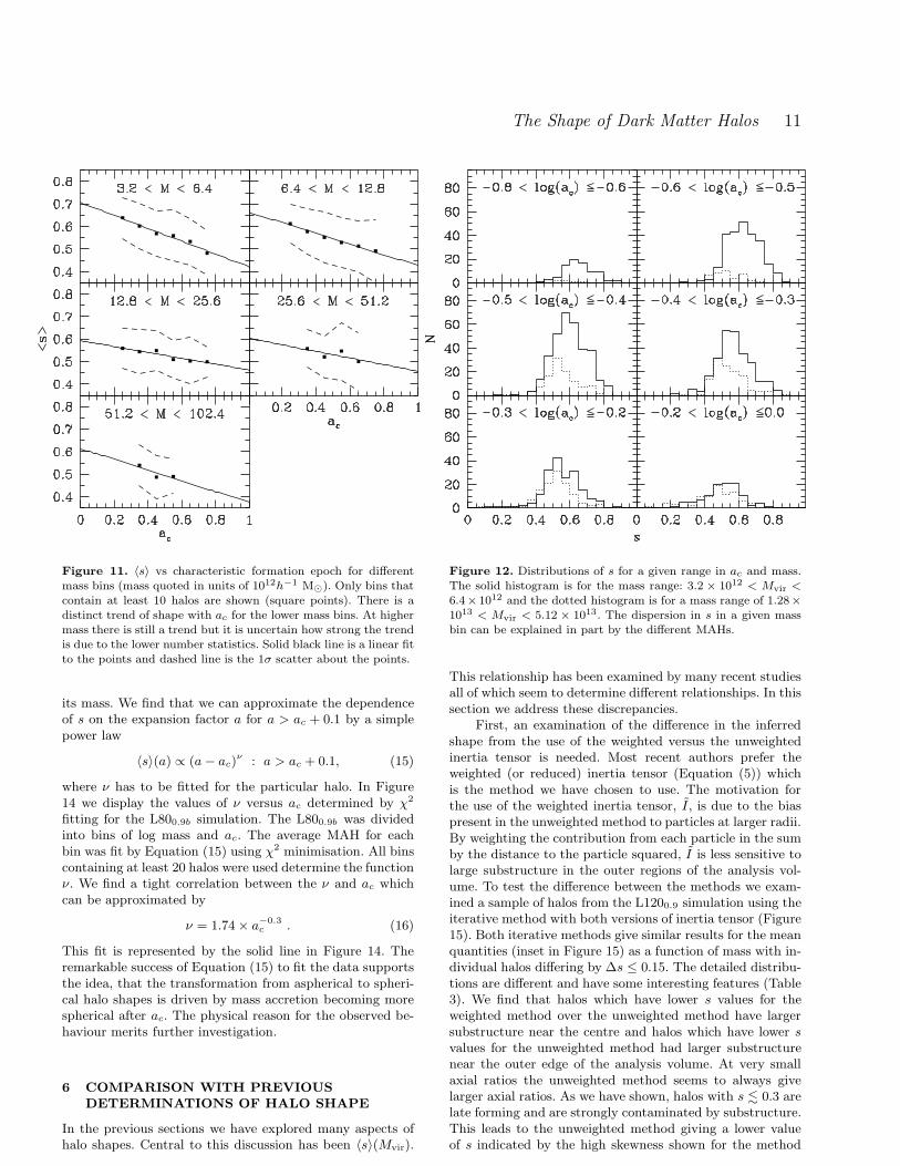
Figure 11. 〈s〉 vs characteristic formation epoch for differentmass bins (mass quoted in units of 1012h−1 M⊙). Only bins thatcontain at least 10 halos are shown (square points). There is adistinct trend of shape with ac for the lower mass bins. At highermass there is still a trend but it is uncertain how strong the trendis due to the lower number statistics. Solid black line is a linear fitto the points and dashed line is the 1σ scatter about the points.

its mass. We find that we can approximate the dependenceof s on the expansion factor a for a > ac + 0.1 by a simplepower law

〈s〉(a) ∝ (a − ac)ν : a > ac + 0.1, (15)

where ν has to be fitted for the particular halo. In Figure14 we display the values of ν versus ac determined by χ2

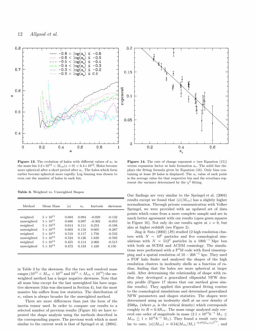
fitting for the L800.9b simulation. The L800.9b was dividedinto bins of log mass and ac. The average MAH for eachbin was fit by Equation (15) using χ2 minimisation. All binscontaining at least 20 halos were used determine the functionν. We find a tight correlation between the ν and ac whichcan be approximated by

ν = 1.74 × a−0.3c . (16)

This fit is represented by the solid line in Figure 14. Theremarkable success of Equation (15) to fit the data supportsthe idea, that the transformation from aspherical to spheri-cal halo shapes is driven by mass accretion becoming morespherical after ac. The physical reason for the observed be-haviour merits further investigation.

6 COMPARISON WITH PREVIOUS

DETERMINATIONS OF HALO SHAPE

In the previous sections we have explored many aspects ofhalo shapes. Central to this discussion has been 〈s〉(Mvir).

Figure 12. Distributions of s for a given range in ac and mass.The solid histogram is for the mass range: 3.2 × 1012 < Mvir <6.4× 1012 and the dotted histogram is for a mass range of 1.28×1013 < Mvir < 5.12 × 1013. The dispersion in s in a given massbin can be explained in part by the different MAHs.

This relationship has been examined by many recent studiesall of which seem to determine different relationships. In thissection we address these discrepancies.

First, an examination of the difference in the inferredshape from the use of the weighted versus the unweightedinertia tensor is needed. Most recent authors prefer theweighted (or reduced) inertia tensor (Equation (5)) whichis the method we have chosen to use. The motivation forthe use of the weighted inertia tensor, I, is due to the biaspresent in the unweighted method to particles at larger radii.By weighting the contribution from each particle in the sumby the distance to the particle squared, I is less sensitive tolarge substructure in the outer regions of the analysis vol-ume. To test the difference between the methods we exam-ined a sample of halos from the L1200.9 simulation using theiterative method with both versions of inertia tensor (Figure15). Both iterative methods give similar results for the meanquantities (inset in Figure 15) as a function of mass with in-dividual halos differing by ∆s ≤ 0.15. The detailed distribu-tions are different and have some interesting features (Table3). We find that halos which have lower s values for theweighted method over the unweighted method have largersubstructure near the centre and halos which have lower svalues for the unweighted method had larger substructurenear the outer edge of the analysis volume. At very smallaxial ratios the unweighted method seems to always givelarger axial ratios. As we have shown, halos with s . 0.3 arelate forming and are strongly contaminated by substructure.This leads to the unweighted method giving a lower valueof s indicated by the high skewness shown for the method

12 Allgood et al.

Figure 13. The evolution of halos with different values of ac inthe mass bin 3.2×1012 < Mvir(z = 0) < 6.4×1012. Halos becomemore spherical after a short period after ac. The halos which formearlier become spherical more rapidly. Log binning was chosen toeven out the number of halos in each bin.

Table 3. Weighted vs. Unweighted Shapes

Method Mean Mass 〈s〉 σs kurtosis skewness

weighted 5 × 1011 0.694 0.094 -0.029 -0.132unweighted 5 × 1011 0.686 0.097 -0.302 -0.053weighted 5 × 1012 0.614 0.111 0.253 -0.188unweighted 5 × 1012 0.603 0.118 0.605 -0.287weighted 5 × 1013 0.518 0.117 1.756 -0.532unweighted 5 × 1013 0.524 0.126 1.628 -0.592weighted 5 × 1014 0.455 0.114 2.066 -0.515

unweighted 5 × 1014 0.472 0.133 1.428 0.150

in Table 3 by the skewness. For the two well resolved massranges (1012 < Mvir < 1013 and 1013 < Mvir < 1014) the un-weighted method has a larger negative skewness. Note thatall mass bins except for the last unweighted bin have nega-tive skewness (this was discussed in Section 4), but the mostmassive bin suffers from low statistics. The distribution ofσs values is always broader for the unweighted method.

There are more differences than just the form of theinertia tensor used. In order to compare our results to aselected number of previous results (Figure 16) we have re-peated the shape analysis using the methods described inthe corresponding papers. The previous work which is mostsimilar to the current work is that of Springel et al. (2004).

Figure 14. The rate of change exponent ν (see Equation (15))versus expansion factor at halo formation ac. The solid line dis-plays the fitting formula given by Equation (16). Only bins con-taining at lease 20 halos is displayed. The ac value of each pointis the average value for that respective bin and the errorbars rep-resent the variance determined by the χ2 fitting.

Our findings are very similar to the Springel et al. (2004)results except we found that 〈s〉(Mvir) has a slightly highernormalisation. Through private communication with VolkerSpringel, we were provided with an updated set of datapoints which come from a more complete sample and are inmuch better agreement with our results (open green squaresin Figure 16). Not only do our results agree at z = 0, butalso at higher redshift (see Figure 2).

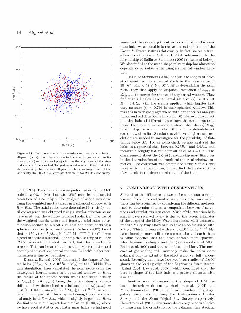
Jing & Suto (2002) (JS) studied 12 high resolution clus-ters with N ∼ 106 particles and five cosmological sim-ulations with N = 5123 particles in a 100h−1 Mpc boxwith both an SCDM and ΛCDM cosmology. The simula-tions were performed with a P3M code with fixed timestep-ping and a spatial resolution of 10 − 20h−1 kpc. They useda FOF halo finder and analysed the shapes of the highresolution clusters in isodensity shells as a function of ra-dius, finding that the halos are more spherical at largerradii. After determining the relationship of shape with ra-dius they developed a generalised ellipsoidal NFW den-sity profile (Figure 17 shows that our method gives sim-ilar results). They applied this generalised fitting routineto the cosmological simulations and determined generalisedNFW parameters and shapes statistics. The shapes weredetermined using an isodensity shell at an over density of2500ρc (where ρc is the critical density) which correspondsroughly to R = 0.3Rvir. The mass range analysed only cov-ered one order of magnitude in mass (2.1 × 1013h−1 M⊙ ≤Mvir . 1 × 1014h−1 M⊙). They found a result very simi-

lar to ours, 〈s〉(Mvir) = 0.54(Mvir/M∗)−0.07[Ωm(z)]0.7

, and

The Shape of Dark Matter Halos 13

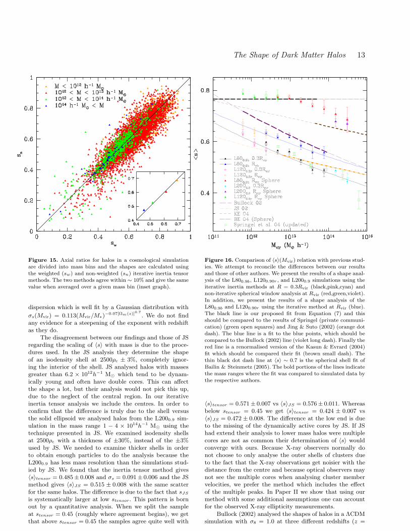
Figure 15. Axial ratios for halos in a cosmological simulationare divided into mass bins and the shapes are calculated usingthe weighted (sw) and non-weighted (sn) iterative inertia tensormethods. The two methods agree within ∼ 10% and give the samevalue when averaged over a given mass bin (inset graph).

dispersion which is well fit by a Gaussian distribution with

σs(Mvir) = 0.113(Mvir/M∗)−0.07[Ωm(z)]0.7

. We do not findany evidence for a steepening of the exponent with redshiftas they do.

The disagreement between our findings and those of JSregarding the scaling of 〈s〉 with mass is due to the proce-dures used. In the JS analysis they determine the shapeof an isodensity shell at 2500ρc ± 3%, completely ignor-ing the interior of the shell. JS analysed halos with massesgreater than 6.2 × 1012h−1 M⊙ which tend to be dynam-ically young and often have double cores. This can affectthe shape a lot, but their analysis would not pick this up,due to the neglect of the central region. In our iterativeinertia tensor analysis we include the centres. In order toconfirm that the difference is truly due to the shell versusthe solid ellipsoid we analysed halos from the L2000.9 sim-ulation in the mass range 1 − 4 × 1014h−1 M⊙ using thetechnique presented in JS. We examined isodensity shellsat 2500ρc with a thickness of ±30%, instead of the ±3%used by JS. We needed to examine thicker shells in orderto obtain enough particles to do the analysis because theL2000.9 has less mass resolution than the simulations stud-ied by JS. We found that the inertia tensor method gives〈s〉tensor = 0.485± 0.008 and σs = 0.091± 0.006 and the JSmethod gives 〈s〉JS = 0.515 ± 0.008 with the same scatterfor the same halos. The difference is due to the fact that sJS

is systematically larger at low stensor. This pattern is bornout by a quantitative analysis. When we split the sampleat stensor = 0.45 (roughly where agreement begins), we getthat above stensor = 0.45 the samples agree quite well with

Figure 16. Comparison of 〈s〉(Mvir) relation with previous stud-ies. We attempt to reconcile the differences between our resultsand those of other authors. We present the results of a shape anal-ysis of the L800.9b, L1200.90r , and L2000.9 simulations using theiterative inertia methods at R = 0.3Rvir (black,pink,cyan) andnon-iterative spherical window analysis at Rvir (red,green,violet).In addition, we present the results of a shape analysis of theL800.9b and L1200.90r using the iterative method at Rvir (blue).The black line is our proposed fit from Equation (7) and thisshould be compared to the results of Springel (private communi-cation) (green open squares) and Jing & Suto (2002) (orange dotdash). The blue line is a fit to the blue points, which should becompared to the Bullock (2002) line (violet long dash). Finally thered line is a renormalised version of the Kasun & Evrard (2004)fit which should be compared their fit (brown small dash). Thethin black dot dash line at 〈s〉 ∼ 0.7 is the spherical shell fit ofBailin & Steinmetz (2005). The bold portions of the lines indicatethe mass ranges where the fit was compared to simulated data bythe respective authors.

〈s〉tensor = 0.571± 0.007 vs 〈s〉JS = 0.576± 0.011. Whereasbelow stensor = 0.45 we get 〈s〉tensor = 0.424 ± 0.007 vs〈s〉JS = 0.472 ± 0.008. The difference at the low end is dueto the missing of the dynamically active cores by JS. If JShad extend their analysis to lower mass halos were multiplecores are not as common their determination of 〈s〉 wouldconverge with ours. Because X-ray observers normally donot choose to only analyse the outer shells of clusters dueto the fact that the X-ray observations get noisier with thedistance from the centre and because optical observers maynot see the multiple cores when analysing cluster membervelocities, we prefer the method which includes the effectof the multiple peaks. In Paper II we show that using ourmethod with some additional assumptions one can accountfor the observed X-ray ellipticity measurements.

Bullock (2002) analysed the shapes of halos in a ΛCDMsimulation with σ8 = 1.0 at three different redshifts (z =

14 Allgood et al.

Figure 17. Comparison of an isodensity shell (red) and a tensorellipsoid (blue). Particles are selected by the JS (red) and inertiatensor (blue) methods and projected on the x–y plane of the sim-ulation box. The shortest/longest axis ratio is s = 0.49 (0.48) forthe isodensity shell (tensor ellipsoid). The semi-major axis of theisodensity shell 0.23Rvir, consistent with JS for 2500ρc isodensity.

0.0, 1.0, 3.0). The simulations were performed using the ARTcode in a 60h−1 Mpc box with 2563 particles and spatialresolution of 1.8h−1 kpc. The analysis of shape was doneusing the weighted inertia tensor in a spherical window withR = Rvir. The axial ratios were determined iteratively un-til convergence was obtained using a similar criterion as wehave used, but the window remained spherical. The use ofthe weighted inertia tensor and iterative axial ratio deter-mination seemed to almost eliminate the effect of using aspherical window (discussed below). Bullock (2002) foundthat 〈s〉(Mvir) ≃ 0.7(Mvir/10

12h−1 M⊙)−0.05(1+z)−0.2 wasa good fit to the simulation. The empirical scaling of Bullock(2002) is similar to what we find, but the powerlaw issteeper. This can be attributed to the lower resolution andpossibly the use of a spherical window. Bullock’s higher nor-malisation is due to the higher σ8.

Kasun & Evrard (2004) determined the shapes of clus-ter halos (M200 > 3 × 1014h−1 M⊙) in the Hubble Vol-ume simulation. They calculated the axial ratios using theunweighted inertia tensor in a spherical window at R200,the radius of the sphere within which the mean densityis 200ρc(z), with ρc(z) being the critical density at red-shift z. They determined a relationship of 〈s〉(Mvir) =0.631[1−0.023 ln(Mvir/10

15h−1 M⊙)](1+z)−0.086. We com-pare our analysis with theirs by performing the same spher-ical analysis at R = Rvir, which is slightly larger than R200.We find that in our largest box simulation (L2000.9) wherewe have good statistics on cluster mass halos we find good

agreement. In examining the other two simulations for lowermass halos we are unable to recover the extrapolation of theKasun & Evrard (2004) relationship. In fact, we see a tran-sition from the Kasun & Evrard (2004) relationship to therelationship of Bailin & Steinmetz (2005) (discussed below).We also find that the mean shape relationship has almost nodependence on radius when using a spherical window func-tion.

Bailin & Steinmetz (2005) analyse the shapes of halosat different radii in spherical shells in the mass range of1011h−1 M⊙ < M . 5 × 1013. After determining the axialratios they then apply an empirical correction of strue =

s√

3measure to correct for the use of a spherical window. They

find that all halos have an axial ratio of 〈s〉 ∼ 0.63 atR = 0.4Rvir with the scaling applied, which implies thatthey measure 〈s〉 ∼ 0.766 in their spherical window. Thisresult is in very good agreement with our spherical analysis(green and red data points in Figure 16). However, we do notfind that halos of different masses have the same mean axialratio. There seems to be some evidence that the 〈s〉(Mvir)relationship flattens out below M∗, but it is definitely notconstant with radius. Simulations with even higher mass res-olution are needed to investigate for the possibility of flat-tening below M∗. For an extra check we also analysed thehalos in a spherical shell between 0.25Rvir and 0.4Rvir andmeasure a roughly flat value for all halos of s = 0.77. Thedisagreement about the 〈s〉(M) relationship most likely liesin the determination of the empirical spherical window cor-rection. The correction was determined using Monte Carlohalos with no substructure, but we find that substructureplays a role in the determined shape of the halo.

7 COMPARISON WITH OBSERVATIONS

Since all of the differences between the shape statistics ex-tracted from pure collisionless simulations by various au-thors can be reconciled by considering the different methodsused to determine shapes, a comparison between observa-tions and simulations is in order. Much of the attention haloshapes have received lately is due to the recent estimatesof the shape of the Milky Way’s host halo. Most estimatesfind the Milky Way’s host halo to have an oblate shape withs ≥ 0.8. This is in contrast with s ≈ 0.6±0.1 for 1012h−1 M⊙halos found in pure collisionless simulations, though thereis some evidence that the halos become more sphericalwhen baryonic cooling is included (Kazantzidis et al. 2004;Bailin et al. 2005) and that some become oblate. The pres-ence of gas cooling will invariably make the halos morespherical but the extent of the effect is not yet fully under-stood. Recently, there have however been studies of the Mgiants in the leading edge of the Sagittarius dwarf stream(Helmi 2004; Law et al. 2005), which concluded that thebest fit shape of the host halo is a prolate ellipsoid withs = 0.6.

Another way of measuring the shape of DM ha-los is through weak lensing. Hoekstra et al. (2004) andMandelbaum et al. (2005) performed studies of galaxy-galaxy weak lensing using the Red-Sequence ClusterSurvey and the Sloan Digital Sky Survey respectively.Hoekstra et al. (2004) determine the average shapes of halosby measuring the orientation of the galaxies, then stacking

The Shape of Dark Matter Halos 15

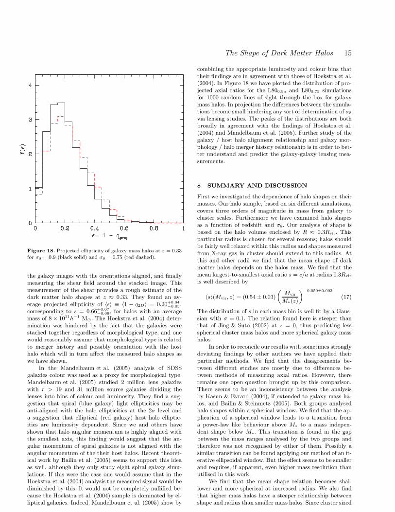
Figure 18. Projected ellipticity of galaxy mass halos at z = 0.33for σ8 = 0.9 (black solid) and σ8 = 0.75 (red dashed).

the galaxy images with the orientations aligned, and finallymeasuring the shear field around the stacked image. Thismeasurement of the shear provides a rough estimate of thedark matter halo shapes at z ≈ 0.33. They found an av-erage projected ellipticity of 〈ǫ〉 ≡ 〈1 − q2D〉 = 0.20+0.04

−0.05 ,corresponding to s = 0.66+0.07

−0.06, for halos with an averagemass of 8 × 1011h−1 M⊙. The Hoekstra et al. (2004) deter-mination was hindered by the fact that the galaxies werestacked together regardless of morphological type, and onewould reasonably assume that morphological type is relatedto merger history and possibly orientation with the hosthalo which will in turn affect the measured halo shapes aswe have shown.

In the Mandelbaum et al. (2005) analysis of SDSSgalaxies colour was used as a proxy for morphological type.Mandelbaum et al. (2005) studied 2 million lens galaxieswith r > 19 and 31 million source galaxies dividing thelenses into bins of colour and luminosity. They find a sug-gestion that spiral (blue galaxy) light ellipticities may beanti-aligned with the halo ellipticities at the 2σ level anda suggestion that elliptical (red galaxy) host halo elliptic-ities are luminosity dependent. Since we and others haveshown that halo angular momentum is highly aligned withthe smallest axis, this finding would suggest that the an-gular momentum of spiral galaxies is not aligned with theangular momentum of the their host halos. Recent theoret-ical work by Bailin et al. (2005) seems to support this ideaas well, although they only study eight spiral galaxy simu-lations. If this were the case one would assume that in theHoekstra et al. (2004) analysis the measured signal would bediminished by this. It would not be completely nullified be-cause the Hoekstra et al. (2004) sample is dominated by el-liptical galaxies. Indeed, Mandelbaum et al. (2005) show by

combining the appropriate luminosity and colour bins thattheir findings are in agreement with those of Hoekstra et al.(2004). In Figure 18 we have plotted the distribution of pro-jected axial ratios for the L800.9a and L800.75 simulationsfor 1000 random lines of sight through the box for galaxymass halos. In projection the differences between the simula-tions become small hindering any sort of determination of σ8

via lensing studies. The peaks of the distributions are bothbroadly in agreement with the findings of Hoekstra et al.(2004) and Mandelbaum et al. (2005). Further study of thegalaxy / host halo alignment relationship and galaxy mor-phology / halo merger history relationship is in order to bet-ter understand and predict the galaxy-galaxy lensing mea-surements.

8 SUMMARY AND DISCUSSION

First we investigated the dependence of halo shapes on theirmasses. Our halo sample, based on six different simulations,covers three orders of magnitude in mass from galaxy tocluster scales. Furthermore we have examined halo shapesas a function of redshift and σ8. Our analysis of shape isbased on the halo volume enclosed by R ≈ 0.3Rvir. Thisparticular radius is chosen for several reasons; halos shouldbe fairly well relaxed within this radius and shapes measuredfrom X-ray gas in cluster should extend to this radius. Atthis and other radii we find that the mean shape of darkmatter halos depends on the halos mass. We find that themean largest-to-smallest axial ratio s = c/a at radius 0.3Rvir

is well described by

〈s〉(Mvir, z) = (0.54 ± 0.03)

(

Mvir

M∗(z)

)−0.050±0.003

(17)

The distribution of s in each mass bin is well fit by a Gaus-sian with σ = 0.1. The relation found here is steeper thanthat of Jing & Suto (2002) at z = 0, thus predicting lessspherical cluster mass halos and more spherical galaxy masshalos.

In order to reconcile our results with sometimes stronglydeviating findings by other authors we have applied theirparticular methods. We find that the disagreements be-tween different studies are mostly due to differences be-tween methods of measuring axial ratios. However, thereremains one open question brought up by this comparison.There seems to be an inconsistency between the analysisby Kasun & Evrard (2004), if extended to galaxy mass ha-los, and Bailin & Steinmetz (2005). Both groups analysedhalo shapes within a spherical window. We find that the ap-plication of a spherical window leads to a transition froma power-law like behaviour above M∗ to a mass indepen-dent shape below M∗. This transition is found in the gapbetween the mass ranges analysed by the two groups andtherefore was not recognised by either of them. Possibly asimilar transition can be found applying our method of an it-erative ellipsoidal window. But the effect seems to be smallerand requires, if apparent, even higher mass resolution thanutilised in this work.

We find that the mean shape relation becomes shal-lower and more spherical at increased radius. We also findthat higher mass halos have a steeper relationship betweenshape and radius than smaller mass halos. Since cluster sized

16 Allgood et al.

halos are on average younger than galaxy sized halos, we arecomparing dynamically different objects. The presence of anincreased amount of massive substructure near the centre ofdynamically young objects may be the reason for the steeperrelation of shape with radius for cluster mass halos thangalaxy mass halos.

Our analysis of the halo shapes as a function of redshiftleads to the following results. Within fixed mass bins theredshift dependence of 〈s〉(Mvir) is well characterised by theevolution of M∗, unlike the findings of Jing & Suto (2002)who predict a much steeper relation of ∝ M−0.07

vir at highredshifts. We find that Equation (17) works well for differentvalues of σ8 (a variation of σ8 results in a variation of M∗which appears as a normalisation parameter in the 〈s〉(Mvir)relation). Also worth noting is that at higher redshift thepossible broken power-law behaviour disappears, but if itwere truly due to M∗ we would expect this, because alreadyby z = 1 M∗ is below our mass resolution.

We find that the 〈s〉(Mvir) at z = 0 for galaxy masshalos is ∼ 0.6 with a dispersion of 0.1. This result is ingood agreement with only one estimate for the axial ra-tio of the Milky Way (MW) halo. Helmi (2004) claimsthat a study of the M giants in the leading edge of thestream tidally stripped from the Sagittarius dwarf galaxyleads to a best fit prolate halo with s = 0.6. After anal-ysis of the same data, Law et al. (2005) confirm this find-ing. Other studies (Ibata et al. 2001; Majewski et al. 2003;Martınez-Delgado et al. 2004) which examined different as-pects of these streams concluded that the MW halo is oblateand nearly spherical with q & 0.8. If the shape of the MWhalo is truly this spherical, it is either at least 2σ more spher-ical than the median, or else baryonic cooling has had alarge effect on the shape of the dark matter halo (see e.g.,Kazantzidis et al. 2004).

Describing halo shapes by the triaxiality parameter Tintroduced by Franx et al. (1991), we find that the majorityof halos are prolate with the fraction of halos being pro-late increasing for halos with Mvir > M∗. Since halo shapesare closely connected to their internal velocity structure, wecompute the angular momentum and the velocity anisotropytensor and relate them to both the orientation of the haloand the triaxiality. In agreement with previous studies wefind that the angular momentum is highly correlated withthe smallest axis of the halo and that the principal axes ofthe velocity anisotropy tensor tend to be highly aligned withthe principal axes of the halo. The strong alignment of allthree axes of the two tensors is remarkable since the velocitytensor tends to be more spherical, thus the determination ofits axes might be degenerate which would disturb the cor-relation with the spatial axes. If the accretion of matterdetermines the velocity tensor the tight correlation betweenvelocity tensor and density shape argues for a determinationof the halo shape by merging processes.

Finally we examine the evolution of shapes by followingthe merger trees of the individual halos. We find that the dif-ferent mass accretion histories of halos cannot fully explainthe observed dispersion about the mean s within fixed massbins. It is likely that an analysis of the three dimensionalaccretion is essential for the explanation of the dispersionat a fixed value of mass and ac. However, halos with ear-lier formation times (lower ac) tend to be more spherical atz = 0. Furthermore, there is a pattern of halos becoming

spherical at a more rapid rate for halos that formed earlierand this rate appears to be independent of the final mass.The evolution of the shape for a > ac +0.1 is well describedby

〈s〉(a) ∝ (a − ac)ν , (18)

where ν = 1.74 × a−0.3c . We detect a definite trend for the

transformation from highly aspherical to more spherical haloshapes after ac. The change of s seems to be less dependenton the total halo mass but strongly influenced by the relativemass increase since ac which suggests that halos are becom-ing more spherical with time due to a change in the accretionpattern after ac from a directional to a more spherical mode.

ACKNOWLEDGEMENTS

We thank Anatoly Klypin for running some of the simula-tions which are used in this work and for help with the oth-ers. We also thank Volker Springel and Eric Hayashi for help-ful private communications. The L1200.9r and L800.9b wererun on the Columbia machine at NASA Ames. The L800.9a,L800.75, and L1200.9 were run on Seaborg at NERSC. BAand JRP were supported by a NASA grant (NAG5-12326)and a National Science Foundation (NSF) grant (AST-0205944). AVK was supported by the NSF under grantsAST-0206216 and AST-0239759, by NASA through grantNAG5-13274, and by the Kavli Institute for Cosmologi-cal Physics at the University of Chicago. RHW was sup-ported by NASA through Hubble Fellowship HF-01168.01-A awarded by Space Telescope Science Institute. JSB wassupported by NSF grant AST-0507816 and by startup fundsat UC Irvine. This research has made use of NASA’s Astro-physics Data System Bibliographic Services.

APPENDIX A: RESOLUTION TESTS

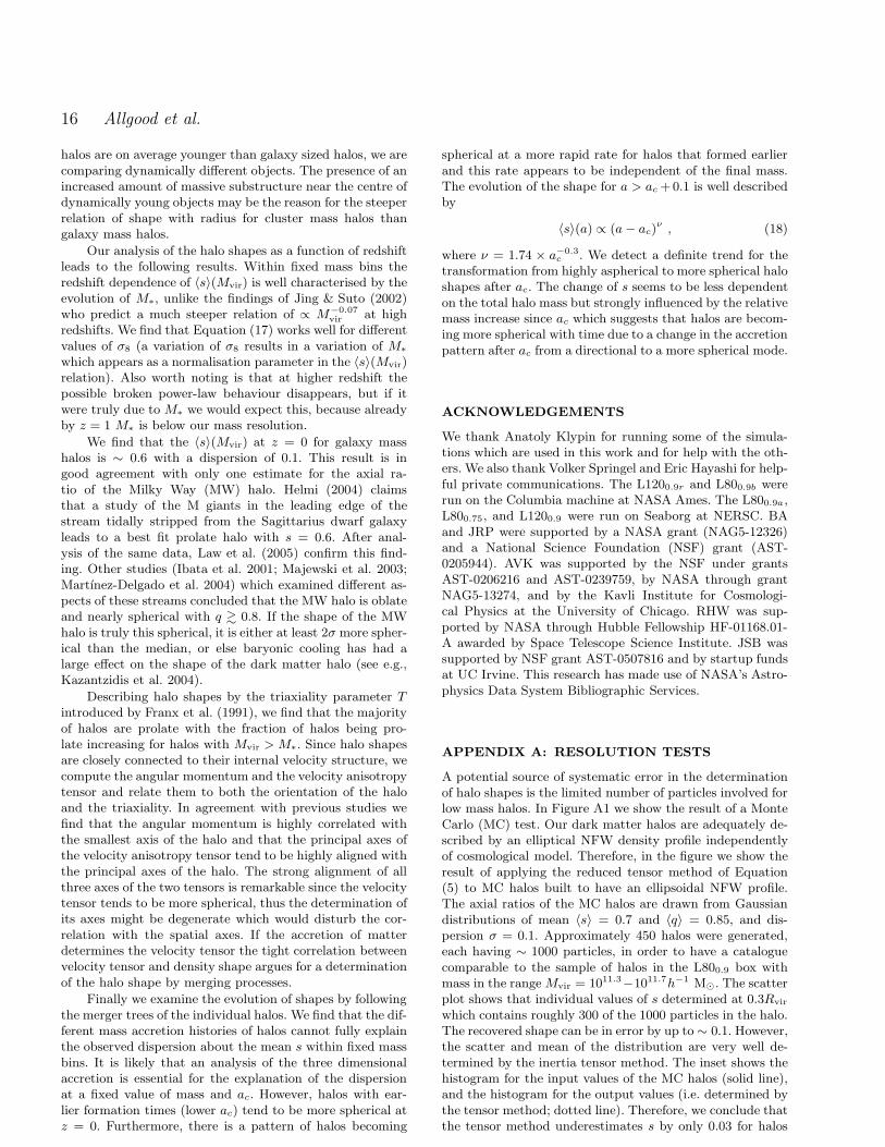
A potential source of systematic error in the determinationof halo shapes is the limited number of particles involved forlow mass halos. In Figure A1 we show the result of a MonteCarlo (MC) test. Our dark matter halos are adequately de-scribed by an elliptical NFW density profile independentlyof cosmological model. Therefore, in the figure we show theresult of applying the reduced tensor method of Equation(5) to MC halos built to have an ellipsoidal NFW profile.The axial ratios of the MC halos are drawn from Gaussiandistributions of mean 〈s〉 = 0.7 and 〈q〉 = 0.85, and dis-persion σ = 0.1. Approximately 450 halos were generated,each having ∼ 1000 particles, in order to have a cataloguecomparable to the sample of halos in the L800.9 box withmass in the range Mvir = 1011.3−1011.7h−1 M⊙. The scatterplot shows that individual values of s determined at 0.3Rvir

which contains roughly 300 of the 1000 particles in the halo.The recovered shape can be in error by up to ∼ 0.1. However,the scatter and mean of the distribution are very well de-termined by the inertia tensor method. The inset shows thehistogram for the input values of the MC halos (solid line),and the histogram for the output values (i.e. determined bythe tensor method; dotted line). Therefore, we conclude thatthe tensor method underestimates s by only 0.03 for halos

The Shape of Dark Matter Halos 17

Figure A1. Results of applying our shape determination proce-dure at 0.3Rvir to 450 Monte Carlo halos produced with deter-mined axial ratios. We found that the error in the recovered valueof s could be as large as ∼ 0.1.

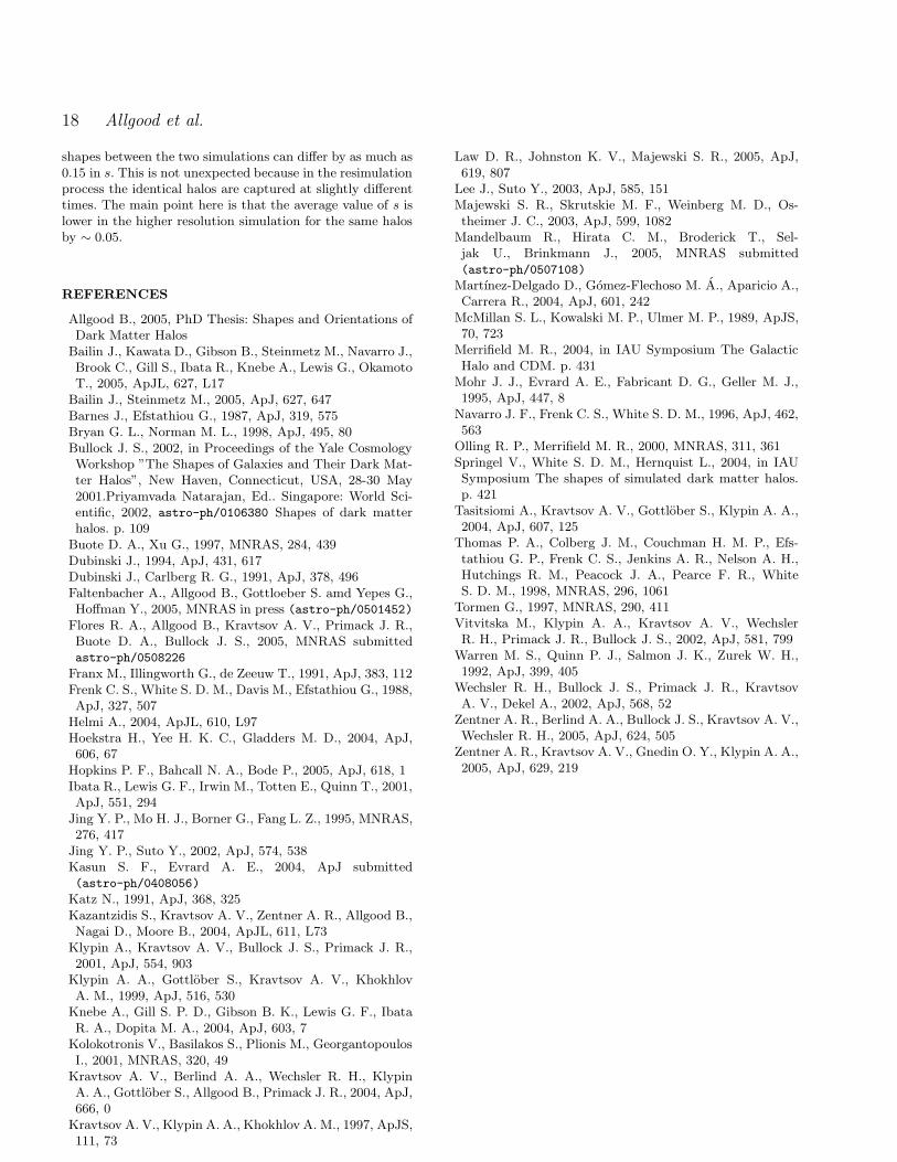
Figure A2. 〈s〉 versus mass. This plot is a replica of Figure 1except we show mass bins below the determined resolution limit.

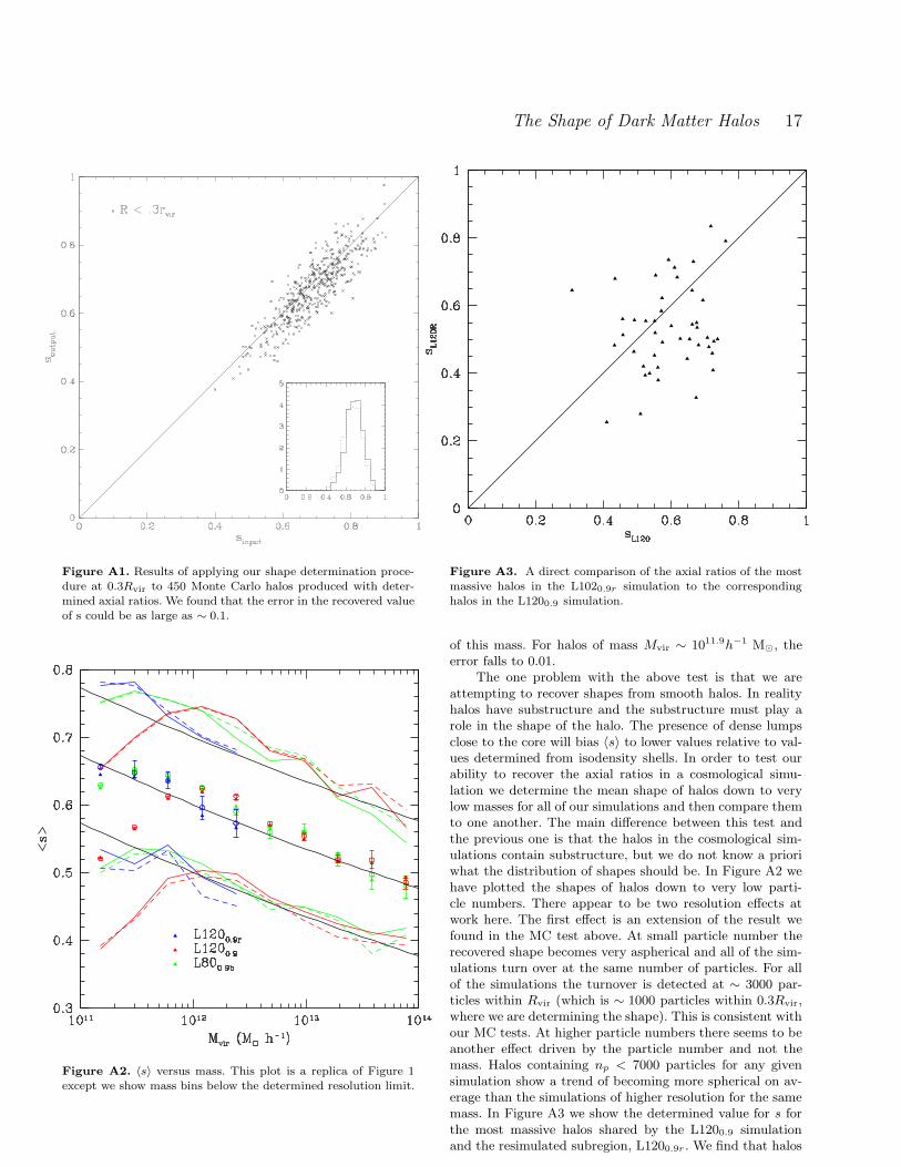
Figure A3. A direct comparison of the axial ratios of the mostmassive halos in the L1020.9r simulation to the correspondinghalos in the L1200.9 simulation.

of this mass. For halos of mass Mvir ∼ 1011.9h−1 M⊙, theerror falls to 0.01.

The one problem with the above test is that we areattempting to recover shapes from smooth halos. In realityhalos have substructure and the substructure must play arole in the shape of the halo. The presence of dense lumpsclose to the core will bias 〈s〉 to lower values relative to val-ues determined from isodensity shells. In order to test ourability to recover the axial ratios in a cosmological simu-lation we determine the mean shape of halos down to verylow masses for all of our simulations and then compare themto one another. The main difference between this test andthe previous one is that the halos in the cosmological sim-ulations contain substructure, but we do not know a prioriwhat the distribution of shapes should be. In Figure A2 wehave plotted the shapes of halos down to very low parti-cle numbers. There appear to be two resolution effects atwork here. The first effect is an extension of the result wefound in the MC test above. At small particle number therecovered shape becomes very aspherical and all of the sim-ulations turn over at the same number of particles. For allof the simulations the turnover is detected at ∼ 3000 par-ticles within Rvir (which is ∼ 1000 particles within 0.3Rvir,where we are determining the shape). This is consistent withour MC tests. At higher particle numbers there seems to beanother effect driven by the particle number and not themass. Halos containing np < 7000 particles for any givensimulation show a trend of becoming more spherical on av-erage than the simulations of higher resolution for the samemass. In Figure A3 we show the determined value for s forthe most massive halos shared by the L1200.9 simulationand the resimulated subregion, L1200.9r . We find that halos

18 Allgood et al.

shapes between the two simulations can differ by as much as0.15 in s. This is not unexpected because in the resimulationprocess the identical halos are captured at slightly differenttimes. The main point here is that the average value of s islower in the higher resolution simulation for the same halosby ∼ 0.05.

REFERENCES

Allgood B., 2005, PhD Thesis: Shapes and Orientations ofDark Matter Halos

Bailin J., Kawata D., Gibson B., Steinmetz M., Navarro J.,Brook C., Gill S., Ibata R., Knebe A., Lewis G., OkamotoT., 2005, ApJL, 627, L17

Bailin J., Steinmetz M., 2005, ApJ, 627, 647Barnes J., Efstathiou G., 1987, ApJ, 319, 575Bryan G. L., Norman M. L., 1998, ApJ, 495, 80Bullock J. S., 2002, in Proceedings of the Yale CosmologyWorkshop ”The Shapes of Galaxies and Their Dark Mat-ter Halos”, New Haven, Connecticut, USA, 28-30 May2001.Priyamvada Natarajan, Ed.. Singapore: World Sci-entific, 2002, astro-ph/0106380 Shapes of dark matterhalos. p. 109

Buote D. A., Xu G., 1997, MNRAS, 284, 439Dubinski J., 1994, ApJ, 431, 617Dubinski J., Carlberg R. G., 1991, ApJ, 378, 496Faltenbacher A., Allgood B., Gottloeber S. amd Yepes G.,Hoffman Y., 2005, MNRAS in press (astro-ph/0501452)

Flores R. A., Allgood B., Kravtsov A. V., Primack J. R.,Buote D. A., Bullock J. S., 2005, MNRAS submittedastro-ph/0508226

Franx M., Illingworth G., de Zeeuw T., 1991, ApJ, 383, 112Frenk C. S., White S. D. M., Davis M., Efstathiou G., 1988,ApJ, 327, 507

Helmi A., 2004, ApJL, 610, L97Hoekstra H., Yee H. K. C., Gladders M. D., 2004, ApJ,606, 67

Hopkins P. F., Bahcall N. A., Bode P., 2005, ApJ, 618, 1Ibata R., Lewis G. F., Irwin M., Totten E., Quinn T., 2001,ApJ, 551, 294

Jing Y. P., Mo H. J., Borner G., Fang L. Z., 1995, MNRAS,276, 417

Jing Y. P., Suto Y., 2002, ApJ, 574, 538Kasun S. F., Evrard A. E., 2004, ApJ submitted(astro-ph/0408056)

Katz N., 1991, ApJ, 368, 325Kazantzidis S., Kravtsov A. V., Zentner A. R., Allgood B.,Nagai D., Moore B., 2004, ApJL, 611, L73

Klypin A., Kravtsov A. V., Bullock J. S., Primack J. R.,2001, ApJ, 554, 903

Klypin A. A., Gottlober S., Kravtsov A. V., KhokhlovA. M., 1999, ApJ, 516, 530

Knebe A., Gill S. P. D., Gibson B. K., Lewis G. F., IbataR. A., Dopita M. A., 2004, ApJ, 603, 7

Kolokotronis V., Basilakos S., Plionis M., GeorgantopoulosI., 2001, MNRAS, 320, 49

Kravtsov A. V., Berlind A. A., Wechsler R. H., KlypinA. A., Gottlober S., Allgood B., Primack J. R., 2004, ApJ,666, 0

Kravtsov A. V., Klypin A. A., Khokhlov A. M., 1997, ApJS,111, 73

Law D. R., Johnston K. V., Majewski S. R., 2005, ApJ,619, 807

Lee J., Suto Y., 2003, ApJ, 585, 151Majewski S. R., Skrutskie M. F., Weinberg M. D., Os-theimer J. C., 2003, ApJ, 599, 1082

Mandelbaum R., Hirata C. M., Broderick T., Sel-jak U., Brinkmann J., 2005, MNRAS submitted(astro-ph/0507108)

Martınez-Delgado D., Gomez-Flechoso M. A., Aparicio A.,Carrera R., 2004, ApJ, 601, 242

McMillan S. L., Kowalski M. P., Ulmer M. P., 1989, ApJS,70, 723

Merrifield M. R., 2004, in IAU Symposium The GalacticHalo and CDM. p. 431

Mohr J. J., Evrard A. E., Fabricant D. G., Geller M. J.,1995, ApJ, 447, 8

Navarro J. F., Frenk C. S., White S. D. M., 1996, ApJ, 462,563

Olling R. P., Merrifield M. R., 2000, MNRAS, 311, 361Springel V., White S. D. M., Hernquist L., 2004, in IAUSymposium The shapes of simulated dark matter halos.p. 421

Tasitsiomi A., Kravtsov A. V., Gottlober S., Klypin A. A.,2004, ApJ, 607, 125

Thomas P. A., Colberg J. M., Couchman H. M. P., Efs-tathiou G. P., Frenk C. S., Jenkins A. R., Nelson A. H.,Hutchings R. M., Peacock J. A., Pearce F. R., WhiteS. D. M., 1998, MNRAS, 296, 1061

Tormen G., 1997, MNRAS, 290, 411Vitvitska M., Klypin A. A., Kravtsov A. V., WechslerR. H., Primack J. R., Bullock J. S., 2002, ApJ, 581, 799

Warren M. S., Quinn P. J., Salmon J. K., Zurek W. H.,1992, ApJ, 399, 405

Wechsler R. H., Bullock J. S., Primack J. R., KravtsovA. V., Dekel A., 2002, ApJ, 568, 52

Zentner A. R., Berlind A. A., Bullock J. S., Kravtsov A. V.,Wechsler R. H., 2005, ApJ, 624, 505

Zentner A. R., Kravtsov A. V., Gnedin O. Y., Klypin A. A.,2005, ApJ, 629, 219