THE UNIVERSITY OF CHICAGO DARK MATTER HALOS ...

THE UNIVERSITY OF CHICAGO

DARK MATTER HALOS AND THEIR ENVIRONMENTS

A DISSERTATION SUBMITTED TO

THE FACULTY OF THE DIVISION OF THE PHYSICAL SCIENCES

IN CANDIDACY FOR THE DEGREE OF

DOCTOR OF PHILOSOPHY

DEPARTMENT OF ASTRONOMY & ASTROPHYSICS

BY

PHILIP MANSFIELD

CHICAGO, ILLINOIS

AUGUST 2020

Dedicated to the 2016-2017 students of the KICP Space Explorers program:

the greatest scientists I have ever met.

“To turn around that close to the summit...,” Hall mused with a shake of his head on May

6 as Kropp plodded past Camp Two on his way down the mountain. “That showed

incredibly good judgment on young Goran’s part. I’m impressed - considerably more

impressed than if he’d continued climbing and made the top.”

— Jon Krakauer, Into Thin Air, pp. 190

TABLE OF CONTENTS

LIST OF FIGURES . . . . . . . . . . . . . . . . . . . . . . . . . . . . . . . . . . . . viii

LIST OF TABLES . . . . . . . . . . . . . . . . . . . . . . . . . . . . . . . . . . . . . ix

ACKNOWLEDGMENTS . . . . . . . . . . . . . . . . . . . . . . . . . . . . . . . . . x

ABSTRACT . . . . . . . . . . . . . . . . . . . . . . . . . . . . . . . . . . . . . . . . xii

1 PROLOGUE . . . . . . . . . . . . . . . . . . . . . . . . . . . . . . . . . . . . . . 1

2 AN INTERGALACTIC MURDER MYSTERY: WHY DO DARK MATTER HALOSDIE TOGETHER? . . . . . . . . . . . . . . . . . . . . . . . . . . . . . . . . . . . 72.1 The Setting: Galaxies and Dark Matter Halos . . . . . . . . . . . . . . . . . 7

2.1.1 Galaxies, Satellite Galaxies, and Distances . . . . . . . . . . . . . . . 72.1.2 Dark Matter . . . . . . . . . . . . . . . . . . . . . . . . . . . . . . . . 102.1.3 Dark Matter Halos and Dark Matter Subhalos . . . . . . . . . . . . . 142.1.4 The Cosmic Web and Large Scale Structure . . . . . . . . . . . . . . 19

2.2 The Crime: Assembly Bias . . . . . . . . . . . . . . . . . . . . . . . . . . . . 222.3 The Suspects: Tides, Heating, and Misadventure . . . . . . . . . . . . . . . . 252.4 The Plan: The Structure of This Thesis . . . . . . . . . . . . . . . . . . . . 28

3 TECHNICAL BACKGROUND . . . . . . . . . . . . . . . . . . . . . . . . . . . . 313.1 Simulations . . . . . . . . . . . . . . . . . . . . . . . . . . . . . . . . . . . . 31

3.1.1 Force Softening . . . . . . . . . . . . . . . . . . . . . . . . . . . . . . 343.2 Halo Finding and Halo Properties . . . . . . . . . . . . . . . . . . . . . . . . 36

4 SPLASHBACK SHELLS OF COLD DARK MATTER HALOS . . . . . . . . . . 434.1 Introduction . . . . . . . . . . . . . . . . . . . . . . . . . . . . . . . . . . . . 434.2 Methods . . . . . . . . . . . . . . . . . . . . . . . . . . . . . . . . . . . . . . 47

4.2.1 Simulations . . . . . . . . . . . . . . . . . . . . . . . . . . . . . . . . 474.2.2 Algorithm Description . . . . . . . . . . . . . . . . . . . . . . . . . . 484.2.3 Definitions of Basic Splashback Shell Properties . . . . . . . . . . . . 554.2.4 Summary of the Algorithm Parameters . . . . . . . . . . . . . . . . . 56

4.3 Tests . . . . . . . . . . . . . . . . . . . . . . . . . . . . . . . . . . . . . . . . 584.3.1 Comparison to Particle Trajectories . . . . . . . . . . . . . . . . . . . 62

4.4 Results . . . . . . . . . . . . . . . . . . . . . . . . . . . . . . . . . . . . . . . 634.4.1 Sample Selection . . . . . . . . . . . . . . . . . . . . . . . . . . . . . 634.4.2 Comparison With Stacked Radial Density Profiles . . . . . . . . . . . 654.4.3 Angular Median Density Profiles of Halos . . . . . . . . . . . . . . . 684.4.4 The Relationship Between Mass, Accretion Rate, and Splashback Radius 734.4.5 Splashback Shell Masses . . . . . . . . . . . . . . . . . . . . . . . . . 774.4.6 Splashback Shell Overdensities . . . . . . . . . . . . . . . . . . . . . . 794.4.7 Splashback Shell Shapes . . . . . . . . . . . . . . . . . . . . . . . . . 79

v

4.5 Summary and Conclusions . . . . . . . . . . . . . . . . . . . . . . . . . . . . 824.6 Appendices . . . . . . . . . . . . . . . . . . . . . . . . . . . . . . . . . . . . 85

4.6.1 An Algorithm for Fast Line of Sight Density Estimates . . . . . . . . 854.6.2 Splashback Candidate Filtering Algorithm . . . . . . . . . . . . . . . 884.6.3 Parameter-Specific Convergence Tests . . . . . . . . . . . . . . . . . . 904.6.4 Setting Rkernel . . . . . . . . . . . . . . . . . . . . . . . . . . . . . . 914.6.5 Setting Nplanes . . . . . . . . . . . . . . . . . . . . . . . . . . . . . . 924.6.6 Computing Moment of Inertia-Equivalent Ellipsoidal Shell Axes . . . 94

5 HOW BIASED ARE COSMOLOGICAL SIMULATIONS? . . . . . . . . . . . . . 965.1 Introduction . . . . . . . . . . . . . . . . . . . . . . . . . . . . . . . . . . . . 965.2 Methods . . . . . . . . . . . . . . . . . . . . . . . . . . . . . . . . . . . . . . 99

5.2.1 Simulations and Halo Finding . . . . . . . . . . . . . . . . . . . . . . 995.2.2 Halo Properties . . . . . . . . . . . . . . . . . . . . . . . . . . . . . . 1025.2.3 Finding Empirical “Convergence Limits” . . . . . . . . . . . . . . . . 102

5.3 The Empirical Nvir Convergence Limits of Simulations . . . . . . . . . . . . 1115.3.1 Typical Convergence Limits . . . . . . . . . . . . . . . . . . . . . . . 1115.3.2 Variation in Limits Between Simulations . . . . . . . . . . . . . . . . 1155.3.3 Differences Between Multidark and Illustris-TNG . . . . . . . . . . . 117

5.4 The Dependence of Halo Properties on Force Softening Scale . . . . . . . . . 1195.4.1 Dependence of the Subhalo Mass Function on ε . . . . . . . . . . . . 122

5.5 Estimating the Impact of Large ε on Vmax . . . . . . . . . . . . . . . . . . . 1245.6 Discussion . . . . . . . . . . . . . . . . . . . . . . . . . . . . . . . . . . . . . 129

5.6.1 Timestepping as an Additional Source of Biases . . . . . . . . . . . . 1295.6.2 What is the “Optimal” ε? . . . . . . . . . . . . . . . . . . . . . . . . 135

5.7 Conclusion . . . . . . . . . . . . . . . . . . . . . . . . . . . . . . . . . . . . . 1365.8 Appendices . . . . . . . . . . . . . . . . . . . . . . . . . . . . . . . . . . . . 138

5.8.1 Recalibrating the Plummer-Equivalence Scale . . . . . . . . . . . . . 1385.8.2 Fitting Parameters For Mean Halo Property Relations . . . . . . . . 143

6 THE THREE CAUSES OF LOW-MASS ASSEMBLY BIAS . . . . . . . . . . . . 1456.1 Introduction . . . . . . . . . . . . . . . . . . . . . . . . . . . . . . . . . . . . 1456.2 Methods . . . . . . . . . . . . . . . . . . . . . . . . . . . . . . . . . . . . . . 151

6.2.1 Simulations and codes . . . . . . . . . . . . . . . . . . . . . . . . . . 1516.2.2 Basic halo properties . . . . . . . . . . . . . . . . . . . . . . . . . . . 1516.2.3 Definition of Halo Boundaries and Subhalos . . . . . . . . . . . . . . 1536.2.4 Halo Sample . . . . . . . . . . . . . . . . . . . . . . . . . . . . . . . . 1576.2.5 Measuring Tidal Force Strength . . . . . . . . . . . . . . . . . . . . . 1586.2.6 Measuring Gravitational Heating . . . . . . . . . . . . . . . . . . . . 1616.2.7 Assembly Bias Statistics . . . . . . . . . . . . . . . . . . . . . . . . . 1626.2.8 Measuring the Connection Between Assembly Bias and Other Variables163

6.3 Analysis . . . . . . . . . . . . . . . . . . . . . . . . . . . . . . . . . . . . . . 1676.3.1 Splashback Subhalos and Assembly Bias . . . . . . . . . . . . . . . . 1676.3.2 Contribution of Tidal Truncation and Gravitational Heating to As-

sembly Bias . . . . . . . . . . . . . . . . . . . . . . . . . . . . . . . . 169

vi

6.3.3 The Spatial and Concentration Distributions of the Halos Responsiblefor Assembly Bias . . . . . . . . . . . . . . . . . . . . . . . . . . . . . 173

6.3.4 Time and Mass Dependence of Assembly Bias . . . . . . . . . . . . . 1786.3.5 Sensitivity to Splashback Subhalo Identification Method . . . . . . . 1796.3.6 Comparison of the Bolshoi and BolshoiP Simulations . . . . . . . . . 180

6.4 Discussion . . . . . . . . . . . . . . . . . . . . . . . . . . . . . . . . . . . . . 1816.4.1 Issues Associated with Proxy Definitions . . . . . . . . . . . . . . . . 1816.4.2 Sensitivity of Results to Definitional Choices . . . . . . . . . . . . . . 1816.4.3 Comparison with Previous Work . . . . . . . . . . . . . . . . . . . . 1846.4.4 Directions for Future Work . . . . . . . . . . . . . . . . . . . . . . . . 188

6.5 Summary and Conclusions . . . . . . . . . . . . . . . . . . . . . . . . . . . . 1896.6 Appendices . . . . . . . . . . . . . . . . . . . . . . . . . . . . . . . . . . . . 191

6.6.1 Effects of Halo Definition on Concentration in the Rockstar Halo Finder1916.6.2 Fast Halo Containment Checks . . . . . . . . . . . . . . . . . . . . . 1946.6.3 Tidal Force Errors . . . . . . . . . . . . . . . . . . . . . . . . . . . . 1956.6.4 Identifying Bound Particles in Halo Outskirts . . . . . . . . . . . . . 200

vii

LIST OF FIGURES

2.1 Simulated image of a dark matter halo . . . . . . . . . . . . . . . . . . . . . . . 162.2 Simulated image of the cosmic web . . . . . . . . . . . . . . . . . . . . . . . . . 202.3 Qualitative illustration of assembly bias . . . . . . . . . . . . . . . . . . . . . . 23

4.1 Overview of the Shellfish algorithm . . . . . . . . . . . . . . . . . . . . . . . 494.2 Shellfish surfaces compared against the density fields of several halos . . . . . 574.3 Convergence tests for various splashback surface properties . . . . . . . . . . . . 594.4 A rare example of the Shellfish algorithm failing catastrophically . . . . . . . 614.5 Comparison between Shellfish surfaces and particle trajectories . . . . . . . . 644.6 Disparity between Rsp measured by Shellfish and by stacked density profiles . 664.7 Demonstrations that spherically averaged profiles lead to biased Rsp. . . . . . . 694.8 Agreement between Rsp measured by Shellfish and the median profile method 724.9 Fit to the Rsp(ΓDK14, ν200m, z) distribution . . . . . . . . . . . . . . . . . . . . 744.10 Fit to the Msp(ΓDK14, ν200m, z) distribution . . . . . . . . . . . . . . . . . . . . 754.11 Illustration of the scatter in the Msp fit. . . . . . . . . . . . . . . . . . . . . . . 754.12 Fit to the ∆sp(ΓDK14, ν200m, z) distribution . . . . . . . . . . . . . . . . . . . . 804.13 The asphericity and ellipticity of splashback surfaces . . . . . . . . . . . . . . . 814.14 The alignment between the major axes of halos and their splashback surfaces . . 814.15 Illustration of the Shellfish ray-tracing algorithm . . . . . . . . . . . . . . . . 844.16 Convergence tests for Shellfish nuisance parameters . . . . . . . . . . . . . . . 93

5.1 Illustration of procedure for finding convergence limits . . . . . . . . . . . . . . 1035.2 The variation in Vmax convergence limits between simulations . . . . . . . . . . 1125.3 The convergence behavior of 〈Vmax/Vvir〉 and 〈c/a〉 as functions of Mvir . . . . . 1135.4 Disagreement between Multidark and IllustrisTNG-Dark . . . . . . . . . . . . . 1175.5 The dependence of various halo properties on force softening scale . . . . . . . . 1215.6 The dependence of subhalo abundances on force softening scale . . . . . . . . . 1225.7 Analytic estimates of halo bias due to large ε . . . . . . . . . . . . . . . . . . . 1305.8 Impact of analytic bias estimates on the full simulation suite. . . . . . . . . . . 1315.9 Impact of force softening on gravitational fields and rotation curves . . . . . . . 139

6.1 Age-dependent clustering with and without splashback subhalos . . . . . . . . . 1496.2 The impact of removing different halo populations on assembly bias . . . . . . . 1676.3 How efficiently different cuts remove assembly bias from the entire halo population1686.4 The distribution of different halo groups throughout the entire simulation box . 1746.5 The distribution of different halo groups around a single dense filament . . . . . 1756.6 The distribution of concentrations for different halo groups . . . . . . . . . . . . 1766.7 The mass and redshift dependence of assembly bias for different halo groups . . 1776.8 The impact of tracing age with a1/2 on assembly bias measurements . . . . . . . 1826.9 The influence of Rockstar parameters on concentration measurements . . . . 1936.10 Tests of the errors associated with approximations of the tidal field around halos 196

viii

LIST OF TABLES

3.1 Simulation parameters . . . . . . . . . . . . . . . . . . . . . . . . . . . . . . . . 323.2 Simulation parameters (continued) . . . . . . . . . . . . . . . . . . . . . . . . . 33

4.1 Mass ranges . . . . . . . . . . . . . . . . . . . . . . . . . . . . . . . . . . . . . . 484.2 Fiducial parameters used by the Shellfish algorithm . . . . . . . . . . . . . . 58

5.1 Convergence limits for different halo properties and simulations . . . . . . . . . 1085.2 Conservative convergence for halo properties with weak ε dependencies . . . . . 1095.3 Simulation parameters of the Chinchilla-ε suite . . . . . . . . . . . . . . . . . . 1205.4 Fit parameters for Eq. 5.13 . . . . . . . . . . . . . . . . . . . . . . . . . . . . . 1415.5 Fit parameters for 〈X〉(Mvir) relations . . . . . . . . . . . . . . . . . . . . . . . 144

6.1 The fraction of halos in Bolshoi which are removed by different cuts . . . . . . . 1706.2 The fraction of halos in BolshoiP which are removed by different cuts . . . . . . 170

ix

ACKNOWLEDGMENTS

Completing a Ph.D is a difficult task: I spent (and continue to spend) perhaps 95% to 99% of

my time being wrong about one issue or another, and the complexity, long time scales, and

self-direction needed to complete a research project make it easy to burn out. I am eternally

grateful that my advisor, Andrey Kravtsov, had very frank conversations with me about

these hurdles during my first year of graduate school. It was this openness and willingness

to discuss all parts of life as an academic that cemented my decision to stay as his student

for these past six years.

We have weathered many storms together. Twice, we experienced the joy of losing

seasons or years worth of work due to subtle technical mistakes. These are the moments

which test your values as a scientist: it would be so easy to simply give up, or to be tempted

by spurious rationalizations for why the problems aren’t that big of a deal. Andrey guided

me through these pivotal moments flawlessly, and in the end they helped form who I am as

a scientist. Outside these big moments, Andrey has done a fantastic job transforming me

into an independent researcher: he knew when to tell me what to do and when to let me

make my own mistakes. I hope to do the same with my own students one day.

Having a good advisor is only part of the story. The writing of this thesis was only

possible due to an army of formal and informal mentors who helped guide me through my

journey. The other leader of UChicago’s Computational Astrophysics group, Nick Gnedin,

has been a constant source of advice since before I even matriculated to UChicago. He has

an uncanny ability to condense weighty advice into concise packages. My collaborators –

and frequent mentors – Benedikt Diemer and Camille Avestruz have helped me immensely

on topics ranging from how to write job applications, to how to run simulations, to how

to format the LATEX in this thesis. Their recent faculty appointments will ensure that they

continue to help students for years to come. Mike Gladders and Dan Fabrycky have also

been very helpful throughout my time in graduate school (both informally and as members

of my thesis committee), as has been my faculty mentor, Dan Hooper.

x

I would also like to thank Hy Trac and Bob Swendsen at Carnegie Mellon, who first

introduced me to the world of physics research and taught me skills that I continue to use to

this day. And I’d like to extend this thanks to Karen Wolfson, my high school AP Physics

teacher. Her classes were what started me down the path to this thesis all those year ago.

Looking back at the sheer number of people who were critical to the creation of this one Ph.D

thesis has really emphasized to me how important it is to actively ensure that all students

have a rich and robust support network.

Beyond research, one of my great passions in graduate school has been teaching and

outreach. I realized how important this was to me as an undergraduate at Carnegie Mellon,

thanks to the guidance and mentoring of David Kosbie when I was a TA in his introductory

programming class, 15-110. At UChicago, many faculty and student helped me to become a

better teacher, especially Randy Landsberg after I was hired as the KICP Space Explorers

instructor. I would like to deeply thank him, Dovetta McKee, Terhonda Palacios, Phillip

Wisecup, and Alex Lathan for the tireless work they put into this program during my time as

the instructor, as well as Brian Nord and Rich Kron for helping to keep the program running

in recent years. And I would like to once again thank Andrey for his endless patience with the

amount of time I spent pursuing these efforts, and the many hours we have spent discussing

the art of course design.

Lastly, I would like to thank my friends and family for the bottomless emotional support

they offered me throughout graduate school, especially in the dark and turbulent times which

accompanied the completion of this thesis. When this world becomes a better place, it will

be your love and passion which took it there.

xi

ABSTRACT

The structure and evolution of the universe at large scales is dominated by dark matter,

particularly large clumps of dark matter called “dark matter halos.” Soon after running the

first large scale, high-resolution simulations, researchers realized that the growth of these

dark matter halos was closely tied to their surrounding environment. This connection is

called “assembly bias.” Although this behavior is well-understood for the largest halos, the

cause of assembly bias for smaller dark matter halos (such as the one which contains our

galaxy, the Milky Way) has remained a mystery for the past fifteen years.

This thesis aims to resolve this mystery.

Accomplishing this goal requires constructing a substantial theoretical framework. One

of the leading proposed causes for assembly bias stems from ambiguity of where halos end

and where their surrounding environment begins. To this end, I develop Shellfish, the first

code which is capable of measuring the boundary between the two, the “splashback surface.”

Additionally, the study of assembly bias requires detailed analysis of large “cosmological”

dark matter simulations. However, despite the long tenure of these simulations, there remain

main unanswered questions about their accuracy. I perform extensive tests on the reliability

of cosmological simulations, assessing the reliability of every major property of dark matter

halos, and identifying previously unknown numerical biases which significantly impact a

number of widely-used simulations.

Finally, using Shellfish to identity halo boundaries and these numerical tests to ensure

reliability, I tackle the problem of galaxy-mass assembly bias. I identify the exact halos

which are responsible for the assembly bias signal and use this identification to isolate the

processes which lead to assembly bias. This analysis shows that galaxy-mass assembly bias

is primarily caused by misidentified “splashback” subhalos, although a modest fraction of

the effect comes from a small number of halos in massive filaments whose growth is slightly

slowed by the tidal fields of their filaments and by gravitational heating.

xii

CHAPTER 1

PROLOGUE

The story of this thesis begins on a paper-strewn table inside a Parisian palace in 1758.

Three French mathematicians worked day and night over that table, desperately trying to

beat a comet in a year-long race.

The comet in question was Halley’s Comet. Decades earlier, England’s Royal Astronomer,

Edmund Halley, had predicted that the comet which would eventually bear his name would

return in roughly 1758 [Cook, 1998].1 Halley was an acolyte of the physicist Sir Isaac Newton

and hoped that the comet would be the final proof that the rest of the world needed to accept

Newton’s theories of physics. While Newton had elegantly explained the previously measured

motion of the planets through the solar system, the relatively static nature of the cosmos

meant that there were few opportunities for him to predict new phenomena. Halley saw such

an opportunity in this comet.

Halley had attempted to use Newton’s theories to model the previous appearances of the

comet, but this turned out to be a far more complicated task than he had anticipated and

he was forced to make very crude approximations [Cook, 1998]. His estimates of the comet’s

path ended up being so inaccurate that the satirist Jonathan Swift devoted an entire chapter

of Gulliver’s Travels to relentlessly mocking Halley in specific and the Newtonian project of

predicting celestial motion in general [Swift, 1726].

Halley’s undoing was the existence of Jupiter and Saturn (as Newton had patiently

explained to him several times; e.g., Newton, 1695). As his comet traveled through the solar

system, it would be tugged slightly off its orbit by the gravity of the solar system’s largest

planets, speeding up or delaying its reappearance by up to two years. Predicting the behavior

1. Although the comet now bears his name, Halley certainly did not discover it. The first unambiguouswritten record of the comet comes from a Chinese astronomical journal in 239 BC [Kronk, 1999]. Halleydid not discover the comet’s periodic nature either: Raban Yehoshua offhandedly mentions the comet’sapproximate period in the Talmud [b. Hor. 10a]. This passage would have first been written down in≈ 200 − 220 CE, but could have entered Jewish oral tradition as early as 700 years prior to being writtendown.

1

of more than three objects interacting through gravity is a famously intractable task (called

“the three-body problem”). This is not the type of calculation which can be worked out on

a blackboard. Or a warehouse full of blackboards. However, these three French scientists

had decided to attack the issue from a fundamentally new angle.

The leader of the group was Alexis Claude Clairaut. Clairaut’s crowning achievement in

life was mentoring Emilie du Chatelet, the woman who developed the concept of conserva-

tion of energy through a stunning combination of theoretical, empirical, and philosophical

work [Zinsser, 2006]. du Chatelet was widely mocked in her time, so if you had asked his

contemporaries, they would focus on other aspects of his work. They would tell you he was

a titan of the French academy. They would laud his skilled but failed attempts to unseat

Newton’s theory of gravity, and his later defection to Newton’s camp [Bodenmann, 2010].

They would tell you of his bitter (but victorious) rivalries with the terrifying and brilliant

mathematician Leonhard Euler and the timid encyclopedia author Jean le Rond d’Alembert

over long-standing mysteries related to the Moon’s orbit [Bodenmann, 2010]. Clairaut hoped

to leverage these earlier accomplishments to solve the mystery of Halley’s comet and hoped

that such a solution would cement him as the country’s pre-eminent astronomer.

Helping Clairaut was the young astronomer Jerome Lalande. While a capable theorist

in his own right, Lalande’s greatest gift was endurance and attention to detail. He made

his name in the field through the creation of painstakingly detailed astronomical tables and

by performing simple but laborious calculations which other astronomers could not bring

themselves to finish [Grier, 2013]. Like Clairaut, Lalande was one of the few prominent

physicists of the era who actively sought out and mentored female students in physics. One

of these former students made the third member of the team, Nicole-Reine Lepaute.

Lepaute was a noblewoman who spent her spare time publishing mathematics and engi-

neering treatises under her husband’s name. Lalande realized her genius while working with

her husband on a clock-making book and the two became lifelong friends and collaborators

[Grier, 2013]. Lepaute was one of the only women during this time period to have an officially

2

recognized position within the French scientific community2 and spent years as one of the

chief contributors to the French Academy of Science’s astronomical almanac. She had an

inhuman endurance for number-crunching, a skill which even the resolute Lalande marveled

at in his memoirs [Lalande, 1792].

Emboldened by the iron stomachs of his colleagues, Clairaut developed his plan of attack

for predicting the return of Halley’s comet. The three of them would sit at their table for

almost a year. They would work through their meals, they would work late into the nights.

Instead of developing an elegant theory for the path of the comet, Clairaut planned to brute

force a solution.

In detail, Clairaut’s plan was to estimate the lag and gain that Jupiter and Saturn

imparted on the comet as it passed them, month by month and degree by degree [see Wilson,

1993, for a full technical summary]. Lalande and Lepaute would recalculate the locations of

the major bodies in the solar system at each step and worked out those planets’ respective

gravitational influence on the comet. Clairaut, sitting at the opposite end of the table, would

take the final step of working out how these forces would perturb the comet. Throughout

the entire process, Clairaut would continually replot the latest data. He would study these

points like a nervous ship captain might scan the horizon for the faintest sign of storm clouds,

looking for faint changes in curvature that might indicate growing errors.

It was a miserable ordeal: the group had started their calculation well within the window

of time in which Halley’s comet could return, and they worked in constant fear that it would

appear before they finished [Grier, 2013]. Clairaut had already used a host of mathematical

tricks to reduce the calculation to its bare essentials, and he introduced increasingly radical

simplifications as the team’s desperation grew. The endless computation was enough to

make the normally stalwart Lalande suffer a mental breakdown, and at times the project

2. There were, of course, many women contributing to the advancement of European astronomy duringthis time period. However, most would be forced to publish under the name of a male family member orwere referred to as “assistants” despite performing work that was indistinguishable from that of their malepeers.

3

was only pushed forward by Lepaute’s utter unflappability in the face of endless arithmetic

[Lalande, 1792].

At last, Clairaut presented their3 results to the French academy of sciences on November

14th. He predicted the comet would return in half a year, with its closest approach to the

Sun occurring on April 15th the following year. The group had gone through the calculation

multiple times, which Clairaut used to tack on an expected error in this prediction: 30 days

[Wilson, 1993].

The real impact of this presentation was somewhat lost on the audience: Clairaut was

not simply outlining one of the first tests of Newton’s theory of gravity, he was reporting the

results of the world’s first true physics simulation.

At the end of March that following year, astronomers saw Halley’s comet appear from

behind the Sun. Due to the geometry of the Sun, the comet, and the Earth, most of the

astronomy community had missed the unfurling of the comet’s dusty tail during its approach.

However, that era’s most prolific comet hunter – a young Charles Messier – had seen Halley’s

comet a few months after Clairaut’s announcement and kept it secret to prevent the more

senior astronomer from changing his answer [Wilson, 1993]. A flurry of calculations took

place to determine when the comet had been closest to the Sun, and the verdict came in:

the prediction was 33 days late.

By the standards of modern error analysis, this was completely consistent with the team’s

estimates. However, Clairaut’s old nemesis, d’Alembert, immediately declared the calcula-

tion a humiliating failure, and many other scientists pointed to a myriad of flaws and errors

in the analysis [Wilson, 1993]. Clairaut argued that not only was the prediction successful,

but that this result was the greatest evidence for Newton’s theory of gravity that the world

had produced to that point. (I am inclined to agree with him.) He would, however, return to

3. Lalande would receive professorship not long afterwards. Lepaute did not get official recognition forher contributions to the project due to a last minute loss of nerve by Clairaut [Grier, 2013]. Lelande woulduse his newfound authority to ensure that she received official scientific positions for the rest of her life[Ogilvie and Harvey, 2000]

4

the calculations every few years as the public debate raged on and somehow always managed

to find a way to reduce the error by a few more days.

Detailed reanalysis centuries later showed that the chief failing of Clairaut’s strategy was

perhaps an opportunity for discovery. If the same analysis had included the then-unknown

planets Neptune and Uranus, it would have been wrong by only two weeks [Wilson, 1993].

But given how little attention Clairaut and his team paid to tracking down the sources of

their errors, it is difficult to say if this was a coincidence.

Clairaut, Lalande, and Lepaute’s work serves as a fitting prototype for simulations as a

whole, whether they are performed by hand or on a computer. Their story demonstrates

some of the core principles behind numerical work.

First, even the simplest physics theories lead to complicated and non-obvious results as

soon as one starts to become interested in complicated systems, such as a comet navigating

through the orbits of large planets. While the behavior of these systems can sometimes be

brought into focus through the power of pure algebra, often times brute force is the only real

path to a solution.

Second, these complicated systems are some of the best opportunities to test our theories

of the universe. While there are no shortage of beautiful theories which can predict symmetric

and simple phenomena, like nearly circular orbits around a star, the rubber really meets the

road once you figure out how these theories behave when predictions and interactions get

messy. This differentiating power is why simulations have been with us since the days of

the first physicists and why they will continue to be performed until the days of the last

physicist.

Third, all simulations are approximations and will fail at some level. The inescapable

question which all simulators must confront is how deeply these failures have crept into

their results. A robust error model is the difference between a career-defining achievement

and an embarrassing public debate that never quite goes away. It is the difference between

interpreting a number as the sum of a thousand arithmetic mistakes or interpreting it as the

5

first evidence for a new planet since the start of recorded history.

This thesis serves as an example what those same principles look like when gravity simu-

lations are fast-forwarded by centuries: past ingenious mechanical models [Holmberg, 1941],

past the first steps into the electronic world [von Hoerner, 1960, Aarseth, 1963], and past

the maturation of cosmological simulations into their current form [e.g. Navarro et al., 1997,

Klypin et al., 1999]. If simulations could prove Newton’s law of gravity when tracing a single

comet pushed human endurance to its limits, what can they do once tracking millions of

galaxies becomes routine?

6

CHAPTER 2

AN INTERGALACTIC MURDER MYSTERY: WHY DO

DARK MATTER HALOS DIE TOGETHER?

The central focus of this thesis is about how dark matter halos are connected to their

environments. Although this thesis will touch on many aspects of this topic, its primary

goal is to resolve a long-standing mystery: what causes galaxy-mass “assembly bias?” The

goal of this chapter is to help a layperson understand the following:

• The basic astrophysical setting within which this mystery takes place. (section 2.1,

“The Setting: Galaxies and Dark Matter Halos”)

• What the mystery is and the context behind why it is important (section 2.2, “The

Crime: Galaxy-Mass Assembly Bias”)

• The different solutions that have been proposed to solve this mystery (section 2.3, “The

Suspects: Tides, Heating, and Misadventure”)

• The strategy behind this thesis and a qualitative overview of its results (section 2.4,

“The Plan: The Structure of This Thesis”).

I have bolded important scientific terms and jargon the first time they appear.

2.1 The Setting: Galaxies and Dark Matter Halos

2.1.1 Galaxies, Satellite Galaxies, and Distances

If you go out on a clear night in the suburbs, you will probably be able to see about a hundred

stars over the course of the night.1 On average, the light from the dimmest of these stars

1. I estimated these numbers through a combination of data-mining the Hipparcos stellar catalog[ESA, 1997] and the conventional wisdom of amateur astronomers on environmental visibility (e.g.,http://www.icq.eps.harvard.edu/MagScale.html). The main factors that determine the number of starsyou’ll see are the weather, how close you are to a major city, and whether you can get above the localtreeline.

7

takes about about 160 years to reach the earth, which means that their typical distances

is roughly 50 parsecs. A parsec is the standard unit of distance in astrophysics and is

geometrically defined through the impact that the earth’s orbit has on the apparent location

of nearby stars. It is such mind-bogglingly large distance that it is difficult to gain true

intuition for what it means (1 parsec is about 31 trillion kilometers), but it is comparatively

easy to use it as a ruler for understanding other distances in the universe: parsecs measure

distances where it is still possible for the human eye to see individual stars.

If you go out to a dark place – a boat on the ocean, a rural farm field, a mountain top

– you can see much further into the universe. The sky will be more full of stars (about

ten times as many: you’ll be able to see stars twice as far away as you could before), but

the main attraction is a dim band of light across the sky: the Milky Way. Most stars

in the universe, including every star we see in the night sky, are members of large clumps

of stars called galaxies. Our own galaxy, the aforementioned Milky Way, is shaped like a

dinner plate and the stars we see in the sky take up the same volume as a mustard seed

near the edge of that dinner plate: our neighborhood of stars is a little more than eight

thousand parsecs from the center of our galaxy [Gravity Collaboration et al., 2019]. As we

look out through the Milky Way, most of its several tens of billions of stars are too dim to

see individually, but collectively blend together into a fuzzy ring of light that encircles the

night sky. This gives us the second rung on our intuitive distance ladder: kiloparsecs – a

thousand parsecs – are used to measure the size of galaxies.2

If the dark place that you traveled to was in the southern hemisphere, you would be able

to see two other dim objects to the south of the Milky Way’s band. These objects are known

as the Magellanic Clouds to modern astronomers.3 They have featured prominently in the

2. Galaxies are quite diverse objects: one of the smallest that I know of is Kim 2, which is 0.024 kpc(2×R1/2) across [Drlica-Wagner et al., 2019, and references therein]. It is only visible because it has ventureddangerously close to the Milky Way. One of the largest that I know of, Abell 2142, is 358 kpc across [Kravtsovet al., 2018] and is in the process of destroying multiple Milky Way-sized galaxies.

3. This is a regrettable convention, given that Magellan did not discover these objects and – more im-portantly – that his first actions upon encountering Pacific islanders on Guam was to kill and mutilateseveral of them and to burn down a village [Pigafetta, 1522]. I would prefer that they were officially referred

8

astronomy and mythology for tens of millennia [e.g. Adams, 1998, Johnson, 1998, Haynes,

1998, Snedegar, 1998, Orchiston, 1998]: by all accounts it would seem that the Magellanic

clouds have been floating in basically the same location since the dawn of human civilization a

hundred thousand years ago. But this apparent lack of movement is an illusion of humanity’s

embarrassingly short tenure relative to the 13.7 billion year lifetime of the universe.4 In

actuality, the Magellanic clouds are nearby satellite galaxies of the Milky Way [Leavitt,

1908, Leavitt and Pickering, 1912]. Along with a swarm of other small, dim satellite galaxies

[e.g. Drlica-Wagner et al., 2019, and references therein], the Magellanic Clouds have been

torn from nearby space by the Milky Way’s gravity and now careen around it on a mess of

interlocking orbits.

The term “satellite” invokes images of the serene, regular motion of a communications

spacecraft around the Earth. This is not the case for satellite galaxies, which live erratic,

violent, and (relatively) short lives. Satellite galaxies can form a variety of temporary align-

ments and structures as they whip around their hosts [Pawlowski, 2018] and can slosh from

side to side in response to outside events [Conn et al., 2013]. The Milky Way has shredded

many satellite galaxies which ventured too close to the massive disk of stars we see in the

night sky [Garrison-Kimmel et al., 2017], and some large satellites have had the audacity to

smash into the Milky Way itself [Belokurov et al., 2018, Helmi et al., 2018]. The drama of

these satellites plays out repeatedly as destroyed objects are replaced by new small galaxies

that the Milky Way’s gravity drags from the local universe. This process ticks on as the

Milky Way slowly creeps towards its own eventual fate.

The reminder of this fate can be seen for most of the year in the Northern Hemisphere.

Just to the south of the Milky Way’s disk is gray blob a few degrees across. It is faint:

the blindspot in the center of your vision prevents you from seeing it if you look directly

either by one the many names given to them by cultures native to the Southern Hemisphere [e.g. Adams,1998, Johnson, 1998, Haynes, 1998, Snedegar, 1998, Orchiston, 1998] or by the constellation-based namingconvention used by modern satellite surveys.

4. Modern measurements indicate that over this time period, the Magellanic Clouds have moved less thana fiftieth of a degree across the sky [van der Marel and Sahlmann, 2016].

9

at it. This is the Andromeda Galaxy, the nearest major galaxy to the Milky Way. The

two are very similar, although Andromeda is a more dominating presence. Like the Milky

Way, Andromeda is a disk galaxy, only bigger [Sick et al., 2015]. Like the Milky Way,

Andromeda is surrounded by a swarm of satellite galaxies, only the swarm is larger and

deeper [McConnachie et al., 2009]. Recent measurements of Andromeda indicate that it will

collide with the Milky Way in about six billion years, an event which will likely destroy both

galaxies [van der Marel et al., 2012, 2019].

Despite its enormity, Andromeda appears tiny to us due to its distance. It is almost a

hundred times further away from the Earth than the center of our own galaxy: 740 kpc or

0.74 Megaparsecs [Ribas et al., 2005, Vilardell et al., 2010]. This is the last rung on our

qualitative distance ladder and the largest distance which the raw human senses have any

connection to. A Megaparsec is the distance at which the entire expanse of the night sky –

all the stars and constellations, the great disk of the Milky Way, its violent satellites, and its

looming demise – are condensed to a faint smudge that you can block out with your thumb.

This is the realm ruled by dark matter.

2.1.2 Dark Matter

Most astronomers believe that the majority of matter in the universe is a completely clear,

completely dark, and completely collisionless fluid called dark matter. In fact, most of the

evidence for dark matter supports a far stricter model where all galaxies are nestled deep

within the centers of large dark matter clumps. This would mean that the growth of galaxies

and their motion through the universe is almost entirely dominated by dark matter: galaxies

form when dark matter lets them form and move where dark matter tells them to move.

This section will focus on why astronomers believe that dark matter exists, while sections

2.1.3 and 2.1.4 will outline how a universe full of dark matter behaves.

The proposition that the universe is filled with dark matter is both breath-taking and

extremely annoying. Astronomy is a measurement-based science whose practitioners were

10

brought up on horror stories of epicycles and spiral nebulae, and accepting a model where

most of important dynamics are governed by a material which is so difficult to observe is a

drastic step. Additionally, decoupling the visible matter from the gravitationally important

matter severely complicates modeling and makes scientific analysis much more difficult. Both

these facts push back strongly against the acceptance of such a model. How on Earth did

the astronomy community end up accepting such a miserable state of affairs?

The question of where this story even starts is an interesting history of science problem.

Many astronomers had caught on to hints of dark matter’s existence since the early 1930’s:

Zwicky [1933] and Smith [1936] noticed that large clusters of galaxies should rip themselves

apart without unseen matter, Babcock [1939] and Oort [1940] measured stars orbiting around

the outskirts of galaxies faster than the visible matter in those galaxies should have allowed,

and Kahn and Woltjer [1959] argued that the Milky Way and Andromeda’s collision course

was only sensible with some form of dark matter. The arguments these authors used were

essentially correct. Perhaps some or all of these authors deserve credit for one of the greatest

discoveries in modern astronomy?

All of these early works were brilliant, but the bar for credit is a bit higher than that. It

is not enough to be right: you must make a strong case. The errors in these early studies

were large and the modeling uncertainties were significant.5 Because of this, scientists at

the time found early arguments for dark matter uncompelling and either ignored them or

published more thorough work contradicting the earlier results [e.g. Schwarzschild, 1954, de

Vaucouleurs, 1959, Page, 1959, Peebles, 1970, Rubin, 2006]. The most famous of these early

studies, Zwicky [1933], received only 12 peer-reviewed citations in its first 40 years – most of

them from other papers written by Zwicky – but retroactively received thousands after the

onrush of support for dark matter in the 70’s.

This onrush was started by the astronomers Vera Rubin and Kent Ford. Ford had

5. For example, Babcock [1939]’s velocity measurements were off from more modern studies, like Carignanet al. [2006], by nearly a factor of two. Astronomers at the time realized that his errors were at least thislarge and were poorly characterized.

11

recently built a revolutionary new spectrograph and was hoping to find an appropriately

grand target for it. Rubin was an analyst leading an effort to use this telescope to measure

how fast Andromeda rotated [Rubin and Ford, 1970, Rubin, 2006].6 Their plan centered

on a physics principle called the Doppler effect. An observant fan of NASCAR or an

attentive pedestrian listening for an ambulance to pass might notice that passing vehicles

sound higher pitched during their approach and lower pitched as they drive away. This is a

fundamental property of all waves, not just sound, and it causes light emitted by an object

approaching an observer to become slightly bluer and light emitted by an object retreating

from an observer to become redder. Astronomers had attempted to use the Doppler effect

to measure Andromeda’s rotation for decades [e.g. Babcock, 1939], but earlier instruments

had required dozens of hours of exposure time to image the faint sources near Andromeda’s

edge, and jitters and telescope repositionings over that timescale seriously compromised the

measurements [Sofue and Rubin, 2001, Rubin, 2006].

Rubin and Ford found that gas clouds at large distance from the bulk of Andromeda’s

visible matter orbited at roughly the same speed as those embedded within it [Rubin and

Ford, 1970]. This is puzzling. The speed that objects orbit at is directly tied to how strongly

they are pulled on by gravity. For example, in our solar system, Mercury travels at a much

faster speed than the Pluto due to the latter’s large separation from the Sun. Since the

force of gravity decreases with distance, a constant speed meant that there was more mass

contained within the orbits of more distant gas clouds, even though there was no visible

matter in those regions. In other words, Andromeda was surrounded by an immense amount

of invisible matter.

Rubin began to give talks about her preliminary results in 1970. She later recounted an

encounter with another astronomer:

After my talk, the esteemed Rudolph Minkowski asked when we would publish

6. Despite my view on who deserves discovery credit, Rubin attributed the discovery of dark matter tothe astronomers Horace Babcock and Jan Oort in a review she coauthored, Sofue and Rubin [2001].

12

the paper. I replied, “There are hundreds more regions that we could observe.”

He looked at me sternly and said, emphatically, “I think you should publish the

paper now.” We did. [Rubin, 2006]

This was fantastic advice. The 70’s would bear witness to a torrent of new evidence for dark

matter and if Rubin had waited to perform hundreds of additional measurements, she likely

would have lost priority. Minkowski may have had some sense that the tide was about to

shift, since he had been working on one of these new lines of evidence [Minkowski, 1962].

The line of evidence in question came from measurements of large clusters of galaxies.

It is much easier to measure the Doppler shift of a bright galaxy that it is to measure the

shift of the dim gas clouds targeted by Rubin and Ford, and astronomers had known that

the galaxies in these clusters moved at high speeds – roughly 1000 km/s – since the 30’s

[Zwicky, 1933, Smith, 1936]. This would be not a problem if these clusters of galaxies were

incredibly massive: if these clusters were several thousand times more massive than the

Milky Way’s stars, galaxies orbiting through them would naturally reach such high speeds.

However, there were nowhere near enough galaxies in these clusters to account for so much

mass through stars alone. Without enormous masses, these high velocities would mean that

every cluster of galaxies in the universe was in the process of ripping itself apart.

This was not a slam dunk argument at first. One could avoid the inevitable conclusion

of dark matter by questioning the assumed distances to the galaxy clusters,7 questioning

the models used to estimate the mass of the stars in a single galaxy, by introducing mostly

dark – but still conventional – plasma in the cluster’s center, or by thinking up any number

of wild dynamical configurations. But by the 70’s, these arguments were becoming almost

impossible to make. By this point, the distances to galaxy clusters were known to about a

factor of two [Tammann, 2006] and the conversion between luminosity and stellar mass had

become reasonably robust (see the review in Faber and Gallagher, 1979). The last remaining

7. This was a rational thing to question in the 30’s, since the prevailing method for measuring distancesto galaxy clusters at the time was through combining mean recession velocities with Hubble [1929]’s wildlyinaccurate H0 ≈ 500 km/s/Mpc.

13

piece of the puzzle was the weight of the plasma in the centers of these clusters.

While this plasma would emit essentially no visible light, the mass of these galaxy clusters

meant that the plasma would shine brightly in high-energy X-rays. If it was possible to

observe these X-rays, their energy would be an independent test of cluster masses, and their

brightness would measure how much of that mass came from the plasma itself. Unfortunately

for astronomers (and fortunately for the human race as a whole), the Earth’s atmosphere

blocks cosmic X-rays from reaching the ground, meaning that this measurement could only

take place from a telescope orbiting the Earth. The first X-ray space telescope, UHURU,

launched in 1970, allowing scientists to study cluster plasma for the first time [e.g., Gursky

et al., 1971]. These measurements showed that these clusters were as massive as galaxy

velocities had implied, but that the plasma was far too light to account for this extra mass.

This substantial mismatch could only be interpreted as evidence for dark matter.

In addition to observational evidence for dark matter, the nascent field of computer

simulations was also critical to establishing this paradigm. Ostriker and Peebles [1973]

performed a set of simulations which showed that the beautiful disks of the Milky Way,

Andromeda, and countless other galaxies would rapidly collapse into a spherical lump of

stars unless embedded within an object at least as large (for example, a large ball of dark

matter). This study, along with ever-improving measurements of the invisible mass around

galaxies [Ostriker et al., 1974, Einasto et al., 1974, Roberts and Whitehurst, 1975] led to

conversions en masse to the dark matter paradigm. By 1979, the popular sentiment in the

astronomy community was well summarized by a famous review paper: “the case for invisible

mass in the universe is very strong and becoming stronger” [Faber and Gallagher, 1979].

At the end of the 70’s, astronomy was on the precipice of a great adventure. The next

sections give a broad overview of our picture of this dark universe after 50 years of exploration.

2.1.3 Dark Matter Halos and Dark Matter Subhalos

Dark matter halos are at the soul of our current understanding of dark matter [e.g. White

14

and Rees, 1978]. Under our current understanding, every galaxy is embedded deep within a

massive dark matter object called a halo. A halo is oblong lump of dark matter that gets

progressively denser and more gravitationally intense as you approach its center.8 Although

the Andromeda galaxy appears to be only a few degrees across from the Earth, its dark

matter halo is about the same size as a basketball held a foot from your nose.9

An image of a simulated dark matter halo is shown in Fig. 2.1. This image demonstrates

the complexity of dark matter halos. The central object is composed of a tempest of inter-

locking streams and smaller halos, and is fed matter from its surroundings by a rich web of

interlocking filaments and sheets (also composed of dark matter). How does such a structure

come into existence?

The expansion and evolution of the universe is at the core of this story. Astronomers

realized that the universe was expanding shortly after discovering that there was a universe

outside the Milky Way [e.g. Friedmann, 1922, Lemaıtre, 1927, Hubble, 1929, Einstein and de

Sitter, 1932]. Reversing this expansion backwards in time implies that billions of years in the

past, the universe was a dense and hot mess filled with roiling particles which flitted in and

out of existence due to quantum mechanics. All dark matter halos started as fluctuations

within this turmoil. The early chaos eventually died away as the universe expanded and

cooled, but these fluctuations remained as slight ripples in the density of the otherwise

featureless and endless expanse of gas and dark matter. Ripples were enough.

While every inch of the universe was still filled with white-hot plasma, these ripples

began their eternal battle with the expansion of the universe. Expansion frequently won

out, pushing the ripples apart and flattening them. But gravity wins for many other rip-

ples, pulling their outskirts tighter and tighter together until they collapse [Gunn and Gott,

1972a, Heath, 1977, Lahav et al., 1991]. These are the first dark matter halos. Their bat-

8. The image you should have in mind when you hear the word is less the ring-shaped halo over an angel’shead and more the diffuse halo of light around the sun.

9. According to the galaxy luminosity-to-halo mass relation that my student, Maria Neuzil, developed aspart of Neuzil et al. [2020].

15

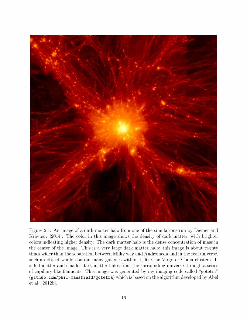
Figure 2.1: An image of a dark matter halo from one of the simulations run by Diemer andKravtsov [2014]. The color in this image shows the density of dark matter, with brightercolors indicating higher density. The dark matter halo is the dense concentration of mass inthe center of the image. This is a very large dark matter halo: this image is about twentytimes wider than the separation between Milky way and Andromeda and in the real universe,such an object would contain many galaxies within it, like the Virgo or Coma clusters. Itis fed matter and smaller dark matter halos from the surrounding universe through a seriesof capillary-like filaments. This image was generated by my imaging code called “gotetra”(github.com/phil-mansfield/gotetra) which is based on the algorithm developed by Abelet al. [2012b].

16

tle against expansion and eventual collapse form a preview for the formation of their much

larger descendants.

To envision a dark matter halo collapsing, imagine a knot in the middle of a sheet.

Imagine twisting that knot and pulling in more and more of the sheet into ever growing

and ever complexifying folds. Imagine pulling in fabric from many sheets in all directions at

once and imagine that this fabric was infused with smaller knots of all sizes. Lastly, imagine

this process in motion, with folds constantly reweaving and oscillating around the knot and

the smaller knots pulling in material as they themselves fall in [see, e.g., Vogelsberger and

White, 2011, Abel et al., 2012b, for visualizations of this process].

What would a human have seen if they were transported back to such an early time?

With a few notable local exceptions, the universe has never been a hospitable place

for humans, and the early universe least of all. For the first few hundred thousand years,

quantum fluctuations and particle collisions would form a wall of instantly blinding light in

all directions. This light would be strong enough to dissolve the human body quite rapidly:

even 400 thousand years after the beginning of the universe, complete atomization would

only take three days.10 If you arrived during this time period, you would bear witness to a

truly cosmic shift in the universe. All around you, the hot light-emitting plasma would be

in the process of condensing into dark neutral hydrogen.

The switch would not be apparent to you immediately: the light from distant plasma

takes time to reach your eyes. By the time the universe became almost entirely neutral11,

every direction you looked would still be the color and temperature of boiling lead. But

as time progresses, this light must come from increasingly distant and ancient expanses of

plasma, giving the expansion of the universe more time to redden and cool the light. After

three million years, this visible plasma is farther away than Andromeda and has degraded to

10. This estimate takes the 3.6 eV carbon-carbon bond energy as a typical bond strength in the humanbody, assumes the human body has 7 × 1027 atoms [Freitas, 1999] and uses [Mosteller, 1987] to estimate a1.9 m2 surface area to the human body.

11. z ≈ 800, TCMB ≈ 2100 K, [Dodelson, 2003]

17

the muddy red of a horseshoe cooling after time in a blacksmith’s forge [see the temperature

tables in Chapman, 2019]. There is nothing but dark matter and formless gas between you

and this wall of fire.

Soon, this light will slip into the infrared, invisible to human eyes, revealing the endless

emptiness and perfect darkness of the universe you now find yourself in. This is not the

darkness of our current universe, which is largely an illusion of our meager eyesight and can

be solved with enough magnification [e.g. Beckwith et al., 2006]. This is a deeper existential

darkness where there is truly nothing to see as far as you might look in every direction.

Ironically, the universe is saved from this dismal, lightless state by its ever-growing dark

matter halos.

As dark matter halos continue to twist and grow, they pull in gas from their surroundings

and much of this gas condenses until it is trapped in the halo’s center. These clouds of gas

are initially held up by their own internal pressure, but grow until their gravity overpowers

their pressure and they collapse into the first stars [Haiman et al., 1996, Tegmark et al.,

1997]. Single stars begin to form in the hearts of dark matter halos throughout the universe.

These primeval stars are enormous and burn hot: their light breaks apart and ionizes the

surrounding gas. As these dark matter halos continue to grow, the gas clouds trapped inside

form larger groups of stars, and the first galaxies begin peek out from behind the receding

neutral gas. These the stars and black holes in these galaxies accelerate the removal neutral

gas even more. In less than a billion years, it is entirely vanquished.

Still, the dark matter halos continue to grow and their growth provides fuel for their inner

galaxies. It takes a further 13 billion years to reach our current universe, and by this time

galaxies have grown from from relatively paltry collections of stars to the massive configura-

tions seen today. Invisibly, their dark matter halos have undergone a similar transformation,

eventually reaching the incredible masses they enjoy today.

The complexity of halo collapse and formation is worthy adversary for modern computer

simulations. Theorists created “simple” models of halo formation which could mostly be

18

worked through by hand [Gunn and Gott, 1972a, Fillmore and Goldreich, 1984, Bertschinger,

1985, Hoffman and Shaham, 1985], but these models did not capture the true mayhem that

accompanies a dark matter halo’s formation and were particularly ineffective at predicting

what halos should look like in the inner regimes where most observations took place. In

pursuit of this issue, many intrepid theorists took a page from Clairaut, Lelande, and Lep-

aute’s book and immediately attempted to brute-force the solution with simulations [White,

1976].12 Unlike their 18th century predecessors, these scientists were not constrained to

simulating a single point: the recent proliferation of Cray-I supercomputers meant that an

astronomer with generous grants and a knack for writing efficient Fortran could simulate a

dark matter halo with several hundred particles. The early stages of this endeavor reached

their conceptual zenith with the publication of Navarro et al. [1997], the first study which

could reliably resolve the inner regions of dark matter halos in realistic environments. (This

paper become one of the most cited theoretical papers in all of astrophysics, according to

the NASA Astrophysics Data System). Since this point, dark matter simulations have con-

tinued to grow exponentially, with largest that I know of containing more than 2 trillion

particles [The Uchuu simulation Ishiyama et al., 2020]. This growth has allowed simulations

to study ever-increasing samples of dark matter halos and to probe the nature of the large

scale structures that they form.

2.1.4 The Cosmic Web and Large Scale Structure

Dark matter halos do not grow in isolation, but as part of a large interconnected structure

of matter which is woven into enormous sheets and filaments. This structure is called the

cosmic web [Bond et al., 1996]. Fig. 2.2 shows a simulated image of a small part of the

cosmic web.

The study of large scale structure is a dense topic, as one might expect from the complex-

12. Simulations of dark matter halos actually predate the dark matter model [Aarseth, 1963, Peebles,1970]. These early works would simulate collections of “galaxies,” but these galaxies were so simplisticallymodeled that the simulations were actually numerically equivalent to dark matter simulations.

19

Figure 2.2: An image of of the cosmic web from one of the simulations run by Diemer andKravtsov [2014]. This image is similar to Fig. 2.2 except that it shows a much larger scale:about a 120 times larger than the distance between the Milky Way and Andromeda. Atlarge scales, the universe is filled with a vast network of filaments and sheets connectingdark matter halos of all sizes. Galaxy surveys show similar structures in the visible universe[famously, in Blanton et al., 2003]. The largest dark matter halos are clumped together inthe densest parts of the cosmic web, a fact – called “mass bias” – which is important tostudies of assembly bias.

20

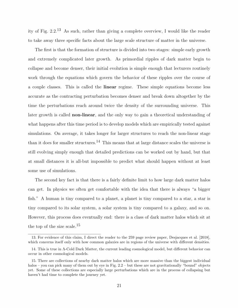
ity of Fig. 2.2.13 As such, rather than giving a complete overview, I would like the reader

to take away three specific facts about the large scale structure of matter in the universe.

The first is that the formation of structure is divided into two stages: simple early growth

and extremely complicated later growth. As primordial ripples of dark matter begin to

collapse and become denser, their initial evolution is simple enough that lecturers routinely

work through the equations which govern the behavior of these ripples over the course of

a couple classes. This is called the linear regime. These simple equations become less

accurate as the contracting perturbation becomes denser and break down altogether by the

time the perturbations reach around twice the density of the surrounding universe. This

later growth is called non-linear, and the only way to gain a theoretical understanding of

what happens after this time period is to develop models which are empirically tested against

simulations. On average, it takes longer for larger structures to reach the non-linear stage

than it does for smaller structures.14 This means that at large distance scales the universe is

still evolving simply enough that detailed predictions can be worked out by hand, but that

at small distances it is all-but impossible to predict what should happen without at least

some use of simulations.

The second key fact is that there is a fairly definite limit to how large dark matter halos

can get. In physics we often get comfortable with the idea that there is always “a bigger

fish.” A human is tiny compared to a planet, a planet is tiny compared to a star, a star is

tiny compared to its solar system, a solar system is tiny compared to a galaxy, and so on.

However, this process does eventually end: there is a class of dark matter halos which sit at

the top of the size scale.15

13. For evidence of this claim, I direct the reader to the 259 page review paper, Desjacques et al. [2018],which concerns itself only with how common galaxies are in regions of the universe with different densities.

14. This is true in Λ-Cold Dark Matter, the current leading cosmological model, but different behavior canoccur in other cosmological models.

15. There are collections of nearby dark matter halos which are more massive than the biggest individualhalos – you can pick many of them out by eye in Fig. 2.2 – but these are not gravitationally “bound” objectsyet. Some of these collections are especially large perturbations which are in the process of collapsing buthaven’t had time to complete the journey yet.

21

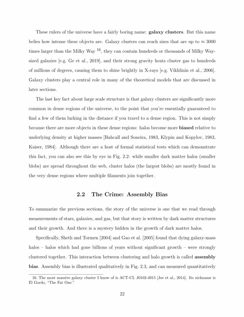
These rulers of the universe have a fairly boring name: galaxy clusters. But this name

belies how intense these objects are. Galaxy clusters can reach sizes that are up to ≈ 3000

times larger than the Milky Way 16, they can contain hundreds or thousands of Milky Way-

sized galaxies [e.g. Ge et al., 2019], and their strong gravity heats cluster gas to hundreds

of millions of degrees, causing them to shine brightly in X-rays [e.g. Vikhlinin et al., 2006].

Galaxy clusters play a central role in many of the theoretical models that are discussed in

later sections.

The last key fact about large scale structure is that galaxy clusters are significantly more

common in dense regions of the universe, to the point that you’re essentially guaranteed to

find a few of them lurking in the distance if you travel to a dense region. This is not simply

because there are more objects in these dense regions: halos become more biased relative to

underlying density at higher masses [Bahcall and Soneira, 1983, Klypin and Kopylov, 1983,

Kaiser, 1984]. Although there are a host of formal statistical tests which can demonstrate

this fact, you can also see this by eye in Fig. 2.2: while smaller dark matter halos (smaller

blobs) are spread throughout the web, cluster halos (the largest blobs) are mostly found in

the very dense regions where multiple filaments join together.

2.2 The Crime: Assembly Bias

To summarize the previous sections, the story of the universe is one that we read through

measurements of stars, galaxies, and gas, but that story is written by dark matter structures

and their growth. And there is a mystery hidden in the growth of dark matter halos.

Specifically, Sheth and Tormen [2004] and Gao et al. [2005] found that dying galaxy-mass

halos – halos which had gone billions of years without significant growth – were strongly

clustered together. This interaction between clustering and halo growth is called assembly

bias. Assembly bias is illustrated qualitatively in Fig. 2.3, and can measured quantitatively

16. The most massive galaxy cluster I know of is ACT-CL J0102-4915 [Jee et al., 2014]. Its nickname isEl Gordo, “The Fat One.”

22

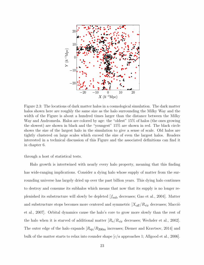
Figure 2.3: The locations of dark matter halos in a cosmological simulation. The dark matterhalos shown here are roughly the same size as the halo surrounding the Milky Way and thewidth of the Figure is about a hundred times larger than the distance between the MilkyWay and Andromeda. Halos are colored by age: the “oldest” 15% of halos (the ones growingthe slowest) are shown in black and the “youngest” 15% are shown in red. The black circleshows the size of the largest halo in the simulation to give a sense of scale. Old halos aretightly clustered on large scales which exceed the size of even the largest halos. Readersinterested in a technical discussion of this Figure and the associated definitions can find itin chapter 6.

through a host of statistical tests.

Halo growth is intertwined with nearly every halo property, meaning that this finding

has wide-ranging implications. Consider a dying halo whose supply of matter from the sur-

rounding universe has largely dried up over the past billion years. This dying halo continues

to destroy and consume its subhalos which means that now that its supply is no longer re-

plenished its substructure will slowly be depleted [fsub decreases; Gao et al., 2004]. Matter

and substructure stops becomes more centered and symmetric [Xoff/Rvir decreases; Maccio

et al., 2007]. Orbital dynamics cause the halo’s core to grow more slowly than the rest of

the halo when it is starved of additional matter [Rs/Rvir decreases; Wechsler et al., 2002].

The outer edge of the halo expands [Rsp/R200m increases; Diemer and Kravtsov, 2014] and

bulk of the matter starts to relax into rounder shape [c/a approaches 1; Allgood et al., 2006].

23

The halo’s spin – already slight – begins to slow down [λ decreases; Vitvitska et al., 2002].

The connection between the age of dark matter halos and the properties of their inner

galaxies is a far more complex topic [e.g. Wechsler and Tinker, 2018], but there are a host

of reasons to expect that galaxy properties are tightly connected to growth histories of their

dark matter halos. Of particular note is the potential connection between halo growth and the

rate the stars form in the halo’s galaxy, since the star formation rate is closely connected to a

host of galaxy properties, like appearance, color, and dust obscuration. Observational studies

have demonstrated a close connection between halo mass and galaxy mass (see Wechsler

and Tinker, 2018 for an overview and Huang et al., 2020 for a particularly breath-taking

recent study), a correlation which requires that star formation and halo growth are strongly

connected. Theoretical models which assume halo growth is the driving factor behind star

formation can be calibrated to predict a wide range of complex observations [e.g. Behroozi

et al., 2018]. Simulations which attempt to model both processes simultaneously explicitly

show a strong connection between them [e.g. Matthee et al., 2017].17

Put more directly: assembly bias means that dark matter halos and their galaxies look

and behave differently in different parts of the universe, even at a fixed halo mass.18

There are a large number of studies which are impacted by this fact. Perhaps no field

of astronomy is more affected than the massive theoretical effort over the past twenty years

to develop theoretical models which attempt to “paint” galaxies onto dark matter halos

so that our observations of the universe can be compared against the unobservable theo-

retical predictions of a dark matter-dominated universe [e.g. Berlind and Weinberg, 2002,

Yang et al., 2003]. However, the majority of these analyses have explicitly assumed that

17. There are some reasons for skepticism. Observationally, some recent studies which purport to measurehalo growth rates in the local universe claim that galaxy and halo growth are uncorrelated [Behroozi et al.,2015, Tinker et al., 2017, O’Donnell et al., 2020]. The theoretical models which assume a connection betweenhalo growth and galaxy growth make some incorrect predictions unless ad hoc components (orphan galaxies)are added to them [e.g. Campbell et al., 2018]. Lastly, simulations that track stars and gas do not resolvemany critical processes, have many tunable parameters, and require complex verification regimens [e.g.Hopkins et al., 2018], which can make it complicated to interpret how strong a given prediction is. Sufficeto say, there are many papers left to be written on this topic.

18. This statement has been confirmed by a wide array of studies, see the overview in Mao et al. [2018].

24

assembly bias never reaches its tendrils into the observable properties of galaxies, meaning

that the existence of assembly bias and the uncertainty in the connection between galax-

ies and their halos has loomed over this field like the Sword of Damocles [Zentner et al.,

2014]. Assembly bias impacts astronomy in less obvious ways, as well. For example, most of

our understanding of dim satellite galaxies comes from observations of a handful of nearby

galaxies [see Carlsten et al., 2020, for an overview]. But all these observations take place in

the same local environment, and that environment is not a particularly common one [Neuzil

et al., 2020]. Any connection between this environment and the structure and character of

these satellite systems could strongly impact our ability to interpret these observations [e.g.

Libeskind et al., 2015].

Efforts to resolve and model the effects of assembly bias have been stymied because it

isn’t clear why assembly bias happens at galaxy masses. Early measurements of assembly

bias were a shot out of the blue: theories of halo growth at the time [most notably Press and

Schechter, 1974] were built on the foundational assumption that large-scale structure had

little-to-no effect on halo properties, and it was clear that radical adaptations were needed

[Gao et al., 2005].

The problem of assembly bias is to theorists as a lantern is to moths, and soon there were

no shortage of reasonable-sounding explanations. However, the proposed causes of assembly

bias would affect halo growth in different ways and would impact different groups of halos,

raising the question of which explanation is actually correct. The following section lists the

most prominent models for this effect.

2.3 The Suspects: Tides, Heating, and Misadventure

The oldest attempted explanations for assembly bias (and those first suggested by Gao et al.,

2005) tried to alter the models of how of primeval dark matter perturbations contract and

collapse [e.g. Sandvik et al., 2007, Desjacques, 2008, Dalal et al., 2008, Chue et al., 2018]. This

undertaking proved to be a fantastic success in understanding how assembly bias impacts

25

galaxy clusters [Dalal et al., 2008], but unfortunately, this success did not translate down to

galaxy masses. There was a simple reason for this: galaxy clusters are massive and unlikely

to be disturbed by larger objects while growing. This means that individual perturbations

can largely be considered in isolation at high masses, but that this analysis will insufficient

for many smaller mass halos.

Because of the failures of single-perturbation collapse models, theorists have ventured

into the multi-object complexities of the non-linear regime. What happens to the growth of

halos when they spend their lifetime navigating beneath the shadows of objects thousands

of times their mass?

One of the most pressing concerns in the non-linear world comes from subhalos which

have temporarily wandered far from their host halos. As discussed in section 2.1.1 and

2.1.3, the satellites of large dark matter halos have a tumultuous life. While some distinct

halos may stop growing when they run out of material to accrete, virtually all subhalos stop

growing as they are tossed about and ripped apart by their hosts [van den Bosch, 2017, gives

an astonishingly complete overview of this topic]. This is a problem because researchers

rarely actually check whether an object is a subhalo. Instead, the typical approach is to

draw an ad hoc boundary around each halo or galaxy19 and use this boundary to determine

which objects are or are not subhalos [e.g. Gao et al., 2005, Wechsler et al., 2006, and many

others].

However, subhalos can actually orbit far beyond the boundaries researchers often adopt

[Balogh et al., 2000]. Because of this, when the most massive halos in the universe are

analyzed with standard techniques, it appears as if they are surrounded by swarms of dying

Milky Way-sized galaxies and halos. Because these massive galaxy clusters are only found

in the densest regions of the universe, this misclassification means the oldest galaxy-mass

halos are also found in these regions. Multiple researchers have attempted to quantify the

impact of these errant subhalos on assembly bias, but came to different conclusions over

19. i.e. The so-called “virial radius.”

26

how important they are [Wang et al., 2009, Li et al., 2013, Wetzel et al., 2014, Sunayama

et al., 2016]. This confusion stems from a combination of different definitions, ambiguity

over when a subhalo first enters its host, and disagreements over the difference between a

subhalo which merely has a distant orbit and a subhalo which has been completely ejected

from its host.

Other groups of researchers have proposed that these massive galaxy clusters play a

second, even more important role: their intense gravitational field can stifle the growth of

halos long before those halos fall into the cluster [Hahn et al., 2009, Behroozi et al., 2014,

Hearin et al., 2016b, Salcedo et al., 2018]. Consider a satellite around the Earth. While this

satellite is close to Earth, it has no trouble orbiting. But at large distances, the Sun’s gravity

will become more important and will eventually pull this satellite out of its orbit around the

Earth and into an orbit around the Sun.20 In this sense, the Sun’s tidal field prevents

objects from orbiting the Earth beyond a certain distance (it’s “tidal radius”). This region

where it is possible to orbit the Earth would decrease in size if the Earth moved closer to the

Sun or if the Sun grew in more massive. Massive galaxy clusters have the same impact on

Milky Way-sized dark matter halos which venture too close to them: the intense tidal fields

limit how far away these smaller halos can attract fresh matter and therefore suppresses

their growth. Because the massive halos hosting these galaxy clusters are clumped together

in the densest regions of the universe, tidal fields can lead to dense portions of the cosmic

web being filled with slowly-growing halos.

A related model proposes that the key factor isn’t tidal fields from individual galaxy

clusters, but instead the fields produced by the filaments and sheets of large scale structure

itself [Hahn et al., 2009, Wang et al., 2011, Paranjape et al., 2018, Musso et al., 2018]. The

20. Where this occurs is a surprisingly subtle topic. The influence of the Sun on objects orbiting theEarth was the subject of several bitter academic fights during the early years of Newtonian astronomy[Bodenmann, 2010] and our friend Alexis Clairaut was a central character in this drama. Clairaut’s lifelongenemy, Leonhard Euler, worked out the fundamentals during the year of Clairuat’s death [Euler, 1765]. Putsimply: at close distances, objects can orbit the Earth. At moderate distances, objects can appear to orbitthe Earth while actually primarily orbiting the Sun (the Moon does this). At large distances neither ispossible and objects can only orbit the Sun.

27

largest of these structures contain immense amounts of mass, meaning that their tidal fields

can can have a strong impact on the objects floating inside of them. If true, this would mean

that assembly bias stems from an effect that impacts all halos in these dense regions, rather

than just the ones that happen to be next to galaxy clusters.

Lastly, some scientists have focused on another property of filaments: the velocity of

objects inside them [Wang et al., 2007, Dalal et al., 2008]. As objects fall towards a massive

filament, their velocity increases. This means that every object within these filaments is

moving around at high speeds. This increased speed makes it more difficult for halos within

these filaments to capture the matter around them and slows down their growth. Like large

scale tidal fields, this effect impacts all halos within filaments, but leads to filaments of

different sizes doing most of the heavy lifting.

To date there has been no attempt to compare or unify these explanations. There have

been many papers arguing for one potential cause or the other, but these works rarely address

competing papers and I am not aware of any which attempted an explicit comparison between

the models. This has led to an unintentional Balkanization of the assembly bias literature,

with authors citing work associated with one class of theories and largely ignoring other

approaches. The goal of this thesis is to unify the theoretical assembly bias literature into a

cohesive model.

2.4 The Plan: The Structure of This Thesis

This thesis compares these different explanations and argues for a synthesized model for

galaxy-mass assembly bias: most assembly bias at this mass scale is caused by misclassified

subhalos. The remainder is caused by the impact of gravitational heating and large-scale tidal

fields on a relatively small fraction of halos in large filaments. I work through how I arrive at

answer this in chapter 6. The journey requires building a substantial theoretical framework:

it requires building tools to measure quantities which have never been measured before and

requires putting simulations through tests which have never been performed before. I build

28

this framework up in chapters 4 and 5. Chapter 3 contains technical background information

shared by all three chapters

At the start of my Ph.D, a number of collaborating research groups showed that simulated

dark matter halos have distinct edges: the splashback surface [Diemer and Kravtsov, 2014,

Adhikari et al., 2014, More et al., 2015].21 The splashback surface is an edge in the density

field around halos which is caused by particles and subhalos “piling up” far away from the

halo halfway through their first orbits. These first studies could not reliably measure this

edge in individual halos, but could find it by combining large groups of halos22 or in simplified

simulations. If it were possible to measure this boundary measure for individual halos, there

would be an unambiguous way to identify subhalos: the splashback boundary splits infalling

matter from all orbiting matter.

Chapter 4 develops the code Shellfish,23 the first tool which could measure splashback

surfaces around individual objects. Although the ultimate goal of this thesis primarily uses

Shellfish to identify subhalos, chapter 4 covers other useful features of splashback surfaces,

ranging from shapes and sizes, to their connection to the inner parts of halos, to their

alignment with large scale structure. This chapter corresponds to the paper Mansfield et al.

[2017]

Although dark matter simulations have existed for decades (see section 2.1.3), many

questions about their reliability remain unanswered. In chapter 5, I perform wide-ranging

tests on many of the highest-resolution dark matter simulations available today. I originally

started writing this chapter to determine the reliability of the halos for assembly bias studies,

but its conclusions are further ranging that this. Chapter 5 performs reliability tests on

many dark matter halo properties (in some cases, these are the first tests that have ever

21. This had been predicted by some early models of halo growth [Fillmore and Goldreich, 1984,Bertschinger, 1985], but the significance of these predictions was not appreciated at the time.

22. This technique would soon be successfully used in observations [More et al., 2016, Chang et al., 2018]

23. The name is an acronym which stands for SHELL Finding In Spheroidal Halos. I came up with thename during the Physical Sciences Division’s happy hour.

29

been performed on these properties), demonstrates that high-resolution simulations disagree

to a larger extent than was previously believed, and shows that many aspects of simulations

depend strongly on a subtle numerical parameter called the “force softening scale” (first

introduced in Aarseth, 1963). Chapter 5 corresponds to the paper Mansfield and Avestruz

[in prep].

With the field set, chapter 6 addresses the central question of this thesis: what causes

galaxy-mass assembly bias? The approach I use in this chapter is to estimate how strongly the

different effects listed in section 2.3 affect every halo in a simulation. Using these estimates, I

determine how efficiently the different effects can create a universe with assembly bias, which

allows me compare how closely connected these different processes are to assembly bias. I

also synthesize the low-mass and high-mass treatments of assembly bias, and resolve some

long-standing disputes over the nature of assembly bias by showing that they are the result

of definitional differences. This chapter continues the tradition of chapters 4 and 5, with a

heavy focus on understanding halo boundaries and an equally heavy focus on demonstrating

the robustness and reliability of various measurements. Chapter 6 corresponds to the paper

Mansfield and Kravtsov [2019].

30

CHAPTER 3

TECHNICAL BACKGROUND

This chapter covers the technical background shared by the later chapters in this thesis.

While this chapter is more pedagogical than chapters 4, 5, and 6, it is more technical than

the preceding chapters.

3.1 Simulations

This thesis uses eight simulation suites: Erebos CBol [Diemer and Kravtsov, 2014, 2015],

Erebos CPla [Diemer and Kravtsov, 2015], Multidark-Planck [Klypin et al., 2016], Chinchilla

[Lehmann et al., 2017], Bolshoi [Klypin et al., 2011], BolshoiP [Klypin et al., 2016], ν2-gc

[Ishiyama et al., 2015], and IllustrisTNG-Dark [Naiman et al., 2018, Pillepich et al., 2018,

Nelson et al., 2018, Marinacci et al., 2018, Springel et al., 2018]. The properties of these

simulations are summarized in Tables 3.1 and 3.1. Erebos CBol is used in chapter 4, every

simulation suite is used in chapter 5, and Bolshoi and BolshoiP are used in chapter 6.

Each simulation suite is the product of one of four simulation codes, each with vary-

ing gravity solvers and timestepping schemes. Bolshoi and BolshoiP were run using ART

[Kravtsov et al., 1997, Kravtsov, 1999, Gottloeber and Klypin, 2008], the Multidark-Planck,

Erebos CBol, Erebos CPla, and Chinchilla suites were run with Gadget-2 [Springel, 2005].

IllustrisTNG-Dark was run using Arepo [Springel, 2010, Weinberger et al., 2019] which

performs gravitational calculations using an updated version of the Gadget-2 gravity-solving

algorithm. ν2-gc was run with GreeM3 [Ishiyama et al., 2012, 2015].

An important aspect of these codes is the scheme they use for setting timestep sizes.

Three of the four codes, Gadget-2, Arepo, and GreeM3 use an adaptive timestepping scheme

dependent on the local gravitational acceleration [Springel, 2005, Weinberger et al., 2019,

Ishiyama, personal communication], and ART timesteps are density-dependent [Klypin et al.,

31

Code Suite ΩM,0 h100 σ8 η Simulation

GreeM3 ν2-GC 0.31 0.68 0.83 0.045 ν2-GC-L

ν2-GC-H1

ν2-GC-H2ART Bolshoi 0.27 0.7 0.82 – Bolshoi

BolshoiP 0.307 0.678 0.823 – BolshoiPGadget-2 Chinchilla 0.286 0.7 0.82 0.025 L125

L250L400

Multidark 0.307 0.678 0.823 0.01 ESMDPLVSMDPLSMDPLMDPL2BMDPLHMDPL

Erebos CBol 0.27 0.7 0.82 0.025 CBol L63CBol L125CBol L250CBol L500CBol L1000CBol L2000

Erebos CPla 0.32 0.67 0.82 0.025 CPla L125CPla L250CPla L500

Arepo IllustrisTNG-Dark 0.3089 0.6774 0.8159 0.012 TNG100-1-DarkTNG100-2-DarkTNG100-3-Dark

Table 3.1: A list of simulations used in this work. The first six columns contain informationcommon to all simulations in a given suite: the code used to run the suite, the suite name,the cosmological parameters ΩM , h100 = H0/(100 km/s/Mpc), σ8, and the Gadget-liketimestepping parameter, η. Note that ART does not use this timestepping scheme (seesection 3.1 for details). This additional columns of this Table are given in Table 3.1.

32

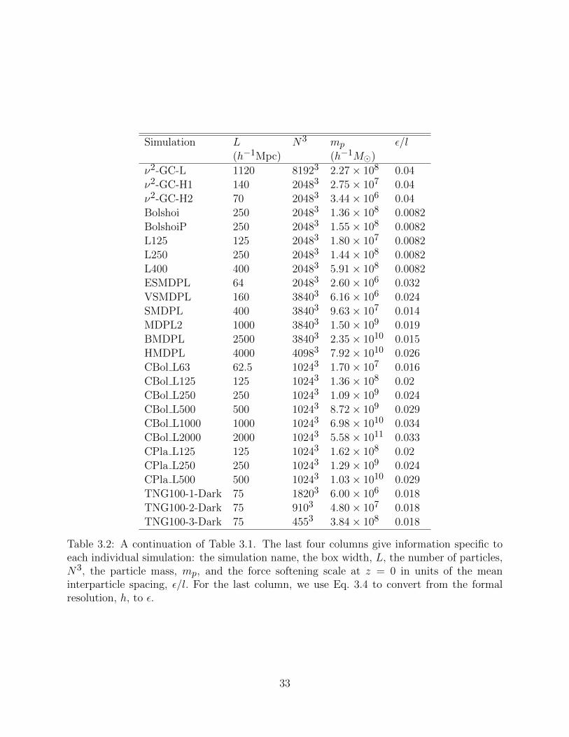
Simulation L N3 mp ε/l

(h−1Mpc) (h−1M)

ν2-GC-L 1120 81923 2.27× 108 0.04

ν2-GC-H1 140 20483 2.75× 107 0.04

ν2-GC-H2 70 20483 3.44× 106 0.04

Bolshoi 250 20483 1.36× 108 0.0082

BolshoiP 250 20483 1.55× 108 0.0082

L125 125 20483 1.80× 107 0.0082

L250 250 20483 1.44× 108 0.0082

L400 400 20483 5.91× 108 0.0082

ESMDPL 64 20483 2.60× 106 0.032

VSMDPL 160 38403 6.16× 106 0.024

SMDPL 400 38403 9.63× 107 0.014

MDPL2 1000 38403 1.50× 109 0.019

BMDPL 2500 38403 2.35× 1010 0.015

HMDPL 4000 40983 7.92× 1010 0.026

CBol L63 62.5 10243 1.70× 107 0.016

CBol L125 125 10243 1.36× 108 0.02

CBol L250 250 10243 1.09× 109 0.024

CBol L500 500 10243 8.72× 109 0.029

CBol L1000 1000 10243 6.98× 1010 0.034

CBol L2000 2000 10243 5.58× 1011 0.033

CPla L125 125 10243 1.62× 108 0.02

CPla L250 250 10243 1.29× 109 0.024

CPla L500 500 10243 1.03× 1010 0.029

TNG100-1-Dark 75 18203 6.00× 106 0.018

TNG100-2-Dark 75 9103 4.80× 107 0.018

TNG100-3-Dark 75 4553 3.84× 108 0.018

Table 3.2: A continuation of Table 3.1. The last four columns give information specific toeach individual simulation: the simulation name, the box width, L, the number of particles,N3, the particle mass, mp, and the force softening scale at z = 0 in units of the meaninterparticle spacing, ε/l. For the last column, we use Eq. 3.4 to convert from the formalresolution, h, to ε.

33

2011]. The former use adaptive time steps, with

∆t =√

2ηε/|~a|. (3.1)

Here, ~a is the local gravitational acceleration, ε is the ‘Plummer-equivalent’ force softening

scale which will be discussed below, and η is a user-defined parameter (also referred to

as ErrTolIntAcc) that is typically set to & 0.01. In practice, ∆t is evaluated for each

particle, the values are used to place particles into the coarsest logarithmic timestepping bin,

∆ti = t02−i, such that ∆ti ≤ ∆t. As such, the actual timestep size a particle experiences

may be smaller than Eq. 3.1 by a factor of two. We note that while the initial GreeM3

implementation used a different adaptive scheme [Ishiyama et al., 2009], GreeM3 used the

adaptive scheme described above to produce ν2-gc (Ishiyama, personal communication).

ART timesteps vary at different depths of the refinement tree, meaning that they depend

on density instead of acceleration. Both Bolshoi and BolshoiP use timesteps of ∆a ≈ 2−3×

10−3 at the 0th (coarsest) refinement level with time steps decreasing by a factor of two for

each successive level of spatial refinement, leading to timesteps of ∆a ≈ 2− 3× 10−6 at the

tenth level [Klypin et al., 2011]. The ART timestepping scheme leads to far finer timesteps

than any of the other simulations considered in this paper.

3.1.1 Force Softening

Cosmological simulations do not model particles as point sources. Infinitesimal point sources

will scatter off one another during close encounters, which leads to aphysical energy exchange

between particles and can potentially thermalize the inner regions of dark matter haloes [see

overview in Ludlow et al., 2019]. Additionally, these close encounters require much finer

timesteps to resolve than typical orbits through a halo’s potential, meaning that codes are

forced to either spend large amounts of computation time resolving an aphysical process

or risk conservation of energy errors (See section 5.6.1). To minimize these effect, codes

34

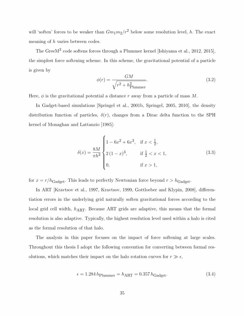
will ‘soften’ forces to be weaker than Gm1m2/r2 below some resolution level, h. The exact

meaning of h varies between codes.

The GreeM3 code softens forces through a Plummer kernel [Ishiyama et al., 2012, 2015],

the simplest force softening scheme. In this scheme, the gravitational potential of a particle

is given by

φ(r) =GM√

r2 + h2Plummer

. (3.2)

Here, φ is the gravitational potential a distance r away from a particle of mass M.

In Gadget-based simulations [Springel et al., 2001b, Springel, 2005, 2010], the density

distribution function of particles, δ(r), changes from a Dirac delta function to the SPH

kernel of Monaghan and Lattanzio [1985]:

δ(x) =8M

πh3

1− 6x2 + 6x3, if x < 12 ,

2 (1− x)3, if 12 < x < 1,

0, if x > 1,

(3.3)

for x = r/hGadget. This leads to perfectly Newtonian force beyond r > hGadget.

In ART [Kravtsov et al., 1997, Kravtsov, 1999, Gottloeber and Klypin, 2008], differen-

tiation errors in the underlying grid naturally soften gravitational forces according to the

local grid cell width, hART. Because ART grids are adaptive, this means that the formal

resolution is also adaptive. Typically, the highest resolution level used within a halo is cited

as the formal resolution of that halo.

The analysis in this paper focuses on the impact of force softening at large scales.

Throughout this thesis I adopt the following convention for converting between formal res-

olutions, which matches their impact on the halo rotation curves for r ε,

ε = 1.284hPlummer = hART = 0.357hGadget. (3.4)

35

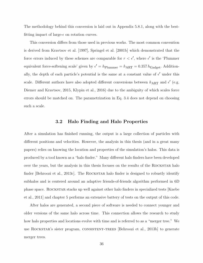
The methodology behind this conversion is laid out in Appendix 5.8.1, along with the best-

fitting impact of large-ε on rotation curves.

This conversion differs from those used in previous works. The most common convention

is derived from Kravtsov et al. [1997], Springel et al. [2001b] which demonstrated that the

force errors induced by these schemes are comparable for r < ε′, where ε′ is the ‘Plummer

equivalent force-softening scale’ given by ε′ = hPlummer = hART = 0.357hGadget. Addition-

ally, the depth of each particle’s potential is the same at a constant value of ε′ under this

scale. Different authors have also adopted different conversions between hART and ε′ (e.g.

Diemer and Kravtsov, 2015, Klypin et al., 2016) due to the ambiguity of which scales force

errors should be matched on. The parametrization in Eq. 3.4 does not depend on choosing

such a scale.

3.2 Halo Finding and Halo Properties

After a simulation has finished running, the output is a large collection of particles with

different positions and velocities. However, the analysis in this thesis (and in a great many

papers) relies on knowing the location and properties of the simulation’s halos. This data is

produced by a tool known as a “halo finder.” Many different halo finders have been developed

over the years, but the analysis in this thesis focuses on the results of the Rockstar halo

finder [Behroozi et al., 2013c]. The Rockstar halo finder is designed to robustly identify

subhalos and is centered around an adaptive friends-of-friends algorithm performed in 6D

phase space. Rockstar stacks up well against other halo finders in specialized tests [Knebe

et al., 2011] and chapter 5 performs an extensive battery of tests on the output of this code.

After halos are generated, a second piece of software is needed to connect younger and

older versions of the same halo across time. This connection allows the research to study

how halo properties and locations evolve with time and is referred to as a “merger tree.” We

use Rockstar’s sister program, consistent-trees [Behroozi et al., 2013b] to generate

merger trees.

36

Dark matter halos are complex objects with a number of scientifically useful properties.

Many of these properties are used throughout the remaining chapters of this thesis. The rest

of this section describes many of their most commonly used properties, as computed by the

Rockstar halo finder.

Bound vs. Unbound Particles: Rockstar separates particles into ‘bound’ and ‘un-

bound’ groups and primarily analyses bound particles. This is done because if particles were

classified with a simple geometric cut, subhalos would be contaminated with a large number

of particles from their host halos. There is no unambiguous way to perform this procedure

due to the importance of tidal fields in true boundedness calculations, but Rockstar takes

a reasonable approach and determines boundedness by performing pairwise potential calcu-

lations and comparing against the kinetic energy of particles in the rest frame of the halo

center.

Halo mass: The most basic properties of a halo are its size and, equivalently, its mass.

In most studies, the ‘overdensity radius’ definition of the halo boundary is used to define

these properties. Under this definition, the halo is a sphere of radius R∆ which encloses the

bound mass M∆ = Mbound(< R∆) such that

M∆ =4π

3∆ρrefR

3∆. (3.5)

Here, ∆ is some constant and ρref is a cosmological reference density. The reference density

is typically either the background matter density, ρm, or the critical density, ρc.

The choice of reference density is more of an art than a science. Chapter 4 reviews

the scientific justification (or lack thereof) for different choice of the halo boundary, but

to clarify notation, the primary radius definition in this thesis is Rvir. Rvir corresponds to

∆ρref as given by the relation in Bryan and Norman [1998]. At various points throughout

this thesis, I also consider the bound masses enclosed within R200m (∆ρref = 200ρm), R200c

(∆ρc = 200ρc), R500c (∆ρref = 500ρc), and R2500c (∆ρref = 2500ρc).

37

Rockstar computes overdensity radii by constructing radial density profiles using only

particles within the coarse-grained friends-of-friends (FOF) group that contains the halo

center. The linking length parameter used to identify the FOF group has a substantial effect

on the convergence properties of M200m (see Appendix 6.6.1).

Virial Scaling: Mvir and Rvir are commonly used as characteristic scales to remove the

dimensionality of other halo properties. Some unscaled halo properties have units of time

in their dimensions, requiring the introduction of a third characteristic scale, the “virial

velocity:”

Vvir =

√GMvir

Rvir. (3.6)

Maximum circular velocity: One of the most fundamental properties of a dark

matter halo is Vmax. Vmax is the maximum velocity reach by a halo’s “rotation curve,”

Vcirc(r) =√GM/r. Vmax enjoys widespread use because it is both closely connected both

to the theoretical distribution of dark matter and to observational quantities like rotation

curves [e.g. Rubin and Ford, 1970]. Vmax is also a non-parametric halo property, meaning

that in principle it can be measured without needing to assume a model for the distribution

of mass throughout the halo1

Vmax is a well-defined halo property in its own right, but when scaled by Vvir, it becomes

a measure of halo “concentration.” Halos whose masses are highly concentrated in their

centers will have higher values of Vmax/Vvir and halos with more diffuse mass distributions

will have lower Vmax/Vvir values.

A related, but distinct, quantity is Vrms,

Vrms =

√∑

i

~vi − 〈~v〉. (3.7)

Here, the sum and average are performed over the velocities of every particle in the halo.

1. In practice, observations of rotation curves generally do not reach radii large enough to resolve Vmax

[e.g. de Blok et al., 2008]. This means that inferring Vmax from observations necessarily has a theoreticaland parametric component.

38

Halo concentration: Although Vmax/Vvir is a useful measurement of concentration,

the most widely used tracer of concentration is cvir = R−2/Rvir, where R−2 is the radius

where the halo’s logarithmic radially-averaged density slope equals -2. Although R−2 can be

measured without adopting a halo model for profiles averaged over large halo populations, the

noise in halo profiles requires fitting a particular functional form if individual measurements

of cvir are required.

This thesis performs fits against the Navarro-Frenk-White (NFW) profile [Navarro et al.,

1997]. The NFW profile has the form

ρ(r) =ρ0

r/Rs(1 + r/Rs)2, (3.8)

where ρ0 and Rs are free parameters of the fit. For this funcitonal form, R−2 = Rs, cvir ≡

Rvir/Rs. This fit is delicate and different fitting strategies lead to different concentration

statistics. Rockstar performs a χ2-minimization of Eq. 3.8 against binned density profiles,

ignoring bins with fewer than 15 particles and heavily down-weighting bins with r < 3εφ.

Related is R1/2, the radius which encloses half of the bound mass within Rvir.

Halo shape: Rockstar follows the recommendations of Zemp et al. [2011], and com-

putes halo shapes using iterative, weighted mass distribution tensors. Specifically, Rock-

star first computes the mass distribution tensor

Mij =

∑Nk (~rk)i(~rk)j |~rk|−2

N∑Nk |~rk|−2

(3.9)

over all bound particles k within Rvir and computes the eigenvalues, λi, of Mij . Then, Rock-

star estimates axis ratios as√λi/λj for each pair of axes, i and j, repeating the process

for all bound particles in an ellipsoid with the corresponding axis ratios and a minimum axis

length of Rvir. This process repeats until axis ratios converge to 1%. Note that the axis

ratio measurement is sensitive to the central mass distribution.

Halo spin: To track halo spin, researchers typically use the dimensionless Peebles and

39

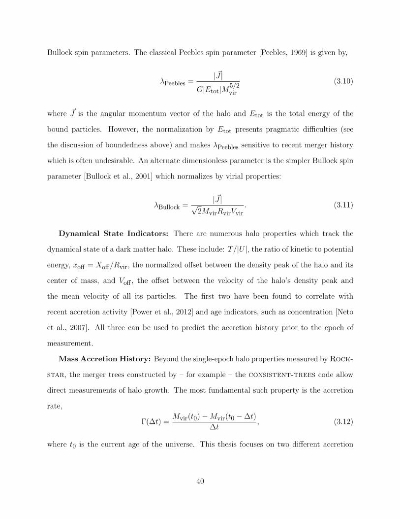
Bullock spin parameters. The classical Peebles spin parameter [Peebles, 1969] is given by,

λPeebles =| ~J |

G|Etot|M5/2vir

(3.10)

where ~J is the angular momentum vector of the halo and Etot is the total energy of the

bound particles. However, the normalization by Etot presents pragmatic difficulties (see

the discussion of boundedness above) and makes λPeebles sensitive to recent merger history

which is often undesirable. An alternate dimensionless parameter is the simpler Bullock spin

parameter [Bullock et al., 2001] which normalizes by virial properties:

λBullock =| ~J |√

2MvirRvirVvir. (3.11)

Dynamical State Indicators: There are numerous halo properties which track the

dynamical state of a dark matter halo. These include: T/|U |, the ratio of kinetic to potential

energy, xoff = Xoff/Rvir, the normalized offset between the density peak of the halo and its

center of mass, and Voff , the offset between the velocity of the halo’s density peak and

the mean velocity of all its particles. The first two have been found to correlate with

recent accretion activity [Power et al., 2012] and age indicators, such as concentration [Neto

et al., 2007]. All three can be used to predict the accretion history prior to the epoch of

measurement.

Mass Accretion History: Beyond the single-epoch halo properties measured by Rock-

star, the merger trees constructed by – for example – the consistent-trees code allow

direct measurements of halo growth. The most fundamental such property is the accretion

rate,

Γ(∆t) =Mvir(t0)−Mvir(t0 −∆t)

∆t, (3.12)

where t0 is the current age of the universe. This thesis focuses on two different accretion

40

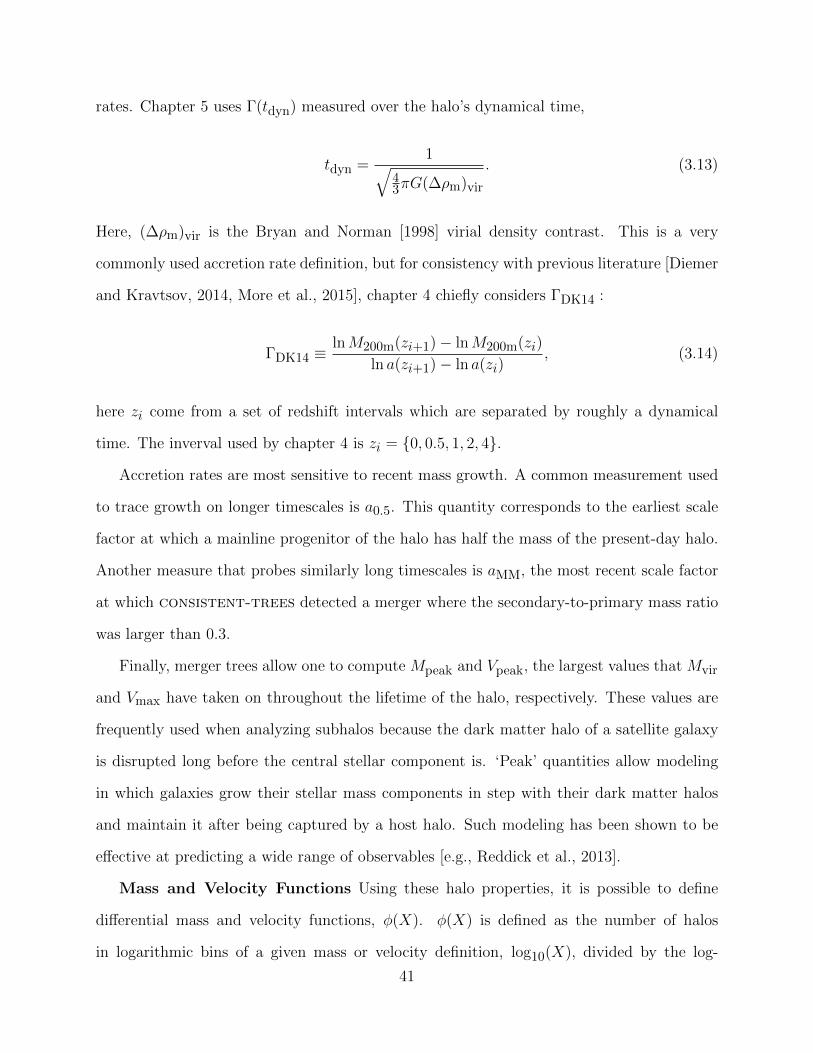
rates. Chapter 5 uses Γ(tdyn) measured over the halo’s dynamical time,

tdyn =1√

43πG(∆ρm)vir

. (3.13)

Here, (∆ρm)vir is the Bryan and Norman [1998] virial density contrast. This is a very

commonly used accretion rate definition, but for consistency with previous literature [Diemer

and Kravtsov, 2014, More et al., 2015], chapter 4 chiefly considers ΓDK14 :

ΓDK14 ≡lnM200m(zi+1)− lnM200m(zi)

ln a(zi+1)− ln a(zi), (3.14)

here zi come from a set of redshift intervals which are separated by roughly a dynamical

time. The inverval used by chapter 4 is zi = 0, 0.5, 1, 2, 4.

Accretion rates are most sensitive to recent mass growth. A common measurement used

to trace growth on longer timescales is a0.5. This quantity corresponds to the earliest scale

factor at which a mainline progenitor of the halo has half the mass of the present-day halo.

Another measure that probes similarly long timescales is aMM, the most recent scale factor

at which consistent-trees detected a merger where the secondary-to-primary mass ratio

was larger than 0.3.

Finally, merger trees allow one to compute Mpeak and Vpeak, the largest values that Mvir

and Vmax have taken on throughout the lifetime of the halo, respectively. These values are

frequently used when analyzing subhalos because the dark matter halo of a satellite galaxy

is disrupted long before the central stellar component is. ‘Peak’ quantities allow modeling

in which galaxies grow their stellar mass components in step with their dark matter halos

and maintain it after being captured by a host halo. Such modeling has been shown to be

effective at predicting a wide range of observables [e.g., Reddick et al., 2013].

Mass and Velocity Functions Using these halo properties, it is possible to define

differential mass and velocity functions, φ(X). φ(X) is defined as the number of halos

in logarithmic bins of a given mass or velocity definition, log10(X), divided by the log-

41

arithmic width of that bin. This thesis considers the mass and velocity definitions of

X ∈Mvir, M2500c, M500c, M200c, M200m, Mpeak, Vmax, Vrms, Vpeak

.

Isolated Halo vs. Subhalo Classification: The classification of halos into “isolated

halos” and “subhalos” plays a critical role in halo analysis, because subhalos behave very

differently from non-subhalos at the same mass. This is because subhalos tend to be rapidly

losing mass and are within extreme tidal environments. Overwhelmingly, the most common

approach is to classify objects within some overdensity radius, R∆, of a larger halo as sub-

halos and everything else as isolate halos. Chapter 6 critically evaluates this approach at

length.

42

CHAPTER 4

SPLASHBACK SHELLS OF COLD DARK MATTER HALOS

This chapter is a modified version of my paper, Mansfield et al. [2017].

4.1 Introduction

In the Cold Dark Matter (CDM) paradigm of structure formation, dark matter halos form

via the collapse of density peaks in the initial random Gaussian perturbation field. In the

commonly used “tophat model” the peak density contrast profile is approximated as uniform

within a given radius [e.g., Tolman, 1934]. The constant overdensity in such approximations

results in a uniform collapse time for different radial shells and a single well-defined collapse

time for the peak. This, along with the assumption that virial equilibrium is reached imme-

diately following collapse, allows one to predict the density contrast within the boundary of

the collapsed objects [Gunn and Gott, 1972b, Heath, 1977, Lahav et al., 1991].

Accordingly, the most commonly used boundary definition for CDM halos is a sphere of

radius R∆ (see Eq. 3.5) for various choices of ∆. However, the overdensity profile in real

Gaussian peaks is not constant, but decreases with increasing radius [see, e.g., Figure 2 in

Dalal et al., 2010]. Because the overdensity within a given radius controls the timing of

the collapse, the collapse of different radial shells in such peaks is extended in time. Real

halos also undergo mergers during their formation, which further redistribute mass within

them. Real CDM halos thus do not have an edge at the density contrast predicted by simple

uniform peak collapse models [see, e.g., Kravtsov and Borgani, 2012, More et al., 2015],

meaning that R∆ radii are a rather arbitrary definition of halo extent and do not correspond

to any particular feature in the density profile or in the profiles of other physical properties

[e.g., Diemer et al., 2013a]. This arbitrariness may be problematic when this radius is used

to classify objects into groups which are meant to be qualitatively distinct from one another,

such as subhalos and isolated halos. Indeed, multiple recent studies have suggested that a

43

significant fraction of the halo assembly bias effect may be due to the fact that some subhalos

which have orbited larger hosts are misclassified as isolated halos when R∆ is used as a halo

boundary for classification [Wang et al., 2009, Wetzel et al., 2014, Sunayama et al., 2016,

Zentner et al., 2016]. However, these so-called “backsplash” halos would still necessarily be

contained within their hosts’ splashback shells, meaning that switching to a splashback-based

definition could help alleviate this issue.

Furthermore, regardless of the choice of ∆ or ρref , contrast-based radius and mass defi-

nitions encounter several problems when the mass accretion histories of halos are estimated.

First, as mentioned above, during major mergers there is mass redistribution within halos,

with a non-trivial amount of mass moving to radii outside of R∆ for typical values of ∆

[Kazantzidis, Zentner, and Kravtsov, 2006]. This causes spherical overdensity masses to be

non-additive during mergers in excess to the degree that would be expected purely from

slingshot processes. Second, the evolution of both ρm and ρcrit with time causes evolution

in R∆ and M∆, even for completely static density profiles. This “pseudo-evolution” of halo

radius and mass typically results in the near doubling of mass of Milky Way-sized halos

between z = 1 and z = 0, even when there is no accretion of new mass [Diemer et al.,

2013b].

Given the problems with the standard R∆ definition, one can ask whether there is a

more physical way to define halo boundary, one which would separate the matter that has

already collapsed (i.e., orbited within halo at least once) and matter that is still infalling onto

halo for the first time. In collapse models of spherical and ellipsoidal peaks with power law

density profiles, such a boundary exists and is associated with a sudden drop in the density

profile of collapsed halos [Fillmore and Goldreich, 1984, Bertschinger, 1985, Adhikari et al.,

2014, Shi, 2016]. The drop is due to the caustic formed by the “pile up” of mass elements

that have just reached the apocenter of their first orbits and is thus the maximum radius of

matter that has orbited through halo at least once.

Recently, such drops in the density profile have also been detected in both simulated and

44

real CDM halos [Diemer and Kravtsov, 2014, Adhikari et al., 2014, More et al., 2015, 2016,

Adhikari et al., 2016]. The most distant apocenters of orbits in real halos form a surface

that we will call the splashback shell. This shell can be viewed as the halo boundary. Due to

the assumption of spherical symmetry, all previous studies have necessarily been restricted

to analyzing the characteristic scale of this shell, the splashback radius, Rsp.

The primary challenge in using the splashback shell as a physical boundary definition for

halos is that it is technically challenging to detect and quantify in individual objects, both

in cosmological simulations and in observations. The key problem is that splashback shells

are generally located at low densities, where the presence of individual neighboring halos or

filaments can complicate the interpretation of the density field.

Consequently, analyses of the splashback radius have so far been carried out using stacked

radial density profiles of either mass or subhalo abundance [Diemer and Kravtsov, 2014,

Adhikari et al., 2014, 2016, More et al., 2015, 2016]. After stacking, Rsp for the popula-

tion is operationally defined as the radius of the steepest logarithmic slope, d ln ρ/d ln r (or

d lnnsub/d ln r). In principle, this procedure averages out the noise in the individual pro-

files, allowing for comparisons of the splashback radius between different halo populations.

However, stacking of different halo profiles can also “wash out” the sharp density gradient

associated with the splashback shells, if such shells exhibit scatter for individual halos.

Studies of the splashback radius based on stacked density profiles have shown that there

is a strong relation between Rsp/R200m and halo mass accretion rate, ΓDK14, [Diemer and

Kravtsov, 2014, More et al., 2015]. ΓDK14 is defined in Eq. 3.14 (although future studies

may benefit strongly from revisiting this choice in definition). Such a dependence is expected

theoretically due to the contraction of particle orbits in a rapidly deepening potential of high-

ΓDK14 halos [Diemer and Kravtsov, 2014, Adhikari et al., 2014].

Hints of density steepening due to the splashback radius in the mass and galaxy distri-

bution around individual clusters have been reported in several recent studies [Rines et al.,

2013, Tully, 2015, Patej and Loeb, 2016, Umetsu and Diemer, 2017]. Interestingly, the first

45

reliable observational estimates of the splashback radius from the radial number density pro-

files of satellite galaxies in clusters are in tension with the predictions of simulations [More

et al., 2016].

The operational simplicity of the stacked-profile approach makes it very useful, particu-

larly when comparing simulations to observations, but it is not without weaknesses. First,

spherical averaging discards all information about the shapes of the splashback shells, even

though the filamentary nature of the cosmic web causes accretion to be highly aspherical,

which implies that splashback shells should also be highly aspherical. Second, the stacking

procedure removes information about individual halos, making it impossible to study the evo-

lution of a single halo’s shell over time, the properties of subhalos contained within shells,

or the scatter around mean relations. Third, the relationship between the splashback radius

estimated from the stacked profiles and the underlying distribution of individual splash-

back radii is unknown and can be complicated. In particular, as we show in section 4.4.3,

the contribution of massive subhalos in a minority of individual density profiles introduces

significant bias in the estimate of the splashback radius derived from stacked profiles.

To address these issues and to explore the properties of splashback shells around indi-

vidual halos, in this chapter we present an algorithm which identifies the splashback shells

around individual halos using single particle snapshots from cosmological N -body simula-

tions, and an implementation of the algorithm in the code Shellfish (SHELL Finding

In Spheroidal Halos), which we use to generate halo catalogs with measured splashback

shells and perform analyses of their basic properties, such as radius and shape, and quantify

their relationships to other halo properties, such as mass accretion rate and peak height.

A public version of Shellfish, along with tutorials and documentation can be found at

github.com/phil-mansfield/shellfish with a Digital Object Identifier (DOI) given by

Mansfield [2017].

This chapter is organized as follows. An overview of our method is shown in Figure 4.1

and our key result, the ΓDK14 - Rsp relation for individual halos, is shown in Figure 4.9. In

46

section 4.2 we describe our algorithm to identify the splashback shells from a halo’s particle

distribution, in section 4.3 we present extensive tests of the correctness and convergence

properties of the shells identified by our implementation of the algorithm. In section 4.4 we

discuss the shapes of the splashback shells and present the relation between shell size and

mass accretion rate. We compare the latter relation to that derived from the stacked profiles,

and show that the stacking introduces significant bias in the estimates of the splashback

radius of rapidly growing halos. We summarize our results in section 4.5. Appendix 4.6.1

contains a description of a high performance ray-tracing algorithm that we developed as a

component of Shellfish.

A reader not interested in the details of the algorithm itself, but only in the properties

of identified shells can skip directly to section 4.4. We caution, however, that proper inter-

pretation of the issues discussed in section 4.4 requires at least a basic understanding of our

shell finding algorithm.

4.2 Methods

4.2.1 Simulations

The analysis in this chapter uses a subset of the suite of simulations first introduced in

Diemer and Kravtsov [2014]. These simulations have box sizes between 62.5h−1 Mpc and

500h−1 Mpc, allowing us to study halos with a wide range of masses and accretion rates.

The simulations, along with the mass ranges which we analyze, are shown in Table 4.2.1.

The numerical details of these simulations are summarized in Tables 3.1 and 3.1 and section

3.1.

Halo catalogs were generated using the Rockstar halo finder [Behroozi et al., 2013d]

and main progenitor lines were found through the merger tree code consistent-trees

[Behroozi et al., 2013e].

47

Name M200m,min M200m,max

(h−1M) (h−1M)

L0500 4× 1014 -

L0250 5× 1013 2× 1014

L0125 7× 1012 5× 1013

L0063 9× 1011 7× 1012

Table 4.1: The mass ranges used for each simulation in this chapter.

4.2.2 Algorithm Description

Our aim is to develop an algorithm which can identify splashback shells around halos using

only their density distribution at a single point in time. In other words, this will be an

algorithm which uses no dynamical information about the halo’s particles and will rely

solely on identifying the density caustic generated by the splashback shell. This restriction

would allow such an algorithm to work on simulations that are only sparsely sampled in

time.

Relaxing this restriction allows for alternative measurements of Rsp which can leverage

the full dynamical information of the simulation. For example, Diemer [2017b] develops

an algorithm, Sparta, for finding splashback radii by locating the apocenters of orbiting

particles which requires access to approximately 100 snapshots over the lifetime of the target

halos. An extended comparison between Sparta and Shellfish can be found in Diemer

et al. [2017].

Below we describe such an algorithm which does not require any dynamical information

and demonstrate that it identifies correct splashback shells, provided that target halos are

resolved with a sufficient number of particles (see section 4.3) and provided that target halos

are not embedded in very dense environments (see section 4.4.3).

Specifically, our algorithm consists of four steps:

48

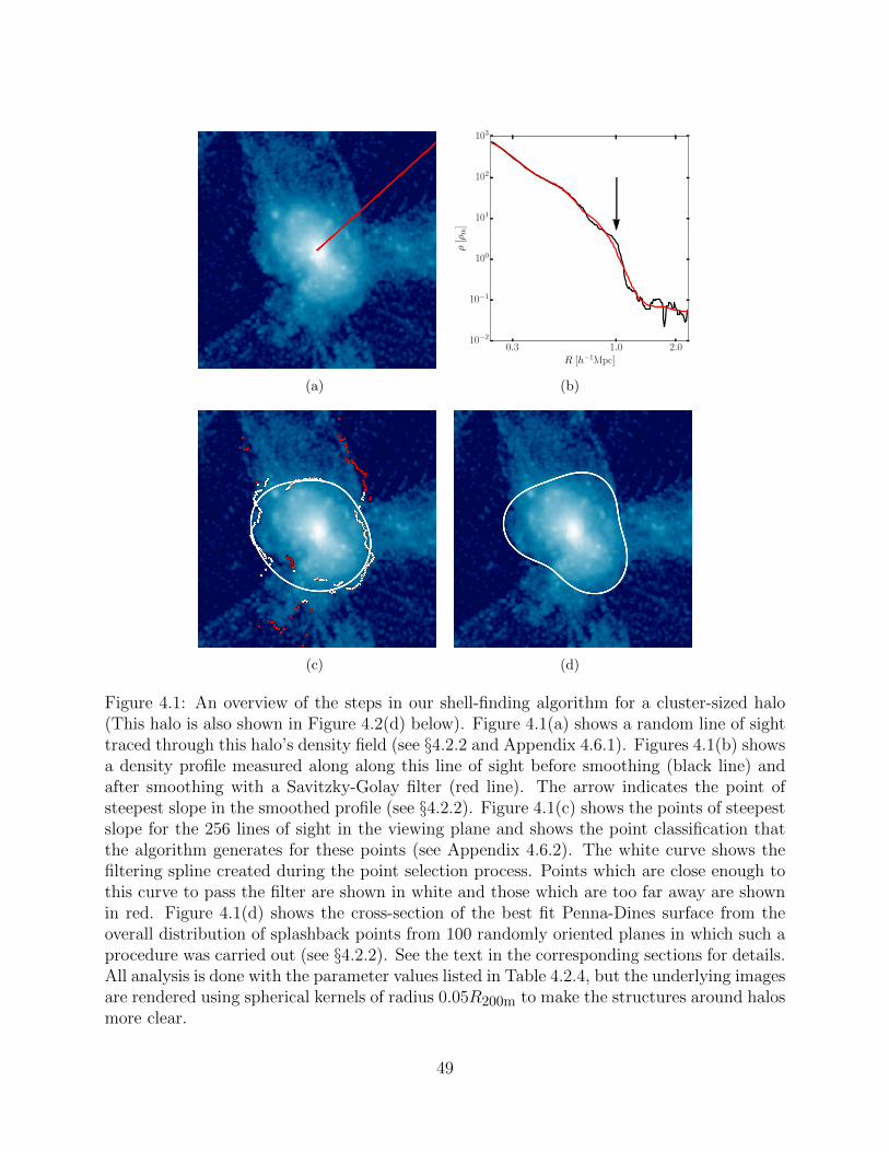
(a)

0.3 1.0 2.0R [h−1Mpc]

10−2

10−1

100

101

102

103

ρ[ρ

m]

(b)

(c) (d)

Figure 4.1: An overview of the steps in our shell-finding algorithm for a cluster-sized halo(This halo is also shown in Figure 4.2(d) below). Figure 4.1(a) shows a random line of sighttraced through this halo’s density field (see §4.2.2 and Appendix 4.6.1). Figures 4.1(b) showsa density profile measured along along this line of sight before smoothing (black line) andafter smoothing with a Savitzky-Golay filter (red line). The arrow indicates the point ofsteepest slope in the smoothed profile (see §4.2.2). Figure 4.1(c) shows the points of steepestslope for the 256 lines of sight in the viewing plane and shows the point classification thatthe algorithm generates for these points (see Appendix 4.6.2). The white curve shows thefiltering spline created during the point selection process. Points which are close enough tothis curve to pass the filter are shown in white and those which are too far away are shownin red. Figure 4.1(d) shows the cross-section of the best fit Penna-Dines surface from theoverall distribution of splashback points from 100 randomly oriented planes in which such aprocedure was carried out (see §4.2.2). See the text in the corresponding sections for details.All analysis is done with the parameter values listed in Table 4.2.4, but the underlying imagesare rendered using spherical kernels of radius 0.05R200m to make the structures around halosmore clear.

49

1. The density field is sampled along tens of thousands 1-d lines of sight anchored at the

center of a halo. The specific design decisions governing how the lines of sight are

oriented and how densities along them are estimated are described in section 4.2.2 and

Appendix 4.6.1, respectively, and are depicted in Figure 4.1(a).

2. The locations of the steepest slope in the density profiles of each line of sight are

estimated using a smoothing filter. This part of the algorithm is described in section

4.2.2 and is depicted in Figure 4.1(c).

3. The set of profiles is pruned to remove the profiles where the point of steepest slope

corresponds to the splashback associated with a nearby halo or filament. The pruning

procedure is described in section 4.2.2 and Appendix 4.6.2 and is depicted in Figure

4.1(c).

4. We fit the 3-d shape of the shell with a smooth, flexible, functional form using the

locations of the steepest slope in the profiles that remain after the pruning step. This

is described in section 4.2.2 and is depicted in Figure 4.1(d).

The design choices made in step 1 are the most important for ensuring good performance

of the algorithm and the design choices made in step 3 are the most important for ensuring

that the identified shells are correct.

The free parameters of the algorithm that will be introduced and discussed in the subse-

quent sections are summarized in Table 4.2.4. The logic and procedures of specific parameter

choices are discussed in Appendix 4.6.3.

Density Estimation Along Lines of Sight

To construct a density profile along a given line of sight we must choose a way to interpolate

particle positions and masses onto that line. For simplicity, we choose to approximate parti-

cles as tophat spheres of radius Rkernel uniform density. Other choices, such as tetrahedral,

50

trilinear, or tricubic tessellations of phase space [e.g., Abel et al., 2012a, Hahn and Angulo,

2016], are also implemented in Shellfish and could in principle be used in this work. How-

ever, we find that these estimators converge slowly and do not allow splashback shells for

halos with N200m . 107 to be identified reliably and thus do not use them in practice. A

detailed convergence study of phase space density estimators will be the subject of future

work.

The algorithm represents every line of sight as an array of Nbins bins logarithmically

distributed between the radii Rmin and Rmax. The density along a line of sight, l, which

passes through a set of constant-density spheres is given by

ρl(r) =i<N∑

i=0

Iintr,ilρiH(r − rin)H(rout − r). (4.1)

Here, i indexes over all particles, Iintr,il is an indicator function which is 1 if l intersects with

the sphere of particle i and is 0 otherwise, ρi is the density of sphere i, H is the Heaviside

step function, and rin and rout are the distances to entrance and exit intersection points of

l for a given sphere, respectively.

Evaluating Equation 4.1 is easy if a conventional estimator (such as cloud-in-cell or SPH)

is used to write densities to an intermediate grid before they are translated onto the lines of

sight, since the grid cell that corresponds to a point at radius r of given ray can be calculated

in O(1) operations. However, using an intermediate grid has a number of disadvantages.

First, maintaining the high-resolution grid required to accurately measure the contours of

the splashback shell consumes a large amount of memory. This restricts the number of halos

which can be maintained in memory at once; when generating large catalogs of shells, this

can force particle catalogs to be read many times, leading to a significant performance cost.

Second, writing the density estimate to a grid is expensive as it involves either an exact

rasterization scheme (see, for example, Powell and Abel 2014) of the objects, or Monte Carlo

sampling of each solid with sufficiently many points to eliminate shot noise in each cell.

51

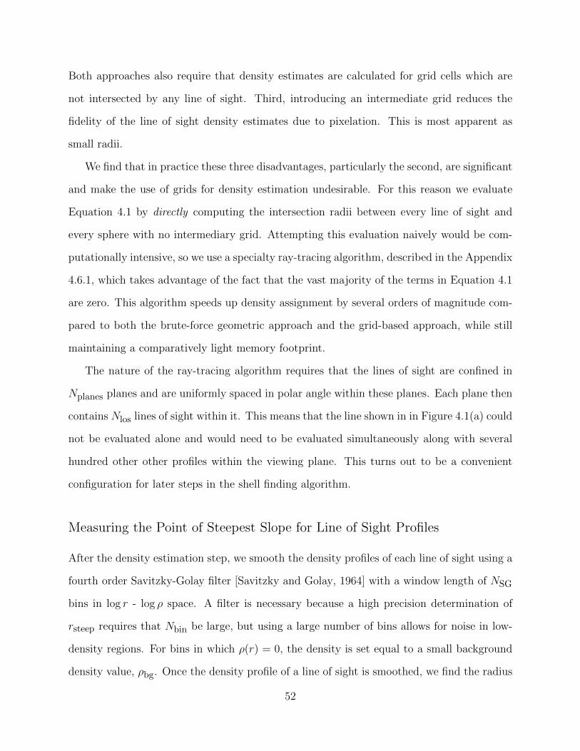
Both approaches also require that density estimates are calculated for grid cells which are

not intersected by any line of sight. Third, introducing an intermediate grid reduces the

fidelity of the line of sight density estimates due to pixelation. This is most apparent as

small radii.

We find that in practice these three disadvantages, particularly the second, are significant

and make the use of grids for density estimation undesirable. For this reason we evaluate

Equation 4.1 by directly computing the intersection radii between every line of sight and

every sphere with no intermediary grid. Attempting this evaluation naively would be com-

putationally intensive, so we use a specialty ray-tracing algorithm, described in the Appendix

4.6.1, which takes advantage of the fact that the vast majority of the terms in Equation 4.1

are zero. This algorithm speeds up density assignment by several orders of magnitude com-

pared to both the brute-force geometric approach and the grid-based approach, while still

maintaining a comparatively light memory footprint.

The nature of the ray-tracing algorithm requires that the lines of sight are confined in

Nplanes planes and are uniformly spaced in polar angle within these planes. Each plane then

contains Nlos lines of sight within it. This means that the line shown in in Figure 4.1(a) could

not be evaluated alone and would need to be evaluated simultaneously along with several

hundred other other profiles within the viewing plane. This turns out to be a convenient

configuration for later steps in the shell finding algorithm.

Measuring the Point of Steepest Slope for Line of Sight Profiles

After the density estimation step, we smooth the density profiles of each line of sight using a

fourth order Savitzky-Golay filter [Savitzky and Golay, 1964] with a window length of NSG

bins in log r - log ρ space. A filter is necessary because a high precision determination of

rsteep requires that Nbin be large, but using a large number of bins allows for noise in low-

density regions. For bins in which ρ(r) = 0, the density is set equal to a small background

density value, ρbg. Once the density profile of a line of sight is smoothed, we find the radius

52

of the steepest logarithmic slope, rsteep.

We choose to use a Savitzky-Golay filter because it is effective at removing small scale

noise and because it generally doesn’t move the location of the point of steepest slope, even

for large window sizes.

We find that the best results are obtained for NSG ≈ Nbin/4 to Nbin/2, as this allows the

filter to remove even moderately large features, such as subhalos. The exact value chosen is

given in Table 4.2.4. For most lines of sight, the density drop associated with crossing the

splashback shell is the most prominent feature in the profile, and thus such an aggressive

filter window does not remove it. The smoothing process will flatten the slope at rsteep, but

the actual value of the slope is not used by our algorithm.

This process is illustrated in Figure 4.1(b), which shows the line of sight highlighted

in Figure 4.1(a). The black curve shows the raw profile after the density estimation step,

the red curve shows the profile after applying a Savitzky-Golay filter with a window size

of NSG = Nbin/2. The vertical arrow shows rsteep for the smoothed profile. This figure

demonstrates several key points. First, the discontinuity due the splashback shell is very

strong. Second, the unsmoothed profile contains several points with slopes steeper than the

splashback discontinuity due to particle noise. Lastly, the location of rsteep has not moved

significantly between the smoothed and unsmoothed profiles.

As mentioned in section 4.2.2 (see also Appendix 4.6.1), the density estimation step of our

algorithm requires that lines of sight are confined to a set of planes. The locations of rsteep for

256 such lines of sight are shown in Figure 4.1(c). This illustrates that, generally, the values

of rsteep found by this step are in good agreement with the visual appearance of density

discontinuities. However, some of the density discontinuities are clearly not associated with

the halo itself but are due to nearby filaments or nearby halos. Although this happens

in the minority of lines of sight, these can bias the shape of the inferred splashback shell

significantly. Therefore, the algorithm makes an additional step in which lines of sight for

which the steepest slope points are likely associated with other halos and filaments are pruned

53

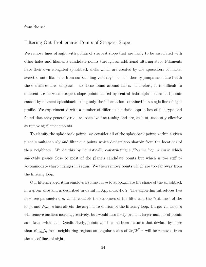
from the set.

Filtering Out Problematic Points of Steepest Slope

We remove lines of sight with points of steepest slope that are likely to be associated with

other halos and filaments candidate points through an additional filtering step. Filaments

have their own elongated splashback shells which are created by the apocenters of matter

accreted onto filaments from surrounding void regions. The density jumps associated with

these surfaces are comparable to those found around halos. Therefore, it is difficult to

differentiate between steepest slope points caused by central halos splashbacks and points

caused by filament splashbacks using only the information contained in a single line of sight

profile. We experimented with a number of different heuristic approaches of this type and

found that they generally require extensive fine-tuning and are, at best, modestly effective

at removing filament points.

To classify the splashback points, we consider all of the splashback points within a given

plane simultaneously and filter out points which deviate too sharply from the locations of

their neighbors. We do this by heuristically constructing a filtering loop, a curve which

smoothly passes close to most of the plane’s candidate points but which is too stiff to

accommodate sharp changes in radius. We then remove points which are too far away from

the filtering loop.

Our filtering algorithm employs a spline curve to approximate the shape of the splashback

in a given slice and is described in detail in Appendix 4.6.2. The algorithm introduces two

new free parameters, η, which controls the strictness of the filter and the “stiffness” of the

loop, and Nrec, which affects the angular resolution of the filtering loop. Larger values of η

will remove outliers more aggressively, but would also likely prune a larger number of points

associated with halo. Qualitatively, points which come from features that deviate by more

than Rmax/η from neighboring regions on angular scales of 2π/2Nrec will be removed from

the set of lines of sight.

54

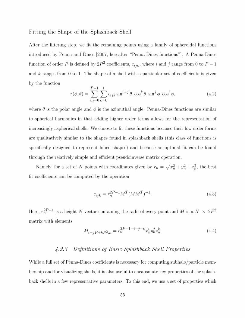
Fitting the Shape of the Splashback Shell

After the filtering step, we fit the remaining points using a family of spheroidal functions

introduced by Penna and Dines [2007, hereafter “Penna-Dines functions”]. A Penna-Dines

function of order P is defined by 2P 2 coefficients, cijk, where i and j range from 0 to P − 1

and k ranges from 0 to 1. The shape of a shell with a particular set of coefficients is given

by the function

r(φ, θ) =P−1∑

i,j=0

1∑

k=0

cijk sini+j θ cosk θ sinj φ cosi φ, (4.2)

where θ is the polar angle and φ is the azimuthal angle. Penna-Dines functions are similar

to spherical harmonics in that adding higher order terms allows for the representation of

increasingly aspherical shells. We choose to fit these functions because their low order forms

are qualitatively similar to the shapes found in splashback shells (this class of functions is

specifically designed to represent lobed shapes) and because an optimal fit can be found

through the relatively simple and efficient pseudoinverse matrix operation.

Namely, for a set of N points with coordinates given by rn =√x2n + y2

n + z2n, the best

fit coefficients can be computed by the operation

cijk = r2P−1n MT (MMT )−1. (4.3)

Here, r2P−1n is a height N vector containing the radii of every point and M is a N × 2P 2

matrix with elements

Mi+jP+kP 2,n = r2P−1−i−j−kn xiny

jnzkn. (4.4)

4.2.3 Definitions of Basic Splashback Shell Properties

While a full set of Penna-Dines coefficients is necessary for computing subhalo/particle mem-

bership and for visualizing shells, it is also useful to encapsulate key properties of the splash-

back shells in a few representative parameters. To this end, we use a set of properties which

55

parameterize the shape of the splashback shells: Rsp, the volume-equivalent splashback ra-

dius; ρsp, the net density of shell; asp, bsp, and csp, the inertia tensor equivalent major axes

of the shell; Esp, the shell ellipticity; and Asp, the shell asphericity:

Rsp ≡(

3Vsp

4π

)1/3

(4.5)

ρsp = Msp/Vsp (4.6)

asp, bsp, csp ≡ Axes(Ix, Iy, Iz) (4.7)

Esp ≡asp

csp− 1 (4.8)

Asp ≡ 1− Ssp

(36πV 2sp)1/3

(4.9)

Here, Vsp is the volume enclosed by the shell, Msp is the mass of all the particles contained

within the shell, Ssp is the surface area of the shell, and Axes(Ix, Iy, Iz) is a function which

computes the axes of a uniform density ellipsoidal shell which has the moments of inertia Ix,

Iy, and Iz. The construction of this function is described in Appendix 4.6.6. In Equation 4.8,

we take the standard convention that asp is the major axis and csp is the minor axis.

Esp is defined such that it is zero for a sphere and increases for increasingly elliptical

shells. Asp is defined such that it is zero for a sphere and increases for increasingly aspherical

shells. Our numerical experiments with randomly-shaped shells indicate that it is probable

that prolate ellipsoids are the surfaces which minimize Asp for a given value of Esp.

4.2.4 Summary of the Algorithm Parameters

The splashback shell finding algorithm described above has 11 free parameters. The pa-

rameters and their adopted fiducial values in in Shellfish are summarized in Table 4.2.4.

Fortunately, there are three empirical properties of this parameter family, which allow for

a fairly straightforward way of choosing their values. First, the shapes of the final splash-

back shells depend only weakly on most of these parameters. Second, the optimal set of

56

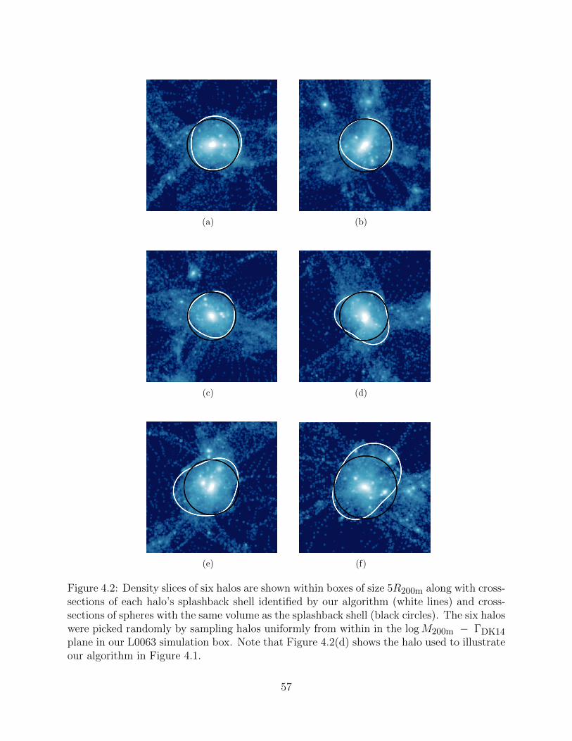
(a) (b)

(c) (d)

(e) (f)

Figure 4.2: Density slices of six halos are shown within boxes of size 5R200m along with cross-sections of each halo’s splashback shell identified by our algorithm (white lines) and cross-sections of spheres with the same volume as the splashback shell (black circles). The six haloswere picked randomly by sampling halos uniformly from within in the logM200m − ΓDK14plane in our L0063 simulation box. Note that Figure 4.2(d) shows the halo used to illustrateour algorithm in Figure 4.1.

57

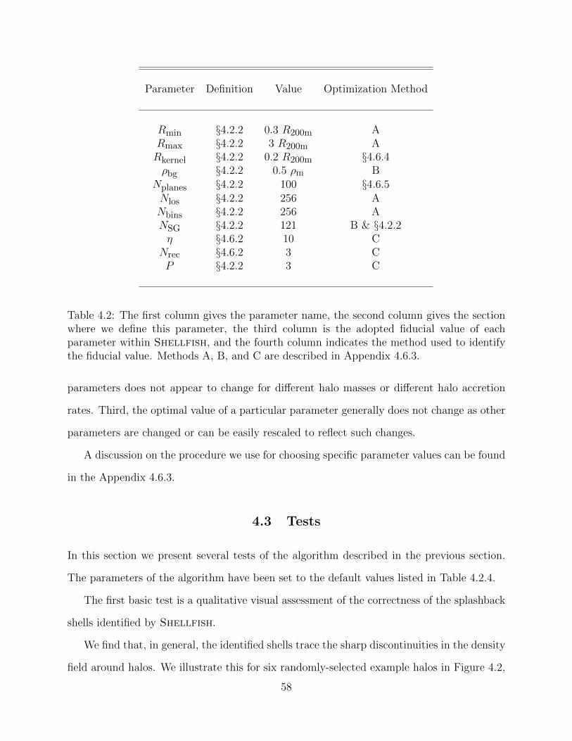
Parameter Definition Value Optimization Method

Rmin §4.2.2 0.3 R200m ARmax §4.2.2 3 R200m ARkernel §4.2.2 0.2 R200m §4.6.4ρbg §4.2.2 0.5 ρm B

Nplanes §4.2.2 100 §4.6.5Nlos §4.2.2 256 ANbins §4.2.2 256 ANSG §4.2.2 121 B & §4.2.2η §4.6.2 10 C

Nrec §4.6.2 3 CP §4.2.2 3 C

Table 4.2: The first column gives the parameter name, the second column gives the sectionwhere we define this parameter, the third column is the adopted fiducial value of eachparameter within Shellfish, and the fourth column indicates the method used to identifythe fiducial value. Methods A, B, and C are described in Appendix 4.6.3.

parameters does not appear to change for different halo masses or different halo accretion

rates. Third, the optimal value of a particular parameter generally does not change as other

parameters are changed or can be easily rescaled to reflect such changes.

A discussion on the procedure we use for choosing specific parameter values can be found

in the Appendix 4.6.3.

4.3 Tests

In this section we present several tests of the algorithm described in the previous section.

The parameters of the algorithm have been set to the default values listed in Table 4.2.4.

The first basic test is a qualitative visual assessment of the correctness of the splashback

shells identified by Shellfish.

We find that, in general, the identified shells trace the sharp discontinuities in the density

field around halos. We illustrate this for six randomly-selected example halos in Figure 4.2,

58

104 105 106

N200m

−0.25

−0.20

−0.15

−0.10

−0.05

0.00

0.05

(Q(N

sub)−Q

(Nfu

ll))/Q

(Nsu

b))

Q = Msp

Q = Rsp

Q = 1 + Asp

Q = 1 + Esp

Figure 4.3: Convergence tests for the properties of splashback shells defined in Equation 4.5 -Equation 4.9 : enclosed mass, Msp, radius of the sphere of equivalent radius, Rsp, ellipticity,Esp, and asphericity, Asp as a function of the number of dark matter particles within R200m,N200m. The vertical dashed line corresponds to N200m = 50, 000, the lower limit used forthe analysis in this chapter, and the shaded vertical region indicates bins which contain twoor fewer halos and are therefore dominated by individual halo error. Within the convergedparticle count range there is typically a scatter of ≈ 2% about the median relation, whichhas not been plotted here for visual clarity. See section 4.3 for details and discussion on thisfigure.

59

where the white curves show the cross-sections of the identified shells and the black circles

show cross-sections of spheres with radii Rsp for those halos. Here Rsp corresponds to the

volume-equivalent definition given in Equation 4.5. While we found that this type of simple

visual inspection proved to be very effective in identifying ineffective filtering algorithms and

parameter sets, it is necessarily a qualitative test and cannot provide a quantitative error

estimate.

In our second test, we compare the values of Rsp measured by Shellfish to halos which

have an unambiguous steepening in their profiles relative to the asymptotic high-R NFW

slope due to the splashback shell. Shellfish is unambiguously incorrect for any halos where

it measures Rsp outside of this steepening region. The difficulty with this test is that is that

it is hard to programmatically detect the extent of this steepening region in a robust way.

Additionally, large substructure and dense filaments can create steepening regions in the

outskirts of host halos which appears similar to the steepening caused by the splashback

shell, but occurs in the wrong locations. For these reasons, we resort to manual inspection

of halos to perform this test.

We inspected the outer profiles of roughly 5,000 z = 0 halos with N200m > 50, 000 and

identified 906 which had a clear steepening of the density profile in their outskirts and did

not have a significant subhalo presence in that region. We then identified the starting and

ending radii that bracketed the steepening region of each of these halos, Rstart and Rend,

by eye. We then compared these radial ranges to Rsp calculated through Equation 4.5. We

found that only four halos had Rsp measurements outside of the ranges measured from the

profiles, corresponding to a minimum failure rate of ≈ 0.5%. Rstart and Rend can span a

wide range of radii (see, e.g., Figure 4.7(a) and Figure 4.16(a)), so this test is not effective at

catching ≈ 20% errors. This test is chiefly sensitive to catastrophic failures, which we found

could be as common as 25% for poorly constructed filtering algorithms or improperly set

parameters. Figure 4.4 shows an example of a typical catastrophic failure. In this case, there

is no strong feature in the surrounding density field which forces Shellfish to generate an

60

Figure 4.4: A density slice around one of the halos which fails the second test described insection 4.3 (i.e. a “catastrophic failure”). The image dimensions and the meanings of thewhite and black curves are identical to those in Figure 4.2. We found that these halos can bevery common for improperly calibrated filtering algorithms, but when the parameters shownin Table 4.2.4 are used, these halos make up only ≈ 0.5% of our total halo population.

unphysical shell. Achieving a low failure rate on this test is a necessary, but not sufficient,

condition for any accurate splashback-measuring code.

As a third test, we also carried out a convergence study of the shell properties defined

in Equations 4.5 - 4.9 with respect to the number of dark matter particles within a halo,

N200m. These were performed by generating a representative sample of halos and fitting

two Penna-Dines shells to each of them. The first shell is calculated using only one eighth

of the halo’s particles and the second is calculated using all the halo’s particles. We use the

notation that the number of particles in subsampled halos is N200m/8 = Nsub, and that the

number of particles in fully sampled halos is N200m = Nfull. The results of this test are

shown in Figure 4.3.

Figure 4.3 shows that for N200m > 50, 000, the systematic error due to particle count in

Msp is at the per cent to sub per cent level, and that the error in Rsp, 1 +Esp, and 1 +Asp

in the same range is at the few per cent level. The shaded region in Figure 4.3 indicates

bins in which our simulation suite produced two or fewer halos. Figure 4.3 indicates that to

identify splashback shells reliably, halos need to be resolved with at least 5× 104 particles.

61

It is not clear to what extent there is a second order trend in radius after the first order

convergence at N200m. It would not be unreasonable to see a trend of this type: as N200m

increases, Shellfish may be able to resolve and fit smaller scale features in halos which

could result in small changes in volume. For this reason, we cannot yet rule out that there

is a systematic . 5% trend with mass for Rsp.

4.3.1 Comparison to Particle Trajectories

As a fourth test of the algorithm, we inspect the trajectories of individual particles near the

splashback shell. Particles near the correctly identified splashback shells can be expected to

be either infalling for the first time or to be at the apocenter of their first orbit. Trajectories

of the infalling particles should be roughly perpendicular to the shell locally and should

not show any deflection when crossing the shell. The trajectories of the particles that have

orbited through the halo should show a sharp turnaround at the shell location. The relative

fractions of particles of these two types will depend on the mass accretion rate of each specific

halo, but the apocenters of particles of the second type should coincide with the identified

splashback shell. Given that our algorithm does not use any information about particles

trajectory, this test is a useful independent check on whether our algorithm identifies shells

corresponding to the actual outermost apocenters of particle orbits.

To perform this test on a target halo, we first use Shellfish to identify a splashback

shell around the halo at some redshift z1 > 0. We then find all particles within some small

distance δ of this shell and track their trajectories through a redshift range z0 < z1 < z2.

The results of such a test are shown for four representative clusters with M200m ≈

1014h−1 M from the L0250 simulation in Figure 4.5, where we used δ = R200m/50, z0 =

0.32, z1 = 0.13, and z2 = 0. The location of the particles at z = z1 is shown by red points.

The trajectories of particles from z0 to z1 are shown as red curves and the trajectories from

z1 to z2 are shown as yellow curves. Infalling particles have red curves pointing outside of

the halo and yellow curves pointing inside the halo. Particles moving outwards have reversed

62

colors: yellow curves pointing to the outside and red curves pointing to the inside. Particles

at their apocenters will have both curves pointing to the inside.

Figure 4.5 shows that for the cluster-sized halos shown, most particles around the splash-

back shell are infalling, as can be expected for rapidly accreting halos. At the same time,

there is a fraction of particles that exhibit a sharp turnaround near the identified splashback

shell: i.e., the apocenters of their orbit coincide with the splashback shell identified from the

density field.

Figure 4.5(c) does show several trajectories in the southern portion of the halo which

travel outside the identified shell. It is not clear whether this is because Shellfish was

unable to identify the correct splashback shell due to the high-density filament or whether

those particles were perturbed from their orbits in later time steps by the nearby subhalo.

Such trajectories, however, are a small fraction of the total.

We have carried out such visual inspection of trajectories for a large number of halos

and found results qualitatively similar to those shown in Figure 4.5. This indicates that

our algorithm is reliably picking out splashback shells that coincide with the most distant

apocenters of particle orbits. This analysis has been confirmed by comparison with an

alternative splashback-measuring code, Sparta, which showed that the radii measured by

Shellfish correspond to high-percentile moments of a halo’s apocenter distribution [Diemer

et al., 2017].

4.4 Results

4.4.1 Sample Selection

To analyze the properties of splashback shells identified using our algorithm we construct

a sample of halos drawn from the halo catalogs of all the simulations listed in Table 4.2.1.

Based on the convergence test results reported in section 4.3 (see Figure 4.3), we select

halos with N200m > 50, 000, so that shell properties are converged to the level . 5%. We

63

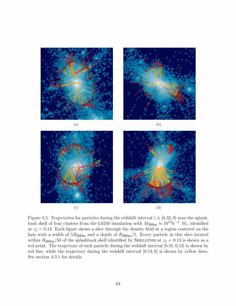
(a) (b)

(c) (d)

Figure 4.5: Trajectories for particles during the redshift interval z ∈ [0.32, 0] near the splash-back shell of four clusters from the L0250 simulation with M200m ≈ 1014h−1 M identifiedat z1 = 0.13. Each figure shows a slice through the density field in a region centered on thehalo with a width of 5R200m and a depth of R200m/5. Every particle in this slice locatedwithin R200m/50 of the splashback shell identified by Shellfish at z1 = 0.13 is shown as ared point. The trajectory of each particle during the redshift interval [0.31, 0.13] is shown byred line, while the trajectory during the redshift interval [0.13, 0] is shown by yellow lines.See section 4.3.1 for details.

64

also restrict the maximum mass of halos drawn from the smaller box simulations so that

the ΓDK14 distribution of the largest halos in those simulations is similar to that of halos

of the same mass in the larger boxes. This limit is imposed because small box size may

limit the mass accretion time of the largest halos, as evolution becomes nonlinear on scales

comparable to the box size. The mass ranges sampled by each box are given in Table 4.2.1.

With these mass limits in place, we construct the halo sample for analysis by subsampling

all host halos within the mass range of each box in such a way as to obtain a uniform

distribution of halos in both logM200m and ΓDK14. This procedure is repeated for z = 0,

z = 0.5, z = 1, and z = 2, resulting in a total sample sizes of 1095, 1198, 846, and 467 halos,

respectively.

4.4.2 Comparison With Stacked Radial Density Profiles

Figure 4.6 presents a comparison between the distribution of Rsp/R200m values measured

by Shellfish and the predictions of stacked profile analysis as a function of accretion rate.

In particular, we choose to compare against the ΓDK14 vs. Rsp/R200m fit reported in More

et al. [2015]. We have chosen z = 0.5 for illustration in this figure, because the z = 0.5 halo

sample contains a good mix of well-converged, high particle-count halos which become more

abundant as redshift decreases, and halos with large accretion rates, which become more

abundant as redshift increases.

The figure shows that at ΓDK14 . 1.5 our algorithm estimates splashback radii similar to

those from stacked profiles, while for ΓDK14 & 1.5, Shellfish estimates progressively larger

Rsp values compared to the values from the stacked profiles. The discrepancy in Rsp/R200m

is ≈ 30% for ΓDK14 ≈ 4. This discrepancy exists at all redshifts.

Given that the tests presented in section 4.3 indicate that our code identifies splashback

shells reliably and estimates their properties to better than 5% accuracy at the resolution

level shown in Figure 4.6, it is highly unlikely that the discrepancy is due to any issue of our

algorithm. In particular, a systematic overestimation of Rsp by 30% would be immediately

65

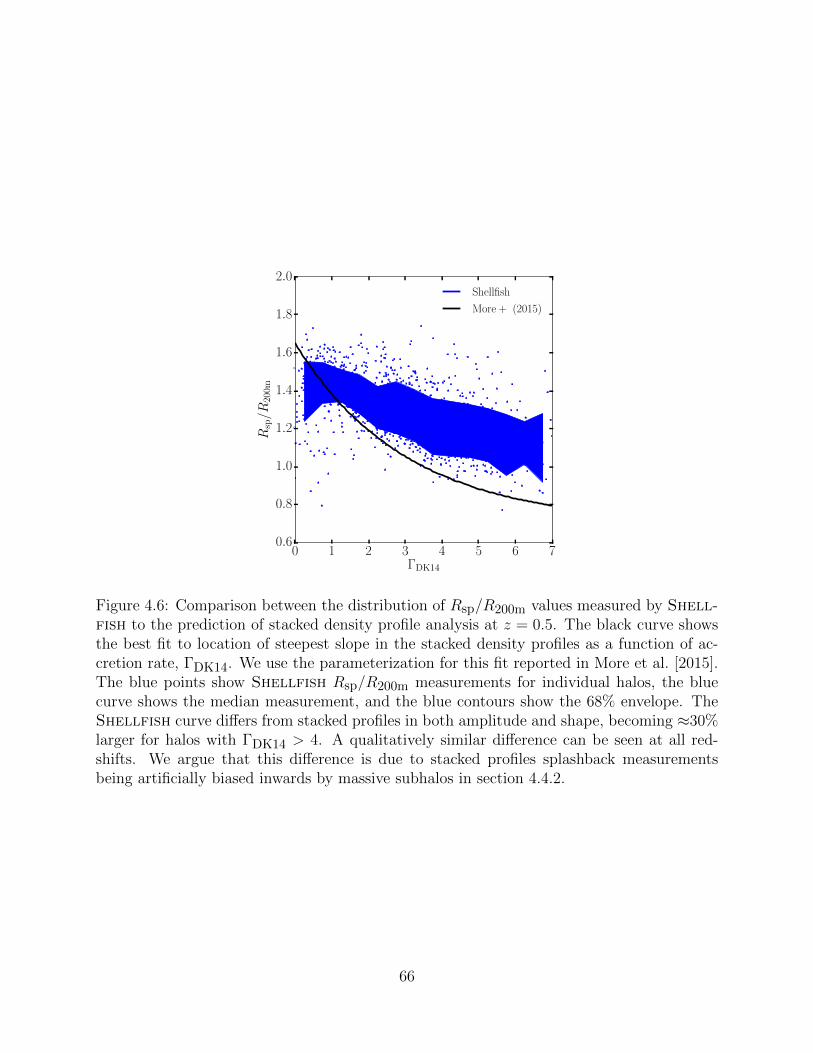
0 1 2 3 4 5 6 7ΓDK14

0.6

0.8

1.0

1.2

1.4

1.6

1.8

2.0R

sp/R

200m

Shellfish

More + (2015)

Figure 4.6: Comparison between the distribution of Rsp/R200m values measured by Shell-fish to the prediction of stacked density profile analysis at z = 0.5. The black curve showsthe best fit to location of steepest slope in the stacked density profiles as a function of ac-cretion rate, ΓDK14. We use the parameterization for this fit reported in More et al. [2015].The blue points show Shellfish Rsp/R200m measurements for individual halos, the bluecurve shows the median measurement, and the blue contours show the 68% envelope. TheShellfish curve differs from stacked profiles in both amplitude and shape, becoming ≈30%larger for halos with ΓDK14 > 4. A qualitatively similar difference can be seen at all red-shifts. We argue that this difference is due to stacked profiles splashback measurementsbeing artificially biased inwards by massive subhalos in section 4.4.2.

66

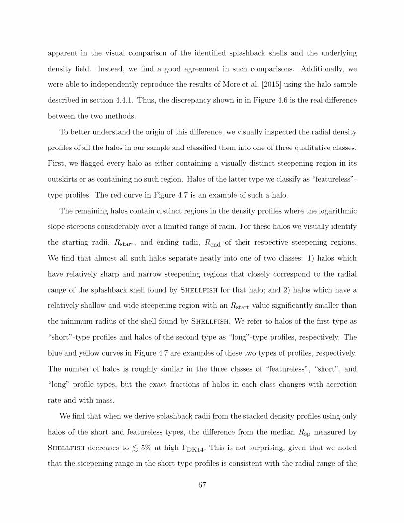
apparent in the visual comparison of the identified splashback shells and the underlying

density field. Instead, we find a good agreement in such comparisons. Additionally, we

were able to independently reproduce the results of More et al. [2015] using the halo sample

described in section 4.4.1. Thus, the discrepancy shown in in Figure 4.6 is the real difference

between the two methods.

To better understand the origin of this difference, we visually inspected the radial density

profiles of all the halos in our sample and classified them into one of three qualitative classes.

First, we flagged every halo as either containing a visually distinct steepening region in its

outskirts or as containing no such region. Halos of the latter type we classify as “featureless”-

type profiles. The red curve in Figure 4.7 is an example of such a halo.

The remaining halos contain distinct regions in the density profiles where the logarithmic

slope steepens considerably over a limited range of radii. For these halos we visually identify

the starting radii, Rstart, and ending radii, Rend of their respective steepening regions.

We find that almost all such halos separate neatly into one of two classes: 1) halos which

have relatively sharp and narrow steepening regions that closely correspond to the radial

range of the splashback shell found by Shellfish for that halo; and 2) halos which have a

relatively shallow and wide steepening region with an Rstart value significantly smaller than

the minimum radius of the shell found by Shellfish. We refer to halos of the first type as

“short”-type profiles and halos of the second type as “long”-type profiles, respectively. The

blue and yellow curves in Figure 4.7 are examples of these two types of profiles, respectively.

The number of halos is roughly similar in the three classes of “featureless”, “short”, and

“long” profile types, but the exact fractions of halos in each class changes with accretion

rate and with mass.

We find that when we derive splashback radii from the stacked density profiles using only

halos of the short and featureless types, the difference from the median Rsp measured by

Shellfish decreases to . 5% at high ΓDK14. This is not surprising, given that we noted

that the steepening range in the short-type profiles is consistent with the radial range of the

67

splashback shells derived by Shellfish, but demonstrates that the difference in Rsp is due

almost entirely to the effect of the halos with the long-type profiles on the stacked density

profile.

Our analysis shows that the steepening region in the density profiles of long-type halos

is not caused by the splashback shell, but by the presence of massive subhalos. Specifically,

visual inspection of the density fields of long-type halos generally reveals that no portion

of the splashback shell can be found as far inwards as Rstart for these halos. Instead, we

almost always find that a massive subhalo is present at R ≈ Rstart for these halos. Thus, the

steepening region is associated with the presence of subhalo, not the splashback. Given that

subhalos in different halos with the same accretion rate will be located at different R, the

combined effect of the massive subhalos on the stacked profile is to “wash out” the signature

of the splashback shell and to bias the start of the steepening region to smaller radii.

Thus, halos with no massive subhalos in the outskirts have the short-type profiles, while

those that do have such subhalos have long-type profiles. Halos that either have large

neighboring halos outside their splashback shells or which exist in dense filaments have the

steepening due to splashback shell erased completely and thus have featureless-type profiles.

The expectation is then that if contribution of massive subhalos is removed from the density

profiles the Rsp derived from the stacked density profiles should be consistent with the values

estimated by Shellfish. We demonstrate that this is the case in the next subsection.

4.4.3 Angular Median Density Profiles of Halos

There are many possible ways of mitigating the contribution of subhalos to the density

profiles of their host halos. We choose one of the simplest methods for doing this, one which

does not rely on the availability of robust subhalo catalogs, and which could, in principle, be

adapted for use on observed galaxy clusters. The idea is to construct density profiles using

the median estimate of density in each radial shell instead of the mean density. A similar

approach has been used in the analysis of the gas distribution in clusters [Zhuravleva et al.,

68

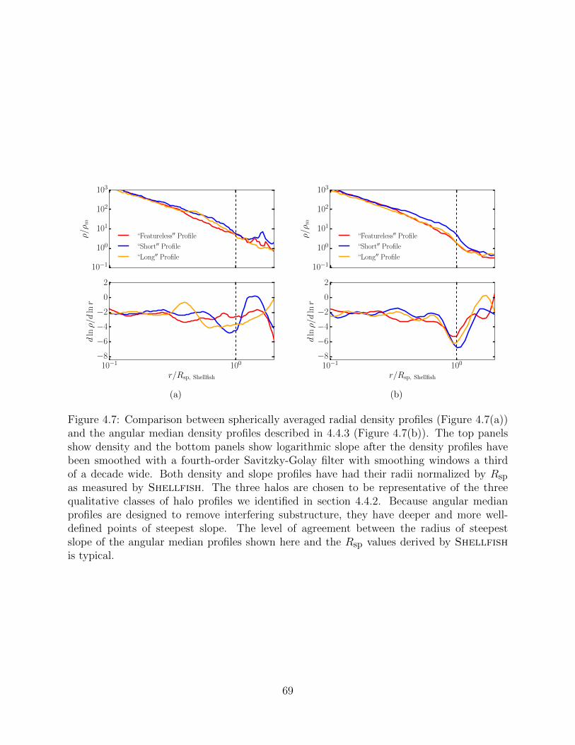
10−1

100

101

102

103

ρ/ρ

m

“Featureless′′ Profile

“Short′′ Profile

“Long′′ Profile

10−1 100

r/Rsp, Shellfish

−8

−6

−4

−2

0

2

dlnρ/d

lnr

(a)

10−1

100

101

102

103

ρ/ρ

m

“Featureless′′ Profile

“Short′′ Profile

“Long′′ Profile

10−1 100

r/Rsp, Shellfish

−8

−6

−4

−2

0

2

dlnρ/d

lnr

(b)

Figure 4.7: Comparison between spherically averaged radial density profiles (Figure 4.7(a))and the angular median density profiles described in 4.4.3 (Figure 4.7(b)). The top panelsshow density and the bottom panels show logarithmic slope after the density profiles havebeen smoothed with a fourth-order Savitzky-Golay filter with smoothing windows a thirdof a decade wide. Both density and slope profiles have had their radii normalized by Rsp

as measured by Shellfish. The three halos are chosen to be representative of the threequalitative classes of halo profiles we identified in section 4.4.2. Because angular medianprofiles are designed to remove interfering substructure, they have deeper and more well-defined points of steepest slope. The level of agreement between the radius of steepestslope of the angular median profiles shown here and the Rsp values derived by Shellfishis typical.

69

2013].

Namely, we split each radial shell of the density profile into N solid angle segments,

e.g., using a two-hemisphere variation on the algorithm described by Gringorten and Yepez

[1992], or the HEALPix pixelation algorithm [Gorski et al., 2005]. We then estimate density,

ρi(r), for each segment i and construct the halo density profile by taking the median of

these densities in each radial shell, ρmed(r) = med [ρi(r)]. This approach is based on the

basic intuition that subhalos are generally much smaller in extent than the host and thus

contribute to a fraction of the solid angle in a given radial shell, while most of the solid

angle will be dominated by the diffuse matter of the host halo. The median density then will

estimate the density of that diffuse component and will be largely insensitive to the outlier

solid angle segments associated with massive subhalos.

Figure 4.7 shows comparisons between usual spherically averaged mean density profiles,

ρ(r), and angular median density profiles ρmed(r) for three representative halos of the dif-

ferent classes described in section 4.4.2. The comparison of the profiles in the two panels

of the figure shows that the angular median profiles of the halos are much more similar to

each other than the mean profile. Unlike the mean density profiles, which have very different

shapes, the angular median density profiles all behave similarly: there is a narrow, sharp

steepening region in the logarithmic profile centered on the radius that Shellfish reports

as Rsp. Thus, the diversity of profile types noted in 4.4.2 is largely absent for profiles of this

type. We also note that the point of steepest slope in angular median profiles is significantly

sharper than it is in mean profiles. Thus the signature of the splashback shell is easier to

detect when halos are analyzed in this way.

To compare Rsp,shell measured by Shellfish to Rsp,med derived from the individual

angular median profiles, we follow the procedure described above for every halo in the sample

described in section 4.4.1. We use 50 solid angle segments per halo with 30 logarithmically-

distributed radial bins per decade. This relatively coarse spacing is needed to make up for the

fifty-fold loss in number statistics and has a non-trivial impact on the maximum fidelity of our

70

angular median profiles: the width of every bin is 8% of the radius at which is occurs. Once

the median profile is computed from these segments, we apply a Savitzky-Golay smoothing

filter with a window size comparable to the characteristic radial width of the regions where

profile slope steepens quickly. We set the window size to a 0.33 dex with the caveat that other

reasonable choices, such as a sixth of half of dex, can induce systematic changes to the mean

Rsp,med of a halo population of ≈ 5%. Thus, the population statistics on Rsp,med cannot be

trusted to accuracies smaller than 5% regardless of any additional statistical error bars, and

that individual Rsp,med values measured this way cannot be measured more accurately than

13%, regardless of additional profile noise. We leave more nuanced accuracy analysis on this

method to a future work, but note that this level of accuracy is sufficient for our purposes,

which is merely to test whether reducing effect of subhalos on the radial profiles results in

Rsp estimates which are qualitatively consistent with the results of Shellfish.

We compare the M200m and ΓDK14 trends between Rsp,shell and Rsp,med for our z = 0.5

halo sample in Figure 4.8 and see fairly good agreement. The high ΓDK14 disagreement has

dropped from & 30% to ≈ 5%. This is consistent with the known systematic uncertainties

in both methods and confirms that the high ΓDK14 disagreement with the estimates of the

splashback radius from the stacked mean density profiles is due to the bias introduced into

these profiles by massive subhalos.

At the same time, at ΓDK14 . 0.5 there is ≈ 15% disagreement between Rsp derived

from the stacked angular median profiles and the median measurements of Shellfish. In

principle, this difference could be caused by either the angular median profile method or

Shellfish, but comparison against another splashback-measuring code, Sparta, which ex-

plicitly tracks particle orbits to find their apocenters, shows tight agreement with Shellfish

at ΓDK14 > 0.5 and a level of discrepancy comparable to that seen for angular median pro-

files at ΓDK14 < 0.5. An extended discussion on how these two methods compare against

one another can be found in Diemer et al. [2017].

It is not surprising that the splashback shell is difficult to measure at these accretion rates.

71

0 1 2 3 4 5 6 7 8ΓDK14

0.8

1.0

1.2

1.4

1.6

1.8

Rsp/R

200m

More et al. (2015)

1012h−1M < M200m < 1013h−1M

1013h−1M < M200m < 1014h−1M

1014h−1M < M200m < 1015h−1M

Shellfish

Median

(a)

0 1 2 3 4 5 6 7 8ΓDK14

−0.20

−0.15

−0.10

−0.05

0.00

0.05

0.10

0.15

0.20

Rm

edia

n/R

Sh

ellfi

sh−

1

z = 0

z = 0.5

z = 1

z = 2

(b)

Figure 4.8: Comparison between the mean Rsp/R200m values measured by Shellfish andby the angular median profile method described in section 4.4.3. The left panel showsmeasurements made by the two methods for different ΓDK14 and M200m bins at z = 0.5.Shellfish measurements are shown as circles on the left side of their respective ΓDK14 bins,and angular median profile measurements are shown as triangles on the right side of theirrespective ΓDK14 bins. Error bars represent only the bootstrapped error on the mean anddo not account for known systematic uncertainty in the angular median profile method (seesection 4.4.3). The right panel shows the median value of RShellfish/Rmedian − 1, for everyhalo in our sample at z = 0, 0.5, 1, and 2. The dashed blue lines show the shape of this curvewhen the angular median profile’s Savitzky-Golay window width is varied to the edges of itsphysically reasonable value range to give a sense of the systematic variability in this method(see section 4.4.3). These two figures illustrate that when large subhalos are removed fromthe density profiles of halos, the location of the point of steepest slope becomes consistentwith the value of Rsp measured by Shellfish. They also illustrate that there is a non-trivialdisagreement between the two methods for very small ΓDK14.

72

At z = 0, pseudo-evolution causes static NFW halos with cvir & 7 to report ΓDK14 > 0.5

purely due to the cosmological evolution of ρm [Diemer et al., 2013b]. This means that the

majority of halos with accretion rates this low must be actively losing particles in order to

offset their illusory accretion rates caused by pseudo-evolution. This particle loss is typically

caused by dense environments, either because the halo is embedded in a massive filament

feeding a cluster or because it is about to merge with a larger halo.

For this reason we believe that our algorithm should not be used to measure halos with

ΓDK14 < 0.5 unless & 15%-level systematic errors are acceptable. We exclude such halos

from all subsequent analysis. This is an aggressive cut for Milky Way-sized halos at low

redshifts, where 20% of halos have ΓDK14 < 0.5. The cut is less severe for halos in all other

mass bins and at all other redshifts, affecting less than 5% of halos in all such parameter

slices. Clusters and high redshift halos in particular are almost completely unaffected by

this cutoff.

4.4.4 The Relationship Between Mass, Accretion Rate, and Splashback

Radius

One of the key results obtained by previous analyses of splashback shells using stacked radial

density profiles [Diemer and Kravtsov, 2014, More et al., 2015, 2016, Adhikari et al., 2016]

is the dependence of the splashback radius in units of the R200m on the mass accretion

rate ΓDK14 (see Equation 3.14): halos with larger accretion rates have smaller values of

Rsp/R200m ≡ Rsp. In this section we present the result of fits to Rsp using the measurements

from Shellfish.

Specifically, we fit the following log-normal distribution to Rsp as a function of ν200m,

73

1 2 3 4 5 6 7ΓDK14

1.0

1.1

1.2

1.3

1.4

1.5

Rsp/R

200m

z = 0.00.75 < ν200m < 1.50

1.50 < ν200m < 2.25

2.25 < ν200m < 3.00

3.00 < ν200m < 3.75

1 2 3 4 5 6 7ΓDK14

1.0

1.1

1.2

1.3

1.4

1.5

Rsp/R

200m

z = 0.50.75 < ν200m < 1.50

1.50 < ν200m < 2.25

2.25 < ν200m < 3.00

3.00 < ν200m < 3.75

1 2 3 4 5 6 7ΓDK14

1.0

1.1

1.2

1.3

1.4

1.5

Rsp/R

200m

z = 1.00.75 < ν200m < 1.50

1.50 < ν200m < 2.25

2.25 < ν200m < 3.00

3.00 < ν200m < 3.75

1 2 3 4 5 6 7ΓDK14

1.0

1.1

1.2

1.3

1.4

1.5

Rsp/R

200m

z = 2.01.50 < ν200m < 2.25

2.25 < ν200m < 3.00

Figure 4.9: Comparison between our fit and Shellfish’s measurements of Rsp/R200m ≡Rsp(ΓDK14, ν200m, z). The thick lines represent the median value of Rsp/R200m in eachΓDK14 bin and the shaded regions indicate the 68% errors on those medians, as determinedby bootstrapping. The thin lines show the median of the distribution given by Equations4.10 -4.12 evaluated at the median ν200m value within the corresponding ν200m bin.

74

1 2 3 4 5 6 7ΓDK14

1.0

1.1

1.2

1.3

1.4

1.5

Msp/M

200m

z = 0.00.75 < ν200m < 1.50

1.50 < ν200m < 2.25

2.25 < ν200m < 3.00

3.00 < ν200m < 3.75

1 2 3 4 5 6 7ΓDK14

1.0

1.1

1.2

1.3

1.4

1.5

Msp/M

200m

z = 1.00.75 < ν200m < 1.50

1.50 < ν200m < 2.25

2.25 < ν200m < 3.00

3.00 < ν200m < 3.75

Figure 4.10: Comparison between our fit and Shellfish’s measurements for Msp/M200m ≡Msp(ΓDK14, ν200m, z). The visualization scheme is identical to the one used in Figure 4.10,with the thin line corresponding to the median of the distribution given by Equations 4.13and 4.14. Note that unlike the fit displayed in Figure 4.9, our Msp has no ν200m dependence,so only a single thin line is plotted. There are several important caveats to this fit, whichwe discuss in section 4.4.5.

−0.2 0.0 0.2 0.4 0.6 0.8log10(ΓDK14)

0.00

0.05

0.10

0.15

log 1

0(M

sp/M

200)

Figure 4.11: Comparison between the Msp median and 68% contours for our data and ourfit given by Equations 4.13 and 4.14 at z = 0. This Figure was made to emphasize theweaknesses in our Msp fit and shows an ≈ 2% − 4% overestimation of the median at highΓDK14 and a similar overestimation of the logarithmic scatter, σdex. An extended discussionof this Figure can be found in section 4.4.5.

75

ΓDK14, and Ωm:

P (Rsp) ∝ exp(− log210(Rsp/Rmed)/2σ2

dex), (4.10)

Rmed = (R0Ωm +R1) exp (αΓDK14) + A, (4.11)

α = η0Ω2m + η1Ωm + η2 + ξν200m. (4.12)

Here R0, R1, A, ξ, η0, η1, and η2 are fit parameters.

As discussed above, our sample only includes halos with ΓDK14 > 0.5. We fit the func-

tional form given by Equations 4.10–4.12 using an implementation of the affine-invariant

Markov Chain Monte Carlo sampling algorithm of Goodman and Weare [2010]. We also

adopt a Heaviside prior on the logarithmic scatter, σdex, to prevent it from becoming non-

positive.

We find that the best fit parameters are

R0 = 0.2181, η0 = −0.1742,

R1 = 0.4996, η1 = 0.3386,

A = 0.8533, η2 = −0.1929,

ξ = −0.04668, σdex = 0.046.

The resulting function is plotted against our data in Figure 4.9.

It is interesting that the radii estimated by Shellfish exhibit a strong dependence on

both mass accretion rate and peak height. This trend can also be seen in other methods

for measuring individual splashback shells around halos, such as the median angular pro-

file method described in section 4.4.3 and the apocenter-based splashback-measuring code

Sparta [Diemer et al., 2017]. The trend cannot be attributed to convergence trends because

all halos used in the sample have N200m above the convergence limit of 5 × 104 found in

section 4.3 and because the mass bounds given in Table 4.2.1 restrict the halos in our sample

76

to a single decade in particle count.

Previous estimates from stacked density profiles only found a strong dependence on

ΓDK14, while a ν200m dependence was either not apparent or weak [e.g., More et al., 2015].

The ν200m dependence is also not predicted in the collapse models of isolated peaks [e.g.,

Adhikari et al., 2014], even though they successfully predict a ΓDK14 dependence. The origin

of the ν200m dependence and the seeming discrepancy with the collapse model is not clear.

Additionally, although we have made an empirical argument that stacked profiles are biased

by massive subhalos, we do not yet propose a physical picture for why this bias should also

erase or decrease trends with ν200m.

4.4.5 Splashback Shell Masses

In contrast to overdensity-based halo definitions, Msp and Rsp are independent (albeit cor-

related) quantities. For this reason we do not fit the same functional form to both Rsp and

Msp. We fit the following log-normal distribution to Msp ≡ Msp/M200m as a function of

ΓDK14 and Ωm:

P (Msp) ∝ exp(− log210(Msp/Mmed)/2σ2

dex), (4.13)

Mmed = (M0Ωm +M1)

(ΓDK14

Γpivot

)α0Ωm+α1. (4.14)

Here Γpivot = 3 is a characteristic pivot value, and M0, M1, α0, and α1 are fit parameters.

Using the same procedure described in section 4.4.4 we obtain the parameters

A0 = 0.192 a0 = −0.0781

A1 = 1.072 a1 = −0.0284

σdex = 0.054

77

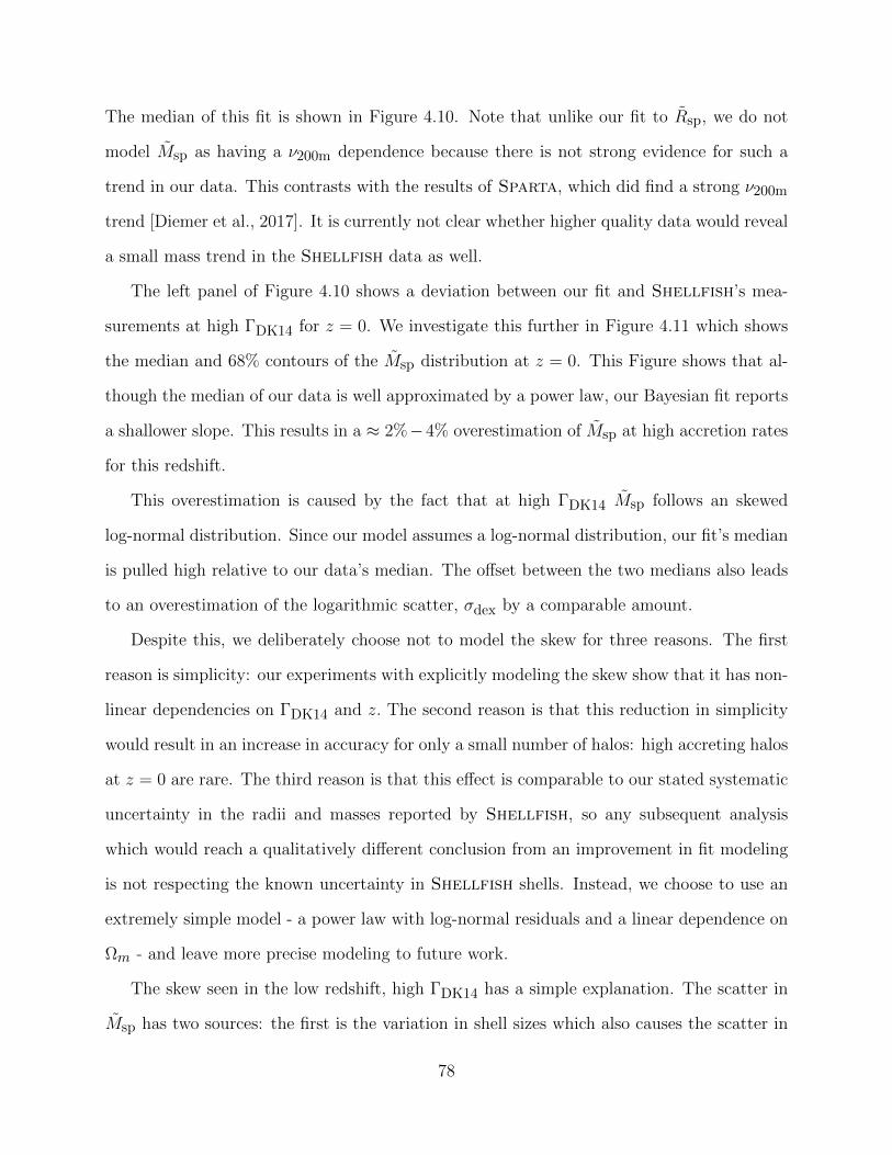
The median of this fit is shown in Figure 4.10. Note that unlike our fit to Rsp, we do not

model Msp as having a ν200m dependence because there is not strong evidence for such a

trend in our data. This contrasts with the results of Sparta, which did find a strong ν200m

trend [Diemer et al., 2017]. It is currently not clear whether higher quality data would reveal

a small mass trend in the Shellfish data as well.

The left panel of Figure 4.10 shows a deviation between our fit and Shellfish’s mea-

surements at high ΓDK14 for z = 0. We investigate this further in Figure 4.11 which shows

the median and 68% contours of the Msp distribution at z = 0. This Figure shows that al-

though the median of our data is well approximated by a power law, our Bayesian fit reports

a shallower slope. This results in a ≈ 2%−4% overestimation of Msp at high accretion rates

for this redshift.

This overestimation is caused by the fact that at high ΓDK14 Msp follows an skewed

log-normal distribution. Since our model assumes a log-normal distribution, our fit’s median

is pulled high relative to our data’s median. The offset between the two medians also leads

to an overestimation of the logarithmic scatter, σdex by a comparable amount.

Despite this, we deliberately choose not to model the skew for three reasons. The first

reason is simplicity: our experiments with explicitly modeling the skew show that it has non-

linear dependencies on ΓDK14 and z. The second reason is that this reduction in simplicity

would result in an increase in accuracy for only a small number of halos: high accreting halos

at z = 0 are rare. The third reason is that this effect is comparable to our stated systematic

uncertainty in the radii and masses reported by Shellfish, so any subsequent analysis

which would reach a qualitatively different conclusion from an improvement in fit modeling

is not respecting the known uncertainty in Shellfish shells. Instead, we choose to use an

extremely simple model - a power law with log-normal residuals and a linear dependence on

Ωm - and leave more precise modeling to future work.

The skew seen in the low redshift, high ΓDK14 has a simple explanation. The scatter in

Msp has two sources: the first is the variation in shell sizes which also causes the scatter in

78

Rsp, the second is the presence or non-presence of high mass subhalos. Since halos with high

accretion rates are more likely to have high mass subhalos than halos with low accretion

rates, the second effect is particularly important for them. If a halo has a massive subhalo

outside of R200m but inside its splashback shell, Msp is scattered high. If a halo has a massive

subhalo inside R200m, both M200m and Msp increase, so Msp scatters towards 1. When the

median of the of the Msp distribution is close to 1, this means that the presence of massive

subhalos has the effect of reducing down scatter and increasing upscatter relative to what

we would expect from variation in shell sizes alone.

4.4.6 Splashback Shell Overdensities

We model the distribution of ∆sp ≡ 200Msp/R200m by taking the ratios of our mass fit

(Equations 4.13 and 4.14) and our radius fit (Equations 4.10 - 4.12). Because our ∆sp

model is derived from our Msp fit, it is subject to the same caveats discussed in section

4.4.5. However, because the dynamic range of ∆sp is larger than that of Msp, the affect of

a few-percent disparity in masses is minimal.

This ratio is shown in Figure 4.12. Median overdensities range between ≈ 70 and ≈ 200

with strong dependencies on peak height, accretion rate, and redshift. The most important

consequence of these relations is that there is not a single classical overdensity boundary

which corresponds to to the splashback shell.

4.4.7 Splashback Shell Shapes

We also investigate the shapes of splashback shells using the asphericity, Asp, and ellipticity,

Esp, parameters defined in Equations 4.9 and 4.8, respectively. A plot of these two quantities

is shown in Figure 4.13. The shaded blue region shows the values of these parameters for

ellipsoids with different axis ratios. The fact that Asp and Esp for all splashback shells

lie above the shaded regions means that the shells are significantly more aspherical than

ellipsoids.

79

1 2 3 4 5 6 7ΓDK14

50

100

150

200

250

∆sp

z = 0.00.75 < ν200m < 1.50

1.50 < ν200m < 2.25

2.25 < ν200m < 3.00

3.00 < ν200m < 3.75

1 2 3 4 5 6 7ΓDK14

50

100

150

200

250

∆sp

z = 1.00.75 < ν200m < 1.50

1.50 < ν200m < 2.25

2.25 < ν200m < 3.00

3.00 < ν200m < 3.75

Figure 4.12: Comparison between our fits and Shellfish’s measurements for ∆sp ≡200Msp/R200m using the ratio of our mass and radius fits. The visualization scheme isidentical to the one used in Figure 4.10, with the thin line corresponding to the median ofthe distribution given by Equations 4.13 and 4.14. There are several important caveats tothis fit, which we discuss in section 4.4.5.

We perform checks for correlation between Asp, Esp and each of M200m, ΓDK14, Rsp,

and redshift, but find no evidence of such correlations.

We also calculated the angle θ∆ between the major axis of a halo’s splashback shell

and the major axis of the underlying dark matter distribution, as reported by the Rockstar

halo finder [Behroozi et al., 2013a]. In Figure 4.14 we show the correlation function for the

angle between these two axes, θ∆. We find anti-correlation at high values of θ∆ and a high

degree of correlation at low values of θ∆, indicating that splashback shells are preferentially

aligned with major axis of the central dark matter distribution. This is consistent with

earlier studies, which have shown that the axis ratios of the matter distribution near the

centers of halos tend to be roughly aligned with the axis ratios near the outskirts of halos

[Jing and Suto, 2002].

80

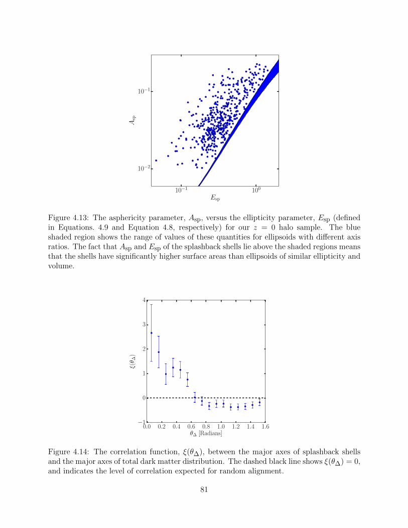
10−1 100

Esp

10−2

10−1

Asp

Figure 4.13: The asphericity parameter, Asp, versus the ellipticity parameter, Esp (definedin Equations. 4.9 and Equation 4.8, respectively) for our z = 0 halo sample. The blueshaded region shows the range of values of these quantities for ellipsoids with different axisratios. The fact that Asp and Esp of the splashback shells lie above the shaded regions meansthat the shells have significantly higher surface areas than ellipsoids of similar ellipticity andvolume.

0.0 0.2 0.4 0.6 0.8 1.0 1.2 1.4 1.6θ∆ [Radians]

−1

0

1

2

3

4

ξ(θ ∆

)

Figure 4.14: The correlation function, ξ(θ∆), between the major axes of splashback shellsand the major axes of total dark matter distribution. The dashed black line shows ξ(θ∆) = 0,and indicates the level of correlation expected for random alignment.

81

4.5 Summary and Conclusions

In this chapter we presented a new algorithm which identifies the splashback shells around

individual halos in simulations. These shells are caused by the caustics formed by matter

at the first apocenter of their orbits around the halo and correspond to rapid drops in the

density field. Our algorithm relies only on the density distribution within a single simulation

snapshot, and is capable of identifying shells with highly aspherical shapes.

We implemented our algorithm in the publicly available1 code Shellfish and performed

extensive tests on the correctness of this code. We performed convergence tests on the

splashback shells found by our code and found that above a convergence limit of N200m =

5× 104, Shellfish can measure properties of splashback shells with . 5% systematic error

(see Figure 4.3 and Figure 4.8(b)) and percent-level stochastic error (see Figure 4.16(b)).

However, we identified a sub-population of halos with low mass accretion rates, ΓDK14 . 0.5,

for which the splashback shell radii estimated by Shellfish are biased low by & 10%. We

therefore recommend that our code not be used for measurements of splashback shells for

halos with ΓDK14 < 0.5. This cutoff removes 20% of Milky Way-sized halos at z = 0 and

has a negligible effect on all larger mass scales and all earlier redshift slices.

We presented the first measurements of several basic properties of splashback shells which

are summarized below:

1. We confirmed that splashback radii generally decrease with increasing mass accretion

rate, as previously found by analyses of stacked halo density profiles. However, we

found that the splashback radii found by Shellfish are larger than these earlier

estimates by 20%-30% for halos with high accretion rates, ΓDK14 & 3. We showed

that the estimate of the splashback radius obtained from the stacked density profiles

is biased low due to the existence of high-mass subhalos in many of these profiles.

2. We used a simple method, completely independent from Shellfish, for mitigating

1. github.com/phil-mansfield/shellfish

82

the effect of substructure on density profiles: the so-called “angular median profile”

method. In this method, radial shells are split into solid angle segments with an

estimate of density in each segment. The halo density at a given radius is then taken to

be the median of all the segments in the corresponding shell. We showed that the effect

of subhalos on these profiles is greatly reduced. Moreover, the angular median profiles

are more self-similar in their outskirts and exhibit a sharper region of profile steepening

(i.e., a much more distinct splashback feature). We showed that the splashback radii

estimated from the stacked angular median profiles are in good agreement with the

results of Shellfish for halos with ΓDK14 & 0.5.

3. We investigated the correlation between splashback radius and mass accretion rate,

the scatter around it, and its evolution with redshift. We presented the first evidence

that the splashback radius depends not only on accretion rate, but also has a strong

dependence on the peak height, ν200m, with larger ν200m halos having systematically

smaller Rsp/R200m at a fixed ΓDK14 and z. We found that the scatter of Rsp/R200m

around the median at a given accretion rate is significant, exceeding 10%. We provided

an accurate fit for Rsp/R200m and its scatter as a function of ΓDK14, ν200m, and Ωm

(see Equations 4.10-4.12 and Figure 4.9). We provided a similar fit for Msp/M200m

(see Equations 4.13 and 4.14 and Figure 4.10). Unlike our fit to Rsp, there are several

minor caveats to our Msp fit, which we discuss in section 4.4.5.

4. We argued that a single classical overdensity density cannot be used as a model of

the location of Rsp because the overdensity of splashback shells have a large dynamic

range and have strong dependencies on mass, accretion rate, and redshift.

5. We studied the shapes of the splashback shells using an ellipticity parameter, Esp, and

an asphericity parameter, Asp (defined in Equations 4.8 and 4.9, respectively). We

showed that splashback shells are generally highly aspherical, with non-ellipsoidal oval

shapes being particularly common.

83

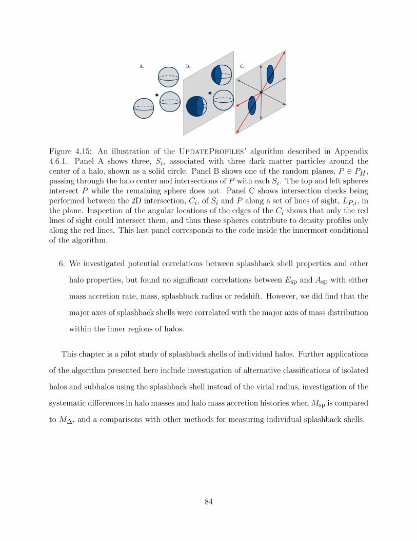
A. B. C.

Figure 4.15: An illustration of the UpdateProfiles’ algorithm described in Appendix4.6.1. Panel A shows three, Si, associated with three dark matter particles around thecenter of a halo, shown as a solid circle. Panel B shows one of the random planes, P ∈ PH ,passing through the halo center and intersections of P with each Si. The top and left spheresintersect P while the remaining sphere does not. Panel C shows intersection checks beingperformed between the 2D intersection, Ci, of Si and P along a set of lines of sight, LP,i, inthe plane. Inspection of the angular locations of the edges of the Ci shows that only the redlines of sight could intersect them, and thus these spheres contribute to density profiles onlyalong the red lines. This last panel corresponds to the code inside the innermost conditionalof the algorithm.

6. We investigated potential correlations between splashback shell properties and other

halo properties, but found no significant correlations between Esp and Asp with either

mass accretion rate, mass, splashback radius or redshift. However, we did find that the

major axes of splashback shells were correlated with the major axis of mass distribution

within the inner regions of halos.

This chapter is a pilot study of splashback shells of individual halos. Further applications

of the algorithm presented here include investigation of alternative classifications of isolated

halos and subhalos using the splashback shell instead of the virial radius, investigation of the

systematic differences in halo masses and halo mass accretion histories when Msp is compared

to M∆, and a comparisons with other methods for measuring individual splashback shells.

84

4.6 Appendices

4.6.1 An Algorithm for Fast Line of Sight Density Estimates

In this Appendix we describe the method our algorithm uses to construct density profiles

along a set of lines of sight via the evaluation of Equation 4.1. Generally, this can be

broken up into two steps: first, the set of all spheres which intersect with a particular

halo, H, is found, and second, for every sphere, S, which intersects with H a procedure

UpdateProfiles(S, H) is run, which evaluates a term in Equation 4.1 corresponding to

S for every line of sight in H.

In general, the first step is straightforward to perform efficiently. Even rudimentary

spatial partitioning (such as breaking the simulation’s particles into ≈ 102 − 103 spatially

coherent segments) results in this step being highly subdominant to the second, making Up-

dateProfiles the only performance bottleneck of this algorithm. A naive implementation

of UpdateProfiles would look like the following:

procedure UpdateProfiles(S, H)

for each L in LH do

if S intersects L then

Renter, Rexit ← IntersectionRadii(L, S)

InsertToProfile(L, ρS, Renter, Rexit)

end if

end for

end procedure

Here, LH is the set of all line of sight profiles belonging to the halo H and ρS is the

density of the sphere S. The existence of two simple functions has been assumed: Inter-

sectionRadii(L, S) calculates the radii at which the line of sight L enters and exits the

sphere S, respectively, and InsertToProfile(L, ρ, R, R′) inserts a rectangular function

with amplitude ρ between R and R′ to the profile corresponding to the line of sight L.

85

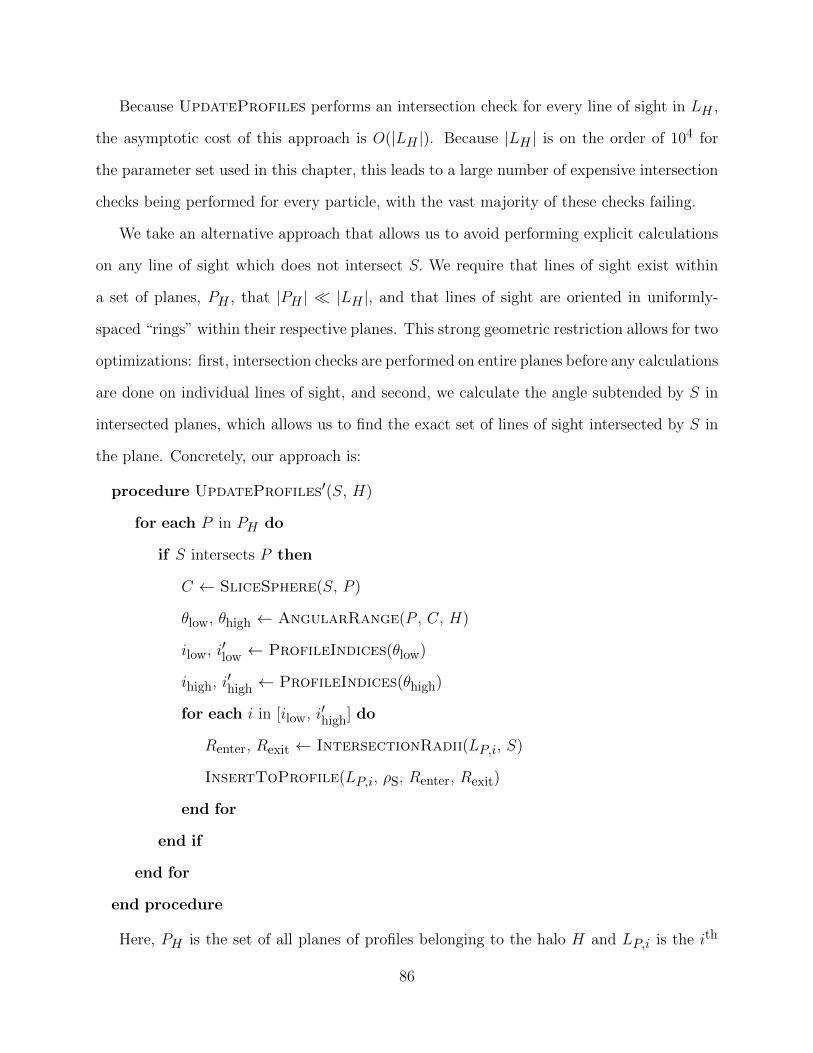
Because UpdateProfiles performs an intersection check for every line of sight in LH ,

the asymptotic cost of this approach is O(|LH |). Because |LH | is on the order of 104 for

the parameter set used in this chapter, this leads to a large number of expensive intersection

checks being performed for every particle, with the vast majority of these checks failing.

We take an alternative approach that allows us to avoid performing explicit calculations

on any line of sight which does not intersect S. We require that lines of sight exist within

a set of planes, PH , that |PH | |LH |, and that lines of sight are oriented in uniformly-

spaced “rings” within their respective planes. This strong geometric restriction allows for two

optimizations: first, intersection checks are performed on entire planes before any calculations

are done on individual lines of sight, and second, we calculate the angle subtended by S in

intersected planes, which allows us to find the exact set of lines of sight intersected by S in

the plane. Concretely, our approach is:

procedure UpdateProfiles′(S, H)

for each P in PH do

if S intersects P then

C ← SliceSphere(S, P )

θlow, θhigh ← AngularRange(P , C, H)

ilow, i′low ← ProfileIndices(θlow)

ihigh, i′high ← ProfileIndices(θhigh)

for each i in [ilow, i′high] do

Renter, Rexit ← IntersectionRadii(LP,i, S)

InsertToProfile(LP,i, ρS, Renter, Rexit)

end for

end if

end for

end procedure

Here, PH is the set of all planes of profiles belonging to the halo H and LP,i is the ith

86

profile within the profile ring corresponding to the plane P . Here, the existence of several

simple functions has been assumed: SliceSphere(S, P ) returns the circle created by slicing

the sphere S by the plane P ; AngularRange(P , C, H) returns two angles specifying the

angular wedge within the plane P which the circle C subtends relative to the center of the

halo H; and ProfileIndices(θ) returns the indices of the two nearest profiles to the angle

θ, with the profile corresponding to the lower angle being returned first. For ease of reading,

the pseudocode which would handle the periodicity of angles at θ = 0 ≡ 2π has been omitted.

This method is illustrated in Figure 4.15. Panel A shows a collection of spheres collected

around a halo center, panel B shows the results of calling SliceSphere on each of these

spheres for a particular plane, and panel C shows the profiles (in red) which would recieve

intersection checks within the innermost loop of UpdateProfiles′.

The asymptotic cost of UpdateProfiles′ is O(|PH |+ IH,S), where IH,S is the number

of profiles in the halo H which intersect the sphere S. Since both |PH | and IH,S are multiple

orders of magnitude smaller than |LH |, this results in a significant increase in performance.

In practice we find that the plane intersection checks are subdominant to the cost of the

innermost loop.

The method described above is further optimized in several ways:

• If InsertToProfile is implemented naively - by representing profiles as arrays con-

taining ρ(r) and updating every element of the profile which is within the inserted

rectangular function - it is the dominant cost of UpdateProfiles′. To prevent this,

we represent our profiles as arrays containing dρ(r)/dr. Since the derivative of a

rectangular function is two delta functions, updating the derivative profile only re-

quires updating array elements close to the edges of the rectangular function (note

that in the discrete case this requires four element updates: two for each edge). Once

UpdateProfiles′ has been called on every target sphere, each derivative profile is

integrated to obtain ρ(r).

• Instead of explicitly performing the 3D IntersectionRadii(LP,i, S), a faster 2D

87

analog is used to find the intersection radii of the projection of LP,i onto P with the

circle C.

• A successful intersection check between P and S is performed in a way which imme-

diately results in the value that would be returned by SliceSphere(S, P ), as these

two calculations share many geometric operations.

This algorithm is straightforward to generalize to non-constant density spheres and to

density estimates constructed from other geometric solids (most notably tetrahedra), al-

though the publicly released version of Shellfish does not allow access to either feature.

4.6.2 Splashback Candidate Filtering Algorithm

The Appendix will outline the filtering algorithm which we qualitatively introduced in section

4.2.2

The first step of constructing the filtering loop is dividing the point distribution into

2Nrec uniformly spaced angular wedges, for some user-defined Nrec. We calculate an anchor

point for each wedge, which is an estimate of the average location of the splashback shell

within that wedge.

The location of the anchor point within the ith wedge is given by

Ranchor,i, θanchor,i = AnchorRadius(0, i), 2πi+ 0.5

2Nrec. (4.15)

Here, i is zero-indexed and AnchorRadius is the following recursive algorithm:

function AnchorRadius(k, i)

θlow ← 2πbi/2kc2k−Nrec

θhigh ← 2π(bi/2kc+ 1)2k−Nrec

f ←WedgeKDE(θlow, θhigh)

if k = Nrec then

return GlobalMaximum(f)

88

else

Ranchor ← AnchorRadius(k + 1, i)

maxes ← LocalMaxima(f)

R′anchor ← minR|Ranchor −R| ∀ R ∈ maxes

if |Ranchor −R′anchor| < Rrefine then

return R′anchor

else

return Ranchor

end if

end if

end function

We assume the existence of three simple functions: GlobalMaximum(f), which re-

turns the global maximum of the function f ; LocalMaxima(f), which returns all the local

maxima of the function f ; and WedgeKDE(θlow, θhigh), which returns a kernel density

estimate (KDE) corresponding to the points contained within the wedge with boundaries

θlow and θhigh. A KDE is a method for converting a set of discrete points into a continuous

density estimate by applying a smoothing kernel to every point. It performs much the same

role as a histogram, except that an explicit choice of bin edges is replaced by an explicit

choice of the smoothing kernel. For our purposes, the most useful property of a KDE is that

it provides a simple way to estimate the point of maximum density. We define our KDE as

the function

KDE(r) =∑

j

exp

(−(r − rj)2

2R2KDE

)(4.16)

where RKDE is a user-defined smoothing scale, and rj is a set of points.

The intuition behind this approach is that most candidate points in the plane correspond

to lines of sight crossing the splashback shell, so the maximum of the k = Nrec KDE is

a good 0th order estimate of of its location. Smaller wedges give more refined estimates.

89

But if their estimate deviates too far from the coarser estimates, it’s likely that the region

corresponds to a filament or a subhalo.

Once anchor points have been found for each wedge, we fit a cubic interpolating spline

to them in the θ - R plane. This spline is the aforementioned filtering loop. To remove

boundary effects, the range of the anchor points is extended to [−2π, 4π) prior to fitting,

but the spline is only ever evaluated in the [0 2π) range. We then remove all points which

are further than some distance, Rfilter from this spline.

This procedure introduces three new free parameters, RKDE, Rrefine, and Rfilter. Tests

indicate that the final shells are robust to changes in RKDE and Rfilter, as long as they are of

the same order of magnitude as Rrefine. For this reason we simplify parameters by requiring

RKDE = Rrefine = Rfilter = Rmax/η. (4.17)

Here η is a tunable parameter which dictates how strict the filtering process is. Higher values

of η are stricter than lower values of η.

4.6.3 Parameter-Specific Convergence Tests

Most of the fiducial values of parameters of our algorithm listed in Table 4.2.4 were set using

one of the following three approaches, which start with constructing a representative sample

of halos and identifying their splashback shells and estimating their properties for a range of

values pi for the selected parameter p.

A: Many parameters are known to be optimized when taken to either the low value or

high value limit, but also decrease the performance of the algorithm as the parameter

approaches this limit. In addition to the shells for the pi values, we also fit a shell with

p set to some very large value, plimit. For each halo we calculate a curve representing

the fractional difference between the shells calculated with pi and with plimit for each

of the properties defined in Equations 4.5 - 4.9. We then set the parameter to the

90

lowest pi which leads to an average fractional error of . 1%.

B: Some parameters are not optimized in either the low or high value limit. For each

halo we construct curves for each of the properties defined in Equations 4.5 - 4.9. We

manually inspect these curves: if they generally show an unchanging “plateau” for

these properties over a wide range of pi values, we set the parameter to an arbitrary

pi in the center of the plateau. The existence of a plateau over a wide range of pi

indicates that the shell shapes depend only weakly on this parameter.

C: For parameters where method B was attempted but a no wide plateau was found, we

incorporate qualitative assessment of the shells into the selection procedure. For a pair

of parameter values, pi and pj , we visually inspect every halo in the test set, compare

the shells produced by both values to the underlying density field, and select one of the

two as a qualitatively better fit. Once this has been completed for every halo, we label

the parameter value with more successful fits as the better value. This allows us to

construct an fitness ordering on all the values of pi. We then select the maximally fit

parameter. In principle, this methodology could lead to researcher-dependent results,

but for the three parameters where we used this method, the optimal value was not

ambiguous.

The specific methods we used to set each algorithm parameter are listed in Table 4.2.4. In

all cases the halo sample is divided into M200m-selected and ΓDK14-selected subsets to test

for parameter dependence on halo properties. In all cases, we found no such dependence.

Parameters which involved additional testing methodology are described below:

4.6.4 Setting Rkernel

In order for our algorithm to identify the splashback shell reliably, we need to sample the

density distribution around the shell well. However, typical densities in this region are (0.1−

10)× ρm (see Figure 4.1(b)) and there are often relatively few particles. To compensate for

91

this, we need to make the radius of the spheres associated with particles, Rkernel sufficiently

large.

To find the optimal value of Rkernel, we use an approach similar to the approach A above.

We generate a representative sample of halos and fit Penna-Dines shells to each halo in the

sample for different values of Rkernel. We then find the smallest converged value of Rkernel

for each halo. An example of this comparison is shown in Figure 4.16(a). This figure also

illustrates the second test described in section 4.3: in ¿99% of cases, Rsp falls within the

visual fall-off region of the halo.

We find that for halos with N200m ≥ 106, properties of the splashback shells converge

for Rkernel & 0.1R200m and for halos with N200m ≈ 5 × 104 for Rkernel & 0.2R200m. For

simplicity, we set Rkernel to 0.2R200m for all halos.

4.6.5 Setting Nplanes

The parameter which has the largest effect on the stochastic error, as opposed to systematic

error, in estimating shell shape is Nplanes. To determine a value for this parameter, we follow

a procedure similar to method A. We identify the splashback shells for a representative sample

of halos for five values of Nplanes, using randomly oriented normal vectors for each plane

so that no lines of sight are shared between two different realizations. We then calculate

the fractional standard deviation between shell properties determined for different random

realizations of a given number of planes Nplanes,√〈Q2〉 − 〈Q〉2/〈Q〉 for each quantity Q

defined in Equations 4.5 - 4.9. This standard deviation is plotted as a function of Nplanes

in Figure 4.16(b). For Nplanes = 100, Shellfish achieves sub-percent level per-halo scatter

in Rsp, Msp, and 1 +Asp and less than 2% scatter in 1 +Esp. We do not find any evidence

that the amplitudes of the curves shown in Figure 4.16(b) depend on halo mass or accretion

rate.

92

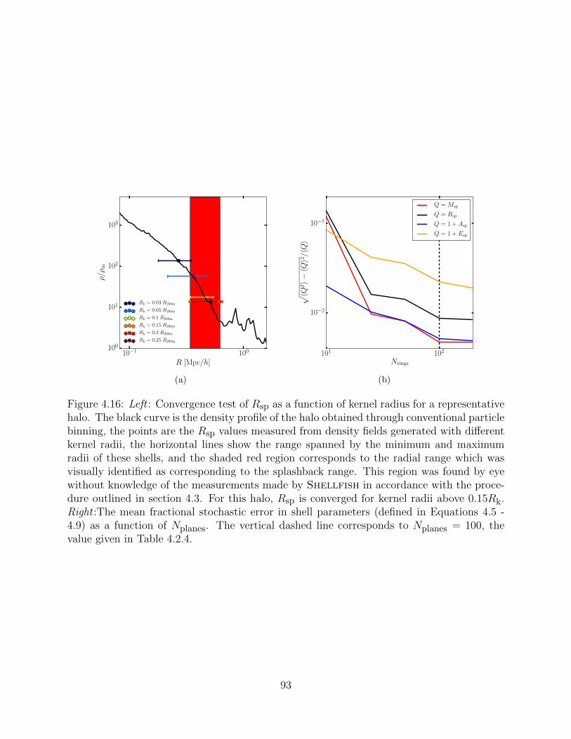
10−1 100

R [Mpc/h]

100

101

102

103

ρ/ρ

m

Rk = 0.03 R200m

Rk = 0.05 R200m

Rk = 0.1 R200m

Rk = 0.15 R200m

Rk = 0.2 R200m

Rk = 0.25 R200m

(a)

101 102

Nrings

10−2

10−1

√〈Q

2〉−〈Q〉2 /〈Q〉

Q = Msp

Q = Rsp

Q = 1 + Asp

Q = 1 + Esp

(b)

Figure 4.16: Left : Convergence test of Rsp as a function of kernel radius for a representativehalo. The black curve is the density profile of the halo obtained through conventional particlebinning, the points are the Rsp values measured from density fields generated with differentkernel radii, the horizontal lines show the range spanned by the minimum and maximumradii of these shells, and the shaded red region corresponds to the radial range which wasvisually identified as corresponding to the splashback range. This region was found by eyewithout knowledge of the measurements made by Shellfish in accordance with the proce-dure outlined in section 4.3. For this halo, Rsp is converged for kernel radii above 0.15Rk.Right :The mean fractional stochastic error in shell parameters (defined in Equations 4.5 -4.9) as a function of Nplanes. The vertical dashed line corresponds to Nplanes = 100, thevalue given in Table 4.2.4.

93

4.6.6 Computing Moment of Inertia-Equivalent Ellipsoidal Shell Axes

It is non-trivial to analytically compute axis ratios from the moments of inertia for a constant-

density ellipsoidal shell. Assuming that the shell is sampled by some collection of particles

with weights mk, the moments can be obtained by calculating the eigenvalues of the mass-

distribution tensor,

Mi,j =∑

k

mk(~rk)i(~rk)j . (4.18)

The eigenvalues of the mass-distribution tensor are straightforward to calculate for a ho-

moeoid: the volume enclosed by two ellipsoids with the same axes ratios and with aligned

major axes a and a′. In the limit where a′ → a, the eigenvalues are given by

Mi = Mtota2i

3, (4.19)

where Mi and ai are the moment and ellipsoid axis aligned with the ith Cartesian axis and

Mtot =∑kmk. Note that this notation for ellipsoid axes is different that the convention

used in Equation 4.7. Although an infinitely thin homoeoid is often equated with a uniform-

density ellipsoid surface in the literature [see, for example Zemp et al., 2011], it actually

corresponds to an ellipsoid surface with a non-uniform density. This non-uniformity means

that major (minor) axes derived from Equation 4.19 are too small (large). This bias increases

with increasing ellipticity: for ellipsoidal shells with axes ratio of ≈ 2 : 1, this can bias

measured axes ratios by tens of per cent.

A more accurate approximation would be to model a uniform density ellipsoidal shell by

the volume enclosed by two ellipsoids with axes a, b, c and a + δ, b + δ, c + δ and to take

δ → 0. This shape gives eigenvalues of

Mi = Mtota2i

5

(aiaj + 3ajak + akaiaiaj + ajak + akai

), (4.20)

which can then be numerically solved to obtain ellipsoid axes. Although for ellipsoids with

94

large axes ratios Equation 4.20 is a closer approximation than Equation 4.19, it still in-

troduces errors close to our Nring = 100 stochastic noise limit. Thus for large axes-ratio

ellipsoids we compute the mapping empirically.

We define the quantities Ai ≡√Mi/Mtot and R ≡ (MiMjMk/M

3tot)

1/6. Note that both

Ai and R can be measured directly from the input point distribution. First, we generate

a grid of ellipsoids in a0/a1 - a0/a2 space. Next we numerically compute A0/A1, A0/A2,

and a0/RV for each ellipsoid. The resultant A0/A1 and A0/A2 values form a sheared grid,

so we Delaunay triangulate [Delaunay, 1934] the A0/A1 - A0/A2 plane and perform linear

interpolation on the resulting triangles. We construct three such interpolators which map

from (A0/A1, A0/A2) pairs to a0/a1, a0/a2, and a0/R, respectively. These interpolators

can then be used to find a0, a1, and a2 using only the eigenvalues of the mass-distribution

tensor.

95

CHAPTER 5

HOW BIASED ARE COSMOLOGICAL SIMULATIONS?

This chapter is a modified version of my paper, Masfield & Avestruz [in prep].

5.1 Introduction

Understanding the non-linear predictions of the Λ Cold Dark Matter (ΛCDM) model requires

the use of simulations. Simulations are required to understand the behavior of almost every

system smaller than the Lagrangian footprint of a large dark matter halo, whether it be the

structure of dark matter halos [e.g. de Blok, 2010], the abundances of galaxies [e.g. Klypin

et al., 2015a] and satellites [e.g. Moore et al., 1999], or the properties of local dark matter

streams [e.g. Vogelsberger et al., 2009].

The most common class of ΛCDM simulation is the N-body simulation that has been

used to model both individual collapsed structures [see review in Griffen et al., 2016] and

large cosmological volumes (see review in section 3.1). While the predictions of ΛCDM

include the behavior of baryons, many simulators and analysts focus on “dark matter only”

(DMO) simulations. Beyond the relative computational efficiency of DMO simulations, the

fundamental reason for the popularity of DMO simulations lies in their parametrization.

Baryonic simulations have a wide range of parameters, many of which have true physical

meaning [e.g. table 2 in Hopkins et al., 2018]. On the other hand, once a cosmology is

specified, a DMO simulation has much smaller set of parameters and all these parameters

are purely numerical. This leads to the core fact that underpins all tests of DMO simulations:

any dependence on parametrization is evidence for numerical bias or error.

In principle, the results of DMO simulations may depend on numerical parameters that

determine initial condition generation, the starting redshift, box size, and “zoom-in” strategy.

Simulations that follow conventional “best practices” usually avoid these effects at small

scales [e.g. Power and Knebe, 2006, Crocce et al., 2006, Knebe et al., 2009, Hahn and Abel,

96

2011]. Beyond this, every N-body code has its own idiosyncratic parametrization, such as the

node opening criteria for a force tree [e.g. Springel et al., 2001b], Adaptive Refinement Tree

(ART) refinement criteria [e.g. Kravtsov et al., 1997], and light-bulb wattage [Holmberg,

1941]. These parametrizations are important, but generally ironed out during the early

development and usage of a particular code.

Instead, our study – similar to most other DMO convergence studies – focuses on the

three most important parameters of DMO simulations: particle mass, mp (or interparticle

spacing, l = L/N), timestepping, and the distribution of mass around each particle (“force

softening”). Statements about the correctness and biases associated with these three param-

eters come from a combination of four classes of analyzes:

• A priori models of numerical effects [e.g. van Kampen, 2000, Dehnen, 2001, Power

et al., 2003, Ludlow et al., 2019] In these studies, simulators create a model of how the

numerical components of a simulation behave, often validating the predictions of this

model with appropriate test simulations, and use that model to infer the correctness

of other simulations.

• Simulations of idealized systems [e.g. Klypin et al., 2015b, van den Bosch and

Ogiya, 2018, Joyce et al., 2020] In these studies, simulators either have a priori knowl-

edge of the exact solution the simulation is expected to produce (such as the simula-

tions of NFW halos in van den Bosch and Ogiya, 2018), or a priori knowledge of some

invariant property of the system (such as the self-similar power spectra analyzed in

Joyce et al., 2020). Measured deviations from a priori expectations are unambiguous

numerical biases.

• Resimulations of realistic systems [e.g. Power et al., 2003, Navarro et al., 2010,

Ludlow et al., 2019] In these studies, simulators resimulate a ΛCDM system with a

variety of numerical parameters. Systems are typically either a single halo [e.g. Power

et al., 2003, Navarro et al., 2010], or a small cosmological box [Ludlow et al., 2019].

97

Since there is no a priori expectation for these simulations, simulators will identify a

region of numerical parameter space where results are locally independent of numerical

parameters and measure deviations relative to this “converged” region.

• Comparison of independent simulations [e.g. Klypin et al., 2015b, Villarreal et al.,

2017b, Child et al., 2018, Fig. 5.3] In these studies, simulators compare independently

run simulations which inhomogogenously sample numerical parameter space, with the

goal of identifying converged parameter ranges. While this type of test is particularly

vulnerable to “false” convergence, it is substantially less labour-intensive than the pre-

vious classes of studies, and is often the only test available for assessing the correctness

of expensive simulations which were not performed as part of a multi-resolution suite.

A simulator interested in assessing the biases of large cosmological DMO simulations – the

class of simulations targeted by this chapter – must rely on tests of all four types of studies.

Although the last class of tests mentioned above will always be a necessary component of

such assessments, simply comparing the results of cosmological simulations cannot establish

that the “converged” solutions which these tests identify are correct. Such an inference must

come from detailed comparison with the other classes of tests.

Despite the vast literature on convergence testing in cosmological DMO simulations,

there are still unknowns, disparities, and limitations to the tests performed. Tests of the

first three types mentioned above focus almost exclusively on radial density profiles at fixed

radii. However, dark matter halos are complex objects with a myriad of scientifically useful

properties. To the best of our knowledge, there are no published reliability requirements for

many commonly used halo properties, such as the offset between a halo”s center of mass and

its most bound particle, Xoff . Even for the most well-tested halo properties, there is no clear

consensus on what is required for reliability; examples including the peak of the rotation

curve, Vmax, or the radius at which the logarithmic slope of the denisty profile is -2, r−2. We

surveyed twelve studies on the concentration mass-relation, all of which measure some form

of r−2. From this survey, we found that the minimum particle counts (Nvir) which different

98

studies analyzed ranged from from 500 to 10,000 particles, with the 1σ scatter spanning

more than a decade [Neto et al., 2007, Duffy et al., 2008, Gao et al., 2008, Zhao et al., 2009,

Prada et al., 2012, Bhattacharya et al., 2013, Ludlow et al., 2013, Dutton and Maccio, 2014,

Diemer and Kravtsov, 2015, Klypin et al., 2016, Poveda-Ruiz et al., 2016, Child et al., 2018].

Lastly, tests focused solely on how many particles halos are resolved with dominate much

of the literature, despite demonstrations that force softening and timestepping have large

effects on halo properties (see sections 5.5 and 5.6.1).

In this work, we aim to complete several components of the analysis needed to rectify

these issues, incorporating components of all four classes of tests discussed above. We per-

form convergence tests using a large inhomogenous suite of publicly available cosmological

simulations. These tests are performed over a wide range of halo properties, including halo

properties which are traditionally overlooked by the testing literature. We also analyze

the impact of timestepping and force softening parameters to extend beyond the standard

particle count parameter. We organise the chapter as follows. In section 5.2 we outline

our methods for comparing cosmological simulations and extracting empirical convergence

limits. In section 5.3 we report these empirical limits and consider the variation in limits

between simulations. In section 5.4, we study the dependence of various halo properties on

the force softening scale. In section 5.5, we outline a model for estimating the impact of

large force softening scales on halo profiles and apply this model to our simulation suites.

Lastly, in section 5.6 we discuss our results (particularly the impact of timestepping), and

in section 5.7 we summarise and conclude our analysis.

5.2 Methods

5.2.1 Simulations and Halo Finding

This chapter uses all the simulations listed in Table 3.1.

We use catalogs constructed by the Rockstar halo finder [Behroozi et al., 2013d]. When

99

available, we also used merger trees constructed by consistent-trees [Behroozi et al.,

2013e] to determine growth history-dependent halo properties. The ν2-gc and IllustrisTNG-

Dark simulation suites do not currently have merger trees available.

The simulations we consider use a number of different versions of the Rockstar halo

finding software. Rockstar has undergone a number of bug fixes since its original release,

and halo catalogs generated with different versions can have significantly different prop-

erty distributions. To understand the impact of different software versions, we obtained

the approximate Rockstar download times and configuration files for every suite consid-

ered in this chapter to identify the corresponding software version (Diemer; Klypin; Becker;

Ishiyama; Behroozi, personal communication).

We then isolated the source of version-dependent results. First, we regenerated halo

catalogs for the CBol L125 simulation using the different versions – matching the exact

commit hash if known – as well as the relevant parameters in each respective configuration

file, and we cross-matched these catalogs against one another. Second, we performed an

extensive review of the Rockstar and consistent-trees version control commit histories1.

By combining these two analyzes, we determined that there were two sets of variables which

gave version-dependent results and that all other variables were consistent between versions.

These variables are (1) the axis ratios calculated within R500c and (2) properties that depend

on internal energy calculations. The Rockstar changelogs document both of these issues,

meaning that, fortunately, our cross-matching of catalogs did not reveal any new significant

inconsistencies.

Incorrect axis ratio measurements affect Erebos CBol and Erebos CPla, which used

Rockstar catalogs generated with code downloaded prior to October 22nd, 2013. There

is no method for correcting this issue, but as discussed below the convergence properties of

these inner axis ratios are largely similar to the conventional larger axis ratios. We therefore

1. available at https://bitbucket.org/gfcstanford/rockstar andhttps://bitbucket.org/pbehroozi/consistent-trees

100

do not analyze this property. Rockstar catalogs generated with code downloaded prior to

May 15th, 2014 have internal energies which are too large by a factor of two. This can be

corrected by replacing variables, X, with updated versions, X ′. In the cases of virial ratio

and Peebles spin parameter, the replacement variables would appear as,

T/|U |′ = 2T/|U | (5.1)

λ′Peebles = λPeebles

√1− T/|U |′√2− T/|U |′

(5.2)

We apply the corrections of Eq. 5.1 to catalogs for the Erebos CBol, Erebos CPla, Bol-

shoi, and BolshoiP suites. We also applied these corrections to Chinchilla L250 and Chin-

chilla L400, but Chinchilla L125 did not require these corrections.

Another potential source of variation amongst Rockstar catalogs is the choice of pri-

mary mass definition, which changes the values of other reported halo properties (see section

4 and appendix A of Mansfield and Kravtsov [2019] for a full discussion). However, we

confirmed that all of the halo catalogs that we consider in our analyzes used Mvir as the

primary mass definition. This particular source of variation does not impact our results.

We also generate Rockstar catalogs for the z = 0 snapshots of the IllustrisTNG-

Dark simulations listed in Table 3.1, made available through the IllustrisTNG public data

release [Nelson et al., 2019]. We used the Rockstar version corresponding to the git hash

99d56672092e88dbed446f87f6eed87c48ff0e77, downloaded on June 10th 2019. We use Mvir as

our primary mass definition, consistent with other catalogs. As with the other catalogs in this

chapter, we do not use strict spherical overdensity masses and removed “unbound” particles

prior to analysis. We use a coarse-grained friends-of-friends linking length of b = 0.28 l for

load-balancing. Note that this last setting leads to inaccurate M200m masses [section 4.3 and

appendix A of Mansfield and Kravtsov, 2019], but we choose this setting for consistency with

the other catalogs used in this study. Some analysis in this chapter also uses Rockstar

catalogs generated for the baryonic IllustisTNG simulations. In these cases, we use the same

101

Rockstar parameters as we do with IllustrisTNG-Dark, but only consider dark matter

particles when computing halo properties.

5.2.2 Halo Properties

The halo properties considered in this chapter are defined and discussed in section 3.2.

There are a number of quantities in Rockstar and consistent-trees catalogs which we do

not explicitly study in this chapter. In most cases this is because the convergence behavior of

these properties is identical to that of another property: we find that the convergence limits

for Γ(tdyn) are essentially the same as accretion rates defined over any other time scale

tracked by any version of consistent-trees. We therefore only consider Γ(tdyn). Similarly, we

find that the convergence properties of b/a, (c/a)(< R500c), and (b/a)(< R500c) are nearly

identical to those of c/a and thus only consider c/a. Later versions of Rockstar track the

maximum single-halo tidal force on each halo, but we do not track convergence behavior

for tidal force calculations. This is because too few of our catalogs contain this property

to achieve meaningful statistics. We additionally note that computing the tidal force on

halos has subtleties that indicate that the approximation used by Rockstar may not be

sufficiently physical (see section 2 of van den Bosch et al., 2018 and section 2.5 and appendix

C of Mansfield and Kravtsov, 2019).

5.2.3 Finding Empirical “Convergence Limits”

In this section, we describe our procedure to establish particle count-based convergence limits

for each halo property. We identify these limits for target accuracy levels. Finally, we note

that this procedure does not rule out the possibility of false convergence.

To identify the corresponding convergence limits for a halo property, X, we:

1. group simulations by approximate cosmology and by subhalo status. We analyze each

subgroup separately.

102

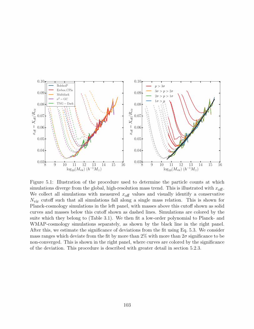
8 9 10 11 12 13 14 15 16log10(Mvir) (h−1M)

0.03

0.04

0.05

0.06

0.07

0.08

0.09

0.10

xoff

=X

off/R

vir

BolshoiP

Erebos CPla

Multidark

ν2 − GC

TNG− Dark

8 9 10 11 12 13 14 15 16log10(Mvir) (h−1M)

0.03

0.04

0.05

0.06

0.07

0.08

0.09

0.10

xoff

=X

off/R

vir

p > 3σ

3σ > p > 2σ

2σ > p > 1σ

1σ > p

Figure 5.1: Illustration of the procedure used to determine the particle counts at whichsimulations diverge from the global, high-resolution mass trend. This is illustrated with xoff .We collect all simulations with measured xoff values and visually identify a conservativeNvir cutoff such that all simulations fall along a single mass relation. This is shown forPlanck-cosmology simulations in the left panel, with masses above this cutoff shown as solidcurves and masses below this cutoff shown as dashed lines. Simulations are colored by thesuite which they belong to (Table 3.1). We then fit a low-order polynomial to Planck- andWMAP-cosmology simulations separately, as shown by the black line in the right panel.After this, we estimate the significance of deviations from the fit using Eq. 5.3. We considermass ranges which deviate from the fit by more than 2% with more than 2σ significance to benon-converged. This is shown in the right panel, where curves are colored by the significanceof the deviation. This procedure is described with greater detail in section 5.2.3.

103

2. visually identify a conservative high-particle count cutoff above which all Mvir − X

relations agree.

3. fit a polynomial-centered distribution to all high-resolution Mvir −X relations.

4. identify the highest particle count at which each simulation has a statistically significant

deviation from the fitted distribution which is larger than a target accuracy level. This

particle count, Ncut is the “convergence limit” for that simulation.

All the steps in this procedure are described in greater depth below and are illustrated in

Fig. 5.1. Some aspects of this procedure are altered for properties which particularly poor

convergence behavior. All such properties are described in depth in section 5.3.

Separation into Subgroups

Because many halo properties depend on cosmology (especially properties which depend

on accretion histories), we separate simulations by cosmology to avoid misinterpreting these

cosmological dependencies as non-convergence. We analyze the WMAP suites Bolshoi, Chin-

chilla, and Erebos CBol as a group and the Planck suites ν2-GC, BolshoiP, Multidark, and

Erebos CPla as a group. The exact parameters used still vary from suite-to-suite, mostly

due to the year of each mission which these simulations attempt to match. This is most

apparent when comparing the Chinchilla suite to other WMAP simulations like Bolshoi or

Erebos CBol (see Table 3.1).

We tested the impact of these small cosmology differences by repeating our analysis with

groups based on the exact cosmological parameters and did not find a meaningful difference

in our results. Because this split significantly reduces the number of simulations which have

higher-resolution boxes available for comparison, we do not use this approach in the rest of

this chapter.

We also separate halos by subhalo and isolated halo status (see section 5.2.2). This

is important both because subhalos and isolated halos may have difference convergence

104

properties and because numerical parametrization can lead to changes in the artificial subhalo

disruption rate [e.g. van den Bosch et al., 2018, van den Bosch and Ogiya, 2018, see also

section 5.4.1]. Artificial disruption would lead to isolated halos being over-represented at a

constant mass, and in cases where host halos and subhalos follow different mass relations

this would propagate to a change in the global mass relation.

Using Rvir to define subhalo status (as we do here) is suboptimal. There is a large popu-

lation of “splashback subhalos” which are qualitatively indistinguishable from other subhalos

but whose orbits have apocenters outside the arbitrarily-defined virialy radius [Balogh et al.,

2000, Mamon et al., 2004, Gill et al., 2005, Ludlow et al., 2009, Bahe et al., 2013, Wetzel

et al., 2014, Xie and Gao, 2015]. Mansfield and Kravtsov [2019] showed that this popu-

lation of misidentified subhalos is responsible for the entire high-concentration tail of the

“isolated” halo population, thus opening the possibility that numerical subhalo disruption

could affect our convergence limits. Although many schemes for identifying splashback sub-

halos exist [see Mansfield and Kravtsov, 2019, for review], we do not use them here: they

rely on merger tree information and/or raw particles data, which are not available for all

the simulations considered here, and these methods have not trivial convergence properties

themselves [Mansfield et al., 2017] which would be a larger complicating issue than subhalo

contamination.

Defining High-Resolution Particle Ranges

For each simulation, we measure the mean value of each property, X, as a function of Mvir

within logarithmic 0.125 dex mass bins. We restrict analysis to mass bins containing at least

100 halos.

We identify non-convergence by identifying where simulations deviate from the mass-

relation implied by the high-resolution regimes of other simulations. We identify a such a

corresponding high-resolution cutoff, NHR, by eye such that no simulations in our sample

deviate from others in their subgroup when mass relations are constructed for halos with

105

Nvir > NHR.

This cutoff is chosen separately for each halo property and each analysis subgroup, al-

though we use the same cutoffs for both Planck and WMAP cosmology. These cutoffs are

shown in Appendix 5.8.2, Table 5.5. Our tests indicate that our results are not sensitive to

the exact NHR choices used.

The cutoff chosen for the Mvir −Xoff relation is shown as the transition of from solid to

dashed lines in the left panel of Fig. 5.1.

As discussed in section 5.2.3 and 5.3.2, several simulations diverge significantly from other

simulations at aberrant high particle counts for various halo properties. These simulations

are not included in our determination of NHR and are discussed extensively throughout

section 5.3.

Fitting Mean Relations

For each halo property, X, we fit the log10(Mvir)−X relation with a Gaussian distribution

with a centroid given by a mass-dependent d-degree polynomial and a 1σ dispersion given

by σ0. Since the posterior distributions for these fits are smooth and unimodal, we do this by

maximising the likelihood function of this model across its parameter space. For each mass

relation, we scale masses by the pivot mass Mpivot = 1012.5h−1M to increase numerical

stability and scale X by (Mvir/Mpivot)α to decrease the polynomial degree needed to fit the

relation. We show the values of d and α used for each halo property in Table 5.5. In the

case of mass and velocity functions relative to the halo property X, we perform fits relative

to log10(φ(X)). We use a pivot value of Vpivot = 1 km/s for velocity functions.

The best-fitting relation for the Mvir − Xoff relation is shown as the black curves in

Fig. 5.1, and σ0 is shown as the gray shaded contour around those curves.

For many halo properties, a subset of simulations diverge significantly from other simu-

lations within the same suite. We manually remove these simulations prior to fitting. The

number of outliers removed for each property is listed in Table 5.5. We remove all ν2-gc

106

boxes, all TNG boxes, VSMDPL, HMDPL, and Chinchilla L250 prior to fitting theMvir−c/a

relation, Chinchilla L250 before fitting the cvir relation, all ν2-gc boxes, VSMDPL, SMDPL,

and CHinchilla L250 prior to fitting the Vmax relation, and Chinchilla L250 prior to fitting

the Vpeak relation.

Three sets of outlier removals require special comment. We found that the Mvir − cvir

relation was well fit by a power law for each simulation suite individually, but that amplitude

and power law index of these relations were noticeably different for each suite. As such, we

fit each suite independently with the additional removal of Chinchilla L250.

As is discussed in section 5.3.2, Illustris-TNG and the high resolution MDPL simulations

appear to “converge” to different Mvir − Vmax relations. Because ν2-gc-H2 and ν2-gc-H1

give aberrant results, the only Planck-cosmology simulations in Table 3.1 which probe halo

masses below Mvir . 1011 h−1M fall into one of these two suites. To avoid a fit which

“splits the difference” between the two, we perform two fits removing VSMDPL and SMDPL

from one fit and all the TNG-Dark boxes from a second fit. We analyze both fits.

This removal of outlier simulations serves to emphasize that these fits cannot be inter-

preted as approximating the “correct” converged solutions for these mass relations, but as

approximating the high-resolution solutions for a particular subset of simulations: we ex-

plicitly do not claim that any individual simulation considered in this chapter is converged

or correct (or that the inverse is true). As such, we do not provide any of the fits produced

from this part of this analysis to prevent their potential misuse.

Identifying Deviations

Traditional convergence tests are either performed by eye or by measuring the mass at which

halo properties deviate from a reference relation by more than some fixed level of acceptable

bias. We do not take these approaches for three reasons: first, even the mass relations

of converged simulations can deviate from the high resolution relation due to Poissonian

noise, cosmic variance, and uncertainties in the underlying fit. This makes percentage cuts

107

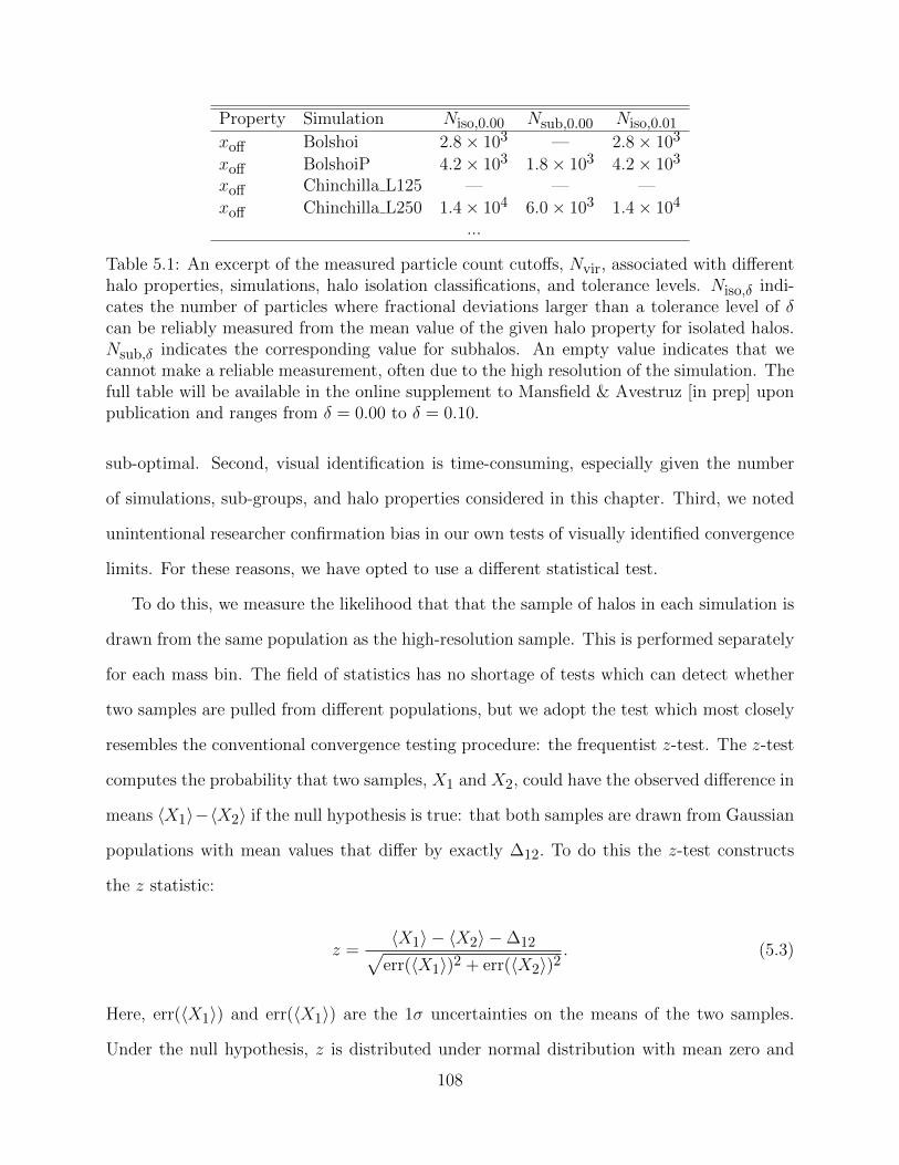
Property Simulation Niso,0.00 Nsub,0.00 Niso,0.01

xoff Bolshoi 2.8× 103 — 2.8× 103

xoff BolshoiP 4.2× 103 1.8× 103 4.2× 103

xoff Chinchilla L125 — — —

xoff Chinchilla L250 1.4× 104 6.0× 103 1.4× 104

...

Table 5.1: An excerpt of the measured particle count cutoffs, Nvir, associated with differenthalo properties, simulations, halo isolation classifications, and tolerance levels. Niso,δ indi-cates the number of particles where fractional deviations larger than a tolerance level of δcan be reliably measured from the mean value of the given halo property for isolated halos.Nsub,δ indicates the corresponding value for subhalos. An empty value indicates that wecannot make a reliable measurement, often due to the high resolution of the simulation. Thefull table will be available in the online supplement to Mansfield & Avestruz [in prep] uponpublication and ranges from δ = 0.00 to δ = 0.10.

sub-optimal. Second, visual identification is time-consuming, especially given the number

of simulations, sub-groups, and halo properties considered in this chapter. Third, we noted

unintentional researcher confirmation bias in our own tests of visually identified convergence

limits. For these reasons, we have opted to use a different statistical test.

To do this, we measure the likelihood that that the sample of halos in each simulation is

drawn from the same population as the high-resolution sample. This is performed separately

for each mass bin. The field of statistics has no shortage of tests which can detect whether

two samples are pulled from different populations, but we adopt the test which most closely

resembles the conventional convergence testing procedure: the frequentist z-test. The z-test

computes the probability that two samples, X1 and X2, could have the observed difference in

means 〈X1〉−〈X2〉 if the null hypothesis is true: that both samples are drawn from Gaussian

populations with mean values that differ by exactly ∆12. To do this the z-test constructs

the z statistic:

z =〈X1〉 − 〈X2〉 −∆12√

err(〈X1〉)2 + err(〈X2〉)2. (5.3)

Here, err(〈X1〉) and err(〈X1〉) are the 1σ uncertainties on the means of the two samples.

Under the null hypothesis, z is distributed under normal distribution with mean zero and

108

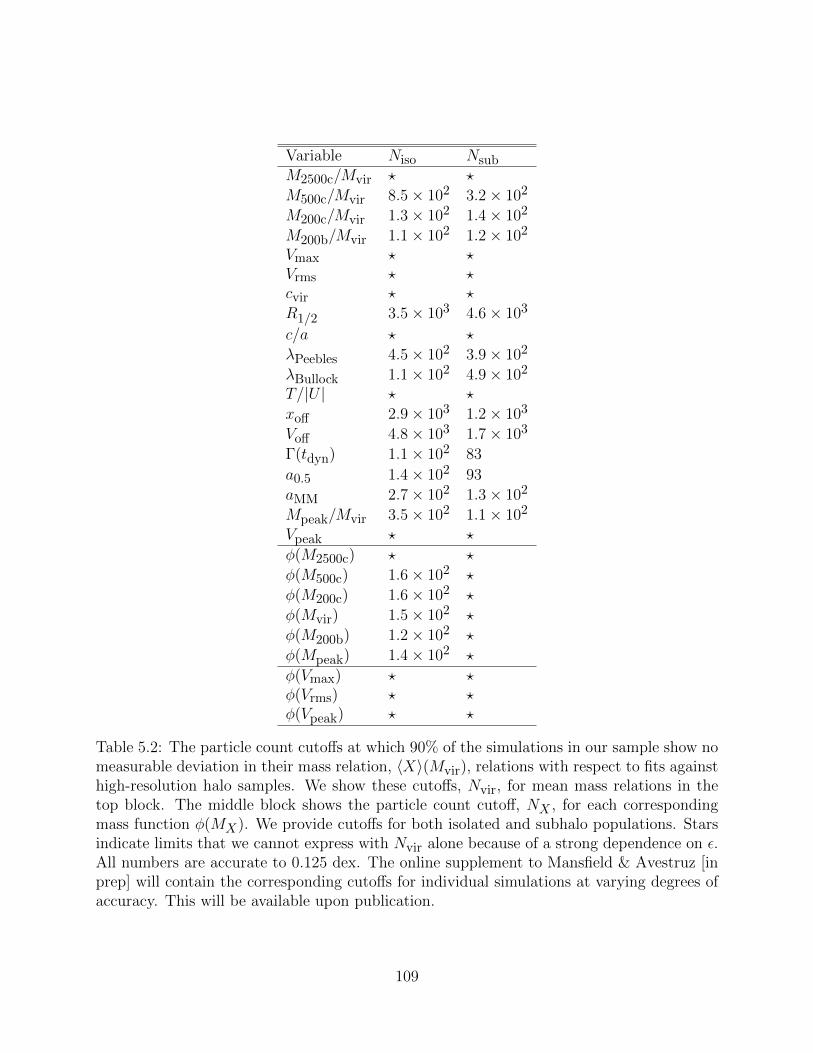
Variable Niso NsubM2500c/Mvir ? ?

M500c/Mvir 8.5× 102 3.2× 102

M200c/Mvir 1.3× 102 1.4× 102

M200b/Mvir 1.1× 102 1.2× 102

Vmax ? ?Vrms ? ?cvir ? ?

R1/2 3.5× 103 4.6× 103

c/a ? ?

λPeebles 4.5× 102 3.9× 102

λBullock 1.1× 102 4.9× 102

T/|U | ? ?

xoff 2.9× 103 1.2× 103

Voff 4.8× 103 1.7× 103

Γ(tdyn) 1.1× 102 83

a0.5 1.4× 102 93

aMM 2.7× 102 1.3× 102

Mpeak/Mvir 3.5× 102 1.1× 102

Vpeak ? ?

φ(M2500c) ? ?

φ(M500c) 1.6× 102 ?

φ(M200c) 1.6× 102 ?

φ(Mvir) 1.5× 102 ?

φ(M200b) 1.2× 102 ?

φ(Mpeak) 1.4× 102 ?

φ(Vmax) ? ?φ(Vrms) ? ?φ(Vpeak) ? ?

Table 5.2: The particle count cutoffs at which 90% of the simulations in our sample show nomeasurable deviation in their mass relation, 〈X〉(Mvir), relations with respect to fits againsthigh-resolution halo samples. We show these cutoffs, Nvir, for mean mass relations in thetop block. The middle block shows the particle count cutoff, NX , for each correspondingmass function φ(MX). We provide cutoffs for both isolated and subhalo populations. Starsindicate limits that we cannot express with Nvir alone because of a strong dependence on ε.All numbers are accurate to 0.125 dex. The online supplement to Mansfield & Avestruz [inprep] will contain the corresponding cutoffs for individual simulations at varying degrees ofaccuracy. This will be available upon publication.

109

standard deviation 1. From this the probability, p, of the measurement under the null

hypothesis can be calculated.

To apply the z-test to a single simulation and a single mass bin centered at the mass M ,

we take the amplitude and 1σ dispersion of best-fitting high resolution relation as 〈X1〉 and

err(〈X1〉), respectively, and the sample mean and the 1σ bootstrapping error of X for the

simulation in that mass bin as 〈X2〉 and err(〈X2〉), respectively. We adopt the convention

that deviations with a probability of less than 5% under the null hypothesis indicate that a

simulation is not converged to the high-resolution relation at that mass.

We show this test in the right panel of Fig. 5.1. Mass relations are color-coded by the

value of p as a function of mass.

In some cases, the derivative of the difference between unconverged mass relations and

the high resolution fit can change sign as a function of mass. This means that as a mass

decreases, an unconverged simulation can briefly cross the high-resolution fit and can falsely

appear to be converged for one or two mass bins. Additionally, since we adopted a 2σ

significance cutoff for non-convergence, some poorly sampled very high resolution bins can

appear to be unconverged. This latter effect can be seen in Fig. 5.1. To handle these edge

cases, we consider only “strings” of consecutive mass bins which all falsify the null hypothesis

with p > 0.05. We take the convergence limit of a simulation to correspond to the lower edge

of the lowest mass bin which is a member of such a string containing at least three mass

bins.

To confirm this procedure, we visually identified convergence limits for every simulation

and halo property in each sub-group without knowledge of the bins that our statistical

method selected. Visual identifications were generally within 0.125-0.25 dex of the statistical

measurements with ∆12 = 0. Qualitatively, no major results in this chapter change if these

visual cutoffs are used. However, as noted above, the particle cutoffs for some halo properties

showed somewhat smaller dispersions when visual cutoffs were used. Inspection of individual

cases caused us to interpret this as confirmation bias.

110

There are some simulations which are converged across the entire mass range used to

fit the high-resolution relation. This is the case for the highest resolution fits in Fig. 5.1.

Rather than extrapolate our fits, the convergence limits of these simulations are left as upper

limits. This is almost always the case for the highest resolution simulation in a sub-group.

In rarer cases, there are simulations which are unconverged across the entire high-resolution

mass range. The convergence limits for these boxes are left as lower limits.

Although all fiducial results reported in this chapter make use of the z-test as described

above, we also extend it to account for the “practical significance” of deviations. Ultimately,

the purpose of cosmological simulations is to facilitate a wide range of analyzes, and different

types of analysis can tolerate different levels of non-convergence. To account for this, we

introduce the parameter δ, which represents a minimum acceptable deviation as a percentage

of the high resolution relation. We then add three additional conditions for a mass bin to

be considered unconverged:

1. |〈X1〉 − 〈X2〉| > δ〈X1〉,

2. pz(∆12 = δ〈X1〉) < 0.05,

3. pz(∆12 = −δ〈X1〉) < 0.05.

Here, pz(∆12) is the probability that the two samples have means that differ by as much as

observed under the null hypothesis that they are drawn from populations which means that

differ by ∆12.

5.3 The Empirical Nvir Convergence Limits of Simulations

5.3.1 Typical Convergence Limits

We use the procedure described in section 5.2.3 to find the particle count, Nvir, at which each

simulation in Table 3.1 deviates from high resolution fits for a given mass relation, 〈X〉(Mvir),

of a halo property X. Table 5.2.3 shows example particle count cutoffs for X = xoff , with

111

0 1 2 3 4 5 6log10(Nvir)

Erebos CBol

Erebos CPla

Multidark

Chinchilla

ν2 − gc

Bolshoi

BolshoiP

TNG−Dark

Vmax

Figure 5.2: The Nvir values below which numerical effects measurably bias mean Vmax valuefor each simulation in Table 3.1. These are conservative limits: all analysis can accept somelevel of numerical bias. There is significant variation in these limits from simulation to simu-lation. We first use color to group simulations by suite, then vertically order the simulationsby particle mass; the bottom dot in each suite corresponds to the highest resolution box ofthat suite. We use points to indicate simulations where we measure diverging behavior andupper limits for simulations where we were not able to measure a divergence. As discussedin section 5.2.3 and shown in Fig. 5.3, the two highest resolution Planck suites, TNG-Darkand Multidark, appear to converge to two different Mvir − Vmax relations. The solid circlesshow cutoff values when the high-resolution fit does not include Multidark boxes and theopen circles show cutoff values when the high-resolution fit does not include TNG-Dark.

112

8 9 10 11 12 13 14 15 16log10(Mvir) (h−1M)

1.05

1.10

1.15

1.20

1.25

1.30

1.35

1.40

1.45

Vm

ax/V

vir

Erebos CBol L63

Erebos CBol L125

Erebos CBol L250

Erebos CBol L500

Erebos CBol L1000

Erebos CBol L2000

8 9 10 11 12 13 14 15 16log10(Mvir) (h−1M)

0.35

0.40

0.45

0.50

0.55

0.60

0.65

0.70

0.75

c/a

Erebos CBol L63

Erebos CBol L125

Erebos CBol L250

Erebos CBol L500

Erebos CBol L1000

Erebos CBol L2000

8 9 10 11 12 13 14 15 16log10(Mvir) (h−1M)

1.05

1.10

1.15

1.20

1.25

1.30

1.35

1.40

1.45

1.50

Vm

ax/V

vir

BolshoiP

Erebos CPla

Multidark

ν2 − GC

TNG− Dark

8 9 10 11 12 13 14 15 16log10(Mvir) (h−1M)

0.35

0.40

0.45

0.50

0.55

0.60

0.65

0.70

0.75

c/a

BolshoiP

Erebos CPla

Multidark

ν2 − GC

TNG− Dark

Figure 5.3: The convergence behavior of 〈Vmax/Vvir〉 and 〈c/a〉 as functions of Mvir. Top:“Classical” convergence tests using the six boxes from the Erebos CBol suite. Each curvecolor corresponds to a different box, and the linestyle transitions from solid to dashed atNvir ≤ 500. In isolation, these plots imply that rotation curve peaks and halo shapes mea-sured for halos above 500 particles are converged. Bottom: The Mvir − Vmax/Vvir andMvir−c/a for every Planck-cosmology simulation suite in Table 3.1. Simulations are coloredby suite and the solid-to-dashed transition still occurs at Nvir ≤ 500. There is disagreementbetween the mass relations above the convergence limit implied by the top plots. The bottomtwo panels contain a number of noteworthy features which we highlight in section 5.3.2.

113

particle count cutoffs provided for both isolated halos and subhalos and example accuracy

tolerances of δ = 0.00 and δ = 0.01. The online supplement of Mansfield & Avestruz [in

prep] will contain results for all properties listed in section 5.2.2 with accuracy tolerances

ranging from δ = 0.00 to δ = 0.10, which will be available upon publication. Blank table

entries indicate that we were not able to make a reliable measurement of a deviation from

the mean mass relation for that property at that accuracy tolerance.

In Table 5.2.3, we show conservative “convergence limits” for many halo properties. These

correspond to Nvir values at which 90% of the simulations in our sample show no measurable

deviation from high resolution fits (δ = 0; section 5.2.3). These limits should be viewed as a

guideline in assessing the acceptable level of numerical bias in an analysis. We recommend

that any analysis using halos with smaller Nvir either use accuracy-dependent limits in Table

5.2.3 or explicitly test for numerical biases and include the systematic uncertainty in the error

estimates.

For each halo property in Table 5.2.3, we have performed detailed tests on how strongly

this property depends on ε (see section 5.4). Properties which strongly depend on ε have

been marked by a ?, as we cannot express convergence limits in terms of Nvir alone.

It is difficult to compare this table to previous tests in the literature. For most of the

common properties with existing testing literature (e.g., Vrms; Evrard et al., 2008 or T/|U |;

Power et al., 2012), we conclude that there is such a strong dependence on ε that we cannot

endorse a single Nvir limit. For many of the remaining properties, such as, xoff or aMM ,

we are not aware of any previous convergence tests. That said, we note that our cutoff for

λPeebles is consistent with the results of Villarreal et al. [2017b], and that our criteria for

isolated halo abundances are consistent with existing literature on the topic [e.g. Angulo

et al., 2012, Ishiyama et al., 2015, Ludlow et al., 2019], although different authors adopt

different target accuracies. Finally, we note that our input catalogs did not have subhalos

with fewer than 50 particles; we were not able to put competitive constraints on mass

definitions with limits near or below this value.

114

5.3.2 Variation in Limits Between Simulations

Fig. 5.2 shows the Nvir values at which every simulation in our suite measurably deviates

from from high resolution fits to 〈Vmax〉(Mvir). These values correspond to Niso,0.00 in Table

5.2.3. These Nvir limits are conservative (δ = 0; see section 5.2.3), and applications which

can accommodate modest biases in 〈Vmax〉 may be able to use halos with smaller values of

Nvir. Nevertheless, the limits shown in Fig. 5.2 show the resolution scales at which numerical

effects begin to measurably influence the behavior of the Vmax distribution.

There is substantial variation in these convergence limits from simulation to simulation,

with many simulations only reaching full statistical convergence at 105 − 106 particles. Be-

cause TNG-Dark and Multidark appear to converge to different Vmax relations (see section

5.3.3), we perform this analysis twice with separate fits to both suites. The filled in circles

correspond to the fit to TNG-Dark and the unfilled circles correspond to the fit to Multidark.

Noe that the limits for TNG-Dark become higher when Multidark is used to fit low-mass

halos, and the opposite is true when TNG-Dark is used. However, the overall scatter in the

convergence limits does not depend on this choice. Note that simulations with WMAP-like

cosmologies (Chinchilla, Erebos CBol, Bolshoi) are unaffected by this fitting choice because

they were fit separately.

The simulations-to-simulation variation in convergence limits is not an artifact of our

convergence procedure. In Fig. 5.3 we qualitatively demonstrate this effect for Vmax and

another commonly used halo property, c/a.

The top panels of Fig. 5.3 show the “classical” convergence test for Vmax and c/a using

the seven boxes in the Erebos CBol suite. We show the mass relations, Vmax −Mvir and

c/a −Mvir, for isolated halos using different colors for each box in the suite. The curves

are solid for halo masses corresponding to particle numbers above 500 and dashed for halo

masses below this particle count. These simulations strongly agree with one another above

this visually-identified convergence limit. There is some slight variation in the amplitude

due to cosmic variance. The agreement seems to indicate that both quantities are converged

115

above 103 particles.

However, we do not find such agreement when comparing across simulation suites. The

bottom two panels of Fig. 5.3 show the same mass relations for all of our Planck-cosmology

simulations. Most of the simulations have many times more particles than the Erebos CBol

suite. As in the top panels, the curves are solid above 500 particles and dashed below. Unlike

the top panels, there is disagreement between the simulations at halo masses corresponding

to approximately 105 particles, even for simulations in the same suite.

We have ruled out many factors outside of numerical non-convergence that could poten-

tially cause a difference in these mass relations. We address these factors in other sections

of this chapter, but we collect them here for convenience.

• As discussed in section 5.2.1, we cross-matched catalogs to demonstrate that varying

versions and parametrizations of the Rockstar halo finder cannot cause this disagree-

ment.

• The statistically estimated cutoffs shown in Fig. 5.2 are consistent in detail with the

qualitative disagreement shown in Fig. 5.3. As described in section 5.2.3, our statis-

tical cutoffs explicitly account for cosmic variance, estimated by jackknife resampling.

Additionally, the disagreement extends to some very large boxes, such as ν2-gc-L. This

means that the disagreement is not caused by cosmic variance.

• Fig. 5.3 only contains isolated halos, so this disagreement cannot be due to the stricter

convergence criteria on subhalo resolution. We have also inspected the distribution of

halo properties at a constant mass to determine that a small population of outliers is

not driving the differences.

• We also see disagreement between simulations in the same suite. Simulations within

the same suite use identical codes, identical cosmologies, and nearly identical initial

conditions setups. This means that differences of this type cannot be the sole cause of

the disagreement.

116

8 9 10 11 12 13 14 15 16log10(Mvir) (h−1M)

1.05

1.10

1.15

1.20

1.25

1.30

1.35

1.40

1.45

1.50

Vm

ax/V

vir

VSMDPL

TNG100− 1− Dark

TNG− Dark

Multidark

Figure 5.4: The same as the lower left panel of Fig. 5.3, except restricted to TNG-Dark andMultidark boxes. TNG100-1-Dark and VSMDPL, which have very similar parametrizations,are emphasized with darker colors. The two suites have converged to different solutions.

5.3.3 Differences Between Multidark and Illustris-TNG

As discussed above, the Multidark suite and the Illustris-TNG suite have converged to two

different 〈Vmax(Mvir)〉 relations. We illustrate this in Fig. 5.4. This difference emphasizes

that convergence alone is not sufficient to establish that a simulation is unbiased, a point

which is discussed further in section 5.1. In the rest of this section we focus on isolating

the cause of such a “false convergence” in detail. In particular, we focus on the TNG100-1-

Dark and VSMDPL boxes, which have very similar parametrizations and are emphasized in

Fig. 5.4.

Numerical differences between cosmological simulations come from a finite list of sources:

cosmology, cosmic variance, halo finders, box size, mp, timestepping, force softening scheme,

ε, initial condition generation, code parameters, and code algorithms.

Cosmology cannot cause the difference between TNG100-1-Dark (Ω = 0.309, h100 =

0.677, σ8 = 0.8159) and VSMDPL (Ωm = 0.307, h100 = 0.678, σ8 = 0.832), as the

Planck-like parameters they adopt are almost identical. Cosmic variance can never lead

117

to false convergence because such fluctuations would be uncorrelated with simulation suite.

Additionally, we find that the cosmic variance estimated through jackknife resampling for

〈Vmax(Mvir)〉 is small relative to the difference between the suites. As discussed at length

in section 5.2.1, we have ruled out halo finder inconsistencies as a potential cause of non-

convergence. Although TNG100-1 (L = 75h−1Mpc) and VSMDPL (L = 160h−1Mpc)

have different box sizes, any small-box effects this large in an L = 75h−1Mpc box would

have been detected in the tests performed by Power and Knebe [2006]. TNG100-1-Dark

(mp = 6.00 × 106 h−1M) and VSMDPL (mp = 6.16 × 106 h−1M) have virtually iden-

tical particle masses, meaning that the source of the false convergence cannot be related

to mass resolution. Gadget-2 and Arepo use the same timestepping criteria, Eq. 3.1, and

TNG100-1 (η = 0.012) and VSMDPL (η = 0.01) use nearly identical values of η, meaning

that timestepping is very similar between the simulations.

Both simulations use the same softening scheme, Eq. 3.3, but TNG100-1-Dark (ε/l =

0.018) and VSMDPL (ε/l = 0.024) use softening lengths that differ by 25%. While small,

this difference could, in principle contribute to the false convergence. However, in section 5.5

we construct an explicit model for the impact of ε/l in this regime. This model predicts that

while both simulations should be biased to slightly low in Vmax due to the adopted values

of ε, this effect is too small to account for the false convergence.

After review of the configuration files for both simulations [Nelson et al., 2019, Yepes,

personal communication], the only meaningful difference between parametrizations is α (also

referred to as facc, and ErrTolForceAcc), which sets the node opening criteria in Gadget’s

force tree. VSMDPL adopts α = 0.01, while TNG100-1-Dark adopts a more conservative

α = 0.0025. The tests in Power et al. [2003] indicate that α = 0.01 can lead to density

biases in regions of halos with N(< R) ≈ 100, but that this effect is also dependent on mass

resolution, meaning that it’s unlikely to contribute to biases which persist across multiple

resolutions. However, the impact of α deserves further study.

Based on the process of elimination, we consider the most likely cause of the false con-

118

vergence seen in Fig. 5.4 to be updates in the Gadget force solver which were made during

the development of Arepo. Gadget-2 dynamically updates force trees to avoid needing to

reconstruct the entire tree for each step taken by particles in the finer time bins [Springel,

2005]. However, Weinberger et al. [2019] found that this process leads to force errors which

are correlated with timestep size, leading to errors which occur predominantly in the central

regions of halos where particles are on short orbits and scattering off one another on short

timescales. This effect would depend chiefly on the acceleration felt by each particle, opening

an avenue for a numerical effect which depends primarily on halo mass and not on resolution.

The cause of this false convergence must be established before high-accuracy measure-

ments of rotation curves at low masses (Mvir . 1010h−1M) can be performed. No state-

ment can be made about which simulation suite(s) have and have not falsely converged until

there is a positive identification of the source of the issue.

5.4 The Dependence of Halo Properties on Force Softening Scale

To investigate the dependence of halo properties on ε, we make use of four convergence

boxes which were initially run as part of the Chinchilla simulation suite (as seen in, e.g.,

Mao et al., 2015, Desmond and Wechsler, 2015, Lehmann et al., 2017).2 These boxes are

resimulations of the same set of initial conditions but with different force softening scales (see

Table 5.4). They were run with L = 125h−1 Mpc, N3 = 10243, ΩM,0 = 0.286, h100 = 0.7,

and mp = 1.44× 108 h−1M. Aside from force softening scale, these boxes are very similar

to the Erebos CBol L125 box (the orange curve in the upper panels of Fig. 5.3). We refer

to this as the Chinchilla-ε suite.

The force softening scales in these boxes span a wide range. In units of the mean in-

terparticle spacing, the smallest force softening scale, in Chinchilla L125 e1, corresponds to

ε/l = 0.0082 a small but not uncommon length which is similar to simulations like Bol-

shoi or any of the Chinchilla boxes. The next smallest, Chinchilla L125 e2, corresponds

2. Access to these catalogs was generously provided by Matthew Becker.

119

Simulations name ε (h−1kpc) ε/lChinchilla L125 e1 1 0.0082Chinchilla L125 e2 2 0.016Chinchilla L125 e5 5 0.041Chinchilla L125 e14 14 0.115

Table 5.3: Simulation parameters of the resimulated convergence boxes of the Chinchilla-εresimulation suite. Shared parameters of these simulations are discussed in section 5.4.

to a fairly typical ε/l = 0.016 which is similar to SMDPL or Erebos CBol L63. Next is

Chinchilla L125 e5, ε/l = 0.041 which is close to the upper limit of ε typically found in cos-

mological simulations and is similar to Erebos CBol L1000 or the ν2-gc boxes. The last box,

Chinchilla L125 e14, has a force softening scale much larger than any box in our simulation

suite: ε/l = 0.115, but which is comparable to the ε suggested by some convergence studies

(see section 5.6.1). Timestepping in each simulation is performed via Eq. 3.1 with η = 0.025,

meaning that timesteps are not constant between simulations.

We compare the mass-trends for every halo property described in section 5.2.2 across the

boxes in the Chinchilla-ε resimulation suite. Most properties, such as Xoff or λBullock show

either little to no dependence on ε or show agreement for typical values of ε and some mild

non-convergence in Chinchilla L125 e14. This is not true for all halo properties.

In Fig. 5.5 we show the Vmax−Mvir, c/a−Mvir, Vrms−Mvir, and T/|U |−Mvir relations

for isolated halos in each of the Chinchilla resimulation boxes. The curves are solid above

the cutoffs listed in Table 5.2.3 and dashed below it. If the traditional convergence tests in

this chapter are correct, one would expect that these trends would not depend on numerical

parametrization above these cutoffs. We find that all four properties vary meaningfully with

ε. These mass relations vary continuously in amplitude and slope across the entire ε range.

To give a sense of the “practical significance” of these trends, we overplot the difference

between the DMO TNG100-2-Dark and the baryonic TNG100-2 as a gray shaded region.

For Vmax and c/a, the shift in halo properties due to numerical effects is comparable to or

greater than the impact of baryons.

120

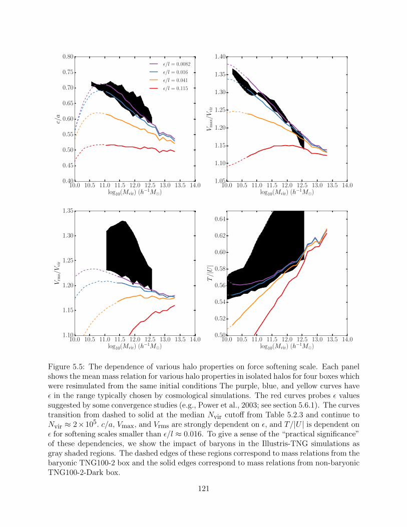
10.0 10.5 11.0 11.5 12.0 12.5 13.0 13.5 14.0log10(Mvir) (h−1M)

0.40

0.45

0.50

0.55

0.60

0.65

0.70

0.75

0.80c/a

ε/l = 0.0082

ε/l = 0.016

ε/l = 0.041

ε/l = 0.115

10.0 10.5 11.0 11.5 12.0 12.5 13.0 13.5 14.0log10(Mvir) (h−1M)

1.05

1.10

1.15

1.20

1.25

1.30

1.35

1.40

Vm

ax/V

vir

10.0 10.5 11.0 11.5 12.0 12.5 13.0 13.5 14.0log10(Mvir) (h−1M)

1.10

1.15

1.20

1.25

1.30

1.35

Vrm

s/V

vir

10.0 10.5 11.0 11.5 12.0 12.5 13.0 13.5 14.0log10(Mvir) (h−1M)

0.50

0.52

0.54

0.56

0.58

0.60

0.62

0.64

T/|U|

Figure 5.5: The dependence of various halo properties on force softening scale. Each panelshows the mean mass relation for various halo properties in isolated halos for four boxes whichwere resimulated from the same initial conditions The purple, blue, and yellow curves haveε in the range typically chosen by cosmological simulations. The red curves probes ε valuessuggested by some convergence studies (e.g., Power et al., 2003; see section 5.6.1). The curvestransition from dashed to solid at the median Nvir cutoff from Table 5.2.3 and continue toNvir ≈ 2×105. c/a, Vmax, and Vrms are strongly dependent on ε, and T/|U | is dependent onε for softening scales smaller than ε/l ≈ 0.016. To give a sense of the “practical significance”of these dependencies, we show the impact of baryons in the Illustris-TNG simulations asgray shaded regions. The dashed edges of these regions correspond to mass relations from thebaryonic TNG100-2 box and the solid edges correspond to mass relations from non-baryonicTNG100-2-Dark box.

121

10−3

10−2

µ×N

(>µ

)

ε/l = 0.0082

ε/l = 0.016

ε/l = 0.041

ε/l = 0.115

10−4 10−3 10−2 10−1 100

µ = M200c, sub/M200c, host

−1.0

−0.5

0.0

0.5

N/N

0.01

6−

1

10−3

10−2

µ3×N

(>µ

)10−1 100

µ = Vmax, sub/Vmax, host

−1.0

−0.5

0.0

0.5

N/N

0.01

6−

1

10−3

10−2

10−1

µ3×N

(>µ

)

10−1 100

µ = Vpeak, sub/Vpeak, host

−1.0

−0.5

0.0

0.5

N/N

0.01

6−

1

Figure 5.6: The impact of force softening on the subhalo abundance within 50 host halosfrom the Chinchilla-ε resimulation suite with masses M200c ≈ 1014. Left: The dependenceof the cumulative subhalo mass function on force softening scale. Plotted are the mean meanfunctions. The solid lines show all subhalos, and the dashed lines show all subhalos within0.25R200c of their hosts. The fractional deviation from the ε = 0.016 simulation is shown inthe bottom panel. center: the same for the mean Vmax subhalo velocity function. Right: thesame for the mean Vpeak subhalo velocity function. The lowest mass subhalos shown in eachplot have ≈ 70 particles. Note that the red curve corresponds to an atypically large valueof ε. The subhalo mass function exhibits only a weak dependence on ε in the outer regimesof the halo. This dependence becomes stronger at small radii, confirming that artificialdisruption is stronger in this regime. The subhalo velocity functions depend more stronglyon ε, even at large radii. Although the impact of ε velocity functions becomes stronger atsmall radii, the strength of the dependence at large radii relative to the dependence seen inthe subhalo mass function implies that most of this effect is from artificial suppression ofVmax and not artificial subhalo disruption.

5.4.1 Dependence of the Subhalo Mass Function on ε

In Fig. 5.6 we show the dependence of the subhalo mass and velocity functions on ε. The

left panel shows the mean subhalo mass functions functions of the 50 largest halos in the

Chinchilla-ε resimulation suite, the middle panel shows the mean subhalo Vmax functions

for these halos, and the right panel shows the mean subhalo Vpeak functions of these halos.

The host halos have particle counts ranging across 5× 105 < N200c < 1.4× 106. We use the

high-density M200c mass definition to study subhalos over the lower density Mvir definition

favored elsewhere in this chapter, as higher density regions survive longer prior to disruption.

Both types of subhalo velocity functions show a strong dependence on force softening scale

122

that becomes stronger when considering subhalos close to the center of the host. Subhalo

mass functions have a weaker dependence on ε, although it also becomes stronger for central

subhalos, implying that artificial subhalo disruption/stripping becomes stronger at small

radii. The difference in ε-dependence between the mass and velocity functions implies that

velocity functions are primarily impacted by artificial suppression of the velocity curve (which

does not affect mass functions and which does not have a radial dependence) more than

artificial subhalo disruption, but that artificial subhalo disruption likely leads to the radial

dependence in ε-dependence.

Note that, as discussed in section 5.1, convergence between independent cosmological

simulations cannot establish correctness. The lack of a strong ε dependence at larger radii

or larger particle counts does not imply that artificial disruption of subhalos is a weak

effect: such a statement requires comparison with idealized simulations. However, these

measurements can be used to constrain disruption models which predict that disruption

rates depend on ε.

The idealized tests in van den Bosch and Ogiya [2018] suggest that some aspects of

artificial subhalo disruption have a strong dependence on force softening scale. They find

that simulations of idealized subhalos experience substantial artificial disruption and that this

disruption occurs even at high subhalo resolutions. The rate of tidal stripping is dependent

on ε across the range of ε values adopted by the Chinchilla-ε test suite. Our results are not

in conflict with these findings, despite the weak dependence of the subhalo mass function on

ε.

van den Bosch and Ogiya [2018] found that numerical factors begin to artificially accel-

erate disruption once halos have already lost & 90−95 per cent of their mass due to physical

disruption. Due to the slope of infalling halo mass function, at any particular snapshot,

the majority of subhalos at a given mass have not yet experienced this level of disruption.

Additionally, the effect of artificial disruption due to force softening is strongest in subhalos

on close orbits, with effect becoming particularly strong at R ≈ 0.1Rvir, a regime which

123

our simulations do not have sufficient resolution to probe. Subhalos on close-orbits are both

located in the deepest part of the host halo’s potential and are most likely to have already

experienced many orbits. While close orbit subhalos make up a small fraction of the host’s

overall volume (and thus of our sample), the best constraints on the faint end of the satel-

lite luminosity function come from the corresponding satellite population of the Milky Way

[e.g. Drlica-Wagner et al., 2019]. Furthermore, the radial dependence of artificial disruption

affects makes it more difficult to compare observed satellite number density profiles to the

predictions of ΛCDM [e.g. Carlsten et al., 2020]. These effects are therefore still important

for cosmological constraints.

The locations of even the most massive subhalos are altered substantially by changes in

ε. It is possible that this is due to chaotic errors in halo phase while orbiting their hosts, but

given that the tidal disruption rate in the host’s central region is dependent on ε, it is also

possible that this is caused by an ε dependence in the dynamical fiction experienced by each

subhalo. This change in positions makes it impossible to directly measure subhalo disruption

using only single-snapshot information. Such analysis would be possible by comparing the

trajectories of subhalo progenitors prior to accretion. We defer such analysis of subhalo

trajectories to future work.

Note that these tests only study the impact of ε on subhalo abundance. Particle count

also substantially impacts the reliability of subhalo velocity functions [e.g. Guo and White,

2014, Klypin et al., 2015b] and must be accounted for accordingly.

5.5 Estimating the Impact of Large ε on Vmax

In sections 5.3.1 and 5.3.2 of this chapter, we showed that the distribution of halo properties

measured in different simulations diverge from one another at unexpectedly high particle

counts. In section 5.4, we showed that varying ε across the range typically used in cosmo-

logical simulations has a large impact on many commonly studied halo properties. In this

section, we construct a model that predicts this behavior for the simplest property we have

124

considered: Vmax.

Previous convergence studies have established three channels that allow halo rotation

curves to depend on ε. In the large ε limit, non-Newtonian forces suppress V (R) with

increasing ε. The suppression is primarily due to how softening reduces centripetal forces

[e.g. Klypin et al., 2015b, van den Bosch and Ogiya, 2018, Ludlow et al., 2019]. As we

show in Fig. 5.9, the suppression of V (R) continues into regimes where the force kernel

is Newtonian because the entire halo responds to the creation of a low-density core. As

we discuss in section 5.6.1, some of this effect may be caused by poor timestep resolution

under some timestepping schemes. In the limit where ε is small, two-body collisions begin to

thermalize the dark matter particles over some local relaxation timescale [e.g. Power et al.,

2003, Navarro et al., 2010, Ludlow et al., 2019]. This causes the otherwise adiabatic orbits of

dark matter particles [e.g. Dalal et al., 2010] to become adiabatic and for the radial velocity

dispersion profile to flatten [e.g. fig. 6 of van den Bosch and Ogiya, 2018]. The dominant

effect of this transformation is that particles in the high velocity tails are transported to

higher radii, leading to decreasing V (r) as this timescale decreases. This timescale depends

primarily on the size of r relative to l [Ludlow et al., 2019], although excessively small ε and

> tHubble measurement timescales increase cause ε dependencies to become more important

[van den Bosch and Ogiya, 2018]. Lastly, in the limit where ε is small and timestepping is

coarse, integration errors (e.g. fig. 9 of Knebe et al., 2000). This last effect is discussed at

length in section 5.6.1. The “art” of configuring a cosmological simulation is in selecting an

ε and ε in a safe regime that avoids all three effects.

We illustrate the dominant trend in the top right panel of Fig. 5.5. Here, we see that

Vmax decreases with increasing ε, implying that large values of ε is the most likely driver of

suppressed rotation curves.

When simulators account for large-ε effects, they typically restrict their analysis to halos

where R > Xε, where X is some constant. To give an idea of the typical values of X

used, we surveyed several papers which studied the concentration-mass relation to identify

125

values for X = 〈r−2〉(Mvir,min)/ε. We found that the minimum values identified ranged from

2.5 ≤ X ≤ 6.4 [Neto et al., 2007, Duffy et al., 2008, Gao et al., 2008, Zhao et al., 2009, Prada

et al., 2012, Bhattacharya et al., 2013, Ludlow et al., 2013, Dutton and Maccio, 2014, Klypin

et al., 2016, Poveda-Ruiz et al., 2016, Child et al., 2018]. This is broadly consistent with

the behavior of Rockstar, which downweights radii larger than 3ε. Diemer and Kravtsov

[2015] performed a detailed review use the results of several zoom-in simulations to conclude

that analysis is safe above > 3ε for individual halos, and that analysis of 〈r−2〉(Mvir) should

be restricted to masses where 〈r−2〉(Mvir) & 8ε to account for scatter in the Mvir − cvir

relation. Below, we take a different approach and use out direct measurements of the impact

of ε on rotation curves (Eq. 5.13) to estimate the impact of ε on the distribution of Vmax in

a halo population.

The left panel of Fig. 5.7 illustrates the rotation curve bias due to the Gadget force

softening scale, as predicted by Eq. 5.13 for different halo profile shapes. We reference Klypin

et al. [2015b] for a mathematical summary of NFW rotation curves and Garrison-Kimmel

et al. [2014] for a similar summary of Einasto rotation curves. Einasto profiles require a

second parameter beyond Rs, α, and provide a more accurate fit than NFW profiles [e.g. Gao

et al., 2008, Springel et al., 2008]. The solid curves in Figure 5.7 show the unbiased rotation

curves for an NFW profile in black and Einasto profiles with α=0.14, 0.18, and 0.22 in red,

yellow, and blue, respectively. The selected α values roughly correspond to the range spanned

by z = 0 halos [e.g. Child et al., 2018]. The dashed lines show the biased rotation curves

predicted by Eq. 5.13 for hGadget = Rmax (ε = 0.278Rmax). The biased maximum velocity,

Vmax,bias, ranges from 0.943Vmax to 0.949Vmax, exhibiting a small systematic uncertainty

due to halo profile shape, which is ≈ 10 percent of Vmax − Vmax,bias. This uncertainty

consistently stays at or below this level relative to Vmax − Vmax,bias regardless of Rmax/ε

By evaluating ξbias = Vmax/Vmax,bias for a range of ε/Rmax, we can empirically construct

the invertible function ξbias(ε/Rmax) for a given halo profile shape. For convenience, we note

126

that for both NFW and Einasto profiles this function is well-fit by,

ξbias = 2−(

1 + (Aε/Rmax)2)β

. (5.4)

We fit this relation for Gadget-like kernels over the range of 0.01 ε/Rmax . hGadget .

5 ε/Rmax. Below this range, Vmax/Vmax,bias is 1 for all practical purposes. Above this range,

Eq. 5.13 is poorly constrained. By minimizing the least-squared error on Vmax/Vmax,bias, we

find that the parameters A = 6.049 and β = 0.05440 lead to errors in Vmax,bias which are .

10−3Vmax for NFW profiles and that the parameters A = 5.884 and β(α) = 0.02754 ln (α)+

0.15566 lead to errors which are . 2 × 10−3 Vmax for Einasto profiles with α ranging from

0.12 to 0.32. However, we use the raw empirical functions in all subsequent analyzes, derived

from whichever force softening kernel is appropriate.

Note, no function describing ξbias(ε/Rmax) can be applied on its own to evaluate the bias

in Vmax because these functions depend on the unbiased value of Rmax, which is unknown.

Therefore, such a function must be combined with a second, independent equation relating

ξbias to Rmax.

For our application, the systematic errors in ξbias due to profile shape are small. We

therefore restrict our analysis to NFW profiles because they depend on only a single param-

eter. With an NFW parametrization, we can directly compute an estimate for ξbias from

the unbiased cvir and Vvir,bias from the halo catalog. The estimate comes in the form of,

ξbias = 0.469

(Vvir,bias

Vmax,bias

)(cvir

f(cvir)

)1/2(

Vvir

Vvir,bias

)(5.5)

where Vvir/Vvir,bias is Eq. 5.13 evaluated at R/ε = 0.469 cvirRmaxε and f(x) = ln (1 + x) −

1/(1 +x). We compute the ratio Vvir,bias/Vmax,bias from halo catalogs, whose measurements

are biased due to ε.

For NFW halos, Rmax = 2.164Rs. This and Eq. 5.5 provide two independent equations

for ξbias(ε/Rmax). For halos with Rmax,bias > Rvir,bias (a criterion that holds for virtually

127

all halos in cosmological simulations), these two relations intersect at exactly one point: a

unique solution for ξbias = Vmax/Vmax,bias. This statement is only true for single parameter

profile models, such as NFW profiles or Einasto profiles with fixed α.

With this de-biasing procedure, we can estimate the unbiased Vmax/Vvir for each halo in

a given cosmological simulation from the biased measurements of Vmax,bias/Vvir,bias. We can

then estimate the mean unbiased Vmax/Vvir(Mvir) in that simulation. Note that the scatter

in the Mvir− Vmax relation means that this estimate cannot only be applied to the mean of

a particular mass bin, but must first be applied to individual halos before finding the mean

relation as described.

The right panel of Fig. 5.7 shows the result of the “de-biased” estimate of Vmax/Vvir for

the Chinchilla resimulation boxes. From this figure, we see that this procedure completely

removes the ε dependence from this sample, implying that the numerical bias of Vmax/Vvir

is primarily due to large ε.

There is a few-per cent dispersion between curves at moderate-to-high masses. While

other numerical effects could cause this dispersion, the level of dispersion is consistent with

the error level associated with the assumption of an NFW profile in our analysis. As dis-

cussed above, assuming a profile shape results in systematic errors in Vmax on the order of

0.1 (Vmax− Vmax,bias). Given that some simulations are estimated to be biased at the 20% -

30% level, a 2%-3% error is to be expected. The dispersion increases at low particle counts

(low halo masses) and small Rmax/ε. While numerical effects could cause this as well, the

dispersion occurs in a regime where corrections are large and Eq. 5.13 is poorly constrained.

In Fig. 5.8, we show the results of applying these bias estimates to various Planck cosmol-

ogy simulations. In this Figure, dashed lines show the measured mean mass trends in each

simulation. The solid lines show results from our de-biasing procedure, which are estimates

of what these trends would have been if not for the large ε bias. We cut off the estimated

trend when they disagree from the measured trend by more than one per cent. As with the

Chinchilla boxes, we are able to account for all of the visibly-apparent deviations from the

128

mean measured trend using our de-biasing procedure for biases due to large ε.

We note that there is still a non-trivial amount of scatter between simulation suites along

the mean trend. While is is possible that this dispersion is also due to numerical factors,

another possible explanation is in variations due to exact cosmology. Despite the fact that all

are “Planck” cosmology simulations, different suites are either associated with data releases

from different years or round their cosmological parameters to a different number of decimal

places.

Lastly, we note that the de-biasing procedure outlined in this section is appropriate for

either qualitatively estimating the impact of ε on a simulation suite (such as the right panel

of Fig. 5.7) or estimating mass ranges robust to biases due to large ε (such as Fig. 5.8). The

procedure should not be used to “correct” the Vmax distribution. The primary reason for

this is that our model assumes an underlying halo profile. In applications where the true

underlying profile is known, there is no need to measure its properties in a simulation.

5.6 Discussion

5.6.1 Timestepping as an Additional Source of Biases

Coarse timesteps have two well-discussed effects on halo profiles [e.g. Power et al., 2003].

First, particles orbiting a smooth potential can artificially gain or lose energy if their orbits

are too poorly resolved in time (e.g. fig. 4 and fig. 6 of Springel, 2005). The exact effect on

these orbits is dependent on a number of factors including the integration scheme, the local

slope of the potential, the ellipticity of the orbits, and the adaptive timestepping scheme

[Springel et al., 2001a, Springel, 2005]. The second effect occurs with particles orbiting

potentials with noise due to small force softening scales. Here, particle-particle scattering

can lead to integration errors (e.g. fig. 9 of Knebe et al., 2000). These collisions do not

conserve energy and will add/remove energy from the affected regions of the halo at a rate

which depends on the collision rate, the depth of each particle’s potential, the length of the

129

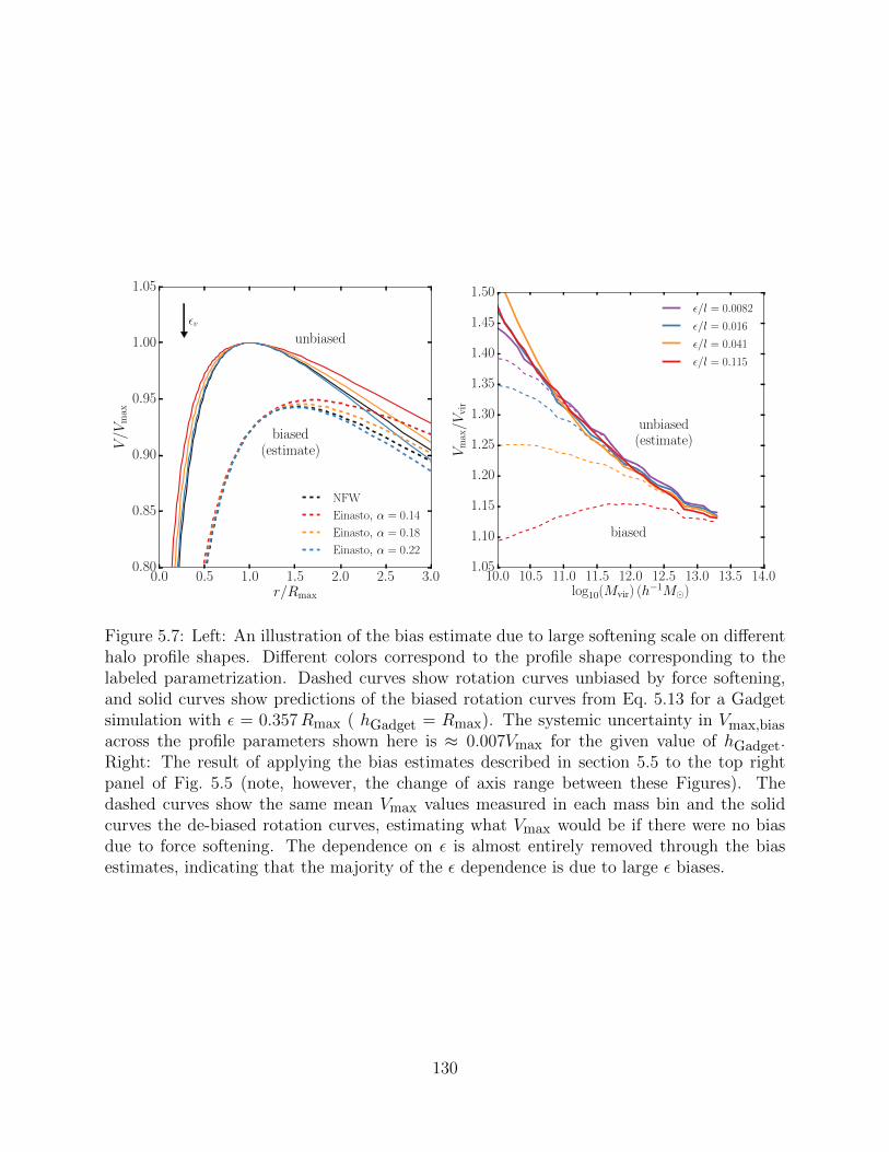
0.0 0.5 1.0 1.5 2.0 2.5 3.0r/Rmax

0.80

0.85

0.90

0.95

1.00

1.05

V/V

max

εv

unbiased

biased(estimate)

NFW

Einasto, α = 0.14

Einasto, α = 0.18

Einasto, α = 0.22

10.0 10.5 11.0 11.5 12.0 12.5 13.0 13.5 14.0log10(Mvir) (h−1M)

1.05

1.10

1.15

1.20

1.25

1.30

1.35

1.40

1.45

1.50

Vm

ax/V

vir

biased

unbiased(estimate)

ε/l = 0.0082

ε/l = 0.016

ε/l = 0.041

ε/l = 0.115

Figure 5.7: Left: An illustration of the bias estimate due to large softening scale on differenthalo profile shapes. Different colors correspond to the profile shape corresponding to thelabeled parametrization. Dashed curves show rotation curves unbiased by force softening,and solid curves show predictions of the biased rotation curves from Eq. 5.13 for a Gadgetsimulation with ε = 0.357Rmax ( hGadget = Rmax). The systemic uncertainty in Vmax,biasacross the profile parameters shown here is ≈ 0.007Vmax for the given value of hGadget.Right: The result of applying the bias estimates described in section 5.5 to the top rightpanel of Fig. 5.5 (note, however, the change of axis range between these Figures). Thedashed curves show the same mean Vmax values measured in each mass bin and the solidcurves the de-biased rotation curves, estimating what Vmax would be if there were no biasdue to force softening. The dependence on ε is almost entirely removed through the biasestimates, indicating that the majority of the ε dependence is due to large ε biases.

130

8 9 10 11 12 13 14 15 16log10(Mvir) (h−1M)

1.05

1.10

1.15

1.20

1.25

1.30

1.35

1.40

1.45

1.50V

max/V

vir

BolshoiP

Erebos CPla

Multidark

ν2 − GC

TNG− Dark

Figure 5.8: Fig. 5.3 recreated with the bias estimates from section 5.5. As in the right panelof Fig. 5.7, dashed curves show the mean mass trends measured in each simulation and thesolid curves show estimates of what these mean trends would have been if not for large εbiases. To emphasize the mass ranges which are affected by these biases, we only plot solidcurves down to mass bins at which they agree with the measured trend to 1 per cent orbetter. Although there is still some dispersion around a mean relation between simulationsuites, all the strong, visually apparent divergences from the mean trend are consistent withbeing caused by large ε. Note that there are many science applications where a Vmax biasof larger magnitudes is perfectly acceptable. This cutoff choice is only meant to mimic thedivergences seen by the eye and does not imply the “usable” mass ranges of these simulationsfor arbitrary analysis. Such a mass range must be developed with the tolerances of a givenanalysis in mind.

131

timestep relative to the collisional timescale.

We will focus our analysis on the standard Gadget timestepping criteria, Eq. 3.1. Only

two of the simulations in Table 3.1 use alternative schemes: Bolshoi and BolshoiP. For

a spherically symmetric NFW potential, Bolshoi and BolshoiP will always have timesteps

that are a factor of ≈ 102 − 103 smaller than a Gadget simulation run with η = 0.025.

Timestepping errors can be ignored for these two boxes.

For any spherically symmetric mass distribution, the Gadget timestepping criteria can

be conveniently rewritten in terms of the number of timesteps per circular orbit:

tcirc

∆t= 28.1

(R

ε

)1/2 ( η

0.025

)−1/2. (5.6)

We use this relationship to quantify integration errors in sections 5.6.1 and 5.6.1.

Integration Errors in Smooth Potentials

Integration errors in smooth potentials, are essentially irrelevant with the conventional Gad-

get integration settings. Tests of smooth integration errors in Power et al. [2003] show that

simulations with constant timestepping converge to ∆V/Vref = 0.1 above radii at which

timesteps per circular orbit satisfy,

tcirc(R)/t200c > A(∆t/tH)α, (5.7)

with A ≈ 15 and α ≈ 5/6. Empirical criteria determine if the underlying potential is smooth

for halos in their study. The results from Power et al. [2003] agree with first-principles

estimates of this class of integration errors. Combining the relation in Eq. 5.7 with Eq. 5.6

and the tcirc/t200c profile of an NFW halo, we arrive at the requirement,

R

ε≥ 4.96× 10−4A2/α

( η

0.025

)(x2 f(c200c)

c2200c f(x)

)2−2/α

. (5.8)

132

Here, x = R/Rs, c200c = R200c/Rs, and f(x) = ln (1 + x)− x/(1 + x). R/ε has only a weak

dependence on c200c and x. For example, concentrations in the range of 5 ≤ c200c ≤ 15, a

10 per cent error in Vmax due to smooth integration errors requires a corresponding range

of 0.6 ≤ Rmax/ε ≤ 1.2.

We note that smooth integration errors are typically subdominant or comparable to

softening-induced errors in the centripetal force. As a comparison, Eq. 5.13 gives ∆V/V ≈

0.20 − 0.30 at distances where Eq. 5.8 predicts a fractional error of 0.1. It is possible that

even this is an overestimate: concentration- and radius-dependence at the level predicted

by Eq. 5.8 – while small – would have been detectable in our tests described in Appendix

5.8.1. However, it is possible that the values in Table 5.8.1 have some dependence on Gadget

timestepping parameter, η, and that high-precision estimates of ∆V/Vref require measure-

ments at the same η as the target simulation. This is a question which deserves further

study.

Integration Errors During Scattering

Excessively small force softening leads to noise in the halo potential. In sufficiently noisy

potentials, integration errors from particle-particle scattering become more severe and require

much smaller timesteps to suppress. The landmark study on these integration errors is

Power et al. [2003]. Empirically, they find that integration errors during scattering occur for

ε < εopt,P03, where we can express the limit on ε with both,

εopt,P03 =2.9R200c√N200c

, (5.9)

and,

εopt,P03/l = 0.076

(Ωm

0.27

)1/3(N200c

103

)−1/6

. (5.10)

133

Here, l is the mean interparticle spacing. Eq. 5.10 is substantially larger than the ε/l values

adopted by virtually all cosmological simulations. Fig. 5.5 shows that any cosmological sim-

ulations which abide by such a limit risk substantial biases in halo properties due to softened

centripetal forces. Subsequent authors have suggested that Eq. 5.9 is too conservative by a

factor of . 2 [Zhang et al., 2019, Ludlow et al., 2019]. However, part of the disagreement

can be accounted for with a correction of the (now non-standard) Plummer equivalence scale

which Power et al. [2003] used: ε = 0.5hGadget.

The most straightforward interpretation of the Power et al. [2003] tests is that particle-

particle scattering in noisy halo potentials should lead to catastrophic non-convergence

in cosmological simulations. Fig. 5 in Power et al. [2003] shows that for halos run at

ε/εopt,P03,v ≈ 5, fractional errors in V (R) should be larger than 0.1 for radii at which

timesteps per circular orbit satisfy Eq. 5.7, with A = 11.2 and α = 0.57. These large

fractional errors would be predicted for the Chinchilla-ε simulation, represented by the blue

curves in Fig. 5.5 at N200c ≈ 103. The small α causes this level of bias to be reached at very

large values of R/ε and to become strongly dependent on c200c and x. A c200c = 10 halo

would be predicted to have biases in Vmax larger than 0.1Vmax for ε > 0.018Rmax!

However, the massive biases predicted by the analysis in the previous paragraph (and

comparable predicted biases used to argue for ε . εopt,P03) are an artefact of the constant

timesteps used in the Power et al. [2003]. Under constant timestepping schemes, the size of a

timestep relative to the smallest possible collisional timescale, tcirc(mp(< ε), ε)/∆t, varies as

ε3/2. This dependence on ε means that the resolution of close orbits worsens as ε decreases.

However, Eq. 5.6 shows that with the standard Gadget timestepping criteria, tcirc(mp(<

ε), ε)/∆t is independent of ε. Timestepping errors are therefore far less catastrophic with the

standard Gadget timestepping criteria.

Other recent convergence studies have investigated the impact of timestepping in the

ε < εopr,P03 regime. Ludlow et al. [2019] performed tests on halos across a wide range of ε

values for η = 0.025 and η = 0.0025. These tests find catastrophic contraction of halos out

134

to large radii at η = 0.025 for ε/l . 0.003, but find that halos in the range of the typical ε

of cosmological simulations are relatively unaffected (see Ludlow et al., 2019 fig. 2).

The non-monotonic behavior in ε is surprising and deserves further study. The onset of

profile contraction occurs at ε/l values that are close to what is needed to avoid large-ε biases

in halo properties. A full characterisation of the profile contraction is therefore of practical

relevance.

One potential explanation for the non-monotonicity is that Eq. 5.6 ensures that collisions

occurring at distances with ε rperi are well-resolved, and the fraction of particle collisions

which occur at ε ≈ rperi decreases as ε decreases. Although the Gadget timestepping scheme

ensures that such collisions are never catastrophically unresolved, modest integration errors

are sill possible. Springel [2005] shows that when using the adaptive timestepping of Gadget-

2, small integration errors tend to decrease the energy of the system. Thus, as epsilon

decreases, the average energy lost per collision increases as the potential of each particle

decreases. In this case, however, the range of collision parameters that lead to rpericenter ≈ ε

also decreases until these collisions are so rare that they are not relevant to the internal

dynamics of the halo.

5.6.2 What is the “Optimal” ε?

A number of studies aim to identify an optimal choice for ε. The [Power et al., 2003]

suggestion for an optimal value, εopt,P03, is shown in Eq. 5.9 and discussed at length in

section 5.6.1. However, cosmological simulations universally use scales smaller than εopt,P03.

The use of smaller ε values is in part because – as Fig. 5.5 and Fig. 5.6 show – halos simulated

at ε = εopt exhibit large biases at the particle counts that cosmological simulations typically

consider. Klypin et al. [2015b] has also noted this effect in their analysis.

Recent convergence studies [van den Bosch and Ogiya, 2018, Ludlow et al., 2019] have

135

argued for an alternative optimal choice in ε:

εopt,VO18/l = 0.017. (5.11)

The level of bias implied by Fig. 5.5 and Fig. 5.6 at εopt,VO18 would be acceptable for many

applications, but is not zero. These Figures do not conclusively establish convergence in ε,

but, the model presented in section 5.5 would predict that

εopt,Vmax/l ≈ 0.008 (5.12)

simulation would exhibit bias in Vmax which is smaller than cosmic variance for simulations

with comparable resolution and box sizes to the Chinchilla-ε.

However, we caution against uncritically accepting Eq. 5.12 as a blanket prescription

for ε for three reasons. Most importantly, the level of acceptable bias in a measurement is

highly dependent on the science target. While striving for zero numerical bias (a formally

impossible goal) is the safest generic option, all analyzes can tolerate at least some deviation

from the true predictions of ΛCDM. Second, this recommendation is based solely on reducing

bias in Vmax. Halo properties which depend on the mass distribution at radii smaller than

Rmax will require smaller ε. Third, our simulation suites did not explicitly establish a range

of converged ε and this recommendation is thus model-dependent. Fourth, poorly-explored

timestepping effects can cause catastrophic halo contraction for ε values somewhat smaller

than Eq. 5.12 for standard timestepping schemes. All four considerations must be accounted

for before applying Eq. 5.12 or any other εopt prescription.

5.7 Conclusion

In this chapter, we study the impact of DMO simulation parameters on halo properties.

We provide several tools to help analysts avoid and quantify these numerical biases. We

136

do this by comparing a number of publicly available cosmological simulation suites against

one another and by measuring the dependence of halo properties on both particle mass and

several secondary simulation parameters. The most important of these is the “force softening

scale”, which controls the effective radius of dark matter particles. We also consider the

impact of coarse timestep size.

• We report the Nvir cutoffs where our cosmological simulations have converged to shared

mass relations (section 5.3.1). We do this for a wide range of halo properties and error

tolerances.

• There are many halo properties (e.g. xoff , a1/2) where these cutoffs are consistent

between simulations. For these properties, most analyzes can simply use a set of

conservative “convergence limits” at modest values of Nvir (Table 5.2.3).

• For similarly high levels of agreement, other commonly used properties (e.g. Vmax,

c/a) behave differently between simulations. Such levels of agreement can require Nvir

as large as ≈ 105 − 106 (section 5.3.2 and Fig. 5.3).

• This disagreement is partially because some simulation suites have internally converged

to different solutions. We demonstrate this for Multidark and IllustrisTNG-Dark (sec-

tion 5.3.3). The reasons for this disagreement between converged simulations are cur-

rently unknown.

• We show that many halo properties (e.g., Vmax, c/a, and subhalo abundances) exhibit

a strong dependence on force softening (section 5.4). The biases associated with this

dependence can be comparable to the impact of baryons on these properties.

• We develop a model which estimates the bias in Vmax due to large force softening scales

(section 5.5). This model predicts the dependence of Vmax on force softening and most

of the dispersion in simulation results for this property.

137

• We review previous studies on timestep size and conclude that commonly used timestep-

ping schemes are unlikely to significantly bias halo properties (section 5.6.1). However,

we outline several open questions in this topic.

We emphasize that all analyzes can accommodate some level of numerical bias. This

chapter does not assert what those levels are. There is nothing incorrect about studying halos

below the most conservative convergence limits, however such analyzes should incorporate

some estimate of the associated systematic uncertainty. The results of this chapter will help

analysts to identify the regimes where this is necessary and to estimate the resultant biases.

5.8 Appendices

5.8.1 Recalibrating the Plummer-Equivalence Scale

Rather than adopting a conversion based on the functional forms of kernels, in this work we

use a novel Plummer equivalence scale, which has been calibrated from the empirical impact

of varying h on halo velocity profiles. As is discussed at length in sections 5.5 and 5.6.1,

large force softening scales can lower the inner densities of halos through a combination of

lowering centripetal accelerations and (in some timestepping schemes) lowering the number

of timesteps per orbit. These effects can impact the density of the halo at radii where forces

are Newtonian as outer layers of the halo correctly respond to numerical density changes in

the halo center.

We compare the results of Klypin et al. [2015b], van den Bosch and Ogiya [2018] and

Ludlow et al. [2019], which measured circular velocity profiles for halos simulated with vary-

ing h for Plummer and Gadget kernels. Klypin et al. [2015b] and van den Bosch and Ogiya

[2018] considered idealized isolated NFW halos, while Ludlow et al. [2019] studied stacked

mass profiles from a series of small cosmological boxes.

We first consider the profiles in Ludlow et al. [2019]. These tests were performed with

a “standard” Gadget timestepping parameter of η = 0.025 and with a higher resolution

138

10−1 100 101

R/h

−1.0

−0.8

−0.6

−0.4

−0.2

0.0

0.2

0.4

(a−a

New

ton)/a

New

ton

Gadget

ART (Kravtsov + 97)

Plummer

10−1 100 101 102 103

R/h

0.6

0.8

1.0

1.2

1.4

V/V

ref

Gadget

Plummer

Figure 5.9: Left: The acceleration errors associated with different force softening schemesfor a test point some distance r from a particle. Distances are noramalized by h, the scheme-specific formal resolution described in section 3.1.1. The points for ART are taken fromKravtsov et al. [1997]. The dashed red line shows the Gadget force error scaled by h =0.357hGadget. This plot illustrates the known fact that the traditional “Plummer-equivalent”conversion between formal resolution parameters leads to similar force errors for r < εφ, buthighly discrepant force errors at larger radii. Right: The impact of different force softeningschemes on halo circular velocity profiles. The points in this plot show the measured errors incircular velocity profiles as a function of the formal resolution, h, for different force softeningschemes. Gadget measurements are from Ludlow et al. [2019], and Plummer measurementsare from Klypin et al. [2015b] and van den Bosch and Ogiya [2018]. Points shown as red “x”scorrespond to measurements from Ludlow et al. [2019] where deviations from the referencerotation curve were caused by timestepping errors. Curves show the results of fits againstEq. 5.13. These fits form the basis for our conversion of formal resolutions onto a sharedscale. See Appendix 5.8.1 for discussion.

139

η = 0.0025. The η = 0.025 boxes were run with formal resolutions of hGadget(z = 0) =

2−6, 2−5, ..., 24 × hGadget,fid for hGadget,fid =0.6642 h−1 kpc and the η = 0.0025 boxes

were run with hGadget(z = 0) = 2−6, 2−5, ..., 29×hGadget,fid. These profiles were stacked

in mass bins centered on M200c = 109, 1010, 1011, 1012h−1M, and widths of 0.3 dex,

corresponding to median N200c values of 6.4× 105, 6.5× 104, 6.3× 103, 6.7× 102, respec-

tively.

This range of parameters means that the Ludlow et al. [2019] measurements can probe the

impact of hGadget across a wide range of halo radii, particle counts, and concentrations. The

η = 0.0025 simulations allow the impact of numerical scattering due to coarse timesteps to be

separated from timestep-independent effects like two-body relaxation effects and overly-large

h.

The variation in profiles between η = 0.0025 boxes is at the per cent level and does not

show strong dependence on h for the small h sclaes probed by these boxes, so we take the

hGadget = hGadget,fid, η = 0.0025 box as our “reference” simulation. Our results are nearly

identical if smaller values of h are used.

For each mass bin and hGadget value in the η = 0.025 boxes, we measure the value of

Vcirc(R)/Vcirc,ref(R) for R = 2−4, 2−3, ..., 22×Rmax,ref , where V (R) is the circular velocity

at radius R, Rmax is the radius at which the circular velocity profile reaches its maximum

value, and quantities subscripted with “ref” are measured in the reference simulation. We

discard Vcirc(R)/Vcirc,ref values at radii smaller than the convergence radii advocated for by

Ludlow et al. [2019], although we find that our fits are strongly insensitive to this minimum

radius. We also remove values which deviate by more than two per cent from values measured

in η = 0.0025 simulations with identical hGadget. While deviations in these regimes are

relevant to convergence studies, they are caused by two-body scattering and time integration

errors and not by errors due to large hGadget.

We find that V (R)/Vref has no meaningful dependence on particle count, radius, or halo

concentration when scaled by hGadget/R [see also, the first three panels of fig. 5 in Ludlow

140

Fit type Scheme A βFree β Gadget 0.172± 0.006 −0.522± 0.010

Plummer 0.580± 0.026 −0.497± 0.016Fixed β = −0.522 Plummer 0.616± 0.011Fixed β = −0.497 Gadget 0.160± 0.002

Table 5.4: The best-fitting parameters for Eq. 5.13 for different force softening schemes.Gadget velocity deviations are measured at η = 0.025.

et al., 2019]. Because of this, we fit these measurements against a function of the form

V (R;h)/Vref(R), specifically:

V (R;h)

Vref(R)= 1− exp

(−(Ah/R)β

). (5.13)

Here, A and β are free parameters. We perform our fit using non-linear least squares mini-

mization, because manual inspection of the likelihood posterior confirms that it is unimodal

and approximately Gaussian near the minimum.

We show this fit in the right panel of Fig. 5.9 and give its best-fitting parameters in

Table 5.8.1. V/Vref measurements removed prior to fitting due to timestepping dependence

are shown as “x”s. As an internal consistency check, we find that this fit predicts deviations

equal to 0.1V (R; h) at 0.76h, which is consistent with fig. 5 in Ludlow et al. [2019].

The lack of dependence on R, particle count, or concentration means that we can safely

compare these fits against tests performed on narrower radius, particle count, and concen-

tration ranges. We combine the R = Rmax measurements from Klypin et al. [2015b] and the

R = Rs/2 measurements from van den Bosch and Ogiya [2018] for our Plummer kernel data

set. Our results are unchanged if we restrict ourselves to the results of either paper.Both

studies analyze idealized NFW profiles instead of cosmological boxes, so we use NFW profiles

as our reference Vref(R) curves. The timestepping schemes used in both papers are substan-

tially more aggressive than an η = 0.025 Gadget simulation, so we do not need to remove

any simulations due to integration errors, as was done for the Ludlow et al. [2019] data set.

However, we do remove the h = 10−4Rvir simulation from van den Bosch and Ogiya [2018]

141

before fitting because that halo is undergoing thermalization at R = Rs/2.

We show this fit in the right panel of Fig. 5.9 and give its best-fitting parameters in Table

5.8.1.

Because A and β are slightly covariant, comparison between the A values of different

fits can only be performed at a constant β. If β is fixed to −0.522 for the Plummer fit,

APlummer = 0.616 ± 0.011, indicating that εGadget = APlummer/AGadget = 0.279 ± 0.006.

Fixing β = −0.497 for the Gadget fit results in εGadget = 0.277±0.006. Because Gadget-like

softening kernels are more common in modern simulations than Plummer kernels, we choose

to noramalize the relation to preserve the commonly-used conversion between hGadget and

ε :

ε = 1.284hPlummer = hART = 0.357hGadget. (5.14)

Note that without comparable ART-based tests, we have arbitrarily chosen to take the

convention from Klypin et al. [2016] that hART = 0.357hGadget. This leads to comparable

mean force errors to Gadget at all radii. No analysis in this chapter relies on this portion of

the convention.

We have performed this fit with several other functional forms in the place of Eq. 5.13 and

found results which are similar. For example, when using V (R; h)/Vref(R) = (1+(Ah/R)2)β

– a form similar to the one used in Klypin et al. [2015b] – we find that ε ranges from

1.29, hPlummer to 1.28hGadget.

While Eq. 5.14 is most appropriate when estimating the effects of reduced centripetal

forces on halo profiles, force softening also impacts halo profiles through two-body scattering

and time integration errors. In regimes where these effects dominate, the depths and shapes

of the kernel potentials may be more important than the long-distance deviations from

Newtonian gravity. If so, these two body-scattering effects would be be best analyzed through

εφ. To prevent readers from needing to frequently convert between ε conventions, we have

142

converted all values used in this chapter to ε, except in cases of specifying an algorithm

which depends on εφ.

We note that Eq. 5.13 appears to “predict” that ε can be made arbitrarily small without

error. This is only true over the R/ε range fitted here and only when timesteps are very

fine. Coarse timesteps lead to very real errors at small ε (see section 5.6.1), the “convergence

radius” which we use to select our fitting ranges has a weak dependence on ε [Ludlow et al.,

2019], and fig. 6 of van den Bosch and Ogiya [2018] shows that aggresively small softening

scales (ε . 10−4Rvir) can accelerate the impact of two-body scattering. Similar effects can

be seen in fig. 13 of Klypin et al. [2015b]. Large ε effects are only a portion of the story.

5.8.2 Fitting Parameters For Mean Halo Property Relations

In this Appendix we give the fitting parameters for each halo property considered in this

chapter. These are listed in Table 5.5.

143

Variable log10(NHR) d α NoutlierM2500c 4 4 0 0M500c 3.25 4 0 0M200c 2 4 0 0M200m 2 4 0 0Vrms 4.5 4 0 0Vmax 2.75 4 0 4?

cvir 3.5 4 0 1?

R1/2 4 4 0 0

c/a 2.70 3 0 9?

λPeebles 3 4 0 0λBullock 3 4 0 0T/|U | 3.5 4 0 0Xoff 4 2 0 0Voff 4 2 0 0Γ(tdyn) 2 3 0 0a0.5 2.5 2 0 0aMM 3 4 0 0Mpeak 2.5 2 0 0Vpeak 3.25 2 0 1

φ(M2500c) 2.5 6 1 0φ(M500c) 2.5 6 1 0φ(M200c) 2.5 6 1 0φ(Mvir) 2.5 6 1 0φ(M200m) 2.5 6 1 0φ(Mpeak) 2.5 6 1 0

φ(Vmax) 3.5 6 3 0φ(Vrms) 3.75 6 3 0φ(Vpeak) 3.5 6 3 0

Table 5.5: The fitting parameters used for each halo property according to the proceduredescribed in section 5.2.3. NHR is the number of particles required for halos to be included inthe fit, d is the degree of the fitted polynomial, α is the power law index of the mass scalingapplied to data prior to fitting, and Noutlier indicates the number of simulations which wereremoved from the fit because they disagreed with other simulations within their own suite athigh particle counts. Properties where outlier removal receives special discussion are markedwith a ?.

144

CHAPTER 6

THE THREE CAUSES OF LOW-MASS ASSEMBLY BIAS

This chapter is a modified version of my paper, Mansfield and Kravtsov [2019].

6.1 Introduction

The most visually striking feature of the large-scale structure of the universe is the clustered,

web-like distribution of galaxies, with vast voids separated by walls and filaments [e.g., Bond

et al., 1996]. Understanding the clustering of galaxies within the context of the Λ+Cold

Dark Matter (ΛCDM) model relies on the generic model in which galaxies are formed by

the dissipation of diffuse baryon plasma within growing dark matter halos [e.g., White and

Rees, 1978]. Galaxy clustering is then interpreted in terms of the clustering of dark matter

halos [e.g., see Desjacques et al., 2018, Wechsler and Tinker, 2018, for recent reviews], which

is generally different from that of matter, i.e. the distribution of halos is “biased,” relative

to the mass distribution [Kaiser, 1984].

Halo bias depends primarily on halo mass [e.g., Mo and White, 1996, Sheth and Tormen,

1999] and this dependence is now both well-understood theoretically and well-calibrated

numerically [Desjacques et al., 2018]. It is also now known that halo bias has secondary

dependencies on other halo properties, such as formation time, concentration, spin, and

ellipticity [Gao et al., 2005, Wechsler et al., 2006, Harker et al., 2006, Gao and White, 2007,

Jing et al., 2007, Li et al., 2008, Faltenbacher and White, 2010, Villarreal et al., 2017a, Sato-

Polito et al., 2018, Han et al., 2019]. The first such secondary dependence was found for halo

formation time and its closely related proxy – halo concentration [Gao et al., 2005, Wechsler

et al., 2006, Harker et al., 2006, Jing et al., 2007] and has become known as “assembly bias.”

Specifically, the bias of “old” halos (early formation time) is generally different than that

of “young” (late formation time) halos, with the difference depending on halo mass and the

definition of formation time[e.g., Li et al., 2008].

145

Assembly bias is important for the theoretical interpretation of galaxy clustering and its

potential to provide useful cosmological constraints [e.g., Abazajian et al., 2005]. There have

been significant observational efforts to detect halo assembly bias on galactic scales [see §5.4

and 6.2 of Wechsler and Tinker, 2018, for a review]. Nevertheless, unambiguous detection

of halo assembly bias on galactic scales proved to be elusive due to the general difficulty

of ensuring that host halo masses of galaxy subsamples with different clustering are similar

[Campbell et al., 2015, Lin et al., 2016]. Lehmann et al. [2017] and Zentner et al. [2019]

showed that simulation-based models with inherent assembly bias due to concentration de-

pendence of halo clustering provide a better fit to clustering of Sloan Digital Sky Survey

(SDSS) galaxies at some luminosities. However, it is not clear whether this is an unam-

biguous detection of assembly bias or improved fit is due to larger flexibility of the model

compensating for a deficiency of the abundance matching assignment of galaxy luminosities.

Hearin et al. [2015, 2016b] showed theoretically that the presence of galaxy conformity – the

tendency of red galaxies to cluster around other red central galaxies – on large scales (i.e., in

the “two-halo regime”) would be a smoking gun of the halo assembly bias. However, this test

also proved to be a non-trivial challenge due both to observational selection biases [Sin et al.,

2017, Tinker et al., 2018] and due to the overall weakness of the two-halo conformity signal

[Berti et al., 2017, Calderon et al., 2018, Tinker et al., 2018]. If low-mass halo assembly bias

does have a signature in galaxy clustering, it would be important to understand its physical

origin in order to construct robust and accurate models. Conversely, if halo assembly bias

does not have observational signatures, it would be important to understand why tracers of

halo age and tracers of galaxy age behave differently.

The focus of this chapter is to understand the physical origin of halo assembly bias,

particularly in the regime of galaxy-scale halo masses. This is distinct from the origin

of assembly bias at large masses, which is related to the properties of the peaks of the

initial Gaussian density perturbations from which these massive halos collapse [Zentner,

2007, Dalal et al., 2008]. Peaks with the same mass but different curvature will cluster

146

differently because peaks with larger curvatures are located in lower-density environments,

while peaks with smaller curvatures are in higher-density regions. This gives rise to assembly

bias because peak curvature is directly related to a halo’s mass accretion history, which is

also affected by tidal torques from the surrounding anisotropic mass distribution [Desjacques,

2008]. Although this curvature-related bias can be reduced by compensating effects found in

some proxies of halo age [Zentner, 2007, Sandvik et al., 2007, Mao et al., 2018], it is present

for other age definitions and when more physical definitions of halo boundaries and masses

are used [Chue et al., 2018].

At smaller halo masses, however, the physics of assembly bias is more complex because

the mass evolution of halos is determined by a combination of the properties of their initial

density peaks, and also by non-linear processes [e.g., Wang et al., 2007, Hahn et al., 2009].

The simple and striking manifestation of this is that the sign of assembly bias switches for

small-mass halos when cvir is used as a measure of halo age [Wechsler et al., 2006, Dalal

et al., 2008].

A number of studies have explored the physical processes that can give rise to halo

assembly bias in the small-mass regime. One readily apparent process is the non-linear effects

that a massive host halo can exert on its smaller-mass neighbors. In particular, “splashback”

(often also called “backsplash”) subhalos pass within the inner regions of a larger halo but

are located outside its virial radius at the epoch of analysis. Typically, analysis is done using

only a single simulation snapshot, and the single-epoch isolation criteria used to distinguish

subhalos from distinct halos will mix splashback subhalos into the distinct halo population.

However, splashback subhalos will have had their mass accretion histories truncated due to

their previous close encounters with their hosts and have thus been studied as a potential

source of low-mass assembly bias [Wang et al., 2009, Li et al., 2008, Wetzel et al., 2014,

Sunayama et al., 2016]

Although splashback subhalos are mostly found within three virial radii of their host

halo, they can give rise to an assembly bias signal at much larger distances. This is because

147

at large scales the spatial distribution of splashback subhalos will track the distribution of

their massive hosts and will therefore be more strongly clustered than that of distinct halos.

A similar effect would occur if subhalos located within the virial radius of their host were

included in the sample used to measure halo clustering and assembly bias. This is illustrated

in Fig. 6.1, which compares the clustering of early- and late-forming halos with splashback

subhalos included and removed, respectively. Removing splashback subhalos significantly

reduces the difference in clustering between the two halo samples, even on scales much

larger than the virial radius of the most massive halos within the volume. Nevertheless,

multiple studies have demonstrated that splashback subhalos alone cannot be responsible

for the entire assembly bias signal [Wang et al., 2009, Sunayama et al., 2016], a fact that can

be seen visually in Fig. 6.1. A similar conclusion was reached by Hearin et al. [2015], albeit

in the related but distinct context of galactic conformity.

Another process that could contribute to assembly bias is the truncation of a halo’s

mass growth by the tidal force generated its most gravitationally-dominant neighbor [Hahn

et al., 2009, Behroozi et al., 2014, Hearin et al., 2016b, Salcedo et al., 2018, Johnson et al.,

2019]. Even though single-halo tidal forces become small beyond ≈ 3 − 5 × Rvir of the

host, the halos truncated by these forces can give rise to large-scale assembly bias in a way

similar to splashback subhalos. A similar truncation of halo mass growth can be caused

by the overall tidal force from all of the surrounding halos and structures in the matter

distribution [Hahn et al., 2009, Wang et al., 2011, Paranjape et al., 2018, Musso et al., 2018],

as the largest filaments and sheets generate strong tidal fields throughout their volumes.

Since these structures can be several tens of Mpc in size, they can comfortably give rise to

assembly bias on large scales. This effect has been characterized in terms of both the tidal

force and the anisotropy of the tidal field, although, in practice, a high degree of anisotropy

tends to correlate with the magnitude of the tidal force, so it is not clear that the two effects

can be separated cleanly.

Finally, the gravitational heating of matter within large-scale structure structure has

148

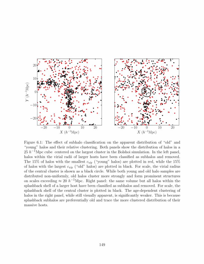
−20 −10 0 10 20X (h−1Mpc)

−20

−10

0

10

20

Y(h−

1M

pc)

−20 −10 0 10 20X (h−1Mpc)

Figure 6.1: The effect of subhalo classification on the apparent distribution of “old” and“young” halos and their relative clustering. Both panels show the distribution of halos in a25 h−1Mpc cube centered on the largest cluster in the Bolshoi simulation. In the left panel,halos within the virial radii of larger hosts have been classified as subhalos and removed.The 15% of halos with the smallest cvir (“young” halos) are plotted in red, while the 15%of halos with the largest cvir (“old” halos) are plotted in black. For scale, the virial radiusof the central cluster is shown as a black circle. While both young and old halo samples aredistributed non-uniformly, old halos cluster more strongly and form prominent structureson scales exceeding ≈ 20 h−1Mpc. Right panel: the same volume but all halos within thesplashback shell of a larger host have been classified as subhalos and removed. For scale, thesplashback shell of the central cluster is plotted in black. The age-dependent clustering ofhalos in the right panel, while still visually apparent, is significantly weaker. This is becausesplashback subhalos are preferentially old and trace the more clustered distribution of theirmassive hosts.

149

been proposed as a process that can contribute to assembly bias [Wang et al., 2007, Dalal

et al., 2008]. For example, matter within the deep potentials of filaments can acquire large

velocities during accretion, and thus cannot be accreted by small-mass halos located within

the filament. The smaller accretion rates of such halos would thus give rise to assembly bias.

Note that although gravitational heating and strong tidal forces generally happen in similar

regions, they are physically distinct phenomena: tidal forces arise via large second derivatives

in the gravitational potential, while gravitational heating is caused by the potential depth.

Although significant effort has been devoted to studying these effects [Wang et al., 2007,

Dalal et al., 2008, Wang et al., 2009, Hahn et al., 2009, Wang et al., 2011, Li et al., 2013,

Wetzel et al., 2014, Sunayama et al., 2016, Hearin et al., 2016b, Paranjape et al., 2018,

Salcedo et al., 2018, Musso et al., 2018, Johnson et al., 2019], their relative importance and

a coherent physical picture for the origin of low-mass halo assembly bias has not yet been

established. The primary goal of this chapter is to rectify this. To this end, we define a set

of quantitative proxies for each of the different processes outlined above and use them to

investigate the relative contribution of these processes to the low-mass assembly bias signal.

Specifically, we examine how efficiently sample cuts defined by each proxy can remove the

signal.

The chapter is organized as follows. In section 6.2 we describe basic definitions and

measurements and describe our cosmological simulations and halo sample, with sections

6.2.5-6.2.6 focusing on the proxies of the processes described above, and section 6.2.8 de-

scribing the core methodology of this chapter. In section 6.3 we present measurements and

estimates of the relative contribution of different processes to low-mass assembly bias. We

discuss topics related to the interpretation of this work in section 6.4 and summarize our

results in 6.5. The key results of this study are presented in Fig. 6.3.

150

6.2 Methods

6.2.1 Simulations and codes

This chapter makes use of the Bolshoi and BolshoiP simulations described in Tables 3.1 and

3.1. We also use the simulations in the Erebos CBol suite for some convergence testing.

Halos in the Bolshoi and BolshoiP simulations were identified using version 0.99RC2+ of

the Rockstar halo finder [Behroozi et al., 2013c], and version 1.0+ of the related consistent-

trees method [Behroozi et al., 2013b] was used to construct halo merger trees. The catalogs

and merger trees we use were downloaded from the CosmoSim database. We use the Shell-

fish algorithm to identify splashback shells – the 3D surfaces formed by the outermost

apocenters of accreted matter [Mansfield et al., 2017]1. We use the Colossus python pack-

age [Diemer, 2018]2 to calculate various relevant cosmological quantities and statistics and

the halotools package [Hearin et al., 2016a]3 to calculate correlation functions efficiently.

6.2.2 Basic halo properties

As discussed in section 3.2, there are many ways to define halo mass. One can use M∆

for a variety of overdensity contrasts, ∆, a non-parametric velocity-based tracer of poten-

tial depth, like Vmax, or a peak-based definition, like Mpeak or Vpeak. It is non-trivial to

compare assembly bias results across different mass definitions. This primarily manifests in

the difference between peak and single-epoch definitions, which treat tidally stripped halos

differently. The choice between Vmax- and M∆-based definitions also affects the strength of

assembly bias because Vmax/Vvir is correlated with halo age. We explore these definitional

choices at length in section 6.4.2, and urge readers to consider the discussion there before

applying our results to alternative definitions.

1. https://github.com/phil-mansfield/shellfish

2. http://www.benediktdiemer.com/code/colossus/

3. https://halotools.readthedocs.io

151

As further discussed in section 3.2, there are a number of definitions of halo age used

in the literature: single-epoch accretion rates [e.g., Lacey and Cole, 1993, Li et al., 2008],

current halo properties - such as concentration - related to a halo’s mass accretion history

[e.g., Wechsler et al., 2006, Villarreal et al., 2017a, Sato-Polito et al., 2018], the epoch at

which a halo first achieved half of its current mass [e.g., Gao et al., 2005], or a characteristic

timescale of an analytic fit to halo mass accretion history [e.g., Wechsler et al., 2002, Zentner,

2007]. In this chapter, we primarily adopt cvir as a tracer of halo age, with older halos having

larger concentrations. We briefly explore the effect of using different definitions in section

6.4.2.

We focus on cvir for several reasons. First, cvir has been demonstrated to strongly

correlate with a number of explicit indicators of halo age [Bullock et al., 2001, Wechsler

et al., 2002, Zhao et al., 2003, Lu et al., 2006, Ludlow et al., 2013, 2014]. ) Although the

correlation of two halo properties does not guarantee a similar effect on clustering [see Mao

et al., 2018], this is not a concern for cvir because it has been shown that low-mass halo

assembly bias behaves similarly for cvir and for the halo age proxy a1/2 [Gao et al., 2005,

Wechsler et al., 2006, Gao and White, 2007, see also our results in section 6.4.2]. Second,

the connection between accretion history and cvir has a solid theoretical underpinning [Zhao

et al., 2003, Lu et al., 2006, Dalal et al., 2010], as demonstrated by the accuracy of the

concentration models based on halo mass accretion history [e.g. Zhao et al., 2003, 2009, Dalal

et al., 2010, Ludlow et al., 2014, Diemer and Joyce, 2019]. Third, the convergence criteria for

halo density profiles [e.g. Power et al., 2003, Navarro et al., 2004, Springel et al., 2008], and

for concentrations [see, e.g., section 3.2 in Diemer and Kravtsov, 2015] are well studied and

it is thus relatively straightforward to identify regimes in which numerical concentrations

can be trusted.

152

6.2.3 Definition of Halo Boundaries and Subhalos

Throughout this chapter, we define subhalos as the halos located within the boundary of

a larger “host halo,” and refer to all non-subhalos as “distinct halos.” Of course, this

classification depends on the definition of halo boundary and will have a clear meaning only

if we use halo boundary definition that corresponds to an actual physical boundary.

Traditionally, spheres of radius Rvir (or some other overdensity radius) are used as halo

boundaries, but this choice has a number of issues [see, e.g., Diemer et al., 2013b, More

et al., 2015]. The first issue is that that there is no commonly-used overdensity radius

that corresponds to any physical change or feature in the radial profiles of various halo

properties [see, e.g., fig. 3 of Diemer et al., 2013a]. The second issue is that many studies

have established that a substantial fraction of bound subhalos and matter have first orbits

whose apocenters take objects out to as far as ≈ 2 − 3 × Rvir of the host halo [Gill et al.,

2005, Ludlow et al., 2012, Mansfield et al., 2017, Diemer, 2017a].

Fortunately, halos do have unambiguous edges manifested as sharp drops in density and

caused by the pileup of particles at the apocenters of their first orbits. These edges in

form 3D surfaces called “splashback shells,” and enclose almost all matter and subhalos ever

accreted by a halo. Halos outside Rvir of their host, but within its splashback shell are called

“splashback subhalos.”4

Splashback subhalos can be identified and removed in one of two ways. The first is a

classification based on the past halo trajectories, where merger trees are used to determine

whether a halo has ever been within a larger host [e.g., Ludlow et al., 2009, Wang et al.,

2009, Diemer, 2017a, Diemer et al., 2017]. The second is to directly identify splashback shells

of halos and flag all halos within them as subhalos. We adopt the second approach as our

fiducial classification method, but employ both throughout the chapter to ensure that our

4. The terminology used to refer to these objects is varied: different authors refer to them as “backsplashsuhalos” or “splashback subhalos,” and often refer to them as “halos” instead of “subhalos.” All theseterms refer to the same concept. Some authors may use the term “flyby [sub]halos” interchangeably with“splashback [sub]halos,” although the former term generally implies that merger tree analysis has been used.

153

results are robust and do not rely on the specifics of either approach.

For lexical clarity, we refer to subhalos identified through merger tree analysis as “flyby

subhalos” and subhalos identified through the construction of splashback shells as “splash-

back subhalos.”

Flyby Subhalos

To identify flyby subhalos, we use the following procedure for each halo in the z = 0 halo

catalog. First, using consistent-trees [Behroozi et al., 2013b], we identify the main-line branch

for the halo, labeling the z = 0 halo the “root halo” and all other halos on the branch its

“progenitor halos.” If any halos on the branch are within the virial radius of another halo

at any redshift, the root is flagged as a flyby subhalo.

This process is complicated by the fact that during major mergers the virial radii of

both merging halos fluctuate significantly and it is common for both host halos to be at

least temporarily identified as subhalos of one another. This can lead to the final host halo

being misidentified as a flyby subhalo of an object that no longer exists once the merger

is complete. To rectify this, if the search of a root halo’s progenitors reveals that some

progenitor, P, is within Rvir of a host halo, H, we only classify the root halo of P as a flyby

subhalo when the following three conditions are met:

1. H must have a root halo at z = 0.

2. The root halo of H must not be within Rvir of the root halo of P.

3. The root halo of H must have a strictly larger mass than the root halo of P.

Our tests indicate that just enforcing conditions 1 and 2 is sufficient to correct the over-

whelming majority of false classifications. This procedure can be extended to root redshifts

other than z = 0.

Although the identification of flyby subhalos is well-defined and only requires the use

of a merger tree, it is not without drawbacks. First, the method uses Rvir, which as we

154

discussed above does not correspond to a physical halo boundary. Second, this approach

does not distinguish between ordinary subhalos with apocenters outside Rvir, and subhalos

that may have undergone dynamical three body interactions that resulted in their unbinding

and ejection and are a qualitatively distinct population from splashback subhalos. Although

a substantial fraction of subhalos may have undergone such interactions [Sales et al., 2007,

Ludlow et al., 2009], we find that halos which have been ejected from the splashback shell

are rare and do not have an impact on our analysis (see section 6.3.5). Third, this method

does not count halos within the splashback shell on their first infall as subhalos, even though

this population is similar to first-infall halos within Rvir, which this method does classify as

subhalos.

Splashback Shell Subhalos

The simplest way to estimate the size of a halo’s splashback shell it to approximate it as a

sphere and estimate its radius from the location of sharp steepening it causes in the halo’s

density and subhalo number density profiles [e.g. Fillmore and Goldreich, 1984, Bertschinger,

1985, Diemer and Kravtsov, 2014, Adhikari et al., 2014, More et al., 2015, Diemer, 2017a,

Diemer et al., 2017]. This radius is then called the “splashback radius,” Rsp. However, the

application of this method for individual halos is not straightforward [see Mansfield et al.,

2017]. In addition, actual splashback shells are not spherical and spherical approximation

may result in misclassification of a certain fraction of subhalos. For this reason, we use the

Shellfish algorithm [Mansfield et al., 2017] to identify fully 3D splashback shells.

The Shellfish algorithm identifies splashback shells by measuring sharp density drops

in many 1D density profiles along tens of thousands of lines of sight around a halo and fits

a flexible smooth 3D surface to their location [Mansfield et al., 2017]. Once Shellfish has

identified splashback shells, we use the efficient intersection-checking method described in

Appendix 6.6.2 to flag all halos within the splashback shell of any larger halo as splashback

subhalos.

155

There are three complications to using Shellfish which must be addressed before it

can be used to construct subhalo catalogs: its N200m convergence limit, the occurrence of

rare but catastrophic fitting failures, and its behavior for low-accreting hosts. We perform

extensive tests on all three issues and find that once accounted for in the ways described

below, they do not have a significant effect on our results.

First, Shellfish has a rather stringent convergence limit and requires that halos have

more than 5 × 104 particles within R200m, the overdensity radius corresponding to ∆ =

200 ρm, to achieve Rsp measurements with accuracy better than 5%. This corresponds to

the M200m & 7 − 8 × 1012 h−1M or Vpeak & 280 km s−1 in the Bolshoi and BolshoiP

boxes. Below this mass, we use the fitting formula for the median Rsp provided in Mansfield

et al. [2017], and flag halos within spheres of radius Rsp instead. Tests using the higher

resolution L0063 CBol box from Diemer and Kravtsov [2014] indicate that this results in a

negligible number of subhalo misclassifications compared to using real Shellfish-identified

splashback shells because the majority of the splashback subhalos in our mass range have

hosts larger than 280 km s−1.

The second complication is that for a small number of host halos [≈ 1%, Mansfield

et al., 2017], irregularities in the local density field cause Shellfish to fail to identify the

correct surface shape, adopting a barbell-shaped surface instead, which can cause subhalos

well within Rvir to be misclassified as distinct halos. To mitigate this, we mark halos as

splashback subhalos if they fall within either their host’s splashback shell or within a sphere

centered on that host of radius Rvir. We analyzed the distribution of the minimum radii

of Shellfish shells in halos which were visually-identified to be unaffected by this surface

fitting failure and found that the minimum radii are generally larger than Rvir. Thus, the

procedure we adopt is unlikely to result in misclassification of distinct host halos as subhalos.

The third complication is that the Shellfish algorithm underestimates the size of splash-

back shells for halos that are accreting slower than the baseline pseudo-evolution accretion

rate [Mansfield et al., 2017]. However, this only lowers the splashback radius by ≈ 10%

156

and few halos massive enough to host subhalos in our target mass range accrete this slowly,

so it is not expected to be a significant issue. Empirically, we find that virtually all flyby

splashback subhalos whose hosts are in this accretion regime are also within the splashback

shells of their hosts (see section 6.3.5), so we do not explicitly account for this effect.

6.2.4 Halo Sample

Although we will examine the mass-dependence of assembly bias in section 6.3.4, the majority

of our analysis focuses specifically on low-mass halos. Our primary concern when defining

a halo sample is to prevent the inclusion of halos whose convergence radii are large enough

that they introduce numerical effects into Rockstar’s measurements of cvir. As mentioned

above, the numerical reliability of density profiles has been well studied, but for cosmological

simulations with small softening scales the exact convergence properties are covariant with

particle count, softening scale, halo mass, and time stepping scheme [Power et al., 2003,

Ludlow et al., 2018], so determining convergence limits for an individual simulation should

always be done through the comparison of carefully constructed multi-box suites.

Because there is only a single Bolshoi box, we place an upper bound on the convergence

limit using the CBol simulation suite described in Diemer and Kravtsov [2015]. Of particular

note is the box CBol L0125, which has the same particle mass to Bolshoi, but which has

much larger timesteps within halo centers, implying that the convergence radius of Bolshoi

should be smaller than that of CBol L0125.5 We find that when using the same Rockstar

version and configuration variables as our Bolshoi catalog, the Vpeak − cvir relation for the

CBol L0125 box agrees with the higher resolution CBol L0063 box above Vpeak = 120 km

s−1, corresponding to a somewhat conservative cutoff particle count of Npeak ≈ 1.3× 103.

Our low-mass halo sample includes halos with 120 km s−1 < Vpeak < 220 km s−1 (ap-

proximately 1.7×1011 h−1 M < Mpeak < 1.2×1012 h−1 M). Due to the slope of the halo

5. The difference in softening scale between these boxes makes an exact comparison difficult without adetailed analysis beyond the scope of this chapter. See Diemer and Joyce [2019] for some additional discussionon the subtleties of comparing Bolshoi to this simulation suite.

157

mass function, the majority of halos will be close to the lower mass limit, making the choice

in upper mass limit less important. We chose the upper mass limit so our sample spans

roughly a factor of eight in Mpeak and find that our results are not particularly sensitive to

this choice.

6.2.5 Measuring Tidal Force Strength

Tidal forces have been proposed as a potential cause of assembly bias [Hahn et al., 2009,

Wang et al., 2009, Hearin et al., 2016b, Salcedo et al., 2018, Paranjape et al., 2018, Johnson

et al., 2019] because they can slow down, stop, or reverse mass accretion. These fields are

strongest in dense environments, such as within large-scale filaments or near the outskirts

of massive halos, allowing distant halos in similar environments to have correlated accretion

histories. Below, we describe methods for measuring the strength of both the single-halo

tidal field, and the large-scale tidal field.

Tidal Force From a Single Halo

A typical simplifying assumption when calculating the tidal force felt by a halo is to assume

that it is primarily caused by a single massive halo. If one also assumes that the point

of interest is orbiting around that halo on a circular orbit, one can compute the tidal Hill

radius, RHill, corresponding to the distance to the nearest two Lagrangian points when the

effective potential is approximated to second order. However, the assumptions that are made

in calculating RHill are not correct for distinct halos in a ΛCDM cosmology. This is because

these halos are almost never on circular orbits around each other and, as we discuss in section

6.2.5, the tidal force generally has a significant contribution from multiple halos and from the

large-scale matter distribution. Thus, formally, the Hill radius is not a physically meaningful

quantity for distinct halos. Nevertheless, the classical Hill radius can be used to estimate

the tidal force of a halo’s most gravitationally-dominant neighbor.

As a simple and definitionally robust proxy for RHill we use the virial radius-scaled

158

distance, Dvir,i, for every distinct halo i:

Dvir,i = minj

RijRvir,j

(6.1)

= 31/3 minj

RijRvir,i

(Mvir,i

3Mvir,j

)1/3

= 31/3 RHill,i

Rvir,i(6.2)

where j runs over all distinct halos within some search radius, R0, which are more massive

than the halo, and Rij is the distance between halos i and j. halos with smaller Dvir

experience larger tidal forces and halos with larger Dvir have smaller tidal forces. As Eq. 6.2

shows, Dvir is proportional to RHill. This means that a rank-ordering by Dvir is equivalent

to a rank-ordering by Rhill/Rvir, while formally Dvir is always a well-defined quantity and

also allows for easy comparison with other assembly bias studies [e.g., Villarreal et al., 2017a,

Salcedo et al., 2018, Johnson et al., 2019]

Our tests indicate that Dvir is well-converged for halos in the mass range 120 km s−1 <

Vpeak < 220 km s−1 for R0 ≈ 100Rvir.

Large-Scale Tidal Radius and Mass

Although the single-source approximation is reasonably accurate for subhalos, our tests in-

dicate that most distinct halos have multiple neighbors which contribute significantly to

the tidal forces they feel. Moreover, we found that large-scale structures in mass distribu-

tion, such as filaments can contribute to the tidal force experienced by halos substantially.

For example, by combining the assumption of cylindrical symmetry with the radial density

profiles of filaments reported in Cautun et al. [2014], we construct a toy model for fila-

ment potentials. Applying this model, we find that even in moderate-sized filaments with

Rfilament & 3h−1 Mpc, the tidal force generated by the filament is comparable to or stronger

than the typical tidal force generated by a halo’s single most gravitationally dominant neigh-

bor.

For this reason, we compute the tidal radius of a halo calculated from the overall matter

159

distribution around a halo, Rtidal, as a proxy for the combined tidal force from all neighbor

halos and structures. To compute Rtidal, we first construct the tidal tensor, T, the Hessian

of the external potential:

T =∑

k

Gmk

(x2k + y2

k + z2k)5/2

×

y2k + z2

k − 2x2k −3xkyk −3xkzk

−3xkyk x2k + z2

k − 2y2k −3ykzk

−3xkzk −3ykzk x2k + y2

k − 2z2k

.

(6.3)

Here, k runs over all particles between two search radii, Rmin and Rmax, mk is the mass of

particle k, and xk, yk, and zk are the components of the displacement vector from the halo

center to particle k. The tidal radius lies along the steepest repulsive axis of the tidal field,

and since the tidal tensor, like all Hessians, equivalently describes the second derivatives at

the origin of a paraboloid with eigenvectors pointing along the paraboloid’s axes, the tidal

field along the chief repulsive axis is given by

Φsteepest(r1) =1

2α1r

21, (6.4)

where α1 is the most negative eigenvalue of T, and r1 is the radial distance along the cor-

responding eigenvector. We then assume that all non-tidal pseudo-forces (most notably the

centrifugal force) are small and that at large distances the halo’s mass is well-approximated

by Mvir, making the tidal radius and the corresponding tidal mass

Rtidal =

(−GMvir

α1

)1/3

; Mtidal = M(< Rtidal) (6.5)

To increase computational efficiency, we make two further approximations. First, we

do not add the tidal contribution from any particles further than 100Rvir, and second, we

subsample particles by a factor of 64 and multiply mk by 64 in Equation 6.3. Our tests

160

indicate that the combined effects of both these approximations on Rtidal are at the sub-

percent level. We set the minimum cutoff radius, Rmin to 10Rvir. This choice is discussed

in detail in Appendix 6.6.3.

Some authors have suggested that the primary feature of interest in the tidal field is its

anisotropy, which can be defined in a number of ways [Wang et al., 2011, Paranjape et al.,

2018]. We chose to use Rtidal as a proxy for the total tidal force for two reasons. First, there

are a number of different proxies for anisotropy and it is not clear a priori which definition

is optimal. Second, we carried out analysis of assembly bias described in sections 6.2.7 and

6.2.8 using αR and qR from Paranjape et al. [2018] and t from Wang et al. [2011] as proxies

for the tidal anisotropy and found that all of these proxies were not as efficient at removing

assembly bias as Rtidal.

6.2.6 Measuring Gravitational Heating

To gauge the contribution of gravitational heating to assembly bias, we use the mass of

bound matter within the tidal radius, Rtidal, defined in the previous section:

Mtidal,b =

∫ Rtidal

0dR

∫ Vesc(R)

0dV

dM

dRdV(6.6)

Here, V is the absolute velocity of a particle relative to the halo center, while Vesc(R) is

the escape velocity at a radius R from the halo center computed assuming that the halo is

well-approximated by an NFW profile:

Vesc = Vvir

2

(1 + cvir) ln (1 + cvirx)

x [(1 + cvir) ln (1 + cvir)− cvir]

1/2

. (6.7)

Here, x = r/Rvir, Vvir =√GMvir/Rvir, and cvir is halo concentration. To speed up particle

containment checks when computing mass profiles, we apply the algorithm described in

Appendix 6.6.2.

161

We also construct the variable

Mβ,b =

∫ β Rvir

0dR

∫ Vesc(R)

0dV

dM

dRdV(6.8)

for some constant β. Mβ,b allows us to isolate the effect of gravitational heating from the

effect of external tidal fields because it does not include a dependence on Rtidal. Although

a range of β were used in our analysis, our results are primarily reported in terms of β = 3,

for reasons we describe in section 6.3.2.

While these approximations are standard practice for computing particle boundedness,

it is likely that they break down significantly in the outskirts of halos. We discuss this in

greater depth in Appendix 6.6.4 and argue that this should not have a significant effect on

our results in section 6.4.1.

6.2.7 Assembly Bias Statistics

To study assembly bias, one must have a statistic that measures how clustering strength

depends on a halo age proxy, cvir in our case. The most direct approach is to split halos into

high-cvir and low-cvir samples, measure the clustering strength of each sample independently

using correlation functions, and compare them. There are multiple ways of doing this,

ranging from measuring the two-point correlation function of halos, ξhh, in each cvir-selected

subsample to measuring the bias function, b(r) = ξhm/ξmm [e.g, Gao et al., 2005, Gao and

White, 2007, Faltenbacher and White, 2010]. While this family of approaches is a valid and

commonly-used, there are a number of associated issues. First, the definition of subsamples

is arbitrary, and the strength of the measured signal depends on this definition somewhat.

Second, if small cvir ranges are chosen to maximize signal strength, statistical errors increase

due to the comparatively small number of halos used.

We use an alternative statistic – the marked correlation function [the MCF, Beisbart and

Kerscher, 2000, Gottlober et al., 2002] – which avoids this issue and which has been used in

162

a number of assembly bias studies [e.g., Wechsler et al., 2006, Villarreal et al., 2017a]. For a

sample of objects with assigned mark, m, the MCF is computed as:

M(r) =〈mimj〉i,j∈P (r) − 〈m〉2

〈m2〉 − 〈m〉2 . (6.9)

Here, P (r) is the set of all pairs which are separated by a distance within the same radial bin

as r. Following Villarreal et al. [2017a], we define concentration marks for halos in narrow

circular velocity bins as their percentile within the cvir distribution of that bin. Specifically,

we use ten logarithmic bins in Vpeak from 120 km s−1 to 220 km s−1. The narrow bin width

is required because the cvir distribution is mass-dependent. This, combined with the mass-

dependence of clustering, would result in illusory assembly bias signals in any halo sample

defined over a sufficiently large mass range.

6.2.8 Measuring the Connection Between Assembly Bias and Other

Variables

To evaluate the relative contribution of different physical processes to assembly bias, we

need a way to gauge how strongly proxies for these processes, such as Dvir, Rtidal, Mβ,b,

Mtidal, or Mtidal,b, are related to assembly bias. One simple way to do this is to measure

the correlation coefficient between cvir and each variable. However, as discussed in section

6.2.8, any approach that relies on measuring the connection between a proxy and formation

time has serious issues.

Instead, in this chapter, we follow an approach similar to that of Villarreal et al. [2017a].

We determine the strength of the connection between assembly bias and a proxy X by

finding the percentage of halos ranked by X that need to be removed from the sample to

eliminate the assembly bias signal. For example, if 30% of halos must be removed according

to X before the assembly bias signal is eliminated, but only 5% of halos must be removed

to achieve this for another proxy, Y, we conclude that the physical process traced by Y has

163

a more significant contribution to assembly bias than the process traced by X.

Specifically, we first sort distinct halos according to a proxy X, then remove a fraction of

halos f = Nremoved/Ntot for a series of f values ranging from 0.01 to Ndistinct/Ntot in steps

of 0.01. We then define fremoved as the minimum f for which the MCF is within 1 − σ of

zero. The sample variance of the MCF is estimated by dividing the simulation box into eight

octants, and performing jackknife resampling these octants at a constant fremoved. Note that

our definition of fremoved is normalized by the total number of halos and not by the number

of distinct halos to make it easier to combine with different subhalo classification schemes.

We use a similar method to estimate the sample variance of fremoved itself, comput-

ing fremoved with each octant removed and performing jackknife resampling. Note that

these errors on fremoved account for contributions from sample variance computed using the

same octants, which means that while the uncertainties accurately estimate the scatter on

measurements in independent boxes, there is likely covariance between the fremoved errors

measured for different proxies within the same simulation. This means that the uncertainty

on the relative ordering of fremoved values for multiple proxies within a single simulation

is likely to be smaller than these errors would estimate. We discuss this further in section

6.3.2.

When calculating fremoved, we compute the MCF in the radial range [6, 10] comoving

h−1 Mpc. We have repeated all analysis in this chapter with several other choices of radial

ranges and did not find any significant qualitative difference in results. The primary result of

moving to larger radii is that the amplitude of the reference MCF becomes smaller relative

to the error, meaning that smaller cutoffs are able to make the signal consistent with zero.

Thus, to be conservative, we use a relatively small-radius cutoff. We illustrate this in Fig. 6.2,

which shows the MCF after distinct halos below the fremoved cutoff for Mtidal,b/Mvir have

been removed from the sample: the MCF is consistent with zero out to 18 h−1 Mpc. We

have repeated all analysis in this chapter using several different radial ranges and results

remain qualitatively similar.

164

We note that this method is effective only for assembly bias models in which halos

are initially unbiased or negatively biased but where a small subset of halos in extreme

environments are pushed to older ages by some non-linear process. If, instead, assembly bias

is strongly present in all environments, there will be no value of fremoved which can remove

it. It is known that assembly bias is present across all halo ages [e.g., see fig. 3 in Wechsler

et al., 2006], so a finding that there are variables with small values of fremoved would already

put interesting constraints on the physics of assembly bias. We discuss this in more depth

in section 6.3.

An important point to note about this approach is that the assembly bias signal may not

remain zero at f values larger than fremoved. In the model that we will outline in section 6.3,

all halos experience “primordial” assembly bias due to the statistics of initial Gaussian

peaks (following the arguments of Dalal et al. 2010), which corresponds to a negative MCF

amplitude. halos below the non-linear mass scale experience various non-linear interactions

which alter their ages in a way which correlates with density, thereby leading to the positive

observed assembly bias. This evolution in the sign of assembly bias for low-mass halos can be

seen in Appendix A of Hahn et al. [2009]. Since very aggressive cuts will eventually reduce

the sample to halos which are within low-density void regions, and are thus in environments

with lower effective non-linear mass scales, the samples of halos defined by larger f values

can display this residual primordial assembly bias signal. Thus, in general we can expect

assembly bias to either remain close to zero or become negative (the sign of the primordial

bias) for larger values of f . Nevertheless, for the fiducial radial range of 6 − 10h−1 Mpc

adopted in our analyses, the assembly bias does remain consistent with zero for larger values

of f .

Note that these considerations do not invalidate our statement that cuts according to

fremoved have “removed” assembly bias: these cuts result in a halo sample with assembly

bias consistent with zero within uncertainties at all radii. Our arguments about what causes

the observed positive assembly bias signal depend on how efficiently a given proxy allows

165

for the construction of such a sample. In principle these arguments could also be made by

measuring how efficiently one recovers the primordial assembly bias signal, but it is not clear

how this would be done in practice.

Difference Between fremoved and Age Correlation

A number of previous studies evaluated the contribution of a given physical process with

an associated proxy, X, by measuring the correlation between X and a proxy of halo age,

A [e.g., Hahn et al., 2009, Wang et al., 2011, Hearin et al., 2016b, Salcedo et al., 2018].

This can be done using the Spearman’s rank coefficient, ρS(A,X), or by measuring the

slope of the average trend X(A). While this approach provides indications of which proxies

correlate well with halo age, by itself it cannot be used to gauge the relative contribution

of different physical processes to assembly bias. This is because a correlation between age

and proxy can only lead to assembly bias if clustering strength also varies strongly as a

function of X. Comparison of the proxy–halo age correlation strength thus does not provide

enough information to unambiguously gauge the contribution of the corresponding process to

assembly bias. For example, Dvir and Rtidal/Rvir have roughly the same level of correlation

with cvir, but halos experience wildly different differential clustering with with respect to

both variables. Consequently, assembly bias is not connected to these two variables with the

same strength.

As an illustration, Table 6.3.2 lists values of fremoved and the Spearman’s rank correlation

coefficient, ρS , between cvir and several different proxies and shows that these two quantities

are almost completely unrelated. We therefore strongly recommend against drawing conclu-

sions about assembly bias from measurements of correlation with halo age [see Mao et al.,

2018, for additional discussion and caveats associated with using correlation coefficients in

the context of assembly bias].

166

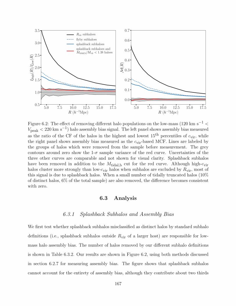
5.0 7.5 10.0 12.5 15.0 17.5R (h−1Mpc)

0.5

1.0

1.5

2.0

2.5

3.0

3.5ξ h

igh(R

)/ξ l

ow(R

)Rvir subhaloes

flyby subhaloes

splashback subhaloes

splashback subhaloes andMtidal,b/Mvir < 1.38 haloes

5.0 7.5 10.0 12.5 15.0 17.5R (h−1Mpc)

0.0

0.1

0.2

0.3

0.4

0.5

0.6

0.7

M(R

)Figure 6.2: The effect of removing different halo populations on the low-mass (120 km s−1 <Vpeak < 220 km s−1) halo assembly bias signal. The left panel shows assembly bias measured

as the ratio of the CF of the halos in the highest and lowest 15th percentiles of cvir, whilethe right panel shows assembly bias measured as the cvir-based MCF. Lines are labeled bythe groups of halos which were removed from the sample before measurement. The greycontours around zero show the 1-σ sample variance of the red curve. Uncertainties of thethree other curves are comparable and not shown for visual clarity. Splashback subhaloshave been removed in addition to the Mtidal,b cut for the red curve. Although high-cvirhalos cluster more strongly than low-cvir halos when subhalos are excluded by Rvir, most ofthis signal is due to splashback halos. When a small number of tidally truncated halos (10%of distinct halos, 6% of the total sample) are also removed, the difference becomes consistentwith zero.

6.3 Analysis

6.3.1 Splashback Subhalos and Assembly Bias

We first test whether splashback subhalos misclassified as distinct halos by standard subhalo

definitions (i.e., splashback subhalos outside Rvir of a larger host) are responsible for low-

mass halo assembly bias. The number of halos removed by our different subhalo definitions

is shown in Table 6.3.2. Our results are shown in Figure 6.2, using both methods discussed

in section 6.2.7 for measuring assembly bias. The figure shows that splashback subhalos

cannot account for the entirety of assembly bias, although they contribute about two thirds

167

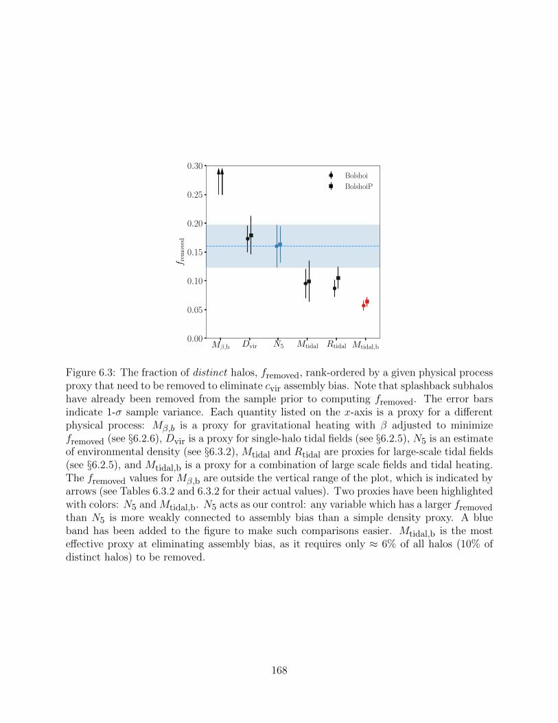
Mβ,b Dvir N5 Mtidal Rtidal Mtidal,b0.00

0.05

0.10

0.15

0.20

0.25

0.30

f rem

oved

Bolshoi

BolshoiP

Figure 6.3: The fraction of distinct halos, fremoved, rank-ordered by a given physical processproxy that need to be removed to eliminate cvir assembly bias. Note that splashback subhaloshave already been removed from the sample prior to computing fremoved. The error barsindicate 1-σ sample variance. Each quantity listed on the x-axis is a proxy for a differentphysical process: Mβ,b is a proxy for gravitational heating with β adjusted to minimizefremoved (see §6.2.6), Dvir is a proxy for single-halo tidal fields (see §6.2.5), N5 is an estimateof environmental density (see §6.3.2), Mtidal and Rtidal are proxies for large-scale tidal fields(see §6.2.5), and Mtidal,b is a proxy for a combination of large scale fields and tidal heating.The fremoved values for Mβ,b are outside the vertical range of the plot, which is indicated byarrows (see Tables 6.3.2 and 6.3.2 for their actual values). Two proxies have been highlightedwith colors: N5 and Mtidal,b. N5 acts as our control: any variable which has a larger fremovedthan N5 is more weakly connected to assembly bias than a simple density proxy. A blueband has been added to the figure to make such comparisons easier. Mtidal,b is the mosteffective proxy at eliminating assembly bias, as it requires only ≈ 6% of all halos (10% ofdistinct halos) to be removed.

168

of the signal. This is consistent with conclusions of the previous studies [Wang et al., 2009,

Sunayama et al., 2016]. The novel feature of this analysis is that we find a similar effect for

two independent definitions of the splashback halos: using evolutionary trajectories (§6.2.3)

and using non-spherical 3D splashback shells identified using the Shellfish code (§6.2.3).

Note also that although results for the two definitions are similar, the two samples of halos

are not identical. Flyby subhalos identified using merger trees are guaranteed to have passed

their orbital pericenter and thus likely have experienced a strong tidal interaction with the

host. On the other hand, when we use Shellfish all subhalos within the splashback shell

are classified as splashback subhalos, including those halos that have entered the shell, but

have not yet passed their pericenter. Given that both halo samples have exactly the same

local environments, the fact that removal of infalling splashback subhalos results only in a

small decrease of the assembly bias signal means that this portion of the assembly bias signal

is due to the stripping subhalos experience during their pericenter passage. Conversely, any

mass growth suppression subhalos experience on their way to pericenter is comparatively

unimportant important.

We further compare the splashback subhalos and flyby subhalos in section 6.3.5.

6.3.2 Contribution of Tidal Truncation and Gravitational Heating to

Assembly Bias

We now investigate how the truncation of halo mass growth by the tidal forces, both from

a halo’s most gravitationally-dominant neighbor and from the entire large-scale matter dis-

tribution, contributes to assembly bias. We also investigate the contribution of dynamical

heating caused by the collapse of matter into sheets and filaments. To this end we use the

five proxies of these processes defined in sections 6.2.5-6.2.6 – Dvir, Rtidal, Mβ,b, Mtidal,

and Mtidal,b – and evaluate what fraction of the distinct halo sample ranked by each of the

proxies must be removed to eliminate the assembly bias signal.

Dvir is the Rvir-normalized distance to the most tidally dominant halo. It is a proxy of

169

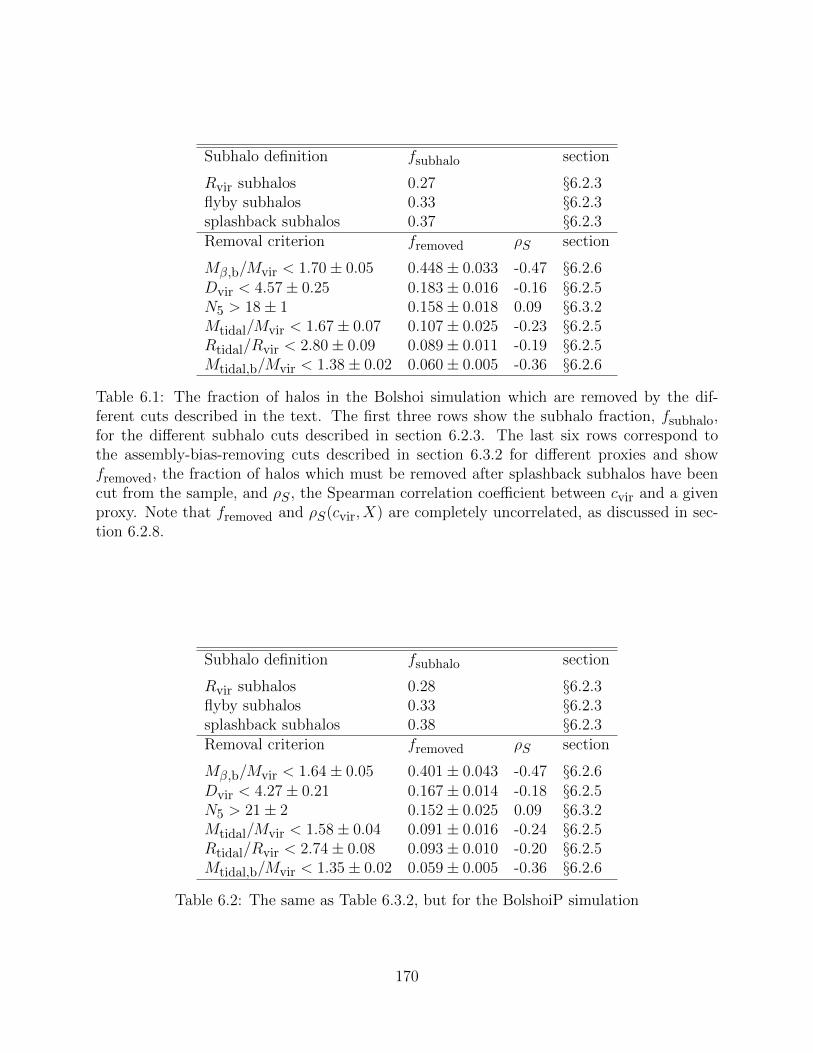
Subhalo definition fsubhalo section

Rvir subhalos 0.27 §6.2.3flyby subhalos 0.33 §6.2.3splashback subhalos 0.37 §6.2.3Removal criterion fremoved ρS section

Mβ,b/Mvir < 1.70± 0.05 0.448± 0.033 -0.47 §6.2.6Dvir < 4.57± 0.25 0.183± 0.016 -0.16 §6.2.5N5 > 18± 1 0.158± 0.018 0.09 §6.3.2Mtidal/Mvir < 1.67± 0.07 0.107± 0.025 -0.23 §6.2.5Rtidal/Rvir < 2.80± 0.09 0.089± 0.011 -0.19 §6.2.5Mtidal,b/Mvir < 1.38± 0.02 0.060± 0.005 -0.36 §6.2.6

Table 6.1: The fraction of halos in the Bolshoi simulation which are removed by the dif-ferent cuts described in the text. The first three rows show the subhalo fraction, fsubhalo,for the different subhalo cuts described in section 6.2.3. The last six rows correspond tothe assembly-bias-removing cuts described in section 6.3.2 for different proxies and showfremoved, the fraction of halos which must be removed after splashback subhalos have beencut from the sample, and ρS , the Spearman correlation coefficient between cvir and a givenproxy. Note that fremoved and ρS(cvir, X) are completely uncorrelated, as discussed in sec-tion 6.2.8.

Subhalo definition fsubhalo section

Rvir subhalos 0.28 §6.2.3flyby subhalos 0.33 §6.2.3splashback subhalos 0.38 §6.2.3Removal criterion fremoved ρS section

Mβ,b/Mvir < 1.64± 0.05 0.401± 0.043 -0.47 §6.2.6Dvir < 4.27± 0.21 0.167± 0.014 -0.18 §6.2.5N5 > 21± 2 0.152± 0.025 0.09 §6.3.2Mtidal/Mvir < 1.58± 0.04 0.091± 0.016 -0.24 §6.2.5Rtidal/Rvir < 2.74± 0.08 0.093± 0.010 -0.20 §6.2.5Mtidal,b/Mvir < 1.35± 0.02 0.059± 0.005 -0.36 §6.2.6

Table 6.2: The same as Table 6.3.2, but for the BolshoiP simulation

170

the one-halo contribution to the tidal force proportional to the traditional Hill radius. Rtidal

is the tidal radius calculated using only the distant matter distribution and Mtidal is the

mass contained within the tidal radius. Mβ,b is the bound mass within β Rvir for a specified

constant β and serves as a proxy of dynamical heating. Finally, Mtidal,b is the bound mass

contained within the tidal radius and serves as a proxy for the combined effects of the total

tidal force and gravitational heating.

Some care needs to be taken in setting β for the proxy Mβ,b. The most straightforward

option would be minimize the value of fremoved across all values of β, but this procedure

selects β ≈ 1.5, which will typically be within the halo’s own splashback shell. Mβ,b therefore

correlates with cvir simply because the latter determines the mass distribution within the

halo. Indeed, we find the Spearman rank coefficient ρS(M(< 1.5 × Rvir), cvir) = −0.26,

even before any unbinding procedure has been used. Instead, we choose to set β = 3. At

this distance, correlations between the total enclosed mass and cvir are negligible, and β Rvir

will generally be larger than Rsp. This choice has little effect on fremoved, which remains

approximately the same for β & 2.

The proxies described above are strongly (anti-)correlated with local matter density.

Thus, when we rank-order halos using these proxies and make cuts, we need to distinguish

this procedure from simple density cuts, which do not differentiate between particular physi-

cal processes that operate in high-density regions. To this end, we use the number of distinct

halos with 120 km s−1 < Vpeak < 220 km s−1 located within X comoving h−1 Mpc of the

center of a halo, NX , as a proxy of the density of the local environment. We tested radii

ranging from 1− 10h−1 Mpc and found that the assembly bias signal can be eliminated by

removing the smallest fraction of halos for X = 5. We thus use N5 as our fiducial local

environmental density proxy.

In Fig. 6.3 we show the fraction, fremoved, of all halos rank-ordered by different proxies

that must be removed to eliminate the assembly bias signal (see section 6.2.8). The corre-

sponding fremoved thresholds for each proxy are presented in Table 6.3.2, and the red curves

171

in Fig. 6.2 show clustering strength as a function of distance after such a cut has been made

to Mtidal,b. Note that statistical errors on the MCF are smaller relative to its amplitude

than errors on the ξhigh(r)/ξlow(r) curve, which is one of the chief reasons that we use the

former in calculations of fremoved.

The first feature apparent in Fig. 6.3 is that it is possible to remove assembly bias by

making a cut on the local density, meaning that assembly bias is only present in high-

density regions. This is consistent with models which predict that low-mass assembly bias

is caused by non-linear processes, but is not necessarily a generic prediction of such models,

as one could imagine assembly bias existing in all regions to different degrees of severity.

Fig. 6.3 also shows that the portion of assembly bias which is not caused by misclassified

splashback subhalos is due to a small number of halos in extreme environments: the cut

Mtidal,b/Mvir < 1.38 removes only 6% of all halos but reduces assembly bias to statistically

undetectable levels. For comparison, the cut to the density proxy N5 removes assembly bias

when 14% of halos are removed.

Further testing shows that there are two reasons why assembly bias can be eliminated by

removing only a small fraction of halos. First, the mean value of cvir ceases to be a strong

function of these proxies once the halos below the fremoved cutoff have been removed from

the sample. Second, halo clustering strength varies strongly as a function of proxy value

within the cutoff range, but is almost constant throughout the remaining sample.

Finally, Fig. 6.3 shows that fremoved for both Dvir, a proxy for the single-halo tidal force,

and Mβ,b, a proxy for dynamical heating, are at least as large as fremoved for N5. Even

if Mβ,b uses values of β small enough that it is primarily picking up features in the halo’s

own density profile, fremoved stays above 0.25. This means that the effect of single-halo

tidal forces and dynamical heating on assembly bias cannot be distinguished from the trivial

effect of environmental density on halo bias, which means that neither can account for the

assembly bias on their own.

In contrast, fremoved for Rtidal, Mtidal, and Mtidal,b are smaller than for N5, indicating

172

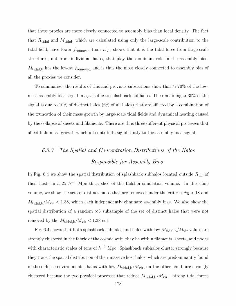
that these proxies are more closely connected to assembly bias than local density. The fact

that Rtidal and Mtidal, which are calculated using only the large-scale contribution to the

tidal field, have lower fremoved than Dvir shows that it is the tidal force from large-scale

structures, not from individual halos, that play the dominant role in the assembly bias.

Mtidal,b has the lowest fremoved and is thus the most closely connected to assembly bias of

all the proxies we consider.

To summarize, the results of this and previous subsections show that ≈ 70% of the low-

mass assembly bias signal in cvir is due to splashback subhalos. The remaining ≈ 30% of the

signal is due to 10% of distinct halos (6% of all halos) that are affected by a combination of

the truncation of their mass growth by large-scale tidal fields and dynamical heating caused

by the collapse of sheets and filaments. There are thus three different physical processes that

affect halo mass growth which all contribute significantly to the assembly bias signal.

6.3.3 The Spatial and Concentration Distributions of the Halos

Responsible for Assembly Bias

In Fig. 6.4 we show the spatial distribution of splashback subhalos located outside Rvir of

their hosts in a 25 h−1 Mpc thick slice of the Bolshoi simulation volume. In the same

volume, we show the sets of distinct halos that are removed under the criteria N5 > 18 and

Mtidal,b/Mvir < 1.38, which each independently eliminate assembly bias. We also show the

spatial distribution of a random ×5 subsample of the set of distinct halos that were not

removed by the Mtidal,b/Mvir < 1.38 cut.

Fig. 6.4 shows that both splashback subhalos and halos with low Mtidal,b/Mvir values are

strongly clustered in the fabric of the cosmic web: they lie within filaments, sheets, and nodes

with characteristic scales of tens of h−1 Mpc. Splashback subhalos cluster strongly because

they trace the spatial distribution of their massive host halos, which are predominantly found

in these dense environments. halos with low Mtidal,b/Mvir, on the other hand, are strongly

clustered because the two physical processes that reduce Mtidal,b/Mvir – strong tidal forces

173

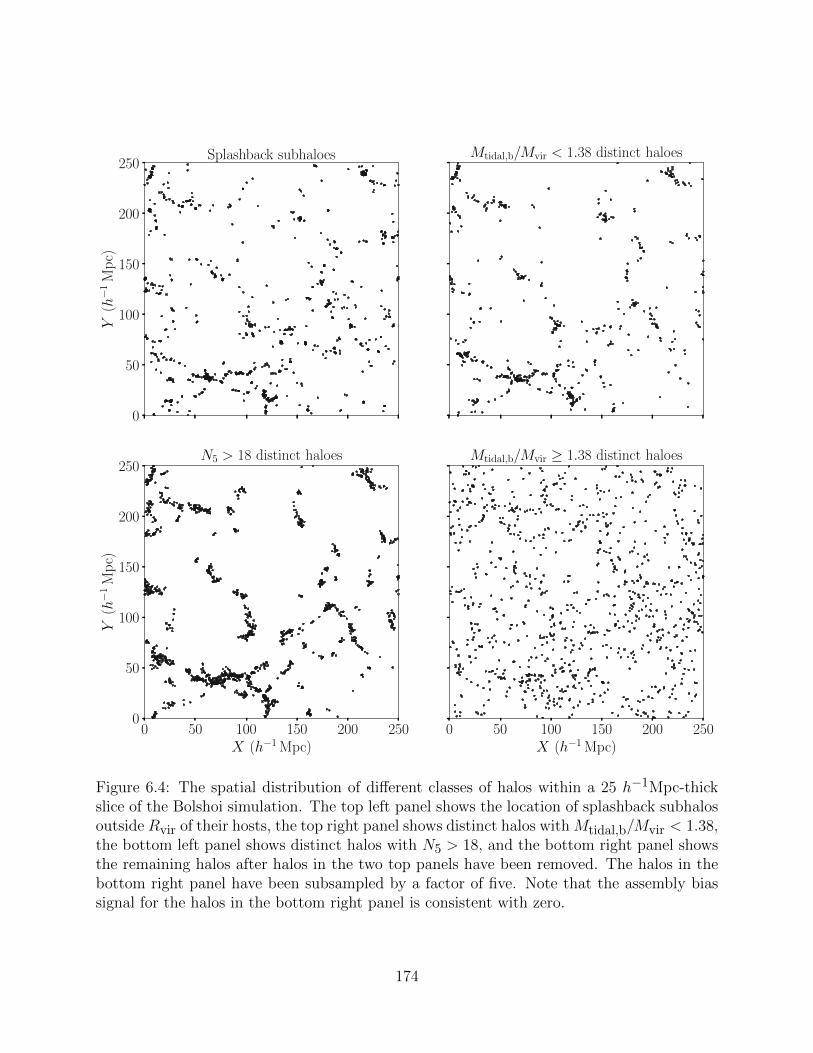
0

50

100

150

200

250

Y(h−

1M

pc)

Splashback subhaloes Mtidal,b/Mvir < 1.38 distinct haloes

0 50 100 150 200 250X (h−1 Mpc)

0

50

100

150

200

250

Y(h−

1M

pc)

N5 > 18 distinct haloes

0 50 100 150 200 250X (h−1 Mpc)

Mtidal,b/Mvir ≥ 1.38 distinct haloes

Figure 6.4: The spatial distribution of different classes of halos within a 25 h−1Mpc-thickslice of the Bolshoi simulation. The top left panel shows the location of splashback subhalosoutside Rvir of their hosts, the top right panel shows distinct halos with Mtidal,b/Mvir < 1.38,the bottom left panel shows distinct halos with N5 > 18, and the bottom right panel showsthe remaining halos after halos in the two top panels have been removed. The halos in thebottom right panel have been subsampled by a factor of five. Note that the assembly biassignal for the halos in the bottom right panel is consistent with zero.

174

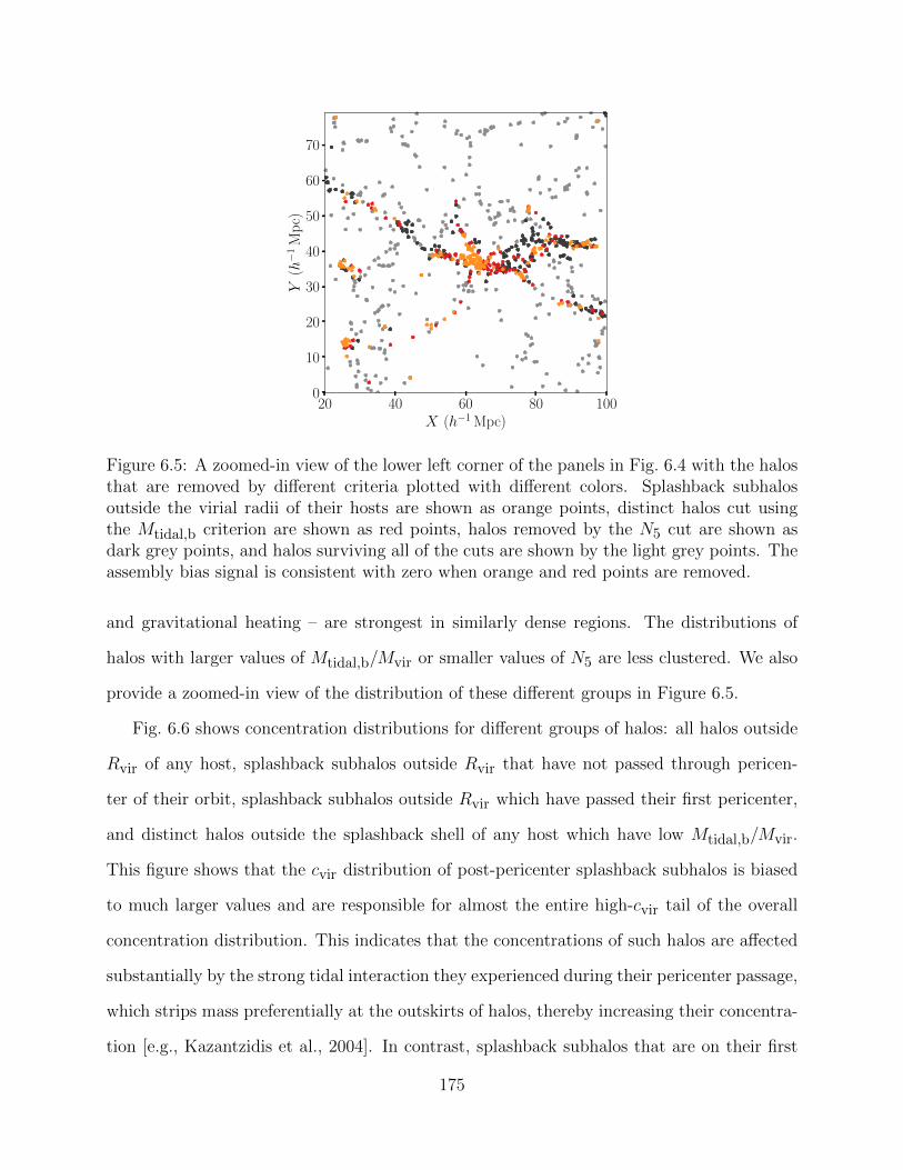
20 40 60 80 100X (h−1 Mpc)

0

10

20

30

40

50

60

70

Y(h−

1M

pc)

Figure 6.5: A zoomed-in view of the lower left corner of the panels in Fig. 6.4 with the halosthat are removed by different criteria plotted with different colors. Splashback subhalosoutside the virial radii of their hosts are shown as orange points, distinct halos cut usingthe Mtidal,b criterion are shown as red points, halos removed by the N5 cut are shown asdark grey points, and halos surviving all of the cuts are shown by the light grey points. Theassembly bias signal is consistent with zero when orange and red points are removed.

and gravitational heating – are strongest in similarly dense regions. The distributions of

halos with larger values of Mtidal,b/Mvir or smaller values of N5 are less clustered. We also

provide a zoomed-in view of the distribution of these different groups in Figure 6.5.

Fig. 6.6 shows concentration distributions for different groups of halos: all halos outside

Rvir of any host, splashback subhalos outside Rvir that have not passed through pericen-

ter of their orbit, splashback subhalos outside Rvir which have passed their first pericenter,

and distinct halos outside the splashback shell of any host which have low Mtidal,b/Mvir.

This figure shows that the cvir distribution of post-pericenter splashback subhalos is biased

to much larger values and are responsible for almost the entire high-cvir tail of the overall

concentration distribution. This indicates that the concentrations of such halos are affected

substantially by the strong tidal interaction they experienced during their pericenter passage,

which strips mass preferentially at the outskirts of halos, thereby increasing their concentra-

tion [e.g., Kazantzidis et al., 2004]. In contrast, splashback subhalos that are on their first

175

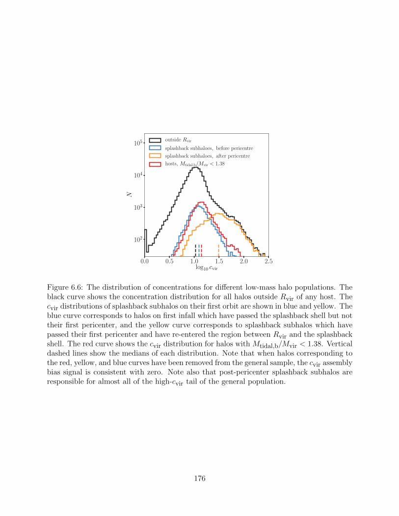
0.0 0.5 1.0 1.5 2.0 2.5log10 cvir

102

103

104

105

N

outside Rvir

splashback subhaloes, before pericentre

splashback subhaloes, after pericentre

hosts, Mtidal,b/Mvir < 1.38

Figure 6.6: The distribution of concentrations for different low-mass halo populations. Theblack curve shows the concentration distribution for all halos outside Rvir of any host. Thecvir distributions of splashback subhalos on their first orbit are shown in blue and yellow. Theblue curve corresponds to halos on first infall which have passed the splashback shell but nottheir first pericenter, and the yellow curve corresponds to splashback subhalos which havepassed their first pericenter and have re-entered the region between Rvir and the splashbackshell. The red curve shows the cvir distribution for halos with Mtidal,b/Mvir < 1.38. Verticaldashed lines show the medians of each distribution. Note that when halos corresponding tothe red, yellow, and blue curves have been removed from the general sample, the cvir assemblybias signal is consistent with zero. Note also that post-pericenter splashback subhalos areresponsible for almost all of the high-cvir tail of the general population.

176

10−1 101 103

Mvir/M∗

−0.3

−0.2

−0.1

0.0

0.1

0.2

0.3

0.4

MC

F(6h−

1M

pc<R<

10h−

1M

pc)

Rvir

splashback shell

Mtidal,b/Mvir < 1.38

N5 > 18

Figure 6.7: The dependence of assembly bias on Mvir, scaled by the non-linear collapse massscale, M∗. This plot was created from the z = 0, 1, 1.4, and 3 snapshots of Bolshoi andshows the median values of Mvir/M∗ in thin Vpeak bins versus the MCF between 6 h−1 Mpc

and 10 h−1 Mpc for each bin. 1 − σ sample variance of the MCFs are plotted as shadedregions. Lines of different color show MCFs for halo samples with different cuts indicatedin the legend. Vpeak bins below our convergence limit of 120 km s−1 and bins with errors

on the MCF larger than 0.1 are not plotted (this typically occurs at Vpeak ≈ 300 km s−1).Non-linear effects strongly reduce assembly bias at low masses but have no impact on high-mass assembly bias because this effect has a different physical origin. However, a single cutto local density is effective at removing assembly bias at all masses.

infall and distinct halos with Mtidal,b/Mvir < 1.38 have comparable concentration distribu-

tions and are only slightly shifted relative to the overall distribution of concentrations. The

modest shift in cvir is consistent with an older age of these halos, rather than the large con-

centration boost in halos that have experienced tidal stripping. We note that the strength

of the high cvir tail becomes weaker if the halo sample is defined by Mvir or Vmax. This is

because halos that lost mass after their first pericenter passage drop out of the Mvir-defined

sample, but stay within the Vpeak defined sample.

177

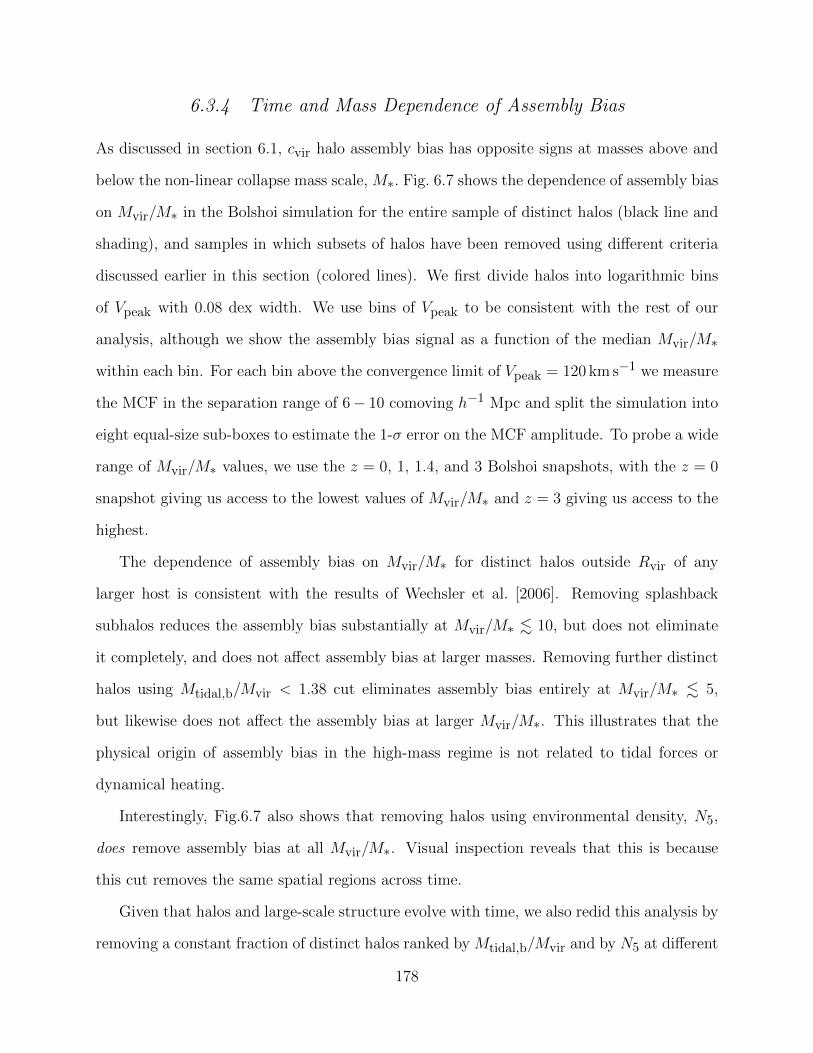
6.3.4 Time and Mass Dependence of Assembly Bias

As discussed in section 6.1, cvir halo assembly bias has opposite signs at masses above and

below the non-linear collapse mass scale, M∗. Fig. 6.7 shows the dependence of assembly bias

on Mvir/M∗ in the Bolshoi simulation for the entire sample of distinct halos (black line and

shading), and samples in which subsets of halos have been removed using different criteria

discussed earlier in this section (colored lines). We first divide halos into logarithmic bins

of Vpeak with 0.08 dex width. We use bins of Vpeak to be consistent with the rest of our

analysis, although we show the assembly bias signal as a function of the median Mvir/M∗

within each bin. For each bin above the convergence limit of Vpeak = 120 km s−1 we measure

the MCF in the separation range of 6− 10 comoving h−1 Mpc and split the simulation into

eight equal-size sub-boxes to estimate the 1-σ error on the MCF amplitude. To probe a wide

range of Mvir/M∗ values, we use the z = 0, 1, 1.4, and 3 Bolshoi snapshots, with the z = 0

snapshot giving us access to the lowest values of Mvir/M∗ and z = 3 giving us access to the

highest.

The dependence of assembly bias on Mvir/M∗ for distinct halos outside Rvir of any

larger host is consistent with the results of Wechsler et al. [2006]. Removing splashback

subhalos reduces the assembly bias substantially at Mvir/M∗ . 10, but does not eliminate

it completely, and does not affect assembly bias at larger masses. Removing further distinct

halos using Mtidal,b/Mvir < 1.38 cut eliminates assembly bias entirely at Mvir/M∗ . 5,

but likewise does not affect the assembly bias at larger Mvir/M∗. This illustrates that the

physical origin of assembly bias in the high-mass regime is not related to tidal forces or

dynamical heating.

Interestingly, Fig.6.7 also shows that removing halos using environmental density, N5,

does remove assembly bias at all Mvir/M∗. Visual inspection reveals that this is because

this cut removes the same spatial regions across time.

Given that halos and large-scale structure evolve with time, we also redid this analysis by

removing a constant fraction of distinct halos ranked by Mtidal,b/Mvir and by N5 at different

178

redshifts rather than using a fixed cut as in Fig. 6.7. The results of such analysis are almost

identical, albeit with slightly higher fremoved.

6.3.5 Sensitivity to Splashback Subhalo Identification Method

As discussed above, we use two different methods to identify splashback subhalos: 1) halos

that move within Rvir of a larger halo at some point during their evolution and (“flyby

subhalos”) 2) halos located within the splashback shell identified by the Shellfish algorithm

(“splashback subhalos”). It is clear that the samples of subhalos identified using these

methods cannot be identical: halos that are on their first approach to a host and are already

within the splashback shell but are still outside Rvir will be classified as splashback subhalos

by the second method, but not the first. Conversely, halos that previously passed within

Rvir of the host, but are now outside of the splashback shell identified by Shellfish will be

identified by the first method, but not the second.

We find that ≈ 40% of splashback subhalos (≈ 4% of all halos) are not identified as flyby

halos, but only ≈ 6 − 8% of flyby subhalos (0.4 − 0.5% of all halos) are not identified as

splashback subhalos. The latter subhalos are misidentified largely around host halos below

convergence limit of the Shellfish algorithm: if we restrict this analysis to host halos that

meet the convergence requirements of N200m > 5 × 104 and ΓDK14 > 0.5 [see Mansfield

et al., 2017, for details], we find that only 1 − 2% of flyby halos (. 0.1% of all halos) are

not identified by the second method. This small fraction indicates that the splashback shells

identified by Shellfish for well-resolved halos capture the vast majority of the splashback

subhalos identified by the traditional subhalo trajectory method. This also indicates that

the fraction of subhalos ejected by three-body interactions via the slingshot process beyond

the splashback shell [Kravtsov et al., 2004, Sales et al., 2007] is quite small and that most of

the subhalos outside Rvir are on their natural dynamical orbit around their host halo. We

note that this conclusion should not be extended to Vpeak < 120 without further testing: it

is plausible that slingshot processes become more significant at lower masses.

179

This is consistent with earlier studies that analyzed the radial distribution of flyby sub-

halos [Ludlow et al., 2009, Wang et al., 2009, Li et al., 2013] and found that flyby subhalos

are common at distances up to 2R200c, with numbers decreasing quickly at larger radii but

with a small population present out to ≈ 4R200c. We find that the radial distribution of

flyby subhalos is due to large size of the splashback shell relative to R200c, its non-spherical

shape, and the substantial scatter between R200c and the maximum radius of the splashback

shell. For our sample of distinct halos, the mean value of Rsp/R200c is 2.16 and the mean

value of Rsp,max/R200c is 2.80 with a 1− σ scatter of ≈ 0.6, where Rsp,max is the maximum

radius of any point on the splashback shell.

Lastly, Figure 6.2 compares the MCF after both methods have been used to remove

splashback subhalos. The difference is small relative to the overall amplitude of the signal.

We also find that when the procedure described in sections 6.2.8 and 6.2.8 is used, both

classification schemes find similar cutoff values. However, fremoved is necessarily ≈ 3%

larger when flyby flagging is used to remove splashback subhalos because these cuts must

also remove infalling splashback subhalos. The exception to this is the Mtidal proxy, which is

higher for almost all splashback subhalos than it is for almost all distinct halos. Thus, Mtidal

cannot remove assembly bias without removing the entire sample. This leads us to conclude

that our general results are robust to differences in the subhalo classification scheme.

6.3.6 Comparison of the Bolshoi and BolshoiP Simulations

All analysis presented above was done using the Bolshoi simulation with cosmological pa-

rameters consistent with the final WMAP mission constraints (see section 6.2.1). To test the

dependence of our results on the assumed cosmology, we repeated all analysis using the Bol-

shoiP simulation, which assumes cosmological parameters consistent with the Planck mission

constraints and found that all of the results are qualitatively consistent. The difference in

Ωm in the Bolshoi and BolshoiP simulations leads to small changes in the cutoff values for

Mβ,b, Dvir, Mtidal, Rtidal, and Mtidal,b, but the values of fremoved are within 0.01 of the

180

values found for the Bolshoi simulation for all cuts, which the exception of the high-error

fremoved value for our least efficient proxy, Mβ,b.

6.4 Discussion

6.4.1 Issues Associated with Proxy Definitions

In this study we define and use several proxies of physical processes that could conceiv-

ably contribute to assembly bias. Of these, Dvir, Rtidal, Mtidal, Mβ,b, and Mtidal,b require

estimating the local tidal force and/or determining whether a given particle is bound or

unbound. However, it is not trivial to accurately determine whether a particle is bound in

the outskirts of halos [see, e.g., Behroozi et al., 2013a, for an extended discussion of related

issues], and strong assumptions and approximations must be employed in the estimates of

tidal forces. Errors made in estimating a particular proxy should result in additional scat-

ter in its correlation with cvir and should increase the uncertainty in our estimate of its

contribution to the assembly bias. As a corollary, improvements in proxy definitions should

only decrease the measured fremoved values. In practice, only Mtidal,b is strongly affected

both by uncertainties in the tidal force estimate and by issues of identifying bound parti-

cles, which means that improvements in proxy estimates would primarily reduce fremoved for

Mtidal,b, while having an equal or lesser effect on our other proxies. This means that such

improvements would not change our conclusions.

A detailed analysis of the errors associated with the approximations necessary for tidal

force calculation can be found in Appendix 6.6.3. A discussion of the issues related to

identification of bound particles can be found in Appendix 6.6.4.

6.4.2 Sensitivity of Results to Definitional Choices

In this section we discuss the impact of the choices and assumptions made in our fiducial

analysis on our results. We have already discussed how our choice of clustering statistic

181

10−1 101 103

Mvir/M∗

−0.3

−0.2

−0.1

0.0

0.1

0.2

0.3

0.4

MC

F(6h−

1M

pc<R<

10h−

1M

pc)

Rvir

splashback shell

Mtidal,b/Mvir < 1.38

N5 > 18

Figure 6.8: The same as Fig. 6.7, but for MCFs defined in terms of −a1/2 instead of cvir.See section 6.4.2 for discussion.

used to estimate assembly bias affects out results in sections 6.2.7 and 6.3.2 (see Fig. 6.2),

so here we focus on the effect of our choices of Vpeak for defining halo samples, Rvir as our

reference halo boundary, and halo concentration as our formation time proxy. Although we

did present justifications for our choices in section 6.2, it is important to assess how sensitive

our results and conclusions are to these choices.

As an alternative to Vpeak, we could define halo samples using Mpeak, Vmax, or Mvir. We

find that sample selection by Mpeak leads to results similar to our fiducial case, but using

Vmax or Mvir leads to a somewhat different behaviour. The amplitude of the MCF with

only Rvir subhalos removed is closer to the amplitude of the MCF with splashback subhalos

removed for a Vpeak or Mpeak cut. However, further removing splashback subhalos with a

Vmax or Mvir cut results in only a small decrease in amplitude. This is because subhalos

generally experience significant mass loss and therefore sample selection based on their peak

mass or circular velocity results in larger subhalo fractions compared to selection on current

mass [cf., also Nagai and Kravtsov, 2005]. The large-cvir tail seen in Fig. 6.6 is weaker when

Vmax or Mvir is used to define the halo samples for the same reason. Our other results,

182

such as the values of fremoved or the spatial distribution of different halo subsets, are largely

unaffected. This is because the halos removed by these cuts have merely had their accretion

histories slowed: they have not experienced significant mass loss.

Although most analysis in this chapter uses splashback shells as halo boundaries, we use

spheres of radius Rvir as halo boundaries when we compute fiducial M(r) curves and when

we classify “flyby” subhalos. We have repeated these analyses using other commonly used

values of ∆ρm, and found that the main difference, unsurprisingly, is in the change of the

amplitude of the reference MCF. Definitions with high values of density contrast, such as

∆ρm = 200ρc or ∆ρm = 500ρc, result in a modest increase of the reference MCF amplitude,

while definitions with low density contrasts, such as ∆ρ = 200ρm, result in a modest decrease

of the MCF amplitude. To decrease the reference MCF amplitude to the level of the MCF

after removal of splashback subhalos requires ∆ρm ≈ 100ρm – close to the typical density

contrast enclosed by the splashback shell [see Fig. 12 in Mansfield et al., 2017]. Changes

in ∆ used for radius definition have little effect on the amplitude of the MCF when flyby

subhalos have been removed because most subhalos have their first pericenters at radii well

within all of the commonly-used definitions of halo radius.

We have chosen to use cvir as a proxy of halo age, but assembly bias behaves differently

for different proxies [e.g., Villarreal et al., 2017a, Mao et al., 2018, Salcedo et al., 2018],

so one would reasonably wonder if halo removal criteria also depend on this choice. A full

investigation of different definitions is beyond the scope of this work, but as a preliminary

discussion, we repeat our analysis for the most commonly used alternative age proxy – the

expansion factor at which the virial mass of the main progenitor of a halo was half of the

halo’s current mass, a1/2:

Mvir(a1/2) =1

2Mvir(acurrent). (6.10)

Note that although large (small) cvir values correspond to old (young) halos, the opposite is

183

true for a1/2. To simplify comparison with cvir-based results, we use −a1/2 as the formation

time proxy, so the sign of the MCF retains the same qualitative meaning.

Results for the −a1/2 proxy are shown in Fig. 6.8, where we use the same cuts that

removed the assembly bias in the cvir-based analysis. The figure shows that stricter cuts

are required to eliminate −a1/2 assembly bias. When we follow the procedure described in

section 6.2.8, the Mtidal,b cut that removes −a1/2 assembly bias results in fremoved = 0.14,

compared to fremoved = 0.06 for cvir assembly bias. Other proxies experience similar in-

creases in fremoved, with the exception of N5, which removes assembly bias for both defini-

tions in almost all bins. The fact that Bolshoi and BolshoiP measurements of fremoved agree

to within 0.01 for all variables (see §6.3.6) indicates that the differences in fremoved between

the cvir and −a1/2 definitions are significant.

Another difference is that in contrast to the cvir MCF, the amplitude of the −a1/2 MCF

does not reverse sign at large halo masses (see Fig. 6.8 and several previous studies: Gao

et al. 2005, Gao and White 2007, Wetzel et al. 2007, Mao et al. 2018, Sato-Polito et al.

2018). This puzzling behaviour at first appears to be inconsistent with the physical origin of

the high-mass assembly bias argued for by Dalal et al. [2008, see also section 9.4 of Zentner

2007]. However, Chue et al. [2018] showed that a1/2 and similar measures of formation

time can be problematic if measured relative to a standard overdensity mass. Because these

definitions do not account for mass in the splashback shell, halos measured at a constant

Mvir actually have a range of “true” splashback-enclosed masses, and the high-mass halos

will preferentially have early a1/2, which increases the level of bias measured for early a1/2

halos. The intersection of this behaviour with Fig. 6.8 requires further study.

6.4.3 Comparison with Previous Work

The effect of splashback subhalos on assembly bias was investigated in a number of recent

studies [Wang et al., 2009, Li et al., 2013, Sunayama et al., 2016], which concluded that

splashback subhalos contribute significantly to low-mass halo assembly bias, but cannot ac-

184

count for the entire signal. These studies used the “flyby” approach to classify subhalos

(similar to the method described in 6.2.3), which can include bona fide splashback subha-

los, as well as subhalos ejected via slingshot effect after dynamical interactions with other

subhalos. However, this classification cannot account for a large number of subhalos within

splashback shells that are on their first infall. This left open the question of the contribution

of such infalling subhalos on assembly bias. In this study we answer this question in section

6.3.5.

Additionally, these studies have not demonstrated the physical origin of the remaining

assembly bias signal. Our results differ from those of Sunayama et al. [2016], which find that

splashback subhalos have little effect on the MCF at large distances (R & 10h−1 Mpc).

Sunayama et al. [2016] used the same simulation and underlying halo catalogs as this chapter,

so this difference is likely due to the fact that their samples are defined by Mvir (see section

6.4.2) and their use of halo bias ratios to measure assembly bias. This statistic results in

larger errors than the MCF, as we discussed in § 6.2.7 and 6.3.2. For example, comparison

of the bin-to-bin scatter in Fig. 3 and Fig. 4 of Sunayama et al. [2016] to the 1-σ error

contours in the right panel of our Fig. 6.2 indicates that their measurements may not have

been sensitive enough to probe large-scale assembly bias.

The conjecture that non-linear tidal and dynamical heating effects can be responsible for

low-mass halo assembly bias was discussed in a number of studies [e.g. Wang et al., 2007,

Dalal et al., 2008, Hahn et al., 2009, Wang et al., 2011, Hearin et al., 2016b, Paranjape et al.,

2018, Salcedo et al., 2018, Musso et al., 2018, Johnson et al., 2019]. Often, arguments for a

particular process are based on establishing existence of a correlation between halo formation

time or halo bias and a proxy for a particular process, such as Rhill, bound mass fraction,

the magnitude of tidal eigenvectors, or various measures of tidal anisotropy. While such

correlations provide useful information, by themselves they are not sufficient to establish

that a given physical process is responsible for assembly bias. This is because the proxies of

all these processes are all strongly correlated: an explicit comparison, such as that shown in

185

Fig. 6.3, is more direct and compelling in identifying the responsible process.

Furthermore, looking at the global connection between halo formation time and a proxy

is problematic for two reasons. First, we show that after splashback subhalos are removed

low-mass halo assembly bias is due to only a small fraction of distinct halos. Thus, analysis

relying on the global correlation strength is not optimal. Second, as discussed in section 6.2.8,

the correlation between a proxy and halo formation time by itself contains no information

about how closely that proxy is related to assembly bias: a strongly correlated proxy which

experiences weak differential clustering, such as Mβ,b, will not contribute to assembly bias.

We avoid both these issues with the procedure described in section 6.2.8.

We find a strong connection between tidal forces from the large-scale mass distribution

and assembly bias in agreement with the conclusions of Hahn et al. [2009], Hearin et al.

[2016b], Salcedo et al. [2018], and Johnson et al. [2019]. However, in contrast with these

studies, we find that this this effect cannot be effectively approximated by assuming that

halos only feel the tidal force of their most gravitationally dominant neighbor. In fact, we

find that when such an approximation is made, the connection is sufficiently weak that

it is likely caused simply because the Hill radius is a crude estimate of local density (see

section 6.3.2). This discrepancy is due to two factors. First, some of these studies do not

perform the type of multi-variate analysis that would be necessary to differentiate between

different contributing physical processes. Second, while these studies effectively map out the

connection between formation time and single-halo tidal proxies, this is unrelated to the

connection between assembly bias and these proxies, an argument we make in section 6.2.8.

Also, contrary to the conclusion of Paranjape et al. [2018], we do not find a compelling

evidence that large-scale tidal anisotropy contributes significantly to assembly bias beyond

what is expected from its correlation with tidal field strength. Nevertheless, given the inac-

curacies associated with all methods based on second-order approximations to the tidal field

(see Appendix 6.6.3), a more detailed study of tidal field anisotropy could prove fruitful,

especially in the context of explicitly studying the tidal environments within structures like

186

sheets and filaments.

Although our results are in qualitative agreement with the conjectures of Wang et al.

[2007] and Dalal et al. [2008] that gravitational heating is a significant component of assembly

bias, we also find that this connection only becomes strong when tracers simultaneously

incorporate both gravitational heating and a halo’s zone of influence over the local tidal

field, such as Mtidal,b.

Our work uses an approach similar to that of Villarreal et al. [2017a], so we have performed

an in-depth comparison with their results. We find broad qualitative agreement between our

Dvir results and the results of Villarreal et al. [2017a], but find that quantitatively the ∆

values they report imply Dvir values smaller than our findings by ≈ 25%.

This difference is due to two factors. First, we find that the sample variance in the

boxes used by Villarreal et al. [2017a] is larger than than they estimated. We estimate the

sample variance using subvolumes of the BolshoiP simulation, which has nearly identical

mass resolution and cosmology to the CPla L0125 box used by Villarreal et al. [2017a] and

find that the actual variance is larger than the uncertainty they estimated by repeatedly

shuffling marks among halos. This means that MCFs in the CPla L0125 box could be

lower due to sample variance, which could thus result in less aggressive conditions for the

removal of assembly bias. Second, while the Rockstar halo finder used in Villarreal et al.

[2017a] and in this chapter is a state-of-the-art tool for measuring the properties of halos

with density contrasts of ∆ & ∆vir [e.g., Knebe et al., 2013], it cannot effectively measure

halo properties at lower density contrasts, such as the ∆ = 20 contrast used by Villarreal

et al. [2017a]. This is because there is no FOF linking length which can fully percolate all

matter out to such large overdensity radii, while also allowing for efficient load-balancing.

This leads to underestimates of halo masses and artefacts in the density profile. Contrary

to the findings of Villarreal et al. [2017a], we find that even with an unusually large linking

length of b = 0.5, virtually all halos have underestimated M20m masses. The ratio Mtrue(<

R20m,Rockstar)/M20m,all,Rockstar has 1 − σ contours of 1.04 − 1.13, with 2σ fluctuations

187

reaching ≈ 2.5. The magnitude of underestimation is significantly worse at more commonly-

used linking lengths. This and the fact that halos no longer follow NFW profiles at large

radii [e.g., Becker and Kravtsov, 2011, Diemer and Kravtsov, 2014], adds biases and noise to

the Rs and RsKlypin values measured by Rockstar. This, in turn, artificially reduces the

amplitude of the MCF. We discuss this issue in greater depth in Appendix 6.6.1.

Our interpretation is consistent with the test presented in Figure 11 of Villarreal et al.

[2017a], which shows that when R20m is used to exclude subhalos, but concentrations are

measured from the halo catalogs constructed using larger ∆, the MCF is not consistent with

zero. We find that when we replicate their analysis using manually-constructed overdensity

profiles, excluding “subhalos” by spheres of radius R20m is no longer capable of mitigating

assembly bias. Larger overdensity radii that are comparable with our reported Dvir cutoff

values are required.

6.4.4 Directions for Future Work

In this chapter, we focus on the dependence of halo bias on cvir, but galaxy properties are

likely related to a number of halo properties. This means that the effects of secondary biases

on galaxy clustering may not be confined to the cvir bias dependence and may remain even if

cvir dependence of bias is removed. As discussed in 6.4.2, this is true even for an alternative

choice of halo formation time proxy, −a1/2. Furthermore, Villarreal et al. [2017a] show that

mitigating secondary biases in axis ratio and spin parameter is more difficult than removing

bias in cvir, although the discussion in section 6.4.3 should be kept in mind when assessing

these results. It would be useful to perform analysis comparable to the one presented here

for a number of other key halo properties to build a more complete understanding of the

physical origin of the corresponding dependencies of halo bias.

One of our key results is that despite the large contribution of tidal forces to cvir assembly

bias, this cannot be shown conclusively when using rough and inaccurate estimates of the

tidal force, such as Dvir or the single-halo Rhill. Although Rtidal defined in section 6.2.5

188

accounts for tidal forces from multiple halos, it still is rather inaccurate, as we show in

Appendix 6.6.3 and discuss in 6.4.1. The accuracy of the tidal force estimate can be improved

by using a higher order approximation of the tidal field, by iteratively recalculating Rtidal and

removing nearby sources accordingly, or by explicitly evaluating the tidal field outside the

halo and identifying the turnover associated with the tidal radius directly. More accurate

estimate of the tidal radius could result in a better identification of halos responsible for

assembly bias. This effort could also be aided by incorporating cosmic web classifiers [see

review by Libeskind et al., 2018], which would allow higher accuracy analytic calculation

of the tidal fields associated with nearby large-scale structure, rather than the low-order

approximations that are required for generic point distributions.

Finally, all of the tidal field and dynamical heating proxy estimators discussed and used in

this chapter are computed from simulated quantities and cannot be immediately be applied

to observations. A follow-up exploration of possible observable proxies that can remove

particular flavors of secondary halo bias using mock catalogs will be a useful future avenue

of research.

6.5 Summary and Conclusions

In this study, we present analysis of the physical causes of assembly bias – the dependence

of halo clustering on proxies of halo age. We present results for assembly bias across a broad

range of masses, redshifts, and several definitions of halo age. Our main focus, however,

is on the detailed analysis of nonlinear processes that modify the primordial assembly bias

during the non-linear stages of structure formation using concentration as our primary age

indicator.

Our results indicate a scenario in which halos of all masses initially exhibit primordial

assembly bias arising from the properties of the initial Gaussian field of density perturbations.

However, the assembly bias of halos with masses smaller than the current nonlinear mass

scale is reduced to zero or to negative levels by three non-linear processes as mass decreases.

189

We first explore the contribution of “splashback subhalos” to assembly bias, where splash-

back subhalos are defined either as halos that have passed within the virial radius of a larger

halo at some point in the past or as halos are located within the splashback shell of a larger

halo, as determined by the method of Mansfield et al. [2017]. Assembly bias is measured

both before and after the removal of these subhalos. We show that splashback subhalos are

responsible for about two thirds of the assembly bias signal, but do not account for the entire

effect. Moreover, it is the subhalos that have passed the pericenter of their orbit at least

once that are responsible for the contribution of subhalos to assembly bias. In addition, we

find that the high-cvir tail of the distinct halo distribution is due almost entirely to these

same post-pericenter subhalos.

At the mass ranges considered in this chapter, we find that the fraction of halos which

have passed within the splashback shells of their hosts but are later located outside them is

small, which indicates that the fraction of halos ejected beyond the splashback shell due to

three-body interactions is small.

We then investigate which additional physical processes contribute to assembly bias.

We do this by constructing proxies of these processes for each halo, ranking distinct halos

according to each proxy, and measuring what fraction of the ranked halos need to be removed

in order for the assembly bias signal to be statistically consistent with zero. We find that

assembly bias is caused by a relatively small number of halos in dense regions. These halos

have had their accretion histories truncated by a combination of large-scale tidal fields and

the high velocities of ambient particles. We also demonstrate that neither process can cause

assembly bias on its own and that these tidal fields are not well-modeled by assuming that the

dominant tidal contribution comes from a single massive neighbor. We further argue that

the commonly-used approach of measuring the correlation between a physical proxy and

halo age cannot be used on its own to draw conclusions about the strength of the connection

between that proxy and assembly bias.

A key finding of this study is that after splashback subhalos are removed, the residual

190

“negative” assembly bias is due to only 10% of distinct halos (5% of all halos). To summarize,

27% of halos are removed due to a traditional Rvir-based subhalo cut, a further 10% are

removed due to a splashback subhalo cut, and finally 6% of all halos are removed due to

the cut based on Mtidal,b/Mvir. These low Mtidal,b/Mvir halos are located within the largest

filaments and are only slightly more concentrated than the general population. However,

their strong spatial clustering results in an outsized effect on the global assembly bias signal.

We find that in the WMAP cosmology, the removal of halos above a certain local density,

as measured by the number of halos within 5h−1 comoving Mpc, N5 > 18, removes assembly

bias for both cvir and a1/2 at all distances across all mass scales and redshifts and that a

similar cut exists in a Planck cosmology. Such a cut removes a much larger fraction of

halos from the sample than the cut in Mtidal,b/Mvir, and thus does not correspond to a real

physical process contributing to assembly bias. Nevertheless, this result indicates that it

may be fruitful to explore whether density-based cuts on mock galaxy catalogs can be used

to remove assembly bias from galaxy samples and motivates further studies in this direction.

6.6 Appendices

6.6.1 Effects of Halo Definition on Concentration in the Rockstar Halo

Finder

The Rockstar halo finder works by dividing the simulation into 3D friends-of-friends (FOF)

groups, adaptively creating smaller 6D FOF groups in phase space, placing halo centers at

the most refined 6D FOF groups, and finally calculating halo properties relative to those

centers [Behroozi et al., 2013c]. The size of the initial 3D FOF groups is set by the input

linking length in units of the mean interparticle separation, b. The accuracy of the halo

properties computed by Rockstar depends on the original 3D FOF groups percolating out

to the baseline overdensity radius of the corresponding halos [More et al., 2011, Behroozi

et al., 2013c]. This is particularly important when fitting halo density profiles: if halo bound-

191

aries extend into the unpercolated regions of the FOF group, the density in the outermost

radial bins will be systematically underestimated, shifting the location of profile features.

In this Appendix, we examine the effect of using different halo definitions on the measured

concentrations.

Behroozi et al. [2013c] perform convergence tests that show that using linking length

of b = 0.28 leads to full percolation within Rvir. They note that when one defines halo

boundary larger than Rvir, a larger linking length should be used and additional tests should

be performed to ensure full percolation within such boundary. We test the effect of the

halo boundary choice by running Rockstar repeatedly on the CBol L0125 simulation from

Diemer and Kravtsov [2015] for a variety of overdensity radii, R∆, with overdensity ranging

from ∆ = 20ρm to ∆ = 1600 ρm for b = 0.28, 0.5 and for a reference catalog with ∆ = ∆vir

and b = 0.28. We then matched halos across the catalogs to our reference Rvir catalog. Our

tests indicate that results are not sensitive to the way this matching is done, so we use a

simple procedure where a halo is considered a “match” if its center lies within 0.25 kpc of

the center of a counterpart in the Rvir catalog. This criterion is sufficient to unambiguously

match most halos, but in the event that multiple halos meet it, we match to the halo in that

group with the closest Mvir to the reference halo. Subhalo and distinct halo status are not

factored in to this matching. We restrict our sample to halos classified as hosts by the ∆vir

catalog with 1011.5 h−1M < Mvir < 1012 h−1M, as measured by the same catalog. The

choice of mass range has only a slight effect on results.

Fig. 6.9 shows the ratio of Rs measured in catalogs constructed for different values of ∆,

denoted Rs,∆, to Rs measured in the reference catalog, denoted Rs, vir. We show this ratio as

a function of ∆ for two values of b. We find that creating catalogs with larger linking lengths

takes an inordinate amount of time, presumably because a large fraction of the simulation

is placed into the same FOF group. The figure shows that .Rs measurements for ∆ . 200

are biased low relative to the values found for ∆ = ∆vir and there is a significant scatter

between the two. The bias is about twice larger for b = 0.28 compared to b = 0.5.

192

102 103

∆/ρm

0.4

0.6

0.8

1.0

1.2

1.4

Rs,

∆/R

s,vir

b = 0.5

b = 0.28

∆ = ∆vir

Figure 6.9: The value of Rs measured by Rockstar using different overdensities, ∆, todefine halo radius, R∆. The scale radii are normalized by the value of Rs measured forthe same halos in a catalog with a primary definition of ∆vir for two different values of theRockstar’s 3D FOF linking length, b. The median values of this ratio are shown as solidlines and the contours enclosing 68% of ratios are shown as shaded regions. Note that Rs

measurements for ∆ . 200 are biased low relative to the values found for ∆ = ∆vir andthere is a significant scatter between the two. The bias is larger for smaller b.

193

The primary implication of this result is that concentrations measured for halos identified

and analyzed by Rockstar using low ∆, such as ∆ = 20 ρm, should not be trusted due to

large systematic bias and scatter. This is due to lack of FOF percolation in the outskirts

of halos, which biases densities in the outskirts low and this, in turn, biases the best-fit Rs

values low. This is also true for other ways of estimating concentration, such as deriving it

from Vmax/Vvir. The context of this fact in relation to our work on assembly bias is discussed

in section 4.3.

Behaviour at commonly used choices, such as ∆ = 200 ρm, 200 ρc, 500 ρc is also note-

worthy. For b = 0.28, the systematic biases on Rs for these three definitions relative to

our reference ∆ = ∆vir catalog are +6%, -5%, and -5%, respectively. While the difference

for ∆ = 200ρm has contributions from lack of percolation, the difference between ∆vir and

higher density definitions must be due to a different effect, such as deviations of halo pro-

files from the fitted NFW form. Any attempt to compare, for example, mass-concentration

relations to the ≈ 5% level measured with different primary definitions should account for

this effect.

Lastly, as discussed in section 2.3, overdensity radii are fundamentally unphysical choices

for halo boundaries, and ∆vir cannot be thought of as a more “correct” choice than other

nearby overdensities. Consequently, Fig. 6.9 should not be interpreted as showing deviations

from the true value of Rs, but merely deviations from a particular reference value where the

FOF groups are known to be percolated.

6.6.2 Fast Halo Containment Checks

Numerous components of the analysis presented in this chapter rely on containment checks,

particularly when computing subhalo status, computing Rtidal, or computing Mtidal. Out

sample contains ≈ 300, 000 halos and the Bolshoi simulations contain 20483 particles each, so

a naive N2 check of every pair of objects would be prohibitively expensive. This is particu-

larly true when identifying splashback subhalos through the surfaces found by Shellfish be-

194

cause Shellfish represents splashback shells using third-order Penna-Dines surfaces, which

take roughly fifty math library function calls to evaluate. In this Appendix, we describe our

approach for computing containment checks.

First, suppose we are given a set of points P , which we must check for containment within

a set of halos, H. First, we construct a uniform 3D grid spanning the simulation volume and

place all elements of P within lists associated with each cell in the grid. Then, for each halo

in H we construct a bounding box fully enclosing its boundary and compute containment

checks for only the particles which reside in grid cells that intersect with it. Because the

lists associated with each grid cell are created once and potentially iterated over many times,

we represent lists as dynamically allocated arrays instead of as linked lists to increase cache

locality. We find that for a grid with 2503 cells containment checks are no longer a significant

component of the runtime cost of any analysis in this chapter.

In the case where a halo boundary is determined by an expensive function f(φ, θ), such

as the Penna-Dines functions used by the Shellfish code to approximate splashback shells,

we use the following procedure to accelerate containment checks. First, for every halo in H,

we compute the minimum and maximum values of f(φ, θ), fmax and fmin. Since a point at a

distance r is automatically contained if r < fmin and automatically not contained if r > fmax,

we only evaluate f(φ, θ) if the points is at a distance, r, that satisfies fmin < r < fmax.

6.6.3 Tidal Force Errors

In this Appendix, we investigate some of the error properties of the tidal radius and discuss

an important approximation made in our calculation of Rtidal, the inclusion of a minimum

cutoff radius when adding contributions to a halo’s local tidal tensor. For the purpose of

clarity, we will refer to the tidal radius calculated after a second-order approximation of

the external gravitational potential has been made as R(2)tidal and the tidal radius when the

exact tidal field is used as R(ex)tidal. Other quantities will use an analogous referencing scheme.

Elsewhere in this chapter, R(2)tidal is referred to as Rtidal. We also take the convention that

195

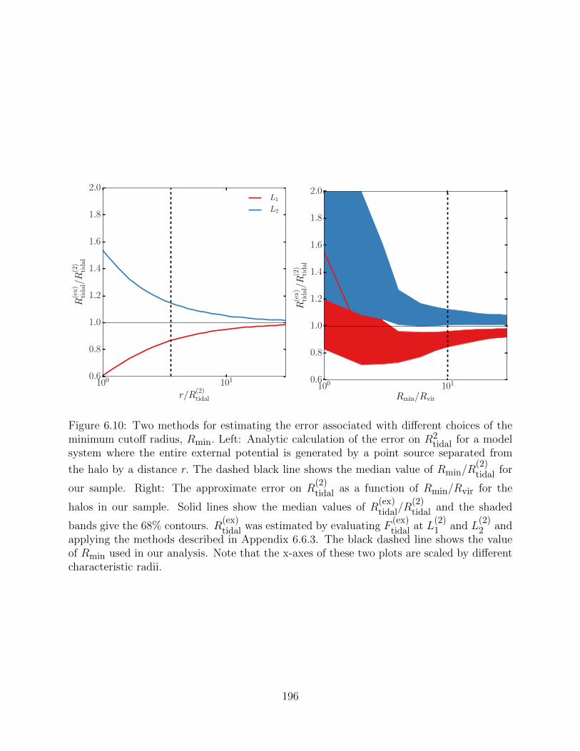
100 101

r/R(2)tidal

0.6

0.8

1.0

1.2

1.4

1.6

1.8

2.0

R(e

x)

tid

al/R

(2)

tid

al

L1

L2

100 101

Rmin/Rvir

0.6

0.8

1.0

1.2

1.4

1.6

1.8

2.0

R(e

x)

tid

al/R

(2)

tid

al

Figure 6.10: Two methods for estimating the error associated with different choices of theminimum cutoff radius, Rmin. Left: Analytic calculation of the error on R2

tidal for a modelsystem where the entire external potential is generated by a point source separated from

the halo by a distance r. The dashed black line shows the median value of Rmin/R(2)tidal for

our sample. Right: The approximate error on R(2)tidal as a function of Rmin/Rvir for the

halos in our sample. Solid lines show the median values of R(ex)tidal/R

(2)tidal and the shaded

bands give the 68% contours. R(ex)tidal was estimated by evaluating F

(ex)tidal at L

(2)1 and L

(2)2 and

applying the methods described in Appendix 6.6.3. The black dashed line shows the valueof Rmin used in our analysis. Note that the x-axes of these two plots are scaled by differentcharacteristic radii.

196

the Lagrangian point between a halo and an external source is L1 and that the point on

the opposite side of the halo is L2. In cases where analysis is performed on halos without a

single external source, L1 is the Lagrangian point with the lowest external potential.

Like the classical RHill derivation, our calculation of R(2)tidal (see Equation 6.5) assumes

that the external tidal field felt by the halo is well-approximated by a second-order hyper-

paraboloid. This is necessary because the tidal tensor which is used to determine the principle

components of the tidal field only contains second derivatives of the gravitational potential.

Note that in the special case where there is only a single external point source,

R(2)tidal =

(3

2

)1/3

R(2)Hill, (6.11)

so the discussion below can be extended to error analysis on the classical Hill radius. Note

that the factor of (3/2)1/3 is because the derivation of R(2)Hill assumes that the halo is on a

circular orbit around the external point source and thus experiences a centrifugal force in

addition to a tidal force, while the derivation of R(2)tidal assumes that all non-tidal pseudo-

forces are zero. Given the scale of errors discussed below, and the fact that this factor

decreases as halos deviate from circular orbits – a configuration which is very rare for distinct

halos – we do not consider this difference to be significant.

We perform two complementary tests on the accuracy of R(2)tidal. First, we analytically

compute R(2)tidal/R

(ex)tidal for a single source at a distance r from a halo, and second, we measure

exact the error on F(2)tidal for our halo sample and combine this with reasonable assumptions

about the shape of the tidal field to estimate upper limits on R(2)tidal/R

(ex)tidal.

We show the results of this first calculation in the left panel of Fig. 6.10. Although

there is no closed-form expression for R(ex)tidal, it can be found numerically by maximizing the

effective potential. We parameterize the error as a function of r/R(2)tidal which also absorbs

the dependence on the mass ratio. We recover the well-known fact that as the mass ratio

between the halo and the external source decreases and the tidal radius increases, the two

197

Lagrangian points become asymmetric and that errors become increasingly significant. This

can also be interpreted as an estimate of the error associated with a particular value inner

cutoff radius for r = Rmin when following the procedure described in section 6.2.5. This

can be considered a worst-case estimate of the error at a given R(2)tidal because the true

matter distribution will generally contain many points at distances larger than Rmin which

contribute significantly to the tidal field.

We perform our second test by first computing L(2)1 , L

(2)2 , R

(2)tidal, and F

(2)tidal for every

halo in our sample for a particular choice of Rmin. Then, we use the raw particle data to

compute the radial and tangential components of F(ex)tidal(L

(2)1 ) and F

(ex)tidal(L

(2)2 ) for these halos.

Particles within Rmin are not included in this calculation. To obtain an estimate of R(ex)tidal

from this, we make two simplifying assumptions about the shape of the tidal field. First,

we assume that the exact Lagrangian points lie along the same axis as a halo’s second-order

Lagrangian points. We find that the tangential components of F(ex)tidal(L

(2)1 ) and F

(ex)tidal(L

(2)2 )

are small compared to the radial components, implying that this is a reasonable assumption.

Second, we assume that along the lines connecting L(2)1 to L

(ex)1 and L

(2)2 to L

(ex)2 , the tidal

force varies slowly enough that it can be well approximated by

F(ex)tidal(r) ∝

r

R(2)tidal

1+α

, (6.12)

Here, α is an arbitrary constant which varies from halo to halo and may be different for

different Lagrangian points within the same halo. It represents the deviation from the

scaling seen when the tidal potential is approximated to second order. In this case,

R(ex)tidal

R(2)tidal

=

F

(ex)tidal(L

(2)i )

F(2)tidal(L

(2)i )

− 1

3+α

, (6.13)

where i indexes over Lagrangian points. This assumption is informed by tests on single-

source effective potentials, which find that for all but the smallest external point sources,

198

−1 < α < 0. For halos where Rmin > R(2)tidal, we would expect that at a constant R

(2)tidal

the tidal field would be varying more quickly at L(2)i when the field is generated by a single

point source than when it is generated by a more diffuse matter distribution, so it’s likely

that this range of α values holds for our simulated halos as well. For this reason we can

place the following upper bound on the error in tidal radius:

|R(ex)tidal/R

(2)tidal − 1| < |F (ex)

tidal/F(2)tidal − 1|−1/2. (6.14)

We show the fractional error in Rtidal using this limit in the right panel of Fig. 6.10 as a

function of the adopted Rmin. Errors balloon uncontrollably for Rmin . 4Rvir but are more

well-behaved at larger radii, with errors dropping to the ≈ 10% level at ≈ 10Rvir.

One interesting feature of this Figure is that for Rmin . 2Rvir, the error on the location

L1 becomes positive. This is likely because this is the characteristic size of the splashback

radius, meaning that the halo’s own particles will be incorporated into the calculation of

F(ex)tidal. Since the tidal force is repulsive, this inclusion of halo particles will reduce the apparent

strength of the field and increase Rtidal.

These tests indicate that for Rmin = 10Rvir, the errors in R(2)tidal which are specifically

due to the second order approximation of the tidal field are small. However, this analysis is

performed at a constant Rmin, so it doesn’t account for errors due to the removal of significant

sources close to the halo. This is not an issue for our analysis because Rtidal is explicitly

a proxy for the large-scale tidal field, and our proxy Dvir is better suited for close sources.

This would, however, become a significant issue for studies which need Rtidal for purposes

other than rank-ordering halos. Further discussion on the impact that improvements in the

accuracy of Rtidal would have on our results can be found in section 6.4.1.

More generally, while the issue of measuring tidal radii around halos with only a single

significant source is well-explored [see §2 in van den Bosch et al., 2018, for a review], and

the tidal radius due to the large scale field can be measured effectively with the tidal tensor,

199

there currently does not exist an effective method for combining these two regimes. We

outline a number of potential approaches which could be used to address this issue in 6.4.4,

but consider the testing and calibration of such methods to be beyond the scope of this

chapter.

6.6.4 Identifying Bound Particles in Halo Outskirts

While the concept of gravitational binding is straightforward to define for particles near

the center of a non-accelerating halo, the same is not true for particles in the outskirts of

halos, especially those experiencing a strong tidal force. These difficulties arise from two key

areas: first, it is difficult to disentangle the potential caused by a halo from the potential

of its surroundings. Although halos have a non-trivial amount of mass stored outside Rvir,

the so-called “two-halo” term starts to dominate the density distribution at r & 1 − 2Rvir

[e.g. Diemer and Kravtsov, 2014], meaning that any calculation of the potential which is

done directly from the density profile or from the particle distribution must be done with

care. Second, for particles near the tidal radius, the effective potential due to the external

tidal field becomes significant. While this issue could in principle be solved by defining

escape velocities relative to the minimum potential at either Lagrangian point, it also means

that boundedness calculations will suffer from the same accuracy issues as the tidal radius

calculations (see Appendix 6.6.3).

The effect of tidal forces on particle escape velocities presents another issue for the analy-

sis in this chapter, specifically. If this effect is taken into account, it means that gravitational

heating and tidal forces can no longer be disentangled. Even a “control” variable like Mβ,b

would depend on the tidal field, and could potentially make gravitational heating appear

to be more a more significant contributor to assembly bias than it actually is. Primarily

because of this reason, and to a lesser extent because of the issues described in the previous

paragraph, we take on the simple and standard boundedness condition given in Eq. 6.7,

but note that the fremoved value for Mtidal,b could become even lower if more sophisticated

200

approaches were used.

201

REFERENCES

S. J. Aarseth. Dynamical evolution of clusters of galaxies, I. MNRAS, 126:223, January

1963. doi: 10.1093/mnras/126.3.223.

K. Abazajian, Z. Zheng, I. Zehavi, D. H. Weinberg, J. A. Frieman, A. A. Berlind, M. R.

Blanton, N. A. Bahcall, J. Brinkmann, D. P. Schneider, and M. Tegmark. Cosmology and

the Halo Occupation Distribution from Small-Scale Galaxy Clustering in the Sloan Digital

Sky Survey. ApJ, 625:613–620, June 2005. doi: 10.1086/429685.

T. Abel, O. Hahn, and R. Kaehler. Tracing the dark matter sheet in phase space. MNRAS,

427:61–76, November 2012a. doi: 10.1111/j.1365-2966.2012.21754.x.

Tom Abel, Oliver Hahn, and Ralf Kaehler. Tracing the dark matter sheet in phase space.

MNRAS, 427(1):61–76, November 2012b. doi: 10.1111/j.1365-2966.2012.21754.x.

Tamra Adams. Dictionary of Nature Myths: Legends of Earth, Sea, and Sky. ABC-CLIO

Inc., 1998.

S. Adhikari, N. Dalal, and R. T. Chamberlain. Splashback in accreting dark matter halos.

JCAP, 11:019, November 2014. doi: 10.1088/1475-7516/2014/11/019.

S. Adhikari, N. Dalal, and J. Clampitt. Observing dynamical friction in galaxy clusters.

ArXiv e-prints, May 2016.

Brandon Allgood, Ricardo A. Flores, Joel R. Primack, Andrey V. Kravtsov, Risa H. Wech-

sler, Andreas Faltenbacher, and James S. Bullock. The shape of dark matter haloes:

dependence on mass, redshift, radius and formation. MNRAS, 367(4):1781–1796, April

2006. doi: 10.1111/j.1365-2966.2006.10094.x.

R. E. Angulo, V. Springel, S. D. M. White, A. Jenkins, C. M. Baugh, and C. S. Frenk.

Scaling relations for galaxy clusters in the Millennium-XXL simulation. MNRAS, 426(3):

2046–2062, November 2012. doi: 10.1111/j.1365-2966.2012.21830.x.

202

Horace W. Babcock. The rotation of the Andromeda Nebula. Lick Observatory Bulletin,

498:41–51, January 1939. doi: 10.5479/ADS/bib/1939LicOB.19.41B.

N. A. Bahcall and R. M. Soneira. The spatial correlation function of rich clusters of galaxies.

ApJ, 270:20–38, July 1983. doi: 10.1086/161094.

Yannick M. Bahe, Ian G. McCarthy, Michael L. Balogh, and Andreea S. Font. Why does

the environmental influence on group and cluster galaxies extend beyond the virial radius?

MNRAS, 430(4):3017–3031, April 2013. doi: 10.1093/mnras/stt109.

Michael L. Balogh, Julio F. Navarro, and Simon L. Morris. The Origin of Star Forma-

tion Gradients in Rich Galaxy Clusters. ApJ, 540(1):113–121, September 2000. doi:

10.1086/309323.

M. R. Becker and A. V. Kravtsov. On the Accuracy of Weak-lensing Cluster Mass Recon-

structions. ApJ, 740:25, October 2011. doi: 10.1088/0004-637X/740/1/25.

Steven V. W. Beckwith, Massimo Stiavelli, Anton M. Koekemoer, John A. R. Caldwell,

Henry C. Ferguson, Richard Hook, Ray A. Lucas, Louis E. Bergeron, Michael Corbin,

Shardha Jogee, Nino Panagia, Massimo Robberto, Patricia Royle, Rachel S. Somerville,

and Megan Sosey. The Hubble Ultra Deep Field. AJ, 132(5):1729–1755, November 2006.

doi: 10.1086/507302.

P. Behroozi, R. Wechsler, A. Hearin, and C. Conroy. UniverseMachine: The Correlation

between Galaxy Growth and Dark Matter Halo Assembly from z=0-10. ArXiv e-prints,

June 2018.

P. S. Behroozi, A. Loeb, and R. H. Wechsler. Unbound particles in dark matter halos. JCAP,

6:019, June 2013a. doi: 10.1088/1475-7516/2013/06/019.

P. S. Behroozi, R. H. Wechsler, and C. Conroy. The Average Star Formation Histories of

203

Galaxies in Dark Matter Halos from z = 0-8. ApJ, 770:57, June 2013b. doi: 10.1088/0004-

637X/770/1/57.

P. S. Behroozi, R. H. Wechsler, and H.-Y. Wu. The ROCKSTAR Phase-space Temporal

Halo Finder and the Velocity Offsets of Cluster Cores. ApJ, 762:109, January 2013c. doi:

10.1088/0004-637X/762/2/109.

P. S. Behroozi, R. H. Wechsler, and H.-Y. Wu. The ROCKSTAR Phase-space Temporal

Halo Finder and the Velocity Offsets of Cluster Cores. ApJ, 762:109, January 2013d. doi:

10.1088/0004-637X/762/2/109.

P. S. Behroozi, R. H. Wechsler, H.-Y. Wu, M. T. Busha, A. A. Klypin, and J. R. Primack.

Gravitationally Consistent Halo Catalogs and Merger Trees for Precision Cosmology. ApJ,

763:18, January 2013e. doi: 10.1088/0004-637X/763/1/18.

P. S. Behroozi, R. H. Wechsler, Y. Lu, O. Hahn, M. T. Busha, A. Klypin, and J. R. Primack.

Mergers and Mass Accretion for Infalling Halos Both End Well Outside Cluster Virial

Radii. ApJ, 787:156, June 2014. doi: 10.1088/0004-637X/787/2/156.

Peter S. Behroozi, Guangtun Zhu, Henry C. Ferguson, Andrew P. Hearin, Jennifer Lotz,

Joseph Silk, Susan Kassin, Yu Lu, Darren Croton, Rachel S. Somerville, and Douglas F.

Watson. Using galaxy pairs to probe star formation during major halo mergers. MNRAS,

450(2):1546–1564, June 2015. doi: 10.1093/mnras/stv728.

C. Beisbart and M. Kerscher. Luminosity- and Morphology-dependent Clustering of Galax-

ies. ApJ, 545:6–25, December 2000. doi: 10.1086/317788.

V. Belokurov, D. Erkal, N. W. Evans, S. E. Koposov, and A. J. Deason. Co-formation of the

disc and the stellar halo. MNRAS, 478(1):611–619, July 2018. doi: 10.1093/mnras/sty982.

Andreas A. Berlind and David H. Weinberg. The Halo Occupation Distribution: Toward

204

an Empirical Determination of the Relation between Galaxies and Mass. ApJ, 575(2):

587–616, August 2002. doi: 10.1086/341469.

A. M. Berti, A. L. Coil, P. S. Behroozi, D. J. Eisenstein, A. D. Bray, R. J. Cool, and

J. Moustakas. PRIMUS: One- and Two-halo Galactic Conformity at 0.2 ¡ z ¡ 1. ApJ, 834:

87, January 2017. doi: 10.3847/1538-4357/834/1/87.

E. Bertschinger. Self-similar secondary infall and accretion in an Einstein-de Sitter universe.

ApJs, 58:39–65, May 1985. doi: 10.1086/191028.

Suman Bhattacharya, Salman Habib, Katrin Heitmann, and Alexey Vikhlinin. Dark Matter

Halo Profiles of Massive Clusters: Theory versus Observations. ApJ, 766(1):32, Mar 2013.

doi: 10.1088/0004-637X/766/1/32.

Michael R. Blanton, David W. Hogg, Neta A. Bahcall, J. Brinkmann, Malcolm Britton,

Andrew J. Connolly, Istvan Csabai, Masataka Fukugita, Jon Loveday, Avery Meiksin,

Jeffrey A. Munn, R. C. Nichol, Sadanori Okamura, Thomas Quinn, Donald P. Schneider,

Kazuhiro Shimasaku, Michael A. Strauss, Max Tegmark, Michael S. Vogeley, and David H.

Weinberg. The Galaxy Luminosity Function and Luminosity Density at Redshift z = 0.1.

ApJ, 592(2):819–838, August 2003. doi: 10.1086/375776.

Siegfried Bodenmann. The 18th-century battle over lunar motion. Physics Today, 63(1):27,

January 2010. doi: 10.1063/1.3293410.

J. R. Bond, L. Kofman, and D. Pogosyan. How filaments of galaxies are woven into the

cosmic web. Nature, 380:603–606, April 1996. doi: 10.1038/380603a0.

G. L. Bryan and M. L. Norman. Statistical Properties of X-Ray Clusters: Analytic and

Numerical Comparisons. ApJ, 495:80–99, March 1998. doi: 10.1086/305262.

J. S. Bullock, T. S. Kolatt, Y. Sigad, R. S. Somerville, A. V. Kravtsov, A. A. Klypin,

205

J. R. Primack, and A. Dekel. Profiles of dark haloes: evolution, scatter and environment.

MNRAS, 321:559–575, March 2001. doi: 10.1046/j.1365-8711.2001.04068.x.

V. F. Calderon, A. A. Berlind, and M. Sinha. Small- and large-scale galactic conformity in

SDSS DR7. MNRAS, 480:2031–2045, October 2018. doi: 10.1093/mnras/sty2000.

D. Campbell, F. C. van den Bosch, A. Hearin, N. Padmanabhan, A. Berlind, H. J. Mo, J. Tin-

ker, and X. Yang. Assessing colour-dependent occupation statistics inferred from galaxy

group catalogues. MNRAS, 452:444–469, September 2015. doi: 10.1093/mnras/stv1091.

Duncan Campbell, Frank C. van den Bosch, Nikhil Padmanabhan, Yao-Yuan Mao, An-

drew R. Zentner, Johannes U. Lange, Fangzhou Jiang, and Antonio Villarreal. The

galaxy clustering crisis in abundance matching. MNRAS, 477(1):359–383, June 2018.

doi: 10.1093/mnras/sty495.

Claude Carignan, Laurent Chemin, Walter K. Huchtmeier, and Felix J. Lockman. The

Extended H I Rotation Curve and Mass Distribution of M31. ApJL, 641(2):L109–L112,

April 2006. doi: 10.1086/503869.

Scott G. Carlsten, Jenny E. Greene, Annika H. G. Peter, Johnny P. Greco, and Rachael L.

Beaton. Radial Distributions of Dwarf Satellite Systems in the Local Volume. arXiv

e-prints, art. arXiv:2006.02444, June 2020.

M. Cautun, R. van de Weygaert, B. J. T. Jones, and C. S. Frenk. Evolution of the cosmic

web. MNRAS, 441:2923–2973, July 2014. doi: 10.1093/mnras/stu768.

C. Chang, E. Baxter, B. Jain, C. Sanchez, S. Adhikari, T. N. Varga, Y. Fang, E. Rozo, E. S.

Rykoff, A. Kravtsov, D. Gruen, W. Hartley, E. M. Huff, M. Jarvis, A. G. Kim, J. Prat,

N. MacCrann, T. McClintock, A. Palmese, D. Rapetti, R. P. Rollins, S. Samuroff, E. Shel-

don, M. A. Troxel, R. H. Wechsler, Y. Zhang, J. Zuntz, T. M. C. Abbott, F. B. Abdalla,

S. Allam, J. Annis, K. Bechtol, A. Benoit-Levy, G. M. Bernstein, D. Brooks, E. Buckley-

Geer, A. Carnero Rosell, M. Carrasco Kind, J. Carretero, C. B. D’Andrea, L. N. da Costa,

206

C. Davis, S. Desai, H. T. Diehl, J. P. Dietrich, A. Drlica-Wagner, T. F. Eifler, B. Flaugher,

P. Fosalba, J. Frieman, J. Garcıa-Bellido, E. Gaztanaga, D. W. Gerdes, R. A. Gruendl,

J. Gschwend, G. Gutierrez, K. Honscheid, D. J. James, T. Jeltema, E. Krause, K. Kuehn,

O. Lahav, M. Lima, M. March, J. L. Marshall, P. Martini, P. Melchior, F. Menanteau,

R. Miquel, J. J. Mohr, B. Nord, R. L. C. Ogando, A. A. Plazas, E. Sanchez, V. Scarpine,

R. Schindler, M. Schubnell, I. Sevilla-Noarbe, M. Smith, R. C. Smith, M. Soares-Santos,

F. Sobreira, E. Suchyta, M. E. C. Swanson, G. Tarle, J. Weller, and DES Collaboration.

The Splashback Feature around DES Galaxy Clusters: Galaxy Density and Weak Lensing

Profiles. ApJ, 864(1):83, September 2018. doi: 10.3847/1538-4357/aad5e7.

William Chapman. Workshop Technology Part 1. Routledge, 2019.

Hillary L. Child, Salman Habib, Katrin Heitmann, Nicholas Frontiere, Hal Finkel, Adrian

Pope, and Vitali Morozov. Halo Profiles and the Concentration-Mass Relation for a ΛCDM

Universe. ApJ, 859(1):55, May 2018. doi: 10.3847/1538-4357/aabf95.

C. Y. R. Chue, N. Dalal, and M. White. Some assembly required: assembly bias in massive

dark matter halos. JCAP, 10:012, October 2018. doi: 10.1088/1475-7516/2018/10/012.

A. R. Conn, G. F. Lewis, R. A. Ibata, Q. A. Parker, D. B. Zucker, A. W. McConnachie, N. F.

Martin, D. Valls-Gabaud, N. Tanvir, M. J. Irwin, A. M. N. Ferguson, and S. C. Chapman.

The Three-dimensional Structure of the M31 Satellite System; Strong Evidence for an

Inhomogeneous Distribution of Satellites. ApJ, 766(2):120, April 2013. doi: 10.1088/0004-

637X/766/2/120.

Alan Cook. Edmond Halley. Charting the heavens and the seas. 1998.

Martın Crocce, Sebastian Pueblas, and Roman Scoccimarro. Transients from initial con-

ditions in cosmological simulations. MNRAS, 373(1):369–381, November 2006. doi:

10.1111/j.1365-2966.2006.11040.x.

207

N. Dalal, M. White, J. R. Bond, and A. Shirokov. Halo Assembly Bias in Hierarchical

Structure Formation. ApJ, 687:12–21, November 2008. doi: 10.1086/591512.

N. Dalal, Y. Lithwick, and M. Kuhlen. The Origin of Dark Matter Halo Profiles. ArXiv

e-prints, October 2010.

W. J. G. de Blok. The Core-Cusp Problem. Advances in Astronomy, 2010:789293, January

2010. doi: 10.1155/2010/789293.

W. J. G. de Blok, F. Walter, E. Brinks, C. Trachternach, S. H. Oh, and Jr. Kennicutt, R. C.

High-Resolution Rotation Curves and Galaxy Mass Models from THINGS. AJ, 136(6):

2648–2719, December 2008. doi: 10.1088/0004-6256/136/6/2648.

Gerard de Vaucouleurs. Classification and Morphology of External Galaxies. Handbuch der

Physik, 53:275, January 1959. doi: 10.1007/978-3-642-45932-07.

Walter Dehnen. Towards optimal softening in three-dimensional N-body codes - I. Min-

imizing the force error. MNRAS, 324(2):273–291, June 2001. doi: 10.1046/j.1365-

8711.2001.04237.x.

B. Delaunay. Sur la sphere vide. Bulletin de l’Academie des Sciences de l’URSS, Classe des

sciences mathematiques et naturelles, 6:793–800, 1934.

V. Desjacques. Environmental dependence in the ellipsoidal collapse model. MNRAS, 388:

638–658, August 2008. doi: 10.1111/j.1365-2966.2008.13420.x.

V. Desjacques, D. Jeong, and F. Schmidt. Large-scale galaxy bias. Physics Reports, 733:

1–193, February 2018. doi: 10.1016/j.physrep.2017.12.002.

Harry Desmond and Risa H. Wechsler. The Tully-Fisher and mass-size relations from

halo abundance matching. MNRAS, 454(1):322–343, November 2015. doi: 10.1093/mn-

ras/stv1978.

208

B. Diemer. The Splashback Radius of Halos from Particle Dynamics. I. The SPARTA Algo-

rithm. ApJs, 231:5, July 2017a. doi: 10.3847/1538-4365/aa799c.

B. Diemer. The splashback radius of halos from particle dynamics: I. The SPARTA algo-

rithm. ArXiv e-prints, March 2017b.

B. Diemer. COLOSSUS: A Python Toolkit for Cosmology, Large-scale Structure, and Dark

Matter Halos. ApJs, 239:35, December 2018. doi: 10.3847/1538-4365/aaee8c.

B. Diemer and M. Joyce. An Accurate Physical Model for Halo Concentrations. ApJ, 871:

168, February 2019. doi: 10.3847/1538-4357/aafad6.

B. Diemer and A. V. Kravtsov. Dependence of the Outer Density Profiles of Halos on Their

Mass Accretion Rate. ApJ, 789:1, July 2014. doi: 10.1088/0004-637X/789/1/1.

B. Diemer and A. V. Kravtsov. A Universal Model for Halo Concentrations. ApJ, 799:108,

January 2015. doi: 10.1088/0004-637X/799/1/108.

B. Diemer, A. V. Kravtsov, and S. More. On the Evolution of Cluster Scaling Relations.

ApJ, 779:159, December 2013a. doi: 10.1088/0004-637X/779/2/159.

B. Diemer, S. More, and A. V. Kravtsov. The Pseudo-evolution of Halo Mass. ApJ, 766:25,

March 2013b. doi: 10.1088/0004-637X/766/1/25.

B. Diemer, P. Mansfield, A. V. Kravtsov, and S. More. The Splashback Radius of Halos from

Particle Dynamics. II. Dependence on Mass, Accretion Rate, Redshift, and Cosmology.

ApJ, 843:140, July 2017. doi: 10.3847/1538-4357/aa79ab.

Scott Dodelson. Modern cosmology. 2003.

A. Drlica-Wagner, K. Bechtol, S. Mau, M. McNanna, E. O. Nadler, A. B. Pace, T. S. Li,

A. Pieres, E. Rozo, J. D. Simon, A. R. Walker, R. H. Wechsler, T. M. C. Abbott, S. Allam,

209

J. Annis, E. Bertin, D. Brooks, D. L. Burke, A. Carnero Rosell, M. Carrasco Kind, J. Car-

retero, M. Costanzi, L. N. da Costa, J. De Vicente, S. Desai, H. T. Diehl, P. Doel, T. F. Ei-

fler, S. Everett, B. Flaugher, J. Frieman, J. Garcia-Bellido, E. Gaztanaga, D. Gruen, R. A.

Gruendl, J. Gschwend, G. Gutierrez, K. Honscheid, D. J. James, E. Krause, K. Kuehn,

N. Kuropatkin, O. Lahav, M. A. G. Maia, J. L. Marshall, P. Melchior, F. Menanteau,

R. Miquel, A. Palmese, A. A. Plazas, E. Sanchez, V. Scarpine, M. Schubnell, S. Serrano,

I. Sevilla-Noarbe, M. Smith, E. Suchyta, and G. Tarle. Milky Way Satellite Census – I. The

Observational Selection Function for Milky Way Satellites in DES Y3 and Pan-STARRS

DR1. arXiv e-prints, art. arXiv:1912.03302, December 2019.

Alan R. Duffy, Joop Schaye, Scott T. Kay, and Claudio Dalla Vecchia. Dark matter halo

concentrations in the Wilkinson Microwave Anisotropy Probe year 5 cosmology. MNRAS,

390(1):L64–L68, Oct 2008. doi: 10.1111/j.1745-3933.2008.00537.x.

Aaron A. Dutton and Andrea V. Maccio. Cold dark matter haloes in the Planck era:

evolution of structural parameters for Einasto and NFW profiles. MNRAS, 441(4):3359–

3374, Jul 2014. doi: 10.1093/mnras/stu742.

Jaan Einasto, Ants Kaasik, and Enn Saar. Dynamic evidence on massive coronas of galaxies.

Nature, 250(5464):309–310, July 1974. doi: 10.1038/250309a0.

A. Einstein and W. de Sitter. On the Relation between the Expansion and the Mean Density

of the Universe. Proceedings of the National Academy of Science, 18(3):213–214, March

1932. doi: 10.1073/pnas.18.3.213.

The HIPPARCOS and TYCHO catalogues. Astrometric and photometric star catalogues de-

rived from the ESA HIPPARCOS Space Astrometry Mission, volume 1200 of ESA Special

Publication, January 1997. ESA.

Leonhard Euler. De motu rectilineo trium corporum se mutuo attrahentium. 1765. URL

http://eulerarchive.maa.org//docs/originals/E327.pdf.

210

A. E. Evrard, J. Bialek, M. Busha, M. White, S. Habib, K. Heitmann, M. Warren, E. Rasia,

G. Tormen, L. Moscardini, C. Power, A. R. Jenkins, L. Gao, C. S. Frenk, V. Springel,

S. D. M. White, and J. Diemand. Virial Scaling of Massive Dark Matter Halos: Why

Clusters Prefer a High Normalization Cosmology. ApJ, 672(1):122–137, January 2008.

doi: 10.1086/521616.

S. M. Faber and J. S. Gallagher. Masses and mass-to-light ratios of galaxies. ARA&A, 17:

135–187, January 1979. doi: 10.1146/annurev.aa.17.090179.001031.

A. Faltenbacher and S. D. M. White. Assembly Bias and the Dynamical Structure of Dark

Matter Halos. ApJ, 708:469–473, January 2010. doi: 10.1088/0004-637X/708/1/469.

J. A. Fillmore and P. Goldreich. Self-similar gravitational collapse in an expanding universe.

ApJ, 281:1–8, June 1984. doi: 10.1086/162070.

Robert A Freitas. Nanomedicine, volume I: basic capabilities, volume 1. Landes Bioscience

Georgetown, TX, 1999.

A. Friedmann. Uber die Krummung des Raumes. Zeitschrift fur Physik, 10:377–386, January

1922. doi: 10.1007/BF01332580.

L. Gao and S. D. M. White. Assembly bias in the clustering of dark matter haloes. MNRAS,

377:L5–L9, April 2007. doi: 10.1111/j.1745-3933.2007.00292.x.

L. Gao, S. D. M. White, A. Jenkins, F. Stoehr, and V. Springel. The subhalo populations

of ΛCDM dark haloes. MNRAS, 355(3):819–834, December 2004. doi: 10.1111/j.1365-

2966.2004.08360.x.

L. Gao, V. Springel, and S. D. M. White. The age dependence of halo clustering. MNRAS,

363:L66–L70, October 2005. doi: 10.1111/j.1745-3933.2005.00084.x.

Liang Gao, Julio F. Navarro, Shaun Cole, Carlos S. Frenk, Simon D. M. White, Volker

Springel, Adrian Jenkins, and Angelo F. Neto. The redshift dependence of the struc-

211

ture of massive Λ cold dark matter haloes. MNRAS, 387(2):536–544, Jun 2008. doi:

10.1111/j.1365-2966.2008.13277.x.

Shea Garrison-Kimmel, Michael Boylan-Kolchin, James S. Bullock, and Evan N. Kirby. Too

big to fail in the Local Group. MNRAS, 444(1):222–236, October 2014. doi: 10.1093/mn-

ras/stu1477.

Shea Garrison-Kimmel, Andrew Wetzel, James S. Bullock, Philip F. Hopkins, Michael

Boylan-Kolchin, Claude-Andre Faucher-Giguere, Dusan Keres, Eliot Quataert, Robyn E.

Sanderson, Andrew S. Graus, and Tyler Kelley. Not so lumpy after all: modelling the de-

pletion of dark matter subhaloes by Milky Way-like galaxies. MNRAS, 471(2):1709–1727,

October 2017. doi: 10.1093/mnras/stx1710.

Chong Ge, Ming Sun, Eduardo Rozo, Neelima Sehgal, Alexey Vikhlinin, William Forman,

Christine Jones, and Daisuke Nagai. X-ray scaling relations from a complete sample of

the richest maxBCG clusters. MNRAS, 484(2):1946–1971, April 2019. doi: 10.1093/mn-

ras/stz088.

S. P. D. Gill, A. Knebe, and B. K. Gibson. The evolution of substructure - III. The outskirts of

clusters. MNRAS, 356:1327–1332, February 2005. doi: 10.1111/j.1365-2966.2004.08562.x.

J. Goodman and J. Weare. Ensemble samplers with affine invariance. Communications in Ap-

plied Mathematics and Computational Science, 5:65–80, January 2010. doi: 10.2140/cam-

cos.2010.5.65.

K. M. Gorski, E. Hivon, A. J. Banday, B. D. Wandelt, F. K. Hansen, M. Reinecke,

and M. Bartelmann. HEALPix: A Framework for High-Resolution Discretization and

Fast Analysis of Data Distributed on the Sphere. ApJ, 622:759–771, April 2005. doi:

10.1086/427976.

S. Gottlober, M. Kerscher, A. V. Kravtsov, A. Faltenbacher, A. Klypin, and V. Muller.

212

Spatial distribution of galactic halos and their merger histories. A&Ap, 387:778–787, June

2002. doi: 10.1051/0004-6361:20020339.

Stefan Gottloeber and Anatoly Klypin. The ART of Cosmological Simulations. arXiv e-

prints, art. arXiv:0803.4343, Mar 2008.

Gravity Collaboration, R. Abuter, A. Amorim, M. Baubock, J. P. Berger, H. Bonnet,

W. Brand ner, Y. Clenet, V. Coude Du Foresto, P. T. de Zeeuw, J. Dexter, G. Du-

vert, A. Eckart, F. Eisenhauer, N. M. Forster Schreiber, P. Garcia, F. Gao, E. Gendron,

R. Genzel, O. Gerhard, S. Gillessen, M. Habibi, X. Haubois, T. Henning, S. Hippler,

M. Horrobin, A. Jimenez-Rosales, L. Jocou, P. Kervella, S. Lacour, V. Lapeyrere, J. B.

Le Bouquin, P. Lena, T. Ott, T. Paumard, K. Perraut, G. Perrin, O. Pfuhl, S. Rabien,

G. Rodriguez Coira, G. Rousset, S. Scheithauer, A. Sternberg, O. Straub, C. Straub-

meier, E. Sturm, L. J. Tacconi, F. Vincent, S. von Fellenberg, I. Waisberg, F. Widmann,

E. Wieprecht, E. Wiezorrek, J. Woillez, and S. Yazici. A geometric distance measurement

to the Galactic center black hole with 0.3% uncertainty. AAp, 625:L10, May 2019. doi:

10.1051/0004-6361/201935656.

Alan Grier. When Computers Were Human. Princeton University Press, 2013.

Brendan F. Griffen, Alexander P. Ji, Gregory A. Dooley, Facundo A. Gomez, Mark Vogels-

berger, Brian W. O’Shea, and Anna Frebel. The Caterpillar Project: A Large Suite of

Milky Way Sized Halos. ApJ, 818(1):10, Feb 2016. doi: 10.3847/0004-637X/818/1/10.

I. I. Gringorten and P. J. Yepez. The Division of a Circular or Spherical Surface Into Equal-

Area Cells or Pixels. Instrumentation Papers, 343:1–7, June 1992.

J. E. Gunn and J. R. Gott, III. On the Infall of Matter Into Clusters of Galaxies and Some

Effects on Their Evolution. ApJ, 176:1, August 1972a. doi: 10.1086/151605.

J. E. Gunn and J. R. Gott, III. On the Infall of Matter Into Clusters of Galaxies and Some

Effects on Their Evolution. ApJ, 176:1, August 1972b. doi: 10.1086/151605.

213

Qi Guo and Simon White. Numerical resolution limits on subhalo abundance matching.

MNRAS, 437(4):3228–3235, February 2014. doi: 10.1093/mnras/stt2116.

H. Gursky, E. Kellogg, S. Murray, C. Leong, H. Tananbaum, and R. Giacconi. A Strong

X-Ray Source in the Coma Cluster Observed by UHURU. ApJL, 167:L81, August 1971.

doi: 10.1086/180765.

O. Hahn and R. E. Angulo. An adaptively refined phase-space element method for cosmolog-

ical simulations and collisionless dynamics. MNRAS, 455:1115–1133, January 2016. doi:

10.1093/mnras/stv2304.

O. Hahn, C. Porciani, A. Dekel, and C. M. Carollo. Tidal effects and the environment

dependence of halo assembly. MNRAS, 398:1742–1756, October 2009. doi: 10.1111/j.1365-

2966.2009.15271.x.

Oliver Hahn and Tom Abel. Multi-scale initial conditions for cosmological simulations.

MNRAS, 415(3):2101–2121, August 2011. doi: 10.1111/j.1365-2966.2011.18820.x.

Zoltan Haiman, Anne A. Thoul, and Abraham Loeb. Cosmological Formation of Low-Mass

Objects. ApJ, 464:523, June 1996. doi: 10.1086/177343.

J. Han, Y. Li, Y. Jing, T. Nishimichi, W. Wang, and C. Jiang. The multidimensional

dependence of halo bias in the eye of a machine: a tale of halo structure, assembly, and

environment. MNRAS, 482:1900–1919, January 2019. doi: 10.1093/mnras/sty2822.

G. Harker, S. Cole, J. Helly, C. Frenk, and A. Jenkins. A marked correlation function

analysis of halo formation times in the Millennium Simulation. MNRAS, 367:1039–1049,

April 2006. doi: 10.1111/j.1365-2966.2006.10022.x.

Roslynn D Haynes. Astronomy and the Dreaming: The Astronomy of the Aboriginal Aus-

tralians. Springer Science Business Media, B. V., 1998.

214

A. Hearin, E. Tollerud, T. Robitaille, M. Droettboom, A. Zentner, E. Bray, M. Craig,

L. Bradley, K. Barbary, C. Deil, K. Tan, M. R. Becker, S. More, H. M. Gunther, and

B. Sipocz. Halotools: Galaxy-Halo connection models. Astrophysics Source Code Library,

April 2016a.

A. P. Hearin, D. F. Watson, and F. C. van den Bosch. Beyond halo mass: galactic conformity

as a smoking gun of central galaxy assembly bias. MNRAS, 452:1958–1969, September

2015. doi: 10.1093/mnras/stv1358.

A. P. Hearin, P. S. Behroozi, and F. C. van den Bosch. On the physical origin of galactic

conformity. MNRAS, 461:2135–2145, September 2016b. doi: 10.1093/mnras/stw1462.

D. J. Heath. The growth of density perturbations in zero pressure Friedmann-Lemaitre

universes. MNRAS, 179:351–358, May 1977. doi: 10.1093/mnras/179.3.351.

Amina Helmi, Carine Babusiaux, Helmer H. Koppelman, Davide Massari, Jovan Veljanoski,

and Anthony G. A. Brown. The merger that led to the formation of the Milky Way’s inner

stellar halo and thick disk. Nature, 563(7729):85–88, October 2018. doi: 10.1038/s41586-

018-0625-x.

Y. Hoffman and J. Shaham. Local density maxima: progenitors of structure. ApJ, 297:

16–22, October 1985. doi: 10.1086/163498.

Erik Holmberg. On the Clustering Tendencies among the Nebulae. II. a Study of Encounters

Between Laboratory Models of Stellar Systems by a New Integration Procedure. ApJ, 94:

385, November 1941. doi: 10.1086/144344.

Philip F. Hopkins, Andrew Wetzel, Dusan Keres, Claude-Andre Faucher-Giguere, Eliot

Quataert, Michael Boylan-Kolchin, Norman Murray, Christopher C. Hayward, Shea

Garrison-Kimmel, Cameron Hummels, Robert Feldmann, Paul Torrey, Xiangcheng Ma,

Daniel Angles-Alcazar, Kung-Yi Su, Matthew Orr, Denise Schmitz, Ivanna Escala, Robyn

215

Sanderson, Michael Y. Grudic, Zachary Hafen, Ji-Hoon Kim, Alex Fitts, James S. Bullock,

Coral Wheeler, T. K. Chan, Oliver D. Elbert, and Desika Narayanan. FIRE-2 simulations:

physics versus numerics in galaxy formation. MNRAS, 480(1):800–863, Oct 2018. doi:

10.1093/mnras/sty1690.

Song Huang, Alexie Leauthaud, Andrew Hearin, Peter Behroozi, Christopher Bradshaw,

Felipe Ardila, Joshua Speagle, Ananth Tenneti, Kevin Bundy, Jenny Greene, Cristobal

Sifon, and Neta Bahcall. Weak lensing reveals a tight connection between dark matter halo

mass and the distribution of stellar mass in massive galaxies. MNRAS, 492(3):3685–3707,

March 2020. doi: 10.1093/mnras/stz3314.

Edwin Hubble. A Relation between Distance and Radial Velocity among Extra-Galactic

Nebulae. Proceedings of the National Academy of Science, 15(3):168–173, March 1929.

doi: 10.1073/pnas.15.3.168.

Tomoaki Ishiyama, Toshiyuki Fukushige, and Junichiro Makino. GreeM: Massively Parallel

TreePM Code for Large Cosmological N -body Simulations. PASJ, 61:1319, Dec 2009.

doi: 10.1093/pasj/61.6.1319.

Tomoaki Ishiyama, Keigo Nitadori, and Junichiro Makino. 4.45 Pflops Astrophysical N-Body

Simulation on K computer – The Gravitational Trillion-Body Problem. arXiv e-prints,

art. arXiv:1211.4406, Nov 2012.

Tomoaki Ishiyama, Motohiro Enoki, Masakazu A. R. Kobayashi, Ryu Makiya, Masahiro

Nagashima, and Taira Oogi. The ν2GC simulations: Quantifying the dark side of the

universe in the Planck cosmology. PASJ, 67(4):61, Aug 2015. doi: 10.1093/pasj/psv021.

Tomoaki Ishiyama, Francisco Prada, Anatoly A. Klypin, Manodeep Sinha, R. Benton Met-

calf, Eric Jullo, Bruno Altieri, Sofıa A. Cora, Darren Croton, Sylvain de la Torre, David E.

Millan-Calero, Taira Oogi, Jose Ruedas, and Cristian A. Vega-Martınez. The Uchuu Sim-

216

ulations: Data Release 1 and Dark Matter Halo Concentrations. arXiv e-prints, art.

arXiv:2007.14720, July 2020.

M. James Jee, John P. Hughes, Felipe Menanteau, Cristobal Sifon, Rachel Mandelbaum,

L. Felipe Barrientos, Leopoldo Infante, and Karen Y. Ng. Weighing “El Gordo” with a

Precision Scale: Hubble Space Telescope Weak-lensing Analysis of the Merging Galaxy

Cluster ACT-CL J0102-4915 at z = 0.87. ApJ, 785(1):20, April 2014. doi: 10.1088/0004-

637X/785/1/20.

Y. P. Jing and Y. Suto. Triaxial Modeling of Halo Density Profiles with High-Resolution

N-Body Simulations. ApJ, 574:538–553, August 2002. doi: 10.1086/341065.

Y. P. Jing, Y. Suto, and H. J. Mo. The Dependence of Dark Halo Clustering on For-

mation Epoch and Concentration Parameter. ApJ, 657:664–668, March 2007. doi:

10.1086/511130.

Diane Johnson. Night Skies of Aboriginal Australia: a Noctuary. Sydney University Press,

1998.

J. W. Johnson, A. H. Maller, A. A. Berlind, M. Sinha, and J. K. Holley-Bockelmann. The

secondary spin bias of dark matter haloes. MNRAS, 486:1156–1166, June 2019. doi:

10.1093/mnras/stz942.

Michael Joyce, Lehman Garrison, and Daniel Eisenstein. Quantifying resolution in cosmolog-

ical N-body simulations using self-similarity. arXiv e-prints, art. arXiv:2004.07256, April

2020.

F. D. Kahn and L. Woltjer. Intergalactic Matter and the Galaxy. ApJ, 130:705, November

1959. doi: 10.1086/146762.

N. Kaiser. On the spatial correlations of Abell clusters. ApJl, 284:L9–L12, September 1984.

doi: 10.1086/184341.

217

S. Kazantzidis, L. Mayer, C. Mastropietro, J. Diemand, J. Stadel, and B. Moore. Den-

sity Profiles of Cold Dark Matter Substructure: Implications for the Missing-Satellites

Problem. ApJ, 608:663–679, June 2004. doi: 10.1086/420840.

S. Kazantzidis, A. R. Zentner, and A. V. Kravtsov. The Robustness of Dark Matter Density

Profiles in Dissipationless Mergers. ApJ, 641:647–664, April 2006. doi: 10.1086/500579.

A. Klypin, G. Yepes, S. Gottlober, F. Prada, and S. Heß. MultiDark simulations: the story

of dark matter halo concentrations and density profiles. MNRAS, 457:4340–4359, April

2016. doi: 10.1093/mnras/stw248.

A. A. Klypin and A. I. Kopylov. The Spatial Covariance Function for Rich Clusters of

Galaxies. Soviet Astronomy Letters, 9:41–44, February 1983.

A. A. Klypin, S. Trujillo-Gomez, and J. Primack. Dark Matter Halos in the Standard

Cosmological Model: Results from the Bolshoi Simulation. ApJ, 740:102, October 2011.

doi: 10.1088/0004-637X/740/2/102.

Anatoly Klypin, Stefan Gottlober, Andrey V. Kravtsov, and Alexei M. Khokhlov. Galaxies

in N-Body Simulations: Overcoming the Overmerging Problem. ApJ, 516(2):530–551,

May 1999. doi: 10.1086/307122.

Anatoly Klypin, Igor Karachentsev, Dmitry Makarov, and Olga Nasonova. Abundance of

field galaxies. MNRAS, 454(2):1798–1810, December 2015a. doi: 10.1093/mnras/stv2040.

Anatoly Klypin, Francisco Prada, Gustavo Yepes, Steffen Heß, and Stefan Gottlober. Halo

abundance matching: accuracy and conditions for numerical convergence. MNRAS, 447

(4):3693–3707, Mar 2015b. doi: 10.1093/mnras/stu2685.

A. Knebe, F. R. Pearce, H. Lux, Y. Ascasibar, P. Behroozi, J. Casado, C. C. Moran,

J. Diemand, K. Dolag, R. Dominguez-Tenreiro, P. Elahi, B. Falck, S. Gottlober, J. Han,

A. Klypin, Z. Lukic, M. Maciejewski, C. K. McBride, M. E. Merchan, S. I. Muldrew,

218

M. Neyrinck, J. Onions, S. Planelles, D. Potter, V. Quilis, Y. Rasera, P. M. Ricker,

F. Roy, A. N. Ruiz, M. A. Sgro, V. Springel, J. Stadel, P. M. Sutter, D. Tweed, and

M. Zemp. Structure finding in cosmological simulations: the state of affairs. MNRAS,

435:1618–1658, October 2013. doi: 10.1093/mnras/stt1403.

Alexander Knebe, Andrey V. Kravtsov, Stefan Gottlober, and Anatoly A. Klypin. On the

effects of resolution in dissipationless cosmological simulations. MNRAS, 317(3):630–648,

Sep 2000. doi: 10.1046/j.1365-8711.2000.03673.x.

Alexander Knebe, Christian Wagner, Steffen Knollmann, Tobias Diekershoff, and Fabian

Krause. On the Starting Redshift Cosmological Simulations: Focusing on Halo Properties.

ApJ, 698(1):266–274, June 2009. doi: 10.1088/0004-637X/698/1/266.

Alexander Knebe, Steffen R. Knollmann, Stuart I. Muldrew, Frazer R. Pearce, Miguel Angel

Aragon-Calvo, Yago Ascasibar, Peter S. Behroozi, Daniel Ceverino, Stephane Colombi,

Juerg Diemand, Klaus Dolag, Bridget L. Falck, Patricia Fasel, Jeff Gardner, Stefan

Gottlober, Chung-Hsing Hsu, Francesca Iannuzzi, Anatoly Klypin, Zarija Lukic, Michal

Maciejewski, Cameron McBride, Mark C. Neyrinck, Susana Planelles, Doug Potter, Vicent

Quilis, Yann Rasera, Justin I. Read, Paul M. Ricker, Fabrice Roy, Volker Springel, Joachim

Stadel, Greg Stinson, P. M. Sutter, Victor Turchaninov, Dylan Tweed, Gustavo Yepes,

and Marcel Zemp. Haloes gone MAD: The Halo-Finder Comparison Project. MNRAS,

415(3):2293–2318, August 2011. doi: 10.1111/j.1365-2966.2011.18858.x.

A. V. Kravtsov and S. Borgani. Formation of Galaxy Clusters. Annual Reviews of Astronomy

& Astrophysics, 50:353–409, September 2012. doi: 10.1146/annurev-astro-081811-125502.

A. V. Kravtsov, A. A. Berlind, R. H. Wechsler, A. A. Klypin, S. Gottlober, B. Allgood, and

J. R. Primack. The Dark Side of the Halo Occupation Distribution. ApJ, 609:35–49, July

2004. doi: 10.1086/420959.

A. V. Kravtsov, A. A. Vikhlinin, and A. V. Meshcheryakov. Stellar Mass—Halo Mass

219

Relation and Star Formation Efficiency in High-Mass Halos. Astronomy Letters, 44(1):

8–34, January 2018. doi: 10.1134/S1063773717120015.

Andrey V. Kravtsov. High-resolution simulations of structure formation in the universe.

PhD thesis, NEW MEXICO STATE UNIVERSITY, Jan 1999.

Andrey V. Kravtsov, Anatoly A. Klypin, and Alexei M. Khokhlov. Adaptive Refinement

Tree: A New High-Resolution N-Body Code for Cosmological Simulations. ApJs, 111(1):

73–94, Jul 1997. doi: 10.1086/313015.

Gary Kronk. Cometography: A Catalog of Comets, volume 1. Cambridge University Press,

1999.

C. Lacey and S. Cole. Merger rates in hierarchical models of galaxy formation. MNRAS,

262:627–649, June 1993. doi: 10.1093/mnras/262.3.627.

O. Lahav, P. B. Lilje, J. R. Primack, and M. J. Rees. Dynamical effects of the cosmological

constant. MNRAS, 251:128–136, July 1991. doi: 10.1093/mnras/251.1.128.

Jerome Lalande. Astronomie. 1792.

Henrietta S. Leavitt. 1777 variables in the Magellanic Clouds. Annals of Harvard College

Observatory, 60:87–108.3, January 1908.

Henrietta S. Leavitt and Edward C. Pickering. Periods of 25 Variable Stars in the Small

Magellanic Cloud. Harvard College Observatory Circular, 173:1–3, March 1912.

B. V. Lehmann, Y.-Y. Mao, M. R. Becker, S. W. Skillman, and R. H. Wechsler. The

Concentration Dependence of the Galaxy-Halo Connection: Modeling Assembly Bias with

Abundance Matching. ApJ, 834:37, January 2017. doi: 10.3847/1538-4357/834/1/37.

G. Lemaıtre. Un Univers homogene de masse constante et de rayon croissant rendant compte

de la vitesse radiale des nebuleuses extra-galactiques. Annales de la Société

Scientifique de Bruxelles, 47:49–59, January 1927.

220

R. Li, L. Gao, L. Xie, and Q. Guo. Assembly bias of dwarf-sized dark matter haloes. MNRAS,

435:3592–3599, November 2013. doi: 10.1093/mnras/stt1551.

Y. Li, H. J. Mo, and L. Gao. On halo formation times and assembly bias. MNRAS, 389:

1419–1426, September 2008. doi: 10.1111/j.1365-2966.2008.13667.x.

N. I. Libeskind, R. van de Weygaert, M. Cautun, B. Falck, E. Tempel, T. Abel, M. Alpaslan,

M. A. Aragon-Calvo, J. E. Forero-Romero, R. Gonzalez, S. Gottlober, O. Hahn, W. A.

Hellwing, Y. Hoffman, B. J. T. Jones, F. Kitaura, A. Knebe, S. Manti, M. Neyrinck,

S. E. Nuza, N. Padilla, E. Platen, N. Ramachandra, A. Robotham, E. Saar, S. Shandarin,

M. Steinmetz, R. S. Stoica, T. Sousbie, and G. Yepes. Tracing the cosmic web. MNRAS,

473:1195–1217, January 2018. doi: 10.1093/mnras/stx1976.

Noam I. Libeskind, Yehuda Hoffman, R. Brent Tully, Helene M. Courtois, Daniel Pomarede,

Stefan Gottlober, and Matthias Steinmetz. Planes of satellite galaxies and the cosmic

web. MNRAS, 452(1):1052–1059, September 2015. doi: 10.1093/mnras/stv1302.

Y.-T. Lin, R. Mandelbaum, Y.-H. Huang, H.-J. Huang, N. Dalal, B. Diemer, H.-Y. Jian,

and A. Kravtsov. On Detecting Halo Assembly Bias with Galaxy Populations. ApJ, 819:

119, March 2016. doi: 10.3847/0004-637X/819/2/119.

Y. Lu, H. J. Mo, N. Katz, and M. D. Weinberg. On the origin of cold dark matter halo density

profiles. MNRAS, 368:1931–1940, June 2006. doi: 10.1111/j.1365-2966.2006.10270.x.

A. D. Ludlow, J. F. Navarro, V. Springel, A. Jenkins, C. S. Frenk, and A. Helmi. The

Unorthodox Orbits of Substructure Halos. ApJ, 692:931–941, February 2009. doi:

10.1088/0004-637X/692/1/931.

A. D. Ludlow, J. F. Navarro, M. Li, R. E. Angulo, M. Boylan-Kolchin, and P. E. Bett.

The dynamical state and mass-concentration relation of galaxy clusters. MNRAS, 427:

1322–1328, December 2012. doi: 10.1111/j.1365-2966.2012.21892.x.

221

A. D. Ludlow, J. F. Navarro, M. Boylan-Kolchin, P. E. Bett, R. E. Angulo, M. Li, S. D. M.

White, C. Frenk, and V. Springel. The mass profile and accretion history of cold dark

matter haloes. MNRAS, 432:1103–1113, June 2013. doi: 10.1093/mnras/stt526.

A. D. Ludlow, J. F. Navarro, R. E. Angulo, M. Boylan-Kolchin, V. Springel, C. Frenk, and

S. D. M. White. The mass-concentration-redshift relation of cold dark matter haloes.

MNRAS, 441:378–388, June 2014. doi: 10.1093/mnras/stu483.

A. D. Ludlow, J. Schaye, and R. Bower. Numerical convergence of simulations of galaxy

formation: the abundance and internal structure of cold dark matter haloes. arXiv e-

prints, page 1, December 2018.

Aaron D. Ludlow, Joop Schaye, and Richard Bower. Numerical convergence of simulations

of galaxy formation: the abundance and internal structure of cold dark matter haloes.

MNRAS, 488(3):3663–3684, Sep 2019. doi: 10.1093/mnras/stz1821.

Andrea V. Maccio, Aaron A. Dutton, Frank C. van den Bosch, Ben Moore, Doug Pot-

ter, and Joachim Stadel. Concentration, spin and shape of dark matter haloes: scatter

and the dependence on mass and environment. MNRAS, 378(1):55–71, June 2007. doi:

10.1111/j.1365-2966.2007.11720.x.

G. A. Mamon, T. Sanchis, E. Salvador-Sole, and J. M. Solanes. The origin of H I-deficiency

in galaxies on the outskirts of the Virgo cluster. I. How far can galaxies bounce out of

clusters? AAp, 414:445–451, February 2004. doi: 10.1051/0004-6361:20034155.

P. Mansfield, A. V. Kravtsov, and B. Diemer. Splashback Shells of Cold Dark Matter Halos.

ApJ, 841:34, May 2017. doi: 10.3847/1538-4357/aa7047.

Phil Mansfield. phil-mansfield/shellfish: Version 1.0.0, April 2017. URL

https://doi.org/10.5281/zenodo.569034.

222

Philip Mansfield and Andrey V. Kravtsov. The Three Causes of Low-Mass Assembly Bias.

arXiv e-prints, art. arXiv:1902.00030, Jan 2019.

Y.-Y. Mao, A. R. Zentner, and R. H. Wechsler. Beyond assembly bias: exploring secondary

halo biases for cluster-size haloes. MNRAS, 474:5143–5157, March 2018. doi: 10.1093/mn-

ras/stx3111.

Yao-Yuan Mao, Marc Williamson, and Risa H. Wechsler. The Dependence of Subhalo

Abundance on Halo Concentration. ApJ, 810(1):21, September 2015. doi: 10.1088/0004-

637X/810/1/21.

Federico Marinacci, Mark Vogelsberger, Rudiger Pakmor, Paul Torrey, Volker Springel, Lars

Hernquist, Dylan Nelson, Rainer Weinberger, Annalisa Pillepich, Jill Naiman, and Shy

Genel. First results from the IllustrisTNG simulations: radio haloes and magnetic fields.

MNRAS, 480(4):5113–5139, Nov 2018. doi: 10.1093/mnras/sty2206.

Jorryt Matthee, Joop Schaye, Robert A. Crain, Matthieu Schaller, Richard Bower, and Tom

Theuns. The origin of scatter in the stellar mass-halo mass relation of central galaxies

in the EAGLE simulation. MNRAS, 465(2):2381–2396, February 2017. doi: 10.1093/mn-

ras/stw2884.

Alan W. McConnachie, Michael J. Irwin, Rodrigo A. Ibata, John Dubinski, Lawrence M.

Widrow, Nicolas F. Martin, Patrick Cote, Aaron L. Dotter, Julio F. Navarro, Annette

M. N. Ferguson, Thomas H. Puzia, Geraint F. Lewis, Arif Babul, Pauline Barmby, Olivier

Bienayme, Scott C. Chapman, Robert Cockcroft, Michelle L. M. Collins, Mark A. Fardal,

William E. Harris, Avon Huxor, A. Dougal Mackey, Jorge Penarrubia, R. Michael Rich,

Harvey B. Richer, Arnaud Siebert, Nial Tanvir, David Valls-Gabaud, and Kimberly A.

Venn. The remnants of galaxy formation from a panoramic survey of the region around

M31. Nature, 461(7260):66–69, September 2009. doi: 10.1038/nature08327.

R. Minkowski. Internal Dispersion of Velocities in Other Galaxies. In George Cunliffe

223

McVittie, editor, Problems of Extra-Galactic Research, volume 15 of IAU Symposium,

page 112, January 1962.

H. J. Mo and S. D. M. White. An analytic model for the spatial clustering of dark matter

haloes. MNRAS, 282:347–361, September 1996. doi: 10.1093/mnras/282.2.347.

J. J. Monaghan and J. C. Lattanzio. A refined particle method for astrophysical problems.

AAp, 149(1):135–143, Aug 1985.

Ben Moore, Sebastiano Ghigna, Fabio Governato, George Lake, Thomas Quinn, Joachim

Stadel, and Paolo Tozzi. Dark Matter Substructure within Galactic Halos. ApJl, 524(1):

L19–L22, October 1999. doi: 10.1086/312287.

S. More, A. V. Kravtsov, N. Dalal, and S. Gottlober. The Overdensity and Masses of the

Friends-of-friends Halos and Universality of Halo Mass Function. ApJs, 195:4, July 2011.

doi: 10.1088/0067-0049/195/1/4.

S. More, B. Diemer, and A. V. Kravtsov. The Splashback Radius as a Physical Halo Bound-

ary and the Growth of Halo Mass. ApJ, 810:36, September 2015. doi: 10.1088/0004-

637X/810/1/36.

S. More, H. Miyatake, M. Takada, B. Diemer, A. V. Kravtsov, N. K. Dalal, A. More,

R. Murata, R. Mandelbaum, E. Rozo, E. S. Rykoff, M. Oguri, and D. N. Spergel. Detection

of the Splashback Radius and Halo Assembly bias of Massive Galaxy Clusters. ArXiv e-

prints, January 2016.

RD Mosteller. Simplified calculation of body-surface area. The New England journal of

medicine, 317(17):1098–1098, 1987.

M. Musso, C. Cadiou, C. Pichon, S. Codis, K. Kraljic, and Y. Dubois. How does the

cosmic web impact assembly bias? MNRAS, 476:4877–4906, June 2018. doi: 10.1093/mn-

ras/sty191.

224

D. Nagai and A. V. Kravtsov. The Radial Distribution of Galaxies in Λ Cold Dark Matter

Clusters. ApJ, 618:557–568, January 2005. doi: 10.1086/426016.

Jill P. Naiman, Annalisa Pillepich, Volker Springel, Enrico Ramirez-Ruiz, Paul Torrey, Mark

Vogelsberger, Rudiger Pakmor, Dylan Nelson, Federico Marinacci, Lars Hernquist, Rainer

Weinberger, and Shy Genel. First results from the IllustrisTNG simulations: a tale of two

elements - chemical evolution of magnesium and europium. MNRAS, 477(1):1206–1224,

Jun 2018. doi: 10.1093/mnras/sty618.

J. F. Navarro, C. S. Frenk, and S. D. M. White. A Universal Density Profile from Hierarchical

Clustering. ApJ, 490:493–508, December 1997. doi: 10.1086/304888.

J. F. Navarro, E. Hayashi, C. Power, A. R. Jenkins, C. S. Frenk, S. D. M. White, V. Springel,

J. Stadel, and T. R. Quinn. The inner structure of ΛCDM haloes - III. Universal-

ity and asymptotic slopes. MNRAS, 349:1039–1051, April 2004. doi: 10.1111/j.1365-

2966.2004.07586.x.

J. F. Navarro, A. Ludlow, V. Springel, J. Wang, M. Vogelsberger, S. D. M. White, A. Jenkins,

C. S. Frenk, and A. Helmi. The diversity and similarity of simulated cold dark matter

haloes. MNRAS, 402:21–34, February 2010. doi: 10.1111/j.1365-2966.2009.15878.x.

Dylan Nelson, Annalisa Pillepich, Volker Springel, Rainer Weinberger, Lars Hernquist,

Rudiger Pakmor, Shy Genel, Paul Torrey, Mark Vogelsberger, Guinevere Kauffmann,

Federico Marinacci, and Jill Naiman. First results from the IllustrisTNG simulations:

the galaxy colour bimodality. MNRAS, 475(1):624–647, Mar 2018. doi: 10.1093/mn-

ras/stx3040.

Dylan Nelson, Volker Springel, Annalisa Pillepich, Vicente Rodriguez-Gomez, Paul Torrey,

Shy Genel, Mark Vogelsberger, Ruediger Pakmor, Federico Marinacci, Rainer Weinberger,

Luke Kelley, Mark Lovell, Benedikt Diemer, and Lars Hernquist. The IllustrisTNG sim-

225

ulations: public data release. Computational Astrophysics and Cosmology, 6(1):2, May

2019. doi: 10.1186/s40668-019-0028-x.

Angelo F. Neto, Liang Gao, Philip Bett, Shaun Cole, Julio F. Navarro, Carlos S. Frenk, Si-

mon D. M. White, Volker Springel, and Adrian Jenkins. The statistics of Λ CDM halo con-

centrations. MNRAS, 381(4):1450–1462, Nov 2007. doi: 10.1111/j.1365-2966.2007.12381.x.

Maria K. Neuzil, Philip Mansfield, and Andrey V. Kravtsov. The Sheet of Giants: Unusual

properties of the Milky Way’s immediate neighbourhood. MNRAS, 494(2):2600–2617,

April 2020. doi: 10.1093/mnras/staa898.

Isaac Newton. Newton, isaac (sir), 1642-1727 to halley, edmond, 1656-1742, Oct 1695.

Christine O’Donnell, Peter Behroozi, and Surhud More. Observing Correlations Between

Dark Matter Accretion and Galaxy Growth: I. Recent Star Formation Activity in Isolated

Milky Way-Mass Galaxies. arXiv e-prints, art. arXiv:2005.08995, May 2020.

Marilyn Bailey Ogilvie and Joy Dorothy Harvey. The biographical dictionary of women

in science : pioneering lives from ancient times to the mid-20th century. New York:

Routledge, 2000.

J. H. Oort. Some Problems Concerning the Structure and Dynamics of the Galactic Sys-

tem and the Elliptical Nebulae NGC 3115 and 4494. ApJ, 91:273, April 1940. doi:

10.1086/144167.

Wayne Orchiston. A Polynesian Astronomical Perspective: the Maori of New Zealand.

Springer Science Business Media, B. V., 1998.

J. P. Ostriker and P. J. E. Peebles. A Numerical Study of the Stability of Flattened Galaxies:

or, can Cold Galaxies Survive? ApJ, 186:467–480, December 1973. doi: 10.1086/152513.

J. P. Ostriker, P. J. E. Peebles, and A. Yahil. The Size and Mass of Galaxies, and the Mass

of the Universe. ApJL, 193:L1, October 1974. doi: 10.1086/181617.

226

Thornton Page. Masses of the double galaxies. AJ, 64:53, March 1959. doi: 10.1086/107865.

A. Paranjape, O. Hahn, and R. K. Sheth. Halo assembly bias and the tidal anisotropy of the

local halo environment. MNRAS, 476:3631–3647, May 2018. doi: 10.1093/mnras/sty496.

A. Patej and A. Loeb. Density Jumps Near the Virial Radius of Galaxy Clusters. ApJ, 824:

69, June 2016. doi: 10.3847/0004-637X/824/2/69.

Marcel S. Pawlowski. The planes of satellite galaxies problem, suggested solutions,

and open questions. Modern Physics Letters A, 33(6):1830004, February 2018. doi:

10.1142/S0217732318300045.

P. J. E. Peebles. Origin of the Angular Momentum of Galaxies. ApJ, 155:393, Feb 1969.

doi: 10.1086/149876.

P. J. E. Peebles. Structure of the Coma Cluster of Galaxies. AJ, 75:13, February 1970. doi:

10.1086/110933.

Michael A. Penna and Kris A. Dines. A simple method for fitting sphere-like surfaces. IEEE

Transactions on Pattern Analysis and Machine Intelligence, 29(9):1673, 2007.

Antonio Pigafetta. First Voyage Round the World by Magellan: Translated from the Accounts

of Pigafetta and Other Contemporary Writers. Number 52. Cambridge University Press,

1522.

Annalisa Pillepich, Dylan Nelson, Lars Hernquist, Volker Springel, Rudiger Pakmor, Paul

Torrey, Rainer Weinberger, Shy Genel, Jill P. Naiman, Federico Marinacci, and Mark Vo-

gelsberger. First results from the IllustrisTNG simulations: the stellar mass content of

groups and clusters of galaxies. MNRAS, 475(1):648–675, Mar 2018. doi: 10.1093/mn-

ras/stx3112.

227

C. N. Poveda-Ruiz, J. E. Forero-Romero, and J. C. Munoz-Cuartas. Quantifying and Con-

trolling Biases in Estimates of Dark Matter Halo Concentration. ApJ, 832(2):169, Dec

2016. doi: 10.3847/0004-637X/832/2/169.

D. Powell and T. Abel. An exact general remeshing scheme applied to physically conservative

voxelization. ArXiv e-prints, December 2014.

C. Power, J. F. Navarro, A. Jenkins, C. S. Frenk, S. D. M. White, V. Springel, J. Stadel,

and T. Quinn. The inner structure of ΛCDM haloes - I. A numerical convergence study.

MNRAS, 338:14–34, January 2003. doi: 10.1046/j.1365-8711.2003.05925.x.

Chris Power and Alexander Knebe. The impact of box size on the properties of dark

matter haloes in cosmological simulations. MNRAS, 370(2):691–701, August 2006. doi:

10.1111/j.1365-2966.2006.10562.x.

Chris Power, Alexander Knebe, and Steffen R. Knollmann. The dynamical state of dark

matter haloes in cosmological simulations - I. Correlations with mass assembly history.

MNRAS, 419(2):1576–1587, January 2012. doi: 10.1111/j.1365-2966.2011.19820.x.

Francisco Prada, Anatoly A. Klypin, Antonio J. Cuesta, Juan E. Betancort-Rijo, and Joel

Primack. Halo concentrations in the standard Λ cold dark matter cosmology. MNRAS,

423(4):3018–3030, Jul 2012. doi: 10.1111/j.1365-2966.2012.21007.x.

W. H. Press and P. Schechter. Formation of Galaxies and Clusters of Galaxies by Self-Similar

Gravitational Condensation. ApJ, 187:425–438, February 1974. doi: 10.1086/152650.

Rachel M. Reddick, Risa H. Wechsler, Jeremy L. Tinker, and Peter S. Behroozi. The Con-

nection between Galaxies and Dark Matter Structures in the Local Universe. ApJ, 771

(1):30, Jul 2013. doi: 10.1088/0004-637X/771/1/30.

Ignasi Ribas, Carme Jordi, Francesc Vilardell, Edward L. Fitzpatrick, Ron W. Hilditch, and

Edward F. Guinan. First Determination of the Distance and Fundamental Properties of

228

an Eclipsing Binary in the Andromeda Galaxy. ApJL, 635(1):L37–L40, December 2005.

doi: 10.1086/499161.

K. Rines, M. J. Geller, A. Diaferio, and M. J. Kurtz. Measuring the Ultimate Halo Mass of

Galaxy Clusters: Redshifts and Mass Profiles from the Hectospec Cluster Survey (HeCS).

ApJ, 767:15, April 2013. doi: 10.1088/0004-637X/767/1/15.

M. S. Roberts and R. N. Whitehurst. The rotation curve and geometry of M31 at large

galactocentric distances. ApJ, 201:327–346, October 1975. doi: 10.1086/153889.

Vera Rubin. Seeing Dark Matter in the Andromeda Galaxy. Physics Today, 59(12):8,

January 2006. doi: 10.1063/1.2435662.

Vera C. Rubin and Jr. Ford, W. Kent. Rotation of the Andromeda Nebula from a Spectro-

scopic Survey of Emission Regions. ApJ, 159:379, February 1970. doi: 10.1086/150317.

A. N. Salcedo, A. H. Maller, A. A. Berlind, M. Sinha, C. K. McBride, P. S. Behroozi, R. H.

Wechsler, and D. H. Weinberg. Spatial clustering of dark matter haloes: secondary bias,

neighbour bias, and the influence of massive neighbours on halo properties. MNRAS, 475:

4411–4423, April 2018. doi: 10.1093/mnras/sty109.

L. V. Sales, J. F. Navarro, M. G. Abadi, and M. Steinmetz. Cosmic menage a trois: the

origin of satellite galaxies on extreme orbits. MNRAS, 379:1475–1483, August 2007. doi:

10.1111/j.1365-2966.2007.12026.x.

H. B. Sandvik, O. Moller, J. Lee, and S. D. M. White. Why does the clustering of haloes

depend on their formation history? MNRAS, 377:234–244, May 2007. doi: 10.1111/j.1365-

2966.2007.11595.x.

G. Sato-Polito, A. D. Montero-Dorta, L. R. Abramo, F. Prada, and A. Klypin. The depen-

dence of halo bias on age, concentration and spin. ArXiv e-prints, October 2018.

229

A. Savitzky and M. J. E. Golay. Smoothing and differentiation of data by simplified least

squares procedures. Analytical Chemistry, 36(8):1627, 1964.

M. Schwarzschild. Mass distribution and mass-luminosity ratio in galaxies. AJ, 59:273,

September 1954. doi: 10.1086/107013.

R. K. Sheth and G. Tormen. Large-scale bias and the peak background split. MNRAS, 308:

119–126, September 1999. doi: 10.1046/j.1365-8711.1999.02692.x.

Ravi K. Sheth and Giuseppe Tormen. On the environmental dependence of halo formation.

MNRAS, 350(4):1385–1390, June 2004. doi: 10.1111/j.1365-2966.2004.07733.x.

X. Shi. The outer profile of dark matter haloes: an analytical approach. MNRAS, 459:

3711–3720, July 2016. doi: 10.1093/mnras/stw925.

Jonathan Sick, Stephane Courteau, Jean-Charles Cuilland re, Julianne Dalcanton, Roelof de

Jong, Michael McDonald, Dana Simard, and R. Brent Tully. The Stellar Mass of M31 as

inferred by the Andromeda Optical & Infrared Disk Survey. In Michele Cappellari and

Stephane Courteau, editors, Galaxy Masses as Constraints of Formation Models, volume

311 of IAU Symposium, pages 82–85, April 2015. doi: 10.1017/S1743921315003440.

L. P. T. Sin, S. J. Lilly, and B. M. B. Henriques. On The Evidence For Large-Scale Galac-

tic Conformity In The Local Universe. MNRAS, 471:1192–1207, October 2017. doi:

10.1093/mnras/stx1674.

Sinclair Smith. The Mass of the Virgo Cluster. ApJ, 83:23, January 1936. doi:

10.1086/143697.

Keith Snedegar. Astronomical Practices in Africa South of the Sahara. Springer Science

Business Media, B. V., 1998.

Yoshiaki Sofue and Vera Rubin. Rotation Curves of Spiral Galaxies. ARA&A, 39:137–174,

January 2001. doi: 10.1146/annurev.astro.39.1.137.

230

V. Springel, J. Wang, M. Vogelsberger, A. Ludlow, A. Jenkins, A. Helmi, J. F. Navarro,

C. S. Frenk, and S. D. M. White. The Aquarius Project: the subhaloes of galactic haloes.

MNRAS, 391:1685–1711, December 2008. doi: 10.1111/j.1365-2966.2008.14066.x.

Volker Springel. The cosmological simulation code GADGET-2. MNRAS, 364(4):1105–1134,

December 2005. doi: 10.1111/j.1365-2966.2005.09655.x.

Volker Springel. E pur si muove: Galilean-invariant cosmological hydrodynamical simu-

lations on a moving mesh. MNRAS, 401(2):791–851, Jan 2010. doi: 10.1111/j.1365-

2966.2009.15715.x.

Volker Springel, Naoki Yoshida, and Simon D. M. White. GADGET: a code for collisionless

and gasdynamical cosmological simulations. New Astron., 6(2):79–117, April 2001a. doi:

10.1016/S1384-1076(01)00042-2.

Volker Springel, Naoki Yoshida, and Simon D. M. White. GADGET: a code for collisionless

and gasdynamical cosmological simulations. New Astron., 6(2):79–117, Apr 2001b. doi:

10.1016/S1384-1076(01)00042-2.

Volker Springel, Rudiger Pakmor, Annalisa Pillepich, Rainer Weinberger, Dylan Nelson,

Lars Hernquist, Mark Vogelsberger, Shy Genel, Paul Torrey, Federico Marinacci, and Jill

Naiman. First results from the IllustrisTNG simulations: matter and galaxy clustering.

MNRAS, 475(1):676–698, Mar 2018. doi: 10.1093/mnras/stx3304.

T. Sunayama, A. P. Hearin, N. Padmanabhan, and A. Leauthaud. The scale-dependence of

halo assembly bias. MNRAS, 458:1510–1516, May 2016. doi: 10.1093/mnras/stw332.

Johnathan Swift. Gulliver’s Travels. 1726.

G. Andreas Tammann. Karl Schwarzschild Lecture: The Ups and Downs of the Hubble

Constant (With 12 Figures). Reviews in Modern Astronomy, 19:1, January 2006. doi:

10.1002/9783527619030.ch1.

231

Max Tegmark, Joseph Silk, Martin J. Rees, Alain Blanchard, Tom Abel, and Francesco

Palla. How Small Were the First Cosmological Objects? ApJ, 474:1, January 1997. doi:

10.1086/303434.

J. L. Tinker, C. Hahn, Y.-Y. Mao, A. R. Wetzel, and C. Conroy. Halo histories versus galaxy

properties at z = 0 II: large-scale galactic conformity. MNRAS, 477:935–945, June 2018.

doi: 10.1093/mnras/sty666.

Jeremy L. Tinker, Andrew R. Wetzel, Charlie Conroy, and Yao-Yuan Mao. Halo histories

versus Galaxy properties at z = 0 - I. The quenching of star formation. MNRAS, 472(2):

2504–2516, December 2017. doi: 10.1093/mnras/stx2066.

R. C. Tolman. Effect of Inhomogeneity on Cosmological Models. Proceedings of the National

Academy of Science, 20:169–176, March 1934. doi: 10.1073/pnas.20.3.169.

R. B. Tully. Galaxy Groups. The Astronomical Journal, 149:54, February 2015. doi:

10.1088/0004-6256/149/2/54.

K. Umetsu and B. Diemer. Lensing Constraints on the Mass Profile Shape and the Splashback

Radius of Galaxy Clusters. ApJ, 836:231, February 2017. doi: 10.3847/1538-4357/aa5c90.

F. C. van den Bosch, G. Ogiya, O. Hahn, and A. Burkert. Disruption of dark matter substruc-

ture: fact or fiction? MNRAS, 474:3043–3066, March 2018. doi: 10.1093/mnras/stx2956.

Frank C. van den Bosch. Dissecting the evolution of dark matter subhaloes in the Bolshoi

simulation. MNRAS, 468(1):885–909, June 2017. doi: 10.1093/mnras/stx520.

Frank C. van den Bosch and Go Ogiya. Dark matter substructure in numerical simulations:

a tale of discreteness noise, runaway instabilities, and artificial disruption. MNRAS, 475

(3):4066–4087, Apr 2018. doi: 10.1093/mnras/sty084.

Roeland P. van der Marel and Johannes Sahlmann. First Gaia Local Group Dynamics:

232

Magellanic Clouds Proper Motion and Rotation. ApJL, 832(2):L23, December 2016. doi:

10.3847/2041-8205/832/2/L23.

Roeland P. van der Marel, Gurtina Besla, T. J. Cox, Sangmo Tony Sohn, and Jay Anderson.

The M31 Velocity Vector. III. Future Milky Way M31-M33 Orbital Evolution, Merging,

and Fate of the Sun. ApJ, 753(1):9, July 2012. doi: 10.1088/0004-637X/753/1/9.

Roeland P. van der Marel, Mark A. Fardal, Sangmo Tony Sohn, Ekta Patel, Gurtina Besla,

Andres del Pino, Johannes Sahlmann, and Laura L. Watkins. First Gaia Dynamics of the

Andromeda System: DR2 Proper Motions, Orbits, and Rotation of M31 and M33. ApJ,

872(1):24, February 2019. doi: 10.3847/1538-4357/ab001b.

Eelco van Kampen. Overmerging in N-body simulations. arXiv e-prints, art. astro-

ph/0002027, February 2000.

A. Vikhlinin, A. Kravtsov, W. Forman, C. Jones, M. Markevitch, S. S. Murray, and L. Van

Speybroeck. Chandra Sample of Nearby Relaxed Galaxy Clusters: Mass, Gas Fraction,

and Mass-Temperature Relation. ApJ, 640(2):691–709, April 2006. doi: 10.1086/500288.

F. Vilardell, I. Ribas, C. Jordi, E. L. Fitzpatrick, and E. F. Guinan. The distance to the An-

dromeda galaxy from eclipsing binaries. A&Ap, 509:A70, January 2010. doi: 10.1051/0004-

6361/200913299.

A. S. Villarreal, A. R. Zentner, Y.-Y. Mao, C. W. Purcell, F. C. van den Bosch, B. Diemer,

J. U. Lange, K. Wang, and D. Campbell. The immitigable nature of assembly bias: the

impact of halo definition on assembly bias. MNRAS, 472:1088–1105, November 2017a.

doi: 10.1093/mnras/stx2045.

Antonio S. Villarreal, Andrew R. Zentner, Yao-Yuan Mao, Chris W. Purcell, Frank C. van

den Bosch, Benedikt Diemer, Johannes U. Lange, Kuan Wang, and Duncan Campbell.

The immitigable nature of assembly bias: the impact of halo definition on assembly bias.

MNRAS, 472(1):1088–1105, Nov 2017b. doi: 10.1093/mnras/stx2045.

233

Maya Vitvitska, Anatoly A. Klypin, Andrey V. Kravtsov, Risa H. Wechsler, Joel R. Primack,

and James S. Bullock. The Origin of Angular Momentum in Dark Matter Halos. ApJ,

581(2):799–809, December 2002. doi: 10.1086/344361.

Mark Vogelsberger and Simon D. M. White. Streams and caustics: the fine-grained structure

of Λ cold dark matter haloes. MNRAS, 413(2):1419–1438, May 2011. doi: 10.1111/j.1365-

2966.2011.18224.x.

Mark Vogelsberger, Amina Helmi, Volker Springel, Simon D. M. White, Jie Wang, Carlos S.

Frenk, Adrian Jenkins, Aaron Ludlow, and Julio F. Navarro. Phase-space structure in the

local dark matter distribution and its signature in direct detection experiments. MNRAS,

395(2):797–811, May 2009. doi: 10.1111/j.1365-2966.2009.14630.x.

S. von Hoerner. Die numerische Integration des n-Korper-Problemes fur Sternhaufen. I. ZAp,

50:184–214, January 1960.

H. Wang, H. J. Mo, and Y. P. Jing. The distribution of ejected subhaloes and its impli-

cation for halo assembly bias. MNRAS, 396:2249–2256, July 2009. doi: 10.1111/j.1365-

2966.2009.14884.x.

H. Wang, H. J. Mo, Y. P. Jing, X. Yang, and Y. Wang. Internal properties and environ-

ments of dark matter haloes. MNRAS, 413:1973–1990, May 2011. doi: 10.1111/j.1365-

2966.2011.18301.x.

H. Y. Wang, H. J. Mo, and Y. P. Jing. Environmental dependence of cold dark matter halo

formation. MNRAS, 375:633–639, February 2007. doi: 10.1111/j.1365-2966.2006.11316.x.

R. H. Wechsler and J. L. Tinker. The Connection Between Galaxies and Their Dark Matter

Halos. Annual Review of Astronomy and Astrophysics, 56:435–487, September 2018. doi:

10.1146/annurev-astro-081817-051756.

234

R. H. Wechsler, J. S. Bullock, J. R. Primack, A. V. Kravtsov, and A. Dekel. Concentra-

tions of Dark Halos from Their Assembly Histories. ApJ, 568:52–70, March 2002. doi:

10.1086/338765.

R. H. Wechsler, A. R. Zentner, J. S. Bullock, A. V. Kravtsov, and B. Allgood. The De-

pendence of Halo Clustering on Halo Formation History, Concentration, and Occupation.

ApJ, 652:71–84, November 2006. doi: 10.1086/507120.

Rainer Weinberger, Volker Springel, and Rudiger Pakmor. The Arepo public code release.

arXiv e-prints, art. arXiv:1909.04667, September 2019.

A. R. Wetzel, J. D. Cohn, M. White, D. E. Holz, and M. S. Warren. The Clustering of

Massive Halos. ApJ, 656:139–147, February 2007. doi: 10.1086/510444.

A. R. Wetzel, J. L. Tinker, C. Conroy, and F. C. van den Bosch. Galaxy evolution near

groups and clusters: ejected satellites and the spatial extent of environmental quenching.

MNRAS, 439:2687–2700, April 2014. doi: 10.1093/mnras/stu122.

S. D. M. White. The dynamics of rich clusters of galaxies. MNRAS, 177:717–733, December

1976. doi: 10.1093/mnras/177.3.717.

S. D. M. White and M. J. Rees. Core condensation in heavy halos - A two-stage theory

for galaxy formation and clustering. MNRAS, 183:341–358, May 1978. doi: 10.1093/mn-

ras/183.3.341.

Curtis Wilson. Clairut’s Calculation of the Eighteenth-century Return of Halley’s Comet.

Journal for the History of Astronomy, 24:1, May 1993. doi: 10.1177/002182869302400101.

Lizhi Xie and Liang Gao. Assembly history of subhalo populations in galactic and clus-

ter sized dark haloes. MNRAS, 454(2):1697–1703, December 2015. doi: 10.1093/mn-

ras/stv2077.

235

Xiaohu Yang, H. J. Mo, and Frank C. van den Bosch. Constraining galaxy formation and

cosmology with the conditional luminosity function of galaxies. MNRAS, 339(4):1057–

1080, March 2003. doi: 10.1046/j.1365-8711.2003.06254.x.

M. Zemp, O. Y. Gnedin, N. Y. Gnedin, and A. V. Kravtsov. On Determining the Shape of

Matter Distributions. ApJs, 197:30, December 2011. doi: 10.1088/0067-0049/197/2/30.

A. R. Zentner. The Excursion Set Theory of Halo Mass Functions, Halo Clustering,

and Halo Growth. International Journal of Modern Physics D, 16:763–815, 2007. doi:

10.1142/S0218271807010511.

A. R. Zentner, A. P. Hearin, and F. C. van den Bosch. Galaxy assembly bias: a signifi-

cant source of systematic error in the galaxy-halo relationship. MNRAS, 443:3044–3067,

October 2014. doi: 10.1093/mnras/stu1383.

A. R. Zentner, A. Hearin, F. C. van den Bosch, J. U. Lange, and A. Villarreal. Constraints

on Assembly Bias from Galaxy Clustering. ArXiv e-prints, June 2016.

A. R. Zentner, A. Hearin, F. C. van den Bosch, J. U. Lange, and A. Villarreal. Con-

straints on assembly bias from galaxy clustering. MNRAS, 485:1196–1209, May 2019. doi:

10.1093/mnras/stz470.

Tianchi Zhang, Shihong Liao, Ming Li, and Liang Gao. The optimal gravitational softening

length for cosmological N-body simulations. Monthly Notices of the Royal Astronomical

Society, 487(1):1227–1232, Jul 2019. doi: 10.1093/mnras/stz1370.

D. H. Zhao, H. J. Mo, Y. P. Jing, and G. Borner. The growth and structure of dark matter

haloes. MNRAS, 339:12–24, February 2003. doi: 10.1046/j.1365-8711.2003.06135.x.

D. H. Zhao, Y. P. Jing, H. J. Mo, and G. Borner. Accurate Universal Models for the

Mass Accretion Histories and Concentrations of Dark Matter Halos. ApJ, 707:354–369,

December 2009. doi: 10.1088/0004-637X/707/1/354.

236

I. Zhuravleva, E. Churazov, A. Kravtsov, E. T. Lau, D. Nagai, and R. Sunyaev. Quanti-

fying properties of ICM inhomogeneities. MNRAS, 428:3274–3287, February 2013. doi:

10.1093/mnras/sts275.

Judith Zinsser. Emile du Chatelet: Daring Genius of the Enlilghtenment. The Penguin

Group, 2006.

F. Zwicky. Die Rotverschiebung von extragalaktischen Nebeln. Helvetica Physica Acta, 6:

110–127, January 1933.

237

THE UNIVERSITY OF CHICAGO DARK MATTER HALOS ...

Documents

Transcript of THE UNIVERSITY OF CHICAGO DARK MATTER HALOS ...