
Catalogues of hot white dwarfs in the Milky Way from GALEX's ...
Upload
khangminh22Category
view
1download
0
ADVERTIMENT. Lʼaccés als continguts dʼaquesta tesi queda condicionat a lʼacceptació de les condicions dʼúsestablertes per la següent llicència Creative Commons: http://cat.creativecommons.org/?page_id=184
ADVERTENCIA. El acceso a los contenidos de esta tesis queda condicionado a la aceptación de las condiciones de usoestablecidas por la siguiente licencia Creative Commons: http://es.creativecommons.org/blog/licencias/
WARNING. The access to the contents of this doctoral thesis it is limited to the acceptance of the use conditions setby the following Creative Commons license: https://creativecommons.org/licenses/?lang=en

DOCTORAL THESIS
The accretion flow onto white dwarfsand its X-ray emission properties
Author:NATALY OSPINA ESCOBAR
Supervisor:Dr. MARGARITA HERNANZ
CARBÓ
Tutor:Dr. JAVIER RODRÍGUEZ VIEJO
A thesis submitted in fulfillment of the requirementsfor the degree of Doctor of Philosophy
in the
UNIVERSITAT AUTÒNOMA DE BARCELONA
DEPARTAMENT DE FÍSICA
June 26, 2017


iii
Abstract
Explosive burning of hydrogen on top of accreting white dwarfs causes nova outbursts.The binary system where classical novae occur is a cataclysmic variable (main sequencestar companion), whereas (some) recurrent novae occur in symbiotic binaries (red gi-ant star companion). The analysis of the X-ray emission from novae in their post out-burst stages provides important information about the nova explosion mechanism andthe reestablishment of accretion. In some cases, like V2487 Oph 1998, observations withXMM-Newton a few years after outburst indicate that accretion was re-established; X-ray spectra look like those of magnetic cataclysmic variables (of the intermediate polarclass). In this work a numerical model of the accretion flow onto magnetic white dwarfsand of their corresponding X-ray emission has been developed to be compared with ob-servations of post outburst novae where accretion is active again. We have obtainedthe distributions of the different physical quantities that describe the emission region,temperature, density, pressure and velocity, for different masses of the white dwarf andaccretion rates. The associated X-ray spectrum is also obtained. These results have beenapplied to the nova V2487 Oph 1998 with the aim to obtain its white dwarf mass sincethis nova has been identified as a good candidate for a recurrent nova and a type Ia Su-pernova progenitor.


v
CONTENTS
Abstract iii
Introduction 1Motivation . . . . . . . . . . . . . . . . . . . . . . . . . . . . . . . . . . . . . . . . 1Contents of this thesis . . . . . . . . . . . . . . . . . . . . . . . . . . . . . . . . . 2
1 White dwarfs in close binary systems 31.1 Cataclysmic variables . . . . . . . . . . . . . . . . . . . . . . . . . . . . . . . 4
1.1.1 Polars . . . . . . . . . . . . . . . . . . . . . . . . . . . . . . . . . . . 51.1.2 Intermediate Polars . . . . . . . . . . . . . . . . . . . . . . . . . . . . 6
1.2 X-rays emission from accreting white dwarfs . . . . . . . . . . . . . . . . . 6
2 Accretion column structure models 112.1 History of post-shock accretion column modeling . . . . . . . . . . . . . . 11
2.1.1 Aizu Model . . . . . . . . . . . . . . . . . . . . . . . . . . . . . . . . 122.1.2 Frank, King & Raine Model . . . . . . . . . . . . . . . . . . . . . . . 17
2.2 A Numerical Model . . . . . . . . . . . . . . . . . . . . . . . . . . . . . . . . 212.2.1 Numerical Method and boundary conditions . . . . . . . . . . . . . 21
Basic equations . . . . . . . . . . . . . . . . . . . . . . . . . . . . . . 21Method of solution . . . . . . . . . . . . . . . . . . . . . . . . . . . . 23Spectra computations . . . . . . . . . . . . . . . . . . . . . . . . . . 24
3 Structure of the emission region 253.1 Cooling function . . . . . . . . . . . . . . . . . . . . . . . . . . . . . . . . . 263.2 Distribution of the physical quantities in the emission region . . . . . . . . 27
Influence of mass . . . . . . . . . . . . . . . . . . . . . . . . . . . . . 30Influence of the accretion rate . . . . . . . . . . . . . . . . . . . . . . 33
3.2.1 Profile comparisons among different models . . . . . . . . . . . . . 393.3 Spectrum continuum . . . . . . . . . . . . . . . . . . . . . . . . . . . . . . . 40
Influence of mass . . . . . . . . . . . . . . . . . . . . . . . . . . . . . 43Influence of the accretion rate . . . . . . . . . . . . . . . . . . . . . . 45

vi
3.3.1 Spectral comparisons among different models . . . . . . . . . . . . 473.3.2 FITS table model . . . . . . . . . . . . . . . . . . . . . . . . . . . . . 49
4 Nova Oph 1998 (V2487 Oph) 554.1 Introduction of Nova Oph 98 (V2487 Oph) . . . . . . . . . . . . . . . . . . 55
4.1.1 High energy observations . . . . . . . . . . . . . . . . . . . . . . . . 564.2 Observations and Analysis . . . . . . . . . . . . . . . . . . . . . . . . . . . . 62
4.2.1 XMM-Newton data . . . . . . . . . . . . . . . . . . . . . . . . . . . . 624.2.2 INTEGRAL data . . . . . . . . . . . . . . . . . . . . . . . . . . . . . 64
4.3 Spectral analysis . . . . . . . . . . . . . . . . . . . . . . . . . . . . . . . . . . 644.4 White dwarf mass estimation . . . . . . . . . . . . . . . . . . . . . . . . . . 82
5 Conclusions 87
Bibliography 89
A General hydrodynamics formulation 99A.1 Mass Conservation . . . . . . . . . . . . . . . . . . . . . . . . . . . . . . . . 99A.2 Momentum Conservation . . . . . . . . . . . . . . . . . . . . . . . . . . . . 100A.3 Energy Conservation . . . . . . . . . . . . . . . . . . . . . . . . . . . . . . . 102
B Computational Method 105B.1 Embedded Runge-Kutta Method . . . . . . . . . . . . . . . . . . . . . . . . 105B.2 The Shooting method . . . . . . . . . . . . . . . . . . . . . . . . . . . . . . . 108B.3 Newton-Raphson method . . . . . . . . . . . . . . . . . . . . . . . . . . . . 109
C FITS format to XSPEC 111C.1 FITS files in IDL . . . . . . . . . . . . . . . . . . . . . . . . . . . . . . . . . . 111
General issues . . . . . . . . . . . . . . . . . . . . . . . . . . . . . . . 111C.2 XSPEC requirements . . . . . . . . . . . . . . . . . . . . . . . . . . . . . . . 114C.3 Preparing data for XSPEC . . . . . . . . . . . . . . . . . . . . . . . . . . . . 114
C.3.1 ASCII TABLES . . . . . . . . . . . . . . . . . . . . . . . . . . . . . . 114C.3.2 FITS TABLES . . . . . . . . . . . . . . . . . . . . . . . . . . . . . . . 115

1
INTRODUCTION
Motivation
White Dwarfs are attractive experimental laboratories where the electron degeneracyplays an important role for supporting the stars against gravity. Accretion in white dwarfsystems can occur through discs, accretion columns or directly onto the magnetic poles,depending of the magnetic field of the white dwarf. A white dwarf accretes matter froma companion star, typically a red dwarf, that fills its Roche lobe. This matter forms anaccretion disc inside the Roche lobe of the white dwarf. The disc, however, is disruptedby the white dwarf magnetic field at some distance from the white dwarf surface. As aresult the accreting matter freely falls onto the white dwarf surface and forms a strongshock near its surface.
An accreting white dwarf is of great importance in the Universe because some of themprobably cause type Ia Supernova explosions as the white dwarf mass reaches the Chan-drasekhar limit, and deliver synthesized heavy elements out to the surrounding space.Because the exact scenario leading to these explosions is still unclear, X-rays are crucial tostudy the recovery of this accretion in outburst and post outburst novae. They providesunique and crucial information about the characteristics of the white dwarf, mass, chem-ical composition, luminosity, the accreted material, chemical composition, and those re-lated with the properties of the binary system, mass accretion rate, which are determiningto understand the explosion mechanism.Soft X-rays reveal the hot white dwarf photosphere, whenever hydrogen nuclear burn-ing is still on and expanding envelope is transparent enough, whereas harder X-raysgive information about the ejecta and/or the accretion flow in the reborn cataclysmicvariable. Therefore, high resolution spectra provide a new way of measuring the mass ofthe white dwarf. The emission line ratios give the plasma temperature of the accretionshock, which through accretion shock theory and a mass-radius relationship, yields thewhite dwarf mass (e.g. Ishida & Fujimoto (1995)).
The purpose of this work is to study the structure of the emission region, temperature,

2 Introduction
density, pressure and gas velocity distributions, and to calculate the X-ray spectrum fromthis region. A numerical model of accretion onto white dwarf is presented and is usedto determine the parameters and the estructure of the emission region of the Nova Oph1998 (V2487 Oph).V2487 Oph has been observed with the XMM-Newton and INTEGRAL satellites in dif-ferent epochs. The analysis of the 4th and 5th observations of XMM-Newton, 4.3 and8.8 years after outburst, respectively are presented. Also, the analysis of the INTEGRALobservations for this nova combined with the XMM-Newton observations are shown. Fi-nally, as the X-ray spectra can be used for white dwarf mass determination, the whitedwarf mass have been determined and compared with the mass determination of Hachisuet al. (2002). We have obtained a value of MWD = 1.39 M which is slightly higher thanthe determined by Hachisu et al. (2002), MWD = 1.35 M, from the visual light curve.
Contents of this thesis
This thesis is organized as follows; In Chapter 1, we briefly review the scenario of whitedwarf binaries in close binary systems and its X-ray emission properties. In Chapter 2,we refer some of the main accretion column structure models which has been utilizedto study the structure of the emission region and to estimate the white dwarf mass. InChapter 3, we describe the physical quantities of the emission region required to modelthe observed X-ray spectra and we represent the spectrum models of the thermal plasma.In Chapter 4, we review the famous Nova Oph 1998, and apply the spectral model tothe XMM-Newton and INTEGRAL data of this nova, and we discuss our new results inrelation to the white dwarf mass estimation. Finally, Chapter 5 summarizes conclusionsof this thesis and describes future prospects.

3
1WHITE DWARFS IN CLOSE BINARYSYSTEMS
White dwarfs (WDs) are the endpoints of stellar evolution of almost 98% of low-massstars with masses smaller than 8−10M. Typical white dwarf masses goes from∼ 0.6M
to a maximum value equal to the Chandrasekhar mass,∼ 1.4M, (Chandrasekhar, 1931).Their chemical composition is either a carbon-oxygen (CO) or an oxygen-neon (ONe)mixture, although it can also be pure He. These stars no longer burn nuclear fuel. In-stead, they are slowly cooling as they radiate away their residual thermal energy to verylow luminosities, typically L ∼ 10−4.5L, when isolated. These stars can also be foundin close binary systems where they can explode when they are accreting matter.
When a binary system contains a compact object such as a white dwarf, gas from the otherstar can accrete onto the compact object. This releases gravitational potential energy,causing the gas to become hotter and emit radiation. There are two main types of binarysystems in which white dwarfs can accrete matter and subsequently explode. The mostcommon case is a cataclysmic variable (CV), where the companion is a main sequence startransferring hydrogen-rich matter. In this system, mass transfer occurs via Roche lobeoverflow. As a consequence of accretion, hydrogen burning in degenerate conditions ontop of the white dwarf leads to a thermonuclear runaway and a nova explosion, whichdoes not disrupt the white dwarf. Therefore, after enough mass is accreted again fromthe companion star, a new explosion will occur with a typical recurrence time of 104−105
years.The second scenario where a white dwarf can explode as a nova is a symbiotic binary,where the white dwarf accretes matter from the stellar wind of a red giant companion.

4 Chapter 1. White dwarfs in close binary systems
This scenario leads to more frequent nova explosions than in cataclysmic variables, withtypical recurrence periods smaller than 100 years.Any differences between the isolated stars and the white dwarfs in CVs might then shedlight on the physics of the accretion process itself.
1.1 Cataclysmic variables
As mentioned above, cataclysmic variables are close binary systems consisting of a whitedwarf (primary star) and a low mass main sequence star or red giant (secondary staror companion star). The secondary star fills its Roche Lobe and the matter overflows thelobe is accreted by the primary white dwarf star (see Warner (1995); Ritter (2010); Knigge,Baraffe, & Patterson (2011) for reviews). As the name, CVs are stars which increase theirbrightness drastically on time scale from as short as a few seconds to several years.
Cataclysmic variables are primarily classified by observational properties as the strengthof the magnetic field and characteristics of its optical variations. These characteristics arein turn believed to depend on the nature of the primary star and the accretion process.Wherefore the strenght of the magnetic field influences the physical conditions in theaccretion and the dominant radiation mechanisms.Systems in which the white dwarf surface magnetic field is < 107 G are called non-magnetic CVs and these systems display a variety of observational characteristics leadingto further sub-types like: (a) classical novae which shows large eruptions of ∼ 6 − 19
magnitudes in the optical; (b) recurrent Novae that are previous novae seen to re-erupt;(c) dwarf novae (DN) that shows regular outbursts of ∼ 2 − 5 magnitudes and they arefurther classified into SU UMa stars showing occasional super-outbursts, Z Cam starsthat shows protracted standstills between outbursts, and U Gem stars that are basicallyall other DN; (d) nova-like variables consisting of VY Scl stars which shows occasionaldrops in brightness and UX UMa stars consisting of all other non-eruptive variables; (e)AM Canum Venaticorum stars (AM CVn), characterized by a very short orbital periodat 5 − 65 min and the absence of hydrogen features but of helium lines. Cataclysmicvariables in which the white dwarf surface magnetic field is very high, i.e., ≥ 107 G, arecalled magnetic CVs (mCVs) and are further classified according to their magnetic fieldstrengths in two varieties known as (a) Polars or AM Her systems, with a magnetic fieldaround 10(7−9) G, and (b) Intermediate Polars (IPs) or DQ Her systems, with a magneticfield lower than Polars, 10(5−7) G. Nevertheles, there are a few mCVs with propertiesthat are intermediate to those of Polars and Intermediate Polars (for details, see Section§ 1.2). Basic classification of CVs is shown in Figure 1.1.
According to the accretion scenario, in the non-magnetic CVs accretion takes place via anaccretion disk produced to conserve the angular momentum of the accreting material. Inthe mCVs, however, the pressure of the magnetic field disrupts completely or partially

1.1. Cataclysmic variables 5
FIGURE 1.1: Clasification of cataclysmic variables. (From Hayashi (2014)).
the accretion disk depending on the strength of the magnetic field and the accreting mate-rial is guided along the magnetic field lines to the poles of the white dwarf in an accretionstream or an accretion curtain.
1.1.1 Polars
As mentioned before, the Polars, or AM Her systems following the name of its represen-tative object, have a strong magnetic field (10−230) MG. Since matter filling up the Rochelobe of the secondary star is captured by the magnetic field lines and accretes onto themagnetic pole, the accretion disk can not be formed around the white dwarf (see Figure1.2).
FIGURE 1.2: Schematic representation of geometry and components of a Polar. (FromCropper (1990)).
As white dwarfs in Polars are strongly magnetized, the most significant X-ray emissionis the cyclotron cooling and it can dominate bremsstrahlung cooling (Lamb & Masters(1979); King & Lasota (1979)). The inclusion of cyclotron cooling lowers the average tem-perature of the emission region and hence softens the X-ray spectrum, which permit ob-serves an excess of soft X-rays in Polars. In addition, this magnetic field is strong enough

6 Chapter 1. White dwarfs in close binary systems
for the orbital and spin periods of its white dwarf to be synchronized, Porb ' Pspin (for areview of Polars, see Cropper (1990)).
1.1.2 Intermediate Polars
Intermediate Polars, also called DQ Her systems, have a magnetic field as strong as 0.1−10 MG. However this white dwarf field is too weak to synchronize its rotation with theorbital rotation (i.e. Pspin Porb).Unlike Polars, most IPs have accreting disks, an schematic view of Intermediate Polarsystem is see in Figure 1.3, whereas in the inner region, the disk is truncated, and thegas almost freely falls onto a white dwarf channeled along its magnetic field. Near thewhite dwarf surface a stationary shock stands to convert the kinematic energy of the bulkgas motion into thermal energy (see Patterson (1994); Hellier (1996) for reviews of IPs).Because the temperature of the shock-heated gas is typically > 10 keV, and the densityis low, hard X-rays are emitted via optically thin thermal emission and cyclotron coolingplays an insignificant role. Then, the heated gas forms a post shock region with a tem-perature gradient, wherein the gas descends while it cools via the X-ray emission (e.g.Aizu (1973); Frank, King, & Raine (1992); Wu (1994); Wu, Chanmugam, & Shaviv (1994)).As a result, the total spectrum from the post-shock region is observed as a sum of multi-temperature emission components.
FIGURE 1.3: Schematic representation of geometry and components of an Intermedi-ate Polar. (From Mason, Rosen, & Hellier (1988)).
1.2 X-rays emission from accreting white dwarfs
Accreting white dwarfs in binary systems have long been known to be X-ray emittersand accretion can occur through discs, accretion columns or a combination of these, de-pending on their magnetic fields.

1.2. X-rays emission from accreting white dwarfs 7
In non-magnetic CVs, in which the magnetic field of the white dwarf is too weak to dis-rupt the accretion disk, the material in the inner disk must dissipate its rotational kineticenergy in order to accrete onto the slowly rotating white dwarf. During their quiescentstate, non-magnetic CVs are profuse sources of hard X-rays, with energies of 10 keV orhigher. The origin of the X-ray emission is thought to be a hot, optically thin plasma inthe boundary layer, i.e. the transition region between the disk and the white dwarf. Thestructure of the boundary layer is poorly understood, and theoretical modeling is compli-cated by the strong shearing and turbulence present in the accretion flow (e.g., Narayan& Popham (1993)). Observations have shown that the X-ray emitting region is generallysmall and close to the white dwarf surface (e.g., Mukai et al. (1997)). Basic accretion the-ory predicts that half of the total accretion energy should emerge from the disk at opticaland ultraviolet (UV) wavelengths, while the other half is released in the hot boundarylayer as X-ray and extreme UV emission (Lynden-Bell & Pringle, 1974).On the other hand, in magnetic CVs like Polars, the ionized infalling matter hits the mag-netic field and coupled onto the magnetic field lines, flowing toward the orbital plane.The matter follows the magnetic field lines until it is piled up in an accretion column inthe vicinity of the white dwarf magnetic poles, just above its surface, where all the radia-tion is emitted as a consequence of the accretion process. Otherwise an accretion disk canform which is disrupted at the magnetospheric radius. Again, the matter is forced alongthe field lines into the magnetic polar regions of the white dwarf, as occurs in typicalsituation for Intermediate Polars scenarios.Early theories for accretion onto a magnetic white dwarf (Aizu (1973), Lamb & Masters(1979) and King & Lasota (1979)) predict that the matter falling in with supersonic ve-locities is decelerated by a factor of ∼ 4 (Rankine Hugoniot conditions) and heated to∼ 108 K in a strong shock standing above the white dwarf surface. Hence, for mag-netic CVs the kinetic energy is released from the post-shock flow in the form of thermalbremsstrahlung at hard X-ray energies with typically kTbr ∼ 10 − 60 keV (Warner, 1995)as well as cyclotron radiation in the optical and infrared. It is expected that half of thehard bremsstrahlung radiation is detected directly and the other half is intercepted by thewhite dwarf photosphere. Here photons with kT ≤ 10 keV are preferentially absorbedand the radiation is re-emitted at lower energies as soft X-rays and extreme ultaviolet(EUV). Reprocessed radiation from the illuminated photosphere is emitted as a black-body soft X-ray component with kTbbody ∼ 25− 100 eV.With increasing magnetic field, cyclotron cooling becomes more and more efficient, re-ducing the maximum temperature in the shock and, hence, increasing the cyclotron emis-sion in comparison with that of thermal bremsstrahlung. For this reason in Polars thecyclotron emission is dominant and in X-rays they are detected mainly at lower energies(soft X-ray band). On the other hand, in systems where the magnetic pressure does notinhibit the formation of the accretion disk, i.e., IPs, due to higher mass flow rate, M , theemergent emission is essently of the thermal bremsstrahlung type.However a fraction of the hard X-rays produced in the post-shock region can illuminatethe white dwarf photosphere and be reflected, and eventually reach the distant observer.

8 Chapter 1. White dwarfs in close binary systems
This effect is visible through the detection of a fluorescent Fe Kα emission line at 6.4 keV,indicating neutral Fe, a clear signature of a mass flow accreting onto the white dwaf.This is likely produced in CVs by reflection in the accretion disk for non-magnetic sys-tems (e.g. Rana et al. (2006)) and in the cooler pre-shock flow (Ezuka & Ishida, 1999) orin the white dwarf surface for magnetic CVs (Matt (1999) for a review). In any case, thisfeature reveals reflection of hard X-rays on cold matter, although a detailed analysis ofspectra reveals that the 6.4 keV line is often associated to Fe complex lines due to thermalbremsstrahlung process. Two other Fe Kα emission lines could be produced by iron in in-termediate states of ionization (Hellier & Mukai, 2004) from plasmas with temperaturesof 107 − 108 K at 6.68 keV (Fe XXV, i.e. He-like Fe) and 6.97 keV (Fe XXVI, i.e. H-likeFe), whereas the fluorescent line comes from relatively neutral iron (Fe I-XVII) havingtemperatures ≤ 106 K. Therefore the observation of the Fe Kα fluorescence emission linerequires that accretion is active. This is quite usual in accreting white dwarfs in mag-netic cataclysmic variables, mostly in Intermediate Polars (Hellier et al. (1996), Fujimoto& Ishida (1997), Haberl, Motch, & Zickgraf (2002)), de Martino et al. (2004), Evans & Hel-lier (2007)), but also in non-magnetic systems (see, e.g., Pandel et al. (2005) and Rana et al.(2006)).
Since IPs host weakly magnetized white dwarfs with respect to Polars this could quali-tatively explain why they are hard X-ray emitters. However, in the last years a soft andrather absorbed X-ray emission has been found in a growing number of IntermediatePolars. The ROSAT satellite was the first to discover IPs with a significant soft X-raycomponent, E < 2 keV, (Mason et al. (1992); Haberl et al. (1994); Motch et al. (1996);Burwitz et al. (1996)). Such a component was also recognized in a few other systemsobserved with BeppoSAX (de Martino et al. (2004)) and with the XMM-Newton (Haberl,Motch, & Zickgraf (2002); de Martino et al. (2004); de Martino et al. (2008); Staude et al.(2008); Evans & Hellier (2007)).Moreover, as noted by Anzolin et al. (2008), in most cases the black-body temperatures,50 − 120 eV, are larger than those found in Polars, 20 − 60 eV, and with a lower soft-/hard flux ratio. The higher temperatures found in IPs indicate higher accretion rates, inline with higher luminosities. Multiple and partial absorption is also seen in the soft X-ray spectra of IPs (e.g., see Girish & Singh (2012)) indicating the presence of complicatedpatterns of absorption by accretion curtains in the line of sight. The detection of a soft X-ray optically thick component in these systems (see Anzolin et al. (2009); Girish & Singh(2012)) poses further questions in the interpretation of the X-ray emission properties ofIPs.
In addition, recent X-ray observations with XMM-Newton of Polars in high states of ac-cretion have revealed an increasing number of systems that do not exhibit a distinct softX-ray component but rather a more ’IP-like’ X-ray spectrum (Ramsay & Cropper (2004);Vogel et al. (2008); Ramsay et al. (2009); Bernardini et al. (2014)). However, the magneticfields and orbital periods of these Polars do not appear to be very dissimilar from all other

1.2. X-rays emission from accreting white dwarfs 9
Polars with a more classic type of behaviour. Hence, the distinction between the two sub-classes now appears less marked than ever before, requiring further investigations andtrying to understand the evolutionary link between IPs and Polars.


11
2ACCRETION COLUMN STRUCTUREMODELS
2.1 History of post-shock accretion column modeling
The standard model of accretion onto white dwarfs was developed in the 1970s by Hoshi(1973) and Aizu (1973).
Hoshi (1973) considered a steady and spherically symmetric accretion model onto whitedwarfs and proposed a fully numerical calculation solving the hydrodynamic equationsby direct numerical integration. Near the white dwarf surface a shock is formed and a hotplasma between the shock front and the white dwarf surface emits thermal radiation, thisregion between the white dwarf’s surface and the shock is called the "emission region".He estimated some physical quantities, for example, an effective temperature and emis-sion measure following his model, however did not calculate the distribution of the phys-ical quantities.
Aizu (1973) analytically calculated the distributions of the temperature and density inparallel to the plasma flow for the pure bremsstrahlung case. He solved hydrodynamicequations using the method of successive approximation and provided a conversion for-mula to determined the white dwarf mass based on the effective temperature of thebremsstrahlung spectrum. Aizu (1973) assumed that the thickness of the emission re-gion, which correspond to the accretion column height, is negligible against the whitedwarf radius. This assumption means that the gravitational potential is constant in the

12 Chapter 2. Accretion column structure models
emission region and there is not energy input.
Since Aizu (1973) assumption is reasonable and the distributions of the physical quanti-ties are useful for estimation of observed spectra, his model had been used to reproducethe observed spectra for more than ten years after his publication.
These models have been developed along the years including different effects like whitedwarf gravity, influence of cyclotron and compton cooling, power-law cooling function,electron conduction and electron leaking and taken into account both planar and spheri-cal geometries. Some of them considered also geometrically extended post-shock region,modified formulation and boundary conditions and solved the hydrodynamic equationsby direct numerical integration and analytical and semi-analytical approximations (e.g.Fabian, Pringle, & Rees (1976); Hayakawa & Hoshi (1976); Katz (1977); King & Lasota(1979); Kylafis & Lamb (1979); Wada et al. (1980); Imamura (1981); Langer, Chanmugam,& Shaviv (1981); Langer, Chanmugam, & Shaviv (1982); Chevalier & Imamura (1982);Frank, J. King, A. R. and Lasota (1983); Imamura & Durisen (1983); Frank & King (1984);Chanmugam, Langer, & Shaviv (1985); Imamura et al. (1987); Wolff, Gardner, & Wood(1989); Wu, Kinwah and Wickramasinghe (1992); Frank, King, & Raine (1992); Wu (1994);Wu, Chanmugam, & Shaviv (1994); Wu, Chanmugam, & Shaviv (1995) Imamura et al.(1996); Woelk, U. and Beuermann (1996); Saxton et al. (1998); Ramsay et al. (1998); Crop-per et al. (1999); Ezuka & Ishida (1999); Saxton (1999); Saxton & Wu (1999);Wu & Cropper(2001); Beardmore, Osborne, & Hellier (2000); Canalle et al. (2005); Saxton et al. (2005);Saxton et al. (2007); Hayashi & Ishida (2014a)).Some of these models were used to estimate the white dwarf masses in several Inter-mediate Polars and Polars (Cropper, Ramsay, & Wu (1998); Ramsay (2000); Revnivtsevet al. (2004); Falanga, Bonnet-Bidaud, & Suleimanov (2005); Suleimanov, Revnivtsev, &Ritter (2005); Brunschweiger et al. (2009); Yuasa et al. (2010); Hayashi & Ishida (2014b)).However, in all these models the accreting plasma was assumed to fall from infinity.Suleimanov et al. (2016) eliminates this assumption and proposed a new method for si-multaneous determination of the white dwarf mass and the magnetospheric radius.
At the moment, Aizu (1973) model is the most widely used in the description of the post-shock accretion column structure. This model and the analytical model of Frank, King,& Raine (2002), which is based on the assumption of constant pressure in the post shockregion, are introduced below.
2.1.1 Aizu Model
Aizu (1973) studied the accretion of gas by a white dwarf. In particular, the structureof a hot plasma formed by accretion. He found that the temperature distribution in theplasma is determined only by the mass of the star, while the density and the thickness ofthe plasma depends also on the accretion rate.

2.1. History of post-shock accretion column modeling 13
The accretion is assumed to be steady and spherically symmetric. Near the stellar surfacea shock front is formed at (r = R + x: shock wave position; where x is the thickness ofthe region and R the stellar radius) and a hot plasma between the front and the surfaceemits thermal bremsstrahlung.If the accretion rate is not small, the plasma density is not small and the cooling timeof the hot plasma is short. Then, the thickness x of this region is small compared withthe stellar radius R and the gravity change in this region can be neglected; At the shockwave, the gas density (ρ), pressure (P ), velocity (v: inward direction is taken as positive)and temperature (T ) have discontinuities. Suffixes f and b are used to refer the front andback sides of the shock wave. In the case of a strong shock these quantities are given byHoshi (1973):
vf = 4vb =
(2GM
R
)1/2
(2.1)
Tb =
(3
8
)(GMmHµ
kR
)(2.2)
ρf = ρb/4 =(4πR2vf
)−1A (2.3)
where G, k, mH and µ are the gravitational constant, the boltzmann constant, the mass ofa hydrogen atom and the mean molecular weight of the falling gas (µ = 0.6151), respec-tively.
The equations of continuity, motion and energy are given respectively by (See details ofgeneral hydrodynamics formulation in Appendix A):
ρvr2 = ρbvb(R+ x)2 = A/4π (2.4)
v
(dv
dr
)+ ρ−1
(dp
dr
)+GM
r2= 0 (2.5)
ρvT
(dS
dr
)= ρεff (2.6)
Where, S is the entropy per unit mass:
S =
(3kT
2µmH
)ln(Tρ−2/3) (2.7)
The hot plasma of this region is assumed to be optically transparent and its energy lossis due only to the thermal bremsstrahlung. Its rate per unit of mass, εff , is given by
1The gas is assumed to be composed only by Hydrogen and Helium with the chemical composition inmass as X = 0.7 and Y = 0.3.

14 Chapter 2. Accretion column structure models
(Hayakawa, Matsuoka, & Sugimoto, 1966):
εff = 4
√π
2
(8e6
3πc2m
)(k
mc2
)1/2 1
µe
∑i
Z2i
µiGρT 1/2 erg/gm s
If the cooling time is defined by:
tc =3kT
2µmHεff(2.8)
its possible write the energy equation (Equation (2.6)) as:
vd
drln(Tρ−2/3) = t−1c (2.9)
Taking the bottom of the emission region as the place where the falling gas cools appre-ciably, the thickness x is estimated as x ∼ vtc, and this quantity can be calculated on theback side of the shock front as:
x ∼ vbtcb ≡ xb (2.10)
For simplicity, Aizu (1973) assumed that the bottom of the emission region coincides withthe stellar surface, neglecting the structure of the photosphere.
Now, introducing non-dimensional quantities:
y = vvb, z = T
Tb, u = r
R+x
and using:α = xb/R (2.11)
q =R
R+ x(2.12)
its possible rewrite Equations (2.4)∼(2.6) in the following forms:
ρ = ρby−1u−2 (2.13)
[y − (3zy−1)]dy + 3dz + (−6zu−1 + 8u−2)du = 0 (2.14)
αqu2y2z1/2d ln(zy2/3u4/3) = du (2.15)
The boundary conditions at the shock front are:
y = z = u = 1 (2.16)
and near the stellar surface where a steady sink of the flow is assumed,
y → 0 z → 0 as u→ q (2.17)

2.1. History of post-shock accretion column modeling 15
The unknown parameter q is determined by Equations (2.13)∼(2.15) together with theboundary conditions (2.16) and (2.17).
The equations are solved in the expansion of α. The zeroth-order quantities are denotedby suffix 0, and the first-order ones by a suffix 1. We select y as independent variablesince the zeroth-order approximation of Equation (2.15) yields at constant u0. Therefore,we can assume the following expansions:
z = z0 + αz1 u = u0 + αu1 q = q0 + αq1
In this expansion the boundary conditions (2.16) and (2.17) become:
z0 = u0 = 1 z1 = u1 = 0 at y = 1 (2.18)
z0 → 0, u0 → q0 and z1 → 0, u1 → q1 as y → 0 (2.19)
Therefore the zeroth-order solutions of Equations (2.14) and (2.15) are:
u0 = 1, q0 = 1 and z0 = y(4− y)/3 (2.20)
The first approximation provides variations of physical quantities as a function of thedistance r. Applying the boundary conditions (2.18), the relation between the relativedistance and relative velocity is given by:
(r −R− x)/R ∼= αu1
= (8/9√
3)α[15 sin−1(1− (y/2))− (5π/2)− (39√
3/4)
+ 15 + (5/2)y + 2y2y(1− (y/4))1/2]
(2.21)
Applying the boundary conditions (2.19) to Equation (2.21), and taking into account thatαq1 = −x/(R+ x) ∼= −x/R, it is possible obtain:
x = −(8/9√
3)xb[15 sin−1(1)− (5π/2)− (39√
3/4)] = 0.605xb (2.22)
The first-order approximation of the relative temperature as a function of the relativevelocity is:
z1 = (64/9√
3)y[(π/6) + (13√
3/16)− sin−1(1− (y/2))
− 1 + y − (y2/2) + (y3/8)y(1− (y/4))1/2](2.23)
The left panel of Figure 2.1 shows z0, z1 and z0 + αz1 as functions of the relative height(r − R)/x. The temperature drops relatively slowly as the gas flows over the emissionregion. The dominant feature of the temperature distribution is determined only by thestellar mass and is not influenced by the accretion rate as long as the latter is not too small.

16 Chapter 2. Accretion column structure models
The right panel of Figure 2.1 shows the square of relative velocity y2 = (v/vb)2 (black),
relative density ρ/ρb (red) and relative pressure (blue) given as functions of (r − R)/x. Itis seen the increase of density as the gas aproaches to the surface is slow over most of theemission region, but it sharp near the surface.
FIGURE 2.1: Left: Temperature distribution in the emission region. In the ordinateare plotted T/Tb = z, its zeroth-order approximation z0 and its correction z1, wherez = z0 + αz1. The abscisa is the height from the WD surface r − R divided by thethickness x of the region. Right: Square of velocity, density and pressure distributionsin the emission region. All quantities are normalized to the values at the shock surface.
(Figure, left and right, adapted from Aizu (1973)).
The relative energy spectrum P0(r, E) is given by:
P0(r, E) = (9√
3/16)(x/kTbxb)y−5/2(4− y)−1/2exp(−β/z0) (2.24)
where β = E/kTb.
If the thickness of the emission region is small compared with the stellar radius, the X-rayluminosity is given by the gravitational energy gained by the gas falling on to the shockfront.
Based on Equation (2.24) it is possible to examine which part of the region contributesmost to the emission at a given X-ray energy. Figure 2.2 shows the results of Equation(2.24) for β = ε/kTb = 2, 1 and 0.25,2 respectively.
From Figure 2.2 it is posible conclude that at E ∼ 2 keV the contribution from the regionclose to the surface is very large, while at E = 15 keV the upper emission region makes adominant contribution.
2For a white dwarfs of mass MWD = 0.29M.

2.1. History of post-shock accretion column modeling 17
FIGURE 2.2: Distribution of emissivity spectrum in the emission region. Three casesof β are shown. The inner panel is a magnified, in abscissa, figure of the upper part
(ε = 0.25kTb). (Figure adapted from Aizu (1973)).
2.1.2 Frank, King & Raine Model
Frank, King, & Raine (2002)3 considered the accretion column (see Figure 2.3) problemfor white dwarfs and derived a simple numerical model for the post-shock region.It’s known from spherical acccretion, that accreting matter is expected to be highly su-personic and essentially in free-fall above the polecaps. Since, in order to accrete, theinfalling material must be decelerated to subsonic velocities and it is expected that somesort of strong shock to occur in the accretion stream.The temperature at the base of the column can be given as
Tb =
(Lacc
4πR2fσ
)1/4
(2.25)
and the gas pressure at the base of the column by
Pb =ρbkTbµmH
(2.26)
which is of the same order as the ram pressure of the infalling material:
Pram = ρv2 (2.27)
where ρb is the density at temperature Tb in the envelope, while ρ is the density in the
3Frank, King, & Raine (2002) corresponds to the 3rd Edition of the book Accretion power in Astrophysics.First Edition is cited as Frank, King, & Raine (1992).

18 Chapter 2. Accretion column structure models
FIGURE 2.3: Accretion column geometry for a magnetized white dwarf. Accretingplasma is assumed circular and uniform across the column. (Frank, King, & Raine
(2002)).
stream just about the region where stopping occurs, i.e. where the gas velocity is equalto v = (2GM/R)1/2.From Equation (2.26) it is possible to find the density ρb in the region where stoppingoccurs
ρb =µmH
kTbPram (2.28)
The aim is try to characterize the structure of this region by ’switching on’ an accretionstream and following the development of the shock and associated cooling mechanismsby using the gas dynamics equations. In order to construct an accretion column model itis necessary specify how the shock-heated material cools. In principle, inserting this intothe energy equation, its possible to obtain the density, temperature, velocity, etc. in thepost-shock gas.
Frank, King, & Raine (2002) considered the case where the accretion column is steady,one-fluid and one-dimensional plasma flow with accretion rate M & 1016g s−1 along amagnetic channel of uniform cross-section with constant gravitational acceleration g =
GM/R2, free-free losses and electron conduction. The assumption g = constant is equiv-alent to assuming a shock heigh, D, much smaller than the white dwarf radius, R. Theyalso assumed that the cooling is purely radiative and the emission is dominated by ther-mal bremsstrahlung.Under these assumptions, and considering z the vertical coordinate, the equations ofmass, momentum and energy conservation can be written as follows
ρv = constant

2.1. History of post-shock accretion column modeling 19
ρvdv
dz+
d
dz
(ρkT
µmH
)+ gρ = 0 (2.29)
d
dz
[ρv
(3kT
µmH+v2
2+ gz
)+ρvkT
µmH
]= −aρ2T 1/2
Here, the ideal gas law has been used
P =ρkT
µmH(2.30)
and the bremsstrahlung emission has been written as
4πjbr = aρ2T 1/2 (2.31)
Using ρv = constant in the third of Equations (2.29), it is possible substract the momen-tum equation and obtain a simplified energy equation
3
2vdT
dz+ T
dv
dz= −aµmH
kρT 1/2 (2.32)
the second of Equations (2.29) can be written in the form
P + ρv2 = Pram + g
∫ D
0ρdz (2.33)
where z = 0 is the base of the column (v ∼ 0). Of course, at this point, the depedence ofρ with z is still unknown and its not possible perform the integration on the right handside which represents the effect of the weight of cooling gas in the column.Because the velocity in a strong shock drops by a factor 1/4 across the shock and the gasis compressed by a factor 4, inmediately behind the shock, the jump conditions are:
v2 =1
4v1 and ρ2 = 4ρ1 (2.34)
shows that the gas pressure P is three-quarters of the ram pressure Pram (Equation (2.28)).Neglecting the integral part then, P reaches the value Pram at z = 0. Thus P varies onlyby a factor 4
3 in the region of interest then, this suggest that
P = constant = Pram (2.35)
Being P constant from gas ideal law we can deduce that ρT is also constant. Therefore,combining with the continuty requeriment of ρv = constant, we obtained:
v
v2=T
Ts=ρ2ρ
(2.36)

20 Chapter 2. Accretion column structure models
And using this in Equation (2.32)
3
2vdT
dz=µmHa
kT 2s
ρ2(−v2)
(2.37)
So that
T 5/2 =µmHa
k
ρ2T2s
(−v2)z + constant (2.38)
At the base of the column, (z = 0), it is expected that v ∼ 0, so T ∼ 0 and the constantmust be very small.Finally it is obtained that
T
Ts=( zD
)2/5(2.39)
where
D =kT
1/2s (−v)
µmHaρ2
Using the definition of a and Drad ∼ −v2trad it is easy to see that D ∼ 13Drad.
The structure found is shown in Figure 2.4.
FIGURE 2.4: Left: Radiative accretion column. Right: the base of the column nearz = 0, showing how the column solutions matches to a quasi-hydrostatic atmospheresolution having affective temperature Tb at the point where T = 0.8Tb. (Image from
Frank, King, & Raine (2002)).
It is necessary to check the self-consistency of the assumptions made deriving this solu-tion. Frank, King, & Raine (2002) neglected the weight term g
∫ D0 ρdz in the integral of the
momentum equation by comparison with the ram pressure term. From Equation (2.36)and Equation (2.39):
g
∫ D
0
ρdz
Pram=
5
3
(GM
R2
)ρ2
D
4ρ2v2ff=
5
12
(D
R
)(2.40)

2.2. A Numerical Model 21
The term ρv2 is neglected by comparison with P ∼= Pram, obtaining finally
ρv2
Pram∼ ρv22
( zD
)2/5/(4ρ2v
22) =
1
4
( zD
)2/5< 1 (2.41)
2.2 A Numerical Model
With the aim of studying the structure of the emission region onto accreting white dwarfs(the temperature, density, pressure and gas velocity distributions) and to calculate theX-ray spectrum of the thermal bremsstrahlung from this region. An accretion columnstructure model is presented in order to compare the X-ray spectrum obtained with theobserved spectra.
2.2.1 Numerical Method and boundary conditions
Basic equations
Given a 1-dimensional cylindrical accretion column, or post-shock region (PSR) the heatedmatter settles down to the WD surface in the subsonic regime and loses energy by opti-cally thin bremsstrahlung. Following the method of Frank, King, & Raine (1992), Cropperet al. (1999) and Suleimanov, Revnivtsev, & Ritter (2005), the accretion flow can be fullydescribed using the following set of hydrodynamical equations, with the mass continuityequation given by
d
dz(ρv) = 0 (2.42)
where z is the spatial coordinate shown in Figure 2.5 whose origin is the WD centre, ρ isthe density and v the flow velocity.The momentum equation is
d
dz(ρv2 + P ) = −GMWD
z2ρ (2.43)
and the energy equation
vdP
dz+ γP
dv
dz= −(γ − 1)Λ (2.44)
These equations must be supplemented by the ideal-gas law (Equation (2.30)).
Here T is the temperature, P is the thermal pressure of the plasma, γ the adiabatic index(γ = 5/3), µ the mean molecular weight of a fully ionized plasma with the solar abun-dance, mH is the mass of a hydrogen atom and G is the constant of gravitation.

22 Chapter 2. Accretion column structure models
FIGURE 2.5: Geometry of the post-shock region model.
The cooling rate Λ due to thermal optically thin radiation is given by
Λ =
(ρ
µmH
)2
ΛN (T ) (2.45)
where ΛN (T ) is the cooling function. In this work ΛN (T ) has been taken for solar chem-ical composition as calculated and tabulated by Sutherland & Dopita (1993) (hereafter,refered as "cooling Sutherland & Dopita").Besides this cooling function, it has been also adopted the expression of total bremsstrahlungemission from Zombeck (1982) (hereafter, refered as "cooling Zombeck").
Λ = 1.4× 10⁻²⁷T 1/2nenZZ2gB(T ) erg cm−3 s−1 (2.46)
Since the contributions of all ions is∑nenZZ
2 ≈ 1.4n2e and gB(T ) ≈ 1.2. Then,
Λ = 2.4× 10⁻²⁷T 1/2n2e erg cm−3 s−1 (2.47)
given that ΛN (T ) = 2.4× 10⁻²⁷T 1/2, finally
Λ = ΛN (T )n2e (2.48)
wherene =
ρ
µemH(2.49)
is the electron number density.

2.2. A Numerical Model 23
The integral of the mass continuity equation (Equation (2.42)) is
ρv = a (2.50)
where a4 is the local mass accretion rate at the WD surface [a] = g s−1 cm−2. Using thisintegral, it is possible to replace ρ in the Equations (2.43) and (2.44) by a/v and with thesubstitution z′ = z0 − z (z0: shock coordinate) finally obtain
dv
dz′= g(z′)
1
v− 1
a
dP
dz′(2.51)
dP
dz′=
(γ − 1)Λa+ g(z′)γPa/v
γP − av(2.52)
whereg(z′) =
GMWD
(z0 − z′)2(2.53)
Method of solution
Equations (2.51) and (2.52) can be solved with the appropriate boundary conditions. As itis commonly accepted the suggestion about a strong adiabatic shock at the top of the post-shock region (z = z0), the equations are solved from the top of the post-shock accretionregion z = z0(z
′ = 0), to white dwarf surface, z = RWD(z′ = z0 − RWD), with thefollowing boundary conditions
v0 = 0.25√
2GMWD/z0 (2.54)
ρ0 =a
v0(2.55)
P0 = 3av0 (2.56)
T0 = 3µmH
kv20 (2.57)
and soft landing
v = 0 (2.58)
at the white dwarf surface (z = 0).
44πr2ρv = M

24 Chapter 2. Accretion column structure models
The white dwarf radius is calculated from the Nauenberg (1972) white dwarf mass-radiusrelation
RWD = 7.8× 108cm
[(1.44MMWD
)2/3
−(MWD
1.44M
)2/3]1/2
(2.59)
The boundary conditions are uniquely given by specifying MWD, a and z05, which is
the distance from the shock front to the white dwarf surface (i.e. the shock height). Ofthem, the shock position z0 matching the boundary conditions is found by iteration usingshooting method.In the numerical code, the application of the shooting method exactly implements multi-dimensional globally convergent Newton-Raphson method, which performs the numer-ical integration using the quality-controlled Runge-Kutta method (see Appendix B fordetails).
Spectra computations
The post-shock region models are optically thin and the relative spectra can be calculatedby integrating the local bremsstrahlung emissivity over the height z
FE =
∫ z0
RWD
j(z)dz (2.60)
where the local emissivity is taken in the following form (Zombeck, 1982):
j(z) = 9.52×10−38(ρ(z)
µmH
)2
T−1/2(z)
(E
kT (z)
)−0.4×exp
(−EkT (z)
)erg cm−3 s−1 (2.61)
With the aim to study the structure of the emission region and determine the mass ofwhite dwarfs and elucidate the magnetic character of the cataclysmic variable, the spectraobtained are provided in a single FITS6 file suitable for the analysis of X-ray observationsin XSPEC (Arnaud (1996)). For details see Section § 3.3.2.
5Vector with initial values of z0 to narrow the shock position or shock height. Because, results dependsslightly on the choice of the starting point.
6Flexible Image Transport System format

25
3STRUCTURE OF THE EMISSIONREGION
The hydrodynamic calculations presented in previous chapter predict the behaviour oftemperature, density, velocity, and pressure in the emission region. By comparing thesepredictions with the continuum of the observed X-ray spectra important parameters ofthe system, such as the white dwarf mass, can be constrained (e.g., Ishida (1991); Cropper,Ramsay, & Wu (1998); Beardmore, Osborne, & Hellier (2000); Ramsay (2000)).The new model presented in Section § 2.2 is differentiated from other models (e.g Crop-per et al. (1999); Suleimanov, Revnivtsev, & Ritter (2005)) mainly on the following threepoints: (1) the cooling function, (2) the assumed initial value of the shock height, and (3)the local mass accretion rate.In the case of the cooling function, the approximation of Zombeck (1982) has been usedbecause it is a simple way to obtain the total emission bremsstrahlung. Also, for com-parison, the computed cooling of Sutherland & Dopita (1993) is adopted since it is oneof the most used in different works (e.g. Suleimanov, Revnivtsev, & Ritter (2005); Brun-schweiger et al. (2009); Yuasa et al. (2010)). Given that the results to solve the Equations(2.51) and (2.52) through the shooting method depends on the choice of the starting point,a vector with initial values of z0 is selected with the aim to improve the calculation of theshock position. A local mass accretion rate of a = 1 g cm−2 s−1, corresponding to an ac-creation rate of M = 1.2 × 10⁻⁷ M/yr for a white dwarf with mass of MWD = 0.7 M,is typically used (e.g., Suleimanov, Revnivtsev, & Ritter, 2005). However, in this case theaccreton rate is taken as M = 4.3× 10⁻⁸ M/yr.

26 Chapter 3. Structure of the emission region
3.1 Cooling function
Close to the white dwarf surface the infalling matter produce a strong shock where thegas is heated up to temperatures of∼ 10−40 keV. The post shock flow becomes subsonicand cools via thermal bremsstrahlung and cyclotron radiation.The cooling mechanism has been the subject of many theoretical studies (e.g., Aizu (1973);Cropper et al. (1999); Canalle et al. (2005); Hayashi & Ishida (2014a)). When the ac-cretion rate of the system is high, & 1016 g s−1, and the white dwarf magnetic field isweak, B ∼ 1 MG, bremsstrahlung cooling usually dominates. If the accretion rate is low,. 1016 g s−1, and the magnetic field is strong, B & 10 MG, then cyclotron cooling is thedominant process, at least near the shock (Lamb & Masters (1979); King & Lasota (1979)).It is straightforward to calculate the post shock accretion flow with only optically thinbremsstrahlung cooling (see e.g., Aizu (1973); Chevalier & Imamura (1982)). The in-clusion of cyclotron cooling complicates the calculations because of large opacity effects(Woelk, U. and Beuermann (1996), Cropper, Ramsay, & Wu (1998), Cropper et al. (1999)).An exact treatment of cyclotron cooling requires to solve the radiative transfer and hydro-dynamic equations simultaneously. This means that is unlikely to find a simply analyticsolution. However, assuming a relatively high local mass accretion rate, > 1 g cm−2s−1,it is possible to ignore cyclotron cooling since it is not important in such conditions(Suleimanov et al., 2016).
Therefore, the cooling rate Λ due to thermal optically thin radiation is given by:
Λ = n2eΛN (T ) (3.1)
where the cooling function ΛN is given by Zombeck (1982) (cooling Zombeck) in theform:
ΛN (T ) = 2.4× 10⁻²⁷T 1/2 (3.2)
Alternatively, the cooling function derived by Sutherland & Dopita (1993) (cooling Suther-land & Dopita) from tabulated values of ΛN as a function of T , and derived for a solarchemical composition is used in the form:
Λ =
(ρ
µmH
)2
ΛN (T ) (3.3)
In this work both cooling functions are used. Figure 3.1 shows the comparison betweenthe cooling function of Zombeck and cooling Sutherland & Dopita, for temperatures fromlog(T ) = 4.0 to 8.5 K and for a mass MWD = 0.8 M and accretion rate M = 4.3 ×10⁻⁸ M/yr.

3.2. Distribution of the physical quantities in the emission region 27
FIGURE 3.1: Normalized cooling functions for solar metallicity and temperatures be-tween log(T ) = (4.0 − 8.5) K. blue line corresponds to cooling Zombeck; green line to
cooling Sutherland & Dopita.
3.2 Distribution of the physical quantities in the emission re-gion
The flux emitted in the shock region depends on the temperature (T ) and density (ρ).These magnitudes, and the related pressure (P ) and velocity (v), change with the distancefrom the shock position, z = z0, to the white dwarf surface, z = RWD, (see Figure 2.5).With the aim to characterize the emission region, these physical quantities are obtainedfor (1) different masses, and (2) different accretion rates. The obtained profiles are alsocompared with those derived previously by Aizu (1973) and Frank, King, & Raine (2002)(Section § 3.2.1).
Figure 3.2 and 3.3 show the run of these magnitudes as a function of the distance in theshock region (z − RWD)/RWD, where z is the spatial coordinate (see Figure 2.5), for awhite dwarf of mass MWD = 0.8 M and accretion rate M = 4.3 × 10⁻⁸ M/yr usingthe Zombeck (Equation (3.1)) and Sutherland & Dopita (1993) cooling function (Equation(3.3)), respectively.

28 Chapter 3. Structure of the emission region
FIGURE 3.2: Pressure (top-left), velocity (top-right), density (bottom-left) and temper-ature (bottom-rigth) profiles with bremsstrahlung cooling approximation of Zombeck
(1982).
FIGURE 3.3: As Figure 3.2, using the results of the cooling function obtained by Suther-land & Dopita (1993).

3.2. Distribution of the physical quantities in the emission region 29
In both cases, Figures 3.2 and 3.3, the velocity is close to zero in the white dwarf surfaceincreasing from there off. It reachs the largest value in the position of the shock. Likewisethe temperature reach its maximun at the shock. On the contrary, the density decreasesas we move away of the white dwarf surface as well as the pressure.
Table 3.1 summarizes the principal parameters of the post shock region for cooling Zombeckand cooling Sutherland & Dopita, respectively.
TABLE 3.1: Estimation of principal physical quantities of the emission region withcooling Zombeck and Sutherland & Dopita for MWD = 0.8 M and M = 4.3 ×
10−8 M/yr.
MWD = 0.8 MParameter Zombeck Sutherland & Dopita
Shock 1.164 RWD 1.059 RWD
Tmin ∼ 2.4× 10⁸ ∼ 2.3× 10⁸
Tmax ∼ 3.8× 10⁸ ∼ 4.0× 10⁸
ρmin ∼ 3.4× 10⁻⁹ ∼ 3.3× 10⁻⁹
ρmax ∼ 9.8× 10⁻⁹ ∼ 8.3× 10⁻⁹
Figure 3.4 shows the direct comparison of the temperature, density, velocity and pressureprofiles of the post shock region obtained using both the Zombeck and Sutherland & Do-pita cooling functions. In the same way, Figure 3.5 shows the normalized temperatureand density profiles in both cases.
FIGURE 3.4: Comparison profiles for: pressure (top-left), velocity (top-right), density(bottom-left) and temperature (bottom-rigth) with pure bremsstrahlung cooling with
(black) cooling functions of Zombeck and (red) Sutherland & Dopita.

30 Chapter 3. Structure of the emission region
FIGURE 3.5: Comparison temperature (asterisk) and density (triangles) profiles for cool-ing Zombeck (magenta) and cooling Sutherland & Dopita (green).
From Figures 3.4 and 3.5 it is possible to appreciate that there are not major differencesin the minimun and maximun values for the different physical quantities. Neverthlessthe main difference between both coolings is the determination of the shock height. Theshock position calculated with cooling Zombeck is greater than the obtained from coolingSutherland & Dopita. The implications of the shock height in the calculated spectrum istreated in detail in subsequent Sections (e.g. Section § 3.3).
Influence of mass
It is also interesting to investigate how these profiles change as a function of the whitedwarf mass. The local mass accretion rate, a, as a function of mass that have been usedare listed in Table 3.2.
TABLE 3.2: Local mass accretion rate per unit area, a, for different masses of whitedwarfs and M = 4.3× 10⁻⁸ M/yr.
M = 4.3× 10⁻⁸ M/yr
MWD (M) a (gr cm−2 s−1)
0.6 2.86000× 10⁻¹
0.8 4.39250× 10⁻¹
1.0 7.19204× 10⁻¹
1.2 1.44905
3.2. Distribution of the physical quantities in the emission region 31
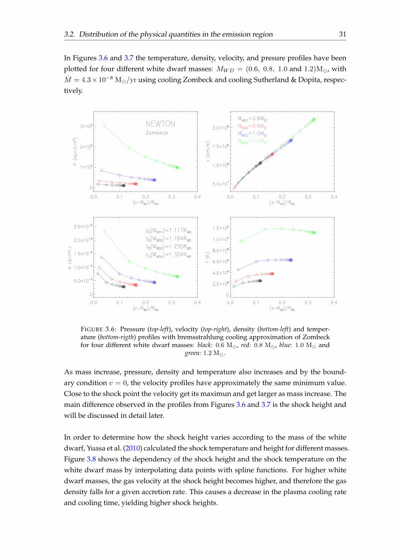
In Figures 3.6 and 3.7 the temperature, density, velocity, and presure profiles have beenplotted for four different white dwarf masses: MWD = (0.6, 0.8, 1.0 and 1.2)M, withM = 4.3×10⁻⁸ M/yr using cooling Zombeck and cooling Sutherland & Dopita, respec-tively.
FIGURE 3.6: Pressure (top-left), velocity (top-right), density (bottom-left) and temper-ature (bottom-rigth) profiles with bremsstrahlung cooling approximation of Zombeckfor four different white dwarf masses: black: 0.6 M, red: 0.8 M, blue: 1.0 M and
green: 1.2 M.
As mass increase, pressure, density and temperature also increases and by the bound-ary condition v = 0, the velocity profiles have approximately the same minimum value.Close to the shock point the velocity get its maximun and get larger as mass increase. Themain difference observed in the profiles from Figures 3.6 and 3.7 is the shock height andwill be discussed in detail later.
In order to determine how the shock height varies according to the mass of the whitedwarf, Yuasa et al. (2010) calculated the shock temperature and height for different masses.Figure 3.8 shows the dependency of the shock height and the shock temperature on thewhite dwarf mass by interpolating data points with spline functions. For higher whitedwarf masses, the gas velocity at the shock height becomes higher, and therefore the gasdensity falls for a given accretion rate. This causes a decrease in the plasma cooling rateand cooling time, yielding higher shock heights.

32 Chapter 3. Structure of the emission region
FIGURE 3.7: As Figure 3.6, using the results of the cooling function obtained by Suther-land & Dopita (1993).
FIGURE 3.8: Results of the numerical solutions of Yuasa et al. (2010) for the shockheight from the white dwarf surface (thick solid line) and the shock temperature (thinsolid line), shown against the white dwarf mass. For comparison, the dashed lineshows the shock temperature calculated by assuming no-gravity in the post shock
region. (Image from Yuasa et al. (2010)).

3.2. Distribution of the physical quantities in the emission region 33
Figure 3.9 shows the behaviour of shock height, z0, as a function of the white dwarf mass,for both cooling functions assuming an accretion rate of M = 4.3×10⁻⁸ M/yr using themodel presented here.
FIGURE 3.9: White dwarf masses as a function of the shock height, z0 in units ofRWD. (Magenta) points corresponds to cooling Sutherland & Dopita; (green) points
corresponds to cooling Zombeck.
Like Yuasa et al. (2010), from Figure 3.9 it is possible appreciate that the flow velocity andtemperature decrease with the height and with the white dwarf mass; values of velocityand temperature at z0 (shock) are largest for more massive white dwarfs. But the densityand pressure increases when the height decreases. However, its values also increases forlarger masses.Also, there is a clear difference in the shock heights calculated with each cooling function,being the values obtained with cooling Zombeck greater than those of cooling Sutherland& Dopita. Moreover, this diference increases with white dwarf mass.
Influence of the accretion rate
The local mass accretion rate, a, can be related to the total accretion rate M via M =
4πR2WDaf , where f is a fraction of the post shock region cross section to the white dwarf
surface area. Since a significantly affects the structure of the post shock region, someauthors (e.g. Yuasa et al. (2010); Hayashi & Ishida (2014a)) have investigated the depen-dence of the local mass accretion rate in the calculation of the properties of the post shockregion.

34 Chapter 3. Structure of the emission region
Figure 3.10 shows the result of the numerical solutions performed by Yuasa et al. (2010)it shows that a lower value of a gives a lower shock temperature at any mass of whitedwarf. But for higher mass, difference of the resulting shock temperatures is more or lessconspicuous.
FIGURE 3.10: Results of the numerical solutions of Yuasa et al. (2010) of the postshock region model when changing the accretion rate. Shock temperatures are plot-ted with solid, long dashed, short dashed, and dotted lines for accretion rates of
a = (0.1, 1.0, 5.0 and 10) g cm−2s−1. (Image from Yuasa et al. (2010)).
For example, for a white dwarf mass of 0.8 M, Yuasa et al. (2010) appreciate a differ-ence of a factor of 1.13 between the results obtained for a = 0.1 g cm−2s−1 and a =
1.0 g cm−2s−1. In the same way, a factor of 1.02 between a = 1.0 g cm−2s−1 and a =
10 g cm−2 s−1. While for a mass of MWD = 1.2 M, the difference increases to factorsof 1.33 and 1.10; this means that the estimated white dwarf mass is affected by less than∼ 30% in the range a = (0.1 − 10)g cm−2s−1 for a white dwarf less massive than 1.2 M
where most white dwarfs are likely to belong. However, some observations suggest thatthe local mass accretion rate distributes in a wider range.
Meanwhile, Hayashi & Ishida (2014a) modelled the post shock region of IntermediatePolars with a local mass accretion rate being floated in the range between 0.0001 and100 g cm−2s−1, considering cylindrical and dipolar geometry.From Hayashi & Ishida (2014a), Figure 3.11 shows the density distributions of the cylin-drical and dipolar post shock accretion columns with the local mass accretion rate of0.0001, 0.01, 1 and 100 g cm−2s−1 in the case of MWD = 0.7 M. In this figure, the rightends of each profile corresponds to the shock front. The other ends are terminated at 0.1
per cent of a post shock accretion column height of each case. This figure implies that thepost shock region becomes taller with a lower local mass accretion rate due to a longer

3.2. Distribution of the physical quantities in the emission region 35
cooling time. When the local mass accretion rate is sufficiently high, a & 5 g cm−2s−1
for a 0.7 M white dwarf, the density increases towards the white dwarf surface witha power-law function of the distance from the white dwarf surface. On the other hand,when the local mass accretion rate is sufficiently low, a 5 g cm−2s−1 for the 0.7 M
white dwarf, the density distribution deviates from the power law.
FIGURE 3.11: Density distributions of the cylindrical (black) and dipolar (red) postshock accretion colums for the white dwarf mass of 0.7 M and a of 0.0001, 0.01, 1,100 g cm−2s−1, obtained from Hayashi & Ishida (2014a) model. The right ends of thedistributions correspond to the tops of the post shock accretion columns. The otherends are terminated at 0.1 per cent of the post shock accretion column height. (Image
from Hayashi & Ishida (2014a))
Figure 3.12, shows a peak in the middle of the post shock accretion column at low enoughlocal mass accretion rate. This is because energy input by gravity overcomes cooling en-ergy loss since the low density reduces the cooling rate, and the tall post shock accre-tion column retains larger amount of gravitational energy to be released below the shockfront. The averaged temperature of the dipolar post shock accretion column monoton-ically decreases as the flow descends the post shock accretion column for the MWD =
0.7 M throughout the range a = (0.0001− 100)g cm−2s−1 unlike the cylindrical case.
Relations between the height of the post shock accretion column and the local mass ac-cretion rate are shown in Figure 3.13 for 0.4 M, 0.7 M and 1.2 M masses. The postshock region constantly extends upwards with the lower local mass accretion rate, butthe slope of the post shock accretion column height abruptly changes at a certain valueof a. At around the high end of a, the height is inverse proportional to a, and the heightof the post shock region is almost identical between the two post shock accretion columngeometries.

36 Chapter 3. Structure of the emission region
FIGURE 3.12: Averaged (solid) and electron (dotted) temperature distributions of thecylindrical (black) and dipolar (red) post shock accretion columns for the white dwarfmass of 0.7 M (left-hand columns) and 1.2 M (right-hand columns) and a of 0.0001,0.01, 1, 100 g cm−2s−1 from bottom to top panels. (Image from Hayashi & Ishida
(2014a)).
The local mass accretion rate significantly affects the structure of the post shock accretioncolumn, and there is a critical rate below which the profiles of the density and temper-ature distributions deviate from those of the Cropper et al. (1999) where the local massaccretion rate is fixed at 1 g cm−2s−1). This happens when the local mass accretion rateis between 5 and 100 g cm−2s−1 for the 0.7 M and 1.2 M white dwarf, respectively, orthe height of the post shock accretion region becomes 1 per cent of the white dwarf radius.

3.2. Distribution of the physical quantities in the emission region 37
FIGURE 3.13: The post shock accretion column heights for the 0.4, 0.7 and 1.2 Mwhite dwarfs as a function of the local mass accretion rate. Black and red lines show thecylindrical and dipolar cases, respectively. The two horizontal dotted lines represent1 and 20 per cent of the white dwarf radius. Note that the heights in this figure are
normalized by each white dwarf radii. (Image from Hayashi & Ishida (2014a)).
In order to examine the dependence of the structure of the accretion rate, calculationswith different accretion rates have been perfomed as shown in Figure 3.14, for coolingZombeck, and Figure 3.15, for cooling Sutherland & Dopita. The values of local massaccretion rates adopted are presented in Table 3.3 for a white dwarf mass of 1.0 M.
TABLE 3.3: Values of accretion rate for a white dwarf mass MWD = 1.0 M.
MWD = 1.0 MM ( M/yr) a (gr cm−2 s−1)
1.0× 10⁻¹⁰ 1.67257× 10⁻³
1.0× 10⁻⁹ 1.67257× 10⁻²
1.0× 10⁻⁸ 1.67257× 10⁻¹
1.0× 10⁻⁷ 1.67257
From Figures 3.14 and 3.15 it is possible to observe that these results are in agreementwith the expected results of Yuasa et al. (2010) and Hayashi & Ishida (2014a). The postshock region extends upwards with a lower a, i.e. the height z0 is evidently proportionalto a−1.When the local mass accretion rate is sufficiently high, the density increases towards thewhite dwarf surface. Moreover, the temperature, shows a peak in the middle of the postshock region (as in Hayashi & Ishida (2014a)). At low enough local mass accretion rate,the temperature increase as local mass accretion rate increase. But, for a higher local massaccretion rate, the temperature starts to decrease inward the white dwarf surface.

38 Chapter 3. Structure of the emission region
FIGURE 3.14: Pressure (top-left), velocity (top-right), density (bottom-left) and temper-ature (bottom-rigth) profiles with bremsstrahlung cooling approximation of Zombeckfor different accretion rates: orange: 1.0×10⁻¹⁰ M/yr, cyan: 1.0×10⁻⁹ M/yr, purple:
1.0× 10⁻⁸ M/yr and black: 1.0× 10⁻⁷ M/yr.
FIGURE 3.15: Pressure (top-left), velocity (top-right), density (bottom-left) and tempera-ture (bottom-rigth) profiles with the results of the cooling function obtained by Suther-land & Dopita and for different accretion rates: orange: 1.0 × 10⁻¹⁰ M/yr, cyan:
1.0× 10⁻⁹ M/yr, purple: 1.0× 10⁻⁸ M/yr and black: 1.0× 10⁻⁷ M/yr.

3.2. Distribution of the physical quantities in the emission region 39
3.2.1 Profile comparisons among different models
The distributions of physical quantities in the post shock region are presented for awhite dwarf mass of MWD = 0.8 M as a function of the distance in the shock region(z − RWD)/RWD using the numerical model described in Section § 2.2 for both coolingfunctions, Zombeck and Sutherland & Dopita, are compared with models of Aizu (1973)and Frank, King, & Raine (2002) described in Sections § 2.1.1 and § 2.1.2, respectively.
FIGURE 3.16: Pressure (top-left), velocity (top-right), density (bottom-left) and tem-perature (bottom-rigth) profiles with pure bremsstrahlung cooling as a function of(z − RWD)/RWD for a white dwarf mass of 0.8 M. (black:) cooling function ofZombeck; (purple:) cooling of Sutherland & Dopita; (cyan:) Frank analytical approxi-
mation; (orange:) Aizu model.
Figure 3.16 shows the profiles with both cooling function, Zombeck (black) and Suther-land & Dopita (purple), and Aizu (1973) (orange) and Frank, King, & Raine (2002) (cyan)approximations. The shock height, z0, obtained is higher with the Aizu (1973) model,meanwhile the calculated with the cooling function of Sutherland & Dopita gives thelower value. Since in Frank, King, & Raine (2002) the shock position should be assumed,it takes the shock height determined with the cooling function of Zombeck.
This variation between the models in the determination of the shock height can be ob-served in Table 3.4 for different masses of white dwarfs.

40 Chapter 3. Structure of the emission region
TABLE 3.4: Shock height for different values of white dwarf masses with purebremsstrahlung cooling, for the cooling functions of Zombeck and Sutherland & Do-
pita, and Aizu and Frank, King & Raine models.
ModelMWD
(M)M (M/yr)
z0 (RWD)
Zombeck Sutherland& Dopita
NEW 0.6 4.3× 10⁻⁸ 1.117 1.0340.8 4.3× 10⁻⁸ 1.164 1.0591.0 4.3× 10⁻⁸ 1.235 1.0921.2 4.3× 10⁻⁸ 1.324 1.1301.4 4.3× 10⁻⁸ 1.451 1.264
FRANK 0.6 4.3× 10⁻⁸ 1.117 —0.8 4.3× 10⁻⁸ 1.164 —1.0 4.3× 10⁻⁸ 1.235 —1.2 4.3× 10⁻⁸ 1.324 —
AIZU 0.6 4.3× 10⁻⁸ 1.258 —0.8 4.3× 10⁻⁸ 1.442 —1.0 4.3× 10⁻⁸ 1.699 —1.2 4.3× 10⁻⁸ 2.095 —
Due to this difference in the shock height, the pressure profile (top-left) between Aizu(1973) and the cooling Zombeck and Sutherland & Dopita seems to be more differentthat it really is. In fact, if the models are compared for the same post shock region thevalues of the pressure are similars. Neverthless the pressure in the anaylitical approxi-mation of Frank, King, & Raine (2002) is assumed to be constant through the emissionregion.
These differences are less evident in the velocity profiles (top-right). The velocities at theshock (maximum velocities) are very similar among the models and the values nearby tothe white dwarf surface are close to zero as is expected from the boundary condition, v =
0. Temperature profiles (bottom-right) exhibit a similar behaviour but, it is noticed thattemperatures of Frank are slightly lower than the other ones. As well as the temperaturesobtained with cooling Sutherland & Dopita are slighlty higher than the determined withthe other models.On the other hand, density profiles (bottom-left) have similar estimations between themodels, the only difference, again, is observed in the pressure profiles (due to the shockheight).
3.3 Spectrum continuum
In Section § 3.2, hydrodynamic calculations were carried out to determine the structure ofthe emission region. The temperature and density distributions obtained have been used

3.3. Spectrum continuum 41
to generate the X-ray spectra emitted from the post shock accretion region with the goalto investigate the behaviour of the flux emitted in the emission region and determine themass of the white dwarf (e.g. Ishida (1991); Cropper, Ramsay, & Wu (1998); Beardmore,Osborne, & Hellier (2000); Ramsay (2000)).
The post shock region model has been computed assuming solar abundances and fullyionized of all the abundant elements in the emission region. From Equation (2.61) thelocal bremsstrahlung emissivity is obtained for all the temperatures T (z) and densitiesρ(z). Since the emergent spectra is the sum of many local emissivity spectra, the totalbremsstrahlung spectra is obtained integrating Equation (2.61) from shock z = z0 (z′ =
0) to surface of the white dwarf z = RWD (z′ = z0 − RWD) (Equation (2.60)), for anenergy range between 1 keV and 100 keV. This assumption is reasonable at temperatureskT > 1 keV, therefore, the computed spectra are realiable at relatively high energiesonly (E & 3 keV). At lower energies, the spectra are dominated by numerous emissionspectral lines and photo-recombination continua (see e.g. Canalle et al. (2005)).Examples of model spectra are presented in Figures 3.17 and 3.18 for a white dwarf massof 0.8 M and an accretion rate M = 4.3 × 10⁻⁸ M/yr for pure bremmstrahlung withthe cooling functions of Zombeck and Sutherland & Dopita, respectively.
FIGURE 3.17: Calculated spectrum from a post shock region with bremsstrahlungcooling approximation of Zombeck and a mass of 0.8 M; plotted in units of
keVcm−2s−1.

42 Chapter 3. Structure of the emission region
FIGURE 3.18: Calculated spectrum from a post shock region with the results of thecooling function obtained by Sutherland & Dopita and a mass of 0.8 M.
With the aim of comparing the spectrum obtained with each cooling function, the Figure3.19 summarizes the two spectra.
FIGURE 3.19: Calculated spectra from a post shock region with bremsstrahlung cool-ing functions of Zombeck ((black)) and Sutherland & Dopita ((red)) and a mass of
0.8 M.

3.3. Spectrum continuum 43
As presented in Section § 3.2, the shock height computed with the cooling function ofZombeck is higher, z0(zck) = 1.164 RWD, than the obtained with the cooling function ofSutherland & Dopita, z0(S&D)
= 1.059 RWD. Thus the amount of flux emited in the shockregion is larger when the shock region is also larger as is observed in Figure 3.19.
Influence of mass
A set of total spectra for four different white dwarfs, MWD = (0.6, 0.8, 1.0 and 1.2) M,and cooling Zombeck and Sutherland & Dopita (Figures 3.20 and 3.21) is obtained. Theaccretion rate is fixed for all the computed spectra models at M = 4.3× 10⁻⁸ M/yr.
FIGURE 3.20: Comparison of model spectra with bremsstrahlung cooling approxima-tion of Zombeck computed for four white dwarf masses: 0.6 M (black asteriks), 0.8 M
(red triangles), 1.0 M (blue triangles) and 1.2 M (green triangles).
Because more massive white dwarfs have smaller radii, the corresponding shock tem-peratures are higher. A higher shock temperature implies a hotter post shock region, andhence a harder X-ray spectrum is observed as it is appreciated in Figures 3.20 and 3.21.

44 Chapter 3. Structure of the emission region
FIGURE 3.21: Comparison of model spectra with the results of the cooling functionobtained by Sutherland & Dopita computed for four white dwarf masses: 0.6 M(black asteriks), 0.8 M (red triangles), 1.0 M (blue triangles) and 1.2 M (green triangles).
The local mass accretion rate changes from a ≈ 0.2 g s−1cm−2 for the lightest white dwarfto a ≈ 10 g s−1cm−2 for the heaviest white dwarf in accordance with the decreasing whitedwarf radius.For less massive white dwarf the maximum of the spectrum is obtained at lower ener-gies,∼ 5 keV, with a sharp drop towards higher energies. The maximum of the spectrumis shifted to higher energy values as the mass increases. For a white dwarf of 1.0M themaximun flux is emitted at about 50 keV.
In addition, to compare both cooling functions, Figure 3.22 shows the spectra for differ-ent masses of white dwarfs and an accretion rate of M = 4.3 × 10⁻⁸ M/yr. Asteriskcorresponds to spectra computed with the cooling function of Zombeck, while the crossesare the spectra for different masses using the tabulated cooling of Sutherland & Dopita,respectively.
As in Figure 3.19, since the emission region of Zombeck is higher than the obtained withSutherland & Dopita, the total bremsstrahlung spectra for different masses are higher forcooling Zombeck and, like before, it is also possible appreciate that the maximum of the

3.3. Spectrum continuum 45
FIGURE 3.22: Comparison of model spectra with cooling Zombeck and Sutherland& Dopita computed for four white dwarf masses: 0.6 M (black asteriks), 0.8 M (red
triangles), 1.0 M (blue triangles) and 1.2 M (green triangles).
spectrum is obtained at lower energies with a sharp drop towards higher energies.
Influence of the accretion rate
Since the local mass accretion rate significantly alters the profiles of the density andtemperature distributions, as discussed in Section § 3.2, the X-ray spectra is calculatedwith the density and temperature distributions obtained there, and it is found that theX-ray spectra also depend on the specific accretion rate. Thus, the X-ray spectra havebeen determined for four different accretion rates M = (1.0 × 10⁻¹⁰, 1.0 × 10⁻⁹, 1.0 ×10⁻⁸, and 1.0 × 10⁻⁷)M/yr and a white dwarf mass of 1.0 M. The correspondingvalues of local mass accretion rate for a MWD = 1.0 M can be appreciated in Table 3.3.Figure 3.23 and 3.24 show the spectra for a total bremsstrahlung emissivity with the cool-ing approximation of Zombeck and cooling function obtained by Sutherland & Dopita,respectively.

46 Chapter 3. Structure of the emission region
FIGURE 3.23: Spectrum for different values of accretion rate: M = 1 × 10⁻⁷M/yr
(orange), M = 1 × 10⁻⁸M/yr (cyan), M = 1 × 10⁻⁹M/yr (purple) and M = 1 ×10⁻¹⁰M/yr (black) and bremsstrahlung cooling approximation of Zombeck.
FIGURE 3.24: Spectrum for different values of accretion rate: M = 1 × 10⁻⁷M/yr
(orange), M = 1 × 10⁻⁸M/yr (cyan), M = 1 × 10⁻⁹M/yr (purple) and M = 1 ×10⁻¹⁰M/yr (black) and with the results of the cooling function obtained by Sutherland
& Dopita.

3.3. Spectrum continuum 47
In order to compare between both cooling types (Zombeck + Sutherland & Dopita), Fig-ure 3.25 shows directly the spectrum for a white dwarf mass of MWD = 1.0 M anddifferent values of accretion rates M = (1.0 × 10⁻¹⁰, 1.0 × 10⁻⁹, 1.0 × 10⁻⁸, and 1.0 ×10⁻⁷) M/yr obtained from each of them.
FIGURE 3.25: Spectrum for different values of accretion rate: M = 1 × 10⁻⁷M/yr
(orange), M = 1 × 10⁻⁸M/yr (cyan), M = 1 × 10⁻⁹M/yr (purple) and M = 1 ×10⁻¹⁰M/yr (black) and bremsstrahlung cooling approximation of Zombeck (asterisks)
and the results of the cooling function obtained by Sutherland & Dopita (crosses).
From Table 3.3 it is possible to appreciate that when the accretion rate, M , is small the spe-cific accretion rate, a, is small. Since the temperature in the post shock accretion region re-duces the X-ray spectra soften. For instance, the continuum radiated by bremsstrahlunggenerally reduces as a decreases, which is prominent above 10 keV because the accretioncolumn becomes cooler and the maximum temperature downs. In contrast, if the accre-tion rate increase, the local mass accretion rate is higher and the temperature in the shockregion increase causing a harder X-ray spectrum as it is demostrated in Figures 3.23, 3.24and 3.25.
3.3.1 Spectral comparisons among different models
Spectra calculated with models of Aizu and Frank are obtained with the aim to comparewith the model presented in this work. Spectrum for a white dwarf mass of MWD =

48 Chapter 3. Structure of the emission region
0.8 M with M = 4.3 × 10⁻⁸ M/yr is presented in Figure 3.26. Purple points corre-spond to the present model with the results of the cooling function obtained by Suther-land & Dopita; black points are the spectra calculated with the cooling approximation ofZombeck; orange points are the calculated spectrum with Aizu’s model; and cyan pointscorrespond to the analytical approximation of Frank under constant pressure.
FIGURE 3.26: Spectrum for a WD of mass MWD = 0.8 M for different models.
Figure 3.26 shows that Aizu spectra is higher than the spectra obtained with the modelof Frank and the model presented here, calculated for both cooling functions. Being theflux computed with the cooling function of Sutherland & Dopita is the lowest. Since thesame accretion rate has been considered for all models, the determining parameter in thespectra calculation is the shock height and therefore the thickness of the emission region.
It is expected that for higher temperatures, the emitted flux would be higher. From theprofiles obtained in Section § 3.2, it can be seen that the maximum temperature of Aizu ishigher than other models, which explains that it has the higher emitted flux. After this,the higher shock temperature is derived by our model using the Sutherland & Dopitacooling. However, the flux emitted derived by this model is not the second largest. Thisemphasizes the importance of the calculation of the height of the shock since the modelcalculated with the cooling of Sutherland & Doipta determines a lower shock height than

3.3. Spectrum continuum 49
those obtained with the other models as can be seen in Table 3.4.
Although Frank’s model has been calculated with the same shock height obtained withthe model with cooling of Zombeck and the model of Frank has lower temperature max-imum than model with cooling approximation of Zombeck, the model of Frank reachesa flux higher at low energies than the model of Zombeck. But, at high energies the fluxemitted from Frank’s model is lower.
3.3.2 FITS table model
In order to fit the model presented in Section § 2.2 to X-ray observations, the spectra ob-tained for different white dwarfs masses and a fixed local mass accretion rate have beenintegrated it into the X-ray spectral fitting package, XSPEC, (Arnaud, 1996).
Using the described method in Sections § 2.2 and § 3.3, spectra have been obtained forsolar abundances and for different masses of white dwarfs from 0.6M to 1.4M with astep of 0.1 M and 1.4)M and an accretion rate M = 4.3× 10⁻⁸M/yr.
Tables with the calculated spectra have been created with IDL programming language froman ASCII file with the information of flux and energies where the energy interval is from0.1 keV to 100 keV with steps of 0.1 keV and for both cooling functions, Zombeck andSutherland & Dopita, following the requirements of XSPEC for additive table models(for details see Appendix C).
A table model, in XSPEC, is a very simple way of fitting with user-defined models and isavailable for a particular class of models. These are models that can be defined by a gridof spectra, with the elements of the grid covering the range of values of the parametersof the model. For instance, for a one-parameter model, a set of model spectra can betabulated for different values of the parameter, P1, P2, P3, etc. The model for a givenvalue of P is calculted by interpolating on the grid model spectrum. The generalizationto more parameters works in the obvious way.As with standard models, the model spectra should be in terms of flux-per-bins and notflux-per-keV. Any set of energy bins can be used, and XSPEC interpolate the model spec-tra onto the appropriate energy bins for the detectors in use. It is therefore a good ideato choose energy bins such that the spectrum is well-sampled over the range of interest.The file structure for these models is a FITS format1.
1The FITS file structure for models in XSPEC is described at: http://heasarc.gsfc.nasa.gov/docs/heasarc/ofwg/docs/general/ogip_92_009/ogip_92_009.htmlAdditional information at:http://www.darts.isas.ac.jp/pub/legacy.gsfc.nasa.gov/software/lheasoft/lheasoft6.3/headas-6.3.2/ftools/spectral/tables/ftp://legacy.gsfc.nasa.gov/fits_info/fits_formats/docs/

50 Chapter 3. Structure of the emission region
Figure 3.27 shows the spectra for different masses using the bremsstrahlung cooling ap-proximation of Zombeck. The aditive table model is called ipzk.fits.
FIGURE 3.27: Spectra obtained from the FITS table model, ipzk.fits, calculated usingthe cooling approximation of Zombeck for all the interval of white dwarf masses.
As in Figure 3.28, spectra have been obtained with the results of the cooling function de-termined by Sutherland & Dopita, ipsd.fits.
Recently, Suleimanov et al. (2016) presented a new set of Intermediate Polar model spec-tra that quantitatively account for the finite size of the magnetosphere. The models arecalculated for a set of magnetospheric radii, expressed in units of white dwarf radii, as-suming a relatively high local mass accretion rate and also ignore cyclotron cooling.
The local mass accretion rate is fixed to a = 1 g s−1cm−2 for all the computed spectralmodels. A set of post.shock region model spectra have been computed for the whitedwarf mass MWD, and the relative magnetospheric radius Rm/R. The grid was com-puted for 56 values of white dwarf mass from 0.3 to 1.4 M with a step of 0.02 M, i.e.2296 models in total. Every post shock region model has been computed for a fixed massaccretion rate M = 1016 g s−1.

3.3. Spectrum continuum 51
FIGURE 3.28: Spectra obtained from the FITS table model, ipsd.fits, calculated usingthe cooling function results of Sutherland & Dopita for all the interval of white dwarf
masses.
In previous work, Suleimanov, Revnivtsev, & Ritter (2005), used the cooling function ΛN
computed by Sutherland & Dopita (1993). But in Suleimanov et al. (2016), they useda cooling function computed by the code APEC (Smith et al., 2001) using the databaseAtomDB2 for a solar chemical composition. The grid has been distributed as an XSPECadditive table model like ipolar.fits3 and publicly available to the scientific commu-nity.
The tabulated model of Suleimanov et al. (2016) for different masses of white dwarfMWD = (0.6, 0.7, ..., 1.4)M and magnetospheric radius Rm/R = 1000, which repre-sent the pseudo-infinity magnetospheric radius, has been plotted in Figure 3.29 with anaccretion rate M = 1.6× 10⁻⁹M/yr.
2http://www.atomdb.org/3https://heasarc.gsfc.nasa.gov/xanadu/xspec/models/ipolar.html
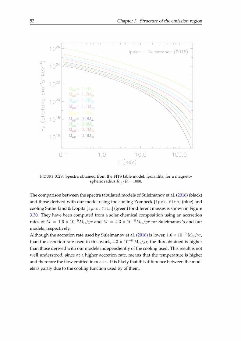
52 Chapter 3. Structure of the emission region
FIGURE 3.29: Spectra obtained from the FITS table model, ipolar.fits, for a magneto-spheric radius Rm/R = 1000.
The comparison between the spectra tabulated models of Suleimanov et al. (2016) (black)and those derived with our model using the cooling Zombeck [ipzk.fits] (blue) andcooling Sutherland & Dopita [ipsd.fits] (green) for diferent masses is shown in Figure3.30. They have been computed from a solar chemical composition using an accrretionrates of M = 1.6 × 10⁻⁹M/yr and M = 4.3 × 10⁻⁸M/yr for Suleimanov’s and ourmodels, respectively.Although the accretion rate used by Suleimanov et al. (2016) is lower, 1.6× 10⁻⁹ M/yr,than the accretion rate used in this work, 4.3 × 10⁻⁸ M/yr, the flux obtained is higherthan those derived with our models independiently of the cooling used. This result is notwell understood, since at a higher accretion rate, means that the temperature is higherand therefore the flow emitted increases. It is likely that this difference between the mod-els is partly due to the cooling function used by of them.

3.3. Spectrum continuum 53
FIGURE 3.30: Spectra for different models and masses of white dwarfs.


55
4NOVA OPH 1998 (V2487 OPH)
In this chapter, the tabulated model in Section § 3.3.2 is applied to XMM-Newton and IN-TEGRAL observations of Nova Ophiuchi 1998 (V2487 Oph).A photoelectric absorption column density, phabs in XSPEC, have been added to the ther-mal bremsstrahlung model in order to fit the observations. Also, a blackbody spectrum,bbody, have been used with the aim to fit the soft part of the spectra of the Nova Oph1998. Since fluorescent Fe Kα line at 6.4 keV have been identified, (Hernanz & Sala, 2002)sometimes is introduced in the spectral analysis through a Gaussian. At the same time,the energy band below 0.3 keV for the XMM-Newton observations have been exclude be-cause of inadequate instrumental response. Finally, as the shock temperature depends onthe mass of the white dwarf, the X-ray spectra is used to determine the mass of the whitedwarf.
4.1 Introduction of Nova Oph 98 (V2487 Oph)
V2487 Oph was optically discovered in outburst on 1998 June 15.561 UT (Nakano et al.,1998) with a visual magnitude of 9.5 and was confirmed as a nova by spectral observa-tions on 1998 June 18 (Filippenko et al., 1998). It was a very fast nova, with t2 ≈ 6.3 days
and t3 ≈ 9.5 days1 (Liller & Jones (1999a); Liller & Jones (1999b)).From observations of the near-IR lines OI λ8446 and λ11287, Lynch et al. (2000) obtaineda color excess E(B−V ) = 0.38± 0.08, and thus a visual extinction AV = 1.16± 0.24 mag.Using an empirical relation to determine the absolute visual magnitude between t2 andMmaxV , they calculated the absolute visual magnitude Mmax
V = −8.8 and estimated an
1t2 and t3 are defined as the elapsed time to decreases of 2 and 3 magnitudes in its visual luminosity,respectively.

56 Chapter 4. Nova Oph 1998 (V2487 Oph)
unusually large distance of d = 27 ± 3 kpc. Given the galactic coordinates of the source,6.60,+7.77, this would situate V2487 Oph above the galactic plane and out of the disk,an unlikely position for this class of object.As this nova was a very fast nova, it is possible that the real maximum of its magnitudehad been missed and that the true absolute visual magnitude had been brighter. Extrap-olating the visual light curve back in time to the pre-discovery data using the expressionin Harris et al. (1999), the magnitude can be estimated to be in the range 6.8 − 9.5 mag,and the final distance obtained is to range between 8 and 27 kpc (Hernanz & Sala, 2002).
Pagnotta, Schaefer, & Xiao (2008) reported, from the Harvard College Observatory archivalphotograph collection, the discovery of a previously unknown eruption of the nova.V2487 Oph was previously classified as a classical nova, but Pagnotta, Schaefer, & Xiao(2008) identified it as a probable recurrent nova based on its large expansion velocitiesand the presence of high excitation lines in the outburst spectrum. They noted that V2487Oph had a magnitude in the B-filter of 10.27 ± 0.11 on 1900 June 20, near its peak mag-nitude of 9.5 observed during the outburst in 1998 (see also Pagnotta et al. (2009)). After-wards they identified V2487 Oph as a strong galactic recurrent nova candidate becauseof its low outburst amplitude, the very fast decline rate, the high expansion velocity, andthe presence of high-excitation lines in its outburst spectrum. In 2002, Hachisu et al.(2002) already was suggested the same idea because the rapid decline and the presenceof a plateau phase in the optical nova’s light curve, which represent common featuresfor the U Sco subclass of recurrent novae. They reproduced the V2487 Oph light curveshape of the 1998 outburst, and identified the nova as a good candidate for a recurrentnova and a type Ia Supernova progenitor. Further, more authors (e.g. Strope, Schaefer, &Henden (2010); Schaefer (2010)) have studied the V2487 Oph optical light curve in deep,and confirmed the connection with a probable recurrent nature for the source.
4.1.1 High energy observations
V2487 Oph has been observed as a high energy source through the detection of differentX-rays satellites like the X-ray Multi-Mirror Mission, XMM-Newton, the INTErnationalGamma-Ray Astrophysics Laboratory, INTEGRAL, and the Rossi X-ray Timing Explorer,RXTE.
Nova Oph 1998 has been detected with the XMM-Newton satellite at five epoch: 2.7, 3.2,3.7, 4.3 and 8.8 years after outburst. Details of the X-ray observations with XMM-Newtonand analysis are discussed below. Also was detected with the INTEGRAL/IBIS satellitein the 20− 100 keV range (Barlow et al., 2006) and later, it was detected with RXTE/PCA(Butters et al., 2011).
These observations in X-rays show that Nova Oph 1998 exhibits characteristics of Inter-mediate Polar and indicate that the white dwarf should be magnetic. In addition, the

4.1. Introduction of Nova Oph 98 (V2487 Oph) 57
shape of the optical curve seem to indicate that the white dwarf in this nova is quitemassive, which is in agreement with the discovery that Nova Oph 1998 is a recurrentnova (Pagnotta et al., 2009); only novae with very massive white dwarfs can erupt asfrequently as recurrent novae, which have recurrence periods smaller than ∼ 100 years,i.e., more than one recorded outburst.
The first study of the X-ray data was performed by Hernanz & Sala (2002) who ana-lyzed the first two XMM-Newton observations of V2487 Oph performed in 2001; first andsecond observation, 2.7 and 3.2 years after outburst, respectively. Figure 4.1 shows theobserved spectra of V2487 Oph with The European Photon Imaging Camera EPIC MOS1,MOS2 and PN data of the second observation. Continuous lines show the models thatbest fit the data from the three instruments simultaneously. The lower panel displays theresiduals between the models and the data in units of sigma. The reduced χ2 of the fit isχ2ν = 1.18.
FIGURE 4.1: Observed spectra of V2487 Oph, EPIC MOS1, MOS2, and PN data (sec-ond observation, done on February 25 2001, 1178 days after outburst). The lower paneldisplays the residuals between the models and the data in units of σ (Image from Her-
nanz & Sala (2002).
V2487 Oph did not appeared as a supersoft X-ray source, which emission is due to resid-ual H-burning on top of the white dwarf but showed a flat continuum shape extendingup to 12 keV. Moreover an excess emission at 6.4 keV corresponding to the neutral Fe Kαfluorescence phenomenon was also detected, mostly due to reflection of high energy pho-tons produced in the accretion process in a CV-like system. This revealed the recovery of

58 Chapter 4. Nova Oph 1998 (V2487 Oph)
the accretion process as soon as ∼ 2.7 years (less than 1000 days) after the nova outburst.In addition, positional correlation with the X-ray source 1RXS J173200.0−1934 detectedby the RASS (ROSAT All-Sky Survey) in 1990 was established, making of V2487 Oph thefirst classical nova observed before and after the outburst in X-rays.
Sala (2004b) (see also Sala (2004a) for details) analyzed the first three observations ofXMM-Newton, 2.7, 3.2 and 3.7 years after outburst. The X-ray spectra detected with theEPIC cameras are shown in Figures 4.2, 4.3 and 4.4.
FIGURE 4.2: V2487 Oph observed spectra 2.7 years after the outburst from the twoEPIC MOS cameras, MOS1 (black), MOS2 (red) and best fit model. The lower paneldisplays the residuals (data minus folded model) in terms of sigmas, with error bars
of size one. (Image from Sala (2004a)).
In all observations the nova was detected as a bright X-ray source. The spectrum is dom-inated by thermal plasma emission and was modeled by a two-temperature MEKALmodel (Mewe, Gronenschild, & van den Oord (1985); Mewe, Lemen, & Oord (1986)). Theχ2ν for the best fit model obtained for the first, second and third observation are 1.07,
1.13 and 1.24, respectively. The best fit thermal plasma model has a cool component, at0.2− 3 keV, and a hot component, with temperatures above ∼ 64 keV for the second andthird observations, and above ∼ 10 keV in the first one. The plasma spectrum at thesehigh temperatures is very flat, and the temperature was not well constrained. In the caseof the first observation, data from the PN camera was missing, and the parameters of themodel were in general less constrained than in the second and third observations.

4.1. Introduction of Nova Oph 98 (V2487 Oph) 59
FIGURE 4.3: Observed spectra of V2487 Oph 3.2 years after outburst and best fit model.Data from the three EPIC cameras are shown: MOS1 (black), MOS2 (red), and PN data(green, with higher count rate), as well as the contribution of each component of thebest-fit model (from left to right, white dwarf atmosphere, low temeprature MEKAL,high temeprature MEKAL and Gaussian emission line). The lower panel displays the
residuals in terms of sigmas. (Image from Sala (2004a)).
In all observations, with the two-component model, the data showed an excess around∼ 6.4 − 6.5 keV and for this reason and additional Gaussian line centered at this energyand with a width σ = 0.6 keV counted for this excess. However, the two-temperaturethermal plasma model not explain well the soft part of the spectrum, which was well fit-ted with a white dwarf atmosphere model (from MacDonald & Vennes (1991)), absorbedby a hydrogen column density of NH = 4 × 1021 cm−2 that is slightly larger than theaverage interstellar absorption in the direction of the source, 2.1 × 1021cm−2, (Dickey &Lockman, 1990). The best fit was obtained with effective temperatures between 64 and74 eV and a bolometric luminosity ∼ 1035 erg s−1, assuming a distance of 10 kpc, whichimplies a radius of the emitting region of 3 × 107 cm for the first observation and of∼ 1.6× 107 cm in the second and third ones. This is clearly smaller than the whole whitedwarf surface, indicating that it must be associated to a hot emitting region of the star.Although the spectral model that fits the data was the same in the three observations, thetotal observed flux decreases with time.
For Sala (2004a), the fact that the emission line at ∼ 6.4− 6.5 keV must be simulated withan additional Gaussian line added to the MEKAL model, which already included the ironlines of the thermal plasma, indicates that it must be powered by some extra mechanism.As a fluorescent line at 6.41 keV can be produced by cold, neutral iron, other fluorescent

60 Chapter 4. Nova Oph 1998 (V2487 Oph)
FIGURE 4.4: Observed spectra of V2487 Oph 3.7 years after outburst and best fit model.The lower panel displays the residuals in terms of sigmas. Data from the three EPICcameras are shown: MOS1 (black), MOS2 (red), and PN data (green, with highercount-rate) as well as the contribution of each component of the best fit model (fromleft to right, white dwarf atmosphere, low temperature MEKAL, high temperature
MEKAL and Gaussian emission line). (Image from Sala (2004a)).
lines can be emitted at higher energies by iron at intermediate states of ionization (Hel-lier, Mukai, & Osborne, 1998). The main fluorescent Kα line emitted by cold, neutral ironcould thus explain the emission line observed for V2487 Oph (Hernanz & Sala, 2002),while the blend with the other fluorescent lines could explain the width of the line. Thisfluorescent Fe Kα line can only be induced by reflection of the X-rays generated in thehot post-shock region of the accretion flow on neutral iron, i.e., on colder material of thedisk or the white dwarf. A reflection effect requires therefore that accretion had beenreestablished by the time of observations.
The kind of spectra found for V2487 Oph is similar to observed for the intermediate po-lars EX Hya and AO Pisc (Ishida, Mukai, & Osborne (1994)); Hellier et al. (1996); Fujimoto& Ishida (1997)). Nevertheless, those cataclysmic variables had thermal plasma spectrastepper than V2487 Oph, indicating cooler plasmas in the accretion stream. The hightemperatures in the shocked plasma may be a consequence of accretion onto a massivewhite dwarf, which would agree with the mass determination of Hachisu et al. (2002),MWD = 1.35 M, from the visual light curve and the numerical model described inHachisu et al. (2002).Also, the parameters of the soft component of the spectrum indicate that it can not be

4.1. Introduction of Nova Oph 98 (V2487 Oph) 61
associated to the emission from the whole white dwarf surface, i.e., it can not be pro-duced by hydrogen burning on the star’s envelope and just only a fraction of the whitedwarf surface is emitting soft X-rays, as observed for V2487 Oph. The presence of thissoft component, typical of magnetic cataclysmic variables, also supports the surprisinglyfast recovery of the accretion process as soon as∼ 2.7 years (less than 1000 days) after thenova outburst (Hernanz & Sala, 2002).
Ferri & Hernanz (2007) showed more spectral features in the V2487 Oph spectra throughthe re-analysis of the XMM-Newton data already presented in Hernanz & Sala (2002)and Sala (2004a) and the first study of optical observations performed in 2002. At leasttwo other thermal lines in the 6 − 7 keV region of these spectra were found, which wereascribed to the emitting plasma beside the fluorescence feature (see also Ferri (2011) fordetails). Thanks to the longer exposition they could present the first X-ray timing analy-sis, besides photometric and spectroscopic data obtained by them in the optical banda atthe Roque de los Muchachos Observatory.
FIGURE 4.5: The EPIC MOS1 (black), MOS2 (red) and PN (green) data modelled witha black body component, a two-temperature MEKAL plasma model plus three Gaus-sian lines at 6.38±0.03 keV, 6.70±0.03 keV and 6.98+0.02
−0.06 keV (best fit model, left-upperpanel), all with photoelectric absorption. Data in the 5− 9 keV energy range modelledwith a MEKAL model at kT w 10 keV on the right-upper panel is also presented,where the 6.68 and 6.97 keV thermal emission line (Fe XXV and Fe XXVI, respectively)can be noticed. Individual spectral components have been added (dashed lines) cor-responding to MOS1 and MOS2 (left-lower panel) and PN (right-lower panel) datafitted with best fit model separately. In the lower part of each image the fit residuals
in σ units are presented (Image from Ferri (2011)).
62 Chapter 4. Nova Oph 1998 (V2487 Oph)
Figure 4.5 shows the MOS1, MOS2 and PN spectra data (0.2 − 15 keV) and the best-fitmodels, i.e. phabs ∗ [bbody + mekal + mekal + gauss + gauss + gauss], which is given bya discrete multi-temperature model composed by MEKAL (Mewe, Gronenschild, & vanden Oord (1985); Mewe, Lemen, & Oord (1986)) components plus the black body contri-bution as the base for the model.
Nevertheless the method used to simulate the emission lines in order to obtain the bestfit has been to model the continuum energy ranges 5.0 − 6.3 and 7.1 − 10.0 keV withthe absorbed higher temperature MEKAL. Ferri (2011) fixed the continuum parameters,extended the fitted range to 5.0 − 10.0 keV, and added a gaussian function to modelthe Fe lines complex and found that this part of the spectra could be modelled by threeGaussians considering each detector separately or altogether, corresponding to neutral,He-like and H-like Kα iron emission. Thus Ferri (2011) constrained by fixing the line en-ergies to 6.40, 6.68 and 6.97 keV, respectively, and forced the three lines to have the samewidth and peak energy in the whole spectrum.Acceptable fits were achieved including two MEKAL components, a black body and in-terstellar absorption assuming that the absorption is uniform around the source, NH =
2.1 × 1021 cm−2, fixed to the value of Dickey & Lockman (1990). The parameters ob-tained by Ferri (2011) were kTbbody = 108+2
−5 eV, kTmin = 0.2 ± 0.1 keV, at 1-σ error,kTmax ≥ 77 keV. Although this model gives a good χ2
ν = 1.4, it does not provide a verygood fit to the data. An emission at 6.38 ± 0.03 keV was also obtained corresponding tothe Fe fluorescent line, 6.70± 0.03 keV for Fe XXV and 6.98+0.02
−0.06 keV for Fe XXVI Kα ironline with equivalent widths (EWs) of 350, 210 and 100 eV, respectively (Hellier et al.,1996).Also a partial covering absorption model, a black body plus a two-temperature opticallythin thermal plasma, simulated with MEKAL, and only one gaussian line accounting forthe Fe Kα fluorescence line at 6.4 keV were include with the aim to improve the χ2
ν . Themodel is given by phabs ∗ pcfabs ∗ (bbody + mekal + mekal + gauss).Although the use of the partial covering absorber improves drastically the χ2
ν , 1.2, thismodel shows residuals between 6.9 and 7 keV and it does not fit very well the Fe H-likeemission line at 6.97 keV.
4.2 Observations and Analysis
4.2.1 XMM-Newton data
Table 4.1 contains the XMM-Newton detections of Nova Oph 1998. This nova was ob-served four times in the X-ray band during 2001 and 2002 with an interval of about 6months between each two consecutive observations and a fifth observation in 2007. Thecounts rate and the total counts are calculated in the 0.2− 10 keV energy range for MOS1and MOS2 and in the 0.2 − 12 keV energy range for PN. The PN camera failed for 2001February 25 observation, so that only the MOS1 and MOS2 data are available.

4.2. Observations and Analysis 63
TABLE 4.1: Log of all the V2487 Oph 1998 detections with XMM-Newton satellite.
Obs
erva
tion
date
Day
s,ye
ars
afte
rou
tbur
stC
amer
aTo
tal(
effe
ctiv
e)ex
posu
reTi
me
(s)
Tota
lcou
nts
(cts
)C
ount
sra
te(c
ts/s
)Fe
br.2
5,20
0198
6d,
2.7
yrM
OS1
7698
(720
6)21
620.3
0±
0.0
1M
OS2
7700
(723
8)20
990.2
9±
0.0
1PN
--
-Se
pt.5
,200
111
78d,
3.2
yrM
OS1
7598
(749
4)23
230.3
1±
0.0
1M
OS2
7597
(751
2)23
290.3
1±
0.0
1PN
5000
(504
0)45
631.0
5±
0.0
1
Febr
.26,
2002
1352
d,3.
7yr
MO
S170
32(5
699)
1653
0.2
9±
0.0
1M
OS2
7033
(587
7)17
630.3
0±
0.0
1PN
4668
(434
6)45
631.0
5±
0.0
2
Sept
.24,
2002
1559
d,4.
3yr
MO
S182
78(7
549)
2416
0.3
2±
0.0
1M
OS2
8278
(758
2)25
020.3
3±
0.0
1PN
6569
(567
8)61
891.0
5±
0.0
1
Mar
c.24
,200
732
12d,
8.8
yrM
OS1
3528
9(3
2984
)12
006
0.3
64±
0.0
03
MO
S235
296
(329
02)
1177
90.3
58±
0.0
03
PN33
342
(308
34)
3875
91.2
42±
0.0
06
64 Chapter 4. Nova Oph 1998 (V2487 Oph)
In this work, the study of the fourth and fifth observations2, 4.3 and 8.8 years after out-burst, of V2487 Oph carried out by the XMM-Newton satellite are presented. The EPICcameras observed the nova for a total exposure time of 8280 with MOS1 and MOS2 and6570 seconds with PN for the fourth observation; and 35290 seconds with MOS1 andMOS2 and 33340 seconds with PN for the fifth observation.
4.2.2 INTEGRAL data
In addition to the XMM-Newton observations, V2487 Oph was detected as a hard X-raysource in the INTEGRAL IBIS/ISGRI (Ubertini et al., 2003) soft gamma-ray Galactic PlaneSurvey, with an emission at kT > 30 keV (Barlow et al., 2006). Re-analyzing the datafrom 22 cataclysmic variables detected with the third INTEGRAL/IBIS survey Landi et al.(2009) confirmed previous indications about V2487 Oph. More recently V2487 Oph alsoappeared in the fourth IBIS/ISGRI soft Gamma-ray Survey Catalog (Bird et al., 2010).
Since V2487 Oph is in the plane of the mission, at least once per month was observed. Thedata reduction is courtesy of Stephane Paltani (private communication) and was reducedwith the Offline Science Analysis, OSA, software version 8, following the standard reduc-tion procedures (Goldwurm et al., 2003). IBIS spectra were extracted in 12 and 24 energychannels. However, it was necesssary added a step included in OSA 9, which consistsin the detection and removal of pixels affected by the presence of glue in the mask. Thisglue is not completely transparent to X-rays, and the inclusion of these pixels leads to thepresence of strong ghosts for the brightest sources. In this crowded area, this cleaning isabsolutely mandatory.The total good time is 2.5 Ms, while the efficiency-corrected exposure, taking into accountvignetting, is 1.7 Ms. The data have been taken over 160 Ms, covering the INTEGRAL ob-servations a bit more than 5 years. Revolutions go from 0046 to 0736. However, becauseof the large number of sources brighter than V2487 Oph in this area, it was necessary toselect pointing where V2487 Oph was on the Eastern side, in order to avoid a too largenumber of bright sources in the Field of view, FOV, which makes the spectral extractionfail.
4.3 Spectral analysis
In order to obtain the basic parameters like the temperature of the black body, the inter-stellar absorption and the mass of the white dwarf and to obtain information about thesoft and hard X-ray emission. The data was analysed with the software package XSPEC(Arnaud, 1996). For the analysis of the EPIC spectra, the tabulated models previouslycomputed, ipzk.fits and ipsd.fits, have been used as an additive table model, AT-ABLE in XSPEC. The channels below 0.3 keV have been ignored because of inadequate
2ID observations: 0085582001 and 0401660101 corresponding to fourth and fifth observations, respec-tively; P.I.: Margarita Hernanz.

4.3. Spectral analysis 65
instrumental response.A simple photoelectric absorption with Verner et al. (1996) cross sections and Lodders(2003) solar abundances is needed to simulate the effect of the hydrogen column densityfor the absorption component, PHABS in XSPEC. In our fit the interstellar absorptionwas set to the value obtained from the absorption calculated from the extinction de-rived by Lynch et al. (2000), from the color excess E(B − V ) = 0.38 ± 0.08. Throughthe empirical relationship between interstellar X-rays absorption and optical extinction,NH/E(B−V ) = 5.9×10²¹ mag−1cm−2, obtaining a value ofNH = 2.2×1021 cm−2; whichis consistent with the interstellar absorption NH = 2.1 × 1021 cm−2 (Dickey & Lockman,1990). Also a black body component, BBODY available in XSPEC, have been used withthe aim to fit the soft part of the spectrum of the Nova Oph 1998.In some cases, Gaussian lines were added to the model to express the neutral, or low ion-ized, Fe Kα emission line at 6.4 keV (Hernanz & Sala, 2002) and also the thermal plasmaHe-line Fe and H-line Fe emission detected by Ferri (2011).
The best fitting for both observations, 4th and 5th, of XMM-Newton and its combinationswith INTEGRAL observations, in 12 and 24 energy channels, are presented below.
FIGURE 4.6: XMM-Newton 4th observation with EPIC MOS1 (black), MOS2 (red) andPN (green) using the cooling approximation of Zombeck. The black body componentis kTbbody = 0.11 keV, the white dwarf mass is obtained MWD = 1.4 M and thereduced chi-square is χ2
ν = 1.8 for 463 degrees of freedom. The lower panel show thefit residuals in σ units.

66 Chapter 4. Nova Oph 1998 (V2487 Oph)
(A) Confidence contour for the black bodytemperature and the normalization.
(B) Confidence contour for the mass of thewhite dwarf and the normalization.
(C) Confidence contour for the black body temperature and NH .
FIGURE 4.7: Confidence contours for the best fit model parameters. Inner, middleand outer circles represent 1σ, 2σ and 3σ levels of confidence, respectively. The cross
marks the best-fit position.
Figure 4.6 corresponds to the 4th observation with XMM-Newton, 4.3 years after outburst,with EPIC MOS1, MOS2 and PN cameras using the additive table model ipzk.fits ob-tained with the cooling expression of Zombeck. The best fit model is given by [phabs ∗(atableipzk.fits) + bbody] giving a χ2
ν = 1.8. The interstellar absorption is fixed atNH = 2.2×1021 cm−2, however a higher absorption is obtained. The kTbbody calculated is0.11 keV, and the white dwarf mass is MWD = 1.4 M. In order to evaluate the errors forevery model component, confidence contours have been performed in Figures 4.7a, 4.7band 4.7c.
As in Figure 4.6, fitting data have been obtained for the 4th observation but using the tab-ulated model ipsd.fits computed with the results of the cooling function obtained bySutherland & Dopita. Figure 4.8 shows the best fit model obtaining a χ2
ν = 1.8. The cal-culated values of NH , kTbbody and MWD are similars to those obtained with the tabulatedmodel with cooling approximation of Zombeck. In addition, the confidence contours,

4.3. Spectral analysis 67
Figures 4.9a to 4.9c, have been obtained in order to evaluate the errors of the differentparameters of the models.
FIGURE 4.8: XMM-Newton 4th observation with EPIC MOS1 (black), MOS2 (red) andPN (green) using the cooling results of Sutherland & Dopita. The black body compo-nent is kTbbody = 0.11 keV, the white dwarf mass is obtained MWD = 1.4 M and thereduced chi-square is χ2
ν = 1.8 for 463 degrees of freedom. The lower panel show thefit residuals in σ units.
The results obtained above suggest that an additional emission process should be in-volved beside bremsstrahlung in order to explain the whole X-rays line emission detectedin the harder part of the spectra (Ferri, 2011).
Since our model does not include emission lines from the thermal plasma, we are not ableto reproduce the entire emission lines using these models. The continuum shape of thedata at harder energies, needs high temperature plasma values to obtain an acceptablefit for this region of the spectrum. However, because at that temperatures most of theatoms are ionized it prevents the production of emission line. To solve this problem, aGaussian component is added to the spectrum to simulate the Fe complex line emissionat higher energies. As high temperatures could produce iron Kα lines from Fe XXV, orHe-like at 6.68 keV, and Fe XXVI, or H-like at 6.97 keV also are included to the modelwith the fluorescent Fe Kα line at 6.4 keV.

68 Chapter 4. Nova Oph 1998 (V2487 Oph)
(A) Confidence contour for the black bodytemperature and the normalization.
(B) Confidence contour for the mass of thewhite dwarf and the normalization.
(C) Confidence contour for the black body temperature and NH .
FIGURE 4.9: Confidence contours for the best fit model parameters. Inner, middleand outer circles represent 1σ, 2σ and 3σ levels of confidence, respectively. The cross
marks the best-fit position.

4.3. Spectral analysis 69
The new model is given by [phabs∗ (atableipzk.fits)+ bbody+3gauss]. The absorptionis initially NH = 2.2 × 1021 cm−2 but after fitting, the value obtained is higher, as in thelast model, probably indicating that the source of the X-ray emission is more absorbedthan by the interstellar medium alone and an intrinsic contribution from the binary sys-tem to the X-ray source is present. The black body temperature is kTbbody = 0.12 keV andthe white dwarf mass is computed asMWD = 1.39 M. The χ2
ν is better than the obtainedwithout considering the Fe lines and is χ2
ν = 1.3. Figure 4.10 show the EPIC data with thenew model and Figures 4.11a, 4.11b and 4.11c its corresponding confidence contours forthe parameters of the model.
FIGURE 4.10: XMM-Newton 4th observation with EPIC MOS1 (black), MOS2 (red) andPN (green) using the cooling approximation of Zombeck. The black body componentis kTbbody = 0.12 keV, the white dwarf mass is obtained MWD = 1.39 M and thereduced chi-square is χ2
ν = 1.3 for 460 degrees of freedom. The lower panel show thefit residuals in σ units.

70 Chapter 4. Nova Oph 1998 (V2487 Oph)
(A) Confidence contour for the black bodytemperature and the normalization.
(B) Confidence contour for the mass of thewhite dwarf and the normalization.
(C) Confidence contour for the black body temperature and NH .
FIGURE 4.11: Confidence contours for the best fit model parameters. Inner, middleand outer circles represent 1σ, 2σ and 3σ levels of confidence, respectively. The cross
marks the best-fit position.

4.3. Spectral analysis 71
In addition to XMM-Newton observations, INTEGRAL IBIS/ISGRI spectra, extracted in 12and 24 channels of energy, have been analyzed with the EPIC data. Figures 4.12 and 4.14show the models that best fit the data from both satellites simultaneously. The model isthe continuum bremsstrahlung model computed in this work and the interstellar absorp-tion model, phabs, plus a black body spectra: [phabs ∗ (atableipzk.fits) + bbody] and[phabs ∗ (atableipsd.fits) + bbody] for tabulatd models ipzk.fits and ipsd.fits,respectively. Figures 4.13a, 4.13b, 4.13c, 4.15a, 4.15b and 4.15c are the corresponding con-fidence contours to evaluate the errors of the model parameters.
FIGURE 4.12: XMM-Newton 4th observation with EPIC MOS1 (black), MOS2 (red)and PN (green) and INTEGRAL observations IBIS/ISGRI (12 channels) (blue) using thetabulated model with cooling approximation of Zombeck. The black body componentis kTbbody = 0.11 keV, the white dwarf mass is obtained MWD = 1.39 M and thereduced chi-square is χ2
ν = 1.7 for 476 degrees of freedom. The lower panel show thefit residuals in σ units.

72 Chapter 4. Nova Oph 1998 (V2487 Oph)
(A) Confidence contour for the black bodytemperature and the normalization.
(B) Confidence contour for the mass of thewhite dwarf and the normalization.
(C) Confidence contour for the black body temperature and NH .
FIGURE 4.13: Confidence contours for the best fit model parameters. Inner, middleand outer circles represent 1σ, 2σ and 3σ levels of confidence, respectively. The cross
marks the best-fit position.
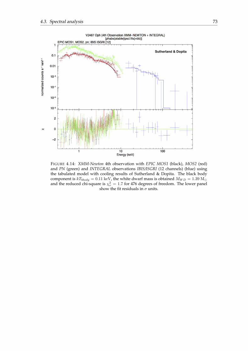
4.3. Spectral analysis 73
FIGURE 4.14: XMM-Newton 4th observation with EPIC MOS1 (black), MOS2 (red)and PN (green) and INTEGRAL observations IBIS/ISGRI (12 channels) (blue) usingthe tabulated model with cooling results of Sutherland & Dopita. The black bodycomponent is kTbbody = 0.11 keV, the white dwarf mass is obtained MWD = 1.39 Mand the reduced chi-square is χ2
ν = 1.7 for 476 degrees of freedom. The lower panelshow the fit residuals in σ units.

74 Chapter 4. Nova Oph 1998 (V2487 Oph)
(A) Confidence contour for the black bodytemperature and the normalization.
(B) Confidence contour for the mass of thewhite dwarf and the normalization.
(C) Confidence contour for the black body temperature and NH .
FIGURE 4.15: Confidence contours for the best fit model parameters. Inner, middleand outer circles represent 1σ, 2σ and 3σ levels of confidence, respectively. The cross
marks the best-fit position.

4.3. Spectral analysis 75
Figures 4.16 and 4.18 present the 5th observation with XMM-Newton, 8.8 years after out-burst, and the INTEGRAL observations for the spectra extracted in 24 channels of energy.The model is the additive table model ipzk.fits or ipsd.fits, according to coolingapproximation; with an interstellar absorption model and a gaussian line close to thevalue of the fluorescence Fe Kα line, however, this gaussian line has not been set to a spe-cific value. The interstellar absorption has been fixed initially as NH = 2.2 × 1021 cm−2
but, as in previous occasions, the absorption obtained is higher, ∼ 3.2 × 1021 cm−2, forboth cases. The spectra display an iron emission line at 6.45 keV corresponding to flu-orescence Fe Kα. The chi-square obtained is χ2
ν = 1.27 for both cases. The blackbodytemperature, kTbbody = 0.10 keV, is consistent with the expected value and the whitedwarf mass is close to the Chandrasekhar limit 1.39 M. The corresponding confidencecontours are presented in Figures 4.17a, 4.17b and 4.17c for the tabulated model with thebremmstrahlung approximation of Zombeck and, in Figures 4.19a, 4.19b and 4.19c forthe results of the cooling function of Sutherland & Dopita.
FIGURE 4.16: XMM-Newton 5th observation with EPIC MOS1 (black), MOS2 (red)and PN (green) and INTEGRAL observations IBIS/ISGRI (24 channels) (blue) usingthe tabulated model with cooling results of Zombeck. The black body componentis kTbbody = 0.10 keV, the white dwarf mass is obtained MWD = 1.39 M and thereduced chi-square is χ2
ν = 1.27 for 1588 degrees of freedom. The lower panel showthe fit residuals in σ units.

76 Chapter 4. Nova Oph 1998 (V2487 Oph)
(A) Confidence contour for the black bodytemperature and the normalization.
(B) Confidence contour for the mass of thewhite dwarf and the normalization.
(C) Confidence contour for the black body temperature and NH .
FIGURE 4.17: Confidence contours for the best fit model parameters. Inner, middleand outer circles represent 1σ, 2σ and 3σ levels of confidence, respectively. The cross
marks the best-fit position.

4.3. Spectral analysis 77
FIGURE 4.18: XMM-Newton 5th observation with EPIC MOS1 (black), MOS2 (red)and PN (green) and INTEGRAL observations IBIS/ISGRI (24 channels) (blue) usingthe tabulated model with cooling results of Sutherland & Dopita. The black bodycomponent is kTbbody = 0.10 keV, the white dwarf mass is obtained MWD = 1.39 Mand the reduced chi-square is χ2
ν = 1.27 for 1588 degrees of freedom. The lower panelshow the fit residuals in σ units.
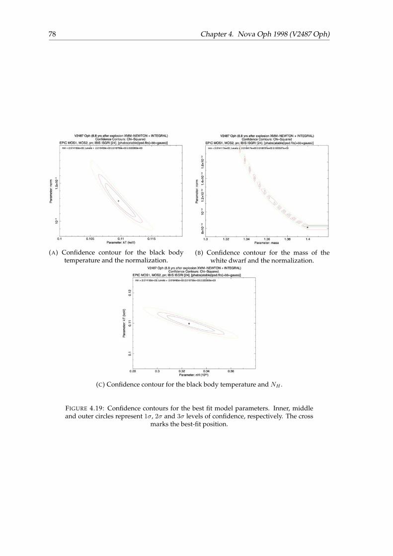
78 Chapter 4. Nova Oph 1998 (V2487 Oph)
(A) Confidence contour for the black bodytemperature and the normalization.
(B) Confidence contour for the mass of thewhite dwarf and the normalization.
(C) Confidence contour for the black body temperature and NH .
FIGURE 4.19: Confidence contours for the best fit model parameters. Inner, middleand outer circles represent 1σ, 2σ and 3σ levels of confidence, respectively. The cross
marks the best-fit position.

4.3. Spectral analysis 79
In order to improve the fit, we have also included three Gaussian lines, correspondingto the iron emission lines; at 6.4 keV corresponding to fluorescence Fe Kα, and thermalplasma He-like and H-like emission. The new model is given by [phabs∗(atableipzk.fits)+bbody+3gauss] for the tabulated model with the bremsstrahlung approximation of Zombeckand [phabs ∗ (atableipsd.fits) + bbody + 3gauss] for the model with the cooling func-tion given by Sutherland & Dopita. figures 4.20 and 4.22 shows the XMM-Newton-EPICand INTEGRAL-IBIS observations for the Nova Oph 1998 and the fitted models. Theiron lines have been fixed to 6.4, 6.68 and 6.97 keV. Also, the interstellar absorptionhas been fixed to NH = 2.2 × 1021 cm−2. The black body temperature, in both cases, iskTbbody = 0.11 keV but the χ2
ν is higher, 1.8 for 1589 degrees of freedom, than the obtainedbefore. Probably because the differences in the absorption. Figures 4.21a, 4.21b and 4.21care the confidence contours for the fitted models with cooling approximation of Zombeckand Figures 4.23a, 4.23b and 4.23c are the confidence contours for the cooling results ofSutherland & Dopita.
FIGURE 4.20: XMM-Newton 5th observation with EPIC MOS1 (black), MOS2 (red)and PN (green) and INTEGRAL observations IBIS/ISGRI (24 channels) (blue) using thetabulated model with cooling approximation of Zombeck. The black body componentis kTbbody = 0.11 keV, the white dwarf mass is obtained MWD = 1.4 M and thereduced chi-square is χ2
ν = 1.8 for 1589 degrees of freedom. The lower panel show thefit residuals in σ units.

80 Chapter 4. Nova Oph 1998 (V2487 Oph)
(A) Confidence contour for the black bodytemperature and the normalization.
(B) Confidence contour for the mass of thewhite dwarf and the normalization.
(C) Confidence contour for the black body temperature and NH .
FIGURE 4.21: Confidence contours for cooling Zombeck. The contours shown are forone, two and three sigma. The cross marks the best-fit position.

4.3. Spectral analysis 81
FIGURE 4.22: XMM-Newton 5th observation with EPIC MOS1 (black), MOS2 (red)and PN (green) and INTEGRAL observations IBIS/ISGRI (24 channels) (blue) usingthe tabulated model with cooling results of Sutherland & Dopita. The black bodycomponent is kTbbody = 0.11 keV, the white dwarf mass is obtained MWD = 1.4 Mand the reduced chi-square is χ2
ν = 1.8 for 1589 degrees of freedom. The lower panelshow the fit residuals in σ units.

82 Chapter 4. Nova Oph 1998 (V2487 Oph)
(A) Confidence contour for the black bodytemperature and the normalization.
(B) Confidence contour for the mass of thewhite dwarf and the normalization.
(C) Confidence contour for the black body temperature and NH .
FIGURE 4.23: Confidence contours for cooling Sutherland & Dopita. The contoursshown are for one, two and three sigma. The cross marks the best-fit position.
4.4 White dwarf mass estimation
The white dwarf mass is a fundamental parameter in cataclysmic binary. It not only gov-erns the dynamics of the orbital motion and the accretion flow, but also is a main parame-ter characterizing the emission of the accretion region. Moreover, it plays a fundamentalrole in the binary evolution, and accurate mass distributions of certain sub-classes canhelp in constraining the accretion history.
As mentioned before, one method to obtain the mass of the white dwarf in magneticcataclysmic variables is through their hard X-ray spectra. In order to derive the whitemass estimated we fitted the model presented in this work to the XMM-Newton-EPICand INTEGRAL-IBIS data of the Nova Oph 1998. Since the X-ray spectrum depends pri-marily on the white mass, using the tabulated model we are able to determine directly anestimate,and its uncertainty, of the white dwarf mass.

4.4. White dwarf mass estimation 83
From the fitting of the models, the white dwarf mass is estimated between MWD =
1.39 M and MWD = 1.40 M which is a higher value than the estimated by Hachisuet al. (2002), MWD = 1.35 M. However, it is consistent with what was expected for thiswhite dwarf.In order to determine the error in the estimation of the mass, confidence contours havebeen obtained.
As shown in Figures 4.7b, 4.9b, 4.11b and similars, the estimate of the error mass does notseem to be good. However, since this anomaly was present in all mass confidence con-tours, we explored what was happening with the calculation of the mass error. For this,synthetic spectra were created from the tabulated models (only the case of the Zombeckcooling approximation was used). Two spectra were created, one for a white dwarf ofmass MWD = 1.15 M and another for a mass of MWD = 1.40 M. The second value ofthe mass of the white dwarf was chosen because it is a similar value (in some cases, evenequal) to the value obtained for V2487 Oph.Since the method used for determining the “best-fit” model in XSPEC is defined as:
χ2 =∑ (C(I)− Cp(I))2
(σ(I))2(4.1)
where σ(I) is the error. A poissonian noise has been added to the synthetic spectra.
Once the synthetic spectra were created, the tabulated model ipzk.fits and an ab-sorption model, PHABS (NH = 0), were fitted to the synthetic observations3. Figure 4.24shows the syntethic spectrum for a white dwarf mass of 1.15 M and poissonian noise.
The best fit model for the synthetic spectrum for a white dwarf mass of MWD = 1.15 M
gives a mass of 1.14756 M, which is very close to the real value. The confidence contourfor the white dwarf mass and its normalization is shown in Figure 4.25.
3[phabs ∗ (atableipzk.fits)]

84 Chapter 4. Nova Oph 1998 (V2487 Oph)
FIGURE 4.24: Synthetic spectrum for a white dwarf mass of 1.15M and poissoniannoise.
FIGURE 4.25: Confidence contour for synthetic spectrum of MWD = 1.15M (Figure4.24). The contours shown are for one, two and three sigma. The cross marks the
best-fit position.
As in Figure 4.24 and 4.25. The spectrum and confidence contour for the mass are shownfor a white mass dwarf of MWD = 1.4M whose value is the upper limit of white dwarf

4.4. White dwarf mass estimation 85
mass of the model.
FIGURE 4.26: Synthetic spectrum for a white dwarf mass of 1.4M and poissoniannoise.
FIGURE 4.27: Confidence contour for synthetic spectrum of MWD = 1.4M (Figure4.26). The contours shown are for one, two and three sigma. The cross marks the
best-fit position.

86 Chapter 4. Nova Oph 1998 (V2487 Oph)
The value obtained for the mass is MWD = 1.39603M, which is in agreement withthe value of the mass, MWD = 1.4M. However, the confidence contours present thesame anomaly as those obtained for the nova V2487 Oph, this indicates that this anomalypresent in the contours is due to the fact that XSPEC can not adequately calculate the er-ror of the mass of the white dwarf, since the value obtained for the masses is one of thelimits (upper or lower) of the model. Nevertheless, despite this anomaly in the contours,the value obtained for the mass of the white dwarf is correct. This allows us to concludethat the value obtained from the masses of the white dwarf of V2487 Oph is correct, de-spite the contours that are obtained.

87
5CONCLUSIONS
In this thesis, we have investigated the emission region of accreting white dwarfs by thenumerical solution of the hydrodynamical differential equations. Based on the calculatedpost shock accretion column structure involving the change of the accretion rate, and us-gin different approximations for bremsstrahlung cooling emission, we present a spectralmodel of the accretion column. Furthermore, we have applied the model to the XMM-Newton and INTEGRAL observations of the Nova Oph 1998.
The hydrodynamic calculations presented in this thesis have allowed us to characterizethe emission region through its main physical quantities, temperature, density, pressureand velocity and also to obtain the position of the shock. These physical quantities havebeen obtained for (1) different masses and (2) different accretion rates and have been com-pared with other approximations computed by different authors. We also improve thecomputational method with the aim to improve the determination of the shock height.By the boundary condition, the velocity is close to zero in the white dwarf surface in-creasing from there off. It reaches the largest value in the shock position. In the sameway, the temperature reachs its maximum value at the shock. On the contrary, the den-sity increases as we approach to the white dwarf surface as well as the pressure.In order to determine the influence of the mass of the white dwarf the profiles of the phys-ical quantities have been obtained for different white dwarf masses. For higher masses,the gas velocity at the shock becomes higher, and therefore the gas density falls for agiven accretion rate. This causes a decrease in the plasma cooling rate, yielding highershock heights.In the same way, the influcence of the accretion rate have been examined. Calculations

88 Chapter 5. Conclusions
with different accretion rates have been performed. The emission region extends up-wards with a lower local mass accretion rate, a, i.e., the height of the shock is evidentlyproportional to a−1. When the local mass accretion rate is sufficiently high, the densityincreases towards the white dwarf surface. Moreover, the temperature shows a peak inthe middle of the emission region. At low enough local mass accretion rate, the temper-ature increase as local mass accretion rate increase. But, for a higher a, the temperaturestarts to decrease inward the white dwarf surface.
Since the emitted flux depends on the temperature and density, it is possible to obtainthe spectrum from these quantities. Because more massive white dwarfs have smallerradii, the corresponding shock temperatures are higher and a higher temperature im-plies a hotter emission region, and hence a harder X-ray spectrum is observed. For lessmassive white dwarfs the maximum of the spectrum is obtained at lower energies. Sincethe local mass accretion rate alters the temperature and density profiles, the X-ray spectraalso depend on the specific accretion rate. The continuum radiated by bremsstrahlunggenerally reduces as a decreases, because the accretion column becomes cooler and themaximum temperature downs.
The model was applied to X-ray observations of Nova Oph 1998. As already was de-mostrated by Hernanz & Sala (2002), the accretion have been reestablished on the cata-clysmic variable less than 100 days after outburst. Since the cataclysmic variable hostingthe nova was also detected before the outburst by ROSAT All Sky Survey, V2487 Ophis the first nova detected in X-rays before and after the outburst and supports the cata-clysmic variable scenario for classical novae (Hernanz & Sala, 2002).
Observations in X-rays show that V2487 Oph exhibits characteristics of Intermediate Po-lars and indicated that the white dwarf should be magnetic. As the spectrum is dom-inated by thermal plasma emission, a thermal bremsstrahlung continuum was appliedwith an absorption model and plus a black body component. As indicated Hernanz &Sala (2002) and Ferri & Hernanz (2007), the spectra display an emission at 6.4 keV cor-responding to the Fe fluorescent line and thermal plasma He-like and H-like emission at6.68 keV and 6.97 keV, respectively.Hachisu et al. (2002) through optical studies of the light curve, indicate that the whitedwarf of this nova is quite massive, MWD = 1.35 M, which is in agreement with therecurrent nature of V2487 Oph and with the white dwarf mass obtained from the X-rayspectra in this work: MWD = (1.39−1.40)M. Although the mass of the white dwarf hasbeen determined with good precision, it would be advisable to include emission lines tothe model in order to improve the fit. In additon, it has been indicated the possibilityof including a more modern cooling function, for example, computed by the code APEC(Smith et al., 2001) using the database AtomDB1 (Foster et al. (2011); Foster et al. (2012)).
1http://www.atomdb.org/

89
BIBLIOGRAPHY
Aizu K. 1973, X-Ray Emission Region of a White Dwarf with Accretion, Progress of Theoret-ical Physics, 49,(4), 1184–1194. ISSN: 0033-068X. DOI: 10.1143/PTP.49.1184. URL:http://adsabs.harvard.edu/abs/1973PThPh..49.1184A.
Anzolin G. 2008, Two new intermediate polars with a soft X-ray component, A&A, 489, 1243–1254. DOI: 10.1051/0004-6361:200810402. arXiv: 0808.1499.
Anzolin G. 2009, Broad-band properties of the hard X-ray cataclysmic variables IGR J00234+6141and 1RXS J213344.1+510725, A&A, 501, 1047–1058. DOI: 10.1051/0004- 6361/200911816. arXiv: 0905.1080 [astro-ph.SR].
Arnaud K. A. 1996, XSPEC: The First Ten Years, Astronomical Data Analysis Software andSystems V, A.S.P. Conference Series. Ed. by J. Jacoby, G.H. and Barnes. 101, p. 17–20.URL: http://adsabs.harvard.edu/abs/1996ASPC..101...17A.
Barlow E. J. 2006, 20-100 keV properties of cataclysmic variables detected in the INTEGRAL/IBISsurvey, MNRAS, 372, 224–232. DOI: 10.1111/j.1365-2966.2006.10836.x.eprint: astro-ph/0607473.
Beardmore A. P. Osborne J. P. And Hellier C, 2000, The multi-temperature X-ray spectrumof the intermediate polar V1223 Sagittarii, Monthly Notices of the Royal AstronomicalSociety, 315,(2), 307–315. ISSN: 0035-8711. DOI: 10.1046/j.1365-8711.2000.03477.x. URL: http://adsabs.harvard.edu/abs/2000MNRAS.315..307B.
Bernardini F. 2014, Swift J2218.4+1925: a new hard-X-ray-selected polar observed with XMM-Newton, MNRAS, 445, 1403–1411. DOI: 10.1093/mnras/stu1819. arXiv: 1409.2257 [astro-ph.HE].
Bird A. J. 2010, The Fourth IBIS/ISGRI Soft Gamma-ray Survey Catalog, Astrophys. J. Suppl.,186, 1–9. DOI: 10.1088/0067-0049/186/1/1. arXiv: 0910.1704 [astro-ph.HE].
Brunschweiger J. 2009, Intermediate polars in the Swift/BAT survey: Spectra and white dwarfmasses, Astronomy & Astrophysics, 127,(1), 8. ISSN: 00046361. DOI: 10.1051/0004-6361/200811285. arXiv: arXiv:0901.3562v1. URL: http://arxiv.org/abs/0901.3562.
Burwitz V. 1996, A new soft intermediate polar: RX J0512.2-3241 in Columba, A&A, 310, L25–L28.

90 BIBLIOGRAPHY
Butters O. W. 2011, RXTE and XMM observations of intermediate polar candidates, A&A, 526,A77, A77. DOI: 10.1051/0004-6361/201015848. arXiv: 1011.5762 [astro-ph.SR].
Canalle J. B. G. 2005, Accretion in dipole magnetic fields: flow structure and X-ray emissionof accreting white dwarfs, Astronomy and Astrophysics, 440, 185–198. DOI: 10.1051/0004-6361:20052706. URL: http://adsabs.harvard.edu/abs/2005A\%26A...440..185C.
Cash J, and Karp A. 1990, A variable order Runge-Kutta method for initial value problemswith rapidly varying right-hand sides, ACM Trans. Math. Softw., 16,(3), 201–222. ISSN:00983500. DOI: 10.1145/79505.79507. URL: http://www.elegio.it/mc2/rk/doc/p201-cash-karp.pdf.
Chandrasekhar S. 1931, The maximum mass of ideal white dwarfs, Journal of Astrophysicsand Astronomy, 74, 81. DOI: 10.1086/143324. URL: http://adsabs.harvard.edu/abs/1931ApJ....74...81C.
Chanmugam G, Langer S. H. And Shaviv G. 1985, Time-dependent accretion onto magneticwhite dwarfs-Effects of cyclotron emission, The Astrophysical Journal, 299, L87–L91. DOI:10.1086/184586. URL: http://adsabs.harvard.edu/full/1985ApJ...299L..87C.
Chevalier R. A. And Imamura J. N. 1982, Linear analysis of an oscillatory instability of ra-diative shock waves, The Astrophysical Journal, 261, 543. ISSN: 0004-637X. DOI: 10.1086/160364. URL: http://adsabs.harvard.edu/abs/1982ApJ...261..543Chttp://adsabs.harvard.edu/doi/10.1086/160364.
Cropper M. 1990, The Polars, Space Science Reviews, 54,(0038-6308), 195–295. DOI: 10.1007/BF00177799. URL: http://adsabs.harvard.edu/abs/1990SSRv...54..195C.
Cropper M. Ramsay G. And Wu K. 1998, White dwarf masses in magnetic cataclysmic vari-ables: multi-temperature fits to Ginga data, Monthly Notices of the Royal AstronomicalSociety, 293,(3), 222–232. ISSN: 0035-8711. DOI: 10.1046/j.1365-8711.1998.00610.x. URL: http://doi.wiley.com/10.1046/j.1365-8711.1998.00610.x.
Cropper M. 1999, Effects of Gravity on the Structure of Postshock Accretion Flows in Mag-netic Cataclysmic Variables, Monthly Notices of the Royal Astronomical Society, 306,684–690. ISSN: 00358711. DOI: 10.1046/j.1365-8711.1999.02570.x. arXiv:9902355 [astro-ph]. URL: http://arxiv.org/abs/astro-ph/9902355.
de Martino D. 2004, BeppoSAX observations of soft X-ray intermediate polars, A&A, 415, 1009–1019. DOI: 10.1051/0004-6361:20034160. eprint: astro-ph/0311557.
de Martino D. 2008, 1RXS J173021.5-055933: a cataclysmic variable with a fast-spinning mag-netic white dwarf, A&A, 481, 149–159. DOI: 10.1051/0004-6361:20078368. arXiv:0801.3649.
Dickey J. M. And Lockman F. J. 1990, H I in the Galaxy, Annu. Rev. Astron. Astrophys., 28,215–261. DOI: 10.1146/annurev.aa.28.090190.001243.

BIBLIOGRAPHY 91
Evans P. A. And Hellier C. 2007, Why Do Some Intermediate Polars Show Soft X-Ray Emis-sion? A Survey of XMM-Newton Spectra, Astrophys. J., 663, 1277–1284. DOI: 10.1086/518552. arXiv: 0704.1388.
Ezuka H. And Ishida M. 1999, Iron Line Diagnostics of the Postshock Hot Plasma in Magnet-icCataclysmic Variables Observed with ASCA, The Astrophysical Journal SupplementSeries, 120,(1), 277–298. ISSN: 00670049. DOI: 10.1086/313181. URL: http://adsabs.harvard.edu/abs/1999ApJS..120..277E.
Fabian A. C. Pringle J. E. And Rees M. J. 1976, X-ray emission from accretion on to whitedwarfs., Monthly Notices of the Royal Astronomical Society, 175, 43–60. URL: http://adsabs.harvard.edu/abs/1976MNRAS.175...43F.
Falanga M, Bonnet-Bidaud J. And Suleimanov V, 2005, INTEGRAL broadband X-ray spec-trum of the intermediate polar V709 Cassiopeiae, Astronomy and Astrophysics, 444,(2),561–564. ISSN: 0004-6361. DOI: 10.1051/0004- 6361:20054002. URL: http://adsabs.harvard.edu/abs/2005A\%26A...444..561F.
Ferri C. 2011, X-ray emission from accreting white dwarfs in post-outburst novae, PhD thesis.Universitat de Barcelona, 175.
Ferri C. And Hernanz M. 2007, V2487 Oph 1998 : a Magnetic Classical Nova ?, 15th EuropeanWorkshop on White Dwarfs ASP Conference Series. Ed. by R Napiwotzki & M.R. Burleigh.372, p. 8–11. URL: http://adsabs.harvard.edu/abs/2007ASPC..372..519F.
Filippenko A. V. 1998, Nova Ophiuchi 1998, , 6943,Foster A. R. 2011, AtomDB v2 . 0 : Atomic Data for X-ray Astrophysics, 2010 NASA Labo-
ratory Astrophysics Workshop. Gaitlinburg, TN: Schultz, David R., p. C2. URL: http://adsabs.harvard.edu/abs/2011nlaw.confC...2F.
Foster A. R. 2012, Updated Atomic Data and Calculations for X-Ray Spectroscopy, The Astro-physical Journal, 756,(2), 128. ISSN: 0004-637X. DOI: 10.1088/0004-637X/756/2/128. URL: http://stacks.iop.org/0004-637X/756/i=2/a=128?key=crossref.b434017b11a0ec2fe162108dbb76f744.
Frank J. King A. And Raine D. 1992, Accretion power in astrophysics.Frank J. King A. And Raine D. 2002, Accretion Power in Astrophysics: Third Edition. Third
Edit. 39, Cambridge University Press, 398. ISBN: 0521620538. URL: http://adsabs.harvard.edu/abs/2002apa..book.....F.
Frank J. And King R. A. 1984, Column accretion onto white dwarfs - Non-local electron trans-port and the soft X-ray excess, Astronomy and Astrophysics, 134, 328–332. URL: http://adsabs.harvard.edu/abs/1984A\%26A...134..328F.
Frank, J. King, A. R. and Lasota J. P. 1983, Column accretion on to white dwarfs, MonthlyNotices of the Royal Astronomical Society, 202,(0035-8711), 183–199. DOI: 10.1093/mnras/202.1.183. URL: http://adsabs.harvard.edu/abs/1983MNRAS.202..183F.
Fujimoto R. And Ishida M. 1997, Mass Determination of the White Dwarf in Magnetic Cat-aclysmic Variables, X-Ray Imaging and Spectroscopy of Cosmic Hot Plasmas. Ed. by F.Makino & K. Mitsuda, p. 561.

92 BIBLIOGRAPHY
Fujimoto R. And Ishida M. 1997, XRay Spectroscopic Observations of EX Hydrae and MassDetermination of the White Dwarf, The Astrophysical Journal, 474,(2), 774–781. ISSN:0004-637X. DOI: 10.1086/303483. URL: http://stacks.iop.org/0004-637X/474/i=2/a=774.
Girish V. And Singh K. P. 2012, X-ray observations of INTEGRAL discovered cataclysmic vari-able IGR J17195-4100, MNRAS, 427, 458–467. DOI: 10.1111/j.1365-2966.2012.21916.x. arXiv: 1208.3425 [astro-ph.HE].
Goldwurm A. 2003, The INTEGRAL/IBIS scientific data analysis, A&A, 411, L223–L229. DOI:10.1051/0004-6361:20031395. eprint: astro-ph/0311172.
Haberl F. Motch C. And Zickgraf F.-J. 2002, X-ray and optical observations of 1RXS J154814.5-452845: A new intermediate polar with soft X-ray emission, A&A, 387, 201–214. DOI: 10.1051/0004-6361:20020347. eprint: astro-ph/0203227.
Haberl F. 1994, Discovery of the new intermediate polar RX J0558.0+5353, A&A, 291, 171–180.Hachisu I. 2002, V2487 Ophiuchi: A strong candidate for a recurrent nova and a progenitor of
Type Ia supernova, The Physics of Cataclysmic Variables and Related Objects, ASP Confer-ence Series. Ed. by B. T. Gnsicke, K. Beuermann, & K. Reinsch. 261, San Francisco, p.629. URL: http://adsabs.harvard.edu/abs/2002ASPC..261..629H.
Harris M. J. 1999, Transient Gamma Ray Spectrometer Observations of Gamma-Ray Lines fromNovae. I. Limits on the Positron Annihilation Line in Five Individual Novae, Astrophys. J.,522, 424–432. DOI: 10.1086/307625. eprint: astro-ph/0004164.
Hayakawa A. And Hoshi R. 1976, Extended X-Ray Emission Region of an Accreting WhiteDwarf, Progress of Theoretical Physics, 55,(4), 1320–1321. ISSN: 0033-068X. DOI: 10.1143/PTP.55.1320. URL: https://academic.oup.com/ptp/article-lookup/doi/10.1143/PTP.55.1320http://adsabs.harvard.edu/abs/
1976PThPh..55.1320H.Hayakawa S. Matsuoka M. And Sugimoto D. 1966, Galactic X-Rays, Space Science Re-
views, 5, 109–163. DOI: 10.1007/BF00179217. URL: http://adsabs.harvard.edu/abs/1966SSRv....5..109H.
Hayashi T. 2014, PhD thesis. Tokyo Metropolitan University, 155.Hayashi T. And Ishida M. 2014a, A new comprehensive X-ray spectral model from the post-
shock accretion column in intermediate polars, Monthly Notices of the Royal Astronomi-cal Society, 438,(3), 2267–2277. ISSN: 00358711. DOI: 10.1093/mnras/stt2342.
— 2014. b, Application of the new comprehensive X-ray spectral model to the two brightestintermediate polars ex hydrae and V1223 sagittarii, Monthly Notices of the Royal Astro-nomical Society, 441,(4), 3718–3723. ISSN: 13652966. DOI: 10.1093/mnras/stu766.
Hellier C. Mukai K. And Osborne J. P. 1998, Iron Kalpha linewidths in magnetic cataclysmicvariables, MNRAS, 297, 526–530. DOI: 10.1046/j.1365-8711.1998.01557.x.eprint: astro-ph/9802040.
Hellier C. 1996, The X-ray spectrum of the intermediate polar AO Piscium, Monthly Noticesof the Royal Astronomical Society, 280, 877–887. DOI: 10.1093/mnras/280.3.877.URL: http://adsabs.harvard.edu/abs/1996MNRAS.280..877H.

BIBLIOGRAPHY 93
Hellier C. 1996, The intermediate polars, Cataclysmic variables and related objects. Astrophysicsand Space Science Library; Proceedings of the 158th colloquium of the International Astro-nomical Union (IAU). Ed. by A. Evans & Janet H. Wood. 208, Keele: Kluwer AcademicPublishers, p. 143. DOI: 10.1007/978- 94- 009- 0325- 8_44. URL: http://adsabs.harvard.edu/abs/1996ASSL..208..143H.
Hellier C. And Mukai K. 2004, On the iron K(alfa) complex in magnetic cataclysmic vari-ables, Monthly Notices of the Royal Astronomical Society, 352,(3), 1037–1040. ISSN:00358711. DOI: 10.1111/j.1365-2966.2004.07995.x.
Hernanz M. And Sala G. 2002, A Classical Nova, V2487 Oph 1998, Seen in X-rays Beforeand After Its Explosion, Science, 298,(5592), 393–395. ISSN: 00368075. DOI: 10.1126/science.298.5592.393. URL: http://www.sciencemag.org/cgi/doi/10.1126/science.298.5592.393.
Hoshi R. 1973, X-Ray Emission from White Dwarfs in Close Binary Systems, Progress ofTheoretical Physics, 49,(3), 776–789. DOI: 10.1143/PTP.49.776. URL: http://adsabs.harvard.edu/abs/1973PThPh..49..776H.
Imamura J. N. 1981, The Ultraviolet and X-Ray Spectra of Accreting Degenerate Dwarfs., PhDthesis. INDIANA UNIVERSITY.
Imamura J. N. And Durisen R. H. 1983, X-ray spectra and light curves of accreting magneticdegenerate dwarfs, The Astrophysical Journal, 268, 291–308. DOI: 10.1086/160954.URL: http://adsabs.harvard.edu/abs/1983ApJ...268..291I.
Imamura J. N. 1987, X-ray and ultraviolet radiation from accreting white dwarfs. IV - Two-temperature treatment with electron thermal conduction, The Astrophysical Journal, 313,298–319. DOI: 10.1086/164969. URL: http://adsabs.harvard.edu/abs/1987ApJ...313..298I.
Imamura J. N. 1996, The Stability Properties of Two-Temperature White Dwarf Radiative ShockWaves, The Astrophysical Journal, 458, 327–337. DOI: 10.1086/176815. URL: http://adsabs.harvard.edu/abs/1996ApJ...458..327I.
Ishida M. 1991, PhD thesis. PhD thesis,Univ. Tokyo, (1991).Ishida M. And Fujimoto R. 1995, Diagnostics of the Postshock Hot Plasma with ASCA - I, Cape
Workshop on Magnetic cataclysmic variables; Astronomical Society of the Pacific ConferenceSeries. 85, p. 132. URL: http://adsabs.harvard.edu/abs/1995ASPC...85..132I.
Ishida M. Mukai K. And Osborne J. P. 1994, Observation of EX Hydrae with ASCA, , 46,L81–L85.
Katz J. I. 1977, X-rays from spherical accretion onto degenerate dwarfs, The Astrophysical Jour-nal, 215, 265–275. DOI: 10.1086/155355. URL: http://adsabs.harvard.edu/abs/1977ApJ...215..265K.
King A. R. And Lasota J. P. 1979, Accretion on to highly magnetized white dwarfs, MonthlyNotices of the Royal Astronomical Society, 188,(3), 653–668. ISSN: 0035-8711. DOI:10.1093/mnras/188.3.653. URL: http://mnras.oxfordjournals.org/content/188/3/653.shorthttps://academic.oup.com/mnras/article-
lookup/doi/10.1093/mnras/188.3.653.

94 BIBLIOGRAPHY
Knigge C. Baraffe I. And Patterson J. 2011, The Evolution of Cataclysmic Variables as Revealedby Their Donor Stars, Astrophys. J. Suppl., 194, 28, 28. DOI: 10.1088/0067-0049/194/2/28. arXiv: 1102.2440 [astro-ph.SR].
Kylafis N. D. And Lamb D. Q. 1979, X-ray and UV radiation from accreting nonmagneticdegenerate dwarfs, The Astrophysical Journal Letters, 228, L105–L110. DOI: 10.1086/182913. URL: http://adsabs.harvard.edu/abs/1979ApJ...228L.105K.
Lamb D. Q. And Masters A. R. 1979, X and UV radiation from accreting magnetic degeneratedwarfs, Astrophys. J. Lett., 234, L117–L122. DOI: 10.1086/183121.
Landi R. 2009, INTEGRAL/IBIS and Swift/XRT observations of hard cataclysmic variables,MNRAS, 392, 630–640. DOI: 10.1111/j.1365- 2966.2008.14086.x. arXiv:0810.1844.
Langer S. H. Chanmugam C. And Shaviv G. 1982, Time-dependent accretion onto mag-netized white dwarfs, The Astrophysical Journal, 258, 289–305. ISSN: 0004-637X. DOI:10.1086/160079. URL: http://adsabs.harvard.edu/abs/1982ApJ...258..289L.
Langer S. H. Chanmugam G, and Shaviv G, 1981, Thermal instability in accretion flows ontodegenerate stars, The Astrophysical Journal, 245, L23. ISSN: 0004-637X. DOI: 10.1086/183514. URL: http://adsabs.harvard.edu/doi/10.1086/183514.
Liller W. And Jones A. 1999a, Light Curves for Nova Mus 1998 and Nova Oph 1998, Infor-mation Bulletin on Variable Stars, 4774,
Liller W. And Jones A. F. 1999b, Light Curves for Nova Sgr 1998 and Nova Sco 1998, Infor-mation Bulletin on Variable Stars, 4664,
Lodders K. 2003, Solar System Abundances and Condensation Temperatures of the Elements,Astrophys. J., 591, 1220–1247. DOI: 10.1086/375492.
Lynch D. K. 2000, 0.8-2.5 Micron Spectroscopy of Nova Ophiuchi 1998, Astrophys. J., 541, 791–801. DOI: 10.1086/309453.
Lynden-Bell D. And Pringle J. E. 1974, The evolution of viscous discs and the origin of thenebular variables., MNRAS, 168, 603–637. DOI: 10.1093/mnras/168.3.603.
MacDonald J. And Vennes S. 1991, Thermal X-ray emission from classical novae in opticaldecline, The Astrophysical Journal, 373, L51–L54. ISSN: 0004-637X. DOI: 10.1086/186049. URL: http://adsabs.harvard.edu/abs/1991ApJ...373L..51Mhttp://adsabs.harvard.edu/doi/10.1086/186049.
Mason K. O. Rosen S. R. And Hellier C. 1988, The accretion geometry of intermediate polars(DQ HER stars), Advances in Space Research, 8, 293–303. DOI: 10.1016/0273-1177(88)90419-X.
Mason K. O. 1992, A new, EUV-bright intermediate polar discovered in the ROSAT Wide FieldCamera all-sky survey, MNRAS, 258, 749–758. DOI: 10.1093/mnras/258.4.749.
Matt G. 1999, X-ray spectroscopy of magnetic CVs, Annapolis Workshop on Magnetic Cata-clysmic Variables. Ed. by C. Hellier & K. Mukai. 157, Astronomical Society of the PacificConference Series, p. 299.
Mewe R. Gronenschild E. H. B. M. And van den Oord G. H. J. 1985, Calculated X-radiationfrom optically thin plasmas. V, , 62, 197–254.

BIBLIOGRAPHY 95
Mewe R, Lemen J. R. And Oord G. H. J. 1986, Calculated X-radiation from optically thinplasmas. VI - Improved calculations for continuum emission and approximation formulae fornonrelativistic average Gaunt factors, Astronomy & Astrophysics Supplement Series, 65,511–536. ISSN: 0365-0138. URL: http://adsabs.harvard.edu/abs/1986A\&AS...65..511M.
Motch C. 1996, New cataclysmic variables from the ROSAT All-Sky Survey., A&A, 307, 459–469.
Mukai K. 1997, The X-Ray Eclipse of the Dwarf Nova HT Cassiopeiae: Results from ASCA andROSAT HRI Observations, Astrophys. J., 475, 812–822. DOI: 10.1086/303571.
Nakano S. 1998, Possible Nova in Ophiuchus, , 6941,Narayan R. And Popham R. 1993, Hard X-rays from accretion disk boundary layers, Nature,
362, 820–822. DOI: 10.1038/362820a0.Nauenberg M. 1972, Analytic Approximations to the Mass-Radius Relation and Energy of Zero-
Temperature Stars, The Astrophysical Journal, 175, 417–430. ISSN: 0004-637X. DOI: 10.1086/151568. URL: http://adsabs.harvard.edu/doi/10.1086/151568.
Pagnotta A. Schaefer B. E. And Xiao L. 2008, V2487 Ophiuchi, , 8951,Pagnotta A. 2009, Discovery of a Second Nova Eruption of V2487 Ophiuchi, Astr. J., 138, 1230–
1234. DOI: 10.1088/0004-6256/138/5/1230. arXiv: 0908.2143 [astro-ph.HE].Pandel D. 2005, X-Ray Observations of the Boundary Layer in Dwarf Novae at Low Accre-
tion Rates, Astrophys. J., 626, 396–410. DOI: 10.1086/429983. eprint: astro-ph/0503114.
Patterson J. 1994, The DQ Herculis stars, , 106, 209–238. DOI: 10.1086/133375.Press W. H. 2003, Numerical recipes in Fortran 77. Second Edi. Press Syndicate of the Uni-
versity of Cambridge, 1003. ISBN: 052143064X.Ramsay G. And Cropper M. 2004, The energy balance of polars revisited, MNRAS, 347, 497–
507. DOI: 10.1111/j.1365-2966.2004.07220.x. eprint: astro-ph/0309527.Ramsay G, 1998, A comparison of white dwarf mass estimators using the intermediate po-
lar XY Ari, Monthly Notices of the Royal Astronomical Society, 297,(4), 1269–1273.ISSN: 0035-8711. DOI: 10.1046/j.1365-8711.1998.01609.x. URL: https://academic.oup.com/mnras/article-lookup/doi/10.1046/j.1365-
8711.1998.01609.xhttp://adsabs.harvard.edu/abs/1998MNRAS.297.
1269R.Ramsay G. 2009, 2XMMiJ225036.9+573154 - a new eclipsing AMHer binary discovered using
XMM-Newton, MNRAS, 395, 416–421. DOI: 10.1111/j.1365-2966.2009.14528.x. arXiv: 0901.3095 [astro-ph.GA].
Ramsay G. 2000, Determining the mass of the accreting white dwarf in magnetic cataclysmicvariables using RXTE data, Monthly Notices of the Royal Astronomical Society, 314,(2),403–408. ISSN: 0035-8711. DOI: 10.1046/j.1365-8711.2000.03239.x. arXiv:9912420 [astro-ph]. URL: http://arxiv.org/abs/astro-ph/9912420https://academic.oup.com/mnras/article-lookup/doi/10.1046/j.1365-
8711.2000.03239.x.

96 BIBLIOGRAPHY
Rana V. R. 2006, Study of Fe Kα lines in Nonmagnetic Cataclysmic Variables Using ChandraHEG Data, Astrophys. J., 642, 1042–1050. DOI: 10.1086/500316. eprint: astro-ph/0512274.
Revnivtsev M. G. 2004, Broadband X-ray Spectrum of the Intermediate Polar V2400 Oph, As-tronomy Letters, 30,(11), 772–778. ISSN: 1063-7737. URL: http://adsabs.harvard.edu/abs/2004AstL...30..772R.
Ritter H. 2010, Formation and evolution of cataclysmic variables ., , 81, 849.Sala G. 2004a, X-ray emission from classical novae, PhD thesis. Universitat de Barcelona,
252.— 2004. b, XRay Emission from Classical Novae, Publications of the Astronomical Soci-
ety of the Pacific, 116,(826), 1154–1154. ISSN: 0004-6280. DOI: 10.1086/427071.URL: http://adsabs.harvard.edu/abs/2004PASP..116.1154Shttp://iopscience.iop.org/article/10.1086/427071.
Saxton C. J. 1999, Stability properties of radiative accretion shocks with multiple cooling pro-cesses., PhD thesis. PhD thesis, Univ. Sydney, Australia , (1999).
Saxton C. J. 1998, Oscillatory instability of radiative shocks with multiple cooling processes,Monthly Notices of the Royal Astronomical Society, 299,(3), 862–876. ISSN: 0035-8711.DOI: 10.1046/j.1365-8711.1998.01839.x. URL: https://academic.oup.com/mnras/article-lookup/doi/10.1046/j.1365-8711.1998.01839.x.
Saxton C. J. And Wu K. 1999, Perturbative analysis of two-temperature radiative shocks withmultiple cooling processes, Monthly Notices of the Royal Astronomical Society, 310,(3),677–692. ISSN: 0035-8711. DOI: 10.1046/j.1365-8711.1999.02967.x. arXiv:9909502v1 [arXiv:astro-ph]. URL: https://academic.oup.com/mnras/article-lookup/doi/10.1046/j.1365-8711.1999.02967.x.
Saxton C. J. 2005, Two-temperature accretion flows in magnetic cataclysmic variables: struc-tures of post-shock emission regions and X-ray spectroscopy, Monthly Notices of the RoyalAstronomical Society, 360,(3), 1091–1104. ISSN: 0035-8711. DOI: 10.1111/j.1365-2966.2005.09103.x. URL: http://adsabs.harvard.edu/abs/2005MNRAS.360.1091S.
Saxton C. J. 2007, X-ray emissions from two-temperature accretion flows within a dipole mag-netic funnel, Monthly Notices of the Royal Astronomical Society, 379, 779–790. ISSN:0035-8711. DOI: 10.1111/j.1365-2966.2007.11958.x. URL: http://adsabs.harvard.edu/abs/2007MNRAS.379..779S.
Schaefer B. E. 2010, Comprehensive Photometric Histories of All Known Galactic RecurrentNovae, Astrophys. J. Suppl., 187, 275–373. DOI: 10.1088/0067-0049/187/2/275.arXiv: 0912.4426 [astro-ph.SR].
Smith R. K. 2001, Collisional Plasma Models with APEC/APED: Emission-Line Diagnostics ofHydrogen-like and Helium-like Ions, The Astrophysical Journal, 556,(2), L91–L95. ISSN:0004637X. DOI: 10.1086/322992. arXiv: 0106478 [astro-ph]. URL: http://adsabs.harvard.edu.ezp-prod1.hul.harvard.edu/abs/2001ApJ...
556L..91S\%5Cnhttp://iopscience.iop.org/1538-4357/556/2/L91/
fulltext/.

BIBLIOGRAPHY 97
Staude A. 2008, The changing accretion states of the intermediate polar MU Camelopardalis,A&A, 486, 899–909. DOI: 10.1051/0004-6361:20067013. arXiv: 0806.0793.
Strope R. J. Schaefer B. E. And Henden A. A. 2010, Catalog of 93 Nova Light Curves: Clas-sification and Properties, Astr. J., 140, 34–62. DOI: 10.1088/0004-6256/140/1/34.arXiv: 1004.3698 [astro-ph.SR].
Suleimanov V. Revnivtsev M. And Ritter H. 2005, RXTE broadband X-ray spectra of interme-diate polars and white dwarf mass estimates, Astronomy and Astrophysics, 435,(1), 191–199. ISSN: 0004-6361. DOI: 10.1051/0004-6361:20041283. arXiv: 0405236v1[arXiv:astro-ph]. URL: http://cdsads.u-strasbg.fr/abs/2005A\&A...435..191Shttp://www.edpsciences.org/10.1051/0004-6361:
20041283.Suleimanov V. 2016, GK Persei and EX Hydrae: Intermediate polars with small magnetospheres,
Astronomy & Astrophysics, 591, A35. ISSN: 0004-6361. DOI: 10.1051/0004-6361/201628301. arXiv: 1604.00232. URL: http://arxiv.org/abs/1604.00232http://www.aanda.org/10.1051/0004-6361/201628301.
Sutherland R. S. And Dopita M. A. 1993, Cooling functions for low-density astrophysical plas-mas, The Astrophysical Journal Supplement Series, 88, 253. ISSN: 0067-0049. DOI: 10.1086/191823. URL: http://adsabs.harvard.edu/doi/10.1086/191823.
Ubertini P. 2003, IBIS: The Imager on-board INTEGRAL, A&A, 411, L131–L139. DOI: 10.1051/0004-6361:20031224.
Verner D. A. 1996, Atomic Data for Astrophysics. II. New Analytic FITS for PhotoionizationCross Sections of Atoms and Ions, Astrophys. J., 465, 487. DOI: 10.1086/177435. eprint:astro-ph/9601009.
Vogel J. 2008, The serendipituous discovery of a short-period eclipsing polar in 2XMMp, A&A,485, 787–795. DOI: 10.1051/0004-6361:20079341. arXiv: 0804.3946.
Wada T.-a. 1980, X-Ray and Infrared Emissions from Accreting Magnetic White Dwarfs: AModel for AM Herculis, Progress of Theoretical Physics, 64,(6), 1986–1994. ISSN: 0033-068X. DOI: 10.1143/PTP.64.1986. URL: http://adsabs.harvard.edu/abs/1980PThPh..64.1986Whttps://academic.oup.com/ptp/article-
lookup/doi/10.1143/PTP.64.1986.Warner B. 1995, Cataclysmic variable stars., Cambridge Astrophysics Series, 28,Woelk, U. and Beuermann K. 1996, Stationary radiation hydrodynamics of accreting magnetic
white dwarfs., Astronomy and Astrophysics, 306, 232–240. URL: http://adsabs.harvard.edu/abs/1996A\%26A...306..232W.
Wolff M. T. Gardner J. H. And Wood K. S. 1989, On the stability of degenerate dwarf radiativeshocks - New one- and two-temperature calculations, The Astrophysical Journal, 346, 833.ISSN: 0004-637X. DOI: 10.1086/168064. URL: http://adsabs.harvard.edu/abs/1989ApJ...346..833Whttp://adsabs.harvard.edu/doi/10.1086/
168064.Wu K. Chanmugam G. And Shaviv G. 1995, X-rays from Magnetic CVs and White Dwarf
Mass Determination, Magnetic Cataclysmic Variables. Cape Workshop on Magnetic cata-clysmic variables; Astronomical Society of the Pacific Conference Series. Ed. by D. A. H.

98 BIBLIOGRAPHY
Buckely & Brian Warner. 85, Cape Town: Astronomical Society of the Pacific, p. 436.URL: http://adsabs.harvard.edu/abs/1995ASPC...85..436W.
Wu K. 1994, Structure of inhomogeneous accretion shocks, Proceedings of the AstronomicalSociety of Australia, 11, 61–64. ISSN: 00669997. URL: http://adsabs.harvard.edu/abs/1994PASAu..11...61W.
Wu K. Chanmugam G. And Shaviv G. 1994, Structure of steady state accretion shocks withseveral cooling functions: Closed integral-form solution, The Astrophysical Journal, 426,664. ISSN: 0004637X. DOI: 10.1086/174103. URL: http://adsabs.harvard.edu/doi/10.1086/174103.
Wu K. And Cropper M. 2001, The lower boundary of the accretion column in magnetic cata-clysmic variables, Monthly Notices of the Royal Astronomical Society, 326,(2), 686–694.ISSN: 00358711. DOI: 10.1046/j.1365-8711.2001.04640.x. arXiv: 0105140[astro-ph].
Wu, Kinwah and Wickramasinghe D. T. 1992, Three-dimensional structured shocks in AMHerculis-type systems. II - Cyclotron emission from ridge-shaped emission regions, MonthlyNotices of the Royal Astronomical Society, 256, 329–338. DOI: 10.1093/mnras/256.2.329. URL: http://adsabs.harvard.edu/abs/1992MNRAS.256..329W.
Yuasa T, 2010, White dwarf masses in intermediate polars observed with the Suzaku satellite, As-tronomy and Astrophysics, 520, A25. ISSN: 0004-6361. DOI: 10.1051/0004-6361/201014542. URL: http://www.aanda.org/10.1051/0004-6361/201014542.
Zombeck M. V. 1982, Hot plasma Emission, Handbook of Space Astronomy and Astrophysics.Cambridge University Press, p. 326. ISBN: 0-521-24194-4.

99
AGENERAL HYDRODYNAMICS FOR-MULATION
An accretion flow is governed entirely by conservation laws: the conservation of mass,the conservation of momentum and the conservation of energy. These conservation lawscan be written in the form of partial differential equations as well as in the form of in-tegral equations. Both forms, will prove to be useful for the numerical methods and aredescribed as follow.
A.1 Mass Conservation
FIGURE A.1: Flow through a volume V with surface ∂V = S.
Consider an arbitrary volume V in the space in which the gas flow takes place. Its surfaceis denoted as ∂V = S with the normal unit vector at each location on the surface denotedas ~n and differential surface element as dS (Figure A.1). Let ρ be the fluid density into the

100 Appendix A. General hydrodynamics formulation
volume V where there are no masses sources of sinks. Then, by mass conservation
D
Dt
∫∫∫VρdV = 0 (A.1)
from kinetic transport theorem1 this equation can be expressed as∫∫∫V
∂ρ
∂tdV +
∫∫Sρ~v · ~ndS = 0 (A.2)
and using the Gauss’ theorem∫∫∫V
~∇ ·GdV =
∫∫SG · ~ndS (A.3)
the surface integral is written as a volume integral in the way∫∫Sρ~v · ~ndS =
∫∫∫V
~∇ · (ρ~v)dV (A.4)
Since all volume integrals are in an arbitrary volume, the mass conservation law, alsocalled continuity equation, is
∂ρ
∂t+ ~∇(ρ~v) = 0 (A.5)
A.2 Momentum Conservation
Applying the second Newton’s law in a volume containing a fluid it is possible to obtain
D
Dt
∫∫∫Vρ~vdV =
∑~F (A.6)
There are two types of forces which can act on a fluid.
• Surface forces, also called short-range forces, have a molecular origin and decreaserapidly with the distance between the interacting elements. They are appreciableonly if the fluid elements are in contact, therefore exist only in the boundary. Sur-face forces over area unit is called stress ~S which depends on time, location, andorientation of the surface element. The total surface force acting on the fluid is∫∫S~SdA. The pressure and friction are examples of short-range forces.
• Body forces, also known as long-range forces, have an origin far away for the zoneof interest. Their strength change very slowly, and act uniformly on all parts of thefluid. The sum of long-range forces, denotes as ~f , is proportional to the volume ofthe fluid. The total body forces acting on the volume is
∫∫∫V~fdV . The gavity is an
example of long-range forces.
1Being G(~r, t) some fluid property per unit volume, then DDt
∫∫∫VGdV =
∫∫∫V
∂G∂tdV +
∫∫SG~v~ndS

A.2. Momentum Conservation 101
therefore, the second Newton’s law is expressed as
D
Dt
∫∫∫Vρ~vdV =
∫∫S
~SdA+
∫∫∫V
~fdV (A.7)
using the kinetic transport theorem, the left-hand side becomes
D
Dt
∫∫∫Vρ~vdV =
∫∫∫VρD
Dt~vdV (A.8)
the first term in the rigth-hand side can be expressed as an volume integral using theGauss’ theorem in the form ∫∫
S
~SdA =
∫∫∫V
~∇σdV (A.9)
where σ is an square array called stress tensor. According to the Cauchy’s theorem, σij ,describes the stress components on any surface. (see Figure A.2).
FIGURE A.2: Components in the surface.
Since now all terms are expressed as volume integrals, the momentun equation can bewritten as
ρD
Dt~v = ~∇σ + ~f (A.10)
applying the kinetic transport theorem, the first term can be expressed as
ρD
Dt~v = ρ
(∂
∂t~v + (~v~∇)~v
)(A.11)
thus, the momentun conservation equation is
ρ
(∂
∂t~v + (~v~∇)~v
)= ~∇σ + ~f (A.12)
Let assume now that the only surface force acting in the fluid is the hydrostatic pressureP . According to the Pascal’s principle, in a fluid at rest the pressure is uniformly trans-mitted in all directions and in all portions of the fluid. Therefore, the pressure is isotropicand σ only has diagonal components. Moreover, all of them have the same value P . Thus,the stress tensor has the form σ = −P I where the minus sign is adopted by convention.

102 Appendix A. General hydrodynamics formulation
Therefore the momentun equation (likewise known as Euler’s equation) is written as
ρ
(∂~v
∂t+ (~v~∇)~v
)= ~f − ~∇P (A.13)
A.3 Energy Conservation
Energy exists in many forms. Consider the two most basic ones: mechanical and thermalenergy. e is the internal (thermal) energy per unit of mass due to microscopic motion andv2/2 the kinetic energy per unit of mass due to macroscopic motion. According to thefirst thermodynamics law, the energy conservation requires
D
Dt
∫∫∫Vρ
(e+
v2
2
)dV = −
∫∫S
~Q · ~ndS −∫∫
S
~Frad · ~ndS +
∫∫∫V
~f · ~vdV +
∫∫S
~S · ~vdS
(A.14)using the kinetic transport theorem, the left hand side term, which accounts for the rateof increment of energy in V can be written as∫∫∫
V
D
Dtρ
(e+
v2
2
)dV (A.15)
and using the Gauss theorem the first term on the rigth hand side, which is the rate ofheat flux into V , can be expressed as
−∫∫
S
~Q · ~ndS = −∫∫∫
V
~∇ · ~QdV (A.16)
In the same way, the second term, which represents the rate of radiation flux into V canbe written as
−∫∫
S
~Frad · ~ndS = −∫∫∫
V
~∇ · ~FraddV (A.17)
the last two terms on the rigth hand side are the rate of work produced by body andsurface forces, respectively. The last term can be rewritten as∫∫
S
~S~vdS =
∫∫S
(σ~n)~vdS =
∫∫S
(σ~v)~ndS =
∫∫∫V
~∇(σ~v)dv (A.18)
Since now all terms are expressed as volume integrals over an arbitrary volume, Equation(A.14) is in the form
D
Dtρ
(e+
v2
2
)= −~∇ ~Q− ~∇~Frad + ~f~v + ~∇(σ~v) (A.19)
applying the kinetic transport theorem, the first term can be expressed as
D
Dtρ
(e+
v2
2
)=
∂
∂t
(ρe+
1
2ρv2)
+ ~∇(ρe+
1
2ρv2)~v (A.20)

A.3. Energy Conservation 103
considering that the only surface force is the hydrostatic pressure, the energy conserva-tion equation can be expressed as
∂
∂t
(ρe+
1
2ρv2)
+ ~∇(ρe+
1
2ρv2)~v = −~∇ ~Q− ~∇~Frad + ~f~v + ~∇(P~v) (A.21)
since ∇(P~v) = P∇~v + ~v~∇P and ∇~v = 0 and moving the pressure term to the left handside, the resulted equation is
∂
∂t
(ρe+
1
2ρv2)
+ ~∇(ρe+
1
2ρv2 + P
)~v = −~∇ ~Q− ~∇~Frad + ~f~v (A.22)


105
BCOMPUTATIONAL METHOD
The solution of the hydrodynamic equations is reduced to solving an initial value prob-lem of ordinary differential equations. This can be performed with the so-called shootingmethod via Newton-Raphson. The equations are integrated numerically using an em-bedded Runge–Kutta method. Integration proceeds between the shock point and thewhite dwarf surface. Each trial starts from an assumed shock height z = z0, where theinitial parameters are set according to the strong shock limit of the Rankine-Hugoniotrelation. The lower limit of the calculation, z = RWD, is specified by the WD mass-radiusrelation. At the WD surface, another boundary condition of the bulk gas speed v = 0 isimposed to fulfill the soft-landing assumption.
B.1 Embedded Runge-Kutta Method
Problems involving ordinary differential equations (ODEs) can always be reduced to thestudy of sets of first-order differential equations. For example the second-order equation
d2y
dx2+ q(x)
dy
dx= r(x) (B.1)
can be rewritten as two first-order equations
dy
dx= z(x)
dz
dx= r(x)− q(x)z(x)
(B.2)
where z is a new variable.

106 Appendix B. Computational Method
The generic problem in ordinary differential equations is thus reduced to the study of aset of N coupled first-order differential equations for the functions yi,
dyi(x)
dx= fi(x, y1, ..., yN ) i = 1, ..., N (B.3)
the embedded Runge-Kutta formulas provide a method to solve numerically the systemwith a stepsize adjustment algorithm based on a fifth-order Runge-Kutta method.For a given stepsize h, the Runge-Kutta method advances the solution from xn to xn+1 =
xn + h, evaluating the functions fi once at the initial point of the interval, once at a trialend point, and twice or more time at trial midpoints, the number of these midpointsdepending on the order of the Runge-Kutta method (in the case of fourth-order Runge-Kutta there are two midpoints).The embedded Runge-Kutta method is based on the use of six function evaluations com-bined in two different ways that give a fifth-order and a fourth-order Runge-Kutta meth-ods. The stepsize is adjusted using the difference between the two solutions of y(x + h)
as an estimation of the truncation error.The general form of a fifth-order Runge-Kutta formula is
k1 = hf(xn, yn)
k2 = hf(xn + a2h, yn + b21k1)
· · ·
k6 = hf(xn + a6h, yn + b61k1 + · · ·+ b65k5)
yn+1 = yn + c1k1 + c2k2 + c3k3 + c4k4 + c5k5 + c6k6 +O(h6)
(B.4)
The embedded fourth-order formula is
y∗n+1 = yn + c∗1k1 + c∗2k2 + c∗3k3 + c∗4k4 + c∗5k5 + c∗6k6 +O(h5) (B.5)
and the estimated truncation error is
∆ = yn+1 − y∗n+1 =6∑i=1
(ci − c∗i )ki (B.6)
where ai, bij , ci and c∗i are the Cask-Karp parameters for embedded Runge-Kutta method(Cash & Karp, 1990), and yn indicates the value of the vector of dependent variables,y = (y1, ..., yN ) at the n step of the integration.The stepsize control is imposed demanding ∆ to be smaller than a given accuracy valueat each step. It is convenient to set the accuracy value for each element of the vector∆ indenpendently, using a vector argument, yscal(1:N), and a tolerance level calledeps, so that ∆(i) = eps × yscal(i). In this work, yscal(i) has been setted asyscal(i) =| y(i) | + | h*dydx(i) |Once the desired accuracy ∆ is determined, some relation between ∆ and the stepsizeh is needed to impose this control. As seen from Eqs. (B.4-B.6), ∆ scales as h5. If we

B.1. Embedded Runge-Kutta Method 107
denote by h1 a stepsize that gives an error ∆1, the stepsize h0 that would give the desiredaccuracy ∆0 can be estimated as
h0 = h1
∣∣∣∣∆0
∆1
∣∣∣∣ 15 (B.7)
If the accuracy of the previous step, ∆1, is larger than the desired accuracy, the same stepwill be recalculated using the new step h1; otherwise, if ∆0 is good enough, h0 will be thestepsize used in the next integration step.In this work the routines rkqs and rkck from Press et al. (2003), which apply the embeddedRunge-Kutta method, have been used.
• Subroutine: rkqs, odeint
rkqs: Subroutine that performs a single step of fifth-order Runge-Kutta integration,with monitoring of local truncation error and corresponding step-size adjustment.The routine rkqs call the routine rkck to take a Cash-Karp Runge-Kutta step.
odeint: Is the driver routine for rkqs, which provides Runge-Kutta integrationover large intervals with adaptative step-size control. It stores intermediate resultsin a common block called path. Also records the number of function evaluationsused, how many steps were successful, and how many were “bad”.
• Uses: rkck, derivs
rkck: Subroutine that given values for n variables y and their derivates dydx knownat x, use the fifth-order Cash-Karp Runge-Kutta method to advance the solutionover an interval h and return the incremented variables as yout. Also return anestimate of the local truncation error in yout using the embedded fourth-ordermethod.
derivs: The subroutine derivs computes the derivates dydx at x, and supplies theinformation to the ODE integrator.
• Inputs:
a) The dependent variable vector y(1:n) and its derivate dydx(1:n) at thestarting value of the independent variable x: In our case, the dependent vari-ables are P0 and v0 and the independent variable is z′ (x in the program).
b) The stepsize htry: this vector is calculated from the given values of h1, x1and x2. h1 is the first stepsize assumed and x1 and x2 are the lower andupper limits of integration respectively, from x1=0 to x2=z0-R.
c) The accuracy eps.
d) The vector yscal(1:n): is calculated in odeint from the given values of hand dydx (dP/dz’; dv/dz’).
• Outputs: x and y. In our case: x corresponds to z′, y(1) to P (z′) and y(2) to v(z′).

108 Appendix B. Computational Method
B.2 The Shooting method
The shooting method is a numerical method for solving a two point boundary valueproblem.A two point boundary value problem is a system of ordinary differential equations withsolution and derivative values specified at more than one point. Most commonly, thesolution and derivatives are specified at two points (boundaries) —usually the startingand ending values of the integration—.Given a set of N coupled first-order ordinary differential equations, satisfying n1 bound-ary conditions at the starting point x1, and a remaining set of n2 = N − n1 boundaryconditions at the final point x2. The differential equations are:
dyi(x)
dx= gi(x, y1, y2, ..., yN ) i = 1, 2, ..., N (B.8)
At x1, the solution is supposed to satisfy
B1j(x1, y1, y2, ..., yN ) = 0 j = 1, ..., n1 (B.9)
and at x2, it is supposed to satisfy
B2j(x2, y1, y2, ..., yN ) = 0 k = 1, ..., n2 (B.10)
The shooting method choose values for all of the dependent variables at one boundary.These values must be consistent with any boundary conditions for that boundary, butotherwise are arranged to depend on arbitrary free parameters whose values are initiallyrandom guess. The ODEs are integrated by initial value methods, arriving at the otherboundary (and/or any interior points with boundary conditions specified).In general, there are discrepancies from the desired boundary values. Now, there is amultidimensional root-finding problem: find the adjustment of the free parameters atthe starting point that zeros the discrepancies at the other boundary point(s).In the “pure” shooting, the integration proceeds from x1 to x2, and tries to match bound-ary conditions at the end of the integration. The implementation of shooting method, inthis case, implements multidimensional, globally convergent Newton-Raphson. It seeksto zero n2 functions of n2 variables. The functions are obtained by integrating N differ-ential equations from x1 to x2.At the starting point x1 there are N starting values yi to be specified, but subject to n1conditions. Therefore there are n2 = N − n1 freely specifiable starting values. Imaginethat these freely specifiable values are the components of a vector V that lives in a vec-tor space of dimension n2, then, it’s necessary write a subroutine (load) that generatesa complete set of N starting values y satisfying the boundary conditions at x1, from anarbitrary vector value of V in which there are no restrictions on the n2 component values.
The routines shoot/funcv and newt from Press et al. (2003) have been used.

B.3. Newton-Raphson method 109
• Subroutine: shoot/funcv, newt
shoot/funcv: The shoot routine is named funcv and is for use with newt. Thisroutine solves a two point boundary value for coupled ODEs by shooting from x1
to x2. The routine integrates the ODEs to x2 using the Runge-Kutta method.
newt: This subroutine uses a globally convergent Newton’s method to adjust thevalues of V until the functions f are zero.
• Uses: derivs, load, odeint, rkqs, score
derivs: The subroutine derivs, supplies derivate information to the ODEs inte-grator.
load: This subroutine generate the initial values for the nvar ODEs at x1 from then2 input coefficients v(1:n2).
odeint: Is the driver routine for rkqs, which provides Runge-Kutta integrationover large intervals with adaptative step-size control. It stores intermediate resultsin a common block called path. Also records the number of function evaluationsused, how many steps were successful, and how many were “bad”.
rkqs: Subroutine that performs a single step of fifth-order Runge-Kutta integration,with monitoring of local truncation error and corresponding step-size adjustment.The routine rkqs call the routine rkck to take a Cash-Karp Runge-Kutta step.
score: The subroutine score evaluate the n2 functions f(1:n2) that ought to bezero to satisfy the boundary conditions at x2. The functions f are returned onoutput.
• Inputs:
a) x0 initial, in our case the initial value is v(1)
b) Integration limits x1 and x2.the lower integration limit is x1 = 0.0.
• Outputs:
a) Functions f. (functions F that are returned)
B.3 Newton-Raphson method
The Newton-Raphson method is a root-finding method for solve equations numerically.This method requires the evaluation of both the function f(x), and the derivate f ′(x), atarbitrary points x.Geometrically, the Newton-Raphson formula consists in extending the tangent line at acurrent point xi until it crosses zero, then setting the next guess xi + 1 to the abscissaof that zero-crossing. Algebraically, the method derives from the familiar Taylor seriesexpansion of a function in the neighborhood of a point,
f(x+ δ) ≈ f(x) + f ′(x)δ +f ′′(x)
2δ2 + · · · (B.11)

110 Appendix B. Computational Method
For small enough values of δ, and for well-behaved functions, the terms beyond linearare unimportant, hence f(x+ δ) = 0 implies
δ = − f(x)
f ′(x)(B.12)
For an efficient realization of Newton-Raphson the user provides a routine that evaluatesboth, the function f(x) and its first derivate f ′(x) at the point x, This is the only input fornewt that the user have to provide.A feature of newt is that you need not supply the Jacobian matrix analytically; the routinewill attempt to compute the necessary partial derivates of F by finite differences in theroutine fdjac.The routine newt assumes that typical values of all components of x and of F are of orderunity, and it can fail if this assumption is badly violated. You should rescale the variablesby their typical values before invoking newt if this problem occurs.
• Subroutine: newt
newt: The newt routine uses the globally convergent multi-dimensional Newton’smethod to seeks to zero n2 functions of n2 variables. The functions are obtained byintegrating N differential equations from x1 to x2.
• Uses: fdjac, fmin, lnsrch, lubksb, ludcmp
fdjac: Subroutine that compute the finite-difference Jacobian, used by newt to solvethe partial derivates by finite differences. This routine uses differents techniques forcomputing numerical derivates.
fmin: The subroutine fmin is a norm of a vector function used by newt.
flnsrch: This routine is used in combination with lubksb to solve linear equationsor invert a matrix. Given a matrix a(1:n,1:n), with physical dimension np bynp, this routine replaces it by the LU decomposition of a rowwise permutation ofitself.
lubksb: Subrotuine to solve the set of n linear equations A · X = B using back-substitution. a is a input, not as the matrix A but rather as its LU decomposition,dtermined by the routine ludcmp. b(1:n) is input as the right hand side vectorB, and returns with the solution vector X . This routine takes into account the pos-sibility that b will begin with many zeros elements, so it is efficient to use in matrixinversion.
ludcmp: The subroutine ludcmp is called to perform approximate line minimiza-tions. It’s used by newtfor search along a line.
• Inputs: The only input to newt is the routine funcv, which evaluates the functionand first derivate at a point x.
• Outputs: Roots of the equation.

111
CFITS FORMAT TO XSPEC
Tables with the calculated spectra have been created with IDL programming language froman ASCII file with the information of flux and energies. The energy interval goes from0.1 keV to 100 keV with steps of 0.1 keV.The instructions below are a brief guide to read and create tables in IDL with the FITSformat requirements of XSPEC for additive table models.
C.1 FITS files in IDL
General issues
• Reading FITS files in IDL:
IDL>fits_info,‘name.fits’
General information of FITS file. Primary header (extension 0) and number of ex-tensions (1, 2, 3,...) with basic information of each one (name of extensions, numberof data, etc.)
– fits_info: Utility in IDL that provides information about the contents of aFITS file.
– ‘name.fits’: FITS file name.
IDL>tabla=MRDFITS(‘name.fits’,1,hd)
Read data and header of the extension 1 of file ‘name.fits’ and save the infor-mation in tabla.

112 Appendix C. FITS format to XSPEC
– MRDFITS: Funtion in IDL allowing users to quickly read FITS files in all stan-dard formats.
– tabla: IDL variable to save data read (it can be any name).
– 1: number of the read extension (in the example above has been read the ex-tension 1).
– hd is the name given to the header of that extension (it can be any name).
IDL>help,tabla
Gives the structure of the extension read above (name of each column, type of data,and an example of how are the data).
– Column 1: Name of the data.
– Column 2: Type of data.
– Column 3: Example of name and data.
IDL>print,tabla.name
Print information of the column name read with MRDFITS for the extension indi-cated previously.
– tabla: IDL variable that has saved the information read with MRDFITS.
– name: Name of one of the columns read in tabla.
IDL>print,tabla
Print all the data information of the extension read above with MRDFITS.
– tabla: IDL variable that has saved the information read with MRDFITS.
IDL>print,hd
Print the header of the extension read with MRDFITS.
– hd: Name given to the header of the extension read with MRDFITS.
• Creating FITS files in IDL:
1. Read data:
Read data spectra.dat and columns from a directory.
IDL>readcol,‘/Users/.../spectra.dat’,col1,col2,col3,col4
– readcol: Read a free-format ASCII file with columns of data into IDLvectors.
2. Create structure1
1There are several data types in IDL: numbers, characters and structures. The structure is a set of severaldata series and can be mixed with numbers and characters and files of different dimensions.

C.1. FITS files in IDL 113
We must create a structure (in the example below we call the structure table)with the data that has been read. The structure is a set of multiple data series.tmp (temporal) creates the structure.
For example from spectra.dat, we will create a table that has two data sets:one called pepe (which will have as much data as column 1) and anothercalled juan (which will have as much data as column 2).
IDL>tmp=table,$
IDL>pepe:dblarr(n_elements(col1)),$
IDL>juan:dblarr(n_elements(col2))
3. Include data columns:
IDL>tmp.(0)=col12
IDL>tmp.(1)=col2
Another way to do the same is:
IDL>tmp.pepe=col1
IDL>tmp.juan=col2
4. Creating the header:
Create a header named header, with a number of rows as column 1 and callthe extension ‘prueba’
IDL>FXBHMAKE,header,n_elements(col1),‘prueba’
– FXBHMAKE: Utility in IDL that create basic FITS binary table extension(BINTABLE) header.
IDL>print,header
or:IDL>print,name_of_the_header
– print: print header created above with FXBHMAKE.
To add information to the header, use the utility:
IDL>SXADDPAR,header,‘COMMENT’,‘additonal comments’,‘more comments’
– SXADDPAR: Procedure in IDL to add or modify a parameter in a FITSheader array.
5. Creating the FITS file:
Create a FITS file called ‘prueba_file.fits’ with the header created pre-viously (header) and the information of the variable tmp.
IDL>MWRFITS,tmp,‘prueba_file.fits’,header,/CREATE
– MWRFITS: Procedure that will write an IDL structure to a FITS file.
6. Adding extensions to FITS file:
IDL>MWRFITS,tmp,‘prueba_file.fits’,header,/SILENT
2IDL start columns in 0.

114 Appendix C. FITS format to XSPEC
C.2 XSPEC requirements
The file structure for models in XSPEC is a FITS format described at:
http://heasarc.gsfc.nasa.gov/docs/heasarc/ofwg/docs/general/
ogip_92_009/ogip_92_009.html
Additional information at:http://www.darts.isas.ac.jp/pub/legacy.gsfc.nasa.gov/software/
lheasoft/lheasoft6.3/headas-6.3.2/ftools/spectral/tables/
ftp://legacy.gsfc.nasa.gov/fits_info/fits_formats/docs/
C.3 Preparing data for XSPEC
C.3.1 ASCII TABLES
The ASCII tables were created with the IDL program create_ascii.pro, but it can becreated with any tool. The important is that the ASCII files contain the necessary infor-mation to create the FITS tables to XSPEC.
Program to create ascii tables: create_ascii.proCompile line: IDL>.r create_ascii.pro
Run line: IDL>ascii
The FITS file, contain three extensions that are described below.
• EXTENSION 1: PARAMETERS
Extension that contains the values of the parameters. In our case the parameter isthe mass of the white dwarf with values:
MWD = (0.6, 0.7, 0.8, 0.9, 1.0, 1.1, 1.2, 1.3, 1.4)M
column 1, row 1: name of the parameter (In our case: masa).
column 2, row 1: Method; 0 if linear, 1 if logarithmic (In our case: 0:linear).
column 3, row 1: Initial; initial value in the fit for the parameter.
column 4, row 1: Delta; parameter delta used in the fit.
column 5, row 1: Minimum; hard lower limit for parameter value.
column 6, row 1: Bottom; soft lower limit for parameter value.
column 7, row 1: Top; soft upper limit for parameter value.
column 8, row 1: Maximum; hard upper limit for parameter value.

C.3. Preparing data for XSPEC 115
column 9, row 1: Numbvals; number of tabulated parameter values (In our casethere are 9 values for the parameter mass).
column 10, row 1: Value; the tabulated parameter values. In this column shouldappear all the values for the parameter (0.6 0.7 0.8 0.9 ...)
Dimension: [n columns× 1 row] (n=parameter values).
In our case: Dim = [10 columns× 1 row] But in the column 10 we have 9 values.
• EXTENSION 2: ENERGIES
Extension containing the energy bins. The energy interval is from 0.1keV to 100keVwith steps of 0.1keV.
Should contain two columns of data where the first column are the values for binsstarting with the lower energy bin and the second column finishing with the higherenergy bin.
Dimension: [n columns×# row] (n=low and high value of energy).
In our case, we have 1000 energy bins: Dim = [2 columns× 1000 row]
• EXTENSION 3: SPECTRA
Extension containing the spectra and parameter values. Should contain two columns.The first column are the values for the parameter and the second column containall the information of the spectra (In our case 1000 values of FE).
Dimension: [n columns × # row] (n=2; n=1:parameter values and n=2:spectralinformation).
In our case, we have 1000 values of FE and 9 values for the parameter (MWD):
Dim = [2 columns× 9 row]; where column 2 has 1000 values.
C.3.2 FITS TABLES
Once the ASCII data files have been created, we can create the FITS tables.
In our case, we created two FITS files. One using the spectra calculated with coolingapproximation of Zombeck and another using the results of the cooling function ofSutherland & Dopita.
Program to create FITS tables: tabla_xspec.proCompile/run line3:
IDL>tabla_xspec,’prueba0’,’par_zkmass.dat’,
’energies_zkmass.dat’,’spectra_zkmass.dat’
IDL>tabla_xspec,’prueba0’,’par_SDmass.dat’,
’energies_SDmass.dat’,’spectra_SDmass.dat’
3Where prueba0 is the output name of FITS file.

116 Appendix C. FITS format to XSPEC
The program tabla_xspec.pro create FITS files for XSPEC.
• Output File: (In the example above: prueba0.fits)
– Zombeck: ipzk.fits
– Sutherland & Dopita: ipsd.fits
Copyright © 2022 FDOKUMEN