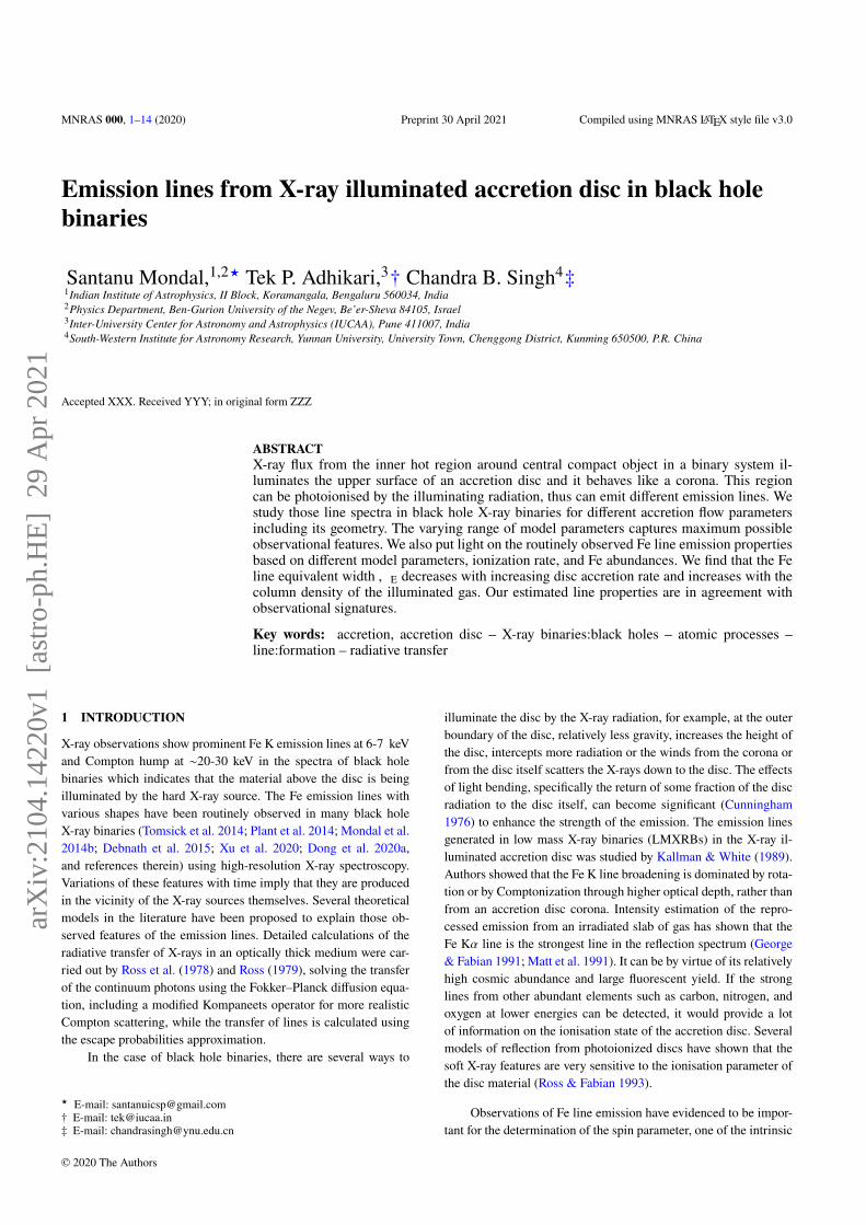
MNRAS 000, 1–14 (2020) Preprint 30 April 2021 Compiled using MNRAS LATEX style file v3.0

Emission lines from X-ray illuminated accretion disc in black holebinaries

Santanu Mondal,1,2★ Tek P. Adhikari,3† Chandra B. Singh4‡1Indian Institute of Astrophysics, II Block, Koramangala, Bengaluru 560034, India2Physics Department, Ben-Gurion University of the Negev, Be’er-Sheva 84105, Israel3Inter-University Center for Astronomy and Astrophysics (IUCAA), Pune 411007, India4South-Western Institute for Astronomy Research, Yunnan University, University Town, Chenggong District, Kunming 650500, P.R. China

Accepted XXX. Received YYY; in original form ZZZ

ABSTRACTX-ray flux from the inner hot region around central compact object in a binary system il-luminates the upper surface of an accretion disc and it behaves like a corona. This regioncan be photoionised by the illuminating radiation, thus can emit different emission lines. Westudy those line spectra in black hole X-ray binaries for different accretion flow parametersincluding its geometry. The varying range of model parameters captures maximum possibleobservational features. We also put light on the routinely observed Fe line emission propertiesbased on different model parameters, ionization rate, and Fe abundances. We find that the Feline equivalent width𝑊E decreases with increasing disc accretion rate and increases with thecolumn density of the illuminated gas. Our estimated line properties are in agreement withobservational signatures.

Key words: accretion, accretion disc – X-ray binaries:black holes – atomic processes –line:formation – radiative transfer

1 INTRODUCTION

X-ray observations show prominent Fe K emission lines at 6-7 keVand Compton hump at ∼20-30 keV in the spectra of black holebinaries which indicates that the material above the disc is beingilluminated by the hard X-ray source. The Fe emission lines withvarious shapes have been routinely observed in many black holeX-ray binaries (Tomsick et al. 2014; Plant et al. 2014; Mondal et al.2014b; Debnath et al. 2015; Xu et al. 2020; Dong et al. 2020a,and references therein) using high-resolution X-ray spectroscopy.Variations of these features with time imply that they are producedin the vicinity of the X-ray sources themselves. Several theoreticalmodels in the literature have been proposed to explain those ob-served features of the emission lines. Detailed calculations of theradiative transfer of X-rays in an optically thick medium were car-ried out by Ross et al. (1978) and Ross (1979), solving the transferof the continuum photons using the Fokker–Planck diffusion equa-tion, including a modified Kompaneets operator for more realisticCompton scattering, while the transfer of lines is calculated usingthe escape probabilities approximation.

In the case of black hole binaries, there are several ways to

★ E-mail: santanuicsp@gmail.com† E-mail: tek@iucaa.in‡ E-mail: chandrasingh@ynu.edu.cn

illuminate the disc by the X-ray radiation, for example, at the outerboundary of the disc, relatively less gravity, increases the height ofthe disc, intercepts more radiation or the winds from the corona orfrom the disc itself scatters the X-rays down to the disc. The effectsof light bending, specifically the return of some fraction of the discradiation to the disc itself, can become significant (Cunningham1976) to enhance the strength of the emission. The emission linesgenerated in low mass X-ray binaries (LMXRBs) in the X-ray il-luminated accretion disc was studied by Kallman & White (1989).Authors showed that the Fe K line broadening is dominated by rota-tion or by Comptonization through higher optical depth, rather thanfrom an accretion disc corona. Intensity estimation of the repro-cessed emission from an irradiated slab of gas has shown that theFe K𝛼 line is the strongest line in the reflection spectrum (George& Fabian 1991; Matt et al. 1991). It can be by virtue of its relativelyhigh cosmic abundance and large fluorescent yield. If the stronglines from other abundant elements such as carbon, nitrogen, andoxygen at lower energies can be detected, it would provide a lotof information on the ionisation state of the accretion disc. Severalmodels of reflection from photoionized discs have shown that thesoft X-ray features are very sensitive to the ionisation parameter ofthe disc material (Ross & Fabian 1993).

Observations of Fe line emission have evidenced to be impor-tant for the determination of the spin parameter, one of the intrinsic

© 2020 The Authors

arX

iv:2

104.

1422

0v1

[as

tro-

ph.H

E]

29

Apr

202

1

2 Mondal et al.

parameters that describe black holes (Laor 1991; Dabrowski et al.1997; Brenneman & Reynolds 2006). It was pointed out by Fabianet al. (1989), that, if the reflected emission comes from the accre-tion disc, then relativistic and Doppler effects would broaden theemission lines, particularly in high spin black hole cases, where if re-flection occurs close to the black hole (Fabian et al. 2000; Reynolds& Nowak 2003; Miller et al. 2008; Steiner et al. 2011; Dauser et al.2012). Recent high-resolution X-ray observation indeed detectedthis line broadening features and was used to estimate the spin pa-rameter of black holes (Iwasawa et al. 1996; Mondal et al. 2016;Dong et al. 2020b, and references therein).

Several models have been introduced in the literature to explainthe emission lines from the disc from time to time. For example,the scattering of photons by cold electrons using Green’s func-tions approach was first derived by Lightman & Rybicki (1980)and Lightman et al. (1981), and their implications for AGN obser-vations discussed in Lightman & White (1988). Guilbert & Rees(1988) proposed a theoretical model to study reflected emission as-suming that irradiation on the surface of the disc was weak enoughso the gas remains neutral, but yet would reprocess the radiation-producing observable spectral features. Matt et al. (1993) studiedemission properties based on mass accretion variation. Zycki et al.(1994) carried out similar calculations including ionisation balanceand thermal balance in the medium along with the distribution ofX-ray intensity with optical depth, yet neglecting the intrinsic emis-sion inside the gas. Later, Magdziarz & Zdziarski (1995) calculatedthe cold reflection using Green’s function approach, highly depen-dent on viewing angle, however, their calculations did not includeline production. Apart from the above mentioned models, there aremany notable models such as, reflionx by Ross & Fabian (1993),TITAN code by Dumont et al. (2000), which was later extendedby Różańska et al. (2002) to treat cases of Compton thick media.Różańska et al. (2002) demonstrated that the use of hydrostaticequilibrium is of crucial importance to study the disc illuminationby the hard X-ray. All other earlier studies assumed constant densityin the material. It has been argued that a plane parallel slab underhydrostatic equilibrium could represent the surface of an accretiondisc more accurately (Nayakshin et al. 2000), and that its reflectedspectrum is, in fact, different from the one predicted by constantdensity models (see also, Rozanska & Czerny 1996; Nayakshin &Kallman 2001; Różańska & Madej 2008; Różańska et al. 2011).Recently, in the last couple of years, Garcia and his collaboratorsproposed a model, xillver, (García et al. 2013) where authorshave updated the above models adding more physical processes andatomic data, to make it more broadly applicable. However, all thesemodels used the incident spectra from the phenomenological powerlaw model, did not take into account the detailed accretion solutionand the effects of flow parameters and its geometry.

Despite the existence of a large number of models in the litera-ture, there is still a lack of understanding of the origin of the corona,its optical depth, and temperature profile to generate physical emis-sion from that region, which is responsible for illuminating the disc.There are models which successfully explain the scenario of scat-tering of soft photons by the corona at different location of the disc(Sunyaev & Titarchuk 1980; Haardt & Maraschi 1993; Zdziarskiet al. 2003), however, without taking into account the physical ori-gin of the corona. Therefore, a self-consistentmodeling of accretion,

as well as emission lines from reflected disc component, remains tobe done, which motivates us to study line emissions using a physi-cal accretion disc model. For our purpose, we use two-componentsolution, TCAF (Chakrabarti & Titarchuk 1995; Chakrabarti 1997,hereafter CT95), generated theoretical spectra. According to thismodel, the so-called truncation of the disc is the location of the shock(Chakrabarti 1989), formed by low angular momentum, hot, sub-Keplerian halo, satisfyingRankine-Hugoniot conditions.Numericalsimulations have shown that the two-component flow forms and isstable even in presence of spatially- and temporally- varying vis-cosity parameters and cooling processes (Giri & Chakrabarti 2013;Giri et al. 2015; Roy & Chakrabarti 2017). Beyond the shocked re-gion, both disc and halo accretion pile up to decide the optical depthand temperature of that region. The same region also upscatters theincoming soft radiation from the disc via inverse Comptonization.The model has indeed a reflection mechanism, where disc to shockand vice-versa interceptions are taken into account in an iterativeway. The disc inclination effect has not been taken into account inthe current model. Later, this model was modified to see the effectsof cooling and mass loss coupled with hydrodynamics (Mondal &Chakrabarti 2013). In the last couple of years, the present model isalso implemented in XSPEC to study both LMXRBs (Debnath et al.2014; Mondal et al. 2014b) and AGNs (Nandi et al. 2019; Mondal& Stalin 2021) data successfully. The observational studies usingthe current model can explain different spectral states, the evolutionof quasi-periodic oscillations (QPOs), estimation of mass and spinof the black hole which covers current research topics in the field.To study the emission line we use publicly available photoionizationcode cloudy C17.01 version (Ferland et al. 2017). Earlier, Bianchiet al. (2006) used cloudy to study the emission lines from 8 nearbySeyfert 2 galaxies and revealed that the soft X-ray emission of allthe objects is likely to be dominated by the photoionized gas. Re-cently, Adhikari et al. (2015, 2016, 2019) used cloudy in detail tostudy emission spectra in the AGN environment and its applicationin different geometry and thermodynamic conditions.

The goal of the present manuscript is (i) to use TCAF modelgenerated spectra to illuminate the disc and to produce emissionlines, (ii) to study how different model parameters (e.g., disc, haloaccretion rates, and the disc geometry) affect line shapes and itsintensity, (iii) to study the effect of Fe abundances (𝐴Fe) and ionisa-tion parameter (b) on the line properties in different spectral states,(iv) to estimate the profile of the equivalent width only of the Felines with disc mass accretion rate, (v) to see the temperature struc-ture of the gas cloud above the disc, and (vi) to use the simulatedFe lines to compare with observed Fe line features of the black holebinaries. In this work, we are not going into the details explainingthe origin of emission lines from other species than iron, which willbe studied in follow-up works.

The paper is organized as follows: in section 2, we discussthe details of the accretion disc model, which is used to generatethe illuminating spectra and how it is used to form emission linesfrom cloudy. In section 3, we describe emission lines variationwith different model parameters for instance, accretion rates (asthe model uses two accretion components), the geometry of theflow, ionisation parameter, and Fe abundance. The equivalent widthprofile with disc mass accretion rate and ionisation parameter andthe temperature structure of the gas cloud are also discussed. Our

MNRAS 000, 1–14 (2020)

Reflection spectra from accretion disc 3

simulated results are also compared with observations. In section 4,the change in shape of Fe lines with model parameters and itsintensity variation is discussed. Finally, we draw our concludingremarks in section 5.

2 MODELLING

In order to generate emission lines, we use theoretical spectra fromChakrabarti (1997)model. In Figure 1,we present a cartoon diagramof the two-component model where a cold, high angular momentumKeplerian disc resides at the equatorial plane and it is flanked by thesub-Keplerian flowwhich we call halo, which is hot and low angularmomentum flow. The optically thin pre-shock halo does not radiateefficiently therefore energy and entropy are advected with the flow.At the center of the co-ordinate, a black hole ofmass𝑀BH is located.For the supply of soft (seed) photons for thermal Comptonization,we assume a Keplerian disc on the equatorial plane, truncated atthe shock radius. This disc emits a flux of radiation the same as thatproduced by a Shakura & Sunyaev (1973) disc. The soft photonsemerging out from the Keplerian disc are reprocessed via Comptonor inverse Compton scattering within the corona. Injected photonsmay undergo a single, multiple or no scattering at all with the hotelectrons in between its emergence from the Keplerian disc and itsescape from the halo. As the radiation passes through the corona,the probability of repeated scattering by the same photon decreasesexponentially, however, the gain in energy is exponentially higher.A balance of these two processes gives a power-law distribution ofthe energy density. For the temperature estimation of the corona,we solve the thermally decoupled two-temperature equations forelectrons and protons. The location of the shock can be found af-ter solving flow equations by providing initial specific energy andspecific angular momentum value to the flow at the outer boundary.However, as we are not solving the transonic flow coupled with theradiative transfer, we use corona size or shock location as a freeinput parameter of the model.

In the present model, we have computed the model spectra dueto thermal Comptonization only. As the innermost region of the discis rapidly falling in and is, in fact, supersonic (Chakrabarti 1989;Chakrabarti & Titarchuk 1995; Mondal & Chakrabarti 2013). Athigh accretion rates, when the flow becomes cold and the thermalComptonization can be ignored, the bulk motion takes the role ofenergy shifting of seed photons. This so-called bulk motion Comp-tonization (BMC) spectrum is decided by the upper limit of the ve-locity of the infalling matter and thus the spectral slope saturates toaround 2.0 even when the accretion rates are varied. The theoreticalworks (Chakrabarti & Titarchuk 1995; Titarchuk & Zannias 1998),Monte Carlo simulations (Laurent & Titarchuk 1999), and the ob-servational results (Shaposhnikov & Titarchuk 2009; Titarchuk &Seifina 2009) all point to these saturation effects. Since this propertyis solely due to the unique properties of a black hole accretion, thisis not affected by our analysis of thermal Comptonization, valid forrelatively lower accretion rates of the Keplerian component.

The theoretical TCAF model uses five parameters namely, (i)mass of black hole (MBH in 𝑀� unit), (ii) disc mass accretion rate( ¤𝑚d), (iii) halo mass accretion rate ( ¤𝑚h). The accretion rates arein the Eddington accretion rate ( ¤𝑀Edd) unit, (iv) location of the

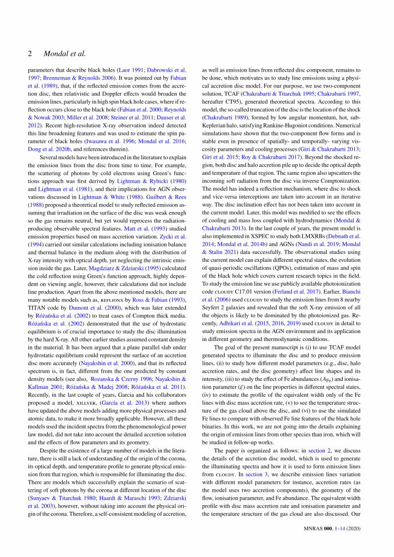
shock or boundary layer of the corona (𝑋s in 𝑟s =2𝐺𝑀BH/𝑐2 unit,where, 𝐺 and 𝑐 are the gravitational constant and speed of lightrespectively). Here, 𝑋s is the boundary layer of the corona and weare solving steady state equations, therefore at any instant standingshock will form at a particular location, and (v) shock compressionratio (𝑅 = 𝜌−/𝜌+, where, 𝜌 is the density of the pre (-) and post (+)shock flow). Here, we briefly discuss howmodel parameters changethe shape of the emitted spectra. Parameters (ii) to (v) collectivelydefines the properties of the disc and corona of the flow, for instance,the electron density and temperature, photon spectrum, and density.The fractional interception of soft photons from the disc by thecorona and vice-versa are taken into account. During the scatteringof soft photons by the corona, cooling also takes place, which isalso responsible for changing spectral shapes (Done et al. 2007;Mondal & Chakrabarti 2013; Yuan & Narayan 2014). All of thesedepend on the mass of the black hole, thus mass estimation can bedone satisfactorily (Molla et al. 2017) by analyzing full outburstdata of different X-ray missions, by keeping the mass of the BHas a free parameter or by keeping the normalization fixed for aparticular outburst for a particular BH, details are explained in thepaper. According to Chakrabarti (1997), if one increases the halorate keeping other parameters unchanged, the model will producea hard spectrum. Similarly, increasing the disc rate leaving otherparameters frozen will produce a soft spectrum. Figure 2 shows thetypical model spectra for varying ¤𝑚d when other parameters arefixed. Increasing ¤𝑚d generates softer spectra. The parameter valuesfor each spectrum are given in the figure. The solid lines show the setof spectra with cutoff at higher energy ∼ 1MeV whereas the dottedlines show cutoff around 100 keV. When the location of the shock isincreased keeping other parameters fixed, the spectrumwill becomeharder. A similar effect can be also seen for the compression ratio(R). The effects are discussed later in subsection 3.3. In general, inoutbursts of black hole binaries, during rising and declining phaseswith different spectral states, all the parameters change smoothly inamultidimensional space (Mondal et al. 2014b; Debnath et al. 2015;Chatterjee et al. 2016; Jana et al. 2016, and others). The accretionrate ratio (ARR, the ratio of disc rate with halo accretion rate) isalso an indicator of spectral states change (Mondal et al. 2014b),where the spectra move from hard (HS) to soft state (SS) throughintermediate states when ARR changes from low to high.

To generate the model spectra we use the outer boundary ofthe disc at 500 𝑟s, extend up to 𝑋s and corona starts from 𝑋s,and extend up to 3 𝑟s. The illuminating radiation contains differentcomponents, including blackbody, Comptonization, and reflection.Photo-ionisation processes are simulated with numerical spectralsynthesis code cloudy version C17.01 (Ferland et al. 2017). Thecloudy solves different radiation steps to generate emission lines(for detail code description and most recent updates see Ferlandet al. 1995, 2017).

In cloudy, a slab of gas is divided into a large number ofthin zones which results a plane parallel open geometry. In thisgeometry, the photon once escaped will be lost to infinity withoutfurther interactions. A spherical closed geometry can be imple-mented to include the multiple interactions of an escaped photonas well. However, for this case of studying illumination of disc bythe photons from corona, the assumption of plane parallel geom-etry is more realistic. Here, we note that the radiative transfer is

MNRAS 000, 1–14 (2020)

4 Mondal et al.

Figure 1. A cartoon diagram of the geometry of the flow (CT95). The scattering of the soft photons from the Keplerian disc are the Zigzag trajectories. Thesephotons are Comptonized by the CENtrifugal pressure supported BOundary Layer (post-shock region of the sub-Keplerian flow or corona) and are radiated ashard X-rays.

solved in 1 dimension only. The radiation field from the accretiondisc is normally incident on the slab of gas and its reprocessingis initiated. We do not take into account the incidence at differentangles. The gas density which has been used as the input parameteris taken from the mass accretion rate, and the column density (𝑁H)is kept constant to 1.28× 1021 cm−2. However, the effect of 𝑁H hasbeen verified in our study in a range. For the detail discussions onthe different possible geometries of the radiation matter interactionsand their implementation in various astrophysical environments, werefer the reader to theHazy11 documentation of cloudy. Moreover,Adhikari et al. (2015); Adhikari (2019) have extensively discussedthe use of open and closed geometries in cloudy for various casesof AGN absorption and emission regions.

The next important assumption we employ in cloudy mod-elling is the use of constant density case. This means that the gasnumber density is kept constant to a given value across all the zonesof the given gas cloud. Here we note that, an alternative situation ofconstant pressure can arise when a gas cloud is illuminated by theradiation energywhere the gas number density is stratified across thezones of cloud. This phenomenon of radiation pressure confinementis discussed and implemented in various photoionized environmentsof different astrophysical systems in the literatures (Różańska et al.2006; Stern et al. 2014; Baskin et al. 2014; Adhikari et al. 2015,2019; Adhikari 2019). However, Adhikari et al. (2018) have shownthat when there is high gas number density and hence the highgas pressure, the radiation pressure confinement is very weak, andthe model structures are very similar between constant density andconstant pressure assumptions. Since the gas number density inthe accretion disc of black hole X-ray binaries are quite high, wechoose to use the constant density assumption for simulating thephotoionisation process.

The level of ionisation is determined by balancing all ionisationand recombination processes. Ionisation processes include photo,Auger, collisional ionisation, and charge transfer. Recombinationprocesses include radiative, low-temperature dielectronic, high tem-

1 www.nublado.org

perature dielectronic, three-body recombination, and charge trans-fer. The free electrons are assumed to have a predominantlyMaxwellian velocity distribution with a kinetic temperature deter-mined by the balance between heating (photoelectric, mechanical,cosmic-ray, etc.) and cooling (predominantly inelastic collisions be-tween electrons and other particles) processes. The line emissionand continuum radiative transfer processes are solved simultane-ously.

The incident radiation illuminates the disc and ionizes it. Theionisation parameter is calculated using the equation:

b =4𝜋𝐹inc𝑛H

erg cm s−1, (1)

where, 𝐹inc is the Hydrogen ionizing flux integrated in the range1-1000 Rydbergs and 𝑛H is Hydrogen number density in cm−3 unit.The chemical composition of the disc is set to default Solar values incloudy and it is mentionedwhen the Fe abundances (𝐴Fe) is varied.Solar abundances in cloudy are adopted from Grevesse & Sauval(1998). The electron number density at some radius r of the flow iscalculated from ¤𝑚h above the disc, given by, 𝑛e = ¤𝑚h

4𝜋𝑟2𝑚p𝑣in cm−3

unit, where 𝑚p and 𝑣 are the mass of the proton and velocity of theinflow, which can be written as 1/𝑟1/2, when the disc radius is awayfrom the black hole. Thus the typical value of 𝑛𝑒 varies in a rangefrom 1.4× 1010-1.4× 1013cm−3 for the accretion rate range 0.001-1 ¤𝑀Edd and 𝑟=500𝑟s. For the purpose of this work, the electrondensity self consistently derived from our model can be used asthe hydrogen number density 𝑛H in the cloudy computations. Themodel parameters used to construct the spectral radiation shape orspectral energy distribution (SEDs), which are used in the cloudymodelling are discussed in each figure.

3 RESULTS

For the gas cloud above the disc which is illuminated by the centralradiation, we have calculated model reflection spectra covering awide range of disc parameters, with disc rate ( ¤𝑚d=0.001 - 2.0), thehalo rate ( ¤𝑚h=0.001, 0.01, 0.1, and 1.5), the shock location (𝑋s=10,30, 50, 80, and 100), the shock compression ratio (𝑅=1.5, 2.5, 3.5,

MNRAS 000, 1–14 (2020)

Reflection spectra from accretion disc 5

10 2 10 1 100 101 102 103

E (keV)1032

1033

1034

1035

1036

1037

1038

L

(erg

s1 )

mh = 1.0

md=0.001md=0.005md=0.020md=0.050md=0.100md=0.200md=0.400

md=0.600md=0.800md=0.900md=1.000md=1.200md=1.500md=2.000

Figure 2. Incident radiation spectra derived from the model for variousvalues of mass accretion rates, ¤𝑚d, when the other model parameters arefixed at ¤𝑚h = 1.0, 𝑋s=30, and 𝑅=2.5. Two clusters of SEDs: a)first clusterwith cut off around 100 keV shown by dotted colored lines, and b) secondcluster which with cut off around 1000 keV shown by solid colored lines.The detail parameters for other SEDs are mentioned with the correspondingfigures.

and 4.0), the ionisation parameter (log b=1, 2, 3, and 4), and the ironabundance (𝐴Fe = 0.5, 1.0, 2.0, and 5.0) relative to its Solar value.The mass of the black hole is fixed at 7𝑀� throughout the paper.These range of parameter values take into account for most of theobserved spectral states and features of black hole binaries, and allparameters have significant effect on emission lines. For simplicity,abundances of all other elements considered are kept fixed at Solarvalues.

3.1 The effect of varying ¤𝑚d

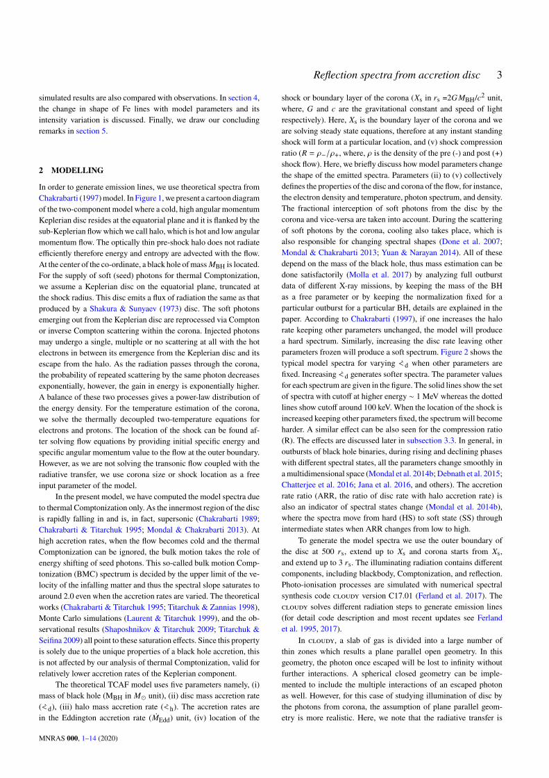
Figure 3 shows reflected spectra for four different values of ¤𝑚d, men-tioned in the figure. In all cases, the incident spectra have ¤𝑚h=1.0,𝑋s = 30, 𝑅 = 2.5, log b = 3, and the iron has Solar abundance(𝐴Fe = 1.0). Increasing ¤𝑚d increases the number of soft photons,thus the intensity of emission lines at the high energy regime of thespectrum decreases, might be due to the presence of less numberof high energy photons, however, the possibility of forming morelines is observed. It is clear from the emission spectra that bothilluminating flux and the spectral shape of the ionizing radiationincident on the surface of the disc have a significant impact on theionisation balance of the gas, and thus on the reflected spectrum.

The equivalent width 𝑊E of an emission line is calculated byusing an expression,

𝑊𝐸 =

∫ 7.2keV

5.5keV

𝐹𝐶𝐸

− 𝐹𝑡𝐸

𝐹𝐶𝐸

𝑑𝐸, (2)

where 𝐹𝐶𝐸and 𝐹𝑡

𝐸are the fluxes in the reflected continuum and

around the line energy centroid respectively. For the purpose ofstudying the emission from highly ionized Fe, we sum up the𝑊E ofFe-emission lines in the energy band 5.5 − 7.2 keV and define it asthe Fe-line𝑊E. In the computations of the𝑊E in this energy band,the contribution of the ions Fe ii to Fe xxvi are considered.

Figure 4 shows that the general trend of𝑊E is decreasing with

10-3 10-2 10-1 100 101 102

E [keV]

107

109

1011

1013

1015

1017

1019

1021

1023

1025

νFν [

erg

/cm

2/s

]

md = 0. 001

md = 0. 005

md = 0. 05

md = 0. 1

Figure 3. Reflected spectra for four different values of the ¤𝑚d, with ¤𝑚d =0.001, 0.005, 0.05, and 0.1. The incident spectrum has log b = 3, and ironhas Solar abundance, the other theoretical model parameters are ¤𝑚h =1.0,𝑀BH=7.0 M� , 𝑋s=30, and 𝑅 = 2.5. Successive spectra have been offset byfactors of 1000 for clearer visibility.

increasing ¤𝑚d. This is expected as at low accretion rate most of thephotons are concentrated at the high energy part of the spectrum,where the Compton scattering becomes important, therefore hardspectra are more efficient in heating the illuminated layer, whichemits more lines. As the accretion rate increases, the incident spec-trum becomes softer thus less number of hard photons participatein line emission. It also shows that increase in column density in-creases 𝑊E, which satisfies that 𝑊E ∝ 𝑁H. The red, blue, green,and black lines correspond to 𝑁H values 1021, 1023, 1024, and 1025

respectively. The 𝑊E is estimated for the lines Feii-Fexxvi. Ourestimated variation of 𝑊E is in the same line of Zycki & Czerny(1994); García et al. (2013), where authors showed that 𝑊E de-creases with increasing photon index (Γ), which is the same in ourmodel as increase in ¤𝑚d makes the spectrum softer thus the highervalue of (Γ). A recent analysis ofMAXI J1820+070 (Xu et al. 2020),showed a similar agreement. However, opposite behavior can alsobe observed if the lines originate from the inner edge of the disc,where the disc moves inward with accretion rate, which increasesrotational velocity, therefore increases line broadening, thus the𝑊E(Tomsick et al. 2009; Debnath et al. 2015). The 𝑊E is also an im-portant measurable quantity to diagnose the evolution of QPOs inthe accretion disc, reported in Galactic black hole GRS 1915+105(Miller & Homan 2005). Earlier the current model was also used toshow the evolution of QPOswith disc accretion rate for the outburst-ing candidates (Mondal et al. 2014b; Chakrabarti et al. 2015), wherethe QPO frequency increases with accretion rate. Thus combiningthese two effects in the future we will be able to study the QPOsevolution consistently from the Fe line fitting. Apart from the vari-ation of the Fe line width, our results also include emission lines atlow energies e.g., N and O to a range between 0.4 to 0.8 keV, whichhave been observed in high-resolution XMM-Newton observation

MNRAS 000, 1–14 (2020)

6 Mondal et al.

0.00 0.25 0.50 0.75 1.00 1.25 1.50 1.75 2.00md [in mEdd]

250

500

750

1000

1250

1500

1750

2000

WE (

5.5-

7.2

keV)

(eV) nH=1.4 × 1013 cm 3

Lines due to Fe II to Fe XXVI

NH = 1e21NH = 1e23NH = 1e24NH = 1e25

Figure 4. 𝑊E of Fe line integrated in the energy range 5.5 − 7.2 keV as afunction of ¤𝑚𝑑 . We extend ¤𝑚𝑑 values to super-Eddington rate to see thetrend of behavior. Various colours represent the 𝑊E computed for variousvalues of 𝑁H. Other theoretical parameters used in these computations are:¤𝑚h =1.0, 𝑀BH=7.0 M� , 𝑋s = 30 and R = 2.5 respectively. In the cloudymodelling, log b = 3.0 and Solar values for Fe abundances are used. Variouscolors in the plot depicts the varying 𝑁H employed.

of black hole candidate Swift J1753.5-0127 (Mostafa et al. 2013).The range of our simulated 𝑊E agrees with estimations from themodel fitted observed data (Titarchuk & Seifina 2009). However, itshould be noted that as the flow comes closer to the black hole withincreasing disc accretion rate, BMC becomes effective, and also thegravitational effects take a significant role, that can skew the lineproperties (Titarchuk & Seifina 2009).

3.2 The effect of varying ¤𝑚h

In Figure 5, we carry out the same task for four different valuesof ¤𝑚h, when ¤𝑚d=0.02 and keeping all other parameters the sameas in Figure 3. As we discussed for increasing ¤𝑚h spectra becomeharder thus increases the high energy photons at high energieswhichaffect the emission features, as the harder illuminating spectra havegreater ionizing efficiency, change the shape of the reflection spectrasignificantly. For ¤𝑚h=0.1 and 1.5 (HS), the illuminated gas is morehighly ionized than for ¤𝑚h=0.001 (SS) and 0.01 (intermediate state).One can observe that more emission lines are visible in the highenergy regime and less lines are observed at low energy regimewhich is due to the outer layer of the illuminated cloud gets fullyionized for higher ¤𝑚h. However, an opposite feature is observed forthe low ¤𝑚h spectra. In the intermediate state (red curve), throughoutthe energy band emission lines are clearly visible with a relativelyhigh intensities.

3.3 The effect of varying geometry

Figure 6 shows emission lines due to variation in accretion geometrye.g. varying size of the corona and its height (h𝑠). Here, we choosefour different values of corona size i.e. 𝑋s, with 𝑋s=10, 30, 50, and100, and four different values of R, with 𝑅=1.5, 2.5, 3.0, and 4.0,from SS to HS through intermediate states. Both parameters changeh𝑠 and also the optical depth of the corona, thus the emitted spectra.

10-3 10-2 10-1 100 101 102

E [keV]

100

102

104

106

108

1010

1012

1014

1016

1018

1020

1022

1024

νFν [

erg

/cm

2/s

]

mh = 0. 001

mh = 0. 01

mh = 0. 5

mh = 1. 5

Figure 5. Reflected spectra for four values of the ¤𝑚h, with ¤𝑚h = 0.001,0.01, 0.1, and 1.5. The incident spectrum has log b = 3, and iron has Solarabundance, the other theoretical model parameters are ¤𝑚d =0.02, 𝑀BH =7.0 M� , 𝑋s = 30.0, and R = 2.5. Successive spectra have been offset byfactors of 1000 for clearer visibility.

The change in 𝑋s and 𝑅, changes the h𝑠 as ∼√(𝑅 − 1)𝑋s/𝑅 and the

total accretion rate at the post-shock region after pilling up of mattercan be written as 𝑅 ¤𝑚h+ ¤𝑚d (Mondal et al. 2014a), indicates that thephysical quantities (temperature and optical depth etc.) of the coronadepends on 𝑅. Furthermore, varying 𝑅 during the outburst phasealso means variable mass outflow, as the TCAF model proposedthat the corona is the base of the mass outflow/jet, which extractsthermal energy from the inner hot region and makes the spectrumsofter (Chakrabarti 1999; Singh & Chakrabarti 2011; Mondal et al.2014a), therefore change in emission line properties. However, inthe present modeling we do not include jet effects. Figure 6a showsthe lines for different 𝑋s, at the intermediate 𝑋s, the intensity of afew lines is higher than low and high 𝑋s, some extra lines are visiblearound 0.3 keV. Figure 6b, shows the lines for different values ofR, with increasing R, spectrum moves from SS to HS, thus highenergy photon intensity increases, which increases the ionisationrate. Therefore more lines are visible with increasing R, especiallybelow 0.01 keV and between 0.2-0.4 keV.

3.4 The effect of varying b

The flux of the continuum that hits the Cloudy gas is fixed by thegas density and the ionization parameter as described in Eq. 1. Theopen geometry (a plane parallel slab with several thin zones) ofthe emitting gas in Cloudy is assumed which is different from thegeometry of how TCAF is formulated. For a given gas cloud, theionization parameter at the illuminated surface is defined. However,in the inner zones of the slab, it can change according to Eq. 1.Nevertheless, with our assumption of constant density gas (with thinslab) this change is negligible. For a closed (spherical) geometry,the change in ionization parameter can be significant and should

MNRAS 000, 1–14 (2020)

Reflection spectra from accretion disc 7

10-3 10-2 10-1 100 101 102

E [keV]

107

109

1011

1013

1015

1017

1019

1021

1023

1025

νFν [

erg

/cm

2/s

]

(a)

Xs = 10rs

Xs = 30rs

Xs = 50rs

Xs = 100rs

10-3 10-2 10-1 100 101 102

E [keV]

107

109

1011

1013

1015

1017

1019

1021

1023

1025

νFν [

erg

/cm

2/s

]

(b)

R= 1. 5

R= 2. 5

R= 3. 0

R= 4. 0

Figure 6. Reflected spectra (a) for four values of the 𝑋s, with 𝑋s = 10, 30, 50, and 100, when 𝑅=2.5 and (b) for four values of R, with 𝑅= 1.5, 2.5, 3.0, and4.0, when 𝑋s=30. The all incident spectra have log b = 3, and iron has Solar abundance, the other theoretical model parameters are ¤𝑚d =0.005, ¤𝑚h = 1.0, and𝑀BH=7.0 M� .

be represented by a distribution (Adhikari et al. 2015). Also, if oneassumes a constant pressure gas (instead of constant density), then,there can be several orders of magnitude difference in ionizationparameter between the illuminated side and the back side of theslab (Adhikari et al. 2016, 2018, 2019, and references therein).Therefore, we examine the effect of b on the emission lines fordifferent values of b applied to two different values of ARR, keepingthe other TCAF model parameters fixed. In both panels of Figure 7,each curve corresponds to a particular value of logb=1, 2, 3, and4. The other model parameters are 𝑀BH=7.0 M� , 𝑋s = 30, R =2.5, and the iron has Solar abundance. In each panel, the plottedspectra have been rescaled for visual clarity. The scaling factorsare, from bottom to top, 1, 103, 106, and 109. The left panel inFigure 7a shows emission spectra whenARR=0.001, i.e. a very hardstate of the illuminating spectrum. On the other hand, Figure 7b,when ARR=20, i.e. a softer state of the illuminating spectrum,and the effects are indeed visible. For the same ARR, increasingb means a higher ionisation rate, which raises the temperature ofthe illuminated region of the slab thus ionize the gas at a largeroptical depth. Hence ions from lower atomic number (Z) elementsare completely stripped from all their elements, while heavy Zelements get partially ionized. Thus the emission spectra lack linesfrommost of the low-Z elements, are either absent or the intensity ofthe lines went down abruptly when log b increases and progressivelyshowing for heavy-Z elements. This specific trend is observed forlog b=4. The Fe K𝛼 line is peaking at 7keV. However, an oppositescenario is observed in Figure 7b when both ARR and b are high.All lines are visible even for higher b in comparison of low ARR(hard state) in the left panel. This infers that in the hard state, thepartly ionized disc can emit more lines as more hard photons takepart in line emission. However, for a fully ionized disc with harderillumination, it emits fewer lines. Whereas in the soft state, the discemits more lines even for a higher ionisation parameter (b) as the

disc does not get completely ionised. However, the left panel withlog b=4 can show up emission lines at low energies if the columndensity of the gas cloud is increased. If the slab thickness is lessand the radiation is hard, it will pass through the slab with littlescattering or without interacting with the medium.

Figure 8 shows the plot of 𝑊E versus ionisation parameter,where 𝑊E tends to decrease with increase in ionisation parameteruntil low ionisation region, however, it sharply increases in higherionisation regime, b > 103. After some value of ionisation, b ∼ 104,again the𝑊E decrease which is because of a wider part of the discbecomes fully ionized, these typical behaviors can also be seenmainly in case of Seyfert 1 galaxies atmosphere (Zycki & Czerny1994). As evidenced from Zycki & Czerny (1994) 𝑊E becomesmaximum around b = 3 × 108 for Seyfert 1 galaxies and decreasesfor further increase in b. The difference of∼ 4 orders ofmagnitude inthe b value at which𝑊E peaks in X-ray binaries and Seyfert galaxiesis due to the considerable difference in their luminosity. Consideringthis point, the results from Figure 8 of this paper corroborate withthe results of Zycki & Czerny (1994) (Figure 19 of their paper).The black, pink, and green curves corresponds to different valuesof 𝑁H. The peak value of 𝑊E is highest for the lowest value of𝑁H = 1022. This is due to the fact that, the larger fraction of theslab of gas with low column density is at high temperature, andthus more ionized, as compared to that with higher column density.This fact can also be realized by looking at the Figure 10, wherethe temperature for the lowest column density stays high even atthe backside of the slab. However, for the case with highest columndensity, the temperature falls off rapidly with the depth of the slaband unable to ionize the Fe inside. Here, we study the dependenceof our result on the ionization parameter defined at the surface ofthe gas cloud. From observations, b is always constrained to have avalue in the range. This is why we are exploring the range of values.

MNRAS 000, 1–14 (2020)

8 Mondal et al.

10-3 10-2 10-1 100 101 102

E [keV]

107

109

1011

1013

1015

1017

1019

1021

1023

νFν [

erg

/cm

2/s

]

(a)

logξ= 1

logξ= 2

logξ= 3

logξ= 4

10-3 10-2 10-1 100 101 102

E [keV]

100

102

104

106

108

1010

1012

1014

1016

1018

1020

1022

νFν [

erg

/cm

2/s

]

(b)

logξ= 1

logξ= 2

logξ= 3

logξ= 4

Figure 7. Reflected spectra for four values of the log b , with log b = 1, 2, 3, and 4. The iron has Solar abundance, 𝑀BH=7.0 M� , 𝑋s = 30 and R = 2.5. Theother disc parameters are (a) ¤𝑚d =0.001, ¤𝑚h = 1.0, and (b) ¤𝑚d =0.02, ¤𝑚h = 0.001. Successive spectra have been offset by factors of 1000 for clearer visibility.

100 101 102 103 104 105

(erg cm s 1)

200

300

400

500

600

700

800

900

WE (

5.5-

7.2

keV)

(eV)

NH = 1e22NH = 5e22NH = 1e23

Figure 8.Variation of equivalentwidths as a function of ionisation parameterb . The incident SEDused for this case is parametrized by: ¤𝑚d =1.2, ¤𝑚h =1.0,𝑀BH=7.0 M� , 𝑋s = 30 and R = 2.5 respectively. In the cloudy modelling,Solar abundances are used and various colors in the plot depicts the varying𝑁H employed.

Similar studies were also carried out by Zycki & Czerny (1994) andGarcía et al. (2013).

3.5 The effect of varying 𝐴Fe

The amount of a particular element present in the gas changes thecontinuum opacity, which in turn affects the photoionisation heat-ing rate. Therefore the abundances for each element are taken intoaccount in a photoionisation effect can greatly affect the ionisationbalance, the observable spectral line features in the reprocessed ra-diation. At the same time, the abundance of a particular elementinfluences the strength of the emission lines. Considering the rele-vant effect of Fe line emission in the analysis of the X-ray spectrafor accreting binary candidates, we have carried out generating

emission spectra in which the Fe abundance is varied between sub-Solar, Solar, and super-Solar values. All other elements consideredin these calculations are set to their Solar values. The effects ofvarying abundance of iron are shown in Figure 9(a-b). The illumi-nating radiation has log b = 3, and the other model parameters arethe same as in Figure 7 for two different spectral states, one is avery hard state when ARR=0.001 (left panel) and the other one isa softer state when ARR=20 (right panel), are shown in Figure 9aand b respectively. In each panel, the plotted spectra have been re-scaled for visual clarity. The scaling factors are, from bottom to top,1, 103, 106, and 109. The effect of 𝐴Fe substantially changes theFe emission features, evident in the emission spectra. For higher𝐴Fe, increases the strength of overall emission lines including Feemission. A significant difference at the low energy emission can beseen, where for higher ARR more lines are visible with higher in-tensity compared to low ARR. The reason behind this is that harderradiation (low ARR) fully ionised the disc therefore less lines aregenerated.

3.6 Temperature profile and the effect of varying disc columndensity 𝑁H

We studied the dependence of our results on the thickness of thecloud by varying the column density of the cloud, 𝑁H. Figure 10shows that increase in optical depth decreases the temperature ofthe illuminated medium for the disc parameter ¤𝑚𝑑 = 1.2, ¤𝑚ℎ = 1.0,𝑋s=30, and 𝑅=2.5. This behaviour is due to the increased repro-cessing of the X-ray photons by the larger surface of the gas cloud.The column density and optical depth considered here can poten-tially affect the temperature structure of the gas cloud by varyingheating and cooling efficiency, thus the strength of the emission.At the surface of the gas layer where illuminating radiation hits ishot and Compton heating and cooling dominates. The temperatureat the surface remains at Compton temperature. In this region ra-

MNRAS 000, 1–14 (2020)

Reflection spectra from accretion disc 9

10-3 10-2 10-1 100 101 102

E [keV]

107

109

1011

1013

1015

1017

1019

1021

1023

1025

νFν [

erg

/cm

2/s

]

(a)

AFe = 0. 5

AFe = 1. 0

AFe = 2. 0

AFe = 5. 0

10-3 10-2 10-1 100 101 102

E [keV]

100

102

104

106

108

1010

1012

1014

1016

1018

1020

1022

νFν [

erg

/cm

2/s

]

(b)

AFe = 0. 5

AFe = 1. 0

AFe = 2. 0

AFe = 5. 0

Figure 9. Reflected spectra for different values of 𝐴Fe, with 𝐴Fe = 0.5, 1.0, 2.0 and 5.0 when log b=3. The TCAF model parameters which are fixed for bothcases are, 𝑀BH=7.0 M� , 𝑋s = 30 and R = 2.5. The accretion rates for the two cases of spectral states are: (a) ¤𝑚d =0.001, ¤𝑚h = 1.0, and (b) ¤𝑚d =0.02, ¤𝑚h =0.001. Successive spectra have been offset by factors of 1000 for clearer visibility.

10 4 10 3 10 2 10 1 100 101

Thomson optical depth

104

105

Tem

pera

ture

(K)

NH=1e21NH=1e23

NH=1e24NH=1e25

Figure 10. Temperature as a function of the optical depth for models withvariation in column densities. The structure presented here is for the incidentSED generated using model parameters ¤𝑚𝑑 = 1.2, ¤𝑚ℎ = 1.0, 𝑋s=30, and𝑅=2.5. log b = 3.0 and Solar values for Fe abundances are used in cloudy.

diation field thermalises, thus the temperature of the gas remainsconstant ∼ 4 × 105 K. As the optical depth increases, cold regionexists and the temperature decreases, after a certain optical depth(∼ 0.05), the temperature falls sharply by orders in magnitude. Ifthe column density is typically low, the cooling rate is also low, thusthe illuminating radiation thermalises the layers of the cloud, thusthe temperature remains constant to a fixed value does not fall as wesee in high column density case. The blue, orange, green, and redcurves show temperature profile for the values of 𝑁H = 1021, 1023,1024, and 1025 respectively. However, the scenarios may change if adifferent set of input SEDs and ionisation parameter are considered.Figure 11 shows the effect of 𝑁H on reflection spectra of Fe linebetween 5.5-7.2 keV, where line intensity increases with increas-

ing column density. It also shows that when intensity increases,line width increases as evident from Figure 4. The change in lineshape and the line to continuum contrast on increasing the columndensity are related to the behaviour of the curve of growth (COG)(i.e., the plot of line 𝑊𝐸 against the ionic column density). Thecurve of growth generally has three parts : linear part (where 𝑊𝐸

increases linearly with ionic column density), exponential part (𝑊𝐸

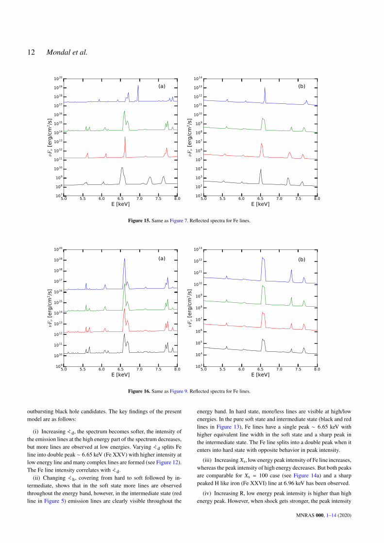
increases exponentially), and saturated part (lines are saturated).Such a behaviour can be seen in Adhikari (2019). For the lowestcolumn density, the emission lines are produced corresponding tothe ionic column density at the linear part of the COG. Once thecolumn density increases, the lines are produced from an exponen-tial part of the COG, hence, having higher 𝑊𝐸 and broader lines.Due to the higher ionic column density, the collisional broadeningbecomes more significant and the line shape becomes complex. Ifwe keep increasing the column density further, it should remain un-changed as we approach the saturated part of COG. The Fe XXVI(6.96 keV) line will show up for the cases where ¤𝑚d is low i.e.more hard photons can contribute and also the ionization rate ishigh. Therefore Figure 15a shows the Fe XXVI line up, whereas thepanel b does not show up as the ¤𝑚d is high and ¤𝑚h is low (typicalsoft-state). Since Figure 11 is shown for the ¤𝑚d = 1.2 (which lackshard X-ray photons), hence the Fe XXVI line is not present there.Furthermore, the 5.6 keV features are not Fe-line features (these areCr and Ti line features not relevant at present). In addition the 6.1(6.07-6.11) keV features for Mn, Ti, Cr, are not relevant at presentas well. We put them for the sake of completeness and in the futurethe high-resolution observations may detect these lines.

MNRAS 000, 1–14 (2020)

10 Mondal et al.

5.5 6.0 6.5 7.0109

1010

1011NH = 1e21

5.5 6.0 6.5 7.01011

1012

1013

NH = 1e23

5.5 6.0 6.5 7.0E (keV)

1012

1013

1014

F

(erg

s1 c

m2 )

NH = 1e24

5.5 6.0 6.5 7.0E (keV)

1012

1013

1014NH = 1e25

Figure 11. Fe-line spectra for various values of 𝑁H and for the same modelparameters as in Fig. 10

4 SHAPE OF FE LINE

In Figure 12, we show Fe line emission for varying ¤𝑚d, same as inFigure 3. Increasing disc mass accretion rate, the observed 6.6 keVand 6.7 keV double lines intensity increases. In all four cases, Feline ∼ 6.6 keV splits into two and many other lines from low Zspecies are produced between 5-8 keV energy band, some of themare mentioned in Figure 11. In this case, ARR value increases refersincrease in disc rate i.e. no of soft photon increases keeping the hotflow component (halo rate) fixed. Therefore spectra become softer.As the ARR value increases the second peak intensity increases andthe first peak decreases. For high ARR, the outer layer of the gascloud falls quickly from very hot phase to cold phase at negligiblysmall Thomson optical depth, therefore it can ionize more layer inthe cloud to emit lines.

However, Figure 13 shows a different line properties whenhalo rate increases from sub-Eddington to Eddington rate, Fe line∼ 6.5 KeV starts splitting and the component at ∼ 6.7 keV hashigher intensity than the lower energy peak. It is also noticeablethat many complex lines are disappeared at low halo rate, and theyappeared at high halo rate, this implies that when spectral statesmove from soft to hard, the intensity of illuminating spectrum athigh energy increases, thus the ionisation rate, producing morelines. Here, increase in hot flow rate refers decrease in ARR whichgeneratemore hard photons to illuminate the disc surface. Therefore,at high ARR ( black and red lines) the illuminating radiation hasnot enough high energy photons to trigger thermal instability asthe temperature of the gas cloud decrease, therefore less no of Fespecies contributed and showed a single sharp peak. As the ARRgoes down (<1, green and blue lines), the temperature of the gascloud increases, the Fe line broadens.

Figure 14a-b show the effect of varying 𝑋s and R on the re-flected Fe line spectra. In both cases, Fe lines showed a double peak∼6.5 keV. Figure 14a shows that increasing 𝑋s, the low energy peakintensity of Fe lines increases, however, in low and high 𝑋s, linesshowed opposite nature compared to the intermediate corona size.Also, an extra emission line ∼7 keV is observed in low and high 𝑋swith the increase in intensity for high 𝑋s, these can be understoodfrom the hardening of the illuminating spectra, and more number

5.0 5.5 6.0 6.5 7.0 7.5 8.0

E [keV]

1010

1011

1012

1013

1014

1015

1016

1017

1018

1019

νFν [

erg

/cm

2/s

]

Figure 12. Same as Figure 3, but for the reflected spectra of the Fe lines.We use offset 100 for all Fe line spectra for visual clarity.

5.0 5.5 6.0 6.5 7.0 7.5 8.0

E [keV]

102

104

106

108

1010

1012

1014

1016

1018

νFν [

erg

/cm

2/s

]

Figure 13. Same as Figure 5, but for the reflected spectra of Fe lines.

of hard photons are contributing in ionizing the disc. Figure 14b,showed an opposite behavior in the double peak Fe line, where theintensity of the low energy peak ∼6.6 keV increases with R, andthe high energy peak intensity did not change much, which showedflipping behavior for 𝑅=4, the strong shock condition. It shouldbe noted that the double peaks which are observed are not due toany gravitational broadening effects nor due to photon bending ef-fects, rather two different transitions of Fe lines at different energies.The low energy iron lines are not shown up, which can be due tocompletely stripped off of the electrons from the atomic levels.

Figure 15 a-b show the effect of varying log b on the reflectedFe line spectra for the same sets of model parameters in Figure 7

MNRAS 000, 1–14 (2020)

Reflection spectra from accretion disc 11

5.0 5.5 6.0 6.5 7.0 7.5 8.0

E [keV]

1010

1011

1012

1013

1014

1015

1016

1017

1018

1019

νFν [

erg

/cm

2/s

]

(a)

5.0 5.5 6.0 6.5 7.0 7.5 8.0

E [keV]

1010

1011

1012

1013

1014

1015

1016

1017

1018

νFν [

erg

/cm

2/s

]

(b)

Figure 14. Same as Figure 6, but for the reflected spectra of Fe lines.

for HS and SS. At the pure HS with low log b, a single and broadFe line is observed at ∼ 6.5 keV. It becomes narrow when log bincreases and the line splits when log b is 3, at very high ionisationvalue the line intensity goes down and an another sharp-peaked lineat 6.96 keV with high intensity is observed. This evidences that thegas becomes so ionized that H like iron (Fe XXVI) is the dominantspecies. However, for the same log b, in the SS Figure 15b, onlyone line is observed at 6.5 keV and it is narrower in low and highlog b. The appearance of the single peak line in the SS follows thesimilar discussion of temperature structure change of the gas cloudwith the hardness of the illuminating radiation. As the ARR is high(� 1), incident radiation has not enough hard photons to triggerthe thermal instability, therefore not many Fe species contributed inline emission.

Figure 16a-b show the effect of varying 𝐴Fe (increases fromblack to blue line) on the reflected Fe line spectra for the same setsof model parameters in HS and SS as in Figure 9. Figure 16a showsthe double peak nature of Fe lines with increasing intensity in lowenergy line, whereas high energy line intensity decreases, this isdue to the hard radiation increases ionisation rate with increasingFe abundances. Thus more complex lines are formed. However, Fig-ure 16b shows a single line with increasing intensity for increasing𝐴Fe, indeed shows a significant effect of Fe abundances. Also, theilluminating spectra have less effect on the temperature structure ofthe gas cloud in the SS (ARR > 1) as less number of hard pho-tons contributed to trigger the thermal instability. However, fromobservation, we see that the line broadens and breaks into a doublepeak during the outburst phase, and the intensity increases as thespectrum moves to the soft state (Mondal et al. 2016) when theinner edge of the disc comes much closer to the BH. These twocombined results infer that gravitational broadening might be moredominating over photoionisation in the soft state, when the Fe linesare originated at the inner edge of the disc.

In the current modeling, we did not consider any gravitational

effect as in Fabian et al. (1989) or Laor (1991). The lines are gener-ated due to photo-ionization processes or due to atomic transitionsin Cloudy. It is also worth mentioning that Cloudy does not havethe gravitational broadening effect, but the broadening due to thethermalmotion of the gas is incorporated. Furthermore, our locationof the shock is not close to the innermost stable circular orbit, ratherfarther away, where the line broadening effect may not be effectiveenough. Moreover, general relativistic or photon bending effects areimportant to get those double-peaked lines, which is beyond thescope of the paper.

5 CONCLUSIONS

In this paper, we have presented reprocessed spectra from an ac-cretion disc, which is emitted as a reflected spectra. The incidentilluminating spectra are generated using TCAF model. Each modelis characterized by the disc and halo mass accretion rates, loca-tion of shock/size of the corona and the shock compression ratioof the flow. Next, the reprocessing of this incident radiation is sim-ulated by using the photoionisation code cloudy, where a disc isparametrized by: the ionisation parameter at the surface, the hy-drogen number density, the column density and the Fe abundancewith respect to its Solar value. The range of parameters we usehere, covers the observed spectral states for accreting black holebinaries. The parameter ranges are following: 0.001 ≤ ¤𝑚d ≤ 2.0,0.001 ≤ ¤𝑚ℎ ≤ 1.5, 10 ≤ 𝑋𝑠 ≤ 100, 1.5 ≤ 𝑅 ≤ 4.0, 1 ≤ log b ≤ 4,and 0.5 ≤ 𝐴Fe ≤ 5. The illuminating spectra consist disc black-body and the Comptonization component of the spectra taking intoaccount the reflection, covering the energy range from 0.001 to1000 keV.

In comparison to other line emission models in the literature,our illuminating spectra vary in amultidimensional parameter spaceincluding the dynamics of the flow, which is indeed observed for

MNRAS 000, 1–14 (2020)

12 Mondal et al.

5.0 5.5 6.0 6.5 7.0 7.5 8.0

E [keV]

107

108

109

1010

1011

1012

1013

1014

1015

1016

1017

1018

1019

1020

νFν [

erg

/cm

2/s

]

(a)

5.0 5.5 6.0 6.5 7.0 7.5 8.0

E [keV]

101

102

103

104

105

106

107

108

109

1010

1011

1012

1013

1014

νFν [

erg

/cm

2/s

]

(b)

Figure 15. Same as Figure 7. Reflected spectra for Fe lines.

5.0 5.5 6.0 6.5 7.0 7.5 8.0

E [keV]

109

1010

1011

1012

1013

1014

1015

1016

1017

1018

1019

1020

νFν [

erg

/cm

2/s

]

(a)

5.0 5.5 6.0 6.5 7.0 7.5 8.0

E [keV]

103

104

105

106

107

108

109

1010

1011

1012

1013

νFν [

erg

/cm

2/s

]

(b)

Figure 16. Same as Figure 9. Reflected spectra for Fe lines.

outbursting black hole candidates. The key findings of the presentmodel are as follows:

(i) Increasing ¤𝑚d, the spectrum becomes softer, the intensity ofthe emission lines at the high energy part of the spectrum decreases,but more lines are observed at low energies. Varying ¤𝑚d splits Feline into double peak ∼ 6.65 keV (Fe XXV) with higher intensity atlow energy line and many complex lines are formed (see Figure 12).The Fe line intensity correlates with ¤𝑚d.(ii) Changing ¤𝑚h, covering from hard to soft followed by in-

termediate, shows that in the soft state more lines are observedthroughout the energy band, however, in the intermediate state (redline in Figure 5) emission lines are clearly visible throughout the

energy band. In hard state, more/less lines are visible at high/lowenergies. In the pure soft state and intermediate state (black and redlines in Figure 13), Fe lines have a single peak ∼ 6.65 keV withhigher equivalent line width in the soft state and a sharp peak inthe intermediate state. The Fe line splits into a double peak when itenters into hard state with opposite behavior in peak intensity.

(iii) Increasing 𝑋s, low energy peak intensity of Fe line increases,whereas the peak intensity of high energy decreases. But both peaksare comparable for 𝑋s = 100 case (see Figure 14a) and a sharppeaked H like iron (Fe XXVI) line at 6.96 keV has been observed.

(iv) Increasing R, low energy peak intensity is higher than highenergy peak. However, when shock gets stronger, the peak intensity

MNRAS 000, 1–14 (2020)

Reflection spectra from accretion disc 13

nature becomes opposite. This can be due to, at strong shock spec-trum becomes harder thus efficiency of illuminating the disc by highenergy photons is more, which emits lines with higher intensity (seeFigure 14b).(v) In the soft spectral state, a single peaked Fe line is produced

for different ionisation parameters, where the line width is less forthe lowest and highest ionisation parameters compared to interme-diate ionisation rate. In contrast, in the pure hard state, line splits athigher ionisation values, and at the highest ionisation value a highintensity, sharp peaked line at 6.96 keV is observed. This impliesthat the gas become so ionized that H like iron (Fe XXVI) is thedominant species. This ion has a large fluorescent yield resulting ina strong line.(vi) A similar feature is observed when Fe abundance is varied.

In soft spectral state, the intensity and width of the single peakedFe line increase with Fe abundance, however, in pure hard state,the lines split into two and the intensity of the low energy peaksincrease with increasing Fe abundance.(vii) Themeasurable quantitywhich relates the observation is the

𝑊E of the Fe lines, which decrease with increasing disc accretionrate, and increases with the column density of the gas cloud. Theequivalent width also decreases with ionisation parameter (b) up toa certain value (b < 103) and then again increases sharply with apeak ∼ 104 and then falls sharply.(viii) The temperature profile of the gas cloud above the disc

changes by orders in magnitude with increasing optical depth, de-pending on the column density of the medium.

In the present paper,we did not fit the simulated Fe lines directlywiththe observed lines. In the future we aim to directly fit the observeddata using the current model as a table model or as a local model.The current model also does not include the inclination effect in thetheoretical model generation, which will be published elsewhere.

ACKNOWLEDGEMENTS

We thank the anonymous referee for making critical commentsthat improved the quality of the manuscript. We thank AgataRóżańska for insightful comments that improved the presentationof the manuscript. SM acknowledges Ramanujan Fellowship (file#RJF/2020/000113) by SERB-DST, Govt. of India and KreitmanFellowship by Kreitman School of Advanced Graduate Studiesat the Ben-Gurion University of the Negev, Israel, during whichthe work was started. T. P. A gratefully acknowledges the Inter-University Center for Astronomy and Astrophysics (IUCAA), Pune,India and the Nicolaus Copernicus Astronomical Center of the Pol-ish Academy of Sciences, Poland for providing the access to theComputational Cluster, where the numerical simulations used inthis paper are performed. C.B.S. is supported by the National Nat-ural Science Foundation of China under grant No. 12073021.

DATA AVAILABILITY

Data information may not be applicable for this article. No newdata has been analyzed as it is mostly a theory-based article. The

numerically created data that support the findings of this study areavailable from the corresponding author, upon reasonable request.

REFERENCES

Adhikari T. P., 2019, Photoionization Modelling as a Density Diagnos-tic of Line Emitting/Absorbing Regions in Active Galactic Nuclei,doi:10.1007/978-3-030-22737-1.

Adhikari T. P., Różańska A., Sobolewska M., Czerny B., 2015, ApJ, 815, 83Adhikari T. P., Różańska A., Czerny B., Hryniewicz K., Ferland G. J., 2016,ApJ, 831, 68

Adhikari T. P., Hryniewicz K., Różańska A., Czerny B., Ferland G. J., 2018,ApJ, 856, 78

Adhikari T. P., Różańska A., Hryniewicz K., Czerny B., Behar E., 2019,ApJ, 881, 78

Baskin A., Laor A., Stern J., 2014, MNRAS, 438, 604Bianchi S., Guainazzi M., Chiaberge M., 2006, A&A, 448, 499Brenneman L. W., Reynolds C. S., 2006, ApJ, 652, 1028Chakrabarti S. K., 1989, ApJ, 347, 365Chakrabarti S. K., 1997, ApJ, 484, 313Chakrabarti S. K., 1999, A&A, 351, 185Chakrabarti S., Titarchuk L. G., 1995, ApJ, 455, 623Chakrabarti S. K., Mondal S., Debnath D., 2015, MNRAS, 452, 3451Chatterjee D., Debnath D., Chakrabarti S. K., Mondal S., Jana A., 2016,ApJ, 827, 88

Cunningham C., 1976, ApJ, 208, 534Dabrowski Y., Fabian A. C., Iwasawa K., Lasenby A. N., Reynolds C. S.,1997, MNRAS, 288, L11

Dauser T., et al., 2012, MNRAS, 422, 1914Debnath D., Chakrabarti S. K., Mondal S., 2014, MNRAS, 440, L121Debnath D., Mondal S., Chakrabarti S. K., 2015, MNRAS, 447, 1984Done C., Gierliński M., Kubota A., 2007, A&ARv, 15, 1Dong Y., García J. A., Liu Z., Zhao X., Zheng X., Gou L., 2020a, MNRAS,493, 2178

Dong Y., García J. A., Steiner J. F., Gou L., 2020b, MNRAS, 493, 4409Dumont A. M., Abrassart A., Collin S., 2000, A&A, 357, 823Fabian A. C., Rees M. J., Stella L., White N. E., 1989, MNRAS, 238, 729Fabian A. C., Iwasawa K., Reynolds C. S., Young A. J., 2000, PASP, 112,1145

Ferland G. J., et al., 1995, in American Astronomical Society MeetingAbstracts. p. 108.02

Ferland G. J., et al., 2017, Rev. Mex. Astron. Astrofis., 53, 385García J., Dauser T., Reynolds C. S., Kallman T. R.,McClintock J. E.,WilmsJ., Eikmann W., 2013, ApJ, 768, 146

George I. M., Fabian A. C., 1991, MNRAS, 249, 352Giri K., Chakrabarti S. K., 2013, MNRAS, 430, 2836Giri K., Garain S. K., Chakrabarti S. K., 2015, MNRAS, 448, 3221Grevesse N., Sauval A. J., 1998, Space Sci. Rev., 85, 161Guilbert P. W., Rees M. J., 1988, MNRAS, 233, 475Haardt F., Maraschi L., 1993, ApJ, 413, 507Iwasawa K., et al., 1996, MNRAS, 282, 1038Jana A., Debnath D., Chakrabarti S. K., Mondal S., Molla A. A., 2016, ApJ,819, 107

Kallman T., White N. E., 1989, ApJ, 341, 955Laor A., 1991, ApJ, 376, 90Laurent P., Titarchuk L., 1999, Astrophysical Letters and Communications,38, 173

Lightman A. P., Rybicki G. B., 1980, ApJ, 236, 928Lightman A. P., White T. R., 1988, ApJ, 335, 57Lightman A. P., Lamb D. Q., Rybicki G. B., 1981, ApJ, 248, 738Magdziarz P., Zdziarski A. A., 1995, MNRAS, 273, 837Matt G., Perola G. C., Piro L., 1991, A&A, 247, 25Matt G., Fabian A. C., Ross R. R., 1993, MNRAS, 262, 179Miller J. M., Homan J., 2005, ApJ, 618, L107Miller J. M., et al., 2008, ApJ, 679, L113Molla A. A., Chakrabarti S. K., Debnath D., Mondal S., 2017, ApJ, 834, 88

MNRAS 000, 1–14 (2020)

14 Mondal et al.

Mondal S., Chakrabarti S. K., 2013, MNRAS, 431, 2716Mondal S., Stalin C. S., 2021, Galaxies, 9, 21Mondal S., Chakrabarti S. K., Debnath D., 2014a, Ap&SS, 353, 223Mondal S., Debnath D., Chakrabarti S. K., 2014b, ApJ, 786, 4Mondal S., Chakrabarti S. K., Debnath D., 2016, Ap&SS, 361, 309Mostafa R., Mendez M., Hiemstra B., Soleri P., Belloni T., Ibrahim A. I.,Yasein M. N., 2013, MNRAS, 431, 2341

Nandi P., Chakrabarti S. K., Mondal S., 2019, ApJ, 877, 65Nayakshin S., Kallman T. R., 2001, ApJ, 546, 406Nayakshin S., Kazanas D., Kallman T. R., 2000, ApJ, 537, 833Plant D. S., Fender R. P., Ponti G., Muñoz-Darias T., Coriat M., 2014,MNRAS, 442, 1767

Reynolds C. S., Nowak M. A., 2003, Phys. Rep., 377, 389Ross R. R., 1979, ApJ, 233, 334Ross R. R., Fabian A. C., 1993, MNRAS, 261, 74Ross R. R., Weaver R., McCray R., 1978, ApJ, 219, 292Roy A., Chakrabarti S. K., 2017, MNRAS, 472, 4689Rozanska A., Czerny B., 1996, Acta Astron., 46, 233Różańska A., Madej J., 2008, MNRAS, 386, 1872Różańska A., Dumont A. M., Czerny B., Collin S., 2002, MNRAS, 332,799

Różańska A., Goosmann R., Dumont A. M., Czerny B., 2006, A&A, 452, 1Różańska A., Madej J., Konorski P., Sadowski A., 2011, A&A, 527, A47Shakura N. I., Sunyaev R. A., 1973, A&A, 500, 33Shaposhnikov N., Titarchuk L., 2009, ApJ, 699, 453Singh C. B., Chakrabarti S. K., 2011, MNRAS, 410, 2414Steiner J. F., et al., 2011, MNRAS, 416, 941Stern J., Laor A., Baskin A., 2014, MNRAS, 438, 901Sunyaev R. A., Titarchuk L. G., 1980, A&A, 500, 167Titarchuk L., Seifina E., 2009, ApJ, 706, 1463Titarchuk L., Zannias T., 1998, ApJ, 493, 863Tomsick J. A., Yamaoka K., Corbel S., Kaaret P., Kalemci E., Migliari S.,2009, ApJ, 707, L87

Tomsick J. A., et al., 2014, ApJ, 780, 78Xu Y., Harrison F. A., Tomsick J. A., Walton D. J., Barret D., García J. A.,Hare J., Parker M. L., 2020, ApJ, 893, 30

Yuan F., Narayan R., 2014, ARA&A, 52, 529Zdziarski A. A., Lubiński P., Gilfanov M., Revnivtsev M., 2003, MNRAS,342, 355

Zycki P. T., Czerny B., 1994, MNRAS, 266, 653Zycki P. T., Krolik J. H., Zdziarski A. A., Kallman T. R., 1994, ApJ, 437,597

This paper has been typeset from a TEX/LATEX file prepared by the author.

MNRAS 000, 1–14 (2020)