arX

iv:a

stro

-ph/

9606

145v

1 2

2 Ju

n 19

96

Grand Unification of Solutions of Accretion and Winds around

Black Holes and Neutron Stars

Sandip K. Chakrabarti1

Goddard Space Flight Center, Greenbelt MD, 20771

and Tata Institute of Fundamental Research, Homi Bhabha Road, Bombay, 4000052

e-mail: I: chakraba@tifrvax.tifr.res.in

: Submitted June 7th, 1995; Appearing in ApJ on June 20th, 1996.

Received ; accepted

– 2 –

ABSTRACT

We provide the complete set of global solutions of viscous transonic flows

(VTFs) around black holes and neutron stars. These solutions describe the

optically thick and optically thin flows from the horizon of the black hole or from

the neutron star surface to the location where the flow joins with a Keplerian

disk. We study the nature of the multiple sonic points as functions of advection,

rotation, viscosity, heating and cooling. Stable shock waves, which join two

transonic solutions, are found to be present in a large region of the parameter

space. We classify the solutions in terms of whether or not the flow can have

a standing shock wave. We find no new topology of solutions other than what

are observed in our previous studies of isothermal VTFs. We particularly stress

the importance of the boundary conditions and argue that we have the most

complete solution of accretion and winds around black holes and neutron stars.

Subject headings: accretion, accretion disks — black hole physics — stars:

neutron – stars: mass loss —- hydrodynamics – shock waves

1 NRC Senior Research Associate at GSFC

2 Permanent Address

– 3 –

1. INTRODUCTION

Standard accretion disk models of Shakura & Sunyaev (1973; hereafter SS73) and

Novikov & Thorne (1973) have been very useful in interpretation of observations in binary

systems and active galaxies (e.g. Pringle 1981; Shapiro & Teukolsky, 1984; Frank et al.,

1992). The description of physical quantities in these models are expressed analytically

and they could be used directly. However, these models do not treat the pressure and

advection terms correctly, since the disk is terminated at the marginally stable orbit (three

Schwarzschild radii for a non-rotating black hole) and no attempt was made to satisfy the

inner boundary condition on the horizon. A second problem arose, when it was pointed

out (Lightman & Eardley, 1974) that the inner regions of these disks are viscously and

thermally unstable. Observationally, there are overwhelming evidences that the disks are

not entirely Keplerian (see, Chakrabarti 1993, 1994, 1995, 1996, hereafter C93; C94; C95;

and C96 respectively). The soft and high states of the galactic and extragalactic black hole

candidates (Tanaka et al., 1989; Ebisawa et al., 1994) are very poorly understood, and it

has been suggested very recently (Chakrabarti & Titarchuk 1995, hereafter CT95) that

this change of states could be attributed to the presence of the sub-Keplerian components

which may include shock waves. The general agreements of the prediction of CT95 with

observations strongly suggest the reality of sub-Keplerian advective flow models.

Paczynski and his collaborators (Paczynski & Bisnovatyi-Kogan, 1980; Paczynski &

Muchotrzeb, 1982) have attempted to include advection and pressure effects in the so-called

transonic accretion disks, although no systematic study of global solutions were performed.

Global solutions of the so-called ‘thick accretion disks’ were possible to obtain only when

the advection term is dropped (e.g., Paczynski & Wiita, 1980). In these accretion disks, the

flow is assumed to have practically constant angular momentum. Some exact solutions of

fully general relativistic thick disks are discussed in Chakrabarti (1985; hereafter C85).

– 4 –

Early attempts to find global solutions of viscous transonic flow (VTF) equations

(Muchotrzeb, 1983; Matsumoto et al. 1984) concentrated much on the nature of the inner

sonic point of these flows which is located around the marginally stable orbit. In the case

of inviscid adiabatic flow, an example of global solution was provided by Fukue (1987) who

performed a study of shocks similar to that in solar winds and galactic jets (e.g., Ferrari et

al., 1985) and found evidence of shock transition as well. In the so-called ‘slim-disk’ model

of Abramowicz et al. (1988), it was tried to show from local solutions that the instabilities

at the inner edge could be removed by addition of the advection term (see, a similar trial

by Taam & Fryxall, 1985; Chakrabarti, Jin & Arnett, 1987, where thermonuclear reaction

in the disk was used to eliminate the instability). The global solution of Abramowicz et

al. was not completely satisfactory to the present author, since the angular momentum,

instead of joining to Keplerian, deviated away from it close to the outer edge (see, Fig. 3

of Abramowicz et al. 1988). First satisfactory global solution of these equations in the

optically thin or thick limit which include advection, viscosity, heating and cooling in the

limit of isothermality condition was obtained by Chakrabarti (1990a, hereafter C90a; 1990b,

hereafter C90b) where disk models of (single) temperature ( >∼ 1.e + 11K) which become

Keplerian far away were considered. Recent self-consistent Comptonization work of CT95

shows that in the presence of soft-photon source from Keplerian component, the protons

can be isothermal (see, Fig. 2 of CT95) in some range of accretion rates (∼ 0.3 − 0.5 times

the Eddington rate) and therefore isothermality condition of C90a,b may be more realistic

than thought before.

In an earlier work (Chakrabarti 1989, hereafter C89), we have presented the complete

classification of global solutions of an inviscid, polytropic transonic flow (see, Fig. 4 of

C89) which showed that in some region of the parameter space, the flow will have multiple

sonic points (e.g., Liang & Thomson, 1980). We also found that within this region, there

is a sub-class of solutions where Rankine-Hugoniot shock conditions are satisfied and shock

– 5 –

waves are formed due to the centrifugal barrier (centrifugally supported shocks). These

shock solutions are perfectly transonic. Matter inflowing into a black hole crosses a sonic

region three times, twice (continuously) at the outer and the inner sonic points, and

once (discontinuously) at the shock location. Four locations, namely, xsi, (i = 1..4) were

identified where these shocks could formally be located, but it was pointed out that only

xs2 and xs3 were important for accretion on black holes since the flow has to be supersonic

on a black hole horizon and xs1 could also be important for a neutron star accretion while

xs4 was a purely formal shock location. In Chakrabarti 90a,and 90b, viscosity was also

added and complete global solutions in isothermal VTFs with and without shocks, were

found. In the language of Shakura-Sunyaev (SS73) viscosity parameter α, it was shown

that if viscosity parameter is less than some critical value αcr, the incoming flow may either

have a continuous solution passing through outer sonic point, or, it can have standing shock

waves at xs3 or xs2 (following notations of C89 or C90a,b) if the flow allows such a solution

in accretion. For α > αcr, a standing shock wave at xs2 persisted, but the flow now had two

continuous solutions — one passed through the inner sonic point, and the other through

the outer sonic point. Later analytical and numerical works (Chakrabarti & Molteni, 1993,

1995; hereafter CM93 and CM95 respectively, Nobuta & Hanawa 1994, Nakayama 1992)

showed that xs3 is stable, and that for α > αcr the continuous solution passing through the

inner sonic point is chosen. We noted that αcr (∼ 0.015 for the isothermal case considered)

was a function of the model parameters, such as the disk temperature, sonic point location

and angular momentum on the horizon. Most importantly, these solutions show that they

join with the Keplerian disks at some distance, depending upon viscosity and angular

momentum (C90a, CM95). This discussion of critical α is valid when the inner sonic point

and angular momentum of the flow at the inner edge is kept fixed (see below).

Extensive numerical simulations of quasi-spherical, inviscid, adiabatic accretion flows

(Molteni, Lanzafame & Chakrabarti 1994; hereafter MLC94), show that shocks form very

– 6 –

close to the location where vertically averaged model of adiabatic flows predict them (C89).

The flow advected its entire energy to the black hole and the entropy generated at the

shock is also totally advected allowing the flow to pass through the inner sonic point. It

was also found, exactly as predicted in C89, that flows with positive energy and higher

entropy form strong, supersonic winds. In presence of viscosity also, very little energy

radiates away (e.g., Fig. 8 of C90a). Having satisfied ourselves of the stability of these

solutions (CM93, MLC94, CM95), we proposed a unified scheme of accretion disks (C93,

C94; C96, and CM95) which combines the physics of formation of sub-Keplerian disks with

and without shock waves depending on viscosity parameters and angular momentum at

the inner edge. We always considered only the stable branch of VTF and our solutions

remained equally valid for black hole and neutron star accretions as long as appropriate

inner boundary conditions are employed. Importance of these findings are currently being

reconsidered in the so-called ‘newly discovered advection dominated model’ (Narayan & Yi,

1994; see Narayan, 1996 and references therein).

In this paper, we make a comprehensive study of the global solutions of the VTF

equations applicable to black hole and neutron star accretion. We remove the restriction

of isothermality condition imposed in C90a and 90b, and made explicit use of the energy

equation. We classify the solutions according to whether or not an accretion flow can have

shock waves. We include the effects of advection, rotation, viscosity, heating and cooling

as before. We discover the existence of two critical viscosity parameters: αc1(xin, lin) and

αc2(xin, lin) which control the nature of the inner regions of the disk (Here, xin and lin

denote the inner sonic point and the angular momentum of the flow on the horizon or star

surface respectively.) Out of these two, αc2 has the same meaning (shock/no-shock) as αcr

in isothermal case (C90a) whereas αc1 (also present in isothermal case, but we did not

explore it before) determines whether the flow would be in the accretion shock regime in

the first place. We assume the standard viscosity type prescription (SS73), but the viscous

– 7 –

stress is assumed to be proportional to the thermal pressure (standard assumption of SS73)

or the total (thermal plus ram) pressure (CM95). The latter is useful when advection

(radial velocity) is important. We also examine the effects of the polytropic index of the

flow on the sonic point behavior and note that typically, for γ <∼ 1.5 there are multiple

sonic points (see, Fig 3.1 of C90b). For γ >∼ 1.5, or generally for higher viscosity or lower

cooling efficiency the outer saddle type sonic points are absent and therefore shocks could

only form if the flow is already supersonic (such as coming from some stellar winds). In all

these cases, even with general heating and cooling, we do not discover any new topologies

other than what are already discovered in C90a and C90b. We argue in Section 5 that

there should not be any new topologies either. We therefore believe that the present result

contains the most complete solutions to date which one may have around a black hole or a

neutron star. We do not consider accretion through nodal points (Matsumoto et al., 1984)

as the stability properties of these solutions are uncertain.

Throughout the paper, we give importance to two fundamental issues related to a

black hole and neutron star accretion: the nature of the sonic points, and the typical

distances (xKep) at which the disk may join a Keplerian disk. Understanding of the nature

of the sonic point is important, since matter accreting on a black hole must pass through

it (C90b). Similarly, knowledge of how xKep depends on viscosity is very crucial because

of the possible role it may have on the observed high energy phenomena, such as novae

outbursts and soft and high states of galactic black hole candidates. The spectra would be a

mixture of the emission from Keplerian and non-Keplerian components (CT95) and we need

to know at what distance the deviation from Keplerian distribution becomes important.

These non-Keplerian flows have been exactly solved using the sonic point analysis and their

properties studied extensively in the past few years using restricted equation of states (C89,

C90a, C90b). In the present paper, we only extend these studies to include more general

heating and cooling processes. Non-axisymmetric, non-Keplerian, vertically averaged flows

– 8 –

which are more difficult to deal with have been solved using self-similarity assumption

(Chakrabarti 1990c; see also Spruit, 1987 who used self-similarity for a disk of constant

height or conical disk without vertical averaging.) with polytropic equation of state. These

studies in the present context of more general heating and cooling will be presented in

future.

In our analysis of black hole and neutron star accretion, we use the Paczynski-Wiita

(1980) potential. This potential is known to mimic the geometry around a Schwarzschild

black hole quite satisfactorily and is widely used in the astrophysical community. One major

misgivings of our present work may be that we do not use general relativity (GR). Our

prior experience of solving inviscid disks in Kerr geometry (Chakrabarti, 1990d) indicates

that no new topological properties emerge when full general relativity is used. Even in

magnetohydrodynamical studies (Takahashi et al., 1990; Englemaier, 1993) no new topology

emerges other than what is observed with pseudo-Newtonian potential (Chakrabarti,

1990e). The generalized equations in Kerr geometry using the prescription of Novikov &

Thorne (1973), but with conserved angular momentum l = −uφ/ut, do not yield any new

topologies either (Chakrabarti, 1996b). Only quantitative change is the possible reversal of

shear stress just outside the horizon (Anderson & Lemos, 1988). In GR one could apply the

inner boundary condition (‘lock-in’ of the flow with the horizon) rigorously than what we

could do with pseudo-Potential. For instance, the definition of angular velocity of matter is

related to the angular momentum (Ω) by (e.g., C85):

Ω =l

λ2

where,

λ2 = −uφut

utuφ=

x2sin2θ

1 − 1x

(The second equality is valid for Schwarzschild geometry. Here, uµs are the four velocity

components and l is the specific angular momentum.) Thus, by definition, independent of

– 9 –

how much angular momentum is carried in by the flow, the flow would have ‘zero’ angular

velocity on the horizon (x = 1). However, when using a pseudo-potential, this condition

is not met: Ω = lin/x2 is a Newtonian definition (lin being the angular momentum of the

inflow on the horizon) and it does not vanish at x = 1, the horizon (here distance x is

measured in units of xg = 2GMBH/c2). Usually this poses no threat. The potential energy

is infinite at x = 1 in this potential, hence, the rotational energy term Ω2x2/2 is always

insignificant at x = 1. The same consideration of ‘locking-in’ condition for a Kerr black hole

implies that the rotational velocity of the flow ‘matches’ with that of the black hole at the

horizon (e.g., Novikov & Thorne, 1973). A pseudo-potential has been constructed with this

consideration (Chakrabarti & Khanna, 1992) which is valid for small Kerr parameter ‘a’

only. For a neutron star solution, the situation is simpler: one just has to choose the final

subsonic branch such that on the star surface, x = R∗, Ω∗R2∗

= lin condition is satisfied. In

the numerical simulations (CM93, MLC94, CM95) the inner boundary condition is achieved

by putting an ‘absorption’ boundary condition at x ∼ 1.

The plan of the paper is the following: in the next section, we present model equations,

description of each terms and show why such flows would have multiple sonic points. In

§3, we present analytical solutions for flow parameters at the sonic points using both the

viscosity prescriptions. In §4, we present results depicting extensively how the solution

topologies depend on the disk parameters. In §5, we briefly argue about the completeness

of our solutions. Finally, in §6, we make concluding remarks.

2. MODEL EQUATIONS

We assume units of length, velocity and time to be xg = 2GMBH/c2, c and 2GMBH/c3

respectively. We assume the flow to be vertically averaged. Comparison of numerical

– 10 –

simulations of thick accretion (MLC94) with analytical results (C89) indicate that

vertically averaged treatments are basically adequate. The equations of motion which we

employ (CT95, C96) are similar to, but not exactly same as those used by Paczynski &

Bisnovatyi-Kogan, 1981; Matsumoto et al. 1984; Abramowicz et al. 1988; C90a,b; Narayan

& Yi, 1994. We use,

(a) The radial momentum equation:

ϑdϑ

dx+

1

ρ

dP

dx+

l2Kep − l2

x3= 0, (1a)

(b) The continuity equation:

d

dx(Σxϑ) = 0, (1b)

(c) The azimuthal momentum equation:

ϑdl(x)

dx− 1

Σx

d

dx(x2Wxφ) = 0, (1c)

(d) The entropy equation:

ΣϑTds

dx=

h(x)ϑ

Γ3 − 1(dP

dx− Γ1

P

ρ

dρ

dx) = Q+ − Q− = αq+ − g(x, M)q+ = f(α, x, M)Q+, (1d)

where,

Γ3 = 1 +Γ1 − β

4 − 3β,

Γ1 = β +(4 − 3β)2(γ − 1)

β + 12(γ − 1)(1 − β)

– 11 –

and β(x) is the ratio of gas pressure to total pressure,

β =

ρkTµmp

13aT 4 + ρkT

µmp

.

Here, a is the Stefan constant, k is the Boltzman constant, mp is the mass of the proton

and µ is the mean molecular weight. Note that for a radiation dominated flow, β ∼ 0, and

Γ1 = 4/3 = Γ3 and for a gas pressure dominated flow, β ∼ 1, and Γ1 = γ = Γ3. Using the

above definitions, eqn. (1d) becomes,

4 − 3β

Γ1 − β[1

T

dT

dx− 1

β

dβ

dx− Γ1 − 1

ρ

dρ

dx] = f(α, x, M)Q+. (1e)

In this paper, we shall concentrate on solutions with constant β. Actually we study

in detail only the special cases, β = 0 and β = 1, so we shall liberally use Γ1 = γ = Γ3.

Similarly, we shall consider the case for f(α, x, M) = constant, though as is clear, f ∼ 0

in the Keplerian disk region and probably closer to or less than 1 near the black hole

depending on the efficiency of cooling (governed by M , for instance). If the cooling process

is ‘super-efficient’, namely, when the flow cools faster than it is heated, f could be negative

as well. Two examples of global solutions with such a possibility, one with bremsstrahlung

cooling in weak viscosity limit (Molteni, Sponholz, & Chakrabarti, 1996; hereafter MSC96)

and the other with Comptonization (CT95) have been recently discussed. Results of the

general equation (1e) will be presented in near future. We use Paczynski-Wiita (1980)

potential to describe the black hole geometry. Thus, lKep, the Keplerian angular momentum

is given by, l2Kep = x3/2(x − 1)2. Here, Wxφ is the vertically integrated viscous stress, h(x)

is the half-thickness of the disk at radial distance x obtained from vertical equilibrium

assumption (C89), l(x) is the specific angular momentum, ϑ is the radial velocity, s is the

entropy density of the flow, Q+ and Q− are the heat gained and lost by the flow, and M

is the mass accretion rate. The constant α above is the Shakura-Sunyaev (SS73) viscosity

parameter which defines the viscous stress as Wxφ = −αW = −αP W , where W is the

– 12 –

integrated pressure P . (We shall refer to this Wxφ as the “P-stress” in future.) As noted

earlier (CM95), instead of having the stress proportional to the thermal pressure W as in

SS73 it is probably more appropriate to use Wxφ = −αΠ = −αΠΠ while studying flows

with significant radial velocity, since, especially, the total pressure (or, the momentum flux)

Π = W + Σϑ2 is continuous across the shock and such a Wxφ keeps the angular momentum

across of the shock to be continuous as well. (We shall refer to this Wxφ as the “Π-stress”

in future.) Except for eq. 1d, other equations are the same as used in our previous studies

(C89 and C90ab). The term g(x, M) ≤ α is a dimensionless proportionality constant, which

will be termed as the cooling parameter. When g → α, the flow is efficiently cooled, but

when g → 0, the flow is heating dominated and most inefficiently cooled. In C89, eq. 1d

was replaced by the adiabatic equation of state P = Kργ with entropy constant K different

in pre-shock and post-shock flows, and in C90a, eqn. 1d was replaced by the isothermal

equation of state W = K2Σ (K being the sound speed of the gas and Σ being the integrated

density of matter). In the present paper, for simplicity, we assume f(α, x, M) = (α − g)/α

=const. We have verified that our conclusions do not change when more general cooling

laws are used instead. Details will be presented in future.

Though in computing angular momentum distribution, we talked about using the

shear stress of the first (1) form, Wxφ(1) = −αW , we wish to note that a second (2) form,

such as, Wxφ(2) = ηxdΩ/dx (e.g., C90a,b) is also used in the literature. However, the latter

choice requires an extra boundary condition, which, in the context of Paczynski-Wiita

(1980) potential is difficult to implement, since on the horizon, various physical quantities

become singular. Thus, in some example of C90a,b, we chose dΩ/dx at the sonic point

assuming angular momentum remains almost constant between the sonic point and the

horizon. While computing the heating term,

Q+ = W 2xφ/η

– 13 –

one could use either Wxφ(1), or , Wxφ(2) or a combination of both! If only Wxφ(1) is

used, no information of ‘actual shear’ is present in the heating term. If only Wxφ(2) is

used the equations become difficult to solve, as the sonic point condition does not remain

algebraic any more. (This was not a problem in C90a and C90b; as the heating equation

was replaced by isothermality condition.) In the present paper, we have chosen to use the

combination of both forms in order that we may be able to do sonic point analysis with

local quantities (Flammang, 1982) at the same time retaining the memory of dΩ/dx of the

flow. We call this prescription as the MIxed Shear Stress (MISStress) prescription. Roughly

speaking, this method is almost equivalent to replacing one factor of dΩ/dx by dΩKep/dx

while other factor of dΩ/dx is kept in tact. Satisfactory preliminary results with this are

already reported in the Appendix of CT95 and C96. We have verified that the results with

only Wxφ(1) are very similar.

In order to understand the origin of multiple sonic points, we consider the property of

constant energy surfaces as in the phase-space analysis in classical mechanics. Integrating

eq. (1a) for an isothermal flow (γ = 1), and ignoring resulting slowly varying logarithmic

thermal energy term, we get the specific energy of the flow to be,

E =1

2ϑ2 +

1

2

l2

x2− 1

2(x − 1).

Note that since the potential energy term (third term) is dominant compared to the

rotational energy term (second term) both at a large distance x → ∞ as well as close to the

horizon x → 1, the behavior of constant energy contours in the phase space (ϑ − x plane,

or, equivalently, in M − x plane for isothermal flows) is hyperabolic (because of the negative

sign in front of (x − 1)−1 term) and as a result, saddle type sonic point is formed. In the

intermediate distance, l ∼ x, the rotational term is dominant and the constant energy

contours are elliptical (because of the positive sign in front of l2/x2 term) and center type

sonic point is formed (C90b). Of course, whether or not all these three sonic points will

– 14 –

be present depends on the angular momentum, polytropic index γ, viscosity, heating and

cooling effects.

From the continuity equation (1b), we obtain the mass accretion rate to be given by,

M = 2πρh(x)ϑ (2)

and from the azimuthal momentum equation,

l − lin =αP

γ

x

ϑa2 (3a)

(see C90a, C90b) using P-stress prescription: Wxφ = −αP W , or,

l − lin = αΠx

ϑa2[

2

3γ − 1+ M2] (3b)

for the Π-stress prescription (CM95) Wxφ = −αΠ(W + Σϑ2). Here M = ϑ/a is the Mach

number of the flow, a being the sound speed (defined by a2 = γP/ρ). The thickness of the

disk is h(x) ∼ ax1/2(x − 1). The integration constant lin represents the angular momentum

at x = 1 which we refer to as the specific angular momentum at the inner edge of the flow,

namely on the horizon. For a neutron star accretion the inner boundary condition has to

be lin = Ω∗R2∗

at x = R∗ as discussed earlier. Since in the regime of the pseudo-Newtonian

potential, v → ∞ and a=finite on the horizon, this identification is justified. The derivation

of the squared bracketed terms of eq. (3b) requires an understanding of the vertically

averaged quantities (C89, Matsumoto et al. 1984),

Σ =∫ h/2

−h/2ρdz = ρeInh W =

∫ h/2

−h/2peIn+1h = peIn+1h (4)

where, ρe, and pe are the equatorial quantities. In terms of n = 1/γ − 1, In is given by,

In =(2nn)2

(2n + 1). (5)

Below, we present results using both the P-stress and Π-stress prescriptions. Though

generally results are similar, angular momentum is found to be continuous across the shock

– 15 –

when we use Π-stress, whereas it is discontinuous when we use P-stress. Thus, the shock

becomes purely compressible type when ram pressure is included in the stress, whereas it

becomes a mixture of shear and compressible types when only thermal pressure is included

(CM95). The other difference is that since there are two terms in Π-stress which come from

the thermal and ram pressures, αP ∼ 2αΠ. We shall discuss both types of flows here for

completeness, though we shall study examples of purely compressible shocks for simplicity

using Π-stress.

3. SONIC POINT ANALYSIS

We solve equations 1(a)-1(e) using a sonic point analysis as before (C89, C90a,b).

3.1. Results Using “P-Stress”

This analysis is done with Wxφ = −αP W . This is used in computing the angular

momentum distribution (3a). However, in computing Q+, we have used MISStress

prescription. Here, one has

Q+ = αPh(x)xdΩ

dx.

Hence eq. (1e) becomes,

2n

a

da

dx− 1

ρ

dρ

dx= αP f(α, x, M)ϑ

dΩ

dx.

The function f will be close to zero in the Keplerian disk at the outer edge due to

efficient cooling process and f < 1 close to the black hole (it could even be negative for

super-cooled system, especially for weakly viscous case, either for optically thin flows with

– 16 –

bremsstrahlung emission, MSC96, or, for optically slim flows with Comptonization process,

CT95). But we choose it to be a constant for simplicity, and also for clarity we use α in

stead of αP in the rest of this section. After some algebra we find,

dϑ

dx=

N

D, (6)

where the numerator is,

N =

[

1

2(x − 1)2− l2

x3− a2

γ

5x − 3

2x(x − 1)

] [

(2n + 1)γ

a2− 2α2f

ϑ2

]

−[

5x − 3

2x(x − 1)+

2lαf

ϑx2− α2fa2

γxϑ2

]

(7a)

and the denominator is,

D =

[

(2n + 1)γ

a2− 2α2f

ϑ2

] [

a2

γϑ− ϑ

]

+

[

1

ϑ+

α2fa2

γϑ3

]

. (7b)

Here, n = (γ − 1)−1, γ being the polytropic index. At the sonic point, the numerator and

the denominator both vanish. From D = 0, one obtains the Mach Number Mc(xc),

M2c (xc) =

[α2f + n + 1 + α2f(α2f + 1) + (n + 1)21/2]

[γ(2n + 1)]≈ 2n

2n + 1for α << 1 (8a)

For N = 0, one obtains an exact expression for the velocity of sound a,

ac(xc) =2A

(B2 − 4AC)1/2 − B (8b)

where,

A = γ(2n + 1 − 2α2f

γM2c

)[1

2(x − 1)2− l2in

x3]

B = − 2linα

x2Mc(2n + 1 + f − 2α2f

γM2c

)

and

C = −(2n + 2 − 2α2f

γM2c

)5x − 3

2x(x − 1)− α2

γM2c x

(2n + 1 + f − 2α2f

γM2c

)

For α = 0, eq. (8a) goes over to M2c (xc) = 2n/(2n + 1) as in C89 and over to M(xc) = 1

for γ = 1 (isothermal flow) as in C90a. Similar limit is obtained for ac(xc) as well. These

– 17 –

conditions allow us to obtain solutions with one less parameter, since two extra vanishing

conditions of numerator and denominator provide two equations while only one extra

unknown (xc) is introduced. The number of parameters required to study shocks does not

change (Abramowicz & Chakrabarti, 1990; C89, C90b). Sonic points occur only where the

sound speed is real and positive (Liang & Thomson, 1980; Abramowicz & Zurek, 1981) and

the saddle type sonic points (which are vital to a global solution, see C90b) occur when

dϑ/dx|c is real and of two different signs (Thompson & Stewart, 1985; Ferrari et al. 1985;

C90b). It is easy to see that above constraints can allow a maximum of two saddle type

sonic points (vital to a shock formation) when γ <∼ 1.5. For higher γ, only inner saddle type

sonic point may form, depending on viscosity and accretion rates (responsible for cooling

parameter g) unless the flow is of constant height, in which case both sonic points will form

even for γ = 5/3 (MSC96).

In order to study shock waves around a black hole, it is crucial to know if the flow has

more than one saddle type sonic point. In a neutron star accretion, one saddle type point

is sufficient. This is due to the fundamental difference in the inner boundary conditions.

In a black hole accretion, the flow first passes through the outer sonic point, and then, if

it passes through a shock, the flow becomes subsonic. It has to pass through another sonic

point to satisfy the ‘supersonic’ boundary condition on the horizon with the radial velocity

equal to the velocity of light and the rotational velocity locked-in with the rotational

velocity of the horizon. At a neutron star boundary, the flow is subsonic, and thus after

a shock the flow need not pass through a sonic point. If it does, however, it has to have

another shock to satisfy the inner boundary condition and the corrotation condition with

the star surface. We shall present exact solutions of these kinds in later sections. Not only

the flow should have two saddle type points, the entropy at the inner sonic point should be

higher compared to the entropy at the outer sonic point and the energy at the inner sonic

point must be smaller or equal to the energy at the outer sonic point (C89). For a wind

– 18 –

flow, these considerations are exactly the opposite. Thus, one must know the nature of the

energy and entropy densities at the sonic points.

Fig. 1a shows entropy s(xc) ∝ a(xc)2n/ρ(xc) vs. specific energy

E(xc) = 0.5ϑ2 + (γ − 1)−1a(xc)2 + 0.5 l(xc)

2/x2c − 0.5 (xc − 1)−1 plots at the sonic

points for γ = 4/3 and αP = 0, 0.4 0.8. The arrows on the curves in the direction

of increasing sonic point location xc. Two side-by-side curves are for f = 0 (cooling

dominated) and f = 1 (heating dominated) respectively (as marked on the curves). For

αP = 0, these two curves coincide. Solid, dashed and dotted regions of the curves are

the saddle, nodal and spiral (circle type for αP = 0) type sonic points respectively (C89,

C90a,C90b). The branches AMB and CMD (while referring similar branches of curves

with non-zero viscosity and heating parameter f , we shall use same notations such as AM ,

MB etc., though we did not mark them on this plot for clarity) are the results on the

inner (xin) and the outer (xout) sonic points with M being the point where an inviscid flow

can pass through the inner and outer sonic points simultaneously. The general “swallow

tail singularity” as seen in these figures was noticed by Lu (1985) though importance of

having different entropy at different sonic points was not noted as a result it was thought

that a flow with the same outer boundary condition may have multiple solutions and

bi-periodicities (e.g. Abramowicz & Zurek, 1981; Lu, 1985). Parameters around the point

M are important to study shock waves in the flow (C89, C90a, C90b). Note that as viscosity

is increased, more and more region containing saddle type sonic points become spiral and

nodal type, particularly, the outer saddle type sonic point recedes farther and the inner one

proceeds inward. For a shock in accretion to be possible, pre-shock flow parameter must lie

somewhere on the branch MD and the post-shock flow parameter must lie somewhere on

MB as long as the energy and entropy conditions: E(xin) ≤ E(xout) and s(xin) ≥ s(xout)

are satisfied. Similarly, for a shock in winds, the pre-shock and post-shock flows must lie

on the branches AM and MC respectively. Typical Rankine-Hugoniot transitions (energy

– 19 –

preserving) are shown by horizontal arrowed dashed lines; difference in entropies at arrow

heads determine the entropy generated at the shocks. In the cases where viscosity (heating)

or g (cooling) is non-zero, the considerations are the same, except that the transitions are

not necessarily horizontal even for Rankine-Hugoniot shocks, because the energy of the

flow at the two sonic points could be quite different. A typical such shock transition in the

accretion a → a is shown on the αP = 0.8 curve (see, C89). For a VTF, the intersection

(like M) still separates two basic types of flows. As the viscosity and f is increased, the

outer sonic point may no longer remain saddle type and only the inner sonic point may

exist. Thus shock transition may no longer be possible. Flow parameters (e.g., the inner

sonic point) originally on the branch of type AM , move over to the branch of type MB

(i.e., below M) as αP is increased from 0 to αc1. Thus for αP < αc1(xin), the flow will

pass though the inner sonic point and join to a Keplerian disk at a large distance (xKep

is determined by eq. 4a). These flows will stay on the branch AM and can participate in

shock-free accretion only and not in accretion shocks. They can also take part in outwardly

moving winds. If αP > αc1(xin), the flow with the same xin, will belong to the branch MB

and shocks become possible. However, it escapes the shock region for αP > αc2(xin). Thus,

for αP > αc2, the flow may pass through the inner sonic point without the shock, although,

due to higher viscosity xKep is smaller (eq. 3a). It is to be noted that the dichotomy in

topology in terms of the variation of α as discussed here is valid only when xin and lin are

held fixed. When α is held fixed, however, critical angular momentum or critical sonic point

location would be obtained which would similarly separate the topologies.

The origin of the critical viscosities is illustrated in Fig. 1b, where we plot two sets

of curves, one for α = 0 and the other for α = 0.01 (marked) around the crossing point

M . The curves marked “inner” and “outer” represent the quantities as the inner and the

outer sonic points are respectively varied. Heating efficiency factor f = 0 is assumed for

illustration. A flow which can pass through an inner sonic point marked “A” even without

– 20 –

viscosity (C89) will approach the point “M” (namely, in a zone which can produce shocks in

winds) as viscosity is increased. For αP = αc1, the point “A” coincides with “M”. αc1 clearly

has to depend on the location of “A” itself, namely, the inner sonic point xin through which

the flow must pass. The inner sonic point xin, in turn, depends on the specific energy and

cooling processes in the flow. With further increase of viscosity, the flow having the same

sonic point xin will slide down this region (and reach at “a”, for example, for αP = 0.01)

while passing through the zone of accretion-shocks (just below M). The point marked

“B”, which was originally within the zone of accretion-shocks, would escape to “b” for

α = 0.01. This escaping process is the origin of αc2. It is easy to show that increasing the

cooling parameter g (or, decreasing heating parameter f) has exactly the opposite effect

on the quantities belonging to the inner sonic point. However, the branch representing

the outer sonic point acts differently. The flow originally passing through the outer sonic

point at “C” slides away (to “c”) from the midpoint “M” as viscosity is increased. This

point thus goes out of the region in which wind shocks could form (C89). Similarly, the

flow with outer sonic point at “D”, which is capable of participating in an accretion shock

(C89) approaches the midpoint “m” and soon cross over “m” so that accretion shocks can

no longer form for the flow passing through that particular outer sonic point. The effect of

increasing the cooling parameter g (or, reducing the heating parameter f) is also the same.

Increasing f brings back the point “d” into accretion shock region, and thereby increasing

the critical viscosity parameter for which shocks can form. These important conclusions

will be illustrated in the next section.

It is to be noted that the actual values of αc1 and αc2 themselves are not only functions

of the heating and cooling parameters and the location of the sonic points (or, equivalently,

energy density of the flow), they also depend on the viscosity prescriptions that is employed.

Thus, e.g., critical viscosity parameters for αP prescription would be roughly twice as

much as for αΠ prescription. Similarly, it would be a little different if Wxφ(1) stress were

– 21 –

used throughout. The only relevant point is that these two crtical values exist which

distinguishes flow topologies.

3.2. Π-Stress

In this case, the analysis is carried out with Wxφ = −αΠΠ. This is used in computing

the angular momentum distribution (3b). Q+ is computed using MISStress prescription of

Section 3.1.

dϑ

dx= −N

D, (9)

where the numerator N is,

N =

[

2n + 1

a− 4naαΠω

(2n + 3)ϑ

] [

a5x − 3

2x(x − 1)+

γ

a(l2

x3− 1

2(x − 1)2)

]

+5x − 3

2x(x − 1)− ω[αΠϑ(

2n

2n + 3

a2

ϑ2+ 1) − 2l2

x2] (10a)

and the denominator D is,

D =

[

2n + 1

a− 4naαΠω

(2n + 3)ϑ

] [

−γ

a(ϑ − a2

γϑ)

]

+1

ϑ− αΠω(1 − 2n

2n + 3

a2

ϑ2). (10b)

Here,

ω =αΠf

ϑ[

2n

2n + 3+

ϑ2

a2].

The exact expressions for the Mach number and the sound velocity at the sonic point xc

are given by,

M2c (xc) =

n + 1 − α2Πf 2n(4n+5)

(2n+3)2+ [(n + 1)2 − 8nα2

Πf(n+1)2

(2n+3)2+ γ2α4

Πf 2( 2n2n+3

)4]1/2

γ(2n + 1) − γα2Πf( 4n

2n+3) + α2

Πf

≈ 2n

2n + 1for αΠ << 1 (11a)

– 22 –

and

ac(xc) =−B + (B2 − 4AC)1/2

2A (11b)

where,

A = D[5xc − 3

2xc(xc − 1)+

γα2Π

M2c xc

+5xc − 3

2xc(xc − 1)+ α2

Πf(2n

2n + 3+ M2

c )2,

B = 2DlinγαΠ

2n2n+3

+ M2c

x2cMc

+ 2αΠflin

2n2n+3

+ M2c

x2cMc

,

C = D[γl2inx3

c

− γ

2(xc − 1)2],

and

D = (2n + 1) − α2Πf

M2c

(2n

2n + 3+ M2

c )4n

2n + 3.

These results also go over to the inviscid solutions (C89) and isothermal solutions (C90a)

in appropriate limits. The nature of the sonic points and the behavior are very similar to

what is shown in Figs. 1(a-b). Differences occur in the angular momentum distribution of

global solutions since Π-stress preserves angular momentum through shock waves as well.

Note that in both of these cases, the heating parameter f always appears along with

the α parameter. This is because of our assumption that the advected flux (Q+ − Q−)

could be written as fQ+. This immediately implies that, as if, cooling also disappears if

α = 0. In general this is not true: cooling can proceed independently of the heating process

depending on cooling rates which are functions the optical depth and accretion rates.

The transonic inviscid disks with bremsstrahlung cooling alone which has this property is

studied in MSC96. In this work global solutions which passes through sonic points and

shocks are presented as functions of accretion rates.

Recently, Narayan & Yi (1994) considered a similar set of equations (1a)-(1e) and

find global solutions using self-similar procedure in Newtonian potential. The solutions

with f → 1 were termed as ‘advection dominated’. Since this treatment is self-similar,

flow does not have any preferred length scale, such as sonic points, or shock waves and

– 23 –

therefore the conclusions derived from this work are likely to be inapplicable or incorrect to

describe astrophysics around black hole or neutron stars (Narayan & Yi, 1995ab; Narayan,

Yi & Mahadevan, 1995; Narayan, McClintock, J.E. & Yi, 1996; Lasota et al., 1996; Fabian

& Rees, 1995). For instance, our Fig.1(a-b) would not simply exist in this self-similar

treatment. The VTF close to the horizon (r ∼ 10 − 100xg) must fall much faster than

a self-similar flow because the gravitational pull is stronger than a Newtonian star, and

therefore emission properties of the hard component would be seriously affected, though

soft components which are emitted from regions far away from the black hole should be

less affected. Secondly, as we shall show, the so-called ‘advection dominated solutions’ do

not constitute any new class of solutions (indeed the terminology itself is unfortunate since,

as well shall see, the flow is actually always rotation dominated close to the black hole,

except, perhaps, just outside the horizon. See, Fig. 7a below). We shall comment on other

differences later.

Before we present the global solutions, we wish to make a few comments about the

viscosity prescriptions and the usefulness of one over the other. In C90a and C90b, we

have used both the cases where, Wxφ(1) = −αP and also where Wxφ(2) = ηxdΩ/dx and

we found (also see, CM95) the results to be similar (η = αPh(x)/ΩKep is the coefficient of

viscosity). In the above discussions we chose the first prescription since it makes the angular

momentum distribution completely algebraical (eqs. 4a, 4b). An important corollary is

that, we could now start the integration by supplying the integration constant lin and the

inner sonic point xc only and derive the location xKep from which the low deviates from

Keplerian disk.

On the other hand, if the second prescription of the viscous stress is used, the angular

momentum distribution would be (C90a, C90b; CM95),

l − lin =αP Px3h

MΩKep

dΩ

dx. (12)

– 24 –

By virtue of the identification of lin to be the flow angular momentum on the horizon, the

flow automatically becomes shear free on the horizon. With this stress, it is easy to show

that,

dϑ

dx=

N

D, (13)

where, the numerator N is,

N =2n

2n + 1

5x − 3

2x(x − 1)+

l2

a2x3− 1

2a2(x − 1)2+

fγ(l − lin)2ϑ√2αP a4x5/2(x − 1)(2n + 1)

(14a)

and the denominator D is,

D =1

ϑ(ϑ2

a2− 2n

2n + 1) (14b)

The first term is related to the geometric compression of the flow, second and the third

terms represent a competition between the gravity and centrifugal force. The fourth

term (containing f is the contribution from the heating/cooling effects. This term comes

separately in the numerator exactly as in the case of bremsstrahlung (MSC96) except that

in latter case the term appears with an opposite sign consistent with cooling in presence

of weak viscosity (f < 0). Otherwise the condition N = 0 here is not very helpful since it

requires a knowledge of l(xc) which is itself a priori not known (eq. 12). The expression is

consistent with α → 0, l → lin or, x → 1, l → lin and thus consistent with inviscid solution

of C89 when f = 0 is chosen. The denominator gives the Mach number at the sonic point

exactly as obtained for inviscid case (C89). One can obtain similar expressions when η in

Wxφ is written in terms of the total pressure (ram plus thermal, eq. 7b of CM95).

This prescription, however, poses a few difficulties: (1) one has to solve one extra

differential equation (eq. 12) for angular momentum; (2) one no longer has an algebraic

condition at the sonic point and therefore study of critical point behavior is difficult

(Flammang, 1982), and finally, (3) one definitely has to start the integration from the

outer edge xKep of the flow, particularly when one is using pseudo-Newtonian potential.

The problem (3) is severe since it would not be known a priori whether the flow would

– 25 –

go through the sonic point for a given choice of outer boundary condition, or even if it is

forced to go, whether the derivatives at the sonic point would be continuous. Because of

these reasons, we have chosen the first prescription (Wxφ = −αP W or Wxφ = −αΠΠ) to

consider the angular momentum distribution while adopting MISStress prescription for the

cooling term.

If the cooling term were chosen using Wxφ = −αP P prescription, one would have Q+

as:

Q+ =W 2

xφ

η= αP Ph(x)ΩKep ∼ αP Pa/

√γ (15)

the sonic point analysis becomes more simplified. The general result, however, remains

qualitatively the same.

No matter what prescriptions are used, the positivity of the sound speed at the sonic

point (obtained from the vanishing condition N = 0) requires that the angular momentum

at the sonic point be sub-Keplerian (cf. eq. 8b, 14a). This was pointed out by Abramowicz

& Zurek (1981) in the context of adiabatic accretion (see, C90b). We prove in this paper

that any transonic disk is necessarily sub-Keplerian at least in some region at and near the

sonic point, provided the advective term Q+ −Q− > 0, i.e., f >∼ 0. Of course, when the flow

is super-cooled (f < 0) it can be sonic even in a super-Keplerian flow depending on the

competition between the geometric heating factor and the cooling factor.

4. SOLUTION TOPOLOGIES

To obtain a complete solution, one must supply the boundary values of energy (or,

accretion rate) and angular momentum for a given type of viscosity (α) and cooling

parameter (g). This is analogous to Bondi solution where only one parameter, namely,

energy density or accretion rate is required. Instead of supplying above mentioned

– 26 –

quantities, we supply here one sonic point location xc and the angular momentum constant

lin (Eq. 3). The equations are integrated from the sonic point inward as in C90a and

C90b till they reach the black hole horizon or the neutron star surface. Similarly, they are

integrated outward till the Keplerian distribution is achieved. In the case of neutron star

accretion, one could supply the outer sonic point instead if the star is big enough to engulf

the inner sonic point within its surface. Without any loss of generality, we choose the

cooling parameter g (i.e., f for a given α) to be a constant in the analysis below.

Our choice of initial parameters xc and lin stems from the following considerations:

since a black hole accretion is transonic (C90ab), the flow has to pass through ‘A’ sonic

point at xc. Secondly, since we want the flow to originate presumably from a Keplerian disk,

it has to carry some angular momentum l(xKep), a part of which would be transported away

by viscosity and the other part must enter through the horizon. Exact amount of entry

of angular momentum lin is not of much concern (unless one is interested in the spin-up

process of a black hole). Thus, lin and l(xKep) are related through eq. (3) and we could

have, in principle, supplied xKep instead. But this is very much uncertain (and is physically

unintuitive) as it could vary anywhere from 10 to 106xg. On the contrary, the acceptable

range of the angular momentum of the accreting solution at the inner edge is very small

(from, say, 1.5 to ∼ 2, see, C89, C90ab). Thus, our approach has always been to choose the

angular momentum at the inner edge as a free parameter, and then integrate backward to

see where the flow deviated from a Keplerian disk (i.e., what angular momentum the flow

started with) in order to have lin on the horizon. In other words, in our approach, xKep is

the eigen value of the problem. As in C90a and C90b, in what follows, we shall use this

approach as well.

4.1. General Behavior of Globally Complete Solutions

– 27 –

Figs. 2(a-b) show examples of global solutions passing through the inner sonic points.

In each small box in Fig. 2a, we plot Mach number M = ϑ/a (vertical scale goes from 0 to

2) as function of the logarithmic radial distance (scale goes from 0 to 50). On the upper

axis, we write αΠ parameters (marked as 0.0001, 0.05, 0.2 and 0.4) and on the left axis we

write the heating parameter f (marked as 0.0, 0.1, 0.5, and 1.0). Each of the grid number

of the 4 × 4 matrix that is formed is written in the upper-left corner of each box. In Fig.

2b, we show the ratio R (vertical scale goes from 0 to 1.5) of disk angular momentum

to the Keplerian angular momentum to emphasize on the degree at which the flow is

non-Keplerian. The short-dashed horizontal lines in each box is drawn at R = 1. Other

parameters fixed for the figures are xc = 2.795, lin = 1.65 and γ = 4/3. In these figures, the

sonic points are not located at M = 1 but at an appropriate number computed assuming

corresponding polytropic index, the viscosity and heating parameter as given in eq. (11a).

Whereas in all these figures the sonic point is saddle type, whether or not the flow

will participate in a shock or remain shock-free will depend on its global topology. In the

first column of Fig. 2a, the flow is almost inviscid and the results are almost independent

of the heating parameter f . The flow joins with the Keplerian disk at several thousand

Schwarschild radii (outside the range of Fig. 2b, but see, Fig. 7b below). The flow leaves

the Keplerian disk and enters the black hole straight away through the inner sonic point.

This open topology is the characteristics of the parameters chosen from the branch AM of

Fig. 1a, i.e., the inflow can pass through inner sonic point without a shock, or, an outflow

will form (with or without a shock), depending on where on the branch AM the parameter

is located. In the second column, the viscosity is higher, and the topologies are closed. This

implies that αΠ > αc1 is already reached and the same inner sonic point brought the flow

from the branch AM to MB. The angular momentum of the flow cannot join a Keplerian

disk unless a shock is formed, or the flow is shock free, but passes only though the outer

sonic point if it exists. For lower heating parameter the flow topology opens up again

– 28 –

when viscosity parameter is further increased (column 3) and the flow again joins with the

Keplerian disk, but only at a tens of Schwarzschild radii (Fig. 2b). In this case, αΠ > αc2

is achieved and the flow topology leaves the accretion shock regime on the branch AM .

For a higher heating parameter f , αc2 is higher, if the sonic point still remains of saddle

type. This is consistent with our understanding (Fig. 1b) that increasing f (or, reducing

g) brings back the flow into the shock regime for a given viscosity parameter. Note that as

f crosses, say, 0.5, i.e., as the cooling become more inefficient, the integral curves change

their character: the spiral with an open end goes from clock-wise to anti-clockwise. The

implication is profound. For f <∼ 0.5 the closed spiral surrounding the open spiral can still

open up to join a Keplerian disk (e.g., grids 13, 23), but for f >∼ 0.5 closed spiral can no

longer join with a disk (e.g., grids 34,43, they could, in principle open up to a ‘Keplerian

wind’ !, see also C90a,b). Thus we prove that only for higher cooling (f <∼ 0.5) and higher

viscosity (α > αc2), Keplerian disk can extend much closer to the black hole, otherwise it

must stay much farther away and the transonic advective solution will prevail.

The change of topologies by a change of viscosity is not surprising. Increase in viscosity

increases angular momentum at the sonic points. At smaller viscosities, the sub-Keplerian

flow becomes Keplerian very far away and as we discussed before (above eq. 3), all the

three sonic points could be present. At a high enough viscosity, flow becomes Keplerian

very quickly and only one (the inner) sonic point is possible. (Note that we mean the

distance from the horizon when we use the phrase ‘far away’ or ‘quickly’.)

Though we shall discuss in detail in section §6, we like to point out the important

result that the flow with a lower viscosity and higher cooling joins with the Keplerian disk

at a farther distance than the flow with a higher viscosity. This implies that a disk with

a differential viscosity with lower viscosity at higher elevation can simultaneously have a

Keplerian disk on the equatorial plane and a sub-Keplerian disk away from the equator.

– 29 –

This has already been observed in isothermal disks (C90b, CM95) and this consideration

has allowed us to construct the accretion disk of more general type (C94, C96a). This also

allowed us to obtain the most satisfactory explanation, to date, of the observed transition

of soft and high states of galactic black hole candidates (CT95, Ebisawa et al, 1996). A

similar picture of accretion flow is obtained when α is kept fixed (even increasing vertically

upward) for the entire disk, but lin or xin also increases away from the equatorial plane.

One requires very special cooling efficiencies to fulfill these constraints.

We continue to emphasize the importance of the understanding of the nature of the

inner sonic points, by varying its locations as in Fig. 3a. We mark xin in each box and

keep other parameters fixed: γ = 4/3, αΠ = 0.05, and f = 0.5. As the sonic point location

is increased, the open topology of the flow (in branch AM) becomes closed (in branch

MB) and ultimately the physical solution ceases to exist as the inner sonic point no longer

remained saddle type (cf. Fig. 1a). The only available solutions remain those passing

through the outer sonic point (discussed later). Note that the inner sonic point continues

to remain saddle type even when it crosses r = 3xg, i.e., marginally stable orbit. This is

because the marginally stable orbit in fluid dynamics (i.e., in presence of pressure gradient

forces) does not play as much special role as in a particle dynamics. It is easy to show that

the similar crossing at r = 3xg takes place for a large range of α parameters. In Fig. 3b,

we vary angular momentum lin (marked on the upper axis) and the heating parameter f

(marked on the left axis) while keeping xin = 2.8 and αΠ = 0.05. We note that for very low

angular momentum, the flow behaves like a Bondi flow, with only a single sonic point. As

angular momentum is increased the topology becomes closed and the flow can enter the

black hole only through a shock or through the outer sonic point if it exists.

So far, we discussed the nature of the inner sonic point. However, as in an inviscid

polytropic flow (Liang & Thomson, 1980; C89), or, isothermal VTF (C90a, and C90b), the

– 30 –

general case that is discussed here also has the three sonic points as is obvious in Fig. 1a.

In Fig. 4, we show Mach number vs. logarithmic distance when xout = 35 is chosen (with

the same scale and other parameters as in Fig. 2a). In the first column, with low viscosity,

the flow either passes through the outer sonic point only, or can pass through a shock and

subsequently through the inner sonic point (if the shock conditions are satisfied). As the

viscosity is increased, the topology is closed and the flow parameters must be different so

as to allow the flow through an outer sonic point (xout > 35) which has an open topology

and which smoothly joins with the Keplerian disk farther away. It could also subsequently

pass through the inner sonic point if shock conditions are satisfied. The choice must finally

depend upon the the flow parameters as illustrated in Fig. 1a. Note that, in general, it is

difficult to have a saddle type outer sonic points for higher αΠ, partly because it is defined

to be about half of αP and partly because the outer sonic point itself recedes at viscosity

is increased (Fig. 1a) and therefore flow does not pass through a given outer sonic point if

the viscosity is raised.

4.2. Solutions which Contain Shock Waves

In Fig. 5a, we present Mach number variation with the logarithmic radial distance.

The Rankine-Hugoniot conditions (namely, conservation of the mass flux, momentum flux

and energy flux at the shock front) in the vertical averaged flow (C89) were used to obtain

the shock locations. The flow parameters chosen are xout = 50, lin = 1.6, αΠ = 0.05, γ = 4/3

and f = 0.5. The shock conditions in turn force the flow to have a shock at xs3 = 13.9

(using notation of C89) and to pass through the inner sonic point at xin = 2.8695. This

location is computed by equating its entropy with the amount of entropy generated at the

shock and subsequently advected by the flow plus the entropy generated in the post-shock

subsonic flow (similar to C90a,b where energy advection conditions were considered).

– 31 –

The shock itself (shown here as the vertical transition with a single arrow) is assumed to

be thin and non-dissipative, i.e., energy conserving. In presence of viscosity, the shock

would be expected to smear out. Thus xs3 calculated assuming infinitesimal shock width

represents an ‘average’ distance of the shock from the black hole. We have shown also a

double-arrowed vertical transition where a shock will form in a neutron star accretion with

subsonic inner boundary condition and the flow locking in with the surface. It is easy to

verify that the shock conditions are satisfied at x = 2.39. A neutron star of mass 1.4M⊙ and

radius r∗ = 10 km (i.e, r∗ = 2.38rg) will marginally fit within the shock. In case the star

surface is bigger than the inner sonic point, the post(single-arrowed)shock branch will be

completely subsonic, and not transonic as is shown here. We have also drawn only xs3. The

other location xs2 ∼ 4, closer to the inner sonic point is unstable as will be shown below.

In order to show that the shock transitions shown in the above Figure are real, and

stable, we show in Fig. 5b, not only the Mach numbers of the subsonic and supersonic

branches, but also other physical quantities along these branches. The solid curves

represent the branch passing through the outer sonic point located at xout = xc = 50

and the long dashed curves represent the branch passing through the inner sonic point at

xin = xc = 2.8695. The flow chooses this subsonic branch for x < xs3 since the entropy of

the flow is higher at the inner sonic point (C89). We have plotted the shock invariant (C89)

function appropriate for a vertically averaged flow,

C =

[

M(3γ − 1) + 2M

]2

2 + (γ − 1)M2, (16)

the angular momentum distribution l(x) (×2), the Mach number distribution M(x), the

total pressure Π (in arbitrary units), the local specific energy E(x), radial velocity and

the proton temperature T = µmpa2/γk (in units of 2 × 1011K). Here, µ = 0.5 for pure

hydrogen, mp and k are proton mass and Boltzmann constant respectively. At the shock,

the temperature goes up and the velocity goes down, in the same way as in our earlier

– 32 –

studies. The solid and dashed curves describing C, Π, E(x) variations intersect at the

shock x = xs3 = 13.9, consistent with the Rankine-Hugoniot condition. Though the total

pressure Π in these two branches intersect at two locations suggesting two shocks (as in

C89, C90ab) only the one we marked is stable, as can be easily verified by a perturbation

of the shock location (CM93). At x = xs3 = 13.9, if the shock is perturbed outwards, the

pressure along the pre-shock flow (solid curve) is higher than that along the post-shock

flow (dashed curve) (Fig. 5b). Thus the shock is pushed inwards. Similarly, if the shock is

perturbed inwards, it is pushed outwards due to higher pressure in post-shock flow. This is

not true for the intersection at xs2 ∼ 4 and therefore the shock solution at xs2 is unstable.

The location of the shock on the neutron star accretion is also obtained in the same way,

but this time one has to compare quantities of the super-sonic branch passing through the

outer sonic point, with the quantities of the sub-sonic branch at x < xin (Fig. 5a).

We discussed only about those shock transitions which do not instantaneously release

energy or entropy at the shock locations. If they do, the shock conditions have to be

changed accordingly (Abramowicz & Chakrabarti, 1990; C90b) and the shock locations

appropriately computed.

So far, we chose only f =constant solutions. One can always choose a suitable function

f(α, x, M) which satisfies f → 0 for x >∼ xKep and f → 0.5 − 1 (depending on cooling

efficiency) for x ∼ xc and redo our exercise. This will clearly be the combination of results

presented above where outer sonic point is chosen for f = 0 and inner sonic point is

chosen for f ∼ 0.5 − 1. A cooling function g(τ) to accomplish this is already presented in

Chakrabarti & Titarchuk (1995). Work with actual heating and cooling is in progress, and

we shall report them in future.

The difference in the boundary conditions in black hole and neutron star cases give

rise to an important observational effect. The bulk motion of the optically thick converging

– 33 –

inflow (Blandford & Payne, 1981) could ‘Comptonize’ soft photons through Doppler effect

to produce a hard spectra of slope ∼ 1.5 (Chakrabarti & Titarchuk, 1995) observed in the

galactic black hole candidates (e.g., Sunyaev et al., 1994). In a neutron star accretion the

flow is subsonic close to the surface and such a power law is neither expected nor observed.

In Fig. 6, we present a montage of solutions involving the shock waves for γ = 4/3.

(αΠ, f) parameter pair is written in each box. Mach number is from 0 to 2 and the radial

distance is varied from 0 to 100. The outer sonic points are located at xout = 50, and the

inner sonic points were determined from the evolution of the flow after the shock, are also

shown. In the boxes containing only the flow from outer sonic point, shock conditions were

not found to be satisfied in a black hole accretion. We therefore did not draw the branch

with inner sonic point, since it would be meaningless to do so. The shocks in black hole and

neutron stars for (αΠ, f) parameters (0.07, 0.1), (0.05, 0.3), and (0.05, 0.5) are located

at 15.025 and 2.38, 10.35 and 2.34, and 13.9 and 2.392 respectively. It is to be noted that

the self-similar solutions in Newtonian potential (e.g., Narayan & Yi, 1994) shocks cannot

form since no length scale is respected by self-similarity assumption and the flow always has

constant Mach number and does not pass through sonic points of any kind. It is to be noted

that for accretion around a neutron star, two shocks (of type xs1 and xs3 in C89 notation)

may form if the star is compact enough. This would make computation of a neutron star

spectra more complicated.

4.3. Advection vs. Rotation, Keplerian vs. Non-Keplerian

As in the past, we define the flow to be advection dominated when ϑ > vφ = l/x

and rotation dominated when ϑ < vφ = l/x. It is interesting to study whether the flow is

dominated by the advection or rotation, as the flow starts deviating from the Keplerian

– 34 –

disk. In Fig. 7a, we present the ratio ϑ/vφ of a few solutions already presented. The

solutions with labels ‘11’, ‘12’ and ‘13’ are from the first row and the solution with label

‘43’ is from from the third column of Fig. 2a. The solution labeled ‘shock’ corresponds

to the case presented in Fig. 5a. Except those marked ‘12’ and ‘43’, other solutions

smoothly match with the Keplerian disk at the outer edge as they become more and more

rotation dominated. Advection domination starts much closer to the black hole, although,

interestingly, flow again becomes rotation dominated as it comes closer to the black hole.

At the shock, the flow goes from advection dominated to rotation dominated although the

angular velocity itself is continuous (Fig. 7b). The solutions marked ‘12’ and ‘43’ are either

to be joined by shock waves (i.e. a flow first passing through the outer sonic point) or, are

not possible at all, since they do not by themselves smoothly join with a Keplerian disk.

In Fig. 7b, we present the ratio of disk angular momentum to the local Keplerian

angular momentum as a function of the logarithmic radial distance. The curves are labeled

by viscosity parameters αΠ. Other parameters of the group labeled ‘A’ are: lin = 1.88,

xin = 2.2, γ = 4/3, f = 0 and of the group labeled ‘B’ are lin = 1.6, xin = 2.8695,

γ = 4/3, f = 0.5. Note that for a given set of flow parameters, as the viscosity is reduced,

the location xKep where the flow becomes Keplerian is also increased (eq. 4a; C90a,b).

Secondly, the flow can become super-Keplerian close to a black hole, a feature assumed

originally in modeling thick accretion disks (e.g. Paczynski & Wiita, 1980). Thirdly, if the

viscosity is high, the flow may become Keplerian immediately close to the black hole. This

behavior may be responsible for hard state to soft state transitions in black hole candidates

as well as novae outbursts which are known to depend on viscosity on the flow. We discuss

this in the final section. Note that the angular momentum distribution of the curve marked

0.05 is continuous even though it has a shock wave at xs3 = 13.9 (Fig. 5a-b).

Since the thick accretion disks are traditionally considered to be those which are

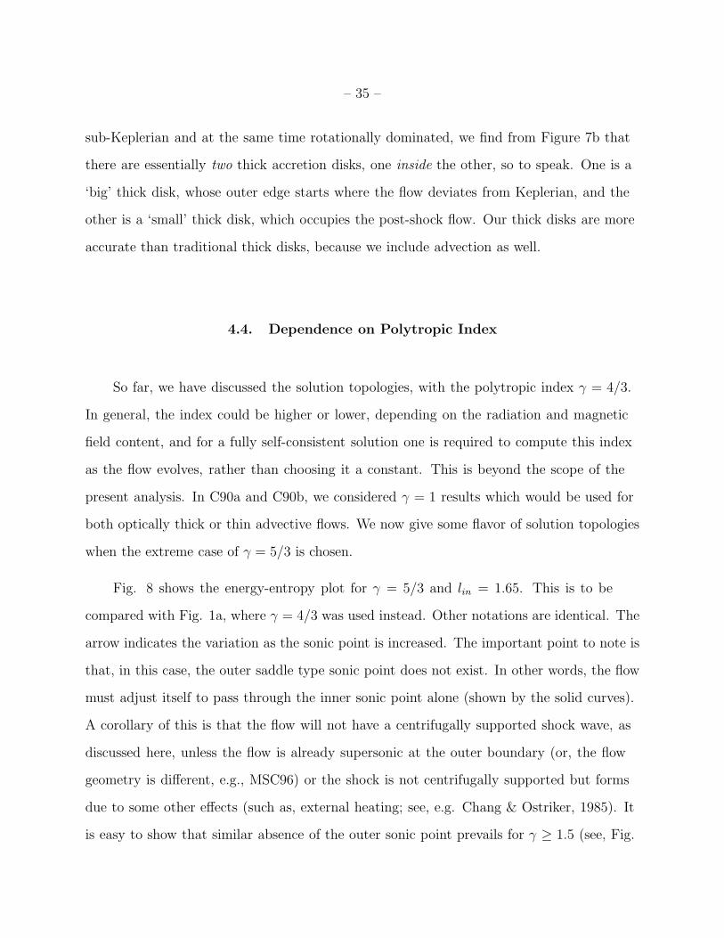
– 35 –

sub-Keplerian and at the same time rotationally dominated, we find from Figure 7b that

there are essentially two thick accretion disks, one inside the other, so to speak. One is a

‘big’ thick disk, whose outer edge starts where the flow deviates from Keplerian, and the

other is a ‘small’ thick disk, which occupies the post-shock flow. Our thick disks are more

accurate than traditional thick disks, because we include advection as well.

4.4. Dependence on Polytropic Index

So far, we have discussed the solution topologies, with the polytropic index γ = 4/3.

In general, the index could be higher or lower, depending on the radiation and magnetic

field content, and for a fully self-consistent solution one is required to compute this index

as the flow evolves, rather than choosing it a constant. This is beyond the scope of the

present analysis. In C90a and C90b, we considered γ = 1 results which would be used for

both optically thick or thin advective flows. We now give some flavor of solution topologies

when the extreme case of γ = 5/3 is chosen.

Fig. 8 shows the energy-entropy plot for γ = 5/3 and lin = 1.65. This is to be

compared with Fig. 1a, where γ = 4/3 was used instead. Other notations are identical. The

arrow indicates the variation as the sonic point is increased. The important point to note is

that, in this case, the outer saddle type sonic point does not exist. In other words, the flow

must adjust itself to pass through the inner sonic point alone (shown by the solid curves).

A corollary of this is that the flow will not have a centrifugally supported shock wave, as

discussed here, unless the flow is already supersonic at the outer boundary (or, the flow

geometry is different, e.g., MSC96) or the shock is not centrifugally supported but forms

due to some other effects (such as, external heating; see, e.g. Chang & Ostriker, 1985). It

is easy to show that similar absence of the outer sonic point prevails for γ ≥ 1.5 (see, Fig.

– 36 –

3.1 of C90b). It is possible that relativistic flows close to a black hole has γ ∼ 13/9 (e.g.,

Shapiro & Teukolsky, 1983), thus may be the possibility of shocks are more generic.

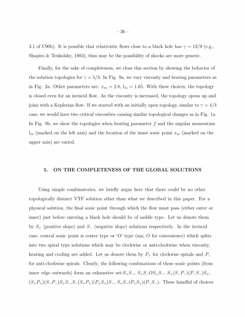
Finally, for the sake of completeness, we close this section by showing the behavior of

the solution topologies for γ = 5/3. In Fig. 9a, we vary viscosity and heating parameters as

in Fig. 2a. Other parameters are: xin = 2.8, lin = 1.65. With these choices, the topology

is closed even for an inviscid flow. As the viscosity is increased, the topology opens up and

joins with a Keplerian flow. If we started with an initially open topology, similar to γ = 4/3

case, we would have two critical viscosities causing similar topological changes as in Fig. 1a.

In Fig. 9b, we show the topologies when heating parameter f and the angular momentum

lin (marked on the left axis) and the location of the inner sonic point xin (marked on the

upper axis) are varied.

5. ON THE COMPLETENESS OF THE GLOBAL SOLUTIONS

Using simple combinatorics, we briefly argue here that there could be no other

topologically distinct VTF solution other than what we described in this paper. For a

physical solution, the final sonic point through which the flow must pass (either outer or

inner) just before entering a black hole should be of saddle type. Let us denote them

by S+ (positive slope) and S− (negative slope) solutions respectively. In the inviscid

case, central sonic point is center type or ‘O’ type (say, O for convenience) which splits

into two spiral type solutions which may be clockwise or anti-clockwise when viscosity,

heating and cooling are added. Let us denote them by P+ for clockwise spirals and P−

for anti-clockwise spirals. Clearly, the following combinations of these sonic points (from

inner edge outwards) form an exhaustive set:S+S−, S+S−OS+S−, S+(S−P−)(P−S−)S+,

(S+P+)(S−P−)S+S−,S−(S+P+)(P+S+)S−, S+S−(P+S+)(P−S−). These handful of choices

– 37 –

are dictated by the fact that a saddle type solution with a positive slope can only join with

a clockwise spiral (this ‘joining’ is indicated by parenthesis) and a saddle type solution

with a negative slope can only join with an anti-clockwise spiral. Except the second case

with ‘O’ type point, which we found in the inviscid flow (C89), the rest have been shown

in various figures of the previous section and C90a and C90b. Although we consider only

vertically averaged flow here, the topologies are not expected to change when a ‘thick’

quasi-spherical flow is considered. Indeed, the presence of shocks would be more generic as

they would appear even outside the equatorial plane because of weaker gravity. Similarly,

when a Kerr black hole is used, the centrifugal barrier become stronger with the increase of

the Kerr parameter because the horizon gets smaller. Thus, the shocks are formed for much

wider parameter range in Kerr geometry.

A fundamental assumption which allowed us to simply classify these solutions is that

the radial forces involved in the momentum equation (eq. 1a) are ‘simple enough’ so that

the velocity variation of the flow could still be reduced into the form (6) or (9) since both the

numerator and the denominator are only algebraic functions and do not involve differential

operators. In the present context, this was possible by choosing Wxφ = −αP prescription

of shear stress. Even then, if the force were more complicated, as in the case of cooler

wind solutions from mass lossing stars where radiative acceleration term with nonlinear

dependence of velocity gradient is included (Castor, Abbott & Klein, 1975), it would not

be possible to reduce the governing equations into a first order differential equation (vital

to the discussions of Bondi-type solutions). Critical curves, instead of critical points would

be present (Flammang, 1982; C90b) solution topologies of which would be more complex.

Discussion on this is beyond the scope of the present analysis.

6. DISCUSSION AND CONCLUSIONS

– 38 –

In this paper, we presented for the first time the global solutions of transonic equations

in presence of viscosity, advection, rotation, generalized heating and cooling. Our VTF

solution starts from a Keplerian disk at the outer edge and enters through the horizon after

passing through sonic point(s). As in our earlier studies of inviscid (C89) and isothermal

VTFs (C90a and C90b), we emphasized here the possibility of the formation of the shock

as well where two transonic solutions are joined together by means of Rankine-Hugoniot

conditions. Though we have used general considerations of heating and cooling, we note

that no new topologies of solutions emerge other than what are discussed in C90a and

C90b. However, unlike in C90a and C90b, where critical viscosities are studied only in the

context of shock formation, our detailed study here indicates that there are indeed two

types of critical viscosities both of which depend on the parameters of the flow. For α < αc1,

accretion through inner sonic point is only allowed (i.e., no shock) or winds with or without

shock is allowed. In this case, the flow joins with a Keplerian disk very far away (Fig.

2a). For αc1 < α < αc2 the flow can have shocks if shock conditions are satisfied, else the

flow will pass through the outer sonic point. For α > αc2, the flow will pass through inner

sonic point again. In this case, the flow joins a Keplerian disk very close (x ∼ 10xg) to the

horizon. Whether both of these critical viscosity parameters exist will depend on the flow

parameters, such as the location of one sonic point, the angular momentum at the inner

edge lin and the heating parameter f . Once we specify these quantities, the entire solution

topology, including the shock location (if present), and the location where the flow joins

with a Keplerian disk are completely determined. Our results depend on the accretion rate

through the cooling parameter g (or, equivalently, through f) and always produce stable

branch of the solution in the M − Σ plane. This is possibly because of our choice that the

cooling could be written as a constant fraction of heating term. We also show that when

the polytropic index is higher than 1.5, in a vertically averaged flow model the outer sonic

point does not exist (though it exists if the disk is thinner, see, MSC96), and therefore,

– 39 –

shocks are possible only if the flow at the outer boundary is already supersonic. Since the

total pressure Π (and not the thermal pressure) is continuous across the shock waves, we

used the Π-stress prescription (CM95) to study shock waves. This prescription is always

valid, and we recommand its uses for the study of astrophysical flows around black holes

and neutron stars, where the advection effect, and therefore ram pressure is important.

Since our VTF solutions have one less free parameter, the M(Σ) relation is monotonic

with positive slope and always represents the stable solutions. In other words, the

thermal/viscous instability is removed completely by the addition of advection effects.

This is true whether or not the flow contains a shock wave. When more general cooling

law is used (with power law dependence on accretion rates, for example), it is possible

that our stable solutions could be ‘destabilized’ in some parameter space spanning M, Σ

as originally discussed by Meyer & Meyer-Hofmeister (1983) (see also, Cannizzo, 1993).

Thus, the problem with our model is not ‘how to stabilize the inner edge of a Keplerian

disk’ but rather, ‘how to destabilize the perfectly stable transonic disks’, if indeed, the

novae outbursts are signatures of such instability. Similarly, because of our choice of

cooling law Q− ∝ Q+, we are unable to show direct influence of accretion rate onto to the

cooling efficiency. Our parametrization indicates that for any accretion rate, higher or lower

efficiency of cooling is possible, just by changing the viscosity parameter. Furthermore, we

find that the variation of xKep with α could be achievable by varying xin and lin as well

(Fig. 3) even when the entire flow has constant viscosity parameter α. These questions are

easily answered by assuming exact cooling laws as far as possible. We shall examine these

solutions in near future.

Unlike the properties of the more complex VTF models, where non-linear radiative

accelerations play major roles, we used simpler momentum equation, relevant for hot flows

close to a compact object. This enabled us not only to obtain global solutions in general,

– 40 –

but also to discuss about the complete set of topologies. Indeed, the same topologies were

seen in isothermal VTFs (C90a and C90b), and we argued that no other type of solutions

are possible either. The same conclusion holds even when more general cooling laws (such

as with power law dependence on density and temperatures) are employed (MSC96). Our

results have the same accuracy as that of the description of the pseudo-Newtonian potential

of a Schwarzschild geometry. But as we discussed in the introduction, no new topologies

have been discovered for inviscid flows when full general relativistic models are solved

(C96b). However, under some circumstances the torque can become negative and the

angular momentum is transported inward. This happens just outside the horizon and does

not affect the solution topologies.

Having not discovered any new topologies, we believe that the unified scheme of global

solutions presented by us (C93, C94, C95, CM95) with the knowledge of isothermal disks

remains valid even for disks with general heating and cooling. In C94, we wrote “... These

findings are very significant as they propose a unifying view of the accretion disks. This

incorporates two extreme disk models into a single framework: for inviscid disks, strong

shocks are produced, and for disks with high enough viscosity, the stable shock disappears

altogether and angular momentum can become Keplerian.” Our present grand unified

global solution describes the most general form of accretion which goes over to the other

disk models presented in the literature. This is not surprising, since we exactly solve the

most general equations. Our disk can pass through either or both the sonic points (when

shocks are present) while joining smoothly with the Keplerian disk at a distance xKep. The

post-shock flow, where the disk is rotationally dominated (Fig. 7a) behaves exactly as the

thick accretion disks (e.g. Paczynski & Wiita, 1980; see MLC94). If the shock does not form,

the sub-Keplerian optically thin flow will behave similar to the ion-supported tori (Rees

et al. 1982) because cooling is inefficient in an optically thin flow, and the entire energy

remains conserved and is advected away (C89). However, our solution is more consistent

– 41 –

than a conventional thick disk model as we include advection term as well, and obtain

the global solutions (see also related discussions in CT95). In MLC94, we have already

verified that the results of vertically averaged solution (C89) are sufficiently accurate. Our

solutions indicate that winds may be produced from the inflow with positive energy (C89;

Fig. 1a) which are verified through extensive numerical simulations (MLC94, Ryu et al.

1995). A knowledge of the dependence of xKep on viscosity enabled us to construct the most

general form of accretion disk, in which Keplerian disk in the equatorial plane is flanked

by sub-Keplerian flows above and below. Post-shock hot matter Comptonizes soft-photons

from the Keplerian disk to produce hard X-rays (CT95). This understanding has resolved

the long standing problem of transition of states of black hole spectra. Furthermore, MSC96

shows that shock oscillations could be responsible for the quasi-periodic oscillation. The

difference of the inner boundary condition in the neutron star and black holes has resulted

in a difference in spectral index from the emergent spectra in soft states (CT95). Our most

general solution can also provide explanations of more complex phenomena, such as the

spectral evolution observed during novae outbursts (Ebisawa et al., 1996). For instance,

during the quiescence stage, viscosity being low, the disk deviates from being Keplerian

farther away (Figs. 2a, 7a, 7b) and the generally optical radiation is accompanied by very

weak X-rays which are produced due to reprocessing of the soft radiation intercepted by

the sub-Keplerian inner disk. As the viscosity at the outer edge is increased due to piling

up of matter (e.g., Cannizzo, 1993), the sub-Keplerian flow first rushes in close to the

black hole (since the in fall time scale is shorter for a sub-Keplerian flow) increasing the

hard X-ray component as commonly observed in the pre-outburst phases (Ebisawa et al.,

1994). Subsequent increase in Keplerian matter close to the black hole increases soft-X-ray

component as is observed. Thus, the present grand unification of the accretion solutions is

more complete, and successfully bridges the gap between the well studied spherical Bondi

flow (e.g., Shapiro, 1973a,b; Ostriker et al., 1976; Begelman, 1978; Colpi, Maraschi &

– 42 –

Treves, 1984; Wandel, Yahil & Milgrom, 1984; Blondin, 1986; Begelman & Chiueh, 1988;

Park & Ostriker, 1989; Park 1990; Nobili, Turolla & Zampieri 1991) and the Keplerian disks

of Shakura & Sunyaev (1973) and Novikov & Thorne (1973). An important ramification of

having sub-Keplerian disks is that the azimuthal velocities are less than that of a Keplerian

flow. The masses of the central object determined from such considerations (e.g., using

Doppler shifts of emitted lines) are naturally higher (Chakrabarti, 1995) than what it

would have been if Keplerian motions were assumed instead. Similarly, due to inefficiency

of emission processes in disks with advection, the masses of the central black holes in active

galaxies (which traditionally equates central luminosities with Eddington luminosities)

might have been seriously underestimated (C96). Fabian & Rees (1995) raise such concerns

recently using self-similar, super-advective flow solutions. However, since we found that the

angular momentum in the accretion is no less than 20 − 50 percent of the Keplerian disk,

the conclusions would be expected to be less dramatic.

The author acknowledges the hospitality of Max-Planck Institute (Garching) and

Landessternwarte (Heidelberg) in the summer of 1994, where this work was partially

completed. He thanks R. Khanna and Stefan Appl (both at Landessternwarte) for

discussions. He also thanks an unknown referee and Paul Wiita for the encouragement

to expand a smaller, cryptic version of this work originally submitted to Astrophysical

Journal Letters (also in the e-print archive under astro-ph/9508060). The present research

is supported through a Senior Research Associateship award from National Academy of

Sciences.

– 43 –

REFERENCES

Abramowicz, M.A. & Chakrabarti, M.A. 1990, ApJ, 350, 281

Abramowicz, M.A., Czerny, B., Lasota, J.P. & Szuzkiewicz, E. 1988, ApJ, 332

Abramowicz, M.A. & Zurek, W.H. 1981, ApJ, 246, 314

Anderson, M.R., & Lemos, J.P.S. 1986, MNRAS, 233, 489

Begelman, M.C. & Chiueh, T. 1988, ApJ, 332, 872

Begelman, M.C. 1978, MNRAS, 185, 847

Blandford, R.D. & Payne, D.G. 1981, MNRAS, 194, 1033

Blondin, J.M. 1986, ApJ, 308, 755

Cannizzo, J.K. 1993, in Accretion Disks in Compact Stellar Systems, ed. J. Craig Wheeler

(Singapore: World Scientific).

Castor, J.I., Abbott, D.C., & Klein, R.I. 1975, ApJ, 195, 157.

Chakrabarti, S.K. 1985, ApJ, 288, 1 (C85)

Chakrabarti, S.K., Jin, L., & Arnett, W.D. 1987, ApJ, 313, 674

Chakrabarti, S.K. 1989, ApJ, 347, 365 (C89)

Chakrabarti, S.K. 1990a, MNRAS, 243, 610 (C90a)

Chakrabarti, S.K. 1990b, Theory of Transonic Astrophysical Flows (Singapore: World

Scientific) (C90b)

Chakrabarti, S.K. 1990c, ApJ, 362, 406

Chakrabarti, S.K. 1990d, ApJ, 350, 275

Chakrabarti, S.K. 1990e, MNRAS, 246, 134

Chakrabarti, S.K. 1992, MNRAS, 256, 300

– 44 –

Chakrabarti, S.K. in Numerical Simulations in Astrophysics, Eds. J. Franco, S. Lizano, L.

Aguilar & E. Daltabuit (Cambridge University Press: Cambridge, 1993) [C93]

Chakrabarti, S.K. 1994, in Proceedings of 17th Texas Symposium (New York Academy of

Sciences, New York) [C94]

Chakrabarti, S.K. 1995, ApJ, 441, 576 [C95]

Chakrabarti, S.K. 1996a, Physics Reports, 266, No. 5-6, 238 [C96a]

Chakrabarti, S.K. 1996b, MNRAS, in press [C96b]

Chakrabarti, S.K., & Molteni, D. 1993, ApJ, 417, 671 [CM93]

Chakrabarti, S.K., & Molteni, D. 1995, MNRAS, 272, 80 [CM95]

Chakrabarti, S.K., & Titarchuk, L. 1995, ApJ (Dec 20th) [CT95]

Chang K. M., & Ostriker, J. P. 1985, ApJ, 288, 428

Colpi, M., Maraschi, L. & Treves, A. 1984, ApJ, 280, 319

Ebisawa, K. et al. 1994, PASJ, 46, 375

Ebisawa, K., Titarchuk, L.G., & Chakrabarti, S.K. 1996, PASJ, 48, No.1 in press

Englmaier, P. Diploma Thesis, University of Heidelberg (1993).

Fabian, A.C., & Rees, M.J. 1995, MNRAS, in press

Flammang, R.A. 1982, MNRAS, 199,833

Ferrari, A., Trussoni, E., Rosner, R. & Tsinganos, T. 1985, ApJ, 294, 397

Frank, J., King, A.R., & Raine, D.J., Accretion Power in Astrophysics (Cambridge

University Press, Cambridge, 1991)

Ipser, J.R. & Price, R.H. 1982, ApJ, 255, 654

Lasota, J.P., Abramowicz, M., Chen, X., Krolik, J.H., Narayan,R., & Yi, I. 1996, preprint

– 45 –

Liang, E.P.T & Thomson, K.A., 1980, ApJ, 240, 271

Lu, J.F., 1985, A&A, 148, 176

Matsumoto, R., Kato, S., Fukue, J., & Okazaki, A.T. 1984, PASJ, 36, 71

Meszaros, P. 1975, A & A, 44, 59

Meyer, F., & Meyer-Hofmeister, E. 1983, A&A, 128, 420

Molteni, D., Lanzafame, G., & Chakrabarti, S.K. 1994, ApJ, 425, 161 [MLC94]

Molteni, D., Sponholz, H., & Chakrabarti, S.K. 1996, ApJ (in press) [MSC96]

Muchotrzeb B. 1983, Acta Astron., 33, 79

Nakayama, K. 1982, MNRAS, 259, 259

Narayan, R., 1996, in “Basic Physics of Accretion Disks” eds. S. Kato et al., Gordon and

Breach Science Publishers (New York, 1996) in press

Narayan, R., & Yi, I. 1994, ApJ, 428, L13

Narayan, R., & Yi, I. 1995a, ApJ, 444, 231

Narayan, R., & Yi, I. 1995b, ApJ, in press

Narayan, R., Yi, I., & Mahadevan, R. 1995, Nature, 374, 623

Narayan, R., McLintock, J.E., & Yi, I. 1996, ApJ, in press

Nobili, L., Turolla, R. & Zampieri, L. 1991, ApJ, 383, 250

Nobuta, K. & Hanawa, T. 1994, PASJ, 46, 257

Novikov, I. & Thorne, K.S. in: Black Holes, eds. C. DeWitt and B. DeWitt (Gordon and

Breach, New York, 1973).

Ostriker, J.P., McCray, R., Weaver, R. & Yahil, A. 1976, ApJ, 208, L61

Paczynski, B. & Bisnovatyi-Kogan, G. 1981, Acta Astron., 31, 283

– 46 –

Paczynski, B. & Wiita, P.J. 1980 A&A, 88, 23

Park, M.G., 1990, ApJ, 354, 64

Park, M.G., & Ostriker, J.P. 1989, ApJ, 347, 679

Pringle, J. 1981, Ann. Rev. Astron. Astrophys., 19, 137

Rees, M., M. J., Begelman, M. C., Blandford, R. D., & Phinney, E. S. 1982, Nature, 295, 17

Ryu, J., Brown, G., Ostriker, J. & Loeb, A. 1995, ApJ, (in press).

Shakura, N.I. & Sunyaev, R.A. 1973, A&A, 24, 337 [SS73]

Shapiro, S.L. 1973a, ApJ, 180, 531

Shapiro, S.L. 1973b, ApJ, 1185, 69

Shapiro, S.L. & Teukolsky, S.A., Black Holes, White Dwarfs and Neutron Stars — the

Physics of Compact Objects (John Wiley & Sons, New York, 1983)

Sunyaev, R. A. et al., 1994, Astron. Lett. 20, 777

Spruit, H.C. 1987, A & A, 184, 173

Taam, R.E. & Fryxell, B.A., 1985, ApJ, 294, 303

Takahashi, M., Nitta, M., Tatematsu, Y., Tomimatsu, A. 1990, ApJ, 363, 206

Tanaka, Y. in Proceedings of the 23rd ESLAB symposium, ed. J. Hunt & B. Battrick, vol.

1, p.3, 1989, (ESA, Paris)

Thompson, J.M.T. & Stewart, H.B., Nonlinear Dynamics and Chaos (John Wiley & Sons

Ltd., 1985)

Wandel, A., Yahil, A. & Milgrom, M., 1984, ApJ, 282, 53

This manuscript was prepared with the AAS LATEX macros v3.0.

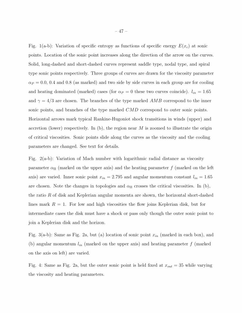
– 47 –

Fig. 1(a-b): Variation of specific entropy as functions of specific energy E(xc) at sonic

points. Location of the sonic point increases along the direction of the arrow on the curves.

Solid, long-dashed and short-dashed curves represent saddle type, nodal type, and spiral

type sonic points respectively. Three groups of curves are drawn for the viscosity parameter

αP = 0.0, 0.4 and 0.8 (as marked) and two side by side curves in each group are for cooling

and heating dominated (marked) cases (for αP = 0 these two curves coincide). lin = 1.65

and γ = 4/3 are chosen. The branches of the type marked AMB correspond to the inner

sonic points, and branches of the type marked CMD correspond to outer sonic points.

Horizontal arrows mark typical Rankine-Hugoniot shock transitions in winds (upper) and

accretion (lower) respectively. In (b), the region near M is zoomed to illustrate the origin

of critical viscosities. Sonic points slide along the curves as the viscosity and the cooling

parameters are changed. See text for details.

Fig. 2(a-b): Variation of Mach number with logarithmic radial distance as viscosity

parameter αΠ (marked on the upper axis) and the heating parameter f (marked on the left

axis) are varied. Inner sonic point xin = 2.795 and angular momentum constant lin = 1.65

are chosen. Note the changes in topologies and αΠ crosses the critical viscosities. In (b),

the ratio R of disk and Keplerian angular momenta are shown, the horizontal short-dashed

lines mark R = 1. For low and high viscosities the flow joins Keplerian disk, but for

intermediate cases the disk must have a shock or pass only though the outer sonic point to

join a Keplerian disk and the horizon.

Fig. 3(a-b): Same as Fig. 2a, but (a) location of sonic point xin (marked in each box), and

(b) angular momentum lin (marked on the upper axis) and heating parameter f (marked

on the axis on left) are varied.

Fig. 4: Same as Fig. 2a, but the outer sonic point is held fixed at xout = 35 while varying

the viscosity and heating parameters.

– 48 –

Fig. 5(a-b): Example of a complete solution which includes a shock wave. αΠ = 0.05,

lin = 1.6, γ = 4/3 and f = 0.5, xout = 50 are used. Shock conditions are satisfied at

x = 13.9 (vertical dashed curve) and the flow subsequently enters the black hole along the

long dashed curves after becoming supersonic at xin = 2.8695. The arrowed curves trace the

complete solution with a shock wave in a black hole accretion. Double arrowed curves denote

the shock solution in a neutron star accretion with sub-sonic inner boundary condition.

In (b), the procedure of obtaining the shock solutions is illustrated by plotting the Mach

invariant C, the total pressure Π and the energy E(x) of the subsonic and super branches

all of which intersect at the shock location. Note that the angular momentum remains

continuous across the shock. Other physical quantities, such as the proton temperature and

the radial velocity are also shown.

Fig. 6: Parametric dependence on the formation and location of shocks in black hole and

neutron star accretions. Single arrows represent shocks in accretion around black holes while

the double arrows represent shocks around compact neutron stars. Pairs of parameters

(αΠ, f) are shown in each box. The outer sonic point is chosen to be at xout = 50. In the

neutron star case, the shock transition takes place only to that particular sub-sonic branch

which corrotates with the star at the star surface.

Fig. 7(a-b): Ratio of (a) radial to azimuthal velocities (vr/vφ) and (b) disk angular

momentum to Keplerian angular momentum (l/lKep) are shown in a few solutions. In (a)

the curves marked with numbers correspond to the grid number of Fig. 2a. The curve

marked ‘shock’ correspond to the solution in Fig. 5a. Solutions except those marked ‘43’

and ‘12’ join smoothly with Keplerian disks as they become rotation dominated. In (b),

the curves are marked with viscosity parameters (the curve marked 0.05 correspond to the

shock solution in Fig. 5a). Note that xKep, where the flow joins a Keplerian disk, depends

inversely on the viscosity parameter. See text for detail.

– 49 –

Fig. 8: Same as Fig. 1a, but drawn for γ = 5/3 to illustrate that the outer saddle type

sonic point does not exist (a feature shared by flows with γ > 1.5 in a vertically averaged

model). Thus the flow from a Keplerian disk must pass only through the inner sonic point.

Centrifugally supported shocks could form only if the flow at outer boundary is already

supersonic (e.g., originated from stellar winds).

Fig. 9(a-b): Similar to Figs. 2-3, showing the variation of solution topologies when γ = 5/3

is chosen. See text for details.

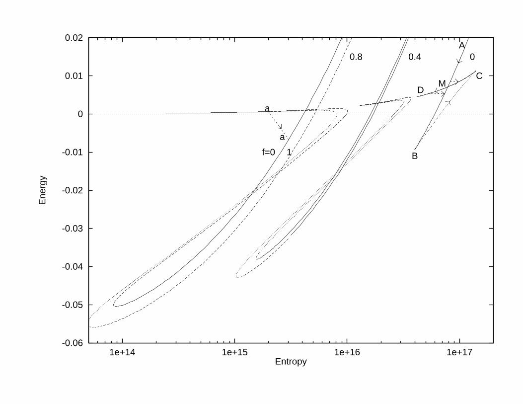
-0.06

-0.05

-0.04

-0.03

-0.02

-0.01

0

0.01

0.02

1e+14 1e+15 1e+16 1e+17

Ene

rgy

Entropy

00.40.8A

M

B

C

D

f=0 1

a

a

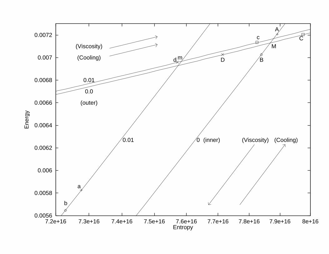
0.0056

0.0058

0.006

0.0062

0.0064

0.0066

0.0068

0.007

0.0072

7.2e+16 7.3e+16 7.4e+16 7.5e+16 7.6e+16 7.7e+16 7.8e+16 7.9e+16 8e+16

Ene

rgy

Entropy

00.01

m

0.0

0.01

(outer)

(inner)

M

A

B

C

D

(Viscosity) (Cooling)

(Viscosity)

(Cooling)

c

d

a

b

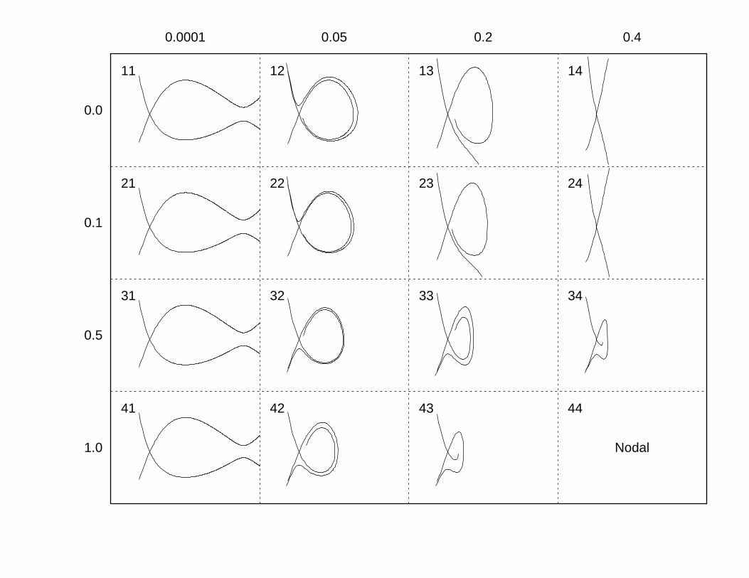
0.0001 0.05 0.2 0.4

1.0

0.5

0.1

0.0

11

21

31

41

12

22

32

42

13

23

33

43

14

24

34

44

Nodal

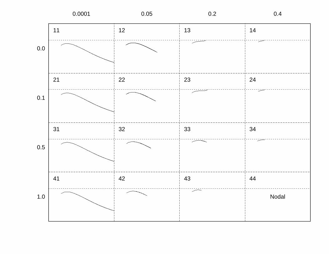
0.0001 0.05 0.2 0.4

1.0

0.5

0.1

0.0

11

21

31

41

12

22

32

42

13

23

33

43

14

24

34

44

Nodal

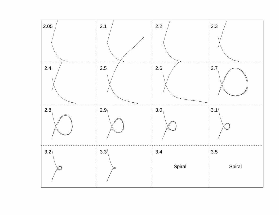
2.05

2.4

2.8

3.2

2.1

2.5

2.9

3.3

2.2

2.6

3.0

3.4

2.3

2.7

3.1

3.5

SpiralSpiral

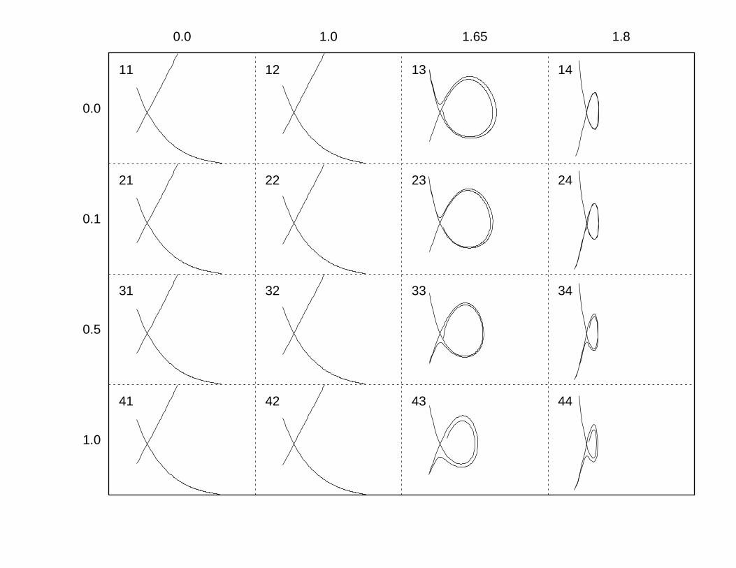
0.0 1.0 1.65 1.8

1.0

0.5

0.1

0.0

11

21

31

41

12

22

32

42

13

23

33

43

14

24

34

44

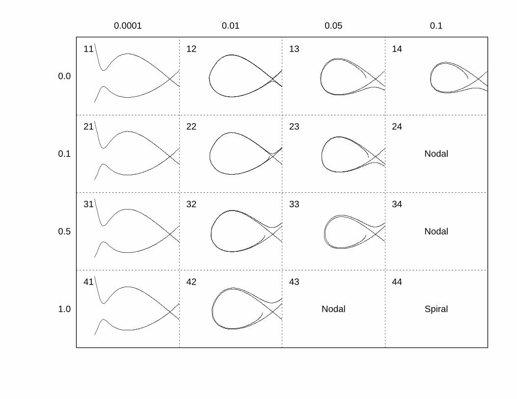
0.0001 0.01 0.05 0.1

1.0

0.5

0.1

0.0

11

21

31

41

12

22

32

42

13

23

33

43

14

24

34

44

Spiral

Nodal

Nodal

Nodal

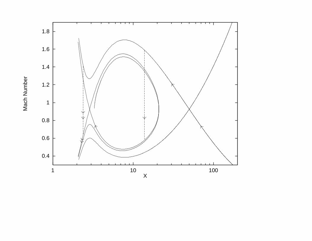
0.4

0.6

0.8

1

1.2

1.4

1.6

1.8

1 10 100

Mac

h N

umbe

r

X

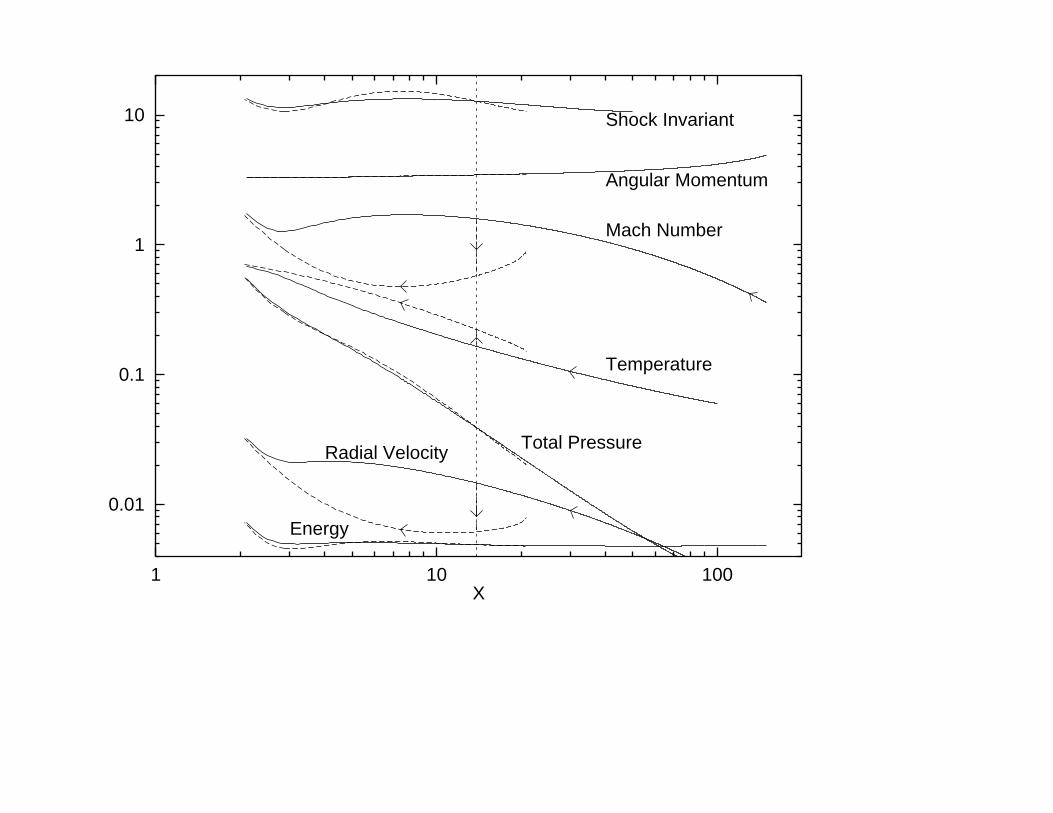
0.01

0.1

1

10

1 10 100X

Shock Invariant

Angular Momentum

Mach Number

Total Pressure

Energy

Temperature

Radial Velocity

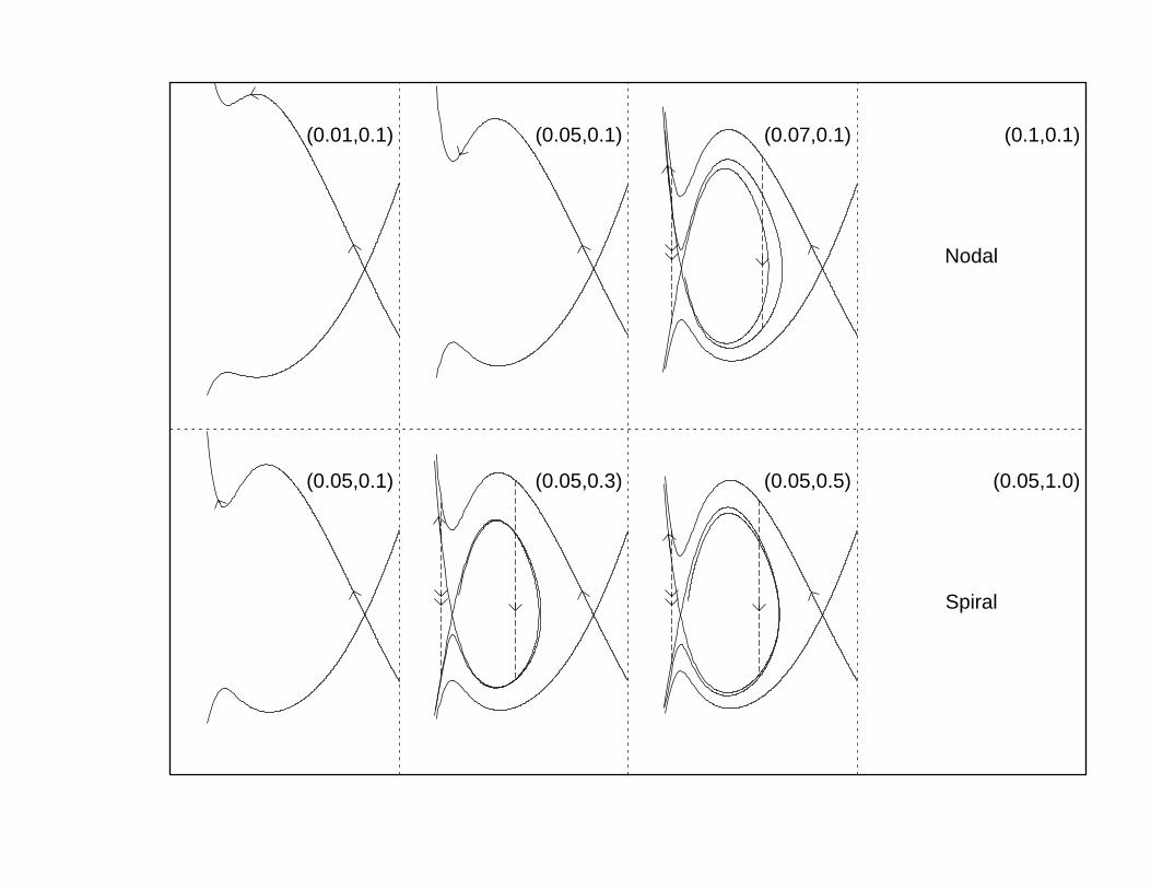
(0.01,0.1)

(0.05,0.1)

(0.05,0.1)

(0.05,0.3)

(0.07,0.1)

(0.05,0.5)

(0.1,0.1)

(0.05,1.0)

Nodal

Spiral

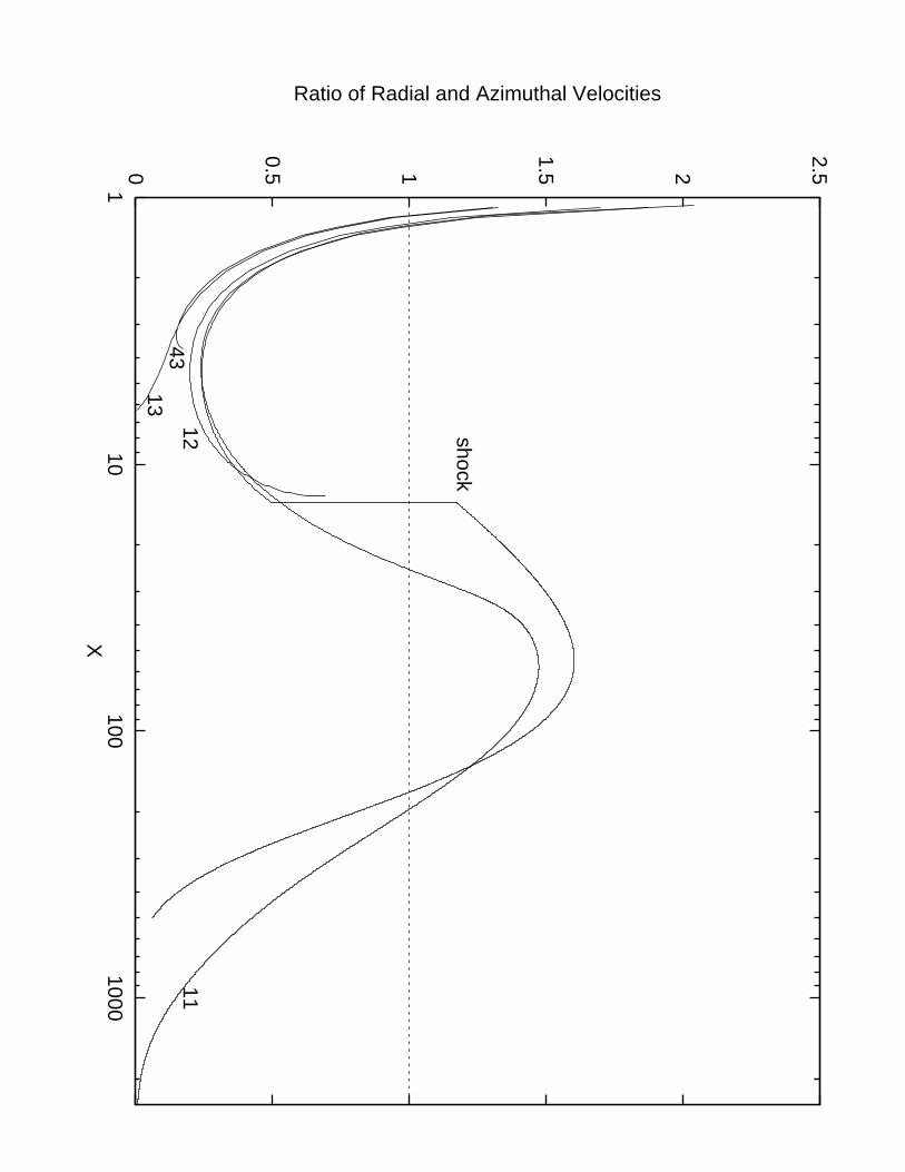
0

0.5 1

1.5 2

2.5

110

1001000

Ratio of Radial and Azimuthal Velocities

X

11

1343

12 shock

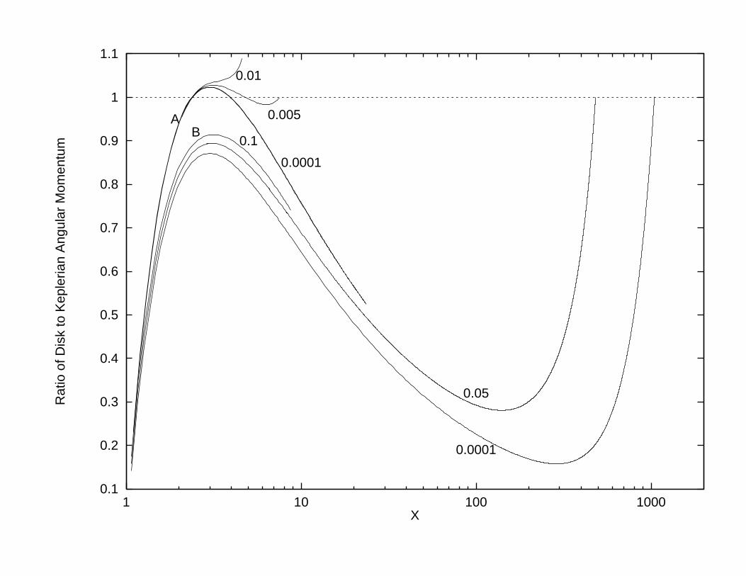
0.1

0.2

0.3

0.4

0.5

0.6

0.7

0.8

0.9

1

1.1

1 10 100 1000

Rat

io o

f Dis

k to

Kep

leria

n A

ngul

ar M

omen

tum

X

AB

0.01

0.005

0.0001

0.0001

0.05

0.1

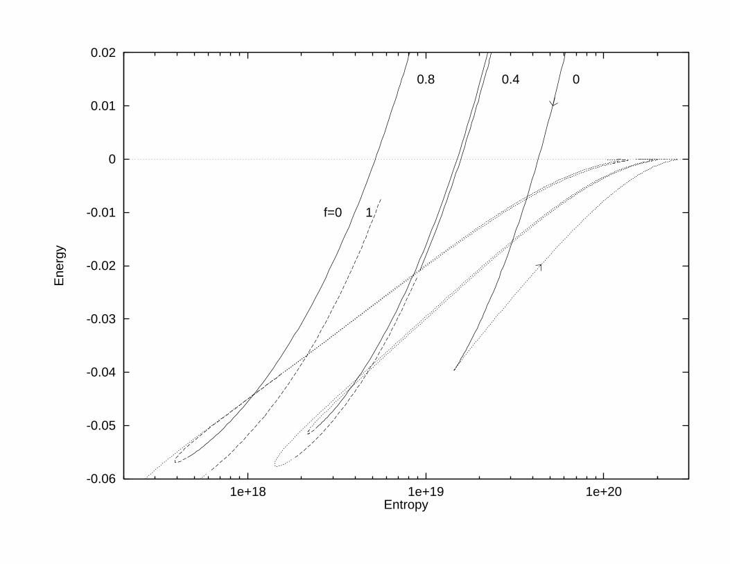
-0.06

-0.05

-0.04

-0.03

-0.02

-0.01

0

0.01

0.02

1e+18 1e+19 1e+20

Ene

rgy

Entropy

00.40.8

f=0 1

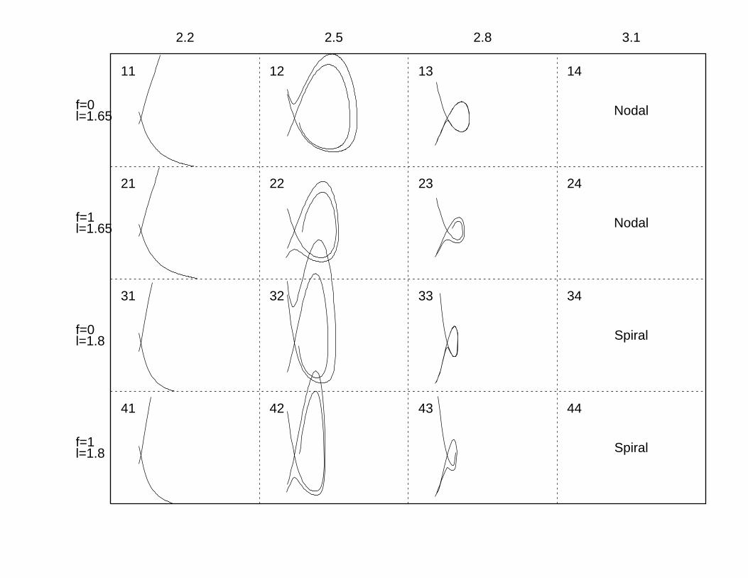
l=1.65

l=1.65

l=1.8

l=1.8

11

21

31

41

12

22

32

42

13

23

33

43

14

24

34

44

Nodal

Nodal

Spiral

Spiral

2.2 2.5 2.8 3.1

f=0

f=1

f=0

f=1

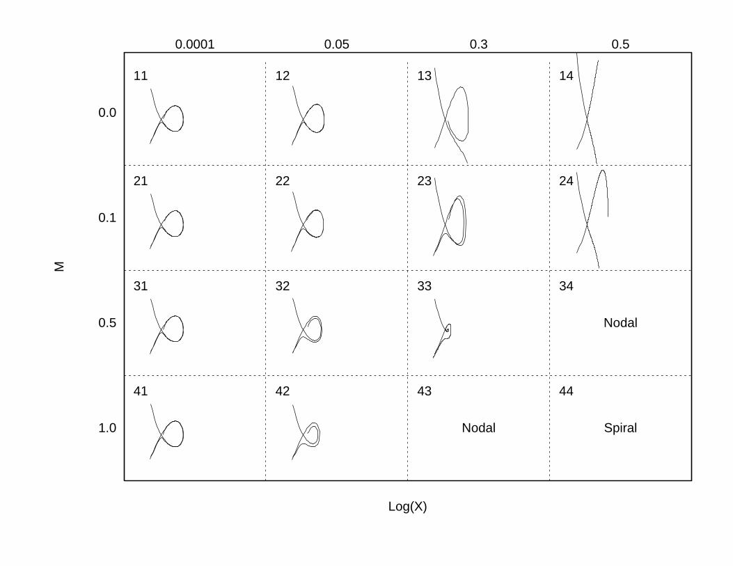
M

Log(X)

0.0001 0.05 0.3 0.5

1.0

0.5

0.1

0.0

11

21

31

41

12

22

32

42

13

23

33

43

14

24

34

44

Nodal Spiral

Nodal