Temperature–depth relationships based on log data from the Los Azufres geothermal field, Mexico

Temperature±depth relationships basedon log data from the Los Azufres

geothermal ®eld, Mexico

Gerardo Garcia-Estrada a,*, Aida Lopez-Hernandez a,Rosa Maria Prol-Ledesma b

aComision Federal de Electricidad, Alejandro Volta 655, Morelia 58290, Mich., MexicobInstituto de Geo®sica, Universidad Nacional Autonoma de Mexico, Mexico

Received 24 February 1999; accepted 22 June 2000

Abstract

Equilibrium temperatures based on log data acquired during drilling stops in the LosAzufres geothermal ®eld were used to study the relationship between temperature, depth andconductive heat ¯ow that di�erentiate production from non-production areas. Temperature

and thermal conductivity data from 62 geothermal wells were analyzed, displaying tempera-ture±depth, gradient±depth, and ternary temperature±gradient±depth plots. In the ternaryplot, the production wells of Los Azufres are located near the temperature vertex, wherenormalized temperatures are over 0.50 units, or where the temperature gradient is over 165�C/km. In addition, the temperature data were used to estimate the depth at which 600�C couldbe reached (5±9 km) and the regional background conductive heat ¯ow (� 106 mW/m2).Estimates are also given for the conductive heat ¯ow associated with the conductive cooling of

an intrusive body (� 295 mW/m2), and the conductive heat ¯ow component in low-perme-ability blocks inside the reservoir associated with convection in limiting open faults (from 69to 667 mW/m2). The method applied in this study may be useful to interpret data from new

geothermal areas still under exploration by comparing with the results obtained from LosAzufres. # 2001 CNR. Published by Elsevier Science Ltd. All rights reserved.

Keywords: Stabilized temperatures; Thermal gradient; Temperature logs; Los Azufres; Mexico

Geothermics 30 (2001) 111±132

www.elsevier.com/locate/geothermics

0375-6505/01/$20.00 # 2001 CNR. Published by Elsevier Science Ltd. All rights reserved.

PI I : S0375-6505(00 )00039 -0

* Corresponding author. Tel.: +52-4-322-7087; fax: +52-4-322-7060.

E-mail address: [email protected] (G. Garcia-Estrada).

1. Introduction

Los Azufres, the second largest geothermal ®eld in Mexico and the ®rst one infractured media, is located in the central sector of the Trans Mexican Volcanic Belt(TMVB), 180 km west of Mexico City (Fig. 1). It had a maximum installed capacityof 98 MWe in 1995 (Gutierrez, 1997) and has an estimated potential of more than200 MWe in the northern sector of the ®eld alone (Suarez, 1997). Los Azufres has

Fig. 1. Location and geologic map of Los Azufres geothermal ®eld.

112 G. Garcia-Estrada et al. / Geothermics 30 (2001) 111±132

been used as a testing area for numerous exploratory techniques, because a com-prehensive set of data is available to evaluate the results. This study is part of aproject to analyse thermal data to estimate the undisturbed initial thermal state of the®eld. The analysis of the relationship among equilibrium temperature, thermal gradient,well depth, and production zones at Los Azufres is based on the simultaneous graphicdisplay of all available data. The objective is to characterize production areas in LosAzufres geothermal ®eld using these three parameters to interpret thermal data onother geothermal zones under exploration.Numerical modelling using TOUGH2 (Pruess, 1989) has been conducted to test

the validity of the results presented here (Garcia, 2000). This model was constrainedby the numerical estimates of thermal gradient and heat ¯ow given here for repre-sentative sectors of Los Azufres geothermal ®eld.

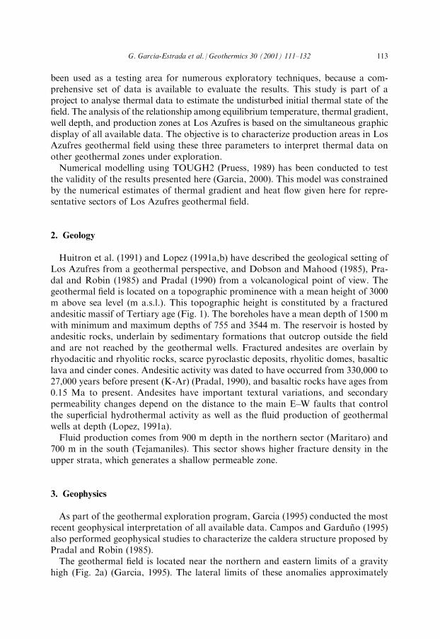
2. Geology

Huitron et al. (1991) and Lopez (1991a,b) have described the geological setting ofLos Azufres from a geothermal perspective, and Dobson and Mahood (1985), Pra-dal and Robin (1985) and Pradal (1990) from a volcanological point of view. Thegeothermal ®eld is located on a topographic prominence with a mean height of 3000m above sea level (m a.s.l.). This topographic height is constituted by a fracturedandesitic massif of Tertiary age (Fig. 1). The boreholes have a mean depth of 1500 mwith minimum and maximum depths of 755 and 3544 m. The reservoir is hosted byandesitic rocks, underlain by sedimentary formations that outcrop outside the ®eldand are not reached by the geothermal wells. Fractured andesites are overlain byrhyodacitic and rhyolitic rocks, scarce pyroclastic deposits, rhyolitic domes, basalticlava and cinder cones. Andesitic activity was dated to have occurred from 330,000 to27,000 years before present (K-Ar) (Pradal, 1990), and basaltic rocks have ages from0.15 Ma to present. Andesites have important textural variations, and secondarypermeability changes depend on the distance to the main E±W faults that controlthe super®cial hydrothermal activity as well as the ¯uid production of geothermalwells at depth (Lopez, 1991a).Fluid production comes from 900 m depth in the northern sector (Maritaro) and

700 m in the south (Tejamaniles). This sector shows higher fracture density in theupper strata, which generates a shallow permeable zone.

3. Geophysics

As part of the geothermal exploration program, Garcia (1995) conducted the mostrecent geophysical interpretation of all available data. Campos and GardunÄ o (1995)also performed geophysical studies to characterize the caldera structure proposed byPradal and Robin (1985).The geothermal ®eld is located near the northern and eastern limits of a gravity

high (Fig. 2a) (Garcia, 1995). The lateral limits of these anomalies approximately

G. Garcia-Estrada et al. / Geothermics 30 (2001) 111±132 113

Fig. 2. Contour maps of geophysical parameters measured in Los Azufres geothermal ®eld. Filled circles

indicate well locations (see well numbers in Fig. 1): (a) residual of the Bouguer anomaly (contours in

mGal, interval = 1 mGal); (b) apparent resistivity obtained with Schlumberger soundings for AB/

2=2000 m (contours in ohm-m, interval 10 ohm-m). The hatched area shows the location of the known

reservoir.


coincide with the 50 ohm-m contour of apparent resistivity with AB/2=2000 mmeasured using a Schlumberger array (Fig. 2b). The identi®ed geothermal reservoiris contained within the 40 ohm-m apparent resistivity values.Campos and GardunÄ o (1995) suggested that the geothermal ®eld might be the

result of magma resurgence in the central sector of the caldera. However, Garcia(1997) considered that the heat source of the geothermal ®eld can not be relateddirectly to the caldera-forming event because it is too old (more than 1.2 Ma beforepresent, according to Pradal, 1990) to expect the thermal anomalies to remain, evenassuming a purely conductive regime. The hydrothermal system must, therefore, berelated to intrusive phenomena younger than 300,000 years.

4. Conceptual model of the internal structure of Los Azufres hydrothermal system

The conceptual model of the Los Azufres hydrothermal system constructed withall available geoscienti®c data (Huitron et al., 1991) indicates that Los Azufresbehaves as a typical high-enthalpy hydrothermal system in rough topography terrainwith predominant secondary permeability. Drilling mud losses and a fast thermalrecovery velocity identify the presence of highly permeable zones, related to activefaulting. Within the reservoir, convection is the main heat transport phenomenon,while in the cap rock and below the reservoir, where low-permeability inhibits convec-tion, conduction is predominant. As a typical hydrothermal system with predominantsecondary permeability, temperature and the governing heat transfer phenomenachange with position faster than in conduction-dominated areas, as a result of thepresence of faults acting as water-¯ow channels.

5. Temperature data

Temperature logs acquired during drilling stops at 62 wells drilled in the area wereused for this study (a table with the equilibrium temperatures and dependant variablesused in this paper is available from the authors). Temperatures are representative ofpre-production data since 86% of the wells were drilled before large-scale productionstarted and all the recent wells have been drilled away from the in¯uence area ofpreviously drilled wells. Pressure logs that were acquired simultaneously with thetemperature measurements in all the wells considered in this study show a hothydrostatic pro®le from the piezometric surface to the bottom of the wells. Pressurecontrol on temperature does not occur. Location of the wells is shown in Fig. 1.Three temperature logs are usually obtained during drilling stops, with elapsed times of

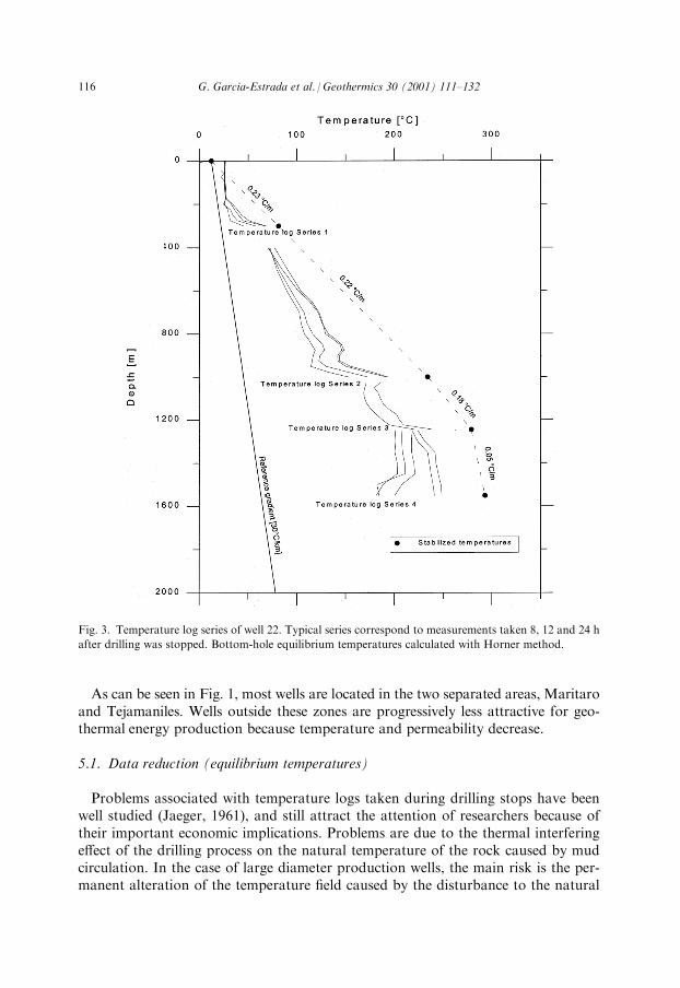
8, 12 and 24 h. At shallow depths temperature logs are obtained at a ®xed depth (300 m).In most bore-holes there are two or three temperature log series at di�erent depths,depending on reservoir engineering requirements, and it is possible to calculate bottom-hole equilibrium temperatures for each series. An example is shown in Fig. 3. Theresulting values are used to estimate a thermal gradient applying the ®nite-di�erencesmethod; for convenience this value is assigned to the mean depth of the interval.


As can be seen in Fig. 1, most wells are located in the two separated areas, Maritaroand Tejamaniles. Wells outside these zones are progressively less attractive for geo-thermal energy production because temperature and permeability decrease.

5.1. Data reduction (equilibrium temperatures)

Problems associated with temperature logs taken during drilling stops have beenwell studied (Jaeger, 1961), and still attract the attention of researchers because oftheir important economic implications. Problems are due to the thermal interferinge�ect of the drilling process on the natural temperature of the rock caused by mudcirculation. In the case of large diameter production wells, the main risk is the per-manent alteration of the temperature ®eld caused by the disturbance to the natural

Fig. 3. Temperature log series of well 22. Typical series correspond to measurements taken 8, 12 and 24 h

after drilling was stopped. Bottom-hole equilibrium temperatures calculated with Horner method.


hydrologic equilibrium. The original formation temperatures are never recovered insuccessful production boreholes after well completion. Drilling temperature logs are,therefore, the best possibility to recover this information.Garcia (1986) conducted numerical tests of di�erent methods to estimate undis-

turbed formation temperatures, in order to understand their scope and limitationsand to de®ne the application criteria for di�erent methods. On the basis of hisresults, the conventional Horner method (Fertl and Wichmann, 1977) was selectedto estimate the equilibrium temperature, after a parameter sensitivity analysis andthe testing of the method for the identi®cation of convective recovery phenomena(Garcia, 1997). Theoretical studies of the recovery phenomenon explain thehypotheses that yield the semi-logarithmic regression, for instance the assumption ofa radial conductive recovery process (Lachenbruch and Brewer, 1959).

5.2. Qualitative graphic analysis and heat ¯ow estimates

The use of numerical modeling programs to explain the presence of thermalanomalies and predict the behaviour of the system should be the ®nal goal of athermal study; however, preliminary results during the feasibility stage can beobtained from a qualitative analysis. Assuming that anomalous phenomena a�ectingwell temperature are random (not biased), a comprehensive data analysis shouldemphasize the regional conductive regime or phenomena less a�ected by local var-iations. Graphic display of the complete data set for a qualitative analysis includedtemperature±depth, temperature gradient±depth and the ternary temperature±depth±temperature gradient plots.Using available thermal conductivity data (Contreras et al., 1988) and gradient

estimation by intervals, the conductive component of heat transfer (heat ¯ow density)was calculated for certain depths. Amean gradient was estimated by linear regression insome wells with a stable temperature gradient at depth, in which heat conductionmay be dominant. This value was used to estimate the depth at which a typicaltemperature for magma could be attained and the deep regional heat ¯ow, whichwas calculated using the mean thermal conductivity. In the following sections adetailed description of the method is given and the results are discussed.

6. Temperature distribution

A contour map calculated by interpolation of temperature data at 1500 m depth ispresented in Fig. 4a. The highest temperatures observed in the ®eld are located in aN±S sector to the east of the 260�C contour. Temperature logs of wells located inthis area (1, 9, 12, 28, 47 and 48) show convection e�ects occurring at temperatureshigher than 300�C below 1500 m depth. There are no N±S faults connecting wells atreservoir depths; similar maximum temperatures in the N-S sector, therefore, suggestthat ¯uids in the northern and the southern zone have a common source, regardlessof the separation between shallow thermal anomalies shown in the temperaturepro®le P-P0 (Fig. 4b). This common thermal energy source may be related to the


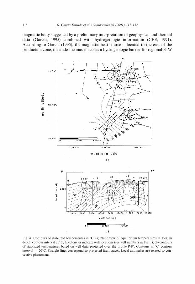
magmatic body suggested by a preliminary interpretation of geophysical and thermaldata (Garcia, 1995) combined with hydrogeologic information (CFE, 1991).According to Garcia (1995), the magmatic heat source is located to the east of theproduction zone, the andesitic massif acts as a hydrogeologic barrier for regional E±W

Fig. 4. Contours of stabilized temperatures in �C: (a) plane view of equilibrium temperatures at 1500 m

depth, contour interval 20�C, ®lled circles indicate well locations (see well numbers in Fig. 1); (b) contours

of stabilized temperatures based on well data projected over the pro®le P-P0. Contours in �C, contourinterval = 20�C. Straight lines correspond to projected fault traces. Local anomalies are related to con-

vective phenomena.


or SE±NW ¯uid ¯ow below the reservoir and, at reservoir depth, the ¯ow of ¯uidsoccurs from east to west along the E±W fault system (Lopez, 1991a).

7. Temperature behavior with depth

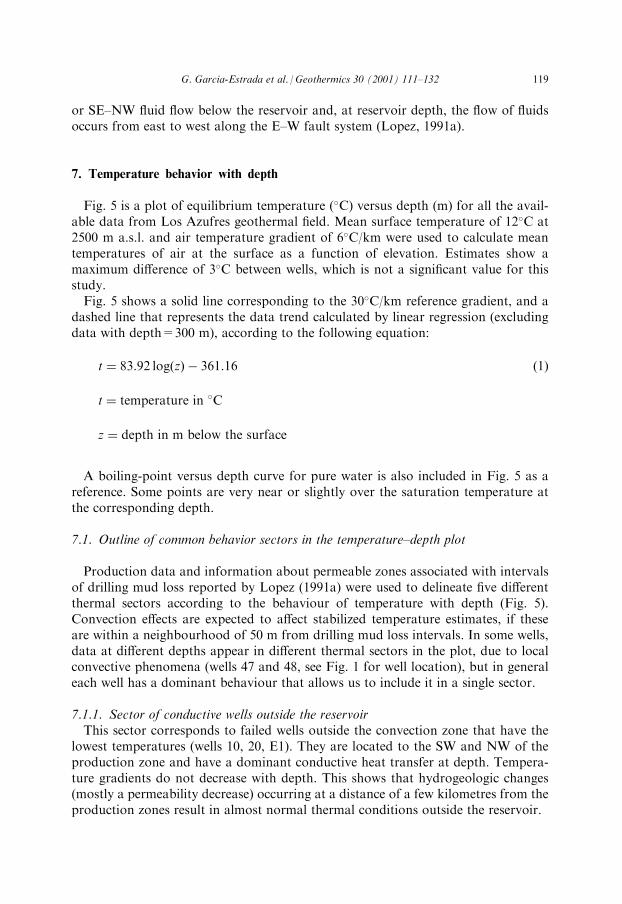
Fig. 5 is a plot of equilibrium temperature (�C) versus depth (m) for all the avail-able data from Los Azufres geothermal ®eld. Mean surface temperature of 12�C at2500 m a.s.l. and air temperature gradient of 6�C/km were used to calculate meantemperatures of air at the surface as a function of elevation. Estimates show amaximum di�erence of 3�C between wells, which is not a signi®cant value for thisstudy.Fig. 5 shows a solid line corresponding to the 30�C/km reference gradient, and a

dashed line that represents the data trend calculated by linear regression (excludingdata with depth=300 m), according to the following equation:

t � 83:92 log z� � ÿ 361:16 �1�

t � temperature in �C

z � depth in m below the surface

A boiling-point versus depth curve for pure water is also included in Fig. 5 as areference. Some points are very near or slightly over the saturation temperature atthe corresponding depth.

7.1. Outline of common behavior sectors in the temperature±depth plot

Production data and information about permeable zones associated with intervalsof drilling mud loss reported by Lopez (1991a) were used to delineate ®ve di�erentthermal sectors according to the behaviour of temperature with depth (Fig. 5).Convection e�ects are expected to a�ect stabilized temperature estimates, if theseare within a neighbourhood of 50 m from drilling mud loss intervals. In some wells,data at di�erent depths appear in di�erent thermal sectors in the plot, due to localconvective phenomena (wells 47 and 48, see Fig. 1 for well location), but in generaleach well has a dominant behaviour that allows us to include it in a single sector.

7.1.1. Sector of conductive wells outside the reservoirThis sector corresponds to failed wells outside the convection zone that have the

lowest temperatures (wells 10, 20, E1). They are located to the SW and NW of theproduction zone and have a dominant conductive heat transfer at depth. Tempera-ture gradients do not decrease with depth. This shows that hydrogeologic changes(mostly a permeability decrease) occurring at a distance of a few kilometres from theproduction zones result in almost normal thermal conditions outside the reservoir.


7.1.2. Sector of conductive and low-permeability wells inside the reservoirThis sector includes wells within the hydrothermal system but very near to its

external boundary (E2, 40, 50, 58) and wells in low-permeability blocks inside thereservoir (3, 23, 44, 47, 48, 54). These wells show moderate convection e�ects andthe temperature can reach between 200 and 250�C at 2000 m depth; however, mostof them are not productive (CFE, 1991; Lopez, 1991a).

Fig. 5. Equilibrium temperature versus depth for all available data. Sectors were traced to groups of wells

with similar thermal and ¯uid production behavior. Solid line represents temperature variation with depth

assuming a reference gradient of 30�C/km. Dashed line indicates the temperature variation with depth for

the calculated linear regression given in Eq. (1). Boiling-point curve for pure water from the ground sur-

face is shown as a reference.


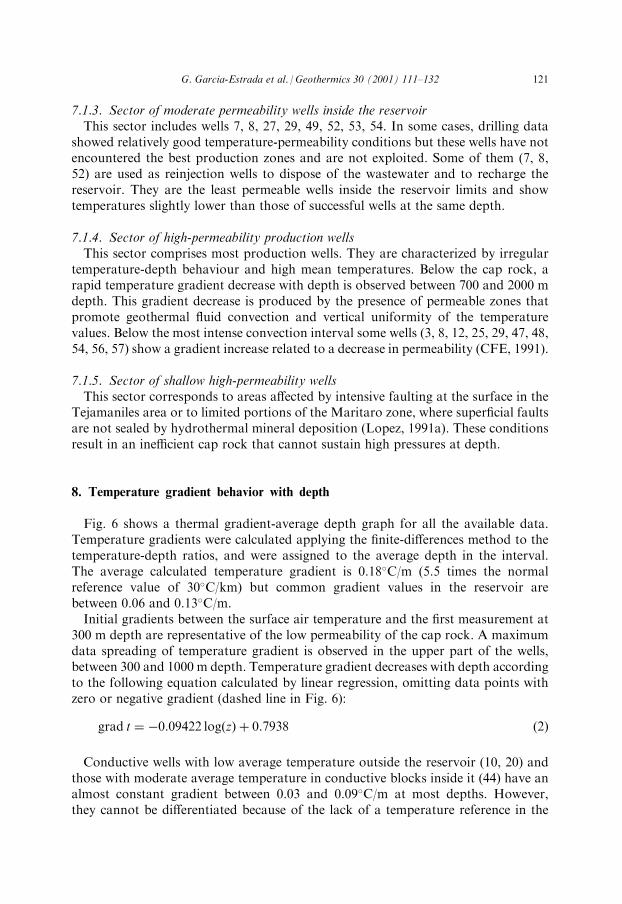
7.1.3. Sector of moderate permeability wells inside the reservoirThis sector includes wells 7, 8, 27, 29, 49, 52, 53, 54. In some cases, drilling data

showed relatively good temperature-permeability conditions but these wells have notencountered the best production zones and are not exploited. Some of them (7, 8,52) are used as reinjection wells to dispose of the wastewater and to recharge thereservoir. They are the least permeable wells inside the reservoir limits and showtemperatures slightly lower than those of successful wells at the same depth.

7.1.4. Sector of high-permeability production wellsThis sector comprises most production wells. They are characterized by irregular

temperature-depth behaviour and high mean temperatures. Below the cap rock, arapid temperature gradient decrease with depth is observed between 700 and 2000 mdepth. This gradient decrease is produced by the presence of permeable zones thatpromote geothermal ¯uid convection and vertical uniformity of the temperaturevalues. Below the most intense convection interval some wells (3, 8, 12, 25, 29, 47, 48,54, 56, 57) show a gradient increase related to a decrease in permeability (CFE, 1991).

7.1.5. Sector of shallow high-permeability wellsThis sector corresponds to areas a�ected by intensive faulting at the surface in the

Tejamaniles area or to limited portions of the Maritaro zone, where super®cial faultsare not sealed by hydrothermal mineral deposition (Lopez, 1991a). These conditionsresult in an ine�cient cap rock that cannot sustain high pressures at depth.

8. Temperature gradient behavior with depth

Fig. 6 shows a thermal gradient-average depth graph for all the available data.Temperature gradients were calculated applying the ®nite-di�erences method to thetemperature-depth ratios, and were assigned to the average depth in the interval.The average calculated temperature gradient is 0.18�C/m (5.5 times the normalreference value of 30�C/km) but common gradient values in the reservoir arebetween 0.06 and 0.13�C/m.Initial gradients between the surface air temperature and the ®rst measurement at

300 m depth are representative of the low permeability of the cap rock. A maximumdata spreading of temperature gradient is observed in the upper part of the wells,between 300 and 1000 m depth. Temperature gradient decreases with depth accordingto the following equation calculated by linear regression, omitting data points withzero or negative gradient (dashed line in Fig. 6):

grad t � ÿ0:09422 log z� � � 0:7938 �2�

Conductive wells with low average temperature outside the reservoir (10, 20) andthose with moderate average temperature in conductive blocks inside it (44) have analmost constant gradient between 0.03 and 0.09�C/m at most depths. However,they cannot be di�erentiated because of the lack of a temperature reference in the


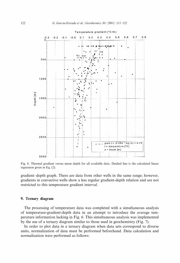
gradient±depth graph. There are data from other wells in the same range; however,gradients in convective wells show a less regular gradient-depth relation and are notrestricted to this temperature gradient interval.

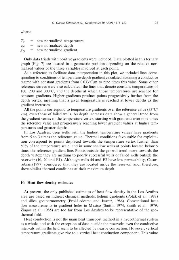
9. Ternary diagram

The processing of temperature data was completed with a simultaneous analysisof temperature-gradient-depth data in an attempt to introduce the average tem-perature information lacking in Fig. 6. This simultaneous analysis was implementedby the use of a ternary diagram similar to those used in geochemistry (Fig. 7).In order to plot data in a ternary diagram when data sets correspond to diverse

units, normalization of data must be performed beforehand. Data calculation andnormalization were performed as follows:

Fig. 6. Thermal gradient versus mean depth for all available data. Dashed line is the calculated linear

regression given in Eq. (2).


Fig.7.Ternary

diagram

thatpresents

relativemeanvalues

of:temperature,depth

andthermalgradientatdi�erentdepthsforallavailable

data.Most

pro-

ductionwellsare

locatednearthetemperature

vertex(T>

50)orunder

thelinecorrespondingto

atemperature

gradient5times

thereference

value(33� C

/km).

Other

reference

curves

are

discussed

inthetext.


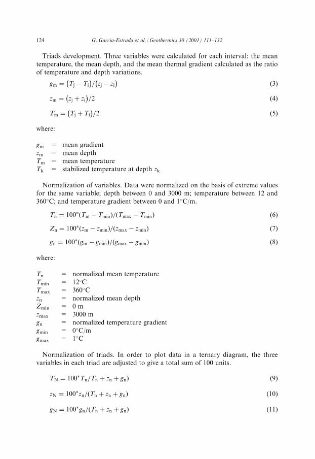
Triads development. Three variables were calculated for each interval: the meantemperature, the mean depth, and the mean thermal gradient calculated as the ratioof temperature and depth variations.

gm � Tj ÿ Ti

ÿ �= zj ÿ zi

ÿ � �3�

zm � zj � zi

ÿ �=2 �4�

Tm � Tj � Ti

ÿ �=2 �5�

where:

gm = mean gradientzm = mean depthTm = mean temperatureTk = stabilized temperature at depth zk

Normalization of variables. Data were normalized on the basis of extreme valuesfor the same variable; depth between 0 and 3000 m; temperature between 12 and360�C; and temperature gradient between 0 and 1�C/m.

Tn � 100� Tm ÿ Tmin� �=�Tmax ÿ Tmin� �6�Zn � 100� zm ÿ zmin� �= zmax ÿ zmin� � �7�gn � 100� gm ÿ gmin� �= gmax ÿ gmin� � �8�

where:

Tn = normalized mean temperatureTmin = 12�CTmax = 360�Czn = normalized mean depthZmin = 0 mzmax = 3000 mgn = normalized temperature gradientgmin = 0�C/mgmax = 1�C

Normalization of triads. In order to plot data in a ternary diagram, the threevariables in each triad are adjusted to give a total sum of 100 units.

TN � 100�Tn=Tn � zn � gn� �9�

zN � 100�zn= Tn � zn � gn� � �10�

gN � 100�gn= Tn � zn � gn� � �11�


where:

TN = new normalized temperaturezN = new normalized depthgN = new normalized gradient

Only data triads with positive gradients were included. Data plotted in this ternarygraph (Fig. 7) are located in a geometric position depending on the relative nor-malized values of the three variables involved at each point.As a reference to facilitate data interpretation in this plot, we included lines corre-

sponding to conditions of temperature-depth-gradient calculated assuming a conductiveregime with constant gradients from 0.033�C/m to nine times this value. Some otherreference curves were also calculated: the lines that denote constant temperatures of100, 200 and 300�C, and the depths at which those temperatures are reached forconstant gradients. Higher gradients produce points progressively further from thedepth vertex, meaning that a given temperature is reached at lower depths as thegradient increases.All the points correspond to temperature gradients over the reference value (33�C/

km), even those of failed wells. As depth increases data show a general trend fromthe gradient vertex to the temperature vertex, starting with gradients over nine timesthe reference value and progressively reaching lower gradient values at higher tem-peratures and greater depths.In Los Azufres, deep wells with the highest temperature values have gradients

from 5 to 3 times the reference value. Thermal conditions favourable for exploita-tion correspond to points displaced towards the temperature vertex further than50% of the temperature scale, and in some shallow wells at points located below 5times the reference gradient line. Points outside the general trend move towards thedepth vertex: they are medium to poorly successful wells or failed wells outside thereservoir (10, 20 and E1). Although wells 44 and E2 have low permeability, Casar-rubias (1997) considered that they are located inside the reservoir and, therefore,show similar thermal conditions at their maximum depth.

10. Heat ¯ow density estimates

At present, the only published estimates of heat ¯ow density in the Los Azufresarea are based on indirect chemical methods: helium quotients (Polak et al., 1988)and silica geothermometry (Prol-Ledesma and Juarez, 1986). Conventional heat¯ow measurements in gradient holes in Mexico (Smith, 1974; Smith et al., 1979;Ziagos et al., 1985) are too far from Los Azufres to be representative of the geo-thermal ®eld.Heat conduction is not the main heat transport method in a hydrothermal system

as a whole, and with the exception of data outside the reservoir, even the conductiveintervals within the ®eld seem to be a�ected by nearby convection. However, verticaltemperature gradients give rise to a vertical heat conduction component. This value


was estimated by intervals in Los Azufres, multiplying the temperature gradient ofthe interval by the thermal conductivity measured in cores where both parameterswere available. In Los Azufres there is a very limited number of thermal con-ductivity measurements (Contreras et al., 1988) but the estimates are valid becauseof the lithologic homogeneity of the ®eld. Table 1 includes heat ¯ow density esti-mates; in a few cases conductivity data from a similar lithologic unit in a nearby wellwere used. Heat ¯ow estimates range between 69 and 668 mW/m2. Low conductiveheat ¯ow within the reservoir is related to low gradients occurring at high averagetemperatures that are produced by convective phenomena (wells 3, 4). Near theouter limit of the reservoir (well 50), low heat ¯ow is the result of a real conductivecondition at depth associated with a small gradient at somewhat lower than averagetemperature (below 200�C at 1500 m depth).In well 20, outside the reservoir limits, heat ¯ow estimates are around 100 mW/m2

associated with temperatures lower than 150�C. Heat ¯ow in this well is slightlyhigher than that observed in the upper part of well 3, which is located in a higherpermeability sector inside the reservoir. Estimates for well 3 in a deep low-perme-ability zone yield heat ¯ow values above 173 mW/m2.Well 29 has low permeability and is located in the highest temperature zone; we

believe that the 295 mW/m2 measured in this well, or similar values, are, therefore,representative of the heat ¯ow in conductive blocks inside the reservoir associatedwith the conductive cooling of a magma body. Very high heat ¯ow, of the order of400 to 600 mW/m2, could be related to conductive blocks with boundaries a�ectedby ¯uids of very di�erent temperatures.

10.1. Thermal gradient and heat ¯ow at the bottom of the wells

We used some selected wells with a more stable temperature-depth relation nearthe bottom in order to study heat transfer below the reservoir, and to estimate arepresentative gradient for each well by linear regression, minimizing local variations.Combined evidence about the absence of drilling mud losses, increase of the temperaturegradient, and low ¯uid production in some cases (CFE, 1991) suggest that permeabilitydecreases below the reservoir and that the conductive heat ¯ow contributionincreases.The results are shown in Table 2. Temperature gradients correspond to the bottom

measurements in the indicated wells, where rocks are either andesites or basaltic-andesites. Heat ¯ow data included in Table 2 were calculated using a constant thermalconductivity of 1.75�0.35 W/m�C, which is the mean value of the data reported byContreras et al. (1988).The most reliable data for heat ¯ow estimation correspond to wells with a linear

temperature-depth behaviour and very low drilling ¯uid losses, indicated by thesuperindex b in Table 2. For instance, wells 10 and 20 outside the reservoir have heat¯ow between 114 and 117 mW/m2, a value slightly higher than the heat ¯ow esti-mation for the thermal province of the Trans-Mexican Volcanic Belt (100 mW/m2).Wells 3 and 44 are located in relatively low-permeability blocks inside the reservoir,and have heat ¯ow values between 124 and 106 mW/m2, respectively. Well E1 is


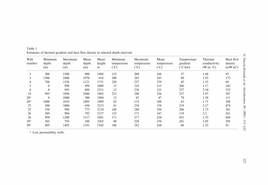
Table 1

Estimates of thermal gradient and heat ¯ow density in selected depth intervals

Well

number

Minimum

depth

Maximum

depth

Mean

depth

Mean

height

Minimum

temperature

Maximum

temperature

Mean

temperature

Temperature

gradient

Thermal

conductivity

Heat ¯ow

density

(m) (m) (m) m (�C) (�C) (�C) (�C/km) (W/m �C) (mW/m2)

3 300 1500 900 1888 132 200 166 57 1.68 95

3 1500 2440 1970 818 200 285 243 90 1.92 173

4 706 1536 1121 1751 220 257 239 45 1.55 69

5 0 998 499 2409 12 218 115 206 1.17 242

8 0 995 498 2311 12 238 125 227 2.34 532

19 995 1096 1046 1803 223 249 236 257 1.97 507

20a 0 1000 500 1994 12 82 47 70 1.58 111

20a 1000 1810 1405 1089 82 133 108 63 1.71 108

22 300 1000 650 2215 81 234 158 219 2.17 474

25 550 996 773 2124 148 240 194 206 1.75 361

26 589 994 792 2127 123 171 147 119 2.2 261

26 994 1240 1117 1801 171 277 224 431 1.55 668

29a 302 793 548 2365 90 228 159 281 1.05 295

50a 889 1492 1191 1545 146 182 164 60 1.52 91

a Low permeability wells.

G.Garcia

-Estra

daet

al./

Geotherm

ics30(2001)111±132

127

located near the northwestern limit of the ®eld, in a sector where ¯uid discharges atthe surface, and has a heat ¯ow of 165 mW/m2.Well 44 is of special interest because it is the deepest well in the ®eld (3544 m). It

has no drilling mud loss intervals below 687 m and has more temperature data thanany other well in Los Azufres. Well 44 is located in a block bounded by active faultsthat act as ¯uid ¯ow channels; these faults are crossed by other producing wells(wells 4 and 15). The heat ¯ow density estimation for well 44 (106 mW/m2) is reliablebecause this well presents a predominantly conductive behaviour.The extrapolation of the bottom-hole temperature in wells 3 and 44 (the most

reliable conductive-dominated wells in the western sector of the reservoir) using thebottom temperature gradient indicates that a typical rhyolitic magma temperature

Table 2

Thermal gradients calculated by linear regression and heat ¯ow density estimates based on bottom-hole

temperatures

Well Thermal Times the Heat ¯ow

number gradient reference density

(�C/km) gradienta (mW/m2)

1 98 3.0 171

3 71 2.1 124

4 85 2.6 149

9 79 2.4 138

10b 65 2.0 114

16 73 2.2 127

19 117 3.6 205

20b 67 2.0 117

21 138 4.2 241

22 105 3.2 184

23 151 4.6 265

25 75 2.3 131

27Ab 122 3.7 214

28 121 3.7 212

29b 116 3.6 204

42 101 3.0 176

43 161 4.9 282

44b 61 1.9 106

47 105 3.2 184

48 108 3.3 189

50 60 1.8 104

51 77 2.3 134

54 66 2.0 116

55 63 1.9 109

56 87 2.6 152

57 105 3.2 184

58b 117 3.5 205

E1b 94 2.9 165

E2 107 3.2 186

a Reference gradient=33 �C/km.b Low permeability wells.


of 600�C could be reached at depths roughly between 7000 and 9000 m. The samecalculations performed with data corresponding to the bottom-hole of well 29 (themost reliable conductive-dominated well in the eastern sector of the ®eld) yield adepth of 5000 m. As these estimates appear low for the top of a magma chamber anddata may be a�ected by errors due to remnant e�ects of convection, we considerthat high temperatures could be associated with very high-temperature waterbetween 5000 and 7000 m depth, or a magma body that could be located at depthsas shallow as 9000 m.

11. Discussion and conclusions

This study is based on the graphic display and the qualitative interpretation ofbottom-hole temperatures at Los Azufres geothermal ®eld. Estimates of temperaturegradient and heat ¯ow densities in the area were done for the ®rst time using boreholetemperature data.The observed gradient changes are much larger than those expected if vertical heat

¯ow was constant and changes were related only to thermal conductivity variations.In the conductive case, we would expect at most a change by a factor of two withrespect to the reference value because thermal conductivity ranges from 1.17 to 2.34W/�C m (Contreras et al., 1988). Preliminary modelling results (Garcia, 2000) showthat the gradient variations are not related to heat ¯ow changes due to the geometryof a magmatic heat source and must, therefore, be related to the distance to openfaults and the temperatures of circulating ¯uids.In Los Azufres, low gradients from 0.05 to 0.08�C/m at depths between 500 and

2000 m may be associated with convection cells where intense water ¯ow exists. Asthey occur at high average temperatures (180±300�C), an up¯ow or a lateral out¯owfrom the reservoir can be identi®ed. Very high temperature gradients (from 0.3 to0.6�C/m) at low-to-moderate average temperatures (<150�C) and depths between 0and 700 m are generally related to low-permeability zones in the cap rock overlyingthe reservoir. Temperature gradients from 0.1 to 0.2�C/m with high average tem-peratures (250±340�C) are observed in impermeable blocks inside or below thereservoir. High gradients (>0.2�C/m) at high temperatures (more than 180�C) atdepths from 500 to 2000 m represent transient thermal phenomena associated withconductive blocks bounded by ¯uids at very di�erent temperature.Bottom-hole equilibrium temperatures are not suitable to evaluate the down¯ow

from steam-heated water in a single well; this phenomenon could be observed in thecomplete set of temperature logs. At Los Azufres this down¯ow is uncommonbecause the pressure at deeper strata is higher than the pressure at shallow acidaquifers. Pressure and temperature logs acquired during drilling stops inside wateror mud-®lled wells are not a�ected by this phenomenon.Constant temperature gradients of about 0.06�C/m are observed in low-temperature

wells outside the reservoir. Some wells located in low-permeability blocks inside thereservoir but near its boundary have gradients of the same order but they occur onlyin limited depth intervals and at higher average temperatures (180±200�C). In the


eastern border of the hydrothermal zone where the presence of a magmatic heatsource is expected, a low-permeability well (29) has a gradient of 0.16�C/m and abottom-hole temperature of 300�C at 2500 m depth.As a consequence of convection in active faults, high temperatures have a more

irregular spatial distribution inside the reservoir than the low temperatures outsideit, where temperature gradients are small and stable. This suggests that low tem-perature wells are less permeable, and low temperature ¯uid movement does notsubstantially disturb the conductive gradient.The equilibrium temperatures in low-permeability wells located inside the reservoir

are low compared with those estimated at the same depth in wells near active faults.If Horner-extrapolated temperatures are good estimates of undisturbed values (evennear faulted zones), then host-rock blocks must have a signi®cant temperature dif-ference with respect to the ¯uids circulating through the faults. This indicates thatthere must be an important unsteady component of horizontal conductive heat ¯owat the block size scale, even under pre-exploitation conditions.In order to explain the observed low conductive gradients in well 44, the condi-

tions that could produce low-vertical conduction phenomena are investigated. In anon-fractured block bounded by active faults, the temperature of the ¯uid circulatingalong the fault planes could act as a boundary condition determining the conductiveheat ¯ow towards the block. The internal temperature of the block would depend onthe temperature di�erences between the boundaries, the conductivity of the rockmatrix and the e�ective permeability.The background regional heat ¯ow was calculated by linear regression using data

from the bottom of conductive wells inside (well 44) and outside the reservoir (wells10 and 20). Estimated values are 106, 114 and 117 mW/m2, respectively. Thesevalues are slightly higher than the heat ¯ow density (around 100 mW/m2) repre-sentative of the Trans Mexican Volcanic Belt (Ziagos et al., 1985). Heat ¯ow calcu-lated with bottom-hole data of other wells show values from 109 mW/m2 (well 55) to282 mW/m2 (well 43), but as these wells were more a�ected by drilling mud losses(Lopez, 1991a) it is di�cult to know the e�ect of convection on the estimated values.Heat ¯ow in well 29 (295 mW/m2) is considered the most reliable estimation of

heat ¯ow associated with the conductive cooling of a magma source located to theeast of the reservoir. The extrapolation of the bottom-hole temperature using thelocal thermal gradient of wells 44, 3 and 9 indicates that a 600�C temperature(representative of a rhyolitic magma) could be attained at depths of 9, 7 and 5 kmdepth, respectively. In low-permeability blocks inside the reservoir there is a localbackground conductive heat ¯ow that varies from 242 mW/m2 (well 5) to 295 mW/m2 (well 29). However, in general, due to temperature di�erences between ¯uidscirculating through faults bounding low-permeability blocks, the conductive heat¯ow inside the reservoir varies from 69 (well 4) to 667 (well 26) mW/m2. In this casethe conductive heat ¯ow is just a component of the mainly convective heat transfer.The use of a ternary graph to display the relationship among temperature, thermal

gradient and depth of wells at Los Azufres geothermal ®eld is most useful in thequalitative analysis of thermal data from a comprehensive perspective. In the ternarydiagram (Fig. 7), the less attractive area for energy production corresponds to the


wells that plot close to the depth vertex, i.e. the deepest wells characterized by lowtemperature gradient and low temperature. This area is the best suited for the studyof the regional conductive regime, as this is the combination that we expect in a heattransfer conductive regime.The wells that plot close to the temperature vertex are shallow wells with high

temperature and low gradients. These are the expected conditions for a well locatedin an area characterized by intense convection phenomena; these are the best-suitedwells for geothermal energy exploitation.The temperature gradient vertex includes shallow boreholes with high gradient,

and low-to-moderate temperature. These conditions are found in wells reachingzones saturated with geothermal ¯uids that are separated from the surface by a caprock with low temperatures near the surface. In some cases, temperature can be highif there are active faults that permit a rapid ascent of ¯uids from the top of thereservoir to the surface. This situation is observed by a relative displacement of thedata to the temperature vertex with a small depth variation.During exploration, thermal characteristics similar to those of wells located in the

border of the reservoir discourage the continuation of a feasibility study, regardlessof the existence of important energy resources in the immediate vicinity. This resultshows that it would be a good strategy to reinterpret the thermal data from apparentlyfailed wells in other projects, from a hydrogeologic perspective.The analysis of the temperature data presented here may be useful for the inter-

pretation of temperature data in other geothermal ®elds under exploration by usingas a reference the relationships observed at Los Azufres.

Acknowledgements

The authors are indebted to Ruben Ostos from the Los Azufres geothermal ®eld forhis assistance in the selection of temperature logs and the computation of equilibriumtemperatures, and to the authorities of the Gerencia de Proyectos Geotermoelectricos(CFE) for their support to this project. Thanks are also extended to Howard Ross,Joe Moore and two anonymous reviewers for their comments and suggestions.

References

Campos, E.J.O., GardunÄ o, M.V.H., 1995. Los Azufres silicic center (Mexico): inferences of caldera

structural elements from gravity, aeromagnetic and geoelectric data. Journal of Volcanology and Geo-

thermal Research 67, 123±152.

Casarrubias, U.Z., 1997. Resultados de la perforacioÂ n exploratoria en la porcioÂ n occidental del campo geo-

teÂ rmico de Los Azufres, MichoacaÂ n, MeÂ xico. Geotermia Revista Mexicana de GeoenergõÂ a 12, 189±207.

CFE (Comision Federal de Electricidad), 1991. CaracterõÂ sticas y capacidades del yacimiento geoteÂ rmico

de Los Azufres, Mich., MeÂ xico. Internal Report of Gerencia de Proyectos Geotermoelectricos OIY AZ

08-91, Comision Federal de Electricidad, Morelia, Mich., 250 pp.

Contreras, E., DomõÂ nguez, B., Iglesias, E., GarcõÂ a, A., HuitroÂ n, R., 1988. Compendio de resultados de

mediciones petrofõÂ sicas de nuÂ cleos de perforacioÂ n del campo geoteÂ rmico Los Azufres. Geotermia

Revista Mexicana de GeoenergõÂ a 4, 9±105.


Dobson, P.F., Mahood, G.A., 1985. Volcanic stratigraphy of the Los Azufres geothermal area, Mexico.

Journal of Volcanology and Geothermal Research 25, 273±287.

Fertl, W.H., Wichmann, P.A., 1977. How to determine static BHT from well-log data. World Oil 184,

101±106.

Garcia, E.G.H., 1986. El caÂ lculo de temperaturas estabilizadas en pozos geoteÂ rmicos. Geotermia Revista

Mexicana de GeoenergõÂ a 2, 297±319.

Garcia, E.G.H., 1995. ReinterpretacioÂ n geofõÂ sica del campo geoteÂ rmico de Los Azufres, Mich. Internal

Report of Gerencia de Proyectos Geotermoelectricos GF-AZ-034/95. Comision Federal de Elec-

tricidad, Morelia, Mich.

Garcia, E.G.H., 1997. Modelo teÂ rmico conceptual del estado inicial del campo Los Azufres, MichoacaÂ n,

MeÂ xico. Internal Report of Gerencia de Proyectos Geotermoelectricos DEX-026-97. Comision Federal

de Electricidad, Morelia, Mich., MeÂ xico, 41 pp.

Garcia, E.G.H., 2000. Modelo del estado teÂ rmico inicial del campo geoteÂ rmico de Los Azufres, Michoa-

caÂ n, MeÂ xico. PhD thesis (in preparation). Universidad Nacional Autonoma de Mexico.

Gutierrez, N.L.C.A., 1997. Resultados de la explotacioÂ n geoteÂ rmica en MeÂ xico en 1996. Geotermia

Revista Mexicana de GeoenergõÂ a 13, 3±13.

Huitron, G.H., Palma, O., Mendoza, H., SaÂ nchez, C., Razo, A., Arellano, F., GutieÂ rrez, L.C.A., Quijano,

J.L., 1991. Los Azufres geothermal ®eld, MichoacaÂ n. In: Salas, G.P., (Ed.), Economic Geology, Mex-

ico, Geological Society of America, The Geology of North America, V. P-3, 59±76.

Jaeger, J.C., 1961. The e�ect of the drilling ¯uid on temperatures measured in bore holes. Journal of

Geophysical Research 66 (2), 563±569.

Lachenbruch, A.H., Brewer, M.C., 1959. Dissipation of the temperature e�ect of drilling a well in Arctic

Alaska. Geological Survey Bulletin 1083-C, 109.

Lopez, H.A., 1991a. AnaÂ lisis estructural del campo geoteÂ rmico de Los Azufres, Mich. InterpretacioÂ n de

datos super®ciales y de subsuelo. Internal Report of Gerencia de Proyectos Geotermoelectricos 11/91.

Comision Federal de Electricidad, Morelia, Mich., 100 pp.

Lopez, H.A., 1991b. GeologõÂ a de Los Azufres. Geotermia, RevistaMexicana de Geoenergia 7 (3), 265±275.

Polak, B.G., Kononov, V.I., Prasolov, E.M., Sharkov, I.V., Prol, R.M., Gonzalez, A., Razo, A., Molina,

B., 1988. First estimates of terrestrial heat ¯ow in the Transmexican Volcanic Belt and adjacent areas

based on isotopic composition of natural helium. Geo®sica Internacional 24, 465±476.

Pradal, E., 1990. La caldera de Los Azufres (Mexique): contexte volcanologique d'un grand champ geo-

thermique. These pour le titre de docteur, Universite Blais Pascal, France 250pp.

Pradal, E., Robin, C., 1985. DeÂ couverte d'une caldera majeur associeÂ e au champ geÂ othermique de Los

Azufres (Mexique). C.R. Academie des Sciences, Paris 132 (Ser II), 135±142.

Prol-Ledesma, R.M., Juarez, G., 1986. Geothermal map of Mexico. Journal of Volcanology and Geo-

thermal Research 28, 351±362.

Pruess, K., 1989. TOUGH2 Ð A general-purpose numerical simulator for multiphase ¯uid and heat ¯ow.

Lawrence Berkeley Laboratory, University of California Report LBL-29400,UC-251, 102 pp.

Smith, D.L., 1974. Heat ¯ow, radioactive heat generation, and theoretical tectonics for north western

Mexico. Earth Planet Scienti®c Letters 23, 43±52.

Smith, D.L., Nuckels III, C.E., Jones, R.L., Cook, G.A., 1979. Distribution of heat ¯ow and radioactive

heat generation in Northern Mexico. Journal of Geophysical Research 84, 2371±2379.

Suarez, A.M.C., 1997. EstimacioÂ n de la energõÂ a contenida en MarõÂ taro, sector norte del campo geoteÂ rmico

de Los Azufres, Mich., MeÂ xico. Geotermia Revista Mexicana de GeoenergõÂ a 13 (No. 2/3), 103±145.

Ziagos, J.P., Blackwell, D.D., Mooser, F., 1985. Heat ¯ow in southern Mexico and the thermal e�ect of

subduction. Journal of Gephysical Research 90, 5410±5420.


Temperature–depth relationships based on log data from the Los Azufres geothermal field, Mexico

Documents

Transcript of Temperature–depth relationships based on log data from the Los Azufres geothermal field, Mexico