Temi di discussione(Working Papers)

Modeling and forecasting macroeconomic downside risk

by Davide Delle Monache, Andrea De Polis and Ivan Petrella

Num

ber 1324M

arch

202

1

Temi di discussione(Working Papers)

Modeling and forecasting macroeconomic downside risk

by Davide Delle Monache, Andrea De Polis and Ivan Petrella

Number 1324 - March 2021

The papers published in the Temi di discussione series describe preliminary results and are made available to the public to encourage discussion and elicit comments.

The views expressed in the articles are those of the authors and do not involve the responsibility of the Bank.

Editorial Board: Federico Cingano, Marianna Riggi, Monica Andini, Audinga Baltrunaite, Marco Bottone, Davide Delle Monache, Sara Formai, Francesco Franceschi, Adriana Grasso, Salvatore Lo Bello, Juho Taneli Makinen, Luca Metelli, Marco Savegnago.Editorial Assistants: Alessandra Giammarco, Roberto Marano.

ISSN 1594-7939 (print)ISSN 2281-3950 (online)

Printed by the Printing and Publishing Division of the Bank of Italy

MODELING AND FORECASTING MACROECONOMIC DOWNSIDE RISK

by Davide Delle Monache*, Andrea De Polis** and Ivan Petrella**

Abstract

We document a substantial increase in downside risk to US economic growth over the last 30 years. By modelling secular trends and cyclical changes of the predictive density of GDP growth, we find an accelerating decline in the skewness of the conditional distributions, with significant, procyclical variations. Decreasing trend-skewness, which turned negative in the aftermath of the Great Recession, is associated with the long-run growth slowdown started in the early 2000s. Short-run skewness fluctuations imply negatively skewed predictive densities ahead of and during recessions, often anticipated by deteriorating financial conditions, while positively skewed distributions characterize expansions. The model delivers competitive out-of-sample (point, density and tail) forecasts, improving upon standard benchmarks, due to the strong signals of increasing downside risk provided by current financial conditions.

JEL Classification: C32, C51, C53, E44, G12. Keywords: business cycle, financial conditions, downside risk, skewness, score driven models. DOI: 10.32057/0.TD.2021.1324

Contents 1. Introduction .......................................................................................................................... 5 2. Motivating evidence ............................................................................................................ 9 3. A time varying Skew-t model for GDP growth ................................................................. 11 3.1 Secular and cyclical variations of GDP growth’s distribution ................................... 16 3.2 Estimation ................................................................................................................... 18 3.3 Forecasts ..................................................................................................................... 19 4. Time variation in the distribution of GDP growth ............................................................. 19 5. Out-of-sample forecast ...................................................................................................... 27 5.1 Point and density forecast ............................................................................................ 27 5.2 Downside risk predictions for the Great Recession ..................................................... 31 6. Dissecting the Financial Condition Index .......................................................................... 33 6.1 Variables selection: “shrink-then-sparsify” ................................................................ 34 6.2 On the importance of financial indicators .................................................................. 35 7. Conclusions ........................................................................................................................ 39 References .............................................................................................................................. 40 Supplementary material .......................................................................................................... 49 _______________________________________ * Bank of Italy, ** University of Warwick.

1 Introduction

The Global Financial Crisis and the subsequent recession left policymakers with sev-

eral new challenges. In a world of persistently sluggish growth, subject to infrequent but

deep recessions, the idea of central bankers as ‘risk managers’ gained renewed popularity

(see Cecchetti, 2008). Policy makers pursuing a ‘plan for the worst, hope for the best ’

approach rely on downside risk measures to assess the distribution of risk around modal

forecasts. Notably, Adrian et al. (2019) uncover a significant negative correlation between

financial conditions and the lower quantiles of the distribution of future real economic

growth, suggesting that financial conditions may provide a relevant signal of downside

risk to economic activity.1 Gadea Rivas et al. (2020) highlight that increasing households

and firms leverage posits a trade-off between deep recessions and prolonged expansions

(see also Jensen et al., 2020). Yet, a number of recent contributions have called into

question the presence of any (type of) asymmetry in business cycle fluctuations, and

have suggested alternative ways of capturing time variation in downside risk (see, e.g.,

Brownlees and Souza, 2020; Carriero et al., 2020a).

Assessing the degree of asymmetry of business cycle fluctuations remains a challeng-

ing task. Nevertheless, failure in detecting unconditional asymmetry of GDP growth’s

distribution does not necessarily rule out the possibility that business cycle skewness is,

at times, sizeable and significant. By investigating the properties of the score of the pre-

dictive likelihood of GDP growth, we provide novel evidence in support of the presence

of conditional asymmetry. Hence, despite unconditional asymmetry over the full sample

remains unsupported by data, conditional skewness, and thus downside risk to economic

growth, feature significant variation over time. Starting from this result, we introduce a

novel flexible methodology to characterize and forecast the conditional distribution of real

economic growth with a parametric skewed Student-t (Skew-t) distribution with time-

varying location, scale, and shape parameters. In order to fully capture the evolution of

the predictive densities, our framework accommodates secular trends and cyclical com-

ponents for each parameter, with the time variation being driven by the scaled score of

the predictive likelihood function (Creal et al., 2013; Harvey, 2013), as well as financial1Loria et al. (2019) show that contractionary shocks to technology, monetary policy, and financial

conditions disproportionately increase downside risk to economic growth.

5

indicators. The latter allow us explore to what extent downside risk to economic growth

reflect imbalances arising in financial markets.

We document that the conditional distribution of GDP growth is characterized by

procyclical skewness fluctuations around a declining trend-skewness. At the onset of

downturns, business cycle swings exhibit significant negative skewness, while expansions

are characterized by positively skewed distributions. Hence, the stark counter-cyclicality

of GDP growth’s volatility (see Jurado et al., 2015, among others) also reflects increasing

downside volatility during recessions, not being entirely matched by upside volatility. On

the other hand, long-run skewness has been decreasing over the last 30 years, partially

accounting for the slowdown in long-run growth observed since the early 2000s (see,

e.g., Cette et al., 2016; Antolin-Diaz et al., 2017), and turning to negative values in the

aftermath of the Great Recession.

Several measures of financial stress have been identified as relevant indicators for

predicting economic downturns. Among others, traditional spread measures (see, e.g.,

Rudebusch and Williams, 2009; Faust et al., 2013), credit and leverage growth (Drehmann

et al., 2010; Jordà et al., 2013), as well as the leverage position of financial intermedi-

aries (Adrian and Shin, 2008) received particular attention. Here, we show that the four

subcomponents of the National Financial Condition Index (NFCI, Brave and Butters,

2012), capturing risk, credit, leverage and nonfinancial leverage developments, leads to

substantial improvements in the fit of the model. The slow building up of nonfinancial

leverage emerges as a key determinant of the scale of distribution, whereas skewness

relates to all the subindices, in particular leverage of financial intermediaries and credit

conditions. Hence, we document that financial deepening in the expansionary phase of the

cycle is associated with positive GDP growth’s skewness, whereas tightening of financial

conditions consistently predict downside risk episodes. Furthermore, financial conditions

significantly contribute to increasing the out-of-sample forecasting accuracy of our model,

in particular during recessions. Our preferred specification delivers well calibrated predic-

tive densities, improving upon competitive benchmarks in terms of point, density and tail

forecasts, as well as leading to timely predictions of the odds of forthcoming recessions.

Although aggregate measures succeed in summarizing a large amount of data, con-

cerns that information relevant for assessing risk can remain undetected persist (see,

6

e.g., Galvão and Owyang, 2018; Carriero et al., 2020b). To address this question, we

perform an out-of-sample variable selection exercise based on the ‘shrink-then-sparsify ’

approach of Hahn and Carvalho (2015) using the full set of predictors feeding into the

NFCI.2 Household debt outstanding emerges as a leading indicator of the build-up of

downside risk throughout our sample. Fluctuations in the balance-sheet size of security

broker-dealers as well as the mortgage-backed securities to treasury yield spread provide

useful signals for gauging the severity of the downside risk during the Great Recession,

highlighting the importance of the intermediary sector (Adrian and Shin, 2008) and the

housing market (see, e.g., Gertler and Gilchrist, 2018). Processing the signal from a large

panel of financial predictors leads to substantial improvements in medium term predic-

tions, with sizable gains associated with the ability of the model to capture the increase

in the downside risk ahead of the 2007-2009 recession.3

Our results highlight the importance of accounting for asymmetric business cycle

fluctuations. These can emerge through nonlinearities in the transmission of Gaussian

shocks (see, e.g., Fernández-Villaverde and Guerrón-Quintana, 2020a), or alternatively

reflect conditionally skewed shocks hitting the economy (as in Bekaert and Engstrom,

2017; Salgado et al., 2019). The procyclical skewness dynamics we document is found to

be associated with a dynamic correlation between the first and second moments, being

positive in expansions, and turning negative in recessions (in line with the empirical

evidence in Carriero et al., 2020a). This further reinforces the necessity of distinguishing

between ‘good’ and ‘bad’ uncertainty, which can potentially impact economic activity

in opposite directions (Segal et al., 2015). Our findings also emphasise the need to

account for the nonlinear relationship between financial conditions and credit availability,

and the distribution of GDP growth (see, e.g., Fève et al., 2019; Fernández-Villaverde

et al., 2019) for policy monitoring (Adrian et al., 2020) and stabilization policy design

(Gadea Rivas et al., 2020; Jordà et al., 2020). Lastly, we corroborate that modeling

business cycle asymmetry within theoretical models entails capturing the fall in trend-2Giannone et al. (2018) warn that sparsity can arise as an artefact of strong a priori beliefs. We

approach sparsity within the purely data-driven framework of Ray and Bhattacharya (2018) which isrobust to this concern, as also argued in Huber et al. (2020).

3The latter finding corroborates the evidence in Alessi et al. (2014), that the central banks’ failure topredict the 2007-2009 downturn can be ascribed to their inability to read the signals from deterioratingfinancial conditions.

7

skewness of economic fluctuations, and the associated increase of downside risk, over the

last three decades (see, e.g., Jensen et al., 2020).

Related literature: This paper builds on the recent literature exploring the relation-

ship between real economic activity and financial conditions (Jordà et al., 2013; Gertler

and Gilchrist, 2018, among others). Giglio et al. (2016), Adrian et al. (2019) and Caldara

et al. (2020) show that measures of systemic risk are more informative about future eco-

nomic downturns, as they better predict lower quantiles of the conditional distribution

of real output growth.4

In contrast to the two-step quantile approach of Adrian et al. (2019), which also re-

quires a distribution to be fitted to the estimated quantiles, we propose a parametric

Skew-t specification, for which we directly model the parameters, that provides great

tractability and flexibility in accounting for the time variation of downside risk. We

propose an observation-driven model to fit and forecast conditional mean, variance and

skewness of GDP growth fluctuations. While models for time-varying asymmetry have

already been introduced by Hansen (1994) and Harvey and Siddique (1999) with ad hoc

laws of motion, we rely on the score-driven framework put forward by Creal et al. (2013)

and Harvey (2013). This setting has proven to be particularly suitable for accommodating

parameters’ time variation under different distributional assumptions (Koopman et al.,

2016).5 Moreover, building on the work of Harvey (2013, Section 2.6) and Schwaab et al.

(2020), we introduce exogenous predictors in the updating equations of the time-varying

parameters. To the best of our knowledge, we are the first to rely on Bayesian estimation

methods within the score-driven setting. This allows us to jointly tackle parameters’

proliferation and incorporate estimation uncertainty when producing forecasts. Specifi-

cally, the latter turns out to be useful in improving medium horizon density forecasts, in

particular during recessions.

Our model allows for, but do not impose, skewness in GDP growth. Yet, we docu-4De Nicolò and Lucchetta (2017) uphold the superior forecasting accuracy of factor-augmented quan-

tile projections to predict economic growth tail risk. Busetti et al. (2020) use expectiles, as opposed toquantiles, to investigate the relationship between GDP growth and financial variables.

5Parameters’ updating based on the score of the predictive likelihood always reduces the localKullback-Leibler divergence between the true conditional density and the model-implied one, even undersevere misspecification (Blasques et al., 2015).

8

ment significant variation in the asymmetry of the conditional distribution. This delivers

substantial gains in predicting downside risk developments over standard volatility mod-

els, whose competitiveness has recently been highlighted by Brownlees and Souza (2020).

Plagborg-Møller et al. (2020) introduce a Skew-t model with time-varying parameters

being linear functions of financial predictors and past GDP growth. Our framework nests

their specification and provides a richer dynamic, able to capture smoother and sharper

variations of the scale and shape parameters. In particular, we introduce persistence

in the skewness of the distribution of GDP growth, in line with the term structure of

the growth-at-risk displaying stronger asymmetry for the short- than for the medium-

run (Adrian et al., 2018), and consistent with the pronounced skewness displayed by

the Survey of Professional Forecasters’ short-term predictions (Ganics et al., 2020). Fi-

nally, unlike alternative approaches, we put forward a two-component specification for

the time-varying parameters of the model, in the spirit of Engle and Lee (1999), to track

both secular and cyclical changes in the underlying distribution of GDP growth. This al-

lows the model to recover well-known stylized facts, such as the Great Moderation period

(McConnell and Perez-Quiros, 2000; Stock and Watson, 2002) and the fall in long-run

GDP growth, and to uncover an increasingly negatively skewed business cycle in the last

part of the sample, which would remain undetected otherwise.

Structure: The remainder of the paper is organized as follows. Section 2 provides

evidence of time-varying business cycle asymmetry. Section 3 presents the model, the

estimation methodology and the forecasting procedure. Section 4 illustrates the charac-

teristics of the conditional distribution of GDP growth, and how they relate to financial

predictors. Section 5 reports the out-of-sample forecast and downside risk prediction

evaluation. In Section 6 we investigate the predictive ability of the large set of financial

indicators. Section 7 concludes.

2 Motivating evidence

Assessing the degree of skewness of GDP growth is notoriously challenging (Neftci,

1984; Morley and Piger, 2012). When measured over the 1973-2018 sample, we obtain a

9

Table 1: Score-based tests for time variation

time-varying time-varyinglocation location & scale

Q Q∗ N Q Q∗ N

Scale2 70.28∗∗∗ 71.39∗∗∗ 1.95∗∗∗

Shape 46.4∗∗∗ 47.13∗∗∗ 0.41∗ 21.44∗∗∗ 21.78∗∗∗ 0.78∗∗∗

Note: Q is the portmanteau test, Q∗ is the Ljung-Box extension and N corresponds to the Nyblom test.The lag length for the Portmanteau and Ljung-Box tests are selected following Escanciano and Lobato(2009). The first two tests are distributed as a χ2 with 1 degree of freedom, the Nyblom test statisticsis instead distributed as a Cramer von-Mises distribution with 1 degree of freedom. ∗ p < 10%, ∗∗ p <5%, ∗∗∗ p < 1%.

negative sample skewness of -0.42. Nevertheless, according to the Bai and Ng (2005) test,

due to the low precision of this estimate over the full sample, one cannot reject the null of

symmetry. However, the absence of skewness in the unconditional distribution does not

necessarily imply the conditional distribution being symmetric as well (Carriero et al.,

2020a). In fact, the difficulty of getting significant skewness estimates can potentially

reflect the dynamic evolution of business cycles properties over time. Using Bai and

Ng (2005)’s test over different rolling windows of 1 to 5 years, the test often rejects the

null of symmetry, with periods of significant negative and positive skewness detected

over the sample. The cyclical behaviour of the test statistics points out at substantial

movements in the skewness of GDP growth, suggesting that prolonged expansions are,

at times, characterized by significant positive skewness, while contractions are associated

with significant negative skewness.6

In this Section, we report a number of tests for the presence of time-varying asym-

metry. Harvey (2013, Section 2.5) highlights that the score of the conditional likelihood

can be used to formally test for the time variation of parameters. As the score incor-

porates information about the level of time variation of the respective parameter, the

Lagrange multiplier principle can be employed to construct appropriate test statistics

(see also Calvori et al., 2017). Within this framework, testing for parameters’ variation

requires starting from a benchmark model, under the null of no time variation of the6See Figure G1 in Appendix G, for a summary of these results.

10

parameter(s) of interest. Here, we assume that GDP growth follows an AR(2) process

with Skew-t innovations, with a shape parameter pinning down the degree of asymme-

try.7 We test for the time variation of the shape parameter considering both the case of

constant volatility and the more realistic case of time-varying volatility. Table 1 reports

the statistics for the Portmanteau (Q), Ljung-Box (Q∗) and Nyblom (1989) (N) tests.

The null hypothesis of a constant shape parameter is strongly rejected, against the alter-

native of time variation.8 Note that the rejection of the Nyblom test, which under the

alternative hypothesis implies that the parameter follows a martingale process, suggests

that the shape parameter is likely to be highly persistent. Starting from this evidence, in

the next Section we introduce a model where the conditional distribution of GDP growth

features time-varying asymmetry.

3 A time varying Skew-t model for GDP growth

Let yt denote the annualized quarter-on-quarter GDP growth at time t. We assume

its conditional distribution can be characterized by a Skew-t (Arellano-Valle et al., 2005;

Gómez et al., 2007), with time-varying location µt, scale σt, and shape %t parameters,

and constant degrees of freedom ν. Specifically,

yt = µt + σtεt, εt ∼ Sktν(0, 1, %t), (1)

with the degrees of freedom ν > 3, the scale parameter σt > 0, and the asymmetry

parameter %t ∈ [−1, 1], such that when it attains negative (positive) values, the distribu-

tion features positive (negative) skewness. The conditional log-likelihood function of the

observation at time t is:

`t = log p(yt|θ, Yt−1) = log C(η)− 1

2log σ2

t −1 + η

2ηlog

[1 +

ηε2t

(1− sgn(εt)%t)2σ2t

], (2)

7Horswell and Looney (1993) show that, when testing for skewness, omitting the presence of kurtosismight deliver misleading results. Repeating the tests with Skew-Normal innovations delivers similarevidence.

8Appendix A provides additional details on the specifics of the tests, as well as alternative specifica-tions for the location and scale of GDP growth, confirming the robustness of these results.

11

with η = 1νbeing the inverse of the degrees of freedom, C(η) =

Γ

(1+η2η

)√πη

Γ(

12η

) , Γ(·) is the

Gamma function, and sgn(·) is the sign function. The vector θ collects all the static

parameters, and Yt−1 = yjt−1j=1 is the information set, up to time t. For %t = 0 we have

the symmetric Student-t distribution, for η → 0 we retrieve the epsilon-Skew-Gaussian

distribution of Mudholkar and Hutson (2000), whereas the distribution collapses to a

Gaussian density when both condition hold.9 Thus, we allow for, but do not impose,

asymmetric innovation terms.

Following the score-driven framework of Creal et al. (2013) and Harvey (2013), we pos-

tulate the driving force for the time-varying parameters to be the score of the predictive

likelihood. Let ft collect the vector of time-varying parameters of interest:

ft+1 = Aft +BXt + Cst, (3)

where A contains autoregressive parameters governing the persistence of the updating,

B collects loadings on the explanatory variables Xt, and C collects the score loadings

adjusting the speed of the updating, given the prediction error. The scaled score, st, is

defined as st = St∇t, where:

∇t =∂`t∂ft

, St = I−12

t = E(− ∂2`t∂ft∂f ′t

)− 12

, (4)

with ∇t being a vector of scores, namely the gradient of the likelihood function `t with

respect to the dynamic parameters, while the scaling matrix St is proportional to the

square root of the Moore-Penrose pseudo-inverse of the Information matrix, It. The re-

sulting scaled score is a martingale difference sequence with conditional variance equal

to the identity matrix. Hence, the parameter updating is defined by the steepest as-

cent direction for improving the model’s local fit. In fact, the direction and magnitude

of the updating are dictated by the steepness and curvature of the likelihood function

relative to the position of the parameters. Therefore, the resulting model belongs to9As opposed to the Skew-t distribution of Azzalini and Capitanio (2003), adopted by Adrian et al.

(2019), among others, in the context of GDP growth, the Skew-t distribution of Gómez et al. (2007)retrieve an information matrix which is always non-singular, and can thus be inverted, provided that|%t| < 1.

12

the observation-driven class, for which the trajectories of the time-varying parameters

are perfectly predictable given past information and the log-likelihood function being

available in closed form (Cox, 1981). The following Proposition provides the closed form

expressions for the gradient and the associated information matrix.

Proposition 1. Given the model specification (1) and the likelihood in (2), the elements

of the gradient ∇t, with respect to location, scale and asymmetry, are:

∂`t∂µt

= 1σ2twtεt,

∂`t∂σ2

t= 1

2σ4t(wtε

2t − σ2

t ),∂`t∂%t

= − 1σ2t

sgn(εt)(1−sgn(εt)%t)

wtε2t , (5)

where wt = (1+η)

(1−sgn(εt)%t)2+ηζ2tand ζt denotes the standardized innovation, ζt = εt

σt. The

associated information matrix reads as follows:

It =

(1+η)

(1+3η)(1−%2t )σ2t

0 − 4c(1+η)

σt(1−%2t )(1+3η)

0 12(1+3η)σ4

t0

− 4c(1+η)

σt(1−%2t )(1+3η)0 3(1+η)

(1−%2t )(1+3η)

. (6)

Proof. See Appendix B.

Proposition 1 highlights the central role of re-weighting the standardized prediction

error (and its square values) for updating of the time-varying parameters. Weights,

wt, penalize extreme standardized innovations depending on the thickness of the tails,

as well as volatility and asymmetry, estimated conditional to time t − 1. The top left

panel of Figure 1 displays the weights associated to the prediction error, for alternative

model parametrizations. In a Gaussian setting (black line), weights are constant and

equal to unity, implying no discounting. On the other hand, when the asymmetry pa-

rameter is zero (red line), the weights display the classic outlier-discounting typical of

the observation driven models with Student-t distributions (see, e.g. Harvey and Luati,

2014; Delle Monache and Petrella, 2017). When the distribution is positively (negatively)

skewed, i.e. for %t < 0 (%t > 0), negative (positive) prediction errors, less likely in ex-

pectation, command a larger update of the parameters. This asymmetric treatment of

the signal of the prediction error is more pronounced as the skewness of the distribution

grows larger (i.e. |%t| → 1).

13

Weights

-5 -4 -3 -2 -1 0 1 2 3 4 50

0.5

1

1.5

2

2.5

3

3.5

4

4.5

5Location

-5 -4 -3 -2 -1 0 1 2 3 4 5-3

-2

-1

0

1

2

3

Scale

-5 -4 -3 -2 -1 0 1 2 3 4 5-2

0

2

4

6

8

10Shape

-5 -4 -3 -2 -1 0 1 2 3 4 5-1.5

-1

-0.5

0

0.5

1

1.5

Figure 1: Prediction error and parameters’ updatingNote: The figures plot the weighting scheme implied by the weights ωt, and the scaled scores, for differentvalues of the prediction error εt. We consider three values of the asymmetry parameter: -0.5 (blue), 0(red) and 0.7 (green). The Gaussian case is reported in black. The scale parameter is set to 1, with 5degrees of freedom.

In order to ensure the scale σt to be positive and the shape %t to lie within the

unit circle, we apply time-invariant, invertible and differentiable “link functions” to these

parameters. In practice, we model γt = log(σt) and δt = arctanh(%t), so that the vector of

time-varying parameters becomes ft = (µt, γt, δt)′. Moreover, we follow Lucas and Zhang

(2016) and scale the score only using the diagonal elements of the information matrix.

14

Therefore, the associated scaled score vector is

st = (J ′tdiag(It)Jt)−12J ′t∇t =

sµt

sγt

sδt

=

√

(1+3η)(1−%2t )

(1+η)wtζt√

(1+3η)2

(wtζ2t − 1)

−sgn(εt)√

(1+sgn(εt)%t)(1+3η)3(1−sgn(εt)%t)(1+η)

wtζ2t

, (7)

where Jt =∂(µt,σ2

t ,%t)

∂(µt,γt,δt)′is the Jacobian matrix associated to the link functions.10 Equation

(7) highlights that the updating of the shape parameter is substantially different from

the ad-hoc filters adopted by Hansen (1994) and Harvey and Siddique (1999), based on

higher order powers of the prediction error.

The remainder of Figure 1 plots the scaled scores against the standardized innovations,

for the location, scale and shape parameters, respectively. Negative prediction errors are

associated with a negative update of the location and a positive update of the shape (i.e.

the distribution becoming more left skewed). The opposite is true for positive prediction

errors, whereas in both cases the scale is updated upward. For extreme values of the

prediction errors, parameters’ update becomes inelastic to the standardized innovations,

as the scaled scores converge to their limiting values. Most importantly, the asymmetry

of the distribution plays a key role in the translation of the standardized prediction error

into a signal for the update of the distribution’s parameters. For instance, when the

distribution is left skewed (i.e. %t > 0) a positive (negative) prediction error leads to

a more (less) pronounced update for the parameters, while the opposite is true in the

case of a positively skew distribution. This property of the updating function is a direct

consequence of the stark asymmetry in the weights. In practice, the model is faster to

update the asymmetry of the distribution when there is evidence for a change of sign.11

In our application, this allows the model to promptly detect shifts in the skewness of

GDP growth around business cycle turning points.10In Appendix B, we show that the score and Information matrix provided in Proposition 1 are still

valid after applying the link functions.11For instance, a large negative prediction error when the distribution is positive skewed will be

perceived as strong signal that there has been a change in the shape of the distribution.

15

3.1 Secular and cyclical variation of GDP growth’s distribution

When modelling the conditional distribution of GDP growth, it is important to allow

for both cyclical and secular movements of the central moments. Several papers have

documented that over the sample under analysis GDP growth has experienced significant

changes in the long run mean (see, e.g. Cette et al., 2016; Antolin-Diaz et al., 2017), as

well as shifts in the volatility (McConnell and Perez-Quiros, 2000; Stock and Watson,

2002), and skewness of the distribution (Jensen et al., 2020) from the late 1980s. At the

same time, Jurado et al. (2015) show that the volatility of GDP growth is countercyclical,

while Giglio et al. (2016) and Adrian et al. (2019) argue that the skewness of the cycle

falls sharply during recessions. To account for these features of the data, we postulate a

two-component specification for the time-varying parameters, in the spirit of Engle and

Lee (1999). We posit a random walk updating for the permanent components, where

these are able to track both smooth variations and sudden breaks in the level of the

parameters. Moreover, we allow a set of predictors, Xt, to have a transitory impact on

the parameters of the distribution.

The location parameter is a linear combination of a trend component, µt, and a

stationary component, µt:

µt+1 = µt+1 + µt+1, (8)

µt+1 = µt + ςµsµt, (9)

µt+1 = φµ,1µt + φµ,2µt−1 + β′µXt + κµsµt, (10)

where the AR(2) specification for the cyclical component is able to recover the character-

istic hump shaped impulse response of the data (see, e.g. Chauvet and Potter, 2013). Fol-

lowing Engle and Rangel (2008), we assume a multiplicative specification for the volatility,

i.e. γt = log(σt) where:

γt+1 = γt+1 + γt+1, (11)

γt+1 = γt + ςγsγt, (12)

γt+1 = φγ γt + β′γXt + κγsγt. (13)

16

Similarly, we posit an additive specification for the unrestricted shape parameter, δt =

arctanh(%t):

δt+1 = δt+1 + δt+1, (14)

δt+1 = δt + ςδsδt, (15)

δt+1 = φδ δt + β′δXt + κδsδt, (16)

that implies %t = tanh(δt+ δt). Therefore, the resulting vector of time-varying parameters

is equal to ft = (µt, µt, γt, γt, δt, δt)′, whose law of motion is described by a restricted

specification of equation (3), as we show in Appendix B.

Plagborg-Møller et al. (2020) consider a time-varying Skew-t specification for GDP

growth and specify the time-varying parameters (location, log-scale and shape) as a linear

function of the set of predictors. In our framework, a specification similar to theirs can be

retrieved setting ςµ, φµ,1, φµ,2, κµ, ςγ, φγ, κγ, ςδ, φδ, κδ = 0. In this case, the sole source

of parameters’ variation stems from the dynamics of the predictors, which generates

substantial variability in the underlying parameters, and thus uncertainty around the

estimates. In contrast, our specification allows for both secular and transitory shifts

in the parameters, where the autoregressive structure of the cyclical components makes

them functions of discounted values of all past predictors and scores (where these latter

are themselves nonlinear functions of past data). Specifically,

µt+1 = µt+1 +t−1∑j=0

ψµ,j(β′µXt−j + κµsµt−j

)(17)

γt+1 = γt+1 +t−1∑j=0

φjγ(β′γXt−j + κγsγt−j

), (18)

δt+1 = δt+1 +t−1∑j=0

φjδ (β′δXt−j + κδsδt−j) (19)

where ψµ,j is a convolution of the autoregressive parameters φµ,1 and φµ,2, which decays

to zero for j →∞, and the long-run components are proportional to the cumulative sum

of past scores. As a result, the time-varying parameters we estimate are smoother and

17

less affected by the noise of data.12

3.2 Estimation

The parameters of the model and the associated conditional distribution of GDP

growth are estimated using Bayesian methods. Maximum likelihood estimates are used to

initialize an adaptive Random-Walk Metropolis-Hastings (ARWMH) algorithm (Haario

et al., 1999). Credible sets for both static and time-varying parameters are obtained from

the empirical distribution functions arising from the resampling.

We set Minnesota-type Normal priors for the AR coefficients of the cyclical parame-

ters, centered around high persistence values. For the location’s AR parameters, we also

introduce a prior on the sum of coefficients, in line with Doan et al. (1984) and Sims

and Zha (1998). We assume Normal priors for the loadings associated to the predictors.

These coefficients are centered around zero, with tight scales in order to avoid overfitting

of the parameters, in the fashion of L2 (Ridge) regularization. The prior distribution

of the score loadings are inverse gamma, as we expect these parameters to be positive.

Lastly, we assume an inverse gamma prior for η.

Appendix D provides an extensive description of the sampling algorithm as well as

the details on the exact prior specification for the parameters. Furthermore, Appendix

E investigates the small sample properties of the model through a Monte Carlo analysis.

When the distribution is symmetric throughout the entire sample, the model correctly

estimates a null shape parameter, with limited variability. Therefore, time variation

in the location and scale is not confounded for time variation of the asymmetry, even

when the former are correlated. Conversely, the model appropriately tracks shifts in the

asymmetry of the distribution when this is a feature of the simulated data. Moreover,

the two-component specification properly disentangles long- and short-lived fluctuations

of the shape parameter.12In addition, our framework allows for non-linearities through the non-linear mapping of the predictors

into the scaled scores, and the non-linear link functions applied to the restricted parameters. This, asdiscussed in the previous Section, provides an automatic down-weighting of the extreme fluctuationsin the data. In Appendix C we highlight that these additional features of the model turns out to beimportant to recover salient features of the distribution of GDP growth, such as the Great Moderation,and significant cyclical variation in the conditional skewness.

18

3.3 Forecasts

For any draw of the model parameters, θ, the last step of the the observation driven

filter (3) provides the optimal one-step-ahead prediction of the parameters of interest

(Cox, 1981). These values can then be used to retrieve the one-step-ahead prediction

density for GDP growth, p(yT+1|θ) = sktν(fT+1(θ)), which allows us to draw the forecast

of interest as p(yT+1) =∫p(yT+1|θ)dθ.

For multiple-steps forecasts additional complications arise from the necessity to sample

the score, and the dependence of the forecasts on the predicted values of the conditioning

variables. In Section 5, we produce forecasts keeping the conditioning variables fixed

to their last observations, akin to assuming a random walk specification for their law

of motion.13 As for the the score vector, we follow Koopman et al. (2018) and adopt a

“bootcasting” algorithm to sample multiple h − 1 dimensional vectors of the scores from

the (scaled) score vector obtained in the estimation, thus avoiding any assumption on

the distribution of the score. Therefore, for a given (bootstraped) draw of the score, and

assuming XT+h = XT , the score filter (3) can be used to obtain fT+h, and thus compute

p(yT+h|θ,XT+h = XT ). The h-step ahead forecast reads p(yT+h) =∫p(yT+h|θ,XT+h =

XT )dθ.

4 Time variation in the distribution of GDP growth

Our model allows to study the characteristics of the conditional distribution of GDP

growth. We place particular emphasis on the asymmetry (skewness) parameter, as we

seek to provide a timely and accurate description of the downside risk to GDP growth.

We use US quarterly data over the period 1973Q1 to 2018Q4 on real economic activity

and financial conditions, as proxied by the NFCI and its four subindices, tracking de-

velopments in the credit, risk, leverage and non-financial leverage markets (Brave and

Butters, 2012). While the risk and credit components closely track the dynamics of the13Therefore, taking advantage of the fact that the underlying predictors in our applications are per-

sistent enough, holding them fixed over the forecast window results in small loss of overall predictingability. As an alternative, one could feed predictions for the explanatory variables into the model, as inHasenzagl et al. (2020). Owning to the persistence of the underlying data, the latter approach producesresults very similar to the one reported here.

19

Table 2: Deviance Information Criterion for alternative specifications

Model DIC DIC Rec

Gaussian AR(2) + GARCH(1,1) 4.926 2.580One-Component Skew-t Model 4.595 2.442One-Component Skew-t Model with NFCI 4.518 2.378One-Component Skew-t Model with 4DFI 4.510 2.390Two-Component Skew-t Model 4.462 2.419Two-Component Skew-t Model with NFCI 4.363 2.354Two-Component Skew-t Model with 4DFI 4.367 2.347

Note: The table reports the Deviance Information Criterion of Spiegelhalter et al. (2002) for 7 differentmodels: a Gaussian AR(2) model with GARCH(1,1) volatility; time-varying parameters Skew-t withtime-invariant long-run components, includes lags of the NFCI, and the four disaggregated financialindices. The last three models allow for time-varying long-run components. In the column DIC Rec weevaluate the DIC measure during recession periods.

NFCI, the leverage indicator, as well as the nonfinancial leverage (NFL) index, provide

important additional information. In particular, the NFL is often regarded as an “early

warning” signal for economic downturns (Mian and Sufi, 2010), and it clearly leads the

(HP-filtered) credit-to-GDP ratio, which is itself considered a leading measure of financial

distress (Drehmann et al., 2010; Jordà et al., 2017).14 In all cases we use two lags of the

predictors.

Table 2 investigates the goodness of fit of several specifications using the Deviance In-

formation Criterion (DIC, Spiegelhalter et al., 2002). The baseline model, featuring both

low frequency and cyclical fluctuations in all the parameters, improves upon a simple

Gaussian model with time-varying volatility as well as compared to a simpler mean-

reverting specification of the time-varying parameters. In particular, the large improve-

ment with respect to the GARCH model further underlines the relevance of time-varying

business cycle skewness. Adding financial predictors further improves the sharpness of

the cyclical component, and delivers lower DIC scores. The four disaggregated financial

indicators slightly worsen the fit when evaluated over the full sample, yet they improve

the performance of the model around turning points, with DIC scores reducing from

2.354 to 2.347, during recessions.15 Based on these results, we now focus on the baseline14See Appendix F for further discussion on the data.15In Section 5, we will show that the specification used in the current Section is associated with

substantial improvements over the one that only includes the NFCI, or the one that does not feature any

20

Expected Value

1975 1980 1985 1990 1995 2000 2005 2010 2015

-4

-2

0

2

4

6

8Standard Deviation

1975 1980 1985 1990 1995 2000 2005 2010 20150

1

2

3

4

5

6

7

8

9

10

Skewness

1975 1980 1985 1990 1995 2000 2005 2010 2015-2.5

-2

-1.5

-1

-0.5

0

0.5

1

1.5

2

2.5Density

1975 1980 1985 1990 1995 2000 2005 2010 2015-15

-10

-5

0

5

10

15

20

Realized

Figure 2: Time-varying moments and densityNote: The plots illustrate the estimated time-varying moments (blue), along with the long-run com-ponents, in red, and 95% confidence bands. The bottom right panel plots the conditional density (i.e.interquartile range and 5th and 95th quantile), along with realizations (dashed, black) of GDP growth.Shaded bands represent NBER recessions.

specification including all the four subindices of the NFCI.

Figure 2 reports the time-varying moments of the distribution of GDP growth, to-

gether with the implied density. The mean moves along the business cycle and displays

sharp contractions during recessions. Volatility features a marked countercyclical be-

haviour, with peaks occurring during recessions, whereas skewness is distinctively pro-

cyclical. While the sample skewness value of -0.42 is mainly due to the large drawdowns

occurring at the onset of recessions, sharp rebounds of the coefficient towards positive

financial indicator as a predictor of the distribution of GDP growth.

21

values accompany economic recoveries. Interestingly, skewness tends to decrease in antic-

ipation of recessions, a feature which we show to be related to the information contained

in the financial indicators affecting the shape of the conditional distribution.

On the same charts, we also report in red the low-frequency component of each of

the moments. That is, the moments of the distribution which would prevail in the

absence of cyclical variations of the model’s parameters. The model neatly captures a

fall in long-run growth, with the expected value falling from roughly 4% in the 1970s, to

roughly 2.3% over the sample, in line with the evidence in Antolin-Diaz et al. (2017). The

model also captures the substantial decline in variance, starting from the mid-1980s. The

Great Moderation (GM) is reflected by the long-run volatility being revised downward

by roughly 30%. According to the decomposition in Figure 2, the high volatility during

the 1970s and 1980s is to a large extent due to cyclical factors. In the most recent

times, such low trend levels suggest that the GM period might not be over (Gadea et al.,

2018). Similarly, long-run skewness displays a downward trend starting in the late 1980s,

markedly falling in the post-2000 sample. As a result, business cycle fluctuations are

characterized by decreasing, but positive, trend-skewness until the onset of the financial

crisis in 2007. In the aftermath of the subsequent recession, this long-term trend turns

to negative values, implying negatively skewed long-run conditional distributions.

Overall, the conditional distribution of GDP growth features mild positive skew over

expansions, whereas downside risk clearly dominates (ahead of, and) during downturns.

Notwithstanding increasing volatility, during recessions we observe marked downward

movements in the lower quantiles of the distribution, not being matched by increases in

the higher quantiles.16

Expected value and variance decomposition The estimated model suggests that

conditional skewness fluctuations are a prominent feature of the predictive distribution of

GDP growth. Here, we illustrate how these shifts affect the central moments of the distri-

bution, besides shaping the behavior of the tails. In particular, the Skew-t model allows16In contrast, when the model is estimated imposing a Gaussian conditional distribution, the widely

documented countercyclicality of GDP growth (see, e.g. Jurado et al., 2015) implies that higher andlower quantiles of the distribution move in opposite direction, so that the fall in the expected value isnecessarily met by a fall in the location.

22

to easily isolate the contributions of the variation in the asymmetry of the distribution

as follows:17

E(yt|Yt−1) = µt − g(η)σt%t, g(η) =4C(η)

1− η, (20)

V ar(yt|Yt−1) = σ2t

(1

1− 2η+ h(η)%2

t

), h(η) =

3

1− 2η− g(η)2, (21)

The expected value and variance are equal to the location and scale of a standard Student-

t distribution with ν = 1ηdegrees of freedom, plus a component which is a function of the

shape parameter of the Skew-t density. This latter is magnified by larger values of σt, for

the expected value, while it disappears for both moments when %t is equal to 0. Figure

4 isolates the contribution of the asymmetry for both the first and second moment.

The expected value decomposition highlights how the location parameter (red line,

left panel) is remarkably stable over the sample, while most of the fluctuations reflect

shifts in the shape of the distribution, with expansions characterized by positive skew-

ness and contractions associated with negative skewness. Interestingly, the contribution

of the asymmetry for positive expected values becomes more muted during the Great

Moderation, whereas the negative drag from the asymmetry remains of substantial im-

portance during recessions. In contrast, the effect of the shape parameter on the second

moment is less pervasive. Nevertheless, it accounts for a non-trivial share of the increase

in variance during recessions, as recently documented by Salgado et al. (2019) in the

cross-section of firms, for several countries.

Equations (20)-(21) also highlight another interesting property of the model. The

procyclical variation in the skewness is reflected into a time-varying correlation between

the mean and the volatility of GDP growth. While the expected value is always nega-

tively affected by shifts of the shape parameter (i.e. ∂E(yt|Yt−1)∂%t

< 0,∀%t, η), an increase

of the the latter is associated with an increase in the variance when the distribution is

negatively skewed (i.e. for %t > 0), and it decrease the variance when the distribution is

positively skewed (i.e. for %t < 0).18 Therefore, the procyclicality in skewness is reflected17Although an expression for the skewness is not available in closed form, a Taylor expansion of the

skewness function attributes almost all of the variation to movements of the shape parameter, whilerelatively remaining insensitive to location and scale.

18In fact, ∂V ar(yt|Yt−1)∂%t

= 2h(η)σ2t %t, and since h(η) > 0 for ν > 3, the shift in the variance will be

23

Expected value

1975 1980 1985 1990 1995 2000 2005 2010 2015-8

-6

-4

-2

0

2

4

6

8Variance

1975 1980 1985 1990 1995 2000 2005 2010 20150

10

20

30

40

50

60

70

Figure 3: Expected value and variance decompositionNote: The plot shows the decomposition of the expected value and variance of GDP growth. We reportin red the contribution of the moment estimator (e.g. location and scale), whereas the blue area identifiesthe contribution of higher order moments. Central moments (black lines) are computed as per Equation(20)-(21). Shaded bands represent NBER recessions.

into a procyclicality in the correlation between mean and variance, which is in line with

findings in Carriero et al. (2020a). These nonlinearities in the interaction between uncer-

tainty and aggregate economic activity are consistent with findings in Segal et al. (2015),

which highlight how “positive uncertainty” (i.e. volatility in the procyclical phases of

the business cycle) tends to be associated with positive expected growth, whereas this

correlation turns negative during contractionary phases of the cycle.19

Accounting for the fall in long-run growth. The upper left panel of Figure 2

shows that the model picks up a substantial fall in the underlying long-run GDP growth.

Following the expected value decomposition in Equation (20), we can assess to what

extent shifts in long-run growth that we observe over the sample reflect a reassessment

of (long-run) risk in GDP growth. Starting in the late 1980s, the distribution of GDP

growth featured decreasing positive skewness. This increase in downside risk maps into

a decline of the long-run growth, as shown in Figure 4, so that roughly two thirds of

the slowdown reflect a reassessment of risk. Notably, the long-run component displays a

of the same sign as the level of the shape parameter (thus opposite sign to the level of the conditionalskewness).

19The possibility that increases in uncertainty leads to expanding economic activity in a DSGE envi-ronment is further highlighted in Fernández-Villaverde and Guerrón-Quintana (2020b).

24

Long-run GDP growth

1975 1980 1985 1990 1995 2000 2005 2010 2015-1

0

1

2

3

4

5

Figure 4: Long-run GDP growthNote: The plot shows the decomposition of the long-run expected value (black lines), akin to takinglimh→∞ E[yt+h]. We report in red the contribution of the long-run location component µt, whereas theblue area identifies the contribution of higher order moments. σt and %t refers to the secular componentsof scale and shape, respectively. Shaded bands represent NBER recessions.

pronounced left tail starting from the Great Recession, thus becoming a negative drag

to the long-term growth. Moreover, notice that the downward trend in long-run growth

is temporarily reversed in correspondence of the IT productivity boom of the mid-1990s,

when long-run growth is revised upward by roughly 0.5%. Interestingly, we find that this

upward revision reflects, to a large extent, a shift in the risk of the upside, rather than

the central tendency, of GDP growth’s distributions.

How important are financial predictors? To gauge the contribution of financial

indicators to the overall variation of these parameters, we exploit the the moving average

representation of the cyclical components in Equations (18) and (19). In Figure 5, we de-

compose γt and δt into a “score-driven” component (κγ∑t−1

j=0 φjγsγt−j and κδ

∑t−1j=0 φ

jδsδt−j,

respectively) and a component reflecting the share of variation driven by the predictors

(β′γ∑t−1

j=0 φjγXt−j and β′δ

∑t−1j=0 φ

jδXt−j, respectively), for which we highlight the contribu-

tion of each financial index. This decomposition highlights the upside of looser financial

conditions (see, Gadea Rivas et al., 2020), which are associated with lower than aver-

age volatility, and distributions that feature mildly positive skewness. NFL is by far

the largest contributor to the variation in the scale parameter, followed by the leverage

indicator, whereas both credit and risk play a limited role. On the contrary, indicators

25

Scale

1975 1980 1985 1990 1995 2000 2005 2010 2015-0.4

-0.2

0

0.2

0.4

0.6

0.8

1

Shape

1975 1980 1985 1990 1995 2000 2005 2010 2015-1

-0.5

0

0.5

1

1.5

Figure 5: Predictive financial conditionsNote: The figures plot the decomposition of the “untransformed” short-term parameters (in black) intoa “Score-driven” (yellow) and a “Predictor-driven” component, for which we highlight all the subcompo-nents. Shaded bands represent NBER recessions.

heterogeneously affect the shape parameter. Specifically, during the severe recessions of

the early 1980s and 2008, the marked increase of the parameter reflects the increasing of

imbalances in the financial markets. Focusing on the latest financial crisis, leverage and

NFL indicators greatly contribute to the increase in negative asymmetry of the predic-

tive distribution, consistently with the leverage-cycle narrative of Mian and Sufi (2010)

and Jordà et al. (2013). Similarly, the credit index is of paramount importance both in

the pre-crisis and crisis period: lower credit spreads before the crash impaired a sharp

increase of the asymmetry parameter, while as the crisis exploded their higher values

pushed the parameter towards further positive values, as argued by Krishnamurthy and

Muir (2017). Risk and NLF tend to positively feed into the dynamics ahead of recessions

(see, e.g. Bekaert and Hoerova, 2014; Hasenzagl et al., 2020, respectively), while credit

and leverage indices contribute to determine the amount of asymmetry recessions are

characterized by. Interestingly, the contribution of financial indicators is muted during

the dot-com recession, in line with the weak link between this recession and financial

predictors, as highlighted by Stock and Watson (2003).

26

5 Out-of-sample evaluation

We further explore the importance of taking into account downside risk time variation,

and its relation to financial variables, within an out-of-sample exercise. We evaluate the

forecasting performance of the model over the period 1993Q1-2018Q4, at the one-quarter

and one-year horizon. In the latter case, the results are reported in terms cumulated

output growth over the next four quarters. Forecasts are obtained from real-time GDP

vintages and evaluated using the latest available release.

We assess the point forecast accuracy via the mean square forecast error (MSFE). Den-

sity forecasts accuracy is evaluated via the predictive log-score and quantile scores. The

latter, put forward by Gneiting and Ranjan (2011), read as wQSt+h =∫ 1

0QS(α)ω(α)dα,

where α represents the quantiles, QS(α) = 2(I(yt+h < F−1(α)) − α)(F−1(α) − yt+h),

with F−1(α) being the empirical quantile function of the density forecast, and ω(α) is a

weighting function. We consider two version of this measure: i) the Continuously Ranked

Probability Score (CRPS), which assigns equal weight to each quantile of the empirical

distribution function (Gneiting and Raftery, 2007), arising for ω(α) = 1, and ii) a scor-

ing rule with ω(α) = (1 − α)2 that assigns higher weights to the lower quantiles of the

distribution function, thus emphasising the accuracy in predicting the left tail of the

distribution. Similarly, when we evaluate the calibration of the predictive densities by

means of the probability integral transforms (PITs) (Diebold et al., 1998), we explicitly

consider the calibration of the the left side of the distribution. Last, we investigate the

use of the model in producing measures of downside risk and predicting recessions.

5.1 Point and density forecasts

Asymmetry and the value of financial predictors. As a first step into our analysis,

we aim at evaluating the importance of accounting for the skewness of the distribution

of GDP growth, as well as assessing whether conditioning on financial predictors leads to

forecast improvements. Brownlees and Souza (2020) show that GARCH models based on

symmetric distributions deliver competitive out-of-sample forecasts for GDP growth-at-

risk. Therefore, we compare our specifications against a Gaussian autoregressive model

27

Table 3: Forecasting performance

Skt Skt Skt Skt Skt SktNFCI 4DFI NFCI 4DFI

One-quarter ahead

MSFE logSFull 0.827

(0.021)0.769(0.025)

0.777(0.054)

0.106(0.139)

0.154(0.066)

0.105(0.203)

Rec. 0.764(0.038)

0.674(0.057)

0.651(0.067)

0.408(0.101)

0.539(0.102)

0.545(0.088)

GFC 0.767(0.129)

0.621(0.107)

0.569(0.085)

0.581(0.244)

0.897(0.142)

0.955(0.103)

CRPS wQSFull 0.916

(0.029)0.890(0.019)

0.903(0.075)

0.910(0.121)

0.870(0.056)

0.888(0.124)

Rec. 0.841(0.027)

0.791(0.045)

0.775(0.063)

0.796(0.031)

0.732(0.054)

0.719(0.049)

GFC 0.825(0.117)

0.720(0.088)

0.666(0.057)

0.798(0.156)

0.679(0.142)

0.642(0.096)

One-year ahead

MSFE logSFull 0.759

(0.046)0.660(0.052)

0.667(0.162)

0.179(0.208)

0.306(0.008)

0.265(0.096)

Rec. 0.853(0.035)

0.715(0.064)

0.671(0.003)

0.346(0.437)

0.652(0.007)

0.713(0.007)

GFC 0.866(0.019)

0.690(0.036)

0.583(0.002)

0.072(0.300)

0.911(0.000)

1.192(0.000)

CRPS wQSFull 0.878

(0.023)0.841(0.009)

0.846(0.045)

0.837(0.044)

0.770(0.039)

0.774(0.153)

Rec. 0.871(0.009)

0.821(0.028)

0.789(0.008)

0.796(0.001)

0.731(0.008)

0.682(0.001)

GFC 0.864(0.004)

0.793(0.015)

0.734(0.003)

0.807(0.000)

0.700(0.018)

0.597(0.001)

Note: The table reports the average forecast metrics relative to the Gaussian model. We use ratiosfor the MSFE, CRSP and wQS, and differences for the logS. Ratios smaller than 1, and positive valuesof the log-score differences indicate that the column-specific model performs better than the Gaussianbenchmark. The p-value for Giacomini and White (2006) test are in parentheses. Values in bold aresignificant at the 10% level; gray shaded cells highlight the best score.

with GARCH innovations.20 Table 3 reports the predictive performance of alternative

Skew-t models against the Gaussian benchmark, for one-quarter and one-year ahead

predictions. In particular, we produce forecasts from (a) a Skew-t model without any

financial predictor, (b) a Skew-t model that includes as predictor only the NFCI and

(c) our baseline Skew-t model, including the four disaggregate financial indices (4DFI).

For all the measures, we report ratios with respect to the Gaussian benchmark, except

for the log-score (logS) for which we report differences. Values in parentheses report the20When innovations are Gaussian the score-driven volatility is akin to a GARCHmodel for the volatility

(see. e.g. Creal et al., 2013; Harvey, 2013).

28

Table 4: Forecast performance with respect to Adrian et al. (2019)

One-quarter ahead One-year ahead

MSFE logS CRPS wQS MSFE logS CRPS wQS

Full 0.977(0.775)

0.031(0.623)

0.975(0.774)

0.986(0.943)

0.873(0.625)

0.113(0.151)

0.964(0.654)

0.962(0.481)

Rec. 0.970(0.799)

0.120(0.248)

0.946(0.077)

0.930(0.236)

0.772(0.329)

0.212(0.131)

0.779(0.002)

0.833(0.278)

GFC 0.965(0.936)

0.274(0.334)

0.907(0.096)

0.917(0.538)

0.652(0.000)

0.802(0.000)

0.698(0.000)

0.692(0.000)

Note: The table reports the average forecast metrics from the Skt -4DFI model relative to Adrian et al.(2019). We use ratios for the MSFE, CRSP and wQS, and differences for the logS. Ratios smaller than1, and positive values of the log-score differences indicate that the Skt 4DFI model performs better thanAdrian et al. (2019). The p-value for Giacomini and White (2006) test are in parentheses. Values inbold are significant at the 10% level; gray shaded cells highlight the best score.

p-values of the Giacomini and White (2006) test for conditional predictive accuracy. We

compare the performance of the models for the entire out-of-sample period, as well as for

the two recessions (Rec.) in our sample, and the Global Financial Crisis (GFC).21 Simply

introducing fat tails and asymmetry improves the forecast accuracy of the model with

respect to the benchmark Gaussian specification. However, further predictive accuracy

is gained when conditioning on financial information. Using the four subcomponents

leads to additional gains during recessions. This is true for both the one-quarter and

one-year ahead forecasts, for which the improvements are in generally larger, irrespective

of the loss function. The gains over the benchmark Gaussian model are quite substantial,

for instance, the baseline Skt−4DFI model produces roughly 25% (35%) improvement in

MSFE, and 10% (15%) and 12% (23%) improvements in the CRPS and wQS, respectively,

for the one-quarter (one-year) ahead forecasts. The gains become even larger if one focuses

on recessions, or just the 2007-2009 recession.

Comparison with Adrian et al. (2019) In Table 4 we report the comparison of the

baseline specification against the model of Adrian et al. (2019).22 Also in this case, the21Within our evaluation sample the two recession occur from 2000Q1 to 2002Q4, and from 2007Q1 to

2009Q4. Test statistics for the Recessions and the GFC periods are to be taken as guidelines given theconsidered small sample.

22For comparability, we follow exactly the procedure of Adrian et al. (2019), using the replication codesaccompanying their paper, but re-estimating the model using real-time vintages of GDP growth.

29

Table 5: Density calibration tests

Skt SktAR(2) ABG 4DFI AR(2) ABG 4DFI

One-quarter ahead One-year aheadDist. 0.561 1.401 0.167 1.688 1.524 0.414

Left tail 0.510 0.567 0.195 3.244 2.295 0.782

Note: The table reports the test statistics for the Rossi and Sekhposyan (2019) tests, based on theCramér-von Mises type tests. The left tail score is computed over the support [0, 0.25]. Values in boldindicate the rejection of the null hypothesis of correct specification of the density forecast at the 10%confidence level. Critical values are obtained by 1000 bootstrap simulations. Gray shaded cells indicatethe lowest value of the statistic.

baseline model specification is associated with better point and density forecasts, and

with significant values arising especially in the recession subperiods.

In particular, it is worth noticing that the forecast gains that we document during

recessions stem from the adaptiveness of the score filter. The shape parameter we estimate

promptly reacts to turning points, thus implying timely fluctuations of the skewness of

the predictive distributions. As a consequence, forecast densities are characterized by

longer left tails during recessions as compared to those implied by the Skew-t model of

Adrian et al. (2019).

Density calibration Table 5 evaluates the calibration of the density forecasts looking

at the properties of the PITs. In particular, we report the test statistic of Rossi and

Sekhposyan (2019) for the Gaussian AR(2) model, the model of Adrian et al. (2019)

(ABG), and our Skew-t model with the four disaggregated financial indices. The test

rejects the null hypothesis that the cumulative distribution function of the PIT lies within

the 10% critical value bands for both the Gaussian benchmark and for the model of Adrian

et al. (2019), for the one-quarter and one-year ahead forecasts. Whereas, the null is not

rejected for our model, neither for the calibration of the entire density, nor for the ‘left

tail’ of the distribution.

How important is parameters’ uncertainty? To answer this question we produce

forecasts from our baseline model fixing the parameters to the (recursively re-estimated)

modal estimates, and we compare their performance with the baseline model’s (which

30

integrate over the estimated parameters). We find that density forecasts, especially over

the medium horizon, are positively affected by the presence of parameters’ uncertainty.

In particular, explicitly accounting for parameters uncertainty leads to sizable gains in

terms of log-scores and weighted quantile scores, in particular during recessions. More-

over, forecasts produced with the modal estimates of the model are found to understate

downside risk, in particular for one year ahead forecasts.23

5.2 Downside risk predictions for the Great Recession

We now turn to the assessment of downside risk predictions, placing particular focus

on the ability of the model to anticipate the build up in downside risk ahead of the

2008 financial crisis, and its reduction during the subsequent recovery. Measures such as

Value at Risk (VaR), as well as the Expected Shortfall (ES) are readily obtained within

our framework. ESαt+h = α−1∫ α

0V aRa

t+h|tda describes the expected growth level for

yt+h < V aRαt+h, corresponding to the (100α)th percentile of the h-step ahead predictive

distribution, whereas the Expected Longrise (EL1−αt+h = α−1

∫ 1

1−α V aRat+h|tda) is the upper

counterpart of the ES. The left hand panel of Figure 6 contrasts the 5% expected shortfall

and the 95% expected longrise for the Gaussian model, the Skew-t model without financial

predictors and our baseline model.

The Gaussian model fails to capture the building-up of risk ahead of the latest reces-

sion, predicting an expected shortfall around zero as the economy enters the recession.

In addition, assuming a symmetric distribution implies that falls in the ES are often

associated with peaks in the EL, as clearly visible during the latest recession, where the

minimum ES corresponds to the maximum EL in 2009Q2. On the other hand, allowing

for Skew-t innovations alleviates both problems, delivers more conservative risk measures

with less erratic longrise figures, and anticipate the build-up of downside risk ahead of the

recession. Conditioning the forecasts on the available subindices of financial conditions

increases the timeliness of the prediction of risk, due to the prompt discounting of finan-

cial overheating. The prediction of the ES falls to roughly −5% in the first quarter of the

recessions, and decreases consistently until the first quarter of recovery, as indicated by a

sharp upward revision. Moreover, within the recession, the model delivers a downwarding23These results are reported in Tables G9 and G10, in Appendix G.

31

Expected longrise and shortfall

2005 2006 2007 2008 2009 2010 2011 2012 2013 2014 2015-15

-10

-5

0

5

10

15Probability of recession

2005 2006 2007 2008 2009 2010 2011 2012 2013 2014 20150

0.1

0.2

0.3

0.4

0.5

0.6

0.7

0.8

AR(2) Skt Skt 4DFI

Figure 6: Expected Shortfall and Expected LongriseNote: We report the ES and EL for α = 0.05. Shaded bands represent NBER recessions.

longrise, predicting modest gains even for the most optimistic scenario. The longrise is

sharply revised upward already for the first post-trough quarter.

Brownlees and Souza (2020) argue that GARCH forecasts provide competitive results

for the dynamics of the lower quantiles. On the contrary, our class of Skew-t models

deliver substantial gains in assessing the downside risk. Evaluating ES accuracy using

the score metric proposed by Taylor (2019) highlights that the baseline model produces

gains of up to 80% with respect to the Gaussian model, and 25% with respect to the

Skew-t model with no predictors, for the one-quarter ahead forecast during the crisis

period; even larger gains are found for the one-year ahead forecast.24

Last, we investigate the ability of the model to predict recessions. The NBER Business

Cycle Dating Committee (BCDC) defines a recession as “[...] a significant decline in

activity spread across the economy, lasting more than a few months [...]”. Within our

forecast distributions of GDP growth up to a one year horizon, we retrieve the probability

of observing any two consecutive negative forecasts for the next four quarters. The

right panel of Figure 6 highlights that combining the information on financial conditions

and allowing for asymmetry in the forecast densities produces a realistic assessment of

recession risk. The implied probability of recession stars picking up earlier as compared24Using different scores, such as the Fissler et al. (2016) loss function, or the tick loss function for the

5% VaR proposed by Giacomini and Komunjer (2005) we document similar gains. The full set of resultsis available in Table G11, in Appendix G.

32

to the other measures, warning against an imminent output contraction. Moreover, the

probability of observing a recession within the forthcoming year recedes sharply when

the recession ends and is already below 5% just a quarter after the end of the recession,

as dated by the BCDC. In contrast, the Gaussian model, as well as the Skew-t model

without conditioning information, starts to produce a reasonable probability of recession

only toward the end of the recession period, and they continue to perceive a substantial

treat of recession many quarters after the formal end of it. We evaluate the ability of

the model to time recessions over the sample 1993-2018, using the Brier score. Deviating

from the Gaussian assumption provides gains of more than 30%, whereas additional gains,

of around 10%, can be directly ascribed to the inclusion of financial predictors. Overall,

these results uncover a significant contribution from financial conditions to the prediction

of downside risk to growth, both in terms of magnitude and timing.

6 Dissecting the Financial Condition Index

In the previous Section, we have highlighted that financial conditions are important

predictors of the distribution of GDP growth. At this stage, a natural question is to what

extent the predictive power of the model can be further improved considering the entire

panel of data that feeds into the NFCI, and what are the indicators useful to predict

downside risk.

To address this question, we consider the full set of 105 (smoothed) indicators of

financial activity that constitute the NFCI. Specifically, to obtain predictors in pseudo-

real-time, we assume that a time t, the set of predictors corresponds to the quarterly

average of the financial indicators from the third week of the previous quarter to the

second week of the current quarter. This approach mimics the information set available to

the econometrician who produces real-time forecasts, and avoids dealing with overlapping

quarters. As indicators enter the predictors’ set at different points in time, for each time

t, we only consider predictors available for at least four years. This implies that the

first forecast produced in 1992Q4 includes less than 50% of the 105 financial indices. As

predictors’ availability steadily increases over the sample, forecasts of the 2001 recession

include 70% of the total predictors, while forecasts of the 2007-2009 recession exploit 85%

33

of the full set of indicators.

6.1 Variables selection: “shrink-then-sparsify”

A potential concern of this exercise lies in the steep increase in the number of param-

eters our model needs to accommodate. When all indicators (and their lags) are included

at the same time, the model features more than 600 coefficients. We tackle this dimension-

ality problem through a “shrink-then-sparsify” strategy (see Hahn and Carvalho, 2015).25

Specifically, the shrinkage of the predictor loadings is induced by means of hierarchical

priors and, in particular, we rely on the Horseshoe (HS) prior specification of Carvalho

et al. (2010): bj ∼ N (0, λjτ), where the hyperparameters λj and τ control the local (co-

efficient specific) and the global shrinkage, respectively. Therefore, λj ∼ HC+(0, 1) and

τ ∼ HC+(0, 1), where HC+(0, 1) denotes the standard Half-Cauchy distribution. Unlike

other common shrinkage priors (e.g. Ridge, Lasso), the HS priors are free of exogenous in-

puts, implying a fully adaptive shrinkage procedure. We add a second sparsification step

to reduce the estimation uncertainty arising from the near-zero shrinkage coefficients. We

approach sparsification through the Signal Adaptive Variable Selector (SAVS) algorithm

of Ray and Bhattacharya (2018). This data-driven procedure specifies the sparsification

tuning parameter as mj = |bj|−2 such that each of the j variables receives a penalization

“ranked in inverse-squared order of magnitude of the corresponding coefficient” (Ray and

Bhattacharya, 2018). The sparsified coefficients are computed as

b∗j = sgn(bj)||Xj||−2 max|bj| · ||Xj||2 −mj, 0

, (22)

where || · || represents the Euclidean norm of the vector Xj. We apply the sparsification

step for each draw of the MCMC algorithm to further account for model uncertainty.

As noted by Huber et al. (2020), this procedure is akin to the idea of Bayesian model

averaging.25Further details on this approach are provided in Section D.2 of Appendix D.

34

0

5

10

15

20

25

30

35

40

45

50

1995 2000 2005 2010 20150

20

40

60

80

100

120

Figure 7: Percentage of predictors for the time-varying parameters over timeNote: For each period, the percentage of predictors corresponds to the number of financial indicatorsthat receive a non-zero loading after the SAVS algorithm has been applied, over the available amount.Shaded bands represent NBER recessions.

6.2 On the importance of financial indicators

The sparsification strategy is highly effective in reducing the number of coefficients

we need to estimate when producing forecasts from a large panel of financial indicators.

Figure 7 plots the evolution over time of the number of financial indicators available

that are selected as predictors for each of the three time varying parameters. These

values are computed as the number of predictors that receive a non-zero loading after

the SAVS algorithm has been applied to the shrinkage parameters.26 The number of

selected coefficients remains steady over time, in spite of the higher number of indicators

that become available over the sample. Interestingly, the number of predictors the model

selects are on average twice as many for the shape parameter than for the location and

scale (roughly 31% vs. 15% and 16% of the available predictors). This highlights the

importance of predicting the asymmetry of the distribution, to appropriately reflect the

underlying uncertainty in GDP growth. Moreover, the number of predictors of the shape

parameters increases ahead of the financial crisis, roughly around the time when the model

starts to predict an increasing downside risk in the one-year ahead forecast. Thus, the

information in the financial indicators maps into substantial gains in prediction accuracy

(as highlighted in Table 6).26Data has been smoothed using a 2-years moving average filter for comparison purposes.

35

The upper panel of Figure 8 reports ten predictors for which the average posterior

probability of inclusion is the highest, for the scale and shape parameters. Overall,

leverage and credit indicators are the most relevant categories of predictors. In particular,

corporate equity issuances (STKGR) and household leverage (HH) show up as the most

important predictors of the asymmetry of the distribution, whereas commercial property

prices (CPH) and the 10-2 year Treasury spread are relevant predictors for the scale.27

The predictors that are selected do not remain constant over time. The lower panel of

Figure 8 reports the most relevant predictors during the Great Recession. In this case, risk

indicators play a more relevant role also in predicting the shape of the distribution. The

financial roots of the crisis are reflected in the selected variable. The amount of traded

security of the broker-dealers over GDP (SBD) and the mortgage backed securities/10-

year Treasury yield spread (CTMBS) provide useful to gauge the increasing downside

risk associated with the GFC outburst. The roots of the GFC are found in the role

of real-estate, as indicated by the presence of housing prices, for the scale, and of the

CTMBS variable, for the shape, as well as highlighting the importance of the shadow

banking sector (as highlighted by Adrian and Shin, 2008).

Evaluated over the full sample, using a large dataset produces forecasts (point and

density) which are in line with the baseline model using the 4 major subindices of the

NFCI (Table 6). In this case, we observe gains for the one-quarter ahead density forecasts,

in particular for the left tail of the distribution, where we report gains of up to 15%

compared to the model of Adrian et al. (2019). The gains become more substantial for

one-year head predictions. We document 10% to 20% improvements in point forecast

during the Great recession. As for left tail of the density, gains reach up to almost 50%

with respect to Adrian et al. (2019). These results further underline the importance

of accounting for broader and detailed financial information sets, when predicting the

distribution of GDP growth, and the relative downside risk, in particular for medium-

term horizon.

27In Appendix G we report the predictors for the location. However, it is worth noting that theirimportance is limited. We also report the full ranking of the predictors for the three parameters.

36

Full sample

Scale

0 2 4 6 8 10

Shape

0 5 10 15 20

GFC sample

Scale

0 5 10 15

Shape

0 5 10 15

Credit Risk Leverage Nonfinancial Leverage

Figure 8: Top 10 predictors for σt and %tNote: The bar plots report the top 10 predictors for each parameter. The x-axis reports average posteriorprobability of inclusion, expressed in percentage terms.

37

Table 6: Forecast performance - Large data model

One-quarter ahead One-year ahead

Skt Skt Skt SktABG 4DFI ABG 4DFI ABG 4DFI ABG 4DFI

MSFE logS MSFE logSFull 1.022

(0.254)1.047(0.335)

−0.015(0.100)

−0.047(0.985)

0.789(0.583)

0.904(0.165)

0.089(0.350)

−0.024(0.644)

Rec. 0.937(0.090)

0.949(0.002)

0.203(0.078)

0.116(0.128)

0.570(0.104)

0.739(0.067)

0.638(0.014)

0.426(0.017)

GFC 0.969(0.090)

1.036(0.022)

0.379(0.002)

0.031(0.004)

0.501(0.096)

0.768(0.001)

1.152(0.000)

0.350(0.000)

CRPS wQS CRPS wQSFull 1.019

(0.133)1.045(0.801)

1.035(0.386)

1.050(0.564)

0.978(0.693)

1.015(0.892)

0.930(0.863)

0.967(0.760)

Rec. 0.915(0.135)

0.960(0.005)

0.866(0.075)

0.940(0.035)

0.746(0.238)

0.958(0.013)

0.639(0.077)

0.767(0.033)

GFC 0.888(0.103)

1.027(0.000)

0.851(0.045)

0.990(0.075)

0.652(0.302)

0.934(0.000)

0.540(0.018)

0.779(0.000)

Note: The table reports the large data model’s average forecast metrics relative to the column-specificmodel. We use ratios for the MSFE, CRSP and wQS, and differences for the logS. Ratios smaller than 1,and positive values of the log-score differences indicate that the large data model performs better thanthe column-specific benchmark. The p-value for Giacomini and White (2006) test are in parentheses.Values in bold are significant at the 10% level; gray shaded cells highlight the best score.

38

7 Conclusions

The severity of the latest financial crisis and the ensuing recession has spurred the

interest of both academics and practitioners in developing models that allow us to better

understand and predict downside risk to economic growth. In this paper, we introduce

a class of parametric models to fully characterize the conditional distribution of GDP

growth. The flexibility of our approach allows us to inspect the dynamics and the drivers

of the parameters relating to the level, uncertainty and asymmetry of business cycle

fluctuations. Procyclical asymmetry is a strong feature of the data, with business cycle

fluctuations characterized by positive skewness in expansions and negative skewness in

recessions. As a result, the correlation between the mean and the variance of the condi-

tional distribution varies over business cycle phases, turning negative during recessions.

These features become even more prominent after we allow measures of financial condi-

tions to drive time variation in the parameters. When financial markets are overheating,

future economic growth becomes more uncertain, not only due to increasing risk, but

also due to deepening negative skewness of the predictive distributions. Leverage and

credit are important signals when assessing downside risk in GDP growth. In particular,

non financial leverage measures anticipate a fall in economic growth, driving the rising

negative asymmetry of the 2007-2009 recession.

Secular changes in the moments of the conditional distribution highlight that the sta-

tistical properties of economic growth have changed dramatically over the last 50 years in

response to permanent shocks. Moreover, we find that, since the 2008 recession, the un-

conditional distribution of GDP growth displays a marked negative skewness, indicating

that the slow recovery observed over the last 10 years stands on very weak ground, and

that well before the COVID-19 crisis there were visible signs of downside risk in economic

activity.

From a policymaking perspective, our results point to the paramount importance of

nonlinearities and non-Gaussianity in capturing the dynamics of downside risk to eco-

nomic growth, and in improving predictions. Conditioning on large financial information

sets delivers sharper forecasts, which accurately characterize the left tail of the predictive

distribution, both on short-and medium-term projections.

39

References

Adrian, T., N. Boyarchenko, and D. Giannone (2019): “Vulnerable Growth,”

American Economic Review, 109, 1263–89.

Adrian, T., F. Duarte, N. Liang, and P. Zabczyk (2020): “NKV: A New Keyne-

sian Model with Vulnerability,” AEA Papers and Proceedings, 110, 470–76.

Adrian, T., F. Grinberg, N. Liang, and S. Malik (2018): “The Term Structure of

Growth-at-Risk,” Discussion Papers 13349, Centre for Economic Policy Research.

Adrian, T. and H. S. Shin (2008): “Financial intermediaries, financial stability and

monetary policy,” Proceedings - Economic Policy Symposium - Jackson Hole, 287–334.

Alessi, L., E. Ghysels, L. Onorante, R. Peach, and S. Potter (2014): “Cen-

tral bank macroeconomic forecasting during the global financial crisis: the european

central bank and federal reserve bank of new york experiences,” Journal of Business &

Economic Statistics, 32, 483–500.

Antolin-Diaz, J., T. Drechsel, and I. Petrella (2017): “Tracking the slowdown

in long-run GDP growth,” Review of Economics and Statistics, 99, 343–356.

Arellano-Valle, R. B., H. W. Gómez, and F. A. Quintana (2005): “Statistical in-

ference for a general class of asymmetric distributions,” Journal of Statistical Planning

and Inference, 128, 427–443.

Azzalini, A. and A. Capitanio (2003): “Distributions generated by perturbation of

symmetry with emphasis on a multivariate skew t-distribution,” Journal of the Royal

Statistical Society: Series B (Statistical Methodology), 65, 367–389.

Bai, J. and S. Ng (2005): “Tests for skewness, kurtosis, and normality for time series

data,” Journal of Business & Economic Statistics, 23, 49–60.

Bekaert, G. and E. Engstrom (2017): “Asset Return Dynamics under Habits and

Bad Environment-Good Environment Fundamentals,” Journal of Political Economy,

125, 713–760.

40

Bekaert, G. and M. Hoerova (2014): “The VIX, the variance premium and stock

market volatility,” Journal of Econometrics, 183, 181–192.

Blasques, F., S. J. Koopman, and A. Lucas (2015): “Information-theoretic opti-

mality of observation-driven time series models for continuous responses,” Biometrika,

102, 325–343.

Brave, S. and R. A. Butters (2012): “Diagnosing the Financial System: Financial

Conditions and Financial Stress,” International Journal of Central Banking, 8, 191–

239.

Brownlees, C. and A. B. Souza (2020): “Backtesting Global Growth-at-Risk,” Jour-

nal of Monetary Economics, Forthcoming.

Busetti, F., M. Caivano, D. Delle Monache, and C. Pacella (2020): “The

time-varying risk of italian GDP,” Temi di discussione (Economic working papers)

1288, Bank of Italy.

Caldara, D., D. Cascaldi-Garcia, P. Cuba-Borda, and F. Loria (2020):

“Understanding Growth-at-Risk: A Markov-Switching Approach,” Unpublished

manuscript.

Calvori, F., D. Creal, S. J. Koopman, and A. Lucas (2017): “Testing for param-

eter instability across different modeling frameworks,” Journal of Financial Economet-

rics, 15, 223–246.

Carriero, A., T. E. Clark, and M. Marcellino (2020a): “Capturing Macroeco-

nomic Tail Risks with Bayesian Vector Autoregressions,” Working Paper 20-02, Federal

Reserve Bank of Cleveland.

——— (2020b): “Nowcasting Tail Risks to Economic Activity with Many Indicators,”

Working Papers WP 20-13, Federal Reserve Bank of Cleveland.

Carvalho, C. M., N. G. Polson, and J. G. Scott (2010): “The horseshoe estimator

for sparse signals,” Biometrika, 97, 465–480.

41

Cecchetti, S. G. (2008): “Measuring the Macroeconomic Risks Posed by Asset Price

Booms,” in Asset Prices and Monetary Policy, University of Chicago Press, NBER

Chapters, 9–43.

Cette, G., J. Fernald, and B. Mojon (2016): “The pre-Great Recession slowdown

in productivity,” European Economic Review, 88, 3–20.

Chauvet, M. and S. Potter (2013): “Forecasting output,” in Handbook of Economic

Forecasting, Elsevier, vol. 2, 141–194.

Cox, D. R. (1981): “Statistical analysis of time series: Some recent developments,”

Scandinavian Journal of Statistics, 93–115.

Creal, D., S. J. Koopman, and A. Lucas (2013): “Generalized autoregressive score

models with applications,” Journal of Applied Econometrics, 28, 777–795.

De Nicolò, G. and M. Lucchetta (2017): “Forecasting tail risks,” Journal of Applied

Econometrics, 32, 159–170.

Delle Monache, D. and I. Petrella (2017): “Adaptive models and heavy tails

with an application to inflation forecasting,” International Journal of Forecasting, 33,

482–501.

Diebold, F. X., T. A. Gunther, and A. Tay (1998): “Evaluating density forecasts,

with Applications to Financial Risk Management,” International Economic Review, 39,

863–883.

Doan, T., R. Litterman, and C. Sims (1984): “Forecasting and conditional projection

using realistic prior distributions,” Econometric Reviews, 3, 1–100.

Drehmann, M., C. E. Borio, L. Gambacorta, G. Jimenez, and C. Trucharte

(2010): “Countercyclical capital buffers: exploring options,” Working Paper 317, Bank

for International Settlement.

Engle, R. F. and G. Lee (1999): “A permanent and transitory component model of

stock return volatility,” in Causality, and Forecasting: A Festschrift in Honor of Clive

42

W. J. Granger, ed. by R. F. Engle and H. White, Oxford: Oxford University Press,

chap. 20, 475–497.

Engle, R. F. and J. G. Rangel (2008): “The spline-GARCH model for low-frequency

volatility and its global macroeconomic causes,” The Review of Financial Studies, 21,

1187–1222.

Escanciano, J. C. and I. N. Lobato (2009): “An automatic portmanteau test for

serial correlation,” Journal of Econometrics, 151, 140–149.

Faust, J., S. Gilchrist, J. H. Wright, and E. Zakrajšsek (2013): “Credit spreads

as predictors of real-time economic activity: a Bayesian model-averaging approach,”

Review of Economics and Statistics, 95, 1501–1519.

Fernández-Villaverde, J. and P. Guerrón-Quintana (2020a): “Estimating

DSGE Models: Recent Advances and Future Challenges,” NBER Working Papers

27715, National Bureau of Economic Research.

——— (2020b): “Uncertainty Shocks and Business Cycle Research,” Review of Economic

Dynamics, 37, 118–166.

Fernández-Villaverde, J., S. Hurtado, and G. Nuño (2019): “Financial Fric-

tions and the Wealth Distribution,” NBER Working Papers 26302, National Bureau of

Economic Research.

Fissler, T., J. F. Ziegel, and T. Gneiting (2016): “Expected shortfall is jointly

elicitable with value-at-risk: implications for backtesting.” Risk.net (www. risk. net/

2439862 ).

Fève, P., P. Garcia Sanchez, A. Moura, and O. Pierrard (2019): “Costly

default and asymetric real business cycles,” TSE Working Papers 19-1048, Toulouse

School of Economics.

Gadea, M. D., A. Gómez-Loscos, and G. Pérez-Quirós (2018): “Great Modera-

tion and Great Recession: From plain sailing to stormy seas?” International Economic

Review, 59, 2297–2321.

43

Gadea Rivas, M. D., L. Laeven, and G. Pérez-Quirós (2020): “Growth-and-Risk

Trade-off,” CEPR Discussion Papers 14492.

Galvão, A. B. and M. T. Owyang (2018): “Financial stress regimes and the macroe-

conomy,” Journal of Money, Credit and Banking, 50, 1479–1505.

Ganics, G., B. Rossi, and T. Sekhposyan (2020): “From Fixed-event to Fixed-

horizon Density Forecasts: Obtaining Measures of Multi-horizon Uncertainty from Sur-

vey Density Forecasts,” CEPR Discussion Papers 14267, Centre for Economic Policy

Research.

Gertler, M. and S. Gilchrist (2018): “What happened: Financial factors in the

great recession,” Journal of Economic Perspectives, 32, 3–30.

Giacomini, R. and I. Komunjer (2005): “Evaluation and combination of conditional

quantile forecasts,” Journal of Business & Economic Statistics, 23, 416–431.

Giacomini, R. and H. White (2006): “Tests of conditional predictive ability,” Econo-

metrica, 74, 1545–1578.

Giannone, D., M. Lenza, and G. E. Primiceri (2018): “Economic predictions with

big data: The illusion of sparsity,” Staff Report 847, Federal Reserve Bank of New

York.

Giglio, S., B. Kelly, and S. Pruitt (2016): “Systemic risk and the macroeconomy:

An empirical evaluation,” Journal of Financial Economics, 119, 457–471.

Gneiting, T. and A. E. Raftery (2007): “Strictly proper scoring rules, prediction,

and estimation,” Journal of the American Statistical Association, 102, 359–378.

Gneiting, T. and R. Ranjan (2011): “Comparing density forecasts using threshold-

and quantile-weighted scoring rules,” Journal of Business & Economic Statistics, 29,

411–422.

Gómez, H. W., F. J. Torres, and H. Bolfarine (2007): “Large-sample inference for

the epsilon-skew-t distribution,” Communications in Statistics—Theory and Methods,

36, 73–81.

44

Haario, H., E. Saksman, and J. Tamminen (1999): “Adaptive proposal distribution

for random walk Metropolis algorithm,” Computational Statistics, 14, 375–396.

Hahn, P. R. and C. M. Carvalho (2015): “Decoupling shrinkage and selection in

Bayesian linear models: a posterior summary perspective,” Journal of the American

Statistical Association, 110, 435–448.

Hansen, B. E. (1994): “Autoregressive Conditional Density Estimation,” International

Economic Review, 35, 705–730.

Harvey, A. and A. Luati (2014): “Filtering With Heavy Tails,” Journal of the Amer-

ican Statistical Association, 109, 1112–1122.

Harvey, A. C. (2013): Dynamic models for volatility and heavy tails: with applications

to financial and economic time series, vol. 52, Cambridge University Press.

Harvey, C. R. and A. Siddique (1999): “Autoregressive conditional skewness,” Jour-

nal of Financial and Quantitative Analysis, 34, 465–487.

Hasenzagl, T., L. Reichlin, and G. Ricco (2020): “Financial Variables as Predic-

tors of Real Growth Vulnerability,” Discussion Paper DP14322, CEPR.

Horswell, R. and S. Looney (1993): “Diagnostic limitations of skewness coefficients

in assessing departures from univariate and multivariate normality: Diagnostic limita-

tions of skewness coefficients,” Communications in statistics-simulation and computa-

tion, 22, 437–459.

Huber, F., G. Koop, and L. Onorante (2020): “Inducing Sparsity and Shrinkage in

Time-Varying Parameter Models,” Journal of Business & Economic Statistics, Forth-

coming.

Jensen, H., I. Petrella, S. H. Ravn, and E. Santoro (2020): “Leverage and

Deepening Business-Cycle Skewness,” American Economic Journal: Macroeconomics,

12, 245–81.

Jordà, Ò., M. Schularick, and A. M. Taylor (2013): “When credit bites back,”

Journal of Money, Credit and Banking, 45, 3–28.

45

——— (2017): “Macrofinancial history and the new business cycle facts,” NBER Macroe-

conomics Annual Report, 31, 213–263.

Jordà, Ò., M. Schularick, and A. M. Taylor (2020): “Disasters Everywhere:

The Costs of Business Cycles Reconsidered,” NBER Working Papers 26962, National

Bureau of Economic Research.

Jurado, K., S. C. Ludvigson, and S. Ng (2015): “Measuring uncertainty,” American

Economic Review, 105, 1177–1216.

Koopman, S. J., A. Lucas, and M. Scharth (2016): “Predicting time-varying pa-

rameters with parameter-driven and observation-driven models,” Review of Economics

and Statistics, 98, 97–110.

Koopman, S. J., A. Lucas, and M. Zamojski (2018): “Dynamic term structure mod-

els with score-driven time-varying parameters: estimation and forecasting,” Working

Papers 258, Narodowy Bank Polski.

Krishnamurthy, A. and T. Muir (2017): “How credit cycles across a financial crisis,”

Working Paper 23850, National Bureau of Economic Research.

Loria, F., C. Matthes, and D. Zhang (2019): “Assessing macroeconomic tail risk,”

Working Papers WP 19-10, FRB Richmond Working Paper.

Lucas, A. and X. Zhang (2016): “Score-driven exponentially weighted moving averages

and Value-at-Risk forecasting,” International Journal of Forecasting, 32, 293–302.

McConnell, M. M. and G. Perez-Quiros (2000): “Output fluctuations in the United

States: What has changed since the early 1980’s?” American Economic Review, 90,

1464–1476.

Mian, A. and A. Sufi (2010): “Household Leverage and the Recession of 2007–09,”

IMF Economic Review, 58, 74–117.

Morley, J. and J. Piger (2012): “The asymmetric business cycle,” Review of Eco-

nomics and Statistics, 94, 208–221.

46

Mudholkar, G. S. and A. D. Hutson (2000): “The epsilon–skew–normal distribution

for analyzing near-normal data,” Journal of Statistical Planning and Inference, 83, 291–

309.

Neftci, S. N. (1984): “Are economic time series asymmetric over the business cycle?”

Journal of Political Economy, 92, 307–328.

Nyblom, J. (1989): “Testing for the constancy of parameters over time,” Journal of the

American Statistical Association, 84, 223–230.

Plagborg-Møller, M., L. Reichlin, G. Ricco, and T. Hasenzagl (2020): “When

is Growth at Risk?” Conference draft, Brooking Paper on Economic Activity.

Ray, P. and A. Bhattacharya (2018): “Signal Adaptive Variable Selector for the

Horseshoe Prior,” arXiv preprint arXiv:1810.09004.

Rossi, B. and T. Sekhposyan (2019): “Alternative tests for correct specification of

conditional predictive densities,” Journal of Econometrics, 208, 638–657.

Rudebusch, G. D. and J. C. Williams (2009): “Forecasting Recessions: The Puzzle

of the Enduring Power of the Yield Curve,” Journal of Business & Economic Statistics,

27, 492–503.

Salgado, S., F. Guvenen, and N. Bloom (2019): “Skewed business cycles,” Working

Paper 26565, National Bureau of Economic Research.

Schwaab, B., X. Zhang, and A. Lucas (2020): “Modeling extreme events: time-

varying extreme tail shape,” Tinbergen Institute Discussion Papers 20-076/III.

Segal, G., I. Shaliastovich, and A. Yaron (2015): “Good and bad uncertainty:

Macroeconomic and financial market implications,” Journal of Financial Economics,

117, 369–397.

Sims, C. A. and T. Zha (1998): “Bayesian methods for dynamic multivariate models,”

International Economic Review, 949–968.

47

Spiegelhalter, D. J., N. G. Best, B. P. Carlin, and A. Van Der Linde (2002):

“Bayesian measures of model complexity and fit,” Journal of the Royal Statistical So-

ciety: Series B (Statistical Methodology), 64, 583–639.

Stock, J. H. and M. W. Watson (2002): “Has the business cycle changed and why?”

NBER Macroeconomics Annual Report, 17, 159–218.

——— (2003): “How did leading indicator forecasts perform during the 2001 recession?”

FRB Richmond Economic Quarterly, 89, 71–90.

Taylor, J. W. (2019): “Forecasting value at risk and expected shortfall using a semipara-

metric approach based on the asymmetric Laplace distribution,” Journal of Business

& Economic Statistics, 37, 121–133.

48

Modeling and forecastingmacroeconomic downside risk:

Supplementary material

49

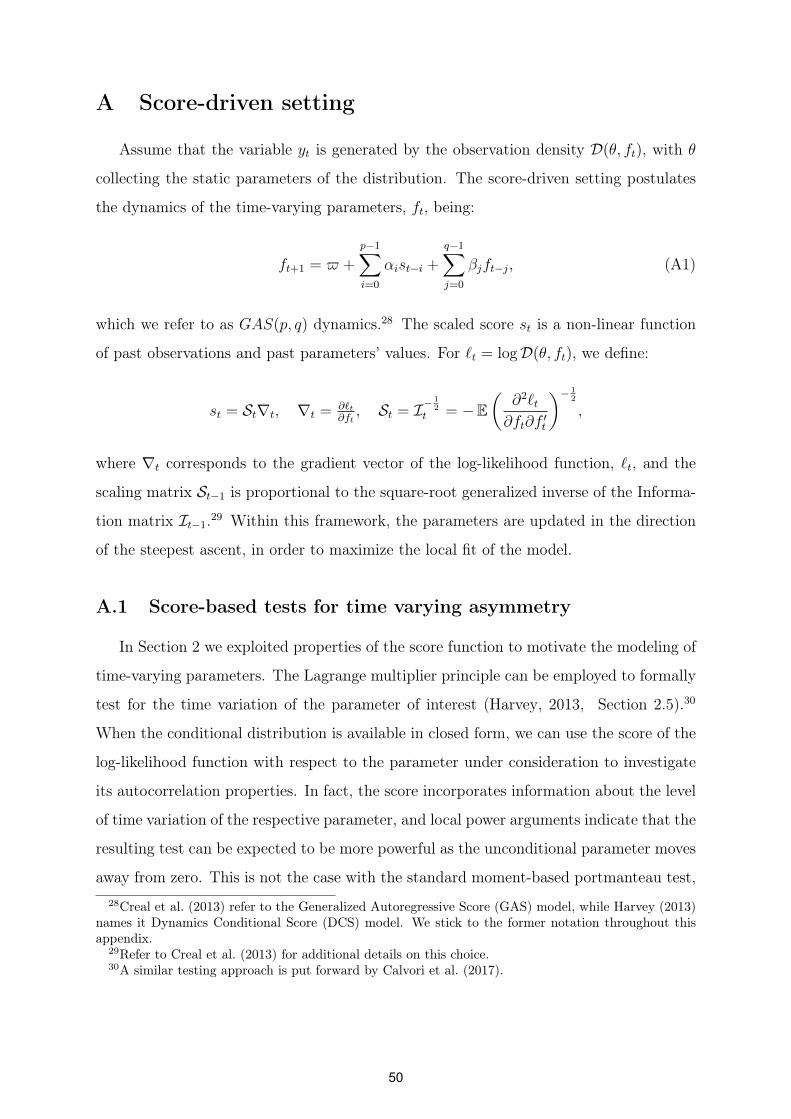
A Score-driven setting

Assume that the variable yt is generated by the observation density D(θ, ft), with θ

collecting the static parameters of the distribution. The score-driven setting postulates

the dynamics of the time-varying parameters, ft, being:

ft+1 = $ +

p−1∑i=0

αist−i +

q−1∑j=0

βjft−j, (A1)

which we refer to as GAS(p, q) dynamics.28 The scaled score st is a non-linear function

of past observations and past parameters’ values. For `t = logD(θ, ft), we define:

st = St∇t, ∇t = ∂`t∂ft, St = I−

12

t = −E(

∂2`t∂ft∂f ′t

)− 12

,

where ∇t corresponds to the gradient vector of the log-likelihood function, `t, and the

scaling matrix St−1 is proportional to the square-root generalized inverse of the Informa-

tion matrix It−1.29 Within this framework, the parameters are updated in the direction

of the steepest ascent, in order to maximize the local fit of the model.

A.1 Score-based tests for time varying asymmetry

In Section 2 we exploited properties of the score function to motivate the modeling of

time-varying parameters. The Lagrange multiplier principle can be employed to formally

test for the time variation of the parameter of interest (Harvey, 2013, Section 2.5).30

When the conditional distribution is available in closed form, we can use the score of the

log-likelihood function with respect to the parameter under consideration to investigate

its autocorrelation properties. In fact, the score incorporates information about the level

of time variation of the respective parameter, and local power arguments indicate that the

resulting test can be expected to be more powerful as the unconditional parameter moves

away from zero. This is not the case with the standard moment-based portmanteau test,28Creal et al. (2013) refer to the Generalized Autoregressive Score (GAS) model, while Harvey (2013)

names it Dynamics Conditional Score (DCS) model. We stick to the former notation throughout thisappendix.

29Refer to Creal et al. (2013) for additional details on this choice.30A similar testing approach is put forward by Calvori et al. (2017).

50

which simply uses the cross-product of standardized residuals (see, e.g. Bollerslev, 1990).

Given the law of motion in Equation (A1), and provided |βj| < 1q−1j=0, we can recover

the (infinite) moving average representation of the filter:

ft+1 = $∗ +∞∑i=0

ψist−i, (A2)

equivalent to a GAS(∞, 0), with $∗ = $(1−β1−β2−...−βq−1)

. Tests can then be carried out

using the score’s autocorrelation function, rs(τ).

Assume the conditional distribution of yt being the Skew-t of Gómez et al. (2007),

yt|Yt−1 ∼ sktν(µt, γ, δ), with log-likelihood

`t(yt|θ, Yt−1) = log C(η)− 1

2log σ2 − 1 + η

2ηlog

[1 +

ηε2t

(1− sgn(εt)%)2σ2

], (A3)

log C(η) = log Γ

(η + 1

2η

)− log Γ

(1

2η

)− 1

2log

(1

η

)− 1

2log π,

where Γ(·) is the Gamma function, sgn(.) is the sign function, and η = 1/ν is the inverse of

the degrees of freedom. To ensure positive scale and bounded shape, we model γ = log σ,

δ = arctanh(%), and the score vector with respect to µ, γ, and δ (scaled by inverse square

root of information matrix as described later in details) will be equal to:

sµ,t

sγ,t

sδ,t

=

√(1 + 3η)

(1 + η)

√

(1− %2)wtζt√(1+η)

2(wtζ

2t − 1)

−√

(1−%2)3

sgn(εt)(1−sgn(εt)%)

wtζ2t

, (A4)

where

wt =(1 + η)

(1− sgn(εt)%)2 + ηζ2t

, ζt =εtσ. (A5)

The scores in Equation (A4) can thus be used to test for the presence of time variation of

the parameters. First, we fix the scale and shape parameters to their maximum likelihood

estimates, γ and δ, respectively, and let µt being the only time-varying parameter. Then,

using the estimated parameters we recover the time series of of the scores sγ and sδ,

which we use to carry out the tests. Specifically, following Harvey and Thiele (2016),

51

which apply this methodology to test against the time variation of correlations, we employ

three different test specifications: the Portmanteau test, Q, the Ljung-Box test, Q∗, and

the Nyblom (1989) test. For all these test, the optimal lag-length is selected following

the methodology of Escanciano and Lobato (2009).

We apply the testing procedure to three different specifications for the dynamics of

µt:

S1: µt = 0 and yt ∼ AR(2) with skew-t innovations sktν(0, σ, %) (see Section 2).

S2: µt ∼ GAS(1, 1) with a unit root (RW);

S3: µt ∼ RW +GAS(1, 2) with stationary roots;

For each case, we consider a specification with constant γ = log σ, and another with

time-varying γt = log σt, following a non-stationary GAS(1, 1) process. Tests’ results,

using data on GDP growth from 1971 to 2018, are reported in Table 1 (Section 2) for

S1, while Table A1 reports the results for S2 and S3. For all the cases and specifications

we reject the null hypothesis of constant shape at the 1% confidence level, for Q and

Q∗. Similarly, the Nyblom specification rejects the null, but the test provide less precise

evidence. While the first two tests leave the alternative hypothesis unspecified, the latter

tests for parameter constancy, against a random walk law of motion. Therefore, we

ascribe such low precision to the stationary nature of the scale parameter.31

31Harvey and Streibel (1998) argue that the Nyblom (1989) test can be used to test against stationary,but highly persistent, alternative hypotheses.

52

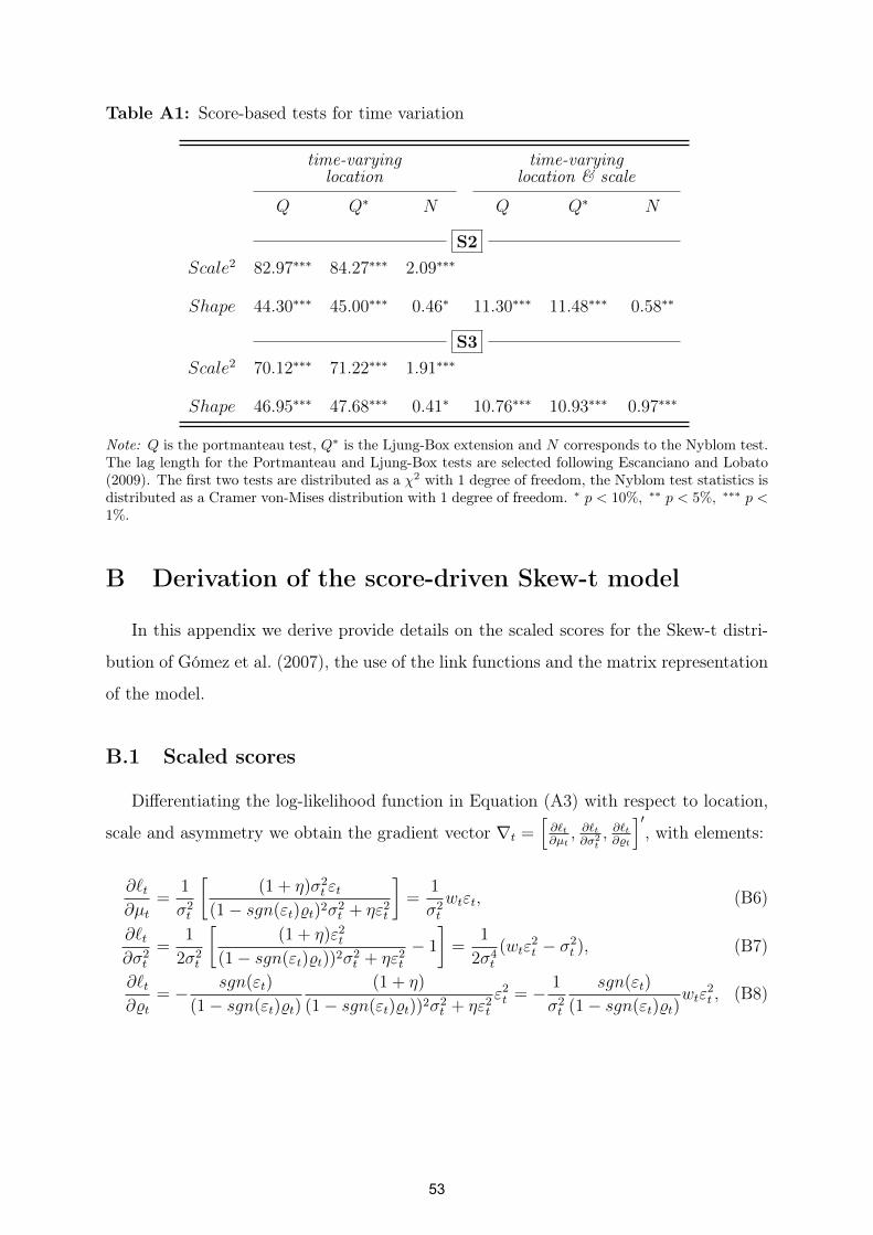
Table A1: Score-based tests for time variation

time-varying time-varyinglocation location & scale

Q Q∗ N Q Q∗ N

S2Scale2 82.97∗∗∗ 84.27∗∗∗ 2.09∗∗∗

Shape 44.30∗∗∗ 45.00∗∗∗ 0.46∗ 11.30∗∗∗ 11.48∗∗∗ 0.58∗∗

S3Scale2 70.12∗∗∗ 71.22∗∗∗ 1.91∗∗∗

Shape 46.95∗∗∗ 47.68∗∗∗ 0.41∗ 10.76∗∗∗ 10.93∗∗∗ 0.97∗∗∗

Note: Q is the portmanteau test, Q∗ is the Ljung-Box extension and N corresponds to the Nyblom test.The lag length for the Portmanteau and Ljung-Box tests are selected following Escanciano and Lobato(2009). The first two tests are distributed as a χ2 with 1 degree of freedom, the Nyblom test statistics isdistributed as a Cramer von-Mises distribution with 1 degree of freedom. ∗ p < 10%, ∗∗ p < 5%, ∗∗∗ p <1%.

B Derivation of the score-driven Skew-t model

In this appendix we derive provide details on the scaled scores for the Skew-t distri-

bution of Gómez et al. (2007), the use of the link functions and the matrix representation

of the model.

B.1 Scaled scores

Differentiating the log-likelihood function in Equation (A3) with respect to location,

scale and asymmetry we obtain the gradient vector ∇t =[∂`t∂µt, ∂`t∂σ2

t, ∂`t∂%t

]′, with elements:

∂`t∂µt

=1

σ2t

[(1 + η)σ2

t εt(1− sgn(εt)%t)2σ2

t + ηε2t

]=

1

σ2t

wtεt, (B6)

∂`t∂σ2

t

=1

2σ2t

[(1 + η)ε2

t

(1− sgn(εt)%t))2σ2t + ηε2

t

− 1

]=

1

2σ4t

(wtε2t − σ2

t ), (B7)

∂`t∂%t

= − sgn(εt)

(1− sgn(εt)%t)

(1 + η)

(1− sgn(εt)%t))2σ2t + ηε2

t

ε2t = − 1

σ2t

sgn(εt)

(1− sgn(εt)%t)wtε

2t , (B8)

53

where

wt =(1 + η)

(1− sgn(εt)%t)2 + ηζ2t

, (B9)

and ζt = εtσt

is the standardized innovations.

The Fisher information matrix is computed as the expected values of outer product

of the gradient vector, for a fixed number of degrees of freedom:

It|t−1 = Et−1[∇t∇′t] =

(1+η)

(1+3η)(1−%2t )σ2t

0 − 4c(1+η)

σt(1−%2t )(1+3η)

0 12(1+3η)σ4

t0

− 4c(1+η)

σt(1−%2t )(1+3η)0 3(1+η)

(1−%2t )(1+3η)

. (B10)

Given we model γt = lnσt and δt = arctanh(%t), for the chain rule we have:

∂`t∂γt

=∂`t∂σ2

t

∂σ2t

∂γt,

∂`t∂δt

=∂`t∂%t

∂%t∂δt

, (B11)

where ∂σ2t

∂γt= 2σ2

t and ∂%t∂δt

= (1 − %2t ). We can thus define the vector of interest as

ft = (µt, γt, δt)′ with the associated Jacobian matrix

Jt =∂(µt, σ

2t , %t)

∂f ′t=

1 0 0

0 2σ2t 0

0 0 1− %2t

. (B12)

As such the scaled score reads:

st = (J ′tdiag(It)Jt)−12J ′t∇t =

sµt

sσt

s%t

=

√

(1+3η)(1−%2t )

(1+η)wtεt√

(1+3η)2

(wtζ2t − 1)

−sgn(εt)√

(1+sgn(εt)%t)(1+3η)3(1−sgn(εt)%t)(1+η)

wtζ2t

. (B13)

To prevent numerical instability, it is often the case to replace the scaling matrix St =

(J ′tdiag(It)Jt)−12 with its smoothed estimator, St = (1− λ)St−1 + λSt, 0 < λ < 1.

54

B.2 Transformed parameters’ scores

Here we provide a proof of the equivalence between the the score vector arising from

the restriction imposed on the scale and shape parameters and that arising by imposing

constraints on the two-component specification. We will drop the time subscript for the

sake of clarity.

Proof. Let consider γ = log σ being the log-scale, it follows that σ = exp γ, and the

gradient is

∂`

∂γ=

∂`

∂σ2

∂σ2

∂γ=

∂`

∂σ22σ2.

Let now consider the multiplicative two-component counterpart σ = σσ, such that γ =

log σ = log σ + log σ = γ + γ. The gradient with respect to the first component reads

∂`

∂γ=

∂`

∂σ2

∂σ2

∂γ

∂γ

∂γ=

∂`

∂σ22σ2.

The same applies for the second component.

Proof. For the shape parameter % = tanh δ, we model δ = arctanh % and the gradient is

∂`

∂δ=∂`

∂%

∂%

∂δ=∂`

∂%(1− %2).

Consider the two-component counterpart δ = (δ + δ), so that % = tanh(δ + δ), it is easy

to see that that

∂`

∂δ=∂`

∂%

∂%

∂δ

∂δ

∂δ=∂`

∂%(1− %2).

The same applies for the second component.

B.3 Matrix representation

Given the vector of time-varying parameters, ft, we can express the score-driven law

of motion of Equation (3) in matrix form.

55

µt

µt

µt−1

γt

γt

δt

δt

︸ ︷︷ ︸ft+1

=

1 0 0 0 0 0 0

0 φµ,1 φµ,2 0 0 0 0

0 1 0 0 0 0 0

0 0 0 1 0 0 0

0 0 0 0 φγ 0 0

0 0 0 0 0 1 0

0 0 0 0 0 0 φδ

︸ ︷︷ ︸

A

µt−1

µt−1

µt−2

γt−1

γt−1

δt−1

δt−1

︸ ︷︷ ︸ft

+

0 0 . . . 0

β1µ β2

µ . . . βkµ

0 0 . . . 0

0 0 . . . 0

β1γ β2

γ . . . βkγ

0 0 . . . 0

β1δ β2

δ . . . βkδ

︸ ︷︷ ︸

B

Xt +

ςµ 0 0

κµ 0 0

0 0 0

0 ςγ 0

0 κγ 0

0 0 ςδ

0 0 κδ

︸ ︷︷ ︸

C

sµt

sγt

sδt

︸ ︷︷ ︸st

,

with Xt being a k-dimensional vector of predictors, at time t.

56

C On the importance of dynamic conditional moments

In this Section, we consider a restricted specification of the model in line with the

work of Plagborg-Møller et al. (2020). As noted in Section 3, when the autoregressive

features of the model is dropped out, and the information content of past prediction

errors (condensed into the score) is ignored, the model collapses to a parametric model

for the distribution of GDP growth akin to the one in Plagborg-Møller et al. (2020).32

Specifically, setting ςµ = φµ,1 = φµ,2 = κµ = ςγ = φγ = κγ = ςδ = φδ = κδ = 0, we obtain

µt+1 = µ+ β′µXt, (C14)

γt+1 = γ + β′γXt, (C15)

δt+1 = δ + β′δXt, (C16)

so that the parameters’ laws of motion become linear functions of predictors only.

We estimate the model above using as predictors the 4 disaggregated components of

the NFCI, as well as the factors used in Plagborg-Møller et al. (2020) (including in both

cases lagged values of GDP growth). Table C2 reports the Deviance Information Criterion

associated to these two specifications. Our baseline model strongly outperforms the two

restricted specifications, both over the whole sample and during recessions. Figure C1

reports the estimated volatility and skewness from the baseline model (in blue) and the

restricted specification (in red). For comparability purposes, both models are estimated

using the disaggregated components of the NFCI as predictors.33 The results of the

restricted specification are broadly in line with those reported by Plagborg-Møller et al.

(2020). The estimated skewness from their model is cyclical but displays large uncertainty,

so that the 90% confidence bands only rarely excludes the zero. Moreover, the simplified

specification of the time-varying model does not display the well-known reduction of the

volatility occurred during the Great Moderation period.

Overall, comparing the restricted model to the baseline specification highlights the

benefits associated with a richer framework, including the score of the predictive like-

lihood, long-run components, and persistent cyclical variations. In terms of volatility32Note that Plagborg-Møller et al. (2020) consider the Skew-t of Azzalini and Capitanio (2003).33The mean GDP growth extracted from the two models displays less noticeable differences.

57

Table C2: Deviance Information Criterion

Model DIC DIC Rec

Skt 4DFI 4.367 2.347Plagborg-Møller et al. (2020) with 4DFI 4.589 2.387Plagborg-Møller et al. (2020) Financial Factor 4.503 2.376

Note: The table reports the Deviance Information Criterion of Spiegelhalter et al. (2002) for the Skt-4DFI specification, and the nested version of Plagborg-Møller et al. (2020), with the four disaggregatedfinancial indices and with the global and financial factors. In the column DIC Rec we evaluate the DICmeasure during recession periods.

estimates, the presence of long-run components, as well as the addition of the score

(which for the volatility is a function of the squared prediction errors) as signal for the

updating, turn out to be of key importance to track the well-established stylized fact

of a substantial decline in volatility from the mid-1980s (McConnell and Perez-Quiros,

2000; Stock and Watson, 2002). Persistent cyclical components, on the other hand, al-

low the model to recover significant variations of the skewness coefficients. This is not

surprising, as the unrestricted model implies that the time variation in the parameters

reflects current and past discounted variation of the predictors (as well as the information

in the scaled score). This implies that high frequency noisy variations of the predictors

are averaged out when incorporated into the time-varying dynamics. Moreover, while

the skewness from both models set on similar levels at the beginning of the sample and

during the 1990s, the asymmetry implied by the restricted specification becomes lower

over the mid 1980s, while attaining higher values after the Global Financial Crisis. This

pattern supports the addition of secular components, able to track the declining trend of

business cycle skewness, as documented by Jensen et al. (2020).

Furthermore, we investigate to what extent our results are affected by the different

choice of financial predictors. Re-estimating our baseline model using the two factors

employed by Plagborg-Møller et al. (2020), we recover very similar time-varying second

and third moments to the one reported for our baseline specification. Volatility displays

a clear countercyclical dynamics, as well as a sharp fall in the mid-1980s. Skewness

exhibits pronounced cyclical variation, with recessions characterized by negatively skewed

conditional distributions, and expansions associated with positively skewed distributions.

58

Standard Deviation

1975 1980 1985 1990 1995 2000 2005 2010 20150

1

2

3

4

5

6

7

8

9

10Skewness

1975 1980 1985 1990 1995 2000 2005 2010 2015-2.5

-2

-1.5

-1

-0.5

0

0.5

1

1.5

2

2.5

Figure C1: Time-varying moments: Skt 4DFI vs. Plagborg-Møller et al. (2020)Note: The plots illustrate the estimated time-varying volatility (left panel) and skewness (right panel)with 95% confidence bands. Results for the Skt -4DFI are reported in blue, while red lines report resultsfor the nested version of Plagborg-Møller et al. (2020)’s model. Shaded bands represent NBER recessions.

Again, one should not be surprised by these broad similarities. The inclusion of the scaled

score as a driver of the time-varying parameters introduces a self-correction mechanism to

the model, which allows the parameters to closely track the most pronounced features of

the data, regardless of the predictors included in the model. In terms of DIC, the baseline

specification with the disaggregated components of the NFCI continues to be preferred

with respect to the alternative factors included by Plagborg-Møller et al. (2020).

D Bayesian estimation

In this section we outline the Bayesian approach for the estimation of the models. We

estimate the vector of static parameters θ, and the time-varying parameters ft, through

the following steps:

( i ) Estimate θ∗ via ML and initialize the sampling algorithm with θ∗

( ii ) Sample θ and ft with the Adaptive Random-Walk Metropolis-Hastings (AR-

WMH)

(iii) Compute the statistics of interest as the percentiles of the empirical distribution

function.

In the following subsections, we detail the prior specifications and the ARWMH algorithm.

59

D.1 Prior specification

Starting from Equations 9 - 16, let φ be a generic first-lag partial autocorrelation,

while ς and κ being generic score loadings for the long-run and short-run equations,

respectively. Let βi ∈ B, be a generic predictor loading for the parameter i, i = µ, σ, %,

and let η be the inverse of the Skew-t degrees of freedom. Prior specifications for these

parameters read:

φ ∼ NID(µφ, σφ) · I(φ∈Φ); (D1)βi ∼ NID(µβ, σ

iβ), i = µ, σ, %; (D2)

ς, κ ∼ G−1(aj, bj), j = ς, κ; (D3) η ∼ G−1(aη, bη) · I(η∈H). (D4)

Prior specification D1 sets the prior distribution for the first autroregressive param-

eters: we target high persistence, with µφ . 1, with a standard tightness of σµ = 0.2,

in line with Bayesian Vector Autoregressive models (see, e.g., Doan et al., 1984; Sims

and Zha, 1998). We restrict the prior distribution to only span the stationary region, Φ,

by truncating the support, which gives rise to an improper prior distribution as in Cog-

ley and Sargent (2005). Predictor loadings are drawn from a Normal distribution with

µβ = 0, and standard deviations σβ are set to small values of 0.05, 0.2 and 0.1 for the

location, scale and shape parameters, respectively. These priors aim at preventing model

overfitting, applying an L2 regularization, akin to the shrinkage induced by a Ridge-type

regression. We set inverse gamma priors for the score loadings, such that they reflect the

a priori expectation of small, but positive coefficients, in line with the properties of the

score-driven filters (for further discussion, see Blasques et al., 2014). We set aς = aκ = 4,

and bς = 3 and bκ = 10, to reflect the properties of the long- and the short-run com-

ponents. Eventually, we use an inverse gamma prior for η, the inverse of the degrees of

freedom parameter, with aη = 2 and bη = 10. In line with Juárez and Steel (2010), these

values allow the distribution to explore a wide range of feasible values, with a mean of 20

and a median of 10. In order to ensure the existence of, at least, the first three moments,

we restrict the support to the H = [0, 0.33] set.

60

We also target the stationarity of the cyclical component of the location through a

prior on the sum of the autoregressive coefficients (Sims and Zha, 1998). Let φS be the

sum of two generic autoregressive coefficients, φS = φ1 + φ2, we assume

φS ∼ N (µφS , σφS) · I(φS∈Φ),

with µφ2 . 1 and and σsφ = 0.2.

D.2 Horseshoe priors and SAVS

Consider the regression model:

yt = b′Xt + et, et ∼ iid(0, σ2eIp) (D5)

the Horseshoe (HS) priors of (Carvalho et al., 2010) posit Ridge-type priors for the coeffi-

cients: bj ∼ N (0, λjτ), where the hyperparameters λj and τ control the local (coefficient

specific) and the global shrinkage, respectively. We follow the original paper in setting

the hyperpriors as:34

λj ∼ HC+(0, 1), τ ∼ HC+(0, 1), (D6)

where HC+(0, 1) denotes the standard Half-Cauchy distributions with density function

p(z) =2

π(1 + z2), z ∈ R+. (D7)

Unlike other common shrinkage priors (e.g. Ridge, Lasso), the HS priors is free of exoge-

nous inputs, implying a fully adaptive shrinkage procedure.

Known pitfalls of shrinkage operators account for parameters not being exactly set to

zero (e.g. Ridge), thus increasing parameter uncertainty, or weak selection performances

when predictors are correlated (e.g. Lasso). A common remedy to the first pathology is34Makalic and Schmidt (2015) exploit the link between the scale mixture of Inverse Gamma distri-

butions to approximate the Half-Cauchy distributions to propose a tractable framework for posteriorsimulation via Gibbs sampling. However, this hierarchy features twice as may parameters (auxiliaryvariables) compared to the original specification.

61

the sparsification of the near-zero elements. Let p be the number of possible predictors,

the sparsification problem can be cast as:

b∗ = argminb

[1

2||Xb−Xb||22 +

p∑j=1

mj|bj|], (D8)

where the sparse coefficients b∗ are obtained minimizing the Euclidean distance between

Xb and the model fit obtained from the shrinkage operator. Additional penalty for

the non-zero parameters is controlled by mj, which represents a variable specific tuning

parameter, generally chosen on the basis of computationally expensive methods (e.g.

cross-validation). In their recent contribution, Ray and Bhattacharya (2018) introduce

a purely data-driven, and less burdensome solution to the choice of the parameter mj,

proven to be robust to correlated designs. They suggest to specify the tuning parameter

asmj = |bj|−2 such that the jth variable receives a penalization “ranked in inverse-squared

order of the magnitude of the corresponding coefficient” (Ray and Bhattacharya, 2018),

an approach similar to the Adaptive Lasso of Zou (2006). The Signal Adaptive Variable

Selector (SAVS) algorithm can then be expressed as:

b∗j = sgn(bj)||Xj||−2 max|bj| · ||Xj||2 −mj, 0

, (D9)

where || · || represents the Euclidean norm of the vector Xj.

D.3 Adaptive Metropolis-Hastings

Posterior estimates of the parameters are obtained via simulation by means of the

Adaptive Metropolis-Hastings algorithm proposed by Haario et al. (1999). Given that

estimated parameters lie in bounded regions of the parameter space, we augment the

algorithm with a rejection step to prevent numerical instability due to invalid parameter

draws. The algorithm works as follows: given the (d × 1) vector of static parameters

θ = (ς ′, κ′, φ′, η)′, we define θj as the draw of the parameters at the jth iteration of the

sampler, generated from the random walk kernel:

θj = θj−1 + σj,sε ε ∼ N (0,ΣjH), (D10)

62

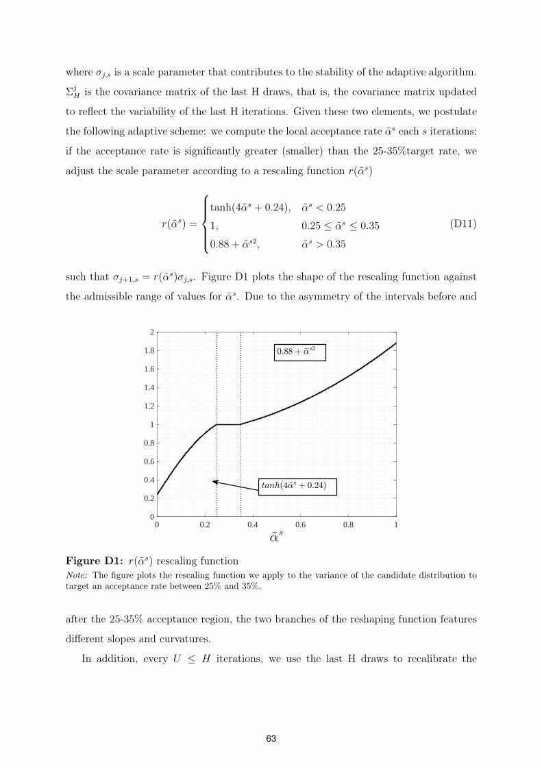
where σj,s is a scale parameter that contributes to the stability of the adaptive algorithm.

ΣjH is the covariance matrix of the last H draws, that is, the covariance matrix updated

to reflect the variability of the last H iterations. Given these two elements, we postulate

the following adaptive scheme: we compute the local acceptance rate αs each s iterations;

if the acceptance rate is significantly greater (smaller) than the 25-35%target rate, we

adjust the scale parameter according to a rescaling function r(αs)

r(αs) =

tanh(4αs + 0.24), αs < 0.25

1, 0.25 ≤ αs ≤ 0.35

0.88 + αs2, αs > 0.35

(D11)

such that σj+1,s = r(αs)σj,s. Figure D1 plots the shape of the rescaling function against

the admissible range of values for αs. Due to the asymmetry of the intervals before and

0 0.2 0.4 0.6 0.8 10

0.2

0.4

0.6

0.8

1

1.2

1.4

1.6

1.8

2

Figure D1: r(αs) rescaling functionNote: The figure plots the rescaling function we apply to the variance of the candidate distribution totarget an acceptance rate between 25% and 35%.

after the 25-35% acceptance region, the two branches of the reshaping function features

different slopes and curvatures.

In addition, every U ≤ H iterations, we use the last H draws to recalibrate the

63

covariance matrix of the proposal distribution: ΣjH = K√

H−1, where K is the (H × d)

centered matrix of the last H draws, obtained as K − E[K]; in this process we also

reinitialize the scale parameter at the value of 2.38√d, as suggested by Gelman et al.

(1996). According to the Metropolis-Hasting procedure, we accept θj with probability

p = min

1, exp(f(θj)− f(θj−1))where f(θ) = log-likelihood× priors. Discarded draws

are replaced by the latest accepted draw. In order to prevent failures of the algorithm,

we discard draws that do not lie in the bounded region of the parameter space, replacing

them as previously specified. We set the number of iterations to 20000, of which we keep

the last 40%. We reduce dependence between consecutive draws by “thinning” each 2 real-

izations. Posterior distributions are eventually obtained from a sample of 4000 iterations.

We adjust the scale parameter each hundred iterations (s = 100), while the adaptive step

takes place every U = 1500 iterations, considering H = 2500 past iterations.35 Markov

Chain properties have been checked by visual inspection, as suggested by Cowles and

Carlin (1996). The algorithm results to be rather efficient, and a complete chain from

the baseline model in Section 4 can be obtained in less than 3 minutes, whereas for the

large data model, a complete chain can be obtained in about 7 minutes.35The adaptive process starts when j ≥ H, while the scale updating takes place from the 100th iteration

64

Algorithm 1: Adaptive Random-Walk Metropolis-Hastings

for j=1,2,...,N do

Generate: θ∗ ∼ N (θj−1, σ2j,sΣ

jH) ;

if θ∗ ∈ Θ then

Evaluate: p = min

1, exp(f(θj)− f(θj−1));

Draw: u ∼ U [0, 1] ;

if u < p then

θj = θ∗, αj = 1 ;

else

θj = θj−1, αj = 0;

end

else

θj = θj−1, αj = 0;

end

if j( mod s) = 0 thenσj+1,s = σj,s ∗ r(αs)

end

if j( mod U) = 0 thenΣj+1H = Cov(θiHi=j−H), σj,s = 2.38√

d

end

end

Note: the notation “a( mod b)” represents the modulo operation, while “−s” indicates the previouss draws.

65

E Monte Carlo Exercise

In this Section we outline a Monte Carlo exercise with the aim of illustrating the

small-sample properties of the Skew-t model described in Section 3. We are interested in

the reliability of the estimates of the asymmetry parameter and, in particular, whether

the model is able to correctly disentangle the movements in the asymmetry parameter

from the movements in the location and scale parameters.

We simulate T=250 observations for the parameters of location, µt, scale, σt, and

asymmetry, %t, for every period t from the Sktν(µt, σt, %t) to obtain the series YtTt=1,

then use to estimate the model discussed in Section 3 (excluding explanatory variables).

Therefore, regardless of the DGP considered we always estimate a two component spec-

ification for all the three time-varying parameters. This approach mimics the true esti-

mation process carried out on real data, to approximate the conditional distribution of

the underlying GDP growth. We first consider ad-hoc specifications for the location and

scale parameters (AR(2) and AR(1), respectively). Then, we turn to DGPs that replicate

closely the dynamic properties of the time-varying parameters we estimate from the the

data (and in particular replicate the correlation between location and scale parameter

that we observe in the data). For the shape parameter, we consider a number of different

DGPs, including no asymmetry, constant asymmetry, a single break in the asymmetry,

and cyclical asymmetry.

In the first DGP, data are simulated from a specification featuring symmetric distribu-

tions, with independent, time-varying location and volatility, therefore aiming at checking

that the model does not pick up any asymmetry when this is not a feature of the data. The

second DGP considers the case in which the asymmetry parameter experiences a jump,

from 0 to 0.5 after 100 observations, hence implying negatively skewed distributions in

the second part of the sample. This case sheds light on the adaptiveness of the model,

and provides a clear framework to illustrate the distinctive role played by the secular

and transitory components. The third and fourth DGPs consider a specification for the

location and scale parameter that replicate the basic features of the estimated location

and scale parameters, e.g. a mildly negative correlation, whereas the shape parameter

66

is constant, either at zero or at a positive value.36 In the last DGP, the asymmetry

parameter varies over time, with cyclical fluctuations. To ensure that we replicate the

cyclical features of the parameters, we simulate the three parameters from a VAR(1),

with parameters estimated on the parameters obtained from the Skt -4DFI specification.

For each DGP we perform N=500 replications and we estimate the parameters of the

two-component model using the estimation approach introduced in the main text, and

detailed in Appendix D.

We simulate µt, γt = log(σt), and δt = arctanh(%t) from the following processes:

DGP1: (No asymmetry)

µt = 0.125 + 1.2µt−1 − 0.25µt−2 + εt, εt ∼ N(0, 0.05);

γt = 0.95γt−1 + εt, εt ∼ N(0, 0.025);

δt = 0.

DGP2: (Single break)

µt = 0.125 + 1.2µt−1 − 0.25µt−2 + εt, εt ∼ N(0, 0.05);

γt = 0.95γt−1 + εt, εt ∼ N(0, 0.025);

δt =

0, t ≤ 100

0.5, t > 100

.

DGP3: (Correlated location, scale and no asymmetry)

µtγt

=

0.29

−0.12

+

0.89 0.01

0.06 0.94]

µt−1

γt−1

+ εt, εt ∼ N(0,Ω),

where

Ω =

0.008 −0.001

−0.001 0.015

and δt = 0, ∀t.

36Specifically, we fit a VAR(1) to the location and log-scale parameters estimated from the data, anduse these estimates for the DGPs.

67

DGP4: (Correlated location, scale and constant asymmetry)

µtγt

=

0.29

−0.12

+

0.89 0.01

0.06 0.94]

µt−1

γt−1

+ εt, εt ∼ N(0,Ω),

where

Ω =

0.008 −0.001

−0.001 0.015

and δt = 0.5, ∀t.

DGP5: (Cyclical asymmetry)

µt

γt

δt

=

0.40

−0.38

−0.33

+

0.85 0.03 −0.06

0.17 0.88 0.13

0.14 −0.09 0.95

µt−1

γt−1

δt−1

+ εt, εt ∼ N(0,Ω),

where

Ω =

0.008 −0.001 −0.007

−0.001 0.015 0.008

−0.007 0.008 0.025

For all the DGPs, the model correctly picks up the time variation in the location and

scale with great precision, and the degree of freedom are estimated without bias. These

results are not reported in the interest of brevity, but are available upon request. Hence,

in what follow we comment on the ability of the model to track the underlying asymmetry

of the distribution. For the first four DGPs, we report the true asymmetry parameter and

the 99, 95, 90 and 75 confidence bands for the estimated counterpart. For the fifth DGP

we consider the median difference between the estimated and the simulated parameters.

Figure E2 and E5 shows that when the distribution is symmetric, the estimated median

parameter, and the associated confidence bands, remain close to zero with small variabil-

ity. Therefore, the model clearly captures the symmetry of the underlying data generating

process, and correctly disentangles the time variations of the volatility for changes in the

asymmetry of the distribution in simple settings (DGP1), as well as when location and

scale are correlated (DGP3). The filter is also able to detect the case with constant neg-

68

ative skewness (DGP4), in spite of the dynamic correlation between location and scale.

The model does not confound variations of the first two moments of the data with varia-

tion of the asymmetry (Figure E6). Interestingly, for all the cases where the asymmetry

parameter is fixed at a positive value, the cyclical components are always estimated to be

approximately zero, suggesting that no variation at all is captured. Whereas, the secular

components show minimal variation, always around the true value.37 For this case we

also investigate what happens when the initialization of the filter is away from the true

parameter. The filter neatly discovers the true level of asymmetry relatively quickly (i.e.

after roughly 20 observations), and the parameter sets around the true value.

In Figure E3 we report the results for the case of a single break in the asymmetry

parameter. Until the jump takes place, the estimated asymmetry remains centered around

zero, while it timely reacts to the jump occurring on the 100th observation. Furthermore,

due to the presence of a slow-moving trend component, the model fully captures the

extent of the asymmetry in the second part of the sample in just 50 observations. Within

this case, we also investigate to what extent the model is able to recognize the persistent

nature of the shift in the asymmetry. Figure E4 reports the estimated secular and the

cyclical components, respectively. The long-run components picks up the jump in a

timely manner, and contributes to most of the variability of the estimated parameter. In

addition, the first few observations after the jump are partly captured by the model as

short-lived movements, revering to zero soon after.

Lastly, we report in Figure E7 the difference, and the associate confidence set, between

the simulated and the estimated parameters. Despite co-movements in the location,

scale and asymmetry parameters, the model clearly captures the cyclical variations of

the latter, reported in red. The estimated parameter converges to the correct values after

few observations, with small deviations, as suggested by the narrow bounds. Key for the

identification of parameters’ variation is that, as discussed in Section 4, shifts in the shape

parameter map into a time-varying correlation between the first and second moments of

the data. Therefore, in spite of the (dynamic) interaction between the key parameters

of the distribution, the model correctly identifies, in a timely manner, movements in the

asymmetry of the distribution.

37These results are not reported but available upon request.

69

0 50 100 150 200 250-0.8

-0.6

-0.4

-0.2

0

0.2

0.4

0.6

0.8

Figure E2: DGP1 - No asymmetry.Note: The median simulated parameter is reported in red, while shades of blue represent the 99th, 95th,90th, 75th, 25th, 10th, 5th and 1st percentiles of the empirical distribution of the estimated parameter.

0 50 100 150 200 250-0.8

-0.6

-0.4

-0.2

0

0.2

0.4

0.6

0.8

Figure E3: DGP2 - Single break in asymmetry.Note: The median simulated parameter is reported in red, while shades of blue represent the 99th, 95th,90th, 75th, 25th, 10th, 5th and 1st percentiles of the empirical distribution of the estimated parameter.

70

Long-run Short-run

0 50 100 150 200 250-0.8

-0.6

-0.4

-0.2

0

0.2

0.4

0.6

0.8

0 50 100 150 200 250-0.8

-0.6

-0.4

-0.2

0

0.2

0.4

0.6

0.8

Figure E4: Secular and cyclical components for the DGP2 case.Note: The median simulated parameter is reported in red, while shades of blue represent the 99th, 95th,90th, 75th, 25th, 10th, 5th and 1st percentiles of the empirical distribution of the estimated parameter.

0 50 100 150 200 250-0.8

-0.6

-0.4

-0.2

0

0.2

0.4

0.6

0.8

Figure E5: DGP3 - Correlated location, scale and no asymmetry.Note: The median simulated parameter is reported in red, while shades of blue represent the 99th, 95th,90th, 75th, 25th, 10th, 5th and 1st percentiles of the empirical distribution of the estimated parameter.

71

0 50 100 150 200 250-0.8

-0.6

-0.4

-0.2

0

0.2

0.4

0.6

0.8

Figure E6: DGP4 - Correlated location, scale and constant negative skewness.Note: The median simulated parameter is reported in red, while shades of blue represent the 99th, 95th,90th, 75th, 25th, 10th, 5th and 1st percentiles of the empirical distribution of the estimated parameter.

0 50 100 150 200 250-0.8

-0.6

-0.4

-0.2

0

0.2

0.4

0.6

0.8

Figure E7: DGP5 - Cyclical asymmetry.Note: The median difference between the simulated and the estimated parameters is reported in red,while shades of blue represent the 99th, 95th, 90th, 75th, 25th, 10th, 5th and 1st percentiles of the empiricaldistribution of such difference.

72

F Data

In this Appendix we provide additional details on the data sources. We focus on (real)

GDP growth in the US, and we measure financial conditions using the Chicago FED

National Financial Condition Index (NFCI), and its subcomponents (Brave and Butters,

2011). The NFCI is a weekly index tracking the status of money markets, debt and equity

markets, and the banking sector (comprehensive of the “shadow” banking sector). The

contribution of these sectors maps into three subindices, each of which gauges financial

conditions in terms of risk, leverage, and credit (refer to Brave and Butters, 2012, for

further details). We use quarterly data on economic activity and financial conditions over

the period 1973Q1 to 2018Q4, where the starting date for the analysis is dictated by the

availability of the NFCI.

As new information is available, these indices are standardized. Thus, when an index

takes a value of 1 (-1), it signals that the financial conditions are one standard deviation

tighter (looser) than their historical average. Consistently with the concept of financial

tightening, the measure relating to the risk subcomponent positively contributes to the

NFCI, reflecting increasing risk premia. In contrast, measures of leverage and credit

receive negative weights in response to lower asset values and declining liquidity in the

financial sector. The top panel of Figure F1 plots the NFCI against GDP growth, whereas

the bottom panels report the NFCI subcomponents. The NFCI (and the three subcom-

ponents) spikes during recessions, as indicated by the gray-shaded bands, and displays

a clear negative correlation with GDP growth, suggesting that periods of financial over-

heating coincide with severe economic troughs, as documented by Adrian et al. (2019).

The NFCI closely tracks the risk subcomponent, due to high weights being attached to

some of the risk variables, such as the VIX index. This is consistent with the observation

that volatility of the stock market is an accurate predictor of financial instability (see,

e.g. Bekaert and Hoerova, 2014). The leverage component shows strong procyclicality,

and tends to pick up on high values before other indices, consistently with the findings

of Adrian and Shin (2010) and Jordà et al. (2013). Lastly, measures of credit spread and

credit risk are contained in the risk and credit components (Krishnamurthy and Muir,

2017).

73

1975 1980 1985 1990 1995 2000 2005 2010 2015-1

0

1

2

3

4

5

-10

-5

0

5

10

15

20

NFCI GDP growth

1975 1995 2015

-2

0

2

4 Risk

1975 1995 2015

-2

0

2

4 Leverage

1975 1995 2015

-2

0

2

4 Credit

1975 1995 2015

-2

0

2

4 Nonfinancial leverage C2G (detrended)

Figure F1: National Financial Condition Index and subcomponentsNote: The top panel illustrates the evolution of the NFCI and of GDP growth. Lower panels plot therisk, leverage, credit and nonfinancial leverage subcomponents, respectively. Shaded bands representNBER recessions.

Alongside these subindices, the Chicago FED also produces the nonfinancial leverage

(NFL) index (bottom right panel of Figure F1). This series tracks developments in the

nonfinancial credit market using data on household and nonfinancial business leverage.

Household data receive weights roughly 1.5 times higher than the latter. Mian and Sufi

(2010) argue that the build up of financial instability leading to the Great Financial Crisis

was mainly due to an “over-leveraged” household sector. Similarly, Jensen et al. (2020)

observe that increasing households and firms leverage anticipates a deepening of business

cycle skewness. A closer examination of the panel suggests that the massive deleveraging

started in the early 2008 coincides with the beginning of the recession in the same year.

This measure can thus be intended as an “early-warning” signal for economic downturns.

In addition, this index is a clear leading indicator of the HP-filtered credit-to-GDP ratio

measure (blue line in the bottom right panel of Figure F1), put forward as a leading

signal of financial distress (Drehmann et al., 2010; Jordà et al., 2017).38

38Hasenzagl et al. (2020) extensively investigate the relation between the Nonfinancial leverage indexand the Credit-to-GDP ratio index for forecasting purposes.

74

Real-time data. In Sections 5 and 6 we evaluate the performance of our models, and

compare them to a number of alternatives, both in an in- an out-of-sample forecasting

exercise. For these exercises, we use real time data on GDP, provided by the Philadelphia

FED’s Real Time Data Research Center. This dataset contains GDP observations avail-

able at a particular vintage date, that is, GDP values available in the second week of the

middle month of each quarter, as described in Croushore and Stark (2001). GDP growth

undergoes substantial revisions, in particular over the first releases, and even more so

around turning points (see, e.g. Croushore, 2011). Despite there is no consensus on what

releases to use as “actual” data for forecast evaluation (Croushore, 2006), we evaluate

models using the latest release.39

While real time data are available for GDP, the same is not true for the NFCI and

its subcomponents. These are common factors in a broad panel of financial indicators,

extracted using state-space methods. As such, these indicators are always revised at

any point in time, when new information arrives. To this extent, we can only use a

pseudo real-time dataset for the NFCI and its subcomponents. In Section 6, we use the

disaggregated contributions of all the financial indicators which form the basis of the

NFCI, as illustrated in Brave and Butters (2012).40 As GDP data are released about 45

days after the end of the reference quarter, we assume that it is at that point in time

that the forecaster estimates the model and produces the forecasts. The weekly nature of

these data allows us to include all the available information, by averaging all the weeks

within the reference quarter, meaning that we can use all the information made available

within the reference quarter. Despite still not being real-time, this method comes the

closest to mimic the available information set at the time of the forecasts.39This choice implies that the forecast error produced by our models also accounts for a “measurement

error” component, induced by possible GDP measurement redefinitions, that took place over the consid-ered forecast sample (for further discussion, see Stark and Croushore, 2002). The results of our forecastexercise would be qualitatively similar to the one reported if we were to target the ‘advanced’ (i.e. third)revision of GDP growth.

40We are grateful to the authors and the Chicago FED for making the full panel of weighted contri-bution of the financial indicators available for this work.

75

F.1 Main data sources and mnemonics

Data on quarterly real economic activity come from the Federal Reserve Bank of St.

Louis FRED dataset (mnemonic; GDPC1). The NFCI and the relative risk, leverage,

nonfinancial leverage and credit subcomponents are downloaded from the same source

(mnemonic: NFCI, NFCIRISK, NFCILEVERAGE, NFCINONFINLEVERAGE and NF-

CICREDIT). These latter are available at the weekly frequency, and they are converted

into quarterly figure by taking the quarterly average. Overlapping weeks are accounted

for in the averaging process: weekly values are computed in only one of the quarterly

variables.41

F.2 Additional details on the disaggregated financial indicators

We are grateful to Scot Brave and the Federal Reserve Bank of Chicago for sharing the

weighted individual contribution to the NFCI. The dataset contains weekly time series

of financial indicators that feed into the factor model generating both the NFCI and its

subcomponens, as illustrated by Brave and Butters (2012). In Tables F1, F2, F3 and F4

we report all the indicators, their mnemonic, and the date they become available for the

index. Figure F2 provides a graphical illustration of the time schedule of the availability

of the predictors. The y-axis reports the years considered in our work in an ascending

order (e.g. most recent times are closer to the origins).

41See https://fredhelp.stlouisfed.org/fred/data/understanding-the-data/how-are-data-aggregated-when-periods-overlap/

76

Table F1: Risk subindex components

Mnemonic Financial Indicator Starting date

ABCP 1-mo. Asset-backed/Financial commercial paper spread 05/01/2001ABSSPREAD BofAML Home Equity ABS/MBS yield spread 05/07/1991CBILL 3-mo. Financial commercial paper/Treasury bill spread 08/01/1971CG Commercial Paper Outstanding 10/11/1995CMBS BofAML 3-5 yr AAA CMBS OAS spread 02/01/1998CPR Counterparty Risk Index (formerly maintained by Credit Derivatives Research) 13/09/2002CTABS FTSE Russell US Global Markets ABS/5-yr Treasury yield spread 01/02/1991CTERM 3-mo./1-wk AA Financial commercial paper spread 10/01/1997CTF FTSE Russell US Global Markets Financial/Corporate Credit bond spread 31/01/1997CTMBS FTSE Russell US Global Markets MBS/10-year Treasury yield spread 27/01/1989FAILS Treasury Repo Delivery Fails Rate 07/10/1994FAILSA Agency Repo Delivery Failures Rate 07/10/1994FAILSC Corporate Securities Repo Delivery Failures Rate 05/10/2001FAILSMBS Agency MBS Repo Delivery Failures Rate 07/10/1994GVL FDIC Volatile Bank Liabilities 01/07/1994LIBID 3-mo. Eurodollar spread (LIBID-Treasury) 08/01/1971MLIQ10 On-the-run vs. Off-the-run 10-yr Treasury liquidity premium 04/01/1985MMF Total Money Market Mutual Fund Assets/Total Long-term Fund Assets 28/12/1984REPO Fed Funds/Overnight Treasury Repo rate spread 24/05/1991REPOA Fed Funds/Overnight Agency Repo rate spread 24/05/1991REPOGR Repo Market Volume (Repurchases+Reverse Repurchases of primary dealers) 07/10/1994REPOMORT Fed Funds/Overnight MBS Repo rate spread 24/05/1991RTERM 3-mo./1-wk Treasury Repo spread 24/05/1991SPR210 10-yr/2-yr Treasury yield spread 20/08/1971SPR23M 2-yr/3-mo. Treasury yield spread 08/01/1971SWAP10 10-yr Interest Rate Swap/Treasury yield spread 03/04/1987SWAP2 2-yr Interest Rate Swap/Treasury yield spread 03/04/1987SWAP3M 3-mo. Overnight Indexed Swap (OIS)/Treasury yield spread 19/09/2003TED 3-mo. TED spread (LIBOR-Treasury) 06/06/1980TERM 1-yr/1-mo. LIBOR spread 10/01/1986USD Advanced Foreign Economies Trade-weighted US Dollar Value Index 12/01/1973VIX CBOE Market Volatility Index VIX 05/01/1990VOL1 1-mo. BofAML Option Volatility Estimate Index 08/04/1988VOL3 3-mo. BofAML Swaption Volatility Estimate Index 06/12/1996

77

Table F2: Leverage subindex components

Mnemonic Financial Indicator Starting date

ABSI Nonmortgage ABS Issuance (Relative to 12-mo. MA) 29/12/2000BDG Broker-dealer Debit Balances in Margin Accounts 29/01/1971BONDGR New US Corporate Debt Issuance (Relative to 12-mo. MA) 01/01/1988CITA Commercial Bank C&I Loans/Total Assets 02/03/1973CMBSI CMBS Issuance (Relative to 12-mo. MA) 28/12/1990COMMODLIQ COMEX Gold/NYMEX WTI Futures Market Depth 04/01/2008CONTA Commercial Bank Consumer Loans/Total Assets 02/03/1973CPH FRB Commercial Property Price Index 02/04/1971D10 10-yr Constant Maturity Treasury yield 08/01/1971DCOMM Commercial Bank Total Unused C&I Loan Commitments/Total Assets 29/06/1990DNET Net Notional Value of Credit Derivatives 07/11/2008EQUITYLIQ CME E-mini S&P Futures Market Depth 04/01/2008FC Total Assets of Finance Companies/GDP 02/04/1971FCORP Total Assets of Funding Corporations/GDP 02/04/1971FINS S&P 500 Financials/S&P 500 Price Index (Relative to 2-yr MA) 06/09/1991GSE Total Agency and GSE Assets/GDP 30/12/1983INS Total Assets of Insurance Companies/GDP 02/04/1971ITA Fed funds and Reverse Repurchase Agreements/Total Assets of Commercial Banks 30/03/1973LPH CoreLogic National House Price Index 02/04/1976MBONDGR New State & Local Government Debt Issues (Relative to 12-mo.h MA) 27/02/2004MBSI Total MBS Issuance (Relative to 12-mo. MA) 29/12/2000MCAP S&P 500, NASDAQ, and NYSE Market Capitalization/GDP 28/06/1985OEQ S&P 500, S&P 500 mini, NASDAQ 100, NASDAQ mini Open Interest 24/09/1999OINT 3-mo. Eurodollar, 10-yr/3-mo. swap, 2-yr and 10-yr Treasury Open Interest 23/06/1995PENS Total Assets of Pension Funds/GDP 02/04/1971RATELIQ CME Eurodollar/CBOT T-Note Futures Market Depth 01/02/2008REIT Total REIT Assets/GDP 02/04/1971RTA Commercial Bank Real Estate Loans/Total Assets 02/03/1973SBD Total Assets of Broker-dealers/GDP 02/04/1971STA Commercial Bank Securities in Bank Credit/Total Assets 02/03/1973STKGR New US Corporate Equity Issuance (Relative to 12-mo. MA) 01/01/1988STLOC Federal, state, and local debt outstanding/GDP 02/04/1971TABS Total Assets of ABS issuers/GDP 30/12/1983W500 Wilshire 5000 Stock Price Index 29/01/1971

Table F3: Nonfinancial Leverage subindex components

Mnemonic Financial Indicator Starting date

HH Household debt outstanding/PCE Durables and Residential Investment 02/04/1971NFC Nonfinancial business debt outstanding/GDP 02/04/1971

78

Table F4: Credit subindex components

Mnemonic Financial Indicator Starting date

A2P2 1-mo. Nonfinancial commercial paper A2P2/AA credit spread 10/01/1997BAA Moody’s Baa corporate bond/10-yr Treasury yield spread 03/01/1986CARSPREAD UM Household Survey: Auto Credit Conditions Good/Bad spread 24/02/1978CBCAR Commercial Bank 48-mo. New Car Loan/2-yr Treasury yield spread 05/05/1972CBPER Commercial Bank 24-mo. Personal Loan/2-yr Treasury yield spread 05/05/1972CCDQ S&P US Bankcard Credit Card: 3-mo. Delinquency Rate 28/02/1992CCG Consumer Credit Outstanding 29/01/1971CCINC S&P US Bankcard Credit Card: Excess Rate Spread 31/01/1992CILARGE FRB Senior Loan Officer Survey: Tightening Standards on Large C&I Loans 13/07/1990CISMALL FRB Senior Loan Officer Survey: Tightening Standards on Small C&I Loans 13/07/1990CRE FRB Senior Loan Officer Survey: Tightening Standards on CRE Loans 12/10/1990CRG S&P US Bankcard Credit Card: Receivables Outstanding 28/02/1992CWILL FRB Senior Loan Officer Survey: Willingness to Lend to Consumers 15/01/1971DBC ABA Value of Delinquent Bank Card Credit Loans/Total Loans 26/02/1999DCLOSE ABA Value of Delinquent Consumer Loans/Total Loans 26/02/1999DHE ABA Value of Delinquent Home Equity Loans/Total Loans 26/02/1999DOTH ABA Value of Delinquent Noncard Revolving Credit Loans/Total Loans 26/02/1999DURSPREAD UM Household Survey: Durable Goods Credit Conditions Good/Bad spread 27/01/1978FG Finance Company Owned & Managed Receivables 29/01/1971HOUSSPREAD UM Household Survey: Mortgage Credit Conditions Good/Bad spread 24/02/1978HY BofAML High Yield/Moody’s Baa corporate bond yield spread 07/11/1986JINC 30-yr Jumbo/Conforming fixed rate mortgage spread 12/06/1998LHY Markit High Yield (HY) 5-yr Senior CDS Index 07/01/2005LIG Markit Investment Grade (IG) 5-yr Senior CDS Index 01/10/2004MBOND 20-yr Treasury/State & Local Government 20-yr GO bond spread 08/01/1971MDQ MBA Serious Delinquencies 30/06/1972MG Money Stock: MZM 01/03/1974MINC 30-yr Conforming Mortgage/10-yr Treasury yield spread 02/04/1971MSWAP Bond Market Association Municipal Swap/20-yr Treasury yield spread 07/07/1989NACMM NACM Survey of Credit Managers: Credit Manager’s Index 15/02/2002NCL Commercial Bank Noncurrent/Total Loans 28/06/1985RRE FRB Senior Loan Officer Survey: Tightening Standards on RRE Loans 12/10/1990SMALL NFIB Survey: Credit Harder to Get 02/11/1973SPCILARGE FRB Senior Loan Officer Survey: Increasing spreads on Large C&I Loans 13/07/1990SPCISMALL FRB Senior Loan Officer Survey: Increasing spreads on Small C&I Loans 13/07/1990

79

A2P2 ABCP

ABSI

ABSSPREADBAABDG

BONDGR

CARSPREAD CBCAR CBILL CBPER CCDQ

CCG CCINCCG

CILARGE

CISM

ALL CITA CMBS CMBSI

COMM

ODLIQ CONTACPHCPRCRECRG CTABS CTERMCTF CTM

BS CWIL

LD10DBC DCLOSE

DCOMM

DHE DNET DOTH

DURSPREAD

EQUITYLIQ FAIL

S FAILSA FAILSC

FAILSM

BSFC FCORPFG

FINS

GSEGVL

HH

HOUSSPREADHYIN

SIT

AJIN

CLHY LIB

IDLIGLPH M

BONDM

BONDGR MBSI MCAP M

DQM

G MIN

C MLIQ

10M

MF M

SWAP

NACMM

NCLNFCOEQOIN

T PENSRATELIQ

REITREPO REPOA REPOGR

REPOMORTRRERTA RTERMSBD SMALL

SPCILARGE

SPCISM

ALL SPR210 SPR23M

STA STKGR STLOC SWAP10 SW

AP2SW

AP3MTABS

TED TERMUSDVIX

VOL1 VOL3 W50

0 HHNF NFLNF

01-O

ct-2

017

01-O

ct-2

012

01-O

ct-2

007

01-O

ct-2

002

01-O

ct-1

997

01-O

ct-1

992

01-O

ct-1

987

01-O

ct-1

982

01-O

ct-1

977

Cre

dit

Ris

kL

ever

age

Non

fina

ncia

l Lev

erag

e

Figure

F2:

Tim

etab

leof

predictors

Note:

The

chartrepo

rttheavailabilityof

the105predictors

over

time,

during

thepe

riod

1973Q1to

2018

Q4.

80

G Additional plots and tablesTable G5: Static parameters

µy µσ φy,1 φy,2 φµ,1 φµ,2 φγ φδ

AR(2) 1.504[1.400,1.622]

0.014[0.013,0.016]

0.337[0.303,0.383]

0.210[0.171,0.249]

0.958[0.954,0.960]

Skt no-X 0.984[0.892,1.073]

−0.192[−0.293,−0.100]

0.833[0.778,0.877]

0.785[0.738,0.828]

Skt NFCI 0.949[0.862,1.034]

−0.176[−0.271,−0.070]

0.675[0.618,0.728]

0.703[0.627,0.772]

Skt 4DFI 1.048[1.002,1.092]

−0.206[−0.257,−0.156]

0.501[0.434,0.569]

0.773[0.720,0.813]

ςµ κµ ςγ κγ ςδ κδ χ η

AR(2) 0.108[0.095,0.121]

0.210[0.123,0.303]

Skt no-X 0.023[0.019,0.028]

0.077[0.062,0.097]

0.029[0.023,0.036]

0.096[0.080,0.118]

0.022[0.018,0.026]

0.095[0.081,0.110]

0.265[0.169,0.354]

0.201[0.171,0.233]

Skt NFCI 0.025[0.020,0.033]

0.074[0.061,0.091]

0.026[0.020,0.034]

0.071[0.058,0.086]

0.026[0.022,0.032]

0.067[0.057,0.079]

0.293[0.215,0.366]

0.173[0.146,0.203]

Skt 4DFI 0.023[0.019,0.028]

0.072[0.059,0.085]

0.025[0.020,0.031]

0.066[0.056,0.075]

0.021[0.018,0.024]

0.075[0.063,0.086]

0.109[0.068,0.148]

0.151[0.130,0.175]

Note: The table reports the estimates of the static parameters for all the models: the Gaussian AR(2),the Skt no-X without predictors, with lags of the NFCI (Skt NFCI) and with lags of the subcomponentsof the index (Skt 4DFI). Confidence intervals at the 68% level are in brackets.

Table G6: Predictor loadings

Skt SktNFCI 4DFI

NFCI Leverage NF Leverage Risk Credit

µt 0.000[−0.004,0.005]

−0.002[−0.007,0.003]

−0.001[−0.005,0.004]

0.000[−0.004,0.004]

0.001[−0.003,0.005]

t σ2t 0.124

[0.078,0.187]0.059

[0.030,0.085]−0.041

[−0.082,0.003]−0.069

[−0.106,−0.036]0.203

[0.165,0.249]

%t 0.308[0.259,0.348]

0.001[−0.045,0.039]

−0.002[−0.034,0.029]

0.140[0.097,0.180]

0.274[0.235,0.313]

µt −0.001[−0.005,0.003]

0.000[−0.004,0.005]

0.000[−0.004,0.004]

0.003[−0.003,0.007]

0.000[−0.005,0.006]

t− 1 σ2t −0.042

[−0.088,0.018]−0.051

[−0.081,−0.021]0.018

[−0.023,0.061]0.086

[0.055,0.119]−0.089

[−0.132,−0.038]

%t −0.231[−0.276,−0.185]

0.050[0.003,0.085]

0.012[−0.020,0.044]

−0.153[−0.194,−0.109]

−0.249[−0.290,−0.208]

Note: 68% confidence intervals are reported in brackets.

81

Table G7: Forecast performance - One quarter ahead

Skt Skt Skt SktAR(2) NFCI 4DFI AR(2) NFCI 4DFI

One-quarter ahead

MSFE logSFull 1.258

(0.120)0.968(0.850)

0.977(0.775)

−0.073(0.503)

0.081(0.195)

0.031(0.623)

Rec. 1.491(0.122)

1.004(0.298)

0.970(0.799)

−0.425(0.139)

0.114(0.612)

0.120(0.248)

GFC 1.696(0.135)

1.053(0.514)

0.965(0.936)

−0.681(0.171)

0.216(0.473)

0.274(0.334)

CRPS wQSFull 1.080

(0.254)0.961(0.546)

0.975(0.774)

1.110(0.180)

0.966(0.664)

0.986(0.943)

Rec. 1.221(0.164)

0.966(0.215)

0.946(0.077)

1.294(0.125)

0.948(0.565)

0.930(0.236)

GFC 1.363(0.141)

0.981(0.278)

0.907(0.096)

1.428(0.114)

0.969(0.966)

0.917(0.538)

One-year ahead

MSFE logSFull 1.326

(0.210)0.946(0.123)

0.898(0.642)

−0.324(0.311)

0.137(0.174)

0.109(0.315)

Rec. 1.166(0.257)

0.845(0.243)

0.790(0.332)

−1.164(0.025)

0.120(0.836)

0.243(0.559)

GFC 1.130(0.242)

0.791(0.000)

0.669(0.000)

−1.361(0.036)

0.353(0.000)

0.922(0.000)

CRPS wQSFull 1.141

(0.272)0.971(0.684)

0.967(0.778)

1.256(0.078)

0.985(0.454)

0.981(0.698)

Rec. 0.990(0.684)

0.816(0.004)

0.784(0.003)

1.229(0.036)

0.912(0.578)

0.855(0.585)

GFC 0.959(0.824)

0.765(0.000)

0.693(0.000)

1.168(0.224)

0.840(0.002)

0.694(0.000)

Note: The table reports the average forecast metrics relative to Adrian et al. (2019). We use ratios forthe MSFE, CRSP and wQS, and differences for the logS. Ratios smaller than 1, and positive values of thelog-score differences indicate that the column-specific model performs better than Adrian et al. (2019).The p-value for Giacomini and White (2006) test are in parentheses. Values in bold are significant atthe 10% level; gray shaded cells highlight the best score.

82

Table G8: Density calibration tests

Skt SktAR(2) ABG 4DFI AR(2) ABG 4DFI

One-quarter ahead One-year aheadDist. 1.178 1.911 0.906 2.399 2.050 1.300

Left tail 1.018 1.439 0.866 2.399 2.050 1.300

Note: The table reports the test statistics for the Rossi and Sekhposyan (2019) tests, based on theKolmogorov-Smirnov type tests. The left tail score is computed over the support [0, 0.25]. Values inbold indicate the rejection of the null hypothesis of correct specification of the density forecast, at the10% confidence level. Critical values are obtained by 1000 bootstrap simulations. Gray shaded cellsindicate the lowest value of the statistic.

Table G9: Forecast performance - Parameter uncertainty

One-quarter ahead One-year ahead

MSFE logS MSFE logSFull 1.010

(0.671)0.019(0.565)

0.914(0.415)

0.099(0.373)

Rec. 1.001(0.988)

0.033(0.588)

0.878(0.349)

0.495(0.000)

GFC 1.068(0.181)

−0.024(0.663)

0.874(0.518)

0.333(0.029)

CRPS wQS CRSP wQSFull 0.998

(0.849)0.999(0.616)

1.004(0.345)

0.942(0.413)

Rec. 0.984(0.469)

0.994(0.578)

0.971(0.551)

0.880(0.011)

GFC 1.046(0.233)

1.044(0.532)

0.988(0.900)

0.909(0.086)

Note: In this table we compare the forecast metrics of the baseline model, Skt 4FDI, against a versionof the same model that does not account for parameter uncertainty (w/o P.U.). The table reports theaverage forecast metrics relative to the w/o P.U. model. We use ratios for the MSFE, CRSP and wQS,and differences for the logS. Ratios smaller than 1, and positive values of the log-score differences indicatethat the baseline model (which allows for uncertainty) performs better than the model without parametersuncertainty. The p-value for Giacomini and White (2006) test are in parentheses.

83

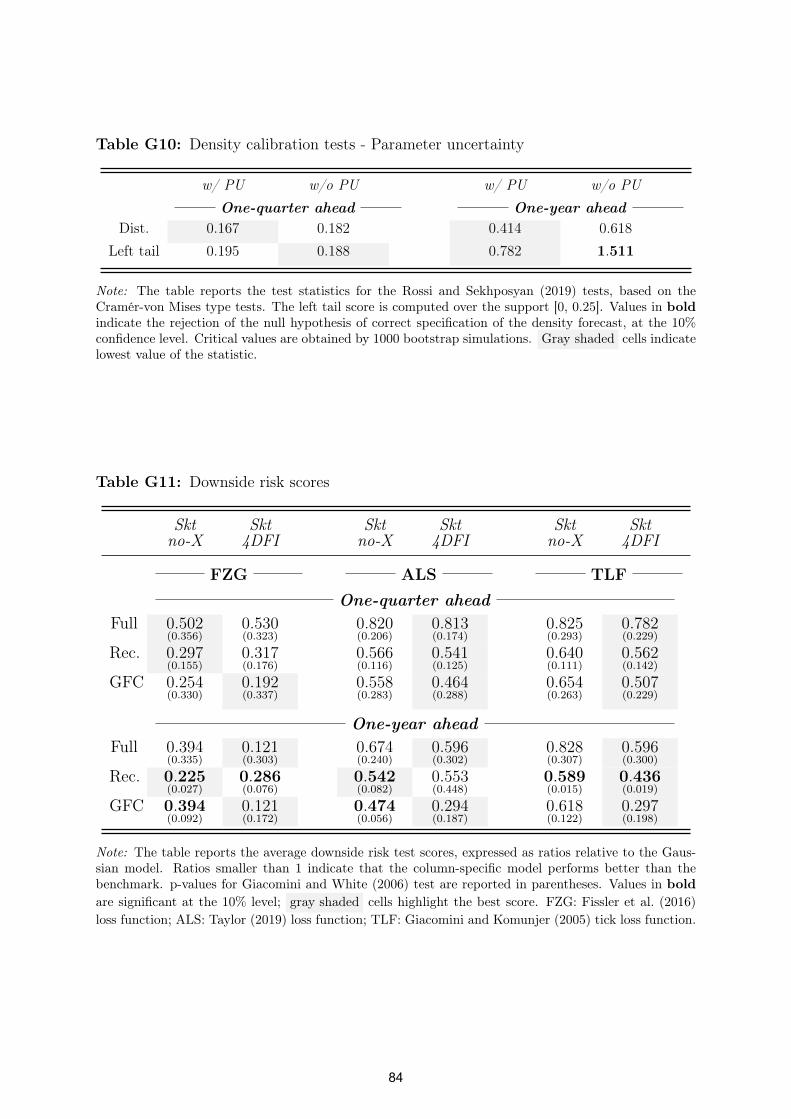
Table G10: Density calibration tests - Parameter uncertainty

w/ PU w/o PU w/ PU w/o PUOne-quarter ahead One-year ahead

Dist. 0.167 0.182 0.414 0.618

Left tail 0.195 0.188 0.782 1.511

Note: The table reports the test statistics for the Rossi and Sekhposyan (2019) tests, based on theCramér-von Mises type tests. The left tail score is computed over the support [0, 0.25]. Values in boldindicate the rejection of the null hypothesis of correct specification of the density forecast, at the 10%confidence level. Critical values are obtained by 1000 bootstrap simulations. Gray shaded cells indicatelowest value of the statistic.

Table G11: Downside risk scores

Skt Skt Skt Skt Skt Sktno-X 4DFI no-X 4DFI no-X 4DFI

FZG ALS TLF

One-quarter aheadFull 0.502

(0.356)0.530(0.323)

0.820(0.206)

0.813(0.174)

0.825(0.293)

0.782(0.229)

Rec. 0.297(0.155)

0.317(0.176)

0.566(0.116)

0.541(0.125)

0.640(0.111)

0.562(0.142)

GFC 0.254(0.330)

0.192(0.337)

0.558(0.283)

0.464(0.288)

0.654(0.263)

0.507(0.229)

One-year aheadFull 0.394

(0.335)0.121(0.303)

0.674(0.240)

0.596(0.302)

0.828(0.307)

0.596(0.300)

Rec. 0.225(0.027)

0.286(0.076)

0.542(0.082)

0.553(0.448)

0.589(0.015)

0.436(0.019)

GFC 0.394(0.092)

0.121(0.172)

0.474(0.056)

0.294(0.187)

0.618(0.122)

0.297(0.198)

Note: The table reports the average downside risk test scores, expressed as ratios relative to the Gaus-sian model. Ratios smaller than 1 indicate that the column-specific model performs better than thebenchmark. p-values for Giacomini and White (2006) test are reported in parentheses. Values in boldare significant at the 10% level; gray shaded cells highlight the best score. FZG: Fissler et al. (2016)loss function; ALS: Taylor (2019) loss function; TLF: Giacomini and Komunjer (2005) tick loss function.

84

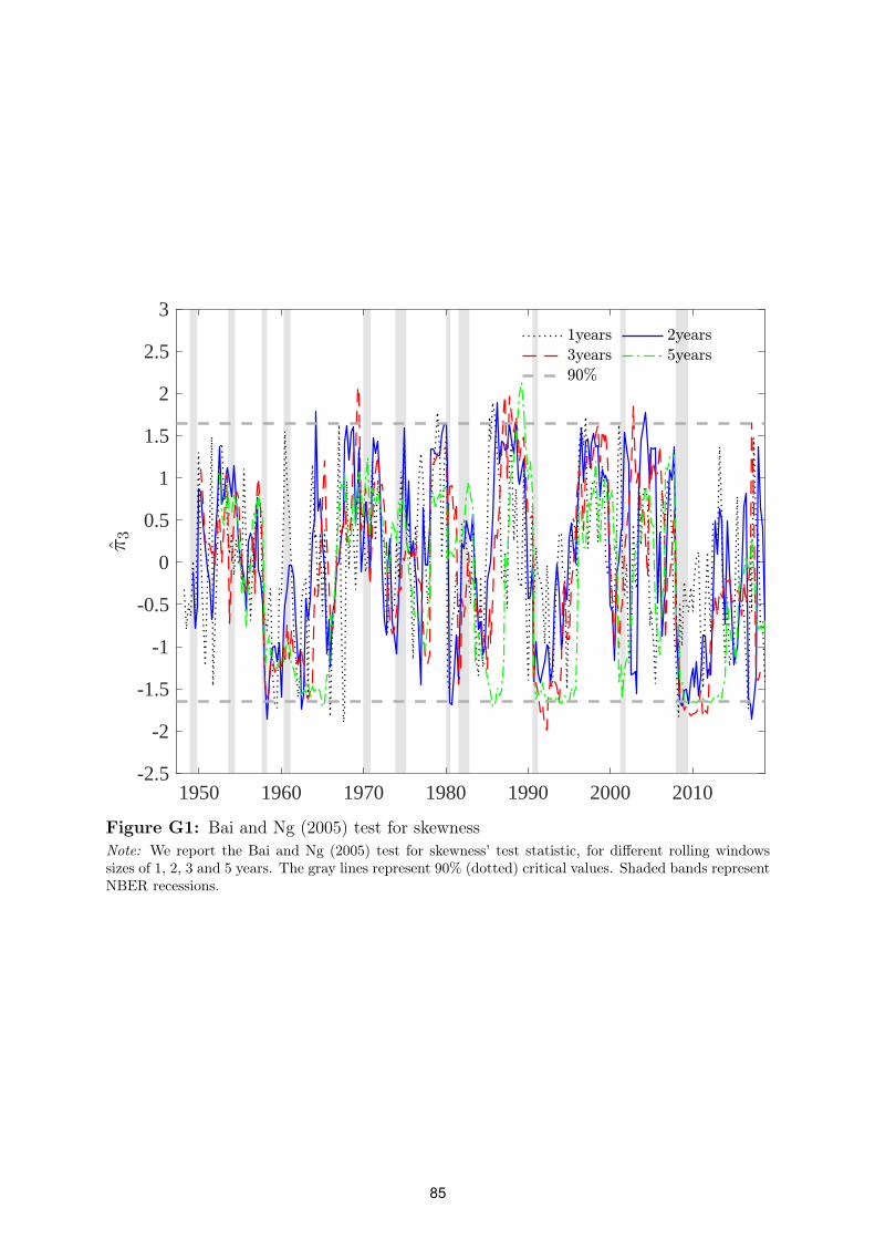
1950 1960 1970 1980 1990 2000 2010-2.5

-2

-1.5

-1

-0.5

0

0.5

1

1.5

2

2.5

3

Figure G1: Bai and Ng (2005) test for skewnessNote: We report the Bai and Ng (2005) test for skewness’ test statistic, for different rolling windowssizes of 1, 2, 3 and 5 years. The gray lines represent 90% (dotted) critical values. Shaded bands representNBER recessions.

85

Skt Skt -NFCI Skt -4DFI

1975 1980 1985 1990 1995 2000 2005 2010 20152.5

2.6

2.7

2.8

2.9

3

3.1

3.2

3.3

3.4

1975 1980 1985 1990 1995 2000 2005 2010 20152.4

2.5

2.6

2.7

2.8

2.9

3

3.1

3.2

3.3

1975 1980 1985 1990 1995 2000 2005 2010 20152.4

2.5

2.6

2.7

2.8

2.9

3

3.1

3.2

3.3

1975 1980 1985 1990 1995 2000 2005 2010 20151

1.5

2

2.5

3

3.5

4

4.5

5

1975 1980 1985 1990 1995 2000 2005 2010 20151

1.5

2

2.5

3

3.5

4

4.5

5

5.5

1975 1980 1985 1990 1995 2000 2005 2010 20151

2

3

4

5

6

7

1975 1980 1985 1990 1995 2000 2005 2010 2015-0.4

-0.3

-0.2

-0.1

0

0.1

0.2

0.3

0.4

0.5

1975 1980 1985 1990 1995 2000 2005 2010 2015-0.6

-0.4

-0.2

0

0.2

0.4

0.6

0.8

1975 1980 1985 1990 1995 2000 2005 2010 2015-0.8

-0.6

-0.4

-0.2

0

0.2

0.4

0.6

0.8

1

Figure G2: Time-varying parametersNote: The plots illustrate the estimated time-varying parameters (black) for the three model specifica-tions. Long-run components are reported in red (right scale). Shaded bands represent NBER recessions.

86

Skt Skt -NFCI Skt -4DFI

1975 1980 1985 1990 1995 2000 2005 2010 20152.2

2.4

2.6

2.8

3

3.2

3.4

1975 1980 1985 1990 1995 2000 2005 2010 20152

2.2

2.4

2.6

2.8

3

3.2

3.4

1975 1980 1985 1990 1995 2000 2005 2010 20150.5

1

1.5

2

2.5

3

3.5

4

4.5

5

1975 1980 1985 1990 1995 2000 2005 2010 20151

1.5

2

2.5

3

3.5

4

4.5

5

1975 1980 1985 1990 1995 2000 2005 2010 20151

1.5

2

2.5

3

3.5

4

4.5

5

5.5

1975 1980 1985 1990 1995 2000 2005 2010 20150

1

2

3

4

5

6

7

1975 1980 1985 1990 1995 2000 2005 2010 2015-0.4

-0.3

-0.2

-0.1

0

0.1

0.2

0.3

0.4

0.5

1975 1980 1985 1990 1995 2000 2005 2010 2015-0.6

-0.4

-0.2

0

0.2

0.4

0.6

0.8

1975 1980 1985 1990 1995 2000 2005 2010 2015-1

-0.8

-0.6

-0.4

-0.2

0

0.2

0.4

0.6

0.8

1

Figure G3: Time-varying parametersNote: The plots compare the in sample (solid gray) and out of sample (dotted black) parameters. Long-run components are reported in scales of red (right scale). Shaded bands represent NBER recessions.

Full sample

0 2 4 6

GFC

0 2 4 6 8

Credit Risk Leverage Nonfinancial Leverage

Figure G4: Top 10 predictors for µtNote: The bar plots report the top 10 predictors for the location parameter. The x-axis reports averageposterior probability of inclusion, expressed in percentage terms.

87

CBCARCITAMMF

STKGRRRESTARTACCG

MINCREIT

INSCBILL

RTERMHH

HOUSSPREADCILARGE

TEDHY

SMALLMCAP

CTERMLIBID

CTABSITA

CONTAD10

CARSPREADSPR210

NCLTABS

SPR23MSBDUSD

DCLOSECWILL

DURSPREADCISMALL

W500ABSSPREAD

NFCDBC

PENSVOL1

BONDGRREPOMORT

SWAP2FAILSA

FAILSMBSCMBSICMBSREPO

FCORPFC

CCDQCRG

STLOCMDQ

DOTHOINTBDGCTFMG

CRESWAP3M

CPHLHY

FGSPCISMALL

MLIQ10REPOGR

VOL3CBPER

CGSPCILARGE

ABSIVIX

TERMREPOA

A2P2LPH

MBONDABCP

DCOMMGSE

MSWAPBAA

MBONDGRLIG

CTMBSGVLFINSDHE

SWAP10FAILS

FAILSCMBSI

CCINCCOMMODLIQ

NACMMJINCCPR

EQUITYLIQDNET

RATELIQOEQ

012345678C

redit

Ris

kL

everage

Nonfin

ancia

l L

everage

Figure

G5:

Predictors-Lo

cation

88

CPHSPR210

CARSPREADREIT

LIBIDDURSPREAD

SPR23MMBOND

FCORPCWILL

BONDGRPENS

FAILSTABS

HOUSSPREADD10

STLOCCONTA

SBDCBPER

REPOGRCG

DOTHCTERM

RTAREPO

CILARGEHH

TERMCBCAR

USDSWAP3M

BAAFC

CMBSIW500

INSMMFLPH

MLIQ10MCAP

CCGCITA

REPOMORTOINTCTF

MBONDGRCCDQ

STKGRSMALL

NCLA2P2MDQMBSI

FAILSMBSRTERM

FGBDG

CISMALLCTABSFAILSCCTMBS

STAABSSPREAD

DCOMMHY

FINSSWAP2

VOL1SPCILARGE

ABCPMSWAP

GSEABSITED

FAILSAMG

CBILLDCLOSE

GVLDHE

COMMODLIQMINCCMBS

RRENFCITA

SWAP10SPCISMALL

OEQCRG

REPOAJINCCRECPR

NACMMVOL3

VIXCCINCDNET

LIGDBC

EQUITYLIQRATELIQ

LHY

02468

10

12

Cred

itR

isk

Lev

erag

eN

on

fin

an

cia

l L

ev

erag

e

Figure

G6:

Predictors-Scale

89

STKGRHH

W500BDG

PENSMGINSD10

SPR23MSTA

FCHY

CBCARSMALL

REPOGRCITA

CMBSISBD

CBPERCWILL

REPOUSDCPH

BONDGRCISMALL

CRECTMBS

CCGCILARGE

SPR210SPCILARGE

MCAPCARSPREAD

FGREPOMORT

ITAFCORPSTLOC

GSETABSMINC

CGLPH

SWAP10TERM

CRGSPCISMALL

VOL1CBILL

NCLCTF

FINSOEQ

CONTARRE

FAILSAABCPFAILS

DCOMMMMF

MLIQ10CTERMSWAP2REPOA

MDQCTABS

SWAP3MA2P2

MSWAPVIX

RTERMDURSPREAD

DHEOINT

ABSSPREADBAA

HOUSSPREADFAILSC

LIBIDGVL

DOTHTED

CMBSDCLOSE

CCDQRTA

REITABSIDBC

MBSIVOL3

FAILSMBSMBOND

CCINCLHYJINC

NACMMNFC

MBONDGRDNET

EQUITYLIQCPRLIG

COMMODLIQRATELIQ

02468

10

12

14

16

18

20

Cred

itR

isk

Lev

erag

eN

on

fin

an

cia

l L

ev

erag

e

Figure

G7:

Predictors-Asymmetry

90

References

Adrian, T., N. Boyarchenko, and D. Giannone (2019): “Vulnerable Growth,”

American Economic Review, 109, 1263–89.

Adrian, T. and H. S. Shin (2010): “Liquidity and leverage,” Journal of Financial

Intermediation, 19, 418–437.

Azzalini, A. and A. Capitanio (2003): “Distributions generated by perturbation of

symmetry with emphasis on a multivariate skew t-distribution,” Journal of the Royal

Statistical Society: Series B (Statistical Methodology), 65, 367–389.

Bekaert, G. and M. Hoerova (2014): “The VIX, the variance premium and stock

market volatility,” Journal of Econometrics, 183, 181–192.

Blasques, F., S. J. Koopman, and A. Lucas (2014): “Stationarity and ergodicity of

univariate generalized autoregressive score processes,” Electronic Journal of Statistics,

8, 1088–1112.

Bollerslev, T. (1990): “Modelling the coherence in short-run nominal exchange rates:

a multivariate generalized ARCH model,” The Review of Economics and Statistics,

498–505.

Brave, S. and R. A. Butters (2012): “Diagnosing the Financial System: Financial

Conditions and Financial Stress,” International Journal of Central Banking, 8, 191–

239.

Brave, S. A. and R. Butters (2011): “Monitoring financial stability: A financial

conditions index approach,” Economic Perspectives, 35, 22.

Calvori, F., D. Creal, S. J. Koopman, and A. Lucas (2017): “Testing for param-

eter instability across different modeling frameworks,” Journal of Financial Economet-

rics, 15, 223–246.

Carvalho, C. M., N. G. Polson, and J. G. Scott (2010): “The horseshoe estimator

for sparse signals,” Biometrika, 97, 465–480.

91

Cogley, T. and T. J. Sargent (2005): “Drifts and volatilities: monetary policies and

outcomes in the post WWII US,” Review of Economic Dynamics, 8, 262–302.

Cowles, M. K. and B. P. Carlin (1996): “Markov Chain Monte Carlo Convergence

Diagnostics: A Comparative Review,” Journal of the American Statistical Association,

91, 883–904.

Creal, D., S. J. Koopman, and A. Lucas (2013): “Generalized autoregressive score

models with applications,” Journal of Applied Econometrics, 28, 777–795.

Croushore, D. (2006): “Forecasting with real-time macroeconomic data,” Handbook of

Economic Forecasting, 1, 961–982.

——— (2011): “Frontiers of real-time data analysis,” Journal of Economic Literature, 49,

72–100.

Croushore, D. and T. Stark (2001): “A real-time data set for macroeconomists,”

Journal of Econometrics, 105, 111–130.

Doan, T., R. Litterman, and C. Sims (1984): “Forecasting and conditional projection

using realistic prior distributions,” Econometric Reviews, 3, 1–100.

Drehmann, M., C. E. Borio, L. Gambacorta, G. Jimenez, and C. Trucharte

(2010): “Countercyclical capital buffers: exploring options,” Working Paper 317, Bank

for International Settlement.

Escanciano, J. C. and I. N. Lobato (2009): “An automatic portmanteau test for

serial correlation,” Journal of Econometrics, 151, 140–149.

Gelman, A., G. O. Roberts, W. R. Gilks, et al. (1996): “Efficient Metropolis

jumping rules,” Bayesian Statistics, 5, 42.

Gómez, H. W., F. J. Torres, and H. Bolfarine (2007): “Large-sample inference for

the epsilon-skew-t distribution,” Communications in Statistics—Theory and Methods,

36, 73–81.

Haario, H., E. Saksman, and J. Tamminen (1999): “Adaptive proposal distribution

for random walk Metropolis algorithm,” Computational Statistics, 14, 375–396.

92

Harvey, A. and M. Streibel (1998): “Testing for a slowly changing level with special

reference to stochastic volatility,” Journal of Econometrics, 87, 167–189.

Harvey, A. and S. Thiele (2016): “Testing against changing correlation,” Journal of

Empirical Finance, 38, 575–589.

Harvey, A. C. (2013): Dynamic models for volatility and heavy tails: with applications

to financial and economic time series, vol. 52, Cambridge University Press.

Hasenzagl, T., L. Reichlin, and G. Ricco (2020): “Financial Variables as Predic-

tors of Real Growth Vulnerability,” Discussion Paper DP14322, CEPR.

Jensen, H., I. Petrella, S. H. Ravn, and E. Santoro (2020): “Leverage and

Deepening Business-Cycle Skewness,” American Economic Journal: Macroeconomics,

12, 245–81.

Jordà, Ò., M. Schularick, and A. M. Taylor (2013): “When credit bites back,”

Journal of Money, Credit and Banking, 45, 3–28.

——— (2017): “Macrofinancial history and the new business cycle facts,” NBER Macroe-

conomics Annual Report, 31, 213–263.

Juárez, M. A. and M. F. Steel (2010): “Model-based clustering of non-Gaussian

panel data based on skew-t distributions,” Journal of Business & Economic Statistics,

28, 52–66.

Krishnamurthy, A. and T. Muir (2017): “How credit cycles across a financial crisis,”

Working Paper 23850, National Bureau of Economic Research.

Makalic, E. and D. F. Schmidt (2015): “A simple sampler for the horseshoe estima-

tor,” IEEE Signal Processing Letters, 23, 179–182.

McConnell, M. M. and G. Perez-Quiros (2000): “Output fluctuations in the United

States: What has changed since the early 1980’s?” American Economic Review, 90,

1464–1476.

Mian, A. and A. Sufi (2010): “Household Leverage and the Recession of 2007–09,”

IMF Economic Review, 58, 74–117.

93

Nyblom, J. (1989): “Testing for the constancy of parameters over time,” Journal of the

American Statistical Association, 84, 223–230.

Plagborg-Møller, M., L. Reichlin, G. Ricco, and T. Hasenzagl (2020): “When

is Growth at Risk?” Conference draft, Brooking Paper on Economic Activity.

Ray, P. and A. Bhattacharya (2018): “Signal Adaptive Variable Selector for the

Horseshoe Prior,” arXiv preprint arXiv:1810.09004.

Sims, C. A. and T. Zha (1998): “Bayesian methods for dynamic multivariate models,”

International Economic Review, 949–968.

Spiegelhalter, D. J., N. G. Best, B. P. Carlin, and A. Van Der Linde (2002):

“Bayesian measures of model complexity and fit,” Journal of the Royal Statistical So-

ciety: Series B (Statistical Methodology), 64, 583–639.

Stark, T. and D. Croushore (2002): “Forecasting with a real-time data set for

macroeconomists,” Journal of Macroeconomics, 24, 507–531.

Stock, J. H. and M. W. Watson (2002): “Has the business cycle changed and why?”

NBER Macroeconomics Annual Report, 17, 159–218.

Zou, H. (2006): “The adaptive lasso and its oracle properties,” Journal of the American

Statistical Association, 101, 1418–1429.

94

(*) Requests for copies should be sent to: Banca d’Italia – Servizio Studi di struttura economica e finanziaria – Divisione Biblioteca e Archivio storico – Via Nazionale, 91 – 00184 Rome – (fax 0039 06 47922059). They are available on the Internet www.bancaditalia.it.

RECENTLY PUBLISHED “TEMI” (*)

N. 1314 – Working horizon and labour supply: the effect of raising the full retirement age on middle-aged individuals, by Francesca Carta and Marta De Philippis (February 2021).

N. 1315 – Bank credit and market-based finance for corporations: the effects of minibond issuances, by Steven Ongena, Sara Pinoli, Paola Rossi and Alessandro Scopelliti (February 2021).

N. 1316 – Is inflation targeting a strategy past its sell-by date?, by Alberto Locarno and Alessandra Locarno (February 2021).

N. 1317 – Declining natural interest rate in the US: the pension system matters, by Jacopo Bonchi and Giacomo Caracciolo (February 2021).

N. 1318 – Can we measure inflation expectations using Twitter?, by Cristina Angelico, Juri Marcucci, Marcello Miccoli and Filippo Quarta (February 2021).

N. 1319 – Identifying deposits’ outflows in real-time, by Edoardo Rainone (February 2021).

N. 1320 – Whatever it takes to save the planet? Central banks and unconventional green policy, by Alessandro Ferrari and Valerio Nispi Landi (February 2021).

N. 1307 – On the design of grant assignment rules, by Francesca Modena, Santiago Pereda Fernandez and Giulia Martina Tanzi (December 2020).

N. 1308 – Monetary policy strategies in the New Normal: a model-based analysis for the euro area, by Fabio Busetti, Stefano Neri, Alessandro Notarpietro and Massimiliano Pisani (December 2020).

N. 1309 – Rare disasters, the natural interest rate and monetary policy, by Alessandro Cantelmo (December 2020).

N. 1310 – The market stabilization role of central bank asset purchases: high-frequency evidence from the COVID-19 crisis, by Marco Bernardini and Annalisa De Nicola (December 2020).

N. 1311 – Equity tail risk in the treasury bond market, by Dario Ruzzi and Mirco Rubin (December 2020).

N. 1312 – Scars of youth non-employment and labour market conditions, by Giulia Martina Tanzi (December 2020).

N. 1313 – The COVID-19 shock and a fiscal-monetary policy mix in a monetary union, by Anna Bartocci, Alessandro Notarpietro and Massimiliano Pisani (December 2020).

N. 1301 – A quantitative analysis of distortions in managerial forecasts, by Yueran Ma, Tiziano Ropele, David Sraer and David Thesmar (November 2020).

N. 1302 – Bargaining power and the Phillips curve: a micro-macro analysis, by Marco J. Lombardi, Marianna Riggi and Eliana Viviano (November 2020).

N. 1303 – The effects of structural reforms: Evidence from Italy, by Emanuela Ciapanna, Sauro Mocetti and Alessandro Notarpietro (November 2020).

N. 1304 – Consumption and Wealth: New Evidence from Italy, by Riccardo De Bonis, Danilo Liberati, John Muellbauer and Concetta Rondinelli (November 2020).

N. 1305 – Do details matter? An analysis of the Italian personal income tax, by Martino Tasso (November 2020).

N. 1306 – Effects of eligibility for central bank purchases on corporate bond spreads, by Taneli Mäkinen, Fan Li, Andrea Mercatanti and Andrea Silvestrini (November 2020).

"TEMI" LATER PUBLISHED ELSEWHERE

2019

ALBANESE G., M. CIOFFI and P. TOMMASINO, Legislators' behaviour and electoral rules: evidence from an Italian reform, European Journal of Political Economy, v. 59, pp. 423-444, WP 1135 (September 2017).

APRIGLIANO V., G. ARDIZZI and L. MONTEFORTE, Using the payment system data to forecast the economic activity, International Journal of Central Banking, v. 15, 4, pp. 55-80, WP 1098 (February 2017).

ARNAUDO D., G. MICUCCI, M. RIGON and P. ROSSI, Should I stay or should I go? Firms’ mobility across banks in the aftermath of the financial crisis, Italian Economic Journal / Rivista italiana degli economisti, v. 5, 1, pp. 17-37, WP 1086 (October 2016).

BASSO G., F. D’AMURI and G. PERI, Immigrants, labor market dynamics and adjustment to shocks in the euro area, IMF Economic Review, v. 67, 3, pp. 528-572, WP 1195 (November 2018).

BATINI N., G. MELINA and S. VILLA, Fiscal buffers, private debt, and recession: the good, the bad and the ugly, Journal of Macroeconomics, v. 62, WP 1186 (July 2018).

BURLON L., A. NOTARPIETRO and M. PISANI, Macroeconomic effects of an open-ended asset purchase programme, Journal of Policy Modeling, v. 41, 6, pp. 1144-1159, WP 1185 (July 2018).

BUSETTI F. and M. CAIVANO, Low frequency drivers of the real interest rate: empirical evidence for advanced economies, International Finance, v. 22, 2, pp. 171-185, WP 1132 (September 2017).

CAPPELLETTI G., G. GUAZZAROTTI and P. TOMMASINO, Tax deferral and mutual fund inflows: evidence from a quasi-natural experiment, Fiscal Studies, v. 40, 2, pp. 211-237, WP 938 (November 2013).

CARDANI R., A. PACCAGNINI and S. VILLA, Forecasting with instabilities: an application to DSGE models with financial frictions, Journal of Macroeconomics, v. 61, WP 1234 (September 2019).

CHIADES P., L. GRECO, V. MENGOTTO, L. MORETTI and P. VALBONESI, Fiscal consolidation by intergovernmental transfers cuts? The unpleasant effect on expenditure arrears, Economic Modelling, v. 77, pp. 266-275, WP 1076 (July 2016).

CIANI E., F. DAVID and G. DE BLASIO, Local responses to labor demand shocks: a re-assessment of the case of Italy, Regional Science and Urban Economics, v. 75, pp. 1-21, WP 1112 (April 2017).

CIANI E. and P. FISHER, Dif-in-dif estimators of multiplicative treatment effects, Journal of Econometric Methods, v. 8. 1, pp. 1-10, WP 985 (November 2014).

CIAPANNA E. and M. TABOGA, Bayesian analysis of coefficient instability in dynamic regressions, Econometrics, MDPI, Open Access Journal, v. 7, 3, pp.1-32, WP 836 (November 2011).

COLETTA M., R. DE BONIS and S. PIERMATTEI, Household debt in OECD countries: the role of supply-side and demand-side factors, Social Indicators Research, v. 143, 3, pp. 1185–1217, WP 989 (November 2014).

COVA P., P. PAGANO and M. PISANI, Domestic and international effects of the Eurosystem Expanded Asset Purchase Programme, IMF Economic Review, v. 67, 2, pp. 315-348, WP 1036 (October 2015).

ERCOLANI V. and J. VALLE E AZEVEDO, How can the government spending multiplier be small at the zero lower bound?, Macroeconomic Dynamics, v. 23, 8. pp. 3457-2482, WP 1174 (April 2018).

FERRERO G., M. GROSS and S. NERI, On secular stagnation and low interest rates: demography matters, International Finance, v. 22, 3, pp. 262-278, WP 1137 (September 2017).

FOA G., L. GAMBACORTA, L. GUISO and P. E. MISTRULLI, The supply side of household finance, Review of Financial Studies, v.32, 10, pp. 3762-3798, WP 1044 (November 2015).

GERALI A. and S. NERI, Natural rates across the Atlantic, Journal of Macroeconomics, v. 62, article 103019, WP 1140 (September 2017).

GIORDANO C., M. MARINUCCI and A. SILVESTRINI, The macro determinants of firms' and households' investment: evidence from Italy, Economic Modelling, v. 78, pp. 118-133, WP 1167 (March 2018).

GOMELLINI M., D. PELLEGRINO and F. GIFFONI, Human capital and urban growth in Italy,1981-2001, Review of Urban & Regional Development Studies, v. 31, 2, pp. 77-101, WP 1127 (July 2017).

LIBERATI D. and M. LOBERTO, Taxation and housing markets with search frictions, Journal of Housing Economics, v. 46, article 101632, WP 1105 (March 2017).

MAGRI S., Are lenders using risk-based pricing in the Italian consumer loan market? The effect of the 2008 crisis, Journal of Credit Risk, v. 15, 1, pp. 27-65, WP 1164 (January 2018).

MERCATANTI A., T. MAKINEN and A. SILVESTRINI, The role of financial factors for european corporate investment, Journal of International Money and Finance, v. 96, pp. 246-258, WP 1148 (October 2017).

"TEMI" LATER PUBLISHED ELSEWHERE

MIGLIETTA A., C. PICILLO and M. PIETRUNTI, The impact of margin policies on the Italian repo market, The North American Journal of Economics and Finance, v. 50, WP 1028 (October 2015).

MONTEFORTE L. and V. RAPONI, Short-term forecasts of economic activity: are fortnightly factors useful?, Journal of Forecasting, v. 38, 3, pp. 207-221, WP 1177 (June 2018).

NERI S. and A. NOTARPIETRO, Collateral constraints, the zero lower bound, and the debt–deflation mechanism, Economics Letters, v. 174, pp. 144-148, WP 1040 (November 2015).

PANCRAZI R. and M. PIETRUNTI, Natural expectations and home equity extraction, Journal of Housing Economics, v. 46, 4, WP 984 (November 2014).

PEREDA FERNANDEZ S., Teachers and cheaters. Just an anagram?, Journal of Human Capital, v. 13, 4, pp. 635-669, WP 1047 (January 2016).

RIGGI M., Capital destruction, jobless recoveries, and the discipline device role of unemployment, Macroeconomic Dynamics, v. 23, 2, pp. 590-624, WP 871 (July 2012).

2020

ALESSANDRI P. and M. BOTTERO, Bank lending in uncertain times, R European Economic Review, V. 128, WP 1109 (April 2017).

ANTUNES A. and V. ERCOLANI, Public debt expansions and the dynamics of the household borrowing constraint, Review of Economic Dynamics, v. 37, pp. 1-32, WP 1268 (March 2020).

ARDUINI T., E. PATACCHINI and E. RAINONE, Treatment effects with heterogeneous externalities, Journal of Business & Economic Statistics, , v. 38, 4, pp. 826-838, WP 974 (October 2014).

BOTTERO M., F. MEZZANOTTI and S. LENZU, Sovereign debt exposure and the Bank Lending Channel: impact on credit supply and the real economy, Journal of International Economics, v. 126, article 103328, WP 1032 (October 2015).

BRIPI F., D. LOSCHIAVO and D. REVELLI, Services trade and credit frictions: evidence with matched bank – firm data, The World Economy, v. 43, 5, pp. 1216-1252, WP 1110 (April 2017).

BRONZINI R., G. CARAMELLINO and S. MAGRI, Venture capitalists at work: a Diff-in-Diff approach at late-stages of the screening process, Journal of Business Venturing, v. 35, 3, WP 1131 (September 2017).

BRONZINI R., S. MOCETTI and M. MONGARDINI, The economic effects of big events: evidence from the Great Jubilee 2000 in Rome, Journal of Regional Science, v. 60, 4, pp. 801-822, WP 1208 (February 2019).

COIBION O., Y. GORODNICHENKO and T. ROPELE, Inflation expectations and firms' decisions: new causal evidence, Quarterly Journal of Economics, v. 135, 1, pp. 165-219, WP 1219 (April 2019).

CORSELLO F. and V. NISPI LANDI, Labor market and financial shocks: a time-varying analysis, Journal of Money, Credit and Banking, v. 52, 4, pp. 777-801, WP 1179 (June 2018).

COVA P. and F. NATOLI, The risk-taking channel of international financial flows, Journal of International Money and Finance, v. 102, WP 1152 (December 2017).

D’ALESSIO G., Measurement errors in survey data and the estimation of poverty and inequality indices, Statistica Applicata - Italian Journal of Applied Statistics, v. 32, 3, WP 1116 (June 2017).

DEL PRETE S. and S. FEDERICO, Do links between banks matter for bilateral trade? Evidence from financial crises, Review of World Economic, v. 156, 4, pp. 859 - 885, WP 1217 (April 2019).

D’IGNAZIO A. and C. MENON, The causal effect of credit Guarantees for SMEs: evidence from Italy, The Scandinavian Journal of Economics, v. 122, 1, pp. 191-218, WP 900 (February 2013).

ERCOLANI V. and F. NATOLI, Forecasting US recessions: the role of economic uncertainty, Economics Letters, v. 193, WP 1299 (October 2020).

MAKINEN T., L. SARNO and G. ZINNA, Risky bank guarantees, Journal of Financial Economics, v. 136, 2, pp. 490-522, WP 1232 (July 2019).

MODENA F., E. RETTORE and G. M. TANZI, The effect of grants on university dropout rates: evidence from the Italian case, Journal of Human Capital, v. 14, 3, pp. 343-370, WP 1193 (September 2018).

NISPI LANDI V., Capital controls spillovers, Journal of International Money and Finance, v. 109, WP 1184 (July 2018).

PERICOLI M., On risk factors of the stock–bond correlation, International Finance, v. 23, 3, pp. 392-416, WP 1198 (November 2018).

"TEMI" LATER PUBLISHED ELSEWHERE

RAINONE E., The network nature of OTC interest rates, Journal of Financial Markets, v.47, article 100525, WP 1022 (July 2015).

RAINONE E. and F. VACIRCA, Estimating the money market microstructure with negative and zero interest rates, Quantitative Finance, v. 20, 2, pp. 207-234, WP 1059 (March 2016).

RIZZICA L., Raising aspirations and higher education. Evidence from the UK's widening participation policy, Journal of Labor Economics, v. 38, 1, pp. 183-214, WP 1188 (September 2018).

SANTIONI, R., F. SCHIANTARELLI and P. STRAHAN, Internal capital markets in times of crisis: the benefit of group affiliation, Review of Finance, v. 24, 4, pp. 773-811, WP 1146 (October 2017).

SCHIANTARELLI F., M. STACCHINI and P. STRAHAN, Bank Quality, judicial efficiency and loan repayment delays in Italy, Journal of Finance , v. 75, 4, pp. 2139-2178, WP 1072 (July 2016).

FORTHCOMING

ACCETTURO A., A. LAMORGESE, S. MOCETTI and D. PELLEGRINO, Housing Price elasticity and growth: evidence from Italian cities, Journal of Economic Geography, WP 1267 (March 2020).

ALBANESE G., E. CIANI and G. DE BLASIO, Anything new in town? The local effects of urban regeneration policies in Italy, Regional Science and Urban Economics, WP 1214 (April 2019).

ALBANESE G., G. DE BLASIO and A. LOCATELLI, Does EU regional policy promote local TFP growth? Evidence from the Italian Mezzogiorno, Papers in Regional Science, WP 1253 (December 2019).

ANZUINI A. and L. ROSSI, Fiscal policy in the US: a new measure of uncertainty and its effects on the American economy, Empirical Economics, WP 1197 (November 2018).

BOLOGNA P., A. MIGLIETTA and A. SEGURA, Contagion in the CoCos market? A case study of two stress events, International Journal of Central Banking, WP 1201 (November 2018).

COVA P., P. PAGANO, A. NOTARPIETRO and M. PISANI, Secular stagnation, R&D, public investment and monetary policy: a global-model perspective, Macroeconomic Dynamics, WP 1156 (December 2017).

DE PHILIPPIS M., Multitask agents and incentives: the case of teaching and research for university professors, Economic Journal, WP 1156 (December 2015).

DEL PRETE S. and M. L. STEFANI, Women as "Gold Dust": gender diversity in top boards and the performance of Italian banks, Economic Notes, Monte dei Paschi di Siena, WP 1014 (June 2015).

FIDORA M., C. GIORDANO and M. SCHMITZ, Real exchange rate misalignments in the Euro Area, Open Economies Review, WP 1042 (January 2018).

HERTWECK M., V. LEWIS and S. VILLA, Going the extra mile: effort by workers and job-seekers, Journal of Money, Credit and Banking, WP 1277 (June 2020).

LI F., A. MERCATANTI, T. MAKINEN and A. SILVESTRINI, A regression discontinuity design for ordinal running variables: evaluating central bank purchases of corporate bonds, Annals of Applied Statistics, WP 1213 (March 2019).

LOSCHIAVO D., Household debt and income inequality: evidence from Italian survey data, Review of Income and Wealth, WP 1095 (January 2017).

METELLI L. and F. NATOLI, The international transmission of US tax shocks: a proxy-SVAR approach, IMF Economic Review, WP 1223 (June 2019).

MOCETTI S., G. ROMA and E. RUBOLINO, Knocking on parents’ doors: regulation and intergenerational mobility, Journal of Human Resources, WP 1182 (July 2018).

NISPI LANDI V. and A. SCHIAVONE, The effectiveness of capital controls, Open Economies Review, WP 1200 (November 2018).

PEREDA FERNANDEZ S., Copula-based random effects models for clustered data, Journal of Business & Economic Statistics, WP 1092 (January 2017).

PERICOLI M. and M. TABOGA, Nearly exact Bayesian estimation of non-linear no-arbitrage term-structure models, Journal of Financial Econometrics, WP 1189 (September 2018).