
Technical Supplement - California Climate Risk and Response
151
Technical Supplement California Climate Risk and Response Fredrich Kahrl and David Roland-Holst November, 2008 Research Paper No. 08102801 DEPARTMENT OF AGRICULTURAL AND RESOURCE ECONOMICS 207 GIANNINI HALL UNIVERSITY OF CALIFORNIA BERKELEY, CA 94720 PHONE: (1) 510-643-6362 FAX: (1) 510-642-1099 http://are.berkeley.edu/~dwrh/CERES_Web/index.html
-
Upload
khangminh22 -
Category
Documents
-
view
0 -
download
0
Transcript of Technical Supplement - California Climate Risk and Response
11/13/08 Page 1
Technical Supplement
California Climate
Risk and Response
Fredrich Kahrl and David Roland-Holst
November, 2008
Research Paper No. 08102801
DEPARTMENT OF AGRICULTURAL AND RESOURCE ECONOMICS
207 GIANNINI HALL
UNIVERSITY OF CALIFORNIA
BERKELEY, CA 94720
PHONE: (1) 510-643-6362
FAX: (1) 510-642-1099
http://are.berkeley.edu/~dwrh/CERES_Web/index.html

11/13/08 Page 2
Contents
1. WATER: BACKGROUND ............................................................................................................................................ 4
WATER INFRASTRUCTURE .................................................................................................................................4 PHYSICAL IMPACTS OF CLIMATE CHANGE..........................................................................................................6 AGRICULTURAL WATER USE..............................................................................................................................9 URBAN WATER USE ........................................................................................................................................13 ADAPTATION OPTIONS.....................................................................................................................................15 FINANCING WATER PROVISION ........................................................................................................................26 AGRICULTURE..................................................................................................................................................32 THE STATE WATER PROJECT ..........................................................................................................................37 ENVIRONMENTAL/RECREATIONAL ....................................................................................................................38
2. ENERGY: BACKGROUND........................................................................................................................................ 40
3. DEMOGRAPHICS: BACKGROUND......................................................................................................................... 58
ENERGY ..........................................................................................................................................................58 AIR QUALITY AND PUBLIC HEALTH ...................................................................................................................60 WATER ............................................................................................................................................................61 LAND AVAILABILITY ..........................................................................................................................................62 NOTES AND REFERENCES ...............................................................................................................................64
4. TRANSPORTATION: BACKGROUND..................................................................................................................... 65
STATE OF CALIFORNIA’S CURRENT TRANSPORTATION INFRASTRUCTURE........................................................67 CLIMATE CHANGE IMPACTS ON TRANSPORTATION...........................................................................................70 SURFACE TRANSPORTATION ...........................................................................................................................71 AVIATION .........................................................................................................................................................75 RAILROADS......................................................................................................................................................78 PORTS AND MARINE TRANSPORTATION ...........................................................................................................79 PIPELINES........................................................................................................................................................81 FINANCING TRANSPORTATION INFRASTRUCTURE.............................................................................................81
5. TOURISM AND RECREATION: BACKGROUND ................................................................................................... 86
NOTES AND REFERENCES ...............................................................................................................................93
6. REAL ESTATE: BACKGROUND.............................................................................................................................. 94
WILDFIRE IMPACTS ..........................................................................................................................................94 WILDFIRES: ADAPTATION.................................................................................................................................99 FLOODING AND STORM IMPACTS ...................................................................................................................100 COASTAL FLOODING: ADAPTATION ................................................................................................................102 NOTES AND REFERENCES .............................................................................................................................103
7. INSURANCE: BACKGROUND ...............................................................................................................................104
CLIMATE CHANGE IMPACTS ...........................................................................................................................104 ADAPTATION FOR THE INSURANCE INDUSTRY ................................................................................................106 NOTES AND REFERENCES .............................................................................................................................109
8. AGRICULTURE: BACKGROUND .......................................................................................................................... 110
GRADUAL CHANGES IN TEMPERATURE ..........................................................................................................111 EXTREME WEATHER CONDITIONS .................................................................................................................121 ADAPTATION..................................................................................................................................................122 NOTES AND REFERENCES .............................................................................................................................125
9. FORESTRY: BACKGROUND ................................................................................................................................. 126
PHYSICAL IMPACTS........................................................................................................................................126

11/13/08 Page 3
ECONOMIC IMPACTS ......................................................................................................................................129 ADAPTATION..................................................................................................................................................130 NOTES AND REFERENCES .............................................................................................................................131
10. FISHERIES: BACKGROUND................................................................................................................................ 132
CALIFORNIA’S FISHING INDUSTRY ..................................................................................................................132 CLIMATE CHANGE IMPACTS ON SQUID AND ADAPTATION OPTIONS................................................................135 CLIMATE CHANGE IMPACTS ON SALMON AND ADAPTATION OPTIONS.............................................................136 NOTES AND REFERENCES .............................................................................................................................137
11. PUBLIC HEALTH: BACKGROUND ..................................................................................................................... 138
CLIMATE CHANGE AND AIR POLLUTION..........................................................................................................138 HEALTH EFFECTS OF OZONE POLLUTION ......................................................................................................142 CLIMATE CHANGE AND EXTREME TEMPERATURES ........................................................................................145 CLIMATE CHANGE AND INCREASED WILDFIRE RATES ....................................................................................147 CLIMATE CHANGE AND INCREASED RISK OF VECTOR-BORNE ILLNESS ..........................................................149 CLIMATE CHANGE AND WATER CONTAMINATION ...........................................................................................149 ADAPTATION STRATEGIES .............................................................................................................................150

11/13/08 Page 4
California Climate Risk and Response Technical Supplement
Detailed Background Documentation
1. Water: Background
California’s water system will change as the result of the physical impacts of climate
change. The demand and supply of water in California are separated by a large
distance, posing a major problem for most water strategies. Even as climate change
adds pressure to California’s water supply, aging water infrastructure makes California’s
water reliability low and adaptations costly.
Population and economic growth in California are expected to be rapid and continuous,
which will put stress on the already outdated water infrastructure. California’s water
supply is concentrated in the north, but the majority of the demand, both agricultural and
urban, is concentrated in the south. The problem has always been to move water
cheaply and effectively from north to south.1 Compounded with global warming, water-
related issues worsen and critically affect the California economy. Left unchecked,
Californians could face enormous economic damages. Environmental, urban, and
agricultural demands will need to be reviewed and reassessed for the upcoming
changes in climate.
Water Infrastructure
Currently, California’s water infrastructure is a system of 1,200 reservoirs, canals,
treatment plants, and levees.2 The system’s tasks include water allocation to
agricultural, urban, and environmental demands, water quality management, and flood
control. The distribution of the 32 million acre-feet of developed water present in
California relies on this system to efficiently carry out its task.3 The age of California’s
infrastructure ranges from being old to ancient. Major water projects like State Water
Project (SWP) and Federal Central Valley Project (CVP) were built more than 30 years
and 50 years ago, respectively. Furthermore, the oldest facilities are more than 100
1 Howitt, Richard and Dave Sunding, Water Infrastructure and Water Allocation in California
(Berkeley: 2007) 181. 2 Department of Water Resources (DWR), California Water Plan Update (Sacramento: Department
of Water Resources, 2005), 3.14. 3 Howitt and Sunding, 2007.

11/13/08 Page 5
years old.4 California’s water system relies on smooth operations of its individual parts.
As one component of the network fails, the interdependent operations in turn decrease
in their capacity. The age of current infrastructure creates an environment where the
water supply is at high risk and vulnerability. The question remains: how did the system
come to be in such a poor state? The main problem is lack of funding needed to
maintain and rehabilitate these facilities as they age.
“Current infrastructure disrepair, outages, and failures and the degradation of local
water delivery systems are in part the result of years of underinvestment in preventive
maintenance, repair, and rehabilitation.”5
Without additional funding, key adjustments necessary to accommodate the needs of a
growing population and changing climate seem improbable. The California Water Plan
Update 2005 details the state’s maintenance backlog to be about $40 billion dollars.
Even without global warming, the failing infrastructure will result in unreliable, poor-
quality, and expensive water supplies for taxpayers.6 Consider water-operating costs
where the effect of only population growth increases the cost of operation by $413
million/year by the year 2050. With a warmer climate, an additional $384 million/year of
operating cost would be increased.7 Estimates from other studies such show numbers
that are of magnitudes greater.
The physical manifestations of operating costs include greater pumping and treatment
costs, as well as movement of water, to areas with higher-valued demands.
Furthermore, infrastructure improvement is fundamentally essential if any other
adaptations are to take place. If infrastructural and distribution capacity is already at its
limit, an increase in water supply is useless if it cannot be moved to where the water is
needed. In 2003, the Metropolitan Water District of Southern California acquired water
from growers of Sacramento but was unable to move it through the Delta because
conveyance was already operating at full capacity.8 This issue is one of the major
barriers facing many of the adaptations discussed in this paper. Thus, by improving
California’s infrastructure now, future water-operating costs can be avoided or lowered
and water supplies can be made more reliable.
The SWP and CVP are two government implemented water projects that are arcane in
nature and unsuited for the changing water use pattern. The approach of these two
programs involves the traditional supply augmentation method. It is built on the
assumption that demand for water is unchanging over time and perfectly inelastic.
4 DWR, 2005, 3.14.
5 DWR, 2005, 3.14.
6 DWR, 2005, 3.14.
7 Medellin et al., 2006,Josue, Julien Harou, Marcelo Olivares, and Jay Lund, Climate Warming and
Water Supply Management in California (California Climate Change Center, 2006) 14. 8 DWR, 2005, 23.8.
11/13/08 Page 6
“Under this planning approach the quantity of water to be delivered by a water project is
fixed, and the only question is how to minimize the costs of supplying it”.9 However,
demand for water is sensitive to price changes and does fluctuate with respect to price
and climate. Another factor that must be taken into account is the source of water
supply that is decreasing and shifting seasonally. The SWP’s projected output is 4.2
million acre-feet of water, and CVP’s projected output is 4.6 million acre-feet. Of CVP’s
4.6 million acre-feet of water, ten percent is allocated to urban contractors and the
remaining 90 percent is distributed among the agricultural contractors. Both of these
projects began in the late 1960’s, but pressure from environmental interests delayed
completion and operations in full capacity. The CVP was modified by the Central Valley
Project Improvement Act to cut water deliveries by one million acre-feet during normal
years and 804 million acre-feet during critical rainfall years.10 Despite these structural
problems, obstacles that arise from global warming have much larger and more
damaging effects on the overall availability of water. Although the Improvement Act
reduced water supply to the population, it only further stresses the urgency for a new
water infrastructure because both the human population and nature must be taken into
consideration when planning for future projects. The Improvement Act also allocated
water to protect wildlife refuges and salmons runs.11
Physical Impacts of Climate Change
Global warming dramatically alters the historical hydrology and environment in
California. Changes that will occur include loss of at least 25 percent of the Sierra
Nevada snowpack, severe winter and spring flooding, longer and drier droughts, and an
increase in sea level.12 All will ultimately result in economic costs to the society as well
as environmental issues.
Loss of Sierra Nevada Snowpack. One of the most significant changes associated
with global warming is the loss of Sierra Nevada snowpack. Californians depend
heavily on the snowpack to supply water during the dry spring and summer months.13
With the possibility of decreasing precipitation from global warming, the reduction of
snowpack can substantially increase the risk of water shortages during summer. Not
only does the loss of snowpack constraint our water supply, but the loss also implies the
disappearance of ecosystems that are built around the snowy landscape, and the loss
of valuable species that cannot be accounted for by a figure. By 2050, the estimated
9 Howitt and Sunding, 182.
10 Howitt and Sunding, 182.
11 Howitt and Sunding, 182.
12 Department of Water Resources, Climate Change in California (NP: Department of Water
Resources, 2007) 2. 13
Luers, Amy L, Daniel R. Cayan, Michael Hanemann, Bart Croes, and Guido France, Our Changing Climate (NP: Climate Change Center, 2006) 6.
11/13/08 Page 7
reduction of snowpack is 4.5 million acre-feet from the historical 15 million acre-feet
available14; moreover, other studies done by the California Climate Change Center
reveals that up to 90 percent of the Sierra snowpack may disappear under high
emission scenario, while 30 percent of the snowpack may still be lost in the most
optimistic of low emission conditions.15 The disappearance of snowpack implies that we
need to construct more reservoirs to store the water that would have been snow. The
result of global warming is an enormous cost on the water systems because we have
replaced costless natural snow reservoirs with man-made ones that need constant
maintenance and funding.
As less water forms into snow, winter precipitation increases and snow melts at an
earlier time, creating a shift in hydrology that puts pressure on the current system of
water storage. Under a study done by California Climate Change Center, stream flows
of major rivers in California all follow the same trend under global warming. The overall
trend projected is a lowering of summer and late-spring runoff for the rivers, including
Sacramento, Merced, and Feather River.16 Scenarios used to model conditions in the
next 80 years show that during winter, the perturbation ratios are the highest. A
perturbation ratio is a ratio of predicted average monthly stream flow over historical
values. A value of one implies that no change has occurred relative to historical trends.
Of the three major rivers studied, an increase in winter precipitation results in highest
perturbation ratios in the winter months. Moreover, summer months show perturbation
ratios that are far below one.17 The overall result is that water supply that would have
been available as melted snow in summer becomes rainwater runoff in winter.
Shift in River Hydrology. A decrease in water supply is expected during the summer.
With the largest environmental flow reductions taking place in the upper Sacramento
River and below the Kewswick Dam, the salmon populations are threatened, as their
return upstream will be significantly more difficult with less water.18 Furthermore,
maintaining reservoir levels, natural or man-made, become increasingly difficult as well.
For example, the water needed to maintain Mono Lake levels are predicted to be
unattainable under the dry-warming change scenario. Another result projected that an
average of 218.5 thousand-acre feet/year of reduced water exports through Friant-Kern
Canal will be needed to keep Millerton Reservoir operational. The consequences of
such reduction in export are monetary losses in the Tulare Basin by the raise of water
scarcity cost by 10-15 percent.19
14
DWR 2. 15
Luers et al., 2006, 15. 16
Vicuña, Sebastian, Predictions of Climate Change Impacts on California Water Resources Using CALSIM II: a Technical Note (Berkeley: California Climate Change Center, 2006) 3. 17
Vicuña 4. 18
Medellin et al., 2006, et al., 2006, 16. 19
Medellin et al., 2006, et al., 2006, 16.

11/13/08 Page 8
Problems arise from not only too little water but also too much water during different
times of the year. If too much water is stored in the reservoirs, there will not be enough
space for the winter precipitation. However, maintaining environmental standards must
also be taken into account when planning California’s water plan. The California
Climate Change Center predicts that water managers will have to balance the need to
fill constructed reservoirs for water supply and the need to maintain reservoir space for
winter flood control in the future.20 The deviation from historical stream flows calls for
actions to be taken in order to improve California’s water storage system.
Flooding. As discussed earlier, the current infrastructure has not been adjusted to
accept this earlier flow of water supply. Although the melting of snowpack shifts only
the timing and does not necessarily decrease the overall water supply, a surge of
heavier stream flow could cause flooding and damage vital levees that protect
freshwater supplies. Those located in the Sacramento-San Joaquin Delta are
especially vital as they protect water supplies needed for the environment, agriculture
and urban uses. Two forces, rising sea level and increased stream flow, are constantly
pressuring on the levees.21 Flooding causes significant financial losses and scars
fragile wetland ecosystems. One such case took place in 2004 when a levee breach
caused seawater to flood into 12,000 acres of farmland and into a major drinking water
source for more than 23 million Californians. The flood was out of projected range and
flood season. The incident can be linked to global warming causing unforeseen and
sudden climatic changes.22 When funds are unable to keep up with the costly repairs of
levees, our environment and supply of fresh water is at stake.
In a recent study, net cost estimates from levee failures ranges from $100 to $250
million dollars for California farmers with a gross loss in farm revenue of about $1.3
billion. The cost range is a reflection of the time frame that the failure takes place:
before or after a drought, or during a wet period.23 Less damage is expected if failure
occurres before a drought. Other consequences of levee failure include land fallowing
as the result of both reduced supply of water and land suitable for farming. Levee
failure has a wide range of impact for urban users. For Southern California specifically,
the cost ranges from $10 to $14 billion depending on the scenario of levee failure. An
important assumption is that water supplies from non-SWP sources are affected by
levee failures. If that were to change, with the supplies unaffected by levee failure, the
20
Luers et al., 2006, 7. 21
DWR, 2005, 3.14. 22
DWR, 2005, 3.15. 23
Hanemann, M., L. Dale, S. Vicuña, D. Bickett, and C. Dyckman. 2006. The Economic Cost of Climate Change Impact On Clifornia Water: A Scenario Analysis. (California Energy Commission, 2008).

11/13/08 Page 9
costs are reduced greatly ranging from $1.8 to $4.1 billion.24 These two scenarios
reflect the large import dependency of urban water supply, which will be discussed later.
Another similar problem that arises from global warming also threatens fresh water
supply. A drop in stream flow during summer months will allow more salt water to
intrude into the delta and other water sources.25 Major water supply affected includes
water pumped from the Sacramento-San Joaquin River Delta. Additional pressure from
the rising sea level significantly degrades coastal wetlands, estuaries, and groundwater
aquifers.26 In the winter of 1997-1998, damages totaling to millions of dollars were
incurred by unexpectedly high storm surges in the San Francisco Bay area. More fresh
water will be needed to flush out the seawater and maintain drinking standards. The
resulting effect is the increased cost needed to maintain water quality. Actual amount
varies depending on the type and scale of the water projects. In critical areas such as
the Central Valley, urbanization and limited river channel capacity have already
increased the risk of flooding. The estimated flood control projects could amount up to
several billion dollars.27
Drought. Though winters can become wetter with global warming, summers conditions
are dramatically worse off than before. In a study done by California Climate Change
Center, the proportion of the year that is under critically dry conditions can increase
more than 2.5 times under high emission scenario. Historical averages taken from
1922-1994 result in 18 percent of the year under critically dry condition; however, under
high emission, that percentage can shoot up to 56 percent. Other emission scenarios
result in similar numbers of 49 percent, 51 percent, and 36 percent.28 Physical impacts
of having half or even a third of the year under critically dry condition are significant.
Coping with such conditions will require large shifts in water use pattern and
management in both urban and agricultural sectors.
Agricultural Water Use
Consider the worst-case scenario in which the climate becomes drier and warmer,
agricultural sector faces large and drastic changes in their water supply. In this study
done by California Climate Change Center, models that resulted in more precipitation
and streamflow were not used, but instead those that resulted in significant decreased
in streamflow were studied to estimate the maximum damage that would occur.
Predictions show that streamflows for the six major rivers studied can decrease as
much as 28 percent under high emission scenario and 18 percent under low emission
24
Hanemann, 1. 25
DWR 1. 26
Luers et al., 2006, 7. 27
Luers et al., 2006, 13. 28
Leurs 15 and Vicuña 6.
11/13/08 Page 10
scenario.29 The scale of streamflow change will directly affect California’s water supply
with California farmers losing as much as 25 percent of the water supply they need.30
With technological advances, crop yields, and changes from agricultural to urban land
use taken into account, the projected agricultural water demand in year 2050 is 29.3
million acre-feet without climate change. An increase of 0.4 million acre-feet to 29.7
million acre-feet results from the dry climate.31 Relatively speaking, the change in
demand is small and can be attributed to the reliance on historical rainfalls for most of
water requirements. All of the increase in demand is located in the Sacramento Valley,
which shows that geographic location plays an important role in determining demand of
water.
Varying levels of scarcity were obtained depending on the growth of population, dryness
of climate, and level of reallocation allowed. Under the dry climate condition, only some
areas face substantial water scarcity while other areas face mild to no water scarcity in
the year 2020. For the most part, agricultural users face mild scarcity except Southern
California agricultural users. Sacramento Valley experiences zero change in water
scarcity. Similarly, San Joaquin and Tulare Basin experience only a small change.
However, Southern Californian agricultural users face a 20 percent water scarcity.32
The reason of such high scarcity is mainly due to the sale of water supply from the
agricultural sector to urban users.
Scarcity rises considerably when the population growth by year 2050 is compounded
with the effect of global warming. In just thirty years, scarcities for all areas are at least
20 percent for all agricultural users. The statewide agricultural scarcity is 24 percent,
with 24 percent in Sacramento Valley, 26 percent in San Joaquin Basin, and 20 percent
in Tulare Basin.33 These numbers reflect the ability for water to be shifted between
regions to optimize for economic needs. However, when water transfers are limited,
water scarcities increase even more. Almost all of this increase is imposed onto
agricultural water users. While limited exports decrease water scarcity for Sacramento
Valley from 24 percent to 21 percent, other regions such as San Joaquin Basin and
Tulare Basin face 52 percent and 25 percent water scarcity respectively. The statewide
scarcity increases from 17 percent to 21 percent.34 Scarcity is likely to be at the level of
the latter case due of the age of California’s water infrastructure. The importance and
benefit of water infrastructure can be seen here. The scarcity of San Joaquin Basin
doubled without the smooth operation of interregional water transfer. Overall,
agricultural regions north of the Tehachapis experience the most water scarcity.
29
Medellin et al., 2006, 3. 30
Luers et al., 2006, 7. 31
Medellin et al., 2006, 5. 32
Medellin et al., 2006, 8. 33
Medellin et al., 2006, 9. 34
Medellin et al., 2006, 9.

11/13/08 Page 11
The economic damages done by water scarcity can be assessed by the amount of
scarcity costs. “Water scarcity costs are the costs seen by local water users from
receiving less water than their ideal economic water delivery.”35 When agricultural
users receive their target water delivery, they see no marginal value for additional water
supply nor face any water scarcity cost, because they are fully utilizing their water
resource in their production to optimize their economic activity. Impacts of water
scarcity in the form of scarcity cost include the reduction of agricultural production and
an increased production cost. When water, a factor of production for crops, is scarce,
the total output of crops will decrease as the result. The reduction of revenue from
producing less is the water scarcity cost. Likewise, when the price of a factor of
production increases, revenue will decrease inducing a cost on the producer. From
another perspective, when water is scarce, farmers will need to upgrade their irrigation
systems to efficiently utilize the water supply.36 This is a water scarcity cost as well
because it would not have been done otherwise if water were not in shortage.
In California, climate change imposes significant costs on agricultural production in the
Sacramento, San Joaquin, and Tulare Basins. Large increase in scarcity costs are
associated with increased scarcity. In particular, a 66 percent increase in scarcity leads
to a 168 percent increase in scarcity cost in the Tulare Basin with dry climate.37 A
single percent increase in scarcity increases cost by more than 1 percent. To put some
numbers on these costs, the projected statewide, urban and agricultural, scarcity cost
with growing population but historical climate results in $349 million/year. If climate
change is considered, the cost shoots up by $263 million/year to a total of $612
million/year.38 Growing population and global warming put a considerable amount of
pressure on the water supply system, resulting in a substantial amount of scarcity cost
from high water demands. Keeping only population growth, the scarcity cost is $193
million/year. The total agricultural scarcity cost from climate change increases the cost
by more than 100 percent at $447 million/year.39 Ultimately, global warming will cause
an increase of about $254 million/year, but it is possible that a lower cost can be
achieved if emission levels can be controlled.
Another factor adding to the economic burden of California’s agricultural system is the
aging infrastructure. Poor water infrastructure results in the inability to transfer water to
areas with higher-value water demand and scarcity. The projected agricultural scarcity
cost from interregional inflexibility will sum up to $145 million/year with dry climate
warming.40 If optimization is allowed, the cost can be reduced by one-third to $302
35
Medellin et al., 2006, 13. 36
Medellin et al., 2006, 13. 37
Medellin et al., 2006, 13. 38
Medellin et al., 2006, 13. 39
Medellin et al., 2006, 14 40
Medellin et al., 2006, 13.
11/13/08 Page 12
million/year. These factors don’t just act independently, but the combined effects of
population growth, climate change, and infrastructure amplify the total damage done.
Due to the geographical nature of California, this scarcity cost is not bore proportionally.
Some areas actually see a decrease in scarcity cost as a consequence of interregional
inflexibility with globally warming. Agricultural users of Sacramento Valley experience a
reduction of $6 million/year and Southern California users a $3 million/year reduction.
Despite the positive reductions in those areas, $38 million/year is added to the San
Joaquin Basin, totaling an increase of $115 million.41 Again, geography plays an
important role in determining the economic damage and water demand. The effects of
this imbalanced burden will make future adaptation costs difficult to allocate.
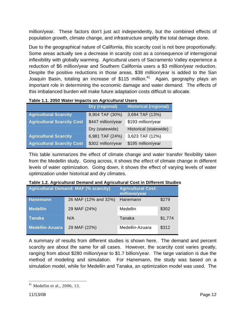
Table 1.1. 2050 Water Impacts on Agricultural Users
Dry (regional) Historical (regional)
Agricultural Scarcity 8,904 TAF (30%) 3,694 TAF (13%)
Agricultural Scarcity Cost $447 million/year $193 million/year
Dry (statewide) Historical (statewide)
Agricultural Scarcity 6,981 TAF (24%) 3,623 TAF (12%)
Agricultural Scarcity Cost $302 million/year $195 million/year
This table summarizes the effect of climate change and water transfer flexibility taken
from the Medellin study. Going across, it shows the effect of climate change in different
levels of water optimization. Going down, it shows the effect of varying levels of water
optimization under historical and dry climates.
Table 1.2. Agricultural Demand and Agricultural Cost in Different Studies
Agricultural Demand: MAF (% scarcity) Agricultural Cost:
millions/year
Hanemann 26 MAF (12% and 32%) Hanemann $279
Medellin 29 MAF (24%) Medellin $302
Tanaka N/A Tanaka $1,774
Medellin-Azuara 29 MAF (22%) Medellin-Azuara $312
A summary of results from different studies is shown here. The demand and percent
scarcity are about the same for all cases. However, the scarcity cost varies greatly,
ranging from about $280 million/year to $1.7 billion/year. The large variation is due the
method of modeling and simulation. For Hanemann, the study was based on a
simulation model, while for Medellin and Tanaka, an optimization model was used. The
41
Medellin et al., 2006, 13.

11/13/08 Page 13
difference lies at the approach of the study; whether starting from an economic or
engineering point of view.
Urban Water Use
Although urban water users experience the same physical impact from global warming,
they face completely different economic effects from agricultural sectors. The estimated
target demands for urban water use are 12.06 million acre-feet in year 2020 and 13.35
million acre-feet by year 2050.42 Population growth and warmer climate increases
demand by about 10 percent over the span of 30 years. However, not all of the regions
in California see an increase in water demand. Specifically, Sacramento Valley actually
sees a 16 thousand acre-feet reduction in urban water use from year 2020 to 2050.
Other regions see an increase in urban demand with a much larger magnitude.
Compared to the 16 thousand acre-feet reduction, Southern Californians will demand an
additional 679 thousand acre-feet and 283 thousand acre-feet for San Joaquin Valley.43
Compared to agricultural water use of 29.7 million acre-feet/year, urban demand is
about 44 percent of agricultural water consumption. In addition to geographic location,
relative size of water demands due to population density may also play an important
role in policy decisions when it comes to costs distribution and adaptations.
Although urban demand is about half of agricultural water use, urban users experiences
scarcity that are much smaller than their relative size in water use. The general trend
observed is that urban users have almost no water scarcity despite the warmer climate.
For 2020, the total water scarcity is estimated to be 123 thousand acre-feet at about 1
percent of total demand. For 2050 with drier climate, urban scarcity still remains at 1
percent with 81 thousand acre-feet shortage.44 The result is startling; there is a
decrease in the amount despite the larger demand and worse condition in 2050.
Compared to urban results, agricultural scarcity is 24 times bigger than urban scarcity at
6.981 million acre-feet in 2050. Furthermore, the urban water scarcity reported above
exists entirely in Southern California with zero scarcity in Sacramento Valley, San
Joaquin Valley, and Tulare Basin. 45 Water market and interregional transfer are the
two major factors in influencing urban water supply. Urban users don’t experience
scarcity because they are able to buy water from agricultural users, which in turn shift
water scarcity to the agricultural sector. In Southern California’s case as with most
urban demands, a large base of imported water is usually the main source of water
42
Medellin et al., 2006, 6. 43
Medellin et al., 2006, 6. 44
Medellin et al., 2006, 9. 45
Medellin et al., 2006, 9.

11/13/08 Page 14
supply. Even though agricultural users are losing water (incurring scarcity cost), the
imported supply is made reliable by urban user’s high willingness to pay.46
Though urban water users have almost no water scarcity, the economic impact of
climate change is still substantial. Two scenarios of economic damage for 2050 were
modeled in the study. The first allows statewide water transfers for optimal economic
usage. In this case, urban scarcity cost is about $44 million/year from population
growth; however, the cost rises by $14.6 million/year to $58.6 million/year with dryer
climate. Of the $58 million/year, Southern California bears about 90 percent of the total
scarcity cost at $53 million/year.47 For the second condition, optimization is limited to
only intra-regional transfers. This scenario is more realistic and representative of
California’s infrastructure if no major modifications have been done by 2050. Under
historical conditions, the scarcity cost is at $154 million/year, a significant $110
million/year increase from those of statewide optimization. With warmer climate, the
cost increases by $10 million/year at $164 million/year, which is smaller than the
increase under statewide optimization.48 Southern California pays 97 percent of the
$164 million/year bill at $158.6 million/year. The results suggest that urban water users,
especially densely populated Southern California, are heavily dependent on the water
market. The maintenance and facilitation of water systems and transportation should
be stressed, as the consequences of not having an adequate system will result in a
huge scarcity cost on water users. Though climate change seems to have smaller
effects than those of infrastructural impacts, it is the combined effects of climate change
and water inflexibility that causes such enormous damages.
Table 1.3. 2050 Water Impacts on Urban Users
Dry (regional) Historical (regional)
Urban Scarcity 204 TAF (2%) 195 TAF (2%)
Urban Scarcity Cost $164 million/year $154 million/year
Dry (statewide) Historical (statewide)
Urban Scarcity 81 TAF (1%) 60 TAF (0%)
Urban Scarcity Cost $58 million/year $44 million/year
Like the agricultural table, the urban table summarizes the effect of climate change and
water flexibility. Urban scarcity is low to begin with, but with sufficient water transfer, a
substantial portion of scarcity can be eliminated. Overall, scarcity remains around 1-2
percent.
Table 1.4. Urban Demand and Urban Cost in Different Studies
46
Medellin et al., 2006, 9. 47
Medellin et al., 2006, 14. 48
Medellin et al., 2006, 14.

11/13/08 Page 15
Urban Demand: MAF (% scarcity) Urban Cost: millions/year
Hanemann 4.2 MAF (7%) [SoCal only] Hanemann $300 [SoCal only]
Medellin 12 MAF (1%) Medellin $58
Tanaka N/A Tanaka $872
Medellin-Azuara 13.3 MAF (<1%) Medellin-Azuara $59
Results from other papers are presented here. Numbers vary greatly due to
assumptions and climate models of each individual study. Hanemann’s paper reflects a
much larger scarcity and cost for the region of Southern California, which dwarfs
statewide results for both the Medellin and Medellin-Azuara studies. Like the
agricultural case, Tanaka’s study contains the largest cost but is over a much longer
timeframe.
Adaptation Options
The evidence has shown that climate change has been and will be causing substantial
economic cost in California. Academic institutes and other state funded agencies have
come up several potential solutions to help prevent and minimize the damage done.
These potential adaptations include: secure additional and reliable water supply,
improve drought preparedness, improve operational flexibility, and promote water use
efficiency.49 There are various methods to achieve these desired outcomes. Keeping
the costs and benefits in mind, some methods are not practical, while others are
excellent candidates for implementation. For most of these options, the cost ranges are
wide; this is due to differences in each specific project including: variations in project
complexity, regional differences in construction and land costs, treatment cost,
availability of infrastructure, etc. The wide range of cost is another barrier to the
implementation of adaptations because actual costs are hard to estimate especially
when the costs are all very high. Consequently obtaining state funding is critical in the
execution of these adaptations. With limited funding, the choice of implementation
depends entirely on the net gain from the adaptations and policymakers in California.
Even so, net benefits and savings remain uncertain without further research and data.
49
DWR, 2005 5.3.

11/13/08 Page 16
Table 1.5. Summary of Adaptation Strategies
Adaptation: Water Market and Transfer
Without a doubt, the most practical answer to water scarcity is increasing water supply.
Obtaining additional water can be easy or difficult depending on the source. These
sources include stored surface water from other users, groundwater, water from crop
idling, and water saved from increased efficiency.50 As the result of an increasing need
to secure additional water supply, a market for sale of water rights has emerged for both
temporary and permanent needs. Water market functions as a flexible source of water
that can be effective when incorporated with other forms of water management
strategies.
The water market has grown substantially since the mid-1980s with the increased
volume of water transferred. Compared to the 80 thousand acre-feet transferred in
1985, the amount of water transferred between districts in 2001 was 1250 thousand
acre-feet. Of the current volume transferred, urban transfers account for about 20
percent while agricultural and environmental transfers have increased to 50 percent and
30 percent.51 Large participation percentage of these two sectors suggests enormous
benefits from water transfers. More water has become available that otherwise wouldn’t
have been. Since 1998, the State Water Project and Central Valley Project have
incorporated water transfer as part of the management strategies to free up to 175
thousand acre-feet of water per year.52 Additional water supply can also be made
available by crop idling of rice and cotton. In Sacramento Valley and San Joaquin
Valley, a total of 700 thousand acre-feet of water can be made available without
significantly damaging the overall agricultural economy (1 percent of countywide
50
DWR, 2005, 23.1. 51
DWR, 2005, 23.3 52
DWR, 2005, 23.1.
Adaptation Strategy Adaptation
Potential
Cost Average Total Cost
Water Market ~1.2 million acre-feet
$75-$185 per acre-foot
N/A
Groundwater and remediation ~2 million acre-feet
$10-$600 per acre-foot
$1.5-$5 billion
Desalination ~0.6 million acre-feet
$250-$2000 per acre-foot
$2 billion
Urban Efficiency ~2.1 million acre-feet
$227-$522 per acre-foot
$99-$236 million/year
Agricultural Efficiency ~1.6 million acre-feet
$35-$900 per acre-foot
$0.3-$2.7 billion
11/13/08 Page 17
economy).53 A developed water market essentially guarantees a new source of water
supply whether temporary or long term.
Consider all the participating regions in California, 75 percent of all transfers originate
within the Sacramento and San Joaquin Valleys, with the remaining transfers taking
place in Southern California, the other major participating region. These three regions
make up the bulk of the water transfers in California. More importantly, studies show
water transfers are predominately localized (probably due to high conveyance cost).
About 75 percent of all transfers take place within the same region, and 25 percent of
those are traded within the same county.54 Although interregional transfers only
accounts for 25 percent, potential benefits are large. With climate change, the cost of
restricting water transfers is projected to be $151 million/year. Even without warmer
climate, the estimated cost of interregional inflexibility is still $108 million/year.55
Water Market and Transfer: Benefits
Water markets result in numerous benefits for the users. Another study, done at the
University of California, Davis, suggests that as much as $1.3 billion/year statewide in
economic benefit can be achieved through water transfers.56 This is possible because
water transfers acts as a safety net for forecasted future water scarcities, which allows
water to be moved from areas with low demand to areas with high scarcity. With a
maximum of 15 percent reduction in water use for exporters, the study suggests that
only mild reduction in deliveries is needed to achieve the significant economic benefits.
Up to 80 percent of economic impact from water scarcity can be reduced when water
transfer is combined with effective water management strategies.57 Thus, by expanding
and encouraging interregional water transfers, there is a large potential in savings.
Simply put, water markets provide “economic incentives for those with high-priority
water rights and contracts but low-valued water uses to sell water to others with more
economically productive water uses”.58 With respect to the water exporter, the sale of
their excess water supply may result in revenues that can be used to fund beneficial
activities. At the district level, the revenue may be used to fund public services or
improve local facilities, environmental conditions or help reduce water rates. For
example, Yuba County Water Agency has spent over $10 million of water revenues on
flood control projects. Another benefit of water transfer is the incentive to improve water
infrastructure in order to minimize cost of transfer.
53
DWR, 2005, 23.5. 54
DWR, 2005, 23.3. 55
Medellin et al., 2006, 22. 56
DWR, 2005, 23.6. 57
DWR, 2005, 23.6. 58
Medellin et al., 2006, 22.
11/13/08 Page 18
“Water markets facilitate the reallocation of water from agricultural to growing urban
uses, as well as more economical operation of water resources to improve the overall
technical efficiency of water management.”59
Conveyance cost and transfer capacity plays a large role in the price of water.
Enhancing these two areas will assist with the reduction of cost and scarcity. At the
private level, farmers who have sold their water supplies are compensated by the
revenues, which they can use to reinvest into the farming business. 60 The farmers are
very likely to profit from the sale of water, because they would have otherwise incurred
a scarcity cost if revenues were too low.61 Secondary economic impacts from water
transfers include the reduction of job losses incurred from water scarcity costs of
farms.62 The environment can also benefit from water transfer. By moving agricultural
water for environmental use, potential habitats that were disturbed by the reduction of
water can now be restored by drawing water from a different source.
Water Market and Transfer: Cost of Implementation
Water transfers, though highly beneficial, have several considerable costs and barriers.
Water purchased is usually costly because the sale price only reflects the cost needed
to make the water physically available. Buyers must also pay conveyance, storage, and
treatment costs that are not included in the initial price of water. The cost of
conveyance can be significant, summing up to as much as 100 percent of the original
price. For example, in 2003, the Environmental Water Account purchased water
ranging from $75 to $185 per acre-foot. The lower prices are water purchased from
Northern California, while higher prices are water purchased from the groundwater bank
in Kern County where conveyance cost is high.63 Lowering theses additional costs can
facilitate and increased usage of the water market.
Water Market and Transfer: Barriers
Another problem with water markets is that agricultural productivity is decreased and
there are cost externalities for farmers not participating in the transfer. Reduction in
demand of farm inputs, raw material, and labor is inevitable with the presence of water
transfer and crop idling.64 Consequently, those sectors will be negatively affected from
an increase export of water. Since the agricultural sector often holds the largest source
of water for transfers, it is crucial to balance the demand for water exports while
maintaining a stable agricultural economy within the exporting region.65 To solve this
59
Medellin et al., 2006, 22. 60
DWR, 2005, 23.5 61
Medellin et al., 2006, 13. 62
DWR, 2005, 23.7. 63
DWR, 2005, 23.6. 64
Howitt and Sunding, 187. 65
DWR, 2005, 23.6.

11/13/08 Page 19
problem, the California Department of Water Resources have already set up regulations
to control the amount of water transferred. The law requires that “water transfers not
unreasonably affect the overall economy of the county which the water is transferred.”66
However, concerns with over-regulation emerge as restrictions may slow down or even
deter short-term transfers that may have multiple benefits. Benefits and profits of water
transfer are sometimes uneven and disproportional, so it is difficult to weigh the net
benefits when some gain while others lose.
Adaptation: Groundwater
Groundwater is a vital source of water that can be used with surface water to provide
optimal water portfolio. The strategy, called conjunctive management, is to recharge
groundwater storage when surface water is available. Substitution of groundwater by
surface water is often needed to take demand off groundwater to allow it to recharge
either naturally or artificially. As soon as a drought hits and surface water is scarce, the
water source will be shifted to the recharged groundwater supply.67
Groundwater: Benefits
With proper monitoring, this strategy can be very effective and implemented both on a
local and regional level. On the regional scale, Southern California has increased its
average-year water deliveries by more than two million acre-feet through conjunctive
management. Through artificial recharge of groundwater aquifers, the groundwater
storage capacity has increased by seven million acre-feet. On the local scale, Santa
Clara Valley Water District obtained 138 thousand acre-feet of storage capacity by
recharging groundwater artificially via local creeks and recharge ponds. They achieved
groundwater levels to those of early 1900s.68 By preventing overexploitation of
groundwater during normal years, conjunctive management has improved water supply
quality and reliability. Potential statewide increase in water deliveries can be up to 500
thousand acre-feet with an additional nine million acre-feet of groundwater storage. A
more aggressive estimate predicts that with a major renovation of existing surface
reservoirs and groundwater, an increase of two million acre-feet for water deliveries and
20 million acre-feet of new storage can be achieved.69 The result of conjunctive
manage is highly dependant on the ability to acquire and recharge surface and
groundwater of suitable water quality. Expansion of current storage and conveyance
infrastructure can result in wider use and flexibility of conjunctive management projects.
In addition to a direct water supply increase, beneficial secondary effects also result
from conjunctive management. One such benefit is the prevention of groundwater
overdraft and land subsidence. Protection of groundwater supplies also help wildlife
66
DWR, 2005, 23.7. 67
DWR, 2005, 4.1. 68
DWR, 2005, 4.1. 69
DWR, 2005, 4.2.
11/13/08 Page 20
habitat such as wetland recover while they recharge. When shifted to groundwater use,
the increase in surface instream flow can lift pressure off aquatic species.70
Moreover, additional groundwater supplies can be obtained through remediation of
contaminated groundwater aquifers. Groundwater remediation is the process of treating
groundwater and improving the water quality to a given standard depending on the use.
Contamination can both occur naturally such as heavy metals or artificially from
industrial, mining operations, or various runoffs. Currently, there are about 18,500 sites
where active cleanup is taking place. Potential supply can meet up to 40 percent of the
state’s water demand.71 Once treated, these aquifers can provide a significant amount
of water, making additional water supply available that would not have been. Even if
treated water do not meet high drinking standards in quality, they may still be allocated
for other uses that can free up drinking water supply. One long-term benefit is that the
groundwater aquifers may eventually be cleaned to the point that no further treatment is
necessary, providing a reliable clean source of water.72 Remediation also has
substantial secondary effects. The avoided costs include foregone profits and taxes
from businesses that decide not to locate in the area with water shortages. Moreover,
controlling contaminants can prevent further spreading and cut down future remediation
costs.
Groundwater: Costs of Implementation
As with the water market, groundwater usage with conjunctive management has many
costs and issues associated with it. With respect to conjunctive management, the cost
can range from $10 to $600 per acre-foot increase in average annual delivery. The
average projected cost reported by Department of Water Resources is $110 per acre-
foot.73 The large range of cost is due to the many factors that influence the costs of
increasing water deliveries. These factors include project complexity, regional
differences in infrastructure, quality of recharged supply, treatment cost, and intended
use. High value for water from urban demands usually results in higher willingness to
pay for these water projects than agricultural users.74
The physical extraction process is especially costly for groundwater remediation. The
costs consist of identifying all the contaminants, the capital cost of the system, and
operation expenses during the length of the project. The reported cost associated with
groundwater cleanup can easily exceed $300 million annually with per-site cost ranging
from $100,000 to $200,000. Despite the high costs, state programs often provide
reimbursement for eligible claimants. Current reimbursements distributed are about
70
DWR, 2005, 4.2. 71
DWR, 2005, 11.1. 72
DWR, 2005, 11.5. 73
DWR, 2005, 4.5. 74
DWR, 2005, 4.4.

11/13/08 Page 21
$180 million annually with some as high as $1.5 million per site. Finally, data from the
California Department of Water Resources predicts that remediation costs could
approach $20 billion over the next 25 years.75
With such a high price tag, some source of groundwater may be difficult to obtain due to
political barriers. The determining factor in the execution of groundwater remediation is
the timing of the result. Remediation can often take years to complete in which the
parties who paid may not receive the benefits by the time remediation has been
completed. Funding can be difficult to obtain when no apparent short-term benefits are
available.76
Groundwater: Barriers
Water transfers tend to increase the incentive for pumping groundwater to substitute for
the surface water sold. Some water right holders will want to sell surface water for profit
by pumping additional groundwater for use. A raise in groundwater pumping causes a
drop in groundwater levels, reduction of water quality, and increases groundwater-
pumping costs for other users.77 These actions conflict with the conjunctive
management system making it harder to implement. The problem exists because
groundwater is loosely regulated by the state. “Because groundwater resources are not
regulated by the state, the implementation of the California water market has sparked
concerns that aquifers will be subject to uncontrolled mining.”78 Because groundwater
is an attractive source of water, California may risk losing a large portion of groundwater
and face high water scarcity if groundwater is not properly controlled.
Nevertheless, groundwater export is not without any regulation. On the local level,
counties often have their own ordinances and agencies managing a portion of
groundwater being exported.79 Since 1995, numerous ordinances have been passed to
prevent and deter excessive groundwater export. By 2002, 22 of the state’s 58 counties
had put ordinances that require the acquisition of a permit before extraction and export
of groundwater.80 The process also includes an environmental review, which makes it
even more difficult for individuals to obtain water rights. So far, results are promising.
Statistics show that groundwater has decreased by 14,300 acre-feet in a county since
implementation in 1990. Totally groundwater exports statewide has been reduced by
19 percent at 932 thousand acre-feet, and total water sales were reduced by 14 percent
at 787 thousand acre-feet since 1996.81 Overall, groundwater is an excellent alternate
75
DWR, 2005, 11.5 76
DWR, 2005, 11.6. 77
Howitt and Sunding, 187; Vicuña et al., 19. 78
Howitt and Sunding, 187. 79
DWR, 2005, 4.5. 80
Howitt and Sunding, 188. 81
Howitt and Sunding, 188.

11/13/08 Page 22
source of water supply; however, both political and financial barriers decrease the
optimal efficient use of the resource.
Adaptation: Desalination
Desalination, a costly process in the past, has become a more common method of
increasing water supply. Due to innovation in desalination technology and the rising
cost of alternative water supply, desalination is becoming more practical. Though
capacity is relatively small and limited, it can be incorporated into the water
management portfolio to provide a more versatile water program. Currently, there are
24 desalination plants in use in California operating on both groundwater and seawater.
Their annual output is about 79,000 acre-feet. Additional plants are in the process of
being built or designed with estimated increase of 29,500 acre-feet of water annually.82
Each region in California is actively approaching desalination with numerous funding in
projects and studies. In the San Francisco Bay Area, local agencies are funding the
planning of a 120,000 acre-feet/year production facility. In Central and Southern
California, studies of planning sustained production of 20,000 and 150,000 acre-
feet/year are also being funded as well.83 The statewide objective is to increase the
water supply from desalination five-fold to 587,200 acre-feet/year. In addition to the 23
operating facilities, a total of 26 more will be constructed by 2030. This is a substantial
increase in the usage of water desalination, which provides strong evidence that
desalination is becoming more affordable.
Desalination: Benefits
In addition to the increase supply of water, desalination can provide water reliability
during drought periods without pressuring groundwater or surface sources that are
already in use. Increasing diversification in water sources can lighten environment
impacts via alternative water sources.84 Feedwater source for desalination are not
limited to only groundwater and seawater; recycled municipal wastewater can also be
treated. Overall, desalination of water is similar to groundwater remediation, which
improves the water quality to a potable level from sources that would have otherwise
been unavailable.
Desalination: Cost of Implementation
Though desalination has become more efficient and cheaper than in the past, it still has
some significant barriers associated with it. These costs can be categorized into
monetary, environmental, and time. In 2005 alone, $25 million dollars were granted to
research and development of desalination projects. Aside from research cost, actual
production cost of water is costly. The estimated cost of increasing desalination water
82
DWR, 2005, 6.1. 83
DWR, 2005, 6.2. 84
DWR, 2005, 6.2.

11/13/08 Page 23
supply by 415,000 acre-feet/year is about $2 billion. These water supplies cost so
much in capital because the lifetime of water producing plants are only 20-30 years.85
Per unit cost of water varies widely, ranging from $250 to $2,000 per acre-foot. The
lowest costs are associated with groundwater desalination and highest with seawater.86
In the study presented earlier, climate change still does not result in a wide usage of
desalination. The average price tag is $1400/acre-foot, which is relatively high
compared to other alternative sources of water. Under the model, only Southern
California, with the highest marginal willing to pay, will approach this method of water
supply producing 5.93 thousand acre-feet of water.87 Due to the factors influencing
production cost, the price varies from region to region depending on the type of
feedwater, proximity of distribution systems, availability and cost of power, and disposal
options of waste.88 Because these projects vary case by case, environmental-specific
investigation is required and often takes a long time to fully estimate the impact and
issue a permit for construction. Another considerable time constraint is the relative
implementation and operating lifetime of the facility. Cost and benefits must be
reevaluated if it takes 20-30 years to implement plans that will only last 20-30 years.
Adaptation: Urban Water Use Efficiency
Urban water use efficiency involves lowering the water demand and per capita water
use through technological or behavioral improvements. The present state of California’s
urban water use efficiency has benefited from much improvement over the past decade.
In some parts of the state, an increase in population did not necessary result in a
proportional increase. As of 2002, Los Angeles Department of Water and Power
reported that water conservation helped keep the city’s water use similar to levels seen
20 years ago.89 Through the efforts of California Urban Water Conservation Council,
urban water agencies cooperate to increase water use efficiency through public
awareness, research and development, and policy incentives. For example, of the
current 2.5 million water efficient toilets installed statewide; there remains ten million
more to be installed and replaced.90 Like the water efficient toilets, large water saving
potential exists in household appliances, hardware, and irrigations. Other forms of
water use efficiency are behavioral incentives. For example, rebates of $450 on
purchases were awarded to people who purchased high efficiency washing machines.
The CALFED Record of Decision estimated that water savings range between 0.8
million and one million acre-feet/year by 2030; furthermore, a more optimistic study
85
DWR, 2005, 6.4. 86
DWR, 2005, 6.5. 87
Medellin et al., 2006, 22. 88
DWR, 2005, 6.4. 89
DWR, 2005, 22.1. 90
DWR, 2005, 22.1.
11/13/08 Page 24
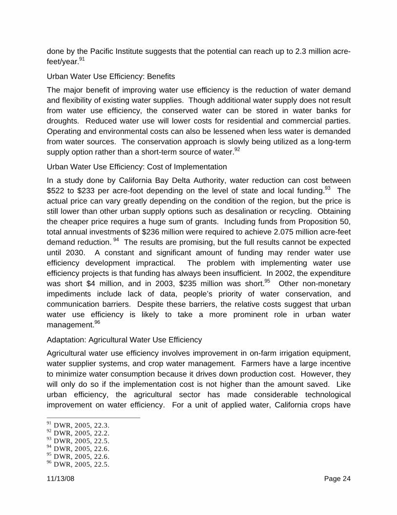
done by the Pacific Institute suggests that the potential can reach up to 2.3 million acre-
feet/year.91
Urban Water Use Efficiency: Benefits
The major benefit of improving water use efficiency is the reduction of water demand
and flexibility of existing water supplies. Though additional water supply does not result
from water use efficiency, the conserved water can be stored in water banks for
droughts. Reduced water use will lower costs for residential and commercial parties.
Operating and environmental costs can also be lessened when less water is demanded
from water sources. The conservation approach is slowly being utilized as a long-term
supply option rather than a short-term source of water.92
Urban Water Use Efficiency: Cost of Implementation
In a study done by California Bay Delta Authority, water reduction can cost between
$522 to $233 per acre-foot depending on the level of state and local funding.93 The
actual price can vary greatly depending on the condition of the region, but the price is
still lower than other urban supply options such as desalination or recycling. Obtaining
the cheaper price requires a huge sum of grants. Including funds from Proposition 50,
total annual investments of $236 million were required to achieve 2.075 million acre-feet
demand reduction. 94 The results are promising, but the full results cannot be expected
until 2030. A constant and significant amount of funding may render water use
efficiency development impractical. The problem with implementing water use
efficiency projects is that funding has always been insufficient. In 2002, the expenditure
was short $4 million, and in 2003, $235 million was short.95 Other non-monetary
impediments include lack of data, people’s priority of water conservation, and
communication barriers. Despite these barriers, the relative costs suggest that urban
water use efficiency is likely to take a more prominent role in urban water
management.96
Adaptation: Agricultural Water Use Efficiency
Agricultural water use efficiency involves improvement in on-farm irrigation equipment,
water supplier systems, and crop water management. Farmers have a large incentive
to minimize water consumption because it drives down production cost. However, they
will only do so if the implementation cost is not higher than the amount saved. Like
urban efficiency, the agricultural sector has made considerable technological
improvement on water efficiency. For a unit of applied water, California crops have
91
DWR, 2005, 22.3. 92
DWR, 2005, 22.2. 93
DWR, 2005, 22.5. 94
DWR, 2005, 22.6. 95
DWR, 2005, 22.6. 96
DWR, 2005, 22.5.

11/13/08 Page 25
increased output by 38 percent and adjusted crop revenue has increased by 11 percent
from 1980 to 2000. 97 The observed progress is only possible through the efforts of the
agricultural industry, state, and federal agencies. Growers who are willing to risk their
crops to adopt new technologies are often the ones that benefit most from the research
of both commercial and academic institutes.
Hardware improvements include upgrading water delivery system, data acquisition,
canal automation, and other operating components that ensure reliable and accurate
water delivery. Large scale change in irrigation systems from furrow/flood to
sprinkler/drip systems have been observed in the recent decade. They incorporate
satellite information on crop and soil conditions to manage water delivery optimally.
This system has been so effective that a change of 16 million acre-feet in water delivery
has been shifted to either sprinkler or micro-irrigation system. The result is a
productivity increase of up to 30 percent.98 High benefits of advance systems also
come with a high price tag. Most growers, especially smaller ones, are unwilling to
make such a substantial investment in upgrading their irrigation system, which are also
more power-intensive than older systems. This change will result in an increase in the
production cost, which profit seeking growers are not interested.
Agricultural Water Use Efficiency: Benefits
Potential benefits from increasing agricultural water use efficiency can result in an
estimated 1.6 million acre-feet/year of reduction in water. This large reduction is not
only beneficial to crop production with lower cost, but also benefits the environment. At
the cost of about $220 million, All American Canal and Colorado River Hydrologic
Region will be able to reduce a total of 94,000 acre-feet/year of irrecoverable flow by
lining the canals.99
Agricultural Water Use Efficiency: Cost of Implementation
Problems associated with agricultural efficiency include limited funding, willingness of
the growers, and poor management. The projected per acre-foot cost ranges from $35
to $900 million, for a total net water savings of 563,000 acre-feet. At this level of
savings, the annual spending can amount between $0.3 billion and $2.7 billion, which
includes the canal renovation cost.100 Like other adaptations mentioned, a large funding
requirement is often the problem with carrying out these projects. Small communities
who need these adaptations the most often lack political and financial means to carryout
these water management practices.101 Even when advance water saving systems are
available, farmers who do not participate or poorly manage their water will not result in
97
DWR, 2005, 3.1. 98
DWR, 2005, 3.4. 99
DWR, 2005, 3.5. 100
DWR, 2005, 3.7. 101
DWR, 2005, 3.7.

11/13/08 Page 26
the desired outcome. Furthermore, some farmers feel that they are not necessarily
using the water they save. They feel that there is no need to conserve water if they do
not have the right to utilize them. However, these obstacles can be overcome. State
funded grants or loans should provide incentives for farmers to adopt new technologies.
On the local level, technical and planning assistance to implement better water
management practices should be funded. Most importantly, public awareness and
priority should be organized to help encourage and educate others in the area of water
conservation. With enough help, conservation levels that surpass those observed in the
past are achievable.
Financing Water Provision
Finance will play a major role in California’s water adaptation efforts. As noted in its
2005 Water Plan Update, California’s prevailing water policy is to “recover costs for
such things as planning, operation, maintenance, capital, administrative, and some
environmental costs. Secondary priorities are maintaining contributions to capital
investment funds for future water projects, settling debts, and recovering external costs
such as third party fees.102 Ad valorem taxes and revenue from bonds not repaid from
water rates are two other tools used to recoup costs.103
In some situations, agencies are not required to recover their full costs of development
and maintenance. This generally occurs when an agency is advancing a social goal
affecting water use. For example, the U.S. Bureau of Reclamation is not required to
recover all costs of supplying water to agriculture. Similarly, because of significant
federal grant funding through the Clean Water Act, urban wastewater treatment projects
are often not required to recover their costs.104
There is variety in the structure of water rates: fixed, tiered, and uniform structures are
all used. Under a fixed pricing structure, users pay the same fixed amount each month,
regardless of water use; a uniform pricing structure means that a user pays a constant
amount per unit of water used (requiring a metering system), and under a tiered
structure the rate paid per unit increases or decreases as use exceeds certain
predetermined amounts. These pricing schemes are not mutually exclusive: a fixed
component might be present within uniform or tiered pricing structures and so on. If
water use is unmetered in an area, fixed assessments such as connection size for
urban areas or acreage irrigated for agriculture might be needed to determine rates.105
102
Department of Water Resources, 2008a, California Water Plan Update, 2009: Volume 2, resource management strategies, economic incentives. 103
Department of Water Resources, [a]. (2005) California Water Plan Update, 2005: Volume 2, resource management strategies. 104
DWR, 2008a. 105
DWR, 2008a.

11/13/08 Page 27
The general trend for California urban water agencies is toward tiered rate structures
where price is based upon the amount of water used. For the tiered systems, price
generally increases as consumption increases: with each additional unit of water used,
the price for subsequent units increase. A problem for densely populated areas is that
within an apartment building, individual tenants are not metered, and thus do not
receive the benefits of conserving under volumetric pricing.106 In some areas,
seasonality is also a pricing issue. Some agricultural water providers also use tiered
pricing schedules. Residential wastewater treatment is generally governed under a flat-
rate pricing scheme, commercial and industrial users are more likely to be to be
charged by volume, and possibly content.107
Decreased consumption of water is the primary motivator for the use of economic
incentives such as low-interest loans, grants, or water pricing rates. However,
alterations to time and amount of use, wastewater volume, and the source of supply are
also common goals. Other benefits can be environmental, social, or as simple as the
avoiding construction of additional supply projects. When faced with higher rates,
consumers can either reduce consumption or pay the higher price. Hopefully the higher
rates would prompt investment in more efficient technologies, or moderation of use
(decreasing landscaping or agricultural acreage).
Setting appropriate water rates is difficult. A water shortage exacerbates this problem
because incremental costs of supply can change (particularly increase) quickly, more
rapidly than rates, making it difficult to recover costs. Under a system not allowing
collection of revenues in excess of cost, a skewed structure might be necessary, with
lower-tier prices being reduced and higher-tier prices increased; this could easily lead to
an increase in average consumption by users situated in the lower-tier, an undesirable
outcome for water management. Also, an increase in the price of surface water could
motivate users to increase consumption of well water, decreasing groundwater volume
and recharge.108
Equity considerations can arise when economic incentives are implemented, such as
when one group of citizens incurs the cost of subsidizing another group without
receiving a proportionate share of the benefit. Also, economic incentives directly
affecting one group of users might have repercussions in secondary markets. An
example is found when the price of water for agricultural users is increased: a decrease
in water use can lead to an alteration of crop patterns and a change in farm labor
required. Communities heavily dependent upon agriculture could potentially suffer, and
106
DWR, 2008a. 107
DWR, 2008a. 108
DWR, 2008a.
11/13/08 Page 28
jobs in the landscaping sector could be similarly affected by an increase in the price of
water in urban areas.109
In 2000, approximately 8.7 million acre-feet of water was used by California cities and
suburbs.110 An immense amount of power is required to transport California’s water
across the state. In fact, the transportation and treatment of water (before and after it is
used) in California consumes about 19 percent of all electricity, and 30 percent of non-
power plant natural gas.111 Many inter-basin transfer systems have notable
hydroelectric capabilities, but the State Water Project (SWP) nonetheless remains a net
energy user. However, wise use of resources, such as using baseline energy to pump
water and generating hydroelectricity during on-peak hours, ensures the SWP works as
efficiently as possible.112
Many local and regional projects which are essential to expanding water supply are
funded through local taxes. An 800,000 acre-foot reservoir in Riverside County, the
Metropolitan Water District’s Diamond Valley Lake, is an example of a project funded for
the most part by local users.113 Other primarily locally-funded projects are planned but
not yet completed, such as an upgrade to San Francisco’s Hetch-Hetchy system and an
expansion to water use from Lake Nacimiento in San Luis Obispo.114
When attempting to enlarge water supplies, an increase in local water prices might be
the most equitable option, as well as potentially having the benefit of a reduction to
consumption, but is often met with resistance.115 Explicit impact fees for new water
might be a good alternative. Such practices are already widely used in Colorado and
Southern Nevada, and would essentially place the responsibility of supply augmentation
upon utilities. In determining an impact fee for a new project such as a development, the
local utility estimates each new home’s approximate portion of costs to the
development. Water resources are effectively packaged together with other community
amenities such as schools, roads, and wastewater systems.116
Residential
A study by the engineering firm Black and Veatch found that from 2003 to 2006, the
average monthly water bill for a single family residence in California increased from
109
DWR, 2008a. 110
Department of Water Resources, 2008b, California Water Plan Update, 2009: Volume 2, resource management strategies, urban water use efficiency. 111
DWR, 2008b. 112
DWR, 2008b. 113
Hanak, E. (2005) Water for Growth: California’s new frontier. Public Policy Institute of California, San Francisco. 114
Hanak, 2005. 115
Hanak, 2005. 116
Hanak, 2005.
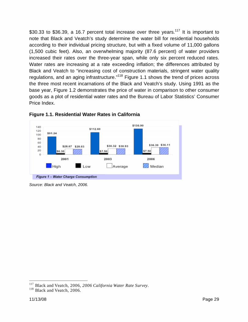
11/13/08 Page 29
$30.33 to $36.39, a 16.7 percent total increase over three years.117 It is important to
note that Black and Veatch’s study determine the water bill for residential households
according to their individual pricing structure, but with a fixed volume of 11,000 gallons
(1,500 cubic feet). Also, an overwhelming majority (87.6 percent) of water providers
increased their rates over the three-year span, while only six percent reduced rates.
Water rates are increasing at a rate exceeding inflation; the differences attributed by
Black and Veatch to “increasing cost of construction materials, stringent water quality
regulations, and an aging infrastructure.”118 Figure 1.1 shows the trend of prices across
the three most recent incarnations of the Black and Veatch’s study. Using 1991 as the
base year, Figure 1.2 demonstrates the price of water in comparison to other consumer
goods as a plot of residential water rates and the Bureau of Labor Statistics’ Consumer
Price Index.
Figure 1.1. Residential Water Rates in California
Source: Black and Veatch, 2006.
117
Black and Veatch, 2006, 2006 California Water Rate Survey. 118
Black and Veatch, 2006.

11/13/08 Page 30
Figure 1.2. Relative Water Prices in California
Source: Black and Veatch, 2006.
Sixteen percent of the suppliers surveyed by Black and Veatch received additional
financial support in the form of “grants, contributions from other funds, special
assessments, general fund transfers, and property taxes.”119 As one might imagine, this
supplementation can lead to lower water rates. From 2001 to 2006, there has not been
a large amount of change in the structure of water rates, though some general trends,
the most noteworthy being as increase in the prevalence of tiered rate structures, as
Figure 1.3 demonstrates. The majority of water users interviewed by Black and Veatch
(61.4 percent) are billed monthly, and most of the remainder (37.5 percent) are billed bi-
monthly.120
Figure 1.3. Water Rate Structures in California
Source: Black and Veatch, 2006.
Geography is an important determinant of water rates. Figure 1.4 shows the remarkable
differences of water rates by county. The price of water in the most expensive county is
more than three times the cost of water in the cheapest county. There is also variety in
119
Black and Veatch, 2006. 120
Black and Veatch, 2006.
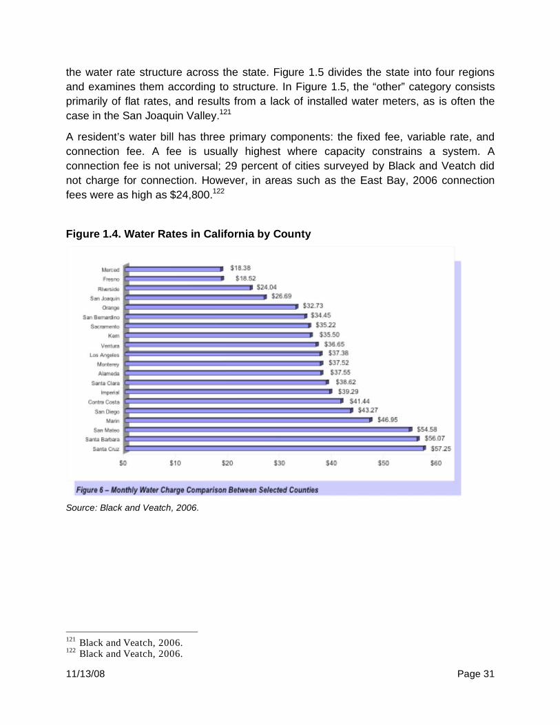
11/13/08 Page 31
the water rate structure across the state. Figure 1.5 divides the state into four regions
and examines them according to structure. In Figure 1.5, the “other” category consists
primarily of flat rates, and results from a lack of installed water meters, as is often the
case in the San Joaquin Valley.121
A resident’s water bill has three primary components: the fixed fee, variable rate, and
connection fee. A fee is usually highest where capacity constrains a system. A
connection fee is not universal; 29 percent of cities surveyed by Black and Veatch did
not charge for connection. However, in areas such as the East Bay, 2006 connection
fees were as high as $24,800.122
Figure 1.4. Water Rates in California by County
Source: Black and Veatch, 2006.
121
Black and Veatch, 2006. 122
Black and Veatch, 2006.
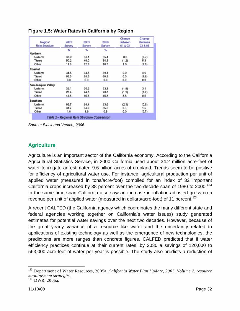
11/13/08 Page 32
Figure 1.5: Water Rates in California by Region
Source: Black and Veatch, 2006.
Agriculture
Agriculture is an important sector of the California economy. According to the California
Agricultural Statistics Service, in 2000 California used about 34.2 million acre-feet of
water to irrigate an estimated 9.6 billion acres of cropland. Trends seem to be positive
for efficiency of agricultural water use. For instance, agricultural production per unit of
applied water (measured in tons/acre-foot) compiled for an index of 32 important
California crops increased by 38 percent over the two-decade span of 1980 to 2000.123
In the same time span California also saw an increase in inflation-adjusted gross crop
revenue per unit of applied water (measured in dollars/acre-foot) of 11 percent.124
A recent CALFED (the California agency which coordinates the many different state and
federal agencies working together on California’s water issues) study generated
estimates for potential water savings over the next two decades. However, because of
the great yearly variance of a resource like water and the uncertainty related to
applications of existing technology as well as the emergence of new technologies, the
predictions are more ranges than concrete figures. CALFED predicted that if water
efficiency practices continue at their current rates, by 2030 a savings of 120,000 to
563,000 acre-feet of water per year is possible. The study also predicts a reduction of
123
Department of Water Resources, 2005a, California Water Plan Update, 2005: Volume 2, resource management strategies. 124
DWR, 2005a.

11/13/08 Page 33
1.6 million acre-feet per year in applied water.125 Potential costs also vary greatly;
assuming the savings due to efficiency gains is the more generous 563,000 acre-feet,
per acre-foot costs could range from $35 to $900, for a total of between $0.3 billion and
$2.7 billion.126
Central Valley annual rainfall ranges from 5 to 30 inches, depending on the region. Over
three-fourths of the precipitation comes from December through April, producing
seasonal droughts and floods as well as heavy runoffs in spring and winter. Water
demand for agriculture is highest in fall and summer, when natural streamflow is at a
minimal, so demand for water quickly outpaced available wellwater and its recharge
from streams and rain.127
Though the Central Valley is geographically a desert, the land was found to be fertile,
and by 1873, plans were formulated with the intention of transferring water from the
Sacramento Valley to the San Joaquin Valley. The California Water Plan was birthed in
the early 30s from fourteen reports written between 1920 and 1932 with funds
appropriated by the state legislature, and examined issues such as drought, flood
control, irrigation issues, and water flow in California.128 The California Water Plan’s first
major venture planned for the construction of a 420 foot dam at Kennett in order to
regulate water flow to Antioch and keep salt water out of Suisun Bay.129 This dam, the
first phase of the Central Valley Project (CVP), was approved by the California
legislature as a state project, funded by the sale of up to $170 million in “revenue”
bonds.130 However, even with the approved bonds, California was unable to finance the
project and was also unable to secure loans or grants under the National Recovery Act.
Eventually, the House of Representatives’ Committee on Rivers recommended $12
million in Federal on the grounds of national benefits to navigation and flood control of
the Sacramento River.131
The federal government assumed control of the project with The Rivers and Harbors Act
of 1935; first few phases were funded by The Emergency Relief Appropriation Act of
1935, and constructed by the U.S. Army Corp of Engineers.132 The Rivers and Harbors
Act was re-authorized in 1937 for $12 million, and the Bureau of Reclamation took over
construction of the Central Valley Project. The first priorities were navigation, regulation,
and flood control of the Sacramento and San Joaquin Rivers; supply for irrigation and
125
DWR, 2005a. 126
DWR, 2005a. 127
Bureau of Reclamation (BoR), undated. The Central Valley Project: Overview. Retrieved 28 August 2008. {http://www.usbr.gov/dataweb/html/cvpintro.html#Intro} 128
Bureau of Reclamation (BoR), undated, 2. The Central Valley Project: General overview. Retrieved 28 August 2008. {http://www.usbr.gov/dataweb/html/cvp.html#general}. 129
BoR, undated, 2. 130
BoR, undated, 2. 131
BoR, undated, 2. 132
BoR, undated.
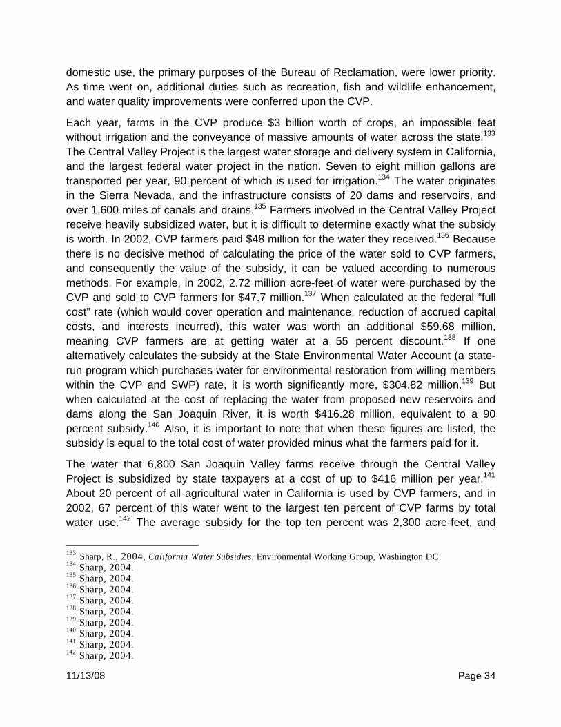
11/13/08 Page 34
domestic use, the primary purposes of the Bureau of Reclamation, were lower priority.
As time went on, additional duties such as recreation, fish and wildlife enhancement,
and water quality improvements were conferred upon the CVP.
Each year, farms in the CVP produce $3 billion worth of crops, an impossible feat
without irrigation and the conveyance of massive amounts of water across the state.133
The Central Valley Project is the largest water storage and delivery system in California,
and the largest federal water project in the nation. Seven to eight million gallons are
transported per year, 90 percent of which is used for irrigation.134 The water originates
in the Sierra Nevada, and the infrastructure consists of 20 dams and reservoirs, and
over 1,600 miles of canals and drains.135 Farmers involved in the Central Valley Project
receive heavily subsidized water, but it is difficult to determine exactly what the subsidy
is worth. In 2002, CVP farmers paid $48 million for the water they received.136 Because
there is no decisive method of calculating the price of the water sold to CVP farmers,
and consequently the value of the subsidy, it can be valued according to numerous
methods. For example, in 2002, 2.72 million acre-feet of water were purchased by the
CVP and sold to CVP farmers for $47.7 million.137 When calculated at the federal “full
cost” rate (which would cover operation and maintenance, reduction of accrued capital
costs, and interests incurred), this water was worth an additional $59.68 million,
meaning CVP farmers are at getting water at a 55 percent discount.138 If one
alternatively calculates the subsidy at the State Environmental Water Account (a state-
run program which purchases water for environmental restoration from willing members
within the CVP and SWP) rate, it is worth significantly more, $304.82 million.139 But
when calculated at the cost of replacing the water from proposed new reservoirs and
dams along the San Joaquin River, it is worth $416.28 million, equivalent to a 90
percent subsidy.140 Also, it is important to note that when these figures are listed, the
subsidy is equal to the total cost of water provided minus what the farmers paid for it.
The water that 6,800 San Joaquin Valley farms receive through the Central Valley
Project is subsidized by state taxpayers at a cost of up to $416 million per year.141
About 20 percent of all agricultural water in California is used by CVP farmers, and in
2002, 67 percent of this water went to the largest ten percent of CVP farms by total
water use.142 The average subsidy for the top ten percent was 2,300 acre-feet, and
133
Sharp, R., 2004, California Water Subsidies. Environmental Working Group, Washington DC. 134
Sharp, 2004. 135
Sharp, 2004. 136
Sharp, 2004. 137
Sharp, 2004. 138
Sharp, 2004. 139
Sharp, 2004. 140
Sharp, 2004. 141
Sharp, 2004. 142
Sharp, 2004.
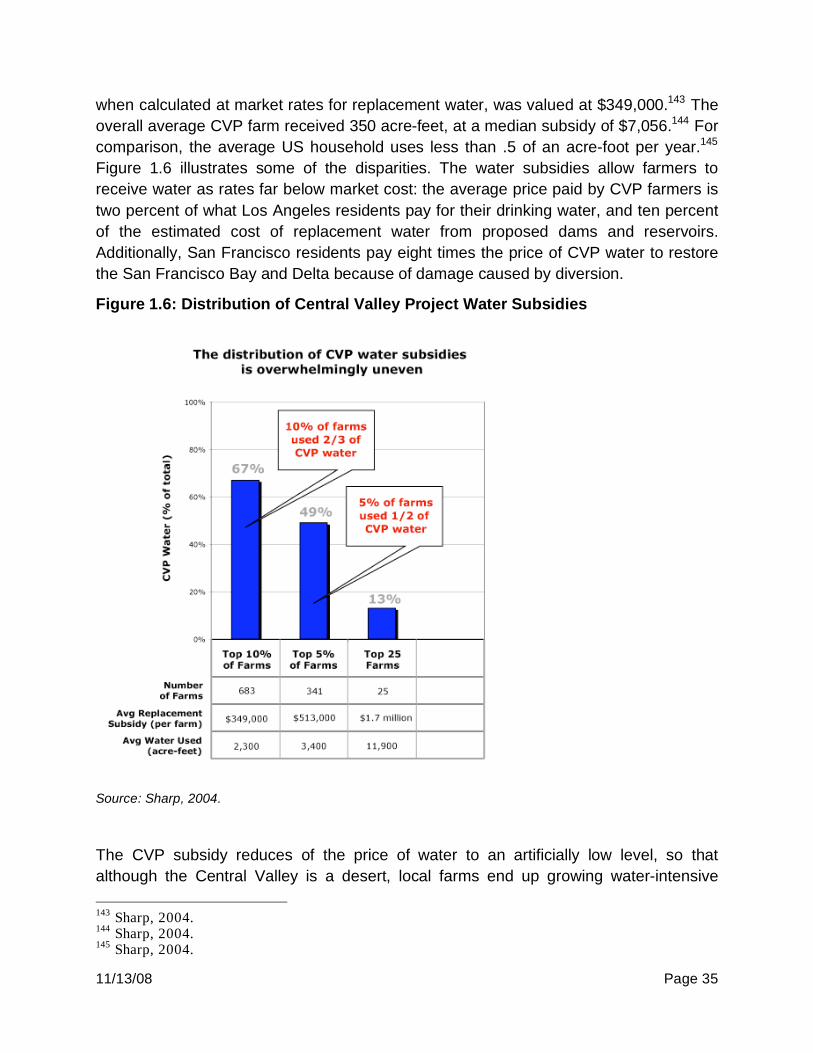
11/13/08 Page 35
when calculated at market rates for replacement water, was valued at $349,000.143 The
overall average CVP farm received 350 acre-feet, at a median subsidy of $7,056.144 For
comparison, the average US household uses less than .5 of an acre-foot per year.145
Figure 1.6 illustrates some of the disparities. The water subsidies allow farmers to
receive water as rates far below market cost: the average price paid by CVP farmers is
two percent of what Los Angeles residents pay for their drinking water, and ten percent
of the estimated cost of replacement water from proposed dams and reservoirs.
Additionally, San Francisco residents pay eight times the price of CVP water to restore
the San Francisco Bay and Delta because of damage caused by diversion.
Figure 1.6: Distribution of Central Valley Project Water Subsidies
Source: Sharp, 2004.
The CVP subsidy reduces of the price of water to an artificially low level, so that
although the Central Valley is a desert, local farms end up growing water-intensive
143
Sharp, 2004. 144
Sharp, 2004. 145
Sharp, 2004.
11/13/08 Page 36
crops such as alfalfa, rice and cotton. The average U.S. farm annually uses 2.48 acre-
feet of water per acre per year, but California farms average 3.37 acre-feet.146 One must
bear in mind that this is a state in which water consumption exceeds natural supply by
1.6 million acre-feet in normal years and 5.1 million acre-feet in drought years.147
Federal taxpayers funded the CVP at a total cost of $3.6 billion.148 The original intent
was for recipients of water to repay the CVP’s capital cost, with an intermediate goal of
$1 billion within 50 years of the project’s completion. (Sharp, 2004) However, by 2002,
60 years after water was first transferred, only 11 percent of the capital cost had been
recovered.149 This is because the 40-year contracts the farmers first signed provided the
water at prices far below what was necessary to recoup the construction outlay.
Considering that 17 of the CVP districts, which consumed a total of about 300,000 acre-
feet of water in 2002, paid only about $2 per acre-foot for water that cost $10 to deliver,
it is no wonder.150 Unlike municipal or industrial beneficiaries of the CVP project,
farmers also receive the additional subsidy of no interest on their obligations. Also, if in
any given year the Bureau of Reclamation believes a CVP district will be unable to
repay any of their obligation, the Bureau simply increases the rates for CVP power
users, labeling this practice “capital relief.”
Overall in 2002, CVP farmers paid an average of $17.14 per acre-foot for their irrigation
water.151 The Bureau of Reclamation conservatively calculates the “full-cost” of an acre-
foot of this water at an average of $38.93 per acre-foot.152 Farmers under the State
Water Project, which is under the jurisdiction of the state and which is similar to the
CVP, paid an average of $50.92 per acre-foot.153 In the same time period, the
Environmental Water Account bought water from willing members within the CVP and
SWP for an average of $129.48.154 Additions to the capacity of water systems coming
from the construction of new or expanded dams and reservoirs along the San Joaquin
River would cost at least $170.42 per acre-foot.155 As mentioned above, residential
users pay much more for water: in the same time period, San Francisco and Los
Angeles residents were paying $625 and $925, respectively.156
146
Sharp, 2004. 147
Sharp, 2004. 148
Sharp, 2004. 149
Sharp, 2004. 150
Sharp, 2004. 151
Sharp, 2004. 152
Sharp, 2004. 153
Sharp, 2004. 154
Sharp, 2004. 155
Sharp, 2004. 156
Sharp, 2004.
11/13/08 Page 37
The State Water Project
The California State Water Project (SWP) is the largest state-built water transportation
and power conveyance system in the nation.157 It consists of 33 storage facilities and 21
primary lakes and reservoirs comprising a total 5.8 million acre-feet.158 The SWP
provides a total of 23 million residents and 755,000 acres of farmland with water.159
Construction began on the SWP unofficially in 1957, officially in 1960 with a $1.75 billion
California bond measure, and by 2001, a total of around $5.2 billion had been spent.160
About 78 percent of funding for infrastructure came primarily from state general
obligation and revenue bonds, but also other sources include tideland oil revenues,
investment earnings, recreation appropriations, and federal flood control payments.161
Short-term funding is financed through commercial paper notes later transformed into
long-term revenue bonds.
Water from the SWP is divided among SWP contractors -- 29 California urban and
agricultural water suppliers. In total, the SWP provides water to two-thirds of
California’s population with seventy percent of the water going to agricultural users and
the remainder to urban users.162 A yearly profile (1999) of expenses for SWP
contractors is as follows: bond repayment (46 percent), operations and maintenance (35
percent), power (18 percent), and replacement reserves, insurance, and miscellaneous
(one percent). Ninety six percent of bond repayment by SWP contractors came from
water supply and power generation; the remainder from recreation, fish and wildlife (two
percent) and flood control (two percent).163
Based on the proportion of water they are allotted, contractors all pay the same rate per
acre-foot of water used for fixed costs (operations, maintenance, and debt service), but
the marginal amount paid per unit of water received depends upon the distance water
must flow, energy consumed in its transport, and the amount consumed. By 2001, $9
billion in payments has been collected.164 The SWP contractors pay all water supply
related costs, totaling about 94 percent of the annual O&M costs of the project. The
remaining six percent is split by the federal government (for joint operation of the San
Luis facilities) and by the state under the designation of general funds for fish and
157
Department of Water Resources, d. The State Water Project Today Retrieved 1 September 2008. http://www.publicaffairs.water.ca.gov/swp/swptoday.cfm?layout=print 158
DWR, d. 159
Department of Water Resources, [b]. California State Water Project Overview. Retrieved 1 September 2008. {http://www.water.ca.gov/swp/index.cfm} 160
Department of Water Resources, [a]. California State Water Project Overview. Retrieved 1 September 2008. {http://www.water.ca.gov/swp/index.cfm} 161
DWR, a. 162
DWR, a. 163
Department of Water Resources, [c]. SWP Contractors Payments. Retrieved 1 September 2008. {http://www.water.ca.gov/swp/docs/swppayments.pdf} 164
DWR, b.
11/13/08 Page 38
wildlife enhancement.165 In a situation similar to the treatment of annual O&M costs, the
SWP agencies repay with interest 89 percent of the capital expenditures incurred
through 1995.166 The remaining 11 percent is paid by the federal government for flood
control (two percent), the state for fish and wildlife enhancement (five percent), and the
remaining four percent from miscellaneous sources.167
Environmental/Recreational
Bonds have funded recent water projects for the restoration of California’s plants and
animals. California voters have passed four bond issues since 1996, and by 2003, 400
projects have been funded by the California Bay-Delta program at a total cost of $490
million.168 CALFED has additionally pledged $150 million per year toward environmental
issues.169
Water-dependant recreation is an important consideration when planning California
water use, and comes in many forms; some such as rafting, swimming, and fishing,
which occurs on lakes, reservoirs, and rivers; other activities, such as wildlife viewing,
picnicking, and camping are enhanced by good health of local water resources.
According to a 2002 public opinion survey by the California Department of Parks and
Recreation, around 150 million adult participation-days were spent in activities directly
dependent on water.170 Many more participation-days were spent on activities such as
hiking and camping that are enhanced by water, and in 2001 water-related recreation
helped draw 28 million tourists to California.171
Between 2001 and 2002, the California Department of Fish and Game collected over
$49 million in revenue from the issuance of sportfishing licenses and stamps.172 Water-
dependent recreation leads to the development of secondary economic activity; local
businesses benefit from increased demand for lodging, food, and services related to
travel. One example is the freshwater fishing industry in California, which is only one of
the many water-dependent activities available, but which contributes $3 billion per year
in revenue. A large part of this economic activity (over $2.3 billion) is from retail sales
and wages and salaries.173 Considerations for recreational activity generally account for
three to six percent of the cost of a water project. For instance, three percent of all
165
DWR, a. 166
DWR, a. 167
DWR, a. 168
DWR, 2005a. 169
DWR, 2005a. 170
DWR, 2005a. 171
DWR, 2005a. 172
DWR, 2005a. 173
DWR, 2005a.

11/13/08 Page 39
capital expenditures in the State Water Plan are recreation-related.174 Yearly costs for
maintenance are also about three percent of the initial outlay.175
A common difficulty in garnering funding for the recreational segment of a given project
is the disconnect between recreational and other water users. Because beneficiaries of
water recreation might not benefit from the other uses of water, it can be difficult to
gather funding from the different groups users in an equitable manner. From the
freshwater fishing example above, one can easily see the difficulty of funneling the
economic consequences of fishing into support for a water project. The Davis-Dolwig
Act also specifies that recreational users may not be charged for the construction of
facilities, a move that could alleviate pressure from some poorer users, but
simultaneously provide an additional barrier to funding.176
174
DWR, 2005a. 175
DWR, 2005a. 176
DWR, 2005a.
11/13/08 Page 40
2. Energy: Background
This section focuses on the relationship between climate change and energy in
California. Climate change will cause more extreme heat days in the summer and this
will challenge our power supply system in California, and therefore, it is essential for us
to learn more about it and enhance our system to adapt to the changes. With increasing
average temperature, the demand of energy in the summertime is expected to increase,
and the inflow for generating hydroelectric power is expected to come earlier. Thus, we
will study the economic impacts that climate change will bring to our power plants and
hydropower systems.
California has been a world leader in energy efficiency. Over the last decade, the
stability of electricity demand per capita in California can be attributed to the energy
efficiency incentives of the state. However, the recent extreme heat events caused by
global warming has already put electricity in California under stress. The electricity
supply system will be challenged by the projected increase in temperature and the
increasing demand of air-conditioning due to the extreme temperature.
Through the effort of conservation, California has low average power consumption per
capita. The population has grown by 80 percent since 1970, and total power
consumption has grown from 148,000 gigawatt-hours (GWh) to 254,000GWh. Since
1975, California’s per capita electricity sales have remained relatively stable. In 2004,
each person in California used 7,100kWh, and was 41 percent lower than the national
average.177
In order to study the impacts of climate change on the energy supply and demand in
California, we need to understand the general energy background of California. Table
2.1 shows the total Electricity System Power in 2007 and the distribution of resources
that are used to produce power in California. Natural gas contributes the largest share
of the total system power and renewable energies (with large hydro) contribute more
than 20 percent of the total system power. The energy produced by coal in-state is low;
however, the total consumption of energy produced by coal in California is about 11
percent, since California has imported energy from other regions, which is made of coal.
177
McCann, R, Burtraw, D, Fripp, M, Moss, S, 2005. Recommendations for the design of modeling and analysis of the electricity sector to guide options for climate policy in California. The California Climate Change Center at UC Berkeley.
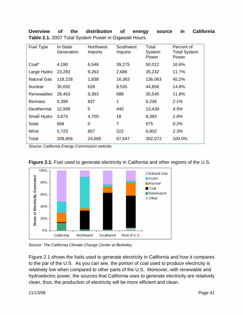
11/13/08 Page 41
Overview of the distribution of energy source in California
Table 2.1. 2007 Total System Power in Gigawatt Hours
Fuel Type In-State Generation
Northwest Imports
Southwest Imports
Total System Power
Percent of Total System Power
Coal* 4,190 6,546 39,275 50,012 16.6%
Large Hydro 23,283 9,263 2,686 35,232 11.7%
Natural Gas 118,228 1,838 16,363 136,063 45.2%
Nuclear 35,692 629 8,535 44,856 14.8%
Renewables 28,463 6,393 688 35,545 11.8%
Biomass 5,398 837 1 6,236 2.1%
Geothermal 12,999 0 440 13,439 4.5%
Small Hydro 3,675 4,700 18 8,393 2.8%
Solar 668 0 7 675 0.2%
Wind 5,723 857 222 6,802 2.3%
Total 209,856 24,669 67,547 302,072 100.0%
Source: California Energy Commission website.
Figure 2.1. Fuel used to generate electricity in California and other regions of the U.S.
Source: The California Climate Change Center at Berkeley.
Figure 2.1 shows the fuels used to generate electricity in California and how it compares
to the par of the U.S. As you can see, the portion of coal used to produce electricity is
relatively low when compared to other parts of the U.S. Moreover, with renewable and
hydroelectric power, the sources that California uses to generate electricity are relatively
clean, thus, the production of electricity will be more efficient and clean.

11/13/08 Page 42
Climate Change Impacts on Electricity Demand
Studies done by the California Energy Commission analyzed the relationship among
climate change, extreme heat, and electricity demand in California, and indicate that
extreme heat events will increase rapidly. The increase in temperature is forecasted by
a model based on three scenarios; A1fi, A2, and B1. A1fi is the higher emission
scenario, which is usually fossil intensive and with rapid introduction of new technologic
and economic growth; A2 is the mid-high emission scenario, which is a heterogeneous
world, with regionally oriented development and slower growth; B1 is the lower emission
scenario and is a convergent world with a rapid transitions to an information-based
economy, and is a “green” scenario. We assume the population trends in these three
scenarios are the same. Furthermore, extreme heat is defined here by the 90 percent
exceedance probability (T90) of the warmest summer days under the current climate.
JJAS is the short form of June, July, August, and September, which represents the
hottest months in a year. The T90, which described as the one-in-ten JJAS high
temperature day’s values, also known as the threshold temperature for the top ten
percent hottest summer days under the current climate. For example, the number of
extreme heat days in Los Angeles, where T90 is currently 95°F, may increase from the
present day value of 12 days per year up to 96 days per year by 2100.178 So, the T90
will be the hottest ten percent summer days under current climate condition, and is
threshold by 95°F. Based on this threshold, we predict that about 96 days by the 2100
summer will over 95°F, and this represented that the extreme heat days will last for the
whole summer.
Since global temperature is increasing, the frequency of the temperature exceeding the
T90 will expect to increase. The Intergovernmental Panel on Climate Change (IPCC)
estimates that global average temperatures could increase by 1.4ºC to 5.8ºC (2.5ºF to
10.4ºF) by 2100 and that the sea level may rise from 0.09 meters to 0.88 meters (0.3
feet to 2.9 feet). According to the historical data from 1960-1990, T90 events occurred
12 times per year on average. Furthermore, extreme heat days are expected to become
more intense, last longer, and occur earlier when compare to the historical reference.
By the period 2005-2034, the average extreme heat days in summer are expected to
double from 12 to about 23-24 days.179
In order to make a forecast of the future climate, different climate models are developed
for the climate stimulations. The Geophysical Fluid Dynamics Laboratory (GFDL) has
developed a medium-sensitivity global circulation model, and the National Center of
Atmospheric Research and the U.S. Department of Energy for modeling the climate and
178
Miller, N, Jin, J, Hayhoe, K, Auffhammer, M, 2007. Climate Change, Extreme Heat, and Electricity Demand in California. California Energy Commission, August 2007, 179
Miller et al., 2007.

11/13/08 Page 43
submitting the results to the Intergovernmental Panel on Climate Change (IPCC) have
developed a low-sensitivity model called Parallel Climate Model (PCM).
Figure 2.2. California-wide projected average number of JJAS T90 days per year from 1975 to 2100.
Source: Franco and Sanstad, 2006.
Figure 2.2 shows the California-wide projected average number of JJAS T90 days per
year from 1975-2100. According to the figure, by the end of the century, the extreme
heat days are expected to increase an average of four times in B1 scenario, 5.5 times in
A2, and 6.5 times in A1fi, which also mean that there are about 50 days in B1, 65 days
in A2, and 80 days in A1fi that will suffer from extreme heat days in the period 2070-
2099’s summertime.180
180
Miller et al., 2007.

11/13/08 Page 44
Table 2.2. T90 threshold values and projected increased number of days exceed the
1961-1990 T90 threshold
Source: Franco and Sanstad, 2006.
Table 2.2 gives us more specific data on how the extreme heat days will affect different
cities in California. According to the table, the T90 threshold value ranged from 27 oC in
San Francisco to 40 oC in Fresno. Due to the geological location, in some cities in
California, like Sacramento and San Bernardino, the T90 thresholds will be over 35 oC.
Thus, in scenario A1fi, these cities might have about 80 days extreme heat days, which
are about 35 oC - 40 oC, in the future summertime. If this happens, people in these cities
will suffer from extreme heat days for almost the entire summer. Generally, 65°F (18°C)
is an average daily mean temperature threshold for human thermal comfort,181 so more
energy will be demanded for cooling as the temperature increases and the average and
peak capacity of the power supply will then be challenged by the rapidly increased
demand especially during the summertime.
181
Miller et al., 2007.

11/13/08 Page 45
Figure 2.3. Electricity demand in the Cal ISO area as function of average daily temperatures in 2004
Source: Franco and Sanstad, 2006.
Table 2.3: Estimated increases in annual electricity and peak load demands for
the A1Fi, A2, and B1 scenarios, relative to the 1961–1990 base period
Source: Franco and Sanstad, 2006.
Under the worst scenario that the temperature will increase 1.9oC in 2010, electricity
requirements will increase by 7,500 gigawatt-hour (GWh) and the peak capacity will
increased by 2,400 megawatts (MW). In this case, we are expecting an increase of
energy and peak generation capacity by 2.6 and 3.7 respectively, from the 2010 base
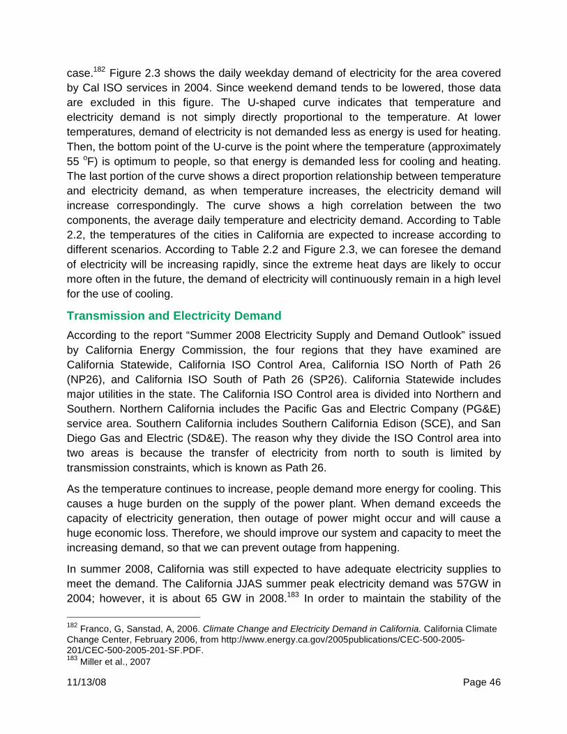
11/13/08 Page 46
case.182 Figure 2.3 shows the daily weekday demand of electricity for the area covered
by Cal ISO services in 2004. Since weekend demand tends to be lowered, those data
are excluded in this figure. The U-shaped curve indicates that temperature and
electricity demand is not simply directly proportional to the temperature. At lower
temperatures, demand of electricity is not demanded less as energy is used for heating.
Then, the bottom point of the U-curve is the point where the temperature (approximately
55 oF) is optimum to people, so that energy is demanded less for cooling and heating.
The last portion of the curve shows a direct proportion relationship between temperature
and electricity demand, as when temperature increases, the electricity demand will
increase correspondingly. The curve shows a high correlation between the two
components, the average daily temperature and electricity demand. According to Table
2.2, the temperatures of the cities in California are expected to increase according to
different scenarios. According to Table 2.2 and Figure 2.3, we can foresee the demand
of electricity will be increasing rapidly, since the extreme heat days are likely to occur
more often in the future, the demand of electricity will continuously remain in a high level
for the use of cooling.
Transmission and Electricity Demand
According to the report “Summer 2008 Electricity Supply and Demand Outlook” issued
by California Energy Commission, the four regions that they have examined are
California Statewide, California ISO Control Area, California ISO North of Path 26
(NP26), and California ISO South of Path 26 (SP26). California Statewide includes
major utilities in the state. The California ISO Control area is divided into Northern and
Southern. Northern California includes the Pacific Gas and Electric Company (PG&E)
service area. Southern California includes Southern California Edison (SCE), and San
Diego Gas and Electric (SD&E). The reason why they divide the ISO Control area into
two areas is because the transfer of electricity from north to south is limited by
transmission constraints, which is known as Path 26.
As the temperature continues to increase, people demand more energy for cooling. This
causes a huge burden on the supply of the power plant. When demand exceeds the
capacity of electricity generation, then outage of power might occur and will cause a
huge economic loss. Therefore, we should improve our system and capacity to meet the
increasing demand, so that we can prevent outage from happening.
In summer 2008, California was still expected to have adequate electricity supplies to
meet the demand. The California JJAS summer peak electricity demand was 57GW in
2004; however, it is about 65 GW in 2008.183 In order to maintain the stability of the
182
Franco, G, Sanstad, A, 2006. Climate Change and Electricity Demand in California. California Climate Change Center, February 2006, from http://www.energy.ca.gov/2005publications/CEC-500-2005-201/CEC-500-2005-201-SF.PDF. 183
Miller et al., 2007

11/13/08 Page 47
power system, we have to reserve a buffer for unplanned fluctuations when there are
system errors. A reserve margin is a measure of the amount of electricity imports and
in-state generation capacity available over average peak demand conditions. There are
two types of reserve margin, planning reserve margin and operating margin. Planning
reserve margin is a target level necessary to cover a certain range of possible system
fluctuations and unexpected emergencies. A low planning reserve margin may result in
a higher chance of customer curtailments. Generally, a 15-17 percent buffer of
additional supplies above typical peak demand is needed to ensure the adequate
supplies of electricity. Under the average summer weather conditions, the electricity
reserve margins in 2008 for California is about 22 percent; even in extreme heat days,
the reserve margins are still approximately 14 percent.184 Operating margin is the target
buffer that is assumed to be sufficient for control area operators to deal with immediate
emergencies or fluctuations in electricity demand. It also represents the amount of
imports and actual, spinning generation above current demand and represents real-time
operations that fluctuate minute by minute. When it drops below a certain level, the
minimum target is usually about seven percent, it will trigger additional purchase of
power and calls for demand response and voluntary interruptible programs to reduce
load. The California Independent Service Operator (California ISO) has divided the
warning level into three stages. Stage one is when the operating reserve is at seven
percent, stage two is at five percent, and stage three is when reserves fall to a level
between three and 1.5 percent,185 depending on the specific operating conditions. The
southern portion of the California ISO (SP26), which includes most of Southern
California, had a 3.8 percent probability of experiencing a staged emergency in 2008
summer according to Figure 2.4, however, it still remains at a comfortable level.
From the above figures and graphs, we might notice that Southern California is actually
hotter than Northern California and will suffer more from climate change than Northern
California. In fact, the power system in California and the other surrounding regions are
interconnected, but at the same time interdependent from each other. It then provides a
broad and reliable network of electricity to each connected area, moreover, the surplus
energy generated in the area, which is connected to the network, can be transferred to
other regions that have a higher demand during the peak demand period, therefore, the
electricity cost can then be reduced. Generally, Southern California will have a higher
demand of electricity than Northern California, so it will import electricity from Northern
California. However, demand of electricity in California is expected to increase rapidly
due to climate change, therefore, a series of problems might happen when Northern
184
Brown, D. 2008. Summer 2008 Electricity Supply and Demand Outlook. California Energy Commission, May 2008, from http://www.energy.ca.gov/2008publications/CEC-200-2008-003/CEC-200-2008-003.PDF. 185
Brown, 2008.

11/13/08 Page 48
California experiences a deficit in electricity and will not be able to export electricity
anymore to Southern California.
Figure 2.4. Loss of Load Probability
Source: Brown, 2008.
The California Independent System Operator will purchase short-term electricity if actual
demand is higher than the day-ahead forecast and need to supplement the scheduled
generation. Electricity can be imported from the generating plants located in other
western states, such as Canada and Mexico. Tables 2.4, 2.5, and 2.6 give us an
overview about California’s electricity interchange. According to these tables, we can
see that the import of electricity from Southern California is much larger than Northern
California. This may be due to the demand of electricity for cooling is high in Southern
California, since Southern California generally has an average temperature higher than
Northern California. So, if climate change continues, the temperature in Southern
California will expect to increase and extreme heat days are more likely to happen.
Then, we can expect Southern California have to import more electricity to meet the
demand, especially in hot summer season. On the other hand, Northern California
imports less energy; moreover, it exports some energy to Southern California. However,
if the temperature increases in the coming future, the demand for energy from Northern
California will absolutely increase and might not be able to provide as much energy to
Southern California. Then, Southern California may have to import even more energy
from other states or western countries. The rapid increase in electricity demand might
then challenge the reserve margin of the power plant, and will lead to outage of power
plants.
Table 2.4: Statewide Net Interchange

11/13/08 Page 49
Table 2.5: NP 26 Net Interchange
Table 2.6: SP 26 Net Interchange
Source: Brown, 2008.
Tables 2.4, 2.5, and 2.6 show the Overall Electricity Transfer in Statewide, and in
Northern and Southern California. According to the graphs, we can see that Northern
California is generally an electricity exporter, and exports a certain amount of energy to
Southern California each year. In 2008, we predict that Northern California will export
3000 MW of electricity to Southern California through Path 26; however, it also imports
surplus electricity generated from other Pacific Northwest regions where energy costs in
those regions are relatively lower than in California. On the other hand, since Southern
California experiences a hotter climate and thus a higher energy demand than Northern
California, it is a major electricity importer and is a large portion of import electricity of
the state. From the graphs, Northern California is currently having a 250 MW net import
from other regions, however, when temperature continues to increase, Northern
California might no longer be self-sustainable in terms of energy and need to import
more energy from nearby areas. Since the energy system is interdependent, the
increase in demand in Northern California will have a series effect on electricity supply
in other regions. Obviously, Northern California will be unable to transfer as much as
energy to Southern California if climate change worsens. Moreover, Southern California
will need to import even more energy from other regions. With the surplus supply of
energy reducing within the energy network, the rapid increasing demand and reducing
supply will drive the price of electricity to rise. Apart from that, due to the increasing

11/13/08 Page 50
demand, we might experience a higher probability of power outage, which might
increase the instability of our electricity system.
Climate Change Impacts on Hydropower
Hydroelectric power is one of the most important energy resources, which contributes
about 15 percent to 20 percent of the total electricity demand in California. California
has about 400 hydroelectric power plants, and produced 43,625 GW-h of electricity in
2007. The Pacific Northwest is along mountain ridges, e.g. Mount Rainer; and due to
the high elevation geological advantages, it is very suitable for the hydroelectric power
generation, which has contributed a significant amount of electricity to the whole region.
The water used for the generation of hydropower comes from the stream inflows
generated by precipitation in winter months and snowmelt during the spring season.
Thus, under the global warming scenario, the California’s hydrology would experience
an earlier timing of stream flows, which might greatly affect the operation of hydropower
plants. According to PG&E, the runoff resources that they used to use to produce
hydropower were groundwater aquifers (38 percent); snowmelt (36 percent); and rainfall
(25 percent). As the temperature increases, the inflow of stream water will come much
earlier as higher portions of precipitation would fall as rain instead of snow. Moreover,
snow pack will also experience an earlier spring snowmelt. Since the energy demand in
California’s summer is much higher than other seasons, this could create a problem of
timing mismatch between energy generation and energy demand, especially with
reservoirs that have low storage capacity. As the summer demand of electricity is high,
we have to store the spring water runoff for the power generation in summer. Thus, the
size of the storage capacity of the reservoirs determines how much water inflow during
springtime could be stored and used for power generation to meet the energy demand
during summertime.
The California Climate Change Center conducted a study on the potential effects of
climate change-induced hydrological changes on high elevation hydropower generation
in California. The study is mainly focusing on a case study on the Sacramento Municipal
Utility District (SMUD) hydroelectric system, which located in El Dorado County. The
hydropower system was built between 1957 and 1985. The whole project includes 11
reservoirs that can store over 425,000 acre-feet (AF) of water, and eight powerhouses
can generate up to 688 MW of power.186
186
Vicuna, S, Leonardson, R, Dracup, J, Hanemann, M. 2005. Climate Change Impacts on High Elevation Hydropower Generation in California’s Sierra Nevada: A Case Study in the Upper American River. California Climate Change Center, March 2006, from

11/13/08 Page 51
Figure 2.5 shows the perturbation ratios, which were based on the climate output
prediction under the greenhouse gases emission scenarios A2 and B1 by using different
climate models, such as NCAR, PCM, and GFDL. The unimpaired natural stream flow
represents the inflow in the period 1960-1990 and was predicted by the GCM (not
actual historical stream flow), and compared with stream flow prediction for 2070-2099.
Therefore, if the ratio is greater than one, it means that the inflow for 2070-2099 is
greater than the inflow for 1960-1990; on the other hand, if the ratio is smaller than one,
it means that the inflow for 2070-2099 is smaller than the inflow for 1960-1990.
According to Figure 2.5, a general pattern is shown in most of the models under
scenarios A2 and B1. The perturbation ratios in between May and September are
always smaller than 1, which represent that the stream flows in spring and summer are
going to decline in the future, however, the spring inflows will come much earlier in
wintertime (around February and March) as the ratios are higher than 1. Figure 2.6
shows monthly average stream flow conditions for Silver Creek to represent inflows into
the Union Valley reservoir in between 1928 –1949. Also, according to Figure 2.7 and
2.8, the perturbation ratios have translated into simulated stream flows under climate
change conditions. When compared to Figure 2.6, we can see from the graph that there
is a significant change in stream flow under climate change, which could be due to early
snow melt from the mountain. A shift in the stream flow period is shown, especially in
model GFDLA2_39, where the high stream flow timing has shifted from May to
February. Moreover, the volume of summer inflows is decreasing as well. Since the
energy demand is relatively high in summer in California, the timing of inflows takes a
significant role in terms of power generation and energy revenue.
http://www.energy.ca.gov/2005publications/CEC-500-2005-199/CEC-500-2005-199-SF.PDF. The remainder of this section is based on this paper.
11/13/08 Page 52
Figure 2.5: Monthly perturbation ratios (based on 2070-2099 climate change
conditions)
Figure 2.6: Unimpaired (pre-dam) inflows to Union Valley, 1928-1949 (Historic scenario)
Source: Vicuna et al., 2005.

11/13/08 Page 53
Figure 2.7 & 2.8: Stream flow conditions (unimpaired inflow to Union Valley) under Climate change scenarios, 2070-2099
Source: Vicuna et al., 2005.
With the SMUD hydroelectric system set up in the Upper American River, we are
interested in the system operation under different hydrological scenarios. According to
Figure 2.9, the patterns show that the hydropower system will maximize its productions
during summertime and minimize its productions during spring and winter, as energy
value during summertime is relatively high. And referring to Table 2.7, the annual
generation of electricity has dropped from 30 percent to 11 percent in different
scenarios. However, when we compare the reduction in power generations with the
reduction in annual inflows, we see that the change in annual inflows are similar to the
annual power generation, thus, we can treat the changes in annual stream flows
induced by the changes in total generation. However, the changes in annual revenue
are always higher than the changes in annual inflows. The annual revenue reduced less
when compared to the annual stream flows, and this shows that the system can reduce
the economic effect by storing the moving water to more valuable months. For example,
the annual stream flow has reduced 29 percent in model PCMB1_38, but the annual
revenue has only reduced 23 percent. This shows that reservoirs and good hydropower
systems can successfully reduce the impacts caused by the change in stream flow to
the economy.
Figure 2.9: Energy revenues: comparison of scenarios

11/13/08 Page 54
Table 2.7
Generation Dollar/year
Percentage change
MWh/year Average
Percentage change
Change in Annual Streamflow
Historical 37319340 1422699
PCMB1_38 28641080 77% 1025497 72% 71%
PCMB1_39 33323870 89% 1233249 87% 86%
GFDLA2_38 25973640 70% 914564 64% 62%
GFDLA2_39 32589481 87% 1208190 85% 86%
Source: Vicuna et al., 2005.
However, the operation of a hydropower generation system not only depends on the
stream flows but also on infrastructure such as reservoirs, powerhouse, and
conveyance capacities. We will mainly focus on how storage capacity of reservoirs can
deal with changes in hydrological conditions. In the SMUD’s Upper American River
project, the storage capacity of more than 400,000 AF in the 11 interrelated reservoirs
represent about 80 percent of average annual inflows into the system. In this study, we
estimate the effect on annual revenue and generation of reservoirs with different
storage capacities under the same hydrological scenario. Scenario one projects all
reservoirs in the system will double in size and scenario two projects all reservoirs in the
system will be reduced to a fourth of their size. The results of the two scenarios are
shown on Table 2.8 and Figures 2.10 and 2.11. As shown on Table 2.8, the total annual
power generated and the associated revenue in scenario one is greater than that in
scenario two. Also, the generation pattern under scenario one is similar to the pattern of
energy value, which indicates that the stream flow can be stored efficiently and be used

11/13/08 Page 55
at the time when energy is in high demand. However, the generation pattern under
scenario two is close to the pattern of stream flow, since most of the inflows are unable
to be stored in reservoirs for later use. This proves the benefits of having reservoirs to
store water and move stream flow from a less valuable month to a more valuable one.
Therefore, as climate change causes snow packs to melt and bringing the stream flows
earlier in springtime, the storage function of reservoirs has become more important to
energy generation and the revenue associated with it. However, these timing effects
should not affect the generation capacity when the storage capacity of the system is
sufficiently large.
Table 2.8: Changes in annual output from the system (as absolute value and as a
percent compared to historical output) for a doubling and a quartering of system
storage capacity
Source: Vicuna et al., 2005.
Figure 2.10: Energy revenues: doubling reservoir capacity
Source: Vicuna et al., 2005.
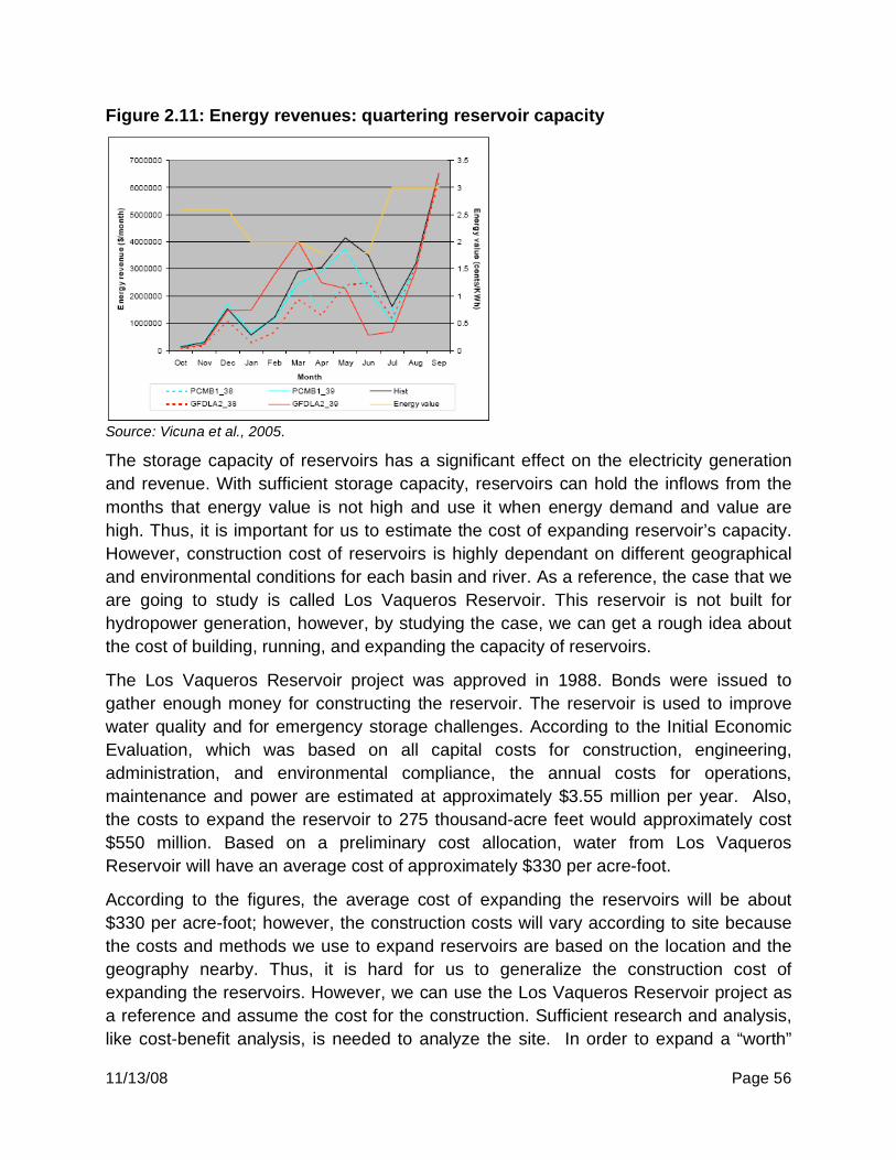
11/13/08 Page 56
Figure 2.11: Energy revenues: quartering reservoir capacity
Source: Vicuna et al., 2005.
The storage capacity of reservoirs has a significant effect on the electricity generation
and revenue. With sufficient storage capacity, reservoirs can hold the inflows from the
months that energy value is not high and use it when energy demand and value are
high. Thus, it is important for us to estimate the cost of expanding reservoir’s capacity.
However, construction cost of reservoirs is highly dependant on different geographical
and environmental conditions for each basin and river. As a reference, the case that we
are going to study is called Los Vaqueros Reservoir. This reservoir is not built for
hydropower generation, however, by studying the case, we can get a rough idea about
the cost of building, running, and expanding the capacity of reservoirs.
The Los Vaqueros Reservoir project was approved in 1988. Bonds were issued to
gather enough money for constructing the reservoir. The reservoir is used to improve
water quality and for emergency storage challenges. According to the Initial Economic
Evaluation, which was based on all capital costs for construction, engineering,
administration, and environmental compliance, the annual costs for operations,
maintenance and power are estimated at approximately $3.55 million per year. Also,
the costs to expand the reservoir to 275 thousand-acre feet would approximately cost
$550 million. Based on a preliminary cost allocation, water from Los Vaqueros
Reservoir will have an average cost of approximately $330 per acre-foot.
According to the figures, the average cost of expanding the reservoirs will be about
$330 per acre-foot; however, the construction costs will vary according to site because
the costs and methods we use to expand reservoirs are based on the location and the
geography nearby. Thus, it is hard for us to generalize the construction cost of
expanding the reservoirs. However, we can use the Los Vaqueros Reservoir project as
a reference and assume the cost for the construction. Sufficient research and analysis,
like cost-benefit analysis, is needed to analyze the site. In order to expand a “worth”

11/13/08 Page 57
expanding reservoir, we have to make sure the benefits from adapting an expanded
reservoir should be able to cover the cost of adaptation.

11/13/08 Page 58
3. Demographics: Background
Demographics are an important factor in determining the impacts of climate change.
The issue of population growth is especially pertinent to California, with one of several
current estimates predicting a growth of two percent every year in California, producing
a doubling of its population to 64 million by 2035. The two percent annual growth rate is
almost double that of the national average growth rate of 1.1 percent.187 The
methodology used to reach this estimate was not mentioned in the study, but other
studies’ estimates that used fertility and migration rates to extrapolate population levels
in the future arrived at somewhat differing conclusions. However, most population
forecasters agreed that by 2020 California will have a population of between 43 and 46
million.188
After 2020, the size of California’s population is less predictable and will depend on the
composition of the population, and future rates of fertility and migration, with estimates
predicting a population between 50 million and around 70 million.189 Not only do
population estimates differ from one study to another, but even population estimates
from the same study often can not pinpoint an exact number for the estimated
population, making it extremely difficult to come up with a single figure. Although the
exact rate of growth cannot be predicted, the forecasted growth rates will have a
tremendous impact on the projected use of energy, water, and land availability as well
as on air quality and transportation infrastructure. In turn, the projected uses of these
three resources will play a fundamental role in determining the impact of climate
change.
Energy
Electricity use will be affected by population growth in two separate ways – first by
increasing the residential demand for electricity and second by generating more
demand in the economic sector due to the creation of new jobs in the economy.
Economic and population growth are the main factors linked to electricity demand
187 Pimentel, David, 'and' Hart, Kelsey. "Rapid Population Growth in California: A Threat to Land and Food Production." Diversity Alliance for Sustainable America 07 17 2005 May 27 2008 <http://www.diversityalliance.org/docs/Pimental-LandandFood.html >. 188
Landis, John and Reilly, Michael. “How We Will Grow: Baseline Projections of the growth of
California’s Urban Footprint through the Year 2100. August 1, 2003. Institute of Urban & Regional
Development. IURD Working Paper Series. Paper WP-2003-04. 30 August 2008.
<http://repositories.cdlib.org/iurd/wps/WP-2003-04> 189
Ibid

11/13/08 Page 59
growth.190 More specifically, it is both the population growth and the spatial distribution
of this growth, along with economic growth that are the main drivers behind electricity
demand. In the 1990’s most of the increase in demand for electricity was in the building
sector. In 2000, the building sector alone comprised of 2/3 of the annual electricity
consumption and 3/4 of the summer peak load.191
Population growth is expected to be the greatest in the inland areas in California (the
Inland Empire, Sacramento Metro and San Joaquin Valley).192 These inland areas
already have higher temperatures than their coastal counterparts, thereby necessitating
even more energy use in the form of air conditioning. With the population growth, the
inland temperatures will soar even higher due to the increase in activities that emit
greenhouse gases. Air conditioner use tends to be the greatest during the day when
temperatures are higher, coinciding with the ‘peak time’ for businesses as well, thereby
increasing the demand for energy during the ‘peak’. Residential air conditioning by itself
makes up nearly as large a portion of the peak load as all industrial sectors
combined.193 Since power plants have to be designed to meet the demand at the peak
rather than the average demand, meeting the peak demand is extremely expensive
since the power plants built to provide peak demand do not operate for very long during
the day.194 In addition, these peak power plants are highly polluting as they are often
inexpensive natural gas power plants.195 Altogether, population growth has the potential
to increase not only overall electricity demand but also peak demand, which would in
turn increase pollution intensity and costs.
Transportation will become yet another factor to reckon with in the face of an increase in
population. A rise in population will necessitate an increase in the number of miles
driven and cause a higher rate of gasoline consumption as well as a higher rate of
greenhouse gas emissions from cars. California has already witnessed an increase in
the number of miles driven at a rate 50 percent faster than the rate of population growth
in the last 20 years. Vehicles emit about 30 percent of the state’s heat-trapping gases,
and are the single greatest source of such emissions.196 Since population growth is
190
Brown, Richard, 'and' Koomey, Jonathon. "Electricity Trends in California:Past Trends and Present Usage Patterns." Energy Policy 31,9 July 2003 849-864. 25 June 2008 <http://enduse.lbl.gov/info/LBNL-47992.pdf>. 191 Ibid 192 "Growth Slows, Diversity Grows In California's Regions." Public Policy Institute of California. May 8, 2002. 02 July 2008 <http://www.ppic.org/main/pressrelease.asp?i=279>. 193 Brown, Richard, 'and' Koomey, Jonathon. "Electricity Trends in California:Past Trends and Present Usage Patterns." Energy Policy 31, 9 July 2003 849-864. 25 June 2008 <http://enduse.lbl.gov/info/LBNL-47992.pdf>. 194 "Peaker Power Plant Fact Sheet." Illinois Environmental Protection Agency. 2007. 25 June 2008 <http://www.epa.state.il.us/air/fact-sheets/peaker-power-plant.html>. 195
Ibid 196
Barringer, Felicity. "California Moves on Bill to Curb Sprawl and Emissions ." 28 08 2008. New York Times . 2 Sep 2008 <http://www.nytimes.com/2008/08/29/us/29sprawl.html?_r=1&oref=slogin

11/13/08 Page 60
expected to be even greater in the inland areas, which have dispersed settlement
patterns, vehicle miles traveled would almost certainly increase as a result of longer
commute times. According to the Public Policy Institute of California, counties with the
longest commute times include San Joaquin Valley and Los Angeles and San
Bernardino counties. 197 These are three of the counties that are expected to experience
some of the highest population growth rates in California, adding significantly to the
number of miles traveled as a result of the longer commutes coupled with rapid growth
rates.198
Other aspects of transportation such as transportation infrastructure will also be put
under great stress in lieu of the expected population growth if it is not expanded to meet
the increase in population. The development of this infrastructure will for the most part
take place inland since that is where a significant part of the population growth is
expected to take place; with the increase in infrastructure inland having a major impact
on climate change by virtue of the increase in greenhouse gas emissions from the
magnitude of the construction efforts. Over the last two decades, there has been a 50
percent increase in population and miles driven and yet California has increased lane
capacity on its highways by seven percent. According to the census bureau, California
comes in at 48th place in investment in highways and 40th overall in infrastructure
investment according to personal income.199 In addition to highways, airports and ports,
which are also extremely vital to California businesses, will also need to be expanded to
meet the demands of a higher population. California’s airports are already working
beyond capacity without much room for expansion, and will need to be improved in
order to be able to cope with the population growth.200 These improvements are
especially vital to the proper functioning of California’s economy.
Air Quality and Public Health
Population growth is also certain to have an effect on the air quality of California by
virtue of the increased emissions. According to an article published in the journal
Demography that addressed recorded population growth and air quality data in
California in the 1980’s, emissions increased as a result of population growth from
197
Barbour, Elisa. “Time to Work”. Public Policy Institute of California: California Counts” February 2006. 30 August 2008. < http://www.ppic.org/content/pubs/cacounts/CC_206EBCC.pdf> 198
Landis, John and Reilly, Michael. “How We Will Grow: Baseline Projections of the growth of California’s Urban Footprint through the Year 2100. August 1, 2003. Institute of Urban & Regional Development. IURD Working Paper Series. Paper WP-2003-04. 30 Auguest 2008. <http://repositories.cdlib.org/iurd/wps/WP-2003-04> 199 Infrastructure." California Business Roundtable. 2006. 02 Jul 2008 <http://www.cbrt.org/infrastructure.html>. 200 Infrastructure." California Business Roundtable. 2006. 02 Jul 2008 <http://www.cbrt.org/infrastructure.html>.
11/13/08 Page 61
residential and commercial sources as well as from vehicles.201As mentioned earlier,
population growth is expected to be higher in the inland areas, where temperatures are
already higher than at the coastal areas, and there the increase in pollution will also be
higher in these inland areas. The increase in pollution and decrease in air quality will be
accompanied by higher temperatures in areas that are hotter than average due to
geographic characteristics. This poses a public health risk for the inland residents, with
the increase in pollution leading to a greater number of respiratory illnesses such as
asthma, and the increase in temperature leading to greater heat related hazards such
as heat stroke, fainting, and dehydration. As can be seen, most of the detrimental
health impacts of climate change as a result of population growth in California are a
result of the spatial distribution of this population growth and the dispersed nature of
pre-existing building patterns, particularly in the suburban inland empire.
Water
California is already witnessing a water crisis, and the impending population growth
would further increase the complicated water supply situation. California’s population is
expected to reach over 47 million by 2020 and by the same year, the urban population
in California is expected to use 12 million acre feet per year (mafy) of water, which is 3.2
mafy more than what was needed in 1995202 This reality, in light of the fact that every
water supply source in California is past its physical or legal capacity to be sustained,
demonstrates the extent of the stress that will be placed on California’s water supply as
a result of population growth. Despite the 3.2 mafy increase in water usage, the per
capita water use is actually expected to less in 2020 than it was in 1995].(02553 mafy
per person in 2020 vs. 0.2848 mafy per person in 1995). Despite this increase in use
efficiency, the amount of water used will still increase by 3.2 mafy due to the increase in
population, which will more than offset the increase in use efficiency. In addition, the
stress on water use will further be exacerbated by the population, especially because of
the spatial distribution of this population growth.
Most of the population growth is going to be taking place in Southern California
(including Imperial, San Diego, Orange, Riverside, San Bernardino, Los Angeles, and
Ventura counties) where the amount of urbanized land will grow from around 800,000
hectares in 1998, to 1,000,000 hectares by 2020) and San Joaquin Valley where the
amount of urbanized land will increase from 181,000 hectares in 1998 to 262,000
hectares by 2020.203 Considering the water crisis that is already plaguing the state, this
201 Cramer, James. "Population Growth and Air Quality in California." Demography 35(1998): 45-56 202 Jenkins, M. W. , J. R. Lund and R. E. Howitt. July 2002. “Impacts of Population Growth and Climate Change on California’s Future Water Supplies”. University of California at Davis. p. 9. 203 Landis, John and Reilly, Michael. “How We Will Grow: Baseline Projections of the growth of California’s Urban Footprint through the Year 2100. August 1, 2003. Institute of Urban & Regional

11/13/08 Page 62
spatial distribution of population growth does not bode well for the shortage. Southern
California already imports a little more than half of it’s water from outside the region ,
and the expected growth in population will only further exacerbate the water shortage.
204 A significant source of water for Southern California is the San Joaquin Delta, which
is experiencing a depletion in its water supply, and there is also a new restriction on
when water can be pumped from the delta in order to protect an endangered species of
fish. Therefore, even if Californians make a great deal of progress in their efficient use
of water, California’s water crisis will continue to be a major force to reckon with in the
future since some of the fastest growth is expected to occur in water scarce areas.
Population growth is only going to increase population driven stresses such as a water
crisis in the future, and it will be especially dire due to the location of the population
growth.
Agricultural water use in the future is also expected to pose a problem for the allocation
of scarce water resources. Currently agriculture uses up 80 percent of California’s
water supply and with the expected rise in population, water will become a highly
contested resource.205 At present, the federal government provides generous subsidies
to pay for water irrigation. These subsidies are estimated to be about $1.2 billion
annually, and with increasing population, agriculture will have to compete even more
fiercely for the water in face of growing human population and industry needs.206
Furthermore, high quality cropland is in danger of being lost to urban sprawl and erosion
and as a result poorer quality marginal land will have to be used for growing crops,
thereby necessitating even more irrigation.
Land Availability
According to estimates of the population doubling to 64 million by 2035, about 32 million
out of California’s 100 million acres will need to be utilized for housing, employment,
and transportation. 207At present, 122,000 acres, approximately 1.5 percent of the land
is lost to urban and industrial sprawl every year.208 In addition to losing land to urban
and industrial sprawl, California is losing land to agriculture, especially for biofuels as
well as for carbon sequestration. The abrupt rise in oil prices spawning the rise of
biofuels has also resulted in the conversion of marginal land into agricultural land strictly
Development. IURD Working Paper Series. Paper WP-2003-04. 30 Auguest 2008. http://repositories.cdlib.org/iurd/wps/WP-2003-04 204 Kightlinger, Jeff. “Southern California's Metropolitan Water District Diversifies Supply Portfolio Amid Protracted Drought”. Verde Exchange. . 01: 08:( Nov 2007). 30 August 2008. 205 Pimentel, David, 'and' Hart, Kelsey. "Rapid Population Growth in California: A Threat to Land and Food Production." Diversity Alliance for Sustainable America 07 17 2005 May 30 2008 <http://www.diversityalliance.org/docs/Pimental-LandandFood.html >. 206 Ibid 207 Ibid 208 Ibid

11/13/08 Page 63
for biofuel purposes. In the next 30 years, greenhouse gases that will be emitted as a
result of the conversion of land (forest or grassland) into new cropland to replace the
grains that had been reassigned to biofuels are expected to increase dramatically.209
Concurrently, there will also be an increase in population and demand for oil in these
next 30 years while the price of oil will be increasing, thereby creating an even greater
need for alternative fuels such as ethanol. This could result in a higher rate of land
conversion, placing an even further restraint on the amount of land available for
expansion for the rising population needs. A combination of losing land to urban sprawl
and biofuel purposes will make it harder for citizens of California to find land to meet
their residential and infrastructural needs while also meeting their agricultural and
natural resource needs such as transportation fuels.
Factors discussed previously such as land availability, energy use and water are all
dependent on the extent of population growth. When each of these categories is further
divided, the importance of the extent of population growth is even more evident as each
subcategory is dependent on the population, and therefore collectively the number of
people has a large effect on the usage of a particular resource. Whether it is the
consumption of water for residential as well as commercial and agricultural purposes, or
the residential and commercial demand for electricity and oil, or the availability of land
for expansion of residential areas and infrastructural purposes -- all of these are heavily
dependent on the number of people in California. However, population growth is rather
unpredictable, thereby making it difficult to come up with accurate estimates about
California’s population in the years to come. There have been several estimates
generated, but the precise number will be unknown because it is impossible to
determine how many people will be born and how many people will die; but even harder
will be to determine the number of immigrants that California will be home to, both
legally and illegally. Currently the projections show that most of this population growth is
going to occur in Southern California, especially in the inland areas where the impact on
climate change is higher as a result of the several factors as discussed earlier. In order
to try to minimize the population growth effects, the California government could
possibly institute policies that would encourage the new population to move into places
that would be lower risk areas. California’s State Assembly passed a measure on the
26th of August which would commit tens of billions of dollars in state and federal
transportation subsidies to cities’ and counties’ fulfillments of efforts to slow down the
increase in driving. The eventual goal is to encourage people to live in areas near
209 " Biofuels, Land Conversion and Climate Change." Hill Heat:Science Policy Legislation Action. 25 April 2008. 04 July 2008 <http://www.hillheat.com/events/2008/04/25/biofuels-land-conversion-and-climate-change>.
11/13/08 Page 64
current development and reduce commutes to work. 210 This measure would hopefully
prove effective in encouraging people to settle in areas that would decrease the
additional impact on climate change by driving less. Other strategies to facilitate the
population growth into areas that would be lower risk in terms of the effects population
growth would have on climate change would be ensure that the risks of living in the area
were reflected in the prices. For example, given the water shortage in Southern
California, if people wanted to settle in areas that were facing a dire water crisis, they
would need to pay a price for the risk, in terms of the price of water as well as the price
of housing. The government would need to get rid of subsidies that distort the true cost
of living in water scarce areas and encourage residents to live in areas that have more
sustainable water resources. Alternatively, in fire-prone areas, residents should have to
pay for the price of the fire risk that is borne by the state through provision of fire-fighting
services as well as the water used in protecting their homes during fires. Most
importantly, the increase in population growth will have to be managed in such a way as
to minimize the impact it would have on climate change.
This in turn, makes a significant difference to the predicted impacts of climate change
because all the predictions are based on human activities. Therefore coming up with an
estimate of the amount of greenhouse gases emitted and produced is highly contingent
on the number of people, but since the number of people is an unknown element, the
prediction could vary quite significantly depending on the population growth estimate
used. Population growth is not only a factor to reckon with in terms of its impact on
climate change, but it is also expected to have a tremendous effect on more imminent
issues such as the water crisis, electricity consumption, and infrastructural capacities. In
summary, population growth is a crucial factor not only for determining the impact on
climate change, but also for shorter term issues like resource management within
California.
Notes and References
210
Barringer, Felicity. "California Moves on Bill to Curb Sprawl and Emissions ." 28 08 2008. New York Times . 2 Sep 2008 <http://www.nytimes.com/2008/08/29/us/29sprawl.html?_r=1&oref=slogin>

11/13/08 Page 65
4. Transportation: Background
Climate change will have an impact on California’s transportation infrastructure with
some impacts being shorter term than others. The components of climate change that
are relevant to California and were looked into were changes in temperatures,
increased precipitation and rise in sea levels. The organization of this section divides
California’s transportation infrastructure into five sub-sections: surface transportation,
aviation, railroads, ports and marine transportation, and pipelines. Within each sub-
sections, first there will overview of impacts from the different components of climate
change and then possible adaptations. There are two sub-sections before the sections
on impacts and adaptation for specific modes of transportation. The first sub-section is
for estimates of the cost of the most immediate climate change impact for California,
which is increased precipitation specifically ENSO events. The second sub-section
deals with the current state of California’s transportation infrastructure. Besides the
effects of increased precipitation, most of the impacts of climate change on
transportation will be felt and have to be dealt with in a longer timeframe (Table 4.1).
Table 4.2. Expected Lifetimes and Impacts for Different Transportation Modes
Transportation Mode Expected Infrastructure Design Life
Main Impacts on Infrastructure
Impact Timeframe
Surface Transportation
Pavement 10-20 years Change in temperatures, increased precipitation and rise in sea levels
Longer term, shorter term, longer term
Bridges 50-100 years Changes in temperatures, rise in sea levels, wind loads
Longer term, longer term, shorter term
Culverts 30-45 years Increased precipitation
Shorter term
Tunnels 50-100 years Rise in sea levels, increased precipitation
Longer term, shorter term
Aviation
Runway pavement 10 years Change in temperatures, increased precipitation and rise in sea levels
Longer term, shorter term, longer term

11/13/08 Page 66
Terminals 40-50 years Change in temperatures, increased precipitation
Longer term, shorter term
Railroads
Rail tracks Up to 50 years Change in temperatures, increased precipitation and rise in sea levels
Longer term, shorter term, longer term
Ports and Marine Transportation
Locks and dams 50 years Rise in sea levels, change in temperatures
Longer term, longer term
Docks and port terminals
40-50 years Rise in sea levels, change in temperatures
Longer term, longer term
Pipelines 100 years Increased precipitation
Shorter term
Climate change will have an important impact on California’s transportation and its
infrastructure, but there are very few211 studies on the potential economic impact of
climate change on transportation operations and its infrastructure. California’s economy
relies heavily on its transportation infrastructure, especially for trade. In 2000 trade
shipments through California were $392 billion, an increase of nearly $100 billion since
four years earlier212. As can be seen in Table 4.2, California has three of the top ten U.S
foreign trade freight gateways by value of shipments in 2005. Of the few studies on the
topic that have been published, there are even less that are detailed and focus
specifically on California. Therefore the possible impacts can only be inferred from
studies of other regions and the economical costs can only estimated.
211
Wilkinson, Robert and Teresa Rounds. 1998. Climate Change and Variability in California; White Paper for the California Regional Assessment. National Center for Ecological Analysis and Synthesis, Santa Barbara, California Research Paper No. 4. Available at "http://www.nceas.ucsb.edu/papers/climate.pdf". duVair, Pierre, Douglas Wickizer, and Mary Jean Burer. 2002: Climate Change and the Potential Implications for California’s Transportation System. In The Potential Impacts of Climate Change on Transportation: Workshop Summary, U.S. Dept. of Transportation, Workshop, 1-2 October. 212
duVair et al., 2002.

11/13/08 Page 67
State of California’s Current Transportation Infrastructure
The current state of infrastructure in the state of California leaves much to be desired.
California currently has $2 trillion of transportation infrastructure. In the last 20 years its
population and miles driven has increased by 50 percent, but its lane capacity increase
on highways has only been 7 percent. It currently ranks 48th in investment in highways
and 40th in overall infrastructure investment213.As of 2006, California’s grade in the
ASCE Infrastructure Report Card is a C-, which is only slightly better than the national
one of a D. The grades for transportation infrastructure and port facilities are not much
better than the grade for the overall infrastructure in the state. These grades only take
into account current transportation infrastructure conditions, needs and demands, but
does not take into account the additional problems and costs that can arise from the
physical impacts of climate change. Even so, these grades are a good starting point to
evaluate California’s current transportation infrastructure.
According to the report, California receives a C- in aviation. This grade is based on
forecasted consistent growth in demand for air transportation while the capacity of the
aviation infrastructure in California is not ready to meet this growth due to limited
capacity and restrictions on infrastructure growth. The proposed annual investment
needed to achieve a B grade through the expansion of airports is $0.5 billion. The report
does not stop there and provides brief overviews of the conditions of the four largest
airports in the state.
The grade that California receives for overall transportation is an even lower D+. The
low grade stems from concerns over capacity and lack of investment besides seismic
upgrades and ongoing maintenance. The proposed investment in needed to bring the
grade up to a B is $17.9 billion per year. Among the transportation related infrastructure
213
California Infrastructure Coalition. Economic Impact of Funding California’s Transportation Infrastructure.

11/13/08 Page 68
in the report, ports received the highest grade of a C+. Current ports infrastructure is in
good condition, but with projected cargo expected to double by 2010 more infrastructure
upgrade is needed. The annual investment proposed for ports infrastructure is $1.2
billion214.
These grades and estimated investments needed for improvements for the different
sectors of California’s infrastructure are a good starting point for the possible impacts of
climate change on transportation infrastructure in general, but they are based on
capacity adequacy of current transportation infrastructure while the impact of climate
change will also affect and to a greater degree the quality side of infrastructure. Climate
change will undoubtedly increase the estimated costs needed to maintain transportation
infrastructure in the state. The importance of transportation infrastructure of course
cannot be denied. The need to increase spending on transportation infrastructure
should not be avoided, but there are also benefits from the increased spending in this
area. Every $1 billion of transportation spending creates 18,000 new jobs in the state.
As can be seen in Figures 1-3, for every construction job created with additional
transportation funding in California, there would be an additional 0.76 jobs in indirect
and induced sectors for a total employment multiplier of 1.76. For every dollar spent on
infrastructure, there will be an additional $0.97 in indirect and induced spending in the
state economy215.
Figure 3.1. Economic Impact of Funding California’s Transportation Infrastructure
214
ASCE California Infrastructure Report Card 2006. 215
California Infrastructure Coalition.
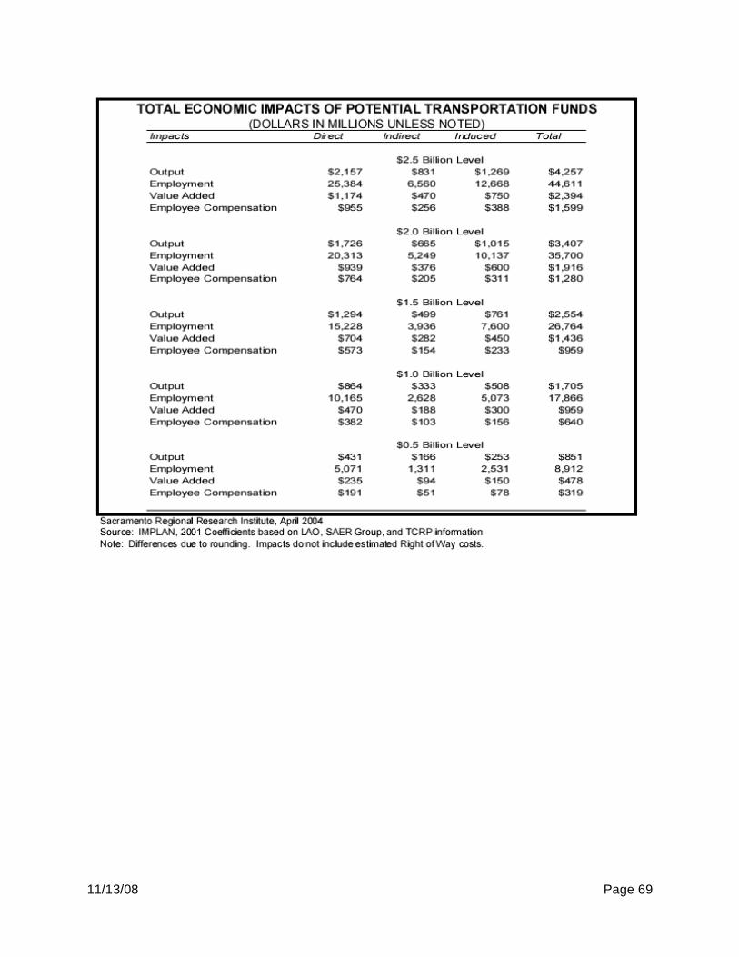
11/13/08 Page 69
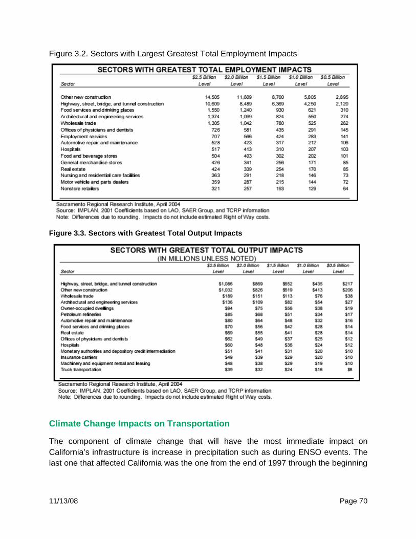
11/13/08 Page 70
Figure 3.2. Sectors with Largest Greatest Total Employment Impacts
Figure 3.3. Sectors with Greatest Total Output Impacts
Climate Change Impacts on Transportation
The component of climate change that will have the most immediate impact on
California’s infrastructure is increase in precipitation such as during ENSO events. The
last one that affected California was the one from the end of 1997 through the beginning

11/13/08 Page 71
of1998. Total losses for California in this event were $1.1 billion216. The effects of that
event hit California and specifically the Bay Area hard. The results of the increased
precipitation were sink holes, landslides, flooded highways and blocked roads. In April
of 1998, Caltrans had estimated the road damage for the Bay Area was $50 million and
for the state’s highway system it was $300 million. The hardest hit state highway was
Route 1, the Pacific Coast Highway where portions were closed for 13 weeks. Most of
the damage for Highway 1 and other roadways was from landslides and washouts.
Another problem was in the increased number of potholes. San Francisco usually fills
about 40 potholes per week, but on the week of February 16, it filled 157 potholes and
statewide by early March, Caltrans had spend more than 116,000 man-hours filling
thousands of potholes. Inland areas also felt the effects of ENSO such the flooding of
entire towns and three underpasses of Highway 99 becoming virtual lakes due to flash
flooding217. The damage estimates do not include the costs of preparation for ENSO,
such as the more than $200 million Caltrans spent to repair storm damage from the
winter of 1996-1997 and the purchase of 295,000 tons of abrasives and 12,000 tons of
deicers for $3.5 million to melt snow and improve traction on mountain roads218. The
preparation for this particular ENSO event was partly due to the $265 million in
damages (approximately $2 billion in losses when adjusted to 1998 dollars) suffered
during the one in 1982-1983. This suggests that the mitigation was effective in lowering
losses219.
Surface Transportation
The expected design life of surface transportation can be varied. For pavement it is 10-
20 years, for bridges it is 50-100 years, for culverts, a conduit used to enclose a flowing
body of water and allow the water to pass underneath a road, railway or embankment, it
is 30-45 years and for tunnels it is 50-100 years. The design lives are on average, but
most infrastructures operate beyond its expected design life. Climate change will have
a negative impact on the expected design lives of all surface transportation.
The first major expected component of climate change is temperature variations
especially increase in temperature for California. Temperature increases in the form of
increases of hot days and heat waves will impact pavement and concrete construction
process, cause thermal expansion on bridge expansion joints and paved surfaces.
Pavement impact includes concerns regarding pavement integrity such as softening,
216
Changnon, S.A. El Niño 1997:1998: The Climate Event of the Century. Oxford, New York: University Press, 2000. 217
http://www.tfhrc.gov/pubrds/julaug98/planning.htm 218
http://ceres.ca.gov/elnino/arar/bth.html 219
Changnon, Stanley A. “Impacts of 1997-98 El Niño- Generated Weather in the United States”. American Meteorological Society 80 (1999).

11/13/08 Page 72
traffic-related rutting and migration of liquid asphalt220. Warmer temperatures can
change the freeze/thaw cycles beneath roadways to the point where infrastructure
damage in the form of heaving or buckling may occur221. The impact of possible
decreases in cold days due to temperature is minimal. Also the benefits of reduced
pavement deterioration from later onset seasonal freeze and earlier onset of seasonal
thaw will be minimal for California.
The second major component of climate change is rising sea levels. Most of the impact
of rising sea levels will be in coastal areas with inundation of roads. In addition
underground tunnels and low lying infrastructure will be subjected more frequent or
severe flooding. Bridges will be particularly affected by the component of climate
change with probably erosion of road base and bridge supports, bridge scour and
reduced clearance under bridges. Bridges will also be affected wind loads, which is
stronger wind speeds and thus loads on bridge structures and possibly more
turbulence.
The last major climate change component is change in precipitation patterns. An
increase in intense precipitation events will increase the flooding of roadways and
subterranean tunnels, increase road washout, landslides and mudslides that damage
roadways. Increased intense precipitation will also create overloading of drainage
systems that can then cause backups and street flooding. Impacts on soil moisture
levels from increased intense precipitation can affect the structural integrity of roads,
bridges and tunnels. There is also an adverse impact of standing water on the road
base. The other side of changes in precipitation patterns is increases in drought
conditions, which can increase the susceptibility to wildfires that can then be a direct
threat to transportation infrastructure. In areas that are deforested by wildfires, there is
increased susceptibility to mudslides. Lastly if the change in precipitation patterns is in
the form of precipitation change from snow to rain in winter and spring thaws, there is
an increased risk of floods from runoffs, landslides, slope failures and damage to roads.
There are also impacts on surface transportation infrastructure from more frequent
storms such as hurricanes, but this is not applicable to California222. Highway 1 already
experiences frequent mudslides and high waves during mild winter storms, as well as
washouts every year. Certain roadways could be closed permanently if there are
significant increases in erosion, landslides or roadway undercutting. Damage from
1997-1998 El Niño event included the repeated washing out of major highways and
220
National Research Council (NRC). Potential Impacts of Climate Change on U.S Transportation. 2008. Transportation Research Board Report 290. 221
Pisano, Paul, Lynette Goodwin and Andrew Stern. 2002: Surface Transportation Safety and Operations: The Impacts of Weather within the Context of Climate Change. In The Potential Impacts of Climate Change on Transportation: Workshop Summary, U.S. Dept. of Transportation, Workshop, 1-2 October. 222
NRC, 2008.

11/13/08 Page 73
smaller roads, isolation of rural communities, destruction of 1,000 feet of the levee along
the Santa Maria River resulting in the flooding of hundreds of acres of agriculture lands
in Ventura County, the undermining of the Union Pacific railroad trestle by surging flows
from the Ventura River and a damaged rail bridge in San Clemente. The cost of this
event to the state was $550 million in total losses and damages223.
Climate change’s impact on transportation is not only limited to its impact on
transportation infrastructure, but will also have economic and operational impacts. The
operational impacts in terms of variations in temperatures vary depending on the sign of
the temperature change. In the case of increases in very hot days and heat waves
besides the obvious impact of vehicle overheating and tire deterioration there is also the
impact of limitations on periods of construction activities due to health and safety
concerns with restrictions typically beginning at 85°F (29.5°C) and possible heat
exhaustion at 105°F (40.5°C). In the other temperature case the impact of the decrease
in very cold days is usually beneficial in the form of fewer cold-related restrictions for
maintenance workers and lower snow and ice removal costs, but all the impact from this
case is minimal for California. In terms of the seasonal temperature change, later onset
of seasonal freeze and earlier onset of seasonal thaw, its impact will be felt through
changes in seasonal weight restrictions, changes in seasonal fuel restrictions, longer
construction season and improved mobility and safety associated with a reduction in
winter weather.
Sea level rise will only impact surface transportation operations in coastal areas where
rising sea levels added to storm surges can result in more frequent interruptions in
travel due to flooding. Change in precipitation patterns will have a great impact on
surface transportation operations. Increase in intense precipitation events will cause
increases in weather-related delays, increases in traffic disruptions, and increases in
flooding of evacuation routes. Also changes in rain, snowfall and seasonal flooding that
can impact safety and maintenance operations and disrupt construction activities.
Increases in drought conditions will increase susceptibility to wildfires that can cause
road closures due to fire threat or reduced visibility. Changes in seasonal precipitation
will provide benefits for safety and reduced interruptions if it is in the form of frozen
precipitation shifting into rainfall, but as mentioned earlier this can also increase risks of
floods, landslides and slopes failure.
In order to deal with climate change, transportation infrastructure has to be changed
and adapted to meet the new climate conditions. Temperature changes in the short
term (30 to 40 years) will have minimal impact on pavement or structural design but
potential significant impact on road, bridge scour and culvert design in cold regions,
which is not that applicable to California. In the long term (40 to 100 years) climate
change will have a significant impact on pavement and structural design, requiring new 223
duVair et al., 2002.

11/13/08 Page 74
materials and better maintenance strategies. Changing precipitation levels in the short
term could affect pavement and drainage design. There could be a need for greater
attention to foundation conditions, more probabilistic approaches to design floods
(hypothetical floods used for planning and floodplain management) and more targeted
maintenance. In the long term, there is going to be an impact on foundation design and
the design of drainage system and culverts. Climate change will also have an impact on
design of pavement sub-grade and materials. Wind loads in the short term (30-40
years) could impact change design factors for design of wind speed and wind tunnel
testing will have to consider more turbulent wind conditions. In the long term, there is
the need for stronger materials and there is an impact on design considerations for
suspended and cable-stayed bridges. There is not much in term of short term for the
effect of sea level rise. In the long term, there will be greater inundation of coastal
areas. To combat this, there is a need for more stringent design standards for flooding
and building in saturated soils. Also, greater protection of infrastructure of infrastructure
is needed in cases when higher sea levels combine with storm surges. The impact of
greater storm surges and wave heights in the short term will be felt in the need for
design changes to bridge heights in vulnerable areas and the need for more
probabilistic approach to predicting storm surges. In the long term, there will be a need
for design changes to bridge design in both superstructure and foundation, a need for
change in material specifications and more protective strategies for critical components.
Besides the adaptations described above, there are also adaptations to the previously
described physical and operations impacts of climate change on surface transportation.
In the case of increases in very hot days and heat waves, the adaptation options to deal
with the infrastructure impact are development of new heat-resistant paving materials
and greater use of heat-tolerant street and highway landscaping. In order to deal with
the limitations on construction activities, there would be a need to shift construction
schedules to cooler parts of the day, which is less important. The changes in operations
to deal with decreases in very cold days are mainly beneficial such as reduction in snow
and ice removal, extension of construction and maintenance season and shortening of
season for use of ice roads, but this is less relevant for California. This last change can
also be used in the case of changing seasonal temperatures in addition to the relaxation
of seasonal weight restrictions. Out of all of these changes the most important one for
California is the one dealing with increases in very hot days and heat waves, but climate
change-infrastructure relationship for California is a topic that is just being broached by
state agencies and is still a relatively unexplored area.
There are various adaptation possibilities for surface transportation infrastructure in the
case of sea level rise coupled with storm surges. In term of changes in infrastructure
design, the adaptation options are elevation of streets and bridges, elevation and
protection of bridge, tunnel and transit entrances, additional drainage canals near
coastal roads and additional pumping capacity for tunnels. Besides these adaptations,

11/13/08 Page 75
there are other possibilities that are more general and that would not only affect
transportation infrastructure but also other areas. These adaptations would be along the
lines of relocating sections of roads inland, protecting high value coastal real estate with
levees, seawalls and dikes, strengthening these structures that are already in place,
restricting development of most vulnerable coastal areas and returning some coastal
areas to nature224. It was estimated in 1989 that the cost to elevate affected streets in
Miami in order to deal with rising ground water levels due to sea level rise was $200
million in 1989 dollars. New Zealand estimated the cost of retrofitting or redesigning its
bridges for climate change and found out that by doing so initial costs are increased by
about 10 percent, but that over the life of the structure the incremental cost is less than
1 percent due to the decreased probability of climate related damage225. The most
important ones in terms of transportation infrastructure are probably the changes in
infrastructure design while the other adaptations are more general and not specifically
dealing with transportation infrastructure.
In the case of precipitation change impact on surface transportation infrastructure and
operations, most of the adaptations are to deal with increases in intense precipitation
events. On the infrastructure side, the adaptation options are protection of critical
evacuation routes, upgrade of road drainage systems, protection of bridge piers and
abutments with riprap and addition of slope retention structures and retaining facilities
for landslides. Other adaptation include increases in culvert capacity, increases in
pumping capacity, increases in the standard for drainage capacity for new
transportation infrastructure and major rehabilitation projects (using assumptions of a
500-year instead of a 100-year storm). On the operations side, the adaptation options
are expansion of systems for monitoring scour of bridge piers and abutments, increase
in monitoring of land slopes and drainage systems, increase in real-time monitoring of
flood levels and integration of emergency evacuation procedures into operations. There
are also other more general adaptations such as greater use of sensors for monitoring
water flows and restriction of development in floodplains. In the case of increases in
drought conditions, the suggested adaption option to deal with the increased probability
of wildfires is vegetation management226.
Aviation
The expected design life of aviation infrastructure varies. For runway pavements it is 10
years while for terminals it is 40-50 years227. Weather has a very direct impact on
aviation. It is responsible for 70 percent of the delays in the National Airspace System 224
NRC, 2008. 225
U.S. Climate Change Science Program. Impacts of Climate Change and Variability on Transportation Systems and Infrastructure: Gulf Coast Study, Phase I. 226
NRC, 2008. 227
NRC, 2008.

11/13/08 Page 76
(NAS) according to FAA statistics. The estimated total national weather impact cost for
accident damage and injuries, delays, and unexpected operating costs is $3 billion228.
The economic costs from the impact of climate change on the aviation industry will
undoubtedly increase these costs for the aviation industry.
The impacts of increases in temperature for aviation infrastructure are heat-related
weathering and buckling of pavement and concrete facilities and heat related
weathering of vehicle stock.
The impact of rising sea levels on aviation infrastructure will only affect airports in
coastal areas through the inundation of airport runways in those areas229. Examples of
coastal airports that would be affected by flooding include the San Francisco, Oakland
and Santa Barbara airports that were built on wetlands back when they were called
swamps and today are about 10 feet above current sea level. Extreme high tides
together with flood conditions are enough to reach close to the existing levels.230 This is
really critical because airports are more expensive to deal with and moving them would
be both problematic and incredibly expensive compared to the relatively easier
adaptation possibilities for pavement and vehicle stock.
The impact of increased intense precipitation on aviation infrastructure is varied. The
first impact is on the structural integrity of airport facilities. Another impact is the
destruction or disabling of navigational aid instruments. Increased intense precipitation
will also create flooding, which can damage runways and other infrastructure. In
addition, pavement drainage systems can be rendered inadequate or damaged from
this change in precipitation pattern and from changes in seasonal precipitation.
Temperature change will have a greater impact in terms of operations for aviation than it
had in terms of infrastructure. Increases in very hot days and heat waves will have an
impact on lift-off load limits at high-altitude or hot-weather climate airports with
insufficient runway lengths. This will result in flight cancellations and limits on payload
(i.e., weight restrictions). In addition delays due to excessive heat are possible and
ground energy consumption will increase. The decrease in very cold days from
temperature change will have some beneficial impacts in terms of aviation operations,
but their impact for California is minimal compared to that of the increase in very hot
days. Among the impacts on operations from this case in temperature change are lower
snow and ice removal costs, reduction in need for deicing and fewer limitations on
228
Kulesa, Gloria. 2002: Weather and Aviation: How does weather affect the safety and operations of airports and aviation, and how does FAA work to manage weather-related effects? In The Potential Impacts of Climate Change on Transportation: Workshop Summary, U.S. Dept. of Transportation, Workshop, 1-2 October. 229
NRC, 2008. 230
duVair et al., 2002.
11/13/08 Page 77
ground crews at airports, which are typically restricted when wind chills below -20°F (-
29°C). Sea levels rise will affect operations in airports in coastal zones creating the
potential for closure or restrictions for airports in these areas.
Changes in precipitation patterns will have a great impact on aviation operations.
Increase in intense precipitation events will increase delays due to convective weather,
increase the probability delays and closing of airports from flooding due to storm water
runoff that exceeds the capacity of collections systems. There are also implications for
emergency evacuation planning, facility maintenance and safety management.
Increases in drought conditions will decrease visibility for airports located in drought
areas with potential increases in wildfires. Changes in seasonal precipitation will have
similar effect on air transportation as it did on land transportation with the benefits of
safety and reduced interruptions if frozen precipitation shifts to rainfall.
As expected from the greater impact of changes in temperatures on aviation operations
compared to infrastructure, there are more adaptation options for aviation in that area.
The adaptation options for aviation infrastructure in the case of increases in very hot
days and heat waves are development of heat-resistant runway paving materials and
extension of runway lengths at high-altitude or hot-weathered airports if it is feasible to
deal with conditions such as high density altitude and payload restrictions that hamper
takeoffs. On the operations side, the adaptations are increase in payload restrictions on
aircraft at high-altitude or hot-weathered airports and increase in flight cancellations. In
the case of decreases in cold days, the adaptations are on the operations side and
beneficial such as reduction in snow and ice removal, and reduction in airplanes
deicing. This last aspect is not that relevant for California since most of the major
airports are not at a relatively high altitude, but there are still some airports that are.
The adaptation options for aviation in the case of sea levels rise only apply to those
airports that are located in coastal areas and are on the infrastructure side. One
adaptation possibility is the elevation of some runways. Other adaptations are
construction or raise of protective dikes and levees, and relocation of runways if
feasible, but this is a regional thing depending on the airport.
The main infrastructure adaptation for aviation to deal with the change in precipitation
patterns of climate change is through increases in drainage capacity and improvement
of drainage systems supporting runways and other paved surfaces. On the operations
side, the adaptations are to be ready for more disruption and delays in air service and
more airport closures in the case of increases in intense precipitation events231. Overall,
weather will have a significant impact on the operations side, however on the cost
231
NRC, 2008.

11/13/08 Page 78
perspective there is not much in terms of infrastructure adaptations besides the
improvements to runways that are similar to the pavement adaptations.
Railroads
The expected design life of rail tracks is up to 50 years. In terms of railroads, floods
produce some of the largest economic damages232. The Midwestern river floods of 1993
flooded or idled over 4000 miles of track and estimated losses were over $200 million.
In 1997 in Kingman, Arizona, a flash flood weakened an existing wooden trestle and led
to the derailment of an Amtrak passenger train with damages of $7.2 million233.
The impacts of increases in temperature for railroads are rail track deformities and
equipment failure is possible when air temperature is above 110°F (43°C)234. Track
misalignments caused by heat kinks are often the reason for train derailments that can
lead to injuries, fatalities, property damage and toxic release of hazardous material.
Another consequence of temperatures extremes is that railroad tracks may be exposed
to uneven thermal expansion when shade is covering nearby sections, which can create
the risk of warp and misalignment to freight traffic235.
The impact of rising sea levels for railroads is only limited to inundation of rail lines in
coastal areas.
The impact of increased intense precipitation on railroads is increased flooding of rail
lines, possible damages to rail-bed support structures and landslides and mudslides
that can damage tracks236. Coastal railroads have had similar problems such as
landslides and mudslides during heavy storms with the results of shutting down of
passenger and freight traffic for days237.
Changes in precipitation patterns will have a similar impact on railroads as it did on
surface transportation. Increases in intense precipitation events will cause increases in
weather-related delays and disruptions of construction activities. Also changes in rain,
snowfall and seasonal flooding that can impact safety. Increases in drought conditions
will increase susceptibility to wildfires. Last, changes in seasonal precipitation will not
have as great of an impact on railroads as it did on other surface transportation.
232
NRC, 2008. 233
Rossetti, Michael A. 2002: Potential Impacts of Climate Change on Railroads. In The Potential Impacts of Climate Change on Transportation: Workshop Summary, U.S. Dept. of Transportation, Workshop, 1-2 October. 234
NRC, 2008. 235
Rossetti 236
NRC, 2008. 237
duVair et al., 2002.

11/13/08 Page 79
The adaptation option for railroad infrastructure to deal with increases in very hot days
and heat waves is to have a greater use of continuous welded rail lines238. Continuous
welded rail lines are more expensive and have been common in main lines since 1950s
in the U.S and they are usually installed at 90 °F to cope with extremes of up to 120 °F.
The cost to replace track range is from $0.5 million to $3 million per mile excluding any
additional right of way expenses239.
The adaptation option for railroad infrastructure to deal with sea level rise coupled with
storm surges is elevated rail lines. In addition there are other more general adaptations
options along the lines of relocating of sections of rail lines inland that affect other areas
besides transportation and that have been already mentioned earlier in the surface
transportation section. In the case of railroad transportation adaptations for the
changes in precipitation patterns aspect of climate change, the adaptation options to
deal with increased frequency of landslides, mudslides and wildfires are similar to those
in the surface transportation section240.
Ports and Marine Transportation
The expected design life for ports and marine transportation varies a little. For locks and
dams it is 50 years while for docks and port terminals it is a little less, 40-50 years.
Ports and marine transportation as expected will be the sub-sector of transportation
most affected by rising sea levels. Rising sea levels will cause higher tides and storm
surges that will necessitate changes in harbor and port facilities to accommodate for
them. There will also be reduced clearance under waterway bridges and mentioned
previously in the surface transportation. Rising sea levels will also create changes in the
navigability of channels with some being more accessible and further inland due to
deeper waters while others will be restricted due to changes in sedimentation rates and
shoal locations241. Harbors may be subjected to wave damage, additional siltation from
storm runoff and other navigation and safety problems242.
The impact of increased intense precipitation on ports and marine transportation will
impact harbor infrastructure through wave damage and storm surges. It will cause
changes in underwater surface and silt and debris buildup, which can affect channel
depth. Changes in seasonal precipitation will cause changes in silt deposition leading to
reduced depth of some inland waterways and impact the long-term viability of some
inland navigation routes.
238
NRC, 2008. 239
U.S. Climate Change Science Program 240
NRC, 2008. 241
NRC, 2008. 242
duVair et al., 2002.

11/13/08 Page 80
Temperature change’s impact on ports and marine transportation infrastructure is
minimal, however it will have an impact on its operation. Increases in very hot days and
heat waves will have an impact on shipping due to warmer water in rivers and lakes.
Decreases in very cold days will a positive impact in shipping through less ice
accumulation on vessels, decks, rigging and docks, less ice fog and fewer ice jams in
ports. The impact from seasonal temperature change is extended shipping season for
inland waterways243. The other side of this is the effect of droughts on the inland river
transportation system. California can learn from the experiences of mid-western states
on the subject such the 1988 drought that affected the Mississippi River that reduced
traffic by one fifth. California’s rivers have similar control mechanisms in place to those
of the Mississippi navigation system to maintain water levels and safeguard navigation
during much of the year, but that may not even be enough as was the case in 1988
where low water levels in the Mississippi River left nearly 4000 barges stranded in
Memphis, Tennessee244.
Sea level rise will not have much impact on the actual operation of ports and marine
transportation, which is in direct contrast with the huge impact this aspect of climate
change has on infrastructure. Combined with more severe storm surges it can lead to
required evacuation and interruption of operations.
Changes in precipitation patterns have an impact on marine transportation. Increases in
intense precipitation events will cause increases in weather-related delays while
increases in drought conditions will have an impact on river transportation routes and
systems. Changes in seasonal precipitation and flow patterns will cause periodic
channel closings or restrictions in the case of flooding increases.
The adaptation options for ports and marine transportation to deal with changes in
temperature are not that many and mainly on the operations side. The only adaptation
on the infrastructure side is in the case later onset of seasonal freeze and earlier onset
of seasonal thaw, where the infrastructure adaptation is to design shallower bottom
vessels for seaway travel. To continue with this aspect of temperature change, the
adaptation in the operations side is through increases in summer load restrictions.
There are also other more general adaptations such as shifts more dredging that come
with environmental and institutional issues. In the case of decreases in cold days, the
operational adaptation will be improvement in operating conditions from less ice
accumulation, fog and jams.
Sea level rise is the aspect of climate change that will have the most direct impact on
ports and marine transportation, therefore it is the area where the implementation of
adaptation options is more critical. On the infrastructure side, the adaptations are the
243
NRC, 2008. 244
duVair et al., 2002.

11/13/08 Page 81
raising of dock and wharf levels and retrofitting of other facilities to provide adequate
clearance, the protection of terminal and warehouse entrances and the elevation of
bridges and other structures. On the operations side, the adaption is in the form of more
frequent bridge openings to handle shipping. There are also other adaptations such as
more dredging of some channels and raising or constructing new jetties and seawalls to
protect harbors.
The impact of changes in precipitation patterns on ports and marine transportation
requires a few adaptations. In the case of increases in intense precipitation events, the
adaptation options are all on the infrastructure side and include the strengthening of
harbor infrastructure to protect it from storm surges and wave damage, and the
protection of terminal and warehouse entrances from flooding. Another possible
adaptation is more dredging on some shipping channels. In contrast, the adaptation
options in the case of increases in drought conditions are on the operations or other
category. The change in operation is through restrictions on shipping due to channel
depth along inland waterways and in other river travel. Other possible adaptations to
deal with this aspect of change in precipitation is release of water from upstream
sources, shifts to other transportation modes and again the option of more dredging on
some shipping channels and harbors. The adaptation options in the case of changes in
seasonal precipitation are similar to those in the previous case of increases in drought
conditions245.
Pipelines
The expected design life of pipelines is 100 years. Temperature shifts resulting from
climate change scenarios are not expected to have much direct or indirect impact on
pipelines because pipelines protected from the effects of temperature change by the
moderating and insulating effects of water and soil246. The main component of climate
change that will have an impact on pipelines is increase in intense precipitation, which
can cause increase scouring of pipelines roadbeds and damages to pipelines
themselves. The adaptation for this impact is in the form of increases in monitoring of
pipelines for exposure, shifting, and scour in shallow waters247.
Financing Transportation Infrastructure
Finance will be an important part of climate change adaptation in the transportation
sector, and we provide a quick synopsis of current financing mechanisms here. The
funding for California’s transportation system primarily comes from a combination of
245
NRC, 2008. 246
U.S. Climate Change Science Program 247
NRC, 2008.
11/13/08 Page 82
federal, state, and local taxes. Other funding sources include fees, assessments, and
private investment. These revenues from these sources go into a number of funding
accounts. California then has a number of programs that guide the use of these funds.
Federal Funds. The IRS collects the Federal fuel excise tax. The revenues are
deposited into the Highway Trust Fund (HTF). 85 percent of the HTF revenues go to
the Highway Account of the HTF while the other 15 percent go to the Transit Account.248
The funds in the Highway Account are distributed among the states as federal funds for
projects on the state highway systems by the Federal Highway Administration (FHWA).
This federal agency has an annual budget of over $30 billion. For the fiscal year of
2007, the FHWA had a total budget of approx. $39.1 billion. In addition, the FHWA is
requesting a budget of $40.1 billion for 2009.249 The funds in this account are mainly
divided into two different programs. The first program is the Federal-aid Highway
Program which provides resources and technical assistance to State and local
governments for constructing, preserving, and improving the National Highway System.
The program also provides resources for urban and rural roads that are eligible for
Federal aid. The second program under the FHWA is the Federal Lands Highway
Program. This program funds public roads and highways that are on federal and tribal
lands that are not a State or local government responsibility. In addition to upkeeping
the highway systems, funds are also put toward promoting safety, congestion mitigation,
and environment issues. The FHWA uses funds toward new technologies research and
outreach projects that promote safety standards. Funds are also given to traffic control
centers in metropolitan areas to help remove congestion on their system. Funds are
also given to projects to support and restore the environment.
The funds in the Transit Account are distributed to regional agencies and local transit
providers in each state by the Federal Transit Administration. This federal agency
distributes federal funds to locally planned, constructed, and operated public
transportation systems throughout the United States. These systems include buses,
subways, light rail, commuter. The FTA is requesting a budget of $10.1 billion for the
fiscal year of 2009. $8.4 billion of the budget is to go for transit services, including
security, planning, bus and railcar purchases and maintenance, facility repair and
construction, and operating expenses. The grants in this budget also goes toward
special transportation needs of he elderly, people with low incomes, and persons with
disabilities. It also hopes to improve the accessibility of over-the-road buses,
alternatives analysis for projects, and to fund the National Transit Database. $59.6
million of the proposed budget is to go toward transit research programs. These
programs include grants to help develop solutions to improve public transportation and
248
Transportation Funding in California, pg. iii-iv. 249
“U.S. Department of Transportation Fiscal Year 2009 Budget in Brief - Federal Highway Administration”, <http://www.dot.gov/bib2009/htm/FHA.html>
11/13/08 Page 83
develop clean fuels and hybrid-electric buses. $1.6 billion of the proposed budget goes
toward capital investment grants. These grants sponsor the construction of new
guideway corridors, and extensions of existing systems. In addition, $48.3 million of the
budget is requested to support transit security. Through its assistance and other
programs, the FTA will use its money toward security training for transit system
employees, emergency preparedness and response, and public awareness efforts. The
rest of the proposed budget is to go toward the salaries of the people overseeing all the
programs involved.250
State Funds. The state of California has four main sources of funding for their
transportation system:
State Fuel Tax California collects an excise tax on gasoline and diesel fuels. 65
percent of this revenue is distributed to California Department of Transportation
(Caltrans). The other 35 percent is given to cities and counties.251
Truck Weight Fees California collects a fee on commercial vehicles based on
their weight. This represents a compensation for the wear and tear on the
roadways.
State Sales Tax California collects a 7.25 percent sales tax. Certain portions of
this tax are put aside for transportation. In 1971, the Transportation
Development Act set aside percent of this state sales tax for transit purposes
only. In order to do so, a Local Transportation Fund (LTF) was set up in each
county to receive the money. The act also extended the state sales tax to
gasoline sales to compensate the state general fund for the loss of the percent
sales tax. Any excess revenues are deposited into the Public Transportation
Account (PTA).252
Proposition 1B Bonds This 2006 bond act provides $19.9 billion to fund projects
that will improve the transportation system.253 For more information on the Prop
1B bonds, please refer to the Prob 1B Bond program below.
California’s highways, local roads, transit and rail, and aviation are funded through a
variety of mechanisms. However, many of these mechanisms are outdated and can no
longer support operations. For instance, many of California’s highways have already
surpassed their intended life. As a result, maintenance costs have continued to grow.
Proposition 1B does provide a one-time additional funding for rehabilitation projects, but
it does not address the problem that maintenance costs are rising faster than current
revenue streams. A proposed solution to increase revenues is to index the gas tax for
250
“U.S. Department of Transportation Fiscal Year 2009 Budget in Brief – Federal Transit Administration, <http://www.dot.gov/bib2009/htm/FTA.html> 251
Transportation Funding in California, pg. iv. 252
Transportation Funding in California, pg. iv. 253
Transportation Funding in California, pg. iv.

11/13/08 Page 84
inflation. This will lead to an increase in the gas tax and will increase the revenues
received. Another proposed approach is to create mileage based fees. An overview of
current funding mechanisms is as follows.
Highways. The main funding account in use for highways is the State Highway
Account. The funds in the State Highway Account get distributed into many different
programs to improve the highway system. Some of the funds are put into maintaining
and operating the current highway systems. Funds are also put into the SHOPP and
Local Assistance programs. The rest of the funds are put into the STIP. In addition to
the state highway account, the STIP also receives funds from the TIF. 25 percent of the
funds in the STIP are given to Caltrans for the Interregional Transportation Improvement
Program (ITIP) which works to improve intercity highways. The other 75 percent of the
funds in the STIP go to Regional Transportation Planning Agencies that run the
Regional Transportation Improvement Program (RTIP) that work to improve regional
highways.254
Local Street and Roads. Local funding comes from a variety of sources. First off,
some of California’s fuel excise tax is given to cities and counties. Local areas also get
some federal and state aid and some funds from the TIF. Local streets and roads also
receive funding from their own local sources.
Transit and Rail. California’s transit and rail system receives funding from a large
variety of sources. One of the sources is the STIP rail funds which consist of funds from
both the SHA and PTA. Like state highway funding, the ITIP funds in STIP are put
toward intercity rail systems while the RTIP funds in STIP are put toward urban and
commuter railway systems. The other sources of funding are the TCRF, Prop 116 Rail
Bond Account, and Federal Transit Aid. These funds are distributed between intercity
rail agencies, commuter rail agencies, and urban agencies by the California
Transportation Commission (CTC). Intercity rail agencies include Pacific Surfliner, San
Joaquin, and Capitol. Commuter rail agencies include Caltrain, ACE, Metrolink, and
Coaster. Urban rail agencies include BART, Muni Metro/Cable Car, LA Metro Rail lines,
Sacramento RT Light Rail, Santa Clara VTA Light Rail, and San Diego Trolley. The
CTC also distributes some of the funds to other transit services like buses and ferries.
Aviation. Currently, the State Aeronautics Account is the only state source of funding
for California’s division of aeronautics. This account receives its revenues from the
18cents/gallon General Aviation Gas Tax and the 2cents/gallon Generation Aviation Jet
Fuel Tax.255 The other source of funds for California’s aviation system is from federal
aid. Unfortunately, the State Aeronautics Account has been decreasing since the fiscal
year 1999-2000. It is estimated that the account will continue to decline until another
254
Transportation Funding in California, Chart 4. 255
Transportation Funding in California, Chart 13

11/13/08 Page 85
funding source is found. The Technical Advisory Committee on Aeronautics (TACA) has
made a couple of recommendations to the CTC to add additional sources of funds to
the Aeronautics Account. One recommendation is to add the revenue received from the
aviation jet fuel sales tax to the Aeronautics Account. Currently, this revenue stream
goes directly into the state and local general funds. By redirecting this revenue into the
Aeronautics account, the State of California will have a dramatic increase of funds to
improve their aviation systems. The TACA also recommends increasing funding for
Caltrans to help smaller airports secure state and federal grants.

11/13/08 Page 86
5. Tourism and Recreation: Background
As the tourism capital of the United States, California depends on its unique array of
natural features to attract visitors from different counties, states, and countries. In 2007,
352.3 million tourists were drawn in by everything from the snowy slopes of Tahoe to
the wide beaches of San Diego. Tourism brings in more money than any other industry
in the state.256 That year tourism brought in around $96.7 billion, showing how these
visitors, and the recreation activities that drew them in, represent the economic success
of the state as a whole.257 These 352.3 million tourists make up an 11.5 percent share
of the annual domestic travelers and a 21.7 percent share of the travelers from abroad
who come to visit the country, showing that Californian tourism is not only good for the
state itself, but the whole nation depends on it as well.258
With the inevitability of some degree of climate change, the tourism sector of the
Californian economy is at risk. This is because so much of California’s tourism depends
on the conditions of the environment and unfortunately the changes in climate are
beginning to affect the conditions of popular recreation areas. Certain outdoor
recreation activities require specific conditions which can be affected by the change in
climate (Table 5.1).
Table 5.1. Recreational Activities Vulnerable to Climate Change259
256
California Travel and Tourism Commission, 2008. California Travel Fast Facts and Highlights 257
California Travel and Tourism Commission, 2008. California Travel Fast Facts and Highlights 258
California Travel and Tourism Commission, 2008. California Travel Fast Facts and Highlights 259
Shaw WD, and JB Loomis. 2008. Frameworks for analyzing the economic effects of climate change on outdoor recreation p. 264

11/13/08 Page 87
These effects are both directly and indirectly linked to climate change as shown in
Figure 5.1 below. The changes in the environment that are caused by climate change
can and most likely will affect the economics of tourism and recreation in California,
therefore it is important to have an idea of what we are risking by continuing to allow the
environment to deteriorate.
Table 5.2. Links between Climate Change and Outdoor Recreation260
In order to better understand California’s current situation, this report will focus on two of
the state’s biggest tourist draws: the powdery slopes of California’s ski industry and the
sandy beaches that have made this state the epitome of vacation leisure. Studying
these two recreation areas will provide us with an estimate of the potential
environmental and economic damages of climate change.
One of the major issues with climate change in California is that the western states are
heating nearly twice as quickly as the rest of the country, even heating up at a faster
rate than the world average. This makes it safe to assume that California will feel the
effects of climate change as much if not more than any other region of the world.
According to Rocky Mountain Climate Organization in association with the Natural
Resources Defense Council:
“The American West has heated up even more than the world as a whole. For the last
five years (2003 through 2007), the global climate has averaged 1.0 degree Fahrenheit
warmer than its 20th century average. For this report, RMCO found that during the 2003
through 2007 period, the 11 western states averaged 1.7 degrees Fahrenheit warmer 260
Shaw WD, and JB Loomis. 2008. Frameworks for analyzing the economic effects of climate change on outdoor recreation p. 264
11/13/08 Page 88
than the region's 20th century average. That is 0.7 degrees, or 70 percent, more
warming than for the world as a whole. And scientists have confirmed that most of the
recent warming in the West has been caused by human emissions of heat-trapping
gases.261”
This extra warming will have numerous effects on the environment, one of which will be
earlier snowmelts and less snow overall. Clearly this is of huge concern to the ski
industry which depends on consistent levels of snowpack year after year in order to run
above operating costs. Because the ski industry’s profit is directly linked to the climate
(more snow = more money), it is easy to see the potential economic effects of climate
change, or more specifically less snow and poorer ski conditions, on the economy.
Every year there are 7.2 million skier visits to the slopes in California.262 Each of the
skiers arrives at the slopes and consumes multiple goods and services including lift
tickets, food, and lodging. On average each of these tourists brings in $68.18 of
revenue to the ski industry, making the total estimated annual revenue of the California
ski industry $490,896,000.263 However the economic effects of the ski industry may
trickle down even more, to the point where whole towns rely on a good ski season for
their livelihood. For instance at Snowbowl ski resort in Flagstaff Arizona, each skier is
estimated to bring in $240 of revenue for the town as a whole (with around 125,000
skiers a year that is about $30 million), losing the snow would mean many lost jobs and
might even mean losing the town.264
Because the west is getting warmer at such an alarming rate, many popular ski areas
on the western side of the country have been subjected to drastic drops in snow levels,
and because of this, slopes in many western states (and even slopes in Switzerland and
France) have seen huge decreases in participation and revenue, sometimes even
shutting down permanently. During the 2006-2007 ski season, due to poor ski climate,
pacific ski slopes lost 16.5 percent of their skier visits and though this is only
representative of a loss of about $80,997,840 to the California economy, it is an
ominous sign of the economic disaster that might be lingering in our future.265 States
like New Mexico and Arizona have already felt the negative effects of the warming west,
as ski visits in New Mexico have dropped 50 percent recently and Arizona has had
nearly 80 percent fewer ski visits over the past few years.266 If California were to follow
suit, it could mean an economic loss of $245,448,000 (50 percent total revenue) or even
$392,716,800 (80 percent). Unfortunately things are only looking worse and worse for
261
Saunders S, and others. 2008. Hotter and Drier: The West’s Changed Climate p. iv 262
California Ski & Snowboard Safety Organization: Ski and Snowboard General Facts (2008) 263
National Ski Areas Association. 2006. 2005/06 Ski Resort Industry Research Compendium: A Summary of Major Research Projects Conducted for National Ski Areas Association 264
Saunders S, and others. 2008. Hotter and Drier: The West’s Changed Climate p. 34 265
Saunders S, and others. 2008. Hotter and Drier: The West’s Changed Climate p. 33 266
Saunders S, and others. 2008. Hotter and Drier: The West’s Changed Climate p. 33

11/13/08 Page 89
the ski industry as resorts struggle to stay afloat, so desperate that some are even
considering the logistics of running ski slopes comprised merely of man-made snow.
The situation with the California ski industry is an example of lost revenue directly linked
to climate change; however there are many instances where the effects of climate
change can have an indirect impact on the state’s economy. The most important
example of this concerns the disappearing of California’s legendary beaches due to
climate change. The difference between analyzing the ski economy and the beach
economy, is that beaches are free; no one pays for the cool water or warm sand. The
beaches in California have a priceless cultural value, however even without any direct
revenue it is possible estimate the value of the economic losses due to beach erosion
and poor climate. Economists look at spending patterns from beach goers and have
developed a few estimates which are applicable here. We will take a look at these
estimates after getting a better understanding of the environmental effects of climate
change on coastal regions.
Climate change poses a few threats to California’s beaches. Experts predict increasing
sea levels which will lead to the inundation of beaches and erosion due to changing
wave patterns, ultimately reducing the total beach area of the state.267 However the
sandy beaches aren’t the only thing at risk; the infrastructure that supports these
beaches is also under threat from climate change:
By the year 2100 experts have estimated that the sea level in California would rise by
about one meter in a worst case scenario, leading to an average loss of 10 meters of
width for all of the state’s beaches; this would be a 26 percent loss of total beach area,
with some beaches disappearing entirely.268 As the sea level rises, more and more of
California’s coast will be vulnerable to the powers of erosion and harsh storms. This
includes many of California’s most popular attractions that involve the beach and are
located right on the coast. Top attractions such as the Santa Cruz Beach Boardwalk
and the Monterey Bay Aquarium (drawing in around 3 million and 2 million annual
guests respectively), depend on the beach and the coastal infrastructure, meaning that
any damage to the shore could put many of these attractions out of business, depriving
the state of some of its most appealing tourist destinations.269
Currently California’s beaches attract around 238 million beach visits a year. These
visitors don’t spend money to get into the beach, but they do bring in money though
other purchases, such as parking, food, lodging, and of course surfboards; all of this
267
Linwood P, and others. 2008. The Economic Impacts of Sea Level Rise on Southern California
Beaches 268
Linwood P, and others. 2008. The Economic Impacts of Sea Level Rise on Southern California Beaches 269
California Travel and Tourism Commission, 2006. Statewide and Regional Tourism Facts and Figures: California Fast Facts 2006.

11/13/08 Page 90
amounting to $5.5 billion in Gross State Product (GSP) and $2.4 billion in Gross
National Product (GNP).270 The overall economic impact of these beaches is even
more significant, as economists predict that the total annual economic value of the
beaches is $8.3 billion to the state and $6 billion to the whole nation.271 If the 26
percent loss in beaches causes an equal drop in annual beach visits, in the year 2100
there could be only 176 million beach visits representing a loss of GSP of about $1.43
billion and a loss of $624 million in GNP. The effects on the overall economy would be
even more drastic, as 26 percent fewer visits would mean around a $2.158 billion drop
in the state economy and a $1.56 billion drop in the economy of the nation. These are
large chunks of money that both the state of California and the entire United States rely
on.
The economic effects of climate change are not all negative. In fact, many experts
believe that changes in the Californian climate are having an overall positive effect on
tourism and recreation revenues. Table 5.1 below, highlights the estimated change in
visitor days for different outdoor recreation activities, based on an estimated 2.5 degree
Celsius increase in temperature by year 2050. The estimates are compiled by two
different duos who have written countless studies on the economics of tourism and
climate change, the first is Loomis and Crespi the second Mendelsohn and Markowski.
270
King, P. 2002. The Potential Loss in Gross National Product and Gross State Product from a Failure to Maintain California’s Beaches. p. 3 271
King, P. 2002. The Potential Loss in Gross National Product and Gross State Product from a Failure to Maintain California’s Beaches. p. 3
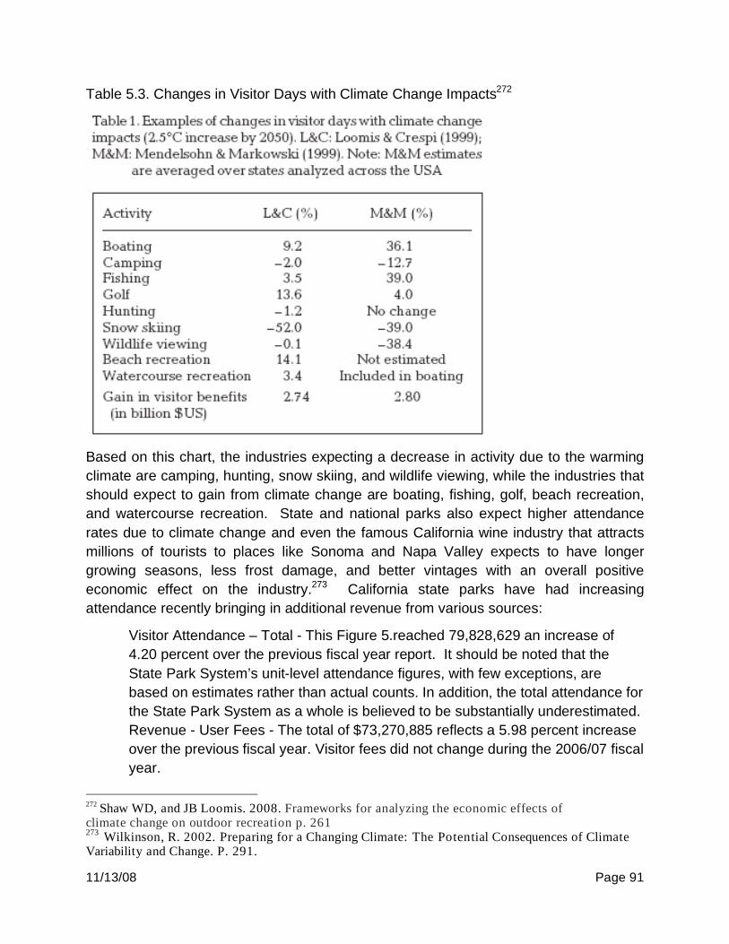
11/13/08 Page 91
Table 5.3. Changes in Visitor Days with Climate Change Impacts272
Based on this chart, the industries expecting a decrease in activity due to the warming
climate are camping, hunting, snow skiing, and wildlife viewing, while the industries that
should expect to gain from climate change are boating, fishing, golf, beach recreation,
and watercourse recreation. State and national parks also expect higher attendance
rates due to climate change and even the famous California wine industry that attracts
millions of tourists to places like Sonoma and Napa Valley expects to have longer
growing seasons, less frost damage, and better vintages with an overall positive
economic effect on the industry.273 California state parks have had increasing
attendance recently bringing in additional revenue from various sources:
Visitor Attendance – Total - This Figure 5.reached 79,828,629 an increase of
4.20 percent over the previous fiscal year report. It should be noted that the
State Park System’s unit-level attendance figures, with few exceptions, are
based on estimates rather than actual counts. In addition, the total attendance for
the State Park System as a whole is believed to be substantially underestimated.
Revenue - User Fees - The total of $73,270,885 reflects a 5.98 percent increase
over the previous fiscal year. Visitor fees did not change during the 2006/07 fiscal
year.
272
Shaw WD, and JB Loomis. 2008. Frameworks for analyzing the economic effects of climate change on outdoor recreation p. 261 273
Wilkinson, R. 2002. Preparing for a Changing Climate: The Potential Consequences of Climate Variability and Change. P. 291.

11/13/08 Page 92
Revenue – Concessions - The total of $11,991,649 reflects an increase of 5.25
percent over the previous year.
Revenue – Miscellaneous - The total of $476,850 reflects an increase of 98.49
percent over the previous year. This seemingly large increase actually reflects
the additional reporting of parking violations fees revenue which includes
$165,359 within the OHMVR Division.
Total Revenue - The System’s total revenue of $85,739,516, the sum of the
above three categories, reflects an increase of 6.15 percent from the prior fiscal
year. The three revenue categories listed above, based on the Department’s
“earnings”, constitute an important part of the State Park and Recreation Fund
(SPRF).274
Surprisingly all of these increases in outdoor recreation participation outweigh the
decreases, leading to an overall boost in the Californian tourism industry. Not
surprisingly, the data from Table 5.1 shows some patterns as far as which industries
have increasing participation and which are decreasing; all of the recreation activities
having to do with water will have increased participation with increased temperatures,
as people flock to the beaches and lakes to beat the heat. On the other hand almost all
of the activities that depend upon a well balanced and maintained ecosystem (hunting,
wildlife viewing, etc.) are predicted to see drops in participation, due to decreasing
biological diversity caused by damages to the environment and disturbances of the
ecosystem’s delicate balance.
Unfortunately it is extremely difficult to gauge climate change and predict its effects on
the environment, and it is even more difficult to Figure 5.out its effect on the tourism and
recreation economy. Though there are many studies in circulation that attempt to
estimate these effects and make predictions of how the economy will react, much more
time, money, and research must be put into this project. The major issues with current
data and research are listed below.
Table 5.4. Weaknesses in Predicting Travel Flows275
274
Planning Division, California Department of Parks and Recreation. 2007. The California State Park System Statistical Report: 2006/07 Fiscal Year. P.7. 275
Gossling, S and M Hall. 2006. UNCERTAINTIES IN PREDICTING TOURIST FLOWS UNDER SCENARIOS OF CLIMATE CHANGE. P. 165

11/13/08 Page 93
Notes and References

11/13/08 Page 94
6. Real Estate: Background
Real estate under climate change will be impacted primarily by property damage from
extreme events – wildfires along the wildland-urban interface and coastal flooding as
rising sea levels lead to coastal levees and beach protections being breached. Wildfire
risk will vary by vegetation type, but is expected to increase 11-55 percent depending
on scenario.276 Coastal flooding damages will come primarily from decreases in the
storm return intervals as events that are now considered extreme become more
frequent.
Wildfire Impacts
Many effects of global warming can influence the incidence and severity of California
wildfires. Even in the mildest of climate change scenarios that include a concerted
effort globally to reduce emissions and lower climate sensitivity, California temperatures
are expected to rise 3 to 5.4 ° F. For higher emissions scenarios, the temperature
increase could reach up to 10.4 ° F by the end of the century277. Rising temperatures
can lead to a number of deleterious effects that impact wildfire risk in California. These
effects include increased spring and summer temperatures, reduced precipitation,
increased evapotranspiration, and an earlier snow-pack melt that can in turn lead to
longer and drier fire seasons in many mid to high elevation forests.278
Westerling and Bryant classify two types of plant-life regimes in California with respect
to wildfire behavior. Energy limited regimes are more characteristic of forested areas
where wildfires are associated strongly with dry conditions and warm temperatures the
year of the fire, giving the forest enough energy to dry out the abundant fuels that are
already present. Moisture limited regimes are more characteristic of grassland and
shrub areas where wildfires are strongly associated with a moisture anomaly the year
before, allowing plentiful vegetation growth which serves as needed fuel to facilitate
wildfire spread in these normally hotter, dryer areas. While actual vegetation regimes
are usually somewhere between the two extremes, they serve as a useful framework for
modeling wildfire behavior under climate change.
Predictions for wildfire risk are more or less certain depending on the cause of that risk.
The primary mechanism by which climate change will affect wildfire in California is
through changes in moisture. The certainty of these predictions varies by regime type.
276
California Climate Change Center. “Our Changing Climate: Assessing the Risks to California.” 2006 277
California Climate Change Center, 2006 278
A. L. Westerling and B. P. Bryant, “Climate Change and Wildfire in California”. Climatic Change 87 (Suppl 1):
S231–S249, 2008.

11/13/08 Page 95
In energy-limited regimes where fire risk is associated with higher temperatures drying
out the available fuel, these predictions are relatively more certain. However, due to the
uncertainty regarding precipitation predictions over the next century, the outlook for
moisture-limited regimes is relatively less certain as they are more associated with
precipitation forecasts than energy-limited regimes.
An early report by Fried et al. on wildfire severity in California under a doubled carbon
scenario suggested that the number of fires escaping their initial containment area
would double and that the total area burned by contained fires would increase 50
percent. They estimated that the fire return interval on grass and brush would be cut in
half279. A more recent study revisits these predictions while correcting many of the
weaknesses of the original methods and considering multiple warming scenarios.280
Table 6.1. Yearly Predictions for the Amador El-Dorado Unit 2070-2099281
Base GFDL A2 GFDL B1 PCM A2 PCM B1
Overall Area
Burned (acres)
475 538 513 516 489
Percent
Increase from Base
n/a 13.2% 8% 8.63% 2.95%
Notes: The Base number of escapes is a model-output simulation of historical values
which closely resemble actual values obtained from the historical record of wildland fire
incidents.282 GFDL and PCM are different climate change models that are similar in
many respects, but GFDL is generally considered a higher-sensitivity model while PCM
is a lower sensitivity model. A2 is a climate change scenario which represents
continued reliance on fossil fuels and little action toward climate change; the effects of
this scenario worsen after the twenty-first century with expected temperature increases
of 3.4 ° C ( by 2100. B1 represents the lowest warming scenario offered by the IPCC
and includes a rapid shifting toward more environmentally friendly technologies with
expected temperature increases of 1.8 ° C by 2100.283
279
. Fried, Jeremy S, Margaret Torn, and Evan Mills. “The Impact of Climate Change on Wildfire Severity: A Regional Forecast for Northern California” Climatic Change 64: 169–191, 2004. 280
Fried, Jeremy S, J. Keith Gilless, William J. Riley, Tadashi J. Moody, Clara Simon de Blas, Katharine Hayhoe, Max Moritz, Scott Stephens, and Margaret Torn. “Predicting the Effect of Climate Change on Wildfire Severity and Outcomes in California: Preliminary Analysis” Energy Commission: Publication No. CEC-500-2005-196-SF. 281
Fried et al. 2005. 44-45. 282
Fried et al. 2005. 32. 283
IPCC, 2007: Summary for Policymakers. In: Climate Change 2007: The Physical Science Basis. Contribution of Working Group I to the Fourth Assessment Report of the Intergovernmental Panel on Climate Change [Solomon, S., D. Qin, M. Manning, Z. Chen, M. Marquis, K.B. Averyt, M.Tignor

11/13/08 Page 96
Table 6.2. Number of Escaped Fires (ESL’s) By Administrative Unit and Scenario284
Administrative Unit
B1: Change BASE to
MIDCEN
A2: Change BASE to
MIDCEN
B1: Change BASE to
ENDCEN
A2: Change BASE to
ENDCEN
Santa Clara
(SCU)
1.74* 1.95* 1.56* 5.31*
Amadaor El
Dorado (AEU)
4.27* 7.44* 3.2* 2.89*
San
Bernardino
(BDU)
2.56* 2.37* -0.2 2.38*
Note: Base ESL refers to a modeled output simulation of historical values. Fried et al
suggest that these results are best interpreted in relative terms based on scenario as
many things can change their absolute values including changes in firefighting methods
and technology among other possibilities. All estimates in this chart are predicted using
a GFDL model.
These estimates are more conservative than the estimates of the former report primarily
due to differences in wind speed predictions. The predicted values of wind speed were
generally not significant or the changes were minor. A study focusing on the Santa Ana
winds indicated that Santa Ana wind occurrences are likely to increase during the
California fire season, but indicated that overall wind occurrences were unlikely to
change dramatically. However, further research in this area is needed in order to better
understand the changes in intensity and duration of Santa Ana occurrences as well as
the multiple complex factors which could affect them.285
and H.L. Miller (eds.)]. Cambridge University Press, Cambridge, United Kingdom and New York, NY, USA. Fried et al. 2005. 11. 284
Fried, Jeremy S., J. Keith Gilless, William J. Riley Tadashi J. Moody, Clara Simon de Blas, Katharine Hayhoe, Max Moritz, Scott Stephens, Margaret Torn. “Predicting the effect of climate change on wildfire behavior and initial attack success”. Climatic Change (2008) 87 (Suppl 1):S251–S264. DOI 10.1007/s10584-007-9360-2 285
Miller & Schlegel. “Climate Change Projected Santa Ana Fire Weather Occurrence” Energy Commission: Publication No. CEC-500-2005-204-SF
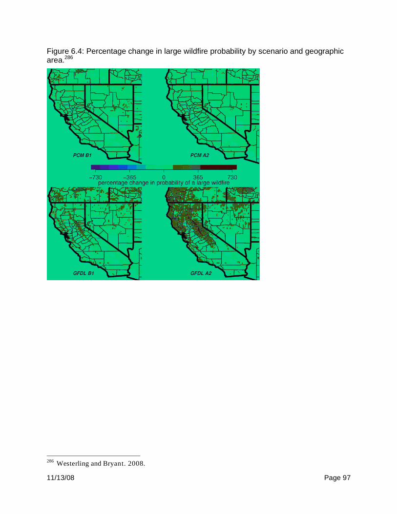
11/13/08 Page 97
Figure 6.4: Percentage change in large wildfire probability by scenario and geographic area.286
286
Westerling and Bryant. 2008.

11/13/08 Page 98
Figure 6.2. Change in California Burned Property Value, Structures and Threatened Structures between 1961-1990 and 2070-2099287
Table 6.2. Relative Impacts on Northern California
B1 PCM B1 GFDL A2 PCM A2 GFDL
Total Value Increase (millions)288
730 1,470 1,470 1,760
CA Large Fires (%) 12 23 34 53
NC Burned Value (%) 21 48 37 96
NC Burned Structures (%) 12 31 26 75
NC Threatened Structures (%)
12 30 25 71
NC Large Fires (%) 15 38 37 90
Note: Total Value is the dollar amount difference between the thirty year period of 1961-1990 and 2070-2099. Large Fires refer to fires >200 ha.
The numbers for Total Value Increase are approximate and represent a change from
one thirty year period to the next. These estimates were obtained by taking the
estimates for average yearly wildfire damage from the California fire plan, converting to
a thirty year period, and applying the Westerling and Bryant damage ratios and then
rounding to the nearest ten-million. While this measure is far from exact, it provides an
287
Westerling and Bryant, 2008. 288
California Board of Foresty. “California Fire Plan”. 1996.

11/13/08 Page 99
order-of-magnitude estimate that can inform policymakers as to the scope of this
problem.
Increases in the percentage of threatened structures were highest for the A2 PCM
scenario, and ranged from 7-21 percent. The total value of property burned increased
15-36 percent, and was highest for the A2 GFDL scenario. The number of large fires
was expected to increase regardless of scenario, but was most severe for A2 GFDL.
Wildfire damages in this analysis are dominated by the proximity of wildfire risk to major
urban centers, primarily the coastal areas of Southern California, the outlying portions of
the Bay Area, and Northeast of Sacramento.289 For example, in the A2 GFDL scenario,
very dramatic changes in wildfire risk for the Sierra Nevada Mountains and Cascades
were predicted but those areas are relatively sparsely populated and thus cause a small
increase in predicted burned property value and structures.
Most of the increased fire risk is expected to occur in energy-limited regimes, so the
bulk of the increased risk will occur in Northern California. These increases
compensate for what were sometimes net improvements in predicted fire risk for
Southern California. As precipitation estimates are uncertain, fire risks for Southern
California are expected to increase slightly or even decrease depending on model
sensitivity and the scenario. The estimated changes in burned property values below
do not take into account any potential feedback from changes in vegetation distribution.
In addition, development levels are held fixed at the 2000 census, so these estimates
do not take into account any changes in housing and development patterns over the
next century.
Wildfires: Adaptation
The majority of damages from wildfires occur in cities with extensive wildland-urban
interfaces, such as the outlying areas of the San Francisco Bay Area, the coastal
counties of Southern California, and northeast Sacramento.290 The most important
adaptation for avoiding additional damages beyond those listed above is to implement a
development strategy which includes minimizing the wildland-urban interface so as to
limit vulnerability to changes in wildfire behavior. Many mid-level elevation forests in
California including the Sierra Nevada foothills are expected to have above average fire
risks and redirecting development or reducing uninsured private exposure in these
areas could avoid a great deal of future damages.
For example, in the Lake Tahoe area the Tahoe Regional Planning Agency (TRPA) and
other governing organizations closely monitor wildfire risk and necessary preventative
289
Westerling and Bryant 2008. 290
Westerling and Bryant 2008.
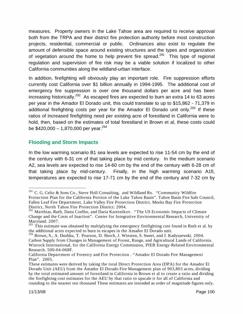
11/13/08 Page 100
measures. Property owners in the Lake Tahoe area are required to receive approval
both from the TRPA and their district fire protection authority before most construction
projects, residential, commercial or public. Ordinances also exist to regulate the
amount of defensible space around existing structures and the types and organization
of vegetation around the home to help prevent fire spread.291 This type of regional
regulation and supervision of fire risk may be a viable solution if localized to other
California communities along the wildland-urban interface.
In addition, firefighting will obviously play an important role. Fire suppression efforts
currently cost California over $1 billion annually in 1994-1995. The additional cost of
emergency fire suppression is over one thousand dollars per acre and has been
increasing historically.292 As escaped fires are expected to burn an extra 14 to 63 acres
per year in the Amador El Dorado unit, this could translate to up to $15,862 - 71,379 in
additional firefighting costs per year for the Amador El Dorado unit only.293 If these
ratios of increased firefighting need per existing acre of forestland in California were to
hold, then, based on the estimates of total forestland in Brown et al, these costs could
be $420,000 – 1,870,000 per year.294
Flooding and Storm Impacts
In the low warming scenario B1 sea levels are expected to rise 11-54 cm by the end of
the century with 6-31 cm of that taking place by mid century. In the medium scenario
A2, sea levels are expected to rise 14-60 cm by the end of the century with 6-28 cm of
that taking place by mid-century. Finally, in the high warming scenario A1fi,
temperatures are expected to rise 17-71 cm by the end of the century and 7-32 cm by
291
C. G. Celio & Sons Co., Steve Holl Consulting, and Wildland Rx. “Community Wildfire Protection Plan for the California Portion of the Lake Tahoe Basin”. Tahoe Basin Fire Safe Council, Fallen Leaf Fire Department, Lake Valley Fire Protection District, Meeks Bay Fire Protection District, North Tahoe Fire Protection District: 2004. 292
Matthias, Ruth, Dana Coelho, and Daria Karetnikov. “The US Economic Impacts of Climate Change and the Costs of Inaction”. Center for Integrative Environmental Research, University of Maryland. 2007. 293
This estimate was obtained by multiplying the emergency firefighting cost found in Ruth et al. by the additional acres expected to burn in escapes in the Amador El Dorado unit. 294
Brown, S., A. Dushku, T. Pearson, D. Shoch, J. Winsten, S. Sweet, and J. Kadyszewski. 2004. Carbon Supply from Changes in Management of Forest, Range, and Agricultural Lands of California. Winrock International, for the California Energy Commission, PIER Energy-Related Environmental Research. 500-04-068F. California Department of Forestry and Fire Protection . “Amador El Dorado Fire Management Plan”. 2005. These estimates were derived by taking the total Direct Protection Area (DPA) for the Amador El Dorado Unit (AEU) from the Amador El Dorado Fire Management plan of 903,803 acres, dividing by the total estimated amount of forestland in California in Brown et al to create a ratio and dividing the firefighting cost estimates for the AEU by that ratio to upscale it for all of California and rounding to the nearest ten thousand These estimates are intended as order of magnitude figures only.
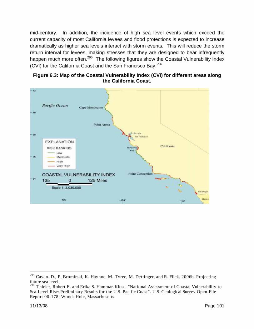
11/13/08 Page 101
mid-century. In addition, the incidence of high sea level events which exceed the
current capacity of most California levees and flood protections is expected to increase
dramatically as higher sea levels interact with storm events. This will reduce the storm
return interval for levees, making stresses that they are designed to bear infrequently
happen much more often.295 The following figures show the Coastal Vulnerability Index
(CVI) for the California Coast and the San Francisco Bay.296
Figure 6.3: Map of the Coastal Vulnerability Index (CVI) for different areas along the California Coast.
295
Cayan. D., P. Bromirski, K. Hayhoe, M. Tyree, M. Dettinger, and R. Flick. 2006b. Projecting future sea level. 296
Thieler, Robert E. and Erika S. Hammar-Klose. "National Assessment of Coastal Vulnerability to Sea-Level Rise: Preliminary Results for the U.S. Pacific Coast". U.S. Geological Survey Open-File Report 00-178: Woods Hole, Massachusetts

11/13/08 Page 102
Shoreline homes account for 16.12 percent of all California homes in 2000297. In
addition, the shoreline areas are home to 4.8 million people, or 14.25 percent of
California’s population. Given the large number of people and high value of property
along the coast, it is generally more efficient to protect California’s coastal homes and
property.298
Coastal Flooding: Adaptation
Coastal adaptation options generally fall into one of two categories: beach nourishment
and hard structure armoring. The cost of protection for a doubling in sea level rise is
more than double of the previous cost. Consequently, differences in adaptation costs
between scenarios can be dramatic. However, the most severe costs associated with
coastal flooding and sea level rise will not be incurred until the latter third of the century
when, depending on scenario, costs will reach 36-257 billion per decade by 2080 and
57-303 billion per decade by 2100.299
Table 6.3. Sea Level Rise and Present Adaptation Investment300
Sea Level Rise 33 cm 50 cm 67 cm
Approximate Present Investment Required
(2000 dollars)301
47 million 117 million 224 million
Plausible
Scenarios302
All All A1fi
297
National Ocean Economics Program: http://noep.mbari.org/. Accessed July 11, 2008. 298
Neumann, Hudgens, Herr, Kassakian. “Appendix XIII: Market Impacts of Sea Level Rise on California Coasts”. CEC 500-03-058CF. 2003. 299
Neumann et al. 2003. 300
Neumann et al. 2003. 301
Neuman et al. 2003. These estimates reflect a model using a 3 percent discount rate. 302
Of the three mentioned above, B1 (low), A2 (medium), A1fi (medium-high), those whose predicted sea level rise range contains the relevant estimate.

11/13/08 Page 103
These estimates do not include any potential value lost to wetland inundation, for which
Neumann et al. were unable to estimate economic cost. Present investment range
indicates the amount of money that would need to be invested now to account for the
risk if discounting is included. More research is needed for careful, site-specific
estimates as well as the specific effects on the San Francisco bay area. The model
used by Neumann et al. may also be useful in making site-specific coastal adaptation
decisions when combined with localized research into dynamic land-use patterns.
Finally, as with wildfire adaptation, the best option may come in changing land-use
patterns and land development of the coastal areas to insure that most of the future
coastal development in California occurs in areas that are not flood prone.
Notes and References
11/13/08 Page 104
7. Insurance: Background
The insurance sector contributes $28 billion per year to California’s GSP and employed
300,777 people in 2006.303 Private insurers pay approximately three quarters of
weather-related losses in the US with federal flood and crop insurance covering the
remainder.304 Insurers have historically played a leading role in loss prevention and are
in a unique position to offer behavior incentives for helping with climate change
mitigation and adaptation.305 One of the biggest challenges facing the industry is the
prevalence of using the past as a model for the future – under climate change the
foundations underlying the success of this strategy for risk modeling start to break
down. Many insurers now use catastrophe models in addition to historically based
models, but much could be gained by both sides from an active private-public
discussion focused on localized weather-related risks making use of both catastrophe
and climate science models to estimate risks and climate change impacts for all
concerned.
Regulating the insurance industry under climate change poses several difficulties for
policy makers. Limiting premiums charged, market withdrawal and circumstances of
coverage denial are all imperfect solutions that may aid rising premiums or low policy-
holding rates in the short-term but may compound the risk of market failures and lack of
coverage in the long-term.
Climate Change Impacts
The insurance industry is in a position to be effected by many of the impacts discussed
in this report. Virtually all branches of insurance will be impacted in some way. Health,
life, property, business interruption, crop, flood, marine and vehicle insurance will all be
impacted with a high degree of certainty.306 Health and life insurance will be impacted
by more heat wave days, electricity interruption, and poor air quality, to name a few
possibilities. Property and flood insurance will be impacted by the increased frequency
of extreme events, many of which have been mentioned in this report. Crop insurance
may suffer not only from expanded pest ranges but also changing crop ranges,
increased drought frequency, and other malaise.
303
Insurance Information Institute. “A Firm Foundation: How Insurance Supports the Economy”. 2008 304
United States Government Accountability Office. “Financial Risks to Federal and Private Insurers in Coming Decades are Potentially Significant.” 2007. 305
Mills, Evan. “Climate Change and the Insurance Industry”. Environmental Energy Technologies Division Newsletter: Vol. 6, No. 3 306
Vellinga, Pier and Evan Mills. “Insurance and Other Financial Services” in Climate Change 2001: Impacts, Adaptation, and Vulnerability. IPCC: 2001.

11/13/08 Page 105
Figure 7.4: Risks to the insurance industry as a result of climate change.307
Within the lower warming range, temperatures are expected to rise 3-5.5 ° F. Sea
levels are expected to rise 6-14 inches. There will be twice as many urban heat wave
days, and 10-35 percent more risk of wildfire, with the forested areas of Northern
307
Velling and Mills. 2001.

11/13/08 Page 106
California being most at risk. In the medium warming range, temperatures are expected
to increase up to 8 ° F. Sea levels are expected to rise up to 22 inches. There will be
up to four times as many urban heat wave days and 55 percent more risk of wildfire. In
the worst scenarios, average temperatures could increase as much as 10.5 ° F and sea
levels could rise by up to 40 inches.308
In all scenarios, air quality is expected to decline. Ozone concentrations will rise by 25-
80 percent, depending on the scenario. Changing temperatures and precipitation
seasons could also expand or alter the ranges of many infectious diseases. Coastal
flooding from extreme precipitation events could lead to water supply contamination and
the spread of water-borne disease. The worst increases in extreme heat in California
will occur in Los Angeles. In addition, days conducive to high ozone formation will
increase 25-35 percent for a lower warming scenario and 75-85 percent for a higher
warming scenario. The extent that these predictions will come true depends on how
California meets air quality regulations in the future in addition to climate change.309
The impacts on public health could be widespread and compounding. Ross, Mills and
Hect summarize the anticipated risks:
Infectious disease vector expansion
Heat stress
Respitory and coronary disease linked with increased allergens, pollution and
temperatures
Waterborne diseases and water-treatment contamination
Physical injury and disease clustering from extreme events
Toxic materials released and distributed by extreme events
Food poisoning, e.g. the strong correlation between salmonella outbreaks and
heat.310
Many of these impacts can combine and interact to cause more severe impacts on
public health, even in the absence of extreme weather events.
Adaptation for the Insurance Industry
There are many risks facing the insurance industry and as the cost of risk of losses
increase, so will the cost of insuring those losses. Insurance is possible when the risks
it insures are quantifiable, diversifiable, fortuitous and economically priced. As
308
California Climate Change Center. 2006. 309
Dreschler et al. 2005 310
Ross, C. E. Mills, S. Hecht. 2007. “Limiting Liability in the Greenhouse: Insurance Risk Management Strategies in the Context of Global Climate Change.” Stanford Environmental Law Journal and the Stanford Journal of International Law, Symposium on Climate Change Risk, Vol 26A/43A:251-334.

11/13/08 Page 107
conditions change in new and potentially unknown ways, insurers may be unable to
quantify the risk. As many areas are affected at the same time across the globe, it
may affect insurers’ ability to diversify. As losses due to climate change become a
regular occurrence, premiums will have to rise to meet them which may increase
premiums to a point where many are unprepared to pay. All of these factors create
potential conditions for market failure.311
To reduce the impact of climate change on the insurance sector, reducing underlying
vulnerability by limiting the capacity for property and health damage is an excellent
place to start. Ensuring that beachfront property is adequately protected will reduce
insured losses and investing in adequate fire prevention will do much the same.
However, there are many other measures that need to be taken in addition to those
already mentioned and public intervention may create more problems than it solves.
For example, the National Flood Insurance Program, while providing a valuable service
and helping keep residents in their homes, also distorts market signals by keeping
insurance premiums artificially low in high risk areas, effectively encouraging
development in areas that might otherwise be considered too risky.312
One of the most important things that can be done to minimize the impacts of climate
change on the insurance industry in California is collaboration between the private and
public sectors on a variety of issues. Information sharing and disclosure is vital.
Scientific data and models produced by public agencies have much to offer the
insurance industry, both public and private. Working to combine the economically-
oriented perspective of insurance loss and catastrophe models with California state
researchers scientific approach may prove mutually beneficial., increasing the predictive
power for both policy makers and private insurers.313
Improved information, analysis and research on a company-to-company, localized basis
so that insurance companies are aware of the full extent of their vulnerability.
Disclosing these risks can prevent capital flight amid concerns of climate change woes.
Developing a standardized reporting format for disclosure of material risks will help spot
problems early, pointing the way for research and technological innovation.314
There are many ways to go about loss prevention to reduce insurers’ exposure.
Prevention can afford huge savings, as was seen with Hurricane Katrina where
insurance customers that instituted engineering recommendations before the hurricane
311
Maynard, Trevor. “Climate Change: Impacts on Insurers and How They Can Help With Adaptation and Mitigation”. The Geneva Papers, 2008, 33, (140–146) 312
Allianz Group and WWF. “Climate Change and Insurance: An Agenda for Action in the United States”. 2006. 313
Mills, Evan. “From Risk to Opportunity: 2007, Insurer Responses to Climate Change”. Ceres: 2007. 314
Ross et al. 2007.

11/13/08 Page 108
hit sustained an eighth of the damages of their less prepared peers.315 While individual
preventative measures would vary in their effectiveness, there are many possibilities
which could reduce losses significantly. Improved building codes and building code
enforcement, especially for homes at risk of high winds, wildfire exposure, coastal
storms or flooding, or any other appreciable climate change related risk would help to
minimize losses should the worst happen.316
As has been mentioned in previous sections, land and development planning is
extremely important. Growing communities in at-risk areas present some of the most
significant possibilities for loss.317 Rebuilding or retrofitting structures to reduce risk can
provide opportunities to increase energy efficiency and help make homes “greener” as
well.
The insurance sector has an opportunity for growth in adaptation. Providing discounts
on insurance for “green” buildings which tend to be more disaster resistant and improve
residential air quality will not just help provide financial incentives to live in those
buildings, but will also help reduce future exposure as those buildings are less
susceptible to future losses. For example, the Fireman’s Fund Insurance Company is
implementing a 5 percent rate credit for the owner’s of “green” buildings since they both
help with mitigation and are more resistant to weather-related damages than traditional
building materials and types.318 Building awareness of these programs will also help
improve insurer’s reputation while increasing their implementation and effectiveness.319
The single largest factor in prevention of heat-related illness is the presence of an air
conditioner in the home, especially central cooling systems. However, the elderly are
less likely to use an air conditioner even if one is available, perhaps due in part to a
decreased ability to perceive heat risks. The poor may be unable to afford the energy
costs of operating one. In addition, air conditioners use fossil fuels which in turn worsen
carbon emissions and increase energy costs. Air conditioners provide more benefits
than temperature relief – cooled, indoor areas provide protection from increased air
pollution levels as well as relief from heat-related environmental stress. Therefore,
ensuring the universality of air conditioner use and helping to subsidize their use for the
most at-risk segments of the population is crucial. Additional research is needed to
315
Dankwa, D. 2006. “FM Global Touts Underwriting by Engineering as Superior.” Best’s Review, p. 93, June. 316
Mills. 2007. 317
Placer paper 318
Allianz and WWF. 2006. 319
Mills. 2007.
11/13/08 Page 109
determine the costs of any such programs and their potential to increase greenhouse
gas emissions.320
Another critical adaptation is the implementation of a public heat warning system,
similar to those used in many other major American cities. Dreschler et al. estimate that
the initial cost of these systems will be $50,000 for each of ten National Weather
Service regions in California and $500,000 per year, based on 5-7 annual extreme heat
events for each major city. Adaptations to air pollution vary widely by how well
California will meet air quality standards in the future. Current compliance costs total to
approximately $10 billion annually, but the outlook for air quality improvements is
uncertain.
Another problem facing California is the expansion of vector-borne diseases. For
example, current mosquito control programs cost California $200 million per year, but
the prediction of the future impact of pest habitat expansion on California’s public health
and insurance costs will require further research.
Notes and References
320
Dreschler, Deborah, Nehzat Motallebi,Michael Kleeman, Dan Cayan, Scripps, Katharine Hayhoe1, Laurence S. Kalkstein, Norman Miller, Scott Sheridan, and Jiming Jin . “Public Health-Related Impacts of Climate Change” CEC-500-2005-197. 2005

11/13/08 Page 110
8. Agriculture: Background
This section highlights the economic impact of climate change on Californian agriculture
by looking at the changes in factors influencing agriculture and at expectations in the
changes in yields and economic values of crops and livestock products. The
information will be divided between how gradual increases in temperature and sudden,
extreme weather conditions will impact agriculture. Suggestions for adaption will be
described though estimates of their cost and success are unavailable.
Agriculture plays an important role in California’s economy so we’ll first look at its
economic value in the state. In 2006, California’s gross state product exceeded $1.6
trillion321 with agriculture grossing $31.4 billion in cash receipts322, or 1.9625 percent of
the GSP. Comparatively, 2005 produced an all-time high of $32.8 billion in receipts and
2004 produced $30.9 billion in receipts, surpassing $30 billion for the first time323. The
2006 output was produced on 26.1 million acres of land for farming and ranching, with
76,000 farms, though acreage has been decreasing324. The $31.4 billion in cash
receipts for 2006 were derived from different goods. Table 8.1 shows the values of the
top five commodities in 2006.
Table 8.1. Value of Top Five Commodities in Cash Receipts in 2006325
Goods Value in billions
Milk and Cream $4.49 Grapes $3.03 Nursery and Greenhouse $2.77 (up from 4th in 2005) Almonds $2.04 (down from 3rd in 2005) Cattle and Calves $1.67
These products are consistently among the top 5 contributors in value to California’s
agriculture and the impact of climate change on their yield will be discussed later.
Agriculture directly and indirectly provides employment for about 1.1 million people,
about 7.4 percent of total employment in California, with concentrations in certain areas
such as parts of the Central Valley where 25 percent of employment comes from
agriculture326.
321
California Legislative Analyst's Office (LAO), Cal Facts 2006, 6 Aug. 2007. 30 June 2008 <http://www.lao.ca.gov/2006/cal_facts/2006_calfacts_econ.htm#economy>. 322
California Department of Food and Agriculture (CDFA), California Agricultural Overview/ Summary -'07. 15 Feb. 2008. 11 June 2008. 323
CDFA, 2008 324
CDFA, 2008 325
CDFA, 2008 326
Cavagnaro, Timothy, Louise Jackson, and Kate Scow, 2006, “Climate Change: Challenges and Solutions for California Agricultural Landscapes,” California Climate Change Center White Paper.

11/13/08 Page 111
California also contributes greatly to US and international agricultural output and
consumption, valued economically and productively. Since 1948, it has placed number
one in state agricultural cash receipts with approximately 13 percent of total US receipts
in current years327 while Texas at number two was worth $16.0 billion in 2006328. Not
only is agriculture valued economically, it is also the majority producer of many varieties
of fruits and crops in the US. Almost 80 percent of the California’s agricultural output
was consumed in the US, showing a high domestic demand as it produces about half of
all US grown fruits, nuts and vegetables329. The 24 percent of production that was
exported in 2006 was worth nearly $9.8 billion, down from $10.9 billion in 2005330,331.
Gradual Changes in Temperature
Different emissions scenarios result in varied changes in temperature but the general
consensus shows a gradual increase in mean temperature. While the mean
temperature of the planet is expected to increase between 1.7° to 4.9°C (3.1°F to 8.8°F)
by 2100332, expectations for California’s temperature are higher. The California Climate
Change Center used PCM and HadCM3 models with scenarios of high and low
emissions to model changes in temperature. The high emissions scenario used factors
of low population growth, very high economic growth, low to medium changes in land-
use, high resource availability and rapid technological change involving coal, oil and
gas, balanced of non-fossil fuels. The low emissions scenario had different conditions,
with low population growth, high economic growth, low energy use, high land-use
change, low resource availability and medium to rapid increases in efficiency and
dematerialization in technology involving coal, oil and gas, balanced of non-fossil fuels.
These conditions led to predictions of summer temperatures increasing between 2.15°C
(3.87°F) and 8.3°C (14.9°F) and winter temperatures increasing between 2.15°C
(3.87°F) and 4.0°C (7.2°F) 333.
Changes may be more significant in the north and northeast regions than the southwest
coastal areas and increases in minimum temperatures may be the most noticeable
though another model suggests that they might decline334. From 2020-2049, in the
Western US, temperatures may increase 1.35°C (2.43°F) and 1.5°C (2.7°F) under the
low and high scenarios of the PCM model and 1.6°C (2.9°F) to 2.0°C (3.6°F) under the
327
Cavagnaro et al., 2006. 328
CDFA, 2008 329
Cavagnaro et al., 2006. 330
LAO, 2007 331
CDFA, 2008 332
Cavagnaro et al., 2006. 333
Cavagnaro et al., 2006. 334
Cavagnaro et al., 2006.
11/13/08 Page 112
low and high scenarios of the HadCM3 model335. During the period of 2070-2099,
California’s temperatures may increase 2.3°C (4.1°F) and 3.8°C (6.8°F) with the low
and high scenarios of the PCM model and 3.3°C (5.9°F) to 5.8°C (10.4°F) with the low
and high scenarios of the HadCM3 model336. However, HadCM2 and Canadian Climate
Center Models with the IS92 emissions scenarios of the Western United States, used in
the national assessment of climate change impacts on the United States, suggested
increases of 2°C (3.6°F) by 2030 and 4.5°C–6°C (8.1°F–10.8°F) by 2090337. Different
models are showing different levels of changes in temperature over time but they show
only small differences in degree. Looking at different emissions scenarios shows a slow
but steady increase of mean temperature for California from the present to 2100. These
slow changes will have impacts on California’s agriculture but the slow rate also allows
farmers to adjust and adapt with these increases in mind.
The gradual increases of temperature can impact various factors that in turn influence
crop production. Factors taken into consideration in this paper are the changes in CO2
levels, pest effect, decrease in chill time, supply of water, changes in photosynthesis
and the length and timing of growing seasons. Increases in temperature combined with
different levels of CO2 can create positive and negative changes in agriculture. Higher
levels of CO2 give plants a high initial growth rate that declines but allows plants a
greater collective growth338. The following table will show impacts of elevated CO2
levels and warmer temperatures.
335
Cavagnaro et al., 2006. 336
Cavagnaro et al., 2006. 337
Cavagnaro et al., 2006. 338
Baldocchi, Dennis, Simon Wong, and Andrew Gutierrez, 2005, “An Assessment of Impacts of Future CO2 and Climate on Agriculture,” Public Interest Energy Research (PIER) White Paper.
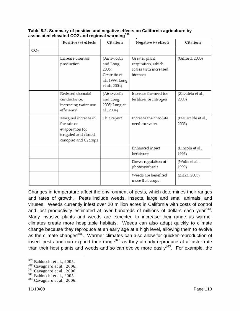
11/13/08 Page 113
Table 8.2. Summary of positive and negative effects on California agriculture by
associated elevated CO2 and regional warming339
Changes in temperature affect the environment of pests, which determines their ranges
and rates of growth. Pests include weeds, insects, large and small animals, and
viruses. Weeds currently infest over 20 million acres in California with costs of control
and lost productivity estimated at over hundreds of millions of dollars each year340.
Many invasive plants and weeds are expected to increase their range as warmer
climates create more hospitable habitats. Weeds can also adapt quickly to climate
change because they reproduce at an early age at a high level, allowing them to evolve
as the climate changes341. Warmer climates can also allow for quicker reproduction of
insect pests and can expand their range342 as they already reproduce at a faster rate
than their host plants and weeds and so can evolve more easily343. For example, the
339
Baldocchi et al., 2005. 340
Cavagnaro et al., 2006. 341
Cavagnaro et al., 2006. 342
Baldocchi et al., 2005. 343
Cavagnaro et al., 2006.
11/13/08 Page 114
olive fly, Mediterranean fruit fly, pink bollworm and others are predicted to increase their
range into the San Joaquin Valley and increase their damage in their current
locations344. The impact of climate change on large and small animals that damage
crops and transmit insects and diseases are unknown but how they react depends on
changes in their habitats and how temperature influences them physically. Pathogens
might grow faster and for longer with warmer temperatures and their range can increase
as crops, insects and animals shift to adapt and new regions grow more hospitable345.
For example, Pierce’s Disease prefers a temperature of 28°C (82°F) and causes
damage to grapes, costing millions in damages and control efforts in Southern
California346. But if temperatures increase in Northern California to the point where
Pierce’s Disease can survive, it can create large economic losses as it affects over 100
species of plants, many of which are important to the agricultural economy, such as
almonds and oranges347. More information is needed on how and where these pests
will develop to effectively minimize their damage. Warming of California’s climates will
benefit weeds, insects and pathogens, increasing growth rates and ranges of survival to
allow for greater damage and economic losses.
Many fruit trees need to experience a number of cold season hours below a critical
temperature (7°C or 45°F), typically referred to as chill time, or their yield and quality will
reduce348. They generally need from 200 to 1200 hours to flower but with climate
change, chill time will likely continue to decrease as warming will lower the number of
days of frost349. Different regions of California are currently losing from 50 to 500 chill
degree hours per year with the greatest changes in the Bay Delta region and the mid-
Sacramento Valley350. Winter chill hours are expected to fall to about 500 hours by
2100, the critical threshold for many fruit trees so farmers may need to replace them or
develop versions that require fewer chill hours351.
Problems of water supply will be covered more extensively in another section but as
climate change affects precipitation and snow levels, agriculture will need to change
according to availability. Increased rainfall and decreased snowpack will lead to less
surface water availability and greater reliance on groundwater352. Depending on the
dry/wetness of the year and water demand, agricultural water supply will shift so
farmers need to prepare for low levels of water availability.
344
Gutierrez, Andrew Paul, Luigi Ponti, C. K. Ellis, and Thibaud d’Oultremont, 2006, “Analysis of Climate Effects on Agricultural Systems,” California Climate Change Center White Paper. 345
Cavagnaro et al., 2006. 346
Cavagnaro et al., 2006. 347
Cavagnaro et al., 2006. 348
Baldocchi et al., 2005. 349
Baldocchi et al., 2005. 350
Baldocchi et al., 2005. 351
Baldocchi et al., 2005. 352
Cavagnaro et al., 2006.

11/13/08 Page 115
Growing season length and times will change as warming decreases days of frost,
changing the development of crops. The last springtime frost and first day of autumn
sum up the growing season so as frost decreases, the growing season lengthens, which
has been happening at about a day per decade in California353. Data on early blooms
indicate an earlier spring leading to a longer growing season which can benefit and
harm crops354. Perennial crops, such as grapes and fruit trees, can benefit from a
longer and warmer growth period but it also leaves fruit trees with less chill time and a
shorter dormancy period355. A longer growing season would mean greater evaporation
and usage of the water supply and a shift in the times of flowering could disrupt
pollination while warming could reduce the viability of pollen356.
Changes in temperature could affect plants ability for photosynthesis as extreme
temperatures cause many plants to cease photosynthesis. While plants cease
photosynthesis at temperatures over 50°C (122°F) and below 10°C (50°F), the ranges
are beyond those estimated in the climate models357. At most, one of the previously
mentioned models suggested an increase in summer temperature of up to 8.3°C
(14.9°F) but as California’s highs are generally in the 90s and low 100s, total cessation
of photosynthesis for long periods seems unlikely. However, higher temperatures can
affect the rate of photosynthesis with higher temperatures leading to decreasing rates.
As temperature changes can affect plants through the previously mentioned effects, it
can lead to changes in yield and quality of crops which in turn changes the economic
value of the crops. However, information regarding models of yield and value were
limited and depended on specific circumstances, such as a doubling of CO2. The next
few tables show expectations of changes in crops with the conditions of their models
that led to these results.
353
Baldocchi et al., 2005. 354
Baldocchi et al., 2005. 355
Baldocchi et al., 2005. 356
Baldocchi et al., 2005. 357
Baldocchi et al., 2005.

11/13/08 Page 116
Table 8.3. Responses of economically important California crop commodities to increased temperature358
Table 8.4. Changes in Crop Yield with Double CO2 359
Wheat Barley Rice Corn Soybean Cotton Potato
+35% +70% +15% +29% +29% +209% +83%
358
Cavagnaro et al., 2006. 359
Baldocchi et al., 2005.

11/13/08 Page 117
Table 8.5. Percent Change in yield relative to current production in San Joaquin Valley
for eight possible changes in precipitation and temperature (Adams et al., 2001)360
360
Baldocchi et al., 2005.

11/13/08 Page 118
Table 8.5 (continued)
Table 8.4 shows how yield is expected to increase due to a doubling of CO2 levels
because it increases photosynthesis, though a long period of exposure decreases the
percent increase in photosynthesis. These estimates contrast with the overall
decreases in yield seen in Table 8.5, where changes temperature, precipitation and
technology were taken into consideration but not changes in CO2 levels. The
information also assumes that there will be adequate water supplies for agriculture.
These two tables show the varied results that different models and considerations have
on forecasting changes in yield.
Special notice should be given to perennial crops because of their limited adaptability
and long periods of development and growth. They require long term investments but
climate change would make some regions currently growing these crops unfavorable
while cooler regions that would warm would become more ideal for them361. More
information is needed on where the greatest decreases and increases of yield of these
361
Lobell, David B., Christopher B. Field, Kimberley N. Cahill, and Celine Bonfils. "Impacts of future climate change on California perennial crop yields: Model projections with climate and crop uncertainties." Agricultural and Forest Meteorology 141 (2006): 208-18.

11/13/08 Page 119
crops would be so farmers can make plans to continue, begin or change their
development since any action with perennial crops would require time. Figure 8.1
shows projected changes in perennial yield with the black line representing median
projections and the shaded areas showing confidence after accounting for climate
uncertainty (dark grey) and confidence after accounting for both climate and crop
uncertainty.
Figure 8.1. Changes in Yield of Perennial Crops362
There is also little information regarding changes in qualities of crops though fruits in
particular are very sensitive. Their rate of development could increase and size
decrease because rising temperatures would increase their heat accumulation, the
number of hours between 45 and 95°F, and decrease their chill hours363. Grapes could
also ripen early and see a reduction in quality due to high temperatures though the
change will be moderate until toward the end of the century where they could ripen one
or two months early364.
Farmers might choose to switch crops and establish in more favorable regions due to
high levels of water usage, inability to produce profitable yields, etc. While annual crops
can be easily moved or replaced, long-lived species such as grapes would require much
362
Lobell et al., 2006. 363
Luers, Amy L., Daniel R. Cayan, Guido Franco, Michael Hanemann, and Bart Croes, comps. Our Changing Climate. California Climate Change Center. 2006. 18 June 2008. 364
Our Changing Climate. et al. 2008

11/13/08 Page 120
time and money to move365. But climates may force certain crops out of production in
current regions. For example, the loss of chilling hours in southern California and the
low temperatures in the north would force olives to grow in central California, the region
currently favorable for olives366. The sensitivity of some of California’s specialty crops to
the effects of climate change, such as fruits and nuts, might lead to decreases in quality
and market value so farmers might choose to replace them for more profitable crops.
However, little information was found on alternatives in crop production and
expectations of switching as climate changes the environment of a region.
Studies show little estimates of changes in economic value of crops as yields and
quality of crops change in California. In the United States, agricultural production is
expected to increase overall so prices will fall and producers will lose while consumers
gain367. Depending on the models used leading to different climate situations, climate
change could lead to agricultural economic losses of $5 billion to $8.1 billion for the US,
not including water-related impacts and in 1990 dollars368. However, California’s
outlook could be vastly different as it will have a water supply problem and currently
have many specialty crops whose demand could fall as costs increase for production369.
Information is scattered on the expected change in economic value of the agricultural
industry in California, with only tidbits on one crop or one region under specific
conditions. For example, the Central Valley is estimated to lose around $278.5 to
$803370 million, reductions of 9 to 26.3 percent of current net revenue371, due to annual
water shortages and $6 billion per year during extremely dry years372. One study using
the Hadley 2 Long Run 2070-2099 model of climate change, based on growing season
degree-days and total precipitation, estimated that California could lose about $750
million annually, estimated in 2002 constant dollars and nearly 15 percent of current
profits373.
365
Gutierrez et al., 2006. 366
Gutierrez et al., 2006. 367
Cavagnaro et al., 2006. 368
Schlenker, Wolfram, W. Michael Hanemann, and Anthony C. Fisher. The Impact of Global Warming on US Agriculture: an Econometric Analysis. Department of Agricultural and Resource Economics and Policy. University of California Berkeley. 2002. 18 June 2008. 369
Cavagnaro et al., 2006. 370
Correction of information from source in footnote 52. 371
Hanemann, M., L. Dale, S. Vicuna, D. Bickett and C. Dyckman. 2006. The Economic Cost of Climate Change Impact on California Water: A Scenario Analysis. California Energy Commission, PIER Energy-Related Environmental Research. <http://www.energy.ca.gov/2006publications/CEC-500-2006-003/CEC-500-2006-003.PDF> 372
The US Economic Impacts of Climate Change and the Costs of Inaction. Center for Integrative Environmental Research, University of Maryland. 2007. 18 June 2008 <http://www.cier.umd.edu/climateadaptation/>. 373
Deschenes, Olivier, and Michael Greenstone. The Economic Impacts of Climate Change: Evidence From Agricultural Profits and Random Fluctuations in Weather. Dept. of Economics, MIT. 2006. 30 June 2008.

11/13/08 Page 121
Gradual changes in temperature also influence dairy production, consistently the top
commodity in California. There are about 5.2 million cattle in California, concentrated
mostly in the Central Valley374. Due to limited water supplies and heat stress, cattle will
have difficulty dealing with higher temperatures375. Cows eat less due to heat stress
because at high temperatures of over 35°C or 95°F, metabolism contributes to a third of
their heat load and they give up feed for reduced heat376. With higher body
temperatures, dairy cows are less efficient and produce a lower milk yield377. The ideal
temperature for cows is between 41 and 77°F because they need to expend energy to
cool themselves when over that range378. This can lead to lower production so when
temperatures increase, towards the end of the century, milk production can decrease by
up to 20 percent379. But if temperatures stay within or below the lower range of
warming, milk production can decrease by 10 percent or less380. This means a loss of
$287-902 million every year381 to the industry currently worth $4.49 billion in
California382.
Extreme Weather Conditions
With climate change, models have shown that California will have more occurrences of
extreme weather, such as heat wave, floods, etc383. At best these would only create
delays in planting but they could also heavily damage crops, costing billions as in the
flood damages of the 1990s384. Heat waves can cause early bolting, reduce
effectiveness of pollination, decrease plants ability for photosynthesis, etc leading to
decreased yield and quality as in the gradual weather changes. But extreme events
can also kill plants that require long periods of growth, such as fruit trees and grapes,
leading to a loss of production for years until they recover or can be replaces.
Information on extreme weather leading to changes in yield and economic value of
crops and dairy is lacking as models show only an increase and intensity of
occurrences.
374
Cavagnaro et al., 2006. 375
Cavagnaro et al., 2006. 376
Cavagnaro et al., 2006. 377
Cavagnaro et al., 2006. 378
Jones, Gerald M., and Charles C. Stallings. "Reducing Heat Stress for Dairy Cattle." Virginia Cooperative Extension 404 (1999). 4 Nov. 1999. 7 Aug. 2008 <http://www.ext.vt.edu/pubs/dairy/404-200/404-200.pdf>. 379
Luers et al., 2008. 380
Luers et al., 2008. 381
The US Economic Impacts of Climate Change and the Costs of Inaction. et al. 2008 382
California Agricultural Overview/ Summary -'07 et al. 2008 383
The US Economic Impacts of Climate Change and the Costs of Inaction. et al. 2008 384
Wilkinson, Robert. California. California Regional Assessment Group. Preparing for a Changing Climate. 23 Apr. 2002. 18 June 2008.
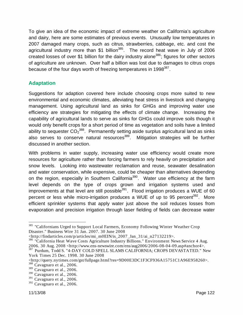
11/13/08 Page 122
To give an idea of the economic impact of extreme weather on California’s agriculture
and dairy, here are some estimates of previous events. Unusually low temperatures in
2007 damaged many crops, such as citrus, strawberries, cabbage, etc. and cost the
agricultural industry more than $1 billion385. The record heat wave in July of 2006
created losses of over $1 billion for the dairy industry alone386; figures for other sectors
of agriculture are unknown. Over half a billion was lost due to damages to citrus crops
because of the four days worth of freezing temperatures in 1998387.
Adaptation
Suggestions for adaption covered here include choosing crops more suited to new
environmental and economic climates, alleviating heat stress in livestock and changing
management. Using agricultural land as sinks for GHGs and improving water use
efficiency are strategies for mitigating the effects of climate change. Increasing the
capability of agricultural lands to serve as sinks for GHGs could improve soils though it
would only benefit crops for a short period of time as vegetation and soils have a limited
ability to sequester CO2388. Permanently setting aside surplus agricultural land as sinks
also serves to conserve natural resources389. Mitigation strategies will be further
discussed in another section.
With problems in water supply, increasing water use efficiency would create more
resources for agriculture rather than forcing farmers to rely heavily on precipitation and
snow levels. Looking into wastewater reclamation and reuse, seawater desalination
and water conservation, while expensive, could be cheaper than alternatives depending
on the region, especially in Southern California390. Water use efficiency at the farm
level depends on the type of crops grown and irrigation systems used and
improvements at that level are still possible391. Flood irrigation produces a WUE of 60
percent or less while micro-irrigation produces a WUE of up to 95 percent392. More
efficient sprinkler systems that apply water just above the soil reduces losses from
evaporation and precision irrigation through laser fielding of fields can decrease water
385
"Californians Urged to Support Local Farmers, Economy Following Winter Weather Crop Disaster." Business Wire 31 Jan. 2007. 30 June 2008 <http://findarticles.com/p/articles/mi_m0EIN/is_2007_Jan_31/ai_n27132219>. 386
"California Heat Wave Costs Agriculture Industry Billions." Environment News Service 4 Aug. 2006. 30 Aug. 2008 <http://www.ens-newswire.com/ens/aug2006/2006-08-04-09.asp#anchor4>. 387
Purdum, Todd S. "4-DAY COLD SPELL SLAMS CALIFORNIA; CROPS DEVASTATED." New York Times 25 Dec. 1998. 30 June 2008 <http://query.nytimes.com/gst/fullpage.html?res=9D00E3DC1F3CF936A15751C1A96E958260>. 388
Cavagnaro et al., 2006. 389
Cavagnaro et al., 2006. 390
Cavagnaro et al., 2006. 391
Cavagnaro et al., 2006. 392
Cavagnaro et al., 2006.

11/13/08 Page 123
use and improve distribution of water though it is expensive and probably more
appropriate for high value crops393. Drip irrigation can be profitable depending on the
crop, for example, it led to higher yields and greater returns in a study of peppers in two
locations in California, but it would also be more appropriate for higher value crops394.
Water can also be saved by allowing agricultural lands to grow fallow during dry years,
decreasing demand and allowing water to be diverted for other uses395.
Breeding based on climate change could produce crops and animals of higher yields
and farmers who could more easily switch crops should look into ones better adapted
for their region. Breeding crops and livestock suited for new climates would take time
and knowledge of varied information, such as reactions to CO2 levels and temperature,
but could lead to benefits of higher yield and greater resistance to problems of heat
stress, pests, etc. With warming across the state, production would be more possible in
the north for crops that need higher temperatures and longer growing seasons, such as
olives and citrus396. As pests will increase, planting crops that are more resistant or
choosing varying crops over time to discourage pests would minimize damages397.
Farmers could also choose crops that are more water efficient while also providing
greater value for increased economic returns. Table 8.6 shows information on the
volume of water needed to produce one kilogram of a crop while Table 8.7 shows the
applied water usage in acre feet per acre. More information is needed on GMOs and
their value in situations of climate change.
393
Cavagnaro et al., 2006. 394
Cavagnaro et al., 2006. 395
Cavagnaro et al., 2006. 396
Cavagnaro et al., 2006. 397
Cavagnaro et al., 2006.
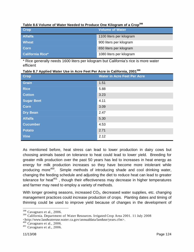
11/13/08 Page 124
Table 8.6 Volume of Water Needed to Produce One Kilogram of a Crop398
Crop Volume of Water
Alfalfa 1100 liters per kilogram
Wheat 900 liters per kilogram
Corn 650 liters per kilogram
California Rice* 1080 liters per kilogram
* Rice generally needs 1600 liters per kilogram but California’s rice is more water efficient
Table 8.7 Applied Water Use in Acre Feet Per Acre in California, 2001399
Crop Water in Acre Feet Per Acre
Grain 1.51
Rice 5.88
Cotton 3.23
Sugar Beet 4.11
Corn 3.09
Dry Bean 2.47
Alfalfa 5.30
Cucumber 4.53
Potato 2.71
Vine 2.12
As mentioned before, heat stress can lead to lower production in dairy cows but
choosing animals based on tolerance to heat could lead to lower yield. Breeding for
greater milk production over the past 50 years has led to increases in heat energy as
energy for milk production increases so they have become more intolerant while
producing more400. Simple methods of introducing shade and cool drinking water,
changing the feeding schedule and adjusting the diet to reduce heat can lead to greater
tolerance for heat401 , though their effectiveness may decrease in higher temperatures
and farmer may need to employ a variety of methods.
With longer growing seasons, increased CO2, decreased water supplies, etc. changing
management practices could increase production of crops. Planting dates and timing of
thinning could be used to improve yield because of changes in the development of
398
Cavagnaro et al., 2006. 399
California. Department of Water Resources. Irrigated Crop Area 2001. 11 July 2008 <http://www.landwateruse.water.ca.gov/annualdata/landuse/years.cfm>. 400
Cavagnaro et al., 2006. 401
Cavagnaro et al., 2006.

11/13/08 Page 125
crops due to new environments and changes in resources402. Many farmers also plan
which crops to plant based on estimates of surface and groundwater water supplies at
the beginning of the growing season403. They can use the information to decide how to
distribute their crops, what they can plan during the season and what lands they can
allow to go fallow. Fallowing land during dry years greatly decreases demand for
surface water and can reduce irrigation requirements by 20 to 30 percent in some
districts404. In pest control, management decisions on which crops, when to plant,
fertilization, irrigation and pest control are all strategies that farmers can implement now
(since they’re being used for dealing with weeds)405. Greater monitoring and more
information that includes consideration on climate change are needed to effectively
manage future changes in pests, weeds and diseases.
Notes and References
402
Cavagnaro et al., 2006. 403
PIER White Paper For The. Climate Change Impacts on Water for Agriculture in California: a Case Study in the Sacramento Valley. California Climate Change Center. 2006. 6 June 2008. 404
Climate Change Impacts on Water for Agriculture in California: a Case Study in the Sacramento Valley. et al. 2008 405
Cavagnaro et al., 2006.

11/13/08 Page 126
9. Forestry: Background
Forestry is an important California industry. The total value of all primary forest
products created in California was 2.3 billion in the year 2000. Of that, 65 percent was
lumber sales and 62 percent were sold in California.406 This industry faces many risks
as a result of climate change, including increased temperatures and changing soil
moisture that may impact timber productivity, growth, and health. As trees become
more stressed, they may become more susceptible to a variety of pest and pathogen
risks. The implications for timber management in California are varied and complicated,
potentially leading to changes in the way forest stands are maintained.
Physical Impacts
Climate change influences California’s forests primarily through changes in
temperatures and moisture availability. While warmer temperatures generally increase
plant productivity, they can also lead to decreased soil moisture. Additional
complications arise from the fact that survivable conditions for seeds, seedlings and
adult trees may vary. Generally, we can expect forests to change in terms of forest
composition, location and productivity as a result of climate change.407
Battles et al408 recently published an extensive paper on the impact of climate change
on California’s forests. This report relies on a case study approach looking specifically
at Amador and El Dorado forests. While it is not possible to generalize from their work
and more research is needed to determine the extent that their results reflect results for
California’s forests as a whole, their work constitutes the most exhaustive survey of
detailed climate change projections for forests in California to date.
In this paper, they described the effect of climate change on tree growth, yield and non-
catastrophic mortality, for both pine plantations and mixed conifer reserve stands. The
most adversely effected tree types were white fir, incense cedar and Douglas fir while
ponderosa and sugar pine were relatively less affected. Changes in forest productivity
were uniformly negative and decreased with time, with one exception – in the less
sensitive version of the reduced emissions scenario (PCM B1), a slight increase in
406
Morgan, Todd A.; Keegan, Charles E., III; Dillon, Thale; Chase, Alfred L.; Fried, Jeremy S.; Weber, Marc N. 2004. “California’s forest products industry: a descriptive analysis”. Gen. Tech. Rep. PNW-GTR-615. Portland, OR: U.S. Department of Agriculture, Forest Service, Pacific Northwest Research Station 407
Shugart, Herman, Roger Sedjo and Brent Sohngen. “Forests and Global Climate Change: Potential Impacts on US Forest Resources”. Pew Center on Global Climate Change: 2003. 408
John J. Battles, Timothy Robards, Adrian Das, Kristen Waring, J. Keith Gilless, Frieder Schurr, John LeBlanc, Gregory Biging, and Clara Simon. “Climate Change Impact on Forest Resources”.

11/13/08 Page 127
productivity was predicted for the first part of the century but with significant declines
thereafter.
Figure 9.5: Growth Changes for Pine and Conifer Forests by Scenario409
Decreases in forest growth by the end of the century ranged for mixed conifer reserve
stands from 3.9 percent in the mildest climate change scenario to 19.4 percent under
the business-as-usual higher-sensitivity model. Growth reductions for pine plantations
ranged from 6.3 percent to 29.4 percent. In most cases, growth decreased gradually
over the course of the century, but in the higher emissions and sensitivity scenarios,
conditions worsened rapidly near the end of the century.
409
Battles et al. 2003. 16.
0
0.05
0.1
0.15
0.2
0.25
0.3
Th
ou
sa
nd
cu
bic
fee
t p
er
acre
pe
r ye
ar
0.284 0.27 0.258 0.229 Reserve GFDL B1 0.284 0.273 0.261 0.252 Reserve PCM A2
0.282 0.277 0.271 0.258 Reserve PCM B1
0.281 0.283 0.274 0.27 Plantation GFDL A2 0.112 0.103 0.096 0.079 Plantation GFDL B1 0.112 0.105 0.097 0.092 Plantation PCM A2 0.11 0.107 0.103 0.096 Plantation PCM B1 0.11 0.112 0.106 0.103
1971-2000 2001-2030 2036-2065 2066-2100

11/13/08 Page 128
Figure 9.6: Yield Changes for Pine and Conifer Forests by Scenario410
Forest yields are expected to follow much the same pattern as forest growth. For
reserve stands, yield decreases will range from 3.9 percent to 18.4 percent. Pine
plantation yields will decrease between 6.9 percent and 30.5 percent. For both reserve
stands and plantations under the B1 (reduced emissions) scenario, yields are expected
to increase slightly during the first third of the century.
As noted above, yield and growth are not the only way that forests will be impacted.
Non-catastrophic mortality is the mortality that can be expected only from changes in
normal weather factors – it does not include wildfires, changes in pest ranges, etc.
Changes were in non-catastrophic mortality are expected to be modest for all scenarios.
Distribution of mortality is expected to change, however, with the weakest trees
becoming weaker over time. Whereas a tree at the 50th percentile of distribution is
expected to have a .983 survival probability in the GFDL A2 scenario, a tree at the 25th
percentile is expected to have a .956 survival probability.
410
Battles et al. 2003. 16
0
0.2
0.4
0.6
0.8
1
1.2
1.4
1.6
1.8
2 T
ho
usa
nd
Bo
ard
Fe
et P
rod
uced
Pe
r A
cre
Pe
r Y
ea
r
Reserve GFDL A2 1.79 1.7 1.63 1.46 Reserve GFDL B1 1.79 1.72 1.65 1.6 Reserve PCM A2
1.77 1.74 1.71 1.63 Reserve PCM B1
1.77 1.78 1.73 1.7 Plantation GFDL A2 0.59 0.55 0.5 0.41 Plantation GFDL B1 0.59 0.56 0.51 0.48 Plantation PCM A2 0.58 0.57 0.53 0.51 Plantation PCM B1 0.58 0.59 0.56 0.54
1971-2000 2001-2030 2036-2065 2066-2100

11/13/08 Page 129
Table 9.1: 50th Percentile Tree Survival Probability by Scenario411
2002 2030 2065 2100
GFDL A2 .998 .997 .993 .983
GFDL B1 .998 .997 .994 .994
PCM A2 .998 .998 .997 .992
PCM B1 .998 .997 .997 .998
In addition to weather-related mortality, California’s forests are in danger from a variety
of pests whose range may be expanded by milder winter temperatures and increased
tree vulnerability. Modeling the variety of complex ecological factors which influence
pest habitat and ecosystem changes is very difficult and more research is needed to
predict the effect that expanded pest ranges may have on forest health. Pests annually
destroy ten times more timber volume than wildland fires.412 However, as the number of
stressed trees increase, the prevalence of these organisms is likely to increase.
Climate change can affect pest organism’s rates of reproduction, development, and
survival. Models exist to predict these effects nationally but need to be adapted
regionally to California. In addition, insects and forest pathogens could have interactive
effects on forest health which may severely impact the timber base. More research in
this area is needed to determine the potential effects of timberland management on pest
habitat ranges and spread.413
Economic Impacts
Among the economic impacts that can be expected from changes in forest growth and
yield are decreasing budgetary revenue for California, and decreased revenue for any
forest harvesters. Lower forest harvests will mean lower payments from the Timber
Yield Tax Law. One of the main challenges for California is to preserve the
sustainability of California’s forestry programs while continuing to produce an adequate
amount of revenue despite declining harvests.414
Table 9.2: Change in Annual Revenue Per Acre415
411
Battles et al. 2003. 18. 412
California Department of Forestry. “Resource Management”. 2005 413
Battles et al. 2003. 21. 414
Battles et al. 2003. 22. 415
These estimates are derived by multiplying the MBF yield changes predicted by Battles et al. by the expected mixed conifer value found in the California State Board of Equalization Timber Harvest Schedule, adopted December 12, 2007. They apply only to the Amador & El Dorado units focused on in the original study.
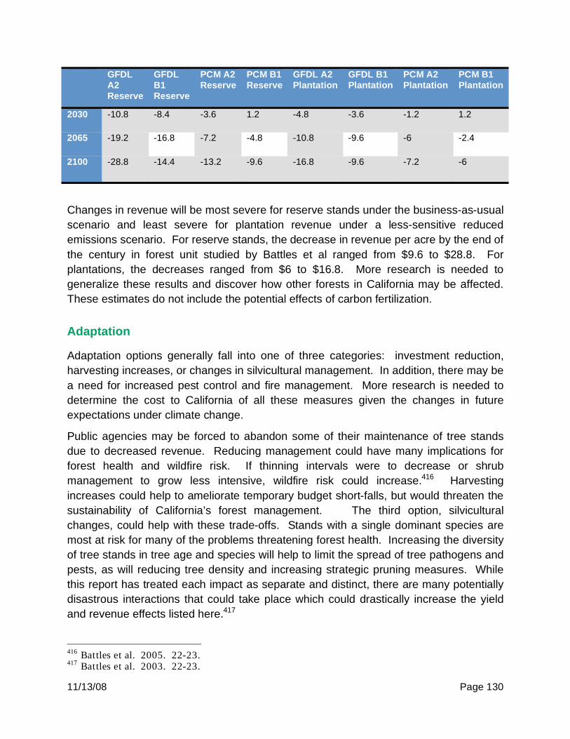
11/13/08 Page 130
GFDL A2 Reserve
GFDL B1 Reserve
PCM A2 Reserve
PCM B1 Reserve
GFDL A2 Plantation
GFDL B1 Plantation
PCM A2 Plantation
PCM B1 Plantation
2030 -10.8 -8.4 -3.6 1.2 -4.8 -3.6 -1.2 1.2
2065 -19.2 -16.8 -7.2 -4.8 -10.8 -9.6 -6 -2.4
2100 -28.8 -14.4 -13.2 -9.6 -16.8 -9.6 -7.2 -6
Changes in revenue will be most severe for reserve stands under the business-as-usual
scenario and least severe for plantation revenue under a less-sensitive reduced
emissions scenario. For reserve stands, the decrease in revenue per acre by the end of
the century in forest unit studied by Battles et al ranged from $9.6 to $28.8. For
plantations, the decreases ranged from $6 to $16.8. More research is needed to
generalize these results and discover how other forests in California may be affected.
These estimates do not include the potential effects of carbon fertilization.
Adaptation
Adaptation options generally fall into one of three categories: investment reduction,
harvesting increases, or changes in silvicultural management. In addition, there may be
a need for increased pest control and fire management. More research is needed to
determine the cost to California of all these measures given the changes in future
expectations under climate change.
Public agencies may be forced to abandon some of their maintenance of tree stands
due to decreased revenue. Reducing management could have many implications for
forest health and wildfire risk. If thinning intervals were to decrease or shrub
management to grow less intensive, wildfire risk could increase.416 Harvesting
increases could help to ameliorate temporary budget short-falls, but would threaten the
sustainability of California’s forest management. The third option, silvicultural
changes, could help with these trade-offs. Stands with a single dominant species are
most at risk for many of the problems threatening forest health. Increasing the diversity
of tree stands in tree age and species will help to limit the spread of tree pathogens and
pests, as will reducing tree density and increasing strategic pruning measures. While
this report has treated each impact as separate and distinct, there are many potentially
disastrous interactions that could take place which could drastically increase the yield
and revenue effects listed here.417
416
Battles et al. 2005. 22-23. 417
Battles et al. 2003. 22-23.

11/13/08 Page 131
Notes and References

11/13/08 Page 132
10. Fisheries: Background
This section describes the impacts of climate change on the fishing industry in
California, focusing on squid and salmon. It will provide information on the various
factors influenced by climate change that will in turn affect the populations of the squid
and salmon. Adaptation strategies will be discussed though it should be noted that
estimates for the economic costs of the impact of climate change and proposed
adaptation methods are unavailable. The following Table 10.summarizes the paper with
climate change impacts that influence squid and salmon and the adaptation and
mitigation options open to each.
Table 10.1. Climate Change Impacts and Adaptation Options for the Squid and Salmon
Industries
Climate Change Impacts Adaptation Options
Squid -Increased Water temperatures -increase growth rates -shorter life spans -smaller hatchlings emerging earlier -need more food per unit body size and oxygen -decrease in ability to handle food shortages -greater impact on surrounding ecosystems -population might shift to other regions -predictability of spawning could fall -Increases in more extreme events and their conditions such as El Niño
-Need more information on the various types of squid and their different environments -Learn how to best preserve the squid, allowing them enough time to adapt themselves because of the fast growth rates
Salmon -Warmer freshwater habitats -Increased winter flooding, reduced summer streamflow -Change in timing of migration influencing the availability of food and presence of predators -increase in ocean temperature influencing their food supply -Pacific Decadal Oscillation- potential impact, causes and predictability unknown
-Increase stream shade -Changing dam operations to increase summer flows -Removing dams -Increase monitoring -Learn how to best preserve their diversity to allow them to adapt
California’s Fishing Industry
Before discussing squid and salmon in particular, let’s first look at the role of the fishing
industry in California. The most specific information available regarding the value of the
fishing industry provided by the U.S. Bureau of Economic Analysis combined it with
“forestry and related activities”. In this category, California had the highest GDP of the

11/13/08 Page 133
states in 2006 with $7,490 million while the second highest was $2,478 million for
Washington418.
Market squid produces the most volume and revenue among California’s commercial
fishing, worth more than $35 million at its peak in 1999-2000419. The majority of the
squid is frozen and exported to China, Japan and Europe, ranking first in volume and
revenue for California’s fishery exports420. The bulk of the market squid revenues have
gone to the Santa Barbara and Los Angeles port areas, with landings in the Southern
fisheries above those in the Northern since the 1980s421. For a better idea of its value
domestically and abroad, the first following Table 10.shows the dollars paid ex-vessel
and the landings in tons for the period of 1981-2002 while the second shows information
on squid exports from 1989-2000.
Figure 10.1. Market Squid: Dollars Paid Ex-vessel and Landings in Tons 1989-2002422
418
"Gross Domestic Product by State- Forestry, fishing, and related activities for All States." Bureau of Economic Analysis Regional Economic Accounts. 5 June 2008. U.S. Department of Commerce. 6 Sept. 2008 <http://www.bea.gov/regional/gsp/>. 419
Sweetnam, Dale, comp. Market Squid Fishery Management Plan Ch. 2. USA. California Department of Fish and Game. 1 Apr. 2005. 29 Aug. 2008 <http://www.dfg.ca.gov/marine/msfmp/index.asp>. 420
Sweetnam, 2008 421
Sweetnam, 2008 422
Sweetnam, 2008

11/13/08 Page 134
Table 10.2. Market Squid Volume and Value Exported 1989-2000423
Figure 10.2. Landings of Salmon in Pounds, in Total and for Various Ports 1990-2002424
Based on the economic values for California’s commercial salmon fishery, recreational
ocean salmon fishery and steelhead fishing in the Sacramento River and tributaries, it is
423
Sweetnam, 2008 424
"California Fish Landings: Live Access Server." Datasets > 1. Simplified list of the 57 most common market categories, for longer time series > 1. Fish, Marine and Anadromous Variable(s): SALMON. Southwest Fisheries Science Center. 1 Sept. 2008 <http://las.pfeg.noaa.gov:8080/las_fish1/servlets/data>.
11/13/08 Page 135
estimated that all salmon fisheries combined contributes approximately 28.8 to 50.6
million dollars annually to the economy425. More specific information on yearly values of
salmon fisheries is unavailable for California alone though the fisheries of California and
Oregon combined average an economic impact of $133 million426. The following Figure
10.shows the landings of salmons in pounds, in total and for each port in California.
Climate Change Impacts on Squid and Adaptation Options
Climate change increases water temperatures, which would affect the development of
the squid, and leads to greater possibilities of extreme ocean events and their
conditions. Higher temperatures increase the squids’ growth rates while shortening
their life-spans, which accelerates turnover of the population427. But it also leads to
hatchlings emerging earlier and at a smaller size, possibly forcing them to mature into
adults faster, which would impact their population structure428. They would also need
more food per unit body size, more oxygen to metabolize faster and a decreased ability
to deal with food shortages429. Their dietary needs would have a greater impact on their
ecosystems with increased temperature and depending on the size of the stock430. The
population themselves might shift to more hospiTable 10.regions for spawning, into
deeper waters unavailable to fishermen431. The predictability of spawning might also
change, making it more difficult for management practices of protecting spawning adults
within enclosures to encourage more eggs432.
Some predictions of climate change include increases in more extreme events, such as
El Niño, as well as its conditions, which could have a devastating impact on the squid
population. In the 1997-1998 season, squid landings fell from their then record high of
110,000 metric tons in 1996-1997 to less than 1,000 metric tons because of the high
temperatures associated with the El Niño event at that time433. At this time, squid also
had slower growth rates and were smaller because of the scarcity of food, with the
425
Barrow, Scott, and Marc Heisdorf. California’s Living Marine Resources: A Status Report, Salmonids: Overview. USA. California Department of Fish and Game. 27 June 2007. California Department of Fish and Game. 1 Sept. 2008. 426
Pacific Fishery Management Council Votes To Allow Lowest Ever 2006 Salmon Fisheries Off California And Oregon. USA. Pacific Fishery Management Council. 10 Apr. 2006. 1 Sept. 2008 <http://www.pcouncil.org/newsreleases/pr040706_sal.pdf>. 427
Pecl, Gretta T., and George D. Jackson. "The potential impacts of climate change on inshore squid: biology, ecology and fisheries." Reviews in Fish Biology and Fisheries (2007). 21 Nov. 2007. SpringerLink. 29 Aug. 2008 <http://www.springerlink.com/content/c06170q14113g33t/>. 428
Pecl and Jackson, 2008. 429
Pecl and Jackson, 2008. 430
Pecl and Jackson, 2008. 431
Pecl and Jackson, 2008. 432
Pecl and Jackson, 2008. 433
Climate Action Report 2002. USA. US Global Change Research Program. 28 May 2002. 29 Aug. 2008 <http://www.usgcrp.gov/usgcrp/library/thirdnatcom/chapter6.htm>.

11/13/08 Page 136
pause in upwelling causing a fall in productivity434. Figure 10.1, seen previously, shows
the sharp fall in landings due to El Niño conditions.
Little information is available on possibilities of mitigation and adaptation to support
squid populations. More information is need on the various types of squid, suited to
their different environments, and their survival needs to understand what can be done to
allow them the best possible chance to grow and adapt themselves. Their initial fast
growth rates and the increase in that rate that will be caused by elevated temperatures
will help them adapt quickly to changes in their environments so it seems best to
understand how to help preserve them and allow them the time to adapt435.
Climate Change Impacts on Salmon and Adaptation Options
Climate change will affect the freshwater and saltwater environments of salmon and
decrease their chances of survival by changing their food supply and the presence of
predators. Increases in winter flooding could hurt the eggs while decreased summer
flooding would raise the temperature of the water, with warm water harmful to
salmon436. Juvenile salmon could be pushed to the ocean earlier, with earlier snow
melts and peak spring streamflows, before there is enough spring phytoplankton to feed
them because they bloom with the summer northerly winds437. The timing of their
arrival could also influence their chances of survival because the balance between
predators and baitfish populations at that time would determine their number of
predators438. The different phases of the Pacific Decadal Oscillation also seem to have
an influence on salmon stocks, with fewer stocks during warm phases and more during
wet phases439. While causes and predictability for the PDO are unknown, some climate
simulations have included them for various reasons so climate change could influence
the duration of the two phases440.
Most adaptation and mitigation plans apply only to the short term and would eventually
become ineffective so it seems best to learn more about how to protect the salmon so
that they can adapt themselves, as with the squid. Several short term options include
increasing stream shade and changing dam operations to increase summer flows to
434
Pecl and Jackson, 2008. 435
Pecl and Jackson, 2008. 436
Carter, Lynne M. US National Assessment of the Potential Consequences of Climate Variability and Change Educational Resources Regional Paper: Pacific Northwest. USA. U.S. Global Change Research Program. 23 May 2007. 29 Aug. 2008 <http://www.usgcrp.gov/usgcrp/nacc/education/pnw/pnw-edu-4.htm>. 437
Carter, 2007. 438
Carter, 2007. 439
Carter, 2007. 440
Mantua, Nate. "The Pacific Decadal Oscillation (PDO." 21 Feb. 2008. Joint Institute for the Study of the Atmosphere and Ocean. 6 Sept. 2008.

11/13/08 Page 137
mitigate warming water temperatures441. Removing dams would also decrease water
temperatures but it would also decrease control over summer flows and water
shortages442. More information and monitoring would help to understand more about
how climate change could affect them and could help set fishing guidelines based on
population levels, such as limiting fishing during warm PDO years443. The diversity of
salmon and ability to survive in various environments helps them adapt so learning how
to and working to protect that diversity would increase their chances of survival444.
Notes and References
441
Carter, 2007. 442
Carter, 2007. 443
Carter, 2007. 444
Carter, 2007.

11/13/08 Page 138
11. Public Health: Background
California is also home to some of the most polluted air in the nation. Californians
are already facing increased rates of health problems associated with high levels of
air pollution which include premature death, respiratory illnesses, and asthma.445
Over 90 percent of people living in California currently breathe unhealthy air.446
However, this threat, already acting upon the public, will become even more harmful
to the public in the future as a result of climate change. Climate change will become
a factor when calculating air pollution levels and for determining health related
effects of pollution. Increasing temperatures facilitate the creation of ground-level
ozone and smog which is already proven to be a threat to human health.447
Increasing temperatures and more intense heat waves in California induced by the
greenhouse effect also result in a different set of public health problems such as
heat-related death and illness and an increased risk and rate of wildfires.448 Other
public health issues of concern are an increased prevalence of vector-borne
diseases and water-borne pathogens; problems associated with increased rainfall
and flooding in California.449 Along with increased rates of public health problems
due to climate change comes increased spending on health care and loss of valued
life, which translates as an economic burden to Californians.
Climate Change and Air Pollution
Though often subtle and acclimated over time, Californians are already burdened
with the effects of high levels of pollution in the air. Many types of air particles
created through a variety of human activities are harmful to human health. Air quality
standards are set by the Air Resources Board to limit the amount of air pollution
released into the air, and thus, to limit the adverse health effects associated with
exposure to air pollutants. In California, the California Ambient Air Quality Standards
(CAAQS) define “the maximum amount of a pollutant that can be present in outdoor
445
“Recent Research Findings: Health Effects of Particulate Matter and Ozone Pollution.” California Environmental Protection Agency, Air Resources Board. January 2004. <http://www.arb.ca.gov/research/health/fs/PM-03fs.pdf> 446
Croes, Bart. “California’s Air Pollution and Climate Change Policies.” California Air Resources Board. Powerpoint. 2007. <http://www.healtheffects.org/Slides/AnnConf2007/Croes.pdf> 447
Parry, Martin L., Canziani, Osvaldo F., Palutikof, Jean P., van der Linden, Paul J., and Hanson, Clair E.,eds. “Climate Change 2007: Impacts, Adaptation, and Vulnerability.” Intergovernental Panel on Climate Change. Cambridge University Press, Cambridge, United Kingdom. 2007. 448
Wilkinson, Robert. “Preparing for a Changing Climate: The Potential Consequences of Climate Variability and Change.” California Regional Assessment Group. September 2002. 449
Wilkinson, 2002.
11/13/08 Page 139
air without threatening the public’s health.”450 These standards set limits on the
concentrations of pollutants in the air. For the sake of analyzing air quality and public
health we are mainly concerned with the pollutants PM2.5, PM10, and ozone.
However, only ozone has a proven connection to climate change patterns and will
be the air pollutant of concern in this analysis.451 Ozone causes health problems
ranging in severity from irritating coughs to chronic respiratory problems, increased
susceptibility to other diseases, decreased lung function and development, and
premature death.452 Illnesses associated with ozone pollution also correlate with
increased spending on health care and economic losses as a result of missed
workdays and schooldays and general limitation of daily activities.453
Climate change contributes to increased levels of the air pollutant ozone through
rising temperatures. A study conducted by the Intergovernmental Panel on Climate
Change found that higher temperatures do result in greater concentrations of ozone
in the air.454 Higher temperatures and increased carbon dioxide emissions in the air
facilitate the creation of ground-level ozone, or smog.455 Smog is inhaled by
California’s population on a daily basis which is why ozone is so harmful to the
health of those who live under ozone-polluted air. Ozone pollution and exposure
over time is considered the culprit for increased rates of respiratory problems in the
long and short run.
Ozone is a gaseous air pollutant that is formed in the atmosphere through reactions
of chemicals which are emitted from automobiles, industrial plants, and consumer
products.456 Ozone, an oxidant, can damage the respiratory tract. It can cause
inflammation and irritation which leads to respiratory symptoms such as coughing,
chest pains, shortness of breath, and the aggravation of asthma symptoms.457 Long-
term exposure to high ozone levels can eventually damage the lung tissue, decrease
lung capacity and function, and make a person more susceptible to long and short
450
“Ambient Air Quality Standards.” California Environmental Protection Agency. Air Resources Board. 27 June 2008. < http://www.arb.ca.gov/research/aaqs/aaqs.htm> 451
Parry et al., 2007. 452
“Review of the California Ambient Air Quality Standard for Ozone.” California Environmental Protection Agency. Air Resources Board. Powerpoint. 28 April 2005. <ftp://ftp.arb.ca.gov/carbis/board/books/2005/042805/05-4-1pres.pdf> 453
Hall, Jane V., Victor Brajer, and Frederick W. Lurmann. “The Health and Related Economic Benefits of Attaining Healthful Air in the San Joaquin Valley.” Cal State Fullerton. Institute for Economic and Environmental Studies. March 2006. 454
Parry et al., 2007. 455
“Climate Change – Health and Environmental Effects.” U.S. Environmental Protection Agency. 24 June 2008. <http://www.epa.gov/climatechange/effects/health.html> 456
“Ozone and Ambient Air Quality Standards.” California Environmental Protection Agency. Air Resources Board. 11 June 2008. < http://www.arb.ca.gov/research/aaqs/caaqs/ozone/ozone.htm> 457
“Ozone and Ambient Air Quality Standards.” California Environmental Protection Agency. Air Resources Board. 11 June 2008. < http://www.arb.ca.gov/research/aaqs/caaqs/ozone/ozone.htm>

11/13/08 Page 140
term respiratory illnesses.458 The current CAAQS for ozone in an 8 hour period is
0.07ppm.459
According to data taken from various counties’ air monitoring stations, since 2001,
average 8 hour ozone concentrations have decreased about 7 percent. 2007 levels
were also about 4 percent lower than 2006 levels. Ozone levels seem to be
declining slowly throughout California on average over the past few years. However,
data still shows that on average, 8 hour ozone levels are still higher than the
CAAQS, 0.07ppm. In 2007, the average 8 hour ozone level throughout California at
its highest was roughly 0.084ppm. This number is the upper bound for ozone levels
in California in 2007, but still shows that many counties in California are still
exceeding the standard for ozone at given times in the year.460
Though data shows that ozone levels have declined over the past few years, we
cannot assume that ozone levels are steadily decreasing and will continue to in the
future. Climate change becomes an issue when discussing ozone levels since
higher temperatures induced by increased greenhouse gas levels facilitate ozone
formation. Population increases are expected to factor into future levels of ozone
pollution as well since population growth will entail more production and more
vehicles on the road, meaning more ozone in the air.461 Rising costs of health care in
general are also expected to factor into higher total economic costs of public
health.462 It is expected that ozone levels will increase by 0.04-0.08ppm, or a 50-100
percent increase over 2006 levels, by the end of the century as temperatures are
expected to increase 3.6-12.6 degrees Fahrenheit.463 The Air Resources Board also
estimates that an increase in temperature by 3.6 degrees Fahrenheit will result in a
0.03ppm increase in ozone concentration.464 The California Climate Change Center
also conducted a report on projected temperature increases in California by the end
458
“Recent Research Findings: Health Effects of Particulate Matter and Ozone Pollution.” California Environmental Protection Agency, Air Resources Board. January 2004. <http://www.arb.ca.gov/research/health/fs/PM-03fs.pdf> 459
“Ozone and Ambient Air Quality Standards.” California Environmental Protection Agency. Air Resources Board. 11 June 2008. < http://www.arb.ca.gov/research/aaqs/caaqs/ozone/ozone.htm> 460
“Air Quality Data Statistics.” Air Resources Board. <http://www.arb.ca.gov/adam> 461
Harley, Robert. “Guiding Future Air Quality Management in Central California: Sensitivity to Changing Climate.” University of California Berkeley. Powerpoint. 20 February 2007. < http://es.epa.gov/ncer/events/calendar/2007/feb20_2/harley_presentation.pdf> 462
Kuehl, Sheila. “Rising Costs and Universal Health Care in California.” Senate Health Committee. 18 July 2008. 463
Drechsler, D. M., N. Motallebi, M. Kleeman, D. Cayan, K. Hayhoe, L. Kalkstein, N. Miller, S. Sheridan, J. Jin. “Public Health-Related Impacts of Climate Change in California.” California Climate Change Center. March 2006. 464
Kleeman, Michael J., and Linda Smith. “Public Health-related Impacts of Climate Change for California. California Environmental Protection Agency. Air Resources Board. 13 December 2005.

11/13/08 Page 141
of the century. They expect temperatures to increase by 3-10.5 degrees
Fahrenheit.465
There are also California Ambient Air Quality Standards set for PM2.5, PM10,
nitrogen dioxide, carbon monoxide, sulfates, hydrogen sulfide, and visibility reducing
particles. PM2.5 is a prominent public health threat in both the long and short term,
and PM10 poses short term health threats.466 However these two pollutants have no
demonstrated relation to fluctuations in temperature or environmental conditions
caused by climate change. Other pollutants for which CAAQS are set mainly cause
public annoyances such as limiting visibility and bad odors, rather than short or long
term health problems and also are not affected by climate change.467
Since California does not attain the standards for ozone and since ozone’s
concentration trends do relate to climate change trends, we will focus on the health
problems caused by this pollutant, the effect that climate change has and will have
on ozone concentrations, and the adverse health effects attributed to increased
temperatures and climate change in relation to air pollution. Ozone pollution is often
grouped together with particulate matter pollution, which is also detrimental to
human health. Many of the estimates of ozone impacts also contain the effects of
particulate matter pollution as well and the impacts of the two can be difficult to
differentiate.
The California Air Resources Board estimates that currently per year, ozone and
particulate air pollution lead to 9,000 hospitalizations and 1,700,000 cases of
respiratory illness including asthma and bronchitis.468 High levels of air pollution can
lead to up to 480,000 cases of lung cancer, 1,300,000 missed school days, and
2,800,000 missed workdays per year.469 ARB also estimates that ozone pollution is
the cause of 800 premature deaths per year.470 The number of cases for each of
these health effects and the costs associated will increase as a result of climate
change if mitigation measures are not implemented and if ozone and temperature
trends are as predicted.
465
“Our Changing Climate: Assessing the Risks to California.” California Climate Change Center. 2006. <http://www.energy.ca.gov/2006publications/CEC-500-2006-077/CEC-500-2006-077.PDF> 466
“Particulate Matter –Overview.” California Environmental Protection Agency. Air Resources Board. 25 April 2005. <http://www.arb.ca.gov/research/aaqs/caaqs/pm/pm.htm> 467
“Ambient Air Quality Standards.” California Environmental Protection Agency. Air Resources Board. 27 June 2008. <http://www.arb.ca.gov/research/aaqs/aaqs.htm> 468
“Recent Research Findings: Health Effects of Particulate Matter and Ozone Pollution.” California Environmental Protection Agency, Air Resources Board. January 2004. <http://www.arb.ca.gov/research/health/fs/PM-03fs.pdf> 469
“Recent Research Findings: Health Effects of Particulate Matter and Ozone Pollution.” California Environmental Protection Agency, Air Resources Board. January 2004. <http://www.arb.ca.gov/research/health/fs/PM-03fs.pdf> 470
Croes, 2007.

11/13/08 Page 142
Health Effects of Ozone Pollution
Long term effects of high levels of ozone exposure may include decreased lung
function, respiratory illness and premature death.471 Short term effects include
asthma attacks and increased risk of attacks, upper and lower respiratory problems,
hospitalizations and emergency room visits for various illnesses, and bronchitis.472
These health problems translate into economic costs. In this section we will discuss
these health effects in greater detail.
Premature Death. Air pollution has shown to be a prominent cause of increased
incidents of premature death in California. It was estimated in 2003 that annual
health and economic costs associated with inadequate air quality, due to particulate
matter and ozone pollution, ranged $36-$136 billion per year and caused 3,000 to
15,000 deaths annually.473 ARB has more recently estimated premature deaths in
California due to all air pollution up to 23,800 per year. Their lower bound estimate
for premature deaths due to all air pollution is 14,800.474 The South Coast Air Quality
Management District (SCAQMD) concluded its 2007 Air Quality Management Plan
that “A considerable number of population-based and laboratory studies have
established a link between increased morbidity and in some instances, earlier
mortality and air pollution,” emphasizing that this correlation between air pollution
and premature death has been proven.475
When only taking only ozone into account, ARB notes that current ozone levels are
hazardous to health, and if current levels persist, 800 ozone-related premature
deaths will ensue each year.476 Particulate matter pollution accounts for 14,000-
23,000 premature deaths per year, indicating that PM pollution is considerably more
detrimental to human health. However, PM pollution is not demonstrably
exacerbated by climate change as ozone is. Economic costs associated with 3,000-
15,000 premature deaths due to air pollution totaled $36-$136 billion in 2003,
accounting for deaths attributable to both particulate matter and ozone pollution.
The Environmental Protection Agency has commented on the criteria for assessing
the costs of premature deaths. The EPA uses the “value of statistical life”, or VSL, to
ascertain the value of premature deaths prevented. Science Daily has summarized
471
Balmes, John R. “Climate Change and Respiratory Health.” University of California Berkeley. Powerpoint. 2003. 472
Hall et al., 2006. 473
Drechsler, D. M., N. Motallebi, M. Kleeman, D. Cayan, K. Hayhoe, L. Kalkstein, N. Miller, S. Sheridan, J. Jin. “Public Health-Related Impacts of Climate Change in California.” California Climate Change Center. March 2006. 474
Croes, 2007. 475
South Coast Air Quality Management District. “2007 Air Quality Management Plan: Appendix I – Health Effects of Air Pollution.” 2007. 476
Croes, 2007.
11/13/08 Page 143
the EPA’s description of a VSL as “the price [adults] would be willing to pay - - i.e.,
what benefits or conveniences someone would be willing to forgo - - in order to
change their risk of death in a given period by a small amount”, or “the value of
extending life.”477 People of all ages have the same VSL. Ozone is likely to cause
1000-1800 premature deaths per year by 2100. The EPA’s most current VSL as of
2006 is estimated at $6.8 million.478 This number is not certain to be steady over
time due to changes in the US economy, and is hard to predict for the future due to
fluctuations in the economy and the public’s reaction to these changes.
Respiratory Disease. Lower respiratory symptoms are classified as coughs, chest
pains, and wheezing. Upper respiratory symptoms include runny nose and eye
irritations.479 Together, these symptoms limit a person’s daily activities whether it is a
child’s absence from school or an adult’s missed workday. These limitations
translate to economic costs when school or work is missed.480 There are also costs
associated with respiratory symptoms for basic medications and other amenities to
care for a sickness. If California were to attain the particulate matter and ozone
standards, this would annually prevent 600,000 cases of lower respiratory
symptoms, and 600,000 cases of upper respiratory symptoms. This would also
prevent 800,000 cases of respiratory illnesses like colds and flus per year.481
Currently, air pollution is the cause of 2,000,000 cases of respiratory illness per year,
which include upper and lower respiratory problems. These “respiratory illnesses”,
upper and lower, do not include long term, chronic illnesses. These illnesses can
generally be treated with over-the-counter or prescription medication. An afflicted
person can also buy amenities to alleviate respiratory irritations. In addition to these
costs, economic costs are incurred even further and to a greater extent when these
respiratory illnesses limit a person’s daily activity, often for multiple days, preventing
him or her from performing daily activities.
Limitation of Daily Activities. Those affected by high levels of air pollution are not
only burdened with monetary costs of treatments and hospital visits, but also incur
economic losses when daily activity is limited. This includes missed school days for
children and missed workdays for adults. According to a report by the Air Resources
Board, air pollution related illness accounted for 1,300,000 school absences per year
477
The National Academies. "Link Between Ozone Air Pollution And Premature Death Confirmed." ScienceDaily 23 April 2008. <http://www.sciencedaily.com /releases/2008/04/080422135728.htm>. 478
Deck, Leland and Lauraine Chestnut. “Recommended Health Benefit Assessments Methods for 2007 AQMP.” Stratus Consulting. South Coast Air Quality Management District. 13 December 2006. 479
Hall et al., 2006. 480
Hall et al., 2006 481
“Recent Research Findings: Health Effects of Particulate Matter and Ozone Pollution.” California Environmental Protection Agency, Air Resources Board. January 2004. <http://www.arb.ca.gov/research/health/fs/PM-03fs.pdf>
11/13/08 Page 144
and 2,800,000 missed workdays per year.482 It has also been estimated that for
every 0.05ppm increase in ozone level, school absences increase by 13.01
percent.483 Each missed work day ranges in value from about $150-$250 (money a
person would be paid for being at work) and each school day missed accounts for a
loss of $70-$90 which includes possible caretaking and the value of time to care for
a child who is sick.484
Hospitalizations and Emergency Room Visits. As illnesses are more prominent
with high air pollution levels, so is the number of hospitalizations for those who
become ill. The estimated value per hospitalization is currently $32,000.485 The
current estimate for the number of hospitalizations each year for various illnesses
associated with high levels of air pollution is 9,000.486 Assuming that the cost of a
hospitalization as a result of air pollution is on the same scale as the cost of a
hospitalization for a general illness, this totals $300 million per year that Californians
must pay currently for hospitalizations that are the result of particulate matter and
ozone levels higher than California’s standards.
Emergency room visits have also been attributed to air pollution. According to the Air
Resources Board if CAAQS are not attained, 4,000 emergency room visits will occur
per year, which are mostly for asthma attacks.487 Each emergency room visit is
estimated to cost a patient up to $400 which means that the total cost of emergency
room visits per year will total $1,600,000.488 Emergency room visits are not
considered long term hospital stays which is why hospitalizations and emergency
room visits are considered separate costs. Hospitalizations include the cost of time
that caretakers must give up to care for a sick person as well.489
Asthma. Asthma is another effect of exposure to high levels of ozone pollution.
Increased exposure to ozone increases the risk of asthma attacks and also
increases the rate of asthma attacks.490 This means there will be an increase in
482
“Recent Research Findings: Health Effects of Particulate Matter and Ozone Pollution.” California Environmental Protection Agency, Air Resources Board. January 2004. <http://www.arb.ca.gov/research/health/fs/PM-03fs.pdf> 483
Hall et al., 2006. 484
Hall et al., 2006. 485
Hall et al., 2006. 486
“Recent Research Findings: Health Effects of Particulate Matter and Ozone Pollution.” California Environmental Protection Agency, Air Resources Board. January 2004. <http://www.arb.ca.gov/research/health/fs/PM-03fs.pdf> 487
“Recent Research Findings: Health Effects of Particulate Matter and Ozone Pollution.” California Environmental Protection Agency, Air Resources Board. January 2004. <http://www.arb.ca.gov/research/health/fs/PM-03fs.pdf> 488
Hall et al., 2006. 489
Hall et al., 2006. 490
Balmes, John R. “Climate Change and Respiratory Health.” University of California Berkeley. Powerpoint. 2003.

11/13/08 Page 145
emergency room admissions and hospitalizations for asthma attacks when ozone
levels increase due to climate change. Asthma is also a very costly illness to treat.
California’s attainment of particulate matter and ozone standards would prevent
2,000 asthma- related emergency room visits. 350,000 asthma attacks would also
be prevented each year.491 On average, asthma attacks account for 38,000
hospitalizations and about 400 deaths per year.492 Economic costs are also
associated with these impacts. $1.3 billion was estimated as the total for asthma
related expenditures including hospitalizations, medication, and missed days from
work in California due to the effects of high PM and ozone levels. This total comes
out to be roughly $5000 per asthma patient annually.493
Climate Change and Extreme Temperatures
Increased average temperatures can lead to increased incidents of heat stress, heat
stroke, hospitalizations, and heat-related deaths.494 Heat waves are expected to be
much more intense and last longer, especially in the month of July when the heat-
related death rate is the highest.495 Public health issues induced by climate change
also result in economic losses to the public in the form of health care spending and
loss of productivity and life.
In Los Angeles, it is predicted that by 2020 the number of days exceeding 90
degrees Fahrenheit will double, and by 2080 that number will be five times what it is
today. Consequently, heat-related mortality is expected to increase by 62-88 percent
for the general population by 2080 in California.496 The California Climate Change
Center estimates that deaths associated with extreme temperatures will increase 2-3
times the number of incidents in 2006 by 2050.497 The Environmental Protection
Agency estimates that in a city like Los Angeles with dry, hot summers, an increase
in average temperature by 3 degrees Fahrenheit can double the rate of heat-related
491
“Recent Research Findings: Health Effects of Particulate Matter and Ozone Pollution.” California Environmental Protection Agency, Air Resources Board. January 2004. <http://www.arb.ca.gov/research/health/fs/PM03fs.pdf> 492
Milet, M., S. Tran, M. Eatherton, J. Flatterly, R. Kreutzer, L. Wohl-Sanchez. “The Burden of Asthma in California: A Surveillance Report.” California Department of Health Services. June 2007. 493
“Recent Research Findings: Health Effects of Particulate Matter and Ozone Pollution.” California Environmental Protection Agency, Air Resources Board. January 2004. <http://www.arb.ca.gov/research/health/fs/PM-03fs.pdf> 494
Fielding, Jonathan E. “Beating the Heat: Public Health and Climate Change.” Southern California Public Health Association. Annnual Conference Powerpoint. 18 April 2008. 495
“Our Changing Climate: Assessing the Risks to California.” California Climate Change Center. 2006. <http://www.energy.ca.gov/2006publications/CEC-500-2006-077/CEC-500-2006-077.PDF> 496
Fielding, Jonathan E. “Beating the Heat: Public Health and Climate Change.” Southern California Public Health Association. Annnual Conference Powerpoint. 18 April 2008. 497
“Our Changing Climate: Assessing the Risks to California.” California Climate Change Center. 2006. <http://www.energy.ca.gov/2006publications/CEC-500-2006-077/CEC-500-2006-077.PDF>

11/13/08 Page 146
deaths.498 The California Office for Environmental Health Hazard has estimated that
for every 10 degree Fahrenheit increase in temperature, deaths increased by 3
percent on any given day.499 Since average temperatures are expected to increase
by 3-12.6 degrees Fahrenheit by the end of the century, this means the number of
heat-related deaths will increase significantly by that time. Elderly people over 65
years old, people with existing heart disease, and infants younger than 1 year old
were groups found to be most susceptible to heat-related death according to
previous “temperature and mortality” studies conducted in counties throughout
California.500
Increased greenhouse gas emissions and increasing temperatures due to global
warming contribute to total premature death cases in California. Heat-related deaths
over the past years have been increasing in California.501 In 2006 the number of
heat-related deaths totaled 140.502 According to the California Climate Change
Center, with climate change trends as expected, total heat-related deaths will total
280-420 in 2050, or 2-3 times the 2006 level.503 By the end of the century the
number of heat-related deaths should total 300-600 each year. Concurrently,
temperature-related deaths rates are expected to increase each year along with
economic costs.
When average temperatures and air pollution levels are both increasing and also
affecting one another, mitigation measures must take all these effects into
consideration to effectively improve air quality and environmental conditions.504 Air
conditioning is a good way to protect against heat waves and is able to alter one’s
environment to prevent heat-induced health problems. However, air conditioning
also comes at a cost to the public.
498
Wilkinson, 2002. 499
Basu, Rupe, and Bart D. Ostro. “Epidemiological Study of Temperature and Mortality in California: Implications for Climate Change.” Air Pollution Epidemiology Section/OEHHA California Environmental Protection Agency. Powerpoint. 15 September 2006. 500
Basu, Rupa, and Paul English. “Public Health Impacts from Climate Change.” California Energy Commission. 21 August 2008. 501
Fielding, Jonathan E. “Beating the Heat: Public Health and Climate Change.” Southern California Public Health Association. Annnual Conference Powerpoint. 18 April 2008. 502
Becerra, Hector, Tami Abdollah, and Carla Hall. “For heat’s victims, a quiet death.” Los Angeles
Times. A-1. 6 September 2007. 503
“Our Changing Climate: Assessing the Risks to California.” California Climate Change Center. 2006. <http://www.energy.ca.gov/2006publications/CEC-500-2006-077/CEC-500-2006-077.PDF> 504
Drechsler, D. M., N. Motallebi, M. Kleeman, D. Cayan, K. Hayhoe, L. Kalkstein, N. Miller, S. Sheridan, J. Jin. “Public Health-Related Impacts of Climate Change in California.” California Climate Change Center. March 2006.

11/13/08 Page 147
Climate Change and Increased Wildfire Rates
Increased temperatures also increase the risk of wildfires occurring which puts
human lives at risk and also exposes the public to extremely polluted air. Wildfires
pose a threat to public health, causing both immediate physical harm and respiratory
problems when extremely polluted air is inhaled.505 One effect of climate change is
changing rainfall patterns. This may mean periods of heavy rain or periods of very
little rain. These dry periods leave land susceptible to wildfires.506 Since many parts
of California, especially Southern California, historically have had high rates of
wildfires, higher temperatures in the summer predicted for California only increases
the risk of wildfires occurring. Dry vegetation in the summer puts the public at risk for
being in the path of a wildfire.507 California also has an arid climate and low levels of
moisture in soil which increases the risk of wildfire even more when temperatures
rise.508 More intense storms due to “El Nino” weather also increase the rate of
lightning strike incidents which are sometimes catalysts for fires. A study conducted
by Anthony L. Westerling modeling fire response to climate change in the Sierra
Nevada has shown that there is an increased rate of fires concurrent with increases
in temperature and decreases in soil moisture in the summer months.509
Wildfires pose a threat to public health as immediate physical threats. However,
wildfires also result in extremely polluted air which can lead to another set of health
problems. Wildfires have shown to contribute to “bad air days” in California, days
with high levels of air pollutant concentrations in the air.510 People with existing
diseases such as heart disease, asthma, and lung disease are especially affected by
wildfire smoke and soot that is inhaled daily when a wildfire is taking place in the
region.511 Children, whose lungs are not fully developed, are also adversely affected
by the inhalation of fire smoke which inhibits lung development.512
505
Lipsett, Michael, and Barbara Materna. “Wildfire Smoke – A Guide for Public Health Officials.” U.S. Environmental Protection Agency. July 2008. 506
Fielding, Jonathan E. “Beating the Heat: Public Health and Climate Change.” Southern California Public Health Association. Annnual Conference Powerpoint. 18 April 2008. 507
Fielding, Jonathan E. “Beating the Heat: Public Health and Climate Change.” Southern California Public Health Association. Annnual Conference Powerpoint. 18 April 2008. 508
Wilkinson, 2002. 509
Wilkinson, 2002. 510
Wu, J., A. Winer, and R. Delfino. “Exposure Assessment of Particulate Matter Air Pollution Before,
During, and After the 2003 Southern California Wildfires.” Atmospheric Environment. January 2006. 511
“Health Threat from Wildfire Smoke.” Departrment of Health and Human Services. Centers for Disease Control and Prevention. 19 April 2007. < http://www.bt.cdc.gov/disasters/wildfires/facts.asp> 512
“Health Threat from Wildfire Smoke.” Departrment of Health and Human Services. Centers for Disease Control and Prevention. 19 April 2007. < http://www.bt.cdc.gov/disasters/wildfires/facts.asp>

11/13/08 Page 148
According to the Union of Concerned Scientists, if average summer temperatures
increase by 5.5-8 degrees Fahrenheit by the 2050, the risk of wildfires increases by
20 percent by that time. They also predict that wildfires will increase in incidence by
50 percent by the end of the century. In very dry areas this risk could increase by up
to 90 percent by 2100.513 According to a study conducted by scientists at the
University of Washington in five regions in the Western United States, it was found
that wildfires accounted for a 1.11ug/m increase in PM2.5 levels over the summer,
when the rate of wildfires is the highest, indicating that the presence of wildfires
definitely contributes to PM2.5 air pollution.514 PM2.5 is an air pollutant that is
proven to be harmful to human health when inhaled, which is why climate change
and in increased risk of wildfires will likely result in increased economic costs for
public health.515
Particulate matter causes numerous adverse health effects in both the short run and
long run if people are continually exposed to concentrations of PM that exceed air
quality standards. For PM2.5, the current CAAQS is 35ug/m for a 24 hour exposure
time.516 ARB discerned that the risk of death (from all causes) increases by 10
percent for every 10ug/m increase in PM2.5 in an annual period.517 Studies
conducted at the University of Washington by Kristin A. Miller and Joel D. Kaufman,
also found that for each 10ug/m increase in PM2.5 concentrations, the risk of a
cardiovascular event increased by 24 percent in women.518 The risk of
cardiovascular death for older women also increases by 76 percent for the same
10ug/m PM2.5 increment.519 According to the American Cancer Society’s
Prevention II study which tracked the health of over 1.2 million people from 1982 to
513
Westerling, A., and B. Bryant. “Change and wildfires around California: Fire modeling and loss modeling.” Sacramento, CA: California Climate Change Center. 2006. <www.energy.ca.gov/2005publications/CEC-500-2005-190/CEC-500-2005-190-SF.PDF> 514
Jaffe, Dan, Hafner, William, Chand, Duli, Westerling, Anthony, and Dominick Spracklan. “Interannual Variations in PM2.5 due to Wildfires in the Western United States.” Enrivonmental Science and Technology. Vol 42, No 8. 28 January 2008. 2812-2818. 515
“Recent Research Findings: Health Effects of Particulate Matter and Ozone Pollution.” California Environmental Protection Agency, Air Resources Board. January 2004. <http://www.arb.ca.gov/research/health/fs/PM-03fs.pdf> 516
“Particulate Matter –Overview.” California Environmental Protection Agency. Air Resources Board. 25 April 2005. < http://www.arb.ca.gov/research/aaqs/caaqs/pm/pm.htm> 517
Croes, Bart. “California’s Air Pollution and Climate Change Policies.” California Air Resources Board. Powerpoint. 2007. <http://www.healtheffects.org/Slides/AnnConf2007/Croes.pdf> 518
Miller, Kristin A., David S. Siscovick, Lianne Sheppard, Kristen Shepherd, Jeffrey H. Sullivan, Garnet L. Anderson, and Joel D. Kaufman. "Long-Term Exposure to Air Pollution and Incidence of Cardiovascular Events in Women." NEJM . Volume 356:447-458, Number 5, 1 February 2007 519
“Revised Proposed 2008 PM2.5 Plan.” San Joaquin Air Pollution Control District. Powerpoint. 30 April 2008. <http://www.valleyair.org/Air_quality_Plans/docs/AQ_Final_adopted_PM2.5/PM25_presentation.pdf>
11/13/08 Page 149
1998, an increased risk of lung cancer and increased risk of dying from existing lung
cancer did, in fact, correlate with increased exposure to air pollution. This study
concluded that “the risk of lung cancer death went up by 8 percent for every 10
micrograms of fine particles per cubic meter of air.” Total deaths from all causes
combined increased by 4 percent for every 10ug/m PM2.5 increment.520
Climate Change and Increased Risk of Vector-Borne Illness
Another concern for public health taking into account climate change is the concern
for increased cases of vector-borne illnesses. Unpredictable rainfall patterns are
expected, varying from long, intense rainy seasons to very dry seasons. Some areas
may experience abnormally high rainfall patterns and more intense storms or “El
Nino” type weather.521 These incidents result greater areas of stagnant water,
breeding grounds for insects that carry vector-borne illnesses. Rising sea levels may
also result in flooding, which would create a greater area of still water.522 This puts
public health at risk of contracting vector-borne diseases when more blood-feeding
insects are present that may carry diseases. Breeding areas for these insects may
also shift to unfavorable locations when climate changes.523 However, according to
Robert Wilkinson, Coordinator of the California Regional Climate Impacts
Assessment in 2002, this concern is not expected to be an economic burden to
Californians.524 There are relatively inexpensive means of treating vector-borne
illnesses and ways to significantly lower the risk of contracting these diseases.
Wilkinson states in his report, “While there is some indication that changing climactic
conditions may increase the risk of vector- and water-borne diseases, sanitation and
public health system infrastructures in the United States should prevent these
diseases from becoming widespread.”525
Climate Change and Water Contamination
Another concern for public health in the face of climate change is water
contamination. With higher rainfall expected in wet seasons, California may see
increased levels of flooding which threatens California’s water supply. This may also
520
“Air Pollution Linked to Deaths from Lung Cancer.” American Cancer Society. 6 March 2002. <http://www.cancer.org/docroot/NWS/content/NWS_1_1x_Air_Pollution_Linked_to_Deaths_From_Lun_Cancer.asp> 521
Wilkinson, 2002. 522
Fielding, Jonathan E. “Beating the Heat: Public Health and Climate Change.” Southern California Public Health Association. Annnual Conference Powerpoint. 18 April 2008. 523
Fielding, Jonathan E. “Beating the Heat: Public Health and Climate Change.” Southern California Public Health Association. Annnual Conference Powerpoint. 18 April 2008. 524
Wilkinson, 2002. 525
Wilkinson, 2002.

11/13/08 Page 150
affect food production if water is contaminated with bacteria or pathogens. When
contaminated water is ingested or contaminated food is eaten, many Californians will
become sick.526 Water-borne infections, like vector-borne illnesses are not seen as a
big economic concern for the future in California because we have the infrastructure
and sanitation systems to deal with water contamination problems.527
Adaptation Strategies
Currently, mitigation measures are being devised, some already imposed, in order to
monitor and regulate air pollutants. One such measure is AB 32 along with
Executive Order S-01-07 which was put into effect in September 2006. For air
basins that exceed air pollution levels set by the CAAQS, State Implementation
Plans are required, outlining means to attain standards and by how much.528 Since
many areas in California currently exceed standards, there are numerous efforts to
decrease PM2.5, PM10, ozone, and greenhouse gas levels to comply with CAAQS
for these pollutants. These methods include changes to physical production
processes, proposals to replace transit vehicles with more vehicles that create less
particulate pollution, and to conduct more stringent and more frequent air quality
tests.529 Emission inventories are taken throughout California and places like the
San Joaquin Valley look to improve these emission inventories with new technology,
more monitoring sites, and more detailed databases.530
AB 32 in accordance with Executive Order S-01-07, signed in September 2006 is a
mitigation measures proposed by Governor Arnold Schwarzenegger ultimately aim
to improve air quality significantly by 2020. The goal of AB 32 is to reach 1990 GHG
levels by 2020. Executive Order S-01-07 calls for a reduction to 2000 GHG emission
levels by 2010, which is about 11 percent below levels that would occur without
regulation, and a reduction to 1990 levels by 2020 which is about 25 percent below
levels that would occur without regulation.531 AB 32 also calls for greenhouse gas
monitoring and for the reporting of emission levels to ensure compliance. If
greenhouse gas emissions are limited, it is assumed that climate change will be less
severe and future temperatures lower than would be if regulation is not
526
Wilkinson, 2002. 527
Wilkinson, 2002. 528
“California State Implementation Plan (SIP).” California Environmental Protection Agency. Air Resources Board. 30 June 2008. < http://www.arb.ca.gov/planning/sip/sip.htm> 529
“Proposed State Strategy for California’s State Implementation Plan (SIP).” California Environmental Protection Agency. Air Resources Board. 6 February 2008. < http://www.arb.ca.gov/planning/sip/2007sip/2007sip.htm> 530
“Revised Proposed 2008 PM2.5 Plan.” San Joaquin Air Pollution Control District. Powerpoint. 30 April 2008. <http://www.valleyair.org/Air_quality_Plans/docs/AQ_Final_adopted_PM2.5/PM25_presentation.pdf> 531
“Assembly Bill No. 32.” September 2006.

11/13/08 Page 151
implemented. In order to attain 1990 greenhouse gas emission levels by 2020 as
stated in AB 32, the California Air Resources Board has discerned that emissions
must be reduced by 173 million metric tons.532
There is much debate as to whether the implementation of AB 32 will, in fact,
improve air quality and public health through the reduction of greenhouse gas levels
in the air. One argument, made by members of the Natural Resource Defense
Council, conveys that the implementation of this measure will result in large
economic benefits for Californians in the public health perspective. They argue that if
measures are carried out correctly, AB 32 could prevent 700 premature deaths
related to all types of air pollution and save Californians a total of $3.2-$5.0 billion a
year by 2020.533 However this is just a small percentage of all premature deaths due
to air pollution which is estimated up be up to 24,000 deaths per year, and just a
small percentage of total costs associated with health effects. Also, with increasing
temperatures and climate change factoring into the situation, AB 32 must account for
increasing health effects that are expected as a result of climate change in order to
accurately target these public health costs.
Physical adaptations are also being made by Californians to improve health and
well-being while breathing overly-polluted air. In order to adapt to climate change
and cope with increasing temperatures and more intense heat waves in the summer,
Californians are turning to air conditioning. Air conditioning has proved to lower the
number of heat-related deaths, and is seen as the most effects means to prevent
heat-related illnesses.534 However, air conditioning also comes at an economic cost
to consumers. According to a representative for Southern California Edison, air
conditioning costs about $230 each month during a heat wave if on for about 18
hours a day.535 This cost can become collectively steep in California. There are also
studies that have expressed concern that increased air conditioning will lead to
increased CO2 emissions, which would counter the positive effects of installing air
conditioning systems to decrease the numbers of premature death.536 However,
these measures may be necessary steps to accommodate climate change that
California will undoubtedly face in the years to come.
532
Towill, Polly, and Oliver Theard. “The Global Warming Solutions Act (AB 32): Raising the Temperature of California Business.” California Environmental Insider. 15 March 2008. 533
Bailey, Diane, Kim Knowlton, and Miriam Rotkin-Ellman. “Boosting the Benefits: Improving Air Quality and Health by Reducing Global Warming Pollution in California.” National Resources Defense Council. June 2008. <http://www.nrdc.org/globalWarming/boosting/boosting.pdf> 534
“Talking About Disaster: Guide for Standard Messages.” National Disaster Education Coalition, Washington, D.C., 1999 535
Becerra, Hector, Tami Abdollah, and Carla Hall. “For heat’s victims, a quiet death.” Los Angeles Times. A-1. 6 September 2007. 536
“Fact Sheet: Climate Change Emission Control Regulations.” California Environmental Protection Agency. Air Resources Board. 4 October 2004.