Setting Optimal Parameters on a VNSfor Music Generation

D. Herremans

Advanced optimization using metaheuristics, April 10th, 2014

University of Antwerp

Operations Research Group

ANT/OR

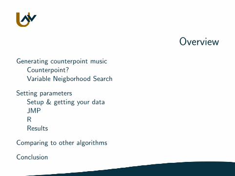
Overview

Generating counterpoint musicCounterpoint?Variable Neigborhood Search

Setting parametersSetup & getting your dataJMPRResults

Comparing to other algorithms

Conclusion

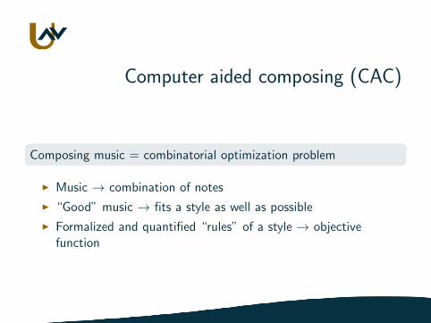
Computer aided composing (CAC)

Composing music = combinatorial optimization problem

Computer aided composing (CAC)

Composing music = combinatorial optimization problem

I Music → combination of notes

I “Good” music → fits a style as well as possible

I Formalized and quantified “rules” of a style → objectivefunction

Counterpoint

I Polyphonic baroque music

I Inspired Bach, Haydn,. . .

I One of the most formally defined musical styles→ Rules written by Fux in 1725

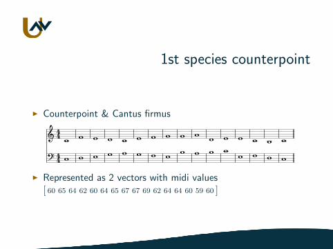
1st species counterpoint

I Counterpoint & Cantus firmus

44 44

I Represented as 2 vectors with midi values[ 60 65 64 62 60 64 65 67 67 69 62 64 64 60 59 60 ]

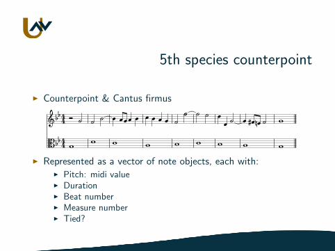
5th species counterpoint

I Counterpoint & Cantus firmus

4444

I Represented as a vector of note objects, each with:I Pitch: midi valueI DurationI Beat numberI Measure numberI Tied?

Quantifying musical quality

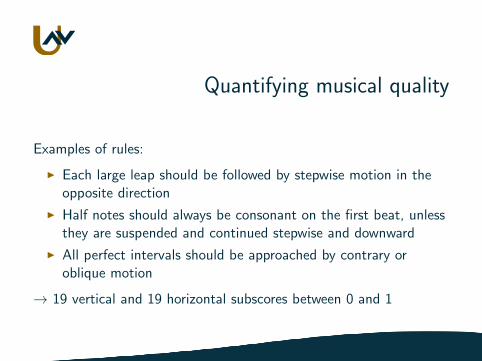
Examples of rules:

I Each large leap should be followed by stepwise motion in theopposite direction

I Half notes should always be consonant on the first beat, unlessthey are suspended and continued stepwise and downward

I All perfect intervals should be approached by contrary oroblique motion

→ 19 vertical and 19 horizontal subscores between 0 and 1

Quantifying musical quality

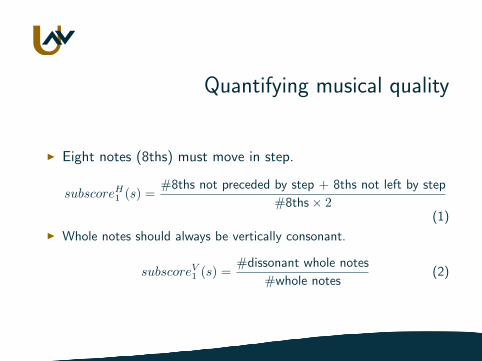
I Eight notes (8ths) must move in step.

subscoreH1 (s) =#8ths not preceded by step + 8ths not left by step

#8ths× 2(1)

I Whole notes should always be vertically consonant.

subscoreV1 (s) =#dissonant whole notes

#whole notes(2)

Quantifying musical quality

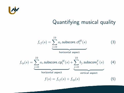
fcf (s) =

19∑i=0

ai.subscore cfHi (s)︸ ︷︷ ︸horizontal aspect

(3)

fcp(s) =

19∑i=0

ai.subscore cpHi (s)︸ ︷︷ ︸

horizontal aspect

+

19∑j=0

bj .subscoreVj (s)︸ ︷︷ ︸vertical aspect

(4)

f(s) = fcf (s) + fcp(s) (5)

Quantifying musical quality

I Weights ai and bjI Specified at input

I Emphasize subscore from start

I Adaptive weights mechanismI Increase weight of subscore with highest valueI Keeps the search in the right direction

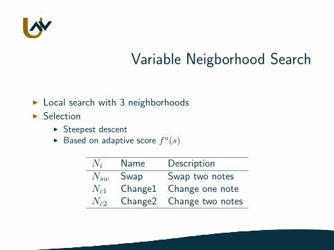
Variable Neigborhood Search

I Local search with 3 neighborhoodsI Selection

I Steepest descentI Based on adaptive score fa(s)

Ni Name Description

Nsw Swap Swap two notesNc1 Change1 Change one noteNc2 Change2 Change two notes

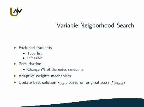
Variable Neigborhood Search

I Excluded framentsI Tabu listI Infeasible

I PerturbationI Change r% of the notes randomly

I Adaptive weights mechanism

I Update best solution sbest, based on original score f(sbest)

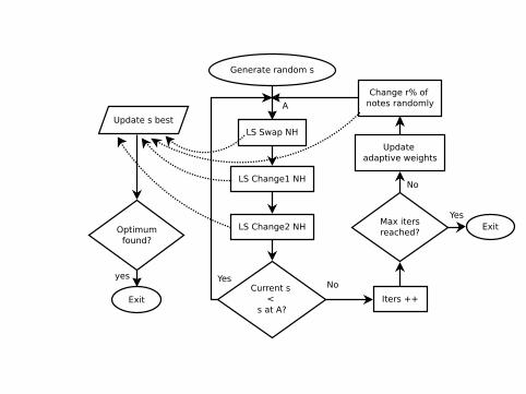
LS Swap NH

LS Change1 NH

LS Change2 NH

Current s <

s at A?

Change r% of notes randomly

YesNo

Update s best

Generate random s

A

Max itersreached?

Update adaptive weights

Iters ++

No

Exit

Exit

Optimumfound?

yes

Yes

Setting parameters

I Are all elements really contributing?

I How do we set their parameters?

→ What needs to be tested?

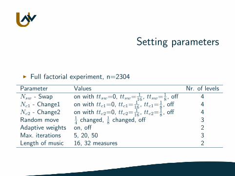
Setting parameters

I Full factorial experiment, n=2304

Parameter Values Nr. of levelsNsw - Swap on with ttsw=0, ttsw= 1

16 , ttsw= 18 , off 4

Nc1 - Change1 on with ttc1=0, ttc1= 116 , ttc1= 1

8 , off 4Nc2 - Change2 on with ttc2=0, ttc2= 1

16 , ttc2= 18 , off 4

Random move 14 changed, 1

8 changed, off 3Adaptive weights on, off 2Max. iterations 5, 20, 50 3Length of music 16, 32 measures 2

What to compare

I Objective function & f(s)

I Time:I System independent, e.g. number of f(s) calculationsI User time

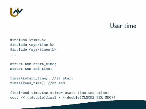
User time

#include <time.h>

#include <sys/time.h>

#include <sys/times.h>

...

struct tms start_time;

struct tms end_time;

times(&start_time); //at start

times(&end_time); //at end

final=end_time.tms_utime- start_time.tms_utime;

cout << ((double)final / ((double)CLOCKS_PER_SEC))

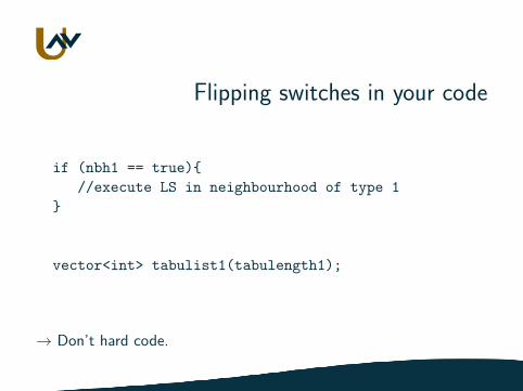
Flipping switches in your code

if (nbh1 == true){

//execute LS in neighbourhood of type 1

}

vector<int> tabulist1(tabulength1);

→ Don’t hard code.

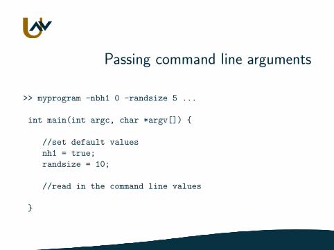
Passing command line arguments

>> myprogram -nbh1 0 -randsize 5 ...

int main(int argc, char *argv[]) {

//set default values

nh1 = true;

randsize = 10;

//read in the command line values

}

Passing command line arguments

int i = 1;

while (i < argc) {

string a = argv[i];

if (argv[i][0] == ’-’) {

string b = argv[i + 1];

if (a == "-randsize") {

randsize = atoi(b.c_str());

} else if (a == "-nbh1") {

if (b == "0") {

nbh1 = false;

}

} i+=2;

}

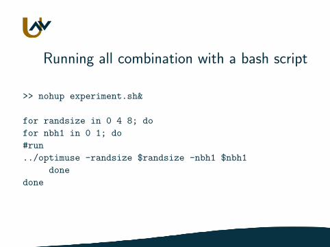
Running all combination with a bash script

>> nohup experiment.sh&

for randsize in 0 4 8; do

for nbh1 in 0 1; do

#run

../optimuse -randsize $randsize -nbh1 $nbh1

done

done

Coping with long runtime

I Parallelize runsI Split up per instance, or nbh,. . .I Use a parallelization script

I Use nohup . . . &

I Split up in two experiment with unrelated parameters

I Design of experiments

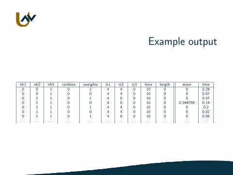
Example output

nh1 nh2 nh3 randsize aweights tt1 tt2 tt3 iters length score time0 0 1 0 1 4 4 0 10 0 0 0.280 0 1 0 0 4 4 0 10 0 0 0.070 1 1 0 1 4 0 0 10 0 0 0.070 1 1 0 0 4 0 0 10 0 0.244755 0.140 1 1 0 1 4 4 0 10 0 0 0.20 1 1 0 0 4 4 0 10 0 0 0.020 1 1 0 1 4 8 0 10 0 0 0.06. . . . . . . . . . . . . . . . . . . . . . . . . . . . . . . . . . . .

Fitting a model

JMP

I Loading data

I Basic linear model, R2

I Interaction effects

I Random effects

I Mean plots

I Profiler

I Interaction plots

R script - reading in data

expdata<-read.table("filename.csv", header=TRUE)

names(expdata)<-c(’nh1’,’randsize’,’tos’,’time’)

attach(expdata)

nh1<-factor(nh1)

randsize<-factor(randsize)

R script - fitting a linear model

//linear model

fit<-lm(tos ~ nh1 + randsize )

//with interaction effects

fit<-lm(tos ~ nh1 * randsize )

//mixed model with a random effects

fit<-lmer(tos ~ nh1 + randsize + (1 | instance) )

summary(fit)

anova(fit)

interaction.plot(nh2, nh3, tos)

→ conjugateprior.org/2013/01/formulae-in-r-anova/

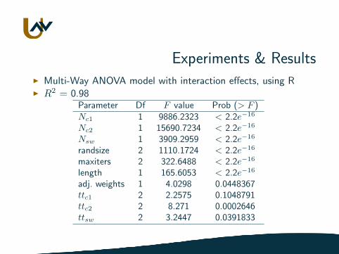
Experiments & ResultsI Multi-Way ANOVA model with interaction effects, using RI R2 = 0.98

Parameter Df F value Prob (> F )Nc1 1 9886.2323 < 2.2e−16

Nc2 1 15690.7234 < 2.2e−16

Nsw 1 3909.2959 < 2.2e−16

randsize 2 1110.1724 < 2.2e−16

maxiters 2 322.6488 < 2.2e−16

length 1 165.6053 < 2.2e−16

adj. weights 1 4.0298 0.0448367ttc1 2 2.2575 0.1048791ttc2 2 8.271 0.0002646ttsw 2 3.2447 0.0391833

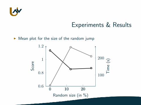
Experiments & Results

I Mean plot for the size of the random jump

0 10 200.6

0.8

1

1.2

Random size (in %)

Sco

re

0 10 20

100

200

Tim

e(s

)

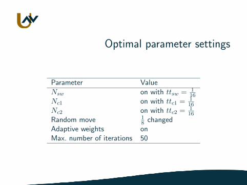
Optimal parameter settings

Parameter Value

Nsw on with ttsw = 116

Nc1 on with ttc1 =116

Nc2 on with ttc2 =116

Random move 18 changed

Adaptive weights onMax. number of iterations 50

Visualising performance

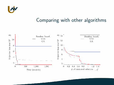
Comparing with other algorithms

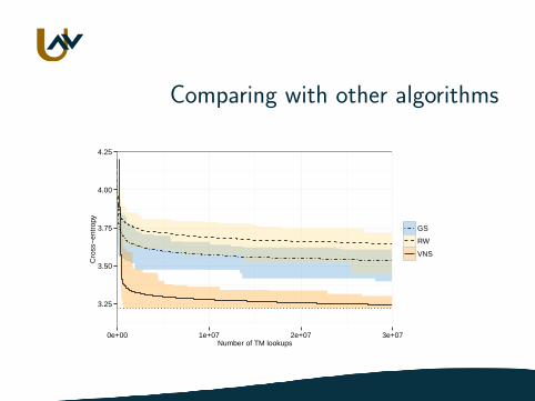
Comparing with other algorithms

3.25

3.50

3.75

4.00

4.25

0e+00 1e+07 2e+07 3e+07Number of TM lookups

Cro

ss−

entr

opy

GS

RW

VNS

Comparing with other algorithms

I Uniform stopping criteria (stagnation – user time –. . . )I Classical non-parametrical tests on population means:

I One-sided Mann-Whitney-Wilcoxon (k = 2)I Tukey-Duckworth (k ≥ 2)I Friedman (k ≥ 2 with b instances)

ResultsI Example of a generated fragment with score 0.556776.

4444

12

Conclusion

Always test your parameters and compare your algorithm to others ifpossible.

Keeping in mind:

I Random effects

I Interaction between factors

I Correct time reference

I Visualisation

Setting Optimal Parameters on a VNSfor Music Generation

D. Herremans

Advanced optimization using metaheuristics, April 10th, 2014

dorien.herremans@uantwerpen.be

University of Antwerp

Operations Research Group

ANT/OR