HAL Id: tel-03234353https://tel.archives-ouvertes.fr/tel-03234353

Submitted on 25 May 2021

HAL is a multi-disciplinary open accessarchive for the deposit and dissemination of sci-entific research documents, whether they are pub-lished or not. The documents may come fromteaching and research institutions in France orabroad, or from public or private research centers.

L’archive ouverte pluridisciplinaire HAL, estdestinée au dépôt et à la diffusion de documentsscientifiques de niveau recherche, publiés ou non,émanant des établissements d’enseignement et derecherche français ou étrangers, des laboratoirespublics ou privés.

Improved numerical schemes for monotonic conservativescalar advection : tackling mesh imprinting and

numerical wettingChristina Paulin

To cite this version:Christina Paulin. Improved numerical schemes for monotonic conservative scalar advection : tacklingmesh imprinting and numerical wetting. General Mathematics [math.GM]. Université Paris-Saclay,2021. English. �NNT : 2021UPASM011�. �tel-03234353�

Thès

e de

doc

tora

tNNT:2021UPA

SM011

Improved numerical schemes formonotonic conservative scalar

advection: tackling meshimprinting and numerical wetting

Schémas numériques améliorés pour l’advection scalaire,monotone et conservative : réduction d’empreinte de

maillage et de mouillage numérique

Thèse de doctorat de l’Université Paris-Saclay

École doctorale n◦ 574, mathématiques Hadamard (EDMH)Spécialité de doctorat : Mathématiques appliquées

Unité de recherche : Université Paris-Saclay, CNRS, ENS Paris-Saclay,Centre Borelli, 91190, Gif-sur-Yvette, France

Référent : ENS Paris-Saclay

Thèse présentée et soutenue à Paris-Saclay,le 04/05/2021, par

Christina PAULIN

Composition du jury :

Prof. Frédéric Pascal PrésidentENS Paris-Saclay, Centre Borelli, FranceProf. Philippe Helluy RapporteurUniversité de Strasbourg, IRMA, FranceProf. Knut-Andreas Lie RapporteurSINTEF, Oslo, NorwayDr. Robin James Richard Williams ExaminateurAWE, Aldermaston, UKDr. William J. Rider ExaminateurSandia, Albuquerque, NM, USA

Direction de la thèse :

Dr. Antoine Llor DirecteurCEA, DAM/DIFDr. Thibaud Vazquez-Gonzalez Co-encadrantCEA, DAM/DIF

Wie alles sich zum Ganzen webt,Eins in dem andern wirkt und lebt!Wie Himmelskräfte auf und nieder steigen...

Johann Wolfgang Goethe

Remerciements

I would like to thank all members of the jury, for your detailed reading and for allof your interesting questions and remarks.

To everyone I met at conferences: whether we chatted at a coffee break, sat togetherat lunch, had diner afterwards, a Whiskey in Glasgow, a glass of wine in Trento,a Bosnian coffee (and lokum) in Sarajevo, not only did you help me with gettingbetter at English, but you were there with your great kindness, advice, insight,cultural explanations and all sorts of discussions. Hopefully we will meet again!À l’équipe de travail: Antoine Llor merci d’avoir proposé ce sujet de thèse. Thibaud,sans toi le rendu du manuscrit n’aurait pas été possible, Rémi, pour nos voyagesen conférence, Renaud, tu m’a appris comment faire des bonnes présentations.Merci à Jean-Philippe, Thierry, Guillaume, Sébastien, William, Bertrand, Marie etMathieu pour toutes vos remarques et suggestions. Et n’oublions pas les collèguesde Bordeaux que j’ai eu l’occasion de rencontrer en conférence, Isabelle, Nicolas,Simon. Merci aussi à Jean-Philippe pour le stage d’avant thèse et notre premièrepublication ensemble avec Renaud.

À l’équipe du centre Borelli (ex CMLA) merci pour l’acceuil charmant dès lepremier jour du stage. À John, Alexandre et Lei.

Aux doctorants et anciens de Ter@tec : Nestor (tu connais toujours une solution,merci pour le partage de tes idées !), Théo, Hoby, Guillaume, Hugo et Hugo, Arthur,Sébastien, Simon, Florian, Anton, Van Man, Alexiane, Julie, Théo, Mathieu.À Éloïse, une amie précieuse, merci pour tout ! À Adrien et Dani merci pour lesdéfis sportifs. À Brigitte, le rayon de soleil. À Guillaume, c’était très motivant defaire le trajet ensemble.Aux doctorants/postdocs que j’ai eu l’occasion de rencontrer (ou mieux connaître)dans ma dernière année de thèse: Mathilde, Albertine, Louise, Sandra, Cécile,Corentin, Éric, Jean-Cédric, Adrien, Baptiste, Bastien, Ronan, Olivier, Victor,Grégoire et Charles.À mes autres amis: Jon j’ai beaucoup apprécié nos sorties cinéma et les balades,

2

Perrine, Ana, Claire, Estelle, Sébastien, Robin, Martin, Constant, Antoine, Guil-laume, Antoine on peut toujours compter sur vous, pour des plans de loisir oud’autres objectifs.

À ma famille en France, merci Christine, Frédéric et Amandine de m’avoir encour-agé tout le long de mes études. A mini familie idr Schwyz, merci vöu mau dass dirimmer a mi glaubt heit und Daniela mini Lieblingsschwöschter, i freue mi uf jedeBsuech vo dir.

A aui mini Fründe us dr Schwyz: e bsundere Dank ad Adilla, Stephan, Silkanny,Andrea, Thomas, a Ufmunterig hets im letschte Johr auso nid gfählt, und au ebsundere Dank ad Lilly, wo immer drfür sorgt dass mir ufem Laufende blibe.

Und zum Schluss no a mi Ma, dr Mattis, mi privat cuisinier, guet dass abermängisch d schwyzer Chuchi au erlaubsch.

3

Contents

Acknowledgement 2

Introduction 70.1 Advection in hydrodynamics, aerodynamics and meteorology . . . . 70.2 Quasi-isotropic second-order advection for the GEEC formalism . . 9

0.2.1 Towards quasi-isotropic numerical diffusion . . . . . . . . . . 100.2.2 1D Slope-And-Bound (SAB): clipping procedure for 1D gra-

dients . . . . . . . . . . . . . . . . . . . . . . . . . . . . . . 110.2.3 N-Dimensional-Slope-And-Bound (ND-SAB) . . . . . . . . . 12

I Towards isotropic transport with co-meshes 14

1 Towards isotropic transport with co-meshes 151.1 Introduction . . . . . . . . . . . . . . . . . . . . . . . . . . . . . . . 151.2 Generic form and properties of the discrete Eulerian transport operator 161.3 Co-mesh approach in 2D . . . . . . . . . . . . . . . . . . . . . . . . 17

1.3.1 Construction of the co-mesh . . . . . . . . . . . . . . . . . . 181.3.2 General method . . . . . . . . . . . . . . . . . . . . . . . . . 181.3.3 Reducing anisotropy . . . . . . . . . . . . . . . . . . . . . . 22

1.4 Conclusion . . . . . . . . . . . . . . . . . . . . . . . . . . . . . . . . 231.5 Appendix . . . . . . . . . . . . . . . . . . . . . . . . . . . . . . . . 24

1.5.1 First-order development and consistency conditions . . . . . 241.5.2 Modified equation applied to the first-order transport scheme

with co-meshes . . . . . . . . . . . . . . . . . . . . . . . . . 261.5.3 Anisotropy and CFL . . . . . . . . . . . . . . . . . . . . . . 28

II Doubly-monotonic constraint on interpolators: bridg-ing second-order to singularity preservation to cancel “nu-

4

merical wetting” in transport schemes 30

2 Doubly-monotonic constraint on interpolators: bridging second-order to singularity preservation to cancel “numerical wetting” intransport schemes 312.1 Introduction . . . . . . . . . . . . . . . . . . . . . . . . . . . . . . . 31

2.1.1 Motivations: “numerical wetting” . . . . . . . . . . . . . . . 312.1.2 Numeric background: Muscl-like scheme . . . . . . . . . . 332.1.3 Present approach: from limiting to clipping of interpolants. . . 352.1.4 . . . and from simple to double monotonicity . . . . . . . . . . 362.1.5 Mapping of interpolants and interpolators, 1D numerical tests 37

2.2 A convenient mapping for bounded monotonic functions . . . . . . 382.2.1 Motivation: bounded monotonic functions as interpolants . . 382.2.2 L2 bounds on bounded monotonic functions . . . . . . . . . 382.2.3 Elliptic coordinates mapping ofMXY (y) . . . . . . . . . . . 41

2.3 Slope-and-bounds interpolants . . . . . . . . . . . . . . . . . . . . . 422.3.1 Background: usual single-slope interpolants . . . . . . . . . 422.3.2 Slope-and-bounds interpolants . . . . . . . . . . . . . . . . . 44

2.4 Doubly-monotonic SAB interpolators . . . . . . . . . . . . . . . . . 462.4.1 Motivation: from interpolant to interpolator . . . . . . . . . 462.4.2 Doubly monotonic interpolators . . . . . . . . . . . . . . . . 462.4.3 Doubly-monotonic second-order SAB interpolators . . . . . . 472.4.4 Mapping of doubly-monotonic-constrained SAB interpolators 50

2.5 Numerical experiments . . . . . . . . . . . . . . . . . . . . . . . . . 502.5.1 General test conditions . . . . . . . . . . . . . . . . . . . . . 502.5.2 Square-wave tests: singularities, numerical wetting . . . . . . 552.5.3 Sine-wave tests: erosion, steepening, terracing . . . . . . . . 602.5.4 Zalesak-wave tests: sharp peaks, . . . . . . . . . . . . . . . . 61

2.6 Conclusions . . . . . . . . . . . . . . . . . . . . . . . . . . . . . . . 632.7 Appendix . . . . . . . . . . . . . . . . . . . . . . . . . . . . . . . . 642.8 Second-order MC slope on non-uniform mesh . . . . . . . . . . . . . 642.9 Front width of an error function profile . . . . . . . . . . . . . . . . 642.10 Convergence study of MC and SB on a Gaussian pulse . . . . . . . 65

III Adapting Slope-And-Bound interpolation to multi-dimensional advection schemes to cancel “numerical wet-ting” 67

3 Adapting Slope-And-Bound interpolation to multidimensional ad-vection schemes to cancel “numerical wetting” 68

5

3.1 Introduction . . . . . . . . . . . . . . . . . . . . . . . . . . . . . . . 683.2 Multidimensional Slope-And-Bound reconstruction algorithm . . . . 72

3.2.1 Linear reconstruction of gradients with weighted least squares 743.2.2 Monotonicity analysis in multi-D to 1D reduction . . . . . . 763.2.3 Nonlinear reconstruction by Slope-And-Bound limitation in

the 1D reference frame . . . . . . . . . . . . . . . . . . . . . 803.2.4 Multidimensional upwind fluxes . . . . . . . . . . . . . . . . 843.2.5 Algorithm . . . . . . . . . . . . . . . . . . . . . . . . . . . . 86

3.3 Results . . . . . . . . . . . . . . . . . . . . . . . . . . . . . . . . . . 873.3.1 Multidimensional Slope-And-Bound reconstruction algorithm 903.3.2 Combining Slope-And-Bound and co-mesh approach . . . . . 91

3.4 Conclusions . . . . . . . . . . . . . . . . . . . . . . . . . . . . . . . 973.5 Appendix . . . . . . . . . . . . . . . . . . . . . . . . . . . . . . . . 99

3.5.1 Weighting factors deduced from gradients of a parabola . . . 993.5.2 Solving linear system (3.27) . . . . . . . . . . . . . . . . . . 100

Conclusion 104

List of Figures 127

List of published works 128

À l’intention du lecteur francophone 130Introduction . . . . . . . . . . . . . . . . . . . . . . . . . . . . . . . . . . 130Conclusion . . . . . . . . . . . . . . . . . . . . . . . . . . . . . . . . . . . 137

6

Introduction

0.1 Advection in hydrodynamics, aerodynamicsand meteorology

Before the era of the first computers John von Neumann, Robert D. Richtmyer,Theodore von Kármán, and Lewis Fry Richardson shaped history as mathematicalpioneers in the fields of nuclear engineering, aerospace engineering, and meteorology[1, 2, 3]. The beginning of the first computer simulations in the 1950s marks amilestone, and in the same decade Francis H. Harlow counts as the pioneer ofComputational Fluid Dynamics (CFD)[4, 5, 6].

CFD codes distinguish Eulerian and Lagrangian formalisms. The Eulerianapproach observes the fluid movement on a fixed grid, whereas in the Lagrangianapproach the mesh moves with the fluid velocity. The theory of the motion of fluidswe know today is based on the work of Leonhard Euler [7], George Gabriel Stokes[8], and Joseph-Louis Lagrange [9]. The following paragraphs discuss a selection ofrecent advances in the fields of hydrodynamics, aerodynamics and meteorology.

In nuclear engineering Lagrangian descriptions were originally used. Lagrangianhydrodynamics is still an important part of most solvers, for instance in InertialConfinement Fusion (ICF) [10, 11]. CAVEAT [12, 13], GLACE [14], and EUC-CLHYD [15] are famous codes of Godunov-type schemes, that simulate laser fusionnumerically. However, the intrinsic entropy production of the acoustic Riemannsolvers lead to too much numerical dissipation. Different approaches to reducethis dissipation are discussed in [16], and in [17, 18] entropy production is reducedin rarefaction region with the isentropic flux. A staggered grid Godunov-likeapproach is introduced in [19]. Further Riemann solvers are discussed in [20]Since the introduction to Arbitrary Lagrangian Eulerian (ALE) [21] formalisms,the advantages of both methods are combined in most hydrocodes [22]. NotablyLagrangian approaches are well-suited to maintaining material interfaces, whereasEulerian approaches are no subject to critical tangling of the underlying meshes.An overview of advection in ALE Finite Elements Methods (FEM) and comparedto Finite Volumes Methods (FVM) is given in [23]. The present work focuses

7

on advection problems in the context similar to FVM. Advection describes thetransport of physical quantities, notably of fluids. It is an important element inthe discretization of the Euler and Navier-Stokes equations. An advection stepis encountered in every CFD solver with its own challenges. The most importantwork of the discretization of advection steps in numerical solvers is discribed asFlux Reconstruction (FR). Fundamental techniques of FR are recapped in [24].The goal of most reconstructions is to improve the space discretization of advectionequations to high order, where spurious numerical oscillations are prohibited withlimitation strategies. Limiters are distinguished in two categories: slope limiterslimit the reconstructed gradient functions, and flux limiters limit the resultingfluxes. The present work focuses on slope limitation, for which an exhaustivebibliography is given in the second and third part. Flux limiters are not lessimportant, for instance, Flux Corrected Transport FCT [25, 26] was introducedin nuclear engineering. FCT solves the continuity equation while maintainingnon-negativity, and the FCT algorithm separates the transport step in two stages:a “convective stage”, where the numerical fluxes are defined and a “antidiffusive(or corrective) stage”, where as its name says the antidiffusive counter parts arecomputed, which are then limited. FCT represents an elaborate approach, wherean antidiffusive formula is used to maintain positivity and the fluxes are carefullylimited without violating conservation. FCT has been studied extensively over thelast few decades, and applications to aerodynamics, meteorolgy and oceanographyhave been developed as well [27].

In aerospace engineering, the development of CFD codes boomed in the 1970swith advances in the aircraft industry [28]. Advection schemes have always beenkey to obtain high-resolution schemes. For instance, the relationship betweencontrol-volume type schemes and fluctuation splitting schemes is introduced in [29],and nonconstant advection speed is discussed with a generalized von Neumannanalysis in [30]. The most recent flux limitation strategies in aerodynamic solversare Residual Distribution (RD) [31, 32, 33, 34, 35], Actif Flux (AF) [36, 37, 38, 39]and the Multidimensional Limiting Process (MLP) [40, 41]. Furthermore, MUSCL(Monotonic Upstream-centered Scheme for Conservation Laws) techniques, origi-nally introduced in [42], are important for aerodynamics. More specific referenceson MUSCL and other limitation strategies are given in the second and third partof the present manuscript.

In meteorology global Numerical Weather Prediction (NWP) systems, suchas the Integrated Forecasting System (IFS), have been developped extensivelyin the recent years. IFS uses Non-oscillatory Forward-in-Time (NFT) Eulerianadvection [43], and an advection step with the Multidimensional Positive DefiniteAdvection Transport Algorithm (MPDATA) [44, 45], which is discretized with exactsecond-order. Before MPDATA advection in meteorology was usually based on

8

Crowley-type schemes [46, 47], which are dissipative advection schemes. Furtherpapers from the author of MPDATA and colleagues should be mentioned as well,for their interesting ideas on advection: [48] discusses transport algorithms, thatcombine Eulerian and Semi-Lagrangian approaches. In [49] interesting thoughtson the advection-interpolation equivalence, and a class of monotonic interpolationschemes inspired by Tremback’s Flux Corrected Transport (FCT) version [50] isdeduced, where, however, the exact conservation constraint has been neglected.More recently mesh adaptivity and remapping have been discussed in MPDATAwith unstructured meshes [51, 52].

0.2 Quasi-isotropic second-order advection for theGEEC formalism

The present study is connected to the multi-fluid quasi-symplectic Geometry,Energy, and Entropy Compatible (GEEC) formalism [53]. GEEC is inspired by theConservative Space- and Time-Staggered (CSTS) scheme [54], where the discreteEuler equations are derived by mimicking a discrete action integral. This formalismleads to both an indirect ALE approach [55, 56], where a Lagrangian step is followedby a remapping phase referred to as “Lagrange-plus-remap”, and a direct ALEapproach [57], where the advection fluxes are directly taken into account. Theadvection steps in the GEEC discretization of the Euler equations use the discreteupwind advection operator D∆t, which is defined through explicit MUSCL fluxesfor advected fields a and b as∫

V

∫t(aDtb)dxdt

an+1c D∆tb

nc = an+1

c

[V n+1c bn+1

c − V nc b

nc + ∆tn+ 1

2∑

d∈D(c)

(Vcdb

nc − Vdcbnd

)], (1)

with volume transfer rate Vcd and cell volume Vc, where c is the cell index and cddesignates the oriented face index between cells c and d, and n the time index withtime step ∆t. Furthermore, D(c) indicates the set of neighboring cells of cell c inthe stencil, where a finite volume point of view is considered, which means thatneighbors have a face in common with cell c (this is detailed in chapter 1 in thecontext of first nearest neighbors).

The goal of the present work is to transform this first-order advection operator(1) to a quasi-isotropic second-order formulation, that optimizes the reduction ofnumerical wetting with an adequate limiter strategy. The modifications of theadvection step developped in the present work must be compatible with the discreteconservation equations for mass, momentum and total energy of the GEEC solver,which derive from a discrete least action principle [53, §4] and write

9

D∆t([αρ]ϕnc

)= 0, (2a)

D∆t([αρ]ϕn−1

c uϕn− 1

2c

)=RHS, (2b)

D∆t([αρ]ϕnc eϕnc

)=RHS?, (2c)

where ϕ is the fluid index, αϕc the volumic fraction of fluid ϕ present in cell c (with∑ϕ α

ϕ = 1), for density ρ, fluid velocity u, and internal energy e. Any further detailabout the designations of the fluid fields on the right hand side is not necessary atthe moment, the interested reader is refered to [53], where the complete algorithmcan be found. The right hand side (RHS) of the discrete momentum equation (2b)describes the pressure gradient in GEEC, whereas the right hand side (RHS?) ofthe discrete total energy equation (2c) is more complex.

Compatible with GEEC and tested in the Eulerian mono-fluid representation,the present work shows two possibilities to transform the discrete upwind advectionoperator (1): (i) the co-mesh strategy, which reduces the anisotropy of the numericaldiffusion produced by the grid orientation effect, is discussed in chapter 1; (ii)the Slope-And-Bound (SAB) reconstruction, which is introduced in 1D in chapter2, and extended to a multidimensional formulation called ND-SAB in chapter 3.These two methods are compatible with each other and tests on this combinationare shown in chapter 3, where the ND-SAB algorithm has been applied to theco-meshes as well.

0.2.1 Towards quasi-isotropic numerical diffusionAdvection is the central ingredient of all numerical schemes for hyperbolic partialdifferential equations and in particular for hydrodynamics. Advection has thus beenextensively studied in many of its features and for numerous specific applications.In more than one dimension, it is most commonly plagued by a major artifact:mesh imprinting (illustrated in Figure 1), which is a numerical effect caused by theorientation of the velocity field with respect to the mesh. Though mesh imprintingis generally inevitable, its anisotropy can be modulated and is thus amenable tosignificant reduction.

A new definition of stencils is introduced by taking into account second nearestneighbors (across cell corners) and the resulting strategy is called “co-mesh ap-proach”. The modified equation is used to study numerical dissipation and tuneenlarged stencils in order to minimize the anisotropy in advection steps.

The work described in chapter 1 was simultanously studied in the contextof incompressible multiphase flow in porous media by [58, 59]. Acting on thesame neighborhood in a Cartesian grid with first and second nearest neighbors, a

10

Figure 1: Mesh imprinting illustrated locally with 2D advection of one cell: theshape of the numerical solution is different for different velocity directions; left:velocity in direction of the x-axis; right: velocity in diagonal direction.

nine-point stencil is introduced for upwind fluxes and is analysed using Fourieranalysis and a criteria is found to deduce an improved 9 point stencil, by meansof the least anisotropic behavior of the angular error, as opposed to the presentwork, which studies the modified equation to derive a criterion in order to reduceanisotropy. Both strategies lead to new coefficients for optimal stencils includingsecond nearest neighbors. [58, 59] were inspired by the work of [60] on the so-called Grid Orientation Effect (GOE). This effect was introduced in the 1980s inthe framework of oil reservoir simulations [61, 62], and was recently studied inGodunov-type schemes [63, 64], and in the study of convergence of quadrilateraland triangular meshes [65, 66, 67].

Chapter 1 shows simulations on first-order advection on Cartesian grids, theirco-meshes and the optimal linear combination of both. The modified equation hasbeen studied in all of these cases and graphs illustrating the diffusive coefficientsdefined in some basis (by functions of the velocity directions) are shown next to thesimulations. Furthermore, results of the co-mesh method on an arbitrarily deformedgrid are shown. The co-mesh strategy succeeds in reducing mesh imprinting in allof these cases.

0.2.2 1D Slope-And-Bound (SAB): clipping procedure for1D gradients

Monotonic interpolation and its avatars are major ingredients of many numericalschemes for solving partial differential equations (PDEs) under Total VariationDiminishing (TVD) or similar constraints. However, despite over forty years ofextensive study of principles and applications, a key aspect of monotonic interpolantdesign can still appear somewhat empirical: how does a monotonic interpolator

11

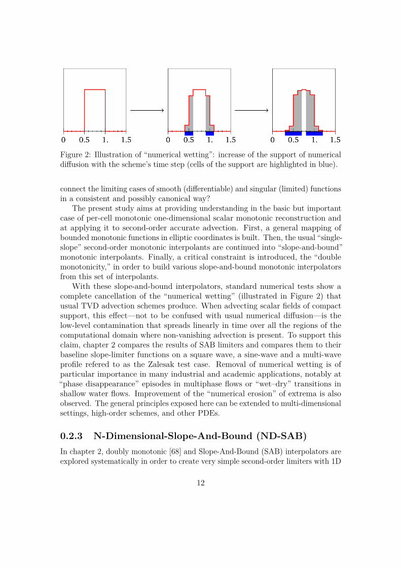
Figure 2: Illustration of “numerical wetting”: increase of the support of numericaldiffusion with the scheme’s time step (cells of the support are highlighted in blue).

connect the limiting cases of smooth (differentiable) and singular (limited) functionsin a consistent and possibly canonical way?

The present study aims at providing understanding in the basic but importantcase of per-cell monotonic one-dimensional scalar monotonic reconstruction andat applying it to second-order accurate advection. First, a general mapping ofbounded monotonic functions in elliptic coordinates is built. Then, the usual “single-slope” second-order monotonic interpolants are continued into “slope-and-bound”monotonic interpolants. Finally, a critical constraint is introduced, the “doublemonotonicity,” in order to build various slope-and-bound monotonic interpolatorsfrom this set of interpolants.

With these slope-and-bound interpolators, standard numerical tests show acomplete cancellation of the “numerical wetting” (illustrated in Figure 2) thatusual TVD advection schemes produce. When advecting scalar fields of compactsupport, this effect—not to be confused with usual numerical diffusion—is thelow-level contamination that spreads linearly in time over all the regions of thecomputational domain where non-vanishing advection is present. To support thisclaim, chapter 2 compares the results of SAB limiters and compares them to theirbaseline slope-limiter functions on a square wave, a sine-wave and a multi-waveprofile refered to as the Zalesak test case. Removal of numerical wetting is ofparticular importance in many industrial and academic applications, notably at“phase disappearance” episodes in multiphase flows or “wet–dry” transitions inshallow water flows. Improvement of the “numerical erosion” of extrema is alsoobserved. The general principles exposed here can be extended to multi-dimensionalsettings, high-order schemes, and other PDEs.

0.2.3 N-Dimensional-Slope-And-Bound (ND-SAB)In chapter 2, doubly monotonic [68] and Slope-And-Bound (SAB) interpolators areexplored systematically in order to create very simple second-order limiters with 1D

12

upwind advection fluxes while attenuating numerical diffusion. A multidimensionalextension called ND-SAB is introduced here as an alternative to classical MUSCLtechniques: the multidimensional gradients are not directly limited, but reduced toa 1D representation, which is called the 1D reference frame. This frame is used forlimitation and for the computation of the total outflow of a cell. This total flux isthen redistributed on the face fluxes.

The key element of the 1D SAB reconstruction is given with the so-calledsecond-order reference point, which is the point given on the cell centroid of cell cthat aligns the central values of the left and right neighboring cells. In uniformgrids this second-order reference point simply corresponds to the mean of theneighboring values, whereas in non-uniform grids it is defined as a weighted mean,with weights given by the respective lengths of the neighboring cells. In the 1Dreference frame of the present ND-SAB algorithm however, the sizes of the left andright neighbors are unknowns and the 1D SAB reconstruction cannot be applieddirectly. It is hence more difficult to define a fully multidimensional extension forthe SAB strategy. In the present work, this is solved by introducing monotonicitythresholds in the 1D reference frame.

Furthermore, the ND-SAB method is compatible with the quasi-isotropic first-order advection introduced in [69]. Results are presented in chapter 3 to supportthis claim in 2D. Similar to the results obtained in chapter 2, numerical wetting isreduced to a compact support with the ND-SAB limitation strategy.

13

Part I

Towards isotropic transport withco-meshes

14

Chapter 1

Towards isotropic transport withco-meshes

1.1 IntroductionVarious existing techniques for reducing the anisotropy of numerical transportresort to either of two strategies: (i) improve the order of accuracy of schemes, or(ii) make mesh and discretization stencil more isotropic. In the latter approach, onecan mention Lagrange-remap schemes for hydrodynamics, where so-called cornerfluxes appear [16, 21], face centered cubic (FCC) or body-centered cubic (BCC)lattices, often used for 3D wave propagation and linear magneto-hydrodynamics(MHD) [70, 71, 72], isotropic finite-differences, to correct lowest order error terms[73], interfacial flux splitting, to reduce mesh-locking effects for the heterogeneous,anisotropic diffusion problem [74], flux-corrected transport (FCT), which treatsmesh-imprinting issues to achieve vorticity preservation [75], geometric correctors,to achieve consistency by constraining convergence to asymptotically regular meshes[66], etc.

Motivated by the development of hydro-codes for Inertial Confinement Fusion(ICF), [11], a novel multi-fluid multi-dimensional direct-ALE hydro-scheme approachwas recently developed [57]. When deriving the scheme—designated as GEECfor Geometry, Energy and Entropy Compatible—a critical step appeared to bethe definition of a proper discrete transport operator. In its present (first-order)form, its displays a significant anisotropic behavior that requires improvement foreffective usage in applications.

The present work thus aims at studying and reducing the 2D anisotropy ofthe discrete first-order transport scheme. For this purpose, we privilege strategy(ii) above to improve isotropy before upgrading the transport operator to higherorder. This is done with an enlarged first-order upwind stencil. Following strategy

15

(i) above would have introduced complexities in the quasi-symplectic design ofthe GEEC scheme due to corner fluxes without actually much improvement onanisotropy to second order.

This approach is inspired by the following quote from P. Roe: “... respecting thecorrect propagation of information under all circumstances. This includes seekingmodes of propagation that are isotropic when they should be.” [76].

1.2 Generic form and properties of the discreteEulerian transport operator

The Eulerian transport operator for a field a under velocity field u writes

Dta = ∂ta+ ∇ · (au). (1.1)

In the ALE context (Arbitrary Lagrangian Eulerian) u is the velocity in thereference frame, defined by the sum of relative-to-grid velocity v and grid velocityw, u = v + w. Remark that by definition v = 0 represents Lagrangian transportby field w, whereas w = 0 represents Eulerian transport by field v.

The generic first-order conservative discretization of the linear Eulerian transportoperator (1.1) writes

D∆tanc = V n+1

c an+1c − V n

c anc + ∆tn

∑d∈D(c)

(anc V

ncd − and V n

dc

), (1.2)

where the transported field a is defined at cell center xc as its average value over(moving mesh) cell c of volume Vc—D(c) being the set of cell labels logicallyconnected to cell c, as defined by the stencil. In order to preserve linearity withrespect to velocity, the volume transfer rates V n

cd must be linear forms of relative-to-grid velocities vnq—which are given at some nodes q related but not necessarilyidentical to the grid nodes—most generally represented by vectors sncdq

V ncd :=

∑q∈Q(c)

vnq · sncdq, (1.3)

—Q(c) being the set of nodes q logically connected to cell c.Elementary analysis of stability and consistency constrain the features of the

transport operator (1.2) as follows: (i) for stability, transport must be upwindedwith respect the velocity direction, i.e. sncdq · vnq ≥ 0 in (1.3), and this makes V n

cd tobe a piecewise linear function of the vnq or

V ncd :=

∑q∈Q(c)

σncdqvnq · sncdq, where σcdq := H(vq · scdq), (1.4)

16

H being the Heaviside function (H(0) = 1/2 is assumed); (ii) to avoid the DeBarartifact [77], velocities vq must be collocated with transported field ac, i.e. only onepoint xq = xc is associated to any V n

cd in (1.3) and scdq reduces to scd := scdc

V ncd := σncdv

nc · sncd; (1.5)

(iii) consistency to first order with the continuous formulation (1.1) requires enforc-ing the following constraints (see Appendix 1.5.1)∑

d∈D(c)(σncdsncd − σndcsndc) = 0, (1.6a)∑

d∈D(c)σncds

ncd ⊗ δxn

cd = V nc I, (1.6b)

where δxncd := xn

d − xnc , and I is the identity matrix.

Condition (1.6a) is trivially ensured in a finite volumes setting where sncd arethe cell face vectors—normal to faces with magnitude given by face area—and ifthe the upwinding factors are consistent, that is if σncd + σndc = 1 for any couple cd.Under these conditions, (1.6a) reduces to the trivial identity∑

d

sncd = 0. (1.7)

Now, condition (1.6b) is far less trivial even in a finite element setting andis strongly dependent on the cell shapes and sizes. As visible from (1.19) inAppendix 1.5.1, the condition is fulfilled with a uniform upwinding factor and auniform Cartesian mesh of squares or cubes in 2 or 3D. It is to be noted however,that conditions (1.6) are always invariant by both affine transformations andconvex linear combinations of transport schemes.

The approach in the present work is to find the (possibly) best discretization tofirst order of the Eulerian transport operator within the framework defined by (1.2),(1.5), and (1.7), and complemented by (1.6b) whenever possible. It can be noticedthat [57] used the same formalism on a structured (but non Cartesian and nonuniform) mesh. This paper goes further by exploiting the freedom left in (1.6) toimprove transport isotropy.

1.3 Co-mesh approach in 2DUsual 2D Cartesian 5-point stencils of finite volume schemes only take into accountfirst nearest neighbors (across cell faces). In the present work so-called co-meshes(as described in chapter 1.3.1) are introduced in order to deal with corner fluxesthrough second nearest neighbors (across cell corners).

17

Figure 1.1: Cell with its first nearest neighbors (white) and its co-cell boundariesconnected to second nearest neighbors (pink).

1.3.1 Construction of the co-meshThe co-mesh represents a fictive grid that links second nearest neighbors (neighborsacross cell corners in the initial mesh) through fictive cell faces (see Fig. 1.1).Notably, the co-mesh defines the vectors s

(2)cd as its face normals, whereas s

(1)cd are

the face normals of the initial mesh. A cell of the co-mesh is called a co-cell. Eachco-cell is built from the cell centers of the first nearest neighbors, where thesecell centers act as the nodes of the co-mesh. This results in two co-meshes for astructured 2D grid, as shown in Fig 1.2. The main idea behind this construction isto build a mesh, on top of the initial one, which omits the numerical informationof the first nearest neighbors. Fig. 1.3b illustrates the volume of the co-cells andhow the omitted parts prevent the co-mesh from having “holes” in it, in order toresult in a well-defined mesh. At the moment, the co-mesh strategy is applied onlyto quadrilateral (but not necessarily Cartesian) structured grids. It is not clear yethow this method will be adaptable to unstructured grids.

Let us remark at this point the importance of computing the cell volumes of theco-meshes V (i)

c exactly, in order to preserve conservation. Considering V (2)c = 2V (1)

c

is of course true in the case of Cartesian meshes. However, this estimate is almostsurely wrong in the case of more general meshes and violates conservation asillustrated in Fig. 1.6.

1.3.2 General methodThe co-mesh approach consists in solving transport terms of a numerical schemeover an initial mesh and several related co-meshes (introduced in 1.3.1) and linearlycombine the resulting schemes ω × scheme + (1− ω)× co-scheme with weight ω.This leads to a 9-point stencil on a fictive mesh as represented in Fig. 1.3.

The notation for the transport operator in (1.2) is not changed; only theneighborhood of cell c is redefined as

D(c) = D1(c) ∪ D2(c), (1.8)

18

Figure 1.2: Meshes and the corresponding co-meshes. Cartesian grid (top) andrandomly distorted quadrilateral grid (bottom).

19

1.3a

1.4a

1.5a

1.3b

1.4b

1.5b

1.3c

1.4c

1.5c

Results for three different schemes given by: ω = 1 (a), ω = 0 (b), and ωopt (c):

Figure 1.3: Initial Cartesian grid (a) and co-mesh (b). Applying the co-meshstrategy is equivalent to applying the initial transport operator on a non-tailingbut volume-preserving octagonal grid (c).

Figure 1.4: Graph of the dimensionless coefficients of matrix M in basis {e, e⊥} ={ v‖v‖ , e⊥} as a function of transport direction θ: e ·M ·e (blue), e⊥ ·M ·e⊥ (green),

and e ·M · e⊥ (red), scaled by h‖v‖.

Figure 1.5: Representation of numerical diffusion on the transport of a “delta”function (four cells at bottom left corner) along directions v = ‖v‖(cos θ, sin θ),for θ = 0, π/8 and π/4; transport over a radius of 96h (where h is the spatialdiscretization step), on a 128× 128 grid, in 192 iterations, with CFL = 0.5.

20

Figure 1.6: Solver applied to co-mesh (ω = 0). Wrong estimation of cell-volumeviolates conservation and monotonicity (left), compared to the correct result (right).(For details on the simulation see Fig. 1.5.)

21

where D1(c) and D2(c) are the sets of respectively first and second nearest neighbors,and vectors scd are weighted with linear factors ω and (1− ω) as

scd =

ωs(1)cd if d ∈ D1(c),

(1− ω)s(2)cd if d ∈ D2(c).

(1.9)

Hence, the co-mesh method applied to the first-order transport scheme D∆tanc =

0 on an Eulerian grid (i.e. V n+1c = V n

c =: Vc = ωV (1)c + (1− ω)V (2)

c ) writesan+1c − anc

∆tn + 1Vc

∑i=1,2d∈Di(c)

(anc V

(i),ncd − and V

(i),ndc

)= 0, (1.10)

where D1(c) and D2(c) are the set of first and second nearest neighbors respectively,and the superscripts (1) and (2) indicate initial and co-mesh. In other words, thegeometry of the co-mesh defines the coefficients of the second nearest neighbors inthe stencil.

1.3.3 Reducing anisotropyThe co-mesh strategy aims at reducing anisotropy. In order to find the mostisotropic transport, we seek the value of ω leading to some minimal measure ofanisotropy. Here, the modified equation [78] is used to study numerical dissipationof (1.10) and to determine ω. The modified equation is the equation that is actuallysolved to higher order by a first-order scheme of a given initial equation. It writes

(∂ta)nc + vx∂xanc + vy∂ya

nc =

(Mxx(∂2

xxa)nc + 2Mxy(∂2xya)nc +Myy(∂2

yya)nc)

(1.11a)

=:(∂x∂y

)tM(v)

(∂x∂y

)anc . (1.11b)

Mxx,Mxy,Myy are the effective diffusive coefficients that characterize the numericalerror, and depend on the magnitude and orientation of the velocity v.

Consider (1.10) for constant transport direction v := ‖v‖(cos θ, sin θ), withθ ∈ [0, π/4]. Then, the stencil is defined through cell c = (i, j) and its donorcells D1(c) = {(i− 1, j), (i, j − 1)} and D2(c) = {(i− 1, j + 1), (i− 1, j − 1)}. Asdetailed in Appendix 1.5.2, the diffusion matrix on the right hand side of (1.11a)has coefficients

Mxx = 12

(1− vx∆t

∆x

)vx∆x, (1.12a)

Mxy = 12

((1− ω)vy −

√vx∆t∆x

vy∆t∆y√vxvy

)∆x, (1.12b)

Myy = 12

((1− ω)vx +

(ω − vy∆t

∆y

)vy

)∆x. (1.12c)

22

Consider matrix M(v) taken in the basis {e, e⊥} = { v‖v‖ , e⊥}, with transport

direction v = ‖v‖(cos θ, sin θ), and transverse direction e⊥ = (− sin θ, cos θ), whichwrites

Mv :=(M‖ M×M× M⊥

)=(

etMe etMe⊥et⊥Me et⊥Me⊥

). (1.13)

Fig. 1.4 shows the coefficients of matrix Mv over transport direction defined by θ.The imbalance between these coefficients reflects the transport anisotropy of thescheme. Transport would be isotropic, if the coefficients of Mv would not change fordifferent transport direction defined by angle θ. Thus, reducing transport anisotropymeans reducing anisotropy of Mv. This is done through numerical optimization byminimizing some functional g(ω) = ‖fω(θ)‖, that describes transport anisotropy ofMv depending on ω. Thus, minimizing over ω leads to an optimal value

ωopt := arg minω∈[0,1]

g(ω) = arg minω∈[0,1]

‖fω(θ)‖. (1.14)

g(ω) ‖M×‖∞ ‖M× − µ(M×)‖2 ‖M‖ − µ(M‖)‖2ωopt 0.58578643762690508 0.587514086875127 0.585863130802334

Table 1.1: Optimized values of ω for three different functionals g.

Table 1.1 shows the optimal ω computed for different minimization functionalg(ω), where µ is the mean value over interval (0, π/4). The results for ωopt are verysimilar for these norms. However, minimizing coefficient M× in the L∞ norm seemsto be the most ideal choice. From now on, the present work refers to the optimalvalue as ωopt = arg minω∈[0,1] ‖M×‖∞ = 0.58578643762690508. Fig. 1.5c and 1.7show the co-mesh strategy with ωopt applied to the Cartesian grid and a randomlydistorted quadrilateral grid.

1.4 ConclusionThe generic formulation for the discrete Eulerian transport operator has beenintroduced. A consistent version has been deduced on the co-mesh approach.The co-mesh strategy leads to improved isotropy for ωopt, as visible by comparingFig. 1.5a to Fig. 1.5c. The co-mesh approach has been introduced on usual 2DCartesian, and distorted quadrilateral structured grids. Transport anisotropy isreduced on all of these general quadrilateral structured grids, where first-orderconsistency is guaranteed on 2D Cartesian, and uniformly distorted Cartesian grids(i.e. grids of identical parallelograms).

23

Figure 1.7: Co-mesh strategy applied to a randomly distorted quadrilateral gridwith ωopt (details on the simulation are provided in Fig. 1.5).

Applying the co-mesh strategy to 3D needs some further considerations. It isnot obvious how this would work, especially because difficulties arise by introducingthird nearest neighbors. However, it is immanent for a 3D extension that themeshes for first to third nearest neighbors are respectively built from hexahedra,rhombic dodecahedra and truncated octahedra in order to respect tessellation.

The co-mesh strategy has been tested on first-order transport on an Eulerian grid.It can be readily inserted in a GEEC approach, which defines a quasi-symplecticALE scheme and requires a consistent fomulation of the transport operator formass, momentum and internal energy equations. A second-order extension is alsobeing investigated.

1.5 Appendix

1.5.1 First-order development and consistency conditionsThis paragraph provides the derivation of consistency conditions (1.6) for thefirst-order discretization (1.2) of the transport operator (1.1). Some details on thespecial case of Cartesian meshes are also provided.

First-order Taylor expansions in time around tn and space around center of

24

mass xnc of cell c give

V n+1c = V n

c + ∆t ∂tV nc +O(∆t2), (1.15a)

an+1c = anc + ∆t (∂ta)nc +O(∆t2), (1.15b)and = anc + δxn

cd · (∇a)nc +O(||δx||2), (1.15c)vq = vnc + δxn

cq · (∇⊗ v)nc +O(||δx||2), (1.15d)

where δxncd := xn

d −xnc and δxn

cq := xnq −xn

c . Combining these expressions and withthe definition of V n

dc in (1.3), the first-order expansion of the transport scheme (1.2)is

(∂ta)nc + ∂tVnc

V nc

anc

+ 1V nc

vnc ·∑d,q

(sncdq − sndcq)anc + 1V nc

∑d,q

δxncq · (∇⊗ v)nc · (sncdq − sndcq)anc

+ 1V nc

∑d,q

−vnc · sndcq δxncd · (∇a)nc = O(∆t, ||δx||), (1.16)

where for simplicity the upwinding factors σcdq have been omitted (i.e. σcdqsdcq →sdcq) and sums on d or q are now restricted by setting scdq = 0 whenever d /∈ D(c)or q /∈ Q(c).

Now, the the Eulerian transport operator can be decomposed as Dta = ∂ta+a∇ · w + ∇ · (av) = ∂ta + a∇ · w + a∇ · v + v ·∇a, and thus term to termidentification to first order with (1.16) yields

∂tVnc

V nc

anc = anc (∇ ·w)nc , (1.17a)

1V nc

∑d,q

vnc · (sncdq − sndcq) anc = 0, (1.17b)

1V nc

∑d,q

δxncq · (∇⊗ v)nc · (sncdq − sndcq) anc = anc (∇ · v)nc , (1.17c)

1V nc

∑d,q

−(vnc · sndcq) (δxncd · (∇a)nc ) = vnc · (∇ac)n. (1.17d)

As these conditions must hold whatever the transported field a and the transport

25

velocity v—that is whatever anc , (∇a)nc , vnc , and (∇⊗ v)nc ,—they simplify into

∂tVnc = V n

c (∇ ·w)nc , (1.18a)∑d,q

(sncdq − sndcq) = 0, (1.18b)∑d,q

(sncdq − sndcq)⊗ δxncq = V n

c I, (1.18c)∑d,q

−sndcq ⊗ δxncd = V n

c I, (1.18d)

where I is the identity matrix. The grid evolution always complies with (1.18a)(it is the so-called GCL condition) thus only the last three conditions need to beretained.

When further restricting the velocity discretization by setting the set of points xq

equal to the single point xc in Vdc, conditions (1.18c) and (1.18d) become identicaland, reintroducing the upwinding factors, the final two conditions provided in (1.6)are obtained.

In the case of a 2D Cartesian mesh with transport between adjacent cells,constraint (1.18d) is simply expanded along x and y coordinates and, with explicitupwinding factors σ, reduces to∑

d∈D(c)σcdscd,xδxcd,x = Vc, (1.19a)

∑d∈D(c)

σcdscd,yδxcd,y = Vc, (1.19b)∑

d∈D(c)σcdscd,xδxcd,y = 0, (1.19c)

∑d∈D(c)

σcdscd,yδxcd,x = 0. (1.19d)

It is readily observed that these conditions are fulfilled with a velocity of uniformdirection and on a uniform mesh: only one donor cell appears in each sum andVc = scdδxcd for any couple of neighboring cells cd.

1.5.2 Modified equation applied to the first-order trans-port scheme with co-meshes

The numerical diffusion coefficients Mxx, Mxy and Myy of the modified equa-tion (1.11a) can be calculated by the following recipe: first the second-orderdevelopment of the scheme is computed and then time derivatives higher thanthe scheme’s order and mixed time and space derivatives are eliminated. The

26

latter is a straight forward computation and can be implemented in any computeralgebra system (CAS) performing symbolic computations, such as Mathematicaor the Python library Sympy. However, this chapter reveals some details for thecalculations on scheme (1.10).

In order to compute the second-order development, the second-order Taylorexpansions in time and space are introduced.

an+1c = anc + ∆t(∂ta)nc + 1

2(∆t)2(∂2tta)nc +O(∆t3), (1.20a)

and = anc + δxncd · (∇a)nc + 1

2δxncd · (∇2a)nc · δxn

cd +O(||δx||3), (1.20b)

with δxncd := xn

d−xnc , for d ∈ Di(c), i = 1, 2. Furthermore, δxn

dc = xnc−xn

d = −δxncd.

Considering a Cartesian grid and a constant velocity vector vd = vc, the spacediscretization can be simplified. Recall from chapter 1.2 that conservation of a fielda is enforced over any volume Vc by constraint ∑d∈D(c) sncd = 0. It follows

∑d∈D(c)

(V ncda

nc − V n

dcand

) (1.20b)=∑

d∈D(c)(σncd + σndc)︸ ︷︷ ︸

=1

sncd · vnc anc︸ ︷︷ ︸

=0

−∑

d∈D(c)σndcs

ndc · vnc

(δxn

cd · (∇a)nc + 12δx

ncd · (∇2a)nc · δxn

cd

). (1.21)

A simple computation shows that (1.18d) is valid on the Cartesian mesh and itsco-mesh. Therefore, the following term on the right hand side of (1.21) can besimplified in this case and becomes

−∑i=1,2d∈Di(c)

σ(i)dc (s(i)

dc ·vc) δxncd·(∇a)nc = ωV (1)

c vc·(∇a)nc+(1−ω)V (2)c vc·(∇a)nc = Vcvc·(∇a)nc .

(1.22)Then, the second-order development writes

(∂ta)nc +vc ·(∇a)nc = −12∆t(∂2

tta)nc + 1Vc

∑i=1,2d∈Di(c)

σ(i)dc s

(i)dc ·vc

(12δx

ncd ·(∇2a)nc ·δxn

cd

). (1.23)

The modified equation is obtained by eliminating the second-order time derivativein (1.23). (∂2

tta)nc is given by differentiation of (1.23) in time. In this expressionthe mixed time and space derivatives (∂2

txa)nc and (∂2tya)nc appear, which can be

eliminated by differentiation of (1.23) in each spatial direction. Remark that thecomputations in (1.19) are valid on the co-mesh of a Cartesian grid, which is used

27

in the following calculations.

(∂2tta)nc = 1

Vc

∑i=1,2d∈Di(c)

σ(i)dc s

(i)dc · vc

(δxcd,x(∂2

txa)nc + δxcd,y(∂2tya)nc

)(1.19)= −vx(∂2

txa)nc − vy(∂2tya)nc ,(1.24a)

(∂2txa)nc = 1

Vc

∑i=1,2d∈Di(c)

σ(i)dc s

(i)dc · vc

(δxcd,x(∂2

xxa)nc + δxcd,y(∂2xya)nc

)(1.19)= −vx(∂2

xxa)nc − vy(∂2xya)nc ,(1.24b)

(∂2tya)nc = 1

Vc

∑i=1,2d∈Di(c)

σ(i)dc s

(i)dc · vc

(δxcd,x(∂2

xya)nc + δxcd,y(∂2yya)nc

)(1.19)= −vx(∂2

xya)nc − vy(∂2yya)nc ,(1.24c)

and therefore

(∂2tta)nc = v2

x(∂2xxa)nc + 2vxvy(∂2

xya)nc + v2y(∂2

yya)nc . (1.25)

Hence, the coefficients of the modified equation (1.11a) write

2Mxx = −∆tv2x + 1

Vc

∑i=1,2d∈Di(c)

σ(i)dc s

(i)dc · vc δx2

cd,x, (1.26a)

2Mxy = −∆tvxvy + 1Vc

∑i=1,2d∈Di(c)

σ(i)dc s

(i)dc · vc δxcd,xδxcd,y, (1.26b)

2Myy = −∆tv2y + 1

Vc

∑i=1,2d∈Di(c)

σ(i)dc s

(i)dc · vc δx2

cd,y. (1.26c)

1.5.3 Anisotropy and CFLConsider constant velocity vector vd = vc. In this case, there are eight possible setsof active donor cells. These sets are defined through the intervals Ik = [kπ4 ,

(k+1)π4 ],

for k ∈ Z/8Z. Choose for instance transport direction v = ‖v‖(cos θ, sin θ), withθ ∈ [0, π4 ], then on the Cartesian mesh, where δxx = δxy =: ∆x, the numericaldiffusion matrix defined in (1.11b) writes

M(v) = 12∆x

(vx (1− ω)vy

(1− ω)vy (1− ω)vx + ωvy

)+ MCFL, θ ∈ [0, π/4], (1.27)

28

with

MCFL = −∆t∆x

(v2x vxvy

vxvy v2y

)(1.28)

Remark that the coefficients of M(v) change for the different sets of donor cellssymmetrically. Fig. 1.4a to 1.4c illustrate the symmetries of M(v) in basis {e, e⊥}over I0 to I3.

Recall the representation of matrix M in basis {e, e⊥} = { v‖v‖ , e⊥}, noted

Mv, with transport direction v = ‖v‖(cos θ, sin θ), and transverse direction e⊥ =(− sin θ, cos θ).

Mv =(M‖ M×M× M⊥

)=(

e ·M · e e ·M · e⊥e ·M · e⊥ e⊥ ·M · e⊥

). (1.29)

The following calculations show that the representation of this matrix in basis{e, e⊥} does not depend on the CFL up to a linear term (and this only for coefficientM‖), as the coefficients of Mv,CFL are constant over θ.

M‖,CFL = e ·MCFL · e = −∆t∆x

(v4x + 2v2

xv2y + v4

y

)= −∆t

∆x(v2x + v2

y︸ ︷︷ ︸= cos2 θ + sin2 θ = 1

)2= −∆t

∆x,

(1.30a)

M×,CFL = e ·MCFL · e⊥ = −∆t∆x

(v3xvx⊥ + vxvy(vxvy⊥ + vx⊥vy) + v3

yvy⊥︸ ︷︷ ︸=sin θ cos θ(− cos2 θ+cos2 θ−sin2 θ+sin2 θ)=0

)= 0,

(1.30b)

M⊥,CFL = e⊥ ·MCFL · e⊥ = −∆t∆x

(v2xv

2x⊥

+ 2vxvx⊥vyvy⊥ + v2yv

2y⊥

)= −∆t

∆x(vxvy + vx⊥vy⊥︸ ︷︷ ︸

= − cos θ sin θ + sin θ cos θ = 0

)2= 0.

(1.30c)

29

Part II

Doubly-monotonic constraint oninterpolators: bridging

second-order to singularitypreservation to cancel “numericalwetting” in transport schemes

30

Chapter 2

Doubly-monotonic constraint oninterpolators: bridgingsecond-order to singularitypreservation to cancel “numericalwetting” in transport schemes

2.1 Introduction

2.1.1 Motivations: “numerical wetting”Transport operators are central elements of the PDEs found in many scientificfields, such as and foremost in physics: not only do they describe actual transportof conserved quantities but they also capture, after proper transformations, thepropagation of invariants in hyperbolic equations. The design and understandingof numerical techniques for transport operators and equations are thus of primeimportance and have drawn an enormous amount of effort over the last seventyyears. Now, as early recognized, most of the difficulties in this far reaching endeavoralready appear in the simplest system: the passive one-dimensional transport of ascalar field y(t, x) by a velocity field u(t, x)

∂ty + ∂x(uy) = ∂ty + u ∂xy + y ∂xu = 0, (2.1)here written in conservative form. Because of its importance, this basic linearequation has attracted special attention, with ensuing publications in staggeringnumbers [79, and refs therein].

On even grids in dimension one, there is now a good understanding of the maindistortions produced by solvers of (2.1): instabilities, smearing of discontinuities

31

and numerical diffusion, oscillations, and loss of conservativity, positivity or mono-tonicity. These can be kept under control by important scheme features whichare now standard items of the numericists’ toolbox: finite volumes approaches,higher-order discretizations, stability analysis, modified equation interpretations,flux upwinding, and TVD flux limitation [79, and refs therein]. However, anotherartifact, here designated as “numerical wetting,” has been somewhat neglected sofar, possibly for being less amenable to usual accuracy-focused topological analysis.

Numerical wetting designates the low-level contamination that spreads linearlyin time over all the regions of the computational domain where non-vanishingtransport is present. It is not to be confused with usual numerical diffusion whichspreads profiles sub-linearly in time, as tθ with θ . 1

2 [80]. Numerical wettingmay appear of marginal importance—and indeed is in terms of numerical accuracywhen compared to other more significant truncation errors—but it turns out to beespecially irritating in practical situations involving fluid mixing and evanescentboundary conditions. Two such situations of interest in industrial and academicapplications will be mentioned here although many others can also be found.

1. “Phase disappearance” in multiphase flows Multiphase or multi-fluidflows appear in numerous applications where they are modeled by coupled Eulerlike equations for their different components. When the flow conditions make one(or more) of the components disappear at a given time and position, numericalwetting forbids its full disappearance, i.e. its volume fraction cannot be madeto cancel to round-off error under the sole action of the transport scheme. Thiscan trigger singular or unstable behavior of the physical model or the numericalscheme: for instance, with highly contrasted compressible fluids such as water andair, pressure relaxation between fluids can become surprisingly stiff at vanishingvolume fractions [81, 82, resp. eq. 6 & § 3.6].

2. “Wet–dry transition” in shallow water flows Shallow water calculationsare generally restricted to positive depth regions, delimited by shores which, phys-ically, can switch between wet and dry as waves propagate. This situation iscaptured by numerical schemes which either forbid full drying of shore cells—athin numerical “film” of liquid is then always present—or provide for a special localtreatment—with a numerical “shore-line” reconstruction. Both options require spe-cial attention as they can induce singular or fragile behavior. This is not surprisingas the shallow water equations are formally identical with a degenerate form of thetwo-fluid flow equations.

More or less empirical and singular fixes of numerical wetting have been devisedby almost all numericists involved in developing practical codes for these twoexamples. Understandably, these recipes have been seldom publicized but a few

32

examples can be found and are worth mentioning here. The basic “brute force”method is to artificially bring to zero all volume fractions falling below a (hopefullylow) predefined threshold, bearing in mind that this may be detrimental to exactconservation over long times. Typical threshold values can be found at 10−3 forslugging in pipes [83, § 4.6 & refs therein] or 10−5 to 10−4 for boiling in nuclearreactors [84, § 7 & refs therein]. These levels can be considered as too high andunsatisfactory and have triggered the development of more subtle approaches. Atthe high end of sophistication, a surprising method was proposed whereby theevolution equations are extended to an artificial domain of negative volume fractionwhere all the closures are deliberately continued so as to mimic the behavior of thesystem at zero volume fraction. The same model equations and numerical schemeare thus applied in a uniform way throughout the computational domain. Thetechnique appears to have been applied only to transport in porous media [85].Similarly, the wet–dry transition in shallow water flows is amenable to widelydifferent numerical treatments [86, § 1 and refs therein].

It must be stressed that the reduction or cancellation of numerical wettingcannot solve all the issues related to phase disappearance (or its formally equivalentavatars) such as thermodynamic consistency. However, it is a critical ingredient totackle such singular situations. Furthermore, through symmetries and dualities,the discretization of transport can sometimes constrain or even fully define thediscretization of all the evolution equations: an example was recently providedby a geometrically consistent discretization of the multi-fluid Euler equations [82].Numerical wetting can thus impact a numerical scheme in many of its featuresbeyond transport terms.

The cancellation of numerical wetting in practical applications was the primarymotivation for the present investigation. Now, when analyzing this problem, theauthors realized that a broader perspective had to be taken in order to provide anhorizon of accessible solutions and to build actual optimal algorithms for wetting-free transport (here to second order). This work will thus be devoted mostly tothe general doubly-monotonic interpolants introduced in subsection 2.1.4, whereascancellation of numerical wetting will appear almost as a byproduct when applyingthe slope clipping introduced in subsection 2.1.3 to the numerical experiments ofsection 2.5.

2.1.2 Numeric background: Muscl-like schemeGeneral methods on numerical solvers of (2.1) are described and analyzed in manystandard textbooks. Beyond their widely different and numerous interpretations—for instance as finite volumes or elements, with Riemann solvers, fluxes, swept fluxes,remap, averaging, etc.—they all involve a common critical feature of major interestfor the present work: flux or slope limiting [79, § 6]. This stems from the much

33

280 BRAhl VAN LEER

-1 0 1 x/ax 2 -1 0 a1 2 -1 0 0 1 2 -1 0 1 2

FIG. 2. The second-order upstream-centered scheme (in particular, scheme III). (1) approxima- ting the initial-value distribution (solid line) in each slab by a linear distribution (broken line) with the same mesh integral. In this case the slopes are determined by least-squares fitting. (2) The ap- proximate initial-value distribution before (solid) and after (broken) convection over a distance crdx. (3) Determining the new linear distributions (broken) in each mesh by least-squares fitting to the convected distribution (solid). (4) The initial values for the next time step.

The quality of scheme (14) varies considerably with the choice of dw. I shall demon- strate this on the basis of three examples. It is assumed everywhere that u > 0.

SCHEME 1. Determine iflu by central differencing of W:

4+(1;2W = B&+(2 ‘2) - Q-(1,,)) = #l&G + L$+,E).

Inserting this into Eq. (14) yields

(16)

w2 = z1,2 - ud,w - (u/4)(1 - u)(d,i-? - A-,rj), (17)

which is just the finite-difference scheme of Fromm [6] applied to mesh averages of w instead of nodal-point values (cf. Van Leer [l, Eq. (34)]). Denoting a translation over +dx by the operator T, we may write (17) as

w2 = {I - u( 1 - T-l) - (u/4)(1 - u) z-(1 + T-1)(1 - T-1)2} w,,, . WI

SCHEME IL Determine dw by differencing w(t”, x):

Ji+(1j2)W = W(tO, Xi+1) - W(tO, Xi). (1%

Defined this way, the quantity dw is independent of the quantity W and must be inte- grated along, requiring a separate storage location. Unlike what we are used to in Snite differencing, the scheme for updating dw differs from the scheme for updating F. We have

m2w = d,w + (4 - u)(ifl:,w - hl12W),

and the full scheme defined in Eqs. (14) and (20) can be written as

(gy2 = ( 1 - u + UT--~ -(u/2)( 1 - a)(1 - T-1) w

1 - T-1 (4 - a)(1 - T-1) I( > irw 1,2 *

The matrix occurring in this equation will be called G”.

(20)

(21)

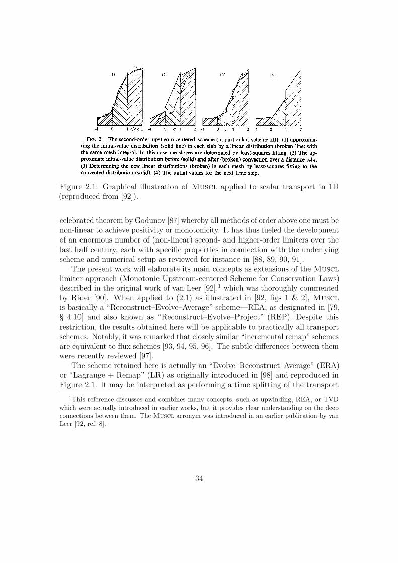
Figure 2.1: Graphical illustration of Muscl applied to scalar transport in 1D(reproduced from [92]).

celebrated theorem by Godunov [87] whereby all methods of order above one must benon-linear to achieve positivity or monotonicity. It has thus fueled the developmentof an enormous number of (non-linear) second- and higher-order limiters over thelast half century, each with specific properties in connection with the underlyingscheme and numerical setup as reviewed for instance in [88, 89, 90, 91].

The present work will elaborate its main concepts as extensions of the Muscllimiter approach (Monotonic Upstream-centered Scheme for Conservation Laws)described in the original work of van Leer [92],1 which was thoroughly commentedby Rider [90]. When applied to (2.1) as illustrated in [92, figs 1 & 2], Musclis basically a “Reconstruct–Evolve–Average” scheme—REA, as designated in [79,§ 4.10] and also known as “Reconstruct–Evolve–Project” (REP). Despite thisrestriction, the results obtained here will be applicable to practically all transportschemes. Notably, it was remarked that closely similar “incremental remap” schemesare equivalent to flux schemes [93, 94, 95, 96]. The subtle differences between themwere recently reviewed [97].

The scheme retained here is actually an “Evolve–Reconstruct–Average” (ERA)or “Lagrange + Remap” (LR) as originally introduced in [98] and reproduced inFigure 2.1. It may be interpreted as performing a time splitting of the transport

1This reference discusses and combines many concepts, such as upwinding, REA, or TVDwhich were actually introduced in earlier works, but it provides clear understanding on the deepconnections between them. The Muscl acronym was introduced in an earlier publication by vanLeer [92, ref. 8].

34

equation (2.1) according to

∂ty + y ∂xu = 0, (2.2a)∂ty + u ∂xy = 0, (2.2b)

which displays an important property: the remap sub-step does not actually performtime evolution and is independent of the Lagrangian sub-step. Indeed, if all detailedcell-to-cell intersections are computed, the geometry and topology of the remappedmesh can be chosen at will, unconstrained by the initial mesh or the mesh distor-tions. This comes with significant advantages: (i) the order of accuracy of the LRstep is given by the lowest of the Lagrangian and remap sub-step orders—no Strangor higher-order splitting is necessary;—(ii) analysis of dissipation and entropy ismuch simpler—only numerical diffusion appears during remap;—(iii) effects ofnon divergence-free, discontinuous, or oddly centered velocity fields [82, § 4.2 forinstance] can be captured properly by the Lagrangian sub-step—yielding possi-bly non-monotonous-but-consistent positive evolution;—iv) remap is intrinsicallyupwind—thus allowing for centered Lagrangian sub-steps;—and v) second-orderaccuracy requires second-order reconstruction for the remap sub-step, but does notrequire any reconstruction for the Lagrangian sub-step if the discretization of u isspace- and time-staggered with respect to that of y.

Following the above remarks, the present work will focus on the monotonicityof reconstruction approaches for the remap sub-step only. However, numericaltests will be carried out on the full LR transport scheme to first- or second-orderaccuracy with a simple reconstruction-free Lagrangian sub-step.

2.1.3 Present approach: from limiting to clipping of inter-polants. . .

The simplest approach to second-order remap in Muscl relies on single-slopeinterpolants in each cell, defined so as to exactly connect the neighboring cellsvalues whenever these are aligned. When cell values depart from alignment, thelinear interpolant may violate the monotonicity condition and its slope must belimited. This limitation also applies on non-uniform meshes [92, § 4] as detailedin [99, § III], or to Courant-number-dependent fluxes. The behavior of the slopestrength as a function of cell average values is usually represented on the so-calledSweby diagram [100, fig. 1]—or more conveniently, on its fully symmetric versionsof Berger–Aftosmis–Muman [99, § II.C, fig. 3] or Waterson [101, § 2, fig. 2].

Similar limiting approaches were also designed for more complex interpolantsin order to increase the order of accuracy, or to better capture extrema or stronggradient regions. Some selected examples are quadratic functions for third orderschemes [92, § 4] or [102]; higher order polynomials [103, and refs therein]; piecewise

35

hyperbolic [104], rational [105], hyperbolic tangent [106], and double logarithm [107]functions for smoother monotonicity conditions; piecewise linear [108, § 4]; quadraticfunctions corrected at smooth extrema [109, 110, 111]. Most notable for thepresent study as discussed in section 2.2, is the method introduced by Desprésand Lagoutière [112, 113], based on a saturated step function and here designatedas “downwind-limited upwind,” which is closely related to interface reconstructiontechniques and to the so-called “reservoir technique” [114].

Except in rare cases, many such schemes mingle the two independent sub-steps of accurate interpolation and monotonicity limitation. This can seriouslyimpact the final limited interpolants by reducing the set of accessible functionsand by requiring more complex calculations: the respective stencils for high-orderinterpolation and monotonicity are very different, especially in dimensions higherthan one. Monotonicity is a scalar constraint defined by only two neighboring cells,irrespective of mesh topology.

This last remark is at the core of the present work: what is the general structureof monotonic interpolants, and how do they connect to a specific configuration werea selected high-order interpolant is exact? In the present work, these issues willbe examined to second-order, with single-slope reconstructions clipped to boundsinstead of slope limited. The set of new possibilities is then widened to the pointthat supplementary conditions need to be introduced in order to avoid inconsistentbehaviors and generate practical schemes. This is the double monotonicity conditionintroduced below in subsection 2.1.4

2.1.4 . . . and from simple to double monotonicityAs already noted by van Leer [92, § 5 & fig. 6], cell interpolants away from extremacan be constrained by monotonicity in two different ways which will be designatedhere as weak and strong. Under weak monotonicity the interpolant is bounded bythe neighboring left and right cell values: this ensures the positive, monotonic, TVD,or BV behavior of the scheme but can let appear inconsistent variations withincells: for instance, despite successive increasing cell values, the interpolant in a cellcan be decreasing while still being bounded by neighboring cells (see Figure 2.2b).This was designated as “stegosaur bias” and is eliminated by a strong monotonicityconstraint [92, eq. 66 & comment below]: the interpolant in a cell must not only bebounded but also display the same increasing or decreasing character as defined bythe neighboring cells (see Figure 2.2c). The rationale for this strong constraint wasconnected to a detailed analysis of dispersion relationships of transport schemes [92,§ 3]—a more refined property than mere TVD, which is seldom analyzed and oftentaken as “implicitly obvious.”

However, in analyzing the behavior of a transport scheme over many successivetime steps, a yet stronger monotonicity condition appears to be required: as

36

a b c d

Figure 2.2: Representations of (a) non-monotonic, (b) weakly monotonic,(c) strongly (non-doubly) monotonic, and (d) doubly monotonic interpolants (solidlines) in a cell constrained by neighboring-cell values. Mean cell values y arerepresented by white dots. In (c) and (d) interpolants that would be generatedfor slightly higher values of y are also represented (dotted lines) so as to visualizedouble monotonicity.

illustrated in Figure 2.2c & d an interpolant function over a given cell must bemonotonic with respect to the mean neighboring-cell values (simple monotonicity)but also be everywhere increasing with respect to the mean cell value (doublemonotonicity). As will be introduced in section 2.4, these two constraints aremore conveniently discussed by distinguishing interpolant and interpolator : theformer is an actual reconstructed function y[x] over a cell with given mean value y,whereas the latter is a reconstruction procedure which generates an interpolanty[x] = z[y, x] as a function of y. Double monotonicity applies to interpolatorsz[y, x].

2.1.5 Mapping of interpolants and interpolators, 1D nu-merical tests

In order to provide guidance on the various acceptable strategies under doublemonotonicity, a new graphical representation of interpolants and interpolators isintroduced in section 2.2 which vastly expands the Sweby diagram. It is basedon elliptic coordinates with respect to poles defined by the order-one constantinterpolant and the downwind-limited upwind interpolant.

Double monotonicity lets define some novel extensions of the classical Min-Mod,Monotonized Centered, Super-Bee, and Ultra-Bee interpolators. Basic 1D transporttests of square wave, sine wave, and Zalesak wave are provided in section 2.5 withthe standard and newly defined interpolators. Specific metrics for the square-wavetransport let monitor mean front widths and front support widths. Full suppressionof numerical wetting will be observed with the new approaches, also with less“numerical erosion” (or better preservation of extrema).

37

2.2 A convenient mapping for bounded mono-tonic functions

2.2.1 Motivation: bounded monotonic functions as inter-polants

Definition 1 (Set of bounded monotonic functions MXY (y)) Let X and Ybe two finite intervals of R. MXY (y) is the set of monotonic functions y[x] from Xtowards Y with given mean

y =∫Xy[x] dx

/∫X

dx. (2.3)

Let I = [0, 1]. M<II(y) is the subset of increasing functions ofMII(y).

Functions in MXY (y) represent, for a monotonic 1D discretization, all themonotonic interpolants over a given mesh cell X, to an interval Y whose boundsare given by values at the neighboring left and right cells. As already mentioned insubsection 2.1.4 and illustrated in Figure 2.2, monotonicity within a cell is sufficientbut not necessary to ensure monotonicity between cell-average values and make aTVD Muscl scheme.

As most of the properties explored in the following are invariant through x-axis shifting, scaling, and inversion, it will be sufficient to simply consider setM<

II(y). With further symmetrization of y[x] into 1− y[−x], the mean value canbe constrained to y ∈ [0, 1

2 ] without loss of generality. Incidentally,MXY (y) andM<

II(y) are convex.

2.2.2 L2 bounds on bounded monotonic functionsDefinition 2 (Edge and middle functions in MXY (y)) To any couple of realnumbers (α, β) ∈ I2 is associated a function yαβ[x] of M<

II(y) designated as an“edge function” and defined as

yαβ[x] =

0 for 0 ≤ x < α(1− y),

(1− β)y(1− α)− (β − α)y for α(1− y) ≤ x < 1− βy,

1 for 1− βy ≤ x ≤ 1.

(2.4)

The “middle function” ofM<II(y) is defined as m = (y11 + y00)/2. The definition

extends toMXY (y) through shifting, scaling, and symmetries.

38

0 1a b1 - y0

1

y

y /2

(1 + y) /2

y0

a

y[x]

a1 a2 b1 b2

b

s[x]

α (1-y) 1- β y

c

yαβ[x]

Figure 2.3: Graphical illustration in support of the Proof of Theorem 1: (a) functiony[x] ∈M<

II(y) (thick line) and its intersection points (circled) with m[x] (doubleline); (b) step function s[x] (thick line) with same intersection points and meanson each interval Ii; (c) “edge” step function yαβ[x] (thick line) of same left andright means as s[x] (and y[x]), and with yαβ[1− y] = y[1− y] = y0.

Direct integration confirms that yαβ and m ∈M<II(y). The step function yαβ

becomes a constant function y for α = β = 0 but notations y00 and y will bepreserved to distinguish function and number. These definitions are important inthe present context as yαβ[x] is an intermediate between the two extremes y00[x]and y11[x], also known as respectively “first order” and “downwind-limited upwind”interpolants [112, 113] in the context of Muscl like numerical schemes for transport.The set of yαβ functions is also a convex generator system forM<

II(y) in the senseof distributions (it is not a free system, however). Incidentally, functions of y00and y11 are related through inversion as y−1

00 [x] = y11[x].

Lemma 1 (L2 radius of edge functions) For any given y, all edge functions ofM<

II(y) are at the same L2-distance of its middle function, i.e. ‖yαβ−m‖22 = y(1−

y)/4. The lemma extends toMXY (y) through shifting, scaling, and symmetries.

Proof This results from direct integration of (2.4). �A stronger result is then obtained:

Theorem 1 (L2 bounds on MXY (y)) For any y ∈M<II(y)

‖y −m‖22 ≤ y(1− y)/4, (2.5)

where m is the middle function ofM<II(y), equality being reached if and only if there

exists (α, β) ∈ I2 such that y = yαβ ∈ M<II(y). The theorem extends to MXY (y)

through shifting, scaling, and symmetries.

39

Proof A function y ∈M<II(y) being given, let ordinate y0 and abscissas a and b

defined as (see Figure 2.3a)

y0 = y[1− y], (2.6a)

y[a] = m[a] = y/2 or a ={

0 if ∀x ∈ [0, 1− y], y[x] > m[a],1− y if ∀x ∈ [0, 1− y], y[x] < m[a],

(2.6b)

y[b] = m[b] = (1 + y)/2 or b ={

1− y if ∀x ∈ [1− y, 1], y[x] > m[b],1 if ∀x ∈ [1− y, 1], y[x] < m[b].

(2.6c)

Let the step function

s[x] =

0 for 0 ≤ x ≤ a1,

y/2 for a1 < x ≤ a2,

y0 for a2 < x < b1,

(1 + y)/2 for b1 ≤ x < b2,

1 for b2 ≤ x ≤ 1,

(2.7)

defined by points a1, a2, b1, and b2 such that s and y have identical means over thefour successive intervals I1 = [0, a], I2 = [a, 1− y], I3 = [1− y, b], and I4 = [b, 1− y],i.e. (see Figure 2.3b)

for i = 1 to 4∫Ii

(y[x]− s[x]

)dx = 0,

thus∫ 1

0s[x] dx =

∫ 1

0y[x] dx = y, and s ∈M<

II(y). (2.8)

This is always possible from the definition of a and b and as y is an increasingfunction, and thus 0 ≤ a1 ≤ a ≤ a2 ≤ b1 ≤ b ≤ b2 ≤ 1. Over each of the fourintervals Ii, y−m is of constant sign and bounded as

∣∣∣y[x]−m[x]∣∣∣ ≤ maxIi

∣∣∣s[x]−m[x]

∣∣∣. The L2 integrals can thus be bounded as∫Ii

(y[x]−m[x]

)2dx ≤ max

Ii

∣∣∣s[x]−m[x]∣∣∣ ∫Ii

∣∣∣y[x]−m[x]∣∣∣ dx

≤ maxIi

∣∣∣s[x]−m[x]∣∣∣ ∫Ii

∣∣∣s[x]−m[x]∣∣∣ dx =

∫Ii

(s[x]−m[x]

)2dx. (2.9)

Thus ‖y −m‖22 ≤ ‖s−m‖2

2.Now, let an edge function yαβ ∈M<

II(y) be defined by its middle value yαβ[1−y] = y0 and by α such that (see Figure 2.3c)∫ a2

a1

(s[x]− yαβ[x]

)dx = 0. (2.10)

40

α exists such that α(1−y) ∈ [a1, a2] because 0 ≤ s[x] = y/2 ≤ y0. 1−βy ∈ [b1, b2] isthus obtained from y0 and α according to (2.4). As s[x] = m[x] over [a1, a2]∪ [b1, b2]and s and yαβ coincide over the complementary domain [0, a1] ∪ [a2, b1] ∪ [b2, 1], itis found ‖s−m‖2

2 ≤ ‖yαβ −m‖22.

Therefore, according to Lemma 1, ‖y −m‖22 ≤ ‖yαβ −m‖2

2 = y(1− y)/4. Theproof also holds for discontinuous y using the left and right limits around thevarious points defined above. �

2.2.3 Elliptic coordinates mapping of MXY (y)Corollary 1 (Elliptic coordinates mapping of MXY (y)) For any y ∈M<

II(y),( ‖y − y00‖2

‖y11 − y00‖2

)2+( ‖y − y11‖2

‖y11 − y00‖2

)2≤ 1, (2.11)

equality being reached if and only if there exists (α, β) ∈ I2 such that y = yαβ. Thecorollary extends toMXY (y) through shifting, scaling, and symmetries.

Proof This results from Lemma 1 and Theorem 1 after elementary algebra,bearing in mind that y00, m, and y11 are aligned and form a diameter. �

(2.11) naturally leads to considering the elliptic coordinates inMXY (y) withrespect to poles y00 and y11: as represented in Figure 2.4, any y ∈ MXY (y) canbe mapped (injection) to a point of the half disk of radius 1

2 bounded by the edgefunctions yαβ—the mapping is one-to-one only along the y00–y11 axis. The halfdisk is both the 2D axi-symmetric projection ofMXY (y) for each y and a polarprojection of theMXY (y) for all y (which are subsets of parallel hyperplanes offunctions). For reference, the classical transformation from elliptic coordinates(d+, d−) with poles (±1

2 , 0) to Cartesian coordinates (x, y) is given by

(x− 12)2 = (1 + d2

+ − d2−)2/4, (2.12a)

y2 = d2+d

2− − (1− d2

+ − d2−)2/4. (2.12b)

The elliptic coordinates mapping provides guidance for designing and evalu-ating general interpolators: it is not restricted to specific profiles such as linearinterpolants as mapped on a Sweby diagram [100, fig. 1] and applies whatever thestencil width and order of the scheme. It has some limitations however, as it is forinstance not one-to-one, not linear, and worse, not convex: in general, the map of aconvex subset ofM<

II(y) may not be convex as a segment connecting two functionsinM<

II(y) maps as a concave arc of hyperbola in the elliptic coordinates.

41

r

ϕ(r )

0 1 2 3

1

2

m y11

Order 1:y00 Middle:

Downwind –limitedupwind:

Edge : yαβ

Order 2

UltraBeeend point

y = ½

y = ¼

Figure 2.4: 2D map of the set of bounded monotonic functions M<II(y) in the

elliptic coordinates from poles y00 and y11: all y are within the half circle centeredon m = (y00 + y11)/2 bounded by yαβ as stated in Corollary 1. The thick linesegments correspond to single-slope interpolants (see subsection 2.3.2) of fixed yvalues ranging from 0 to 1

2 in steps of 116 . The 2nd order point is the interpolant

that would result from any second-order scheme over a uniform mesh. The insert isthe usual Sweby diagram [100, fig. 1] of these single-slope interpolants which maptwo-to-one in the half circle (as represented by the corresponding lines and endpoints).

2.3 Slope-and-bounds interpolants

2.3.1 Background: usual single-slope interpolantsAmong all possible interpolants, affine functions obviously play a central role:they are the algebraically simplest to approximate smooth functions to secondorder, and for given y, depend on only one parameter, the slope g. They havethus been extensively studied and are at the core of all second-order schemes withnumerous possible closures [88, 89, 90, 91, for reviews]. The present work willonly consider the four most basic slope definitions usually designated as Min-Mod(MM), Monotonized Centered (MC, also known as Barth–Jespersen), Super-Bee(SB), and Ultra-Bee (UB, also known as Upper-Bound). With the usual shifting,scaling, and symmetrizing onM<

II(y) but on a non-uniform grid, these are defined

42

as2 (remember that 0 < y ≤ 12)

gMM[y] = 2 min{ 1− y

1 + h1,

y

1 + h0

}h0,1=1= y, (2.13a)

gMC[y] =1+2h01+h1

(1− y) + 1+2h11+h0

y

1 + h1 + h0

h0,1=1= 12 , (2.13b)

gSB[y] = 2 max{ 1− y

1 + h1,

y

1 + h0

}h0,1=1= 1− y, (2.13c)

gUB[y] = 2 min{

(1− y), y}

= 2 y. (2.13d)

where the left and right cells widths, h0 and h1, are scaled by the current cell width,and the expression for the MC slope is justified in Appendix 2.8. All the slopescollapse to the exact second-order interpolant for aligned cell values, at

gXX[y] = gO2 = 2/(2 + h1 + h0), for y = yO2 = (1 + h0)/(2 + h1 + h0). (2.14)

The definitions in (2.13) however, do not yield I-bounded interpolants in generaland must thus be either limited, corrected, or clipped: following the remarks insubsection 2.1.3, this is how accurate interpolation and monotonicity limitation arehere separated.

The traditional approach for limitation of slopes as those in (2.13) basicallyamounts to the substitution

gXX Lim. = min{gXX, gUB

}. (2.15)

As expected the MM slope is unchanged by this limitation step. Now, monotonicitycan be achieved more generally by modifying the shape of affine interpolants whenrequired. In principle, higher-degree polynomials—such as parabolic interpolantswhich are the next most algebraically simple and are usually invoked for third-order accuracy [92, 102]—could be a possibility but they almost always displaynon-monotonic behavior for some values of y. Rational [105] or transcendental [106]functions could also be considered.

We here select the simplest non-algebraic extension, whereby single-slope in-terpolants are merely “clipped” to bounds, thus producing slope-and-bound andslope-and-two-bounds interpolants. These interpolants, as defined below in subsec-tion 2.3.2, are still described by a single parameter (the slope g) and connect toeach other in a continuous way.

2In these formulae, the threshold value of y contained in the min and max functions may differfrom 1

2 for non-uniform grids. As previously noticed [99], Sweby-like diagrams can be centered oneither of the monotonicity or second order thresholds. Monotonicity is clearly privileged here.

43

2.3.2 Slope-and-bounds interpolantsDefinition 3 (Slope-and-bounds interpolants) Single-Slope (SS), Slope-And-Bound (SAB), and Slope-And-Two-Bounds (SAB2) interpolants are defined bythe respective functions y ∈ M<

II(y) which depend on a single parameter g ∈ R+

(remember that 0 < y ≤ 12)

y[x] =

y + g × (x− 1

2), for 0 ≤ g < 2y,max

{0,√

2yg + g × (x− 1)}, for 2y ≤ g < 1/(2y),

min{

1,max{

0, 12 + g × (x− 1 + y)

}}, for 1/(2y) ≤ g <∞.

(2.16)The definition extends toMXY (y) through shifting, scaling, and symmetries.

The slope-and-bounds functions do not aim at being “close” to the yαβ edgefunctions, less at being “dense” in M<

II(y), but they continuously connect y00and y11 for respective slopes g = 0 and g →∞. Connection to the saturated stepfunction y11—the downwind-limited upwind of Després and Lagoutière [112, 113]—is an especially interesting feature that few interpolants display. Incidentally,the inverses of SS, SAB, and SAB2 functions are themselves SAB2, SAB, andSS functions respectively—thus extending the connection y−1

00 [x] = y11[x] alreadynoted in subsection 2.2.2.

Proposition 1 (Elliptic coordinates of slope-and-bounds interpolants) Single-Slope (SS), Slope-And-Bound (SAB), and Slope-And-two-Bounds (SAB2) inter-polants have squared elliptic coordinates from poles y00 and y11 given respectivelyby (remember that 0 < y ≤ 1

2)

‖y − y00‖22 =

g2/12, for 0 ≤ g < 2y,y(

23√

2yg − y), for 2y ≤ g < 1/(2y),

y(1− y)− 1/(6g), for 1/(2y) ≤ g,

(2.17a)

‖y − y11‖22 =

y(1− y)(1− g) + g2/12, for 0 ≤ g < 2y,y(1− 4

3√

2yg + yg), for 2y ≤ g < 1/(2y),

1/(12g), for 1/(2y) ≤ g.

(2.17b)

The proposition extends toMXY (y) through shifting, scaling, and symmetries.

Proof This results from direct integration of (2.16). �Applying (2.12) to (2.17), the set of SS functions for any given value of y is found

to map on the half disk as a straight segment connected to the y00 point as visible

44

y00 m c y11

O2

UB

SS lines

SAB lines

SAB2 line

Figure 2.5: 2D map (elliptic coordinates from poles y00 and y11) of slope-and-boundand slope-and-two-bounds interpolants (SAB zone, thick lines) for fixed y valuesfrom 0 to 1

2 in steps of 116 : these extend the corresponding single-slope interpolants

of same y values (thin lines, see also Figure 2.4) and make a full connection from y00to y11 running close to the yαβ edge.

on Figure 2.4. The segments for various y can be put in one-to-one correspondencewith vertical lines on the Sweby diagram [100, fig. 1b] (see insert on Figure 2.4)which is traditionally used for mapping SS interpolants and interpolators overcoordinates (r, φ) = (1/y − 1, g/y). The Sweby diagram however, is unsuitable tomap any other type of interpolant such as SAB or SAB2. Two canonical pointsalong the y = 1

2 line are marked in both representations of Figure 2.4: the “second-order” (on uniform grid) and “Ultra-Bee” points for respectively g = 1

2 and 1. Fornon-uniform grids, the “second-order” point may not coincide with the middle ofthe first-order to Ultra-Bee segment.

Inspection of Figure 2.4 reveals that single-slope interpolants only sample asmall leaf-shaped portion on the map of interpolants, skewed towards the first-orderpoint y00 on which they collapse as y → 0. This reduced sampling of the spaceof accessible interpolants is a major theoretical motivation for introducing theslope-and-bounds interpolants of Definition 3.

Applying again (2.12) to (2.17), the set of SAB and SAB2 functions, for anygiven value of y, are found to map on the half disk as lines extending the SS segmentsand connecting to the y11 point as visible on Figure 2.5. These lines run typicallyhalfway between the middle function m and the edge functions yαβ. For smallvalues of y a very significant expansion of accessible interpolants is thus achieved.However, the SAB2 interpolants will appear unsuitable for practical second-orderapplications for being incompatible with the doubly monotonic constraint to bediscussed in section 2.4.

Incidentally, the reduced elliptic coordinates for SAB2 interpolants deducedfrom (2.17) depend on a single parameter, the combination y(1− y)g: as visible inFigure 2.5, this collapses the SAB2 lines for any y into what can be found to be a

45

portion of circle of radius 13 centered on c = 1

3y00 + 23y11.

2.4 Doubly-monotonic SAB interpolators

2.4.1 Motivation: from interpolant to interpolatorThe present discussion has been focused so far on some general properties ofinterpolants, i.e. bounded monotonic functions y ∈ MXY (y). Though useful forgeneral understanding, it does not provide clues on actual prescriptions to build aninterpolator z[y, x], which yields an interpolant y[x] = z[y, x] for any given y value.Only for special values of y is it possible to prescribe y[x] in a univocal way: forinstance, second-order interpolants must be exact for y = yO2 as given in (2.14).

The prescription of interpolator formulae, often believed to proceed from wellestablished principles, is actually based on perceived self-evidences or trial-and-errorstrategies. A common example is the improperly-called “second-order region” inthe Sweby diagram (see inset of Figure 2.8) which is in fact posited by constrainingthe interpolated slope to be a convex combination of left and right slopes [100,§ 3 & fig. 1]—as given for instance by the MM and SB in (2.13). Yet, stablesecond-order TVD interpolators extending beyond this region have actually beenconsidered and successfully used [115].

Here, with the present positivity or monotonicity driven approach, it appearsmore consistent to constrain interpolators z to be doubly monotonic.

2.4.2 Doubly monotonic interpolatorsDefinition 4 (Doubly monotonic interpolators) A doubly increasing interpo-lator is a function z from I2 to I which is increasing for each of its variables the otherbeing fixed, and verifies

∫z[y, x] dx = y. Therefore ∀y ∈ I, y[x] = z[y, x] ∈M<

II(y)is an interpolant. The definition extends toMXY (y) through shifting, scaling, andsymmetries: these extended interpolators remain increasing in the first variable ybut will be designated as “doubly monotonic.”

Remark 1 The usual SS limited interpolants such as defined in (2.13, 2.15) areobviously doubly monotonic.

For prescribing interpolator formulae, this definition may appear somewhatloose, but with complementary constraints it provides an accessible optimal “hori-zon:” useful interpolators are generally defined by following this horizon. Twocomplementary constraints of importance will be explored in subsection 2.4.3 asillustrated in Figure 2.6: (i) exact linear profile when y is at the second-order alignedvalue (2.14) and (ii) slope-and-bound profiles in Definition 3. These conditions will

46

allow for the preservation of compact support—with the ensuing cancellation ofnumerical wetting.

In principle the doubly monotonic condition with supplementary constraints canbe applied to any shape of interpolator but it can lead to very convoluted conditionson z as a function of y—this is already visible on quadratic functions. As willappear in subsection 2.4.3 however, application of this condition to slope-and-boundinterpolators is straightforward as it reduces to conditions at the edges of the slope.In all the following, only doubly-monotonic second-order SAB interpolators will beconsidered.

2.4.3 Doubly-monotonic second-order SAB interpolatorsThe principle of double monotonicity is illustrated in figure Figure 2.6 for variousSS interpolators on a uniform grid: at y = 1

2 the slope exactly aligns with theneighboring cell values (here assuming uniform mesh) but evolves along differentstrategies as y decreases. Usual approaches, which focus on regularity and adjustthe slope to the lowest (MM), mean (MC), or highest (SB) values built from theneighboring cell values (see Figure 2.6a–c), are compatible with double monotonicitybut do not take full advantage of it. The lowest and highest slope values areactually constrained by the intersection points of the second-order line with thecell boundaries: this defines two novel interpolators designated here as Min-Mod−and Super-Bee+

gMM−[y] = 2(y − h0

2 + h0 + h1

)h0,1=1= 2y − 1/2, (2.18a)

gSB+[y] = 2( 2 + h0

2 + h0 + h1− y

)h0,1=1= 3/2− 2y. (2.18b)

respectively represented in Figure 2.6f and d.As y keeps diminishing, the steeper interpolators MC, SB, and SB+ eventually

reach the boundary values from the neighboring cells. In a pure SS strategy, theseinterpolators have then no other choice than reducing the slope value all the wayto zero at y = 0 as illustrated in Figure 2.6b–d—this is the usual monotonicitylimit of the Sweby diagram. In contrast, the SAB strategy opens many moreoptions of which only two canonical choices will be examined here, designated as“SAB-Balanced” and “SAB-Maximal.” As illustrated in respective Figure 2.6g–i andFigure 2.6l–n, the former preserves the slope of the interpolant as if at the boundarythreshold, and the latter preserves the intersection point of the interpolant withthe neighboring cell as if at the boundary threshold. Elementary calculations ofthese conditions let define in a unified way the SS and SAB-extended interpolatorsas in Definition 3, where g are a functions of y given by (remember that 0 < y ≤ 1

2)

47

MM SS

a

MC SS

b

SB SS

c

SB+ SS

d

UB SS

e

Wettin

g−→

MM- SS

f

MCSAB Bal

g

SBSAB Bal

h

SB+SAB Bal

i

UBSAB Bal

j

O1 SS

k

MCSAB Max

l

SBSAB Max

m

SB+SAB Max

n

UBSAB Max

o

←−

Drying

←− Diffusive Compressive −→

Figure 2.6: Graphical representations of various doubly-monotonic Single-Slope(SS) and Slope-And-Bound (SAB) interpolators on a uniform grid: (a) to (e) usualwetting (SS) interpolators of (2.13) Min-Mod (MM), Monotonized-Centered (MC),Super-Bee (SB), Super-Bee+ (SB+, see description in subsection 2.4.3), and Ultra-Bee (UB); (f) Min-Mod− interpolator (MM−, see description in subsection 2.4.3);(g) to (j) Mildly wetting Slope-And-Bound (SAB) extensions of the MC to UBinterpolators in (b) to (e); (k) Order-one most diffusive interpolator (for reference);(l) to (o) Least wetting Slope-And-Bound (SAB) extensions of the MC to UBinterpolators in (b) to (e). All profiles are plotted for y values from 0 to 1

2 in stepsof 1

16 . The dashed line marks the exact second-order interpolation at y = 12 .

48

MC

y00 m c y11

O2

UB

SB

y00 m c y11

O2

UB

SB+

y00 m c y11

O2

UB

UB

y00 m c y11

O2

UB

Figure 2.7: 2D maps (elliptic coordinates from poles y00 and y11) of the four doubly-monotonic interpolators MC, SB, SB+, and UB (see Figure 2.6) in their usualSingle-Slope versions (dashed lines) and Slope-And-Bound extensions, Balanced(dotted lines) and Maximal (solid lines).

if y ≥ yXX, then gXX Bal[y] = gXX Max[y] = gXX[y],from (2.13, 2.18),

if y < yXX, then

gXX[y] = 2y,gXX Bal[y] = 2yXX,

gXX Max[y] = 2(yXX

)2/y,

(2.19)

with thresholds

yMC = 12 + h0 + h1

h0,1=1= 14 , (2.20a)

ySB = 12 + h1

h0,1=1= 13 , (2.20b)

ySB+ = 1 + h0/22 + h0 + h1

h0,1=1= 38 , (2.20c)

yUB = 12 . (2.20d)

The corresponding trajectories of the interpolators in the elliptic coordinatesmapping are represented in Figure 2.7. As expected, the SS and SAB-Max followopposite paths as y → 0, the former reaching the order-one limit at y00 and thelatter ending close to the UB point. More surprising are the trajectories of theSAB-Bal version which seem to depart from the SS trajectories but eventuallyreach the y00 point.

49

2.4.4 Mapping of doubly-monotonic-constrained SAB in-terpolators

The impact of the doubly-monotonic constraint on SAB interpolators can beappreciated through its mapping in elliptic coordinates—and on the Sweby diagramfor their SS parts.

Let a doubly-monotonic-constrained SAB interpolator be given by Definition3, where g is some function of y, g[y]. Because an SAB interpolant y[x] = z[y, x]is a continuous piecewise linear function of x, double monotonicity for any x isobtained if and only if ∂

∂yz[y, x] ≥ 0 is ensured at all knot points x. According to

Definition 3, this translates into conditions on g[y]

0 ≤ 2− g′[y] and 0 ≤ 2 + g′[y] if g[y] ≤ 2y, (2.21a)

0 ≤(y/g[y]

)′and 0 ≤

(g[y]/y

)′if g[y] > 2y. (2.21b)

Starting from any given yi value, these differential inequalities provide the lowerand upper bounding functions

g±[yi, y] = g±i ± 2(y − yi) if g±[yi, y] ≤ 2y, (2.22a)g±[yi, y] = g±i × (y/yi)±1 if g±[yi, y] > 2y. (2.22b)

which define local cones within which g[y] is always constrained.Lengthy but straightforward calculations provide the elliptic coordinates of

g±[yi, y] functions (3.55) represented as line bundles in Figure 2.8. The firstcondition (2.22a) applies to SS interpolators and can also be mapped on the Swebydiagram as bundles of straight lines shown in insert to Figure 2.8. Functionsg±[yO2, y] limit the area of doubly-monotonic second-order-accessible interpolants,as represented by the shaded region in Figure 2.8 for yO2 = 1

2 (uniform mesh). Fromtheir definitions, it thus appears that gMM−[y] = g−[yO2, y] and gSB+[y] = g+[yO2, y].The so-called “second-order region” traditionally defined by the MM and SBinterpolators in the Sweby diagram [100, § 3 & fig. 1] (see inset of Figure 2.8)actually appears more restrictive than the doubly-monotonic second-order-accessiblezone. However, this latter zone appears to be restricted to the left hand side of thediagram, and it remains an open question to determine the second-order-accessibledomain of interpolants if the SAB shape is not imposed.

2.5 Numerical experiments

2.5.1 General test conditionsThe three tests consisted in the transport of three standard profiles under aconstant and uniform velocity field u = 1 over a 1D periodic domain [0, 1] over an

50

r

ϕ(r )

0 1 2 3

1

2

y00 m c y11

O2

UB

Doubly -monotonic2nd -O.-accessible zone

Figure 2.8: 2D map (elliptic coordinates from poles y00 and y11) of evenly-sampledlimiting cones of double monotonicity (thin lines) defined by slopes g±[yi, y] (3.55)which constrain SAB interpolators: when varying y, the trajectory of a doublymonotonic interpolator must, at any point, stay within the local limiting cone.Dotted lines are SAB interpolants of varying slopes and gien y values from 0 to 1

2in steps of 1

16). The dark, medium and light gray areas map the interpolantsaccessible from the second-order point (for uniform mesh) as given respectivelyby Sweby [100, fig. 1b], by doubly-monotonic Single-Slope interpolators (SS),and by doubly-monotonic Slope-And-Bound interpolators (SAB) in (2.16). Thecorresponding curves and regions for the SS interpolators are also mapped on theusual Sweby diagram [100, fig. 1] in insert.

integer number of cycles. These elementary but revealing profiles were selectedto benchmark the SAB interpolators over the three main features of interest here:(i) a square wave for step singularities, (ii) a single sine wave for smooth functions,and (iii) the Zalesak combined wave for extrema (as defined in [116, § 8.1]).

Each test was carried out for all the 15 interpolators of Figure 2.6 (definedby (2.13, 2.16, 2.18, 2.19, 2.20)) on a 100 cells mesh, under three numerical settings:two on uniform mesh at Courant numbers 1

2 and 110 , and one with random non-

uniform cell widths spanning a 3:1 range and with a maximal Courant numberof 1

2—similar random-mesh tests have been carried out [99, § III.D, fig. 6 & App. B].This accounted for 45 runs on each profile but depending on relevance, all resultsare not necessarily reported—tests with the MM, MM− and O1 interpolators werecarried out as references, their behavior being already well known.

Data processing was test dependent and is described in the following subsections.No convergence tests were carried out as they fall out of the scope of the presentstudy and their interpretation is highly convoluted for non-linear and singularity-dependent schemes.

51

0 ¼ ½ ¾ 1x

0

¼

½

¾

1

y [x ]

MC

a

0 ¼ ½ ¾ 1x

-16

-12

-8

-4

0

Log[y (1 - y )]

b

0 ¼ ½ ¾ 1x

0

¼

½

¾

1

y [x ]

SB

c

0 ¼ ½ ¾ 1x

-16

-12

-8

-4

0

Log[y (1 - y )]

d

0 ¼ ½ ¾ 1x

0

¼

½

¾

1

y [x ]

SB+

e

0 ¼ ½ ¾ 1x

-16

-12

-8

-4

0

Log[y (1 - y )]

f

0 ¼ ½ ¾ 1x

0

¼

½

¾

1

y [x ]

UB

g

0 ¼ ½ ¾ 1x

-16

-12

-8

-4

0

Log[y (1 - y )]

h

Figure 2.9: Square-wave profiles after uniform cyclic transport over one periodof 100 cells at Courant number 1

2 : rows (a–b), (c–d), (e–f), and (g–h) computedwith respective “Monotonised Centered,” “Super-Bee,” “Super-Bee+,” and “Ultra-Bee” interpolators (MC, SB, SB+, and UB in corresponding columns of Figure2.6), each limited as “Single-Slope,” “Balanced Slope-and-Bound,” and “MaximalSlope-and-Bound” respectively in solid, dotted, and dashed rows (SS, SAB-Bal,and SAB-Max in corresponding rows of Figure 2.6). Initial profile is represented bythin lines in column (a–g). Profile differences between SS, SAB-Bal, and SAB-Maxversions appear marginal on standard profiles y[x] in column (a–g) but are revealedin logarithmic scale log

(y[x](1 − y[x])

)in column (b–h). Significant numerical

wetting is present at similar strengths with all the single-slope interpolators, but itis absent with all the slope-and-bound interpolators.

52

0 ¼ ½ ¾ 1x

0

¼

½

¾

1

y [x ]

MC

a

0 ¼ ½ ¾ 1x

-16

-12

-8

-4

0

Log[y (1 - y )]

b

0 ¼ ½ ¾ 1x

0

¼

½

¾

1

y [x ]

SB

c

0 ¼ ½ ¾ 1x

-16

-12

-8

-4

0

Log[y (1 - y )]

d

0 ¼ ½ ¾ 1x

0

¼

½

¾

1

y [x ]

SB+

e

0 ¼ ½ ¾ 1x

-16

-12

-8

-4

0

Log[y (1 - y )]

f

0 ¼ ½ ¾ 1x

0

¼

½

¾

1

y [x ]

UB

g

0 ¼ ½ ¾ 1x

-16

-12

-8

-4

0

Log[y (1 - y )]

h

Figure 2.10: Same as Figure 2.9 with Courant number 110 : profile asymmetry is

now present and numerical diffusion is now higher for the MC interpolators.

53

0 ¼ ½ ¾ 1x

0

¼

½

¾

1

y [x ]

MC

a

0 ¼ ½ ¾ 1x

-16

-12

-8

-4

0

Log[y (1 - y )]

b

0 ¼ ½ ¾ 1x

0

¼

½

¾

1

y [x ]

SB

c

0 ¼ ½ ¾ 1x

-16

-12

-8

-4

0

Log[y (1 - y )]

d

0 ¼ ½ ¾ 1x

0

¼

½

¾

1

y [x ]

SB+

e

0 ¼ ½ ¾ 1x

-16

-12

-8

-4

0

Log[y (1 - y )]

f

0 ¼ ½ ¾ 1x

0

¼

½

¾

1

y [x ]

UB

g

0 ¼ ½ ¾ 1x

-16

-12

-8

-4

0

Log[y (1 - y )]

h

Figure 2.11: Same as Figure 2.9 on a random mesh (1:3 spread of mesh width,Courant number 1

2 with respect to smallest cell): some profile asymmetry is presentas in Figure 2.10 but now, the balanced slope-and-bound interpolators (dotted lines)reduce but do not fully cancel the numerical wetting effect. A form of terracingalso appear in the wet zones.

54

2.5.2 Square-wave tests: singularities, numerical wettingThe initial condition is defined over [0, 1] as

y[x] ={

1 if 14 ≤ x < 3

4 ,

0 otherwise,(2.23)

and the final time is t = 1 (one full cycle). Final y[x] profiles are shown for allthe interpolators and the three numerical settings in columns (a–g) of Figures2.9, 2.10, 2.11. No visually significant differences can be observed between the SS,SAB-Bal, and SAB-Max versions in each of the MC, SB, SB+ and UB families.Front spreading is of course reduced when going from MC to UB.

A more relevant representation for observing numerical wetting is provided bythe logarithmic error with respect to the exact solution log10

(y[x](1− y[x])

). In

order to screen overly noisy and irrelevant small values at the round-off level, thequantity is clipped as

log10

(H[y(1− y)− ε

](y(1− y)− ε

)+ ε

), (2.24)

where H is the Heaviside function and ε is a threshold typically set to the inversedynamic range of calculations—here ε = 2−50 for double-precision floating-pointnumbers. Significant differences now appear between the SS, SAB-Bal, and SAB-Max versions as visible in columns (b–h) of Figures 2.9, 2.10, 2.11:

• all the SS interpolators experience spreading of the front support, or numericalwetting, with identical exponential tails of y[x](1−y[x]) and some asymmetrybetween leading and trailing edges when the Courant number departs from 1

2 ;

• all the SAB-Max interpolators preserve a compact support of the front,possibly with some asymmetry when the Courant number departs from 1

2 ;

• all the SAB-Bal interpolators preserve a compact support of the front foruniform mesh, but do experience a partial numerical wetting for non-uniformmesh with high asymmetry and some form of “terracing.”

Inspection of Figure 2.6 reveals that interpolators can be defined to continuouslyconnect the SS and SAB-Max extremes: some interpolators in between shouldthus behave in intermediate ways between wetting and non-wetting. The SAB-Balinterpolators appear to display a form of mixed behavior.

55

0 ¼ ½ ¾ 1t0

2

4

6

8

aℓFrt (t ) for O1, MM-, MM,

& MC (SS, SAB-Bal, & SAB-Max )

0 ¼ ½ ¾ 1t0

1

2

3

bℓFrt (t ) for SB

(SS, SAB-Bal, & SAB-Max )

0 ¼ ½ ¾ 1t0

1

2

3

cℓFrt (t ) for SB+

(SS, SAB-Bal, & SAB-Max )

0 ¼ ½ ¾ 1t0

1

2

3

dℓFrt (t ) for UB

(SS, SAB-Bal, & SAB-Max )

Figure 2.12: Time evolution of mean front widths `Frt(t) (2.25a) in the simulationsof Figures 2.9, 2.10, 2.11: (a) diffusive interpolators O1, MM−, and MM (fromtop towards bottom in respectively solid black, red dotted, and blue dashed lines),and MC (nine lowest lines), (b) SB interpolators, (c) SB+ interpolators, (d) UBinterpolators; SS, SAB-BAL, and SAB-Max versions (respectively solid black, reddotted, and blue dashed lines) in each of the MC, SB, SB+, and UB are displayed in(a) to (d); for each interpolator, the three simulation conditions (Courant numbers 1

2and 1

10 , and non-uniform mesh) are shown with identical line types. For legibility,time filtering was applied on some of the data sets.

56

0 ¼ ½t0

10

20

30

40

50

a

ℓSup(t ) for SS

0 ¼ ½t0

5

10

15

20

25

b

ℓSup(t ) / ℓFrt(t ) for SS

0 ¼ ½ ¾ 1t0

5

10

15

c

ℓSup(t ) for SAB-Bal

0 ¼ ½ ¾ 1t0

2

4

6

8

d

ℓSup(t ) / ℓFrt(t ) for SAB-Bal

0 ¼ ½ ¾ 1t0

2

4

6

8

10

e

ℓSup(t ) for SAB-Max

0 ¼ ½ ¾ 1t0

1

2

3

f

ℓSup(t ) / ℓFrt(t ) for SAB-Max

Figure 2.13: Time evolution of front support widths `Sup(t) (2.25b) in mean cellunits and in `Frt units in respective columns (a–e) and (b–f) from the simulations ofFigures 2.9, 2.10, 2.11: (a–b) usual SS interpolators (notice expanded time scale),(c–d) balanced SAB interpolators, and (e–f) maximal SAB interpolators; Courantnumbers of 1

2 (solid black lines), 110 (blue dashed lines), and 1

2 on non-uniform mesh(red dotted lines); in each color and line type of each frame, interpolators are MC,SB, SB+, and UB in that order from top to bottom. For legibility, time filteringwas applied on some of the data sets.

57

Quantification of these observations is provided by the mean front width andthe front support width, defined here in numbers of mean cell widths

`Frt =√

2π2 nc

(∑c yc(1− yc)hc

)/(∑c hc

), (2.25a)

`Sup = 12nc

(∑cH[yc(1− yc)− ε

]hc

)/(∑c hc), (2.25b)

where c and hc are cell labels and cell widths, and nc is the number of cells (here100). A factor 1/2 is present in both (2.25a, 2.25b) to take into account the presenceof two fronts over the summation domain and factor

√2π in (2.25a) is justified in

Appendix 2.9.Time evolution of mean front widths `Frt(t) for all the simulations are rep-

resented in Figure 2.12. For order-one, MM (standard and MM−), and MCinterpolators display respective t2, t3, and t4 late-time growths, partly visible inFigure 2.12a. The t2 are t3 diffusion are well known from previous studies of equiva-lent equations [117, 80], but the t4 diffusion appears to be approximate and inducedby the closeness of a super-convergence effect: when neglecting non-linearities,MC interpolators reduce to Fromm’s scheme which is known to be fourth-ordersuper-convergent for Courant number 1

2 [117, 80, resp. tab. 1 & eq. 20]. In contrast,all the compressive SB, SB+, and UB interpolators in respective Figure 2.12bto d, quickly reach constant but diverse front widths between one and three cells.Numerical conditions (Courant number and mesh regularity) appear to have littleimpact on `Frt(∞), but in each family the SS, SAB-Bal, and SAB-Max versionsproduce progressively smaller values by up to 50%.

Time evolution of front support widths `Sup(t) for all the simulations arerepresented in Figure 2.12. Noise and discrete step artifacts are necessarily presentdue to the inherently thresholded definition of `Sup but can be reduced by timefiltering. As visible in Figure 2.12a, all the usual SS interpolators produce an initialclose-to-linear rapid growth of `Sup, followed by a progressive slowdown due to thesaturation of the computation domain and the round-off truncation at low y(1− y)values. In contrast, all the SAB-Max interpolators produce modest growths of`Sup(t) which appear to be constrained by the underlying growths of the meanfront widths `Frt: this is confirmed by the evolution of the `Sup/`Frt ratio in Figure2.12f, which is practically constant at about 2 in all cases. For all the standard SSinterpolators, the `Sup/`Frt ratio grows rapidly and can reach (non-universal) valuesof about 15, see Figure 2.12b. As analyzed above for `Frt, the SAB-Bal interpolatorsbehave for `Sup as the SAB-Max interpolators, except on the non-uniform gridwhere a SS-like behavior is observed, see Figures 2.12c and d.

58

0 ¼ ½ ¾ 1x

-1

-½

0

½

1

MM-

SS

×10

a

0 ¼ ½ ¾ 1x

-1

-½

0

½

1

MMSS

×10

b

0 ¼ ½ ¾ 1x

-1

-½

0

½

1

MCSS

×10

c

0 ¼ ½ ¾ 1x

-1

-½

0

½

1

MCSAB Bal

×10

d

0 ¼ ½ ¾ 1x

-1

-½

0

½

1

MCSAB Max

×10

e

0 ¼ ½ ¾ 1x

-1

-½

0

½

1

SBSS

×10

f

0 ¼ ½ ¾ 1x

-1

-½

0

½

1

SBSAB Bal

×10

g

0 ¼ ½ ¾ 1x

-1

-½

0

½

1

SBSAB Max

×10

h

0 ¼ ½ ¾ 1x

-1

-½

0

½

1

SB+SS

i

0 ¼ ½ ¾ 1x

-1

-½

0

½

1

SB+SAB Bal

j

0 ¼ ½ ¾ 1x

-1

-½

0

½

1

SB+SAB Max

k

0 ¼ ½ ¾ 1x

-1

-½

0

½

1

UBSS

l

0 ¼ ½ ¾ 1x

-1

-½

0

½

1

UBSAB Bal

m

0 ¼ ½ ¾ 1x

-1

-½

0

½

1

UBSAB Max

n

Figure 2.14: Sine-wave profiles after uniform cyclic transport over four periods of100 cells computed with the interpolators of Figure 2.6 (except the order-one O1)for three numerical conditions in each frame: Courant numbers 1

2 ,110 , and

12 on

non-uniform mesh (in respectively black solid, red dotted, and blue dashed lines).Initial profile is represented by thin lines and ×10 vertically expanded views of themaximum are provided for interpolators MM, MC, and SB.

59

2.5.3 Sine-wave tests: erosion, steepening, terracingThe initial condition is defined over [0, 1] as

y[x] = − cos[2πx], (2.26)

and the final time is t = 4 (four cycles). Final y[x] profiles are shown for all theinterpolators and the three numerical settings in Figure 2.14. Significant differencesare revealed when going from diffusive (MM) to compressive interpolators and fromwetting (SS) to non-wetting (SAB-Max):

• Over-compressive interpolators SB+ and UB in Figures 2.14i and l produce“terracing” or “staircasing” of smooth monotonic regions as first observedin [118, fig. 9]. The behavior of the SB+ interpolator Figure 2.14i is in agree-ment with a previous conjecture [115, § 4 Con. 4.1], whereby slope limitersabove the SB limit in the Seby diagram (designated as over-compressive)produce terracing. SAB extensions of SB+ and UB in Figures 2.14i to nappear to worsen this effect.

• Strongly over-compressive interpolators, as here the SAB extensions of UB inFigures 2.14m and n, produce “micro-terracing,” an effect previously observedwith the most compressive interpolator, the “downwind-limited upwind” y11from [112, 113, resp. figs. 3 & 6].

• Compressive interpolators SB in Figures 2.14f to h, do not produce terracingbut steepen slopes and cancel second derivatives almost everywhere, leavingpiecewise linear functions but preserving extremal values. SAB extensions donot appear to have impact on this effect.

• Diffusive interpolators MM− and MM in Figures 2.14a and b, producesignificant erosion of extrema while keeping smooth but distorted profiles.

• Balanced interpolants MC provide the best trade-off between the erosion andsteepening artifacts. The SAB extensions reduce erosion even further.

• Remarkably, all these properties appear to be independent of the numericalconditions of Courant number and mesh uniformity.

Convergence tests have not been attempted: all the interpolators except UBare formally second-order accurate, but accuracy (or lack of it) at late times isdominated by non-linearities and singularities where second-order is necessarilylost. Instead, a simple quantitative measure of erosion is here provided by thereduction of the maximum amplitude of the wave as a function of time. The resultin Figure 2.15 for the MC interpolators only show significant improvements fromthe SAB corrections in all conditions.

60

0 1 2 3 4t

0.

0.5

1.

1.5

× 10-2 MC interpolators

Figure 2.15: Time evolution of the amplitude reduction in the sine-wave tests ofFigures 2.14c to e with the MC interpolators in its usual SS, SAB-Bal, and SAB-Max extensions (respectively black solid, red dotted, and blue dashed lines). Fromtop to bottom in each series of same line type numerical conditions are successivelyCourant number 1

10 , and Courant number 12 with uniform and non-uniform meshes.

2.5.4 Zalesak-wave tests: sharp peaks,This test was adapted from from [119] in [116, § 8.1]. Following this last reference,the initial condition is defined over [−1, 1] as

y[x] =

exp[− log 2

((x+ 7

10)/0.03)2]

if x ∈ [−0.8,−0.6],

1 if x ∈ [−0.4,−0.2],1− 10

∣∣∣x− 110

∣∣∣ if x ∈ [0.0, 0.2],√1− 100 (x− 1

2)2 if x ∈ [0.4, 0.6],0 otherwise.

(2.27)

and the final times are t = 8 and 20 (four and ten cycles). Simple sampling of thisfunction is sufficient for second-order investigations (corrections to generate cellvalues are added for higher order). Other studies may consider different final times[120, 121, 89] in order to enhance departures from the exact solution. Intermediateand final y[x] profiles are shown in Figure 2.16 for the MC interpolator, in thethree SS and SAB versions and for Courant numbers 1

2 and 110 on uniform mesh.

Limiters other than MC have not been considered as the induce severe distortionsat late times as expected from the sine-wave test results in Figure 2.5.3.

The results in Figure 2.16 appear very similar to those previously reported [89,fig. 5 for instance]: numerical diffusion is more detrimental at Courant number 1

10than 1

2 . The impact of SAB extensions appears marginal—cancellation of numericalwetting is not shown—except at maxima were it improves peak amplitudes by upto 10% when numerical diffusion has not yet mixed the peaks (see Figure 2.16c).Amplitudes are less properly captured when peaks are defined by fewer mesh cells.

61

-1 -½ 0 ½ 1x

0

¼

½

¾

1a

-1 -½ 0 ½ 1x

0

¼

½

¾

1b

-1 -½ 0 ½ 1x

0

¼

½

¾

1c

-1 -½ 0 ½ 1x

0

¼

½

¾

1d

Figure 2.16: Zalesak wave profiles after uniform cyclic transport over four (a–b) andten (c–d) periods of 200 cells computed with the MC interpolator in its standardSS and modified SAB-Bal and SAB-Max versions (respectively dashed, dotted andsolid thick lines) at Courant numbers 1

2 and 110 (respectively columns (a–c) and

(b–d)). Thin line: initial condition.

62

2.6 ConclusionsThis work has provided some insight on the following aspects of monotonic con-servative interpolation in the context of Muscl-like solvers for 1D hyperbolicequations:

• A general topological property of monotonic 1D interpolants provides a newconvenient mapping in elliptical coordinates with respect to the two extremeinterpolants (see Figures 2.4, 2.5).

• A new constraint, double monotonicity, appears natural for crafting newinterpolator formulae.

• According to double monotonicity, the usual second-order interpolators Min-Mod and Super-Bee can be redesigned into more “extreme” versions Min-Mod− and Super-Bee+ (see Figure 2.6).

• The simple extension of Single-Slope (SS) interpolants into Slope-And-Bounds(SAB) interpolants appears as most natural to comply with monotonicityconditions while widely expanding the accessible points in the ellipticalcoordinates mapping.

• According to double monotonicity, the Min-Mod, Monotonized-Centered,Super-Bee, and Ultra-Bee interpolators can be extended into SAB versions(see Figure 2.6).

• As confirmed numerically, compact support preservation—here designated as“numerical non-wetting” behavior—is obtained by using SAB extensions ofany interpolator MC, SB, SB+, and UB (see Figures 2.9, 2.10, 2.11), withotherwise limited changes in overall behavior.

• Well-known numerical “terracing” and “micro-terracing” effects appear onthe SAB extensions of only the “over-compressive” interpolators SB+ andUB (see Figure 2.14).

• Numerical erosion of extrema are also significantly reduced for the SAB-extended MC interpolators compared to the original SS MC (see Figure2.15).

The new SAB-extended interpolators can bring a simple and efficient option totackle issues of phase-disappearance in multiphase flows and of wet–dry transition inshallow water flows. Also related although not specifically explored here, interfacecapture—instead of interface tracking, with smooth interfaces spread over typicallyup to three cells—could also benefit from this approach.

63

Some fundamental questions are now open. What is the most general second-order accessible zone under double monotonicity (not constrained by SAB interpola-tion as in Figure 2.8)? What interpolator features control the wetting–non-wettingtransition, as observed between the SAB-Bal and SAB-Max? Though understand-ing of the terracing phenomenon is still elusive [115, § 4 Con. 4.1], why is it notmuch affected by the SAB extension of usual SS interpolators?

Higher-dimensional extensions of the non-wetting SAB interpolator approachshould be feasible and are being actively pursued.

2.7 Appendix

2.8 Second-order MC slope on non-uniform meshA Monotonic Centered (MC) slope definition (2.13b) is always constrained to matchthe exact second-order value (2.14). However, there is not a unique definition when ydeparts from yO2.

The expression retained here is defined as a “best quadratic approximation:”gMC[y] is the mean middle-cell averaged slope of the quadratic polynomial whichhas average values 0, y, and 1 on the three cells. Introducing an unknown quadraticpolynomial q[x], this definition amounts to

gMC[y] =∫ 1

0q′[x] dx, (2.28a)

y =∫ 1

0q[x] dx, 0 =

∫ 0

−h0q[x] dx, 1 =

∫ 1+h1

1q[x] dx/h1. (2.28b)

Elementary calculations let eliminate q[x] form these expressions and eventuallyyield (2.13b).

2.9 Front width of an error function profileAn estimate of front width through an integral expression like (2.25a) must bescaled to actually provide a consistent value. This value can be adjusted so as to beexact for some predefined front shape: linear, cubic, sine, hyperbolic tangent, etc.Here the error function shape was retained because it is the exact late-time profilefor usual diffusion as produced by order-one interpolators and also because it turnsout to be a very close approximation of diffusive order-two front shapes. This waspreviously observed with the MM interpolator whose analytical front shape canbe obtained explicitly [80, § 5.2 & fig. 4]. An rigorous analysis of front shapes for

64

other second-order interpolators such as MC, though feasible in principle, wouldbe complex and is unavailable at this time.

For an error function profile y[x] = 12(1 + erf[x]), the front width is estimated

as the inverse maximum gradient 12∇ erf[0] at the center of the profile. The

√2π

factor in (2.25a) therefore derives from the identity

12∇ erf[0]

∫ ∞−∞

14

(1 + erf[x]

)(1− erf[x]

)dx = 1√

2π, (2.29)

which is obtained from elementary calculus.

2.10 Convergence study of MC and SB on a Gaus-sian pulse

65

Limiter N L1 error Order L2 error Order L∞ error OrderMC 256 2.31× 10−4 5.63× 10−5 7.84× 10−3

512 4.34× 10−5 1.02× 10−5 2.61× 10−3

1024 8.29× 10−6 1.82× 10−6 8.62× 10−4

2048 1.52× 10−6 3.20× 10−7 2.83× 10−4

4096 2.83× 10−7 5.54× 10−8 9.20× 10−5

8192 5.21× 10−8 9.56× 10−9 2.98× 10−5

16384 9.52× 10−9 1.63 1.63× 10−9 1.64 9.57× 10−6 1.07MC SAB 256 5.84× 10−5 1.02× 10−5 1.84× 10−3

512 9.23× 10−6 1.42× 10−6 5.10× 10−4

1024 1.49× 10−6 2.20× 10−7 1.48× 10−4

2048 2.39× 10−7 3.55× 10−8 4.40× 10−5

4096 3.83× 10−8 5.77× 10−9 1.31× 10−5

8192 6.20× 10−9 9.38× 10−10 3.94× 10−6

16384 1.02× 10−9 1.88 1.53× 10−10 2.08 1.18× 10−6 1.33SB 256 1.62× 10−3 2.04× 10−4 1.73× 10−2

512 4.64× 10−4 4.86× 10−5 7.85× 10−3

1024 1.27× 10−4 1.09× 10−5 3.53× 10−3

2048 3.31× 10−5 2.38× 10−6 1.40× 10−3

4096 8.45× 10−6 5.21× 10−7 5.76× 10−4

8192 2.14× 10−6 1.14× 10−7 2.34× 10−4

16384 5.36× 10−7 1.15 2.52× 10−8 1.4 9.29× 10−5 0.68SB SAB 256 1.64× 10−3 2.09× 10−4 1.95× 10−2

512 4.64× 10−4 4.87× 10−5 8.68× 10−3

1024 1.27× 10−4 1.08× 10−5 3.42× 10−3

2048 3.30× 10−5 2.38× 10−6 1.49× 10−3

4096 8.44× 10−6 5.20× 10−7 5.93× 10−4

8192 2.13× 10−6 1.14× 10−7 2.40× 10−4

16384 5.36× 10−7 1.16 2.52× 10−8 1.43 9.52× 10−5 0.77

Table 2.1: Error analysis and convergence study of the Monotonized-Central andSuper-Bee Slope-And-Bound interpolators (MC SAB, SB SAB) compared to theiroriginal slope-limiter variants (MC, SB). The computations were performed onthe Gaussian pulse exp[−100(x− 0.5)2] over one period on 100 cells with a CFLnumber of 0.5.

66

Part III

Adapting Slope-And-Boundinterpolation to multidimensional

advection schemes to cancel“numerical wetting”

67

Chapter 3

Adapting Slope-And-Boundinterpolation to multidimensionaladvection schemes to cancel“numerical wetting”

3.1 IntroductionIn the context of multidimensional advection, limiters are needed to avoid spuriousoscillations [122, 42, 123, 28]. The main objective of limiters such as ultrabee,superbee and Barth-Jespersen is to steepen gradients in order to catch discontinuitiesexactly. However, these limiters are too compressive and transform smooth wavesinto square waves. [68] introduces Slope-And-Bound (SAB) interpolators computedfrom a given gradient reconstruction and compared to their classical limiter functions(minmod, superbee, monotonized central, ultrabee). The SAB approach wasinspired by the downwind-limited upwind flux [124], which preserves functions witha compact support, with a similar behavior as the ultrabee limiter: square wavesand “delta” functions are spread over no more than two or three cells respectively.However, so-called staircasing is observed for sinusoidal functions. This drawbackhas been analysed in [68] with a categorisation of 1D second-order interpolatorfunctions, and their influence on numerical wetting is discussed, which is definedas the “low-level contamination that spreads linearly in time over all the regionsof the computational domain where non-vanishing transport is present.” Twoapplications are mentioned: (i) phase disappearance in multiphase or multi-fluidflows, where numerical wetting is present in fluid mixing; (ii) wet-dry transition inshallow water flows, where boundary conditions are tricky to handle because ofthe disappearance of the fluid in cells on the boundary. The main founding of [68]

68

can be resumed in two results: (i) the steep gradients that were introduced withthe SAB interpolators succeed in reducing the numerical wetting in the stencil; (ii)the effect of staircasing is prohibited in the case of monotonized central gradientreconstructions, as opposed to SAB interpolation based on superbee gradients,where this numerical phenomenon is still present.

In the present work the focus lies on slope limitation strategies. Note that slopelimiters and flux limiters are equivalent [125]. The maximum principle plays animportant role in the developement of slope limiters. Multidimensional maximumprinciple regions have been introduced in [126]. Admissible reconstruction, generalmaximum principle and positivity preserving properties were discussed in [127, 128].These principles are discussed in the context of the Monotonic Upstream-centeredScheme for Conservation Laws (MUSCL), which was originally introduced in [42].Slope limitation is a 1D concept, where gradients are somehow expressed by 1Dslopes. Strategies like MUSCL Alternating Direction (AD) [129] circumvent thisproblem by projecting the multidimensional fluxes via directional splitting. Thebasic ideas of the MUSCL methods are stated in [130]. An extensive stabilityanalysis is given in [131]. Further studies on that topic include the discussion ofmonotonic fluxes in the context of discrete maximum principles [132] (see also[133]), limiting with gradient components [134], and moment limiter [135, 136]. Acomparison of the major troubles in recent work on flux and slope limiters anda comparison of both strategies is given in [137]. Flux splitting [138] and moregeneral introductions to upwind schemes [139, 140, 29, 76] must be mentioned aswell.

SAB interpolation counts in the category of slope limitation. The key ideaof SAB interpolation is to limit a chosen gradient reconstruction with clippingvia bounds defined by the cell data of neighbors in the stencil. [137] pointsout that limiting criteria in slope limiter strategies are generally insufficient toensure the (local) Discrete Maximum Principle (DMP) property, which results inovershoots and undershoots. This topic is discussed for Discontinuous Galerkin (DG)methods in [135]. Inspirations on strategies to ensure the DMP property with anoptimal correction factor can be found in [137] and references therein. Furthermore,remapping techniques [141, 142, 143] and multilevel methods [144, 145, 146, 147]are discussed in this context.

Before detailing the present work, some important references on the general topicof Flux Reconstruction (FR) are indicated. FR strategies are used to improve thespace discretization of advection equations to high order. Fundamental techniquesof FR are recaped in [24], limiter strategies in [125], famous high-order methodson unstructured grids in [148], conical unstructured meshes in [149]. While slopelimiters have already been mentioned above, the most famous flux limitationmethods are: Flux Corrected Transport (FCT) [25, 26, 27], Actif Flux (AF)

69

[36, 37, 38, 39] and Residual Distribution (RD) [31, 32, 150, 33, 34]. Recentadvances compare and combine these methods [37, 38, 35].

The most popular high-order techniques are (i) refinement strategies of meshes;and (ii) high-order polynomial reconstructions for fluxes [151, 152, 153]. Thefirst is not regarded in the present work, nevertheless two examples should bementioned anyway: Adaptive Mesh Refinement (AMR) [145] and anisotropic meshadaptation [154, 155]. The second is discussed with some further examples: In thiscontext one must mention the Multi-dimensional Optimal Order Detection (MOOD)[156, 157], where different types of interpolators are tested simultaniously andflaws on the polynomial reconstruction are detected automatically. Furthermore,Discontinuous Galerkin (DG) methods are widely used nowadays [158, 159, 160, 161],numerous adaptations are possible, such as a posteriori subcell limiting techniques[162], or Discontinuous Galerkin Spectral Element Methods (DGSEM) [163]. [30]discusses a stability analysis in nonconstant coefficient advection for DG schemes inaerodynamics applications. Essentially Non-Oscillatory (ENO) [164] and WeightedEssentially Non-Oscillatory (WENO) [165] are one of the most famous high-orderreconstruction and interpolation strategies.

The goal of the present work is to introduce a multidimensional extension ofthe Slope-And-Bound (SAB) limitation, that does not use directional splitting,but fully mimicks a multidimensional gradient before applying a 1D limitingprocedure. In this context the 1D reference frame is introduced, which definesthe framework requirement for 1D SAB limitation. Although this method differsfrom usual flux reconstruction strategies, the main problem — common to mostslope limiter methods — still remains: the resulting reconstructed flux must beretransformed to the multidimensional setup. The present work mimicks themonotonized central gradient in the multidimensional setup with a weighted least-squares gradient reconstruction. Reconstruction of least-squares gradients canbe found in [166] and references therein. Furthermore, a method of higher-orderleast-squares reconstructions is presented in [167]. In order to give a proof ofconcept, the formalism is restricted to second order in this paper. Higher orderextensions could for instance use the Piecewiese Parabolic Method (PPM) [168].In the context of the GEEC scheme [53], which is a quasi-symplectic, multi-fluiddirect-ALE approach, the advection operator must be as simple as possible andmust at the same time correct numerical wetting, which is a major artifact ofhydrocodes. This work extends the GEEC advection operator to second order andis compatible with the co-mesh approach [69], which corrects the grid orientationeffect.

The core part of this work is the ND-SAB algorithm which is introduced stepby step in chapter 3.2 and summarized in chapter 3.2.5. Each section focuseson a particular technique: 3.2.1 states a weighted least-squares approximation

70

that fits best the stencil; 3.2.2 introduces the 1D reference frame that mimicksthe multidimensional gradient with a 1D slope and aggregates the upwind anddownwind cell data; 3.2.3 applies the 1D slope-and-bound (SAB) limitation strategy[68] to the 1D reference frame and the total upwind flux of each cell is computed asthe integral of the resulting SAB interpolator function over a certain flux domain;3.2.4 redistributes the total flux to the face fluxes of the multidimensional setting;Several redistribution weighting factors are introduced for which results are shownin chapter 3.3. Chapter 3.2.5 summarizes the algorithm combining these techniques.Furthermore, the present second-order reconstruction strategy is compatible withthe co-mesh approach [69], which corrects the grid orientation effect. Results areshown to support this claim for both the 2D SAB algorithm and the co-meshapproach in chapter 3.3.

Notationa advected field,a(x) interpolator function of the advected field,u velocity in the reference frame (ALE context: u = v + w),v relative-to-grid velocity,w grid velocity,cd oriented index from cell c to cell d — also designates face between cells c and d,φ, φcd total (outgoing) flux, and face flux,Vcd flux support,xcd centroid of flux support,acd central value on xcd,Vcd volume transfer rate,σcd upwind coefficient,scd outward normal vector,Vc cell volume,α(ξ) 1D reduction of the interpolator function a(x),

α(ξ) = α1ξ + α0 (with slope α1 and its affine shift α0),∆ξc flux support in 1D reduction,−, + cell indices in 1D reduction (of donor cell c− and receiver cell c+),α−, α+ 1D reduction of neighboring fields,ac, αc central values (in multi-D and 1D) on cell centroid,a±c , α±c monotonicity thresholds (in multi-D and 1D),α?,± Slope-And-Bound limitation coefficient,H(x) Heaviside function (H(0) = 1/2 is assumed), H(x) = 1

2(1 + sign(x)),S[a,b](x) clipping function, S[a,b](x) = max{a,min{x, b}}.

71

Figure 3.1: Illustration of ND-SAB algorithm in four steps.

3.2 Multidimensional Slope-And-Bound reconstruc-tion algorithm

The present work introduces a multidimensional extension of the Slope-And-Bound(SAB) limitation strategy named ND-SAB, as an alternative to classical MUSCLtechniques for advection problems. The ND-SAB algorithm (illustrated in Figure3.1) goes as follows in four steps: (i) a gradient reconstruction technique is chosen(the present work considers a 2D least squares approximation, section 3.2.1), (ii)the multidimensional gradients are reduced to a 1D representation called the 1Dreference frame (section 3.2.2), (iii) limitation takes place in this 1D referenceframe, which then defines the total outflow of the cell called 1D flux (section 3.2.3),(iv) this total flux of cell c is then redistributed to the face fluxes of the upwindneighboring cells (section 3.2.4).

Mathematically, the advection equation for a conserved quantity — expressedhere by the scalar field a — writes

∂ta+ ∇ · (au) = 0. (3.1)

In this continuity equation, u is the velocity field and ∇· the divergence operator.[69] introduces the generic discrete explicit upwind Eulerian advection operator ina first-order description. Using a similar notation, the basic MUSCL scheme thatsolves equation (3.1) writes

V n+1c an+1

c − V nc a

nc +

∑d

(φncd(∆tn)− φndc(∆tn)) = 0, (3.2)

where φcd(∆t) represents the flux advected in time ∆t from cell c towards celld, Vc is the volume of cell c and D(c) the set of neighboring cells defined by thescheme’s stencil. Defining a high-order expression of the advection flux meansgiving a high-order description of the following integral

72

Figure 3.2: Illustrations of geometrical variables: centroid xcd of flux supportVcd = Vcd∆t (left), outward normal vector scd and upwind coefficient σcd (right).

φncd(∆tn) =∫Vn

cd

anc (x) dx, (3.3)

with Vncd the flux support and anc (x) the reconstructed field function on cell c attime index n. Let (3.3) be the GEEC upwind flux [169, 53], then the flux supportwrites

Vncd =V ncd∆tn, (3.4a)

V ncd :=σncdsncd · vnc , (3.4b)σncd :=H(sncd · vnc ), (3.4c)

where Vcd is geometrically defined by the upwind coefficient σcd, with the Heavisidefunction H, the outward normal vector scd and the relative-to-grid velocity vc(see illustration on Figure 3.2). As described in the GEEC formalism, this choicefor the flux support is suitable for direct-ALE multi-fluid flow. The ArbitraryLagrangian Eulerian (ALE) framework introduces the relative-to-grid velocity vand grid velocity w, with u = v + w.

Consider a classical second-order reconstruction strategy. The reconstructedfield is expressed as a linear function given by the first-order Taylor expansion atpoint xn

c

anc (x) = anc + (∇a)nc · (x− xnc ) . (3.5)

For traditional slope reconstructions the integral (3.3) can be simplified with (3.5)and the total flux of cell c can be written as a function of ∆tn.

φnc (∆tn) =∑d

φncd(∆tn) =∑d

ancdVncd∆tn, (3.6a)

φncd = ancdVncd∆tn, (3.6b)

73

where ancd = anc (xncd) is the reconstructed value on the centroid of the flux domain

V ncd∆tn. The coordinates of the centroid xn

cd can be computed through the nodesof the polygonal flux domain. In the case of a constant velocity vn the flux domainis a parallelepiped (as illustrated in Figure 3.2) and xn

cd can be deduced directlyfrom xcd — being the center of face cd — as follows

xncd = xn

cd −vn∆tn

2 . (3.7)

At this point, so-called non-limited slopes are introduced with (3.5), for whichthe discrete advection equation (3.1) is not TVD. In order to be TVD, limitationmust be added. Standard limitation strategies on multidimensional gradients (∇a)care discussed in [125, 130] and references therein. In the present work the fluxintegral (3.3) is computed more explicitly as the integral of a SAB interpolatorover the flux domain (explanations are given in chapter 3.2.3), i.e. the resultingflux is not necessarily of the form (3.6b).

To facilitate writing, the time index n is omitted from now on: consider all fieldvariables given at time tn. Let it be emphasized that the notation stays generic thisway and amenable to any time-discretization (such as the leap-frog formulation inGEEC).

3.2.1 Linear reconstruction of gradients with weighted leastsquares

Linear reconstructions in multiple dimensions are commonly computed by aweighted least squares (LS) approximation [166]. The linear approximation (3.5)that best fits the neighboring cells is given by

(∇a)c = arg min∇a

∑d

wcd ((∇a)c · δxcd + ac − ad)2 , (3.8)

where wcd is the weighting factor of the least squares problem, which is explainedin this chapter below for the 1D and 2D cases.

Solving the extremal problem (3.8) leads to

(∇a)c = M−1c ·

∑d

wcdδxcd(ad − ac), (3.9a)

Mc =∑d

wcdδxcd ⊗ δxcd. (3.9b)

Gradients on a non-uniform grid are usually computed as functions defined bylinear factors, which depend on the cell dimensions of the considered cells, see forinstance [125]. The present approach aims to mimick the second-order gradientreconstructions via second-order polynomials and defines the weighting factors wcdof the present least-squares gradients (∇a)c.

74

Second-order accurate weighting factor in 1D

The main idea here is to deduce the weighting factor of a second-order accurategradient reconstruction as linear factors that define the gradient of a second-orderpolynomial. Computations following this strategy are given in Appendix 3.5.1 andthe following 1D weights are obtained

w± = h∓ + hc/2h± + h∓ + hc

, (3.10)

where, the indices ± designate the right and left neighbors in the stencil, h is the1D volume. Furthermore, the 1D gradient g writes

g = w−g+ + w+g−. (3.11)

In the present work (3.11) is seen as an extension of the monotonized centralgradient [42] to non-uniform meshes.

Second-order accurate weighting factor in multi-D

The multidimensional weighting factor is deduced by mimicking the 1D gradient(3.11). With δxc± = ±1

2(h± + hc) gradient (∇a)c (3.9a) projected to 1D writes

(∇a)c∣∣∣1D

= M−1c

(12wc+(h+ + hc)(a+ − ac)−

12wc−(h− + hc)(a− − ac)

), (3.12a)

Mc = wc+(h+ + hc)2

4 + wc−(h− + hc)2

4 . (3.12b)

Identifying (3.12a) with (3.11) leads to

wc± =h∓ + hc

214(h± + hc)2 . (3.13)

The multidimensional weighting factor wcd that corresponds to wc± in 1D isnot unique.

wcd =

∑d′ 6=d

Vd′ +Vc

#D(c)δx2

cd

, d ∈ D(c). (3.14)

This choice here uses the number of neighbors #D(c) in the stencil around cellc as a factor in order to include unstructured grids with an arbitrary number ofneighboring cells.

Comparing (3.10) and (3.13) we observe that both weights (which are deducedfrom a parabolic function), somehow include the geometry of the other cells in thestencil.

75

Figure 3.3: Illustration of fluxes φ1D(∆ξc) and φ1D(∆ξ = 1) in the 1D referenceframe over cell c.

3.2.2 Monotonicity analysis in multi-D to 1D reductionIt is a delicate problem to define rules to limit fluxes and gradients in a multidimen-sional setup. The goal of this chapter is to carefully construct a 1D representationof the numerical flux, which is linked to its multidimensional data and to definethe monotonicity thresholds therein, which assure the framework requirement forSlope-And-Bound (SAB) interpolators described in the next chapter.

This chapter is divided in two paragraphs. First, the 1D reference frame isconstructed, second, the monotonicity thresholds are defined therein.

Construction of 1D reference frame

The 1D reference frame mimicks the multidimensional data and in a 1D represen-tation: It defines the redimensioning of the linear approximation ac(x) on cell c toa 1D analogon on interval [0, 1].

α(ξ) = α1ξ + α0, (3.15)

with slope coefficient α1 and affine shift α0.The analogon of (3.6a) in the 1D reference frame is expressed as a function of

the flux support ∆ξ = ξ1 − ξ0 and writes

φ1Dc (∆ξ) =

∫ ξ1

ξ0α(ξ) dξ =

[12α1ξ

2 + α0ξ]ξ1

ξ0

. (3.16)

76

Let (∆ξ)c be the flux support at time lapse ∆t on [0, 1], which is resized by thevolume size Vc and writes

(∆ξ)c = ∆t∑d VcdVc

. (3.17)

Furthermore, consider a certain time step ∆t1 describing the time lapse forwhich the volume of the total flux domain coincides with the volume Vc, i.e. forwhich ∆t∑d Vcd = Vc. In other words

∆t1 = Vc/∑d

Vcd, (3.18)

describes the time lapse that is needed for emptying cell c.Now, the next part of the construction of the 1D reference frame is to determine

the coefficients α0 and α1 of (3.15): They can be deduced by identifying themultidimensional second-order upwind flux (3.6a) and its reduction in the 1Dreference frame (3.16) at the two specific time lapses ∆t and ∆t1, which define theeffectively advected upwind flux, and the maximal possible flux. This is describedwith the linear system

φc(∆t)

= φ1Dc (∆ξc), with ξ0 = 1−∆ξc, ξ1 = 1, (3.19a)

φc(∆t1

)= φ1D

c

(∆ξ = 1

), with ξ0 = 0, ξ1 = 1, (3.19b)

Figure 3.3 illustrates the 1D reference frame with the effective upwind fluxφ1Dc (∆ξc) and the maximal flux φ1D

c (∆ξ = 1).Solving the linear system (3.19) leads to

α0 = φc(∆t1)− 12α1, (3.20a)

α1 = 2(φc(∆t)− φc(∆t1)∆ξc)∆ξc(1−∆ξc)

. (3.20b)

With (3.15) the central value writes

αc = α(ξ = 1

2

)= α0 + 1

2α1. (3.21)

Furthermore, the field data α± of the neighboring cells c± in the 1D referenceframe is computed as averaged values aggregating donor cells and receiver cells

α+ =∑d

Vcd∑d Vcd

αd, (3.22a)

α− =∑d

Vdc∑d Vdc

αd, (3.22b)

77

Figure 3.4: Zones beyond the monotonicity thresholds α±c (red) and the TVDthresholds α± indicating where limitation is needed for different central values(blue).

where index + designates the aggregation of upwind neighboring cells (illustratedin Figure 3.3 as the right neighbor) and − designates the aggregation of downwindneighboring cells (illustrated in Figure 3.3 as the left neighbor). Thus, the upwindflux goes from cell c to cell c+.

Monotonicity thresholds in 1D reference frame

The monotonicity thresholds define the limit at which reconstructed gradientsmust be limited in order to obtain a monotonic scheme. The difficulty in the 1Dreference frame is the lack of knowledge about the respective sizes h± of the leftand right neighboring cells, which are needed to compute traditional limitationstrategies [125] and the SAB interpolators [68]. The present work uses a strategythat mimicks the monotonicity thresholds in the 1D reference frame. Computationsare given in this chapter.

Figure 3.4 illustrates the monotonicity and TVD thresholds for a given linearfunction in the 1D reference frame. Beyond these thresholds, limitation is neededto prevent spurious oscillations, which is where the classical limiter function act.The simplest way to do that is to truncate the gradient to zero, which is usuallydone beyond the TVD threshold, whereas between the monotonicity and the TVDthreshold non-zero gradients are desired. In the present work, this is called the

78

SAB zone, and defines the zone where SAB interpolators are defined (see nextsection 3.2.3).

Let a±c be the monotonicity thresholds in the multidimensional representation(with xc the centroid) and α±c the monotonicity thresholds in the 1D referenceframe. The linear functions analogon to (3.5) and (3.15) on the monotonicitythresholds write

a± (x) = a±c + (∇a)±c · (x− xc) , (3.23a)α±(ξ) = α±1 ξ + α±0 . (3.23b)

Recall that the reference frame is defined on the intervall [0, 1]. Thus, the 1Dmonotonicity thresholds α±c are defined at ξ = 1

2 and only require α±1 , α±0 .

α±c = α±(ξ = 1

2

)= 1

2α±1 + α±0 . (3.24)

Assume that α±1 , α±0 are defined by equations (3.19), which describe two linearsystems — on the lower and upper monotonicity thresholds. The threshold fluxeswrite (analogously to (3.6a) and (3.16))

φ±c (∆t) =∑d

(a±c + (∇a)±c · (xcd(∆t)− xc)

)Vcd∆t, (3.25a)

φ1D,±c (∆ξ) =

∫ ξ1

ξ0α±(ξ) dξ =

[12α±1 ξ

2 + α±0 ξ]ξ1

ξ0

. (3.25b)

However, the field variables a±c , (∇a)±c on the monotonicity thresholds areunknown. This means some further information is needed to approximate theassociated gradients: the 1D monotonicity threshold slopes are delimited by theleft and right values α± given in (3.22). This is illustrated in figure 3.4 and theaffine shifts α±0 (defined at ξ = 0) can mathematically be written as

α±0 = α± −12α±1 (1∓ 1). (3.26)

Hence, α±0 are given in 3.26 and α±1 are deduced from the two linear systems(±):

(∇a)±c = arg min∇a

maxλ

∑d

wcd((∇a)±c · δxcd + a±c − ad

)2+ λ

(Vc(∇a)±c ·X

),

(3.27a)φ±c(∆t) = φ1D,±

c (∆ξc), with ξ0 = 1−∆ξc, ξ1 = 1, (3.27b)

φ±c(∆t1) = φ1D,±

c

(∆ξ = 1

), with ξ0 = 0, ξ1 = 1, (3.27c)

α±0 = α± −12α±1 (1∓ 1). (3.27d)

79

The formula for the resulting slope coefficients α±1 are too long to state here.For completeness, the solutions of these linear systems are given in Appendix 3.5.2.

3.2.3 Nonlinear reconstruction by Slope-And-Bound limi-tation in the 1D reference frame

This chapter is divided in three paragraphs: (i) the generic second-order SABinterpolator is introduced; (ii) the SAB limitation strategy [68] is explained inthe 1D reference frame; (iii) the flux integration of a generic second-order SABinterpolator is given.

In [68], a categorisation of second-order interpolator functions is stated, and themost accurate interpolator is deduced by some rule connected to the second-orderreference point: the second-order reference point is the central value (the value givenon the cell centroid) of cell c that connects the mean values of the left and rightneighboring cells in alignement. Thus, it depends linearly on the respective sizes ofthe neighboring cells. In the case of a uniform grid, the level of the second-orderreference point is exactly in the middle between the levels of left and right centralvalues. However, in the present ND-SAB algorithm, where the SAB limitation takesplace in the 1D reference frame, the sizes of of the neighboring cells are unknownand thus, the 1D reference point is unknown in the 1D reference frame.

Second-order Slope-And-Bound interpolator in the 1D reference frame

The generic second-order SAB interpolator consists in three linear parts: a leftbound, which is a constant function (at α− over an interval of length η−), a middlepart, which is defined by a gradient reconstruction through a first-order polynomial(with slope α1 and its affine shift α0), and a right bound, which is again a constantfunction (at α+ over an interval of length η+). As illustrated in Figure 3.6 the SABinterpolator is defined locally on cell c resized on the interval [0, 1] by the 6-tuple(α1, α0, η±, α±) and writes

α(ξ) =

α−, if ξ ∈ [0, η−],

α1ξ + α0, if ξ ∈ [η−, 1− η+],α+, if ξ ∈ [1− η+, 1].

(3.28)

Remark that Single-Slope interpolators can be interpreted as SAB interpolatorswhere both the left and the right bound are of size zero — which is why (3.28) isrefered to as the “generic” SAB interpolator.

80

Figure 3.5: Left: SAB interpolator (blue) with reference point α∗,− and monotonicitythreshold slope (red); right: slope support η?,− of the SAB interpolator, andillustration of the preserved integral (blue) given by (3.31).

Slope-And-Bound limitation strategy in the 1D reference frame

This paragraph explains the SAB limitation strategy in the 1D reference frame.Before detailing the construction of the SAB interpolator functions, the linkof the present work with the doubly-monotonic constraint of article [68] mustbe emphasized: The slope reconstruction strategy introduced above in chapter3.2.2 suggests limitation with SAB interpolators verifying the doubly-monotonicconstraint [68, §4.3] (defined in the present work in chapter 2.4), which excludes theslope-and-two-bounds (SAB2) interpolators, i.e. the previously introduced genericSAB interpolator reduces to a particular form of a slope with at most one bound,which is the subject of this chapter. Indeed, the SAB2 interpolators are not second-order accurate as they do not align the second-order reference point [68, §3.1, (3.2)](stated in the present work in equation (2.14)) with the central values of the leftand right cells [68].

In particular, gradients reconstructed with a least squares approximation (3.8)verify the doubly-monotonic constraint. Thus, the SAB strategy is an adequatechoice to limit linear approximation α(ξ) (3.15) in the 1D reference frame.

The previously computed 1D reference slopes α(ξ) need limitation if they arebeyond the threshold slopes (with the threshold zones illustrated in figure 3.4).The limitation criterion is stated via the central value αc (3.21) of the referenceslope and the central values α±c (3.24) of the threshold slopes: Limitation is neededif

αc /∈ [min{α±c },max{α±c }], (limitation constraint) (3.29)

81

0 η− 1− η+ 1

α0

α−

α+

cc− c+

η− α(ξ) = α

1ξ+ α

0 η+

Figure 3.6: Illustration of the generic second-order Slope-And-Bound interpolatordefined by the 6-tuple (α1, α0, η±, α±) on a cell c resized to [0, 1].

whereas TVD truncation to first-order is added beyond the TVD thresholds, i.e. if

αc /∈ [min{α±},max{α±}]. (TVD limitation constraint) (3.30)

The SAB strategy limits the slopes beyond the monotonicity thresholds α±cgiven in (3.24) by interpolation via a reference point called α?,± (defined below andillustrated in figure 3.5). Under preservation of the mean value of the cell quantity

αc = 1Vc

∫Vc

α(ξ)dη. (3.31)

This defines a unique SAB interpolator of the following form: (i) the generic formreduces to two linear parts, where either the left or the right bound is of size zero(i.e. η− = 0 or η+ = 0); (ii) the bounds are defined by α± given in (3.22); (iii) themiddle part is the slope part and reaches the corresponding reference point α?,+ orα?,− on the unbounded side. The interpolation reference points α?,± are computedvia the threshold slopes α±c (ξ) (3.23b) with

α?,± = α± ∓ α±1 . (3.32a)

And the slope support η?,± is determined by preservation of the volume under theinterpolator defined by (3.31) and illustrated in figure 3.5.

η?,± = 2(αc − α∓)α?,± − α∓

. (3.33)

Then, the two 4-tuples (α+1 , α

+0 , η

+±) and (α−1 , α−0 , η−±) can be deduced with

82

η+− = 0, (3.34a)η+

+ = S[0,1](1− η?,+), (3.34b)

α+1 = α?,+ − α−

η?,+, (if η?,+ 6= 0, and 0 otherwise), (3.34c)

α+0 = α?,+. (3.34d)

η−− = S[0,1](1− η?,−), (3.35a)η−+ = 0, (3.35b)

α−1 = α+ − α?,−

η?,−, (if η?,− 6= 0, and 0 otherwise), (3.35c)

α−0 = α?,− − α−1 . (3.35d)

For improved performances of the implemented algorithm, the previous computa-tions can be combined with two boolean coefficients σ± that indicate which thresholdgoverns the interpolator function (i.e. (−) governs if αc ∈ [min{α−, α−c },max{α−, α−c }]and (+) governs if αc ∈ [min{α+, α

+c },max{α+, α

+c }]), with α± given in (3.22).

σ± = ((α±c − αc)(αc − α±) > 0). (3.36)

Recall that limitation is needed as described by limitation constraint (3.29).Let σ0 be the boolean where no limitation is needed.

σ0 = ((α+c − αc)(αc − α−c ) ≥ 0). (3.37)

Furthermore, the standard first-order truncation is added for the TVD constraint(3.30) with

σTVD = ((α+ − αc)(α− − αc) ≥ 0). (3.38)

Flux integration of a generic second-order Slope-And-Bound interpola-tor in 1D

The SAB limitation strategy is a novel linear approximation introduced in [68] asan alternative to standard limitation strategies of type “limiter function times slope”or “limiter function times flux”. Thus, for this novel type of linear approximationsthe simplification (3.6b) is not valid anymore. This paragraph explains how the fluxintegral (3.3) is computed for a generic second-order Slope-And-Bound interpolator(3.28).

83

0 η− 1− η+ 1

α0

α−

α+

cc− c+

η−

η+

l1

l1l2

l1l2l3

Figure 3.7: Flux support parameters l1, l2 and l3 of flux integration with the genericsecond-order Slope-And-Bound interpolator. Different sizes of flux supports areindicated in color (violet, blue, green).

As illustrated in figure 3.7, the flux parts on the three SAB parts are integratedone by one. Consider the upwind flux going form the reference cell c to the right.Let the SAB parts be numerated from the right to the left: 1→ right bound, 2→middle part, 3→ left bound. The corresponding lengths l1, l2, and l3 of each partare deduced from the 1D flux domain δφ as follows

l1 = min{δφ, η+}, (3.39a)l2 = min{δφ − l1, 1− η+ − η−}, (3.39b)l3 = max{0,min{δφ − l1 − l2, η−}}, (3.39c)δφ = l1 + l2 + l3. (3.39d)

Usually the 1D flux domain is defined by δφ = v∆t, whereas in the 1D reductionreference frame it is defined by (3.17) with δφ = (∆ξ)c.

Then, the total flux φ1Dc (∆t) is the sum of the three integral parts given by

those lengths

φ1Dc (∆t) = l1α+ + l2 (α1(1− l1 − l2/2) + α0) + l3α−, (3.40)

where α1(1− l1 − l2/2) + α0 is the mean value of the middle part.

3.2.4 Multidimensional upwind fluxesThe total flux amount φ1D

c (∆t) for each cell c, was computed in the previous chapterwith the SAB philosophy, which introduces steep gradients for limited slopes. The

84

difficulty in the multidimensional setup is to define a rule to separate the total fluxamount φ1D

c and redistribute the corresponding parts to the upwind face fluxes φcdof cell c.

Weighted redistribution

In this section a redistribution strategy is presented, which uses positive convexweighting factors ωcd for the redistribution of φ1D

c (∆t):

φcd(∆t) = ωcdφ1Dc (∆t), (3.41a)∑

d

ωcd = 1. (3.41b)

There are three intuitive choices of weighting factors:

ωcd = Vcd∑d Vcd

, (3.42a)

ωcd = Vcdac(xcd(∆t))∑d Vcdac(xcd(∆t))

= Vcdacd∑d Vcdacd

, (3.42b)

ωcd ={ωcd if correction is needed,ωcd else.

(3.42c)

The first choice (3.42a) uses Vcd and is thus purely geometric and was alreadyintroduced in the computation of α± (3.22) in the 1D reference frame. Thesecond choice (3.42b) uses a preference for the gradient direction, where the valuesacd = anc (xcd) are linearly reconstructed with gradient (∇a)c (3.9a) and in order toavoid negative values in the weighting factors, negative values are truncated to 0.And the third choice (3.42c) is a linear combination of the first two choices, undersome constraint regarding corrections for optimal flux redistribution. The presentwork suggests a correction on the inflow fluxes, which is discussed as follows:

By construction the previously introduced total flux amount φ1Dc (∆t) corre-

sponds exactly to the total outflow flux of cell c

φc(∆t) =∑d

φcd(∆t) = φ1Dc (∆t)

∑d

ωcd︸ ︷︷ ︸=1

= φ1Dc (∆t). (3.43)

Regarding the MUSCL scheme (3.2) with an Eulerian description (i.e. a constantgrid Vc := V n

c = V n+1c ), an+1

c , the outflow flux φoutc and the inflow flux φin

c write

85

an+1c = anc −

φoutc

Vc+ φin

c

Vc, (3.44a)

φoutc =

∑d

φncd(∆tn) (3.43)= φ1Dc (∆t), (3.44b)

φinc =

∑d

φndc(∆tn) =∑d

ωdcφ1Dd (∆t). (3.44c)

In order to prevent overshoot and undershoot, the discrete maximum principle(DMP) must be verified, which states

anmin ≤ an+1c ≤ anmax. (3.45)

The present work obts to correct the fluxes whenever (3.45) is violated byadapting the redistribution weighting factor (3.42c). The DMP (3.45) with theregarded MUSCL scheme (3.44) writes

anmin ≤ anc −φ1Dc (∆t)Vc

+∑d ωdcφ

1Dd (∆t)

Vc≤ anmax. (3.46)

This expression shows that the redistribution weights only act on the inflow fluxφinc . (Recall that φdc = −φcd.) Therefore, verifying (3.46) means that each cell

must receive a correct amount of inflow. In the following this is called the inflowproblem. The simplest way to solve this inflow problem is presented here withredistribution weight (3.42c), which applied to the solver as follows: (i) the facefluxes are computed with weight (3.42b); (ii) the validation of the DMP (3.46) ischecked; (iii) wherever the DMP is invalid, the inflow fluxes need correction. Hence,ωcd is corrected in the downwind neighboring cells with (3.42a).

The attentive reader might remark that this correction is not an ideal choice,as it does not exactly verify the DMP property on general grids and with arbiraryvelocities. As a matter of fact, on a Cartesian grid and with a constant velocityvector, the weights (3.42a) are constants and verify ∑d ωdc = 1, which is not thecase with weight (3.42b), where the sum of the inflow weight coefficients can exceed1. Hence, the hybrid redistribution weight (3.42c) separates the total flux moreevenly than (3.42b) does. Results of all three choices of (3.42) are shown in section3.3.

3.2.5 AlgorithmThe ND-SAB algorithm is summarized step-by-step: (i) reconstruction of a mul-tidimensional gradient (ii) reduction of the multidimensional gradient to the 1D

86

reference frame, and an aggregation of upwind (+) and downwind (−) data from thestencil defines the bounds of the SAB strategy, (iii) SAB limitation and computationof the total upwind flux of cell c (in the 1D reference frame), iv) redistribution ofthe total flux to the face fluxes in the multidimensional setup.

(∇a)c α1, α0 α±1 , α±0 α± (α1, α0, η±)limited φ1Dc (∆t) φcd(∆t)

(3.9a)(3.20)

(3.27)(3.22)

(3.34), (3.35)(3.40)

(3.42)3.2.1 3.2.2 3.2.3 3.2.4

Table 3.1: ND-SAB: the multidimensional SAB reconstruction algorithm.

There are two main techniques crucial to this algorithm: approximation oflinear data (through weighted least squares) and the dimensional reduction to the1D reference frame, which are used twice: The first time, these techniques are usedin the computation of gradient (∇a)c and the 1D reduction slope coefficients α1, α0,which can be computed in two seperated steps. Whereas the second time, thecomputation of the monotonicity thresholds at a±c with (∇a)±c and the 1D reductionslope coefficients α±1 , α±0 are given by one inseperable linear system of equations(3.27) (in other words: here a±c represents an additional unknown compared to thefirst system of equations where ac is known — i.e. one more equation is needed tosolve the linear system, which is why (3.26) has been added to the linear system(3.27)).

3.3 Results

In this section the advection problem of a circle on a uniform Cartesian grid isshown for constant velocities. The velocity vectors are defined by angle θ as

v(θ) = ||v||(cos(θ), sin(θ)). (3.47)Each figure shows the results of three simulations superposed in one figure, wherethe three directions θ ∈ {0, π/8, π/4} are chosen. Remark that choosing othermultiples of π/8 for θ give the same results (up to symmetry).

87

Figure 3.8: Initialisation of circle with radius r = 0.7 and density ρ = 1 on aCartesian grid on [0, 1]2 with 100× 100 cells. Density plots of ρ (left) and ρ(1− ρ)(right).

88

z

rc,min

rc,max

r

Figure 3.9: Radius parameters of a cell c on a circle with radius r and center z.

The simulations consider mono-fluid advection of the density field ρ, withCFL= 0.5 and final time T = 0.5. This is described by the MUSCL scheme (3.2)with ac = ρc and the second-order flux computed with the ND-SAB algorithmpresented in this work. Given a circle at center z(0.205, 0.205) with radius 0.7 ona Cartesian grid on [0, 1]2 with 100 × 100 cells. The density field in each cell cis initialized at 1 inside the circle; 0 outside the circle; and with a density valueρ ∈ [0, 1] on the sphere. The latter is approximately computed with a simpleformula considering the minimal and maximal distances of a given cell c to thecenter of the circle z via the nodes n ∈ N (c).

ρc = S[0,1]

(r − rc,min

rc,max − rc,min

), (3.48a)

rc,min = minn∈N (c)

||n− z||2, (3.48b)

rc,max = maxn∈N (c)

||n− z||2. (3.48c)

Remark that the clipping function S[0,1] assures the initialization for cells notcontaining the sphere of the circle. Figure 3.9 illustrates a cell on the sphere,i.e. the case rmin < r < rmax.

Figure 3.8 shows the density plots ρ and ρ(1− ρ) of the initial condition: Theplot on the left (ρ) is the originally scaled solution, whereas the plot on the right(ρ(1− ρ)) illustrates whatever values are not either zero or one. This second plotapplied to the solution data of the present scheme illustrates best the support of thenumerical diffusion and is thus systematically added to all the figures. Furthermore,plots in log scale of the latter (i.e. plots of log(|ρ(1− ρ)|)) are added to illustratethe numerical wetting in the results (over the support of the numerical diffusionrespectively).

89

Figure 3.10: First-order baseline. Cartesian grid on [0, 1]2 with 100 × 100 cells,CFL= 0.5 and final time T = 0.5. Density plots of ρ (left), ρ(1− ρ) (middle), andlog(|ρ(1− ρ)|) (right).

Figure 3.11: Non-limited second-order baseline with least squares gradient recon-struction. Cartesian grid on [0, 1]2 with 100× 100 cells, CFL= 0.5 and final timeT = 0.5. Density plots of ρ (left), ρ(1− ρ) (middle), and log(|ρ(1− ρ)|) (right).

3.3.1 Multidimensional Slope-And-Bound reconstructionalgorithm

Results of the present ND-SAB algorithm with the weighted redistribution intro-duced in section 3.2.4 are shown for the three weighting factors given in (3.42).Before showing these figures, baseline schemes are introduced with (3.2) for first-order and second-order non-limited fluxes:

Figure 3.10 shows the results for the first-order flux given by

φorder1cd = acVcd∆t, (3.49a)φorder1dc = adVdc∆t. (3.49b)

Figure 3.11 shows the non-limited second-order flux given by (3.6b). Recall,

φnon−limitedcd = acdVcd∆t = ac(xcd)Vcd∆t, (3.50a)φnon−limiteddc = adcVdc∆t = ad(xdc)Vdc∆t. (3.50b)

90

The results obtained with this non-limited second-order reconstruction signifi-cantly diminish the first-order numerical diffusion. However, the non-limited fluxleads to strong overshooting. Regarding figure 3.11, overshoots are observed inthe left plot where the density variable ρ clearly exceeds 1 in the center of thecircle, which is greater than the maximal value of the initial condition and is thusviolating monotonicity. In the logarithmic plot on the right the numerical wettingis observed as oscillations.

The three weighting factors (3.42) have been tested on a Cartesian grid with aconstant velocity field. (3.42a) only depends on the grid orientation with respectto the velocity direction, i.e. the ωcd are constant for every cell c, where d indicatesthe south, east, north and west neighbors. Results are shown in figures 3.12. Inthese simulations with constant velocities on a Cartesian grid, no overshoot orundershoot have been observed, however a lot of numerical diffusion (similar tofirst-order reconstructions) exists perpendicular to the velocity direction of thethird simulation (θ = π/4). (3.42b) reduces this numerical diffusion, however itintroduces strong overshoot and undershoot, as can be observed in figures 3.13.(3.42c) is used to correct these overshoot and undershoot locally with the first choice,wherever correction is desirable. This is illustrated in figures 3.14. Furthermore,and most importantly the plots on the right in figures 3.13 and 3.14 show thatnumerical wetting has been reduced significantly.

3.3.2 Combining Slope-And-Bound and co-mesh approachDespite the reduction of the numerical diffusion with the second-order strategypresented in this work, mesh imprinting is still present and can be observed in allthe previous figures 3.10-3.14. Mesh imprinting has been improved with the co-mesh approach in [69], where results are shown for the baseline first-order MUSCLscheme (3.49). The co-mesh approach [69] is compatible with the present ND-SABalgorithm. Figures 3.15 show the results of the ND-SAB algorithm with fluxredistribution factor (3.42c) and combined with the co-mesh strategy introducedin chapter one.

The co-mesh approach corresponds to a linear combination of solving theadvection step with “ω× mesh + (1− ω)× co-meshes”: two co-meshes define eacha covering of the initial mesh and the scheme reads

0 = 1Vc

(V n+1c an+1

c − V nc a

nc + ω

∑d

(φ

(1),ncd − φ(1),n

dc

)+ 1− ω

2∑d

(φ

(2),ncd − φ(2),n

dc

)+ 1− ω

2∑d

(φ

(3),ncd − φ(3),n

dc

)), (3.51)

where Vc = ωV (1)c + 1−ω

2 V (2)c + 1−ω

2 V (3)c on an Eulerian grid (Vc := V n+1

c = V nc ), and

91

Figure 3.12: Second-order reconstruction with ND-SAB algorithm and flux redistri-bution weight (3.42a). Cartesian grid on [0, 1]2 with 100× 100 cells, CFL= 0.5 andfinal time T = 0.5. Density plots of ρ (left), ρ(1− ρ) (center), and log(|ρ(1− ρ)|)(right).

Figure 3.13: Second-order reconstruction with ND-SAB algorithm and flux redistri-bution weight (3.42b). Cartesian grid on [0, 1]2 with 100× 100 cells, CFL= 0.5 andfinal time T = 0.5. Density plots of ρ (left), ρ(1− ρ) (center), and log(|ρ(1− ρ)|)(right).

Figure 3.14: Second-order reconstruction with ND-SAB algorithm and flux redistri-bution weight (3.42c). Cartesian grid on [0, 1]2 with 100× 100 cells, CFL= 0.5 andfinal time T = 0.5. Density plots of ρ (left), ρ(1− ρ) (center), and log(|ρ(1− ρ)|)(right).

92

φ(1),ncd = φncd(∆tn) the flux of the initial mesh, (2) and (3) indicate the corresponding

fluxes on the co-meshes, which are both build as instructed in [69] via nodes definedon the cell-centers of the initial Cartesian mesh. Furthermore, [69] introduces anoptimal linear factor ω = ωopt = 0.5858, which was deduced through analysis ofthe modified equation of the advection scheme.

Mesh imprinting is significantly reduced with the co-mesh approach in figures3.15 compared to figures 3.14. This result is once again illustrated on the initialCartesian mesh, the co-mesh and the optimal combination of both meshes, withdensity plots in Figures 3.16 and the plots showing the support of the numericaldiffusion in Figures 3.17.

Let this result be discussed in detail: Figures 3.18 and 3.19 show the results ofthe novel multidimensional ND-SAB algorithm together with the co-mesh apporachon the initial mesh (bottom left), its co-mesh (bottom right) and the optimallinear combination of the resolution on initial mesh and co-meshes (top right): thecorresponding density plots are shown in Figure 3.16, profiles over slices centeredin the center of the circles are shown in direction of the velocity vectors v(θ) =||v||(cos(θ), sin(θ)) given by θ ∈ {0, π/8, π/4} (in Figure 3.18), and perpendicularto the velocity directions (in Figure 3.19).

The velocity vectors (3.47) of the present simulations are given by θ ∈ {0, π/8, π/4}.Up to symmetry any other choice of a multiple of π/8 for θ leads to the sameresults, which represent three categories: (i) θ ∈ {kπ/2|k ∈ Z} aligns the velocityvectors with the grid; (ii) θ ∈ {kπ/4|k ∈ Z} aligns the velocity vectors with thediagonal of the grid; (iii) θ ∈ {kπ/8|k ∈ Z} represents some intermediate directionwithout alignement of the grid.

These three categories are distinguished in Figures 3.18 and 3.19 with threedifferent colors: (i) in red (dashed); (ii) in green (dotted); (iii) in blue (dashed);There is not much variation observed on the plots over slices following the velocitydirection (Figures 3.18). On the figures perpendicular to the velocity directions

Figure 3.15: Second-order reconstruction with ND-SAB algorithm and co-mesh.Cartesian grid on [0, 1]2 with 100 × 100 cells, CFL= 0.5 and final time T = 0.5.Density plots of ρ (left), ρ(1− ρ) (center), and log(|ρ(1− ρ)|) (right).

93

Figure 3.16: Density plot ρ of ND-SAB second-order reconstruction with co-meshstrategy: solutions are shown on the initial grid (left), the co-meshes (center), andan optimal linear combination of initial grid and its co-meshes (right).

Figure 3.17: Density plot ρ(1− ρ) (illustrating support of numerical diffusion) ofND-SAB second-order reconstruction with co-mesh strategy: solutions are shownon the initial grid (left), the co-meshes (center), and an optimal linear combinationof initial grid and its co-meshes (right).

94

Figure 3.18: Slices in velocity directions: solutions are shown on the initial grid(bottom left), the co-mesh (bottom right) and for an optimal linear combination ofinitial grid and its co-mesh (top right).

95

Figure 3.19: Slices transversal to the velocity directions: solutions are shown onthe initial grid (bottom left), the co-mesh (bottom right) and for an optimal linearcombination of initial grid and its co-mesh (top right).

96

(Figures 3.19) on the other hand, anisotropic behavior is observed on the initialmesh (bottom left): no diffusion is marked on the red plot (velocity direction θ = 0);as well as on the co-mesh (bottom right): no diffusion is marked on the green plot(velocity direction θ = π/4); this is explained by the grid orientation effect, wherecells have been canceled out of the stencil. The plots with the co-mesh strategy (topright) indicate no directional difference, which signifies a quasi-isotropic behavior.

3.4 ConclusionsThe goal of the present work is to reduce numerical wetting, which is a majorartifact of the advection step in hydrocodes. Advection problems are often solvedwith a multi-fluid discretization and encounter deformed meshes. To solve thisproblem, a second-order, explicit, upwind advection operator using SAB limitationis introduced, compatible with the GEEC scheme [53], which is a quasi-symplectic,multi-fluid direct-ALE formalism and a MUSCL formulation is used for the advec-tion steps.

The present ND-SAB algorithm is introduced here as an alternative to classicalMUSCL techniques. Furthermore, it is compatible with the co-mesh approach[69], which corrects the grid orientation effect. Results are presented for both the2D SAB algorithm and the co-mesh approach: numerical wetting and the gridorientation effect have been reduced.

The present ND-SAB algorithm is limited to uniform Cartesian grids and con-stant velocity fields. Extensions to arbitrary meshes and non-constant velocitiesare work in progress. The current description of the advection scheme in suchconditions does not guarantee the validity of the DMP property. Indeed, overshoot-ing has been observed in experiences on arbitrarily deformed Cartesian grids andnon-constant, but divergence free velocity fields. In order to be compatible withthe advection steps of the multi-fluid, ALE GEEC solver, the SAB reconstructionadvection step should be free of overshooting for any deformation of the Cartesiangrid and any divergence free velocity field.

As identified in the DMP of the present algorithm (3.46), corrections added tothe flux redistribution step are acting on the inflow fluxes of the neighboring cellsin the stencil for a given total outflow flux amount. Attemps to search for an “exactcorrection” of the inflow problem have been tackled by tracking the cells whereovershoot/undershoot occur and correcting the fluxes responsible. The naive versiongiven by the hybrid redistribution weighting factor (3.42) shows some interestingresults, however, for more general cases of deformed meshes and arbitrary velocities,further corrections are needed. The most intuitive idea is to correct the total inflow(of the cell with the overflow problem) in a manner that it corresponds exactlyto the maximal possible flux amount that could flow in. Preferences on where

97

the maximal flux amount should come from must be discussed, and a criterionto deduce a “privileged flux direction” must be defined, and the rest of the fluxis redistributed to the other upwind faces. Different criteria could be considered:(i) the velocity direction, (ii) the gradient direction, (iii) maximum values of thepreviously discussed weighting factors (3.42), (iv) some combination of what ismentioned here.

Other adaptations for the present algorithm should be investigated as well, whilepreserving the SAB philosophy: (i) choose a gradient reconstruction; (ii) definebounds with the cell data of the neighbors in the stencil (upwind neighbors areaggregated to the right and downwind neighbors to the left); (iii) clip the gradients,such that the resulting interpolator function fits between the two bounds and themean value of the cell is preserved. In 1D the SAB strategy only depends on thedefinition of the gradient reconstruction, and the computation of the outflow fluxis straightforward. [68] shows results for different gradients inspired by minmod,superbee and monotonized central reconstructions. However, the multidimensionalextension (summarized in table 3.1) is more complex, where choosing a gradientreconstruction does not directly define the rules for computing an outflow flux. Asmentioned above, adaptation of the fourth step has been explored in the presentwork, and further tests are work in progress. Regarding the other steps of thealgorithm, the influence of choosing a different gradient reconstruction in the firststep should be investigated as well. Furthermore, the reconstruction of the boundsshould be discussed as well. The present formulas (3.22) were introduced here assome intuitive choice, where the levels of the bounds are constructed by weightingthe cell data of the neighboring cells with the respective sizes of the flux supports.Instead of using weighting functions, min and max functions could be consideredfor instance.

In conclusion, the SAB limitation strategy is an interesting tool to reducenumerical wetting in advection problems. We plan to investigate the effect ofthe present SAB algorithm in the advection step of the multi-fluid GEEC solver,where discretizations of the Euler equations (discrete mass, momentum, and energyconservation equations) are given with MUSCL advection fluxes. In this contextthe advection scheme must be adapted to a general ALE approach with movinggrids. Furthermore, the 1D SAB limitation is examined in a 2D MUSCL ADI code(MUSCL: Monotonic Upstream-centered Scheme for Conservation Laws [42], AD:Alternating Direction [129]), where directional limitations are fully 1D and thusbetter suited to compare traditional limiter functions such as superbee with the SABsuperbee version. Last but not least, extensions to higher-order reconstructionsare debated as well. A third-order technique could be established with parabolicreconstructions and bounds.

98

3.5 Appendix

3.5.1 Weighting factors deduced from gradients of a parabolaThis section shows the computations that justify the weighting factors (3.10). Themain idea is to deduce the seeked coefficients as weights that define the gradientof a reconstructed polynomial that is accurate at the scheme’s order. Thus, for asecond-order accurate gradient a locally parabolic function p is considered.

Let p be centered over the center of cell c, i.e. at xc = 0, and g be its gradientat this point. Then, a general parabola with coefficients a and c writes

p(x) = ax2 + gx+ c. (3.52)

Assume that the integrals of p over cell c and its left and right neighbors c±equals their corresponding mean values times the cell volume. With the 1D cellvolumes h this translates into ∫

Vc

p(x)dx = achc, (3.53a)∫Vc−

p(x)dx = ac−h−, (3.53b)∫Vc+

p(x)dx = ac+h+. (3.53c)

Integrating (3.53) leads to the mean values of each cell

ac = c+ 112h

2ca (3.54a)

a± = c± 12(hc + h±)g + 1

12(3h2c + 6hch± + 4h2

±)a, (3.54b)

where ac is the value at xc = 0, ac− at xc− = −12(hc + hc−) and ac+ at xc+ =

12(hc + hc+).

The traditional right and left gradients [125] given by mean values (3.54b) write

g± = ±2(a± − ac)(hc + hc±)

(3.54b)= g ± 13(hc + 2h±)a. (3.55)

Now, we are interested in deducing weighting factors w±, such that the seekedslope g is of the form

g = w+g+ + w−g−(3.55)= (w+ + w−)g + a

3(w+(hc + 2h+)− w−(hc + 2h−)). (3.56)

Thus, the following linear system must be solved.

99

1 = w+ + w−, (3.57a)0 = w+(hc + 2h+)− w−(hc + 2h−). (3.57b)

Hence,

w± = h∓ + hc/2h± + h∓ + hc

. (3.58)

3.5.2 Solving linear system (3.27)This section shows how the linear systems (3.27) with unknowns α±0 , α±1 , a±c , (∇a)±cis explicitely written in 2D. For the sake of completeness, the expressions for α±1and α±0 are stated — which are obtained with SymPy (the python computer algebralibrary).

Let (∇a)±c =(a±xa±y

), v =

(vxvy

), and δx, δy be the components of δxcd =

xd − xc =(xd − xcyd − yc

)=:(δxδy

).

α±1 −

1∆ξc(1−∆ξc)

((a±x vx + a±

y vy)

(∆t1 −∆t)∆t∑d

Vcd

)= 0,

(3.59a)12α

±1 + α±

0 −∑d

Vcd∆t1a±c −

∑d

(xcd(∆t1)− xc)Vcd∆t1a±x −

∑d

(ycd(∆t1)− yc)Vcd∆t1a±y = 0,

(3.59b)12(1∓ 1)α±

1 + α±0 = α±,

(3.59c)∑d

wcd(xd − xc)a±c +

∑d

wcdδx2a±x +

∑d

wcdδxδya±y =

∑d

wcd(xd − xc),

(3.59d)∑d

wcd(yd − yc)a±c +

∑d

wcdδxδya±x +

∑d

wcdδy2a±y =

∑d

xcd(yd − yc).

(3.59e)

Which is expressed in terms of AX = b with

100

A± =

1 0 0 A14 A1412 1 A23 A24 A25

12 (1∓ 1) 1 0 0 0

0 0 A43 A44 A450 0 A53 A45 A55

(3.60)

=

1 0 0 −

vx(∆t1−∆t)∆t∑

dVcd

∆ξc(1−∆ξc) −vy(∆t1−∆t)∆t

∑dVcd

∆ξc(1−∆ξc)12 1 −

∑d Vcd∆t1 −

∑d(xcd(∆t1)− xc)Vcd∆t1 −

∑d(ycd(∆t1)− yc)Vcd∆t1

12 (1∓ 1) 1 0 0 0

0 0∑d wcd(xd − xc)

∑d wcdδx

2 ∑d wcdδxδy

0 0∑d wcd(yd − yc)

∑d wcdδxδy

∑d wcdδy

2

,

X± = (α±1 , α

±0 , a

±c , a

±x , a

±y )t, (3.61)

b± = (0, 0, b3, b4, b5)t = (0, 0, α±,∑d

wcd(xd − xc),∑d

xcd(yd − yc))t. (3.62)

Solving these systems with SymPy by inverting the 5× 5 matrices A± finallyleads to α±1 , α±0 , which are given in the corresponding SymPy output in figures3.20 and 3.21.

101

Figure 3.20: Sympy output for linear system (+), where X1 = α+1 and X2 = α+

0 .

Figure 3.21: Sympy output for linear system (–), where X1 = α−1 and X2 = α−0 .

102

Conclusion

103

Conclusion

A novel discretization for the explicit, upwind advection operator (1) of the GEECsolver has been introduced. More precisely the GEEC formalism defines a direct-ALE scheme for an arbitrary number of fluids, and thus acts on arbitrarily deformedCartesian grids. The direct-ALE formulation of GEEC provides a second-orderLagrangian description, whereas the Eulerian description is defined by the advectionoperator (1), which is only at first-order. The present work adds two techniques toimprove the formulation in (1): (i) the co-mesh strategy [69], which reduces meshimprinting; (ii) the ND-SAB reconstruction algorithm, which defines a straightforward second-order reconstruction technique and represents an alternative strategyto classical directional splitting methods. The main objective of SAB is to reducenumerical wetting in the advection step of a hydrodynamic solver.

The present ND-SAB reconstruction algorithm was tested on uniform Cartesiangrids and constant velocity fields. Extensions to the general case of arbitrarymeshes and non-constant velocities are work in progress. The current descriptionof the ND-SAB algorithm does not guarantee the validity of the (local) DiscreteMaximum Principle (DMP) property in the general case. Indeed, overshooting hasbeen observed in experiments on arbitrarily deformed Cartesian grids and non-constant, but divergence free velocity fields. Let it be emphasized that the herebyintroduced advection operator is described for an Eulerian formalism, which isfully compatible with the multi-fluid ALE GEEC solver, and acts on the advectionstep in GEEC. It is not clear yet whether the issues of overshooting in the presentND-SAB algorithm will be worked out in GEEC by the ALE description or ifadditional flux corrections are needed. The main difference between working onEulerian grids and the ALE formulation of the upwind advection operator (1),concerns the flux support, which in this case, is given by arbitrarily deformedquadrilaterals, due to node velocities. In a first approach, this only changes thecomputations of the centroids on which estimated values are calculated.

As discussed in chapter three, a strategy that corrects the DMP property onEulerian grids should be considered. Furthermore, it is more likely to guaranteea good behavior of GEEC, once the DMP property is satisfied. Especially as thepresent ND-SAB reconstruction algorithm is amenable to changes, while preserving

104

the SAB philosophy on: (i) choosing a different gradient reconstruction; (ii) adaptingthe computations of the bounds for the SAB clipping in the 1D reference frame(upwind neighbors are aggregated to the right and downwind neighbors to the left);(iii) correcting redistribution weights of the total flux amount that is redistributedto the face fluxes (in the last step of the algorithm).

In conclusion, the ND-SAB limitation strategy is an interesting tool to reducenumerical wetting in advection problems, while preserving compact supports, andit is compatible with the co-mesh approach, which reduces mesh imprinting. Themain advantage of these techniques is that the physical fields are kept collocatedand thus introduce no further complexity to the GEEC solver. Let it be emphasizedthat both the co-mesh and the ND-SAB limitation strategy are not limited to theGEEC solver, but are designed for more general use of explicit upwind advectionoperators.

105

Bibliography

[1] F. G. Shuman, “History of numerical weather prediction at the nationalmeteorological center,” Weather and Forecasting, vol. 4, no. 3, pp. 286–296,1989.

[2] J. Slotnick, A. Khodadoust, J. Alonso, D. Darmofal, W. Gropp, E. Lurie, andD. Mavriplis, “Cfd vision 2030 study: a path to revolutionary computationalaerosciences,” 2014.

[3] R. Kimura, “Numerical weather prediction,” Journal of Wind Engineeringand Industrial Aerodynamics, vol. 90, no. 12-15, pp. 1403–1414, 2002.

[4] F. H. Harlow, M. Evans, and R. D. Richtmyer, A machine calculation methodfor hydrodynamic problems. Los Alamos Scientific Laboratory of the Universityof California, 1955.

[5] F. H. Harlow, “Hydrodynamic problems involving large fluid distortions,”Journal of the ACM (JACM), vol. 4, no. 2, pp. 137–142, 1957.

[6] F. H. Harlow, “Fluid dynamics in group t-3 los alamos national laboratory:(la-ur-03-3852),” Journal of Computational Physics, vol. 195, no. 2, pp. 414–433,2004.

[7] L. Euler, “Principes généraux du mouvement des fluides,” Mémoires del’Académie des Sciences de Berlin, pp. 274–315, 1757.

[8] G. G. Stokes, “On the steady motion of incompressible fluids,” Transactionsof the Cambridge Philosophical Society, vol. 7, p. 439, 1848.

[9] J. L. de Lagrange, Mécanique analytique, vol. 1. Mallet-Bachelier, 1853.

[10] P.-H. Maire, “Contribution to the numerical modeling of inertial confinementfusion,” tech. rep., Bordeaux-1 Univ., 2011.

[11] B. Zohuri, Inertial confinement fusion driven thermonuclear energy. Springer,2017.

106

[12] F. L. Addessio, J. R. Baumgardner, J. K. Dukowicz, N. L. Johnson, B. A.Kashiwa, R. M. Rauenzahn, and C. Zemach, “Caveat: A computer code forfluid dynamics problems with large distortion and internal slip,” Unknow,1992.

[13] S. Atzeni, “The physical basis for numerical fluid simulations in laser fusion,”Plasma physics and controlled fusion, vol. 29, no. 11, p. 1535, 1987.

[14] B. Després and C. Mazeran, “Lagrangian gas dynamics in two dimensions andlagrangian systems,” Archive for Rational Mechanics and Analysis, vol. 178,no. 3, pp. 327–372, 2005.

[15] P.-H. Maire, R. Abgrall, J. Breil, and J. Ovadia, “A cell-centered lagrangianscheme for two-dimensional compressible flow problems,” SIAM Journal onScientific Computing, vol. 29, no. 4, pp. 1781–1824, 2007.

[16] D. E. Burton, N. R. Morgan, T. C. Carney, and M. A. Kenamond, “Reductionof dissipation in lagrange cell-centered hydrodynamics (cch) through cornergradient reconstruction (cgr),” Journal of Computational Physics, vol. 299,pp. 229–280, 2015.

[17] C. Paulin, J.-P. Braeunig, and R. Motte, “Isentropic correction for collocatedlagrange-remap scheme,” Computers & Mathematics with Applications, vol. 78,no. 2, pp. 623–642, 2019.

[18] J.-P. Braeunig, “Reducing the entropy production in a collocated lagrange–remap scheme,” Journal of Computational Physics, vol. 314, pp. 127–144,2016.

[19] N. R. Morgan, K. N. Lipnikov, D. E. Burton, and M. A. Kenamond, “Alagrangian staggered grid godunov-like approach for hydrodynamics,” Journalof Computational Physics, vol. 259, pp. 568–597, 2014.

[20] E. F. Toro, Riemann solvers and numerical methods for fluid dynamics: apractical introduction. Springer Science & Business Media, 2013.

[21] C. W. Hirt, A. A. Amsden, and J. Cook, “An arbitrary lagrangian-euleriancomputing method for all flow speeds,” Journal of computational physics,vol. 14, no. 3, pp. 227–253, 1974.

[22] A. J. Barlow, P.-H. Maire, W. J. Rider, R. N. Rieben, and M. J. Shashkov,“Arbitrary lagrangian–eulerian methods for modeling high-speed compressiblemultimaterial flows,” Journal of Computational Physics, vol. 322, pp. 603–665,2016.

107

[23] D. Fressmann and P. Wriggers, “Advection approaches for single-and multi-material arbitrary lagrangian–eulerian finite element procedures,” Computa-tional Mechanics, vol. 39, no. 2, pp. 153–190, 2007.

[24] F. Witherden, P. Vincent, and A. Jameson, “High-order flux reconstructionschemes,” in Handbook of numerical analysis, vol. 17, pp. 227–263, Elsevier,2016.

[25] J. P. Boris and D. L. Book, “Flux-corrected transport. i. SHASTA, a fluidtransport algorithm that works,” Journal of computational physics, vol. 11,no. 1, pp. 38–69, 1973.

[26] S. T. Zalesak, “Fully multidimensional flux-corrected transport algorithms forfluids,” Journal of computational physics, vol. 31, no. 3, pp. 335–362, 1979.

[27] D. Kuzmin, R. Löhner, and S. Turek, Flux-corrected transport: principles,algorithms, and applications. Springer, 2012.

[28] P. Roe, “My way: A computational autobiography,” Communications onApplied Mathematics and Computation, vol. 2, no. 3, pp. 321–340, 2020.

[29] D. Sidilkover and P. Roe, “Unification of some advection schemes in twodimensions.,” tech. rep., INSTITUTE FOR COMPUTER APPLICATIONSIN SCIENCE AND ENGINEERING HAMPTON VA, 1995.

[30] J. Manzanero, G. Rubio, E. Ferrer, and E. Valero, “Dispersion-dissipationanalysis for advection problems with nonconstant coefficients: Applications todiscontinuous galerkin formulations,” SIAM Journal on Scientific Computing,vol. 40, no. 2, pp. A747–A768, 2018.

[31] H. J. Paillere, “Multidimensional upwind residual distribution schemes forthe euler and navier-stokes equations on unstructured grids,” 1995.

[32] H. Deconinck, K. Sermeus, and R. Abgrall, “Status of multidimensionalupwind residual distribution schemes and applications in aeronautics,” inFluids 2000 Conference and Exhibit, p. 2328, 2000.

[33] H. Deconinck and M. Ricchiuto, “Residual distribution schemes: foundationsand analysis,” Encyclopedia of computational mechanics, 2004.

[34] R. Abgrall, “Residual distribution schemes: current status and future trends,”Computers & Fluids, vol. 35, no. 7, pp. 641–669, 2006.

108

[35] R. Abgrall, “A combination of residual distribution and the active fluxformulations or a new class of schemes that can combine several writings ofthe same hyperbolic problem: application to the 1d euler equations,” arXivpreprint arXiv:2011.12572, 2020.

[36] T. A. Eymann and P. L. Roe, “Multidimensional active flux schemes,” in21st AIAA computational fluid dynamics conference, p. 2940, 2013.

[37] P. L. Roe, T. Lung, and J. Maeng, “New approaches to limiting,” in 22ndAIAA Computational Fluid Dynamics Conference, p. 2913, 2015.

[38] P. L. Roe, J. Maeng, and D. Fan, “Comparing active flux and discontinuousgalerkin methods for compressble flow,” in 2018 AIAA Aerospace SciencesMeeting, p. 0836, 2018.

[39] W. Barsukow, J. Hohm, C. Klingenberg, and P. L. Roe, “The active fluxscheme on cartesian grids and its low mach number limit,” Journal of ScientificComputing, vol. 81, no. 1, pp. 594–622, 2019.

[40] K. H. Kim and C. Kim, “Accurate, efficient and monotonic numerical methodsfor multi-dimensional compressible flows: Part ii: Multi-dimensional limitingprocess,” Journal of computational physics, vol. 208, no. 2, pp. 570–615, 2005.

[41] J. S. Park, S.-H. Yoon, and C. Kim, “Multi-dimensional limiting process forhyperbolic conservation laws on unstructured grids,” Journal of Computa-tional Physics, vol. 229, no. 3, pp. 788–812, 2010.

[42] B. Van Leer, “Towards the ultimate conservative difference scheme. iv. a newapproach to numerical convection,” Journal of computational physics, vol. 23,no. 3, pp. 276–299, 1977.

[43] C. Kühnlein, W. Deconinck, R. Klein, S. Malardel, Z. P. Piotrowski, P. K.Smolarkiewicz, J. Szmelter, and N. P. Wedi, “Fvm 1.0: a nonhydrostaticfinite-volume dynamical core for the ifs,” Geoscientific model development,vol. 12, pp. 651–676, 2019.

[44] P. K. Smolarkiewicz, “A fully multidimensional positive definite advectiontransport algorithm with small implicit diffusion,” Journal of ComputationalPhysics, vol. 54, no. 2, pp. 325–362, 1984.

[45] P. K. Smolarkiewicz, “Multidimensional positive definite advection transportalgorithm: an overview,” International journal for numerical methods influids, vol. 50, no. 10, pp. 1123–1144, 2006.

109

[46] W. Crowley, “Second-order numerical advection,” Journal of ComputationalPhysics, vol. 1, no. 4, pp. 471–484, 1967.

[47] P. K. Smolarkiewicz, “On forward-in-time differencing for fluids,” Monthlyweather review, vol. 119, no. 10, pp. 2505–2510, 1991.

[48] P. K. Smolarkiewicz and P. J. Rasch, “Monotone advection on the sphere:An eulerian versus semi-lagrangian approach,” Journal of the AtmosphericSciences, vol. 48, no. 6, pp. 793–810, 1991.

[49] P. K. Smolarkiewicz and G. A. Grell, “A class of monotone interpolationschemes,” Journal of Computational Physics, vol. 101, no. 2, pp. 431–440,1992.

[50] C. J. Tremback, J. Powell, W. R. Cotton, and R. A. Pielke, “The forward–in-time upstream advection scheme: Extension to higher orders,” MonthlyWeather Review, vol. 115, no. 2, pp. 540–555, 1987.

[51] J. Szmelter and P. K. Smolarkiewicz, “Mpdata error estimator for meshadaptivity,” International journal for numerical methods in fluids, vol. 50,no. 10, pp. 1269–1293, 2006.

[52] J. Szmelter and M. Gillard, “A multidimensional positive definite remappingalgorithm for unstructured meshes,” Computers & Fluids, vol. 200, p. 104454,2020.

[53] T. Vazquez-Gonzalez, A. Llor, and C. Fochesato, “A mimetic numericalscheme for multi-fluid flows with thermodynamic and geometric compatibilityon an arbitrarily moving grid,” International Journal of Multiphase Flow,vol. 132, p. 103324, 2020.

[54] A. Llor, A. Claisse, and C. Fochesato, “Energy preservation and entropyin lagrangian space-and time-staggered hydrodynamic schemes,” Journal ofComputational Physics, vol. 309, pp. 324–349, 2016.

[55] A. Marboeuf, Schémas ALE multi-matériaux totalement conservatifs pourl’hydrodynamique. PhD thesis, Université Paris-Saclay (ComUE), 2018.

[56] A. Marboeuf, A. Claisse, and P. Le Tallec, “Conservative and entropy con-trolled remap for multi-material ale simulations with space-staggered schemes,”Journal of Computational Physics, vol. 390, pp. 66–92, 2019.

[57] T. Vazquez-Gonzalez, Conservative and mimetic numerical schemes forcompressible multiphase flows simulation. Theses, Université Paris-Saclay,June 2016.

110

[58] K. Laurent, Étude de nouveaux schémas numériques pour la simulation desécoulements à rapport de mobilités défavorable dans un contexte EOR. PhDthesis, Université Paris-Saclay, 2019.

[59] K. Laurent, É. Flauraud, C. Preux, Q. H. Tran, and C. Berthon, “Designof coupled finite volume schemes minimizing the grid orientation effect inreservoir simulation,” Journal of Computational Physics, vol. 425, p. 109923,2021.

[60] R. Eymard, C. Guichard, and R. Masson, “Grid orientation effect in coupledfinite volume schemes,” IMA Journal of Numerical Analysis, vol. 33, no. 2,pp. 582–608, 2013.

[61] G. R. Shubin and J. B. Bell, “An analysis of the grid orientation effect innumerical simulation of miscible displacement,” Computer methods in appliedmechanics and engineering, vol. 47, no. 1-2, pp. 47–71, 1984.

[62] F. S. V. Hurtado, C. R. Maliska, and A. F. C. da Silva, “On the factorsinfluencing the grid orientation effect in reservoir simulation,” in 19th In-ternational Congress of Mechanical Engineering, pp. 5–9, ABCM Brasilia,2007.

[63] K.-A. Lie and S. Noelle, “An improved quadrature rule for the flux-computation in staggered central difference schemes in multidimensions,”Journal of scientific computing, vol. 18, no. 1, pp. 69–81, 2003.

[64] S. Dellacherie, P. Omnes, and F. Rieper, “The influence of cell geometryon the godunov scheme applied to the linear wave equation,” Journal ofComputational Physics, vol. 229, no. 14, pp. 5315–5338, 2010.

[65] M. Berndt, K. Lipnikov, M. Shashkov, M. F. Wheeler, and I. Yotov, “Super-convergence of the velocity in mimetic finite difference methods on quadrilat-erals,” SIAM Journal on Numerical Analysis, vol. 43, no. 4, pp. 1728–1749,2005.

[66] D. Bouche, J.-M. Ghidaglia, and F. Pascal, “Error estimate and the geometriccorrector for the upwind finite volume method applied to the linear advectionequation,” SIAM Journal on Numerical Analysis, vol. 43, no. 2, pp. 578–603,2005.

[67] F. Pascal, “On supra-convergence of the finite volume method for the linearadvection problem,” in ESAIM: proceedings, vol. 18, pp. 38–47, EDP Sciences,2007.

111

[68] C. Paulin, A. Llor, T. Vazquez-Gonzalez, J.-P. Perlat, and É. Heulhard deMontigny, “Doubly-monotone constraint on interpolators: bridging second-order to singularity preservation to cancel “numerical wetting” in transport,”In preparation.

[69] C. Paulin, É. Heulhard de Montigny, and A. Llor, “Towards isotropic transportwith co-meshes,” Coupled Systems Mechanics, vol. 9, no. 1, pp. 63–75, 2020.

[70] M. E. Potter, M. Lamoureux, and M. Nauta, “An FDTD scheme on a face-centered-cubic (FCC) grid for the solution of the wave equation,” Journal ofcomputational physics, vol. 230, no. 15, pp. 6169–6183, 2011.

[71] M. Salmasi and M. Potter, “Discrete exterior calculus approach for discretizingMaxwell’s equations on face-centered cubic grids for FDTD,” Journal ofComputational Physics, vol. 364, pp. 298–313, 2018.

[72] B. Hamilton and S. Bilbao, “On finite difference schemes for the 3-d waveequation using non-cartesian grids,” in Proceedings of Stockholm MusicalAcoustics Conference/Sound and Music Computing Conference, pp. 592–599,2013.

[73] A. Kumar, “Isotropic finite-differences,” Journal of Computational Physics,vol. 201, no. 1, pp. 109–118, 2004.

[74] K. M. Terekhov, B. T. Mallison, and H. A. Tchelepi, “Cell-centered nonlinearfinite-volume methods for the heterogeneous anisotropic diffusion problem,”Journal of Computational Physics, vol. 330, pp. 245–267, 2017.

[75] T. B. Lung and P. L. Roe, “Toward a reduction of mesh imprinting,” Inter-national Journal for Numerical Methods in Fluids, vol. 76, no. 7, pp. 450–470,2014.

[76] P. Roe, “Multidimensional upwinding,” in Handbook of Numerical Analysis,vol. 18, pp. 53–80, Elsevier, 2017.

[77] R. DeBar, “Fundamentals of Kraken code,” Tech. Rep. Report UCIR-17366,Lawrence Livermore National Laboratory, 1974.

[78] R. Warming and B. Hyett, “The modified equation approach to the stabilityand accuracy analysis of finite-difference methods,” Journal of computationalphysics, vol. 14, no. 2, pp. 159–179, 1974.

[79] R. Leveque, Finite Volume Methods for Hyperbolic Problems. Cambridge,2002.

112

[80] J. W. Banks, T. Aslam, and W. J. Rider, “On sub-linear convergence forlinearly degenerate waves in capturing schemes,” J. Comput. Phys., vol. 227,no. 14, pp. 6985–7002, 2008.

[81] T. Vazquez-Gonzalez, A. Llor, and C. Fochesato, “Ransom test results fromvarious two-fluid schemes: is enforcing hyperbolicity a thermodynamicallyconsistent option?,” Int. J. Multiph. Flow, vol. 81, pp. 104–112, 2016.

[82] T. Vazquez-Gonzalez, A. Llor, and C. Fochesato, “A mimetic numericalscheme for multi-fluid flows with thermodynamic and geometric compatibilityon an arbitrarily moving grid,” Int. J. Multiph. Flow, vol. 132, p. 103324,2020.

[83] B. I. Krasnopolsky and A. A. Lukyanov, “A conservative fully implicitalgorithm for predicting slug flows,” J. Comput. Phys., vol. 355, pp. 597–619,2018.

[84] R. Nourgaliev and M. Christon, “Solution algorithms for multi-fluid-flowaveraged equations,” Tech. Rep. Report INL/EXT-12-27187, Idaho NationalLaboratory, 2012.

[85] M. Panfilov and M. Rasoulzadeh, “Reconsidering remap methods,” Transp.Porous Media, vol. 83, no. 1, pp. 73–98, 2010.

[86] Y. Xing and C. W. Shu, “A survey of high order schemes for the shallowwater equations,” J. Math. Study, vol. 47, no. 3, pp. 221–249, 2014.

[87] S. K. Godunov, “Finite difference method for numerical computation of discon-tinuous solutions of the equations of fluid dynamics,” Math. Sb., vol. 47(89),no. 3, pp. 271–306, 1959. Translated by I. Bohachevsky.

[88] N. P. Waterson and H. Deconinck, “Design principles for bounded higher-order convection schemes – a unified approach,” J. Comput. Phys., vol. 224,no. 1, pp. 182–207, 2007.

[89] F. Kemm, “A comparative study of TVD-limiters – well-known limiters andan introduction of new ones,” Internat. J. Numer. Methods Fluids, vol. 67,no. 4, pp. 404–440, 2011.

[90] W. J. Rider, “Reconsidering remap methods,” Internat. J. Numer. MethodsFluids, vol. 76, no. 9, pp. 587–610, 2014.

[91] D. Zhang, C. Jiang, D. Liang, and L. Cheng, “A review on TVD schemesand a refined flux-limiter for steady-state calculations,” J. Comput. Phys.,vol. 302, pp. 114–154, 2015.

113

[92] B. van Leer, “Towards the ultimate conservative difference scheme. IV. Anew approach to numerical convection,” J. Comput. Phys., vol. 23, no. 3,pp. 276–299, 1977.

[93] J. K. Dukowicz and J. R. Baumgardner, “Incremental remapping as a trans-port/advection algorithm,” J. Comput. Phys., vol. 160, no. 1, pp. 318–335,2000.

[94] P. H. Lauritzen, C. Erath, and R. Mittal, “On simplifying ‘incremental remap’-based transport schemes,” J. Comput. Phys., vol. 230, no. 22, pp. 7957–7963,2011.

[95] P. A. Ullrich, P. H. Lauritzen, and C. Jablonowski, “Some considerations forhigh-order ‘incremental remap’-based transport schemes: edges, reconstruc-tions, and area integration,” Internat. J. Numer. Methods Fluids, vol. 71,no. 9, pp. 1131–1151, 2013.

[96] M. Klima, M. Kucharik, and M. Shashkov, “Local error analysis and com-parison of the swept- and intersection-based remapping methods,” Commun.Comput. Phys., vol. 21, no. 2, pp. 526–558, 2017.

[97] D. Kuzmin, “A new perspective on flux and slope limiting in discontinuousGalerkin methods for hyperbolic conservation laws,” Comput. Methods Appl.Mech. Engrg., vol. 373, no. 22, p. 113569, 2021.

[98] W. F. Noh, “CEL: a time-dependent, two-space-dimensional, coupledEulerian-Lagrange code,” Tech. Rep. Report UCRL-7463, U. California,Lawrence Radiation Laboratory, 1963.

[99] M. Berger, M. Aftosmis, and S. Muman, “Analysis of slope limiters onirregular grids,” in 43rd AIAA Aerospace Sciences Meeting and Exhibit, 2005.

[100] P. K. Sweby, “High resolution schemes using flux limiters for hyperbolicconservation laws,” SIAM J. Numer. Anal., vol. 21, no. 5, pp. 995–1011,1984.

[101] N. P. Waterson, “A symmetric formulation for flux-limited convectionschemes,” Internat. J. Numer. Methods Fluids, vol. 56, no. 8, pp. 1575–1581,2008.

[102] P. Colella and P. R. Woodward, “The Piecewise Parabolic Method (PPM) forgas-dynamical simulations,” J. Comput. Phys., vol. 54, no. 15, pp. 174–201,1984.

114

[103] S. Del Pino and H. Jourdren, “Arbitrary high-order schemes for the linear ad-vection and wave equations: application to hydrodynamics and aeroacoustics,”C. R. Math., vol. 342, pp. 441–446, 2006.

[104] A. Marquina, “Local piecewise hyperbolic reconstruction of numerical fluxesfor nonlinear scalar conservation laws,” SIAM J. Sci. Comput., vol. 15, no. 4,pp. 892–915, 1994.

[105] F. Xiao, T. Yabe, and T. Ito, “Constructing oscillation preventing scheme foradvection equation by rational function,” Comput. Phys. Commun., vol. 93,no. 1, pp. 1–12, 1996.

[106] F. Xiao, Y. Honma, and T. Kono, “A simple algebraic interface capturingscheme using hyperbolic tangent function,” Internat. J. Numer. MethodsFluids, vol. 48, no. 3, pp. 1023–1040, 2005.

[107] R. Artebrant and H. Schroll, “Limiter-free third order logarithmic reconstruc-tion,” SIAM J. Sci. Comput., vol. 28, no. 1, pp. 359–381, 2006.

[108] T. Buffard and S. Clain, “Monoslope and multislope MUSCL methods forunstructured meshes,” J. Comput. Phys., vol. 229, no. 10, pp. 3745–3776,2010.

[109] P. Colella and M. D. Sekora, “A limiter for PPM that preserves accuracy atsmooth extrema,” J. Comput. Phys., vol. 227, no. 15, pp. 7069–7076, 2008.

[110] M. D. Sekora and P. Colella, “Extremum-preserving limiters for MUSCL andPPM,” 2009.

[111] A. J. Kriel, “Error analysis of flux limiter schemes at extrema,” J. Comput.Phys., vol. 328, pp. 371–386, 2017.

[112] B. Després and F. Lagoutière, “Un schéma non linéaire anti-dissipatif pourl’équation d’advection linéaire,” C. R. Acad. Sci. Ser. I: Math., vol. 328,no. 10, pp. 939–943, 1999.

[113] B. Després and F. Lagoutière, “Contact discontinuity capturing schemes forlinear advection and compressible gas dynamics,” J. Sci. Comput., vol. 16,no. 10, pp. 939–943, 2001.

[114] F. Alouges, F. De Vuyst, G. Le Coq, and E. Lorin, “The reservoir technique:a way to make Godunov-type schemes zero or very low diffuse. Applicationto Colella-–Glaz solver,” Eur. J. Mech. B Fluids, vol. 27, no. 6, pp. 643–664,2008.

115

[115] K.-A. Lie and S. Noelle, “On the artificial compression method for second-order nonoscillatory central difference schemes for systems of conservationlaws,” SIAM J. Sci. Comput., vol. 24, no. 4, pp. 1157–1174, 2003.

[116] G. Jiang and C. Shu, “Efficient implementation of weighted ENO schemes,”J. Comput. Phys., vol. 126, no. 1, pp. 202–228, 1996.

[117] D. Bouche, G. Bonnaud, and D. Ramos, “Comparison of numerical schemesfor solving the advection equation,” Appl. Math. Lett., vol. 16, no. 2, pp. 147–154, 2003.

[118] D. Book, J. Boris, and K. Hain, “Flux-corrected transport II: generalizationsof the method,” J. Comput. Phys., vol. 18, no. 3, pp. 248–283, 1975.

[119] S. Zalesak, “A preliminary comparison of modem shock-capturing schemes:linear advection,” in Advances in Computer Methods for Partial DifferentialEquations (R. Vichnevetsky and R. Stepleman, eds.), Handbook of NumericalAnalysis, pp. –1, IMACS, New Brunswick, 2016.

[120] B. Leonard, “The ULTIMATE conservative difference scheme applied tounsteady one-dimensional advection,” Comput. Methods Appl. Mech. Engrg.,vol. 88, no. 1, pp. 17–74, 1991.

[121] A. Suresh and H. T. Huynh, “Accurate monotonicity-preserving schemes withRunge–Kutta time stepping,” J. Comput. Phys., vol. 136, no. 1, pp. 83–99,1997.

[122] A. Harten, “High resolution schemes for hyperbolic conservation laws,” Jour-nal of computational physics, vol. 135, no. 2, pp. 260–278, 1997.

[123] P. K. Sweby, “High resolution schemes using flux limiters for hyperbolicconservation laws,” SIAM journal on numerical analysis, vol. 21, no. 5,pp. 995–1011, 1984.

[124] B. Després and F. Lagoutière, “Un schéma non linéaire anti-dissipatif pourl’équation d’advection linéaire,” Comptes Rendus de l’Académie des Sciences-Series I-Mathematics, vol. 328, no. 10, pp. 939–943, 1999.

[125] M. Berger, M. Aftosmis, and S. Muman, “Analysis of slope limiters onirregular grids,” in 43rd AIAA Aerospace Sciences Meeting and Exhibit,p. 490, 2005.

[126] M. Hubbard, “Multidimensional slope limiters for MUSCL-type finite volumeschemes on unstructured grids,” Journal of Computational Physics, vol. 155,no. 1, pp. 54–74, 1999.

116

[127] S. Clain, “Finite volume L∞-stability for hyperbolic scalar problems,” preprintHAL available at http://hal. archives-ouvertes. fr/hal-00467650/fr, 2010.

[128] T. Buffard and S. Clain, “Monoslope and multislope MUSCL methods forunstructured meshes,” Journal of Computational Physics, vol. 229, no. 10,pp. 3745–3776, 2010.

[129] D. W. Peaceman and H. H. Rachford, Jr, “The numerical solution of parabolicand elliptic differential equations,” Journal of the Society for industrial andApplied Mathematics, vol. 3, no. 1, pp. 28–41, 1955.

[130] J. L. F. Azevedo, L. F. Figueira da Silva, and D. Strauss, “Order of accuracystudy of unstructured grid finite volume upwind schemes,” Journal of theBrazilian Society of Mechanical Sciences and Engineering, vol. 32, no. 1,pp. 78–93, 2010.

[131] F. Haider, J.-P. Croisille, and B. Courbet, “Stability analysis of the cellcentered finite-volume muscl method on unstructured grids,” NumerischeMathematik, vol. 113, no. 4, pp. 555–600, 2009.

[132] T. Barth, R. Herbin, and M. Ohlberger, “Finite volume methods: foundationand analysis,” Encyclopedia of Computational Mechanics Second Edition,pp. 1–60, 2018.

[133] R. Eymard, T. Gallouët, and R. Herbin, “Finite volume methods,” Handbookof numerical analysis, vol. 7, pp. 713–1018, 2000.

[134] S. May and M. Berger, “Two-dimensional slope limiters for finite volumeschemes on non-coordinate-aligned meshes,” SIAM Journal on ScientificComputing, vol. 35, no. 5, pp. A2163–A2187, 2013.

[135] A. Giuliani and L. Krivodonova, “A moment limiter for the discontinuousgalerkin method on unstructured triangular meshes,” SIAM Journal onScientific Computing, vol. 41, no. 1, pp. A508–A537, 2019.

[136] A. Giuliani and L. Krivodonova, “A moment limiter for the discontinuousgalerkin method on unstructured tetrahedral meshes,” Journal of Computa-tional Physics, vol. 404, p. 109106, 2020.

[137] D. Kuzmin, “A new perspective on flux and slope limiting in discontinuousgalerkin methods for hyperbolic conservation laws,” Computer Methods inApplied Mechanics and Engineering, vol. 373, p. 113569, 2021.

117

[138] H. Deconinck, P. L. Roe, and R. Struijs, “A multidimensional generalizationof roe’s flux difference splitter for the euler equations,” Computers & fluids,vol. 22, no. 2-3, pp. 215–222, 1993.

[139] R. J. LeVeque, “Wave propagation algorithms for multidimensional hyperbolicsystems,” Journal of computational physics, vol. 131, no. 2, pp. 327–353,1997.

[140] J. O. Langseth and R. J. LeVeque, “A wave propagation method for three-dimensional hyperbolic conservation laws,” Journal of Computational Physics,vol. 165, no. 1, pp. 126–166, 2000.

[141] P. Bochev and M. Shashkov, “Constrained interpolation (remap) of divergence-free fields,” Computer methods in applied mechanics and engineering, vol. 194,no. 2-5, pp. 511–530, 2005.

[142] M. Kucharik, M. Shashkov, and B. Wendroff, “An efficient linearity-and-bound-preserving remapping method,” Journal of computational physics,vol. 188, no. 2, pp. 462–471, 2003.

[143] L. Margolin and M. Shashkov, “Second-order sign-preserving conservative in-terpolation (remapping) on general grids,” Journal of Computational Physics,vol. 184, no. 1, pp. 266–298, 2003.

[144] A. Cervone, S. Manservisi, and R. Scardovelli, “An optimal constrainedapproach for divergence-free velocity interpolation and multilevel vof method,”Computers & fluids, vol. 47, no. 1, pp. 101–114, 2011.

[145] A. Giuliani and L. Krivodonova, “Adaptive mesh refinement on graphicsprocessing units for applications in gas dynamics,” Journal of ComputationalPhysics, vol. 381, pp. 67–90, 2019.

[146] C. Leroy, G. Oger, D. Le Touzé, and B. Alessandrini, “2d validation of ahigh-order adaptive cartesian-grid finite-volume characteristic-flux modelwith embedded boundaries,” International Journal of Mathematical andComputational Sciences, vol. 5, no. 10, pp. 1622–1628, 2011.

[147] P. Bigay, G. Oger, P.-M. Guilcher, and D. Le Touzé, “A weakly-compressiblecartesian grid approach for hydrodynamic flows,” Computer Physics Com-munications, vol. 220, pp. 31–43, 2017.

[148] H. Huynh, Z. J. Wang, and P. E. Vincent, “High-order methods for computa-tional fluid dynamics: A brief review of compact differential formulations onunstructured grids,” Computers & fluids, vol. 98, pp. 209–220, 2014.

118

[149] A. Bernard-Champmartin, P. Hoch, and N. Seguin, Stabilité locale et montéeen ordre pour la reconstruction de quantités volumes finis sur maillagesconiques non-structurés en dimension 2. PhD thesis, CEA, CEA/DAM/DIF,Bruyères-le-Châtel, France; Univ-Rennes1; Université Paris 6, 2020.

[150] A. Csık, M. Ricchiuto, and H. Deconinck, “A conservative formulation of themultidimensional upwind residual distribution schemes for general nonlinearconservation laws,” Journal of computational physics, vol. 179, no. 1, pp. 286–312, 2002.

[151] M. Dumbser and C.-D. Munz, “Building blocks for arbitrary high orderdiscontinuous galerkin schemes,” Journal of Scientific Computing, vol. 27,no. 1, pp. 215–230, 2006.

[152] V. A. Titarev and E. F. Toro, “Ader: Arbitrary high order godunov approach,”Journal of Scientific Computing, vol. 17, no. 1, pp. 609–618, 2002.

[153] S. Del Pino and H. Jourdren, “Arbitrary high-order schemes for the linear ad-vection and wave equations: application to hydrodynamics and aeroacoustics,”Comptes Rendus Mathematique, vol. 342, no. 6, pp. 441–446, 2006.

[154] F. Alauzet and A. Loseille, “A decade of progress on anisotropic mesh adap-tation for computational fluid dynamics,” Computer-Aided Design, vol. 72,pp. 13–39, 2016.

[155] P.-J. Frey and F. Alauzet, “Anisotropic mesh adaptation for cfd computations,”Computer methods in applied mechanics and engineering, vol. 194, no. 48-49,pp. 5068–5082, 2005.

[156] S. Clain, S. Diot, and R. Loubère, “A high-order finite volume method forsystems of conservation laws—multi-dimensional optimal order detection(mood),” Journal of computational Physics, vol. 230, no. 10, pp. 4028–4050,2011.

[157] M. Kucharik and R. Loubère, “High-accurate and robust conservative remap-ping combining polynomial and hyperbolic tangent reconstructions,” Com-puters & Fluids, p. 104614, 2020.

[158] B. Cockburn, G. E. Karniadakis, and C.-W. Shu, “The development ofdiscontinuous galerkin methods,” in Discontinuous Galerkin Methods, pp. 3–50, Springer, 2000.

119

[159] J. Manzanero, C. Redondo, G. Rubio, E. Ferrer, E. Valero, S. Gómez-Álvarez,and Á. Rivero-Jiménez, “A high-order discontinuous galerkin solver for mul-tiphase flows,” in Spectral and High Order Methods for Partial DifferentialEquations ICOSAHOM 2018, pp. 313–323, Springer, Cham, 2020.

[160] X. Liu, N. R. Morgan, and D. E. Burton, “A lagrangian discontinuous galerkinhydrodynamic method,” Computers & Fluids, vol. 163, pp. 68–85, 2018.

[161] N. R. Morgan, X. Liu, and D. E. Burton, “A lagrangian discontinuous galerkinhydrodynamic method for higher-order elements,” in 2018 AIAA AerospaceSciences Meeting, p. 1092, 2018.

[162] M. Dumbser, O. Zanotti, R. Loubère, and S. Diot, “A posteriori subcelllimiting of the discontinuous galerkin finite element method for hyperbolicconservation laws,” Journal of Computational Physics, vol. 278, pp. 47–75,2014.

[163] A. M. Rueda-Ramírez, E. Ferrer, D. A. Kopriva, G. Rubio, and E. Valero,“A statically condensed discontinuous galerkin spectral element method ongauss-lobatto nodes for the compressible navier-stokes equations,” Journal ofComputational Physics, p. 109953, 2020.

[164] T. Sonar, Mehrdimensionale ENO-Verfahren: Zur Konstruktion nichtoszilla-torischer Methoden für hyberbolische Erhaltungsgleichungen. Springer-Verlag,2013.

[165] C.-W. Shu, “Essentially non-oscillatory and weighted essentially non-oscillatory schemes,” Acta Numerica, vol. 29, pp. 701–762, 2020.

[166] W. Rider and D. Kothe, “Constrained minimization for monotonic recon-struction,” in 13th Computational Fluid Dynamics Conference, p. 2036, 1997.

[167] F. Haider, B. Courbet, and J.-P. Croisille, “A high-order interpolation for thefinite volume method: The coupled least squares reconstruction,” Computers& Fluids, vol. 176, pp. 20–39, 2018.

[168] P. Colella and P. R. Woodward, “The piecewise parabolic method (ppm) forgas-dynamical simulations,” Journal of computational physics, vol. 54, no. 1,pp. 174–201, 1984.

[169] T. Vazquez-Gonzalez, A. Llor, and C. Fochesato, “A novel GEEC (Geometry,Energy, and Entropy Compatible) procedure applied to a staggered direct-ALE scheme for hydrodynamics,” European Journal of Mechanics-B/Fluids,vol. 65, pp. 494–514, 2017.

120

List of Figures

1 Mesh imprinting illustrated locally with 2D advection of one cell:the shape of the numerical solution is different for different velocitydirections; left: velocity in direction of the x-axis; right: velocity indiagonal direction. . . . . . . . . . . . . . . . . . . . . . . . . . . . 11

2 Illustration of “numerical wetting”: increase of the support of nu-merical diffusion with the scheme’s time step (cells of the supportare highlighted in blue). . . . . . . . . . . . . . . . . . . . . . . . . 12

1.1 Cell with its first nearest neighbors (white) and its co-cell boundariesconnected to second nearest neighbors (pink). . . . . . . . . . . . . 18

1.2 Meshes and the corresponding co-meshes. Cartesian grid (top) andrandomly distorted quadrilateral grid (bottom). . . . . . . . . . . . 19

1.3 Initial Cartesian grid (a) and co-mesh (b). Applying the co-meshstrategy is equivalent to applying the initial transport operator on anon-tailing but volume-preserving octagonal grid (c). . . . . . . . . 20

1.4 Graph of the dimensionless coefficients of matrix M in basis {e, e⊥} ={ v‖v‖ , e⊥} as a function of transport direction θ: e ·M · e (blue),

e⊥ ·M · e⊥ (green), and e ·M · e⊥ (red), scaled by h‖v‖. . . . . . 201.5 Representation of numerical diffusion on the transport of a “delta”

function (four cells at bottom left corner) along directions v =‖v‖(cos θ, sin θ), for θ = 0, π/8 and π/4; transport over a radius of96h (where h is the spatial discretization step), on a 128× 128 grid,in 192 iterations, with CFL = 0.5. . . . . . . . . . . . . . . . . . . 20

1.6 Solver applied to co-mesh (ω = 0). Wrong estimation of cell-volumeviolates conservation and monotonicity (left), compared to the correctresult (right). (For details on the simulation see Fig. 1.5.) . . . . . . 21

1.7 Co-mesh strategy applied to a randomly distorted quadrilateral gridwith ωopt (details on the simulation are provided in Fig. 1.5). . . . . 24

2.1 Graphical illustration of Muscl applied to scalar transport in 1D(reproduced from [92]). . . . . . . . . . . . . . . . . . . . . . . . . . 34

121

2.2 Representations of (a) non-monotonic, (b) weakly monotonic, (c) strongly(non-doubly) monotonic, and (d) doubly monotonic interpolants(solid lines) in a cell constrained by neighboring-cell values. Meancell values y are represented by white dots. In (c) and (d) inter-polants that would be generated for slightly higher values of y arealso represented (dotted lines) so as to visualize double monotonicity. 37

2.3 Graphical illustration in support of the Proof of Theorem 1: (a) func-tion y[x] ∈M<

II(y) (thick line) and its intersection points (circled)with m[x] (double line); (b) step function s[x] (thick line) with sameintersection points and means on each interval Ii; (c) “edge” stepfunction yαβ[x] (thick line) of same left and right means as s[x] (andy[x]), and with yαβ[1− y] = y[1− y] = y0. . . . . . . . . . . . . . . 39

2.4 2D map of the set of bounded monotonic functionsM<II(y) in the

elliptic coordinates from poles y00 and y11: all y are within the halfcircle centered on m = (y00 + y11)/2 bounded by yαβ as stated inCorollary 1. The thick line segments correspond to single-slopeinterpolants (see subsection 2.3.2) of fixed y values ranging from 0to 1

2 in steps of 116 . The 2nd order point is the interpolant that would

result from any second-order scheme over a uniform mesh. Theinsert is the usual Sweby diagram [100, fig. 1] of these single-slopeinterpolants which map two-to-one in the half circle (as representedby the corresponding lines and end points). . . . . . . . . . . . . . . 42

2.5 2D map (elliptic coordinates from poles y00 and y11) of slope-and-bound and slope-and-two-bounds interpolants (SAB zone, thicklines) for fixed y values from 0 to 1

2 in steps of 116 : these extend

the corresponding single-slope interpolants of same y values (thinlines, see also Figure 2.4) and make a full connection from y00 to y11running close to the yαβ edge. . . . . . . . . . . . . . . . . . . . . . 45

2.6 Graphical representations of various doubly-monotonic Single-Slope(SS) and Slope-And-Bound (SAB) interpolators on a uniform grid:(a) to (e) usual wetting (SS) interpolators of (2.13) Min-Mod (MM),Monotonized-Centered (MC), Super-Bee (SB), Super-Bee+ (SB+,see description in subsection 2.4.3), and Ultra-Bee (UB); (f) Min-Mod− interpolator (MM−, see description in subsection 2.4.3); (g) to(j) Mildly wetting Slope-And-Bound (SAB) extensions of the MCto UB interpolators in (b) to (e); (k) Order-one most diffusiveinterpolator (for reference); (l) to (o) Least wetting Slope-And-Bound (SAB) extensions of the MC to UB interpolators in (b) to(e). All profiles are plotted for y values from 0 to 1

2 in steps of 116 .

The dashed line marks the exact second-order interpolation at y = 12 . 48

122

2.7 2D maps (elliptic coordinates from poles y00 and y11) of the fourdoubly-monotonic interpolators MC, SB, SB+, and UB (see Figure2.6) in their usual Single-Slope versions (dashed lines) and Slope-And-Bound extensions, Balanced (dotted lines) and Maximal (solidlines). . . . . . . . . . . . . . . . . . . . . . . . . . . . . . . . . . . 49

2.8 2D map (elliptic coordinates from poles y00 and y11) of evenly-sampled limiting cones of double monotonicity (thin lines) definedby slopes g±[yi, y] (3.55) which constrain SAB interpolators: whenvarying y, the trajectory of a doubly monotonic interpolator must,at any point, stay within the local limiting cone. Dotted lines areSAB interpolants of varying slopes and gien y values from 0 to 1

2in steps of 1

16). The dark, medium and light gray areas map theinterpolants accessible from the second-order point (for uniformmesh) as given respectively by Sweby [100, fig. 1b], by doubly-monotonic Single-Slope interpolators (SS), and by doubly-monotonicSlope-And-Bound interpolators (SAB) in (2.16). The correspondingcurves and regions for the SS interpolators are also mapped on theusual Sweby diagram [100, fig. 1] in insert. . . . . . . . . . . . . . . 51

2.9 Square-wave profiles after uniform cyclic transport over one periodof 100 cells at Courant number 1

2 : rows (a–b), (c–d), (e–f), and (g–h)computed with respective “Monotonised Centered,” “Super-Bee,”“Super-Bee+,” and “Ultra-Bee” interpolators (MC, SB, SB+, andUB in corresponding columns of Figure 2.6), each limited as “Single-Slope,” “Balanced Slope-and-Bound,” and “Maximal Slope-and-Bound” respectively in solid, dotted, and dashed rows (SS, SAB-Bal,and SAB-Max in corresponding rows of Figure 2.6). Initial profile isrepresented by thin lines in column (a–g). Profile differences betweenSS, SAB-Bal, and SAB-Max versions appear marginal on standardprofiles y[x] in column (a–g) but are revealed in logarithmic scalelog

(y[x](1− y[x])

)in column (b–h). Significant numerical wetting

is present at similar strengths with all the single-slope interpolators,but it is absent with all the slope-and-bound interpolators. . . . . . 52

2.10 Same as Figure 2.9 with Courant number 110 : profile asymmetry

is now present and numerical diffusion is now higher for the MCinterpolators. . . . . . . . . . . . . . . . . . . . . . . . . . . . . . . 53

123

2.11 Same as Figure 2.9 on a random mesh (1:3 spread of mesh width,Courant number 1

2 with respect to smallest cell): some profile asym-metry is present as in Figure 2.10 but now, the balanced slope-and-bound interpolators (dotted lines) reduce but do not fully cancel thenumerical wetting effect. A form of terracing also appear in the wetzones. . . . . . . . . . . . . . . . . . . . . . . . . . . . . . . . . . . 54

2.12 Time evolution of mean front widths `Frt(t) (2.25a) in the simulationsof Figures 2.9, 2.10, 2.11: (a) diffusive interpolators O1, MM−,and MM (from top towards bottom in respectively solid black, reddotted, and blue dashed lines), and MC (nine lowest lines), (b) SBinterpolators, (c) SB+ interpolators, (d) UB interpolators; SS, SAB-BAL, and SAB-Max versions (respectively solid black, red dotted,and blue dashed lines) in each of the MC, SB, SB+, and UB aredisplayed in (a) to (d); for each interpolator, the three simulationconditions (Courant numbers 1

2 and 110 , and non-uniform mesh) are

shown with identical line types. For legibility, time filtering wasapplied on some of the data sets. . . . . . . . . . . . . . . . . . . . 56

2.13 Time evolution of front support widths `Sup(t) (2.25b) in mean cellunits and in `Frt units in respective columns (a–e) and (b–f) from thesimulations of Figures 2.9, 2.10, 2.11: (a–b) usual SS interpolators(notice expanded time scale), (c–d) balanced SAB interpolators,and (e–f) maximal SAB interpolators; Courant numbers of 1

2 (solidblack lines), 1

10 (blue dashed lines), and 12 on non-uniform mesh (red

dotted lines); in each color and line type of each frame, interpolatorsare MC, SB, SB+, and UB in that order from top to bottom. Forlegibility, time filtering was applied on some of the data sets. . . . . 57

2.14 Sine-wave profiles after uniform cyclic transport over four periods of100 cells computed with the interpolators of Figure 2.6 (except theorder-one O1) for three numerical conditions in each frame: Courantnumbers 1

2 ,110 , and

12 on non-uniform mesh (in respectively black

solid, red dotted, and blue dashed lines). Initial profile is representedby thin lines and ×10 vertically expanded views of the maximumare provided for interpolators MM, MC, and SB. . . . . . . . . . . . 59

2.15 Time evolution of the amplitude reduction in the sine-wave tests ofFigures 2.14c to e with the MC interpolators in its usual SS, SAB-Bal, and SAB-Max extensions (respectively black solid, red dotted,and blue dashed lines). From top to bottom in each series of sameline type numerical conditions are successively Courant number 1

10 ,and Courant number 1

2 with uniform and non-uniform meshes. . . . 61

124

2.16 Zalesak wave profiles after uniform cyclic transport over four (a–b)and ten (c–d) periods of 200 cells computed with the MC interpolatorin its standard SS and modified SAB-Bal and SAB-Max versions(respectively dashed, dotted and solid thick lines) at Courant num-bers 1

2 and 110 (respectively columns (a–c) and (b–d)). Thin line:

initial condition. . . . . . . . . . . . . . . . . . . . . . . . . . . . . . 62

3.1 Illustration of ND-SAB algorithm in four steps. . . . . . . . . . . . 723.2 Illustrations of geometrical variables: centroid xcd of flux support

Vcd = Vcd∆t (left), outward normal vector scd and upwind coefficientσcd (right). . . . . . . . . . . . . . . . . . . . . . . . . . . . . . . . . 73

3.3 Illustration of fluxes φ1D(∆ξc) and φ1D(∆ξ = 1) in the 1D referenceframe over cell c. . . . . . . . . . . . . . . . . . . . . . . . . . . . . 76

3.4 Zones beyond the monotonicity thresholds α±c (red) and the TVDthresholds α± indicating where limitation is needed for differentcentral values (blue). . . . . . . . . . . . . . . . . . . . . . . . . . . 78

3.5 Left: SAB interpolator (blue) with reference point α∗,− and mono-tonicity threshold slope (red); right: slope support η?,− of the SABinterpolator, and illustration of the preserved integral (blue) givenby (3.31). . . . . . . . . . . . . . . . . . . . . . . . . . . . . . . . . 81

3.6 Illustration of the generic second-order Slope-And-Bound interpo-lator defined by the 6-tuple (α1, α0, η±, α±) on a cell c resized to[0, 1]. . . . . . . . . . . . . . . . . . . . . . . . . . . . . . . . . . . . 82

3.7 Flux support parameters l1, l2 and l3 of flux integration with thegeneric second-order Slope-And-Bound interpolator. Different sizesof flux supports are indicated in color (violet, blue, green). . . . . . 84

3.8 Initialisation of circle with radius r = 0.7 and density ρ = 1 on aCartesian grid on [0, 1]2 with 100×100 cells. Density plots of ρ (left)and ρ(1− ρ) (right). . . . . . . . . . . . . . . . . . . . . . . . . . . 88

3.9 Radius parameters of a cell c on a circle with radius r and center z. 893.10 First-order baseline. Cartesian grid on [0, 1]2 with 100× 100 cells,

CFL= 0.5 and final time T = 0.5. Density plots of ρ (left), ρ(1− ρ)(middle), and log(|ρ(1− ρ)|) (right). . . . . . . . . . . . . . . . . . 90

3.11 Non-limited second-order baseline with least squares gradient recon-struction. Cartesian grid on [0, 1]2 with 100× 100 cells, CFL= 0.5and final time T = 0.5. Density plots of ρ (left), ρ(1− ρ) (middle),and log(|ρ(1− ρ)|) (right). . . . . . . . . . . . . . . . . . . . . . . 90

3.12 Second-order reconstruction with ND-SAB algorithm and flux re-distribution weight (3.42a). Cartesian grid on [0, 1]2 with 100× 100cells, CFL= 0.5 and final time T = 0.5. Density plots of ρ (left),ρ(1− ρ) (center), and log(|ρ(1− ρ)|) (right). . . . . . . . . . . . . 92

125

3.13 Second-order reconstruction with ND-SAB algorithm and flux redis-tribution weight (3.42b). Cartesian grid on [0, 1]2 with 100 × 100cells, CFL= 0.5 and final time T = 0.5. Density plots of ρ (left),ρ(1− ρ) (center), and log(|ρ(1− ρ)|) (right). . . . . . . . . . . . . 92

3.14 Second-order reconstruction with ND-SAB algorithm and flux re-distribution weight (3.42c). Cartesian grid on [0, 1]2 with 100× 100cells, CFL= 0.5 and final time T = 0.5. Density plots of ρ (left),ρ(1− ρ) (center), and log(|ρ(1− ρ)|) (right). . . . . . . . . . . . . 92

3.15 Second-order reconstruction with ND-SAB algorithm and co-mesh.Cartesian grid on [0, 1]2 with 100 × 100 cells, CFL= 0.5 and finaltime T = 0.5. Density plots of ρ (left), ρ(1 − ρ) (center), andlog(|ρ(1− ρ)|) (right). . . . . . . . . . . . . . . . . . . . . . . . . . 93

3.16 Density plot ρ of ND-SAB second-order reconstruction with co-meshstrategy: solutions are shown on the initial grid (left), the co-meshes(center), and an optimal linear combination of initial grid and itsco-meshes (right). . . . . . . . . . . . . . . . . . . . . . . . . . . . 94

3.17 Density plot ρ(1 − ρ) (illustrating support of numerical diffusion)of ND-SAB second-order reconstruction with co-mesh strategy: so-lutions are shown on the initial grid (left), the co-meshes (center),and an optimal linear combination of initial grid and its co-meshes(right). . . . . . . . . . . . . . . . . . . . . . . . . . . . . . . . . . 94

3.18 Slices in velocity directions: solutions are shown on the initial grid(bottom left), the co-mesh (bottom right) and for an optimal linearcombination of initial grid and its co-mesh (top right). . . . . . . . 95

3.19 Slices transversal to the velocity directions: solutions are shown onthe initial grid (bottom left), the co-mesh (bottom right) and for anoptimal linear combination of initial grid and its co-mesh (top right). 96

3.20 Sympy output for linear system (+), where X1 = α+1 and X2 = α+

0 . 1023.21 Sympy output for linear system (–), where X1 = α−1 and X2 = α−0 . 1024.1 Illustration de l’empreinte du maillage appliqué localement à une

maille: les formes de la solution numérique sont différentes selon ladirection de la vitesse; gauche: vitesse en direction de l’axe x; droite:vitesse en direction diagonale. . . . . . . . . . . . . . . . . . . . . . 134

4.2 Illustration du “mouillage numérique”: augmentation du support dela diffusion numérique avec le pas de temps du schema (les maillesdu support sont accentuées en bleu). . . . . . . . . . . . . . . . . . 135

4.3 Simulations avec une advection d’ordre un : sur un maillage cartésiensur [0, 1]2 avec 100× 100 mailles, CFL= 0.5 et temps final T = 0.5.Profils de densité ρ (gauche), ρ(1− ρ) (milieux), et log(|ρ(1− ρ)|)(droite). . . . . . . . . . . . . . . . . . . . . . . . . . . . . . . . . . 137

126

4.4 Méthode des co-mesh dans une advection d’ordre un : sur un maillagecartésien sur [0, 1]2 avec 100× 100 mailles, CFL= 0.5 et temps finalT = 0.5. Profils de densité ρ (gauche), ρ(1 − ρ) (milieux), etlog(|ρ(1− ρ)|) (droite). . . . . . . . . . . . . . . . . . . . . . . . . 137

4.5 Simulations avec l’algorithme ND-SAB : sur un maillage cartésiensur [0, 1]2 avec 100× 100 mailles, CFL= 0.5 et temps final T = 0.5.Profils de densité ρ (gauche), ρ(1− ρ) (milieux), et log(|ρ(1− ρ)|)(droite). . . . . . . . . . . . . . . . . . . . . . . . . . . . . . . . . . 138

4.6 Simulations avec l’algorithme ND-SAB combiné avec la stratégie desco-mesh : sur un maillage cartésien sur [0, 1]2 avec 100× 100 mailles,CFL= 0.5 et temps final T = 0.5. Profils de densité ρ (gauche),ρ(1− ρ) (milieux), et log(|ρ(1− ρ)|) (droite). . . . . . . . . . . . . 138

127

List of published works

Papers:

• 2021 Article (prép.), Adapting Slope-And-Bound interpolation to multidi-mensional advection schemes to cancel “numerical wetting”, C. Paulin, T.Vazquez-Gonzalez, J.-P. Perlat, A. Llor.

• 2021 Article (prép.), Doubly-monotone constraint on interpolators: bridgingsecond-order to singularity preservation to cancel “numerical wetting” intransport schemes, C. Paulin, A. Llor, T. Vazquez-Gonzalez, J.-P. Perlat, É.Heulhard de Montigny.

• 2020 C. Paulin, É. Heulhard de Montigny, A. Llor, Towards isotropic transportwith co-meshes, Coupled Systems Mechanics.

Talks:

• Slope-And-Bound Limiter: an Extension to 2D, ECCOMAS Congress 2020,Paris (France).

• Towards isotropic transport with co-meshes, ECCOMAS MSF 2019, Sarajevo(Bosnia-Herzegovina).

Posters:

• Co-Meshes: Towards Isotropic Transport, GAMNI 2020, Paris (France).

• Towards isotropic transport with co-meshes, MultiMat 2019, Trento (Italy).

128

À l’intention du lecteurfrancophone

129

Introduction

Advection en hydrodynamique, aérodynamique andmétéorologieAvant l’ère des premiers ordinateurs, John von Neumann, Robert D. Richtmyer,Theodore von Kármán et Lewis Fry Richardson ont façonné l’histoire en tant quepionniers dans les domaines de l’ingénierie nucléaire, de l’ingénierie aérospatialeet de la météorologie [1, 2, 3]. Le début des premières simulations numériquesdans les années 1950 marque un premier jalon, et dans la même décennie FrancisH.Harlow est le père de la Mécanique des Fluides Numérique (MFN ou CFD pourComputational Fluid Dynamics en Anglais) [4, 5, 6].

Les codes CFD distinguent les formalismes eulériens et lagrangiens. L’approcheeulérienne observe le mouvement du fluide sur un maillage fixe, alors que dansl’approche lagrangienne, le maillage se déplace avec la vitesse du fluide. La théoriedu mouvement des fluides que nous connaissons aujourd’hui est basée sur les travauxde Leonhard Euler [7], George Gabriel Stokes [8] et Joseph-Louis Lagrange [9]. Lesparagraphes suivants présentent une sélection des progrès récents dans les domainesde l’hydrodynamique, l’aérodynamique et de la météorologie.

C’est dans le domaine du génie nucléaire, que les formalismes lagrangiens ontété introduits. L’hydrodynamique lagrangienne est toujours une partie importantedans la plupart des solveurs, par exemple pour la Fusion par Confinement Inertiel(FCI) [10, 11]. CAVEAT [12, 13], GLACE [14] et EUCCLHYD [15] sont des codescélèbres de schémas de type Godunov, qui simulent numériquement la fusion laser.Cependant, la production d’entropie est une propriété intrinsèque des solveursacoustiques de Riemann et conduit à une dissipation numérique trop grande.Différentes approches sont discutées afin de réduire cette dissipation dans [16], etdans [17, 18] le flux isentropique est introduit pour réduire la production d’entropiepour les ondes de détente, aussi appelées ondes de raréfaction. Une approche detype Godunov à maillage décalée est introduite dans [19]. D’autres solveurs deRiemann sont discutés dans [20]. Depuis l’introduction du formalisme ArbitraireLagrangien Eulérien ALE [21], les avantages des deux méthodes sont combinés dansdes nombreux codes hydrodynamiques [22]. Notamment les approches lagrangiennessont bien adaptées au maintien des interfaces matérielles, alors que les approcheseulériennes ne font pas l’objet de distorsions critiques de maillages. Un aperçu del’advection dans les Méthodes des Éléments Finis (MEF) et comparé aux Méthodesdes Volumes Finis (MVF) est donné dans [23]. Le présent travail se concentresur les problèmes d’advection dans un contexte de volumes finis. L’advectiondécrit le transport de quantités physiques, notamment de fluides. C’est un élémentimportant dans la discrétisation des équations d’Euler et de Navier-Stokes. Une

130

étape d’advection est rencontrée dans chaque solveur CFD avec ses propres défis. Letravail le plus important de discrétisation des étapes d’advection dans les schémasnumériques est celui de la reconstruction du flux (FR pour Flux Reconstruction enanglais). Les techniques fondamentales de FR sont rappelées dans [24]. L’objectifde la plupart des reconstructions est d’améliorer la discrétisation spatiale deséquations d’advection à un ordre élevé, où les oscillations numériques parasites sontévitées avec des stratégies de limitation. Les limiteurs se divisent en deux catégories:les limiteurs de pente limitent les fonctions de gradient reconstruites, tandis queles limiteurs de flux limitent les flux résultants. Le présent travail se concentresur la limitation de pente, pour laquelle une bibliographie exhaustive est donnéedans la deuxième et la troisième partie de ce manuscrit. Les limiteurs de flux nesont pas moins importants : par exemple, une correction du flux est proposée parla méthode FCT (pour Flux Corrected Transport en anglais) [25, 26], qui a étéintroduite dans l’ingénierie nucléaire. FCT résout l’équation de continuité tout enmaintenant la non-négativité, et l’algorithme FCT sépare l’étape du transport endeux étapes: une “étape convective”, où les flux numériques sont définis et une“étape antidiffusive (ou corrective)”, où, comme son nom l’indique, les contre-partiesantidiffusives sont calculées puis limitées. FCT représente une approche élaborée,où une formule antidiffusive est utilisée pour maintenir la positivité et les fluxsont soigneusement limités sans violer la conservation. Le FCT a été largementétudié au cours des dernières décennies, et des applications à l’aérodynamique, à lamétéorologie et à l’océanographie ont également été développées [27].

Dans l’ingénierie aérospatiale, le développement des codes CFD s’est intensifiédans les années 1970 avec les progrès de l’industrie aéronautique [28]. Afin d’obtenirdes schémas à haute résolution, les améliorations dans les étapes d’advectiondes schémas sont cruciales. Par exemple, la relation entre les schémas de typevolume de contrôle et les schémas fluctuation splitting est introduite dans [29],et la vitesse d’advection non constante est discutée avec une analyse de vonNeumann généralisée dans [30]. Les stratégies de limitation de flux les plus récentesdans les solveurs aérodynamiques dénombrent les méthodes RD (pour ResidualDistribution) [31, 32, 33, 34, 35], AF (pour Actif Flux) [36, 37, 38, 39], et MLP(pour Multidimensional Limiting Process) [40, 41]. De plus, les techniques detype MUSCL (pour Monotonic Upstream-centered Scheme for Conservation Laws),introduites à l’origine dans [42], sont importantes pour l’aérodynamique. Desréférences plus spécifiques sur MUSCL et d’autres stratégies de limitation sontdonnées dans la deuxième et la troisième partie du présent manuscrit.

En météorologie, les systèmes mondiaux de Prévision Numérique du Temps(PNT ou NWP pour Numerical Weather Prediction en anglais), tels que le systèmede prévision intégré (IFS pour Integrated Forecasting System), ont été largementdéveloppés ces dernières années. IFS utilise une advection eulérienne avec le

131

schéma NFT (pour Non-Oscillatory Forward-in-Time) [43], et une étape d’advectionavec l’algorithme MPDATA (pour Multidimensional Positive Definite AdvectionTransport Algorithm) [44, 45] avec un ordre deux exact. Avant MPDATA, l’advectionen météorologie était généralement basée sur des schémas de type Crowley [46, 47],qui sont des schémas d’advection dissipatifs. D’autres articles de l’auteur deMPDATA et de ses collègues devraient également être mentionnés, pour leursidées intéressantes sur l’advection: [48] discute des algorithmes de transport, quicombinent des approches eulériennes et semi-lagrangiennes. Dans [49], des réflexionsintéressantes sur l’équivalence de l’advection-interpolation, et une classe de schémasd’interpolation monotone inspirés de la version FCT de Tremback [50] est déduite,où, cependant, une contrainte de conservation exacte a été négligée. Plus récemment,des méthodes d’adaptabilité de maillages et de projections ont été discutés dansMPDATA avec des maillages non structurés [51, 52].

Advection quasi-isotropique à l’ordre deux dansle formalisme GEECLa présente étude est liée au formalisme multi-fluide quasi-symplectique avecCompatibilité Géométrique, Énergétique et Entropique (GEEC) [53]. GEECest inspiré du schéma décalé en temps et en espace conservative (CSTS pourConservative Space- and Time-Staggered en anglais) [54], où les équations d’Eulerdiscrètes sont dérivées en utilisant un mimétisme d’une intégrale d’action discrète.Ce formalisme conduit à la fois à une approche ALE indirecte [55, 56], où une étapelagrangienne est suivie d’une phase de projection (remapping) appelée “Lagrange-plus-projection” (ou encore “Lagrange-plus-remap”), et à une approche ALE directe[57], où les flux d’advection sont directement pris en compte dans les équationsd’évolution. Les étapes d’advection dans la discrétisation GEEC des équationsd’Euler utilisent l’opérateur d’advection amont (upwind) discret D∆t, qui est définipar des flux de type MUSCL explicites pour les champs advectés a et b avec∫

V

∫t(aDtb)dxdt

an+1c D∆tb

nc = an+1

c

[V n+1c bn+1

c − V nc b

nc + ∆tn+ 1

2∑

d∈D(c)

(Vcdb

nc − Vdcbnd

)], (4.1)

avec le taux de transfer de volume Vcd et le volume de la maille Vc, où c est l’indexde la maille et cd designe l’index de la face orientée entre les maille c et d, et nest l’index du temps avec le pas de temps ∆t. D(c) designe l’ensemble des maillesvoisines à la maille c dans le stencil, qui est défini dans le cadre des volumes finiscomme mailles aillants une face en commun avec la maille c (ce qui est détaillédans le chapitre 1 dans le contexte de premier plus proche voisin).

132

L’objective de ces travaux est de transformer cet opérateur d’advection d’ordreun (4.1) en une formulation quasi-isotrope à l’ordre deux, qui optimise la réductiondu mouillage numérique avec une stratégie de limiteur compatible. Les modificationsde l’étape d’advection développées dans ces travaux doivent être compatibles avecles équations de conservation discrètes pour la masse, la quantité de mouvement etl’énergie totale du solveur GEEC, qui dérivent d’un principe de moindre actiondiscrète [53, §4]:

D∆t([αρ]ϕnc

)= 0, (4.2a)

D∆t([αρ]ϕn−1

c uϕn− 1

2c

)=RHS, (4.2b)

D∆t([αρ]ϕnc eϕnc

)=RHS?, (4.2c)

où ϕ est l’indice du fluide, αϕc la fraction volumique du fluide ϕ présente dans lamaille c (avec ∑ϕ α

ϕ = 1). Ces équations décrivent l’advection pour la densitéρ, la vitesse du fluide u et l’énergie interne e. Les parties droites des équations— (RHS) pour la quantité de mouvement (4.2b) et (RHS?) pour l’énergie totale(4.2c) — sont pour le moment ignorés, le lecteur intéressé est renvoyé à [53], oùl’algorithme complet peut être trouvé.

Compatible avec GEEC et testé dans la représentation eulérienne mono-fluide,ces travaux montrent deux possibilités pour transformer l’opérateur d’advectionamont discret (4.1): (i) la stratégie de co-mesh, qui réduit l’anisotropie de la diffusionnumérique produit par l’effet d’orientation du maillage, est discuté dans le chapitre1; (ii) la reconstruction Slope-And-Bound (SAB), qui est introduite dans le chapitre2 en 1D, et étendue dans le chapitre 3 à une formulation multidimensionnelle appeléeND-SAB. Ces deux méthodes sont compatibles l’une avec l’autre et les tests surcette combinaison sont présentés dans le chapitre 3, où l’algorithme ND-SAB aégalement été appliqué aux co-mesh.

Vers une diffusion numérique quasi-isotropeL’advection est l’ingrédient central de tous les schémas numériques pour les équa-tions aux dérivées partielles hyperboliques et en particulier pour l’hydrodynamique.L’advection a ainsi été largement étudié dans ses fonctionnalités et pour de nom-breuses applications spécifiques. En dimension supérieure à un, il est le plus souventhanté par un artefact majeur: l’empreinte de maillage (ou mesh imprinting enanglais, voir Figure 4.1), qui est un effet numérique causé par l’orientation duchamp de vitesse par rapport au maillage. Bien que l’empreinte de maillage soitgénéralement inévitable, son anisotropie peut être modulée et se prête donc à uneréduction significative.

133

Figure 4.1: Illustration de l’empreinte du maillage appliqué localement à une maille:les formes de la solution numérique sont différentes selon la direction de la vitesse;gauche: vitesse en direction de l’axe x; droite: vitesse en direction diagonale.

Une nouvelle définition des stencils est introduite en prenant en compte lesdeuxièmes voisins les plus proches (à travers les coins des mailles) et la stratégierésultante est appelée “approche co-mesh”. L’équation modifiée est utilisée pourétudier la dissipation numérique et régler les stencils agrandis afin de minimiserl’anisotropie de l’advection.

Les travaux décrits dans le chapitre 1 ont été simultanément étudiés dans lecontexte d’écoulement multiphasique incompressible en milieu poreux par [58, 59].Agissant sur un même voisinage dans un maillage cartésien avec des premier etsecond plus proches voisins, un stencil à neuf points est introduit pour les fluxamont. Celui-ci est analysé à l’aide de l’analyse de Fourier et un critère esttrouvé pour déduire un comportement le moins anisotrope de l’erreur angulaire,par opposition aux travaux sur le co-mesh, qui étudie l’équation modifiée pourdériver un critère afin de réduire l’anisotropie. Les deux stratégies conduisent à denouveaux coefficients qui permettent d’ajouter les seconds plus proches voisins afinde trouver des stencils optimaux vis-à-vis du comportement anisotrope. [58, 59]ont été inspirés par [60] sur l’effet d’orientation du maillage (GOE pour GridOrientation Effect en anglais). Cet effet a été introduit dans les années 1980 dansle cadre de la prospection pétrolière [61, 62], et a été récemment étudié dans desschémas de type Godunov [63, 64], ainsi que dans des études de convergence desmaillages quadrilatéraux et triangulaires [65, 66, 67].

Le chapitre 1 montre des simulations sur l’advection d’ordre un sur des maillagescartésiens, leurs co-mesh et la combinaison linéaire optimale des deux. L’équationmodifiée a été étudiée dans tous ces cas et des graphiques illustrant les coefficientsdiffusifs définis dans une certaine base (en fonction de la direction de la vitesse) sontprésentés avec les résultats des simulations. De plus, les résultats de la méthode co-mesh sur un maillage arbitrairement déformé sont présentés. La stratégie co-meshréussit à réduire l’empreinte de maillage dans tous ces cas.

134

Figure 4.2: Illustration du “mouillage numérique”: augmentation du support de ladiffusion numérique avec le pas de temps du schema (les mailles du support sontaccentuées en bleu).

Pente-Borne 1D: une procédure de “clipping” pour les gra-dients en 1D

L’interpolation monotone et ses avatars sont des ingrédients majeurs de nombreuxschémas numériques pour résoudre des équations aux dérivées partielles (EDP) souscontrainte TVD (Total Variation Diminishing) ou similaires. Cependant, malgréplus de quarante ans d’étude approfondie des principes et des applications, unaspect clé de la conception d’interpolateurs monotones peut encore paraître quelquepeu empirique: comment un interpolateur monotone relie-t-il les cas limites defonctions lisses (différentiables) et singulières (limitées) de manière canonique?

La présente étude vise à fournir une compréhension dans le cas de base de lareconstruction monotone scalaire en 1D, soit monotone par maille, et à l’appliquerà l’advection à l’ordre deux. Tout d’abord, une cartographie générale des fonctionsmonotones bornées en coordonnées elliptiques est construite. Ensuite, les interpo-lateurs classiques monotones à l’ordre deux “à une seule pente” (single-slope enanglais) sont transformé en interpolateurs monotones “pente-borne” (Slope-And-Bound SAB en anglais). Enfin, une contrainte critique est introduite, la “doublemonotonicité”, pour construire divers interpolateurs monotones de type pente-borneà partir de cet ensemble d’interpolateurs.

Avec ces interpolateurs pente-borne, les tests numériques standard montrent uneannulation complète du “mouillage numérique” (ou numerical wetting en anglais,voir Figure 4.2) que produisent les schémas d’advection TVD habituels. Lorsde l’étape d’advection d’un champ scalaire à support compact, cet effet - à nepas confondre avec la diffusion numérique habituelle - est la contamination debas niveau qui se propage linéairement dans le temps sur toutes les régions dudomaine de calcul où l’advection “non-disparaissant” (non-vanishing en anglais)reste présente. Pour appuyer cette affirmation, le chapitre 2 compare les résultats

135

des limiteurs SAB et les compare à leurs fonctions de limiteur de pente de base surune onde carrée, une onde sinusoïdale et un profil multi-onde appelé le cas test deZalesak. La suppression du mouillage numérique est d’une importance particulièredans de nombreuses applications industrielles et académiques, notamment lorsd’épisodes de “disparition de phase” dans les écoulements multiphasiques ou detransitions “humide-sec” (wet-dry en anglais) dans les écoulements en eau peuprofonde, décrits par les équations de Barré de Saint-Venant. Une amélioration de“l’érosion numérique” des extrema est également observée. Les principes générauxexposés ici peuvent être étendus aux paramètres multidimensionnels, aux schémasd’ordre élevé et à d’autres EDP.

Pente-borne n-dimensionnelleDans le chapitre 2, les interpolateurs doublement monotones [68] et pente-borne(SAB pour Slope-And-Bound) sont explorés systématiquement afin de créer deslimiteurs d’ordre deux très simples avec des flux d’advection 1D tout en atténuant ladiffusion numérique. Une extension multidimensionnelle appelée ND-SAB (pour N-Dimensional Slope-And-Bound) est présentée ici comme alternative aux techniquesMUSCL classiques: les gradients multidimensionnels ne sont pas directement limités,mais réduits à une représentation 1D, que l’on appelle le référentiel 1D (ou 1Dreference frame). Ce référentiel est utilisée pour la limitation et pour le calcul duflux total d’une maille. Ce flux total est ensuite redistribué sur les flux aux faces.

L’élément clé de la reconstruction 1D SAB est donné avec le point de référenced’ordre deux, qui est le point donné au centre de gravité de la maille c qui aligne lesvaleurs des centre de gravité de ses voisins de gauche et de droite. Dans les maillesuniformes, ce point de référence d’ordre deux correspond simplement à la moyennedes valeurs voisines, tandis que dans les maillages non uniformes, il est définicomme une moyenne pondérée, avec des poids donnés par les longueurs respectivesdes mailles voisines. Cependant, dans ce référentiel 1D du présent algorithmeND-SAB, les tailles des mailles voisines à gauche et à droite sont inconnues et lareconstruction 1D SAB ne peut pas être appliquée directement. Il est donc plusdifficile de définir une extension totalement multidimensionnelle de la stratégieSAB. Dans ces travaux, ceci est résolu en introduisant des seuils de monotonicitédans ce référentiel 1D.

De plus, la méthode ND-SAB est compatible avec l’advection quasi-isotroped’ordre un en utilisant la stratégie des co-mesh, introduite dans [69]. Les résultatssont présentés dans le chapitre 3 et rappelé ici dans les figures 4.3 à 4.6: troissimulations d’advection d’un cercle sont superposées dans chaque image. Les simu-lations sont définies par des vecteurs de vitesse constant v(θ) = ||v||(cos(θ), sin(θ)),pour les trois directions choisies θ ∈ {0, π/8, π/4}. De la même façon que pourles résultats obtenus dans le chapitre 2, le mouillage numérique est réduit à un

136

Figure 4.3: Simulations avec une advection d’ordre un : sur un maillage cartésiensur [0, 1]2 avec 100 × 100 mailles, CFL= 0.5 et temps final T = 0.5. Profils dedensité ρ (gauche), ρ(1− ρ) (milieux), et log(|ρ(1− ρ)|) (droite).

Figure 4.4: Méthode des co-mesh dans une advection d’ordre un : sur un maillagecartésien sur [0, 1]2 avec 100×100 mailles, CFL= 0.5 et temps final T = 0.5. Profilsde densité ρ (gauche), ρ(1− ρ) (milieux), et log(|ρ(1− ρ)|) (droite).

support compact, ce qui peut être observé avec les représentations logarithmiquesdes résultats dans ces figures 4.5 et 4.6 de droite.

ConclusionUne nouvelle discrétisation pour l’opérateur d’advection amont explicite (4.1) dusolveur GEEC a été introduite. Plus précisément le formalisme GEEC définitun schéma ALE direct pour un nombre arbitraire de fluides, et agit ainsi sur desmaillages cartésiennes déformées arbitrairement. La formulation ALE directe deGEEC fournit une description lagrangienne à l’ordre deux, alors que la descriptioneulérienne est définie dans l’opérateur d’advection (4.1), qui n’est qu’à l’ordre un.Ces travaux ajoutent deux techniques pour améliorer la formulation de (4.1): (i)la stratégie co-mesh [69], qui réduit l’empreinte du maillage; (ii) l’algorithme dereconstruction ND-SAB, qui définit une technique de reconstruction simple à l’ordredeux et représente une stratégie alternative aux méthodes classiques de “splitting”

137

Figure 4.5: Simulations avec l’algorithme ND-SAB : sur un maillage cartésien sur[0, 1]2 avec 100× 100 mailles, CFL= 0.5 et temps final T = 0.5. Profils de densitéρ (gauche), ρ(1− ρ) (milieux), et log(|ρ(1− ρ)|) (droite).

Figure 4.6: Simulations avec l’algorithme ND-SAB combiné avec la stratégie desco-mesh : sur un maillage cartésien sur [0, 1]2 avec 100× 100 mailles, CFL= 0.5et temps final T = 0.5. Profils de densité ρ (gauche), ρ(1 − ρ) (milieux), etlog(|ρ(1− ρ)|) (droite).

138

directionnel. L’objectif principal de ND-SAB est de réduire le mouillage numériquedans l’étape d’advection d’un solveur hydrodynamique.

Le présent algorithme de reconstruction ND-SAB a été testé sur des maillagescartésiens uniformes et des champs de vitesse constante. Des extensions au casgénéral des maillages arbitraires et des vitesses non constantes sont en cours.La description actuelle de l’algorithme ND-SAB ne garantit pas la validité de lapropriété du principe du maximum discret (DMP pour Discrete Maximum Principle,éventuellement local) dans le cas général. En effet, des “overshoots” ont été observédans les expériences sur des maillages cartésiens arbitrairement déformés et avecdes champs de vitesse non constant (à divergence nulle). Soulignons que l’opérateurd’advection introduit ici est décrit pour un formalisme eulérien, qui est entièrementcompatible avec la description multi-fluide en représentation ALE-directe du solveurGEEC, et agit sur l’étape d’advection dans GEEC. Il n’est pas encore clair si lesproblèmes d’“overshoots” dans sa forme actuel de l’algorithme ND-SAB serontrésolus dans GEEC par sa description ALE ou si des corrections supplémentairesde flux seront nécessaires. La principale différence entre travailler sur des maillageseulériens et la formulation ALE de l’opérateur d’advection amont (4.1), concernele support du flux, qui dans ce cas, est donné par des quadrilatères arbitrairementdéformés, en raison des vitesses aux nœuds. Dans une première approche, cela nemodifie que les calculs des centres de gravité sur lesquels les valeurs estimées sontcalculées.

Comme discuté dans le chapitre 3, une stratégie qui corrige la propriété DMPsur les maillages eulériennes devrait être envisagée. En outre, il est plus susceptiblede garantir un bon comportement dans GEEC, une fois que la propriété DMP estsatisfaite. D’autant que le présent algorithme de reconstruction multidimensionnelleND-SAB est flexible à des changements, tout en préservant la philosophie SABsur: (i) le choix de la reconstruction de différents gradients; (ii) une adaptation descalculs de bornes dans le référentiel 1D (où les voisins amont sont agrégés à droiteet les voisins aval à gauche); (iii) corriger les poids de redistribution de la quantitétotale du flux qui est redistribuée aux flux aux faces (dans la dernière étape del’algorithme).

En conclusion, la stratégie ND-SAB est un outil intéressant pour réduire lemouillage numérique dans les problèmes d’advection en préservant un supportcompacte, et il est naturellement compatible avec l’approche co-mesh, qui réduitl’empreinte de maillage. Le principal avantage de ces techniques est que lesgrandeurs physiques sont maintenues colocalisées et n’introduisent donc aucunecomplexité supplémentaire pour le solveur GEEC. Soulignons que le co-mesh etla stratégie de limitation ND-SAB ne sont pas limités au solveur GEEC, maissont conçus pour une utilisation plus générale des opérateurs d’advection amontexplicites.

Titre: Schémas numériques améliorés pour l'advection scalaire, monotone et conservative

: réduction d'empreinte de maillage et de mouillage numérique

Mots clés: Advection, monotonicité, conservation, ordre deux, empreinte de maillage, mouillagenumérique.

Résumé: Le CEA met en ÷uvre des méthodesnumériques pour ses calculs hydrodynamique sousdes contraintes particulièrement sévères : advectionset déformations sur de grandes échelles, évolutionsisentropiques et sous chocs forts, équations d'étatcomplexes et mélanges de matériaux, couplages àd'autres physiques multiples et complexes, maillagesimportants requérant des ordinateurs massivementparallèles, etc.

Dans ce contexte le schéma GEEC (pour Ge-ometry, Energy, and Entropy Compatible) a étédéveloppé dans de récents travaux au CEA. Ceschéma est d'ordre deux en temps et en espace,hormis l'advection relative à la grille qui n'est qued'ordre un. Le travail présenté ajoute deux tech-niques mutuellement compatibles a�n d'améliorerla formulation de l'opérateur de transport avecson objectif principal qui consiste à réduire l'e�etd'�empreinte de maillage� ainsi que le �mouillagenumérique�: (i) la stratégie de �co-mesh� cor-rige le comportement anisotrope de l'advection em-

preint sur les solutions numériques et causé parl'orientation du champ de vitesse relativement aumaillage, phénomène aussi connu sous le nom d'�e�etd'orientation du maillage�; (ii) l'algorithme de re-construction ND-SAB (pour n-dimensional Slope-And-Bound ou encore en français pente-borne n-dimensionnelle) dé�nit une technique de reconstruc-tion à l'ordre deux directe, et peut être vu commeune alternative à des stratégies classiques de type�splitting directionnel�. La technique ND-SAB estinspirée de la stratégie de limitation SAB en 1D,qui introduit une méthode de �clipping� pour la re-construction de pentes avec le but de supprimer lemouillage numérique.

Les deux techniques sont validées individuelle-ment et combinées sur des maillages cartésiens avecdes simulations à des vitesses constantes. Uneprochaine étape sera d'intégrer dans GEEC cettenouvelle forme de l'opérateur de transport d'ordredeux, sachant qu'elle y est déjà entièrement compat-ible dans sa formulation multi-�uide et ALE-directe.

Title: Improved numerical schemes for monotonic conservative scalar advection: tackling

mesh imprinting and numerical wetting

Keywords: Advection, monotonicity, conservation, second order, mesh imprinting, numerical wetting.

Abstract: The French atomic energy commis-sion (CEA, France) deploys speci�c numerical meth-ods to carry out its hydrodynamics simulations un-der especially severe constraints : advection and de-formation over long distances, isentropic evolutionsand strong shocks, complex equations of state andmaterial mixtures, coupling with other various andcomplex physics, large meshes requiring massivelyparallel computers, etc.

In this context the numerical scheme GEEC (Ge-ometry, Energy, and Entropy Compatible) was re-cently developed at CEA. GEEC is generally second-order in space and time, except for the advection op-erator relative to the mesh which is only �rst-order.The present work adds two techniques compatiblewith each other to improve the formulation of theadvection operator with the main objective of reduc-ing �mesh-imprinting� and �numerical wetting�: (i)

the �co-mesh� strategy corrects the anisotropic be-havior of advection imprinted on the numerical solu-tion and caused by the orientation of the grid withrespect to the velocity �eld, which is also known as�grid orientation e�ect�; (ii) the n-dimensional Slope-And-Bound (ND-SAB) reconstruction algorithm de-�nes a straight forward second-order reconstructiontechnique, and can be seen as an alternative strategyto classical directional splitting methods. The ND-SAB technique is inspired by the 1D SAB limitationstrategy, which introduces a �clipping� method forslope reconstructions with the goal of suppressingnumerical wetting.

Both techniques have been validated individu-ally and combined on uniform Cartesian grids withsimulations for constant velocities. Future works willinclude testing this novel form of a second-order ad-vection operator fully compatible with GEEC in itsmulti-�uid direct-ALE formalism.

Université Paris-SaclayEspace Technologique / Immeuble DiscoveryRoute de l’Orme aux Merisiers RD 128 / 91190 Saint-Aubin, France

140