arX

iv:c

ond-

mat

/050

9618

v1 [

cond

-mat

.sta

t-m

ech]

23

Sep

2005

Non-equilibrium wetting transition in a magnetic

Eden model

Julian Candiaa and Ezequiel V. Albanob

aDepartamento de Fısica, UNLP, CC67, 1900 La Plata, ArgentinabInstituto de Investigaciones Fisicoquımicas Teoricas y Aplicadas

(INIFTA), UNLP, CONICET, Suc.4, CC16, 1900 La Plata, Argentina

January 2, 2014

Abstract

Magnetic Eden clusters with ferromagnetic interaction between nearest-

neighbor spins are grown in a confined 2d-geometry with short range magnetic

fields acting on the surfaces. The change of the growing interface curvature

driven by the field and the temperature is identified as a non-equilibrium

wetting transition and the corresponding phase diagram is evaluated.

1 Introduction

The study of irreversible growth models is a subject that has attracted growing atten-tion during the last decades. Nowadays, this interdisciplinary field has experienceda rapid progress due to both, their interest in many subfields of physics, chemistryand biology, as well as by their relevance in numerous technological applications.Recent progress in our understanding of growth phenomena, with special emphasison the properties of rough interfaces, has been extensively reviewed [1, 2, 3, 4, 5].On the other hand, the interaction of a bulk phase of a system with a wall or a sub-strate may result in the occurrence of very interesting wetting phenomena. Wettingtransitions have been experimentally observed and theoretically studied in a greatvariety of systems in thermal equilibrium, for reviews see e.g.[6, 7]. In contrast, thestudy of wetting phenomena under non-equilibrium conditions has, so far, receivedmuch less attention. Within this context, very recently Hinrichsen et al. [8] have in-troduced a non-equilibrium growth model of a one-dimensional interface interactingwith a substrate. The interface evolves via adsorption-desorption processes which

1

depart from detailed balance. Changing the relative rates of these processes, a tran-sition from a binding to a non-binding phase is reported [8]. In fact, in the studyof wetting phenomena under equilibrium conditions, wetting transitions are usuallyassociated to the onset of unbinding of an interface from a wall [9]. The aim of thiswork is to study the properties of a non-equilibrium wetting transition which takesplace in a variant of the irreversible Eden growth model[10], where the particlesare replaced by spins which may adopt two different orientations. Such model isknown as the Magnetic Eden Model (MEM) and has been proposed by Ausloos etal. [11]. The MEM has originally been motivated by the study of the structuralproperties of magnetically textured materials [11]. In the present work, the growingsystem is confined between two parallel walls where short range boundary magneticfields interact with the spins. Our investigation of the properties of the MEM insuch stripped geometry is also motivated by recent experiments where the growthof quasi-one-dimensional strips of Fe on a Cu(111) vicinal surface has been studied[12]. Also, in a related context, the study of the growth of metallic multilayers haveshown a rich variety of new physical phenomena. Particularly, the growth of mag-netic layers of Ni and Co separated by a Cu spacer layer has recently been studied[13]. In this case, the interaction between magnetic atoms in the bulk of the respec-tive layer may be different than that of such atoms at the surface in contact withthe Cu layer. Such interaction may, in principle, be modeled by introducing a shortrange boundary magnetic field, as we have proposed in the present work.

2 The model and the

Monte Carlo simulation method

In the classical Eden model [10] on the square lattice, the growth process starts byadding particles at the immediate neighborhood (the perimeter) of a seed particle.Subsequently, particles are sticked at random to perimeter sites leading to the for-mation of compact clusters with a self-affine interface [2, 3, 4]. The magnetic Edenmodel (MEM) [11] considers an additional degree of freedom due to the spin of thegrowing particles. While early studies of the MEM have been performed using asingle seed placed at the center of the sample [11], for the purposes of the presentwork we have adopted a different geometry. In fact, we have studied the MEM onthe square lattice in a rectangular (or stripped) geometry of L × M (1 ≤ i ≤ M ,1 ≤ j ≤ L) with L ≫ M . The seed is a column of L spins located at i = 1 andcluster growth takes place in one direction only, say for i ≥ 2. Open boundary con-ditions are also considered. A surface magnetic field H , acting on the sites placedat j = 1 and j = L, accounts for the interaction between the walls and the spins. Itis assumed that each spin Sij may adopt two possible orientations, namely up anddown (i.e., Sij = ±1). Clusters are grown by selectively adding spins at perimeter

2

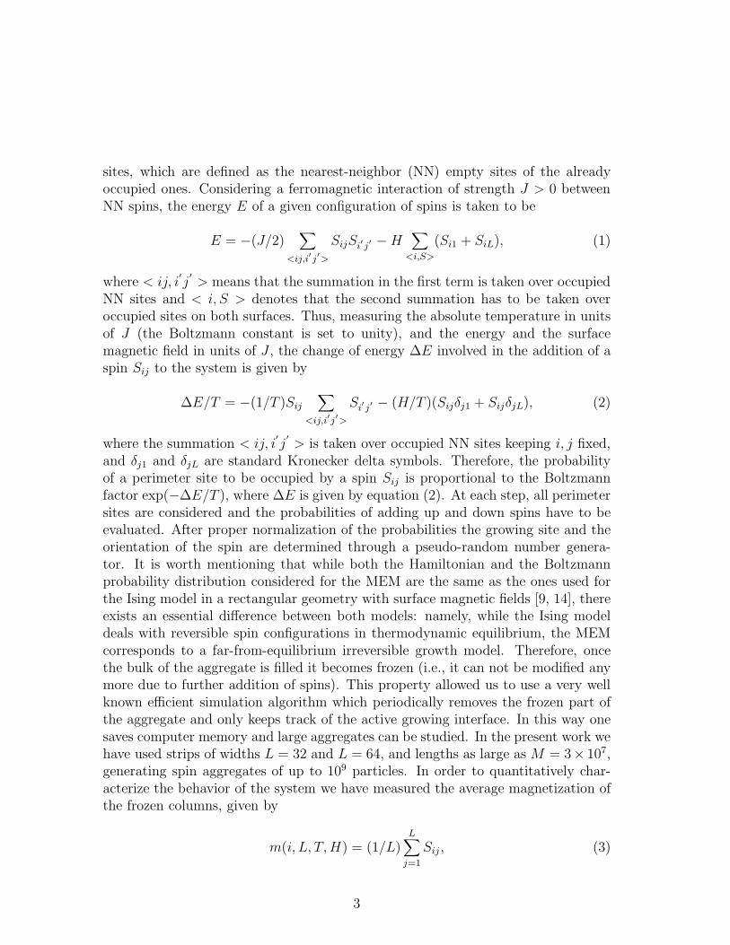
sites, which are defined as the nearest-neighbor (NN) empty sites of the alreadyoccupied ones. Considering a ferromagnetic interaction of strength J > 0 betweenNN spins, the energy E of a given configuration of spins is taken to be

E = −(J/2)∑

<ij,i′j′>

SijSi′j′ − H

∑

<i,S>

(Si1 + SiL), (1)

where < ij, i′

j′

> means that the summation in the first term is taken over occupiedNN sites and < i, S > denotes that the second summation has to be taken overoccupied sites on both surfaces. Thus, measuring the absolute temperature in unitsof J (the Boltzmann constant is set to unity), and the energy and the surfacemagnetic field in units of J , the change of energy ∆E involved in the addition of aspin Sij to the system is given by

∆E/T = −(1/T )Sij

∑

<ij,i′j′>

Si′j′ − (H/T )(Sijδj1 + SijδjL), (2)

where the summation < ij, i′

j′

> is taken over occupied NN sites keeping i, j fixed,and δj1 and δjL are standard Kronecker delta symbols. Therefore, the probabilityof a perimeter site to be occupied by a spin Sij is proportional to the Boltzmannfactor exp(−∆E/T ), where ∆E is given by equation (2). At each step, all perimetersites are considered and the probabilities of adding up and down spins have to beevaluated. After proper normalization of the probabilities the growing site and theorientation of the spin are determined through a pseudo-random number genera-tor. It is worth mentioning that while both the Hamiltonian and the Boltzmannprobability distribution considered for the MEM are the same as the ones used forthe Ising model in a rectangular geometry with surface magnetic fields [9, 14], thereexists an essential difference between both models: namely, while the Ising modeldeals with reversible spin configurations in thermodynamic equilibrium, the MEMcorresponds to a far-from-equilibrium irreversible growth model. Therefore, oncethe bulk of the aggregate is filled it becomes frozen (i.e., it can not be modified anymore due to further addition of spins). This property allowed us to use a very wellknown efficient simulation algorithm which periodically removes the frozen part ofthe aggregate and only keeps track of the active growing interface. In this way onesaves computer memory and large aggregates can be studied. In the present work wehave used strips of widths L = 32 and L = 64, and lengths as large as M = 3× 107,generating spin aggregates of up to 109 particles. In order to quantitatively char-acterize the behavior of the system we have measured the average magnetization ofthe frozen columns, given by

m(i, L, T, H) = (1/L)L∑

j=1

Sij , (3)

3

which plays the role of an order parameter. Also, the probability distribution of theorder parameter PL(m, T, H) has been evaluated [15].

3 Results and discussion

It is worth mentioning that we have restricted ourselves to the H ≥ 0 case withoutloosing generality. In fact, first we have checked that the magnetic Eden growthprocess in a confined geometry is characterized by an initial transient followed by anon-equilibrium stationary state that is independent from the starting seed. So, wehave particularly employed an initial seed entirely constituted by up spins through-out. Thus, changing the sign of the applied field (H → −H) corresponds to invertspin orientation at every lattice site. Then, the order parameter probability distri-bution can be simply obtained by replacing PL(m) → PL(−m). Analogous replace-ments also hold for other observables that can be computed from PL(m), such asthe average of the absolute column magnetization defined below (see equation 4).

Figure 1 shows typical plots of the probability distribution of the order param-eter, as obtained for different temperatures and fields (unless otherwise stated, weconsider the case of strip width L = 32 throughout). Since the surface field isalways assumed to be positive, all distributions are biased towards positive valuesof m. Figure 1(a) shows a typical low-temperature distribution that correspondsto T = 0.5. There one observes that for weak fields two peaks of PL(m) clearlyemerge at m = ±1. Particularly, for H = 0 the distribution is symmetric andthe average magnetization vanishes. As naturally expected, for H > 0 the peak atm = 1 is higher due to the applied surface fields. This result points out that thesystem undergoes fluctuations, since spin columns happen to be mainly builded upby parallel-aligned spins with a single orientation, either up or down. Increasingthe field (H ≥ 0.75) the negative peak of PL(m) vanishes showing that the surfacefield is strong enough in order to suppress such fluctuations. At T = 0.8 (figure1(b)), PL(m) is strongly biased by the field and only small peaks at m = −1 canbe observed for very weak fields (H < 0.25). It should also be noted that the cur-vature of PL(m) changes, as compared to figure 1(a). In fact, at T = 0.8 and forweak fields the amount of disorder in the aggregate is large enough so that PL(m)becomes peaked around m ≃ 0 and the average magnetization is close to zero. TheGaussian-like shape of the distribution curves for H < 0.5 becomes distorted by theeffect of the field causing a shift of the whole distribution towards larger values ofm as well as the occurrence of a sharper peak at m = 1, that grows with increas-ing the applied field and becomes dominant for H ≥ 1. For higher temperatures(T = 1.0 in figure 1(c)) the Gaussian shape for weak fields can clearly be observed,while the bias caused by the field has minor influence as compared with the formercases (figures 1(a-b)). Due to the observed fluctuations of m(T, L, H), the order

4

−1 −0.5 0 0.5 1m

0

0.025

0.05

PL(m

)

H = 0.00H = 0.50H = 0.75H = 1.00

−1 −0.5 0 0.5 10

0.2

0.4

0.6

0.8H = 1.00

(a)

−1 −0.5 0 0.5 1m

0

0.05

0.1

PL(m

)

H = 0.00H = 0.75H = 1.00H = 1.75

(b)

−1 −0.5 0 0.5 1m

0

0.02

0.04

0.06

0.08

PL(m

)

H = 0.00H = 0.75H = 1.25H = 1.75

(c)

Figure 1: Plots of the order parameter distribution function PL(m) vs m obtained fordifferent values of H as indicated in the figures. (a) Results for T = 0.5. The verticalaxis has been truncated in order to allow a detailed observation of the dependenceof PL(m) with m. The inset shows a plot of PL(m) vs m obtained taking H = 1.0,where the sharp peak at m = 1 can be observed. (b) and (c) show results obtainedfor T = 0.8 and T = 1.0, respectively. More details in the text.

5

0.2 0.4 0.6 0.8 1T

0.2

0.4

0.6

0.8

1

<|m

|>

H = 0.00H = 0.50H = 0.75H = 1.00H = 1.25H = 1.50H = 2.00

(a)

0 1 2 3H

0.2

0.4

0.6

0.8

1

<|m

|>

T = 0.40T = 0.50T = 0.60T = 0.70T = 0.80T = 0.90T = 1.00

(b)

Figure 2: (a) Plots of the order parameter versus the temperature obtained fordifferent values of the surface magnetic field as indicated in the figure. (b) Isothermsshowing the dependence of the order parameter with the surface magnetic field,obtained for the temperatures indicated in the figure.

parameter as defined by equation (3) will tend to vanish upon averaging over allfrozen columns. Therefore, in order to avoid this effect, it is convenient to redefinethe order parameter as the average of the absolute column magnetization [9], i.e.

< |m(L, T, H)| >= (1/M∗)M∗∑

i=1

|m(i, L, T, H)|, (4)

where M∗ < M is the number of frozen columns where the growing process hasdefinitively stopped, that is, the number of completely filled columns.

Figure 2(a) shows the dependence of < |m(L, T, H)| > on the temperature fordifferent values of the field, while figure 2(b) shows the plots of < |m(L, T, H)| > vs.H obtained at different fixed temperatures. At low temperatures (say T < 0.4)

6

(a)

(b)

(c)

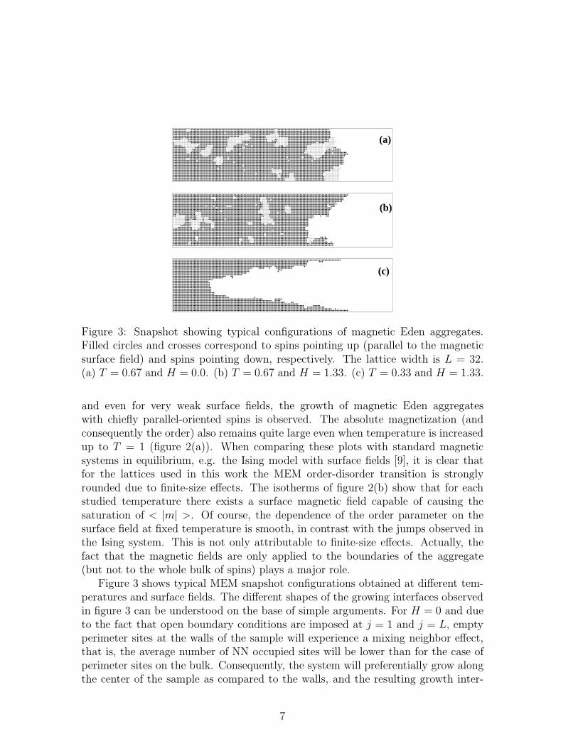
Figure 3: Snapshot showing typical configurations of magnetic Eden aggregates.Filled circles and crosses correspond to spins pointing up (parallel to the magneticsurface field) and spins pointing down, respectively. The lattice width is L = 32.(a) T = 0.67 and H = 0.0. (b) T = 0.67 and H = 1.33. (c) T = 0.33 and H = 1.33.

and even for very weak surface fields, the growth of magnetic Eden aggregateswith chiefly parallel-oriented spins is observed. The absolute magnetization (andconsequently the order) also remains quite large even when temperature is increasedup to T = 1 (figure 2(a)). When comparing these plots with standard magneticsystems in equilibrium, e.g. the Ising model with surface fields [9], it is clear thatfor the lattices used in this work the MEM order-disorder transition is stronglyrounded due to finite-size effects. The isotherms of figure 2(b) show that for eachstudied temperature there exists a surface magnetic field capable of causing thesaturation of < |m| >. Of course, the dependence of the order parameter on thesurface field at fixed temperature is smooth, in contrast with the jumps observed inthe Ising system. This is not only attributable to finite-size effects. Actually, thefact that the magnetic fields are only applied to the boundaries of the aggregate(but not to the whole bulk of spins) plays a major role.

Figure 3 shows typical MEM snapshot configurations obtained at different tem-peratures and surface fields. The different shapes of the growing interfaces observedin figure 3 can be understood on the base of simple arguments. For H = 0 and dueto the fact that open boundary conditions are imposed at j = 1 and j = L, emptyperimeter sites at the walls of the sample will experience a mixing neighbor effect,that is, the average number of NN occupied sites will be lower than for the case ofperimeter sites on the bulk. Consequently, the system will preferentially grow alongthe center of the sample as compared to the walls, and the resulting growth inter-

7

0 10 20 30j

−20

−10

0

10

<IR

j>

H = 0.00H = 0.50H = 1.00H = 1.50H = 2.00

Figure 4: Plots of the averaged interface profile versus j obtained for T = 0.7and different values of the surface magnetic field as indicated in the figure. The plotcorresponding to H = 2.0 has been truncated in order to allow a detailed observationof the profile’s curvature for lower H values.

face will exhibit a convex shape (figure 3(a)). For H > 0, the growing probabilityof perimeter sites at the walls of the system will be favored by an additional proba-bilistic factor given by exp(±H/T ), as it follows from equation (2). If H/T becomeslarge enough, the preferential growth along the walls will dominate (figures 3(b) and3(c)) and the interface curvature will become concave. So, from a qualitative pointof view, the figures 3(a,b,c) allow us to expect the occurrence of a convex-concavetransition in the curvature of the growth interface. Such transition is identified asa non-equilibrium magnetic wetting transition, since a concave interface wets thewalls while they remain dry when the interface grows with convex curvature.

In order to perform a quantitative study of the wetting transition it is convenientto define the location and the curvature of the growing interface. We assume thateach row of the system contributes with the outermost perimeter site (i.e., the onewith the largest value of the longitudinal i−th coordinate, for a given row number j)to the growing interface. Let Ij(t) be the i−th abscissa corresponding to the j−throw at time t. Then, the interface center of mass, that we take as the location ofthe interface at time t, I(t), is given by

I(t) = (1/L)L∑

j=1

Ij(t). (5)

Subsequently one can evaluate the coordinates of the interface relative to its centerof mass location at time t, namely IRj(t) = Ij(t) − I(t), j = 1, 2, ..., L. In this waywe obtain a set { IRj(t) } that appropriately describes the interface at any time t

8

1.2 1.4 1.6 1.8H

−0.012

−0.008

−0.004

0

0.004

b

HW

Figure 5: Plot of b versus H obtained for T = 2.00. The dotted line shows the pointwhere b changes its sign allowing us to identify the critical wetting field (Hw), asindicated in the figure. More details in the text.

during the growing process. In order to increase the statistics, we may evaluate theaverage relative interface < IRj > given by

< IRj >= {1/(tf − ti + 1)}tf∑

t=ti

IRj(t) (6)

where we take into account interface coordinates measured at different times betweenti and tf .

Figure 4 shows plots of < IRj > vs. j corresponding to T = 0.7 for differentvalues of the surface field H . There, it becomes evident how the applied field drivesthe convex-concave curvature change. The curved interfaces have been fitted bymeans of a fourth-degree polynomial given by p(j) = a + b(j − jc)

2 + c(j − jc)4,

where jc = (L + 1)/2. All fits were characterized by a dominant quadratic termwhich defined the interface curvature and a practically negligible quartic coefficient.Thus, the sign change of the quadratic coefficient b allows the identification of theconvex-concave curvature transition: for b > 0 the interface is concave and thecluster wets the walls, while for b < 0 it is convex and the walls remain dry. So,given a fixed temperature T , the magnetic field at the wetting transition Hw is theone that corresponds to b = 0. Figure 5 shows a plot of b vs. H obtained for T = 2.0,where the change of sign of b can clearly be observed. In this example, by means ofa linear interpolation, the value Hw = 1.67 ± 0.03 is obtained.

Following this procedure, we can quantitatively obtain the wetting phase diagramHw vs. T . These results are shown in figure 6, which corresponds to strip widthsL = 32 and L = 64. They also suggest that the location of the critical wet non-wet

9

0 1 2 3T

0

1

2

3

HW

L = 32L = 64

WET PHASE

NON−WET PHASE

Figure 6: Wetting phase diagram, Hw vs T , showing the critical line at the boundarybetween the wet and non-wet phases. Results obtained for L = 32 and L = 64, asindicated in the figure.

curve is only weakly sensitive to finite-size effects. The monotonic growth of the Hw

vs. T curves shown, reflects the fact that a larger surface magnetic field is neededin order to stabilize the thermal noise caused by higher temperatures.

4 Conclusions

In this work, rectangular strips on the square lattice are used to grow magnetic Edenclusters with ferromagnetic interactions between nearest neighbor spins and shortrange magnetic fields applied at the surfaces. For weak surface fields, the mixingneighbor effect at the surface causes the growth of convex interfaces. However, whenthe field is increased, the preferential growth of spins along the surface turns theinterface curvature concave. Such curvature change has been rationalized in termsof a wetting transition, and the corresponding wet non-wet phase diagram has beenevaluated. We expect that the present study will stimulate further work in thefield of non-equilibrium wetting transitions, a topic of widespread technological andscientific interest which has remained almost unexplored till the present.

Acknowledgments

This work is supported financially by CONICET, UNLP, CIC (Bs. As.), ANPCyTand Fundacion Antorchas (Argentina) and the Volkswagen Foundation (Germany).

10

References

[1] F. Family and T. Vicsek, Dynamics of Fractal Surfaces. World Scientific, Sin-gapore (1991).

[2] A. L. Barabasi and H. E. Stanley, Fractal Concepts in Surface Growth. Cam-bridge University Press, New York (1995).

[3] Fractals and Disordered Media, Eds. A. Bunde and S. Havlin, Springer-Verlag,Heidelberg (1991).

[4] Fractals in Science, Eds. A. Bunde and S. Havlin, Springer-Verlag, Heidelberg(1995).

[5] M. Marsili, A. Maritan, F. Toigo and J. R. Banava. Rev. Mod. Phys. 68, 963(1996).

[6] S. Dietrich, in Phase Transitions and Critical Phenomena, edited by C. Domband J. L. Lebowitz. Academic Press, London (1988). Vol. 12, p. 1.

[7] A. O. Parry. J. Phys. Condensed Matter. 7, 10761 (1996).

[8] H. Hinrichsen, R. Livi, D. Mukamel and A. Politi. Phys. Rev. Lett. 79, 2710(1997).

[9] E. V. Albano, K. Binder, D. Heermann and W. Paul. Surf. Sci. 223, 151 (1989).

[10] M. Eden, in: Symp. on Information Theory in Biology, edited by H. P. Yockey,Pergamon Press, New York (1958) and Proceedings of the Fourth BerkeleySymposium on Mathematics, Statistics and Probability, edited by F. NeymanUniversity of California Press, Berkeley (1961). Vol. IV, p. 223.

[11] M. Ausloos, N. Vandewalle and R. Cloots. Europhys. Lett., 24, 629 (1993), N.Vandewalle and M. Ausloos. Phys. Rev. E. 50, R635 (1994).

[12] J. Shen et al. Phys. Rev. B. 56, 2340 (1997).

[13] U. Bovensiepen et al. Phys. Rev. Lett. 81, 2368 (1998).

[14] E. V. Albano, K. Binder and W. Paul. J. Phys. A.(Math. & Gen.) 30, 3285(1997).

[15] K. Binder. Z. Phys. B 43, 119 (1981).

11