
Public and private sector wages interactions in a general equilibrium model

A model of equilibrium institutions∗
Bernardo Guimaraes† Kevin D. Sheedy
Sao Paulo School of Economics (FGV) London School of Economics
& London School of Economics
First draft: 19th October 2009
This draft: 1st December 2010
Abstract
In order to understand inefficient institutions, one needs to understand what might
cause the breakdown of a political version of the Coase Theorem. This paper considers
an environment populated by ex-ante identical agents and develops a model of power
and distribution where institutions (the “rules of the game”) are set to maximize payoffs
of those individuals in power. They are constrained by the threat of rebellion, where any
rebels would be similarly constrained by further threats. Equilibrium institutions are
the fixed point of this constrained maximization problem. This model can be applied
to different economic environments. Private investment depends on credible limitations
on expropriation, which can only be achieved if power is not as concentrated as those
in power would like it to be, ex-post. Endogenously, this enables the group in power to
act as government committed to protection of property rights, which would otherwise
be time inconsistent. But the “political” Coase Theorem does not hold. Since sharing
power implies sharing rents, capital taxation is inefficiently high.
JEL classifications: E02; O43; P48.
Keywords: government; political economy; public goods; capital taxation; time
inconsistency.
∗We thank Bruno Decreuse, Erik Eyster, Carlos Eduardo Goncalves, Ethan Ilzetzki, Per Krusell,Dirk Niepelt, Andrea Prat, Ronny Razin and seminars participants at U. Amsterdam, the Anglo-French-Italian Macroeconomic Workshop, U. Carlos III, Central European University, ColumbiaUniversity, CREI conference “The political economy of economic development”, ESSIM 2010, Insti-tute for International Economic Studies, London School of Economics, Paris School of Economics, U.Sao Paulo, Sao Paulo School of Economics/FGV, U. Surrey, and U. St. Gallen for helpful comments.†Corresponding author: Sao Paulo School of Economics (FGV), Email:

And Samuel told all the words of the Lord unto the peoplethat asked of him a king.
And he said, This will be the manner of the king that shallreign over you: He will take your sons, and appoint them forhimself, for his chariots, and to be his horsemen; and someshall run before his chariots. . . .
And he will take your daughters to be confectionaries, andto be cooks, and to be bakers. . . .
He will take the tenth of your sheep: and ye shall be hisservants.
And ye shall cry out in that day because of your king whichye shall have chosen you; and the Lord will not hear you inthat day.
Nevertheless the people refused to obey the voice of Samuel;and they said, Nay; but we will have a king over us;
That we also may be like all the nations; and that our kingmay judge us, and go out before us, and fight our battles.
1 Samuel 8:10–20
1 Introduction
Institutions are defined by North (1990) as the “rules of the game”, or the “humanly devised
constraints that shape human interaction”. Differences in institutions go a long way in ex-
plaining the huge disparities in income across the globe as they affect incentives for agents
to invest, produce and exchange.1 Even though institutions may serve the interests of elites,
a fundamental question is why this gives rise to huge economic inefficiencies, that is, why is
there no “political” equivalent of the Coase Theorem?
This paper builds a model to address that question. The model starts from a world of
ex-ante identical individuals. The group in power (the elite) and the rules laying down the
allocation of resources will both be endogenously determined in equilibrium, with the goal of
maximizing the payoffs of those who will be in the elite. The elite and the rules comprise the
equilibrium institutions.2
The only constraint on the choice of institutions is the threat of “rebellions”, which destroy
the prevailing institutions. There are no other “technological” constraints on which institutions
1For example, see North and Weingast (1989), Engerman and Sokoloff (1997), Hall and Jones (1999) andAcemoglu, Johnson and Robinson (2005).
2Recently, some models have been developed aiming at understanding institutions. Greif (2006) combinesa rich historical analysis of trade and institutions in medieval times with economic modelling, part of whichfocuses on the form of government and political institutions that emerged in Genoa. Acemoglu and Robinson(2006, 2008) analyse conditions leading to democracy or dictatorship in an environment where an elite is tryingto maintain its power, while citizens prefer a more egalitarian state. In Besley and Persson (2009a,b, 2010),society comprises two groups of agents that alternate in power, and make investments in two technologies thatrespectively allow the state to tax people and to enforce contracts. The exogenous parameters are the extentof political turnover and institutional (or demographic) features that determine how much one group caresabout the other. They obtain predictions consistent with the data on state capacity and fiscal capacity, civilwars, and different forms of taxation.
1

are feasible, thus the issue will be the incentives for creating and destroying institutions. In
the absence of rebellion, the rules prescribed by the chosen institutions are followed. This
means that an elite can establish institutions laying down credible rules as long as it avoids
rebellions. So although institutions will be chosen in the interests of an elite, this does not
preclude the emergence of a “political” Coase Theorem. But crucially, once institutions have
been destroyed, the new institutions that will arise cannot be constrained by the past rules or
any other deals made earlier. This reflects the commitment problems analysed in Acemoglu
(2003) and Acemoglu, Johnson and Robinson (2005).
Rebellions are costly, reflecting the fact that conflict is costly. Importantly, anyone can
participate in a rebellion, including members of the current elite. Moreover, there is no limit
to the number of rebellions: after any group takes power, there is always another opportunity
for rebellion. The cost of conflict for rebels is proportional to the number of individuals in
power who do not take part in the rebellion.
Since individuals are ex-ante identical and self-interested, the notion of equilibrium institu-
tions is independent of the competence, benevolence, or factional affiliation of the individuals
comprising the elite. Hence, once a rebellion has succeeded in destroying the current institu-
tions, the rebels will have the same objectives and face the same constraints as those formerly
in power. As in George Orwell’s Animal Farm, there is no intrinsic difference between the
“men” and the “pigs”, but in equilibrium, some individuals will be “more equal” than others.
In the model, it is not conflict per se, but rather the threat of conflict that shapes in-
stitutions by constraining the actions of those in the elite. No conflict occurs in equilibrium
owing to the absence of both randomness in the conflict technology and uncertainty about the
actions of individuals.
The incentives to rebel depend on what members of a new elite would be able to extract
once in power, which is also true of rebellions against institutions set up by the rebels, and
so on. Given that all individuals are ex-ante identical, there is no fundamental reason why
different institutions would be chosen following a rebellion, so the paper focuses on Markovian
equilibria. The equilibrium institutions are thus the fixed point of the constrained maximiz-
ation problem of the elite in power subject to the threat of rebellion, where the rebels would
be similarly constrained by further threats of rebellion.
There is no restriction on the composition of a group launching a rebellion. Since the
most disgruntled individuals have the most to gain from a rebellion, discouraging the “most
profitable” rebellion a fortiori discourages all possible rebellions. It follows that the equilibrium
institutions assign payoffs to producers according to a maximin rule, and hence, payoffs of those
outside the elite (the “producers”) are equalized. Furthermore, as the survival of institutions
depends on those in the elite not defecting and joining a rebellion, payoffs of those in power
must also be equalized. In other words, sharing power implies sharing rents.
2

In an endowment economy, there is a basic trade-off that characterizes the equilibrium
institutions. The larger the elite (and hence the greater the number of people with a stake
in defending the institutions), the greater the amount of taxes that can be levied, but the
proceeds need to be divided among more people. The problem can be represented as a choice
of the size of the elite and taxes to maximize the payoff of a member of the elite, subject to
the constraint of avoiding a rebellion by producers. This “no-rebellion” constraint acts as a
participation constraint for the producers.
Do the equilibrium institutions lead to the elite acting as a “government” in any meaningful
sense of the term? That is, are institutions that are designed to maximize the payoffs of those
in power ever congruent with the interests of the people? In some cases, the answer turns
out to be yes. For example, suppose there is a technology that transforms the output of the
producers into a public good that benefit everyone, and which has no impact on any other
aspect of the environment. Such a public good will be optimally provided in equilibrium, as
if it had been chosen by a benevolent government.
This outcome is consistent with a world characterized by a political Coase Theorem. The
ability of the elite to set down rules is analogous to the possibility of contracting in the
“regular” Coase Theorem. The notion of the elite constrained by the threat of rebellion means
that there is a “price” attached to policy actions affecting those outside the elite, analogous
to the existence of markets in the Coase Theorem.
A natural application of the model is to the taxation of investment proceeds. The model
is extended so that once institutions are formed and after no rebellion has occurred, workers
have access to an investment technology. However, the fruits of this investment are realized
only after a lag, during which time there is another round of opportunities for rebellion in
which both workers and members of the elite can participate. Since the cost of investing is
sunk, it does not affect individuals’ incentives to rebel, so by the maximin principle for payoffs
in equilibrium explained earlier, the group in power would have incentives to expropriate fully
individuals’ investments.
Although institutions could in principle prescribe any level of capital taxation, whatever
is chosen must be “rebellion-proof” after investment decisions have been made. The problem
is that the capital arising from investment increases incentives for attacks on the current
institutions that lead to new rules permitting full capital expropriation. Thus it is necessary
to raise the cost of rebelling. This can only be done by expanding the size of the elite. The
problem cannot be solved through taxes and transfers as such instruments can only redistribute
disgruntlement with the institutions, decreasing rebellion incentives for some, but raising them
for others.
In equilibrium, to ensure there will be no incentives to rebel against the existing institutions
— leading inevitably to full expropriation — the elite has to be large so that if a rebellion
3

were to take place after investment decisions had been made, the equilibrium size of the
subsequent elite would be smaller than the current one. This is the only way to prevent
members of the elite simply launching a costless rebellion from within that maintains intact
the elite’s composition (a rebellion is costless if the entire elite is willing to defect). Following
a rebellion, there would then be insufficient places for all the current elite in the subsequent
one. Thus, some members of the elite will oppose changing the institutions, and so conflict
with them makes it costly to expropriate capital.
Adding the possibility of investment to the model thus gives rise to a larger elite. Sharing
power among a wider group of individuals allows the elite to act as a government committed
to a certain set of policies that would otherwise be time inconsistent. The model highlights the
importance of sharing power as a way to guarantee stability of institutions and thus incentives
for investment. This resonates with Montesquieu’s doctrine of the separation of powers, which
is now accepted and followed in all well-functioning systems of government. It is important
to note that in the model, power is not shared among those individuals who are actually
investing. The extra individuals in the elite in no sense represent or care about those who
invest — but they do care about their own rents under the status quo. Thus, this group
of self-interested individuals acts a government that commits to some protection of property
rights.
Although it is possible to sustain protection against expropriation in equilibrium, capital
taxation is set far from efficiently, so the political Coase Theorem breaks down. While in
general it would be optimal from the point of view of society to have a larger group in power
in order to guarantee that the fruits of investment would not be expropriated, the equilibrium
elite chooses taxes on investment that are too high.3
There are two reasons for the inefficiently high level of captital taxation. First, the elite
cannot extract all surplus from investors as the effort required to invest is private information.
In equilibrium, the payoff of those who invest is larger than the payoff of the workers who do
not invest, so the no-rebellion constraint for the investors is not directly binding.
The second (and more interesting) distortion follows from the distributional effects of
protecting against expropriation. Since members of the elite can bring down the institutions
more easily if they take part in a rebellion (because in that case they won’t defend the current
institutions), they must receive rents. As lower capital taxes require more power sharing, they
also imply more rent sharing. This goes against the interests of each individual in the elite.
These reasons allow us to understand why a political Coase Theorem breaks down in this
case. The first reason mentioned above is the unobservability of investors’ surpluses. The
second reason for the failure of the Coase Theorem is essentially the inseparability of power
3This is in accordance with the empirical literature that highlights the importance of institutions guaran-teeing protection against government expropriation. For example, the results in Acemoglu and Johnson (2005)suggest that such institutions are more important than those that facilitate contracting among private agents.
4

and rents: it is not possible in equilibrium to add individuals to the elite and grant them a
payoff lower than their peers. That leads to an endogenous limitation (which is binding) on
the set of possible transfers.
While the model is quite abstract, it is congruent with a number of historical examples,
some of which are discussed later in the paper: the disappearance of private corporations (the
societas publicanorum) when power was concentrated under the Roman emperors; the need
for a militarily strong leader (podesta) to guarantee stability in a society (medieval Genoa)
where other strong groups could seize power; the tenacious resistance of the Stuart Kings of
England to sharing power with Parliament.
Section 2 presents the model of power and distribution. The benchmark provision of
public goods is briefly analysed in section 3, and the case of private investment in presented
in section 4. Section 5 draws some conclusions.
1.1 Related literature
Since Downs (1957) emphasized the importance of studying governments composed of self-
interested agents, a vast literature on political economy has developed (see, for example,
Persson and Tabellini, 2000). Most of this literature focuses on democracies, so institutions
are not themselves explained in terms of the decisions of self-interested agents. But in much of
the developing world and during most of human history, political regimes have differed greatly
from democracies.
This paper shares important similarities with the literature on coalition formation, as ana-
lysed by Ray (2007).4 As in that literature, the process of establishing rules is non-cooperative,
but it is assumed that such rules are followed. Moreover, the modelling of rebellions here is
related to the idea of blocking in coalitions (Part III of Ray, 2007) in the sense that there is no
explicit game-form, as in cooperative game theory. The distinguishing feature of this model is
the “rebellion technology” that must be used in order to replace existing institutions by new
ones.
The model assumes that the institutions established by the incumbent army determine
the allocation of resources once production has taken place. But how would those institutions
manage to affect the allocation of goods ex post? As pointed out by Basu (2000) and Mailath,
Morris and Postlewaite (2001), laws and institutions do not change the physical nature of the
game, all they can do is affect how agents coordinate on some pattern of behaviour. But in
reality, laws and institutions are seen to have a strong impact on behaviour, and this feature
must be present in any model of institutions.
4 Baron and Ferejohn (1989) analyse bargaining in legislatures using this approach. Levy (2004) studiespolitical parties as coalitions. Recent contributions include Acemoglu, Egorov and Sonin (2008) Piccione andRazin (2009).
5

The view of this paper is similar to the application of Schelling’s (1960) notion of focal
points in the organization of society, as put forward by Myerson (2009). The “rules of the
game” are self-enforcing as long as society coordinates on punishing whomever deviates from
the rules — and whomever deviates from punishing the deviators. For example, if the laws
specify how much an individual must pay or receive from another, and if both expect to be
harshly punished if they fail to comply (along with any “higher-order” deviators) then the
laws will be self enforcing.
Following this, theorizing about institutions is theorizing about (i) how rules (or focal
points) are chosen, and (ii) how rules can change. For example, Myerson (2004) explores the
idea of justice as a focal point influencing the allocation of resources in society. This paper
takes a more cynical view towards our fellow human beings. Here, the individuals in power
choose the laws and institutions to maximize their own payoffs, and those institutions can
only be destroyed by a rebellion — wiping out the old institutions, and making way for new
ones. There is no modelling of the post-production game.
This paper is also related to the literature on social conflict and predation, surveyed by
Garfinkel and Skaperdas (2007).5 It is easy to envisage how conflict could be important in
a state of nature: individuals could devote their time to fighting and stealing from others.
However, when there are fights, there are deadweight losses. Thus, people would be better
off if they could agree on transfers to avoid conflict. This paper presupposes such deals are
possible: producers pay taxes to the group in power, which allocates resources according to
some predetermined rules. Here, differently from the literature on conflict, individuals fight
to be part of the group that sets the rules, not over what has been produced. Moreover, they
fight in groups, not as isolated individuals.
There are theoretical models focused on political issues that lead to inefficiencies in protec-
tion of property rights. Examples include Glaeser, Scheinkman and Shleifer (2003), Acemoglu
(2008), Guriev and Sonin (2009) and Myerson (2010). Here, the possibility of capital ex-
propriation and the consequent need to protect property rights is just a natural consequence
of the possibility of investment and the “rebellion technology” that allows institutions to be
destroyed and replaced.
Lastly, it is possible to draw an analogy between this paper and models of democracy
(Persson and Tabellini, 2000) in the sense that the “election technology” there is replaced by
a “rebellion technology” here.
5For instance, see Grossman and Kim (1995), Hirshleifer (1995), and also Hafer (2006), Dal Bo and Dal Bo(2010) for some recent contributions.
6

2 The model of power and distribution
This section presents an analysis of equilibrium institutions in a simple endowment economy.
Subsequent sections extend this analysis to richer environments where there is scope for insti-
tutions to affect economic outcomes.
2.1 Environment
There is an area containing a measure-one population of ex-ante identical individuals indexed
by ı ∈ Ω. Individuals receive utility U from their own consumption C of a homogeneous good
and disutility if they exert fighting effort F :
U = u(C)− F, [2.1]
where u(·) is a strictly increasing and weakly concave function.
Individuals who become workers (ı ∈ W) have access to a production technology that
yields an exogenous quantity q of goods. Individuals who are currently in power (ı ∈ P) have
a positive fighting strength (parameterized by δ) without needing to exert fighting effort F .
Individuals who remain in power cannot simultaneously become workers.6
Institutions (the “rules of the game”) specify the identities of the individuals in power
(the set P), referred to as the elite, and the allocation of resources. Once institutions exist,
the rules they specify laying down the allocation of resources are respected by all individuals
unless a successful rebellion occurs. These rules can specify any transfers between individuals
subject only to leaving each individual ı with a non-negative quantity of consumption C(ı) ≥ 0
and satisfying an overall budget constraint. If a worker ı ∈ W faces an individual-specific tax
τ(ı) paid to the elite then his consumption is
Cw(ı) = q− τ(ı). [2.2]
Tax revenue is used to finance the consumption of the elite. If Cp(ı) is the individual-specific
consumption of a member of the elite ı ∈ P then the budget constraint is∫PCp(ı)dı =
∫Wτ(ı)dı. [2.3]
A successful rebellion destroys the existing institutions, paving the way for the creation
of new ones. Any subsequent institutions would also be subject to the threat of rebellion,
and so on. A rebellion succeeds if the fighting strength of the rebel army exceeds that of the
6The assumption that those in power do not receive the same endowment as workers is not essential forthe main results. However, it is not unreasonable to suppose there is some opportunity cost for individuals ofbeing in power.
7

incumbent army. The rebel army can include any individual who expects to receive a place in
the subsequent elite once the current institutions have been destroyed. Members of the rebel
army can convert F units of fighting effort (for which there is a disutility according to [2.1])
into F units of fighting strength. The incumbent army comprises those individuals currently
in power (who each have fighting strength δ) who would lose their place in the elite after
destruction of the current institutions. Individuals can only fight as part of a rebellion or to
defend institutions from a rebellion. There is no fighting between isolated individuals over
resources nor an ability for isolated individuals to resist the allocation of resources imposed
by the prevailing institutions.
The sequence of events is depicted in Figure 1. An elite takes power and establishes
institutions. There are then opportunities for rebellion. If a successful rebellion occurs, new
institutions are established, potentially changing the elite, with these institutions also being
subject to subsequent threats of rebellion. When no rebellions occur, workers produce goods,
the rules laid down by the prevailing institutions are implemented, and payoffs are received.
Individuals have no ability to commit themselves to take actions at later stages of the game
except where there is no utility loss in sticking to the commitment ex post.
Figure 1: Sequence of events
Rebellion?
yes
no
No elite New institutions
Production, taxes, payoffs
2.2 Institutions
The analysis begins by considering a stage of Figure 1 at which institutions have just been
established. These institutions specify the distribution of power and the allocation of resources.
Formally, institutions are a collection I = P ,W , τ(·), Cp(·), where P is the set of individuals
in power, W is the set of workers, τ(·) is a function specifying the distribution of taxes across
workers, and Cp(·) is a function specifying the distribution of consumption within the elite.
The sets P andW partition the set of all individuals Ω. The taxes τ(·) and elite consump-
tion levels Cp(·) must satisfy the budget constraint [2.3] and the non-negativity constraints on
8

each individual’s consumption.
Once institutions exist, there is an opportunity for rebellions to occur.
2.3 Rebellions
A rebellion (if successful) destroys the current institutions, making way for the creation of new
ones, which will change the allocation of power, resources, or both. A rebellion succeeds if
the fighting strength of the rebels exceeds the fighting strength of those defending the current
institutions. Rebellions can include any individuals, even those who belong the current elite.
Although rebellions destroy the current institutions, a rebellion does not include a binding
manifesto for what new institutions will be set up following its success. Thus, the rebels
cannot commit themselves in advance to create particular institutions in the future.
Although the rebellion does not set down binding plans for the construction of subsequent
institutions, beliefs about what institutions would be created following the destruction of
the current ones influence incentives to take part in a rebellion. However, the fact that an
individual might gain from the success of a rebellion is not a sufficient reason for him to fight in
support of it. Fighting is costly, while no individual’s fighting effort is pivotal in determining
which side wins. Hence there are strong incentives for free-riding that armies must overcome.
Armies must therefore provide direct incentives for individuals to exert fighting effort,
but there is limit to what incentives they can credibly offer. Once the fighting is over, the
effort cost is sunk, so unless the subsequent institutions can credibly treat two individuals
differently, one of whom fought and one of whom shirked, who would otherwise have identical
continuation utility, there can be no incentive for individuals to fight. As will be seen, such
differences in payoffs would reduce the utility of the subsequent elite, so there is no incentive
to honour past inducements to fight. This true for both financial rewards for fighting (the
“carrot”) and punishments for shirking (the “stick”).
The only exception to this is that there will be incentives after a successful rebellion for
power-sharing among a group that will comprise the new elite. Since all individuals are ex-
ante identical and self-interested, those in the elite do not care with whom they share power.
As will be seen, those in the elite are able to obtain a higher payoff than those outside, so
membership of the new elite can be offered as a credible incentive to fight. In the event of
shirking, the place could be offered to someone else, which is a punishment that is costless for
the elite to carry out because of the existence of a pool of identical replacements who would
like to join.
These arguments lead to the restriction that the rebel army can only include those who
expect to have a place in the subsequent elite. The amount of fighting effort put in by each
individual must also be individually rational. Let p′e denote beliefs about post-rebellion elite
size p′, and C ′ep (·) beliefs about the distribution of consumption among members of the post-
9

rebellion elite. The notation ′ is used denotes an aspect of the institutions that would be
created following a successful rebellion, with the superscript e denoting beliefs about these. It
is not possible to for particular individuals taking part in the rebellion to be credibly promised
particular levels of consumption from the distribution C ′ep (·), so the expected payoff U ′ep from
belonging to the post-rebellion elite is the following simple average:
U ′ep =1
p′e
∫P ′u(C ′ep ())d, [2.4]
assuming this elite will itself avoid losing power through a rebellion (as will be confirmed
later). Consider an individual ı who would receive utility U(ı) under the prevailing institutions
I = P ,W , τ(ı), Cp(ı). The maximum amount of fighting effort this individual would find it
individually rational to exert (assuming he expects a place in the subsequent elite) is denoted
by F (ı), and the set of individuals willing to exert positive amounts of effort conditional on
receiving a place in the post-rebellion elite is F :
F (ı) = U ′ep − U(ı), and F = ı ∈ Ω | F (ı) > 0, [2.5]
where U(ı) is evaluated under the current institutions I .
Formally, a rebellion is entirely characterized by an elite selection function E ′ : p′ → P,
which determines the identities of those who would have a place in the new elite if the rebellion
succeeds in destroying the current institutions. This is a mapping from the size p′ of the
subsequent elite to the set of (measurable) subsets of Ω, denoted by P. The function E ′(·)has the property that E ′(p′) is a set of measure p′, and if p′1 ≤ p′2 then E ′(p′1) ⊆ E ′(p′2), so all
those included in a smaller elite would also belong a larger elite.
Given an elite selection function E ′(·), the prevailing institutions I ≡ P ,W , τ(ı), Cp(ı),and beliefs p′e and U ′ep about the post-rebellion institutions, the rebel army R and the incum-
bent army A are
R = E (p′e) ∩ F , and A = P\ (E (p′e) ∩ F) . [2.6]
The rebel army can include any individuals willing to exert a positive amount of fighting
effort conditional on being members of the subsequent elite. This can include those who
belong to the current elite. The idea is that individuals cannot commit themselves to defend
the current institutions if a rebellion occurs and they receive a credible opportunity to obtain
a higher payoff than the current institutions grant them. The incumbent army includes those
individuals who are in power according to the current institutions who do not join the rebel
army. Individuals outside the elite will not join the incumbent army owing to the free-riding
problems discussed earlier, so only those who Thus those who are neither part of the current
elite nor expect to have a place in a subsequent elite take no part in the fighting.
10

Individual ı ∈ R in the rebel army exerts the individually rational fighting effort F (ı) from
[2.5], which translates into fighting strength F (ı). Those in the incumbent army have fighting
strength δ each. The rebellion succeeds if and only if∫RF (ı)dı >
∫Aδdı, [2.7]
that is, if the fighting strength of the rebel army exceeds that of the incumbent army. For
simplicity, the fighting strength of each army is linear in the fighting strength of its members,
and the fighting strength of the rebels is equal to their fighting effort (which affects utility
linearly). There is no uncertainty about the amount of fighting effort exerted given beliefs
about the post-rebellion institutions, nor about the outcome given the fighting strength of the
armies. Thus the outcome of any conflict is non-stochastic.
This approach to modelling the threat of conflict allows for a simple representation of the
constraints on institutions if they are to survive the threat of rebellion, without accounting
explicitly for the punches and sword thrusts. The parameter δ measures the fighting strength
of an individual in power who defends the current institutions, and this defensive strength is
possessed by such an individual without requiring fighting effort.
One interpretation of the parameter δ is that the individuals in power under the current
institutions possess some defensive fortifications, such as a castle, which place them at an
immediate fighting advantage over any rebels. A broader interpretation is that any existing
institutions feature a customary chain of authority, that is, the implementation of any rules in a
society depends on individuals knowing from whom they are to take orders, in the expectation
of punishment if they disobey. A rebellion must supplant one system of authority with another,
and the rebels face a more severe coordination problem than those already in power because
they must convince enough people that they are the new source of authority and reach a
tipping point where people come to expect others to start obeying the rebels rather than the
existing elite. In this case, defections from the elite, where those in power join the rebels, are
helpful not just for the extra fighting effort but also for the failure of these individuals to play
their role in defending the current institutions.
It is also possible to interpret [2.7] in a world where no actual fighting takes place. In this
interpretation, the rebels must incur a sunk effort cost to demonstrate they have the strength
and are sufficiently well-organized to overcome the physical defences of the incumbent and the
coordination problems inherent in launching a rebellion. Once the remaining elite members
see this tipping point is reached, they surrender without a fight.
There are two differences in the treatment of the incumbent army and the rebel army
in [2.7], one essential, and one an inessential simplification. The simplification is that each
individual currently in power has fighting strength δ, and that this is inelastic with respect to
fighting effort F . As will be seen, the current elite has a several margins along which it can
11

adjust institutions to ensure it remains in power. Adding an extra margin of being able to
increase fighting strength for those in power who do not join the rebels does not fundamentally
change the nature of the problem. On the other hand, it is essential that there is an asymmetry
between the mapping from fighting effort to strength for the incumbents and for the rebels.
If both were identical then the notion of being “in power” would be meaningless and thus all
agents would be treated symmetrically.
Although the term rebellion has been used to describe the process of destoying the current
institutions, the formal definition encompasses revolutions, coups d’etat, suspensions of con-
stitutions, as well as rebellions in the conventional sense of the term. This is because rebellion
is rebellion against the current institutions, which comprise the rules allocating resources as
well as the identities of the elite, and the participants in rebellions are not restricted to those
outside the elite. The only difference between these different types of rebellion is in who the
participants are in the rebel and incumbent “armies”. The model is set up with one general
notion of rebellion that nests all these cases.
2.4 Establishing institutions
There is an elite-selection function E : Ω → P(Ω) with the property that E (p) has measure
p, and p ≤ p′ implies E (p) ⊆ E (p′). A rebellion can replace the elite selection function.
Or E : Ω→ 2Ω.
Predetermined selection function:
E(p) = E(·)
[To reiterate, the rebellion does not determine the size of the subsequent elite, nor the
allocation of resources to be laid down by the subsequent institutions, but it does determine
the identities of those who will hold power, conditional on the subsequent elite being of a
given size.]
Following a rebellion, new institutions are created to maximize the average payoff of the
elite, whose identities are determined by the elite selection rule E (·). Starting from no prior
institutions, the problem is of an identical form, with nature drawing a random elite selection
rule.
[The only commitments the rebels enter into (the identities of the elite conditional on size)
those from which they have no incentive to deviate from ex post.]
The choice variables are the size p of the group in power, the distribution of taxes τ(ı)
levied on workers, and the distribution of consumption Cp(ı) for elite members. Together with
12

the elite selection rule, these determine the institutions I ≡ P ,W , τ(ı), Cp(ı):
P = E (p), and W = Ω\E (p). [2.8]
Individuals in power get utility from their consumption, and as discussed, are able to
have fighting strength δ in defence of their institutions without an effort cost owing to their
entrenched position. This means that conditional on avoiding rebellions, their payoff is Up(ı) =
u(Cp(ı)).
To avoid losing power through a rebellion, the elite must avoid any profitable rebellions.
That is, given beliefs p′e and U ′ep , the institutions solve the following constrained maximization
problem:
maxp,τ(ı),Cp(ı)
1
p
∫E (p)
Up(ı)dı s.t.
∫E ′(p′e)
maxU ′ep − U(ı), 0 ≤∫
E (p)\E ′(p′e)
δdı for all E ′(·). [2.9]
Since individuals are ex ante identical and self-interested, the restriction that P = E (p)
does not impose any loss of utility on those that get to be in the elite. Thus, the elite selection
rule, which is the only state variable in this problem inherited from the earlier rebellion stage,
has no effect on the maximized value of average elite utility. What does matter is beliefs about
the institutions that would be set up following a rebellion.
Once new institutions I ≡ P ,W , τ(ı), Cp(ı) are created, there are opportunities for
rebellion as described earlier. Any subsequent institutions would also be subject to the threat
of rebellion, ad infinitum.
The proportion p of individuals in the elite is such that it maximizes the average utility of
those in the elite.7 In other words, the elite shares power with an extra individual if and only
if this increases its average payoff. This assumption captures the idea that the distribution
of power reflects the interests of the elite, not the welfare of society. Given the size p, the
composition of the elite depends on a predetermined ordering set at the time of the previous
rebellion.8
The distribution of (lump-sum) taxes τ(·) levied on workers and the distribution of con-
sumption of members of the elite Cp(·) is set to maximize the average elite payoff. No exogen-
ous restrictions are imposed on taxation beyond the natural bound of what workers possess.9
7Moving away from the assumption that the elite maximizes its average payoff would require modelling itshierarchy, which is beyond the scope of the paper. See Myerson (2008) for a model addressing this question.
8Since all individuals are ex ante identical, the particular identities of those with whom power is sharedhave no effect on the elite’s average payoff. In a situation where there were no pre-existing institutions, arandom ordering is used to determine the composition of the elite.
9Taxes can be contingent on any observable variables, but this does not play any role in the endowment-economy version of the model. Taxes cannot be contingent on agents’ identities, which would imply thatidentities become state variables, making the analysis much more complicated. In equilibrium, though, theelite has no incentives to set taxes specifically contingent on identities alone.
13

The choices of elite size and the distribution of resources to maximize elite payoffs are
constrained by the threat of rebellion, as described below. Once institutions are established,
each worker gets to know the tax τ(ı) he faces and each member of the elite gets to know his
consumption Cp(ı). Further threats of rebellion are then considered.
2.5 Equilibrium
Equilibrium institutions are those that maximize the average utility of those in power subject
to there being no profitable rebellion. The choice variables are the size of the elite p, the
payoffs of each member of the elite, and a tax distribution τ(·) specifying a lump-sum tax for
each worker ı ∈ W . The equilibrium institutions are the result of the following constrained
maximization problem:
maxp,τ(·)
1
p
∫PUp(ı)dı s.t.
∫R∩W
(U ′ep − Uw(τ(ı))
)dı+
∫R∩P
(U ′ep − Up(ı)
)dı ≤ δ(p− d), [2.10]
for all sets R such that P[R] = p′e, where p′e is the belief about the size of the elite if a
rebellion succeeds, U ′ep is the expected utility of those in the elite under the institutions that
would be established in case of a successful rebellion, and d = P[R ∩ P ] is the measure of
defectors from the current elite. The solution to [2.10] depends on p′e and U ′ep .
Once the current institutions are destroyed by a rebellion, new ones are formed to maximize
the average utility of those who will be in the new elite. The choice of p′ is not constrained
by the size of the rebel army P[R], the assumption being that the extension of power to an
additional individual must be in the interests of all other members of the elite. The order in
which individuals join the elite is set down by the predetermined ordering that characterizes
the rebellion. The new elite also maximizes over a tax distribution τ ′(·). In equilibrium, the
earlier beliefs p′e and U ′ep must be equal to the actual values of p′ and U ′p given the absence of
uncertainty.
The maximization problem characterizing p′ and τ ′(·) is of an identical form to that in [2.10]
for p and τ(·) owing to the irrelevance of history: the cost of conflict is sunk and additive; and
the choice of new institutions is not constrained by the size of the rebel army. Thus, there
are no state variables, and hence no fundamental reason why different institutions would be
chosen at each point. It is therefore natural to focus on Markovian equilibria.
A Markovian equilibrium is a solution to the maximization problem [2.10] with p = p′ = p′e;
an identical distribution of taxes over workers: P[τ(ı) ≤ τ] = P[τ ′(ı) ≤ τ] for all τ; an identical
distribution of consumption over members of the elite: P[Cp(ı) ≤ C] = P[C ′p(ı) ≤ C] for all
C. The following result demonstrates some features of any Markovian equilibrium.
Proposition 1 Any Markovian equilibrium must have the following properties:
14

(i) Equalization of workers’ payoffs: Uw(ı) = Uw for all ı (with measure one)
(ii) Sharing power implies sharing rents: Up(ı) = Up for all ı (with measure one)
(iii) The set of constraints in [2.10] is equivalent to a single “no-rebellion” constraint:
Uw(τ) ≥ Up′ − δp
p′. [2.11]
(iv) Power determines rents: Up − Uw = δ
Proof See appendix A.1.
These results do not rely on risk aversion (they also hold for a linear utility function). When
all workers receive the same endowment, payoff equalization is equivalent to tax equalization.
The intuition for the equalization of worker payoffs is that as only a subset of individuals takes
part in a rebellion, the elite wants to maximize the utility of the subset with the minimum
utility. This is achieved by equalizing workers’ utility. Introducing inequalities in payoffs
reduces the average utility of a subset of size p′ with minimum utility, so it necessarily makes
it harder to avoid a rebellion.10
An analogous argument implies that heterogeneity in elite payoffs is undesirable because it
makes it harder to avoid rebellions from within the elite at the same time as ensure an overall
high payoff for them. Because the cost of rebelling is proportional to the measure of members
of the elite who do not defect, any inequality will lead the least satisfied individuals in the
elite to participate in a rebellion.
The single “no-rebellion” constraint in the third part of the proposition is the effective
constraint faced by the elite when the rebellion includes no defectors and payoffs of workers
are equalized. Once this is satisfied, all other constraints are redundant. An immediate
consequence of this is that the power parameter δ determines the size of the rents received by
members of the elite in a Markovian equilibrium.
Therefore, the maximization problem characterizing the equilibrium institutions has the
following recursive form
maxp,τ
Up(p, τ) s.t. Up(p′, τ ′)− δ pp′≤ Uw(τ), [2.12]
where p′ and τ ′ solve an identical problem taking p′′ and τ ′′ as given, and so on.
10This result is different from those found in some models of electoral competition such as Myerson (1993).In the equilibrium of that model, politicians offer different payoffs to different agents. But there is a similaritywith the model here because in neither case will agents’ payoffs depend on their initial endowments.
15

As tax revenue (1− p)τ is equally shared among the elite, utility is
Up(p, τ) = u
(1− pp
τ
).
The payoff of those in the elite is increasing in the tax τ and decreasing in the size of
the elite p. The tradeoff between the two is represented by the convex indifference curves in
Figure 2. The elite has two margins to ensure that it avoids rebellions. It can reduce taxes (the
“carrot”), or increase its size, as this means that rebels must fight a larger incumbent army
(the “stick”). This corresponds to the upward-sloping no-rebellion constraint. The maximum
is at the tangency point. With linear preferences, the constraint is a straight line, as depicted
in Figure 2. With risk aversion, the constraint implies that τ would be a concave function of
p.
Figure 2: Trade-off between elite size and taxation
2.6 Examples
There are two exogenous parameters in the model: the power parameter δ, and the endowment
q of a worker. The following examples illustrate the workings of the model for some particular
utility functions.
16

2.6.1 Linear utility
When the utility function is u(C) = C, the maximization problem of the elite is
maxp,τ
(1− p)τp
s.t. C ′p − δp
p′≤ q − τ. [2.13]
Substituting tax τ from the constraint into the objective function yields:
Cp =1− pp
(q − C ′p + δ
p
p′
). [2.14]
The following first-order condition with respect to p is obtained:
Cp
1− p= (1− p) δ
p′. [2.15]
Imposing Markovian equilibrium (p = p′ and C ′p = Cp) in [2.14] yields:
Cp = (1− p)(q + δ).
Combining this equation with [2.15] (imposing p = p′ again) implies:
p∗ =δ
q + 2δ, C∗p =
(q + δ)2
q + 2δ, and C∗w =
(q + δ)2
q + 2δ− δ.
With a linear utility function, the size of the elite is a function of q/δ.
The relationship between the power parameter δ and the key endogenous variables of the
model is shown in Figure 3 for q = 1.
If δ/q ≥ (1 +√
5)/2, consumption of workers is zero. To make the problem interesting,
it is sensible to restrict the parameters to ensure workers obtain positive consumption, which
requires δ/q < (1 +√
5)/2.
The power parameter δ affects the equilibrium in three ways. First, an increase in δ makes
the incumbent army stronger because the rebels have to bear a higher cost to defeat it. This
leads to an increase in τ and a decrease in p. Second, the payoff that the rebels will receive
once in power increases as their position would also be stronger once they have supplanted
the current elite, making rebellion more attractive. This effect makes the position of the elite
weaker, leading it to decrease τ , and increase p. Third, an increase in δ raises the effectiveness
of the marginal fighter in the incumbent army, leading the elite to increase its size in order to
extract higher taxes. As long as Cw > 0, the third effect dominates and the size of the elite is
increasing in δ.
17

Figure 3: The case of linear utility
0 0.2 0.4 0.6 0.8 1 1.2 1.4 1.60
0.1
0.2
0.3
0.4
δ
a
0 0.2 0.4 0.6 0.8 1 1.2 1.4 1.60
0.5
1
1.5
2
δ
Con
sum
ptio
n
Ca
Cp
2.6.2 Log utility
When the utility function is u(C) = logC, the maximization problem of the elite is
maxp,τ
log
((1− p)τ
p
)s.t. log
(C ′p)− δ p
p′≤ log(q − τ). [2.16]
Substituting τ from the constraint into the objective function, the following first-order condi-
tion is obtained:1
1− p+
1
p=δC ′p exp−δp/p′
p′τ.
Imposing Markovian equilibrium (p = p′ and C ′p = (1− p)τ/p) in the above yields:
p = (1− p)2δ exp−δ,
which implies that:
p∗ =2δ exp−δ
1 + 2δ exp−δ+√
1 + 4δ exp−δ.
The size of the elite is independent of a worker’s endowment q. As consumption of a worker
increases, so does the amount of goods he is willing to surrender in order to avoid conflict.
18

It is also instructive to note how the output of the economy is distributed among individu-
als. The following condition is obtained by imposing equilibrium and using the no-rebellion
constraint:
C∗p =(1− p)q
p+ (1− p) exp−δ, and C∗w =
exp−δ(1− p)qp+ (1− p) exp−δ
. [2.17]
The consumption of members of the elite and workers is proportional to q. The output of
the economy (1− p)q is divided among all individuals in the economy, with workers getting a
fraction exp−δ of what someone in the elite receives. The value of q (affecting the size of
the pie) has no influence on the shares of each individual owing to log utility in consumption.
The relationship between the power parameter δ and the key endogenous variables of the
model is shown in Figure 4.
Figure 4: The case of log utility
0 1 2 3 40
0.05
0.1
0.15
0.2
0.25
a
δ
0 1 2 3 4-1.4
-1.2
-1
-0.8
-0.6
-0.4
-0.2
0
wel
fare
δ
0 1 2 3 40
2
4
6
8
10
cons
umpt
ion
δ
0 1 2 3 4-2
-1
0
1
2
3
utilit
y
δ
CaCp
UaUp
The size of the elite p is positively related to δ for δ < 1 and decreasing in δ otherwise.
An increase in δ raises the effectiveness of the marginal fighter in the incumbent army. When
δ is relatively small, this leads to an increase in the size of the elite and higher taxes. But as
δ becomes larger, reducing the consumption of workers leads to greater incentives for them to
rebel, leading the elite to choose a smaller p and a smaller τ .
Output in the economy is negatively related to p. So it reaches its lowest level at δ = 1
19

when p reaches its maximum. However, welfare is everywhere decreasing in δ owing to the
negative distributional effects of increases in δ.
3 The provision of public goods
In the previous section there was no scope for the elite to do what governments are customarily
thought to do, such as the provision of public goods. This section introduces a technology
that allows for production of public goods. It is then natural to ask whether such public goods
would be provided, since unlikely atomistic individuals, the elite can set up institutions that
determine taxes and spending on the provision of public goods. The question is of whether a
political Coase Theorem will arise in this setting.
The new technology converts units of output into public goods. If g units of goods per
capita are converted using the technology then everyone receives an extra f(g) units of the
consumption good. The utility of an individual is thus u(C + f(g)).
Per-capita consumption is
(1− p)q − g + f(g).
A benevolent social planner would choose g such that
f ′(gO) = 1, [3.1]
to maximize the final amount of goods available for consumption. Note that the choice of g
is independent of p.
The assumptions of section 2 are now modified so that the institutions include the provision
of public goods g. All individuals observe the choice of g and take it into account when
determining how much fighting effort they are willing to make in a rebellion.
The consumption of a worker is now
Cw(τ, g) = q − τ + f(g), [3.2]
and the consumption of a member of the elite is:
Cp(p, τ, g) =τ(1− p)− g
p+ f(g). [3.3]
20

The equilibrium institutions are the solution of the following maximization problem:
maxp,τ,g
u
(τ(1− p)− g
p+ f(g)
)s.t. U ′p − δ
p
p′≤ U (q + f(g)− τ) ,
with p = p′ , τ = τ ′ and g = g′. [3.4]
Setting up the Lagrangian and taking the first-order conditions with respect to τ and g yields:
u′(Cp)
(−1
p+ f ′(g)
)= λU ′(Cw)f ′(g),
u′(Cp)
(1− pp
)= −λU ′(Cw),
and combining both leads to:
f ′(g∗) = 1.
This is the same equation as [3.1] for the case of the benevolent social planner, so the public
good is optimally provided.
Who benefits from public good provision? The distribution of output among the individuals
depends on the particular utility function. For example, with log utility, the following payoffs
analogous to [2.17] are obtained:
C∗p =(1− p)q + f(g)− gp+ (1− p) exp−δ
, and C∗w =exp−δ((1− p)q + f(g)− g)
p+ (1− p) exp−δ.
Thus, even though the elite is extracting rents from workers, this does not preclude it from
acting as if it were benevolent in other contexts. An implication is that the welfare of workers
could be larger or smaller compared to a world in which no-one can compel others to act
against their will. This reflects the ambivalence effects of having a ruling elite (or a king) on
ordinary people.11
The “no-rebellion” constraint implies that the elite cannot disregard the interests of the
workers. Provision of public goods slackens the “no-rebellion” constraint, while the taxes raised
to finance them tighten the constraint. By optimally trading off the benefits of the public
good against the cost of provision, the elite effectively maximizes the size of the pie, making
use of transfers to ensure everyone is indifferent between rebelling or not. By not rebelling,
those outside the elite essentially acquiesce to the “offer” made by the elite, analogous to the
contracting that underlies the regular Coase Theorem.
The result is far from surprising and can be obtained in several other settings. This is
discussed by Persson and Tabellini (2000) in the context of voting and elections. Here the
result provides a benchmark where a political Coase Theorem holds.
11As stressed by the prophet Samuel.
21

4 Investment
This section adds the possibility of investment to the analysis of equilibrium institutions.
Individuals can now exert effort to obtain a greater quantity of goods, but there is a time lag
between the effort being made and the fruits of the investment being realized. During this span
of time, there are opportunities for rebellion against the prevailing institutions. The model is
otherwise identical to that of section 2. In particular, there are no changes to the mechanism
through which institutions are created and destroyed. However, if investment occurs then
this changes incentives for rebellion, and thus the incentives of the elite over the choice of
institutions. The following analysis considers to what extent the equilibrium institutions will
provide incentives for individuals to invest, and whether these institutions are efficient, that
is, consistent with a political Coase theorem.
4.1 Environment
Figure 5 depicts the sequence of events. The first part of the sequence resembles the model of
section 2 (as shown in Figure 1), but now following the creation of institutions that initially face
no rebellion, some individuals receive an investment opportunity and decide whether to take
it. Once investment decisions are made, there is another round of opportunities for rebellion,
with new institutions established if a rebellion occurs. When the prevailing institutions do
not trigger any rebellion, production takes place, taxes are paid, and payoffs are received. In
equilibrium, the elite at the pre-investment stage will choose institutions that survive rebellion
at all points.
Figure 5: Sequence of events
Rebellion?
Rebellion?
yes
no
No elite New institutions
Production, taxes, payoffs
Producers can invest
yes
no
New institutions
Following the establishment of institutions at the first stage, each individual ı ∈ Ω will
22

either be in power (a member of the elite) (ı ∈ P), or an economically active individual not
in the elite (ı ∈ N ).
A fractionφ of the economically active agents (those outside the elite) receive an investment
opportunity.12 This opportunity specifies an amount of effort θ (in utility terms) required to
receive an amount κ of goods at the post-investment stage (the same amount for all investors),
referred to as capital. The effort cost is an i.i.d. draw from a uniform distribution:
θ ∼ Uniform[θ, θ]. [4.1]
An individual’s draw of θ is private information, while the amount of capital k he possesses
(k ∈ 0, κ) is publicly observable. Individuals are free to decide whether to invest based on
their draw of θ and what they expect to be able to keep of the resulting capital. At the stage
where the pre-investment stage institutions are determined, the draw of θ is not known even
to the individual.13
All economically active individuals continue to receive an endowment of q units of goods
at the final stage in addition to any investment proceeds. Let I denote the set of individuals
taking an investment opportunity, with the remaining individuals in N referred to as workers
(ı ∈ W). Denote the measures of these sets by i and w.
At the post-investment stage, individuals are either members of the elite (ı ∈ P), workers
(ı ∈ W), or capitalists (ı ∈ K) (those holding a notional claim to κ units of goods already
produced). There is a total stock of capital K:
K = iκ. [4.2]
Utility is:
U(ı; θ) = u(C)−Θ− F. [4.3]
This means that taxes can be contingent on capital, but not on effort. As before, lump-sum
taxes are available.
For analytical tractability, agents’ preferences are linear in consumption, so u(C) = C.
This allows for relatively simple closed-form solutions.
It is assumed that the measure of people who get an investment opportunity φ is smaller
12Allowing the elite to invest adds extra complications to the model. It might be thought important to haveinvestors inside the elite to provide appropriate incentives. As will be seen, this is not necessary.
13This modelling device places individuals behind a “veil of ignorance” about their talents as investors whenthe pre-investment stage institutions are determined. This avoids having to track whether talented investorsare disproportionately inside or outside the elite, which would add a (relevant) state variable to the problemof determining the pre-investment stage institutions, significantly complicating the analysis. However, it willturn out that the no-rebellion constraint is slack for those individuals outside the elite at the pre-investmentstage, so this assumption may not be so important.
23
than a threshold:
0 < φ < φ, [4.4]
which ensures that a non-negligible measure of workers will not invest.14
4.2 Equilibrium institutions
Characterizing the equilibrium institutions requires working backwards from the post-investment
stage, determining the equilibrium institutions if a rebellion were to occur at that point, and
then analysing what institutions will be chosen by the elite at the pre-investment stage.
The unique Markovian equilibrium off the equilibrium path is
p† =δ
q + 2δ, U †p(K) =
(q + δ)2
q + 2δ+K.
Let Uw denote the utility of a worker:
Uw = q− τq. [4.5]
Let Ui(θ) denote the utility of an investor (someone who actually invests, not just gets an
opportunity) of type θ:
Ui(θ) = (q− τq) + (κ− τκ)− θ. [4.6]
The utility of a capitalist (an investor, once the effort cost of acquiring the capital is sunk,
hence all capitalists receive the same utility):
Uk = (q− τq) + (κ− τκ). [4.7]
Let Un denote the expected utility of an individual outside the elite (at the pre-investment
stage before type is realized):
Un = (1− φ)Uw + φEmaxUi(θ),Uw.
The type θ is private information drawn from a uniform distribution:
θ ∼ Uniform[θ, θ].
The threshold effort level θ for the marginal investor is defined by Ui(θ) = Uw. Let θe denote
the average value of effort θ for investors and s the fraction of those who receive the opportunity
14If the parameter restriction in [??] does not hold, the nature of the binding constraints might change andthe problem becomes more algebrically convoluted. While this analysis could in principle add some twists tothe results, it would not affect any of the conclusions in this paper, so it is left for future research.
24

who actually take it:
s = P[θ ≤ θ], θe = E[θ|θ ≤ θ].
For the uniform distribution:
s =θ− θθ− θ
, θe =θ+ θ
2.
Restrictions on parameters:
0 < θ < θ ≤ κ.
The threshold θ satisfies
κ− τκ = θ. [4.8]
The utility to the non-elite can be written as:
Un = (1− φs)Uw + φsE[Ui(θ)|θ ≤ θ].
Or alternatively in terms of the surplus:
Un = (1− φs)Uw + φsUi(θ) + φSi(θ),
where the surplus is given by
Si(θ) = Emaxθ− θ, 0. [4.9]
Given indifference at the margin:
Un = Uw + φSi(θ). [4.10]
The pre-investment stage no-rebellion constraint is:
Un ≥ U ′p − δp
p′. [4.11]
The general post-investment constraint can be written as:
add this [4.12]
The post-investment stage no-rebellion constraint for a rebellion from within the existing
elite is
Up ≥ U †p(K)− δp− p†
p†.
There are always enough current elite members to carry out this rebellion since we will consider
only p values such that p ≥ p†. On the other hand, there may not be enough workers w to
25

recruit a full rebel army of size p†.
Note that this does not mean that elite members would want to quit and become capitalists.
They can only become non-elite, receiving Un, which satisfies ...
Since there are no capitalists in the rebel army, the remaining post-investment stage no-
rebellion constraint is
(1− σ)p†(U †p(K)− Uw) + σp†(U †p(K)− Up) = δ(p− σp†),
where σ is the fraction of the p† rebels drawn from the existing elite. Depending on the values
of p and s, there may not be enough workers w = (1− p)(1−φs) to make up the entire rebel
army. Let σ denote the minimum fraction of current elite members joining the rebel army as
a fraction of the rebel army size. This satisfies:
σ = max
1− (1− p)(1− φs)
p†, 0
.
Under our assumptions, 0 ≤ σ < 1. The no-rebellion constraint is therefore required to hold
for all σ ≤ σ < 1.
The payoff of the elite is derived from the budget constraint:
Up = Cp =(1− p)p
(τq + φsτκ). [4.13]
4.2.1 Post-investment stage after a rebellion
Suppose that a rebellion occurs at some point after investment decisions have been made. The
continuation value of any individual’s utility from this point on is U = C−F since any invest-
ment costs θ are sunk (and enter utility additively). An argument similar to Proposition 1
shows that the institutions chosen by the elite in the unique Markovian equilibrium would
equalize payoffs for all those outside the elite (who become workers), and equalize payoffs
within the elite. The notional claims of capitalists to the proceeds of their earlier investments
are disregarded and the capital is distributed by the elite according to a new set of institutional
rules.
The budget constraint faced by the elite is
pCp = (1− p)τq +K,
where K is the total stock of capital resulting from past investment decisions. The utility of
the 1 − p workers (including dispossessed capitalists) is Uw = Cw = q − τq. Combining this
26

with the budget constraint allows the utility of the elite Up = Cp to be expressed as follows
Up =(1− p)(q− Uw) +K
p.
The single no-rebellion constraint faced by the elite is
Uw ≤ U ′p − δp
p′.
The post-rebellion institutions are chosen to maximize Up in p and τq, with τκ = 1 to avoid
dispersion in payoffs owing to now irrelevant past claims to capital, respecting the no-rebellion
constraint. Markovian equilibrium is imposed, noting now that institutions can be a function
of the natural state variable K. Denote the unique Markovian equilibrium values following a
post-investment stage rebellion using a † superscript. The equilibrium is:
p† =δ
q + 2δ, U †p(K) =
(q + δ)2
q + 2δ+K, and U †w(K) =
(q + δ)2
q + 2δ− δ+K. [4.14]
The equilibrium size of the elite p† is the same as that found in the simple model of section 2.6.1
and is independent of K.15 The results show that were a rebellion to occur at the post-
investment stage, the entire K would be expropriated and equally distributed among the
whole population.
The intuition here is that the continuation utility function for an expropriated capitalist is
the same as that of an individual who never possessed any capital in the first place. This means
that both of these individuals must necessarily secure the same payoff through their potential
participation in a threatened rebellion (with both having the same ability to translate effort
into fighting strength). Capitalists who could make a binding commitment to put in a larger
amount of fighting effort than would be ex-post rational after expropriation would be able to
avoid full expropriation, as might those whose preferences are not additively separable. In the
absence of an ability to commit to actions that are irrational ex post, and with preferences
implying that bygones are bygones, the unique Markovian equilibrium of the post-investment
stage rebellion game necessarily reduces all capitalists to the consumption level of a worker.
4.2.2 Equilibrium institutions
The now familiar argument of Proposition 1 implies that the elite has incentives to avoid
creating dispersion in workers’ payoffs orthogonal to capital holdings. This means that the
elite’s maximization problem reduces to the choice of its size p, a level of lump-sum taxation
τq levied on all workers, and a tax τκ paid by all those workers who hold κ units of capital.
15This analytically convenient finding is owing to the linearity of utility in consumption.
27

The choice of capital taxation τκ determines workers’ effort threshold for investment. A
worker will invest if his idiosyncratic effort cost θ is smaller than θ∗, where
θ∗ = κ− τκ. [4.15]
This determines the fraction s of workers who will choose to invest:
s = φ
(θ∗ − θLθH − θL
), [4.16]
and the capital stock at the second stage, K = s(1− p)κ.
The payoff of a member of the elite is
Up =(1− p) (τq + sτκ)
p.
At the point where the pre-investment institutions are determined, individual workers
do not know whether they will receive and investment opportunity and do not know their
idiosyncratic effort costs θ. The expected utility of a worker net of effort costs is
EUw = q − τq + sE [κ− τκ − θ|θ ≤ θ∗] = q − τq + sθ∗ − θL
2.
Therefore, similar to what is obtained in section 2, the first-stage no-rebellion constraint is:
q − τq + sθ∗ − θL
2≥ U ′p − δ
p
p′[4.17]
The consumption of those workers who choose not to invest is q−τq, whereas those who did
invest are able to consume q−τq+κ−τκ, which is larger than the former (because κ−τκ > 0).
Therefore, workers who have invested are not willing to make as much fighting effort to destroy
the current institutions. Consequently, their no-rebellion constraint is not binding, creating
incentives for the elite to expropriate their capital.
The no rebellion constraint in the post-investment stage is then:
p
((q + δ)2
q + 2δ+ (1− p)sκ
)− (p− d)(q − τq)− dUp ≤ δ(p− d). [4.18]
Any rebellion will comprise d members of the elite and p−d workers. The measure of defectors
d cannot be larger than p, and the measure of workers in a rebellion (p− d) cannot be larger
than the measure of workers without capital, (1− p)(1− s). The constraint [4.18] must hold
for all values of d in this region.
The following proposition describes some key features of any equilibrium with investment.
28
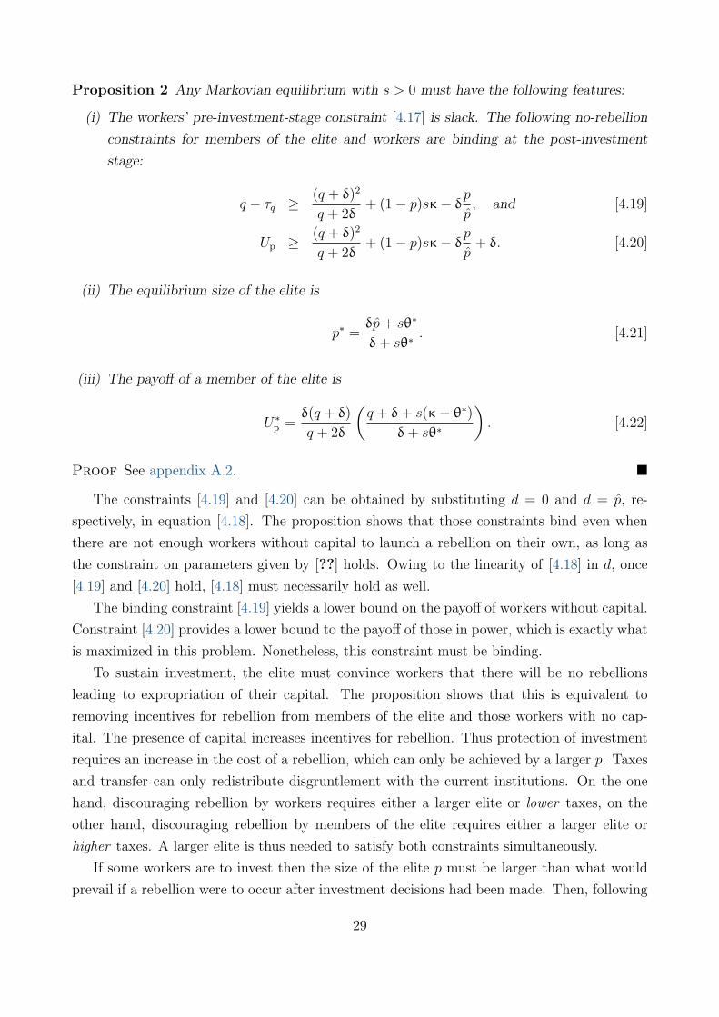
Proposition 2 Any Markovian equilibrium with s > 0 must have the following features:
(i) The workers’ pre-investment-stage constraint [4.17] is slack. The following no-rebellion
constraints for members of the elite and workers are binding at the post-investment
stage:
q − τq ≥(q + δ)2
q + 2δ+ (1− p)sκ− δp
p, and [4.19]
Up ≥(q + δ)2
q + 2δ+ (1− p)sκ− δp
p+ δ. [4.20]
(ii) The equilibrium size of the elite is
p∗ =δp+ sθ∗
δ+ sθ∗. [4.21]
(iii) The payoff of a member of the elite is
U∗p =δ(q + δ)
q + 2δ
(q + δ+ s(κ− θ∗)
δ+ sθ∗
). [4.22]
Proof See appendix A.2.
The constraints [4.19] and [4.20] can be obtained by substituting d = 0 and d = p, re-
spectively, in equation [4.18]. The proposition shows that those constraints bind even when
there are not enough workers without capital to launch a rebellion on their own, as long as
the constraint on parameters given by [??] holds. Owing to the linearity of [4.18] in d, once
[4.19] and [4.20] hold, [4.18] must necessarily hold as well.
The binding constraint [4.19] yields a lower bound on the payoff of workers without capital.
Constraint [4.20] provides a lower bound to the payoff of those in power, which is exactly what
is maximized in this problem. Nonetheless, this constraint must be binding.
To sustain investment, the elite must convince workers that there will be no rebellions
leading to expropriation of their capital. The proposition shows that this is equivalent to
removing incentives for rebellion from members of the elite and those workers with no cap-
ital. The presence of capital increases incentives for rebellion. Thus protection of investment
requires an increase in the cost of a rebellion, which can only be achieved by a larger p. Taxes
and transfer can only redistribute disgruntlement with the current institutions. On the one
hand, discouraging rebellion by workers requires either a larger elite or lower taxes, on the
other hand, discouraging rebellion by members of the elite requires either a larger elite or
higher taxes. A larger elite is thus needed to satisfy both constraints simultaneously.
If some workers are to invest then the size of the elite p must be larger than what would
prevail if a rebellion were to occur after investment decisions had been made. Then, following
29

a post-investment rebellion, the post-rebellion elite would never include all members of the
existing elite. Since some of them would lose their status, there can be no rebellion which
commands the unanimous support of the current elite. In the language of the model, for any
possible rebellion, even if the rebel army were exclusively drawn from the current elite, others
in the elite would constitute the incumbent army that would defend the current institutions
against the rebellion, as destruction of their institutions would lead to them becoming workers.
This incumbent army would impose costs on those wanting to destroy the current institutions.
This cost however would have been zero if all existing members could be guaranteed a place
in the post-rebellion elite.
Creating incentives for investment thus requires power sharing: the elite is larger than
what would otherwise prevail without the possibility of investment. But importantly, in the
model, power is not shared with those who are actually investing. The extra members of
the elite have no special function and have no access to any technology directly protecting
property rights. Their role is to oppose changes to the status quo, with them fighting against
rebellions from workers, and especially from other members of the elite. They do this merely
because they would lose from rebellions that dislodge them from the ruling elite.
The choice of τκ (which determines s) represents limitations on expropriation, and p cap-
tures the distribution of power in society. Credible limitations on expropriation require greater
protection of the institutions. Institutions can only be protected from those who hold power
if some of them fear losing power if the institutions are destroyed. That can only be achieved
if power is not as concentrated as those in power would like it to be, ex-post.
This analysis relies on two key assumptions. First, institutions survive and cannot be
modified without a rebellion. This assumption is necessary for the sheer existence of an en-
vironment where rules are followed. It captures the idea that elites can in principle create
institutions that tie their hands when they would want to tax all the workers’ output, expro-
priate capital or deviate from commitments to provide public goods. If institutions could be
easily modified, the “game” would have no “rules”. Second, were a rebellion to occur, there
can be no enforcement of deals made prior to the rebellion. This reflects the commitment
problem highlighted by Acemoglu (2003). The underlying idea is that institutions are needed
to enforce deals, but there are no “meta-institutions” to enforce deals concerning the choice
of institutions themselves.
Because the destruction of institutions leads to unconstrained optimization over all dimen-
sions of the new institutions, the current elite might struggle to agree to launch a rebellion,
even if they are the only participants in the rebellion. If it were possible for optimization
following a rebellion to be restricted to certain areas, this might make credible commitments
impossible. For example, if the composition of the elite were defined by page one of the
constitution, but limitations on expropriation were on page two, then being able to rebel
30

against page two but at the same time commiting not to touch page one would annihilate the
credibility of page two.
Differentiating the expression in [4.22] with respect to s, noting that θ∗ is a function of s
defined in [4.16], yields the first-order condition:
κs2 + 2(q + 2δ)s− φ
θH − θL(δκ− θL(q + 2δ)) = 0
where θ∗ is also a function of s. One root of this equation is negative. The positive root yields
the value for s∗ as long as it is between 0 and φ, in which case:
s∗ =
√(q + 2δ
k
)2
+φ
θH − θL
(δ− (q + 2δ)
θL
k
)− q + 2δ
k. [4.23]
Otherwise, the problem yields a corner solution for s. In particular, s∗ = 0 if
δκ− θL(q + 2δ) < 0⇒ κ
θL− 1 > 1 +
q
δ,
and s∗ = φ if
φ <1
θH − θL
(δ− (2θH − θL)
q + 2δ
κ
).
As mentioned above, the no-rebellion constraint for workers with good investment oppor-
tunities is not binding. Thus, the distribution of income does not correspond exactly to the
distribution of power. Economic prosperity is related to having more citizens with slack no-
rebellion constraints, which requires institutions that protect their investments. The model
allows the elite (costlessly) to build those institutions. As in equilibrium agents will only invest
if those institutions are there, is in the best interest of the elite to build them?
4.3 The efficient choice of capital taxes
As long as κ > θH , if capital could be directly protected from expropriation at no cost,
investing would always be efficient. However, in this model, that might not be true. If there
is investment, more people have to be in the elite in order to prevent a rebellion, which entails
an opportunity cost.
The efficient benchmark in this case is the following: taxes on capital τκ are chosen by
a benevolent agent, knowing that everything else (p and τq) will be determined in equilib-
rium, from the problem of maximizing payoffs of the group in power subject to the threat of
rebellions, as discussed above.
In the case of section 3, such a benevolent agent could not create a better economic outcome
with a different choice of g. In that case, the public good is efficiently provided. Here, is
31

protection of property rights efficiently provided? If not, is it underprovided or overprovided
and why?
For a given τκ, restrictions determine p and τq. The capital tax τκ determines s, which pins
down the elite size, p∗, as any smaller p would lead to a rebellion at the second stage. Taxes
on q would be such that the constraint in [4.19] is binding.
Welfare in the economy is given by:
W = pUp + (1− p)Uw + (1− p)sθ∗ − θL
2
Since Up = Uw + δ in equilibrium,
W = Up − (1− p)δ+ (1− p)sθ∗ − θL
2[4.24]
There are two differences between the expressions for W and Up. The second term in
[4.24] is related to the distribution of resources in the economy. The third term is the investor
surplus.
Substituting p = p∗ and rearranging:
W =δ(q + δ)
q + 2δ
(q + s(κ− θ∗)δ+ sθ∗
+s2(θH − θL)
2φ(δ+ sθ∗)
)The first-order condition with respect to s is obtained by differentiating the above equation,
using [4.16]:
2κ− θL2
s2 + (δ+ 2q)s− φ
θH − θL(δκ− (q + δ)θL) = 0
One root of this equation is negative. The other yields the solution for the optimal fraction
of investors sO, as long as it is between 0 and φ. In that case,
sO =
√(δ+ 2q)2 + 2φ 2κ−θL
θH−θL(δκ− (q + δ)θL)− (δ+ 2q)
2κ− θL[4.25]
The following proposition establishes the breakdown of the political Coase Theorem when
private investment is possible but subject to expropriation:
Proposition 3 Unless sO and s∗ are both equal to 0 or φ,
sO > s∗
Proof See appendix A.3.
32

The constrained welfare-maximizing choice of s leads to more investment than the equi-
librium choice for two reasons: first, the equilibrium choice of capital taxes does not take into
account investors’ surpluses (the third term in [4.24]). As θ is not observable, it is impossible
for the elite to extract rents from those who invested, at the margin. Consequently, the no-
rebellion constraint for those who invested is slack. A political Coase theorem does not hold
here because of the non-observability of effort, θ, which makes it impossible to write rules
contingent on it.
The second (and more interesting) distortion follows from the distributional effects of pro-
tecting against expropriation (the second term in [4.24]). Protection of property rights requires
sharing power. Sharing power requires sharing rents, because a rebellion including members
of the elite is less costly in terms of fighting effort. Thus while a larger elite might allow for
profitable investment and higher output, it also reduces the fraction of output appropriated
by a member of the elite. Hence, in equilibruim, institutions leading to lower output might
arise owing to the impact of the distribution of power on the distribution of income.
The association between power and rents sets an endogenous limit on the set of possible
transfers, leading to a break down of a political Coase Theorem. The elite could implement the
constrained-optimal allocation, which requires a larger p, but the threat of rebellion constrains
their choice of the extra elite members’ payoffs.
The inefficiently high capital taxes can be interpreted as insufficient protection against
expropriation of property. Recent empirical work has highlighted the importance of institu-
tions that prevent the government from expropriating individuals’ resources. But why would
expropriation of property be so susceptible to political failures? Why would a political Coase
Theorem fail to apply in this particular case? The model here sheds light on this question.
Last, a note on the effect of the power parameter δ. In section 3, the welfare of workers
in an economy with institutions and a self-interested elite might be larger than the welfare
of workers in an economy where no transfers can be enforced. The possibility of establishing
rules allows for the provision of public goods. However, a larger δ can only harm the workers,
as it makes possible higher taxes and leads to a worse income distribution. In contrast, in an
economy with a very small δ, there cannot be investment (s is always equal to 0). If δ is low
enough, it is not even efficient to protect property – that would require a very large increase
in the elite, which entails an opportunity cost. A larger δ allows the elite to keep its power,
which will be used for their own good, but might also allow them to (partly) protect private
property.
4.4 Analogies with historical examples
The results show the importance of sharing power to stimulate investment and prevent changes
in the rules of the game that lead to expropriation. They also show that rulers will not share
33

power as much as would be efficient. Although the model is too abstract to match any given
historical example precisely, the results resonate with a number of examples.
Broadly speaking, the extra individuals in power required to protect property rights (p∗−p)might be interpreted as a “parliament” or any other group of people with power to deter
changes in institutions – from outsiders and, especially, from insiders. Parliaments are usually
thought of as representing those who elected their members, but so are democractically elected
presidents, and members of parliaments are not only useful for defending minorities. Power
sharing makes institutions more stable because it makes it costly for some members of the
elite to replace the current institutions with new ones – with potentially different rules on how
power is distributed and on the limits to how much can be extracted from producers. Once
power is concentrated, institutions are subject to the whims of those in power. In the words
of Montesquieu, “Princes who have wanted to make themselves despotic have always begun
by uniting in their person all magistracies.”
Malmendier (2009) studies what he considers the earliest precursors of the modern business
corporation, the Roman societas publicanorum. Their demise occurred with the transition from
the Roman Republic to the Roman Empire. According to Malmendier (2009), one possible
reason for their demise is that “the Roman Republic was a system of checks and balances.
But the emperors centralized power and could, in principle, bend law and enforcement in
their favor”. In other words, while power was decentralized, it was possible to have rules that
guaranteed the property rights of the societas publicanorum, presumably because changing
the rules would require some of the individuals in power to launch an attack on some of their
peers, which was costly. Once power was centralized, protection agaisnt expropriation was not
possible any longer.
Greif (2006) analyses the importance of the podesteria system for interclan cooperation in
medieval Italy. The podesta, an individual coming from another city who would be in power
for a year, was generously paid and played an important role in the building of cities such
as Genoa by allowing for cooperation and investment. Interestingly, Greif argues that the
podesta had to be sufficiently strong because otherwise, if one clan had defeated its rival, it
could easily defeat the podesta as well. Translating this into the language of the model, the
strength of the podesta (p∗− p) had to be large enough to ensure he could not be defeated by
a clan, which would then be able to change the institutions.16
In seventeenth-century Britain, the Glorious Revolution led to power sharing between King
and Parliament. By accepting the Bill of Rights, King William III accepted that power would
be shared between him and the parliament. North and Weingast (1989) argued that the
Glorious Revolution led to secure property rights and elimination of confiscatory government.
Shortly after the Glorious Revolution, the government could borrow much more, and at sub-
16Greif (2006), pp. 239–240.
34

stantially lower rates. This was certainly in the interest of the king, yet the Stuart kings had
strongly resisted sharing power with Parliament. According to the model, secure property
rights require just such power sharing, so that it is costly for the king to rewrite the rules ex
post. However, the existence of a parliament with real power implies that rents have to be
shared, so even if the pie becomes larger, the share of the king might be smaller.
5 Conclusions
Governments and institutions play a key role in development by making it possible to direct
resources to the provision of public goods and by enforcing collective choices. However, what is
called a government in some of the poorest countries bears little resemblance to its counterpart
in the most developed nations. As noted in the book of Samuel, those with power to choose
the “rules of the game”, guided by their own interests, might choose policies that are not
necessarily good from the point of view of society. Indeed, in far too many cases, the warnings
of Samuel remain as relevant as ever.17
This paper provides a model where institutions are set to maximize the payoffs of the group
in power. That assumption and the threat of rebellions are the main elements of the model.
When private investment is considered, a risk of expropriation emerges. In order to protect
investment, sharing power is needed. That is the only way to prevent those in power from
tearing up the old rules and expropriating capital. However, sharing power requires sharing
rents, because those with power can use it against the other members of the elite. This imposes
limits to the available set of transfers and leads to the breakdown of a political Coase Theorem.
There is not enough power sharing and consequently capital taxes are excessively high — too
little protection of investment.
This framework could be used in a number of ways. First, it could be explored to under-
stand which factors allow for more or less power sharing — and thus investment. It would
also be interesting to analyse other sources of inefficiencies. Also, agents are homogeneous
ex ante, with heterogeneity is an equilibrium outcome, but ex-ante heterogeneity of various
forms could be incorporated into the model (for example, ethnic differences, as in Caselli and
Coleman (2006)). There are no rebellions in equilibrium, but these could arise if the model
had some stochastic elements added.
References
Acemoglu, D. (2003), “Why not a political Coase theorem? Social conflict, commitment,
and politics”, Journal of Comparative Economics, 31(4):620–652. 2, 30
17For a model of the trade-off that having a government (or a “king”) entails, see Grossman (2002).
35

——— (2008), “Oligarchic versus democratic societies”, Journal of the European Economic
Association, 6(1):1–44 (March). 6
Acemoglu, D., Egorov, G. and Sonin, K. (2008), “Coalition formation in non-
democracies”, Review of Economic Studies, 75(4):987–1009 (October). 5
Acemoglu, D. and Johnson, S. (2005), “Unbundling institutions”, Journal of Political
Economy, 113(5):949–995. 4
Acemoglu, D., Johnson, S. and Robinson, J. A. (2005), “Institutions as a fundamental
cause of long-run growth”, in P. Aghion and S. N. Durlauf (eds.), Handbook of Economic
Growth, North-Holland, chap. 6, pp. 386–472. 1, 2
Acemoglu, D. and Robinson, J. A. (2006), Economic Origins of Dictatorship and Demo-
cracy, Cambridge University Press. 1
——— (2008), “Persistence of power, elites, and institutions”, American Economic Review,
98(1):267–293 (March). 1
Baron, D. P. and Ferejohn, J. A. (1989), “Bargaining in legislatures”, American Political
Science Review, 83(4):1181–1206 (December). 5
Basu, K. (2000), Prelude to Political Economy, Oxford University Press. 5
Besley, T. and Persson, T. (2009a), “The origins of state capacity: Property rights,
taxation, and politics”, American Economic Review, 99(4):1218–1244 (September). 1
——— (2009b), “Repression or civil war?”, American Economic Review, 99(2):292–297
(May). 1
——— (2010), “State capacity, conflict and development”, Econometrica, forthcoming. 1
Caselli, F. and Coleman, W. J., II (2006), “On the theory of ethnic conflict”, Working
paper, London School of Economics. 35
Dal Bo, E. and Dal Bo, P. (2010), “Workers, warriors and criminals: Social conflict in
general equilibrium”, Journal of the European Economic Association, forthcoming. 6
Downs, A. (1957), “An economic theory of political action in a democracy”, Journal of
Political Economy, 65(2):135–150 (April). 5
Engerman, S. L. and Sokoloff, K. L. (1997), “A view from economic historians of the
United States”, in S. H. Haber (ed.), How Latin America fell behind, Stanford University
Press, chap. 10, pp. Haber, Stephen H. 1
36

Garfinkel, M. R. and Skaperdas, S. (2007), “Economics of conflict: An overview”, in
T. Sandler and K. Hartley (eds.), Handbook of Defense Economics, vol. 2, North-Holland,
chap. 22, pp. 649–709. 6
Glaeser, E., Scheinkman, J. and Shleifer, A. (2003), “The injustice of inequality”,
Journal of Monetary Economics, 50(1):199–222 (January). 6
Greif, A. (2006), Institutions and the Path to the Modern Economy, Cambridge University
Press. 1, 34
Grossman, H. I. (2002), “‘Make us a king’: anarchy, predation, and the state”, European
Journal of Political Economy, 18(1):31–46 (March). 35
Grossman, H. I. and Kim, M. (1995), “Swords or plowshares? A theory of the security of
claims to property”, Journal of Political Economy, 103(6):1275–1288 (December). 6
Guriev, S. and Sonin, K. (2009), “Dictators and oligarchs: A dynamic theory of contested
property rights”, Journal of Public Economics, 93(1–2):1–13 (February). 6
Hafer, C. (2006), “On the origins of property rights: Conflict and production in the state
of nature”, Review of Economic Studies, 73(1):119–143 (February). 6
Hall, R. E. and Jones, C. I. (1999), “Why do some countries produce so much more output
per worker than others?”, Quarterly Journal of Economics, 114(1):83–116 (February). 1
Hirshleifer, J. (1995), “Anarchy and its breakdown”, Journal of Political Economy,
103(1):26–52 (February). 6
Levy, G. (2004), “A model of political parties”, Journal of Economic Theory, 115(2):250–277
(April). 5
Mailath, G., Morris, S. and Postlewaite, A. (2001), “Laws and authority”, Working
paper, Princeton University. 5
Malmendier, U. (2009), “Law and finance at the origin”, Journal of Economic Literature,
47(4):1076–1108. 34
Myerson, R. B. (1993), “Incentives to cultivate favored minorities under alternative electoral
rules”, American Political Science Review, 87(4):856–869 (December). 15
——— (2004), “Justice, institutions and multiple equilibria”, Chicago Journal of International
Law, 5(1):91–107. 6
37

——— (2008), “The autocrat’s credibility problem and foundations of the constitutional
state”, American Political Science Review, 102(1):125–139. 13
——— (2009), “Learning from Schelling’s Strategy of Conflict”, Journal of Economic Literat-
ure, 47(4):1109–1125. 6
——— (2010), “Capitalist investment and political liberalization”, Theoretical Economics,
5(1):73–91. 6
North, D. C. (1990), Institutions, institutional change, and economic performance, Cam-
bridge University Press. 1
North, D. C. and Weingast, B. R. (1989), “Constitutions and commitment: The evol-
ution of institutional governing public choice in seventeenth-century England”, Journal of
Economic History, 49(4):803–832 (December). 1, 34
Persson, T. and Tabellini, G. (2000), Political Economics: Explaining Economic Policy,
MIT Press. 5, 6, 21
Piccione, M. and Razin, R. (2009), “Coalition formation under power relations”, Theor-
etical Economics, 4(1):1–15 (March). 5
Ray, D. (2007), A Game-Theoretic Perspective on Coalition Formation, Oxford University
Press. 5
Schelling, T. C. (1960), The Strategy of Conflict, Harvard University Press. 6
A Technical appendix
A.1 Proof of Proposition 1
Start by fixing a particular choice of institutions, that is, a choice of army size p and the distributionof consumption across agents. These choices also determine the composition of P and W. Thisparticular choice of institutions does not lead to any rebellion if and only if
maxR
∫R∩W
(U ′p − Uw(ı))dı+∫R∩P
(U ′p − Up(ı))dı+ δd≤ δp s.t. P[R] = p′,
where the size of the subsequent incumbent army p′, as well as U ′p, is taken as given. For a given R,d is the measure of the set R∩P. Now define disjoint sets Rw ≡ R∩W and Rp ≡ R∩P, and notethat the maximization problem above is equivalent to
maxRw,Rp
(p′ − d)U ′p −
∫Rw
Uw(ı)dı+ d(U ′p + δ)−∫Rp
Up(ı)dı
≤ δp s.t. P[Rw ∪Rp] = p′. [A.1.1]
38

Now make the following definitions:
Uw ≡1
1− p
∫WUw(ı)dı, Up ≡
1p
∫PUp(ı)dı, and [A.1.2a]
Uw(rw) = minRw s.t. P[Rw]=rw
1rw
∫Rw
Uw(ı)dı, Up(rp) = min
Rp s.t. P[Rp]=rp
1rp
∫Rp
Up(ı)dı
.
[A.1.2b]
These definitions implyUw(rw) ≤ Uw, [A.1.3a]
with equality if and only if (i) Cw(ı) = Cw for all ı (with measure one), or (ii) u′′(·) = 0 and rw = 1−p.Analogously,
Up(rp) ≤ Up, [A.1.3b]
with equality if and only if (i) Cp(ı) = Cp for all ı (with measure one), or (ii) u′′(·) = 0 and rp = p.The definitions in [A.1.2a] imply that the constraint [A.1.1] is equivalent to
maxd∈D(p,p′)
(p′ − d)U ′p − (p′ − d)Uw(p′ − d) + d(U ′p + δ)− dUp(d)
≤ δp, [A.1.4]
where D(p, p′) ≡ [max0, p+ p′ − 1,minp, p′]. Rearranging terms yields
p′(U ′p−Uw)+ maxd∈D(p,p′)
d(Uw − Up + δ) + (p′ − d)(Uw − Uw(p′ − d)) + d(Up − Up(d))
≤ δp, [A.1.5]
making use of the definitions in [A.1.2a] again.Now consider a Markovian equilibrium with p = p′ and U ′p = Up. Let
D ≡ maxd∈[max0,2p−1,p]
d(Uw − Up + δ) + (p− d)(Uw − Uw(p− d)) + d(Up − Up(d))
, [A.1.6]
where d∗ is the smallest value (without loss of generality) of d that maximizes the above expression.The single constraint [A.1.4] to which the equilibrium institutions are subject must be binding. Thus,by substituting the solution of the problem in [A.1.6] into [A.1.4], and after some rearrangement:
pUp − d∗Up(d∗) = (p− d∗)(δ+ Uw(p− d∗). [A.1.7]
First, note that d∗ < p, otherwise higher taxes on workers would be feasible. Substituting theinequalities in [A.1.3a] and [A.1.3b] into [A.1.7] yields
Uw − Up + δ ≥ 0,
with equality if payoffs are equalized among army members and among workers. Thus, if payoffs areequalized, then the value of D in [A.1.6] is necessarily zero.
Now suppose that payoffs among the workers are not equalized. Then (Uw−Uw(p−d)) is strictlypositive for d > 2p− 1 since this ensures p− d < 1− p, the total measure of workers. Moreover, ford < p, the coefficient multiplying this term in [A.1.6] is positive as well. As the other terms in [A.1.6]would be non-negative, and since such a choice of d is feasible (as p < 1), the value of D would bepositive. As has been seen, D = 0 is possible if institutions equalize payoffs within groups. This canbe achieved without affecting the other terms in the constraint [A.1.5], and without decreasing theobjective function. Hence, in a Markovian equilibrium, payoffs of workers must be equalized.
Analogously, if payoffs among army members are not equalized, then (Up − Up(d)) is strictlypositive for d < p. For d > 0, this term has a positive coefficient in [A.1.6]. Such a choice is feasible
39

(p < 1), and the other terms appearing in [A.1.6] would be non-negative. Again, D would hencebe positive. Since D = 0 is feasible, a similar argument to that above shows that payoffs of armymembers must be equalized.
A.2 Proof of Proposition 2
Suppose there is a Markovian equilibrium with a positive fraction of investors. That is, s∗ > 0, withan elite size p = p′ = p∗, and with elite payoff Up = U ′p = U∗p .
Parameter restriction on the number of individuals receiving investment opportunities
Define the quadratic function Q(ϕ) as follows:
Q(ϕ) = (κ− θ)ϕ2 +(
q + δ+ p†κ− (κ− θ))ϕ− δ, [A.2.1]
where p† is given in [4.14]. Since κ ≥ θ, the equation Q(ϕ) = 0 always has one and only one positiveroot. Denote this root by φ. Using the expression for the smallest root of a quadratic equationtogether with the product of roots formula:
φ =2δ(
q + δ+ p†κ− (κ− θ))
+√(
q + δ+ p†κ− (κ− θ))2 + 4δ(κ− θ)
,
which can be rearranged to yield:
φ =δ
q + δ+ p†κ− 12
((q + δ+ p† + (κ− θ))−
√(q + δ+ p†κ+ (κ− θ))2 − 4(q + p†κ)(κ− θ)
) .[A.2.2]
This is the bound for φ given in [4.4]. The restriction 0 < φ < φ is imposed throughout.Since Q(0) = −δ < 0 and Q(1) = q+p†κ > 0, it follows that 0 < φ < 1. The term in parentheses
in [A.2.2] is non-negative because κ ≥ θ, and hence
φ ≥ δ
q + δ+ p†κ>
δ
q + δ>
q + δq + 2δ
= 1− p†,
using the formula for p† from [4.14]. Consequently, the restriction 0 ≤ φ < φ implies
1− φs > p†, [A.2.3]
for all s ∈ [0, 1].
No capitalists in a rebel army with a binding no-rebellion constraint
With a positive fraction of investors, the marginal investor’s effort θ∗ satisfies θ∗ = κ − τ∗κaccording to [4.8]. It follows from [4.5] and [4.7] that the payoff of a capitalist Uk and a worker Uw
are related by:U∗k = U∗w + θ∗. [A.2.4]
Since s∗ > 0, θ∗ > θ > 0, and thus U∗k > U∗w.According to [4.10], the expected payoff Un of an individual outside the elite at the pre-investment
stage is equal to that of a worker at the post-investment stage Uw plus the expected surplus toinvestors Si(θ):
U∗n = U∗w + φSi(θ∗). [A.2.5]
40

Eliminating U∗w from equations [A.2.4] and [A.2.5] implies
U∗n = U∗k −(θ∗ − φSi(θ∗)
). [A.2.6]
The Markovian equilibrium must satisfy the pre-investment stage no-rebellion constraint [4.11], whichrequires
U∗n ≥ U∗p − δ. [A.2.7]
Substituting equation [A.2.6] into [A.2.7] implies
U∗k ≥(U∗p − δ
)+(θ∗ − φSi(θ∗)
). [A.2.8]
Note that the definition of the investors’ surplus Si(θ) in [4.9] implies that
θ− φSi(θ) = (θ− Si(θ)) + (1− φ)Si(θ) = (1− φ)Si(θ) + Eminθ, θ > 0,
for any s > 0, since θ > θ > 0. Together with [A.2.8], this implies that U∗k > U∗p − δ.The group of capitalists is of size k = (1 − p)φs, while the rebel army at the post-investment
stage is of size p†. Note that 1− k ≥ p† is equivalent to (1−φs) + pφs ≥ p†, which must hold giventhe inequality in [A.2.3]. Therefore, there are always enough non-capitalists (workers, members ofthe pre-investment stage elite) to fill the rebel army at the post-investment stage. Combined withboth U∗k > U∗w and U∗k > U∗p − δ, replacing a capitalist in the rebel army with either a worker ora member of the existing elite would strictly improve the net fighting strength of the rebel armyrelative to the incumbent army. Thus a rebel army including a positive measure of capitalists cannotfeature a binding no-rebellion constraint in a Markovian equilibrium.
It follows that the general post-investment stage no-rebellion constraint [4.12] needs only takeaccount of rebel armies comprising some combination of workers and existing elite members. Thiscan be written as
σp†(U†p(K)− Up
)+ (1− σ)p†
(U†p(K)− Uw
)≤ δ(p− σp†), [A.2.9]
where σ is the fraction of the rebel army of size p† filled by members of the current elite, with theremaining fraction 1 − σ filled by workers. The constraint [A.2.9] implicitly assumes U†p(K) > Up
and U†p(K) > Uw. The fraction σ must satisfy σp† ≤ p and (1 − σ)p† ≤ w to be feasible, where p isthe number of existing elite members and w = (1 − p)(1 − φs) is the number of workers under thepre-investment stage institutions. Hence for institutions to avoid rebellion, [A.2.9] must hold for allσ ∈ [σ, σ], where σ and σ are given by
σ = max
0, 1− (1− p)(1− φs)p†
, and σ = min
p
p†, 1. [A.2.10]
By rearranging [A.2.9], it is equivalent to
σ(Up − δ) + (1− σ)Uw ≥ U†p(K)− δ pp†
for all σ ∈ [σ, σ]. [A.2.11]
The pre-investment stage elite must be larger than the elite after a post-investment stage rebellion
Consider the possibility that p∗ ≤ p† in a Markovian equilibrium. In this case, [A.2.10] impliesσ∗ = p∗/p† ≤ 1. If it were the case that U∗p < U†p(K) then by evaluating the general no-rebellion
41

constraint [A.2.9] at σ = σ∗ the following is obtained:
σ∗(U†p(K)− U∗p) + (1− σ∗)(U†p(K)− U∗w) ≤ 0,
assuming U†p(K) ≥ Uw. This inequality cannot hold when U∗p < U†p(K), so it must be the case that
U∗p ≥ U†p(K).
Now evaluate the general no-rebellion constraint [A.2.11] at σ = σ∗ and note that [4.5] impliesU∗w = C∗w = q− τ∗q to obtain:
(1− σ∗)τ∗q ≤ σ∗(U∗p − δ) + (1− σ∗)q− U†p(K∗) + δp∗
p†. [A.2.12]
In the case that σ∗ = 0, this inequality reduces to τ∗q ≤ q − U†p(K) + δp∗/p†. Substituting this intoequation [4.13] for Up:
U∗p ≤(1− p)p
(q + φs∗(κ− θ∗)− U†p(K) + δ
p∗
p†
).
Combining this with the inequality U∗p ≥ U†p(K) and rearranging yields:
(1− p∗)(
q + φs∗(κ− θ∗) + δp∗
p†
)− U†p(K) ≥ 0. [A.2.13]
Now consider the remaining case where σ∗ > 0. By multiplying both sides of the expression forUp in [4.13] by (1− φs∗)p∗/p† and using the formula σ∗ = 1− ((1− p∗)(1− φs∗))/p† from [A.2.10]:
1− φs∗
p†p∗U∗p = (1− σ∗)τ∗q + (1− σ∗)φs∗(κ− θ∗).
Combining this with the inequality [A.2.12] yields:
1− φs∗
p†p∗U∗p ≤ σ∗U∗p + (1− σ∗)(q + φs∗(κ− θ∗))− U†p(K) + δ
p∗
p†− δσ∗.
Using again the formula σ∗ = 1− ((1− p∗)(1− φs∗))/p† that applies when σ∗ > 0:(1− φs∗
p†− 1)U∗p ≤ (1− σ∗)(q + φs∗(κ− θ∗))− U†p(K) + δ
p∗
p†− δσ∗.
Since it is known that U∗p ≥ U†p(K) and as the parameter restriction [A.2.3] implies (1−φs∗)/p† − 1
is a positive number:(1− φs∗
p†− 1)U†p(K) ≤ (1− σ∗)(q + φs∗(κ− θ∗))− U†p(K) + δ
p∗
p†− δσ∗.
Substituting again the expression for σ∗ from [A.2.10] and rearranging terms yields:
1− φs∗
p†
((1− p∗)
(q + φs∗(κ− θ∗) + δ
p∗
p†
)− U†p(K)
)− σ∗ δ
p†(p† − p∗) ≥ 0.
Since p∗ ≤ p† in this case, the above implies that inequality [A.2.13] must hold. Therefore thisinequality holds for both σ∗ = 0 and σ∗ > 0.
Using the capital accumulation equation [4.2] and the rebellion at the post-investment stage
42

equilibrium in [4.14] to substitute for U†p(K):
(1− p)(
q + φs(κ− θ) + δp
p†
)− U†p(K) = (1− p)
(q− φsθ+ δ
p
p†
)− (q + δ)2
q + 2δ. [A.2.14]
By using the expression for p† from [4.14], note that
(1− p†)(
q− φsθ+ δ)
=(q + δ)2
q + 2δ− q + δ
q + 2δφsθ. [A.2.15]
By expanding the following brackets and using the expression for p†:
(1− p)(
q− φsθ+ δp
p†
)− (1− p†)
(q− φsθ+ δ
p†
p†
)= −(q + 2δ)(p†− p)((p†− p) +φsθ). [A.2.16]
Combining equations [A.2.14], [A.2.15] and [A.2.16] yields:
(1− p)(
q + φs(κ− θ) + δp
p†
)− U†p(K) = − q + δ
q + 2δφsθ− (q + 2δ)(p† − p)((p† − p) + φsθ).
This finding demonstrates that inequality [A.2.13] cannot hold in a Markovian equilibrium withs∗ > 0 and p∗ ≤ p†. But [A.2.13] has been shown to be necessary for a Markovian equilibrium toexist in this case. Therefore, it must be the case that p∗ > p† if s∗ > 0 in a Markovian equilibrium.
If p > p† then [A.2.10] implies that σ = 1. Given the linearity of the general post-investmentstage no-rebellion constraint [A.2.11], it follows that this holds for all σ ∈ [σ, σ] if and only if it holdsat σ = σ and σ = σ = 1. These two extremes, together with the pre-investment stage no-rebellionconstraint [4.11] constitute the relevant set of three constraints on the institutions in a Markovianequilibrium:
Un ≥ U ′p − δp
p′; [A.2.17a]
σ(Up − δ) + (1− σ)Uw ≥ U†p(K)− δ pp†
; [A.2.17b]
Up ≥ U†p(K)− δp− p†
p†. [A.2.17c]
The pre-investment stage constraint and the post-investment stage constraint for the elite cannotboth bind
Suppose that both [A.2.17a] and [A.2.17c] bind. It follows that U∗n = U∗p − δ, and by using theexpression for Un in [4.10] this implies that U∗w is given by
U∗w =(U∗p − δ
)− φSi(θ∗).
Hence note thatσ∗(U∗p − δ) + (1− σ∗)U∗w = (U∗p − δ)− (1− σ∗)φSi(θ∗). [A.2.18]
The binding constraint [A.2.17c] implies
U∗p − δ = U†p(K∗)− δp∗
p†,
43

which combined with [A.2.18] yields
σ∗(U∗p − δ) + (1− σ∗)U∗w =(U†p(K∗)− δp
∗
p†
)− (1− σ)φSi(θ∗) < U†p(K∗)− δp
∗
p†,
since Si(θ∗) > 0 for θ∗ > 0. This violates [A.2.17b], so [A.2.17a] and [A.2.17c] cannot both hold in aMarkovian equilibrium.
At least one no-rebellion constraint including some outside the elite must bind at some stage
Observe that if neither [A.2.17a] nor [A.2.17b] are binding then τq can be increased by somepositive amount (holding all other institutional variables constant) while still satisfying both of theseconstraints (see [4.5] and [4.10]), but strictly increasing the elite payoff Up (see [4.13]), and hencecontinuing to satisfy [A.2.17c]. This clearly cannot be an equilibrium.
At least one no-rebellion constraint at the post-investment stage must bind
Now suppose that only [A.2.17a] is binding in a Markovian equilibrium. The equilibrium cantherefore be characterized by solving the maximization problem of the elite subject only to [A.2.17a]holding with equality. Using the expression for Un from [4.10] and Uw = Cw:
Cw + φSi(θ) = U ′p − δp
p′.
This binding constraint can be used to eliminate τq from the expression for Up in [4.13], noting thatCw = q− τq according to [4.5]. Hence the tax τq is
τq = q + φSi(θ)− U ′p + δp
p′.
Given the threshold investment effort θ, the capital tax τκ must satisfy τκ = κ− θ according to [4.8].Therefore, using [4.13], the elite payoff is
Up =(1− p)p
(q + φSi(θ)− U ′p + δ
p
p′+ φs(κ− θ)
). [A.2.19]
This is now an unconstrained maximization problem in p and s (with θ being a function of s, andtaking future beliefs p′ and U ′p as given). The first-order condition with respect to p is
q + φs(κ− θ) + φSi(θ) + δp2
p′− U ′p = 0. [A.2.20]
In a Markovian equilibrium, the elite payoff must satisfy U∗p = U ′p, thus by using equation [A.2.19]:
U∗p = (1− p∗)(q + δ+ φs∗(κ− θ∗) + φSi(θ∗)).
Imposing Markovian equilibrium (p∗ = p′) in the first-order condition [A.2.20] and substituting forU∗p yields:
p∗ =δ
q + 2δ+ φs∗(κ− θ∗) + φSi(θ∗),
which implies p∗ < p† when s∗ > 0, since θ∗ ≤ κ and Si(θ∗) > 0. This violates the condition p∗ > p†
derived earlier that must be satisfied in Markovian equilibrium.
44
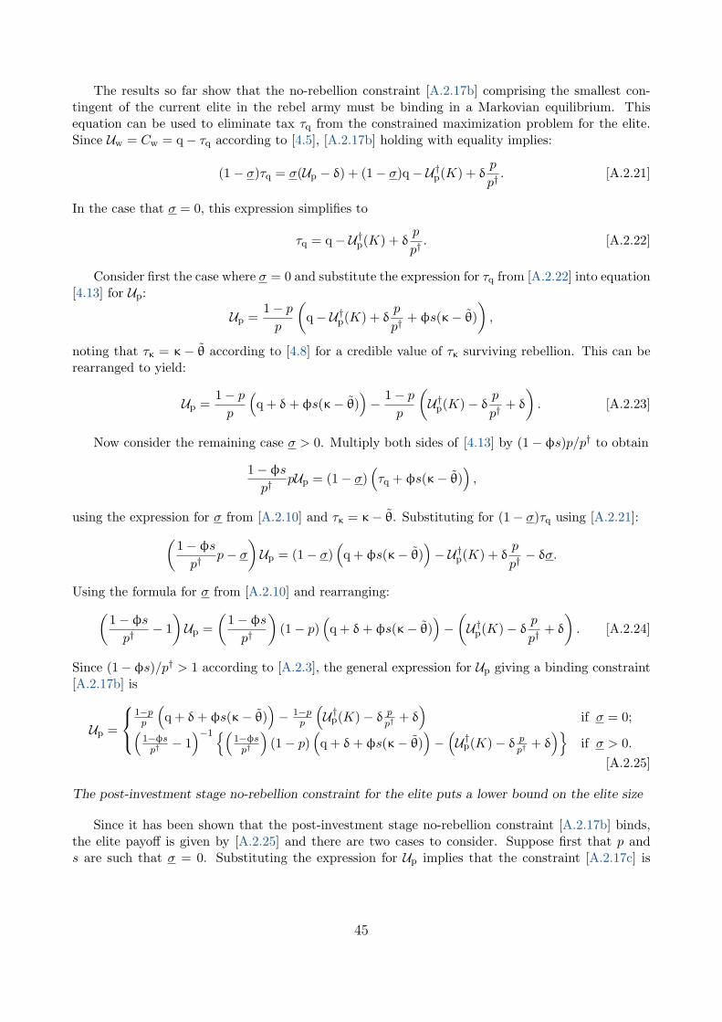
The results so far show that the no-rebellion constraint [A.2.17b] comprising the smallest con-tingent of the current elite in the rebel army must be binding in a Markovian equilibrium. Thisequation can be used to eliminate tax τq from the constrained maximization problem for the elite.Since Uw = Cw = q− τq according to [4.5], [A.2.17b] holding with equality implies:
(1− σ)τq = σ(Up − δ) + (1− σ)q− U†p(K) + δp
p†. [A.2.21]
In the case that σ = 0, this expression simplifies to
τq = q− U†p(K) + δp
p†. [A.2.22]
Consider first the case where σ = 0 and substitute the expression for τq from [A.2.22] into equation[4.13] for Up:
Up =1− pp
(q− U†p(K) + δ
p
p†+ φs(κ− θ)
),
noting that τκ = κ − θ according to [4.8] for a credible value of τκ surviving rebellion. This can berearranged to yield:
Up =1− pp
(q + δ+ φs(κ− θ)
)− 1− p
p
(U†p(K)− δ p
p†+ δ). [A.2.23]
Now consider the remaining case σ > 0. Multiply both sides of [4.13] by (1− φs)p/p† to obtain
1− φsp†
pUp = (1− σ)(τq + φs(κ− θ)
),
using the expression for σ from [A.2.10] and τκ = κ− θ. Substituting for (1− σ)τq using [A.2.21]:(1− φsp†
p− σ)Up = (1− σ)
(q + φs(κ− θ)
)− U†p(K) + δ
p
p†− δσ.
Using the formula for σ from [A.2.10] and rearranging:(1− φsp†
− 1)Up =
(1− φsp†
)(1− p)
(q + δ+ φs(κ− θ)
)−(U†p(K)− δ p
p†+ δ). [A.2.24]
Since (1−φs)/p† > 1 according to [A.2.3], the general expression for Up giving a binding constraint[A.2.17b] is
Up =
1−pp
(q + δ+ φs(κ− θ)
)− 1−p
p
(U†p(K)− δ p
p†+ δ)
if σ = 0;(1−φsp†− 1)−1 (
1−φsp†
)(1− p)
(q + δ+ φs(κ− θ)
)−(U†p(K)− δ p
p†+ δ)
if σ > 0.[A.2.25]
The post-investment stage no-rebellion constraint for the elite puts a lower bound on the elite size
Since it has been shown that the post-investment stage no-rebellion constraint [A.2.17b] binds,the elite payoff is given by [A.2.25] and there are two cases to consider. Suppose first that p ands are such that σ = 0. Substituting the expression for Up implies that the constraint [A.2.17c] is
45

equivalent to
1− pp
(q + δ+ φs(κ− θ)
)− 1− p
p
(U†p(K)− δ p
p†+ δ)≥ U†p(K)− δ p
p†+ δ,
which can be rearranged as follows:
(1− p)(
q + δ+ φs(κ− θ))≥ U†p(K)− δ p
p†+ δ. [A.2.26]
Alternatively, suppose σ > 0. Since the parameter restriction in [A.2.3] holds, the no-rebellionconstraint [A.2.17c] is equivalent to(
1− φsp†
− 1)Up ≥
(1− φsp†
− 1)(U†p(K)− δ p
p†+ δ),
and hence by substituting the expression for Up from [A.2.25]:(1− φsp†
)(1−p)
(q + δ+ φs(κ− θ)
)−(U†p(K)− δ p
p†+ δ)≥(
1− φsp†
− 1)(U†p(K)− δ p
p†+ δ).
Rearranging terms leads to an equivalent inequality
(1− p)(
q + δ+ φs(κ− θ))≥ U†p(K)− δ p
p†+ δ,
which is identical to the condition [A.2.26] derived for the case σ = 0. Therefore, the inequality[A.2.26] is equivalent to [A.2.17c] for all values of σ.
Now use equations [4.2] and [4.14] to replace the terms K, p†, and U†p(K) appearing in [A.2.26].This yields an equivalent inequality:
(1− p)(
q + δ+ φs(κ− θ))≥ (q + δ)2
q + 2δ+ (1− p)φsκ− (q + 2δ)p+ δ.
By rearranging terms, this can be simplified as follows:(δ+ φsθ
)p ≥ δ2
q + 2δ+ φsθ. [A.2.27]
Now define πp(s) for a given value of s:
πp(s) ≡ δp† + φsθδ+ φsθ
, [A.2.28]
and note that using the formula for p† in [4.14] shows that [A.2.27] is equivalent to p ≥ πp(s). Thisplaces a lower bound on the elite size for a given s if the elite’s no-rebellion constraint [A.2.17c] is tobe satisfied. Define Πp(s) = [πp(s), 1] to be the set of p values satisfying the constraint [A.2.17c] fora given value of s. Finally, observe that
πp(s) =(
δ
δ+ φsθ
)p† +
(φsθ
δ+ φsθ
)> p†,
for all s > 0.
46

Either the post-investment constraint for the elite or the pre-investment constraint must bind
First consider p and σ values where σ = 0. By substituting the post-investment stage rebellionequilibrium outcome U†p(K) from [4.14] and the capital accumulation equation [4.2] into [A.2.25]:
Up =1− pp
(φs(κp− θ) + δ
p
p†− δp†
).
Partially differentiating with respect to p yields:
∂Up
∂p=(δp† + φsθ
) 1p2−(δ
p†+ φsκ
). [A.2.29]
Define πM(s) as follows:
πM(s) =
√δp† + φsθδ/p† + φsκ
,
and hence observe from [A.2.29] that Up is strictly decreasing in p for p > πM(s) when σ = 0, with σdefined in [A.2.10].
Note that the definition of πM(s) implies
πM(s) =δp† + φsθ
(δ/p† + φsκ)πM(s),
and suppose for contradiction that πM(s) ≥ πp(s). Under this supposition, it follows that
πM(s) ≤ δ+ φsθδ/p† + φsκ
. [A.2.30]
But it can be seen that
δp† + φsθδ+ φsθ
− δ+ φsθδ/p† + φsκ
=δφsθ(1− p†)2
p†(δ+ φsθ
)(δp†
+ φsκ) > 0,
for all s > 0, and by using the expression for πp(s) in [A.2.28] and [A.2.30], the inequality πM(s) ≤πp(s) is obtained. This contradicts the original supposition, so it must be the case that πM(s) < πp(s)for all s > 0.
Now consider the behaviour of Up in the case that σ > 0. Again substituting for U†p(K) and Kin [A.2.25] using [4.2] and [4.14]:
Up =(1− p)
(1−φsp†
)(q + δ+ φs(κ− θ)
)− (q+δ)2
q+2δ − (1− p)φsκ+ δ pp†− δ
1−φsp†− 1
.
Taking the partial derivative with respect to p:
∂Up
∂p=
(δp†
+ φsκ)−(
1−φsp†
)(q + δ+ φs(κ− θ)
)1−φsp†− 1
. [A.2.31]
Note that the quadratic Q(ϕ) defined in [A.2.1] can be alternatively expressed as
Q(ϕ) = (δ+ p†κϕ)− (1−ϕ)(q + δ+ (κ− θ)ϕ),
47

and hence the partial derivative in [A.2.31] can be written as follows:
∂Up
∂p=
1p†Q(φs)−
(1−φsp†
)φs(θ− θ)
1−φsp†− 1
.
The upper bound φ for φ in equation [A.2.2] is the unique positive root of the quadratic equationQ(ϕ) = 0, where Q(ϕ) is defined in [A.2.1]. Since Q(0) = −δ < 0, it follows that ϕ < φ impliesQ(ϕ) < 0. Furthermore, for all s ∈ [0, 1], φ < φ implies φs < φ < 1, so Q(φs) < 0. The conditionφ < φ is also sufficient for [A.2.3] to hold, and it must be the case that θ ≤ θ, so [A.2.31] impliesthat Up is strictly decreasing in p for all p and s values where σ > 0.
Finally, suppose there is a Markovian equilibrium p∗ and s∗ > 0 in which both no-rebellionconstraints [A.2.17a] and [A.2.17c] are slack. If the elite’s post-investment constraint [A.2.17c] is slackthen the argument earlier shows that p∗ > πp(s∗). Since it has been shown that πp(s∗) > πM(s∗),it follows that Up is strictly decreasing in p if σ∗ = 0 at the Markovian equilibrium. Furthermore,in the case that σ∗ > 0, it is also true that Up is strictly decreasing in p. The binding constraint[A.2.17b] has already been imposed when deriving the expressions for Up in [A.2.25], if both [A.2.17a]and [A.2.17c] are slack then p can be varied in a neighbourhood of p∗ (holding s constant at s∗).This means that it is feasible to increase the elite payoff Up, so this case cannot be a Markovianequilibrium.
The pre-investment no-rebellion constraint cannot bind
Now consider a Markovian equilibrium p = p′ = p∗ and s = s∗ > 0 where the pre-investmentstage no-rebellion constraint [A.2.17a] is binding:
U∗n = U∗p − δ.
Together with the link between Un and Uw from [4.10], it follows that:
U∗w = (U∗p − δ)− φSi(θ∗). [A.2.32]
First consider the case where σ∗ = 0. Since constraint [A.2.17b] is known to bind:
U∗w = U†p(K)− δp∗
p†,
and hence by combining this with equation [A.2.32]:
U∗p =(U†p(K)− δp
∗
p†+ δ)
+ φSi(θ∗).
Setting this equal to the equation for Up from [A.2.25] in the case σ∗ = 0 (evaluated at the Markovianequilibrium) and rearranging yields:
(1− p∗)(
q + δ+ φs∗(κ− θ∗))
=(U†p(K)− δp
∗
p†+ δ)
+ φSi(θ)p∗.
Use the expressions for p† and U†p(K) from [4.14] evaluated at K = (1 − p∗)φs∗κ according to [4.2]to solve for p∗:
p∗ =δp† + φs∗θ∗
δ+ φs∗θ∗ − φSi(θ∗). [A.2.33]
48

Note thatsθ− Si(θ) = sθ− Emaxθ− θ, 0 = sθ− s(θ− θe) = sθe,
where θe = E[θ|θ ≤ θ]. It follows that the denominator of [A.2.33] is strictly positive and thus
δp† + φsθδ+ φsθ− φSi(θ)
>δp† + φsθδ+ φsθ
= πp(s),
for all s > 0, where πp(s) is as defined in [A.2.28].The second case to consider is σ∗ > 0, where the binding constraint [A.2.17b] now requires
σ∗(U∗p − δ) + (1− σ∗)U∗w = U†p(K)− δp∗
p†.
Multiplying both sides of [A.2.32] by (1− σ∗) and substituting into the above yields:
U∗p =(U†p(K)− δp
∗
p†+ δ)
+ (1− σ∗)φSi(θ∗).
Combining this with the formula for Up from [A.2.25] for σ∗ > 0 (evaluated at the Markovianequilibrium) leads to the following equation:(
1− φs∗
p†− 1)(U†p(K)− δp
∗
p†+ δ)
+(
1− φs∗
p†− 1)
(1− σ∗)φSi(θ∗)
=(
1− φs∗
p†− 1)
(1− p∗)(
q + δ+ φs∗(κ− θ∗))−(U†p(K)− δp
∗
p†+ δ).
By simplifying this equation:
(1− p∗)(
q + δ+ φs∗(κ− θ∗))
=(U†p(K)− δp
∗
p†+ δ)
+(
1− φs∗
p†− 1)φSi(θ∗)(1− p∗),
and substituting for U†p(K) implies the following solution for p∗:
p∗ =δp† + φs∗θ∗ +
(1−φs∗p†− 1)φSi(θ∗)
δ+ φs∗θ∗ +(
1−φs∗p†− 1)φSi(θ∗)
. [A.2.34]
The restriction [A.2.3] implies ((1−φs)/p†− 1) is positive, and Si(θ) is positive for s > 0. It followsthat
δp† + φsθ+(
1−φsp†− 1)φSi(θ)
δ+ φsθ+(
1−φsp†− 1)φSi(θ)
>δp† + φsθδ+ φsθ
= πp(s),
for all s > 0, where πp(s) is as defined in [A.2.28].Hence for a given value of s, the Markovian equilibrium value of p associated with a binding
constraint [A.2.17a] is given by p = πn(s) where:
πn(s) ≡
δp†+φsθ
δ+φsθ−φSi(θ)if σ = 0;
δp†+φsθ+(
1−φs
p†−1)φSi(θ)
δ+φsθ+(
1−φs
p†−1)φSi(θ)
if σ > 0,[A.2.35]
49

with σ being the value of the expression in [A.2.10] evaluated at the Markovian equilibrium. In allcases it has been seen that the elite’s post-investment stage no-rebellion constraint is equivalent toπn(s) > πp(s).
Since constraint [A.2.17b] is known to be binding and as the post-investment stage no-rebellionconstraint [A.2.17c] for the elite can be written as
Up ≥ U†p(K)− δ pp†,
the constraint [A.2.17c] is equivalent to
Up − δ ≥ σ(Up − δ) + (1− σ)Uw,
and thus(1− σ)(Up − δ− Uw) ≥ 0.
Since σ < 1 for all p < 1, it follows that [A.2.17c] is equivalent to Up − δ− Uw ≥ 0.Now consider a deviation of p away from the Markovian equilibrium value p∗, holding s = s∗
constant. The beliefs p′ and U ′p remain unchanged at their Markovian equilibrium values (p′ = p∗
and U ′p = U∗p). Using equation [4.10], the pre-investment stage no-rebellion constraint [A.2.17a] isequivalent to
Uw + φSi(θ∗) ≥ U∗p − δp
p∗, [A.2.36]
where the payoff Uw is evaluated at a general value of p, but holds s = s∗ (and hence θ = θ∗)constant. Now write the binding constraint [A.2.17b] in the following form:
Uw =(U†p(K)− δ p
p†
)− σ(Up − δ− Uw),
and substitute into [A.2.36] to obtain an inequality equivalent to the constraint [A.2.17a]:(U†p(K)− δ p
p†
)− σ(Up − δ− Uw) + φS∗i (θ∗) ≥ U∗p − δ
p
p∗.
Replacing the values of K and U†p(K) using equations [4.2] and [4.14] shows that the above is equi-valent to:(
δ
(1p†− 1p∗
)+ φκs∗
)p ≤
((q + δ)2
q + 2δ+ φκs∗ − U∗p
)+ φSi(θ∗)− σ(Up − δ− Uw). [A.2.37]
The Markovian equilibrium value of p is given by p∗ = πn(s∗) for the function πn(s) defined in [A.2.35].The earlier analysis showed that πn(s∗) > πp(s∗) for all cases where s∗ > 0, and πp(s∗) > p†. Itfollows that p∗ > p†, so the coefficient of p in [A.2.37] is strictly positive. Therefore the pre-investmentstage no-rebellion constraint [A.2.17a] holds if and only if
p ≤ p∗ − σ(Up − δ− Uw)
δ(
1p†− 1
p∗
)+ φκs∗
, [A.2.38]
where
p∗ ≡
((q+δ)2
q+2δ + φκs∗ − U∗p)
+ φSi(θ∗)
δ(
1p†− 1
p∗
)+ φκs∗
, [A.2.39]
50

noting that p∗ is independent of the particular value of p under consideration. It depends only onthe Markovian equilibrium values of p∗ and s∗. Let Πn(s∗) denote the set of feasible values of p givens = s∗ and p′ = p∗ and U ′p = U∗p .
Since p∗ = πn(s∗) > πp(s∗), the post-investment stage constraint [A.2.17c] for the elite must beslack in a Markovian equilibrium at p = p∗ and s = s∗ with [A.2.17a] binding. Thus it must be thecase that σ∗(U∗p −δ−U∗w) ≥ 0. Since p∗ is a feasible value of p by construction (p∗ ∈ Πn(s∗)), it mustsatisfy the inequality [A.2.38]. Thus evaluating [A.2.38] at p = p∗ and rearranging terms yields:
p∗ ≥ p∗ +σ(U∗p − δ− U∗w)
δ(
1p†− 1
p∗
)+ φκs∗
≥ p∗,
so the term p∗ defined in [A.2.39] is an upper bound for the Markovian equilibrium value of p.Now consider setting p = πp(s∗). Since the post-investment stage constraint [A.2.17c] binds at
this point, Up− δ−Uw = 0, so [A.2.38] implies that πp(s∗) ∈ Πn(s∗) if and only if πp(s∗) ≤ p∗. Sincep∗ ≥ p∗ = πn(s∗) > πp(s∗), this inequality necessarily holds, so p = πp(s∗) is certain to satisfy theconstraint [A.2.17a]. As πp(s∗) > πM(s∗), it is always the case that moving from p = p∗ to p = πp(s∗)strictly increases Up. Because such a change satisfies all no-rebellion constraints and strictly increasesUp, this argument shows that the original point p∗ cannot be a Markovian equilibrium.
The elite’s objective function after imposing the no-rebellion constraints that bind
The analysis so far has shown that the pre-investment stage constraint [A.2.17a] is slack, whileboth post-investment stage no-rebellion constraints [A.2.17b] and [A.2.17c] are binding. Constraint[A.2.17c] implies
Up = U†p(K)− δ pp†
+ δ. [A.2.40]
Since [A.2.17b] binds, the elite payoff Up can be obtained from equation [A.2.25]. Making use of[A.2.40], in the case σ = 0 the payoff Up satisfies
Up =1− pp
(q + δ+ φs(κ− θ)
)− 1− p
pUp,
which impliesUp = (1− p)
(q + δ+ φs(κ− θ)
). [A.2.41]
Similarly, in the case σ > 0, the expression for the payoff Up from [A.2.25] combined with [A.2.40]implies: (
1− φsp†
− 1)Up =
(1− φsp†
)(1− p)
(q + δ+ φs(κ− θ)
)−(U†p(K)− δ p
p†+ δ),
which can be simplified to obtain:
Up = (1− p)(
q + δ+ φs(κ− θ)),
the same as found in [A.2.41]. Therefore the expression for Up from [A.2.41] is valid in all cases underconsideration.
Using [A.2.28], the binding post-investment stage constraint [A.2.17c] for the elite requires that
p =δp† + φsθδ+ φsθ
, [A.2.42]
51

for a given value of s and hence θ. It follows that
1− p =δ(1− p†)δ+ φsθ
=δ(q + δ)q + 2δ
1δ+ φsθ
.
By substituting this into the expression for Up in [A.2.41]:
Up =δ(q + δ)q + 2δ
q + δ+ φs(κ− θδ+ φsθ
. [A.2.43]
This completes the proof.
A.3 Proof of Proposition 3
The value of s∗ is given by the positive root of the quadratic:
Σ∗(s) = κs2 + 2(q + 2δ)s− φ
θH − θL(δκ− (q + 2δ)θL)
and the value of sO is given by the positive root of:
ΣO(s) =2κ− θL
2s2 + (δ+ 2q)s− φ
θH − θL(δκ− (q + δ)θL)
Now,
Σ∗(s)− Σ∗(O) =θL
2s2 + 3δs+
φδθL
θH − θLwhich is positive for all s > 0. As both quadratic functions are convex and have at least one negativeroot, any positive root of Σ∗(s) must be smaller than a positive root of ΣO(s).
52
Copyright © 2022 FDOKUMEN