Systematic, large-scale national biodiversity surveys: NeoMaps as a model for tropical regions

BIODIVERSITYRESEARCH

Systematic, large-scale nationalbiodiversity surveys: NeoMaps as amodel for tropical regionsJose R. Ferrer-Paris1,†, Jon P. Rodrıguez1*, Tatjana C. Good1,

Ada Y. Sanchez-Mercado1,†, Kathryn M. Rodrıguez-Clark1,

Gustavo A. Rodrıguez1 and Angel Solıs2

1Centro de Ecologıa, Instituto Venezolano de

Investigaciones Cientıficas (IVIC), Apartado

20632, Caracas, 1020-A, Venezuela,2Instituto Nacional de Biodiversidad

(INBio), Apartado 22-3100, Santo Domingo

de Heredia, Costa Rica

*Correspondence: Jon P. Rodrıguez, Centro

de Ecologıa, Instituto Venezolano de

Investigaciones Cientıficas (IVIC), Apartado

20632, Caracas 1020-A, Venezuela.

E-mail: [email protected]

†Present address: Centro de Estudios

Botanicos y Agroforestales, Instituto

Venezolano de Investigaciones Cientıficas

(IVIC), Sede IVIC-Zulia, Apartado 20632,

Caracas, 1020-A, Venezuela

ABSTRACT

Aim To test a method for rapidly and reliably collecting species distribution

and abundance data over large tropical areas [known as Neotropical Biodiversity

Mapping Initiative (NeoMaps)], explicitly seeking to improve cost- and time-

efficiencies over existing methods (i.e. museum collections, literature), while

strengthening local capacity for data collection.

Location Venezuela.

Methods We placed a grid over Venezuela (0.5 9 0.5 degree cells) and applied

a stratified sampling design to select a minimum set of 25 cells spanning envi-

ronmental and biogeographical variation. We implemented standardized field

sampling protocols for birds, butterflies and dung beetles, along transects on

environmental gradients (‘gradsects’). We compared species richness estimates

from our field surveys at national, bioregional and cell scales to those calculated

from data compiled from museum collections and the literature. We estimated

the variance in richness, composition, relative abundance and diversity between

gradsects that could be explained by environmental and biogeographical

variables. We also estimated total survey effort and cost.

Results In one field season, we covered 8% of the country and recorded 66%

of all known Venezuelan dung beetles, 52% of Pierid butterflies and 37% of

birds. Environmental variables explained 27–60% of variation in richness for all

groups and 13–43% of variation in abundance and diversity in dung beetles

and birds. Bioregional and environmental variables explained 43–58% of the

variation in the dissimilarity matrix between transects for all groups.

Main conclusions NeoMaps provides reliable estimates of richness, composi-

tion and relative abundance, required for rigorous monitoring and spatial

prediction. NeoMaps requires a substantial investment, but is highly efficient,

achieving survey goals for each group with 1-month fieldwork and about US$

1–8 per km2. Future work should focus on other advantages of this type of

survey, including the ability to monitor the changes in relative abundance and

turnover in species composition, and thus overall diversity patterns.

Keywords

Birds, butterflies, dung beetles, Neotropical Biodiversity Mapping Initiative,

richness, Venezuela.

INTRODUCTION

Tropical Latin America houses an enormous share of the

world’s biodiversity (Myers et al., 2000; Rahbek & Graves,

2001; Pimm & Brown, 2004). Developing measures to

describe spatial patterns and detect temporal trends in bio-

diversity is fundamental for systematic conservation planning,

management and monitoring, as well as for meeting many

DOI: 10.1111/ddi.12012ª 2012 Blackwell Publishing Ltd http://wileyonlinelibrary.com/journal/ddi 215

Diversity and Distributions, (Diversity Distrib.) (2013) 19, 215–231

international legal conservation obligations (Dobson, 2005;

UNEP, 2007). However, even the simplest measures of biodi-

versity based on species distributions, richness and relative

abundance are lacking for the vast majority of Neotropical

taxa and ecosystems (Prance, 1994; Castro & Locker, 2000;

Patterson, 2001; Rodrıguez, 2003).

A solution to this lack of basic knowledge is to carry out

large-scale, systematic surveys (e.g. Duro et al., 2007; Nielsen

et al., 2009). Various random sampling techniques and

exhaustive surveys have been tested in the industrialized

world, with notable examples in Australia, Europe and North

America (e.g. Margules, 1989; Sauer & Droege, 1990; Gib-

bons et al., 1993; Margules & Redhead, 1995; Sauer et al.,

2008; Eaton et al., 2009; EuMon, 2009). However, such

large-scale systematic monitoring efforts are scarce in the

tropical regions, where most initiatives have been concen-

trated in networks of field stations across several countries,

but with low sampling intensity within any individual region

(Ahumada et al., 2011; Jurgens et al., 2012).

Taxonomists and conservation-oriented ecologists and

biologists are overwhelmingly concentrated in industrialized

nations (Gaston & May, 1992; UNPD, 2003; Rodrıguez et al.,

2005). Unless developing countries can build up their own

institutions and cadre of competent researchers, little effec-

tive biodiversity monitoring will be accomplished (Barret

et al., 2001; Rodrıguez et al., 2006). A major conservation

research problem is thus how best to accomplish such moni-

toring within time-scales relevant to urgent management

needs, at the lowest possible cost and effort (Pereira &

Cooper, 2006; Sutherland et al., 2009).

A common response to this sampling efficiency question

has been to make use of surrogate measures of environmen-

tal diversity or to rely on previously collected data. Environ-

mental diversity summarizes the variability in environmental

conditions across a given area along continuous gradients,

usually based on ordination of multiple variables, and can be

estimated using maps of climate variables, geophysical char-

acteristics and remotely sensed land cover (Faith & Walker,

1996). However, environmental diversity may not accurately

capture the complex patterns in species richness and compo-

sition resulting from biogeographical processes and historical

events (Hortal & Lobo, 2006). Previously collected data have

been used in an attempt to overcome this weakness, and

come from specimens deposited in natural history museums

or herbaria, field guides and in-depth surveys at few loca-

tions (Ponder et al., 2001; Chernoff et al., 2003; Ridgely

et al., 2003). Statistical modelling can combine sparse histori-

cal data with environmental variables for predictive mapping

of species distribution or richness, but taxonomic, temporal

and spatial biases in sampling effort can impose serious limi-

tations on this approach (Yesson et al., 2007; Sastre & Lobo,

2009).

As an alternative, we propose a cost-effective, systematic

monitoring programme for the assessment of tropical biodi-

versity, which we tested in Venezuela and may serve as a

model for other tropical countries. With the Neotropical

Biodiversity Mapping Initiative (NeoMaps), we aimed to pro-

duce conservation-relevant estimates of species richness and

relative abundance while explicitly addressing the problems of

cost and time required for large-scale surveys and strengthen-

ing the local capacity necessary to carry them out (Rodrıguez

& Sharpe, 2002). Our aim was not to provide complete inven-

tories, which existing methods accomplish well, but rather to

provide estimates of indexes based on community composi-

tion and relative abundance. These are difficult to derive from

existing information, but are valuable for monitoring (Linden-

mayer & Likens, 2010), modelling (Ferrier & Guisan, 2006)

and to complement distributional and species richness data at

the national, regional and local levels (Hortal & Lobo, 2005a).

We present results from work conducted between 2001

and 2010 and evaluate three specific questions in the context

of our larger aims: (1) How much does NeoMaps add to

prior knowledge of species inventories in Venezuela? (2)

How reliable is the NeoMaps baseline for future monitoring

goals? (3) How representative is the NeoMaps sample for

community-level modelling and prediction? We first devel-

oped a biogeographically and environmentally stratified sam-

pling design to minimize the effort necessary to characterize

diversity within our sampling universe. Next, we compiled

prior knowledge of birds, butterflies and dung beetles from

the literature and natural history collections. Then, we con-

ducted field surveys for these same groups. Finally, we analy-

sed and compared the patterns derived from these diverse

data to assess the relative benefits of each source of informa-

tion and highlight directions for future research.

The present study focused on birds (Aves), butterflies (Lepi-

doptera: Rhopalocera) and dung beetles (Coleoptera: Scara-

baeinae) in Venezuela. We chose these groups for three

principal reasons. First, existing standardized sampling meth-

ods make large-scale sampling feasible for them (Newmark,

1985; Gardner et al., 2008b; Sauer et al., 2008; Schmeller et al.,

2009; Ferrer-Paris et al., 2013; Rodrıguez et al., 2012). Second,

they are found throughout the ecosystems they occupy, play-

ing a variety of roles as herbivores, pollinators, predators, pri-

mary and secondary seed dispersers and ‘compost recyclers’,

among others (Kremen, 1994; Nichols et al., 2007; Roy et al.,

2007; Gardner et al., 2008a; Sirami et al., 2009). Third, several

global and regional initiatives focus on the study of these three

groups (Avian Knowledge Network, 2009; TABDP, 2009; Sca-

rabNet, 2011), but Neotropical and particularly Venezuelan

data are scarce in most of them. Venezuela, with its wide vari-

ety of ecosystems within a fairly large geographical region

(< 1,000,000 km2) and a good road network comparable in

density to most Neotropical countries (Digital Chart of the

World Data retrieved from Hijmans et al., 2012), represents

an ideal pilot location for testing NeoMaps protocols (MARN,

2000; Szeplaki et al., 2001; Aguilera et al., 2003).

METHODS

Our sampling universe consisted of the 170 cells with at least

30% terrestrial coverage that were accessible by road within

216 Diversity and Distributions, 19, 215–231, ª 2012 Blackwell Publishing Ltd

J. R. Ferrer-Paris et al.

the Venezuelan Biodiversity Grid (VBG) (Fig. 1, Data S1 in

Supporting Information). Contemporary environmental fac-

tors are well known to affect the patterns of species richness

and relative abundance (Currie, 1991; Brown & Mehlman,

1995; Guegan et al., 1998; Gaston, 2000; Rahbek & Graves,

2001; Ricklefs, 2004), and provide a framework for an objec-

tive classification and stratification of the territory for eco-

logical surveys (Bunce et al., 1996). We compiled available

spatial datasets for altitude, temperature, precipitation, num-

ber of dry months, total forest cover and deciduous forest

cover and calculated the mean and range of values for each

cell in our sampling universe (Bliss & Olsen, 1996; DeFries

et al., 2000; Hijmans et al., 2005; Table 1). We used princi-

pal component analysis (PCA) to compact these variables

into three independent axes with a biophysical interpretation

(Jongman et al., 1995) that explained 71% of the total vari-

ance. The first, an ‘elevation-seasonality’ axis, was dominated

by mean elevation, precipitation mean and range, tempera-

ture range and the mean number of dry months per year.

The second, a ‘forest cover’ axis, was influenced by the mean

and range of the total and deciduous forest cover. The third,

a ‘humidity’ axis, reflected mean precipitation, the range of

the number of dry months and the range of the deciduous

forest cover (Table 1, Data S1).

Given that environmentally similar locations in different

regions may have different species assemblages due to their

particular histories (Ricklefs, 2004), we next divided the sam-

pling universe into major biogeographical regions (Linares,

1988; MARN, 2000; Hilty, 2003), further grouped by prox-

imity and similarity, to minimize size differences among

biogeographical units (Metzger et al., 2005). The final set

consisted of five bioregions (Fig. 1), from west to east:

(1) Occident (OC), a combination of the Perija mountain

range, the Maracaibo Lake basin and the Lara-Falcon

drylands; (2) Andean mountains (AM); (3) Coastal moun-

tains (CM), grouping the central and eastern segments of the

Cordillera de la Costa; (4) Orinoco floodplain (LL), known

in Venezuela as llanos, and (5) Guayana shield (GS).

Applying a random stratified sampling design, we selected

a minimum set of cells with equal representation of environ-

mental and biogeographical variation (Beever, 2006; Ruxton

& Colegrave, 2006), and up to four additional cells targeting

those regions or habitat types that were considered subre-

presented.

With limited resources, there is always a trade-off between

the number of cells sampled and the sampling effort in each

cell (Beever, 2006). To optimize sampling effort, a 40-km

road transect was identified within each cell covering the

largest possible gradient in environmental variation (Austin

& Heyligers, 1991; Wessels et al., 1998). Sampling sites were

located along these ‘gradsects’ according to the taxon-specific

protocols and were spaced sufficiently apart to minimize spa-

tial and temporal autocorrelation (Liebhold & Sharov, 1998;

Fisher, 1999). For butterflies, 8–12 sampling points were

Figure 1 The Venezuelan Biodiversity Grid, showing the sampling universe (shaded cells) divided into the bioregions considered:

Occident (OC), Andean mountains (AM), Coastal mountains (CM), Orinoco floodplain (LL), Guayana shield (GS). Inset shows

Venezuela at the northern tip of South America.

Diversity and Distributions, 19, 215–231, ª 2012 Blackwell Publishing Ltd 217

Neotropical biodiversity surveys

visited each day, with the starting point/direction chosen ran-

domly, and consecutive points located at least 4 km apart.

For dung beetles, baited traps were placed in groups, with at

least 5 km between groups. For birds, point counts were

performed 800 m apart, resulting in 50 stops per gradsect.

Sampling protocols were developed during 2001–05 to ensure

that fieldwork was simple, repeatable and relatively rapid

(Table 2, Ferrer-Paris et al., 2013; Rodrıguez et al., 2012).

Since 2001, NeoMaps has invested more than 2000 per-

son-hours sampling butterflies, 200,000 trap-hours sampling

dung beetles and 150 person-hours counting birds. The pres-

ent study examines a subset of these data (Table 2). For but-

terflies, we included the Pieridae collected in 2006, of which

all specimens were adequately identified. Sampling effort var-

ied from 23 to 70 person-hours per gradsect. For dung bee-

tles, we used all 2009 gradsects where specimens had been

completely identified, and complemented it with six grad-

sects from 2006 to generate a pooled dataset. Sampling effort

was usually 4500–6500 trap-hours per gradsect, except for

two cases with 3000–4000 trap-hours. For birds, we used the

data for the 27 gradsects visited in 2010, with 150 min of

effort by one person at each gradsect (50 point

counts 9 3 min/point count).

For the analysis, we first summarized results from field

surveys (‘NeoMaps’ data) on species richness at a national

and bioregional level and compared them with pre-existing

knowledge from museums and the literature (‘prior’ data,

Tables S1–S3) and with the values obtained using all sources

of data (‘total’ data). Then, we analysed the relationship

between environmental and biogeographical variables with

different measures of species diversity between transects

(abundance, richness, diversity and composition). All analy-

ses were performed using R (R Core Development Team,

2005) and the vegan add-on package (Dixon, 2003).

Relative performance of NeoMaps and prior data

We examined estimates of species richness and, where possi-

ble, diversity, composition and relative abundance in NeoM-

aps and prior data at three spatial scales: national,

bioregional and individual cells. Adequately surveyed cells

were defined as those with enough records for the applica-

tion of any richness estimator. Alternatively, inadequately

surveyed cells were those with few records leading to very

low (near zero) or very high (greater than Sobs) standard

errors, unrealistic estimates of richness, and/or to very wide

confidence intervals for completeness (Nakamura & Soberon,

2008).

National species accumulation curves were calculated from

a ‘species by site’ matrix S of the number of individuals of

each species detected in each cell (NeoMaps data) or the

number of records of each species in each cell (prior data).

We used the method of moments with an unconditioned

standard deviation to estimate the mean of each species

accumulation curve and its 95% confidence intervals

(Colwell et al., 2004).

At a bioregional scale, we compared the average and the

total number of species in each bioregion, using Chao’s for-

mula for incidence-based estimation of species richness for

each bioregion and for the entire sampling universe. We esti-

mated inventory completeness as Cchao = Sobs/Schao (Chao

et al., 2005; Nakamura & Soberon, 2008) for NeoMaps data,

prior data and total data.

At the individual cell scale, we tried to move beyond com-

parisons of the simple number of species detected to include

measures of diversity, composition and relative abundance.

However, this was not straightforward because data sources

had different units (e.g. number of records vs. number of

individuals). Thus, for prior data, we applied the frequency-

based formula of (Chao et al. 2005), but many cells were

inadequately surveyed (see Tables S4–S6; Nakamura &

Soberon, 2008). For birds, we assumed that the lists of

expected species based on the literature and expert knowl-

edge represented the ‘true’ species richness for the cells sam-

pled by NeoMaps, and calculated the Jaccard index of biotic

dissimilarity between them (Chao et al., 2005). For NeoMaps

data, we were able to estimate species richness, diversity,

Table 1 Biological, physical and climatic variables initially

considered for the environmental stratification of NeoMaps’

0.5 9 0.5° cells, showing their relative weight on the first three

principal components (PC1–3). The eigenvalue of the fourth

component was 0.75, and the sum of the eigenvalues of the

remaining components was 2.12.

Variable Abbreviation PC1 PC2 PC3

Longitude of

cell centre

long (*) – – –

Latitude of

cell centre

lat (*) – – –

Mean elevation elev.avg �0.41 0.16 0.18

Range of elevation (*) – – –

Mean total annual

precipitation

prec.avg �0.26 �0.33 �0.45

Range of total

annual precipitation

prec.rng �0.45 0.07 �0.17

Mean annual

temperature

(*) – – –

Range of annual

temperature

temp.rng �0.42 0.20 �0.23

Mean number of

dry months

Dry.avg 0.45 0.18 �0.17

Range of number of

dry months

Dry.rng �0.03 0.21 �0.60

Mean total forest

cover

cover.avg �0.25 �0.48 �0.09

Range of total

forest cover

cover.rng �0.19 �0.36 �0.22

Mean deciduous

forest cover

Dec.avg 0.18 �0.51 �0.24

Range of deciduous

forest cover

Dec.rng 0.22 �0.35 �0.42

Eigenvalue 3.05 2.45 1.58

(*) Collinear variables excluded from further analyses.



composition and relative abundance per cell directly

(Tables S4–S6). These estimates included (1) a richness

estimator based on abundances of species [abundance-base

coverage estimation (ACE); Colwell & Coddington, 1994],

(2) the Shannon–Wiener index of diversity (H) (Luoto et al.,

2004), (3) Chao’s version of the Jaccard index of dissimilar-

ity (Dchao) between cells (Chao et al., 2005) and (4) the stan-

dard deviation of log-abundances (log r). We used the

species by site matrix described above (S) and calculated the

estimators (1), (2) and (4) for each row, using the raw num-

ber of individuals as a measure of relative species abundance

for each transect. We applied (3), Dchao, to each pair of rows

in S in order to estimate biotic dissimilarity or beta diversity

between gradsects, generating a new matrix, D.

Explanatory power of stratifying variables

For NeoMaps data, we examined the explanatory power of

environmental gradients, biogeographical strata and spatial

location with respect to the variation in species richness

(SACE), diversity (H) and relative abundance (log r). For

each variable, we fitted a series of linear models to examine

potential predictors in a ‘variable by site’ matrix (E). We fit-

ted all possible combinations of models using continuous val-

ues of the three PCA axes for each cell (regression on principal

components, Legendre & Legendre, 2003), with biogeographi-

cal region as a categorical variable, and a second-order polyno-

mial of the longitude (long) and latitude (lat) of each cell.

Thus, our full model took the form y = PC1 + PC2 +PC3 + BIOREG + (long + lat)2, in which y was either SACE, H

or log r. Because imperfect detection of species, especially in

more complex habitats, might lead to sampling errors whose

standard deviation is not constant across all values of explana-

tory variables, we used weighted least squares to improve

model performance (Carroll & Ruppert, 1988). In our case, we

used a measure of completeness, CACE, as an estimate of the

weights for each observation. We then calculated a small-sam-

ple-size-corrected version of the Akaike Information Criterion

(AICc) for each model, ranked the models according to their

relative differences in AICc (DAICc) and calculated their AICc

weights (wi Burnham et al., 2011).

Finally, to evaluate how environmental variables and/or

bioregions explained the variation in species composition, we

applied a permutational multivariate analysis of variance

(PMANOVA) to D using the contents of E as the indepen-

dent variables and applying a simple model with no interac-

tions. PMANOVA is a nonparametric analogue to MANOVA

and describes how variation in a multivariate distance matrix

may be attributed to different experimental treatments or

uncontrolled covariates (Anderson, 2001; McArdle & Ander-

son, 2001). This method relies on distance matrices rather

than least squares, and significance of the terms is assessed by

using pseudo-F-ratios based on sequential sums of squares

from permutations of the raw data (McArdle & Anderson,

2001).

RESULTS

Relative performance of NeoMaps and prior data

Published and museum records for all taxa were distributed

throughout the VBG, covering between 36% and 52% of the

country, but fewer than half of those cells could be consid-

ered to be adequately surveyed (Fig. 2). Montane regions

(AM and CM in Fig. 1) contained cells that were well cov-

ered by prior surveys for all three groups, while GS was well

surveyed for dung beetles and birds. However, in LL and

OC, prior data were only adequate for birds.

In the equivalent of 1 month of fieldwork, NeoMaps cov-

ered c. 15% of the sampling universe (8% of the country),

detected 52% of previously recorded pierid butterflies, 37%

of birds and 66% of dung beetles, and extended the coverage

of georeferenced data for these groups. NeoMaps surveys

nearly doubled the number of adequately surveyed cells

within the sampling universe for dung beetles (prior data:

32; NeoMaps added 25) and butterflies (prior data: 24;

NeoMaps added 27), including several cells that had no prior

data at all (15 new cells for butterflies and nine for dung

beetles, mostly in GS and LL). For birds, there was consider-

able overlap between NeoMaps and prior data: 20 of 27

NeoMaps cells had prior data, and 11 of those could be con-

sidered adequately surveyed prior to NeoMaps (Fig. 2).

Table 2 Summary of NeoMaps field surveys and sampling effort (2001–10). For butterflies and birds, fieldwork is measured in person-

hours; for dung beetles, it is measured in trap-hours.

Taxon Year Objective

Cells

(n)

Fieldwork

(h)

No. of

persons

Specimens or

observations

Identified

(%) Data used in this article

Butterflies 2003–05 Calibration 10 309 10 5413 69 All cells, one family:

5504 specimens2006 National survey 27 1268 20 23,796 57

2009–10 National survey 29 885 32 11,530 61

Dung beetles 2005 Calibration 5 25,419 10 16,457 100

2006 Pilot survey 9 44,111 20 24,738 100 6 cells: 12,688 specimens

2009–10 National survey 26 129,816 32 c. 70,000 74 19 cells: 58,590 specimens

Birds 2001–02 Calibration 4 52 3 5451 90

2010 National survey 27 107.5 24 12,518 97 All cells, 1 day of sampling:

8573 observations



With respect to richness estimates, in general NeoMaps

had a slightly better performance than prior data at the scale

of the cells, but had mixed performance at larger geographi-

cal scales. For the Pieridae, NeoMaps richness estimates were

lower than values reported or estimated from prior data at

both national and bioregional levels, and bioregional esti-

mates were very similar despite the great differences observed

by previous data sources (Table 3). Disagreement between

data sources was more evident in bioregions that had been

better sampled in the past, such as CM, where NeoMaps

captured only a small fraction of known species and pro-

vided only one or two new species records, resulting in small

changes in the total estimates (Fig. 3, Table 3). NeoMaps’

cell averages for pierid species richness were higher and vari-

ation lower than for previous data (Fig. 4), and in direct

comparison of cells sampled by both data sources, NeoMaps

had larger values of Sobs in 14 of 18 cells, but differences

between sources were not significant (Wilcoxson-signed-rank

test, Z = 1.76, P-value = 0.08, Table S4). NeoMaps estimates

of completeness were very high at all scales (almost always

above 70%, Tables 3 and S4), and while prior data have

reached an almost complete national inventory, regional

completeness was comparable, between 67% and 88%

(Table 3).

For dung beetles, NeoMaps data performed almost uni-

formly better than prior data: the total numbers of species

at national, regional and local levels, as well as incidence-

based estimates, were the same or higher in NeoMaps data,

except in the Andes (Figs 3 and 4, Tables 3 and S5). At the

national level, completeness was similar for all sources

(Table 3). Both NeoMaps and prior data made similar pre-

dictions for LL and OC, but NeoMaps predicted the highest

richness in GS and CM, while prior data had the highest

estimates in AM. However, total Sobs and SChao were higher

than estimates from either of NeoMaps or prior data

(Table 3). In 15 of 17 cells with data from both sources,

NeoMaps achieved consistently higher values of Sobs (Wil-

coxson-signed-rank test, Z = 3.410, P-value < 0.001) and

very high CACE values that suggested nearly complete local

inventories (Table S5). NeoMaps had intermediate values of

Figure 2 Geographical distribution of samples used in this study for butterflies, dung beetles, and birds. Circles indicate cells visited

by NeoMaps survey teams since 2005; in black are those used in the present analysis (see Table 2). Grey cells are those with

georeferenced records from museums, literature or biodiversity databases: dark grey=adequately surveyed cells, pale grey=inadequately

surveyed.



0 20 40 60 80

040

8012

0 Butterflies

Viloria (1990): 106 spp.

0 20 60 100

040

8012

0

Dung beetles

ScarabNet: 120 spp.

0 20 60 100

050

010

0015

00

Aves

Hilty (2003): 1383 spp.

VBG cells

Acc

umul

ated

spe

cies

rich

ness

Figure 3 Species accumulation curves

for all cells sampled in the sampling

universe by NeoMaps field surveys (dark

grey 95% confidence interval) and by

prior data sources (museums or

literature, pale grey 95% confidence

interval) for butterflies, dung beetles, and

birds. The dotted accumulation curve in

the dung beetle chart is for NeoMaps

data using only formally described

species (see methods). The horizontal

dotted line represents total described

species to date in each group according

to the best available published source.

Butterflies

020

4060 7681

Dung beetles

010

2030

40 42

Aves

010

020

030

0

AM LLOC CM GY

434

25%

50%

75%

1.5 interquantilerange

Outlyingobservations

NeoMaps Previousdata

Num

ber o

f spe

cies

per

cel

l

Figure 4 Species richness in different

bioregions (Fig. 1) estimated from

NeoMaps and previous data sources for

butterflies, dung beetles, and birds.



Table

3Estim

ates

ofspeciesrichnessin

each

bioregionandthewhole

samplinguniverse

(see

Fig.1foracronym

s)from

NeoMaps,other

datasources

andalldatacombined.

NeoMaps

Prior

Total

nS o

bs

S chao

Cchao

nS o

bs

S chao

Cchao

nS o

bs

S chao

Cchao

Butterflies

OC

738

60.22±13.26

0.63

(0.56–0.71)

2157

75.38±10.53

0.76

(0.69–0.82)

2263

73.32±6.56

0.86

(0.80–0.92)

AM

329

38.85±6.45

0.75

(0.65–0.84)

1389

119.03

±14.24

0.75

(0.70–0.79)

1391

125.32

±16.45

0.73

(0.68–0.77)

CM

424

26.45±2.55

0.91

(0.80–1.01)

1781

92.12±7.05

0.88

(0.83–0.93)

1882

96.73±9.09

0.85

(0.80–0.90)

LL

824

30.4

±5.92

0.79

(0.67–0.91)

2761

91.15±15.17

0.67

(0.61–0.73)

3065

95.38±15.62

0.68

(0.63–0.74)

GS

525

28.6

±3.85

0.87

(0.76–0.99)

1828

38.08±8.00

0.74

(0.63–0.84)

2238

44.4

±5.92

0.86

(0.76–0.95)

SU27

5762.5

±4.39

0.91

(0.85–0.97)

96106

111.63

±4.18

0.95

(0.92–0.98)

105

110

115.63

±4.18

0.95

(0.92–0.98)

Dungbeetles

OC

335

55.05±11.54

0.64

(0.56–0.71)

1421

53±23.32

0.4(0.33–0.47)

1746

72.04±13.82

0.64

(0.57–0.70)

AM

543

64.13±10.85

0.67

(0.60–0.74)

1357

129.25

±36.59

0.44

(0.40–0.48)

1380

160.67

±34.85

0.5(0.46–0.53)

CM

451

94.68±21.53

0.54

(0.49–0.59)

1841

61.17±11.31

0.67

(0.60–0.74)

1871

120.85

±22.74

0.59

(0.54–0.63)

LL

447

67.17±11.31

0.7(0.63–0.77)

3332

62.08±19.27

0.52

(0.44–0.59)

3366

92.28±12.83

0.72

(0.66–0.77)

GS

991

127±15.87

0.72

(0.67–0.76)

2840

58.06±11.65

0.69

(0.61–0.77)

33115

151.75

±14.89

0.76

(0.72–0.80)

SU25

134

207.92

±27.82

0.64

(0.61–0.68)

106

105

155±21.36

0.68

(0.64–0.72)

114

193

283.74

±29.43

0.68

(0.65–0.71)

Birds

OC

5175

263.89

±26.52

0.66

(0.64–0.69)

24426

624.83

±38.77

0.68

(0.67–0.70)

25450

626.09

±34.67

0.72

(0.71–0.73)

AM

3149

393.16

±65.6

0.38

(0.36–0.39)

13512

634.24

±23.75

0.81

(0.80–0.82)

13526

644.22

±23.16

0.82

(0.80–0.83)

CM

5198

503.31

±82.76

0.39

(0.38–0.41)

19574

682.94

±22.04

0.84

(0.83–0.85)

22595

708.78

±22.81

0.84

(0.83–0.85)

LL

6203

285.22

±24.73

0.71

(0.69–0.74)

38475

799.11

±73.29

0.59

(0.58–0.61)

41492

757.69

±58.39

0.65

(0.64–0.66)

GS

8291

408.19

±27.14

0.71

(0.70–0.73)

26637

772.54

±25.9

0.82

(0.81–0.84)

28664

799.04

±26.09

0.83

(0.82–0.84)

SU27

526

684.9±30.04

0.77

(0.76–0.78)

120

1044

1133.39±18.22

0.92

(0.91–0.93)

129

1075

1164.65±18.42

0.92

(0.92–0.93)

n,number

ofcellssurveyed;S o

bs,speciesobserved

inallcellscombined;S c

hao,incidence-based

estimateofspeciesrichness±SE

;Cchao,estimated

completenessoftheinventory

(range),based

onS c

hao.



Cchao (50–70%) at the bioregional level, which were similar

to total values and significantly higher than values for prior

data in OC, AM and LL, although they were significantly

lower in CM.

Finally, for birds, NeoMaps data performed similarly as

for Pieridae at national level, detecting fewer species than

prior data and adding few new species records per region

(Fig. 3, Table 3). At the bioregional level, NeoMaps data

improved inventories in OC and LL, where total complete-

ness was significantly higher than for prior data (with low to

medium values of CACE). NeoMaps’ cell values of Sobs had

slightly higher means and smaller variation than prior data,

especially in OC and LL (Fig. 4), but in direct comparison of

cells sampled by both data sources, NeoMaps had signifi-

cantly higher values in nine previously inadequately surveyed

cells and significantly lower values in nine of 11 previously

adequately surveyed ones (Wilcoxson-signed-rank test,

Z = 2.666, P-value = 0.007, and Z = �2.40, P-value = 0.016,

respectively, Table S6). Unlike other taxonomic groups,

though, observed and estimated richness corresponded

poorly for both data sources, because both sources detected

more species in GS, but predicted more species elsewhere

(CM for NeoMaps and LL for prior data), which does not

seem to be correct according to the relevant literature (Hilty,

2003 and references in Table S3).

At local level, NeoMaps data captured only a small pro-

portion of previously known richness: SACE for NeoMaps

data was only 40% of the expected species lists for each tran-

sect (range: 16–76%), and their correlation was weak (Pear-

son r = 0.40, t = 2.192, d.f. = 25, P = 0.037), particularly in

GS, where species lists included more than 400 species but

NeoMaps estimates were low (Table S6 and Fig. S1).

Excluding GS improved the correlation (Pearson r = 0.69,

t = 3.966, d.f. = 17, P = < 0.001). NeoMaps estimates of

biotic distance were also well correlated with estimates based

on prior data (Fig. S1, Mantel r = 0.639, P = 0.001 with GS,

and r = 0.706, P = 0.001 without GS, based on 1000 permu-

tations).

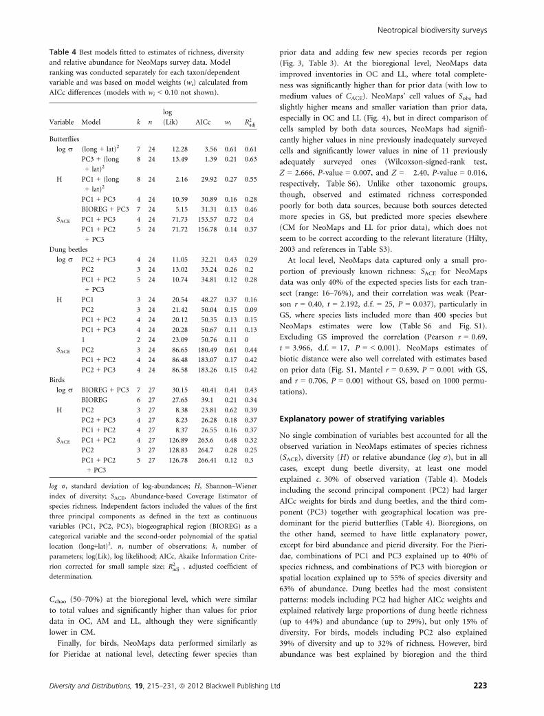
Explanatory power of stratifying variables

No single combination of variables best accounted for all the

observed variation in NeoMaps estimates of species richness

(SACE), diversity (H) or relative abundance (log r), but in all

cases, except dung beetle diversity, at least one model

explained c. 30% of observed variation (Table 4). Models

including the second principal component (PC2) had larger

AICc weights for birds and dung beetles, and the third com-

ponent (PC3) together with geographical location was pre-

dominant for the pierid butterflies (Table 4). Bioregions, on

the other hand, seemed to have little explanatory power,

except for bird abundance and pierid diversity. For the Pieri-

dae, combinations of PC1 and PC3 explained up to 40% of

species richness, and combinations of PC3 with bioregion or

spatial location explained up to 55% of species diversity and

63% of abundance. Dung beetles had the most consistent

patterns: models including PC2 had higher AICc weights and

explained relatively large proportions of dung beetle richness

(up to 44%) and abundance (up to 29%), but only 15% of

diversity. For birds, models including PC2 also explained

39% of diversity and up to 32% of richness. However, bird

abundance was best explained by bioregion and the third

Table 4 Best models fitted to estimates of richness, diversity

and relative abundance for NeoMaps survey data. Model

ranking was conducted separately for each taxon/dependent

variable and was based on model weights (wi) calculated from

AICc differences (models with wi < 0.10 not shown).

Variable Model k n

log

(Lik) AICc wi R2adj

Butterflies

log r (long + lat)2 7 24 12.28 �3.56 0.61 0.61

PC3 + (long

+ lat)28 24 13.49 �1.39 0.21 0.63

H PC1 + (long

+ lat)28 24 �2.16 29.92 0.27 0.55

PC1 + PC3 4 24 �10.39 30.89 0.16 0.28

BIOREG + PC3 7 24 �5.15 31.31 0.13 0.46

SACE PC1 + PC3 4 24 �71.73 153.57 0.72 0.4

PC1 + PC2

+ PC3

5 24 �71.72 156.78 0.14 0.37

Dung beetles

log r PC2 + PC3 4 24 �11.05 32.21 0.43 0.29

PC2 3 24 �13.02 33.24 0.26 0.2

PC1 + PC2

+ PC3

5 24 �10.74 34.81 0.12 0.28

H PC1 3 24 �20.54 48.27 0.37 0.16

PC2 3 24 �21.42 50.04 0.15 0.09

PC1 + PC2 4 24 �20.12 50.35 0.13 0.15

PC1 + PC3 4 24 �20.28 50.67 0.11 0.13

1 2 24 �23.09 50.76 0.11 0

SACE PC2 3 24 �86.65 180.49 0.61 0.44

PC1 + PC2 4 24 �86.48 183.07 0.17 0.42

PC2 + PC3 4 24 �86.58 183.26 0.15 0.42

Birds

log r BIOREG + PC3 7 27 30.15 �40.41 0.41 0.43

BIOREG 6 27 27.65 �39.1 0.21 0.34

H PC2 3 27 �8.38 23.81 0.62 0.39

PC2 + PC3 4 27 �8.23 26.28 0.18 0.37

PC1 + PC2 4 27 �8.37 26.55 0.16 0.37

SACE PC1 + PC2 4 27 �126.89 263.6 0.48 0.32

PC2 3 27 �128.83 264.7 0.28 0.25

PC1 + PC2

+ PC3

5 27 �126.78 266.41 0.12 0.3

log r, standard deviation of log-abundances; H, Shannon–Wiener

index of diversity; SACE, Abundance-based Coverage Estimator of

species richness. Independent factors included the values of the first

three principal components as defined in the text as continuous

variables (PC1, PC2, PC3), biogeographical region (BIOREG) as a

categorical variable and the second-order polynomial of the spatial

location (long+lat)2. n, number of observations; k, number of

parameters; log(Lik), log likelihood; AICc, Akaike Information Crite-

rion corrected for small sample size; R2adj , adjusted coefficient of

determination.



principal component (43%, Table 4). Alternative models fit-

ted with ordinary least squares (unweighted observations)

show similar results, but the percentage of explained varia-

tion was much lower for butterflies and moderately higher

for birds and dung beetles (results not shown).

For species composition, results were more consistent

across taxonomic groups: the explanatory power of environ-

mental variables and bioregions was slightly higher in all

cases, and the role of variables reversed. Bioregions explained

between 30% and 44% of the variance in species composi-

tion for all groups, with an additional 12–15% explained by

PCA scores (Table 5). Residual variance was lower in butter-

flies and birds than it was in dung beetles.

DISCUSSION

Here, we aimed to develop comparable and efficient esti-

mates of species richness, composition and relative abun-

dance at different geographical scales, so that major changes

may eventually be detected in subsequent sampling seasons.

In general, the NeoMaps protocols achieved these aims well:

although results varied across scales and taxonomic groups,

we sampled comparable numbers of species, with lower vari-

ance as prior data and with a lower time and resource

investment per unit area. Our sampling design produced

estimates of diversity and relative abundance that were

impossible to produce with prior data.

The performance of a systematic survey approach such as

NeoMaps must consider the taxonomic group, scale and

expected outputs. For example, if a survey is intended to

improve the knowledge of a taxonomic group at the national

level, the primary goal should be to maximize complemen-

tarity with existing sources, by targeting either poorly known

species groups (such as dung beetles in Venezuela) or poorly

surveyed regions for an otherwise well-known group (like

birds in OC and LL, or butterflies in GS). Alternatively, if

the main goal is to provide a baseline for monitoring, then

the survey should focus on indicator species or diversity pat-

terns that are expected to respond to human-driven change

(Lindenmayer & Likens, 2010). But if the intended output is

to infer or predict diversity patterns from the observed

locations to the entire region or country, then the focus

should be on robust estimation of correlations with environ-

mental variables and performance of a spatially representa-

tive sampling (Teder et al., 2007). Below, we examine the

relative merits of NeoMaps for inventory, monitoring and

modelling.

Contribution of NeoMaps sampling to a more

complete inventory

Inventories aim to obtain an accurate species list for a loca-

tion or a region, including the typically large number of rare

species in an area (Longino & Colwell, 1997). NeoMaps is of

limited use for inventories at large geographical scales (coun-

try or bioregion), because only a fraction of the species

recorded over many years of previous research were detected.

NeoMaps’ ability to fill in local and regional knowledge gaps

was higher, but depended on the level of prior knowledge

for each taxonomic group. For well-known groups such as

birds, NeoMaps made modest contributions to a larger

inventory: in previously well-surveyed cells, NeoMaps

detected only a fraction of the previously recorded birds spe-

cies (Table S6), but samples in new cells improved regional

estimates and completeness in regions that had less prior

study, such as LL and OC (Table 3).

Table 5 PMANOVA analysis of NeoMaps species composition estimate.

Taxon Variable d.f.

Sum of

squares

Mean

squares F R2 P

Pieridae BIOREG 4 1.881 0.470 4.948 0.434 0.001

PC1 1 0.420 0.420 4.424 0.097 0.005

PC2 1 0.181 0.180 1.900 0.042 0.097

PC3 1 0.047 0.048 0.502 0.011 0.741

Residuals 19 1.805 0.095 0.417

Total 26 4.334 1

Scarabaeinae BIOREG 4 2.333 0.583 2.221 0.300 0.002

PC1 1 0.436 0.435 1.658 0.056 0.106

PC2 1 0.164 0.164 0.624 0.021 0.769

PC3 1 0.392 0.392 1.494 0.050 0.146

Residuals 17 4.464 0.262 0.573

Total 24 7.789 1

Birds BIOREG 4 2.867 0.717 3.860 0.384 0.001

PC1 1 0.535 0.535 2.881 0.072 0.001

PC2 1 0.250 0.250 1.347 0.034 0.183

PC3 1 0.283 0.283 1.521 0.038 0.104

Residuals 19 3.529 0.186 0.473

Total 26 7.463 1

F, value of the F-statistic; d.f., degrees of freedom; R2, adjusted coefficient of determination; P, P-value.



By contrast, for more poorly known groups, such as dung

beetles, NeoMaps’ contribution to species inventories was

significant at all geographical scales, helping to solve an

historic taxonomic bottleneck (Kim & Byrne, 2006). NeoM-

aps contributed many new species records for all regions and

increased the regional and national totals beyond estimates

based on prior data (Fig. 4, Table 3), this is true even when

excluding unnamed taxa (Fig. 3). For example, NeoMaps

detected only 40–60% of the known Eurysternus and Onth-

ophagus species (Pulido & Zunino, 2007; Genier, 2009), but

added three (E. impressicolis, O. acuminatus and O. rubres-

cens) previously reported from Colombia or Brazil. In the

genera Ateuchus and Uroxys, there were 23 unnamed mor-

phospecies compared to just seven and two named species in

the literature for Venezuela (Martınez, 1988; Martınez &

Martınez, 1990). Thus, NeoMaps made a significant contri-

bution to the knowledge of this understudied group.

For Pieridae, NeoMaps’ geographical coverage was compa-

rable to the previous coverage of well-surveyed cells, but it

did not improve current knowledge substantially. Although it

is a well-known group at the national scale with a nearly

complete inventory, there are many local gaps in geographi-

cal coverage, and regional lists are far from complete (Fig. 2,

Table 3). In three of five regions, > 68 years of prior data

resulted in twice as many species as NeoMaps (Fig. 4), due

primarily to rare species with a low detection probability

(Lobo, 2008). Among the species absent were eight relatively

widespread (seven or more cell records in prior data) and 19

very restricted species (one or two cells in prior data) (Le

Crom et al., 2004; Bollino & Costa, 2007). Even with or with-

out NeoMaps’ contribution, however, butterfly richness in

Guayana remains underrepresented (Table 3, Fig. 4). A close

examination shows that both common, widespread species (e.

g. Phoebis agarite and Itaballia pandosia) and uncommon ones

(e.g. several species in genera Dismorphia and Enantia) are

missing from both prior data sources and NeoMaps. Indeed,

this region is considered one of the most species-rich but

least-studied areas for Venezuelan butterflies (Viloria, 2000).

Although NeoMaps was not designed for this purpose, an

optimal sampling design for inventories would be much like a

gap analysis: first identifying well-surveyed sites and then

defining a set of complementary locations that best represent

environmental conditions in the non-surveyed portions of the

sampling universe (Hortal & Lobo, 2005b; Williams et al.,

2006). For groups with poor prior data, more cells would need

to be added, or sampling effort increased per cell, or comple-

mentary methods added to increase detectability.

Reliability of baseline for future monitoring

Monitoring species richness and diversity through time does

not require an exhaustive account of all species, but rather an

informative metric that is representative of the variable of

interest and sensitive enough to detect changes in time

(Beever, 2006); by these criteria, NeoMaps data clearly outper-

form prior data (Rivadeneira et al., 2009; Jaric & Ebenhard,

2010). When local samples are repeatable and low in variance,

and species detectability is high or at least constant, they can

be reliably used to estimate local richness and other measures

of species diversity and composition and to make compari-

sons in time and space (Yoccoz et al. 2001). Incomplete local

surveys may still be useful for monitoring, provided that they

achieve an acceptable level of completeness and remain repre-

sentative of the assemblage (Colwell & Coddington, 1994;

Beccaloni & Gaston, 1995). For example, NeoMaps dung

beetle samples captured high number of species with high

completeness (Table 3), while bird local estimates were

correlated with species richness in cells with low to moderate

richness (< 400 sp.), and measures of biotic distance based on

NeoMaps data were correlated with expected dissimilarity

(Table S6, Fig. S1; Rodrıguez et al., 2012).

The most straightforward approach to using NeoMaps

data for monitoring would be to focus on the subset of taxa

that it reliably detected, including common and widespread

species, and use them as biodiversity or ecological indicators

(Larsen et al., 2009). For example, common butterfly species

have experienced large changes in distribution and abun-

dance in parts of Europe, both declining or increasing, and

these changes have been related to habitat/landscape changes

(Van Dyck et al., 2009). Trends in populations of species

with high or moderately high abundance are easier to detect

than trends in rare species, or species with high fluctuations

in abundance (Meyer et al., 2010). Furthermore, the abun-

dance of moderately common species can be used either as

an direct indicator of changes in habitat or a predictor of

the likelihood of presence/absence of other species with cor-

related habitat-use patterns but much lower detectability

(Mac Nally et al., 2003). The richness and composition esti-

mates used here (SACE, SChao, DChao) estimated a proportion

of undetected species for each site, but did not consider sys-

tematic factors that could affect detectability within (e.g. dif-

ferences between species) or between sites (e.g. landscape or

habitat structures). Estimates of detection probability could

be built into the monitoring design through replicated sam-

ples across sites (Kery & Schmid, 2004; Dorazio et al., 2006)

or through a double sampling approach, which makes use of

intensive sampling in selected calibration sites (Rodrıguez

et al., 2012).

NeoMaps sampling could of course be improved using a

general conceptual framework for future monitoring. Includ-

ing a measure of threats (e.g. climate change, deforestation,

desertification) or management interventions (e.g. conserva-

tion areas, reforestation programmes) in the sampling design

would increase the capability of NeoMaps to evaluate their

effects on any detected change, rather than just document

general trends (Lindenmayer & Likens, 2010). For example,

the degree and timing of land use changes and fragmentation

could be used as a measure of habitat modification and loss,

which are considered major drivers of species extinction risk

for terrestrial arthropods and birds (Thomas & Abery, 1995;

Koh et al., 2004; Thomas et al., 2004; BirdLife International,

2008). In the case of dung beetles, abundance appears to



decline with increasing habitat modification, and open

habitat communities contain a hyperabundance of few small-

bodied species (Nichols et al., 2007). This expected relation-

ship between habitat fragmentation and the number of

individuals of small-bodied species could be easily explored

with NeoMaps data in a long-term monitoring programme.

Representative sampling for community-level

prediction

NeoMaps captured much of the range of variation in a set of

derived environmental and biogeographical variables, which

successfully explained a considerable proportion of the varia-

tion in species richness and relative abundance (Table 4) and

a greater proportion in composition (Table 5). Such vari-

ables were clearly influenced by attributes such as habitat

heterogeneity, precipitation and temperature (Table 1),

which have been highlighted as important determinants of

spatial richness patterns for birds, butterflies and dung bee-

tles (Beccaloni & Gaston, 1995; Rahbek & Graves, 2001; van

Rensburg et al., 2002; Hayes et al., 2009). NeoMaps’ design

aimed to balance the contribution of these ecological and

historical components to produce data suitable for several

techniques of species-level and community-level prediction

of diversity patterns (Ferrier & Guisan, 2006), which are use-

ful for extrapolation at national and bioregion scales, facili-

tating planning, monitoring and action (Colwell & Coddington,

1994; Gotelli & Colwell, 2001). In these applications, prior

data had major limitations due to incomplete geographical

and environmental coverage and unbalanced taxonomic

representation (Loiselle et al., 2008). NeoMaps data from

dung beetles at all scales and from birds at the local scale

were as representative as prior data – but not so for

butterflies. For species-level prediction, taxonomical bias

might still be an important limitation because several species

are underrepresented in our samples.

Again, our results point to ways for improving sampling

design to increase the number of sampled species and improve

their spatial representation. Bioregional and environmental

variables explained a great proportion of compositional pat-

terns, but sample selection might need to be optimized for

each group separately in future surveys, spreading samples

along the gradients with the strongest associations with varia-

tion in the group (Hortal & Lobo, 2005a).

As expected, forest cover (PC2) was the variable that best

correlated with NeoMaps estimates of bird species richness

and diversity per cell, even though completeness was lower in

increasingly forested areas. The distribution of bird abundances

(log r) was related to bioregion and the humidity gradient

(PC3). Indeed, higher species diversity and evenness is to be

expected in forested areas, where detectability is probably lower

(or more heterogeneous) due to the complexity of the habitat,

while higher concentrations of individuals were expected in the

seasonally flooded Llanos (Stotz et al., 1996).

For dung beetles, forest cover was also the most important

variable explaining richness and abundance, but elevation-

seasonality was more correlated with diversity. These results

are in agreement with studies in other Neotropical regions

(Escobar et al., 2006; Nichols et al., 2007), and suggest that

NeoMaps should increase sampling effort at low elevations

and in forested regions in future surveys. Finally, for butter-

flies, the spatial component and the humidity gradient (PC3)

were better related to the patterns observed, but other evi-

dence (like the absence of a great proportion of mountain

species) suggests that we are underestimating the importance

of the elevational (PC1) and the forest cover gradient (PC2)

to species richness (Beccaloni & Gaston, 1995; Le Crom

et al., 2004).

Cost-effectiveness

The efficacy of any biodiversity monitoring effort must be

evaluated not only in terms of the quantity or thoroughness

of the data collected, but also by the investments made to

obtain those data (Margules & Austin, 1991; Gardner et al.,

2008b; Bried, 2009). The total monetary cost of NeoMaps in

the present study (including field and laboratory equipment,

survey costs and salaries for experts in taxonomic identifica-

tion) was a substantial investment (US$ 362,820), but con-

sidering the area sampled, the investment was more efficient

than other initiatives (about US$ 1–8 per km2 sampled vs.

US$ c. 70–90 per km2 for other multitaxa Neotropical biodi-

versity assessments; Gardner et al., 2008b). For conservation

planning, monitoring and management, the area covered is

more relevant than the number of specimens sampled; the

most important conservation actions take place increasingly

within particular units of space (i.e. in protected areas)

rather than on a species-by-species basis (Beever, 2006; Legg

& Nagy, 2006). This is particularly the case when the taxa

being monitored are used as indicators, rather than as being

of particular conservation interest in their own right (Larsen

et al., 2009). Thus, the NeoMaps sampling design was clearly

preferable in cost-effectiveness, and its applicability in other

Neotropical countries with similar infrastructure should be

straightforward (also see Supporting Information).

None of these figures include transportation costs to or

between sampling localities, although this is likely to repre-

sent a relatively smaller investment (compared to the total) if

sampling relies on a good road network where costs would

rise proportionally to the number of sampled localities, the

distance between them and the mean transportation cost per

km, which is tightly linked to mean gas prices. Each of

NeoMaps’ surveys in Venezuela required around 18,000 km

of road travel between and within sampling units, which

would cost around 2000–3000 US$ in most South American

countries, assuming gas prices between 1.1 and 1.6 US$ per l,

and a consumption of 10 km l�1.

Sampling localities outside the road network might be very

important for inventory purposes, but would increase total

survey costs, limiting the number of localities that can be

sampled. For Venezuela, we estimated that sampling one

locality outside the road network could require a 10-fold



increase in costs, compared to a locality within the road net-

work. The difference is due mostly to higher transportation

costs, increased travelling time between localities and the lar-

ger personnel or time investment needed to achieve an

equivalent sampling effort.

Such an investment might be reasonable if the selected

localities contribute significantly to an improvement in the

overall data or information gathered by the survey. This is

arguably the case when the primary goal of the survey is

inventorying, and the chosen methods have high detectability

or completeness, or when the additional localities represent

very different environmental conditions that are complemen-

tary to those already sampled. However, we consider that the

actual extent and density of available roads in South America

would be sufficient to sample the principal ecosystems or

ecoregions in most countries, except Bolivia and the Guay-

anas (Hijmans et al., 2012).

CONCLUSIONS

The challenge of monitoring tropical biodiversity requires a

long-term, sustained effort and the continuous evaluation of

methods, procedures and goals (Lindenmayer & Likens,

2010). Ultimately, a comprehensive biodiversity survey strat-

egy for a tropical country like Venezuela should draw infor-

mation from all available complementary sources, including

large-scale national surveys, museum or literature records

and regional and local research initiatives. Systematic

national biodiversity surveys such as NeoMaps have a partic-

ularly important role to play, by providing estimates of rela-

tive abundance, and thus diversity and composition,

required for rigorous monitoring and spatial prediction of

community-level attributes. It is clear, however, that NeoM-

aps’ simple sampling design will need to be refined in future,

as data emerging from the surveys are examined in the light

of taxon-specific patterns and comprehensive sets of environ-

mental variables. Such analyses will allow the exploration of

modifications in either the spatial sampling design or the

field survey protocols (or both) to improve the likelihood of

detecting biodiversity changes, and thus support monitoring,

or provide data adequate for predicting spatial patterns at

the community level.

In future, it will also be important to evaluate additional

advantages of NeoMaps-type sampling efforts not considered

in depth here, including the ability to estimate relative abun-

dances and species absences, and thus overall diversity pat-

terns – all of which are difficult or impossible to estimate

with traditional museum data and the taxonomic literature

(Beck & Kitching, 2007).

ACKNOWLEDGEMENTS

We are grateful for support from the Biodiversity Analysis

Unit of the Andean Centre for Biodiversity Conservation

at Conservation International, the Conservation Technology

Support Program, the Disney Wildlife Conservation Fund,

EcoHealth Alliance, the Venezuelan Fondo Nacional de

Ciencia, Tecnologıa e Innovacion, the Instituto Venezolano

de Investigaciones Cientıficas, the Latin America and

Caribbean Program of the National Audubon Society, Pro-

vita and UNESCO. Major funding was provided by Total

Venezuela, S. A., as part of the Program for the Support

of the Conservation of the Biodiversity of Venezuela,

under the framework of the Ley Organica de Ciencia,

Tecnologıa e Innovacion (LOCTI). We are particularly

indebted to L. A. Solorzano, A. Grajal and C. J. Sharpe

for their involvement at earlier stages of NeoMaps. This

project would have been impossible without the help of

hundreds of national and international student and profes-

sional volunteers. Museum data were facilitated by R. A.

Briceno (MEJMO), J. Clavijo, L. J. Joly and Q. Arias

(MIZA), and J. Camacho (MALUZ). Comments from Lluis

Brotons and three anonymous referees helped improve the

manuscript.

REFERENCES

Aguilera, M., Azocar, A. & Gonzalez-Jimenez, E. (2003) Bio-

diversidad en Venezuela. Tomo I y II. Fundacion Polar.

Ministerios de Ciencia y Tecnologıa. Fondo Nacional de

Ciencia, Tecnologıa e Innovacion, Caracas, Venezuela.

Ahumada, J.A., Silva, C.E.F., Gajapersad, K., Hallam, C., Hur-

tado, J., Martin, E., McWilliam, A., Mugerwa, B., O’Brien,

T., Rovero, F., Sheil, D., Spironello, W.R., Winarni, N. &

Andelman, S.J. (2011) Community structure and diversity

of tropical forest mammals: data from a global camera trap

network. Philosophical Transactions of the Royal Society B:

Biological Sciences, 366, 2703–2711.

Anderson, M.J. (2001) A new method for non-parametric

multivariate analysis of variance. Austral Ecology, 26,

32–46.

Austin, M.P. & Heyligers, P.C. (1991) New approach to vege-

tation survey design: gradsect sampling. Nature conservation:

cost effective biological surveys and data analysis. CSIRO –

Commonwealth Scientific and Industrial Research Organi-

zation, Canberra, Australia.

Avian Knowledge Network (2009) Avian knowledge network:

an online database of bird distribution and abundance.

Available at: http://www.avianknowledge.net (accessed 3

October 2010).

Barret, C.B., Brandon, K., Gibson, C. & Gjertsen, H. (2001)

Conserving tropical biodiversity amid weak institutions.

BioScience, 51, 497–502.

Beccaloni, G.W. & Gaston, K.J. (1995) Predicting species

richness of Neotropical forest butterflies: ithomiinae (Lepi-

doptera: Nymphalidae) as indicators. Biological Conserva-

tion, 71, 77–86.

Beck, J. & Kitching, J. (2007) Estimating regional species

richness of tropical insects from museum data: a compari-

son of a geography-based and sample-based methods. Jour-

nal of Applied Ecology, 44, 672–681.



Beever, E.A. (2006) Monitoring biological diversity: strate-

gies, tools, limitations, and challenges. Northwestern Natu-

ralist, 87, 66–79.

BirdLife International (2008) State of the world’s birds: indi-

cators for our changing world. BirdLife International, Cam-

bridge, UK.

Bliss, N.B. & Olsen, L.M. (1996) Development of a 30-arc-

second digital elevation model of South America. Pecora

Thirteen, Human Interactions with the Environment – Per-

spectives from Space, Sioux Falls, SD.

Bollino, M. & Costa, M. (2007) An illustrated annotated

check-list of the species of Catasticta (s.l.) Butler (Lepidop-

tera: Pieridae) of Venezuela. Zootaxa, 1469, 1–42.

Bried, J.T. (2009) Information costs of reduced-effort habitat

monitoring in a butterfly recovery program. Journal of

Insect Conservation, 13, 615–626.

Brown, J.H. & Mehlman, D.W. (1995) Spatial variation in

abundance. Ecology, 76, 2028–2043.

Bunce, R.G.H., Barr, C.J., Clarke, R.T., Howard, D.C. & Lane,

A.M.J. (1996) Land classification for strategic ecological

survey. Journal of Environmental Management, 47, 37–60.

Burnham, K.P., Anderson, D.R. & Huyvaert, K.P. (2011)

AIC model selection and multimodel inference in behav-

ioral ecology: some background, observations, and compar-

isons. Behavioral Ecology and Sociobiology, 65, 23–35.

Carroll, R.J. & Ruppert, D. (1988) Transformation and

weighting in regression. Chapman & Hall, New York.

Castro, G. & Locker, I. (2000) Mapping conservation invest-

ments: an assessment of biodiversity funding in Latin Amer-

ica and the Caribbean. Biodiversity Support Program,

Washington, DC.

Chao, A., Chazdon, R.L., Colwell, R.K. & Shen, T.J. (2005) A

new statistical approach for assessing similarity of species

composition with incidence and abundance data. Ecology

Letters, 8, 148–159.

Chernoff, B., Machado-Allison, A., Riseng, K. & Montamba-

ult, J. (2003) Una evaluacion rapida de los ecosistemas

acuaticos de la cuenca del Rıo Caura, Estado Bolıvar, Vene-

zuela, no. 28. Conservation International, Washington, DC.

Colwell, R.K. & Coddington, J.A. (1994) Estimating terres-

trial biodiversity through extrapolation. Philosophical

Transactions of the Royal Society B: Biological Sciences, 345,

101–118.

Colwell, R.K., Mao, C.X. & Chang, J. (2004) Interpolating,

extrapolating, and comparing incidence-based species accu-

mulation curves. Ecology, 85, 2717–2727.

Currie, D.J. (1991) Energy and large-scale patterns of ani-

mal-species and plant-species richness. American Naturalist,

137, 27–49.

DeFries, R., Hansen, M., Townshend, J.R.G., Janetos, A.C. &

Loveland, T.R. (2000) A new global 1 km data set of per-

cent tree cover derived from remote sensing. Global Change

Biology, 6, 247–254.

Dixon, P.M. (2003) VEGAN, a package of R functions for

community ecology. Journal of Vegetation Science, 14,

927–930.

Dobson, A. (2005) Monitoring global rates of biodiversity

change: challenges that arise in meeting the Convention on

Biological Diversity (CBD) 2010 goals. Philosophical Trans-

actions of the Royal Society B: Biological Sciences, 360,

229–241.

Dorazio, R.M., Royle, J.A., Soderstrom, B. & Glimskar, A.

(2006) Estimating species richness and accumulation by

modeling species occurrence and detectability. Ecology, 87,

842–854.

Duro, D.C., Coops, N.C., Wulder, M.A. & Han, T. (2007)

Development of a large area biodiversity monitoring sys-

tem driven by remote sensing. Progress in Physical Geogra-

phy, 31, 235–260.

Eaton, M.A., Balmer, D.E., Conway, G.J., Grise, S., Hall, P.

V., Hearn, R., Musgrove, D., Risely, A.J. & Wootton, S.

(2009) The state of the UK’s birds 2008. T, Sandy, Bedford-

shire, RSPB, BTO, WWT, CCW, NIEA, JNCC, NE and

SNH, Bedfordshire, UK.

Escobar, F., Lobo, J.M. & Halffter, G. (2006) Assessing the

origin of Neotropical mountain dung beetle assemblages

(Scarabaeidae: Scarabaeinae): the comparative influence of

vertical and horizontal colonization. Journal of Biogeogra-

phy, 33, 1793–1803.

EuMon (2009) EU-wide monitoring methods and systems of

surveillance for species and habitats of Community interest,

Developed and maintained by EuMon, EBONE, and SCALES

for the European biodiversity monitoring community. Avail-

able at: http://eumon.ckff.si/index1.php (accessed 27 April

2010).

Faith, D.P. & Walker, P.A. (1996) Environmental diversity:

on the best-possible use of surrogate data for assessing the

relative biodiversity of sets of areas. Biodiversity and

Conservation, 5, 399–415.

Ferrer-Paris, J.R., Sanchez-Mercado, A. & Rodrıguez, J.P.

(2013) Optimizacion del muestreo de invertebrados tropi-

cales: un ejemplo con escarabajos coprofagos (Coleoptera:

Scarabaeinae) en Venezuela. Revista de Biologıa Tropical,

61, in press.

Ferrier, S. & Guisan, A. (2006) Spatial modelling of biodiver-

sity at the community level. Journal of Applied Ecology, 43,

393–404.

Fisher, B.L. (1999) Improving inventory efficiency: a case

study of leaf-litter ant diversity in Madagascar. Ecological

Applications, 9, 714–731.

Gardner, T.A., Hernandez, M.I.M., Barlow, J. & A., P.C.

(2008a) Understanding the biodiversity consequences of

habitat change: the value of secondary and plantation for-

ests for neotropical dung beetles. Journal of Applied Ecology,

45, 883–893.

Gardner, T.A., Barlow, J., Araujo, I.S. et al. (2008b) The

cost-effectiveness of biodiversity surveys in tropical forests.

Ecology Letters, 11, 139–150.

Gaston, K.J. (2000) Global patterns in biodiversity. Nature,

405, 220–227.

Gaston, K.J. & May, R.M. (1992) Taxonomy of taxonomists.

Nature, 356, 281–282.



Genier, F. (2009) Le genre Eurysternus Dalman, 1824 (Scara-

baeidae: Scarabaeinae: Oniticellini), revision taxonomique et

cles de determination illustrees. Pensoft Publishers, Sofia,

Bulgary.

Gibbons, D.W., Chapman, R. & Reid, J. (1993) The new atlas

of breeding birds in Britain and Ireland: 1988–91. T. & A.D.

Poyser, London, UK.

Gotelli, N.J. & Colwell, R.K. (2001) Quantifying biodiversity:

procedures and pitfalls in the measurement and compari-

son of species richness. Ecology Letters, 4, 379–391.

Guegan, J.F., Lek, S. & Oberdorff, T. (1998) Energy availabil-

ity and habitat heterogeneity predict global riverine fish

diversity. Nature, 391, 382–384.

Hayes, L., Mann, D.J., Monastyrskii, A.L. & Lewis, O.T.

(2009) Rapid assessments of tropical dung beetle and

butterfly assemblages: contrasting trends along a forest dis-

turbance gradient. Insect Conservation and Diversity, 2, 194

–203.

Hijmans, R.J., Cameron, S.E., Parra, J.L., Jones, P.G. & Jarvis,

A. (2005) Very high resolution interpolated climate sur-

faces for global land areas. International Journal of Clima-

tology, 25, 1965–1978.

Hijmans, R.J., Guarino, L. & Mathur, P. (2012) DIVA-GIS

version 7.5 manual. Available at: http://www.diva-gis.org/

gdata/ (accessed 2 February 2012).

Hilty, S.L. (2003) Birds of Venezuela, 2nd edn. Princeton

University Press, Princeton, NJ.

Hortal, J. & Lobo, J.M. (2005a) An ED-based protocol for

the optimal sampling of biodiversity. Biodiversity and Con-

servation, 14, 2913–2947.

Hortal, J. & Lobo, J.M. (2005b) A synecological framework

for systematic conservation planning. Biodiversity Informat-

ics, 9, 16–45.

Hortal, J. & Lobo, J.M. (2006) Towards a synecological

framework for systematic conservation planning. Biodiver-

sity Informatics, 3, 16–45.

Jaric, I. & Ebenhard, T. (2010) A method for inferring

extinction based on sighting records that change in fre-

quency over time. Wildlife Biology, 16, 267–275.

Jongman, R.H.G., Ter Braak, C.J.F. & van Tongeren, O.F.R.

(1995) Data analysis in community and landscape ecology.

Cambridge University Press, Cambridge, UK.

Jurgens, N., Schmiedel, U., Haarmeyer, D.H. et al. (2012)

The BIOTA Biodiversity Observatories in Africa—a

standardized framework for large-scale environmental

monitoring. Environmental Monitoring and Assessment, 184,

655–678.

Kery, M. & Schmid, H. (2004) Monitoring programs need to

take into account imperfect species detectability. Basic and

Applied Ecology, 5, 65–73.

Kim, K.C. & Byrne, L.B. (2006) Biodiversity loss and the tax-

onomic bottleneck: emerging biodiversity science. Ecology

Research, 21, 794–810.

Koh, L.P., Sodhi, N.S. & Brook, B.W. (2004) Co-extinctions

of tropical butterflies and their hostplants. Biotropica, 36,

272–274.

Kremen, C. (1994) Biological inventory using target taxa: a

case study of the butterflies of Madagascar. Ecological

Applications, 4, 407–422.

Larsen, F.W., Bladt, J. & Rahbek, C. (2009) Indicator taxa

revisited: useful for conservation planning? Diversity and

Distributions, 15, 70–79.

Le Crom, J.F., Llorente Bousquets, J., Constantino, L.M. &

Salazar, J.A. (2004) Mariposas de Colombia. Tomo II: pieri-

dae. Carlec Ltda, Bogota, Colombia.

Legendre, P. & Legendre, L. (2003) Numerical ecology. Else-

vier Science B.V., Amsterdam, the Netherlands.

Legg, C.J. & Nagy, L. (2006) Why most conservation moni-

toring is, but need not be, a waste of time. Journal of

Environmental Management, 78, 194–199.

Liebhold, A.M. & Sharov, A.A. (1998) Testing for correlation

in the presence of spatial autocorrelation in insect count

data. Population and community ecology for insect manage-

ment and conservation (ed. by J. Baumgartner, P. Brandm-

ayr and B.F.J. Manly), pp. 11–117. Balkema, Rotterdam,

the Netherlands.

Linares, O.J. (1988) Mamıferos de Venezuela. Sociedad Con-

servacionista Audubon de Venezuela, Caracas, Venezuela.

Lindenmayer, D.B. & Likens, G.E. (2010) The science and

application of ecological monitoring. Biological Conserva-

tion, 140, 1317–1328.

Lobo, J.M. (2008) Database records as a surrogate for sam-

pling effort provide higher species richness estimations.

Biodiversity and Conservation, 17, 873–881.

Loiselle, B.A., Jorgensen, P.M., Consiglio, T., Jimenez, I.,

Blake, J.G., Lohmann, L.G. & Montiel, O.M. (2008) Pre-

dicting species distributions from herbarium collections:

does climate bias in collection sampling influence model

outcomes? Journal of Biogeography, 35, 105–116.

Longino, J.T. & Colwell, R.K. (1997) Biodiversity assess-

ment using structured inventory: capturing the ant fauna

of a tropical rain forest. Ecological Applications, 7, 1263–

1277.

Luoto, M., Virkkala, R., Heikkinen, R.K. & Rainioc, K.

(2004) Predicting bird species richness using remote sens-

ing in boreal agricultural-forest mosaics. Ecological Applica-

tions, 14, 1946–1962.

Mac Nally, R., Fleishman, E., Fay, J.P. & Murphy, D.D.

(2003) Modelling butterfly species richness using mesoscale

environmental variables: model construction and validation

for mountain ranges in the Great Basin of western North

America. Biological Conservation, 110, 21–31.

Margules, C.R. (1989) Introduction to some Australian

developments in conservation evaluation. Biological Conser-

vation, 50, 1–11.

Margules, C.R. & Austin, M.P. (1991) Nature conservation:

cost effective biological surveys and data analysis. CSIRO –

Commonwealth Scientific and Industrial Research Organi-

zation, Canberra, Australia.

Margules, C.R. & Redhead, T.D. (1995) Guidelines for using

the BioRap methodology and tools. CSIRO and World Bank

BioRap Project, Dickson, Australia.



MARN (2000) Primer informe de paıs para la Convencion

sobre Diversidad Biologica. Ministerio del Ambiente y los

Recursos Naturales, Caracas, Venezuela.

Martınez, A. (1988) Algunos Scarabaeinae neotropicales nue-

vos o poco conocidos. Revista Cientıfica UNET, 2, 85–90.

Martınez, A. & Martınez, A. (1990) Dos nuevas especies de

Ateuchus Weber (Coleoptera: Scarabaeinae: Ateuchina).

Boletın de Entomologıa Venezolana, 5, 159–163.

McArdle, B.H. & Anderson, M.J. (2001) Fitting multivariate

models to community data: a comment on distance-based

redundancy analysis. Ecology, 82, 290–297.

Metzger, M.J., Bunce, R.G.H., Jongman, R.H.G., Mucher, C.

A. & Watkins, J.W. (2005) A climatic stratification of the

environment of Europe. Global Ecology and Biogeography,

14, 549–563.

Meyer, C.F.J., Aguiar, L.M.S., Aguirre, L.F. et al. (2010)

Long-term monitoring of tropical bats for anthropogenic

impact assessment: gauging the statistical power to detect

population change. Biological Conservation, 143, 2797–

2807.

Myers, N., Mittermeier, R.A., Mittermeier, C.G., da Fonseca,

G.A.B. & Kent, J. (2000) Biodiversity hotspots for conser-

vation priorities. Nature, 403, 853–858.

Nakamura, M. & Soberon, J. (2008) Use of approximate

inference in an index of completeness of biological inven-

tories. Conservation Biology, 23, 469–474.

Newmark, W.D. (1985) Legal and biotic boundaries of Wes-

tern North American national parks: a problem of congru-

ence. Biological Conservation, 33, 197–208.

Nichols, E., Larsen, T. & Spector, S. (2007) Global dung bee-

tle response to tropical forest modification and fragmenta-

tion: a quantitative literature review and meta-analysis.

Biological Conservation, 137, 1–19.

Nielsen, S., Haughland, D., Bayne, E. & Schieck, J. (2009)

Capacity of large-scale, long-term biodiversity monitoring

programmes to detect trends in species prevalence. Biodi-

versity and Conservation, 18, 2961–2978.

Patterson, B.D. (2001) Fathoming tropical biodiversity: the

continuing discovery of Neotropical mammals. Diversity

and Distributions, 7, 191–196.

Pereira, H.M. & Cooper, H.D. (2006) Towards the global

monitoring of biodiversity change. Trends in Ecology and

Evolution, 21, 123–129.

Pimm, S.L. & Brown, J.H. (2004) Domains of diversity. Sci-

ence, 304, 831–833.

Ponder, W.F., Carter, G.A., Flemons, P. & Chapman, R.R.

(2001) Evaluation of museum collection data for use in

biodiversity assessment. Conservation Biology, 15, 648–

657.

Prance, G.T. (1994) A comparison of the efficacy of higher

taxa and species numbers in the assessment of biodiversity

in the neotropics. Philosophical Transactions of the Royal

Society B: Biological Sciences, 345, 89–99.

Pulido, L.A. & Zunino, M. (2007) Catalogo preliminar de los

Onthophagini de America (Coleoptera: Scarabaeine Scara-

baeinae). M3M Monografıas, 7, 93–129.

R Core Development Team (2005) The R project for statistical

computing. Version v 2.3.1. R Core Development Team,

Vienna, Austria.

Rahbek, C. & Graves, G.R. (2001) Multiscale assessment of

patterns of avian species richness. Proceedings of the

National Academy of Sciences of the United States of Amer-

ica, 98, 4534–4539.

van Rensburg, B.J., Chown, S.L. & Gaston, K.J. (2002) Spe-

cies richness, environmental correlates, and spatial scale: a

test using South African birds. The American Naturalist,

159, 566–577.

Ricklefs, R.E. (2004) A comprehensive framework for global

patterns in biodiversity. Ecology Letters, 7, 1–15.

Ridgely, R.S., Allnutt, T.F., Brooks, T., McNicol, D.K., Mehl-

man, D.W., Young, B.E. & Zook, J.R. (2003) Digital distri-

bution maps of the birds of the Western Hemisphere version

1.0. NatureServe, Arlington, VA.

Rivadeneira, M.M., Hunt, G. & Roy, K. (2009) The use of

sighting records to infer species extinctions: an evaluation

of different methods. Ecology, 90, 1291–1300.

Rodrıguez, J.P. (2003) Challenges and opportunities for sur-

veying and monitoring tropical biodiversity – a response to

Danielsen et al. Oryx, 37, 411–411.

Rodrıguez, J.P. & Sharpe, C.J. (2002) NeoMaps: the Neo-

tropical biodiversity mapping initiative. Cotinga, 17, 13–14.

Rodrıguez, J.P., Simonetti, J.A., Premoli, A. & Marini, M.A.

(2005) Conservation in Austral and Neotropical America:

building scientific capacity equal to the challenges. Conser-

vation Biology, 19, 969–972.

Rodrıguez, J.P., Rodrıguez-Clark, K.M., Oliveira-Miranda, M.

A., Good, T. & Grajal, A. (2006) Professional capacity

building: the missing agenda in conservation priority

setting. Conservation Biology, 20, 1340–1340.

Rodrıguez, G.A., Rodrıguez, J.P., Ferrer-Paris, J.R. & San-

chez-Mercado, A. (2012) A nation-wide standardized bird

survey scheme for Venezuela. The Wilson Journal of Orni-

thology, 124, 230–244.

Roy, D.B., Rothery, P. & Brereton, T. (2007) Reduced-effort

schemes for monitoring butterfly populations. Journal of

Applied Ecology, 44, 993–1000.

Ruxton, G.D. & Colegrave, N. (2006) Experimental design for

the life-sciences. Oxford University Press, New York, NY.

Sastre, P. & Lobo, J.M. (2009) Taxonomist survey biases and

the unveiling of biodiversity patterns. Biological Conserva-

tion, 142, 462–467.

Sauer, J.R. & Droege, S. (eds) (1990) Survey designs and sta-

tistical methods for the estimation of avian population trends.

U.S. Fish and Wildlife Service, Washington, DC.

Sauer, J.R., Hines, J.E. & Fallon, J. (2008) The North Ameri-

can Breeding Bird Survey, results and analysis 1966–2007.

version 5.15.2008. USGS Patuxent Wildlife Research Center,

Laurel, MD.

ScarabNet (2011) Scarabaeinae research network. Available at:

http://216.73.243.70/scarabnet/ (accessed 2 May 2011).

Schmeller, D.S., Henry, P.Y., Julliard, R., Clobert, J., Gruber,

B., Dziock, F., Lengyel, S., Nowicki, P., Deri, E., Budrys, E.,



Kull, T., Tali, K. & Bauch, B. (2009) Advantages of volun-

teer-based biodiversity monitoring in Europe. Conservation

Biology, 23, 307–316.

Sirami, C., Brotons, L. & Martin, J.L. (2009) Do bird spatial

distribution patterns reflect population trends in changing

landscapes? Landscape Ecology, 24, 893–906.

Stotz, D.F., Fitzpatrick, J.W., Parker, T.A., III & Moskovits,

D.K. (1996) Neotropical birds. Ecology and conservation.

University of Chicago Press, Chicago, IL.

Sutherland, W.J., Adams, W.M., Aronson, R.B. et al. (2009)

One hundred questions of importance to the conservation

of global biological diversity. Conservation Biology, 23, 557–

567.

Szeplaki, E., Garcıa, L., Rodrıguez, J. & Gonzalez, E. (2001)

Estrategia nacional sobre diversidad biologica y su plan de

accion. Ministerio del Ambiente. Oficina Nacional de Div-

ersidad Biologica, Caracas, Venezuela.

TABDP (2009) Tropical Andean Butterfly Diversity Program.

Available at: http://www.andeanbutterflies.org/index.html

(accessed 1 April 2009).

Teder, T., Moora, M., Roosaluste, E., Zobel, K., Partel, M.,

Koljalg, U. & Zobel, M. (2007) Monitoring of biological

diversity: a common-ground approach. Conservation Biol-

ogy, 21, 313–317.

Thomas, C.D. & Abery, J.C.G. (1995) Estimating rates of

butterfly decline from distribution maps – The effect of

scale. Biological Conservation, 73, 59–65.

Thomas, J.A., Telfer, M.G., Roy, D.B., Preston, C.D., Green-

wood, J.J.D., Asher, J., Fox, R., Clarke, R.T. & Lawton, J.H.

(2004) Comparative losses of British butterflies, birds, and

plants and the global extinction crisis. Science, 303, 1879–

1881.

UNEP (2007) Global environment outlook: environment for

development (GEO4). United Nations Environment Pro-

gramme (UNEP) and Progress Press Ltd, Valletta, Malta.

UNPD (2003) UNDP Annual Report 2003. United Nations

Development Programme, New York, NY.

Van Dyck, H., Van Strien, A.J., Maes, D. & Van Swaay, C.A.

M. (2009) Declines in common, widespread butterflies in a

landscape under intense human use. Conservation Biology,

23, 957–965.

Viloria, A.L. (2000) Estado actual del conocimiento taxono-

mico de las mariposas (Lepidoptera: Rhopalocera) de Ven-

ezuela. Hacia un proyecto CYTED para el inventario y

estimacion de la diversidad entomologica en Iberoamerica,

PRIBES-2000, pp. 261–274. Monografıas Tercer Milenio,

Zaragoza, Espana.

Wessels, K.J., Jaarsveld, A.S.V., Grimbeek, J.D. & Linde, M.J.

V.D. (1998) An evaluation of the gradsect biological survey

method. Biodiversity and Conservation, 7, 1093–1121.

Williams, P., Faithb, D., Mannec, L., Sechrestd, W. & Pre-

stone, C. (2006) Complementarity analysis: mapping the

performance of surrogates for biodiversity. Biological

Conservation, 128, 253–264.

Yesson, C., Brewer, P.W., Sutton, T., Caithness, N., Pahwa, J.

S., Burgess, M., Gray, W.A., White, R.J., Jones, A.C., Bisby,

F.A. & Culham, A. (2007) How global is the global biodi-

versity information facility? PLoS ONE, 2, e1124.

Yoccoz, N.G., Nichols, J.D. & Boulinier, T. (2001) Moni-

toring of biological diversity in space and time. Trends

in Ecology and Evolution, 16, 446–453.

SUPPORTING INFORMATION

Additional Supporting Information may be found in the

online version of this article:

Data S1 Methods

Figure S1 Estimated versus expected species richness per

transect (top) and biotic distance between transects (bottom)

for Birds

Table S1 List of published sources for Pieridae distribution

data in Venezuela

Table S2 List of published sources for Scarabaeinae distribu-

tion data in Venezuela

Table S3 List of published sources for bird’s distribution

data in Venezuela

Table S4 Richness, diversity and completeness estimates for

the Pieridae data set in NeoMaps and previous data sources

Table S5 Richness and completeness estimates for dung bee-

tles’ data set in NeoMaps and previous data sources

Table S6 Richness and completeness estimates for bird’s data

set in NeoMaps and previous data sources

As a service to our authors and readers, this journal provides

supporting information supplied by the authors. Such mate-

rials are peer-reviewed and may be re-organized for online

delivery, but are not copy-edited or typeset. Technical sup-

port issues arising from supporting information (other than

missing files) should be addressed to the authors.

BIOSKETCH

NeoMaps is collaborative research effort based at the Vene-

zuelan Institute for Scientific Investigation (www.neomaps.

org). Our aim is to create an efficient and cost-effective

method for quantifying the distribution and abundance of

tropical biodiversity at large geographical scales. Although

our initial focus is on Venezuela, we are exploring imple-

mentation of our spatial sampling design and field survey

protocols in other Neotropical regions.

Author contributions: J.R.F.P., J.P.R., T.G. and A.S.M.

conceived the study; J.R.F.P., T.G. and G.A.R. led the field

teams; J.R.F.P., A.S. and G.A.R. identified the specimens; J.R.

F.P. analysed the data; and T.G., A.S.M., K.M.R.C., J.R.F.P.

and J.P.R. planned and wrote the manuscript.

Editor: Lluıs Brotons



Systematic, large-scale national biodiversity surveys: NeoMaps as a model for tropical regions

Documents

Transcript of Systematic, large-scale national biodiversity surveys: NeoMaps as a model for tropical regions