Synergies and trade-offs of climate change mitigation policies
146
Synergies and trade-offs of climate change mitigation policies: an integrative assessment approach AUTHOR: DIRK-JAN VAN DE VEN DIRECTORS: MIKEL GONZÁLEZ-EGUINO and IÑAKI ARTO TUTOR: MARTA ESCAPA GARCÍA YEAR: 2019 (cc)2019 DIRK-JAN VAN DE VEN (cc by-nc-sa 4.0)
-
Upload
khangminh22 -
Category
Documents
-
view
0 -
download
0
Transcript of Synergies and trade-offs of climate change mitigation policies
Synergies and trade-offs of
climate change mitigation
policies: an integrative
assessment approach
AUTHOR: DIRK-JAN VAN DE VEN
DIRECTORS: MIKEL GONZÁLEZ-EGUINO and IÑAKI ARTO
TUTOR: MARTA ESCAPA GARCÍA
YEAR: 2019
(cc)2019 DIRK-JAN VAN DE VEN (cc by-nc-sa 4.0)


i
Resumen Tesis Doctoral Synergies and trade-offs of climate change mitigation policies: an integrative assessment
approach / Impactos y sinergias de las políticas de mitigación del cambio climático: un enfoque de análisis integrado
Dirk-Jan van de Ven
El efecto de la actividad humana en la temperatura global comenzó a analizarse en la literatura científica
en 1938, mientras que en 1987 se confirmó con un alto nivel de certeza su impacto en el cambio climático
global. Con el objetivo de mitigar los peligrosos efectos del cambio climático, en 1997 se estableció el
protocolo de Kyoto, que comprometía a los países desarrollados a reducir sus emisiones de gases de
efecto invernadero (GEIs) mediante un sistema de “cap-and-trade”. Sin embargo, la falta de acuerdo
global (no fue aceptado por algunos países) hizo que las políticas aplicadas en ciertos países
incrementaran las emisiones en regiones fuera del acuerdo. Después de años de intensa negociación, un
significativo cambio en el paradigma de la política internacional condujo al Acuerdo de París en 2015,
donde todos los países del mundo acordaron limitar el incremento de temperatura global por debajo de
los 2°C. Tanto los países desarrollados como en desarrollo definieron, con un carácter voluntario, sus
objetivos de reducción de emisiones, así como las políticas necesarias para alcanzar dichos objetivos, en
línea con otras prioridades locales y nacionales. El carácter voluntario ha hecho que el proceso de
ratificación del Acuerdo de París haya sido más rápido.
Sin embargo, el análisis de los compromisos voluntarios demuestra que no serán suficientes para cumplir
con el objetivo de estabilización del incremento de temperatura a nivel global por debajo de los 2°C, lo
que pone de manifiesto la necesidad de establecer objetivos de reducción de emisiones más ambiciosos.
El nivel de transformación necesario para alcanzar los objetivos no sólo va a limitar los daños del cambio
climático, sino que tendrá múltiples efectos en diferentes ámbitos de la sociedad. Dicha transformación
generará distintos impactos y co-beneficios económicos, sociales o medioambientales, y, a su vez, tendrá
una influencia directa en el coste de alcanzar dichos objetivos. Por ejemplo, la sustitución de centrales de
carbón por plantas de energía solar reducirá las muertes prematuras derivadas de la contaminación, pero
modificará los usos de suelo. Por lo tanto, la identificación de políticas climáticas que maximicen
beneficios considerando todos los posibles co-efectos podría ser una estrategia efectiva para convencer
a los tomadores de decisiones de aumentar la ambición de los objetivos, dado que, siendo los co-efectos
en su mayoría positivos, aumentará el grado de aceptación de la sociedad.
La comunidad científica, desde 1980, ha utilizado modelos económicos para el diseño de las políticas
climáticas. Además, muchos de ellos se han conectado con modelos climáticos, energéticos o de uso de
suelo, en el marco de los modelos de análisis integrado. Los escenarios desarrollados con este tipo de
modelos integrados suelen ser utilizados para estimar los esfuerzos de mitigación necesarios para evitar
los daños generados por el cambio climático. La pluralidad de dichos modelos los convierte en una
herramienta ideal para investigar las conexiones de las políticas climáticas con otros objetivos, un área de
creciente interés para los distintos agentes sociales, y en línea con el reciente cambio de paradigma en la
política climática internacional.

ii
En este contexto, el principal objetivo de esta tesis doctoral es avanzar en el desarrollo de herramientas
y metodologías que permitan una evaluación integrada de los efectos de las políticas climáticas que
emanan del Acuerdo de París, teniendo en cuenta sus potenciales impactos y co-beneficios en distintos
ámbitos.
Los modelos de análisis integrado han sido utilizados tradicionalmente para analizar distintos escenarios
climáticos de mitigación y sus implicaciones en términos de cambios en el sistema energético, el uso de
suelo, las emisiones o el clima. Sin embargo, dependiendo del interés inicial de los desarrolladores de este
tipo de modelos, algunos módulos tienen un nivel de detalle sustancialmente mayor que otros, por lo que
están en continua evolución, debido al creciente interés en proporcionar información cada vez más
detallada de las implicaciones de las políticas de climáticas. Esta tesis contribuye a incrementar el nivel de
detalle de los modelos de análisis integrado mediante el desarrollo de módulos y enlaces con otros
modelos, proporcionando una visión más holística y sistémica de las interacciones existente entre los
objetivos de las políticas climáticas y el resto políticas.
Estos desarrollos son utilizados a lo largo de la tesis para analizar los co-beneficios y externalidades de los
escenarios climáticos de mitigación. Primero, el capítulo 2 examina los beneficios de un cambio de
comportamiento social en la Unión Europea en términos de emisiones de GEIs y usos de suelo tanto
dentro como fuera de la Unión Europea. Segundo, el capítulo 3 se centra en la evaluación de los impactos
potenciales en términos de uso de suelo del despliegue de la energía solar en regiones de alta densidad
como la Unión Europea, India, Japón y Corea del Sur. Tercero, el capítulo 4 analiza el efecto de distintas
tecnologías de generación eléctrica tanto en términos de reducción de emisiones como de seguridad
energética en la Unión Europea. Por último, el capítulo 5, explora los efectos simultáneos de subsidios a
distintas tecnologías en África del Este, en relación con distintos Objetivos de Desarrollo Sostenible: acción
climática, mejora en la salud y acceso a la energía. Estos análisis permiten ver el amplio rango de las
consecuencias derivadas de las políticas climáticas y sus efectos en otros objetivos, así como sus
diferencias geográficas.
El potencial del cambio de comportamiento en la mitigación del cambio climático
La mayoría de la literatura científica se centra en soluciones tecnológicas para la mitigación del cambio
climático. Por contra, los cambios de comportamiento, que pueden jugar un rol significativo en la
reducción de emisiones a un coste cero, han recibido una menor atención. El capítulo 2 de esta tesis
doctoral explora el potencial de mitigación de los cambios de comportamiento en la Unión Europea,
considerando distintos aspectos como la alimentación, la movilidad o la demanda de los hogares.
Sin necesidad de nuevos desarrollos tecnológicos e inversiones adicionales, los cambios en el estilo de
vida como el cambio de dieta, hábitos de movilidad o el reciclado de residuos, contribuyen de una manera
significativa a la reducción de emisiones de GEIs. Para capturar dichas implicaciones (directas e indirectas)
se utiliza un modelo de análisis integrado que combina integra una representación de la economia, el
sistema energético, el uso de suelo y el sistema climático. Los resultados muestran que un cambio de
comportamiento riguroso podría reducir las emisiones de GEI’s per cápita hasta un 16%. Un cuarto de
esta reducción se daría fuera de la Unión Europea, debido a cambios en el uso de suelo. Los cambios en
la dieta, incluyendo aquellos menos radicales como simplemente la adopción de una “dieta sana” (que

iii
podría reducir la huella de carbono alrededor de un 5%) serían los cambios más efectivos en términos de
emisiones, con un gran porcentaje de estas reducciones fuera de la Unión Europea, debido a las
implicaciones que tendrían en términos de reducción de la deforestación a nivel mundial.
Los ahorros en las emisiones por cambios de comportamiento que ocurren dentro de la Unión Europea
contribuirían a la reducción de los costes de los objetivos de europeos de mitigación entre un 15% y un
30%. Además, muchos de estos cambios generarían beneficios adicionales como ahorros monetarios,
mejoras en la salud humana y bienestar animal. Por todo esto, es importante considerar el potencial de
los cambios en el comportamiento en el diseño de las políticas climáticas, y también en el desarrollo de
modelos de análisis integrado, ya que la interacción de estos cambios de comportamiento con las
soluciones tecnológicas podría cambiar los resultados en los distintos escenarios de mitigación.
Emisiones y necesidades de uso de suelo asociadas al desarrollo de la energía solar
Las tecnologías asociadas al uso de recursos renovables están caracterizadas por una intensidad de uso
del uso de suelo significativamente mayor que la de los combustibles fósiles. Por eso, la transición hacia
energías renovables va a intensificar la competición por el uso de la tierra a nivel global. Debido a la
esperada relevancia de la energía solar en un futuro descarbonizado, el capítulo 3 trata de cuantificar la
ocupación de suelo y las emisiones relacionadas con el uso de suelo derivadas de la instalación de energía
solar hasta 2050 en distintas regiones, dentro de un contexto de acción climática consistente con el
Acuerdo de París. El capítulo se centra en aquellas regiones en las que se espera que los impactos sean
más relevantes debido, sobre todo, a la alta explotación actual de la tierra: la Unión Europea, India, Japón
y Corea del Sur.
Excepto para el caso de la biomasa, la literatura científica no suele considerar los efectos en términos de
uso de suelo de la instalación de nuevas energías renovables. En este capítulo se desarrolla un modelo
que permite analizar estas relaciones. Con un nivel de penetración de las energías renovables de un 50-
80% en el mix eléctrico, el suelo ocupado por energía solar representaría alrededor de un 2%, 1% y 3.5%
del total de la tierra en la Unión Europea, India y, en su conjunto, Japón y Corea del Sur, respectivamente.
Son porcentajes significativos puesto que son valores similares al área actual urbanizada en dichas
regiones. Por cada 100 hectáreas de infraestructura solar instalada en la Unión Europea, India y Japón y
Corea del Sur, indirectamente se eliminarían 35, 29 y 52 hectáreas de bosque natural, respectivamente.
Las emisiones derivadas del cambio del uso de suelo hasta 2050 serían iguales a un tercio de las emisiones
del ciclo de vida total de la energía solar y alrededor del 10%, 2% y 6% de las emisiones de la electricidad
generada utilizando gas natural en la Unión Europea, India y Japón y Corea del Sur, respectivamente. A
pesar de que los impactos en la tierra son significativos, el periodo de retorno en términos de emisiones
derivadas del cambio en el uso de suelo de la energía solar (en sustitución del gas) en estas regiones sería
de 6, 1 y 4 meses, respectivamente, lo que representaría alrededor de 8, 40 y 12 veces menos que el
periodo de retorno del uso de biomasa para los mismos niveles de penetración en el mix eléctrico.
Estos resultados indican que es recomendable considerar los impactos en términos de ocupación de suelo
derivados de la expansión de todas las energías renovables (no solamente de la biomasa) y las emisiones

iv
derivadas de cambios en el uso de la tierra en el diseño de políticas climáticas de mitigación, sobre todo
en aquellas regiones con mayor densidad poblacional.
Optimización de carteras tecnológicas para la generación eléctrica en la Unión Europea en un contexto
de mitigación del cambio climático
El capítulo 4 muestra un enlace entre un modelo de análisis integrado y un modelo de análisis de carteras
de inversión que permite evaluar los posibles impactos de distintas opciones de generación eléctrica en
términos de mitigación de emisiones y de seguridad energética en la Unión Europea hasta 2050. Las
tecnologías recogidas en este análisis son la solar fotovoltaica, la solar térmica, la eólica, la generación
nuclear, la biomasa y la captura y almacenamiento de CO2.
La metodología desarrollada se basa en el uso de un modelo de análisis integrado para estimar el efecto
marginal de los subsidios a cada una de las seis tecnologías mencionadas en la reducción de emisiones y
en la seguridad energética (medida como el ratio entre la producción de energía doméstica entre el
consumo total de energía) en la Unión Europea hasta 2050. Estos efectos marginales muestran que la
mayoría de tecnologías renovables tendrán un efecto positivo tanto en la reducción de emisiones como
en la seguridad energética. Sin embargo, algunas tecnologías como la biomasa o la captura y
almacenamiento de CO2 podrían reducir la seguridad energética, debido a que necesitan recursos que la
Unión Europea tendría que importar.
Los resultados de este modelo se conectan con un análisis de carteras que estima qué carteras de
tecnologías de generación de electricidad específicas serían óptimas (en el sentido de Pareto) y robustas
frente a cambios en los parámetros. Los resultados muestran que existen combinaciones de subsidios a
la generación de electricidad que, de una manera robusta, reducen las emisiones de GEIs e incrementan
la seguridad energética.
La metodología aplicada en este análisis debería ser considerada por los tomadores de decisiones, dado
que genera información que va a reducir sustancialmente la incertidumbre a la hora de diseñar los
distintos subsidios para la promoción de las energías renovables, lo que es de especial importancia dada
la falta de información sobre los futuros desarrollos tecnológicos.
Análisis integrado y optimización de distintos Objetivos de Desarrollo Sostenible en África del Este
Los países en vías de desarrollo, especialmente los del África Sub-Sahariana, se enfrentan al desafío de
hacer compatible su desarrollo económico con el logro de los objetivos en materia de política climática.
En este sentido, el capítulo 5 se centra en los co-beneficios de la acción climática en distintos Objetivos
de Desarrollo Sostenible en África del Este.
El uso generalizado de la biomasa tradicional en los hogares en África del Este tiene importantes efectos
negativos en términos de salud humana y como medioambientales. Por otro lado, las políticas para
satisfacer las necesidades energéticas en esta región tienen efectos en, por lo menos, tres Objetivos de
Desarrollo Sostenible: acción climática, mejora de la salud e incremento del acceso a la energía. Este
estudio utiliza un modelo de análisis integrado para simular el impacto de los subsidios a distintas
tecnologías, las políticas de uso de suelo y de la combinación de ambas medidas en las emisiones de GEIs,

v
la exposición a la contaminación y el acceso a la energía en África del Este, considerando distintas
narrativas socioeconómicas.
Los resultados muestran que las políticas de uso de suelo, basadas en la promoción de la producción y
uso de bioenergía de manera sostenible, pueden reducir las emisiones de GEIs en la región cerca de un
10%, pero retrasarían la consecución de objetivos relacionados con la mejora en la salud o el acceso a la
energía. Una cartera óptima de subsidios a tecnologías energéticas de 11 a 14 dólares per cápita hasta
2030 podría reducir las emisiones de GEIs hasta un 10%, reduciendo, a su vez, las muertes prematuras
derivadas de la contaminación en un 20% e incrementando el acceso a la energía en hasta un 15%.
Después de 2030, tanto las políticas de uso de suelo como los subsidios a las tecnologías se convierten en
menos coste-efectivas y más dependientes del desarrollo generalizado de la región. El análisis muestra
que los subsidios al biogás deberían priorizarse tanto en el corto como en el largo plazo, mientras que los
subsidios a los gases licuados del petróleo (salud y acceso a la energía), a la solar fotovoltaica (acceso a la
energía), al etanol (clima y salud) y al carbón vegetal (clima; si se combina con políticas de uso de suelo)
dependerán del Objetivo de Desarrollo Sostenible que el tomador de decisiones (local o internacional)
considere más relevante a la hora de financiar la transición hacia energías limpias.
A pesar de que muchos de los países de África del Este incluyen políticas tecnológicas y de uso de suelo
en sus objetivos voluntarios de reducción de emisiones, este estudio muestra que cada tecnología
contribuye de manera diferente a cada objetivo y a cada grupo de personas, mientras que demuestra la
importante conexión entre los dos tipos de política. Por eso, las políticas climáticas en esta región (y en
los países en desarrollo en general) podrían beneficiarse del análisis integrado, ya puede aplicarse para
identificar las sendas óptimas de transición.
Conclusiones
El objetivo de esta tesis doctoral es analizar los impactos y las sinergias de distintas políticas de mitigación
del cambio climático. Para ello, se ha utilizado un modelo de análisis integrado que conecta distintos
sistemas como el energético, el socioeconómico, el climático y el uso de suelo. También se han
desarrollado módulos específicos y se han integrado los resultados con distintos métodos y herramientas
con el objetivo de analizar los impactos de una forma consistente. Los resultados de la tesis muestran que
las políticas de mitigación del cambio climático están directamente relacionadas con otros objetivos, lo
que podría ser de interés tanto para los tomadores de decisiones como para la comunidad científica, sobre
todo la centrada en la investigación interdisciplinar.
La tesis doctoral está compuesta por cuatro estudios diferenciados, y cada uno analiza la relación de las
políticas climáticas con otros objetivos como el uso de suelo, la seguridad energética, la salud o el acceso
a la energía en un contexto de desarrollo. Sin embargo, se han obtenido importantes conclusiones
generales. Durante todos los capítulos se aprecia una clara relación entre las políticas climáticas con otros
objetivos, tanto en el caso de las soluciones basadas en cambios de comportamiento como en las
tecnológicas. Es por esto que la conexión del diseño de las políticas de mitigación con otros objetivos
específicos para cada región se presenta como un elemento esencial, no sólo para reducir los costes de la
consecución de los objetivos, sino para obtener apoyo social, dado que, en caso de que una política
climática afecte negativamente a otros objetivos, su implementación podría generar una importante
resistencia en la sociedad.
vi
Mientras que las políticas económicas genéricas, como el sistema de comercio de derechos de emisión,
pueden ser efectivas para conseguir una determinada reducción de emisiones al menor coste posible, en
algunos casos, desde un punto de vista más holístico, podría ser más beneficioso adoptar una serie de
medidas más complejas a pesar de suponer un mayor coste. La principal diferencia del Acuerdo de París
frente el Protocolo de Kyoto es la capacidad de cada región para definir sus propios objetivos de
mitigación, lo que podría ser más adecuado para combatir el cambio climático, dado que cada región
comprende de una forma más detallada sus prioridades o circunstancias nacionales. Esta flexibilidad del
paradigma actual de política climática internacional debería ser tenido en cuenta por la comunidad
científica a la hora de diseñar y desarrollar herramientas de análisis integrado que permitan relacionar las
políticas climáticas con otros objetivos, de forma que sean útiles a la hora de incrementar la ambición de
los objetivos climáticos y, por tanto, mitigar de una manera más efectiva los efectos adversos del cambio
climático.

I
Acknowledgements
I would like to thank various persons close to me whose support helped me a lot in the last four years
developing this thesis. This work wouldn’t have been so fruitful without you.
First of all, I would like to thank my supervisors Mikel González-Eguino and Iñaki Arto, who have given me
the chance to start this PhD thesis at the Basque Centre for Climate Change, and on who I could always
count during the past years. Due to their rich experience, both in doing research and in academic
publishing, their dedication to the development of my thesis from the very start has been very helpful.
And despite being usually overloaded with other work, they were able to manage our Low Carbon group,
which has been continually growing over the last years, with a lot of dedication and care. I would also like
to thank my tutor Marta Escapa García, who has helped a lot from the bureaucratic side and whose
flexibility has been invaluable, both to start and finish the PhD process.
I would also like to thank other colleagues from the Basque Centre for Climate Change, as without them
the process of this PhD thesis would not have been so fruitful nor entertaining. First of all, I thank
Sébastien Huclin, Alevgul Sorman, Xaquin García-Muros, Ignacio Cazcarro, Cristina Pizarro and Alejandro
Rodrigues Zuñiga from the Low Carbon team, and especially my closest colleague and friend Jon
Sampedro, who did his PhD in parallel with me and who has accompanied me in many meetings, travels,
publications, and the intensive learning process of a completely new methodology. I also thank Ambika
Markanday and Bosco Lliso for making the many office hours more entertaining, and Guillermo Pardo,
Silvestre García-de Jalón and Agustín del Prado for their support on academic topics.
The collaboration with other national and international researchers has also contributed significantly to
this PhD thesis. Therefore, I would also like to thank my colleague and friend Iñigo Capellan-Peréz from
the University of Valladodid, Page Kyle and Leon Clarke from the Joint Global Change Research Institute,
Francis Xavier Johnson from the Stochholm Environmental Institute, and Alexandros Nikas, Haris Doukas
and Aikaterini Forouli from the National Technical University of Athens.
Ik zou ook graag mijn ouders bedanken die, ondanks de grote geografische afstand, me altijd het gevoel
hebben gegeven in de buurt te zijn, en zeker als ik ze ergens voor nodig heb. Met hun geregelde bezoekjes
aan Bilbao en de hulp betreft het huis hier, hebben ze hele PhD proces een heel stuk aangenamer
gemaakt.
Y, por último, me gustaría agradecer a mi pareja, quien se ha convertido en mi esposa durante este
periodo. Sin su voluntad de moverse conmigo a Bilbao, esta tesis nunca hubiera sido posible. Su apoyo
durante estos años ha sido clave para llegar hasta el final y su alegría siempre me ha dado motivación para
seguir cada día. Además, el hecho de que vayamos a ser padres este mismo año, ha sido el empujón más
importante para la finalización de esta tesis doctoral. Gracias por tu apoyo y cariño.

II
III
Outcomes from this PhD thesis
Papers
Published Forouli, A., Doukas, H., Nikas, A., Sampedro, J., & Van de Ven, D. J. (2019). Identifying optimal technological
portfolios for European power generation towards climate change mitigation: A robust portfolio analysis
approach. Utilities Policy, 57, 33-42.
van de Ven, D. J., González-Eguino, M., & Arto, I. (2018). The potential of behavioural change for climate
change mitigation: a case study for the European Union. Mitigation and adaptation strategies for global
change, 23(6), 853-886.
van de Ven, D. J., & Fouquet, R. (2017). Historical energy price shocks and their changing effects on the
economy. Energy Economics, 62, 204-216.
Submitted 2019, Submitted to “Environmental Research Letters”: “Integrated Policy Assessment and Optimization
over Multiple Sustainable Development Goals in Eastern Africa”. Dirk-Jan Van de Ven, Jon Sampedro,
Francis Johnson, Rob Bailis, Aikaterini Forouli, Alexandros Nikas, Sha Yu, Guillermo Pardo, Silvestre García
de Jalón, Marshall Wise, Haris Doukas
2019, Submitted to “Nature Sustainability”: “The potential land use requirements and related land use
change emissions of solar energy”. Dirk-Jan Van de Ven, Iñigo Capellan-Peréz, Iñaki Arto, Ignacio Cazcarro,
Carlos de Castro, Pralit Pratel, Mikel Gonzalez-Eguino
2019, Submitted to “Climate Policy”: “Assessing stakeholder preferences on low-carbon energy
transitions”. Cristina Pizarro-Irizar, Mikel Gonzalez-Eguino, Wytze van der Gaast, Iñaki Arto, Jon Sampedro,
Dirk-Jan van de Ven
2019, Submitted to “Energy” (revisions): “A note on flexible hydropower and security of supply: Spain
beyond 2020”. Luis Maria Abadie, José M. Chamorro, Sébastien Huclin, Dirk-Jan van de Ven
2019, Submitted to “Environmental Innovations and Societal Transitions” (minor revisions): “Evaluating
integrated impacts of low-emission transitions in the livestock sector”. Eise Spijker, Annela Anger-Kraavi,
Dirk-Jan Van de Ven, Hector Pollitt
2018, Submitted to “Environmental Innovations and Societal Transitions”: “Local perspectives on risks in
the lower-carbon transition of the Alberta Oil Sands”. Luis D. Virla, Dirk-Jan van de Ven, Jon Sampedro,
Oscar van Vliet, Alistair Smith, Hector Pollitt, Jenny Lieu
Ongoing “Future impacts of ozone driven damages on agricultural systems”. Jon Sampedro, Stephanie Waldhoff,
Dirk-Jan Van de Ven, Guillermo Pardo, Rita Van Dingenen, Maria Jose Sanz, Agustín del Prado
“Linking integrated assessment modelling and portfolio analysis for robust policy assessment over
multiple sustainable development goals in Eastern Africa”. Aikaterini Forouli, Alexandros Nikas, Dirk-Jan
van de Ven, Jon Sampedro, Haris Doukas

IV
Conferences 01/2019 XIV Congreso de la Asociación Española para la Economía Energética: “Identifying optimal
technological portfolios for European power generation towards climate change mitigation: A robust
portfolio analysis approach”. A Coruña, Spain. Awarded first prize for young researchers in Energy
Economics by Red Eléctrica de España.
11/2018, IAMC 2018: Eleventh Annual Meeting of the Integrated Assessment Modelling Consortium, “Identifying optimal subsidy portfolios to simultaneously achieve SDG 3 (health), 7 (energy access) and 13 (climate action) in Eastern Africa”. Sevilla, Spain 02/2018, XIII Congreso de la asociación española para la economía energética: “The Potential Land-use Impacts from Solar Energy”. Zaragoza, Spain 10/2017, JGCRI GCAM Community Modeling Meeting: “The Potential Land-use Impacts from Solar Energy” (Poster). College Park, MD, United States 04/2017, 1st International Conference on Energy Research & Social Science "Rethinking Risk and Transition Pathways: The role of behavioural changes in the EU-27 climate change mitigation portfolio”. Sitges, Spain 07/2016, BC3 Summer School 2016: Climate Change Challenges after Paris Agreement. Donostia, Spain

V
Table of Contents Summary / Resumen: i-v
Acknowledgements I
Outcomes from this PhD thesis III
Table of Contents V
Figures VII
Tables IX
Abstract XI
Chapter 1: Introduction ......................................................................................................................1
Motivation................................................................................................................................................. 3
Objectives ................................................................................................................................................. 3
Methodology ............................................................................................................................................. 7
Global Change Assessment Model (GCAM) .......................................................................................... 7
Robust Portfolio Analysis ...................................................................................................................... 7
Structure ................................................................................................................................................. 12
Chapter 2: The potential of behavioural change for climate change mitigation .................................. 15
Introduction ............................................................................................................................................ 17
Method ................................................................................................................................................... 18
Use of GCAM ....................................................................................................................................... 19
Options for behavioural change ......................................................................................................... 19
Baseline emissions and comparison ................................................................................................... 25
Results ..................................................................................................................................................... 25
Overview ............................................................................................................................................. 25
Discussion of individual results ........................................................................................................... 27
Behavioural profiles ............................................................................................................................ 28
Sensitivity analysis based on timing of behavioural change adoption ............................................... 30
Impact on domestic EU Climate Policy ............................................................................................... 32
Global “footprint” impact ................................................................................................................... 33
Co-benefits .......................................................................................................................................... 34
Discussion and conclusions ..................................................................................................................... 36
Discussion and limitations .................................................................................................................. 36
Conclusions and policy recommendations ......................................................................................... 37
Annex: Background modelling of mobility and housing options ............................................................ 38
Mobility options .................................................................................................................................. 38
Waste options ..................................................................................................................................... 41
Chapter 3: The potential land use requirements and related land use change emissions of solar energy
........................................................................................................................................................ 45
Introduction ............................................................................................................................................ 47
Method ................................................................................................................................................... 50
Solar Land-use module........................................................................................................................ 50
Use of non-competing space on rooftops and in wasteland .............................................................. 51
Scenarios ............................................................................................................................................. 52
Results ..................................................................................................................................................... 55

VI
Land Occupation ................................................................................................................................. 56
Land use change emissions ................................................................................................................. 58
Solar energy vs Bioenergy ................................................................................................................... 59
Discussion................................................................................................................................................ 61
Annex ...................................................................................................................................................... 63
Solarland module: supplementary information.................................................................................. 63
Other assumptions .............................................................................................................................. 65
Chapter 4: Identifying optimal technological portfolios for European electricity generation towards
climate change mitigation ................................................................................................................ 69
Introduction ............................................................................................................................................ 71
Method ................................................................................................................................................... 72
Step 1: Problem formulation .............................................................................................................. 73
Step 2: Input data (GCAM scenarios) .................................................................................................. 76
Step 3: Uncertainty Management and Robustness Assessment ........................................................ 76
Results ..................................................................................................................................................... 77
Conclusions ............................................................................................................................................. 78
Chapter 5: Integrated Policy Assessment and Optimisation over Multiple Sustainable Development
Goals in Eastern Africa ..................................................................................................................... 80
Introduction ............................................................................................................................................ 83
Background ............................................................................................................................................. 85
Challenges ........................................................................................................................................... 85
Solutions.............................................................................................................................................. 85
Method ................................................................................................................................................... 86
A. Scenario design ............................................................................................................................... 87
B. Models and methods ...................................................................................................................... 88
C. Definitions of Sustainable Development indicators ....................................................................... 93
Results ..................................................................................................................................................... 96
Impact of baseline, land policy and SSP scenarios on cooking energy and electricity access ............ 96
Impacts of technology subsidies on SDG progress ............................................................................. 98
Pareto-optimal and SSP robust technology subsidy portfolios ........................................................ 101
Discussion.............................................................................................................................................. 103
Conclusions ........................................................................................................................................... 105
Annex .................................................................................................................................................... 105
Chapter 6: Conclusions ................................................................................................................... 116
Conclusions ........................................................................................................................................... 118
Further research ................................................................................................................................... 120
Bibliography……………………………………………………………………………………………………………………………………122

VII
List of Figures Figure 1.1: Graphical representation of modelling structure in GCAM. Source: (Leon Clarke 2013) ........... 8
Figure 2.1: focus of this study within GCAM structure ............................................................................... 19
Figure 2.2: Carbon emissions in EU-27 region until 2050 in two scenarios (million tons of CO-eq) .......... 25
Figure 2.3: Per capita GHG emission reduction compared to baseline emissions for the three behavioural
profiles, accumulated from 2011 to 2050. Total savings are split between different domestic sectors and
savings outside the EU-27 area. .................................................................................................................. 30
Figure 2.4: Footprint impact due to adoption of behavioural change in EU-27 on GHG emissions outside
the EU-27, representing in detail the savings within the non-domestic share from Figure 2 .................... 33
Figure 2.5: Per capita amount of cropland that would be diverted into other land uses due to behavioural
change in EU-27 (average for period 2011-2050) ....................................................................................... 33
Figure 3.1: Comparison of solar irradiance and latitude between the European Union, India, Japan and
South-Korea. Source: https://power.larc.nasa.gov/ (NASA Langley Atmospheric Sciences Data
Center, n.d.) ................................................................................................................................................ 49
Figure 3.2: Overview of Agro-Ecological Zones (AEZs; A), and solar yields (B) and relative land costs
compared to capital costs of solar systems (C) for each AEZ. Note that there is regional breakdown
between “EU-15” (representing the EU up to 2004) and “EU-12” (representing countries that entered the
EU from 2004 onwards, except Croatia) and between Japan and South-Korea. This means that if the same
AEZ (number, see panel A) overlaps over these separated regions, they are treated as separated land
regions......................................................................................................................................................... 51
Figure 3.3: Example of intended penetration rates of all renewables in the electricity mix of the EU (30%-
90%) and dominant technology starting around 8% in 2020. The intended penetration rate of the
dominant technology (either solar energy, bio-energy, or non-land occupying technologies; see Method
section) slowly dominates the renewable energy mix in each scenario. ................................................... 54
Figure 3.4: Realized solar penetration over time for each scenario. Darker lines represent higher solar
penetration scenarios.. ............................................................................................................................... 54
Figure 3.5: Solar electricity in 2050 by technology for each scenario (reaching 24% average PV module
efficiency in 2050) ....................................................................................................................................... 56
Figure 3.6: Geographical distribution of land occupied by solar energy within each region.. .................... 57
Figure 3.7: Global land-cover changes by 2050 due to solar expansion, for a range of solar energy
penetration levels and for an average efficiency of installed solar modules of 24% by 2050. ................... 58
Figure 3.8: Land use change emissions related to land occupation per MJ of solar energy from 2020 to 2050
.................................................................................................................................................................... 59
Figure 3.9: Graphical representation of CO2 pay-off principle, showing scale differences between solar-
and bio-energy and between regions. For 53-55% penetration scenarios and solar module efficiency
ranging from 16% in 2020 to 24% in 2050 .................................................................................................. 61
Figure 3.10: Representation of how the solarland module is included within the energy system in GCAM.
Adapted from: (JGCRI 2016) ....................................................................................................................... 63
Figure 3.11: Representation of how the solarland module is included in the land competition structure of
every AEZ in GCAM. Land uses in grey and green do not compete for land. Adapted from: (JGCRI 2016) 64
Figure 3.12: assumed costs of solar technologies ...................................................................................... 66
Figure 3.13: Potential output and additional costs in $(1975) (standard cost unit in GCAM) per EJ for PV
and CSP installed in Indian Wasteland ........................................................................................................ 67
Figure 4.1: Proposed approach steps ......................................................................................................... 73

VIII
Figure 4.2: Cost effectiveness of electricity technology subsidies in 2050 in terms of emission reductions
and energy security ..................................................................................................................................... 76
Figure 4.3: Final Pareto front of robust portfolios ...................................................................................... 78
Figure 5.1: Visualisation of the three-dimensional challenge for Eastern Africa (in every panel surrounded
by green boundary), with (A) the share of population that lacks access to modern cooking fuels in 2015
(IEA 2017a); (B) the death rate from indoor air pollution per 100,000 people in 2015 (Forouzanfar et al.
2016); and (C) the non-renewable biomass (NRB) fraction of fuelwood production in 2009, assuming
“normal” exploitation of the commercial surplus (Robert Bailis et al. 2015). ............................................ 84
Figure 5.2: Flowchart showing outline of study design and Method section ............................................. 87
Figure 5.3: Historical (until 2015, dashed) and projected premature deaths per 1000 tons of indoor PM2.5
emissions by period. The lines represent the lower and upper bounds (in grey) and the median value (in
blue). ........................................................................................................................................................... 91
Figure 5.4: Modelled progress in climate action, health and energy access goals in eastern Africa, for three
different SSPs and for a scenario with and without land policy (land policy impact on electricity access is
negligible and results have been omitted). ................................................................................................ 97
Figure 5.5: Separately rural and urban energy access for cooking energy and electricity for each SSP, by
cooking method and tier level respectively ................................................................................................ 97
Figure 5.6: Supply and demand for forest resources, and supply of electricity, by SSP and category ....... 98
Figure 5.7: for a range of SSP outcomes, total subsidy spending for 100% subsidy scenarios for each subsidy
pathway and separated between subsidies for cooking stoves and for energy production (A) and subsidy
spending relative to % of technology pathway subsidised (B; baseline scenario). NOTE: logarithmic scale
used to distinguish pathways at lower levels of subsidisation) .................................................................. 99
Figure 5.8: For SSP2 baseline & land policy scenario, effects of 100% subsidy scenarios on rural and urban
cooking energy mix ..................................................................................................................................... 99
Figure 5.9: Miscellaneous results for PV (A), biogas (B), Ethanol (C), Charcoal (D) and Fuelwood (E) subsidy
pathways ................................................................................................................................................... 100
Figure 5.10: Cost effectiveness of energy technology subsidies in terms of GHG emissions, premature
mortality and energy access levels for scenarios with and without land policy, by 2020, 2030 and 2040.
.................................................................................................................................................................. 101
Figure 5.11: Technology subsidy portfolios for a “low” budget that are Pareto-optimal in terms of
simultaneously avoiding GHG emissions, premature deaths and improving energy access for baseline and
land policy scenarios in 2020, 2030 and 2040. Size of dots determine robustness to SSP uncertainty. .. 102
Figure 5.12: Technology subsidy portfolios for a “high” budget that are Pareto-optimal in terms of
simultaneously avoiding GHG emissions, premature deaths and improving energy access for baseline and
land policy scenarios in 2020, 2030 and 2040. Size of dots determine robustness to SSP uncertainty. .. 103

IX
List of Tables Table 2.1: List of behavioural options in this study .................................................................................... 20
Table 2.2: Healthy diet assumptions ........................................................................................................... 21
Table 2.3: Food consumption and waste in EU-27, 2010 ........................................................................... 22
Table 2.4: Overview of GHG emission savings per behavioural option ...................................................... 26
Table 2.5: List of behavioural options adopted for each profile ................................................................. 29
Table 2.6: Overview of GHG emission savings per behavioural profile ...................................................... 29
Table 2.7: Sensitivity analysis of results based on starting year of behavioural change ............................ 31
Table 2.8: Regional impact of behavioural change, climate policy and a combination of both ................. 32
Table 2.9: Expected co-benefits of behavioural options ............................................................................ 35
Table 2.10: Assumptions made to model car-sharing impact .................................................................... 40
Table 2.11: Assumed unavoidable waste streams from different food categories (% of total weight) ..... 43
Table 3.1: Regional characteristics relevant for land requirements of solar energy. In bold the
characteristics that make each of the chosen regions relevant for this study. .......................................... 49
Table 3.2: Overview of solar penetration scenarios in literature of future electricity mix ........................ 53
Table 3.3: Realized penetration levels of solar energy per region and aimed penetration level ............... 55
Table 3.4: Land occupation characteristics for a range of solar penetration levels and future solar PV
module efficiencies by 2050 ....................................................................................................................... 57
Table 3.5: Land use change emissions and payback periods for solar and bioenergy penetration scenarios,
for a range of future solar module efficiencies ........................................................................................... 60
Table 3.6: Calibrated 2015 electricity mix of regions/countries in this study ............................................ 66
Table 4.1: technologies included in each subsidy pathway for the EU electricity sector ........................... 73
Table 4.2: Overview of problem definition ................................................................................................. 75
Table 4.3: ITA results ................................................................................................................................... 77
Table 4.4: Distribution of energy security improvement, emission reductions and subsidy budget over
different electricity generation technologies for three POPs, identified in Figure 4.3 .............................. 78
Table 5.1: Example of SSP-based uncertainty boundaries for robustness (LPG technology) ..................... 93
Table 5.2: Assumed emission GWPs ........................................................................................................... 94
Table 5.3: Indicative electric appliances per tier level. Source: (World Bank 2015): table 6.13 ................ 95
Table 5.4: Indicative electricity supply required per tier level. SHS = Solar home system. Source: (World
Bank 2015): table 6.3 .................................................................................................................................. 95
Table 5.5: Energy access tier categories for measuring cooking access ..................................................... 96
Table 5.6: Total impact and contributions per technology for 6 selected Pareto optimal subsidy portfolios
with “low” budgets ................................................................................................................................... 102
Table 5.7: Appearance of the measures taken in this study in the INDCs of individual Eastern African
countries ................................................................................................................................................... 104
Table 5.8: Cost, conversion and emission assumptions for newly added or changed sectors in GCAM . 105
Table 5.9: Overview of assumptions and sources for mini-grids and solar PV installations and costs .... 109
Table 5.10: Assumptions for rotation forestry and agroforestry.............................................................. 110
Table 5.11: Assumptions on residential energy use based on Demographic and Health Surveys (DHS) in
eastern African countries .......................................................................................................................... 110
Table 6.1: Identified synergies and trade-offs of climate policies and strategies studied in this thesis. . 119

X

XI
Abstract
The large degree of transformational change that would be necessary to limit global temperature change
to 2°C would not only avoid dangerous climate change, but will affect societies in many more aspects.
Depending how these transformations are designed, they can have co-benefits and trade-offs for other
economic, social or environmental objectives and influence the policy costs of reaching such objectives.
The aim of this thesis is to assess synergies and trade-offs of climate change mitigation policies. For this
purpose, an IAM has been used that integrates socioeconomic, energy, land and climate systems.
Additional modules to this model have been designed throughout the course of the PhD, as well as a link
with another method to process model outputs with the aim of assessing synergies and trade-offs and
check for robustness of specific policies.
More concretely, chapter 2 analyses the role of behavioural change in the climate change mitigation
portfolio, and its impact on climate policy costs. Chapter 3 looks at the land use occupation of solar energy
and the related environmental impacts in terms of land cover change and land use change emissions. In
the next chapters, a link is introduced between an integrated assessment model and robust portfolio
analysis. Chapter 4 uses this link to optimise low-carbon power technology investment portfolio in order
to achieve both greenhouse gas emission savings and energy security improvement, while chapter 5 uses
the link by optimizing energy technology subsidies, mixed with land policies, in developing countries to
achieve simultaneous progress in three different Sustainable Development Goals.


1
Introduction

2

3
Motivation The effect of human activities on global temperatures was first described scientifically by Callendar in
1938 and the topic continued in the scientific debate in the following decades. By 1975, the seriousness
and proximity of the effect of greenhouse gases (GHGs) on climatic change was firstly expressed in the
scientific community (Broecker 1975). In 1986 and 1987, NASA climate scientist James Hansen gave
testimony to the United States Congress on global warming, mentioning "global warming has reached a
level such that we can ascribe with a high degree of confidence a cause and effect relationship between
the greenhouse effect and the observed warming" (Hansen et al. 1988). Given the global scale of the
problem, the Intergovernmental Panel on Climate Change (IPCC) was founded in 1988, dedicated to
providing the world with an objective scientific view of climate change, its natural, political and economic
impacts and risks, and possible response options (Weart 2008). Four years later, the United Nations
Framework Convention on Climate Change (UNFCCC) was adopted with the objective to "stabilize GHG
concentrations in the atmosphere at a level that would prevent dangerous anthropogenic interference
with the climate system".
The Kyoto protocol was signed in 1997 after a series of UNFCCC meetings, with the attempt to address
the growth in GHG emissions on a global scale. The policy design of the Kyoto Protocol, both from the
perspective of global burden sharing and national implementation of emission reduction targets, was
based for a large part on that of the Montreal Protocol: an international agreement signed in 1987 with
the purpose of reducing the global production of ozone-depleting gases, primarily chlorofluorocarbons
(CFCs) (Morrisette 1989). By the time of the Kyoto Protocol (1997), policies under the Montreal Protocol
already had curtailed over 70% of global ozone-depleting substances, primarily through reductions in the
United States (US) and the European Union (EU) (UNEP Ozone Secretariat 2008). The policy design of the
Montreal Protocol has often been mentioned as a key to its success (Sunstein 2007; Schmalensee and
Stavins 2017; Brack 2017; Gonzalez, Taddonio, and Sherman 2015; Daniel et al. 2012). In the US, and
initially also in the EU, tradable emission permits were used to cut down CFCs in an economically efficient
way (Hammitt 2010). Between 1986 and 1994, about 85% of (forecasted) CFCs had been mitigated for an
average price of $7,50 per kg in the US (Hammitt 2000), translating to a policy cost of CFC reduction of
less than 0.01 % of Gross Domestic Product (GDP)1.The burden sharing process of the Montreal Protocol,
in which developed regions initiated the CFC mitigation process with ambitious reduction targets, and less
developed countries following later, is also seen as an important pillar of the Protocol´s success (Brack
2017; Gonzalez, Taddonio, and Sherman 2015).
Similarly, the Kyoto Protocol was based largely on these two pillars: OECD member countries were
assigned obligatory greenhouse gas (GHG) reduction targets, to be achieved through the Emission Trading
Scheme (ETS) which allowed companies to buy and sell GHG emission permits according to their needs,
while non-OECD countries had no GHG reduction targets whatsoever during the first commitment period
(2008-2012). An additional innovation to the Kyoto Protocol was the Clean Development Mechanism
(CDM), in which actors in OECD countries had the flexibility to abate some part of their GHG reductions in
non-OECD countries through buying Certified Emission Reduction units (CERs) from these countries. The
perception behind this policy was that abatement costs are significantly lower in developing countries
(and the source of GHG emissions does not matter for its atmospheric impact), while it would
simultaneously drive clean development investments in such regions (J. Goldemberg et al. 1995).
1Calculated by multiplying the price by the total reduction for each year between 1986 and 1994 (Hammitt 2000), and dividing this by total US GDP (World Bank 2019) in these years.

4
However, the Kyoto protocol has not proven very successful, as it was never ratified by the US, the biggest
emitter of GHG emissions at the time, and many other countries dropped out during or after the first
commitment period by the end of 2012 (UN Treaty Database 2019). In those countries that ratified the
Protocol with bindings targets for 2012, guaranteed through tradable emissions permits for GHG
emissions, the policy did contribute to a moderate net reduction in GHG emissions (Cludius et al. 2018;
Shishlov, Morel, and Bellassen 2016), but global emissions kept increasing significantly (Janssens-
Maenhout et al. 2017), and carbon leakage from those countries in the Protocol to those outside the
Protocol to some extent has contributed to this increase (Aichele and Felbermayr 2015).
So why was the Montreal Protocol so successful in taking on ozone depletion, while the Kyoto protocol,
based on a similar mechanism, has not been successful in taking on climate change? Various answers to
this questions have been given in literature, ranging from very specific policy design failures (Daniel et al.
2012; Rosen 2015) to broad claims about the difference in certainty and cost-effectiveness of both
problems (Philander 2018; Sunstein 2007). However, a key explanation can be found in the enormous
differences between the level of transformational change required to address ozone depletion and
climate change. Ozone depletion has been largely caused by CFC inputs in the chemical industry, and has
been addressed by large efficiency improvements in this specific industry and by replacing the remaining
inputs with hydrofluorocarbons (HFCs) (McCulloch, Midgley, and Ashford 2003). Instead, to address
climate change, large reductions in anthropogenic Carbon dioxide (CO2), Methane (CH4), Nitrous oxides
(N2O), and also HFCs are needed, translating to transformations in all industrial systems, in agricultural
systems, in transport use, in domestic energy use and probably even in the human diet. Needless to say,
addressing climate change requires far more involvement from all layers in society than addressing ozone
depletion. This high level of transformational change will clearly not only avoid dangerous levels of climate
change, but will affect societies in many more aspects (Edenhofer et al. 2014). Depending how these
transformations are designed, they can have co-benefits and adverse side-effects for other economic,
social or environmental objectives and influence the policy costs of such objectives (Clarke et al. 2014).
For example, policies that limit climate mitigation to 2 degrees Celsius will yield significant co-benefits by
avoiding air pollution (Markandya et al. 2018b), but also increase global competition for land (Scheidel
and Sorman 2012).
The intention to address climate change through the same mechanisms as ozone depletion, i.e. through
binding global emission reduction objectives to be achieved by economic policies such as taxes, quotas
and tradable permits, might have been underestimating the differences between these two global
problems with respect to the scale of transformation and interrelatedness with other objectives. While
tradable permits are proven to be very cost-effective in reducing emissions through achieving higher
efficiency and replacing inputs, both in the case of CFCs (Hammitt 2000) and GHG emissions (Cludius et
al. 2018), a potential problem with such policies is that they do not discriminate in how emissions are
avoided, and purely focus on cost-effectiveness and not on other features of low-emission pathways. A
key example of this problem under the Kyoto Protocol can be found in the misuse of the CDM: in order to
abate GHG emissions as cheap as possible, private actors in OECD countries massively2 bought CERs from
refrigerant manufacturers in non-OECD countries, achieved by eliminating HFC-23, a very potent GHG.
Such HFC-23 elimination projects were so profitable that manufacturers in non-OECD countries built new
factories to produce more of this harmful gas (Carbon Trust 2009). Apart from the counterproductive
2 Up to 59% of all CERs in the EU ETS by 2010 (The Economist 2010)

5
outcome of this policy, it also did not contribute at all to clean development in non-OECD countries, which
was one of the intentions of the CDM.
Instead, the scale of the climate change mitigation challenge and its interrelatedness with other policy
objectives requires a broader set of policies which often depend on local conditions. A paradigm shift from
controlled global action to largely voluntary national and sub-national action to mitigate climate change
came first to expression at the UNFCCC in 2010 (Hourcade and Shukla 2015) and became the primary pillar
of the Paris Agreement in 2015 (Chan, Brandi, and Bauer 2016; Kinley 2017), representing the most recent
international agreement to address the global issue of climate change. In the Paris Agreement, each
nation has proposed its Nationally Determined Contribution (NDC), proposing a set of policies and
ambitions for 2030 which it deems achievable and in line with national or regional priorities. While the
current mitigation effort proposed by countries in their NDCs will not be sufficient to stay below 2 degrees
temperature increase (Robiou du Pont et al. 2016; Fawcett et al. 2015), this change of angle from
obligatory to voluntary climate action seems to be successful in terms of global accordance on climate
action as the ratification process of the Paris Agreement has been much faster than that of the Kyoto
Protocol3. Although the US has again announced to drop out of the agreement, this time it is not expected
to have such negative ramifications for the participation of other countries as it had for the Kyoto Protocol
because climate objectives fit better to other national objectives and are less seen as additional
obligations (Pickering et al. 2018).
In contrast to the Kyoto Protocol, all developing countries have also proposed mitigation objectives in the
Paris Agreement, often even more ambitious than those of developed countries (Robiou du Pont et al.
2016). Most of NDCs from developing countries offer unconditional mitigation efforts as well as additional
efforts that depend on various conditions, such as funding from developed countries through the Green
Climate Fund (GCF), a fund established within the UNFCCC framework to assist developing countries in
adaptation and mitigation practices to counter climate change (Climate Analytics 2017). Also, only months
before the Paris Agreement in 2015, the United Nations defined the Sustainable Development Goals4
(SDGs), which is seen as a roadmap for the sustainable development of developing countries until 2030.
Climate change mitigation objectives have synergies with many of those SDGs, and the NDCs of developing
countries served as a good opportunity to achieve progress on multiple SDGs that are linked to climate
action, and receive funding for those goals (Dzebo et al. 2017).
The scientific community has intended to support climate policy development through the use of
economic models since the 1980s (J. Edmonds and Reilly 1983; Rotmans 1990; Schrattenholzer 1981;
Nordhaus 1992), and many of these models have grown into Integrated Assessment Models (IAMs) by
linking economic models with climate, energy system, land use models (JGCRI 2017; Stehfest et al. 2014).
Scenarios from these models have been used in all IPCC reports to calculate the required mitigation efforts
to avoid dangerous levels of climate change (Edenhofer 2015) and numerous studies have been
performed on specific interactions related to climate or other environmental policies. Despite strong
criticisms (Pindyck 2013a), the plurality of IAMs make them an ideal tool to investigate the interlinkage of
climate policies with other policy objectives, a topic of increasing interests by policymakers and in line
with recent paradigm changes in the field of international climate policy (Doukas et al. 2018).
3 https://unfccc.int/process/the-kyoto-protocol/status-of-ratification and https://unfccc.int/process/the-paris-agreement/status-of-ratification 4 https://www.un.org/sustainabledevelopment/sustainable-development-goals/

6
Objectives The objective of this PhD thesis is to contribute to the assessment of climate policy under the Paris
Agreement and its potential co-benefits and trade-offs with other policy objectives. For that purpose, the
first objective is to contribute to the design of IAMs and tools to abstract policy-relevant information
from these models. IAMs are usually used to assess different climate change mitigation scenarios and the
interaction between socioeconomic, energy, land use, emission and climate variables. However,
depending on the initial interests of IAM developers, some modules are modelled in more detail than
others, and the level of interactions in IAMs is continuously increasing due to growing demands for
granularity by policymakers. This thesis contributes to the granularity of IAMs by developing additional
modules and interactions, depending on the policy question. Also, this thesis links an IAM with a portfolio
analysis tool which can be used to abstract robust policy-relevant information from such models.
The second objective of this thesis is to contribute to the assessment of co-benefits and adverse side-
effects of climate change mitigation pathways. First, I look at the benefits of behavioural change in the
EU on GHG emissions and land use inside and outside the EU (Chapter 2). Second, the potential adverse
side-effects of the expansion solar energy in terms of increasing global land use are assessed in dense
regions such as the EU, India, Japan and South Korea (Chapter 3). Third, the contribution of different
power generation technologies to both emissions reductions and energy security in the EU is analysed
(Chapter 4) and fourth, I look at the simultaneous impacts of land and energy technology subsidies in
eastern Africa on different SDG objectives: climate action, good health and energy access (Chapter 5).
These analyses will give an idea of the wide range of consequences that climate policies can have on other
relevant policy objectives, as well as the geographical differences of such consequences.

7
Methodology The Global Change Assessment Model (GCAM) has been used for all four studies in this thesis. In three
of the studies, separate modules are developed which enable to study novel interlinkages in the climate
change mitigation context. The next subsection will give a detailed overview of the GCAM core model, its
assumptions and purposes, while the details of the new modules are included in the different chapters of
the thesis. The additional GCAM modules developed in this thesis are elaborated in the separate chapters
for each study.
Additionally, in two of the case studies of this thesis, the GCAM model has been connected with a robust
portfolio analysis to analyse Pareto-optimality and robustness of GCAM outcomes. This method is also
described in this methodology section.
Global Change Assessment Model GCAM is an open-source integrated assessment model that was developed by the Joint Global Change
Research Institute, a partnership between the Pacific Northwest National Laboratory (PNNL) and the
University of Maryland. It is a dynamic-recursive, partial equilibrium model with technology-rich
representations of the economy, the energy and agricultural sector, and land use, linked to a climate
model that can be used to explore climate change mitigation policies, such as carbon taxes, carbon
trading, regulations and accelerated deployment of energy technology. See Figure 1.1 for a graphical
representation.
The model is disaggregated into 32 geopolitical regions and operates in 5-year time steps from 1990 to
2100. GCAM and its predecessors (e.g. MiniCAM) have been widely used in applications investigating
future emission scenarios and energy technology pathways (J. A. Edmonds, Wise, and MacCracken 1994;
S. Rao et al. 2017). GCAM is one of the four models chosen to develop the Representative Concentration
Pathways of the IPCC’s 5th Assessment Report (Pachauri et al. 2015) and has been included in almost all
major climate/energy assessments over the last few decades. Representative applications of the GCAM
model include those of Edmonds and Reilly, 1983; Reilly et al., 1987; Edmonds, Wise and MacCracken,
1994; Calvin et al., 2009; Wise et al., 2009; Ebi et al., 2014; Fisher et al., 2014; Collins et al., 2015; Shi et
al., 2017.
The energy system in GCAM includes primary energy resource production, energy transformation and the
use of final energy forms to deliver energy services. The model distinguishes between depletable and
renewable resources. Depletable resources include fossil fuels such as oil (both conventional and
unconventional), gas, coal, and uranium (for nuclear power); renewable resources include different types
of biomass (purpose-grown, municipal waste and residue), wind (on- and off-shore), geothermal energy,
hydropower, rooftop solar photovoltaic (PV) equipment and non-rooftop solar, including Concentrated
Solar Power (CSP).
Land use and agricultural output in GCAM are calibrated for pre-defined Agro-Ecological Zones (AEZs),
which sub-divide geo-political regions in 18 different types of land regions, based on differences in climate
zones (tropical, temperate, boreal) and the length of growing periods for crops (Monfreda, Ramankutty,
and Hertel 2009). The combination of geo-political and AEZs regions add up to a total of 283 land regions
8
globally, which are divided in land uses, such as commercial uses (crops, forestry) and non-commercial
uses (natural forest, scrubs).
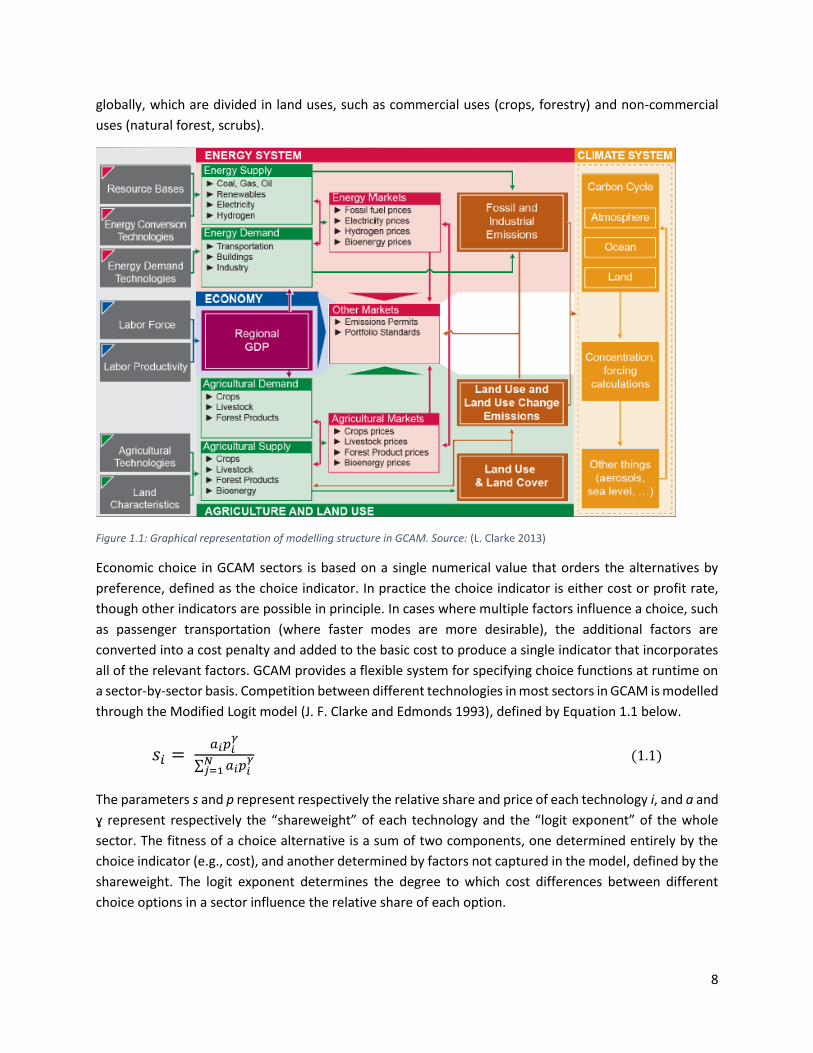
Figure 1.1: Graphical representation of modelling structure in GCAM. Source: (L. Clarke 2013)
Economic choice in GCAM sectors is based on a single numerical value that orders the alternatives by
preference, defined as the choice indicator. In practice the choice indicator is either cost or profit rate,
though other indicators are possible in principle. In cases where multiple factors influence a choice, such
as passenger transportation (where faster modes are more desirable), the additional factors are
converted into a cost penalty and added to the basic cost to produce a single indicator that incorporates
all of the relevant factors. GCAM provides a flexible system for specifying choice functions at runtime on
a sector-by-sector basis. Competition between different technologies in most sectors in GCAM is modelled
through the Modified Logit model (J. F. Clarke and Edmonds 1993), defined by Equation 1.1 below.
𝑠𝑖 = 𝑎𝑖𝑝𝑖
𝛾
∑ 𝑎𝑖𝑝𝑖𝛾𝑁
𝑗=1
(1.1)
The parameters s and p represent respectively the relative share and price of each technology i, and a and
ɣ represent respectively the “shareweight” of each technology and the “logit exponent” of the whole
sector. The fitness of a choice alternative is a sum of two components, one determined entirely by the
choice indicator (e.g., cost), and another determined by factors not captured in the model, defined by the
shareweight. The logit exponent determines the degree to which cost differences between different
choice options in a sector influence the relative share of each option.

9
Equation 1.2 below shows how the market share (s) of alternative options (i,j) in GCAM depends on the
pre-defined shareweight (a) and the price or cost (p) of each alternative, while the relevance of the latter
depends on the logit exponent. The values of the shareweights in each market are estimated by comparing
the costs and market share of each alternative in the base year. In markets where the end product of each
alternative is exactly equal, such as the electricity market, shareweights are assumed to converge in the
long term, such that only cost differences determine the share of each choice in the long term (by 2100).
Competition between technologies in the electricity sector is based on the Levelised Costs of Energy
(LCOE), dividing costs for capital, resources and maintenance by the output of electricity.
𝑠𝑖
𝑠𝑗=
𝑎𝑖
𝑎𝑗 (
𝑝𝑖
𝑝𝑗)
γ
(1.2)
Economic land use decisions in GCAM are based on a logit model of sharing (McFadden 1974) with relative
inherent profitability of using land for competing purposes. The interpretation of this sharing system in
GCAM is that there is a distribution of profit behind each competing land use within a region, rather than
a single point value. Each competing land use option has a potential average profit over its entire
distribution. The share of land allocated to any given use is based on the probability that that use has the
highest profit among the competing uses. The relative potential average profits are used in the logit
formulation, where an option with a higher average profit will get a higher share than one with a lower
average profit. The profit rate is the difference between the market price of the commodity and the
production costs, which depend on land rent, fertilizer costs, other non-land costs and the crop yield. A
land node structure defines the level of competition between different land uses. For example,
competition between different crops is more intense than competition between crops and forest, while
competition between crops/forest with pastures is again less intense.
GCAM tracks GHGs, including CO2 (from fossil fuels, industrial porcesses and land use change), CH4, N2O
and HFCs. The model also tracks air pollutants such as organic and black carbon (OC and BC), sulphur
dioxide (SO2), nitrogen oxides (NOx), carbon monoxide (CO) and non-methane volatile organic compound
(NMVOC). GHG emissions drive radiative forcing and ultimately temperature change through the climate
module, while air pollutants can be used to abstract potential health or crop damages. Taxes can be added
to any emission type which would increase the costs of emission-intensive activities. To fix emissions to a
certain level, emission caps can also be added, which function as tradable emission permits and
endogenously calculate the required emission price in order to stay below the given cap. Welfare loss
from emissions mitigation efforts through such policies can be calculated through a “deadweight loss”
approach (Bradley, Watts, and Williams 1991), and depends on the marginal abatement cost curve, which
is implicitly calculated through the detailed technological characterization of energy and agricultural
sectors in GCAM.
Population and GDP per geopolitical region are exogenously given in GCAM. This means that climate
policies have no macro-economic consequences. Population and GDP estimates, among other parameters
such as for example technology costs, crop yields and emission factors, are defined for five different
Shared Socioeconomic Pathways (SSPs)(O’Neill et al. 2014). These SSPs serve as narratives with all
parameters in each SSP being consistent within this narrative. The “Middle of the Road” narrative (SSP 2),

10
with medium values for all parameters, is used in chapter 2, 3 and 4, while chapter 5 looks at multiple
narratives.
Robust Portfolio Analysis A robust, multi-objective optimisation framework based on the principles of portfolio analysis and
stochastic uncertainty analysis is employed for GCAM outcomes in chapter 4 and 5. The multi-objective
optimisation process leads to the identification of Pareto optimal portfolios (POPs) of technology subsidies
that are robust to the implicit uncertainty of model outcomes.
Unlike single-objective optimisation, where the optimal solution of the problem is usually unique, the
optimal solution in multi-objective optimisation is a set of performances across the various objective
functions, for the optimisation of the complete set of which there emerge conflicts. Multi-objective
optimisation can be described in mathematical terms as follows (minimisation):
min 𝑦 = [𝑓1(𝑥), 𝑓2(𝑥), . . . , 𝑓𝑛(𝑥)] 𝑠. 𝑡𝑜. 𝑥 ∈ 𝛺 (1.3)
Where 𝛺 is the feasible solution area and 𝑓1(𝑥), …, 𝑓𝑛(𝑥) are 𝑛 objective functions having conflict with
each other.
A solution in multi–objective optimisation is optimal (Pareto optimal solution) if there exists no other
feasible solution that can increase the performance of the portfolio against one criterion without causing
a simultaneous decrease against another criterion (assuming maximisation). The set of all Pareto optimal
solutions is a Pareto optimal set (PS). The result of the optimisation process is a Pareto front (PF) of
different efficient solutions, which feature a near-optimal trade-off between the objectives (Branke et al.
2009; Metaxiotis and Liagkouras 2012):
𝑃𝐹 = {𝑦 = [𝑓1(𝑥), 𝑓2(𝑥), . . . , 𝑓𝑛(𝑥)]𝑇|𝑥 ∈ 𝑃𝑆}
(1.4)
Among the most widely used methods to generate the set of Pareto optimal portfolios in multi-objective
optimisation problems is the ε-constraint method. The main idea in the ε-constraint method is to optimise
one of the objective functions using the other objective functions (𝑝 – 1) as constraints. This study utilises
the AUGMECON 2 method, an extension of the ε -constraint method (Mavrotas and Florios 2013) for
driving the tri-objective optimisation model and generating the set of optimal portfolios. The AUGMECON
2 method guarantees the generation of all Pareto optimal solutions, while avoiding the generation of
other, non-optimal solutions. The portfolio optimisation problem is solved in the General Algebraic
Modelling System (GAMS).
Many parameters in GCAM are uncertain and to take this uncertainty into account, a stress test analysis
is executed to identify which of the technology subsidy portfolios on the Pareto optimal front are most
robust to differences in parameter values. The uncertain model parameters are considered to be
stochastic, by sampling their values using a uniform distribution. At first, the “no uncertainty” Pareto Front
is determined, referring to the set of portfolios that are obtained after the execution of the model, using
deterministic values for all of the uncertain parameters. Then, Monte Carlo simulation is performed
iteratively to sample random values for the uncertain parameters from the uniform distributions, and the
model is then solved to generate the set of Pareto optimal portfolios. Eventually, the execution of multiple

11
Monte Carlo iterations results in a large number of differentiated Pareto fronts, which are analysed to
draw conclusions over the robustness of the portfolios consisting the Pareto front when no uncertainty is
considered. In both chapters where robustness analysis has been applied, 1,000 Monte Carlo iterations
are performed. In chapter 4, uncertainty is treated as stochastic using the iterative trichotomic approach
(ITA; Mavrotas and Pechak 2013), while in chapter 5, uncertainty is treated as deterministic through
additional GCAM scenarios.
The ITA approach proposes an “iterative” process developed in a series of computation round. In each
computation round all POPs are allocated in three sets: the green set, the red set and the grey set.
Eventually, in each round, ITA divides the optimal portfolios in the three subsets depending on their
degree of participation in the T generated Pareto sets. The green set includes the portfolios that are
present in all Pareto sets (PS_1, ..., PS_T) of the computation round, the red set includes the portfolios
that were produced in the initial computational round but are not present in any of T Pareto sets in current
computational round and the grey set includes portfolios that are present in some of T Pareto sets. In the
first round (round with maximum uncertainty), a maximum number of portfolios is generated as candidate
final POPs. The first round results only in green and grey sets, as there is no portfolio to be excluded (red
set) from the Pareto set. In subsequent rounds some of these initial optimal portfolios are not present
anymore in any of the T Pareto sets, so they join the red set. Along this process, the uncertainty of the
model’s parameters is reduced (e.g. by reducing the standard deviation of a normal probability
distribution or shrinking the interval of a uniform probability distribution). As the uncertainty is reduced,
more portfolios from the grey set move to the green one (robust portfolios). Eventually, and as
uncertainty gradually decreases, each one of the initial POPs is characterised as red or green, resulting in
obtaining the final robust Pareto set.
Deterministic uncertainty is estimated by means of scenario analysis: applying a range of parameter values
in GCAM and abstract the results from GCAM runs as the potential uncertainty range. Specifically, the
same policy scenarios can be run with a wider range of parameter values, such as defined in different
SSPs, representing a wide range of possible scenarios. The range of the SSP simulation outcomes, which
are different for each technology, define the ranges of the uniform distribution around the middle point
of this range. Within this context, robustness is measured as a score from 1 to 1,000, based on the amount
of Monte Carlo runs in which this portfolio is on the PF.

12
Structure
The rest of the PhD thesis is structured as follows. Chapter 2 examines the role that voluntary behavioural
change could play in climate change mitigation pathways. Mainstream literature on climate change
concentrates overwhelmingly on technological solutions for this global long-term problem, while a change
towards climate friendly behaviour could play a role in emission reduction and has received little
attention. This study focuses on the potential climate mitigation by behavioural change in the European
Union covering many behavioural options in food, mobility and housing demand which do not require any
personal up-front investment. GCAM is used to capture both their direct and indirect implications in terms
of greenhouse gas emissions. The results indicate that modest to rigorous behavioural change could
reduce per capita footprint emissions by 6% to 16%, out of which one fourth will take place outside the
EU, predominantly by reducing land use change. The domestic emissions savings would contribute to
reduce the costs of achieving the NDC goal of the EU by 13.5% to 30%. Moreover, many of these options
would also yield co-benefits such as monetary savings, positive health impacts or animal wellbeing.
Chapter 3 analyses potential adverse side-effects of solar power on land use change. The transition to
renewable energies will intensify the global competition for land. However, except for bioenergy,
literature quantifying the environmental impacts of their expansion is scarce. Due to the expected
relevance of solar energy in a decarbonized future, potential solar land requirements and related land use
change emissions are computed for a selection of regions previously identified as vulnerable: the EU,
India, Japan and South Korea. A novel method is developed within GCAM to assign land requirements to
solar energy. At 50-80% penetration level in the electricity mix in those regions, solar energy will occupy
1-5% of total land by 2050; land use change emissions making up for about one third of total life cycle
emissions and up to 10% of emissions from natural gas fired electricity through the indirect competition
with natural forest land.
In chapter 4, the link between GCAM and robust portfolio analysis is introduced by measuring trade-offs
between the potential of different low-carbon electricity technologies to mitigate CO2 emissions and
improve energy security in the EU by 2050. The technologies considered include photovoltaics (PV),
concentrated solar power (CSP), wind, nuclear, biomass and carbon capture and storage (CCS). The
proposed approach measures the marginal impact of subsidies for the six power generation technologies
until 2050 on CO2 emissions reduction and energy security improvement, measured as energy production
as a percentage of energy consumption within the EU. These GCAM outputs are linked with a robust
portfolio analysis, based on Pareto optimality for portfolio analysis and Iterative Trichotomic Approach
for robustness analysis, defining specific Pareto optimal portfolios of electricity generation technologies
as the most robust to changes in parameters. The results are presented and discussed, mainly in terms of
highlighting the robustness of the Pareto optimal solutions, which is essential for policymakers to be more
confident when selecting technology portfolios that feature a high degree of uncertainty, regarding their
vulnerability to different future developments.
In chapter 5, co-benefits of climate finance for other development goals are investigated in a developing
country context. Heavy reliance on traditional biomass for household energy in eastern Africa has
significant negative health and environmental impacts. The African context for energy access is rather
different from historical experiences elsewhere as challenges in achieving energy access have coincided
with major climate ambitions. Policies focusing on household energy needs in eastern Africa contribute
to at least three Sustainable Development Goals (SDGs): Climate Action, Good Health, and Improved

13
Energy Access. This study uses GCAM to simulate the impact of land policies and technology subsidies, as
well as the interaction of both, on Greenhouse gas (GHG) emissions, exposure to air pollution and energy
access in eastern Africa under a range of socioeconomic pathways. The results show that land policies
focusing on increasing the sustainable output of biomass resources can reduce GHG emissions in the
region by about 10%, but also slightly delay progress in health and energy access goals. An optimised
portfolio of energy technology subsidies of 11 to 14 dollars per capita up to 2030 can yield another 10%
savings in GHG emissions, as well as 20% lower mortality related to air pollution, while improving energy
access by up to 15%. After 2030, both land and technology subsidy policies become less cost-effective,
and more dependent on the overall development path of the region. The analysis shows that subsidies
for biogas technology should be prioritised in both the short and long term, while the distribution of a
potential subsidy budget over LPG (health and energy access), PV (energy access), ethanol (climate and
health) and charcoal (climate; if linked to land policies) pathways would depend on the most relevant
sustainable development goal from the perspective of local policymakers or international organisations
such as the GCF.
Finally, chapter 6 draws overall conclusions on synergies and trade-offs of climate mitigation policies, and
lines out potential future research lines.

14

15
The potential of behavioural
change for climate change
mitigation

16

17
Introduction Mainstream literature on climate change concentrates overwhelmingly on technological solutions for this
global long-term problem. Research effort has focused primarily on how the portfolio of existing and
future technologies can contribute to meet the world’s energy demand over the next century and, at the
same time, limit GHG emissions so that they are consistent with a stabilisation of temperature increase
below 1.5 – 2 degrees Celsius with respect pre-industrial levels. For example, Pacala and Socolow (2004)
showed that there is already a portfolio of measures that, if implemented, can deliver a significant
reduction of emission during the first half of the century. Fifteen different measures were proposed in
that influential paper to reduce GHG emissions (1 Gigatons of carbon (GtC) per year and option), out of
which only one of these measures was a behavioural-based solution: reduce the use of private vehicles
by 50%.
The mitigation effort that will be needed is so great that additional changes in human behaviour will be
necessary. According to Field et al. (2014), “The existence of limits to adaptation suggests
transformational change may be a requirement for sustainable development in a changing climate — that
is, not only for adapting to the impacts of climate change, but for altering the systems and structures
economic and social relations, and beliefs and behaviours that contribute to climate change and social
vulnerability” (technical summary, page 89). Samadi et al. (2016) argue that since behavioural changes
towards more sustainable lifestyles have considerable potential to contribute to public policy goals and
may even be indispensable for achieving some of these goals, future lifestyle assumptions should be
assessed separately from technological assumptions in future energy scenarios.
Apart from a handful of papers focusing on the housing and mobility demand (Dietz et al. 2009; Gifford,
Kormos, and McIntyre 2011; van Sluisveld et al. 2016), food demand (Bajželj et al. 2014; Hallström,
Carlsson-Kanyama, and Börjesson 2015; Elke Stehfest et al. 2009), or an overall set of behavioural
measures (Wynes and Nicholas 2017; Faber et al. 2012), the total mitigation potential due to behavioural
action has received little attention in literature (Barker et al. 2007; Roy et al. 2012). However, those few
studies trying to quantify the impacts of behavioural change show substantive potentials for climate
change mitigation. For example, Dietz et al. (2009) examine the achievable near-term reductions by
altered adoption and use of available technologies in housing and mobility demand in the US. They found
17 household action types in 5 behaviourally distinct categories by use of data on the most effective
documented interventions that did not involve new regulatory measures. According to this study, the US
could save an estimated 123 million metric tons of carbon per year in 10 years (20% of total household
direct emissions or 7.4% of US national emissions), with little or no reduction in household well-being.
Also for food demand, Bajželj et al. (2014) show a large mitigation potential for behavioural change. Using
a global land-system model to estimate the impact of changing food demand on GHG emissions, they
show that demand side reductions, such as reducing food waste and adopting a “healthy” diet, could more
than offset the projected increase in GHG emissions from the agricultural sector due to global population
growth.
Most of the above mentioned studies on the potential of behavioural change for climate change
mitigation are based on adding up the emission savings of separately calculated behavioural mitigation
options (in the case of housing and mobility demand) or on sector-specific models (in the case of food

18
demand). Only two studies use a multi-sectoral IAMs (in both studies using IMAGE5) to model the overall
impacts of preference changes in housing and mobility demand (van Sluisveld et al. 2016) and food
demand (Stehfest et al. 2009). Although IAMs might not be ideal to represent the mitigation impacts of
behavioural change due to methodological limitations, the limited representation of lifestyle changes in
IAMs and general limitations in integrated assessment (van Sluisveld et al. 2016, p. 316-317), they are
useful to analyse the interaction of behavioural change with other measures, such as technological change
or policies.
Since IAMs are commonly used by policymakers to assess different climate scenarios, it is important that
the quantitative potential of behavioural changes in these scenarios is highlighted more prominently and
independently of technology decisions (Samadi et al. 2016). In recent years, shared socioeconomic
pathways (SSPs) have been increasingly used in IAMs to assess socioeconomic uncertainty in future
climate scenarios (O’Neill et al. 2014). Each of these SSPs represent a package of background
circumstances that greatly influences future scenarios. Future lifestyles form a part of these background
circumstances, along with many other uncertainties.
This study focuses on the potential climate mitigation by behavioural change in the EU6 that goes beyond
the studies by Dietz et al. (2009), van Sluisveld et al. (2016) and Bajželj et al. (2014) as: a) it covers many
of the options in food, mobility and housing demand, not only in the energy or food domain; and b) it uses
GCAM, which captures the direct and indirect implications in terms of emissions. The results will focus on
per capita GHG emissions savings due to behavioural change- with the recognition that behaviour change
is not straightforward and some people will change their behaviour more easily than others7. Finally, this
study discusses the co-benefits that are related to many forms of pro-environmental behaviour.
While literature on the potential benefits of pro-environmental behaviour seems scarce, there is extensive
literature on the question as of why people behave environmentally friendly and how to boost this kind
of behaviour (Poortinga, Steg, and Vlek 2004; Ohe and Ikeda 2005; Fujii 2006; Ohtomo and Hirose 2007;
Quimby and Angelique 2011; Shwom and Lorenzen 2012; Masud et al. 2015). The primary focus of this
study however is the positive question on the extent to which climate-friendly behaviour can contribute
to climate mitigation and not on the normative question on how people can adapt their behaviour and
what are the appropriate instruments to achieve that. However, since the normative question is obviously
related to the positive question, a short summary of the literature on the normative question is given in
the discussion section.
Method The method section is structured as follows. First, the application of GCAM for the purpose of this study
will be elaborated. Then, the assumptions behind each modelled behavioural option will be shown.
Finally, the baseline and policy scenario that are run on the background of these options will be briefly
discussed.
5 Integrated Model to Assess the Global Environment, for details: http://themasites.pbl.nl/models/image/index.php/Welcome_to_IMAGE_3.0_Documentation 6 The focus is on the EU-27, so excluding Croatia which joined the EU in mid-2013. The reason behind this is that the GCAM model does not yet include Croatia in the modelled EU-region. Croatia represented about 0.83% of total population and 0.33% of total GDP in the European Union in 2015 (source: EuroStat). 7 Factors like income and household size (Poortinga, Steg, and Vlek 2004) and social influences (Staats, Harland, and Wilke 2004) are of high importance, among other factors.
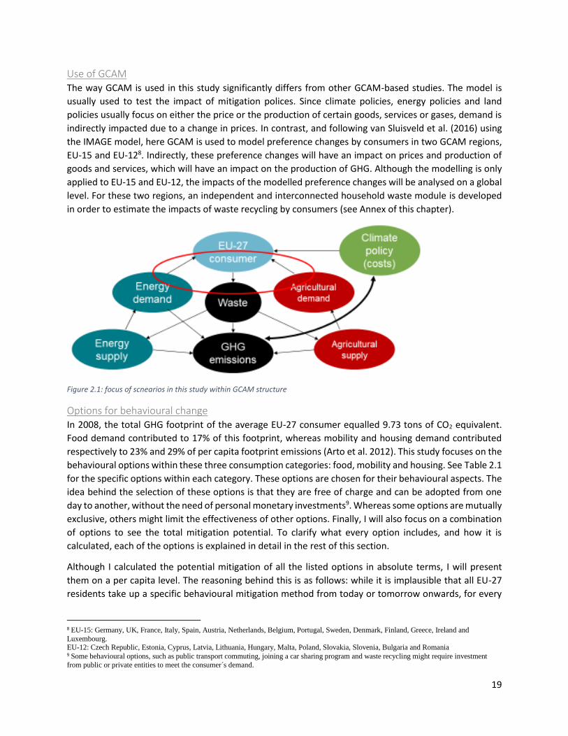
19
Use of GCAM The way GCAM is used in this study significantly differs from other GCAM-based studies. The model is
usually used to test the impact of mitigation polices. Since climate policies, energy policies and land
policies usually focus on either the price or the production of certain goods, services or gases, demand is
indirectly impacted due to a change in prices. In contrast, and following van Sluisveld et al. (2016) using
the IMAGE model, here GCAM is used to model preference changes by consumers in two GCAM regions,
EU-15 and EU-128. Indirectly, these preference changes will have an impact on prices and production of
goods and services, which will have an impact on the production of GHG. Although the modelling is only
applied to EU-15 and EU-12, the impacts of the modelled preference changes will be analysed on a global
level. For these two regions, an independent and interconnected household waste module is developed
in order to estimate the impacts of waste recycling by consumers (see Annex of this chapter).
Figure 2.1: focus of scnearios in this study within GCAM structure
Options for behavioural change In 2008, the total GHG footprint of the average EU-27 consumer equalled 9.73 tons of CO2 equivalent.
Food demand contributed to 17% of this footprint, whereas mobility and housing demand contributed
respectively to 23% and 29% of per capita footprint emissions (Arto et al. 2012). This study focuses on the
behavioural options within these three consumption categories: food, mobility and housing. See Table 2.1
for the specific options within each category. These options are chosen for their behavioural aspects. The
idea behind the selection of these options is that they are free of charge and can be adopted from one
day to another, without the need of personal monetary investments9. Whereas some options are mutually
exclusive, others might limit the effectiveness of other options. Finally, I will also focus on a combination
of options to see the total mitigation potential. To clarify what every option includes, and how it is
calculated, each of the options is explained in detail in the rest of this section.
Although I calculated the potential mitigation of all the listed options in absolute terms, I will present
them on a per capita level. The reasoning behind this is as follows: while it is implausible that all EU-27
residents take up a specific behavioural mitigation method from today or tomorrow onwards, for every
8 EU-15: Germany, UK, France, Italy, Spain, Austria, Netherlands, Belgium, Portugal, Sweden, Denmark, Finland, Greece, Ireland and
Luxembourg. EU-12: Czech Republic, Estonia, Cyprus, Latvia, Lithuania, Hungary, Malta, Poland, Slovakia, Slovenia, Bulgaria and Romania 9 Some behavioural options, such as public transport commuting, joining a car sharing program and waste recycling might require investment
from public or private entities to meet the consumer´s demand.

20
specific individual it is not at all implausible to change his/her behaviour from one day to the next. Also,
while some individuals are convinced about reducing their food waste and joining a car sharing program,
others might prefer to follow a healthy diet and recycle their waste. Since preferences differ between
individuals, I chose to show the mitigation potential and co-benefits on a per capita level.
Table 2.1: List of behavioural options in this study
Food demand Mobility demand Housing demand
Healthy diet
Vegetarian diet
Vegan diet
Food waste reduction
Public transport commuting
Carpool commuting
Teleworking
Urban Cycling
Car sharing / Car club
Avoid short flights
Closer holidays
Eco-driving
Reduce heating / cooling
Organic waste recycling
Paper waste recycling
Plastic/metal/glass waste recycling
Food Demand This section explains how behavioural options regarding food consumption are modelled. See Kyle et al.
(2011) for the methods and data sources used to model the agricultural and land-use system into GCAM.
- Healthy Diet
The assumed average healthy diet is considered to be ̀ healthy' on the basis of nutritional evidence (Willett
2017; World Health Organization 2003; American Heart Association 2014). Following Bajželj et al. (2014),
the dietary preferences in the EU-27 are respected, but with some foods that are deemed unhealthy
above or below certain levels capped. See Table 2.2 for the precise current and assumed healthy diet for
both EU-15 and EU-1210 11.
- Vegetarian Diet
A vegetarian diet does not include any meat, but does include dairy products and potentially fish products.
This option is modelled by setting all the consumption of the GCAM categories Beef, Pork, Poultry and
Sheep/Goat to zero. The reduction of calories will be replaced with the GCAM category MiscCrop
(including, between others, all kind of legumes, vegetables, fruits and nuts) until the daily net amount12
of 2500 calories per person per day is reached.
- Vegan Diet
Different than the vegetarian diet, the vegan diet does also not include dairy and fish products. The
modelling method is exactly the same, replacing dairy products with MiscCrop products until the daily net
amount13 of 2500 calories per person per day is reached.
10 I separate the diet in EU-15 and EU-12 due to their relevant dietary preferences. Estimations from Bajželj et al. (2014) for West-Europe are used as a proxy for EU-15 and the estimations for East-Europe as a proxy for EU-12. 11 Since the food categories in GCAM do not exactly match with the categories in Table 2.2, the absolute changes in kcal/person/day were applied to the GCAM food category containing the relevant category of Table 2.2. 12 Net amount of calories after the subtraction of all producer and consumer food waste 13 See previous footnote

21
Table 2.2: Healthy diet assumptions
Food Current diet [1] Healthy diet [2] Diet change
EU-15 EU-12 EU-27 EU-15 EU-12
Kcal / person / day % change
Vegetables 58 64 136 134 % 113 %
Fruits 91 53 119 30.8 % 125 %
Sugar / Sweeteners 318 308 150 -53 % -51 %
Vegetable oils 514 326 360 -30 % 10.4 %
Red meat [3] 260 180 57 -78 % -68 %
Poultry 67 70 70 4.5 % 0 %
Eggs 39 48 40 2.6 % -17 %
Dairy 391 313 300 -23 % -4.2 %
Fish [4] 56 40 50 -11 % 25 %
All other food [5] 933 1209 1218 30.5 % 0.7 %
TOTAL 2727 2611 2500 -8.3 % -4.3 %
[1] (FAO 2011a)
[2] Applying caps as interpreted by Bajželj et al. (2014)
[3] Respecting the cultural red meat preferences within EU-15 and EU-12
[4] Due to limitations in global fisheries, these are kept constant at an EU-27 average
[5] Respecting the cultural food preferences within EU-15 and EU-12
- Food Waste Reduction
Since waste is a rather subjective term, there are several approaches to account for food losses.
Technically, food used as feed for animals could be considered as food waste, as it involves a loss in final
calories for human purposes. Furthermore, waste can be distinguished at the agricultural, postharvest,
processing, distribution and consumption levels (Kummu et al. 2012; Bajželj et al. 2014) and consumption
waste can be distinguished between avoidable, possibly avoidable (that some people eat and some people
do not, like bread crusts or potato skins) and unavoidable food waste like vegetable peelings and meat
carcasses (WRAP 2008a; Van Westerhoven 2013). Since I am focusing on behavioural mitigation, solely
avoidable (including 50% of possibly avoidable) food waste on the consumer level is considered.
Estimates from (FAO 2011b) are used to separate out the percentage of consumption waste from final
food demand. Since the food demand estimations in GCAM are also based on FAO data, this seems the
most sensible source for making assumptions on food waste. See Table 2.3 for the assumed food waste
in EU-27 for different types of food.
A food waste reduction potentially reduces GHG emissions in two ways: less final food demand leads to
less agricultural emissions and less food waste leads to less waste emissions. The latter, however, depends
on what happens with the food waste: emission savings of a food waste reduction will be significant if this
food waste would otherwise get landfilled, but the net effect would be negative if the food will otherwise

22
be composted and used as a fertilizer, replacing mineral fertilizers (Bogner et al 2007). The current EU-27
recycling rate will be assumed for this behavioural option, unless this option is combined with the Organic
Waste Recycling14 option. More details on these calculations follow in the section on organic waste
recycling.
Table 2.3: Food consumption and waste in EU-27, 2010
Food Total EU-27 Consumption [1] Total waste [2] Consumer waste [2]
Kcal / person / day % of total consumption
Cereals 1177 34 % 22 %
Roots and Tubers 136 52 % 10 %
Oilseeds and Pulses 863 19.5 % 3 %
Fruits and Vegetables 288 46 % 13.5 %
Meat 570 22 % 10 %
Fish and Seafood 180 31 % 8 %
Dairy products 315 12.5 % 7 %
TOTAL 3529.9 28.1 % 12.2 %
[1] Includes all related industry and consumer wastes; FAOSTAT
[2] FAO (2011), “Global food losses and food waste – Extend, causes and prevention.
Mobility Demand
This section explains how behavioural options regarding to transport use are modelled. For a detailed
documentation on how the transport system is modelled in GCAM, see Mishra et al. (2013). The GCAM
model uses estimates from the TREMOVE model (European Commission 2010a) for the base year
calibration values in EU-15 and EU-12. Although the data from the TREMOVE model are based on
modelled estimates rather than real observations, for reasons of consistency the same model is used for
more detailed estimates such as the share of urban transport or commuting transport in total transport
demand.
- Public Transport Commuting
This behavioural option assumes all commuting transport demand in EU-27 (i.e. from home to work and
back) will be met by public transport services (i.e. bus and rail transport). The current regional public
transport mix (i.e. the share of bus and rail transport) is extrapolated to meet all commuting transport
demand from 2015 onwards.
- Carpool Commuting
Similar to the previous option, the focus is again on the current shares for commuting transport in EU-15
and EU-12 and assume them to stay the same into the future. Similar to Dietz et al. (2009), this behavioural
option is translated into numbers by stating a load factor of 2 for every commute car-trip, which is a
14 The combined effect of food waste reduction and organic waste recycling applies to two out of three behavioural profiles in the results section.

23
minimal definition of car-pooling. Current commuting transport demand that is met by public transport
and bike/motorbike use is left untouched.
- Teleworking
In order to model the effects of working one day per week from home, demand for passenger commuting
has been deducted by one fifth15. This method implicitly assumes that EU-27 citizens would normally work
5 days per week away from home.
- Urban Cycling
This option aims to quantify the potential of bicycle usage for any purpose in urban areas only: trips within
urban areas are on average quite short and streets within cities are generally flatter than streets outside
cities. For non-urban passenger trips, it would be too difficult to generalise the potential for all EU-27
member states. As a benchmark for the urban cycling potential, the urban cycling rate in the Netherlands
(i.e. highest rate in the region) is expanded to the whole EU-27.
- Car sharing / Car clubs
Over the last decade, car sharing programs have been increasing significantly in popularity in the USA and
Europe. Car-sharing is an innovative mobility option that allows individuals to pay for and use
automobiles—on an as-needed basis—through membership programs (Millard-Ball et al. 2005). Although
users of car sharing programs generally tend to drive less on average compared to car owners, due to the
constant (rather than decreasing) marginal costs of driving that are faced in a car sharing program (Chen
and Kockelman 2015), an equal amount of driven passenger kilometres by cars is assumed in this
behavioural option in order to solely focus on the environmental benefits of car sharing, while the total
amount of driven kilometres stays the same. This option assumes that shared cars are used for all car-
driven kilometres.
Ignoring the behavioural impact of car sharing on transport mode switching, there are two main channels
through which car sharing would decrease emissions: lower industrial emissions related with car
production and a higher average fuel efficiency due to a faster replacement rate of car-club vehicles
compared to privately owned vehicles (Chen and Kockelman 2015). Although the faster replacement rate
due to higher utilization rates of car-club vehicles do limit the savings in industrial emissions, the latter
does not seem to be cancelled out completely. In other words, intensively used car-club vehicles seem to
drive a higher amount of total kilometres during their significantly shorter lifetimes16.
- Avoid Short Flights
The idea behind this behavioural option is to avoid flying whenever there is a ‘realistic’ travel alternative.
With a realistic alternative, another way to get to the desired destination using a different transport mode
is meant, that does not take more than 10 hours of travelling. About 25% of all passenger kilometres on
15 Note that we did not model any changes in heating or cooling demand, assuming that the individual’s heating/cooling demand at home and at work will be equal. 16 This could be supported by the argument that due to their intensive usage, car-sharing vehicles need significantly more maintenance over its lifetime. GHG emissions related to maintenance are a lot lower than those related to production of vehicles (own elaboration based on the World Input-Output Database, WIOD)
24
intra-EU flights are estimated to be avoidable by these standards, and it is implicitly assumed that it
remains 25% until 2050.
This behavioural options assumes that these 25% of passenger kilometres will instead be travelled by a
mix of coach, train, high-speed-rail and carpool transport.
- Closer Holidays
This behavioural option focuses on intercontinental leisure flights. Here, it is assumed that 50% of all
intercontinental leisure trips (with an average distance of about 5000 km per trip) are replaced by intra-
EU trips with an average trip distance of 1000 km. All these replacing intra-EU trips will be performed by
intra-EU air transportation.
- Eco-Driving
The focus of this option is on the application of “eco-driving” by car drivers. Eco-driving is a term used to
describe energy efficient use of vehicles. It is a relatively easy way to reduce fuel consumption from road
transport so that less fuel is used to travel the same distance (Carsten et al. 2016a). Although training
might be necessary, every driver can choose to adapt this driving style, making it purely behavioural. Apart
from fuel savings, eco-driving also avoids aggressive driving behaviour and is expected to increase road
safety in general. Eco-driving techniques will be applied to all car-driven kilometres in this behavioural
option.
Housing Demand
For housing demand, the building sector structure in GCAM (Kyle et al. 2010) is relevant as well as another
innovation to the GCAM model zooming in on the municipal waste sector. See the Annex of this chapter
for more details on this innovation.
- Reduce Heating and Cooling
For the effects of a voluntary reduction in heating consumption in the winter season, a thermostat set-
back from the average 21 degrees Celsius to 20 degrees Celsius is assumed. Such an indoor temperature
change can be easily compensated by wearing extra clothing. Additionally, a reduced use of air-
conditioning in summer is assumed, increasing the target temperature from 25.5 to 26.5 degree Celsius.
- Organic waste recycling
This behavioural option assumes that all organic waste from households will be separated by the
consumer, and therefore composted rather than landfilled or incinerated. The produced compost will be
used to replace mineral fertilizers and sequester some of the carbon to the soil.
- Paper/carton waste recycling
This behavioural option assumes that all consumer paper waste will be recycled and used for producing
new paper. Note that in 2010, EU-28 was the region with the highest amount of paper waste recycling
globally (68%; EDPR 2015), so extra gains from recycling will be relatively limited.
- Plastic/metal/glass waste recycling

25
This behavioural option assumes the recycling of all plastic, metal and glass waste by consumers. The
composition of this category (i.e. the relative amount of plastics, metal and glass) is assumed to stay the
same over time.
Baseline emissions and comparison To compare the impacts of these behavioural mitigation options, two scenarios are used: a baseline
scenario with no climate policy and another scenario with a climate policy based on the NDC adopted by
the EU in the Paris Agreement, promising emission reductions up to 80% by 2050 compared to 1990
emission levels17. Socioeconomic indicators from SSP2 are used for both scenarios, with separate waste
module (see Annex of this chapter) to capture the relative impact of waste reduction and recycling by
consumers. Figure 2.2 shows the evolution of GHG emissions with and without climate policy.
Figure 2.2: Carbon emissions in EU-27 region until 2050 in two scenarios (million tons of CO-eq)
Apart from the GHG emissions in EU-27 itself, from a consumption-based approach European citizens
would also be responsible for a significant amount of GHG emissions in other parts of the world through
consumption of imported goods. Similarly, other regions are responsible for GHG emissions inside EU-27.
Some of the behavioural mitigation options have a significant impact on GHG emissions in other parts of
the world, and so reduce the total carbon footprint without contributing towards the EU-27 emission
targets, as these are not attributed as EU-27 emission savings in the UNFCCC framework. However, since
this study focuses on the per capita emission savings due to behavioural change, it should not matter
whether these savings take place in his/her house, in a neighbouring country or on the other side of the
world. Therefore, the total per capita emission savings (regional and global) are counted for every
behavioural option and, to have some kind of reference point, compared to per capita EU-27 emission
saving targets based on the EU NDC.
Results
Overview This section shows the results in terms of GHG emissions and put these in perspective. Table 2.4 shows
an overview of the total per capita GHG emission savings related to the baseline emissions for the period
17 With intermediate reduction targets of 20% in 2020, 40% in 2030 and 60% in 2040 compared to 1990 emission levels. http://www4.unfccc.int/submissions/indc/Submission%20Pages/submissions.aspx
0
200
400
600
800
1000
1200
1400
1600
1800
1990 2005 2010 2015 2020 2025 2030 2035 2040 2045 2050
Baseline
Climate
Policy
following
EU NDC

26
2011-2050, assuming that these behavioural options would be adapted immediately18. Apart from these
savings, it shows the share of Fossil Fuel & Industry (FFI) CO219 emission savings within the total GHG
emission savings. Finally, the table also shows the share of emissions that are saved domestically within
EU-27. All other emission savings have been realized in other regions in the world.
Table 2.4: Overview of GHG emission savings per behavioural option
Behavioural option Avoided GHG emissions:
Total 2011-2050 % CO2 (FFI) [1] % Domestic [2]
Food demand:
Vegan diet -8.2% 3.6% 66.1%
Vegetarian diet -7.0% 4.7% 51.0%
Healthy diet -5.3% 4.6% 58.9%
Food waste reduction -2.4% 3.1% 49.5%
Mobility demand:
Public transport commuting -0.7% 93.1% 86.2%
Carpool commuting -1.2% 92.3% 89.3%
Teleworking -0.3% 92.3% 89.1%
Urban Cycling -0.6% 92.8% 89.3%
Car sharing / Car club -1.1% 87.3% 89.6%
Avoid short flights -0.5% 93.2% 88.1%
Closer holidays -0.5% 93.4% 88.9%
Eco-driving -0.6% 92.3% 89.4%
Housing demand:
Reduce heating / cooling -0.6% 88.7% 89.0%
Organic waste recycling -1.1% 8.1% 93.6%
Paper waste recycling -0.6% 86.2% 125.9% [3]
Plastic/metal/glass waste recycling -1.7% 93.9% 92.9%
[1] Fossil Fuel & Industry: Includes all CO2 emissions related to fossil fuel use, but no CO2 emissions from land use change
[2] Share of emission reductions within EU-27 region
[3] Since this option reduces CO2 sequestration from foresting i.e. increases GHG emissions in other regions (by reducing demand for forest products), more than 100% of emission reductions occur in the within the EU-27.
Some of these behavioural options would imply monetary savings for the consumer (see the part on co-
benefits later in this section). Literature suggests that these monetary savings will yield rebound effects,
decreasing its effectiveness on total emission savings (Grabs 2015; Druckman et al. 2011). The final
18 Since the first model gives projection from 2015 onwards, in this case “immediately” means from 2015 onwards. 19 FFI CO2 includes all CO2 emissions related to fossil fuel use, but no CO2 emissions from land use change

27
rebound effect depends on where the monetary savings are spent on. The lower the GHG intensity of the
re-spending of savings, the lower the rebound effect of behavioural change. In some cases, re-spending
could even save more emissions, if they are invested in, for example, rooftop solar installations or electric
vehicles to replace their previous vehicle. Since no rebound effects are modelled, it is implicitly assumed
that the re-spending of eventual savings have a negligible GHG intensity on average. Given the intrinsic
motivation that is necessary to adopt green behaviour, the assumption that this intrinsic motivation will
extend to eventual re-spending of savings seems reasonable.
Discussion of individual results
Food Demand
As Table 2.4 shows, behavioural change in the demand for food leads to very significant GHG emission
savings. For example, adopting a healthy diet would reduce accumulated per capita GHG emissions
between 2011 and 2050 by 5.3%, only 4.6% of these GHG emission savings are fossil fuel related CO2
emissions and 58.9% of these emission savings will occur within the EU. Fossil fuel related CO2 emissions
only accounts for a very marginal share of all food-related emission savings. Instead, methane emission
savings from the livestock industry, abated nitrogen oxides from soil utilization and negative land use
change emissions due to decreasing land pressure from the agricultural system add up to the gross of the
GHG savings due to behavioural change in the food sector. The majority of emission savings for each of
the options is due to land use change (i.e. avoiding deforestation), mainly outside of the EU.
It is important to keep in mind that a combination of food waste reduction with either of the diet changes
strongly diminishes the impact of a food waste reduction. This is due to the fact that the majority of
emissions in the food sector comes from meat consumption, and if less meat is consumed less is wasted
as well.
Mobility Demand
In comparison to food demand, behavioural change in mobility demand leads to predominantly domestic
CO2 savings. Generally, every option yields CO2 savings due to either a reduction of car or air travel. The
fact that not all emissions savings are domestic CO2 emissions has to do with the footprint emissions in
other regions related to the production of petroleum products, predominantly from unconventional oil.
The only exception regarding the source of emission savings in the transport sector is the behavioural
option of car sharing / car clubs. This option implicitly suggests that fewer cars are produced, and
therefore mainly leads to savings in industrial emissions. However, about 37% of the emission savings due
to car-sharing are the result of increase in average fuel efficiency due to a higher replacement rate of
heavily used shared cars.
One rather surprising result is that commuting by carpooling is more beneficial than commuting by public
transport. It is important to keep in mind that the supply of public transport facilities is assumed to
increase proportionally with higher utilization of public transport. This means that the load factor of every
bus and train does not change as a result of higher utilisation, whereas the load factor of cars does change
as a result of carpooling. This assumption might be subject to debate and a higher load factor for trains
and buses might be expected if more people decide to use them due to economics of density (Caves and
Christensen 1988). However, since the spatial dimension is missing in GCAM, it is hard to provide
consistent estimates on the extent to which load factors should increase due to higher use of public
transport systems.

28
Housing Demand
Emissions in housing demand are mainly related to waste recycling: Table 2.4 shows that reducing heating
in winter and cooling in summer has only a marginal effect on total emission savings. The recycling of
organic waste leads to mainly methane emission savings due to reduced landfill emissions - the emission
savings due to replacement of mineral fertilizers by compost and carbon sequestration by the use of
compost does only marginally weigh up against the increased composting emissions. By contrast,
industrial and paper waste recycling predominantly impact the demand for industrial energy, since it costs
significantly more energy to make paper, metal, glass and plastic from raw materials than from recycled
materials. This might explain why in many EU member states, recycling rates of paper, plastic, metal and
glass are high relative to recycling rates of organic products: the recycled end-product of predominantly
paper and metal is significantly more valuable than that of organic waste.
As explained in the Annex of this chapter on the waste module, it is assumed here that separated waste
will always be recycled, whereas mixed waste will always be landfilled or burned. However, there exist
technologies that can filter out certain types of waste from initially mixed household waste in order to
recycle it. These technologies are already often used for metal waste. The impact of Plastic/Metal/Glass
recycling might therefore be overestimated, as some of these products might anyway be recycled in the
future, with or without the contribution of the consumer.
Behavioural profiles In order to provide an estimate of the total potential emission reduction, the savings in all categories
cannot be simply added up. Some options are mutually exclusive (such as the diet choices) and other
options limit the impact of each other (for example diet change and food waste reduction or carpooling,
eco-driving and teleworking). Therefore, three different profiles for the adoption of green behaviour are
described, each with a different mix of behavioural options that are adopted. Following Autio, Heiskanen,
and Heinonen (2009), each profile is intended to represent a realistic behavioural style that people can
identify themselves with, ranging from a very active to a more passive form of behavioural change. See
Table 2.5 for the behavioural options included for each profile.
Enthusiastic Profile: The enthusiastic adaptor is the typical person that does anything in his/her means to
limit the personal footprint. He or she does not eat any meat or other animal products, does not
unnecessarily waste any food, does not have a car, uses a bicycle whenever possible or public transport
otherwise, applies eco-driving techniques using rental cars when travelling to places impossible to reach
without a car, tries to avoids flying by taking alternative transport and by avoiding far destinations, prefers
to put some extra clothes in winter or less clothes in summer instead of putting the thermostat or A/C
higher and separates all types of household waste.
Conscious Profile: The conscious adapter is well aware of all the environmental consequences of his/her
actions, but does not want to give up certain basic needs for this. Instead, he or she is the modern
metropolitan role model for environmental consumerism. He or she follows a healthy diet, without
unnecessarily wasting any food, does not have a car and uses public transport and rental cars to get
around (always applying eco-driving), tries to avoid flying when possible but does not want to give up
exotic long-distance holidays. Finally, he or she separates all types of household waste.
Convenient Profile: The convenient adapter is more or less informed about the environmental impact of
his or her actions, but does not want to make significant adaptation to their lifestyle in order to reduce

29
this impact. Instead, he or she adopts some easy forms of green behaviour, such as reducing his or her
food waste, carpooling with a colleague to work, applying eco-driving techniques and separating paper
and other packaging waste from all other waste.
Table 2.5: List of behavioural options adopted for each profile
“Enthusiastic Profile” “Conscious Profile” “Convenient Profile”
Food:
Vegan diet
Food waste reduction
Mobility:
Teleworking
Car sharing / Car club
Cycling
Public Transport commuting
Avoid Short Flights
Closer Holidays
Eco-Driving
Housing:
Less heating / cooling
Organic waste recycling
Paper/Carton recycling
Plastic/Metal/Glass recycling
Food:
Healthy diet
Food waste reduction
Mobility:
Teleworking
Car sharing / Car club
Public Transport commuting
Avoid Short Flights
Eco-Driving
Housing:
Organic waste recycling
Paper/Carton recycling
Plastic/Metal/Glass recycling
Food:
Food waste reduction
Mobility:
Carpool commuting
Teleworking
Eco-Driving
Housing:
Paper/Carton recycling
Plastic/Metal/Glass recycling
Combining several behavioural options that are discussed in this study makes up to significant mitigation
portfolios. Table 2.6 shows that up to 16.2% of emissions can be saved when adopting many behavioural
options.
Table 2.6: Overview of GHG emission savings per behavioural profile
Total 2011-2050 % CO2 (FFI) [1] % Domestic [2]
Convenient profile -5.6% 59.4% 76.4%
Conscious profile -12.0% 35.7% 71.1%
Enthusiastic profile -16.2% 34.8% 74.5%
[1] Fossil Fuel & Industry: Includes all CO2 emissions related to fossil fuel use, but no CO2 emissions from land
use change
[2] Share of emission reductions within EU-27 region
As this mitigation potential through behavioural action is very significant, it can be compared to the total
required mitigation promised by the EU in the Paris Agreement. Translating this agreed promise to
cumulative per capita emissions, about 50 tons of carbon per capita have to be mitigated before 2050
compared to the baseline scenario. This is 39.6% of total emissions in the period 2011-2050 according to

30
the baseline scenario. Figure 2.3 shows that the carbon reduction per capita due to the adoption of a
climate-friendly behavioural profile reaches up to 14 tons of carbon equivalent, or 19 tons if the total
footprint impact is counted20.
Figure 2.3: Per capita GHG emission reduction compared to baseline emissions for the three behavioural profiles, accumulated from 2011 to 2050. Total savings are split between different domestic sectors and savings outside the EU-27 area.21
An important conclusion to draw from this figure is that significant contributions can be made due to
costless behavioural change, up to one third of the total EU mitigation target or over 40% when the total
“footprint” impact would count. But even modest behavioural change could mitigate 7 tons of carbon per
capita, or 5.5 domestic tons accounting for 11% of the total EU mitigation target. The amount of emission
savings however decreases if a climate policy is active, since the GHG-intensity of all consumption
categories will decrease due to such a policy. This interaction will be discussed in more detail later in this
section.
Sensitivity analysis based on timing of behavioural change adoption One rather strong assumption of the estimates in this section has been that modelled behavioural change
will start immediately, from the very first period after the base year, in this case 201522. Although it is not
impossible for any of the behavioural options to start from tomorrow onwards, it might be more realistic
to expect a later starting date due to different barriers. Table 2.7 therefore gives the total emission savings
compared to the baseline scenario dependent on when the individual starts to adopt a behavioural profile.
20 Although the figure seems to give slightly higher percentages, it should not be forgotten to subtract the small increase in emissions due to less biomass use from the total emission reduction. See also the next footnote. 21 The sector “Biomass use” represents the change in biomass use for different end-use sectors. If positive, biomass use has decreased (which automatically leads to decreasing GHG emissions in the intermediate or end-use sectors) and the other way around. This is the way the GCAM model accounts for biomass emissions. 22 Since GCAM runs in 5-year periods and the base year is 2010, the closest modelling year to the writing of this chapter is 2015. I am aware that this is effectively in the past, but the idea behind this is that the behavioural option is applied immediately. The 1-2 years of difference have a negligible effect on the total impact of each option.
-22 -20 -18 -16 -14 -12 -10 -8 -6 -4 -2 0 2
Convenient
Conscious
Enthusiastic
Tons of carbon-equivalent per capita
CO2 - Biomass use
CO2 - Building
CO2 - Industry
CO2 - Transportation
CO2 - Electricity
CO2 - Gas systems
CO2 - Liquid systems
CO2 - Land use change
CH4 - Waste Management
CH4 - Agriculture
N2O
Non-domestic

31
Table 2.7: Sensitivity analysis of results based on starting year of behavioural change
Behavioural option Total avoided emissions compared to baseline if behaviour is adopted by year: [1]
2015 2020 2025 2030 2035 2040 2045 2050
Food demand:
Vegan diet -8.18% -7.79% -7.33% -6.84% -6.32% -5.77% -5.21% -4.62%
Vegetarian diet -6.99% -6.70% -6.37% -6.03% -5.66% -5.27% -4.87% -4.45%
Healthy diet -5.27% -5.01% -4.73% -4.43% -4.11% -3.77% -3.43% -3.06%
Food waste reduction -2.38% -2.24% -2.09% -1.93% -1.77% -1.60% -1.43% -1.26%
Mobility demand:
Public transport commuting
-0.73% -0.65% -0.59% -0.51% -0.42% -0.32% -0.23% -0.12%
Carpool commuting -1.16% -1.12% -1.04% -0.91% -0.74% -0.56% -0.39% -0.20%
Teleworking -0.25% -0.23% -0.21% -0.18% -0.15% -0.12% -0.09% -0.05%
Urban Cycling -0.60% -0.52% -0.46% -0.39% -0.32% -0.25% -0.17% -0.09%
Car sharing / Car Club -1.06% -1.06% -0.96% -0.84% -0.68% -0.51% -0.35% -0.18%
Avoid short flights -0.47% -0.42% -0.39% -0.34% -0.28% -0.22% -0.16% -0.08%
Closer holidays -0.49% -0.43% -0.38% -0.33% -0.27% -0.21% -0.15% -0.08%
Eco-driving -0.59% -0.58% -0.54% -0.47% -0.39% -0.29% -0.20% -0.10%
Housing demand:
Reduce heating / cooling -0.60% -0.52% -0.44% -0.37% -0.30% -0.22% -0.15% -0.08%
Organic waste recycling -1.09% -0.93% -0.80% -0.67% -0.53% -0.40% -0.27% -0.13%
Paper waste recycling -0.56% -0.54% -0.47% -0.41% -0.33% -0.25% -0.18% -0.09%
Plastic/metal/glass waste recycling
-1.66% -1.46% -1.27% -1.08% -0.87% -0.66% -0.46% -0.23%
Behavioural profiles:
Convenient -5.89% -5.48% -4.99% -4.41% -3.77% -3.09% -2.41% -1.68%
Conscious -11.96% -11.19% -10.28% -9.28% -8.21% -7.06% -5.89% -4.65%
Enthusiastic -16.24% -15.18% -13.93% -12.55% -11.08% -9.54% -7.96% -6.31%
[1] In the case of land use change emissions, all emission reductions are count to the year the behavioural change takes place, also if the new vegetation is not completely grown yet.
This table shows that even when individuals start being conscious about climate change, and act
accordingly around 2025, solely by costless behavioural change they can mitigate 10% compared to the
baseline emissions, which is equal to one fourth of the individuals’ share of the total mitigation target in
the EU. Such an emission reduction is still significant and could be a more realistic target for most
individuals and policy-makers than an immediate adoption of the enthusiastic profile.

32
Impact on domestic EU Climate Policy The majority of GHG emission savings due to behavioural change take place in the region itself. As can be
seen in Table 2.6 and Figure 2.3, domestic emission savings contribute for around 75% of the total
emission savings related with adoption of different behavioural profiles. As mentioned in the previous
section, the European Union submitted an NDC to the Paris Agreement in 2015, committing itself to
significant reductions in GHG emissions.
There are various ways in which a climate policy can take form. Here, a cap-and-trade emission permit
policy is assumed in which the determined carbon reductions as promised in the EU NDC are set and the
GHG price in the market is variable. Such a price on GHG gases is expected to impact technology choices
such that the necessary GHG emission cap is reached using the least-cost technological options. While
there is certainly an overlap between the GHG emission savings due to a cap-and-trade policy and climate-
friendly behavioural change, a large part of the GHG emissions that would be abated by adopting one of
the identified behavioural profiles would be unabated in case of a cap-and-trade climate policy. This is
because the sectors that are impacted by the adoption of these profiles are generally the sectors that do
not respond strongly to GHG emission prices.
Table 2.8 shows an overview on the domestic impact of climate-friendly behavioural change with and
without a cap-and-trade climate policy running on the background. It follows from these results that the
policy costs related to a climate policy to realize the EU NDC by 2050 could be significantly reduced if the
average EU citizen adopted a climate-friendly behavioural profile. Since the sectors targeted by such
behavioural change are among the most expensive to be impacted by a climate policy in terms of policy
costs, the impact that adopting a behavioural profile has on policy costs is larger than one would expect
from the initial GHG emission savings.
Table 2.8: Regional impact of behavioural change, climate policy and a combination of both
Scenario Accumulated GHG
emission savings within
EU-27 in 2011-2050 [1]
Total policy costs
2020-2050
Trillion €(2010)
Per capita policy
costs 2020-2050
€(2010)
Baseline + Convenient profile -4.5% N/A N/A
Baseline + Conscious profile -8.5% N/A N/A
Baseline + Enthusiastic profile -12.1% N/A N/A
EU NDC -39.6% 1.99 3971.6
EU NDC + Convenient profile -39.6% 1.72 3431.0
EU NDC + Conscious profile -39.6% 1.54 3080.9
EU NDC + Enthusiastic profile -39.6% 1.40 2793.2
[1] Percentages with respect to baseline emissions, see Figure 2.2

33
Global “footprint” impact All behavioural options in this analysis have been modelled as consumer side preference changes. Thus,
all behavioural change is independent from climate policies, and might be adopted due to environmental
awareness as well as monetary, health or animal wellbeing considerations. An important co-benefit of
this type of mitigation is that final demand for the polluting good or service has inherently disappeared.
In contrast, a carbon tax would simply force demand away by imposing monetary implications. Although
a carbon tax might also lead to directed technical change towards less polluting processes and products
(Acemoglu et al. 2012; Aghion et al. 2016), a short to medium term pressure will exist towards
consumption of the polluting good or service. In the case of zero or lower carbon taxes in other regions,
this pressure will often lead to both industrial and terrestrial carbon leakage23 (González-Eguino et al.
2017).
Figure 2.4: Footprint impact due to adoption of behavioural change in EU-27 on GHG emissions outside the EU-27, representing in detail the savings within the non-domestic share from Figure 2.324
Figure 2.5: Per capita amount of cropland that would be diverted into other land uses due to behavioural change in EU-27 (average for period 2011-2050)
23 Terrestrial carbon leakage defines the relocation of agricultural production due to a land use tax in the policy region. 24 See footnote 21 for an explanation on the “biomass use” sector.
-6 -5 -4 -3 -2 -1 0 1
Convenient
Conscious
Enthusiastic
Tons of carbon-equivalent per capita
CO2 - Buildings
CO2 - Industry
CO2 - Transportation
CO2 - Biomass use
CO2 - Electricity
CO2 - Gas systems
CO2 - Liquid systems
CO2 - Land use change
CH4
N2O
0 200 400 600 800 1000 1200
Convenient
Conscious
Enthusiastic
m2 per capita
Forest
Grassland
Pasture land
Shrub land
Biomass
Other arable land

34
Although a limited form of carbon leakage might exist in the case of behavioural change through the
depressing effect it could have on global energy and food commodity prices, this effect seems hardly
visible in the results (see positive emissions in Figure 2.4). In fact, the results indicate that this effect will
be more than offset by the reduced footprint emissions that behavioural environmentalism has (see
negative emissions in Figure 2.4). A decreasing demand for food and energy in the EU-27 frees up
agricultural land in other regions and avoids emissions related to the mining of energy resources.
Like in Bajželj et al. (2014) and Alexander et al. (2015), a strong impact of diet changes and food waste
reduction on (mainly) global land use change emissions (Figure 2.4) and land availability (Figure 2.5) can
be observed. Interestingly, as shown in Figure 2.5 the reduction of land footprint by EU consumers would
not only allow forest, grass, pasture and shrubs to grow back where they used to grow (or prevent them
to be used for agriculture), but also encourage the production of biomass energy due to lower land costs.
Consequently, the share of biomass in the global energy mix will significantly grow, crowding out fossil
fuel use (see Figure 2.4).
Finally, Figure 2.4 also shows small impact of behavioural change on the emissions related to liquids (oil
refining) and gas processing. A lower demand for fossil fuels in the EU saves emissions related with the
production of these fuels in other regions. Similarly, a saving in methane emissions can be observed,
mainly due to a reduction in fossil fuel production.
Co-benefits Several of the behavioural options discussed have significant co-benefits for either the adopters
themselves or society as a whole. Although these co-benefits are not quantified in this analysis, they play
an important role in the attractiveness to adopt a certain behaviour. Table 2.9 gives a brief overview of
the potential co-benefits that go along with the adoption of behavioural options.
This table shows that most behavioural options yield monetary co-benefits and also either personal of
societal health co-benefits. For example, non-meat food products are generally cheaper than meat
products and cycling, carpooling and flight avoiding also generally save money just as putting the
thermostat to a lower level in winter. Car sharing and public transport systems could save individuals
money as well, depending on the specific car share program or public transport operator.
Adopting a healthy diet is by definition good for someone’s own health, whereas the adoption of a
vegetarian and vegan diet could be good for one’s health as well, depending on the exact diet
specifications25. Similarly, cycling could be healthy in the sense that it keeps someone fit, but it could
simultaneously be unhealthy due to greater respiration of urban air pollution and the increased
chance of street accidents (De Hartog et al. 2010), whereas eco-driving could only decrease one’s
possibility to be involved in a car accident (Carsten et al. 2016b), improving the health impact for eco-
driving on average.
Any option that reduces the amount of toxic gases in densely populated areas, generally due to transport,
improves society’s health by doing so. Furthermore, the recycling of different waste streams improves
public health directly if alternatively, the waste would have ended up on the streets, but also indirectly if
25 A vegan diet with too little protein consumption is for example rather unhealthy.

35
the waste would otherwise be incinerated or landfilled. Both waste management practices release gases
that negatively impact public health.
Table 2.9: Expected co-benefits of behavioural options
Behavioural option: Co-benefits:
Monetary Own health Society health Animal
wellbeing
Food demand:
Healthy diet x x x
Vegetarian diet x ~ x
Vegan diet x ~ x
Food waste reduction x x
Mobility demand:
Public transport commuting ~ x
Carpool commuting x x
Teleworking x x
Urban Cycling x ~ x
Car sharing / Car club ~ x
Avoid short flights x
Closer holidays x
Eco-driving x x x
Housing demand:
Reduce heating / cooling x
Organic waste recycling x
Paper waste recycling x
Plastic/metal/glass waste
recycling
x x
X = certain co-benefit
~ = dependent on specific attributes
Finally, the reduction of meat consumption, even by a reduction of animal food waste, reduces the
number of animals suffering in animal husbandry industries. This is the major reason why people generally
adopt a vegetarian or vegan diet. The recycling of plastic waste also improves animal wellbeing as it
prevents microplastics ending up in their food-chain (Derraik 2002).
Apart from these co-benefits, voluntary engagement in pro-environmental behaviour seems to
significantly improve someone´s subjective well-being according to evidence from the United States
(Jacob, Jovic, and Brinkerhoff 2009), Canada (Schmitt et al. 2018), Germany (Welsch and Kühling 2011),
Sweden (Kaida and Kaida 2016), Spain (Suárez-Varela, Guardiola, and González-Gómez 2016) and China
(Xiao and Li 2011). For example, using samples from Canada and the United States, Schmitt et al (2018)
confirm significantly positive impact on subjective well-being for 37 out of 39 pro-environmental

36
behaviours, including 9 behaviours of which the potential mitigation effort has been analysed in this
study26.
Another important conclusion is that it is hard to imagine any negative side-effects related to any of the
modelled behavioural options with either monetary or health consequences27. Because of that, the only
remaining incentives of why not to adopt these behavioural options will be driven by barriers such costs
in terms of time or effort or personal preferences (Fujii 2006; Quimby and Angelique 2011).
Discussion and conclusions
Discussion and limitations Generally, as the limited studies in literature have shown, a change towards climate friendly behaviour by
citizens can reduce GHG emissions substantially. Apart from that, many of these options usually have
negative monetary costs and in some cases imply significant health co-benefits. This study analyses the
impacts of preference changes that could contribute to the climate change mitigation portfolio, but for
the normative question on how to change these preferences, I have to rely on the extensive existing
literature on this topic.
There seem to be several psychological barriers to behavioural change (Lorenzoni, Nicholson-Cole, and
Whitmarsh 2007; Whitmarsh 2009; Quimby and Angelique 2011), even if the individual´s welfare or
subjective well-being effect is positive (Gifford 2011; Schmitt et al. 2018). Being aware of the dangers of
climate change helps the adoption of pro-environmental behaviour (PEB), but certainly not guarantees it
(Semenza et al. 2008; Ohe and Ikeda 2005; Ozaki 2011; Lin 2013; Masud et al. 2015). Moreover, literature
confirms that the adoption of PEBs has, apart from sociodemographic variables, a lot to do with
environmental attitudes. These attitudes are, apart from influenced by environmental awareness and risk
perception, but also by personal and social values such as social justice, community, frugality, and
personal integrity (Fujii 2006; Gadenne et al. 2011; Hards 2011; Howell 2013; Poortinga, Steg, and Vlek
2004).
In order to boost the adoption of PEBs by citizens, public policy might be necessary. Since this study
focuses on costless behavioural change due to preference changes, it is a matter of discussion if taxation
should be a way to convince consumers to change their behaviour. Being taxed away from the
consumption of a certain good is not the same as a preference change (although taxes can have some
signalling effects, reducing the inherent demand for the good). Although recent literature indicates that
taxes on unhealthy food products containing a certain amount of fat or sugar, as well as subsidies for
healthy food products, have been very effective (Thow, Downs, and Jan 2014), such taxes do not
necessarily increase consumer welfare (Lusk and Schroeter 2012) if the consumer inherently would have
preferred the taxed product.
Alternatively, consumers could be inherently convinced to change their preferences, for example by
consistent public awareness campaigns about climate change (Fujii 2006; Lorenzoni, Nicholson-Cole, and
Whitmarsh 2007). According to Howell (2013), such campaigns should provide a more holistic view of a
lower-carbon future, rather than simple recommendations to combat climate change, as it increases
26 The behavioural options from this study that appear to positively influence subjective well-being according to Schmitt et al (2018) are: Vegetarian diet, Urban cycling, Car sharing / car club, Public transport and Carpool commuting (insignificant impact), Reduce heating / cooling, Organic waste recycling/composting, Paper waste recycling and Plastic/Metal/Glass waste recycling. 27 Unless a wrong implementation of the option is applied, such as a vegan diet without protein consumption or a suicidal cycling style.

37
intrinsic motivation to adopt and sustain PEB. According to O’Neill and Nicholson-Cole (2009), it is
important that such campaigns are not fearful, but rather link to individuals’ everyday emotions and
concerns in the context of climate change. In terms of mitigation, a way of doing this is by relating climate
change to local environmental issues and personal concerns, emphasising the additional benefits of PEBs
(Lorenzoni, Nicholson-Cole, and Whitmarsh 2007). For example, persuasive campaigns against the
consumption of meat have been realized by animal protection and food-focused NGOs. According to
Laestadius et al. (2014), environmental NGO’s have however shown little incentives to campaign for a
reduction in meat consumption as they appeared to be reluctant to mount campaigns explicitly
encouraging personal behaviour change of any type. It makes sense that, when significant co-benefits are
related with a certain type of behaviour (see previous section), the willingness of consumers to adopt this
behaviour will increase. In any case, whether there are significant co-benefits involved or not, public
awareness about climate change could be improved (Sheppard 2005; Moser 2010).
Finally, voluntary mitigation by the public to adjust lifestyles can be maximized only if the general public
and other stakeholders see the benefits of such sacrifices, which requires legislative and regulatory
measures from industry, commerce, and government. Ultimately, effective mitigation of climate change
requires both structural and behavioural changes toward a more sustainable society (Semenza et al.
2008). The results from this study confirm that costless behavioural change can potentially contribute to
a significant part of the total necessary climate change mitigation efforts, but that the majority of
mitigation efforts still have to come from structural transformation in the energy system. Therefore, it is
important that behavioural change appears in future energy and climate scenarios for policymakers, so
that it’s potential can be assessed independent of technology decisions (Samadi et al. 2016).
Conclusions and policy recommendations This chapter explored the mitigation potential of various types of behavioural actions in the food,
transport and household sector, and sketches different green consumption profiles. Unlike Dietz et al.
(2009), the behavioural options considered do not require investments in new or cleaner technologies.
Therefore, there will be no need for upfront investments to be made by the consumer, which is an
important barrier for making energy-saving investments (Costanzo et al. 1986; Gadenne et al. 2011). From
an analytic point of view, the absence of technology requirements allows us to compare and add these
results to mitigation portfolios that are based on the adoption of cleaner technologies, with few
overlapping emission savings.
A thorough analysis of the results show that costless behavioural change can contribute, if adopted
immediately, up to one third of the EU target of GHG emissions by 2050, rising to 40% if all footprint
emissions would count. But even a more convenient way of behavioural change as well as an average
environmentally conscious living style adopted a bit later could contribute to 14% and 25% of the total
mitigation effort respectively.
The use of GCAM allows also to measure the international aspects of domestic behavioural changes.
Interestingly, environmentally friendly behavioural change reduces emissions in other regions, which
means that the positive “footprint” effect dominates the negative “carbon leakage” effect in the case of
behavioural change. In contrast, forcing environmentally friendly behaviour with a GHG emission tax
typically yields some carbon leakage to other regions (González-Eguino et al. 2017).

38
The inability to model the rebound effects of potential monetary savings of green behaviour with the
model forced us to assume the monetary savings to be spent GHG-neutral. However, such rebound effects
can reduce the total effectiveness of green behaviour up to 34% for housing and mobility options
(Druckman et al. 2011) and 49% for food options (Grabs 2015). These limitations could be overcome in
the future with the support of other modelling tools such as agent-based models and computable general
equilibrium modes.
The co-benefits of environmentally friendly behaviour can be in some cases significant and, therefore,
could also encourage citizens to adopt this behaviour. There are a lot of potential gains in behavioural-
based mitigation if the citizens of the EU follow a more sustainable lifestyle. The adoption of a sustainable
lifestyle in developed regions might simultaneously yield a more sustainable lifestyle in developing regions
by giving a better example (Lange and Meier 2009). Surely in the case of behavioural options that imply
significant co-benefits for the adopter, ´leapfrogging´ of sustainable lifestyle features might be a realistic
climate mitigation strategy for developing regions (Schäfer, Jaeger-Erben, and dos Santos 2011). A good
example of behavioural change from a developed nation could therefore be of relevant value for future
climate scenarios.
To conclude, policy makers predominantly look at taxes and subsidies in order to provide technological
solutions to reach their climate targets. As follows from this analysis, behavioural effects can play a
significant role in climate change mitigation portfolio and this potential should therefore be reflected in
scenario studies aiming to provide comprehensive advice to policy makers (Samadi et al. 2016). More
specifically, the results from this study imply that policymakers should put more effort in education and
awareness programs in order to promote green behaviour by citizens, where it is important to focus on a
more holistic view of a low-carbon future (Howell 2013) as well as individuals’ everyday emotions and
concerns in the context of climate change (O’Neill and Nicholson-Cole 2009), for example by linking PEB
with the additional benefits that come along with them. The policy costs of such measures are usually low
compared to the implementation of taxes and subsidies and, in addition, they often lead to significant
public co-benefits in terms of health and land use.
Annex: Background modelling of mobility and housing options
Mobility options - Public Transport Commuting
In the base year (2010), around 20.7% and 17.9% of total passenger kilometres in respectively EU-15 and
EU-12 were due to commuting between home and work. Of this commuting transport demand, only
15.1% in EU-15 and 29.3% in EU-12 is being met by public transport services (European Commission
2010b).
- Carpool Commuting
In the base year, car trips yielded around 76.2% of the total commuting passenger kilometres in EU-15,
while around 58% in EU-12. Car load factors28 for commuting transport were 1.19 in EU-15 and 1.87 in EU-
12, whereas car load factors for all car transport were 1.65 and 2 respectively (European Commission
2010b). Assuming a car load factor for commuting transport of 2 while respecting the share of commuting
kilometres in total passenger kilometres (20.7% and 17.9% in EU-15 and EU-12 respectively), the overall
28 The average amount of people carried by one car.

39
load factor for all 4-wheel driven transport modes are increased to 1.85 in EU-15 and 2.05 in EU-12 to
model this behavioural option. Finally, in order to model only the emission savings as a result of this
behavioural change, any kind of price elastic behaviour in favour of car transport following this adjustment
has been cancelled out.
- Teleworking
Since the commuting share of passenger transport is 20.7% and 17.9% in the EU-15 and EU-12 respectively
(see previous options), total passenger transport demand was reduced by 4.14% in EU-15 and 3.6% in EU-
12.
- Urban Cycling
According to European Commission (2010), slow mode transport (walking and cycling) accounts for 18.9%
of total urban passenger transport in the Netherlands in 2010, while total urban passenger transport
accounts for about 29% of all passenger transport. Assuming the same percentage of slow mode transport
in urban areas for the whole of EU-27, this comes down to an average share of 5.4% of total passenger
transport that would be met by walking and cycling together. GCAM reports the share of walking to
account for 1.9% of passenger transport in EU-27 in 2010, so the potential share of bicycles in total EU-27
passenger demand is assumed to be around 3.5%. Note that while the cycling share is kept to 3.5% during
all periods for this behavioural option, the walking share is subject to market competition (and decreases
rapidly due to an increasing cost of travel time, see also: Mishra et al. 2013).
- Car sharing / Car clubs: methods and assumptions
The calculation used to make assumptions on both effects (based on various references) is as follows.
Based on a ratio of 27 members per shared car in the United States, Millard-Ball et al. (2005) report an
amount of 14.9 cars to be taken off the road for every car-club vehicle. Applying the ratio of 20 members
per shared car in Europe, the estimate for Europe would be 11 cars per car-club vehicle. Correcting this
estimate by the 40% reduction in vehicle kilometres of car-share members compared to private vehicle
owners, this ratio comes down to 11 x 0.6 = 6.62. Finally, Chen and Kockelman (2015) state that the
average privately owned new vehicle is replaced after approximately 6 years, whereas commercial car-
club operations replace cars every 2 to 3 years due to more vehicle kilometres and faster wear and tear
(Mont 2004). Assuming that the wear and tear to the car and the remaining life time is the same for
privately sold second hand cars and those sold by car sharing companies, it can be stated that a privately
owned vehicle has 2 to 3 times the lifetime of a car-club vehicle. Applying a lifetime ratio of 2.529, this
means that every car-sharing vehicle takes 6.62 / 2.5 = 2.65 vehicles off the production line when assuming
that there is no reduction in car use between car owners and car sharers. Furthermore, an energy
consumption related to car manufacture of 30 GJ per vehicle (Sullivan, Burnham, and Wang 2010) is
assumed, as well as a growing demand for cars proportionally to the growing demand for passenger
kilometres in both EU-15 and EU-12. See Table 2.10 for a summary on the assumptions made for modelling
the impacts of car sharing.
29 This lifetime ratio is also applied to the assumed vehicle lifetime in GCAM (decreasing from 25 to 10 years), resulting in an increasing average fuel efficiency of cars.

40
Table 2.10: Assumptions made to model car-sharing impact
Parameter Source Value Multiplier
Vehicles replaced per car-club vehicle in USA (Millard-Ball et al. 2005)
14.9
Correction for members per car-club vehicle in Europe (Millard-Ball et al. 2005)
20/27
Correction for reduced VKM by car-sharers compared to car owners
(Millard-Ball et al. 2005)
0.6
Shared vehicle lifetime compared to privately owned vehicle lifetime30
(Chen and Kockelman 2015; Mont 2004)
0.4
Reduction of vehicle production for every car-sharing vehicle
2.65
Manufacturing energy use per vehicle Sullivan et al (2010) 30 GJ
Amount of passenger car sales in EU-27 in 2010 (base year) Oica.net 13.8 million
- Avoid Short Flights
All the passenger kilometres on national flights within EU-27 member states31 and all flights to
neighbouring countries (multiplied by half if at least one of the partner countries is a large country such
as Germany, France, UK, Italy, or Spain32) are summed to have a rough estimate of the potentially
avoidable flights. About 25% of all passenger kilometres on intra-EU flights are found to be avoidable by
these standards, and implicitly assume that it remains 25% until 2050.
As an alternative to flying for medium distance trips, a new category is modelled with 4 possible travel
alternatives: coach, train, high-speed-rail and carpooling. Although these transport modes are copied
from the original GCAM model, significantly higher speeds are assumed for long distance bus, train and
car transport (80, 100 and 100 respectively) and a higher load factor for cars33. Initially each of these
categories take an equal share of the passenger kilometres to be replaced, but the mix between
technologies is subject to mode competition as in other GCAM sectors.
- Closer Holidays
A rough analysis of Eurostat data on intercontinental passenger kilometres from EU-15 and EU-12 shows
that respectively 85% and 91.5% of passenger kilometres are for leisure purposes and that the average
intercontinental leisure trip by EU-15 and EU-12 consumers is respectively about 5900 km and 2680 km
long. These estimates are implicitly assumed not to change until 2050.
30 See footnote 29 31 Although some countries like Germany, France, Spain, Italy and the UK have large distances from one outer point to the other outer point, there are usually good train and bus connections available within the country borders. 32 i.e. a flight from Brussels to Paris is considered to be avoidable but a flight from Brussels to Marseille unavoidable. The number of flights between Belgium and France is divided by two to have an estimate of avoidable flights. 33 A load-factor of 2.8 is used, which is the average load factor of trips with BlaBlaCar, one of Europe’s biggest carpooling platforms for long distance trips (Munger 2018)

41
- Eco-Driving
According to the ecoDriver project, the EU initiative that started in 2010 to promote this fuel-efficient
driving style, the long-term fuel reduction due to eco-driving is estimated to be 5% (Carsten et al. 2016b).
Following this number, this behavioural option is modelled by increasing the efficiency of all 4-wheel light
duty vehicles by 5% from 2015 onwards.
- Reduce Heating and Cooling
To model the reduced usage of heating, the HDD input (heating degree days) was modified from 4920 to
4625 in EU-15 and from 6311 to 5930 in EU-12, a change that reduces the need for heating in winter by
about 1 degree Celsius. Similarly, the CDD input (cooling degree days) was modified from 373 to 328 in
EU-15 and from 343 to 302 in EU-12 to model a reduced use of air-conditioning in summer.
Waste options To model the impacts of waste recycling by consumers, the focus is on the three main streams of
consumer waste: organic waste, paper/carton waste and non-paper packaging waste (consisting of mainly
plastics, metals and glass). In most EU member states, it is possible for households to effectively recycle
these types of waste by separating them. For modelling simplicity, 100% of separated waste is assumed
to be recycled (8% actually ended up between mixed waste in 2010, predominantly separated organic
waste in landfills) and that 0% of mixed waste is assumed to be recycled (8% of mixed waste was actually
recycled in 2010).
Since 66% of household waste ended up between mixed waste in 2010, it is hard to determine the
contents of these waste streams. To know the contents of these waste streams, necessary for modelling
the potential emission reductions, assumptions have to be made. To do so, a best practice example of
waste separation in Europe is taken as example to gain information about the average household waste
streams. According to (GAIA 2012), European best example is a door-to-door waste collection program in
Usurbil, Hernani, and Oiartzun in the province of Gipuzkoa, Basque Country, Spain. The three towns
together represented 33628 citizens with a GDP per capita level close to the EU-27 average. Except for
the 20% of waste that was collected from street bins and local street cleaning services, all household
waste in these villages was separately collected. The household waste in these villages consisted of 46.8
% organic waste (of which 33.8% food and 13% garden waste), 18.3% paper/carton waste, 32.3% industrial
packaging waste (including 14.1% glass and 15.2% plastic and metal) and 2.6% other waste, such as
chemicals or minerals
Since all EU-27 member states have a different waste collection scheme with regionally different
priorities, the assumptions above on the total household waste composition have been extended every
member state and the separated waste streams in each member state have been deducted from these
assumed waste streams. The remaining waste (i.e. the composition after deducting the separated waste
streams per member state) is assumed to be the composition of waste within the mixed waste stream. By
these assumptions, 45.6% of all mixed household waste in the EU-27 is organic, 13.6% paper/carton, 33%
non-paper packaging waste and a remainder of 7.8% mineral or chemical waste (left out of the model).
For the services and industrial sector (accounting for nearly one third of all mixed waste), waste has
traditionally been much better separated. Therefore, the same mixture of separated waste is assumed to
hold for mixed waste streams from these sectors, which are relatively small. Finally, data shows about

42
one fifth of the mixed waste to come from the waste collection industry. This is intentionally separated
waste that has a degree of mixture too high to be recycled. Here it is simply assumed the average assumed
waste composition as in the other 80% of mixed waste. The final assumed mixed waste contents in EU-27
are assumed to be 34.3% organic waste, 15.4% paper/carton waste, 31.2% non-paper packaging waste
and 19.1% other waste (mainly mineral). Note that the non-household sectors have only been modelled
to have a full picture on all waste streams. All the behavioural options do apply to household waste only.
In total, 89% of all mixed waste in EU-27 was treated within the area34, with the majority being landfilled
(in some cases with methane recovery for biogas production). However, there is an important trend going
on in Germany, the Benelux and Scandinavia to incinerate mixed waste, either with or without energy
recovery. In the baseline estimates, it is assumed that open burning and unmanaged landfilling of waste
will be phased out linearly until 2050 and also managed landfilling will be phased out linearly until 2100,
following Directive 2008/98/EC on waste management.
For the total emissions from landfilling, data from the European Environment Agency (EEA)35 on landfill
emissions on managed and unmanaged landfill sites is used. Following the IPCC guidelines (IPCC 2007),
unmanaged landfill sites have on average 40% less emissions per unit of waste compared to managed
landfills36. For modelling simplicity, all landfill emissions in one period are assumed to come from waste
that is landfilled in the same period. To fit the modelled waste streams (stemming from EuroStat data)
with the EEA landfill emissions data, the methane yields per type of waste stream from Weitz et al. (2002)
are used. Following the IPCC guidelines, CO2 emissions from municipal waste management are not
modelled.
- Organic waste
Organic waste consists of both food waste and garden waste. Since food waste in EU-27 has been
modelled, all other organic household waste is assumed to consist of garden waste (the relative share of
garden waste is in line with the distribution in our case example of Gipuzkoa as explained in the beginning
of this section). From 2010 onwards, per capita garden waste is assumed to remain constant over time.
Food waste consists of unavoidable food waste (which is a by-product of food consumption,
predominantly skins and peels of fruits and vegetables, carcasses of pork and chicken, coffee and tea
disposals) and avoidable food waste from the production, distribution and consumption of food. The
unavoidable waste stream by GCAM food category are estimated by connecting the share of unavoidable
waste compared to avoidable waste as reported by WRAP (2008) with FAO (2011) estimates of avoidable
food waste by food category. Estimates for unavoidable coffee and tea waste streams (NonFood-
MiscCrop) come from Van Westerhoven (2013). See the assumed estimates in Table 2.11.
Landfilling of organic waste results in large amounts of methane due to the anaerobic decomposition of
organic materials. These are responsible for 2.75% of total GHG emissions in EU-27 in 2010. When
incinerated, there will be no methane emissions from organic waste but there will be CO2 emissions, which
34 With the other 11% being either exported or simply lost out of sight 35 http://www.eea.europa.eu/data-and-maps/data/data-viewers/greenhouse-gases-viewer 36 The reason that unmanaged landfills are assumed to yield less CH4 emissions is based on the assumption that these are less dense and more widespread (open garbage field) than managed landfills, such that there is less anaerobic degradation of biogenic sources. Obviously these unmanaged garbage fields have other negative side effects on landscapes and potentially health.

43
have a significantly lower warming potential37. The energy density of organic waste, however, is very low,
so energy recovery from incineration is not very productive. Finally, the preferred treatment for organic
waste is to compost it using anaerobic digestion, creating both biogas and a valuable organic fertilizer
replacing mineral fertilizers and returning about 15% of the organic carbon contents back into the soil.
This is a form of carbon sequestration (IPCC 2007). Some methane emissions are released in the
composting process, but these are limited compared to the methane released with landfilling. In the same
way as landfill emissions, data from EEA on composting emissions are linked with Eurostat data on total
tonnes composted to estimate the methane and nitrous oxide emissions per unit of food and garden
waste composted. Finally, estimates from Boldrin et al. (2010) Zero Waste Europe (2015) are used to
estimate the total carbon and nitrogen content of both food and garden waste.
Table 2.11: Assumed unavoidable waste streams from different food categories (% of total weight)
Cereals 2.22% Meat 13.63%
Oilseeds & Pulses 3.05% Fish 23.44%
Fruits & Vegetables 15.51% Dairy 0.46%
Rice 1.67% Coffee & Tea 11.06%
Root Tubers 2.08%
Source: Comparison between (WRAP 2008b), (FAO 2011b) and (Van Westerhoven 2013)
- Paper/carton waste
Paper waste has been separated, since nearly every EU member state offers the possibility to recycle
paper and carton waste. Since paper products are made from pulp, which is obtained from forest
products, the GCAM model can be helpful in calculating the emissions related to paper waste recycling.
Like food and garden waste, paper waste is organic and therefore leads to methane emissions when
landfilled. However, the rate in which one ton of paper waste produces methane is only about one fourth
compared to that of food waste (Weitz et al. 2002a). When incinerated, paper products can yield
significant energy recovery due to an energy density that is more than twice that of food and garden
waste. Finally, recycling of paper waste leads to significant GHG savings: producing new paper out of
recycled paper reduces the amount of energy needed for paper production by 40% (EIA 2006). However,
with about 80% of the extra energy needed coming from biomass (black liquor) due to the high amount
of wood waste in these production locations38, paper production from pulp consumes the majority of the
biomass energy in the EU-27 energy mix for industrial products.
- Plastic/metal/glass waste
Although industrial products such as plastic, metal and glass do not emit GHG emissions when landfilled,
they do emit other pollutants, which are currently not modelled within GCAM. These pollutants are also
emitted when incinerated, along with CO2. Glass and metal waste might also lead to health damages or
complicate the whole waste collection procedure by cutting into garbage bags due to their sharp edges.
37 Since food waste is a renewable source of (potential) energy, CO2 emissions resulting from food waste management are not counted by the IPCC standards. CH4 emissions due to landfilling are counted, as these would not have been released in a natural situation where the food would degrade aerobically. 38 https://www.afandpa.org/about/af-pa-staff/statistics

44
Incineration with energy recovery from predominantly plastic waste is interesting due to its high energy
density: around 50% higher than paper waste and 4 times higher than food and garden waste. Plastic,
metal and glass waste however is generally valuable when recycled: compared to producing new
products, using recycled plastic, metal or glass reduces industrial energy use by 70%, 60-95% and 5-30%
respectively (The Economist 2007). Given the average mixed waste composition in the EU-27, the average
tonne of recycled industrial products is assumed to save about 30% of industrial energy compared to
making the same final industrial products from virgin material (Zero Waste Europe 2015b). It is important
to note is that the majority of savings comes from recycling metal waste, which saves 60% to 95% (for
aluminium) compared to making these products from virgin materials.

45
The potential land use
requirements and related land
use change emissions of solar
energy

46

47
Introduction The technologies harnessing renewable energy sources are characterized by a land use efficiency several
orders of magnitude lower than fossil fuels (Capellán-Pérez, de Castro, and Arto 2017). As a consequence,
the transition to these sources of energy is expected to intensify the global competition for land (G. L. Rao
and Sastri 1987; S Nonhebel 2003; Scheidel and Sorman 2012). For example, the sprawl of bioenergy has
been already identified as the major driver of recent land use change (LUC) in the developed regions
(Trainor, McDonald, and Fargione 2016; Don et al. 2012). This competitive element causes a diversity of
environmental impacts intensifying biodiversity loss, water use or indirect land use change (iLUC)
emissions, i.e. emissions produced by using high yielding cropland for bioenergy purposes and therefore
indirectly converting highly vegetated land elsewhere in the world to cropland to meet global food
demand (Sanderine Nonhebel 2005; Ovando and Caparrós 2009; Calvin et al. 2014; Christopher B. Field,
Campbell, and Lobell 2008; Gasparatos et al. 2017). For example, the literature estimates iLUC emissions
for liquid biofuels in the same magnitude order than combustion emissions of fossil fuels (Searchinger et
al. 2008; Overmars et al. 2011; Fargione et al. 2008; de Castro et al. 2013).
For other sources of renewable energy other than biomass, land requirements and the associated
environmental impacts remain understudied in the literature from a quantitative point of view (Capellán-
Pérez, de Castro, and Arto 2017; Gasparatos et al. 2017). In the case of solar energy, the competitive
element is usually expected to be negligible due to its higher relative energy density compared to other
renewable energies and the possibility to integrate it in urban areas or non-productive land (de Vries, van
Vuuren, and Hoogwijk 2007; Timilsina, Kurdgelashvili, and Narbel 2012; Sanderine Nonhebel 2005;
Jacobson and Delucchi 2011), and as such is currently excluded from official statistical reporting and
integrated assessment models (IAMs). However, recent studies based on satellite views of existing utility-
scale solar energy (USSE), either in the form of photovoltaics (PV) or concentrated solar power (CSP), show
a land use efficiency of up to six times lower than initial estimates based on theoretical grounds (De Castro
et al. 2013; Rebecca R. Hernandez, Hoffacker, and Field 2014; Ong et al. 2013). Applying such observed
land use estimates also reduces the potential contribution of rooftop space for solar energy compared to
estimates based on theoretical grounds (Capellán-Pérez, de Castro, and Arto 2017; Paul Denholm and
Margolis 2008).
The installation of USSE on land is subject to a diversity of constraints: resource constraints, which are
related to the solar irradiance in a certain area; geographical constraints such as the slope of the land; and
regulatory constraints, e.g. the protected status of the land, often related to ecosystem and wildlife
preservation (Rebecca R. Hernandez, Hoffacker, and Field 2015; Lopez et al. 2012; Deng et al. 2015; Turney
and Fthenakis 2011; Rebecca R Hernandez et al. 2016; Mahtta, Joshi, and Jindal 2014). Therefore, it is
commonly argued that solar power should be installed on deserts and dry scrubland which has abundant
solar resource and are generally not suitable for human activities (usually referred to as “wasteland”)
(Trieb et al. 2012; Mahtta, Joshi, and Jindal 2014; Rebecca R Hernandez et al. 2016). However, beyond
hard restrictions, other features such as the lack of human settlements, road, electricity and water
infrastructure, also complicate the construction, operation and maintenance of solar power in these areas
(Rebecca R. Hernandez, Hoffacker, and Field 2015). On top of that, spatial frictions might occur if land
which is classified as “wasteland” by official sources is in reality a biodiversity hotspot (Lovich and Ennen
2011; R. R. Hernandez et al. 2014) or the home of vulnerable human communities (Yenneti, Day, and
Golubchikov 2016; Sharma et al. 2015). Recent developments show that USSE in densely populated
countries is often installed in arable land and in some cases even in forest land (Rebecca R Hernandez et

48
al. 2016; De Marco et al. 2014; Prados 2010; De Castro et al. 2013), driving environmental impacts such
as LUC emissions for the same reasons as bioenergy does (Turney and Fthenakis 2011; R. R. Hernandez et
al. 2014).
Due to the potential relevance of solar energy in a decarbonized future, this study aims to quantify the
potential land occupation and related LUC emissions of solar energy installed up to 2050, within a storyline
of global climate action as proposed in the Paris Agreement (NDCs) with increased ambitions after 2030
(Fawcett et al. 2015). To give a comparable picture of the relative sustainability of solar energy, these
estimates are compared with CO2 emissions from natural gas fired electricity, and with LUC emissions
related to bio-energy.
This study concentrates on three regions: EU, India and jointly Japan and South-Korea, because of two
main reasons:
- Results on land use impacts were expected to be more relevant (Capellán-Pérez, de Castro, and
Arto 2017)
- A negligible or, in the case of India, well quantified potential of solar energy in so-called wasteland
(Mahtta, Joshi, and Jindal 2014), reduces uncertainty about the outcomes of this study.
Notwithstanding, these regions differ in terms of solar irradiation, latitude, land cover, energy use per
capita and energy system. Table 3.1 shows some specific conditions of these three regions compared to
US and China, where land availability frictions will be likely of less intensity. The EU has no deserts and a
very limited amount of scrubland, and aiming for ambitious renewable energy targets, already in the
medium term. India has a fast population growth and an even faster growing use of energy per unit of
land, while urban space per capita is very limited and the majority of its land is used for sown or potential
cropland. Japan and South Korea are characterized by very high energy use within a limited land surface,
which consists mostly out of forestland. In contrast, countries such as the United States and China have
either a lower population density, energy use density, higher urban space per capita or consist for a
significant share out of deserts and scrubland that could potentially host solar power without involving in
land competition. Recent observations indeed show that about half of solar energy in California is installed
in either urban areas or scrubland (Rebecca R Hernandez et al. 2016).
Higher solar irradiance translates to more energy output from the same panel and thus less land
requirements per unit of energy. On the other hand, higher latitude translates to more shading of either
PV panels or CSP mirrors, increasing the required land area for USSE to prevent self-shading of panels or
mirrors (Martín-Chivelet 2016). Both solar irradiance and latitude strongly vary between the northern and
Mediterranean part of the EU, while conditions in Japan and SK are more homogenous and are
comparable to the Mediterranean part of Europe. With a higher DNI and lower latitude, conditions in
India are considerably more favourable, with the north western part of the country being recognized as a
solar energy hotspot (Mahtta, Joshi, and Jindal 2014). Figure 3.1 shows the relative geographical
differences between the EU, India, Japan and South Korea. See the Method section how DNI and latitude
influence land requirements of USSE in the three regions.

49
Table 3.1: Regional characteristics relevant for land requirements of solar energy. In bold the characteristics that make each of the chosen regions relevant for this study.
Focus
Region:
Population
density
(inhabitants
per km2)
(Final)
Energy use
density
(TJ per
km2)
Urban
space per
capita
(m2)
Share of land occupied by
land use type:
Solar in
electricity
mix (IEA
2012)
Renewable
electricity
target
(approx.)
[3]
Desert/
scrub-
land
Arable
land
Forest
land
2010 2050
[1]
2010 2050
[1]
2010 2010 2015 2030
European
Union
128 119 16.9 17.4 209 4.0 % 28.6 % 44.9 % 3.3 % 47.5 % [4]
India 405 521 9.6 31.7 18 9.7 % 55 % 24.2 % 0.4 % 24 % [1]
Japan &
S-Korea
429 399 70 56 77 2.1 % 12 % 81.5 % 2.5 % 22 % [5]
USA 36 49 9.7 10.2 595 8.6 % 18.1 % 36.5 % 0.8 %
China 144 136 10.8 12.8 41 15.7% 13.5 % 18.6 % 0.8 %
[1] Own estimates for 2050 are taken from a reference scenario run by GCAM based on SSP2 parameters (O’Neill et al. 2014). India target of 40% of electricity capacity based on non-fossil resources translate to 30% of non-fossil electricity output of which one fifth (6% of total electricity) is nuclear energy, based on a GCAM reference scenario with SSP2 parameters.
[2] (Klein Goldewijk et al. 2011)
[3] Based on initial renewable energy targets as proposed in Paris Agreement NDCs, either explicit or implicit (UNFCCC 2019).
[4] (E3MLab & IIASA 2016)
[5] (Lennon 2017)
Figure 3.1: Comparison of solar irradiance and latitude between the European Union, India, Japan and South-Korea. Source: https://power.larc.nasa.gov/ (NASA Langley Atmospheric Sciences Data Center, n.d.)

50
Method
Solar Land-use module An additional module has been developed for the GCAM model to link the consumption of solar energy
with land use, competing with other commercial (crops, timber and intensive pastures) or non-
commercial (non-commercial forest, pasture and arable land, scrubland) land uses. See part A in Figure
3.2 for an overview of the AEZs within the three focus regions of this study.
To introduce competition between existing land uses and land for solar energy, a yield in terms of energy
output per unit of land has been defined for every AEZ. Equation 3.1 defines this yield for each AEZ, which
depends on average solar irradiation (I) per AEZ, average efficiency of solar power plants (f1) at the year
of installation (t), the averaged performance ratio over the life cycle of the solar power plant (f2) and the
land occupation ratio (f3) (De Castro et al. 2013; Capellán-Pérez, de Castro, and Arto 2017). To estimate I
per AEZ, we overlapped the solar irradiance annual average data (NASA Langley Atmospheric Sciences
Data Center, n.d.) (tilt radiation, i.e. the position where the tilt coincides with the latitude, which is the
optimal position of PV panels to take advantage of the solar resource at each location) with each AEZ and
geopolitical region in GCAM 4 using a GIS tool. The land occupation ratio, defined by equation 3.2,
depends on the packing factor (PF) of PV panels or mirrors and the Generator-to-system area (GSR) which
is assumed to be 0.7 following real world observations (De Castro et al. 2013; Ong et al. 2013). The packing
factor again depends on the average latitude of each AEZ and is defined by equation 3.3: the further from
the equator, the more space is needed between the different panels or mirrors to avoid self-shading, so
the lower the packing factor. The theoretical equation of PF dependent on the sun elevation, the sun
azimuth and the tilt angle, which can be simplified assuming that tilt coincides with the latitude (β=∅) and
taking the conservative shading criterion of avoiding shading only at noon (Martín-Chivelet 2016). For
simplicity, the PF estimation is based on on fixed tracking PV systems. Solar yields can slightly differ (about
25% in both ways) for 1- or 2-axis PV tracking systems or for CSP systems (Ong et al. 2013).
𝜌𝑒𝐴𝐸𝑍 = 𝐼𝐴𝐸𝑍 ∙ 𝑓1
𝑡 ∙ 𝑓2 ∙ 𝑓3𝐴𝐸𝑍
(3.1)
𝑓3𝐴𝐸𝑍 = 𝐺𝑆𝑅 ∙ 𝑃𝐹𝐴𝐸𝑍 (3.2)
𝑃𝐹𝐴𝐸𝑍 = 𝑐𝑜𝑠 𝛽𝐴𝐸𝑍 +𝑠𝑖𝑛 𝛽𝐴𝐸𝑍
tan(66.55°−∅𝐴𝐸𝑍) (3.3)
Part B in Figure 3.2 of the SM defines the solar yield per AEZ. Note that this figure only represents the land
inputs per unit of energy output. The capital inputs per unit of output depend only on IAEZ , f1t and f2 and
given that the land costs only make up for only 0.05 to 2 % of the total costs of solar power (see part C in
Figure 3.2), investors in solar energy tend to choose the location predominantly based on solar irradiance
instead of the solar energy yield per land unit (Figure 3.1). Consistently exporting or importing large shares
of solar energy between geographically and/or politically distinct regions faces both technical and
geopolitical challenges. Therefore, I have chosen a conservative assumption that solar energy must be
produced and consumed in the same geopolitical GCAM region. Further details and assumptions are listen
in the Annex of this chapter.

51
Figure 3.2: Overview of Agro-Ecological Zones (AEZs; A), and solar yields (B) and relative land costs compared to capital costs of solar systems (C) for each AEZ. Note that there is regional breakdown between “EU-15” (representing the EU up to 2004) and “EU-12” (representing countries that entered the EU from 2004 onwards, except Croatia) and between Japan and South-Korea. This means that if the same AEZ (number, see panel A) overlaps over these separated regions, they are treated as separated land regions.
Use of non-competing space on rooftops and in wasteland Rooftop space is often used for smaller scale PV systems, and have the advantage of not competing for
space with other uses and avoiding some of the losses related to electricity transmission and distribution.
On the other side, rooftop spaces are often not optimal, and only about 2 to 3 % of urbanized surface area

52
can be used for PV systems (Capellán-Pérez, de Castro, and Arto 2017). Taking these limits into account,
rooftop space is limited to 3% of expected urbanized land by 2050 (end year of the scenarios in this study)
in each geo-political region, while non-optimality of rooftop space has been modelled through an supply
curve which represents increasing capital costs for each additional space used for rooftop PV systems (P
Denholm and Margolis 2008).
Wasteland is identified as land that is not used and neither has potential for any other productive use
from a human perspective, such as deserts and dry scrubland. By default, deserts are exempted from land
competition in GCAM, while only 10% of current scrubland is included in the land competition module,
taking into account both non-fertility of scrubland as well as the protected status of some of these land
areas. However, except for those with protected status, most of these areas are suitable for solar power.
The EU, Japan and SK have no deserts and a limited amount of scrubland (see Table 3.1), which in many
cases are protected. Therefore, apart from the 10% of scrubland which enter by default into the land
competition module, no availability of wasteland is assumed in these regions. For India, the pre-identified
potential for PV and CSP capacity in wasteland (Mahtta, Joshi, and Jindal 2014) is included to the model
as an alternative to competitive land. Further assumptions are listen in the Annex of this chapter.
Scenarios In order to identify the effects that solar energy and bioenergy pathways have on land use and land use
change emissions, three pathways have been modelled achieving a defined penetration level in the
electricity mix from 2020 to 2050, using different electricity generation technologies:
- Solar energy pathway (S): land-based PV, rooftop-based PV, CSP
- Bioenergy pathway (B): Conventional, biomass gasification, CCS, Combined Heat and Power
(CHP).
- Non-land-occupying pathway (NL): wind, geothermal, rooftop-based PV, nuclear (in scenarios
where penetration level cannot be reached with the first 3 technologies together)
The land occupation impacts of solar and bioenergy are identified using equation 3.4. Land use change
emissions per unit of output from 2020 to 2050 have been calculated using equation 3.5. Finally, the CO2
payback period has been calculated using equation 3.6. In these equations, the subscript r defines the
region, i defines the technologies included in either the solar- or bioenergy pathway, p the penetration
level of these technologies in the electricity mix, NL defines non-land-occupying energy technologies and
i(l) represents land-competing solar- or bioenergy, so not taking into account solar energy based on
rooftops/wasteland or bioenergy from waste/agricultural residues. The parameter a defines the CO2
emission factor per unit of output of the alternative thermal electricity generation technology (i.e. natural
gas, coal). Scenarios are run until 2050, but delayed LUC emissions (due to differences in vegetation yet
to be grown) are abstracted until 2100.
𝐿𝑎𝑛𝑑 𝑜𝑐𝑐𝑢𝑝𝑎𝑡𝑖𝑜𝑛𝑖,𝑝,𝑟 = 𝑙𝑎𝑛𝑑 𝑓𝑜𝑟 𝑖𝑖,𝑝,𝑟 − 𝑙𝑎𝑛𝑑 𝑓𝑜𝑟 𝑖𝑁𝐿,𝑝,𝑟 (3.4)
𝐿𝑈𝐶 𝑝𝑒𝑟 𝑜𝑢𝑡𝑝𝑢𝑡 𝑢𝑛𝑖𝑡𝑖,𝑝,𝑟 = ∑ (𝐿𝑈𝐶𝑖−𝐿𝑈𝐶𝑁𝐿)2020 𝑡𝑜 2050
𝑝,𝑟
∑ (𝑜𝑢𝑡𝑝𝑢𝑡 𝑖𝑖−𝑜𝑢𝑡𝑝𝑢𝑡 𝑖𝑁𝐿)2020 𝑡𝑜 2050𝑝,𝑟
(3.5)
𝐶𝑂2 𝑝𝑎𝑦𝑏𝑎𝑐𝑘 𝑝𝑒𝑟𝑖𝑜𝑑𝑖(𝑙),𝑝,𝑟,𝑎 = ∑ (𝐿𝑈𝐶𝑖−𝐿𝑈𝐶𝑁𝐿)2020 𝑡𝑜 2100
𝑝,𝑟
𝑜𝑢𝑡𝑝𝑢𝑡𝑖(𝑙)2050=𝑚𝑎𝑥∗ 𝑎
(3.6)

53
Penetration levels
As this study focuses on future scenarios in the context of global climate action, I focus on a range of solar
energy penetration scenarios that are coherent with a decarbonizing electricity mix. See Table 3.2 for an
overview of solar energy penetration estimates in literature focusing on a largely or completely
decarbonized electricity mix in 2050.
Table 3.2: Overview of solar penetration scenarios in literature of future electricity mix
Electricity generation Share electricity generation
Target year
Total elect.
% RES
PV (incl. rooftop)
CSP PV (incl. rooftop)
CSP Total solar
scenario TWh/y % TWh/y TWh/y % % % Source
(Greenpeace 2015)
E[R] global
2050 49,852 92% 9,914 8,138 19.9% 16.3% 36.2% Table 13.1.8
ADV E[R] global
2050 67,535 100% 13,613 14,035 20.2% 20.8% 40.9% Table 13.1.9
(Jacobson et al. 2017)
WWS global
2050 103,368 100% 49,609 10,081 48% 9.72% 57.6% Table S6, S8
WWS EU-28
2050 10,678 100% 4,588 491 43% 5% 47.6% Table S6, S9
WWS India
2050 8,725 100% 4,248 1,024 49% 12% 60.4% Table S6, S11
WWS Japan
2050 2,197 100% 1,873 86% 85.3% Table S6, S10
WWS S Korea
2050 1,699 100% 1,237 203 73% 11.93% 84.8% Table S6, S10
(Singer et al. 2011)(WWF)
global 2050 35,389 100% 10,278 6,000 29% 17.0% 46.0% Table A1
(Pam et al. 2017)(EWG)
global 2050 48,800 100% 69% 0% 69.0% Figure 1
(Breyer et al. 2017)
global 2030 49,408 100% 21668 44% 44% Table 2
Europe 2030 5,127 100% 1384 27% 27% Table 2
India/ SAARC
2030 3,376 100% 1880 56% 56% Table 2
North-east Asia
2030 13,496 100% 6986 52% 52% Table 2
In order to cover this wide range of possible penetration rates of solar energy, scenarios aiming for a total
RES (renewable electricity share; wind, solar, biomass, geothermal, hydro) ranging from 30% to 90% in
10% steps by 2050 were implemented. For each penetration level in each region, there is one scenario for
each technology pathway (S, B and NL, see Scenarios section), where this technology becomes dominant
over time. Total electricity output is fixed between all scenarios. See Figure 3.3 for a visual representation
of the modelled penetration targets for the European Union. Although Table 3.2 mentions predominantly
scenarios with 100% RES, this study does not aim for scenarios with a 100% share of RES, as backup
systems based on natural gas are used at high penetration rates of intermittent energy sources (see
Annex). Pathways for India, Japan and South-Korea were similar but starting from a different point,
relevant to the actual share of RES by 2015.
In scenarios in which bioenergy is the dominant technology, less bioenergy is used in non-electricity
sectors, due to higher bioenergy prices. This leads to slightly higher mitigation costs in such scenarios
which are not included in the comparison. Therefore, the LUC effects of bioenergy electricity scenarios
will be slightly underestimated. For scenarios with solar energy and non-land occupying technology

54
dominance, regional bioenergy consumption is fixed. Bioenergy consumption in other regions is fixed in
all scenarios, to avoid higher mitigation costs due to land pressure in other regions for scenarios with
bioenergy and solar energy dominance, improving the comparability of scenario results.
Figure 3.3: Example of intended penetration rates of all renewables in the electricity mix of the EU (30%-90%) and dominant technology starting around 8% in 2020. The intended penetration rate of the dominant technology (either solar energy, bio-
energy, or non-land occupying technologies; see Scenarios section) slowly dominates the renewable energy mix in each scenario.
Figure 3.4: Realized solar penetration over time for each scenario. Darker lines represent higher solar penetration scenarios. See Scenarios section for more details on the modelled penetration levels.
Due to various factors, such as the rigidity of the energy system (e.g. long lifespan of already installed
generation capacity) and the way hydro-electricity is modelled in GCAM (as a fixed expected annual
output; JGCRI 2016), actual penetration levels in each scenario do not meet intended targets. Also, the
scenario aiming for 90% penetration in Japan and South Korea was unfeasible and was dropped. Actual
penetration levels of solar energy are listed in Table 3.3. Figure 3.4 visualizes those scenarios and also
shows that total electricity output is slightly increasing at higher solar penetration rates. This happens due
0%
10%
20%
30%
40%
50%
60%
70%
80%
90%
100%
2020 2025 2030 2035 2040 2045 2050
Intendedpenetrationrate of allRES
Intendedpenetrationrate ofdominanttechnology

55
to the requirement of additional natural gas-based back-up electricity systems which are required to
balance electricity demand and supply such high penetration rates. See the Annex of this chapter for a
more detailed explanation.
Table 3.3: Realized penetration levels of solar energy per region and aimed penetration level
Region \ penetration target 30% 40% 50% 60% 70% 80% 90%
European Union 25.7 34.8 43.9 53.0 62.2 71.3 78.6
India 30.2 38.0 45.9 53.8 61.8 65.5 77.8
Japan and South Korea 27.5 36.8 46.1 55.4 64.8 74.1 X
Future efficiency of solar energy
A wide variety of PV technologies currently exists at commercial level, and even more at research stage,
with varying levels of performance. Although very high efficiencies can be obtained in research prototypes
in the laboratory (>40%), the weighted average of global panel PV efficiency currently being installed
(2017) is around 16% (Fraunhofer Institute for Solar Energy Systems 2018). Multi-Si technology currently
dominates the market with around 62% of new solar capacity (increasing trend in the last 25 years),
followed by Mono-Si (33%), and the remaining 5% of capacity have been using thin-films (Fraunhofer
Institute for Solar Energy Systems 2018).
The efficiency of solar panels has been increasing in the last decades from ~8% in the 1980s. However,
although potential for further technological improvement still exists, uncertainties exist on the future
efficiency levels of PV due to factors such as thermodynamic limits (e.g. 34% for single junction cells, a.k.a
Shockley–Queisser limit), increasing costs with technological complexity (e.g. multi-junction cells) and the
trade-off between performance, flexibility and mineral availability (De Castro et al. 2013; Grandell and
Höök 2015; Valero et al. 2018; Nathan S. Lewis 2016).
This is a key parameter in our analysis given that a higher efficiency produces the same amount of
electrical power on a smaller area, i.e. reducing its land footprint. Thus, to take into account the
uncertainties in future technological developments and market share, three equally probable scenarios
are considered for global PV module efficiencies of capacity installed by 2050: 20, 24 and 28%. No
efficiency paths have been identified for CSP systems separately, and therefore the same progress is
assumed relative to current efficiencies as for PV. This efficiency parameter is set equally for all countries
since the current PV market is considered to be global.
At the lower bound (20%), simpler, cheaper and more flexible technologies such as thin-film (e.g.
amorphous silicon or organic cells), all using more abundant minerals, would dominate the market (De
Castro et al. 2013; Nathan S. Lewis 2016; Kaltenbrunner et al. 2012; Shukla, Sudhakar, and Baredar 2016).
The middle path (24%) corresponds to a scenario where single-junction technologies reach their maximum
practical potential efficiency reachable at industrial production-level (Mayer et al. 2015; Swanson 2005).
Finally, 28% reflects a scenario where more complex and expensive technologies such as multi-junction
technologies or perovskite solar would take a significant share of the market by 2050 (Mayer et al. 2015;
Philipps et al. 2014).
Results Figure 3.5 shows for each scenario the amount of solar energy generated by 2050, divided by different
solar energy technologies. It shows that utility-scale PV is the dominant solar energy technology in each

56
of the regions. Residential PV is relatively more dominant in the EU, while storage systems and CSP are
more important in India. The rest of this section shows the land use consequences of these scenarios.
Figure 3.5: Solar electricity in 2050 by technology for each scenario (reaching 24% average PV module efficiency in 2050)
Land Occupation Table 3.4 shows the absolute and relative land requirements of solar energy, based on land that is
(potentially) useful for human purposes (i.e. excluding “wasteland” and rooftops), for the simulated
scenarios at different penetration rates and for the range of future solar PV module efficiencies. Due to
the lower irradiance and higher latitude of Europe, absolute land use of per unit of solar output is almost
twice as high as in Japan and SK and three times higher as in India (see part B of Figure 3.2). In the most
extreme scenarios of high solar energy penetration and lowest solar PV modules efficiency, solar energy
would require around 110,000 km2, 40,000 km2 and 20,000 km2 of land in respectively the EU, India and
jointly Japan and SK, making up for respectively 2.8 %, 1.3 % and 5.2 % of all land area in those regions.
As there are significant differences in solar irradiance within these regions, land occupation in relatively
attractive areas can be twice as high as the regional average, as can be seen in Figure 3.6 for scenarios
with a 53-55% penetration of solar energy.
The future land requirements of solar energy for each scenario and region can be put in perspective
compared to the current level of built-up environment and agricultural cropland. From an environmental
point of view, USSE is comparable to urbanized land, while from the perspective of size and utility, USSE
is comparable to agricultural cropland, both requiring large plots of relatively flat land at limited height to
capture as much sunlight as possible. In all regions, a large part of the built-up environment (urban and
solar land) will consist of solar panels or mirrors (CSP) by 2050 if a significant part of the produced
electricity comes from solar power. Land for solar would represent 80-100% of the current EU urban land,
and over 100% for India (140-180%) and Japan and South-Korea (120-160%). From a different perspective,
a significant part of the sunlight captured for commercial use would be used for electricity purposes
instead of agricultural purposes, especially in Japan and SK (29-39%) and the EU (7.7-10%).

57
Table 3.4: Land occupation characteristics for a range of solar penetration levels and future solar PV module efficiencies by 2050
Focus
Region:
Solar
penetra-
tion
level [1]
Useful [2] land
occupation by 2050
Relative solar land occupation by 2050
Rooftop
generation
Average
“useful"
[2] land
occupation
% of
total
elect.
Solar
energy
Bioenergy
(%domestic)
% of total
land area
Compared
to urban
area in 2010
Compared
to crop area
in 2050 [3]
% of total
solar elect.
2020–2050
m2 per GJ
solar elect.
2020-2050 1000 Km2
European
Union
26 % 21 – 28 366 (45 %) 0.5 – 0.7 % 20 – 27 % 1.9 – 2.5 % 26 – 27 % 5.3 – 6.7
53% 53 – 69 614 (38 %) 1.3 – 1.7 % 50 – 66 % 4.8 – 6.3 % 14 – 15 % 6.1 – 7.8
79 % 85 – 111 969 (32 %) 2.1 – 2.8 % 81 – 106 % 7.7 – 10 % 9.6 – 10 % 6.5 – 8.2
India 30 % 10 – 14 596 (16 %) 0.3 – 0.5 % 46 – 62 % 0.6 – 0.9 % 9.4 – 10 % 1.8 – 2.3
54 % 20 – 26 1051 (12 %) 0.7 – 0.9 % 88–118 % 1.2 – 1.6 % 5.7 – 6.0 % 1.8 – 2.3
78 % 30 – 41 1516 (10 %) 1.0 – 1.4 % 137–182 % 1.9 – 2.5 % 3.4 – 3.6 % 1.9 – 2.5
Japan and
South-
Korea
28 % 5 - 6 185 (17 %) 1.2 – 1.6 % 36 – 48 % 8.3 – 11 % 23 – 25 % 3.6 – 4.3
46 % 9 – 12 279 (13 %) 2.3 – 3 % 68 – 89 % 16 – 21 % 16 – 17 % 3.7 – 4.5
74 % 16 – 21 429 (10 %) 4 – 5.2 % 120 – 157 % 29 – 39 % 10 – 11 % 3.8 – 4.8
[1] These are realized penetration levels. See Scenarios section in the SM for more information.
[2] Useful land occupation does not include the use of wasteland or rooftop space. Wasteland in India host
about 11.5 – 12 % of solar energy throughout all penetration scenarios of solar energy in India. See Method
section and Annex of this chapter for more details about wastelands in India.
[3] Future crop area is abstracted from the same modelled scenario
Figure 3.6: Geographical distribution of land occupied by solar energy within each region. See Method section and part A of Figure 3.2 for more information on the land distribution used in this study.
From a land cover perspective, “solarland” is a new type of land use, currently occupying an insignificant
amount of land at global scale. Therefore, in scenarios with a high share of solar energy in the future
electricity mix, current land uses have to make way for solarland. Figure 3.7 shows land cover changes as

58
a result of the land requirements for solar energy (see Table 3.4) within each of the three regions and land
cover changes outside these regions, contributing to terrestrial carbon leakage (González-Eguino et al.
2017). Within each region, solar energy expansion predominantly replaces or avoids future land
conversions to other commercial land, such as cropland or commercial forest (e.g. for timber products).
The magnitude of these commercial land cover changes depends largely on the region where solar energy
penetration takes place. As crop productivities in the EU, Japan and SK are relatively high, displaced
cropland area in these regions cause a larger increase in cropland area outside these areas, while in India,
where crop productivities are relatively low, the opposite effect can be observed. This effect is smaller at
lower penetration levels in the EU, Japan and SK, as more marginal cropland is transformed to solarland
due to the low relative profitability of this cropland. Either directly or indirectly, expansion in solar energy
will predominantly reduce non-commercial land cover on a global scale: for every 100 hectares of
solarland in the EU, 31 to 43 hectares of natural forest will be cleared throughout the world, depending
on the penetration level. The same amount of solarland in India will clear 27 to 30 hectares of natural
forest land, and in Japan and SK, the ratio is 49 to 54 hectares. The location of these forest land clearings
depend strongly on the type of crops that will be displaced within each region.
Figure 3.7: Global land-cover changes by 2050 due to solar expansion, for a range of solar energy penetration levels and for an average efficiency of installed solar modules of 24% by 2050.
Land use change emissions Figure 3.8 and Table 3.5 show the LUC emissions per unit of solar energy installed between 2020 and 2050
associated to the different simulated scenarios. Table 3.5 also shows the emissions per m2 of land
occupation by solar energy, which reflect how productive the occupied land would be for agriculture or
forestry. At high solar penetration levels in the EU, direct and indirect LUC emissions between 2020 and
2050 reach 8.5-11.5 grams CO2 per megajoule (MJ) of electricity, which represent about 10% of the
emissions from natural gas combustion for producing the same amount of electricity. At lower
penetration rates, LUC emissions equal around 5 to 7 % of emissions from natural gas combustion in the

59
EU, Japan and SK. The favourable conditions for solar energy in combination with a relatively low cropland
productivity in India translate to LUC emissions of around 2 grams of CO2 per MJ of solar electricity at any
penetration level.
Since land for USSE predominantly replaces commercial land growing crops or timber products within
each region, solar energy expansion displaces commercial timber production to currently unproductive or
unused arable land in other regions, indirectly increasing carbon sequestration outside the region where
the expansion takes place. At higher solar penetration rates however, increasing land pressure causes
more natural forests to be used for timber production as the potential for using currently unproductive
and unused arable land is limited, which increases land use change emissions outside the region. This
effect is best visible for solar penetration scenarios in the EU, due to the high absolute amount of land use
(See Figure 3.7).
Figure 3.8: Land use change emissions related to land occupation per MJ of solar energy from 2020 to 2050
Solar energy vs Bioenergy Integrated assessment models which link energy, economy, land and climate modules tend to rely strongly
on the production of dedicated bioenergy crops in global climate change mitigation scenarios (Popp et al.
2014). This section compares the land occupation and related LUC emissions of solar energy with those
of bioenergy within such a model.
Table 3.4 shows that land requirements for reaching certain levels of electricity penetration with solar
energy are still significantly lower than land requirements to meet those same levels with bioenergy. Since
yields for bioenergy crops are highly correlated with other crop yields, in contrast to the land use efficiency
of solar energy, for which the latter can be installed in marginal land with limited crop yields, one would
also expect higher land use impacts for bioenergy due to the displacement of more productive cropland
(Christopher B. Field, Campbell, and Lobell 2008; Overmars et al. 2011; Searchinger et al. 2008). However,
Table 3.5 shows that LUC emissions per square metre of dedicated land tend to be higher for solarland
than for dedicated bioenergy cropland in most of the scenarios in this study. The reason behind this is
that, due to a combination of technical and geopolitical reasons, solar energy is likely to be produced
relatively close to the consumption point, while the market for bioenergy is global. As land tends to be
more valuable in densely populated regions, this restriction can be problematic for reaching high solar

60
energy penetration levels in such regions. In contrast, up to 90% of land to grow the required bioenergy
crops is located in other regions at high bioenergy penetration levels (see Table 3.4). In optimal market
circumstances, as assumed in this study, bioenergy crops are imported from those regions with low
projected productivity for other productive land uses and reasonable projected bioenergy productivity,
translating to relatively low LUC emissions per m2 of land dedicated to growing bioenergy crops.
Table 3.5: Land use change emissions and payback periods for solar and bioenergy penetration scenarios, for a range of future solar module efficiencies
Penetra-tion level
Direct and indirect land use change (LUC) emissions due to solar energy *
Emissions by land area ** CO2 payback period relative to electricity from natural gas ***
% of 2050
elect. mix
Within
region
Outside
region
Total
Solar energy Bioenergy Solar energy Bioenergy
Average grams of CO2 per MJ electricity – 2020 to 2050
Kg CO2 per global m2 of (useful) land
Months
European
Union
26 % 5.2 to 7.2 -1.8 to -1.3 3.5 to 6.0 3.6 to 4.3 3 3.8 to 6.0 46.9
53 % 6.4 to 8.5 0.9 to 1.3 7.3 to 9.8 ~ 5.9 3.1 5.3 to 7.1 49.2
79 % 6.9 to 9.5 1.5 to 1.9 8.5 to 11.5 ~ 6.4 3 5.7 to 7.3 49.3
India 30 % 2.1 to 2.6 -1.1 to -0.5 1.0 to 2.1 1.3 to 2.4 2.3 0.5 to 1.1 41.7
54 % 2.4 to 2.8 -0.8 to -0.4 1.6 to 2.5 2.5 to 3.0 2.3 0.7 to 1.1 43.2
78 % 2.2 to 2.6 -0.6 to -0.3 1.6 to 2.3 2.9 to 3.2 2.4 0.7 to 1.1 43.9
Japan and South-
Korea
28 % 4.4 to 6.1 -0.9 to 0.2 3.5 to 6.3 3.7 to 5.8 2.7 2.3 to 4.4 47.7
46 % 5.4 to 7.3 -0.6 to 0.2 4.8 to 7.4 5.0 to 6.1 2.6 2.7 to 4.2 47.3
74 % 6.1 to 8.0 0.0 to 0.6 6.1 to 8.6 6.0 to 6.6 2.7 3.0 to 4.3 48.9
* Dividing all LUC emissions from 2020 to 2050 to the total amount of generated electricity (including non-land-based sources, such as solar rooftops, wasteland or waste-to-energy plants for bioenergy)
** Dividing all LUC emissions from 2020, including delayed emissions until 2100, by the total land area dedicated to solar and bioenergy by
2050 (maximum point)
*** Calculated assuming a thermal efficiency of 50% for natural gas power plants
While emissions per m2 might be higher for solar energy, energy productivity per m2 is also significantly
higher, which causes the average LUC emission footprint (CO2 per MJ) of solar energy to be significantly
lower than that of bioenergy. Comparing LUC emissions with combustion emissions in a given period, as
is done in Figure 3.8 and which follows the accounting principles of the United Nations Framework
Convention on Climate Change for land use change emissions (United Nations 2012), can be problematic
due to the effects of timing. Most LUC emissions tend to occur instantly, i.e. through deforestation, while
avoided combustion emissions are saved continuously throughout a longer period of time. Therefore, the
concept of “payback period” is commonly used to compare the LUC emission impacts of different types
of bioenergy, which measures how long it takes until the emission savings related to the replacement of
fossil energy with bioenergy reach the level of LUC emissions caused by the land clearing to grow these
bioenergy crops (Elshout et al. 2015; Fargione et al. 2008). Using this same concept, Table 3.5 compares
the payback period of solar- and bioenergy for electricity, replacing electricity from natural gas
combustion. The table shows that payback periods of solar energy depend significantly on the penetration
level and future solar module efficiencies, but in general are significantly lower than for bioenergy and

61
will never get as high as one year. See Figure 3.9 for a graphical visualization of the difference in payback
periods between solar- and bioenergy. Note that these results do only focus at solar and bioenergy based
in land that is useful for human purposes. Solar energy in urban areas and wasteland, as well as bioenergy
from waste or agricultural residue, is assumed not to contribute to any LUC emissions.
Figure 3.9: Graphical representation of CO2 pay-off principle, showing scale differences between solar- and bio-energy and between regions. For 53-55% penetration scenarios and solar module efficiency ranging from 16% in 2020 to 24% in 2050
Discussion When quantifying the carbon footprint of renewable energy, literature solely focuses on emissions in the
manufacturing, transport and construction phases of solar energy systems (Pehl et al. 2017). By defining
the land requirement of solar energy within an integrated assessment model that integrates energy, land,
socioeconomic and climate systems, this study estimates the geographical land use requirements and
related LUC emissions of solar energy within climate change mitigation scenarios. The obtained results
represent a contribution to the novel field of research which analyses the environmental impacts of
significantly up scaling renewables other than biomass (Miller and Keith 2018).
A combination of technical and geopolitical reasons complicates the installation of solar energy far from
consumption points. Therefore, high solar energy penetration in relatively densely populated regions with
high energy per capita demands can require a significant share of land in such regions, up to about 2.8%
in the EU and 5.2% in Japan and SK, respectively reaching and surpassing the current built-up area in these
regions. The most relevant factors influencing the land use per unit of solar energy are solar irradiation,
latitude, and future solar module efficiencies. On a regional scale, land for solar energy predominantly
competes with cropland and commercial forest land. On a global scale however, 27 to 54% of the required
land will indirectly displace natural forest land, with large environmental consequences (Powers and Jetz
2019). LUC emissions for solar energy projects in developed regions such as the EU, Japan and SK between
2020 and 2050 make up for 5 to 10% of emissions from natural gas combustion for power generation.
Despite a high population density, LUC emissions related to solar energy in India are significantly lower,
due to a combination of higher solar irradiance, lower latitude and lower cropland productivity. With LUC
emission payback periods of 1 to 7 months, solar energy is significantly more sustainable in terms of land

62
use impacts per unit of electricity than bioenergy, which has to replace natural gas for electricity during 4
years to offset LUC emissions related to its land occupation.
Numerous Life Cycle Assessments (LCA) have been performed for solar energy, with a very wide range of
results depending on many factors, such as the year of construction, solar module efficiency, mounting
system, solar irradiation and more (Ludin et al. 2018). Among relatively recent LCAs on mono-crystalline
and multi-crystalline silicon PV modules with an efficiency of around 15-16 %, which represent the average
solar module currently in the global market, estimated CO2-equivalent greenhouse gas emissions per MJ
of electricity range from 4 to 20 grams, depending strongly on the solar irradiation where the modules
are installed (Ludin et al. 2018; Louwen et al. 2016). Comparing that estimate with the results from this
study means that land-related emissions for new solar projects are about half the amount of current
capital-related life cycle emissions, or one third of total life cycle emissions of new solar projects.
It is often proposed to install solar energy within the urban environment or in wasteland, avoiding issues
with land competition or LUC emissions(Rebecca R. Hernandez, Hoffacker, and Field 2015; Mahtta, Joshi,
and Jindal 2014). However, suitable locations for installing solar in the urban environment are very limited
(Capellán-Pérez, de Castro, and Arto 2017), while land classified as wasteland might actually be
biodiversity-rich and be home of vulnerable human communities (Yenneti, Day, and Golubchikov 2016;
Lovich and Ennen 2011). Therefore, a more promising solution to reduce the land footprint of solar energy
in densely populated regions, apart from reducing energy demand (Grubler et al. 2018), is to combine
solar energy with agriculture within the same land area through the concept of agrivoltaic systems (Dupraz
et al. 2011). While early test sites using this concept seem promising (Amaducci, Yin, and Colauzzi 2018),
it has not been included in this paper’s modelling task, as more research is required to get realistic
estimates of the concept’s potential.
Using an existing integrated assessment model to perform this study on the potential land impacts of solar
energy expansion, I was bound to the limitations of this model. One of these limitations was the
geographical distribution of land regions in the model (see Method section), which defined the boundaries
of the geographical competition to host solar energy within each region. This pre-defined distribution was
originally based on differences in crop yields, but is not ideal for defining the geographical diversity of
solar energy “yields” within a region (see part B of Figure 3.2). This limitation could be dampened in future
work by using land cover layers that match better with geographical differences in solar irradiation and
latitude. It was also not possible to differentiate between land suitable for vegetative uses such as
agriculture, forestry or pasture and land suitable for solar energy, generally limited by slope of the land
(Deng et al. 2015). Therefore, it is implicitly assumed that those hectares that are converted to solarland
in our scenarios, are also suitable for hosting solar energy. Similarly, for those land areas suitable for solar
energy and not suitable for commercial crops or forests, such as dry scrubland and deserts, the inclusion
of a “wasteland” category in India should resolve a large part of this limitation. To extend the analysis
performed in this study to other regions, it is important to have a well-quantified potential for solar energy
in “wasteland”. The larger this potential, the higher will be the uncertainty of the obtained results.
To date, land use for solar energy is negligible compared to other human land uses. However, the obtained
results show that in future scenarios with a largely decarbonized electricity system, high penetration rates
of solar energy will require significant amounts of land to be filled with solar panels or mirrors to capture
sunlight. This novel type of land use might become more significant in the future than several other human
land uses which are currently being tracked; hence, it is recommended to official agencies to start tracking

63
it. Similarly, the inclusion of this new type of land competition in integrated energy-land-climate models
would therefore be beneficial to capture a larger range of implications of specific energy scenarios.
Annex
Solarland module: supplementary information The solarland module specifies the requirement of land for land-based solar energy. These systems, either
in the form of PV or CSP, only enter into the energy system through electric power generation. At the
electricity consumption point, centrally generated electricity competes with distributed generation,
dominated by rooftop solar systems. Figure 3.10 shows how the energy system in GCAM demands
solarland through this module.
Figure 3.10: Representation of how the solarland module is included within the energy system in GCAM. Adapted from: (JGCRI 2016)
Solar energy produced on solarland in different AEZs (see Method section in chapter 1 and part A of Figure
3.2) compete for their market share within the solar subsector of electricity, separately within each GCAM
region. The scenarios in this study, stimulating solar technologies (including rooftop solar) to represent
up to 90% of the electricity mix, imply large subsidies, bringing costs down to around zero in some cases.
Therefore, competition between different AEZs in the solar market, and also between utility scale power
(“Electric Power Generation” in Figure 3.10) or distributed rooftop solar, goes through the Logit model
(see equation 3.7 and 3.8) instead of the Modified Logit model (see equation 1.1 and 1.2 in the Method
section in chapter 1), as the former behaves better for values close to zero (Train 2003; JGCRI 2016). Here,
s and p representing respectively the relative share and price of each technology (i,j), and a and β
representing respectively the “shareweight” of each technology and the “logit coefficient” of the whole
sector.
𝑠𝑖 = 𝑎𝑖exp (𝛽𝑝𝑖)
∑ 𝑎𝑖exp (𝛽𝑝𝑖)𝑁𝑗=1
(3.7)

64
𝑠𝑖
𝑠𝑗=
𝑎𝑖
𝑎𝑗exp (𝛽(𝑝𝑖 − 𝑝𝑗)) (3.8)
The shareweight of each AEZ, defining a pre-determined technology preference, has been defined by the
relative share of the total land area of that AEZ within every region. For example, this means that if the
LCOE in each AEZ of a certain region were exactly equal, solar energy production would be evenly spread
over the region with each AEZ hosting the share which corresponds to its share of total land area. Similarly,
the shareweight of solar energy from wasteland in India (see Method section of this chapter) equals the
total relative wasteland area in India (ATLAS 2011), and the shareweight of rooftop solar is equal to the
relative share of urban land by 2010 and increases proportionally with simulated population increase until
2050.
Figure 3.11: Representation of how the solarland module is included in the land competition structure of every AEZ in GCAM. Land uses in grey and green do not compete for land. Adapted from: (JGCRI 2016)
The solarland module introduces competition of solarland with other land uses. See Figure 3.11 for a
graphical representation of how solarland enters into the land use competition structure of GCAM. Since
the type of land required for solar energy matches most with the type of land required for growing crops,
solarland has been included within the “Crops” land node. This means that, upon observation of real world
trends, solarland is assumed to primarily replace cropland or other non-used arable land (De Marco et al.
2014; Rebecca R Hernandez et al. 2016; Prados 2010; De Castro et al. 2013). Indirectly, solarland will
compete with forestland (managed and unmanaged) and both scrub- and grassland that is assumed not
to be protected and to be suitable for crops. In a more indirect way, solarland also competes with pastoral
land. Rooftop solar is assumed to enter in urban land, which is exogenous in GCAM, while wasteland is
assumed to be located in deserts and dry scrubland that is not suitable for crops, and therefore also
exogenous.

65
Like in other studies (Mahtta, Joshi, and Jindal 2014; Deng et al. 2015; de Vries, van Vuuren, and Hoogwijk
2007), some limitations are implemented for the possibility of installing utility scale solar capacity in some
AEZs, primarily based on solar resources. Utility Scale PV capacity is excluded for AEZ 13 to 16 (see part A
of Figure 3.2), which are located in far northern areas with very little radiation and extreme seasonal
variability or in highly mountainous areas. In mountainous areas, solar irradiance can be relatively high,
but high slopes prevent the installations of utility scale PV systems. Instead, rooftop PV systems in these
areas are implicitly included in our estimate for total rooftop potential in each region (see Method section
of this chapter). CSP technologies only use direct normal component of sunlight intensity, which is limited
or subject to high variability in many regions, making CSP systems uneconomical in such regions (de Castro
and Capellán-Pérez 2018; Mahtta, Joshi, and Jindal 2014; Deng et al. 2015). Therefore, the potential of
CSP is limited to north western India and some parts of southern Europe (AEZ 1 to 9 and a small part of
AEZ 10 in western Europe).
Other assumptions
Update of solar generation and costs
GCAM is calibrated until 2010, which means that by structure, the technological “preferences” of 2010
are remembered into the future. This has significant implications for solar energy. Compared to no-policy
scenarios in GCAM, the actual output of solar electricity in 2015 (IEA 2017b) is about 4 times higher in the
EU and 10 times higher in Japan. This increased “preference” has important implications for actual and
future land use for solar power in all scenarios. Therefore, to take these developments into account, the
electricity mix and total electricity consumption for the EU, India, Japan and South-Korea have been
calibrated for 2015 following the IEA energy balance database (IEA 2017b). More detailed sources are
used to estimate the share of utility-scale and residential PV in the EU and Japan (SolarPower Europe
2014; Hahn 2014). For India and South-Korea, where the penetration of solar PV in 2015 was insignificant,
equal shares of utility-scale and residential PV are assumed in 2010, and the relative shares of 2015 follow
from model optimization.
Capital costs of solar energy systems are expected to decrease in the future, while the efficiency of the
technology is expected to increase. For the future costs of solar energy projects, GCAM considers on
learning-curve models (Muratori et al. 2017). The higher estimates for overnight capital costs of
residential PV and utility-scale PV as reported by the IEA (IEA 2015) have been used for 2015, while median
estimates have been used for the costs of CSP. For future periods, the original GCAM learning curve has
been applied until 2050 (Muratori et al. 2017). See Figure 3.12 for the assumed cost evolution of the solar
technologies used. However, these assumptions do not affect the results given that the level of total solar
penetration is imposed and both PV and CSP technologies are assumed to have the same power density.
See Table 3.6 for the electricity mix calibrated for 2015. The considered cut-off size between utility-scale
and residential PV is 250 kWp. Utility-scale PV contributes to central electric power generation, while
residential PV is treated as rooftop solar in the model (see Figure 3.10). Preferences for all solar
technologies are modelled to converge by 2050. Nuclear power in Japan, which is below 1% in 2015 due
to the Fukushima incident in 2011, is modelled to return step by step such that it represents 20% of
Japanese electricity by 2030, as is projected in the Japanese NDC submission (UNFCCC 2019).

66
Figure 3.12: assumed costs of solar technologies
Table 3.6: Calibrated 2015 electricity mix of regions/countries in this study
% of total
electricity in 2015 EU-27 India Japan South Korea
Fossil energy 42.60% 81.89% 82.15% 67.28%
Bioenergy 6.24% 1.92% 3.98% 0.57%
Nuclear 26.58% 2.71% 0.93% 29.80%
Other renewables 21.23% 13.08% 9.51% 1.65%
Utility Scale PV 1.95% 0.37% 1.95% 0.65%
Residential PV 1.23% 0.04% 1.49% 0.05%
CSP 0.17% 0.00% 0.00% 0.00%
Source: (IEA 2017b; SolarPower Europe 2014; Hahn 2014)
Indian Wasteland
In contrast to the EU, Japan and South-Korea and despite its high population density, India has plenty of
land identified as wasteland. Wasteland is land that is not used for human purposes, such as desert- and
scrubland, degraded pasture and degraded cropland, old mining grounds and various other land
categories (ATLAS 2011). Installing solar power on wasteland avoids competition with agricultural land.
By excluding land with an average slope greater than 2.1% and land with low solar irradiance, Mahtta et
al. (2014) estimate the maximum amount of solar power capacity that could be installed on wasteland to
be 6000 GW for PV and 2500 GW for CSP. Using a 20% average capacity factor, this translates into 37.84
EJ per year and 15.77 EJ per year of electricity of PV and CSP respectively.
Although this land is currently considered to be wasteland by the central government, some of this land
could potentially be turned into cropland or grazing land by, for example, chemical fertilisation. GCAM
assumes that 10% of current grass- and scrubland could potentially overcome physical and bureaucratic
limitations to be turned into commercial land (cropland, grazing land or commercial forest land). Since
the purpose of this study is to measure the impacts on land competition, the overlap between wasteland
that could become commercial and wasteland that is suitable for solar power (Mahtta, Joshi, and Jindal
2014) is estimated and results to be 13.4% of (i.e. the solar power potential in current wasteland that is
included into land competition by GCAM assumptions). Since this 13.4% will already be included in the
land competition module of GCAM, the remaining 86.6% of the solar power potential is modelled as an
alternative “resource” that can host solar power capacity without entering into land use competitions.
However, due to the limitations of solar capacity in desert- and scrubland, such as grid proximity, water
availability and remoteness from inhabited places, it is assumed that the construction and wiring costs of
such installations (25% of total costs for large scale solar power projects in 2014; Hahn 2014) could
increase up to 100% in the most remote parts of these wasteland areas. On top of that, for CSP projects,
the lack of cooling water could require air cooling, which consumes 7-9% of the produced electricity, while
hybrid air/water cooling in the case of some water availability requires 5% of the produced electricity (DoE
2009). Therefore, the cost of CSP in wasteland are assumed to increase by up to 9% of the installation
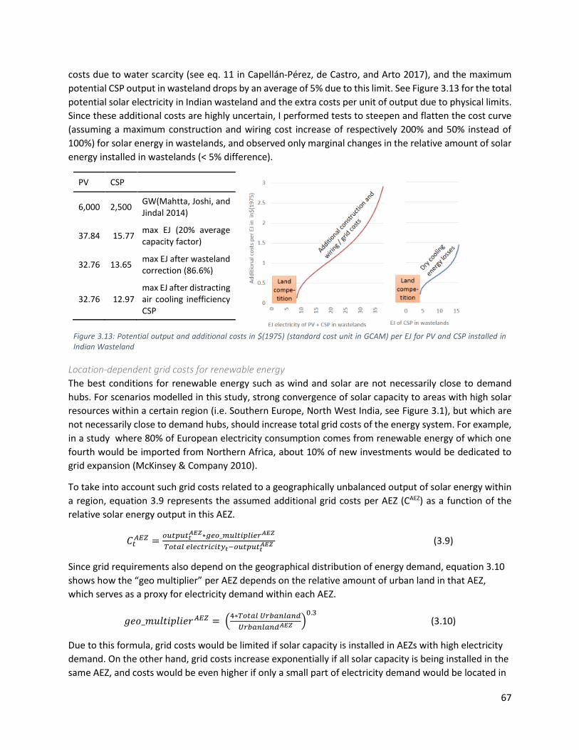
67
costs due to water scarcity (see eq. 11 in Capellán-Pérez, de Castro, and Arto 2017), and the maximum
potential CSP output in wasteland drops by an average of 5% due to this limit. See Figure 3.13 for the total
potential solar electricity in Indian wasteland and the extra costs per unit of output due to physical limits.
Since these additional costs are highly uncertain, I performed tests to steepen and flatten the cost curve
(assuming a maximum construction and wiring cost increase of respectively 200% and 50% instead of
100%) for solar energy in wastelands, and observed only marginal changes in the relative amount of solar
energy installed in wastelands (< 5% difference).
PV CSP
6,000 2,500 GW(Mahtta, Joshi, and Jindal 2014)
37.84 15.77 max EJ (20% average capacity factor)
32.76 13.65 max EJ after wasteland correction (86.6%)
32.76 12.97 max EJ after distracting air cooling inefficiency CSP
Figure 3.13: Potential output and additional costs in $(1975) (standard cost unit in GCAM) per EJ for PV and CSP installed in Indian Wasteland
Location-dependent grid costs for renewable energy
The best conditions for renewable energy such as wind and solar are not necessarily close to demand
hubs. For scenarios modelled in this study, strong convergence of solar capacity to areas with high solar
resources within a certain region (i.e. Southern Europe, North West India, see Figure 3.1), but which are
not necessarily close to demand hubs, should increase total grid costs of the energy system. For example,
in a study where 80% of European electricity consumption comes from renewable energy of which one
fourth would be imported from Northern Africa, about 10% of new investments would be dedicated to
grid expansion (McKinsey & Company 2010).
To take into account such grid costs related to a geographically unbalanced output of solar energy within
a region, equation 3.9 represents the assumed additional grid costs per AEZ (CAEZ) as a function of the
relative solar energy output in this AEZ.
𝐶𝑡𝐴𝐸𝑍 =
𝑜𝑢𝑡𝑝𝑢𝑡𝑡𝐴𝐸𝑍∗𝑔𝑒𝑜_𝑚𝑢𝑙𝑡𝑖𝑝𝑙𝑖𝑒𝑟𝐴𝐸𝑍
𝑇𝑜𝑡𝑎𝑙 𝑒𝑙𝑒𝑐𝑡𝑟𝑖𝑐𝑖𝑡𝑦𝑡−𝑜𝑢𝑡𝑝𝑢𝑡𝑡𝐴𝐸𝑍 (3.9)
Since grid requirements also depend on the geographical distribution of energy demand, equation 3.10
shows how the “geo multiplier” per AEZ depends on the relative amount of urban land in that AEZ,
which serves as a proxy for electricity demand within each AEZ.
𝑔𝑒𝑜_𝑚𝑢𝑙𝑡𝑖𝑝𝑙𝑖𝑒𝑟𝐴𝐸𝑍 = (4∗𝑇𝑜𝑡𝑎𝑙 𝑈𝑟𝑏𝑎𝑛𝑙𝑎𝑛𝑑
𝑈𝑟𝑏𝑎𝑛𝑙𝑎𝑛𝑑𝐴𝐸𝑍 )0.3
(3.10)
Due to this formula, grid costs would be limited if solar capacity is installed in AEZs with high electricity
demand. On the other hand, grid costs increase exponentially if all solar capacity is being installed in the
same AEZ, and costs would be even higher if only a small part of electricity demand would be located in

68
this AEZ. Costs are calibrated such that total grid costs at high penetration scenarios in the EU represent
about 5% of the total LCOE with a balanced geographical distribution of solar energy generation and up
to 15% with an unbalanced geographical distribution of solar energy (i.e., all solar energy installed in the
AEZ 8 and 9; see part A of Figure 3.2). These assumptions are expanded to India, Japan and South-Korea.
Management of RES variability in GCAM
At high penetration rates of intermittent energy sources such as wind and solar in the electricity system,
storage or back-up systems are required to meet electricity demand at all hours. Therefore, GCAM
assumes increasing back-up requirements with intermittent energy penetration. The cost of a backup
technology is modelled on a gas turbine with a 5% capacity factor. To avoid back-up costs, solar and wind
energy can be combined with on-site capital-intensive storage systems (i.e., electric batteries; Wise et al.
2010).
Both back-up and storage systems increase the total land requirements for solar energy. In the case of
back-up systems, total electricity production increases for the same level of final electricity demand, which
means that more solar energy has to be installed to reach a certain penetration level, and consequently
more land is required to host the additional solar energy. For example, with a target of 80% solar in the
electricity mix with 10 EJ electricity demand, 8 EJ solar would be produced. However, given that gas
backup increases total required electricity production by 0.4 EJ (5%), a total of 8.32 EJ of solar would be
required to actually reach 80% of total electricity production, ultimately increasing the land requirements
for solar energy. Storage systems suffer full-cycle efficiency losses. Therefore, more solar capacity is
required to make up for these losses, hence increasing land use. To take these losses into account, a 15%
lower land use efficiency for solar energy with storage has been assumed (based on a 75% average round-
trip efficiency of storage systems and 60% of solar electricity being stored; Paul Denholm and Margolis
2008).
Trade in bio-energy
While GCAM assumes a global market for bio-energy by default, domestic and imported resources have
been separated for the purpose of this study. Although it makes economic sense in various occasions to
trade bio-energy resources over large distances due to large differences in production costs, the transport
costs for imported biomass are on average higher than for regionally produced bio-energy (Hamelinck,
Suurs, and Faaij 2005). In order to control the origin of biomass production and to represent the bio-
energy market more realistically, domestic bio-energy production has been separated in the three focus
markets (EU-27, India, Japan + South-Korea). Following Hamelinck et al (2005), transport costs of imported
bio-energy are set to 3.15 $(2015) per GJ and are 33% higher than transport costs for domestically
produced bio-energy ($2.36 per GJ), while keeping average transport costs of total bio-energy
consumption in 2010 equal to other regions and as assumed by default ($2.63 per GJ). This change is
predominantly important for those scenarios where bio-energy technologies are modelled as the
dominant renewable energy technology (See Scenarios section of this chapter).
69
Identifying optimal
technological portfolios for
European electricity generation
towards climate change
mitigation

70

71
Introduction The EU has set a long-term goal of reducing greenhouse gas (GHG) emissions by 80-95%, when compared
to 1990 levels, by 2050. Towards achieving this target, the Commission has published an Energy Roadmap
for 2050 to explore cost-efficient ways to make the European economy more climate-friendly and less
energy-consuming, while also increasing competitiveness and security of supply (European Commission
2016a). One quarter of global GHG emissions was caused by fossil fuel combustion in power plants, while
in Europe emissions of fuel combustion by energy industries amounted to 28.2% of total GHG emissions
(Janssens-Maenhout et al. 2017). Decarbonising electricity generation is therefore crucial to the efforts
towards climate change mitigation (Arvesen et al. 2018) and has the potential to almost totally eliminate
CO2 emissions by 2050, by exploiting renewable energy sources (e.g. solar, wind, biomass, etc.), using
other low-emission alternatives like nuclear power plants, or maturing and diffusing carbon capture and
storage (CCS) technologies in fossil fuel power stations (European Commission 2016b).
On the basis of the above, the need to secure support for coordinated environmental, climate, and energy
planning emerges. Particularly, the process of designing technological mixes for electricity generation
takes on special significance in the context of energy and environmental planning. In this process, cost-
related parameters are first examined; however, other characteristics must also be taken into
consideration, including the level of dependence on imported resources; the corresponding energy
security and efficiency of the territory; and the social and environmental impact that the use of the
available technologies might entail (Valentine 2011). Thus, energy planning facilitates the long-term
design of the electricity generation mix that best reconciles security of supply, sustainability (economic,
social and environmental) and competitiveness (Hickey, Lon Carlson, and Loomis 2010). What is also
important is the diverse nature and uncertain potential of energy technologies that currently are or may
later be available to mitigate GHG emissions (Pugh et al. 2011). The long service life of power generation
assets and the high level of uncertainty, both stemming from the horizon subject to analysis, strongly
impact the different variables of the selection problem, which are a synthesis of technological, economic,
regulatory and environmental variables (deLlano-Paz et al. 2017). This further poses a challenge to
policymakers trying to invest funds in an optimal electricity generation portfolio (Pugh et al. 2011).
Typically, integrated assessment modelling can prove very valuable to meeting the challenges of
sustainability (Jakeman and Letcher 2003) and give fruitful insights in the tradeoffs and synergies among
policy goals; support the identification of important cross-sector interactions; and to some extent
consider uncertainty, in factors such as population and economic growth, technology development,
human behavior, and climate change (Shi et al. 2017). Furthermore, IAMs typically treat uncertainty
deterministically, i.e. by means of scenarios (Nikas, Doukas, and Papandreou 2019); Jakeman and Letcher
(2003) recognise the need for improved techniques of uncertainty and sensitivity analysis as a central
challenge in the use of IAMs. Last but not least, climate-economy modelling by means of IAMs typically
excludes policymakers and other stakeholder groups or, limits their participation to the extent of partly
formulating the assumptions, by which modelling simulations are driven (van Vliet, Kok, and Veldkamp
2010).
As a valuable tool in the management of such complex environmental and energy problems (Uusitalo et
al. 2015), decision support systems have the potential to effectively summarise and bring together
various, distinct consequences related to alternative planning options (Doukas 2013). As the recent
literature suggests, a broadly established approach to meeting the challenges associated with the

72
definition of energy plans for a certain territory or region can be found in Modern Portfolio Theory (MPT).
Typically, the portfolio approach is based on the solution of problems with one objective function seeking
to minimise either the cost or the risk of the portfolio, subject to different constraints, also considering
that real electricity generation assets can be defined in terms of cost or return and economic risk, for each
alternative technology (deLlano-Paz et al. 2017). The most exhaustive and complete reviews on the
application of MPT in energy planning are found in the studies of Delarue et al. (2011) and Jano-Ito and
Crawford-Brown (2017).
It is noteworthy that, given that problems of this particular domain are subject to numerous objectives
and criteria, the existence of a single optimal solution leading to one particular course of action, upon
which the decision maker has no influence, is rarely achieved or meaningful. A solution to this challenge
lies in the identification of a Pareto set of optimal solutions (Hamilton et al. 2015). Reaching a set of near-
optimal solutions provides a much more fruitful input into the decision making process (Lempert et al.
2016), and is easier to explain than any other practical recommendation. Such analysis is crucial as it can
provide a measure of confidence in the ability to differentiate between different decisions (Jakeman and
Letcher 2003; Weyant 2017). Portfolio analysis is commonly employed in applications with multiple
objectives and widely supports stochastic treatment of uncertainty.
In this study, a link between GCAM and Portfolio Analysis is developed, providing more fruitful and robust
policy recommendations. Baker and Solak (2011) have previously used modelling results from the
Dynamic Integrated Climate-Economy (DICE) model and MiniCAM (older version of the GCAM model)
IAMs in a stochastic optimisation-oriented PA; while Pugh et al. (2011) aggregated different technological
scenarios from the GCAM model into one specific scenario and built a Ranked ROI-oriented optimal R&D
electricity generation portfolio. The present study, however, utilises GCAM outputs to evaluate electricity
generation technologies by simultaneously considering two optimisation criteria, namely maximisation of
CO2 reduction and energy security, and deals with stochastic uncertainty instead of discrete scenarios to
obtain robust optimal technological portfolios.
Method Both GCAM and Robust Portfolio Analysis have certain concrete advantages in supporting decision making
in environmental and energy planning as well as climate policy. This study makes an endeavor to
synthesise these models in an integrated approach and provide stakeholders with a fully featured, robust
decision support framework. The first step features the formulation of the Portfolio Analysis model, in the
aim of providing a set of optimal alternatives (Pareto set), instead of one optimal solution, which is rarely
the case in this problem domain. To formulate the bi-objective problem, suitable objective functions
(optimisation criteria) and constraints must be first defined. The second step requires the application of
the GCAM model in order to extract key quantitative information on the climate-energy bi-objective
problem to be solved. The outputs of the IAM can be inserted as parameters in the bi-objective model
(e.g. as objective function coefficients, constraints, etc.). In the next step, the optimisation process is
enhanced with robustness features. The selected method of multi–objective modelling, namely the
AUGMECON2 method, supports incorporation of stochastic uncertainty by appropriately applying Monte
Carlo simulation and the ITA technique. Finally, these three discrete steps lead to a specific, well-defined
set of robust optimal portfolios. This kind of information is highly important for decision makers when

73
selecting technological portfolios that feature a high degree of uncertainty regarding their Pareto
optimality. The proposed approach is summarised in concrete steps in the Figure 4.1.
Figure 4.1: Proposed approach steps
Step 1: Problem formulation This study suggests an integrated approach to evaluate the performance of electricity generation
technologies on an EU-27 level and in a timescale until 2050. To achieve this, a bi-objective programming
mοdel for PA under uncertainty is utilised so that numerical results provided by the GCAM model can be
appropriately aggregated.
The analysis particularly focuses on six low-carbon generation technologies (𝑖 = 1 … 6), namely T1: solar
PV, T2: solar CSP, T3: wind, T4: nuclear, T5: biomass and T6: CCS. The focus is on these six technologies as
they are highly relevant for subsidisation in the near future towards reducing CO2 emissions at the EU
level. Furthermore, geothermal or other technologies with smaller potential, however relevant, are not
included to avoid complicating the portfolio analysis. See Table 4.1 for a list of what is exactly subsidised
under each technology pathway T.
Table 4.1: technologies included in each subsidy pathway for the EU electricity sector
PV CSP Wind Nuclear Biomass CCS - PV - PV with storage
- CSP - CSP with storage
- Onshore wind - Onshore wind with storage
- Third generation nuclear plants
- Conventional - Bio-gasification - Combined heat and power
Additional CCS costs of Coal, Biomass, Gas and Oil power plants
Input from the GCAM model provides ten different subsidy values (𝑗 = 1 … 10), calculated as a
multiplication of the unitary subsidies ($/GJ of electricity output, from 10 to 100% of the LCOE in 2010)
with the electricity consumption of the analysed technology in 2050. As the short-term impact of policies

74
promoting new technologies is considerably reduced by the rigidity of the electricity system, the robust
portfolio analysis is applied in the results for 2050 so that the effects of the technologies can be clearly
visible.
The problem is solved according to two optimisation criteria. The first objective function seeks to
maximise the reduction of GHG emissions corresponding to specific budget investment:
𝑚𝑎𝑥𝑖𝑚𝑖𝑠𝑒 𝑍2 = ∑ ∑ 𝐺𝐻𝐺𝑟𝑒𝑑𝑢𝑐𝑡𝑖𝑜𝑛(𝑖, 𝑗) ∗ 𝐵(𝑖, 𝑗)
10
𝑗=1
6
𝑖=1
Where 𝐺𝐻𝐺𝑟𝑒𝑑𝑢𝑐𝑡𝑖𝑜𝑛(𝑖, 𝑗) is the emissions reduction achieved by the 𝑖th technology under budget
option 𝑗.
The second objective is to maximise the system’s energy security again in relation to the allocated budget.
𝑚𝑎𝑥𝑖𝑚𝑖𝑠𝑒 𝑍1 = ∑ ∑ 𝑆𝑒𝑐𝑢𝑟𝑖𝑡𝑦 (𝑖, 𝑗) ∗ 𝐵(𝑖, 𝑗)
10
𝑗=1
6
𝑖=1
Where 𝑆𝑒𝑐𝑢𝑟𝑖𝑡𝑦 (𝑖, 𝑗) is the contribution to energy security of technology 𝑖 under budget option 𝑗.
The objective functions’ coefficients, namely emissions reduction (𝐺𝐻𝐺𝑟𝑒𝑑𝑢𝑐𝑡𝑖𝑜𝑛(𝑖, 𝑗)) and energy
security (𝑆𝑒𝑐𝑢𝑟𝑖𝑡𝑦 (𝑖, 𝑗)) are collected as an outcome of the GCAM model. The decision variables of the
model are binary. The binary variables 𝐵𝑖, 𝑗 represent the existence of the “𝑖 technology and 𝑗 subsidy”
options corresponding to the specific technology selection ((𝐵𝑖, 𝑗 = 1) or not (𝐵𝑖, 𝑗 = 0)).
The model also incorporates five specific constraints.
1. First of all, a budget constraint is used in order to secure that the cumulative cost of approved
applications does not exceed a previously defined, overall budget.
∑ ∑ 𝑆𝑢𝑏𝑠𝑖𝑑𝑦 (𝑖, 𝑗) ∗ 𝐵(𝑖, 𝑗) ≤ 𝑚𝑎𝑥𝐵𝑢𝑑𝑔𝑒𝑡
10
𝑗=1
6
𝑖=1
Where 𝑚𝑎𝑥𝐵𝑢𝑑𝑔𝑒𝑡 is the total available budget and 𝑆𝑢𝑏𝑠𝑖𝑑𝑦 (𝑖, 𝑗) the 𝑗th cost option of
technology 𝑖. In the specific application, the available budget is set equal to 35% of the maximum
cost of all six technologies.
2. This application also defines a minimum bound of emissions reduction to be achieved by the
portfolio.
∑ ∑ 𝐺𝐻𝐺𝑟𝑒𝑑𝑢𝑐𝑡𝑖𝑜𝑛 (𝑖, 𝑗) ∗ 𝐵(𝑖, 𝑗) ≥ 𝑚𝑖𝑛𝐸𝑚𝑖𝑠𝑠𝑖𝑜𝑛𝑠
10
𝑗=1
6
𝑖=1
Where 𝑚𝑖𝑛𝐸𝑚𝑖𝑠𝑠𝑖𝑜𝑛𝑠 is the minimum required reduction of GHG emissions and
𝐺𝐻𝐺𝑟𝑒𝑑𝑢𝑐𝑡𝑖𝑜𝑛 (𝑖, 𝑗) the emissions reduction when selecting the 𝑗th cost option of technology 𝑖.

75
The emission reduction target is set equal to 40% of the emissions reduction that would be
achieved if all technologies were subsidised at 100% of their total cost.
3. Specific bounds are imposed to control the distribution of budget across the energy generation
technologies, and with a focus on specific energy sources. In particular, it is considered preferable
that nuclear projects do not dominate a portfolio, due to a lack of public support in several
countries in the EU. This condition is expressed with the following constraint, defined as “nuclear
energy is not allowed to be receive more than 30% of the total available budget”:
𝑆𝑢𝑏𝑠𝑖𝑑𝑦(𝑁𝑢𝑐𝑙𝑒𝑎𝑟, 𝑗) ∗ 𝐵(𝑁𝑢𝑐𝑙𝑒𝑎𝑟, 𝑗) < 0.3 ∗ 𝑚𝑎𝑥𝐵𝑢𝑑𝑔𝑒𝑡, ∀ 𝑗 = 1 … 10
4. The next constraint allows for the determination of specific energy technology preferences.
Through this particular constraint wind and photovoltaic energy are preferred as dominant
technological sources, and the allocation of budget in such generation technologies “must thus
collectively equal to more than 40% of the total available budget”.
𝑆𝑢𝑏𝑠𝑖𝑑𝑦(𝑃𝑉, 𝑗) ∗ 𝐵(𝑃𝑉, 𝑗) + 𝑆𝑢𝑏𝑠𝑖𝑑𝑦(𝑤𝑖𝑛𝑑, 𝑗) ∗ 𝐵(𝑤𝑖𝑛𝑑, 𝑗) ≥ 0.4 𝑚𝑎𝑥𝐵𝑢𝑑𝑔𝑒𝑡, ∀ 𝑗 = 1 … 10
5. In order to assure that only one budget option is allocated per technology, the following
constraint is added.
∑ 𝐵(𝑖, 𝑗)
10
𝑗=1
≤ 1, ∀ 𝑖 = 1 … 6
The constraint guarantees that, in the case of purchasing a new technology with a certain amount
of budget, purchasing the same technology with another amount of budget is not possible.
Table 4.2: Overview of problem definition
Decision Variables Description
𝑩𝒊, 𝒋
If 𝐵𝑖, 𝑗 =1 the pair “𝑖 technology and 𝑗
subsidy” is approved.
Otherwise if 𝐵𝑖, 𝑗 =0 the corresponding
technology-subsidy pair is rejected.
Objective Functions Description
𝒎𝒂𝒙𝒊𝒎𝒊𝒔𝒆 𝒁𝟏 maximise the reduction of GHG emissions
corresponding to specific subsidy
𝒎𝒂𝒙𝒊𝒎𝒊𝒔𝒆 𝒁𝟐 maximise the system’s energy security
corresponding to specific subsidy
Constraints Description
Budget constraint Overall implementation cost must be less
than 35% of maximum (i.e. if all technologies
were subsidised at 100%).
Emissions reduction target Overall emissions reduction must be greater
than 40% of maximum (i.e. if all technologies
were subsidised at 100%).

76
Nuclear constraint Participation of Nuclear power cannot be
greater than 30%.
Wind and PV dominance More than 40% of the total available budget
must be allocated to wind and PV energy.
Unique subsidy constraint One budget option can be allocated per
technology.
Step 2: Input data (GCAM scenarios) From each subsidy scenario, the following outcomes are abstracted for the year 2050:
- Sum of total subsidies spent
- EU-wide CO2 reduction compared to baseline scenario
- EU-wide increase in energy security, here defined as energy self-sufficiency: 𝐸𝑛𝑒𝑟𝑔𝑦 𝑝𝑟𝑜𝑑𝑢𝑐𝑡𝑖𝑜𝑛 𝑤𝑖𝑡ℎ𝑖𝑛 𝐸𝑈
𝐸𝑛𝑒𝑟𝑔𝑦 𝑐𝑜𝑛𝑠𝑢𝑚𝑝𝑡𝑖𝑜𝑛 𝑤𝑖𝑡ℎ𝑖𝑛 𝐸𝑈
For calculating the subsidy, the unitary subsidies ($/energy unit, from 10 to 100% of the energy technology
Levelised Cost of Energy - LCOE) are multiplied with electricity consumption of the examined technology
in 2050. LCOE is calculated from a mixed set of data on capital and maintenance costs, efficiency, capacity
factors, etc. The modelling assumptions used in this chapter are documented in Muratori et al. (2017).
From these outputs, the cost effectiveness for reducing emissions and improving energy security can be
expressed, which are the key drivers for technologies to be on the Pareto front. Figure 4.2 shows the
GCAM outputs in terms of cost-effectiveness for emission reductions and energy security. In terms of
emission reductions, biomass and CCS technologies are most cost-effective up to around 100 billion dollar
of subsidies, and are then bypassed by nuclear and wind technologies. PV and CSP are less cost-effective
in reducing emissions by baseline GCAM assumptions. In terms of energy security, both CCS and biomass
have a negative impact on energy security in the EU, as the inputs for those technologies will be for a large
part imported from outside the region. Instead, all other technologies contribute positively to energy
security, and nuclear and wind technologies are again more cost-effective than PV and CSP.
Figure 4.2: Cost effectiveness of electricity technology subsidies in 2050 in terms of emission reductions and energy security
Step 3: Uncertainty Management and Robustness Assessment After selecting the input data the PA model as described in Step 1 is run, resulting in a set of optimal
portfolios, i.e. the Pareto Front, the robustness of which is assessed through the iterative trichotomic
approach (ITA; Mavrotas and Pechak 2013) in this step.

77
The uncertainty characterising the estimation of technology performance, in reducing GHG emissions as
well as contributing to energy security, is expressed by introducing normal distributions for relevant
technologies’ values. Specifically, the mean value for the normal distributions is set equal to the estimated
values as obtained from the runs of the GCAM model, and the standard deviation of the iterations equal
to 5%, 4%, 3%, 2%, 1%, and 0% corresponding to six ITA rounds. The whole process (model building,
random sampling, Pareto set generation) is implemented within the GAMS platform. 1,000 Monte Carlo
iterations are performed for each ITA computation round. It must be noted that, in the specific
application, a 94% acceptance threshold for the green set is determined (if a portfolio is present in 94%
of Pareto sets i.e. in 940 out of 1,000).
The results of multi-objective ITA are shown in Table 4.3. There are in total 842 POPs that participate in
1,000 Pareto sets of the initial round. At subsequent iterations, the standard deviation of sampling
distributions is reduced as shown in the first column of Table 4.3. Eventually, on the last round the final
Pareto set is obtained; this comprises 16 POPs of R&D electricity generation technologies. The additional
information that ITA gives is that it reveals which of these 16 portfolios can be considered more certain
than others. The degree of certainty for each portfolio is directly related to the corresponding round that
it enters the green set (the earlier the portfolio enters the green set, the more certain the decision maker
can be about its Pareto optimality).
Table 4.3: ITA results
Green Red Grey
𝝈 = 𝟓% Round 1 0 0 842
𝝈 = 𝟒% Round 2 0 321 521
𝝈 = 𝟑% Round 3 1 546 295
𝝈 = 𝟐% Round 4 2 704 136
𝝈 = 𝟏% Round 5 3 779 60
𝝈 = 𝟎% Round 6 16 826 0
Results The 16 POPs that survived the ITA check for robustness are drawn in Figure 4.3, representing the robust
Pareto front of this optimisation problem. The size of the bubbles represents the robustness levels,
identified by the round in which this POP appeared in the green set (Table 4.3). POP A represents the most
robust set, while also representing an “optimal” package of simultaneous contribution to emission
reductions and energy security. POP B is the second-most-robust set, and the best choice if focusing more
on emission reductions, while POP C is a less robust set, but the best choice if focusing more on energy
security. For these three POPs, Table 4.4 shows the distribution of the subsidy budget over the different
technologies, as well as the contribution of each technology to emissions reductions and energy security
improvements. This table shows that under the constraints of this portfolio analysis, and with a subsidy
budget of nearly 3 trillion $(2015), this budget will be predominantly spent on PV, while wind and nuclear
contribute most to emission reductions and energy security. The contribution of biomass and CCS
technologies in such a package depend largely on the importance of energy security from the perspective
of the policymaker. Note that, at a lower budget, these portfolios will change and predominantly the less
cost-effective technologies, such as PV and CSP, will lose their share of the total budget.
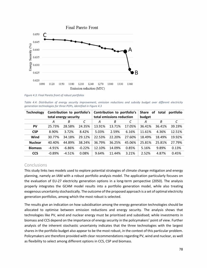
78
Figure 4.3: Final Pareto front of robust portfolios
Table 4.4: Distribution of energy security improvement, emission reductions and subsidy budget over different electricity generation technologies for three POPs, identified in Figure 4.3
Technology Contribution to portfolio’s total energy security
Contribution to portfolio’s total emissions reduction
Share of total portfolio budget
A B C A B C A B C
PV 25.73% 28.58% 24.35% 13.91% 13.71% 17.05% 36.41% 36.41% 39.19%
CSP 8.90% 3.72% 8.42% 5.03% 2.59% 6.16% 11.61% 4.36% 12.51%
Wind 30.77% 34.18% 29.12% 22.53% 22.20% 27.60% 18.49% 18.49% 19.92%
Nuclear 40.40% 44.89% 38.24% 36.79% 36.25% 45.06% 25.81% 25.81% 27.79%
Biomass -4.91% -6.86% -0.22% 12.10% 14.09% 0.85% 5.16% 9.89% 0.13%
CCS -0.89% -4.51% 0.08% 9.64% 11.44% 3.21% 2.52% 4.87% 0.45%
Conclusions This study links two models used to explore potential strategies of climate change mitigation and energy
planning, namely an IAM with a robust portfolio analysis model. The application particularly focuses on
the evaluation of EU-27 electricity generation options in a long-term perspective (2050). The analysis
properly integrates the GCAM model results into a portfolio generation model, while also treating
exogenous uncertainty stochastically. The outcome of the proposed approach is a set of optimal electricity
generation portfolios, among which the most robust is selected.
The results give an indication on how subsidisation among the energy generation technologies should be
allocated to optimise between emission reductions and energy security. The analysis shows that
technologies like PV, wind and nuclear energy must be prioritised and subsidised; while investments in
biomass and CCS depend on the importance of energy security in the policymakers’ point of view. Further
analysis of the inherent stochastic uncertainty indicates that the three technologies with the largest
shares in the portfolio budget also appear to be the most robust, in the context of this particular problem.
Policymakers are therefore provided with clear recommendations regarding PV, wind and nuclear, as well
as flexibility to select among different options in CCS, CSP and biomass.

79
It is important to note that the calculated outputs of this analysis are strongly dependent on the modelling
assumptions; the results should be carefully interpreted, while taking into consideration the assumptions
outlined and referred to in the “Input Data” section. For instance, introducing other power generation
options, or applying a different budget, could have an impact on the resulting subsidisation portfolios and
therefore constitute an interesting future direction of the proposed research.
Finally, it should be noted that by providing information on the level of certainty associated with resulting
policy options thereby maximising the robustness of the results and adding value for policymakers, the
latter are not actively involved in the study. There is huge potential in involving both policymakers and
other stakeholder groups in policy analysis, in order to understand the motives and strategies of all actors
relevant in the required transformations (Turnheim et al. 2015), as well as exploit their expertise to bridge
knowledge gaps and further reduce the various uncertainties in this domain (Nikas et al. 2017). In this
respect, it would be interesting to work with stakeholders and decision makers in climate action, by
expanding the method to some other regions and/or technologies, or eliminating any of the used ones;
as well as to better incorporate real-world context in the modelling assumptions, constraints and
parameters of the modelling exercise.

80

81
Integrated Policy Assessment
and Optimisation over Multiple
Sustainable Development Goals
in Eastern Africa

82
83
Introduction Heavy reliance on traditional biomass for household energy in developing countries has significant
negative health and environmental impacts (Masera et al. 2015), a problem that is especially acute in sub-
Saharan Africa (SSA). Household air pollution (HAP) from the use of solid cooking fuels is among the top
three environmental risk factors contributing to illness and death worldwide. In SSA, children under 5 die
at higher rates from HAP exposure than in any other world region (Forouzanfar et al. 2016). Meanwhile,
SSA hosts many woodfuel “hotspots”, where a large fraction of fuelwood and charcoal is harvested
unsustainably, contributing significantly to GHG emissions (Robert Bailis et al. 2015) and forest
degradation (Kiruki et al. 2017; Ndegwa et al. 2016). Moreover, with only around 20% of its population
having access to modern energy sources, energy access levels in SSA are lower than in any other region
(World Bank and IEA 2017).
All three problems—air pollution, GHG emissions and energy access—are recognised by the United
Nations in its 2030 Agenda for Sustainable Development, in which ambitious SDGs are proposed to solve
each of them by 2030 through SDG 3 (good health), SDG 7 (affordable and clean energy) and SDG 13
(climate action). Although focusing on improving access to modern energy sources is showed to help
progress in many other SDGs, including those on health and climate action (Nerini et al. 2017), countries
in SSA would have to achieve unprecedented rates of progress to obtain universal electricity access within
the coming decades (N. D. Rao and Pachauri 2017), as proposed in SDG 7. Instead, improving the efficiency
of biomass energy systems is a cost-effective alternative for reducing forest degradation and HAP in the
short term (Smeets, Johnson, and Ballard-Tremeer 2012; Nerini, Ray, and Boulkaid 2017).
This high dependence of rural communities in SSA on locally gathered energy sources, often with resulting
forest degradation and health problems, was no different in pre-industrial eras of currently developed
countries (Elias and Victor 2005). Over time, the energy systems of these countries went through a long
transition path with multiple radical and incremental innovations (Geels and Schot 2007), each innovation
bringing in energy service cost savings and/or quality improvements (Fouquet 2010). Leapfrogging of
modern technologies by technologically poor countries is a well-known concept. Technologies without
long supply chains or network infrastructure are more likely to be adopted via leapfrogging in developing
countries (Tukker 2005; Szabó et al. 2013). The African context for energy access is rather different from
historical experiences elsewhere as challenges in achieving energy access and installing energy
infrastructure have coincided with major climate ambitions and climate impacts (Agbemabiese and
Nkomo 2012). Furthermore, increasing reliance on charcoal in SSA may impose significant ecological
constraints unless overall dependence on traditional biomass is reduced in favour of modern energy
sources and services (Santos et al. 2017). Consequently, innovative frameworks are needed that can
reconcile energy access, health and climate ambitions along a feasible but nevertheless ambitious
timeframe.
In regions where the lack of access to modern energy sources and consequential high dependence on
unsustainably harvested traditional biomass are major causes of GHG emissions and premature mortality,
land policies and technology subsidies will likely constitute effective policy instruments for sustainable
development. The GCF has been founded to fund such initiatives in developing countries, which are often
cost-effective in mitigating GHG emissions, but which would not be exercised due to a lack of financial
means. Due to a combination of demographic and climate conditions, eastern Africa is a hotspot for

84
unsustainable biomass harvesting (Robert Bailis et al. 2015). Exploring synergies of climate action with
other SDGs and analysing uncertainty of policy prescriptions are key to effective climate policy and
research (Doukas et al. 2018). This study therefore uses GCAM to simulate the impact of land policies and
technology subsidies, as well as the interaction of both, on GHG emissions, exposure to air pollution and
energy access in Eastern Africa under a range of socioeconomic pathways. Subsequently, a robust
portfolio analysis is further applied to optimally allocate a subsidy budget over different technologies to
simultaneously tackle these three interrelated problems.
Figure 5.1: Visualisation of the three-dimensional challenge for Eastern Africa (in every panel surrounded by green boundary), with (A) the share of population that lacks access to modern cooking fuels in 2015 (IEA 2017a); (B) the death rate from indoor air pollution per 100,000 people in 2015 (Forouzanfar et al. 2016); and (C) the non-renewable biomass (NRB) fraction of fuelwood production in 2009, assuming “normal” exploitation of the commercial surplus (Robert Bailis et al. 2015).
C
B
A
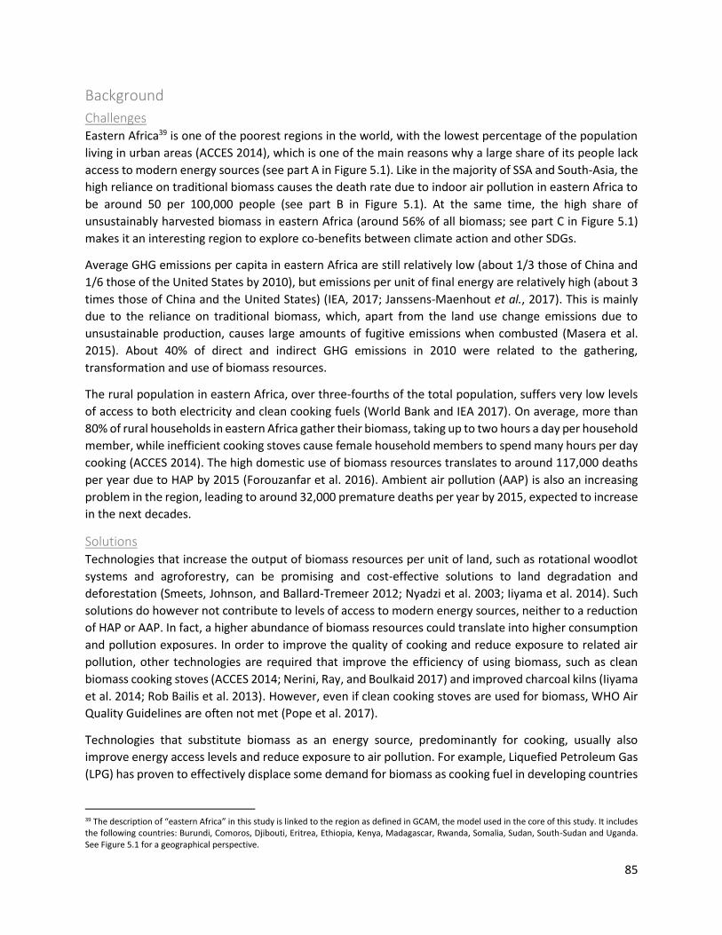
85
Background
Challenges Eastern Africa39 is one of the poorest regions in the world, with the lowest percentage of the population
living in urban areas (ACCES 2014), which is one of the main reasons why a large share of its people lack
access to modern energy sources (see part A in Figure 5.1). Like in the majority of SSA and South-Asia, the
high reliance on traditional biomass causes the death rate due to indoor air pollution in eastern Africa to
be around 50 per 100,000 people (see part B in Figure 5.1). At the same time, the high share of
unsustainably harvested biomass in eastern Africa (around 56% of all biomass; see part C in Figure 5.1)
makes it an interesting region to explore co-benefits between climate action and other SDGs.
Average GHG emissions per capita in eastern Africa are still relatively low (about 1/3 those of China and
1/6 those of the United States by 2010), but emissions per unit of final energy are relatively high (about 3
times those of China and the United States) (IEA, 2017; Janssens-Maenhout et al., 2017). This is mainly
due to the reliance on traditional biomass, which, apart from the land use change emissions due to
unsustainable production, causes large amounts of fugitive emissions when combusted (Masera et al.
2015). About 40% of direct and indirect GHG emissions in 2010 were related to the gathering,
transformation and use of biomass resources.
The rural population in eastern Africa, over three-fourths of the total population, suffers very low levels
of access to both electricity and clean cooking fuels (World Bank and IEA 2017). On average, more than
80% of rural households in eastern Africa gather their biomass, taking up to two hours a day per household
member, while inefficient cooking stoves cause female household members to spend many hours per day
cooking (ACCES 2014). The high domestic use of biomass resources translates to around 117,000 deaths
per year due to HAP by 2015 (Forouzanfar et al. 2016). Ambient air pollution (AAP) is also an increasing
problem in the region, leading to around 32,000 premature deaths per year by 2015, expected to increase
in the next decades.
Solutions Technologies that increase the output of biomass resources per unit of land, such as rotational woodlot
systems and agroforestry, can be promising and cost-effective solutions to land degradation and
deforestation (Smeets, Johnson, and Ballard-Tremeer 2012; Nyadzi et al. 2003; Iiyama et al. 2014). Such
solutions do however not contribute to levels of access to modern energy sources, neither to a reduction
of HAP or AAP. In fact, a higher abundance of biomass resources could translate into higher consumption
and pollution exposures. In order to improve the quality of cooking and reduce exposure to related air
pollution, other technologies are required that improve the efficiency of using biomass, such as clean
biomass cooking stoves (ACCES 2014; Nerini, Ray, and Boulkaid 2017) and improved charcoal kilns (Iiyama
et al. 2014; Rob Bailis et al. 2013). However, even if clean cooking stoves are used for biomass, WHO Air
Quality Guidelines are often not met (Pope et al. 2017).
Technologies that substitute biomass as an energy source, predominantly for cooking, usually also
improve energy access levels and reduce exposure to air pollution. For example, Liquefied Petroleum Gas
(LPG) has proven to effectively displace some demand for biomass as cooking fuel in developing countries
39 The description of “eastern Africa” in this study is linked to the region as defined in GCAM, the model used in the core of this study. It includes the following countries: Burundi, Comoros, Djibouti, Eritrea, Ethiopia, Kenya, Madagascar, Rwanda, Somalia, Sudan, South-Sudan and Uganda. See Figure 5.1 for a geographical perspective.

86
and contribute to net reductions in GHG emissions and HAP (Singh, Pachauri, and Zerriffi 2017; Bruce et
al. 2018). Ethanol cooking stoves have clear benefits for HAP as well, although GHG benefits depend on
the feedstock used to produce ethanol (Gopal and Kammen 2009), and examples for large-scale
implementation are limited (Benka-Coker et al. 2018; Mudombi et al. 2018b). Biogas has proven to be
successful in improving energy access, avoiding forest degradation and improving health (Gosens et al.
2013; Clemens et al. 2018), and is particularly interesting for rural households in eastern Africa as such
systems require local resources, predominantly animal manure (M.G. Mengistu et al. 2015; Gwavuya et
al. 2012). Electric cooking is the cleanest possible way of cooking, as no emissions are released in the
cooking process. Photovoltaics (PV) also reduce emissions related to electricity production to the very
minimum, and their flexibility allows for affordable electricity off the central grid (Mandelli et al. 2016).
While cooking on electricity is not common for off-grid households due to high voltage requirements
(World Bank 2015), rural PV and to a lesser extent biogas can improve energy access through many other
applications (Rahman et al. 2014; Dalla Longa et al. 2018; Szabó et al. 2011).
In the last decades, numerous projects have been developed to scale up the use of clean cooking stoves,
many of them depending on financial support (Quinn et al. 2018; Clemens et al. 2018; Usmani, Steele, and
Jeuland 2017) and in many cases funded by the GCF40. Subsidies for clean energy technologies can help
overcome barriers and improve households´ access to modern forms of energy, in support of sustainable
development (Töpfer 2017). While most of such projects succeed in increasing ownership of such stoves,
sustained use is not always guaranteed, with “stove stacking” as a result, often related to availability,
reliability, economic flexibility and cultural factors (Ruiz-Mercado and Masera 2015). With increasing
income, households seem to be willing to pay the additional cost for clean cooking options like ethanol
(Takama, Tsephel, and Johnson 2012); however, continued use, as compared to initial adoption, also
depends on factors such as reliability of fuel supply over time (Mudombi et al. 2018a).
Method The goal of this study is to estimate an optimal mix of technology and land policies to simultaneously
reduce GHG emission, reduce exposure to air pollution and improve energy access. In the core of this
analysis, GCAM is used to simulate future policy and socioeconomic scenarios for eastern Africa. Through
different methodologies, outputs from each policy scenario are translated to progress parameters that
are relevant to SDG objectives. These parameters are fed into a robust portfolio analysis that finds a mix
of policies that maximises progress in each of the SDGs in a Pareto-optimal way that is robust for a range
of socioeconomic pathways. Figure 5.2 gives an outline of the study design and the Method section.
40 https://www.greenclimate.fund/what-we-do/projects-programmes

87
Figure 5.2: Flowchart showing outline of study design and Method section
A. Scenario design Three different socioeconomic pathways have been considered, each with a scenario with and without
land policies, making up for six scenarios to assess the interactions of these two factors. On top of each of
these scenarios, six different technology pathways and 20 different subsidy levels have been modelled,
resulting in a total of 720 policy scenarios implemented in the model runs, to investigate the impact of
land policies and technology subsidies on GHG emissions, health, and energy access:
- 3 SSPs41 for each initial GCAM scenario:
o SSP2: A middle of the road pathway, based on historical patterns
o SSP3: A rocky road pathway, featuring high population, low GDP per capita, urbanisation,
crop yields, technological progress and pollution controls
o SSP5: A fossil-fuelled pathway, featuring low population, high GDP per capita,
urbanisation, crop yields, technological progress and pollution controls
- 2 initial GCAM scenarios:
o NO LAND POLICY: baseline without options to increase sustainable forest output
o LAND POLICY: scenario that includes educational policies, to be fully effective by 203042,
focusing on teaching forest and agricultural land owners how to increase the sustainable
supply of biomass by rotation forestry and agroforestry practices.
41 These SSPs were selected to include the widest range of possible scenarios, where SSP3 is seen as a lower extreme and SSP5 as a higher extreme to economic development. SSP projections were used for: population, income, urbanisation, supply and demand for both energy and agricultural commodities and emission factors. 42 This means that, by 2030, land owners are indifferent between applying and not applying these methods and are driven by profit maximisation. As such programs are assumed to take time, the program is assumed to be for 33% effective by 2020 and for 66% effective by 2025.

88
- 20 subsidy scenarios for 6 different technology pathways43, where technology costs are subsidised
in 5% steps until 100%44. See Table 5.8 in this chapter’s Annex for all assumed technologies, costs
and efficiencies of the technologies included in these pathways:
o LPG path: LPG stoves and fuel production costs
o PV path: electric stoves and PV projects (utility-scale, mini-grid and off-grid)
o Biogas path: Biogas digesters and burners
o Ethanol path: Ethanol stoves and fuel production costs
o Improved Charcoal path: Improved charcoal stoves and improved charcoal kilns
o Improved Fuelwood path: Improved fuelwood stoves and suitable woody biomass
feedstocks
If modelled on top of a land policy scenario, the charcoal and fuelwood technology subsidies are linked to
sustainable biomass inputs. In other words, as a condition for receiving subsidies for producing charcoal
with improved kilns, or producing woody biomass feedstocks suitable for improved cooking stoves,
production inputs have to come from sustainable woodlot or agroforestry systems.
In a next step, the policy outcomes in terms of progress on each of our three objectives are extracted for
the years 2020, 2030 and 2040 for a robust portfolio analysis. Two different annual subsidy budget
constraints are applied to this process:
- Low: starting from $ 3.5 billion (USD at 2015 values) in 2020 (~$11 per capita), increasing by 5%
per year, reaching $ 5.7 billion by 2030 (~$14 per capita) and $ 9.3 billion by 2040 (~$20 per
capita).
- High: starting from $ 10.5 billion in 2020 (~$32 per capita), increasing by 5% per year, reaching $
17.4 billion by 2030 (~$43 per capita) and $ 27.9 billion by 2040 (~$60 per capita).
Finally, an optimal subsidy portfolio is identified for each of these three timepoints, with and without a
land policy, and for each subsidy budget, adding up to a total of 12 subsidy portfolios. The robustness level
of each portfolio is measured by the extent to which the policy outcomes depend on socioeconomic
variables, summarised in the different SSPs.
B. Models and methods
GCAM adaptations
The geopolitical region of Eastern Africa has been adjusted for this study to better replicate the actual
situation. As with GCAM-China (Yu et al. 2014) and GCAM-India (Yu et al. 2017), urban energy demand
was separated from rural energy demand and specific residential energy demands, such as cooking,
lighting, refrigeration and TVs were separated from other residential energy uses. Furthermore, the
provision of centrally generated electricity to rural areas faces additional costs related to the required
extensions in transmission and distribution networks, while mini-grids have been added as an alternative
for rural energy demand. Mini-grid electricity can be generated by diesel engines, biogas installations,
solar PV or mini-hydro. Electricity can also be generated off-grid using solar energy with battery back-up.
Charcoal production has been separated from other industrial activities and uses fuelwood as an input,
43 Subsidies are modelled for technology pathways instead of individual stoves to avoid stove stacking, which undermines the cost effectiveness of financial support and is more challenging to model. 44 For all pathways, the subsidies cover all capital costs. Capital costs for fuels are calculated as the difference between the final consumer price and the price of required production inputs (for LPG, the price of crude oil is taken as the “input” price). Implicitly, subsidy policies for LPG and Ethanol will be rationed to avoid subsidised fuels to be used for transport.

89
with different potential kiln technologies, each with different capital costs, efficiency and other energy
inputs and outputs. Sustainable fuelwood supply was separated from unsustainable fuelwood supply.
Sustainable supply requires a large base of forested land but does not have a direct impact on land use
change emissions and can only increase if other land uses are replaced by forestry. Unsustainable
fuelwood supply needs existing forest land to be cut down and therefore causes land use change
emissions that are equal to the CO2 content of fuelwood45. Since the amount of untouched forest area in
Eastern Africa is limited, unsustainable supply is subject to a hard limit46. The supply of manure has been
linked to the animal sector. Manure is set as a secondary output from cattle, pigs, poultry, sheep and
goats and can be used for direct combustion (dung), for digesting to produce biogas or for non-energy
purposes. In half of the scenarios, land use policies are applied, in which more wood-productive rotation
forestry systems are included as an alternative for regular forestry as well as the possibility of agroforestry,
e.g. mixing trees in agricultural land (see Table 5.10 in Annex). See Table 5.8 in this chapter’s Annex for an
overview of all cost, efficiency and emission assumptions and references.
The choice function applied in GCAM fits very well to the eastern African context, as it avoids full
convergence to a single cost-effective technology for cooking or electricity generation by recognising the
diverse set of preferences within the region. The shareweights defining the residential energy mix for
cooking (
Table 5.11 in Annex) and the share of PV in off-grid generation (
Table 5.9 in Annex) have been calibrated for 2015 instead of 2010, to represent more recent preferences
and market structures. On top of the default GCAM structure, three measures have been applied to adapt
economic choice better to the reality in eastern Africa:
- Upfront investment costs of cooking stoves is one of the main barriers for the adoption of
improved cooking stoves in low-income households (Bensch, Grimm, and Peters 2015). This
barrier is taken into account by assuming income-dependent discount rates (DR) for cooking
stoves and electrical appliances, varying by time, between urban and rural consumers, and
between SSPs. The same income-to-DR curve is applied as in a similar exercise for India (Ekholm
et al. 2010), ranging up to 80% for rural households in 2010. For more costly and long lasting
technology such as PV and biogas systems, a market DR of 13% is applied, as literature shows that
the uptake of such systems depend largely on access to financial credit (Gujba et al. 2012; Mulu
Getachew Mengistu et al. 2016).
- From a consumer perspective, the time needed to obtain an energy source plays an important
role for cooking fuel preferences, apart from the price of the stove and the energy source. It is
important to take the relevance of time into account, as fuelwood gathering, nowadays the most
common way to obtain energy for cooking in Sub-Saharan Africa (ACCES 2014), will become less
preferred as income increases, holding everything else constant. Therefore, gathered fuelwood
for cooking purposes is separated from purchased fuelwood. The costs of gathered fuelwood are
defined by the value of the time spent on gathering, and an additional cost related to fuelwood
45 The IPCC estimate for a CO2 content of 110 kg per GJ of fuelwood has been used 46 Using FAO data, the total above-ground carbon stock in Eastern Africa was estimated to contain 2127 million tons of carbon. Dividing this by the carbon content of one exajoule (EJ) of fuelwood energy, 30 million tons of carbon (110 tons of CO2), it is assumed that total unsustainable fuelwood supply cannot surpass 71 EJ, which is equal to 45 years of consumption at 2009 levels (1.58 EJ of unsustainable fuelwood consumption; Bailis et al., 2015).

90
scarcity. The costs for purchased fuelwood (defined as Market fuelwood in Table 5.8) is defined
by the same scarcity component, on top of the observed retail price of fuelwood. The time costs
of fuelwood gathering has been calibrated for 2015 based on the estimated amount of households
gathering and purchasing their fuelwood, and is assumed to increase proportionally with average
GDP per capita in the region. Improved biomass cooking stoves often require smaller pieces of
wood, adding extra labour costs to users who gather their resources, while some stoves are
directly designed to use purchased wood briquettes or pellets. Due to these limitations to use
gathered wood for improved cooking stoves, only purchased wood is assumed to be suitable for
such cooking stoves.
- By default, GCAM does not take into account power requirements for energy consumption.
However, power and reliability constraints limit the potential of off-grid and (to a lesser extend)
mini-grid electricity for many household applications (Bhattacharyya 2012; World Bank 2015).
Therefore, a market called “power charge” is implemented into the Eastern Africa region in
GCAM, which comes as a secondary output of centralized grid electricity with a 1-to-1 ratio and
of mini-grid electricity with a 1-to-2 ratio. Power charge is then modelled as a secondary input for
electric cooking and air-conditioners with a 1-to-1 ratio and to refrigerators and “other
appliances” with a 1-to-2 ratio. Lighting and TVs do not require any power charge and thus are
assumed to be able to fully function with off-grid energy solutions (World Bank 2015).
Air pollution models
Household air pollution (HAP)
HAP is one of the most hazardous risk factors for households in developing countries, which still rely
significantly on solid fuels for residential use (mainly cooking). In absolute terms, never before did so many
people rely on solid fuels for residential uses as nowadays (3 billion; Bruce et al., 2015). The use of those
fuels inside household creates high levels of PM2.5, which result in demonstrated health impacts.
According to the World Health Organization (WHO), household air pollution driven premature deaths
would reach 3.8 million each year. Using data for India, Balakrishnan et al. (2013) created an econometric
model showing the variables that have a significant impact on exposure to HAP and the evaluation of the
affecting variables has also been recently reported by the WHO (WHO 2018).
However, there is not a common way to transform indoor emissions into PM2.5 concentration levels, which
makes it difficult to estimate the exposure inside a household, without data coming from empirical
studies. In this study, a soft direct link was created between indoor PM2.5 primary47 emissions and indoor
PM2.5 concentrations. First, the historical HAP deaths of East African countries (Forouzanfar et al. 2016)
are compared with the primary PM2.5 emissions from cooking (Bond et al. 2007). Combining these data, it
is possible to calculate the resulting premature deaths per unit of PM2.5 emissions. Since GBD database
provides a range of observed deaths instead of a single value (lower bound, median and upper bound),
deaths per unit of emission were calculated for the complete range. Nevertheless, during this study, the
median value has been used. However, when validating this procedure I realized that the correlation drops
around 1% per year between 2010 and 201548, so that same annual drop is applied to future projections.
Historical and assumed future coefficients are visible in Figure 5.3. Then, by applying the projected median
47 Primary PM2.5 emissions are approximated by adding up black carbon (BC) and organic carbon (OC) emissions 48 This decline can be attributed to features such as ventilation and the cooking location (Balakrishnan et al. 2013) or features as health care and household size that affect the impact of exposure to air pollution on pre-mature deaths.

91
coefficients to future PM2.5 indoor emissions (output of the GCAM model), future premature deaths are
directly estimated.
Figure 5.3: Historical (until 2015, dashed) and projected premature deaths per 1000 tons of indoor PM2.5 emissions by period. The lines represent the lower and upper bounds (in grey) and the median value (in blue).
One limitation of this methodology is that all of the secondary particles created from the emission of other
pollutants, such as SO2, are left out out of the study. However, consulted experts have pointed out that,
for analysing HAP, these secondary elements do not play a very significant role, while there are important
factors for ambient air pollution effects.
Ambient air pollution (AAP)
AAP derived from residential emissions has only been explored in a limited number of other studies (Chafe
et al. 2014), while recent literature has demonstrated that it is an important factor in some parts of the
World (Conibear et al. 2018). In this study, ambient air pollution is calculated for each region by
introducing the emission projections obtained from the GCAM model into the air quality TM5-FASST
model.
TM5-FASST is a source-receptor air quality model that reports the ambient air pollution related mortalities
from a defined emission set. To that end, the model calculates the PM2.5 and O3 concentration levels by
adding up the emissions of a wide range of pollutants and their inter-regional interactions. As this model
is divided into 56 regions and covers the entire world in 100x100 km grids, it is adequate to apply to
Eastern Africa. All the details and documentation about the model are provided by Van Dingenen et al.
(2018). In order to connect this model to the GCAM model, GCAM emissions have been re-allocated into
country level based on the IIASA RCP emission database, and then re-aggregated into TM5-FASST regions.
The detailed procedure can be found in Markandya et al. (2018).
Finally, the calculated mortalities for direct (indoor) and indirect (ambient) air pollution are added up to
estimate the total impact of each scenario on mortality, which can be seen as an indicator for overall
exposure to air pollution.
Robust Portfolio Analysis
In order to evaluate the impacts that different subsidy portfolios have on climate action, health and
energy access, a multi-objective optimisation framework based on the principles of portfolio analysis has
been used. Based on the cost effectiveness of technology subsidies for each of these three goals, the
0
50000
100000
150000
200000
250000
300000
350000
400000
1990 1995 2000 2005 2010 2015 2020 2025 2030 2035 2040 2045 2050
Pre
mat
ure
dea
ths
per
10
00
to
ns
of
ind
oo
r P
M2
.5 e
mis
sio
ns

92
optimisation identifies Pareto-optimal subsidy portfolios under a given subsidy budget, and the
robustness of each portfolio to a wide range of variables in the GCAM model. Key parts on the proposed
methodology are explained in the Method section of chapter 1.
Portfolio Analysis Optimisation
Here, a tri–objective optimisation problem is modelled, since this study optimises over three evaluation
criteria or objectives:
1) Maximisation of GHG emission reductions
2) Maximisation of avoided premature deaths
3) Maximisation of energy access tier change
To optimise certain subsidy budgets over six different technologies, twelve optimisation problems are
solved, outlined in the Scenarios section (A).
The input datasets used for the portfolio analysis come from GCAM. These datasets provide information
on the contribution of each technology to each of the objective functions under twenty (20) different
subsidy values. The GCAM modelling exercise is based on the SSP datasets to find the margins of
uncertainty around policy effectiveness, which are used for the stress test analysis. In the context of
eastern Africa, SSP3 and SSP5 can be seen as extreme scenarios of respectively low and high development,
and are expected to represent the margins of uncertainty for policy implementation, although in a few
situations, the average conditions as represented in SSP2 translate to highest or lowest cost-effectiveness.
The results for SSP1 and SSP4 are expected to lie in most cases within the margins of the three modelled
SSPs, and these SSPs have therefore not been run explicitly.
For the portfolio analysis, in particular, the midpoint of the ranges of the three SSP modelling outcomes
is used. The outcome of each of the twelve portfolio analysis optimisation runs constitutes a Pareto Front
of optimal energy portfolios. Each portfolio is a set of energy technologies, among which different
subsidisation levels are distributed, corresponding to different contribution to the optimisation criteria.
Information on how each technology participates in the portfolios in terms of subsidy, GHG emissions
reduction, energy access and pollution-related mortality reduction can be easily extracted from the
portfolio analysis.
Robustness Analysis
The proposed approach effectively assesses the robustness of the resulting optimal portfolios, by
examining the effects of both deterministic and stochastic (non–deterministic) uncertainty.
Deterministic uncertainty is assumed by means of scenario analysis: different scenarios have been
analysed in terms of technology performance in each of the abovementioned parameters, but also in
terms of the maximum budget that can be granted to support these technologies. Regarding stochastic
uncertainty, which is inherent in these parameters, this is incorporated into the model through a Monte
Carlo simulation. At first, the “no uncertainty” Pareto Front is determined, referring to the set of portfolios
that are obtained after the execution of the model, using deterministic values for all of the uncertain
parameters. Then, Monte Carlo simulation is performed iteratively to sample random values for the
uncertain parameters from the uniform distributions, and the model is then solved to generate the set of
Pareto optimal portfolios. Eventually, the execution of multiple Monte Carlo iterations results in a large

93
number of differentiated Pareto fronts, which are analysed to draw conclusions over the robustness of
the portfolios consisting the Pareto front when no uncertainty is considered. In this analysis, 1,000 Monte
Carlo iterations are performed, and the robustness score of each portfolio is defined by the number of
Monte Carlo runs in which this portfolio appears on the Pareto front.
As stated above the GCAM model is run for the three SSP scenarios separately for every subsidy level. The
SSPs are seen here as an uncertain set of conditions that affect the performance of every technological
subsidy policy. The purpose of the robust portfolio analysis is to define robust subsidy portfolios for any
of the SSPs 2, 3 and 5 that might be valid in the future. In this way, the range of the SSP simulation
outcomes, which are different for each technology, define the ranges of the uniform distribution. An
example of how the range of the three SSP outcomes affects the uncertainty boundaries of a certain
technology is given in Table 5.1. The uncertainty ranges differ among the technologies. As it is clearly
indicated in the table, the higher the range of the SSP outcomes is, the wider the range of uncertainty in
the uniform distribution is considered. A portfolio analysis problem, in which technologies with narrow
uncertainty boundaries are optimised, is thus expected to be more robust among the different SSPs
compared to one with wide uncertainty range, depicting vulnerability to the SSP simulation outcomes. To
better clarify this, in the unusual scenario where the resulting performance of a technology is identical
among the different SSPs, the portfolios resulting from the optimisation will be completely robust, when
uncertainty is examined in terms of different SSP realisation.
Table 5.1: Example of SSP-based uncertainty boundaries for robustness (LPG technology)
Mid-point of the performances across three SSPs
Range of performances across the three SSPs
% Range of performances across the three SSPs
Energy access
Air pollution exposure
Climate impact
Energy access
Air pollution exposure
Climate impact
Energy access
Air pollution exposure
Climate impact
0.000439 62.9566 0.17109 4.2E-06 0.436791 0.001689 0.96% 0.69% 0.99%
0.003189 455.108 1.24059 2.25E-05 2.955247 0.016963 0.71% 0.65% 1.37%
0.00579 825.195 2.25515 3.66E-05 12.78863 0.033728 0.63% 1.55% 1.50%
0.161016 23751.5 59.9151 0.00087 746.8392 1.943537 0.54% 3.14% 3.24% Uncertainty boundaries (ranges of the uniform distribution) = distance from avg. of the % Range of performances across the 3 SSPs
[0.99,1.01]
[0.98,1.02]
[0.98,1.02]
C. Definitions of Sustainable Development indicators This study tries to allocate land and technology policies to optimise the progress among three SDGs,
concretely climate action (SDG 13), good health (SDG 3) and improved energy access (SDG 7). This section
describes how these SDGs are translated to measurable outputs from the models that are used.
Climate action:
For Climate Action, the focus is on GHG emissions which are extracted from the GCAM model. For the
purpose of this study, emissions of gases with a direct global warming potential (GWP), such as Carbon
Dioxide (CO2), Methane (CH4), Nitrous Oxides (N2O), but also on gases with an indirect GWP related to
ozone formation such as Carbon Monoxide (CO) and Non-Methane Volatile Organic Compounds (NMVOC)
are tracked. Table 5.2 shows the assumed GWPs of these gases.

94
Good health
Health progress is defined by reductions in premature mortality due to indoor and outdoor air pollution,
predominantly caused by the direct and indirect smoke from cooking stoves. While air pollution also
causes non-lethal health damage, mortality is used as a proxy for total exposure to air pollution in the
region.
Table 5.2: Assumed emission GWPs
Gas 100-yr Global Warming Potential (GWP)
Carbon Dioxide (CO2) 1
Methane (CH4) 21
Nitrous Oxides (N2O) 310
Carbon Monoxide (CO) 1.9
Non-Methane Volatile Organic Compounds (NMVOC)
3.4
Source: Fourth Assessment Report by the IPCC (2007) https://www.ipcc.ch/publications_and_data/ar4/wg1/en/ch2s2-10-2.html
Improved energy access
For the access to affordable and clean energy, the tier-framework methodology as defined by the World
Bank (2015) is followed, taking the average of two separate “tier” measurements, ranging from 1 (no
access or low quality) to 5 (high access and quality), one for electricity access and another one for cooking
with an equal weight for both, leaving out energy access for heating in this exercise as the need for heating
is limited in Eastern Africa.
Electricity access
The modelled GCAM scenarios provide total rural and urban consumption of electricity for lighting, TVs,
refrigeration, air conditioners, cooking and other uses. For estimating household electricity access, these
totals have to be translated to electric services for each individual household. The variety of appliances
per household is used as a proxy of access to energy services. See Table 5.3 for a list of indicative electric
appliances per tier level. Electric cooking stoves are excluded, as they will be included in the cooking
energy access estimation (see section A: scenarios). The electricity supply of each household requires a
certain amount of power capacity which depends on the variety of electric appliances per household.
Table 5.4 indicates the required power supply systems at each tier level. Since power capacity
requirements are linked to appliances in GCAM through the “power charge” market (see GCAM
adaptations in previous section), identifying the variety of appliances per each individual household would
give a good impression of the quality of their electricity supply.
Levels of energy consumption in tier 1, which use solely batteries as a source of electricity supply, are too
small to be able to distinguish from tier 0 within this modelling framework. Therefore, tier 0 and 1 are
joined together, calling it tier 1, and representing households with no direct electricity access. GCAM
outputs are translated to household tier levels through the following assumptions:
- Tier 5: Percentage of households using an air conditioner. Implicitly, these households are assumed to
also use a refrigerator and TV and no household uses more than one air-conditioning system49.
49 Although some households will have more than 1 refrigerator or air-conditioning system, the quantity of such households to be so low that it will hardly impact the energy access tier structure.

95
- Tier 4: Percentage of households using a refrigerator, except for those in tier 5, implicitly assuming that
all those households also use a TV and that no household uses more than one refrigerator.
- Tier 3: Percentage of households using a TV, except for those in tier 4 or 5 and except those households
which do not at least consume 219 kwh (washing machine + food processor) per year in the category
“other appliances”50. The number of households that consumes at least 219 kwh per year for other
appliances, is calculated by subtracting the share of households in tier 4 multiplied by 340 kwh and the
share of households in tier 5 multiplied by 500 kwh from total consumption in this category, and dividing
this by 219.
- Tier 2: Percentage of households that is not linked to other tier levels.
- Tier 1: Percentage of households with no direct electricity supply. The percentage of households using
kerosene for lighting is used as a proxy for this category, and kerosene use per household in this category
is estimated by estimating total kerosene use for lighting in 2010 divided by the estimated number of
households without electricity access in 2010 (88% of rural households and 35% of urban households51).
Table 5.3: Indicative electric appliances per tier level. Source: (World Bank 2015): table 6.13
Appliances Watt equivalent per unit
Hours per day Minimum annual consumption, in kWh
Tier 1 Tier 2 Tier 3 Tier 4 Tier 5
Task lighting 1 / 2 4 / 8 1.5 2.9 2.9 5.8 5.8
Phone charging 2 2 / 4 1.5 2.9 2.9 2.9 2.9
Radio 2 / 4 2 / 4 1.5 5.8 5.8 5.8 5.8
General lighting 12 4 / 8 / 12 17.5 17.5 35 52.5
Air circulation 20 / 40 4 / 6 / 12 /18 29.2 87.6 175.2 262.8
Television 20 / 40 2 14.6 29.2 29.2 29.2
Food processing 200 0.5 36.5 36.5 36.5
Washing machine 500 1 182.5 182.5 182.5
Refrigerator 300 6 657.0 657.0
Iron 1100 0.3 120.5 120.5
Air conditioner 1500 3 1,642.5
Total 4.5 73 365 1,250 3,000
Table 5.4: Indicative electricity supply required per tier level. SHS = Solar home system. Source: (World Bank 2015): table 6.3
Capacity Tier 1 Tier 2 Tier 3 Tier 4 Tier 5
Power capacity ratings (minimum in W or daily Wh)
3 W 50 W 200 W 800 W 2000 W
12 Wh 200 Wh 1 kWh 3.4 kWh 8.2 kWh
Supported appliances
Very low-power appliances
Low-power appliances
Medium-power appliances
High-power appliances
Very high-power appliances
Typical Supply Technologies
Solar lantern
Rechargeable battery, SHS
Medium SHS, fossil fuel-based generator, mini-grid
Large SHS, fossil fuel-based generator, mini-grid, central grid
Large fossil fuel-based generator, central grid
50 Washing machines are a better proxy for tier 3 households than TVs according to Table B2, but no data has been found on the use of washing machines in eastern Africa. Therefore, an additional requirement for tier level 3 is implemented based on consumption in the category “other appliances”, which includes washing machines. 51 Source: https://data.worldbank.org/indicator/eg.elc.accs.zs
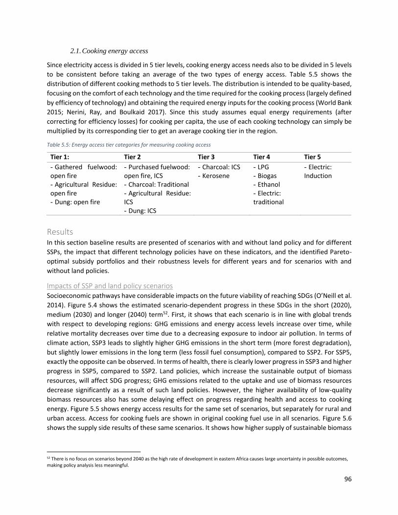
96
2.1. Cooking energy access
Since electricity access is divided in 5 tier levels, cooking energy access needs also to be divided in 5 levels
to be consistent before taking an average of the two types of energy access. Table 5.5 shows the
distribution of different cooking methods to 5 tier levels. The distribution is intended to be quality-based,
focusing on the comfort of each technology and the time required for the cooking process (largely defined
by efficiency of technology) and obtaining the required energy inputs for the cooking process (World Bank
2015; Nerini, Ray, and Boulkaid 2017). Since this study assumes equal energy requirements (after
correcting for efficiency losses) for cooking per capita, the use of each cooking technology can simply be
multiplied by its corresponding tier to get an average cooking tier in the region.
Table 5.5: Energy access tier categories for measuring cooking access
Tier 1: Tier 2 Tier 3 Tier 4 Tier 5
- Gathered fuelwood: open fire - Agricultural Residue: open fire - Dung: open fire
- Purchased fuelwood: open fire, ICS - Charcoal: Traditional - Agricultural Residue: ICS - Dung: ICS
- Charcoal: ICS - Kerosene
- LPG - Biogas - Ethanol - Electric: traditional
- Electric: Induction
Results In this section baseline results are presented of scenarios with and without land policy and for different
SSPs, the impact that different technology policies have on these indicators, and the identified Pareto-
optimal subsidy portfolios and their robustness levels for different years and for scenarios with and
without land policies.
Impacts of SSP and land policy scenarios Socioeconomic pathways have considerable impacts on the future viability of reaching SDGs (O’Neill et al.
2014). Figure 5.4 shows the estimated scenario-dependent progress in these SDGs in the short (2020),
medium (2030) and longer (2040) term52. First, it shows that each scenario is in line with global trends
with respect to developing regions: GHG emissions and energy access levels increase over time, while
relative mortality decreases over time due to a decreasing exposure to indoor air pollution. In terms of
climate action, SSP3 leads to slightly higher GHG emissions in the short term (more forest degradation),
but slightly lower emissions in the long term (less fossil fuel consumption), compared to SSP2. For SSP5,
exactly the opposite can be observed. In terms of health, there is clearly lower progress in SSP3 and higher
progress in SSP5, compared to SSP2. Land policies, which increase the sustainable output of biomass
resources, will affect SDG progress; GHG emissions related to the uptake and use of biomass resources
decrease significantly as a result of such land policies. However, the higher availability of low-quality
biomass resources also has some delaying effect on progress regarding health and access to cooking
energy. Figure 5.5 shows energy access results for the same set of scenarios, but separately for rural and
urban access. Access for cooking fuels are shown in original cooking fuel use in all scenarios. Figure 5.6
shows the supply side results of these same scenarios. It shows how higher supply of sustainable biomass
52 There is no focus on scenarios beyond 2040 as the high rate of development in eastern Africa causes large uncertainty in possible outcomes, making policy analysis less meaningful.

97
due to land policies also translate to higher demand, and also shows the contribution of mini-grids to rural
electricity access.
Figure 5.4: Modelled progress in climate action, health and energy access goals in eastern Africa, for three different SSPs and for a scenario with and without land policy (land policy impact on electricity access is negligible and results have been omitted).
Figure 5.5: Separately rural and urban energy access for cooking energy and electricity for each SSP, by cooking method and tier level (see Method section C) respectively

98
Figure 5.6: Supply and demand for forest resources, and supply of electricity, by SSP and category
Impacts of technology subsidies on SDG progress Technology subsidies in developing countries have the potential to reduce reliance on traditional biomass
and increase energy access through leapfrogging towards more efficient ways to use biomass resources
or towards modern energy technologies (Goldemberg 1998). By applying six different pathways of
technology subsidies upon both the baseline and land policy scenario, up to 2040, the impact of these
subsidies on progress towards each of the three SDGs that are analysed in this study is measured.
Figure 5.7 shows total subsidy spending in scenarios with 100% subsidised technologies, on the short,
medium and longer term, separately for each of technology pathway, and divided between “fuel costs”
(technology to produce energy in each pathway) and “stove costs” (technology to use each energy carrier
for cooking purposes). The figure also shows how subsidy spending increases as a higher share of the costs
is subsidised. This increase is often exponential, as the higher a technology subsidy, the higher the uptake
of this technology. Figure 5.8 shows the impacts of 100% technology subsidies on the cooking energy mix,
separately for rural and urban households. It shows that LPG and PV subsidies have a very high uptake in
urban households, and on the longer term also in rural households. Instead, biogas subsidies only have a
persistent impact on cooking choices in rural households, while the maximum impact of ethanol and
charcoal technology subsidies on the rural and urban cooking mix is limited. Fuelwood technology
subsidies have profound impacts on the cooking energy mix in both rural and urban households, and while
they accelerate the uptake of clean cooking stoves significantly, they also delay the transition to modern
cooking fuels. Miscellaneous results for subsidy scenarios are shown in Figure 5.9. It shows a profoundly
different impact of PV subsidies on electricity access between rural and urban households: in rural areas,
such subsidies help a shift from tier 1 (no access) to tier 2, while in urban areas, they shift households
from tier 2 to tier 3. Subsidies for biogas systems slightly increase total manure uptake, and significantly
increase the use of manure for biogas purposes. It shows that land policies have a profound impact on

99
the way how ethanol and charcoal subsidies affect the use of different production technologies, and on
the impact of fuelwood subsidies on land degradation.
Figure 5.7: for a range of SSP outcomes, total subsidy spending for 100% subsidy scenarios for each subsidy pathway and separated between subsidies for cooking stoves and for energy production (A) and subsidy spending relative to % of technology pathway subsidised (B; baseline scenario). NOTE: logarithmic scale used to distinguish pathways at lower levels of subsidisation)
Figure 5.8: For SSP2 baseline & land policy scenario, effects of 100% subsidy scenarios on rural and urban cooking energy mix

100
Figure 5.9: Miscellaneous results for PV (A), biogas (B), Ethanol (C), Charcoal (D) and Fuelwood (E) subsidy pathways

101
Figure 5.10: Cost effectiveness of energy technology subsidies in terms of GHG emissions, premature mortality and energy access levels for scenarios with and without land policy, by 2020, 2030 and 2040.
Figure 5.10 shows the relative cost effectiveness of technology subsidy packages53 (as described in section
A: Scenarios). I that subsidies for biogas systems are the most cost-effective for each of the indicators,
scenarios and years: depending on the subsidy level and the socioeconomic pathway, subsidies for biogas
systems translate to GHG abatement costs as low as $17 per ton of CO2-equivalent, and avoid one air
pollution-related death for every $30,000 invested54. In contrast, subsidies for fuelwood pathways are
only reasonably cost-effective for reducing GHG emissions in the short term (2020), with the condition
that subsidies are tied to land policies. Subsidies for charcoal pathways are more cost-effective and, if tied
to land policies, they are the second-best option for mitigating climate change in terms of cost
effectiveness and robustness. LPG and ethanol subsidies are second-best options for improving health in
the short and medium term. Subsidies for solar PV are very cost-effective for improving overall energy
access in the short term, but long-term effects depend strongly on the development pathway (i.e. with
higher development, PV subsidies contribute relatively less to energy access levels). The figure also shows
that, throughout all scenarios, the impact of socioeconomic pathways cause technology subsidy impacts
to become more uncertain over time.
Pareto-optimal and SSP robust technology subsidy portfolios Subsidies for each of the technology pathways in this study contribute to at least one of the SDGs analysed
in this study, and most technologies contribute to all three SDGs simultaneously (Figure 5.10). However,
depending on the scenario and the point in time, some technology pathways are more cost-effective than
53 Cost effectiveness of technology subsidies on progress in energy access should be interpreted as billion $(2015) per increased energy access tier level in the entire region (i.e. average increase over all households). Take into account that such region-wide increments in energy access have taken currently developed countries several decades to centuries (Fouquet 2010). 54 Note that the maximum impact of each technology subsidy package is limited, even if they are 100% subsidised. These limits are most clear for ethanol, charcoal and biogas pathways, due to biophysical limits to the availability or sustainability of the main inputs for these technologies (sugarcane/molasses, fuelwood and animal manure for ethanol, charcoal and biogas respectively)

102
others for a specific SDG (and some result in negative outcomes). Therefore, technology subsidy portfolios
are identified that are both Pareto-optimal in contributing to each of the three SDGs, and at the same
time robust over a range of future socioeconomic pathways. Figure 5.11 shows these portfolios with a
lower subsidy budget for a baseline and land policy scenario in 2020, 2030 and 2040. For each scenario
and year, one portfolio is selected that is relatively robust to SSP uncertainty and representative for the
Pareto curve of that scenario, and show the distribution of subsidies and impacts of these portfolios in
Table 5.6.
Figure 5.11: Technology subsidy portfolios for a “low” budget that are Pareto-optimal in terms of simultaneously avoiding GHG emissions, premature deaths and improving energy access for baseline and land policy scenarios in 2020, 2030 and 2040. Size of dots illustrates robustness against SSP uncertainty. For an interactive three-dimensional version of this figure: https://www.bc3research.org/dj.vandeven/3D_low.html
Table 5.6: Total impact and contributions per technology for 6 selected Pareto optimal subsidy portfolios with “low” budgets
Global warming potential Air pollution related Mortality Energy Access Tier
Port-folio Figure 5.11
Impact (Mt
CO2eq)
Relative contribution by technology (% of Total)*
Impact (1000
deaths)
Relative contribution by technology (% of Total)*
Impact Δtier level
Relative contribution by technology (% of Total)*
L PV bg et ch fw L PV bg et Ch fw L PV bg et ch fw
A 69.0 33 8 51 5 2 0+ 29.0 18 4 75 2 2 0 0.256 23 20 52 3 1 0+
B 64.7 31 10 48 5 6 0+ 28.3 17 5 73 2 4 0 0.261 21 24 50 2 3 0+
C 123.7 13 8 72 7 1 0 34.2 9 5 80 5 2 0 0.286 12 17 63 7 1 0
D 117.9 19 6 69 2 4 0+ 34.1 14 3 78 1 4 0 0.266 20 13 64 0 3 0
E 89.7 32 18 50 0 0+ 0 26.0 24 9 67 0 0 0 0.213 31 21 48 0 0 0
F 130.2 37 14 49 0+ 0+ 0 29.3 29 7 63 0+ 0+ 0 0.25 37 16 47 0 0+ 0
* These numbers represent relative contributions of each technology to the SDG progress of the total subsidy portfolio. Numbers are rounded to whole percentage levels, and 0+ defines a small positive number before rounding. L = LPG, bg =biogas, et = ethanol, ch = charcoal, fw = fuelwood, Mt = million ton
The figure and table show that, in the short and medium term, technology subsidy portfolios contribute
more to each of the SDGs without a land policy. In terms of GHG emissions, this can be explained by a

103
higher margin for improvement without land policy, i.e. replacing biomass consumption will avoid further
forest degradation. Since subsidising charcoal is more cost-effective if combined with a land policy (see
Figure 5.10), charcoal subsidies make up a higher share of the subsidy portfolio in scenarios with land
policy, and therefore these portfolios contribute less to health and energy access goals. In the longer term
(2040), the opposite can be observed: technology subsidies contribute more to SDGs in the land policy
scenario. This can be explained by a higher scarcity of biomass resources by 2040 in a scenario without
land policy, which leads to higher consumption of non-biomass energy sources, even without technology
subsidies, and therefore a lower impact of these subsidies. In each portfolio, subsidies for biogas systems
contribute most to each of the SDGs, and mostly to progress in terms of health. This can be explained by
the relative attractiveness of biogas systems in rural areas (see Figure 5.8), where predominantly
unhealthy fuelwood stoves will be replaced.
These modelling results show that an efficient allocation of relatively low technology subsidy portfolios of
11 to 14 dollars per capita per year can improve energy access levels by up to 15%, while reducing GHG
emissions in the region by over 10% and avoiding around 20% of air pollution-related deaths in the short
and medium term. Higher subsidy budgets of > 32 dollar per capita per year (Figure 5.12) are relatively
less cost-effective, since the most cost-effective solutions (see Figure 5.10) are already included in low
subsidy budgets.
Figure 5.12: Technology subsidy portfolios for a “high” budget that are Pareto-optimal in terms of simultaneously avoiding GHG emissions, premature deaths and improving energy access for baseline and land policy scenarios in 2020, 2030 and 2040. Size of dots determine robustness to SSP uncertainty. For an interactive 3-dimensional version of this figure: https://www.bc3research.org/dj.vandeven/3D_high.html
Discussion While subsidies to any technology yield the desired outcomes in a modelling exercise, in the real world
this can be significantly harder. In the developing country context of eastern Africa, the dominance of
traditional biomass and the availability of “free” fuelwood in combination with social conditions in rural

104
areas make “leapfrogging” towards modern energy technologies less straightforward than in models,
which largely depend on the technical and economic viability of such technologies (Murphy 2001). The
relation between land use policies and technology policies is quite important as land use policies lead to
increased dependence on biomass at a later stage, which is a type of rebound effect, since the greater
availability of biomass effectively makes it easier and cheaper to gather and use biomass. Consequently,
the combination of land use policies and technology subsidies needs to be tailored to the context of each
country and in some cases also at sub-national level. It is also not necessarily cost-effective to subsidise
the costs of a shift to modern energy over a long period: Figure 5.10 shows that technological solutions
become costlier and thus less effective in the longer term.
More detailed analysis at sub-national level and in some cases at local or district level could reveal
significant differences in patterns of demand and supply, related to differences in income, biomass
scarcity and other factors. Policies supporting sustainable land use, for example, might target those areas
where higher productivity could support non-consumptive forest uses (recreation, tourism, various
ecosystem services) while areas that are more prone to exploitation might instead support more effort
on technology subsidies. The success of policies subsidising biogas installations depends also on local
conditions, such as water availability and livestock ownership. In other words, policies and institutions
may need to be more local and less national in their application. Designing such policies, however,
requires a more disaggregated analysis than can be provided through this approach, as has been done
through the MOFUSS model (Ghilardi et al. 2016). In the meantime, those technologies that are cost-
effective and robust across different scenarios, such as biogas, may warrant additional support beyond
subsidies to ensure sustained use: e.g. creating robust maintenance facilities, training technicians,
ensuring access to spare parts, etc. (Rupf et al. 2015; Clemens et al. 2018).
Table 5.7: Appearance of the measures taken in this study in the INDCs of individual Eastern African countries
Country Demand side measures in INDC Land Policy measures in INDC
LPG PV Biogas Ethanol Improved Charcoal Kilns
Improved Cooking Stoves
Rotation Forestry
Agro-forestry
Burundi N E E N E E E E
Djibouti E E N N N N N E
Ethiopia I E I I I I E E
Eritrea E E E N E E E I
Kenya I E I I I I I I
Madagascar I E I I E E E E
Rwanda E E E N E E E E
Somalia E E E N E E E E
Sudan E E N I N E E E
South-Sudan I E I N N E E E
Uganda I E I I I E E E
E = Explicitly mentioned as INDC measures I = Could be implicitly part of mentioned INDC measures N = Not mentioned as INDC measures Source: http://www4.unfccc.int/submissions/indc/Submission%20Pages/submissions.aspx
Table 5.7 shows the measures included in the (intended) National Determined Contributions of the region.
Essentially all mention land policy measures in one way or another, since land use is now widely
recognised as a critical factor in meeting climate goals. Demand-side measures are not as prominent but,
in many cases, also included. What few countries have done is to explore the interaction between

105
demand-side measures and land use policies, which has been addressed in this paper, at least to some
first approximation for the region as a whole. Consequently, the results suggest a need for more
investigation of these interactions, and greater disaggregation in models and data. Coupling more detailed
data on biomass extraction that reveals hotspots (Robert Bailis et al. 2015) with forward-looking demand
studies could inform the Nationally Determined Contributions and identify feasible solutions that occupy
a more manageable policy space.
Conclusions This study links two methods used to explore potential co-benefit strategies for climate change mitigation,
increasing energy access and reducing exposure to air pollution. GCAM is used to reflect as best as possible
the energy/resource situation in eastern Africa and to simulate the effects of subsidising a selection of
technologies, as well as a robust portfolio analysis to find optimal portfolios of subsidies to identify trade-
offs in progress across three SDGs, by reducing GHG emissions, reducing exposure to air pollution and
increasing energy access until 2040. The portfolio analysis systematically integrates the GCAM model
results into a portfolio generation model, while also treating stochastic uncertainty related to
socioeconomic development pathways in eastern Africa.
The results give an indication of how effective land policies and technology subsidies are in simultaneously
mitigating climate change, reducing exposure to air pollution, and increasing energy access, and which
combinations of policies are most successful in doing so. The analysis shows that biogas technologies
should be prioritised and subsidised in both the short and long term, showing very high cost-effectiveness
for progress across all three SDGs. Subsidies for most other energy technologies focused on in this study
are also relatively cost-effective in the short-to-medium term, and the distribution of a certain subsidy
budget over LPG (health and energy access), PV (energy access), ethanol (GHG emissions and health) and
charcoal (GHG emissions; if linked to land policies) pathways would depend on the preferred SDG in the
policymakers’ point of view. Subsidies for fuelwood pathways are less cost-effective, even if linked to land
policies to guarantee the sustainable production of biomass inputs. Land policies alone can avoid up to
10% of total GHG emissions in the region in the near term, while having a somewhat delaying effect for
progress regarding health and energy access goals. Optimally allocated technology subsidies of around 11
to 14 dollars per capita in the short-to-medium term have the potential to avoid another 10% of GHG
emissions, while avoiding around 20% of deaths by reducing exposure to air pollution, and improving
energy access by up to 15%. Both land and technology subsidy policies become relatively less effective
and more uncertain in the longer term. Thus there are trade-offs across these goals and the respective
SDGs, which need to be better analysed and researched in order to guide policies and finance programs,
such as those of the GCF.
Annex Table 5.8: Cost, conversion and emission assumptions for newly added or changed sectors in GCAM
Emission factor
Input / Source Output / Technology
Non-energy Costs [1]
Coefficient [1]
CO2 CO CH4 NM-VOC
N2O SO2 Nox BC OC
From To $(2015) per GJ output
Input per Output
Kg per GJ
Coal [2] [2] 100.1
Refined Liquids [2] [2] 71.9
Natural Gas [2] [2] 52.1

106
Unsustainable Fuelwood
[2] [2] 110.0
Refined Liquids Diesel 12.11 1
Diesel Diesel Rural 4.15 1
Refined Liquids Kerosene 8.79 1
Kerosene Kerosene Rural 3.66 1
Refined Liquids LPG (t.p. 1) 27.97 1
LPG LPG Rural 6.54 1
Solar Central Grid Electricity / PV (t.p. 2)
59.31 - 15.80 1
Diesel Mini-grid Electricity / Diesel engine
8.81 - 8.14 3.33 - 2.94 0.052 0.009 0.007 0.002 0.44 0.186 0.006 0.003
Local Biogas Mini-grid Electricity / Gas turbine
8.81 - 8.14 3.33 - 2.94 6E-05 0.003 8E-06 3E-04 8E-07 1E-04 2E-06 8E-07
Mini-Hydro Mini-grid Electricity / Mini-Hydro
21.94 - 26.79 1
Solar Mini-grid Electricity / PV (t.p. 2)
70.03 - 18.66 1
Central Grid Electricity
Rural Residential Electricity
18.06 – 15.26 1.283 - 1.269
Mini-Grid Electricity
Rural Residential Electricity
9.03 – 7.63 1.117 - 1.104
Rooftop PV standalone
Rural Residential Electricity (t.p. 2)
143.29 - 43.52 1
Central Grid Electricity
Urban Residential Electricity
9.03 – 7.63 1.246 - 1.234
Rooftop PV connected
Urban Residential Electricity (t.p. 2)
95.26 - 25.46 1
Rooftop PV standalone
Urban Residential Electricity (t.p. 2)
143.29 - 43.52 1
Fuelwood Charcoal Production / EM kiln
0.00 2.20 12.94 2.865 4.163 0.009 0 0.004 0.081 0.364
Fuelwood Charcoal Production / Hot Tail kiln (t.p. 5)
0.62 2.04 14.21 2.179 1.743 5E-04 0 0.002 0.133 0.594
Diesel Charcoal Production / Hot Tail kiln
0.012 “ “ “ “ “ “ “ “
Fuelwood Charcoal Production / Container kiln (t.p. 5)
9.96 1.72 2.503 0.965 2.503 1.643 0 0 1.172 0.262
Diesel Charcoal Production / Container kiln
0.008 “ “ “ “ “ “ “ “
Charcoal Production / Container kiln
Electricity 10.39 “ “ “ “ “ “ “ “
Fuelwood Charcoal Production / Container kiln mini-grid (t.p. 5)
12.61 1.72 2.503 0.965 2.503 1.643 0 0 1.172 0.262
Diesel Rural Charcoal Production /
0.008 “ “ “ “ “ “ “ “

107
Container kiln mini-grid
Charcoal Production / Container kiln mini-grid
Mini-grid Electricity
10.39 “ “ “ “ “ “ “ “
Charcoal Production
Charcoal (Retail) 7.00 1.00
Fuelwood Market Fuelwood (t.p. 6)
3.50 1.00
Fuelwood or Market Fuelwood
Residential Cooking / Traditional
0.00 7.14 44.45 2.549 10.52 0.038 0.26 0.419 0.47 2.102
Market Fuelwood
Residential Cooking / ICS (t.p. 6)
0.63 5.26 40.02 0.682 10.13 0.032 0.222 0.357 0.401 1.793
Manure use for energy
Residential Cooking / Traditional
0.00 10.00 39.47 4.537 14.98 0.245 0.185 0.384 1.968 8.801
Manure use for energy
Residential Cooking / ICS
0.63 7.69 20.68 2.341 20.73 0.205 0.11 0.229 1.171 5.237
Agricultural Residue
Residential Cooking / Traditional
0.00 7.14 28.34 3.277 3.667 0.021 0.128 0.511 0.652 2.915
Agricultural Residue
Residential Cooking / ICS
0.63 5.26 17.62 1.526 8.571 0.056 0.084 0.335 0.427 1.91
Charcoal Residential Cooking / Traditional
0.16 4.17 25.93 1.487 6.136 0.022 0.152 0.244 0.055 0.491
Charcoal Residential Cooking / ICS (t.p. 5)
0.63 3.33 22.73 0.863 5.559 0.019 0.129 0.209 0.047 0.419
Kerosene Residential Cooking / Kerosene
0.83 2.70 – 2.47 0.045 0.008 0.007 0.002 0.382 0.162 0.005 0.002
LPG Residential Cooking / LPG (t.p. 1)
2.08 1.89 – 1.61 0.021 0.002 0.003 2E-04 6E-04 0.084 8E-04 3E-04
Ethanol Residential Cooking / Ethanol (t.p. 4)
2.08 1.89 – 1.61 0.021 7E-04 0.003 4E-05 6E-04 0.084 8E-04 3E-04
Biogas Residential Cooking / Biogas (t.p. 3)
0.83 1.89 – 1.61 3E-05 0.002 5E-06 2E-04 5E-07 8E-05 1E-06 5E-07
Electricity Residential Cooking / Electric (t.p. 2)
2.04 1.37 0 0 0 0 0 0 0 0
Electricity Residential Cooking / Induction (t.p. 2)
5.21 1.19 0 0 0 0 0 0 0 0
Regional biomass
Ethanol / cellulosic ethanol (t.p. 4)
38.4 2.06 – 1.95
Regional sugar for ethanol
Ethanol / sugar cane ethanol (t.p. 4)
28.6 1
Ethanol Ethanol Rural 4.27 1
SugarCrop (in kg)
Regional sugar for ethanol (in GJ)
582.5
Molasses (in kg) Regional sugar for ethanol (in GJ)
2018.7
Sugar production (in
Molasses (secondary output; in kg)
6.14
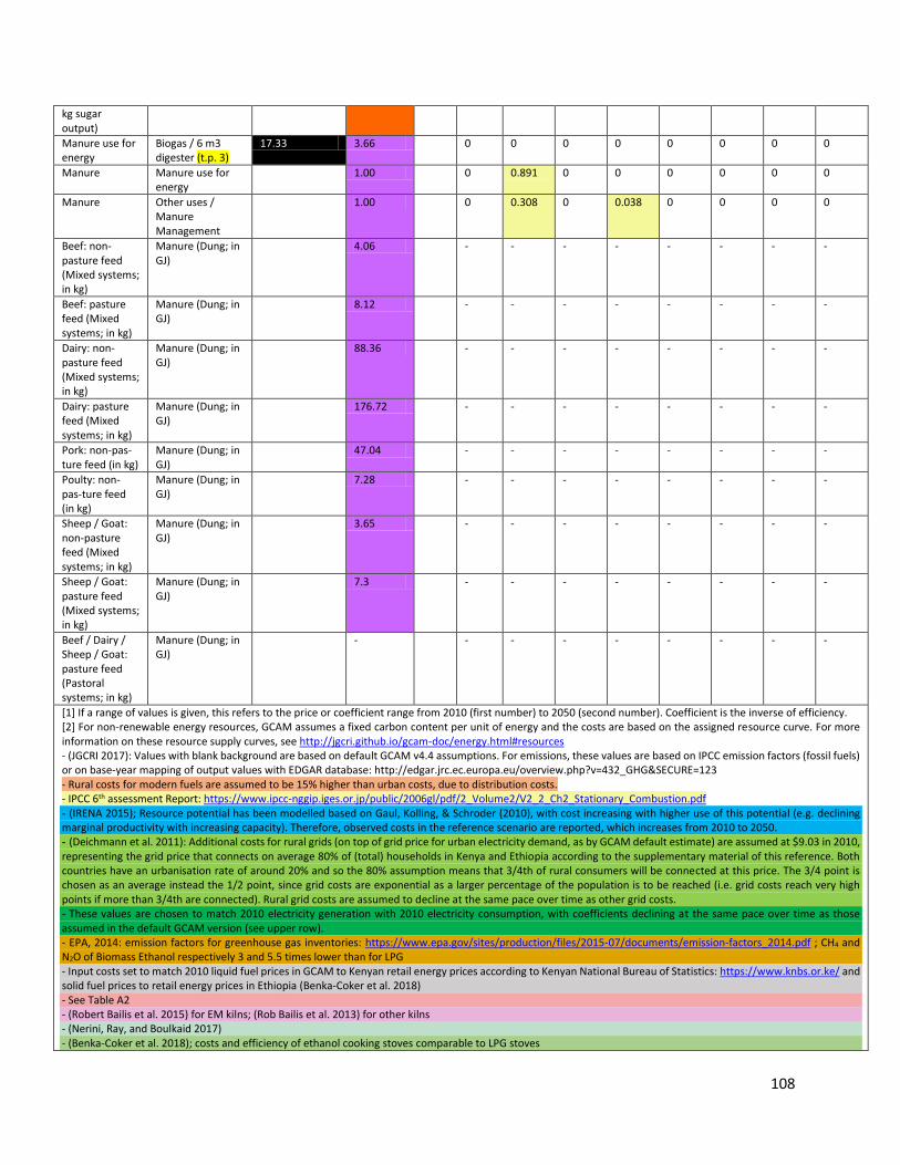
108
kg sugar output)
Manure use for energy
Biogas / 6 m3 digester (t.p. 3)
17.33 3.66 0 0 0 0 0 0 0 0
Manure Manure use for energy
1.00 0 0.891 0 0 0 0 0 0
Manure Other uses / Manure Management
1.00 0 0.308 0 0.038 0 0 0 0
Beef: non-pasture feed (Mixed systems; in kg)
Manure (Dung; in GJ)
4.06 - - - - - - - -
Beef: pasture feed (Mixed systems; in kg)
Manure (Dung; in GJ)
8.12 - - - - - - - -
Dairy: non-pasture feed (Mixed systems; in kg)
Manure (Dung; in GJ)
88.36 - - - - - - - -
Dairy: pasture feed (Mixed systems; in kg)
Manure (Dung; in GJ)
176.72 - - - - - - - -
Pork: non-pas-ture feed (in kg)
Manure (Dung; in GJ)
47.04 - - - - - - - -
Poulty: non-pas-ture feed (in kg)
Manure (Dung; in GJ)
7.28 - - - - - - - -
Sheep / Goat: non-pasture feed (Mixed systems; in kg)
Manure (Dung; in GJ)
3.65 - - - - - - - -
Sheep / Goat: pasture feed (Mixed systems; in kg)
Manure (Dung; in GJ)
7.3 - - - - - - - -
Beef / Dairy / Sheep / Goat: pasture feed (Pastoral systems; in kg)
Manure (Dung; in GJ)
- - - - - - - - -
[1] If a range of values is given, this refers to the price or coefficient range from 2010 (first number) to 2050 (second number). Coefficient is the inverse of efficiency. [2] For non-renewable energy resources, GCAM assumes a fixed carbon content per unit of energy and the costs are based on the assigned resource curve. For more information on these resource supply curves, see http://jgcri.github.io/gcam-doc/energy.html#resources - (JGCRI 2017): Values with blank background are based on default GCAM v4.4 assumptions. For emissions, these values are based on IPCC emission factors (fossil fuels) or on base-year mapping of output values with EDGAR database: http://edgar.jrc.ec.europa.eu/overview.php?v=432_GHG&SECURE=123 - Rural costs for modern fuels are assumed to be 15% higher than urban costs, due to distribution costs. - IPCC 6th assessment Report: https://www.ipcc-nggip.iges.or.jp/public/2006gl/pdf/2_Volume2/V2_2_Ch2_Stationary_Combustion.pdf - (IRENA 2015); Resource potential has been modelled based on Gaul, Kolling, & Schroder (2010), with cost increasing with higher use of this potential (e.g. declining marginal productivity with increasing capacity). Therefore, observed costs in the reference scenario are reported, which increases from 2010 to 2050. - (Deichmann et al. 2011): Additional costs for rural grids (on top of grid price for urban electricity demand, as by GCAM default estimate) are assumed at $9.03 in 2010, representing the grid price that connects on average 80% of (total) households in Kenya and Ethiopia according to the supplementary material of this reference. Both countries have an urbanisation rate of around 20% and so the 80% assumption means that 3/4th of rural consumers will be connected at this price. The 3/4 point is chosen as an average instead the 1/2 point, since grid costs are exponential as a larger percentage of the population is to be reached (i.e. grid costs reach very high points if more than 3/4th are connected). Rural grid costs are assumed to decline at the same pace over time as other grid costs. - These values are chosen to match 2010 electricity generation with 2010 electricity consumption, with coefficients declining at the same pace over time as those assumed in the default GCAM version (see upper row). - EPA, 2014: emission factors for greenhouse gas inventories: https://www.epa.gov/sites/production/files/2015-07/documents/emission-factors_2014.pdf ; CH4 and N2O of Biomass Ethanol respectively 3 and 5.5 times lower than for LPG - Input costs set to match 2010 liquid fuel prices in GCAM to Kenyan retail energy prices according to Kenyan National Bureau of Statistics: https://www.knbs.or.ke/ and solid fuel prices to retail energy prices in Ethiopia (Benka-Coker et al. 2018) - See Table A2 - (Robert Bailis et al. 2015) for EM kilns; (Rob Bailis et al. 2013) for other kilns - (Nerini, Ray, and Boulkaid 2017) - (Benka-Coker et al. 2018); costs and efficiency of ethanol cooking stoves comparable to LPG stoves

109
- (Gopal and Kammen 2009); ratio molasses to sugar production calculated as SugarCrop input (kg) -/- Sugar output (kg) divided by sugar output (kg) - (APEC 2010); non-feedstock costs assumed as additional costs for sugar cane and cellulosic ethanol - (Smith et al. 2000); Table 4: using estimates for dung and must (agricultural residue) “tm” stoves a s proxy for Traditional and “ivc” stoves as proxy for ICS, based on inputs. For fuelwood, the difference between Acacia-3R (proxy for Traditional) and Acacia-ivs (proxy for ICS) is applied to the GCAM default values for biomass emissions in Eastern Africa (see green reference). - (Garland et al. 2017); used to re-allocate default GCAM BC and OC emissions between fuelwood and charcoal - (Saud et al. 2011); for ICS, the difference in CO emission factors (see grey reference) is assumed to explain 71% of the differences in BC and OC factors, based on (Carter et al. 2017) - Assuming emission factors differences between traditional and ICS for charcoal follow the same trend as for fuelwood, corrected by assumed relative efficiency improvements of ICS - Based on dividing 13% of the costs (fixed charge rate for capital with lifetime of 8 years or more) of a 6 m3 biogas digester ($932 according to the Uganda Domestic Biomass Programme + 15% per year for operation and maintenance) by the amount of biogas it tends to produce annually (8.76 GJ), assuming a 5% dry matter content, 30 days retention time and caloric value of 55 MJ per kg of CH4 - Represents amount of livestock products (in kg) needed for 1 GJ of manure output (higher means less manure per kg of final product), assuming caloric content of manure according to (Santoianni et al. 2008); 100% manure availability is assumed for livestock while being fed with non-pasture feed, 50% for livestock in mixed systems while feeding itself with pasture, and 0% for livestock in fully pastoral systems. t.p. refers to Technology Pathway, and represent the subsidised pathways 1 to 6 (see section A: Scenarios of Method section)
Table 5.9: Overview of assumptions and sources for mini-grids and solar PV installations and costs
2013 2013 2010 2013 2015
Total off-grid capacity in MW
PV off-grid capacity in MW
Total Eastern Africa in Tera Joules
Burundi 1.23 0.40 Total off-grid electricity 1318.36 1770.78 2072.56
Djibouti 1.00 0.16 Off-grid PV electricity 7.2 338.04 600
Ethiopia 20.89 13.28 Off-grid diesel electricity
811.16
Eritrea 0.56 0.56 Off-grid mini-hydro electricity
500
Kenya 29.00 10.00 - Translation of capacity values in left column to electricity output, assuming 65% and 22.5% capacity factors for non-PV (diesel engines and mini-hydro) and PV respectively - Estimated by assuming same share total electricity production compared to 2013 - For 2010, given the small number, all solar is assumed to be generated off-grid. For 2015, a continuation of the trend from 2010 to 2013 is assumed. - (Gaul, Kolling, and Schroder 2010); rough estimation - Calculated as Total off-grid -/- PV -/- mini-hydro
Madagascar 15.16 3.00
Rwanda 1.58 0.30
Somalia 0.96 0.96
Sudan 22.21 8.47
Uganda 7.55 3.46
For 2010 and 2015: (IEA 2015), For battery costs surplus costs: (Ardani et al. 2017). For post-2015, cost path based on GCAM projections (Muratori et al. 2017).
Total Eastern Africa 100.13 40.58
Total in GWh 339.039488 79.9930285
- (IRENA 2015) - (Ondraczek 2013) - (SEI 2016) - Based on a global database of electricity generation capacity off the main grid by country (for those countries which have data available), a regression analysis is applied to estimate the amount of off-grid capacity for countries with no data available: Off-grid MW = [3.08 – 0.045*(Electrification Rate) + 0.021*(Urban share of population)] * (Total TW electricity generation) The amount of off-grid PV capacity is estimated from another regression analysis by: Off-Grid PV MW = [-508.55 + 108.65*(Annual Solar Irradiance) + 4.38*(GDP per capita)] * (Population in Billions) For Somalia and Eritrea, these formulas ended up of PV off-grid capacity being larger than total off-grid capacity, so PV off-grid capacity was limited such that it provides all assumed off-grid capacity.
0
1000
2000
3000
4000
5000
6000
7000
8000
9000
10000
20
10
20
15
20
20
20
25
20
30
20
35
20
40
20
45
20
50
Ove
rnig
ht
Cap
ital
Co
sts
in $
(20
15
)
Assumed capital costs for PV systems
Utility-scale PV
Commercial PV(proxy for mni-gridPV)Rooftop PV

110
Table 5.10: Assumptions for rotation forestry and agroforestry
Land area
Woodlot (Acacia) production in forestry [1] (ton/hect/yr)
Above ground carbon uptake [2] (ton C/hect /yr)
Below ground carbon uptake [3] (ton C/hect/ yr)
% of max wood prod. in cropland with max 10% crop yield loss [4]
GCAM Crop type
Compatibility coefficient for agroforestry (competition for light, water and nutrients) [5]
AEZ01 0.04 0.02 0.02 70% Corn 80%
AEZ02 3.02 1.74 1.23 64% FiberCrop 90%
AEZ03 5.51 3.17 1.72 58% MiscCrop 39%
AEZ04 7.5 4.31 1.79 52% OilCrop 80%
AEZ05 9.01 5.18 1.64 46% OtherGrain 90%
AEZ06 10.02 5.76 1.44 40% PalmFruit 0%
AEZ07 0.04 0.02 0.02 70% Rice 0%
AEZ08 3.02 1.74 1.23 64% Root_Tuber 100%
AEZ09 5.51 3.17 1.72 58% SugarCrop 80%
AEZ10 7.5 4.31 1.79 52% Wheat 100%
AEZ11 9.01 5.18 1.64 46% Pasture 0%
AEZ12 10.02 5.76 1.44 40% Biomass 0%
[1] (Nyadzi et al. 2003; Iiyama et al. 2014): Acacia has been chosen as tree species as it is compatible with charcoal production; Values based on productivity range in reference. These values are also the assumed yields for Rotation Forestry. [2] A conversion factor of 0.50 was assumed to transform dry timber to carbon content (Nair 2011a; García de Jalón et al. 2018) [3] It was assumed that belowground carbon sequestration was between 25% and 90% of aboveground carbon sequestration depending on the potential suitability for agriculture of the agro-ecological zones (Nair 2011b). [4] (García de Jalón et al. 2018); for each crop, this value has to be multiplied with the last column ([5]) and the woodlot yield for the actual wood production per hectare ([1]) [5] Tree crops and Rice are assumed not to be compatible with the studied agroforestry systems. Pasture and biomass have been excluded for concerns on modelling realism
Table 5.11: Assumptions on residential energy use based on Demographic and Health Surveys (DHS) in eastern African countries
Eastern Africa average:
% of households in cooking with: % of households owning a: Household size***:
Elect Gas* Keros Charc Wood Crop Dung TV Refrig Airco**
2010 Urban 1.9% 6.9% 11.4% 48.8% 28.1% 1.6% 1.1% 44.58% 16.73% 4.00% 5.13784
[1] Rural 0.0% 0.3% 0.4% 6.6% 86.0% 2.9% 3.7% 5.09% 0.90% 0.01% 6.230655
2015 Urban 9.8% 7.0% 7.7% 45.8% 28.5% 0.5% 0.5% 54.81% 19.84% 4.13% 4.97206
[2] Rural 0.2% 0.6% 0.3% 7.3% 85.1% 2.5% 3.9% 6.62% 0.93% 0.02% 6.089795
Source DHS: ICF International, 2015. The DHS Program STATcompiler. Funded by USAID. https://www.statcompiler.com * Gas includes LPG, biogas and natural gas ** Air-conditioner ownership interpreted from: https://www.jraia.or.jp/english/World_AC_Demand.pdf, assuming 1% of air-conditioners to be in rural areas *** Source household size: https://globaldatalab.org/areadata/hhsize/ Based on DHS data from: 2010 cooking mix based on: Burundi, Ethiopia, Kenya, Madagascar, Rwanda, Uganda (representing 70% of urban, 84% of rural population) 2015 cooking mix based on: Ethiopia, Kenya, Madagascar, Rwanda, Uganda (representing 68% of urban, 79% of rural population) Appliance ownership based on: Burundi, Ethiopia, Kenya, Rwanda, Uganda (representing 60% of urban, 75% of rural population)

116
Conclusions and further
research

117

118
Conclusions The aim of this thesis is to assess synergies and trade-offs of climate change mitigation policies. For this
purpose, an IAM has been used that integrates socioeconomic, energy, land and climate systems.
Additional modules to this model have been designed throughout the course of the PhD, as well as a link
with another method to process model outputs with the aim of assessing synergies and trade-offs and
check for robustness of specific policies. The outputs of this thesis show that climate change mitigation
policies are strongly linked with other potential policy objectives, which may be of interest for
policymakers and the scientific community of cross-cutting research.
However, the use of IAMs for climate policy has been criticised on the use of arbitrary functional forms
and parameter values and therefore potentially misleading outputs for climate policy (Pindyck 2013b,
2017). In this thesis, I tried to avoid this “misuse” of the model through the way each study is focused:
- by focusing on already existing climate objectives as documented in NDCs, whether or not based
on proper decision making, the discussion on the social cost of carbon is circumvented.
- when developing new IAM modules, all parameters are based on documented values and
functional forms are calibrated by checking if model simulations match recent real-world
observations.
- by documenting model outcomes as a difference between the policy and the “baseline” scenario
without policy, such that, if a core function of the model is flawed, it will affect all scenarios, but
the difference between scenarios will be considerably less flawed.
- by applying an additional tool to check and select model outcomes based on robustness to
parameter changes.
Nevertheless, the outcomes of this study, certainly those expressed in absolute numbers, should be taken
with caution, as it is virtually impossible to assess the full range of uncertainty through an IAM.
Despite their limitations, IAMs are an ideal tool to assess synergies and trade-offs between climate policies
and other policy objectives (Clarke et al. 2014). Specifically, the integration of scientific knowledge on
both energy and land systems in GCAM makes it an ideal tool to assess trade-offs between energy-based
and land-based objectives for the design of climate policies. But also the function of economic choice in
GCAM, recognising different preferences between consumers and identified through historical
observations, has been of high value for assessing behavioural consumer changes in the EU and household
cooking choices in eastern Africa. From my point of view, these benefits of using a model with
documented knowledge and with internationally recognised capabilities outweigh the potential flaws that
this approach would entail.
This thesis consists of four separate studies, contributing to different parts of knowledge on how climate
policies interact with other potential policy objectives such as land use, energy security, health and energy
access in a development context. Though, some general conclusions can be drawn from this thesis.
Throughout all chapters, a clear interaction between climate change mitigation policies and other policy
objectives can be observed, both when focusing on behavioural and technological solutions (see Table 6.1
for an overview of the identified synergies and trade-offs throughout all chapters). Therefore, linking the
design of climate change mitigation policies with other region-specific policy objectives is often crucial,
not only for achieving these other policies at a lower policy cost and therefore inherently decreasing the
policy costs of achieving mitigation objectives, but also to gain sufficient support from society for implying

119
such climate policies. In contrast, if a certain climate policy clearly strikes with other policy objectives, its
introduction will likely cause resistance.
While generic economic policies such as tradable emission permits may have the capability to achieve an
emission reduction goal at the lowest possible policy costs, in many cases it might actually be beneficial
from a holistic point of view to adopt a more complex set of policies, even if that entails higher policy
costs. The main difference of the Paris Agreement compared to the Kyoto Protocol, i.e. the possibility for
every nation to define its own mitigation targets, might better fit to the climate change problem, as each
nation understands its domestic circumstances and priorities. However, this flexibility of the current
paradigm of international climate policy should be exploited better by the scientific community, providing
policymakers with integrated analysis comparing climate objectives with other policy objectives (Doukas
et al. 2018), a necessity that might also help to make NDCs more ambitious and therefore successfully
mitigate dangerous climate change.
Table 6.1: Identified synergies and trade-offs of climate policies and strategies studied in this thesis.
Chapter Regional focus
Policy / strategy Synergies Trade-offs
Ch 2: The potential of behavioural change for climate change mitigation
EU Food-related behavioural change
Avoiding global LUC
Mobility/household behavioural change
Improving health (not quantified)
Ch 3: The potential land use requirements and related land use change emissions of solar energy
EU India Japan S Korea
Using solar energy (and bio-energy for comparison) to decarbonize electricity sector
Land occupation and indirect LUC
Ch 4: Identifying optimal technological portfolios for European power generation towards climate change mitigation
EU Subsidies for specific low-carbon technologies in the power sector
Increasing energy self-sufficiency (solar, wind and nuclear)
Decreasing energy self-sufficiency (CCS and biomass)
Ch 5: Integrated policy assessment and optimisation over multiple sustainable development goals in eastern Africa
Eastern Africa
Land policies to increase sustainable biomass output
Slight decrease in health and energy access objectives
Technology subsidy policies to replace traditional biomass use
Significant increase of health and energy access objectives

120
Further research Future research in the field of integrated assessment modelling probably will need to focus more on the
impacts of climate policies on non-climate objectives, and vice versa, instead of informing only about
climate policies such as carbon taxes or caps (Pindyck 2017). As such objectives differ strongly between
regions, it is also important for future research on climate policy to listen well to local stakeholders. For
every country or region, different pathways can be evaluated to achieve a given mitigation objective, and
potential synergies and trade-offs of those pathways can be compared. To do so, strong interactions are
required between different academic fields to produce strong and robust cross-cutting research. Also,
from a practical point of view, outcomes from IAMs should be more frequently tailored, potentially with
alternative tools or methods as is done in chapter 4 and 5 of this thesis, to provide policymakers with
more useful and certain results. Given the enormous range of uncertainty behind modelling outcomes,
just comparing results from different IAMs in model ensembles is not necessarily useful from a
policymaker´s perspective (Doukas et al. 2018).
Specifically related the studies provided in this thesis, there is plenty of potential further research to be
done. First, behavioural change can be integrated better into IAMs, as they are likely necessarily to achieve
ambitious climate ambitions. More concretely, it would be interesting to quantify the co-benefits of
different types of behavioural change and compare those with the co-benefits of technological solutions.
Second, the impacts of solar energy on land use can also be compared to other local policy objectives,
such as reducing water scarcity and reducing nitrogen leakage. Through that context, the land occupation
of solar energy can also have local synergies with other environmental objectives, despite contributing to
an indirect decline in natural forest land. Third and last, the modelling exercise done for eastern Africa
can be extended to more developing regions and with more sub-regional detail to give a more complete
picture of the potential of climate finance to reduce emissions in developing countries, while contributing
to other SDGs.

121

122
Bibliography:
ACCES. 2014. “Clean and Improved Cooking in Sub-Saharan Africa: A Landscape Report,” no. 98664: 182. https://doi.org/98664.
Acemoglu, Daron, Philippe Aghion, Leonardo Bursztyn, and David Hemous. 2012. “The Environment and Directed Technical Change.” American Economic Review 102 (1): 131–66.
Agbemabiese, Lawrence, and Jabavu Nkomo. 2012. “Enabling Innovations in Energy Access: An African Perspective.” Energy Policy 47 (June): 38–47. https://doi.org/10.1016/J.ENPOL.2012.03.051.
Aghion, Philippe, Antoine Dechezleprêtre, David Hemous, Ralf Martin, and John Van Reenen. 2016. “Carbon Taxes, Path Dependency, and Directed Technical Change: Evidence from the Auto Industry.” Journal of Political Economy 124 (1): 1–51.
Aichele, Rahel, and Gabriel Felbermayr. 2015. “Kyoto and Carbon Leakage: An Empirical Analysis of the Carbon Content of Bilateral Trade.” Review of Economics and Statistics 97 (1): 104–15.
Alexander, Peter, Mark D A Rounsevell, Claudia Dislich, Jennifer R Dodson, Kerstin Engström, and Dominic Moran. 2015. “Drivers for Global Agricultural Land Use Change: The Nexus of Diet, Population, Yield and Bioenergy.” Global Environmental Change 35: 138–47.
Amaducci, Stefano, Xinyou Yin, and Michele Colauzzi. 2018. “Agrivoltaic Systems to Optimise Land Use for Electric Energy Production.” Applied Energy 220 (June): 545–61. https://doi.org/10.1016/J.APENERGY.2018.03.081.
American Heart Association. 2014. “The American Heart Association’s Diet and Lifestyle Recommendations.” www.heart.org/HEARTORG/GettingHealthy/NutritionCenter/HealthyEating/The-American-Heart-%0AAssociations-Diet-and-Lifestyle-Recommendations_UCM_305855_Article.jsp.
APEC. 2010. “Biofuel Costs, Technologies and Economics in APEC Economies: Final Report.”
Ardani, Kristen, Eric O ’ Shaughnessy, Ran Fu, Chris Mcclurg, Joshua Huneycutt, and Robert Margolis. 2017. “Installed Cost Benchmarks and Deployment Barriers for Residential Solar Photovoltaics with Energy Storage: Q1 2016.” NREL. https://www.nrel.gov/docs/fy17osti/67474.pdf.
Arto, I, A Genty, J M Rueda-Cantuche, A Villanueva, and V Andreoni. 2012. “Global Resources Use and Pollution: Vol. I, Production, Consumption and Trade (1995-2008).” EUR 25462. Luxembourg: European Commission Joint Research.
Arvesen, Anders, Gunnar Luderer, Michaja Pehl, Benjamin Leon Bodirsky, and Edgar G. Hertwich. 2018. “Deriving Life Cycle Assessment Coefficients for Application in Integrated Assessment Modelling.” Environmental Modelling & Software 99 (January): 111–25. https://doi.org/10.1016/j.envsoft.2017.09.010.
ATLAS. 2011. “Wasteland Atlas of India.” Hyderabad: National Remote Sensing Centre (NRSC). http://www.dolr.nic.in/WastelandsAtlas2011/Wastelands_Atlas_2011.pdf.
Autio, Minna, Eva Heiskanen, and Visa Heinonen. 2009. “Narratives of ‘Green’Consumers—the Antihero, the Environmental Hero and the Anarchist.” Journal of Consumer Behaviour: An International Research Review 8 (1): 40–53.
Bailis, Rob, Charissa Rujanavech, Puneet Dwivedi, Adriana de Oliveira Vilela, Howard Chang, and Rogério Carneiro de Miranda. 2013. “Innovation in Charcoal Production: A Comparative Life-Cycle Assessment of Two Kiln Technologies in Brazil.” Energy for Sustainable Development 17 (2): 189–200. https://doi.org/10.1016/j.esd.2012.10.008.
Bailis, Robert, Rudi Drigo, Adrian Ghilardi, and Omar Masera. 2015. “The Carbon Footprint of Traditional Woodfuels.” Nature Climate Change 5 (3): 266–72. https://doi.org/10.1038/nclimate2491.
Bajželj, Bojana, Keith S. Richards, Julian M. Allwood, Pete Smith, John S. Dennis, Elizabeth Curmi, Christopher a. Gilligan, et al. 2014. “Importance of Food-Demand Management for Climate Mitigation.” Nature Climate Change 4 (October): 924–29. https://doi.org/10.1038/nclimate2353.
Baker, Erin, and Senay Solak. 2011. “Climate Change and Optimal Energy
Technology R&D Policy.” European Journal of Operational Research 213 (2): 442–54. https://doi.org/10.1016/j.ejor.2011.03.046.
Balakrishnan, Kalpana, Santu Ghosh, Bhaswati Ganguli, Sankar Sambandam, Douglas F Barnes, and Kirk R Smith. 2013. “State and National Household Concentrations of PM2.5 from Solid Cookfuel Use: Results from Measurements and Modeling in India for Estimation of the Global Burden of Disease.” Environmental Health.
Barker, Terry, Igor Bashmakov, Lenny Bernstein, Jean Bogner, Peter Bosch, Rutu Dave, Ogunlade Davidson, Brian Fisher, Michael Grubb, and Sujata Gupta. 2007. “Summary for Policymakers.” In Climate Change 2007: Mitigation of Climate Change: Contribution of Working Group III to the Fourth Assessment Report of the Intergovernmental Panel on Climate Change, 1–24. Cambridge University Press.
Benka-Coker, Megan L., Wubshet Tadele, Alex Milano, Desalegn Getaneh, and Harry Stokes. 2018. “A Case Study of the Ethanol CleanCook Stove Intervention and Potential Scale-up in Ethiopia.” Energy for Sustainable Development 46: 53–64. https://doi.org/10.1016/j.esd.2018.06.009.
Bensch, Gunther, Michael Grimm, and Jörg Peters. 2015. “Why Do Households Forego High Returns from Technology Adoption? Evidence from Improved Cooking Stoves in Burkina Faso.” Journal of Economic Behavior and Organization 116: 187–205. https://doi.org/10.1016/j.jebo.2015.04.023.
Bhattacharyya, Subhes C. 2012. “Energy Access Programmes and Sustainable Development: A Critical Review and Analysis.” Energy for Sustainable Development 16 (3): 260–71. https://doi.org/10.1016/J.ESD.2012.05.002.
Boldrin, Alessio, Karin R Hartling, Maria Laugen, and Thomas H Christensen. 2010. “Environmental Inventory Modelling of the Use of Compost and Peat in Growth Media Preparation.” Resources, Conservation and Recycling 54 (12): 1250–60.
Bond, Tami C., Ekta Bhardwaj, Rong Dong, Rahil Jogani, Soonkyu Jung, Christoph Roden, David G. Streets, and Nina M. Trautmann. 2007. “Historical Emissions of Black and Organic Carbon Aerosol from Energy-Related Combustion, 1850-2000.” Global Biogeochemical Cycles 21 (2): n/a-n/a. https://doi.org/10.1029/2006GB002840.
Brack, Duncan. 2017. International Trade and the Montreal Protocol. Routledge.
Bradley, R A, E C Watts, and E R Williams. 1991. “Limiting Net Greenhouse Gas Emissions in the United States.” https://doi.org/10.2172/5775139.
Branke, J., B. Scheckenbach, M. Stein, K. Deb, and H. Schmeck. 2009. “Portfolio Optimization with an Envelope-Based Multi-Objective Evolutionary Algorithm.” European Journal of Operational Research 199 (3): 684–93. https://doi.org/10.1016/J.EJOR.2008.01.054.
Breyer, Christian, Dmitrii Bogdanov, Ashish Gulagi, Arman Aghahosseini, Larissa S N S Barbosa, Otto Koskinen, Maulidi Barasa, et al. 2017. “On the Role of Solar Photovoltaics in Global Energy Transition Scenarios.” Progress in Photovoltaics: Research and Applications 25 (8): 727–45. https://doi.org/10.1002/pip.2885.
Broecker, Wallace S. 1975. “Climatic Change: Are We on the Brink of a Pronounced Global Warming?” Science 189 (4201): 460–63.
Bruce, Nigel, Rachel Anderson de Cuevas, Jessie Cooper, Bessem Enonchong, Sara Ronzi, Elisa Puzzolo, Bertrand MBatchou, and Daniel Pope. 2018. “The Government-Led Initiative for LPG Scale-up in Cameroon: Programme Development and Initial Evaluation.” Energy for Sustainable Development 46: 103–10. https://doi.org/10.1016/j.esd.2018.05.010.
Bruce, Nigel, Dan Pope, Eva Rehfuess, Kalpana Balakrishnan, Heather Adair-Rohani, and Carlos Dora. 2015. “WHO Indoor Air Quality Guidelines on Household Fuel Combustion: Strategy Implications of New Evidence on Interventions and Exposure–Risk Functions.” Atmospheric Environment 106 (April): 451–57. https://doi.org/10.1016/J.ATMOSENV.2014.08.064.
Callendar, G S. 1938. “The Artificial Production of Carbon Dioxide and Its

123
Influence on Temperature.” Quarterly Journal of the Royal Meteorological Society 64 (275): 223–40. https://doi.org/10.1002/qj.49706427503.
Calvin, Katherine, James Edmonds, Ben Bond-Lamberty, Leon Clarke, Son H. Kim, Page Kyle, Steven J. Smith, Allison Thomson, and Marshall Wise. 2009. “2.6: Limiting Climate Change to 450 Ppm CO2 Equivalent in the 21st Century.” Energy Economics, International, U.S. and E.U. Climate Change Control Scenarios: Results from EMF 22, 31 (Supplement 2): S107–20. https://doi.org/10.1016/j.eneco.2009.06.006.
Calvin, Katherine, Marshall Wise, Page Kyle, Pralit Patel, Leon Clarke, and Jae Edmonds. 2014. “Trade-Offs of Different Land and Bioenergy Policies on the Path to Achieving Climate Targets.” Climatic Change 123 (3–4): 691–704. https://doi.org/10.1007/s10584-013-0897-y.
Capellán-Pérez, Iñigo, Carlos de Castro, and Iñaki Arto. 2017. “Assessing Vulnerabilities and Limits in the Transition to Renewable Energies: Land Requirements under 100% Solar Energy Scenarios.” Renewable and Sustainable Energy Reviews 77: 760–82. https://doi.org/10.1016/j.rser.2017.03.137.
Carbon Trust. 2009. “Global Carbon Mechanisms: Emerging Lessons and Implications.” https://www.carbontrust.com/resources/reports/advice/global-carbon-mechanisms/.
Carsten, Oliver, Samantha Jamson, Rino Brouwer, Dennis Kooijman, Pablo Mejuto, Johan Olstam, Saint Pierre Guillaume, and Andrew Winder. 2016a. “D1.6: Final Publishable Summary Report. EcoDriver Project.” https://cordis.europa.eu/docs/projects/cnect/1/288611/080/deliverables/001-Part1Finalpublishablesummaryreport160612.pdf.
———. 2016b. “D1.6: Final Publishable Summary Report. EcoDriver Project.”
Carter, Ellison, Christina Norris, Kathie L. Dionisio, Kalpana Balakrishnan, William Checkley, Maggie L. Clark, Santu Ghosh, et al. 2017. “Assessing Exposure to Household Air Pollution: A Systematic Review and Pooled Analysis of Carbon Monoxide as a Surrogate Measure of Particulate Matter.” Environmental Health Perspectives 125 (7): 1–12. https://doi.org/10.1289/EHP767.
Castro, Carlos de, and Iñigo Capellán-Pérez. 2018. “Concentrated Solar Power: Actual Performance and Foreseeable Future in High Penetration Scenarios of Renewable Energies.” BioPhysical Economics and Resource Quality 3 (3): 14. https://doi.org/10.1007/s41247-018-0043-6.
Castro, Carlos de, Óscar Carpintero, Fernando Frechoso, Luis J. de Miguel, and Margarita Mediavilla. 2013. “A Top-down Approach to Assess Physical and Ecological Limits of Biofuels.” Energy 64: 506–12. https://doi.org/10.1016/j.energy.2013.10.049.
Castro, Carlos De, Margarita Mediavilla, Luis Javier Miguel, and Fernando Frechoso. 2013. “Global Solar Electric Potential: A Review of Their Technical and Sustainable Limits.” Renewable and Sustainable Energy Reviews 28 (November 2016): 824–35. https://doi.org/10.1016/j.rser.2013.08.040.
Caves, Douglas W, and Laurits R Christensen. 1988. “The Importance Of Economies Of Scale, Capacity Utilitzation.” Logistics and Transportation Review 24 (1): 3.
Chafe, Zoë A., Michael Brauer, Zbigniew Klimont, Rita Van Dingenen, Sumi Mehta, Shilpa Rao, Keywan Riahi, Frank Dentener, and Kirk R. Smith. 2014. “Household Cooking with Solid Fuels Contributes to Ambient PM2.5 Air Pollution and the Burden of Disease.” Environmental Health Perspectives, September. https://doi.org/10.1289/ehp.1206340.
Chan, Sander, Clara Brandi, and Steffen Bauer. 2016. “Aligning Transnational Climate Action with International Climate Governance: The Road from Paris.” Review of European, Comparative & International Environmental Law 25 (2): 238–47. https://doi.org/10.1111/reel.12168.
Chen, T. Donna, and Kara M. Kockelman. 2015. “Carsharing’s Life-Cycle Impacts on Energy Use and Greenhouse Gas Emissions,” no. Brown 2010: 16.
http://www.caee.utexas.edu/prof/kockelman/public_html/TRB15carsharingLCA.pdf.
Clarke, John F., and J.A. Edmonds. 1993. “Modelling Energy Technologies in a Competitive Market.” Energy Economics 15 (2): 123–29. https://doi.org/10.1016/0140-9883(93)90031-L.
Clarke, L. 2013. “Introduction to the GCAM Community Modeling Meeting.” In Joint GCAM Community Modeling Meeting. College Park, Maryland, USA.
Clarke, L., K. Jiang, K. Akimoto, M. Babiker, G. Blanford, K. Fisher-Vanden, J.-C. Hourcade, et al. 2014. “Assessing Transformation Pathways.” In Climate Change 2014: Mitigation of Climate Change. Contribution of Working Group III to the Fifth Assessment Report of the Intergovernmental Panel on Climate Change, 413–510.
Clemens, Harry, Rob Bailis, Anne Nyambane, and Victoria Ndung’u. 2018. “Africa Biogas Partnership Program: A Review of Clean Cooking Implementation through Market Development in East Africa.” Energy for Sustainable Development 46 (October): 23–31. https://doi.org/10.1016/J.ESD.2018.05.012.
Climate Analytics. 2017. “Synthesis of the LDCs’ NDCs Analysis.” https://climateanalytics.org/media/synthesis_of_the_ldcs____ndcs_analysis_impact_2017.10.04.pdf.
Cludius, Johanna, Vicky Duscha, Nele Friedrichsen, and Katja Schumacher. 2018. “Cost-Efficiency of the EU Emissions Trading System: An Evaluation of the Second Trading Period.” Economics of Energy & Environmental Policy 8 (1). https://doi.org/10.5547/2160-5890.8.1.jclu.
Collins, W. D., A. P. Craig, J. E. Truesdale, A. V. Di Vittorio, A. D. Jones, B. Bond-Lamberty, K. V. Calvin, et al. 2015. “The Integrated Earth System Model Version 1: Formulation and Functionality.” Geosci. Model Dev. 8 (7): 2203–19. https://doi.org/10.5194/gmd-8-2203-2015.
Conibear, Luke, Edward W. Butt, Christoph Knote, Stephen R. Arnold, and Dominick V. Spracklen. 2018. “Residential Energy Use Emissions Dominate Health Impacts from Exposure to Ambient Particulate Matter in India.” Nature Communications 9 (1). https://doi.org/10.1038/s41467-018-02986-7.
Costanzo, Mark, Dane Archer, Elliot Aronson, and Thomas Pettigrew. 1986. “Energy Conservation Behavior: The Difficult Path from Information to Action.” American Psychologist 41 (5): 521.
Dalla Longa, Francesco, Teun Strikkers, Tom Kober, and Bob van der Zwaan. 2018. “Advancing Energy Access Modelling with Geographic Information System Data.” Environmental Modeling & Assessment 23 (6): 627–37. https://doi.org/10.1007/s10666-018-9627-1.
Daniel, John S, Susan Solomon, Todd J Sanford, Mack McFarland, Jan S Fuglestvedt, and Pierre Friedlingstein. 2012. “Limitations of Single-Basket Trading: Lessons from the Montreal Protocol for Climate Policy.” Climatic Change 111 (2): 241–48.
Deichmann, Uwe, Craig Meisner, Siobhan Murray, and David Wheeler. 2011. “The Economics of Renewable Energy Expansion in Rural Sub-Saharan Africa.” Energy Policy 39 (1): 215–27. https://doi.org/10.1016/j.enpol.2010.09.034.
Delarue, Erik, Cedric De Jonghe, Ronnie Belmans, and William D’haeseleer. 2011. “Applying Portfolio Theory to the Electricity Sector: Energy versus Power.” Energy Economics 33 (1): 12–23. https://doi.org/10.1016/j.eneco.2010.05.003.
deLlano- Paz, Fernando, Anxo Calvo-Silvosa, Susana Iglesias Antelo, and Isabel Soares. 2017. “Energy Planning and Modern Portfolio Theory: A Review.” Renewable and Sustainable Energy Reviews 77 (Supplement C): 636–51. https://doi.org/10.1016/j.rser.2017.04.045.
Deng, Yvonne Y., Martin Haigh, Willemijn Pouwels, Lou Ramaekers, Ruut Brandsma, Sven Schimschar, Jan Grözinger, and David de Jager. 2015. “Quantifying a Realistic, Worldwide Wind and Solar Electricity Supply.” Global Environmental Change 31: 239–52. https://doi.org/10.1016/j.gloenvcha.2015.01.005.
Denholm, P, and R Margolis. 2008. “Supply Curves for Rooftop Solar Pv-Generated Electricity for the United States.” https://digitalscholarship.unlv.edu/renew_pubs/25.

124
Denholm, Paul, and Robert M. Margolis. 2008. “Land-Use Requirements and the per-Capita Solar Footprint for Photovoltaic Generation in the United States.” Energy Policy 36 (9): 3531–43. https://doi.org/10.1016/j.enpol.2008.05.035.
Derraik, Jose G B. 2002. “The Pollution of the Marine Environment by Plastic Debris: A Review.” Marine Pollution Bulletin 44 (9): 842–52.
Dietz, Thomas, Gerald T Gardner, Jonathan Gilligan, Paul C Stern, and Michael P Vandenbergh. 2009. “Household Actions Can Provide a Behavioral Wedge to Rapidly Reduce US Carbon Emissions.” Proceedings of the National Academy of Sciences of the United States of America 106 (44): 18452–56. https://doi.org/10.1073/pnas.0908738106.
Dingenen, Rita Van, Frank Dentener, Monica Crippa, Joana Leitao, Elina Marmer, Shilpa Rao, Efisio Solazzo, and Luana Valentini. 2018. “TM5-FASST: A Global Atmospheric Source-Receptor Model for Rapid Impact Analysis of Emission Changes on Air Quality and Short-Lived Climate Pollutants.” Atmospheric Chemistry and Physics Discussions, February, 1–55. https://doi.org/10.5194/acp-2018-112.
DoE, U S. 2009. “Concentrating Solar Power Commercial Application Study: Reducing Water Consumption of Concentrating Solar Power Electricity Generation.” Report to Congress. Washington, DC: USDOE.
Don, Axel, Bruce Osborne, Astley Hastings, Ute Skiba, Mette S Carter, Julia Drewer, Heinz Flessa, et al. 2012. “Land-Use Change to Bioenergy Production in Europe: Implications for the Greenhouse Gas Balance and Soil Carbon.” GCB Bioenergy 4 (4): 372–91. https://doi.org/10.1111/j.1757-1707.2011.01116.x.
Doukas, Haris. 2013. “Modelling of Linguistic Variables in Multicriteria Energy Policy Support.” European Journal of Operational Research 227 (2): 227–38. https://doi.org/10.1016/j.ejor.2012.11.026.
Doukas, Haris, Alexandros Nikas, Mikel González-Eguino, Iñaki Arto, and Annela Anger-Kraavi. 2018. “From Integrated to Integrative: Delivering on the Paris Agreement.” Sustainability 10 (7). https://doi.org/10.3390/su10072299.
Druckman, Angela, Mona Chitnis, Steve Sorrell, and Tim Jackson. 2011. “Missing Carbon Reductions? Exploring Rebound and Backfire Effects in UK Households.” Energy Policy 39 (6): 3572–81.
Dupraz, C., H. Marrou, G. Talbot, L. Dufour, A. Nogier, and Y. Ferard. 2011. “Combining Solar Photovoltaic Panels and Food Crops for Optimising Land Use: Towards New Agrivoltaic Schemes.” Renewable Energy 36 (10): 2725–32. https://doi.org/10.1016/j.renene.2011.03.005.
Dzebo, A., C. Brandi, H. Janetschek, G. Savvidou, K. Adams, and S. Chan. 2017. “Exploring Connections between the Paris Agreement and the 2030 Agenda for Sustainable Development.” SEI Policy Brief. https://www.sei.org/publications/connections-paris-agreement-2030-agenda/.
E3MLab & IIASA. 2016. “Technical Report on Member State Results of the EUCO Policy Scenarios.” https://doi.org/10.1109/BEC.2012.6376833.
Ebi, Kristie L., Stephane Hallegatte, Tom Kram, Nigel W. Arnell, Timothy R. Carter, Jae Edmonds, Elmar Kriegler, et al. 2014. “A New Scenario Framework for Climate Change Research: Background, Process, and Future Directions.” Climatic Change 122 (3): 363–72. https://doi.org/10.1007/s10584-013-0912-3.
Edenhofer, Ottmar. 2015. Climate Change 2014: Mitigation of Climate Change. Vol. 3. Cambridge University Press.
Edenhofer, Ottmar, Ramon Pichs-Madruga, Youba Sokona, Jan C. Minx, Ellie Farahani, Kadner Susanne, Kristin Seyboth, et al. 2014. Climate Change 2014: Mitigation of Climate Change. Contribution of Working Group III to the Fifth Assessment Report of the Intergovernmental Panel on Climate Change. Cambridge University Press, Cambridge, UK and New York, 2014. Cambridge, United Kingdom and New York, NY, USA: Cambridge university press. https://doi.org/10.1017/CBO9781107415416.
Edmonds, J. A., M. A. Wise, and C. N. MacCracken. 1994. “Advanced Energy Technologies and Climate Change: An Analysis Using the Global Change Assessment Model (Gcam).” PNL-9798. Pacific
Northwest National Laboratory (PNNL), Richland, WA (United States).
Edmonds, Jae, and John Reilly. 1983. “A Long-Term Global Energy- Economic Model of Carbon Dioxide Release from Fossil Fuel Use.” Energy Economics 5 (2): 74–88. https://doi.org/10.1016/0140-9883(83)90014-2.
EIA. 2006. “Saving Energy Recycling Paper & Glass.” Ekholm, Tommi, Volker Krey, Shonali Pachauri, and Keywan Riahi. 2010.
“Determinants of Household Energy Consumption in India.” Energy Policy 38 (10): 5696–5707. https://doi.org/10.1016/j.enpol.2010.05.017.
Elias, Rebecca J, and David G Victor. 2005. “Energy Transitions in Developing Countries: A Review of Concepts and Literature.” Program on Energy and Sustainable Development, Working Paper. Stanford: Stanford University.
Elshout, P M F, R van Zelm, J Balkovic, M Obersteiner, E Schmid, R Skalsky, M van der Velde, and M A J Huijbregts. 2015. “Greenhouse-Gas Payback Times for Crop-Based Biofuels.” Nature Climate Change 5 (May): 604. https://doi.org/10.1038/nclimate2642.
European Commission. 2010a. “TREMOVE Model V3.3.2.” European Commission. http://ec.europa.eu/environment/archives/air/models/tremove.htm.
———. 2010b. “TREMOVE Model V3.3.2.” European Commission. ———. 2016a. “The Roadmap for Transforming the EU into a
Competitive, Low-Carbon Economy by 2050.” https://ec.europa.eu/clima/sites/clima/files/2050_roadmap_en.pdf.
———. 2016b. “The Roadmap for Transforming the EU into a Competitive, Low-Carbon Economy by 2050.”
Faber, Jasper, A Schroten, M Bles, M Sevenster, A Markowska, M Smit, C Rohde, E Dütschke, J Köhler, and M Gigli. 2012. “Behavioural Climate Change Mitigation Options and Their Appropriate Inclusion in Quantitative Longer Term Policy Scenarios.” Delft: CE Delft.
FAO. 2011a. “Global Food Losses and Food Waste—Extend, Causes and Prevention.” Rome. http://www.fao.org/3/a-i2697e.pdf.
———. 2011b. “Global Food Losses and Food Waste—Extend, Causes and Prevention.” Rome.
Fargione, Joseph, Jason Hill, David Tilman, Stephen Polasky, and Peter Hawthorne. 2008. “Land Clearing and the Biofuel Carbon Debt.” Science 319 (5867): 1235–38. https://doi.org/10.1126/science.1152747.
Fawcett, Allen A, Gokul C Iyer, Leon E Clarke, James A Edmonds, Nathan E Hultman, Haewon C McJeon, Joeri Rogelj, et al. 2015. “Can Paris Pledges Avert Severe Climate Change?” Science 350 (6265): 1168 LP – 1169. https://doi.org/10.1126/science.aad5761.
Field, C.B., V.R. Barros, K.J. Mach, M.D. Mastrandrea, M. van Aalst, W.N. Adger, D.J. Arent, et al. 2014. “Technical Summary.” In Climate Change 2014: Impacts, Adaptation, and Vulnerability. Part A: Global and Sectoral Aspects. Contribution of Working Group II to the Fifth Assessment Report of the Intergovernmental Panel on Climate Change, 35–94. http://www.ipcc.ch/pdf/assessment-report/ar5/wg2/WGIIAR5-TS_FINAL.pdf.
Field, Christopher B., J. Elliott Campbell, and David B. Lobell. 2008. “Biomass Energy: The Scale of the Potential Resource.” Trends in Ecology & Evolution 23 (2): 65–72. https://doi.org/10.1016/j.tree.2007.12.001.
Fisher, Brian, Brian P. Flannery, Giacomo Marangoni, Haewon McJeon, Holger Rogner, Jérôme Hilaire, Jae Edmonds, et al. 2014. “Limited Impact on Decadal-Scale Climate Change from Increased Use of Natural Gas.” Nature 514 (7523): 482. https://doi.org/10.1038/nature13837.
Forouzanfar, Mohammad H, Ashkan Afshin, Lily T Alexander, H Ross Anderson, Zulfiqar A Bhutta, Stan Biryukov, Michael Brauer, et al. 2016. “Global, Regional, and National Comparative Risk Assessment of 79 Behavioural, Environmental and Occupational, and Metabolic Risks or Clusters of Risks, 1990–2015: A Systematic Analysis for the Global Burden of Disease Study 2015.” The Lancet

125
388 (10053): 1659–1724. https://doi.org/10.1016/S0140-6736(16)31679-8.
Fouquet, Roger. 2010. “The Slow Search for Solutions: Lessons from Historical Energy Transitions by Sector and Service.” Energy Policy 38 (11): 6586–96. https://doi.org/10.1016/J.ENPOL.2010.06.029.
Fraunhofer Institute for Solar Energy Systems. 2018. “Photovoltaics Report.” In . https://www.ise.fraunhofer.de/content/dam/ise/de/documents/publications/studies/Photovoltaics-Report.pdf.
Fujii, Satoshi. 2006. “Environmental Concern, Attitude toward Frugality, and Ease of Behavior as Determinants of pro-Environmental Behavior Intentions.” Journal of Environmental Psychology 26 (4): 262–68. https://doi.org/10.1016/j.jenvp.2006.09.003.
Gadenne, David, Bishnu Sharma, Don Kerr, and Tim Smith. 2011. “The Influence of Consumers’ Environmental Beliefs and Attitudes on Energy Saving Behaviours.” Energy Policy 39 (12): 7684–94.
GAIA. 2012. “On The Road to Zero Waste: Successes and Lessons from around the World.” Quezon City, Philippines. http://www.no-burn.org/wp-content/uploads/On-the-Road-to-Zero-Waste.pdf.
García de Jalón, Silvestre, Anil Graves, Joao H.N. Palma, Adrian Williams, Matt Upson, and Paul J. Burgess. 2018. “Modelling and Valuing the Environmental Impacts of Arable, Forestry and Agroforestry Systems: A Case Study.” Agroforestry Systems 92 (4): 1059–73. https://doi.org/10.1007/s10457-017-0128-z.
Garland, Charity, Samantha Delapena, Rajendra Prasad, Christian L’Orange, Donee Alexander, and Michael Johnson. 2017. “Black Carbon Cookstove Emissions: A Field Assessment of 19 Stove/Fuel Combinations.” Atmospheric Environment 169: 140–49. https://doi.org/10.1016/j.atmosenv.2017.08.040.
Gasparatos, Alexandros, Christopher N.H. Doll, Miguel Esteban, Abubakari Ahmed, and Tabitha A. Olang. 2017. “Renewable Energy and Biodiversity: Implications for Transitioning to a Green Economy.” Renewable and Sustainable Energy Reviews 70 (April): 161–84. https://doi.org/10.1016/J.RSER.2016.08.030.
Gaul, Mirco, Fritz Kolling, and Miriam Schroder. 2010. “Policy and Regulatory Framework Conditions for Small Hydro Power in Sub-Saharan Africa.” EU Energy Initiative Partnership Dialogue Facility (EUEI PDF).
Geels, Frank W., and Johan Schot. 2007. “Typology of Sociotechnical Transition Pathways.” Research Policy 36 (3): 399–417. https://doi.org/10.1016/j.respol.2007.01.003.
Ghilardi, Adrián, Robert Bailis, Jean-François Mas, Margaret Skutsch, José Alexander Elvir, Alexander Quevedo, Omar Masera, Puneet Dwivedi, Rudi Drigo, and Ernesto Vega. 2016. “Spatiotemporal Modeling of Fuelwood Environmental Impacts: Towards Improved Accounting for Non-Renewable Biomass.” Environmental Modelling & Software 82 (August): 241–54. https://doi.org/10.1016/J.ENVSOFT.2016.04.023.
Gifford, Robert. 2011. “The Dragons of Inaction: Psychological Barriers That Limit Climate Change Mitigation and Adaptation.” American Psychologist 66 (4): 290.
Gifford, Robert, Christine Kormos, and Amanda McIntyre. 2011. “Behavioral Dimensions of Climate Change: Drivers, Responses, Barriers, and Interventions.” Wiley Interdisciplinary Reviews: Climate Change 2 (6): 801–27. https://doi.org/10.1002/wcc.143.
Goldemberg, J., R. Squitieri, J. Stiglitz, A. Amano, X. Shaoxiong, and R. Saha. 1995. “Introduction: Scope of the Assessment.” In Climate Change 1995: Economic and Social Dimensions of Climate Change. Contribution of Working Group III to the Second Assessment Report of the Intergovernmental Panel on Climate Change (J.P. Bruce et Al. Eds.), 125–44. Cambridge, United Kingdom and New York, NY, USA: Cambridge university press. https://doi.org/10.2277/0521568544.
Goldemberg, José. 1998. “Leapfrog Energy Technologies.” Energy Policy 26 (10): 729–41.
González-Eguino, Mikel, Iñigo Capellán-Pérez, Iñaki Arto, Alberto Ansuategi, and Anil Markandya. 2017. “Industrial and Terrestrial Carbon Leakage under Climate Policy Fragmentation.” Climate Policy 17 (sup1): S148–69.
https://doi.org/10.1080/14693062.2016.1227955. Gonzalez, Marco, Kristen N Taddonio, and Nancy J Sherman. 2015. “The
Montreal Protocol: How Today’s Successes Offer a Pathway to the Future.” Journal of Environmental Studies and Sciences 5 (2): 122–29.
Gopal, Anand R, and Daniel M Kammen. 2009. “Molasses for Ethanol: The Economic and Environmental Impacts of a New Pathway for the Lifecycle Greenhouse Gas Analysis of Sugarcane Ethanol.” Environmental Research Letters 4 (4): 044005. https://doi.org/10.1088/1748-9326/4/4/044005.
Gosens, Jorrit, Yonglong Lu, Guizhen He, Bettina Bluemling, and Theo A.M. Beckers. 2013. “Sustainability Effects of Household-Scale Biogas in Rural China.” Energy Policy 54 (March): 273–87. https://doi.org/10.1016/J.ENPOL.2012.11.032.
Grabs, Janina. 2015. “The Rebound Effects of Switching to Vegetarianism. A Microeconomic Analysis of Swedish Consumption Behavior.” Ecological Economics 116: 270–79.
Grandell, Leena, and Mikael Höök. 2015. “Assessing Rare Metal Availability Challenges for Solar Energy Technologies.” Sustainability (Switzerland) 7 (9): 11818–37. https://doi.org/10.3390/su70911818.
Greenpeace. 2015. “Energy [R]Evolution 2015.” http://www.greenpeace.org/international/Global/international/publications/climate/2015/Energy-Revolution-2015-Full.pdf.
Grubler, Arnulf, Charlie Wilson, Nuno Bento, Benigna Boza-Kiss, Volker Krey, David L McCollum, Narasimha D Rao, et al. 2018. “A Low Energy Demand Scenario for Meeting the 1.5 °C Target and Sustainable Development Goals without Negative Emission Technologies.” Nature Energy 3 (6): 515–27. https://doi.org/10.1038/s41560-018-0172-6.
Gujba, Haruna, Steve Thorne, Yacob Mulugetta, and Kavita Rai. 2012. “Financing Low Carbon Energy Access in Africa.” Energy Policy 47 (June): 71–78. https://doi.org/10.1016/J.ENPOL.2012.03.071.
Gwavuya, S.G., S. Abele, I. Barfuss, M. Zeller, and J. Müller. 2012. “Household Energy Economics in Rural Ethiopia: A Cost-Benefit Analysis of Biogas Energy.” Renewable Energy 48 (December): 202–9. https://doi.org/10.1016/j.renene.2012.04.042.
Hahn, Edgar. 2014. “The Japanese Solar PV Market and Industry -Business Opportunities for European Companies-.” EU-JAPAN Centre for Industrial Cooperation. http://www.infobusiness.bcci.bg/content/file/PVinJapan_EU_JPCindC.pdf.
Hallström, Elinor, Annika Carlsson-Kanyama, and Pål Börjesson. 2015. “Environmental Impact of Dietary Change: A Systematic Review.” Journal of Cleaner Production 91: 1–11.
Hamelinck, Carlo N., Roald A.A. Suurs, and André P.C. Faaij. 2005. “International Bioenergy Transport Costs and Energy Balance.” Biomass and Bioenergy 29 (2): 114–34. https://doi.org/10.1016/j.biombioe.2005.04.002.
Hamilton, Serena H., Sondoss ElSawah, Joseph H.A. Guillaume, Anthony J. Jakeman, and Suzanne A. Pierce. 2015. “Integrated Assessment and Modelling: Overview and Synthesis of Salient Dimensions.” Environmental Modelling & Software 64 (February): 215–29. https://doi.org/10.1016/j.envsoft.2014.12.005.
Hammitt, James K. 2000. “Are The Costs of Proposed Environmental Regulations Overestimated?” Environmental and Resource Economics 16 (July): 281–301.
———. 2010. “CFCs: A Look Across Two Continents.” In Choosing Environmental Policy, 170–86. Routledge.
Hansen, J, I Fung, A Lacis, S Lebedeff, D Rind, R Ruedy, G Russell, and Peter Stone. 1988. “Prediction of Near-Term Climate Evolution: What Can We Tell Decision-Makers Now.” In Preparing for Climate Change, Proceedings of the First North American Conference on Preparing for Climate Change: A Cooperative Approach. Washington DC: Government Institutes, 35–47.
Hards, Sarah. 2011. “Social Practice and the Evolution of Personal Environmental Values.” Environmental Values 20 (1): 23–42.
Hartog, Jeroen Johan De, Hanna Boogaard, Hans Nijland, and Gerard Hoek. 2010. “Do the Health Benefits of Cycling Outweigh the

126
Risks?” Environmental Health Perspectives 118 (8): 1109–16. Hernandez, R. R., S. B. Easter, M. L. Murphy-Mariscal, F. T. Maestre, M.
Tavassoli, E. B. Allen, C. W. Barrows, et al. 2014. “Environmental Impacts of Utility-Scale Solar Energy.” Renewable and Sustainable Energy Reviews 29: 766–79. https://doi.org/10.1016/j.rser.2013.08.041.
Hernandez, Rebecca R., Madison K. Hoffacker, and Christopher B. Field. 2014. “Land-Use Efficiency of Big Solar.” Environmental Science and Technology 48 (2): 1315–23. https://doi.org/10.1021/es4043726.
———. 2015. “Efficient Use of Land to Meet Sustainable Energy Needs.” Nature Climate Change 5 (4): 353–58. https://doi.org/10.1038/nclimate2556.
Hernandez, Rebecca R, K Hoffacker, Michelle L Murphy-mariscal, Grace C Wu, Madison K Hoffacker, Michelle L Murphy-mariscal, Grace C Wu, and Michael F Allen. 2016. “Solar Energy Development Impacts on Land Cover Change and Protected Areas.” Proceedings of the National Academy of Sciences 113 (12): E1768–E1768. https://doi.org/10.1073/pnas.1602975113.
Hickey, Emily A., J. Lon Carlson, and David Loomis. 2010. “Issues in the Determination of the Optimal Portfolio of Electricity Supply Options.” Energy Policy, Greater China Energy: Special Section with regular papers, 38 (5): 2198–2207. https://doi.org/10.1016/j.enpol.2009.12.006.
Hourcade, Jean-Charles, and P.-R. Shukla. 2015. “Cancun’s Paradigm Shift and COP 21: To Go beyond Rhetoric.” International Environmental Agreements: Politics, Law and Economics 15 (4): 343–51. https://doi.org/10.1007/s10784-015-9305-6.
Howell, Rachel A. 2013. “It’s Not (Just)‘the Environment, Stupid!’ Values, Motivations, and Routes to Engagement of People Adopting Lower-Carbon Lifestyles.” Global Environmental Change 23 (1): 281–90.
IEA. 2012. Energy Balances of OECD Countries 1960-2010 and Energy Balances of Non-OECD Countries 1971-2010. Paris, France: International Energy Agency.
———. 2015. “Executive Summary: Projected Costs of Generating Electricity,” no. December. https://www.iea.org/Textbase/npsum/ElecCost2015SUM.pdf.
———. 2017a. “Energy Access Outlook 2017: From Poverty to Prosperity.” Vol. 94. https://doi.org/10.1787/9789264285569-en.
———. 2017b. Energy Balances of OECD Countries 1960-2015 and Energy Balances of Non-OECD Countries 1971-2015. Paris, France: International Energy Agency.
Iiyama, Miyuki, Philip Dobie, Mary Njenga, Geoffrey Ndegwa, and Ramni Jamnadass. 2014. “The Potential of Agroforestry in the Provision of Sustainable Woodfuel in Sub-Saharan Africa.” Current Opinion in Environmental Sustainability 6 (February): 138–47. https://doi.org/10.1016/J.COSUST.2013.12.003.
IPCC. 2007. “Climate Change 2007: The Physical Science Basis. Contribution of Working Group I to the Fourth Assessment Report of the Intergovernmental Panel on Climate Change [Solomon, S., D. Qin, M. Manning, Z. Chen, M. Marquis, K.B. Averyt, M.Tignor and H.L. Miller .” Cambridge University Press, Cambridge, United Kingdom and New York, NY, USA.
IRENA. 2015. “Off-Grid Renewable Energy Systems: Status and Methodological Issues.” http://www.irena.org/DocumentDownloads/Publications/IRENA_Off-grid_Renewable_Systems_WP_2015.pdf.
Jacob, Jeffrey, Emily Jovic, and Merlin B. Brinkerhoff. 2009. “Personal and Planetary Well-Being: Mindfulness Meditation, Pro-Environmental Behavior and Personal Quality of Life in a Survey from the Social Justice and Ecological Sustainability Movement.” Social Indicators Research 93 (2): 275–94. https://doi.org/10.1007/s11205-008-9308-6.
Jacobson, Mark Z., and Mark A. Delucchi. 2011. “Providing All Global Energy with Wind, Water, and Solar Power, Part I: Technologies, Energy Resources, Quantities and Areas of Infrastructure, and Materials.” Energy Policy 39 (3): 1154–69. https://doi.org/10.1016/j.enpol.2010.11.040.
Jacobson, Mark Z., Mark A. Delucchi, Zack A.F. Bauer, Savannah C. Goodman, William E. Chapman, Mary A. Cameron, Cedric Bozonnat, et al. 2017. “100% Clean and Renewable Wind, Water, and Sunlight All-Sector Energy Roadmaps for 139 Countries of the World.” Joule 1 (1): 108–21. https://doi.org/10.1016/j.joule.2017.07.005.
Jakeman, A. J., and R. A. Letcher. 2003. “Integrated Assessment and Modelling: Features, Principles and Examples for Catchment Management.” Environmental Modelling & Software, Applying Computer Research to Environmental Problems, 18 (6): 491–501. https://doi.org/10.1016/S1364-8152(03)00024-0.
Jano-Ito, Marco A., and Douglas Crawford-Brown. 2017. “Investment Decisions Considering Economic, Environmental and Social Factors: An Actors’ Perspective for the Electricity Sector of Mexico.” Energy 121 (Supplement C): 92–106. https://doi.org/10.1016/j.energy.2017.01.016.
Janssens-Maenhout, G., M. Crippa, D. Guizzardi, M. Muntean, E. Schaaf, J.G.J. Olivier, J.A.H.W. Peters, and K.M. Schure. 2017. Fossil CO2 and GHG Emissions of All World Countries. https://doi.org/10.2760/709792.
JGCRI. 2016. “GCAM v4.3 Documentation.” 2016. http://jgcri.github.io/gcam-doc/v4.3/toc.html.
———. 2017. “GCAM v4.4 Documentation.” 2017. http://jgcri.github.io/gcam-doc/v4.4/toc.html.
Kaida, Naoko, and Kosuke Kaida. 2016. “Pro-Environmental Behavior Correlates with Present and Future Subjective Well-Being.” Environment, Development and Sustainability 18 (1): 111–27. https://doi.org/10.1007/s10668-015-9629-y.
Kaltenbrunner, Martin, Matthew S White, Eric D Głowacki, Tsuyoshi Sekitani, Takao Someya, Niyazi Serdar Sariciftci, and Siegfried Bauer. 2012. “Ultrathin and Lightweight Organic Solar Cells with High Flexibility.” Nature Communications 3 (April): 770. https://doi.org/10.1038/ncomms1772.
Kinley, Richard. 2017. “Climate Change after Paris: From Turning Point to Transformation.” Climate Policy 17 (1): 9–15. https://doi.org/10.1080/14693062.2016.1191009.
Kiruki, Harun M, Emma H van der Zanden, Žiga Malek, and Peter H Verburg. 2017. “Land Cover Change and Woodland Degradation in a Charcoal Producing Semi-Arid Area in Kenya.” Land Degradation & Development 28 (2): 472–81. https://doi.org/10.1002/ldr.2545.
Klein Goldewijk, Kees, Arthur Beusen, Gerard van Drecht, and Martine de Vos. 2011. “The HYDE 3.1 Spatially Explicit Database of Human-Induced Global Land-Use Change over the Past 12,000 Years.” Global Ecology and Biogeography 20 (1): 73–86. https://doi.org/10.1111/j.1466-8238.2010.00587.x.
Kummu, M., H. de Moel, M. Porkka, S. Siebert, O. Varis, and P.J. Ward. 2012. “Lost Food, Wasted Resources: Global Food Supply Chain Losses and Their Impacts on Freshwater, Cropland, and Fertiliser Use.” Science of The Total Environment 438 (November): 477–89. https://doi.org/10.1016/J.SCITOTENV.2012.08.092.
Kyle, Page, Leon Clarke, Fang Rong, and Steven J Smith. 2010. “Climate Policy and the Long-Term Evolution of the US Buildings Sector.” The Energy Journal, 145–72.
Kyle, Page, P. Luckow, K. Calvin, William Emanuel, Nathan Mayda, and Yuyu Zhou. 2011. “GCAM 3.0 Agriculture and Land Use: Data Sources and Methods.” PNNL Technical Report.
Laestadius, Linnea I, Roni A Neff, Colleen L Barry, and Shannon Frattaroli. 2014. “‘We Don’t Tell People What to Do’: An Examination of the Factors Influencing NGO Decisions to Campaign for Reduced Meat Consumption in Light of Climate Change.” Global Environmental Change 29: 32–40.
Lange, Hellmuth, and Lars Meier. 2009. The New Middle Classes: Globalizing Lifestyles, Consumerism and Environmental Concern. Springer Science & Business Media.
Lempert, Robert J, Drake Warren, Ryan Henry, Robert W Button, Jonathan Klenk, and Kate Giglio. 2016. Defense Resource Planning under Uncertainty: An Application of Robust Decision Making to Munitions Mix Planning. Rand Corporation.
Lennon, Amanda. 2017. “South Korea Targets 58.5GW of Renewables by

127
2030.” PV Tech. 2017. https://www.pv-tech.org/news/south-korea-announce-8th-basic-plan-for-long-term-energy-generation.
Lin, Shis-Ping. 2013. “The Gap between Global Issues and Personal Behaviors: Pro-Environmental Behaviors of Citizens toward Climate Change in Kaohsiung, Taiwan.” Mitigation and Adaptation Strategies for Global Change 18 (6): 773–83. https://doi.org/10.1007/s11027-012-9387-1.
Lopez, Anthony, Billy Roberts, Donna Heimiller, Nate Blair, and Gian Porro. 2012. “US Renewable Energy Technical Potentials: A GIS-Based Analysis.” https://www.nrel.gov/docs/fy12osti/51946.pdf.
Lorenzoni, Irene, Sophie Nicholson-Cole, and Lorraine Whitmarsh. 2007. “Barriers Perceived to Engaging with Climate Change among the UK Public and Their Policy Implications.” Global Environmental Change 17 (3–4): 445–59.
Louwen, Atse, Wilfried G.J.H.M. Van Sark, André P.C. Faaij, and Ruud E.I. Schropp. 2016. “Re-Assessment of Net Energy Production and Greenhouse Gas Emissions Avoidance after 40 Years of Photovoltaics Development.” Nature Communications 7: 1–9. https://doi.org/10.1038/ncomms13728.
Lovich, Jeffrey E, and Joshua R Ennen. 2011. “Wildlife Conservation and Solar Energy Development in the Desert Southwest, United States.” BioScience 61 (12): 982. https://doi.org/10.1525/bio.2011.61.12.8.
Ludin, Norasikin Ahmad, Nur Ifthitah Mustafa, Marlia M. Hanafiah, Mohd Adib Ibrahim, Mohd Asri Mat Teridi, Suhaila Sepeai, Azami Zaharim, and Kamaruzzaman Sopian. 2018. “Prospects of Life Cycle Assessment of Renewable Energy from Solar Photovoltaic Technologies: A Review.” Renewable and Sustainable Energy Reviews 96 (April): 11–28. https://doi.org/10.1016/j.rser.2018.07.048.
Lusk, Jayson L, and Christiane Schroeter. 2012. “When Do Fat Taxes Increase Consumer Welfare?” Health Economics 21 (11): 1367–74.
Mahtta, Richa, P. K. Joshi, and Alok Kumar Jindal. 2014. “Solar Power Potential Mapping in India Using Remote Sensing Inputs and Environmental Parameters.” Renewable Energy 71: 255–62. https://doi.org/10.1016/j.renene.2014.05.037.
Mandelli, Stefano, Jacopo Barbieri, Riccardo Mereu, and Emanuela Colombo. 2016. “Off-Grid Systems for Rural Electrification in Developing Countries: Definitions, Classification and a Comprehensive Literature Review.” Renewable and Sustainable Energy Reviews 58 (May): 1621–46. https://doi.org/10.1016/j.rser.2015.12.338.
Marco, Antonella De, Irene Petrosillo, Teodoro Semeraro, Maria Rita Pasimeni, Roberta Aretano, and Giovanni Zurlini. 2014. “The Contribution of Utility-Scale Solar Energy to the Global Climate Regulation and Its Effects on Local Ecosystem Services.” Global Ecology and Conservation 2 (October): 324–37. https://doi.org/10.1016/j.gecco.2014.10.010.
Markandya, Anil, Jon Sampedro, Steven J. Smith, Rita Van Dingenen, Cristina Pizarro-Irizar, Iñaki Arto, and Mikel González-Eguino. 2018a. “Health Co-Benefits from Air Pollution and Mitigation Costs of the Paris Agreement: A Modelling Study.” The Lancet Planetary Health 2 (3): e126–e133.
Markandya, Anil, Jon Sampedro, Steven J Smith, Rita Van Dingenen, Cristina Pizarro-Irizar, Iñaki Arto, and Mikel González-Eguino. 2018b. “Health Co-Benefits from Air Pollution and Mitigation Costs of the Paris Agreement: A Modelling Study.” The Lancet Planetary Health 2 (3): e126–33. https://doi.org/10.1016/S2542-5196(18)30029-9.
Martín-Chivelet, Nuria. 2016. “Photovoltaic Potential and Land-Use Estimation Methodology.” Energy 94: 233–42. https://doi.org/10.1016/j.energy.2015.10.108.
Masera, Omar R., Rob Bailis, Rudi Drigo, Adrian Ghilardi, and Ilse Ruiz-Mercado. 2015. “Environmental Burden of Traditional Bioenergy Use.” Annual Review of Environment and Resources 40 (1): 121–50. https://doi.org/10.1146/annurev-environ-102014-021318.
Masud, Muhammad Mehedi, Rulia Akhtar, Rafia Afroz, Abul Quasem Al-Amin, and Fatimah Binti Kari. 2015. “Pro-Environmental Behavior and Public Understanding of Climate Change.” Mitigation and
Adaptation Strategies for Global Change 20 (4): 591–600. https://doi.org/10.1007/s11027-013-9509-4.
Mavrotas, George, and Kostas Florios. 2013. “An Improved Version of the Augmented ε-Constraint Method (AUGMECON2) for Finding the Exact Pareto Set in Multi-Objective Integer Programming Problems.” Applied Mathematics and Computation 219 (18): 9652–69. https://doi.org/10.1016/j.amc.2013.03.002.
Mavrotas, George, and Olena Pechak. 2013. “Combining Mathematical Programming and Monte Carlo Simulation to Deal with Uncertainty in Energy Project Portfolio Selection.” In Assessment and Simulation Tools for Sustainable Energy Systems, 333–56. Green Energy and Technology. Springer, London.
Mayer, Johannes N., Dr. Simon Philipps, Noha Saad Hussein, Dr. Thomas Schlegl, and Charlotte Senkpiel. 2015. “Current and Future Cost of Photovoltaics.” https://www.ise.fraunhofer.de/en/publications/studies/studie-current-and-future-cost-of-photovoltaics-long-term-scenarios-for-market-development-system-prices-and-lcoe-of-utility-scale-pv-systems.html.
McCulloch, Archie, Pauline M Midgley, and Paul Ashford. 2003. “Releases of Refrigerant Gases (CFC-12, HCFC-22 and HFC-134a) to the Atmosphere.” Atmospheric Environment 37 (7): 889–902. https://doi.org/10.1016/S1352-2310(02)00975-5.
McFadden, Daniel. 1974. “Frontiers in Econometrics, Chapter Conditional Logit Analysis of Qualitative Choice Behavior.” Academic Press.
McKinsey & Company. 2010. “Transformation of Europe’s Power System until 2050 Including Specific Considerations for Germany Electric Power and Natural Gas Practice.” https://www.mckinsey.com/~/media/mckinsey/dotcom/client_service/epng/pdfs/transformation_of_europes_power_system.ashx.
Mengistu, M.G., B. Simane, G. Eshete, and T.S. Workneh. 2015. “A Review on Biogas Technology and Its Contributions to Sustainable Rural Livelihood in Ethiopia.” Renewable and Sustainable Energy Reviews 48 (August): 306–16. https://doi.org/10.1016/J.RSER.2015.04.026.
Mengistu, Mulu Getachew, Belay Simane, Getachew Eshete, and Tilahun Seyoum Workneh. 2016. “Factors Affecting Households’ Decisions in Biogas Technology Adoption, the Case of Ofla and Mecha Districts, Northern Ethiopia.” Renewable Energy 93: 215–27. https://doi.org/10.1016/j.renene.2016.02.066.
Metaxiotis, K., and K. Liagkouras. 2012. “Multiobjective Evolutionary Algorithms for Portfolio Management: A Comprehensive Literature Review.” Expert Systems with Applications 39 (14): 11685–98. https://doi.org/10.1016/J.ESWA.2012.04.053.
Millard-Ball, Adam, Gail Murray, Jessica Ter Schure, Christine Fox, and Jon Burkhardt. 2005. Car-Sharing: Where and How It Succeeds. http://onlinepubs.trb.org/onlinepubs/tcrp/tcrp_rpt_108.pdf.
Miller, Lee M., and David W. Keith. 2018. “Climatic Impacts of Wind Power.” Joule 2 (12): 2618–32. https://doi.org/10.1016/j.joule.2018.09.009.
Mishra, Gouri Shankar, Page Kyle, Jacob Teter, Geoffrey M Morrison, Son H Kim, and Sonia Yeh. 2013. “Transportation Module of Global Change Assessment Model (GCAM) Model Documentation – Version 1.0 Project Description,” no. June.
Monfreda, Chad, Navin Ramankutty, and Thomas W Hertel. 2009. “Global Agricultural Land Use Data for Climate Change Analysis.” Economic Analysis of Land Use in Global Climate Change Policy 14: 33.
Mont, Oksana. 2004. “Institutionalisation of Sustainable Consumption Patterns Based on Shared Use.” Ecological Economics 50 (1–2): 135–53.
Morrisette, Peter M. 1989. “The Evolution of Policy Responses to Stratospheric Ozone Depletion.” Nat. Resources J. 29: 793.
Moser, Susanne C. 2010. “Communicating Climate Change: History, Challenges, Process and Future Directions.” Wiley Interdisciplinary Reviews: Climate Change 1 (1): 31–53.
Mudombi, Shakespear, Anne Nyambane, Graham P. von Maltitz, Alexandros Gasparatos, Francis X. Johnson, Manuel L. Chenene, and Boris Attanassov. 2018a. “User Perceptions about the Adoption and Use of Ethanol Fuel and Cookstoves in Maputo,

128
Mozambique.” Energy for Sustainable Development 44 (June): 97–108. https://doi.org/10.1016/J.ESD.2018.03.004.
———. 2018b. “User Perceptions about the Adoption and Use of Ethanol Fuel and Cookstoves in Maputo, Mozambique.” Energy for Sustainable Development 44 (June): 97–108. https://doi.org/10.1016/J.ESD.2018.03.004.
Munger, Michael C. 2018. Tomorrow 3.0: Transaction Costs and the Sharing Economy. Cambridge University Press.
Muratori, Matteo, Catherine Ledna, Haewon McJeon, Page Kyle, Pralit Patel, Son H. Kim, Marshall Wise, Haroon S. Kheshgi, Leon E. Clarke, and Jae Edmonds. 2017. “Cost of Power or Power of Cost: A U.S. Modeling Perspective.” Renewable and Sustainable Energy Reviews 77 (April): 861–74. https://doi.org/10.1016/j.rser.2017.04.055.
Murphy, James T. 2001. “Making the Energy Transition in Rural East Africa: Is Leapfrogging an Alternative?” Technological Forecasting and Social Change 68 (2): 173–93. https://doi.org/10.1016/S0040-1625(99)00091-8.
Nair, P. K. Ramachandran. 2011a. “Methodological Challenges in Estimating Carbon Sequestration Potential of Agroforestry Systems.” In , 3–16. https://doi.org/10.1007/978-94-007-1630-8_1.
———. 2011b. “Methodological Challenges in Estimating Carbon Sequestration Potential of Agroforestry Systems.” In , 3–16. https://doi.org/10.1007/978-94-007-1630-8_1.
NASA Langley Atmospheric Sciences Data Center. n.d. “Average Monthly and Annual Direct Normal Irradiance Data, One-Degree Resolution of the World, 1983-2005.” https://geo.nyu.edu/catalog/stanford-fd535zg0917.
Nathan S. Lewis. 2016. “Research Opportunities to Advance Solar Energy Utilization.” Science 351 (6271): aad1920-1–9. https://doi.org/10.1126/science.aad1920.22.
Ndegwa, Geoffrey M, Udo Nehren, Friederike Grüninger, Miyuki Iiyama, and Dieter Anhuf. 2016. “Charcoal Production through Selective Logging Leads to Degradation of Dry Woodlands: A Case Study from Mutomo District, Kenya.” Journal of Arid Land 8 (4): 618–31. https://doi.org/10.1007/s40333-016-0124-6.
Nerini, Francesco Fuso, Charlotte Ray, and Youssef Boulkaid. 2017. “The Cost of Cooking a Meal. the Case of Nyeri County, Kenya.” Environmental Research Letters 12 (6). https://doi.org/10.1088/1748-9326/aa6fd0.
Nerini, Francesco Fuso, Julia Tomei, Long Seng To, Iwona Bisaga, Priti Parikh, Mairi Black, Aiduan Borrion, et al. 2017. “Mapping Synergies and Trade-Offs between Energy and the Sustainable Development Goals.” Nature Energy, 1–6. https://doi.org/10.1038/s41560-017-0036-5.
Nikas, Alexandros, Haris Doukas, Jenny Lieu, Rocío Alvarez Tinoco, Vasileios Charisopoulos, and Wytze van der Gaast. 2017. “Managing Stakeholder Knowledge for the Evaluation of Innovation Systems in the Face of Climate Change.” Journal of Knowledge Management 21 (5): 1013–34.
Nikas, Alexandros, Haris Doukas, and Andreas Papandreou. 2019. “A Detailed Overview and Consistent Classification of Climate-Economy Models.” In Understanding Risks and Uncertainties in Energy and Climate Policy, 1–54. Springer.
Nonhebel, S. 2003. “Land-Use Changes Induced by Increased Use of Renewable Energy Sources.” In Global Environmental Change and Land Use, edited by A J Dolman, A Verhagen, and C A Rovers, 187–202. Dordrecht: Springer Netherlands. https://doi.org/10.1007/978-94-017-0335-2_8.
Nonhebel, Sanderine. 2005. “Renewable Energy and Food Supply: Will There Be Enough Land?” Renewable and Sustainable Energy Reviews 9 (2): 191–201. https://doi.org/10.1016/j.rser.2004.02.003.
Nordhaus, W. D. 1992. “An Optimal Transition Path for Controlling Greenhouse Gases.” Science 258 (5086): 1315–19. https://doi.org/10.1126/science.258.5086.1315.
Nyadzi, G I, R M Otsyina, F M Banzi, S S Bakengesa, B M Gama, L Mbwambo, and D Asenga. 2003. “Rotational Woodlot Technology
in Northwestern Tanzania: Tree Species and Crop Performance.” Agroforestry Systems 59 (3): 253–63. https://doi.org/10.1023/B:AGFO.0000005226.62766.05.
O’Neill, Brian C., Elmar Kriegler, Keywan Riahi, Kristie L. Ebi, Stephane Hallegatte, Timothy R. Carter, Ritu Mathur, and Detlef P. van Vuuren. 2014. “A New Scenario Framework for Climate Change Research: The Concept of Shared Socioeconomic Pathways.” Climatic Change 122 (3): 387–400. https://doi.org/10.1007/s10584-013-0905-2.
O’Neill, Saffron, and Sophie Nicholson-Cole. 2009. “‘Fear Won’t Do It’ Promoting Positive Engagement with Climate Change through Visual and Iconic Representations.” Science Communication 30 (3): 355–79.
Ohe, Mizue, and Saburo Ikeda. 2005. “Global Warming: Risk Perception and Risk-Mitigating Behavior in Japan.” Mitigation and Adaptation Strategies for Global Change 10 (2): 221–36. https://doi.org/10.1007/s11027-005-6138-6.
Ohtomo, Shoji, and Yukio Hirose. 2007. “The Dual-Process of Reactive and Intentional Decision-Making Involved in Eco-Friendly Behavior.” Journal of Environmental Psychology 27 (2): 117–25. https://doi.org/10.1016/j.jenvp.2007.01.005.
Ondraczek, Janosch. 2013. “The Sun Rises in the East (of Africa): A Comparison of the Development and Status of Solar Energy Markets in Kenya and Tanzania.” Energy Policy 56: 407–17. https://doi.org/10.1016/j.enpol.2013.01.007.
Ong, Sean, Clinton Campbell, Paul Denholm, Robert Margolis, and Garvin Heath. 2013. “Land-Use Requirements for Solar Power Plants in the United States.” Golden, CO: National Renewable Energy Laboratory.
Ovando, Paola, and Alejandro Caparrós. 2009. “Land Use and Carbon Mitigation in Europe: A Survey of the Potentials of Different Alternatives.” Energy Policy 37 (3): 992–1003. https://doi.org/10.1016/j.enpol.2008.10.041.
Overmars, Koen P., Elke Stehfest, Jan P.M. Ros, and Anne Gerdien Prins. 2011. “Indirect Land Use Change Emissions Related to EU Biofuel Consumption: An Analysis Based on Historical Data.” Environmental Science & Policy 14 (3): 248–57. https://doi.org/10.1016/j.envsci.2010.12.012.
Ozaki, Ritsuko. 2011. “Adopting Sustainable Innovation: What Makes Consumers Sign up to Green Electricity?” Business Strategy and the Environment 20 (1): 1–17.
Pacala, S, and R Socolow. 2004. “Stabilization Wedges: Solving the Climate Problem for the Next 50 Years with Current Technologies.” Science 305 (5686): 968 LP – 972. https://doi.org/10.1126/science.1100103.
Pachauri, Rajendra K, Leo Meyer, Gian-Kasper Plattner, and Thomas Stocker. 2015. IPCC, 2014: Climate Change 2014: Synthesis Report. Contribution of Working Groups I, II and III to the Fifth Assessment Report of the Intergovernmental Panel on Climate Change. IPCC.
Pam, Manish, Dmitrii Bogdanov, Arman Aghahosseini, Solomon Oyewo, Ashish Gulagi, Michael Child, Hans-Josef Fell, and Christian Breyer. 2017. “Global Energy System Based on 100% Renewable Energy - Power Sector,” no. October 2018: 143. http://energywatchgroup.org/wp-content/uploads/2017/11/Full-Study-100-Renewable-Energy-Worldwide-Power-Sector.pdf.
Pehl, Michaja, Anders Arvesen, Florian Humpenöder, Alexander Popp, Edgar G. Hertwich, and Gunnar Luderer. 2017. “Understanding Future Emissions from Low-Carbon Power Systems by Integration of Life-Cycle Assessment and Integrated Energy Modelling.” Nature Energy 2 (12): 939–45. https://doi.org/10.1038/s41560-017-0032-9.
Philander, S George. 2018. Is the Temperature Rising?: The Uncertain Science of Global Warming. Princeton University Press.
Philipps, Simon P, Andreas W Bett, A J Nozik, G Conibeer, and M C Beard. 2014. “III–V Multi-Junction Solar Cells.” Advanced Concepts in Photovoltaics 11: 87–117.
Pickering, Jonathan, Jeffrey S. McGee, Tim Stephens, and Sylvia I. Karlsson-Vinkhuyzen. 2018. “The Impact of the US Retreat from the Paris Agreement: Kyoto Revisited?” Climate Policy 18 (7): 818–

129
27. https://doi.org/10.1080/14693062.2017.1412934. Pindyck, Robert S. 2017. “The Use and Misuse of Models for Climate
Policy.” Review of Environmental Economics and Policy 11 (1): 100–114. https://doi.org/10.1093/reep/rew012.
Pindyck, Robert S. 2013a. “Climate Change Policy: What Do the Models Tell Us?” Journal of Economic Literature 51 (3): 860–72. https://doi.org/10.1257/jel.51.3.860.
———. 2013b. “Climate Change Policy: What Do the Models Tell Us?” Journal of Economic Literature 51 (3): 860–72. https://doi.org/10.1257/jel.51.3.860.
Poortinga, Wouter, Linda Steg, and Charles Vlek. 2004. “Values, Environmental Concern, and Environmental Behavior: A Study into Household Energy Use.” Environment and Behavior 36 (1): 70–93.
Pope, Daniel, Nigel Bruce, Mukesh Dherani, Kirstie Jagoe, and Eva Rehfuess. 2017. “Real-Life Effectiveness of ‘Improved’ Stoves and Clean Fuels in Reducing PM2.5 and CO: Systematic Review and Meta-Analysis.” Environment International 101 (April): 7–18. https://doi.org/10.1016/J.ENVINT.2017.01.012.
Popp, Alexander, Steven K Rose, Katherine Calvin, Detlef P Van Vuuren, Jan Phillip Dietrich, Marshall Wise, Elke Stehfest, et al. 2014. “Land-Use Transition for Bioenergy and Climate Stabilization: Model Comparison of Drivers, Impacts and Interactions with Other Land Use Based Mitigation Options.” Climatic Change 123 (3–4): 495–509.
Powers, Ryan P, and Walter Jetz. 2019. “Global Habitat Loss and Extinction Risk of Terrestrial Vertebrates under Future Land-Use-Change Scenarios.” Nature Climate Change 9 (4): 323–29. https://doi.org/10.1038/s41558-019-0406-z.
Prados, María José. 2010. “Renewable Energy Policy and Landscape Management in Andalusia, Spain: The Facts.” Energy Policy 38 (11): 6900–6909. https://doi.org/10.1016/j.enpol.2010.07.005.
Pugh, Graham, Leon Clarke, Robert Marlay, Page Kyle, Marshall Wise, Haewon McJeon, and Gabriel Chan. 2011. “Energy R&D Portfolio Analysis Based on Climate Change Mitigation.” Energy Economics, Special Issue on The Economics of Technologies to Combat Global Warming, 33 (4): 634–43. https://doi.org/10.1016/j.eneco.2010.11.007.
Quimby, Christine C., and Holly Angelique. 2011. “Identifying Barriers and Catalysts to Fostering Pro-Environmental Behavior: Opportunities and Challenges for Community Psychology.” American Journal of Community Psychology 47 (3–4): 388–96. https://doi.org/10.1007/s10464-010-9389-7.
Quinn, Ashlinn K., Elisa Puzzolo, Katherine Dickinson, Rachel Sturke, Darby W. Jack, Sumi Mehta, Anita Shankar, Kenneth Sherr, and Joshua P. Rosenthal. 2018. “An Analysis of Efforts to Scale up Clean Household Energy for Cooking around the World.” Energy for Sustainable Development 46 (October): 1–10. https://doi.org/10.1016/J.ESD.2018.06.011.
Rahman, Md. Mizanur, Mohammad Mahmodul Hasan, Jukka V. Paatero, and Risto Lahdelma. 2014. “Hybrid Application of Biogas and Solar Resources to Fulfill Household Energy Needs: A Potentially Viable Option in Rural Areas of Developing Countries.” Renewable Energy 68 (August): 35–45. https://doi.org/10.1016/j.renene.2014.01.030.
Rao, G.L., and V.M.K. Sastri. 1987. “Land Use and Solar Energy.” Habitat International 11 (3): 61–75. https://doi.org/10.1016/0197-3975(87)90020-8.
Rao, Narasimha D, and Shonali Pachauri. 2017. “Energy Access and Living Standards: Some Observations on Recent Trends.” Environmental Research Letters 12 (2): 025011. https://doi.org/10.1088/1748-9326/aa5b0d.
Rao, Shilpa, Zbigniew Klimont, Steven J. Smith, Rita Van Dingenen, Frank Dentener, Lex Bouwman, Keywan Riahi, et al. 2017. “Future Air Pollution in the Shared Socio-Economic Pathways.” Global Environmental Change 42 (January): 346–58. https://doi.org/10.1016/j.gloenvcha.2016.05.012.
Reilly, J. M., J. A. Edmonds, R. H. Gardner, and A. L. Brenkert. 1987. “Uncertainty Analysis of the IEA/ORAU CO₂ Emissions Model.” The Energy Journal 8 (3): 1–29.
Robiou du Pont, Yann, M Louise Jeffery, Johannes Gütschow, Joeri Rogelj, Peter Christoff, and Malte Meinshausen. 2016. “Equitable Mitigation to Achieve the Paris Agreement Goals.” Nature Climate Change 7 (December): 38. https://doi.org/10.1038/nclimate3186.
Rosen, Amanda M. 2015. “The Wrong Solution at the Right Time: The Failure of the Kyoto Protocol on Climate Change.” Politics & Policy 43 (1): 30–58. https://doi.org/10.1111/polp.12105.
Rotmans, Jan. 1990. Image: An Integrated Model to Assess the Greenhouse Effect. Vol. 1. Environment & Assessment. Dordrecht: Springer Netherlands. https://doi.org/10.1007/978-94-009-0691-4.
Roy, Joyashree, Anne-Maree Dowd, Adrian Muller, Shamik Pal, and Ndola Prata. 2012. “Lifestyles, Well-Being and Energy.” In Global Energy Assessment (GEA), 1527–48. Cambridge University Press.
Ruiz-Mercado, Ilse, and Omar Masera. 2015. “Patterns of Stove Use in the Context of Fuel–Device Stacking: Rationale and Implications.” EcoHealth 12 (1): 42–56. https://doi.org/10.1007/s10393-015-1009-4.
Rupf, Gloria V., Parisa A. Bahri, Karne de Boer, and Mark P. McHenry. 2015. “Barriers and Opportunities of Biogas Dissemination in Sub-Saharan Africa and Lessons Learned from Rwanda, Tanzania, China, India, and Nepal.” Renewable and Sustainable Energy Reviews 52 (December): 468–76. https://doi.org/10.1016/J.RSER.2015.07.107.
Samadi, Sascha, Marie Christine Gr??ne, Uwe Schneidewind, Hans Jochen Luhmann, Johannes Venjakob, and Benjamin Best. 2016. “Sufficiency in Energy Scenario Studies: Taking the Potential Benefits of Lifestyle Changes into Account.” Technological Forecasting and Social Change. https://doi.org/10.1016/j.techfore.2016.09.013.
Santoianni, Dawn A, Matthew F Bingham, Dawn M Woodard, and Jason C Kinnell. 2008. “Power from Animal Waste-Economic, Technical, and Regulatory Landscape in the United States.” In Journal of Electric Utilities Environmental Conference, 2:1–37.
Santos, M. J., Stefan C. Dekker, Vassilis Daioglou, Maarten C. Braakhekke, and Detlef P. van Vuuren. 2017. “Modeling the Effects of Future Growing Demand for Charcoal in the Tropics.” Frontiers in Environmental Science 5 (June). https://doi.org/10.3389/fenvs.2017.00028.
Saud, T., T. K. Mandal, Ranu Gadi, D. P. Singh, S. K. Sharma, M. Saxena, and A. Mukherjee. 2011. “Emission Estimates of Particulate Matter (PM) and Trace Gases (SO2, NO and NO2) from Biomass Fuels Used in Rural Sector of Indo-Gangetic Plain, India.” Atmospheric Environment 45 (32): 5913–23. https://doi.org/10.1016/j.atmosenv.2011.06.031.
Schäfer, Martina, Melanie Jaeger-Erben, and Aguinaldo dos Santos. 2011. “Leapfrogging to Sustainable Consumption? An Explorative Survey of Consumption Habits and Orientations in Southern Brazil.” Journal of Consumer Policy 34 (1): 175–96. https://doi.org/10.1007/s10603-010-9150-5.
Scheidel, Arnim, and Alevgul H. Sorman. 2012. “Energy Transitions and the Global Land Rush: Ultimate Drivers and Persistent Consequences.” Global Environmental Change 22 (3): 588–95. https://doi.org/10.1016/j.gloenvcha.2011.12.005.
Schmalensee, Richard, and Robert N Stavins. 2017. “The Design of Environmental Markets: What Have We Learned from Experience with Cap and Trade?” Oxford Review of Economic Policy 33 (4): 572–88. https://doi.org/10.1093/oxrep/grx040.
Schmitt, Michael T., Lara B. Aknin, Jonn Axsen, and Rachael L. Shwom. 2018. “Unpacking the Relationships Between Pro-Environmental Behavior, Life Satisfaction, and Perceived Ecological Threat.” Ecological Economics 143: 130–40. https://doi.org/10.1016/j.ecolecon.2017.07.007.
Schrattenholzer, Leo. 1981. “The Energy Supply Model MESSAGE.” Searchinger, Timothy, Ralph Heimlich, Richard A Houghton, Fengxia Dong,
Amani Elobeid, Jacinto Fabiosa, Simla Tokgoz, Dermot Hayes, and Tun-Hsiang Yu. 2008. “Use of U. S. Croplands for Biofuels Increases Greenhouse Gases Through Emissions from Land Use Change.” Science 319 (2008): 1238–40.

130
https://doi.org/10.1126/science.1151861. SEI. 2016. “Renewable Energy Mini-Grids: An Alternative Approach to
Energy Access in Southern Africa.” https://www.sei-international.org/mediamanager/documents/Publications/SEI-DB-2016-SADC-mini-grids.pdf.
Semenza, Jan C, David E Hall, Daniel J Wilson, Brian D Bontempo, David J Sailor, and Linda A George. 2008. “Public Perception of Climate Change: Voluntary Mitigation and Barriers to Behavior Change.” American Journal of Preventive Medicine 35 (5): 479–87.
Sharma, Chandan, Ashish K. Sharma, Subhash C. Mullick, and Tara C. Kandpal. 2015. “Assessment of Solar Thermal Power Generation Potential in India.” Renewable and Sustainable Energy Reviews 42 (February): 902–12. https://doi.org/10.1016/J.RSER.2014.10.059.
Sheppard, Stephen R J. 2005. “Landscape Visualisation and Climate Change: The Potential for Influencing Perceptions and Behaviour.” Environmental Science & Policy 8 (6): 637–54.
Shi, Wenjing, Yang Ou, Steven J. Smith, Catherine M. Ledna, Christopher G. Nolte, and Daniel H. Loughlin. 2017. “Projecting State-Level Air Pollutant Emissions Using an Integrated Assessment Model: GCAM-USA.” Applied Energy 208 (Supplement C): 511–21. https://doi.org/10.1016/j.apenergy.2017.09.122.
Shishlov, Igor, Romain Morel, and Valentin Bellassen. 2016. “Compliance of the Parties to the Kyoto Protocol in the First Commitment Period.” Climate Policy 16 (6): 768–82. https://doi.org/10.1080/14693062.2016.1164658.
Shukla, Akash Kumar, K. Sudhakar, and Prashant Baredar. 2016. “A Comprehensive Review on Design of Building Integrated Photovoltaic System.” Energy and Buildings 128 (September): 99–110. https://doi.org/10.1016/J.ENBUILD.2016.06.077.
Shwom, Rachael, and Janet A. Lorenzen. 2012. “Changing Household Consumption to Address Climate Change: Social Scientific Insights and Challenges.” Wiley Interdisciplinary Reviews: Climate Change 3 (5): 379–95. https://doi.org/10.1002/wcc.182.
Singer, Stephan, Jean-Philippe Denruyter, Barney Jefries, Owen Gibbons, Ellen Hendrix, Martin Hiller, Richard McLellan, and Donald Pols. 2011. WWF ENERGY REPORT: 100% RENEWABLE ENERGY BY 2050. http://assets.panda.org/downloads/101223_energy_report_final_print_2.pdf.
Singh, D., S. Pachauri, and H. Zerriffi. 2017. “Environmental Payoffs of LPG Cooking in India.” Environmental Research Letters 12 (11). https://doi.org/10.1088/1748-9326/aa909d.
Sluisveld, Mari?sse A.E. van, Sara Herreras Mart?nez, Vassilis Daioglou, and Detlef P. van Vuuren. 2016. “Exploring the Implications of Lifestyle Change in 2 ?C Mitigation Scenarios Using the IMAGE Integrated Assessment Model.” Technological Forecasting and Social Change 102 (January): 309–19. https://doi.org/10.1016/j.techfore.2015.08.013.
Smeets, Edward, Francis X Johnson, and Grant Ballard-Tremeer. 2012. “Keynote Introduction: Traditional and Improved Use of Biomass for Energy in Africa.” In Bioenergy for Sustainable Development in Africa, edited by Rainer Janssen and Dominik Rutz, 3–12. Dordrecht: Springer Netherlands. https://doi.org/10.1007/978-94-007-2181-4_1.
Smith, Kirk R, R Uma, V V N Kishore, Junfeng Zhang, V Joshi, and M a K Khalil. 2000. “GREENHOUSE IMPLICATIONS OF HOUSEHOLD STOVES : An Analysis for India.” Annu. Rev. Energy Environ., 741–63. https://doi.org/10.1146/annurev.energy.25.1.741.
SolarPower Europe. 2014. “Global Market Outlook for Solar Power 2015-2019.” Global Market Outlook. https://doi.org/10.1787/key_energ_stat-2014-en.
Staats, Henk, Paul Harland, and Henk A. M. Wilke. 2004. “Effecting Durable Change.” Environment and Behavior 36 (3): 341–67. https://doi.org/10.1177/0013916503260163.
Stehfest, E., D. van Vuuren, T. Kram, L. Bouwman, R. Alkemade, M. Bakkenes, H. Biemans, et al. 2014. Integrated Assessment of Global Environmental Change with IMAGE 3.0 - Model Description and Policy Applications.
Stehfest, Elke, Lex Bouwman, Detlef P. Van Vuuren, Michel G J Den Elzen, Bas Eickhout, and Pavel Kabat. 2009. “Climate Benefits of
Changing Diet.” Climatic Change 95 (1–2): 83–102. https://doi.org/10.1007/s10584-008-9534-6.
Suárez-Varela, Marta, Jorge Guardiola, and Francisco González-Gómez. 2016. “Do Pro-Environmental Behaviors and Awareness Contribute to Improve Subjective Well-Being?” Applied Research in Quality of Life 11 (2): 429–44. https://doi.org/10.1007/s11482-014-9372-9.
Sullivan, J L, A Burnham, and M Wang. 2010. “Energy-Consumption and Carbon-Emission Analysis of Vehicle and Component Manufacturing.” Argonne National Lab.(ANL), Argonne, IL (United States).
Sunstein, Cass R. 2007. “Of Montreal and Kyoto: A Tale of Two Protocols.” Harv. Envtl. L. Rev. 31: 1.
Swanson, R M. 2005. “Approaching the 29% Limit Efficiency of Silicon Solar Cells.” In Conference Record of the Thirty-First IEEE Photovoltaic Specialists Conference, 2005., 889–94. https://doi.org/10.1109/PVSC.2005.1488274.
Szabó, S., K. Bódis, T. Huld, and M. Moner-Girona. 2013. “Sustainable Energy Planning: Leapfrogging the Energy Poverty Gap in Africa.” Renewable and Sustainable Energy Reviews 28 (December): 500–509. https://doi.org/10.1016/J.RSER.2013.08.044.
Szabó, S, K Bódis, T Huld, and M Moner-Girona. 2011. “Energy Solutions in Rural Africa: Mapping Electrification Costs of Distributed Solar and Diesel Generation versus Grid Extension.” Environmental Research Letters 6 (3): 034002. https://doi.org/10.1088/1748-9326/6/3/034002.
Takama, Takeshi, Stanzin Tsephel, and Francis X. Johnson. 2012. “Evaluating the Relative Strength of Product-Specific Factors in Fuel Switching and Stove Choice Decisions in Ethiopia. A Discrete Choice Model of Household Preferences for Clean Cooking Alternatives.” Energy Economics 34 (6): 1763–73. https://doi.org/10.1016/j.eneco.2012.07.001.
The Economist. 2007. “The Price of Virtue.,” 2007. http://www.economist.com/node/9302727.
———. 2010. “‘Carbon Markets: The Smoking Greenhouse Gun.’” 2 September, 2010. http://www.economist.com/node/16944921?zid=300&ah=e7b9370e170850b88ef129fa625b13c4.
Thow, Anne Marie, Shauna Downs, and Stephen Jan. 2014. “A Systematic Review of the Effectiveness of Food Taxes and Subsidies to Improve Diets: Understanding the Recent Evidence.” Nutrition Reviews 72 (9): 551–65.
Timilsina, Govinda R., Lado Kurdgelashvili, and Patrick A. Narbel. 2012. “Solar Energy: Markets, Economics and Policies.” Renewable and Sustainable Energy Reviews 16 (1): 449–65. https://doi.org/10.1016/j.rser.2011.08.009.
Töpfer, Klaus. 2017. Energy Subsidies. Edited by Anja Von Moltke, Colin McKee, and Trevor Morgan. Routledge. https://doi.org/10.4324/9781351283205.
Train, Kenneth. 2003. Discrete Choice Methods with Simulation. Cambridge university press.
Trainor, Anne M, Robert I McDonald, and Joseph Fargione. 2016. “Energy Sprawl Is the Largest Driver of Land Use Change in United States.” PLOS ONE 11 (9): 1–16. https://doi.org/10.1371/journal.pone.0162269.
Trieb, Franz, Christoph Schillings, Thomas Pregger, and Marlene O’Sullivan. 2012. “Solar Electricity Imports from the Middle East and North Africa to Europe.” Energy Policy 42 (March): 341–53. https://doi.org/10.1016/J.ENPOL.2011.11.091.
Tukker, Arnold. 2005. “Leapfrogging into the Future: Developing for Sustainability.” International Journal of Innovation and Sustainable Development 1 (1/2): 65. https://doi.org/10.1504/IJISD.2005.008087.
Turney, Damon, and Vasilis Fthenakis. 2011. “Environmental Impacts from the Installation and Operation of Large-Scale Solar Power Plants.” Renewable and Sustainable Energy Reviews 15 (6): 3261–70. https://doi.org/10.1016/j.rser.2011.04.023.
Turnheim, Bruno, Frans Berkhout, Frank Geels, Andries Hof, Andy McMeekin, Björn Nykvist, and Detlef van Vuuren. 2015.

131
“Evaluating Sustainability Transitions Pathways: Bridging Analytical Approaches to Address Governance Challenges.” Global Environmental Change 35 (2015): 239–53. https://doi.org/10.1016/j.gloenvcha.2015.08.010.
UN Treaty Database. 2019. “7. a Kyoto Protocol to the United Nations Framework Convention on Climate Change.” 2019. https://treaties.un.org/pages/ViewDetails.aspx?src=TREATY&mtdsg_no=XXVII-7-a&chapter=27&lang=en.
UNEP Ozone Secretariat. 2008. “Basic Facts and Data on the Science and Politics of Ozone Protection,” 2008.
UNFCCC. 2019. “UNFCCC, NDC Registry.” 2019. https://www4.unfccc.int/sites/NDCStaging/Pages/All.aspx.
United Nations. 2012. Report of the Conference of the Parties Serving as the Meeting of the Parties to the Kyoto Protocol on Its Seventh Session, Held in Durban from 28 November to 11 December 2011: Decision 2/CMP.7 - Land Use, Land-Use Change and Forestry. https://unfccc.int/resource/docs/2011/cmp7/eng/10a01.pdf.
Usmani, Faraz, Jason Steele, and Marc Jeuland. 2017. “Can Economic Incentives Enhance Adoption and Use of a Household Energy Technology? Evidence from a Pilot Study in Cambodia.” Environmental Research Letters 12 (3): 035009. https://doi.org/10.1088/1748-9326/aa6008.
Uusitalo, Laura, Annukka Lehikoinen, Inari Helle, and Kai Myrberg. 2015. “An Overview of Methods to Evaluate Uncertainty of Deterministic Models in Decision Support.” Environmental Modelling & Software 63 (Supplement C): 24–31. https://doi.org/10.1016/j.envsoft.2014.09.017.
Valentine, Scott Victor. 2011. “Emerging Symbiosis: Renewable Energy and Energy Security.” Renewable and Sustainable Energy Reviews 15 (9): 4572–78. https://doi.org/10.1016/j.rser.2011.07.095.
Valero, Alicia, Antonio Valero, Guiomar Calvo, and Abel Ortego. 2018. “Material Bottlenecks in the Future Development of Green Technologies.” Renewable and Sustainable Energy Reviews 93 (October): 178–200. https://doi.org/10.1016/J.RSER.2018.05.041.
Vliet, Mathijs van, Kasper Kok, and Tom Veldkamp. 2010. “Linking Stakeholders and Modellers in Scenario Studies: The Use of Fuzzy Cognitive Maps as a Communication and Learning Tool.” Futures 42 (1): 1–14.
Vries, Bert J M de, Detlef P. van Vuuren, and Monique M. Hoogwijk. 2007. “Renewable Energy Sources: Their Global Potential for the First-Half of the 21st Century at a Global Level: An Integrated Approach.” Energy Policy 35 (4): 2590–2610. https://doi.org/10.1016/j.enpol.2006.09.002.
Weart, Spencer R. 2008. The Discovery of Global Warming. Harvard University Press.
Weitz, Keith A., Susan A. Thorneloe, Subba R. Nishtala, Sherry Yarkosky, and Maria Zannes. 2002a. “The Impact of Municipal Solid Waste Management on Greenhouse Gas Emissions in the United States.” Journal of the Air & Waste Management Association 52 (9): 1000–1011. https://doi.org/10.1080/10473289.2002.10470843.
———. 2002b. “The Impact of Municipal Solid Waste Management on Greenhouse Gas Emissions in the United States.” Journal of the Air & Waste Management Association 52 (9): 1000–1011. https://doi.org/10.1080/10473289.2002.10470843.
Welsch, Heinz, and Jan Kühling. 2011. “Are Pro-Environmental Consumption Choices Utility-Maximizing? Evidence from Subjective Well-Being Data.” Ecological Economics 72 (December): 75–87. https://doi.org/10.1016/j.ecolecon.2011.04.015.
Westerhoven, M Van. 2013. “Bepaling Voedselverliezen in Huishoudelijk Afval in Nederland.” Vervolgmeeting 2013, 2013, CREM: Amsterdam.
Weyant, John. 2017. “Some Contributions of Integrated Assessment Models of Global Climate Change.” Review of Environmental Economics and Policy 11 (1): 115–37.
https://doi.org/10.1093/reep/rew018. Whitmarsh, Lorraine. 2009. “Behavioural Responses to Climate Change:
Asymmetry of Intentions and Impacts.” Journal of Environmental Psychology 29 (1): 13–23.
WHO. 2018. “WHO Housing and Health Guidelines.” https://doi.org/978 92 4 155037 6.
Willett, Walter. 2017. Eat, Drink, and Be Healthy: The Harvard Medical School Guide to Healthy Eating. Simon and Schuster.
Wise, Marshall, Katherine Calvin, Allison Thomson, Leon Clarke, Benjamin Bond-Lamberty, Ronald Sands, Steven J. Smith, Anthony Janetos, and James Edmonds. 2009. “Implications of Limiting CO2 Concentrations for Land Use and Energy.” Science 324 (5931): 1183–86. https://doi.org/10.1126/science.1168475.
Wise, Marshall, Page Kyle, Patrick Luckow, and Leon Clarke. 2010. “Representing Wind and Solar Energy in GCAM: Current Issues.” In . https://web.stanford.edu/group/emf-research/docs/ccii/2010/Presentations/Clarke8-4.pdf.
World Bank. 2015. “Beyond Connections: Energy Access Redefined.” Technical Report 008/15: 1–244. http://www.worldbank.org/content/dam/Worldbank/Topics/Energy and Extract/Beyond_Connections_Energy_Access_Redefined_Exec_ESMAP_2015.pdf.
———. 2019. “GDP (Current US$).” World Development Indicators. 2019. https://data.worldbank.org/indicator/NY.GDP.MKTP.CD.
World Bank, and IEA. 2017. “GLOBAL TRACKING FRAMEWORK 2017: Progress toward Sustainable Energy.” https://doi.org/10.18356/1ae18cd9-en.
World Health Organization. 2003. “Diet, Nutrition and the Prevention of Chronic Diseases.” World Health Organization Technical Report Series. Vol. 916. https://doi.org/ISBN 92 4 120916 X ISSN 0512-3054 (NLM classification: QU 145).
WRAP. 2008a. “The Food We Waste.” http://wrap.s3.amazonaws.com/the-food-we-waste-executive-summary.pdf.
———. 2008b. “The Food We Waste.” Wynes, Seth, and Kimberly A Nicholas. 2017. “The Climate Mitigation
Gap: Education and Government Recommendations Miss the Most Effective Individual Actions.” Environmental Research Letters 12 (7): 074024. https://doi.org/10.1088/1748-9326/aa7541.
Xiao, Jing Jian, and Haifeng Li. 2011. “Sustainable Consumption and Life Satisfaction.” Social Indicators Research 104 (2): 323–29.
Yenneti, Komali, Rosie Day, and Oleg Golubchikov. 2016. “Spatial Justice and the Land Politics of Renewables: Dispossessing Vulnerable Communities through Solar Energy Mega-Projects.” Geoforum 76 (November): 90–99. https://doi.org/10.1016/J.GEOFORUM.2016.09.004.
Yu, Sha, Jiyong Eom, Yuyu Zhou, Meredydd Evans, and Leon Clarke. 2014. “Scenarios of Building Energy Demand for China with a Detailed Regional Representation.” Energy 67: 284–97. https://doi.org/10.1016/j.energy.2013.12.072.
Yu, Sha, Qing Tan, Meredydd Evans, Page Kyle, Linh Vu, and Pralit L. Patel. 2017. “Improving Building Energy Efficiency in India: State-Level Analysis of Building Energy Efficiency Policies.” Energy Policy 110 (November 2016): 331–41. https://doi.org/10.1016/j.enpol.2017.07.013.
Zero Waste Europe. 2015a. “The Potential Contribution of Waste Management to a Low Carbon Economy.” https://zerowasteeurope.eu/downloads/the-potential-contribution-of-waste-management-to-a-low-carbon-economy/.
———. 2015b. “The Potential Contribution of Waste Management to a Low Carbon Economy.”
P.T.