Mitigation of Subsynchronous Resonance with Thyristor ...
66
Mitigation of Subsynchronous Resonance with Thyristor Controlled Series Compensation in the Great Britain Power Network Espen Fossen Master of Science in Electric Power Engineering Supervisor: Olimpo Anaya-Lara, ELKRAFT Co-supervisor: Raymundo Enrique Torres-Olguin, ELKRAFT Department of Electric Power Engineering Submission date: June 2016 Norwegian University of Science and Technology
-
Upload
khangminh22 -
Category
Documents
-
view
1 -
download
0
Transcript of Mitigation of Subsynchronous Resonance with Thyristor ...

Mitigation of Subsynchronous Resonancewith Thyristor Controlled SeriesCompensation in the Great Britain PowerNetwork
Espen Fossen
Master of Science in Electric Power Engineering
Supervisor: Olimpo Anaya-Lara, ELKRAFTCo-supervisor: Raymundo Enrique Torres-Olguin, ELKRAFT
Department of Electric Power Engineering
Submission date: June 2016
Norwegian University of Science and Technology


i
Problem description
One of the greatest challenges in the modern power sector is increased power demand and the
integration of renewable energy sources. This is especially a challenge when the energy sources
are located in other geographical areas than the energy demand.
The Great Britain power network is an example of such a system where large power transfer is
needed. Here series compensation can be part of the solution. When series compensating, more
power can be transferred without construction of new lines. However a by-product of series
compensation can be resonance between the mechanical and electrical part of the system, this
is called subsynchronous resonance. In this thesis, mitigation of this in the Great Britain power
network is studied with the use of thyristor controlled series compensation.

ii
Preface
This master thesis aims to study the possible mitigation of Subsynchronous Resonance in a se-
ries compensated Great Britain transmission network, with the use of Thyristor Controlled Se-
ries Compansation (TCSC). The thesis is ending a two year masters program in Electric Power
Engeneering at NTNU and is carried out during the spring of 2016. The readers background is
assumed to be on a Bachelor/Masters level in Electric Power Engeneering. The cover picture is
a TCSC deliverd by ABB, operating in Imperatriz, Brazil.
Trondheim, 2016-06-07
sign.
Espen Fossen

iii
Acknowledgment
First I would like to thank Olimpo Anaya-Lara, Professor at the Department of Electric Power
Engineering at Norwegian University of Science and Technology and at the University of Strath-
clyde Glasgow, for being my main supervisor. Olimpo has provided the thesis, and he has been
helping me with problems and guided me on to the right path throughout the thesis work.
I would also like to thank Raymundo Enrique Torres-Olguin, Postdoctoral at the Departure
of Electrical Engineering at Norwegian University of Science and Technology, for being my co-
supervisor, helping me with problems and especially simulation issues. I very much appreciate
that he has prioritized to use time on me and this thesis.
As this thesis is the last work in my master’s degree, I would also like to thank my fellow
students, friends, family and girlfriend for being supportive, and part of my life throughout my
time studying.
E.F.

iv
Summary
In this thesis, the use of thyristor controlled series compensation (TCSC) are studied as a tool to
mitigate resonance between the mechanical and electrical part of a series compensated Great
Britain power network. A literature study on the field is performed, and simulation tools are
used to test cases in the network. The network and TCSC are designed and modeled, simulations
run and results analyzed.
The results from simulations have proved that with fixed compensation there is a limited
amount of power that can be transferred, and that mitigation of resonance is needed. It is shown
that the TCSC indeed mitigates the resonance, making it possible to increase compensation and
hence power transfer to a higher level. It is noted that the variable compensation device also
contributes to a more stable system in other ways than mitigating of resonance.

v
Sammendrag
I denne masteroppgaven er bruken av thyristorkontrollert seriekompensering (TCSC) vurdert
som en mulighet for å redusere og dempe resonans mellom den mekaniske og elektriske delen
av Storbritanias seriekompenserte kraftnett. En litteraturstudie på området ble gjennomført og
simuleringsverktøy er brukt for å teste uilke scenarioer i nettet. Nettet og TCSC er designet og
modellert, simuleringer gjennomført og resultater analysert.
Resultatene fra simuleringene har bevist at det er begrenset hvor mye kraft som kan over-
føres med vanlig seriekompensering før det blir resonans og at tiltak trengs om kraftoverførin-
gen skal økes. Det blir vist at TCSC demper resonansen og gjør det mulig å øke kraftflyten. Det
er også bemerket at den variable kompanseringen gjør systemet mer stabilt utover det å dempe
resonans.

vi
Acronyms
TCSC Thyristor Controlled Series Compensation
SSO Subsynchronous Oscillations
SSR Subsynchronous Resonanse
FACTS Flexible AC Transmission Systems
IEEE FBM Institute of Electrical and Electronics Engineers First Benchmark Model

Contents
Preface . . . . . . . . . . . . . . . . . . . . . . . . . . . . . . . . . . . . . . . . . . . . . . . . ii
Acknowledgment . . . . . . . . . . . . . . . . . . . . . . . . . . . . . . . . . . . . . . . . . . iii
Summary . . . . . . . . . . . . . . . . . . . . . . . . . . . . . . . . . . . . . . . . . . . . . . . iv
Sammendrag . . . . . . . . . . . . . . . . . . . . . . . . . . . . . . . . . . . . . . . . . . . . v
Acronyms . . . . . . . . . . . . . . . . . . . . . . . . . . . . . . . . . . . . . . . . . . . . . . vi
1 Introduction 1
1.1 Background . . . . . . . . . . . . . . . . . . . . . . . . . . . . . . . . . . . . . . . . . . 2
1.2 Assumptions . . . . . . . . . . . . . . . . . . . . . . . . . . . . . . . . . . . . . . . . . . 4
1.3 Methodology . . . . . . . . . . . . . . . . . . . . . . . . . . . . . . . . . . . . . . . . . . 4
1.4 Scope of work . . . . . . . . . . . . . . . . . . . . . . . . . . . . . . . . . . . . . . . . . 5
1.5 Structure of the Report . . . . . . . . . . . . . . . . . . . . . . . . . . . . . . . . . . . . 5
2 Reactive Power Compensation and Subsynchronous Oscillations 6
2.1 Reactive Power and Reactive Power Compensation . . . . . . . . . . . . . . . . . . . 7
2.2 Series Reactive Power Compensation . . . . . . . . . . . . . . . . . . . . . . . . . . . 9
2.3 Variable Reactive Power Compensation . . . . . . . . . . . . . . . . . . . . . . . . . . 11
2.4 Thyristor Controlled Series Compensation . . . . . . . . . . . . . . . . . . . . . . . . 12
2.4.1 TCSC Blocking mode . . . . . . . . . . . . . . . . . . . . . . . . . . . . . . . . . 13
2.4.2 TCSC Bypass mode . . . . . . . . . . . . . . . . . . . . . . . . . . . . . . . . . . 13
2.4.3 TCSC Phase controlled mode . . . . . . . . . . . . . . . . . . . . . . . . . . . . 13
2.4.4 Design of TCSC . . . . . . . . . . . . . . . . . . . . . . . . . . . . . . . . . . . . 16
2.5 Subsynchrounous Oscillations . . . . . . . . . . . . . . . . . . . . . . . . . . . . . . . 18
2.5.1 Subsynchrounous Resonance . . . . . . . . . . . . . . . . . . . . . . . . . . . . 22
vii

CONTENTS viii
3 System modeling and results 23
3.1 Model of Power System . . . . . . . . . . . . . . . . . . . . . . . . . . . . . . . . . . . . 24
3.2 Implementing Multimass and increasing Fixed Compensation . . . . . . . . . . . . 27
3.3 Implementing TCSC . . . . . . . . . . . . . . . . . . . . . . . . . . . . . . . . . . . . . 29
3.4 TCSC with Controller in Closed loop . . . . . . . . . . . . . . . . . . . . . . . . . . . . 31
3.5 Modeling of System with double lines from Northern Scotland . . . . . . . . . . . . 33
3.6 Reactive Power Event . . . . . . . . . . . . . . . . . . . . . . . . . . . . . . . . . . . . . 35
3.7 Power Outage Event . . . . . . . . . . . . . . . . . . . . . . . . . . . . . . . . . . . . . 37
4 Summary and Further Work 39
4.1 Discussion . . . . . . . . . . . . . . . . . . . . . . . . . . . . . . . . . . . . . . . . . . . 40
4.2 Conclusion . . . . . . . . . . . . . . . . . . . . . . . . . . . . . . . . . . . . . . . . . . . 43
4.3 Further Work . . . . . . . . . . . . . . . . . . . . . . . . . . . . . . . . . . . . . . . . . . 44
Bibliography 45
A Great Britain Power System Information I
A.1 Lines . . . . . . . . . . . . . . . . . . . . . . . . . . . . . . . . . . . . . . . . . . . . . . II
A.2 Loads . . . . . . . . . . . . . . . . . . . . . . . . . . . . . . . . . . . . . . . . . . . . . . II
A.3 Transformers . . . . . . . . . . . . . . . . . . . . . . . . . . . . . . . . . . . . . . . . . II
A.4 Generators . . . . . . . . . . . . . . . . . . . . . . . . . . . . . . . . . . . . . . . . . . . III
A.4.1 Synchronous Generator . . . . . . . . . . . . . . . . . . . . . . . . . . . . . . . III
A.4.2 Exciters . . . . . . . . . . . . . . . . . . . . . . . . . . . . . . . . . . . . . . . . . III
A.4.3 Governors and Turbines . . . . . . . . . . . . . . . . . . . . . . . . . . . . . . . IV
A.4.4 Multimass in Northern Scotland Generator . . . . . . . . . . . . . . . . . . . IV
B Study case data V
C Model in PSCAD VI

List of Tables
2.1 Sizes and ratings of some TCSCs in operation around the world . . . . . . . . . . . 17
2.2 Modes of IEEE FBM six mass model . . . . . . . . . . . . . . . . . . . . . . . . . . . . 21
3.1 Summary of study cases in thesis . . . . . . . . . . . . . . . . . . . . . . . . . . . . . . 24
3.2 Great Britain power system model parameters . . . . . . . . . . . . . . . . . . . . . . 25
3.3 Inertias, Torotional stiffness, self and mutual damping coefficients of IEEE FBM
model for SSR. . . . . . . . . . . . . . . . . . . . . . . . . . . . . . . . . . . . . . . . . 27
A.1 Line data . . . . . . . . . . . . . . . . . . . . . . . . . . . . . . . . . . . . . . . . . . . . II
A.2 Load data . . . . . . . . . . . . . . . . . . . . . . . . . . . . . . . . . . . . . . . . . . . . II
A.3 Transformer data . . . . . . . . . . . . . . . . . . . . . . . . . . . . . . . . . . . . . . . II
A.4 Synchronous generator data . . . . . . . . . . . . . . . . . . . . . . . . . . . . . . . . III
A.5 Excitor data . . . . . . . . . . . . . . . . . . . . . . . . . . . . . . . . . . . . . . . . . . III
A.6 Governor and Turbine data . . . . . . . . . . . . . . . . . . . . . . . . . . . . . . . . . IV
A.7 Inertias, Torotional stiffness, self and mutual damping coefficients of IEEE FBM
model for SSR. . . . . . . . . . . . . . . . . . . . . . . . . . . . . . . . . . . . . . . . . IV
B.1 Study case data . . . . . . . . . . . . . . . . . . . . . . . . . . . . . . . . . . . . . . . . V
ix

List of Figures
1.1 Flowchart of the steps taken in thesis. . . . . . . . . . . . . . . . . . . . . . . . . . . . 4
2.1 Simplified transmission line equivalent circuit . . . . . . . . . . . . . . . . . . . . . . 8
2.2 Simplified transmission line equivalent circuit with series compensation . . . . . . 10
2.3 Fixed series capacitor system delivered by ABB in Asmunti, Finland . . . . . . . . . 10
2.4 Equivalent circuit of the TCSC . . . . . . . . . . . . . . . . . . . . . . . . . . . . . . . 12
2.5 Simplified equivalent circuit of the TCSC. . . . . . . . . . . . . . . . . . . . . . . . . . 14
2.6 Example of TCSC impedance level as a function of firing angle. . . . . . . . . . . . . 15
2.7 TCSC system delivered by ABB in Imperatriz, Brazil. . . . . . . . . . . . . . . . . . . 15
2.8 Example of TCSC impedance levels as a function of firing angle for different ca-
pacitor and inductor values arranged by ωrω1
relationships. . . . . . . . . . . . . . . . 17
2.9 Simplified mass representation of parts of a steam turbine rotor . . . . . . . . . . . 19
2.10 Mass representation of parts of a steam turbine rotor with inertia, stiffness and
damping constants. . . . . . . . . . . . . . . . . . . . . . . . . . . . . . . . . . . . . . . 19
2.11 Mechanical representation of a four mass turbine generator . . . . . . . . . . . . . . 20
3.1 Great Britain power system model . . . . . . . . . . . . . . . . . . . . . . . . . . . . . 25
3.2 Active power flow in Northern Scotland line as a function of % compensation. . . . 26
3.3 Mechanical representation of IEEE FBM model for SSR. . . . . . . . . . . . . . . . . 27
3.4 Electrical frequency in the system at different levels of % compensation. . . . . . . 28
3.5 Model of power system with both fixed compensation and TCSC. . . . . . . . . . . 29
3.6 Electricl frequency in the two simulated systems with equal degree of compensation. 30
x

LIST OF FIGURES 0
3.7 Active power flow in Northern Scotland line as a function of % compensation with
both fixed compensation and fixed combined with TCSC. . . . . . . . . . . . . . . . 31
3.8 Closed loop controller used with the TCSC. . . . . . . . . . . . . . . . . . . . . . . . . 32
3.9 Electrical frequency of system and firing angle when TCSC is closed loop controlled. 32
3.10 Power system model with double lines, fixed compensation and TCSC in one of
the lines. . . . . . . . . . . . . . . . . . . . . . . . . . . . . . . . . . . . . . . . . . . . . 33
3.11 Power system model with double lines, fixed compensation in both and TCSC in
one line. . . . . . . . . . . . . . . . . . . . . . . . . . . . . . . . . . . . . . . . . . . . . 34
3.12 Electrical frequency response when active power is controlled in one of the two
parallel lines. . . . . . . . . . . . . . . . . . . . . . . . . . . . . . . . . . . . . . . . . . . 34
3.13 System with both fixed compensation and TCSC. Reactive power event. . . . . . . . 35
3.14 Electrical frequency responce to reactive power event. Open and closed loop in-
cluding firing angle. . . . . . . . . . . . . . . . . . . . . . . . . . . . . . . . . . . . . . . 36
3.15 System with both fixed compensation and TCSC. Loss of active power event. . . . . 37
3.16 Electrical frequency response to active power outage event. Open and closed loop
including firing angle. . . . . . . . . . . . . . . . . . . . . . . . . . . . . . . . . . . . . 38

Chapter 1
Introduction
This chapter gives an introduction to the work done. The chapter consists of a background section,
containing the problem, the objective and an overview of the literature studied. After this comes
a section with the relevant assumptions made in the project work. The methodology and scope of
work are explained and lastly the structure of the rest of the report is presented.
1

CHAPTER 1. INTRODUCTION 2
1.1 Background
Some of the greatest challenges in the modern power sector are increased power demand and
the integration of renewable energy sources. These challenges are especially prominent when
the energy sources are located in other geographical areas than the energy demand. With the
global warming challenge and large population growth combined with urbanization, there has
been an escalating demand and acceptance for both locally and globally environmental-friendly
solutions when constructing and reinforcing power systems. Increased power transfer by the
use of compensation is one of the solutions to this challenge. Reinforcement, by reactive power
compensation is increasingly important as opposed to conventional construction of new lines
due to the smaller footprint it has on the local and global environment.
Great Britain is one example of a power system with the challenges described. In this thesis,
the Great Britain power network will be studied with respect to reactive power compensation,
its challenges, mostly subsynchronous resonance and how to mitigate it. Great Britain has a
large need for an increased power flow between the north and the south o f the island. There is a
great production surplus in the north due to much hydro power and other emerging renewable
energy production, and in the south there is a production deficit due to a high population.
It has been known a long time that compensation with fixed capacitors in series, is a both
cost and resource effective way of improving power flow compared to conventional construc-
tion of new lines. A typical problem with fixed series compensation however, can be subsyn-
chronous resonance (SSR). The compensation changes the electrical natural frequency of the
system, and it can become near the frequency of mechanical oscillations from the generators,
causing resonance between the electrical and mechanical system. This resonance will lead to
failure of the system if correct measures are not taken.
The objective of this thesis is to study the use of thyristor controlled series compensation
(TCSC) as a substitute or addition to the fixed compensation. TCSC can potentially mitigate
the SSR. The TCSC is a reactive power compensating FACTS devise with many benefits such as
variable compensation and power control.
Reactive power compensation have been used almost as long as AC electric power. In 1977
the researchers F. Ilicento and E. Cinieri published a paper named: "Comparative Analysis of Se-

CHAPTER 1. INTRODUCTION 3
ries and Shunt Compensation Schemes for AC Transmission Systems", so series compensation
have also been studied a long time. Up until the 1950s, the compensated reactive power was ad-
justed by manual switching, but when W. Shockleys thyristor was invented [1], variable reactive
power compensation was much more accessible. Today variable reactive power compensation
is done by FACTS devices. The TCSC is one of these devices. The technology is relatively new,
and there is currently eight TCSC in operation around the world today. This means that there is
room for more research on the TCSC device and its effect on power systems.
The literature studied for the work on this thesis is mainly books and articles. Some Phd. the-
ses, IEEE standards, and industry product references are also cited. In the project work prior to
this thesis, books such as Understanding FACTS, Thyristor Based FACTS Controllers for Electrical
Transmission Systems, Standard Handbook for Electrical Engineers and Power System Stability
and Control were much used to understand the operation and benefits of the TCSC. A chap-
ter in the book Power Electronic Control in Electrical Systems has been especially important for
understanding the TCSC.
Several articles have been used to collect data for the design of the Great Britain network
model, some of these are: [2][3].
To understand the concept of SSR, the books Power System Stability and Control (both the
one from P. Kundur and the one from Machowski, Bialek and Bumby) are much used. The book
Power System Dynamics Stability and Control is also used to some extent.
As mentioned there is currently not many TCSC in operation around the world. This thesis
will build on and add to the studies of SSR mitigation with the TCSC. The fact that the TCSC will
be studied on the Great Britain system will make the results more unique.

CHAPTER 1. INTRODUCTION 4
1.2 Assumptions
Following, the assumptions made in this thesis are listed:
• Great Britain power system is simplified to consist of only four buses. This simplification
seems large, but the system has sufficiently details for many investigation purposes [3].
Here, all parameters are set to resemble actual power system parameters.
• A six mass model (IEEE FBM) is implemented in one generator to simulate the mechanical
oscillations of the system leading to SSR.
• The transmission lines in the power system is represented with pi-equivalents.
• The transmission lines in the system are simplified in the sense that they have no resis-
tance. There will of course be less loss of active power because of this, but will not affect
SSR related measures such as natural system electrical frequency.
1.3 Methodology
The methodology is explained in the folloing flowchart, see Figure 1.1. A literature review was
conducted before any other work on this thesis was done. Reactive compensation, fixed and
TCSC was studied in addition to subsynchronous oscillations and subsynchronous resonance
in particular. The model developed of the Great Britain power network in the previous project
work was used, and more details were added to study the SSR. Among this, a multimass model
was implemented in one of the generators. When SSR occurred, a TCSC was implemented in
several cases and events to study its ability to mitigate SSR.
Figure 1.1: Flowchart of the steps taken in thesis.

CHAPTER 1. INTRODUCTION 5
1.4 Scope of work
Subsynchronous oscillations are not a large problem in most cases, but they must be accounted
for if they interact with other dynamics of the system such as:
• Subsynchronous resonance with series compensated transmission lines.
• Power system controls, such as controls for FACTS or HVDC.
• Network switching and faults.
This thesis will mainly focus on the first item, subsynchronous resonance with series com-
pensated transmission lines. The other two are also relevant, and the interaction with FACTS
and HVDC is increasingly important as more renewable energy sources will be integrated in the
future grid.
The scope of the work is to establish SSR in the Great Britain network simulation as it would
appear in real life. After this, implement a TCSC in the network, study how it affect the system
and if it can be used to mitigate SSR.
1.5 Structure of the Report
The rest of the report is structured as follows.
Chapter 2 provides the theoretical background necessary to understand the work described
in this thesis. Here the topics will be focused on the reactive power, compensation, the TCSC and
the SSR phenomena. The TCSC theory is studied with the goal to understand both the operation
of the TCSC, and its impact on power systems.
In Chapter 3 the modeling, simulation and results are presented and described. Chapter 4
contains a discussion and conclusion section in addition to recommendations for further work.

Chapter 2
Reactive Power Compensation and
Subsynchronous Oscillations
This chapter contains the theoretical background needed to understand the work in this thesis.
First, reactive power, reactive power compensation and why it is needed is explained. Second
sections on series and variable reactive power compensation are included. After this the TCSC and
its effects on a power system are explained. The work on compensation and TCSC is based on an
earlier project work.
Lastly a section on subsynchronous oscillation with focus on subsynchronous resonance is in-
cluded to have an understanding of why and when it occurs, and what measures that can be taken
to mitigate it.
6

CHAPTER 2. REACTIVE POWER COMPENSATION AND SUBSYNCHRONOUS OSCILLATIONS 7
2.1 Reactive Power and Reactive Power Compensation
The main essence of reactive power in an AC power system is the angle difference between the
voltage and current, i.e. if the current is lagging or leading the voltage. Reactive power can be
both produced and consumed by generators, loads and transmission lines/cables.[4]
When transmitting or consuming power using alternating current, reactive elements in the
network; inductors and capacitors, temporarily store energy in magnetic and electric fields re-
spectively. An inductor storing energy in magnetic fields, is making the current lag the voltage
(V = L did t ), while a capacitor storing energy in an electric field, making the current lead the volt-
age (i = C dVd t ). These elements do not dissipate power, but have a contribution to the currents
and voltage levels in the network, thereby indirectly affecting both stability, transmission capa-
bility and loss of active power[5].
The total impedance Z (reactance if purely inductive) of one line in a circuit is given by the
sum of inductive and capacitive impedance ZL and ZC as follows
Z = ZL +ZC (2.1)
where
ZL = jωL, ZC = 1
jωC(2.2)
where L and C are the inductance and capacitance andω=2πf with f beeing the frequency og the
system.
Equatition (2.1) shows that if ZL is larger than the absolute value of ZC , the line in the cir-
cuit in total has an inductive impedance (reactance). A transmission line has an inductive series
reactance and this is modeled with an inductor in the equivalent circuit. There is also shunt sus-
ceptance in every line, and this is modeled by shunt capacitor(s). In reality, an infinite amount
of inductances and capacitances are distributed across the line, but is often represented as one
or two large inductors/capacitors in the equivalent circuit. An example of this is shown in Figure
2.1.
The reactive power consumed or produced by a transmission line is mainly dependent of the
series reactance of the line, but the shunt susceptance do also contribute. The reactive power

CHAPTER 2. REACTIVE POWER COMPENSATION AND SUBSYNCHRONOUS OSCILLATIONS 8
Rl i ne Ll i ne
Cl i ne Cl i ne
+ +
− −
VS VR
Figure 2.1: Simplified transmission line equivalent circuit
consumed by a line is given by
Qc l i ne = I 2ZL li ne (2.3)
where I is the current flowing and ZL li ne is the series inductive reactance of the line.
The reactive power produced is given by
Qp l i ne =V 2
ZC l i ne(2.4)
where V is the voltage level and ZC l i ne is the paralell capacitive impedance of the line.
The total reactive power produced or consumed in a line is given by
Qtot al l i ne =Qp l i ne −Qc l i ne (2.5)
As equation (2.3) and (2.4) show, the consumed reactive power is depend on the current
through the line while the produced reactive power depends on the voltage level. In a transmis-
sion lines the voltage is fairly constant and the loading (current) vary over time. This means that
the total reactive power produced or consumed in the line given in equation (2.5) will vary [6].
In addition to the reasons mentioned earlier (stability, transmission capability and loss of
active power) the right amount of reactive power is important to satisfy the costumers need for
reactive loads.
If the reactive power consumed per km in a line is greater than the reactive power produced,
long lines will consume large amounts of reactive power. To be able to satisfy the reactive power

CHAPTER 2. REACTIVE POWER COMPENSATION AND SUBSYNCHRONOUS OSCILLATIONS 9
demand, compensation can be used as an option to generators producing and lines transferring
large amounts of reactive power.
There are two main methods of compensating reactive power; shunt and series compensa-
tion. Compensation units in parallel and series are tools to artificially change the shunt suscep-
tance and series inductance of a transmission line.
There are many types of both shunt and series compensation; capacitors and inductors are
used, both separately and placed together in parallel and often controlled by either mechanical
switching or power electronics [4] [7] [8] [9] [10].
2.2 Series Reactive Power Compensation
The main purpose of series compensation is to increase the power flow in a line or lines in a
network.
The active power flow of a transmission line is determined mainly by four variables:
P = VSVR
Xsi n δ (2.6)
where VS is the magnitude of the voltage at the sending end of the line, VR on the receving end.
δ is the angle difference between them, and X is the reactance of the line. See Figure 2.1 for
a representation of a line. The active power flow can be manipulated by changing any one of
these variables. When series compensating reactive power, a capacitor is placed in series with
the transmission line. Its purpose is to virtually make the line shorter by counteracting the lines
inductive reactance X.
While shunt compensation often is used to to manipulate the voltage levels, and as a by-
product changing the power flow, series compensation is the most effective alternative if the
objective is to increase the power flow [4][10]. Series compensating is more effective than shunt
compensation due to the fact that the reactive power from a series capacitor is proportional to
the square of the current, as opposed to a shunt capacitor which is proportional to to square of
the voltage. This makes the series capacitor 3-6 times more effective than the same capacitor
placed in parallel [11]. A disadvantage is that the series capacitor must be fully insulated from

CHAPTER 2. REACTIVE POWER COMPENSATION AND SUBSYNCHRONOUS OSCILLATIONS 10
ground.
In long overhead lines the inductive series reactance consumes more reactive power than
the shunt susceptance produce. This means that a long overhead lines in total consumes a large
amount of reactive power and the voltage drop across the line is large. The need for compen-
sation therefore arise. An effective way of compensating in this case, is to place a capacitor in
series with the line, opposing the inductive series reactance, and reducing the electrical length
of the line. A byproduct of this is that the natural electrical frequency of the system is changed
and it can lead to SSR (this will be further explained in section 2.5). An equivalent circuit of a
series compensated line is shown in Figure 2.2,and Figure 2.3 shows a 85 µF , 369 MVar fixed
capacitor delivered by ABB in Asmunti, Finland.
Rl i ne Ll i neCcomp
Cl i ne
+ +
− −
VS VR
Figure 2.2: Simplified transmission line equivalent circuit with series compensation
Figure 2.3: Fixed series capacitor system delivered by ABB in Asmunti, Finland

CHAPTER 2. REACTIVE POWER COMPENSATION AND SUBSYNCHRONOUS OSCILLATIONS 11
When series compensating, the losses in the parallel/neighboring lines decrease due to the
increased power flow in the compensated line. However, studies show that the total losses of the
system will be greater than without the compensation, due to the increased loss in the compen-
sated line (higher power flow). If there should be an outage of a line in paralell to a compensated
line, the compensated line often exceeds its loadability level if it is already operated close to its
limit. Both of these problems can be avoided if a variable level of compensation is used.
Placing variable compensation in series with the line instead of, or in addition to a fixed ca-
pacitor, makes it possible to also control the power flow in the line. This is also useful when
demand is varying . Series compensation have many benefits compared with shunt compensa-
tion and some of these will be discussed in the next section [4][8][10][9][12].
2.3 Variable Reactive Power Compensation
It have been possible to provide a variable reactive power compensation for many years [1].
This can be done by placing multiple capacitors, inductors or both in either series or parallel
with a line/bus, and manually switching them in and out. The manual switching means that
the reactive power is compensated in steps. Here there is a compromise between number of
capacitors/inductors and switches (price and complexity) and the smoothness of compensation
(performance).
Power electronics makes it possible to have a continuous variable reactive power compen-
sation. By using semiconductors with controlling capabilities such as thyristors (turn on capa-
bility) or gate turn off thyristors and transistors (turn on/off capability), reactive power can be
varied if the semiconductors are controlled in a correct way. The current flowing through the
semiconductors is controlled to vary continuously, and thereby reactive power is varied contin-
uously. However this compensation technique comes at a price compared to the conventional
switching technique; when thyristors and transistors are controlled and reactive power continu-
ously varied, harmonics are injected to the system. Harmonics are components multiple of the
fundamental frequency. These harmonics can damage equipment and give increased losses.
Harmonic filtering may therefore be necessary [4][13].

CHAPTER 2. REACTIVE POWER COMPENSATION AND SUBSYNCHRONOUS OSCILLATIONS 12
2.4 Thyristor Controlled Series Compensation
The thyristor controlled series compensator (TCSC) is a device that is able to change the impedance
of a transmission line rapidly, smoothly and continuously. This is done by placing a thyristor
controlled reactor (TCR) in parallel with a fixed capacitor. This configuration is then placed in
series with a transmission line.
Figure 2.4 shows the simplified equivalent of the TCSC. A practical module of the TCSC does
also need some protection (much of the same protection is needed for the fixed compensation).
Reactor
T hyr i stor s
+ −
C apaci tor
VT C SC
Vi nd+ −
IC ap
Ii nd
ITC SC
Figure 2.4: Equivalent circuit of the TCSC
The total impedance of the TCSC is determined by the current flowing through the capacitor
and the inductor, respectively. The ability to control the thyristors makes it possible to control
the total impedance. The thyristors are controlled by the firing angle α. They can be fired when
the capacitor voltage and current has the same polarity. Therefore it is only possible to fire the
forward-connected thyristor in the range of 90−180° [14].
The thyristors can operate in three fundamental modes:
– Blocking mode
– Bypass mode
– Phase controlled mode

CHAPTER 2. REACTIVE POWER COMPENSATION AND SUBSYNCHRONOUS OSCILLATIONS 13
2.4.1 TCSC Blocking mode
In the first mode, the thyristors operate in the blocking mode (α= 180°). All the current is flow-
ing through the capacitor, making the total impedance
ZTC SC = XC (2.7)
where ZTC SC is the total impedance of the TCSC device and XC is the reactance of the capacitor
in the TCSC.
2.4.2 TCSC Bypass mode
In the second mode the thyristors operate in is the bypass mode (α= 90°). Here the configura-
tion would operate like if the thyristors where short circuited (bypassed), except for the small
voltage drop over them. This makes the total impedance of the configuration equal to the par-
allel of XC and XL , (XC ∥ XL) ie.
ZTC SC = XC XL
XC +XL(2.8)
where XC is the reactance of the capacitor and XL is the reactance of the inductor in the TCSC.
In all TCSC designs this impedance is inductive because of the size of the inductor compared to
the capacitor.
2.4.3 TCSC Phase controlled mode
In the third possible mode of the thyristors, the phase controlled mode, the firing angle could
be anywhere in the range of 90−180°, except for the angles to close to the resonant point and
very close to 90 or 180° (electrical resonance is when two impedances are equal and cancel each
other out. This is for example at 148° in Figure 2.6). Firing the thyristors in this range (90 - 180°),
creates a current flowing in the inductor. This current can, depending on the firing angle be
either in the same direction as or oppose the capacitor current. The effect of this can be a loop
flow in the circuit, which increases the voltage drop over the capacitor, and hence the overall
CHAPTER 2. REACTIVE POWER COMPENSATION AND SUBSYNCHRONOUS OSCILLATIONS 14
compensation. The formula for the total compensation is given in equation 2.9 [14][15].
ZTC SC =−XC + (XC +XLC )2θ+ si n2θ
π−4X 2
LC cos2θkt ankθ− t anθ
πXL(2.9)
where
XLC = XC XLXC−XL
,
θ =π−αand
k = ωoω
, ωo =√
1LC , ω= 2π f
An example of the compensation with respect to the firing angle is given in Figure 2.6. This
plot is produced by using equation (2.9).
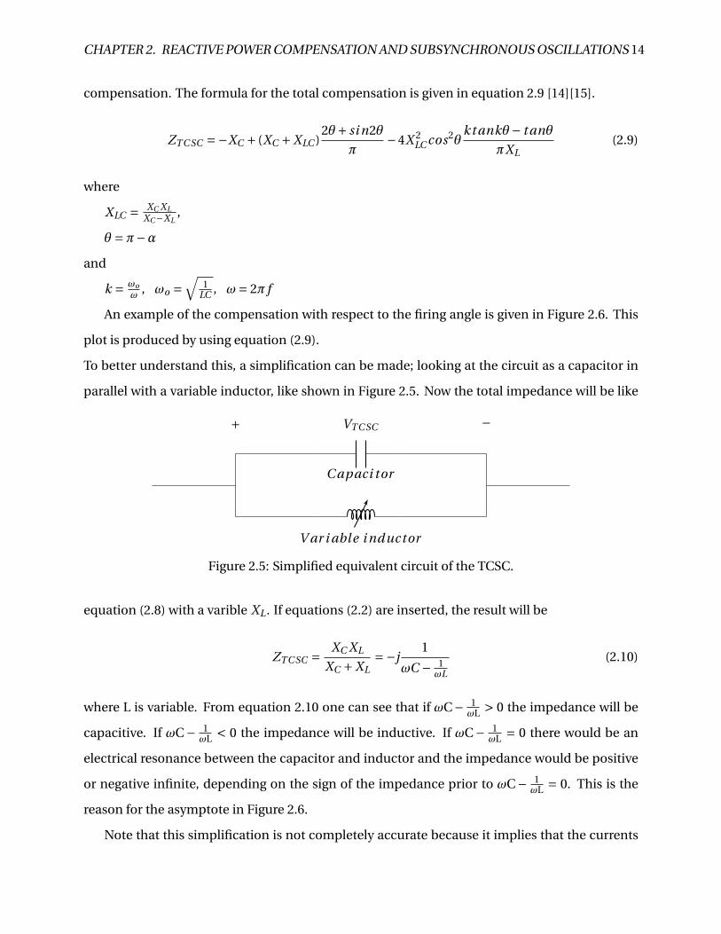
To better understand this, a simplification can be made; looking at the circuit as a capacitor in
parallel with a variable inductor, like shown in Figure 2.5. Now the total impedance will be like
+ −
C apaci tor
V ar i able i nductor
VT C SC
Figure 2.5: Simplified equivalent circuit of the TCSC.
equation (2.8) with a varible XL . If equations (2.2) are inserted, the result will be
ZTC SC = XC XL
XC +XL=−j
1
ωC − 1ωL
(2.10)
where L is variable. From equation 2.10 one can see that if ωC− 1ωL > 0 the impedance will be
capacitive. If ωC− 1ωL < 0 the impedance will be inductive. If ωC− 1
ωL = 0 there would be an
electrical resonance between the capacitor and inductor and the impedance would be positive
or negative infinite, depending on the sign of the impedance prior to ωC− 1ωL = 0. This is the
reason for the asymptote in Figure 2.6.
Note that this simplification is not completely accurate because it implies that the currents

CHAPTER 2. REACTIVE POWER COMPENSATION AND SUBSYNCHRONOUS OSCILLATIONS 15
Figure 2.6: Example of TCSC impedance level as a function of firing angle.
and voltages are pure sinusoidal. Of course in a TCSC the currents and voltages are impacted by
the controlling thyristors, making them non-sinusoidal [11].
As shown in Figure 2.6, there is always an impedance area in which the TCSC can not operate,
this area is important to have in mind when designing the TCSC (choosing sizes of inductor and
capacitor).
Figure 2.7 shows TCSC delivered by ABB in opertion in Imperatriz, Brazil.
Figure 2.7: TCSC system delivered by ABB in Imperatriz, Brazil.

CHAPTER 2. REACTIVE POWER COMPENSATION AND SUBSYNCHRONOUS OSCILLATIONS 16
2.4.4 Design of TCSC
When a TCSC is designed, it is important to choose the right values of the capacitor and induc-
tor. The price and size of the components are the main limitations. The sizes of the components
affect each other, and this is important to have in mind when designing the TCSC. There are
some important points that must be considered in the design:
1. XC must be larger than XL . If this requirement is not fulfilled, there will be no resonance
point and the TCSC will only operate in the capacitive mode. An example of this is in
Figure 2.8d.
2. If XLXC
< 19 there will be more than one resonance point. This limits the operating area of
the TCSC.
3. The resonance frequency ωr = 1pLC
must be much larger than the power frequency ω1 =2π f . This is so the capacitor voltage can be reversed within a half power period.
4. The resonance frequency ωr must also be far away from the harmonics of the power fre-
quency, ie. ωr 6= nω1 where n = 1,2,3, ...
5. It is usually possible to achieve a capacitive reactance of about three times the blocking
mode capacitive reactance, before getting to close to resonance point. When choosing
capacitor value, this must be considered with respect to the need for compensation, the
line reactance, and whether or not there will be fixed capacitors in series in addition to the
TCSC.
6. A large inductor gives a lower current through it, and thyristor ratings and cost will be
lower. A large inductor is also contributing to smaller harmonics components.
7. With a small inductor, the capacitor voltage reversal will be fast and good, and a small
value is also be beneficial if a fault occurs by limiting its size.
For all practical purposes ω1ωr
< XLXC
, this means that if point 3 is fulfilled, so is point 1. Figure 2.8
shows the impedance range as a function of firing angle for different values of capacitors and
inductors arranged with respect to ω1ωr
relationships (firing angle of resonance). As explained in
the points above, the resonance angle is given by the relationship between the capacitor and
inductor. A high inductor value compared to the capacitor can give no resonant points, and a

CHAPTER 2. REACTIVE POWER COMPENSATION AND SUBSYNCHRONOUS OSCILLATIONS 17
low can give more than one resonant points. The capacitor value must as explained be chosen
with the desired capacitive compensation in mind. A larger capacitor (lower capacitance) gives
more capacitive compensation [16]. Other important factors to consider while choosing capaci-
tor and inductor sizes are the voltage and current limits. Both thyristors , inductor and capacitor
can not have to high currents through them to prevent damage and overheating, and the insula-
tion level is limiting the voltages. These requirements are of course fulfilled for operating TCSCs
Figure 2.8: Example of TCSC impedance levels as a function of firing angle for different capacitorand inductor values arranged by ωr
ω1relationships.
around the world, and some these can be seen in Table 2.1 [13][17].
Table 2.1: Sizes and ratings of some TCSCs in operation around the world
TCSC Kayenta ASC Slatt TCSC Brazil TCSCVoltage level [kV] 230 500 550Rated current [A] 1000 2900 1500Capacitance [µF ] 193 350 200Inductance [mH ] 8.5 3.5 7
ω1ωr
2.5 2.9 2.7

CHAPTER 2. REACTIVE POWER COMPENSATION AND SUBSYNCHRONOUS OSCILLATIONS 18
2.5 Subsynchrounous Oscillations
In most power system analysis, all parts of the rotor of a turbine generator is assumed to have
an infinite stiffness between them. Hence it can be represented as a single mass with one iner-
tia constant. This mass is accountable for all oscillations with other generators in the system at
a frequency between 0.2 and 2 Hz, and the single mass method is acceptable in most cases of
power system analysis. However, this representation is a large simplification of the turbine gen-
erator, especially the steam turbine generator, and can not be used under certain circumstances
[18].
The steam turbine generator is composed of several masses with different inertia constants,
and a finite stiffness and damping between them. In addition to the generator part, there is a
high and intermediate pressure part of the rotor, and often there is two masses for the low pres-
sure part. If the generator has an exciter, this too will have a unique mass. This means that when
an external force is applied to the masses, they will react differently because of the different in-
ertias. The shafts connecting the masses will twist due to the finite stiffness, and a torque will
be transmitted to the neighboring masses. The neighboring mass will the react in the same way,
and this will repeat down the shaft, and torotional oscillations occur. Every generator rotor will
have unique torotional natural frequencies or modes dependent on its design. The oscillations
can be increased if the network have a certain configuration, or have certain devices imple-
mented. Some of these circumstances will be discussed in greater detail later. The oscillations
will reduce the lifetime of the shaft, and in extreme cases lead to shaft failure [19].
To avoid shortened lifetime or failure, it is important to understand these oscillations, when
they arise, and how to prevent them.
Figure 2.9 shows a simplified mass representation of parts of a steam turbine generator. Mass
2 and 3 could as an example represent the low and intermediate pressure part of the rotor. Mass
1 which is not included, could be the generator mass.
In Figure 2.9, τ2 and τ3 are the applied torques. The other drawn torques are the result-
ing shaft torques. ω0 is the angular frequency of the system, while ω2 and ω3 are the angular
frequency of the masses. δ2 and δ3 are the resulting displacement of the masses.
As an example, mass 2 will be studied. When newtons second law is applied to this mass, the

CHAPTER 2. REACTIVE POWER COMPENSATION AND SUBSYNCHRONOUS OSCILLATIONS 19
τ2 τ3
−τ21 τ23 −τ23 τ34
ω2ω0
ω3ω0
δ2 δ3mass 2 mass 3
Figure 2.9: Simplified mass representation of parts of a steam turbine rotor
motion equation is given by
J2dδ2
2
d t 2= τ2 −τ21 +τ23 (2.11)
where J2 is the moment of inertia for mass 2, τ2 is the applied torque and τ21 τ23 are the torques
in the shafts on each side of mass 2. These torques are given by the damping and stiffness in
the shaft between the masses, the difference between the displacement of the them, and the
difference between the rate of change in the two masses. In Figure 2.10 the masses and shafts
are shown with the belonging inertia, stiffness and damping.
J2, D22 J3, D33
mass 2 mass 3
ω2ω0
ω3ω0
δ2 δ3
k12 D12 k23 D23 k34 D34
Figure 2.10: Mass representation of parts of a steam turbine rotor with inertia, stiffness anddamping constants.
The shaft torques are given by the equations:
τ21 = k21(δ2 −δ1)+D21
(dδ2
d t− dδ1
d t
)(2.12)
and
τ23 = k23(δ3 −δ2)+D23
(dδ3
d t− dδ2
d t
)(2.13)
When inserting equation (2.12) and (2.13) into equation (2.11), and considering the self damp-
ing of mass 2 (the D22 term in the equation), the resulting second order equation becomes:

CHAPTER 2. REACTIVE POWER COMPENSATION AND SUBSYNCHRONOUS OSCILLATIONS 20
J2dδ2
2
d t 2= τ2 −k21(δ2 −δ1)−k23(δ2 −δ3)−D21
(dδ2
d t− dδ1
d t
)−D23
(dδ2
d t− dδ3
d t
)−D22
dδ2
d t(2.14)
If now difference between the system angular frequency and the angular frequency of a mass,
for example mass 2 is considered as ∆ω2=ω2 −ω0, there is two state variables per mass in the
system. Since ∆ω2 = dδ2d t , equation (2.14) can be written as the first order equation (2.15)
J2d∆ω2
d t= τ2 −k21(δ2 −δ1)−k23(δ2 −δ3)−D21(∆ω2 −∆ω1)−D23(∆ω2 −∆ω3)−D22∆ω2 (2.15)
There will be an equation like this for each mass in the system. A representation of a simple
four mass system is shown in Figure 2.11. A four mass system like this will have four equations.
J1 J2 J3 J4
HPI PLPGE N
k12
D12
D11
k23
D23
D22
k34
D34
D33 D44
Figure 2.11: Mechanical representation of a four mass turbine generator
By considering the angles and angular frequencies state variables, the equations can be rep-
resented by a matrix equation on the form
x = Ax +Bu (2.16)
where A is the state matrix, B is the driving matrix, x is a vector of state variables such as the
angles δ of equation (2.14) and u a vector of inputs, here the change in torque∆τ applied to each
mass. This equation can be used to find the natural frequencies of the rotor. The state matrix A
is given by
A =0 1
K D
(2.17)
where 0 is a null matrix, 1 is the identity matrix, K is the stiffness matrix and D is the damping
matrix. For the example system in Figure 2.11 the K and D matrix are

CHAPTER 2. REACTIVE POWER COMPENSATION AND SUBSYNCHRONOUS OSCILLATIONS 21
K =
−k12J1
k12J1
k12J2
−k12−k23J2
−k23J2
k23J3
−k23−k34J3
k34J3
k34J4
−k34J4
(2.18)
D =
−D12−D11J1
D12J1
D12J2
−D12−D23−D22J2
D23J2
D23J3
−D23−D34−D22J3
D34J3
D34J4
−D34−D44J4
(2.19)
The driving matrix B can be written as
B =[
0 J−1]T
(2.20)
where J−1 for the case in the example is a 4 x 4 matrix where the diagonals are 1/J1, 1/J2, 1/J3
and 1/J4.
However, to find the natural frequencies of the rotor, the B matrix is not necessary, because
it is calculated by assuming no change in input torque (u=0). Using u=0 gives the equation
x = Ax (2.21)
The solution of this equation, gives the eigenvalues and eigenvectors. As an example the
modes of IEEEs FBM multimass model are calculated using the data in Table A.7 and computer
software. The Modes are presented below in Table 2.2.
Table 2.2: Modes of IEEE FBM six mass model
Mode no. 1 2 3 4 5 6Frequency [Hz] 14.4 14.4 18.5 23.3 29.5 43.1
Note that the first benchmark model has six masses, that is why there are six modes. If the
system in Figure 2.11 would be used, there would be four modes, one four each connection
between the masses, and one for the oscillations of the entire rotor.

CHAPTER 2. REACTIVE POWER COMPENSATION AND SUBSYNCHRONOUS OSCILLATIONS 22
2.5.1 Subsynchrounous Resonance
If the sub-natural frequencies of the eigenvalues found in previous sectioin ( fsub) are similar to
the network natural frequency ( fer ), the oscillations from the generator(s) will be amplified.
fer ≈ fsub (2.22)
and
fsub = f0 − fT M (2.23)
where f0 is network frequency, and fT M is the torotional frequency found in calculated
eigenvalues (natural frequencies of rotor or torotional modes of oscillation).
These frequencies can now be used to find the compensation level of the line that will get
SSR. If the equations (2.22) and(2.23) is solved for fT M they become
fT M ≈ f0 − fer (2.24)
where
fer = f0
√XC
X ′′ +XT +XL(2.25)
XC is the reactance of the compensating capacitor, and X ,,, XT and XL are the subtransient re-
actance of the generator, the reactance of the transformer, and the line reactance.
The torotional frequencies are very weakly coupled with the overall system, so when system
impedance (network natural frequency) is changed, these frequencies stay the same. SSR occurs
when the sub natural frequency is close to one or more shaft frequencies.
Since the mode frequencies of the rotor can not be changed, and the network natural fre-
quency is changed with compensation, this is where both the problem and some of the solution
in this thesis arise (problem when only using fixed compensation, and solution when imple-
menting TCSC).
As researchers have proposed, the TCSC does not mitigate SSR only by changing the impedance.
If a TCSC is placed in the system with constant impedance, it can mitigate SSR by adding more
electrical damping with effective control and firing [20][21][22][23].

Chapter 3
System modeling and results
This chapter shows the procedure and modeling of the power systems used in this project work.
It describes, and gives a visual understanding of the systems studied and prensents the results
obtained from the studies.
23

CHAPTER 3. SYSTEM MODELING AND RESULTS 24
In the table below, the different stydycases in this report are summarized. Abberiviations
used are explaind further down.
Table 3.1: Summary of study cases in thesis
Case Fixed Compensation Multimass TCSC Event Double lines1 VAR NO NO NO NO2 VAR YES NO NO NO3 VAR YES OL NO NO4 YES YES OL/CL NO NO5 YES YES OL/CL NO YES6 YES YES OL/CL QOU T YES7 YES YES OL/CL POU T YES
VAR =Several simulations are done with variable fixed compensation.
OL = Simulation(s) are done with TCSC, and controller in open loop.
OL/CL = Simulation(s) are done with TCSC, and controller in both open and closed loop, often
starting with open, then switching to closed loop after a period of time.
QOU T = Event with consumed reactive power outage.
POU T = Event with active load outage.
3.1 Case 1: Model of Power System
The first step in this work is to model the power network. The model is a simplification of the
Great Britain power system, and consists of four buses with three generators and two loads. The
data for the generators are found in [2], the load, line and transformer data are found in [3].
Most of the base model for these simulations were made in the project work prior tho this
master thesis, now, more details are implemented. The model is build in the program PSCAD
which is a tool for describing electromagnetic transients.
Figure 3.1 shows the modeled system equivalent circuit, and its data is summarized in Table
3.2. The system consist of four buses where the upper buses represents the north and south
of Scotland, where there is a surplus of power due to large power production. The lower bus
is representing England and Wales, where there is a deficit of power due to high consumption.
Between the areas there are transmission lines where the power is flowing.

CHAPTER 3. SYSTEM MODELING AND RESULTS 25
Figure 3.1: Great Britain power system model
Due to the fact that there is a large surplus in the north of Great Britain, and a deficit in the
south (in addition to the potential for more renewable energy production inn the north), there
is a great need for power transfer from the north to the south.
A logical step to increase the power flowing from north to south as seen in section 2.2, is
implementing series compensation as shown in Figure 3.1.
Several simulations are done, and Figure 3.2 shows the power flowing in the Northern Scot-
land line as a function of the degree of compensation of the system. The degree of compensation
Table 3.2: Great Britain power system model parameters
Size Voltage NoteG1 2800 MVA 33 kV Star groundedG2 2400 MVA 33 kV Star groundedG3 21000 MVA 400 kV Star groundedT1 2800 MVA, j22.4Ω 33/400 kV Delta/Star connectedT2 2400 MVA, j11.2Ω 33/400 kV Delta/Star connectedLi ne14 0.001+j3.1Ω 400 kVLi ne24 0.001+j31.4Ω 400 kV UncompensatedLi ne34 0.001+j15.6Ω 400 kVLoad3 17730 MW + 2485 MVar 400 kVLoad4 2000 MW 400 kV

CHAPTER 3. SYSTEM MODELING AND RESULTS 26
of the line is defined by
% comp = XC
XLtot(3.1)
where XC is the reactance of the fixed capacitor and XLtot is the total reactance of the system
seen from the generator in Northern Scotland (without the compensation).
Figure 3.2: Active power flow in Northern Scotland line as a function of % compensation.
As Figure 3.2 clearly shows, the power flowing in the line is increasing with increasing degree
of fixed compensation. This is expected according to section 2.2.
However, a large fixed series compensation can not be done without consideration regard-
ing natural network frequency and resonance. The fact that the electrical resonance frequency
of the system will change like described in section 2.5 will eventually lead to SSR if the compen-
sation reaches a certain degree.

CHAPTER 3. SYSTEM MODELING AND RESULTS 27
3.2 Case 2: Implementing Multimass and increasing Fixed Com-
pensation
For a study of the subsynchronous resonance in the system to be possible, the PSCAD model
needs some further implementations. To simulate a steam turbine rotor, a "multimass" model
is implemented in the Northern Scotland generator. Values for inertia are assigned to each mass,
as well as damping and stiffness between the masses, as described in section 2.5. The number of
masses, and data which is used, are the same as in the IEEE first benchmark model on subsyn-
chronous resonance. The data is found in [3], and is displayed in Table 3.3. The first benchmark
model is a six mass model, like shown in Figure 3.3.
E X GE N LPB LP A I P HP
k12
D12D11
k23
D23D22
k34
D34D33
k45
D45D44
k56
D56D55 D66
Figure 3.3: Mechanical representation of IEEE FBM model for SSR.
Table 3.3: Inertias, Torotional stiffness, self and mutual damping coefficients of IEEE FBM modelfor SSR.
Inertia [ MW sMV A ] Stiffness [ pu T
r ad ] Self- and mut. damping [ pu Tpu Speed dev. ]
HHP 0.092897 k12 19.303 D11,D22 0
HI P 0.155589 k23 34.929 D33,D44,D55,D66 0.1
HLP A 0.858670 k34 52.038 D12 0.005
HLPB 0.884215 k45 70.858 D23,D34,D45,D56 0.2
HGE N 0.868495 k56 2.822
HE X 0.0342165
Now with the first benchmark model implemented, the fixed compensation can be increased,
and realistic results is expected considering SSR. From simulations, Figure 3.4 is produced. It
shows the electrical frequency of the system at different levels of compensation, ie. when the
line is compensated to 40 % or 48 % etc.

CHAPTER 3. SYSTEM MODELING AND RESULTS 28
Figure 3.4: Electrical frequency in the system at different levels of % compensation.
Figure 3.4 shows that the system has low frequency variations (SSR) at compensation levels
below 48 % compensation, but can not be compensated more than to 48 %, before it gets unsta-
ble due to the SSR. A higher compensation after this point, means a faster crash of the system,
as all other compensation levels above 48 % is unstable. This means that the sub- natural fre-
quency of the system is to close to one or more of the rotors natural modes of oscillation at these
levels.
When Figure 3.4 and 3.2 is studied, the results show that to be able to transfer more power
(in this case more than about 2 GW) in the Northern Scotland line, measures have to be taken.
Implementing a TCSC in the network might be a solution.

CHAPTER 3. SYSTEM MODELING AND RESULTS 29
3.3 Case 3: Implementing TCSC
To test if it is possible to increase the compensation and hence the power flow even further than
with the fixed compensation, a TCSC (L = 5mH ,C = 400µF ) is designed and implemented in
the system in series with the fixed capacitor. The design is done in accordance with the theory
of section 2.4.4, and it is a relatively small TCSC. The system is shown in Figure 3.5.
Figure 3.5: Model of power system with both fixed compensation and TCSC.
Figure 3.6 shows the case with only the fixed compensation at the critical level 48 %, and the
case where the TCSC is implemented in addition. The TCSC firing angle and the size of the fixed
capacitor is set to values that will make the total compensation of the hybrid system also equal
to 48 %.
From Figure 3.6 it is clear that, at least in the case where the compensation level is 48 %,
there is a significant improvement by using the hybrid fixed compensation and TCSC system.
This is due to an added damping from the TCSC.
To further investigate if the hybrid system is making it possible to increase the compensation
degree even more, the firing angle of the TCSC and the size of the fixed capacitor is varied, and
simulations are done. Note that in all of the test cases, the TCSCs controller is in open loop
(constant firing angle), this means that the TCSC is having a fixed reactance.
Figure 3.7 shows the power flow in the Northern Scotland line, as a function of % of com-
pensation both for the fixed capacitor, and the hybrid capacitor and TCSC case. The TCSC firing

CHAPTER 3. SYSTEM MODELING AND RESULTS 30
Figure 3.6: Electricl frequency in the two simulated systems with equal degree of compensation.
angle and the size of the fixed capacitor is varied to show different compensation levels. All
plotted cases are stable, and have a relatively low frequency variation.
The results making up Figure 3.7 shows that a TCSC, even a small one, can improve the power
flow of this system with 500 MW compared to a fixed capacitor, and around 1 GW compared with
no compensation.
In these cases, the TCSC is set to have a firing angle so that it is operating in inductive mode,
as described in section 2.4. Here the fixed capacitor and the TCSC will have opposite signs of
the reactance (the much larger fixed compensation is used to compensate, and the TCSC has
the function of varying the reactance).
In many scenarios if there is not already fixed compensation in the system, one would nat-
urally insert a larger TCSC and run it in the capacitive mode. In theory this is no problem com-
pared with the hybrid solution and one could expect the same results. However, with the model
of the power system and TCSC firing system there is simulation problems. Some successful sim-
ulations have been done with the TCSC in capacitive mode, but the compensation level is not
close to the obtained 75 % by the hybrid system.

CHAPTER 3. SYSTEM MODELING AND RESULTS 31
Figure 3.7: Active power flow in Northern Scotland line as a function of % compensation withboth fixed compensation and fixed combined with TCSC.
As mentioned there is many scenarios were there is a need to vary or change the impedance
of the line. This can be done with a closed loop controller. The controller could have references
such as current, power or impedance. The reference values can be adjusted when needed.
3.4 Case 4: TCSC with Controller in Closed loop
To further study the effect on SSR when impedance is changed, a closed loop controller is im-
plemented in the TCSC. The controller is show in Figure 3.8 [14].
A simulation is done where the fixed capacitor is 80µF and the TCSC is starting in open loop
at 100 °. After 15 seconds the controller goes from open to closed loop with a power flowing in
the Northern Scotland line as a reference.
Figure 3.9 show the frequency of the system, and the firing angle of the controller.
When the controller firing angle increases from 100 degrees, the inductive impedance in-
creases like shown in Figure 2.6. The firing angle of the TCSC goes from 100 ° to 130 ° and gives

CHAPTER 3. SYSTEM MODELING AND RESULTS 32
Figure 3.8: Closed loop controller used with the TCSC.
Figure 3.9: Electrical frequency of system and firing angle when TCSC is closed loop controlled.
a change in the total compensation from 70 to 58 %. As seen in Figure 3.9 frequency response
(SSR) is clearly improving with a higher inductive compensation from the TCSC.
The reason for the sudden saturation of the firing angle at 130 ° is an intentional design fea-
ture. If firing angle had not been forced to stop increasing at 130 °, the firing angle would con-
tinue increasing until the TCSC entered the resonance area described in section 2.4.
Intuitively the reason for the TCSCs failure to reach a steady firing angle would be that it is
designed too small. This is however not the case, as the power set point of the controller is close
to the power in the line at open loop operation. A reason for the TCSCs inability to reach a steady
firing angle on its own, could be that the total system with generator production in this case is
not that affected by the change of impedance in the line.

CHAPTER 3. SYSTEM MODELING AND RESULTS 33
3.5 Case 5: Modeling of System with double lines from North-
ern Scotland
To have a more accurate representation of the Great Britain power network, a double line is
implemented in Northern Scotland.
If the fixed capacitor and the TCSC now is placed in one of the lines as shown in Figure 3.10,
there is no problems with SSR in any of the simulations. The line can now be compensated all
the way to the degree where all power is flowing in the one line.
Figure 3.10: Power system model with double lines, fixed compensation and TCSC in one of thelines.
With the double lines, the TCSC can also operate in the capacitive mode without stimulation
crashing. Several TCSC sizes are tested. However, there are some uncertainty with these cases,
and not all results are as expected, therefor no plots are used in the report.
Now one small fixed capacitor is placed in each line (the compensation level is so small that
SSR is not an issue). The TCSC is placed in one of the lines, and a closed loop power controller
is initialized after 15 seconds. The network is shown in Figure 3.11.
The results of the simulation is shown in Figure 3.12. Here it is clear that the power is reach-
ing the desired level after approximately six seconds of closed loop operation. This means that
the design of the TCSC controller is satisfactory. There is however some oscillations in the power
in this case.
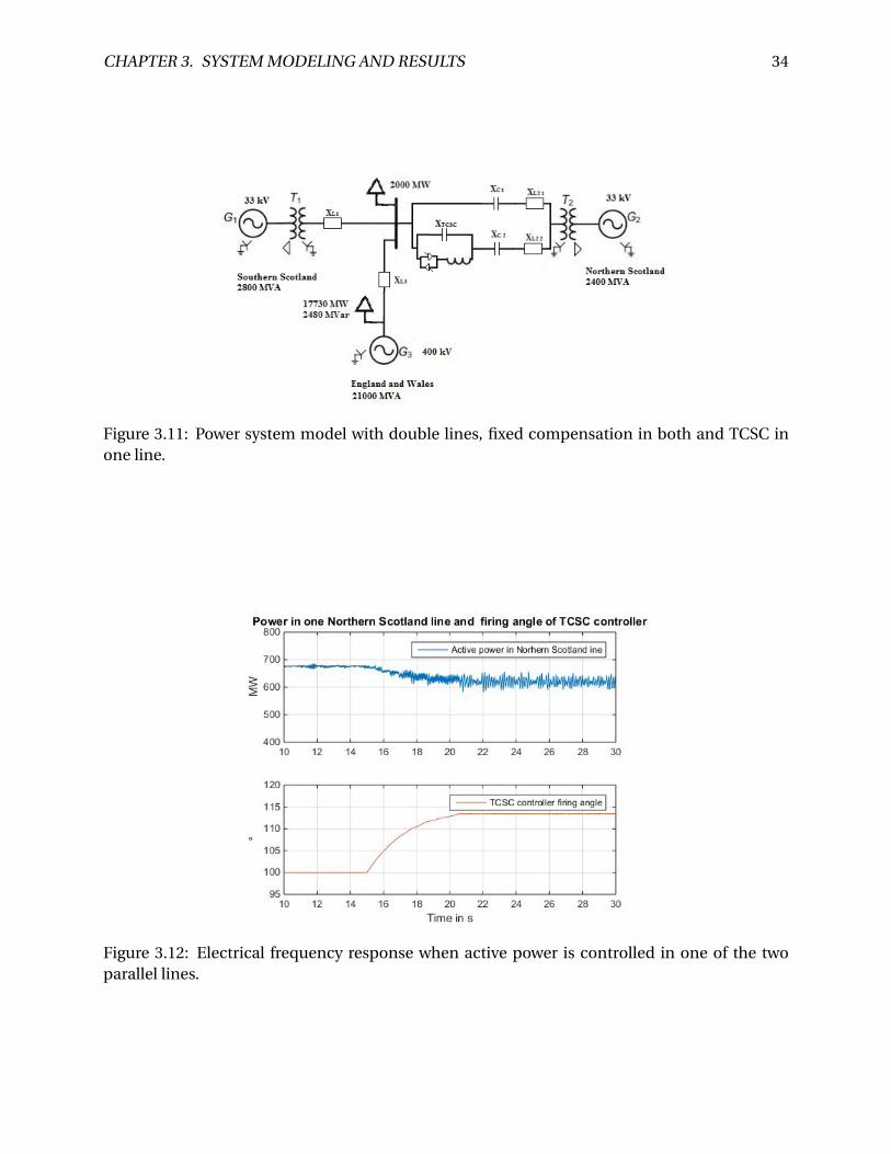
CHAPTER 3. SYSTEM MODELING AND RESULTS 34
Figure 3.11: Power system model with double lines, fixed compensation in both and TCSC inone line.
Figure 3.12: Electrical frequency response when active power is controlled in one of the twoparallel lines.

CHAPTER 3. SYSTEM MODELING AND RESULTS 35
3.6 Case 6: Reactive Power Event
To further show the value of the TCSC and have a more realistic network, the fixed compensation
the lines are increased. Now the system is more vulnerable to contingencies regarding SSR. As a
possible event, an 2400 MVar capacitive load is inserted at the load bus in the north. Inserting
produced capacitive reactive power is the same as removing consumed reactive power from the
system. This can be relevant if for instant a inductive compensating reactor is isolated from the
network due to fault, or a large load at the end of a sea cable is suddenly disconnected. Figure
3.13 shows the setup for this case study.
Figure 3.13: System with both fixed compensation and TCSC. Reactive power event.
This event is run with two scenarios:
• one where the TCSC is run in open loop, (100 °).
• one where the TCSC is switched from open (100 °) to closed loop (increasing from 100 °)
0.5 seconds after the event occurs. This is to change the total compensation level of the
system.
Figure 3.14 shows the electrical frequency in the systems in both cases, and firing angle of
the TCSC controller in the closed loop case.
From figure 3.14 it is clear that the system becomes unstable after the event if impedance is
not changed. From the frequency plot, one can clearly see SSR appearing in the open loop case.

CHAPTER 3. SYSTEM MODELING AND RESULTS 36
Not many seconds after the event, the system crashes.
However, when the controller of the TCSC is set to closed loop 0.5 seconds after the event,
the system stabilizes after few seconds. The reference of the controller is set so that the inductive
impedance of the TCSC will increase.
Figure 3.14: Electrical frequency responce to reactive power event. Open and closed loop in-cluding firing angle.
Note that the TCSC will most likely be operated in closed loop at all times in real life, but here
it is shown in open loop to begin with to better see the possibilities and uniqueness of the TCSC.
This also shows how a system with fixed compensation (even with the damping of the TCSC) is
more vulnerable to SSR than a system with variable compensation.

CHAPTER 3. SYSTEM MODELING AND RESULTS 37
3.7 Case 7: Power Outage Event
Another event is simulated in the same system as described earlier. Now instead of a change in
reactive power, a load of 1200 MW is disconnected from the load bus in the north. The system
with the event is seen in Figure 3.15. Note that 1200 MW is removed from the original load in
the north, leaving it with a size of 800 MW.
Figure 3.15: System with both fixed compensation and TCSC. Loss of active power event.
The outage event will decrease the current flowing in the system, and making the consumed
reactive power decrease. The produced reactive power will mostly stay the same due to the
relatively constant voltage in the lines.
In this case as well as in the previous, two scenarios are simulated; one with constant impedance
(open loop), and one with increasing impedance (closed loop).
Figure 3.16 shows again that the case with the constant impedance is having an increasing
frequency variation due to SSR and eventually crash. For the closed loop case the frequency
settles at almost the same levels as before the event.

CHAPTER 3. SYSTEM MODELING AND RESULTS 38
Figure 3.16: Electrical frequency response to active power outage event. Open and closed loopincluding firing angle.

Chapter 4
Summary and Further Work
This chapter is a summary chapter with a discussion and a conclusion section. Lastly there is a
section containg some recommendations for future work.
39

CHAPTER 4. SUMMARY AND FURTHER WORK 40
4.1 Discussion
Subsynchronous resonance have been the main field of study in this thesis. The Great Britain
transmission network have been used as a study case. The model of the Great Britain network is
simplified, but all the data used for the model is found in several prestigious articles.
As explained in the introduction, compensation is necessary in this network due to the need
for efficient power transfer from North to South of the island. This is described in the theory of
section 2.2. In section 3.1, this theory is proved by simulating several different study cases with
variable compensation. When the power flow from the North to the South is increasing with
increasing compensation, the results are validating both the theory, and the model of the Great
Britain power network.
In section 3.1, no SSR is occurring at any level of compensation. This is due to the fact that
the system is not sufficiently detailed yet. A multimass model is implemented to have a more
detailed model. IEEEs first benchmark model on SSR is used. All power systems consists of
several smaller generators all with different design, but here one model is used for simplicity.
This seems to be the norm in other SSR studies as well. The IEEE model is of course made to
simulate real generators, so in this regard the result will still be valid.
When the multimass is implemented in the system, the results of section 3.2 shows that the
expected SSR is "successfully" produced when compensation reaches a certain degree. When
the IEEE FBM is previously used in other studies, SSR have occurred with similar degrees of
compensation. This validates that the multimass model is correctly implemented, and that the
calculations done on compensation levels are reliable. As seen in section 3.2 it seems that a
higher compensation, leads to a more unstable system. This is however not necessarily true, as
the system could in theory be stable at compensation levels making the sub-natural network fre-
quency far enough away from (between two) natural frequencies of rotor as described in section
2.5.1. A clearer picture of this would be provided with more time and resources. A procedure for
presenting it would be to manually calculate the eigenvalues of the system at different levels of
compensation and plotting the results as done in [3].
To study the effect of the TCSC, it is implemented in the compensated line. The design of
the TCSC is done according to the theory of section 2.4.4 and to get a satisfactory range of com-
CHAPTER 4. SUMMARY AND FURTHER WORK 41
pensation. According to theory, the range of the possible reactance values of the TCSC will be
enough to both affect power flow and natural network frequency if needed.
From Figure 3.6, where two system electrical frequencies are plotted with the same degree
of compensation, one having the TCSC implemented, it can be seen that implementing a TCSC
is clearly damping the oscillations. This means that the TCSC is mitigating SSR independent of
compensation level ie. damping oscillations by just being in the system.
The TCSC is adding a damping to the system, and Figure 3.7 is showing that this makes it
possible to compensate further than 50 % without SSR occurring. The results show that with a
TCSC, there is many scenarios where more power can be transferred than without. However,
when studying this case, it became clear that not all compensation levels and combination of
TCSC with firing angle and fixed capacitor is stable. Some combinations did not end with a
successful power flow. Here it would have been interesting to have done the eigenvalue stud-
ies mentioned previously. From this study, the power flow from the north of Scotland can be
improved with more than 25 % by implementing a TCSC. From this it is clear that to increase
power flow, the TCSC is a highly attractive choice for this network compared to construction of
new lines.
In section 3.4 the usefulness of controlling the firing angle is studied. A system with ini-
tially large compensation is having a TCSC implemented with it changing from a small induc-
tive state to a more inductive state. Initially there are relatively large oscillations in the electrical
frequency, but when the firing angle and hence reactance of the TCSC changes, these oscilla-
tions are reduced with a magnitude of approximately ten. The results of Figure 3.9 shows that
by changing the reactance and the sub-network natural frequency moving it away from the me-
chanical torotional frequencies is important if SSR is to be avoided. These results are confirm-
ing the theory of section 2.5.1, and showing that TCSC is able to change the network natural
frequency.
The double lines from the north of Scotland in section 3.5 is implemented to have a more
accurate model of the real Great Britain network. Simulations done until this point are still valid
in showing the SSR and the value of the TCSC in a general sense, as two smaller identical lines
with double the reactance of the original line would not have an impact on the results. One
concern would be that it might not be economically the best decision to have two smaller TCSCs

CHAPTER 4. SUMMARY AND FURTHER WORK 42
the two lines. A more reasonable case is to have fixed compensation in one line, and a TCSC (and
in this thesis fixed compensation) in the other.
To further study the effect of the TCSC, some specific cases are simulated. The first is one
where consumed reactive power is removed from the network. As discussed in section 3.6, this
could happen if a reactive load or line is disconnected from the network, or a load at the end
of a sea cable being disconnected making the cable consume less reactive power. As reactive
power is significant to the network natural frequency this change was expected to have an im-
pact on the system, and produce SSR. Figure 3.14 shows that without variable compensation,
SSR is occurring and system will eventually crash, while in the case with the TCSC in closed loop
the electrical frequency settles quickly. This implies that initially the sub-network natural fre-
quency was close to a torsional mode, and that the effect of contingency made the system enter
instability.
In section 3.7 another contingency is occurring. Here much of the same is happening as
less load leads to a change in the reactive power consumed by the system. The TCSCs ability
to change its reactance is shown to be very valuable in these kind of contingency events, and
having a TCSC would make the network much more robust.
It is important to note that there is simulated many cases with several different settings on
parameters in this thesis. Only a few is presented in the report. Not all contingency events or
compensation levels will lead to SSR and one must note that the events plotted are selected due
to the SSR occurrence and mitigation. However these events are very likely to happen in a power
system and although they not have a high probability, power systems must be designed to have
high reliability.
Although this thesis is focused on the Great Britain power network, much of the results can
be generalized and applied to other power networks with need of large power transfers over long
distances. As SSR inevitably becomes a problem with some level of compensation, the TCSC
would be of use in many power network whose need for greater power transfer is present.

CHAPTER 4. SUMMARY AND FURTHER WORK 43
4.2 Conclusion
The work of the thesis started with a continuation of a project work. A model of the Great Britain
power network was developed further and with greater detail from previous project. The power
flow and other variables where monitored and the model was continuously validated. It was
early shown that with a higher degree of series compensation comes a higher power flow. This
was expected and used as a validation of theory and model.
In the beginning of the project, the SSR was not a problem in simulations. The reason was
that the model did not have sufficient details. Therefore a multimass model was successfully
implemented in one of the generators of the model. Now in section 3.2, more in line with the
theory on highly compensated systems, SSR was occurring. The SSR limited the series compen-
sation of the system close to the limits of similar studies on the subject.
After designing a TCSC, simulations where run with both the TCSC and fixed compensation
in the system. These simulation where compared to simulations with only fixed compensation
with equal degree of compensation. In section 3.3 it is clear that the TCSC is adding damp-
ing to the system, and it is successfully shown that it mitigates SSR. From this section it is also
shown that with a TCSC the Great Britain network can have nearly twice the compensation level
compared with only fixed compensation.
The connection between the control of the TCSC and the occurrence of SSR is presented in
section 3.4. In the example presented, the ability to control the TCSC reactance is proven to be
of great importance when mitigating oscillations.
When the other TCSCs was designed and implemented to fully replace the fixed compensa-
tion of the system, the simulations did not behave as expected and often crashed. Therefor if
the objective was to fully replace the fixed compensation with the TCSC, there would be needed
more work on that specific case. It can be hinted that the SSR mitigating ability of one large
TCSC is as good or better than a combination of fixed compensation and a smaller TCSC, but in
this system research is needed to assertively conclude.
After some more detailing of the network model, there was done some specific case studies
in section 3.6 and 3.7. Here the TCSCs ability to mitigate SSR occurring from contingencies was
proved.

CHAPTER 4. SUMMARY AND FURTHER WORK 44
From this thesis it can be stated that the TCSC would be a good option for increased power
transfer in the Great Britain power network, and other networks with similar power transfer
challenges regarding SSR. Other benefits that come with the TCSC is the ability to control power
flow, both under normal operation and during contingencies.
4.3 Further Work
As mentioned earlier, some further work would be to study the TCSC as a full replacement for
the fixed compensation in the network. This is very relevant as both all the compensation and
SSR mitigation can be done with one unit.
Calculations of eigenvalues in the system with different degrees of compensation both fixed
and TCSC would also be an interesting addition to this thesis. This would give a clearer picture
of the limitations and improvements of the network regarding stability. It would also be helpful
when studying contingencies in the system.
Lastly the interaction between the TCSC and other FACTS or HVDC-terminals could be an
interesting field to study as a continuation of this thesis. This will be increasingly relevant in the
future, as quickly emerging renewables and technology improvements will increase the use of
FACTS/HVDC all over the world.

Bibliography
[1] W. Long and S. Nilsson, “Hvdc transmission: Today and yesterday,” IEEE power & energy
magazine, 2007.
[2] F. M. Hughes, O. Anaya-Lara, N. Jenkins, and G. Strbac, “Control of dfig-based wind gener-
ation for power network support,” IEEE TRANSACTIONS ON POWER SYSTEMS, 2005.
[3] C. E. Ugalde-Loo, J. B. Ekanayake, and N. Jenkins, “Subsynchronous resonance in a series-
compensated great britain transmission network,” IET Generation, Transmission & Distri-
bution, 2012.
[4] Standard Handbook for Electrical Engineers. Mc Graw Hill, 16 ed., 2013.
[5] J. J. Grainger and J. W. D. Stevenson, Power System Analysis. McGraw-Hill Education, 1994.
[6] N. Mohan, Electric Power Systems: A First Course. Wiley, 2012.
[7] T. Miller, Reactive Power Control in Electric Systems. Wiley, 1982.
[8] J. Dixon and J. Rodriguez, “Reactive power compansation technologies: State-of-the-art
review,” Proceedings of the IEEE, 2005.
[9] I. Kiran and J. Laxmi.A., “Shunt versus series compensation in the improvement of power
system performance.,” INTERNATIONAL JOURNAL OF APPLIED ENG. RESEARCH, 2010.
[10] F. Iliceto and E. Cinieri, “Comparative analysis of series and shunt compensation schemes
for ac transmission systems.,” IEEE, 1977.
[11] R. M. Mathur and R. K. Varma, Thyristor-based FACTS controllers for electrical transmssion
systems. Wiley, 2002.
45

BIBLIOGRAPHY 46
[12] R. M. Malizewwski, B. M. Pasternack, and L. Paulson, “Power flow control in a highly inte-
grted transmission network,” CIGRE Paper 37-303, 1990.
[13] N. G. Hingorani and L. Gyugyi, Understanding Facts. Wiley, 1999.
[14] O.Anaya-Lara, E.Acha, V.G.Agelidis, and T. Miller, Power Electronic control in Electrical Sys-
tems. Newnes Power Engineering Series, 2002.
[15] M. N. Moschakis, E. A. Leonidaki, and N. Hatziargyriou, “Considerations for the application
of thyristor concontrol series capacitors to radial power distribution circuits,” IEEE, 2003.
[16] M.Nayeripour and M. M. Mansouri, “Analyze of real switching angle limits in tcsc on ca-
pacitor and inductor values and their selection factors,” International Journal of Advanced
Science and Technology, 2013.
[17] C. Gama, L. Angquist, G. Ingestrom, and M. Noroozian, “Commisioning and operative ex-
periance of tcsc for damping power oscillation in the brazilian north-south interconnec-
tion,” Cigre, 2000.
[18] P. Kundur, Power System Stability and Control. McGraw-Hill, 1994.
[19] J. Machowski, J. W. Bialek, and J. R. Bumby, Power System Dynamics, Stability and Control.
Wiley, 2012.
[20] V. Zhu, R. Spee, R. Mohler, G. Alexander, W. Mittelstadt, and D. Maratukulam, “An empt
study of ssr mitigation using the thyristor controlled series capacitor,” IEEE Transaction on
Power Delivery, 1995.
[21] N. Kakimoto, A. Ilda, M. Seki, K. Minoyama, and T. Takuma, “Clarifiction of the ssr mitiga-
tion mechanism of a tcsc,” Electrical Engineering in Japan, 1997.
[22] C. Z. Qianjin Liu and, L. Angquist, and S. Rudin, “Using tcsc scheme for ssr mitigation in a
radial transfer corridor,” International Conference on Power System Technology, 2006.
[23] R. Zheng, G. Li, and J. Liang, “Capability of tcsc on ssr mitigation,” Journal of Power and
Energy Engineering, 2015.

Appendix A
Great Britain Power System Information
The system is a four bus system. Generator 1 is at bus 1, generator 2 at bus 2 and generator 3 at
bus 3. Bus 4 is the connection point for all the other buses, and the north load lies at this bus.
I

APPENDIX A. GREAT BRITAIN POWER SYSTEM INFORMATION II
A.1 Lines
Table A.1: Line data
Line Impedance [Ω]1-4 0.001+j3.42-4 0.001+j31.43-4 0.001+j15.7
A.2 Loads
Table A.2: Load data
Bus [MW]/ph [MVar]/ph Ref. voltage (l-g) [kV]3 5910 828 144.44 667 0 144.4
A.3 Transformers
Table A.3: Transformer data
Transformer 1 Transformer 2Rating [MVA] 2800 2400Configuration ∆/Y (∆ lags Y) ∆/Y (∆ lags Y)Voltage ratio 33/400 33/400Leakage reactance [Ω] 22.4 11.2Air core reactance [pu] 0.2 0.2Magnetizing current [%] 1 1Knee voltage [pu] 1.17 1.17

APPENDIX A. GREAT BRITAIN POWER SYSTEM INFORMATION III
A.4 Generators
A.4.1 Synchronous Generator
Table A.4: Synchronous generator data
Generator 1 Generator 2 Generator 3Rating [MVA] 2800 2400 21000Rated RMS Current [kA] 49 42 30.3Rated RMS Voltage (l-n)[kV] 19.05 19.05 230.9Base angular frequency [rad/sec] 314.16 (2π50) 314.16 (2π50) 314.16 (2π50)Inertia constant [s] 3.84 2.89 5Mechanical Friction and Windage [pu] 0.04 0.04 0.04Neutral Series Resistance [pu] 105 105 105
Neutral Series Reactance [pu] 0 0 0Iron Loss Resistance [pu] 300 300 300Armature Time Constant (Ta) [s] 0.278 0.278 0.278Potier Reactance (Xp ) [pu] 0.17 0.17 0.163Unsaturated Reactance (Xd ) [pu] 2.13 2.13 2.0Unsaturated Transient Reactance (X ′
d ) [pu] 0.308 0.308 0.35Unsaturated Sub-Transient Reactance (X ′′
d ) [pu] 6.0857 6.0857 5Unsaturated Transient Time (Open)(T ′
do) [s] 0.234 0.234 0.28Unsaturated Sub-Transient Time (Open) (T ′′
do) [s] 0.0526 0.0526 0.039Unsaturated Reactance (Xq ) [pu] 2.07 2.07 1.9Unsaturated Sub-Transient Reactance (X ′
q ) [pu] 0.234 0.234 0.375Unsaturated Sub-Transient Time (Open) (T ′′
qo) [s] 0.3538 0.3538 0.071Ramp-up time when source [s] 0.1 0.1 0.1Initial terminal voltage [pu] 1.1 1.1 0.9Initial phase [rad] 0.0764 0 0
A.4.2 Exciters
Table A.5: Excitor data
Exciters 1,2 & 3Regulator Gain (KA) [pu] 400Regulator Time Constant (TA) [s] 0.02Max Internal Regulator Voltage [pu] 14.5Min Internal Regulator Voltage [pu] -14.5Max Regulator Output [pu] 6.03Min Regulator Output [pu] -5.43

APPENDIX A. GREAT BRITAIN POWER SYSTEM INFORMATION IV
A.4.3 Governors and Turbines
Table A.6: Governor and Turbine data
Hydro Governor 1 & 3 Hydro Governor and Turbine 2Permanent Droop [pu] 0.04 1.0Temporary droop [pu] 0.35 0.01Max Gate Position [pu] 1.0 Base Frequency [Hz] 50Min Gate Position [pu] 0 Controller Real Pole Gain [pu] 0.88Max Gate Opening Rate [pu] 0.16 Controller Proportional Gain[pu] 3.7Min Gate Closing Rate [pu/s] 0.16 Controller Integral Gain [pu] 0.44Pilot Valve and Servomotor Time Constant [s] 0.05 Controller Real Pole Time Constant [s] 0.02Servo Gain [pu] 5.0 Turbine Lead Time Constant [s] 0.01Main Servo Time Constant [s] 0.25 Turbine Lag Constant [s] 0.01Reset or Dashpot Time Constant [s] 6.0 Inverse Gate Velocity Limit [s/pu] 4.8
Time Constant for Smoothing Tm0 [s] 0.02Hydro Turbine 1 & 3 Conversion Constant 1.9
Head at rated conditions [pu] 1.0 Governor Time Constant [s] 0.05Output Power at rated conditions [pu] 1.0 Gate Velocity Time Constant [s] 0.01Gate position at rated conditions [pu] 1.0 Gate Position Control Rate Limit [pu/s] 0.22Rated no load Flow [pu] 0.05 Temporary Droop Time Gain 0Initial Operating Head [pu] 1.0Water starting time [s] 2.0Penstock Head Loss Coefficient [pu] 0.02Turbine Damping Constant [pu] 0.5
A.4.4 Multimass in Northern Scotland Generator
Table A.7: Inertias, Torotional stiffness, self and mutual damping coefficients of IEEE FBMmodel for SSR.
Inertia [ MW sMV A ] Stiffness [ pu T
r ad ] Self- and mut. damping [ pu Tpu Speed dev. ]
HHP 0.092897 k12 19.303 D11,D22 0
HI P 0.155589 k23 34.929 D33,D44,D55,D66 0.1
HLP A 0.858670 k34 52.038 D12 0.005
HLPB 0.884215 k45 70.858 D23,D34,D45,D56 0.2
HGE N 0.868495 k56 2.822
HE X 0.0342165

Appendix B
Study case data
Table B.1: Study case data
Case C [µF ] TCSC [° ] Event1 ∞ -133 - -2 ∞, 150, 122, 120, 118 - -3a 122, 90 -,130 -3b 117-51 125 - 133 -4 80 100 - 130 -5 2 x 400 100 - 114 -6 2 x 50 100 - 130 2400 MVar out7 2 x 55 100 - 110 1200 MW out
V

Appendix C
Model in PSCAD
Below a snip of one of the models made in the thesis is shown (Case 7).
VI

APPENDIX C. MODEL IN PSCAD VII