Surface reflectance estimation by the dichromatic model

Shoji Tominaga Osaka Electro-Communication University Neyagawa. Osaka 572 Japan

Surface Reflectance Estimation by -

the Dichromatic Model *

A method is described for estimating the surface-spectral reflectances of glossy objects when the color signal is a mi.nure of diJiuse reflections, specular reflections, and interreflections. The objects are inhomogeneous dielectric materials, and the reflected light is measured using a spectroradiometer. We first describe the main idea: the color signals, reflectedfrom two closely apposed surfaces with a single interreflection between them, can be e2x- pressed by a linear combination of the illuminant spectrum and two diJiuse spectral reflection functions. We introduce a representation in which each of these three terms is projected onto a point on a unit sphere. Estima- tion of the difiise reflection functions is then reduced to finding the vertices of the spherical triangle. Next, an algorithm is described to estimate the locations of the vertices of dlfuse reflectance functions from the measured samples. The reliability ofthe algorithm is demonstrated in an experiment using two plastic objects with glossy sur- -faCe.Y. 0 I996 John U'iley & Sons, Inc.

Kcy words: surface spectral reflectance, reflectance estimation, illuminant estimation, dichromatic reflection model, highlight, interreflection, color signal.

INTRODUCIION

Knowledge of the surface-spectral reflectance of objects in a scene is important in color measurement and in many color applications, including computer vision, computer graphics, and color reproduction. Precise measurements of the surface-spectral reflectances are usually made using a spectrometer under carefully controlled experimental conditions. For example, Vrhel et al.' re- ported the measurement procedure of reflectance spectra of flat objects, oriented to reduce specularities, and whose position can be alternated with a calibrated white standard.

* Presented at the ISCC First Panchromatic Conference, Wil- liamsburg, Virginia, February 12-15, 1995. 0 1996 John Wiley &Sons, Inc.

104 CCC 0361-2317/96/020104-11

In many applications, however, it may be necessary to estimate the surface reflectances of complex objects in place. In these applications it may be difficult or impossible to flatten the surface, or to exclude all specularities from measurement. Moreover, in some applications, such as remote sensing, it may be impossible to move the object or place a standard in the scene. In these cases, the light reflected from the object, which we call the color signal, may include diffuse reflections, specular highlights, and also mirror-like interreflections from other nearby surfaces.

This article describes a method for estimating the surface-spectral reflectances of glossy objects when the color signal is a mixture of diffuse reflections, specular reflections, and interreflections. We suppose that the objects are inhomogeneous dielectric materials, and the reflected light is measured at many wavelengths using a spectrometer. The algorithms described here rely on the dichromatic reflection model, introduced by Shafer.3 This model applies well to dielectrics for which the specular reflection component mirrors the ill~mination.~

The calculations in this article extend the work in a series of related articles. Tominaga and Wandell 5-6 proposed algorithms for estimating the illuminant's spectral power distribution and the permissible solution bands of the reflectance functions by measuring two inhomogeneous object surfaces. Interreflection effects are neglected in these algorithms. In computer vision, Klinker et al.' detected highlights in color images based on the dichromatic reflection model. Shafer et a1.* described a color model for interreflection between two surfaces. Healey' tried spectral reflectance estimation using highlights. Drew et a1.I' proposed an approach to interreflection between two Lambertian surfaces. Novak et al. I '

presented methods for estimating scene parameters from image data.

In the following, we first describe the main idea: when the dichromatic model holds, the high-dimensional color signals reflected from a pair of surfaces can be approximated by a linear combination of the illuminant

COLOR research and application

mattecluster

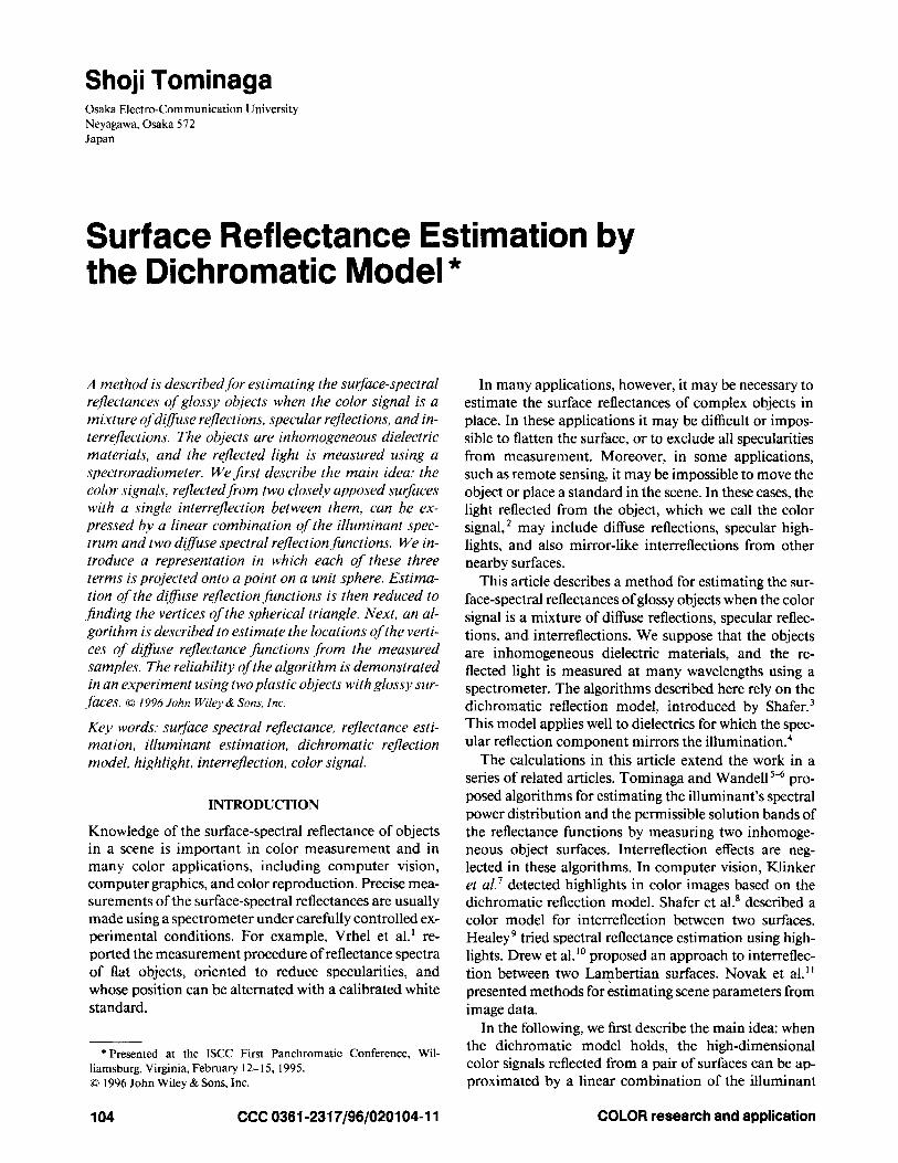
FIG. 1. The distribution of the color signals from a single, isolated object, projected onto the color signal plane. The points typically follow one of a few characteristic shapes, such as a skewed L. The points segregate into two clusters corresponding to the interface and body processes.

spectrum and two smoothly varying diffuse spectral reflection functions. We introduce a representation in which each of these three terms is projected onto a point on the unit sphere. We show that projections of the color signals measured from the surfaces will fall along a spherical triangle. When the dichromatic reflection model holds, estimation of the diffuse reflectance functions and illuminant spectral power distributions is equivalent to finding the three vertices of the triangle. The measured color signals are sample points along this triangle, but these sample points do not necessarily include the vertices of this triangle. In the next section, an algorithm is described to estimate the locations of these vertices from the sample measurements. In the third section the results of applying this algorithm to a simple scene comprising two apposed glossy surfaces are described, and the reliability of the algorithm is evaluated.

of the illumination from the interface of the surface. The body reflection, ce(x)S( A)E( A ) , arises from illumination rays that pass beyond the body interface and are scattered from within the surface. The body reflection is also called the diffuse reflection for scattering. The relative spectral power distributions of these two components are constant across the surface. Differences in the color signal arise only because the relative contributions from these two factors, described by the weights cI( x) and ce(x), vary across the surface due to the geometric properties of illumination, observation, and surface ori- entation. According to the dichromatic model, the color signals observed from an isolated object fall in a two-dimensional subspace that we call the color signal plane.

Figure 1 shows a sketch of typical distribution of the color signals projected onto the color signal plane. Each circle indicates the observation point from one location on the object surface. Klinker et al." showed that, if an object is convex and smooth, the observations on the color plane will be distributed in the shape of a skewed T. If the phase angle between the illumination and observation is small, the histogram shape becomes a skewed L or a dogleg as shown in Fig. 1. This property also holds if we observe only a single highlight area on the surface. The distribution of the observations is com- posed of two linear clusters: the body cluster and the interface cluster that come from areas of the surface domi- nated by one or the other type of reflection process.

Modeling Interreflection

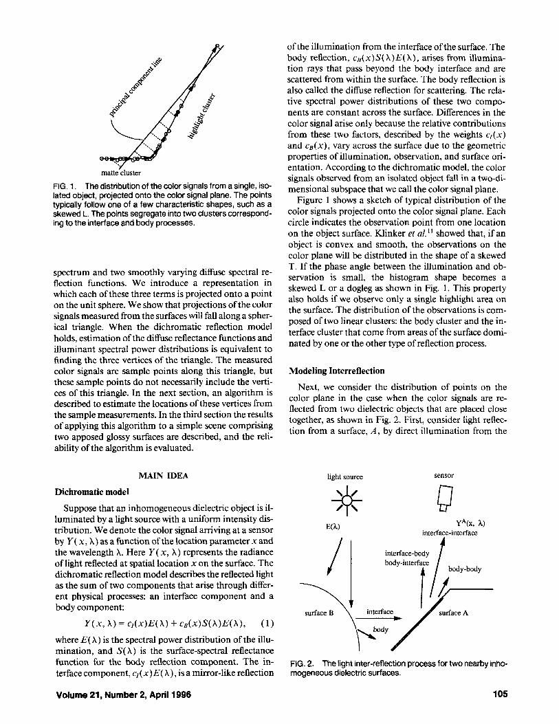
Next, we consider the distribution of points on the color plane in the case when the color signals are reflected from two dielectric objects that are placed close together, as shown in Fig. 2. First, consider light reflection from a surface, A , by direct illumination from the

MAIN IDEA light source sensor

Y*b, A)

Dichromatic model

Suppose that an inhomogeneous dielectric object is illuminated by a light source with a uniform intensity dis-

by Y ( x, A) as a function of the location parameter x and the wavelength A. Here Y ( x, A ) represents the radiance of light reflected at spatial location x on the surface. The dichromatic reflection model describes the reflected light as the sum of two components that arise through different physical processes: an interface component and a body component:

interface-interface tribution. We denote the color signal arriving at a sensor E(A)

body-body

interface

y ( x , A ) = cI(x)E(A) + cE(x)s(A>E(A), (1)

where E( A ) is the spectral power distribution of the illumination, and S( A ) is the surface-spectral reflectance fUnction for the body reflection component. The interface component, cI( x )E( A), is a mirror-like reflection

FIG. 2. The light inter-reflection process for two nearby inhomogeneous dielectric surfaces.

Volume 21, Number 2, April 1996 105

single light source. Because of the dichromatic property, this reflection consists of two terms of the body and interface reflection components. A nearby surface, B , pro- vides a second source of illumination onto the surface A . For simplicity, we assume that the interreflection is based on only one bounce between two surfaces, and neglect the influence of multiple bounces. This assump- tion is reasonable because of the anticipated reduction in signal strength across several reflections.

The color signal from the surface A is then described as follows:

Y “ ( x , A )

= wi(x)SA(X)E(X) + w;4(x )E(A) + Y A B ( X , A). (2 )

The first two terms in the right-hand side represent the dichromatic reflection components by direct illumination from the light source, where SA( A ) is the body-spectral reflectance function of the surface A , and wf (x) and w: (x) are the weighting coefficients at location x on the surface A . The third term YAB( x, A ) represents the interreflection component by light that was already reflected by the surface B. By multiplication of dichromatic reflection, this interreflection term is described as a sum of four terms of body-interface, interface-body, interface- interface, and body-body as shown in Fig. 2. For example, the term body-interface means the reflection process that body reflection occurs on surface B , and then the reflected illumination causes interface reflection on surface A . The term body-body represents the reflection process that body reflection occurs on both surfaces A and B . This body reflection will be very weak compared with the other components, because ( a ) the reflected light is diffused widely and { b) the resulting reflectance is determined on multiplication of the body-spectral reflectances ofA and B.8,‘3 Ignoring this term and grouping the others yields a color signal from the surface A containing three terms:

Y 4(x, A) = wfz(x)S”( A)E( A )

+ W ; P b B ( X ) S B ( A ) E ( A ) + w:z(X)E(X) , ( 3 )

where wf2(x) = w;S(x) + w;f ,”(x) and w:‘,(x) = w:’(x) + If we divide the color signal by the illumination, we

obtain an expression that we will call the total reflectance, of object A in the context of object B, namely

W;”<x,.

S A ( X , A )

= w&(x)SA(A) + w:‘bB(x)SB(X) + w;42(x). (4)

In the right-hand side of the above, the first term represents the object color of the surface A , which is produced by body reflection of A itself. The second term is the object color of the surface B by mirror-like reflection of A . The third term is the light-source color, which is produced by interface reflection ofA itself, and partly by the interface-interface process.

The total reflectance of surface A is a linear combina-

tion of a constant function and two smoothly varying spectral reflectance functions SA( X ) and S E ( A ) . Hence, we find that when the approximations we have made hold, the total reflectance function we anticipate from surface A , and also by symmetry from B , will equal the sum of three separate terms. The color signal at each point on the two surfaces will differ only by the relative weight of each of the three terms.

Illurninant Estimation

Let us consider the following sequence of illuminant estimation problems. First, suppose that we have data from a single specular surface. We can use the pattern of measurements within the color plane (see Fig. 1 ) to cluster the data into interface and body reflection terms. To the extent that we can separate these measurements ac- curately, and that we can measure the very intense specular points, the illuminant spectrum can be predicted from the interface reflections. l 2 A procedure for predicting the illuminant from a signal specular surface is given in the Appendix.

When we have color signal measurements from two different objects under a single illuminant, the illuminant estimation can be made even more reliably by using the algorithm described in Tominaga and Wandell.5 This algorithm takes advantage of the fact that each surface spans a two-dimensional color signal plane and that the intersection of the planes is a vector in the direction of the illuminant spectral power distribution (see also Lee, l4 and D’Zmura and Lennie I s ) . If we have interreflections between two surfaces, the color signal from each surface is no longer constrained to fall within a plane. However it should be noted that the specular highlight regions on the surface include almost no interreflection effect. Therefore, we can apply the above method for illurninant estimation to the data set chosen from the highlight regions. The procedure given in the Appendix is used in the present article.

Definition of Color Signal Sphere and Surface Reflectance Sphere

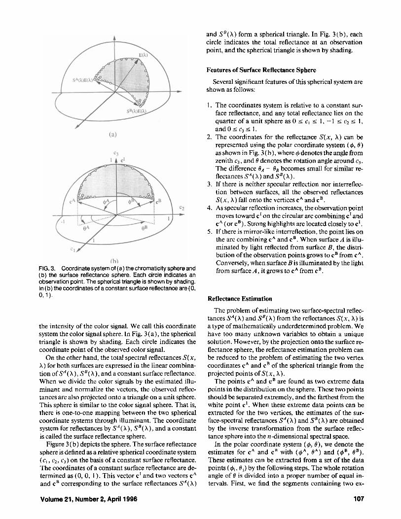
For convenience of the spectral analysis, all the spectra are sampled at A 1 , A2, . . . , A, of the visible wavelength, and described by n-dimensional column vectors. All color signals Y ( x, A ) observed from two surfaces fall in a three-dimensional subspace of the n-dimensional vector space, which is spanned by the three vectors of SA(A)E(A), SB(A)E(A) , and E(A). When we normalize all the vectors to a unit length, all the observed color signals are projected onto a unit sphere [see Fig. 3 (a)]. Because the color signals are positive combinations of the three vectors, all the projected observations are located on a spherical triangle or inside it as shown in Fig. 3 (a). Three vertices of the triangle correspond to illumination, and two object colors of surfaces A and B . The coordinates on the sphere include no information about

106 COLOR research and application

and SB(A) form a spherical triangle. In Fig. 3(b), each circle indicates the total reflectance at an observation point, and the spherical triangle is shown by shading.

Features of Surface Reflectance Sphere

shown as follows: Several significant features of this spherical system are

1. The coordinates system is relative to a constant surface reflectance, and any total reflectance lies on the quarter of a unit sphere as 0 I cI I 1, - 1 I c2 I 1, a n d O s c 3 s 1.

2. The coordinates for the reflectance S(x, A ) can be represented using the polar coordinate system ( I $ , 0 ) as shown in Fig. 3 (b), where C p denotes the angle from zenith c3, and 0 denotes the rotation angle around c3. The difference - BE becomes small for similar reflectances SA( A ) and SB( A ) .

3. If there is neither specular reflection nor interreflection between surfaces, all the observed reflectances S(x, A ) fall onto the vertices cA and cB.

4. As specular reflection increases, the observation point moves toward c' on the circular arc combining c1 and C" (or cB) . Strong highlights are located closely to c'.

5. If there is mirror-like interreflection, the point lies on the arc combining C" and cB. When surface A is illuminated by light reflected from surface E , the distribution of the observation points grows to cB from cA. Conversely, when surface B is illuminated by the light from surface A , it grows to cA from cB. FIG. 3. Coordinate system of (a) the chromaticity sphere and

(b) the surface reflectance sphere. Each circle indicates an observation point. The spherical triangle is shown by shading. In (b) the coordinates of a constant surface reflectance are (0 , 0,1). Reflectance Estimation

the intensity of the color signal. We call this coordinate system the color signal sphere. In Fig. 3 (a), the spherical triangle is shown by shading. Each circle indicates the coordinate point of the observed color signal.

On the other hand, the total spectral reflectances S(x, A ) for both surfaces are expressed in the linear combination of SA( A ) , SB( A ) , and a constant surface reflectance. When we divide the color signals by the estimated illuminant and normalize the vectors, the observed reflectances are also projected onto a triangle on a unit sphere. This sphere is similar to the color signal sphere. That is, there is one-to-one mapping between the two spherical coordinate systems through illuminant. The coordinate system for reflectances by SA( A ) , SB( A ) , and a constant is called the surface reflectance sphere.

Figure 3 (b) depicts the sphere. The surface reflectance sphere is defined as a relative spherical coordinate system ( cI , c2, c3) on the basis of a constant surface reflectance. The coordinates of a constant surface reflectance are determined as (0, 0, 1 ). This vector c' and two vectors C"

and cB corresponding to the surface reflectances SA( A )

The problem of estimating two surface-spectral reflectances SA( A ) and SB( A ) from the reflectances S(x, A ) is a type of mathematically underdetermined problem. We have too many unknown variables to obtain a unique solution. However, by the projection onto the surface reflectance sphere, the reflectance estimation problem can be reduced to the problem of estimating the two vertex coordinates C" and cB of the spherical triangle from the projected points of S( x, A ) .

The points C" and cB are found as two extreme data points in the distribution on the sphere. These two points should be separated extremely, and the farthest from the white point c'. When these extreme data points can be extracted for the two vertices, the estimates of the surface-spectral reflectances SA( A ) and SB( A ) are obtained by the inverse transformation from the surface reflectance sphere into the n-dimensional spectral space.

In the polar coordinate system ($, 0) , we denote the estimates for cA and cB with (4A, 0") and ( I$B, eB). These estimates can be extracted from a set of the data points ( I$i, 0 j) by the following steps. The whole rotation angle of 6 is divided into a proper number of equal in- tervals. First, we find the segments containing two ex-


treme values O A = min B j and BB = max Bj. Next, the farthest points are extracted from the data sets by max( &, 0 A ) and max ( &, 0 B ) , which belong to the same segments of 0.

The simple algorithm of extracting the extreme data points is useful for a large data set observed from a wide region of two object surfaces, including highlight and matte regions. However, it should be noted that the above procedure is apparently available only when the two vertices of the spherical triangle are represented by pixels as shown in Fig. 3 (b). If only highlight or interreflection regions of the surfaces are given, one or more of the vertices will be missing. In this case, detecting the extreme data points is unreliable for estimating the vertex coordinates.

In the following section, we propose a generalized algorithm for estimating surface-spectral reflectances from the measured color signals that are available in the case of sparse data.

REFLECTANCE ESTIMATION ALGORITHM

Suppose that the total reflectance S(x, A ) is obtained by the division Y ( x, A ) / E ( A ) with the estimate of the illuminant E( A ) .

Projection onto a Surface Reflectance Sphere

total reflectance onto the spherical system. The following procedure is proposed for projecting the

1.

2.

3.

4.

Assume that m reflectance spectra are obtained from different locations on two object surfaces. The total reflectances are represented by the n-dimensional column vectors si ( i = 1,2,. . . , m) with llsiII = 1. Three principal-component vectors { u I , u2, u3} are calculated for this set of spectral data. These vectors are fit to the unit vector i using linear regression as i =

A new orthonormal basis { v l , v2, v3 is created so that i is coincident with one basis as v3 = i , and the remaining v1 and v2 are perpendicular to i . The Gram-Schmidt procedure is used for this basis transformation. The basis { v1 , v2, v3 } is calculated from { uI , u2, u3} , andi as

k,ul + k2U2 + k 3 ~ 3 .

v3 = i

v2 = u2 - (i .u2)i

vI = u3 - (i-u3)i - (v2-u3)vz, ( 5 )

where each vector is normalized with vi / 11 vi 11 ( i = 1, 2,3). The total reflectance si is mapped onto the surface reflectance sphere. Let c ( = cl, cz, c3]') be the three- dimensional vector of the spherical system. Then the nx3 matrix V = [ v1 , v2, v3] is a transformation matrix, and the vector c is obtained from c' = S'V.

1 4'3

FIG. 4. Search of the permissible solution area. The hatched areas mean the solution areas for cA and cB on the surface reflectance sphere.

Searching Permissibie Solution Bands

An algorithm is proposed for finding the permissible solution bands for two surface-spectral reflectances when the vertices of the spherical triangle cA and cB are missing. Figure 4 depicts an example of the permissible solution areas on the surface reflectance sphere.

Let us describe our reflectance estimation problem in a mathematically compact form. Let f l and f2 be n-dimensional vectors for the surface-spectral reflectance functions SA( A ) and SB( A ) , respectively. All the total reflectance vectors si ( i = 1, 2, . . . , m ) should be expressed in a linear combination of fl , f2, and i as

si = aifl + &f2 + yii ( i = 1,2,. . . , m). ( 6 )

Suppose that we wish to compute the solution of the above equation. This problem is difficult to solve because the two vectors f l and f2 are unknown, and the weights a;, pi , and yi are also unknown. It is not a linear estimation problem, but a complicated nonlinear problem. All the unknown physical quantities must have nonnegative values:

q r O , & r O , y , r O ( i = l , 2 , . . . , m )

fl 2 0, f22-0. ( 7 ) The solution of ( 6 ) satisfying the constraints (7) is not necessarily unique.

An effective method for directly searching a set of solutions can be proposed using the surface reflectance sphere. The present problem is not an optimization problem. Given si ( i = 1,2, . . . , m ) , all combinations of f l and fz satisfying the equation ( 6 ) and the constrains (7) are regarded as a set of permissible solutions.

First, the total reflectances si are expressed in terms of the orthonormal basis v1 , v2, i } as

( 8 ) si = cilvl + cizv2 + ci3i, ( i = 1,2, . . . , m ) ,


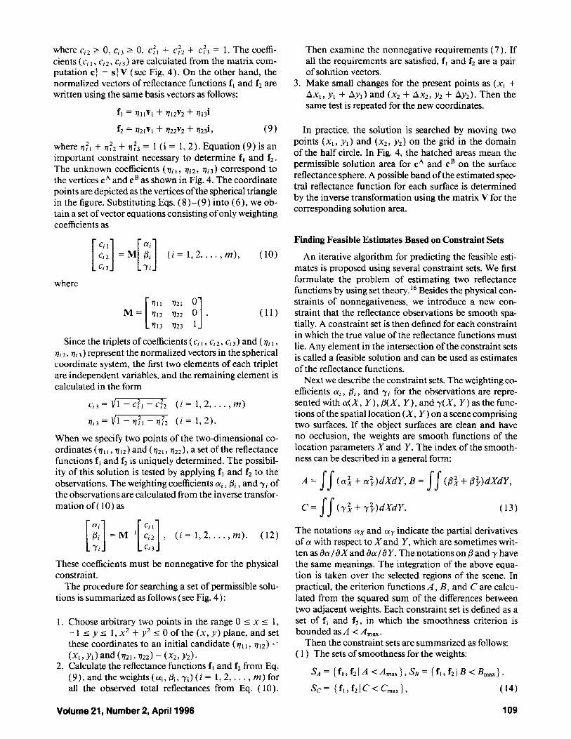
where cf2 2 0, c f3 2 0, cf, + cf2 + cf3 = 1. The coefficients (c, c, 2 , c, 3) are calculated from the matrix com- putation c: = s: V (see Fig. 4) . On the other hand, the normalized vectors of reflectance functions f l and f2 are written using the same basis vectors as follows:

f l = vlIv1 + 712vZ + q I 3 i

f2 = 72lv1 + 722v2 + V23i, (9)

where q f , + vf2 + 7f3 = 1 (i = 1, 2) . Equation (9) is an important constraint necessary to determine f l and f2. The unknown coefficients ( v , ~ , q t 2 , q 1 3 ) correspond to the vertices cA and cB as shown in Fig. 4. The coordinate points are depicted as the vertices ofthe spherical triangle in the figure. Substituting Eqs. (8)-(9) into ( 6 ) , we obtain a set of vector equations consisting of only weighting coefficients as [:::I ( i = l , Z . . . , m ) , (10)

where

Since the triplets of coefficients (cj c j 2 , c i 3 ) and ( 7 ; I ,

q j 2 , qi 3 ) represent the normalized vectors in the spherical coordinate system, the first two elements of each triplet are independent variables, and the remaining element is calculated in the form

c , ~ = V1 - c f l - c f 2 ( i = 1,2, . . . , m )

q r 3 = V1 - V f , - V f * ( i = 1,2).

When we specify two points of the two-dimensional coordinates ( v1 I , v I 2 ) and ( q 2 , , 722), a set of the reflectance functions f l and f2 is uniquely determined. The possibil- ity of this solution is tested by applying f, and f2 to the observations. The weighting coefficients a j , I s j , and y j of the observations are calculated from the inverse transformation of ( 10) as

These coefficients must be nonnegative for the physical constraint.

The procedure for searching a set of permissible solutions is summarized as follows (see Fig. 4):

1. Choose arbitrary two points in the range 0 I x I I , - 1 I y I 1, x2 + y 2 I 0 of the (x, y ) plane, and set these coordinates to an initial candidate ( t l l , v12) =

2. Calculate the reflectance functions f l and f2 from Eq. (9) , and the weights ( ai, pi, ri) ( i = 1, 2, . . . , m) for all the observed total reflectances from Eq. (10).

( X I , ~ I ) ~ ~ ~ ( V ~ I , V ~ Z ) = (x2 ,~2) .

3.

Then examine the nonnegative requirements (7) . If all the requirements are satisfied, fl and f2 are a pair of solution vectors. Make small changes for the present points as (x, + A x , , y , + Ay,) and (x2 + Ax2, y2 + Ay2). Then the same test is repeated for the new coordinates.

In practice, the solution is searched by moving two points fxl , yl) and (x2, y2) on the grid in the domain of the half circle. In Fig. 4, the hatched areas mean the permissible solution area for cA and cB on the surface reflectance sphere. A possible band of the estimated spectral reflectance function for each surface is determined by the inverse transformation using the matrix V for the corresponding solution area.

Finding Feasible Estimates Based on Constraint Sets

An iterative algorithm for predicting the feasible estimates is proposed using several constraint sets. We first formulate the problem of estimating two reflectance functions by using set theory.16 Besides the physical constraints of nonnegativeness, we introduce a new constraint that the reflectance observations be smooth spa- tially. A constraint set is then defined for each constraint in which the true value of the reflectance functions must lie. Any element in the intersection of the constraint sets is called a feasible solution and can be used as estimates of the reflectance functions.

Next we describe the constraint sets. The weighting coefficients ai, p i , and y j for the observations are repre- sentedwith a ( X , Y ) , p ( X , Y),andy(X, Y)asthefunc- tions of the spatial location (X, Y ) on a scene comprising two surfaces. If the object surfaces are clean and have no occlusion, the weights are smooth functions of the location parameters X and Y. The index of the smoothness can be described in a general form:

The notations ax and a indicate the partial derivatives of a with respect to Xand Y, which are sometimes written as d a / d X and da/dY. The notations on p and y have the same meanings. The integration of the above equation is taken over the selected regions of the scene. In practical, the criterion functions A , B, and C are calculated from the squared sum of the differences between two adjacent weights. Each constraint set is defined as a set of f l and f2, in which the smoothness criterion is bounded as A < Amax .

Then the constraint sets are summarized as follows: ( 1 ) The sets of smoothness for the weights:

s, = { f l , fi I A < A m a x } 9 SB = { f ~ 3 f2 I B < B m a x } 9

SC = { f l , f2 I C < Cmax } 9 (14)


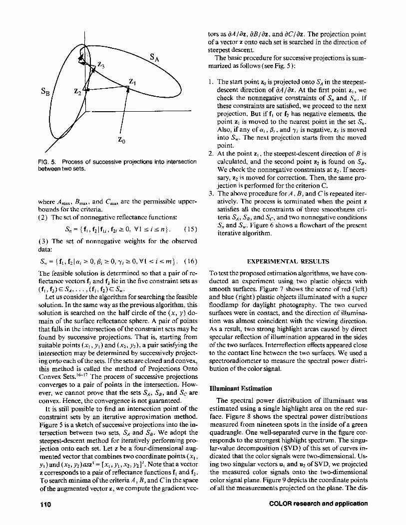
FIG. 5. Process of successive projections into intersection between two sets.

where A,,,, B,,,, and C,,, are the permissible upper- bounds for the criteria. (2 ) The set of nonnegative reflectance functions:

s,,= { f l , f 2 1 f l i , f 2 j 2 0 , v1 < i s - n } . ( 1 5 )

( 3 ) The set of nonnegative weights for the observed data:

S,,= { f l , f 2 ( O I i 2 0 , P i 2 0 , Y i 2 0 , Q 1 s i s r n } . (16)

The feasible solution is determined so that a pair of reflectance vectors fl and f2 lie in the five constraint sets as

Let us consider the algorithm for searching the feasible solution. In the same way as the previous algorithm, this solution is searched on the half circle of the (x, y ) domain of the surface reflectance sphere. A pair of points that falls in the intersection of the constraint sets may be found by successive projections. That is, starting from suitable points (x,, yI ) and (x2 , y 2 ) , a pair satisfying the intersection may be determined by successively projecting onto each of the sets. If the sets are closed and convex, this method is called the method of Projections Onto Convex Sets. ‘‘-I7 The process of successive projections converges to a pair of points in the intersection. How- ever, we cannot prove that the sets S,, S,, and & are convex. Hence, the convergence is not guaranteed.

It is still possible to find an intersection point of the constraint sets by an iterative approximation method. Figure 5 is a sketch of successive projections into the intersection between two sets, S, and s,. We adopt the steepest-descent method for iteratively performing projection onto each set. Let z be a four-dimensional augmented vector that combines two coordinate points ( x I , yl ) and (x2, y~ )asz‘ = [ x I , y1 , x2, y2] ‘. Note that a vector z corresponds to a pair of reflectance functions f I and f2. To search minima of the criteria A , B , and C in the space of the augmented vector z, we compute the gradient vec-

( f l , f 2 ) E S A , . . . , ( f l , f 2 ) E & v .

tors as dAldz, dBldz, and d C l d z . The projection point of a vector z onto each set is searched in the direction of steepest descent.

The basic procedure for successive projections is summarized as follows (see Fig. 5 ) :

1.

2.

3.

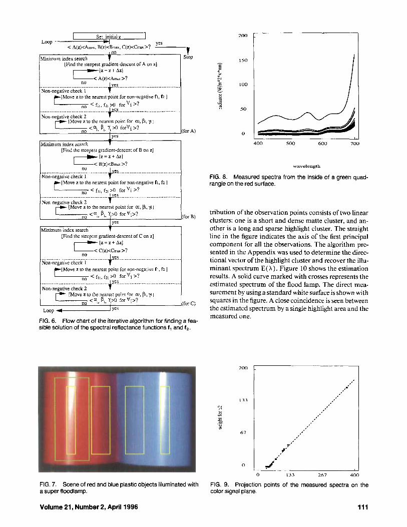
The start point ~0 is projected onto S, in the steepest- descent direction of dA/az . At the first point zl, we check the nonnegative constraints of S,, and S,. If these constraints are satisfied, we proceed to the next projection. But if f l or fi has negative elements, the point zI is moved to the nearest point in the set S,. Also, if any of ai, pi, and y i is negative, z1 is moved into S,. The next projection starts from the moved point. At the point zI , the steepest-descent direction of B is calculated, and the second point z2 is found on S,. We check the nonnegative constraints at z2. If necessary, 22 is moved for correction. Then, the same projection is performed for the criterion C. The above procedure for A B , and Cis repeated iteratively. The process is terminated when the point z satisfies all the constraints of three smoothness criteria SA, S,, and S,, and two nonnegative conditions S, and Sw,. Figure 6 shows a flowchart of the present iterative algorithm.

EXPERIMENTAL RESULTS

To test the proposed estimation algorithms, we have con- ducted an experiment using two plastic objects with smooth surfaces. Figure 7 shows the scene of red (left) and blue (right) plastic objects illuminated with a super floodlamp for daylight photography. The two curved surfaces were in contact, and the direction of illumination was almost coincident with the viewing direction. As a result, two strong highlight areas caused by direct specular reflection of illumination appeared in the sides of the two surfaces. Interreflection effects appeared close to the contact line between the two surfaces. We used a spectroradiometer to measure the spectral power distribution of the color signal.

Illurninant Estimation

The spectral power distribution of illurninant was estimated using a single highlight area on the red surface. Figure 8 shows the spectral power distributions measured from nineteen spots in the inside of a green quadrangle. One well-separated curve in the figure corresponds to the strongest highlight spectrum. The singular-value decomposition (SVD) of this set of curves indicated that the color signals were two-dimensional. Us- ing two singular vectors uI and u2 of SVD, we projected the measured color signals onto the two-dimensional color signal plane. Figure 9 depicts the coordinate points of all the measurements projected on the plane. The dis-


I Set initial z 1 LOOP Yes < A(z)<Amax, B(z)<Bmax, C(z)<Crnax>?

no

I no rlinimum index search 1

[Find the steepest gradient-descent of A on z] [z = z t Az] r < A(z)<Amax >?

...................................... es ................................... Non-negative check no 1 f

+[Move z to the nearest point for non-negative fi , fz I

(for C)

< fi i , f i l >O for vi >? ..................................... ..Jyes.-. ............................... Non-negative check 2 1

[Move z to the nearest point for ai, pi, p 1

I stop

[or A) A-

llinimum index search 1 [Find the steepest gradient-descent of B on z]

[z = z + Az] i < B(z)<Bmax >? ....................................... Yes ..................................... Non-negative check no I +

+[Move z to the nearest point for non-negative h, f i 1 < fl;, f i i >O for v i >?

....................................... &es ..................................... Non-negarive check 2

[Move z to the nearest point for al, PI, p 1

(for B)

Minimum index search [Find the steepest gradient-descent of C on z]

< C(z)<Cmlu >? .......................................

no Non-negative check I

*[Move z to the nearest point for non-negative f1, f2 I + < f i t , f2;0 f o r v i >? ........................................ Yes ..................................... Non-negative check 2

200

150

2 ;% 9 -G LOO E 8 8 z 50

.- V

400 500 600 700

wavelength

FIG. 8. Measured spectra from the inside of a green quadrangle on the red surface.

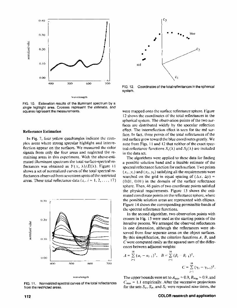
tribution of the observation points consists of two linear clusters: one is a short and dense matte cluster, and an- other is a long and sparse highlight cluster. The straight line in the figure indicates the axis of the first principal component for all the observations. The algorithm presented in the Appendix was used to determine the directional vector of the highlight cluster and recover the illuminant spectrum E( A ) . Figure 10 shows the estimation results. A solid curve marked with crosses represents the estimated spectrum of the flood lamp. The direct measurement by using a standard white surface is shown with squares in the figure. A close coincidence is seen between the estimated spectrum by a single highlight area and the measured one.

0 133 267 400

FIG. 7. Scene of red and blue plastic objects illuminated with a super Roodlamp.

FIG. 9. Projection points of the measured spectra on the color signal plane.


0.40

0.30

0.20

400 500 600 700

wavelength

FIG. 10. Estimation results of the illuminant spectrum by a single highlight area. Crosses represent the estimate, and squares represent the measurements.

Reflectance Estimation

In Fig. 7, four yellow quadrangles indicate the complex areas where strong specular highlight and interreflection appear on the surfaces. We measured the color signals from only the four areas and neglected the remaining areas in this experiment. With the above-estimated illuminant spectrum the total surface-spectral reflectances was obtained as Y ( x, X ) / E ( X ) . Figure 1 1 shows a set of normalized curves of the total spectral reflectances observed from seventeen spots of the restricted areas. These total reflectance data (s,, i = 1, 2, . . . , 17)

400 SO0 600 700

wavelength

FIG. 11. Normalized spectral curves of the total reflectances from the restricted areas.

0

8

# red

c3

0 blue m m

0.

FIG. 12. Coordinates of the total reflectances in the spherical system.

were mapped onto the surface reflectance sphere. Figure 12 shows the coordinates of the total reflectances in the spherical system. The observation points of the two surfaces are distributed widely by the specular reflection effect. The interreflection effect is seen for the red surface. In fact, three points of the total reflectances of the red surface grow toward the blue coordinates greatly. We note from Figs. 1 I and 12 that neither of the exact spectral-reflectance functions Sl ( A ) and S2( A ) are included in the data set.

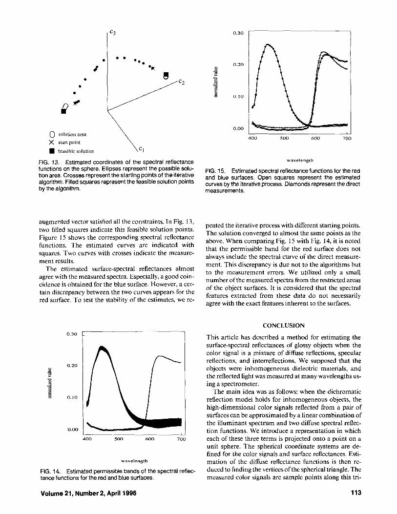
The algorithms were applied to these data for finding a possible solution band and a feasible estimate of the spectral reflectance function for each surface. Two points (x, , y , ) and ( x2, y 2 ) satisfying all the requirements were searched on the grid in equal spacing of (Ax, Ay) = (0.01, 0.01) in the domain of the surface reflectance sphere. Then, 46 pairs of two coordinate points satisfied the physical requirements. Figure 13 shows the estimated coordinate points on the reflectance sphere, where the possible solution areas are represented with ellipses. Figure I4 shows the corresponding permissible bands of the spectral reflectance functions.

In the second algorithm, two observation points with crosses in Fig. 13 were used as the starting points of the iterative process. We arranged the observed reflectances in one dimension, although the reflectances were observed from four separate areas on the object surfaces. By this simplification, the criterion functions A , B , and C were computed easily as the squared sum of the differences between adjacent weights:

A = 2 (a, - a,-i)*,

16 16

B = C ( P l - P,-112, i= I i= I

16

C = C (Ti - Ti-])*. I = I

The upper bounds were set to A,,, = 0.9, B,,, = 0.9, and C,,, = 1.1 empirically. After the successive projections for the sets S, , S,, and S,. were repeated nine times, the


0 solution area X start point

feasible solution

FIG. 13. Estimated coordinates of the spectral reflectance functions on the sphere. Ellipses represent the possible solution area. Crosses represent the starting points of the iterative algorithm. Filled squares represent the feasible solution points by the algorithm.

augmented vector satisfied all the constraints. In Fig. 13, two filled squares indicate this feasible solution points. Figure 15 shows the corresponding spectral reflectance functions. The estimated curves are indicated with squares. Two curves with crosses indicate the rneasure- ment results.

The estimated surface-spectral reflectances almost agree with the measured spectra. Especially, a good coincidence is obtained for the blue surface. However, a cer- tain discrepancy between the two curves appears for the red surface. To test the stability of the estimates, we re-

0.30

0.20 - 8 s 3 e

0.10

0.00 I

400 500 600 700

wavelength

FIG. 14. Estimated permissible bands of the spectral reflectance functions for the red and blue surfaces.

0.30

0.20 P 7 1 E E

0.10

0.00

400 500 600 700

wavelength

FIG. 15. Estimated spectral reflectance functions for the red and blue surfaces. Open squares represent the estimated curves by the iterative process. Diamonds represent the direct measurements.

peated the iterative process with different starting points. The solution converged to almost the same points as the above. When comparing Fig. 15 with Fig. 14, it is noted that the permissible band for the red surface does not always include the spectral curve of the direct measurement. This discrepancy is due not to the algorithms but to the measurement errors. We utilized only a small number of the measured spectra from the restricted areas of the object surfaces. It is considered that the spectral features extracted from these data do not necessarily agree with the exact features inherent to the surfaces.

CONCLUSION

This article has described a method for estimating the surface-spectral reflectances of glossy objects when the color signal is a mixture of diffuse reflections, specular reflections, and interreflections. We supposed that the objects were inhomogeneous dielectric materials, and the reflected light was measured at many wavelengths using a spectrometer.

The main idea was as follows: when the dichromatic reflection model holds for inhomogeneous objects, the high-dimensional color signals reflected from a pair of surfaces can be approximated by a linear combination of the illuminant spectrum and two diffuse spectral reflection functions. We introduce a representation in which each of these three terms is projected onto a point on a unit sphere. The spherical coordinate systems are defined for the color signals and surface reflectances. Esti- mation of the diffuse reflectance functions is then reduced to finding the vertices ofthe spherical triangle. The measured color signals are sample points along this tri-


angle, but the sample points do not necessarily include the vertices.

Next, a computational method was proposed to estimate the locations of the vertices of diffuse reflectance function from the sample measurements. The first algorithm can find the permissible solution bands of two reflectance functions, and the second one can predict the feasible estimates by using several constraint sets.

The reliability of the proposed method was demonstrated in an experiment using two plastic objects with glossy surfaces. The illuminant spectrum was estimated from a single highlight area. The surface-spectral functions were estimated from a small number of the spectra that were measured from the restricted areas on the surfaces.

APPENDIX

In this appendix, we give an algorithm to predict the illuminant spectrum from a single surface of an inhomogeneous dielectric object. By assuming that the spatial directions of illumination and observation are close, the illuminant spectrum is estimated from the directional vector of the interface cluster on the color signal plane as shown in Fig. I . The procedure for illuminant estimation is described as follows:

I .

2.

3.

4.

5 .

The axis of the first principal component is determined for a set of all the observations on the color signal plane. The component axis is segmented into equal in- tervals, and the linear clusters are divided on the segmented axis. The mean coordinates are calculated for the observations belonging to each segment. The one-dimensional array of the directional vectors is constructed by connecting the mean coordinates of adjacent segments. The turning point where the directional vector changes is detected, and the array is split into two classes. We average the directional vectors in the interface cluster. The estimate of the illuminant E( A ) is then obtained by transforming the averaged vector into the spectral space with two basis vectors.

ACKNOWLEDGMENT

The author would like to thank Prof. Brian Wandell for his helpful discussions and comments on the manu- script.

I. M. J. Vrhel, R. Gershon. and L. S. Iwan, Measurement and analysis of object reflectance spectra, Color Res. Appl. 19,4-9 ( 1994).

2. B. A. Wandelf, Foundalion c!f Vision, Sinauer Associates. Sunder- land, MA 1995, p. 28 I .

3. S. A. Shafer, Using color to separate reflection components, Color Res. Appl. 10,210-218( 1985).

4. S. Tominaga, Dichromatic reflection models for a variety of materials. Color Rex. Appl. 19,277-285 ( 1994).

5. S. Tominaga and B. A. Wandell, The standard surface reflectance model and illuminant estimation, J. Opf. SOC. Am. A 6, 576-584 (1989).

6. S. Tominaga and B. A. Wandell, Component estimation of surface spectral reflectance, J. Opl. Soc. Am. A 7,312-317 (1990).

7. G. J. Klinker, S. A. Shafer, and T. Kanade, The measurement of highlights in color images, Inf . J. Computer Vision 2,7-32 ( 1988).

8. S. A. Shafer, T. Kanade, G. J. Winker, and C. L. Novak, Physics- based models for early vision by machine, SPIE Proceedings 1250,

9. G. Healey, Estimating spectral reflectance using highlights, Image L’k. Cornput. 9, 333-337 (1991).

10. M. S. Drew and B. V. Funt, Variational approach to interreflection in color images, J. Opf. Soc. Am. A 9 , 1255-1265 (1992).

11. C. 1 . Novak and S. A. Shafer, Methods for estimating scene parameters from color histograms, J. Opt. Soc. Am. A l l , 3020-3036 (1994).

12. G. J. Winker, S. A. Shafer. and T. Kanade, A physical approach to color image understanding. Int. J . Computer Vision 4, 7-38 (1990).

13. R. Bajcsy, S. W. Lee, and A. Leonardis, Image segmentation with detection of highlights and inter-reflections using color, given at the Image Understanding and Machine Vision Topical Meeting, Cape Cod, 1989.

14. H. C. Lee, Method for computing the scene-illuminant chromaticity from specular highlights. J. Opt. SOC. Am. ,4 3, 1694-1699 (1986).

15. M. DZmura and P. Lennie, Mechanisms of color constancy, J. Opt. SOC. Am. A3, 1662-1682( 1986).

16. G. Sharma and H. J. Trussell, Characterization of scanner sensi- tivity, lS&TundSIDk ColorImuging Conf: 103-107, 1993.

17. C. 1. Podilchuk and R. J. Mammone, Image recovery by convex projections using a least-squared constraint, J. Opt. Soc. A m A 7, 517-521 (1990).

222-235 (1990).

Received 28 August 1995; accepted 3 1 October 1995


Surface reflectance estimation by the dichromatic model

Documents

Transcript of Surface reflectance estimation by the dichromatic model