1

Adaptive Protocols for LakeOkeechobee Operations

South Florida Water Management District

Developed in Cooperation with:

US Army Corps of Engineers, Jacksonville District

and the

Florida Department of Environmental Protection

2

ACKNOWLEDGEMENTS

The Adaptive Protocols for Lake Okeechobee Operations were developed toprovide guidance in operations for protection of Lake Okeechobee and downstreamecosystems while providing a reliable water supply for agricultural and urban areas thatdepend on the Lake. This document was developed as a cooperative effort by staff in theEcosystem Restoration, Water Supply, and Operations Control and MaintenanceEngineering Departments of the South Florida Water Management District, and staff at theJacksonville District of the United States Army Corps of Engineers and the FloridaDepartment of Environmental Protection.

Project Manager

Karl Havens (E-mail: khavens@sfwmd.gov)

Principal Contributors

Alaa Ali Lehar BrionLuis Cadavid Peter DoeringDan Haunert Jayantha ObeysekeraStephen Smith David SwiftPaul Trimble Walter Wilcox

Supporting Contributors

Gaea Crozier Julio FanjulDale Gawlik Marian Heitzman Cal Neidrauer Jose OteroGordon Romeis (FDEP) Cecile Ross Shawn Sculley Fred SklarChristopher Smith (USACE) Suzanne Sofia (USACE)

Project Oversight

Ken Ammon Larry GerryJohn Mulliken Susan GrayTommy Strowd Patricia Strayer

Advisory Assistance

Water Resources Advisory Commission

3

TABLE OF CONTENTS

Acknowledgements 2

List of Acronyms 4

Executive Summary 5

Introduction and Purpose 6

Legal Framework 8

Background 10

Adaptive Assessment 12

Specific Procedure for Environmental Water Deliveries 16

Application of Regional Performance Measures 17

Lake Okeechobee Performance Measures 17

Estuary Performance Measures 23

Water Supply Performance Measures 27

Everglades Performance Measures 47

STA Performance Measures 55

Regional Simulation Modeling 57

References 64

Appendix I – Information Regarding the Palmer Drought Index 74

Appendix II – Restoration Targets and Minimum Flows and Levels 75in the Everglades Protection Area

4

LIST OF ACRONYMS

AWC = available water contentCE = Caloosahatchee EstuaryCERP = Comprehensive Everglades Restoration ProgramC&SF = Central and Southern Florida (flood control project)CPC = Climate Prediction CenterEAA = Everglades Agricultural AreaECP = Everglades Construction ProjectENP = Everglades National ParkEPA = Everglades Protection AreaFDEP = Florida Department of Environmental ProtectionFFWCC = Florida Fish and Wildlife Conservation CommissionHSM = Hydrologic Systems Modeling DivisionLEC = Lower East CoastLECRWSP = Lower East Coast Regional Water Supply PlanLNWR = Loxahatchee National Wildlife RefugeLONISF, LONIMSF = Lake Okeechobee Net Inflow Seasonal (and Multi-Seasonal)ForecastsLOSA = Lake Okeechobee Service AreaMFL = Minimum Flow and LevelNGVD = National Geodetic Vertical Datum of 1929 (formerly called “mean sea level”)NSM = Natural Systems ModelP = phosphorusPA = Position Analysis (modeling procedure)PDSI = Palmer Drought Severity IndexSA-1, SA-2, SA-3 = Service Areas 1, 2 and 3SAV = submerged aquatic vegetationSFWMD = South Florida Water Management DistrictSFWMM = South Florida Water Management ModelSLE = St. Lucie EstuarySTA = Stormwater Treatment AreaTC = tributary conditionsRECOVER = Restoration Coordination and Verification (a CERP program)USACE = United States Army Corps of EngineersUSEPA = United States Environmental Protection AgencyVEC = Valued Ecosystem Component (key biota in the estuaries)WCA = Water Conservation AreaWRAC = Water Resources Advisory CommissionWSE = Water Supply and Environment (current lake regulation schedule)

5

EXECUTIVE SUMMARY

Adaptive Protocols for Lake Okeechobee Operations

Lake Okeechobee is the heart of the Central and Southern Florida Flood ControlProject and an interconnected regional aquatic ecosystem. It has multiple functions,including flood control, agricultural and urban water supply, navigation, recreation, andfish & wildlife enhancement. As such, operation of the Lake impacts a wide range ofenvironmental and economic issues. Lake operations must carefully consider the entireand sometimes conflicting needs of the Project. A new regulation schedule for LakeOkeechobee, called WSE (Water Supply and Environment), was adopted by the UnitedStates Army Corps of Engineers (USACE) and the South Florida Water ManagementDistrict (SFWMD) in July 2000. The schedule provides increased flexibility relative toearlier flood control schedules, and was specifically designed to “optimize environmentalbenefits at minimal or no impact to competing lake purposes.”

The lake regulation schedule tells water managers when it is necessary to releasewater from the Lake for project purposes (e.g., flood protection). Release decisions aredetermined by elevation of the Lake surface, which varies with season, and by recentrainfall amounts and future climate projections. Except at extreme high water level, theregulation schedule does not specify exact discharges. It also does not address situationswhere water deliveries from Lake Okeechobee may be needed to deal with water resourceproblems (e.g., high salinity that is affecting submerged plants) in downstream systems,such as the Caloosahatchee River and Estuary. However, the Water Control Plan for theLake does authorize release of water from the Lake independent of regulatory releases, forwater supply for fish and wildlife and for saltwater management.

This document spells out in greater detail how water managers can meet the intentof the WSE lake regulation schedule and the Water Control Plan provisions. In particular,it is a tool to guide operational actions regarding volumes of water to release from theLake for regulatory purposes and procedures to be followed for addressing downstreamwater resource opportunities. This document lays out a process that includes input fromthe public, other agencies, the SFWMD Governing Board, and technical input fromexperts at the USACE, SFWMD, and Florida Department of Environmental Protection(FDEP). Technical information regarding the need for water releases from the Lake isbased on a set of quantitative performance measures of ecosystem health and water supplyconditions that have a strong foundation in regional environmental science andengineering.

A key feature of Adaptive Protocols is balancing water supply, flood protection,and environmental protection within the constraints of the approved lake regulationschedule and Water Control Plan. Adaptive Protocols will be a continual adaptationprocess, in the sense that they will be adjusted, as necessary, to deal with unforeseenissues not accounted for in this document.

6

1. Introduction and Purpose

Lake Okeechobee is the heart of the Central and Southern Florida (C&SF) FloodControl Project and of an interconnected regional aquatic ecosystem, and as such, itsoperation affects a range of environmental and economic issues. Operations of the lakeaccommodate numerous, and sometimes conflicting, project purposes. A key feature ofAdaptive Protocols is balancing water supply, flood protection, and environmentalprotection.

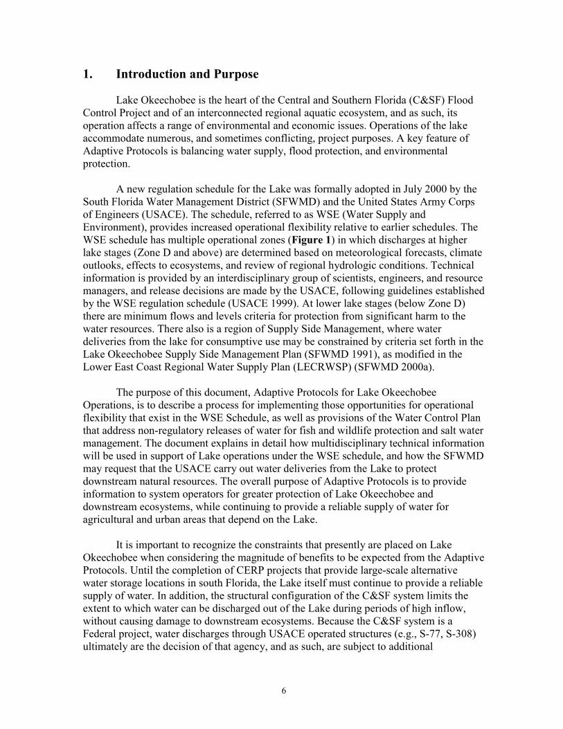
A new regulation schedule for the Lake was formally adopted in July 2000 by theSouth Florida Water Management District (SFWMD) and the United States Army Corpsof Engineers (USACE). The schedule, referred to as WSE (Water Supply andEnvironment), provides increased operational flexibility relative to earlier schedules. TheWSE schedule has multiple operational zones (Figure 1) in which discharges at higherlake stages (Zone D and above) are determined based on meteorological forecasts, climateoutlooks, effects to ecosystems, and review of regional hydrologic conditions. Technicalinformation is provided by an interdisciplinary group of scientists, engineers, and resourcemanagers, and release decisions are made by the USACE, following guidelines establishedby the WSE regulation schedule (USACE 1999). At lower lake stages (below Zone D)there are minimum flows and levels criteria for protection from significant harm to thewater resources. There also is a region of Supply Side Management, where waterdeliveries from the lake for consumptive use may be constrained by criteria set forth in theLake Okeechobee Supply Side Management Plan (SFWMD 1991), as modified in theLower East Coast Regional Water Supply Plan (LECRWSP) (SFWMD 2000a).

The purpose of this document, Adaptive Protocols for Lake OkeechobeeOperations, is to describe a process for implementing those opportunities for operationalflexibility that exist in the WSE Schedule, as well as provisions of the Water Control Planthat address non-regulatory releases of water for fish and wildlife protection and salt watermanagement. The document explains in detail how multidisciplinary technical informationwill be used in support of Lake operations under the WSE schedule, and how the SFWMDmay request that the USACE carry out water deliveries from the Lake to protectdownstream natural resources. The overall purpose of Adaptive Protocols is to provideinformation to system operators for greater protection of Lake Okeechobee anddownstream ecosystems, while continuing to provide a reliable supply of water foragricultural and urban areas that depend on the Lake.

It is important to recognize the constraints that presently are placed on LakeOkeechobee when considering the magnitude of benefits to be expected from the AdaptiveProtocols. Until the completion of CERP projects that provide large-scale alternativewater storage locations in south Florida, the Lake itself must continue to provide a reliablesupply of water. In addition, the structural configuration of the C&SF system limits theextent to which water can be discharged out of the Lake during periods of high inflow,without causing damage to downstream ecosystems. Because the C&SF system is aFederal project, water discharges through USACE operated structures (e.g., S-77, S-308)ultimately are the decision of that agency, and as such, are subject to additional

7

constraints. These include USACE operational authorizations, such as the navigationmission, and periodic constraints such as scheduled and emergency structure maintenance.Adaptive Protocols are not solutions to the problems facing the Lake or other natural areasin south Florida. Rather, they represent a flexible process for optimizing how the Lake isoperated within the constraints of existing authorizations, using a process that givescareful consideration to various competing uses of the water resource.

Adaptive protocols are implemented in two ways:

(a) where the WSE schedule indicates that water must be released from the Lake for floodcontrol purposes, but does not indicate the exact amount of water to be discharged (inthe decision tree, these releases only are specified as “up to” some maximal amount);and

(b) where the Water Control Plan authorizes releases of water from the Lake for watersupply, fish and wildlife protection, and salt water management in downstream waterresources.

WSE Releases

When the lake regulation schedule requires that water must be released from thelake to the estuaries and/or Water Conservation Areas (WCAs), SFWMD experts onestuarine, lake, and wetland ecology will provide scientific input with regard to the effectsof various discharge volumes. Technical experts on agricultural and urban water supplywill provide similar input regarding the anticipated effects on that use of the waterresource. In general, when flood protection releases are required by the WSE schedule,risks to agricultural or urban water supply are low, because that issue has been accountedfor within the schedule’s two decision trees that can be viewed at: http://www.saj.usace.army.mil/h2o//lib/documents/WSE/index.html. The fact that a flood protection release isrequired indicates that the lake is high and/or conditions in upstream tributaries are wetand heavy rainfall is projected in the watershed. Likewise, when releases are required bythe WSE schedule, it is implicit that the Lake’s littoral zone will benefit from those waterreleases, which will reduce Lake water level and thereby minimize ecological stress.Consequently, impacts to downstream ecosystems, including the east and west coastestuaries and WCAs, are major considerations. Those impacts will be evaluated on thebasis of existing conditions in the ecosystems, as quantified by the performance measuresdescribed in Section 5 of this document. Consideration also will be given to opportunitiesto minimize impacts in the longer term. The latter is important because past experienceshows that low-volume discharges carried out in a pro-active manner can reduce the laterneed for more damaging high-volume discharges and also reduce littoral zone impacts dueto rapidly rising stages. This array of technical information will form the basis forSFWMD input regarding the specific volume and duration of flood control releases underthe WSE schedule, actions that are the responsibility of the USACE.

8

Environmental Water Deliveries

There may be circumstances where the regulation schedule does not indicate thatwater should be released from Lake Okeechobee for flood protection, but water deliveriesfrom the Lake are needed to protect downstream ecosystems. These releases areauthorized by the Water Control Plan (Sections 7-08 to 7-10) and by Florida Statutes(Chapter 373, F.S.). For example, freshwater deliveries from the Lake may be required toreduce salinity in the Caloosahatchee River or flush out an algal bloom in that samesystem. SFWMD staff will approach such releases in a pro-active manner by briefing theGoverning Board at their regularly scheduled monthly meeting, prior to carrying out theactual operation. Information presented to the Board will include expected benefits andpotential risks of the operation, and the specific duration and magnitude of flow that areanticipated to occur. If environmental water delivery actually is needed during thesubsequent month, the SFWMD will request that the USACE carry out the operation forthe specified period of time and at the specified rate of flow. Downstream and in-lakeresponses to the lake water release will be carefully monitored, as well as changes inclimate or hydrologic conditions that might influence benefits or potential risks. TheGoverning Board will be briefed regarding the results of the operation at their nextregularly scheduled meeting. They will also be apprised of the facts related to potentialadditional releases of water. The overall process for making environmental waterdeliveries is designed to protect the ecosystem, but also minimize the risk of havingpermitted users experience water use restrictions (SFWMD 1991, 2000b).

The Water Resources Advisory Commission (WRAC) provided the followingrecommendations in regard to environmental water deliveries from Lake Okeechobee --

(a) The Adaptive Protocols should include the option of making environmental waterdeliveries to the Caloosahatchee River or other downstream water resources, butwith a 10-day average discharge volume not exceeding 300 cfs, unless specificallyauthorized by the Governing Board of the SFWMD.

(b) Environmental water deliveries, as specified in item (a), should occur only whenthe Lake is in Zone D or above in the WSE Regulation Schedule. Otherwise, theyshould only occur with specific approval by the Governing Board of the SFWMD.

(c) The SFWMD should take advantage of opportunities where the WSE schedule callsfor discharges to the WCAs to provide freshwater to meet up to 300 cfs demands ofthe Caloosahatchee ecosystem, as long as that water is not required by the WCAs.

2. Legal Framework

Lake Okeechobee structures within the C&SF Project are operated pursuant to theWater Control Plan for Lake Okeechobee and the Everglades Agricultural Area, which is afederal regulation. The Water Control Plan contains the Lake Okeechobee RegulationSchedule, which at the present time, is the WSE Schedule. As the local sponsor of the

9

C&SF Project, the District is subject to, and bound by, federal regulations, such as theWater Control Plan.

The Water Control Plan provides for regulatory releases (s. 7-03, WCP), watersupply releases for estuarine, Everglades National Park, agriculture, urban and fish andwildlife purposes (S. 7-10, WCP); fish and wildlife preservation and enhancement (S. 7-09, WCP); and water quality protection (S. 7-08, WCP). Some specific considerationsmentioned in the Water Control Plan are ecological status of the Lake's littoral zone andestuaries, climate outlooks and projected water use demands. As part of this overallscheme, the lake regulation schedule establishes ranges for regulatory releases for floodcontrol and requires discharges to be identified based on multiple objectives in a decisiontree format. The Water Control Plan authorizes non-regulatory releases, such as watersupply releases to the estuaries, within any zone. As stated in the Water Control Plan, theDistrict is responsible for allocating water (e.g., issuing consumptive use permits oradopting water reservations) from Lake Okeechobee for water supply purposes.

Independent of the federal regulations, under Chapter 373, F.S., the District has theauthority to establish, maintain and regulate water levels in water bodies owned,maintained or controlled by the District and to regulate discharges into, or withdrawalsfrom water bodies through "Works of the District" SS. 373.086, 373.103(4), F.S. Thisauthority is implemented to effectuate the purposes of Chapter 373, including floodcontrol, water supply, environmental protection and water quality protection. See Sections373.016, 373.036 and 373.1501, F.S. Lake Okeechobee is a "work of the district"pursuant to Chapter 25209, Laws of Florida.

Decisions made for water releases from Lake Okeechobee for environmental watersupply or management of water levels for environmental purposes, such as protection ofthe lake’s littoral zone, must be made consistent with the Water Control Plan and Chapter373, F.S. Specific guidance on these releases, such as the alternative flow rangesprovided for making regulatory releases in the schedule, is not provided in the WaterControl Plan. Therefore, pursuant to its authority under Chapter 373, the District hasidentified procedures and relevant performance measures in this Document to be used inthe decision making process for reviewing the need for and viability of these types ofreleases.

This Document is intended to formalize the process for District input to theUSACE for Lake Okeechobee operations under the WCP. It is also intended to establishan internal process for staff to obtain policy direction from the Executive Office and theGoverning Board on significant operational policy issues. It applies where ranges orobjectives are provided for determining flood control and water supply releases underexisting federal and state authority. It is not intended to establish, dictate or regulate waterlevels or operations. Full discretion of the USACE and the District, as the local sponsor, tooperate the C&SF project is retained as provided in the WCP. The document is not self-executing, and does not bind the district or any other person to take, or not to take, anyspecific action.

10

3. Background

The Adaptive Protocols for Lake Okeechobee Operations address an informationneed identified in the Final Environmental Impact Statement (EIS) of the WSE schedule(USACE 1999, p. 63), where it is indicated that “Releases through various outlets may bemodified to minimize damages or obtain additional benefits. Consultation with Evergladesand estuarine biologists is encouraged to minimize adverse effects to downstreamecosystems.” The Adaptive Protocols include the process whereby this flow modificationand expert consultation occurs. All of the operations under Adaptive Protocols areconsistent with existing authority provided by the Water Control Plan for the Lake.

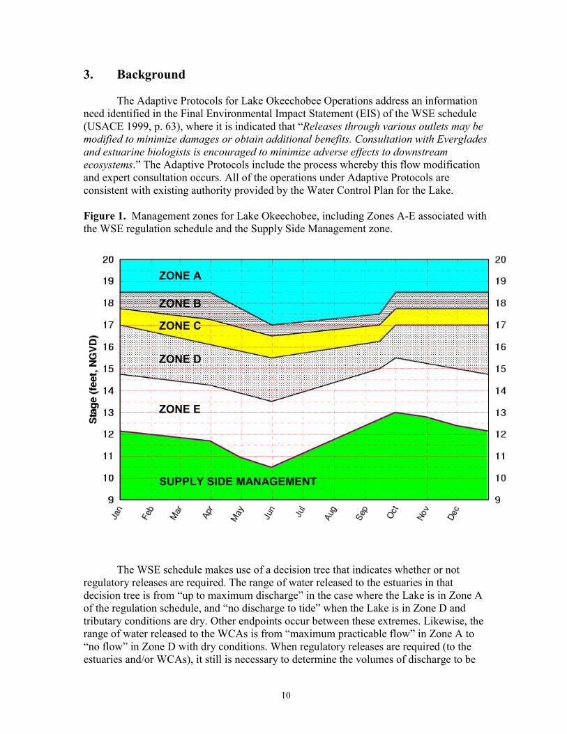
Figure 1. Management zones for Lake Okeechobee, including Zones A-E associated withthe WSE regulation schedule and the Supply Side Management zone.

The WSE schedule makes use of a decision tree that indicates whether or notregulatory releases are required. The range of water released to the estuaries in thatdecision tree is from “up to maximum discharge” in the case where the Lake is in Zone Aof the regulation schedule, and “no discharge to tide” when the Lake is in Zone D andtributary conditions are dry. Other endpoints occur between these extremes. Likewise, therange of water released to the WCAs is from “maximum practicable flow” in Zone A to“no flow” in Zone D with dry conditions. When regulatory releases are required (to theestuaries and/or WCAs), it still is necessary to determine the volumes of discharge to be

ZONE A

ZONE B

ZONE C

ZONE D

SUPPLY SIDE MANAGEMENT

ZONE E

11

made to each downstream water body. The schedule only provides information onpossible ranges of discharge volumes, not exact amounts. When regulatory releases arenot required by the schedule, the SFWMD, under its authority to water supply dischargesfrom the Lake (Chapter 373, F.S.), will consult with the USACE and FDEP, and mayrequest such releases for the purpose of protecting regional water resources.

Under ideal circumstances, water levels in the Lake would not rise into any of thezones where WSE-driven regulatory releases are required, or fall into the region of SupplySide Management. In reality, those conditions do occur because water levels in the Lakeare driven by regional rainfall and runoff, rates of evapotranspiration, and amount of watersupply demand. Regional restoration projects identified in the Comprehensive EvergladesRestoration Program (CERP) include alternative water storage locations that are expectedto help attenuate peak flow during periods of high rainfall, and take some pressure off theLake as a regional water supply source. This should help reduce the occurrence ofundesirable high and low water levels, respectively. However, until the CERP isimplemented, innovative operational protocols must be applied within the constraints ofthe existing infrastructure and operational and legal authorities to ensure that watermanagers can take advantage of certain opportunities to maximize benefits for the waterresource and its various uses.

In addition to language in the Final Environmental Impact Statement for the WSERegulation Schedule (USACE 1999), the LECRWSP (SFWMD 2000a, p. 307-308)explicitly refers to development of flexible operational protocols. That document statesthat the protocols should: (1) have specific stated goals and objectives; (2) have real-timeperformance measures that “include success criteria for all significant environmentalcomponents, water shortage implementation, flood control management, and waterquality assessment;” and (3) be flexible, providing the “capability to pro-actively react tochanging climatological outlooks and environmental conditions.” Development ofAdaptive Protocols, as part of the larger regional water supply planning effort, isconsistent with the policy direction provided in Florida Statutes (Section 373.016). Detailsregarding this authorization may be found in the LECRWSP (SFWMD 2000a, p. 7).Under certain conditions, Adaptive Protocols also might provide the SFWMD with theopportunity to address recovery and prevention strategies for meeting Minimum Flowsand Levels (MFLs) in the Lower East Coast Regional Planning Area. MFLs were adoptedin September 2001 for the Caloosahatchee Estuary, Lake Okeechobee, the EvergladesProtection Area, the Biscayne Aquifer, and the Lower West Coast Aquifer, and in 2002for the St. Lucie Estuary. It is recognized, however, that until a number of CERP projectsare completed, MFLs for these areas cannot always be met with existing water resourcesand project infrastructure. Adaptive Protocols will allow the SFWMD to take advantage ofperiodic opportunities, but are not a MFL recovery plan.

12

3. Adaptive Assessment

3a. Overview of the Process

Adaptive Protocols for Lake Okeechobee are patterned after the AdaptiveAssessment process of the Comprehensive Everglades Restoration Plan’s RestorationCoordination and Verification (RECOVER) program. Adaptive Assessment is a process ofpassive adaptive management, or “learning by doing,” which involves active monitoringof system responses to operations, quantifying those responses using a set of resourceperformance measures, and then making subsequent operational changes with theincreased knowledge base that comes from this feedback process. The process of AdaptiveProtocols includes: (a) twice-yearly public workshops, at the beginning of the wet and dryseasons, where Lake operations are discussed in a venue that allows for a high degree ofinput from agencies, tribes, and the general public; (b) quarterly update meetings with theWater Resources Advisory Commission (WRAC); (c) monthly briefings of the SFWMDGoverning Board, and (d) real-time operations of the lake, in coordination with theUSACE and FDEP. The semi-annual workshops and quarterly meetings with the WRACwill take the place of the “WSE meetings” that have occurred in the past.

3b. Semi-Annual Public Workshops

An important component of the Adaptive Protocols is gathering constructive inputfrom the wide range of agencies and members of the general public concerned with andknowledgeable about the regional water resource. Past experience indicates that the bestvenue for two-way dialogue between agency staff and stakeholders is an open publicworkshop that is focused on one particular topic, in this case the management of waterlevels in Lake Okeechobee. The WRAC provided the following specific recommendationregarding semi-annual workshops:

The Adaptive Protocols process should include open public workshops at the startof wet and dry seasons to receive public comments, review regional conditions,examine past operations and their benefits / impacts, and discuss operations for thenext six months.

Following this recommendation, open public workshops will be held at the beginning ofeach wet and dry season (in May - June and November - December, respectively). Theseworkshops will include presentations by SFWMD and USACE staff on: (a) operationsduring the past season; (b) environmental and/or water supply benefits achieved; (c)benefits not achieved or impacts documented; (d) present status of the regional system; (e)short and long-term climate outlook, including drought index conditions; and (f) projectedstage in the Lake and other regional surface water storage locations based on PositionAnalysis modeling (see section 5c). On the basis of this information, staff will present tothe audience the anticipated operations for the upcoming wet or dry season. Results of theworkshop, including a technical summary and overview of public input, will be presentedto the Governing Board at their next regularly scheduled meeting. This briefing of the

13

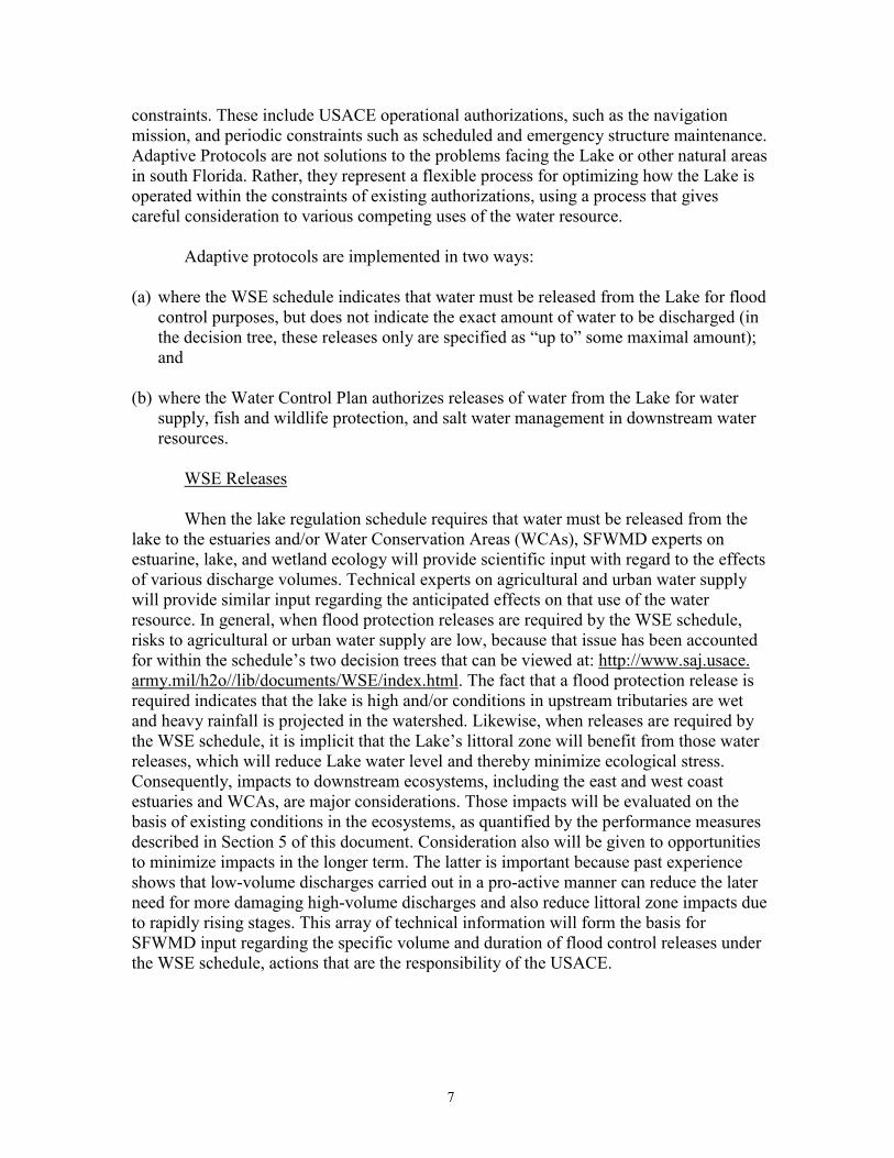
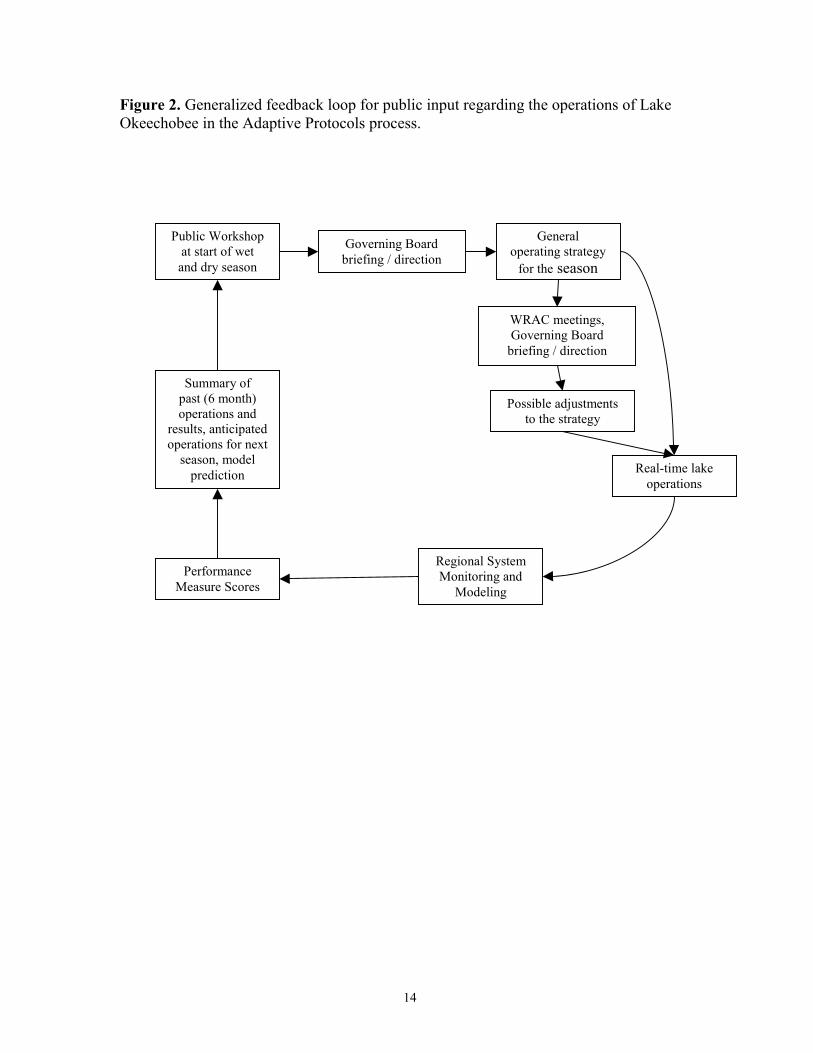
Board will define the general Lake operating conditions for the next wet or dry season.The overall process is illustrated as a feedback loop in Figure 2.

3c. Quarterly Meetings with the WRAC

Meetings with the Water Resources Advisory Commission provide an additional(quarterly) venue for dialogue with other agencies, tribes, and the general public aboutmanagement of the Lake. The WRAC includes a representative from the SFWMDGoverning Board, and representatives from the USACE, other state, federal, and tribalagencies, and major interest groups. WRAC members have a unique understanding ofSouth Florida water resource issues, and as such, can view the Lake Okeechobee situationin a broad-based regional context. As indicated above, the SFWMD Governing Board alsowill be briefed on the status of Lake operations on a monthly basis, as part of theirregularly scheduled meetings. These components of the feedback process are included inFigure 2.

3d. Real-Time Lake Operations

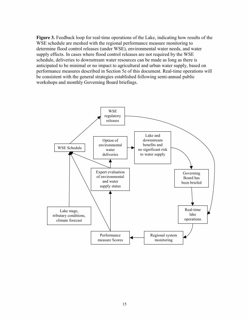
On a weekly or more frequent basis (depending on circumstances), technical staffwill provide input (Figure 3) to system operators, including updates of weather andclimate conditions, regional hydrologic conditions, the status of regional water resources,and results from decision trees in the WSE regulation schedule. This technical informationis used by the USACE to determine amounts of water to release from the lake under theWSE schedule. Water deliveries for protection of downstream ecosystems, made under theSFWMD authority to provide water supply, will be consistent with the operationsdescribed at the prior briefing of the SFWMD Governing Board, and also will follow thespecific process described in Section 4 of this document.

3e. Regional System Monitoring and Performance Measures

Central to the adaptive protocol process are a set of ecosystem and water supplyperformance measures (quantifiable measures of success with defined targets), and aregional monitoring program that provides the information necessary to deriveperformance measure scores. This monitoring includes a variety of system attributes(listed in more detail below) including estuary salinity ranges, lake water levels, keybiological indicators, as well as regional water supply needs. The individual performancemeasures and the monitoring necessary to quantify their status and trends are described indetail, along with their technical foundation, in subsequent sections of this document.Performance measures are used both to assist in real-time operations of the Lake, and toprovide a summary of system performance at the public workshops and the WRAC andGoverning Board briefings.

14

Figure 2. Generalized feedback loop for public input regarding the operations of LakeOkeechobee in the Adaptive Protocols process.

Public Workshopat start of wetand dry season

Summary ofpast (6 month)operations and

results, anticipatedoperations for next

season, modelprediction

Regional SystemMonitoring and

Modeling

Real-time lakeoperations

Generaloperating strategy

for the season

PerformanceMeasure Scores

Governing Boardbriefing / direction

WRAC meetings,Governing Board

briefing / direction

Possible adjustmentsto the strategy

15

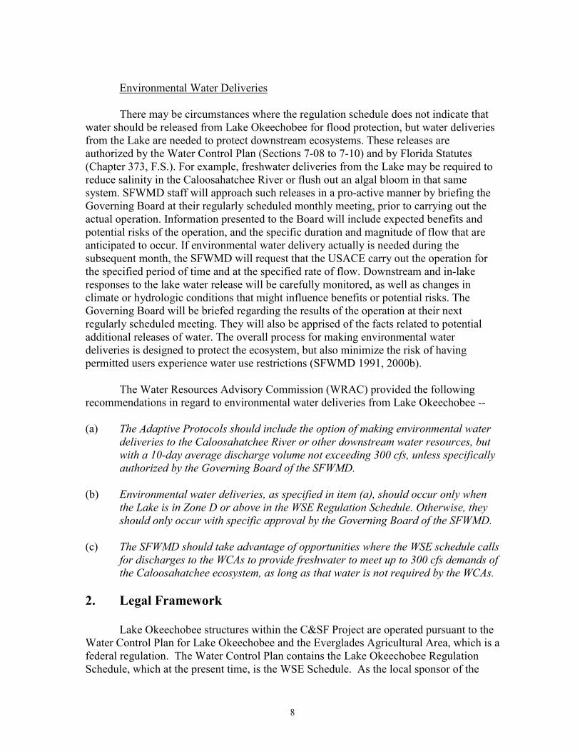
Figure 3. Feedback loop for real-time operations of the Lake, indicating how results of theWSE schedule are meshed with the regional performance measure monitoring todetermine flood control releases (under WSE), environmental water needs, and watersupply effects. In cases where flood control releases are not required by the WSEschedule, deliveries to downstream water resources can be made as long as there isanticipated to be minimal or no impact to agricultural and urban water supply, based onperformance measures described in Section 5e of this document. Real-time operations willbe consistent with the general strategies established following semi-annual publicworkshops and monthly Governing Board briefings.

Regional systemmonitoring

Real-timelake

operations

WSE Schedule

Lake stage,tributary conditions,

climate forecast

Lake anddownstreambenefits and

no significant riskto water supply

Performancemeasure Scores

Expert evaluationof environmental

and watersupply status

GoverningBoard has

been briefed

WSEregulatoryreleases

Option ofenvironmental

waterdeliveries

16

4. Specific Procedure for Environmental Water Deliveries

Adaptive Protocols are designed to identify potential “win-win” situations inwhich one or more environmental resources can benefit from a Lake release and wherethere is anticipated to be minimal or no adverse effect on meeting future agricultural orurban water supply needs. The process carefully examines potential benefits and risks tothe Lake in regard to its ecological integrity and the established Lake MFL criteria. Whenall pertinent facts indicate that a water delivery to a downstream resource is likely to berequired in the upcoming month, the Governing Board will be briefed at their nextregularly scheduled meeting. If conditions develop as expected and the environmentalwater delivery becomes necessary, a request will be made to the USACE to dischargewater from their structures at the volume and duration that does not exceed what wasreported at the Governing Board briefing. Prior to the environmental water delivery, therewill be a posting of information on the Lake Operations web site of the SFWMD[www.sfwmd.gov] to notify affected interests of the operation.

During an environmental water delivery, the following additional procedures willapply. The overarching principle is that the SFWMD Governing Board has been briefedon the operation, and that the environmental water deliveries are supported by the USACEand FDEP. When the Lake is below Zone D of the WSE Regulation Schedule, or whenenvironmental deliveries are required in excess of 300 cfs (10-day average), the SFWMDinput to the USCAE on whether to make the environmental deliveries will be based onspecific Governing Board discussion and direction.

(a) Regular meetings will be held by the directors of Water Supply, EcosystemRestoration, and Operations Control, along with a representative of Office ofCounsel, to discuss status of the ongoing operation. Consideration will be given tochanges based on both environmental responses and water supply implications.

(b) During the operations, technical staff will consult on a regular basis with theUSACE and FDEP, discuss status of the operation and observed system responses,and indicate whether or not there is a need for any change in the water delivery.Changes might include increased or decreased discharge volume or duration,within the constraints established at the prior Governing Board briefing.

(c) Monitoring and assessment will occur to document water delivery effects ondownstream ecosystem(s), changes in the Lake, and any changes in water supplyrisk to ensure a sound technical basis for the discussions stated in (a) and (b)above.

(d) In addition to posting updates on the Lake Operations web site regarding the statusof the operation, there will be periodic press releases to notify the public of theoperation status and its documented benefits.

17

(e) SFWMD staff will document the operation on the web site, including its duration,benefits to the environmental resources, and any effects, or lack thereof, on theLake and regional water supply.

5. Application of Regional Performance Measures

For each distinct environmental region of the system (Lake Okeechobee,Caloosahatchee Estuary, St. Lucie Estuary, and Water Conservation Areas of theEverglades Protection Area), a set of hydrologic and biological performance measures willbe used in the Adaptive Protocols process to identify the need for water releases from theLake. Water supply performance measures also will be used to identify the level of risk tothat use of the Lake resource. Hydrologic and water supply performance measures arepatterned after those developed in the LECWSP and the WSE regulation schedule review.Actions to release water from the Lake for protection of natural resources will be based onthe regional performance measures. The ultimate goal is to use operational flexibility tofacilitate benefits to the environment without impacting other uses of the Lake.

5a. Lake Okeechobee Performance Measures

5a.1 Hydrologic Performance Measures

Hydrologic performance measures for the Lake are documented in the LECRWSPand the Lake Okeechobee Conceptual Ecosystem Model (Havens 2000) for theRestoration Coordination and Verification (RECOVER) program of CERP. They arebased on over a decade of rigorous science and peer-reviewed literature (e.g., Maceina1993, Aumen and Gray 1995, Havens 1997, Havens et al. 1999). The followingparagraphs describe the scientific basis of performance measures and the approach forusing them as part of the Adaptive Protocols. Along with the hydrologic performancemeasures, assessment of the Lake’s biological status will be based on a comprehensive setof measures, including submerged aquatic vegetation, emergent wetland plants, benthicalgae, water clarity, nutrient concentrations, and algal blooms. This information will bethe basis for technical input to operators regarding expected Lake responses to waterdischarges.

There are a total of four hydrologic performance measures for Lake Okeechobee.Three identify adverse impacts from extreme high and low water, and one identifies anannual minimum water level target of approximately 13.5 ft NGVD (National GeodeticVertical Datum of 1929, formerly called mean sea level) in spring, which has documentedecosystem benefits.

Extreme High Stage

A Lake stage of 17 ft NGVD can adversely effect the Lake’s littoral zone, evenwhen it is of short duration. During the late 1990s, the Lake stage exceeded 17 ft NGVD

18

on a number of occasions. The high water levels facilitated the movement of wind-drivenwaves into the western shoreline, resulting in the erosion of several hundred meters of thewestern littoral zone where it is in contact with the open water of the lake (Hanlon andBrady 2001). Large areas of bulrush and other plants were torn from the lake bottom andpiled on the shoreline, forming a “berm” of dead plant material and fine organic matter(Havens et al. 2001a). This berm acted as a local source of turbidity, preventing light fromreaching the adjacent lake bottom, even when stages dropped to 13 ft NGVD. As a result,the shoreline area was devoid of submerged plants; these plants are a critical habitat forfish populations (Furse and Fox 1994). Submerged plants did not re-colonize the area nearthe berm until the Lake stage fell to near 12 ft NGVD (Havens et al. 2001a). When theLake stage is at 17 ft NGVD or more there also is evidence that nutrient-rich water fromthe open-water zone (TP > 100 ppb) is transported into the interior littoral marsh, whichnormally is pristine and nutrient poor (TP < 10 ppb). This has been documented to causeecological changes, including altered periphyton structure and function (Havens et al.1999) and possibly an expansion of cattail. When littoral plants and periphyton change,higher trophic levels also may be affected in the littoral food web of Lake Okeechobee(Havens et al. 2001b, c).

Prolonged Moderate High Stage

Prolonged, moderately high (>15 ft NGVD) stages also result in undesirablebiological and water quality impacts in the Lake. The WSE regulation schedule wasdeveloped, in part, with this concept in mind. This is reflected by the fact that the base ofthe regulatory discharge zone (bottom of Zone D) rises above 15 ft NGVD for just a shortperiod of time, peaking at just 15.5 ft NGVD.

The mechanism of impact when the stage is above 15 ft NGVD for many monthsrelates to the depth of the water and increased turbidity. With deeper water, reducedamounts of light reach the lake bottom, resulting in a reduction of submerged plant growthalong the shoreline. This phenomenon is well documented in Florida lakes (Canfield et al.1985), and by cause-and-effect experiments dealing with Vallisneria (eelgrass) from LakeOkeechobee (Grimshaw et al. 2002). In addition, when stage in Lake Okeechobee is above15 ft NGVD, there is transport of re-suspended mud sediment particles from mid-lake tonear-shore areas that support submerged plant communities (Maceina 1993, Havens andJames 1999, Havens 2002). The consequence is that submerged plants progressivelydecline under prolonged high-stage conditions due to light limitation. In the late 1990s,after several successive years of high stage, submerged plant coverage in LakeOkeechobee was very sparse, and there were dramatic declines in the Lake’s sport fishpopulations (Florida Fish and Wildlife Conservation Commission [FFWCC], publicpresentations in 1999 and 2000). When more favorable conditions occurred in summer2000 (stage near 12 ft NGVD after a managed recession), submerged plant coverageincreased from 5,000 to over 40,000 acres (Havens et al. 2001a). This is similar to thecoverage documented during the late 1980s and early 1990s, after a period of similar lowstage (Richardson and Harris 1995). In addition to biological impacts, stage above 15 ftNGVD (yearly average) also is linked with higher concentrations of phosphorus (Canfieldand Hoyer 1988, Havens 1997). This may be due to increased phosphorus transport from

19

mid-lake to near-shore areas (Maceina 1993, Havens 1997) and/or loss of phosphorusassimilation by plants and attached algae (Phlips et al. 1993). Submerged plant beds andalgae are a tremendous sink for phosphorus in shallow lakes, often preventing algalblooms from occurring even when high external loading of phosphorus occurs (Scheffer etal. 1994, Havens and Schelske 2001, Havens et al. 2001d). As indicated previously, theyalso are key areas for fish nesting and foraging activities.

Extreme Low Stage

Effects of extreme low stage (<11 ft NGVD) are documented in the SFWMD(2000c) Minimum Flows and Levels document, and therefore, only a brief summary isprovided here. When water levels in the Lake are approaching such an extreme low, therewill have been concerns about water supply, estuarine ecology, and saltwater intrusion incoastal areas, as well as recreation and navigation in the Lake and adjacent waterways,which impact the local and regional economy. These concerns could restrict waterdischarges from the Lake for downstream natural resource protection. If an extreme lowstage persists for several months, it can threaten the littoral zone of the Lake by drying outmarsh habitat so that it cannot be used by fish, wading birds, migratory waterfowl, thefederally endangered Snail Kite, alligators, or other animals (Havens 2002). Extreme lowstage also dries out pristine interior littoral areas such as Moonshine Bay, allowing them tobe taken over by exotic plants such as Melaleuca and torpedograss, which invade morerapidly when soils are not flooded (Lockhart 1995, Smith et al. 2001). An important aspectof extreme low stage is that its impacts depend on return frequency. As long as an extremelow stage does not occur more often than once every 6-7 years, it can provide somebenefits to the littoral community. For example, it can favor fires that burn accumulatedcattail thatch, and allow buried seeds of native marsh plants to germinate.

Spring Water Level (June)

Research on the Lake’s submerged aquatic vegetation community indicates thatlate spring (early June) water levels near 13.5 ft NGVD could support a healthier andmore widespread community than what has occurred in the Lake under higher stageconditions (Havens et al. 2001a, Grimshaw et al. 2002). A healthier submerged vegetationcommunity, in turn, would provide a wide range of benefits to the Lake’s fishery, wadingbird community, and near-shore water quality and clarity. The submerged vegetation, asnoted previously, is considered a keystone component of the Lake community. Lake stagefalling from a maximum of near 15.5 ft NGVD in fall-winter to below 13.5 ft NGVD inJune would provide other benefits to the ecosystem. It would concentrate prey resources ata time when wading birds and other predators are establishing nests in the littoral zone andraising their young. This could provide a food base to support healthy populations.Likewise, the receding water would allow birds, apple snails, and other animals toconstruct nests or lay eggs on emergent plants at locations above the water that minimizerisks from predators and flooding. One important consequence of this, however, is that ifwater levels reverse by >0.5 ft / month during a period of decline, damage can potentiallyoccur to these nests and eggs.

20

Two aspects of spring water level are evaluated with performance measures: (1)the actual stage of the Lake relative to the optimal 15.5 to 13.5 ft NGVD decline fromJanuary to June, and (2) the presence of stage reversals during this period of time.

5a.2 Lake Okeechobee Biological Performance Measures

In addition to monitoring and assessing hydrologic conditions in the Lake, theSFWMD monitors key biological indicators of ecosystem health. For Adaptive Protocols,the focus will be on two keystone communities of the lake that are known to be highlyresponsive to changes in water level – the submerged aquatic vegetation and near-shorebulrush. These communities provide critical habitat for fish and wildlife, they stabilizelake sediments, and the plants and their associated periphyton (attached algae) removenutrients from the water, directly benefiting water quality. They both are being measuredin existing monitoring programs carried out by the SFWMD. Although there presently arenot similar programs to evaluate the status of the lake’s animal communities, these areexpected to become available in the near future, as part of the monitoring program insupport of the Comprehensive Everglades Restoration Plan (CERP). When that occurs,there also will be regular monitoring data on the lake for wading birds and forage fish, andpossibly benthic invertebrates and open-water fish communities.

Submerged vegetation is monitored at three different spatial and temporal scalesby the SFWMD, in a program that started in 1998. First, sampling is conducted on amonthly basis to obtain semi-quantitative data on the status of submerged and emergentplant communities at approximately 10 sentinel stations around the lakeshore. Second,quarterly quantitative sampling is done at stations located along 16 shoreline transects, inorder to quantify plant species composition and biomass. Taken together, this informationis used to evaluate seasonal changes in the community. It provides information on plantresponses to changing water levels on a relatively short time scale, and can be used asinput to real-time operations. Third, yearly maps of submerged vegetation are developedby intensive sampling at over 500 locations around the lake shore, near the end of eachyear’s peak growing season (August to September). This provides information on the totalnumber of acres of plants that the lake gained (or lost) under the prevailing hydrologicconditions of a calendar year. This sampling program has indicated that submergedaquatic vegetation can cover more than 40,000 acres when water levels are favorable (e.g.,summer 2000 and 2002), as compared to <5,000 acres during periods of prolonged highwater level (e.g., 1996 to 1999).

Shoreline bulrush communities also are sampled monthly, in a qualitative surveyfrom boat and/or helicopter, and quarterly quantitative sampling is done at six sentinelstations around the north and west lakeshore. In the quarterly sampling, plant stemdensities and heights are recorded, along with water depth and transparency. Theseprograms provide information on plant responses to changing water levels at a relativelyshort time scale, for input to real-time system management. On a yearly basis, high-resolution aerial photography and Geographic Information Systems (GIS) technologydetermine the spatial extent of bulrush and other emergent plants along the lakeshore. Thisprovides information on the total number of acres of plants in the lake in any given year.

21

In the early 1990s, when favorable water levels occurred, there was up to 4,700 acres ofbulrush. In the late 1990s, as a result of high water level, the acreage was reduced tobelow 1,000. Bulrush has partly recovered since then, as a result of low water levels in2000-2001, and a dense community of spikerush also has developed along the lake shore.These communities are providing important fish and wildlife habitat along the northwestshore, in an area where much of the littoral habitat has been degraded due to torpedograssand cattail expansion. Under favorable water levels, the lake should be able to supportmore than 5,000 acres of shoreline bulrush and spikerush.

A detailed description of sampling methods for submerged and emergent aquaticvegetation in Lake Okeechobee is provided on the SFWMD web site, at the followinglocation: www.sfwmd.gov/lo_statustrends/ecocond/lo_veg.html

5a.3 Performance Measure Integration and Application

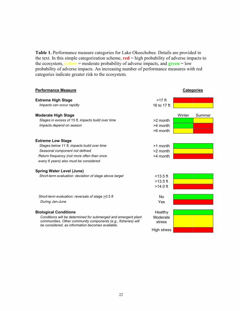
Table 1 summarizes the performance measure evaluation scheme that scientistswith expertise in the hydrology and biology of Lake Okeechobee will use to evaluateconditions of the ecosystem. A simple color scheme is used, where red = high risk ofadverse impacts or adverse impacts actually documented, yellow = moderate risk ofadverse impacts, and green = little or no potential for adverse impacts. [Note: if you havea black and white copy of this document, the three color categories appear to be grey, lightgrey, and dark grey, respectively]. In regard to the performance measure dealing withprolonged moderate high stage, ecosystem impacts depend on whether the conditionoccurs in winter or summer (when plants and animals are actively growing). Under thisscheme, an increasing number of performance measures with black scores indicate agreater risk of damage to the Lake ecosystem. As previously described, this informationwill be considered in the context of similar performance measure scores from theestuaries, the Everglades Protection Area, and agricultural and urban water supply.

22

Table 1. Performance measure categories for Lake Okeechobee. Details are provided inthe text. In this simple categorization scheme, red = high probability of adverse impacts tothe ecosystem, yellow = moderate probability of adverse impacts, and green = lowprobability of adverse impacts. An increasing number of performance measures with redcategories indicate greater risk to the ecosystem.

Performance Measure Categories

Extreme High Stage >17 ft Impacts can occur rapidly 16 to 17 ft

Moderate High Stage Winter Summer Stages in excess of 15 ft, impacts build over time >2 month Impacts depend on season >4 month

>6 month

Extreme Low Stage Stages below 11 ft, impacts build over time >1 month Seasonal component not defined >2 month Return frequency (not more often than once >4 month every 6 years) also must be considered

Spring Water Level (June) Short-term evaluation: deviation of stage above target <13.5 ft

>13.5 ft>14.0 ft

Short-term evaluation: reversals of stage >0.5 ft No During Jan-June Yes

Biological Conditions Healthy Conditions will be determined for submerged and emergent plant communities. Other community components (e.g., fisheries) will be considered, as information becomes available.

Moderatestress

High stress

23

5b. Estuary Performance Measures

5b.1 Hydrologic Performance Measures

The St. Lucie Estuary (SLE) and the Caloosahatchee Estuary (CE) are largebrackish-water systems on the east and west coast of Florida, respectively, which have thepotential to provide vital habitat for substantial populations of fish and invertebrates thathave biological and economic importance. The hydrology of both systems has beenaltered by modification of drainage basins and by artificial connections to LakeOkeechobee. Freshwater input to these systems varies dramatically during a typical year.At times Lake discharge and surface runoff can be of sufficient magnitude to turn theseestuaries entirely fresh. At other times, they receive virtually no surface runoff andsalinity of the estuaries increases. Annual fluctuations in salinity often exceed thetolerance limits of many estuarine organisms (Haunert and Startzman 1985, Chamberlainand Doering 1998).

The St. Lucie Canal (C-44) and the Caloosahatchee River Canal (C-43) connectthese estuaries to Lake Okeechobee. While serving a flood control function, these canalsalso provide a route for supplying water when the estuaries may benefit from additionalfreshwater.

In order to develop environmentally sensitive water release plans from the Lake tothe estuaries, biological and physical information was needed to determine a desirablerange and frequency of flows. This work is summarized in Chamberlain and Doering(1998) and Haunert and Konyha (2000). In brief, the Valued Ecosystem Componentapproach, developed by the U.S. Environmental Protection Agency (USEPA 1987) as part ofits National Estuary Program, has been used to make these determinations. The approach hasbeen modified to focus on providing critical estuarine habitat. In many instances, that habitatis biological and typified by one or more prominent species. In other cases the habitat may bephysical, such as an open water oligohaline zone. Enhancing and maintaining thesebiological and physical habitats should lead to a generally healthy and diverse ecosystem.Providing a suitable salinity and water quality environment for the habitat-forming species orgroups of species should ensure their continued dominance. These salinity and water qualityrequirements form the basis for establishing minimum flows, and guidelines for dischargingfreshwater to estuaries.

Examples of biological habitat are oyster bars and grass beds, with prominent speciesbeing the American oyster, Crassostrea virginica and the SAVs, Vallisneria americana,Halodule wrightii, and Thalassia testudinum. The ecological functions and value of grassand oyster beds are well established (Loosanoff and Nomejko 1951, Fonseca et al. 1983,Virnstein et al 1983, Fonseca and Fisher 1986, Newell 1988, Fonseca 1989, Fonseca andCahalan 1992 , Zieman 1982, Phillips 1984, Thayer et al. 1984, Kenworthy et al. 1988,Zieman and Zieman 1989).

24

Utilizing the application of the resource-based management strategy or VECapproach, a favorable range of inflow and related salinity was established. The range offlows considered necessary to maintain a favorable range of salinity is 350 cfs to 2,000 cfsfor the SLE and 300 cfs to 2,800 cfs for the CE (Chamberlain and Doering 1998, Haunertand Konyha 2000).

St. Lucie Estuary Performance Measures

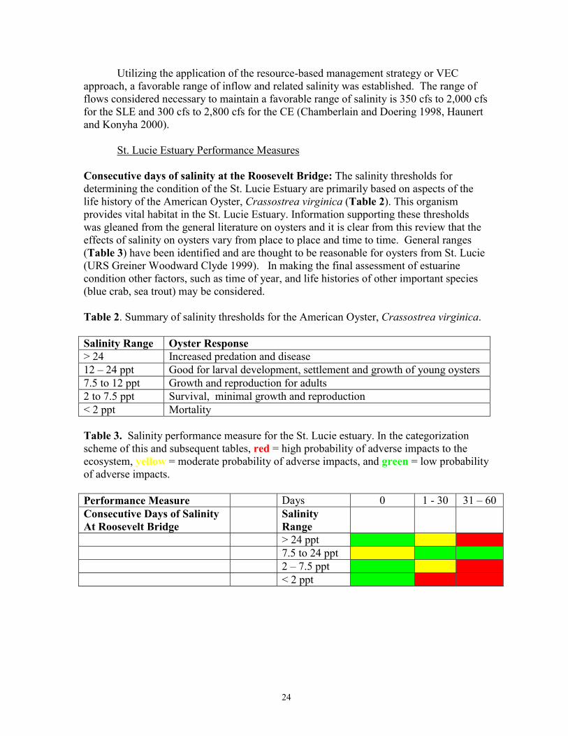
Consecutive days of salinity at the Roosevelt Bridge: The salinity thresholds fordetermining the condition of the St. Lucie Estuary are primarily based on aspects of thelife history of the American Oyster, Crassostrea virginica (Table 2). This organismprovides vital habitat in the St. Lucie Estuary. Information supporting these thresholdswas gleaned from the general literature on oysters and it is clear from this review that theeffects of salinity on oysters vary from place to place and time to time. General ranges(Table 3) have been identified and are thought to be reasonable for oysters from St. Lucie(URS Greiner Woodward Clyde 1999). In making the final assessment of estuarinecondition other factors, such as time of year, and life histories of other important species(blue crab, sea trout) may be considered.

Table 2. Summary of salinity thresholds for the American Oyster, Crassostrea virginica.

Salinity Range Oyster Response> 24 Increased predation and disease12 – 24 ppt Good for larval development, settlement and growth of young oysters7.5 to 12 ppt Growth and reproduction for adults2 to 7.5 ppt Survival, minimal growth and reproduction< 2 ppt Mortality

Table 3. Salinity performance measure for the St. Lucie estuary. In the categorizationscheme of this and subsequent tables, red = high probability of adverse impacts to theecosystem, yellow = moderate probability of adverse impacts, and green = low probabilityof adverse impacts.

Performance Measure Days 0 1 - 30 31 – 60Consecutive Days of SalinityAt Roosevelt Bridge

SalinityRange> 24 ppt7.5 to 24 ppt2 – 7.5 ppt< 2 ppt

25

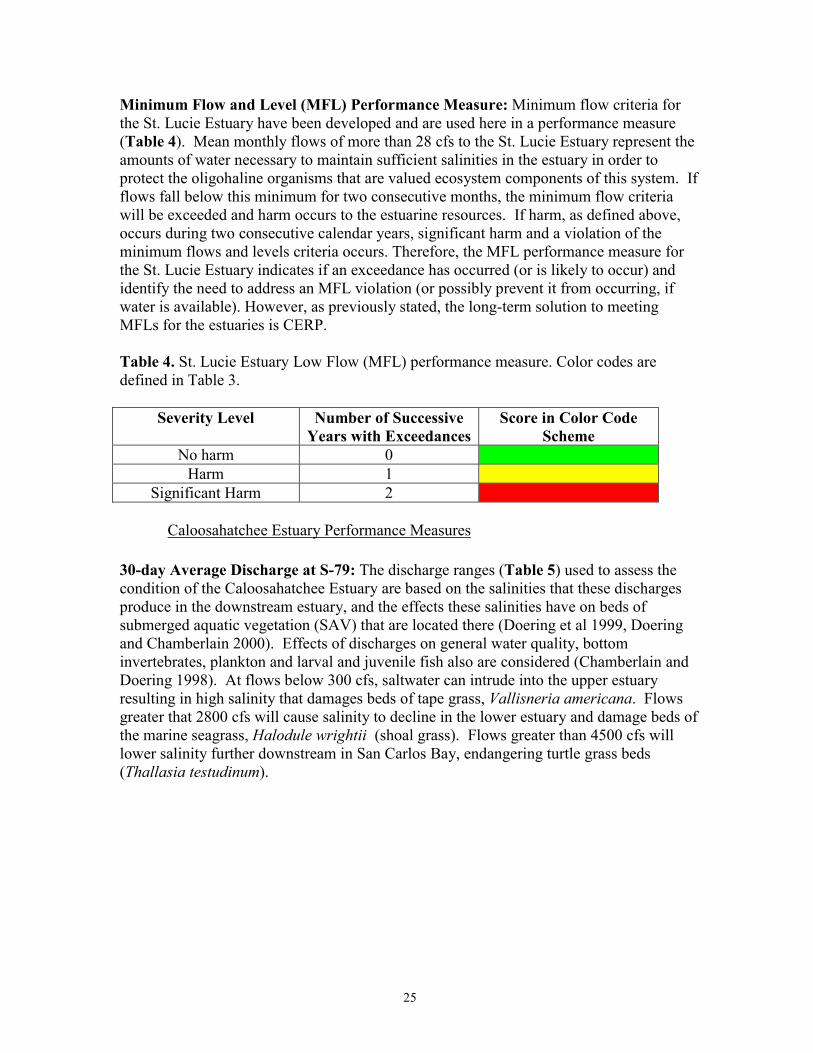
Minimum Flow and Level (MFL) Performance Measure: Minimum flow criteria forthe St. Lucie Estuary have been developed and are used here in a performance measure(Table 4). Mean monthly flows of more than 28 cfs to the St. Lucie Estuary represent theamounts of water necessary to maintain sufficient salinities in the estuary in order toprotect the oligohaline organisms that are valued ecosystem components of this system. Ifflows fall below this minimum for two consecutive months, the minimum flow criteriawill be exceeded and harm occurs to the estuarine resources. If harm, as defined above,occurs during two consecutive calendar years, significant harm and a violation of theminimum flows and levels criteria occurs. Therefore, the MFL performance measure forthe St. Lucie Estuary indicates if an exceedance has occurred (or is likely to occur) andidentify the need to address an MFL violation (or possibly prevent it from occurring, ifwater is available). However, as previously stated, the long-term solution to meetingMFLs for the estuaries is CERP.

Table 4. St. Lucie Estuary Low Flow (MFL) performance measure. Color codes aredefined in Table 3.

Severity Level Number of SuccessiveYears with Exceedances

Score in Color CodeScheme

No harm 0Harm 1

Significant Harm 2

Caloosahatchee Estuary Performance Measures

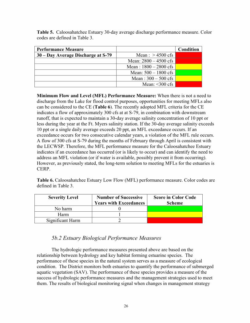
30-day Average Discharge at S-79: The discharge ranges (Table 5) used to assess thecondition of the Caloosahatchee Estuary are based on the salinities that these dischargesproduce in the downstream estuary, and the effects these salinities have on beds ofsubmerged aquatic vegetation (SAV) that are located there (Doering et al 1999, Doeringand Chamberlain 2000). Effects of discharges on general water quality, bottominvertebrates, plankton and larval and juvenile fish also are considered (Chamberlain andDoering 1998). At flows below 300 cfs, saltwater can intrude into the upper estuaryresulting in high salinity that damages beds of tape grass, Vallisneria americana. Flowsgreater that 2800 cfs will cause salinity to decline in the lower estuary and damage beds ofthe marine seagrass, Halodule wrightii (shoal grass). Flows greater than 4500 cfs willlower salinity further downstream in San Carlos Bay, endangering turtle grass beds(Thallasia testudinum).

26

Table 5. Caloosahatchee Estuary 30-day average discharge performance measure. Colorcodes are defined in Table 3.

Performance Measure Condition30 – Day Average Discharge at S-79 Mean : > 4500 cfs

Mean: 2800 – 4500 cfsMean : 1800 – 2800 cfs

Mean: 500 – 1800 cfsMean : 300 – 500 cfs

Mean: <300 cfs

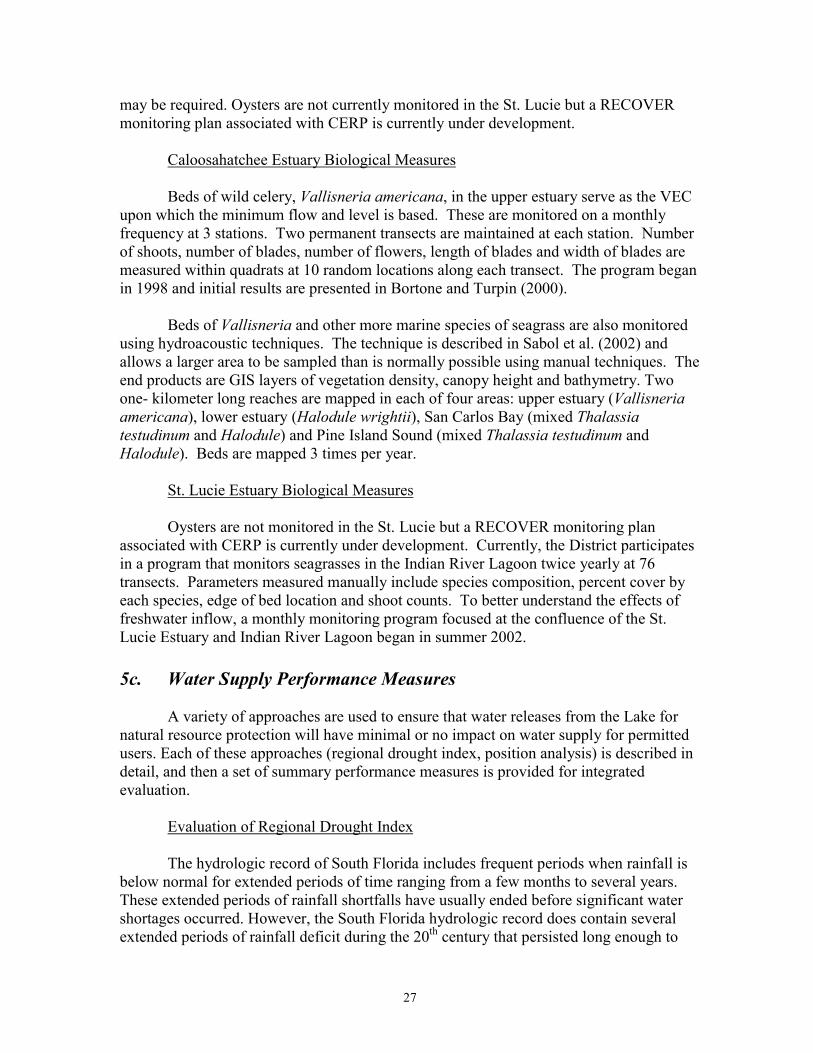
Minimum Flow and Level (MFL) Performance Measure: When there is not a need todischarge from the Lake for flood control purposes, opportunities for meeting MFLs alsocan be considered to the CE (Table 6). The recently adopted MFL criteria for the CEindicates a flow of approximately 300 cfs at at S-79, in combination with downstreamrunoff, that is expected to maintain a 30-day average salinity concentration of 10 ppt orless during the year at the Ft. Myers salinity station. If the 30-day average salinity exceeds10 ppt or a single daily average exceeds 20 ppt, an MFL exceedance occurs. If anexceedance occurs for two consecutive calendar years, a violation of the MFL rule occurs.A flow of 300 cfs at S-79 during the months of February through April is consistent withthe LECWSP. Therefore, the MFL performance measure for the Caloosahatchee Estuaryindicates if an exceedance has occurred (or is likely to occur) and can identify the need toaddress an MFL violation (or if water is available, possibly prevent it from occurring).However, as previously stated, the long-term solution to meeting MFLs for the estuaries isCERP.

Table 6. Caloosahatchee Estuary Low Flow (MFL) performance measure. Color codes aredefined in Table 3.

Severity Level Number of SuccessiveYears with Exceedances

Score in Color CodeScheme

No harm 0Harm 1

Significant Harm 2

5b.2 Estuary Biological Performance Measures

The hydrologic performance measures presented above are based on therelationship between hydrology and key habitat forming estuarine species. Theperformance of these species in the natural system serves as a measure of ecologicalcondition. The District monitors both estuaries to quantify the performance of submergedaquatic vegetation (SAV). The performance of these species provides a measure of thesuccess of hydrologic performance measures and the management strategies used to meetthem. The results of biological monitoring signal when changes in management strategy

27

may be required. Oysters are not currently monitored in the St. Lucie but a RECOVERmonitoring plan associated with CERP is currently under development.

Caloosahatchee Estuary Biological Measures

Beds of wild celery, Vallisneria americana, in the upper estuary serve as the VECupon which the minimum flow and level is based. These are monitored on a monthlyfrequency at 3 stations. Two permanent transects are maintained at each station. Numberof shoots, number of blades, number of flowers, length of blades and width of blades aremeasured within quadrats at 10 random locations along each transect. The program beganin 1998 and initial results are presented in Bortone and Turpin (2000).

Beds of Vallisneria and other more marine species of seagrass are also monitoredusing hydroacoustic techniques. The technique is described in Sabol et al. (2002) andallows a larger area to be sampled than is normally possible using manual techniques. Theend products are GIS layers of vegetation density, canopy height and bathymetry. Twoone- kilometer long reaches are mapped in each of four areas: upper estuary (Vallisneriaamericana), lower estuary (Halodule wrightii), San Carlos Bay (mixed Thalassiatestudinum and Halodule) and Pine Island Sound (mixed Thalassia testudinum andHalodule). Beds are mapped 3 times per year.

St. Lucie Estuary Biological Measures

Oysters are not monitored in the St. Lucie but a RECOVER monitoring planassociated with CERP is currently under development. Currently, the District participatesin a program that monitors seagrasses in the Indian River Lagoon twice yearly at 76transects. Parameters measured manually include species composition, percent cover byeach species, edge of bed location and shoot counts. To better understand the effects offreshwater inflow, a monthly monitoring program focused at the confluence of the St.Lucie Estuary and Indian River Lagoon began in summer 2002.

5c. Water Supply Performance Measures

A variety of approaches are used to ensure that water releases from the Lake fornatural resource protection will have minimal or no impact on water supply for permittedusers. Each of these approaches (regional drought index, position analysis) is described indetail, and then a set of summary performance measures is provided for integratedevaluation.

Evaluation of Regional Drought Index

The hydrologic record of South Florida includes frequent periods when rainfall isbelow normal for extended periods of time ranging from a few months to several years.These extended periods of rainfall shortfalls have usually ended before significant watershortages occurred. However, the South Florida hydrologic record does contain severalextended periods of rainfall deficit during the 20th century that persisted long enough to

28

cause substantial water shortages. The 1980-81, 1989-90, and 2000-01 droughts are recentexamples of a prolonged period of rainfall deficit in which large cutbacks were necessaryfor both urban and agricultural areas in order to protect regional water resources. On anaverage, these events have occurred once or twice every 10 years. These more significantdrought periods often begin relatively unnoticed with below normal rainfall during the wetseason. Normally the Lake may gain 2 to 3 feet of storage from excess runoff from itsenormous tributary basin (~4,000 square miles) during the wet season. However, whenwet season rainfall is below normal, the majority of rainfall is lost to evapotranspirationwith only minimum amounts of runoff actually reaching the Lake. The Lake water levelmay actually decline during the wet season. Since tributary conditions are the firstindicator of the onset of droughts, it is critical to the regions dependent on LakeOkeechobee for water supply that releases to tide not be made during these periods eventhough water levels in the Lake may be slightly higher than is normally desirable for thebenefit of the littoral zone.

The years of 1980, 1988, and 2000 are specific cases in which the wet season hadbelow normal rainfall that eventually led to water shortages. In the future, until additionalstorage is available, Lake stages should be managed as efficiently as possible to reduce therisk of water shortage during such periods. The WSE operational schedule includes anintricate decision tree that integrates recent short-term rainfall (previous month) anomaliesthroughout the Lake tributaries with the available meteorological and climatic forecasts tomost proficiently balance the competing objectives of water supply, flood protection, andwater resource enhancement. Due to the tremendous size of the upstream tributary basinas well as the uncertainty of climate forecasts, it is concluded that the Palmer DroughtSeverity Index (Appendix I), should be monitored for existing surpluses or deficits thathave accumulated from persistent rainfall anomalies. This index, although notincorporated directly into the WSE Operational Decision Tree, is useful for defining arange of opportunities within the field of discretion provided by the schedule. Using thedecision tree, tributary moisture conditions would have precluded any large regulatoryreleases from being made prior to the four major drought periods listed above. In three ofthe four cases, climate forecasts would have been useful in predicting below normalrainfall for the upcoming dry season.

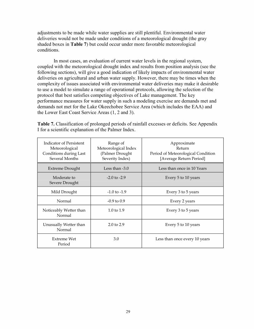
Although the WSE schedule calls for flexibility to be included in theimplementation of operational guidelines (as indicated above in section 2), the originalschedule documentation and model simulations only included performance measures for aspecific set of operational rules. They did not directly include the full spectrum ofoperational flexibility allowed within the WSE operational guidelines. It is important thatthe operational flexibility be used in cases that have the potential to increase theperformance of one competing objective without hurting others. Table 7 classifies rainfallanomalies in terms of ranges of the Palmer Drought Severity Index. When estuarine, Lake,and/or Everglades performance measures indicate a need for water deliveries for naturalresource protection, the current tributary condition as classified by the Palmer Indexshould also be considered. The Palmer Index allows the identification of meteorologicaldrought (significantly reduced rainfall) several months before a hydrologic drought(significantly reduced reserve water storage) occurs. This allows for operational

29

adjustments to be made while water supplies are still plentiful. Environmental waterdeliveries would not be made under conditions of a meteorological drought (the grayshaded boxes in Table 7) but could occur under more favorable meteorologicalconditions.

In most cases, an evaluation of current water levels in the regional system,coupled with the meteorological drought index and results from position analysis (see thefollowing sections), will give a good indication of likely impacts of environmental waterdeliveries on agricultural and urban water supply. However, there may be times when thecomplexity of issues associated with environmental water deliveries may make it desirableto use a model to simulate a range of operational protocols, allowing the selection of theprotocol that best satisfies competing objectives of Lake management. The keyperformance measures for water supply in such a modeling exercise are demands met anddemands not met for the Lake Okeechobee Service Area (which includes the EAA) andthe Lower East Coast Service Areas (1, 2 and 3).

Table 7. Classification of prolonged periods of rainfall excesses or deficits. See AppendixI for a scientific explanation of the Palmer Index.

Indicator of PersistentMeteorological

Conditions during LastSeveral Months

Range of Meteorological Index

(Palmer DroughtSeverity Index)

ApproximateReturn

Period of Meteorological Condition[Average Return Period]

Extreme Drought Less than -3.0 Less than once in 10 Years

Moderate toSevere Drought

-2.0 to -2.9 Every 5 to 10 years

Mild Drought -1.0 to -1.9 Every 3 to 5 years

Normal -0.9 to 0.9 Every 2 years

Noticeably Wetter thanNormal

1.0 to 1.9 Every 3 to 5 years

Unusually Wetter thanNormal

2.0 to 2.9 Every 5 to 10 years

Extreme WetPeriod

3.0 Less than once every 10 years

30

Position Analysis

Position analysis (PA) (Hirsh 1978, Smith et al. 1992, Tasker and Dunne 1997,Cadavid et al. 1999) is a form of risk analysis that will be used by staff to provideadditional input regarding potential effects of release decisions on agricultural and urbanwater supply. Given the current state of the system, position analysis evaluates the risksand potential benefits associated with specific operational plans for South Florida’s watermanagement system over a period of several months. It relies on the simulation of a largenumber of possible outcomes using current conditions as the initial values for modeling.To be most useful, PA needs to incorporate the broadest range of meteorologicalconditions that may occur in the future, but cannot be used to specifically forecast futureevents.

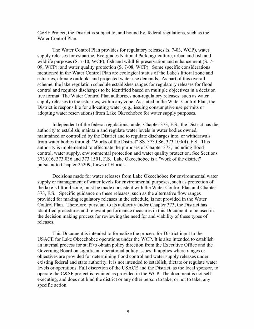
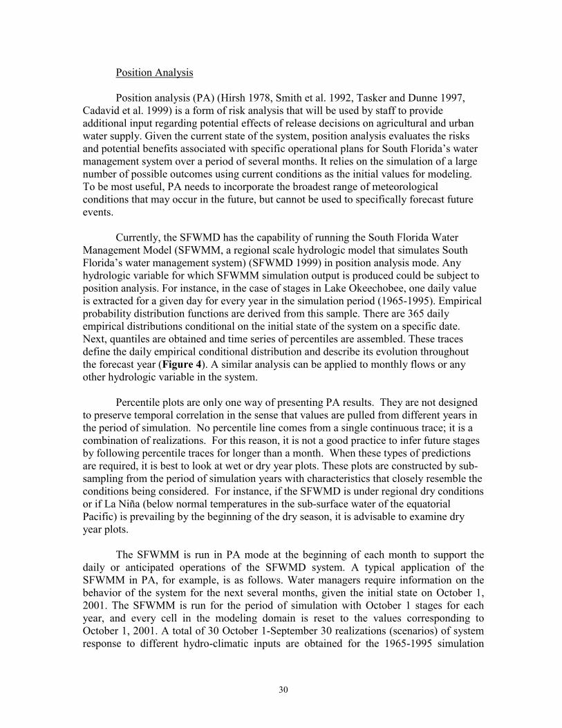
Currently, the SFWMD has the capability of running the South Florida WaterManagement Model (SFWMM, a regional scale hydrologic model that simulates SouthFlorida’s water management system) (SFWMD 1999) in position analysis mode. Anyhydrologic variable for which SFWMM simulation output is produced could be subject toposition analysis. For instance, in the case of stages in Lake Okeechobee, one daily valueis extracted for a given day for every year in the simulation period (1965-1995). Empiricalprobability distribution functions are derived from this sample. There are 365 dailyempirical distributions conditional on the initial state of the system on a specific date.Next, quantiles are obtained and time series of percentiles are assembled. These tracesdefine the daily empirical conditional distribution and describe its evolution throughoutthe forecast year (Figure 4). A similar analysis can be applied to monthly flows or anyother hydrologic variable in the system.

Percentile plots are only one way of presenting PA results. They are not designedto preserve temporal correlation in the sense that values are pulled from different years inthe period of simulation. No percentile line comes from a single continuous trace; it is acombination of realizations. For this reason, it is not a good practice to infer future stagesby following percentile traces for longer than a month. When these types of predictionsare required, it is best to look at wet or dry year plots. These plots are constructed by sub-sampling from the period of simulation years with characteristics that closely resemble theconditions being considered. For instance, if the SFWMD is under regional dry conditionsor if La Niña (below normal temperatures in the sub-surface water of the equatorialPacific) is prevailing by the beginning of the dry season, it is advisable to examine dryyear plots.

The SFWMM is run in PA mode at the beginning of each month to support thedaily or anticipated operations of the SFWMD system. A typical application of theSFWMM in PA, for example, is as follows. Water managers require information on thebehavior of the system for the next several months, given the initial state on October 1,2001. The SFWMM is run for the period of simulation with October 1 stages for eachyear, and every cell in the modeling domain is reset to the values corresponding toOctober 1, 2001. A total of 30 October 1-September 30 realizations (scenarios) of systemresponse to different hydro-climatic inputs are obtained for the 1965-1995 simulation

31

period, each equally likely to take place in the future. Application of PA to the operationsof the SFWMD is described in detail by Cadavid et al. (1999, 2001).

Figure 4. Lake Okeechobee stage position analysis results for October 1, 2001.

For guiding real-time operations, PA, percentile plots and other specific types ofyear plots can be used as decision guidance tools in determining impacts or benefitsderived from specific adaptive protocols for Lake Okeechobee operations. However, thegraph or type of result and how to use it depends on the operational scenario. Anapplication example for Lake Okeechobee stage is depicted in Figure 4. The percentileplots provide estimates of the likelihood of Lake stage falling into different operationalzones, given the current conditions in the SFWMD system. For instance, if current Lakestages are in the upper half of Zone E, the percentile plot will provide the probability andtiming of going into Zone D. On the other hand, if current Lake stages are low, thepercentile plot will indicate the probability of receding into the Supply Side ManagementZone and the probable times when this would happen. In the case that simple operationalprotocols are proposed, back-of-the-envelope computations can be used to determine howsuch operations could modify the future likelihood of the Lake transitioning into lower orhigher stages.

32

Evaluation of Water Supply Shortage Risk

Evaluation of water supply shortage risk is based on assigning different risk levelsto a series of categories or performance measure indicators, associated with differentelements in the system, such as tributary basins, storage components and different types ofwater users. The way in which risk levels are presented and summarized will help in theLake Okeechobee releases decision process. The water supply risk levels considered inthis evaluation are Low (L), Moderate (M) and High (H). The categories and theguidelines to assign the risk levels are presented below. The abbreviations in parenthesisrepresent the short name assigned to each category. If stages in the WCA’s and the Lakeare low, environmental water deliveries from the Lake to coastal systems (e.g., theCaloosahatchee Estuary) are considered to have a higher risk to agricultural and urbanwater supply than if one or both of those areas have adequate water in storage.

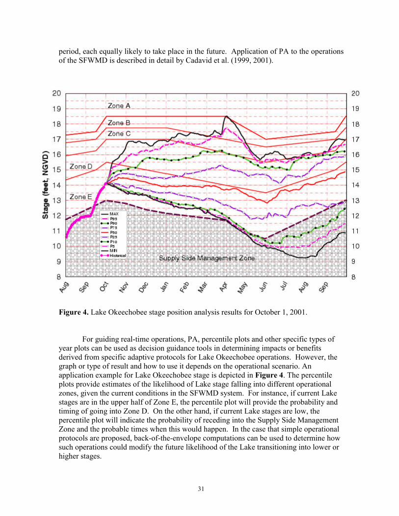
Performance Measure 1 -- Projected Lake Okeechobee Stage Within the NextTwo Months (LOK): Obtained from the Position Analysis (PA) results and thecorresponding Lake Okeechobee stage tracking chart, this indicator gives the zone withinwhich Lake stage most likely would be during the next two months. These graphs areposted at the SFWMD web page. Possible outcomes and risk levels are as follows:

Projected Lake Okeechobee Stagefor next two months

Risk Level

Zone D or Above LZone E MSSM H

The PA results and the tracking chart for Lake Okeechobee are posted at:

http://www.sfwmd.gov/org/pld/hsm/reg_app/opln/pa_recent.html

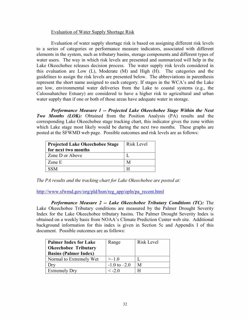
Performance Measure 2 -- Lake Okeechobee Tributary Conditions (TC): TheLake Okeechobee Tributary conditions are measured by the Palmer Drought SeverityIndex for the Lake Okeechobee tributary basins. The Palmer Drought Severity Index isobtained on a weekly basis from NOAA’s Climate Prediction Center web site. Additionalbackground information for this index is given in Section 5c and Appendix I of thisdocument. Possible outcomes are as follows:

Palmer Index for LakeOkeechobee TributaryBasins (Palmer Index)

Range Risk Level

Normal to Extremely Wet >–1.0 LDry -1.0 to –2.0 MExtremely Dry < -2.0 H

33

PDSI values are obtained from:

http://www.cpc.ncep.noaa.gov/products/analysis_monitoring/cdus/palmer_drought/

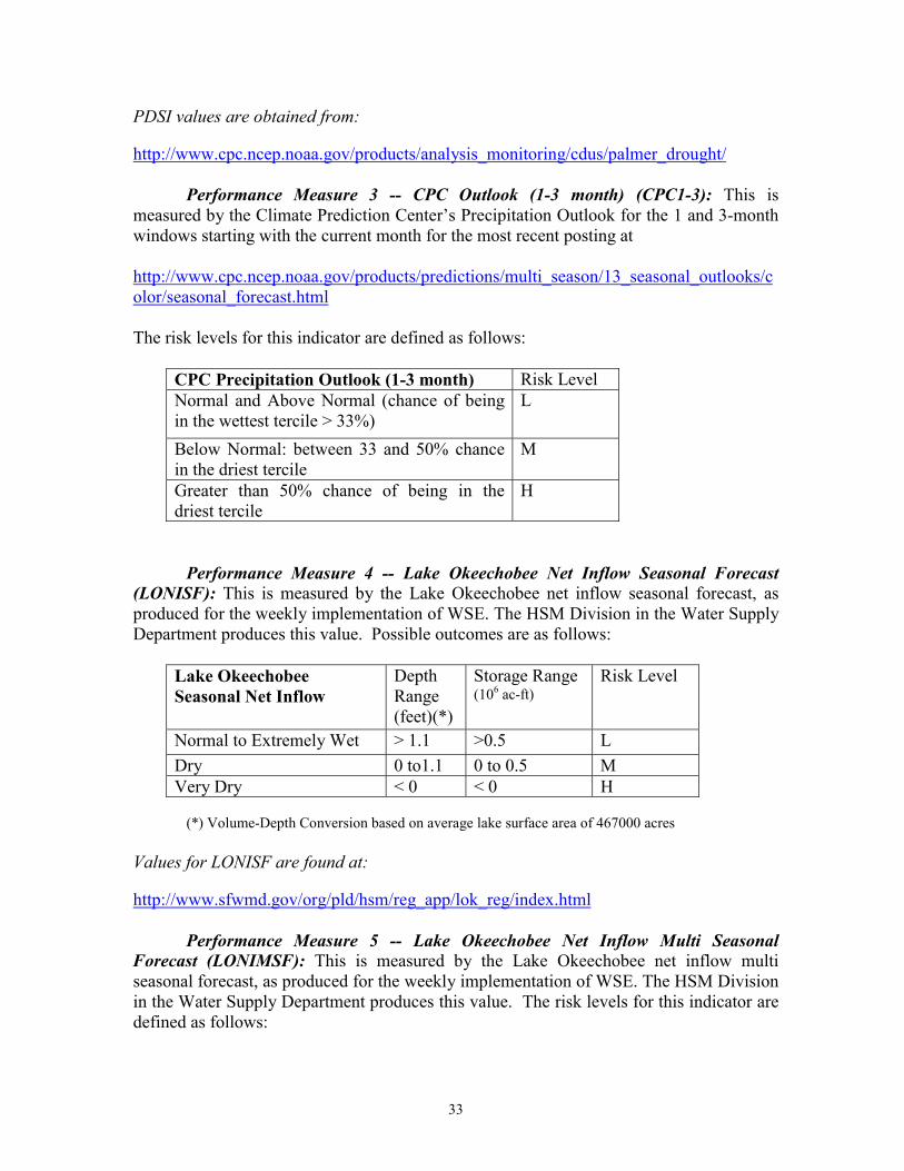
Performance Measure 3 -- CPC Outlook (1-3 month) (CPC1-3): This ismeasured by the Climate Prediction Center’s Precipitation Outlook for the 1 and 3-monthwindows starting with the current month for the most recent posting at

http://www.cpc.ncep.noaa.gov/products/predictions/multi_season/13_seasonal_outlooks/color/seasonal_forecast.html

The risk levels for this indicator are defined as follows:

CPC Precipitation Outlook (1-3 month) Risk LevelNormal and Above Normal (chance of beingin the wettest tercile > 33%)

L

Below Normal: between 33 and 50% chancein the driest tercile

M

Greater than 50% chance of being in thedriest tercile

H

Performance Measure 4 -- Lake Okeechobee Net Inflow Seasonal Forecast(LONISF): This is measured by the Lake Okeechobee net inflow seasonal forecast, asproduced for the weekly implementation of WSE. The HSM Division in the Water SupplyDepartment produces this value. Possible outcomes are as follows:

Lake OkeechobeeSeasonal Net Inflow

DepthRange(feet)(*)

Storage Range(106 ac-ft)

Risk Level

Normal to Extremely Wet > 1.1 >0.5 LDry 0 to1.1 0 to 0.5 MVery Dry < 0 < 0 H

(*) Volume-Depth Conversion based on average lake surface area of 467000 acres

Values for LONISF are found at:

http://www.sfwmd.gov/org/pld/hsm/reg_app/lok_reg/index.html

Performance Measure 5 -- Lake Okeechobee Net Inflow Multi SeasonalForecast (LONIMSF): This is measured by the Lake Okeechobee net inflow multiseasonal forecast, as produced for the weekly implementation of WSE. The HSM Divisionin the Water Supply Department produces this value. The risk levels for this indicator aredefined as follows:

34

Lake OkeechobeeMulti Seasonal NetInflow

DepthRange(feet)(*)

Range(106 ac-ft)

Risk Level

Wet > 3.2 > 1.5 LNormal 1.1 to 3.2 0.5 to 1.5 MDry < 1.1 < 0.5 H

(*) Volume-Depth Conversion based on average lake surface area of 467000 acres

Values for LONIMSF are found at:

http://www.sfwmd.gov/org/pld/hsm/reg_app/lok_reg/index.html

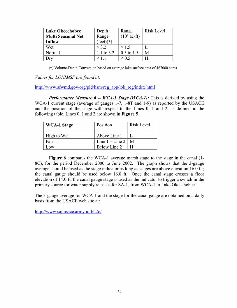
Performance Measure 6 -- WCA-1 Stage (WCA-1): This is derived by using theWCA-1 current stage (average of gauges 1-7, 1-8T and 1-9) as reported by the USACEand the position of the stage with respect to the Lines 0, 1 and 2, as defined in thefollowing table. Lines 0, 1 and 2 are shown in Figure 5

WCA-1 Stage Position Risk Level

High to Wet Above Line 1 LFair Line 1 – Line 2 MLow Below Line 2 H

Figure 6 compares the WCA-1 average marsh stage to the stage in the canal (1-8C), for the period December 2000 to June 2002. The graph shows that the 3-gaugeaverage should be used as the stage indicator as long as stages are above elevation 16.0 ft.;the canal gauge should be used below 16.0 ft. Once the canal stage crosses a floorelevation of 14.0 ft, the canal gauge stage is used as the indicator to trigger a switch in theprimary source for water supply releases for SA-1, from WCA-1 to Lake Okeechobee.

The 3-gauge average for WCA-1 and the stage for the canal gauge are obtained on a dailybasis from the USACE web site at:

http://www.saj.usace.army.mil/h2o/

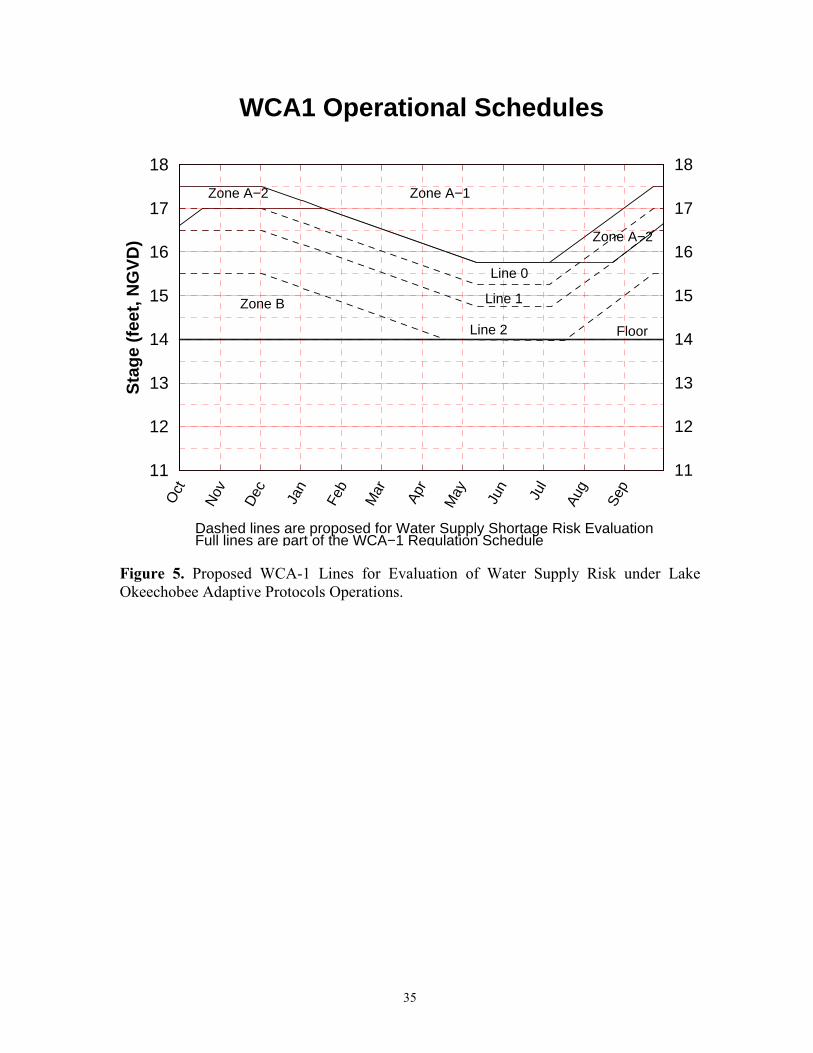
35

Oct

Nov

Dec Jan

Feb

Mar Apr

May Jun

Jul

Aug

Sep

11

12

13

14

15

16

17

18

Sta

ge

(fee

t, N

GV

D)

WCA1 Operational Schedules

11

12

13

14

15

16

17

18

Floor

Zone B

Zone A−1Zone A−2

Zone A−2

Line 2

Line 1

Line 0

Dashed lines are proposed for Water Supply Shortage Risk EvaluationFull lines are part of the WCA−1 Regulation Schedule

Figure 5. Proposed WCA-1 Lines for Evaluation of Water Supply Risk under LakeOkeechobee Adaptive Protocols Operations.

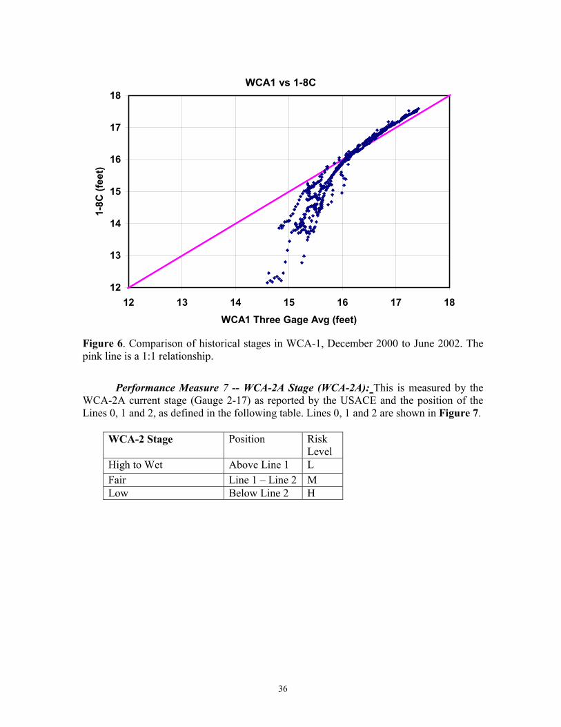
36

Figure 6. Comparison of historical stages in WCA-1, December 2000 to June 2002. Thepink line is a 1:1 relationship.

Performance Measure 7 -- WCA-2A Stage (WCA-2A): This is measured by theWCA-2A current stage (Gauge 2-17) as reported by the USACE and the position of theLines 0, 1 and 2, as defined in the following table. Lines 0, 1 and 2 are shown in Figure 7.

WCA-2 Stage Position RiskLevel

High to Wet Above Line 1 LFair Line 1 – Line 2 MLow Below Line 2 H

WCA1 vs 1-8C

12

13

14

15

16

17

18

12 13 14 15 16 17 18WCA1 Three Gage Avg (feet)

1-8C

(fee

t)

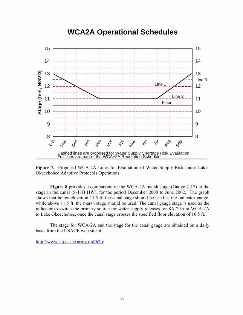
37

Oct

Nov

Dec Jan

Feb

Mar Apr

May Jun

Jul

Aug

Sep

8

9

10

11

12

13

14

15

Sta

ge

(fee

t, N

GV

D)

WCA2A Operational Schedules

8

9

10

11

12

13

14

15

Dashed lines are proposed for Water Supply Shortage Risk EvaluationFull lines are part of the WCA−2A Regulation Schedule

Floor

Line 0

Line 2

Line 1

Figure 7. Proposed WCA-2A Lines for Evaluation of Water Supply Risk under LakeOkeechobee Adaptive Protocols Operations.

Figure 8 provides a comparison of the WCA-2A marsh stage (Gauge 2-17) to thestage in the canal (S-11B HW), for the period December 2000 to June 2002. The graphshows that below elevation 11.5 ft. the canal stage should be used as the indicator gauge,while above 11.5 ft. the marsh stage should be used. The canal gauge stage is used as theindicator to switch the primary source for water supply releases for SA-2 from WCA-2Ato Lake Okeechobee, once the canal stage crosses the specified floor elevation of 10.5 ft.

The stage for WCA-2A and the stage for the canal gauge are obtained on a dailybasis from the USACE web site at:

http://www.saj.usace.army.mil/h2o/

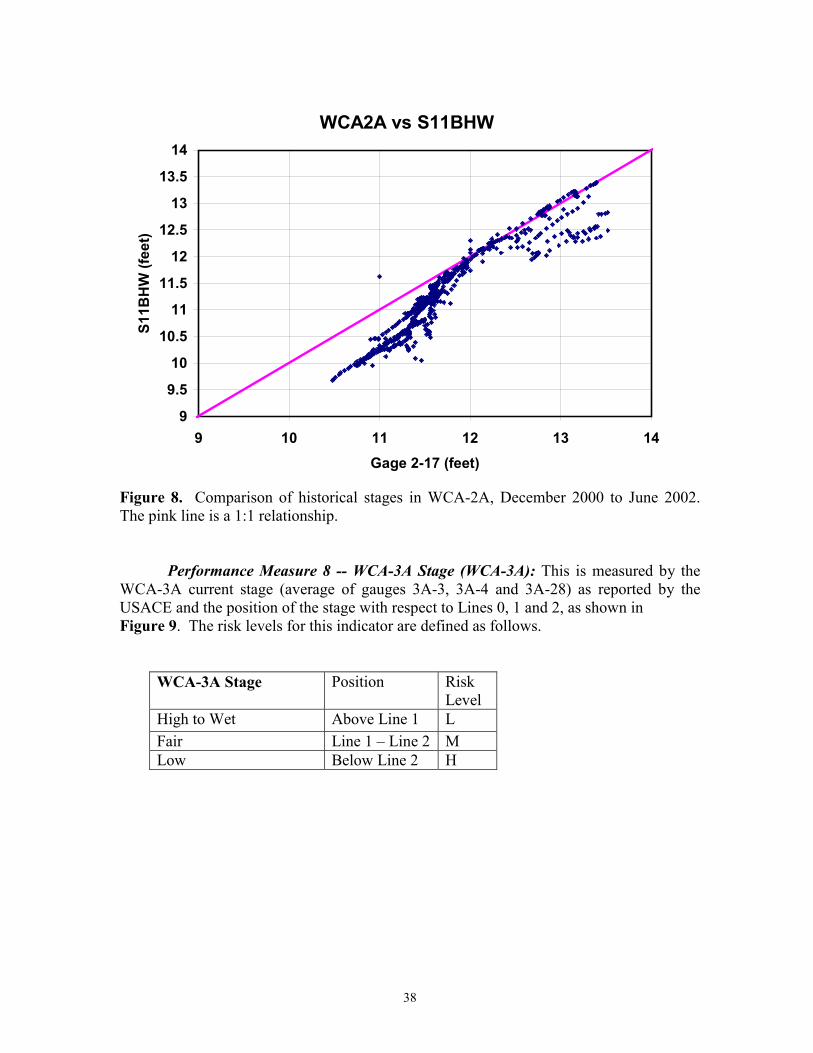
38

Figure 8. Comparison of historical stages in WCA-2A, December 2000 to June 2002.The pink line is a 1:1 relationship.

Performance Measure 8 -- WCA-3A Stage (WCA-3A): This is measured by theWCA-3A current stage (average of gauges 3A-3, 3A-4 and 3A-28) as reported by theUSACE and the position of the stage with respect to Lines 0, 1 and 2, as shown inFigure 9. The risk levels for this indicator are defined as follows.

WCA-3A Stage Position RiskLevel

High to Wet Above Line 1 LFair Line 1 – Line 2 MLow Below Line 2 H

WCA2A vs S11BHW

9

9.5

10

10.5

11

11.5

12

12.5

13

13.5

14

9 10 11 12 13 14Gage 2-17 (feet)

S11B

HW

(fee

t)

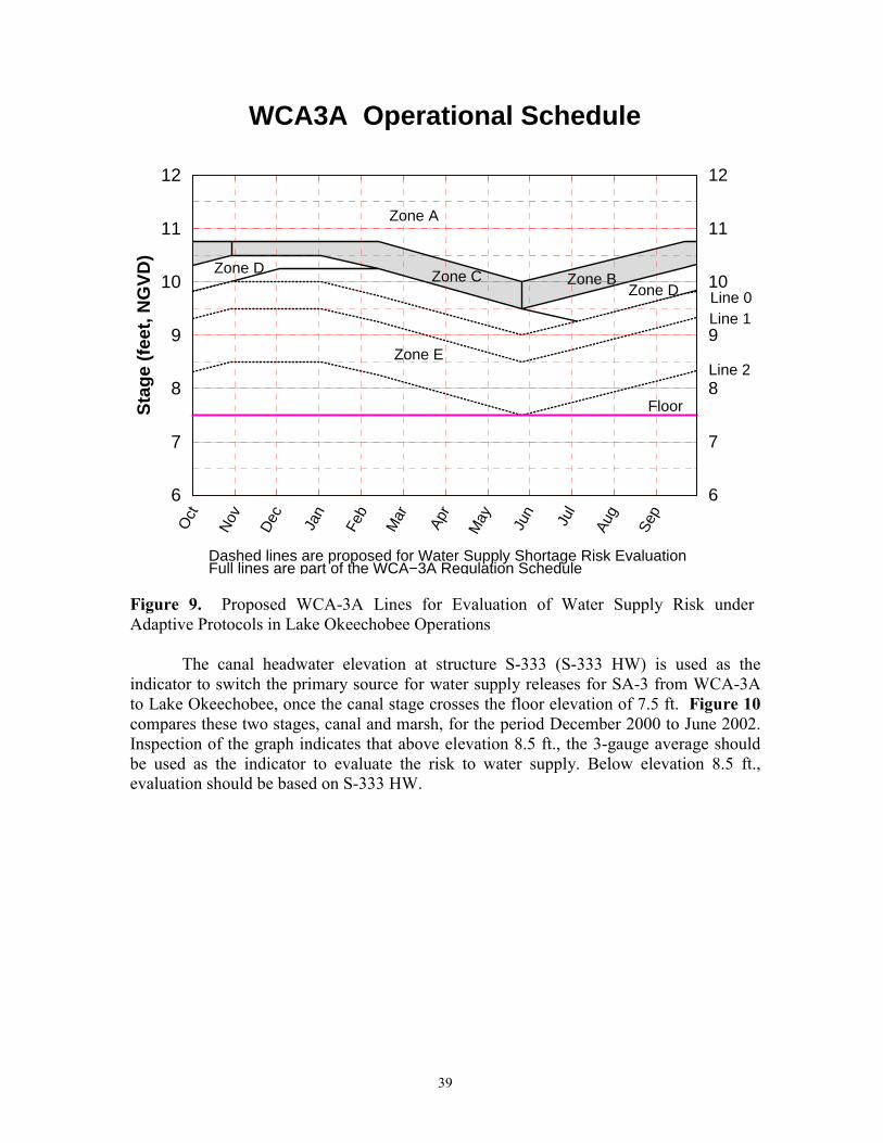
39

Oct

Nov

Dec Jan

Feb

Mar Apr

May Jun

Jul

Aug

Sep

6

7

8

9

10

11

12

Sta

ge

(fee

t, N

GV

D)

WCA3A Operational Schedule

6

7

8

9

10

11

12

Zone A

Zone CZone D

Zone E

Zone BZone D

Floor

Line 1

Line 2

Line 0

Dashed lines are proposed for Water Supply Shortage Risk EvaluationFull lines are part of the WCA−3A Regulation Schedule

Figure 9. Proposed WCA-3A Lines for Evaluation of Water Supply Risk underAdaptive Protocols in Lake Okeechobee Operations

The canal headwater elevation at structure S-333 (S-333 HW) is used as theindicator to switch the primary source for water supply releases for SA-3 from WCA-3Ato Lake Okeechobee, once the canal stage crosses the floor elevation of 7.5 ft. Figure 10compares these two stages, canal and marsh, for the period December 2000 to June 2002.Inspection of the graph indicates that above elevation 8.5 ft., the 3-gauge average shouldbe used as the indicator to evaluate the risk to water supply. Below elevation 8.5 ft.,evaluation should be based on S-333 HW.

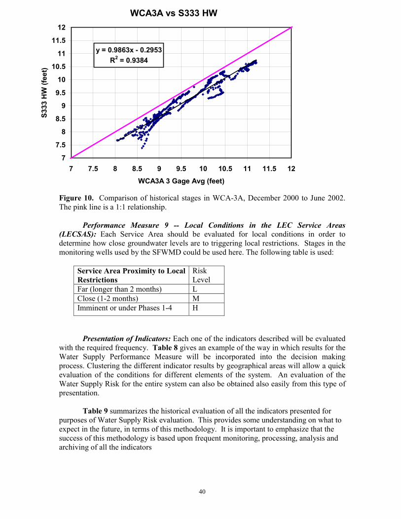
40

Figure 10. Comparison of historical stages in WCA-3A, December 2000 to June 2002.The pink line is a 1:1 relationship.

Performance Measure 9 -- Local Conditions in the LEC Service Areas(LECSAS): Each Service Area should be evaluated for local conditions in order todetermine how close groundwater levels are to triggering local restrictions. Stages in themonitoring wells used by the SFWMD could be used here. The following table is used:

Service Area Proximity to LocalRestrictions

RiskLevel

Far (longer than 2 months) LClose (1-2 months) MImminent or under Phases 1-4 H

Presentation of Indicators: Each one of the indicators described will be evaluatedwith the required frequency. Table 8 gives an example of the way in which results for theWater Supply Performance Measure will be incorporated into the decision makingprocess. Clustering the different indicator results by geographical areas will allow a quickevaluation of the conditions for different elements of the system. An evaluation of theWater Supply Risk for the entire system can also be obtained also easily from this type ofpresentation.

Table 9 summarizes the historical evaluation of all the indicators presented forpurposes of Water Supply Risk evaluation. This provides some understanding on what toexpect in the future, in terms of this methodology. It is important to emphasize that thesuccess of this methodology is based upon frequent monitoring, processing, analysis andarchiving of all the indicators

WCA3A vs S333 HW

y = 0.9863x - 0.2953R2 = 0.9384

7

7.5

8

8.5

9

9.5

10

10.5

11

11.5

12

7 7.5 8 8.5 9 9.5 10 10.5 11 11.5 12WCA3A 3 Gage Avg (feet)

S333

HW

(fee

t)

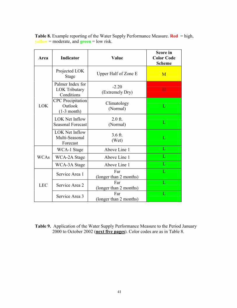
41

Table 8. Example reporting of the Water Supply Performance Measure. Red = high,yellow = moderate, and green = low risk.

Area Indicator ValueScore in

Color CodeScheme

Projected LOKStage Upper Half of Zone E M

Palmer Index forLOK Tributary

Conditions

-2.20(Extremely Dry) H

CPC PrecipitationOutlook

(1-3 month)

Climatology(Normal) L

LOK Net InflowSeasonal Forecast

2.0 ft.(Normal) L

LOK

LOK Net InflowMulti-Seasonal

Forecast

3.6 ft.(Wet) L

WCA-1 Stage Above Line 1 L

WCA-2A Stage Above Line 1 LWCAsWCA-3A Stage Above Line 1 L

Service Area 1 Far(longer than 2 months)

L

Service Area 2 Far(longer than 2 months)

LLEC

Service Area 3 Far(longer than 2 months)

L

Table 9. Application of the Water Supply Performance Measure to the Period January2000 to October 2002 (next five pages). Color codes are as in Table 8.

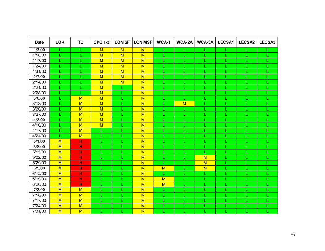
42

Date LOK TC CPC 1-3 LONISF LONIMSF WCA-1 WCA-2A WCA-3A LECSA1 LECSA2 LECSA3

1/3/00 L L M M M L L L L L L1/10/00 L L M M M L L L L L L1/17/00 L L M M M L L L L L L1/24/00 L L M M M L L L L L L1/31/00 L L M M M L L L L L L2/7/00 L L M M M L L L L L L2/14/00 L L M M M L L L L L L2/21/00 L L M L M L L L L L L2/28/00 L L M L M L L L L L L3/6/00 L M M L M L L L L L L3/13/00 L M M L M L M L L L L3/20/00 L M M L M L L L L L L3/27/00 L M M L M L L L L L L4/3/00 L M M L M L L L L L L4/10/00 L M M L M L L L L L L4/17/00 L M L L M L L L L L L4/24/00 L M L L M L L L L L L5/1/00 M H L L M L L L L L L5/8/00 M H L L M L L L L L L5/15/00 M H L L M L L L L L L5/22/00 M H L L M L L M L L L5/29/00 M H L L M L L M L L L6/5/00 M H L L M M L M L L L6/12/00 M H L L M L L L L L L6/19/00 M H L L M M L L L L L6/26/00 M H L L M M L L L L L7/3/00 M M L L M L L L L L L7/10/00 M M L L M L L L L L L7/17/00 M M L L M L L L L L L7/24/00 M M L L M L L L L L L7/31/00 M M L L M L L L L L L

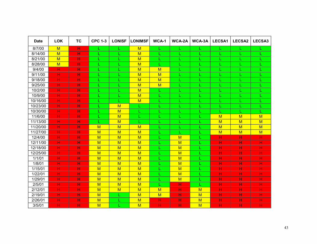
43

Date LOK TC CPC 1-3 LONISF LONIMSF WCA-1 WCA-2A WCA-3A LECSA1 LECSA2 LECSA3

8/7/00 M H L L M L L L L L L8/14/00 M H L L M L L L L L L8/21/00 M H L L M L L L L L L8/28/00 M H L L M L L L L L L9/4/00 H H L L M M L L L L L9/11/00 H H L L M M L L L L L9/18/00 H H L L M M L L L L L9/25/00 H H L L M M L L L L L10/2/00 H H L L M L L L L L L10/9/00 H H L L M L L L L L L10/16/00 H H L L M L L L L L L10/23/00 H H L M L L L L L L L10/30/00 H H L M L L L L L L L11/6/00 H H L M L L L L M M M11/13/00 H H L M L L L L M M M11/20/00 H H M M M L L L M M M11/27/00 H H M M M L L L M M M12/4/00 H H M M M L M L H H H12/11/00 H H M M M L M L H H H12/18/00 H H M M M L M L H H H12/25/00 H H M M M L M L H H H1/1/01 H H M M M L M L H H H1/8/01 H H M M M L M L H H H1/15/01 H H M M M L M L H H H1/22/01 H H M M M L M L H H H1/29/01 H H M M M L M L H H H2/5/01 H H M M M L H L H H H2/12/01 H H M M M M H M H H H2/19/01 H H M L M M H M H H H2/26/01 H H M L M H H M H H H3/5/01 H H M L M H H M H H H

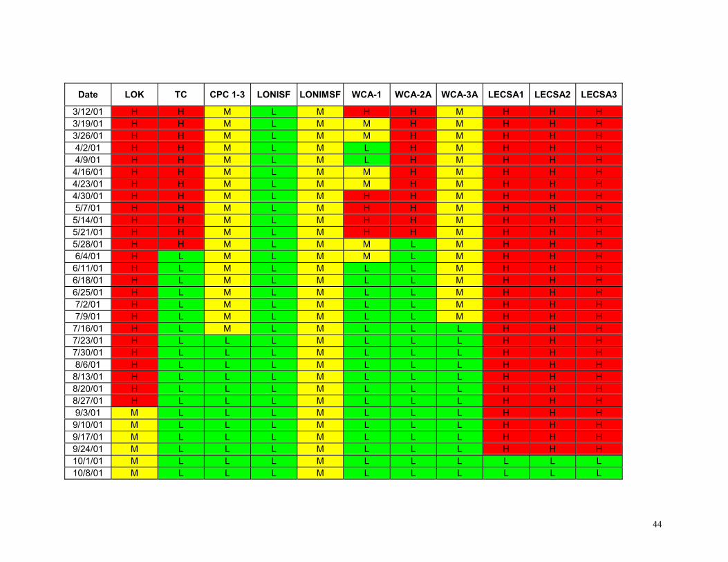
44

Date LOK TC CPC 1-3 LONISF LONIMSF WCA-1 WCA-2A WCA-3A LECSA1 LECSA2 LECSA3

3/12/01 H H M L M H H M H H H3/19/01 H H M L M M H M H H H3/26/01 H H M L M M H M H H H4/2/01 H H M L M L H M H H H4/9/01 H H M L M L H M H H H4/16/01 H H M L M M H M H H H4/23/01 H H M L M M H M H H H4/30/01 H H M L M H H M H H H5/7/01 H H M L M H H M H H H5/14/01 H H M L M H H M H H H5/21/01 H H M L M H H M H H H5/28/01 H H M L M M L M H H H6/4/01 H L M L M M L M H H H6/11/01 H L M L M L L M H H H6/18/01 H L M L M L L M H H H6/25/01 H L M L M L L M H H H7/2/01 H L M L M L L M H H H7/9/01 H L M L M L L M H H H7/16/01 H L M L M L L L H H H7/23/01 H L L L M L L L H H H7/30/01 H L L L M L L L H H H8/6/01 H L L L M L L L H H H8/13/01 H L L L M L L L H H H8/20/01 H L L L M L L L H H H8/27/01 H L L L M L L L H H H9/3/01 M L L L M L L L H H H9/10/01 M L L L M L L L H H H9/17/01 M L L L M L L L H H H9/24/01 M L L L M L L L H H H10/1/01 M L L L M L L L L L L10/8/01 M L L L M L L L L L L

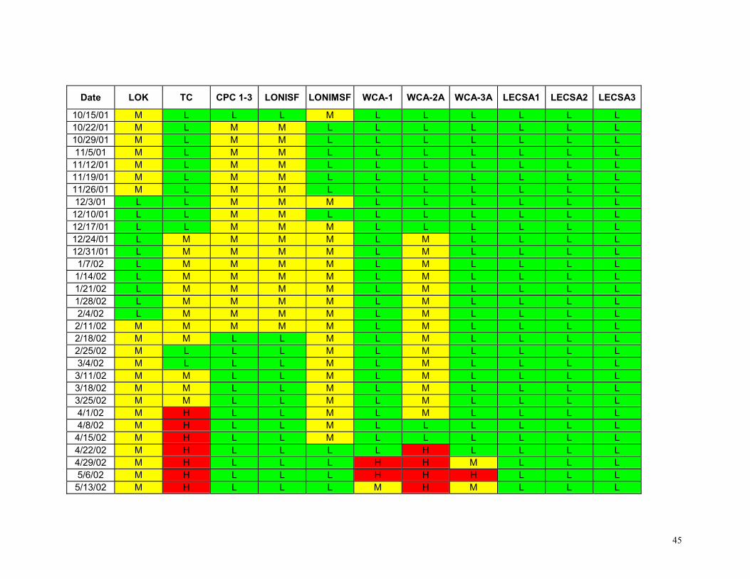
45

Date LOK TC CPC 1-3 LONISF LONIMSF WCA-1 WCA-2A WCA-3A LECSA1 LECSA2 LECSA3

10/15/01 M L L L M L L L L L L10/22/01 M L M M L L L L L L L10/29/01 M L M M L L L L L L L11/5/01 M L M M L L L L L L L11/12/01 M L M M L L L L L L L11/19/01 M L M M L L L L L L L11/26/01 M L M M L L L L L L L12/3/01 L L M M M L L L L L L12/10/01 L L M M L L L L L L L12/17/01 L L M M M L L L L L L12/24/01 L M M M M L M L L L L12/31/01 L M M M M L M L L L L1/7/02 L M M M M L M L L L L1/14/02 L M M M M L M L L L L1/21/02 L M M M M L M L L L L1/28/02 L M M M M L M L L L L2/4/02 L M M M M L M L L L L2/11/02 M M M M M L M L L L L2/18/02 M M L L M L M L L L L2/25/02 M L L L M L M L L L L3/4/02 M L L L M L M L L L L3/11/02 M M L L M L M L L L L3/18/02 M M L L M L M L L L L3/25/02 M M L L M L M L L L L4/1/02 M H L L M L M L L L L4/8/02 M H L L M L L L L L L4/15/02 M H L L M L L L L L L4/22/02 M H L L L L H L L L L4/29/02 M H L L L H H M L L L5/6/02 M H L L L H H H L L L5/13/02 M H L L L M H M L L L

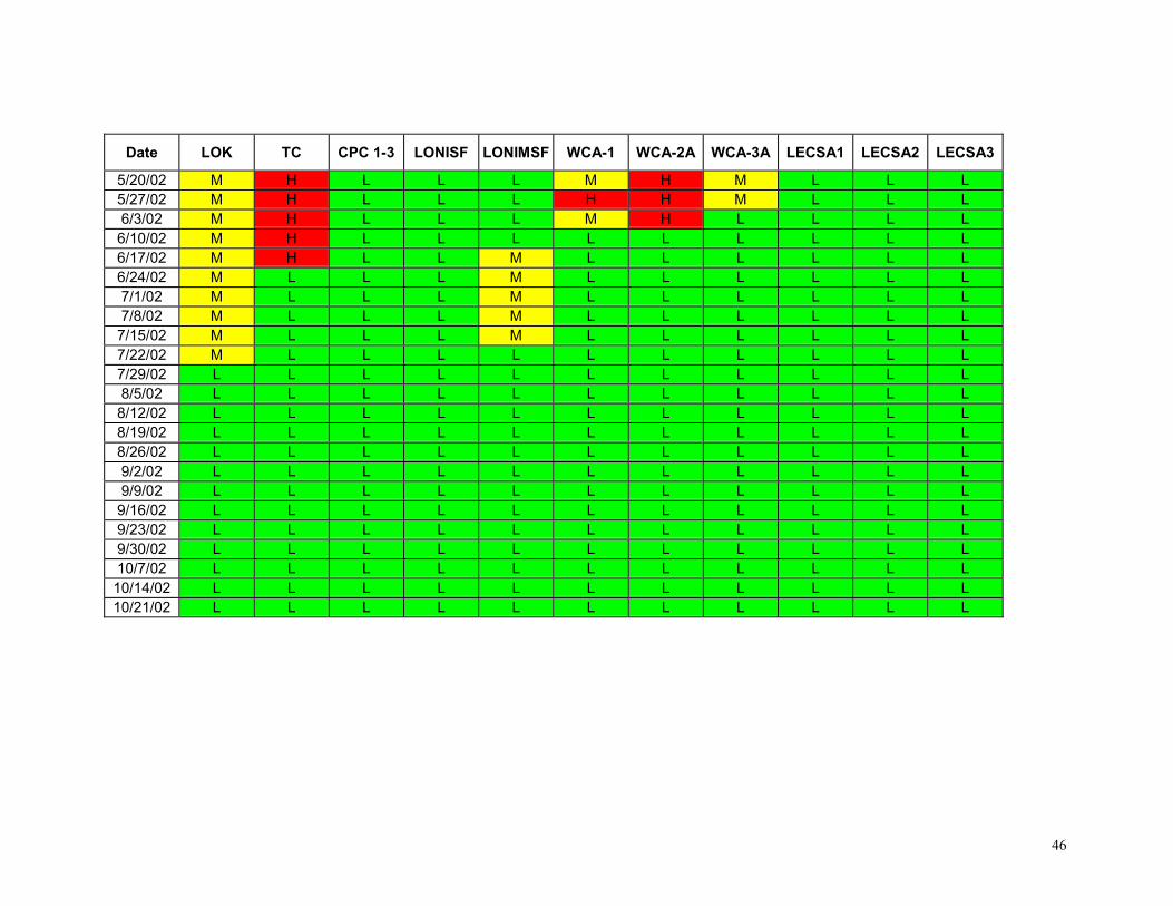
46

Date LOK TC CPC 1-3 LONISF LONIMSF WCA-1 WCA-2A WCA-3A LECSA1 LECSA2 LECSA3

5/20/02 M H L L L M H M L L L5/27/02 M H L L L H H M L L L6/3/02 M H L L L M H L L L L6/10/02 M H L L L L L L L L L6/17/02 M H L L M L L L L L L6/24/02 M L L L M L L L L L L7/1/02 M L L L M L L L L L L7/8/02 M L L L M L L L L L L7/15/02 M L L L M L L L L L L7/22/02 M L L L L L L L L L L7/29/02 L L L L L L L L L L L8/5/02 L L L L L L L L L L L8/12/02 L L L L L L L L L L L8/19/02 L L L L L L L L L L L8/26/02 L L L L L L L L L L L9/2/02 L L L L L L L L L L L9/9/02 L L L L L L L L L L L9/16/02 L L L L L L L L L L L9/23/02 L L L L L L L L L L L9/30/02 L L L L L L L L L L L10/7/02 L L L L L L L L L L L10/14/02 L L L L L L L L L L L10/21/02 L L L L L L L L L L L

47

5c. Everglades Protection Area

Performance measures for the Everglades Protection Area are based on publishedtechnical information as well as best professional judgment and are intended to be used asguidance for water management decisions within the scope of current regulatoryrequirements, operational logistics, and remediation technology.

5c.1 Everglades Hydrologic Performance Measures

Hydrologic performance measures for the Everglades are documented in the C&SFProject Comprehensive Review Study (USACE 1999) and the Everglades Ridge andSlough Conceptual Ecosystem Model (Davis 2000) for the Restoration Coordination andVerification (RECOVER) program of CERP. They are based on numerous runs of theNatural System Model (NSM) and over a decade of rigorous science and peer-reviewedliterature (e.g., Swift and Nicholas 1987, Urban et al. 1993, Davis and Ogden 1994,Newman et al. 1998, Gawlik and Rocque 1998, Sklar et al. 2002). The following narrativedescribes their scientific basis and the approach for using them as part of the AdaptiveProtocols. Along with the hydrologic performance measures, assessment of the Evergladesecological status will be based on a set of biological indicators, including tree islands,wading bird foraging requirements, peat loss, emergent wetland plants, and nutrientconcentrations. All of this information will be taken into consideration in regard to waterreleases from Lake Okeechobee to the Everglades ecosystem.

There are three hydrologic performance measures. Two of these relate to impactsassociated with extreme high and low water, and one identifies a desired spring recessionrate of 3.5 cm per week, which has documented impacts associated with wading birdforaging and nesting success.

Extreme High or Low Stages

As wetland soils are exposed to air, the oxidation of organic matter accelerates,which results in soil loss and an increase in bio-available P (inorganic forms) (Newman etal. 1998, Newman et al. 2001). In addition, structural changes may occur during theprocess of consolidation and compaction, which results in decreased soil porosity andsome irreversible loss of water-holding capacity (Kushlan 1990 and references therein).Another consequence of low stages is a loss of dry season aquatic refugia, and anincreased potential for peat-fire. Although these disturbances occurred in the historicEverglades, their frequency is thought to have increased as a result of altered hydrology(Alexander and Crook 1974, Gunderson and Snyder 1994). Moreover, recovery frompeat-fire in present times can be difficult in the face of existing levels of marshdegradation. For example, where peat-fire may have once simply converted sawgrassstands into sloughs through elevation changes, it may now encourage the opportunisticexpansion of cattail that can be supported by high antecedent levels of soil P (Smith et al.2001, Smith and Newman 2001).

48

For aquatic organisms, reduced water depths and/or hydroperiod typically lead todiminished population size, particularly of small fishes (Loftus and Eklund 1994). Whensurface water disappears, the use of foraging sites by wading birds decreases rapidly(Bancroft et al. 1994). Under these circumstances, birds will fly increasing distances fromthe colony to find suitable foraging habitat (i.e., presence of surface water). At somedistance from the nest, however, it becomes energetically unprofitable to transport food tothe young. In addition, nesting sites are adversely impacted when surface water directlyunder a colony site is absent, thus providing access to mammalian predators (Rodgers1987, Frederick and Collopy 1989). Under these conditions the adults will abandon thenesting colony (Bancroft et al. 1994).

Abnormally high stages similarly cause biological degradation. Deep waterinhibits tree island seed germination, sapling growth, and induces high levels ofphysiological stress in many tree species (Craighead 1971, Gunderson et al. 1988; Worth1987). Wading bird prey becomes dispersed, which reduces foraging efficiency andsubsequent nesting success during the breeding season (Kushlan 1976a, Kushlan 1986,Hoffman et al. 1994, Gawlik in review). In addition, deer populations can be adverselyaffected by high-water conditions (Light and Dineen 1994). For the Cape Sable SeasideSparrow, an endangered species, areas of dry ground are an absolute requirement duringthe nesting season from mid-March to mid-June (Kushlan and Bass 1983, Nott et al. 1998,Stevenson and Anderson 1994). Sparrow habitat conditions have generally been assessedby stage readings from gauges that are in close proximity to various sub-populations.Water management operations must attempt to provide for suitable breeding habitat andremedy any situations where water levels exceed ground levels in critical areas. In thisregard, specific operating procedures have been outlined and continue to undergo furtherrefinement (Dial Cordy & Associates 2000).

Natural System Targets

One approach that has been used to identify desirable hydrologic conditions thatwould benefit the physical, chemical and biological components of the ecosystem is theuse of the Natural Systems Model (NSM). The NSM was developed to provide anestimate of pre-drainage flows and stages throughout the Everglades system, prior tohuman influence on the landscape (Fennema et al. 1994). The NSM (version 4.5) uses thesame calibrated algorithms as those incorporated in the South Florida Water ManagementModel (SFWMM) to represent surface and ground water flows within the region, exceptthat roads, canals, water management structures, and urban well fields are not contained inthe NSM. Estimates of pre-drainage soil topography and historical Everglades landscapevegetation communities are also incorporated into the NSM. Output from the NSMincludes surface and ground water levels at various locations as well as overland flow,ground water flow, and evapotranspiration. The NSM uses recent rainfall data (1965-1995) to predict how water would flow through an unmodified South Florida’s hydrologicsystem. The NSM is regarded as the most comprehensive tool available that describes thehydrology of South Florida prior to human influence and, therefore, provides a reasonableestimate of the hydrologic patterns needed to restore the ecosystem.

49

The NSM output has been used as planning targets for both the C&SFComprehensive Review Study (USACE 1999) and the LECRWSP (SFWMD 2000a). Forthe purposes of this report, the modified NSM stage targets as presented in the LECRWSPwere used to estimate target stages for a network of gauges within the EvergladesProtection Area (EPA). For the purpose of evaluating EPA performance in the AdaptiveProtocols, deviations between the LECRWSP-based restoration targets and actual stagesof EPA indicator gauges will be evaluated (Appendix II, Figure II-1). In this way,hydrologic performance measures will be directly tied to both the CERP and LECRWSPrestoration objectives and will integrate the needs of many different users (i.e., flora andfauna, as well as water supply users) on a temporal and spatial basis.

Extreme Low Stage

Providing water flows and stages to meet statutorily defined Minimum Flows andLevels (MFL) criteria were also considered an important component of the AdaptiveProtocols. Generally stated, a MFL for a given watercourse or aquifer shall be the limit atwhich further withdrawals would be significantly harmful to the water resources orecology of the area (Chapter 373.0421 Florida Statutes). On September 10, 2001, theGoverning Board of the SFWMD adopted Rule 40E-8, which defines MFL criteria for theEverglades as well as Lake Okeechobee, the Biscayne aquifer and the CaloosahatcheeRiver. Appendix II, Table II-1 provides a summary of these criteria for the EPA.

MFL criteria established for the EPA are based on the protection of Evergladeshydric soils (organic peat and marl) due to the fact that (a) over 90% of the soils within theEPA are comprised of either peat or marl, and (b) most of the plants and animals whichinhabit the Everglades region depend, at least in part, on the hydrologic regime thatproduces hydric soils. Therefore, maintenance of a hydrologic regime, which protectsthese soils from significant harm, will also help protect Everglades plant and animalcommunities and their habitat.

MFL Criteria for Peat-Forming Wetlands: Water levels within wetlands overlyingorganic peat soils within the water conservation areas, Rotenberger and Holey Landwildlife management areas, and Shark River Slough (Everglades National Park) shall notfall 1.0 feet or more below ground surface, as measured at various key gauges as shown inFigure II-1 (Appendix II), for one or more days during a period in which the water levelhas remained below ground for a minimum of 30 days, at specific return frequencies asspecified in Appendix II, Table II-1.

MFL Criteria for Marl-Forming Wetlands: Water levels within marl-formingwetlands that are located east and west of Shark River Slough, the Rocky Glades, andTaylor Slough within Everglades National Park shall not fall 1.5 feet below groundsurface, as measured at a key gauge (Figure II-1, Appendix II), for one or more daysduring a period in which the water level has remained below ground for a minimum of 90days, at specific return frequencies for different areas, as identified in Appendix II, TableII-1.

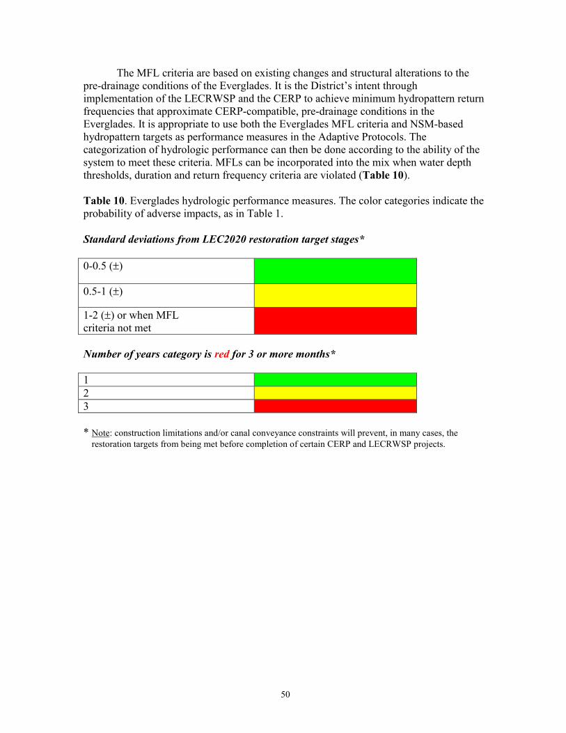
50

The MFL criteria are based on existing changes and structural alterations to thepre-drainage conditions of the Everglades. It is the District’s intent throughimplementation of the LECRWSP and the CERP to achieve minimum hydropattern returnfrequencies that approximate CERP-compatible, pre-drainage conditions in theEverglades. It is appropriate to use both the Everglades MFL criteria and NSM-basedhydropattern targets as performance measures in the Adaptive Protocols. Thecategorization of hydrologic performance can then be done according to the ability of thesystem to meet these criteria. MFLs can be incorporated into the mix when water depththresholds, duration and return frequency criteria are violated (Table 10).

Table 10. Everglades hydrologic performance measures. The color categories indicate theprobability of adverse impacts, as in Table 1.

Standard deviations from LEC2020 restoration target stages*

0-0.5 (�)

0.5-1 (�)

1-2 (�) or when MFLcriteria not met

Number of years category is red for 3 or more months*

123

* Note: construction limitations and/or canal conveyance constraints will prevent, in many cases, therestoration targets from being met before completion of certain CERP and LECRWSP projects.

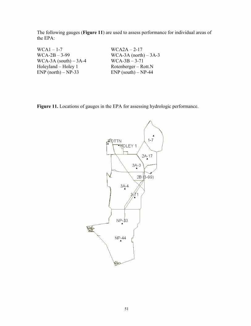
51

The following gauges (Figure 11) are used to assess performance for individual areas ofthe EPA:

WCA1 – 1-7 WCA2A – 2-17WCA-2B – 3-99 WCA-3A (north) – 3A-3WCA-3A (south) – 3A-4 WCA-3B – 3-71Holeyland – Holey 1 Rotenberger – Rott.NENP (north) – NP-33 ENP (south) – NP-44

Figure 11. Locations of gauges in the EPA for assessing hydrologic performance.

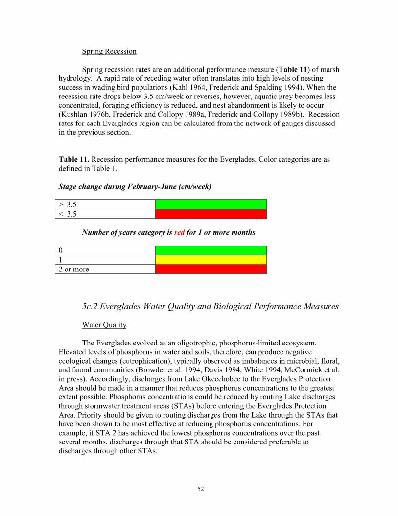
52

Spring Recession

Spring recession rates are an additional performance measure (Table 11) of marshhydrology. A rapid rate of receding water often translates into high levels of nestingsuccess in wading bird populations (Kahl 1964, Frederick and Spalding 1994). When therecession rate drops below 3.5 cm/week or reverses, however, aquatic prey becomes lessconcentrated, foraging efficiency is reduced, and nest abandonment is likely to occur(Kushlan 1976b, Frederick and Collopy 1989a, Frederick and Collopy 1989b). Recessionrates for each Everglades region can be calculated from the network of gauges discussedin the previous section.

Table 11. Recession performance measures for the Everglades. Color categories are asdefined in Table 1.

Stage change during February-June (cm/week)

> 3.5< 3.5

Number of years category is red for 1 or more months

012 or more

5c.2 Everglades Water Quality and Biological Performance Measures

Water Quality

The Everglades evolved as an oligotrophic, phosphorus-limited ecosystem.Elevated levels of phosphorus in water and soils, therefore, can produce negativeecological changes (eutrophication), typically observed as imbalances in microbial, floral,and faunal communities (Browder et al. 1994, Davis 1994, White 1994, McCormick et al.in press). Accordingly, discharges from Lake Okeechobee to the Everglades ProtectionArea should be made in a manner that reduces phosphorus concentrations to the greatestextent possible. Phosphorus concentrations could be reduced by routing Lake dischargesthrough stormwater treatment areas (STAs) before entering the Everglades ProtectionArea. Priority should be given to routing discharges from the Lake through the STAs thathave been shown to be most effective at reducing phosphorus concentrations. Forexample, if STA 2 has achieved the lowest phosphorus concentrations over the pastseveral months, discharges through that STA should be considered preferable todischarges through other STAs.

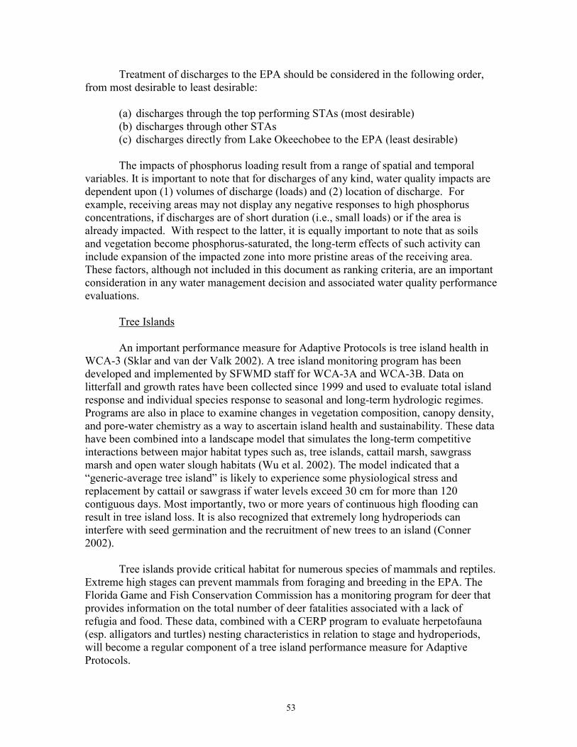
53

Treatment of discharges to the EPA should be considered in the following order,from most desirable to least desirable:

(a) discharges through the top performing STAs (most desirable)(b) discharges through other STAs(c) discharges directly from Lake Okeechobee to the EPA (least desirable)

The impacts of phosphorus loading result from a range of spatial and temporalvariables. It is important to note that for discharges of any kind, water quality impacts aredependent upon (1) volumes of discharge (loads) and (2) location of discharge. Forexample, receiving areas may not display any negative responses to high phosphorusconcentrations, if discharges are of short duration (i.e., small loads) or if the area isalready impacted. With respect to the latter, it is equally important to note that as soilsand vegetation become phosphorus-saturated, the long-term effects of such activity caninclude expansion of the impacted zone into more pristine areas of the receiving area.These factors, although not included in this document as ranking criteria, are an importantconsideration in any water management decision and associated water quality performanceevaluations.

Tree Islands

An important performance measure for Adaptive Protocols is tree island health inWCA-3 (Sklar and van der Valk 2002). A tree island monitoring program has beendeveloped and implemented by SFWMD staff for WCA-3A and WCA-3B. Data onlitterfall and growth rates have been collected since 1999 and used to evaluate total islandresponse and individual species response to seasonal and long-term hydrologic regimes.Programs are also in place to examine changes in vegetation composition, canopy density,and pore-water chemistry as a way to ascertain island health and sustainability. These datahave been combined into a landscape model that simulates the long-term competitiveinteractions between major habitat types such as, tree islands, cattail marsh, sawgrassmarsh and open water slough habitats (Wu et al. 2002). The model indicated that a“generic-average tree island” is likely to experience some physiological stress andreplacement by cattail or sawgrass if water levels exceed 30 cm for more than 120contiguous days. Most importantly, two or more years of continuous high flooding canresult in tree island loss. It is also recognized that extremely long hydroperiods caninterfere with seed germination and the recruitment of new trees to an island (Conner2002).

Tree islands provide critical habitat for numerous species of mammals and reptiles.Extreme high stages can prevent mammals from foraging and breeding in the EPA. TheFlorida Game and Fish Conservation Commission has a monitoring program for deer thatprovides information on the total number of deer fatalities associated with a lack ofrefugia and food. These data, combined with a CERP program to evaluate herpetofauna(esp. alligators and turtles) nesting characteristics in relation to stage and hydroperiods,will become a regular component of a tree island performance measure for AdaptiveProtocols.

54

Wading Birds

Performance measures for restoration of the Everglades ridge & slough landscapeinclude targets for wood storks, ibis, herons, and egrets. As a CERP goal of sustainednesting in the Everglades these targets should supplement the Everglades SpringRecession performance measure mentioned above. There are two performance measuresfor water patterns during the wading bird nesting season (Feb 1 – May 15). First, thenumber of water level reversals that occur as the result of water management activitiesduring the dry down, with the ultimate goal of zero reversals. Water level reversals > 1.5cm during the nesting season can cause wading birds to abandon nests (Kushlan 1986).Second, a strong wading bird nesting effort seems to occur when water levels during mid-March (nesting initiation) are within a certain window, which differs by region. In WCA1, water levels for March 15th between 15.5 - 16.4 ft. at gauge 1-9 with a strong recessionrate thereafter (roughly 3.5 cm/week) is optimal. In WCA 3, water levels for March 15th

between 9.3 - 10.5 ft. at gauge 3A-4 with a strong recession rate thereafter is optimal.Providing optimal water levels in March with a strong water recession and no artificialreversals during the nesting season should provide wading birds with the opportunity forgood nesting. However, extremes water events have always occurred in the Evergladesand are probably beneficial to the system when they occur at frequencies predicted by theNSM. Historical data show that there have always been years with poor wading birdnesting events. Extreme water events in the Everglades should occur at appropriatefrequencies.

Ratio of Cattail to Sawgrass (C/S)

Lake releases to the Everglades could enhance the spread of cattails by a variety ofmechanisms, including plant responses to deeper water and elevated P concentrations.Cattail are better “equipped” to deliver oxygen to their roots than sawgrass (Sklar et al.2000) therefore, lake releases that result in very high stages may increase the C/S ratio,especially where soil nutrients are relatively high. Where sawgrass has just burned, a rapidincrease in water depth will actually kill the sawgrass (Herndon et al 1991, Gunderson andSynder 1994, 404 field observations 2001) and increase the C/S ratio.

Adaptive Protocols for a C/S performance measure will use the PTP monitoringprogram and the 404 Permit monitoring program to supply current C/S data. Thesemonitoring programs examine the vegetation trends in relation to hydrology and waterquality and can be used as input to real-time system management. Biannual aerialphotography and GIS will supplement these data by providing information on the totalextent of these high C/S zones.

The effects of human-induced P enrichment are most evident in the northernEverglades. Ecological responses; surface and porewater nutrient changes, periphyton,macrophyte and invertebrate community composition, soil nutrient status, diel oxygencharacteristics, to P enrichment are being measured along existing nutrient gradients(McCormick et al. 1996; McCormick et al. 1997, McCormick et al. 1998, Miao and Sklar

55

1998 , McCormick et al. 1999, McCormick et al. 2001, Newman et al. 2001a, Newman etal. 2002). This extensive peer-reviewed research and monitoring program has been underway in WCA 2A since 1994 and in the LNWR since 1996. In 1999, a one year study wasinitiated in WCA 3A and Taylor slough (Everglades National Park) to assess whether thesouthern Everglades would have similar sensitivity to P enrichment and determinewhether marl-based wetlands would respond differently than peat-based wetlands.

The 404 monitoring and research program, created to document biological changesdownstream of the Stormwater Treatment Areas (STAs), is located in western WaterConservation Area 2A and STA5, adjacent to the Rotenberger Wildlife Management Area.Permanent monitoring stations established along these hydrologic and water qualitygradients measure water quality, hydrology, soils, periphyton and macrophytes. Surfacewater quality samples are collected monthly. Porewater and diel oxygen profiles arecollected quarterly. Periphyton is also sampled quarterly for nutrients, chlorophyllproduction and taxonomy. Soil cores are collected on an annual basis. Several types ofmacrophyte sampling techniques are utilized to monitor changes in species compositionand physiological processes. Both a macrophyte biomass harvest (aboveground biomassand nutrients) and permanent vegetation plots (species composition, growth rates) areconducted annually. A general plant survey around each monitoring station is performedtwice a year. Shoot re-growth is also measured on sawgrass and cattail plants twice ayear. Additionally, aerial mapping is performed in both areas to document changes incattail coverage.

5e. STA Performance Measures

Within the scope of the Lake Okeechobee operations, water deliveries will bemade to the STAs. A general discussion of water supply deliveries needed to preventdryout of the STAs is provided in the LECRWSP (SFWMD, May 2000). Additionalinformation is provided below.

The STAs are part of the overall Everglades protection program mandated by the1994 Everglades Forever Act and the 1991 Settlement Agreement to the FederalEverglades lawsuit (amended 2001). The STAs, as part of the Everglades ConstructionProject, are large constructed wetlands designed to reduce phosphorus concentrations instormwater originating from the EAA, C-139 and Western C-51 basins, as well as releasesfrom Lake Okeechobee, prior to discharging into the Water Conservation Areas of theEverglades Protection Area. There are state and federal regulatory and legal requirementsto ensure the STAs operate effectively at removing phosphorus. The biologicalphosphorus removal mechanism within each STA requires sustained growth of vegetationand accumulation of biomass. Water reservations from Lake Okeechobee for the STAswill be needed to maintain the water quality functions of the STAs and reduce thepotential for nutrient releases associated with dry periods.

The long term phosphorus removal mechanism for the STAs is the growth andsubsequent deposition of organic matter as new sediment - in short, accumulation ofbiomass. To ensure that the organic sediment does not release phosphorus on exposure to

56

air, the operational target for the STAs is to maintain a minimum depth of six inches. Thepotential impacts of dry out within the STAs will vary depending on site-specific soil,vegetation and hydrology. Those impacts may include:

(a) death of wetland vegetation due to dehydration;(b) growth of undesirable vegetation (exotics, dog fennel, and other terrestrial

species) as the organic soil is exposed to the air;(c) resuspension of phosphorus from the soil into surface waters upon re-wetting;(d) a period following re-flooding, lasting a year or more, during which time

phosphorus reduction may be greatly reduced, depending on the severity of thedrought and the health of the vegetation. Upon re-wetting, it may be necessaryto take individual treatment cells off line as the STA vegetation re-growsbefore the cell produces a net reduction in phosphorus as required by permit.

There also is evidence that dry out and subsequent re-wetting of an STA may stimulate themercury methylation process, which in turn may induce potential risks to wildlife on-siteand in the downstream Everglades.

STA Performance Measure 1 – Water Depths

The success of STAs in removing phosphorus is directly linked to the health andviability of the vegetated communities within the STAs. Three general types of vegetatedcommunities are used in the STAs: cattail, sawgrass and other marsh species, andsubmerged aquatic vegetation (SAV). Even during dry weather (including droughtconditions), it is important that these vegetated communities receive water to ensure thatthey will be effective in removing phosphorus during future storm events. There are threecritical water depth thresholds used in operating the STAs.

Optimal performance. For optimal phosphorus removal performance, it is desired tomaintain operating depths of 18 to 24 inches above average ground level.

Improvement. A sub-optimal performance threshold is for STA outflow concentrations tobe marginally better than inflow, thereby ensuring there is a slight improvement. Tominimize the potential for organic sediment within the STAs to release phosphorus uponexposure to the air, a minimum depth of 6 inches above average ground level is to bemaintained whenever possible.

Vegetation viability. Based on best available scientific information, the three vegetationcommunities have unique minimum depths required to keep the vegetation alive (Table12). For cattail, a stress threshold is approximately 6 inches below ground. For SAV, amortality threshold is approximately 6 inches above ground. For sawgrass and other mixedmarsh species, it appears that there is no mortality threshold.

57

Table 12. Relationships between health of various vegetation types and water level in theSTAs.

Vegetation Type OptimalPerformance

Improvement Vegetation Stressor Mortality

Cattail 12-18 inches aboveground

6 inches aboveground

6 inches belowground

Sawgrass andmixed marsh

12-18 inches aboveground

6 inches aboveground

No minimum depth

SubmergedAquatic Vegetation

18-24 inches aboveground

6 inches aboveground

6 inches aboveground

Estimates of Supplemental Deliveries to the STAs

During the dry season or in periods of drought, water supply deliveries from theLake can effectively maintain the necessary water depths within the STAs. It isanticipated that the volume of Lake Okeechobee water necessary to maintain the waterquality function of the STAs (Table 13) will be considerably less than other water supplydeliveries from the Lake.

Table 13. Simulated Mean Annual Water Supply from Lake Okeechobee to MaintainMinimum 0.5-ft Depth (based on December 2001 BASERR2R 1965-1995 simulationresults of the South Florida Water Management Model).

STAAverage

SupplementalWater Delivery

acre-ft/yr

MaximumAnnualDeliveryacre feet

AverageDemand Not

Metacre-ft/yr

STA-1E 367 4301 219STA-1W 29 869 290STA-2 90 1366 200

STA-3/4 0 0 0STA-5 13 311 74STA-6 1001 4252 687Total 1,499 8,774 1,764

6. Regional Simulation Modeling

In an effort to determine the possible impacts of the Adaptive Protocol strategy, ahydrologic simulation exercise was performed using the South Florida Water ManagementModel (SFWMM) (SFWMD, 1999). Additional information about this model is providedat http://www.sfwmd.gov/org/pld/hsm/models/sfwmm/index.html. Due to the fact thatreleases under Adaptive Protocols are inherently dependent on many changing factors thatmay not be completely captured during the course of model simulations, the following

58

information should only be used to assess the order of magnitude of potential impacts toagricultural and urban water supply.

6a. Modeling Assumptions

The modeling strategy was designed to compare a base condition that is verysimilar to the 95BSRR scenario used for the development of the Lower East Coast WaterSupply Plan (SFWMD, 2000a) to several alternatives representing operational changesassociated with Adaptive Protocols. For all scenarios, climatic data for the 31-year periodcovering 1965-1995 was analyzed. The key assumptions in the base condition (referred toas 95NEW) are:

� WSE Schedule for Lake Okeechobee� 1995 wellfield demands as simulated in the LEC Regional Water Supply Plan� Revised Supply-Side Management with a “trigger line” at 13 ft. NGVD on October 1,

sloping down to 10.5 ft. on June 1� All Lake Okeechobee Service Areas, including the Brighton and Big Cypress

Seminole Tribal lands, will be subject to cutbacks as determined by the Supply-SideManagement policies

� No forward pumping

Three alternatives were modeled for comparison to 95NEW. The first, denoted as95N50, incorporated all of the base assumptions of 95NEW as well as a minimum deliveryof 50% to the Lake Okeechobee Service Area (LOSA) during periods of Supply-SideManagement (SSM) cutbacks for Lake Okeechobee. This scenario is consistent with theapproach taken in allocating water during the 2000-2001 drought and provides a betterframe of reference than does 95NEW for determining the level of impact of adaptiveprotocol releases on agricultural water supply. Simulation 95NEW uses a minimumdelivery of 33% to LOSA during periods of SSM cutbacks for Lake Okeechobee as wasassumed in the LECRWSP (SFWMD, 2000a).

The final two alternatives, 3N50 and 6N50, include environmental supplementalreleases from Lake Okeechobee to the Caloosahatchee Estuary, as a proposed adaptiveprotocol strategy. These two scenarios incorporate all of the assumptions of 95N50 as wellas additional Lake Okeechobee demand applied at S-79 to meet environmental needs ofthe Caloosahatchee Estuary. The magnitude of this demand is 300 cfs for the scenarioreferred to as 3N50 and 600 cfs for the scenario referred to as 6N50. The intent of thesescenarios is to investigate the impact to water supply if releases are made from LakeOkeechobee to meet environmental demand in the Caloosahatchee Estuary when Lakestages are in Zone D of the WSE schedule or higher. It is important to note that demand atS-79 does not translate into supplemental demand entirely on Lake Okeechobee, but ratheris first met by runoff from the C43 basin. Only the portion of demand not met by C43basin runoff becomes a demand on Lake Okeechobee and then is subject to conveyanceand operational constraints prior to being delivered. For example, the Lake must be inZone D or higher of WSE to make releases to the Estuary. As an extra protection to watersupply, in the event that conditions at the onset of a dry season indicate a very dry ambient

59

condition or predict a drier than normal condition for that season, the simulatedsupplemental discharges to the estuary were discontinued during that dry season. Thiscriteria done by using the Palmer Drought Severity Index (PDSI) and a surrogate to LaNina conditions in the Pacific Ocean, which is known to have a reasonable correlation torainfall during the dry season in Florida. Specifically, when, for any year in the 1965-1995 period of simulation, the PDSI on October 1st for Climate Division 4 (Lake tributarybasins) was below -2.5 or the NINO3 index in the Pacific Ocean on October 1st was below-0.6, the estuary demands at S-79 were made equal to zero for the dry season starting onthat particular calendar year. For simplicity, only the releases to the CaloosahatcheeEstuary were simulated in the 3N50 and 6N50 alternatives. However, it is assumed thatthese releases represent, at least in the 6N50 scenario, the total quantity that might bereleased under Adaptive Protocols to all areas of the South Florida regional system.Consequently, the modeling results reported here should provide sufficient information todetermine possible impacts to water supply due to the implementation of the AdaptiveProtocol strategy.

6b. Modeling Results

Lake Okeechobee Service Area (LOSA)

The service area of the Lake for water supply includes the Everglades AgriculturalArea (EAA), Caloosahatchee Basin, St. Lucie Basin, and numerous smaller basinsprimarily located in the northern half of the Lake perimeter. These basins depend on theLake as the primary source of water for agriculture and other uses. When the water levelsin the Lake are too low during dry periods, the current management policy calls forcutbacks in water supply. Such cutbacks are based on the SFWMD Supply-SideManagement Policy (Hall, 1991), which is the primary tool for managing water supplyreleases from the Lake during extremely dry periods. Historically, users of LakeOkeechobee water have been and still are concerned about any water management actionthat may result in low Lake levels and increased cutback volumes. Water ShortageCutback statistics for Lake Service Area basins for all years as simulated by SFWMM arepresented in Table 14. Additionally, the LOSA performance during the seven worst yearsof water supply cutbacks for the SFWMM period of simulation is shown in Figure 12.

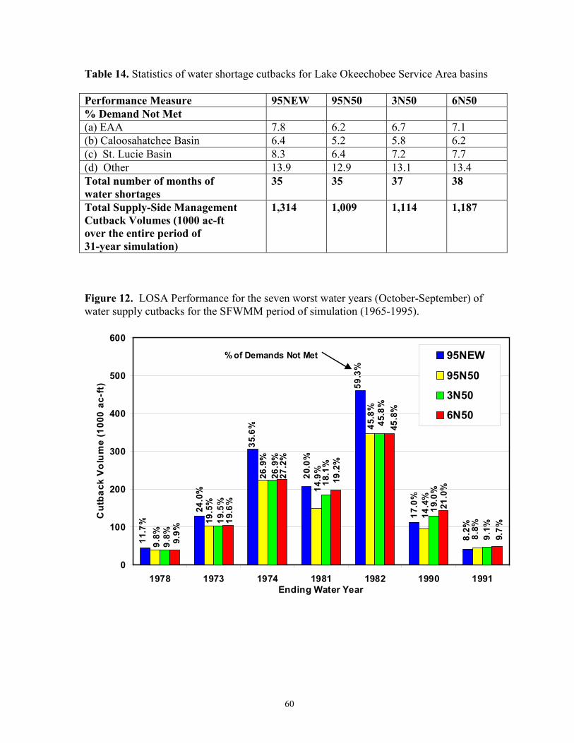
60

Table 14. Statistics of water shortage cutbacks for Lake Okeechobee Service Area basins

Performance Measure 95NEW 95N50 3N50 6N50% Demand Not Met(a) EAA 7.8 6.2 6.7 7.1(b) Caloosahatchee Basin 6.4 5.2 5.8 6.2(c) St. Lucie Basin 8.3 6.4 7.2 7.7(d) Other 13.9 12.9 13.1 13.4Total number of months ofwater shortages

35 35 37 38

Total Supply-Side ManagementCutback Volumes (1000 ac-ftover the entire period of31-year simulation)

1,314 1,009 1,114 1,187

Figure 12. LOSA Performance for the seven worst water years (October-September) ofwater supply cutbacks for the SFWMM period of simulation (1965-1995).

0

100

200

300

400

500

600

1978 1973 1974 1981 1982 1990 1991Ending Water Year

Cut

back

Vol

ume

(100

0 ac

-ft)

95NEW

95N50

3N50

6N50

% of Demands Not Met

19.5

%

19.6

%19

.5%

24.0

%

14.4

%

21.0

%19

.0%

17.0

%

19.2

%18

.1%

14.9

%20.0

%

27.2

%26

.9%

26.9

%35

.6%

9.7%

9.1%

8.8%

8.2%

9.9%

9.8%

9.8%11

.7%

45.8

%45

.8%

45.8

%59

.3%

61

Lower East Coast Service Areas (LECSAs)

The Lower East Coast Service Areas (LECSAs) are located in an urban region atthe southeastern tip of the Florida peninsula. With a population of over five million, themain source of water for LECSAs is a surficial aquifer (primarily the Biscayne aquifer).The aquifer is primarily recharged by local rainfall via drainage into a complex network ofcanals. The maintenance of minimum pre-established water levels in these canals iscrucial in preventing saltwater intrusion that could threaten the quality of the waterwithdrawn from the surficial aquifer. During dry periods, the urban service areas receivewater from the Water Conservation Areas (WCAs). When water is not available in theWCAs, i.e. their water levels are below their “floor” elevations, additional supplies areimported from Lake Okeechobee to maintain the canals. Because of this dependence, it isimportant to ensure that deliveries from Lake Okeechobee to the urban area aremaintained under different operational scenarios. This situation will improve as additionalsources of water from CERP projects are implemented to replace any potential losses dueto changes in the regional system.

The comparison of the base simulation against the three scenarios simulated usingthe SFWMM is shown in Table 15. The frequency (number of months) and percentage ofsimulated water supply cutbacks in the Lower East Coast Service Areas are shown inFigures 13 and 14, respectively. (Note: Service Area 1 in Table 9 is broken down intoLECSA1 and LECSA Northern Palm Beach County in these two Figures).

6c. Modeling Conclusions

It is recognized that large releases of water from Lake Okeechobee (e.g. to meetenvironmental demands in Caloosahatchee Estuary) may have potential impacts on watersupply in the Lake Okeechobee and Lower East Coast Service Areas, particularly duringdroughts. However, regional modeling simulations indicate that the effect of the simulatedadaptive releases (0 - 600 cfs) on existing water supply needs is minimal. A limited set ofmodeling scenarios was investigated as discussed in the previous section. A more detaileddiscussion of these simulations and additional performance measures can be found athttp://www.sfwmd.gov/org/pld/hsm/reg_app/opln/ADP/index.html.

Actual releases under Adaptive Protocols will be made on a case-by-case basiswith due consideration of checks and balances as discussed in Section 4. Futureopportunities via additional modeling and/or evaluation of conditions prior to adaptivereleases within the scope of the WSE schedule will be explored as they impact watersupply in LOSA and LECSAs.

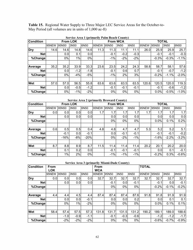
62

Table 15. Regional Water Supply to Three Major LEC Service Areas for the October-to-May Period (all volumes are in units of 1,000 ac-ft)

Service Area 1 (primarily Palm Beach County)Condition From LOK From WCA TOTAL

95NEW 95N50 3N50 6N50 95NEW 95N50 3N50 6N50 95NEW 95N50 3N50 6N50Dry 14.6 14.6 14.8 14.6 11.3 11.3 11.1 11.1 26.0 25.9 25.9 25.7

Net 0.0 0.1 0.0 -0.1 -0.2 -0.3 -0.1 -0.1 -0.3%Change 0% 1% 0% -1% -2% -2% -0.3% -0.3% -1.1%

Average 35.2 35.2 33.9 33.3 23.6 23.5 24.2 24.3 58.8 58.7 58.1 57.6Net 0.0 -1.2 -1.8 -0.1 0.6 0.7 -0.1 -0.7 -1.2

%Change 0% -4% -5% -1% 2% 3% -0.2% -1.1% -2.0%

Wet 57.0 57.0 56.5 55.8 63.6 63.6 63.5 63.5 120.6 120.5 120.0 119.3Net 0.0 -0.5 -1.2 -0.1 -0.1 -0.1 -0.1 -0.6 -1.2

%Change 0% -1% -2% 0% 0% 0% 0.0% -0.5% -1.0%

Service Area 2 (primarily Broward County)Condition From LOK From WCA TOTAL

95NEW 95N50 3N50 6N50 95NEW 95N50 3N50 6N50 95NEW 95N50 3N50 6N50Dry 0.0 0.0 0.0 0.0 1.7 1.7 1.7 1.7 1.7 1.7 1.7 1.7

Net 0.0 0.0 0.0 0.0 0.0 0.0 0.0 0.0 0.0%Change 0% 0% 0% 0.0% 0.1% 0.2%

Average 0.6 0.5 0.5 0.4 4.8 4.8 4.7 4.7 5.3 5.2 5.2 5.1Net -0.1 0.0 -0.1 0.0 -0.1 -0.1 -0.1 -0.1 -0.2

%Change -16% -8% -20% 0% -2% -1% -1.6% -2.2% -3.2%

Wet 8.7 8.8 8.9 8.7 11.5 11.4 11.4 11.4 20.2 20.1 20.2 20.0Net 0.1 0.2 0.0 -0.1 -0.1 -0.1 0.0 0.1 -0.1

%Change 1% 2% 0% -1% -1% -1% -0.2% 0.3% -0.6%

Service Area 3 (primarily Miami-Dade County)Condition From

LOKFromWCA

TOTAL

95NEW 95N50 3N50 6N50 95NEW 95N50 3N50 6N50 95NEW 95N50 3N50 6N50Dry 0.0 0.0 0.0 0.0 32.7 32.7 32.7 32.7 32.7 32.7 32.7 32.7

Net 0.0 0.0 0.0 -0.1 0.0 -0.1 -0.1 0.0 -0.1%Change 0% 0% 0% -0.2% -0.1% -0.2%

Average 4.4 4.4 4.5 4.4 87.4 87.4 87.4 87.6 91.8 91.8 91.9 91.9Net 0.0 0.0 -0.1 0.0 0.0 0.2 0.0 0.1 0.1

%Change 0% 1% -2% 0% 0% 0% 0.0% 0.1% 0.1%

Wet 58.4 57.4 57.5 57.3 131.8 131.7 131.5 131.2 190.2 189.1 189.0 188.6Net -1.0 -0.9 -1.1 -0.1 -0.3 -0.6 -1.2 -1.2 -1.7

%Change -2% -2% -2% 0% 0% 0% -0.6% -0.7% -0.9%

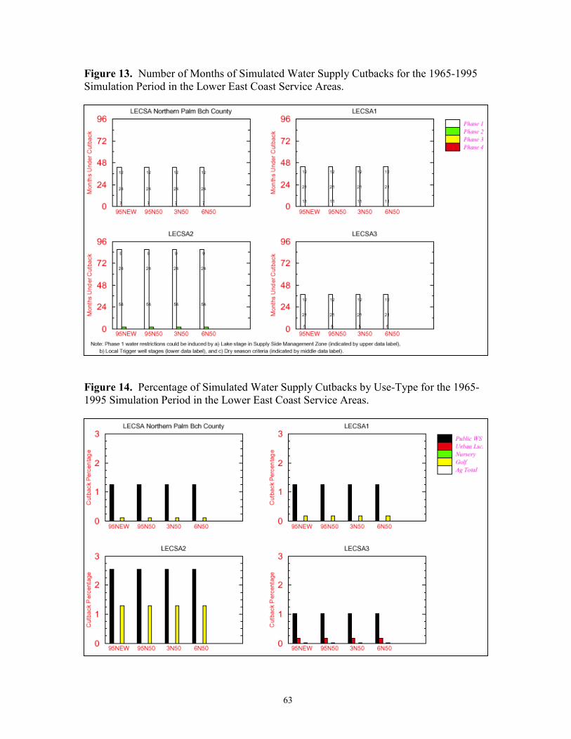
63

Figure 13. Number of Months of Simulated Water Supply Cutbacks for the 1965-1995Simulation Period in the Lower East Coast Service Areas.

Figure 14. Percentage of Simulated Water Supply Cutbacks by Use-Type for the 1965-1995 Simulation Period in the Lower East Coast Service Areas.

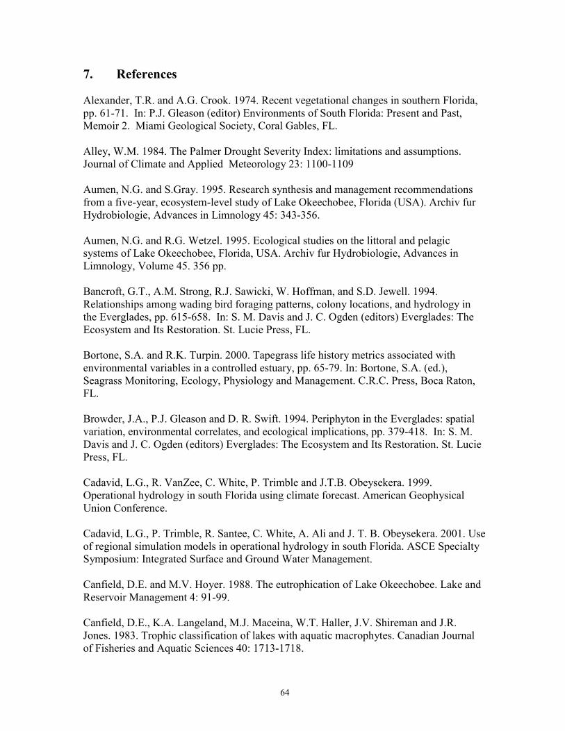
64

7. References

Alexander, T.R. and A.G. Crook. 1974. Recent vegetational changes in southern Florida,pp. 61-71. In: P.J. Gleason (editor) Environments of South Florida: Present and Past,Memoir 2. Miami Geological Society, Coral Gables, FL.

Alley, W.M. 1984. The Palmer Drought Severity Index: limitations and assumptions.Journal of Climate and Applied Meteorology 23: 1100-1109

Aumen, N.G. and S.Gray. 1995. Research synthesis and management recommendationsfrom a five-year, ecosystem-level study of Lake Okeechobee, Florida (USA). Archiv furHydrobiologie, Advances in Limnology 45: 343-356.

Aumen, N.G. and R.G. Wetzel. 1995. Ecological studies on the littoral and pelagicsystems of Lake Okeechobee, Florida, USA. Archiv fur Hydrobiologie, Advances inLimnology, Volume 45. 356 pp.

Bancroft, G.T., A.M. Strong, R.J. Sawicki, W. Hoffman, and S.D. Jewell. 1994.Relationships among wading bird foraging patterns, colony locations, and hydrology inthe Everglades, pp. 615-658. In: S. M. Davis and J. C. Ogden (editors) Everglades: TheEcosystem and Its Restoration. St. Lucie Press, FL.

Bortone, S.A. and R.K. Turpin. 2000. Tapegrass life history metrics associated withenvironmental variables in a controlled estuary, pp. 65-79. In: Bortone, S.A. (ed.),Seagrass Monitoring, Ecology, Physiology and Management. C.R.C. Press, Boca Raton,FL.

Browder, J.A., P.J. Gleason and D. R. Swift. 1994. Periphyton in the Everglades: spatialvariation, environmental correlates, and ecological implications, pp. 379-418. In: S. M.Davis and J. C. Ogden (editors) Everglades: The Ecosystem and Its Restoration. St. LuciePress, FL.

Cadavid, L.G., R. VanZee, C. White, P. Trimble and J.T.B. Obeysekera. 1999.Operational hydrology in south Florida using climate forecast. American GeophysicalUnion Conference.

Cadavid, L.G., P. Trimble, R. Santee, C. White, A. Ali and J. T. B. Obeysekera. 2001. Useof regional simulation models in operational hydrology in south Florida. ASCE SpecialtySymposium: Integrated Surface and Ground Water Management.

Canfield, D.E. and M.V. Hoyer. 1988. The eutrophication of Lake Okeechobee. Lake andReservoir Management 4: 91-99.

Canfield, D.E., K.A. Langeland, M.J. Maceina, W.T. Haller, J.V. Shireman and J.R.Jones. 1983. Trophic classification of lakes with aquatic macrophytes. Canadian Journalof Fisheries and Aquatic Sciences 40: 1713-1718.

65

Chamberlain, R.H. and P.H. Doering. 1998. Preliminary estimate of optimum freshwaterinflow to the Caloosahatchee Estuary: a resource-based approach. Proceedings of theCharlotte Harbor Public Conference and Technical Symposium, pp. 121-131.

Craighead, F.C. 1971. The trees of south Florida. Vol. 1. The Natural Environments andTheir Succession. University of Miami Press, Coral Gables, Florida.

Davis, S. and J. Ogden. 1994. Everglades: The Ecosystem and its Restoration. St. LuciePress, Delray Beach, FL.

Dial Cordy and Associates, Inc. 2001. Interim operational plan (IOP) for protection ofthe Cape Sable seaside sparrow. Prepared for the U.S. Army Corps of Engineers,Jacksonville District.

Doering, P.H. and R.H. Chamberlain. 2000. Experimental studies on the salinity toleranceof turtle grass Thalassia testudinum, pp. 81-97. In: Bortone, S.A. (ed.), SeagrassMonitoring, Ecology, Physiology and Management. C.R.C. Press, Boca Raton, FL.

Doering, P.H., R.H. Chamberlain, K.M. Donohue and A.D. Steinman. 1999. Effect ofsalinity on the growth of Vallisneria americana Michx. From the Caloosahatchee Estuary,Florida. Florida Scientist 62: 89-105.

Estevez, E.D. 2000. A Review and Application of Literature Concerning Freshwater FlowManagement in Riverine Estuaries. Mote Marine Lab. Tech. Report 680.

Fennema, R.J., C.J. Neidrauer, R.A., Johnson, T.K. MacVicar and W.A. Persins. 1994. Acomputer model to simulate natural Everglades hydrology. pp. 249-290. In: S.M. Davisand J.C. Ogden (editors) Everglades: The Ecosystem and Its Restoration. St. Lucie Press,FL.

Fonseca, M.S., J.C. Zieman, G.W. Thayer and J.S. Fisher. 1983. The role of currentvelocity in structuring eelgrass (Zostera marina) meadows. Estuarine and Coastal ShelfScience 17: 367-380.

Fonseca, M.S. and J.S. Fisher. 1986. A comparison of canopy friction and sedimentmovement between four species of seagrass with reference to their ecology anddistribution. Marine Ecology Progress Series 29:15-22.

Fonseca, M.S. 1989. Sediment stabilization by halophila decipiens in comparison to otherseagrasses. Estuarine and Coastal Shelf Science 29: 501-507.

Fonseca, M.S. and J.A. Cahalan. 1992. A preliminary evaluation of wave attentuation byfour species of seagrass. Estuarine and Coastal Shelf Science 35: 565-576.

Frey, D.G. 1946. Oyster bars of the Potomac River. U.S. Fish and Wildlife ServiceSpecial Report. 32:1-93.

66

Frederick, P.C. and M.W. Collopy. 1989. Researcher disturbance in colonies of wadingbirds: effects of frequency of visit and egg marking on reproductive parameters. ColonialWaterbirds 12:152-157.

Frederick, P.C. and M.G. Spalding. 1994. Factors affecting reproductive success ofwading birds (Ciconiiformes) in the Everglades ecosystem, pp. 659-692. In: S.M. Davisand J.C. Ogden (editors) Everglades: The Ecosystem and Its Restoration. St. Lucie Press,FL.

Furse, J.B. and Fox, D.D. 1994. Economic fishery valuation of five vegetationcommunities in Lake Okeechobee, Florida. Proceedings, Southeastern Association of Fishand Wildlife Agencies 48: 575-591.

Gawlik, D. and D.A. Rocque. 1998. Avian communities in bayheads, willowheads andsawgrass marshes of the central Everglades. Wilson Bulletin 110: 45-55.

Gilmore, R.G. 1995. Environmental and biogeographic factors influencing ichthyofaunaldiversity: Indian River Lagoon. Bulletin of Marine Science 57: 153-170.

Grimshaw, H.J., K.E. Havens, B. Sharfstein, A. Steinman, D. Anson, T. East, R.P. Maki,A. Rodusky and K.R. Jin. 2002. The effects of shading on morphometric and meteristiccharacteristics of wild celery, Vallisneria americana Michx., transplants from LakeOkeechobee, Florida. Archiv fur Hydrobiologie 155: 65-81.

Gunderson, L.H., J.R. Stenberg and A.K. Herndon. 1988. Tolerance of five hardwoodspecies to flooding regimes in south Florida. In: D.J. Wilcox (editor) InterdisciplinaryApproaches to Freshwater Wetlands Research. Michigan State University Press, AnnArbor, MI.

Gunderson, L.H. and J.R. Snyder. 1994. Fire patterns in the southern Everglades, pp.307-322. In: S.M. Davis and J.C. Ogden (editors) Everglades: The Ecosystem and ItsRestoration. St. Lucie Press, FL.

Hanlon, C.G. and M. Brady. 2002. The distribution of bulrush and influence ofenvironmental conditions on plant growth during a 26 year period in a shallow subtropicallake, Lake Okeechobee, Florida, USA. Aquatic Botany, in review.

Hanlon, C.G. and Langeland, K. 2000. Comparison of experimental strategies to controltorpedograss. Journal of Aquatic Plant Management 38: 40-47.

Haunert, D.E. and K. Konyha 2000. Establishing St. Lucie Estuary Watershed InflowTargets to Enhance Mesohaline Biota. South Florida Water Management District.Technical Memo. Unpublished.

67

Haunert, D.E. and J.R. Startzman. 1985. Short term effects of a freshwater discharge onthe biota of the St. Lucie Estuary, Florida. Technical Publication 85-1, South FloridaWater Management District, West Palm Beach, FL.

Havens, K.E. 1997. Water levels and total phosphorus in Lake Okeechobee. Lake andReservoir Management 13: 16-25.

Havens, K.E. 2000. Lake Okeechobee conceptual ecosystem model. Technical documentin support of Restoration Coordination and Verification (RECOVER) program of theComprehensive Everglades Restoration Plan.

Havens, K.E. 2002. Hydrologic goals for a large subtropical lake: development andapplication in a regional ecosystem restoration program. Lake and Reservoir Management,in press.

Havens, K.E., J.R. Beaver, T.L. East, A.J. Rodusky, B. Sharfstein, A. St. Armand andA.D. Steinman. 2001b. Nutrient effects on producers and consumers in the littoralplankton and periphyton of a subtropical lake. Archiv fur Hydrobiologie, in press.

Havens, K.E., T.L. East, A.J. Rodusky and B. Sharfstein. 1999. Littoral periphytonresponses to nitrogen and phosphorus: an experimental study in a subtropical lake.Aquatic Botany 63: 267-290.

Havens, K.E., B. Gu, B. Fry, C. Kendall, G.L.Warren and A.J. Rodusky. 2001c.Comparative analysis of littoral and pelagic food webs in a subtropical lake using stableisotope and gut content analyses. Archiv fur Hydrobiologie, in review.

Havens, K.E. and R.T. James. 1999. Localized changes in transparency linked to mudsediment expansion in Lake Okeechobee, Florida: ecological and managementimplications. Lake and Reservoir Management 15: 54-69.

Havens, K.E., K.R. Jin, A.J. Rodusky, B. Sharfstein, M.A. Brady, T.L. East, N. Iricanin,R.T. James, M.C. Harwell and A.D. Steinman. 2001a. Hurricane effects on a shallow lakeecosystem and its response to a controlled manipulation of water level.TheScientificWorld 1: 44-70.

Havens, K.E. and C.L. Schelske. 2001. The importance of considering biologicalprocesses when setting total maximum daily loads (TMDL) for phosphorus in shallowlakes and reservoirs. Environmental Pollution 113: 1-9.

Havens, K.E., A.D. Steinman and S.J. Hwang. 2001d. Phosphorus uptake by plankton andperiphyton in relation to irradiance and phosphate availability in a subtropical lake (LakeOkeechobee, Florida, USA). Archiv fur Hydrobiologie 151: 177-201.

Hirsch, R. M. 1978. Risk analysis for a water supply system – Occoquan Reservoir,Fairfax and Prince William Counties, Virginia. Hydrologic Science Bulletin 23: 476-505.

68

Hwang, S.J., K.E. Havens and A.D. Steinman. 1998. Phosphorus kinetics of planktonicand benthic assemblages in a shallow subtropical lake. Freshwater Biology 40: 729-745.

Kahl, M. P., Jr. 1964. Food ecology of the wood stork (Mycteria americana) in Florida.Ecological Monographs 34: 97-117.

Kenworthy, W.J., G.W. Thayer and M.S. Fonseca. 1988. The utilization of seagrassmeadows by fishery organisms. p.548-560. In Hook. D.D., et al (eds), The ecology andmanagement of wetlands, Vol. 1. Ecology of Wetlands. Timber Press, Portland, OR.

Kushlan, J.A. 1990. Freshwater marshes, pp. 281-428. In: R.L.Myers and J.J. Ewel (eds.)Ecosystems of Florida. University of Central Florida Press, Orlando, FL.

Kushlan, J.A. and O.L. Bass, Jr. 1983. Habitat use and the distribution of the Cape Sableseaside sparrow, pp. 139-146. In: T.L. Quay, J.B. Funderberg, Jr., D.S. Lee, E.F. Potter,and C.S. Robbins, eds. Occasional Papers of the North Carolina Biological Survey, 1983-1985; Raleigh, NC.

Lewis, F.G. III. 1984. Distribution of macrobenthic crustaceans associated with Thalassia,Halodule, and bare sand substrata. Marine Ecology Progress Series 19: 101-113.

Light, S.S. and J.W. Dineen. 1994. Water control in the Everglades: a historicalperspective, pp. 47-84. In: S.M. Davis and J.C. Ogden, editors. Everglades: Theecosystem and its restoration. St. Lucie Press, FL.

Lockhart, C.S. 1995. The effect of water level variation on the growth of Melaleucaseedlings from the Lake Okeechobee littoral zone. MS Thesis, Florida Atlantic University,Boca Raton, FL.

Loftus, W.F. and A.M. Eklund. 1994. Long-term dynamics of an Everglades small-fishassemblage, pp. 461-483. In: S.M. Davis and J.C. Ogden, editors. Everglades: Theecosystem and its restoration. St. Lucie Press, FL.

Loosanoff, V.L. 1951. Feeding of oysters in relation to tidal stages and to periods of lightand darkness. Biological Bulletin (Woods Hole). 90(3):244-264.

Maceina, M.J. 1993. Summer fluctuations in planktonic chlorophyll a concentrations inLake Okeechobee, Florida: the influence of lake levels. Lake and Reservoir Management8: 1-11.

McCormick et al. 1999. Ecological needs of the Everglades, Chapter 3, 1999 EvergladesInterim Report. South Florida Water Management District, 3301 Gun Club Road, WestPalm Beach, Florida.

69

McCormick, P.V., S. Newman, S.L. Miao and T.D. Fontaine. 1998. Field research andmonitoring studies to support derivation of Class III water quality criteria for phosphorusin the Arthur R. Marshall Loxahatchee National Wildlife Refuge: year two (1997)progress report. South Florida Water Management District, West Palm Beach, FL.

McCormick, P.V., S. Newman, S.L. Miao and T.D. Fontaine. 1999. Field research andmonitoring studies to support derivation of Class III water quality criteria for phosphorusin the Arthur R. Marshall Loxahatchee National Wildlife Refuge: year three (1999)progress report. South Florida Water Management District, West Palm Beach, FL.

McCormick, P.V., S. Newman, D.E. Gawlik, D. Marley, K.R. Reddy and T.D. Fontaine.2001. Effects of anthropogenic phosphorus inputs on the Everglades. Pp. 83-126, in:Porter, J.W. and Porter, K.G. (Eds.), The Everglades, Florida Bay, and Coral Reefs of theFlorida Keys: An Ecosystem Sourcebook. CRC Press, Boca Raton, FL.

McCormick, P.V., S. Newman, G.G. Payne, S. L. Miao, K.R. Reddy and T.D. Fontaine.2000. Ecological effects of phosphorus enrichment in the Everglades. Chapter 3. 2000Everglades Consolidated Report. South Florida Water Management District, West PalmBeach, FL.

McCormick, P. V., P. S. Rawlik, K. Lurding, E.P. Smith and F.H. Sklar. 1996. riphyton-water quality relationships along a nutrient gradient in the Florida Everglades. Journal ofthe North American Benthological Society 15: 433-449.

Miao, S. L. and F. H. Sklar. 1998. Biomass and nutrient allocation of sawgrass and cattailalong a nutrient gradient in the Florida Everglades. Journal of Wetland Ecology andManagement 5: 245-263.

Mote Marine Laboratory. 1995. St. Lucie Estuary Nutrient Assessment Research Plan.contract No C-4148. Phase IIID – Report. Mote Marine Laboratory Technical Report No.409. 81 p.

Newell, R.I.E. 1988. Ecological changes in Chesapeake Bay: are they the result ofoverharvesting the American Oyster, Crassostrea virginica? Understanding the estuary:advances in Chesapeake Bay research. Chesapeake Bay Research Consortium Publication129: 29-31.

Newman, S.,S.L. Miao, M.B. McCollum, R.B.E. Shuford III. 2001. Field research andmonitoring studies to support derivation of a Class III water quality criterion forphosphorus in the Arthur R. Marshall Loxahatchee National Wildlife Refuge: Year five(2000) progress report. South Florida Water Management District, West Palm Beach, FL.

Newman, S., P. V. McCormick, S.L. Miao, J.A. Laing, W.C. Kennedy, M.B. O’ Dell.2002. The effect of phosphorus enrichment on the nutrient status of a northern Evergladesslough. Wetlands Ecology and Management, in press.

70

Newman, S., J. Schuette, J.B. Grace, K. Rutchey, T. Fontaine, K.R. Reddy, and M.Pietrucha. 1998. Factors influencing cattail abundance in the northern Everglades. AquaticBotany 60: 265-280.

Newman, S., H. Kumpf, J.A. Laing and W.C. Kennedy. 2001. Decomposition responses tophosphorus enrichment in an Everglades (USA) slough. Biogeochemistry 54: 229-250.

Nott, M.P., O.L. Bass, Jr., D.M. Fleming, S.E. Killeffer, N. Fraley, L. Manne, J.L.Curnutt, J.M. Brooks, R. Powell and S.L. Pimm. 1998. Water levels, rapid vegetationalchanges, and the endangered Cape Sable seaside sparrow. Animal Conservation 1:23-32.

Nungesser, M.K., J.M. Newman, C. Combs, T. Lynch, M. Chimney and R. Meeker. 2001.Optimization research for the Stormwater Treatment Areas. Chapter 6. 2001 EvergladesConsolidated Report. South Florida Water Management, District.West Palm Beach, FL.

Palmer, W.C. 1965. Meteorological drought. Research Paper No. 45. U.S. WeatherBureau. [NOAA Library and Information Services Division, Washington, D.C. 20852]

Phillips, R.C. 1984. The ecology of eelgrass meadows in the pacific northwest: acommunity profile. U.S. Fish and Wildlife Service USFWS / OBS - 84/24. 85p.

Phlips, E.J., P.V. Zimba, M.S. Hopson and T.L. Crisman. 1993. Dynamics of the planktoncommunity in submerged plant dominated regions of Lake Okeechobee, Florida, USA.Proceedings, International Association of Theoretical and Applied Limnology 25: 423-426.

Richardson, J.R. and T.T. Harris. 1995. Vegetation mapping and change detection in theLake Okeechobee marsh ecosystem. Archiv fur Hydrobiologie, Advances in Limnology45: 17-39.

Richter, B.D. 1997. How much water does a fover need? Freshwater Biology 37: 231-249.

Rodgers, J.A. 1987. On the anti-predator advantages of coloniality: a word of caution.Wilson Bulletin 99: 269-270.

Sabol, B.M., R.E. Melton, Jr., R. Chamberlain, P. Doering and K. Haunert. 2002.Evaluation of a digital echo sounder system for detection of submersed aquatic vegetation.Estuaries 25: 133-141.

Scheffer, M., M. Van den Berg, A. Breukelaar, C. Breukers, H. Coops, R. Doef and M.L.Meijer. 1994. Vegetated areas with clear water in turbid shallow lakes. Aquatic Botany49: 193-196.

Settlement Agreement. 1991. United States of America vs. South Florida WaterManagement District. Case no. 88-1886-CIV-HOEVELER, July 26, 1991.

71

SFWMD. 1991. Lake Okeechobee supply-side management plan. South Florida WaterManagement District, West Palm Beach, FL.

SFWMD.1999. A primer to the South Florida Water Management Model (Version 3.5).South Florida Water Management District, West Palm Beach, Florida.

SFWMD. 2000a. Lower east coast regional water supply plan. Planning document, SouthFlorida Water Management District, West Palm Beach, FL.

SFWMD. 2000b. In 2000 the Governing Board of the South Florida Water ManagementDistrict authorized a lowering of water shortage management zones for Lake Okeechobeesupply-side management by 0.5 ft.

SFWMD. 2000c. Minimum flows and levels for Lake Okeechobee, the Everglades, andthe Biscayne Aquifer. South Florida Water Management District, West Palm Beach, FL.

Sklar, F.H., L. Brandt, D. DeAngelis, C. Fitz, D. Gawlik, S. Krupa, C. Madden, F.Mazzotti, C. McVoy, S. Miao, D. Rudnick, K. Rutchey, K. Tarboton, L. Vilchek and Y.Wu. 2000. The hydrological needs of the Everglades. Pp.2.1-2.62, in: Redfield, G. (Ed.),The Everglades 2000 Consolidated Report. South Florida Water Management District,West Palm Beach, FL.

Sklar, F. C. McVoy, R. VanZee, D. Gawlik, K. Yarboton, D. Rudnick and S. Miao. 2002.Effects of altered hydrology on the ecology of the Everglades. Pp. 83-126, in: Porter, J.W.and Porter, K.G. (Eds.), The Everglades, Florida Bay, and Coral Reefs of the FloridaKeys: An Ecosystem Sourcebook. CRC Press, Boca Raton, FL.

Smith, D., M. Smart and C. Hanlon. 2001. Hydrologic influences on torpedograssestablishment in Lake Okeechobee, Florida. Aquatic Botany, in review.

Smith, J.P., J.R. Richardson and M.W. Callopy. 1995. Foraging habitat selection amongwading birds at Lake Okeechobee, Florida, in relation to hydrology and vegetation cover.Archiv fur Hydrobiologie, Advances in Limnology 45: 247-285.

Smith, S.M., S. Newman, P.B. Garrett and J.A. Leeds. 2001. Effects of above- and below-ground fire on soils of a northern Everglades marsh. Journal of Environmental Quality (inpress).

Smith, S.M. and S. Newman. 2001. Growth of southern cattail (Typha domingensis, Pers.)in response to fire-related soil conditions in a northern Everglades marsh. Wetlands 21:363-369.

Smith J. A., G.N. Day, and M.D. Kane. 1992. Nonparametric framework for long-rangestream flow forecasting. Journal of Water Resources Planning and Management, ASCE118: 82-92.

72

Sogrard, S.M., G.V.N. Powell and J.G. Holmquist. 1989. Utilization by fishes of shallow,seagrass-covered banks in Florida Bay: 1. Species composition and spatial heterogeneity.Environmental Biology of Fishes 24: 53-65.

Stevenson, H.M. and B.H. Anderson. 1994. The birdlife of Florida. University Press ofFlorida; Gainesville, FL.

Swift, D.R. and R.B. Nicholas. 1987. Periphyton and water quality relationships in theEverglades water conservation areas, 1978-1982. South Florida Water ManagementDistrict, West Palm Beach, FL.

Tasker G.D., and P.D. Dunne. 1997. Bootstrap position analysis for forecasting low flowfrequency. Journal of Water Resources Planning and Management, ASCE 123: 359-367.

Thayer, G.W., W.J. Kenworthy and M.S. Fonseca.1984. The ecology of eelgrass meadowsof the Atlantic coast: A community profile. U.S. Fish and Wildlife Service USFWS/OBS-84/02. 148 p.

Urban, N.H., S.M. Davis and N.G. Aumen. 1993. Fluctuations in sawgrass and cattail inEverglades Water Conservation Area 2A under varying nutrient, hydrologic and fireregimes. Aquatic Botany 46: 203-223.

URS Greiner Woodward Clyde. 1999. Distribution of oysters and submerged aquaticvegetation in the St. Lucie Estuary. Report for the South Florida Water ManagementDistrict, Project 96F1212.

USACE. 1999. Lake Okeechobee regulation schedule study – final environmental impactstatement. Planning document, U.S. Army Corps of Engineers, Jacksonville, FL.

USEPA. 1987. Estuary Program Primer, U.S. Environmental Protection Agency, Office ofMarine and Estuarine Protection, Washington, D.C.

Virnstein, R.W., P.S. Mikkelsen, K.D. Cairns and M.A. Capone. 1983. Seagrass bedsversus sand bottoms: the trophic importance of their associated benthic invertebrates.Florida Scientist 46: 363-381.

Ward, L.G., W.M. Kemp and W.R. Boynton. 1984. The influence of waves and seagrasscommunities on suspended particles in an estuarine embayment. Mar. Geol. 59:85-103.

White, P.S. 1994. Vegetation pattern and process in the Everglades ecosystem, pp. 445-460. In: S. M. Davis and J. C. Ogden (editors) Everglades: The Ecosystem and ItsRestoration. St. Lucie Press, FL.

Worth, D. 1987. Environmental responses of Water Conservation Area 2A to reduction inregulation schedule and marsh draw down. Technical publication 87-5. South FloridaWater Management District. West Palm Beach, FL.

73

Zieman, J.C. 1982. The ecology of the seagrasses of South Florida: a community profile.U.S. Fish and Wildlife Service. FWS / OBS - 82/25, 158 p.

Zieman, J.C. and Zieman, R.T. 1989. The ecology of the sawgrass meadows of the westcoast of Florida: a community profile. U.S. Fish and Wildlife Service Biological Report.85 (7.25). 155 p.

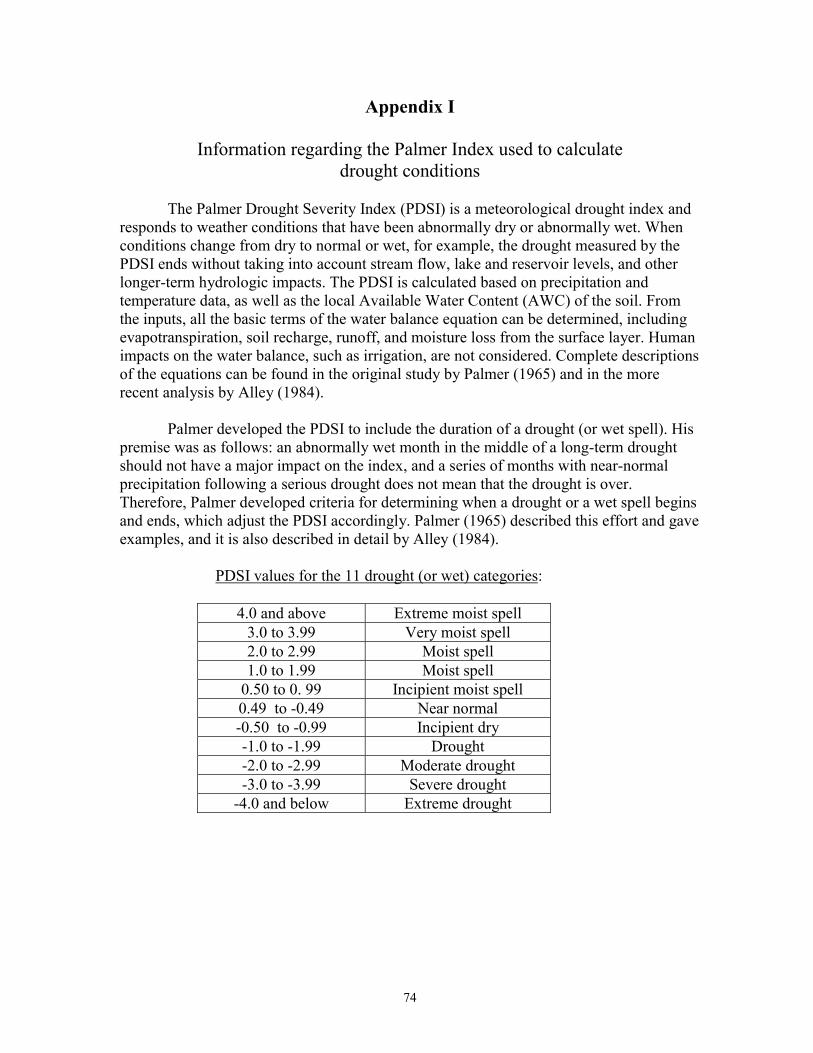
74

Appendix I

Information regarding the Palmer Index used to calculatedrought conditions

The Palmer Drought Severity Index (PDSI) is a meteorological drought index andresponds to weather conditions that have been abnormally dry or abnormally wet. Whenconditions change from dry to normal or wet, for example, the drought measured by thePDSI ends without taking into account stream flow, lake and reservoir levels, and otherlonger-term hydrologic impacts. The PDSI is calculated based on precipitation andtemperature data, as well as the local Available Water Content (AWC) of the soil. Fromthe inputs, all the basic terms of the water balance equation can be determined, includingevapotranspiration, soil recharge, runoff, and moisture loss from the surface layer. Humanimpacts on the water balance, such as irrigation, are not considered. Complete descriptionsof the equations can be found in the original study by Palmer (1965) and in the morerecent analysis by Alley (1984).

Palmer developed the PDSI to include the duration of a drought (or wet spell). Hispremise was as follows: an abnormally wet month in the middle of a long-term droughtshould not have a major impact on the index, and a series of months with near-normalprecipitation following a serious drought does not mean that the drought is over.Therefore, Palmer developed criteria for determining when a drought or a wet spell beginsand ends, which adjust the PDSI accordingly. Palmer (1965) described this effort and gaveexamples, and it is also described in detail by Alley (1984).

PDSI values for the 11 drought (or wet) categories:

4.0 and above Extreme moist spell3.0 to 3.99 Very moist spell2.0 to 2.99 Moist spell1.0 to 1.99 Moist spell

0.50 to 0. 99 Incipient moist spell0.49 to -0.49 Near normal-0.50 to -0.99 Incipient dry-1.0 to -1.99 Drought-2.0 to -2.99 Moderate drought-3.0 to -3.99 Severe drought

-4.0 and below Extreme drought

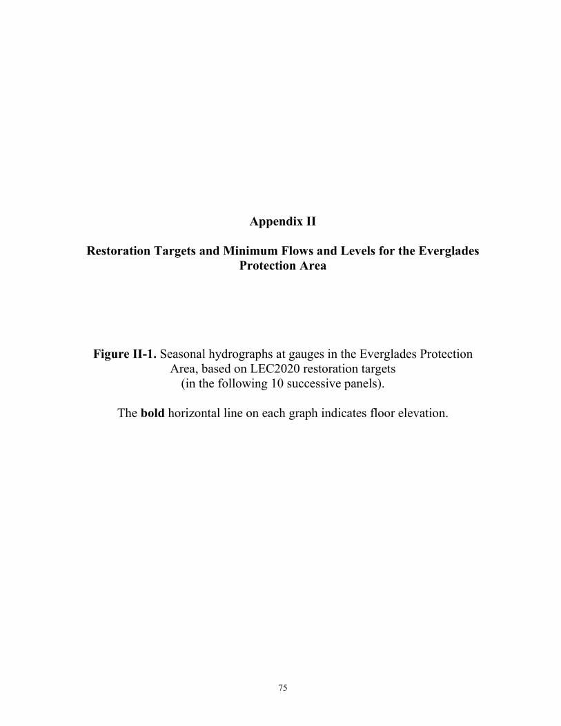
75

Appendix II

Restoration Targets and Minimum Flows and Levels for the EvergladesProtection Area

Figure II-1. Seasonal hydrographs at gauges in the Everglades ProtectionArea, based on LEC2020 restoration targets

(in the following 10 successive panels).

The bold horizontal line on each graph indicates floor elevation.

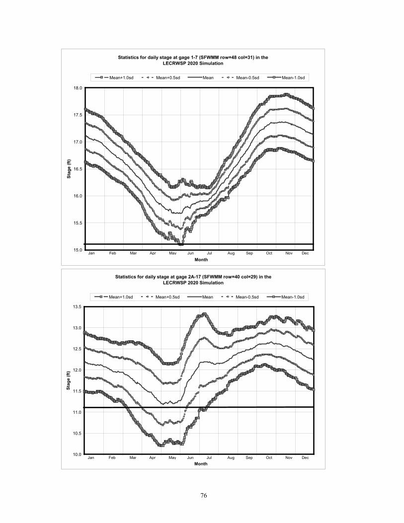
76

Statistics for daily stage at gage 1-7 (SFWMM row=48 col=31) in the LECRWSP 2020 Simulation

15.0

15.5

16.0

16.5

17.0

17.5

18.0

Month

Stag

e (ft

)

Mean+1.0sd Mean+0.5sd Mean Mean-0.5sd Mean-1.0sd

Jan JulJunMayAprMarFeb NovOctSepAug Dec

Statistics for daily stage at gage 2A-17 (SFWMM row=40 col=29) in the LECRWSP 2020 Simulation

10.0

10.5

11.0

11.5

12.0

12.5

13.0

13.5

Month

Stag

e (ft

)

Mean+1.0sd Mean+0.5sd Mean Mean-0.5sd Mean-1.0sd

Jan JulJunMayAprMarFeb NovOctSepAug Dec

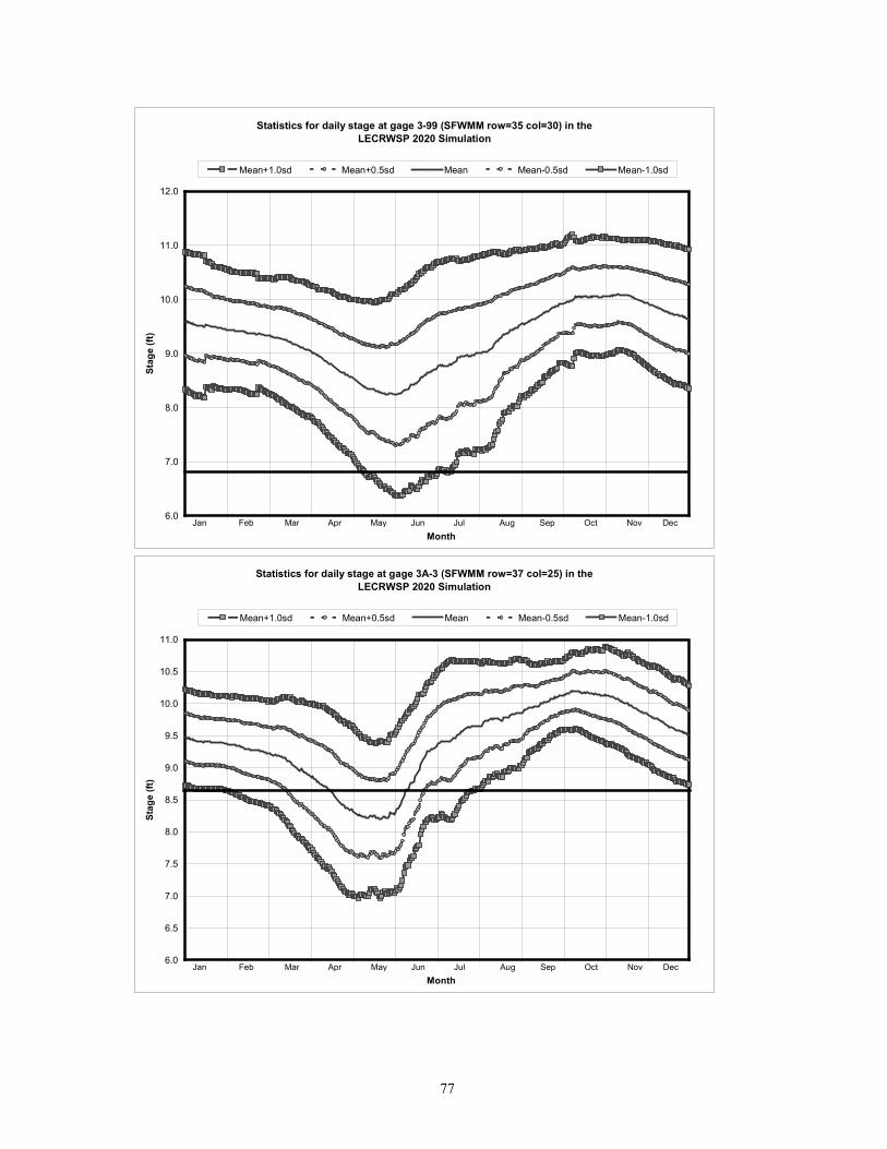
77

Statistics for daily stage at gage 3-99 (SFWMM row=35 col=30) in the LECRWSP 2020 Simulation

6.0

7.0

8.0

9.0

10.0

11.0

12.0

Month

Stag

e (ft

)

Mean+1.0sd Mean+0.5sd Mean Mean-0.5sd Mean-1.0sd

Jan JulJunMayAprMarFeb NovOctSepAug Dec

Statistics for daily stage at gage 3A-3 (SFWMM row=37 col=25) in the LECRWSP 2020 Simulation

6.0

6.5

7.0

7.5

8.0

8.5

9.0

9.5

10.0

10.5

11.0

Month

Stag

e (ft

)

Mean+1.0sd Mean+0.5sd Mean Mean-0.5sd Mean-1.0sd

Jan JulJunMayAprMarFeb NovOctSepAug Dec

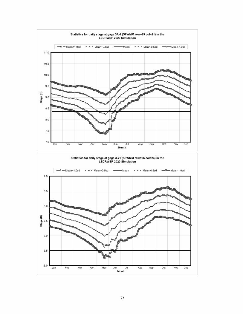
78

Statistics for daily stage at gage 3A-4 (SFWMM row=29 col=21) in the LECRWSP 2020 Simulation

7.0

7.5

8.0

8.5

9.0

9.5

10.0

10.5

11.0

Month

Stag

e (ft

)

Mean+1.0sd Mean+0.5sd Mean Mean-0.5sd Mean-1.0sd

Jan JulJunMayAprMarFeb NovOctSepAug Dec

Statistics for daily stage at gage 3-71 (SFWMM row=26 col=24) in the LECRWSP 2020 Simulation

6.0

6.5

7.0

7.5

8.0

8.5

9.0

Month

Stag

e (ft

)

Mean+1.0sd Mean+0.5sd Mean Mean-0.5sd Mean-1.0sd

Jan JulJunMayAprMarFeb NovOctSepAug Dec

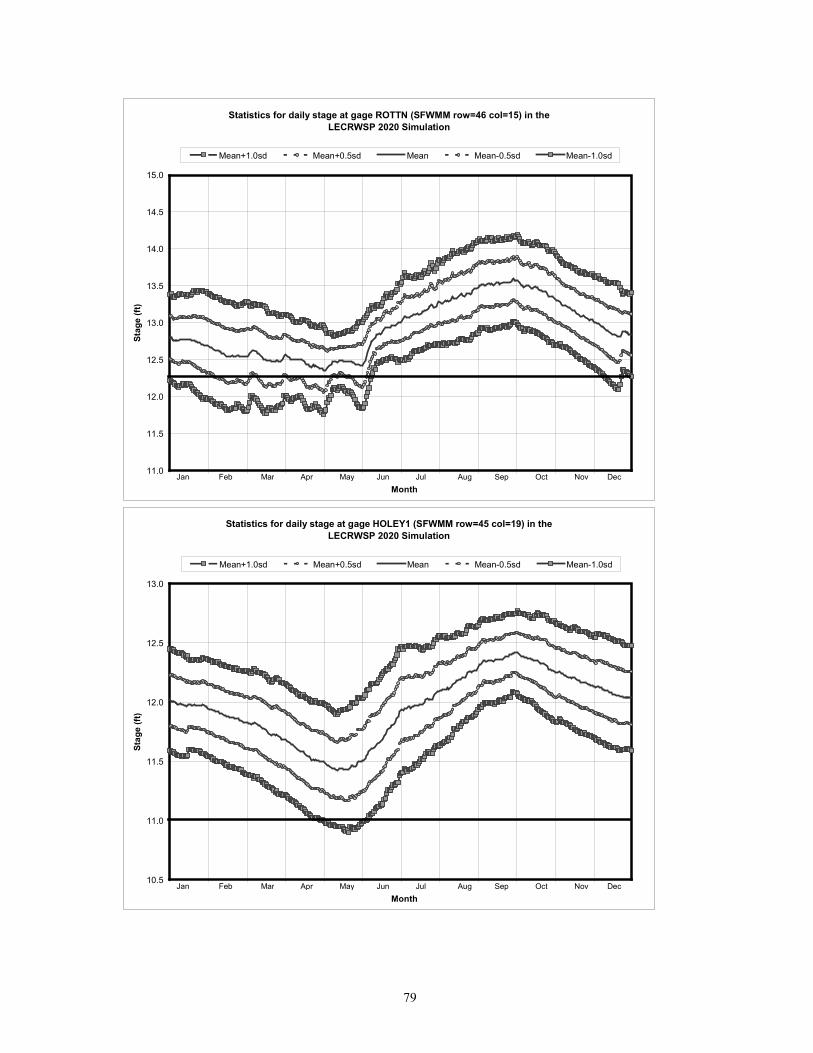
79

Statistics for daily stage at gage ROTTN (SFWMM row=46 col=15) in the LECRWSP 2020 Simulation

11.0

11.5

12.0

12.5

13.0

13.5

14.0

14.5

15.0

Month

Stag

e (ft

)

Mean+1.0sd Mean+0.5sd Mean Mean-0.5sd Mean-1.0sd

Jan JulJunMayAprMarFeb NovOctSepAug Dec

Statistics for daily stage at gage HOLEY1 (SFWMM row=45 col=19) in the LECRWSP 2020 Simulation

10.5

11.0

11.5

12.0

12.5

13.0

Month

Stag

e (ft

)

Mean+1.0sd Mean+0.5sd Mean Mean-0.5sd Mean-1.0sd

Jan JulJunMayAprMarFeb NovOctSepAug Dec

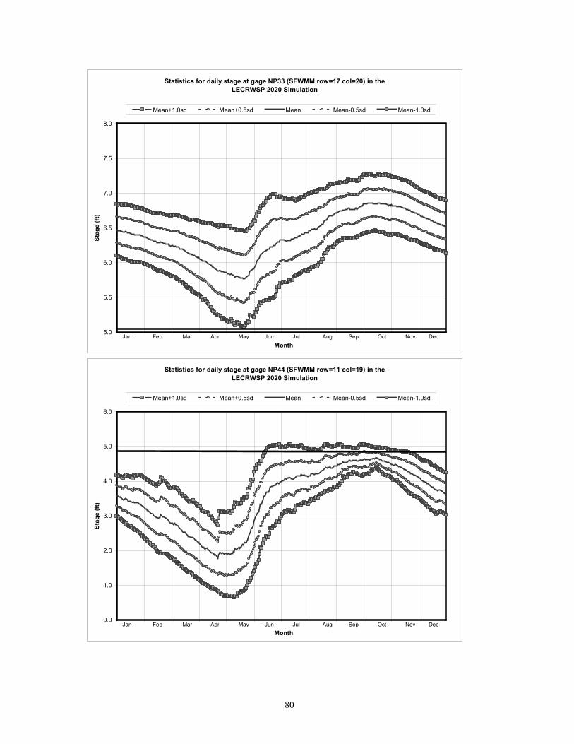
80

Statistics for daily stage at gage NP33 (SFWMM row=17 col=20) in the LECRWSP 2020 Simulation

5.0

5.5

6.0

6.5

7.0

7.5

8.0

Month

Stag

e (ft

)

Mean+1.0sd Mean+0.5sd Mean Mean-0.5sd Mean-1.0sd

Jan JulJunMayAprMarFeb NovOctSepAug Dec

Statistics for daily stage at gage NP44 (SFWMM row=11 col=19) in the LECRWSP 2020 Simulation

0.0

1.0

2.0

3.0

4.0

5.0

6.0

Month

Stag

e (ft

)

Mean+1.0sd Mean+0.5sd Mean Mean-0.5sd Mean-1.0sd

Jan JulJunMayAprMarFeb NovOctSepAug Dec

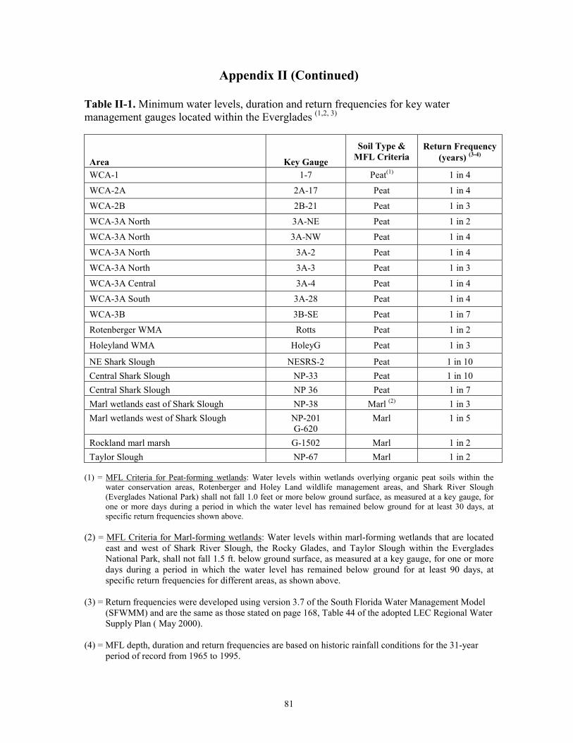
81

Appendix II (Continued)

Table II-1. Minimum water levels, duration and return frequencies for key watermanagement gauges located within the Everglades (1,2, 3)

Area Key Gauge

Soil Type &MFL Criteria

Return Frequency(years) (3-4)

WCA-1 1-7 Peat(1) 1 in 4

WCA-2A 2A-17 Peat 1 in 4

WCA-2B 2B-21 Peat 1 in 3

WCA-3A North 3A-NE Peat 1 in 2

WCA-3A North 3A-NW Peat 1 in 4

WCA-3A North 3A-2 Peat 1 in 4

WCA-3A North 3A-3 Peat 1 in 3

WCA-3A Central 3A-4 Peat 1 in 4

WCA-3A South 3A-28 Peat 1 in 4

WCA-3B 3B-SE Peat 1 in 7

Rotenberger WMA Rotts Peat 1 in 2

Holeyland WMA HoleyG Peat 1 in 3

NE Shark Slough NESRS-2 Peat 1 in 10Central Shark Slough NP-33 Peat 1 in 10Central Shark Slough NP 36 Peat 1 in 7Marl wetlands east of Shark Slough NP-38 Marl (2) 1 in 3Marl wetlands west of Shark Slough NP-201

G-620Marl 1 in 5

Rockland marl marsh G-1502 Marl 1 in 2Taylor Slough NP-67 Marl 1 in 2

(1) = MFL Criteria for Peat-forming wetlands: Water levels within wetlands overlying organic peat soils within thewater conservation areas, Rotenberger and Holey Land wildlife management areas, and Shark River Slough(Everglades National Park) shall not fall 1.0 feet or more below ground surface, as measured at a key gauge, forone or more days during a period in which the water level has remained below ground for at least 30 days, atspecific return frequencies shown above.

(2) = MFL Criteria for Marl-forming wetlands: Water levels within marl-forming wetlands that are locatedeast and west of Shark River Slough, the Rocky Glades, and Taylor Slough within the EvergladesNational Park, shall not fall 1.5 ft. below ground surface, as measured at a key gauge, for one or moredays during a period in which the water level has remained below ground for at least 90 days, atspecific return frequencies for different areas, as shown above.

(3) = Return frequencies were developed using version 3.7 of the South Florida Water Management Model(SFWMM) and are the same as those stated on page 168, Table 44 of the adopted LEC Regional WaterSupply Plan ( May 2000).

(4) = MFL depth, duration and return frequencies are based on historic rainfall conditions for the 31-yearperiod of record from 1965 to 1995.

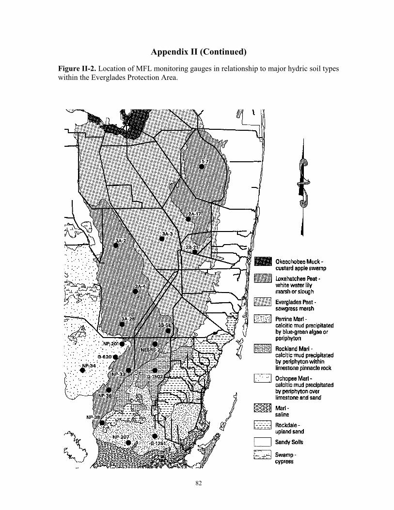
82

Appendix II (Continued)

Figure II-2. Location of MFL monitoring gauges in relationship to major hydric soil typeswithin the Everglades Protection Area.