ICN regions BA t max Peak (mm) (continued) BA t max Peak (mm)X Y Z X Y Z

Subcortical networks ITG (93)Caudate (57) L inferior temporal gyrus 19 42.9 −51 −63 −9

R caudate nucleus 71.4 12 0 15 R inferior temporal gyrus 19 39.2 51 −60 −9L caudate nucleus 66.7 −9 0 15 PreCG (56)

Putamen (8) L precentral gyrus 4 36.4 −48 −6 48R putamen 69.6 21 12 −6 R precentral gyrus 4 36.7 51 −6 48L putamen 70.4 −21 9 −3 L supplementary motor area 6 31.4 0 0 66

Putamen (13) MCC (90)R putamen 76.4 27 6 −3 Bi middle cingulate cortex 32 37.5 3 18 39L putamen 69.7 −30 −3 0 pInsula (71)

Thalamus (15) R insula 13 50.5 45 −3 3R thalamus 49.2 9 −15 6 L insula 13 41.4 −45 −6 3L thalamus 52.1 −9 −18 6 L IPL (76)

Auditory networks L inferior parietal lobule 40 50.6 −42 −51 51STG (99) L middle frontal gyrus 46 29.8 −48 33 21

L superior temporal gyrus 13 38.0 −51 −33 18 L inferior temporal gyrus 37 27.8 −57 −54 −12R superior temporal gyrus 13 36.6 51 −30 21 MiFG (47)

STG (98) R middle frontal gyrus 9 42.3 45 15 33R superior temporal gyrus 21 47.8 63 −24 0 L middle frontal gyrus 9 36.0 −42 9 33L superior temporal gyrus 41 44.8 −57 −21 3 IFG (88)

Somatomotor networks R inferior frontal gyrus 46 37.3 48 39 0PreCG (2) L inferior frontal gyrus 46 39.1 −48 33 9

R postcentral gyrus 6 74.8 57 −6 27 aInsula (21)L postcentral gyrus 6 70.1 −54 −9 30 R insula 47 56.7 33 24 −6R cerebellum (VI) 17.7 18 −66 −18 L insula 47 51.7 −30 24 −3L cerebellum (VI) 19.3 −18 −63 −21 R medial frontal gyrus 6 27.6 6 30 39

R PoCG (10) IPL (59)R postcentral gyrus 3 57.6 42 −24 60 R inferior parietal lobule 40 49.0 57 −45 42L cerebellum (VI) 17.7 −24 −51 −24 L inferior parietal lobule 40 45.6 −57 −45 39

L PoCG (14) MiFG (36)L postcentral gyrus 3 57.5 −42 −24 57 R middle frontal gyrus 10 44.2 30 54 6R cerebellum (VI) 23.2 21 −51 −24 L middle frontal gyrus 10 45.6 −30 54 12L supplementary motor area 6 19.6 −3 −12 54 SMA (29)

SMA (58) Bi supplementary motor area 6 45.0 −3 15 60Bi supplementary motor area 24 46.3 3 −3 48 R STG+IFG (66)

ParaCL (37) R superior temporal gyrus 22 43.9 57 −48 15Bi paracentral lobule 6 65.8 −3 −24 66 R inferior frontal gyrus 47 22.2 51 30 −3

PoCG (45) PHG (81)L postcentral gyrus 2 52.4 −57 −24 36 R ParaHippocampal gyrus 28 37.2 24 −18 −21R postcentral gyrus 4 41.4 57 −21 39 L ParaHippocampal gyrus 28 35.0 −21 −18 −21

ParaCL (30) Default −mode networksBi paracentral lobule 6 46.8 −18 −9 66 Precuneus (20)

SPL (9) Bi precuneus 7 68.7 −6 −72 39R superior parietal lobule 7 52.1 18 −54 66 Bi middle cingulate cortex 23 39.5 0 −24 30L superior parietal lobule 5 52.4 −21 −45 63 Precuneus (44)

Visual networks Bi precuneus 7 65.2 0 −54 51MTG (77) PCC (39)

L middle temporal gyrus 39 42.3 −48 −72 9 L posterior cingulate 30 67.7 −12 −57 15R middle temporal gyrus 39 44.5 48 −63 9 R posterior cingulate 30 67.8 15 −54 15

LingualG (79) PCC (28)R lingual gyrus 19 50.0 21 −72 −6 Bi posterior cingulate cortex 23 65.7 3 −36 27L lingual gyrus 18 44.7 −18 −75 −6 R AG (64)

Cuneus (60) R angular gyrus 40 62.6 45 −66 42Bi cuneus 18 60.8 0 −84 24 R Precuneus 7 35.1 6 −63 39

CalcarineG (46) R superior frontal gyrus 8 30.4 24 33 54L calcarine gyrus 30 66.1 −9 −69 9 ACC (26)R calcarine gyrus 30 63.3 15 −66 9 Bi anterior cingulate cortex 32 57.0 −3 45 3

Cuneus (27) L AG (75)Bi cuneus 17 62.6 3 −87 3 L angular gyrus 39 56.7 −48 −66 33

FFG (43) L Precuneus 7 49.1 0 −60 33L fusiform gyrus 37 50.5 −27 −48 −12 R angular gyrus 39 31.7 51 −63 30R fusiform gyrus 37 52.5 30 −42 −15 L superior frontal gyrus 8 22.0 −18 39 51

R MOG (82) L medial frontal gyrus 10 20.2 −3 51 −6R middle occipital gyrus 19 47.0 36 −84 6 MiFG+SFG (48)

L MOG (89) L middle frontal gyrus 8 33.0 −24 24 48L middle occipital gyrus 18 42.4 −27 −90 0 L superior frontal gyrus 8 34.0 0 33 48

MOG (80) R middle frontal gyrus 8 29.8 21 27 45R middle occipital gyrus 18 70.8 30 −93 0 L MTG+IFG (87)L middle occipital gyrus 18 65.6 −27 −96 −3 L middle temporal gyrus 21 42.4 −57 −39 −3

SOG (61) L inferior frontal gyrus 44 39.2 −54 18 12L superior occipital gyrus 19 45.0 −36 −81 30 Cerebellar networksR superior occipital gyrus 19 47.1 39 −75 36 R CB (12)

Cognitive control networks R cerebellum (crus 2) 51.6 33 −75 −39R IPL (67) L cerebellum (crus 2) 26.9 −30 −78 −36

R inferior parietal lobule 40 52.3 45 −39 51 L CB (7)R middle frontal gyrus 46 33.3 48 42 15 L cerebellum (crus 2) 38.2 −36 −60 −42R inferior frontal gyrus 44 29.6 54 9 24 CB (32)R inferior temporal gyrus 37 27.7 57 −54 −9 Bi cerebellum (VI) 43.9 15 −66 −24

Supplementary Table 1. Peak Coordinates of ICNs

Tracking whole-brain connectivity dynamics in the resting-state

D DIFFERENCE (POST-PROCESSED − ORIGINAL)

SC

AU

D

SM

VIS

CC

DM

CB

SC

AUD

SM

VIS

CC

DM

CB

B AVERAGE FC, ORIGINAL

C AVERAGE FC, FULLY POST-PROCESSED

A EFFECT OF POST-PROCESSING STEPS ON MOTION-RELATED VARIANCE

Subject 349

Subject 367

Subject 52

20 40 60 80 100 120 1400

1

2

Frame # (TR = 2 s)

FD

(m

m)

0

1

2

3 Subject 360

DV

AR

S (

std

)

Subject 267

Subject 124

Original TCs, all components

Original TCs, just ICNs

Regression of realignment parameters

Regression + outlier removal

20 40 60 80 100 120 1400

1

2

Frame # (TR = 2 s)

FD

(m

m)

0

1

2

3

DV

AR

S (

std

)

20 40 60 80 100 120 1400

1

2

Frame # (TR = 2 s)

FD

(m

m)

0

1

2

3

DV

AR

S (

std

)

Figure S1. Effects of motion removal at the subject (A) and group levels (B-D). In (A), we display the

framewise displacement (FD, bottom panel) computed from realignment parameters, and the root-mean-square of

the temporal differential of components TCs (DVARS, top panel, see Power JD et al., 2012) for the three example

subjects (left column) and three additional subjects chosen at random (right column). From the large spikes in

DVARS, it is clear that the original TCs of all components (solid blue line) as well as just ICN components

(dotted blue line) are contaminated with motion-related variance. Regression of realignment parameters and their

derivatives (green line) reduces motion influence in some cases, but additional outlier removal (black line) offers

much greater improvement. The effect of post-processing can be seen in the difference between stationary FC

matrices computed from the original TCs (B) and fully post-processed TCs (regression of realignment parameters

and outlier removal) (C), as shown in panel (D). In agreement with (Power JD et al., 2012), we observe motion-

induced increases in short-range connections (e.g., between SM ICNs) and, to a lesser extent, decreases in long-

range connections (e.g., between SC and VIS ICNs).

∆ corr

ela

tion (

r)

−0.1

0

+0.1corr

ela

tion (

r)

−0.62

0

+0.62

Subcortical Networks

Component 57, Caudate

mm 51 = Zmm 0 = Ymm 21 = X

t−sta

tisti

c

−71.4

0

71.4

Component 8, Putamen

mm 6− = Zmm 21 = Ymm 12 = X

mm 3− = Zmm 9 = Ymm 12− = X

t−sta

tisti

c

−70.4

0

70.4

Component 13, Putamen

mm 3− = Zmm 6 = Ymm 72 = X

mm 0 = Zmm 3− = Ymm 03− = X

t−sta

tisti

c

−76.4

0

76.4

Component 15, Thalamus

mm 6 = Zmm 81− = Ymm 9− = X

t−sta

tisti

c

−52.1

0

52.1

Auditory networks

Component 99, STG

mm 81 = Zmm 33− = Ymm 15− = X

mm 12 = Zmm 03− = Ymm 15 = X

t−sta

tisti

c

−38.0

0

38.0

Component 98, STG

mm 0 = Zmm 42− = Ymm 36 = X

mm 3 = Zmm 12− = Ymm 75− = X

t−sta

tisti

c

−47.8

0

47.8

Figure S2. SMs of ICNs. ICNs are divided into the same groups shown in Figure 2 and are thresholded at |t| > 20,

where one-sample t-statistics have been computed across the single-subject SMs. Sagittal, coronal, and axial

slices are shown at the maximal t-statistic for clusters larger than 3 cm3.

Somatomotor networks

Component 2, PreCG

X = 57 mm Y = −6 mm Z = 27 mm

X = −54 mm Y = −9 mm Z = 30 mm

t−sta

tistic

−74.8

0

74.8

Component 10, R PoCG

X = 42 mm Y = −24 mm Z = 60 mm

t−sta

tistic

−57.6

0

57.6

Component 14, L PoCG

X = −42 mm Y = −24 mm Z = 57 mm

t−sta

tistic

−57.5

0

57.5

Component 58, SMA

X = 5 mm Y = −3 mm Z = 48 mm

t−sta

tistic

−46.3

0

46.3

Component 37, ParaCL

X = −5 mm Y = −24 mm Z = 66 mm

t−sta

tistic

−65.8

0

65.8

Component 45, PoCG

X = −57 mm Y = −24 mm Z = 36 mm

X = 57 mm Y = −21 mm Z = 39 mm

t−sta

tistic

−52.4

0

52.4

Component 30, ParaCL

X = −18 mm Y = −9 mm Z = 66 mm

t−sta

tistic

−46.7

0

46.7

Component 9, SPL

X = −21 mm Y = −45 mm Z = 63 mm

t−sta

tistic

−52.4

0

52.4

Visual networks

Component 77, MTG

X = −48 mm Y = −72 mm Z = 9 mm

X = 48 mm Y = −63 mm Z = 9 mm

t−sta

tistic

−44.5

0

44.5

Component 79, LingualG

X = 21 mm Y = −72 mm Z = −6 mm

X = −18 mm Y = −75 mm Z = −6 mm

t−sta

tistic

−50.0

0

50.0

Component 60, Cuneus

X = 0 mm Y = −84 mm Z = 24 mm

t−sta

tistic

−60.8

0

60.8

Component 46, CalcarineG

X = −9 mm Y = −69 mm Z = 9 mm

t−sta

tistic

−66.1

0

66.1

Component 27, Cuneus

X = 5 mm Y = −87 mm Z = 3 mm

t−sta

tistic

−62.6

0

62.6

Component 43, FFG

X = −27 mm Y = −48 mm Z = −12 mm

X = 30 mm Y = −42 mm Z = −15 mm

t−sta

tistic

−52.5

0

52.5

Component 82, R MOG

X = 36 mm Y = −84 mm Z = 6 mm

t−sta

tistic

−47.0

0

47.0

Component 89, L MOG

X = −27 mm Y = −90 mm Z = 0 mm

t−sta

tistic

−42.4

0

42.4

Visual networks continued

Component 80, MOG

X = 30 mm Y = −93 mm Z = 0 mm

X = −27 mm Y = −96 mm Z = −3 mm

t−sta

tistic

−70.8

0

70.8

Component 61, SOG

X = −36 mm Y = −81 mm Z = 29 mm

X = 39 mm Y = −75 mm Z = 36 mm

t−sta

tistic

−47.1

0

47.1

Cognitive control networks

Component 67, R IPl

X = 45 mm Y = −39 mm Z = 51 mm

X = 48 mm Y = 42 mm Z = 15 mm

t−sta

tistic

−52.3

0

52.3

Component 93, ITG

X = −51 mm Y = −63 mm Z = −9 mm

X = 51 mm Y = −60 mm Z = −9 mm

t−sta

tistic

−42.9

0

42.9

Component 56, PreCG

X = −48 mm Y = −6 mm Z = 48 mm

X = 51 mm Y = −6 mm Z = 48 mm

t−sta

tistic

−36.7

0

36.7

Cognitive control networks continued (1)

Component 90, MCC

X = 5 mm Y = 18 mm Z = 39 mm

t−sta

tistic

−37.5

0

37.5

Component 71, pInsula

X = 45 mm Y = −3 mm Z = 3 mm

X = −45 mm Y = −6 mm Z = 3 mm

t−sta

tistic

−50.5

0

50.5

Component 76, L IPL

X = −42 mm Y = −51 mm Z = 51 mm

X = −48 mm Y = 33 mm Z = 21 mm

t−sta

tistic

−50.6

0

50.6

Component 47, MiFG

X = 45 mm Y = 15 mm Z = 33 mm

X = −42 mm Y = 9 mm Z = 33 mm

t−sta

tistic

−42.3

0

42.3

Component 88, IFG

X = 48 mm Y = 39 mm Z = 0 mm

X = −48 mm Y = 33 mm Z = 9 mm

t−sta

tistic

−39.1

0

39.1

Component 21, aInsula

X = 33 mm Y = 24 mm Z = −6 mm

X = −30 mm Y = 24 mm Z = −3 mm

t−sta

tistic

−56.7

0

56.7

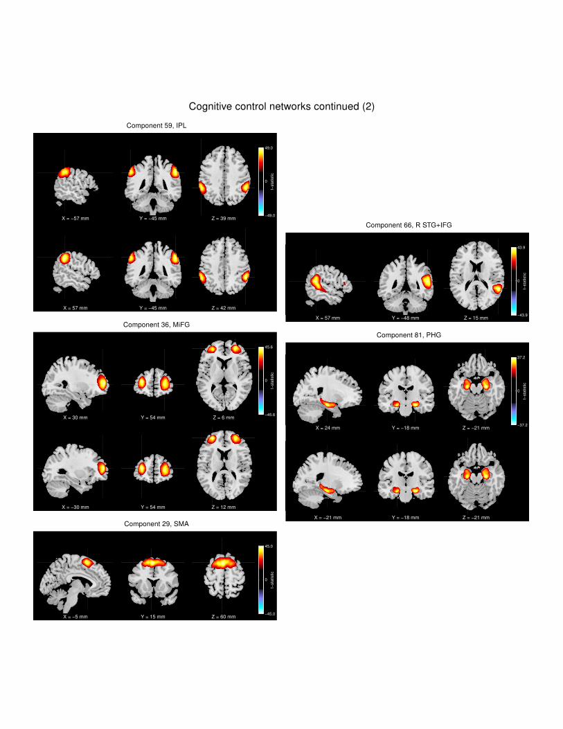
Cognitive control networks continued (2)

Component 59, IPL

X = −57 mm Y = −45 mm Z = 39 mm

X = 57 mm Y = −45 mm Z = 42 mm

t−sta

tistic

−49.0

0

49.0

Component 36, MiFG

X = 30 mm Y = 54 mm Z = 6 mm

X = −30 mm Y = 54 mm Z = 12 mm

t−sta

tistic

−45.6

0

45.6

Component 29, SMA

X = −5 mm Y = 15 mm Z = 60 mm

t−sta

tistic

−45.0

0

45.0

Component 66, R STG+IFG

X = 57 mm Y = −48 mm Z = 15 mm

t−sta

tistic

−43.9

0

43.9

Component 81, PHG

X = 24 mm Y = −18 mm Z = −21 mm

X = −21 mm Y = −18 mm Z = −21 mm

t−sta

tistic

−37.2

0

37.2

Default-mode networks

Component 20, Precuneus

X = −6 mm Y = −72 mm Z = 39 mm

X = 0 mm Y = −24 mm Z = 30 mm

t−sta

tistic

−68.7

0

68.7

Component 44, Precuneus

X = 0 mm Y = −54 mm Z = 51 mm

t−sta

tistic

−65.2

0

65.2

Component 39, PCC

X = 15 mm Y = −54 mm Z = 15 mm

t−sta

tistic

−67.8

0

67.8

Component 28, PCC

X = 5 mm Y = −36 mm Z = 27 mm

t−sta

tistic

−65.7

0

65.7

Component 64, R AG

X = 45 mm Y = −66 mm Z = 42 mm

X = 24 mm Y = 33 mm Z = 54 mm

X = 6 mm Y = −63 mm Z = 39 mm

t−sta

tistic

−62.6

0

62.6

Component 26, ACC

X = −5 mm Y = 45 mm Z = 3 mm

t−sta

tistic

−57.0

0

57.0

Component 75, L AG

X = −48 mm Y = −66 mm Z = 33 mm

X = 0 mm Y = −60 mm Z = 33 mm

t−sta

tistic

−56.7

0

56.7

Default-mode networks continued

Component 48, MiFG+SFG

X = 0 mm Y = 33 mm Z = 48 mm

t−sta

tistic

−34.0

0

34.0

Component 87, L MTG+IFG

X = −57 mm Y = −39 mm Z = −3 mm

X = −54 mm Y = 18 mm Z = 12 mm

t−sta

tistic

−42.4

0

42.4

Cerebellar networks

Component 12, R CB

X = 33 mm Y = −75 mm Z = −39 mm

t−sta

tistic

−51.6

0

51.6

Component 7, L CB

X = −36 mm Y = −60 mm Z = −42 mm

t−sta

tistic

−38.2

0

38.2

Component 32, CB

X = 15 mm Y = −66 mm Z = −24 mm

t−sta

tistic

−43.9

0

43.9

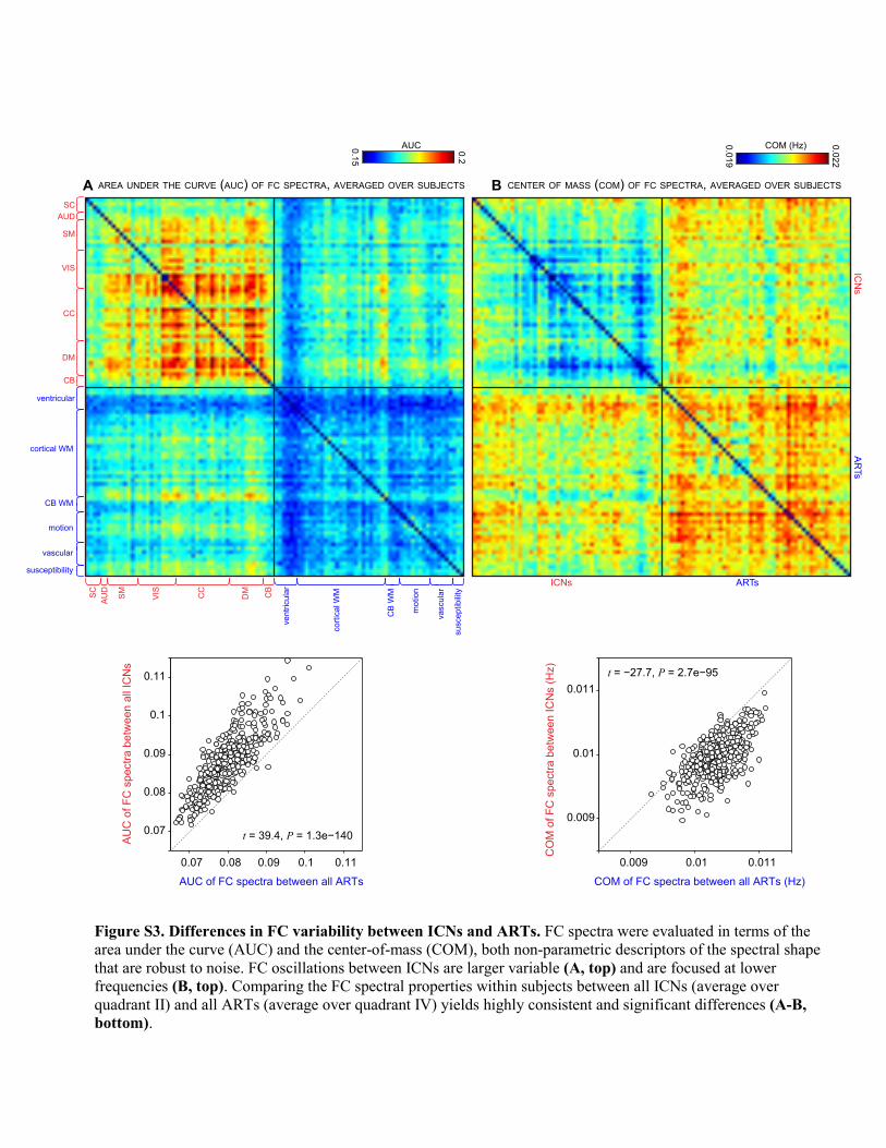
AREA UNDER THE CURVE (AUC) OF FC SPECTRA, AVERAGED OVER SUBJECTSA

0.07 0.08 0.09 0.1 0.11

0.07

0.08

0.09

0.1

0.11

AUC of FC spectra between all ARTs

AU

C o

f F

C s

pe

ctr

a b

etw

ee

n a

ll IC

Ns

t = 39.4, P = 1.3e−140

0.009 0.01 0.011

0.009

0.01

0.011

COM of FC spectra between all ARTs (Hz)

CO

M o

f F

C s

pe

ctr

a b

etw

ee

n I

CN

s (

Hz)

t = −27.7, P = 2.7e−95

AUC0.15

0.2

ICNs ARTs

ICN

sA

RTs

SC

AUD

SM

VIS

CC

DM

CB

ventricular

cortical WM

CB WM

vascular

susceptibility

motion

SC

AU

D

SM

VIS

CC

DM

CB

ve

ntr

icu

lar

co

rtic

al W

M

CB

WM

va

scu

lar

su

sce

ptib

ility

mo

tio

n

CENTER OF MASS (COM) OF FC SPECTRA, AVERAGED OVER SUBJECTSB

COM (Hz)0.0

19

0.022

Figure S3. Differences in FC variability between ICNs and ARTs. FC spectra were evaluated in terms of the

area under the curve (AUC) and the center-of-mass (COM), both non-parametric descriptors of the spectral shape

that are robust to noise. FC oscillations between ICNs are larger variable (A, top) and are focused at lower

frequencies (B, top). Comparing the FC spectral properties within subjects between all ICNs (average over

quadrant II) and all ARTs (average over quadrant IV) yields highly consistent and significant differences (A-B,

bottom).

423 (14%) 333 (11%) 263 (9%) 249 (8%)

1093 (36%) 975 (32%) 593 (20%) 497 (16%) 383 (13%) 243 (8%) 227 (8%) 215 (7%) 209 (7%)

463 (15%) 299 (10%) 279 (9%)

311 (10%)

255 (8%) 225 (7%)

507 (17%) 487 (16%) 419 (14%) 393 (13%) 351 (12%) 319 (11%)

341 (11%) 295 (10%) 283 (9%) 279 (9%) 265 (9%) 263 (9%) 233 (8%) 231 (8%)

317 (10%) 289 (10%) 243 (8%) 317 (10%) 265 (9%)

607 (20%) 491 (16%) 387 (13%) 357 (12%) 225 (7%) 281 (9%) 183 (6%)

1933 (64%) 1710 (57%) 1531 (51%) 1248 (41%) 1173 (39%) 1030 (34%) 879 (29%) 812 (27%) 755 (25%)

k = 9k = 3 k = 10k = 8k = 7k = 6k = 5k = 4k = 2

S1

S2

S3

S4

S5

S6

S7

S8

S9

S10

Figure S4. Cluster centroids for k = 2 to 10. For each k, the k-means algorithm was applied with 500 repetitions

to the subject exemplar windows (3026 instances). The gray rectangle highlights the clustering result presented in

the main text. The total number and percentage of occurrences is listed above each centroid.

281 (9%)441 (15%)377 (12%) 393 (13%)1063 (35%) 193 (6%) 281 (9%)

305 (10%)451 (15%)353 (12%) 401 (13%)1069 (35%) 207 (7%) 277 (9%)

275 (9%)369 (12%)367 (12%) 441 (15%)1035 (34%) 237 (8%) 286 (10%)

301 (10%)425 (14%)365 (12%) 455 (15%)973 (32%) 241 (8%) 271 (9%)

263 (9%)429 (14%)319 (11%) 425 (14%)1021 (34%) 263 (9%) 267 (9%)

129 (8%)235 (15%)185 (12%) 219 (14%)535 (35%) 103 (7%) 121 (8%)

159 (11%)195 (13%)187 (12%) 209 (14%)489 (33%) 115 (8%) 145 (10%)

S1 S2 S3 S4 S5 S6 S7

A

B

CLUSTER CENTROIDS FROM BOOTSTRAP RESAMPLES

CLUSTER CENTROIDS FROM SPLIT-HALF ANALYSIS

SA

MP

LE

1S

AM

PL

E 2

SA

MP

LE

3S

AM

PL

E 4

SA

MP

LE

5H

AL

F 1

HA

LF

2

Figure S5. Cluster centroids for bootstrap resamples (A) and split-half samples (B). In (A), subjects were

resampled and the k-means algorithm was applied with 500 repetitions to the subject exemplar windows (∼3000 to ∼4000 instances depending on the sample). In (B), the subjects were split into two groups and the k-means

algorithm was applied with 500 repetitions to the subject exemplars in that group (∼1500 instances). The total

number and percentage of occurrences is listed above each centroid.

ORIGINAL DATA

SR1: CONSISTENT FOURIER PHASE SHIFT

SR2: INCONSISTENT FOURIER PHASE SHIFT

50 100 150 200 250

−0.5

0

0.5

Corr

ela

tion (

z)

time (s)

CalcarineG (46) to MCC (90)

CalcarineG (46) to pInsula (71)

CalcarineG (46) to PreCG (56)

50 100 150 200 250

−0.5

0

0.5

Corr

ela

tion (

z)

time (s)

50 100 150 200 250

−0.5

0

0.5

Corr

ela

tion (

z)

time (s)

438 (14%)

61 (2%)

423 (14%)

401 (13%)

0 (0%)

243 (8%)

249 (8%)

0 (0%)

265 (9%)

473 (16%)

232 (8%)

289 (10%)

458 (15%)

20 (1%)

357 (12%)

496 (16%)

1674 (55%)

1030 (34%)

511 (17%)

1039 (34%)

419 (14%)

CLUSTER CENTROIDS (k = 7)AVERAGE OF SUBJECT EXEMPLARS

EXAMPLE FC TIMESERIESA

B C

S1 S2 S3 S4 S5 S6 S7

subject 124

Figure S6. Clustering results with surrogate datasets. (A) Demonstration of surrogate data creation from the

original FC timeseries (top) using a consistent Fourier phase shift (SR1, middle) and inconsistent phase shift

(SR2, bottom). In SR1, the FC timeseries maintain their phase relationships. In SR2, phase relationships (and thus

covariance structures) are disrupted. Neither consistent nor inconsistent Fourier phase shifting alters the mean,

variance, or temporal autocorrelation of individual FC timeseries, as demonstrated by the very similar average

subject exemplars shown in (B) for original data (top) SR1 (middle) and SR2 (bottom). (C) Cluster centroids for

original data (top, identical to Figure S4, k = 7), SR1 (middle), and SR2 (bottom). Clustering of exemplars from

SR2 fails to replicate the centroids observed in original data and SR 1: two clusters (S2 and S3) are empty and all

others strongly resemble the mean shown in (B). This suggests it is the patterns of covariance (preserved in SR1),

rather than distinctions in mean or variance, that drive the clustering.

0 50 100 150 200 250 300

−2

−1

0

1

2

Time (s)

Am

plit

ude

0

10

20

30

40

50

Dis

tance fro

m centr

oid

0 50 100 150 200 250 300

Time (s)

state 1 state 2 state 3 state 4 state 2

centroid 1

centroid 2

centroid 3

centroid 4

centroid 1 centroid 2 centroid 3 centroid 4

CLUSTER CENTROIDS

SIMULATED DYNAMIC “NEURAL” FUNCTIONAL CONNECTIVITY

true stateestimated state

STATE TRANSITIONS

A

B

C

1

101 10 −1

+1

FC

2 4 6 8 10 120

0.2

0.4

0.6

Number of clusters (k)

Clu

ste

r valid

ity index

k = 4

Figure S7. Validation of clustering approach with simulated data. (A) Simulated BOLD timeseries for ten

nodes are generated under a model of dynamic neural connectivity where 4 states are possible (State 2 repeats).

Simulation parameters (TR = 2 s, 148 volumes) are matched to experimental data; connectivity states are modeled

after clusters observed in real data (e.g., Figure 5). (B) Windowed covariance matrices are estimated from the

simulated timeseries and are subjected to k-means clustering with the L1 distance metric. The elbow criterion

correctly identifies k = 4 clusters, and cluster centroids show high similarity to the true states. (C) The distance of

each window to each cluster centroid. The assignment of individual windows to states is very accurate. Distances

and state assignments are plotted at the time point corresponding to the center of the window.