�����������������

Citation: Liu, Z.; Quan, Y.; Wu, Y.;

Xing, M. Super-Resolution Range and

Velocity Estimations for SFA-OFDM

Radar. Remote Sens. 2022, 14, 278.

https://doi.org/10.3390/rs14020278

Academic Editor: Ali Khenchaf

Received: 14 December 2021

Accepted: 6 January 2022

Published: 7 January 2022

Publisher’s Note: MDPI stays neutral

with regard to jurisdictional claims in

published maps and institutional affil-

iations.

Copyright: © 2022 by the authors.

Licensee MDPI, Basel, Switzerland.

This article is an open access article

distributed under the terms and

conditions of the Creative Commons

Attribution (CC BY) license (https://

creativecommons.org/licenses/by/

4.0/).

remote sensing

Article

Super-Resolution Range and Velocity Estimations forSFA-OFDM RadarZhixing Liu 1 , Yinghui Quan 1,*, Yaojun Wu 1 and Mengdao Xing 2,3

1 Department of Remote Sensing Science and Technology, Xidian University, Xi’an 710071, China;liuzx@stu.xidian.edu.cn (Z.L.); yjwu@xidian.edu.cn (Y.W.)

2 National Laboratory of Radar Signal Processing, Xidian University, Xi’an 710071, China; xmd@xidian.edu.cn3 Academy of Advanced Interdisciplinary Research, Xidian University, Xi’an 710071, China* Correspondence: yhquan@mail.xidian.edu.cn; Tel.: +86-029-88201236

Abstract: Sparse frequency agile orthogonal frequency division multiplexing (SFA-OFDM) signalbrings excellent performance to electronic counter-countermeasures (ECCM) and reduces the com-plexity of the radar system. However, frequency agility makes coherent processing a much morechallenging task for the radar, which leads to the discontinuity of the echo phase in a coherentprocessing interval (CPI), so the fast Fourier transform (FFT)-based method is no longer a valid wayto complete the coherent integration. To overcome this problem, we proposed a novel scheme to esti-mate both super-resolution range and velocity. The subcarriers of each pulse are firstly synthesizedin time domain. Then, the range and velocity estimations for the SFA-OFDM radar are regarded asthe parameter estimations of a linear array. Finally, both the super-resolution range and velocity areobtained by exploiting the multiple signal classification (MUSIC) algorithm. Simulation results areprovided to demonstrate the effectiveness of the proposed method.

Keywords: sparse frequency agility; orthogonal frequency division multiplexing; subcarrier synthe-sis; multiple signal classification; super-resolution range and velocity

1. Introduction

With the rapid development of electronic technology, orthogonal frequency divisionmultiplexing (OFDM) technology has already been widely applied in communicationsystems [1–3]. Its advantages include robustness against Inter Symbol Interference (ISI) andInter Carrier Interference (ICI), high spectral efficiency and ease of implementation [4,5], etc.

In recent years, OFDM has also attracted more and more attention in radar applications,such as radar imaging [6,7], radar detection [8,9] and integration radar and communica-tion [10–12]. As a multi-carrier wide-band radar, the OFDM radar has the major drawbackof a large baseband bandwidth. Meanwhile, to improve the range resolution, a largerbandwidth is also necessary. This requires that OFDM radar hardware has sufficienthigh sampling and data processing rates. To reduce the hardware requirements, manyresearchers are studying the stepped-OFDM radar, the core idea of which is to reduce theinstantaneous bandwidth of the OFDM radar. In [13], an OFDM phase-coded stepped-frequency (OFDM-PCSF) waveform is presented, whereby a high range resolution (HRR)is achieved by synthesizing multiple narrowband signals. However, this only applies tolow velocity targets. A similar stepped-carrier OFDM-radar waveform is investigatedin [14], which can simultaneously achieve the high-resolution range and velocity but witha much lower baseband bandwidth. Nuss et al. [15,16] propose a frequency comb OFDMradar signal to overcome the hardware limitations. It also can obtain HRR profiles, but itsunambiguous velocity is sustained at the cost of a decreased unambiguous range.

Furthermore, frequency agility [17–19] is introduced into the OFDM radar by Lel-louch et al. [20,21]. Each pulse transmits a narrowband signal, while the carrier frequencies

Remote Sens. 2022, 14, 278. https://doi.org/10.3390/rs14020278 https://www.mdpi.com/journal/remotesensing

Remote Sens. 2022, 14, 278 2 of 16

are randomly varied from pulse to pulse, bringing not only excellent performance in elec-tronic counter-countermeasures (ECCM), but also significantly reducing the instantaneousbandwidth of the OFDM radar system [22]. However, frequency agility leads to the discon-tinuity of echo phase in a coherent processing interval (CPI), so the fast Fourier transform(FFT)-based method cannot complete coherent integration. In [20], different patterns forfrequency agility based on OFDM waveform are investigated. It shows that the spread sub-carriers hopping presents a very sharp peak in both delay and scale domains. Meanwhile,the Doppler processing concept is proposed. Subcarriers with the same frequencies areutilized to process Doppler, and the rest contribute to agility. Nevertheless, this methodrequires a longer coherent processing time, and range cell migration (RCM) may be needed.It cannot obtain super-resolution range and velocity simultaneously. A similar frequencyagile stepped waveform is proposed [21]. The multiple narrowband signals are synthesizedto obtain the HRR profile, which is only suitable for a single stationary or low-speed pointtarget. In [23], a frequency-agile sparse OFDM radar with short sequences of narrowbandpulses of different bandwidths is proposed, and the compressed sensing (CS) theory isapplied to obtain a high-resolution range-velocity profile. In [24], the influence of a state-of-the-art frequency-modulated continuous wave (FMCW) on stepped and sparse OFDM isexamined, and zeroing of interfered samples in the frequency domain is used to suppressFMCW-interference. An interference-robust processing for OFDM radar signals using CS ispresented in [25]. This method is not only suitable for random OFDM, but also applied forstepped or standard OFDM.

Based on the previous work, the super-resolution range and velocity estimations forthe sparse frequency agile OFDM (SFA-OFDM) radar is studied in this paper. Similarly tothe frequency agile stepped OFDM waveform proposed in [20,23], the SFA-OFDM radarsignal’s agile pattern is grouped subcarrier frequency random hopping, and the bandwidthof each pulse is equal. However, the difference is that each SFA-OFDM radar subcarrieris a narrow-band linear frequency modulation (LFM) signal, and some frequencies areunused during a CPI, i.e., the number of pulses in a CPI is less than the total number ofavailable frequencies. The SFA-OFDM radar signal is sparse [26] in the time–frequencydomain. Therefore, it is difficult to track and predict by jamming.

The main works in our paper are as follows. Firstly, for a moving target, the SFA-OFDM radar’s mathematical model is derived. A merit of the SFA-OFDM radar is that theECCM performance is more robust and the limitations of system hardware are overcome.Secondly, to obtain the super-resolution range–velocity of the SFA-OFDM radar simulta-neously, we introduce a signal processing method, in which the parameter estimations ofthe SFA-OFDM radar is equivalent to that of a linear array, and the MUSIC algorithm [27]is applied to achieve the super-resolution range and velocity estimations. Thirdly, theperformance of the proposed parameter estimations algorithm for the SFA-OFDM radaris analyzed. The Cramér-Rao lower bounds (CRLBs) on parameter estimations using theSFA-OFDM radar signal are derived. Finally, the effectiveness of the proposed method isproved by several simulation experiments. Compared with the Doppler processing methodproposed in [20], the proposed method solves the conflict between the frequency agilityand coherent processing. It can obtain the super-resolution range and velocity in a CPI. Itsrange–velocity resolution is only related to the size of the grid, and the smaller the gridsize, the higher the resolution will be.

The remainder of this paper is organized as follows. In Section 2, the mathematicalmodel of the SFA-OFDM radar signal is established. Section 3 describes the proposedrange–velocity estimation scheme. The performance of the proposed method is discussedin Section 4. Several numerical simulation experiments are presented to validate theproposed method in Section 5. Finally, Section 6 concludes the paper.

2. SFA-OFDM Radar Signal Model

In this section, first, the SFA-OFDM radar signal is introduced. Then, the receivedsignal model for the moving target is established.

Remote Sens. 2022, 14, 278 3 of 16

An illustration of the SFA-OFDM radar signal model [20,28] is given in Figure 1. Weassume that the SFA-OFDM radar transmits M pulses in a CPI. Each pulse consists of K or-thogonal subcarriers with bandwidth ∆ f , and all the subcarriers are the narrow-band LFMsignal. The initial carrier frequency of mth pulse is fm = f0 + amB, m ∈ {0, 1, . . . , M− 1},where f0 denotes the lowest carrier frequency, am is the mth frequency modulation codewhich is randomly selected from N, am ∈ {0, 1, . . . , N − 1}, N is the total number ofavailable frequencies, and N > M. B is the frequency step. The radio frequency (RF) signalof the SFA-OFDM radar can be modeled as

st(t) =M−1

∑m=0

sb(t) · exp(j2π fmt)

=M−1

∑m=0

K−1

∑k=0

ωkrect(

t−mTr

Tp

)· exp

[jπγ(t−mTr)

2]· exp[j2π( fm + k∆ f )t],

(1)

where ωk represents the frequency weighting coefficient of the kth subcarrier. Tr and γ are,respectively, the pulse repetition interval and the chirp rate. Tp denotes the pulse durationand rect(·) is the standard rectangle function.

rect(x) ={

1, 0 ≤ x ≤ 1,0, otherwise.

(2)

Frequency

TimepTrT

rMT

tota

lB

NB

=

f BK

f=

0f LFM Signal

Figure 1. SFA-OFDM radar signal model in the time–frequency domain.

Assume that there is a target which is an isotropic point scatterer model in a scenario,and it is moving along the line of sight of the radar with a uniform speed. The radial rangeand velocity are, respectively, r0 and v. Received radar echo is a delay of the transmittedsignal. At time tm, the range between the radar and target is r(tm) = r0 + vtm. Then, thedelay of the mth pulse can be written as

τ(tm) =2r(tm)

c=

2(r0 + vtm)

c, (3)

Remote Sens. 2022, 14, 278 4 of 16

where tm = mTr stands for the slow time and c is the speed of light. The radar echo can bedescribed as

sr(t) =M−1

∑m=0

K−1

∑k=0

ξωkrect[

t−mTr − τ(tm)

Tp

]· exp

{jπγ[t−mTr − τ(tm)]

2}·

exp{j2π( fm + k∆ f )[t− τ(tm)]}+ η(t),

(4)

where ξ denotes the back scattering coefficient of the target and η(t) is additive whiteGaussian noise with zero mean. The SFA-OFDM radar carrier frequencies are randomlyvaried from pulse to pulse. Hence, the received echo from the mth pulse needs to multiplyby the expression exp[−j2π( fm + k∆ f )t]. After down-conversion, the received signal canbe formulated as

s′r(t) =M−1

∑m=0

K−1

∑k=0

σωkrect[

t−mTr − τ(tm)

Tp

]· exp

{jπγ[t−mTr − τ(tm)]

2}·

exp[−j2π fmτ(tm)] · exp[−j2πk∆ f τ(tm)] + η(t) · exp[−j2π( fm + k∆ f )t].

(5)

3. Signal Processing

In this section, we propose a new scheme to estimate the range and velocity for theSFA-OFDM radar. First, the subcarriers of each pulse are synthesized to obtain an LFMsignal with a larger bandwidth. Then, the pulse compression is performed in each pulse.Finally, the MUSIC algorithm is applied to estimate the super-resolution range and velocity.

3.1. Subcarrier Synthesis Processing

As shown in Figure 2, after down-conversion, the low-pass filter banks are uti-lized to separate the subcarriers. The pass band of each filter is equivalent to the band-width of the subcarrier, i.e., the pass band of each filter is [0, ∆ f ]. Let η′(t) = η(t) ·exp[−j2π( fm + k∆ f )t]. After filtering, the kth subcarrier of the mth pulse can be repre-sented as

sm,k(t) =ξωkrect[

t−mTr − τ(tm)

Tp

]· exp

{jπγ[t−mTr − τ(tm)]

2}·

exp[−j2π fmτ(tm)] · exp[−j2πk∆ f τ(tm)] + η′m,k(t),(6)

substituting (3) into (6), we can further obtain

sm,k(t) =ξωkrect[

t−mTr − τ(tm)

Tp

]· exp

{jπγ[t−mTr − τ(tm)]

2}·

exp[−j4π( fm+k∆ f )

r0

c

]· exp

[−j4π( fm+k∆ f )

vtm

c

]+ η′m,k(t).

(7)

Next, we synthesize the K subcarrier in time domain. First, the time shift is performedon the subcarrier. Because the time shift interval is usually a non-integer multiple of thesampling interval, we transform the signal from the time domain to the frequency domainto realize the time shift. The kth time-shift phase factor is [29]

φtimek = exp

[−j2πTp fr

(k +

1− K2

)](8)

where fr ∈{− fs

2 , fs2

}, fs is the sampling rate. After the time shift, the kth subcarrier of the

mth pulse is as follows

Remote Sens. 2022, 14, 278 5 of 16

s′m,k(t)= IFFT

{φtime

k FFT[sm,k(t)]}

= ξωkrect

[t− τ(tm)− Tp(k + 1/2− K/2)

Tp

]· exp

{jπγ

[t− τ(tm)− Tp(k + 1/2− K/2)

]2}·exp

[−j4π( fm+k∆ f )

r0

c

]· exp

[−j4π( fm+k∆ f )

vtm

c

]+ η′m,k(t),

(9)

where t = t−mTr is the fast time. Then, the frequency shift is needed to reconstruct thesignal spectrum. Like the time shift, the frequency shift is realized by multiplying thefrequency-shift phase factor in time domain, and the kth frequency-shift phase factor canbe described as [29]

φf rek = exp

[−j2π∆ f t

(k +

1− K2

)], (10)

after the frequency shift, the kth subcarrier of the mth pulse can be represented as

s′′m,k(t)= s′m,k(t) · φ

f rek

= ξωkrect

[t− τ(tm)− Tp(k + 1/2− K/2)

Tp

]· exp

{jπγ

[t− τ(tm)

]2}·exp

[−j4π f ′m

( r0

c

)]· exp

[−j4π f ′m

(vtm

c

)]· exp

{jπγ

[Tp

(k +

1− K2

)]2}+ η′m,k(t),

(11)

where f ′m = fm −(

1−K2

)∆ f . In (11), there is a phase factor exp

{jπγ

[Tp

(k + 1−K

2

)]2}

that

may result in the signal phase discontinuity after subcarrier synthesis processing. Hence,the subcarrier phase should be corrected. The kth phase correction factor is [29]

φcorrk = exp

{−jπγ

[Tp

(k +

1− K2

)]2}

, (12)

then, the kth subcarrier can be expressed as

s′′m,k(t)= ξωkrect

[t− τ(tm)− Tp(k + 1/2− K/2)

Tp

]· exp

{jπγ

[t− τ(tm)

]2}·exp

[−j4π f ′m

( r0

c

)]· exp

[−j4π f ′m

(vtm

c

)]+ η′m,k(t),

(13)

to simplify the analysis, let ωk = 1. To acquire a wideband LFM signal, the K subcarri-ers should be superimposed in time domain, and the mth wideband LFM signal can bewritten as

Sm(t)=

K

∑k=0

s′′m,k(t)

=K

∑k=0

ξrect

[t− τ(tm)− Tp(k + 1/2− K/2)

Tp

]· exp

{jπγ

[t− τ(tm)

]2}·exp

[−j4π f ′m

( r0

c

)]· exp

[−j4π f ′m

(vtm

c

)]+ η′m(t).

(14)

From (14), we can see that the subcarriers of mth pulse are synthesized to produce an LFMsignal with bandwidth K∆ f . The carrier frequency of each pulse is f ′m that is randomlyhopping from pulse to pulse. Thus, the SFA-OFDM radar can be equivalent to the traditionalfrequency agile radar, i.e., each pulse is an LFM signal and the carrier frequencies are variedin a random manner [30].

Remote Sens. 2022, 14, 278 6 of 16

thm Subcarrierradar echo

Time-frequency domain

Filters

+mf

f

+3mf

f

+2mf

fmf Synthesis

Time domainTime domain

Figure 2. Block diagram of subcarrier synthesis processing.

After the pulse compression, the mth pulse can be expressed as

S′m(t)= Sm

(t)⊗ S

(−t)

= ξ ′sinc{

πB[t− τ(tm)

]}· exp

{jπγ

[t− τ(tm)

]2} · exp{−j4π

[f0 −

(1− K)2

∆ f]( r0

c

)}· exp

[−j4πamB

( r0

c

)]· exp

[−j4π f ′m

(vtm

c

)]+ η′m

(t),

(15)

where S(t)= rect

(t

KTp

)· exp

[jπγ

(t)2]

, ⊗ denotes convolution operation, ξ ′ = ξ · δ, and δ

is the range compression gain.

3.2. Super-Resolution Range and Velocity Estimations

In order to facilitate the analysis, Formulae (15) can be rewritten as

S′m(t)= A

(t)· ϕr(m) · ϕv(m) + η′m(t), (16)

where A(t)= ξ ′sinc

{πB[t− τ(tm)

]}· exp

{jπγ

[t− τ(tm)

]2} · exp{−j4π

[f0 − (1−K)

2 ∆ f]( r0

c)}

is

the constant terms. ϕr(m) = exp[−j4πamB

( r0c)]

and ϕv(m) = exp[−j4π f ′m

(vtm

c

)]de-

note the range phase term and the velocity term, respectively. Formulae (16) is the singlepulse echo signal. In radar system, we need to deal with echo data in a CPI. Therefore, werearrange the M pulses into a data matrix along the slow time. The data matrix can berepresented as

S = a(r)� a(v) · A + η, (17)

where � stands for Hadamard product. S =[S′0(t), S′1(t), . . . , S′M−1

(t)]T, a(r)=[ϕr(0),

ϕr(1), . . . , ϕr(M− 1)]T, a(v)=[ϕv(0), ϕv(1), . . . , ϕv(M− 1)]T and η =[η′0(t), η′1(t), . . .

η′M−1(t)]T. [·]T represents the transpose operator. Furthermore, let a(r, v)=a(r)� a(v)

that contains the range and velocity information of the target, and all the received signalscan be rewritten as

S = a(r, v)A + η. (18)

From (18), we can see that the received signal model of the SFA-OFDM radar is similar tothat of the linear array. The data matrix S can be equivalent to the multiple synchronoussampling of the linear array [31] with M array elements. The number of sampling points ofthe SFA-OFDM radar along the fast time is similar to the number of snapshots of the lineararray. The vector a(r, v) is equivalent to the array steering vector. Consequently, the rangeand velocity estimations for the SFA-OFDM radar can be regarded as the two-dimensionalparameter estimations of the array signal.

In array signal processing, the MUSIC algorithm can be applied to obtain the super-resolution parameter estimation. Similarly, in this paper, we use the MUSIC algorithm toestimate the range and velocity for the SFA-OFDM radar. The steps are as follows, thecovariance matrix of the echo data is used to acquire the signal and noise subspace based

Remote Sens. 2022, 14, 278 7 of 16

on eigenvalue decomposition at first. Then, the spectral function is constructed using theorthogonality between signal and noise subspace. Finally, the range and velocity of thetarget are estimated by spectral peak search.

From (18), we can obtain the covariance matrix of the echo data. The covariance matrixof the echo data is

RS = E{

S(S)H}

= a(r, v)E{

AAH}

a(r, v)H + σ2 I,(19)

where E{·} denotes the expectation operator and (·)H represents the complex conjugatetranspose operator. The eigenvalue decomposition of the covariance matrix RS can bedescribed as

RS = USΛSUHS , (20)

where US = [u0, u1, . . . , uM−1] is an eigenvector matrix. ΛS is a diagonal matrix thatconsists of the eigenvalues of RS. For the MUSIC algorithm, the number of targets shouldbe estimated in advance when we acquire signal and noise subspace. In this paper, weassume that the number of targets is known. Equation (20) can be rewritten as

RS = UsΛsUHs +UnΛnUH

n , (21)

where Us denotes the signal subspace. Λs is a diagonal matrix with elements being theeigenvalue of signal subspace. Un represents the noise subspace. Λn is a diagonal matrixwith elements being the eigenvalue of noise subspace.

To obtain the range and velocity, we need to search over all the possible range andvelocity of the target. Hence, we usually divide the range–velocity space uniformly intomultiple grids. The size of the grid is related to the range and velocity resolution, i.e., thesmaller the grid is, the higher the range and velocity resolution will be. In this paper, wedivide the unambiguous range and velocity into X×Y grids uniformly. The search matrixcan be written as

A =[a(r0, v0), a(r0, v2), . . . , a(r0, vY−1), . . . . . . , a(rX−1, v0), a(rX−1, v2), . . . , a(rX−1, vY−1)], (22)

a(rx, vy

)= a(rx)� a

(vy)

=[

ϕrx (0)ϕvy(0), ϕrx (1)ϕvy(1), . . . , ϕrx (M− 1)ϕvy(M− 1)]T

,(23)

ϕrx (m) = exp[−j4πamB

(x∆r

c

)], (24)

ϕvy(m) = exp[−j4π f ′m

(y∆vtm

c

)], (25)

where ∆r is the resolution range. ∆v is the velocity resolution. Then, the spectral functionis constructed as follow [32]

P(r, v) =1

aH(r, v)UnUHn a(r, v)

, (26)

where a(r, v) ∈ A. According to the orthogonality of signal and noise subspace, the spectralfunction will form the spectral peaks. The range and velocity of the target can be obtainedby searching the spectral peaks.

3.3. Resolving Range Ambiguity

As demonstrated in Section 3.2, the range of the target is estimated by the rangesteering vector, and its maximum unambiguity range is

Rmax=c

2B=

c2K∆ f

. (27)

Remote Sens. 2022, 14, 278 8 of 16

However, the target range is usually much larger than the maximum unambiguity rangein practice. Therefore, we need to resolve range ambiguity. After pulse compression, thecoarse range of the target can be obtained, and in this time the maximum unambiguityrange of the SFA-OFDM radar is R′max=

cTr2 . Usually, it can satisfy target detection demand.

Hence, the range ambiguity number can be calculated by the coarse range. The target rangecan be expressed as

Rreal = εRmax + Rmusic, (28)

where ε =⌊

RcRmax

⌋denotes the range ambiguity number. b·c is the round-down. Rc stands

for the coarse range. Rmusic is the estimated value by the MUSIC algorithm.

4. Performance Evaluation

In this section, the range and velocity resolution of the SFA-OFDM radar are ana-lyzed. Moreover, the performance of the proposed range and velocity estimate algorithmis discussed.

4.1. Range and Velocity Resolution

As described in Section 3, the range–velocity space is divided into multiple gridsuniformly. Thus, the range and velocity resolution are related to the size of the grid. In thispaper, assume that the maximum unambiguity range is discretized into X grids, and therange resolution can be represented as

∆r =Rmax

X=

c2KX∆ f

, (29)

the maximum unambiguity velocity can be written as

Vmax =λ

2Tr, (30)

where λ = cf0

is the wavelength. Similarly, the velocity resolution is also related to the sizeof the grid, i.e., the smaller the grid size is, the higher the velocity resolution will be. Thevelocity resolution is defined by

∆v =Vmax

Y=

λ

2YTr. (31)

Judging from (29) and (31), for the SFA-OFDM radar, range–velocity super-resolutioncan be achieved simultaneously. However, with the improvement of resoultion, the compu-tational complexity will increase sharply. Thus, we should strike a balance between therange–velocity resolution and the computational complexity in practice.

4.2. CRLBs on Range and Velocity Estimations

CRLB, a lower bound for the variance of an unbiased estimator, is usually used toevaluate the performance of different estimators [33]. In this subsection, to evaluate therange and velocity estimation performance of the proposed scheme, the CRLBs on rangeand velocity estimates for the SFA-OFDM radar are derived.

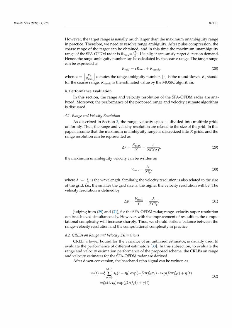
After down-conversion, the baseband echo signal can be written as

sr(t) =ξM−1

∑m=0

sb(t− τ0) exp(−j2π fmτ0) · exp(j2π fdt) + η(t)

=ξs(t, τ0) exp(j2π fdt) + η(t)

(32)

Remote Sens. 2022, 14, 278 9 of 16

where s(t, τ0) =M−1∑

m=0sb(t− τ0) exp(−j2π fmτ0). τ0=

2r0c is the time delay. fd=

2vλ is the

Doppler shift. Assume that the signal is sampled G times with time interval ∆t, and thegth sample can be described as

sr(g) = ξs(g∆t, τ0) exp(j2π fdg∆t) + η(g∆t). (33)

Suppose that the noise η(g∆t) is white Gaussian noise with zero mean and varianceσ2. Thus, the conditional probability density function (PDF) [33] of sr can be formulated as

p(sr|τ0, v ) =1

(2πσ2)G2

exp

[G−1

∑g=0− 1

2σ2 |sr(g)− ξs(g∆t, τ0) exp(j2π fdg∆t)|2]

, (34)

where sr = [sr(0), sr(1), . . . , sr(G− 1)]T . According to the PDF, the log-likelihood func-tion [33] is

ln p(sr|τ0, v ) = − ln(

2πσ2) G

2 − 12σ2

[G−1

∑g=0|sr(g)− ξs(g∆t, τ0) exp(j2π fdg∆t)|2

]. (35)

Next, we need to calculate the Fisher information matrix I. The Fisher information ma-trix [33] is defined as

I =

−E[

∂2 ln p(sr |τ0,v)∂τ0

2

]−E[

∂2 ln p(sr |τ0,v)∂τ0∂v

]−E[

∂2 ln p(sr |τ0,v)∂v∂τ0

]−E[

∂2 ln p(sr |τ0,v)∂v2

] , (36)

let the time interval ∆t tend to zero. Substituting (35) into (36), we can obtain

I11 = −E[

∂2 ln p(sr|τ0, v)∂τ02

]=

2|ξ|2

N0

∫ +∞

−∞

∣∣∣∣∂s(t, τ0)

∂τ0

∣∣∣∣2dt, (37)

I12 = −E[

∂2 ln p(sr|τ0, v)∂τ0∂v

]=

2|ξ|2

N0Re{∫ +∞

−∞j4π

λts∗(t, τ0)

∂s(t, τ0)

∂τ0dt}

, (38)

I21 = −E[

∂2 ln p(sr|τ0, v)∂v∂τ0

]=I12, (39)

I22 = −E[

∂2 ln p(sr|τ0, v)∂v2

]=

2|ξ|2

N0

16π2

λ2

∫ +∞

−∞t2|s(t, τ0)|

2dt. (40)

Hence, the CRLBs on time delay and velocity estimations can be expressed as

CRLB(τ0)=I22

I11 I22 − I12 I21, (41)

CRLB(v)=I11

I11 I22 − I12 I21. (42)

From (41), the CRLB on range estimation is

CRLB(r0)=c2CRLB(τ0)

4. (43)

5. Simulations

In this section, several numerical simulations are performed to verify the effective-ness of the proposed processing scheme. The range–velocity estimation performance isalso analyzed.

Remote Sens. 2022, 14, 278 10 of 16

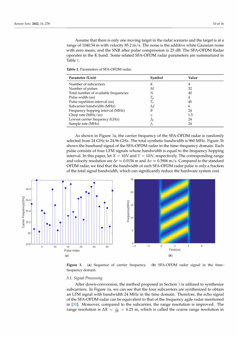
Assume that there is only one moving target in the radar scenario and the target is at arange of 1040.54 m with velocity 85.2 m/s. The noise is the additive white Gaussian noisewith zero mean, and the SNR after pulse compression is 25 dB. The SFA-OFDM Radaroperates in the K band. Some related SFA-OFDM radar parameters are summarized inTable 1.

Table 1. Parameters of SFA-OFDM radar.

Parameter (Unit) Symbol Value

Number of subcarriers K 4Number of pulses M 32Total number of available frequencies N 40Pulse width (us) Tp 4Pulse repetition interval (us) Tr 40Subcarrier bandwidth (MHz) ∆ f 6Frequency hopping interval (MHz) B 24Chirp rate (MHz/us) γ 1.5Lowest carrier frequency (GHz) f0 24Sample rate (MHz) fs 24

As shown in Figure 3a, the carrier frequency of the SFA-OFDM radar is randomlyselected from 24 GHz to 24.96 GHz. The total synthetic bandwidth is 960 MHz. Figure 3bshows the baseband signal of the SFA-OFDM radar in the time–frequency domain. Eachpulse consists of four LFM signals whose bandwidth is equal to the frequency hoppinginterval. In this paper, let X = 10N and Y = 10N, respectively. The corresponding rangeand velocity resolution are ∆r ≈ 0.0156 m and ∆v ≈ 0.3906 m/s. Compared to the standardOFDM radar, we find that the bandwidth of each SFA-OFDM radar pulse is only a fractionof the total signal bandwidth, which can significantly reduce the hardware system cost.

5 10 15 20 25 30

Pulse Index

24.8

25

25.2

25.4

25.6

25.8

Car

rier

Fre

quen

cy(G

Hz)

(a)

4 2 0 2 4 6

Time(us)

0

5

10

15

20

25

Fre

quen

cy(M

Hz)

﹣ ﹣

(b)

Figure 3. (a) Sequence of carrier frequency. (b) SFA-OFDM radar signal in the time–frequency domain.

5.1. Signal Processing

After down-conversion, the method proposed in Section 3 is utilized to synthesizesubcarriers. In Figure 4a, we can see that the four subcarriers are synthesized to obtainan LFM signal with bandwidth 24 MHz in the time domain. Therefore, the echo signalof the SFA-OFDM radar can be equivalent to that of the frequency agile radar mentionedin [30]. Moreover, compared to the subcarrier, the range resolution is improved. Therange resolution is ∆R = c

2B = 6.25 m, which is called the coarse range resolution in

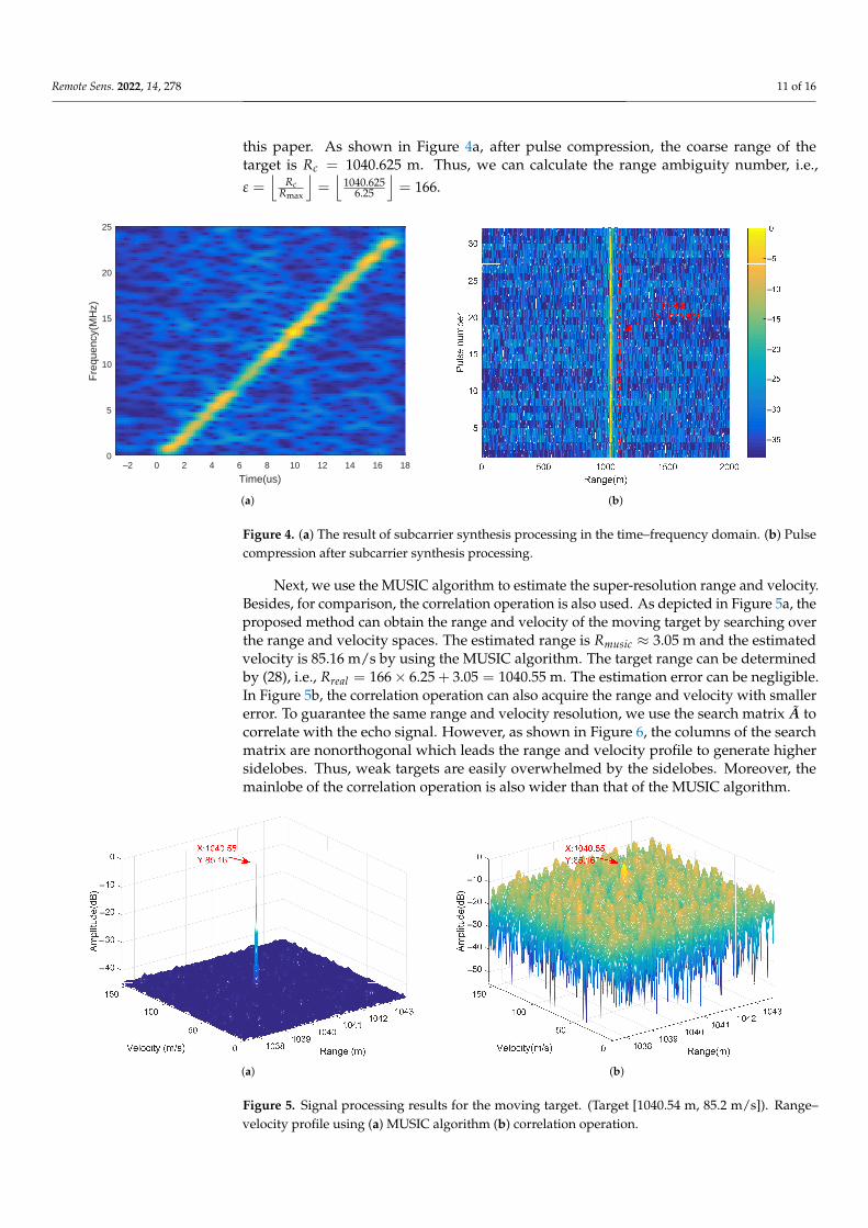
Remote Sens. 2022, 14, 278 11 of 16

this paper. As shown in Figure 4a, after pulse compression, the coarse range of thetarget is Rc = 1040.625 m. Thus, we can calculate the range ambiguity number, i.e.,ε =

⌊Rc

Rmax

⌋=⌊

1040.6256.25

⌋= 166.

2 0 2 4 6 8 10 12 14 16 18

Time(us)

0

5

10

15

20

25

Fre

quen

cy(M

Hz)

﹣

(a)

﹣

﹣

﹣

﹣

﹣

﹣

﹣

(b)

Figure 4. (a) The result of subcarrier synthesis processing in the time–frequency domain. (b) Pulsecompression after subcarrier synthesis processing.

Next, we use the MUSIC algorithm to estimate the super-resolution range and velocity.Besides, for comparison, the correlation operation is also used. As depicted in Figure 5a, theproposed method can obtain the range and velocity of the moving target by searching overthe range and velocity spaces. The estimated range is Rmusic ≈ 3.05 m and the estimatedvelocity is 85.16 m/s by using the MUSIC algorithm. The target range can be determinedby (28), i.e., Rreal = 166× 6.25 + 3.05 = 1040.55 m. The estimation error can be negligible.In Figure 5b, the correlation operation can also acquire the range and velocity with smallererror. To guarantee the same range and velocity resolution, we use the search matrix A tocorrelate with the echo signal. However, as shown in Figure 6, the columns of the searchmatrix are nonorthogonal which leads the range and velocity profile to generate highersidelobes. Thus, weak targets are easily overwhelmed by the sidelobes. Moreover, themainlobe of the correlation operation is also wider than that of the MUSIC algorithm.

﹣

﹣

﹣

﹣

(a)

﹣

﹣

﹣

﹣

﹣

(b)

Figure 5. Signal processing results for the moving target. (Target [1040.54 m, 85.2 m/s]). Range–velocity profile using (a) MUSIC algorithm (b) correlation operation.

Remote Sens. 2022, 14, 278 12 of 16

1038 1039 1040 1041 1042 1043

Range(m)

45

40

35

30

25

20

15

10

5

0

Am

plitu

de(d

B)

CorrelationMUSICReal range

﹣

﹣

﹣

﹣

﹣

﹣

﹣

﹣

﹣

(a)

0 50 100 150

Velocity(m/s)

45

40

35

30

25

20

15

10

5

0

Am

plitu

de(d

B)

CorrelationMUSICReal velocity

﹣

﹣

﹣

﹣

﹣

﹣

﹣

﹣

﹣

(b)

Figure 6. Range and velocity profiles (a) Range profile at 1040.54 m. (b) Velocity profile at 85.2 m/s.

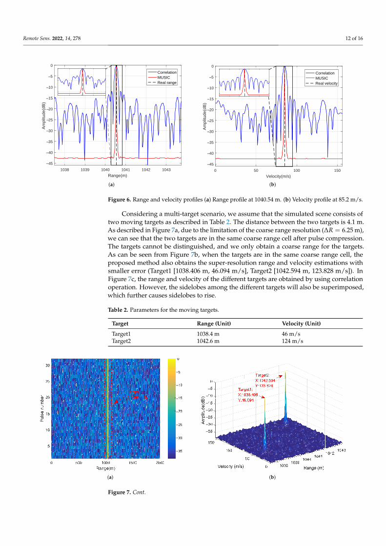
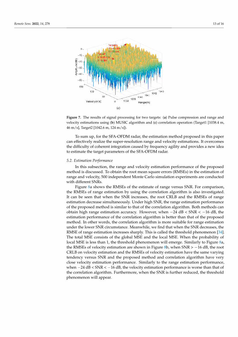
Considering a multi-target scenario, we assume that the simulated scene consists oftwo moving targets as described in Table 2. The distance between the two targets is 4.1 m.As described in Figure 7a, due to the limitation of the coarse range resolution (∆R = 6.25 m),we can see that the two targets are in the same coarse range cell after pulse compression.The targets cannot be distinguished, and we only obtain a coarse range for the targets.As can be seen from Figure 7b, when the targets are in the same coarse range cell, theproposed method also obtains the super-resolution range and velocity estimations withsmaller error (Target1 [1038.406 m, 46.094 m/s], Target2 [1042.594 m, 123.828 m/s]). InFigure 7c, the range and velocity of the different targets are obtained by using correlationoperation. However, the sidelobes among the different targets will also be superimposed,which further causes sidelobes to rise.

Table 2. Parameters for the moving targets.

Target Range (Unit) Velocity (Unit)

Target1 1038.4 m 46 m/sTarget2 1042.6 m 124 m/s

﹣

﹣

﹣

﹣

﹣

﹣

﹣

(a)

﹣

﹣

﹣

﹣

﹣

﹣

﹣

(b)

Figure 7. Cont.

Remote Sens. 2022, 14, 278 13 of 16

﹣

﹣

﹣

﹣

﹣

(c)

Figure 7. The results of signal processing for two targets: (a) Pulse compression and range andvelocity estimations using (b) MUSIC algorithm and (c) correlation operation (Target1 [1038.4 m,46 m/s], Target2 [1042.6 m, 124 m/s]).

To sum up, for the SFA-OFDM radar, the estimation method proposed in this papercan effectively realize the super-resolution range and velocity estimations. It overcomesthe difficulty of coherent integration caused by frequency agility and provides a new ideato estimate the target parameters of the SFA-OFDM radar.

5.2. Estimation Performance

In this subsection, the range and velocity estimation performance of the proposedmethod is discussed. To obtain the root mean square errors (RMSEs) in the estimation ofrange and velocity, 500 independent Monte Carlo simulation experiments are conductedwith different SNRs.

Figure 8a shows the RMSEs of the estimate of range versus SNR. For comparison,the RMSEs of range estimation by using the correlation algorithm is also investigated.It can be seen that when the SNR increases, the root CRLB and the RMSEs of rangeestimation decrease simultaneously. Under high SNR, the range estimation performanceof the proposed method is similar to that of the correlation algorithm. Both methods canobtain high range estimation accuracy. However, when −24 dB < SNR < −16 dB, theestimation performance of the correlation algorithm is better than that of the proposedmethod. In other words, the correlation algorithm is more suitable for range estimationunder the lower SNR circumstance. Meanwhile, we find that when the SNR decreases, theRMSE of range estimation increases sharply. This is called the threshold phenomenon [34].The total MSE consists of the global MSE and the local MSE. When the probability oflocal MSE is less than 1, the threshold phenomenon will emerge. Similarly to Figure 8a,the RMSEs of velocity estimation are shown in Figure 8b, when SNR > −16 dB, the rootCRLB on velocity estimation and the RMSEs of velocity estimation have the same varyingtendency versus SNR and the proposed method and correlation algorithm have veryclose velocity estimation performance. Similarly to the range estimation performance,when −24 dB < SNR < −16 dB, the velocity estimation performance is worse than that ofthe correlation algorithm. Furthermore, when the SNR is further reduced, the thresholdphenomenon will appear.

Remote Sens. 2022, 14, 278 14 of 16

4

28 26 24 22 20 18 16 14 12 10 8 6

SNR(dB)

10

10 3

10 2

10 1

100

101

Roo

t mea

n sq

uare

err

or o

f ran

ge(m

)

Correlation algorithmproposed methodRoot CRB of range

﹣ ﹣ ﹣ ﹣ ﹣ ﹣ ﹣ ﹣ ﹣ ﹣ ﹣ ﹣

﹣

﹣

﹣

﹣

(a)

2

28 26 24 22 20 18 16 14 12 10 8 6

SNR(dB)

10

10 1

100

101

102

Roo

t mea

n sq

uare

err

or o

f vel

ocity

(m/s

) Correlation algorithmproposed methodRoot CRB of velocity

﹣

﹣

﹣ ﹣ ﹣ ﹣ ﹣ ﹣ ﹣ ﹣ ﹣ ﹣ ﹣﹣

(b)

Figure 8. RMSEs of range and velocity estimations. (a) RMSEs in the estimation of range. (b) RMSEsin the estimation of velocity.

6. Conclusions

In this paper, to achieve the super-resolution range and velocity estimations simul-taneously, a new signal processing scheme for the SFA-OFDM radar is investigated. Itcan effectively solve the problem of coherent integration caused by frequency agility. Thesubcarriers of each pulse are synthesized to an LFM signal at first. Then, the parame-ter estimations for the SFA-OFDM radar are equivalent to that of a linear array and theMUSIC algorithm is introduced to obtain the super-resolution range and velocity. Therange–velocity resolution of the SFA-OFDM radar is only related to the size of the gridwhen the frequency hopping interval B is determined. Theoretical analyses and numericalexperiments show that the proposed signal processing scheme can estimate the range andvelocity of targets with small error. In future work, the communication information willbe embedded in the varied frequencies to realize the integration of radar and commu-nication. Moreover, the SFA-OFDM waveform will be used for super-resolution radarimaging, which can enhance the ECCM performance of the radar system while reducingthe system complexity.

Author Contributions: Conceptualization, Z.L. and Y.Q.; methodology, Z.L.; software, Z.L.; val-idation, Y.Q. and M.X.; formal analysis, Y.W.; investigation, Z.L.; resources, Y.Q.; data curation,Z.L.; writing—original draft preparation, Z.L.; writing—review and editing, Z.L.; visualization, Z.L.;supervision, Y.Q.; project administration, Y.Q.; funding acquisition, Y.Q. All authors have read andagreed to the published version of the manuscript.

Funding: This work was supported by National Natural Science Foundation of China (61772397).

Institutional Review Board Statement: Not applicable.

Informed Consent Statement: Not applicable.

Data Availability Statement: The data is available to readers by contacting the corresponding author.

Acknowledgments: The author would like to thank the Institute of Advanced Remote Sensing Technology.

Conflicts of Interest: The authors declare no conflict of interest.

References1. Hwang, T.; Yang, C.; Wu, G.; Li, S.; Li, G.Y. OFDM and Its Wireless Applications: A Survey. IEEE Trans. Veh. Technol. 2009,

58, 1673–1694. [CrossRef]2. Siriwongpairat, W.; Su, W.; Olfat, M.; Liu, K.R. Multiband-OFDM MIMO coding framework for UWB communication systems.

IEEE Trans. Signal Process. 2006, 54, 214–224. [CrossRef]

Remote Sens. 2022, 14, 278 15 of 16

3. Wang, M.M.; Xiao, L.; Brown, T.; Dong, M. Optimal symbol timing for OFDM wireless communications. IEEE Trans. Wirel.Commun. 2009, 8, 5328–5337. [CrossRef]

4. Wang, J.; Zhang, B.; Lei, P. Ambiguity function analysis for OFDM radar signals. In Proceedings of the 2016 CIE InternationalConference on Radar (RADAR), Guangzhou, China, 10–13 October 2016; pp. 1–5. [CrossRef]

5. Demeechai, T.; Chang, T.G.; Siwamogsatham, S. Performance of a Frequency-Domain OFDM-Timing Estimator. IEEE Commun.Lett. 2012, 16, 1680–1683. [CrossRef]

6. Zhang, T.; Xia, X.G. OFDM Synthetic Aperture Radar Imaging With Sufficient Cyclic Prefix. IEEE Trans. Geosci. Remote Sens. 2015,53, 394–404. [CrossRef]

7. Slimane, Z.; Abdelmalek, A.; Feham, M. OFDM Based UWB Synthetic Aperture Through-wall Imaging Radar. In Proceedingsof the 2008 Third International Conference on Broadband Communications, Information Technology Biomedical Applications,Pretoria, South Africa, 23–26 November 2008; pp. 293–300. [CrossRef]

8. Sen, S.; Tang, G.; Nehorai, A. Multiobjective Optimization of OFDM Radar Waveform for Target Detection. IEEE Trans. SignalProcess. 2011, 59, 639–652. [CrossRef]

9. Chabriel, G.; Barrère, J. Adaptive Target Detection Techniques for OFDM-Based Passive Radar Exploiting Spatial Diversity. IEEETrans. Signal Process. 2017, 65, 5873–5884. [CrossRef]

10. Liu, Y.; Liao, G.; Chen, Y.; Xu, J.; Yin, Y. Super-Resolution Range and Velocity Estimations With OFDM Integrated Radar andCommunications Waveform. IEEE Trans. Veh. Technol. 2020, 69, 11659–11672. [CrossRef]

11. Chiriyath, A.R.; Ragi, S.; Mittelmann, H.D.; Bliss, D.W. Novel Radar Waveform Optimization for a Cooperative Radar-Communications System. IEEE Trans. Aerosp. Electron. Syst. 2019, 55, 1160–1173. [CrossRef]

12. Cao, N.; Chen, Y.; Gu, X.; Feng, W. Joint Radar-Communication Waveform Designs Using Signals From Multiplexed Users. IEEETrans. Commun. 2020, 68, 5216–5227. [CrossRef]

13. Huo, K.; Deng, B.; Liu, Y.; Jiang, W.; Mao, J. The principle of synthesizing HRRP based on a new OFDM phase-coded stepped-frequency radar signal. In Proceedings of the IEEE 10th International Conference on Signal Processing Proceedings, Beijing,China, 24–28 October 2010; pp. 1994–1998. [CrossRef]

14. Schweizer, B.; Knill, C.; Schindler, D.; Waldschmidt, C. Stepped-Carrier OFDM-Radar Processing Scheme to Retrieve High-Resolution Range-Velocity Profile at Low Sampling Rate. IEEE Trans. Microw. Theory Tech. 2018, 66, 1610–1618. [CrossRef]

15. Nuss, B.; Mayer, J.; Marahrens, S.; Zwick, T. Frequency Comb OFDM Radar System With High Range Resolution and LowSampling Rate. IEEE Trans. Microw. Theory Tech. 2020, 68, 3861–3871. [CrossRef]

16. Nuss, B.; de Oliveira, L.G.; Zwick, T. Frequency Comb MIMO OFDM Radar With Nonequidistant Subcarrier Interleaving. IEEEMicrow. Wirel. Components Lett. 2020, 30, 1209–1212. [CrossRef]

17. Quan, Y.; Wu, Y.; Li, Y.; Sun, G.; Xing, M. Range–Doppler reconstruction for frequency agile and PRF-jittering radar. IET RadarSonar Navig. 2018, 12, 348–352. [CrossRef]

18. Huang, P.; Dong, S.; Liu, X.; Jiang, X.; Liao, G.; Xu, H.; Sun, S. A Coherent Integration Method for Moving Target Detection UsingFrequency Agile Radar. IEEE Geosci. Remote Sens. Lett. 2019, 16, 206–210. [CrossRef]

19. Huang, T.; Liu, Y.; Xu, X.; Eldar, Y.C.; Wang, X. Analysis of Frequency Agile Radar via Compressed Sensing. IEEE Trans. SignalProcess. 2018, 66, 6228–6240. [CrossRef]

20. Lellouch, G.; Pribic, R.; van Genderen, P. OFDM waveforms for frequency agility and opportunities for Doppler processing inradar. In Proceedings of the 2008 IEEE Radar Conference, Rome, Italy, 26–30 May 2008; pp. 1–6. [CrossRef]

21. Lellouch, G.; Pribic, R.; van Genderen, P. Frequency agile stepped OFDM waveform for HRR. In Proceedings of the 2009International Waveform Diversity and Design Conference, Kissimmee, FL, USA, 8–13 February 2009; pp. 90–93. [CrossRef]

22. Long, X.; Li, K.; Tian, J.; Wang, J.; Wu, S. Ambiguity Function Analysis of Random Frequency and PRI Agile Signals. IEEE Trans.Aerosp. Electron. Syst. 2021, 57, 382–396. [CrossRef]

23. Knill, C.; Schweizer, B.; Sparrer, S.; Roos, F.; Fischer, R.F.H.; Waldschmidt, C. High Range and Doppler Resolution by Applicationof Compressed Sensing Using Low Baseband Bandwidth OFDM Radar. IEEE Trans. Microw. Theory Tech. 2018, 66, 3535–3546.[CrossRef]

24. Knill, C.; Schweizer, B.; Stephany, S.; Werbunat, D.; Waldschmidt, C. FMCW-Interference of Frequency Agile OFDM Radars. InProceedings of the 2020 17th European Radar Conference (EuRAD), Utrecht, The Netherlands, 10–15 January 2021; pp. 160–163.[CrossRef]

25. Knill, C.; Schweizer, B.; Waldschmidt, C. Interference-Robust Processing of OFDM Radar Signals Using Compressed Sensing.IEEE Sens. Lett. 2020, 4, 1–4. [CrossRef]

26. Rida, I.; Al-Maadeed, S.; Mahmood, A.; Bouridane, A.; Bakshi, S. Palmprint Identification Using an Ensemble of SparseRepresentations. IEEE Access 2018, 6, 3241–3248. [CrossRef]

27. Schmidt, R. Multiple emitter location and signal parameter estimation. IEEE Trans. Antennas Propag. 1986, 34, 276–280. [CrossRef]28. Cheng, F.; He, Z.; Liu, H.; Li, J. The parameter setting problem of signal OFDM-LFM for MIMO radar. In Proceedings of the 2008

International Conference on Communications, Circuits and Systems, Xiamen, China, 25–27 May 2008; pp. 876–880. [CrossRef]29. Lord, R.; Inggs, M. High range resolution radar using narrowband linear chirps offset in frequency. In Proceedings of the 1997

South African Symposium on Communications and Signal Processing, COMSIG ’97, Grahamstown, South Africa, 9–10 September1997; pp. 9–12. [CrossRef]

Remote Sens. 2022, 14, 278 16 of 16

30. Li, Y.; Huang, T.; Xu, X.; Liu, Y.; Wang, L.; Eldar, Y.C. Phase Transitions in Frequency Agile Radar Using Compressed Sensing.IEEE Trans. Signal Process. 2021, 69, 4801–4818. [CrossRef]

31. Zoltowski, M. Synthesis of sum and difference patterns possessing common nulls for monopulse bearing estimation with linearrays. IEEE Trans. Antennas Propag. 1992, 40, 25–37. [CrossRef]

32. Friedlander, B. A sensitivity analysis of the MUSIC algorithm. IEEE Trans. Acoust. Speech Signal Process. 1990, 38, 1740–1751.[CrossRef]

33. Kay, S.M. Fundamentals of Statistical Signal Processing: Estimation and Detection Theory; PRT Prentice Hall: Englewood Cliffs, NJ,USA, 1993.

34. Trees, H.L.V. Optimum Array Processing: Part IV of Detection, Estimation, and Modulation Theory; Wiley: Hoboken, NJ, USA, 2004.