Regional velocity modelling and depth conversion Otway ...

Regional velocity modelling and depth conversionOtway Basin, Victoria

J. Dunne & M. Boyd

Victorian Gas Program Technical Report 39

October 2020

VICTORIAN GAS PROGRAM

Authorised by the Director, Geological Survey of Victoria Department of Jobs, Precincts and Regions1 Spring Street Melbourne Victoria 3000Telephone (03) 9651 9999

© Copyright State of Victoria, 2020.

Department of Jobs, Precincts and Regions 2020

Except for any logos, emblems, trademarks, artwork and photography this work is made available under the terms of the Creative Commons Attribution 4.0 International License. To view a copy of this license, visit creativecommons.org/licenses/by/4.0/. It is a condition of this Creative Commons Attribution 4.0 International License that you must give credit to the original author who is the State of Victoria.

This document is also available in an accessible format at www.djpr.vic.gov.au

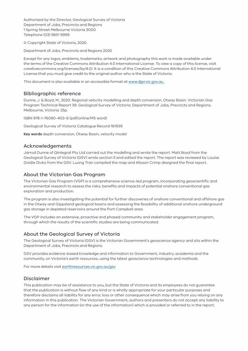
Bibliographic referenceDunne, J. & Boyd, M., 2020. Regional velocity modelling and depth conversion, Otway Basin. Victorian Gas Program Technical Report 39. Geological Survey of Victoria. Department of Jobs, Precincts and Regions. Melbourne, Victoria. 25p.

ISBN 978-1-76090-403-6 (pdf/online/MS word)

Geological Survey of Victoria Catalogue Record 161939

Key words depth conversion, Otway Basin, velocity model

AcknowledgementsJarrod Dunne of QIntegral Pty Ltd carried out the modelling and wrote the report. Matt Boyd from the Geological Survey of Victoria (GSV) wrote section 5 and edited the report. The report was reviewed by Louise Goldie Divko from the GSV. Luong Tran compiled the map and Allyson Crimp designed the final report.

About the Victorian Gas ProgramThe Victorian Gas Program (VGP) is a comprehensive science-led program, incorporating geoscientific and environmental research to assess the risks, benefits and impacts of potential onshore conventional gas exploration and production.

The program is also investigating the potential for further discoveries of onshore conventional and offshore gas in the Otway and Gippsland geological basins and assessing the feasibility of additional onshore underground gas storage in depleted reservoirs around the Port Campbell area.

The VGP includes an extensive, proactive and phased community and stakeholder engagement program, through which the results of the scientific studies are being communicated.

About the Geological Survey of VictoriaThe Geological Survey of Victoria (GSV) is the Victorian Government’s geoscience agency and sits within the Department of Jobs, Precincts and Regions.

GSV provides evidence-based knowledge and information to Government, industry, academia and the community, on Victoria’s earth resources, using the latest geoscience technologies and methods.

For more details visit earthresources.vic.gov.au/gsv

DisclaimerThis publication may be of assistance to you, but the State of Victoria and its employees do not guarantee that the publication is without flaw of any kind or is wholly appropriate for your particular purposes and therefore disclaims all liability for any error, loss or other consequence which may arise from you relying on any information in this publication. The Victorian Government, authors and presenters do not accept any liability to any person for the information (or the use of the information) which is provided or referred to in the report.

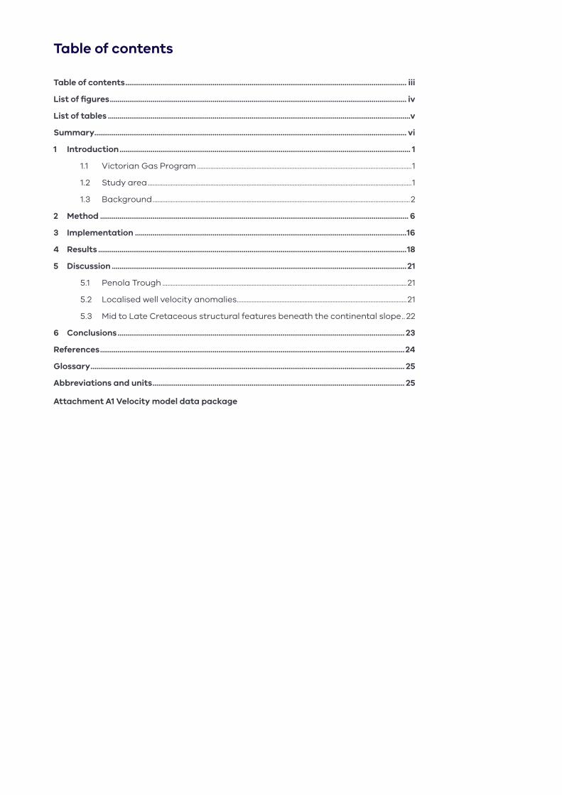
Table of contents

Table of contents ................................................................................................................................................. iii

List of figures ......................................................................................................................................................... iv

List of tables ............................................................................................................................................................v

Summary................................................................................................................................................................. vi

1 Introduction ...................................................................................................................................................... 1

1.1 Victorian Gas Program ..................................................................................................................................1

1.2 Study area ................................................................................................................................................................1

1.3 Background ............................................................................................................................................................2

2 Method ............................................................................................................................................................... 6

3 Implementation ............................................................................................................................................16

4 Results ...............................................................................................................................................................18

5 Discussion ........................................................................................................................................................21

5.1 Penola Trough ....................................................................................................................................................21

5.2 Localised well velocity anomalies .......................................................................................................21

5.3 Mid to Late Cretaceous structural features beneath the continental slope .. 22

6 Conclusions .................................................................................................................................................... 23

References .............................................................................................................................................................24

Glossary .................................................................................................................................................................. 25

Abbreviations and units .................................................................................................................................. 25

Attachment A1 Velocity model data package

List of figures

Figure 1.1 Extent of the updated Otway Basin velocity model. ...................................................................2

Figure 1.2 Examples of seismic velocity-based versus well-based time-depth data from the Otway Basin converted to average velocity. ...............................................................4

Figure 1.3 Raw time-depth data supplied from synthetic ties re-datumed to mudline/ground level and displayed relative to a single V0-k fit. ....................................................5

Figure 2.1 The Sediment Surface and Basement time maps used to build the velocity model for depth conversion. The map extent indicates the study area. ............... 7

Figure 2.2 Offshore Otway Basin well database showing edited time-depth pairs, correction factors and V0-k parameter fit. .........................................................................................8

Figure 2.3 Onshore Otway Basin well database showing edited time-depth pairs, correction factors and V0-k parameter fit. ........................................................................................8

Figure 2.4 Vint 3D model built from the sediment and basement time surfaces and the global V0-k trend. ................................................................................................................................................9

Figure 2.5 Edited well time-depth relations and KF well logs loaded into Petrel™ and extended with gradual tapering to a value of 1 (no velocity adjustment) through the basement..................................................................................................................................................... 10

Figure 2.6 Populated KF sub–volume model with basement (TWT) and wells with KF property. .................................................................................................................................................................. 10

Figure 2.7 Horizon slice through KF model at the Eumeralla surface. ................................................. 11

Figure 2.8 Derivation of the calibrated Vave model, starting with a) the raw Vave volume, which is multiplied by b) the KF model to give c) an initial (unsmoothed) calibrated Vave . .................................................................................................................................... 12

Figure 2.9 Top Sherbrook Group raw depth conversion (TVDSS). .........................................................13

Figure 2.10 Top Eumeralla Formation raw depth conversion (TVDSS). .............................................13

Figure 2.11 Initial residual error assessment for the Sherbrook Group and Eumeralla Formation depth conversions using tops taken direction from well completion reports for the wells (black dots). .....................................................................................14

Figure 2.12 Isopach quality control from the raw depth converted events (hotter colours indicate thicker intervals). .........................................................................................................................14

Figure 2.13 Velocity extraction on the basement showing a) artefacts that are mostly caused by the necessary coarseness of the velocity model and b) mitigation using heavy lateral smoothing. The impact on the raw depth maps is shown c) before and d) after lateral smoothing. .....................................................................15

Figure 3.1 Profile showing five primary unconformable horizons (layers) and the 500 ms velocity ramp layer below the top of the basement used as basis for the velocity model. ............................................................................................................................................................... 17

Figure 3.2 Section showing the velocity profile with depth of burial, well corrections, limits and basement velocity applied.................................................................................... 17

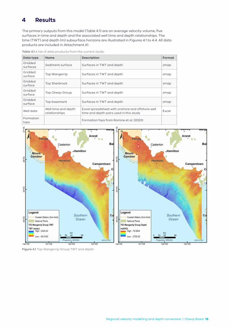
Figure 4.1 Top Wangerrip Group TWT and depth. ..............................................................................................18

Figure 4.2 Top Sherbrook Group TWT and depth. .............................................................................................19

Figure 4.3 Top Eumeralla Formation TWT and depth. ....................................................................................19

Figure 4.4 Basement TWT and depth. ........................................................................................................................20

Figure 5.1 Top of the Sherbrook Group depth surface (blue horizon in section) showing structural features present beneath the continental slope. ....................................... 22

List of tables

Table 1.1 Comparison of well versus processing velocity seismic depth conversion methods. ............................................................................................................................................................3

Table 2.1 Time surfaces supplied and their usage during the depth conversion. ........................ 7

Table 3.1 Horizons and zones used to populate the Petrel™ property model. ..............................16

Table 4.1 A list of data products from the current study. ..............................................................................18

Regional velocity modelling and depth conversion | Otway Basin vi

Summary

As part of the Victorian Gas Program (VGP), the Geological Survey of Victoria (GSV) is studying the Otway Basin’s petroleum systems components (reservoir, seal and source), to assess its petroleum prospectivity and to estimate the potential for further conventional gas discoveries onshore and offshore within Victoria’s jurisdiction.

A velocity model was built to convert time surfaces to depth as part of the Otway Basin three-dimensional (3D) geological framework model (Romine et al., 2020). Further work was required to extend the model across the Penola Trough in South Australia and south to the base of the continental slope offshore so that these key areas could be included in petroleum systems analysis.

This new model will ensure that all available seismic interpretations are depth converted for use in petroleum systems modelling across the full extent of the VGP study area and over known hydrocarbon accumulations and associated source rocks onshore and offshore. These key areas are important to petroleum systems modelling. Each area has been identified as either: a) having potential to contribute to gas accumulations within the Victorian part of the Otway Basin; b) an analogue for significant Otway Basin petroleum system components; or c) a distal element of an active petroleum system in the Otway Basin.

This updated velocity model was built using a single best fit depth of burial velocity equation derived from well data to closely approximate the vertical seismic velocities across the study area. This approximation of the velocity field was then modified using direct measurement at wells to match the velocity at each well location.

This study provides a relatively simple and robust methodology for later refinement and extension of the velocity model as required for future basin analysis.

Regional velocity modelling and depth conversion | Otway Basin 1

1 Introduction

1.1 Victorian Gas Program

The Victorian Gas Program (VGP) is a comprehensive program of scientific research and related activities to assess the potential for further discoveries of onshore conventional gas and offshore gas in Victoria, and whether the State’s current underground gas storage capacity could be expanded.

As part of the VGP, the Geological Survey of Victoria (GSV) is assessing the petroleum prospectivity and calculating an estimate of prospective gas resources of the Otway and Gippsland geological basins. The VGP is also examining the risks, benefits and impacts associated with onshore conventional gas to inform decisions of Government.

Models that describe the depth and distribution of the layers of rocks within the Otway Basin are required for the VGP petroleum systems studies. One of the primary data sets used to create these models are seismic surveys that have been acquired by industry and government in the Otway Basin over the last 50 years.

Seismic surveys record the time it takes for vibrations to travel from a vibration source to an underground rock layer and back to a receiver at the surface. Where wells intersect these layers, the relationship between the seismic time data and the well depth data can be used to convert the seismic time data into depth. These relationships can be extrapolated away from the wells. The method applied in this study used these relationships to create equations and correction factors to build the velocity model. The resultant model was then used to perform a depth conversion of the seismic data.

This approach to velocity modelling differs from the previous depth conversion (Romine et al., 2020), which used stacking (or seismic processing) velocities as its primary input. The well-based velocity modelling used in this approach improves the previous depth conversion by making it simpler to extend into areas with poor data coverage. This new velocity model also has a larger spatial extent to enable inclusion of highly relevant elements of working petroleum systems, which are present in the Otway Basin, both onshore and offshore.

1.2 Study area

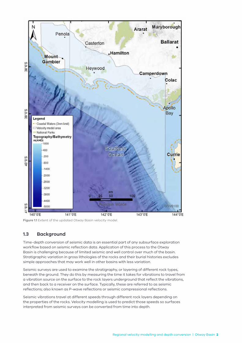
The Otway Basin is a north-west to south-east trending basin that extends for 500 kilometres along the onshore and offshore parts of south-western Victoria and into South Australia. The onshore Otway Basin geoscience program covers the Victorian onshore basin from the northern tip of the Otway Ranges, across south-west Victoria to the South Australian border. The updated velocity model extends outside the VGP study area across the Penola Trough in South Australia and south to the base of the continental slope offshore. (Figure 1.1).


Figure 1.1 Extent of the updated Otway Basin velocity model.

1.3 Background

Time-depth conversion of seismic data is an essential part of any subsurface exploration workflow based on seismic reflection data. Application of this process to the Otway Basin is challenging because of limited seismic and well control over much of the basin. Stratigraphic variation in gross lithologies of the rocks and their burial histories excludes simple approaches that may work well in other basins with less variation.

Seismic surveys are used to examine the stratigraphy, or layering of different rock types, beneath the ground. They do this by measuring the time it takes for vibrations to travel from a vibration source on the surface to the rock layers underground that reflect the vibrations, and then back to a receiver on the surface. Typically, these are referred to as seismic reflections; also known as P-wave reflections or seismic compressional reflections.

Seismic vibrations travel at different speeds through different rock layers depending on the properties of the rocks. Velocity modelling is used to predict those speeds so surfaces interpreted from seismic surveys can be converted from time into depth.


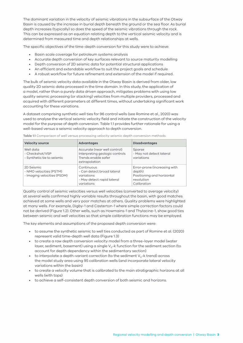
The dominant variation in the velocity of seismic vibrations in the subsurface of the Otway Basin is caused by the increase in burial depth beneath the ground or the sea floor. As burial depth increases (typically) so does the speed of the seismic vibrations through the rock. This can be expressed as an equation relating depth to the vertical seismic velocity and is determined from measured time and depth relationships at wells.

The specific objectives of the time-depth conversion for this study were to achieve:

• Basin scale coverage for petroleum systems analysis• Accurate depth conversion of key surfaces relevant to source maturity modelling• Depth conversion of 2D seismic data for potential structural applications• An efficient and extendable workflow to suit the project goals and schedule • A robust workflow for future refinement and extension of the model if required.

The bulk of seismic velocity data available in the Otway Basin is derived from older, low quality 2D seismic data processed in the time domain. In this study, the application of a model, rather than a purely data driven approach, mitigates problems with using low quality seismic processing (or stacking) velocities from multiple providers, processed and acquired with different parameters at different times, without undertaking significant work accounting for these variations.

A dataset comprising synthetic well ties for 96 control wells (see Romine et al., 2020) was used to analyse the vertical seismic velocity field and initiate the construction of the velocity model for the purpose of depth conversion. Table 1.1 provides further rationale for using a well-based versus a seismic velocity approach to depth conversion.

Table 1.1 Comparison of well versus processing velocity seismic depth conversion methods.

Velocity source Advantages Disadvantages

Well data- Checkshot/VSP- Synthetic tie to seismic

Accurate (near well control)Interpreting geologic controlsTrends enable safer extrapolation

Sparse - May not detect lateral variations

2D Seismic- NMO velocities (PSTM)- Imaging velocities (PSDM)

Continuous- Can detect broad lateral variations- May detect rapid lateral variations

Error-prone (increasing with depth)Positioning and horizontal resolutionCalibration

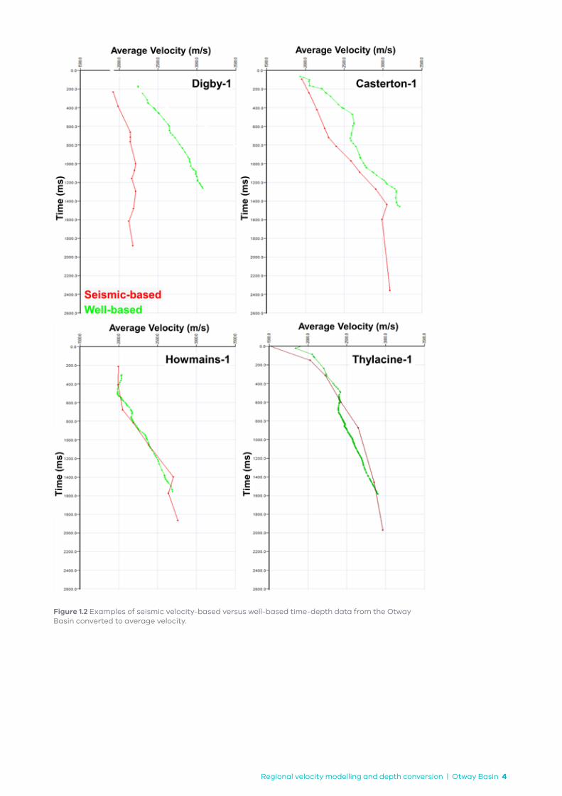
Quality control of seismic velocities versus well velocities (converted to average velocity) at several wells confirmed highly variable results throughout the basin, with good matches achieved at some wells and very poor matches at others. Quality problems were highlighted at many wells. For example, Digby-1 and Casterton-1 where simple correction factors could not be derived (Figure 1.2). Other wells, such as Howmains-1 and Thylacine-1, show good ties between seismic and well velocities so that simple calibration functions may be employed.

The key elements and assumptions of the proposed depth conversion were:

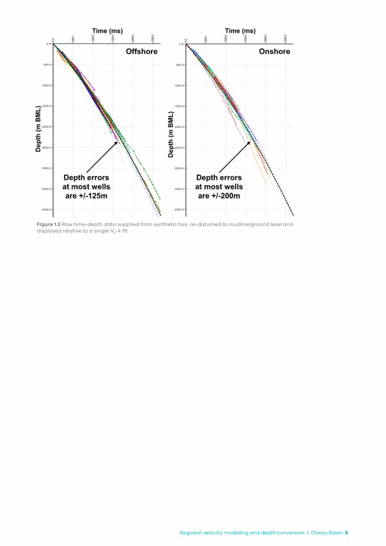
• to assume the synthetic seismic to well ties conducted as part of Romine et al. (2020) represent valid time-depth well data (Figure 1.3)

• to create a raw depth conversion velocity model from a three-layer model (water layer, sediment, basement) using a single V0-k function for the sediment section (to account for depth dependency within the sedimentary section)

• to interpolate a depth-variant correction (to the sediment V0-k trend) across the model study area using 95 calibration wells (and incorporate lateral velocity variations within the basin)

• to create a velocity volume that is calibrated to the main stratigraphic horizons at all wells (with tops)

• to achieve a self-consistent depth conversion of both seismic and horizons.


Figure 1.2 Examples of seismic velocity-based versus well-based time-depth data from the Otway Basin converted to average velocity.


Figure 1.3 Raw time-depth data supplied from synthetic ties re-datumed to mudline/ground level and displayed relative to a single V0-k fit.


2 Method

The approach used in this report is often referred to as the V0-k method. A three-layer model was implemented, whereby the water layer (where it exists offshore) was represented by a constant interval velocity of 1500 m/s. This interval velocity can be used to depth convert a time map of the sea floor using:

where zsf is in metres and tsf is in milliseconds.

Depth conversion (of horizons) to any level within the second (sediment) layer can then be achieved using:

where the V0-k values are estimated as global constants and only over the second (sediment) layer after re-datuming the time-depth well database to the sea floor.

At this point, the method is referred to as a two-layer V0-k depth conversion. An example of how the V0-k values can be derived is shown in Figure 2.2. In the expression above, the velocity term is an average velocity (Vave), which represents a single velocity (non-measurable velocity) to depth convert each layer. The equivalent interval velocity (Vint) can be determined using .

The method itself can be extended to an arbitrary number of layers. In this study, a third layer (the basement) was introduced with a constant velocity. Some additional complexity is required when the goal is to create a velocity volume for a one-step depth conversion using this method. These complexities are detailed in the remainder of this methods section.

The theoretical basis of the method is to represent mechanical and/or chemical compaction of rocks via the k term. This enables sensible extrapolation below the depth of well control, and thus sensible depth conversions in deeper parts of the model. The method is well suited in both clastic and carbonate settings where compaction accounts for most of the velocity dependence of the rocks. Constant velocity layers, such as evaporites and basement rocks can be handled by recasting the method in terms of interval velocities, provided that top and base horizons are available for the constant velocity layers. This method of determining the k term is similar to that of Smallwood (2002) who used the seafloor to constrain k in an area with a rapidly changing water depth.

Time-depth conversion methods can become very complicated once an attempt is made to reduce prediction errors at well control. This is sometimes referred to as “residual force-fitting” and it is mostly required to correct for limitations in the geophysics. Ideally, it should be implemented in a way that produces depth corrections that appear geologically meaningful.

The workflow for residual force-fitting method used in this study involved:

• Reducing depth conversion errors at the calibration wells to zero for all points along the well paths using correction factor logs, which were obtained by dividing the calibration well average velocity by the modelled velocity or V0-k

• 3D modelling in Petrel™ to interpolate or extrapolate the calibration well “correction factors” over the full study area, with key stratigraphic horizons guiding sensible interpolation between the calibration wells

• Multiplying the “correction factor” model and the Vave volume (derived from the multi-layer V0-k method) to calibrate the depth conversion of horizons, faults and seismic

• Assessing remaining uncertainty at non-calibration wells and applying a second stage of residual force-fitting to several horizons (thus further reducing errors in areas away from well control).

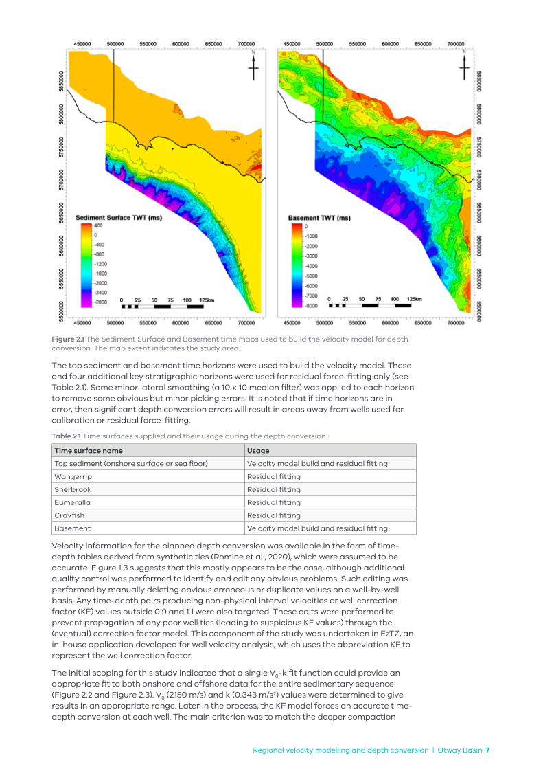
As the equations and discussion above indicate, the input data required for calibrated depth conversions include time maps, velocities and well tops. Figure 2.1 shows the key boundary layer time maps (as indicated in Table 2.1). The study area is indicated by the map extent and covers both the Victorian and South Australian parts of the Otway Basin and extends from onshore to offshore.


Figure 2.1 The Sediment Surface and Basement time maps used to build the velocity model for depth conversion. The map extent indicates the study area.

The top sediment and basement time horizons were used to build the velocity model. These and four additional key stratigraphic horizons were used for residual force-fitting only (see Table 2.1). Some minor lateral smoothing (a 10 x 10 median filter) was applied to each horizon to remove some obvious but minor picking errors. It is noted that if time horizons are in error, then significant depth conversion errors will result in areas away from wells used for calibration or residual force-fitting.

Table 2.1 Time surfaces supplied and their usage during the depth conversion.

Time surface name Usage

Top sediment (onshore surface or sea floor) Velocity model build and residual fitting

Wangerrip Residual fitting

Sherbrook Residual fitting

Eumeralla Residual fitting

Crayfish Residual fitting

Basement Velocity model build and residual fitting

Velocity information for the planned depth conversion was available in the form of time-depth tables derived from synthetic ties (Romine et al., 2020), which were assumed to be accurate. Figure 1.3 suggests that this mostly appears to be the case, although additional quality control was performed to identify and edit any obvious problems. Such editing was performed by manually deleting obvious erroneous or duplicate values on a well-by-well basis. Any time-depth pairs producing non-physical interval velocities or well correction factor (KF) values outside 0.9 and 1.1 were also targeted. These edits were performed to prevent propagation of any poor well ties (leading to suspicious KF values) through the (eventual) correction factor model. This component of the study was undertaken in EzTZ, an in-house application developed for well velocity analysis, which uses the abbreviation KF to represent the well correction factor.

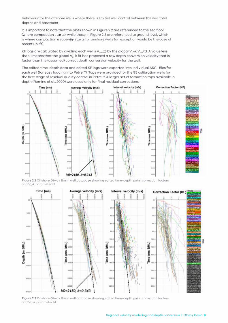
The initial scoping for this study indicated that a single V0-k fit function could provide an appropriate fit to both onshore and offshore data for the entire sedimentary sequence (Figure 2.2 and Figure 2.3). V0 (2150 m/s) and k (0.343 m/s2) values were determined to give results in an appropriate range. Later in the process, the KF model forces an accurate time-depth conversion at each well. The main criterion was to match the deeper compaction


behaviour for the offshore wells where there is limited well control between the well total depths and basement.

It is important to note that the plots shown in Figure 2.2 are referenced to the sea floor (where compaction starts), while those in Figure 2.3 are referenced to ground level, which is where compaction frequently starts for onshore wells (an exception would be the case of recent uplift).

KF logs are calculated by dividing each well’s Vave(t) by the global V0-k Vave(t). A value less than 1 means that the global V0-k fit has proposed a raw depth conversion velocity that is faster than the (assumed) correct depth conversion velocity for the well.

The edited time-depth data and edited KF logs were exported into individual ASCII files for each well (for easy loading into Petrel™). Tops were provided for the 95 calibration wells for the first stage of residual quality control in Petrel™. A larger set of formation tops available in depth (Romine et al., 2020) were used only for final residual corrections.

Figure 2.2 Offshore Otway Basin well database showing edited time-depth pairs, correction factors and V0-k parameter fit.

Figure 2.3 Onshore Otway Basin well database showing edited time-depth pairs, correction factors and V0-k parameter fit.


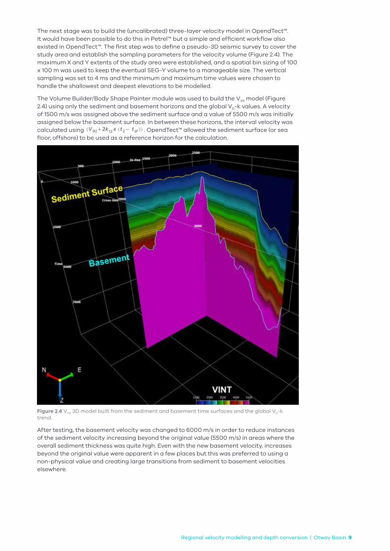
The next stage was to build the (uncalibrated) three-layer velocity model in OpendTect™. It would have been possible to do this in Petrel™ but a simple and efficient workflow also existed in OpendTect™. The first step was to define a pseudo-3D seismic survey to cover the study area and establish the sampling parameters for the velocity volume (Figure 2.4). The maximum X and Y extents of the study area were established, and a spatial bin sizing of 100 x 100 m was used to keep the eventual SEG-Y volume to a manageable size. The vertical sampling was set to 4 ms and the minimum and maximum time values were chosen to handle the shallowest and deepest elevations to be modelled.

The Volume Builder/Body Shape Painter module was used to build the Vint model (Figure 2.4) using only the sediment and basement horizons and the global V0-k values. A velocity of 1500 m/s was assigned above the sediment surface and a value of 5500 m/s was initially assigned below the basement surface. In between these horizons, the interval velocity was calculated using . OpendTect™ allowed the sediment surface (or sea floor, offshore) to be used as a reference horizon for the calculation.

Figure 2.4 Vint 3D model built from the sediment and basement time surfaces and the global V0-k trend.

After testing, the basement velocity was changed to 6000 m/s in order to reduce instances of the sediment velocity increasing beyond the original value (5500 m/s) in areas where the overall sediment thickness was quite high. Even with the new basement velocity, increases beyond the original value were apparent in a few places but this was preferred to using a non-physical value and creating large transitions from sediment to basement velocities elsewhere.


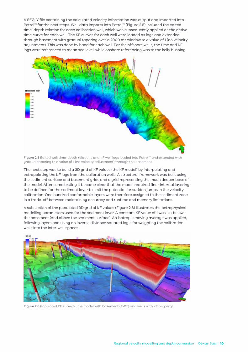
A SEG-Y file containing the calculated velocity information was output and imported into Petrel™ for the next steps. Well data imports into Petrel™ (Figure 2.5) included the edited time-depth relation for each calibration well, which was subsequently applied as the active time curve for each well. The KF curves for each well were loaded as logs and extended through basement with gradual tapering over a 2000 ms window to a value of 1 (no velocity adjustment). This was done by hand for each well. For the offshore wells, the time and KF logs were referenced to mean sea level, while onshore referencing was to the kelly bushing.

Figure 2.5 Edited well time-depth relations and KF well logs loaded into Petrel™ and extended with gradual tapering to a value of 1 (no velocity adjustment) through the basement.

The next step was to build a 3D grid of KF values (the KF model) by interpolating and extrapolating the KF logs from the calibration wells. A structural framework was built using the sediment surface and basement grids and a grid representing the much deeper base of the model. After some testing it became clear that the model required finer internal layering to be defined for the sediment layer to limit the potential for sudden jumps in the velocity calibration. One hundred conformable layers were therefore assigned to the sediment zone in a trade-off between maintaining accuracy and runtime and memory limitations.

A subsection of the populated 3D grid of KF values (Figure 2.6) illustrates the petrophysical modelling parameters used for the sediment layer. A constant KF value of 1 was set below the basement (and above the sediment surface). An isotropic moving average was applied, following layers and using an inverse distance squared logic for weighting the calibration wells into the inter-well spaces.

Figure 2.6 Populated KF sub–volume model with basement (TWT) and wells with KF property.


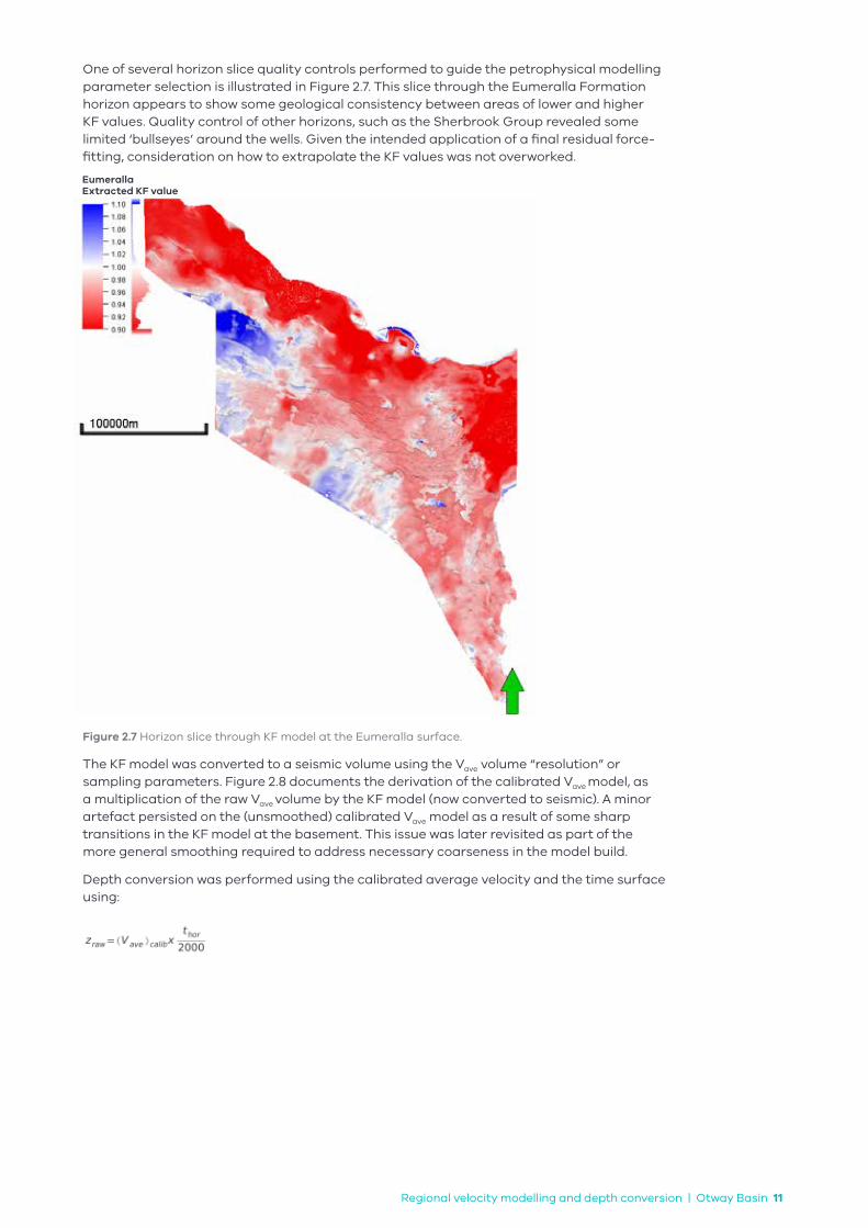
One of several horizon slice quality controls performed to guide the petrophysical modelling parameter selection is illustrated in Figure 2.7. This slice through the Eumeralla Formation horizon appears to show some geological consistency between areas of lower and higher KF values. Quality control of other horizons, such as the Sherbrook Group revealed some limited ‘bullseyes’ around the wells. Given the intended application of a final residual force-fitting, consideration on how to extrapolate the KF values was not overworked.

Figure 2.7 Horizon slice through KF model at the Eumeralla surface.

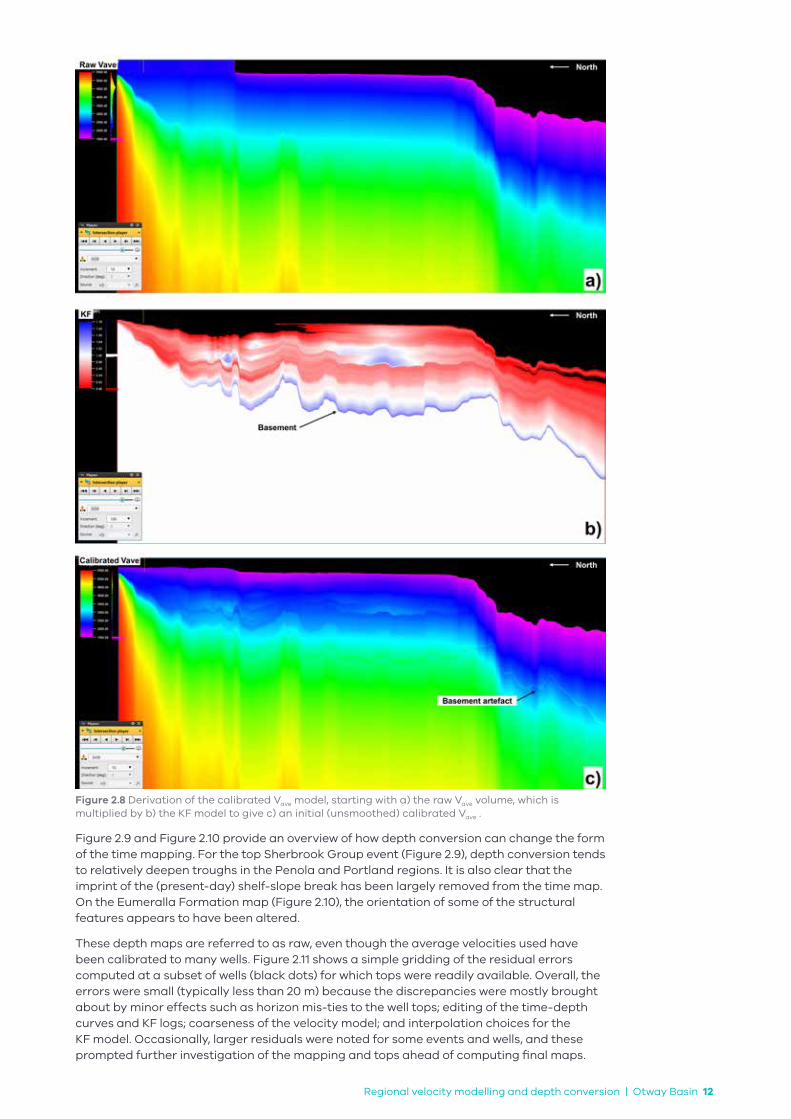
The KF model was converted to a seismic volume using the Vave volume “resolution” or sampling parameters. Figure 2.8 documents the derivation of the calibrated Vave model, as a multiplication of the raw Vave volume by the KF model (now converted to seismic). A minor artefact persisted on the (unsmoothed) calibrated Vave model as a result of some sharp transitions in the KF model at the basement. This issue was later revisited as part of the more general smoothing required to address necessary coarseness in the model build.

Depth conversion was performed using the calibrated average velocity and the time surface using:

EumerallaExtracted KF value


Figure 2.8 Derivation of the calibrated Vave model, starting with a) the raw Vave volume, which is multiplied by b) the KF model to give c) an initial (unsmoothed) calibrated Vave .

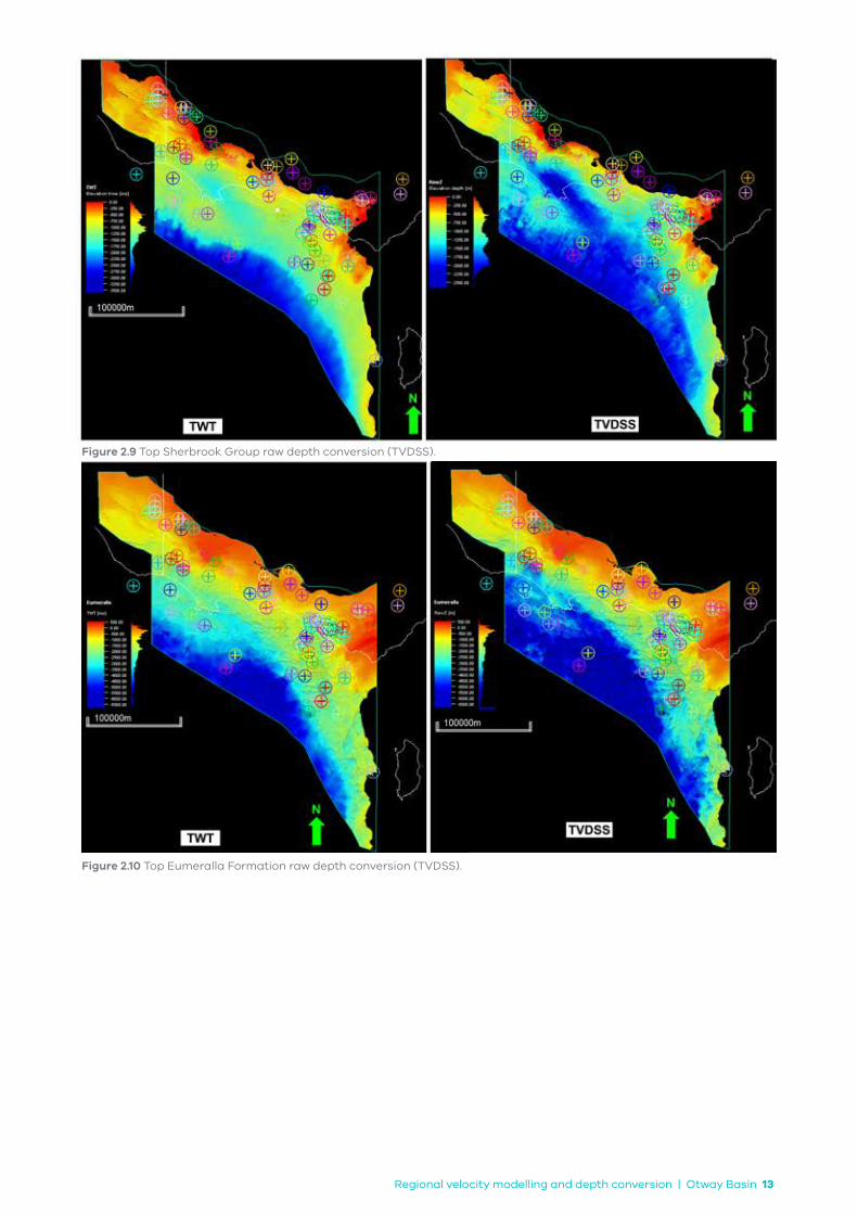
Figure 2.9 and Figure 2.10 provide an overview of how depth conversion can change the form of the time mapping. For the top Sherbrook Group event (Figure 2.9), depth conversion tends to relatively deepen troughs in the Penola and Portland regions. It is also clear that the imprint of the (present-day) shelf-slope break has been largely removed from the time map. On the Eumeralla Formation map (Figure 2.10), the orientation of some of the structural features appears to have been altered.

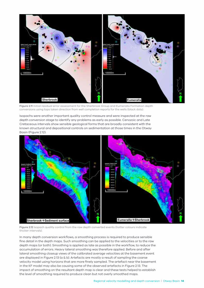
These depth maps are referred to as raw, even though the average velocities used have been calibrated to many wells. Figure 2.11 shows a simple gridding of the residual errors computed at a subset of wells (black dots) for which tops were readily available. Overall, the errors were small (typically less than 20 m) because the discrepancies were mostly brought about by minor effects such as horizon mis-ties to the well tops; editing of the time-depth curves and KF logs; coarseness of the velocity model; and interpolation choices for the KF model. Occasionally, larger residuals were noted for some events and wells, and these prompted further investigation of the mapping and tops ahead of computing final maps.


Figure 2.9 Top Sherbrook Group raw depth conversion (TVDSS).

Figure 2.10 Top Eumeralla Formation raw depth conversion (TVDSS).


Figure 2.11 Initial residual error assessment for the Sherbrook Group and Eumeralla Formation depth conversions using tops taken direction from well completion reports for the wells (black dots).

Isopachs were another important quality control measure and were inspected at the raw depth conversion stage to identify any problems as early as possible. Cenozoic and Late Cretaceous intervals show sensible geological forms that are broadly consistent with the known structural and depositional controls on sedimentation at those times in the Otway Basin (Figure 2.12).

Figure 2.12 Isopach quality control from the raw depth converted events (hotter colours indicate thicker intervals).

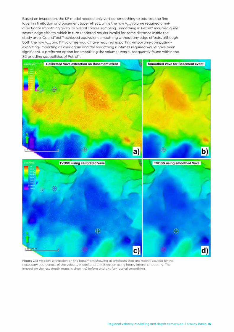
In many depth conversion workflows, a smoothing process is required to produce sensible fine detail in the depth maps. Such smoothing can be applied to the velocities or to the raw depth maps (or both). Smoothing is applied as late as possible in the workflow, to reduce the accumulation of errors. Heavy lateral smoothing was therefore applied. Before and after lateral smoothing closeup views of the calibrated average velocities at the basement event are displayed in Figure 2.13 (a & b). Artefacts are mostly a result of sampling the coarse velocity model using horizons that are more finely sampled. The artefact near the basement in the KF model may also be causing some of the observed artefacts in Figure 2.13. The impact of smoothing on the resultant depth map is clear and these tests helped to establish the level of smoothing required to produce clean but not overly smoothed maps.


Based on inspection, the KF model needed only vertical smoothing to address the fine layering limitation and basement taper effect, while the raw Vave volume required omni-directional smoothing given its overall coarse sampling. Smoothing in Petrel™ incurred quite severe edge effects, which in turn rendered results invalid for some distance inside the study area. OpendTect™ achieved equivalent smoothing without any edge effects, although both the raw Vave and KF volumes would have required exporting-importing-computing-exporting-importing all over again and the smoothing runtimes required would have been significant. A preferred option for smoothing the volumes was subsequently found within the 3D gridding capabilities of Petrel™.

Figure 2.13 Velocity extraction on the basement showing a) artefacts that are mostly caused by the necessary coarseness of the velocity model and b) mitigation using heavy lateral smoothing. The impact on the raw depth maps is shown c) before and d) after lateral smoothing.


3 Implementation

Throughout the Victorian Gas Program, the GSV used Petrel™ for the construction of geological models. This workflow was implemented within Petrel™ to enable new data to be integrated with existing seismic data and later refinement.

Petrel’s property modelling functions were used to extract well correction factors (KF) from the KF property model. A V0-k velocity volume (initially constructed using OpendTect™) was reproduced in Petrel™ using the same method and equations with additional layers derived from the main supersequence boundaries (Table 3.1). By using supersequence boundaries to shape the cells within the velocity volume, the need for final smoothing of the resultant grids was greatly reduced.

A two-way time (TWT) surface was constructed from the topography and bathymetry grids that were only available in depth. A fixed velocity of 1500 m/s for the bathymetry below sea-level and a fixed velocity of 1900 m/s for the topography above sea level was used to convert those surfaces to time. These values were also used in the Otway Basin 3D geological framework model depth conversion (Romine et al., 2020) that relied on seismic velocities. While rock properties vary above sea level, the relatively short distance between the ground surface and sea level onshore means potential errors attributable to this constant interval velocity are below 10 m.

Property models in Petrel™ are volumes sub-divided by surfaces and layers. In this case, layers were based on four horizons that represent the major unconformities or sequence boundaries in TWT that were extended to cover the entire study area (Table 3.1 and Figure 3.1).

Table 3.1 Horizons and zones used to populate the Petrel™ property model.

Layer number

Horizon ZoneNumber of layers in each zone

1 Sediment surface Sediment surface to top Wangerrip 2

2 Top Wangerrip Top Wangerrip to top Sherbrook 2

3 Top Sherbrook Top Sherbrook to top Otway Group 4

4 Top Otway Group Top Otway Group to top basement 6

5 Top basement Top basement to 15 000 milliseconds 10

6500 milliseconds below top basement

Top basement to 500 milliseconds below top basement

3

7 15 000 millisecond base of model 1

Note: while the Crayfish subgroup is a regional unconformity, it is limited to the onshore and was not used in the framework construction.

The property model consisted of a volume with 200 x 200 m cells and 25 layers (Table 3.1). Zones were divided into layers based on their thickness and extent. A ten-layer zone extending 500 milliseconds beneath basement was inserted to reduce any artefacts created by a rapid transition from the sediment to basement velocity. This effectively smoothed the most rapid velocity transition in the model. As ten of the layers were below basement, the sedimentary section was modelled using 15 layers. A section through the velocity volume is shown in Figure 3.2.

The TWT “sediment surface” horizon was used to create a depth of burial volume using the V0-k velocity equation. A V0 value of 2150 ms and a k value of 0.343 was determined the most appropriate. The correction factor (KF) was resampled from the property model for this dataset. Basement was set at a fixed velocity of 5500 m/s. A 500 millisecond thick transition zone was used to smooth the velocity from the base of the sedimentary section to the basement.

The KF values ranged from 0.65 to 1.22; however, after resampling using an arithmetic mean into the 200 m x 200 m x 25-layer volume, the minimum and maximum corrections applied were limited to 0.90 to 1.10.


Figure 3.1 Profile showing five primary unconformable horizons (layers) and the 500 ms velocity ramp layer below the top of the basement used as basis for the velocity model.

Figure 3.2 Section showing the velocity profile with depth of burial, well corrections, limits and basement velocity applied.


4 Results

The primary outputs from this model (Table 4.1) are an average velocity volume, five surfaces in time and depth and the associated well time and depth relationships. The time (TWT) and depth (m) subsurface horizons are illustrated in Figures 4.1 to 4.4. All data products are included in Attachment A1.

Table 4.1 A list of data products from the current study.

Data type Name Description Format

Gridded surfaces

Sediment surface Surfaces in TWT and depth zmap

Gridded surface

Top Wangerrip Surfaces in TWT and depth zmap

Gridded surface

Top Sherbrook Surfaces in TWT and depth zmap

Gridded surface

Top Otway Group Surfaces in TWT and depth zmap

Gridded surface

Top basement Surfaces in TWT and depth zmap

Well dataWell time and depth relationships

Excel spreadsheet with onshore and offshore well time and depth pairs used in this study

Excel

Formation tops

Formation fops from Romine et al. (2020)

Figure 4.1 Top Wangerrip Group TWT and depth.


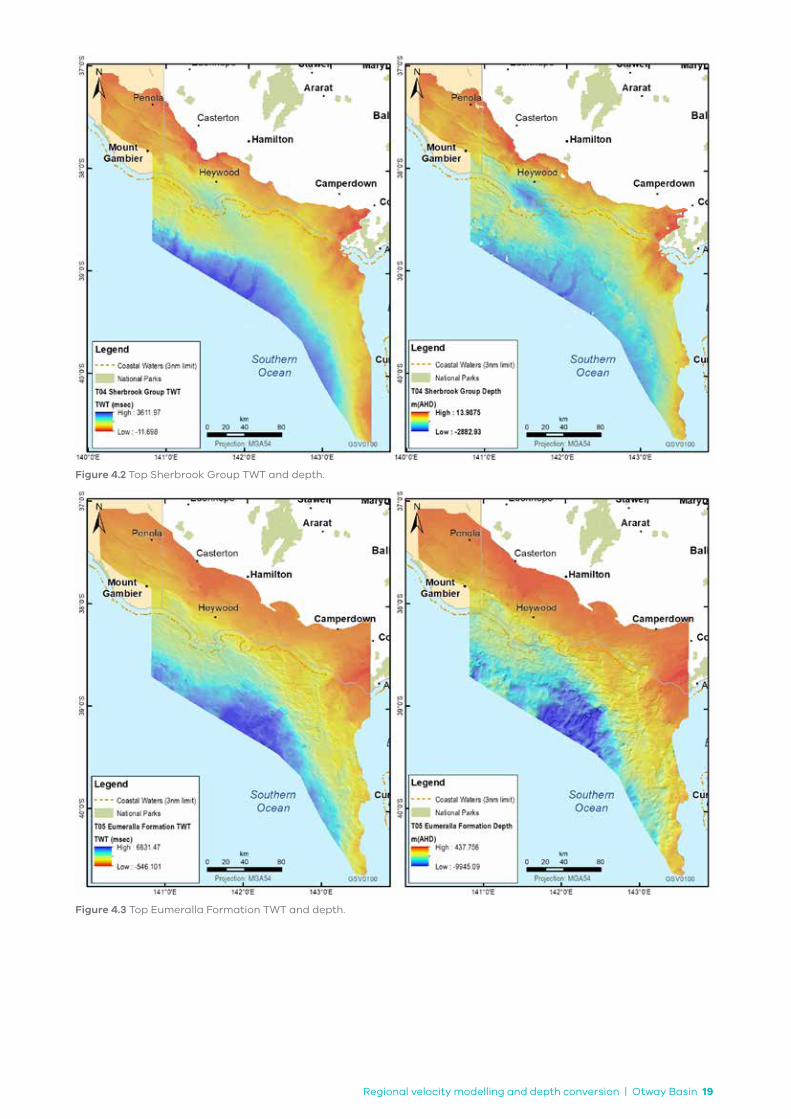
Figure 4.2 Top Sherbrook Group TWT and depth.

Figure 4.3 Top Eumeralla Formation TWT and depth.


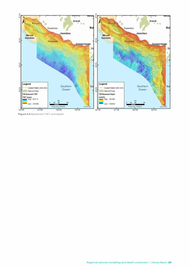
Figure 4.4 Basement TWT and depth.


5 Discussion

There is no absolute solution to a regional depth conversion that incorporates multiple seismic surveys acquired and processed over more than 50 years. A method employed previously in the Otway Basin to create a velocity model for depth conversion used seismic stacking velocities calibrated to well velocities (Romine et al., 2020). Al-Chalabi (1994) and Etris et al. (2002) cautioned against this approach as stacking velocities are primarily created for time domain processing and imaging and are not considered reliable vertical velocity proxies. However, the approach applied in that study (based on Petkovic, 2004) was rigorous and has created useful products.

The goal of this study was to supply depth surfaces suitable for modelling petroleum system elements; specifically, generation and expulsion of gas. Depth of burial is a key component of petroleum systems studies and this aligns with the V0-k method of depth conversion, which relies on depth of burial as the primary control for velocity trends.

The modified V0-k approach used in this study was able to produce depth surfaces that fit the available well data, used consistent assumptions where data was sparse or not available and captured all of the relevant petroleum systems elements in the Otway Basin.

While the workflow for this depth conversion involved the use of three applications (EzTZ, OpendTect™ and PetrelTM) the GSV implemented the key elements of this study in Petrel™.

Further improvements to the depth conversion may be possible with the inclusion of additional well ties and improved controls on velocity using modern 3D depth migrated seismic data. However, data density over much of the Otway Basin is limited and increased data density and quality may only result in local improvement of the velocity model. The modular workflow in this study will enable further improvement as additional data becomes available.

5.1 Penola Trough

Additional seismic interpretation, regional time surfaces and well data was incorporated into this model to enable the inclusion of wells from the South Australian part of the Penola Trough where there is a proven petroleum system. The inclusion of the Penola Trough was a key requirement of this study as it has meant that South Australian gas discoveries could be included in VGP petroleum systems modelling.

5.2 Localised well velocity anomalies

Some wells have velocities that vary significantly from the best fit V0-k relationship, having a similar slope but with an offset. This implies that the rocks have, in the past, been buried deeper than they are currently. Corrections for these are built into the KF velocity volume. It is likely in the onshore Casterton-1 and Digby-1 wells, that these velocity variations are the result of uplift and erosion. (Figure 1.2). Similar local trends are also apparent in some of the wells in the eastern onshore Otway Basin. Onshore, these velocity trends are apparent on some, but not all, structural highs suggesting uplift along associated faults.

Offshore, Holford et al. (2010) and Robson et al. (2018) interpreted uplift related velocity trends from the relatively sparse offshore well data. In the current study, these variations were accounted for in the KF velocity component. These broad trends were not apparent onshore. In the deepest parts of the Early Cretaceous depocentres, the V0-k relationship appears relatively unperturbed; suggesting rocks in the centre of the large depocentres are presently at their maximum depth.

There may be potential to use local variations in velocity to further constrain the tectonic history of the onshore Otway Basin.


5.3 Mid to Late Cretaceous structural features beneath the continental slope

Gas fields offshore, near the continental shelf, contain some of the largest gas discoveries in the Otway Basin. This study extends the Otway Basin 3D geological framework model (Romine et al., 2020) depth converted surfaces beneath the present-day continental shelf to enable petroleum systems modelling of the hydrocarbon generation responsible for these accumulations. To enable this additional interpretation, gridding was undertaken in this area. Mapping and accurate depth conversion of features beneath the continental slope is notoriously difficult. However, this study does show structural trends that warrant discussion.

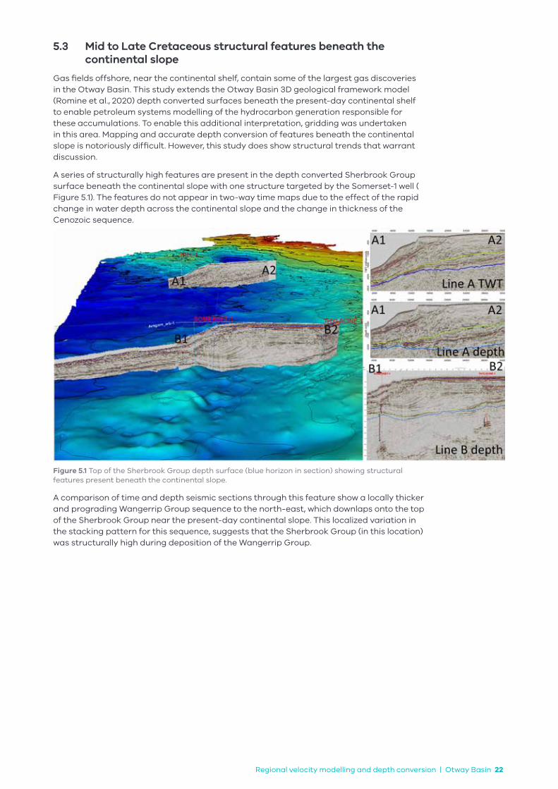
A series of structurally high features are present in the depth converted Sherbrook Group surface beneath the continental slope with one structure targeted by the Somerset-1 well ( Figure 5.1). The features do not appear in two-way time maps due to the effect of the rapid change in water depth across the continental slope and the change in thickness of the Cenozoic sequence.

Figure 5.1 Top of the Sherbrook Group depth surface (blue horizon in section) showing structural features present beneath the continental slope.

A comparison of time and depth seismic sections through this feature show a locally thicker and prograding Wangerrip Group sequence to the north-east, which downlaps onto the top of the Sherbrook Group near the present-day continental slope. This localized variation in the stacking pattern for this sequence, suggests that the Sherbrook Group (in this location) was structurally high during deposition of the Wangerrip Group.


6 Conclusions

The depth conversion method, as applied to regional time surfaces from the Otway Basin, was an efficient solution that took advantage of products from Romine et al. (2020). The workflow built a calibrated, basin-scale velocity model using commonly available software (in combination) such as OpendTect™ and Petrel™. Regionally consistent, accurate depth conversion of key stratigraphic horizons for basin modelling was achieved.

The accuracy level achieved in this study is appropriate for regional petroleum systems modelling using 2D seismic data. However, for exploration prospect mapping, or field development studies, it is recommended to consider and compare to seismic velocity approaches using modern depth processed seismic velocities undertaken over restricted areas of interest where 3D seismic data is available.

Further reduction of the uncertainty might also be achieved using a similar workflow to the one used in this study by revisiting the synthetic to seismic ties using a best-practice well tie workflow and by implementing a multi-layer V0-k depth conversion. This could take some time to achieve as many more wells in the basin would need to be tied to seismic.

Finally, as more seismic datasets become available in the Otway Basin, either through new acquisition or from reprocessing efforts (e.g. with modern pre-stack depth migration processing), it should become possible to reduce uncertainty even further by using these seismic velocities. Until that time and in areas not covered by new data, this regional depth conversion should prove helpful to those interested in exploring new plays and frontier regions of the Otway Basin.


References

AAPG, 2020. AAPG WIKI. https://wiki.aapg.org Accessed 26th August 2020.

AL-CHALABI, M., 1994. Seismic velocities - a critique. First Break, 12(12), pp. 589–596.

APPEA, 2020. Australian oil and gas glossary. www.appea.com.au/industry-in-depth/australian-oil-and-gasglossary/ Accessed 26th August 2020.

ETRIS, E.L., CRABTREE, N.J. & DEWAR, J.D., 2002. True Depth Conversion: More Than a Pretty Picture. Recorder, Canadian Society of Exploration Geophysicists, 26 (9).

GEOSCIENCE AUSTRALIA, 2020. Australian Energy Resources Assessment, Appendices -glossary. https://aera. ga.gov.au/#!/glossary Accessed 26th August 2020.

HOLFORD, S.P., HILLIS, R.R., DUDDY, I.R., GREEN, P.F., TUITT, A.K. & STOKER, M.S., 2010. Impacts of Neogene-recent compressional deformation and uplift on hydrocarbon prospectivity of the passive southern Australian margin. APPEA Journal, 50, pp. 267–286.

PETKOVIC, P., 2004. Time depth functions for the Otway Basin. Geoscience Australia Record 2004/02, 49p.

ROBSON, A.G., HOLFORD, S.P., KING, R.C., & KULIKOWSKI, D., 2018. Structural evolution of horst and half-graben structures proximal to a transtensional fault system determined using 3D seismic data from the Shipwreck Trough, offshore Otway Basin, Australia. Marine and Petroleum Geology, 89, pp. 615–634.

ROMINE, K., VIZY, J., NELSON, G., LEE, J.D., BAIRD, J. & BOYD, M., 2020. Regional 3D geological framework model, Otway Basin, Victoria. Victorian Gas Program Technical Report 35. Department of Jobs, Precincts and Regions. Melbourne, Victoria. 265p.

SCHLUMBERGER, 2020. Oilfield Glossary. https://www.glossary.oilfield.slb.com/ Accessed 26th August 2020.

SMALLWOOD, J.R., 2002. Use of V0-K depth conversion from shelf to deepwater: How deep is that brightspot? First Break, 20, pp. 99–107.

SPE INTERNATIONAL, 2020. Petrowiki. petrowiki.org/PetroWiki Accessed 26th August 2020.


Glossary

Term Explanation

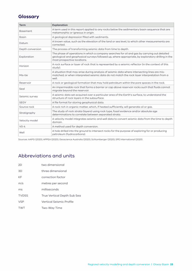
BasementA term used in this report applied to any rocks below the sedimentary basin sequence that are metamorphic or igneous in origin.

Basin A geological depression filled with sediments.

DatumA known value, such as the elevation of the land or sea level, to which other measurements are corrected.

Depth conversion The process of transforming seismic data from time to depth.

ExplorationThe phase of operations in which a company searches for oil and gas by carrying out detailed geological and geophysical surveys followed up, where appropriate, by exploratory drilling in the most prospective locations.

HorizonA rock surface or layer of rock that is represented by a seismic reflector (in the context of this study).

Mis-tieA situation that may arise during analysis of seismic data where intersecting lines are mis-matched; or when interpreted seismic data do not match the rock layer interpretation from a well.

Reservoir A rock or geological formation that may hold petroleum within the pore spaces in the rock.

SealAn impermeable rock that forms a barrier or cap above reservoir rocks such that fluids cannot migrate beyond the reservoir.

Seismic surveyA seismic data set acquired over a particular area of the Earth’s surface, to understand the structure of rock layers in the subsurface.

SEGY A file format for storing geophysical data.

Source rock A rock rich in organic matter, which, if heated sufficiently, will generate oil or gas.

StratigraphyThe study of rock strata (layers) using rock type, fossil evidence and/or absolute age determinations to correlate between separated strata.

Velocity modelA velocity model integrates seismic and well data to convert seismic data from the time to depth domain.

V0-k A method used for depth conversion.

WellA hole drilled into the ground to intersect rocks for the purpose of exploring for or producing petroleum (hydrocarbons).

Sources: AAPG (2020); APPEA (2020); Geoscience Australia (2020); Schlumberger (2020); SPE International (2020).

Abbreviations and units

2D two dimensional

3D three dimensional

KF correction factor

m/s metres per second

ms milliseconds

TVDSS True Vertical Depth Sub Sea

VSP Vertical Seismic Profile

TWT Two-Way Time

Regional velocity modelling and depth conversion Otway ...

Documents

Transcript of Regional velocity modelling and depth conversion Otway ...