Study of rotational ground motion in the near field region

Marco STUPAZZINI1, Josep DE LA PUENTE2, Chiara SMERZINI3,

Martin KÄSER4, Heiner IGEL4, Alberto CASTELLANI1

Corresponding Author:

Marco STUPAZZINI

Department of Structural Engineering

Politecnico di Milano

P.zza Leonardo da Vinci, 32

20133 Milano, Italy

Mail : stupa@stru.polimi.it

Tel: +39 02 2399 4317

Fax: +39 02 2399 4220

Web: http://www.stru.polimi.it

1

ABSTRACT

During the nineteenth century observational seismologists recorded mainly the earthquake induced

translational wave field, while the rotational motion still nowadays remains poorly observed and

investigated. We aim at further understanding the rotational ground motion and its relation to the

translational wave field with a special emphasis on the near field, few wavelengths away from the

hypocenter, where damage related to rotational motion might need to be considered. A broad

picture of the available values of rotational amplitudes and their variability is obtained by gathering

most of the published data on strong rotational motion. To obtain a more detailed picture, we

perform a large scale 3D numerical study of a strike-slip event in the Grenoble valley, where a

combination of topographic, source, and site effects produces a realistic wave field. We analyzed

the synthetic dataset in terms of the rotational and translational peak amplitudes and their

dependence on two effects: non linear soil behaviour and source directivity. On soft soil deposit,

we observe Peak Ground Rotation of 1 mrad and the Peak Ground Rotation Rate of 10 mrad/s, for

Mw 6.0 event. Those values show a strong dependence on the hypocenter location, the local site

conditions and the topographical features, inducing a variability of almost one order of magnitude

in a range of distances of 20 km. Finally, we compare our numerical results in terms of Peak

Ground Velocity, PGV, vs. Peak Ground Rotation, ωPG , with field data obtained at similar

scenarios (e.g. Parkfield) by array techniques to investigate the relation between translational and

rotational amplitudes expected in the near-field for shallow medium-sized earthquakes. Results of

our numerical simulation fit reasonably well with those observed in past studies. Furthermore, the

spatial variations of /PGV PGω ratio show a trend that is correlated with the velocity structure of

the model under study.

2

Introduction

Earthquakes radiate large amounts of energy, mostly as seismic waves. Studies of the rotational

components of ground motion preceded and have lasted longer than either the modern seismology

(late 1800s to present) or the engineering strong-motion seismology (1930s to present) (Trifunac

2008a). Nevertheless for technical and historical reasons, as clearly explained by Trifunac (2008b),

during the nineteenth century seismologists recorded through different devices, seismometers or

accelerometers, only the three degrees of freedom associated with the translational motion (i.e.

velocity, , ,x y zu u u u⎡= ⎣ ⎤⎦ ), or acceleration along a Cartesian reference frame, implicitly neglecting

the rotational components of the motion. Nevertheless, the investigation of the latter cannot be

obviated a priori in risk assessment studies, as it has already been acknowledged that rotational

ground motion plays a role in the dynamic response and damage induced by certain earthquakes on

buildings (Richter 1958, Newmark 1969, Stratta & Griswold 1976, Gupta & Trifunac, 1989,

Kalkan & Graizer 2007).

A direct observation of earthquake-induced rotational ground motion is possible using devices

sensitive to torsion as tilt meters or, more recently, solid state devices (Nigbor 1994), ring lasers

(Stedman et al. 1995) and broadband rotation meters (Lin et al., 2009). However, such devices are

not in common use and most frequently the rotational components of motion are indirectly

estimated from array measurements (e.g. Spudich et al. 1995, Huang 2003, Suryanto et al. 2006,

Ghayamghamian & Nouri 2007, Spudich 2008). The records of translational and rotational

components of motion have been proved to be useful, for example, in the extraction of local phase

velocities or the back-azimuth of events (Igel et al. 2005; 2007) or in recovering the static

displacement (Trifunac & Todorovska 2001, Graizer 2005, Graizer 2006, Pillet & Virieux 2007).

3

Regardless the recent interest in the field, studies of recorded rotational ground motion, for

teleseismic or local events, are still rare and our knowledge of the rotational wave field is largely

insufficient.

In spite of the lack of observed data, numerical studies have been performed aiming at computing

synthetic time histories in order to investigate the influence of important factors on the rotational

motion and, in particular, their expected maximum amplitudes. A pioneering numerical study was

accomplished by Bouchon & Aki (1982) and further numerical experiments have followed (Lee &

Trifunac 1987, Takeo 1998, Wang et al., 2008). In our case, we simulate several events in a 3D

model of an Alpine valley at Grenoble, France, with an alluvium filled basin so that topographic,

soil and source effects can be all considered. The synthetic results are compared with data retrieved

mainly from array experiments, and investigated in terms of the following ratio as already done by

Wang et al. (2008) and Fichtner & Igel (2008):

( ) 2( )

hs

z

PGV x cPG xω

≈ , (1)

where ( )hPGV x is the maximum value in time of 22yx uu + at location x , ( )zPG xω is the peak

ground vertical rotation and sc can be regarded as a scaling factor between translational and

rotational peak ground motion. For a site on parallel layers, excited by plane waves, sc represents

the phase velocity of a frequency component (Trifunac 1982). Furthermore, without any loss of

generality, the rotational motion can be separated into two parts: one associated with pure shear,

involving the contributions from SH and Love waves and resulting in rotational motion around the

vertical axis (Lee & Trifunac, 1985), and the other one associated with P, SV and Rayleigh waves

and resulting in rotational motion around the horizontal axis (Lee & Trifunac, 1987). For both

4

decompositions, the Fourier spectrum of rotations is proportional to the ratio between the Fourier

spectrum of velocity and the phase velocity (Trifunac & Todorovska, 2001).

The separation into two parts implies the knowledge of the polarization of the incident wavefield

and this information is not trivial to recover on a practical ground, even if some recent works seems

to be promising on this issue (Langston et al., 2008).

When the ratio is taken of the peak velocity and peak rotation in time, it becomes an "average" or

"equivalent" phase velocity at the site. In the absence of recorded strong motion rotation data,

investigating the correlation of this ratio, sc ,with the local velocity allows us to address the question

of whether we can obtain reliable peak rotational motion estimates straight from peak ground

measurements of translational motions.

The paper is structured as follows. First, we give an overview on studies related to rotational

ground motion recordings, both observational and numerical, and the general trends and

characteristics observed in them. In the next section, we introduce and validate a 3D method to

simulate the translational and rotational ground motion produced in complex scenarios. A particular

case study follows, where we simulate a MW = 6.0 strike-slip earthquake occurring in the Grenoble

valley. Moreover, we compare the rotational wave field both at the bedrock and the sedimentary

basin and we draw peak ground motion maps for different magnitudes, sediment mechanical

properties and source hypocenter locations. Finally, we put our synthetic dataset in direct

comparison with past simulations and observations in terms of the ratio given by Eq. 1 to draw

conclusions about the correlation between translational and rotational ground motion and its

physical implications.

Past studies in rotational seismology

5

In the last decades few studies have shown direct measurements of rotations, thus leading to large

uncertainties in the order of magnitudes of rotations likely to occur for a given earthquake scenario.

Therefore, it is important to synthesize in a comprehensive way a selection of the data available in

the literature. Specifically, we chose data which might be of relevance for seismic engineering

studies, namely those recorded in the near field (few wavelengths away from the epicenter) or

showing relatively strong rotation amplitudes, even if recorded at greater distance.

For sake of completeness, we combine field data records with synthetic studies, observations at stiff

and soft soils, array-derived with single-point measurements and those generated by different

source mechanisms. A proper labeling helps subdividing them into groups which can be directly

compared to each other. In the following, we present briefly the sources of data that we use and

which are listed in Table I.

A pioneering work was published by Bouchon & Aki (1982), who adopted a semi-analytical

method to derive strains, tilts and rotations in the proximity of a buried 30 km long strike slip fault

with seismic moment 8x1018 Nm, obtaining a peak ground rotation of the order of 3 10-4 rad while

the corresponding rotational rate was about 1.5 10-3 rad/sec. Later on, different analyses have tried

to record and characterize ground rotational motions. Most of these studies are based on indirect

estimates of surface ground rotations from two-dimensional seismic arrays (see e.g. Castellani &

Boffi, 1986; Oliveira & Bolt, 1989; Bodin et al., 1997; Singh et al, 1997; Huang, 2003; Spudich &

Fletcher, 2008). The most significant drawback of such an approach is the limited frequency

content (typically lower than 2 Hz), due to the relatively large separation distance between adjacent

receivers. Besides field observations, ground rotations have been also investigated from a

theoretical point of view. Those studies rely either on the theory of elastodynamics for plane wave

propagation in ideal media (Trifunac, 1982; Lee & Trifunac, 1985) or on kinematic source models

6

(Takeo & Ito, 1997). The direct measurement of rotations has been obtained at great distances from

important earthquakes using ring laser instruments (McLeod et al., 1998; Pancha et al., 2000;

Cochard et al., 2006; Igel et al., 2005 and 2007) and in the near field through triaxial rotational

sensors (Nigbor 1994; Takeo, 1998). In particular, Nigbor measured an explosive source, whereas

Takeo recorded an earthquake swarm in 1997, offshore the city of Ito in Japan. The two largest

events of that swarm have seismic moments of 1.2 1017 Nm and 2.7 1016 Nm and were recorded at

3.3 km from the fault. The maximum measured rotational rates around the vertical axis were,

respectively, 3.3 10-3 rad/s and 8.1 10-3 rad/s, several times higher than what was predicted by

Bouchon & Aki (1982), even though the seismic moment of the two events was about two orders of

magnitude smaller than the one simulated by the authors. This discrepancy cannot be explained as a

malfunction or limited sensitivity of the instruments, therefore the author claimed that the large

rotational velocities might be induced by either the heterogeneity of slip velocity along the fault or

the local rheology. These two factors may play a crucial role, particularly in the near field, as was

stressed by Huang (2003) and Spudich & Fletcher (2008).

Numerical method validation

As a complement to the recorded data, we use synthetic rotational seismograms obtained with the

Spectral Element Method (SEM), first introduced for the solution of the elastodynamic problems by

Priolo and Seriani (1991), Faccioli et al. (1997) and Komatitsch & Vilotte (1998). Here we adopt

the version implemented in the software package GeoELSE (Stupazzini et al., 2008). A detailed

description can be also found at http://geoelse.stru.polimi.it. In order to validate the reliability of

the rotational output produced by our method, we compare our results with those obtained with the

highly accurate ADER-DG method (Käser & Dumbser, 2006 and Dumbser & Käser, 2006).

7

Both numerical codes have been used on the HLRB 2 of the Leibniz Rechenzentrum München and

on the TETHYS cluster (Oeser et al., 2006) of the Department of Earth Sciences, Geophysics, of

the Ludwig-Maximilians-Universität München.

Both methods are, essentially, high-order finite element methods explicit in the time domain,

able to accurately model large velocity contrasts, attenuation effects and finite-source kinematics,

all of them crucial aspects for reproducing realistic earthquake scenarios in complex geological

configurations. In the SEM based code, absorbing boundaries are implemented through the Stacey

(1988) first order P3 paraxial conditions.

We choose first to cross-validate the synthetics produced by our methods, both translational and

rotational, for two established tests proposed by the Southern California Earthquake Center (Day et

al., 2007). Those are the so-called LOH.1 and LOH.2 tests, where the acronym LOH stands for

Layer Over Halfspace. Both of them describe a flat half-space, on top of which lies a thin low-

velocity layer. The main difference between both tests is that LOH.1 uses a point-source whereas

LOH.2 uses a source with finite extent, thus leading to different waveforms and frequency contents.

For the translational motion, both methods have already been tested against quasi-analytical

solutions (Stupazzini, 2004, Dumbser & Käser, 2006). The setup of the tests and an example of the

computational mesh for SEM are depicted in Figure 1. The parameters describing both models are

shown in the legend. Besides the translational motion ( , ,x y zu u u u⎡ ⎤= ⎣ ⎦ ), we output rotational

ground motion, which is defined as

⎟⎟⎠

⎞⎜⎜⎝

⎛∂∂

−∂∂

=z

uyu yz

x 21ω , ⎟

⎠⎞

⎜⎝⎛

∂∂

−∂∂

=xu

zu zx

y 21ω , 1

2y x

z

u ux y

ω∂⎛ ⎞∂

= −⎜ ⎟∂ ∂⎝ ⎠ (2)

and their corresponding rotational velocities and accelerations

8

ii

dωω= dt

, 2

ii 2

d ω= dt

ω with x,y,z=i . (3)

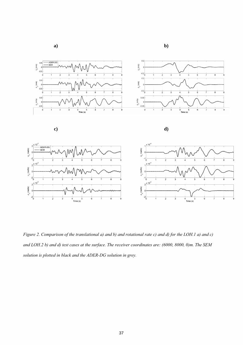
A comparison of the synthetics obtained with both methods can be found in Figure 2. In this

case, the SEM solution has been computed with a mesh of 352,800 hexahedral elements using

polynomials of degree 4 to describe the variables while the ADER-DG solution has been computed

with polynomials of degree 3 and a mesh with 782,542 tetrahedral elements. The agreement

between both methods is remarkable, and only after 7 seconds some major differences arise owing

to the spurious reflections coming from the absorbing boundaries. It can be further observed that

the ωz motion is delayed with respect to other signals, as it is only sensitive to SH motion. Similar

results characterized the records of all stations.

From these tests we conclude that both methods’ solutions are in satisfactory agreement and that

they are able to produce reliable translational and rotational synthetic seismograms in three-

dimensional setups.

A study case: Grenoble valley (French Alps)

Studies by Bouchon & Aki (1982), Lee & Trifunac (1985) and Castellani & Boffi (1986)

indicated that rotational ground motion could be important in the near-field and for surface waves.

Although in recent time direct (Nigbor, 1994; Takeo, 1998) and indirect (Graizer, 1989; Huang,

2003) measurements of rotation have received a certain emphasis, still the number of available

records is extremely limited and, furthermore, there are only a few examples of data in the near

field region (Spudich & Fletcher, 2008). As a consequence, our level of knowledge on the

magnitude of rotational ground motions to be expected for a given earthquake scenario is still

limited.

9

In this paper, we make use of 3D numerical modeling to reproduce the rotational wave field

generated by strike-slip earthquakes in the near field. We choose as our study area the Grenoble

valley (French Alps) for two main reasons. First of all, when it comes to large scale numerical

simulations, the validity of the results is hard to assess. As models grow complex, the amount of

parameters to be taken into account increases severely and so does the possibility of introducing

unexpected errors in the computation. The Grenoble case, in particular, has the great advantage of

having been successfully benchmarked by cross-validation between many state-of-the-art

simulation techniques (Chaljub 2006), including the SEM and ADER-DG methods used in the

previous section. This increases significantly our degree of confidence in the synthetic results. A

second but not less important reason is the fact that the Grenoble valley offers the chance to

investigate many factors which can be crucial for amplification phenomena in the near field such as

site, topographic, and source directivity effects.

The model of the Grenoble valley has been constructed using a 250 m resolution digital

elevation model (DEM) of the surrounding topography and of the shape of the basin. The basin’s

soil is described by the following polynomial variation with depth z (measured in m):

VP = 1450+1.5z, VS = 300+19z1/2, ρ = 2140+0.125z, QS = QP = 50 (4)

where VP and VS are the P- and S-wave velocities (in m/s), respectively, ρ is the mass density (in

kg/m3), and QP and QS are P- and S-wave quality factors. The surrounding bedrock is two-layered,

with VP = 5600 m/s and VS = 3200 m/s, between 0 and 3 km depth, and VP = 5920 m/s and VS =

3430 m/s, between 3 and 27 km depth.

In the following, the GeoELSE version of the Spectral Element Method has been used to

compute the synthetic seismograms. A linear visco-elastic material is used to model the attenuation.

10

The final computational mesh consists of 216,972 elements, the size of which ranges from a

minimum of about 20 m inside the alluvial basin up to 900 m at some bedrock areas. The mesh has

been designed to propagate frequencies up to 2 Hz. A detailed description of the mesh generation

can be found in Stupazzini et al., (2008).

We use the source specification denoted as “Strong motion 1” case by Chaljub (2006) and which

corresponds to a MW = 6.0 earthquake originated at the Eastern segment of the Belledonne Border

Fault (see Figure 3a). The fault is defined as a 9 km x 4.5 km rectangle where “in plane” rupture

occurs with a uniform slip of 1 m. The mechanism is strike slip, right-lateral (strike = 45°, dip =

90° and rake = 180°). The rupture propagates circularly from the hypocenter, located at the centre

of the fault, with velocity vr = 2.8 km/s. The time history of the seismic moment tensor source is

described by an approximate Heaviside function of the type:

⎥⎦

⎤⎢⎣

⎡⎟⎠⎞

⎜⎝⎛

ττ−

+=22021

21

0 /t.erf)t(M , (5)

where erf is the error function and τ = 1.116 s is a rise time. These values are selected for the slip

velocity to be approximately 1 m/s. A total of 750 spectral nodes are contained in the fault. In the

following sections we also refer to a smaller earthquake (MW=4.5) simulated for the same fault

plane. In that case, we use a smaller rectangular fault, measuring 4 km x 3 km, where the total slip

has been reduced to a value of 0.02m, leaving the remaining parameters unchanged with respect to

the MW=6.0 event.

Figure 4 presents synthetic velocity and rotational waveforms recorded on a receiver located in

the middle of the 2D profile (Figure 3), namely R29 of Grenoble benchmark specification (Chaljub

et al., 2007 and Dumbser et al., 2007), obtained with source denoted as “Strong motion 1”. Figure 5

compares velocity and scaled torsion amplitude spectra of R29 (scaling factor is equal to 2000).

Referring to Trifunac (1982) and Spudich et al. (2008) this figure shows that ground torsion spectra

11

are related to the velocity spectra through a suitable scaling factor. The issue regarding the

correlation of the latter with the actual equivalent propagation velocity, the velocity structure of the

basin and local site conditions will be addressed in the section "Synthetic ratios between

translational and rotational peak values".

Parametric study of near-fault earthquake ground motion in the Grenoble Valley

ur study of the Grenoble MW=6.0 scenario begins by investigating the effect of various

pa

O

rameters in the rotational and translational motion records. This allows us to discern those

parameters which more strongly affect the rotational wave field and get a wider view on the

variability of the amplitudes that we can expect. In particular, we record the peak ground motion

recorded at a very dense array of synthetic stations inside and near the alluvial basin of Grenoble.

Our observables are the peak ground vertical rotation, zPGω , and the peak ground horizontal

rotation, PG hω , defined as the maximum of zω and of 2 2x yω ω , respectively. Similarly, we use

the peak of their respective time derivatives or “rates” ( P

+

G zω and hPGω ).

In this contribution two main phenomena are studie urce d ityd: so irectiv and the presence of a

non linearly behaving soil at the basin. The source directivity effect for the Grenoble case was

studied by Stupazzini et al. (2008) and has here been recomputed, now outputting the rotational

motion components. Three different directivity cases are studied: neutral, forward and backward. In

the neutral case the hypocenter is located in the middle of the fault plane (Hypocenter 1), as has

been described in last section. The other two consider that the hypocenter is situated very close to

the NE or SW tips of the fault (Hypocenters 2 and 3, respectively), while keeping the total slip and

12

the slip rate function unaltered. As a result, all three earthquakes have the same magnitude but their

radiation pattern is much larger in the direction directly opposed to their hypocenter position. The

exact location of the hypocenters for all three cases can be seen in Figure 6.

The second source of variability of ground motion is the presence of a non linear vico-elastic

so

il (NLE), instead of the linear visco-elastic (EL) one. The non linear visco-elastic soil model

implemented in GeoELSE can be regarded as a generalization to 3D load conditions of the classical

G-γ and D-γ curves used within 1D linear-equivalent approaches (e.g. Kramer, 1996), where G, D

and γ are shear modulus, damping ratio and 1D shear strain, respectively. Namely, to extend those

curves to the 3D case, a scalar measure of shear strain amplitude was considered as:

max ( , ) max ( ) ( ) , ( ) ( ) , ( ) ( )I II I III II IIIx t x t x t x t x t x tγ ε ε ε ε ε ε= ⎡ − − −⎣ ⎦, , , , , ,x t ⎤ (6)

where

Iε , IIε and IIIε are the principal values of the strain tensor. Once the value of γmax is

ca a the iclculated t gener position x and generic time t, this value is introduced in the G-γ and D-γ

curves and the corresponding parameters are updated for the following time step. Therefore, unlike

the classical linear-equivalent approach, the initial values of the dynamic soil properties are

recovered at the end of the excitation. The G-γ and D-γ curves specifically calibrated on the

Grenoble shallow soil materials described by Jerram et al. (2006) were adopted in this work (Figure

7).

The results of our parametric study have been partly plotted in Figure 8. The first column shows

the peak ground rotational motion with the assumption of linear visco-elastic (EL) material inside

the alluvial basin, while the second shows analogous results with non linear visco-elastic material

(NLE). The three rows presents the different results obtained respectively with backward (Hypo3),

neutral (Hypo1) and forward (Hypo2) directivity. Finally the combined effect of directivity and

linear/non linear soil descriptions is summarized in Table II in terms of PGω and PGω . The

13

results are here provided for the entire parametric study and the various sub-areas in which the

Grenoble valley was subdivided.

As a reference we can take the values obtained for a linear visco-elastic basin with neutral

directivity. In this case we observe peak values of zPGω =1.69 mrad, hPGω =1.31 mrad for the

rotations and zPGω =8.24 mrad/s, hPGω =8.66 mrad/ he rotation rat stly recorded at the

southern tip of the Y-shaped basin (Area 2 of Table II), owing to the constructive interference

between the local sedimentary structure and the radiation pattern. As a general trend (see Table II),

we can observe that the combination of forward directivity and non linear elasticity produces the

strongest rotational motions whereas the combination of backward directivity and linear elasticity

produces the smallest amplitudes.

Another conclusion from our s

s for t es, mo

tudy is that, for the earthquake source used in this example, two

ma

ion and rotation rate

ma

in potentially dangerous areas can be identified. One of them is the whole southern tip (Area 2

of Table II) of the basin and the other is the part of the basin located closest to the fault, i.e. its

northeastern tip (Area 1 of Table II). Peak rotation and rotation rate maxima are consistently

recorded at those two areas, particularly at their eastern most sides. This clustering of the maxima

towards the edge of the basin is further increased in the presence of non linear soils (see Figure 8).

The northwestern tip of the basin (Area 3 of Table II), on the other hand, always records values of

rotation and rotation rates around five times smaller than the other basin areas.

The observed range of variability, from “worst” to “best” case, for both rotat

xima is of around a factor of 3 for the vertical components and around a factor 6 for the

horizontal components. Most of the variation is coming from directivity effects, although the non-

linear soil behavior can also play a significant role (see Table II). Previous fault normal PGV

studies (Stupazzini et al. 2008) found a similarly strong effect of the directivity on the maximum

recorded PGV values, which can range from 0.35 m/s for H3 seismic source up to 2.09 m/s for H2.

As a consequence, both 3D and soil effects produce large spatial variability in the rotational motion

14

which cannot be accounted for using simplified models (i.e.: 2D models or only visco-elastic

constitutive behaviour).

Synthetic ratios between translational and rotational peak values

In the present Section we explore to what extent rotational and translational motions are

co

rrelated, in particular we address the question of whether we can have a reasonable estimate of

peak rotational motion from the corresponding translational motion studies in near source regions.

In this contribution we rely on simplified models (see e.g. Igel et al., 2005 and 2007; Cochard et al.

2006) which assume an incident transversally polarized plane wave, for example along the y axis.

This implies that the displacement can be described as 0, ( / ), 0⎡ ⎤= −⎣ ⎦y au u t x V , aV being the phase

velocity. Under this assumption, at any time, trans d otation rate, or

equivalently velocity and rotation, are in phase and the amplitudes are related by:

verse acceleration an r

( , ) / ( , ) 2ω = −u x t x t V y z a (7)

The assumption of plane wave incidence is expected to hold for a considerable part of the

ob

acceleration and

rot

served ground motion whenever the epicentral distance is large compared to the considered

wavelengths and source dimensions (Igel et al., 2005). In the near field region the hypothesis of

plane wave is no longer valid and a larger variability of the ratio can be expected.

Nevertheless Wang et al. (2008) showed that the ratio between peak ground

ation rate ( ( ) / ( ) 2h z sPGA x PG x cω = ), equivalent to rotation (Eq. 1), could provide important

information regarding the basin structure even in the near field. Wang et al. (2008) analyzed a

hypothetical MW=7.0 strike-slip event occurring along the Newport-Inglewood fault embedded in

15

the 3D Los Angeles basin, and showed that high values of sc are located outside the basin and low

values inside. The only exception to the proportionality between translational and rotational motion

happens in the region around the fault, where the sc value could be used to constrain the rupture

process (Takeo & Ito, 1997; Takeo, 1998). In the following we present map of the ratio between

peak ground velocity and rotation.

The quantity sc in Eq. 1 is the scaling factor between translational and rotational peak ground

motions as estimated by either empirical or numerical data. Under the assumption that SH and Love

waves are the predominant contributions, which seems a reasonable approximation in the proximity

of shallow strike-slip events, as in Grenoble case, Eq. 1 provides a simplified approach for

evaluating . aV

Applying Eq. 1 to the set of 14400 6-component synthetic seismograms at the Grenoble basin

and surrounding we obtain the map of the value of sc at the model’s surface. The results, regarding

the northern part of the model, are plotted in Figure 9b, where we can see how the basin (black

color) is clearly distinguishable from the surrounding bedrock. We recall that the basin has S-wave

velocities varying with depth according to Eq. 4, whereas the bedrock is a homogeneous material

with 3200m/s S-wave velocity, and that the two northern tips of the Y shaped alluvial basin of

Grenoble end abruptly, according to the benchmark specification. In addition, we observe a strong

correlation between cs and the depth basin map (Figure 3b). Furthermore we aim at investigating

the effect that has the pronounced topography (Figure 9a) in the surrounding of the Grenoble valley

on the rotational and translational wavefield. Figures 9c and 9b show, respectively, the and hPGV

zPGω maps with an adequate scaling to observe variations in those peak values due to topography.

The map shows a clear topographic amplification as already investigated in other context by

many authors (i.e.: Geli et al. 1988, Paolucci et al. 1999). The vertical rotational motion seems to

hPGV

16

show a different and more complex pattern, related with (i) the slope of the mountain and (ii) its

convexity or concavity with respect to the direction from the radiation source.

Keeping in mind that the actual S-wave velocity has a value of 3200 m/s, we can observe that

strong variations occur at both sides of the mountains’ crests, due to the zPGω variations just

discussed. All main topographic features in the region between both alluvial valleys are clearly

visible in the cs map. Finally, we can observe the fault trace in the cs map as a zone of very low

values, mainly due to the high values (roughly between 30 mrad/s and 80 mrad/s) of

zPGω recorded locally, just on top of the fault.

Comparison between Grenoble synthetics and data of past studies

Adopting Eq. 1 we study the relation between rotational and translational motion for a collection of

data which must be discussed carefully due to their different origins and qualities. We can basically

divide the data in three distinct subgroups. The first are peak rotational and translational values

obtained in past studies, mainly those labeled 1 to 16 in Table I, for which we do not possess the

whole time histories. A second data subgroup are field recordings, array derived, for which detailed

information is available. Those are labeled 17 to 24 in Table I. In particular, 17 to 20 are data

obtained by Paolucci & Smerzini (2008) through an empirical procedure based on a suitable spatial

interpolation technique of displacement recordings from dense arrays at Parkway Valley, New

Zealand (points 16 and 17) and UPSAR, California (points 18 and 19). For the data values 17 to 20

we plot the average value (filled circle) and their minimum and maximum value (denoted by bars).

Also the estimates recently derived by Spudich & Fletcher (2008) for the 2004 Mw=6.0 Parkfield

event and three aftershocks (in order of decreasing magnitude, Mw=5.1, Mw=4.9 and Mw=4.7),

labelled from 21 to 24 in Table I, are used. In this case the authors applied the so-called “seismo-

geodetic” approach to the UPSAR recordings in order to derive tilts and torsions. Referring to

17

Spudich & Fletcher (2008), we considered three sub-array estimates for each event, filtered in the

frequency band between 0.1 and 1.4 Hz (points from 21 to 24) for comparison purposes with the SE

synthetics with a maximum frequency of 2 Hz. The third and last data subgroup is the synthetics

obtained for the numerical study of the Grenoble valley, for Mw=6.0 and Mw=4.5 scenarios,

subdivided into records obtained at the outcropping bedrock and inside the alluvial basin. All

synthetics used are computed for the case of neutral directivity and visco-elastic soil behavior.

The complete dataset is presented in Figure 10. Although the comparison is not straightforward

as we are combining a wide range of magnitudes, epicentral distances and sources of data, when

attention focuses on the synthetic PGVh- zPGω pairs, some interesting features can be noted.

Primarily, the synthetic data, subdivided into alluvial and bedrock conditions, suggest a linear trend

between PGVh and zPGω in log-log space. In order to have a quantitative estimate of such a

tendency, we decided to perform a linear regression of the synthetic data. The best-fitted lines turn

out to be:

10 10 3.96z hLog PG Log PGVω = − at outcropping bedrock, (8)

10 10 3.34z hLog PG Log PGVω = − in the alluvial basin. (9)

The coefficient of proportionality of both Eqs. 8 and 9 is naturally very close to 1, suggesting a

linear relationship between and hPGV zPGω , in agreement with Eq. 1, at least for the considered

range of frequencies (0.1-2.0Hz). Specifically, two straight lines, superimposed in Figure 10, with

sc ~ 4500m/s (thick line) and sc ~1000 m/s (thin line) describe with reasonable accuracy the zPGω

values obtained at the outcropping bedrock and on the basin, respectively, for both the Mw=4.5 and

Mw=6 earthquake scenarios. If, on one side, synthetic data show a linear trend regardless of

magnitude, the dependence on site effects turns out to be pronounced. Passing from soft alluvial

18

conditions to outcropping bedrock, the PGVh / zPGω ratio increases by factor of about 4, in

average.

Nevertheless, it should be noted that the interpretation of sc as the actual representative phase

velocity might be misleading. As also commented by Spudich & Fletcher (2008), aV sc can be

reasonably regarded as a scaling factor between peak rotations and translations rather than a true

phase velocity at the selected model.

The array-derived estimates retrieved by Paolucci & Smerzini (2008) (points from 17 to 20)

show very similar values and trend with respect to the synthetics. Their behavior alone is also

remarkably linear leading to sc ~ 1000 m/s, irrespectively of the different site conditions. As a

matter of fact, while points 17 and 18 fit fairly well with the synthetics calculated in the soft

alluvial basin, points 19 and 20, which correspond more to bedrock conditions, seem not to be

consistent with the ratio sc ~ 4500 m/s as inferred from the numerical simulations. The sub-array

estimates of Spudich & Fletcher (2008) (see points from 21 to 24) are consistent with synthetics,

provided the relatively stiff conditions of the UPSAR.

The single available direct measurement of the ratio /hPGV PG zω seems to be significantly

larger than all the simulated and array-derived estimates (point 13). However, this data refers to an

explosion rather than an earthquake, so that the comparison may be improper. Unfortunately, the

measurements from Takeo (1998) can not be used on the present study, since only rotation rates

records of the Mw~5.0 Ito-Japan events, are available. Nevertheless, also Spudich & Fletcher (2008)

commented a substantial disagreement between Takeo’s measurements and empirical estimates for

the reasons shortly illustrated previously. Thus, his direct measurements of rotation rates turns out

to be larger, by factor of 5-60, than other estimates and the ratio of /hPGV PG zω is systemically

higher than those of Parkfield and Chi-Chi earthquakes (see Spudich & Fletcher 2008).

19

At this point we can try to answer whether or not we can infer zPGω from . As a first

approximation, it is clear that an average trend exists, mainly following Eq. 1, which allows for a

rough estimation of the average rotational peak values given a suitable measure of the phase

velocity at the receiver site. This might be helpful for quick estimates, although Figure 10 shows us

the large variability displayed in the Grenoble area. This indicates that average values only are not

sufficient to explain the complex behavior of rotational ground motions at the surface. More

detailed pictures of rotational energy distribution should be obtained, preferably by deploying

rotational sensors or seismometer arrays, in order to further identify more complex factors not only

related to the local phase velocity but to other factors as topography, spatial incoherence or source-

related effects.

hPGV

Conclusions

In this paper we show a selection of available data concerning observed and synthetic rotational

motion mainly regarding near field and strong motion earthquakes. The lack of observation testifies

the need to investigate more carefully the role of rotations, almost neglected in seismological and

hazard assessment studies. Using two well-established and accurately validated numerical

techniques (SEM, ADER-DG) we simulated the rotational wavefield induced by a MW=6.0 and a

MW=4.5 earthquake, occurring in the valley of Grenoble (French alps). The expected peak ground

rotation ( PGω ) values on receivers located on soft soil is roughly 1 mrad and the peak ground

rotation rate ( PGω ) 10 mrad/s. Those values show a strong dependence on the hypocenter

location, the local site conditions and the topographical features, inducing a variability of almost

one order of magnitude in a range of distances of 20 km.

20

Numerical simulations show also a general trend correlating the maximum of rotational and

translational motion. As a first approximation the estimate of zPGω can be regarded as linearly

proportional to , being the proportionality related to the mechanical properties of the medium

around the receivers. Furthermore, this observation seems to be relatively independent of the

magnitude of the earthquake. However, the overall collection of -

hPGV

hPGV zPGω pairs shows a large

variability of up to 2 orders of magnitude around the average trend.

Concluding, we remark the need of records of rotational components of the seismic wavefield

coupled with classical translational motions, which can be achieved only with rotational sensors

specifically designed. Only this kind of records could in the future assess a definitive answer to the

relationship between velocity and rotation, and offer a set of data capable to explain the large

variability that rotations seem to show.

Data and Resources

Detailed specification of the ESG 2006 benchmark for ground motion simulation in the Grenoble

valley, where provided by the organization committee to the benchmark participants. All other data

used in this paper came from published sources listed in the references

Acknowledgments

This work enjoyed the cooperation of many individuals and institutions during its different

stages. This work has been financially supported by the Marie-Curie Training Network SPICE

(Seismic Wave Propagation and Imaging in Complex Media). We deeply thank CRS4, and in

particular F. Maggio and L. Massidda, for the essential cooperation in the development of

GeoELSE; P. Spudich and J. Fletcher for providing the peak ground rotation and velocity values

observed at the UPSAR array in Parkfield California and for the fruitful discussion. R. Paolucci for

the useful suggestions and L. Scandella for collaborating to develop the subroutines for non linear

21

elastic soil behaviour; E. Chaljub for organizing the Grenoble benchmark and providing the

necessary information for constructing and processing the numerical model; E. Faccioli for his

continuing support since the early stage of development of GeoELSE. We also gratefully

acknowledge the cooperation with the Leibniz Rechenzentrum in München and the support of

J.Oeser from the Department of Earth Sciences, Geophysics, running the TETHYS cluster. We are

also grateful to Prof. M.D. Trifunac, W. Lee and an anonymous reviewer; their detailed revision

helped us in improving significantly the manuscript.

22

References

Bodin, P., J. Gomberg, S. K. Singh, and M. Santoyo (1997). Dynamic deformations of shallow sediments in the Valley

of Mexico, Part I: Three-dimensional strains and rotations recorded on a seismic array, Bull. Seism. Soc. Am., 87,

528 - 539.

Bouchon, M., and K. Aki (1982). Strain, tilt, and rotation associated with strong ground motion in the vicinity of

earthquake faults, Bull. Seism. Soc. Am., 72, 1717-1738.

Castellani, A., and Boffi, G. (1986). “Rotational components of the surface ground motion during an earthquake.”

Earthquake Eng. Struct. Dyn., 14,5, 751–767.

Chaljub E. (2006). Numerical Benchmark of 3D Ground Motion Simulation in the Valley of Grenoble, French Alps,

http://esg2006.obs.ujf-grenoble.fr/BENCH2/benchmark.html.

Chaljub E., D. Komatitsch, J.-P. Vilotte, Y. Capdeville, B. Valette and G. Festa (2007), Spectral Element Analysis in

Seismology, in Advances in Wave Propagation in Heterogeneous Media, edited by Ru-Shan Wu and Valérie

Maupin, Advances in Geophysics, Elsevier, 48, 365-419

Cochard A., H. Igel, A. Flaws, B. Schuberth, J. Wassermann, W. Suryanto (2006) Rotational motions in seismology:

theory, observation, simulation, in Earthquake source asymmetry, structural media and rotation effects , eds.

Teisseyre et al., Springer Verlag

Day S. M., J. Bielak, D. Dreger, R. Graves, S. Larsen, K. B. Olsen and A. Pitarka (2001). Tests of 3D Elastodynamic

Codes: Final Report for Lifelines Project 1A02, Technical report, Pacific Earthquake Engineering Research

Center, University of California, Berkeley.

23

Day, S.M., R. Graves, J. Bielak, D. Dreger, S. Larsen, K.B. Olsen, A. Pitarka and L. Ramirez-Guzman (2007). Model

for Basin Effects on Long-Period Response Spectra in Southern California, Earthquake Spectra, in press.

Dumbser, M. and M. Käser (2006). An arbitrary high order discontinuous Galerkin method for elastic waves on

unstructured meshes II: the three-dimensional isotropic case, Geophys. J. Int., 167, 319–336.

Dumbser M., Kaeser M. and F. T. Eleuterio (2007) "An arbitrary high-order Discontinuous Galerkin method for elastic

waves on unstructured meshes - V. Local time stepping and p-adaptivity", Geophys. J. Int., 171, 695-717 doi:

10.1111/j.1365-246X.2007.03427.x

Faccioli E, F. Maggio, R. Paolucci, A. Quarteroni (1997). 2D and 3D elastic wave propagation by a pseudo-spectral

domain decomposition method. Journal of Seismology, 1, 237-251.

Fichtner, A. and H. Igel (2008). Sensitivity densities for rotational ground motion measurements, submitted to BSSA.

Géli, L., Bard, P.-Y. and Jullien, B., 1988, The effect of topography on earthquake ground motion: a review and new

results, Bull. Seism. Soc. Am. 78, 42–63.

Ghayamghamian M. R. and G. R. Nouri, 2007, On the characteristics of ground motion rotational components using

Chiba dense array data, Earthquake Engng Struct. Dyn. 2007; 36:1407–1429, DOI: 10.1002/eqe.687

Graizer, V. M. (1989). “Bearing on the problem of inertial seismometry.” Izv., Acad. Sci., USSR, Phys. Solid Earth,

25, 1, 26–29.

Graizer, V. M. (2005). “Effect of tilt on ground motion data processing.” Soil Dyn. Earthquake Eng., 25,3, 197–204.

24

Graizer, V. M. (2006a). “Equation of pendulum motion including rotation sand its implications to the strong-ground

motion.” Earthquake source asymmetry, structural media, and rotation effects, Monograph, 471–491.

Graizer, V. M. (2006b). “Tilts in strong ground motion.” Bull. Seismol. Soc. Am., 96,6, 2090–2102.

Gupta V. K. and M. D. Trifunac, (1989), “Investigation of building response to translational and rotational earthquake

excitations”, Report CE 89-02, University of Southern California, Los Angeles, CA.

Huang, B.-S. (2003). Ground rotational motions of the 1999 Chi-Chi, Taiwan, earthquake as inferred from dense array

observations, Geophys. Res. Let., 30, 40-1 - 40-4, doi: 10.1029/2002GL015157.

Igel H, Schreiber U, Flaws A, Schuberth B, Velikoseltsev A, Cochard A. (2005) Rotational motions induced by the M

8.1 Tokachi-oki earthquake, September 25, 2003. Geophysical Research Letters 2005; 32:L08309. doi:

10.1029/2004GL022336

Igel, H., A. Cochard, J. Wassermann, A. Flaws, U. Schreiber, A. Velikoseltsev, and N. Dinh (2007). Broad-band

observations of earthquake-induced rotational ground motions, Geophys. J. Int., 168, 182-196, doi:

10.1111/j.1365-246X.2006.03146.x.

Jerram J., P. Foray, S. Labanieh and E. Flavigny (2006). Characterising the non linearities of lacustrine clays in the

Grenoble basin, Proc. 3rd Int. Symp. on the Effects of Surface Geology on Seismic Motion (ESG), Grenoble,

France.

Kalkan E. and Graizer V. (2007) Coupled tilt and translational ground motion response spectra. ASCE J Struct Eng;

133(5):609–19.

25

Käser, M. and M. Dumbser (2006). An arbitrary high-order discontinuous Galerkin method for elastic waves on

unstructured meshes – I. The two-dimensional isotropic case with external source terms, Geophys. J. Int., 166,

855–877.

Käser, M., M. Dumbser and J. de la Puente (2006). An efficient ADER-DG method for 3-Dimensional seismic wave

propagation in media with complex geometry, in Proceedings of ESG 2006, Third International Symposium on the

Effects of Surface Geology on Seismic Motion, Laboratoire Central des Ponts et Chausses. 1, 455–464.

Komatitsch D. and J.P. Vilotte (1998). The spectral element method: an efficient tool to simulate the seismic response

of 2D and 3D geological structures. Bull. Seism. Soc. Am., 88, 368-392.

Kramer, S.L. (1996). Geotechnical Earthquake Engineering, Prentice Hall, Inc., Upper Saddle River, New Jersey

Langston C. A., Lee W.H.K., Lin C. J., and Liu C.C. (2008). “ Seismic Wave Strain, Rotation, and Gradiometry for

the 4 March 2008 TAIGER Explosions”, submitted to Bull. Seism. Soc. of America

Lee, V. W., and Trifunac, M. D. (1985). “Torsional accelerograms.” Soil Dyn. Earthquake Eng., 4,3, 132–142.

Lee, V.W. and Trifunac, M.D. (1987). “Rocking Strong Earthquake Accelerations”, Int. J. Soil Dynam. Earthqu.

Engng, Vol. 6, pp. 75-89.

Lin, C.-J., C.-C. Liu, and W.H.K. Lee (2008), Recording rotational and translational ground motions of two TAIGER

explosions in northeastern Taiwan on March 4, 2008, Bull. Seism. Soc. Am., in review.

McLeod, D.P., Stedman, G.E., Webb, T.H. & Schreiber, U., 1998. Comparison of standard and ring laser rotational

seismograms, Bull. seism. Soc. Am., 88, 1495–1503.

26

Newmark, N.M., 1969. Torsion in symmetrical buildings. Proc. Fourth World Conference on Earthquake Engineering,

Santiago, Chile, 3, 19-32.

Niazi, M. (1986). “Inferred displacements, velocities and rotations of a long rigid foundation located at El Centro

differential array site during the 1979 Imperial Valley, California earthquake.” Earthquake Eng. Struct. Dyn., 14,4,

531–542.

Nigbor, R. L. (1994). “Six-degree of freedom ground motion measurement.” Bull. Seismol. Soc. Am., 84,4, 1665–

1669.

Oeser, J., H.-P. Bunge, and M. Mohr (2006), Cluster Design in the Earth Sciences: TETHYS, in High Performance

Computing and Communications - Second International Conference, HPCC 2006, Munich, Germany, Lecture

Notes in Computer Science, vol. 4208, edited by Michael Gerndt and Dieter Kranzlmüller, pp. 31-40, Springer,

doi:10.1007/11847366_4.

Oliveira, C.S., and B.A. Bolt (1989). Rotational components of surface strong ground motion, Earthq. Eng. Struct.

Dyn., 18, 517-526.

Paolucci R. and Smerzini C.,"Earthquake-induced transient ground strains from dense seismic networks", accepted and

in press in Earthquake Spectra

Paolucci P., Faccioli E. and Maggio F., "3D Response analysis of an instrumented hill at Matsuzaki, Japan, by a

spectral method", Journal of Seismology 3: 191–209, 1999.

Pancha, A., Webb, T.H., Stedman, G.E., McLeod, D.P. & Schreiber, K.U., 2000. Ring laser detection of rotations from

teleseismic waves, Geophys. Res. Let., 27, 3553–3556.

27

Pillet, R. and J. Virieux, The effects of seismic rotations on inertial sensors, Geophys. J. Int., (2007) 171, 1314–1323,

doi: 10.1111/j.1365-246X.2007.03617.x

Richter, C. F. (1958). Elementary Seismology, W. H. Freeman, San Francisco, 129-132.

Singh, S.K., Santoyo, M., Bodin, P.&Gomberg, J., 1997. Dynamic deformations of shallow sediments in the Valley of

Mexico, part ii: single-station estimates, Bull. seism. Soc. Am., 87, 540–550.

Spudich, P., L.K Steck, M. Hellweg, J. Fletcher, and L.M. Baker (1995). Transient stresses at Parkfield, California,

produced by the M7.4 Landers earthquake of June 28, 1992: observations from the UPSAR dense seismograph

array, J. Geophys. Res. 100, 675-690.

Spudich, P., and J. Fletcher (2008). Observation and prediction of dynamic ground strains, tilts and torsions caused by

the M6.0 2004 Parkfield, California, earthquake and aftershocks derived from UPSAR array observations,

accepted to BSSA

Stacey, R., (1988). Improved transparent boundary formulations for the elastic wave equation, Bull. Seism. Soc. Am.,

78, 2089-2097.

Stedman GE, Li Z, Bilger HR. Side band analysis and seismic detection in a large ring laser. Applied Optics 1995;

34:7390–7396.

Stratta, J. L., and Griswold, T. F. (1976). Rotation of footing due to surface waves. Bull. Seismol. Soc. Am., 66 1, 105–

108.

Stupazzini M. (2004) A spectral element approach for 3D dynamic soil-structure interaction problems. Ph.D. thesis

Politecnico di Milano, Italy.

28

Stupazzini M., Paolucci R., Igel H. (2008), "Near-fault earthquake ground motion simulation in the Grenoble Valley by

a high-performance spectral element code", submitted to BSSA

Suryanto, W., H. Igel, J. Wassermann, A. Cochard, B. Schuberth, D. Vollmer, F. Scherbaum, U. Schreiber, and A.

Velikoseltsev (2006). First comparison of array-derived rotational ground motions with direct ring laser

measurements, Bull. Seism. Soc. Am., 96, 2059-2071, doi: 10.1785/0120060004.

Takeo, M. and H.M. Ito (1997). What can be learned from rotational motions excited by earthquakes, Geophys. J. Int.,

129, 319-329.

Takeo, M. (1998). Ground rotational motions recorded in the near-source region of earthquakes, Geophys. Res. Let.,

25, 789-792.

Trifunac, M.D. (1982). A note on rotational components of earthquake motions for incident body waves, Int. J. Soil

Dynamics and Earthquake Engineering, 1, 11-19.

Trifunac, M. D., and Todorovska, M. I. (2001). “A note on the usable dynamic range of accelerographs recording

translation.” Soil Dyn. Earthquake Eng., 21,4, 275–286.

Trifunac, M.D. (2008a). “75th Anniversary of strong motion observation—A historical review”, (submitted for

publication).

Trifunac, M.D. (2008b). “Rotations in structural response”, (submitted for publication).

29

Wang H., Igel H., Gallovic F. and A. Cochard (2008), Source and basin effects on rotational ground motions:

comparison with translations, submitted for publications to BSSA

30

AUTHORs AFFILIATIONS

1Department of Structural Engineering, Politecnico di Milano

P.zza Leonardo da Vinci 32, 20133, Milano, Italy

2Institut de Ciències del Mar CSIC, 37-49. E-08003, Barcelona, Spain

3Doctoral School of Earthquake Engineering and Engineering Seismology, ROSE School, via

Ferrata 1, Pavia, 27100, ITALY

4 Department für Geo- und Umweltwissenschaften Sektion Geophysik, Ludwig-Maximilians

Universität, Theresienstrasse 41, 80333, München, Germany

31

TABLES

Table I – List of selected literature data, mainly recorded in the near field (few wavelengths away from the

epicenter) or showing relatively strong rotation amplitudes even if recorded at greater distance. Peak values

of horizontal ground velocity ( ), vertical ground rotation (hPGV zPGω ) and rotational velocity ( zPGω )

about the vertical axis. Additional information concerning the data type, the source parameters (magnitude,

epicentral distance R and source mechanism) and type of soil (a simplified classification was assumed

between soft and stiff soil).

EQ. parameters

Reference # Data

type Mw

R

[km]

Source

mech.

Type

of soil

hPGV

[m/s]

zPGω

[rad]

zPGω

[rad/s]

Symbo

l

1 6.6 1 SS 1 1 2 10-4 1.2 10-3 Bouchon

& Aki

(1982) 2

2

6.6 1 SS 1 1.6 3 10-4 1.5 10-3

Lee &

Trifunac

(1985)

3 2 6.6 10 N.A. 1 0.45 1 10-4 1.2 10-3

Niazi (1986) 4 1 6.6 5 SS 2 0.203 2.75 10-4 7 10-4

5 5.6 6 N.A. 1 0.15 7.4 10-6 N.A Oliveira &

Bolt (1989) 6

1

5.7 30 N.A 1 0.12 8.5 10-6 N.A

32

7 5.8 22 N.A 1 0.30 1.46 10-5 N.A

8 6.7 84 N.A 1 0.06 6.8 10-6 N.A

9 7.8 79 N.A 1 0.391 3.93 10-5 N.A

Castellani &

Boffi (1989) 10 2 6.6 18 SS 1 0.06923 3.06 10-5 1.04 10-4

Nigbor

(1994) 11 3

1

kton 1 Expl. 1 0.2780 6.6 10-4 2.4 10-2

12 6.7 311 R 2 0.03 5.6 10-5 N.A Bodin et al.;

Singh et al.

(1997) 13

1

7.5 305 R 2 0.11 2.07 10-4 N.A

14 3 5.7 3.3 SS 1 0.29 N.A. 3.3 10-3 Takeo

(1998) 15 3 5.3 3.3 SS 1 0.20 N.A. 8.1 10-3

Huang

(2003) 16 1 7.7 6 T 1 0.33 1.71 10-4 N.A

17 4.2 81 N.A. 2 4.06 10-4

Mean 1.64 10-7

Min 8.79 10-8

Max 3.38 10-7

2.4 10-4

1.75 10-4

4.7 10-4

18

1

4.9 81 N.A. 2 5.2 10-3

Mean 2.25 10-6

Min 1.16 10-6

Max 3.33 10-6

3.2 10-3

1.8 10-3

5.0 10-3

Data

retrieved

with the

methodology

illustrated in

Paolucci &

Smerzini

(2008)

19 1

6.0 11.6 SS 1 0.25 Mean 8.98 10-5

Min 4.07 10-5

1.3 10-3

3.5 10-4

33

Max 1.51 10-4 1.6 10-3

20 6.5 65 SS 1 0.165

Mean 7.68 10-5

Min 4.23 10-5

Max 1.25 10-4

8.2 10-4

2.8 10-4

1.6 10-3

0.25 Broad Band 8.81 10-5 1.09 10-3

21 6.0 8.8 SS 1 0.20

0.28

0.27

Array1-3 2.25E-05

Array8-11 6.17E-05

Array5-12 3.56E-05

1.39 10-4

4.48 10-4

2.23 10-4

1.19 10-2 Broad Band 4.69 10-6 9.44 10-5

22 4.7 14.0 SS 1 1.27 10-2

9.16 10-2

1.19 10-2

Array1-3 1.64 10-6

Array8-11 1.88 10-6

Array5-12 1.43 10-6

9.12 10-6

1.08 10-5

7.47 10-6

6.02 10-2 Broad Band 2.0 10-5 4.46 10-4

23 5.1 14.4 SS 1 4.41 10-2

5.96 10-2

6.91 10-2

Array1-3 3.48 10-6

Array8-11 5.14 10-6

Array5-12 4.42 10-6

2.10 10-5

3.22 10-5

2.49 10-5

2.74 10-2 Broad Band 1.36 10-5 2.47 10-4

Spudich &

Fletcher

(2008)

24

1

4.9 18.3 SS 1 2.0 10-2

3.0 10-2

3.15 10-2

Array1-3 2.73 10-6

Array8-11 5.67 10-6

Array5-12 3.16 10-6

1.23 10-5

2.69 10-5

1.64 10-5

34

Legend of Table I

Data type: Source

Mechanism

Soil Type

1 = array-derived. ( or for

data from #17 to #20)

2 = numerical/semi-analytical ( )

3 = measured ( )

SS = strike-slip

T = thrust

R = reverse

Distinction between soft and stiff soil were based on Vs30: soft if Vs30 < 300 m/s

1 = stiff (black marker face color, e.g.: or )

2 = soft (white marker face color, e.g.: or )

Table II. Maximum rotational ( PGω [mrad]) and rotational rate ( PGω [mrad/s]) motion for the

different hypocenters considered in this parametric study. Results are subdivided into four areas: three

located on soft sediments (1, 2 and 3) and the surrounding bedrock, as illustrated in the sketch at right-hand

side of the table. The acronyms EL and NLE refer to the visco-elastic and non linear visco-elastic analyses,

respectively. In bold character are highlighted the maximum of each analysis.

Area 1 Area 2 Area 3 Bedrock

zPGω hPGω zPGω hPGω zPGω hPGω zPGω

hPGω

Hypo. EL NLE EL NLE EL NLE EL NLE EL NLE EL NLE EL EL

1 1.15 1.22 0.74 0.91 1.69 1.54 1.31 1.75 0.44 0.48 0.52 0.55 0.15 0.16

2 1.74 1.80 1.48 1.98 1.56 2.20 1.89 3.15 0.38 0.40 0.44 0.45 0.28 0.09

3 0.94 1.34 0.63 0.70 0.44 0.48 0.26 0.30 0.33 0.38 0.34 0.35 0.17 0.11

zPGω hPGω zPGω hPGω zPGω hPGω

zPGω

hPGω

Hypo EL NLE EL NLE EL NLE EL NLE EL NLE EL NLE EL EL

1 5.33 8.08 4.10 6.38 8.24 9.53 8.66 13.90 1.85 2.37 2.19 2.13 0.71 0.52

2 7.34 12.73 8.01 13.49 8.84 15.54 12.62 25.49 1.40 2.10 1.71 1.90 1.35 0.51

3 5.43 9.86 3.94 5.33 2.08 2.72 1.84 2.17 1.38 1.47 1.52 1.51 0.88 0.64

35

FIGURES

Figure 1. a) One of four symmetric quarters of the LOH (Day et al., 2001) test cases, consisting of a

surface layer, 1 km thick (Material 1: ρ= 2600kg/m3, VS = 2000m/s, VP = 4000m/s), overlying a bedrock

(Material 2: ρ = 2700 kg/m3, VS = 3464 m/s, VP = 6000 m/s). The hypocenter and rupture surface of case

LOH.2 are also shown, together with the receiver locations for the following Figure 2. b) Spectral element

mesh adopted for the LOH.1 and LOH.2 cases. Notice the mesh refinement at the low-velocity layer.

36

a) b)

c) d)

Figure 2. Comparison of the translational a) and b) and rotational rate c) and d) for the LOH.1 a) and c)

and LOH.2 b) and d) test cases at the surface. The receiver coordinates are: (6000, 8000, 0)m. The SEM

solution is plotted in black and the ADER-DG solution in grey.

37

Figure 3 – a) The 3D hexahedral spectral element mesh used for the computation of the Grenoble scenario

with the GeoELSE software package. For simplicity, the spectral elements are shown without the Gauss-

Lobatto-Legendre nodes. b) Topography and alluvial basin shape.

38

Figure 4. Synthetic velocity and rotational waveforms recorded on a receiver located in the middle of the 2D

profile (Figure 3), namely R29 of Grenoble benchmark specification (Chaljub et al., 2007, Dumbser et al.,

2007), obtained with source denoted as "Strong motion 1" and by SEM.

Figure 5. Velocity (black thick line) and scaled torsion (thin dashed line) amplitude spectra of R29 for the

Mw 6.0 and 4.5.

39

Figure 6. Hypocenter location possibilities. Isochrones of the triggered slip starting from hypocenter 1 are

shown as thin lines. The rupture propagates circularly from the selected hypocenter with vr=2800 m/s.

Figure 7 – Curves of normalized shear modulus (G) and damping ratio (D) as a function of shear strain (γ),

adopted for the alluvium shallow materials in the Grenoble basin (Jerram et al., 2006).

40

Figure 8. Set of 3D simulations used as parameter study. Maps of zPGω . Six scenarios are considered: backward directivity (Hyp. 3), neutral directivity (Hyp. 1) and forward directivity (Hyp. 2) characterized by linear visco-elastic (EL) and non linear visco-elastic (NLE) soil behavior.

41

Figure 9 – Effect of the topography on the peak motion values. a) map of the elevation of the northern part of the Grenoble area. b) cs values, which capture most of the topographic features seen in the elevation map. c) and d)hPGV zPGω values, scaled in order to highlight variations in the zone of interest.

42

Figure 10 – Synthetic values of Peak Ground horizontal Velocity ( ) vs. Peak Ground Rotation

(

hPGV

zPGω ) in logarithmic scale obtained with MW=6.0 and M W=4.5, neutral directivity and linear visco-

elastic soil behavior. Superimposed are the individual data retrieved from literature, listed in Table I. Data

from 18 to 21 are plotted in terms of average value (filled circle) and their minimum and maximum value

(denoted by bars).

43