Studies in the Characterisation of Magnetic Force Microscope ...
337
Studies in the Characterisation of Magnetic Force Microscope Probe Noor-E-Mateen Dissertation submitted for the degree of Doctor of Philosophy Department of Materials Science and Engineering University of Sheffield November 2016
-
Upload
khangminh22 -
Category
Documents
-
view
4 -
download
0
Transcript of Studies in the Characterisation of Magnetic Force Microscope ...

Studies in the Characterisation of
Magnetic Force Microscope Probe
Noor-E-Mateen
Dissertation submitted for the degree of
Doctor of Philosophy
Department of Materials Science and Engineering
University of Sheffield
November 2016

Dedicated to
Umma & Bawa

Acknowledgements
Acknowledgements
I would like to express my gratitude to Professor Rainforth for supporting and advising
me during my research as well as dissertation preparation. I would also like to thank
him for his patience and continuous backing throughout this long and arduous journey.
Special thanks are also due to Professor Davies, Professor Schrefl, Professor Mathews,
Dr Morley & Professor Allwood for their timely assistance and support in various
aspects of my research and dissertation completion. Thanks are also due to Professor
Tang, Dr Fry & Dr Kisielewski for providing the samples crucial for the completion of
this project. Special thanks to Mr Walker, Mr Hawksworth, Mr Fletcher, Mr Kangley &
Ms Bussey for their helpfulness.
I am duly grateful to Department of Material Sciences and Engineering, University of
Sheffield & National Physical Laboratories (NPL) UK for their financial support
towards this project. I wish to convey my gratitude to all those who helped me, provided
the necessary support and guidance, individually as well as collectively, morally and/or
financially
Special thanks to the staff of Disability & Dyslexia Student Support Centre for being
exceptionally supportive and caring. Ms Basa, Ms Clifford and Ms Jones deserve
special mention here, as their continuous encouragement and support helped me
tremendously. They equipped me with the necessary tools, which enabled me to work
more effectively. Here I must also mention thanks to Ms Kitchen from University
Counselling Services and Dr Portlock from University Health Services for their care and
support.
There are not enough words to express my gratitude for my parents Col (Retd) & Mrs
Abdul Majid Malik, for instilling qualities like persistence and perseverance. Without
their moral and financial support, I would not have been able to pursue my dreams.
Here I would also thank my sisters and brother-in-law, niece and nephew for their
constant encouragement. Thank you to my older sister Dr Mobeen Malik and brother-
in-law Dr Herve’ Jacquiau for supporting me financially during this project. Most
importantly, I am grateful to my younger sister Arfa, my niece Michelle & nephew Sean
for keeping me happy. Finally yet importantly, I would like to thank my husband,
colleague and friend Simon Rigby for having patience, understanding and in particular
for being my friend.
Thank you everyone.

Abstract
Abstract
By N. E. Mateen (Tara Rigby)
Abstract
A magnetically coated tip is a fundamental part of the MFM instrument. These tips’ are
bought commercially and/or individually manufactured in various shapes and sizes and
with various material coatings and thicknesses. The sheer extent of possible
combinations and the lack of a truly standard and reproducible tip is perhaps, one of the
major contributing factors that prevent a complete understanding of the instrument and
its characteristics and a full comprehension of how the tip interacts with a sample.
While the MFM instrument is capable of generating qualitative images, a full
metrological characterisation of its magnetic probe is one of the major concerns.
In this research project, the practical implications of a diagnostic sample in the form of a
simple geometrical wire structure have been demonstrated. With the aid of
mathematical modelling, the understanding of the interaction between the tip and the
sample is improved. In addition, this research explored the effects of systematic
reduction of a tip’s magnetic volume and its resulting images. It highlighted the
significance of magnetic volume in image capture and provided a comprehensive
quantitative insight in image type, reproducibility and quality. This project thus
represents a further step towards the characterisation of MFM probes, which has the
potential for ultimately benefitting the nano-magneto-electronic and data storage
industry.

Related Publications & Conferences
Related Publications & Conferences
By N. E. Mateen (Tara Rigby)
Related Publications
Tang, S.L., Gibbs, M.R.J., Davies, H.A., Liu, Z.W., Mateen, N.E., Nie, B. and
Du, Y.W.: “The Possible Origin of RE-Fe-B Thin Films With c-Axis Texture”,
Journal of Applied Physics. 103, 07E113 (2008)
Tang, S.L., Gibbs, M.R.J., Davies, H.A., Liu, Z.W., Lane, S.C., and Mateen,
N.E., Du, Y.W.: “Fabrication of RE-Fe-B Films With Highly c-Axis Texture and
Excellent Hard Magnetic Properties”, Journal of Applied Physics. 101, 09K501-
03 (2007)
Tang, S.L., Gibbs, M.R.J., Davies, H.A., Liu, Z.W., Lane, S.C., and Mateen,
N.E.: “An Effective Route for The Fabrication of Rare Earth-Iron-Boron Thin
Films having Strong c-Axis Texture and Excellent Hard Magnetic Properties”,
Journal of Applied Physics. 101, 013910-05 (2007)
Related Conferences
Introduction to COMSOL 5.2a & Application builder Sheffield, Inox Dine,
Level 5, Students Union Building, University of Sheffield (Aug2016)
COMSOL Introduction to Multiphysics Modelling Workshop, AMP
Technology Centre, Advanced Manufacturing Park, Sheffield (Oct2014)
Magnetic Microscopy, Intermag Europe 2008, The IEEE Magnetic Society
Conference, Madrid (May 2008) - Poster
Nanoscale Magnetics: Applications and Opportunities, The UK Magnetics
Society, University of Manchester, Manchester (Sep2005) - Poster
Sputter Deposition Systems One Day Training Course - Department of
Engineering Materials, University of Sheffield, Sheffield (Jun2005)
Advances in Magnetics Symposium with Wolfarth Lecture, the Institute of
Physics, London (Apr 2005)

Table of Contents
Table of Contents
By N. E. Mateen (Tara Rigby)
i
Table of Contents
List of Figures & Tables .............................................................................................................................. iv
List of Abbreviations .................................................................................................................................... v
1 INTRODUCTION TO MAGNETIC FORCE MICROSCOPY ........................................................ 1
1.1 General .................................................................................................................................... 1
1.2 Objective of The Study............................................................................................................. 3
1.3 Project Outline ......................................................................................................................... 4
1.4 References ............................................................................................................................... 6
2 FUNDAMENTALS.............................................................................................................................. 9
2.1 Introduction.............................................................................................................................. 9
2.2 Magnetism: Types .................................................................................................................. 10
2.2.1 Electrons and moments .................................................................................................. 11
2.2.2 Magnetic ordering and exchange ................................................................................... 12
2.2.3 Magnetisation and hysteresis ......................................................................................... 15
2.2.4 Temperature dependence ............................................................................................... 17
2.3 Magnetic Phenomenon: Microscopic Scale ............................................................................ 17
2.3.1 Exchange ....................................................................................................................... 18
2.3.2 Anisotropy...................................................................................................................... 19
2.4 Magnetic Domains, Domain Walls and Magnetic Switching Processes .................................. 26
2.4.1 Domain formation, walls and energy associated with walls ............................................ 29
2.4.2 Types of domain walls .................................................................................................... 31
2.4.3 Single domain particles .................................................................................................. 33
2.4.4 Magnetic switching – wall movement and moment rotation ............................................ 34
2.4.5 Hysteresis: hard or soft materials .................................................................................. 35
2.5 Stray Fields Above The Surface of Ferromagnets ................................................................... 38
2.6 Summary ................................................................................................................................ 40
2.7 References ............................................................................................................................. 40
3 MAGNETIC FORCE MICROSCOPY ............................................................................................ 43
3.1 Introduction............................................................................................................................ 43
3.2 What is MFM? ....................................................................................................................... 44
3.3 What is an MFM Probe?......................................................................................................... 45
3.4 Sensing Magnetic Stray Field Gradients ................................................................................. 46
3.4.1 Contrast formation: MFM images .................................................................................. 47
3.4.2 Separating magnetic signal and artefacts ....................................................................... 50
3.5 The Importance of MFM Probes............................................................................................. 52
3.5.1 What is an ideal probe? ................................................................................................. 52
3.5.2 Assumptions for an idealistic probe ................................................................................ 53
3.5.3 Non-idealistic, real probe............................................................................................... 55
3.6 Imaging Concerns: Tip and Sample Considerations ................................................................ 57
3.7 Summary ................................................................................................................................ 58
3.8 References ............................................................................................................................. 59
4 MFM PROBES: A REVIEW ............................................................................................................ 68
4.1 Introduction............................................................................................................................ 68
4.2 MFM Probe Styles: Type & Shape ......................................................................................... 69
4.2.1 Thin iron wires: The first prototype ................................................................................ 69
4.2.2 Pyramidal type: The commercial success ....................................................................... 70

Table of Contents
Table of Contents
By N. E. Mateen (Tara Rigby)
ii
4.2.3 The customised probes: Shapes & Materials .................................................................. 71
4.3 Probe Production .................................................................................................................... 76
4.3.1 Fabrication techniques: A comparison ........................................................................... 76
4.3.2 Probe fabrication/modification: FIB milling .................................................................. 78
4.3.3 MFM probe materials .................................................................................................... 80
4.3.4 Effect on MFM image: Probe vs. sample materials ........................................................ 83
4.4 MFM Quantification .............................................................................................................. 87
4.4.1 Magnetic stray fields and gradients (real probe case) .................................................... 93
4.5 Probe Characterisation ........................................................................................................... 95
4.5.1 Probe calibration ........................................................................................................... 96
4.6 Summary .............................................................................................................................. 100
4.7 References ........................................................................................................................... 103
5 TECHNIQUES, MATERIALS & INITIAL OBSERVATIONS ................................................... 116
5.1 Introduction.......................................................................................................................... 116
5.2 AFM & MFM ...................................................................................................................... 116
5.2.1 AFM & MFM: Typical pyramidal shaped probes ......................................................... 119
5.2.2 AFM & MFM: General Parameters for Image Capture ............................................... 121
5.2.3 Probe materials selection and use ................................................................................ 124
5.2.4 MFM image reproducibility: Physical contamination or noise artifacts ....................... 126
5.2.5 MFM Fly Height Variation: Effect on Magnetic Tape Data.......................................... 129
5.2.6 MFM Fly Height: Effect on single crystal RE-FeB with CoCr standard pyramidal tip .. 132
5.2.7 Image Definition: CoCr tip and REFeB single crystal .................................................. 136
5.3 Focused Ion Beam Milling ................................................................................................... 144
5.3.1 Focused Ion Beam: Operational Principle .................................................................. 144
5.3.2 JEOL Fabrika: Focused Ion Beam Miller .................................................................... 147
5.3.3 Prevention of Ion Contamination in FIB Milling: A Method ........................................ 149
5.3.4 Tip-Sample Interaction: A Prediction ........................................................................... 151
5.3.5 Procedure and Parameters During FIB Milling of The CoCr Tip/s .............................. 154
5.3.6 Probe Used for FIB Milling ......................................................................................... 155
5.4 Current Wire Configuration And Fabrication By Electron Beam Lithography ...................... 156
5.4.1 Experimental Setup of Nanowires................................................................................. 159
5.5 Summary .............................................................................................................................. 161
5.6 References ........................................................................................................................... 162
6 ANALYSIS OF MAGNETIC STRAY FIELD GRADIENTS FOR MFM PROBE
CHARACTERISATION: MODELLING VS. EXPERIMENTAL RESULTS .......................... 167
6.1 Modelling Setup And Results ............................................................................................... 167
6.2 Variation In Stray Fields Due To Fly Heights ....................................................................... 175
6.2.1 Model height positions representation for MFM Lift and Linear heights ...................... 175
6.2.2 Comparison between experimental MFM data with the MathCAD model (Lift vs. linear
heights) ........................................................................................................................ 177
6.2.3 Modelled fly height variations ...................................................................................... 180
6.2.4 Fly height variations in MFM vs. modelled data .......................................................... 182
6.2.5 MFM tip type/materials vs. Model ................................................................................ 184
6.2.6 Tip type/materials with fly height variations vs. Modelled data .................................... 188
6.3 Variations in MFM and model due to current directions in wires ................................. 198
6.4 Effect of tip magnetisation directions on MFM data: A Comparison ............................ 199
6.5 Modelling the influence of Hy and Hz component superposition on the MFM
data signal ............................................................................................................................ 203
6.6 Introduction of Matrix Transformations for The Observation of y And z Component
Contribution in The Magnetic Fields and Their Respective Gradients................................... 203

Table of Contents
Table of Contents
By N. E. Mateen (Tara Rigby)
iii
6.6.1 Modelling results: Effect on the magnetic fields with angular variations ...................... 206
6.6.2 Effect on the magnetic field gradients and second derivative of fields with angular
variations for Hzθ w.r.t both y and z .............................................................................. 208
6.7 Estimation of The Tip Magnetisation Angles and y And z Components Contribution in The
MFM Data Sets .................................................................................................................... 210
6.8 Summary .............................................................................................................................. 216
6.9 References ........................................................................................................................... 218
7 MAGNETICALLY ACTIVE PROBE VOLUME ......................................................................... 220
7.1 MFM Probe Volume Investigations ...................................................................................... 220
7.2 MFM Tip Volume Reduction ............................................................................................... 221
7.3 Estimation of CoCr Layer Thickness .................................................................................... 225
7.4 Estimation of Tip Magnetic Volume..................................................................................... 227
7.5 Modelled Estimation of Tip’s Magnetic Volume .................................................................. 229
7.6 Effect of Tip Reduction on Standard Magnetic Sample ........................................................ 239
7.7 Estimation of Tip Moment ................................................................................................... 245
77.1 Evaluation of the constant Kp for various tips ............................................................... 245
7.7.2 Estimation of tip moment by using Model data in conjunction with Experimental data . 247
7.7.3 Estimation of tip magnetisation and effective volume at various heights at arbitrary y
positions ...................................................................................................................... 263
7.8 Summary & Further Discussion............................................................................................ 267
7.9 References ........................................................................................................................... 270
8 PROBE-SAMPLE VARIATIONS: EFFECT ON MFM IMAGING ............................................ 274
8.1 Impact of Tip-Sample Variations on Magnetic Imaging........................................................ 274
8.2 Soft Multilayered Au/Co Thin Film With CoCr, Step5 And Low-Moment CoCr Tips .......... 275
8.3 Thin Film Re-Feb Samples: The Magnetic Images From CoCr, Step 5, LM-Ni And Metglas®
Tips ...................................................................................................................................... 280
8.3.1 Thin Film RE-FeB Samples: The surface topography and roughness ........................... 281
8.3.2 Thin Film RE-FeB Samples: The magnetic images from CoCr, Step5,LM-Ni and Metglas®
tips ............................................................................................................................... 283
8.3.3 RE-FeB Sample grown at 300˚C: Effect on the image .................................................. 289
8.4 An Observation of Bulk Re-FeB Single Crystal: Impact of Effective Volume of The Tip on
The Image ............................................................................................................................ 295
8.5 Summary .............................................................................................................................. 304
8.6 References ........................................................................................................................... 304
9 CONCLUSIONS & FUTURE WORK ........................................................................................... 307
9.1 Conclusion ........................................................................................................................... 307
9.2 Future Work ......................................................................................................................... 312
9.3 References ........................................................................................................................... 314
Appendix:3.A ...................................................................................................................................... 315
Appendix:4.A ...................................................................................................................................... 316
Appendix:6.A ...................................................................................................................................... 320
Appendix:6.B ...................................................................................................................................... 321
Appendix:6.C ...................................................................................................................................... 322
Appendix:6.D ...................................................................................................................................... 324
Appendix:6.E ...................................................................................................................................... 326

List of Figures
iv
List of Figures & Tables
By N. E. Mateen (Tara Rigby)
List of Figures
Figure 2.1 ............... 13
Figure 2.2 ............... 14
Figure 2.3 ............... 14
Figure 2.4 ............... 16
Figure 2.5 ............... 23
Figure 2.6 ............... 27
Figure 2.7 ............... 28
Figure 2.8 ............... 30
Figure 2.9 ............... 32
Figure 2.10 ............. 36
Figure 2.11 ............. 37
Figure 2.12 ............. 39
Figure 2.13 ............. 39
Figure 3.1 ............... 44
Figure 3.2 ............... 47
Figure 3.3 ............... 49
Figure 3.4 ............... 54
Figure 3.5 ............... 56
Figure 4.1 ............... 70
Figure 4.2 ............... 72
Figure 4.3 ............... 73
Figure 4.4 ............... 74
Figure 4.5 ............... 75
Figure 4.6 ............... 81
Figure 4.7 ............... 82
Figure 4.8 ............... 89
Figure 4.9 ............... 91
Figure 4.10 ............. 92
Figure 4.11 ............. 99
Figure 5.1 ............. 117
Figure 5.2 ............. 119
Figure 5.3 ............. 120
Figure 5.4 ............. 121
Figure 5.5 ............. 123
Figure 5.6 ............. 125
Figure 5.7 ............. 127
Figure 5.8 ............. 128
Figure 5.9 ............. 130
Figure 5.10 ........... 131
Figure 5.11 ........... 131
Figure 5.12 ........... 133
Figure 5.13 ........... 135
Figure 5.14 ........... 138
Figure 5.15 ........... 139
Figure 5.16 ........... 140
Figure 5.17 ........... 141
Figure 5.18 ........... 142
Figure 5.19 ........... 145
Figure 5.20 ........... 147
Figure 5.21 ........... 150
Figure 5.22 ........... 152
Figure 5.23 ........... 153
Figure 5.24 ........... 157
Figure 5.25 ........... 158
Figure 5.26 ........... 159
Figure 5.27 ........... 160
Figure 5.28 ........... 161
Figure 6.1 ............. 168
Figure 6.2 ............. 169
Figure 6.3 ............. 172
Figure 6.4 ............. 173
Figure 6.5 ............. 174
Figure 6.6 ............. 175
Figure 6.7 ............. 176
Figure 6.8 ............. 178
Figure 6.9 ............. 179
Figure 6.10 ........... 181
Figure 6.11 ........... 183
Figure 6.12 ........... 186
Figure 6.13 ........... 190
Figure 6.14 ........... 196
Figure 6.15 ........... 198
Figure 6.16 ........... 200
Figure 6.17 ........... 201
Figure 6.18 ........... 206
Figure 6.19 ........... 207
Figure 6.20 ........... 208
Figure 6.21 ........... 209
Figure 6.22 ........... 211
Figure 7.1 ............. 222
Figure 7.2 ............. 224
Figure 7.3 ............. 225
Figure 7.4 ............. 226
Figure 7.5 ............. 229
Figure 7.6 ...... 233-234
Figure 7.7 ............. 236
Figure 7.8 ............. 237
Figure 7.9 ............. 239
Figure 7.10 ........... 240
Figure 7.11 ........... 242
Figure 7.12 ........... 244
Figure 7.13 ........... 252
Figure 7.14 ........... 255
Figure 7.15 ........... 258
Figure 7.16 ........... 260
Figure 7.17 ........... 262
Figure 8.1 ..............276
Figure 8.2 ..............278
Figure 8.3 ..............282
Figure 8.4 ..............282
Figure 8.5 ..............284
Figure 8.6 ..............287
Figure 8.7 ..............288
Figure 8.8 ..............290
Figure 8.9 ..............293
Figure 8.10 ............296
Figure 8.11 ............297
Figure 8.12 ............298
Figure 8.13 ............300
Figure 8.14 ............301
Figure 6.D.1 ..........324
Figure 6.D.2 ..........325
Figure 6.E.1...........326
Figure 6.E.2...........327
List of Tables
Table 5.1 ...............121
Table 5.2 ...............122
Table 5.3 ...............155 Table 6.1 ...............195
Table 6.2 ...............213
Table 7.1 ...............227
Table 7.2 ...............231
Table 7.3 ...............232
Table 7.4 ...............245
Table 7.5 ...............246
Table 7.6 ...............256
Table 7.7 ...............265
Table 7.8 ...............266
Table 8.1 ...............291
Table 8.2 ...............292
Table 3.A ..............315
Table 6.A.1 ...........320
Table 6.B.1 ............321
Table 6.C.1 ............322
Table 6.C.2 ............323

List of Abbreviations
List of Abbreviations
By N. E. Mateen (Tara Rigby) v
List of Abbreviations
SPM - scanning Probe Microscopy
AFM - atomic force microscopy
MFM - magnetic force microscopy
SEM - scanning electron microscope
TEM - transmission electron
microscopy
SIM - scanning ion microscopy image
RIE - reactive ion etching
FIB - focused ion beam milling
E-Beam - electron beam
EBL - electron beam lithography
EBD - electron beam deposition
EBID - electron beam induced
deposition
MBE - molecular beam epitaxy
SQUID - superconducting quantum
interference device
MESP - metal coated etched silicon
probe
MWNT - Multi-Walled Nano Tube
CNT - carbon nanotubes
PMA - perpendicular magnetic
anisotropy
NIST - National Institute of Standards
and Technology
DI 3000 - Digital Instruments 3000
PD - photo detector
- the exchange integral
ra - the radius of the atom
r3d - the radius of the 3d shell
- domain width
B-S law - Biot-Savart law
- source point in 3D Cartesian
coordinates
- measurement point for the magnetic
field
- fly height
- lift fly height
- linear fly height
- resonance/true frequency
- shift in the resonant frequency
- drive frequency
- phase
- phase shift
- force
- force in z direction
- force gradient in z direction
- spring constant
- proportionality constant (=Q/k)
- quality factor
- magnetisation
- tip moment in z direction
- volume of the magnetic material
- applied field strength
– sample’s stray field in z
direction
- magnetic susceptibility of a material
- permeability of free space
t,w &b - thickness, width & separation
- current
- current density
CoCr - Cobalt Chromium
REFeB - Rare Earth Iron Boron
Metglas® -
LM - low moment
FWHM - full width half maximum
SD - standard deviation
RMS - root mean square
STP - standard temperature and
pressure

Introduction
Chap1 - Introduction to Magnetic Force Microscopy
By N. E. Mateen (Tara Rigby) 1
Introduction to Magnetic Force Microscopy
1.1 General
The research in nanotechnology has seen exponential growth in recent years, due to an
insatiable demand of gadget miniaturisation and throughput maximisation {1} and
magnetic phenomena lies at the heart of much of it{2-10}. The initial impetus for
producing structures and/or devices in micrometre/sub-micrometre scale came from a
desire for handy, light and portable devices that retain the performance and power of
their processors. Alternatively, greater densities in components push the performance
beyond that was previously possible. The electronics industry worldwide realised that
the miniaturisation would open the gateway to entirely new fields of limitless potential.
For example, fields like nanomagnetism, which encompass concepts like micro-
magnetoelectronics and spintronics. These new concepts in turn created a strong impact
on the field of fabricating nanoscale magnetic structures and devices.
In parallel to the efforts in the commercial sector, branches such as magnetic materials
and devices have been established for purely academic purposes, which are concerned
with the understanding of the underlying physics of fabrication, analysing techniques,
and nanoscaled structures. The progress in one field is inadvertently coupled with
improvement and understanding of another. Imaging techniques – synonymous to
spatial resolution – plays a key role in interlinking of various fields.
Thus, the simultaneous demand for appropriate tools for visualising and analysing
micro/nano magnetic structures/devices having the additional capabilities to produce
good spatial resolution arose. Since then, the development of new and improvement of
existing imaging techniques that have the potential of analysing magnetic properties
with high resolution have undergone a renaissance.

Introduction
Chap1 - Introduction to Magnetic Force Microscopy
By N. E. Mateen (Tara Rigby) 2
Magnetic Force Microscopy (MFM) is a widely used instrument in science, for
example, it is an important tool in the field of magnetic surface imaging. MFM is an
effective and powerful analytical tool for investigating ultra-fine magnetic structures on
a micrometre and submicrometre scale {11}. It is a nondestructive technique, which can
easily provide sub-50 nm resolution and is capable of determining magnetic
configurations in isolated, as well as in dense nanostructures. MFM is an offspring of
atomic force microscopy (AFM) {12}, except that it responds to the magnetic stray field
gradient from a sample. This is especially true for the near-surface stray-field variations
from magnetic samples. Hence, MFM can be defined as an instrument that is sensitive
to stray magnetic field gradients and allows the visualization of magnetic nanostructures
{13}, thin film materials {14} and patterned media {15, 16}. Its applicability ranges
from data tracks on data storage devices {17}, to the basic domain observations of
magnetic devices {18}. Such basic research on magnetic materials as well as their
industrial applications creates an increasing demand for high-resolution magnetic
imaging methods. The most intriguing possibility for MFM is as a data recovery tool
{19} whereby magnetically-stored data can be read. Generally, MFM yields qualitative
information {20} about magnetic samples. However, in order to make MFM a
quantitative technique {21, 22} further investigation is needed for better calibration of
the magnetic probe/tip.
In order to attain ultra-high resolution images research is being conducted in various
areas of MFM. For instance, one of the most active areas of research focuses on the
calibration of the magnetic tips {23-25} with respect to the observed magnetic structures
{26}. This research is crucial to accurately characterise and analyse magnetic structures
and/or to better interpret the results. This is because the true nature of interactions that
take place between the tip and sample are not yet well understood. Moreover, because
of a frequent lack of definition of the magnetic state of the tip, its behaviour in a

Introduction
Chap1 - Introduction to Magnetic Force Microscopy
By N. E. Mateen (Tara Rigby) 3
sample's stray field and its influence on the sample magnetisation may lead to artefacts,
image perturbations and misinterpretations {27}. To explain these unknown variables of
magnetic tips theoretical investigations have led to various proposed models {16, 28}.
The simplest and most popular model amongst researchers is the point dipole
approximation {29}. However, it is still not an exact solution and further research
continues.
1.2 Objective of the study
In short, this project mainly concentrated on -
1. Improvement of the mathematical model {23} to conform better to the experimental
results, while considering the involvement of both ‘z’ as well as ‘y’ components of
the field gradients rather than only the ‘z’ component* and how they affect the final
image data.
2. Further enhancement of the model to help focus on the MFM instruments’ linear
and lift fly height modes, during image capture, at various fly heights and locations.
3. Studies of improved modelled and experimental investigations with the view to
predicting the magnetisation direction of the tip, at a specific point during the
sample scan. In addition, to find out if the angle the tip magnetisation makes with
the sample during imaging scans could be estimated.
4. Studies into the MFM tip volume and estimation of how much of it is actively
involved in the image formation. Prediction of the tip volume and magnetisation
contribution at any point during the scan by using various tips was another aspect
investigated.
* as considered in previous studies

Introduction
Chap1 - Introduction to Magnetic Force Microscopy
By N. E. Mateen (Tara Rigby) 4
5. The research included the observations of diverse range of magnetic samples by
using various tips, in order to certify whether each tip-sample interaction is unique.
1.3 Project outline
In the first chapter, MFM is introduced to the reader. It then states the objective of the
study conducted, as well as a brief outline of the project.
Chapter 2 deals with the general concepts of magnetism, its various types, why
ferromagnets are different from other types of magnetism, this chapter then outlines the
various types of magnetic energies and anisotropies involved under specific conditions.
It then talks about the formation of domains, the types and nature of domain walls,
when and how they move generating what is known as hysteresis. The chapter ends
with a brief discussion about the stray fields over the surface of magnets.
Chapter 3 discusses what is an MFM and its’ probe, how image contrast is formed and
if the desired signals could be separated from artifacts. It also covers topics such as
importance of the probe in image formation, the desired (idealistic) characteristics of a
probe and the assumptions associated with them. Furthermore, the chapter briefly cover
topics such as what is a non-ideal real probe and tip-sample considerations that must be
taken into account when using the instrument.
The fourth chapter gives a comprehensive review of various MFM probes, their shapes,
styles and materials used. From the first probe prototype through to the latest available
in the market were reviewed. This chapter also reviews various fabrication techniques,
which are used for the production of the MFM probes and what are the potential
benefits or disadvantages of using a particular technique. It covers the importance of the
material coating and its thickness on the probes. At the end of chapter four MFM
quantification as well as probe characterisations is reviewed.

Introduction
Chap1 - Introduction to Magnetic Force Microscopy
By N. E. Mateen (Tara Rigby) 5
The fifth chapter comprehensively covers MFM as a technique. With the help of
preliminary experimentation, the chapter highlights the core issues of the technique. It
also describes the focused ion beam (FIB) technique in detail along with issues relating
to FIB. In this chapter the basis for tip modification is also theorised, which was later
implemented during the course of the project. Lastly, it covers the current carrying
wires, fabrication, set up and some possible issues associated with it.
The beginning of chapter 6 deals with the improvement of a mathematical model taken
from Kebe et al. {23}, to cater for both linear and lift fly height modes of the MFM
instrument. With the help of the upgraded model, variations in the experimental results
regarding different fly height modes were estimated at various fly heights. Furthermore,
the variations in the final image data, of different tips having different coating materials
with respect to the different fly heights in the linear as well as the lift fly height modes,
were investigated. Moreover, the effects of tip(s) magnetisation direction, with the help
of the model, were studied. The mathematical model was then further improved to
better conform with and understand the experimental results. In addition, it was
investigated if the model was able to predict factors such as the angle of magnetisation
of the tip or whether it could be used to obtain information about the contribution of
either or both the ‘y’ as well as the ‘z’ component in the MFM image data.
Chapter 7 ponders at the question regarding the active involvement of magnetic volume
of the tip during a typical MFM image formation. To find out the effect of tip volume
on the final image formation, the process of tip trimming was realised along with the
estimation of the volume of magnetic material on the tip itself. The tip was subjected to
scanning standard magnetic tape sample after every reduction step in order to check its
resilience and integrity. Once all the parameters were acquired, the modified tip along
with the standard and soft tips was used, in conjunction with the upgraded model, to
estimate the moment of those tips. Furthermore, the investigations into, if and to what
Introduction
Chap1 - Introduction to Magnetic Force Microscopy
By N. E. Mateen (Tara Rigby) 6
degree the reduced volume affects the image data were also carried out. Lastly,
estimation in the possible variations in the tip magnetisation and the volume involved at
various fly heights at various locations during the image capture was examined.
In chapter 8, the impact of tip-sample variations on the magnetic images is discussed by
using various types of tips with different samples. It shows the behaviour of a variety of
tips (standard, modified and low-moment) with samples such as thin Au/Co multilayer
film, REFeB thin films (properties ranged from amorphous to strong perpendicular
anisotropy) as well as bulk REFeB single crystal. At the end of the chapter, the question
of how the magnetic volume of the tip(s) affects the image formation is scrutinised.
Finally, this dissertation closes with a general conclusion and a discussion of future
work. This is to provide the reader an overall picture of the research concluded therein
and to illustrate that although the work here is a step forward, a more needs to be done
to full comprehend the complex MFM tip-sample interaction and its interpretation.
1.4 References
{1} Toigo, J. W.; "Avoiding a data crunch", Scientific American, vol. 282, pp. 58-
+, 2000.
{2} Liu, Z., Liang, Z., Wu, S., and Liu, F.; "Treatment of municipal wastewater by
a magnetic activated sludge device", Desalination and Water Treatment, vol.
53, pp. 909-918, 2015.
{3} Bruvera, I. J., Hernandez, R., Mijangos, C., and Goya, G. F.; "An integrated
device for magnetically-driven drug release and in situ quantitative
measurements: Design, fabrication and testing", Journal Of Magnetism And
Magnetic Materials, vol. 377, pp. 446-451, 2015.
{4} Li, W., Buford, B., Jander, A., and Dhagat, P.; "Acoustically Assisted Magnetic
Recording: A New Paradigm in Magnetic Data Storage", Ieee Transactions On
Magnetics, vol. 50, 2014.
{5} Allia, P., Barrera, G., Tiberto, P., Nardi, T., Leterrier, Y., and Sangermano, M.;
"Fe3O4 nanoparticles and nanocomposites with potential application in
biomedicine and in communication technologies: Nanoparticle aggregation,
interaction, and effective magnetic anisotropy", Journal Of Applied Physics,
vol. 116, 2014.
{6} Xu, Y. and Yang, Y.; "Self-assembled magnetic storage device for computer,
has iron-molybdenum thin film layer that is provided in contact surface of

Introduction
Chap1 - Introduction to Magnetic Force Microscopy
By N. E. Mateen (Tara Rigby) 7
silicon dioxide nanometer ball, and annular track grooves which are formed
in hard disk substrate", CN203552697-U, Jiangsu Haina Magnetic Nano New
Material, 2014.
{7} Wan, H.; "Handheld device such as Apple iPad, has processor arranged
within housing and coupled to sensor, and is programmed to determine stored
data in response to perturbations in magnetic fields from magnetic storage
media", US8928602-B1, Mcube Inc, 2015.
{8} Stoebe, T. W. and Ellison, D. J.; "Magnetic data storage drive e.g. hard disc
drive, for notebook type computers, has self-assembled monolayer comprising
magnetic function to reduce dispersion of magnetic fields from magnetic
surface to working surface of slider", US2015002960-A1, Stoebe T W; Ellison
D J, 2015.
{9} Okawa, N. and Okazaki, K.; "Magnetic head for magnetic data storage system
i.e. disk drive system, for reading from and/or writing to hard disk, has soft
magnetic layer whose close-packed plane is positioned parallel to air bearing
surface of magnetic head", US2015029610-A1, Hgst Netherlands Bv, 2013.
{10} Cheng, C., Jiang, H., Li, Z., Shao, J., and Wu, Y.; "Device for rapid detection of
drugs based on the content of the magnetic immunoassay technology,
comprises a liquid container, magnetic field generating apparatus, nanobeads
collection device, and nanobeads testing equipment", CN103344753-A, Third
Res Inst Min Public Security, 2013.
{11} Martin, Y. and Wickramasinghe, H. K.; "Magnetic Imaging By Force
Microscopy With 1000-Å Resolution", Applied Physics Letters, vol. 50, pp.
1455-1457, 1987.
{12} Binnig, G. and Rohrer, H.; "Scanning Tunneling Microscopy", IBM Journal
Of Research And Development, vol. 30, pp. 355-369, 1986.
{13} Folks, L., Street, R., Woodward, R. C., and Babcock, K.; "Magnetic Force
Microscopy Images of High-Coercivity Permanent Magnets", Journal of
Magnetism and Magnetic Materials, vol. 159, pp. 109-118, 1996.
{14} Neu, V., Grossmann, F., Melcher, S., Fahler, S., and Schultz, L.; "A Local
Magnetization Study of Epitaxial Nd-Fe-B Films by Magnetic Force
Microscopy", Journal Of Magnetism And Magnetic Materials, vol. 290, pp.
1263-1266, 2005.
{15} Zhu, X. B. and Grutter, P.; "Magnetic Force Microscopy Studies of Patterned
Magnetic Structures", IEEE Transactions on Magnetics, vol. 39, pp. 3420-
3425, 2003.
{16} Saito, H., Rheem, Y. W., and Ishio, S.; "Simulation of High-Resolution MFM
Tips for High-Density Magnetic Recording Media with Low Bit Aspect Ratio",
Journal Of Magnetism And Magnetic Materials, vol. 287, pp. 102-106, 2005.
{17} Porthun, S., Abelmann, L., and Lodder, C.; "Magnetic Force Microscopy of
Thin Film Media for High Density Magnetic Recording", Journal of
Magnetism and Magnetic Materials, vol. 182, pp. 238-273, 1998.
{18} Heydon, G. P., Rainforth, W. M., Gibbs, M. R. J., Davies, H. A., Bishop, J. E.
L., Tucker, J. W., Huo, S., Pan, G., Mapps, D. J., and Clegg, W. W.;
"Investigation of The Response of A New Amorphous Ferromagnetic MFM
Tip Coating with An Established Sample and A Prototype Device", Journal Of
Magnetism And Magnetic Materials, vol. 214, pp. 225-233, 2000.
{19} Sobey, C. H.; "Recovering unrecoverable data: the need for drive-independent
data recovery", Data Recovery Labs, Inc.: www.ChannelScience.com 2006.

Introduction
Chap1 - Introduction to Magnetic Force Microscopy
By N. E. Mateen (Tara Rigby) 8
{20} Koblischka, M. R., Hewener, B., Hartmann, U., Wienss, A., Christoffer, B., and
Persch-Schuy, G.; "Magnetic Force Microscopy Applied in Magnetic Data
Storage Technology", Applied Physics A-Materials Science & Processing, vol.
76, pp. 879-884, 2003.
{21} Lohau, J., Kirsch, S., Carl, A., Dumpich, G., and Wassermann, E. F.;
"Quantitative Determination of Effective Dipole and Monopole Moments of
Magnetic Force Microscopy Tips", Journal of Applied Physics, vol. 86, pp.
3410-3417, 1999.
{22} McVitie, S., Ferrier, R. P., Scott, J., White, G. S., and Gallagher, A.;
"Quantitative Field Measurements From Magnetic Force Microscope Tips
and Comparison with Point and Extended Charge Models", Journal of Applied
Physics, vol. 89, pp. 3656-3661, 2001.
{23} Kebe, T. and Carl, A.; "Calibration of Magnetic Force Microscopy Tips by
Using Nanoscale Current-Carrying Parallel Wires", Journal of Applied
Physics, vol. 95, pp. 775-792, 2004.
{24} Liu, C. X., Lin, K., Holmes, R., Mankey, G. J., Fujiwara, H., Jiang, H. M., and
Cho, H. S.; "Calibration of Magnetic Force Microscopy using Micrometre
Size Straight Current Wires", Journal of Applied Physics, vol. 91, pp. 8849-
8851, 2002.
{25} Kong, L. S. and Chou, S. Y.; "Study of Magnetic Properties of Magnetic Force
Microscopy Probes Using Micrometrescale Current Rings", Journal of Applied
Physics, vol. 81, pp. 5026-5028, 1997.
{26} Abelmann, L., Porthun, S., Haast, M., Lodder, C., Moser, A., Best, M. E., van
Schendel, P. J. A., Stiefel, B., Hug, H. J., Heydon, G. P., Farley, A., Hoon, S. R.,
Pfaffelhuber, T., Proksch, R., and Babcock, K.; "Comparing The Resolution of
Magnetic Force Microscopes Using The CAMST Reference Samples", Journal
Of Magnetism And Magnetic Materials, vol. 190, pp. 135-147, 1998.
{27} Digital Instruments, I.; "Dimention 3100 Instruction Manual: version 4.31ce",
Copyright 1997.
{28} Hug, H. J., Stiefel, B., van Schendel, P. J. A., Moser, A., Hofer, R., Martin, S.,
Guntherodt, H. J., Porthun, S., Abelmann, L., Lodder, J. C., Bochi, G., and
O'Handley, R. C.; "Quantitative Magnetic Force Microscopy on
Perpendicularly Magnetized Samples", Journal Of Applied Physics, vol. 83,
pp. 5609-5620, 1998.
{29} Hartmann, U.; "The Point Dipole Approximation In Magnetic Force
Microscopy", Physics Letters A, vol. 137, pp. 475-478, 1989.
Fundamentals
Chap2 – Fundamentals
By N. E. Mateen (Tara Rigby)
9
Fundamentals
2.1 Introduction
Scientists long wondered if the forces of electricity and magnetism were related. The
relationship between electricity and magnetism is now commonly known as
electromagnetism and was first experimentally established by Oërsted in 1820*. He
demonstrated for the first time that a magnetic needle is significantly deflected by a
current-carrying conductor. That observation led him to realise that a wire with an
electric current flowing through it is capable of producing a magnetic field.
In the same year, Jean Claud Biot in collaboration with his colleague Felix Savart came
up what is now known as the Biot-Savart law {1-3}. Although Oërsted had published his
findings in 1820, Biot and Savart became the first ones to publish an accurate,
quantitative, mathematical analysis of the phenomenon. They proved that a magnetic
field, at some point in space, is produced by a distribution of electric current flowing
through a conductor. At that time however, they were unaware of the origins of the
atomic moments basis of which lies in quantum mechanics. That is, the law relates the
magnitude, direction, and position in space of the electric current to the magnetic field.
Finally in 1865 Maxwell completed Oërsted’s work by introducing a set of
mathematical equations {2} bridging the gap between electricity and magnetism.
According to electromagnetic theory, if a current I is passing through a closed circuit of
vector area A, the magnetic moment m (vector quantity) of that circuit can be defined as
IA† {4} and its intensity is measured in Am
2. The moment of the current loop is
perpendicular to the plane of the loop (right hand rule). Here it is worth pointing out that
* By the beginning of the seventeenth century, suspicions were circulating amongst the scientific
community, that there might indeed be a link between the electric and magnetic phenomena † IA defines the widely accepted notation of magnetic moment recommended by Somerfield. However, in
some\texts notation µoIA has also been used (Kennelly notation) {4}.

Fundamentals
Chap2 – Fundamentals
By N. E. Mateen (Tara Rigby)
10
both electric currents as well as the electrons of a system*, contribute towards the
magnetic moment of a material.
2.2 Magnetism: Types
Although historically† the science of magnetism is an extensive one, only the basic
concepts relevant to the MFM technique would be discussed here. Principally
ferromagnetic materials‡ are the subject of interest in this dissertation. As most
materials used during the course of this project fall in the category of ferromagnets,
therefore a significant portion of the discussions here would deal with them, although,
every so often, the term ‘magnet’ or ‘magnetism’ is used to imply materials that fall into
the category known as ferromagnets. However, in order to understand ferromagnets, it
is usually beneficial to know a little about other type of magnetic materials.
In reality, not every magnetic material exhibits ferromagnetism. Only the materials,
which possess the capability of exhibiting spontaneous magnetisation (i.e. the presence
of a net magnetic moment even in the absence of an applied field), are called
ferromagnetic materials {6} or ferri-magnetic materials. A magnetic moment (or
magnetic dipole moment) can be defined as the quantity or measure of a body that
determines the torque§ in an applied field.
In general, all matter exhibit some kind of magnetism, i.e. everything in the universe
exhibits some kind of magnetic behaviour. In fact, the term magnetism is an umbrella
* That is, in magnetic materials the dipoles (both atomic and molecular) have magnetic moments because
of their quantised orbital angular momentum as well as the constituent elementary particles spin (such as
electrons and quarks); Unknown at the time of Biot-Savart † The first observations of magnetic behaviour were made in China (probably during the Han dynasty)
and by the ancient Greeks who, independently, found that loadstone, a naturally occurring oxide of iron
(now known as magnetite), sometimes manifested ferromagnetic characteristics. The Chinese were the
first to exploit this material- for crop alignment and for marine navigations. The first detailed
investigations into the magnetic phenomena were undertaken in the 15th and early 16
th century by William
Gilbert {5} physician to Queen Elizabeth 1st of England
‡ elements such as Fe, Ni and Co
§ the object's tendency to align with a magnetic field

Fundamentals
Chap2 – Fundamentals
By N. E. Mateen (Tara Rigby)
11
term, which covers a host of materials having different properties. Most materials only
exhibit weak magnetic behaviour in the presence of external fields*. Some materials
exhibit a slight attractive behaviour whereas some others show a slight repulsion to
external fields.
Scientifically, these materials are categorised due to their ability to respond to external
fields. There are three main categories namely diamagnetism - show a slight repulsion
to external fields, paramagnetism - a slight attractive behaviour is exhibited in external
fields and ferromagnetism - show strong magnetic behaviour even in the absence of
external fields. Ferromagnetic materials possess an internal ordering. Above a certain
temperature, all materials exhibiting ferromagnetic behaviour begin to show
paramagnetic behaviour. Furthermore, there are materials known as ferrimagnetism -
these materials exhibit slight magnetic behaviour in the absence of an external field.
However, they are weaker than a ferromagnetic material and then there are materials
that fall in the category known as anti-ferromagnetism. The anti-ferromagnetic materials
behave like paramagnetic materials; however, unlike paramagnetic materials these
possess internal ordering. In addition, there are further categories such as
superparamagnetism - in which when the physical size of ferromagnetic/ferrimagnetic
materials is reduced below a threshold level a change in the behaviour occurs subject to
subtle thermal fluctuations and superconductors - a separate dedicated branch of
materials, which behave like perfect diamagnets near absolute kelvin temperatures.
2.2.1 Electrons and moments
The origins of these magnetic phenomena can be best explained with the help of
quantum mechanics. The fundamental distinction lies in the orientation of electrons’
spin and their orbital angular momentum. The spin - a purely quantum mechanical
* External fields could be generated by current conductors or other magnetic materials capable of
producing them

Fundamentals
Chap2 – Fundamentals
By N. E. Mateen (Tara Rigby)
12
concept - of the electrons has only two allowed states +1/2 or -1/2, i.e. the electrons in a
shell can only have opposing spin directions, generally referred to as positive (or spin
up) and negative (or spin down). In a free atom, the magnetic moment of an electron has
contribution from its spin and its orbital angular momentum. In a solid however, the
total magnetic moment is dominated by the electronic spin and the electron orbits
become locked in the structure (thus, there is negligible or no contribution from the
orbital motion) and are not influenced by external fields. Consequently, in most
(crystalline) solids of interest (like ferromagnets), orbital moments of the electrons are
quenched i.e. in various atoms they cancel out {1, 2, 7}. It could be said that the cause of
magnetic moments is the local alignment of atoms along with the electrons spin.
At the crux is the spin, associated with the electrons of the material and the arrangement
of those electrons with their neighbouring electrons and atoms that dictate what type of
magnetic behaviour the material would display. It is the filling up of the electrons in
their outer most shells and their interaction with their neighbouring atoms that dictate
the behaviour of a particular material. In cases where the spins of electrons remain
uncompensated (or parallel) then there would be a resultant net spin momentum, and
therefore a magnetic moment. Thus, some atoms show an inherent magnetic moment*
while others do not. In some materials such as Fe, Ni and Co, there is a strong
interaction between the atomic magnetic moments whereas in others the moments do
not interact collectively. The net alignment and amplitude of the magnetic moments
relative to the applied field, defines these materials.
2.2.2 Magnetic ordering and exchange
The interaction between the spins of two neighbouring electrons is known as exchange.
Exchange is a quantum mechanical effect and is responsible for the phenomenon of
* The atoms of a ferromagnet possess a permanent magnetic moment {7}. However, in ferromagnetic
systems such as Fe-Si not every atom possesses a magnetic moment – the Si creates an appropriate
separation of Fe atoms

Fundamentals
Chap2 – Fundamentals
By N. E. Mateen (Tara Rigby)
13
ferromagnetism, ferrimagnetism and antiferromagnetism. The Pauli Exclusion Principle
{8} lies at the core of the concept of exchange. As exchange is the cause for the
alignment or anti alignment (i.e. magnetic ordering) of spins of neighbouring electrons,
in some cases, making conditions conducive for the moments to line up in a particular
direction spontaneously.
Fig. 2.1: Schematic illustrations of different type of magnetic order inside the
materials (a) a material showing no magnetic order, (b) shows a material exhibiting
a ferromagnetic sample, (c) represents an antiferromagnetic system and (d) is a
ferrimagnetic material. The arrows represent magnetic moments having specific
directions. (Schematic made by N.E.Mateen)
Figure 2.1 represents some of the materials mentioned earlier like ferromagnetic,
antiferromagnetic and ferrimagnetic materials. If each arrow given in the figure 2.1
represents a magnetic moment having a particular direction, then figure 2.1(a) would
represent the magnetic ordering of a paramagnetic material. Figure 2.1(b) would
represent a ferromagnet, (c) illustrate an antiferromagnetic material and (d) would be
representative of a ferrimagnetic material.
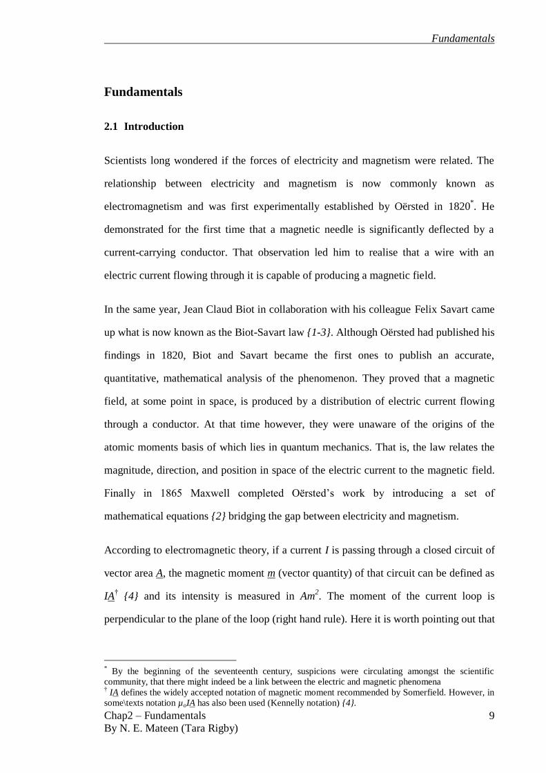
Figure 2.2 illustrates the magnetisation response of some of the well-known categories
of materials in the presence of an external applied field. As can be seen from figure 2.2
the magnetisation M is plotted against the magnetic field H for ferro-, para-, and
diamagnetic materials.
In the case of ferromagnetic materials, since there is already spontaneous magnetisation
due to strong exchange forces, all the collective atomic moments in the form of a
domain tend to rotate in the direction of the applied field.
Fundamentals
Chap2 – Fundamentals
By N. E. Mateen (Tara Rigby)
14
Fig. 2.2: Magnetisation response of various materials when a magnetic field is
applied. (Schematic made by N.E.Mateen)
In magnetism the word ‘domain’ is generally used for an area in a magnetic material
where all the collective atomic moments are aligned i.e. the magnetisation direction is
aligned For ferromagnetic materials, the point at which all the collective moments
become aligned to the applied field is generally referred to as the saturation
magnetisation. In paramagnets however, as there is no collective behaviour of the
atomic moments, an extremely large field must be applied to orient the direction of each
moment parallel to the field. Conversely, when a diamagnetic substance is exposed to a
field, a negative magnetisation effect is produced.
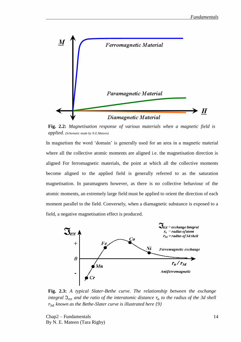
Fig. 2.3: A typical Slater-Bethe curve. The relationship between the exchange
integral and the ratio of the interatomic distance to the radius of the 3d shell
known as the Bethe-Slater curve is illustrated here {9}

Fundamentals
Chap2 – Fundamentals
By N. E. Mateen (Tara Rigby)
15
In figure 2.3, the Slater-Bethe curve shows the exchange integral as a function of
ra/r3d, where ra is the radius of the atom and r3d is the radius of the 3d shell, for some 3d
transition metals {6}. The distinction between ferromagnetic elements and
antiferromagnetic elements is illustrated by the Bethe-Slater curve in figure
2.3.
The elements Fe, Co and Ni have positive values of the exchange integral and are
ferromagnetic. Mn has a negative value of and is antiferromagnetic.
Ferromagnetism can also occur in 4f lanthanide elements i.e. the rare earth elements
such as Nd, Pr and Sm due to spin-orbit coupling, with high values of ex between spin
and orbital moments. Alloys based on mixtures of the ferromagnetic 3d and 4f elements,
such as Sm-Co and Nd-Fe are also ferromagnetic and thus are the basis for
technologically important hard magnetic materials such as SmCo5 {10} and Nd2Fe14B
{11, 12}. The high magnetisation is associated with the 3d elements while the large
anisotropy results from the 4f elements.
2.2.3 Magnetisation and hysteresis
In magnetic materials (as shown in figure 2.1) there are many magnetic moments
distributed throughout the sample. When observed collectively in some ferro/ferri-
magnetic materials this can lead to a non-zero net magnetic moment. In such a case
when this non-zero net magnetic moment is divided by the volume V of that material
gives the net magnetisation (magnetic moment per unit volume) of that material.
⁄ (2.1)
In the absence of an applied field, the net moment is zero in case of paramagnetic (the
moments not aligned in any particular direction) or antiferromagnetic materials (with an
internal alignment of moments). Hence, net magnetisation of paramagnetic or
antiferromagnetic materials is zero only for zero applied fields. However, for

Fundamentals
Chap2 – Fundamentals
By N. E. Mateen (Tara Rigby)
16
paramagnets if the external field is applied the magnetisation is proportional to the
applied magnetic field H,
(2.2)
where χ is the proportionality constant known as the magnetic susceptibility. For a
ferromagnet, the relationship between
magnetisation with respect to the field is
nonlinear, therefore
(2.3)
A hysteresis loop best describes the behaviour
of a ferromagnetic material when the
magnetisation is plotted with respect to an
applied field. Figure 2.4 illustrates the
magnetisation response of a ferromagnetic material with increasing or decreasing
external field. As to why the magnetisation of a ferromagnet behaves in such a way and
what is happening inside the material is described in section 2.4.5.
The relationship between the magnetisation M, the applied field H and magnetic
induction B* (also known as the magnetic flux density) is given as,
( ) (2.4)
(2.5)
Where is the permeability in free space, and J is the magnetic polarisation of the
system.
* the quantity used to measure the strength of a magnetic field
Fig. 2.4: Hysteresis loop showing
the variation in M as H changes. (Schematic made by N.E.Mateen)

Fundamentals
Chap2 – Fundamentals
By N. E. Mateen (Tara Rigby)
17
2.2.4 Temperature dependence
Most magnetic phenomena are temperature dependent to some degree*. However, some
magnetic materials are more dependent on temperature than others are. For example,
ferro/ferrimagnetic materials change their magnetic properties above a certain
temperature known as the Curie temperature {5} whereas antiferromagnetic materials
change their properties above the Néel temperature. Above this temperature, magnetic
materials transform their ordering and randomise their moments. A ferromagnetic
material will become paramagnetic because of such a shift in temperature. Nevertheless,
diamagnet materials are the only ones, which could be said to be independent of
temperature.
2.3 Magnetic Phenomenon: Microscopic Scale
Micromagnetism is the theory of magnetic moments and describes the underlying
magnetic structure on both the micro and nano scale. The specific properties of
magnetic micro- and nanostructures result from a complicated interplay between several
energy terms {13}. The understanding of the magnetisation process in magnetic
materials requires a detailed description of the magnetic structure as a prerequisite. The
theory of micromagnetism provides the mathematical framework to describe
magnetostatics of the magnetised structures.
It is convenient to describe the magnetic behaviour using several competing energy
terms. These terms can be summarised as a combined energy density E of a magnetic
system. The behaviour of a ferromagnet when exposed to several competing energy
terms is known as the “combined energy density” or “Landau free energy” which can be
expressed as,
(2.6)
* Except for diamagnetism which is mostly temperature independent

Fundamentals
Chap2 – Fundamentals
By N. E. Mateen (Tara Rigby)
18
where is the energy associated with exchange interactions, is the
energy associated with various anisotropies of the material, is dipolar (or
magnetostatic) also known as the shape energy of the system and is the energy
involved when the magnetisation interacts with an external magnetic field. In cases
where there is no external applied field ( ) the total energy equation
becomes,
(2.7)
The interactions these energies are generally associated with, are described below
2.3.1 Exchange
Exchange is a quantum mechanical effect between indistinguishable particles, resulting
from Pauli’s exclusion principle* and is therefore electrostatic in origin. There is no
concept of indistinguishable particles in classical physics. Therefore, there is no concept
of exchange either. The effect is due to the wave function of indistinguishable particles
subject to exchange symmetry (i.e. remaining either symmetric or anti-symmetric when
two particles are exchanged). Exchange help explain both ferromagnetism as well as
antiferromagnetism. In ferromagnetic materials, exchange tries to keep adjacent spins
aligned parallel, thus producing spontaneous magnetisation while keeping the energy at
a minimum. In such cases, due to the overlapping of the orbitals of adjacent atoms
having unpaired electrons, the distribution of those electrons in space becomes such that
they move away from each other, having their spins lining up parallel (i.e. electronic
moments lining up parallel) as opposed to the spins being aligned antiparallel. In other
words, electrons carrying parallel spins do not stay in close proximity to each other and
thus there is a reduction in the energy associated with their electrostatic interactions in
* ‘No two electrons can have the same set of four quantum numbers and occupy the same space’ or ‘two
electrons cannot have the same wave function unless their spin is antiparallel’. Thus, apart from the
electric repulsion, parallel spin electrons (i.e. aligned magnetic moments) tend to repel as well. Only
when the spin of the electrons is antiparallel can there be attraction

Fundamentals
Chap2 – Fundamentals
By N. E. Mateen (Tara Rigby)
19
such a material. This reduction in turn further favours the parallel spin configuration by
creating a stable state. However, in anti-ferromagnetic materials, the spins of the
electrons are antiparallel (i.e. opposing signs/directions) and is energetically favourable.
Ferromagnetic materials in their saturation state exhibit minimum exchange energy but
this might not necessarily hold true for other competing energies that might play a role
in the system. Thus, the exchange energy in ferromagnets always favours the parallel
alignment of the electronic magnetic moments. Conversely, exchange energy will be
stored in the system if two adjacent electronic magnetic moments are not aligned with
each other.
For ferromagnetic materials like Fe, Co and Ni, outer most electrons lie in the outermost
metallic band i.e. containing the Fermi energy level. Electrons with parallel spin prefer
to avoid each other due to the Pauli’s exclusion principle and this allows the coulomb
interaction (i.e. electrostatics) to be reduced, which is favourable. All such materials
should be ferromagnetic because of low energy and because there is lower coulomb
interaction if the spins lie parallel.
2.3.2 Anisotropy
Magnetic anisotropy is the phenomenon by which the energy of a group of spins
depends upon the direction in which they are pointing. If energy minimization occurs
when the magnetisation spontaneously aligns along a particular direction in the sample
then that direction is commonly referred to as an easy axis. Rotating the magnetisation
away from these easy axes increases the energy of the system. When this energy reaches
a maximum, the associated direction is called a hard axis. The maximum magnetic
anisotropy energy is the difference between the sample being magnetised along the hard
and easy axes. Each anisotropy contribution has an associated anisotropy constant.

Fundamentals
Chap2 – Fundamentals
By N. E. Mateen (Tara Rigby)
20
When defining anisotropy generally the symmetry of the system is taken into account.
The most common symmetries are uniaxial and cubic*. The uniaxial symmetry is
twofold, repeats every 180° whereas cubic symmetry is four fold, and thus repeats every
90°. A material may have several easy and hard axes depending on the type of dominant
anisotropy energy. There are different types of anisotropies - namely
magnetocrystalline, shape, surface and strain/stress/magnetoelastic. A brief discussion
on main magnetic anisotropies is given below,
i) Magnetocrystalline anisotropy
Of all these anisotropies, only the magnetocrystalline anisotropy is intrinsic to the
material. This is mainly due to spin orbit coupling. The magnetocrystalline anisotropy
describes the coupling of the electrons spin to the crystal lattice by a spin orbit coupling
energy. When an external field drives the reorientation of the spin of an electron, the
orbit of that electron also tends to be re-oriented. Concurrently, the orbit of the electron
is strongly coupled to the lattice and therefore it would resist the attempt to rotate the
spin axis. Due to magnetocrystalline anisotropy, different energies are involved in
magnetising a specimen in different crystallographic directions. The magnetocrystalline
anisotropy acts in such a way that the magnetisation tends to be directed along certain
crystallographic axes which correspond accordingly to easy directions of magnetisation
{13}.
The magnetocrystalline anisotropy results in preferred crystallographic directions along
which all the aligned spins or net magnetisation lie. For an effective hard magnetic
material, there should be only one preferred axis. Thus, the best permanent magnets are
based on non-cubic structures, such as hexagonal or tetragonal with the easy axis in the
* For the uniaxial case, the energy density can be written as,
where Ku is the uniaxial
anisotropy constant having units of J/m3, and θ is the spin orientation with respect to symmetry direction
{2}. The energy density variables of cubic anisotropy would be given by the expression
where K1 is the cubic anisotropy constant and αi is the direction cosine of the
spin along axis i.

Fundamentals
Chap2 – Fundamentals
By N. E. Mateen (Tara Rigby)
21
c direction. For example, hexagonal ferrites and rare earth – transition metal alloys such
as Nd2Fe14B {14}.
In amorphous samples, no crystalline anisotropy is present because they lack long-range
structural order. These normally do not have preferred direction(s) of magnetisation and
hence can be easily magnetised in any direction. However, it is possible by field
annealing to align atomic pairings in alloys parallel to the field such that a small degree
of anisotropy is introduced {15}.
ii) Shape anisotropy
Shape anisotropy has its origins in the magnetostatic energy. The shape anisotropy is
also called self-demagnetisation/dipolar energy (see section 2.3.2(ii)(1) below). It
should be made clear here that the shape anisotropy is usually included as part of the
dipolar or magnetostatic energy term, rather than anisotropy energy. For materials
where there is no crystalline anisotropy present*, the anisotropy is predominantly
dependent upon the shape of the material rather than its crystalline structure. More
importantly reducing/changing the dimensions of a magnetic material leads to strong
shape anisotropy e.g. 3D (bulk ) > 2D (thin films ) >
1D (wires ) > 0D (dots ).
Aligning all the spins in a bulk sample along the easy magnetocrystalline anisotropy
direction may produce a large magnetic stray field outside the sample. Shape anisotropy
becomes especially important for thin films when they are magnetised perpendicular to
the plane of the film. In such cases, the demagnetisation factor (see section 2.3.2(ii)(1)
below) becomes large and very significant. For example, AlNiCo where there are
elongated ferromagnetic particles in a non-magnetic or weakly magnetic matrix aligned
preferably in a common direction.
* or the sample is a crystallographically isotropic - polycrystalline

Fundamentals
Chap2 – Fundamentals
By N. E. Mateen (Tara Rigby)
22
(1) Demagnetisation field and magnetostatic energy
The demagnetisation field is a direct consequence of shape anisotropy as well as
magnetisation of the sample and thus it depends on both these factors. A demagnetising
field is generated by the surface charges (i.e. surface poles), passing internally through
the sample. It is dependent on pole strength and pole separation in the sample. In the
presence of an applied field, a finite sized ferromagnetic sample would be magnetised in
a particular direction. However, the field experienced by such a sample would not be
equal to the applied field. This is because of the presence of magnetic poles present at
the surface of magnetised ferromagnetic samples, as they generate a magnetic field,
which opposes the applied field. Hence, the difference between the applied field and the
field experienced by the magnetised sample is called the demagnetising field {2}.
(2.8)
where Hi is the field experienced by the sample, Ha is the applied field and Hd is the
demagnetising field. The strength and direction of the demagnetising field vary inside a
sample (from one position to another). As the lateral dimensions of the sample change,
the factor responsible for producing demagnetising field also changes. This factor is
known as the ‘demagnetising’ or ‘shape’ factor {2, 3, 16}denoted by the symbol N and
is a tensor quantity dependent upon the sample’s shape. The demagnetising field Hd (in
terms of the tensor quantity N and sample magnetisation) can be written as,
∑ (2.9)
where Hdi is the ith component of the demagnetising field, Mk is the kth component of
magnetisation vector and the tensor Nik* is the demagnetising factor. Equation 2.9
represents the ideal demagnetising field for an ellipsoidal shape. An ellipsoid shape is
* The demagnetising factor and depends on geometry of the magnetic sample. For a thin, out of plane-
magnetised film, the demagnetising factor is 1 and for in plane magnetisation it is 0 {2}. Thus, a large
field is required to magnetise a sample with large demagnetising factor

Fundamentals
Chap2 – Fundamentals
By N. E. Mateen (Tara Rigby)
23
the only shape in which, when a uniform external field is applied, the magnetisation
produces a uniform demagnetising field. It is difficult to calculate the demagnetising
field of an arbitrarily shaped body* {2}. However, the shape effects only become
significant at small aspect ratios and larger demagnetising factors {2}.
Fig. 2.5: A schematic diagram of surface charge distribution and origins of shape
anisotropy in case of thin film {22}
For an ultrathin film, for instance, the magnetisation will be strongly preferred along its
longer axis, i.e. in the plane of the film. This is because the magnetostatic energy is
minimised when the spins lie parallel to the plane, thus favouring in-plane
magnetisation for small surface charges across the thin edges of the film. A component
of out-of-plane magnetisation leads to surface charges on the larger areas (top and
bottom) of the thin film (see figure 2.5) thus having a higher energy. Hence, for a thin
film sample the easy axis will lie in the plane of the thin film, providing that there is not
an overriding effect arising from strong magnetocrystalline anisotropy. However, many
ultra-thin films are designed to have perpendicular magnetic anisotropy, so the
magnetization prefers to lie out of plane. In such cases of ultra-thin films, although the
magnetostatic energy is minimized when magnetization is in plane but the interface-
related anisotropy terms can overcome this.
* However, there have been studies performed regarding the demagnetisation of non-ellipsoidal shapes
{16-21}. For non-ellipsoidal samples, Burg and Wolf suggested that the demagnetising factor not only
varies as a function of position inside the sample but also as a function of the magnetic properties of the
sample {19}

Fundamentals
Chap2 – Fundamentals
By N. E. Mateen (Tara Rigby)
24
The demagnetising or magnetostatic energy in a material favours the nullification of
free poles, thus reducing the field exhibited by the magnetised material. Consequently,
the system favours paths of closed magnetisation inside the material. The magnetostatic
energy {3} can be expressed as,
∫
∫
(2.10)
where and are magnetostatic energy and the magnetostatic field of the sample
respectively. The factor ½ in equation 2.10 ensures that each dipole moment interaction
with the field is counted once (‘to take into account that each moment contribution
twice, once as a field and once as a moment’ {11}). In terms of saturation magnetisation
and the demagnetising factor, the same equation may be represented as,
∫
(2.11)
where is saturation magnetisation and is the demagnetisation factor of the
sample. Sakurai et al. {17} demonstrated that some geometrical shapes (such as
rectangular based pyramidal structures) exhibit their demagnetising energies
independent of the direction of magnetisation. This is also true of a spherical shape
sample for which .
iii) Magnetic surface anisotropy
The broken crystal symmetry at a surface can give rise to a uniaxial anisotropy, which
favours the perpendicular alignment of magnetisation with respect to the sample
surface. This can be important for thin films or when considering magnetisation
adjacent to the surface.
Although magnetisation changes and changes in spin polarisation may also be important
at interfaces. However, the surface anisotropy can be a strong and dominating effect of
the surface of a material in some circumstances and the concept was first propounded by

Fundamentals
Chap2 – Fundamentals
By N. E. Mateen (Tara Rigby)
25
Néel in 1954 {2}. Surfaces or thin films have different properties to those of bulk
materials. In a crystalline material, the surface atoms have a lower symmetry
environment due to the absence of adjacent atoms on the free space side of the crystal
surface. However, the bulk atoms have a symmetrical environment. Surface anisotropy
can be represented in the form of a surface energy density*, where
is the surface anisotropy constant and is angle of spontaneous magnetisation
normal to the surface {23}. The value of depends on the nature of the lattice
structure and surface orientation. The surface symmetry may not be higher than
uniaxial. Thus, near the surface, the symmetry breakdown from cubic to uniaxial still
occurs.
iv) Strain anisotropy
Lattice deformations influence the spin-orbit interactions and can thereby change the
anisotropy strength and direction. If a magnetic material experiences any stress/strain
then the material may experience magnetoelastic anisotropy. Magnetoelastic anisotropy
is frequently a significant factor in materials such as Fe, FeCo and FeGa. For example,
steel magnets having a highly dislocated, strained structures induced by martensitic
transformations†.
For a crystalline structure, when dealing with lattice strains (in realistic situations), the
system will deform spontaneously to keep the total free energy to a minimum. The
energy associated with such deformations is known as the magnetoelastic energy. This
is exemplified in particular by the non-uniform elastic strains associated with high
densities of lattice dislocations such as in quenching steels, which were the basis of the
* ‘in many works the definition
is often used and therefore has an opposite sign in
comparison with Néel’ {23} † A transformation that is usually driven by either mechanical deformation or change in temperature, they
are diffusionless shear transformations {24}

Fundamentals
Chap2 – Fundamentals
By N. E. Mateen (Tara Rigby)
26
early forms of permanent magnets. Similarly, strains associated with impurity particles
result in strain anisotropy {25}.
2.4 Magnetic domains, domain walls and magnetic switching processes
Magnetic ‘domains’ {13} are the regions within which the direction of magnetisation is
largely uniform in ferromagnetic materials. Although each individual region is
magnetised to saturation, adjacent regions have their own independent magnetisation
direction. The local anisotropy and/or external fields determine the direction of
magnetisation. In case of local anisotropy, the magnetisation tends to lie in an easy
direction (i.e. easy axis), within the domain. However, local anisotropy and/or external
fields also limit the possible orientation of the domains. Furthermore, the exchange
energy tends to oppose the formation of multiple domains. The domain patterns in a
material may be complicated due to the contributions of various energy terms of similar
magnitudes.
Figure 2.6 shows a schematic representation of ferromagnetic domains, in the absence
of an external field (a) - having some orientation of magnetisation within them. In the
presence of an external field (b), the domains having magnetisation roughly in the
direction of the applied field would tend to grow until only one large domain is left (c).
When the external field is further increased (d), then the magnetisation in the remaining
domain rotates, aligning its direction with that of the field direction.
When a material is in its demagnetised state, various domains have magnetisation
direction which are different to each other and which may cancel each other’s effects
(figure 2.6(a)). In such cases, given a sufficiently large number of random orientations,
the material may show a zero (or nearly zero) net magnetisation. Hence, magnetic fields
outside the material may not be easily detected. However, when the magnetisation
directions of various domains are aligned with each other, such materials produce large

Fundamentals
Chap2 – Fundamentals
By N. E. Mateen (Tara Rigby)
27
magnetic fields. Rare Earth Iron Boron (REFeB) alloys are commonly used to make
‘permanent’ magnets {26, 27} and in ideal cases, keep their domains aligned. In
transverse sections through sample of such alloys, domains may follow fractal patterns
whereas sections parallel to the easy direction manifest linear domain patterns.
Fig. 2.6: A schematic representation of ferromagnetic domains, (a) is shown in the
absence of an applied field. When an external field is applied (b) the magnetisation of
the domains that has a major component in the direction of the field direction tend to
grow. The thick arrows represent the magnitude and direction of the applied field and
the thin arrows inside the rectangular domains show the direction of magnetisation. At
higher applied fields the domain tend to push out the walls with only one single domain
with the direction of magnetisation roughly in the direction of the applied field (c).
Upon further increment of the applied field, the magnetisation of the domain will fully
align itself in the direction of the applied field (d). The boundaries dividing the domains
are called domain walls. (Schematic made by N.E.Mateen)
Domain ‘walls’ {13} are boundaries separating one domain from the other. These walls
are transitions from a domain state to its neighbouring domain state. The transition takes
place over several atomic spacing and is not abrupt. The width of this transition is called

Fundamentals
Chap2 – Fundamentals
By N. E. Mateen (Tara Rigby)
28
the domain wall thickness. The individual moments rotate to change the direction of
magnetisation from one domain to the next, as shown schematically in figure 2.7.
Fig. 2.7: A schematic representation of a Bloch domain wall in which the
magnetisation rotates from one domain (a) state to another (c). The arrows represent
the direction of magnetisation. The width of the transition is called the domain wall
thickness as shown in (b). (Schematic made by N.E.Mateen)
The domain wall thickness depends mainly on the balance between the magnetic
anisotropy and the exchange energy. This energy balance regulates the width of the
domain wall. The exchange energy of the material favours a wider domain wall with
slow moment rotation from one site to another which means no specific spin
configurations and no set domains. Thus, the moments tend to lie away from easy
directions despite the presence of anisotropy. However, in ferromagnets the magnetic
anisotropy increases due to the lack of specific spin orientation in the easy direction.
Therefore, the presence of anisotropy energy in the region of the domain walls favours
narrow domain walls in order to minimise the moments that are not parallel to the easy
magnetisation directions. Mathematically the domain wall thickness for a 180° or Bloch
wall could be written as,
√ (2.12)

Fundamentals
Chap2 – Fundamentals
By N. E. Mateen (Tara Rigby)
29
here A is exchange stiffness constant (not the area) and Ku is uniaxial anisotropy
constant {13}. The exchange stiffness constant ⁄ , where is the
exchange integral, is spin and is the lattice constant {28}.
2.4.1 Domain formation, walls and energy associated with walls
The domain pattern for a magnetic material is dependent on the size and geometry of
the specimen. The direction of magnetisation of the domains is determined by the
exchange, anisotropy and dipolar (magnetostatic) energy. The domain wall energy {13}
is the product of energy density per unit area and total wall area and is
given as . The energy density (for a sample of known thickness and
length) is required to stabilise a domain wall of any type. It can be written as (for a
uniaxial case) {29},
√ (2.13)
The total energy density is the addition of the exchange and anisotropy energies stored
per unit wall volume and for a given material.
The process of domain formation occurs in order to balance the total energy of the
system and tends to modify with increasing magnetising field as long as the end state
has a lower energy than the initial state. When the energy expenditure of increased
domain wall area becomes greater than the energy usage of reducing the magnetostatic
energy of the system, the process of further domain formation ceases.
Figure 2.8(a) represents a ferromagnetic sample having a single domain state.
Generally, a single domain state is observed either when a sample is magnetised to
saturation or when the dimensions of the sample favour the existence of a single domain
(section 2.4.3). In either case, the sample would have large magnetostatic energy* due to
* i.e. stray field or dipolar or demagnetising energy

Fundamentals
Chap2 – Fundamentals
By N. E. Mateen (Tara Rigby)
30
surface charges. The sample can remain in a single domain state or it may subdivide
into multiple domains as shown in figure 2.8(b-d), to minimise the total energy of the
system*. The presence of uniaxial anisotropy favours the alignment of domains parallel
to the anisotropy axis. Dividing the configuration into two domains reduces the
magnetostatic energy.
Fig. 2.8: Schematic of a single domain in its saturated state having large
magnetostatic energy (a). Introduction of more domain walls reduces the
magnetostatic energy further (b), but increases the wall energy (c). Formation of
closure domains ensures that there are no magnetic flux lines outside the sample are
schematically illustrated in (d), thus reducing magnetostatic energy contribution
down to zero. (Schematic made by N.E.Mateen)
The presence of multiple domains (figure 2.8(c)) significantly reduces the magnetostatic
energy still further. The lowest energy is achieved when closure domains occur at the
ends to give closed magnetic loops. This is because the domain splitting enables the
* The division shown in figure 2.8 is equally possible with cubic symmetry for the anisotropy; the only
difference would be if the end closure domains form

Fundamentals
Chap2 – Fundamentals
By N. E. Mateen (Tara Rigby)
31
magnetic field lines outside the sample to close into adjacent domain(s), thus favouring
the lower magnetostatic energy configuration of the system.
If the total energy of the saturated state of a large single domain is , then after the
domain splitting into nth approximately equal volumes with the help of (n-1)th
domain
walls, the expression for the reduced energy of the system could be written as,
(2.14)
As n becomes very large, the stray field approaches zero.
The formation of closure domains ensures that the magnetostatic energy reduces almost
to zero as shown in figure 2.8(d). The formation of closure domains removes the
presence of free poles, thus resulting in pole avoidance. This happens in cases where the
sample has little or no applied field and it has the correct anisotropy symmetry. In a
crystalline sample, elastic anisotropies are induced by the formation of closure domains
because of the introduction of strain into the system by production of walls at 90° next
to the 180° walls. Thus, due to magnetoelastic energy, the closure domain would be
favoured.
2.4.2 Types of domain walls
Two major types of domains (mentioned earlier in section 2.4.1) are the stripe domains
separated by 180° domain walls and closure domains having 90° domain walls along
with 180° walls. However, some other types of domain walls are also found in magnetic
materials. The 180° walls are generally referred to as Bloch walls; however, they are
also dependent on the saturation magnetisation as well as the film thickness. That is in
thicker films and bulk, the 180˚ walls are usually Bloch walls. In materials with
sufficient thickness (or bulk materials), the divergence of the magnetisation is zero for a
Bloch wall and therefore they are preferred.

Fundamentals
Chap2 – Fundamentals
By N. E. Mateen (Tara Rigby)
32
Fig. 2.9: The three main types of domain walls are shown here, (a) represents the 180°
Bloch wall, (b) shows the Néel wall and (c) is the combination of the Bloch and Néel
wall called the Cross-tie wall. (Schematic made by N.E.Mateen)
Typically, if the thickness of the material is lower than the width of the Bloch wall, a
Néel wall will exist. The film thickness at which the domain walls change in type
depends on the domain wall width. Below a certain thickness, walls known as Néel
walls become energetically favourable, as the spin rotates within the plane of
magnetisation. For such thicknesses, the Bloch walls become less energetically
favourable - as the cost of the spins, rotating away from the plane of the film would be
large. Thus, the Bloch wall may be converted into a Néel wall near the surface in order
to compensate for the magnetostatic energy. Therefore, for very thin films Néel walls
Fundamentals
Chap2 – Fundamentals
By N. E. Mateen (Tara Rigby)
33
are preferred. With further decrease in sample thickness, the Néel wall width increases,
which minimises the magnetostatic energy.
Another type of wall is called the Cross-Tie wall formed by intermixing of Bloch and
Néel walls. When Bloch and Néel walls become unstable, their large magnetostatic
energy is reduced if the polarisation of the walls is altered. This brings about the
formation of Cross-Tie walls. The schematics of the three types of walls is given in
figure 2.9, where (a) shows a typical 180° Bloch wall, (b) shows a thinner material
having a relatively broader Néel wall and (c) represents a cross-tie wall.
2.4.3 Single domain particles
A small particle may exhibit a single domain state when its size is smaller than or
comparable to the domain wall width {13}. Therefore, no domain wall can be formed if
the diameter where is the domain wall thickness. Thus, a stable
particle with no domain wall(s) present in it can only be created, if the energy required
to form a domain wall, is greater than the system’s magnetostatic energy. If the
crystalline particle is spherical in shape, having a radius r, then the excess energy
required to overcome magnetostatic energy is given by √ . The
magnetostatic energy required to make a single domain into a multidomain particle {2,
13} is given by ⁄ . For large where the magnetisation direction is along
the easy axis, the size of the particle under which a single domain state will occur is
given in terms of its critical radius,
√ ⁄ (2.15)
However, for a particle whose magnetisation may follow the surface contours and
where the anisotropy is weak, the exchange energy contribution would increase.
Therefore, in cases such as uniformly magnetised sphere, the expression given in
equation 2.15 would no longer be valid. However, it has been found that the critical

Fundamentals
Chap2 – Fundamentals
By N. E. Mateen (Tara Rigby)
34
radius for low anisotropy single domain particles is larger than for particles of high
anisotropy {2}.
2.4.4 Magnetic field-driven magnetic switching – wall movement and moment
rotation
Magnetic switching is driven by mainly reducing the Zeeman energy as well as the
overall energy of the system and thus increasing the alignment of spins with an applied
field. Switching can take place in a magnetic material under the influence of an external
field through two distinct processes: coherent rotation of domains and domain wall
motion.
In an ideal* system coherent rotation of the magnetisation occurs. In an attempt to
restore spins to the easy direction, a torque is exerted in the opposite direction by
anisotropy of the system. A stable spin direction is then reached by a balancing of the
respective torques and hence a trade-off between the anisotropy and the applied field
occurs.
In multi-domain processes, magnetisation reversal can take place through either domain
wall displacement or domain nucleation. Whilst reversals by coherent rotation are
collective the domain processes are slower as they are sequential in nature {30}. A
domain with spin alignment in the direction of switching can nucleate around
inhomogeneities such as sample edges or surface defects. The wall adjacent to that
domain would advance by rotating its spins in such a way that it realigns the spins of all
the adjacent domains, which have different directions to the nucleated domain. In the
case of a large number of nucleation events, the walls of each domain travel a short
distance before coalescing with neighbouring domains. This type of domain process is
common in magnetic thin films.
* A system without any impurities or pinning sites, a single domain system
Fundamentals
Chap2 – Fundamentals
By N. E. Mateen (Tara Rigby)
35
For domain wall displacement with a small number of nucleation events, the wall itself
travels over a larger distance, thus increasing the size of the magnetic domains, which
have their spin orientation in the direction of applied field. However, any large defect(s)
and/or a “feature” with a dimension of the order of a domain wall width may impede the
propagation of domain walls. These features are generally known as “pinning centres”
or “pinning sites” {3}. The domain wall displacement can thus be controlled through the
pinning mechanism. This leads to complex magnetisation mechanisms, due to
imbalances in the energy states of the material.
2.4.5 Hysteresis: hard or soft materials
Domain and domain wall processes can be explained with the help of the hysteresis
loop. When the applied field is varied, the average magnetisation in the material
lags behind the applied field, thus creating a hysteresis loop (or M-H curve), as shown
in figure 2.10.
The initial magnetisation curve from the demagnetised state is shown in figure 2.10(a-
e), with the corresponding domains and domain walls as the sample goes from its
demagnetised state to saturation magnetisation. In the demagnetised state, the
magnetostatic energy of the sample is minimal. Such a sample would have multiple
domain walls as shown in figure 2.10(a). As the field is increased, domain walls start to
propagate through the sample, thus increasing the size of the domains, which have a
component of magnetisation direction towards the applied field (figure 2.10(b to c)).
The remaining domains and domain walls, which possess magnetisation components
pointing in any other direction to the applied field, shrink and may eventually,
disappear.

Fundamentals
Chap2 – Fundamentals
By N. E. Mateen (Tara Rigby)
36
Upon further increment of the applied field, the magnetisation direction of the domain
starts to move by coherent rotation towards the direction of the applied field (figure
2.10(d)).
Fig. 2.10: Hysteresis loop showing the variation in as changes. The initial
magnetisation curve from its demagnetised state is shown with the corresponding
domains and domain walls (a-e), as the sample goes from its demagnetised state to
saturation magnetisation. Once saturation occurs and the field is reversed, the
magnetisation curve follows the outer hysteric loop, showing the remanence, coercive
and anisotropy fields. (Schematic made by N.E.Mateen)
Here, the domain walls completely disappear (or are unable to move due to defects and
pinning sites) and the domain’s individual magnetic moments align themselves along
the field direction. Once the moments are fully aligned, any further increments of
applied field will not influence the domain(s) magnetisation direction within the applied
field, thus, leading to magnetic saturation denoted by (figure 2.10(e)). Once
saturated, the magnetisation does not go back to its original demagnetised state, when

Fundamentals
Chap2 – Fundamentals
By N. E. Mateen (Tara Rigby)
37
the field is reduced to zero. This behaviour is known as hysteresis. A hysteresis loop is
unique to that particular sample, although careful duplication of a sample may produce a
nearly identical loop.
When the field is reversed after saturation, the magnetisation curve starts to follow the
outer hysteretic loop (figure 2.10). The magnetisation no longer retraces its original path
upon field reversal, when the field is reduced to zero. The value of magnetisation is
called the remanence, and is denoted by on the hysteresis curve shown in figure
2.10. From in figure 2.10, if the field is increased in the opposite direction, the
magnetisation will further decrease. The field that is required to bring back to zero is
known as the coercive field, .
With the help of these properties, an M-H curve can explain the magnetic hardness or
softness of a material. For example, consider the loop shown in figure 2.11(a). The
material has both a large remanence and a large coercive field. Materials having a large
anisotropy field tend also to have a higher coercive field. Such materials are known as
hard magnetic materials.
(a) (b) (c) Fig. 2.11: Hysteresis loop showing the variation in M as H changes. (a) Represents a
sample, which has a high anisotropy field and thus a high coercive field is a
magnetically hard material; (b) shows an example of a soft magnetic material with
low coercivity and anisotropy. (c) Represents a particle, which has a single domain
state, influenced by moment rotation only (Schematic made by N.E.Mateen)
Figure 2.11(b) shows the hysteresis of a material, which has lower coercive field
compared to that of figure 2.11(a), thus, representative of a moderate system. Moderate

Fundamentals
Chap2 – Fundamentals
By N. E. Mateen (Tara Rigby)
38
to soft materials are used in data storage and recording media. An ideal data storage
material would have quite high remanence and significantly low coercivity. Materials
having very low anisotropy fields and low coercive fields are generally called “soft
magnetic materials”, they maybe polycrystalline or amorphous. A loop generated by a
material particle, having zero coercivity (low anisotropy or a hard axis loop) is shown in
figure 2.11(c). Although, ferromagnetic single domain particles exhibit hysteresis but do
not typically follow the loop in part 2.11(c). The materials exhibiting a hysteresis as
shown in figure 2.11(c) come under the category of superparamagnetic particles. They
switch their magnetisation direction due to random atmospheric thermal fluctuations.
Hence, they put a physical limit to data storage and recording device miniaturisation
commonly known as superparamagnetic limit.
The simplest classification for ferromagnetic materials could be of high coercive
(strong/hard) and low coercive (weak/soft) magnetic materials. The behaviour of both
soft and hard magnetic materials is, however, influenced markedly by extrinsic factors
such as microstructure inclusions and thermal history {3}.
2.5 Stray fields above the surface of ferromagnets
Ferromagnetic materials (as well as current carrying conductors) generate stray fields,
which can influence other materials in their close proximity. In a ferromagnet, the
magnetic stray fields are generated wherever there is a discontinuity in the
magnetisation of the body ( due to magnetic poles, which may be referred to
as free charges (an analogy with the electric charges). Stray fields may find their origins
in the domains or the domain walls themselves.
Figure 2.12(a) shows a schematic diagram of a ferromagnet having periodic domains of
width ‘b’ (as ), and each domain has a direction of magnetisation opposite to
that of its neighbouring domains. Therefore, the magnetic charges at the surface

Fundamentals
Chap2 – Fundamentals
By N. E. Mateen (Tara Rigby)
39
alternate. This periodicity gives rise to the stray fields emanating from the sample, as
represented in figure 2.12(b).
(a) (b) Fig. 2.12: A schematic of a cross-sectional semi-infinite sample, (a) showing periodic
domains and (b) magnetic charges on the surface giving rise to a magnetic field
distribution {2}
In the case of Bloch domain walls, (figure 2.9) free charges (i.e. poles) would arise on
the wall surface separating the two domains. For example, for relatively thin materials,
stray fields are generated when Bloch walls intersect with the surfaces of the material.
For cross-tie walls, alternating magnetic charging occurs due to an unbalanced mixture
of the Bloch and Néel walls. All these phenomena give rise to stray fields.
(a) (b) Fig. 2.13: A schematic comparison of magnetic media having in-plane magnetisation
called longitudinal media (a), and media having the magnetisation direction
perpendicular surface of the sample plane (b), called perpendicular media {2}
Figure 2.13 shows a schematic of two different configurations of stray fields. The stray
fields generated by a longitudinal data storage media: the magnetisation lies within the
plane of the media (a) whereas, for perpendicular media (b) the magnetisation lies out of
plane of the material.

Fundamentals
Chap2 – Fundamentals
By N. E. Mateen (Tara Rigby)
40
Stray fields (Macro-, micro- or nanoscopic range) associated with a magnetic material
or current carrying conductors (on surface or embedded in microcircuits) can be
successfully detected with a sensor of known parameters. Although semiconductor
materials are the most commonly available field sensor (via the Hall effect), magnetic
(such as ferromagnetic, or superparamagnetic) {31}, electromagnetic{32} or optical{33-
35}sensors are also available. Both the Bitter Method {5, 13} and the MFM {31} are
simple techniques sensitive to stray magnetic field. In case of Bitter method, a fine
magnetic powder is applied to the surface of the magnetic material, the powder particles
align themselves with the surface stray field gradient of the magnetic sample {13} that
can then be examined by using a suitable optical microscope. An MFM, on the other
hand, produces force gradient images because of the interactions between a magnetic
probe (integrated with a cantilever) and a sample’s magnetic stray field gradient by
raster scanning over the sample’s surface. These interactions translate into a change in
resonant frequency of the cantilever. The change in resonant frequency of the cantilever
thus leads to formation of a force gradient images.{36}
2.6 Summary
In this chapter, some basic magnetic phenomena occurring on various length scales
have been discussed. Furthermore, the various types of magnetic materials and their
associated energies have also been summarised. Magnetic domains, domain walls and
magnetic switching processes have been briefly reviewed along with various types of
domains walls and single/multidomain particles.
2.7 References
{1} Jiles, D.; "Introduction to Magnetism and Magnetic Materials". London:
Chapman & Hall, Second Edition, 1998.
{2} O'Handley, R. C.; "Modern Magnetic Materials: Principles and Applications".
New York: John Wiley & Sons, Inc., 2000.

Fundamentals
Chap2 – Fundamentals
By N. E. Mateen (Tara Rigby)
41
{3} Bertotti, G.; "Hysteresis in Magnetism: For Physicists, Materials Scientists,
and Engineers": Academic Press, Inc, 1998.
{4} Carpenter, C. J.; "Definitions and Roles of The Electromagnetic Field
Vectors", IEE Proceedings-Science Measurement And Technology, vol. 146,
pp. 73-82, 1999.
{5} Chikazumi, S.; "Physics of Ferromagnetism", Second ed: Oxford University
Press Inc., New York, 1997.
{6} Rudden, M. N. and Wilson, J.; "Elements of Solid State Physics". Chichester:
John Wiley & Sons, 1993.
{7} Bozorth, R.; "Ferromagnetism", 3rd ed. New York: IEEE Press, 2003.
{8} Nolting, W. and Ramakanth, A.; "Quantum Theory of Magnetism".
Heidelberg: Springer 2009.
{9} Getzlaff, M.; "Fundamentals of Magnetism": Springer Berlin Heidelberg,
2008.
{10} Wei, L., Zhaohui, G., and Yongquan, G.; "Latest Developments and
Applications of Sm-Co Based Magnets", Magnetic Materials Ind. Co., Ltd. :
http://www.micro-magnet.com/Latest-Developments-and-Applications-of-Sm-
Co-Based-Magnets.html, Copyright © 2006
{11} IHS Engineering360; "NdFeB (Neodymium Iron Boron) Industrial Magnets
Datasheets",
http://www.globalspec.com/ds/1005/areaspec/material_neodymium_iron_boron,
Copyright © 2015
{12} Direct Industry: The Online Industrial Exhibition; "NdFeB magnets", Direct
Industry: The Online Industrial Exhibition:
http://www.directindustry.com/industrial-manufacturer/ndfeb-magnet-
79965.html, Copyright © 2015
{13} Hubert, A. and Schafer, S.; "Magnetic Domains: The Analysis of Magnetic
Microstructures": Springer-Verlag Berlin Heidelberg New York, 1998.
{14} Tang, S. L., Gibbs, M. R. J., Davies, H. A., Liu, Z. W., Lane, S. C., and Mateen,
N. E.; "An Effective Route for The Fabrication of Rare Earth-Iron-Boron
Thin Films Having Strong c-Axis Texture and Excellent Hard Magnetic
Properties", Journal Of Applied Physics, vol. 101, 2007.
{15} Jiang, J. Z., Pankhurst, Q. A., and Gibbs, M. R. J.; "The Effect of Field
Annealing on Moment Canting in Amorphous Fe78Si9B13", Journal Of
Magnetism And Magnetic Materials, vol. 140, pp. 323-324, 1995.
{16} Joseph, R. I. and Schloman.E; "Demagnetizing Field In Nonellipsoidal
Bodies", Journal Of Applied Physics, vol. 36, pp. 1579-&, 1965.
{17} Sakurai, S., Soda, N., Kobayashi, M., and Rowlands, G.; "Geometries With The
Demagnetizing Energy Independent of The Direction of Magnetization",
IEEE Transactions On Magnetics, vol. 43, pp. 982-991, 2007.
{18} Tomlinson, S. L. and Farley, A. N.; "Micromagnetic Model for Magnetic
Force Microscopy Tips", Journal Of Applied Physics, vol. 81, pp. 5029-5031,
1997.
{19} Brug, J. A. and Wolf, W. P.; "Demagnetizing Fields In Magnetic
Measurements .2. Bulk And Surface Imperfections", Journal Of Applied
Physics, vol. 57, pp. 4695-4701, 1985.
{20} Brug, J. A. and Wolf, W. P.; "Demagnetizing Fields In Magnetic
Measurements .1. Thin Disks", Journal Of Applied Physics, vol. 57, pp. 4685-
4694, 1985.

Fundamentals
Chap2 – Fundamentals
By N. E. Mateen (Tara Rigby)
42
{21} Rhodes, P. and Rowlands, G.; "Demagnetising Energies of Uniformly
Magnetized Rectangular Blocks", presented at Proc. Leeds Phil. Lit. Soc, 1954.
{22} Cowburn, R. P.; "Magnetic Switching and Domain Structure in Ultrathin
Epitaxial Magnetic Films", Department of physics, vol. PhD. Cambridge:
University of Cambridge, 1996.
{23} Kaneyoshi, T.; "Introduction to Surface Magnetism": CRC press, 1991.
{24} University of Cambridge; "Martensitic Phase Transformations - A Simple
Example", http://www.doitpoms.ac.uk/tlplib/superelascity/index.php, 19Oct,
Copyright © 2004-2015.
{25} Nalwa, H. S.; "Magnetic Nanostructure", 2nd
ed. USA: American Scientific,
2002.
{26} Liu, W., Jiang, J. H., Wu, J. S., and Li, G.; "Magnetic Force Microscope Study
on Anisotropic NdFeB Permanent Magnets", Transactions Of Nonferrous
Metals Society Of China, vol. 13, pp. 1410-1414, 2003.
{27} Al-Khafaji, M. A.; "Magnetic Force Microscopy of NdFeB Hard Magnetic
Alloys", Engineering Materials, vol. PhD. Sheffield: University of Sheffield,
1998, pp. 266.
{28} Anonymous; " Lecture 26: Magnetic Domains ", MIT OpenCourseWare:
http://ocw.mit.edu, 2013.
{29} Support Note No. 229, R. B.; "Magnetic Force Microscopy (MFM) Applicable
to Dimension™ Series and MultiMode™ Systems: Digital Instruments",
2000.
{30} Olson, C. D. and Pohm, A. V.; "Flux Reversal In Thin Films Of 82-Percent
Ni, 18-Percent Fe", Journal Of Applied Physics, vol. 29, pp. 274-282, 1958.
{31} Martin, Y. and Wickramasinghe, H. K.; "Magnetic Imaging By Force
Microscopy With 1000-Å Resolution", Applied Physics Letters, vol. 50, pp.
1455-1457, 1987.
{32} Chen, Y. J., Leong, S. H., Huang, T. L., Ng, K. W., Hu, S. B., Yuan, Z. M., and
Ng, V.; "A Comparative Study of Write Field Ddistribution of Trailing-Edge
Shielded and Unshielded Perpendicular Write Heads by Quantitative
Magnetic Force Microscopy", Applied Physics Letters, vol. 92, 2008.
{33} "Recording Head: Efficient Kerr Microscopy", 2006.
{34} Chumakov, D., McCord, J., Schafer, R., Schultz, L., Vinzelberg, H., Kaltofen,
R., and Monch, I.; "Nanosecond Time-Scale Switching of Permalloy Thin
Film Elements Studied by Wide-Field Time-Rresolved Kerr Microscopy",
Physical Review B, vol. 71, 2005.
{35} Schafer, R., Argyle, B. E., and Trouilloud, P. L.; "Domain Studies in Single-
Crystal Ferrite Metal-In-Gap Heads With Image-Enhanced, Wide-Field, Kerr
Microscopy", IEEE Transactions On Magnetics, vol. 28, pp. 2644-2646, 1992.
{36} NT-MDT; "Magnetic Force Microscopy: Quantitative Results Treatment",
<http://www.ntmdt.ru> Copyright © 1998-2015.

Magnetic Force Microscopy
Chap3 - Magnetic Force Microscopy
By N. E. Mateen (Tara Rigby) 43
Magnetic Force Microscopy
3.1 Introduction
In order to observe the magnetic micro/nano-structures, various imaging techniques
such as magnetic force microscopy* (MFM) {2-5}, Bitter method {6, 7}, magneto-
optical methods {6, 8-10} and transmission electron microscopy (TEM) {6, 11, 12} have
been developed. Many of these techniques are capable of producing high quality
magnetic images as well as providing quantitative information about the specimen.
However, almost all the techniques suffer from high costs, laborious and time-
consuming sample preparation procedures, or limited special resolution, except perhaps
for MFM and the Bitter method.
Though the Bitter technique is sensitive, easy to use and highly cost effective it is
handicapped by its limited magnetic field range of 10kA/m (or 10µA/nm) {6}
(Appendix: 3.A). MFM on the other hand, is a cost effective, sensitive, high-resolution
technique, which requires minimum sample preparation. Consequently, MFM is easy to
operate and applicable under various environmental conditions for instance in vacuum
{13-15} or low temperature {16-20}. The progress made in the last three decades has
turned MFM from a research tool into one of the most widely used magnetic imaging
techniques. Overall throughput of this instrument is the adequate compared to its
alternative approaches. However, they are complementary techniques, each with their
own advantages and disadvantages.
Despite the progress made, rigorous research is still required, especially in the areas of
improvement of the techniques overall resolution but more importantly in efforts
towards quantifying the image data. If MFM could be made into a quantitative
technique then its application in the field of metrology would also skyrocket.
* In 1987 Martin and Wickramasinghe {1} developed the magnetic force microscope (MFM), for the
observation of magnetic structures

Magnetic Force Microscopy
Chap3 - Magnetic Force Microscopy
By N. E. Mateen (Tara Rigby) 44
3.2 What is MFM?
A magnetic force microscope (MFM) is capable of generating images of the spatial
variation of magnetic forces originating from a magnetic sample’s surface. In other
words, the microscope is sensitive to the spatial derivatives of the magnetic stray fields
generated by the sample. These stray fields result from the divergence of magnetisation†
(as stated in chapter 2) and therefore MFM is an indirect method for gauging samples
magnetisation. The MFM can also be regarded as a ‘magnetic charge-imaging device’
{21, 22} because it generates an image from the resulting charge accumulation at the
surface of the sample.
† for bulk and for the surface
Fig. 3.1: A schematic representation an MFM, z is defined as the flying height of the
tip and is taken as the co-ordinate direction perpendicular to the sample surface. The
laser is shone at the backside of the tip and a photo detector (PD) senses the change
in the cantilevers’ frequency. The blue dotted lines represent the stray field lines
emanating from the sample (Image made by N.E.Mateen)

Magnetic Force Microscopy
Chap3 - Magnetic Force Microscopy
By N. E. Mateen (Tara Rigby) 45
MFM uses the magnetic probe - a force sensor - to detect these magnetic force gradients
of the source material (having a specific direction of magnetisation) by raster scanning
over the surface of the sample at a certain height. A laser is shone at the backside of the
tip and a position sensitive photodiode detector (PD) senses the change in the
cantilevers’ frequency. Hence, the digital image of the MFM is the result of a highly
precise laser set up that is sensitive to the oscillations of the cantilever due to the
magnetic field gradients the cantilever detects as shown in figure 3.1
3.3 What is an MFM probe?
At the core of the MFM is the probe - a magnetic tip attached to a cantilever {23}.
Generally, the probe is coated with a magnetic material. The term MFM probe has
generally come to symbolise the magnetically active volume of the force sensor {24,
25}.
The term magnetically active volume implies that there is only some portion of volume
of the total material on the probe, which plays an active part in the final image
formation. This term ‘active volume’ or in some cases, ‘the effective volume’ is a
theoretical term {26, 27} and is subject to further debate (see chapter 7). The term
‘probe’ may be used only to represent the tip or it may refer to the combination of both
the tip and the cantilever. This choice of terminology might depend on the active
contribution of both amount and type of magnetic material in the image formation‡ .
The magnetic probe attached at a free end of a biasing member (piezoelectric actuator)
deflects (having a set of frequency) in response to the magnetic forces between it and
the sample {30}.
‡ This is because the dimensions of the probe are too small to avoid magnetic coating on cantilever with
the commercially available manufacturing/coating techniques {28} Therefore, in most commercial probes,
both tip and the cantilever is magnetically coated {29} unless otherwise stated {23}

Magnetic Force Microscopy
Chap3 - Magnetic Force Microscopy
By N. E. Mateen (Tara Rigby) 46
3.4 Sensing magnetic stray field gradients
The interactions between the tips and the sample lie at the heart of MFM technique.
This interaction (between the tip and the sample) results in a shift in the resonant
frequency of the cantilever. The changes in frequency are recorded in the form of a
force gradient map. This shift in resonance can be measured in a number of ways such
as phase, amplitude or through a feedback loop {6, 31}.
At any instant, the motion of the cantilever is dependent on distance between probe and
sample, the amplitude (or frequency) of a given probe and on the local magnetic field
gradient experienced. At low amplitude, the cantilever oscillations remain uninfluenced
by the tip-sample interactions resulting in no field sensitivity. In addition, if the tip-
sample separation is too large the field sensitivity is significantly reduced. In such cases
no external force gradient could be detected therefore, a zero force gradient can then
be assumed {32} and the resonant frequency can be denoted of the cantilever by f0.
However, at a reduced tip-sample separation the interactive tip-sample forces influence
the cantilever oscillations. Now the cantilever behaves under the influence of tip-sample
interaction as if it had modified amplitude. Thus, the presence of a force gradient will
shift the resonant frequency of the probe by ⁄ if the force gradient
is
small compared to the spring constant . Therefore, it could be said that there is a
tension between cantilever amplitude and tip height from the sample. With higher
amplitudes and lower tip heights greater sensitivity could be offered.
In practice, the force derivative is most commonly determined by measuring the
cantilever phase variation and therefore, has been used in this dissertation. The phase
of the probe oscillation also changes rapidly around the resonant frequency. This can be
measured by a signal proportional to the resonant frequency shift i.e., change in
resonant frequency (see figure 3.2). When a cantilever is excited (due to the stray field

Magnetic Force Microscopy
Chap3 - Magnetic Force Microscopy
By N. E. Mateen (Tara Rigby) 47
gradients of the samples) in the predominantly z direction§ and its excitation frequency
approaches the resonant frequency, the phase is shifted by and can be expressed as
⁄ (3.1)
where Q is the quality factor**
and k is spring constant.
The resonant frequency shift can also be detected by using a phase locked feedback loop
{38} where the phase is monitored and the driving frequency is altered to maintain the
phase lag at a constant value corresponding to the resonance condition {39}.
Another factor favouring phase measurements (over both frequency and amplitude
methods) is the relative simplicity and its additional capability of rendering relatively
higher resolution of the images {32}.
3.4.1 Contrast formation: MFM images
The magnetic contrast image generated by the MFM is of the stray field gradient of the
sample, relative to the direction of magnetisation of the tip. The inhomogeneous
§ Extensive research has been conducted in the area of cantilever modes of excitation {23, 34-37},
however, for convenience only z-axis is assumed **
The quality factor is dependent on the cantilever’s intrinsic properties such as its mass, resonant
frequency and damping factor {23, 36}
Fig. 3.2: Shift in phase at a given drive frequency {33}

Magnetic Force Microscopy
Chap3 - Magnetic Force Microscopy
By N. E. Mateen (Tara Rigby) 48
magnetic stray field sensed by the tip is due to both attractive and repulsive forces
acting upon it. The images in MFM are mostly generated with image contrast formed by
the phase shift and any change in phase shift depends on the direction of the positive or
negative force gradient.
For images to be created, the measured signal is allocated to a grey scale. These grey
values represent different magnetic field gradient strengths of sample interaction with
the consistently magnetised probe. The variation of interactive magnetic forces between
the magnetic probe and the sample changes the magnitude of the phase-shift††
, which
results in an overall higher or lower contrast {40}. Thus, image (phase) contrast is the
difference between the lowest and highest phase shifts. Conventionally‡‡
positive phase
shifts produced by repulsive force interactions or negative phase shifts by attractive
force interactions between the probe and the sample are allocated lighter or darker
contrast in the MFM image respectively {41}. MFM software is also capable of
determining the average value of all the phase shifts, in a particular region of the
sample. This value is called the mean phase value {42}.
Depending on the type of probe-sample interactions, figure 3.3 shows repulsive,
attractive and neutral/grey scale MFM image contrast {43}. However, these contrast
scales are due to interaction of the tip, typically magnetised in this z-direction and the
dominating z-component of magnetic stray field of the sample. The right side of the
figure shows no contrast or grey scale/neutral area. The MFM image renders no contrast
because the magnetisation of the sample lies in the plane and its contribution to the z-
component is negligible. The tip therefore does not experience attractive or repulsive
forces acting upon it and there is no change in the phase shift.
††
The magnitude of the phase-shift generally reflects the vertical component of the stray fields emanating
out of samples ‡‡
In case of mathematical analysis to match the results with the experiments a negative sign may be
included with the phase shift {41}

Magnetic Force Microscopy
Chap3 - Magnetic Force Microscopy
By N. E. Mateen (Tara Rigby) 49
Fig. 3.3: A Schematic cross-sectional presentation of a longitudinal magnetic storage
media and a number of bits with certain direction of the magnetisation are shown.
Also indicated is the magnetic stray field emanating from the bit transitions. Bottom
figure shows the expected MFM image contrast for three different types of bit
transitions as resulting either from repulsive, attractive or no interaction of the tip
with the sample {43}
The contrast formation in MFM is a complex process because of its dependence upon
numerous factors {44} enumerated below:
a) the direction of magnetisation of the sample and the tip
b) tip shape
c) coating thickness
d) tip-sample distance
e) the drive amplitude of the tip and
f) tip amplitude set points and tilt angles which are different for different types of
magnetic structures with respect to the samples surface.

Magnetic Force Microscopy
Chap3 - Magnetic Force Microscopy
By N. E. Mateen (Tara Rigby) 50
3.4.2 Separating magnetic signal and artefacts
Magnetic signals are sensed by the probe, at a certain position above the sample’s
surface, due to the probe interaction with the stray field gradients of the sample. The
magnetic signals are not the only signals the probe may encounter. There are other
forces present at or near the surface of the magnetic sample, which can be picked up by
the probe. These forces interfere in the process of magnetic image capture if the probe-
sample distance lies within their respective ranges. It is therefore imperative that the
magnetic signals are separated from such forces as the interference of any unwanted
force can produce image artefacts. The resulting image would then not be a true
magnetic representation. These near surface forces include electrostatic, capillary
wetting interactions, quantum mechanical and the van der Waal force§§
{32, 46}. Most
of these forces fall off rapidly with distance from the surface. However, the magnetic
forces have longer range and can persist at a distance from the sample surface beyond
the Coulombic forces. Hence, the signal from the magnetic force can be separated from
the Coulombic forces provided the tip/sample separation is sufficiently large.
Scientists successfully exploited these differences in the dependencies of the signals on
distances {47, 48}. Much work was done {1} to keep the probe in the range of dominant
magnetic signals and to control the probe-sample separation, especially in cases where
the sample’s surfaces were relatively rough {4, 50-55}. The initial studies {56-58}
relating to the constant probe-sample separation encountered problems when
investigators had to deal with irregular sample surfaces because this resulted in a
variable probe-sample distance. It could not then be ensured that forces, such as van der
§§
Van der Waals forces originate from the interatomic distances and can be both short and long range.
Below 10nm probe-sample distance, the van der Waals force increase. Due to the difficulty in
determination of the actual tip shape, it is difficult to ‘model’ actual distance dependence of the van der
Waals forces {32}. Compared to van der Waals interactions the magnetic interactions have a shorter
range. This is because the span of influence of the magnetic interaction is determined by the inverse third
power of the separation distance. Conversely, in case of, van der Waals interactions the separation
distance fall off with the inverse first power {45}

Magnetic Force Microscopy
Chap3 - Magnetic Force Microscopy
By N. E. Mateen (Tara Rigby) 51
Waal’s, remained reasonably constant with respect to the magnetic forces, thus resulting
in image artefacts {59}. Later, the surface topography was used as a reference point
because the van der Waal’s forces could generate good quality surface images. The
images generated are called AFM images {53, 60-64}, since ‘atomic’ forces are used to
generate these. In this method, researchers {56} kept the probe-sample distance larger
than the set distance for the surface topography imaging. The drawback was to maintain
a constant probe-sample distance and making sure that the magnetic signal and the
surface topography remained separate over the entire surface.
In the early 90s Hosaka et al. {55, 58, 65-67} introduced an idea of separating the
magnetic signal from other surface signals. By using both a constant repulsive force
control and a magnetic force gradient measurement, they measured magnetic force
gradient image and a surface structure image. If the height is kept low enough the short
range van der Waals forces come into play and interfere with the long range magnetic
forces. The most effective way for the separation of the topographic and the magnetic
forces is with lift heights. This is a good way of acquisition of topographic as well as the
magnetic information at the same time. One major advantage of this is as the magnetic
features are strongly connected to the surface features of the sample which is extremely
useful in the interpretation of magnetic features observed. A similar method is used in
the commercial MFM to separate the magnetic signal from the unwanted artefacts***
. A
set distance (~20nm to 1μm) from the sample is generally given for the probe to operate.
This method is commonly known as ‘tapping Liftmode’ {33, 68}.
As MFM mainly detects the relatively long-range magnetic forces between the tip and
the sample, for it to work effectively a minimum distance of about 10 nanometres {69}
is required between the probe and the sample for it to be able to sense the small
***
Image artifacts could also arise from other environmental factors such as a contamination of the tip
apex or that of the sample, image noise and/or acoustic vibrations. Such artifacts are generally catered for
by using a vibration/sound proof table and using the instrument in a clean room environment or using the
MFM in vacuum

Magnetic Force Microscopy
Chap3 - Magnetic Force Microscopy
By N. E. Mateen (Tara Rigby) 52
magnetic stray fields. Depending on the strength of the stray field gradients emanating
from the tip and the sample, the detection range of an MFM typically ranges from tens
of nanometres to a few micrometres {33}.
3.5 The importance of MFM Probes
The accuracy of MFM images depend on the magnetic properties of the probe, which
are dependent on the type of magnetic material, its amount by volume, the size, the
shape of material on the tip or shape of the tip itself including the distance between tip
and sample. A probe selected for imaging a particular sample should be suitable for that
sample at least. For example, a probe with very strong magnetic field strength may
change the magnetic configuration i.e. ‘write’ on a soft sample {24, 70-74}, conversely
a probe with a significantly weak field strength may be influenced itself by a strong
field from the sample {75-81}. Ideally, the same probe should be used for a complete
study if comparative studies are to be conducted.
Without sufficient understanding of the behaviour of a probe, accurate image
interpretation is not possible. However, due to the involvement of various factors in the
probe, the probe-sample interactions are complex to understand. In an effort to aid in
understanding, generally the process is made simpler by assuming a probe behaves
ideally.
3.5.1 What is an ideal MFM probe?
An ideal MFM probe should have a tip made of (or coated with) a magnetic material
having a volume small enough to exhibit a weak but stable magnetic field so that the
tip’s field does not perturb the sample magnetisation in any way. Although attempts for
manufacturing ideal probes have been made {70, 77-79, 82-98}, the majority of the
MFM probes available commercially {23, 28, 29, 99} are much more complex.

Magnetic Force Microscopy
Chap3 - Magnetic Force Microscopy
By N. E. Mateen (Tara Rigby) 53
Therefore, it is convenient to make some simplistic assumptions regarding real probes
in order to investigate them.
3.5.2 Assumptions for an idealistic probe
When considering the probe-sample magnetic interactions, normally a number of
assumptions are made in order to simplify a highly complex process of image formation
and its interpretation. As the focus of this study was the MFM probe, the behaviour of
the cantilevers was not studied extensively. For all intent and purposes, the cantilever
behaves as is normally expected for a typical magnetic image measurement. Arguably,
if there were any inconstancies in the cantilever’s behaviour, those disparities would
appear as contributing factors toward the final MFM image formation. Extensive studies
of the cantilever have been performed in the literature {17, 23, 34-37, 91, 100-111}.
Some common assumptions of the cantilever and tip are:
a) That the cantilever is parallel to the surface plane of the sample and that the stray
field gradient over the sample surface is sensitive to the probe-sample (tip-sample)
interaction force or its gradient in the perpendicular (z) direction as shown in figure
3.4(a).
b) That the tip shape is perfectly symmetrical as represented in figure 3.4(a) and that the
magnetic coating on the tip is uniform.
c) That the tip apex is the active contributor in the formation of a magnetic image. The
contributions from the base of the tip (attached to the cantilever) as well as the
cantilever itself are considered weak and are ignored {23, 35, 37, 105}).
d) That the MFM tip is made of a material that can consistently maintain its
magnetisation direction once magnetised so that the tip moment is constrained as shown
in figure 3.4(b). The probe behaviour is considered stable if the tip moment(s) (hard tip

Magnetic Force Microscopy
Chap3 - Magnetic Force Microscopy
By N. E. Mateen (Tara Rigby) 54
with high coercivity) do not vary in direction or magnitude under the influence of the
stray field experienced above a sample surface.
Fig. 3.4: An ideal cantilever position with its ideal MFM pyramidal shaped tip and
initial magnetisation direction perpendicular to the sample surface as represented
schematically in (a). Furthermore, in ideal cases it is expected that the magnetisation
direction does not change while the MFM probe scans the sample as shown in (b). In
real cases however, the cantilever might not be parallel to the samples surface, the
pyramidal tip shape may be asymmetrical even though the magnetisation direction of
the tip might have been initially perpendicular to the samples surface as shown in (c).
However, during an MFM scan the precise direction of the magnetisation is
unpredictable, as there is always a possibility of some amount of tip and/or the sample
influencing each other (d). (Schematic made by N.E.Mateen)
e) That the tip stray field does not locally change (write) a magnetisation distribution
into the sample together with its stray field gradient or vice versa.
f) If a domain structure is present in the tip coating then the domain structure does not
change during the measurement.
Generally, it is considered that if some of these assumptions are not taken into
consideration for a specific probe-sample arrangement the image interpretation becomes
too complex to understand. A few assumptions might be necessary to simplify the
complex processes, however, the aim should always be to keep the scenario as real as
possible in order to understand and utilise the real behaviour of the tip and/or the sample
or both as shown in figure 3.4(c-d).

Magnetic Force Microscopy
Chap3 - Magnetic Force Microscopy
By N. E. Mateen (Tara Rigby) 55
3.5.2.1 Magnetic stray fields and stray field gradients
When the stray fields generated by the sample interact with the moment of the MFM
probe, the probe experiences a force written as,
(3.2)
For simplification, clause a) given in section 3.5.2 is considered. Therefore, the equation
3.2 in the perpendicular (z) direction for a tip moment and sample can be written as,
(
⁄ ) (3.3)
and a force gradient
( ⁄ ) (3.4)
where
is the magnetic moment of the tip and
is the stray field from the
sample. The interaction of the tip stray field with the sample magnetisation can also be
considered due to the principle of reciprocity {112-114}. In that case, the notation of tip
and sample in equations 3.3 and 3.4 could be reversed i.e.,
and
. Equations
3.3 and 3.4 are true for simple image interpretations where a magnetic probe interacts in
a non-perturbative manner with the sample.
3.5.3 Non-idealistic, real probe
In real cases, multiple factors such as those mentioned above (complicated probe
geometries and magnetic structure) are involved in the process of the MFM image
formation (see figure 3.4(c-d)). These factors contribute towards the image instability in
general and may introduce image artefacts as well. Hence, the actual process of MFM
image formation is quite complex and one has to have a shrewd eye to be able to detect
the real from the defective images. If only the surface of a probe is coated with
magnetic material, then the tip shape, the type and amount of magnetic materials coated

Magnetic Force Microscopy
Chap3 - Magnetic Force Microscopy
By N. E. Mateen (Tara Rigby) 56
on the probe are amongst a few factors that affect the resulting magnetic image
significantly. In other words, the magnetic image (of a particular sample) as portrayed
by the MFM, would be subject to the tip’s magnetic behaviour in relation to the
specimen under investigation.
Figure 3.5 illustrates the complex surfaces involved in a typical commercial tip
(pyramidal in shape). These surfaces introduce uncertainties into any quantitative
modelling and hence image interpretation. In practice, when tips are fabricated, the
probe is first manufactured with Si and then a deposition technique such as sputtering
{115} is utilised to deposit the magnetic coating. However, as the area covered by the
sputtering techniques is generally huge compared to the area needed to be coated i.e.,
only the tip, both the tip and the cantilever are coated with magnetic material.
Therefore, this method might be excellent for batch fabrication but has some major
issues when it comes to the image quality. As a result, whole tip batches may be of high
quality or merely acceptable. For high performance tips, such as by Veeco, the
manufacturers usually charge at premium rates, as those tips are easily available, show
stable behaviour that is suitable for a wide variety of samples having moderate†††
magnetic properties. Furthermore, in case of batch-fabricated probes the thickness on
†††
midrange coercivity
(a) (b) Fig. 3.5: SEM image of the top of a commercial CoCr MFM pyramidal tip (a), and
as viewed from the side (b) (Image captured by N.E.Mateen)

Magnetic Force Microscopy
Chap3 - Magnetic Force Microscopy
By N. E. Mateen (Tara Rigby) 57
the sidewalls of the tip may not be uniform as the quoted thicknesses for coating is
equivalent to a monolithic film.
As there are non-zero stray fields and gradients in the region of the tip’s base as well as
cantilever arm a significant force could be contributed from those areas. Furthermore,
the z-direction is not exactly in the plane of any side of the pyramid, giving the
possibility of sensitivity to off-axis stray-field-gradients. In addition, the cantilever is
not parallel to the sample surface in most MFM instruments. The thin film geometry in
the tip will, to first order, dictate that the dipole moment is in the plane of the coating
(shape anisotropy), and thus may not be quite aligned with the z-axis of the
measurement geometry.
3.6 Imaging Concerns: Tip and Sample considerations
One of the biggest problems in magnetic force microscopy is image reproducibility
{116}. It has been observed that even if the magnetic tips are taken from the same batch,
there is a difference in the quality of the images produced {117}. As mentioned there are
several factors involved that make the image reproducibility difficult, therefore there is
a need for an extensive study of the characterisation and calibration of the magnetic tips.
Due to the size, amount and nature of the material involved in the probe-sample
interaction (including the possible effects of probe sample distance), it is improbable to
have any two probes, which can be used in metrology giving the same quantitative
results. However, with precise instrumentation and fabrication techniques it might be
possible to manufacture probes within an accurate tolerance range, which might make it
possible to use a probe quantitatively with respect to a reference sample. Alternatively,
it may be used qualitatively with respect to images it captured from different locations
of the same sample or various samples (provided all the other parameters‡‡‡
be kept the
‡‡‡
Given parameters during the image capture operation as well as tip-sample distance and the tip
magnetisation direction etc.

Magnetic Force Microscopy
Chap3 - Magnetic Force Microscopy
By N. E. Mateen (Tara Rigby) 58
same). Currently, it is speculated that there are limitations for making two separate
probes of the same specifications capable of producing identical images of the sample
due to the limitations of manufacturing techniques {116}.
In order to understand how and where these image uncertainties originate from, one
must look closely at the shape, size, structure and magnetic properties of the material
used in MFM probes and what are the factors affecting them.
3.7 Summary
This chapter covers the MFM probe and its limitations. The MFM has been introduced
here. Alternate instruments such as the Bitter technique have been mentioned so that the
benefits of the MFM can be fully appreciated.
Since the magnetic probe senses magnetic stray field gradients, the interaction between
the probe and the sample. In particular, terms such as the spring constant, the cantilevers
and resonant frequency have been introduced. Whether the force on the probe is
attractive (darker) or repulsive (lighter) the grey scale recreation of the field gradient
will be mapped as the probe raster scans the image area. The general output format for a
MFM is a force gradient map that shows the magnetic contrast formed by the phase
shift (figure 3.1).
Under certain circumstances, artefacts can be introduced into the MFM signal. Section
3.4.2 explains how these artefacts can be avoided or at least minimised. As well as
artefacts, another issue with the MFM instrument that requires some consideration is the
assumption that we make for an idealistic probe. While no real probe can truly follow an
idealistic approach, section 3.5.2 tries to outline some of the issues associated with real
probes, which are typically batch, fabricated commercial tips.

Magnetic Force Microscopy
Chap3 - Magnetic Force Microscopy
By N. E. Mateen (Tara Rigby) 59
In short, this chapter dealt with some basic information about the MFM, for example,
what is MFM, what is MFM probe and what is the importance of the probe. It also
raised issues regarding the well-known assumptions surrounding the probes and the
expectations based on those idealistic assumptions. In the end, the concept of the non-
idealistic probes was introduced. Special emphasis was laid on the concerns§§§
related to
the image formation, due to the interactive relationship of the probe with the sample.
3.8 References
{1} Martin, Y. and Wickramasinghe, H. K.; "Magnetic Imaging By Force
Microscopy With 1000-Å Resolution", Applied Physics Letters, vol. 50, pp.
1455-1457, 1987.
{2} De Lozanne, A.; "Application of Magnetic Force Microscopy in
Nanomaterials Characterization", Microscopy Research And Technique, vol.
69, pp. 550-562, 2006.
{3} Hartmann, U.; "Magnetic Force Microscopy", Annual Review of Materials
Science, vol. 29, pp. 53-87, 1999.
{4} Hartmann, U.; "Theory of Magnetic Force Microscopy", Journal of Vacuum
Science & Technology a-Vacuum Surfaces and Films, vol. 8, pp. 411-415, 1990.
{5} Wadas, A. and Grutter, P.; "Theoretical Approach to Magnetic Force
Microscopy", Physical Review B, vol. 39, pp. 12013-12017, 1989.
{6} Hubert, A. and Schafer, S.; "Magnetic Domains: The Analysis of Magnetic
Microstructures": Springer-Verlag Berlin Heidelberg New York, 1998.
{7} Chikazumi, S.; "Physics of Ferromagnetism", Second ed: Oxford University
Press Inc., New York, 1997.
{8} Allwood, D. A., Xiong, G., Cooke, M. D., and Cowburn, R. P.; "Magneto-
Optical Kerr Effect Analysis of Magnetic Nanostructures", Journal Of Physics
D-Applied Physics, vol. 36, pp. 2175-2182, 2003.
{9} Cantwell, P. R., Gibson, U. J., Allwood, D. A., and Macleod, H. A. M.; "Optical
Coatings for Improved Contrast in Longitudinal Magneto-Optic Kerr Effect
Measurements", Journal Of Applied Physics, vol. 100, 2006.
{10} Gibson, U. J., Holiday, L. F., Allwood, D. A., Basu, S., and Fry, P. W.;
"Enhanced Longitudinal Magnetooptic Kerr Effect Contrast in Nanomagnetic
Structures", IEEE Transactions on Magnetics, vol. 43, pp. 2740-2742, 2007.
{11} Matteucci, G., Frost, B. G., and Medina, F. F.; "Study of The Field Around
Magnetic Force Microscopy Probes Using Electron Holography",
Ultramicroscopy, vol. 99, pp. 95-102, 2004.
{12} Signoretti, S., Beeli, C., and Liou, S. H.; "Electron Holography Quantitative
Measurements on Magnetic Force Microscopy Probes", Journal of Magnetism
and Magnetic Materials, vol. 272-76, pp. 2167-2168, 2004.
§§§
inherently attached with the MFM probe

Magnetic Force Microscopy
Chap3 - Magnetic Force Microscopy
By N. E. Mateen (Tara Rigby) 60
{13} Dreyer, M., Lohndorf, M., Wadas, A., and Wiesendanger, R.; "Ultra-High-
Vacuum Magnetic Force Microscopy of The Domain Structure of Ultra-Thin
Co Films", Applied Physics A-Materials Science & Processing, vol. 66, pp.
S1209-S1212, 1998.
{14} Leinenbach, P., Losch, J., Memmert, U., and Hartmann, U.; "Ultrahigh
Vacuum Magnetic Force Microscopy on In Situ Grown Iron Thin Films",
Applied Physics A-Materials Science & Processing, vol. 66, pp. S1191-S1194,
1998.
{15} Yamaoka, T., Watanabe, K., Shirakawabe, Y., Chinone, K., Saitoh, E., Tanaka,
M., and Miyajima, H.; "Applications of High-Resolution MFM System with
Low-Moment Probe in A Vacuum", IEEE Transactions On Magnetics, vol. 41,
pp. 3733-3735, 2005.
{16} Hug, H. J., Moser, A., Jung, T., Fritz, O., Wadas, A., Parashikov, I., and
Guntherodt, H. J.; "Low-Temperature Magnetic Force Microscopy", Review
Of Scientific Instruments, vol. 64, pp. 2920-2925, 1993.
{17} Yuan, C. W., Batalla, E., Zacher, M., Delozanne, A. L., Kirk, M. D., and
Tortonese, M.; "Low-Temperature Magnetic Force Microscope Utilizing A
Piezoresistive Cantilever", Applied Physics Letters, vol. 65, pp. 1308-1310,
1994.
{18} Volodin, A., Temst, K., Van Haesendonck, C., and Bruynseraede, Y.; "Low
Temperature Magnetic Force Microscopy with Enhanced Sensitivity Based on
Piezoresistive Detection", Review Of Scientific Instruments, vol. 71, pp. 4468-
4473, 2000.
{19} Callaghan, F. D., Yu, X., and Mellor, C. J.; "Variable Temperature Magnetic
Force Microscopy with Piezoelectric Quartz Tuning Forks as Probes
Optimized using Q-Control", Applied Physics Letters, vol. 87, 2005.
{20} Seo, Y., Cadden-Zimansky, P., and Chandrasekhar, V.; "Low-Temperature
High-Resolution Magnetic Force Microscopy using A Quartz Tuning Fork",
Applied Physics Letters, vol. 87, 2005.
{21} Proksch, R.; "Recent Advances in Magnetic Force Microscopy", Current
Opinion in Solid State & Materials Science, vol. 4, pp. 231-236, 1999.
{22} Hubert, A., Rave, W., and Tomlinson, S. L.; "Imaging Magnetic Charges With
Magnetic Force Microscopy", Physica Status Solidi B-Basic Research, vol.
204, pp. 817-828, 1997.
{23} Jenkins, N. E., DeFlores, L. P., Allen, J., Ng, T. N., Garner, S. R., Kuehn, S.,
Dawlaty, J. M., and Marohn, J. A.; "Batch Fabrication and Characterization of
Ultrasensitive Cantilevers with Submicrometre Magnetic Tips", Journal Of
Vacuum Science & Technology B, vol. 22, pp. 909-915, 2004.
{24} Tomlinson, S. L. and Hill, E. W.; "Modelling The Perturbative Effect of MFM
Tips on Soft Magnetic Thin Films", Journal Of Magnetism And Magnetic
Materials, vol. 161, pp. 385-396, 1996.
{25} Leinenbach, P., Memmert, U., Schelten, J., and Hartmann, U.; "Fabrication and
Characterization of Advanced Probes for Magnetic Force Microscopy",
Applied Surface Science, vol. 145, pp. 492-496, 1999.
{26} Tomlinson, S. L., Hoon, S. R., Farley, A. N., and Valera, M. S.; "Flux Closure
in Magnetic Force Microscope Tips", IEEE Transactions On Magnetics, vol.
31, pp. 3352-3354, 1995.

Magnetic Force Microscopy
Chap3 - Magnetic Force Microscopy
By N. E. Mateen (Tara Rigby) 61
{27} Tomlinson, S. L. and Farley, A. N.; "Micromagnetic Model for Magnetic
Force Microscopy Tips", Journal Of Applied Physics, vol. 81, pp. 5029-5031,
1997.
{28} Grutter, P., Rugar, D., Mamin, H. J., Castillo, G., Lambert, S. E., Lin, C. J.,
Valletta, R. M., Wolter, O., Bayer, T., and Greschner, J.; "Batch Fabricated
Sensors for Magnetic Force Microscopy", Applied Physics Letters, vol. 57, pp.
1820-1822, 1990.
{29} Grutter, P., Rugar, D., Mamin, H. J., Castillo, G., Lin, C. J., McFadyen, I. R.,
Valletta, R. M., Wolter, O., Bayer, T., and Greschner, J.; "Magnetic Force
Microscopy with Batch-Fabricated Force Sensors", Journal of Applied
Physics, vol. 69, pp. 5883-5885, 1991.
{30} Valera, M. S. and Farley, A. N.; "A High Performance Magnetic Force
Microscope", Measurement Science & Technology, vol. 7, pp. 30-35, 1996.
{31} Hug, H. J., Stiefel, B., van Schendel, P. J. A., Moser, A., Hofer, R., Martin, S.,
Guntherodt, H. J., Porthun, S., Abelmann, L., Lodder, J. C., Bochi, G., and
O'Handley, R. C.; "Quantitative Magnetic Force Microscopy on
Perpendicularly Magnetized Samples", Journal Of Applied Physics, vol. 83,
pp. 5609-5620, 1998.
{32} Porthun, S., Abelmann, L., and Lodder, C.; "Magnetic Force Microscopy of
Thin Film Media for High Density Magnetic Recording", Journal of
Magnetism and Magnetic Materials, vol. 182, pp. 238-273, 1998.
{33} Digital Instruments, I.; "Dimention 3100 Instruction Manual: version 4.31ce",
Copyright © 1997.
{34} Dicarlo, A., Scheinfein, M. R., and Chamberlin, R. V.; "Magnetic Force and
Force Gradient Microscopy Utilizing An Ultra-Sensitive Vertical Cantilever
Geometry", Scanning Probe Microscopies Ii, vol. 1855, pp. 187-194, 1993.
{35} Van den Bos, A. G., Van Dijk, A. C. J., Heskanp, I. R., Abelmann, L., and
Lodder, J. C.; "A New Concept in Magnetic Force Microscope Cantilevers", in
Magnetic Storage Systems Beyond 2000, vol. 41, Nato Science Series, Series Ii:
Mathematics, Physics and Chemistry, 2001, pp. 307-312.
{36} Rast, S., Gysin, U., Ruff, P., Gerber, C., Meyer, E., and Lee, D. W.; "Force
Microscopy Experiments with Ultrasensitive Cantilevers", Nanotechnology,
vol. 17, pp. S189-S194, 2006.
{37} Koblischka, M. R., Wei, J. D., Richter, C., Sulzbach, T. H., and Hartmann, U.;
"Advanced Cantilevers for Magnetic Force Microscopy and High Frequency
Magnetic Force Microscopy", Scanning, vol. 30, pp. 27-34, 2008.
{38} Dunn, D.; "Phase-Locked Loops", US4069462-A, Data General Corporation,
1978.
{39} Hobbs, P. C. D., Abraham, D. W., and Wickramasinghe, H. K.; "Magnetic
Force Microscopy With 25 nm Resolution", Applied Physics Letters, vol. 55,
pp. 2357-2359, 1989.
{40} Chen, D. C., Chiang, D. P., and Yao, Y. D.; "Quantitative Analysis of
Magnetization Reversal in Patterned Strip Wire by Magnetic Force
Microscopy", Journal Of Magnetism And Magnetic Materials, vol. 304, pp. 23-
26, 2006.
{41} Lohau, J., Kirsch, S., Carl, A., Dumpich, G., and Wassermann, E. F.;
"Quantitative Determination of Effective Dipole and Monopole Moments of
Magnetic Force Microscopy Tips", Journal of Applied Physics, vol. 86, pp.
3410-3417, 1999.

Magnetic Force Microscopy
Chap3 - Magnetic Force Microscopy
By N. E. Mateen (Tara Rigby) 62
{42} Chen, Y. S., Cheng, K. W., Yu, C., Lee, S. F., Liou, Y., Hsu, J. H., and Yao, Y.
D.; "Magnetic Reversal for Different Shaped Corners in Sub-Micrometre
Half-Ring Wires by Mean Phase Analyses of Magnetic Force Microscopy",
Journal Of Magnetism And Magnetic Materials, vol. 310, pp. 2606-2608, 2007.
{43} Nalwa, H. S.; "Magnetic Nanostructure", 2nd
ed. USA: American Scientific,
2002.
{44} Hopster, H. and Oepen, H. P.; "Magnetic Microscopy of Nanostructures":
Springer-Verlag Berlin Heidelberg Germany, 2005.
{45} Garcia, A. A.; "Bioseparation Process Science": Blackwell publishing, 1999.
{46} Zhu, Y.; "Modern Techniques for Characterizing Magnetic Materials":
Springer, 2005.
{47} Matey, J. R. and Blanc, J.; "Scanning Capacitance Microscopy", Journal Of
Applied Physics, vol. 57, pp. 1437-1444, 1985.
{48} Saenz, J. J., Garcia, N., Grutter, P., Meyer, E., Heinzelmann, H., Wiesendanger,
R., Rosenthaler, L., Hidber, H. R., and Gunterodt, H. J.; "Observation of
Magnetic Forces by The Atomic Force Microscope", Journal Of Applied
Physics, vol. 62, pp. 4293-4295, 1987.
{49} Anonymous; "Magnetic Force Data Analysis Method For Magnetic
Recording Medium Using Magnetic Force Microscope|Involves Detecting
Magnetic Force and Surface Roughness Image Using Magnetic Force Data
and Surface Roughness Data", JP10123156-A, Toshiba Kk,
{50} Elings, V. B. and Gurley, J. A.; "Atomic Force Microscope Two Phase
Scanning Method|Obtaining and Storing Topographical Information and,
With Second Scan, Measuring Parameter of Surface Other Than Topography,
Such as Surface Magnetic Fields", US5418363-A; US5418363-B1, Digital
Instr Inc, 1995.
{51} Heike, S.; "Magnetic Force Microscope for Measuring Magnetic Field
Distribution on Surface of Neodymium-Iron-Boron Magnet, has Distance-
Hold Unit to Hold Distance as Probe Does Not Contact With Specimen While
Controlling Displacement of Cantilever", US2012319679-A1; JP2013002970-
A, Hitachi Ltd, 2012.
{52} Heike, S. and Hashizume, T.; "Scanning Probe Microscope Used for
Measuring Magnetic Force Distribution on Surface of Sample Such as Hard
Disk Drive Head has Distance Control Unit that Measures Height Distribution
on Surface of Sample Using Electrostatic Force", JP2012013575-A, Hitachi
Ltd, 2012.
{53} Wadas, A.; "The Theoretical Aspect of Atomic Force Microscopy used for
Magnetic-Materials", Journal Of Magnetism And Magnetic Materials, vol. 71,
pp. 147-150, 1988.
{54} Wadas, A., Grutter, P., and Guntherodt, H. J.; "Analysis of Magnetic Bit
Pattern by Magnetic Force Microscopy", Journal of Vacuum Science &
Technology a-Vacuum Surfaces and Films, vol. 8, pp. 416-420, 1990.
{55} Hosaka, S., Kikukawa, A., Honda, Y., Koyanagi, H., and Tanaka, S.;
"Simultaneous Observation of 3-Dimensional Magnetic Stray Field and
Surface-Structure Using New Force Microscope", Japanese Journal Of
Applied Physics Part 2-Letters, vol. 31, pp. L904-L907, 1992.
{56} Schonenberger, C., Alvarado, S. F., Lambert, S. E., and Sanders, I. L.;
"Separation of Magnetic and Topographic Effects in Force Microscopy",
Journal Of Applied Physics, vol. 67, pp. 7278-7280, 1990.

Magnetic Force Microscopy
Chap3 - Magnetic Force Microscopy
By N. E. Mateen (Tara Rigby) 63
{57} Proksch, R. and Dahlberg, E. D.; "Optically Stabilized, Constant-Height Mode-
Operation of A Magnetic Force Microscope", Journal Of Applied Physics, vol.
73, pp. 5808-5810, 1993.
{58} Hosaka, S., Kikukawa, A., and Honda, Y.; "High-Resolution of Magnetic
Force Microscope Image Using A Just-On-Surface Magnetic Force
Microscope", Japanese Journal Of Applied Physics Part 1-Regular Papers Short
Notes & Review Papers, vol. 33, pp. 3779-3784, 1994.
{59} Bhushan, B.; "Scanning Probe Microscopy in Nanoscience and
Nanotechnology 2", vol. 2. Berlin: Springer 2011.
{60} Binning, G., Rohrer, H., Gerber, C., and Weibel, E.; "Surface Studies By
Scanning Tunneling Microscopy", Physical Review Letters, vol. 49, pp. 57-61,
1982.
{61} Erlandsson, R., McClelland, G. M., Mate, C. M., and Chiang, S.; "Atomic Force
Microscopy Using Optical Interferometry", Journal Of Vacuum Science &
Technology A-Vacuum Surfaces And Films, vol. 6, pp. 266-270, 1988.
{62} Grutter, P., Meyer, E., Heinzelmann, H., Rosenthaler, L., Hidber, H. R., and
Guntherodt, H. J.; "Application Of Atomic Force Microscopy To Magnetic-
Materials", Journal Of Vacuum Science & Technology A-Vacuum Surfaces
And Films, vol. 6, pp. 279-282, 1988.
{63} Gautier, B., Fares, B., Prudon, G., and Dupuy, J. C.; "Imaging by Atomic Force
Microscopy of The Electrical Properties Difference of The Facets of Oxygen-
Ion-Induced Ripple Topography in Silicon", Applied Surface Science, vol.
231-2, pp. 136-140, 2004.
{64} Lee, S. H. and Jung, K. S.; "Magnetic Manipulation of A Microcantilever for
A New Concept in Atomic Force Microscopy", IEEE Transactions On
Magnetics, vol. 43, pp. 2737-2739, 2007.
{65} Hosaka, S., Kikukawa, A., Honda, Y., and Koyanagi, H.; "Study of Magnetic
Stray Field Measurement on Surface Using New Force Microscope", Japanese
Journal Of Applied Physics Part 2-Letters, vol. 31, pp. L908-L911, 1992.
{66} Hosaka, S., Kikukawa, A., Honda, Y., and Hasegawa, T.; "Just-On-Surface
Magnetic Force Microscopy", Applied Physics Letters, vol. 65, pp. 3407-3409,
1994.
{67} Hosaka, S., Kikugawa, A., Koyanagi, H., Hosoki, S., and Hasegawa, T.;
"Surface Observing Apparatus and Method", Hitachi Ltd., Tokyo, Japan,
1995.
{68} Support Note No. 229, R. B.; "Magnetic Force Microscopy (MFM) Applicable
to Dimension™ Series and MultiMode™ Systems: Digital Instruments",
2000.
{69} le Febre, A. J., Luttge, R., Abelmann, L., and Lodder, J. C.; "Field Emission to
Control Tip-Sample Distance in Magnetic Probe Recording", presented at
Proceedings of the International Conference on Nanoscience and Technology,
2007.
{70} Tomlinson, S. L., Farley, A. N., Hoon, S. R., and Valera, M. S.; "Interactions
between Soft Magnetic Samples and MFM Tips", Journal Of Magnetism And
Magnetic Materials, vol. 158, pp. 557-558, 1996.
{71} Kong, L. S., Shi, R. C., Krauss, P. R., and Chou, S. Y.; "Writing Bits of
Longitudinal Quantized Magnetic Disk using Magnetic Force Microscope
Tip", Japanese Journal Of Applied Physics Part 1-Regular Papers Short Notes &
Review Papers, vol. 36, pp. 5109-5111, 1997.

Magnetic Force Microscopy
Chap3 - Magnetic Force Microscopy
By N. E. Mateen (Tara Rigby) 64
{72} Kong, L. S., Zhuang, L., and Chou, S. Y.; "Writing and Reading 7.5 Gbits/in(2)
Longitudinal Quantized Magnetic Disk Using Magnetic Force Microscope
Tips", IEEE Transactions On Magnetics, vol. 33, pp. 3019-3021, 1997.
{73} Phillips, G. N. and Suzuki, T.; "Quantitative Analysis of Written Bit
Transitions in 5 Gbit/in(2)
Media by Magnetic Force Microscopy", Journal of
Magnetism and Magnetic Materials, vol. 175, pp. 115-124, 1997.
{74} Wadas, A., Dreyer, M., Lohndorf, M., and Wiesendanger, R.; "Novel 'Writing'
Using Magnetic Force Microscopy in Ultrahigh Vacuum", IEEE Transactions
On Magnetics, vol. 33, pp. 4050-4052, 1997.
{75} Hopkins, P. F., Moreland, J., Malhotra, S. S., and Liou, S. H.;
"Superparamagnetic Magnetic Force Microscopy Tips", Journal of Applied
Physics, vol. 79, pp. 6448-6450, 1996.
{76} Liou, S. H., Malhotra, S. S., Moreland, J., and Hopkins, P. F.; "High Resolution
Imaging of Thin-Film Recording Heads by Superparamagnetic Magnetic
Force Microscopy Tips", Applied Physics Letters, vol. 70, pp. 135-137, 1997.
{77} Heydon, G. P., Rainforth, W. M., Gibbs, M. R. J., Davies, H. A., Hill, G.,
Bishop, J. E. L., Tucker, J. W., Huo, S., Pan, G., Mapps, D. J., and Clegg, W.
W.; "Magnetic Force Microscopy of Soft Magnetic Films", in Electron
Microscopy And Analysis 1999, Institute Of Physics Conference Series, Kiely,
C. J., Ed. Bristol: Iop Publishing Ltd, 1999, pp. 307-310.
{78} Memmert, U., Muller, A. N., and Hartmann, U.; "Probes for Magnetic Force
Microscopy Imaging of Soft Magnetic Samples", Measurement Science &
Technology, vol. 11, pp. 1342-1347, 2000.
{79} Garcia, J. M., Thiaville, A., Miltat, J., Kirk, K. J., Chapman, J. N., and Alouges,
F.; "Quantitative interpretation of Magnetic Force Microscopy Images from
Soft Patterned Elements", Applied Physics Letters, vol. 79, pp. 656-658, 2001.
{80} Schreiber, S., Savla, M., Pelekhov, D. V., Iscru, D. F., Selcu, C., Hammel, P. C.,
and Agarwal, G.; "Magnetic Force Microscopy of Superparamagnetic
Nanoparticles", Small, vol. 4, pp. 270-278, 2008.
{81} Liu, X., Isomura, S., and Morisako, A.; "Magnetic Force Microscope Probes
With High Resolution by Soft Magnetic Vortex", IEEE Transactions On
Magnetics, vol. 48, pp. 3673-3676, 2012.
{82} Arie, T., Nishijima, H., Akita, S., and Nakayama, Y.; "Carbon-Nanotube Probe
Equipped Magnetic Force Microscope", Journal of Vacuum Science &
Technology B, vol. 18, pp. 104-106, 2000.
{83} Cayetano, V. O., Moler, K. A., and Straver, E. W. J.; "Novel Carbon Nanotube
Tips: En Route to High Resolution and Ultra Sensitive Force Detection in
Magnetic Force Microscopy", Copyright © 2000.
{84} Arie, T., Yoshida, N., Akita, S., and Nakayama, Y.; "Quantitative Analysis of
The Magnetic Properties of A Carbon Nanotube Probe in Magnetic Force
Microscopy", Journal of Physics D-Applied Physics, vol. 34, pp. L43-L45,
2001.
{85} Yoshida, N., Arie, T., Akita, S., and Nakayama, Y.; "Improvement of MFM
Tips Using Fe-Alloy-Capped Carbon Nanotubes", Physica B-Condensed
Matter, vol. 323, pp. 149-150, 2002.
{86} Yoshida, N., Yasutake, M., Arie, T., Akita, S., and Nakayama, Y.;
"Quantitative Analysis of The Magnetic Properties of Metal- Capped Carbon
Nanotube Probe", Japanese Journal of Applied Physics Part 1-Regular Papers
Short Notes & Review Papers, vol. 41, pp. 5013-5016, 2002.

Magnetic Force Microscopy
Chap3 - Magnetic Force Microscopy
By N. E. Mateen (Tara Rigby) 65
{87} Deng, Z. F., Yenilmez, E., Leu, J., Hoffman, J. E., Straver, E. W. J., Dai, H. J.,
and Moler, K. A.; "Metal-Coated Carbon Nanotube Tips for Magnetic Force
Microscopy", Applied Physics Letters, vol. 85, pp. 6263-6265, 2004.
{88} Kuramochi, H., Uzumaki, T., Yasutake, M., Tanaka, A., Akinaga, H., and
Yokoyama, H.; "A Magnetic Force Microscope Using CoFe-Coated Carbon
Nanotube Probes", Nanotechnology, vol. 16, pp. 24-27, 2005.
{89} Akinaga, H., Semba, Y., Yokoyama, H., Yasutake, M., Kuramochi, H., Senba,
Y., and Senba, S.; "Probe for Scanning-Type Magnetic Force Microscope, has
Ferromagnetic Alloy Layer Containing Specific Alloy and Having Preset
Surface Roughness, Provided at Surface of Carbon Nanotube",
JP2006184141-A; CN1801399-A; KR2006076721-A; US2008166560-A1;
US7495215-B2; JP4452827-B2; CN1801399-B, Dokuritsu Gyosei Hojin
Sangyo Gijutsu So; Sii Nanotechnology Kk; Atsumitec Kk; Sii Nanotechnology
Inc; Nat Inst Advanced Ind Sci&Technology; Nat Inst Advanced Ind Sci &
Technology; Sii Nano Technology Inc, 2006.
{90} Winkler, A., Mühl, T., Menzel, S., Kozhuharova-Koseva, R., Hampel, S.,
Leonhardt, A., and Büchner, B.; "Magnetic Force Microscopy Sensors Using
Iron-Filled Carbon Nanotubes", Journal Of Applied Physics, vol. 99, 2006.
{91} Chen, I. C., Chen, L. H., Gapin, A., Jin, S., Yuan, L., and Liou, S. H.; "Iron-
Platinum-Coated Carbon Nanocone Probes on Tipless Cantilevers for High
Resolution Magnetic Force Imaging", Nanotechnology, vol. 19, 2008.
{92} Wolny, F., Weissker, U., Mühl, T., Leonhardt, A., Menzel, S., Winkler, A., and
Büchner, B.; "Iron-Filled Carbon Nanotubes as Probes for Magnetic Force
Microscopy", Journal Of Applied Physics, vol. 104, 2008.
{93} Tanaka, K., Yoshimura, M., and Ueda, K.; "High-Resolution Magnetic Force
Microscopy Using Carbon Nanotube Probes Fabricated Directly by
Microwave Plasma-Enhanced Chemical Vapor Deposition", Journal Of
Nanomaterials, 2009.
{94} Weissker, U., Loeffler, M., Wolny, F., Lutz, M. U., Scheerbaum, N., Klingeler,
R., Gemming, T., Mühl, T., Leonhardt, A., and Büchner, B.; "Perpendicular
Magnetization of Long Iron Carbide Nanowires Inside Carbon Nanotubes
Due to Magnetocrystalline Anisotropy", Journal Of Applied Physics, vol. 106,
2009.
{95} Banerjee, P., Wolny, F., Pelekhov, D. V., Herman, M. R., Fong, K. C.,
Weissker, U., Mühl, T., Obukhov, Y., Leonhardt, A., Büchner, B., and Hammel,
P. C.; "Magnetization Reversal in An Individual 25 nm Iron-Filled Carbon
Nanotube", Applied Physics Letters, vol. 96, 2010.
{96} Wolny, F., Muehl, T., Weissker, U., Lipert, K., Schumann, J., Leonhardt, A.,
and Buechner, B.; "Iron Filled Carbon Nanotubes as Novel Monopole-Like
Sensors for Quantitative Magnetic Force Microscopy", Nanotechnology, vol.
21, 2010.
{97} Manago, T., Asada, H., Uzumaki, T., Takano, F., Akinaga, H., and Kuramochi,
H.; "The Advantages of The Magnetic Structure in Ferromagnetic-Film-
Coated Carbon Nanotube Probes", Nanotechnology, vol. 23, 2012.
{98} Lisunova, Y., Heidler, J., Levkivskyi, I., Gaponenko, I., Weber, A., Caillier, C.,
Heyderman, L. J., Klaeui, M., and Paruch, P.; "Optimal Ferromagnetically-
Coated Carbon Nanotube Tips for Ultra-High Resolution Magnetic Force
Microscopy", Nanotechnology, vol. 24, pp. 105705-105705, 2013.

Magnetic Force Microscopy
Chap3 - Magnetic Force Microscopy
By N. E. Mateen (Tara Rigby) 66
{99} Ohodnicki, P., Webler, B., Deshpande, A., and Wiezorek, J. M. K.;
"Interpretation of Magnetic Force Microscopy Contrast Using Commercially
Available Batch Tips for Investigation of Surface Magnetic Domain Structure
in Polycrystalline Bulk Equiatomic L1(0) FePd", Metallurgical And Materials
Transactions A-Physical Metallurgy And Materials Science, vol. 38A, pp. 2479-
2487, 2007.
{100} Dicarlo, A., Scheinfein, M. R., and Chamberlin, R. V.; "Magnetic Force
Microscopy Utilizing an Ultrasensitive Vertical Cantilever Geometry", Applied
Physics Letters, vol. 61, pp. 2108-2110, 1992.
{101} Dicarlo, A., Scheinfein, M. R., and Chamberlin, R. V.; "Magnetic Force
Microscope Utilizing an Ultra-Small-Spring-Constant Vertically Cantilevered
Tip", Ultramicroscopy, vol. 47, pp. 383-392, 1992.
{102} Bruland, K. J., Garbini, J. L., Dougherty, W. M., and Sidles, J. A.; "Optimal
Control of Force Microscope Cantilevers .2. Magnetic Coupling
Implementation", Journal Of Applied Physics, vol. 80, pp. 1959-1964, 1996.
{103} Garbini, J. L., Bruland, K. J., Dougherty, W. M., and Sidles, J. A.; "Optimal
Control of Force Microscope Cantilevers .1. Controller Design", Journal Of
Applied Physics, vol. 80, pp. 1951-1958, 1996.
{104} Cunningham, M. J., Jenkins, D. F. L., and Khalid, M. A. H.; "Cantilever
Vibration Control by Electrostatic Actuation for Magnetic Force Microscopy",
Sensors and Actuators a-Physical, vol. 63, pp. 125-128, 1997.
{105} Takahashi, H., Ando, K., and Shirakawabe, Y.; "Self-Sensing Piezoresistive
Cantilever and its Magnetic Force Microscopy Applications",
Ultramicroscopy, vol. 91, pp. 63-72, 2002.
{106} Straver, E.; "Cantilever-Based Measurements on Nanomagnets and
Superconductors", The Department of Applied Physics, vol. Doctor of
Philosophy. Stanford: Stanford University, 2004 pp. 170.
{107} Duch, M., Plaza, J. A., Villanueva, G., Perez, R., Esteve, J., Errachid, A., and
Samitier, J.; "Fabrication and Characterization of Co-Ni Magnetic
Cantilevers", 2005 Spanish Conference on Electron Devices, Proceedings,
2005, pp. 201-204.
{108} Kirsch, M., Koblischka, M. R., Wei, J. D., and Hartmann, U.; "Preparation of
Ferrite-Coated Magnetic Force Microscopy Cantilevers", Journal Of Vacuum
Science & Technology B, vol. 25, pp. 1679-1683, 2007.
{109} Mouaziz, S., Dysli, A., Brugger, J., and Boero, G.; "Highly Sensitive
Cantilevers, With and Without Magnetic Tip, for Magnetic Resonance Force
Microscopy", Transducers '07 & Eurosensors Xxi, Digest Of Technical Papers,
Vols 1 And 2, pp. U777-U778, 2007.
{110} Chakraborty, I. and Balachandran, B.; "Cantilever Dynamics With Attractive
And Repulsive Tip Interactions", IMECE 2009: Proceedings Of The ASME
International Mechanical Engineering Congress And Exposition, Pts A And B,
vol. 10, 2009, pp. 443-449.
{111} Koblischka, M. R., Kirsch, M., Pfeifer, R., Getlawi, S., Rigato, F., Fontcuberta,
J., Sulzbach, T., and Hartmann, U.; "Different Types of Ferrite Thin Films as
Magnetic Cantilever Coating for Magnetic Force Microscopy", Journal Of
Magnetism And Magnetic Materials, vol. 322, pp. 1697-1699, 2010.
{112} Wright, C. D. and Hill, E. W.; "Reciprocity in Magnetic Force Microscopy",
Applied Physics Letters, vol. 67, pp. 433-435, 1995.

Magnetic Force Microscopy
Chap3 - Magnetic Force Microscopy
By N. E. Mateen (Tara Rigby) 67
{113} Wright, C. D. and Hill, E. W.; "A Reciprocity-Based Approach to
Understanding Magnetic Force Microscopy", IEEE Transactions On
Magnetics, vol. 32, pp. 4144-4146, 1996.
{114} Wright, C. D. and Hill, E. W.; "Reciprocity Based Transfer Function Analysis
in Magnetic Force Microscopy", Applied Physics Letters, vol. 68, pp. 1726-
1728, 1996.
{115} Campbell, S.; "The Science and Engineering of Microelectronic Fabrication".
New York: Oxford University Press 2001.
{116} Abelmann, L., Porthun, S., Haast, M., Lodder, C., Moser, A., Best, M. E., van
Schendel, P. J. A., Stiefel, B., Hug, H. J., Heydon, G. P., Farley, A., Hoon, S. R.,
Pfaffelhuber, T., Proksch, R., and Babcock, K.; "Comparing The Resolution of
Magnetic Force Microscopes Using The CAMST Reference Samples", Journal
Of Magnetism And Magnetic Materials, vol. 190, pp. 135-147, 1998.
{117} Al-Khafaji, M. A.; "Magnetic Force Microscopy of NdFeB Hard Magnetic
Alloys", Engineering Materials, vol. PhD. Sheffield: University of Sheffield,
1998, pp. 266.

MFM Probes: A Review
Chap4 - MFM Probes: A Review
By N. E. Mateen (Tara Rigby) 68
MFM Probes: A Review
4.1 Introduction
The MFM probe was introduced in chapter three and was explained in an idealistic
manner. However, in this chapter the probe and its related issues will be reviewed in
light of the available literature. Here, a concerted effort is made to open up potential
avenues for improvement by identifying the MFM probe’s shortcomings.
Since the inception of the MFM technique until now, the focus of attention has been on
the improvement of the microscope’s resolution {1-3}. However, the factors that cause
difficulties in MFM probe calibrations {4-7} have also been amongst the forerunners of
the race for the technique to become quantitative {7-13}. Concurrently, studies have
been conducted to understand the complex processes of probe-sample interactions {14-
18} that may lead to better understanding of how these interactions affect the overall
image formation. Interestingly, the quest for understanding the tip-sample interaction
has led to several* novel magnetic microscopy techniques. Consequently, to this day,
the field of MFM, its image interpretation especially the magnetic probe
characterisation, is quite active.
In order to understand the MFM probe, it is important to know its magnetic history†.
From the contribution of the manufacturing technique‡, which defines the shape of the
probe, to the material composition§, the material deposition
**, the thickness of the
deposited material, and the probe’s surface morphology, control over the magnetic
* Such as, phase difference MFM {19}, non-contact bimodal MFM {20}, switching magnetisation MFM
{21}, torsional resonance mode MFM {22}, magnetic exchange force microscopy {23}, frequency
modulated MFM {24}, variable field MFM {25}, low noise MFM {26}, variable temperature MFM {27},
low temperature MFM {28} and just on surface MFM {29} to name a few † i.e. the hysteresis (see chapter 2)
‡ i.e. etching {30, 31} (chemical/reactive ion), focused ion beam {32, 33} or electron beam deposition
{34} etc. § i.e. crystal structure and orientation, grain size, polycrystalline or amorphous
** i.e. sputtering and/or evaporation {35, 36}

MFM Probes: A Review
Chap4 - MFM Probes: A Review
By N. E. Mateen (Tara Rigby) 69
properties is important for the improvement of the MFM probe as a whole. The
magnetic materials used to produce the probes are important to understand probe
behaviour under various conditions, whether they are inherent and/or external*. All
techniques involved in the manufacture of a (new and/or modification of a pre-existing)
MFM probe play an important contribution in the resulting magnetic properties of the
sensor, thereby the quality/quantitativeness of the image produced. Thus, the magnetic
probe, to some extent, can be tailored to required specification using various fabrication
techniques.
4.2 MFM Probe Styles: Type & Shape
Over the years, a variety of MFM probes having different shapes and sizes have been
manufactured and subsequently studied. This diversity came about due to the insatiable
demand for higher resolution, better quality imaging and later followed by a tremendous
demand for quantification of the observed results. Some historically noteworthy MFM
probe styles have been mentioned here, including the manufacturing techniques along
with some of the magnetic material conventionally used.
4.2.1 Thin iron wires: The first prototype
The first successful archetypal probes used in the MFM were made by bending a thin
piece of iron wire, the apex of which was further sharpened by etching {37, 38}. These
tips were used in the pioneering collaborative works of Martin and Wickramasinghe in
1987 {1, 39, 40}, where for the first time the scanning probe microscopy {41-44} was
specifically designed for the observation of magnetic materials using a magnetically
sharpened probe. These iron wire probes were later replaced by better, robust probes,
* Inherent conditions i.e., conditions during the manufacturing processes, which might directly influence
the magnetic structure thereby initial magnetic state of the probe. External conditions refer to the
condition the magnetic probe was exposed to after its manufacture, for example, if it was magnetised in a
certain direction prior to capturing the image. An amalgamation of such a condition gives rise to
hysteresis, which is of great importance to the MFM probe and thus the final image formation

MFM Probes: A Review
Chap4 - MFM Probes: A Review
By N. E. Mateen (Tara Rigby) 70
which were capable of being mass-produced and catered for a wide variety of materials
to be studied. Such probes are discussed in the next section.
4.2.2 Pyramidal type: The commercial success
Out of all the probes manufactured to date, the ‘pyramidal’ type probe has single
handedly dominated the market for decades. After the fabrication of the first magnetic
probes, researchers frantically worked to produce the commercially viable probes and in
their quest, they experimented with an array of magnetic force sensors from thin iron
wires to nickel foils to wires made of tungsten {1, 31, 45}. Finally, in the early 1990s
scientists {30, 31}, working on the improvement of the MFM came up with the micro-
cantilevers made of silicon and then coated them with suitable magnetic materials.
Fig. 4.1: Shows SEM images of (a) an uncoated Si tip (apex) (b) a Si tip coated with
FePd (c) FePt and (d) CoPt film. The tips’ shown from (b) to (d) are MFM tips {46}
Although, there are many other methods that have been used for the production of MFM
probes, most commercial probes* use the electrochemical etching
† technique for
fabrication. The most successful and thus most commonly used methods in the
production of pyramidal shaped MFM probes are etching {37}, reactive ion etching
*Used in scanning force microscopy (magnetic/non-magnetic)
† Also known as wet chemical etching
MFM Probes: A Review
Chap4 - MFM Probes: A Review
By N. E. Mateen (Tara Rigby) 71
{47} and/or deep reactive ion etching {31}. Thus far, the wet etching technique is an
excellent method for mass production i.e., batch fabrication {38}. A typical commercial
tip is made by wet chemical etching in the shape of a pyramid and then a magnetic
material* with desired properties being deposited to make it an MFM tip {31}. However,
one major drawback with batch-fabricated commercial probes (using etching) is that
there are recurrent variations† in the physical shape and/or size of the probe. Moreover,
once the magnetic coating is added onto the Si probe the dissimilarities tend to become
pronounced. Figure 4.1 (from the works of Ishihara et al. {46}) represents an excellent
example of variations caused by the deposition of magnetic material onto sharp Si
probes.
Even though these pyramidal type tips are most commonly available tips, their
complicated geometry further makes them difficult to characterise and/or calibrate.
However, research in this area is still active. Figure 4.2(a) shows a typical example of a
batch fabricated commercial pyramidal shaped tip. The most common methods for
depositing the magnetic materials, onto the pyramidal shaped Si based probe, are
sputtering and/or evaporation {35, 36}.
4.2.3 The customised probes: Shapes & Materials
Over time a substantial variety of fabrication methodologies became available, mostly
used for the enhancement in spatial resolution {1, 48, 49}, mainly to enhance the
resolution laterally {50} or perpendicularly {51}. This enhancement in resolution was
achieved by way of modification of the (generic pyramidal shaped) probes. Either by
changing the shape of a pre-existing probe (making it high aspect ratio), before or after
the deposition of the magnetic material, or by depositing the magnetic material in a
specific way, or a combination of, the user was provided with a large array of
* e.g., Co, Fe or Ni etcetera, sometimes additionally coated with a protective coating layer such as Cr
† Specially at the tip apex, the crucial contributing part in the tip-sample interaction and hence image
formation

MFM Probes: A Review
Chap4 - MFM Probes: A Review
By N. E. Mateen (Tara Rigby) 72
opportunities to explore. Thus, the probes could be customised to the specific needs and
demands of the user.
Thus came the era of the highly varied MFM probes all designed to achieve some
specific requirement. For example, to observe high density recording media {55-64},
soft magnetic materials {19, 65-67} or for that matter hard magnetic materials {57, 68-
74}. This prompted the quest for a perfect probe, which was sensitive enough to give
ultra-high resolution {75-78} and be used to observe a variety of materials. In this
Fig. 4.2: (a) shows the typical pyramidal shaped tip usually made by etching method
{37, 38}. 4.2(b) shows use of focused ion beam by directly milling any tip to a very
precise tip and then depositing the magnetic materials on tip of the sharpened tip
{52}. Figure 4.2(c) represents the electron beam deposition technique {53}. Figure
4.2(d) shows a carbon nanotube having a miniscule magnetic probe particle attached
at one end of the nanotube. The carbon nanotube is normally attached to the apex of
pyramid at the free end of cantilever {54}

MFM Probes: A Review
Chap4 - MFM Probes: A Review
By N. E. Mateen (Tara Rigby) 73
pursuit, scientists discovered {2, 3, 18} that if the probe was made or modified in such a
way that at the apex, only a small i.e., nanometre sized magnetic particle remained, then
the resolution could increase significantly with the possibility of studying diverse
materials {79}.
Although the scientific community discovered early on that even similar probes were
capable of producing highly variable images {80}, they continued to use a plethora of
fabrication and deposition techniques to produce tips, each claiming to deliver better
results than the next one. Techniques such as focused ion beam milling (FIB)* {76, 81},
electron beam deposition (EBD) {82-84} and carbon nanotubes (CNT) {3, 85-91}
became amongst the few favoured methodologies for making high aspect ratio magnetic
probes, in the hope of enhancing resolution even further (see figure 4.2 (c-d)).
Fig. 4.3: Examples from literature showing the use of focused ion beam milling in the
manufacture/modification of MFM probes {33, 50, 52, 76, 88, 92, 93}
An example showing an assortment of probes† predominantly made by using the FIB
technique can be seen in figure 4.3(a-g). Here one must keep in mind that FIB milling
technique is one example, amongst a wide range of other techniques (such as CNTs,
* A dry-etch method, using ions such as Ga
+ to bombard the target area and etch/mill the required material
† produced for the sole purpose for improvement in image resolution

MFM Probes: A Review
Chap4 - MFM Probes: A Review
By N. E. Mateen (Tara Rigby) 74
EBD etc.) used in tip manufacture. For more information on figure 4.3, please refer to
Appendix: 4.A.
Fig. 4.4: Shows the improvement of spatial resolution over the years in the MFM
technique due to the probe customisation. The graph shows the most commonly used
fabrication techniques as well as the materials selected to achieve high spatial
resolution over time {55}
In the quest to improve resolution a wide range of magnetic materials were also
investigated. From crystalline {79} to amorphous {94, 95}, single to multilayered {96,
97}, having an even wider range of magnetic properties from material having high
magnetic moments and coercivity {98} to low moments {99, 100} to zero remanence
and superparamagnetic {63, 101}, all such materials have been used as the MFM probe
coating at one or more instances. As a result, new areas of research opened up, for
example, switching magnetization magnetic force microscopy {21}. At present, there is
a huge range of specialised tips that can be tailor made for general ultra-high resolution
and/or lateral or perpendicular resolution {51, 56, 102}.

MFM Probes: A Review
Chap4 - MFM Probes: A Review
By N. E. Mateen (Tara Rigby) 75
As mentioned earlier, a major part of MFM technique was dedicated to the ability of the
instrument to resolve. Since the inception of MFM, there have been a substantial
number of publications {1-3, 18, 21, 40, 55, 82, 102} regarding the improvement on the
image resolution. In 2013, Futamoto et al. summarised the progress made during the
years regarding the high-resolution arena* as shown in figure 4.4. In addition, they
claimed the highest resolution attained so far, i.e. below 8nm†.
Irrespective of the resolution achieved by various
fabrication techniques, the commercially manufactured
batch fabricated pyramidal shaped MFM probes made by
the etching technique still dominated the MFM field.
However, it is not necessarily true that a successful
fabrication method might always produce the best probes.
A functional design is also important. An example of a
design issue is the CantiClever© tip
‡.
Figure 4.5 represents an example of a tip made by both
wet and reactive ion etching (RIE) techniques {47, 103}.
These tips were commercially introduced under the name of ‘CantiClever©’ for their
high-resolution and mass production capabilities, though they failed to take over the
market. Apart from the hefty price tag, the tips failed to perform due to breakage. The
tip mounting was a major issue due to the design of the tips§. The tip design was such
that these CantiClever© tips could only be mounted on a customised tip holder, adding
to the overall cost. In addition the CantiClever©
tips were designed specifically for
* with the help of the popular probe enhancement techniques like FIB, CNT and standard Si based probes
as well as the magnetic materials used as coatings † Using base-Si tips’ of ~8nm diameter each, coated with 20nm of Co, Fe65Co35, Fe50Pd50 and Co50Pt50
(at.%) individually. Where Co, Fe65Co35 are soft materials with low coercivity and Fe50Pd50, Co50Pt50 are
hard materials with high coercivity {55} ‡ 50nm Co layer coated on the tip plane of 50nm thickness
§ As the design of the CantiClever
© tips’ was not suited to fit the standard SPM tip holders and was far
more cumbersome compared to any other tip mounting
Fig. 4.5: Shows a
CantiClever© tip, an
example of the RIE
technique {47}

MFM Probes: A Review
Chap4 - MFM Probes: A Review
By N. E. Mateen (Tara Rigby) 76
resolution enhancement but managed only 30nm*. Thus, other than the technique used
in MFM probe fabrication, the efficiency of the MFM technique strongly relies on
effectiveness in the probe’s design as well as the material selected.
4.3 Probe Production
To select a particular fabrication technique amongst a host of available methods, one
must carefully consider the pros and cons of the technique. However, no single
technique is free from its shortcomings. It depends on the user to make the decision if
the benefits outweigh the drawbacks. The best way is to do a comparison between the
potentially suitable techniques and select the one best suited to the needs of the project.
4.3.1 Fabrication techniques: A comparison
Studies have been performed on both E-Beam (Electron Beam) and FIB (Focused Ion
Beam) fabrication showing about 50% reproducibility at feature sizes of 30 nm for E-
Beam and 10 nm for FIB {52}. In the case of EBD (Electron Beam Deposition) and the
MWNT (Multi-Walled Nano Tube) the smallest achievable size of tip shaft could be
down to 5nm {104}. However in 2013 Lisunova et al. {3} reported the use of CNT
(Carbon Nano Tube) tips having as low as 20nm diameter with a minimum of 5nm Co
layer† deposited by the MBE
‡ (Molecular Beam Epitaxy) deposition technique.
Although CNTs have been hailed close to ideal MFM high aspect ratio probes which
could be approximated to a monopole {7, 105-107} for achieving superb resolution. To
date mass-producing CNT§ tips has been a challenge on its own, when combined with
the MBE technique the probes are limited to research purposes only. Depending on the
* Was tested only on the CAMST reference samples, CoxNi1-x/Pt multilayers {80}
† with a further of 10nm of Au as protective coating
‡ MBE is a highly specialised material coating technique in which the material of choice is deposited on
to the substrate as single atomic layers (at a rate of 4nm/hour) under ultra-high vacuum (10-10
mbar), with
360˚ sample-rotation. This method is famous for its atomic precision and a lack of impurities. § Reproducibility is an issue, especially the angle of the CNT tip with respect to the sample within an
acceptable tolerance level. The reason being is that during the standard material deposition processes (e.g.
sputtering or evaporation), the CNT tips have a high tendency of buckling (bent/damaged)

MFM Probes: A Review
Chap4 - MFM Probes: A Review
By N. E. Mateen (Tara Rigby) 77
specific requirements MBE might be a good deposition technique but its very attributes
could be deemed as it biggest flaws*. For any tip to be mass-produced commercially the
instruments must have a high yield and must be cost effective, although highly
specialised, MBE is neither. In contrast the sputter deposition {15, 65, 94, 95, 108-114}
is the most widely accepted methodology for material coatings on the MFM probes, as
it is both, cost effective and has a high yield. After sputtering, the deposition technique
of choice is evaporation {76, 78, 115-119}.
Both the EBD and FIB techniques have been successfully utilised in the fabrication of
ultra-small MFM tips, to look at the feature sizes with FWHM (Full-Width Half-
Maximum) of less than 20 nm {120}. An aspect that the EBD technique severely lags
behind FIB is in the area of batch fabrication with very high precision. The FIB is
widely accepted as a commercial tool for fabrication in general. The EBD technique on
the other hand, is more suited for laboratory scale tip fabrication {104}.
An important consideration to keep in mind while choosing a specific tool is the
throughput. Belova et al. {82} used the EBID† technique and claimed to attain the
resolution of 10nm. Essentially EBID uses the same principal of operation as the FIB
deposition {121} except that instead of using ions it uses electrons for the material
deposition and hence has a good throughput. The magnetic tips manufactured with a
combination of fabrication tools such as FIB and EBID provide improved resolution of
approximately 15nm {33} to 10nm {82, 120} along with directional information about
the magnetic field emanating from a sample {122}. Generally, for both FIB and EBID
technique there is a compromise between the tip reproducibility with mechanical
integrity and the signal to noise ratio.
* a highly time consuming/slow material deposition method
† Electron Beam Induced Deposition

MFM Probes: A Review
Chap4 - MFM Probes: A Review
By N. E. Mateen (Tara Rigby) 78
Although EBL (Electron Beam Lithography) and PL (Photo Lithography) {35, 123,
124} are also widely accepted techniques, like every other technique, they also have
some drawbacks; for instance both involve lengthy procedures. Comparatively, FIB is a
straightforward technique. Furthermore, FIB operates with ions, which are less
influenced by magnetic stray fields compared to electrons. Thus, FIB milling is used as
a direct-etch technique. The only limitation of FIB is the effect of ion implantation on
the magnetic material. The ions may produce a magnetically dead layer during the
milling process {125, 126}. However, this limitation can be overcome to some extent by
lowering the dose* of ions where critical features are to be trimmed.
4.3.2 Probe fabrication/modification: FIB milling
The FIB milling has been hailed as a promising technique† due to its high yield and
throughput. The research for improved MFM image resolution with the help of the FIB
technique proved to be quite successful and many groups {33, 50, 76, 93, 128-131} have
used FIB milling instrument due to its capabilities‡. This type of success combined with
the availability of the machine§ made FIB an ideal candidate to be used for probe
investigations during this project.
However, FIB milling has some issues, which are important to discuss in the light of
published literature. The FIB is indeed associated with an inherent problem of ion
implantation in the surface of the target material. This issue has been highlighted in the
case of nanoscale magnetic thin films and is known to either produce a superficial dead
layer or at worst change the magnetic properties of the probes. Unless the ion
implantation is required or is part of a study {121}, it is generally an unwanted
* The FIB milling systems are capable of reducing the accelerating voltage of the beam from conventional
30kV down to 1-2kV {127}, which would further reduce the potential dead layer from a few 100nm to
about 5 nm † in the fabrication/modification of MFM probes
‡ to manufacture/enhance some pre-existing probes to improve results
§ In the Department of Electrical Engineering, University of Sheffield

MFM Probes: A Review
Chap4 - MFM Probes: A Review
By N. E. Mateen (Tara Rigby) 79
phenomenon and in some cases cause of concern. Figure 4.3 gives several examples of
FIB milling used for probe modification/enhancement used in the MFM. For example
the works of Koblischka et al. {92} (see figure 4.3(a)), Litvinov et al. {122} (see figure
4.3(b)), Gao et al. {33} (see figure 4.3(e)) and Folks et al. {50} (see figure 4.3(f)) are to
name a few.
The easiest way to avoid ion contamination is to use the FIB milling on an uncoated tip
to acquire the desired shape and then coat the magnetic materials as per requirement
{52, 93}. Both Koblischka et al. {92} and Litvinov et al. {122} adopted this approach
hence avoiding the problem of ion contamination altogether. Although, the MFM tip
used by Gao et al. {33} was completely made of high coercive magnetic material. They
approached the issue of avoiding unwanted ion exposure by using the FIB milling from
lateral directions* (see figure 4.3(e)). However, they did not mention any effects of ion
implantation on the magnetic properties of the tip†.
Nevertheless, when FIB milling is to be used on thin magnetic films coated on the tips,
there is a possibility of Ga+ implantation even in areas that are not to be milled. This
issue of latent ion contamination, over a large area, was raised by Folks et al. {50} (see
figure 4.3(f)). Essentially, it is inevitable that some unintentional‡ ion implantation
and/or milling onto the substrate occur due to the ion impacts§ onto the exposed field
size area. Thus whenever there is an area to be located or focused upon for the FIB
milling, that area would suffer from some dose (albeit a very small one) of ion
exposure. The solution suggested was minimisation of the ion-beam exposure time.
* The tip was rotated so that unwanted areas were eroded away, leaving a needle like high aspect ratio tip
in the centre † If there had been some ion implantation at the apex a magnetically dead layer would have been created,
the tip would still be magnetic and would have produced reasonably good MFM image results ‡ Without actually starting the milling process
§ The ion impacts emit secondary electrons that are detected in order to provide an image of the area to be
located

MFM Probes: A Review
Chap4 - MFM Probes: A Review
By N. E. Mateen (Tara Rigby) 80
While reducing the ion dose* or exposure time does help reduce the ion contamination,
but it does not completely eliminate the problem {52}. For the voltage reduction from
30kV to 2kV the potential damaged layer thickness reduces from ~22nm to ~1nm
respectively for Si TEM samples {127}. To use the FIB technique for the purposes
required for this project, it was imperative that a method was devised to ensure
negligible to no ion implantation at or near the tip apex (chapter 5, section 5.3.4).
4.3.3 MFM probe materials
In addition to the shape of the tip†, the type of material, the thickness of that material,
the conditions under which the material was deposited onto the tip, all play a significant
part in the overall tip response. Although research on the materials used in the
production of MFM probes is extensive. Due to the availability of a variety of
deposition techniques‡, the magnetic properties of the probes could be specifically
engineered for the desired purpose. Quite a few material coatings are now available
commercially for the desired MFM imaging.
However, a few systematic studies have been conducted directly related to the diverse
properties of a tip due to its material coating thickness and/or material coatings. For
example one of the earlier studies conducted in the effect of material coating thickness
for a pyramidal shaped tip made of Metglas® 2605SC (Fe81B13.5Si3.5C2), was done by
Scott et al. in 1999 {133}. Metglas® tip's magnetic properties relied heavily on the
coating thickness of the material.
Scott et al. observed that the tips with coating thickness equivalent or higher than
~40nm showed low coercivity and behaved as soft tips. However, any coating thickness
* operating at low energies (1-2kV) enable the FIB to minimise the possible ion damage to a bare
minimum † Made possible by the various fabrication/modification techniques discussed earlier
‡ Such as, evaporation, sputtering, and molecular bean epitaxy etc. {3, 76, 78, 108, 109, 114, 118, 119,
132}

MFM Probes: A Review
Chap4 - MFM Probes: A Review
By N. E. Mateen (Tara Rigby) 81
of the tip lower than 40nm made it behave like a high coercivity harder tip. They
reasoned that below a threshold thickness, the Metglas® material might not have been
uniformly coated onto the pyramidal shaped tip. Furthermore, for a tip coating thickness
of ~100nm, the decrease in the shape anisotropy would make the results differ from
thinner coatings of ~50nm. They concluded that the coating thickness of the material on
the tip critically influences the tip characteristics {133}.
(a) (b)
Fig. 4.6: SEM image of ~20nm thick Metglas® 2605SC (Fe81B13.5Si3.5C2) coated MFM
tip (a) and zoomed in on the apex showing the material clusters on the tip instead of a
uniform coating as initially expected by Scott et al. in 1999 {133} (b) (Images
captured/produced by N.E.Mateen)
The estimated magnetic layer thickness of a tip is generally assumed equivalent to that
on a flat sample surface (for example on top of the cantilever surface). However, the
thickness over a flat cantilever surface might not be the same as over a three-
dimensional probe. Therefore, for thicknesses as low as 30nm on a tip apex as Scott et
al. {133} attempted to create, it was likely that disjointed clusters were present at/or near
the probe apex where the thickness was probably measured.at the cantilever base. As a
result, the magnetic properties of the tip were found to be different, as Scott et al. {133}
did observe for tips having thicknesses less than ~40nm. Figure 4.6 shows the SEM
images of a Si based probe coated with ~20nm Metglas® (made by Scott et al. in 1999
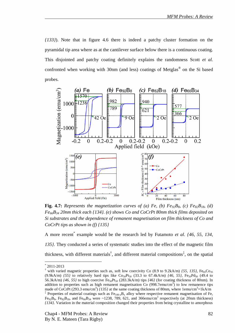
MFM Probes: A Review
Chap4 - MFM Probes: A Review
By N. E. Mateen (Tara Rigby) 82
{133}). Note that in figure 4.6 there is indeed a patchy cluster formation on the
pyramidal tip area where as at the cantilever surface below there is a continuous coating.
This disjointed and patchy coating definitely explains the randomness Scott et al.
confronted when working with 30nm (and less) coatings of Metglas® on the Si based
probes.
Fig. 4.7: Represents the magnetization curves of (a) Fe, (b) Fe92B8, (c) Fe82B18, (d)
Fe66B34 20nm thick each {134}. (e) shows Co and CoCrPt 80nm thick films deposited on
Si substrates and the dependence of remanent magnetisation on film thickness of Co and
CoCrPt tips as shown in (f) {135}
A more recent* example would be the research led by Futamoto et al. {46, 55, 134,
135}. They conducted a series of systematic studies into the effect of the magnetic film
thickness, with different materials†, and different material compositions
‡, on the spatial
* 2011-2013
† with varied magnetic properties such as, soft low coercivity Co (8.9 to 9.2kA/m) {55, 135}, Fe65Co35
(9.9kA/m) {55} to relatively hard tips like Co50Pt50 (33.3 to 67.4kA/m) {46, 55}, Fe50Pd50 (49.4 to
56.3kA/m) {46, 55} to high coercive Fe50Pt50 (283.3kA/m) tips {46} (for coating thickness of 80nm). In
addition to properties such as high remanent magnetisation Co (998.7emu/cm3) to low remanence tips
made of CoCrPt (293.3 emu/cm3) {135} at the same coating thickness of 80nm, where 1emu/cm
3=1kA/m
‡ Properties of material coatings such as Fe100-xBx alloy where respective remanent magnetisation of Fe,
Fe92B8, Fe82B18, and Fe66B34 were ~1238, 789, 621, and 366emu/cm3 respectively (at 20nm thickness)
{134}. Variation in the material composition changed their properties from being crystalline to amorphous

MFM Probes: A Review
Chap4 - MFM Probes: A Review
By N. E. Mateen (Tara Rigby) 83
resolution. Figure 4.7 represents a few examples of the magnetic properties for material
or composition variation, taken from the literature {134, 135}. Their conclusions
corroborated past and present research* on the subject {3, 73, 85, 86, 95, 133, 136}, that
the resolution is both dependent on the magnetic properties† of the coated material, its
coating thickness as well as the tip shape.
It is interesting that most materials used in the probe coatings are generally compared to
the standard pyramidal CoCr probes. In addition, the materials used as the probe
coatings have been diverse. From materials such as Re-FeB {79} (known for their strong
magnetic properties i.e. high remanence and coercivity {70, 74, 137}) to Metglas®
(known for its soft magnetic properties i.e. low coercivity and shape anisotropy {61, 94,
95, 133, 138}) to superparamagnetic (known for low remanence and essentially zero
coercivity {63, 101}).
4.3.4 Effect on MFM image: Probe vs. sample materials
In 1997 Hubert et al. {139} proposed a method of segregation between the magnetic
image contrast mechanisms depending on the magnetic properties of the probe material‡
with respect to the properties of the sample to be observed. As the tip-sample interactive
behaviour might not be rigid during an MFM measurement, it is important to be familiar
with the type of tip and its expected behaviour to be able to distinguish between types of
images§ it might produce. Thus, a single MFM scan may produce an image containing
one or more of these contrast mechanisms occurring. Hubert et al. named the three
distinct categories for image contrast mechanisms due to the relative tip-sample
interactions as hysteresis, charge and susceptibility contrast {139, 140}.
* May it be done on pyramidal tips or CNTs; From hard CoCr to soft NiFe {73, 136}, CoCr and Metglas®
tips’ with height variations {95}, thickness variation in Metglas® tips {133}, 40nm CoCrTa pyramidal vs.
high aspect ratio probe vs. Fe-CNT probe {86} and Co coated CNT with thickness variations {3} † e.g. magnetic anisotropy: crystalline or shape etc. or low or high remanent magnetisation
‡ Hardness – high coercivity or softness – low coercivity
§ E.g. if the resulting image pattern is of sample domains or its domain walls

MFM Probes: A Review
Chap4 - MFM Probes: A Review
By N. E. Mateen (Tara Rigby) 84
i) Magnetically hard probes
CoCr, CoCrPt and CoPt are some popular tips having magnetic properties such as
moderately high coercivity. They are generally used for imaging materials with similar
moderate to high coercivity {33, 85, 141, 142}. However, for a probe either made of* or
coated with a hard magnetic material having weak† stray fields only extending to
localised areas on the sample, charge contrast would be likely to be the dominant
mechanism in generating the MFM image. Such stable probes could also be used to
image relatively softer magnetic materials without the unwanted image perturbations.
This scenario is closest to the ideal probe, which possess a small volume generating
weak but stable fields. Campanella et al. used a high aspect ratio NdFeB nonmagnetic
tip to observe hard and soft magnetic samples with a reasonable degree of success {79.}.
In case of strong interaction, if the stray field of the sample (or the probe) is strong
enough to bring about a permanent change the magnetisation of the probe (or the
sample)‡ such contrast is generally known as hysteresis contrast. That is, if a tip with
relatively hard§ magnetic coating is used on a comparatively soft
** sample then there is
a greater probability of the tip altering/writing {143, 144} over the original magnetic
domain pattern of the sample. Although this altering capability of the tip has potential
MFM applications for the data storage industry {145}. However, it is less suited for true
image generation or interpretation, as strong tip fields would require hard magnetic
samples for good image contrast. According to Hubert et al. {139, 146} for good MFM
imaging practices, such effects should generally avoided††
.
* a hard magnetic material, which is quite rare these days as it might be counterproductive to the
requirements of an MFM † Generation weak fields could be made possible in case of a high aspect ratio probe with a tiny yet stable
magnetic particle at the tip apex, e.g. CNT with a magnetic coating like CoFe(80:20) and CoCr(80:20)
{85} ‡ Irreversible changes in magnetisation lead to artefacts in the image
§ Generally high coercivity and/or magnetic moment
** Generally low coercivity and/or moment
†† even though a modest resolution and sensitivity may be possible

MFM Probes: A Review
Chap4 - MFM Probes: A Review
By N. E. Mateen (Tara Rigby) 85
ii) Magnetically soft probes
A major motivation for the use of soft tips is the difficulty in imaging soft materials
using standard tips, due to potential sample alteration/writing* {143, 144}. FeCo, Co
{55} and NiFe {72, 136} are all examples of soft tips with relatively low coercivity.
Mostly, these tips have the tendency of aligning their magnetic moments with a
sample’s external stray field and could be used for low coercivity material imaging† {30,
31}. The image contrast mechanism where the probe and the sample may influence each
other but the magnetisation is reversible and is called susceptibility‡ contrast {139, 146}.
Amorphous tips (such as FeSiBC also known as Metglas®§
) {61, 94, 95, 133, 138} and
the superparamagnetic (such as Fe/SiO2) {63, 101} tips also come under the category of
magnetically soft tips. These tips have been found {94} to be useful particularly for the
observation of domains and domain walls. The overall image contrast of these tips
should remain the same (mostly attractive i.e., dark {94}). Although, for probes with
low coercivity and low remanent magnetisation i.e. superparamagnetic tips, the
magnetisation is generally expected to change its orientation every time the tip passes
over a magnetic feature**
.
Interest in amorphous probes like Metglas® was sparked to circumvent the randomness
observed, in tip to tip response, due to the crystalline nature of commercially available
probes such as CoCr {95}. Unless the crystal orientation at the tip apex was known and
a certain tip behaviour expected, randomly oriented crystallites were the major cause of
* Temporarily or permanent i.e. perturbing effects due to the tip stray field on the sample magnetisation
† In cases, where neither the probe nor the sample could be deemed stable, care should be taken when
interpreting the results ‡ Magnetic susceptibility is a 'quantitative measure of the magnetisation of material in relation to an
applied field. The magnetic susceptibility of a material χ, is equal to the ratio of the magnetization M
within the material to the applied field strength H, or χ = M/H. This ratio, is the volume susceptibility,
because magnetisation essentially involves a certain measure of magnetism (dipole moment) per unit
volume' {147} § Approximate coating thickness equal or greater than 40nm
** which have perpendicular stray field gradient

MFM Probes: A Review
Chap4 - MFM Probes: A Review
By N. E. Mateen (Tara Rigby) 86
variation in tip response*. In 1999 Heydon et al. {95}, attempted to provide a simplistic
solution by using an amorphous soft tip made of Metglas®†
. Moreover, Heydon et al.
showed that low coercivity amorphous (Co91Nb6Zr3) films could easily be imaged using
tips coated with Metglas® (FeSiBC) material {61, 138}. This amorphous tip relaxed the
microstructural limitations, reducing the problems of tip reproducibility as well as
image interpretation to some extent. In addition the properties of a Metglas® tip proved
to reduce the perturbations of the magnetic structure of the magnetic samples observed
as well {61}.
Interestingly, as mentioned earlier, Scott et al. {133} showed that the characteristics of
the soft amorphous Metglas® tips rely heavily on the coating thickness of the material
onto the tip apex. The low but finite coercivity of Metglas® allowed the use of the same
tip in different modes. The permanent moment tip was sensitive to the sign of the stray
field specifically while analysing soft or hard samples at certain tip-sample separation.
At low fly height, the stray field of a hard magnetic sample reversibly controlled the
magnetisation of high permeability sensitive tips. In addition, the Metglas® tip’s wear
resistance and hardness makes it an ideal candidate for use in a variety of hard as well as
soft materials. Due to the versatility and resilience of the Metglas® tips, such tips
‡ were
used during the course of this project extensively.
The superparamagnetic tips however, have been employed to image write fields above
thin film recording heads {63, 101}. They have also been classed as a low signal to
noise ratio (i.e. have diminished tip memory effects), thus the tip moment effects are
* Piramanayagam et al. {2, 17, 18, 51, 56, 102} came up with a solution regarding the randomness of the
moment direction, due to the orientation of the crystallites, at the tip apex. They proposed tips with
perpendicular magnetic anisotropy (PMA). To achieve PMA tips they used seed layers (Ta and Ru) to
control the crystallographic orientation of the CoCrPt:SiO2 layers and the compared the results with tips
coated with the same material without the seed layers † The Metglas
® tip they fabricated offered a low coercivity, high moment (i.e. good signal-to-noise ratio),
and high susceptibility (i.e. simpler image interpretation) ‡ Fabricated by Heydon, G. P. in 1998-99, University of Sheffield, Dept. Mat. Sc. & Engn., Sheffield S1
3JD, S Yorkshire, England

MFM Probes: A Review
Chap4 - MFM Probes: A Review
By N. E. Mateen (Tara Rigby) 87
significantly reduced {101}. The research in soft amorphous tips gave a new insight to
the behaviour of the MFM probe while it interacts with the sample stray fields.
4.4 MFM Quantification
The vast diversity of the MFM probes led to a pressing need to quantify the MFM
image results and hence, quantification soon became a priority. A need for data*
quantification gained momentum simultaneously {10, 11, 148, 149} with the quest for
ultimate resolution. This need was realised because the images obtained, although they
were of good quality, they were mostly subjective. Furthermore, obtaining high quality
magnetic images was one thing but producing quantifiable results became a field of
study on its own. In order to quantify the image data, some kind of standardisation was
required†. Thus, the need to characterise the tip became the next priority. To
characterise the probe, a special calibration sample was required which could help
quantify the tip‡, which in turn would play a pivotal role in the quantification of the
results§. At the same time, the enhancement in analytical calculations and computer
simulations helped the scientists to estimate the best possible solutions to the problems
they were facing in their laboratories regarding the probe behaviour.
As the progress in the various arenas of the MFM made way, issues like image
reproducibility or separating the magnetic signal from the surface topography became
prominent. Where the introduction of tapping mode {150} solved the problem of surface
topography breaking through into the magnetic imagery to some extent, groups of
researchers came together {80} in an effort to ensure that all the MFM instruments
showed the same or at least similar images. They discovered that the images taken by
different MFM instruments of the same sample, sometimes using probes of same or
* gathered from the image
† as a standardised scientific instrument used for metrology
‡ which is much more complex (due to its shape and material coatings) compared to the samples to be
observed § in the form of image maps

MFM Probes: A Review
Chap4 - MFM Probes: A Review
By N. E. Mateen (Tara Rigby) 88
similar properties showed significant variations in the images. Although Goddenhenrich
et al. did the preliminary work in the area of tip calibration {4} but work done by
Abelmann et al. {80} highlighted the need for calibration {5, 151, 152} and thus
characterisation {84, 95, 133, 153, 154} of the MFM probes.
More to the point, in order to get quantifiable results, it became important to know how
the probes were interacting with the samples {14, 67}, giving rise to questions like how
much are the probes influencing their respective samples {143, 144} and/or vice versa?
With such probe-sample interactive influences in cases where there was a high
probability of image perturbations {30, 118, 138, 155, 156} and/or image artifacts {157,
158}, more questions arose. For example, how could such image discrepancies be
detected and resolved successfully? In addition, as the MFM probes are three-
dimensional in shape their behaviour is quite complicated and hence difficult to study.
To date, it has been difficult to distinguish between the subtle tip induced effects or that
of the sample onto the overall image formation.
Work done by Iglesias-Freire et al. {157} on (what they deemed as) MFM image
artifacts induced by the tip, is significant in the fundamental understanding of the tip
contribution in the overall image formation. Their work was a small example of the
image complexities in a broader spectrum of the tip-sample interactive behaviour.
Iglesias-Freire et al. {157} showed successfully and quantifiably, that the tip’s
behaviour could be multifaceted*, with the help of computer modelling and experiments.
* Their {157} findings indicated that the tip behaviour could be more flexible during the tip-sample
interaction than previously assumed. They presumed the apex behaved as a soft tip sensitive to field
gradients of the sample, hence readily switching its magnetisation whereas the rest of the tip showed more
stability. There is always a possibility that the moments at the tip apex may respond more readily to the
sample’s fields (or an external field) compared to the rest of the tip magnetisation direction, making the
results uncertain and difficult to interpret. In fact, for completely soft tip coatings there might be a degree
of certainty of how a tip will behave. For a relatively harder i.e., expected 'stable' tip the behaviour
becomes more random and depends on the strength and field distributions of the sample being observed.
There is a wide range of tips whose magnetic properties lie between very hard (stable) or very soft (highly

MFM Probes: A Review
Chap4 - MFM Probes: A Review
By N. E. Mateen (Tara Rigby) 89
As the magnetisation switching, at the apex of
some probes could act as a source of
misinterpretations* in the MFM results
†.
However, if the switching could be understood
better, then the random switching could possibly
be understood as something other than artifactual.
Although Iglesias-Freire et al {157} were correct
in suggesting that the effects observed in their
images were indeed induced by the tips, yet more
research is needed to fully categorise such a tip
response as ‘artifacts’.
It might be argued that the possibility of a portion
of a tip to switch its magnetisation is quite high‡,
especially if the sample fields are comparable to
the field required to induce the switching and the
tip’s magnetisation direction is at a certain angle
with the sample fields. However, Iglesias-Freire
et al {157} conducted their experiments in the
presence of an external field so that the tip§ apex
was constantly magnetised in one direction**
. Then any influence from the sample††
fields on the tip’s behaviour‡‡
could be registered discretely and distinctly. They
switchable magnetisation). It is the tip which lies within this range that one must be careful of while
attempting to interpret the results * what might be construed as image artifacts
† especially interpreting the domain structure
‡ Depending on the tip history as well as its magnetic properties such as coercivity and remanent
magnetisation § CoNi
** compared to the rest of the tip
†† Permalloy
‡‡ prompting it to switch
Fig. 4.8: (a, c & e) Represent the
cross sections in the x-z direction
of the magnetic field above the
permalloy dot and showing the
formation of the rings and the disc
due to the amplitude of the
oscillating cantilever, at a lift
height of 230nm. The rings or
discs could be observed in the
frequency shift images represented
in (b, d & f), where H is the
external applied field {157}

MFM Probes: A Review
Chap4 - MFM Probes: A Review
By N. E. Mateen (Tara Rigby) 90
observed the tip switching* in the form of discrete rings and discs of varying sizes,
which appeared depending on the tip’s fly height. Unsurprisingly, they discovered that
the amplitude of the cantilever oscillations potentially dictated the size of the imaging
plane, in z direction. Thus for a certain scan height, the tip amplitude created a ring (or a
disc) of a different size in the resulting images as shown in figure 4.8.
Thus, larger the amplitude of the tip, larger would be the effective thickness of the
imaged plane, the thicker the imaged ring structure. If the tip amplitude was set large
enough, the discrete contour lines of the sample field, at a certain height, might get
completely enveloped within the z thickness area, producing the image of a disc†. Thus,
these authors managed to create a tip that had the capability of mapping the z
component of the sample’s field at a given height. When stacked up next to each other
the amalgamated images could render a three dimensional image of the magnetic field
lines emanating from the sample, effectively in the z direction.
On the other hand, to resolve the issues such as image perturbations, Lisunova et al.‡ {3}
attempted to reduce the tip perturbative effects by optimising highly specialised tips
such as ferromagnetically-coated carbon nanotube tips. They took single walled CNTs,
used MBE to coat the Co magnetic material and claimed to fabricate ‘sensitive, non-
perturbative, small volume and high anisotropy tips’§.
With the development of highly sophisticated computers**
, more and more complex
problems could be modelled and simulated with ease. Irrespective of what the scientific
community was attempting to achieve, in their need for the quantification of results,
they have started to rely heavily on analytical and computational modelling. A good
example would be the work done by Preisner et al. {159} in 2009. They used the finite
* Due to the sample’s fields
† Instead of a ring
‡ ‘non-perturbative imaging of nanoscale spin structures in soft magnetic materials’ {3}
§ for both hard and soft thin films
** with ever-increasing computational powers, software specifically dedicated for complex calculations

MFM Probes: A Review
Chap4 - MFM Probes: A Review
By N. E. Mateen (Tara Rigby) 91
element method (FEM) based micromagnetic model to calculate the tip-sample
interactions with a purpose of increasing the accuracy of the MFM technique. In their
model, they used the magnetic properties of a CoCr-tip* and an AlNiCo sample
†.
Fig. 4.9: (a) Shows the magnetic flux density (contour lines) of the 3D model and (b)
magnetic flux density of the 3D model represented by vector notation {159}
Figure 4.9 shows a three dimensional model of a tip, the sample and the magnetic flux
density due to the tip-sample interaction. Figure 4.9(a) represents the magnetic flux
density in the form of contour lines and 4.9(b) shows the same model represented by
vector notation.
* Orthogonally magnetised with respect to the sample
† Alternately magnetised

MFM Probes: A Review
Chap4 - MFM Probes: A Review
By N. E. Mateen (Tara Rigby) 92
Although the model constructed by Preisner et al. was a simplistic representation of the
tip (at least), yet it showed that the majority of the interaction between the tip and the
sample took place at the tip apex. This model* is a good prototype to be used in the
basic understanding of the tip-sample interaction in a quantitative way.
Fig. 4.10: A possible consequence of Van der Waal forces on the MFM phase shift as
a function of lift height {74}
To optimise a tip with respect to the sample being observed and to produce best possible
results with a certain degree of repeatability, the experiments must be conducted in a
systematic quantifiable way. An example would be a study conducted by Al-Khafaji
{74} regarding the tip-sample interaction with respect to the lift height as shown in
figure 4.10. He used a standard CoCr tip and varied the tip’s lift heights from 20 to
1300nm with respect to the hard Nd-FeB crystal he was studying.
* Based on realistic parameters, although they did not do detailed force calculations to include magneto-
mechanical coupling nor did they consider a hysteresis model

MFM Probes: A Review
Chap4 - MFM Probes: A Review
By N. E. Mateen (Tara Rigby) 93
By systematically observing the images thus produced, he optimised the tip he used to
give the best results* at a lift height of around ~200nm. As the strength of the magnetic
signal detected by the probe, depends on the probe-sample distance and the overall
magnetic properties of the probe with respect to the sample.
4.4.1 Magnetic stray fields and gradients (real probe case)
Although Iglesias-Freire et al {157} might have highlighted yet another complexity that
could present itself in the magnetic image formation, detailed calculation regarding the
tip behaviour in that case have not yet to come to light. Nevertheless, the dependence of
magnetic force with respect to the magnetic properties of the tip (hard or soft) is stated
here. These scenarios are relatively more realistic compared to the magnetic force
calculation for idealistic probes (as described in section 3.5.2.1, chapter 3).
i) Magnetically hard probes
Due to the variations in the magnetic coating on the tip, its shape and dimensions,
calculations of the magnetic tip as its volume integral cannot be disregarded for a more
realistic approach. Furthermore, as the field† from the sample cannot be constant over
the entire tip, the resulting errors‡ generated could be quite significant. To make the
calculation accurate some potential solutions have been discussed by Hug (using
Fourier transforms) {5, 140} or Saito (using direct integration) {103, 160-163}. The
MFM response can be obtained by performing integration over the volume of the
probe§. Hence, to calculate the total force, all the dipole moments would be integrated
over the entire volume of the tip. By representing the tip moment in terms of its
* Maximised the phase shift signal
† constantly changing from point to point in space due to the features (size and strength) of the observed
sample ‡ due to the assumptions of an idealistic probe (see chapter 3)
§ Provided the details of probe dimensions are known

MFM Probes: A Review
Chap4 - MFM Probes: A Review
By N. E. Mateen (Tara Rigby) 94
magnetisation and volume, ∫ the expression in equation 3.2
(chapter 3) for magnetically hard tips, can then be re-written as,
∫ (4.1)
Where represents the magnetisation of the tip, V is its volume and is the
magnetic field of the sample. Considering that the magnetisation direction of the sample
is still in the z direction* from its surface the equations 3.3 and 3.4 may be written as,
∫ (
⁄ ) (4.2)
and
∫
( ⁄ ) (4.3)
The only possible way of incorporation, the true values of and , would be
with the help of extensive computer modelling and simulations, due to their colossal
computational powers. Lately work done by Li et al. {2, 17, 18} is quite interesting as
regards to conducting extensive micromagnetic simulations, for optimisation of PMA†
tips or estimating the effect of tip-coating microstructure or studying the effects of
different magnetic anisotropies of the tips, on the spatial resolution.
ii) Magnetically soft probes
For a soft tip, which follows the stray field of the sample , the tip’s
magnetisation could be written as , where χ is the susceptibility of the
material. As a soft tip would be more susceptible to the field gradients generated by the
sample, the moment of the tip can be represented as,
∫ (4.4)
* For simplification and convenience
† Perpendicular magnetic anisotropy

MFM Probes: A Review
Chap4 - MFM Probes: A Review
By N. E. Mateen (Tara Rigby) 95
where χ is the susceptibility of the tip (assumed constant), and V the volume of (active)
magnetic material on the tip. Hence,
∫ (4.5)
In case, the sample is perpendicularly magnetised relative to its surface then force and
force gradient responsible for producing the MFM signal can then be written as,
∫ [ ( ⁄ )]
(4.6)
and
∫
[ (
⁄ )] (4.7)
As the very tip is supposed to follow exactly the field of the sample
∫ [(
⁄ ) (
⁄ )] (4.8)
4.5 Probe Characterisation
To understand the probe-sample interaction fully, the probe must be understood first
hence the need for probe characterisation, especially if the results are to be optimised
quantitatively. Questions like why certain probes have the capability of producing a
consistent set of images and others do not (for a given sample) may become easy to
answer. If the true behaviour of the probes could be understood, then using that
information to tailor the MFM to a specific requirement would also become far easier.
For example, a characterised, quantified probe may help in the improvement of image
resolution {55} or in imaging 3D field maps of the sample {157}. Many methodologies
have been used to characterise a range of probes {50, 84, 95, 115, 133, 153, 154, 164}.
One such example of tip characterisation would be joint work done by Scott et al. {133,
153} and Heydon et al. {95, 133}. They characterised tips coated with soft amorphous
Metglas® material with various coating thicknesses by using Lorentz electron

MFM Probes: A Review
Chap4 - MFM Probes: A Review
By N. E. Mateen (Tara Rigby) 96
tomography and MFM* technique. The more quantitative the process of probe
characterisation, the better suited the probe would be for a given task, which may lead
to MFM being widely accepted as a standardised technique used in metrology.
The behaviour of tip or that of the sample should be known to estimate the behavioural
contribution of the other, to have some quantifiable results. Generally, a calibration
sample is prepared with known properties to help quantify and characterise a tip.
Usually the tip’s shape added with its magnetic properties makes it complex to study or
to understand, hence, it is difficult to procure a tip that could be used as a calibration
device. However, a sample with known magnetisation distribution and/or stray fields
could ideally be used to calibrate, quantify and characterise an MFM probe.
Nevertheless, the task of tip characterisation is quite complex due to some degree of
unpredictability† (that is the probabilistic nature of magnetic behaviour) of the tip when
interacting with a certain sample in real time. In this project, an attempt was made to
understand and characterise a set of tips‡ (see chapters 6-8) by using a customised
§
calibration sample along with a set of samples having a wide range of magnetic
properties.
4.5.1 Probe calibration
Over the years, a number of calibration samples have been used to quantify and
characterise the MFM tip response. For instance the standard magnetic tape {166}, the
hard disks {4}, magnetotactic bacterium {167}, magnetic line arrays {168} as well as
current carrying structures of various configurations like, loops/rings {105, 149, 169-
* MFM of the Metglas
® tips was conducted by using NIST standard sample {165}
†As there might be non-linear, i.e. hysteric behaviour involved. The tip behaviour could be deemed
unpredictable or probabilistic because it is not possible to obtain its true hysteric behaviour due to the
small size. Mostly it is assumed that the coating at the tip apex behaves similar to that of its cantilever or
base, where taking hysteresis measurements might be relatively easier due to a larger area and relatively
flat surfaces. Furthermore the coating thickness at the base may be significantly different to that on the
three dimensional tip ‡ having different magnetic properties
§ See chapter 5

MFM Probes: A Review
Chap4 - MFM Probes: A Review
By N. E. Mateen (Tara Rigby) 97
173} and straight lines/wires {6, 151, 174}. Of late, Graphene Hall sensors {175} have
been added to the list of calibration devices that have been used for the MFM probe.
In the case of the magnetic tape, the hard disks, magnetic line arrays magnetotactic
bacterium, the calibration could be regarded as rudimentary, as either, the fields of the
calibration sample could not be determined precisely or had the possibility of being
altered during the tip calibration procedure. In addition, the lack of controllability of
such calibration samples for situations like very hard to very soft tips was a major
setback. Hence, to quantify the probe the calibration samples needed to be versatile, so
that a wide range of MFM probes could be calibrated from the same sample of known
properties.
The calibration samples with the required versatility are the current carrying conductors.
Irrespective of the shape*, these samples
† have a unique vantage point. As the current in
such conductors could be varied, their stray fields could thereby be manipulated as
desired. Thus, these calibration samples have been used extensively to calibrate,
quantify and characterise a range of MFM tips with more accuracy. Furthermore, the
tips thus calibrated‡ were used in studying samples such as Co/Pt dot {176}. With the
help of calibration samples (like current rings), the absolute value of the magnetic field
at the tip position can be calculated. By varying the current densities (or the currents) in
a conductor, the field generated could be controlled and with the help of Biot-Savart’s
law and its strength at a specific point in space can be calculated. Hence, by using the
field of known strength, its influence on the stray field of a magnetic material can be
deduced. The influence of the field on the magnetic material can also be gauged if the
magnetic material’s distance from the source field is varied. The MFM technique is
especially sensitive to all such variations. Nevertheless, the calibration also depends on
* rings or straight wires
† current carrying conductors
‡ In this case by using well-defined current carrying ring structures; The current rings as a calibration
sample were fabricated by electron-beam lithography {105, 149, 169-172}.

MFM Probes: A Review
Chap4 - MFM Probes: A Review
By N. E. Mateen (Tara Rigby) 98
the size of the structure that was used to determine the calibrated values. Thus, the
feature-size dependency has to be taken into account {5, 173, 177}.
Although, a flat calibration sample* might be preferred due to its capability of dealing
with a wider range of spatial frequencies† which might correspond to an MFM image
‡.
Whilst embedded current structures do exist§ {178-180} and indeed MFM has been used
as a fault detection mechanism**
. For the sole purpose of calibration of MFM tips,
preparation of planerised/embedded samples might be considered cumbersome,
especially if there are the added limitations of certain fly heights††
. In addition, the
magnetisation distribution through the embedded layers must be well known in order to
calculate the stray fields. The reason why such samples are not commonly used as the
probe calibration devices is that the accuracy and precision required for a probe
calibration sample is paramount. The embedded structures bring a certain degree of
uncertainty to the scenario in addition to the MFM only being able to detect the signal at
significantly larger probe-sample distances {178}.
While it was found that a magnetic tip calibrated with the help of the current carrying
rings served its purpose, the rings nonetheless could only calibrate tips destined to
observe structures with similar stray field geometry, for example magnetic dots {176,
181} and rings {171}. Consequently, different calibration schemes for MFM-tips had to
be introduced for quantitative investigation of samples other than magnetic dots or
rings.
* So that issues like the variations caused by the sample topography might be avoided
† domain sizes in a limited size area
‡ a few micrometres squared
§ In the integrated circuits
** Commonly known as failure sites
†† low fly heights e.g. 10-50nm depending thickness of the layer required to planerise the topographical
structures on the sample

MFM Probes: A Review
Chap4 - MFM Probes: A Review
By N. E. Mateen (Tara Rigby) 99
(a) (b) Fig. 4.11: Shows examples of current carrying calibration structures with the
schematics of the current flow directions and SEM micrographs of wire
configurations. Current rings made of varying ring diameters are illustrated in figure
4.11(a) whereas 4.11(b) shows straight wire structures.{6, 149, 151, 169}
Figure 4.11 shows a few examples of current carrying calibration structures for the
MFM tip. The figure 4.11 also shows the schematics of the current flow directions and
SEM micrographs of wire configurations. Current rings made of varying ring diameters
are illustrated in figure 4.11(a) whereas 4.11(b) shows straight wire structures. In 2004
Kebe et al. {6} used parallel current carrying conductors to calibrate MFM tips. They
used the current-carrying wires of various lateral dimensions {6, 151} and dealt with the
determination of * as well as locating the imaginary position of that
on the z-
axis in the thin film tips {6} (in conformance with the point probe approximation
{107})†.
In all such studies conducted by Kebe et al. {6} or Carl et al. {171}, the y component of
the magnetic field was ignored, under the assumption that compared to the z component
its value is negligible. It was also assumed that the tip position lies at the exact midpoint
of the sample‡, and the wire symmetry is assumed perfect. Kebe et al. {6} expected the
y component to be zero at the exact midpoint between the current wire samples for a tip,
* the z-component of the magnetic dipole moment of the tip
† the y direction was the direction in which the tip scanned the sample (parallel) and z was the
perpendicular height direction of the tip from the sample ‡ Dead centre of the parallel wire configuration

MFM Probes: A Review
Chap4 - MFM Probes: A Review
By N. E. Mateen (Tara Rigby) 100
which was perfectly magnetised in the z direction only. In reality however, only under
ideal circumstances could the y component of the tip moment be ignored completely.
The reason being, as mentioned earlier, that there is a large deviation in the tip sizes and
shapes as well as the symmetry of the sample or that of the tip cannot be guaranteed
under general circumstances. Hence, the premise that Kebe et al. {6} or Carl et al. {171}
used was too idealistic.
The work carried out in this thesis used a calibration sample similar to that used by
Kebe et al. {6}. However, this* project concentrated on the variations in fly height
modes† of the MFM tip(s) with respect to the sample observed at various locations, in
the experimental as well as the modelling regime. It also dealt with the contribution of
magnetic volume of a tip on the image formation as well as the effects of tip
magnetisation angles (and/or the samples gradient field angles) during a set scan with
respect to the sample. That is, the contributions of the (x and/or y) components other
than perpendicular (z) direction in the tip-sample interaction were studied in detail an
area, which was not covered by previous research. That is, the numerical analysis in
conjunction with the experimental observations to determine the amount of contribution
from y component of the magnetic field during the magnetic image formation was
attempted during the course of this project. The contribution of the y component is one
of the aspects that will be examined in depth in chapters 6‡.
4.6 Summary
Keeping in view the objective of this thesis, this chapter gives a detailed account of
previous research conducted on various aspects of the MFM probe. Starting from the
historical accounts of the initial formation of the probes, the shapes used and the
* This thesis
† Lift and linear
‡ the results from the review article from Kebe and Carl {6} were initially recalculated as verification and
understanding of the numerical methodology, using the MathCAD 2000i Professional software
MFM Probes: A Review
Chap4 - MFM Probes: A Review
By N. E. Mateen (Tara Rigby) 101
materials utilised to highlighting the diversity* that the MFM technique faced in the race
towards the resolution improvement. The MFM technique, due to the complexities of its
probes and thus the resulting convolutions in the image interpretations, needed to be
quantified. The MFM probe therefore needed to be characterised for a specific
requirement. In order to characterise the probe, a sample was required of known
properties, generally regarded as a calibration sample.
Some of the mainstream fabrication tools used for probe manufacture/enhancements
have been mentioned and compared. The FIB has been given special attention because
not only was it found to be the most versatile tool† available (according to literature) but
also it was the instrument of choice to aid in the fulfilment of few aspects of this project.
As FIB milling could aid in the evaluation of active and/or effective magnetic volume
coated on the probe, in the image formation. Moreover, the use of FIB milling could
also help in answering questions like, does the effective volume reside only at or near
the apex of the MFM probe or extends beyond the apex? In addition, how is the active
magnetic volume linked to the MFM images qualitatively and/or quantitatively? If the
volume does play a part, then how could it be manipulated, to improve the image
properties and maybe the resolution? To date, these questions have not been thoroughly
examined and the FIB technique was selected in an attempt to address some of these
questions during the course of this project (see the result section).
Although the improvement of the MFM technique is an on-going process, due to the
tremendous variety of magnetic materials‡ being researched and potentially used as an
MFM probe (in its entirety or as its coating), it is still arduous to make the technique
fully quantitative. With time due to the steady advancement of computational prowess
* including the pros and cons
† which has been heavily used in the studies of the MFM probe behaviour or simply in the improvement
of image resolution by way of enhancing or modifying the magnetic probe. The focused ion beam
technique has been used extensively for fabrication and modification of MFM tips due to its precision and
flexibility. ‡ with an array of varying magnetic properties, due to shape, size, coating thickness etc.

MFM Probes: A Review
Chap4 - MFM Probes: A Review
By N. E. Mateen (Tara Rigby) 102
of numerical and/or simulations software*, more and more researchers have become
heavily reliant on such an aid to predict, optimise and/or compare the experimental
results. This amalgamation of experimental results with the computational predictions
has greatly improved the understanding of the tip-sample interaction as a whole.
Computational software such as MathCAD†, Origin
‡ and AutoCAD
§ have been heavily
used during the course of this project other than the built-in software that accompany
techniques like MFM, FIB milling or e-Beam lithography.
The researchers also realised that in order to quantify the MFM technique, the probe
need to be characterised and then calibrated. Although an indirect method, the probes
could possibly be quantified by using calibrated samples (that could in turn be used to
calibrate/characterise the probe(s)). Works in relation to such calibration samples have
also been re-examined at the end of this chapter, with an eye for potential improvements
in the methodology used for a more realistic tip scenario. Although efforts have been
made to devise an all-purpose general calibration sample, capable of characterising the
MFM, but there is room for improvement. It is this work, which has also been pushed
forward in this project as will be described in later chapters (see chapter 6, 7 & 8).
The next chapter deals with the instrumentation, fabrication and methodology that were
used during the research conducted in this project. In addition, the fifth chapter also
deals with some preliminary control experiments relevant to the results presented in this
project.
* used the computers
† See chapters 6. Used for estimation the stray fields and their gradients
‡ Used for image conversions, interpretations and pixel counting. See result section
§ Tip shape modelling and volume estimation. See chapter 7

MFM Probes: A Review
Chap4 - MFM Probes: A Review
By N. E. Mateen (Tara Rigby) 103
4.7 References
{1} Martin, Y. and Wickramasinghe, H. K.; "Magnetic Imaging By Force
Microscopy With 1000-Å Resolution", Applied Physics Letters, vol. 50, pp.
1455-1457, 1987.
{2} Li, H., Wei, D., and Piramanayagam, S. N.; "Micromagnetic Study of Effect of
Tip-Coating Microstructure on The Resolution of Magnetic Force
Microscopy", Applied Physics a-Materials Science & Processing, vol. 110, pp.
217-225, 2013.
{3} Lisunova, Y., Heidler, J., Levkivskyi, I., Gaponenko, I., Weber, A., Caillier, C.,
Heyderman, L. J., Klaeui, M., and Paruch, P.; "Optimal Ferromagnetically-
Coated Carbon Nanotube Tips for Ultra-High Resolution Magnetic Force
Microscopy", Nanotechnology, vol. 24, pp. 105705-105705, 2013.
{4} Goddenhenrich, T., Lemke, H., Muck, M., Hartmann, U., and Heiden, C.;
"Probe Calibration in Magnetic Force Microscopy", Applied Physics Letters,
vol. 57, pp. 2612-2614, 1990.
{5} van Schendel, P. J. A., Hug, H. J., Stiefel, B., Martin, S., and Guntherodt, H. J.;
"A Method for The Calibration of Magnetic Force Microscopy Tips", Journal
of Applied Physics, vol. 88, pp. 435-445, 2000.
{6} Kebe, T. and Carl, A.; "Calibration of Magnetic Force Microscopy Tips by
Using Nanoscale Current-Carrying Parallel Wires", Journal of Applied
Physics, vol. 95, pp. 775-792, 2004.
{7} Vock, S., Wolny, F., Mühl, T., Kaltofen, R., Schultz, L., Büchner, B., Hassel,
C., Lindner, J., and Neu, V.; "Monopolelike Probes for Quantitative Magnetic
Force Microscopy: Calibration and Application", Applied Physics Letters, vol.
97, 2010.
{8} Sievers, S., Braun, K.-F., Eberbeck, D., Gustafsson, S., Olsson, E., Schumacher,
H. W., and Siegner, U.; "Quantitative Measurement of the Magnetic Moment
of Individual Magnetic Nanoparticles by Magnetic Force Microscopy", Small
(Weinheim an der Bergstrasse, Germany), vol. 8, pp. 2675-2679, 2012.
{9} Haeberle, T., Haering, F., Pfeifer, H., Han, L., Kuerbanjiang, B., Wiedwald, U.,
Herr, U., and Koslowski, B.; "Towards Quantitative Magnetic Force
Microscopy: Theory and Experiment", New Journal of Physics, vol. 14, 2012.
{10} Nenadovic, M., Strbac, S., and Rakocevic, Z.; "Quantification of The Lift
Height for Magnetic Force Microscopy Using 3D Surface Parameters",
Applied Surface Science, vol. 256, pp. 1652-1656, 2010.
{11} Gomez, R. D., Pak, A. O., Anderson, A. J., Burke, E. R., Leyendecker, A. J., and
Mayergoyz, I. D.; "Quantification of Magnetic Force Microscopy Images
using Combined Electrostatic and Magnetostatic Imaging", Journal of Applied
Physics, vol. 83, pp. 6226-6228, 1998.
{12} Proksch, R., Skidmore, G. D., Dahlberg, E. D., Foss, S., Schmidt, J. J., Merton,
C., Walsh, B., and Dugas, M.; "Quantitative Magnetic Field Measurements
with The Magnetic Force Microscope", Applied Physics Letters, vol. 69, pp.
2599-2601, 1996.
{13} Gibson, G. A. and Schultz, S.; "A High-Sensitivity Alternating-Gradient
Magnetometer for Use in Quantifying Magnetic Force Microscopy", Journal
Of Applied Physics, vol. 69, pp. 5880-5882, 1991.

MFM Probes: A Review
Chap4 - MFM Probes: A Review
By N. E. Mateen (Tara Rigby) 104
{14} Ness, H. and Gautier, F.; "Theoretical-Study of The Interaction between a
Magnetic Nanotip and a Magnetic Surface", Physical Review B, vol. 52, pp.
7352-7362, 1995.
{15} Liou, S. H.; "Comparison of Magnetic Images Using Point and Thin-Film
Magnetic Force Microscopy Tips", IEEE Transactions On Magnetics, vol. 35,
pp. 3989-3991, 1999.
{16} Engel-Herbert, R., Schaadt, D. M., and Hesjedal, T.; "Analytical and
Numerical Calculations of The Magnetic Force Microscopy Response: A
Comparison", Journal Of Applied Physics, vol. 99, 2006.
{17} Li, H., Wei, D., and Piramanayagam, S. N.; "Micromagnetic Studies on
Resolution Limits of Magnetic Force Microscopy Tips With Different
Magnetic Anisotropy", Journal Of Applied Physics, vol. 111, 2012.
{18} Li, H., Wei, D., and Piramanayagam, S. N.; "Optimization of Perpendicular
Magnetic Anisotropy Tips for High Resolution Magnetic Force Microscopy by
Micromagnetic Simulations", Applied Physics a-Materials Science &
Processing, vol. 112, pp. 985-991, 2013.
{19} Passeri, D., Dong, C., Angeloni, L., Pantanella, F., Natalizi, T., Berlutti, F.,
Marianecci, C., Ciccarello, F., and Rossi, M.; "Thickness Measurement of Soft
Thin Films on Periodically Patterned Magnetic Substrates by Phase
Difference Magnetic Force Microscopy", Ultramicroscopy, vol. 136, pp. 96-
106, 2014.
{20} Schwenk, J., Marioni, M., Romer, S., Joshi, N. R., and Hug, H. J.; "Non-
Contact Bimodal Magnetic Force Microscopy", Applied Physics Letters, vol.
104, 2014.
{21} Cambel, V., Precner, M., Fedor, J., Soltys, J., Tobik, J., Scepka, T., and
Karapetrov, G.; "High Resolution Switching Magnetization Magnetic Force
Microscopy", Applied Physics Letters, vol. 102, 2013.
{22} Kaidatzis, A. and Garcia-Martin, J. M.; "Torsional Resonance Mode Magnetic
Force Microscopy: Enabling Higher Lateral Resolution Magnetic Imaging
Without Topography-Related Effects", Nanotechnology, vol. 24, 2013.
{23} Lazo, C. and Heinze, S.; "First-Principles Study of Magnetic Exchange Force
Microscopy With Ferromagnetic and Antiferromagnetic Tips", Physical
Review B, vol. 84, 2011.
{24} Saito, H., Lu, W., Hatakeyama, K., Egawa, G., and Yoshimura, S.; "High
Frequency Magnetic Field Imaging by Frequency Modulated Magnetic Force
Microscopy", Journal Of Applied Physics, vol. 107, 2010.
{25} Jaafar, M., Gomez-Herrero, J., Gil, A., Ares, P., Vazquez, M., and Asenjo, A.;
"Variable-Field Magnetic Force Microscopy", Ultramicroscopy, vol. 109, pp.
693-699, 2009.
{26} Saito, H., Sunahara, R., Rheem, Y., and Ishio, S.; "Low-Noise Magnetic Force
Microscopy with High Resolution by Tip Cooling", IEEE Transactions On
Magnetics, vol. 41, pp. 4394-4396, 2005.
{27} Callaghan, F. D., Yu, X., and Mellor, C. J.; "Variable Temperature Magnetic
Force Microscopy with Piezoelectric Quartz Tuning Forks as Probes
Optimized using Q-Control", Applied Physics Letters, vol. 87, 2005.
{28} Hug, H. J., Moser, A., Jung, T., Fritz, O., Wadas, A., Parashikov, I., and
Guntherodt, H. J.; "Low-Temperature Magnetic Force Microscopy", Review
Of Scientific Instruments, vol. 64, pp. 2920-2925, 1993.

MFM Probes: A Review
Chap4 - MFM Probes: A Review
By N. E. Mateen (Tara Rigby) 105
{29} Hosaka, S., Kikukawa, A., Honda, Y., and Hasegawa, T.; "Just-On-Surface
Magnetic Force Microscopy", Applied Physics Letters, vol. 65, pp. 3407-3409,
1994.
{30} Grutter, P., Rugar, D., Mamin, H. J., Castillo, G., Lin, C. J., McFadyen, I. R.,
Valletta, R. M., Wolter, O., Bayer, T., and Greschner, J.; "Magnetic Force
Microscopy with Batch-Fabricated Force Sensors", Journal of Applied
Physics, vol. 69, pp. 5883-5885, 1991.
{31} Grutter, P., Rugar, D., Mamin, H. J., Castillo, G., Lambert, S. E., Lin, C. J.,
Valletta, R. M., Wolter, O., Bayer, T., and Greschner, J.; "Batch Fabricated
Sensors for Magnetic Force Microscopy", Applied Physics Letters, vol. 57, pp.
1820-1822, 1990.
{32} Tseng, A. A.; "Recent Developments in Micromilling using Focused Ion
Beam Technology", Journal Of Micromechanics And Microengineering, vol.
14, pp. R15-R34, 2004.
{33} Gao, L., Yue, L. P., Yokota, T., Skomski, R., Liou, S. H., Takahoshi, H., Saito,
H., and Ishio, S.; "Focused Ion Beam Milled CoPt Magnetic Force
Microscopy Tips for High Resolution Domain Images", IEEE Transactions On
Magnetics, vol. 40, pp. 2194-2196, 2004.
{34} Utke, I., Bret, T., Laub, D., Buffat, P., Scandella, L., and Hoffmann, P.;
"Thermal Effects During Focused Electron Beam Induced Deposition of
Nanocomposite Magnetic-Cobalt-Containing Tips", Microelectronic
Engineering, vol. 73-74, pp. 553-558, 2004.
{35} Campbell, S.; "The Science and Engineering of Microelectronic Fabrication".
New York: Oxford University Press 2001.
{36} Westwood, W.; "Sputter Deposition". New York: AVS, 2003.
{37} Nonnenmacher, M., Greschner, J., Wolter, O., and Kassing, R.; "Scanning
Force Microscopy with Micromachined Silicon Sensors", Journal of Vacuum
Science & Technology B, vol. 9, pp. 1358-1362, 1991.
{38} Wolter, O., Bayer, T., and Greschner, J.; "Micromachined Silicon Sensors for
Scanning Force Microscopy", Journal of Vacuum Science & Technology B,
vol. 9, pp. 1353-1357, 1991.
{39} Martin, Y., Rugar, D., and Wickramasinghe, H. K.; "High-Resolution Magnetic
Imaging of Domains in TbFe by Force Microscopy", Applied Physics Letters,
vol. 52, pp. 244-246, 1988.
{40} Wickramasinghe, H. K. and Martin, Y.; "High-Resolution Magnetic Imaging
By Force Microscopy", Journal Of Applied Physics, vol. 63, pp. 2948-2948,
1988.
{41} Binning, G., Rohrer, H., Gerber, C., and Weibel, E.; "Surface Studies By
Scanning Tunneling Microscopy", Physical Review Letters, vol. 49, pp. 57-61,
1982.
{42} Binnig, G. and Rohrer, H.; "Scanning Tunneling Microscopy", IBM Journal
Of Research And Development, vol. 30, pp. 355-369, 1986.
{43} Binnig, G. and Rohrer, H.; "Scanning Tunneling Microscopy - From Birth To
Adolescence", Reviews Of Modern Physics, vol. 59, pp. 615-625, 1987.
{44} Binnig, G. and Rohrer, H.; "Scanning Tunneling Microscopy - From Birth To
Adolescence", Uspekhi Fizicheskikh Nauk, vol. 154, pp. 261-278, 1988.
{45} Schonenberger, C. and Alvarado, S. F.; "Understanding Magnetic Force
Microscopy", Zeitschrift Fur Physik B-Condensed Matter, vol. 80, pp. 373-383,
1990.

MFM Probes: A Review
Chap4 - MFM Probes: A Review
By N. E. Mateen (Tara Rigby) 106
{46} Ishihara, S., Ohtake, M., and Futamoto, M.; "Magnetic Force Microscope Tips
Coated with FePd, FePt, and CoPt Alloy Films", Thin Solid Films, vol. 546,
pp. 205-210, 2013.
{47} van den Bos, A., Heskamp, I., Siekman, M., Abelmann, L., and Lodder, C.;
"The CantiClever: A Dedicated Probe for Magnetic Force Microscopy", IEEE
Transactions on Magnetics, vol. 38, pp. 2441-2443, 2002.
{48} Grutter, P., Jung, T., Heinzelmann, H., Wadas, A., Meyer, E., Hidber, H. R., and
Guntherodt, H. J.; "10-nm Resolution by Magnetic Force Microscopy on
FeNdB", Journal of Applied Physics, vol. 67, pp. 1437-1441, 1990.
{49} Hobbs, P. C. D., Abraham, D. W., and Wickramasinghe, H. K.; "Magnetic
Force Microscopy With 25 nm Resolution", Applied Physics Letters, vol. 55,
pp. 2357-2359, 1989.
{50} Folks, L., Best, M. E., Rice, P. M., Terris, B. D., Weller, D., and Chapman, J.
N.; "Perforated Tips for High-Resolution In-Plane Magnetic Force
Microscopy", Applied Physics Letters, vol. 76, pp. 909-911, 2000.
{51} Piramanayagam, S. N., Ranjbar, M., Tan, E. L., Tan, H. K., Sbiaa, R., and
Chong, T. C.; "Enhanced Resolution in Magnetic Force Microscopy using
Tips With Perpendicular Magnetic Anisotropy", Journal Of Applied Physics,
vol. 109, 2011.
{52} Khizroev, S. and Litvinov, D.; "Focused-Ion-Beam-Based Rapid Prototyping
of Nanoscale Magnetic Devices", Nanotechnology, vol. 15, pp. R7-R15, 2004.
{53} Koblischka, M. R., Hewener, B., Hartmann, U., Wienss, A., Christoffer, B., and
Persch-Schuy, G.; "Magnetic Force Microscopy Applied in Magnetic Data
Storage Technology", Applied Physics A-Materials Science & Processing, vol.
76, pp. 879-884, 2003.
{54} Cayetano, V. O., Moler, K. A., and Straver, E. W. J.; "Novel Carbon Nanotube
Tips: En Route to High Resolution and Ultra Sensitive Force Detection in
Magnetic Force Microscopy", Copyright © 2000.
{55} Futamoto, M., Hagami, T., Ishihara, S., Soneta, K., and Ohtake, M.;
"Improvement of Magnetic Force Microscope Resolution and Application to
High-Density Recording Media", IEEE Transactions On Magnetics, vol. 49,
pp. 2748-2754, 2013.
{56} Piramanayagam, S. N., Ranjbar, M., Sbiaa, R., Tavakkoli K G, A., and Chong,
T. C.; "Characterization of High-Density Bit-Patterned Media Using Ultra-
High Resolution Magnetic Force Microscopy", Physica Status Solidi-Rapid
Research Letters, vol. 6, pp. 141-143, 2012.
{57} Lu, W., Li, Z., Hatakeyama, K., Egawa, G., Yoshimura, S., and Saito, H.; "High
Resolution Magnetic Imaging of Perpendicular Magnetic Recording Head
Using Frequency-Modulated Magnetic Force Microscopy with A Hard
Magnetic Tip", Applied Physics Letters, vol. 96, 2010.
{58} Choi, M., Yang, J. M., Lim, J., Lee, N., and Kang, S.; "Measurement and
Analysis of Magnetic Domain Properties of High-Density Patterned Media by
Magnetic Force Microscopy", IEEE Transactions On Magnetics, vol. 45, pp.
2308-2311, 2009.
{59} Chen, Y. J., Leong, S. H., Huang, T. L., Ng, K. W., Hu, S. B., Yuan, Z. M., and
Ng, V.; "A Comparative Study of Write Field Ddistribution of Trailing-Edge
Shielded and Unshielded Perpendicular Write Heads by Quantitative
Magnetic Force Microscopy", Applied Physics Letters, vol. 92, 2008.

MFM Probes: A Review
Chap4 - MFM Probes: A Review
By N. E. Mateen (Tara Rigby) 107
{60} Moser, A., Xiao, M., Kappenberger, P., Takano, K., Weresin, W., Ikeda, Y., Do,
H., and Hug, H.; "High-Resolution Magnetic Force Microscopy Study of
High-Density Transitions in Perpendicular Recording Media", Journal Of
Magnetism And Magnetic Materials, vol. 287, pp. 298-302, 2005.
{61} Heydon, G. P., Rainforth, W. M., Gibbs, M. R. J., Davies, H. A., Bishop, J. E.
L., Tucker, J. W., Huo, S., Pan, G., Mapps, D. J., and Clegg, W. W.; "Magnetic
Force Microscopy of Recording Heads", in Electron Microscopy And Analysis
1999, Institute Of Physics Conference Series, Kiely, C. J., Ed. Bristol: Iop
Publishing Ltd, 1999, pp. 331-334.
{62} Porthun, S., Abelmann, L., and Lodder, C.; "Magnetic Force Microscopy of
Thin Film Media for High Density Magnetic Recording", Journal of
Magnetism and Magnetic Materials, vol. 182, pp. 238-273, 1998.
{63} Liou, S. H., Malhotra, S. S., Moreland, J., and Hopkins, P. F.; "High Resolution
Imaging of Thin-Film Recording Heads by Superparamagnetic Magnetic
Force Microscopy Tips", Applied Physics Letters, vol. 70, pp. 135-137, 1997.
{64} Wago, K., Sueoka, K., and Sai, F.; "Magnetic Force Microscopy of Recording-
Heads", IEEE Transactions On Magnetics, vol. 27, pp. 5178-5180, 1991.
{65} Liu, X., Isomura, S., and Morisako, A.; "Magnetic Force Microscope Probes
With High Resolution by Soft Magnetic Vortex", IEEE Transactions On
Magnetics, vol. 48, pp. 3673-3676, 2012.
{66} Memmert, U., Muller, A. N., and Hartmann, U.; "Probes for Magnetic Force
Microscopy Imaging of Soft Magnetic Samples", Measurement Science &
Technology, vol. 11, pp. 1342-1347, 2000.
{67} Tomlinson, S. L., Farley, A. N., Hoon, S. R., and Valera, M. S.; "Interactions
between Soft Magnetic Samples and MFM Tips", Journal Of Magnetism And
Magnetic Materials, vol. 158, pp. 557-558, 1996.
{68} Tang, S. L., Gibbs, M. R. J., Davies, H. A., Mateen, N. E., Nie, B., and Du, Y.
W.; "The Possible Origin of RE-Fe-B Thin Films With c-Axis Texture",
Journal Of Applied Physics, vol. 103, 2008.
{69} Tang, S. L., Gibbs, M. R. J., Davies, H. A., Liu, Z. W., Lane, S. C., Mateen, N.
E., and Du, Y. W.; "Fabrication of RE-Fe-B Films With Highly c-Axis
Texture and Excellent Hard Magnetic Properties", Journal Of Applied
Physics, vol. 101, 2007.
{70} Tang, S. L., Gibbs, M. R. J., Davies, H. A., Liu, Z. W., Lane, S. C., and Mateen,
N. E.; "An Effective Route for The Fabrication of Rare Earth-Iron-Boron
Thin Films Having Strong c-Axis Texture and Excellent Hard Magnetic
Properties", Journal Of Applied Physics, vol. 101, 2007.
{71} Al-Khafaji, M. A., Marashi, S. P. H., Rainforth, W. M., Gibbs, M. R. J., Davies,
H. A., Bishop, J. E. L., and Heydon, G.; "MFM of Nanocrystalline NdFeB: A
Study of The Effect of Processing Route on The Micromagnetic Structure",
Journal Of Magnetism And Magnetic Materials, vol. 190, pp. 48-59, 1998.
{72} Al-Khafaji, M. A., Jones, D. G. R., Rainforth, W. M., Gibbs, M. R. J., Davies,
H. A., and Harris, I. R.; "Magnetic Force Imaging of Domain Structures for A
(Pr/Nd)FeB Alloy", Journal Of Applied Physics, vol. 83, pp. 2715-2718, 1998.
{73} Al-Khafaji, M., Rainforth, W. M., Gibbs, M. R. J., Bishop, J. E. L., and Davies,
H. A.; "The Origin and Interpretation of Fine Scale Magnetic Contrast in
Magnetic Force Microscopy: A Study Using Single-Crystal NdFeB and A
Range of Magnetic Force Microscopy Tips", Journal Of Applied Physics, vol.
83, pp. 6411-6413, 1998.

MFM Probes: A Review
Chap4 - MFM Probes: A Review
By N. E. Mateen (Tara Rigby) 108
{74} Al-Khafaji, M. A.; "Magnetic Force Microscopy of NdFeB Hard Magnetic
Alloys", Engineering Materials, vol. PhD. Sheffield: University of Sheffield,
1998, pp. 266.
{75} Yang, G., Tang, J., Kato, S., Zhang, Q., Qin, L. C., Woodson, M., Liu, J., Kim,
J. W., Littlehei, P. T., Park, C., and Zhou, O.; "Magnetic Nanowire Based High
Resolution Magnetic Force Microscope Probes", Applied Physics Letters, vol.
87, 2005.
{76} Phillips, G. N., Siekman, M., Abelmann, L., and Lodder, J. C.; "High
Resolution Magnetic Force Microscopy using Focused Ion Beam Modified
Tips", Applied Physics Letters, vol. 81, pp. 865-867, 2002.
{77} Chou, S. Y., Wei, M. S., and Fischer, P. B.; "An Ultra-High-Resolution Single-
Domain Magnetic Force Microscope Tip Fabricated Using Nanolithography",
IEEE Transactions On Magnetics, vol. 30, pp. 4485-4487, 1994.
{78} Fischer, P. B., Wei, M. S., and Chou, S. Y.; "Ultrahigh-Resolution Magnetic
Force Microscope Tip Fabricated Using Electron-Beam Lithography",
Journal Of Vacuum Science & Technology B, vol. 11, pp. 2570-2573, 1993.
{79} Campanella, H., Jaafar, M., Llobet, J., Esteve, J., Vazquez, M., Asenjo, A., del
Real, R. P., and Plaza, J. A.; "Nanomagnets With High Shape Anisotropy and
Strong Crystalline Anisotropy: Perspectives on Magnetic Force Microscopy",
Nanotechnology, vol. 22, 2011.
{80} Abelmann, L., Porthun, S., Haast, M., Lodder, C., Moser, A., Best, M. E., van
Schendel, P. J. A., Stiefel, B., Hug, H. J., Heydon, G. P., Farley, A., Hoon, S. R.,
Pfaffelhuber, T., Proksch, R., and Babcock, K.; "Comparing The Resolution of
Magnetic Force Microscopes Using The CAMST Reference Samples", Journal
Of Magnetism And Magnetic Materials, vol. 190, pp. 135-147, 1998.
{81} Cespedes, O., Luu, A., Rhen, F. M. F., and Coey, J. M. D.; "Fabrication of
Magnetic Force Microscopy Tips via Electrodeposition and Focused Ion
Beam Milling", IEEE Transactions On Magnetics, vol. 44, pp. 3248-3251,
2008.
{82} Belova, L. M., Hellwig, O., Dobisz, E., and Dan Dahlberg, E.; "Rapid
Preparation of Electron Beam Induced Deposition Co Magnetic Force
Microscopy Tips with 10 nm Spatial Resolution", The Review of Scientific
Instruments, vol. 83, pp. 093711-093711, 2012.
{83} Utke, I., Hoffmann, P., Berger, R., and Scandella, L.; "High-Resolution
Magnetic Co Supertips Grown by A Focused Electron Beam", Applied Physics
Letters, vol. 80, pp. 4792-4794, 2002.
{84} Ruhrig, M., Porthun, S., Lodder, J. C., McVitie, S., Heyderman, L. J., Johnston,
A. B., and Chapman, J. N.; "Electron Beam Fabrication and Characterization
of High-Resolution Magnetic Force Microscopy Tips", Journal Of Applied
Physics, vol. 79, pp. 2913-2919, 1996.
{85} Kuramochi, H., Asada, H., Uzumaki, T., Yui, H., Iitake, M., Takano, F.,
Akinaga, H., and Manago, T.; "Material Dependence of Magnetic Force
Microscopy Performance using Carbon Nanotube Probes: Experiments and
Simulation", Journal Of Applied Physics, vol. 115, 2014.
{86} Wolny, F., Mühl, T., Weissker, U., Leonhardt, A., Wolff, U., Givord, D., and
Büchner, B.; "Magnetic Force Microscopy Measurements in External
Magnetic Fields-Comparison Between Coated Probes and An Iron Filled
Carbon Nanotube Probe", Journal Of Applied Physics, vol. 108, 2010.

MFM Probes: A Review
Chap4 - MFM Probes: A Review
By N. E. Mateen (Tara Rigby) 109
{87} Wolny, F., Weissker, U., Mühl, T., Leonhardt, A., Menzel, S., Winkler, A., and
Büchner, B.; "Iron-Filled Carbon Nanotubes as Probes for Magnetic Force
Microscopy", Journal Of Applied Physics, vol. 104, 2008.
{88} Winkler, A., Mühl, T., Menzel, S., Kozhuharova-Koseva, R., Hampel, S.,
Leonhardt, A., and Büchner, B.; "Magnetic Force Microscopy Sensors Using
Iron-Filled Carbon Nanotubes", Journal Of Applied Physics, vol. 99, 2006.
{89} Deng, Z. F., Yenilmez, E., Leu, J., Hoffman, J. E., Straver, E. W. J., Dai, H. J.,
and Moler, K. A.; "Metal-Coated Carbon Nanotube Tips for Magnetic Force
Microscopy", Applied Physics Letters, vol. 85, pp. 6263-6265, 2004.
{90} Yoshida, N., Arie, T., Akita, S., and Nakayama, Y.; "Improvement of MFM
Tips Using Fe-Alloy-Capped Carbon Nanotubes", Physica B-Condensed
Matter, vol. 323, pp. 149-150, 2002.
{91} Arie, T., Nishijima, H., Akita, S., and Nakayama, Y.; "Carbon-Nanotube Probe
Equipped Magnetic Force Microscope", Journal of Vacuum Science &
Technology B, vol. 18, pp. 104-106, 2000.
{92} Koblischka, M. R., Hartmann, U., and Sulzbach, T.; "Improvements of The
Lateral Resolution of The MFM Technique", Thin Solid Films, vol. 428, pp.
93-97, 2003.
{93} Liu, Z. Y., Dan, Y., Jinjun, Q. J., and Wu, Y. H.; "Magnetic Force Microscopy
using Focused Ion Beam Sharpened Tip with Deposited Antiferro-
Ferromagnetic Multiple Layers", Journal of Applied Physics, vol. 91, pp. 8843-
8845, 2002.
{94} Heydon, G. P., Rainforth, W. M., Gibbs, M. R. J., Davies, H. A., Bishop, J. E.
L., Tucker, J. W., Huo, S., Pan, G., Mapps, D. J., and Clegg, W. W.;
"Investigation of The Response of A New Amorphous Ferromagnetic MFM
Tip Coating with An Established Sample and A Prototype Device", Journal Of
Magnetism And Magnetic Materials, vol. 214, pp. 225-233, 2000.
{95} Heydon, G. P., Rainforth, W. M., Gibbs, M. R. J., Davies, H. A., McVitie, S.,
Ferrier, R. P., Scott, J., Tucker, J. W., and Bishop, J. E. L.; "Preparation and
Characterisation of A New Amorphous Tip Coating for Application in
Magnetic Force Microscopy", Journal of Magnetism and Magnetic Materials,
vol. 205, pp. L131-L135, 1999.
{96} Shen, Y. T. and Wu, Y. H.; "Response Function Study of A New Kind of
Multilayer-Coated Tip for Magnetic Force Microscopy", IEEE Transactions on
Magnetics, vol. 40, pp. 97-100, 2004.
{97} Casey, S. M., Lord, D. G., Grundy, P. J., Slade, M., and Lambrick, D.; "Single
Layer and Multilayer Tip Coatings in Magnetic Force Microscopy", Journal
Of Applied Physics, vol. 85, pp. 5166-5168, 1999.
{98} Liu, F., Li, S., Bai, D., Wang, J., Li, Z., Han, D., Pan, T., and Mao, S.;
"Characteristics of Magnetic Force Microscopy Magnetics on High Moment
Perpendicular Magnetic Recording Writers With High Coercivity Probes",
Journal Of Applied Physics, vol. 111, 2012.
{99} Kirtley, J. R., Deng, Z., Luan, L., Yenilmez, E., Dai, H., and Moler, K. A.;
"Moment Switching in Nanotube Magnetic Force Probes", Nanotechnology,
vol. 18, 2007.
{100} Yamaoka, T., Watanabe, K., Shirakawabe, Y., Chinone, K., Saitoh, E., Tanaka,
M., and Miyajima, H.; "Applications of High-Resolution MFM System with
Low-Moment Probe in A Vacuum", IEEE Transactions On Magnetics, vol. 41,
pp. 3733-3735, 2005.

MFM Probes: A Review
Chap4 - MFM Probes: A Review
By N. E. Mateen (Tara Rigby) 110
{101} Hopkins, P. F., Moreland, J., Malhotra, S. S., and Liou, S. H.;
"Superparamagnetic Magnetic Force Microscopy Tips", Journal of Applied
Physics, vol. 79, pp. 6448-6450, 1996.
{102} Ranjbar, M., Piramanayagam, S. N., Sbiaa, R., Chong, T. C., and Okamoto, I.;
"Advanced Magnetic Force Microscopy for High Resolution Magnetic
Imaging", Nanoscience and Nanotechnology Letters, vol. 4, pp. 628-633, 2012.
{103} Saito, H., van den Bos, A., Abelmann, L., and Lodder, J. C.; "High-Resolution
MFM: Simulation of Tip Sharpening", IEEE Transactions on Magnetics, vol.
39, pp. 3447-3449, 2003.
{104} Koblischka, M. R. and Hartmann, U.; "Recent Advances in Magnetic Force
Microscopy", Ultramicroscopy, vol. 97, pp. 103-112, 2003.
{105} Lohau, J., Kirsch, S., Carl, A., Dumpich, G., and Wassermann, E. F.;
"Quantitative Determination of Effective Dipole and Monopole Moments of
Magnetic Force Microscopy Tips", Journal of Applied Physics, vol. 86, pp.
3410-3417, 1999.
{106} Wolny, F., Mühl, T., Weissker, U., Lipert, K., Schumann, J., Leonhardt, A., and
Büchner, B.; "Iron Filled Carbon Nanotubes as Novel Monopole-Like Sensors
for Quantitative Magnetic Force Microscopy", Nanotechnology, vol. 21, pp.
435501-435501, 2010.
{107} Hartmann, U.; "The Point Dipole Approximation In Magnetic Force
Microscopy", Physics Letters A, vol. 137, pp. 475-478, 1989.
{108} Koblischka, M. R., Kirsch, M., Pfeifer, R., Getlawi, S., Rigato, F., Fontcuberta,
J., Sulzbach, T., and Hartmann, U.; "Different Types of Ferrite Thin Films as
Magnetic Cantilever Coating for Magnetic Force Microscopy", Journal Of
Magnetism And Magnetic Materials, vol. 322, pp. 1697-1699, 2010.
{109} Amos, N., Lavrenov, A., Fernandez, R., Ikkawi, R., Litvinov, D., and Khizroev,
S.; "High-Resolution and High-Coercivity FePtL1(0) Magnetic Force
Microscopy Nanoprobes to Study Next-Generation Magnetic Recording
Media", Journal Of Applied Physics, vol. 105, 2009.
{110} Chen, I. C., Chen, L. H., Gapin, A., Jin, S., Yuan, L., and Liou, S. H.; "Iron-
Platinum-Coated Carbon Nanocone Probes on Tipless Cantilevers for High
Resolution Magnetic Force Imaging", Nanotechnology, vol. 19, 2008.
{111} Amos, N., Ikkawi, R., Haddon, R., Litvinov, D., and Khizroev, S.; "Controlling
Multidomain States to Enable Sub-10-nm Magnetic Force Microscopy",
Applied Physics Letters, vol. 93, 2008.
{112} Wei, J. D., Kirsch, M., Koblischka, M. R., and Hartmann, U.; "Optimization of
High-Frequency Magnetic Force Microscopy by Ferrite-Coated Cantilevers",
Journal Of Magnetism And Magnetic Materials, vol. 316, pp. 206-209, 2007.
{113} Liou, S. H. and Yao, Y. D.; "Development of High Coercivity Magnetic Force
Microscopy Tips", Journal Of Magnetism And Magnetic Materials, vol. 190, pp.
130-134, 1998.
{114} Bauer, P., Bochem, H. P., Leinebach, P., Memmert, U., and Schelten, J.;
"Magnetic Refinement of Tips for Magnetic Force Microscopy", Scanning,
vol. 18, pp. 374-378, 1996.
{115} Jenkins, N. E., DeFlores, L. P., Allen, J., Ng, T. N., Garner, S. R., Kuehn, S.,
Dawlaty, J. M., and Marohn, J. A.; "Batch Fabrication and Characterization of
Ultrasensitive Cantilevers with Submicrometre Magnetic Tips", Journal Of
Vacuum Science & Technology B, vol. 22, pp. 909-915, 2004.

MFM Probes: A Review
Chap4 - MFM Probes: A Review
By N. E. Mateen (Tara Rigby) 111
{116} Champagne, A. R., Couture, A. J., Kuemmeth, F., and Ralph, D. C.;
"Nanometer-Scale Scanning Sensors Fabricated using Stencil Lithography",
Applied Physics Letters, vol. 82, pp. 1111-1113, 2003.
{117} Dreyer, M., Lohndorf, M., Wadas, A., and Wiesendanger, R.; "Ultra-High-
Vacuum Magnetic Force Microscopy of The Domain Structure of Ultra-Thin
Co Films", Applied Physics A-Materials Science & Processing, vol. 66, pp.
S1209-S1212, 1998.
{118} Skidmore, G. D. and DanDahlberg, E.; "Improved Spatial Resolution in
Magnetic Force Microscopy", Applied Physics Letters, vol. 71, pp. 3293-3295,
1997.
{119} Zhou, L., McVitie, S., and Chapman, J. N.; "Magnetic Imaging of Magnetic
Force Microscope Tips", Journal Of Magnetism And Magnetic Materials, vol.
148, pp. 237-238, 1995.
{120} Koblischka, M. R., Hartmann, U., and Sulzbach, T.; "Improving The Lateral
Resolution of The MFM Technique to The 10 nm Range", Journal of
Magnetism and Magnetic Materials, vol. 272-76, pp. 2138-2140, 2004.
{121} Hyun, C., Lee, A. K. H., and de Lozanne, A.; "Focused Ion Beam Deposition
of Co71Cr17Pt12 and Ni80Fe20 on Tips for Magnetic Force Microscopy",
Nanotechnology, vol. 17, pp. 921-925, 2006.
{122} Litvinov, D. and Khizroev, S.; "Orientation-Sensitive Magnetic Force
Microscopy for Future Probe Storage Applications", Applied Physics Letters,
vol. 81, pp. 1878-1880, 2002.
{123} Pain, L., Tedesco, S., and Constancias, C.; "Direct Write Lithography: The
Global Solution for R&D and Manufacturing", Comptes Rendus Physique,
vol. 7, pp. 910-923, 2006.
{124} Solak, H. H.; "Nanolithography with Coherent Extreme Ultraviolet Light",
Journal Of Physics D-Applied Physics, vol. 39, pp. R171-R188, 2006.
{125} Park, C. M., Bain, J. A., Clinton, T. W., and van der Heijden, P. A. A.; "Effects
of Focused-Ion-Beam Irradiation on Perpendicular Write Head
Performance", Journal Of Applied Physics, vol. 93, pp. 6459-6461, 2003.
{126} Park, C. M. and Bain, J. A.; "Local Degradation of Magnetic Properties in
Magnetic Thin Films Irradiated by Ga+ Focused-Ion-Beams", IEEE
Transactions On Magnetics, vol. 38, pp. 2237-2239, 2002.
{127} Mayer, J., Giannuzzi, L. A., Kamino, T., and Michael, J.; "TEM Sample
Preparation and FIB-Induced Damage", MRS Bulletin, vol. 32, pp. 400-407,
2007.
{128} Khizroev, S., Bain, J. A., and Litvinov, D.; "Fabrication of Nanomagnetic
Probes via Focused Ion Beam Etching and Deposition", Nanotechnology, vol.
13, pp. 619-622, 2002.
{129} McGrouther, D., Nicholson, W. A. P., Chapman, J. N., and McVitie, S.;
"Focused Ion Beam Irradiation of Ferromagnetic Thin Films in The
Presence of An Applied Field", Journal Of Physics D-Applied Physics, vol. 38,
pp. 3348-3353, 2005.
{130} Huang, H. S., Lin, M. W., Sun, Y. C., and Lin, L. J.; "Improving The Spatial
Resolution of A Magnetic Force Microscope Tip via Focused Ion Beam
Modification and Magnetic Film Coating", Scripta Materialia, vol. 56, pp. 365-
368, 2007.
{131} Tseng, A. A.; "Recent Developments in Nanofabrication using Focused Ion
Beams", Small, vol. 1, pp. 924-939, 2005.

MFM Probes: A Review
Chap4 - MFM Probes: A Review
By N. E. Mateen (Tara Rigby) 112
{132} Volodin, A., Temst, K., Van Haesendonck, C., and Bruynseraede, Y.; "Low
Temperature Magnetic Force Microscopy with Enhanced Sensitivity Based on
Piezoresistive Detection", Review Of Scientific Instruments, vol. 71, pp. 4468-
4473, 2000.
{133} Scott, J., McVitie, S., Ferrier, R. P., Heydon, G. P., Rainforth, W. M., Gibbs, M.
R. J., Tucker, J. W., Davies, H. A., and Bishop, J. E. L.; "Characterisation of
FeBSiC Coated MFM Tips Using Lorentz Electron Tomography and MFM",
IEEE Transactions on Magnetics, vol. 35, pp. 3986-3988, 1999.
{134} Ohtake, M., Soneta, K., and Futamoto, M.; "Influence of Magnetic Material
Composition of Fe100-xBx Coated Tip on The Spatial Resolution of Magnetic
Force Microscopy", Journal Of Applied Physics, vol. 111, 2012.
{135} Nagano, K., Tobari, K., Ohtake, M., and Futamoto, M.; "Effect of Magnetic
Film Thickness on the Spatial Resolution of Magnetic Force Microscope
Tips", Joint European Magnetic Symposia, vol. 303, Journal of Physics
Conference Series, Spalek, J., Ed., 2011.
{136} AlKhafaji, M. A., Rainforth, W. M., Gibbs, M. R. J., Bishop, J. E. L., and
Davies, H. A.; "The Effect of Tip Type and Scan Height on Magnetic Domain
Images Obtained by MFM", IEEE Transactions On Magnetics, vol. 32, pp.
4138-4140, 1996.
{137} Castaldi, L., Davies, H. A., and Gibbs, M. R. J.; "Co-sputtering of hard
magnetic Re-Fe-B thin films with high maximum energy product", 2002.
{138} Heydon, G. P., Rainforth, W. M., Gibbs, M. R. J., Davies, H. A., Hill, G.,
Bishop, J. E. L., Tucker, J. W., Huo, S., Pan, G., Mapps, D. J., and Clegg, W.
W.; "Magnetic Force Microscopy of Soft Magnetic Films", in Electron
Microscopy And Analysis 1999, Institute Of Physics Conference Series, Kiely,
C. J., Ed. Bristol: Iop Publishing Ltd, 1999, pp. 307-310.
{139} Hubert, A., Rave, W., and Tomlinson, S. L.; "Imaging Magnetic Charges With
Magnetic Force Microscopy", Physica Status Solidi B-Basic Research, vol.
204, pp. 817-828, 1997.
{140} Hug, H. J., Stiefel, B., van Schendel, P. J. A., Moser, A., Hofer, R., Martin, S.,
Guntherodt, H. J., Porthun, S., Abelmann, L., Lodder, J. C., Bochi, G., and
O'Handley, R. C.; "Quantitative Magnetic Force Microscopy on
Perpendicularly Magnetized Samples", Journal Of Applied Physics, vol. 83,
pp. 5609-5620, 1998.
{141} Rastei, M. V., Abes, M., Bucher, J. P., Dinia, A., and Pierron-Bohnes, V.;
"Field-Dependent Behavior of A Magnetic Force Microscopy Tip Probed by
Means of High Coercive Nanomagnets", Journal Of Applied Physics, vol. 99,
2006.
{142} Heydon, G. P., Farley, A. N., Hoon, S. R., Valera, M. S., and Tomlinson, S. L.;
"Resonant Torque Magnetometry: A New In-Situ Technique for Determining
The Magnetic Properties of Thin Film MFM Tips", IEEE Transactions On
Magnetics, vol. 33, pp. 4059-4061, 1997.
{143} Kong, L. S., Zhuang, L., and Chou, S. Y.; "Writing and Reading 7.5 Gbits/in(2)
Longitudinal Quantized Magnetic Disk Using Magnetic Force Microscope
Tips", IEEE Transactions On Magnetics, vol. 33, pp. 3019-3021, 1997.
{144} Kong, L. S., Shi, R. C., Krauss, P. R., and Chou, S. Y.; "Writing Bits of
Longitudinal Quantized Magnetic Disk using Magnetic Force Microscope
Tip", Japanese Journal Of Applied Physics Part 1-Regular Papers Short Notes &
Review Papers, vol. 36, pp. 5109-5111, 1997.

MFM Probes: A Review
Chap4 - MFM Probes: A Review
By N. E. Mateen (Tara Rigby) 113
{145} Zhu, X. B. and Grutter, P.; "Magnetic Force Microscopy Studies of Patterned
Magnetic Structures", IEEE Transactions on Magnetics, vol. 39, pp. 3420-
3425, 2003.
{146} Hubert, A. and Schafer, S.; "Magnetic Domains: The Analysis of Magnetic
Microstructures": Springer-Verlag Berlin Heidelberg New York, 1998.
{147} The Editors of Encyclopædia Britannica and Manchanda, K.; "Magnetic
Susceptibility", Encyclopædia Britannica:
http://www.britannica.com/EBchecked/topic/357313/magnetic-susceptibility, 13
Jul, Copyright © 2014.
{148} Khizroev, S. K., Jayasekara, W., Bain, J. A., Jones, R. E., and Kryder, M. H.;
"MFM Quantification of Magnetic Fields Generated by Ultra-Small Single
Pole Perpendicular Heads", IEEE Transactions on Magnetics, vol. 34, pp.
2030-2032, 1998.
{149} Kong, L. S. and Chou, S. Y.; "Quantification of Magnetic Force Microscopy
Using A Micrometrescale Current Ring", Applied Physics Letters, vol. 70, pp.
2043-2045, 1997.
{150} Virgil B. Elings, J. A. G.; "Tapping atomic force microscope", US5412980 A,
Digital Instruments, Inc., 1992.
{151} Liu, C. X., Lin, K., Holmes, R., Mankey, G. J., Fujiwara, H., Jiang, H. M., and
Cho, H. S.; "Calibration of Magnetic Force Microscopy using Micrometre
Size Straight Current Wires", Journal of Applied Physics, vol. 91, pp. 8849-
8851, 2002.
{152} Van Schendel, P. J. A., Hug, H. J., Hoffmann, R., Martin, S., Kappenberger, P.,
Lantz, M. A., and Guntherodt, H. J.; "Applications of Tip Calibration in
Magnetic Force Microscopy (MFM)", Magnetic Storage Systems Beyond
2000, vol. 41, pp. 313-316, 2001.
{153} Scott, J.; "Characterisation of MFM Tip Stray Fields using Lorentz Electron
Tomography", Department of Physics and Astronomy, vol. PhD. Glasgow:
University of Glasgow, 2001, pp. 175.
{154} Leinenbach, P., Memmert, U., Schelten, J., and Hartmann, U.; "Fabrication and
Characterization of Advanced Probes for Magnetic Force Microscopy",
Applied Surface Science, vol. 145, pp. 492-496, 1999.
{155} Fang, Y.-K., Li, W., Sun, W., Zhu, M.-G., Guo, Z.-H., and Han, B.-S.;
"Revealing of Magnetic Domains of Strong Bulk Anisotropic Permanent
Magnets via Magnetic Force Microscopy", Journal Of Magnetism And
Magnetic Materials, vol. 345, pp. 176-179, 2013.
{156} Frost, B. G., vanHulst, N. F., Lunedei, E., Matteucci, G., and Rikkers, E.;
"Study of The Leakage Field of Magnetic Force Microscopy Thin-Film Tips
Using Electron Holography", Applied Physics Letters, vol. 68, pp. 1865-1867,
1996.
{157} Iglesias-Freire, O., Bates, J. R., Miyahara, Y., Asenjo, A., and Gruetter, P. H.;
"Tip-Induced Artifacts in Magnetic Force Microscopy Images", Applied
Physics Letters, vol. 102, 2013.
{158} Windmill, J. F. C. and Clegg, W. W.; "A Novel Magnetic Force Microscope
Probe Design", IEEE Transactions On Magnetics, vol. 36, pp. 2984-2986, 2000.
{159} Preisner, T., Greiff, M., Bala, U. B., and Mathis, W.; "Numerical Computation
of Magnetic Fields Applied to Magnetic Force Microscopy", Compel-The
International Journal For Computation And Mathematics In Electrical And
Electronic Engineering, vol. 28, pp. 120-129, 2009.

MFM Probes: A Review
Chap4 - MFM Probes: A Review
By N. E. Mateen (Tara Rigby) 114
{160} Saito, H., Rheem, Y. W., and Ishio, S.; "Simulation of High-Resolution MFM
Tips for High-Density Magnetic Recording Media with Low Bit Aspect Ratio",
Journal Of Magnetism And Magnetic Materials, vol. 287, pp. 102-106, 2005.
{161} Saito, H., Yatsuyanagi, D., Ishio, S., Ito, A., Kawamura, H., Ise, K., Taguchi, K.,
and Takahashi, S.; "Simulation of High-Resolution MFM Tip Using
Exchange-Spring Magnet", Journal Of Magnetism And Magnetic Materials,
vol. 310, pp. E939-E940, 2007.
{162} Saito, H., Chen, J., and Ishio, S.; "Principle of Magnetic Field Analysis by
MFM Signal Transformation and its Application to Magnetic Recording
Media", IEEE Transactions On Magnetics, vol. 35, pp. 3992-3994, 1999.
{163} Saito, H., Chen, J., and Ishio, S.; "Description of Magnetic Force Microscopy
by Three-Dimensional Tip Green's Function for Sample Magnetic Charges",
Journal Of Magnetism And Magnetic Materials, vol. 191, pp. 153-161, 1999.
{164} Weis, T., Krug, I., Engel, D., Ehresmann, A., Hoink, V., Schmalhorst, J., and
Reiss, G.; "Characterization of Magnetic Force Microscopy Probe Tip
Remagnetization For Measurements in External In-Plane Magnetic Fields",
Journal Of Applied Physics, vol. 104, 2008.
{165} Rice, P., Russek, S. E., Hoinville, J., and Kelley, M. H.; "Optimizing The NIST
Magnetic Imaging Reference Sample", IEEE Transactions On Magnetics, vol.
33, pp. 4065-4067, 1997.
{166} Support Note No. 229, R. B.; "Magnetic Force Microscopy (MFM) Applicable
to Dimension™ Series and MultiMode™ Systems: Digital Instruments",
2000.
{167} Proksch, R. B., Schaffer, T. E., Moskowitz, B. M., Dahlberg, E. D., Bazylinski,
D. A., and Frankel, R. B.; "Magnetic Force Microscopy of The Submicrometre
Magnetic Assembly in a Magnetotactic Bacterium", Applied Physics Letters,
vol. 66, pp. 2582-2584, 1995.
{168} Landis, S., Rodmacq, B., and Dieny, B.; "Fabrication of Submicrometre
Magnetic Line Arrays for Magnetic Force Microscopy Tip Calibration",
Microelectronic Engineering, vol. 73-74, pp. 790-796, 2004.
{169} Kong, L. S. and Chou, S. Y.; "Study of Magnetic Properties of Magnetic Force
Microscopy Probes Using Micrometrescale Current Rings", Journal of Applied
Physics, vol. 81, pp. 5026-5028, 1997.
{170} Wassermann, E. F., Burgel, C., Carl, A., and Lohau, J.; "Magnetization
Measurements on The Nanometer-Scale", Journal of Magnetism and Magnetic
Materials, vol. 239, pp. 220-223, 2002.
{171} Carl, A., Lohau, J., Kirsch, S., and Wassermann, E. F.; "Magnetization
Reversal and Coercivity of Magnetic-Force Microscopy Tips", Journal of
Applied Physics, vol. 89, pp. 6098-6104, 2001.
{172} Carl, A., Kirsch, S., Lohau, J., Weinforth, H., and Wassermann, E. F.;
"Magnetization Reversal of Nanostructured Co/Pt Multilayer Dots and Films
Studied with Magnetic Force Microscopy and MOKE", IEEE Transactions on
Magnetics, vol. 35, pp. 3106-3111, 1999.
{173} Goryachev, A. V. and Popkov, A. F.; "Calibration Parameters for The Probing
Tip of A Magnetic Force Microscope in The Field of A Test Current Loop",
Technical Physics, vol. 51, pp. 1223-1228, 2006.
{174} Yongsunthon, R., McCoy, J., and Williams, E. D.; "Calibrated Magnetic Force
Microscopy Measurement of Current- Carrying Lines", Journal of Vacuum

MFM Probes: A Review
Chap4 - MFM Probes: A Review
By N. E. Mateen (Tara Rigby) 115
Science & Technology a-Vacuum Surfaces and Films, vol. 19, pp. 1763-1768,
2001.
{175} Panchal, V., Iglesias-Freire, O., Lartsev, A., Yakimova, R., Asenjo, A., and
Kazakova, O.; "Magnetic Scanning Probe Calibration Using Graphene Hall
Sensor", Ieee Transactions On Magnetics, vol. 49, pp. 3520-3523, 2013.
{176} Lohau, J., Carl, A., Kirsch, S., and Wassermann, E. F.; "Magnetization
Reversal and Coercivity of A Single-Domain Co/Pt Dot Measured with A
Calibrated Magnetic Force Microscope Tip", Applied Physics Letters, vol. 78,
pp. 2020-2022, 2001.
{177} Jaafar, M., Asenjo, A., and Vazquez, M.; "Calibration of Coercive and Stray
Fields of Commercial Magnetic Force Microscope Probes", IEEE
Transactions On Nanotechnology, vol. 7, pp. 245-250, 2008.
{178} Pu, A., Thomson, D. J., and Bridges, G. E.; "Location of Current Carrying
Failure Sites in Integrated Circuits by Magnetic Force Microscopy at Large
Probe-to-Sample Separation", Microelectronic Engineering, vol. 86, pp. 16-23,
2009.
{179} Pu, A. and Thomson, D. J.; "Sub-Micrometre Resolution Magnetic Force
Microscopy Mapping of Current Paths With Large Probe-to-Sample
Separation", Measurement Science & Technology, vol. 18, pp. L19-L22, 2007.
{180} Pu, A.; "Magnetic Force Microscopy Imaging of Current Paths in Integrated
Circuits with Overlayers": University of Manitoba (Canada), 2007.
{181} Lohau, J., Kirsch, S., Carl, A., and Wassermann, E. F.; "Quantitative
Determination of The Magnetization and Stray Field of A Single Domain
Co/Pt Dot with Magnetic Force Microscopy", Applied Physics Letters, vol. 76,
pp. 3094-3096, 2000.

Methods, Materials & Preliminary Observations
Chap5 - Techniques, Materials & Initial Observations
By N. E. Mateen (Tara Rigby) 116
Techniques, Materials & Initial Observations
5.1 Introduction
The parameters essential to the instrument functionality with the relevant materials,
methods and some preliminary observations are discussed here. Some techniques used
in the manufacturing and/or modification of the MFM probes have been described in
chapter 4, as part of the literature review. In this chapter, only those techniques and
materials, which were used in this project, would be dealt with.
Electron Beam Lithography (EBL) was used for the fabrication of the sample current
wire structures for MFM calibration (manufactured by Dr Paul Fry*). EBL is a common
technique, its functioning and working principles could be found from any
microfabrication book {1}. Details regarding wire structures are given in section 5.4.
The FIB instrument however, was extensively used during the course of this project. It
was not only used to modify an MFM tip due to its milling capabilities but also metal
deposition† capabilities were also utilised during the course of this project. In addition to
this, some initial experimental observations would also be described in this chapter.
Details of other experimental techniques, such as scanning electron microscope (SEM),
which were used for general-purpose imaging of the physical dimensions and
magnification of tip(s) or MFM calibration structures, could be found in the literature
{2-6}.
5.2 AFM & MFM
The atomic and magnetic force microscope used during the course of this project is
shown in figure 5.1. It was a Nanoscope Dimension 3000 Scanning Probe Microscope
* The Department of Electronics and Electrical Engineering, University of Sheffield, Sheffield, UK
† The experiments relating to the FIB deposition capabilities have not been included in this dissertation
due to lack of conclusive results

Methods, Materials & Preliminary Observations
Chap5 - Techniques, Materials & Initial Observations
By N. E. Mateen (Tara Rigby) 117
manufactured by Digital Instruments. The instrumental set up consisted of a controller,
two monitors and an on-axis video microscope for the tip-sample positioning, image
display system and software for image processing and data extraction*.
The basic essential components required for the
operation of any AFM/MFM are a sharp tip
(which is magnetic in the case of MFM) on a
flexible cantilever, sensitive deflection detector,
mechanical scanning system (piezoelectric),
servo system (to maintain the desired
interaction force). The instrument was operated
in the tapping/lift mode {7, 8}. Details of basic
operation and functionality of the technique for
both AFM and MFM can be found in {8}.
The maximum area of about 100x100μm2 down to a few 100s of nanometres could be
scanned with the help of AFM/MFM without compromising the image integrity. It was
observed during this project that to capture stable unperturbed images below the scan
sizes of 1x1μm2 was quite difficult.
AFM images can be captured simultaneously with the MFM imaging. The instrument
has to trace the surface topography (AFM) as a reference first, so that with that
knowledge in its feedback systems, it could set a specified distance above the sample
later for the MFM imaging. For any type of height or roughness measurements, the
AFM mode is the best choice as any change in the topography could be recorded in the
form of phase shift. The MFM software is equipped with the options of the step height,
* which came with the equipment
Fig. 5.1: Shows a Nanoscope
Dimension 3000 Scanning Probe
Microscope used during the course
of this project (Photograph courtesy by
S.L.Rigby)

Methods, Materials & Preliminary Observations
Chap5 - Techniques, Materials & Initial Observations
By N. E. Mateen (Tara Rigby) 118
section analysis and the root mean square (RMS) roughness of any given sample for a
specified area.
The MFM mode has the capability of measuring magnetic field gradients up to 3μm tip
fly height from the surface of the sample while scanning a maximum area of about
100μmx100μm. The instrument could also work in nanometre regime at a tip height of
10nm above the sample’s surface while scanning an area of 100nm by 100nm. The
MFM used during this project was optimised for working at tip fly heights of about 20
to 300nm while scanning areas in the range of 1x1 to 50x50μm2. For most experiments
conducted here the scan sizes range was kept between 1.5x1.5μm2 to 25x25μm
2. These
scan sizes were selected depending on the desired images quality and/or quantity.
As mentioned in chapter 4, active research is currently going on to enhance the spatial
resolution of MFM captured images. To improve the spatial resolution limit or to study
the limiting factors involved in restricting the resolution, one must be mindful of the
following things at all times. First, that there is a physical limit to the scan size the
instrument can handle without introducing image distortions and artifacts, further
constrained by the pixel limit, which is linked directly with the interpretation of the
data. Like a digital camera, an MFM instrument has a maximum pixel limit, which was
512 pixels (also known as samples per line) for the instrument used here. Most of the
images used in this dissertation were captured at 512 samples per line. Furthermore, the
scan speed was also kept slow so that there were no excessive drag effects due to fast
scan speeds of the tip scanning which may potentially add to image perturbations.
However, a drawback of keeping the scan speeds slow is time and one image could take
up to 30 to 45 minutes in optimal conditions.
The best operating conditions for the instrument are a dust free, vibration free
environment, if possible in vacuum {9-12}, and ultra-low temperatures {13-17}.
Normally such extreme environments are introduced to reduce the extra noise and

Methods, Materials & Preliminary Observations
Chap5 - Techniques, Materials & Initial Observations
By N. E. Mateen (Tara Rigby) 119
impurities from the working conditions However, not many MFM apparatus are
operated in high vacuum or at ultra-low temperature conditions, for instance the
instrument used during this project. Indeed the MFM instrument used in this project was
placed on a noise dampening air table.
5.2.1 AFM & MFM: Typical pyramidal shaped probes
A typical example of a standard
AFM probe is shown in the figure
5.2, where (a) shows the complete
tip along with its adjoining
cantilever, which in turn is
attached to the Si base. This base is
the portion of the tip visible to the
naked eye and with the help of fine
tweezers is clamped in position in
the holder, which is then mounted
onto the instrument.
A crude way to distinguish
between an MFM from an AFM probe is the length of the cantilever. Other than that,
both the AFM and the MFM tips look identical. Although they are usually kept,
separate in their respective marked containers. To a trained eye, generally the cantilever
of the MFM probes is visually longer in length compared to the AFM probe. From the
figure 5.2 (b) it can be seen that the probe shown in the SEM image is an AFM probe
due to the relatively shorter length of its cantilever. The difference in the cantilever
length between AFM probes to that of MFM probes is due to the required differences in
their operational frequencies. The fact that an MFM probe carries extra magnetic
material as an additional mass onto the cantilever in addition to being an AFM probe, an
Fig. 5.2: (a) shows a complete SEM picture of an
SPM probe, (b) is the zoomed up SEM image of
the probe, the apex and the cantilever can be
clearly seen. The SEM in (c) shows the
pyramidal tip only. Notice the significant
reduction in the dimensions from the Si base to
the cantilever to the tip apex. Scanning probe
microscopy is a generic name for probes which
encompass both the AFM as well as the MFM
(Image captured by N.E.Mateen)

Methods, Materials & Preliminary Observations
Chap5 - Techniques, Materials & Initial Observations
By N. E. Mateen (Tara Rigby) 120
example of the operational frequency of an MFM probe would be 60KHz. Whereas
AFM probes need only be used to capture the topographic images and thus might
operate at the frequency of 250KHz. Thus, for a particular probe to operate optimally,
the frequencies required for the technique to work would be different {18}.
The MFM probes have the required coating of the
suitable magnetic material (like Co) and usually a
protective coating (like Cr) to stop corrosion due to
environmental factors like humidity etc. The SEM
image in figure 5.2 (c) is a magnified image of the
probe. The apex is the crucial part, which senses the
relevant forces, and helps create a topographical or a
magnetic image as a result. (Chapter 3, figure 3.4).
Figure 5.3 shows an SEM image of a typical MFM
pyramidal type tip and some of its measured
dimensions given in the respective table 5.1. The
dimensions of the MFM probe ensure that it
effectively senses the magnetic force interactions so
that the distribution of the magnetic forces from the
sample is efficiently detected. The dimensions of a
commercially available MFM probe sensor are generally quoted as ~225±10µm length,
~45±3µm width and ~2.5±1µm thickness for the cantilever with a tip of ~10±3µm
height and ~100±30nm apex diameter tip attached at the free end of the cantilever {8,
19}. As mentioned before the tip shape used in the MFM is pyramidal. However, other
shapes more specific for individual or specialised cases may be available or
manufactured.
Fig. 5.3: Shows a typical
MFM pyramidal tip with its
cantilever. A taper makes the
cantilever wider at the back of
the cantilever, probably for
better laser focusing area at
the back. (Image captured by
N.E.Mateen)

Methods, Materials & Preliminary Observations
Chap5 - Techniques, Materials & Initial Observations
By N. E. Mateen (Tara Rigby) 121
The data given in table 5.1 was
measured from the SEM images of
the magnetic tip, like the one shown
in the figure 5.3. Note there is a
variation in the cantilever dimensions
at the top from those of the bottom. In
table 5.1, the ‘top’ of the cantilever
represents the tip’s front/top side and
the ‘bottom’ is the back where the
laser is shown.
5.2.2 AFM & MFM: General Parameters for Image Capture
The setup and parameters used to generate and capture
images will be described here. Figure 5.4 shows a typical
AFM image of the standard calibration grid. To create
this image the AFM tip was firstly mounted carefully on
the tip holder, which was then placed on the piezoelectric
device. Once in position, the laser was adjusted to
maximise the signal to be detected by a photo detector.
In figure 5.4, a standard AFM calibration grid was
imaged. The scan area for this image was 25x25μm2. As there was no particular need
for positioning like x, y or angled offsets for the standard AFM calibration sample these
parameters were kept at zero.
Normally, for the combined AFM/MFM images, any commercial magnetic tip can be
used. Some parameters commonly used in the MFM instrument are shown in table 5.2.
Tip Height ~13.9±2µm
Cantilever Head
Width, Top ~54±4µm
Width, Bottom ~87±4µm
Cantilever
Width, Top ~43±4µm
Width, Bottom ~77±4µm
Length, Top ~174±6µm
Length, Bottom ~194±6µm
Thickness ~4±2µm
Table 5.1: Typical dimensions of a Veeco
MESP MFM tip and its cantilever (Data
measured by N.E.Mateen)
Fig. 5.4: AFM image of
standard 200 nm pitch
grid. (Image captured by
N.E.Mateen)

Methods, Materials & Preliminary Observations
Chap5 - Techniques, Materials & Initial Observations
By N. E. Mateen (Tara Rigby) 122
AFM AFM/MFM
Auto-tuning
Resonant frequency range ~100-400kHz ~40-100kHz
Target Amplitude 2V 2V
Frequency offset/peak offset 5-10% 5-10%
Scan controls
Scan area 1x1μm2-100x100μm
2 1x1μm
2-100x100μm
2
Angle of scan direction 0-360° 0-360°
Scan rate ≤1Hz ≤1Hz
Feedback
controls
Integral gain 0.5 0.4
Proportional gain 0.7 0.6
Amplitude set point 1.59V 1.52V
Drive frequency ~367kHz ~58kHz
Interleave
controls
Interleave mode Off Linear/Lift
Lift scan height - 5nm-3μm
Channel 1
Data type Height Height
Data scale 300nm 300nm
Scan line Main Main
Channel 2
Data type - Phase/Frequency/Amplitude
Data scale - ~3°
Scan line Interleave
Table 5.2: Some commonly used parameters setting for the AFM tip and MFM tip,
which is capable of capturing both AFM and MFM images simultaneously {8} (Data
collected by N.E.Mateen)
After mounting the MFM tip, it is then auto-tuned to find its respective resonant
frequency. For MFM tips such as the Veeco CoCr the resonant frequency range of 40 to
100 kHz is considered optimal, the value for the CoCr tip used in figure 5.5 was 58 kHz.
In order to capture a good MFM image (as shown in figure 5.5), typically the scan rate
or the scan speed was kept low. In the data channel {8}, the mode was selected to height
and the z range was set at 300nm (see table 5.2). The image was captured while the tip
was in the trace sequence using the values from the main set up.
For the capture of the image illustrated in figure 5.5, both the AFM and the MFM
images of the same sample are produced simultaneously. The procedure and set up is
the same as that for the AFM, however, for the magnetic image to be captured
simultaneously, the interleave control is also activated. The interleave control panel is
switched off in the case of AFM; however it is of critical importance for the correct
function of the MFM. To capture an MFM image, like shown in figure 5.5, (a standard
magnetic tape), the main and interleave control may have to be auto-tuned separately
(depending on what type of magnetic sample is to be observed).

Methods, Materials & Preliminary Observations
Chap5 - Techniques, Materials & Initial Observations
By N. E. Mateen (Tara Rigby) 123
Fig. 5.5: Left hand side shows the AFM image of the standard magnetic tape sample.
The surface topography can be seen in the image clearly. The right hand side of the
image shows magnetic patterns of the same area. The scan area is 25x25µm2 at a fly
height of 60nm and the phase data set at 3˚ (Image captured by N.E.Mateen)
However, for samples such as standard magnetic tape represented in figure 5.5, the
‘main controls’ parameters were used for both AFM/MFM drive amplitudes. Apart from
for the MFM in the interleave controls the scan height mode was switched on to the lift
mode with the scan height of 20nm. In order to capture both the AFM and the MFM
simultaneously in the second channel box the phase mode was selected with the data
range value of 3° with the tip scan direction set to retrace, thus creating two
simultaneous images of surface topography as well as the magnetic gradient image on
top of the samples surface.
Nonetheless, for high coercivity magnetic samples (for example single crystal RE-FeB
discussed later in section 5.2.6 and 5.2.7) {20-23} the drive amplitude of the main
feedback system becomes inadequate due to strong attractive and repulsive forces on the
tip from the sample’s stay fields. In order to get both AFM as well as MFM images
without any topographical or magnetic distortion affecting either image the parameters
in the interleave mode were adjusted independent of the main controls. An interleave
drive amplitude parameter of ~1500mV is appropriate (as shown successfully during the

Methods, Materials & Preliminary Observations
Chap5 - Techniques, Materials & Initial Observations
By N. E. Mateen (Tara Rigby) 124
course of this project) for samples like RE-FeB which allow both images stay
independent and artefact free.
5.2.3 Probe materials selection and use
There are probably as many numbers of tip coatings available as there are magnetic
materials. Any magnetic material (predominantly ferromagnetic) could potentially be
used as a magnetic sensor and hence an MFM tip, as mentioned in chapter 3 and 4. In
this dissertation, other than the commercially available standard CoCr tips a few other
tips were also used. They were Metglas® tip(s)
*, commercial low moment Ni (LM-Ni)
tips† and modified versions
‡ of a single standard CoCr tip. All the MFM measurements
during this project were performed at standard temperature and pressure (STP).
A standard MESP CoCr tip batch having moderate coercivity in the range of about ~32
to 39.8kA/m (by Veeco) was selected because these are the most commonly used
commercial MFM tips available. A CoCr tip is a robust tip, which generally does not
influence the magnetic material, nor can easily be influenced by it. Therefore, it is
suitable for conducting observations on materials with moderate to high coercivity
values§. The tip itself (like an AFM tip) is made of (n) doped Si. It is then coated with a
layer of Cr (1-10nm) and then a layer of CoCr about 10 to 250nm thick, with a
coercivity of ~32kAm-1
. These are general guidelines provided by the manufacturer and
specific composition and thickness are not provided due to proprietary reasons.
*Amorphous material coated on batch of Si based tips with varying thicknesses, made in University of
Sheffield in 1999 by Dr. G. P. Heydon {24-26}. † Only once facet of the pyramidal Si based tip was coated with Ni material
‡ As mentioned in section 5.3.3
§ Too low values and the domain patterns will be swamped by the tip’s field itself and the tip would act as
a writing tool instead of reading i.e. it normal function. Conversely, if the coercive values are too high,
there is a danger of tip’s magnetisation direction being reversed randomly during scanning and thus
rendering the results difficult to interpret

Methods, Materials & Preliminary Observations
Chap5 - Techniques, Materials & Initial Observations
By N. E. Mateen (Tara Rigby) 125
An AFM image representing the surface topography and an MFM image showing the
corresponding domain pattern, at the 2D* base of a commercial batch fabricated CoCr
coated tip can be seen in figure 5.6. The MFM image in figure 5.6 was captured having
the scan area of 1x1µm2 at a fly height of 20nm and the phase data set at 3˚.
Fig. 5.6: Shows an AFM (left) and its corresponding MFM (right) image of the flat
area† of a commercial pyramidal CoCr tip by using another CoCr tip from the same
batch. The MFM image was captured at the fly height of 20nm with the phase data set
to 3˚ encompassing an area of 1x1µm2 (Image captured by N.E.Mateen)
From the surface topography of the CoCr film (LHS) of the image in figure 5.6, it can
be noticed that the individual grains of about 30±6nm in diameter, form clusters of
about 121±22nm. However, from the magnetic part of the figure 5.6, the domain
patterns indicate areas of attraction or repulsion of the order of 211±32nm, which is
approximately double the size of the clusters. Assuming these values (give above) to be
correct, for a tip coated with crystalline material, the defining factor in the success of a
* Imaging the domain structure at the tip apex was not possible as the tip is usually located at the end of a
freestanding cantilever. Furthermore as the area, cantilever included, is too small (i.e. few tens of
nanometres in dimensions) for the optical camera to locate, it becomes exceedingly difficult to image the
magnetic structure on the tip itself. However, there are techniques like Lorentz microscopy {27} and
electron holography {28, 29} to observe the magnetic fields emanating from the tip apex † This is the relatively larger area at the bound end of the cantilever which is usually clamped in the
holder

Methods, Materials & Preliminary Observations
Chap5 - Techniques, Materials & Initial Observations
By N. E. Mateen (Tara Rigby) 126
particular tip is determined by the way the material is deposited on the tip (at the tip
apex) and by the tip shape {26}.
There was not much data readily available on the CoCr, LM-Ni and the Metglas® tips
used in this project. Therefore, some basic assumptions were made regarding the tips to
extract some meaningful values. Where possible with the help of SEM and/or AFM the
thickness of the tips’ coatings was estimated. While the coating thickness of the
amorphous Metglas® tip(s) were estimated to be ~40nm on the flat surface of the tip
(i.e., the base) with the help of AFM*, the estimation of the coating thickness of the
CoCr tip was done with the help of SEM images† (see section 8.3). This was because
the Metglas® tips were manufactured at the University and hence had a known
thickness verified by the AFM. However, according to the manufacturers the thickness
of the material coated on the commercial tips could be anywhere between 10 to 250nm,
which was not helpful for the required research purposes. Therefore, the coating
thickness for those tips had to be measured with the help of SEM images.
5.2.4 MFM image reproducibility: Physical contamination or noise artifacts
MFM can sometimes suffer from image artefacts. Charged particles from the
surrounding areas might become attached to the tip and deteriorate the resulting
magnetic image. The effect of such an occurrence would be dominant on the AFM side
of the topographical image (e.g. certain level of feature broadening or doubling would
occur) and a subtle reduction of the MFM image contrast might occur. This is mostly
expected when the MFM measurements are not performed under high vacuum
conditions, as was the case during this project. At a cursory glance, this might be
thought to be the case in figure 5.7, which shows an abrupt change in contrast about
1/5th
the way down the image.
* Easier when some kind of step is available to measure
† In case there is no step available to measure from the AFM

Methods, Materials & Preliminary Observations
Chap5 - Techniques, Materials & Initial Observations
By N. E. Mateen (Tara Rigby) 127
Fig. 5.7: Correlated image pairs of AFM/MFM using a CoCr tip on a standard
magnetic tape sample, scanning an area of 25x25µm2at a fly height of 20nm, having the
phase data set at 3˚ (Image captured by N.E.Mateen)
However, there was no apparent broadening of topographical features in the left hand
side of the image (AFM) observed. The change in contrast was only observed in the
MFM image, not the AFM image. Note also that around 4/5th
of the image down there
seems to be a topographical feature big enough to interfere in the MFM image, which
did not alter to a significant degree the AFM or the MFM scan of the image. Subsequent
SEM studies revealed (not shown here) no particulate contamination on this tip before
or after the AFM/MFM scan. The absence of any foreign contaminant was indicative of
some kind of change in the tip’s magnetic behaviour i.e. in the form of a change in the
magnetisation direction. In fact, no tip contamination was observed during any image
produced during this project.
It is clear that a tip (such as a standard CoCr) can render image variations with slight
changes in the magnetisation direction during scanning. It is also possible that the same
tip* used at different times on the same sample could render slightly different magnetic
* Magnetised in the same direction

Methods, Materials & Preliminary Observations
Chap5 - Techniques, Materials & Initial Observations
By N. E. Mateen (Tara Rigby) 128
images*. An example of such variations is shown in figure 5.8, where a standard CoCr
tip was used to image the standard magnetic tape.
(a) (b)
(c) (d)
(e) (f)
(g) (h)
Fig. 5.8: Shows correlated sequential MFM images along with their respective line
scans on the right hand side of each image. Note that all (a, c, e & g) are areas of the
standard magnetic tape captured using the same CoCr tip. It can be seen in (b, d, f & h)
that each time the image is taken the quality is somewhat improved or deteriorated due
to variations in the tip-sample interaction (Image captured & processed by N.E.Mateen)
* In the form of image clarity and sharpness, i.e. the overall image quality might have reduced

Methods, Materials & Preliminary Observations
Chap5 - Techniques, Materials & Initial Observations
By N. E. Mateen (Tara Rigby) 129
It should be noted that all the images in figure 5.8 were captured in sequence (i.e. during
one uninterrupted* scan). The only variations that were made during the capture of the
subsequent images were to the scan sizes†, however consequently unintended changes in
the sample locations‡ were observed for smaller scan sizes. All the images shown in the
figure 5.8 were captured at the scan size of 3.13x3.13µm2 with the scan rate set to
0.439Hz (with a tip velocity of 2.74814µm/s). Therefore, the variations observed in
figure 5.8 were not due to the scan speeds for a particular scan size. The variations in
the figure 5.8 might have arisen as the direction of remanent magnetisation was slightly
off the perpendicular c-axis or was subject to slight variations during scanning process.
Furthermore, it is expected that every time a tip is magnetised before engaging the
sample for an image scan, there would be minor variations in the magnetisation
direction, especially in the area of the tip, which has a significant contribution during an
image formation. Other possibilities might include the ambient conditions of the room,
changes in atmospheric humidity, subtle variations in temperature/pressure etc. The
current observations concurred with the work done by Abelmann et al.{30}.
5.2.5 MFM Fly Height Variation: Effect on Magnetic Tape Data
Some basic control experiments were conducted at the initial stages of this project. The
reason was to check the optimal functionality of the instrument as well as to have a
better understanding§ of how parameters like the tip’s fly height have an impact on the
final image formation. The effect of the tip fly height can be observed graphically as
shown in figure 5.9. Line data analysis**
was done using single-pixel scan line or an
average of multiple pixel scan lines. In this case, single pixel lines were used because
* Tip being consistently engaged to the sample
† Scan sizes were sequentially changed from 3.13x3.13μm
2 to 25x25μm
2 and then back to 3.13x3.13μm
2
several times to study the image variations effects at smaller scan size areas (larger scans not shown here) ‡ When scan/field sizes are varied from smaller to larger back to smaller sizes there is usually a shift in
the location such that sometimes the tip has to be shifted to the desired location manually § And to have hands on experience
** This can also be done by using the inbuilt tool in the MFM software known as ‘section analysis’

Methods, Materials & Preliminary Observations
Chap5 - Techniques, Materials & Initial Observations
By N. E. Mateen (Tara Rigby) 130
the variation from pixel to pixel was large and thus the error in the data would have
increased significantly by averaging. Averaging is usually done to reduce random error
such as noise in samples such as parallel wires (see section 5.4).
Fig. 5.9: Shows line scans of the MFM images captured using a commercial CoCr tip
on a standard magnetic tape sample (see figure 5.5) with increasing fly heights from
20 to 200nm (Data gathered and processed by N.E.Mateen)
Figure 5.9 represents line scan data of length 2µm of the magnetic tape sample within
the area location as shown in figure 5.5, with variation in the scanning fly height of the
tip using Tapping/Lift ™ mode, from 20 to 200nm with the regular increments of 20nm.
The phase data was set at 3˚. It can be seen that with the increase of fly height the
magnetic signal drops significantly within the range of a few hundred nanometres. At
about the height of 200nm it becomes difficult to distinguish between the background
noise to that of the magnetic signal. Contrary to imaging weak magnetic signals at
higher fly heights, at very lower fly heights, e.g., below 20nm, surface topographical
signals start to break through as artefacts to the magnetic image.

Methods, Materials & Preliminary Observations
Chap5 - Techniques, Materials & Initial Observations
By N. E. Mateen (Tara Rigby) 131
The surface topography in figure 5.10 (same as figure 5.5)
can be seen as signal breakthrough in the magnetic image
at low fly heights in figure 5.11(a). The diagonal lines are
visible running from the top right hand side to bottom left
side of the image. The effect of fly height can be observed
from the figure 5.11. The images were taken from the
same area 25x25 μm2 of standard magnetic tape sample,
with the lift fly height varying from 10 nm to 350 nm. It is
evident that though the image on the top left hand corner
shows the magnetic patterns very clearly, but at the same
time, the surface topography can also be observed which is considered as an artefact in
the magnetic image.
Fig. 5.11: Magnetic tape standard sample was scanned using a CoCr tip having an
area of 25x25μm2, at 3° phase data and fly heights ranging from 10 to 250nm (left to
right) (Images captured by N.E.Mateen)
The lift height of 50 to 100nm showed good contrast of images, whereas with further
height increments the image resolution progressively degrades. Eventually with the lift
Fig. 5.10: Shows the
surface topography of
the standard magnetic
tape sample, same as
figure 5.5(a) (Data
gathered and processed by
N.E.Mateen)

Methods, Materials & Preliminary Observations
Chap5 - Techniques, Materials & Initial Observations
By N. E. Mateen (Tara Rigby) 132
height of 350nm, the magnetic structure becomes difficult to observe, as the signal
becomes too weak. From the graph shown in figure 5.9, it is evident that in order to get
an optimal magnetic image with relatively good contrast, the scan fly height should be
close to the sample surface, provided the surface topography does not interfere.
5.2.6 MFM Fly Height: Effect on single crystal RE-FeB with CoCr standard
pyramidal tip
For a hard magnetic sample, the effect of fly height have a different impact on the
resulting magnetic images compared to the fly height variations observed when a
similar CoCr tip was used to observe the standard magnetic tape (see figures 5.6 and
5.8).
A REFeB single crystal sample {21} is another example of the effect of the fly height
variations with a standard CoCr tip, shown in the figure 5.12. Figure 5.12(a) shows the
AFM topographical image of the REFeB sample and figure 5.12(b) represent the MFM
images of the variations in fly heights (from 5nm to 2.5μm). REFeB are renowned for
its strong magnetic properties {21-23} and the magnetic signals can be picked up at the
noteworthy lift height of 2.5 micrometres*. The magnetisation of a REFeB bulk single
crystal used in this project was directed primarily in the perpendicular direction to the
surface i.e. out of plane.
The domains observed through the MFM (at relatively lower fly heights ~100nm) were
the generic ‘flower like’ patterns. These ‘flower like’ domain patterns are known to
become further refined closer to the samples surface {31} i.e. the fine scale features
were expected to be distinctly noticeable near the samples surface. Such domain
formations of a REFeB bulk single crystal come under the category of branching
* Physical limit of the MFM instrument used in this project

Methods, Materials & Preliminary Observations
Chap5 - Techniques, Materials & Initial Observations
By N. E. Mateen (Tara Rigby) 133
domains. Branching is the progressive domain refinement towards the surface by
iterated generations of domains {31}.
(a)
(b)
Fig. 5.12: Shows the REFeB single crystal sample of 25x25μm2 scan area, where (a)
represents the AFM topography and (b) shows the MFM images captured at various fly
heights with a standard CoCr tip. The fly height variations were carried out from 5nm
to 2500nm with the phase data set at 3˚ (Images captured by N.E.Mateen)
Hence, the effect of the lift height plays a crucial role in the image formation, quantity
and quality. Therefore, it is mandatory to optimize the scan lift height before final MFM
images are captured. For REFeB bulk single crystal the magnetic image obtained at the
substantial lift heights (i.e., about 1 to 2.5μm) bore almost no resemblance to the
patterns that were observed at lower fly heights (i.e., about 50 to 100 nanometres) near
the sample surface. In spite of the considerable difference, the images captured were of
the exact same location (as shown in figure 5.12(a)) of the sample. At the fly height of

Methods, Materials & Preliminary Observations
Chap5 - Techniques, Materials & Initial Observations
By N. E. Mateen (Tara Rigby) 134
5nm, the surface topography became visible, compromising the magnetic images (top
left image shown in figure 5.12(b)). The magnetic patterns at lower fly heights showed a
highly complex fine scale structure (top middle and right hand side of the figure
5.12(b)), however, at higher fly heights (greater than 100nm i.e., bottom row of the
figure 5.12(b)) the contrast becomes almost black and white with fine scale magnetic
details get obscured. This meant that the MFMs phase shift data at 3˚ was no longer
significant to cater for the signal strength at higher fly heights. Increasing the phase shift
data to a higher value would obscure the data acquired at lower fly heights. Further
work was conducted to understand the tip-sample interactive behaviour, particularly for
REFeB samples (see chapter 8, section 8.4).
To observe the magnetic behaviour of REFeB single crystal further, line scan analysis
was conducted as shown in figure 5.13. The left hand side of the graphs shows the fly
height scale whereas the right hand side represents the phase shift data. The phase shift
data in this case was kept constant at 3˚. A compromise in order to compare the data
taken at various fly heights without changing any other parameter was made. According
to the data shown in figure 5.13, for very low fly heights* like 5 or 10nm, some of the
magnetic signal seemed to be truncated due to the 3˚ phase setting. When the data was
gathered in the range of fly heights of 25 to 100nm the phase shift signal fitted nicely
within the phase data of 3˚.
At the fly height of 500nm the fine details of the attractive and repulsive magnetic
signals seemed to be lost. There was however, a sharp increase of the image contrast
indicating that most or the maximum and minimum extremities of the data remained out
of the range of 3˚ phase data set for the image. At even higher fly heights, in the range
of 1μm to 2.5μm, most of the detail of the magnetic signal, even the variation seen at
500nm fly height, seemed to have been lost and only an aggregate of the attractive or
* Apart from the possible topographical interference

Methods, Materials & Preliminary Observations
Chap5 - Techniques, Materials & Initial Observations
By N. E. Mateen (Tara Rigby) 135
repulsive magnetic signal seemed to have remained. Note at the fly heights of 20μm and
above, the phase shift signal again appeared to have fitted in the 3˚ phase data set, thus
indicating a certain reduction in the image contrast.
Fig. 5.13: Shows line scans of the MFM images captured using a commercial CoCr
tip on single crystal REFeB sample (see figure 5.12) with increasing fly heights from
20 to 200nm (Data gathered and processed by N.E.Mateen)

Methods, Materials & Preliminary Observations
Chap5 - Techniques, Materials & Initial Observations
By N. E. Mateen (Tara Rigby) 136
From the graphs shown in figure 5.13, it is clear that, the image contrast fluctuates at
various fly heights*. Other than very low fly heights where the magnetic signal is
intermixed with the topographical data, the magnetic patterns show relatively less image
contrast but high image definition in the form of fine scale magnetic detail. However, as
the fly height was increased, the image contrast initially increased and then at very high
fly height it reduced again, losing the magnetic fine details in the process. The loss of
image contrast at fly height in micrometre range may be attributed to weakening of the
overall magnetic signal.
Therefore, depending on the requirements of the user different fly heights might be
suitable for different purposes. For example, if one was interested in studying the finer
details of the magnetic patterns working in the range of above 20nm to below 300nm fly
height range might be suitable compared to someone whose interest lies in working with
the maximum signal strength. Of course these observations indicate and verify that the
tip’s magnetisation direction and how it interacts with the sample remain the crucial part
in the final image formation.
5.2.7 Image Definition: CoCr tip and REFeB single crystal
The single crystal REFeB sample is known to have fine scale structures at the edges of
its domain patterns {22}. Using a standard pyramidal CoCr tip the capability of the
MFM high definition and/or the tip’s ability to fully resolve such structures was tested
before the main set of experiments commenced (chapter 6-8). It must be noted that the
tip was randomly selected from a standard batch of ten tips†.
For hard magnetic materials such as REFeB, the default settings of the MFM instrument
are inadequate to cope with the strong magnetic fields. Due to strong magnetic forces,
sometimes the tip can physically start hitting the samples surface resulting in physically
* For hard magnetic materials like bulk REFeB single crystal with complex magnetic patterns
† It must also be kept in mind that the behaviour of tips may vary even from the same batch
Methods, Materials & Preliminary Observations
Chap5 - Techniques, Materials & Initial Observations
By N. E. Mateen (Tara Rigby) 137
damaging the tip and/or the sample. In other cases, the topographic breakthrough may
start to occur in the MFM images as well as the magnetic breakthrough on the AFM
images. Therefore, to separate the topographical signal from the magnetic signal,
interleave controls not only have to be turned on but have to be fine-tuned {32} and set
to values* which would aid in separation of the magnetic signal from its topographical
counterpart.
Figure 5.14(a) shows the relatively smooth surface topography of the REFeB sample
where 5.14(b) represents the corresponding magnetic pattern of the same area of
6.85x6.85µm2. The fly height for all the MFM scans was kept at 40nm.
When the scan was repeated at the same place but with a reduced scan area of
2.84x2.84µm2, the magnetic image appeared somewhat clearer as shown in figure
5.14(b1). Further reducing the scan size to 1.43x1.43µm2 as shown in 5.14(b2) and then
to 1.01x1.01µm2 shown in 5.14(b3) greatly improved the image quality, as more pixel
information was available.
Note that in figure 5.14(b3), the fine scaled features of the magnetic pattern seemed to
be better resolved, thus making the overall image a high quality, high definition image.
As a smaller area was scanned, notice that the image contrast was automatically
adjusted with respect to the surrounding features†. In 5.14(b), this area was relatively
dark. Compared to some features, which looked completely white indicating that the
phase shift values were off scale and the phase data set of 20˚ was not quite adequate for
that image. However, for area of magnetic pattern shown in figure 5.14(b3) the phase
data of 20˚ was adequate.
* For example, interleave drive amplitude and set point. A good practice is to start changing the interleave
drive amplitude values close to the value of main drive amplitude. As any sudden change might damage
the tip and in some cases the sample as well † A built-in feature of the MFM instrument

Methods, Materials & Preliminary Observations
Chap5 - Techniques, Materials & Initial Observations
By N. E. Mateen (Tara Rigby) 138
Fig. 5.14: a) Shows the AFM image of the REFeB single crystal at an area of
6.85x6.85µm2, (b) represents the corresponding MFM image of the same area showing
the rickrack pattern. (b1, b2 & b3) show the zoomed up area (marked by yellow circle
in (b & b1) same as(a)). All MFM images had the lift height of 40nm at the phase
contrast set to 20˚ (Images captured by N.E.Mateen)

Methods, Materials & Preliminary Observations
Chap5 - Techniques, Materials & Initial Observations
By N. E. Mateen (Tara Rigby) 139
Therefore, such images can contain both dominant and some subtle magnetic features*
and some of the subtle information about the magnetic domain patterns might be lost.
To observe such small and/or weak features in depth, the scan area needs to be reduced.
For example, scan size was reduced from figure 5.14(b) to 5.14(b3). If the pixel count in
each captured image were the same i.e. 512 per scan line†, then the information per
pixel for a reduced scan area would increase. Provided the tip behaviour is not
compromised and remains as expected i.e. no change in the magnetisation direction or
particulate contamination occurs‡.
Fig. 5.15: Shows the slight variations in the phase shift highlighted by the variations
of the colour spectrum (Images captured & process by N.E.Mateen)
Figure 5.15 is a three dimensional representation of figure 5.14(b3). It seems that the
NdFeB single crystal c-axis magnetic patterns are formed by the superposition of
clusters of small domains and their respective domain walls. Apparently, the tip
* The magnetic features having significantly large phase shift values would dominate the image and the
features with lesser phase shift might not be seen clearly in the resulting MFM image. † As in this case being discussed
‡ Note that a larger number of pixels in an image over a certain scan area do not guarantee a higher image
resolution as such

Methods, Materials & Preliminary Observations
Chap5 - Techniques, Materials & Initial Observations
By N. E. Mateen (Tara Rigby) 140
experiences its transition from attraction to repulsion in small steps probably near the
domain wall boundaries.
Fig. 5.16: Two consecutive scans of the same area (marked by the yellow circle) show
image distortion scale due to tip wobble. In (a) two parallel domain lines are seen but
in (b) the lines appear to have been curved towards the left (Images captured by
N.E.Mateen)
When capturing an MFM image at very small scan sizes (and if the purpose of the study
is to observe highly resolved fine scale magnetic features) then the observer should be
aware of the slight image distortions that may occur from image to image. An example
of such distortions is given in figure 5.16(a) and (b). In the first MFM image (figure
5.16(a)), the fine magnetic patterns* in area marked by the yellow circle appear almost
straight, but when the same area was scanned (and captured as an MFM image) a
second time the diagonal lines appear slightly distorted. Here one can only speculate
that the magnetic pattern lines were true in the first image and became distorted in the
second.
Figure 5.17 shows an even smaller scan area of the same size from images represented
in figure 5.14 (b), (b1), (b2) and (b3). As shown earlier that in figure 5.17(a) and (b)
significant loss of information occurs as the scan area become ‘pixelated’ thus
obscuring any minute details regarding tip-sample interactive behaviour. Such details
* Diagonal pattern lines from top left hand side to bottom right hand side corner

Methods, Materials & Preliminary Observations
Chap5 - Techniques, Materials & Initial Observations
By N. E. Mateen (Tara Rigby) 141
can be seen in (c) and (d) clearly, as the information is not lost due to lack of image
pixels. MFM image anomalies in (c) and (d) on a small length scale are due to the tip’s
behaviour in relation to the sample.
Fig. 5.17: Significant pixilation in (a) and (b) obscures minute details regarding tip-
sample interactive behaviour which, can be seen in (c) and (d) due to a smaller
scanning area. MFM image anomalies can be seen in (c) and (d) on a small length
scale are due to the tips behaviour in relation to the sample (Images captured by
N.E.Mateen)
As the tip raster scans the sample abrupt jumps sometimes occur before a transition
point from dark to light (or vice versa) is reached, thus minute tip response delay per
scan line. The raster scan direction in these scans was from right to left and all images
were captured while scanning from bottom to top. This might also be interpreted as the
inherent measurement error in a typical single scan line. For these scans i.e., (c) and (d)

Methods, Materials & Preliminary Observations
Chap5 - Techniques, Materials & Initial Observations
By N. E. Mateen (Tara Rigby) 142
the abrupt jumps occurred at about the length scale of 6 to 8 pixels, hence producing an
uncertainty of about 24 to 32 nm.
Fig. 5.18: The pixels per scan in this image were 510x510. Since the image area was
1.01x1.01µm2, a single pixel would be approximately equal to 2x2nm
2, the limiting
factor to the image resolution. However, in case of the MFM phase shift image the fine
scale magnetic features could be seen clearly down to a few pixels (a). The
corresponding AFM surface topography does not show any physically significant
features indicating no topographical breakthrough had occurred (b). Line trace data (c)
from both the magnetic (a) and topographic (b) images taken at the exact same
location, highlight the magnetic features being of magnetic origin and were consistent
with known features in REFeB (Images captured and graph made by N.E.Mateen)
Methods, Materials & Preliminary Observations
Chap5 - Techniques, Materials & Initial Observations
By N. E. Mateen (Tara Rigby) 143
As mentioned earlier, to observe high resolution it is mandatory that the scan size area is
minimised and the number of pixels per scan line at a maximum. To measure a feature
size quantitatively, several pixels might be required. The thinnest lines that are clearly
visible in figure 5.18(a) are about 3 to 5 pixels* thick. Then in this case, the thickness
(measured at full width half-maximum (FWHM)) of the possible domain walls was
approximately 5nm±2nm to 9nm±2nm as can be seen in figure 5.18(c). The surface
topography of the exact area is shown in figure 5.18(b). The topographic line traces in
figure 5.18(c) highlight the features shown in figure 5.18(a) of being magnetic in origin
and therefore consistent with known features in REFeB.
This estimation might be true as 5±2nm would be in the agreement with the findings of
work done by Kreyssig et al. on REFeB {33}. In 2009 Kreyssig et al. demonstrated that
the magnetic domain patterns of the bulk NdFeB propagate from the surface into the
bulk showing structural features equivalent to the domains wall thickness of about 6nm.
They used techniques like Kerr and Faraday microscopy for their observations. Their
findings were in agreement with the observations made in the figure 5.18 i.e., the
observable feature width to be approximately 5nm to 9nm†. These observations indicate
that the observable features in figure 5.18 were most likely to be domain walls.
To ensure the resolution of the MFM image is based on a true representation of the
sample (i.e. its ‘true resolution’), the observed sample pattern needs to be verified by
some other complementary technique as it is easy to mistake image artifacts as the
possible resolution of the magnetic sample. At the least attempts must be made to use
multiple tips of the similar and different kinds to verify the basic patterns.
* Depending on the location at which the measurement was taken. If the feature appears to be 1 pixel in
size then it cannot be accurately measured † Limited only by the pixel size of the captured image

Methods, Materials & Preliminary Observations
Chap5 - Techniques, Materials & Initial Observations
By N. E. Mateen (Tara Rigby) 144
5.3 Focused Ion Beam Milling
The technique, which was used significantly during the course of this project, apart
from MFM, was FIB. The make and model of the FIB instrument used was JEOL
'Fabrika'*, which was comprised of a JEOL 6500F SEM with an Orsay Physics Ga
+ ion
column attached.
Focused ion beam (FIB) {34, 35} is similar in principles and appearance to a scanning
electron microscope and/or electron beam lithography machine because the basic
principles are almost the same for all these instruments. The difference lies in the
incident radiation, which is usually a gallium ion beam in case of FIB, which defines the
interaction of the particles with the target materials. The charged particles can either
impinge against and knock ions/atoms out of a target material, or imbed themselves
inside it or make a fine coating layer on it. The first process comes under the category of
milling or dry etching, the second is called ion implantation and the third is called
sputtering or deposition. In the case of FIB, instead of using an electron beam to
irradiate the sample, a beam of ions (e.g. gallium) is used. The instrument consists of
the ion beam source, a set of electrostatic lenses and a scanning system, which allows
the ion beam to be focused and then scanned over the surface of the sample with
nanometer precision. Due to the extensive use of FIB in this project some details
regarding the machines are given here.
5.3.1 Focused Ion Beam: Operational Principle
Ion beam systems could be divided into two major sections; a plasma source, which
generates ions, and the extracting grid, which extracts ions from the plasma source and
accelerates them towards the substrate. The ion beam has many advantages over other
high-energy particle beams. For example, as compared to photons or electrons, ions are
* was located in the department of electronic and electrical engineering, University of Sheffield

Methods, Materials & Preliminary Observations
Chap5 - Techniques, Materials & Initial Observations
By N. E. Mateen (Tara Rigby) 145
much heavier and could strike with much greater energy density on the target to directly
mill patterns on substrate materials.
Fig. 5.19: Schematic representation of a focused ion beam milling/deposition system
{36, 37}
In a FIB, a high-vacuum chamber is equipped with the focused ion beam (FIB) probe,
which is positioned on a multi-axis tilt stage. This high-vacuum chamber also houses
the ion column. Ions are generated inside the column, which contains all elements
responsible for the acceleration and then focussing of those ions. Furthermore, the ion
column is also responsible for the deflection of the resulting ion beam. Due to field
emission, ions are obtained from the metal surface, by the application of electric fields.
A small area of emission (approx. 10nm) and particularly high intensity (approx.
106A/cm²sr
*) are achieved using a liquid metal ion source. The ion optical system,
which is integrated in the ion column, is responsible for the small emission area. This
small emission area is the reason for the strong focusing of the ion beam. Before being
focused through an electrostatic lens to a beam minimum (of ~7nm in diameter), the
* Steradians = solid angle measurement

Methods, Materials & Preliminary Observations
Chap5 - Techniques, Materials & Initial Observations
By N. E. Mateen (Tara Rigby) 146
ions are accelerated to energies of about 30keV and have ion currents in the range of
~10pA to 40nA. With the help of a computer, the ion beam scans over the surface of the
sample. Secondary electrons are generated when the impinging ions interact with the
sample surface. A secondary electron sensor, resulting in high-resolution images,
detects these electrons. While induced secondary electrons can be produced when the
ions hit the surface, due to their mass, these ions can also become implanted producing
defects or even remove material from the sample. In a direct writing mode, a process
called sputter erosion intentionally removes local material from the sample by means of
the focused ion beam. Figure 5.19 shows a schematic diagram of a typical focused ion
beam machine.
Another aspect of FIB is that it can be used as an imaging tool. The ion beam in FIB,
like the electron beam in the SEM, can raster scan across the specimen to produce high
magnification images provided the beam current is kept low (about 6pA) for imaging.
This image produced by the secondary electrons due to ions is called a scanning ion
microscopy image (SIM). The imaging capability permits accurate location of regions to
be modified by setting the beam current to higher levels (up to 4nA). The beam position
in both the imaging and specimen modification modes is digitally controlled.
Even at very low beam currents, a major setback for using ions is that they can erode
any area which gets exposed to them {38-42}. For milling/eroding of a magnetic sample
by the FIB, the slightest exposure can erode hence alter the magnetic properties
permanently and compromise the studies carried out. Therefore a lot of research has
been dedicated to this particular area as the changes in the magnetic properties due to
ion implantation must thoroughly be investigated and understood {39, 43-48} in order to
significantly and effectively employ the FIB instrument.

Methods, Materials & Preliminary Observations
Chap5 - Techniques, Materials & Initial Observations
By N. E. Mateen (Tara Rigby) 147
A method to comprehensively avoid the ion exposure to the protected magnetic area
was devised, details of which are given in section 5.3.4. In the next section however,
only the main working aspects of the FIB techniques shall be mentioned in detail.
5.3.2 JEOL Fabrika: Focused Ion Beam Miller
The 6500F SEM in the JEOL 'Fabrika' was capable of achieving the resolution down to
1nm level and the Orsay Physics ion column had the capability of producing a
resolution level down to 7nm with the Ga+ ion beam. As part of this project (the MFM
tip modification*), the FIB was operated using a range of Ga
+ probe currents ranging
from a few nA to 0.1pA. The probe current and the spot size were dependent on the
condenser and aperture settings of the beam column. The minimum achievable Ga+ ion-
beam spot size during the studies conducted in this project was 9nm. The SEM’s
operating voltage was set at 15kV with an electron current emission of 100µA. The FIB
column operated at 30kV with a beam current chosen to optimise the procedure being
undertaken. However, the general working ion current was 1.5µA. The working
pressure for the focused ion milling was around 10-8
mbar.
The respective positions of the FIB
column with respect to the vertical
SEM column and the tilt stage† are
shown schematically in figure 5.20.
To locate the area to be milled for
using a FIB miller a SIM image
needed to be generated. Due to the
angular difference between the ion beam and electron beam columns, the position of the
SIM image was initially out of focus and different to the SEM image. The vertical
* discussed in article 5.3.3 and in detail in chapter 7
† which had the ability of tilting from +68° to -2° with the capability of x, y, or z directional motion and
rotation
Fig. 5.20: Schematic representation of a
focused ion beam milling/deposition system
{49}

Methods, Materials & Preliminary Observations
Chap5 - Techniques, Materials & Initial Observations
By N. E. Mateen (Tara Rigby) 148
position (z-direction) of the stage was readjusted so that the SIM image could be better
focused and positioned. In both SEM as well as FIB the crosswire in the Fabrika
software helped in bringing the two image locations together. Normally when a suitable
position was selected, the SEM was turned off to reduce the excessive particles in the
chamber.
5.3.2.1 Orsay Physics Raith/Elphy Quantum
The Orsay Physics software controlled the overall milling process and Raith Software
executed the beam rastering. The Raith surface editor* was started the moment an image
was captured as various actions could then be executed directly on the captured image.
A few parameters that could be controlled by the software are; Beam Current, which,
defines the total dose received by the exposed area. The Beam Spot Size: for Fabrika
was 9nm. A time set to dwell on a spot was called the Dwell Time. This spot ideally
should be exactly equivalent to the spot size of the focused ion beam. Another
parameter was the Step Size, which was the size of each step the beam spot took to
jump from one position to the next position. Line Repeat was the number of times each
line in the pattern was repeated and Element Repeat was the number of times the
created patterns was repeated. The Direction defined the scan orientations, either
horizontal or vertical. The Area Dose was the amount of dose (energy) measured as the
product of beam current with the dwell time divided by square of step size (µAs/cm2)
defined area dose the sample in order for the material to be milled away. Lastly, the
Time, which was the duration of the exposure by using factors, mentioned above. The
parameters adopted for the modification of the selected MFM tips by the use of FIB and
its related software programmes are discussed in the section.5.3.5 table 5.3.
* an integrated part of the software platform. Once the surface editor was opened, a tool set allowed an
interactive interface where modifications were performed

Methods, Materials & Preliminary Observations
Chap5 - Techniques, Materials & Initial Observations
By N. E. Mateen (Tara Rigby) 149
5.3.3 Prevention of Ion Contamination in FIB Milling: A Method
A feature of the FIB is (the generally unwanted) ion implantation in the material to be
milled away thereby changing the properties of the sample. This ion implantation is the
major cause of limitation of the FIB instruments when used for magnetic materials in
particular {50}. The ions tend to change the surface properties of the material as well as
its magnetic properties by ion implantation. Usually the magnetic materials, which are
exposed to any type of ion irradiation, become magnetically harder and their coercivity
increases due to additional defects in the physical structure {46}. However, this very
effect was necessary to avoid during the MFM tip modification in order to acquire
accurate data representing the properties associated with change in magnetic volume
(chapter 7). Special care must be taken to avoid the unwanted ion implantations into the
magnetic material coated on the tip.
Although the aforementioned focused ion beam milling method may have the capability
to curb the excessive ion exposure, there might still be exposure to some extent from the
ionic field used (for location of the area involved) (see chapter 4 section 4.3.2). To
estimate the tip’s magnetic coating (hence the volume), it was imperative that a new
method was devised to ensure minimal (i.e., negligible) ion implantation at the area of
interest (i.e. the tip apex).
The only way to avoid complete ion exposure to the areas of interest i.e. at tip apex, was
to ensure that those areas were not exposed to the ions, even from the field of view
produced as a result of the ion exposure*. Therefore, in the method finally adopted in
this study, for the investigation into tip’s magnetic volume, an edge at the base of the
pyramidal tip was exposed to the FIB field of view. The pyramid’s edge was brought
under the field of view by moving the stage on which the tip was mounted. This ensured
* A mandatory step to locate the relevant area and to verify the angle of the ion beam exposure

Methods, Materials & Preliminary Observations
Chap5 - Techniques, Materials & Initial Observations
By N. E. Mateen (Tara Rigby) 150
maximum protection from unnecessary ion implantation on the tip itself including its
apex.
(a) (b)
(c) (d) Fig. 5.21: A schematic of tip milling by the focused ion beam; (a) shows the base of
one edge of the tip in the field of view of the ions of image formation and the area
which had been selected for the focused milling. (b) Shows all the fields of view where
the tip imaging was taken as well as the portion where the milling occurred. In (c) the
resulting reduced tip dimensions are schematically shown and (d) illustrate that the
whole procedure was repeated to further reduce the tip dimensions (Image made by
N.E.Mateen)
Figure 5.21 shows schematic illustrations of the method mentioned above. It shows a
top view of the pyramidal tip structure on a cantilever’s free end. With the help of Raith
software, the exact location to be milled was chosen and marked, then executed using
the FIB.

Methods, Materials & Preliminary Observations
Chap5 - Techniques, Materials & Initial Observations
By N. E. Mateen (Tara Rigby) 151
The base of one side of the tip was moved under the field of view of the ions
(represented by the blue shaded square, which was fixed). Solid blue lines represent the
area of the tip milled away with the focused ion beam; the arrows symbolize the raster
path of the focused beam in the given area.
As mentioned above, the tip was rotated instead of moving the ion field of view to
locate the required area for each milling step, ensuring the expected tip’s areas of
interest at/near apex remain unexposed. If each side of the pyramidal tip were
hypothetically labeled as 1, 2, 3, and 4 then keeping the milling procedure in view,
figure 5.21 (a) shows the top view of a tip having only the base of tip face 1 exposed to
the field of view. Note in figure 5.21 the active field of view was represented by the
blue shaded square at the bottom of the picture; first milling the tip facet number one
(a), going on to tip facet number two by rotation, followed by milling of facet number
three. In figure 5.21 (b), tip facet number four was under the field of view of the ions.
After the appropriate milling of all four facets (figure 5.21 (b)), Step1 was completed, as
represented by figure 5.21 (c). The whole process was repeated to obtain Step2 as
shown in figure 5.21 (d) similar to (b). The process was repeated until the tip was milled
down to Step5, as close to the tip apex as possible, beyond which there could be a real
possibility of the tip apex being damaged. All sides were milled to similar dimensions;
however, as the field view was from top of the tip, therefore, depending on the slope of
each facet there might be some variation*.
5.3.4 Tip-Sample Interaction: A Prediction
In figure 5.22, a scaled representation of an MFM tip with respect to the example
sample underneath is shown. Generally, the height of an MFM tip (images measured
from the base of the cantilever to the tip apex through a selection of SEM) is estimated
* Factors, which may affect the results, for example, various shape anisotropies for each milled Step

Methods, Materials & Preliminary Observations
Chap5 - Techniques, Materials & Initial Observations
By N. E. Mateen (Tara Rigby) 152
to be about 7-15µm having the base length approximately 9µm and width of about 3µm.
The typical fly height (i.e. the distance from the tip apex to that of the surface of the
sample) of the tip in the case discussed here is about 150nm. The samples generally
observed by an MFM may vary from a few nanometres to a few micrometres in their
magnetic patterns and/or periodicity. In addition, the magnetic properties of the
materials could range from very soft (low-moment, low-coercivity) to very hard (high
moment, high coercivity)*.
Fig. 5.22: Shows a scaled schematic of an MFM tip with respect to the example sample
underneath (Image made by N.E.Mateen)
In figure 5.22, the sample shown has the periodicity of about one micrometre and was
assumed to be of moderate moment and coercivity, as an example. If the tip was to be
milled to 5 times in approximately equal amounts, from the top view in such a case, the
change brought about in the physical shape of the tip may look similar to the
illustrations represented in figured 5.23.
* And/or any combination thereof

Methods, Materials & Preliminary Observations
Chap5 - Techniques, Materials & Initial Observations
By N. E. Mateen (Tara Rigby) 153
(a) (b)
(c) (d)
(e) (f) Fig. 5.23: Shows the expected changes in the tip shape after it would be milled by
using the FIB machine, in steps (Image made by N.E.Mateen)
Figure 5.23 (a)* is an illustration of a complete pyramidal tip as procured from the
manufacturer. Taking the case where the sample produces a moderate field that may not
be able to entirely interact with the tip other than the apex and its immediate
* Same as figure 5.22

Methods, Materials & Preliminary Observations
Chap5 - Techniques, Materials & Initial Observations
By N. E. Mateen (Tara Rigby) 154
surrounding areas as represented in (a). After the first reduction of the magnetic material
from the base of the tip, the shape of the tip may look like as illustrated in figure 5.23
(b). Not only the volume of the material coated on the tip is expected to be reduced but
also the magnetic connection to the tip’s cantilever material would probably sever.
The sample’s field may or may not then be covered by the remainder of the tip in its
entirety, subsequent milling by the FIB, could be expected to look like the illustrations
given in figure 5.23 (c-f). It might be reasonable to expect that with each step reducing
the magnetic coating on the tip into smaller and smaller portions until in the last step
only a tiny bit of magnetic particle/needle might remain at the apex. Consequently*, a
relatively decreasing portion of the field may remain to interact with a reduced tip
material.
From these assumptions, one might predict† that other than general magnetic imaging,
such a trimmed tip may additionally be able to image magnetically soft materials as well
as may also acquire the capacity of potentially detecting the domain walls of hard
magnetic materials. Provided the behaviour of the residual magnetic material on the tip
remains stable.
5.3.5 Procedure and Parameters During FIB Milling of The CoCr Tip/s
The selected MFM tip/s were processed using FIB milling in five major steps. Tip
modifications were first designed and later executed, using suitable beam parameters on
the FIB/Raith software, as shown in table 5.3. The time ranges in the last column of the
table allow generation of an even ion beam area dosage on each facet during one milling
step, in an empirical fashion, for the different facet areas.
* Under the assumption that the original field of the sample does not change
† Due to the limited magnetic material left on the tip

Methods, Materials & Preliminary Observations
Chap5 - Techniques, Materials & Initial Observations
By N. E. Mateen (Tara Rigby) 155
The FIB milling was used to investigate the amount of magnetic material contribution
due to the tip apex, in the image formation. The exact position for milling could only be
identified once the ion beam was activated. This situation provided a dilemma, as the
activation of the ion beam could also damage the area of interest at the tip apex. This
problem was solved by positioning the ion beam very carefully.
Table. 5.3: Milling parameters used for the tip modification using Raith Software (Data
collected by N.E.Mateen)
With the position set in close proximity to the tip apex by the SEM, angle of the stage
(sample plane in relation to the beam) was adjusted. The ion beam was kept well away
from the apex of the tip to protect the magnetic layer from Ga+ ions. Under operating
conditions, the condenser was set to 10kV at an aperture number of 4. Only during the
final step of the tip milling was the condenser set to 13kV, at the same aperture (see
Table 5.3).
5.3.6 Probe Used for FIB Milling
The standard CoCr tip/s selected for modification using FIB have been previously* used
to observe a variety of samples, ranging from the current carrying conductors, standard
magnetic tape to hard RE-FeB thin and bulk samples. The selected CoCr tip/s showed
resilience and had magnetically stable behaviour and were capable of producing high
quality stable MFM images while they were thoroughly tested by having multiple scans
on a variety of samples (see chapter 6-8). The tip/s were always magnetised in the
normal direction before an image was captured, unless otherwise stated.
* During the course of this project

Methods, Materials & Preliminary Observations
Chap5 - Techniques, Materials & Initial Observations
By N. E. Mateen (Tara Rigby) 156
Although care was taken to ensure minimal to no tip contamination, SEM images before
and after each milling step further ensured there were no additional physical changes at
the apex (see chapter 7, figure 7.2). During the whole milling procedure as well as
during MFM image capture, no random particle contamination was observed.
5.4 Current Wire Configuration and Fabrication by Electron Beam
Lithography
Any microscopy tools - optical, electron, or scanning probe – possesses the capabilities
to be used for influencing (writing) instead of sensing a specimen (reading). Scanning
electron microscopes (SEM) has the capability to be converted into an electron beam
lithography (EBL) tool {1, 51-54} and can offer a relatively inexpensive solution,
although, the EBL machine can also be obtained commercially. The EBL machine used,
for the fabrication of current carrying wires sample during the course of this project,
was the property of the department of Electronics and Electrical Engineering, University
of Sheffield.
After the design of the parallel current carrying nanowires was finalised by using Raith
computer software, the files containing the selected structures were then given to Dr P.
Fry to be created by using EBL. As the physical wire structures manufactured with the
EBL machine were made by Dr P. Fry therefore, details of this technique and
subsequent wire fabrication procedure would not be given here. The system used by Dr
P. Fry was Raith 150 EBL system capable of achieving a beam resolution of 2nm at
20kV beam voltage.
For the design of wire configuration, the Raith computer software was capable of
precisely drawing the required structures and then transferring the selected pattern to the
desired equipment in the form of compatible file formats. Once the files were

Methods, Materials & Preliminary Observations
Chap5 - Techniques, Materials & Initial Observations
By N. E. Mateen (Tara Rigby) 157
successfully transferred to the machine, the pattern was then written on to the suitable
substrate.
A SiO2 insulator was selected as a substrate as it avoids any current seepage that might
occur through the substrate. Concerns regarding the surface roughness of SiO2 were
mitigated by profiling the substrate surfaces using AFM. The AFM roughness studies
suggested <2nm of surface roughness. The wire structures required for the MFM using
the EBL technique were made from 99.99% pure Au wires. Figure 5.24 shows a
schematic of the wire configuration.
The functional wire configuration was made to correspond geometrically as well as
electrically with modelled configuration in chapter 6. The wire configurations, which
were fabricated for MFM tip characterisation, had lengths of about »200µm, width 1µm
and thickness of ~70nm* above the surface of the sample. In parallel wires, the second
*The 1µm width and 70nm wire thickness was decided based on the study conducted by Kebe et al. {55}
Fig. 5.24: A schematic of the selected design for the manufacture of the current
carrying wires as produced in the Raith software (Image captured by N.E.Mateen)

Methods, Materials & Preliminary Observations
Chap5 - Techniques, Materials & Initial Observations
By N. E. Mateen (Tara Rigby) 158
wire was the continuation of the first wire, which curved into a semicircle after 200µm
of length and traced back its path having a given distance from the first wire as
illustrated in figure 5.24 and figure 5.25(b).
The wire configuration used for the metrological comparison with the modelled work
had a separation of 2µm. The straight length of the twin parallel wires was considerably
longer compared to their other dimensions such as width, thickness and mutual
separation. Hence, the wire lengths were regarded as infinite compared to that of other
dimensions for the purpose of this study. The larger bond pads made from
photolithography were made for connections to an external current source as shown in
figure 5.25 (a). Figure 5.25 (b) shows the wire structures chosen for the MFM tip
Fig. 5.25: SEM images of Au current conducting wires on SiO2 chip. (a) shows the
large bond pads connected to the nanowires for the connection to the current source,
(b) shows the image of wire having a separation of 2µm and (c) shows a close-up of
straight wire having the predetermined dimension required for the characterisation
(Image captured by N.E.Mateen)

Methods, Materials & Preliminary Observations
Chap5 - Techniques, Materials & Initial Observations
By N. E. Mateen (Tara Rigby) 159
characterisation by using the EBL technique. Figure 5.25(c) shows the zoom up of a
single wire. A section on these wires shown in 5.25(b) was used for the phase shift
measurements via MFM tips.
Fig. 5.26: (a) Shows the relative scale of the tip with respect to the current wires. The
image is a scaled model (in AutoCAD) of an original CoCr tip pyramid and the current
wire sample. (b) Represents the zoomed up area of the tip in relation to the sample
wires. The distance between the tip apex to that of the sample’s surface is 150nm
compared to the dimension of the wires or those of the tip, which are in the range of
micrometres (Image made by N.E.Mateen)
Figure 5.26 represents to scale the schematic representation of the current wire
configuration with respect to the magnetic tip, 150nm above the sample surface. The
scaled model was designed in AutoCAD software to help visualise the relative scales of
the tip with respect to the sample.
5.4.1 Experimental Setup of Nanowires
Figure 5.27 shows the experimental set up for the current nanowire structures for MFM
imaging. A direct current source (not shown) was used for passing direct current
through parallel straight wires. A direct current source “D.C. Current Calibrator” by
Time Electronics Limited, Kent, England, type 1024, having the current ranging

Methods, Materials & Preliminary Observations
Chap5 - Techniques, Materials & Initial Observations
By N. E. Mateen (Tara Rigby) 160
capabilities of 9.999µA to 99.999mA was used for passing stable direct current through
parallel straight wires.
(a) (b) Fig. 5.27: The experimental set up for the current nanowires (a) on the MFM instrument
(b) connected to current calibrator source (not shown) (Photograph courtesy by S.L.Rigby)
To ensure that the stray field gradient generated by the current carrying wires and
detected by magnetic tip was free from any inductive or capacitive perturbations, the
sample stage and wires from other unused redundant wire configurations were
connected to the earth terminal on the current calibrator.
Once the apparatus was adjusted on the stage of the MFM, a current up to few mA was
passed through the wires to check structural integrity of the wires as well as to avoid
damage to the piezoelectric actuator by sudden current increments. Therefore, a small
amount of current was required to pass through the structures prior to the MFM tip
engagement with the sample.
The wire configuration after fabrication was tested for resistance and power dissipation
(Joule losses). It is important to control the latter, as it is directly dependent on the
current passing through the wires. The acceptable wire structure typically had resistance
of about 80Ω and power dissipation 0.13 Watts at current of 40mA, for the MFM tip

Methods, Materials & Preliminary Observations
Chap5 - Techniques, Materials & Initial Observations
By N. E. Mateen (Tara Rigby) 161
characterisation. All fabricated wires were inspected by SEM and structures containing
obvious defects (e.g. in figure 5.28) were rejected. Further research regarding non-
uniformities and their potential effects on the resulting MFM image and its contrast
values was not the objective of this project and can be found in the literature {56-60}.
(a)
(b)
Fig. 5.28: (a) An SEM image of defects and discontinuities in a wire made for MFM
calibration, (b) A schematic of the wire defect and the resulting hot spot (Image
captured and made by N.E.Mateen)
5.5 Summary
This chapter covers the instruments, methods and material used during the course of this
thesis. Furthermore, some initial control/optimisation experiments are also discussed
here. The instruments mentioned here capture/record information and produce or
modify existing structures to make them more suited to the task. Techniques like
AFM/MFM and FIB have been covered here as they were repeatedly used in this
project. The techniques discussed in this chapter were used to observe, modify or
manufacture structures like the wire calibration sample.
Tip modification involved the precise FIB technique that made it possible to mill MFM
tips in such a way that the damage during processing was kept minimal. All these
techniques and methodology followed with a few examples were covered here and in so

Methods, Materials & Preliminary Observations
Chap5 - Techniques, Materials & Initial Observations
By N. E. Mateen (Tara Rigby) 162
doing, the diversity in instrumentation available for MFM research was demonstrated.
Furthermore, some intriguing preliminary results prompted additional investigations as
would be discussed in the results chapters 6-8.
5.6 References
{1} Campbell, S.; "The Science and Engineering of Microelectronic Fabrication".
New York: Oxford University Press 2001.
{2} Pease, R. F. W. and Nixon, W. C.; "High Resolution Scanning Electron
Microscopy", Journal Of Scientific Instruments, vol. 42, pp. 81-&, 1965.
{3} Oatley, C. W.; "The Early History of The Scanning Electron Microscope",
Advances In Imaging And Electron Physics, vol. 133, pp. 7-34, 2004.
{4} Oatley, C. W.; "The Early History Of The Scanning Electron-Microscope",
Journal Of Applied Physics, vol. 53, pp. R1-R13, 1982.
{5} Nixon, W. C.; "Scanning Electron Microscopy", J R Microsc Soc, vol. 83, pp.
213-216, 1964.
{6} Nixon, W.; "History and Early Developments of the Scanning Electron
Microscope within Cambridge University", Electron Microscopy 1998, Vol 1,
pp. 27-28, 1998.
{7} Virgil B. Elings, J. A. G.; "Tapping atomic force microscope", US5412980 A,
Digital Instruments, Inc., 1992.
{8} Digital Instruments, I.; "Dimention 3100 Instruction Manual: version 4.31ce",
Copyright © 1997.
{9} Yamaoka, T., Watanabe, K., Shirakawabe, Y., Chinone, K., Saitoh, E., Tanaka,
M., and Miyajima, H.; "Applications of High-Resolution MFM System with
Low-Moment Probe in A Vacuum", IEEE Transactions On Magnetics, vol. 41,
pp. 3733-3735, 2005.
{10} Leinenbach, P., Losch, J., Memmert, U., and Hartmann, U.; "Ultrahigh
Vacuum Magnetic Force Microscopy on In Situ Grown Iron Thin Films",
Applied Physics A-Materials Science & Processing, vol. 66, pp. S1191-S1194,
1998.
{11} Dreyer, M., Lohndorf, M., Wadas, A., and Wiesendanger, R.; "Ultra-High-
Vacuum Magnetic Force Microscopy of The Domain Structure of Ultra-Thin
Co Films", Applied Physics A-Materials Science & Processing, vol. 66, pp.
S1209-S1212, 1998.
{12} Wadas, A., Dreyer, M., Lohndorf, M., and Wiesendanger, R.; "Novel 'Writing'
Using Magnetic Force Microscopy in Ultrahigh Vacuum", IEEE Transactions
On Magnetics, vol. 33, pp. 4050-4052, 1997.
{13} Volodin, A., Temst, K., Van Haesendonck, C., and Bruynseraede, Y.; "Low
Temperature Magnetic Force Microscopy with Enhanced Sensitivity Based on
Piezoresistive Detection", Review Of Scientific Instruments, vol. 71, pp. 4468-
4473, 2000.
{14} Nazaretski, E., Mewes, T., Pelekhov, D. V., Hammel, P. C., and Movshovich,
R.; "Low Temperature Magnetic Resonance Force Microscope: Design and

Methods, Materials & Preliminary Observations
Chap5 - Techniques, Materials & Initial Observations
By N. E. Mateen (Tara Rigby) 163
Performance", Low Temperature Physics, Pts A and B, vol. 850, pp. 1641-
1642, 2006.
{15} Seo, Y., Cadden-Zimansky, P., and Chandrasekhar, V.; "Low-Temperature
High-Resolution Magnetic Force Microscopy using A Quartz Tuning Fork",
Applied Physics Letters, vol. 87, 2005.
{16} Yuan, C. W., Batalla, E., Zacher, M., Delozanne, A. L., Kirk, M. D., and
Tortonese, M.; "Low-Temperature Magnetic Force Microscope Utilizing A
Piezoresistive Cantilever", Applied Physics Letters, vol. 65, pp. 1308-1310,
1994.
{17} Hug, H. J., Moser, A., Jung, T., Fritz, O., Wadas, A., Parashikov, I., and
Guntherodt, H. J.; "Low-Temperature Magnetic Force Microscopy", Review
Of Scientific Instruments, vol. 64, pp. 2920-2925, 1993.
{18} Woszczyna, M., Zawierucha, P., Swiatkowski, M., Gotszalk, T., Grabiec, P.,
Nikolov, N., Mielczarski, J., Mielczarska, E., Glezos, N., Ivanow, T., Ivanowa,
K., Sarov, Y., and Rangelow, I. W.; "Quantitative Force and Mass
Measurements Using The Cantilever With Integrated Actuator and Deflection
Detector", Microelectronic Engineering, vol. 86, pp. 1043-1045, 2009.
{19} Koblischka, M. R., Wei, J. D., Richter, C., Sulzbach, T. H., and Hartmann, U.;
"Advanced Cantilevers for Magnetic Force Microscopy and High Frequency
Magnetic Force Microscopy", Scanning, vol. 30, pp. 27-34, 2008.
{20} Al-Khafaji, M. A., Marashi, S. P. H., Rainforth, W. M., Gibbs, M. R. J., Davies,
H. A., Bishop, J. E. L., and Heydon, G.; "MFM of Nanocrystalline NdFeB: A
Study of The Effect of Processing Route on The Micromagnetic Structure",
Journal Of Magnetism And Magnetic Materials, vol. 190, pp. 48-59, 1998.
{21} Al-Khafaji, M. A.; "Magnetic Force Microscopy of NdFeB Hard Magnetic
Alloys", Engineering Materials, vol. PhD. Sheffield: University of Sheffield,
1998, pp. 266.
{22} Al-Khafaji, M., Rainforth, W. M., Gibbs, M. R. J., Bishop, J. E. L., and Davies,
H. A.; "The Origin and Interpretation of Fine Scale Magnetic Contrast in
Magnetic Force Microscopy: A Study Using Single-Crystal NdFeB and A
Range of Magnetic Force Microscopy Tips", Journal Of Applied Physics, vol.
83, pp. 6411-6413, 1998.
{23} AlKhafaji, M. A., Rainforth, W. M., Gibbs, M. R. J., Bishop, J. E. L., and
Davies, H. A.; "The Effect of Tip Type and Scan Height on Magnetic Domain
Images Obtained by MFM", IEEE Transactions On Magnetics, vol. 32, pp.
4138-4140, 1996.
{24} Heydon, G. P., Rainforth, W. M., Gibbs, M. R. J., Davies, H. A., Bishop, J. E.
L., Tucker, J. W., Huo, S., Pan, G., Mapps, D. J., and Clegg, W. W.;
"Investigation of The Response of A New Amorphous Ferromagnetic MFM
Tip Coating with An Established Sample and A Prototype Device", Journal Of
Magnetism And Magnetic Materials, vol. 214, pp. 225-233, 2000.
{25} Scott, J., McVitie, S., Ferrier, R. P., Heydon, G. P., Rainforth, W. M., Gibbs, M.
R. J., Tucker, J. W., Davies, H. A., and Bishop, J. E. L.; "Characterisation of
FeBSiC Coated MFM Tips Using Lorentz Electron Tomography and MFM",
IEEE Transactions on Magnetics, vol. 35, pp. 3986-3988, 1999.
{26} Heydon, G. P., Rainforth, W. M., Gibbs, M. R. J., Davies, H. A., McVitie, S.,
Ferrier, R. P., Scott, J., Tucker, J. W., and Bishop, J. E. L.; "Preparation and
Characterisation of A New Amorphous Tip Coating for Application in

Methods, Materials & Preliminary Observations
Chap5 - Techniques, Materials & Initial Observations
By N. E. Mateen (Tara Rigby) 164
Magnetic Force Microscopy", Journal of Magnetism and Magnetic Materials,
vol. 205, pp. L131-L135, 1999.
{27} Scott, J.; "Characterisation of MFM Tip Stray Fields using Lorentz Electron
Tomography", Department of Physics and Astronomy, vol. PhD. Glasgow:
University of Glasgow, 2001, pp. 175.
{28} Signoretti, S., Beeli, C., and Liou, S. H.; "Electron Holography Quantitative
Measurements on Magnetic Force Microscopy Probes", Journal of Magnetism
and Magnetic Materials, vol. 272-76, pp. 2167-2168, 2004.
{29} Matteucci, G., Frost, B. G., and Medina, F. F.; "Study of The Field Around
Magnetic Force Microscopy Probes Using Electron Holography",
Ultramicroscopy, vol. 99, pp. 95-102, 2004.
{30} Abelmann, L., Porthun, S., Haast, M., Lodder, C., Moser, A., Best, M. E., van
Schendel, P. J. A., Stiefel, B., Hug, H. J., Heydon, G. P., Farley, A., Hoon, S. R.,
Pfaffelhuber, T., Proksch, R., and Babcock, K.; "Comparing The Resolution of
Magnetic Force Microscopes Using The CAMST Reference Samples", Journal
Of Magnetism And Magnetic Materials, vol. 190, pp. 135-147, 1998.
{31} Hubert, A. and Schafer, S.; "Magnetic Domains: The Analysis of Magnetic
Microstructures": Springer-Verlag Berlin Heidelberg New York, 1998.
{32} Support Note No. 229, R. B.; "Magnetic Force Microscopy (MFM) Applicable
to Dimension™ Series and MultiMode™ Systems: Digital Instruments",
2000.
{33} Kreyssig, A., Prozorov, R., Dewhurst, C. D., Canfield, P. C., McCallum, R. W.,
and Goldman, A. I.; "Probing Fractal Magnetic Domains on Multiple Length
Scales in Nd2Fe14B", Physical Review Letters, vol. 102, 2009.
{34} Tseng, A. A.; "Recent Developments in Nanofabrication using Focused Ion
Beams", Small, vol. 1, pp. 924-939, 2005.
{35} Tseng, A. A.; "Recent Developments in Micromilling using Focused Ion
Beam Technology", Journal Of Micromechanics And Microengineering, vol.
14, pp. R15-R34, 2004.
{36} IBM-Almaden's-Materials-Characterization-and-Analysis-Lab; "Focussed Ion
Beam (FIB)", http://www.almaden.ibm.com/st/, Copyright © 1994-2015.
{37} Lehrer, C.; "Focused Ion Beam Application", vol. 2005,
http://www.iisb.fraunhofer.de/en/, Ed. Erlangen: Fraunhofer-Institut für
Integrierte Systeme und Bauelementetechnologie (IISB), 2005.
{38} Mayer, J., Giannuzzi, L. A., Kamino, T., and Michael, J.; "TEM Sample
Preparation and FIB-Induced Damage", MRS Bulletin, vol. 32, pp. 400-407,
2007.
{39} Park, C. M., Bain, J. A., Clinton, T. W., and van der Heijden, P. A. A.; "Effects
of Focused-Ion-Beam Irradiation on Perpendicular Write Head
Performance", Journal Of Applied Physics, vol. 93, pp. 6459-6461, 2003.
{40} Lugstein, A., Brezna, W., Hobler, G., and Bertagnolli, E.; "Method to
Characterize The Three-Dimensional Distribution of Focused Ion Beam
Induced Damage in Silicon after 50 keV Ga+ Irradiation", Journal Of Vacuum
Science & Technology A, vol. 21, pp. 1644-1648, 2003.
{41} Park, C. M. and Bain, J. A.; "Local Degradation of Magnetic Properties in
Magnetic Thin Films Irradiated by Ga+ Focused-Ion-Beams", IEEE
Transactions On Magnetics, vol. 38, pp. 2237-2239, 2002.
{42} Yamamoto, T., Yanagisawa, J., Gamo, K., Takaoka, S., and Murase, K.;
"Estimation of Damage-Induced by Focused Ga Ion-Beam Irradiation",

Methods, Materials & Preliminary Observations
Chap5 - Techniques, Materials & Initial Observations
By N. E. Mateen (Tara Rigby) 165
Japanese Journal Of Applied Physics Part 1-Regular Papers Short Notes &
Review Papers, vol. 32, pp. 6268-6273, 1993.
{43} Dev, B. N., Bera, S., Satpati, B., Goswami, D. K., Bhattacharjee, K., Satyam, P.
V., Yamashita, K., Liedke, O. M., Potzger, K., Fassbender, J., Eichhorn, F., and
Groetzschel, R.; "Nonmagnetic to Magnetic Nanostructures via Ion
Irradiation", Microelectronic Engineering, vol. 83, pp. 1721-1725, 2006.
{44} McGrouther, D., Nicholson, W. A. P., Chapman, J. N., and McVitie, S.;
"Focused Ion Beam Irradiation of Ferromagnetic Thin Films in The
Presence of An Applied Field", Journal Of Physics D-Applied Physics, vol. 38,
pp. 3348-3353, 2005.
{45} McGrouther, D. and Chapman, J. N.; "Nanopatterning of A Thin
Ferromagnetic CoFe Film by Focused-Ion-Beam Irradiation", Applied
Physics Letters, vol. 87, 2005.
{46} Blomeier, S., McGrouther, D., O'Neill, R., McVitie, S., Chapman, J. N., Weber,
M. C., Hillebrands, B., and Fassbender, J.; "Modification of The Magnetic
Properties of Exchange Coupled NiFe/FeMn Films by Ga+ Ion Irradiation",
Journal Of Magnetism And Magnetic Materials, vol. 290, pp. 731-734, 2005.
{47} Vieu, C., Gierak, J., Launois, H., Aign, T., Meyer, P., Jamet, J. P., Ferre, J.,
Chappert, C., Devolder, T., Mathet, V., and Bernas, H.; "Modifications of
Magnetic Properties of Pt/Co/Pt Thin Layers by Focused Gallium Ion Beam
Irradiation", Journal Of Applied Physics, vol. 91, pp. 3103-3110, 2002.
{48} Warin, P., Hyndman, R., Glerak, J., Chapman, J. N., Ferre, J., Jamet, J. P.,
Mathet, V., and Chappert, C.; "Modification of Co/Pt Multilayers by Gallium
Irradiation - Part 2: The Effect of Patterning using A Highly Focused Ion
Beam", Journal Of Applied Physics, vol. 90, pp. 3850-3855, 2001.
{49} Frabboni, S. and Gazzadi, G. L.; "Focused Ion Beam", http://www.s3.infm.it,
Copyright © 2006.
{50} Khizroev, S. and Litvinov, D.; "Focused-Ion-Beam-Based Rapid Prototyping
of Nanoscale Magnetic Devices", Nanotechnology, vol. 15, pp. R7-R15, 2004.
{51} Pain, L., Tedesco, S., and Constancias, C.; "Direct Write Lithography: The
Global Solution for R&D and Manufacturing", Comptes Rendus Physique,
vol. 7, pp. 910-923, 2006.
{52} Pain, L., Icard, B., Manakli, S., Todeschini, J., Minghetti, B., Wang, V., and
Henry, D.; "Transitioning of Direct e-beam Write Technology from Research
and Development into Production Flow", Microelectronic Engineering, vol. 83,
pp. 749-753, 2006.
{53} Hudek, P. and Beyer, D.; "Exposure Optimization in High-Resolution E-beam
Lithography", Microelectronic Engineering, vol. 83, pp. 780-783, 2006.
{54} Choudhury, P. R.; "Hand Book of Microlithography, Micromachining, and
Microfabrication; Vol.1 Microlithography", vol. 1: SPIE-International Society
for Optical Engine, 1997.
{55} Kebe, T. and Carl, A.; "Calibration of Magnetic Force Microscopy Tips by
Using Nanoscale Current-Carrying Parallel Wires", Journal of Applied
Physics, vol. 95, pp. 775-792, 2004.
{56} Yongsunthon, R., Stanishevsky, A., Williams, E. D., and Rous, P. J.; "Mapping
Electron Flow using Magnetic Force Microscopy", Applied Physics Letters,
vol. 82, pp. 3287-3289, 2003.

Methods, Materials & Preliminary Observations
Chap5 - Techniques, Materials & Initial Observations
By N. E. Mateen (Tara Rigby) 166
{57} Yongsunthon, R., Rous, P. J., Stanishevsky, A., Slegrist, K., and Williams, E.
D.; "Phase Imaging of Buried Structures", Applied Surface Science, vol. 210,
pp. 6-11, 2003.
{58} Yongsunthon, R., Williams, E. D., McCoy, J., Pego, R., Stanishevsky, A., and
Rous, P. J.; "Test of Response Linearity for Magnetic Force Microscopy
Data", Journal of Applied Physics, vol. 92, pp. 1256-1261, 2002.
{59} Yongsunthon, R., Stanishevsky, A., McCoy, J., and Williams, E. D.;
"Observation of Current Crowding near Fabricated Voids in Gold Lines",
Applied Physics Letters, vol. 78, pp. 2661-2663, 2001.
{60} Yongsunthon, R., McCoy, J., and Williams, E. D.; "Calibrated Magnetic Force
Microscopy Measurement of Current- Carrying Lines", Journal of Vacuum
Science & Technology a-Vacuum Surfaces and Films, vol. 19, pp. 1763-1768,
2001.

Results & Discussion
Chap6 - Analysis of Magnetic Stray Field Gradients for MFM Probe
Characterisation: Modelling vs. Experimental Results
By N. E. Mateen (Tara Rigby)
167
Analysis of Magnetic Stray Field Gradients for MFM Probe
Characterisation: Modelling vs. Experimental Results
6.1 Modelling setup and results
Since the stray field of the tip can affect the sample stray field and vice versa,
understanding the tip-sample interaction is complex. To complicate matters further, real
probes do not follow the generally accepted ideal assumptions that are covered in
chapter 3, section 3.5. These assumptions need to be re-examined if the tip-sample
interaction of real non-idealistic probes are to be better understood.
A sample of known parameters (parallel current carrying wire structure) was selected in
order to understand its behaviour with the help of improved mathematical modelling*.
This was done so that the stray magnetic field from the sample could then be compared
to scenarios that are more realistic. The variations of the experimentally obtained MFM
images were compared to the modelling work to give some insight into the complex tip-
sample interaction. Furthermore, this study may help to understand the tip behaviour
with respect to a given sample of known properties.
First, a sample with a specific geometry was selected, which was then modelled using
MathCAD software. Once the parameters were optimised with the help of the model,
the sample was then fabricated with e-beam lithography.
Figure 6.1 shows a scaled sketch of the parallel wires with respect to the MFM tip† in
two dimensional y-z coordinates. Here two parallel wire structures can be seen having
thickness t~70nm (0.07µm), width w of 1µm and separated by a distance b. The
distance between the MFM tip apex to the surface of the sample is 150nm (0.15µm).
* Improvement over the modelling done by Kebe et al.{1} and Kong et al. {2, 3}
† It should be kept in mind that the MFM tips along with their cantilevers are usually completely coated
with the magnetic material. The question whether there is a contribution of the magnetic cantilever in the
image formation will be dealt with later chapters

Results & Discussion
Chap6 - Analysis of Magnetic Stray Field Gradients for MFM Probe
Characterisation: Modelling vs. Experimental Results
By N. E. Mateen (Tara Rigby)
168
The MFM tip dimensions were approximately 7µm in height, 12µm in length and about
10µm in width having a typical pyramidal shape. It is clear from the scaled figure that
the tip is significantly larger compared to the samples (current conductors) to be studied.
Fig. 6.1: Scaled illustration of the MFM tip dimensions with respect to the current wire
structure. The typical pyramidal tip is considerably large compared to the sample to be
investigated (Schematic made by N.E.Mateen)
The geometry of the wires was such that the current I flowing through them should be
equal but in an opposite direction (for instance ±70mA, making current density I/wt or j
(mA/m2) in the wires to be ±1x10
12A/m
2).
For modelling, the Biot-Savart law (B-S law) was used to calculate the magnetic field
H, generated by the wire structures at any point in space using Cartesian coordinates.
The general expression used for modelling calculations is,

Results & Discussion
Chap6 - Analysis of Magnetic Stray Field Gradients for MFM Probe
Characterisation: Modelling vs. Experimental Results
By N. E. Mateen (Tara Rigby)
169
∫ [
( ) ( )
(| |) ] ( )
(6.1)
where j is the current density passing through the wires, r(x,y,z) is the source point in
3D cartesian coordinates and r΄(x΄,y΄,z΄) is the point where the magnetic field is to be
measured as represented schematically in figure 6.2.
Fig. 6.2: Shows a schematic representation of the two current carrying wire structures
with respect to the MFM tip apex in the Cartesian coordinate system. Here the length l
of the wire structures is oriented along the x-axis. The width of the wires is given by w,
thickness t and the separation between them is denoted by b. The tip positions would
be somewhere in the z-axis coordinates and the motion generally would take place
along the y-axis direction. The source r is a point in space having (x,y,z) components
at any point above the wire structure and r’ is the field point at the tip (Schematic made by
N.E.Mateen)

Results & Discussion
Chap6 - Analysis of Magnetic Stray Field Gradients for MFM Probe
Characterisation: Modelling vs. Experimental Results
By N. E. Mateen (Tara Rigby)
170
To keep modelling simplistic, the length of the wires in the x-direction was considered
infinite compared to their width w (which is in y-direction) and thickness is defined by t
(which lies in z-direction) with separation b between them (which is also in y-direction
and is kept at a value of 2µm). Now, if x is infinite compared to other dimensions of the
wire structures then equation 6.1 could be written as,
∫ ∫ ∫ [
( )
{( ) ( )
( )
}
⁄
( )
{( ) ( )
( )
}
⁄]
(6.2)
Due to the symmetry, size and shape of the wires any contributions from the x direction
along the length of the wires would be equal on both sides. Since the tip motion would
be in y-direction only, it would make any x-contribution negligible and therefore, can be
safely ignored.
First, an expression for a single current carrying wire was calculated for the remaining y
and z direction components. The final equation can be written as,
( ) | ( )| | ( )| (6.3)
where
( )
[
[( ) {
( ) ( )
( ) ( ) } ( ) {
( ) ( )
( ) ( ) }]
[ ( ) { (
)
(
)}]
[ ( ) { (
) (
)}]] (6.4)
and
( ) [
[( ) {
( ) ( )
( ) ( ) } ( ) {
( ) ( )
( ) ( ) }]
[ (
) { (
) (
)}]
[ ( ) { (
) (
)}]] (6.5)

Results & Discussion
Chap6 - Analysis of Magnetic Stray Field Gradients for MFM Probe
Characterisation: Modelling vs. Experimental Results
By N. E. Mateen (Tara Rigby)
171
As the second wire of width w is at a distance b away from the first wire along the y
direction, therefore y in equation 6.5 is replaced by y-(w+b). So the expression for the
second wire becomes
( ) | ( )| | ( )| (6.6)
where
( ) [
[( ) {
( ) [{ ( )} ]
( ) { ( )} } ( ) {
( ) ({ ( )} )
( ) { ( )} }]
[ { ( )} { (
{ ( )}) (
{ ( )})}]
[ ({ ( )}
) { (
{ ( )} ) (
{ ( )} )}]] (6.7)
and
( ) [
[{ ( )} {
{ ( )} ( )
{ ( )} ( ) } ({ ( )}
) {({ ( )} ) ( )
({ ( )} ) ( ) }]
[ ( ) { (
{ ( )}
) (
{ ( )}
)}]
[ ( ) { (
{ ( )}
) (
{ ( )}
)}]] (6.8)
The expression for the total magnetic field for a pair of parallel current carrying wires,
( ) ( ) ( ) {| ( )| | ( )|} {| ( )|
| ( )|} | ( )| | ( )| (6.9)
where
( ) { ( ) ( )} (6.10)
( ) { ( ) ( )} (6.11)
The mathematical model described so far is based on work done by Kebe & Carl {1}.
However, the difference in the past compared to current work lies in the extension of the

Results & Discussion
Chap6 - Analysis of Magnetic Stray Field Gradients for MFM Probe
Characterisation: Modelling vs. Experimental Results
By N. E. Mateen (Tara Rigby)
172
model to not only study the z component of the stray field (at a particular point in
space), but also the influence of y component of the magnetic stray field have also been
investigated. Furthermore, the overall influence of y and z components in the y direction
cutting across the wires was studied (in keeping with the conventional MFM scanning
direction of the probe across the wire structure). By sweeping the values in y direction, a
full map of the potential behaviour of the stray fields could be estimated at or near the
conducting nanowires.
Fig. 6.3: The graph shows the variation of HZ and HY with a wire separation b=2.0µm
and the model height of z= 100nm. In this case, j1 i.e., I1 is positive and I2 is negative
which is referred to as normal bias scenario, where the subscript 1 or 2 represent the
wire positions from the left (Graph made by N.E.Mateen)
By simply plotting the magnetic field components Hz & Hy along the y direction a trend
represented in the figure 6.3 is produced above the wire structures (marked as the wire
positions in the graph). The calculations were made for a z height of 100nm. The
separation between the wires was kept constant at b=2µm. It should be noted that the Hz
component of the field shows a symmetric behaviour whereas the y component shows
asymmetry due to the opposing current directions in the wire structures. The current
directions in the wires were modelled as opposing each other to be consistent with the
experimental wire structure setup (see chapter 5). Due to the symmetry of the

Results & Discussion
Chap6 - Analysis of Magnetic Stray Field Gradients for MFM Probe
Characterisation: Modelling vs. Experimental Results
By N. E. Mateen (Tara Rigby)
173
calibration sample and as current direction changes in the second wire the magnetic
field generated on top of wires follow the right hand rule of B-S law. This could be
inferred from Hy component in figure 6.3.
In order to follow the graphs (modelled and experimental) it would be convenient to
observe the behaviour of the predicted sensor or the real tip in small steps. One position
of interest is from y=0µm to y=1µm. The second position of interest would be from
y=1µm to y=3µm (the b separation also called the wire separation) and the third
position of interest would be from y=3µm to y=4µm (see appendix 6.A for some
specific values in tabular form). Similarly, the Hy values can also be followed along the
y-axis. However, unlike the Hz the Hy not only mirrors the trend over the first wire but it
is flipped due to the opposing current direction in the second wire.
Fig. 6.4: The graphs show the variation of (a) δHz/δz, (b) δHz/δy, (c) δHy/δz and (d)
δHy/δy with a wire separation b=2.0µm at the height of z= 100nm. The small steps
visible from y=0 to 1µm and y=3 to 4 µm are to denote the wire positions in the model
as well as the MFM data (Graph made by N.E.Mateen)
Partial differentiation of equation 6.10 and 6.11 with respect to z and y respectively
results in equations 6.12 6.13, 6.14 and 6.15 that are represented in graphical form in
figure 6.4(a-d).

Results & Discussion
Chap6 - Analysis of Magnetic Stray Field Gradients for MFM Probe
Characterisation: Modelling vs. Experimental Results
By N. E. Mateen (Tara Rigby)
174
( )
{ ( ) ( )} (6.12)
( )
{ ( ) ( )} (6.13)
( )
{ ( ) ( )} (6.14)
( )
{ ( ) ( )} (6.15)
Note that figure 6.4 (d) is the inverted form of (a) and both are symmetrical over the
wires whereas (b) and (c) are the same. Figure 6.5 shows the double partial differentials
of HZ and HY in equations 6.12-6.15. These graphs (in figures 6.2-6.4) show the general
trend of the variation of z and y components of the magnetic fields, their gradients and
second derivatives of the stray field gradients along the y direction (the dominating
direction of tip motion in practice).
Fig. 6.5: Graphs showing the variation of (a) δ2HZ/δz
2, (b) δ
2HZ/δy
2, (c) δ
2HY/δz
2 and
(d) δ2HY/δy
2 with a wire separation b=2.0µm at height z= 100nm (Graph made by
N.E.Mateen)
Figure 6.5 shows the y and z components of the second derivative of magnetic field H
derived from the partial differential equations as required in the formula for the phase
shift calculation of the MFM given in (equation 3.1, in section 3.4, chapter 3). Parts (a)
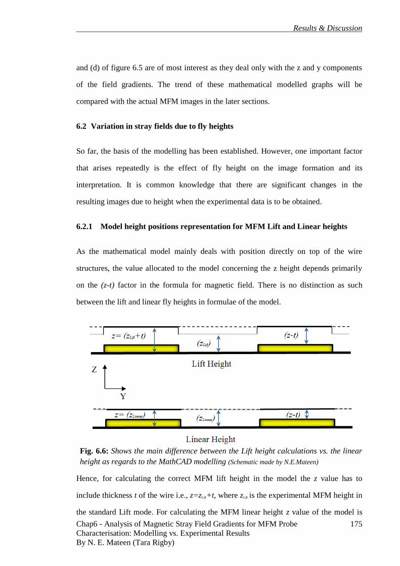
Results & Discussion
Chap6 - Analysis of Magnetic Stray Field Gradients for MFM Probe
Characterisation: Modelling vs. Experimental Results
By N. E. Mateen (Tara Rigby)
175
and (d) of figure 6.5 are of most interest as they deal only with the z and y components
of the field gradients. The trend of these mathematical modelled graphs will be
compared with the actual MFM images in the later sections.
6.2 Variation in stray fields due to fly heights
So far, the basis of the modelling has been established. However, one important factor
that arises repeatedly is the effect of fly height on the image formation and its
interpretation. It is common knowledge that there are significant changes in the
resulting images due to height when the experimental data is to be obtained.
6.2.1 Model height positions representation for MFM Lift and Linear heights
As the mathematical model mainly deals with position directly on top of the wire
structures, the value allocated to the model concerning the z height depends primarily
on the (z-t) factor in the formula for magnetic field. There is no distinction as such
between the lift and linear fly heights in formulae of the model.
Hence, for calculating the correct MFM lift height in the model the z value has to
include thickness t of the wire i.e., z=zLift+t, where zLift is the experimental MFM height in
the standard Lift mode. For calculating the MFM linear height z value of the model is
Fig. 6.6: Shows the main difference between the Lift height calculations vs. the linear
height as regards to the MathCAD modelling (Schematic made by N.E.Mateen)

Results & Discussion
Chap6 - Analysis of Magnetic Stray Field Gradients for MFM Probe
Characterisation: Modelling vs. Experimental Results
By N. E. Mateen (Tara Rigby)
176
kept the same as the MFM linear height i.e. z=zLinear, where zLinear is the experimental
height in the linear mode. This is schematically presented in figure 6.6.
Fig. 6.7: Shows the variation of z values in the MathCAD modelled data with respect to
(a) MFM Lift height mode and (b) Linear height mode. When the zLift and zLinear are set a
100nm above the sample the values for the model are set at 170nm and 100nm
respectively to compensate for the height variation in the MFM lift mode (Graphs made by
N.E.Mateen)
For example, if the MFM experimental setup was given the lift height of 100nm then the
z selected to represent the corresponding modelled values would be 170nm where
t=70nm, thus making the modelled height on top of the wires 100nm. On the other
hand, if the same height were selected in the linear mode of MFM that is 100nm then
the z value in the modelled setup would remain at 100nm at the top of the wires.

Results & Discussion
Chap6 - Analysis of Magnetic Stray Field Gradients for MFM Probe
Characterisation: Modelling vs. Experimental Results
By N. E. Mateen (Tara Rigby)
177
Figure 6.7 shows the difference represented in the modelled data of the lift height (a)
and linear height (b) of the MFM fly height modes. The magnetic fields and their stray
field gradients are much strongly influenced in case of linear mode simply because in
reality the sensor scans at a distance much closer to the wire structures compared to the
lift height mode (see appendix 6.B with some specific values in tabular form).
6.2.2 Comparison between experimental MFM data with the MathCAD model
(Lift vs. linear heights)
In figure 6.8 the MFM data is plotted against the respective MathCAD model. Data
from an MFM scan of the physical sample with ⁄ are compared
with the MathCAD calculations in Figure 6.8. The MFM images were captured at lift
and linear height mode of 100nm in both cases. The field size was 5x5µm2. The tip used
was a CoCr standard pyramidal shape scanning across the wire structures in the y
direction according to the model. The phase shift in the MFM is directly proportional to
the square of stray field gradients; therefore, the MFM data is plotted against the
modelled data of the equivalent parameters.
The MFM data represented here were averaged over approximately 20 scan lines
extracted from the MFM images directly. The sample setup used the reversed biased
current configuration*, which was kept the same for the model. Technically, due to the
predictions of the model the MFM data should follow either the y component or the z
component of the second derivative of the gradient provided the tip shows stability. To
clarify this, it should be noted that unless otherwise stated the MFM tip was always
magnetised in the normal direction at the start of every experimental setup.
* The variation in the MFM imagery due to reverse bias current configuration are discussed separately in
section 6.2.7

Results & Discussion
Chap6 - Analysis of Magnetic Stray Field Gradients for MFM Probe
Characterisation: Modelling vs. Experimental Results
By N. E. Mateen (Tara Rigby)
178
In the case of the graphs in figure 6.8 as far as the variation between the lift and the
linear mode is concerned, the MFM image follows a somewhat predictable trend of a
general increase in the overall change of phase shift signal.
Fig. 6.8: Illustrates the experimental MFM data for lift i.e. zlift=100nm (a) and linear
i.e. zlinear=100nm (b) heights with respect to the MathCAD model having the
corresponding parameters i.e. z=170nm (a) and z=100nm (b) respectively. Here both
the y and z components of the field gradients are also represented. The current direction
in this case was negative for both experiments and the model I=-70mAmps i.e. j=-
1x10¹²
A/m2 starting from the LHS wire structure (explained later) (Graphs made by
N.E.Mateen)
The lift height signals are relatively weaker than the linear height signals for obvious
increase in the fly height over the structures. Here it is prudent to point out an inherent
trait associated with all the MFM images captured using the lift height mode. This

Results & Discussion
Chap6 - Analysis of Magnetic Stray Field Gradients for MFM Probe
Characterisation: Modelling vs. Experimental Results
By N. E. Mateen (Tara Rigby)
179
involves the knowledge of the general shape of the signal detector/sensor (in this case
the CoCr pyramidal tip). Owing to the physical shape of the tip and the surface features
(if any) of the sample in question, the magnetic signal from the wire structures always
appears broader on top of the wires.
Fig. 6.9: Shows the wire topography in (a) along with its respective MFM image of lift
height of 100nm in (b) and the linear height of 100nm in (c). The solid white lines
bracketing the second wire shown in (a) is equal to 1µm, which is the same as the
magnetic signal recorded in (c) for the linear height. However, the width of the signal in
(b) is ~120nm more than the physical wire structure (Images captured by N.E.Mateen)
This broadening can be observed clearly from the lift height MFM images as well as the
linear heights along with their respective topography in figure 6.9. There could be
several explanations for this, the obvious being the tip shape. Other possibilities may
include the relatively greater distance from the sample or the extra contribution of the
magnetic signal at the tip sides with the wire edges. This difference above the wires can
be seen in figure 6.8 (a) and (b).
If the MFM image and model in 6.8 (a) is considered, it is quite clear that the MFM data
follows both y as well as z components of the force gradients. However, it seems that

Results & Discussion
Chap6 - Analysis of Magnetic Stray Field Gradients for MFM Probe
Characterisation: Modelling vs. Experimental Results
By N. E. Mateen (Tara Rigby)
180
the magnetic experimental data is flipped in relation to its modelled counterpart. It could
be because the tip magnetisation direction was in the opposite direction to the modelled
predictions. Other than that, the MFM data behaviour was symmetrical across the wires,
predominantly following z component of the force gradient with only slight influence
from the y component. Only in cases where the tip magnetisation is perfectly
perpendicular to the samples surface, complete z component dominance with zero
contribution from the y component could be achieved*. Nevertheless, evidence suggests
that for most cases the situation is less than ideal and therefore, the y (or z) component
cannot be completely ignored†.
Coming back to figure 6.9 (b), an increase of approximately 120nm from the actual wire
structure of 1µm is significant with an error margin of ±10nm‡ for each image in this
data set. Moreover, when it comes to the observation of sub-micrometre magnetic
domain structures for instance, this number of ~120nm cannot be easily ignored.
Therefore, care must be taken when observing nanometre scaled magnetic features. The
fly height at which the images were captured as well as the shape and size of the tip
must also be kept in consideration.
6.2.3 Modelled height variations
An example to show the modelled equivalent variations of z height (to both the MFM
lift as well as the linear height) for δ2Hz/δz
2 is shown in figure 6.10. The model
parameters were set to normal bias, that is, at positive current I=70mA for the first wire
and vice versa as per the physical structures. The setup was such that the model
* Conversely, in the cases where the magnetisation direction is parallel to the samples surface the y
component would be dominant having zero contribution from the z component † regardless of how little contribution it is theorised to have on the overall image
‡ In this particular case, an error margin of ±10nm was simply because the scan size for these particular
images was5x5µm2. As each image was captured using 512x512 pixel area, therefore, one pixel in the
image would be limited to 10nm, thus producing a systematic error/ambiguity

Results & Discussion
Chap6 - Analysis of Magnetic Stray Field Gradients for MFM Probe
Characterisation: Modelling vs. Experimental Results
By N. E. Mateen (Tara Rigby)
181
represented both the lift and linear fly heights at various distances above the
sample/wires.
Fig. 6.10: Shows the trend of modelled equivalent z (lift and linear fly heights) for
δ2Hz/δz
2. Column (a, c, e) show the modelled equivalent z (lift height) of 270, 220, and
170nm respectively. Similarly column (b, d, f) represent the respective modelled
equivalent z (linear height) of 200, 150, and 100nm respectively (Graphs made by
N.E.Mateen)
For example at probable 200, 150 and 100nm lift and linear fly heights, the respective
model equivalents in δ2Hz/δz
2, are shown in figure 6.10 as 270, 220, 170nm and 200,
150, 100nm respectively.
Of course, as the sensor*-sample distance between the linear heights is always less
compared to the lift height mode, therefore the respective signal would be significantly
large for linear compared to lift. The respective experimental considerations are
illustrated in the next section.
* Here the word ‘sensor’ denotes the magnetic tip. However as the model is based on Biot-Savart Law it
keeps silent about the tip to sensor, it only estimated the field and/or its gradients as a given point in 3D
space.

Results & Discussion
Chap6 - Analysis of Magnetic Stray Field Gradients for MFM Probe
Characterisation: Modelling vs. Experimental Results
By N. E. Mateen (Tara Rigby)
182
6.2.4 Fly height variations in MFM vs. modelled data
In the previous section, the variation in y and z components of force gradient signal was
systematically represented for both the lift as well as linear type fly height modes. This
was done to give a general idea of how the signal would vary for each case may it be the
lift height or the linear height mode.
In practice, most MFM is undertaken in lift height mode unless there is a particular
demand for the linear fly height mode. This is because for linear height the sample
needs to be flat and polished however most samples observed may not be completely
flat or have some kind of features on them. This is generally catered for by the feedback
loop in the lift height mode. Hence, the lift height mode is preferred as it is safer and
less damaging to the tip or the sample. In cases where the samples are flat, the lift height
mode would behave similar to a measurement done using the linear height.
Figure 6.11 represents the MFM data extracted from images captured using the Step 5
(i.e., modified CoCr tip*) having scan sizes of 4x4µm
2, I=70mA in the first wire
† with
zLift of (a) 150, (b) 100 and (c) 50nm. The corresponding modelled parameters were
j1=70/wt (a) z=220nm, (b) z=170nm and (c) z=120nm.
The modified Step 5 CoCr tip was randomly selected, as the purpose was to show the
general behaviour of the MFM signal as a function of the fly height. It is expected that
the overall signal will drop when the fly height is increased. Close observation of figure
6.11 (a-c) indicates that the MFM data does follow the modelled values, noticeably the
y component of the force gradient represented by the red line. However, the slope of the
signal in-between the wires does not follow exactly the model prediction.
* Details regarding the tip modification i.e. step 5, are given in chapter 8
†The wire on the left throughout this dissertation is considered the first of the two wires. If ‘I’, ‘I1’ or ‘j1’is
written positive then by default the first wire is positive consequently the second wire is considered
negative due to current direction. This is referred to as normal bias here.

Results & Discussion
Chap6 - Analysis of Magnetic Stray Field Gradients for MFM Probe
Characterisation: Modelling vs. Experimental Results
By N. E. Mateen (Tara Rigby)
183
Fig. 6.11: Shows both the MFM as well as the modelled data of δ2Hy/δy
2 and δ
2Hz/δz
2 of
the same tip (Step 5) at various fly heights zLift of (a) 150, (b) 100 and (c) 50nm and the
corresponding modelled z values were (a) z=220nm, (b) z=170nm and (c) z=120nm
respectively (Graphs made by N.E.Mateen)
At lower fly heights, closer to sample’s surface the variation in slope of the signal
compared to the modelled values for both y and z component between the wires is
considerably enhanced. Observing from the left side of the data range the probe senses

Results & Discussion
Chap6 - Analysis of Magnetic Stray Field Gradients for MFM Probe
Characterisation: Modelling vs. Experimental Results
By N. E. Mateen (Tara Rigby)
184
the first wire and shows an attractive force behaviour (represented by the negative phase
shift values). However, the behaviour does not exactly match either the y or the z
components as the modelled lines (red and yellow) show.
In fact, close observation of the MFM data indicates that it follows almost entirely the y
component of the force gradient above, as well as in between the wire structures. When
the probe passes over the first wire structure it experiences an attractive force thus
showing a negative phase shift as per the prediction of the model. The only difference is
that in the real case, as the probe is attached to a physical cantilever (hence not free), so
it was unable to jump back to its predictive positive phase shift position immediately.
Moreover, like the true follower of the predicted y component it does not symmetrically
go through the zero phase shifts at y=2µm, instead it tries to follow the z component
and increases quite rapidly towards the positive of the phase shift. The phase shift MFM
signal kept increasing (that is the tip is repulsed from the sample) until it became closer
to the second wire at y=3µm. At y=3µm unlike the modelled expectation of the signal
dropping towards the attractive, negative phase shift, it jumps straight up (further
repulsed) and then plateaus over the wire structure (see figure 6.11(a)). However, as the
height is decreased and the probe sample distance is reduced not only the phase shift
signals are stronger but at y=3µm the MFM signal following the modelled trend to dip
towards the attractive values slightly before reverting to the repulsive phase. This
behaviour is indicative of a slight z component interfering with otherwise y component
domination.
6.2.5 MFM tip type/materials vs. Model
Figure 6.12 shows the effect of various magnetic coatings on the MFM probes and their
effect on the final image formations. The corresponding MathCAD model data plotted
on each MFM graph helps interpret the dominating MFM image trends, whether the
MFM follows the z component of the wire structures or the y component. This might

Results & Discussion
Chap6 - Analysis of Magnetic Stray Field Gradients for MFM Probe
Characterisation: Modelling vs. Experimental Results
By N. E. Mateen (Tara Rigby)
185
indirectly reveal the information about the tip state and its relative magnetisation
direction.
The set of data represented in figure 6.12 is interesting as it not only emphasises that the
model does not impart any information about the tip, its behaviour or its contribution in
the final image formation but also because it highlights each tip contribution in the
image formation may be unique, even if it shows broadly similar behaviour.
Nonetheless, the comparison of the experimental data with the model prediction allows
an insight into how the stray magnetic field interacts with the tip. The modelling
specifies only the information about the wire sample behaviour and not the tip.
Therefore, studying the behaviour of the tip individually as well as in comparison with
other tips should become somewhat simpler. Three different tips were used here namely
the standard pyramidal CoCr tip, a custom modified version of the same tip referred
here to as Step 5* and a Metglas
®† tip. Although there is a huge variety of magnetic tips
available commercially or custom made, these three tips were selected mainly due to
convenience as they were more than sufficient to show that irrespective of the tip type
or shape the results would have remained consistent.
The MFM data represented in figure 6.12 for various tips was gathered using settings of
8x8um2
scan size at lift height zLift=150nm. Every effort was made to keep the wires
central to the scan area and the fast scan direction was kept perpendicular to the length
of the wires. The current direction through the wire structure was kept at I=+70mA. The
model used equivalent parameters as the actual MFM for both the z and y components
* Step 5 is the fifth step in the modification of a standard pyramidal CoCr commercial tip. The
modifications were done with focused ion beam milling method to acquire a tiny magnetic particle at the
tip apex. The details of the modifications, the shape and size of the tip are extensively discussed in
chapter 8. † Metglas
® tip used here was an old pyramidal Si tip which was sputter coated with 100nm Metglas
®
2605SC amorphous ribbon (Fe81B13.5Si3.5C2) at University of Sheffield by G. P Heydon in 1999

Results & Discussion
Chap6 - Analysis of Magnetic Stray Field Gradients for MFM Probe
Characterisation: Modelling vs. Experimental Results
By N. E. Mateen (Tara Rigby)
186
of the stray field gradients δ2Hz/δz
2 & δ
2Hy/δy
2, thus, t=70nm, z=zLift+t=220nm,
w=1um, b=2um, j1=+70/wt.
Fig. 6.12: Shows the variations in the MFM data of different probes (a) Standard
pyramidal CoCr tip, (b) Modified CoCr (Step 5) (c) Metglas®
with the modelled data.
The modelled parameters were kept the same as the MFM data for comparative reasons
(Graphs made by N.E.Mateen)

Results & Discussion
Chap6 - Analysis of Magnetic Stray Field Gradients for MFM Probe
Characterisation: Modelling vs. Experimental Results
By N. E. Mateen (Tara Rigby)
187
The graphs in figure 6.12 provide a wealth of information about the tip behaviour. As
the tip was scanned across the current wire structures, its behaviour was captured in the
form of phase shift. An average of 20 scan lines was used to construct the MFM data
plots. The average was taken in order to reduce the inherent noise in these types of
MFM data sets {1}. The graphs can be studied in several smaller sections or in certain
areas where the tip’s behavioural study might be of some interest. For instance, the
areas where the tip transitions on top of the wires, on top of the wires themselves and
the area in between the two wires are of considerable interest. It is worth noting how the
tip interacts with the wires as well as how it behaves between the wires, as the magnetic
stray field gradients from both the wires influence the tip there.
Let us compare the behaviour of the three tips above the wire at the left hand side first.
At a y position of 0.5µm the value extracted from MFM data of CoCr tip was
approximately equal to -0.19˚. At the same position of y the respective values of Step 5
and that of Metglas® tip were found to be ~-0.23˚ and ~-0.17˚ respectively. The
modelled values for the y=0.5µm position the derivatives of y and z stray field gradients
were equal to 5.09x10¹³
kA/m3 and -8.51x10
11 kA/m
3 respectively. Similarly for the sake
of argument if MFM data and model values were extracted at y positions of 3.5µm (i.e.,
middle of the second wire structure, having opposing current direction) they would be
~0.20˚ (CoCr), 0.26˚ (Step 5), 0.41˚ (Metglas®) and -5.09x10¹³
kA/m3 (y component)
and -8.51x10¹¹
kA/m3 (z component) respectively.
Now this behaviour of the MFM data compared to the y or z component of the field
gradient could be construed as odd (non-conformal). In this particular case, although the
MFM signal seems to follow mainly the y component of the stray field gradient, when it
comes to the tip response on top of the wire structures, it could be insinuated that the tip
behaves in the reverse fashion to the model predictions. For example, from negative
values of phase shift (attractive) on top of the first wire on the left to positive values

Results & Discussion
Chap6 - Analysis of Magnetic Stray Field Gradients for MFM Probe
Characterisation: Modelling vs. Experimental Results
By N. E. Mateen (Tara Rigby)
188
(repulsive) of the model at the same position. Thus, it appears that the MFM data does
not rigorously follow the modelled predictions, especially at the wire edges. However,
on closer inspection, when it comes to the MFM tip sensing an attraction towards the
first wire, for instance, after the initial attractive pull at y=-0.1µm (see figure 6.12) the
tip is unable to retract enough to be pushed towards the positive phase shift values at
about y=0.1µm, as predicted in the model. Nevertheless, while passing right above the
centre of the wire itself the tip does follow the same trend as the model predicts but at a
much lower set of phase shift values. Likewise for the second wire at y=2.9µm the
MFM signal shows the beginning of tip retraction but then failing to revert back to
attractive (negative) phase shift values like the model forecasts at y=3.1µm. Still, at the
central wire position y=3.5µm like the first wire the data mimics the predicted model
trend and stays in the retracted mode.
It is also interesting to note the MFM data in the area between the two wires and its
comparison with the model estimate (for the y component) follow similar trends. As can
be seen from the figure 6.12 that the tip variations do not affect the overall behavioural
trends as such, yet each tip contributed to the picture in its own unique way, implying
that such variations can be exploited according to the particular demands of the user.
6.2.6 Tip type/materials with fly height variations vs. Modelled data
The variation between the various tip’s behaviour were represented in the previous
section, however, in this section the tip variation is shown with the addition of the lift
height changes and how the height incorporates itself in the overall resulting tips-sample
image formation.
Figure 6.13 gives another set of results of two different tip types, one modified Step 5
CoCr and the other home deposited Metglas® on pyramidal Si tip. These two tips
should behave differently compared to each other, as they have a different shape and

Results & Discussion
Chap6 - Analysis of Magnetic Stray Field Gradients for MFM Probe
Characterisation: Modelling vs. Experimental Results
By N. E. Mateen (Tara Rigby)
189
composition of the magnetic material. Figure 6.13 (a, c &e) represent the MFM data
gathered for the modified Step 5 CoCr tip at lift heights of 150, 100 and 50nm
respectively. This MFM data was plotted against the corresponding MathCAD model of
z height equivalent of 220, 170 and 120nm. Similarly figure 6.13 (b, d & f) shows the
MFM data acquired from the scans using the Metglas® tip at lift height of 150, 100 and
50nm respectively. However, the corresponding model values remain the same. As
mentioned earlier, the model does not cater for the effects of the tip or any variation
caused by it thereafter in the overall signal formation i.e., tip-sample interaction. Thus,
the model possesses the unique capability of providing an excellent platform to study
the variations caused due to the differences in the magnetic tips, both structurally as
well as materially. Since the wire sample was based on the model having known
configurations, therefore it could be placed amongst the top contenders for the
standardised metrological estimations of MFM tips.
Figure 6.13 also draws the attention to the apparent limitations the tips experience when
responding to the sample stray fields while scanning directly on top of the sample
current wires. It is well documented that the MFM tips are themselves limited by their
cantilevers {4-10}. Depending on the flexibility or rigidity of the cantilever itself, the
sensitivity of the tips greatly influences the overall image formation and this
phenomenon can be clearly observed by scrutinising the graphs in figure 6.13. The
change in the fly height accentuates this point even further.
The tip behaviour with respect to the fly height can be observed in three separate
sections on the graph with MFM and model data. First, while passing on top of the first
wire (LHS), second, through the area above the spacing between the two wires, finally
when the tip passes over the second current wire (RHS). Here the performance of the
two tips on top of each wire is discussed and the next section is dedicated to the spacing
between the two wires and the corresponding tip response.

Results & Discussion
Chap6 - Analysis of Magnetic Stray Field Gradients for MFM Probe
Characterisation: Modelling vs. Experimental Results
By N. E. Mateen (Tara Rigby)
190
Fig. 6.13: Highlights the contribution of the tip in the magnetic image formation due to
tip-sample interaction. Additionally the figure further draws attention to the
differences in behaviour of different tips as it not only differs from tip to tip but also
there are variations at different fly heights that can be clearly observed (Graphs made by
N.E.Mateen)
If only the first wire was considered at various fly heights for the two different tips, then
two things could be observed. Firstly, the MFM Step 5 CoCr tips’ response around
y=1µm, when the fly height is decreased as shown in figure 6.13 (a), (c) to (e), the tip
shows increased sensitivity as expected. Yet just at around y≥1µm i.e., beyond the wire
structure the tip senses a large repulsive force which is more pronounced at lower fly
heights like in figure 6.13 (e) and it traces the model predictions very closely. However,
just before the y=1µm, that is, y≤1µm the MFM data shows that the tip response to the
wire structure itself was somewhat limited. It appears that the tip response on top of the
wires is not as pronounced as estimated by the model, especially for lower values of lift
heights. The tip behaviour near and above the second wire structure is similar.
Overall, the data from MFM using Step 5 tip gives the impression that the tip responds
to the initial push of attraction or repulsion just before or after the wire structures. In

Results & Discussion
Chap6 - Analysis of Magnetic Stray Field Gradients for MFM Probe
Characterisation: Modelling vs. Experimental Results
By N. E. Mateen (Tara Rigby)
191
doing so, the MFM data tends to follow the predicted trends from the model.
Nevertheless, once the overwhelming attraction or repulsion has set in the tip finds itself
difficult to flip especially when the tip material is CoCr and even though for this Step 5
tip, its size and magnetic coated material has been considerably reduced (figure 6.13 (a),
(c) & (e)). Some values of the MFM data for both the Step5 and Metglas® tips at
various fly heights as well as the corresponding model values, at y positions at and near
the first and the second wire are shown in appendix 6.C.
For the other part of the figure 6.13 (b), (d) & (f), at same lift height variations as the
Step 5 tip scans, the tip used was the amorphous Metglas® coated. Here, the MFM data
followed a similar trend to that of the data gathered by Step 5 tip, with some distinct
differences. The Metglas® tip showed more flexibility in following the expected trends
predicted by the models. Figure 6.13 (b) shows a very good agreement with the y
components stray field gradient prediction of the model. The data gathered at the first
wire almost idealistically replicates the projected model. The trend agreement can be
clearly seen at the values of y=-0.1, 0 & 0.1µm as well as at y=0.9, 1 & 1.1µm, it even
shows the similar attraction the tip feels at y=0.5µm.
It is interesting how the MFM data from the Metglas® tip behaves in the area between
the wire structures. The Metglas® tip is the only sensor in this study that truly passed
through the phase shift value of zero at exactly y=2µm, which is the prediction the
model makes as well. Yet, when the data of the tip is considered for the second wire
structure it, like the Step 5 study, does not fully follow the model trend. When the tip
retracts back and reaches the approximate position of y=2.9µm, according to the model
it should revert to the negative until it reaches the attractive phase shift at around
y=3.1µm. However, the tip does not do that and continues to retract up to y=3.5µm. The
tip follows similar behaviour to the other edges of the second wire near y=4µm.

Results & Discussion
Chap6 - Analysis of Magnetic Stray Field Gradients for MFM Probe
Characterisation: Modelling vs. Experimental Results
By N. E. Mateen (Tara Rigby)
192
Furthermore, the Metglas® tip data when observed with respect to the fly height
variations as shown in the figure 6.13 (b), (d) & (f), emphasises the lack of sensitivity of
the tip to follow the stray field gradients of the sample as represented by the model.
Moreover, for the lower fly heights, the tip expectedly shows a high sensitive response
to the gradients of the stray fields from the sample, as Metglas® is a magnetically “soft”
amorphous material and thus the tip behaviour may be comparable to a super-
paramagnetic tip. Even then, it seems that the tip response does not truly follow the
expected behaviour, which, in this case would be to follow the y component of the stray
field. Ideally, the soft tip should mainly be dominated by the stray field gradients of the
sample in the z direction, that is, the z component should have been the dominating
factor.
The reason behind such tip response in Metglas® tip might be the dependence of the tip
on flexibility or rigidity of the cantilever of the tip. However, it seems unlikely that the
magnetic coating on the cantilever part of the probe plays a significant role in the
asymmetrical MFM data over the wire structures, particularly given that the Step 5 tip
shows similar behaviour as far as scanning directly above the wire. The similarity in
data obtained from Step 5 and Metglas® tip(s) at the wire edges is indicative of the
physical shape of the wire structures themselves that may contribute in the attainment of
such results.
Nonetheless, the overall variations in the behaviour of the tips with respect to the wire
structures, the distance between them as well as the effect of fly height variations seem
to suggest that not only did those different tips show different behaviour on the same
sample (that is obvious), but at different fly heights as well.
Further explanation of the behaviour of three tips is given here. In the case of the
standard commercially available CoCr tip shown in figure 6.12(a), it can be argued that
because of the asymmetry prevalent in both the tip shape and orientation, the measured
Results & Discussion
Chap6 - Analysis of Magnetic Stray Field Gradients for MFM Probe
Characterisation: Modelling vs. Experimental Results
By N. E. Mateen (Tara Rigby)
193
signal will be asymmetrical and different from tip to tip. This asymmetry can also be
attributed to the field in the tip, because the tip field is affected by the stray field of the
sample plus the remnant field from magnetisation before experiment.
It is curious to note that even though the tip shape and orientation of the in-house grown
Metglas® tip was also asymmetrical like that of the commercial CoCr tip, the MFM data
indicated that the tip’s physical asymmetry does not affect the final image formation.
In figures 6.12(c) and 6.13(b), (d) & (f), the Metglas® tip demonstrates that the stray
field from the sample is symmetrical, which is in direct agreement with the modelled
predictions. The reason for symmetrical behaviour is that the signal from the Metglas®
tip might be moment dependant and therefore, the tip response should be determined
entirely by the stray field of the sample. Furthermore, Metglas® tips may have very low
coercivity. The similarity of model and experimental results demonstrate this to be true,
and any differences could be attributed to the limit of resolution in the experimental
image from the physical size of the tip (see fig 6.1).
Now looking at the figure 6.12(b) and 6.13(a), (c) & (e), the Step 5 tip (a commercial
CoCr tip modified into a needle type tip (see chapter 7, with a small CoCr material left
at the tip apex), demonstrates similar asymmetry to that of the CoCr tip. Here the
asymmetry cannot be directly attributed to the physical size of the tip, as the dimensions
of the magnetic volume remaining on the tip apex are small to limit the resolution in the
experimental image. If the argument of the asymmetry in the tip shape and orientation is
considered then that might be a plausible explanation of the asymmetrical imaging
result. In addition, for Step 5 tip, even if the tip field is expected to be too weak to
influence the MFM image results, the tip’s remanent field from magnetisation before
experiment may contribute significantly in the final image formation.

Results & Discussion
Chap6 - Analysis of Magnetic Stray Field Gradients for MFM Probe
Characterisation: Modelling vs. Experimental Results
By N. E. Mateen (Tara Rigby)
194
The Step 5 tip behaviour described above may help explain the image results
particularly in figure 6.13(e). Bearing in mind that the tips were all magnetised
beforehand in the z direction, if the tip retained its magnetisation direction (or close to
it) in its remnant state, then the z component of the stray field from the sample would
become the dominant factor in the resulting image. Although, the data still shows y
component of the stray field gradients of the sample to be the dominant signals sensed
by the Step 5 tip, there is a slight influence of z component as well in the final image.
These results pose an interesting question: Is it true that if the tip is magnetised in the z
direction, in the resulting MFM image, only the z component of the stray field gradients
is observed? Alternatively, is there a possibility that more often than not, both the y as
well as the z components contribute to a significant extent in the final image formation?
In an attempt to answer these questions, further investigations were carried out, given in
the next few sections.
6.2.6.1 Tip fly height variations vs. model at arbitrary y positions
The spacing between the two parallel current wires is the area of significant interest,
especially if the current wire configuration is to be accepted as a standard calibration
sample for the MFM probes. A handful of studies {1, 3, 11} have been done in this area
and have generally mentioned that the central position i.e., spacing between the current
wires parallel or circular, is the position where the stray field gradients are the most
stable and symmetrical and thus ideal for the tip quantitative calibration of the MFM.
These studies also emphasise that the tip (which, is always assumed to be magnetised, in
the z direction) only detects the z component of the stray field gradients emanating from
the sample. In addition to the claims such as the y component does not play any
significant role in the final image formation or that its contribution is so little that it can
be ignored.

Results & Discussion
Chap6 - Analysis of Magnetic Stray Field Gradients for MFM Probe
Characterisation: Modelling vs. Experimental Results
By N. E. Mateen (Tara Rigby)
195
It has been found during the course of this study that those claims could only be
effective for a specific scenario and cannot be generalised as such. In the sections
discussed above it has been observed amply clearly that in certain cases even if the tips
were magnetised in the z direction the resulting image from the MFM may still have a
dominating y component.
y,
(µm
) Lift
Height,
(nm)
Phase shift, ∆Φ (deg.) - avg. of 20 lines δ2Hy/δy
2,
(kA/m3)
δ2Hz/δz
2,
(kA/m3)
CoCr S.D. Step 5 S.D. Metglas® S.D.
(1012
) (1012
)
1.3
150 -0.04 ±0.02 -0.11 ±0.07 -0.26 ±0.08 -77 -37
100 -0.06 ±0.02 -0.15 ±0.05 -0.43 ±0.04 -74 -64
50 -0.11 ±0.02 -0.26 ±0.12 -0.67 ±0.06 -58 -93
20 -0.13 ±0.07 -0.66 ±0.11 -1.17 ±0.02 -41 -110
1.5
150 -0.02 ±0.02 -0.08 ±0.05 -0.17 ±0.06 -23 -28
100 -0.03 ±0.02 -0.10 ±0.05 -0.24 ±0.05 -19 -34
50 -0.07 ±0.02 -0.20 ±0.09 -0.40 ±0.05 -13 -39
20 -0.08 ±0.03 -0.51 ±0.09 -0.67 ±0.06 -8.8 -41
1.7
150 -0.02 ±0.02 -0.04 ±0.04 -0.10 ±0.06 -8.2 -18
100 -0.02 ±0.03 -0.06 ±0.04 -0.15 ±0.05 -6.4 -21
50 -0.05 ±0.02 -0.13 ±0.09 -0.21 ±0.04 -4.3 -22
20 -0.05 ±0.03 -0.32 ±0.08 -0.37 ±0.07 -2.8 -23
Table 6.1: Shows the change on phase shift values of MFM for various tips (CoCr,
Step 5 and Metglas®
) along with their corresponding y and z components of force
gradient values at y positions of 1.3, 1.5 and 1.7µm away from the first wire. The
MFM data presented here has an average of about 20 scan lines along with its
corresponding standard deviation error given next to it (Data produced by N.E.Mateen)
Table 6.1 is taken from the data extracted by the MFM and its respective modelled
counterpart. Tip behaviour of three different tips, CoCr, Step 5 (modified CoCr) and
Metglas® were studied at three arbitrary y positions, for instance at y=1.3, 1.5 and
1.7µm, at various lift heights. In order to show a general trend of the signal response, all
these particular y positions lie in the area between the two wires. The exact central
position between the wires was not taken (y=2µm) as the expected value for the y
component at that position is zero. Therefore, the positions selected are off-centred. The
corresponding modelled y and z components of the stray field gradients are also

Results & Discussion
Chap6 - Analysis of Magnetic Stray Field Gradients for MFM Probe
Characterisation: Modelling vs. Experimental Results
By N. E. Mateen (Tara Rigby)
196
represented in the table 6.1. The MFM data presented here is an average of 20 scan
lines.
Fig. 6.14: Represents lift height variation of three different MFM tips (CoCr, Step 5
and Metglas®
) along with the model predictions, at three random y positions (y=1.3,
1.5 and 1.7µm) between the wire structures (Graphs made by N.E.Mateen)

Results & Discussion
Chap6 - Analysis of Magnetic Stray Field Gradients for MFM Probe
Characterisation: Modelling vs. Experimental Results
By N. E. Mateen (Tara Rigby)
197
The data shown in table 6.1 can be represented in the form of graphs shown in figure
6.14. The graphs in figure 6.14 help visualise how at certain locations between the
wires, the MFM and its proportional modelled data vary with respect to fly heights. It
should be kept in mind that the model only shows the expected stray field gradient
behaviour at a certain point in space, in this case whatever the z value assigned to it and
nothing of the tip. There were bound to be differences as the lift height was incorporated
into the scenario.
The difference in the signal sensitivity of each tip is quite significant at lower lift
heights e.g., 20nm compared to higher fly heights like 150nm. It can thus be generalised
that the tip behaviour show similarities at higher fly heights but is markedly different
closer to the sample when compared to the other tips. The fact that the Step 5 tip and the
Metglas® tip show similar response to the stray field gradient compared to the standard
CoCr tip figure 6.14(a), (b), & (c) , with the change in lift height positions, indicates
that these two tips are more highly prone to change in the stray magnetic field than the
CoCr tip. Furthermore, the phase shift values for Step 5 tip at large fly heights tends to
be closer to those of CoCr tip values, however as the fly height was lowered the Step 5
tip shows tendencies more like the Metglas® tip. It is interesting to note the trends of the
model (y and z component) as a function of height. Even though dominance of the y
component is evident from the MFM scans (figure 6.12 & 6.13) and matches nicely
with the y component of the model, figure 6.14 shows tip behaviour(s) following the z
component of the model as a function of height.
The general slopes following the trend that the three tips show for the fly height
variations, leaned towards the z component of the stray field gradients from the model
predictions. The y component shows trends that tend to go in the opposite direction
from that of the experimental data.

Results & Discussion
Chap6 - Analysis of Magnetic Stray Field Gradients for MFM Probe
Characterisation: Modelling vs. Experimental Results
By N. E. Mateen (Tara Rigby)
198
6.3 Variations in MFM and model due to current directions in wires
It is a given that whenever there is any mention of the reversal of current direction that
the magnetic image produced would symmetrically reverse. Nevertheless, when the
current biasing was reversed in the case of the wire structures the MFM data thus
produced did not show symmetrical results in their entirety as predicted.
Figure 6.15 shows the MFM data using the standard CoCr tip scanning at a lift height of
100nm (z height for the modelled predictions was 170nm) when (a) current is forward
biased I=70mA (b) the current direction is set to reverse biased. Similarly figure 6.15(c)
shows the forward biasing of the current at a linear fly height of 100nm (z=100nm for
model) compared to (d) as having the current setting as reverse for the same linear fly
height.
Fig. 6.15: Highlights the variation in both the MFM as well as the model values as the
current directions in the wires are reversed. (a) & (b) show the current direction
reversal in the wires when the tip scan height is set to lift mode of 100nm. (c) & (d)
show the data with the height mode set to linear at 100nm (Graphs made by N.E.Mateen)
The interpretation of these results is somewhat complicated. In this case, as the tip was
magnetised in the z direction and only the current in the wire structures changes in
direction, therefore, whatever the resulting MFM image data is gathered it should only

Results & Discussion
Chap6 - Analysis of Magnetic Stray Field Gradients for MFM Probe
Characterisation: Modelling vs. Experimental Results
By N. E. Mateen (Tara Rigby)
199
show the effect of current reversal in the wires. Hence, the MFM data should show
similar behaviour to that of the predictions made by the MathCAD model.
From the figure 6.15(a) where the current is forward biased, the data reveals that the tip
shows sensitivity to the z component of the stray field gradients, especially on top or
near the physical current wires, but in the opposite direction to that of z component of
the model prediction. In the area between the wires, it seems to be following the y
component, yet again in the reverse direction as predicted by the model. This goes on to
show that the tip magnetisation might just be the reverse of z magnetisation therefore
the results are symmetric but opposite.
Similarly the case shown in figure 6.15(b) when the current direction is reversed, the
model value of I is set at -70mA. The MFM data symmetry to the z component is still
dominant compared to the presence of the y component, which can be observed in the
areas between the wires. The high and low points in the phase shift of the MFM data
have reversed as predicted.
Figure 6.15(c) & (d) show the same current reversal with the only difference that the
linear fly height were involved in the extraction of data instead of the lift heights, the
reason being that it is a direct approach when the experimental data is compared to the
modelled estimates. Of course, as the tip used here was a standard CoCr tip therefore
some degree of asymmetry was envisaged.
6.4 Effect of tip magnetisation directions on MFM data: A Comparison
A schematic of the tip magnetisation direction is shown in the figure 6.16. With the help
of a strong Re-FeB bulk magnet the tip is magnetised in the desired direction. However,
the tip magnetisation direction is usually a crude estimate especially when the tip shape
and the tip angle with its cantilever are unknown.

Results & Discussion
Chap6 - Analysis of Magnetic Stray Field Gradients for MFM Probe
Characterisation: Modelling vs. Experimental Results
By N. E. Mateen (Tara Rigby)
200
Unless the tip is specially customised and has a known shape size and angle, it is
impossible to know with certainty the precise magnetisation direction after the tip has
been exposed to a strong magnetic influence. Nevertheless, this is an incessant debate
and is not the main point of interest here. Here the influence of the tip magnetisation
direction is studied with respect to the current wire sample and its effect on the overall
tip sample interaction.
Fig. 6.16: Shows the schematic of the tip magnetisation direction. When the tip needs to
be magnetised it is brought in close proximity of a very strong magnetic field. Here the
tip was magnetised in (a) normal, (b) horizontal and (c) reverse direction with the help
of a bulk Re-FeB magnet (Schematisc made by N.E.Mateen)
A commercially available CoCr tip was magnetised in the normal direction and then the
MFM data was obtained when tip raster scanned over the sample at a lift height of
150nm (see figure 6.17(a)). The equivalent model height was kept at 220nm for the
experimental compensation. Now the figure 6.17(b) shows the tip behaviour with the
wires when it magnetised in the horizontal direction with the same lift height of 150nm
and at the exact same area of scanning and in figure 6.17(c) the tip was magnetised in
the reverse to the normal direction that is shown in (a).
While the tip magnetisation direction was changed, there were some key points to
observe. Firstly, how the behaviour of the tip over the wire structures corresponds to tip

Results & Discussion
Chap6 - Analysis of Magnetic Stray Field Gradients for MFM Probe
Characterisation: Modelling vs. Experimental Results
By N. E. Mateen (Tara Rigby)
201
magnetisation direction with no change in the fly height or the current direction
(Normal bias) wire configuration of the sample.
Fig. 6.17: Shows three scenarios of the effect that the tip magnetisation has in the tip-
sample interaction. (a) shows the interaction when the CoCr tip is magnetised in the
normal direction, (b) represents the behaviour of the tip when it is magnetised in the
horizontal direction and (c) when the tip is magnetised in the opposite to the normal
direction (Graphs made by N.E.Mateen)

Results & Discussion
Chap6 - Analysis of Magnetic Stray Field Gradients for MFM Probe
Characterisation: Modelling vs. Experimental Results
By N. E. Mateen (Tara Rigby)
202
The second point worth noting was the effect of tip behaviour as it scanned the area
between the wires and how does it relate to the overall image formation. More
importantly, do the experimental results agree with the model?
The tip behaviour in figure 6.17(a) is what was expected for a tip magnetised in a
particular z direction. The reason that this could be only a comparative exercise was
because the magnetic orientation of the magnetising sample holder was (and is
generally) unknown, even though it is still relatively easy to study the effects that the tip
magnetisation orientation would have on the image.
The tip was then magnetised in the horizontal direction and the resulting graph can be
seen in figure 6.17(b). Theoretically, in the case of tip being horizontally magnetised the
y component of the sample stray fields should be the dominant signal in the MFM data.
This did not seem to be the case. It appeared as if both y as well as z components were
almost equally influencing the MFM data signal (6.17(b)), whereas figure 6.17(a)
showed a domination of y component. Keeping these findings in mind, the tip behaviour
of 6.17(c) was somewhat predictable. Again, the y component was the dominant factor
in the image formation. Although, the overall responses of 6.17(c) were similar to that
of figure 6.17(a); however, by close observation the tip behaviour directly above the
wire edges showed a subtle deviation; a slightly greater repulsion at the exterior wire
edges compared to the interior wire edges as compared to figure 6.17(a).
To sum up, the tip behaviour between the wires was predominantly y component but the
areas above the wires show distinct changes. Take first the left hand wire for instance,
in 6.17(a) there is y component domination with a slight agreement with the z
component; in 6.17(b) however, both the y and the z component play a significant role
in image formation. On the other hand, in 6.17(c), although the y component still
dominated the overall image with some contribution from the z component, but the z
component shows a direction opposite to that of 6.17(a).

Results & Discussion
Chap6 - Analysis of Magnetic Stray Field Gradients for MFM Probe
Characterisation: Modelling vs. Experimental Results
By N. E. Mateen (Tara Rigby)
203
6.5 Modelling the influence of Hy and Hz component superposition on the MFM
data signal
The work presented so far gave quantitative results and helped establish that the y as
well as z-components of the stray field gradient has considerable significance and
neither of these can be ignored. It can however be safely assumed that one component
of the stray field (z or y) may dominate the tip’s sensitivity over the other depending on
the physical orientation of the tip with respect to the sample as well as the tip’s
magnetisation direction. Due to the asymmetrical trends of the resulting experimental
graphs with respect to the modelled graphs for both the z and y gradients of Hz as well
as Hy, it was still difficult to pinpoint the dominant component taking part in the
resulting image formation in real scenarios. Every result presented thus far in this thesis
points to the fact that each tip has a direction of magnetisation (i.e., net moment), which
could be in any direction. Therefore, there is a strong indication that the MFM signal
could be the superposition of Hz and Hy effects.
Due to orthogonality of y & z field components, they cannot be wholly combined to
estimate the force on a tip. However, from the experimental results and comparisons it
is evident that the dominance of the field components depends on the orientation of the
stray fields with respect to the tip.
6.6 Introduction of matrix transformations for the observation of y and z
component contribution in the magnetic fields and their respective gradients
In order to estimate the extent of the signal superposition from the real cases, a probable
solution would be to consider rotation matrices/transformation matrices {12-14} or in
other words the rotation of axes. It has been established that the mathematical model
used so far only gives information of the current wire sample and nothing about the tip
itself. It only gives the information of either y or z coordinates dominance. This is

Results & Discussion
Chap6 - Analysis of Magnetic Stray Field Gradients for MFM Probe
Characterisation: Modelling vs. Experimental Results
By N. E. Mateen (Tara Rigby)
204
because the coordinated system selected for the calculation was fixed in space. The
magnetic field was calculated for the current wires at a certain point in space. As the
basic equation used in the modelling was dependant on y and z variables it was easy to
estimate the field value at a given y position at a certain z distance high. Then the
question was what happens in the space in between the two extremities.
To make the model more realistic and conform to the experimental data, the axes must
be rotated. In mathematical terms this rotational transformation is generally approached
in two ways commonly known as the alias rotation or the alibi rotation {15}. In one
case, the coordinate axes are rotated and the relevant vector is transformed into the other
desired coordinate axes. In the second case known as the alibi rotation, the axis itself is
fixed and the relevant vectors are transformed. Both these cases give essentially the
same results. These types of rotation are generally used in the field of robotics {13, 16},
in finding out coordinates for the robotic arms. For finding how the magnetic field H(y,z)
of the current wires behave other than in the direction of unit vectors ŷ or ẑ, that is, in
the coordinates where direction of the unit vectors is ŷ” and ẑ”. The rotation matrix
used for this purpose is given in equation 6.16,
[
] [
] [ ] (6.16)
This can be written as,
(6.17)
Equation 6.17 can become after rearrangement
(6.18)
Substituting values from equation 6.16 into equation 6.9
( ) | ( )| | ( )| (6.9)

Results & Discussion
Chap6 - Analysis of Magnetic Stray Field Gradients for MFM Probe
Characterisation: Modelling vs. Experimental Results
By N. E. Mateen (Tara Rigby)
205
becomes,
( ) | ( )|{ } | ( )|{ }
(6.19)
After rearrangement of the equation 6.19 becomes,
( ) {| ( )| | ( )| } { | ( )|
| ( )| } (6.20)
Equation 6.20 can also be written as,
( ) { } { } (6.21)
where,
| ( )| | ( )| (6.22)
and,
| ( )| | ( )| (6.23)
To check the equation, if θ=0˚ then the equation 6.20 reduces to
( ) | ( )| | ( )| (6.24)
Notice equation 6.24 is equivalent to equation 6.9, however, if θ=90˚ then the equation
6.20 becomes
( ) | ( )| | ( )| (6.25)
The equations 6.24 and 6.25 show that the direction of HY and HZ has changed due to
angle θ. HY has moved in the direction of ẑʺ and HZ in the ŷʺ. Furthermore, the negative
sign indicating the direction of HZ is reversed. This can be illustrated with the help of
the diagram shown in figure 6.18.

Results & Discussion
Chap6 - Analysis of Magnetic Stray Field Gradients for MFM Probe
Characterisation: Modelling vs. Experimental Results
By N. E. Mateen (Tara Rigby)
206
Fig. 6.18: Shows the rotation of the axes if the magnetic field vector is to be
translated into the other coordinate axes. y and z were the original orthogonal axes
and y” and z” are the new rotational axes (Schematic made by N.E.Mateen)
Since the objective here was to show how the model could be improved to achieve the
desired more realistic results, which conform better to the experimental data, and not to
further complicate the analysis, therefore, only a part of the equation 6.20 would be
used. Only the change in z” component will be discussed as y” component would show
the same result but in a different direction.
6.6.1 Modelling results: Effect on the magnetic fields with angular variations
The initial parameters selected for this model remain the same* as were used for the
initial setup for the original model (section 6.1). Plotting the graph Hzθ against the y
* The z height was set at 100nm, with I=70mA. The wire parameter width w=1μm and the thickness
remains at t=70nm with the wire separation of b=2µm

Results & Discussion
Chap6 - Analysis of Magnetic Stray Field Gradients for MFM Probe
Characterisation: Modelling vs. Experimental Results
By N. E. Mateen (Tara Rigby)
207
positions spanning across width of the wires, with angle θ varying from 0˚ to 90˚ is
given in figure 6.19.
Fig. 6.19: Shows the rotation of angle θ in Hzθ in the new axes coordinates z”. At
θ=0˚the value of Hzθ becomes equivalent to |HZ(y,z)|, which is correct for the axis in
the z direction. The basic parameters for the model were z=100nm, t=70nm, w=1um,
j1=70/wt, b=2um (Graphs made by N.E.Mateen)
Figure 6.19 represent the variation of Hzθ (equation 6.23) with the angle θ, where θ is
varied between 0˚ to 90˚. It can be seen from figure 6.19 that when θ=0˚,
| ( )|, which is true. At θ=90˚, | ( )|, which is also true. This goes on to
show that at any value of θ other than 0˚ or 90˚ there is indeed a superposition of the
| ( )| and | ( )| signals.
In figure 6.19, the graphs shown at angles 0˚ (blue line) and 90˚ (red line) are the same
as shown in figure 6.3. It was not surprising that θ=0˚ and 90˚ yield similar results as
previously for Hz and Hy terms since for these angles only one field component is
carried forward. Although, the model does provide the possibility for predicting the
fields or their respective gradients at angles other than 0˚ and 90˚. Therefore, it would
be prudent to assume that better comparisons can be deduced between the data produced
here and the experimental data.

Results & Discussion
Chap6 - Analysis of Magnetic Stray Field Gradients for MFM Probe
Characterisation: Modelling vs. Experimental Results
By N. E. Mateen (Tara Rigby)
208
6.6.2 Effect on the magnetic field gradients and second derivative of fields with
angular variations for Hzθ w.r.t both y and z
The graphs presented in figure 6.20 show the variations in the stray field gradients (a)
with respect to the y component and (b) with respect to the z component when the angle
θ is changed from 0˚ to 90˚*.
Fig. 6.20: Shows the variation of (a) δHzθ/δz, (b) δHzθ/δy with the height of z= 100nm,
wire thickness of t=70nm and separation b=2.0µm. When the angles are varied, the z
dominant component is influenced by the y component of the field gradients. At
around θ=45˚ both the y and the z components contribute equally to the resulting
gradients. The position from y=0 to 1µm and y=3 to 4 µm are to denote the wire
positions in the model (Graphs made by N.E.Mateen)
* See appendix 6.D for individual changes with respect to angles in the z component (figure 6.20(a)) as
well as y component (figure6.20(b))

Results & Discussion
Chap6 - Analysis of Magnetic Stray Field Gradients for MFM Probe
Characterisation: Modelling vs. Experimental Results
By N. E. Mateen (Tara Rigby)
209
In figure 6.20(a) data at angles 0˚ and 90˚, is same as figure 6.4(a) δHz/δz and (b)
δHz/δy. Similarly, the graphs in figure 6.20(b) are comparable to those in figure 6.4(c) &
(d). These findings go on to verify the calculations performed earlier in addition to the
further information they impart for any given angle.
Fig. 6.21: Shows the variation of (a) δ2Hzθ/δz
2, (b) δ
2Hzθ/δy
2 at the height of z=
100nm. At various angles, the influence of y and z components of the stray field
gradients can be observed (Graphs made by N.E.Mateen)
Predictably, now the double derivatives, which are part of the formula for the force
gradient and which in turn is used for the calculation of the change in phase shift,

Results & Discussion
Chap6 - Analysis of Magnetic Stray Field Gradients for MFM Probe
Characterisation: Modelling vs. Experimental Results
By N. E. Mateen (Tara Rigby)
210
needed to be tested (see chapter 3). The figure 6.21* represents the rate of change of the
stray field gradients with respect to z and y.
Notice that with the variation of the angles the z dominant component starts to be
influenced by the y component of the second derivative of the field. For the sake of
argument if the dominating component at θ=0˚ is the z component. Then as the angle is
increased, the influence of the z component is reduced being replaced by the y
component. At around θ=45˚ both the y and the z components contribute equally to the
resulting gradients. Moreover, at θ=90˚ the z component totally disappears only leaving
a complete domination from the y component of the gradients, as would be expected.
As expected the data trend represented in the figure 6.21(a) at θ=0˚ corresponds exactly
to the data represented in the figure 6.5(a), but when the angles are increased and reach
θ=90˚ the data does not correspond to the graphs of figure 6.5(b), instead it corresponds
to the graph presented in figure 6.5(c). Here the updated version of the MathCAD model
shows that with the introduction of the angles, the combination sets should be that of
figure 6.5(a) and(c) and figure 6.5(b) and (d), and probably not as previously assumed†.
Keeping these new findings in view, the MFM data for the tip magnetisation directions
was compared to the modelled results to see if the updated version of the model
conformed to the experimental data better.
6.7 Estimation of the tip magnetisation angles and y and z components
contribution in the MFM data sets
Once the model was tested having the new additional changes, the task of testing it with
real MFM data was undertaken. Figure 6.22 shows the MFM data for the standard CoCr
* See appendix 6.E for individual changes with respect to angles in the z component (figure 6.21(a)) as
well as y component (figure6.21(b)) † before the examination of angular variations

Results & Discussion
Chap6 - Analysis of Magnetic Stray Field Gradients for MFM Probe
Characterisation: Modelling vs. Experimental Results
By N. E. Mateen (Tara Rigby)
211
tip having three different magnetisation directions (figure 6.18) represented along with
the corresponding modelled data.
Fig. 6.22: Shows the MFM data with its corresponding modelled data representing the
perspective angles and direction of preferred y and z components (Graphs made by
N.E.Mateen)

Results & Discussion
Chap6 - Analysis of Magnetic Stray Field Gradients for MFM Probe
Characterisation: Modelling vs. Experimental Results
By N. E. Mateen (Tara Rigby)
212
However, this time the modelled data that was the closest (having a certain angle and
hence orientation) match the respective MFM data was presented in the figure 6.22.
These respective angles give a reasonable indication as to where, in the direction of
coordinate axes, does the tip sample interaction lie, (other than the pure y or pure z
direction).
All the three graphs (set of MFM data with its corresponding modelled orientation and
appropriate matching angle) given in figure 6.22(a-c) tend to suggest that the tip
magnetisation had indeed a distinct direction for each case i.e., θ=60˚ for normally
magnetised, θ=75˚ for horizontally magnetised and θ=60˚ for reversed magnetised CoCr
tip modelled for δ2Hy/δy
2. Hence, now the angle of the interaction of the stray field
gradients or the magnetic fields themselves emanating from the wire structures, at a
certain height with respect to the tip magnetisation, could be accurately predicted with
the help of the improved model.
Figure 6.22(a) (same as figure 6.18(a)) represents the MFM data captured while the tip
scanned over the current wires having I=70mA, while the tip was magnetised in the
normal direction. The corresponding modelled data suggested that the y” direction not
only dominated when the tip was normal and horizontal magnetised (figure 6.22(b)).
But when the tip was magnetised in the reverse direction it was the z” that apparently
became the dominant component according to the model (figure 6.22(c)). Although part
of the same equation (eq. 6.20), at the angle of 60˚, the tip magnetisation directions
could be accurately predicted by the restructured model data. The tip magnetised
horizontally follows the similar trend to that of normalised magnetised tip with the
difference of the angle. The horizontally magnetised tip shows an inclination at the
angle of 75˚ instead of 60˚. As mentioned earlier this tip when magnetised in various
directions strongly indicated the y component’s dominance with little influence from the
z component of the stray field gradients and the second derivative of the field. Here, the

Results & Discussion
Chap6 - Analysis of Magnetic Stray Field Gradients for MFM Probe
Characterisation: Modelling vs. Experimental Results
By N. E. Mateen (Tara Rigby)
213
updated version of the model also indicated the dominance of what would otherwise be
the y component of the stray field gradients i.e., δ2Hyθ/δy
2.
For consistency if only the y” is considered for all three tip magnetisation directions,
normal, horizontal and reverse, the corresponding angles would then be 60˚, 75˚ and
300˚ respectively with the help of the model*. If the magnetisation of the tip was known,
then the y and z components of the tip magnetisation could be predicted with the help of
the angles given, by using basic trigonometric functions. For example, if the value of tip
magnetisation |Ms| was 4x10⁵A/m {17}, then the predicted angles of the tip, the y and
components of the magnetisation for normal, horizontal and reverse direction would be
as represented as given in table 6.2.
CoCr tip direction θ My (A/m) Mz (A/m)
(˚) (10+05
) (10+05
)
Nor. 60 2.00 3.46
Hor. 75 1.04 3.86
Rev. 300 2.00 -3.46
Table 6.2: Shows My and Mz components of the tip magnetisation as predicted by the
model angles for δ2Hyθ/δy
2(Data produced by N.E.Mateen)
From the values estimated in the table 6.2, the Mz showed the highest value at
3.86x10⁵A/m with My at its minimum value of 1.04x10
5A/m when the tip was
magnetised in the horizontal direction. Typically, it is expected that the tip magnetised
in the normal and/or reverse direction would have the maximum Mz values with My
values so small that they can be ignored. However, the data presented in table 6.2 show
that the expected tip magnetisation direction might be different to the initial
expectations. Moreover, the y and z component amalgamation makes the task of
understanding the tip-sample interactive behaviour complex. When the tip
magnetisation direction was normal the Mz had the value of 3.46x10⁵A/m with My at
* At this point the predicted modelled angles would still be a somewhat crude estimation, as precise
calculations of all possible angles are required to exactly match a particular MFM data set with a
particular angle

Results & Discussion
Chap6 - Analysis of Magnetic Stray Field Gradients for MFM Probe
Characterisation: Modelling vs. Experimental Results
By N. E. Mateen (Tara Rigby)
214
2.00x10⁵A/m, which is the same values for the reversed magnetised tip except for the
change in sign for Mz.
Although, the change in the behaviour of the tip with the magnetisation reversal was
expected, the tip shape and the cantilever position with respect to the sample can still
pose a challenge to predict the exact angle of tip magnetisation especially when the
magnetisation is reversed. As the tip shape and the cantilever angle could introduce an
inherent asymmetry to the tip magnetisation angle (as mentioned in chapter 3).
Additionally, the variations in the model values with every degree change are difficult
to observe in the experimental data with factors such as noise disrupting the signal.
Consequently, if some changes in the magnitude during the tip magnetisation reversal
were observed, it would be a strong indication that directional angle of the tip
magnetisation has shifted to some extent. For example, for the angle of 240˚ both the Mz
and My values would be reversed to -2.00x10⁵A/m and -3.46x10
5A/m respectively
compared to the normally magnetised tip direction. Thus, there would be no observable
change in the Mz direction of the tip but due to the change in the y direction reversal the
slope in-between the two wire structures would invert. Similar to the MFM
experimental data slopes given in figure 6.15(a) compared to that of figure 6.22(b).
Although, the two MFM images were captured by using different CoCr tips, but as the
wire parameters were similar i.e. the current direction, the y component had changed for
both those cases the relative direction of the z component remained the same.
These results go on to show how the model based on Biot-Savart law can be modified to
estimate the tips angles that influence the image formation based on the tip-sample
interaction in reality. These results presented here are in their preliminary phase, but
they successfully show an enhanced methodology to interpret the data produced by the
MFM when the tip magnetisation is not exactly at the perpendicular z or parallel y
direction with respect to the sample plane, which is an approach that is more realistic. It

Results & Discussion
Chap6 - Analysis of Magnetic Stray Field Gradients for MFM Probe
Characterisation: Modelling vs. Experimental Results
By N. E. Mateen (Tara Rigby)
215
is a known fact that even if the tip is magnetised in a certain direction (y or z); the final
remnant state of the tip (at the time of image capture) is almost never in the idealistic y
or z directions and is always some percentage of both.
Furthermore, this enhancement of the model solves the problem of the additional
‘negative’ sign in front of the force equation. As the directional angles not only indicate
the y or z component dominance but also the ‘positive’ or ‘negative’ z direction of the
tip’s magnetisation.
It is common practice to magnetise any MFM tip from a hard magnet (placed in a
specifically designed holder in which, the tip is placed while being clamped to the tip
holder*). However, the magnetisation direction may deviate from the direction with
which the tip was initially magnetised either due to the tip shape or due to the samples
stray fields. In this case, the magnetisation of the tip changes direction in either, y or z
direction or, both y and z direction, during scanning, any change would be detected
from the MFM image data. In such cases, the improved model can indicate accurately
the direction of magnetisation including any variation in ‘y’ as well as the ‘z’
components can also be monitored.
Alekseev et al. {18} claimed to significantly improve the dipole model and
demonstrated† that both ‘y’ and ‘z’ component of tip magnetisation have different
magnetic behaviours. According to them, the ‘y’ component followed the external field
and the ‘z’ component of magnetisation of the tip stays unchanged. Their conclusions
and the conclusions drawn by Iglesias-Freire et al. {19} were somewhat similar.
Iglesias-Freire et al. deemed the wobble at the tip apex as artifacts, because during a
scan any perturbation (i.e. the variations in the ‘y’ component) due to the sample is
difficult to separate from the overall data acquisition. Whereas Alekseev et al. were of
* Which in turn is then placed in the MFM instrument
† By using soft tips with hard samples

Results & Discussion
Chap6 - Analysis of Magnetic Stray Field Gradients for MFM Probe
Characterisation: Modelling vs. Experimental Results
By N. E. Mateen (Tara Rigby)
216
the view that due to shape anisotropy of the tip, the vertical (i.e. z) component remains
almost constant and only the horizontal (i.e. y) component behaves like a soft tip prone
to flip its direction of magnetisation along with the stray field direction of the sample.
Although they were also of the view that the reversal of the magnetising field in the y
direction has no influence on the final image, which might be true for the case they
investigated. However, due to the complexity of the MFM probe, it cannot be said with
certainty that the influence of the y component magnetisation direction is negligible.
Additionally, the model presented in this chapter is able to predict conclusively if any
such influence does occur temporarily or permanently.
Overall, the results presented in this chapter, compliment and further the findings of
both Alekseev et al. as well as Iglesias-Freire et al. Here both modelling in conjunction
with experiments agree, for any given tip in relation to the samples stray fields, it is
impossible to predict with certainty the ultimate behaviour of the tip, especially when
the tips magnetisation at its apex is weak enough to be influenced by the sample fields.
However, the amended model given here accurately calculates the position of the y
and/or z components*, irrespective of y or z component being constant or varied.
The sheer numbers of variables involved in the final image formation are too many to
be controlled by the user and hence prevents from reproducing the magnetic images
precisely. Each scan produces a unique image map at that instance in time. Furthermore,
only close approximations can be achieved under similar conditions. Thus, the exact
reproducibility of an MFM image could be down to random statistical probability.
6.8 Summary
The experimental data was taken under various conditions such as at different fly
heights by using both the lift as well as the linear mode. Experiments were also
* In confirmation with the experimental results

Results & Discussion
Chap6 - Analysis of Magnetic Stray Field Gradients for MFM Probe
Characterisation: Modelling vs. Experimental Results
By N. E. Mateen (Tara Rigby)
217
performed to see the effect that the current biasing of the wire structure have on the tip-
sample interactive behaviour. Furthermore, the tip magnetisation directions and its
effects in the tip sample interaction were also analysed. All these experimental studies
were done in conjunction with the improved modelling, which could cater for the
variations in the lift and linear fly heights.
However, during the analysis of initial data it became evident that the model was still
limited when interpreting the results in terms of y and/or z component dominance of
either the sample stray field gradients and/or the tip magnetisation. Furthermore, there
was strong indication that there was to some extent a signal superposition occurring
which has the contributions from both the y as well as the z component of the field
gradients.
An attempt to improve the MathCAD model further to better conform to the
experimental results was then undertaken with the help of some necessary
modifications. The enhanced version of the model proved to be a better-equipped tool
for interpreting the tip’s behaviour during the tip-sample interaction. Moreover, the
model was capable of predicting tip’s potential magnetisation orientation and
magnitude* with respect to the current wire structures. The model along with the data
gathered by the MFM conclusively proved that the final image formation, i.e., the tip-
sample interaction is never ideal. The tip is almost never truly magnetised in the
idealistic z direction (perpendicular to the plane of the sample). The tip is generally
sensitive to both y as well as z components of the change in the stray field gradients
(i.e., second derivative of the magnetic field) emanating from the samples responsible
for generating the phase shift in the image. The scenario where the tip can predictably
be magnetised fully in the z direction could only be true for some highly specialised
cases. Mostly, the tip magnetisation roughly stays in the direction in which the tips was
* If the remanent magnetisation of the tip was known

Results & Discussion
Chap6 - Analysis of Magnetic Stray Field Gradients for MFM Probe
Characterisation: Modelling vs. Experimental Results
By N. E. Mateen (Tara Rigby)
218
initially magnetised guided by its shape, unless it is strongly swayed by the stray field
gradients of the sample.
However, unlike special cases {18, 19} as mentioned in section 6.7, the results presented
here represent a more generalised case where the magnetisation direction of any type of
tip* with respect to any type of sample could be quite accurately predicted along with
some information about the respective ‘y’ as well as its ‘z’ components. With these
results, one need not randomly assume the direction of magnetisation at the any given
point during the scan. With the help of the improved model, one can find out the angle
of the tips magnetisation† and magnitude (provided the tip volume is known, see chapter
7) from the image data gathered.
6.9 References
{1} Kebe, T. and Carl, A.; "Calibration of Magnetic Force Microscopy Tips by
Using Nanoscale Current-Carrying Parallel Wires", Journal of Applied
Physics, vol. 95, pp. 775-792, 2004.
{2} Kong, L. S. and Chou, S. Y.; "Quantification of Magnetic Force Microscopy
Using A Micronscale Current Ring", Applied Physics Letters, vol. 70, pp.
2043-2045, 1997.
{3} Kong, L. S. and Chou, S. Y.; "Study of Magnetic Properties of Magnetic Force
Microscopy Probes Using Micronscale Current Rings", Journal of Applied
Physics, vol. 81, pp. 5026-5028, 1997.
{4} Chakraborty, I. and Balachandran, B.; "Cantilever Dynamics With Attractive
And Repulsive Tip Interactions", IMECE 2009: Proceedings Of The ASME
International Mechanical Engineering Congress And Exposition, Pts A And B,
vol. 10, 2009, pp. 443-449.
{5} Van den Bos, A. G., Van Dijk, A. C. J., Heskanp, I. R., Abelmann, L., and
Lodder, J. C.; "A New Concept in Magnetic Force Microscope Cantilevers", in
Magnetic Storage Systems Beyond 2000, vol. 41, Nato Science Series, Series Ii:
Mathematics, Physics and Chemistry, 2001, pp. 307-312.
{6} Takahashi, H., Ando, K., and Shirakawabe, Y.; "Self-Sensing Piezoresistive
Cantilever and its Magnetic Force Microscopy Applications",
Ultramicroscopy, vol. 91, pp. 63-72, 2002.
* hard/soft
† if there was change in the magnetisation direction during the scanning process in y, z or both y and z
directions, the MFM image data would hold that information which then could be interpreted into
quantifiable data

Results & Discussion
Chap6 - Analysis of Magnetic Stray Field Gradients for MFM Probe
Characterisation: Modelling vs. Experimental Results
By N. E. Mateen (Tara Rigby)
219
{7} Jenkins, N. E., DeFlores, L. P., Allen, J., Ng, T. N., Garner, S. R., Kuehn, S.,
Dawlaty, J. M., and Marohn, J. A.; "Batch Fabrication and Characterization of
Ultrasensitive Cantilevers with Submicron Magnetic Tips", Journal Of
Vacuum Science & Technology B, vol. 22, pp. 909-915, 2004.
{8} Wei, J. D., Kirsch, M., Koblischka, M. R., and Hartmann, U.; "Optimization of
High-Frequency Magnetic Force Microscopy by Ferrite-Coated Cantilevers",
Journal Of Magnetism And Magnetic Materials, vol. 316, pp. 206-209, 2007.
{9} Koblischka, M. R., Wei, J. D., Richter, C., Sulzbach, T. H., and Hartmann, U.;
"Advanced Cantilevers for Magnetic Force Microscopy and High Frequency
Magnetic Force Microscopy", Scanning, vol. 30, pp. 27-34, 2008.
{10} Woszczyna, M., Zawierucha, P., Swiatkowski, M., Gotszalk, T., Grabiec, P.,
Nikolov, N., Mielczarski, J., Mielczarska, E., Glezos, N., Ivanow, T., Ivanowa,
K., Sarov, Y., and Rangelow, I. W.; "Quantitative Force and Mass
Measurements Using The Cantilever With Integrated Actuator and Deflection
Detector", Microelectronic Engineering, vol. 86, pp. 1043-1045, 2009.
{11} Liu, C. X., Lin, K., Holmes, R., Mankey, G. J., Fujiwara, H., Jiang, H. M., and
Cho, H. S.; "Calibration of Magnetic Force Microscopy using Micron Size
Straight Current Wires", Journal of Applied Physics, vol. 91, pp. 8849-8851,
2002.
{12} Stroud, K. A.; "Advanced Engineering Mathematics with additions by Booth, D.
J.", 5th edition ed: Palgrave Macmillan, Hamshire, UK, 2011.
{13} Milford, M.; "Transformation Matrices ", Introduction to Robotics ENB339,
YouTube: milfordrobotics, (C) Wyeth, G. & Milford, M., Queensland University
of Technology, Brisbane, Australia, Jul 28, 2011.
{14} Arfken, G. B. and Weber, H. J.; "Mathematical Methods for Physicists", 4th
ed. London: Academic Press, 1995.
{15} Weisstein, E. W.; " Alibi Transformation ", From MathWorld:
http://mathworld.wolfram.com/AlibiTransformation.html Jul 28 2012.,
Copyright © 1999-2013.
{16} Bajd, T., Mihelj, M., Lenarčič, J., Stanovik, A., and Munih, M.; "Robotics,
Intelligent systems, Controls and Automation: Science and Engineering".
New york: Springer, 2010.
{17} Suess, D., Schrefl, T., and Fidler, J.; "Reversal Modes, Thermal Stability and
Exchange Length in Perpendicular Recording Media", IEEE Transactions On
Magnetics, vol. 37, pp. 1664-1666, 2001.
{18} Alekseev, A., Popkov, A., Shubin, A., Pudonin, F., and Djuzhev, N.; "Effect of
Horizontal Magnetization Reversal of The Tips on Magnetic Force
Microscopy Images", Ultramicroscopy, vol. 136, pp. 91-95, 2014.
{19} Iglesias-Freire, O., Bates, J. R., Miyahara, Y., Asenjo, A., and Gruetter, P. H.;
"Tip-Induced Artifacts in Magnetic Force Microscopy Images", Applied
Physics Letters, vol. 102, 2013.

Results & Discussion
Chap7 - Magnetically Active Probe Volume
By N. E. Mateen (Tara Rigby) 220
Magnetically Active Probe Volume
7.1 MFM probe volume investigations
In the previous chapter, solutions to the question like the influence of tip’s
magnetisation direction, its fly height and the accumulative contribution of ‘y’ and ‘z’
component of the fields were addressed. The observations of the inherent dependence of
fly heights on the data obtained, the effects of tip materials used, and how MFM signal
data* can be used to predict the angle of tip/sample magnetisation were made. The
MFM data along with the appropriate modelled parameters yielded a useful insight and
helped formulate some useful predictions regarding the tip as well as the tip-sample
behaviour. The model did indeed prove to be a great tool in making predictions
regarding tips magnetisation angles, and the angle contributions of ‘y’, ‘z’ components
from the stray fields of the sample, relevant to specific fly heights, when used in
conjunction with the experimental data. Thus, the enhanced model made the direction of
magnetisation of the tip with respect to the wire samples relatively easier to predict.
Nonetheless, where the modelled current conductors helped gather a wealth of
information about the magnetic stray field gradients of the sample, they on their own
divulged only indirect information about the magnetic probe itself. What the
model/experimental results did not help to predict was the magnetic volume† of the tip.
Consequently, it was also unable to predict how much of the tip’s magnetic volume is
actively involved in the image formation. With this information, the MFM tip needed to
be studied with the view of its volume contribution, which along with the information
about tip magnetisation direction in turn would convey some information regarding the
moments of the tip.
*By using same tips with different magnetisation direction or different MFM tips with same
magnetisation direction at various fly heights † Or active magnetic volume of the tip: It is believed to be the volume of the magnetic material on the tip
that actively participates in the final image formation in an MFM

Results & Discussion
Chap7 - Magnetically Active Probe Volume
By N. E. Mateen (Tara Rigby) 221
To put into perspective the active volume from the MathCAD model-MFM
experimental estimate, an experiment was devised in parallel by systematically*
modifying commercial CoCr tips using FIB milling. A process of sequential reduction
was performed on the selected tip. The tip’s performance was tested at each stage whilst
ensuring that the tip was not damaged during the reduction process. In addition to
finding out how this tip volume affected the magnetic sample imagery, various sets of
samples were also investigated using various tips and compared to the amended tip†.
7.2 MFM tip volume reduction
The lack of reproducibility in commercial manufactured of the MFM tips in addition to
coating the entire tip (including its cantilever) makes it difficult to estimate the volume
of magnetic material coated exclusively on the tip. Determining which portion of that
tip is actually involved in the tip-sample interaction makes it an interesting study on its
own.
The probe selected for estimation of magnetic (and effective magnetic) volume by tip
reduction/modification were the standard (Veeco) MESP CoCr tip having intermediate
coercivity‡ (about 39.8kA/m). To estimate its magnetic volume accurately, the tips must
be in optimal working condition and must be able to produce good magnetic images.
They had to be robust to be modified by FIB milling. After reduction, their integrity was
tested each time by capturing an image of standard magnetic tape§. The criterion for the
modification was trimming until further shaving of the tip material would cause total
loss of magnetic signal.
* For details of the tip modification procedure, see chapter 5
† Although volumes of multiple tips were reduced, only the best performing tip was selected
‡ Representative of most standard commercially available tips
§ All, save one tip, got rejected either due to tip contamination or destruction of the apex during milling
process

Results & Discussion
Chap7 - Magnetically Active Probe Volume
By N. E. Mateen (Tara Rigby) 222
Figure 7.1 shows an actual aerial view of the area exposed to Ga+ ions. The tip apex and
a portion of the cantilever are represented schematically extending an otherwise
standard ion beam image. To avoid ion contamination that could potentially affect the
magnetic properties of the tip, its apex was kept out of the field of view during the entire
milling process. The tip and cantilever presented in Figure 7.1 show a yellow frame
delimiting the direct ion exposure area of one tip facet. The position selected for milling
was chosen to ensure that the apex was never exposed to Ga+ ions at any time (as
illustrated by the box in Figure 7.1). As mentioned in section 5.3.4 the ion milling on all
four facets could only be accomplished by rotating and readjusting the tip position with
respect to the beam field size.
Fig. 7.1: Schematic representation of tip and cantilever as placed in the FIB mill. The
white frame delimits the area exposed to the Ga+ ions from the FIB column. The area at
the base of the tip and the area to be milled away by the focused ion beam were
included in the field size. The tip apex was kept away from the ion exposed areas (Images
captured by N.E.Mateen)
The SEM image position of the frame indicates the area for milling prior to Step2 as
Step1 had already been milled. The area to be milled in Step2 was demarcated based on
the computerised image generated by the Raith software. Calculations of the time, and

Results & Discussion
Chap7 - Magnetically Active Probe Volume
By N. E. Mateen (Tara Rigby) 223
area, dose for a specified milling area were also undertaken at this stage (see chapter 5,
section 5.3.3). All four facets were milled equally and sequentially before proceeding to
the next step. Once the area of the tip facet was milled to desired specifications, the tip
could then be rotated to align the next facet to be milled with the field view of FIB,
using the Orsay Physics software.
FIB milling removed significant quantities of the tip pyramid and coating of magnetic
material but little attempt was made to remove magnetic material from the cantilever
arm itself. The decision not to remove excessive material was partly driven by the
timescales involved in FIB milling but chiefly because the amount of modifications*
was sufficient for the purpose of this study. From Step1 through to Step5 milling was
initiated from the base of the tip to decouple† magnetically the tip pyramid from the
cantilever at its base, and then gradually moving inwards towards the tip apex in small
increments.
Figure 7.2 shows SEM images of each successive stage in the FIB process from a
different angle. In Step1 to Step3, it was clear that morphology at the pyramid apex did
not change as more material was removed. The sharply defined pyramid edges of the
original tip profile having the thickness of tip coating intact were replicated in later
images after Step1. With the precautions mentioned earlier, the magnetic material,
which remained on the tip after each step, was essentially undamaged. Still it was
possible that this non-damaged state included negligible or considerably reduced Ga+
implantation from the FIB column, which is unavoidable in an FIB chamber. After
successful completion of each milling step, the tip was observed with the SEM to
confirm magnetic‡ and structural integrity.
* at/near the base of the pyramidal area
† apart from some possible dipolar interactions
‡ The magnetic charge contrast shows up as a different shade of grey compared to the Si underneath

Results & Discussion
Chap7 - Magnetically Active Probe Volume
By N. E. Mateen (Tara Rigby) 224
(a) Unmodified (b) Step1
(c) Step 2 (d) Step 3
(e) Step 4 (f) Step 5 Fig. 7.2: SEM images of the successive stages of FIB milling of a standard CoCr coated
MESP MFM tip (Images captured by N.E.Mateen)

Results & Discussion
Chap7 - Magnetically Active Probe Volume
By N. E. Mateen (Tara Rigby) 225
7.3 Estimation of CoCr Layer
Thickness
The first stage towards the evaluation of
volume of the magnetic material coated on
the tip is to determine the thickness of the
magnetic coating on the otherwise Si based
(i.e. AFM) tip. To estimate the thickness of
the tip’s magnetic coating, edge profiles of
several facets of the milled tip/s at various
milling stages were measured with the help
of the SEM images. One such profile of a
facet is shown in figure 7.3(a).
The area where milling took place allowed
a clear distinction between the magnetic
CoCr coating layers from the underneath
(non-magnetic) Si layer. For convenience,
boundaries and edges of the tip were
redrawn on the SEM image shown in
Figure 7.3(b). The upper dark layer near the
top of the tip is the magnetically coated layer and bottom milled layer is the Si without
the magnetic coating. The boundary between the two materials showed the edge of the
remaining magnetic coating on the tip. The length scale used for the measurement of the
tip was obtained from the SEM image that was captured at 15 kV having magnification
of X8500 and a working distance of 21.2mm.
By simple geometry and knowledge of the dimensions of the tip, the thickness of its
magnetic layer was found to be approximately 60±3nm, perpendicular to the surface of
Fig. 7.3: (a) Image of single facet of the
milled edge of standard CoCr tip
captured via SEM. (b) Schematic
representation of image (a) showing the
magnetic layer. The transition between
the magnetic layer and the underneath
exposed Si is also represented (Images
captured and made by N.E.Mateen)

Results & Discussion
Chap7 - Magnetically Active Probe Volume
By N. E. Mateen (Tara Rigby) 226
the tip’s facet. It is worth noting that the thickness estimate is based upon the mill angle
and the observed band thickness of the magnetic layer.
Fig. 7.4: SEM micrographs showing the four facets of the tip apex (a) the outer facet,
(b) inner facet, (c) left face and (d) the right facet. The original shape of the apex is
clearly visible (Images captured by N.E.Mateen)
This might not be representative of the whole film everywhere due to the physical
restrictions of the instruments used to coat the film on the Si tip and cantilever. For the
sake of argument even if the instruments used commercially to coat these types of tips
are highly precise, the Si tip shape is almost certainly imperfect. By using simple
trigonometry the magnetic layer coating thickness, perpendicular to the base (away from
the base of the tip) on the cantilever was estimated to be ~327±3nm. Therefore, the
likely range of film thickness on the MFM tip apex would be analogous to that on the
flat cantilever base i.e. ~300±50nm (see section 7.5, figure 7.6(l) and figure 7.7(f)). It
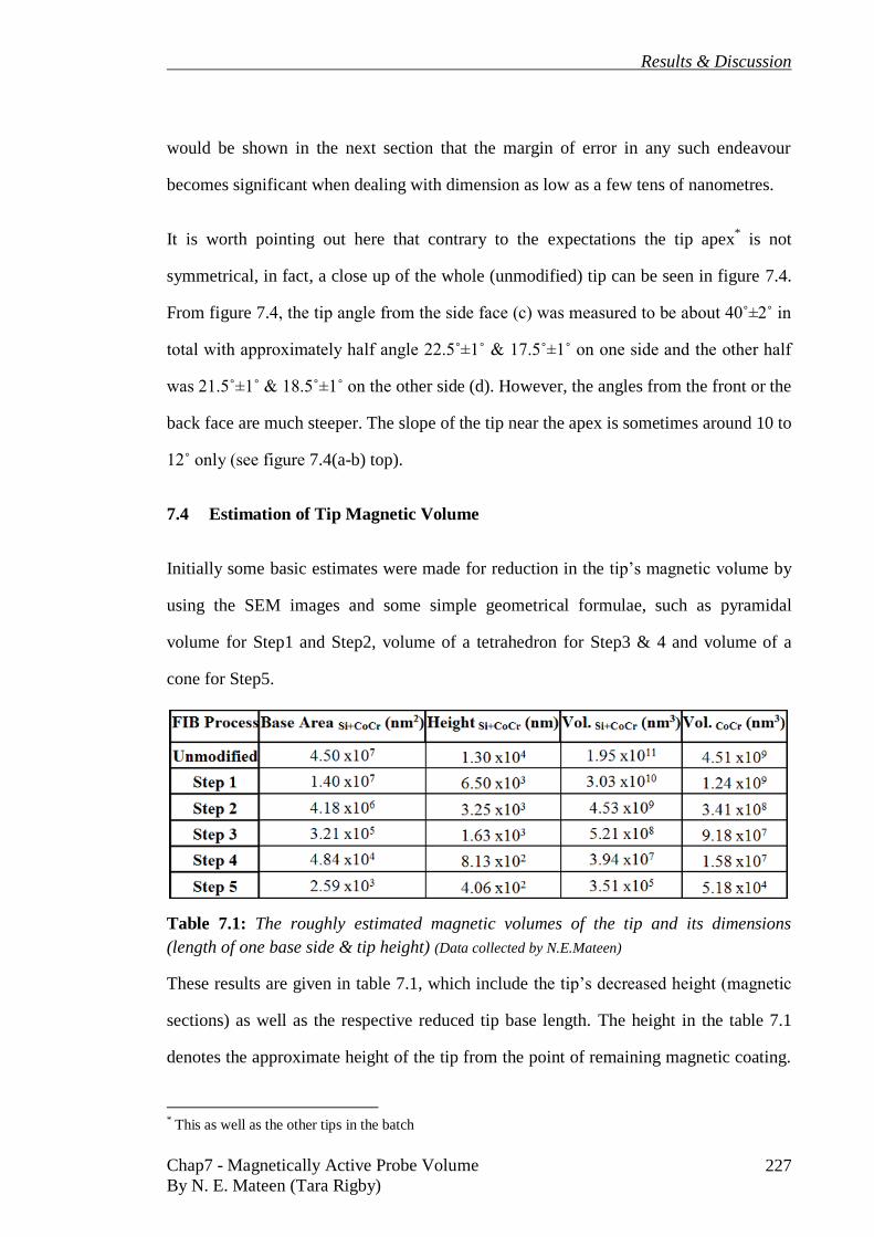
Results & Discussion
Chap7 - Magnetically Active Probe Volume
By N. E. Mateen (Tara Rigby) 227
would be shown in the next section that the margin of error in any such endeavour
becomes significant when dealing with dimension as low as a few tens of nanometres.
It is worth pointing out here that contrary to the expectations the tip apex* is not
symmetrical, in fact, a close up of the whole (unmodified) tip can be seen in figure 7.4.
From figure 7.4, the tip angle from the side face (c) was measured to be about 40˚±2˚ in
total with approximately half angle 22.5˚±1˚ & 17.5˚±1˚ on one side and the other half
was 21.5˚±1˚ & 18.5˚±1˚ on the other side (d). However, the angles from the front or the
back face are much steeper. The slope of the tip near the apex is sometimes around 10 to
12˚ only (see figure 7.4(a-b) top).
7.4 Estimation of Tip Magnetic Volume
Initially some basic estimates were made for reduction in the tip’s magnetic volume by
using the SEM images and some simple geometrical formulae, such as pyramidal
volume for Step1 and Step2, volume of a tetrahedron for Step3 & 4 and volume of a
cone for Step5.
Table 7.1: The roughly estimated magnetic volumes of the tip and its dimensions
(length of one base side & tip height) (Data collected by N.E.Mateen)
These results are given in table 7.1, which include the tip’s decreased height (magnetic
sections) as well as the respective reduced tip base length. The height in the table 7.1
denotes the approximate height of the tip from the point of remaining magnetic coating.
* This as well as the other tips in the batch

Results & Discussion
Chap7 - Magnetically Active Probe Volume
By N. E. Mateen (Tara Rigby) 228
Firstly, the volume of the total tip was determined and then the volume of the Si
(without the magnetic coating) was estimated. The difference between the two values
was the remainder magnetic volume of the tip calculated for each step.
The remaining magnetic volume of the tip after Step5 could also be estimated by using
the SEM images of the tip apex, (side view) shown magnified in figure 7.5(a) and (b).
The tip apex was approximated to be 30nm in diameter. If the thickness of the CoCr
magnetic coating was about 60nm and the diameter of the tip at the end of the last step,
(Step5) was around 30nm then the volume of remainder of the magnetic material would
approximately be the volume of a cylinder, on the assumption that after FIB the tip apex
had an almost circular area. Depending on how the angles were selected for the tip apex,
the vertical height estimation might vary considerably. With these assumptions, the
volume of the magnetic material after Step5 was calculated to be where the
radius is and is the vertical thickness of magnetic material at the apex. Therefore,
volume of the approximate cylindrical magnetic particle would be
2.44x10⁵±3.7x10
4nm
3 for half angle of 10˚±1˚ at the apex at the vertical height of
346±52nm. This value is bigger than the magnetic volume calculated in table
7.1(Step5). However, if the half angle was taken to be 17.5˚±1˚ near the apex, the
cylindrical height estimation would be ~200±21nm giving the volume to be
1.41x10⁵±1.5x10
4nm
3.
Taking anisotropy and exchange constants and saturation magnetisation for CoCr from
the literature (K=3x10⁵J/m
3, A=10
-11J/m, Ms=4x10
5A/m {1}) the critical radius
* for
single domain particle behaviour was estimated {2} to be 80 nm by using the formula
below;
√ ⁄ (7.1)
*is the radius beyond which the particle will no longer be able to retain its single domain state and would
become multidomain

Results & Discussion
Chap7 - Magnetically Active Probe Volume
By N. E. Mateen (Tara Rigby) 229
According to this argument, a particle whose radius might be equivalent to, or smaller
than, this critical value should have to be a single domain, and only those particulate
structures, whose radius might be greater than the value given above, would possess
multidomain configuration. Therefore, the CoCr tip, milled to Step5, possessed at its
apex a magnetic particle (conical shaped or might be construed as cylindrical at best)
whose radius was reduced below the critical radius. Thus, it may be assumed that Step5
of FIB milling resulted in a volume of magnetic material on the apex exhibiting single
domain in behaviour. As shown above, the radius of the tip calculated, using these
parameters was approximately 80nm or less, which seemed to be supported by SEM
image of the modified tip shown in figure 7.5(b). To test if the Step4 equivalent
spherical radius lay within the critical range of the value for a single domain particle,
then using the values from table 7.1, the equivalent spherical radius came out to be
~156nm, which is almost twice as big, thus suggesting the apparent presence of
multidomain structure in the magnetic coating in Step4.
7.5 Modelled Estimation of Tip’s Magnetic Volume
The magnetic volumes calculated in table 7.1 were estimated from basic geometrical
formulae, using the scaled data from SEM images. In order to verify the accuracy of the
Fig. 7.5: (a) SEM image of the CoCr tip milled after the fifth and final step. (b) x10
magnification of the tip framed in (a) (Images captured by N.E.Mateen)

Results & Discussion
Chap7 - Magnetically Active Probe Volume
By N. E. Mateen (Tara Rigby) 230
above results the tip’s magnetic volume was estimated with the help of modelling
software AutoCAD. Provided initial parameters are fed into the software correctly, a
higher degree of accuracy is expected from the modelled tip reduction simulations.
To set up the model the spatial coordinates from the SEM data were collected carefully,
before and after each milling step at various angles in addition to the five major
positions of the top, outer, inner, right and left faces with respect to the cantilever of the
tip. In order to get the tip’s physical structure as accurate as possible, especially near the
apex region, the SEM images at various magnifications (typically between x6K and
x12K) were used. The zoom up and capture process continued, until the images were no
longer in focus, and image distortion began to set in.
Once the data was taken, the model with the help of AutoCAD software was set up for
the unmodified tip. At the base of the tip, a parameter (p1) was drawn in AutoCAD
from the SEM images* taken from the top view. At that point, the magnetic coating
thickness covering the entire tip, as well as the cantilever was unknown. The first set of
data became available after the tip was milled to achieve what is referred to in this
dissertation as Step1. The estimation of the coating thickness was then made (section
7.3). With an estimate of the average magnetic coating thickness on the tip, the
respective values along the x-axis were fed into the AutoCAD. These values helped
make a second boundary parameter (p2) inside that of the first parameter (p1) thus
making a second frame† inside the first frame. Two-dimensional frames were
constructed at positions where the original tip was FIB milled in an attempt to keep the
appropriate thickness variation along the x-axis. After the outer frames were completed,
they were then converted into solid objects. By deducting the inner solid (Si layer) from
* Pixel to scale conversion
† In AutoCAD initially line frames were built representing outer perimeters of the tip at various heights
(see chapter 5 for details)

Results & Discussion
Chap7 - Magnetically Active Probe Volume
By N. E. Mateen (Tara Rigby) 231
the outer solid (Si plus magnetic layer) leaves a thin shell, which is essentially the
magnetic coating. The data extracted from the model is given in the table 7.2.
In table 7.2, the volume of the CoCr tip for Step5 estimated by the AutoCAD software
was 2.47x10⁵nm
3 with the potential error of about ±6.89x10
4nm
3, making the volume at
the apex range between 1.78x10⁵nm
3 and 3.16x10
5nm
3, which could be compared to the
values 1.41x10⁵±1.5x10
4nm
3 or 2.44x10
5±3.7x10
4nm
3 stated in the previous section.
CoCr Tip Perimeter
(nm) Base Area (nm
2)
Si Vol.
(nm3)
CoCr
Height
(est. base
to apex)
(nm)
CoCr Vol.
(nm3)
Error
SEM
Image
Pixel
Coord.
(nm)
SEM
Spot
Size
(nm)
Total
(nm)
Unmod. 2.52x10⁴ 2.71x10
7 9.52x10
10 1.02x10
4 7.28x10
9 ±140 ±1 ±141
Step1 1.36x10⁴ 1.14x10
7 6.39x10
10 7.51x10
3 3.23x10
9 ±150 ±1 ±151
Step2 7.30x10³ 3.28x10
6 2.48x10
10 1.75x10
3 9.46x10
8 ±179 ±1 ±180
Step3 8.91x10² 3.80x10
4 3.69x10
8 8.01x10
2 1.28x10
7 ±29 ±1 ±30
Step4 2.34x10² 3.74x10
3 4.03x10
7 4.79x10
2 1.43x10
6 ±30 ±1 ±31
Step5 1.01x10² 7.29x10
2 7.21x10
6 3.88x10
2 2.47x10
5 ±40 ±1 ±41
Table 7.2: The magnetic volume of the apex with the area and perimeter of the base of
the tip as calculated using AutoCAD. The table also provided the probable errors of
each coordinate determined from SEM graphs (pixel resolution & clarity) and the
estimated error in the CoCr thickness (Data collected by N.E.Mateen)
The errors in table 7.2 were calculated using scale bars with pixel counts for each SEM
image, as the simulation precision was dependent on them. In estimating the tip volume,
both the geometrical method and the AutoCAD simulation had their respective pros and
cons. In the direct approach, there is always an ambiguity regarding the height value of
the tip volume or radius at its apex. However, in the simulated method no such problem
arose. In fact, the estimated height, especially at the apex, is in the similar range
~388±41nm as was estimated for the magnetic layer coating on the cantilever
~327±3nm. These similarities lead to the generalisation that the overall coating
thickness on the cantilever and that on the tip apex have similar values but not the same.
As the FIB milling was done from the top of the tip, it cut the area/tip facets straight

Results & Discussion
Chap7 - Magnetically Active Probe Volume
By N. E. Mateen (Tara Rigby) 232
down making the sides significantly varied in height with respect to the tip base.
Therefore, the estimated tip heights were averaged for each step milled. Figure 7.6
shows the irregular milled edges of the tip.
Now, if the volume of Step5 simulated by AutoCAD is converted into a spherical
volume to compare with a single domain particle size estimated in equation 7.1
approximately 80nm. The conversion of the simulated cylindrical volume to a spherical
particle size renders the radius of ~39±4nm.
CoCr Tip CoCr Vol.
(nm3)
Eq. Sph. Radius
(nm)
Unmodified 7.28x10⁹±2.80x10
6 1202±<1
Step1 3.23x10⁹±3.44x10
6 917±<1
Step2 9.46x10⁸±5.83x10
6 609±1
Step3 1.28x10⁷±2.70x10
4 145±<1
Step4 1.43x10⁶±2.98x10
4 70±1
Step5 2.47x10⁵±6.89x10
4 39±4
Table 7.3: Spherical volume approximation for the CoCr volumes for each step after
FIB milling (Data collected by N.E.Mateen)
Table 7.3 shows the volumes of the magnetic layer after each step, along with their
estimated errors, and their equivalent spherical volumes. It suggests that the critical
volume for both Step4 and Step5 should be below the predicted spherical volume, thus
suggesting a probable single domain state in both of them.
However, considering the final shape of the tip after Step5 milling it is likely that there
is some form of domain formation at the very apex of the tip. Even so, the overall
behaviour of such a tip could be taken as that of an extended dipole {3, 4}. Although not
to the extent of potential dipolar tips achieved by the CNTs it would not be farfetched to
state that the tip behaviour should be much more stable compared to its unmodified
state.
AutoCAD computations were the best way to know how and what portions of the
magnetic coated layers were milled and how, as a result, the intermediate milling steps

Results & Discussion
Chap7 - Magnetically Active Probe Volume
By N. E. Mateen (Tara Rigby) 233
played a role in understanding the behaviour of the tip. As it was vital to identify how
the reduction in magnetic material affects the tip-sample interaction.
(a) Unmodified CoCr tip (b) CoCr shell of the unmodified tip
(c) Step1 (d) Magnetic coating in Step1
(e) Step2 (f) Magnetic coating in Step2
Fig. 7.6: The successive FIB tip steps (a, c, e, g, i, & k) show the magnetic tip with its
base (CoCr and Si) and (b, d, f, h, j, & l) show the magnetic shell of the tip (CoCr) only.
(h, j, & l) show tip at 7 times magnification (Images made by N.E.Mateen)

Results & Discussion
Chap7 - Magnetically Active Probe Volume
By N. E. Mateen (Tara Rigby) 234
(g) Step3 (h) Magnetic coating in Step3
(i) Step4 (j) Magnetic coating in Step4
(k) Step5 (l) Magnetic coating in Step5
Fig. 7.6: The successive FIB tip steps (a, c, e, g, i, & k) show the magnetic tip with its
base (CoCr and Si) and (b, d, f, h, j, & l) show the magnetic shell of the tip (CoCr) only.
(h, j, & l) show tip at 7 times magnification (Images made by N.E.Mateen)
Generally, simulations done regarding the magnetic properties and behaviour of the tip
are simplistic (see chapter 4, figure 4.8). It would have been interesting to observe the

Results & Discussion
Chap7 - Magnetically Active Probe Volume
By N. E. Mateen (Tara Rigby) 235
results of magnetic simulations by using the modelled tip (shape and structure)
however, that task is for the future and not investigated during the course of this work.
Figure 7.6 shows a set of simulated images with and without the Si base under the
magnetic coated layer of the tip. The wire structures were shown under the tip to bring
the relative tip-sample size and distance in perspective. The ratios and dimension of the
tip with respect to the wire sample were all modelled to scale. The modelled wires were
1µm in width and 70nm thick having a gap of 2µm between them (as mentioned in
chapter 6).
The tip apex was 150nm higher than the wires and 220nm higher than substrate under
the wires, set at height zero, in the model. The tip base at cantilever was at ~10440nm in
the model, therefore the total tip height was ~10220nm (10.22µm). The estimation of tip
height was accurate, as typically the tip heights vary between 8 to 13 micrometres.
Furthermore, figure 7.6 demonstrates that the unmodified tip size is massive compared
to sample structure (current wires). Conversely, by Step5, the reduction in dimensions
of the tip became significant once more compared to the sample features. Figure 7.6(l)
also suggests that the remaining magnetic material on the apex is approximately a
cylindrical/needle shape.
Figure 7.7 shows the same FIB-Tip reduction from a side view, where (a) shows the
standard tip side, (b) representing Step1 down to (f) showing the needle like remainder
of the tip apex. The Si base in this case is represented in blue to show the distinction
between the magnetic and the non-magnetic layer. Figure 7.7(f) indicates that the aspect
ratio of the remaining tip length vs. its diameter is about 13:1 for Step5.
Thus, by Step5, due to the shape, it could be speculated that there was a strong tendency
of the tip behaving like an ‘extended dipolar tip’ {3, 4}. If this were true then the tip at
Step5 should be expected to behave like a highly stable tip, which would not be

Results & Discussion
Chap7 - Magnetically Active Probe Volume
By N. E. Mateen (Tara Rigby) 236
influenced by the strong fields emanating from the samples. Thus, making Step5, a tip
universally suited for imaging both very soft and very hard samples. Suited for soft
samples because the magnetic coating left on the tip, inadvertently making the volume*
very small would have relatively weak fields as not to influence the stray field gradients
of the samples observed.
(a) Unmodified (b) Step1 (c) Step2
(d) Step3 (e) Step4 (f) Step5
Fig. 7.7: Side view of the AutoCAD representing successive stages of CoCr coated tip
after each milling step. The images focus on the magnetic part tips respective shape.
The blue represents the Si base of the tip (Images made by N.E.Mateen)
The suitability for the observation of magnetically hard samples would arise from the
remaining aspect ratio of the needle like tip structure. As the tip should be normally
magnetised along its long axis, it would not be easily influenced by an external field
gradient.
* Effective or otherwise

Results & Discussion
Chap7 - Magnetically Active Probe Volume
By N. E. Mateen (Tara Rigby) 237
Fig. 7.8: SEM micrographs showing the outer (a, c, e, & g) and the right (b, d, f, & h)
facet of the tip from Step2 to Step5.(a’-h’) show the corresponding magnified images of
(a-h) respectively (Images captured by N.E.Mateen)

Results & Discussion
Chap7 - Magnetically Active Probe Volume
By N. E. Mateen (Tara Rigby) 238
Confirmation of whether or not the tip apex was significantly altered came from further
SEM images captured at various positions with higher magnification settings as shown
in figure 7.8. The outer (a, c, e, & g) and the right (b, d, f, & h) facets of the tip from
Step2 to Step5 having the SEM magnification of x17000 with the working distance of
20.2mm are represented in figure 7.8. The SEM micrographs a’-h’ shown in the top
right hand corner of a-h represent further magnification x85000 to show clearly the area
of interest at the apex. The SEM images of Step0 and Step1 are not shown here because
the apex was completely intact until the Step3 as can be seen in figure 7.8 (a-d) and (a’-
d’) respectively. For convenience, at the top right hand corner of each SEM micrograph
in figure 7.8(a’-h’) are the corresponding schematic representations of tip orientation
with respect to the cantilever. From figure 7.8g’ and h’ although the apex had
significantly reduced sides making its appearance more needle like, no reduction of
height was observed at the top of the tip apex. Furthermore, no noticeable change in the
tip height from the base was observed.
From figure 7.7(e) and 7.9(a-e), the aspect ratio for Step4 can be estimated at around
~6:1. For other milled steps, the ratios are rather difficult to estimate due to the complex
structure of the magnetic layer on the Si base as shown in figure 7.6. However, the
estimated height of the tip after each step is given in table 7.2.
Figure 7.9(a-e) shows the tip after Step4 and (f-j) represent the remaining tip at Step5.
In figure 7.9(a) and (f) the tip stage was tilted to an angle of 60˚ from a normal stage
position of 45˚ for a clearer SEM image of the apex. The tip’s outer, inner, left and right
facets are shown in the SEM images in figure 7.9(b-e) and (g-j), respectively. The SEM
images in figure 7.9 not only showed that apex remained intact for the most part but that
sufficient material reduction also took place after Step4.

Results & Discussion
Chap7 - Magnetically Active Probe Volume
By N. E. Mateen (Tara Rigby) 239
As can be seen form figure 7.9 the tapering near the tip apex in Step5 may be indicative
of a slightly larger volume of tip material at the apex than estimated by the AutoCAD
software (see table 7.2)
Fig. 7.9: SEM images of Step4 CoCr tip (a-e) with their corresponding images
captured at the Step5 (f-j) having the same tip orientation each time. Bottom left hand
corner of images in (a-e) are the schematics of the tip orientation (Images captured by
N.E.Mateen)
7.6 Effect of tip reduction on standard magnetic sample
After each milling step, the tip’s integrity was confirmed with the help of the standard
magnetic tape sample. This standard test sample has periods of about 200nm. Once the
tip was milled and then used to observe the magnetic pattern, it was noted that the
magnetic pattern appeared to have better resolution with a slight increase in the image
contrast, as seen in figure 7.10(b). Similarly, in figure 7.10(c) when the tip edges were
further reduced (Step2) finer magnetic details appeared to come into focus.

Results & Discussion
Chap7 - Magnetically Active Probe Volume
By N. E. Mateen (Tara Rigby) 240
Nevertheless, as the tip was milled further, figure 7.10(d) Step3, the magnetic image
loses its previously improved definition from Step2, while still maintaining the image
brightness.
Further tip milling in Step4 (figure
7.10(e)) the magnetic image possibly
improves slightly compared to Step3 but
the image seemed to have lost its clarity
compared to (c). Here it could be
speculated that the magnetic signal might
have become weaker due to a significant
amount of the tip material being milled
away. This reduction in the physical
dimensions has already been mentioned
(see figure 7.7 & 7.8). The last milling,
Step5, produced an MFM image with an
overall weak image contrast, nevertheless
the remaining magnetic volume was
significantly reduced thus inclusion of
signal to noise ratio in the image.
The reason for the increased noise in the MFM image for Step5 could be two fold. One
cause might simply be the significant decrease of magnetic volume producing a weaker
signal. Alternatively, some level of Ga+ ion implantations during the tip edge trimming
might have instigated the noise. It could, quite possibly, be an amalgamation of both,
the signal weakening, and ion implantation on a nano-scaled volume. Irrespective of the
weakness and noise in the signal, the MFM image did retain its integrity. The drawback
though was that it became difficult to reach a conclusive decision regarding the
Fig. 7.10: MFM of the standard magnetic
tape captured by using (a) original CoCr
tip (b) Step1, (c) Step2, (d) Step3, (e) Step4
and (f) Step5 respectively (Images captured
by N.E.Mateen)

Results & Discussion
Chap7 - Magnetically Active Probe Volume
By N. E. Mateen (Tara Rigby) 241
enhancement of the image resolution. Generally, the smaller the magnetic volume, with
a limited stray field range detection, the better the expected resolution of the magnetic
features. Of course, the material, its coating method and its anisotropy also play a
significant contribution in the improvement of the image resolution {5-8}. In figure
7.10, it is also possible that due to the reduction in the magnetic volume of the tip, the
magnetisation direction of the tip could have started to be influenced by the stray field
gradients of the sample.
A closer inspection of the magnified MFM images of the magnetic tape, given in figure
7.11, reveal the effects of tip edge trimming on the resulting images. The MFM image
line scans show an improvement in the image definition and clarity in Step1 and Step2
shown in figure 7.11(c & e) with the corresponding line scans in 7.11(d & f). In Step3,
the magnetic image became hazy like the images captured by the unmodified tip. Figure
7.11(g, h, and their scans i & j) seem to have lost their focus. Beyond Step2 if there was
improvement in image definition, the noise and weak signal made it difficult to assess
the image integrity conclusively, further confirming the results shown in figure 7.10.
From the MFM line scans in figure 7.11, as the tip volume was reduced to Step2, it
could be speculated that the resulting tip moment was ideally suited to the stray
magnetic field gradients of the sample, consequently producing high definition images.
In addition to the reduction of the magnetic volume from the tip edges, the resulting
magnetisation direction due to the remaining shape might primarily cause image
definition enhancement. Furthermore, it could be insinuated that the reduced magnetic
volume in Step2 approaches the tip’s effective volume, which is the volume close to the
apex that provides field sensitivity.
This study suggested that finding the effective magnetic volume of a material coated on
a Si tip, for any image formation, is difficult to predict accurately. The only certainty
that tip trimming provided was to ensure that the effective magnetic material volume in

Results & Discussion
Chap7 - Magnetically Active Probe Volume
By N. E. Mateen (Tara Rigby) 242
each step was restricted by the physical volume of the tip coating.
Thus, as the tip’s physical volume was reduced, the effective volume was either
(a) Unmodified CoCr tip (b)
(c) Step1 CoCr tip (d)
(e) Step2 CoCr tip (f)
(g) Step3 CoCr tip (h)
(i) Step4 CoCr tip (j)
(k) Step5 CoCr tip (l)
Fig. 7.11: MFM images of the magnetic tape, with their corresponding pixel line scans,
after each step of the FIB milling process (Images captured and graphs made by N.E.Mateen)

Results & Discussion
Chap7 - Magnetically Active Probe Volume
By N. E. Mateen (Tara Rigby) 243
proportionately limited or remained unaffected for a particular sample’s field gradients.
As the field gradient values for a given height above the sample vary from point to point
in space, it is plausible that the effective volume increases or decreases according to the
sample stray field at that point in space. In case the effective volume was reduced by
limited trimming, it would only be influenced by limited stray fields of the sample
contrary to when it might have been significantly affected by the larger variations in the
stray fields before trimming.
Of course, it is not as simple as estimating the effective volume and finding the best-
resolved and highly defined magnetic image. The magnitude and direction of
magnetisation (of the tip-coated material) plays an important role in the formation of a
high definition image. In addition to the tip’s physical volume, its effective magnetic
volume*, the motion of the tip and changes in the field gradients from the sample all
combine to produce an image that comprises a complex combination of processes.
However, it is clearly crucial to the interpretation and quantification to know the volume
of the magnetically active material on the tip. However, the effective volume is very
difficult to measure and it might only be successfully estimated with the combination of
magnetic simulations and experiment.
Figure 7.12 shows the peak height and the FWHM† of the ridge approximately located
at y=2.75µm in figure 7.11. Gaussian fitting was done in Origin software on the data
represented in each of the graphs in figure 7.11(b, d, f, h & j) to obtain the FWHM and
peak height values. The lower the FWHM value the better the image definition‡, the
higher the peak value§ the better the image contrast.
* Generally construed as the magnetic volume which actively contributes towards the image formation
and which might be only a small portion of the entire magnetic volume of the tip † Abbreviation for full width half maximum
‡ Which some may call image resolution
§ Which is the different between the maximum and the minimum of the phase shift data

Results & Discussion
Chap7 - Magnetically Active Probe Volume
By N. E. Mateen (Tara Rigby) 244
Fig. 7.12: Shows the full width half maximum (blue) and the peak height value (green)
of the central ridge at y~2.75µm (shown in figure 7.11(b, d, f, h & j)) for each step of
the CoCr tip after FIB milling (Graph made by N.E.Mateen)
Figure 7.12, suggests that the image definition and the contrast improved until Step2,
but then there was a sudden reduction of both the contrast and definition for Step3. It
was not clear why this was. It was not because of tip contamination as no contamination
was observed in the SEM. Alternatively, it could be a slight change in the magnetisation
in the tip. Whatever happened between Step2 and Step3, one thing is certain that the
definition as well as the contrast did slightly improve by Step5 again. However, the
change was not as marked as it was when the tip was milled to Step1 or Step2.
Whatever the physical magnetic volume left at the tip with its shape (see figure 7.6-7.8)
the MFM image could be said to be optimised at Step2. Before and after this milling
step the volume, which inadvertently affects the moment of the tip, was either too large
or too small to observe the magnetic tape sample optimally. Yet the volume of the tip
at/near Step2 may not be optimum for any other sample observed. It might be prudent to
infer that in order to optimise the tip-sample interaction effectively, the tip material,
structures size i.e. volume and shape as well as its magnetisation must be compatible to
the sample’s stray field gradients.

Results & Discussion
Chap7 - Magnetically Active Probe Volume
By N. E. Mateen (Tara Rigby) 245
7.7 Estimation of tip moment
In chapters 6, the stray field gradients were modelled (with the help of MathCAD) for
the current carrying conductors and compared with the actual MFM data gathered using
various tips. Then the model was extended to predict the angle of tip magnetisation
direction with respect to the sample’s field gradients. In this section the stray field
gradient data extracted from the model was used in conjunction with the information
gathered from the experimental MFM data, to estimate parameters like moment of the
tip, as the moment of the tip is the volume integral of the tip’s magnetisation.
7.7.1 Evaluation of the constant Kp for various tips
Table 7.4 shows the tip parameters extracted from the auto-tuning of the tips before they
were set up for the MFM measurements along with their estimated physical magnetic
volumes. The auto-tune parameters were used for the estimation of the Q/k values
because these values are generated directly by the tip whatever shape size it may have.
Tip(s) f0
kHz
fd
kHz
Δf0
kHz Q
k
N/m
Kp=Q/k
m/N
Vmag
m3
|Ms|
A/m
CoCr 56.80 56.72 0.08 704.57 0.26 2746.84 7.28x10⁻¹⁸
4.00x10⁵
{1}
Step1 57.91 57.82 0.09 632.63 0.27 2326.71 3.23x10⁻¹⁸
4.00x10⁵
Step2 58.43 58.33 0.10 597.64 0.28 2140.53 9.46x10⁻¹⁹
4.00x10⁵
Step3 58.57 58.47 0.11 551.56 0.28 1960.74 1.28x10⁻²⁰
4.00x10⁵
Step4 58.60 58.50 0.10 567.39 0.28 2014.16 1.43x10⁻²¹
4.00x10⁵
Step5 58.73 58.63 0.11 551.53 0.28 1944.06 2.47x10⁻²²
4.00x10⁵
Metglas® 70.17 70.07 0.09 773.45 0.48 1599.36 1.88x10
-18 1.17x10
6{9}
Ni-LM 61.32 61.25 0.07 837.86 0.32 2595.62 2.30x10⁻¹⁸
7.00x10⁵{10}
Table 7.4: Data shows the parameters required for CoCr (Unmod-Step5),
Metglas2605SC ( ) and low moment Ni tips. The magnetic volume data
for the CoCr tip and its milled steps was calculated using AutoCAD and estimated for
Metglas®
tip of 100nm vertical thickness and LM-Ni tip with only one face magnetically
coated. The last column represents the probable saturation magnetisation of such tips
from literature (Data collected by N.E.Mateen)
In table 7.4 f0 represents the values of the true frequency of the cantilever, fd shows the
drive frequency and ∆f0 is the change in the true frequency. These values are used in the

Results & Discussion
Chap7 - Magnetically Active Probe Volume
By N. E. Mateen (Tara Rigby) 246
calculation of the quality factor Q. The value of the spring constant k was generated
during the auto-tuning of the tip cantilever. Vmag gave the values of the physical volume
of the magnetic material coated on the tip whereas the values of |Ms|* were gathered
from the literature {1, 9, 10} for the required materials.
Note that the spring constant for the same tip was almost unchanged but shows
variations for different coated tips. However, the Q values however change, hence the
proportionality constant Kp changes as well. A downward trend can be seen as the tip
was trimmed from its original pyramidal shape. Although the variation in the Kp values
seem erratic but overall the values decreased from standard (unmodified) tip to trimmed
Step5. Even though the value of Kp is considered to be constant for one tip it is also
believed that once the tip is in the presence of any field† these values may effectively
change {11}. How much or how little this change in values is difficult to estimate,
however, any change would be represented in the overall image formation, which may
lead to an increase in the error values in the results.
Tip(s) Vmag
m3
|Ms|
A/m
|mtip
|
Am2
CoCr 7.28x10⁻¹⁸
4.00x10⁵
{1} 2.91 x10⁻¹²
Step5 2.47x10⁻²²
4.00x10⁵ 9.88 x10
-17
Metglas® 1.88x10
-18 1.17x10
6{9} 2.20x10
-12
Table 7.5: A general estimation of the magnetic moment of the tip (Data collected by
N.E.Mateen)
An estimation of the tip moment could be made by using the estimated tip volume and
the |Ms| values see table 7.5. Assuming the tip edges were not trimmed the by using the
SEM images given in figure 7.8 and 7.9 along with estimation of the remaining tip
height from AutoCAD, the approximate apex volume would approximately be 7.31x10-
21±3.75x10
-21m
3. Therefore, for magnetisation used in table 7.5, the apex moment would
be about 2.92x10⁻¹⁵
±1.5x10⁻¹⁵
Am2. Due to large margin of error, this approximate at the
* It was unfortunate that the Ms for the tips used in this project could not be measured due to lack of time
and resources † Fields generated other than the tip itself, i.e. the samples stray fields in this case

Results & Discussion
Chap7 - Magnetically Active Probe Volume
By N. E. Mateen (Tara Rigby) 247
apex moment value, would lie somewhere less than the estimated values of Step3 but
greater than Step4. Thus, this apex moment value would be much smaller than that
assessed for the CoCr tip given in table 7.5. As the main tip-sample interaction is
usually assumed at the tip apex, therefore it is also widely believed that the effective tip
volume lies at the apex.
7.7.2 Estimation of tip moment by using Model data in conjunction with
Experimental data
In chapter 6, the mathematical model was improved to incorporate both the y and the z
components to better conform to and interpret the experimental data. However, the
model (as mentioned earlier) does not predict anything about the tip itself. This lack of
information regarding the tip in the model could be used in a constructive manner if
used in conjunction with the experimental data. The experimental data has both signals
from the tip as well as the sample, i.e. the tip-sample interactive data. If the model only
represents the data from the sample at a given location in space, then anything that is
not part of the sample signal has to come from the tip. Using this information, the
unknown variables like the tip moment may be deduced successfully. Provided the tip’s
volume is known, which has already been estimated in section 7.4 and 7.5, the tip’s
magnetisation at a given point above the sample and/or its field may also be
successfully estimated. While predicting the tip’s magnetic parameters one must always
be wary that the tip might also detect forces other than the magnetic force (which are
not incorporated in the model).
In the literature {12, 13} the formula for the evaluation of the magnetic moment of the
tip is given as under;
( ⁄ ) (
⁄ ) (7.1)

Results & Discussion
Chap7 - Magnetically Active Probe Volume
By N. E. Mateen (Tara Rigby) 248
where represent the phase shift. The term 180/π was added to make the right hand
side of the equation equivalent to the left hand side of the formula {12}. is the
permeability of free space. The quantity is the proportionality constant equal
to the quality factor Q associated with the tip’s cantilever and k which is the spring
constant of the tip. The tip moment, equivalent to the product of tips remanent*
magnetisation and magnetic volume, ∫
. The term ⁄
represents the double derivative of the stay fields of the respective sample (see chapter
6).
In table 7.4, section 7.7.1, the value of Kp was extracted from the experimental tip data
from the auto-tune parameters. After updating the right hand side of the phase shift
formula by replacing the double derivative of the field from its y or z component to
appropriately incorporating the direction angle θ with the correct lift height (see chapter
6), the formula can be written as,
( ⁄ ) ( ⁄ ) (7.2)
Note that the extra negative sign {12-14} used in literature as the moment i.e.
magnetisation directional compensator, was dropped because the directional angle
incorporated to the (double derivative of the field) equation in chapter 6 automatically
compensates for it. Furthermore, note that the values of and in the above formula
come from the MFM experimental data and the stray field gradients (of current carrying
conductors) came from using the MathCAD modelling (chapter 6). Consequently, the
angle upon which the stray field gradient would be dependent on, the mtip
, would be true
for that angle (i.e. direction) only.
* Even though the tips were always magnetised before each study but it is realistic to assume that the tip’s
magnetisation is not at saturation while scanning but somewhere near its remanent state. Of course the
magnetic fields from the sample would affect the magnetisation of the tips i.e. tip-sample interactions and
may in some instances saturate the tip in one direction or another

Results & Discussion
Chap7 - Magnetically Active Probe Volume
By N. E. Mateen (Tara Rigby) 249
To simplify the problem, the experimental phase shift data was divided by the constants
(also obtained from the experimental data) then only the moment of tip and the stray
field gradient from the sample would be left to deal with. The equation then can be
written as
( ⁄ ) ⁄ ( ⁄ ) (7.3)
Rearranging the equation 7.3 the moment of the tips can be estimated
( ⁄ ) ( ⁄ )⁄ (7.4)
7.7.2.1 A method to extract MFM data for tip moment estimation
In order to extract valuable information from the formula given above it is important to
understand the methodology used for the data extraction, in the form of phase shift,
from the MFM images. Normally the phase shift is adjusted to a zero value so that it
is easier to observe the negative and positive tip response to the field gradients of the
sample. The zero value is set* to represent the central/midway grey of the MFM contrast
of black and white.
However, when the MFM image is captured†, it is a seemingly random set of coloured
pixel values. These pixel values are assigned values between 0 and 255 (8-bit colour
map)‡. Where zero generally represents the complete black pixel colour and 255
represents the completely white pixel colour§. However, for ‘section analysis’ the MFM
(using its proprietary software) repopulates the data and sets the mean value to zero
* Even in the software provided
† In *.tiff file format
‡ In case the colour depth is higher, then it is advisable to covert the data into 8 bit as this conversion
converts the image into basic grey scale and is much simpler to process. Besides no extra information
could be extracted from excessive colour depth as the number of data points are set. This is true when it
comes to assigning tangible values to the data points § In MFM, the dark colours generally represent the attractive forces and lighter colours are indicative of
repulsive forces

Results & Discussion
Chap7 - Magnetically Active Probe Volume
By N. E. Mateen (Tara Rigby) 250
phase shift*. To manipulate the data in any way for the purpose required, it first had to
be extracted from the original MFM images. This raw data generally needs further
processing to get the same information as shown by the MFM software. This data
extraction was performed using Origin software. Further processing, if required, could
easily be performed in either Origin or MS Excel. For example, phase adjustment to
zero degrees. Nonetheless, for the purpose of data extraction of the MFM phase shift
and in conjunction with the modelled values, no attempt was made to adjust the central
grey position†. Each additional image processing or manipulation step has some bearing
on the results; therefore, to keep it simplistic no data adjustment was done‡. The second
important reason for using the ‘raw’ (unadjusted) phase shift values was to extract the
true data from the images. Although it seemed convenient to compare various MFM
data sets by phase shift adjustment (to zero or some other value), but at the same time
by doing so the overall tip’s true response with respect to the sample might be
inadvertently lost. Good comparative data can be gathered from the phase shift adjusted
values but the truly ‘unique’ nature of the tip response might be lost during such
processing. Processing after the phase adjustment might be equally acceptable, but for
these investigations, raw phase shift data was used. An example of the use of raw data is
that one can observe the tip’s response in its truest of form relative to the overall
contrast of the image, for instance in the past researchers have seen an overall negative
(attractive) response in Metglas® coated tips of certain thickness {17-19}.
A straightforward method to extract the effective moment values from the experimental
MFM image data was to divide the MFM data by the modelled values of ⁄
(see equation 7.3 above). The only problem was the possibility of singularities,
* In degree units
† The phase shift adjustment and equating to zero grey scale was done in the previous chapters for
graphical representational purposes. This adjustment is a common practice throughout literature with few
exceptions {12, 13, 15, 16} ‡ For the estimation of the magnetic moment of the tip

Results & Discussion
Chap7 - Magnetically Active Probe Volume
By N. E. Mateen (Tara Rigby) 251
depending on the zero point value in the modelling data*. When the set of values (from
the double differential of the magnetic field) dropped to zero† and the MFM data was
divided by them, singularities were a real possibility. Any such anomalies were avoided
largely because the model used the same y increment values across the wire positions as
the experimental data. The main reason for doing this was to ensure that for every value
of ‘y’ in the experimental data there would be a corresponding value in the model data
so that the division process could take place efficiently.
The phase data for the CoCr, Step5 and Metglas® tips was set at 3˚ see chapter 6).
Therefore, the black 0 and white 255 image pixel values were assigned the phase data
values from 0˚ to 3˚ respectively‡. Figure 7.13 shows the experimental and the modelled
data as a function of distance y (similar to that of figure 6.12). However, here on the left
hand side the MFM values are represented in the form of raw phase shift data, converted
directly from the image pixel values to the phase shift values in degrees. Also
represented in the figure 7.13 is the scale for the MFM data after dividing it by the
constant§ values as stated in equation 7.3.
All the MFM data presented here was at least averaged over 21 scan lines at various
locations on the wire structures. The error bars represent the standard deviation in the
data collected. Note that in the case of Step5 due to the increase in the noise levels there
is an overall larger error. As mentioned earlier (chapter 6 & 7), the case for the noise
increment in Step5 was due to the physical reduction of magnetic volume and thus
weakening of the overall signal detection.
* If the MFM data was to be phase adjusted to zero the problem might have been doubled by the possible
0/0 anomaly, a purely mathematical problem. This scenario was avoided by using the raw phase shift data † Outside the vicinity of the current carrying conductors for y dominant component
‡ It should be noted that if the phase data range is not set appropriately, some crucial image information
might be truncated i.e. lost. This loss of information will occur if the phase shift values are larger than the
set parameter range of let’s say from 0˚ to 3˚. The MFM software in such a case would just show a
complete black and/or white pixel value. § taken from table 7.4 & 7.5

Results & Discussion
Chap7 - Magnetically Active Probe Volume
By N. E. Mateen (Tara Rigby) 252
Fig. 7.13: Shows the MFM data vs. the corresponding angular modelled data of (a)
Standard pyramidal CoCr tip, (b) Modified CoCr (Step5) (c) Metglas®
. The two scale
bars on the left hand side of the graph represent the raw phase shift values and the
phase shift values divided by the constant values (equation 7.3). Right hand side shows
the δ2Hyθ⁄δy
2. The angle used in the model to correspond to the CoCr tip data was
θ=15˚, for Step5 θ=5˚ and for Metglas®
it was θ=0˚ (Graphs made by N.E.Mateen)
On the right hand side are the values of the gradient ⁄ with the appropriate
angle fitted for each tip is shown (figure 7.13). For the CoCr tip data (figure 7.13 (a))

Results & Discussion
Chap7 - Magnetically Active Probe Volume
By N. E. Mateen (Tara Rigby) 253
the corresponding angle was θ=15˚, for Step5 θ=5˚ (figure 7.13 (b)) and for Metglas® it
was θ=0˚ (figure 7.13 (c)) respectively.
As there was no change in the setup of the current wire structures therefore these angles
were indicative of the tip’s angle of magnetisation. This variation in the tip
magnetisation angles could be due to various reasons, such as the position of the tips
when they were being magnetised on the magnetisation holder. Another reason might be
that the shape of the tips may force the magnetisation to stay at a certain angle position,
or in the case of strong sample fields, the angle of the tips may have inadvertently
readjusted themselves for most stable configuration under a given scenario.
Nevertheless, it is interesting that the direction of magnetisation for both the CoCr
(unmodified) and its modified Step5 tip is similar but not the same. The Metglas®
tip
shows almost slight to no angular change.
This variation in the tip magnetisation angles might also explain the discrepancy in the
values of tip moments for the CoCr tip compared to the Step5 tip given in table 7.5
compared to the signal strength shown in figure 7.13. Due to the angle of magnetisation
of CoCr tip, which was larger than that of Step5, there could be a decrease in the
magnitude in the CoCr tip in the dominant direction, which would explain why the
signal strength of Step5 tip is apparently greater than CoCr tip. Other reasons might
include the additional acquired stability of the Step5 tip as well as its direction of
magnetisation the due to trimming.
For the raw MFM data shown in figure 7.13, the CoCr (a) and the Metglas® (c) tips
showed an overall repulsive tendency whereas the Step5 (b) tip behaviour was that of
neutrality or possibly slightly attractive. In other words, the tip’s behaviour with respect
to the background contrast showed the overall tip’s tendency towards an attractive or
repulsive behaviour. However, whether tendency has any effect on the phase shift
sensitivity of the tip is another matter, which needs further exploration. Irrespective of

Results & Discussion
Chap7 - Magnetically Active Probe Volume
By N. E. Mateen (Tara Rigby) 254
where the phase shift base line value lies relative to the overall image contrast, the
beginning values and the end values of each scan line* were not the same, which ideally
should have been the same as represented in the model. Yet, for all tips used in this
study, a change was observed in the base line contrast to either a higher or a lower
value† relative to the initial value at the beginning of the scan. Therefore, it was quite
difficult to have a well-defined base line to compare to other phase shift changes.
7.7.2.2 Variation in estimated tip moment for different tips
Figure 7.14(a) shows the variations in the estimated tip moments, mtip
, of the CoCr,
Step5, and that of the Metglas® tip along the entire scan length ‘y’. Figure 7.14(b) gives
the same data focused on the moment variations at, and near, the wire structures. The
dark yellow represents the unmodified pyramidal CoCr tip, the blue represents the Step5
tip and the dark red shows the behaviour of the Metglas® tip over the length of the scan
in (a) and on top of the wires in (b).
It seems that the tips’ experience sharp transitions at certain points during the scan.
These transitions occur at the beginning and end of each wire and approximately at the
centre of the two wire structures i.e. 2μm. In cases where the tip experiences both the y
as well as the z components involved i.e. θ≠0˚, the transition positions were slightly
shifted. For the CoCr tip one such significant transition occurred at approximately
y=2.19μm, similarly at y=2.06μm for Step5 but y=2.00μm for Metglas® tip as θ=0˚. It
seems that with the increase in the angle these transitional peaks tend to shift away from
the central position between the wires and towards the wire themselves.
In chapter 6 it was mentioned that the exact central position between the wires (y=2µm)
was not taken into account as the expected value for the y component at that position
theoretically goes to zero. However, it was observed that although it is expected to go to
* From left to right
† Depending on the tip’s behaviour over the respective wire structure

Results & Discussion
Chap7 - Magnetically Active Probe Volume
By N. E. Mateen (Tara Rigby) 255
zero the value did not. In figure 7.14 the tip moment showed a sharp increase or
decrease in its magnitude and direction but does not go to zero or show a singularity, as
might be theoretically expected.
Fig. 7.14: (a) Shows the estimated tip moment variations along the entire length of the
scan y by using equation 7.4 for all three tips whereas (b) illustrates the same graph
with emphasis to the tip behaviour on top of the wire structures. The dark yellow circles
represent the unmodified pyramidal CoCr tip, the blue diamond represents the Step5 tip
and the dark red shows the behavioural trend of the Metglas®
tip (Graphs made by
N.E.Mateen)
7.7.2.3 Estimated tip moment response for various heights at arbitrary y positions
Similar tip moment data to that of figure 7.14 was generated for the CoCr unmodified
(Step0), Step5 and Metglas® tip for each lift height of 20, 50, 100 and 150nm (see figure
6.13, chapter 6).

Results & Discussion
Chap7 - Magnetically Active Probe Volume
By N. E. Mateen (Tara Rigby) 256
y,
(µm
) Lift
Height,
(nm)
mtip
(Am2) - avg. of 21 lines
CoCr S.D. (±) Step 5 S.D. (±) Metglas
S.D. (±)
(10-17
) (10-17
) (10-17
) 1.3
150 -4.82 0.14 -3.66 0.55 -6.04 0.74
100 -4.29 0.11 -6.57 0.39 -5.28 0.53
50 -4.68 0.13 -8.35 1.00 -3.92 0.68
20 -6.41 0.30 -16.10 1.03 -4.72 0.32
1.5
150 -13.90 0.46 -12.00 1.80 -24.90 2.44
100 -14.10 0.36 -26.00 1.55 -28.80 1.99
50 -17.30 0.53 -35.70 3.27 -36.80 2.07
20 -23.50 0.90 -75.10 5.24 -71.70 6.09
1.7
150 -32.90 1.08 -33.60 4.10 -79.80 7.09
100 -34.90 0.99 -72.10 4.12 -96.70 5.81
50 -41.20 1.05 -105.00 7.58 -154.00 8.05
20 -54.40 2.50 -217.00 12.70 -324.00 21.10
Table 7.6: Shows the estimated values of tip moment for CoCr, Step 5 and Metglas®
tips at y positions of 1.3, 1.5 and 1.7µm. The values are representative of an average of
about 21 scan lines along with their corresponding standard deviation errors (Data
produced by N.E.Mateen)
Table 7.6 (which is similar to table 6.4) shows the tip moment values for the CoCr,
Step5 and Metglas® tips, at three arbitrary y positions, y=1.3, 1.5 and 1.7µm, at lift
heights in the range 20-150nm. The tip moment values for Step5 were very close (or
slightly greater) that those of the unmodified CoCr and Metglas®
tip(s), even though
Step5 has a much-reduced tip volume compared to the CoCr and Metglas® tips. A
reduced tip volume should imply a relatively reduced tip moment or net magnetisation
(see table 7.5). However, from the graphs shown in figure 7.13, the signal strength was
for CoCr was the weaker compared to Step5, which might be due to its magnetisation
orientation in a certain direction that in turn would affect the magnitude of the tip
magnetisation (see chapter 6).
The increase in signal for Step5 could be due to the shape change of the tip. The
orientation of the tip magnetisation could have increased the magnitude of the
magnetisation for the component, which was more sensitive to the detection of stray
field gradients. It must be noted that a slight change in the direction of the tip’s
magnetisation angle could be enough to bring about a major change in the scan data

Results & Discussion
Chap7 - Magnetically Active Probe Volume
By N. E. Mateen (Tara Rigby) 257
(figure 7.13(b)). If anything, the sharp change in the phase shift values of Step5 at the
top of wire edges indicates a directionally* defined tip. However, in case of current
structures, there was an increase in overall image noise† for Step5, which may have
resulted in increased error. Furthermore, as the magnetic particle on the tip apex is
subjected to hysteresis (a minor loop‡), some increased Barkhausen noise might be
experienced from the additional impurities and/or dislocations, a possible consequence
from the ion implantation.
The data in Table 7.6 is shown graphically is shown in figure 7.15, which shows the tip
moment variations in magnitude and direction with respect to lift height. Note the
negative signs only represent the tip(s) tendency towards attraction at the given scan
locations. Although a general trend of decreasing mtip
with increasing, height was
observed but that seemed to be strongly dependent on the tip orientation and position
with respect to the wire structures. For example, at y=1.3μm the CoCr tip shows a slight
decrease of tip moment with the increase of height, which may mean less usage of the
effective volume.
For Step5, this decrease of the ‘effective’§ tip moment was significant from the fly
height of 20nm to that of 150nm, indicating that the Step5 was sensitive at lower fly
heights compared to its unmodified version (CoCr). Contrary to the unmodified CoCr
and Step5 tip(s), the Metglas® tip at y=1.3μm position showed a slightly opposite trend.
It appears that the effective tip moment at higher fly heights had slightly increased.
*Due to the reduced volume (reduced degrees of freedom for the tip moments) and better directional
definition of the tip. Such a tip may be able to produce better image definition/resolution † one explanation for the extra noise could be due to ion implantation from the milling procedure, another
could be low signal strength ‡ A loop that does not achieve a saturating field is called a minor hysteresis loop, while one that does is
called the outer loop §The tip moment is a quantity which is inherently tied to the magnetic volume of that tip, but at higher fly
heights all of that volume and hence the moments might not be the active contributors towards the final
image formation, hence the term ‘effective’ tip moment or ‘effective’ tip volume. From the figure 6.13,
chapter 6, it would be safe to infer that there was no change in the direction of tips’ moments, thus was
not the reason for any change during various fly heights.

Results & Discussion
Chap7 - Magnetically Active Probe Volume
By N. E. Mateen (Tara Rigby) 258
Fig. 7.15: Represents the estimated tip moment values with respect to lift height of
CoCr, Step5 and Metglas®
tip, at y positions 1.3, 1.5 & 1.7µm. The CoCr (Step0) is
represented by the dark yellow line, the blue shows the Step5 response and the dark
red shows the response of the Metglas®
tip (Graphs made by N.E.Mateen)

Results & Discussion
Chap7 - Magnetically Active Probe Volume
By N. E. Mateen (Tara Rigby) 259
Depending on the sensitivity of the tips, these slight changes may be construed as within
tolerance limits and could be considered as almost constant. Furthermore, this behaviour
of the Metglas® tip could be put down as a possible error due to the slight uncertainty of
the given fly heights vs. the instruments actual fly height*. In all for the graphs in figure
7.15(a), the tip moments effectively increase as the distance between the tip and the
sample decrease (at low fly heights).
Similar trends of the CoCr tip, its Step5 version and the Metglas® tip could be observed,
in figure 7.15(b) y=1.5μm & (c) y=1.7μm, for various fly heights. Apart from the fact
that all the tips tend to show an increase of tip moment values as the y position is chosen
closer to the central location between the wires (y=1.7 μm), a noticeable change
occurred in the Metglas® tip
†. Both the unmodified CoCr as well as its modified version
Step5 tip maintained somewhat similar behaviour at y=1.5μm and y=1.7μm as the fly
height was increased as that of y=1.3μm. For all three positions on the wire, there was a
noticeable change in the Step5 tip moment with the change in the heights compared to
CoCr. On the other hand, for the Metglas® tip, at y=1.5μm (figure 7.15(b)) and (figure
7.15(c)) y=1.7μm, with the height increase, the tip moment estimates decreased, unlike
its behaviour at y=1.3μm. Furthermore, at the wire position of y=1.7μm the Metglas®
tip follows the trend of Step5 tip quite closely. Out of the three scenarios‡ of the tips
properties, the Step5 tip (at least at these ‘y’ locations) showed stability as well as
sensitivity.
From table 7.6 and figure 7.15, it could be observed that some Step5 calculated tip
moments are greater than those from volume in table 7.5. One reason might be the use
of height at very end of the tip for equation 7.4. Another reason might be that the Step5
*Although, the possibility of such fly height discrepancy was low.
† From slightly increasing moment values for higher fly heights at y=1.3μm position to decreasing values
at higher fly heights and close to central wire locations i.e. y-1.7μm ‡ CoCr tip - a commercial fully coated, relatively hard and stable tip, Step5 tip – same CoCr tip with
significantly reduced volume, a stable and possibly weak tip and Metglas® tip – an established {18}
amorphous soft tip.
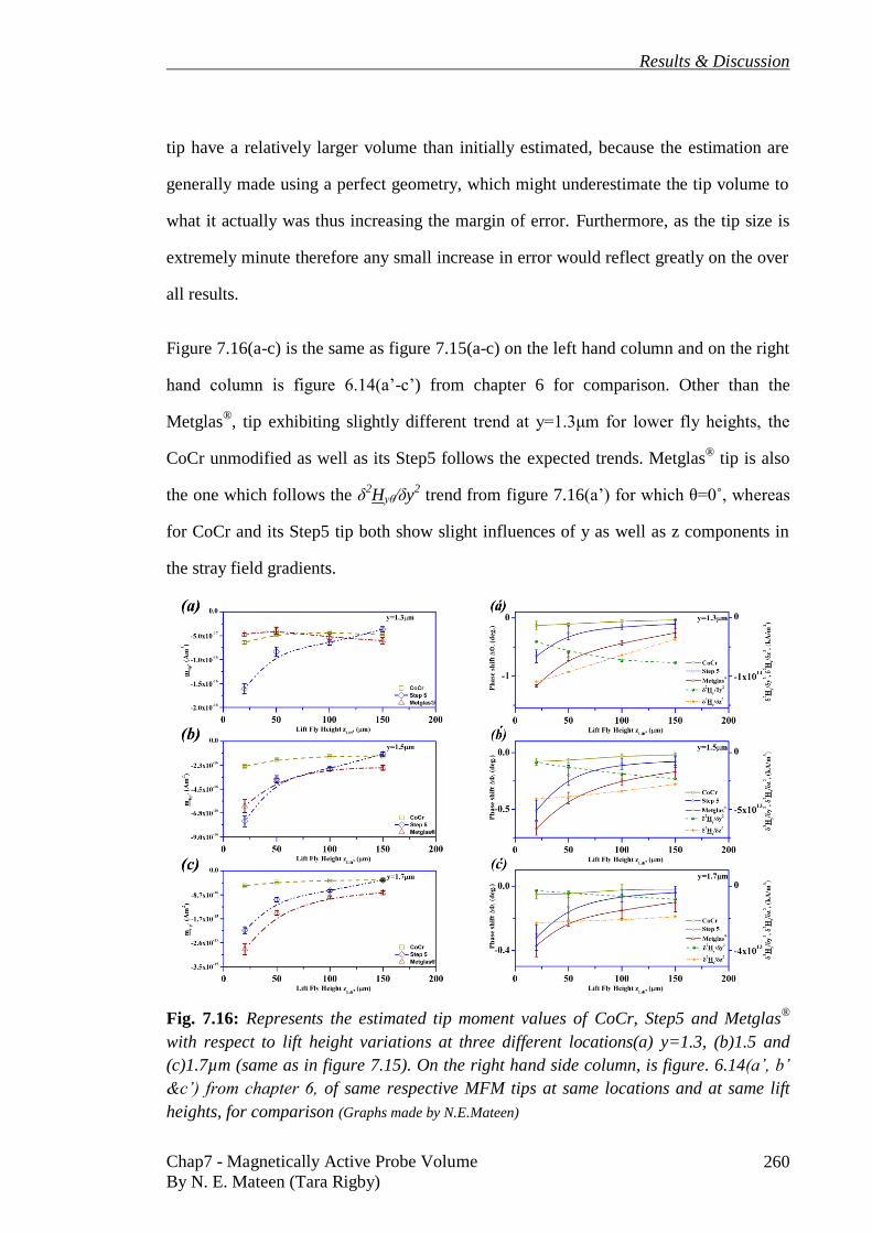
Results & Discussion
Chap7 - Magnetically Active Probe Volume
By N. E. Mateen (Tara Rigby) 260
tip have a relatively larger volume than initially estimated, because the estimation are
generally made using a perfect geometry, which might underestimate the tip volume to
what it actually was thus increasing the margin of error. Furthermore, as the tip size is
extremely minute therefore any small increase in error would reflect greatly on the over
all results.
Figure 7.16(a-c) is the same as figure 7.15(a-c) on the left hand column and on the right
hand column is figure 6.14(a’-c’) from chapter 6 for comparison. Other than the
Metglas®, tip exhibiting slightly different trend at y=1.3μm for lower fly heights, the
CoCr unmodified as well as its Step5 follows the expected trends. Metglas® tip is also
the one which follows the δ2Hyθ⁄δy
2 trend from figure 7.16(a’) for which θ=0˚, whereas
for CoCr and its Step5 tip both show slight influences of y as well as z components in
the stray field gradients.
Fig. 7.16: Represents the estimated tip moment values of CoCr, Step5 and Metglas®
with respect to lift height variations at three different locations(a) y=1.3, (b)1.5 and
(c)1.7µm (same as in figure 7.15). On the right hand side column, is figure. 6.14(a’, b’
&c’) from chapter 6, of same respective MFM tips at same locations and at same lift
heights, for comparison (Graphs made by N.E.Mateen)

Results & Discussion
Chap7 - Magnetically Active Probe Volume
By N. E. Mateen (Tara Rigby) 261
7.7.2.4 Tip moment response magnitude for average and mean values at various
heights
In figure 7.17(a), gives the magnitude of the tip moments, averaged over the entire 8μm
scan length, for increasing fly heights. Figure 7.17(b) shows the tip moment, as the
mean magnitude of only the maximum (repulsive) and the minimum (attractive) values
of the scan, at given fly heights. The results are intriguing if the data is analysed as the
aggregate of absolute values averaged over the entire scan as in figure 7.17(a), the only
significant variation for the change in the fly heights was that of the Metglas® tip. The
Metglas® tip at the fly height of 20nm showed the highest average magnitude of the tip
moments decreasing rapidly as the height increased. Furthermore, the Metglas®
tip
moment magnitude values on average were greater than the values of CoCr and Step5,
even at the fly height of 150nm. Contrary to the Metglas® tip behaviour, CoCr and
Step5 tip(s) show relatively little to no change with fly height variations. On closer
observation, the Step5 tip showed a slight magnitude increase at the fly height of 50nm
compared to fly heights of 100 or 150nm but then drops to a low value again at 20nm
height. The unmodified CoCr tip shows even less variation and remains relatively
constant for all fly heights. It might be speculated that the CoCr tip shows a probable
increase of moment magnitude at the fly height of 100nm, but that is not at all clear
from the figure 7.17(a).
The maximum magnitude of a tip’s moment (for a particular tip type) at a particular fly
height can be observed in figure 7.17(b). The CoCr tip shows the maximum magnitude
of the tip moment at the fly height of 100nm. For the CoCr tip there was significant
decrease in moment magnitude at both higher (i.e. 150nm) or lower fly heights (i.e.
50nm and 20nm) compared to that observed at the fly height of 100nm.

Results & Discussion
Chap7 - Magnetically Active Probe Volume
By N. E. Mateen (Tara Rigby) 262
At the fly height of 50nm, the Step5 tip showed the maximum tip moment magnitude.
When fly height was 20nm, the magnitude of the Step5 tip moment was relatively less
than the 50nm height.
Fig. 7.17: (a) Represents the magnitude of tip moment values, averaged over the entire
scan length of ~8μm, with respect to lift height variation of three different CoCr, Step5
and Metglas® tips, whereas (b) shows the magnitude of mean tip moment values i.e.
mean of only the maximum and the minimum value for each tip scan, at various fly
heights. The dark yellow colour represents the CoCr tip values, blue shows the Step5
tip values and dark red shows the Metglas®
tip values, the lines are a guide to the eyes
only (Graphs made by N.E.Mateen)
However, the tip moment values progressively decreased at increasing fly heights of
100nm and 150nm. In the case of the Metglas® tip a steady increase in the values of tip
moment magnitude was observed with the decrease in the fly heights. If a decrease in

Results & Discussion
Chap7 - Magnetically Active Probe Volume
By N. E. Mateen (Tara Rigby) 263
the magnitude of the tip moment after hitting a maximum were to be expected, it would
probably be below 20nm fly height. However, for the given fly height values it seems
that the Step5 had the maximum tip moment magnitude at 50nm height and the CoCr tip
achieved its maximum at 100nm. This was indicative of the Step5 tip’s optimal working
height to be 50nm and CoCr tip’s optimal height at 100nm. It might be construed from
the observations mentioned above that for a particular tip a particular fly height could be
best for optimal operation.
The results in figure 7.17(b) are also interesting for the reason that they verify the
presence and effects of short-range forces such as van der Waals forces that are known
to affect the MFM image results at low fly heights. The previous work of Al-Khafaji et
al.{20} mention such observations when a study of bulk single crystal RE-FeB using
standard CoCr tips at various fly heights was carried out. Al-Khafaji et al. showed (see
figure 4.9) that the phase shift value was at its maximum at the fly height of 200nm, at
lower fly height it was suggested the interplay of short-range forces.
7.7.3 Estimation of tip magnetisation and effective volume at various heights at
arbitrary y positions
If the tip moment is known for a particular height and position then in order to estimate
its magnetisation at that point, the volume of the tip must be known. It might be argued
that for the total volume of the tip, only the maximum attainable magnetisation i.e.
saturation magnetisation may be estimated, as the total magnetic volume of the tip may
or may not be fully involved in the process of image formation. Only a small portion of
the total volume of the tip coating may be significant for the final image, as this
percentage is strongly dependent of the tip-sample interaction itself at a particular
position in space. Put simply, a sample with relatively weak magnetic field strength may

Results & Discussion
Chap7 - Magnetically Active Probe Volume
By N. E. Mateen (Tara Rigby) 264
only be able to influence* a small portion of the tip’s magnetisation (dependent on its)
volume. Therefore, in estimations of tips magnetisation or volume, one must be careful
and be wary of potentially false or misleading results.
In this section, an attempt has been made to estimate the magnetic properties of the tip
by the use of the tip’s moment calculations and the volume estimations carried out
earlier in the chapter. Such magnetic properties would only give solution for the case†
when all of the magnetic volume‡ on the tip may be used. Still it might be able to shed
some light on the tip’s potential behaviour compared to the real behaviour and thus help
understand the tip’s sample interactive behaviour a little better. The tip magnetisation§
values found in the literature for standard CoCr tips lie in the range of 4x10⁵ {1} to
7.568x10⁵**
{12} and for Metglas®
1.17x10⁶ {9} (See table 7.4). Nonetheless, the values
from the literature were used to have an estimate how the respective values of tip
magnetisation of field might behave. In addition to this, the interpretation of such results
could be complicated as each tip(s) magnetisation changes at different rates at a
particular height and position during the scan.
Table 7.7 shows the tip magnetisation values calculated using the tip moment and the
tip volume. The tip magnetisation had the highest values for the Step5 tip compared to
the CoCr unmodified as well as the amorphous Metglas® tip. Apparently Step5 was the
only tip which showed magnetisation closer to (or higher than) the values quoted in the
literature. This could be indicative of the tip volume, its shape and the direction of
magnetisation all contributing constructively towards the higher value of the remanent
* Or conversely influenced by
† That might not be the case in reality
‡ Under the assumption that the tips total physical volume is equivalent to its active volume
§ It was unfortunate that the magnetisation of the tips used in this project could not be measured due to
lack of time and resources available at that time
** Average value of the remanent magnetization of various MESP-type MFM tips that were used by
Kebe et al. {12} was Mtip
=756,8 emu/cm3. Kebe et al. measured the magnetization M
tip was with
(SQUID) a superconducting quantum interference device magnetometer. They noted that Mtip
varies only
slightly for different tips taken from the same wafer.

Results & Discussion
Chap7 - Magnetically Active Probe Volume
By N. E. Mateen (Tara Rigby) 265
tip magnetisation. Conversely, it could also be interpreted as the contribution of the tip
volume in CoCr and Metglas® tip(s) is much less than the actual physical volume
y,
(µm
) Lift
Height,
(nm)
Mtip
(A/m) - avg. of 21 lines
CoCr S.D. (±) Step 5 S.D. (±) Metglas
S.D. (±)
(10+00
) (10+05
) (10+01
)
1.3
150 -6.62 0.19 -1.48 0.22 -3.22 0.40
100 -5.90 0.15 -2.66 0.16 -2.81 0.28
50 -6.43 0.18 -3.38 0.41 -2.09 0.36
20 -8.80 0.41 -6.51 0.42 -2.51 0.17
1.5
150 -19.10 0.63 -4.85 0.73 -13.30 1.30
100 -19.30 0.49 -10.50 0.63 -15.40 1.06
50 -23.70 0.73 -15.50 1.37 -19.60 1.11
20 -32.30 1.23 -30.40 2.12 -38.20 3.24
1.7
150 -45.20 1.48 -13.60 1.66 -42.50 3.78
100 -48.00 1.36 -29.20 1.67 -51.50 3.09
50 -56.60 1.44 -42.30 3.07 -82.00 4.29
20 -74.70 3.44 -87.90 5.14 -173.00 11.30
Table 7.7: Shows the estimated values of tip magnetisation for CoCr, Step 5 and
Metglas®
tips at y positions of 1.3, 1.5 and 1.7µm. The values are representative of an
average of about 21 scan lines along with their corresponding standard deviation
errors (Data produced by N.E.Mateen)
One possibility was that the volume measurements of Step5 with the help of AutoCAD
(tables 7.2 & 7.3) may still be too simplistic as it does not take into account the slight
tapering of the milled edges (see figure 7.9). Instead it abruptly cuts off the unwanted
tip edges (see figures 7.6 & 7.7), thus the tip volume values may be smaller than the
actual figures. Clearly, this was not a concern for the CoCr unmodified Step0. In fact,
for Step0 CoCr tip the probability was that a small portion of the total physical volume
(likely near the apex) was influenced by the sample’s stray field gradients. However,
estimating the effective volume could only be achieved by computer simulation*.
Using the respective values of the tip’s remanent magnetisations from the literature†, the
tip volume could be estimated. Table 7.8 shows the corresponding values of the tip
volume if tip moment values from table 7.6 and the average tip remanent magnetisations
* Computer simulations were beyond the scope of this project
† If assumed constant

Results & Discussion
Chap7 - Magnetically Active Probe Volume
By N. E. Mateen (Tara Rigby) 266
for the respective tips, (see table 7.4, CoCr 4x10⁵ {1} and Metglas
® 1.17x10
6 {9}), are
assumed to be correct. The estimated tip volume for the Step5 was 2.47x10⁻²²
±6.89x10-
23 m
3 (table 7.2). It is interesting that the volume of all the three tips show more or less
similar data range to that of Step5 comparatively. This could very well be the ‘effective’
volume of the respective tips. This would indeed support the theoretical predictions of
‘effective’ volume of the tip, considerably smaller than the total physical volume of the
tip {21}.
y,
(µm
) Lift
Height,
(nm)
Vtip
(m3) - avg. of 21 lines
CoCr S.D. (±) Step 5 S.D. (±) Metglas
S.D. (±)
(10-23
) (10-23
) (10-23
)
1.3
150 12.00 0.35 9.14 1.37 5.15 0.64
100 10.70 0.27 16.40 0.98 4.51 0.45
50 11.70 0.32 20.90 2.50 3.34 0.58
20 16.00 0.75 40.20 2.58 4.03 0.27
1.5
150 34.80 1.14 30.00 4.51 21.30 2.09
100 35.20 0.89 65.00 3.88 24.60 1.70
50 43.10 1.32 95.70 8.44 31.40 1.77
20 58.70 2.24 188.00 13.10 61.20 5.20
1.7
150 82.20 2.69 83.90 10.30 68.10 6.05
100 87.30 2.47 180.00 10.30 82.50 4.96
50 103.00 2.61 261.00 18.90 131.00 6.87
20 136.00 6.26 543.00 31.70 277.00 18.00
Table 7.8: Shows the estimated values of tip volume for CoCr, Step 5 and Metglas®
tips
at y positions of 1.3, 1.5 and 1.7µm (Data produced by N.E.Mateen)
The ‘effective’ volume for any tip is a function of stray field gradients from the sample
and thus is subject to change for different samples with different stray fields*. The
problem become further complicated when the direction of the tip’s magnetisation
changes even slightly†. As in the case of the current wire structures, the response from
the CoCr tip was weak to begin with. More than likely, it was because of the orientation
of the tip magnetisation and its effect on the magnitude in that particular direction or the
* from sample to sample and even point to point in the same sample
† Changing the ‘y’ or ‘z’ component dominance and hence the final image formation

Results & Discussion
Chap7 - Magnetically Active Probe Volume
By N. E. Mateen (Tara Rigby) 267
effective volume or an amalgamation of both that was contributing towards the final
image formation?
7.8 Summary & Further discussion
Yamaoka et al. {22-24} suggested that if the thickness of an MFM tip coating is
reduced, then the moment reduces with the overall volume of the tip. The results
presented in this chapter strongly suggest that even if the moments may be reduced with
the reduction of the overall volume, it is very hard to observe the effect of such a
reduction in MFM studies. The direction of these moments coupled with the overall
domain formations in the tip would have a significant effect on the results.
The image contrast is expected to be reduced, for tips having lower net moments.
However, in section 7.6 this assumption was shown not to be true. It was observed that
after the first few milling steps the overall image definition and contrast was improved
for the standard magnetic tape sample. Further milling to Step5 significantly reduced
the tip’s overall volume that the final signal became altogether weak and there appeared
a significant increase in noise. It might be argued here that the initial signal increase
occurred due to the change in the tip shape coupled with the favourable direction of
magnetisation Step2 was the optimal stage for the observation of the magnetic tape.
Thus even if the net moment was being reduced the tip did not behave proportionately
to that reduction.
The Step5 tip, in figure 7.13, showed a weaker image contrast and increased noise
indicative of lower net moment. However, the phase shift signal was greater than that of
the unmodified CoCr tip for the current wire structures indicating that although
essentially the same tip(s) behave vastly different to different samples. In the
investigation with the current wires, the Step5 tip data showed more tip sensitivity to the
stray field gradients from the observed wire sample.

Results & Discussion
Chap7 - Magnetically Active Probe Volume
By N. E. Mateen (Tara Rigby) 268
Investigations were also carried out to verify the commonly believed final image
formation dependence on only the material near/at the tip apex. Although there were
strong indications towards the tip apex being the main contributor in the MFM image
formation this was not entirely true and is subject to further investigations probably with
the help of power computer simulation, which were beyond the scope of this project and
fit for future investigations. There was strong evidence that the volume within close
vicinity of the apex plays some role in the tip-sample interaction. Here it could also be
speculated that depending on the position and the tip-sample relation, the effective
volume is subject to change during a particular scan and would definitely vary from
sample to sample.
Thus, for the investigation carried out in this chapter it could be concluded that each
tip’s behaviour for a given sample is different for a given location. A set of tips may
show similar behaviour or trends but when considered under specific conditions, each
tip is unique*. It is this uniqueness of every tip, which may be utilised in understanding
the sample’s behaviour better. Thus, it would not be wrong to suggest that each tip
sample interaction is unique as well. However, similar tips, i.e. material, shape and
history (for example Fe-CNTs) with samples† of a specific kind (such as hard disk
drives), the results might be averaged to some acceptable extent.
As the list of variables involved is huge, it is quite impossible to replicate any two tips
exactly. For argument’s sake, if two identical tips are possible‡, in the dimensions
§ that
the MFM tips need to work at are so small that any slightest of variation may become
significant. From the inherent properties**
of the material, factors like the tip’s
magnetised state during the scan, its relative distance from the sample to its relative
* And as such behaves uniquely
† Same/similar nature
‡ May be by using a deposition technique such as MBE
§ 10s of nm
** Conditions under which it was deposited, to its shape, thickness and its magnetic history

Results & Discussion
Chap7 - Magnetically Active Probe Volume
By N. E. Mateen (Tara Rigby) 269
location in space, its speed of scanning and most importantly the sample’s interaction
with it, are some of the factors that contribute in influencing the final image formation.
From the findings mentioned above, there were strong indications of the tip behaviour
would be unique for any given scenario.
It can also be concluded that for every tip ‘effective’ volume there is a corresponding
sample strength, which will optimise the tip sample interaction for that particular tip,
and the sample at a particular height. The smaller the tip volume, the smaller the net
moment, but it cannot be expected that the moment would (or would not) flip or change
direction for every sample, as it is highly dependent on the type of sample being
observed.
A shortfall with the estimated moment of the tip (in the literature*), is that the values are
usually estimated only for a fixed point in space above a sample† (usually at some
central location) with presumed symmetric field distribution. Generally, any asymmetry
in the data is ignored as it increases the uncertainty in the calibration/estimation process.
The fact that (fine scale) asymmetry‡ is an inherent part of MFM should not be ignored
(where possible), in order to have a true understanding of the phenomena involved in
the final image formation and thus its quantitative interpretation. This is especially true
if the investigations involve the data sensitive to small-scale variations, captured at low
scan heights e.g. 10 to 200nm range (see chapter 6). The most probable cause might be
the presence of stronger fields influencing significant volume of the tip. Furthermore, at
such low fly heights the asymmetric position of the tip due to its cantilever in addition
to the limitations due to the cantilever§ significantly influencing the tips motion. Hence
* Irrespective of point dipole approximation {4, 13, 25-27} or volume integral calculations over the entire
tip {28-34} † Manufactured sample generally in the shape of circles, current rings or meso- /nanodots and sometimes
parallel-current wires. ‡ Originating from the pinning of the cantilever end, its complex motion (local and along scan length) to
the uncertainty in the fine scale changes in the moment/magnetisation of the tip especially at low fly
heights § Being pinned at one end

Results & Discussion
Chap7 - Magnetically Active Probe Volume
By N. E. Mateen (Tara Rigby) 270
the tip-sample interaction resulting in asymmetric image production of symmetric
structures on the sample. Due to the acceptance of the symmetrical parameters in
mainstream literature {12-14, 35, 36}, the mathematical models also conform to such
symmetric parameters. Further refinement was required for the model to become more
like the realistic cases (see chapter 6), still the model is far from perfect as it does not
cater for the extra noise that the MFM signal generally has.
Furthermore, generally the literature emphasises on the position central to the
calibration sample as in case of Kebe et al. {12} and corresponding modelled values.
They rely on the assumption that the z component of the tip is the dominating part in the
MFM image and thus the theoretical modelling emphasises on the z component as well.
Indeed, it might be true in some cases but certainly not all, as shown in the chapter 6.
Although the z component of the tip may be more dominant than other configurations
found commonly in the MFM tips but the tip’s shape also has a crucial role on
determining where the actual magnetisation direction would lie. Estimating the z
component of tip’s parameters at the central position is convenient for some studies as
the z component of the model gives non-zero values, which is not the case for the entire
model values spanning over scan width also shown in chapter 6.
7.9 References
{1} Suess, D., Schrefl, T., and Fidler, J.; "Reversal Modes, Thermal Stability and
Exchange Length in Perpendicular Recording Media", IEEE Transactions On
Magnetics, vol. 37, pp. 1664-1666, 2001.
{2} O'Handley, R. C.; "Modern Magnetic Materials: Principles and Applications".
New York: John Wiley & Sons, Inc., 2000.
{3} Wolny, F., Muehl, T., Weissker, U., Lipert, K., Schumann, J., Leonhardt, A.,
and Buechner, B.; "Iron Filled Carbon Nanotubes as Novel Monopole-Like
Sensors for Quantitative Magnetic Force Microscopy", Nanotechnology, vol.
21, 2010.
{4} Wolny, F., Mühl, T., Weissker, U., Lipert, K., Schumann, J., Leonhardt, A., and
Büchner, B.; "Iron Filled Carbon Nanotubes as Novel Monopole-Like Sensors
for Quantitative Magnetic Force Microscopy", Nanotechnology, vol. 21, pp.
435501-435501, 2010.

Results & Discussion
Chap7 - Magnetically Active Probe Volume
By N. E. Mateen (Tara Rigby) 271
{5} Ranjbar, M., Piramanayagam, S. N., Sbiaa, R., Chong, T. C., and Okamoto, I.;
"Advanced Magnetic Force Microscopy for High Resolution Magnetic
Imaging", Nanoscience and Nanotechnology Letters, vol. 4, pp. 628-633, 2012.
{6} Li, H., Wei, D., and Piramanayagam, S. N.; "Micromagnetic Study of Effect of
Tip-Coating Microstructure on The Resolution of Magnetic Force
Microscopy", Applied Physics a-Materials Science & Processing, vol. 110, pp.
217-225, 2013.
{7} Li, H., Wei, D., and Piramanayagam, S. N.; "Optimization of Perpendicular
Magnetic Anisotropy Tips for High Resolution Magnetic Force Microscopy by
Micromagnetic Simulations", Applied Physics a-Materials Science &
Processing, vol. 112, pp. 985-991, 2013.
{8} Lisunova, Y., Heidler, J., Levkivskyi, I., Gaponenko, I., Weber, A., Caillier, C.,
Heyderman, L. J., Klaeui, M., and Paruch, P.; "Optimal Ferromagnetically-
Coated Carbon Nanotube Tips for Ultra-High Resolution Magnetic Force
Microscopy", Nanotechnology, vol. 24, pp. 105705-105705, 2013.
{9} Yang, Y., Gao, J., Wang, Z., Li, M., Li, J.-F., Das, J., and Viehland, D.; "Effect
of Heat Treatment on The Properties of Metglas Foils, and Laminated
Magnetoelectric Composites Made Thereof", Materials Research Bulletin, vol.
46, pp. 266-270, 2011.
{10} Abraham, D. W. and McDonald, F. A.; "Theory of Magnetic Force Microscope
Images", Applied Physics Letters, vol. 56, pp. 1181-1183, 1990.
{11} Hartmann, U.; "Magnetic Force Microscopy", Annual Review of Materials
Science, vol. 29, pp. 53-87, 1999.
{12} Kebe, T. and Carl, A.; "Calibration of Magnetic Force Microscopy Tips by
Using Nanoscale Current-Carrying Parallel Wires", Journal of Applied
Physics, vol. 95, pp. 775-792, 2004.
{13} Lohau, J., Kirsch, S., Carl, A., Dumpich, G., and Wassermann, E. F.;
"Quantitative Determination of Effective Dipole and Monopole Moments of
Magnetic Force Microscopy Tips", Journal of Applied Physics, vol. 86, pp.
3410-3417, 1999.
{14} Lohau, J., Kirsch, S., Carl, A., and Wassermann, E. F.; "Quantitative
Determination of The Magnetization and Stray Field of A Single Domain
Co/Pt Dot with Magnetic Force Microscopy", Applied Physics Letters, vol. 76,
pp. 3094-3096, 2000.
{15} Digital Instruments, I.; "Dimention 3100 Instruction Manual: version 4.31ce",
Copyright © 1997.
{16} Alekseev, A., Popkov, A., Shubin, A., Pudonin, F., and Djuzhev, N.; "Effect of
Horizontal Magnetization Reversal of The Tips on Magnetic Force
Microscopy Images", Ultramicroscopy, vol. 136, pp. 91-95, 2014.
{17} Heydon, G. P., Rainforth, W. M., Gibbs, M. R. J., Davies, H. A., Bishop, J. E.
L., Tucker, J. W., Huo, S., Pan, G., Mapps, D. J., and Clegg, W. W.;
"Investigation of The Response of A New Amorphous Ferromagnetic MFM
Tip Coating with An Established Sample and A Prototype Device", Journal Of
Magnetism And Magnetic Materials, vol. 214, pp. 225-233, 2000.
{18} Scott, J., McVitie, S., Ferrier, R. P., Heydon, G. P., Rainforth, W. M., Gibbs, M.
R. J., Tucker, J. W., Davies, H. A., and Bishop, J. E. L.; "Characterisation of
FeBSiC Coated MFM Tips Using Lorentz Electron Tomography and MFM",
IEEE Transactions on Magnetics, vol. 35, pp. 3986-3988, 1999.

Results & Discussion
Chap7 - Magnetically Active Probe Volume
By N. E. Mateen (Tara Rigby) 272
{19} Heydon, G. P., Rainforth, W. M., Gibbs, M. R. J., Davies, H. A., McVitie, S.,
Ferrier, R. P., Scott, J., Tucker, J. W., and Bishop, J. E. L.; "Preparation and
Characterisation of A New Amorphous Tip Coating for Application in
Magnetic Force Microscopy", Journal of Magnetism and Magnetic Materials,
vol. 205, pp. L131-L135, 1999.
{20} Al-Khafaji, M. A.; "Magnetic Force Microscopy of NdFeB Hard Magnetic
Alloys", Engineering Materials, vol. PhD. Sheffield: University of Sheffield,
1998, pp. 266.
{21} Preisner, T., Greiff, M., Bala, U. B., and Mathis, W.; "Numerical Computation
of Magnetic Fields Applied to Magnetic Force Microscopy", Compel-The
International Journal For Computation And Mathematics In Electrical And
Electronic Engineering, vol. 28, pp. 120-129, 2009.
{22} Yamaoka, T., Watanabe, K., Shirakawabe, Y., Chinone, K., Saitoh, E., and
Miyajima, H.; "Observations of Single Magnetic Domain Wall in Nanomagnet
by Magnetic Force Microscopy", Japanese Journal Of Applied Physics Part 1-
Regular Papers Brief Communications & Review Papers, vol. 45, pp. 2230-
2233, 2006.
{23} Yamaoka, T., Watanabe, K., Shirakawabe, Y., Chinone, K., Saitoh, E., Tanaka,
M., and Miyajima, H.; "Applications of High-Resolution MFM System with
Low-Moment Probe in A Vacuum", IEEE Transactions On Magnetics, vol. 41,
pp. 3733-3735, 2005.
{24} Yamaoka, T.; "High-Sensitivity, High-Resolution Magnetic Force Microscopy
System", Journal of the Magnetics Society of Japan, vol. 27, pp. 429-433, 2003
{25} Li, H. J., Wang, Y., Wang, S. M., Zhong, H., and Wei, D.; "Micromagnetic
Analysis of Effective Magnetic Dipole Position in Magnetic Force Microscope
Tip", IEEE Transactions On Magnetics, vol. 46, pp. 2570-2578, 2010.
{26} Goryachev, A. V. and Popkov, A. F.; "Calibration Parameters for The Probing
Tip of A Magnetic Force Microscope in The Field of A Test Current Loop",
Technical Physics, vol. 51, pp. 1223-1228, 2006.
{27} Wu, Y. H., Shen, Y. T., Liu, Z. Y., Li, K. B., and Qiu, J. J.; "Point-Dipole
Response From A Magnetic Force Microscopy Tip With A Synthetic
Antiferromagnetic Coating", Applied Physics Letters, vol. 82, pp. 1748-1750,
2003.
{28} Saito, H., Yatsuyanagi, D., Ishio, S., Ito, A., Kawamura, H., Ise, K., Taguchi, K.,
and Takahashi, S.; "Simulation of High-Resolution MFM Tip Using
Exchange-Spring Magnet", Journal Of Magnetism And Magnetic Materials,
vol. 310, pp. E939-E940, 2007.
{29} Saito, H., Rheem, Y. W., and Ishio, S.; "Simulation of High-Resolution MFM
Tips for High-Density Magnetic Recording Media with Low Bit Aspect Ratio",
Journal Of Magnetism And Magnetic Materials, vol. 287, pp. 102-106, 2005.
{30} Saito, H., van den Bos, A., Abelmann, L., and Lodder, J. C.; "High-Resolution
MFM: Simulation of Tip Sharpening", IEEE Transactions on Magnetics, vol.
39, pp. 3447-3449, 2003.
{31} van Schendel, P. J. A., Hug, H. J., Stiefel, B., Martin, S., and Guntherodt, H. J.;
"A Method for The Calibration of Magnetic Force Microscopy Tips", Journal
of Applied Physics, vol. 88, pp. 435-445, 2000.
{32} Saito, H., Chen, J., and Ishio, S.; "Description of Magnetic Force Microscopy
by Three-Dimensional Tip Green's Function for Sample Magnetic Charges",
Journal Of Magnetism And Magnetic Materials, vol. 191, pp. 153-161, 1999.

Results & Discussion
Chap7 - Magnetically Active Probe Volume
By N. E. Mateen (Tara Rigby) 273
{33} Saito, H., Chen, J., and Ishio, S.; "Principle of Magnetic Field Analysis by
MFM Signal Transformation and its Application to Magnetic Recording
Media", IEEE Transactions On Magnetics, vol. 35, pp. 3992-3994, 1999.
{34} Hug, H. J., Stiefel, B., van Schendel, P. J. A., Moser, A., Hofer, R., Martin, S.,
Guntherodt, H. J., Porthun, S., Abelmann, L., Lodder, J. C., Bochi, G., and
O'Handley, R. C.; "Quantitative Magnetic Force Microscopy on
Perpendicularly Magnetized Samples", Journal Of Applied Physics, vol. 83,
pp. 5609-5620, 1998.
{35} Lohau, J., Carl, A., Kirsch, S., and Wassermann, E. F.; "Magnetization
Reversal and Coercivity of A Single-Domain Co/Pt Dot Measured with A
Calibrated Magnetic Force Microscope Tip", Applied Physics Letters, vol. 78,
pp. 2020-2022, 2001.
{36} Carl, A., Lohau, J., Kirsch, S., and Wassermann, E. F.; "Magnetization
Reversal and Coercivity of Magnetic-Force Microscopy Tips", Journal of
Applied Physics, vol. 89, pp. 6098-6104, 2001.

Results & Discussion
Chap8 - Probe-Sample Variations: Effect on MFM Imaging
By N.E.Mateen (Tara Rigby) 274
Probe-Sample Variations: Effect on MFM Imaging
8.1 Impact of tip-sample variations on magnetic imaging
The impact of the variations that occur in the tips and the sample when the tip and
sample interact with each other on the image formation are investigated in this chapter.
The properties of a particular sample are complex; it becomes increasingly difficult to
predict how a particular tip is going to behave with such a sample. Unless the specific
properties of the tip or those of the sample are known, only then the tip-sample
interactive data (in the form of images) may begin to deliver any meaningful
quantitative results. The tips as well as the samples can be generalised in broad
categories, and it is prudent to group certain types of tips for particular types of sample
observation (see chapter 4). Nevertheless, when it comes to extracting significant
numbers from the raw data for the tips, it becomes a tedious and laborious task.
Furthermore, due to the complex nature of the tip-sample interaction, the numbers are
usually estimates or guidelines for the data interpretation and do not fully explain the
inner workings of a tip. For that, detailed computerised* tip-sample modelling is a likely
solution to understand the intricate workings of a tip and its interaction with various
samples. This task was not undertaken during this project and should be pursued in the
future. The modelling of the tips is quite complicated, as the tip must be modelled to the
exact 3D specifications. Realistically each tip should be modelled individually, as no
two tips are 100% alike. That is because normally each tip varies slightly from its so-
called identical counterpart, if not significantly. Since all MFM tips are three
dimensional in nature, the tip behavioural predications are far more complex than
normally anticipated.
* Using software’ like AutoCAD {1}, GiD {2} FEMME {3} or COMSOL {4} using FEM {5}.

Results & Discussion
Chap8 - Probe-Sample Variations: Effect on MFM Imaging
By N.E.Mateen (Tara Rigby) 275
To show the diverse range and complicated yet unique nature of each individual tip-
sample interaction, in this chapter samples such as thin film Au/Co soft multilayers, thin
film hard REFeB* as well as single crystal REFeB were studied. Also included in the
study is the Step5 tip (trimmed version of the CoCr tip) as well as the other tips such as
Metglas®, low-moment CoCr and low-moment Ni tips, where possible in order to
conduct comparative studies.
8.2 Soft multilayered Au/Co thin film with CoCr, Step5 and low-moment CoCr
tips
In this section, three tips were used to observe the behaviour of a soft magnetic sample.
The standard CoCr pyramidal (unmodified) tip failed to produce any visible magnetic
image while observing magnetically soft Au/Co multilayers. The Au/Co multilayered
sample was prepared by magnetron sputtering and was provided by M Kisielewski {6}.
The composition was [Co(1nm)/Au(1.5nm)]x15. The absence of a MFM image was
because the field from the CoCr tip was too strong and was capable of temporarily re-
writing the magnetic configuration to remove field contrast. Clearly, the tip strength
should always be such that it does not significantly change or damage the magnetic
patterns on the sample unless the purpose of the tip is to write on top of the sample.
Therefore, a tip such as a low moment CoCr tip was used. However, as was shown in
previous results chapters that the Step 5 (CoCr trimmed) tip showed a stronger signal
for the current wires and weak response to the standard magnetic tape. Therefore, Step 5
tip was also used in the observation of the Au/Co soft multilayers. As the low-moment
CoCr tip and Au/Co multilayer sample were only temporarily available, the
investigations with low moment CoCr tip and the multilayer sample were limited.
However, the real test was of the Step5 tip if it showed the same or at least similar
* grown at different temperatures to achieve highly perpendicular anisotropy

Results & Discussion
Chap8 - Probe-Sample Variations: Effect on MFM Imaging
By N.E.Mateen (Tara Rigby) 276
domain structure of Au/Co multilayer films compared to the low moment tip. It was
expected that the Step5 tip would act like a low moment tip as well because of the
substantial reduction of the magnetic volume.
Fig. 8.1: Show the AFM image (a) of Au/Co multilayered soft sample. The respective
domain patterns observed using MFM low moment MESP Veeco CoCr tip (b) and FIB
modified Step5 CoCr tip (c) are also shown here (Images captured by N.E.Mateen)
Figure 8.1(a) shows the surface topography of Au/Co multilayered sample. Figure
8.1(b-c) represent the MFM image captured with phase shift data of the sample having
maze like domain pattern. Figure 8.1(b) illustrates the domain patterns of the sample by
using the low moment MESP Veeco CoCr tip and 8.1(c) shows the domain patterns of
the same sample imaged via MFM using Step5 (standard CoCr) tip. Similar to the

Results & Discussion
Chap8 - Probe-Sample Variations: Effect on MFM Imaging
By N.E.Mateen (Tara Rigby) 277
results obtained by the modified tip for standard magnetic tape (see chapter 7), the
overall image brightness was reduced significantly for the Step5 tip. This reduction
could be attributed to the significantly reduced magnetic volume of the Step5 tip. Here
it might be argued that the ‘effective’ magnetic volume of the Step5 might have been
modified in such a way as to produce a much weaker signal. It should be kept in mind
that although the ‘effective’ volume is limited by the physical volume of the magnetic
coating, it is also dependent on the initial magnetisation direction as well as nature of
the stray magnetic field from the sample. Notice that the phase data setting was reduced
to 1˚ for Step5 tip from 3˚ setting of low moment commercial tip.
Even though the phase shift signal was weak and there was some noise in the image
generated by the Step5 tip (figure 8.1(c)), the overall image shows much more
uniformity and stability as compared to the low moment CoCr tip.
It is imperative to keep the instrumental settings as consistent as possible for good
comparative studies and observations. For example, the lift height for this particular
case study was kept to be 40nm having the (approximate) same scan location on the
sample. The MFM images had the scan area of 2.5x2.5µm2. Throughout this
dissertation, the fly heights were selected as the minimum that was reasonably
achievable to ensure that no small-scale features were missed out, and the maximum
magnetic details were captured by the MFM. In this case, the fly height of 40nm was
selected for both the tips. Breakthrough of the topographical contrast was a limitation
for the low-moment CoCr tip, but for the Step5 tip, there were no such problems even at
a fly height of 20nm.
Figure 8.2 shows the MFM image taken using the low moment CoCr tip in (a) with its
corresponding section analysis (line scan for one pixel line data) shown in (b) and Step5
tip MFM data shown in part (c). Figure 8.2(d) shows the corresponding line scan of the
MFM data gathered in (c). Due to the significant variation in the brightness of the

Results & Discussion
Chap8 - Probe-Sample Variations: Effect on MFM Imaging
By N.E.Mateen (Tara Rigby) 278
images, the phase data for Step5 was set on a lower value as mentioned earlier. There
was no expected length scale change between the two images. One quite noticeable
variation in the MFM image data collected using the low moment CoCr tip and the
Step5 tip was that the overall signal in the low moment CoCr tip seemed to be roughly
equal (repulsive or lighter phase shift compared to the troughs) within the margin of
error. Conversely, with the Step5 tip the image data shows relatively thinner peaks to
the slightly broader troughs, in addition to the overall darker contrast representing
attractiveness of the tip with the sample.
Fig. 8.2: Shows soft Au multilayers using (a) CoCr LM (b) line scan from across the
image given in (a) Step5 tip is used in the MFM imaging of the soft multilayer sample
in (c) along with its line scan graph shown in (d) (Images captured by N.E.Mateen)
The overall numbers of domain periods remain the same. For the low moment CoCr tip,
the total wavelength (on average) was found to be 207±33nm and for the Step5 tip the
wavelength was 198±36nm. Although the sum of light and dark domains for the images
using both the tips is very close to each other (i.e. within the margin of error),
nevertheless, it is interesting that both the tips magnetised in the same direction, and

Results & Discussion
Chap8 - Probe-Sample Variations: Effect on MFM Imaging
By N.E.Mateen (Tara Rigby) 279
showed slightly opposing behaviour*. The graph of figure 8.2(b) is more of a simple
sinusoidal wave compared to the graph represented in figure 8.2(d). Thus, figure 8.2(d)
might be indicative of the Step5 tips’ capability of following the domains more
precisely with improved detail and sharper transitions through the domain wall width.
However, differences between types of tip as well as significant tip-to-tip variations of
some type were observed. These findings again indicate that each tip has its own unique
behaviour when it interacts with a particular sample. It is also interesting that on larger
scales (larger scan areas and relatively higher fly heights), the general behaviour of
similar types of tips with a particular sample is quite alike. However, when fine scale
magnetic structures especially at low fly heights of are observed, the tip-sample
interaction seems to be inherently unique†.
In the graphs shown in figure 8.2(b) & (d) the phase shift calculations used the
maximum and minimum values of the total area exposed in the MFM image. It made
the image intensity for Step5 MFM lower than zero phase-shift (on average). To
estimate the peak and trough values the graphs used had averaging data instead of using
the maximum and minimum method.
As mentioned, depending on the definition of magnetic resolution {7-11}, it could be
argued that the resolution in the Step5 tip might have increased marginally (as the pixel
size and the area scanned were kept equal in both the images). Although, one tip image
is hampered by the topographical break through and the other image seemed to be too
weak to be dominated by the background noise, still the combinations of using both the
*The width of peaks formed by using LM-CoCr tip were relatively wider compared to those formed by
the Step5 tip and the width of troughs made by Step5 tip were relatively wider than the troughs formed by
using LM-CoCr tip. For the low moment CoCr tip the FWHM of domain peaks and troughs were
109±33nm and 98±0 respectively whereas for the Step5 tip the FWHM values for similar domain peaks
and troughs were 83±21nm and 115±15nm respectively (see figure 8.2(b) & (d)) † Keeping in view the findings thus far, it would be appropriate to state that no two tips are alike and
therefore, no two tip-sample interactions are alike. There is always some inadvertent variation in the
form, structure or the magnetic history of the tip

Results & Discussion
Chap8 - Probe-Sample Variations: Effect on MFM Imaging
By N.E.Mateen (Tara Rigby) 280
tips helped verify the dimensions of the sample structure. At least these results verified
the stability and integrity of the Step5 tip, and helped in establishing it as a
multipurpose and robust tip, which so far could be successfully used in the observation
of soft and moderate materials.
8.3 Thin Film RE-FeB Samples: Observations using CoCr*, Step 5
†, LM-Ni
‡ and
Metglas®§
tips
Tang, et al. grew four samples of RE-FeB about 600nm thick at different temperatures
of 300˚C, 430˚C, 470˚C and 510˚C on Si substrate with 200 nm of Ta as a buffer layer
in an effort to increase the c-axis texture and the hard magnetic properties such as the
angle**
of anisotropy {12-14}. Tang, et al. wanted to fabricate the excellent permanent
magnetic films with highly perpendicular anisotropy. One of the methods used in the
assessment, of whether the RE-FeB films possessed hard magnetic properties
specifically high perpendicular anisotropy due to sample growth-temperature variations,
was the MFM instrument.
In this study, the four RE-FeB samples (in as-grown state) were observed using four tips
with different magnetic properties. Although the main purpose was to observe the
behaviour of distinctly varied MFM tips with respect of a magnetically hard sample i.e.
the effect on MFM imaging with probe-sample variations. Another reason to investigate
a diverse range of MFM tips was to select the best tip suited for such RE-FeB film(s).
* standard
† trimmed CoCr
‡ part coated commercial
§ home grown at University of Sheffield
**parallel or perpendicular to the surface of the film sample

Results & Discussion
Chap8 - Probe-Sample Variations: Effect on MFM Imaging
By N.E.Mateen (Tara Rigby) 281
One tip was the standard CoCr tip*; the second was the same tip trimmed to Step5
† and
another was a commercial low moment Ni tip‡ was used. The fourth tip was the
Metglas® tip
§.
It would be reasonable to assume that the CoCr and Ni tips used had their magnetic
material deposited with a commercial sputtering instrument. The material on the CoCr
was deliberately milled away later for Step5. The Metglas® material was deposited to a
standard Si tip with a non-commercial sputtering instrument {16}. However, the Ni tip
had the material deposited only on one of the four faces of the typical pyramidal tip and
hence confining the moments to a limited volume**
in a way similar to that of the milled
tip in Step5††
. Thus, all in all the term ‘effective volume’ may only be another simplistic
way of interpreting a complex problem.
Due to the amorphous nature of Metglas®, a certain degree of consistency in the images
was expected, as there was no crystalline anisotropy to influence the resulting magnetic
image from by the MFM. The details of these tips have already been given in the works
of Heydon et al. and Scott et al.{15, 16}.
8.3.1 Thin Film RE-FeB Samples: The surface topography and roughness
Figure 8.3 gives AFM images with their respective section analysis of the four samples
to show the correlation between the magnetic images (see section 8.3.2 & 8.3.3) with
their corresponding topographical counterpart. There was not difference in the AFM
images takes by using Step5, LM-Ni or Metglas® tip of the four samples and therefore
* pyramidal commercially available
† This Step5 CoCr tip was treated as an individual tip as the physical magnetic volume was significantly
reduced (see sections 7.4 & 7.5 in chapter 7) ‡ which, according to the information provided by the manufacturer, had the magnetic material coating on
one face only and hence low moment § an amorphous material expected to be very soft
** With a particular shape and size
†† Although the shape and size of the two were significantly different

Results & Discussion
Chap8 - Probe-Sample Variations: Effect on MFM Imaging
By N.E.Mateen (Tara Rigby) 282
the AFM images taken from the standard CoCr tip are shown in figure 8.3. The AFM
knowledge was helpful in the study of the c-texture and hard perpendicular anisotropic
magnetic properties of the material and the possible manufacturing method.
Fig. 8.3: AFM images of RE-FeB (A1) 300ºC, (A2) 430ºC, (A3) 470ºC & (A4) 510ºC
using a standard CoCr tip. The corresponding line scans are given under each image
(Graphs plotted by N.E.Mateen)
The surface roughness of the film topography is shown in figure 8.4. This emphasises
the limitation set on the lift height due to the significantly rough samples. The
roughness also indicates that the c-axis perpendicular anisotropy was achieved when the
crystal growth (in the final sample4) was mainly in the c-axis {14}.
Fig. 8.4: Surface roughness over the area of 10x10μm2 of the 600 nm RE-FeB on 200nm
Ta buffer layer grown on Si at substrate temperatures of 300ºC, 430ºC,470ºC and
510ºC (Graph plotted by N.E.Mateen)
300 330 360 390 420 450 480 5100
2
4
6
8
10
12
14
RM
S R
ougnes
s, n
m
Substrate Temperaturs at Growth, °C
Surface Roughness of ReFeB Films

Results & Discussion
Chap8 - Probe-Sample Variations: Effect on MFM Imaging
By N.E.Mateen (Tara Rigby) 283
8.3.2 Thin Film RE-FeB Samples: The magnetic images from CoCr*, Step 5
†,
LM-Ni‡ and Metglas
®§ tips
The sample grown at 300˚C (sample1) was dominated by the stripe domains with some
scattered spike domains indicating that most of the sample had some out of plane
anisotropy yet there was some indication of perpendicular anisotropy in the c-axis. For
films grown at 400˚C (sample2) the stripe domains reduce in width and length as
compared to sample1, and the spike domains become more evident in this REFeB
sample scattered between the stripe patterns. At 470˚C (sample3) the stripe domains
become almost extinct and the spike domains started to dominate the sample. The films
grown at 510˚C (sample4) only the spike domains existed, the stripe (nested) domains
were completely absent. These properties of the samples provided an excellent basis for
the investigation of a variety of tips.
Figure 8.5 shows a sequence of MFM images representing the four magnetic films as
captured using a variety of tips**
. Figure 8.5(a1) through to (a4) were all scanned using
the standard CoCr tip, similarly from image 8.5(b1) to (b4) low moment Ni tip was
used, 8.5(c1) to (c4) used the Metglas® soft tip and from (d1) to (d4) the Step5 CoCr
trimmed tip was represented. All images were scanned using a lift height of 50nm since
the film sample in (a4-d4) had surface topography that restricted the fly height to at
least 50nm (see section 8.3.1, figures 8.3 and 8.4). All the image data was captured at
the phase setting of 3˚ in the MFM instrument.
* standard
† trimmed CoCr
‡ part coated commercial
§ home grown at University of Sheffield
**from standard moderately hard to softer tips

Results & Discussion
Chap8 - Probe-Sample Variations: Effect on MFM Imaging
By N.E.Mateen (Tara Rigby) 284
Fig. 8.5: Four different tips were used to observe the behaviour of Re-FeB (NdFeB) thin
film samples (a) standard pyramidal CoCr tip, (b) a low moment Ni (one face coated)
commercial tip, (c) home grown* Metglas
® tip & (d) the Step5
† (modified CoCr) tip. The
four samples of thin film Re-FeB home grown‡ at different temperatures (1) 300ºC, (2)
430, (3) 470 & (4) 510 respectively observed using the four tips. For instance, MFM
image in (a1) is of the thin sample grown at 300˚C using standard CoCr tip. All images
were captured at a lift height of 50nm with phase setting of 3˚; each image represented
here shows an area of 5x5µm2
(Images captured by N.E.Mateen)
* Metglas® tip used in this study was part of a set of Metglas tips grown at the University of Sheffield in
1998 by Heydon, G. P {16}. † Step5 tip was modified by Mateen, N. E. using FIB at the University of Sheffield in 2006.
‡ Re-FeB sample grown at varying temperatures at the University of Sheffield in 2005 by Tang, S. L. for
the study of c-axis texture and hard magnetic properties {12}

Results & Discussion
Chap8 - Probe-Sample Variations: Effect on MFM Imaging
By N.E.Mateen (Tara Rigby) 285
The variations in the domain patterns can be clearly seen as a function of film growth
with temperature, figure 8.5. What was more interesting were the effects variety of tips
had on the final image formation of the exact same set of samples at same locations.
Here it is worth remembering some of the characteristics of the tips used in this study.
For example, the CoCr tip used, was considered moderately magnetically hard and the
physical magnetic volume on the pyramidal area of the tip was estimated to be
approximately 7.28x10⁹±2.80x10
6nm
3 (see chapter 7). As for the low moment Ni tip,
one of the selling points from the manufacturer was that only one face of a typical
pyramidal tip was coated with Ni, claiming to be low moment.
If it is assumed that the Ni tip had approximately the same amount coated thickness of
material as a standard CoCr tip but only on one of its pyramidal faces then the magnetic
volume of such a tip would be approximately 2.3x10⁹±2.80x10
6nm
3, which is little less
than one third of the total volume of CoCr tip. The estimated volume of a tip coated
with 40nm Metglas® would be around 7.51x10
8±5.83x10
6nm
3, which is almost
equivalent to the volume estimate comparable to Step2 (see table 7.2 in chapter 7). The
physical magnetic volume left at the Step5 tip stage (also in table 7.2) was around
2.47x10⁵±6.89x10
4nm
3. Keep in mind that only two tips in this study were related and
had the exact same tip apex i.e., the CoCr standard tip and Step5 tip.
The change in physical volume alone affects a tip’s interactive properties as well as
other contributing factors such as shape anisotropy, magneto crystalline anisotropy or
any other inherent magnetic properties of the tip like the magnetic history. As
mentioned in section 7.6, chapter 7 the optimal magnetic volume for the observation of
the standard magnetic tape sample was at or near Step2. By observing the values of the
magnetic volume given in the paragraph above, one could expect that the respective tip
moments were accordingly reduced. A decrease in total magnetic volume might be
indicative of less magnetic moment; however, the tip’s magnetisation direction also

Results & Discussion
Chap8 - Probe-Sample Variations: Effect on MFM Imaging
By N.E.Mateen (Tara Rigby) 286
plays a significant role in the final image formation. Softer tips are expected to be
strongly dependant on their magnetic susceptibility, volume and magnetic fields from
the sample. All these factors add to the complexity of the tips behavioural dependence.
There was a marked increase in magnetic signal intensity when the set of samples were
observed using MFM (figure 8.5(1-4), left to right) except sample2 (430˚C). The
average phase shift intensity increased from <2˚ to >8˚. This increase was consistent,
irrespective of which tip was used to capture the image. However, every tip-sample
showed individual variations in the increase/decrease in the magnetic signal. This could
be seen by observing the line graphs of the MFM image data represented in figure 8.6.
On comparison of the whole set of tip-sample interactive behaviour for sample1 (300˚C)
all tips showed similar signal intensity but when sample4 (510˚C) was observed each tip
behaved differently.
The CoCr tip showed quite an increase in the phase shift signal intensity >±4˚ shown in
figure 8.6(a4) but when the same sample was observed using a low moment Ni tip, the
signal intensity (although the largest for the Ni tip in the four samples measured) was
lower than the CoCr tip. This behaviour of the Ni tip might be attributed to the lower
volume of the tip (i.e., lower net moment). Additionally the total image phase shift
seemed to tend towards the darker (attractive) side, a clear indication of a relatively low
moment tip. When the behaviour of Metglas® tip was investigated in 8.6(c4), there was
considerable increase of signal indicative of a high moment tip. Furthermore, there were
no clear indications of tip flipping, implying that although the Metglas® was high
moment tip but had coercivity value sufficient as not to allow the samples fields to
affect the tip stability. As Metglas®
was also considered a soft amorphous tip {15, 16};
it was not a low moment tip. On the contrary, this Metglas® tip was a relatively high
moment tip. It is due to this high moment, the image (phase shift) signal was the
strongest amongst the other tips.

Results & Discussion
Chap8 - Probe-Sample Variations: Effect on MFM Imaging
By N.E.Mateen (Tara Rigby) 287
Fig. 8.6: The line graphs or the section analysis of the MFM images given in figure
8.5, the phase setting were changed to 15˚ to ensure no data was truncated. NdFeB
films grown at temperatures ranging from 300 to 510˚C were used to observe the effect
the tip behaviour had on the receptive MFM data. (a1-4) represents the set of
temperature-varied samples using just the CoCr tip, (b1-4) shows the section analysis
of the set of samples using LM-Ni tip, (c1-4) illustrates the data using the Metglas®
tip
and lastly (d1-4) shows the set of samples observed by using the Step5 tip respectively
(Graphs plotted by N.E.Mateen)
When the Metglas® tip was used to image the sample4* it showed the maximum signal
intensity almost exceeding the 10˚ setting of phase data, which was more than both the
CoCr and the Ni tips. The physical magnetic volume of this Metglas® tip was estimated
to be less than the CoCr or the Ni tip and it was 40nm of amorphous coating. This tip
shows a significantly greater response when it comes within the range of sample4. Thus,
in the case of the Metglas® tip it appears that this particular tip was dependent entirely
on its magnetic volume and that the effective portion of the volume varied considerably
* (510˚C) of the RE-FeB set

Results & Discussion
Chap8 - Probe-Sample Variations: Effect on MFM Imaging
By N.E.Mateen (Tara Rigby) 288
from sample to sample. Other than being hailed as a soft tip {17}, the major difference
as compared to other tips was that it was amorphous with high moment.
When the Step5 tip was used to image sample4, the signal intensity was found to be the
lowest of all the tips used. In fact, due to the lower intensity, the Step5 tip was the only
tip that managed to show the domain structure of the RE-FeB film grown at 510˚C
(sample4) without any need for changing the phase data settings. This suggested that the
physical limitation of the magnetic volume prove to be beneficial in most cases
including this.
In figure 8.7, notice that the magnetic image data captured for the sample4 using the Ni
tip and the Step5 tip were relatively constrained in the variation of image signal
intensity from sample to sample and the CoCr as well as the Metglas® tips had almost
similar intensities for amorphous phase REFeB films (Sample1). It is also interesting
that up to sample3 all tips showed a steady increase in signal intensity. However, in
sample4 the Metglas® tip overshoots the intensity of the CoCr tip, showing the
maximum response to the stray field of the sample4.
Fig. 8.7: The overall signal intensity increase of various tips when the sample growth
temperatures were increased. The dotted lines are used as a guide to the eye (Graph
plotted by N.E.Mateen)

Results & Discussion
Chap8 - Probe-Sample Variations: Effect on MFM Imaging
By N.E.Mateen (Tara Rigby) 289
The Ni tip began to show evidence of (what may be called) instability in sample2 (see
figure 8.5(b2)) and which increased in sample3 (see figure 8.5(b3)). In case of sample4,
the instability of the Ni tip was so pronounced that it became difficult to distinguish
between the tip magnetisation (i.e., moment) reversal and the unperturbed image. The
effect on the images captured by the Metglas® coated tip was more profound. However,
the Metglas® tip flipped its magnetisation state quite readily in sample2 and sample3.
For sample4, the Metglas® tip seemed to be overwhelmed for the phase shift range of 3˚
and the overall interaction of the tip-sample is repulsive instead of normally expected
attractive interaction (see figure 8.5(c1-c4). These observations were interesting,
thought provoking and merit further investigation in the future.
8.3.3 RE-FeB Sample grown at 300˚C: Effect on the image
Sample1 (300˚C) was an interesting sample as it was mostly amorphous with a few
scattered crystallites with perpendicular anisotropy. Hence, sample1 was a good
example for both the horizontal as well as the vertical stray fields. Investigations in this
section are mostly concentrated at the sample1 with the four tips mentioned above.
MFM images with four different tips represented in figure 8.8 show stripe (nested)
domains.
Stripe domain patterns are generally observed in amorphous films with the principle
component of magnetisation lying in plane {18}, suggesting an amorphous phase of
REFeB has been deposited at this temperature. Gao, et al., further reaffirmed this in
their work on Re-Fe-B thin film grown at 300˚C {19}. In this study however, MFM
observations show that the stripe domains dominate most of the sample area (figure
8.5), with only a few scattered spike domains (crystallites) to be seen.

Results & Discussion
Chap8 - Probe-Sample Variations: Effect on MFM Imaging
By N.E.Mateen (Tara Rigby) 290
Fig. 8.8: Re-FeB sample grown at 300˚C observed with four tips of differing properties
along with their corresponding line graphs to show the subtle variation in the imaging
of the same domain patterns. Scan size of 2x2µm2, lift height of 50nm and the phase
data set to 3˚ were the parameters set of these images (Images and graphs plotted by
N.E.Mateen)
In figure 8.8, the same area of the sample1 was imaged using the four tips as used to
generate figure 8.5. The (b), (d), (f) and (h) show the line scans of the respective images
shown in (a), (c), (e) and (g). The domains imaged are roughly evenly spread in the case

Results & Discussion
Chap8 - Probe-Sample Variations: Effect on MFM Imaging
By N.E.Mateen (Tara Rigby) 291
of CoCr tip, Ni, Metglas® and Step5. Interestingly the Ni (c) and Metglas
® (e) tips seem
to have brighter image contrast. That is, the Ni and Metglas® tips appear to be in a
repulsive mode compared to the CoCr and Step5 tips. However, similar to the trend
observed in figure 8.2(d) Step5 tip in figure 8.8(h) also showed a less sinusoidal wave
pattern with sharper transition between domain patterns. Furthermore, the domain
pattern image in 8.8(g) also show that the domain transition from one state to another is
more defined indicating that the Step5 tip response is little more sensitive compared to
its counterpart.
However, the periods shown in the given area of the sample remain the same. From
figure 8.8 the variation in domain widths could be estimated and compared when using
the given four tips. Table 8.1 represents the values extracted from the graphs in figure
8.8 for all four tips. The average value of the domain width seems to be smallest for the
Step5 tip with significant standard deviation (SD) values.
Average
Values
Tips Used
Peaks Troughs DWidth PeriodTotal
nm S.D. nm S.D. nm S.D. nm S.D.
CoCr tip 137 ±11 140 ±15 138 ±13 277 ±12
LM-Ni tip 142 ±19 147 ±27 144 ±22 290 ±21
Metglas® tip 145 ±48 130 ±59 138 ±51 290 ±44
Step5 tip 131 ±50 126 ±55 128 ±51 257 ±28
Table 8.1: Average values of peaks and troughs i.e., white (repulsive force) and dark
(attractive force) for the four tips used in this study. From these averages the domain
width as well as the total period was estimated along with their respective standard
deviations. The standard deviation represents the variation in the domain widths
(Data produced by N.E.Mateen)
To test the variation in estimates of domain widths given in table 8.1 for an area of
2x2µm2 (mainly dominated by the stripe domains) compared to a larger area size of
10x10µm2, the domain widths were calculated by using the formula found in the
literature {18}. For the larger scan size area the domain width were calculated using the
section analysis data taken in the direction of the (near perpendicular) stripe domains
{19} from at least five various locations, for more accuracy.

Results & Discussion
Chap8 - Probe-Sample Variations: Effect on MFM Imaging
By N.E.Mateen (Tara Rigby) 292
⁄ (8.1)
where lt and in are the total test line length and the
number of intersections with the domain lines
respectively. Although in this case the average
domain widths from all four tips lie very close to
each other with very small SD there was a marked
difference of ~50nm between the values calculated
with the help of the formula in table 8.2 as compared
to the values in table 8.1. Even though both sets of values in the respective tables 8.1
and 8.2 are correct, the reason for the variation lies in the size of the area considered in
each case. In table 8.1, the scan line section was only 2µm and thus the domain width
calculated takes a smaller area with predominant stripe domains without any spike
domain pattern in the vicinity. In contrast, table 8.2 provides data from a five times
larger area of 10x10µm2, which was large enough to include a more complex domain
structure like the nodule like spike domains as shown in figure 8.9. The spike domains
along with the stripe domains, contribute towards the average domain width of the
sample under discussion.
From the observation made above, it is apparent that not only the tip’s behaviour at a
particular height and the sample interaction contribute to the final image formation but
the field size and location of the sample is as important. On average, all four tips
behaved in a similar manner as far as the estimation of domain dimensions were
concerned (for the samples1), subject to acceptable tolerance.
It is important to note that each image could be uniquely identified, which in turn could
be traced back to tip used in the tip-sample interaction. Thus, each tip left its own
unique mark during the image capture. Acceptable tolerance ranges may vary greatly
and strongly depending upon the requirements of the user.
Tips Used
Avg. Dwidth
nm S.D.
CoCr 179 ±8
LM-Ni 188 ±12
Metglas® 183 ±4
Step5 185 ±7
Table 8.2: Domain width
estimated from using the
formula {18} (Data produced by
N.E.Mateen)

Results & Discussion
Chap8 - Probe-Sample Variations: Effect on MFM Imaging
By N.E.Mateen (Tara Rigby) 293
Fig. 8.9: Larger rotated image scan areas along with its corresponding section analysis
of sample1 (300˚C) captured by using (a-b) CoCr tip, (c-d) low moment Ni tip, (e-f)
Metglas® tip and (g-h) modified Step 5 tip respectively (Images and graphs produced by
N.E.Mateen)
Figure 8.9 provides a larger area than shown in figure 8.5* along with their respective
line scans, which show the variation in the phase shift data. These variations in the
signal amplitude also produce an impact on the domain widths as represented in table
8.2. Furthermore, each tip’s response to the same sample at almost the same position at
the same instrument setting was slightly yet consistently different, giving a strong
indication to the fact that the tip-sample interaction is indeed unique.
* The images were rotated so that they could all fit on the same page

Results & Discussion
Chap8 - Probe-Sample Variations: Effect on MFM Imaging
By N.E.Mateen (Tara Rigby) 294
For the 40nm coated Metglas® tip, an interesting observation was that it did give both a
positive/light and negative/dark contrast as is seen from the magnetic images captured
by it (see figures 8.9(e), 8.8(e) and figure 8.5(c1-c4), in a fairly unique way. In the
works of Heydon et al. {16, 17}, for tip having coating thickness of 30nm it was
predicted that such tips may have some remanence and coercivity and were found to be
relatively hard. Heydon et al. also emphasised that the tip having coating thickness
greater than 50nm were relatively stable and had lower coercivity to be amorphous and
to give an overall negative contrast.
However, when the Metglas®
tip (~40nm thick) used in this study scanned areas with
higher perpendicular anisotropy (for example sample4, (see figure 8.5 c4)) an attractive
(negative/dark) contrast behaviour was observed. Similarly, when the tip was used to
observe samples1, the tip behaved predictably by always reverting to a dark/negative
phase shift wherever it encountered a (high perpendicular c-axis anisotropic) spike
domain in the sample. Nonetheless, the overall contrast of the images captured using the
Metglas® tip was lighter than the other tips, indicative of a high moment tip.
While the other tips detected the attractive or repulsive force gradients at and/or near the
nodes of the stripe domains for every image of sample 1, the Metglas® tip showed a
consistent attractive behaviour. In other words, the Metglas®
tip behaved quite
predictably as long as the sample fields were slightly out of plane (i.e., amorphous stripe
domains) but not when the sample fields became completely perpendicular as in
sample4. As the sample fields tend towards high perpendicular anisotropy, the Metglas®
tip appeared to show the largest response to the sample fields. This is a small example
indicative of the Metglas® tip not always showing an attractive/negative phase shift.
These were interesting results and shed further light of the work done by Heydon et al.

Results & Discussion
Chap8 - Probe-Sample Variations: Effect on MFM Imaging
By N.E.Mateen (Tara Rigby) 295
8.4 An observation of bulk RE-FeB single crystal: Impact of effective volume of
the tip on the image
A study was conducted with the CoCr tip and the respective Step1 and Step5 (milled
versions of the same tip) on bulk single crystal RE-FeB. Bulk single crystal is known to
have hard magnetic properties and highly complex domain structures {20-22}. The
settings of the MFM instrument were kept as consistent as possible and the lift height
used for the tip to scan the sample, was 20nm for this investigation. Before the scanning
would commence the tips were magnetised every time in the same direction with the
same magnetisations holder. In order to keep the study influence free, every effort was
made to keep the parameters as consistent as possible.
However, FIB milling of the tip changed some of the parameters that the instruments
adjusted automatically. For example, the auto-tune values changed each time the tip was
trimmed. The reason being that the tip physically lost some of its mass and thus there
were some changes in the cantilever frequency. It would be an interesting just to note
how much the parameters of the same tip in general changed if it was not moved from
its holder or when it was removed and replaced in its holder as that too could change the
position of the tip slightly.
Figure 8.10(a) shows the surface of the sample via AFM of an area of approximately
2.5x2.5µm2, where (b) represents a magnetic image formed by the interaction of the
standard CoCr pyramidal tip. Figure 8.10(c) shows the resulting image formation at the
exact same area of the single crystal, using the modified CoCr tip referred here as Step1.
Lastly, figure 8.10(d) shows the magnetic domain image (of the same area) by using the
Step5 tip, which was FIB milled to a needle-like structure (as mentioned in chapter 7).
In addition to the large changes observed in the phase shift data in the form of the signal
intensity, at a glance, the domain patterns look significantly different. The only known

Results & Discussion
Chap8 - Probe-Sample Variations: Effect on MFM Imaging
By N.E.Mateen (Tara Rigby) 296
change was the trimming of the tip (hence, the reduction in the physical magnetic
volume, which in turn was expected to influence the effective magnetic volume of the
tip).
Fig. 8.10: (a) shows the AFM of the single crystal RE-FeB area observed by the
standard pyramidal CoCr tip, (b) represents the corresponding MFM image with the
same tip, (c) the MFM image of the exact same area captured using the CoCr tip after
FIB trimming (Step1). In (d) a significant reduction in the magnetic signal was
observed as the tip was sufficiently trimmed down near its apex (Step5). All MFM
images were captured at the lift height of 20nm and all the other instrumental settings
were kept the same (Images captured by N.E.Mateen)
It should be noted that the CoCr, Step1 and Step5 tip had the same apex. Having the
same apex and still showing completely different magnetic images indicated that the tip
apex, although a contributing factor, was not the only active area (solely influential) in
the formation of a magnetic image. It might be that the magnetic influence of the tip
coating could reach beyond the apex.

Results & Discussion
Chap8 - Probe-Sample Variations: Effect on MFM Imaging
By N.E.Mateen (Tara Rigby) 297
The CoCr tip (unmodified or Step0), had the maximum phase shift of 46˚ (see figure
8.10(b)) and Step1 had a maximum phase shift of 41.6˚ (see figure 8.10(c)) for the same
area captured. When the CoCr tip had its volume reduced by FIB milling almost to its
apex (i.e. Step5 figure 8.10(d)) it showed a maximum phase shift of 8.72˚ and the signal
was reduced about ~5 times that of in figure 8.10(b). As the tip volume was reduced, the
signal/amplitude decreased. This can be better explained/visualised from the 3D graphs
in figure 8.11 representing the same magnetic images shown in figure 8.10.
Fig. 8.11: Illustrates 3D graphs of the MFM scans shown in figure 8.10, (a) represents
CoCr unmodified tip i.e. Step0, (b) shows the Step1 and (c) Step5. The phase shift
variations are shown in the form of rainbow colours. Red being the maximum or
repulsive and blue the minimum or attractive phase shift region (Graphs plotted by
N.E.Mateen)
The 3D graphs in figure 8.11 were made keeping all the parameters of phase shift the
same in all cases of (a) CoCr tip, (b) the Step1 and (c) Step5. The variations in the phase
shift were represented in the form of the rainbow colours. Red represents the maximum

Results & Discussion
Chap8 - Probe-Sample Variations: Effect on MFM Imaging
By N.E.Mateen (Tara Rigby) 298
values, which lie in the positive/repulsive phase-shift region and the blue shows the
negative attractive phase shift change. As all the parameters in the graphs were kept
constant for comparative reasons, therefore it becomes very difficult to see any patterns
in the figure 8.11(c). Of course, there were magnetic patterns in that image but when
compared with the other two images it seemed negligible variations in the phase shift
data.
However, when the same image (figure 8.11(c)) was captured at the phase data setting
of 15˚ (taken with Step5 tip), it showed highly defined magnetic patterns (figure 8.12).
At this setting of 15˚, the MFM images of the CoCr and Step1 tip showed only black
and white image contrast, and all image details were lost.
Fig. 8.12: Shows the same MFM micrograph as in figure 8.10(d) and 8.11(c); however,
the phase data range was set on 15˚ instead of 60˚. The magnetic features are much
more vivid here. This image has the magnetic information limited to ~36nm2, as one
pixel is equivalent to ~6nm across (Images captured by N.E.Mateen)

Results & Discussion
Chap8 - Probe-Sample Variations: Effect on MFM Imaging
By N.E.Mateen (Tara Rigby) 299
The MFM image of the same area captured using Step5 tip at phase shift of 15˚ is
shown in figure 8.12. The vivid magnetic pattern in figure 8.12, captured by using the
Step5 tip, at a first glance still looks different compared to figure 8.10(b) & (c) and
complex. Yet it should be remembered that it is the same sample with exact the same
area. It is only the tip and its very small remaining volume, which enabled this pattern to
emerge.
Figure 8.12 shows only the Step5 tip’s response to the sample field gradients. If each
shade could be considered, the direction of field or field gradients with their particular
directions with respect to the tips magnetisation then the Step5 tip manages to capture
the areas of most variability (at the fly height of 20nm), thus enabling the observation of
finer details and changes in the domains and/or domain wall directions.
The structure of magnetic patterns might be complex but the tip is converting the stray
field into attraction or repulsion. In a 2D image, each shade represents a change in the
direction in the field the tip detects with respect to its own magnetisation direction as
mentioned before. The same image observed in 3D in figure 8.13, showed the wavy or
‘rick rack’ magnetic patterns as areas of higher gradients. If these were domain walls
then the Step5 type tip not only was good for imaging soft, moderate and hard samples
but also for the observation of fine scale details of domains or domain walls of very
hard samples like RE-FeB single crystal.
In figure 8.13 the 3D graphs representing the magnetic images scanned by the Step5 tip
show their maximum phase shift settings. The larger scan area (figure 8.13(b)) does
suggest that the tip’s field of detection for gradients were limited to a small local area
hence making it prone to detecting the domain walls rather than the domains
themselves. Larger scan areas reveal that on the same sample the intensity of the field
gradients may change. The intensity increased in this case (figure8.13). Such variations

Results & Discussion
Chap8 - Probe-Sample Variations: Effect on MFM Imaging
By N.E.Mateen (Tara Rigby) 300
coupled with larger tip volumes may produce an averaging effect in the images captured
by Step0 and Step1.
Fig. 8.13: (a) Shows 3D graph of RE-FeB crystal captured with Step5 (b) represents
the same graph area when zoomed out at the scan size of 12.5x12.5µm2 from an area of
6.25x6.25µm2 as in (a) (Graphs plotted by N.E.Mateen)
A larger scan size area of the single crystal sample is shown in figure 8.14 to emphasise
the fact that at the same position three very different images were captured using the
standard CoCr tip and its modified versions. Corresponding magnetic patterns were
marked in the images given in figure 8.14 to eradicate any ambiguity that some factor
other than the tip(s) was playing a part in the image formation. The area just below the
mark 4 in the images was shown in figure 8.10.

Results & Discussion
Chap8 - Probe-Sample Variations: Effect on MFM Imaging
By N.E.Mateen (Tara Rigby) 301
Fig. 8.14: (a-c) Shows the larger MFM scan areas of the RE-FeB single crystal
represented in figure 8.10(b-d) respectively. The dotted square in each image represent
the exact physical location of the sample (topographic image not shown here) and the
numbers 1-5 are indicative of the respective domain locations for each image. (a) used
the standard CoCr tip phase data setting at 60˚ (b) used the Step1 at phase data setting
at 60˚ and (c) utilised Step5 tip respectively phase data setting at 15˚. (a) & (b) indicate
that the tip magnetisation direction did not change completely during scanning.Step5
shown in (c) indicated that it behaved very much like a low moment tip (Images captured
by N.E.Mateen)
The magnetic images in figure 8.14(a) and (b) were captured at the phase data setting of
60˚ while the image captured using Step5 had the setting of 15˚. The unmodified tip,
Step0 and the modified version Step1 showed stability and did not seem to flip their
magnetisation direction. This was verified by the lack of contrast change from black to
white in the images given in figure 8.14(a) & (b). Nonetheless, there is always a
possibility that the angle of magnetisation might have changed along with the lowering

Results & Discussion
Chap8 - Probe-Sample Variations: Effect on MFM Imaging
By N.E.Mateen (Tara Rigby) 302
of the net moment, as there was definitely less magnetic material on the base of the tips
compared to the unmodified version of the same tip.
Step5 however, as shown in figure 8.14(c) depicts a distinctly different picture. As the
single crystal has a strong perpendicular anisotropy amongst the samples observed so
far, the Step5 tip in relation to the sample behaves like a relatively low moment tip. The
magnetisation of Step5 tip might be construed as flipping its magnetisation direction
every time it scans over the areas of significantly higher field gradients, as traditionally
expected from low moment tips. Note that the earlier experiments showed that Step5 tip
generally behaved as a reasonably stable tip from soft multilayers to reasonably harder
materials like thin film RE-FeB. For example when Step5 tip was used to observe high
perpendicular anisotropy thin film RE-FeB sample grown at 400˚C (see section 8.3.2)
the tip behaved most resiliently, even though the phase shift values were low enough
that disturbance from noise started to interfere in the images. In fact, as can be observed
from figure 8.14(c), in case of single crystal RE-FeB sample, the image had no apparent
noise problems. Thus, the Step5 tip seemed to have been a perfect tip for the
observation of bulk RE-FeB as the changes in the tips magnetisation direction* helped
observe in depth the possible wall boundaries of the otherwise highly complex
microstructure. Furthermore, the image in figure 8.14(c) using Step5 tip seems to be the
least perturbed. The magnetic structures did not seem distorted skewed or stretched,
which might have been the case with Step0 tip image in figure 8.14(a) and Step1 tip
image in figure 8.14 (b).
Collectively these images in figure 8.14 might give some indication that the standard
CoCr tip’s contribution in the image formation (a) not only included the magnetic
* Iglesias et al. {23} mentioned (see chapter 4, section 4.4) of the capability of a tip which could map the z
component of the samples gradients as the tip apex acted as a soft tip capable of sensing the subtle
variation in the field gradients. They also emphasised the significance the fly height of the tip has in
regards to the image maps. It is highly likely the Step5 tip is capable of image mapping the sample in a
similar fashion

Results & Discussion
Chap8 - Probe-Sample Variations: Effect on MFM Imaging
By N.E.Mateen (Tara Rigby) 303
coating on the pyramidal section but also the coating on the base of the tip*. In addition,
the base of the cantilever that may have contributed towards the image formation as the
sample observed was expected to be a considerably hard material with perpendicular
stray fields. Furthermore, with so much of a magnetic volume being actively involved in
the image formation, the image in (a) lost some of its finer details. However, the phase
shift values were a maximum and had to be set at around 60˚ in order to capture the
magnetic images†. When the sample was imaged with reduced magnetic volume and
somewhat altered base shape of the tip (b), the resulting image could be observed at a
relatively smaller phase setting, but still it could be reasonably assumed that the
magnetic volume of the tip involved in the process of image formation was still
significantly active. It is a strong possibility that all the magnetic volume, which
remained on the tip, was active in case of RE-FeB magnets in figure 8.14(b). Moreover,
the near needle shape of the Step5 tip and its small volume must have been completely
active due to large perpendicular gradients from the sample. However, due to very small
physical volume, the image only represents the gradients that lie within its range of
detection and sensitivity.
Thus, from the observations made with Step5 tip on the resulting images (8.14(c)) it
would be reasonable to suggest that the tip sensitivity became limited to a specific range
of stray fields (thus field gradients)‡. If that were the case then the Step5 tip captured the
magnetic domain walls, instead of the domains§ especially in case of RE-Fe-B single
crystal sample. Therefore, not only the tip sensitivity changed and may have become
less sensitive/responsive to a relatively larger range of stray fields and their gradients,
but also the tip sensitivity may become limited to a relatively smaller range of the stray
fields (and their gradients). This happened especially for Step5 due to the highly
* Which might have also included the magnetic coating on the tip cantilever
† without the tip hitting the sample and being damaged as a result
‡ emanating from the sample
§ which are at much larger length scales compared to domain walls

Results & Discussion
Chap8 - Probe-Sample Variations: Effect on MFM Imaging
By N.E.Mateen (Tara Rigby) 304
reduced volume (i.e., limited active/effective volume) and a very small needle like
shape (i.e., a probable change in the shape anisotropy).
8.5 Summary
Yamaoka et al. {24-26} suggested that if the thickness of an MFM tip coating is
reduced, then the moment reduces with the overall volume of the tip, a fact which is
further confirmed by these investigations. Although the moment might be reduced due
to reduction of the magnetic material, it is only the material near and at the tip apex,
which predominantly contributes to the final image formation. In addition, the low net
moment makes the image contrast weaker but in these studies, it can be observed that
the contrast might be low compared to other tips yet showed stability, especially for
hard, high coercive material like REFeB. This observation could be verified by the
studies done with the modified CoCr tip i.e., Step5 on the REFeB bulk as well as thin
films.
Thus, it can be concluded that for every tip volume there is a corresponding sample
strength which will optimise the tip sample interaction for that particular tip, and the
sample (at a particular height). The smaller the tip volume, the smaller the net moment
for a given material, but it cannot be expected that the magnetisation direction would
change for every sample everywhere even for the purported superparamagnetic tips, as
it is highly dependent on the type of sample, its relative field strength being a major
contributing factor. However, it can safely be said, as a general rule, that higher the field
strength of the sample to be observed the more active the tip volume would be, thereby
more contribution from the tip in the tip-sample interaction.
8.6 References
{1} Autodesk Inc.; "Autodesk AutoCAD", http://www.autodesk.co.uk/, Copyright
© 2013-2015.

Results & Discussion
Chap8 - Probe-Sample Variations: Effect on MFM Imaging
By N.E.Mateen (Tara Rigby) 305
{2} CIMNE International Center for Numerical Methods in Engineering; "GiD -
The Personal Pre and Post Processor", http://www.gidhome.com/, Copyright
© 2013-2015.
{3} SUESSCO Simulations; "FEMME", http://www.suessco.com/simulations/,
Copyright © 2013-2015.
{4} COMSOL Inc.; "COMSOL Multiphysics
", http://www.uk.comsol.com/,
Copyright © 2013-2015.
{5} Preisner, T., Greiff, M., Bala, U. B., and Mathis, W.; "Numerical Computation
of Magnetic Fields Applied to Magnetic Force Microscopy", Compel-The
International Journal For Computation And Mathematics In Electrical And
Electronic Engineering, vol. 28, pp. 120-129, 2009.
{6} Kisielewski, M.; "Personal Communication", Mateen, N. E. and Gibbs, M. R.
J., Eds. Sheffield, 2008.
{7} Martin, Y. and Wickramasinghe, H. K.; "Magnetic Imaging By Force
Microscopy With 1000-Å Resolution", Applied Physics Letters, vol. 50, pp.
1455-1457, 1987.
{8} Grutter, P., Jung, T., Heinzelmann, H., Wadas, A., Meyer, E., Hidber, H. R., and
Guntherodt, H. J.; "10-nm Resolution by Magnetic Force Microscopy on
FeNdB", Journal of Applied Physics, vol. 67, pp. 1437-1441, 1990.
{9} Cayetano, V. O., Moler, K. A., and Straver, E. W. J.; "Novel Carbon Nanotube
Tips: En Route to High Resolution and Ultra Sensitive Force Detection in
Magnetic Force Microscopy", Copyright © 2000.
{10} Folks, L., Best, M. E., Rice, P. M., Terris, B. D., Weller, D., and Chapman, J.
N.; "Perforated Tips for High-Resolution In-Plane Magnetic Force
Microscopy", Applied Physics Letters, vol. 76, pp. 909-911, 2000.
{11} Lisunova, Y., Heidler, J., Levkivskyi, I., Gaponenko, I., Weber, A., Caillier, C.,
Heyderman, L. J., Klaeui, M., and Paruch, P.; "Optimal Ferromagnetically-
Coated Carbon Nanotube Tips for Ultra-High Resolution Magnetic Force
Microscopy", Nanotechnology, vol. 24, pp. 105705-105705, 2013.
{12} Tang, S. L., Gibbs, M. R. J., Davies, H. A., Liu, Z. W., Lane, S. C., and Mateen,
N. E.; "An Effective Route for The Fabrication of Rare Earth-Iron-Boron
Thin Films Having Strong c-Axis Texture and Excellent Hard Magnetic
Properties", Journal Of Applied Physics, vol. 101, 2007.
{13} Tang, S. L., Gibbs, M. R. J., Davies, H. A., Liu, Z. W., Lane, S. C., Mateen, N.
E., and Du, Y. W.; "Fabrication of RE-Fe-B Films With Highly c-Axis
Texture and Excellent Hard Magnetic Properties", Journal Of Applied
Physics, vol. 101, 2007.
{14} Tang, S. L., Gibbs, M. R. J., Davies, H. A., Mateen, N. E., Nie, B., and Du, Y.
W.; "The Possible Origin of RE-Fe-B Thin Films With c-Axis Texture",
Journal Of Applied Physics, vol. 103, 2008.
{15} Scott, J., McVitie, S., Ferrier, R. P., Heydon, G. P., Rainforth, W. M., Gibbs, M.
R. J., Tucker, J. W., Davies, H. A., and Bishop, J. E. L.; "Characterisation of
FeBSiC Coated MFM Tips Using Lorentz Electron Tomography and MFM",
IEEE Transactions on Magnetics, vol. 35, pp. 3986-3988, 1999.
{16} Heydon, G. P., Rainforth, W. M., Gibbs, M. R. J., Davies, H. A., McVitie, S., Ferrier, R. P., Scott, J., Tucker, J. W., and Bishop, J. E. L.; "Preparation and
Characterisation of A New Amorphous Tip Coating for Application in
Magnetic Force Microscopy", Journal of Magnetism and Magnetic Materials,
vol. 205, pp. L131-L135, 1999.

Results & Discussion
Chap8 - Probe-Sample Variations: Effect on MFM Imaging
By N.E.Mateen (Tara Rigby) 306
{17} Heydon, G. P., Rainforth, W. M., Gibbs, M. R. J., Davies, H. A., Bishop, J. E.
L., Tucker, J. W., Huo, S., Pan, G., Mapps, D. J., and Clegg, W. W.;
"Investigation of The Response of A New Amorphous Ferromagnetic MFM
Tip Coating with An Established Sample and A Prototype Device", Journal Of
Magnetism And Magnetic Materials, vol. 214, pp. 225-233, 2000.
{18} Hubert, A. and Schafer, S.; "Magnetic Domains: The Analysis of Magnetic
Microstructures": Springer-Verlag Berlin Heidelberg New York, 1998.
{19} Gao, J., Tang, S., Li, Y., Xia, W., Tang, T., and Du, Y.; "The Evolution of
Magnetic Domain Structure with Magnetic History in Amorphous Film with
Perpendicular Anisotropy", Journal Of Applied Physics, vol. 112, 2012.
{20} Al-Khafaji, M., Rainforth, W. M., Gibbs, M. R. J., Bishop, J. E. L., and Davies,
H. A.; "The Origin and Interpretation of Fine Scale Magnetic Contrast in
Magnetic Force Microscopy: A Study Using Single-Crystal NdFeB and A
Range of Magnetic Force Microscopy Tips", Journal Of Applied Physics, vol.
83, pp. 6411-6413, 1998.
{21} Al-Khafaji, M. A.; "Magnetic Force Microscopy of NdFeB Hard Magnetic
Alloys", Engineering Materials, vol. PhD. Sheffield: University of Sheffield,
1998, pp. 266.
{22} Al-Khafaji, M. A., Marashi, S. P. H., Rainforth, W. M., Gibbs, M. R. J., Davies,
H. A., Bishop, J. E. L., and Heydon, G.; "MFM of Nanocrystalline NdFeB: A
Study of The Effect of Processing Route on The Micromagnetic Structure",
Journal Of Magnetism And Magnetic Materials, vol. 190, pp. 48-59, 1998.
{23} Iglesias-Freire, O., Jaafar, M., Perez, L., de Abril, O., Vazquez, M., and Asenjo,
A.; "Domain Configuration and Magnetization Switching in Arrays of
Permalloy Nanostripes", Journal Of Magnetism And Magnetic Materials, vol.
355, pp. 152-157, 2014.
{24} Yamaoka, T., Watanabe, K., Shirakawabe, Y., Chinone, K., Saitoh, E., and
Miyajima, H.; "Observations of Single Magnetic Domain Wall in Nanomagnet
by Magnetic Force Microscopy", Japanese Journal Of Applied Physics Part 1-
Regular Papers Brief Communications & Review Papers, vol. 45, pp. 2230-
2233, 2006.
{25} Yamaoka, T., Watanabe, K., Shirakawabe, Y., Chinone, K., Saitoh, E., Tanaka,
M., and Miyajima, H.; "Applications of High-Resolution MFM System with
Low-Moment Probe in A Vacuum", IEEE Transactions On Magnetics, vol. 41,
pp. 3733-3735, 2005.
{26} Yamaoka, T.; "High-Sensitivity, High-Resolution Magnetic Force Microscopy
System", Journal of the Magnetics Society of Japan, vol. 27, pp. 429-433, 2003.

Conclusions & Future Work
Chap9 - Conclusions & Future Work
By N. E. Mateen (Tara Rigby) 307
Conclusions & Future Work
9.1 Conclusion
The relationship between an MFM tip* and the sample
† along with the impact their
interactive behaviour makes on the image, was extensively investigated. For this
purpose, the mathematical model‡ was improved and then used in combination with the
image data gathered from the experiments. The enhanced model was thus successfully
implemented to predict the probe parameters for the image quantification. Three tips
were used in this study namely, standard CoCr§, trimmed Step5 and thin film
**
Metglas®††
tips.
In order to predict the tips parameters quantitatively a purpose built sample consisting
of gold parallel wires‡‡
was constructed as a standard test bed for testing various tips
and their behaviours. Although, it was ensured that no surface topography of the wire
interfered with the magnetic images taken here, it is, nonetheless, important to make the
wires close to ideal as possible. As MFM tips scan over the surface of a wire, the fly
height mode alters the MFM instrumentation adjustments regarding the position of the
tip with respect to the sample. This complicates the image interpretation process
because the tip shape is not symmetrical.
* Chiefly pyramidal CoCr (standard and trimmed Step5) and Metglas
® tips were used additionally, low-
moment CoCr and low-moment (side coated) Ni tips were also used for some experimental investigation † Most experiments were performed using straight parallel wire current conductors in conjunction with
the mathematical model to extract quantitative data. The standard magnetic tape was also used as test
sample. Additional samples such as Au/Co soft multilayer, REFeB (thin and bulk) to ensure a sufficient
variation in the type of samples used. ‡ Further developed from the works of Kebe et al. {1} which were based on Biot-Savart law for the
calibration sample of current carrying parallel wire-structures § ~327±3nm measured at the cantilever base or ~388±41nm at the tip apex for both the original CoCr as
well as Step5 (as they were the same) tip **
~40nm measured at the cantilever base ††
amorphous ‡‡
The sample configuration was conceived from the works of Kebe et al. {1}

Conclusions & Future Work
Chap9 - Conclusions & Future Work
By N. E. Mateen (Tara Rigby) 308
Subsequent studies* suggested that the ‘y’ component definitely plays a significant role
in the formation of final MFM image(s) along with the contribution of the ‘z’
component. This result contradicts the popular belief, found in the prevailing literature,
which suggest only ‘z’ component contributes in the final image and ‘y’ component is
negligible (if at all).
The mathematical model used by Kebe et al. {1} was enhanced to incorporate the
variations caused in the MFM images by using different fly height modes, i.e. lift fly
height mode or linear fly height mode. As the two modes use a different approach and
the images captured by them are different when there is surface topography involved in
the sample.
The mathematical modelling work has shown not only the variation that the stray field
gradients that may be encountered when various (‘z’ and ‘y’-components of the field)
are investigated with respect to the tip fly height but also the effects of currents as it
varies on the resulting image. Thus, the improved model dealt with the sample
topography by making a reasonable adjustment for the fly height in a standard MFM
instrument.
A method was devised and then implemented, for the modification of an MFM tip, with
the help of FIB milling, with a view to minimise† the damage to the tips integrity by ion
implantation. The tip was milled in 5 stages, with the tip used to generate MFM images
for each stage.
After successful reduction of the commercial CoCr MFM tip(s) and estimation of the
thickness of the magnetic coating, magnetic imaging of the magnetic tape‡ was
conducted. It was concluded that for the magnetic tape, the tip performance became
* Using original CoCr, Step5 as well as the Metglas
® tip(s)
† If not completely eradicate
‡ a standard test sample

Conclusions & Future Work
Chap9 - Conclusions & Future Work
By N. E. Mateen (Tara Rigby) 309
optimal between the FIB milling steps 2 to 3. It is speculated that the reason of the
increase in tip’s performance might be due to the remaining magnetic volume of the tip
after step 2. It is also likely that the remaining shape of the tip and the magnetisation
direction* became favourable for the imaging of the magnetic tape after step 2.
However, when the standard CoCr tip versus its FIB milled counterpart Step5† was used
to image a variety of samples (such as thin current conductors, magnetic tape, soft
Au/Co multilayered film, thin REFeB film and bulk single crystal REFeB), the tip’s
behaviour, as anticipated, differed for each sample used. After the volume reduction,
Step5 tip behaviour was markedly different from the original CoCr tip. Therefore, it was
shown beyond doubt that the tip apex is not the only part that actively contributes
towards the image formation. The apex might still be the major contributing factor in
the image formation but the tip’s eventual shape, volume and magnetisation direction
were also of crucial importance in the final image formation.
The first most noticeable change in all the images (of every sample used apart from the
current conductors) due to the volume reduction to Step5 was the drop in the signal
strength. For example, the signal strength for CoCr standard tip was found to be at least
3 to 5 times greater than that of Step5 when used for the samples such as thin REFeB
film and bulk single crystal REFeB. Where the standard tip was capable of producing
good images on average, it was found that high signal strength obscured many finer
details‡. Only the modified Step5 tip’s resolution and ability to image finer
§ domain
structures remained resolute. The only potential down side working with Step5 tip was
* Even though the tip was always magnetised in the exact same way with the same magnetising source,
unless otherwise stated † the tip apex of the standard CoCr and Step5 was the same because it was originally same tip
‡ For example, the fine scale structure present in bulk REFeB sample
§ detailed

Conclusions & Future Work
Chap9 - Conclusions & Future Work
By N. E. Mateen (Tara Rigby) 310
that the phase shift data setting had to be put considerably lower (~3* to 5
† times)
compared to standard tip settings.
For current conductors, the phase shift data for the CoCr tip over the wire structures
showed relatively less change compared to that of Step5 (see chapter 6, figure 6.12).
This difference could again be attributed to the lesser volume, shape and magnetisation
direction of the Step5 versus the unmodified original CoCr tip. In the case of the current
conductors, the variations in the magnetisation direction‡ could be ruled out as the major
cause of the image variations. As the tip was magnetised in the same fashion for both
cases (Step5 and CoCr) (see chapter 6, figure 6.12 and compare it with figure 6.18,
which shows the effect on the images because of change in the magnetisation direction).
Thus, the possible cause of the image variation for the current conductors was the
reduced tip volume.
Although there was an increase in the noise in the signal in Step5, the signal near the
wire edges was better resolved. Therefore, it could be concluded that Step5 tip had the
ability to not only better resolve but also become sensitive to local minute§ stray field
gradients. In contrast, the unmodified CoCr tip, with due to its larger volume**
has a
rather averaged out effect on the resulting image. For the current conductors this effect
of volume variation (amongst the tip) was easier to notice compared to other magnetic
samples having complex domain patterns. As the current wire structures were small and
discrete in shape and size compared to an average magnetic sample††
, therefore any
* For example, Au/Co soft multilayers
† For REFeB samples
‡ This could be quantitatively measured with the help of the improved mathematical model. Although
there were almost always slight angular variations found in the magnetisation direction (in either ‘y’ and
‘z’ components or both ‘y’ and ‘z’ components) of the tip, but they were not large enough to be of
significant consequence in this case § Approximately areas less than 100nm
2
** ~ 2.95x10
4 times
†† Where there are domain patters, which extend to all the area scanned and beyond. In addition to the
variations in the shape and sizes of those domains including the highly varied stray field gradients (in
some cases like bulk REFeB sample)

Conclusions & Future Work
Chap9 - Conclusions & Future Work
By N. E. Mateen (Tara Rigby) 311
variation in the resulting image could be solely attributed to the variations within the
tip(s).
This volume contribution of the tip in the images might also be the reason why a tip like
Step5 might be able to capture fine scale details (or even domain walls) of sample like
bulk REFeB whereas a standard CoCr tip can only capture the generic larger domains of
the same sample. Furthermore, for the same reasons in case of Au/Co soft film
multilayers the Step5 tip shows reasonable images whereas the CoCr tip fails to produce
any image at all.
These findings suggest that the Step5 tip, gives a low contrast high-resolution, yet
magnetically stable and a robust tip would be ideal for imaging soft as well as hard
magnetic materials. The modified (Step5) tip was shown to be capable of observing a
range of materials, hard and soft*. As mentioned above, this tip was not only used to
observe single crystal and thin films of REFeB as well as soft Au/Co multilayered films.
It was also able to resolve the finer details of a variety of magnetic samples, which were
not either visible† or otherwise clear
‡ with standard (unmodified) CoCr tip.
Interpretation of the MFM images has always been difficult due to the lack of detailed
understanding regarding the tip-sample interactive behaviour. The changes within a tip
might be reversible or irreversible, depending on the sample’s relationship with that
particular tip. By reducing the tip’s volume and keeping the apex unaltered, it was
observed that any changes that occurred within the tip influenced the resulting image, of
the sample observed, in a specific way. Thus, variations in the final images caused from
the use of a different tip could easily be ruled out.
* Generally, soft tips are exclusively used to observe soft magnetic materials and relatively harder tips are
used to observe hard magnetic materials † In case of soft Au/Co multilayered films
‡ In case of single crystal bulk REFeB sample

Conclusions & Future Work
Chap9 - Conclusions & Future Work
By N. E. Mateen (Tara Rigby) 312
It has been successfully shown that changes of any kind* in an MFM tip would result in
significantly changing the relationship of that tip with the sample it is interacting with
(during a scan) and therefore, the resulting image. While it is true that an MFM tip is
capable of generating reproducible images, to some acceptable level (subject to
requirement), however, it is not true for all cases. In any case, the relationship between
the tip and the sample, under given conditions, was found to be (similar, yet) unique. It
is thus concluded in light of this project that the tip-sample interaction is unique for
each observed tip and the sample combination.
9.2 Future Work
The experimental investigations of the current carrying calibration sample revealed that
the physical integrity of the test wire is imperative. As the wires need to be used as
MFM probe calibration sample, efforts should be made to ensure high standards. For the
test wire structures, the wire morphology is dependent mainly on the materials and the
manufacturing technique. Issues like current constriction and hot spots adversely affect
the resulting image measurements† so improvement in the construction of the wire
structures would prove to be beneficial. A method must be devised to ensure such issues
do not arise‡. It would be interesting if the effects of surface roughness could be
extensively studied and the impact the wire coarseness might have on the overall MFM
probe calibration results. Similarly, the issue of noise is another major concern that
needs attention. With the new manufacturing technologies, these issues may possibly be
resolved. However, this area is open to further investigations.
Additionally, in some cases sample topography contributes to the practical problems,
especially when the topography of the calibration sample does not match that of the
sample to be investigated. As most samples used in the MFM studies are either flat or
* Temporary or permanent
† As the wire samples to be used for the calibration of MFM probes need to have very precise geometries
‡ especially when the wire structures are to be used as MFM probe calibration sample(s)

Conclusions & Future Work
Chap9 - Conclusions & Future Work
By N. E. Mateen (Tara Rigby) 313
polished, it would be beneficial if the test sample were planerised* as well. Either this
can be dealt with by using only planerised sample configurations or alternatively,
altering the software to cater for any topographical changes that may bring about any
significant change in the image interpretation. Although, the later method was used and
applied in this project, the former still is a possible avenue for future instigations.
In addition, it would be beneficial for the MFM tip characterisation if the discrepancies
such as the change in image contrast due to change in the scan size, or noise/electrical
interference, could be reduced or eradicated.
The study conducted has not only provided valuable information in regards to the
characterisation of the MFM probes, but also the role of a tip’s magnetic volume in the
image formation. This study also brought into focus, the uniqueness of the tip-sample
interaction by using a variety of tips and samples. Nevertheless, several aspects need
further refinement. For example, even with the enhancement of the model used in MFM
probe characterisation, parameters like the signal contribution from the tip cantilever
were not investigated. In this regard, the MFM probe has not been comprehensively
deciphered.
In case of the tip modification, even if excess ion implantation was reduced by
completely avoiding the target area in the ion field, new methods should be devised to
remove the unwanted implantation by the FIB instrument absolutely.
It would be beneficial to devise high aspect ratio magnetic tips in a cost effective way
by the improvement of existing commercial technologies so that a better metrologically
characterised MFM probes become easily available.
Another promising investigative avenue is to model the MFM probe and the sample
extensively. By manipulating various parameters of the probe and the sample, further
* For the ease of calibration if required

Conclusions & Future Work
Chap9 - Conclusions & Future Work
By N. E. Mateen (Tara Rigby) 314
incite in the workings of the probe along with its sample could bring about better
understanding of the image formation. In addition, the impact of the cantilever on the
probes overall performance with respect to the sample would also be a good area for
future investigations.
9.3 References
{1} Kebe, T. and Carl, A.; "Calibration of Magnetic Force Microscopy Tips by
Using Nanoscale Current-Carrying Parallel Wires", Journal of Applied
Physics, vol. 95, pp. 775-792, 2004.

Appendices
Appendix: 3.A
By N. E. Mateen (Tara Rigby) 315
Appendix: 3.A
Method Of
Domain
Observation
Sensitivity Of
Small
Variations in
Magnetisation
Evaluation of
Magnetisation
Vector
Allowed
Magnetic
Field Range
Sample
Preparation
Quality
Requirements
Necessary
Capital
Investment
MFM Good Indirect 300kA/m Low Moderate
Bitter Very Good Indirect 10kA/m Moderate/Low Low
Defocused TEM Very Good Indirect 300kA/m High High
Differential TEM Good Quantitative 100kA/m High Very High
Holography TEM Good Quantitative 10kA/m Very High Very High
Pol. SEM Good Quantitative 10kA/m Very High Very High
Digital MO Good Quantitative Any Moderate High
Magneto-optic Fair Direct Any High Moderate
Table 3.A: The table shows various magnetic imaging techniques with their instrument
specific pros and cons {1}
3.A References
{1} Hubert, A. and Schafer, S.; "Magnetic Domains: The Analysis of Magnetic
Microstructures": Springer-Verlag Berlin Heidelberg New York, 1998.

Appendices
Appendix 4.A
By N. E. Mateen (Tara Rigby) 316
Appendix: 4.A
Koblischka et al. first milled using the FIB technique using an uncoated pyramidal
shaped tip into a sharp needle shape to give a high aspect ratio. Then the magnetic
material (CoCr) was coated onto a sharpened tip from one side as shown in chapter 4
figure 4.3(a) {1}. They suggested that due to the spatial concentration of magnetic
coating on to the tip apex, the field gradient becomes significant. By using tips in figure
4.3(a), even if the field magnitude was low, they claimed that the field gradient was
high and on average obtained spatial resolution of about 20nm {1-3}.
In figure 4.3(b), Khizroev and Litvinov et al. used the FIB technique to sharpen the tip
to form a needle with a flat apex. They deposited a double-layered magnetic material
(Cr/CoCrPt~40nm and Ti/CoCrPt~11nm) as a tiny magnetic particle on to the flattened
tip apex. According to them, due to the in-plane and out-of-plane magnetisation of the
layered materials, the tip became sensitive to in-plane and out-of-plane field
components of the magnetic field gradients {4, 5}. They also claimed that the
dimensions of the achieved particle was ~50nm in diameter and 10nm in height and that
it not only increased the spatial resolution of the MFM image but also helped in relating
the physical size of the actual particle to the point dipole approximation. With this
method of fabrication, an MFM probe of any type of magnetic material could be used in
point probe approximation{6}.
Liu et al., with the help of a FIB trimmed tip coated on one side with the multilayered
soft magnetic coatings (Ta3-NiFe2-FeMn20-CoFe20) (figure 4.3(c)), reasoned that it
enables a tip to stabilise and improve the image resolution compared to the conventional
multi-sided coated pyramidal tip {7}.
Phillips et al. FIB milled batch fabricated Co tips (figure 4.3(d)) in such a way that all
the magnetic material was removed except from the high aspect ratio thin bars of Co

Appendices
Appendix 4.A
By N. E. Mateen (Tara Rigby) 317
attached to one side of the pyramidal tip {8}. A magnified image of ~50nm thick Co
material is shown on the top left hand side of figure 4.3(d). Their research was yet
another attempt to increase the resolution of the MFM and claimed that a resolution
could be achieved down to 30nm using these tips.
Gao et al. claimed that their tips, made of high coercivity bulk CoPt material were FIB
milled into a spike near the apex (figure 4.3(e)) and were capable of achieving the
resolution of about 15nm on average {9}. However, they attempted to avoid excessive
ion contamination from FIB into the magnetic surface by milling the tip from the lateral
direction. They claimed that the lateral orientation of the ion beam prevents
modification of magnetic properties at or near the tip apex. Therefore, they speculated
that even if the surface magnetic layer may have been damaged, the magnetically active
layer underneath would still be capable of producing reasonable MFM images.
Folks et al. FIB milled a hole at the tip apex of a batch fabricated CoCr tip, as shown in
figure 4.3(f). They argued that the reason for drilling a hole at the apex and magnetising
it in the direction parallel to the long axes of the cantilever was to enhance the imaging
of in-plane components of the stray magnetic field {10}. For that, they assumed that the
magnetisation distribution of the sample dominates the MFM signal from these
perforated tips as it interacts with the stray field from the pole gap. Thus, the diameter
of the hole milled at the tip determines the image resolution. They claimed to attain a
resolution comparable with that achievable for out-of-plane fields. Furthermore, they
hypothesised that the smaller the perforation at the tip apex the higher the image
resolution and that it is determined by the diameter of the hole milled at the apex.
Winkler et al. made a perforation at the apex of a non-magnetic pyramidal tip by the use
of FIB shown in figure 4.3(g) and once the perforation had sufficient depth, Fe filled
carbon nanotube (Fe-MWCNT) was inserted in the perforation {11}. Winkler et al.
claimed that these nanotube MFM probes have a significant potential for high spatial

Appendices
Appendix 4.A
By N. E. Mateen (Tara Rigby) 318
resolution of magnetic stray field as well as topography. Due to the high aspect ratio for,
iron nanowires within the nanotubes the authors claimed that the probes could be
considered as stationary effective magnetic monopole moments opening the possibility
of quantitative stray field measurements. However, considering the probe to be a
monopole is an approximation yet to be proved. More serious downside of a
magnetically filled carbon nanotube MFM probe manufacturing process is that it needs
to be optimised for the commercial batch fabrication.
4.A References
{1} Koblischka, M. R., Hartmann, U., and Sulzbach, T.; "Improving The Lateral
Resolution of The MFM Technique to The 10 nm Range", Journal of
Magnetism and Magnetic Materials, vol. 272-76, pp. 2138-2140, 2004.
{2} Koblischka, M. R., Hartmann, U., and Sulzbach, T.; "Improvements of The
Lateral Resolution of The MFM Technique", Thin Solid Films, vol. 428, pp.
93-97, 2003.
{3} Koblischka, M. R., Hewener, B., Hartmann, U., Wienss, A., Christoffer, B., and
Persch-Schuy, G.; "Magnetic Force Microscopy Applied in Magnetic Data
Storage Technology", Applied Physics A-Materials Science & Processing, vol.
76, pp. 879-884, 2003.
{4} Khizroev, S. and Litvinov, D.; "Focused-Ion-Beam-Based Rapid Prototyping
of Nanoscale Magnetic Devices", Nanotechnology, vol. 15, pp. R7-R15, 2004.
{5} Litvinov, D. and Khizroev, S.; "Orientation-Sensitive Magnetic Force
Microscopy for Future Probe Storage Applications", Applied Physics Letters,
vol. 81, pp. 1878-1880, 2002.
{6} Hartmann, U.; "The Point Dipole Approximation In Magnetic Force
Microscopy", Physics Letters A, vol. 137, pp. 475-478, 1989.
{7} Liu, Z. Y., Dan, Y., Jinjun, Q. J., and Wu, Y. H.; "Magnetic Force Microscopy
using Focused Ion Beam Sharpened Tip with Deposited Antiferro-
Ferromagnetic Multiple Layers", Journal of Applied Physics, vol. 91, pp. 8843-
8845, 2002.
{8} Phillips, G. N., Siekman, M., Abelmann, L., and Lodder, J. C.; "High
Resolution Magnetic Force Microscopy using Focused Ion Beam Modified
Tips", Applied Physics Letters, vol. 81, pp. 865-867, 2002.
{9} Gao, L., Yue, L. P., Yokota, T., Skomski, R., Liou, S. H., Takahoshi, H., Saito,
H., and Ishio, S.; "Focused Ion Beam Milled CoPt Magnetic Force
Microscopy Tips for High Resolution Domain Images", IEEE Transactions On
Magnetics, vol. 40, pp. 2194-2196, 2004.
{10} Folks, L., Best, M. E., Rice, P. M., Terris, B. D., Weller, D., and Chapman, J.
N.; "Perforated Tips for High-Resolution In-Plane Magnetic Force
Microscopy", Applied Physics Letters, vol. 76, pp. 909-911, 2000.

Appendices
Appendix 4.A
By N. E. Mateen (Tara Rigby) 319
{11} Winkler, A., Mühl, T., Menzel, S., Kozhuharova-Koseva, R., Hampel, S.,
Leonhardt, A., and Büchner, B.; "Magnetic Force Microscopy Sensors Using
Iron-Filled Carbon Nanotubes", Journal Of Applied Physics, vol. 99, 2006.

Appendices
Appendix 6.A
By N. E. Mateen (Tara Rigby) 320
Appendix: 6.A
Now, if the z component were to be traced, the beginning would be from the left (in
figure 6.3) as it is the first wire structure. According to the model at any point z moving
along the y-axis the values of y or z can be estimated. At y=0µm the yellow line
representing Hz is at its minimum value of -27.87kA/m. Then it moves right across the
wire to the positive value of 35.58kA/m at y=1µm.
Depending on the wire separation b (which in this
case was 2µm) the value of Hz starts to decrease
until the centre of the wires at y=2µm. The value
of the z component of the field at z=100nm drops
down to 15.41kA/m. Since the second wire has
opposing current direction, therefore the values of
Hz would act as the mirror image of the first wire.
Therefore at y=3µm the value becomes 35.58kA/m
followed by-27.87kA/m at y=4µm. After that, the
signal again gradually drops to zero. This can also
be presented in a simple tabular form (see table 6.A.1).
y, (µm) Hz, (kA/m) Hy, (kA/m)
0 -27.87 -16.72
0.5 3.75 -32.04
1 35.58 -16.66
1.5 17.83 -0.76
2 15.41 -3.98x10⁻¹⁴
2.5 17.83 0.76
3 35.58 16.66
3.5 3.75 32.04
4 -27.87 16.72
6 -2.48 0.10
Table 6.A.1: Shows the
corresponding values of Hy and
Hz at given y positions (Data
produced by N.E.Mateen)

Appendices
Appendix 6.B
By N. E. Mateen (Tara Rigby) 321
Appendix: 6.B
In figure 6.7, the modelled results of y and z components of the stray field gradients are
presented to show the difference between the lift and linear heights. Here z height was
chosen to be 170nm for lift height and 100nm for linear height to represent the actual
position in the MFM setup of 100nm of lift and linear heights. There is noticeable
increase in the maximum signal in case of linear height 3.73x10¹⁵
kA/m3, compared to
the lift height 6.66x10¹⁴
kA/m3, due to assumed sensor position relative to the wire
structures. Note that the current ‘I’ for the first wire is set to be negative i.e., I=-70mA,
which was done to make the model values comparable to the real sample setup.
The data presented in a familiar tabular form is given in table 6.B.1 at some y positions
across the current wires that might be of some interest.
y, (µm)
Modelled Lift Height Modelled Linear Height
δ2Hy/δy
2 δ
2Hz/δz
2 δ
2Hy/δy
2 δ
2Hz/δz
2
(1011
) (1011
) (1011
) (1011
)
0 0 6660 0 37300
0.5 -416 8.61 -223 8.70
1 -31.6 -6640 -15.6 -37200
1.5 192 340 103 404
2 0 156 0 164
2.5 -192 340 -103 404
3 31.6 -6640 15.6 -37200
3.5 416 8.61 223 8.70
4 29.6 6660 14.6 37300
6 -2.51 -13.8 -1.22 -14
Table 6.B.1: Shows the corresponding values of δ2Hy/δy
2 and δ
2Hz/δz
2 for equivalent
lift and linear heights of 100nm at given y positions (Data produced by N.E.Mateen)

Appendices
Appendix 6.C
By N. E. Mateen (Tara Rigby) 322
Appendix: 6.C
The respective values of the MFM data for both the Step5 and Metglas® tips at various
fly heights as well as the corresponding model values, at y positions at or near the first
wire (see figure 6.13(a, c, & e) are shown in Table 6.C.1. The MFM data was averaged
over about 20 scan lines, the respective standard deviation (SD) values are also given in
the table.
y,
(µm
) Lift
Height,
(nm)
Phase shift, ∆Φ (deg.) - avg. of 20 lines δ2Hy/δy
2,
(kA/m3)
δ2Hz/δz
2,
(kA/m3)
Step 5 S.D. Metglas® S.D.
(1011
) (1011
)
-0.1
150 - - -0.19 ±0.05 -2100 -1400
100 - - -0.61 ±0.07 -3800 -1100
50 - - -0.86 ±0.02 -6200 1400
0.0
150 - - -0.18 ±0.05 0.0 -3500
100 -0.40 ±0.11 -0.46 ±0.05 0.0 -6700
50 - - -0.79 ±0.02 0.0 -19000
0.1
150 -0.33 ±0.05 -0.21 ±0.07 2200 -1500
100 -0.49 ±0.06 -0.36 ±0.06 3900 -1100
50 -0.92 ±0.03 -0.76 ±0.01 6200 1300
0.5
150 -0.36 ±0.02 -0.25 ±0.06 510 -8.5
100 -0.48 ±0.04 -0.42 ±0.04 420 -8.6
50 -0.93 ±0.03 -0.81 ±0.01 280 -8.7
0.9
150 -0.25 ±0.06 -0.25 ±0.06 2200 1500
100 -0.33 ±0.06 -0.30 ±0.05 3900 1100
50 -0.87 ±0.03 -0.72 ±0.05 6200 -1300
1.0
150 -0.37 ±0.02 -0.46 ±0.09 42 3500
100 -0.45 ±0.07 -0.39 ±0.14 32 6600
50 -0.92 ±0.05 -0.71 ±0.06 20 19000
1.1
150 -0.25 ±0.05 -0.38 ±0.08 -2100 1400
100 -0.18 ±0.05 -0.66 ±0.02 -3800 1100
50 -0.43 ±0.07 -0.86 ±0.03 -6200 -1400
Table 6.C.1: The MFM data extracted from both the Step 5 and Metglas® tips at
various lift heights of 150, 100, 50nm at the positions having the y values at or near
the first current wire structure. The current was forward bias that is I=70mAmps
(perpendicular to the plane of the paper pointing inwards towards the paper).
Corresponding MathCAD parameters: 90<z<220nm, t=70nm, w=1um, j1=+70/wt,
b=2um (Data produced by N.E.Mateen)
Table 6.C.2 shows the values of the MFM and the modelled data at positions near and at
the second current wire (see figure 6.13(b, d, & f).

Appendices
Appendix 6.C
By N. E. Mateen (Tara Rigby) 323
y,
(µm
) Lift
Height,
(nm)
Phase shift, ∆Φ (deg.) - avg. of 20 lines δ
2Hy/δy
2,
(kA/m3)
δ2Hz/δz
2,
(kA/m3)
Step 5 S.D. Metglas® S.D.
(1011
) (1011
) 2.9
150 0.15 ±0.05 0.28 ±0.08 2100 1400
100 0.08 ±0.03 0.30 ±0.04 3800 1100
50 0.19 ±0.07 0.54 ±0.05 6200 -1400
3.0
150 0.23 ±0.09 0.31 ±0.05 -420 3500
100 0.11 ±0.05 0.41 ±0.04 -320 6600
50 0.09 ±0.06 0.75 ±0.07 -200 19000
3.1
150 0.24 ±0.07 0.33 ±0.06 -2200 1500
100 0.17 ±0.04 0.47 ±0.06 -3900 1100
50 0.22 ±0.07 0.79 ±0.04 -6200 -1300
3.5
150 0.25 ±0.07 0.37 ±0.07 -510 -8.5
100 0.13 ±0.04 0.54 ±0.06 -420 -8.6
50 0.19 ±0.07 0.88 ±0.06 -280 -8.7
3.9
150 0.27 ±0.05 0.32 ±0.05 -2200 -1500
100 0.15 ±0.05 0.51 ±0.06 -3900 -1100
50 0.20 ±0.09 0.85 ±0.03 -6200 1300
4.0
150 0.17 ±0.08 0.20 ±0.04 -39 -3500
100 0.12 ±0.06 0.45 ±0.09 -30 -6700
50 0.25 ±0.10 0.80 ±0.05 -19 -19000
4.1
150 - - 0.15 ±0.05 2100 -1400
100 - - 0.35 ±0.10 3800 -1100
50 - - 0.63 ±0.10 6200 1400
Table 6.C.2: Represents the MFM data extracted from both the Step 5 and Metglas®
tips at various lift heights of 150, 100, 50nm at the positions having the y values at or
near the second current wire. The current was forward bias at I=70mAmps
(perpendicular to the plane of the paper pointing outwards going away from the
paper). Corresponding MathCAD parameters: 90<z<220nm, t=70nm, w=1um, j2=-
70/wt and b=2um (Data Produced by N.E.Mateen)

Appendices
Appendix: 6.D
By N. E. Mateen (Tara Rigby) 324
Appendix: 6.D
Fig. 6.D.1: Shows the variation of δHzθ/δz, with the height of z= 100nm, wire thickness
of t=70nm and separation b=2.0µm. When the angles are varied, the z dominant
component is influenced by the y component of the field gradients. At around θ=45˚
both the y and the z components contribute equally to the resulting gradients. The
position from y=0 to 1µm and y=3 to 4 µm are to denote the wire positions in the model
(Graphs plotted by N.E.Mateen)

Appendices
Appendix: 6.D
By N. E. Mateen (Tara Rigby) 325
Fig. 6.D.2: Shows the variation of δHzθ/δy with a wire separation b=2.0µm at the height
of z= 100nm. With the variation of the angles, the z dominant component is influenced
by the y component of the field gradients. At around θ=45˚ both the y and the z
components contribute equally to the resulting gradients. The position from y=0 to 1µm
and y=3 to 4 µm are to denote the wire positions in the model (Graphs plotted by
N.E.Mateen)

Appendices
Appendix: 6.E
By N. E. Mateen (Tara Rigby) 326
Appendix: 6.E
Fig. 6.E.1: Shows the variation of δ2Hzθ/δz
2, with the height of z= 100nm. At various
angles, the influence of y and z components of the stray field gradients can be observed
(Graphs plotted by N.E.Mateen)

Appendices
Appendix: 6.E
By N. E. Mateen (Tara Rigby) 327
Fig. 6.E.2: Shows the variation of δ2Hzθ/δy
2 with height of z= 100nm. At various angles,
the influence of y and z components of the stray field gradients can be observed (Graphs
plotted by N.E.Mateen)