Strut-and-Tie models for the design of non-flexural elements

HAL Id: tel-02132474https://tel.archives-ouvertes.fr/tel-02132474

Submitted on 17 May 2019

HAL is a multi-disciplinary open accessarchive for the deposit and dissemination of sci-entific research documents, whether they are pub-lished or not. The documents may come fromteaching and research institutions in France orabroad, or from public or private research centers.

L’archive ouverte pluridisciplinaire HAL, estdestinée au dépôt et à la diffusion de documentsscientifiques de niveau recherche, publiés ou non,émanant des établissements d’enseignement et derecherche français ou étrangers, des laboratoirespublics ou privés.

Strut-and-Tie models for the design of non-flexuralelements : computational aided approach

Gustavo Mendoza Chavez

To cite this version:Gustavo Mendoza Chavez. Strut-and-Tie models for the design of non-flexural elements : com-putational aided approach. Civil Engineering. Université Paris-Est, 2018. English. NNT :2018PESC1030. tel-02132474

https://tel.archives-ouvertes.fr/tel-02132474

https://hal.archives-ouvertes.fr

Thèse présentée pour obtenir le grade de

Docteur de l’Université Paris-Est

Spécialité: Génie Civil

par

Gustavo Mendoza ChávezEcole Doctorale : Sciences, Ingénierie et Environnement

Strut-and-Tie models for the design ofnon-flexural elements: computational

aided approach

Thèse soutenue le 10 juillet devant le jury composé de:

Patrick de Buhan Directeur de thèseGuillaume Hervé-Secourgeon Co-encadrantChristophe Rouzaud Co-encadrantPierre-Alain Nazé Co-encadrantFabrice Gatuingt RapporteurDelphine Brancherie RapporteurPanagiotis Kotronis ExaminateurFrancis Barré Invité

Acknowledgements

I would like to express my deep gratitude to my research supervisors, for their patientguidance, enthusiastic encouragement and useful critiques of this research work.

I wish to acknowledge the support and also the guidance received from personal ofGéodynamique & Structure. Thanks for your trust in the project. Worth to mention thesupport received by the "Consejo Nacional de Ciencia y Tecnología (CONACYT)" and the"Consejo Mexiquense de Ciencia y Tecnología (COMECyT)". In particular, I am gratefulfor the opportunity they gave me to share my project and experiences in my country.

I would also like to extend my thanks to the technicians, the interns, the students andthe staff of the ESTP: thank you for the time we shared.

I wish to thank those who were always there; my friends, my girlfriend, my family, andspecially quiero agradecer a mis padres.

Contents

Acknowledgements ii

Contents vi

Introduction 2Background . . . . . . . . . . . . . . . . . . . . . . . . . . . . . . . . . . . . . . 3Summary of research contributions . . . . . . . . . . . . . . . . . . . . . . . . . 7Thesis structure . . . . . . . . . . . . . . . . . . . . . . . . . . . . . . . . . . . . 8Related work . . . . . . . . . . . . . . . . . . . . . . . . . . . . . . . . . . . . . 9

1 Design of reinforcement for non-flexural elements: a review. 111.1 Reinforced concrete elements . . . . . . . . . . . . . . . . . . . . . . . . . . 13

1.1.1 Flexure theory for reinforced concrete . . . . . . . . . . . . . . . . . 131.1.2 Elements in compression . . . . . . . . . . . . . . . . . . . . . . . . 151.1.3 Elements resisting to diagonal tension and shear . . . . . . . . . . . 16

1.2 Finite element models for RC structures . . . . . . . . . . . . . . . . . . . 181.2.1 Membranes . . . . . . . . . . . . . . . . . . . . . . . . . . . . . . . 191.2.2 Slabs and shells . . . . . . . . . . . . . . . . . . . . . . . . . . . . . 211.2.3 3D solid modelling . . . . . . . . . . . . . . . . . . . . . . . . . . . 331.2.4 Structural analysis and design using non-linear modelling . . . . . . 34

1.3 Strut-and-Tie models . . . . . . . . . . . . . . . . . . . . . . . . . . . . . . 351.3.1 Discontinuity regions . . . . . . . . . . . . . . . . . . . . . . . . . . 361.3.2 Fundamentals . . . . . . . . . . . . . . . . . . . . . . . . . . . . . . 361.3.3 Design procedure . . . . . . . . . . . . . . . . . . . . . . . . . . . . 371.3.4 Recommendations and thumb rules to be taken into account . . . . 431.3.5 Remarks . . . . . . . . . . . . . . . . . . . . . . . . . . . . . . . . . 44

1.4 Non-Linear strut-and-tie model approach . . . . . . . . . . . . . . . . . . . 441.5 Summary . . . . . . . . . . . . . . . . . . . . . . . . . . . . . . . . . . . . 44

2 Automatic strut-and-tie models 462.1 Structural optimisation . . . . . . . . . . . . . . . . . . . . . . . . . . . . . 48

2.1.1 General problem definition . . . . . . . . . . . . . . . . . . . . . . . 482.1.2 Solution procedure . . . . . . . . . . . . . . . . . . . . . . . . . . . 512.1.3 Exact solution tools . . . . . . . . . . . . . . . . . . . . . . . . . . . 532.1.4 Optimality Criteria (OC) based methods . . . . . . . . . . . . . . . 54

v

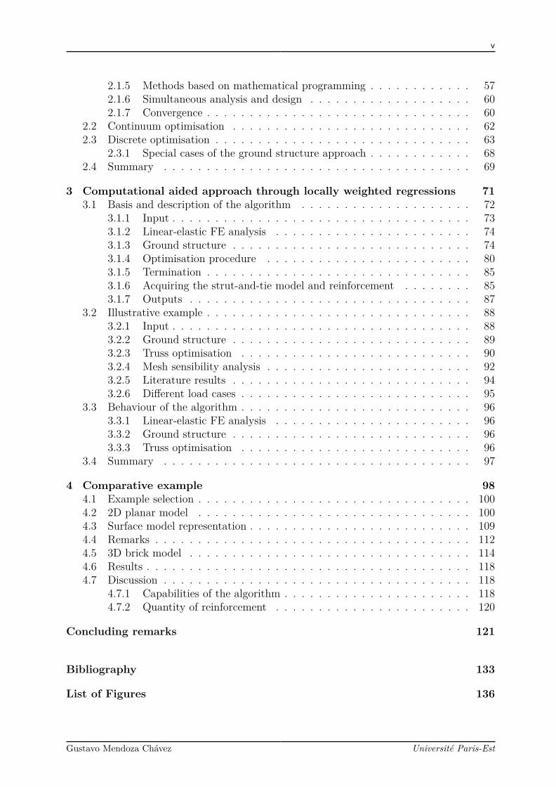
2.1.5 Methods based on mathematical programming . . . . . . . . . . . . 572.1.6 Simultaneous analysis and design . . . . . . . . . . . . . . . . . . . 602.1.7 Convergence . . . . . . . . . . . . . . . . . . . . . . . . . . . . . . . 60

2.2 Continuum optimisation . . . . . . . . . . . . . . . . . . . . . . . . . . . . 622.3 Discrete optimisation . . . . . . . . . . . . . . . . . . . . . . . . . . . . . . 63

2.3.1 Special cases of the ground structure approach . . . . . . . . . . . . 682.4 Summary . . . . . . . . . . . . . . . . . . . . . . . . . . . . . . . . . . . . 69

3 Computational aided approach through locally weighted regressions 713.1 Basis and description of the algorithm . . . . . . . . . . . . . . . . . . . . 72

3.1.1 Input . . . . . . . . . . . . . . . . . . . . . . . . . . . . . . . . . . . 733.1.2 Linear-elastic FE analysis . . . . . . . . . . . . . . . . . . . . . . . 743.1.3 Ground structure . . . . . . . . . . . . . . . . . . . . . . . . . . . . 743.1.4 Optimisation procedure . . . . . . . . . . . . . . . . . . . . . . . . 803.1.5 Termination . . . . . . . . . . . . . . . . . . . . . . . . . . . . . . . 853.1.6 Acquiring the strut-and-tie model and reinforcement . . . . . . . . 853.1.7 Outputs . . . . . . . . . . . . . . . . . . . . . . . . . . . . . . . . . 87

3.2 Illustrative example . . . . . . . . . . . . . . . . . . . . . . . . . . . . . . . 883.2.1 Input . . . . . . . . . . . . . . . . . . . . . . . . . . . . . . . . . . . 883.2.2 Ground structure . . . . . . . . . . . . . . . . . . . . . . . . . . . . 893.2.3 Truss optimisation . . . . . . . . . . . . . . . . . . . . . . . . . . . 903.2.4 Mesh sensibility analysis . . . . . . . . . . . . . . . . . . . . . . . . 923.2.5 Literature results . . . . . . . . . . . . . . . . . . . . . . . . . . . . 943.2.6 Different load cases . . . . . . . . . . . . . . . . . . . . . . . . . . . 95

3.3 Behaviour of the algorithm . . . . . . . . . . . . . . . . . . . . . . . . . . . 963.3.1 Linear-elastic FE analysis . . . . . . . . . . . . . . . . . . . . . . . 963.3.2 Ground structure . . . . . . . . . . . . . . . . . . . . . . . . . . . . 963.3.3 Truss optimisation . . . . . . . . . . . . . . . . . . . . . . . . . . . 96

3.4 Summary . . . . . . . . . . . . . . . . . . . . . . . . . . . . . . . . . . . . 97

4 Comparative example 984.1 Example selection . . . . . . . . . . . . . . . . . . . . . . . . . . . . . . . . 1004.2 2D planar model . . . . . . . . . . . . . . . . . . . . . . . . . . . . . . . . 1004.3 Surface model representation . . . . . . . . . . . . . . . . . . . . . . . . . . 1094.4 Remarks . . . . . . . . . . . . . . . . . . . . . . . . . . . . . . . . . . . . . 1124.5 3D brick model . . . . . . . . . . . . . . . . . . . . . . . . . . . . . . . . . 1144.6 Results . . . . . . . . . . . . . . . . . . . . . . . . . . . . . . . . . . . . . . 1184.7 Discussion . . . . . . . . . . . . . . . . . . . . . . . . . . . . . . . . . . . . 118

4.7.1 Capabilities of the algorithm . . . . . . . . . . . . . . . . . . . . . . 1184.7.2 Quantity of reinforcement . . . . . . . . . . . . . . . . . . . . . . . 120

Concluding remarks 121

Bibliography 133

List of Figures 136

Gustavo Mendoza Chávez Université Paris-Est

vi

List of Tables 137

A Other examples 138A.1 Trimmed deep wall . . . . . . . . . . . . . . . . . . . . . . . . . . . . . . . 138A.2 Trimmed square . . . . . . . . . . . . . . . . . . . . . . . . . . . . . . . . . 140

B Anchorage: different load cases 142B.1 Load eccentricity of 0.75 meters . . . . . . . . . . . . . . . . . . . . . . . . 142

B.1.1 Input . . . . . . . . . . . . . . . . . . . . . . . . . . . . . . . . . . . 142B.1.2 Ground structure . . . . . . . . . . . . . . . . . . . . . . . . . . . . 143B.1.3 Truss optimisation . . . . . . . . . . . . . . . . . . . . . . . . . . . 145B.1.4 Literature results . . . . . . . . . . . . . . . . . . . . . . . . . . . . 146

C 3D strut-and-tie model corbel 147


Introduction

Within the field of Reinforced Concrete (RC) structures and more specifically, at the designof non-flexural elements such as corbels, nibs, and deep beams, the rational procedure ofconception and justification referred as Strut-and-Tie Method (STM) has shown someadvantages over classical algorithms of reinforcement computation based on FE analysis(eg. Wood-Armer or Capra-Maury).

The STM remains a suitable alternative for the design of concrete structures presentingeither elastic or plastic behaviour whose application framework is well defined in concretestructures’ design codes like the EuroCodes and the AASHTO-LRFD Bridge Design Spec-ifications. Nevertheless, this method has the main inconvenient of requiring a high amountof resources investment in terms of highly experienced personal or in terms of computa-tional capacity for, respectively, its manual application or an automatic approach throughtopology optimisation.

The document proposes a light alternative, in terms of required iterations, to the au-tomation of the STM, which starts from the statement that the resultant struts and ties ofa suitable ST model can be distributed according to the direction of the principal stresses,σIII and σI , obtained from a planar or a three-dimensional FE model.

RésuméDans le domaine des structures en Béton Armé (BA) et plus spécifiquement, lors de la con-ception d’éléments non-flexibles tels que les corbeaux, les poutres bayonnetts et les poutresprofondes, la Méthode Bielle-Tirant (MBT) présente des avantages par rapport aux algo-rithmes classiques de calcul de ferraillage basé sur l’analyse FE (par exemple Wood-Armorou Capra-Maury).

La Methode Bielle-Tirant reste une alternative adaptée pour la conception de structuresen béton présentant un comportement élastique ou plastique dont le cadre d’application estbien défini dans les codes de conception des structures en béton comme les EuroCodes et lesspécifications de conception des ponts AASHTO-LRFD. Néanmoins, cette méthode présentel’inconvénient majeur de nécessiter un investissement important en ressources humainesou en capacité de calcul pour, respectivement, son application manuelle ou une approcheautomatique par optimisation de topologie.

Le document propose une alternative légère, en termes d’itérations requises, à l’automa-tisation de la MBT, qui part de l’affirmation que les entretoises résultantes et les attachesd’un modèle ST approprié peuvent être distribuées selon la direction des contraintes prin-cipales, σIII et σI , obtenus à partir d’un modèle préliminaire aux EF.

3

BackgroundIn the industrial context of engineering, most of the structural elements in reinforced con-crete structures are conceived under the Bernoulli and Navier’s hypotheses. Nevertheless,these solutions face problems when treating local non-flexural regions of the structurewhere the strain distribution is significantly nonlinear (corbels, openings, gussets or nearthe surroundings of concentrated loads). Sharp discontinuities can occur in the directionof internal forces and it is imperative to provide a proper reinforcement able resist the ten-sion while being consistent with the pertinent codes in terms of the quantity, distribution,anchorage length, etc. In many cases, standard guides found in the construction manualslike the ACI detailing recommendations or in the EuroCodes fulfil the design but it is upto the structural engineer to decide whether special considerations are or are not needed.

For the exceptional cases, the structural engineer should isolate specific regions, analysethem and provide the required reinforcement computed through a convenient methodology.

The work of Schlaich [Schlaich et al., 1987] describes in detail the use of ST models asa reliable solution to treat the denominated D-regions (where D stands for discontinuity,disturbance or detail). Discontinuity (which is associated with high shear stresses) iseither static (as a result of concentrated loads) or geometric (as a result of abrupt changeof geometry) or both [El-Metwally and Chen, 2017]. In brief, this procedure proposes thatthe real structure should be replaced by a fictitious skeletal structure whose geometryallows keeping the boundary conditions and load case, of the real structure, in such away that it complies with the Bernoulli hypothesis. This can be achieved by imposingan idealised truss-like distribution of inner forces, where the compressive forces are takenby inner concrete bar-type elements (struts) and the tensile forces are taken by the steelreinforcement (ties); a third type of elements, the nodes, connect the struts and ties at theirextremities to assure the interaction between different elements. One of the shortcomingsof the applications of ST models is that, in most of the cases the model should be carriedout through a manual procedure by a highly experienced engineer.

However, the models can also be established through an elastic FE analysis of the wholestructure by considering the direction of the principal stresses along the geometry or, inrecent years, by powerful structural optimisation procedures.

Due to the interest that the STM has taken during the last decades, an effort to automa-tise its application has been done by different research groups all around the world. Com-puter aided approaches such as CAST [Kuchma and Tjhin, 2001], or the one establishedin "Computer graphics in detailing of ST models" [Alshegeir and Ramirez, 1992], proposetools that overlaps images of the direction fields of principal stresses over an interactiveCAD-like interface. The interface allows the user to manually propose a suitable ST modelwhose distribution of elements follows the trajectory of the linear elastic stresses. Thisprocedure simplifies the selection and evaluation of feasible ST systems requiring, however,the intervention of a skilled structural engineer at the earliest stage of the method.

On the other hand, structural optimisation procedures have been also applied to findtruss-like structural configurations out of plain concrete structures. Most commonly ap-plied for aeronautics, optimisation problems can be stated for a large variety of elementsand structures found in the civil engineering field. Current approaches of structural op-timisation are based on iterative Finite Element Analysis (FEA) where, according to itsrepresentation, two approaches can be distinguished:


4

• Continuum optimisation.

• Discrete optimisation.

In the application of continuum optimisation, the structure is discretised into continuumfinite elements such as plates, shells or bricks. The process is focused on determining theoptimal layout through the placement of a given isotropic material within the limits of amaterial domain Ωmat.

Even if some authors believe that optimal ST models can be found starting fromcontinuum-type optimal topology, [Bendsøe et al., 1994, Almeida et al., 2013], the char-acteristics of the discrete and continuum structures are very different, and there is nounified criteria for constructing truss topologies from the results of optimal finite elementsolutions [Starčev-Ćurčin et al., 2013, Baldock and Shea, 2006]: this step relies on empiri-cal selection and experience. Most of the ST models product of this type of optimisationdo not provide mechanism free structures when replaced by their associated truss topology.This can be seen as major drawback with respect of the current constructive guidelinesand codes. In addition, due to the characteristics presented by the interaction concrete-reinforcement and according to some studies, [Swan et al., 1999], a more adequate STmodel would be found through a discrete optimisation.

Another type of applied optimisation is referred as discrete structural optimisation.In this approach, the structure is represented by skeletal systems. Most of the availableliterature establishes the problem of truss optimisation as a ground structure approach,[Bendsøe and Sigmund, 2003], where a group of n joints is proposed and a set, or thetotality, of all the m possible elements connecting the joints are considered to form theinitial truss system. Then, the optimisation process can be established inside an iterativealgorithm where the chosen structure gradually evolves according to predefined criteriaand active constraints at each step. At each iteration, the cross sections can vary and takea value from a given list (discrete variables) or take any possible value between a range(continuous variables) .

As it can be inferred, this type of structural optimisation has been developed for skeletalstructures such as steel trusses but, in recent years, its application has been extended tosolid RC structures through the STM [Muttoni et al., 2015].

Even though the ground structure approach has been proved a powerful tool for com-puting ST models allowing the optimisation to be seen as a relatively simple sizing problem,it arises many difficulties principally related to: 1) the singularity of the stiffness matrix,K, 2) the stability of the optimised structure, and 3) the optimality of the structure perse.

The first complication derives from the fact that, during the optimisation process, theelement cross section, ai, could approach or even reach a zero value, which has obviousrepercussion on the diagonal of the stiffness matrix. To solve it, the possibility of zerocross sections is not permitted and in most cases, an inferior limit, amin, is imposed for ai(ai > 0 or ai ≥ amin).

A non-zero lower bound will generally produce "secondary" elements whose only pur-pose is often only to guaranty the non-singularity condition on the global stiffness matrixand to avoid inner mechanisms on the structure. Such elements are often erased or simplyignored at the last stage of the optimisation, [Ohsaki and Swan, 2002]. This decision im-


5

plies that most optimal designs have a singular matrix and present potential mechanismswhen described as a part of the ground structure leading to the second listed complication.

The third complication is related to the choice of the ground structure itself. Theground structure approach may or may not lead to the optimal structure according tothe group of nodes proposed (quantity and position) and the set of allowed elements; theoptimal structure appears to be limited by the original geometrical restrictions and possibleconnections. An alternative to overcome this difficulty is to treat the coordinates of thestructural nodes as a variable within the optimisation procedure.

Taking also the nodal coordinates as variables allows to adapt the geometry to theboundary may induce improvements in terms of performance or weight reductions. Never-theless, the structure is still strongly dependant on the initial layout: number of elementsand connectivity.

To summarise, regardless the fact that existent procedures are suitable for computingST models, the obtained trusses are still highly dependant on the selected initial trussand, consequently, on the experience of the structural engineer. Even though the selectionof a "good" initial truss could be an easy task for "classic" or well referenced examples,complication arises when dealing with complex load cases (in plane and out of plane loads,multiple loads, displacements, etc.), whimsical geometries or three-dimensional models.

Ideally, a tool intended to find ST models should propose and evaluate truss-like struc-tures keeping the experienced based decisions as minimum as possible. The results mustbe feasible, not only from the point of view of mechanics but also from the point of viewof the construction codes. Additionally to these needs, the results shall be economicallyviable which is an evidence that a sort of optimisation procedure must be involved.

In the context of nuclear civil works, the conception of non-flexural elements (e.g. deepbeam, joints, trimmed walls) has become such a common task that most of the times theydo not receive the detailing that they deserve during their modelling. The design andjustification of these elements is frequently based on force equilibrium along FE modelsbased on shell elements that must be checked for transitions between different thicknesses,gradient in the mesh size, verification of sides-thickness ratios, etc; aspects that couldproduce a diminution in the model accuracy if an exhausting detailing is not executed.

The development of a light computational tool able to threat a large variety of structuralproblems and, also, able to automatically propose optimised reinforcement of concretestructures based on the STM, could represent a huge improvement in the industrial context.The main advantages are listed below:

• Decision support in the design process. Most of the times, decisions in theearlier stages of design are not made based on rigorous justified structural aspects but,they are made based on previous experience or intuition of the engineer. Computer-aided tools can provide non-experienced engineers with a justified insight of complexproblems.

• Automatic analysis and justification of local zones. This is desirable in theearly stages of a project, permitting a wider and more thorough exploration of thedesign space than could be achieved manually.

• Time saving through computer-aided design tools. Within the detailing phase,computer-aided design has the potential to save engineer time by avoiding the need


6

of a layout search trough a manually iterative process. During the post-treatmentphase, the saves in time can be achieved by avoiding manual smoothing of the resultscommonly carried out when using FE based algorithms such as C&M.

• More realistic representations of 3D structures. Compared to models basedon shell and plate elements, ST models (specially 3D ones) represent a more accuraterepresentation of the stress distribution and may lead to a better steel reinforcementdistribution.

• Marketability. The use of optimisation may produce a substantial interest in themarket.

All previously listed advantages may lead to a reduction in engineer-time consumption,computational time and even to a more adequate steel reinforcement distribution.

Whether the advantages may seem quite straightforward, the algorithmic developmentand implementation of a computational tool still must overcome several issues:

• Consistency between rational approaches and optimisation techniques.Whether at first sight the idea of rational approach seems to be incompatible withautomatised iterative procedures, the amalgam between this two ideas should beestablished in order to present an effective STM tool.

• Ill-conditioned results. As mentioned, some design optimisation processes throwresults full of mechanisms when expressed as ST model. However, as it will bediscussed in Chapter 3, discrete optimisation methods are capable of handling suchcomplications if special considerations are made.

• Engineer’s lack of experience and knowledge required to implement opti-misation methods. Most of the available structural optimisation programmes orcomplementary modules require technical and theoretical expertise. This need makesof them a difficult or even an inaccessible tool to structural designers who do not usethem on a regular basis.

• Prohibitive time consumption. Since design time is never unlimited, the opti-misation procedure cannot be allowed to become critical and the amounts of timedevoted to building up a model and parameter adjusting should be small.

• Prohibitive computational cost. The developed algorithm should not requireprohibiting computational efforts.

• Accordance to practical reinforcement layout. Considering that in practice,steel reinforcement is preferred to be placed along principal directions, the resultsmust be easily projected into those reinforcement axis.

• Consistency with current codes of construction and recommendations.Maybe the most important gap to be close, or at least to be reduced, is the disparitybetween the characteristics of the results product of optimisation procedures and therecommendations and thumb rules found in construction codes.


7

This document presents a consistent and rational approach for the generation of Strut-and-Tie models for D-regions in accordance to practical reinforcement layout. The pre-sented approach intends to present a practical alternative for the design of non-flexuralregions.

The research presented in this thesis is motivated by two principal aspects of the currentengineering practice:

1. The concerns regarding the justification of non-flexural elements through FE basedprocedures conceived fundamentally for flexural phenomena.

2. The disparity between the vast volume of academic literature in the field of structuraloptimisation and the low practical application in RC structures.

The core research objective is therefore to contribute towards reducing the evident gapbetween the rational approach known as Strut-and-Tie and automatic applied method-ologies based on finite element analysis industrially applied. The accompanying centralhypothesis is that based on the direction fields of principal stresses, plausible ground struc-tures can be automatically proposed and optimised to create suitable Strut-an-Tie modelsrespecting consideration of industrial specific issues.

The research objective is achieved through the proposal of ground structure constructiontechnique and an investigation of optimisation methods and techniques focusing on discreteFully Stressed Design (FSD) for simultaneous size, topology, and geometric optimisation.

Additionally, the approach proposed within this document is coded in Matlab environ-ment; the developed algorithm is applied and compared to studied cases of elements whoseST models are found in the literature.

Summary of research contributionsA thorough discussion of the research contributions of this thesis, in the context of previouswork, is presented within the concluding chapter. A brief summary is presented in thissection.

• The methods proposed in this work, discussed in chapters 3 and 4, contribute to thedevelopment of an open computational-aided tool addressed to the building industry.

• A straightforward algorithm has been developed to automatically generate feasibleinitial ground structures out of common FE analysis results.

• Examples of application are presented and directly compared to results found in theliterature. Additionally, an example has been performed in order to compare resultswith those expected from an industrial design.

• An efficient discrete optimisation technique, able to point out a suitable ST model,has been adapted to the rational process of layout selection.

• Following the recommendations found in the building codes (specially the EuroCodes), an exhaustive revision of the elements has been performed not only in termsof material resistance but also regarding spacial and size constraints.


8

Thesis structureThis work consists of 5 chapters intended to explore the optimisation of Strut-and-Tiemodels in the structural design of non-flexural zones. Major themes are developed in thiswork and an original contribution is proposed. To guide the reader, before tackling themain subject, a brief introduction is presented at the beginning of each chapter. In thesame spirit, each chapter ends with a discussion of the content. The structure of the thesisis then presented with an overview of each subsequent chapter.

Chapter 1 presents a review and comparison of the state-of-the-art in academic researchand building engineering practice, to explore the analysis and design of non-flexural ele-ments. For this purpose, a list of methods was chosen to be discussed. The selection ofmethods and engineering practices to be discussed was made regarding its appearance inrecent scientific bibliography and its reference or mention in current building codes. Thischapter highlights the main advantages and disadvantages of the selected methods topics.

Chapter 2 explores the vast domain of structural optimisation. This chapter summarisethe optimisation techniques and procedures applied to the optimisation of structures withinthe civil works domain. The text is principally focused on the use of discrete optimisationin the building industry, choice that is justified within the chapter. This area of applicationis not intended to be exclusive, since generality is desirable in any method, but rather toprovide a unifying theme to the distinct elements of this thesis.

Chapter 3 describes and introduces the application of the developed algorithm. Thecomputational aided procedure is dismembered and each step and sub-algorithm is pre-sented. In order to compare the performance of the proposed algorithm, this chapterpresents the results of its application on an example extracted from the literature. At thisstage, the comparison focuses in aesthetic aspects such as quantity of resultant elements,distribution and inclination, geometrical aspects directly related with the optimisation pro-cess and the automatic selection of the initial truss. A parametric study is carried out todisplay the advantages and disadvantages of the application of the proposed methodology.

Chapter 4 presents a case that directly compares the results of the proposed algorithmto those obtained through a model that follows a common engineering practice.

The document concludes by summarising the results of the preceding research anddiscussing future work required in developing these methods.


9

Related workThe computational power of common desktop computers increases every year. This hasbeen one of the main aspects that have brought the use of advanced analysis programs ofresearch institutes closer to the designer in engineering practice. At the same time, thishas impulse the research institutes to develop new techniques and software to better suitthe needs of current practice engineers.

Listed here below are some research programs or research topics that have been devel-oped by different research groups The list, not aiming to be exhaustive, contains notablework that is considered to be related with the main topic of this thesis.

CAD interfaces. The CAST (Computer Aided Strut-and-Tie) program is a graphicallyinteractive design tool developed in the University of Illinois. The program , designedto serve as an instructional device for students and practitioners, guides the user to thestages of the Strut-and-Tie Method. To help the user in the selection of a truss, anelastic finite element analysis feature is being developed to generate stress contours andprincipal stress trajectories. The designer manually defines the truss by first selecting thelocation of the centre of the nodes and then forming truss members by interconnectingthese nodes [Kuchma and Tjhin, 2001]. Similar tools have been developed by differentauthors [Alshegeir and Ramirez, 1992].

SPanCAD is a software for interactive design of shear walls and deep beams of irregulargeometry developed by the Technische Universiteit Delft.

The program SPanCAD is implemented on a finite element program containing onlytwo types of elements: a stringer element (straight bar) and a panel element (rectangle orquadrilateral). According to [Blaauwendraad and Hoogenboom, 2002] SPanCAD is devel-oped to apply the coarsest mesh for a given geometry.

Based on a three design step process that allows to obtain the need of reinforcementfor shear walls, deep beams and cellular structures.

The first step is the construction of the model. Using its experience and rules of thumb,the user builds up the model by placing the stringers and panels within the structure. Thesoftware proceeds to perform the linear-elastic analysis for all load combinations.

In the second step, the user selects the reinforcement based on force flow computed inthe precedent stage. For elements in tension the cross-section area depends on the positionand diameter of the bars. With all input quantities being determined and entered into theprogram, the software performs a nonlinear analysis. The model used accounts for concretecracking in the tensioned stringers and panels. A revision of the steel is performed at thispoint: the reinforcement of the stringers is must remain within the linear-elastic domainwhile the panel reinforcement can yield.

For the third and final step, the user improves the reinforcement using the just computedforce flow and crack widths.

A strut-tie2017 http://astruttie.aroad.co.kr/index.php/advisor/

Stress tubes is an approach developed at the Asian Institute of Technology, Bangkok


10

The described methodology intends to construct suitable Strut-and-Tie models basedon linear-elastic Finite Element models. The "extraction" of the models is based on adirect comparison of every principal direction and pointing out groups of elements pre-senting similar stress trajectories. The following steep deal with the selection of the crosssection. Having identified those groups of elements belonging the same trajectory, all thestress vectors are directed in to vertical direction and scattered along the vertical axis.Then plan area of those scattered points is divided in to grid introducing sufficient gridspacing in which each cell in the grid represent the cross section area of the strut or tie[Dammika and Anwar, 2013].

Stress field topology The stress field method has traditionally been based on the as-sumption of a rigid-plastic stress-strain law without tensile strength for the concrete. Ne-glecting the tensile strength of concrete requires placing a minimal amount of reinforcementfor crack control to ensure a satisfactory behaviour of the structure. This reinforcementensures that no brittle failure occurs at cracking and that the cracks are suitably smearedover the element at the serviceability limit state. The development of stress fields with theprevious assumptions allows a great freedom in the choice of the load-carrying mechanismof a structure.

Continuum structural optimisation techniques. Since early research by Bendsøeand Kikuchi [Bendsøe and Kikuchi, 1988], topology optimisation has been recognized asan important technique to figure out the optimal structure layout within the given de-sign domain. Recently, this technique has been introduced as a most efficient method insearching for optimum structure and Strut-and-Tie optimal patterns.

Micro trusses. Nowadays, several authors intend to implement this method to the RCfield (e.g. [Zhong et al., 2016, Nagarajan et al., 2010]). The micro truss is based on theframework method proposed by [Hrennikoff, 1941], in which the structure is replaced by anequivalent pattern of truss elements. Then, each element is given physical characteristicsaccording to geometrical parameters or through an optimisation procedure with the aimto erase or “deactivate” low stress elements from the structure.


Chapter 1

Design of reinforcement fornon-flexural elements: a review.

In the Civil Engineering field, most of the conventional reinforced concrete structures aredesigned as frame systems. Ascribable to their structural configuration, the geometry ofthe resistant members, and their predominant flexural performance, the global behaviourof a structure can be accurately represented through analytic or numerical models basedon flexural beam theory. For this type of elements, the need of reinforcement can be easilycomputed by determining the internal equilibrium of the resistant forces (given by the steeland concrete) and the resulting system of local forces. On the other hand, at a local scale,zones where the stresses due to shear are predominant over those generated by bending,tend to develop non-flexural elements; in general, these elements are out of the range ofvalidity of beam theory and require a different approach to be implemented.

According to reference [Devadas, 2003], most of the cracks and failures of the structuresoccur due to an inadequate attention to detailing. Often, these problems are located atgeometrical discontinuities such as joints, trims or elements presenting an abrupt changein their thickness but also, in the zones under the effect of exceptional concentrated forces,case of corbels and nibs. In such situations, complex stress states arise and must be takeninto account while designing the reinforcement.

As in all other zones of a structure, the main requirements are that all the existingforces from the surroundings could be safely transmitted to the supporting members and/orfoundations. Sharp discontinuities can occur in the direction of internal forces and it isimperative to provide a proper reinforcement able resist the tension while being consistentwith the pertinent codes in terms of the quantity, distribution, anchorage length, etc.

In many cases, standard guides found in the construction manuals like the ACI detailingrecommendations or in the EuroCodes fulfil the design but it is up to the structural engineerto decide whether special considerations are or are not needed.

For the exceptional cases, the structural engineer should isolate specific regions, analysethem and provide the required reinforcement computed through a convenient methodology.

In this chapter are discussed some of the most widely used methodologies for the designof the reinforcement at non-flexural elements and, more generally, applied at disturbedregions. The first section briefly treats the theory applied to the design of common elementsand behaviour hypothesis. The second section addresses to the use of the FEM for thestructural design. Finally, the Strut-and-Tie method is presented in the third section.

12

Dimensionement des armatures pour des éléments non-soumis aux effets de flexion.Dans le domaine du génie civil, la plupart des structures conventionnelles en béton armésont conçues comme des systèmes de portiques. Compte tenu de leur configuration struc-turelle, de la géométrie des éléments résistants et de leur performance prédominante enflexion, le comportement global d’une structure peut être représenté avec précision à l’aidede modèles analytiques ou numériques basés sur la théorie de la flexion. Pour ce typed’éléments, le besoin de renforcement par armatures noyées peut être facilement calculé endéterminant l’équilibre interne des sections résistantes (acier et béton) et le système résul-tant des forces locales. D’autre part, à l’échelle locale, les zones où les contraintes dues aucisaillement sont prédominantes par rapport à celles générées par la flexion ont tendanceà développer des éléments non flexibles ; en général, la théorie des poutres ne s’appliquantpas à ces éléments, leur traitement nécessite de mettre en oeuvre une approche différente.

Selon [Devadas, 2003], la plupart des fissures et des défaillances des structures se pro-duisent en raison d’une attention insuffisante aux détails. Souvent, ces problèmes sontlocalisés dans des discontinuités géométriques telles que des joints, des remplissages oudes éléments présentant un changement brusque de leur épaisseur mais aussi sous l’effetde forces concentrées exceptionnelles dans les zones de liaisons comme les corbeaux et lesbaïonnettes. Des états de contraintes complexes apparaissent et doivent être pris en comptelors de la conception du ferraillage.

Comme dans toutes autres zones d’une structure, les forces existantes doivent être trans-mises aux éléments de support et/ou aux fondations en limitant la concentration de con-traintes. De fortes discontinuités peuvent ainsi se produire suivant la direction des effortsinternes. Il est alors impératif de prévoir un ferraillage approprié capable de résister à latraction tout en étant cohérent avec les codes pertinents en termes de quantité, de distri-bution, d’ancrage, etc.

Dans la plupart des cas, les guides trouvés dans les manuels de construction comme lesrecommandations de l’ACI ou dans les EuroCodes répondent à la conception, mais il estde la responsabilité de l’ingénieur structure de décider si des considérations spéciales sontou non nécessaires.

Pour les cas exceptionnels et suivant les recommandations faites dans la littérature telleque [Schlaich et al., 1987] et [Hsu, 1992], l’ingénieur structure devrait isoler des régionsspécifiques, les analyser et dimensionner le ferraillage au moyen d’une méthodologie ap-propriée.

Dans ce travail de recherche sont discutées certaines des méthodologies les plus large-ment utilisées pour la conception du ferraillage de renforcement des éléments non travail-lant en flexion et, plus généralement, les approches mises en oeuvre dans les régions ditesperturbées. La première section traite brièvement de la théorie appliquée à la conceptiond’éléments communs et des hypothèses de comportement. La deuxième section porte surl’utilisation de la méthode des Éléments Finis pour la conception structurelle. Pour finir,la méthode bielle-tirant est présentée.


13

1.1 Reinforced concrete elementsA structure can be defined as a well-organised load-bearing system composed by a set ofproperly connected elements intended to withstand forces. On the other hand, ReinforcedConcrete (RC) is a composite material in which concrete’s relatively low tensile strength iscounteracted by the inclusion of reinforcement (commonly steel bars). Thus, a reinforcedconcrete structure can be seen as an organised system formed of individual compositeelements made up of concrete and steel that, properly connected, display an adequateload-bearing capacity, stiffness, deformability and energy-dissipating capacity.

Most reinforced concrete structures can be subdivided into beams, slabs, and columns;beams and slabs are elements subjected primarily to flexure (bending) while columns aregenerally subjected to axial compression and bending. In addition to this subdivision, thenon-flexural elements can be pointed out as elements whose behaviour does not correspondto neither flexion nor compression.

The combination of the bending and shear loads produces maximum normal and shear-ing stresses in a specific plane inclined with respect to the global axis of the structure. Ina 3 point bending test, the principal stress in tension acts at an approximately along a 45oplane to the normal at sections close to the supports. Due to the low tensile strength ofconcrete material, diagonal cracking develops along planes perpendicular to the plane ofprincipal tensile stress. These are zones where shear failure, or strictly speaking diagonaltension failure, governs over flexural or compressive ones; hence special considerations musttake place while designing.

1.1.1 Flexure theory for reinforced concreteAmong all the phenomena concerning RC structures, the flexural behaviour (moment ver-sus curvature relationship) is one of the most well studied. The theory of flexure thatallows the analyse of the resistance of a reinforced concrete beam, is based in three basicassumptions:

• Plane sections, perpendicular to the axis of bending, remain plane.

• The strain in the concrete is equal to the strain in the reinforcement at the samelevel.

• The stresses along the element can be computed from the strains by using stress-strain curves for each individual material (concrete and steel).

Few words must be said about the above assumptions. The first one is the traditional“plane sections remain plane” assumption made in Euler-Bernoulli theory for beams madeof any material. The second assumption implies a perfect bonding condition between theconcrete and the steel

The third assumption needs to be attached to reference stress-strain relationships likethe ones depicted in figure 1.1. Concrete model generally consists of a parabola (equations1.1) from zero stress to the compressive strength of the concrete. The strain that corre-sponds to the peak compressive stress, ε0, is often assumed to be 0.002 for normal strengthconcrete.


14

A

Idealised

B

Design

s

e

kfyk

fyk

fyd

fydE

s

eud

euk

(a) Assumed steel reinforcement stress-strain

ec2

ec 2u

ee

c3

ec 3u

f

f

cd

ck

sc

0

A

Bi-linear

diagram

B

Parabola-rectangle

diagram

(b) Assumed concrete stress-strain for thedesign of cross-sections

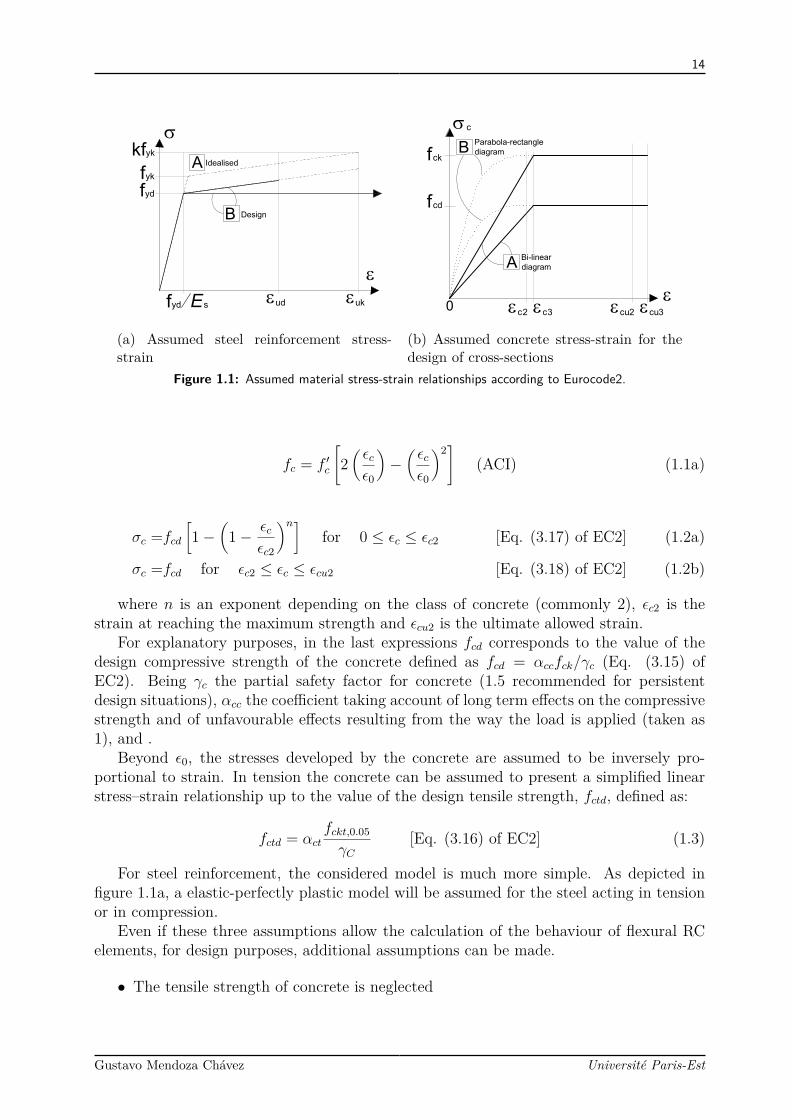
Figure 1.1: Assumed material stress-strain relationships according to Eurocode2.

fc = f ′c

[2(εcε0

)−(εcε0

)2]

(ACI) (1.1a)

σc =fcd[1−

(1− εc

εc2

)n]for 0 ≤ εc ≤ εc2 [Eq. (3.17) of EC2] (1.2a)

σc =fcd for εc2 ≤ εc ≤ εcu2 [Eq. (3.18) of EC2] (1.2b)

where n is an exponent depending on the class of concrete (commonly 2), εc2 is thestrain at reaching the maximum strength and εcu2 is the ultimate allowed strain.

For explanatory purposes, in the last expressions fcd corresponds to the value of thedesign compressive strength of the concrete defined as fcd = αccfck/γc (Eq. (3.15) ofEC2). Being γc the partial safety factor for concrete (1.5 recommended for persistentdesign situations), αcc the coefficient taking account of long term effects on the compressivestrength and of unfavourable effects resulting from the way the load is applied (taken as1), and .

Beyond ε0, the stresses developed by the concrete are assumed to be inversely pro-portional to strain. In tension the concrete can be assumed to present a simplified linearstress–strain relationship up to the value of the design tensile strength, fctd, defined as:

fctd = αctfckt,0.05

γC[Eq. (3.16) of EC2] (1.3)

For steel reinforcement, the considered model is much more simple. As depicted infigure 1.1a, a elastic-perfectly plastic model will be assumed for the steel acting in tensionor in compression.

Even if these three assumptions allow the calculation of the behaviour of flexural RCelements, for design purposes, additional assumptions can be made.

• The tensile strength of concrete is neglected


15

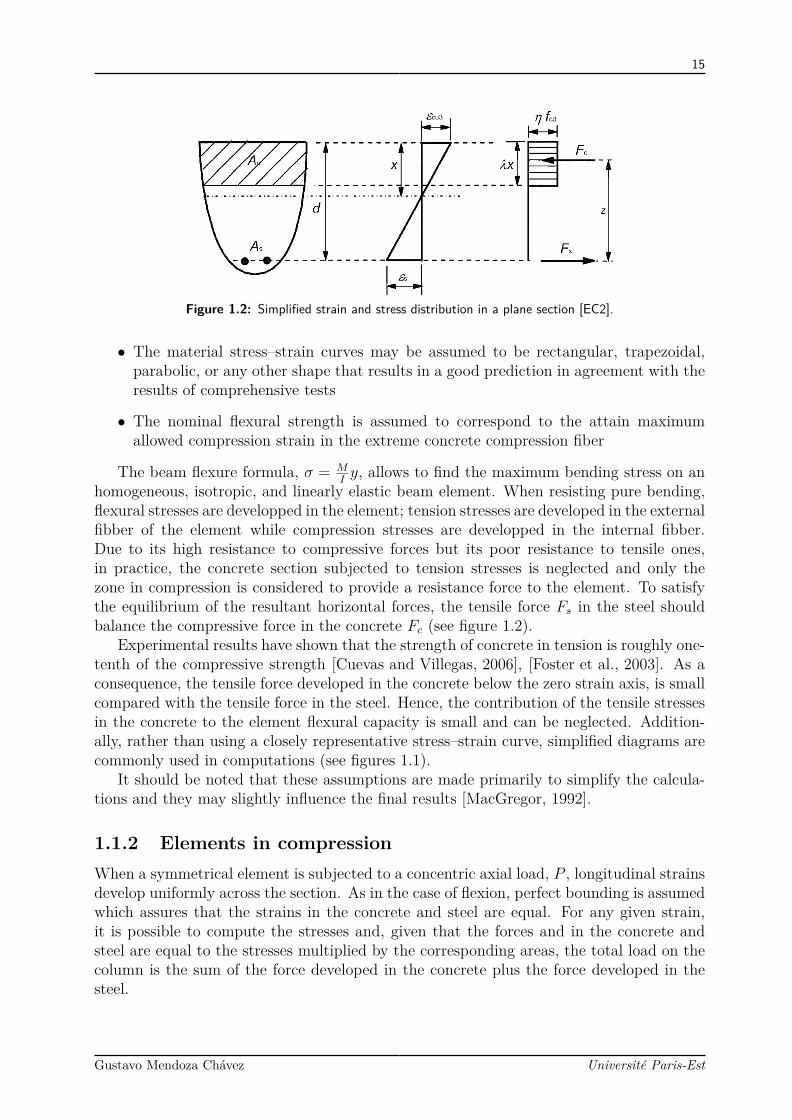
Figure 1.2: Simplified strain and stress distribution in a plane section [EC2].

• The material stress–strain curves may be assumed to be rectangular, trapezoidal,parabolic, or any other shape that results in a good prediction in agreement with theresults of comprehensive tests

• The nominal flexural strength is assumed to correspond to the attain maximumallowed compression strain in the extreme concrete compression fiber

The beam flexure formula, σ = MIy, allows to find the maximum bending stress on an

homogeneous, isotropic, and linearly elastic beam element. When resisting pure bending,flexural stresses are developped in the element; tension stresses are developed in the externalfibber of the element while compression stresses are developped in the internal fibber.Due to its high resistance to compressive forces but its poor resistance to tensile ones,in practice, the concrete section subjected to tension stresses is neglected and only thezone in compression is considered to provide a resistance force to the element. To satisfythe equilibrium of the resultant horizontal forces, the tensile force Fs in the steel shouldbalance the compressive force in the concrete Fc (see figure 1.2).

Experimental results have shown that the strength of concrete in tension is roughly one-tenth of the compressive strength [Cuevas and Villegas, 2006], [Foster et al., 2003]. As aconsequence, the tensile force developed in the concrete below the zero strain axis, is smallcompared with the tensile force in the steel. Hence, the contribution of the tensile stressesin the concrete to the element flexural capacity is small and can be neglected. Addition-ally, rather than using a closely representative stress–strain curve, simplified diagrams arecommonly used in computations (see figures 1.1).

It should be noted that these assumptions are made primarily to simplify the calcula-tions and they may slightly influence the final results [MacGregor, 1992].

1.1.2 Elements in compressionWhen a symmetrical element is subjected to a concentric axial load, P , longitudinal strainsdevelop uniformly across the section. As in the case of flexion, perfect bounding is assumedwhich assures that the strains in the concrete and steel are equal. For any given strain,it is possible to compute the stresses and, given that the forces and in the concrete andsteel are equal to the stresses multiplied by the corresponding areas, the total load on thecolumn is the sum of the force developed in the concrete plus the force developed in thesteel.


16

(a) Bending. (b) Diagonal tension. (c) Shear.

Figure 1.3: Failure patterns as a function of beam slenderness [Nawy, 2000].

This additional contribution of the resistance can be approached as the product ofthe steel transverse, as, area multiplied by the yielding stress, σy. Hence, the maximumresisting load, P0, that a prismatic concrete section reinforced with longitudinal steel candevelop is given by:

P0 = φσcac + asσy (1.4)where ac represents the concrete’s cross section and φ is reduction factor that takes into

account geometric imperfections.In real structures is not common to find elements working under pure compressive

actions. Due to accidental eccentricity in addition to the fact that almost every structureis continuous, the axial loading and bending moments are considered together. Mostdesign codes recommend to take into consideration the effects of elements subjected toflexo-compression even if the structural analysis points out zero bending forces.

1.1.3 Elements resisting to diagonal tension and shearAs depicted in the last paragraphs, the behaviour of a simply supported reinforced concretebeam under bending effects produce compressive stresses above the neutral axis and tensionstresses under it. The maximum bending moment is found under the centroid of theloading. Its intensity decreases toward the supports and the shear stress increases. Themajor principal stress acts along a plane tilted approximately 45o to the normal at sectionsclose to the support. Due to the concretes low tensile resistance, diagonal cracking isformed perpendicular to the tension stresses. To prevent this cracks, diagonal tensionreinforcement has to be provided.

Diagonal tension failure, figure 1.3b, occurs in elements where the shear span/depthratio is of an intermediate "magnitude" (a/d between 2.5 and 5.5). For smaller shearspan/depth ratios (a/d between 1 to 2.5) the failure is mainly attributed to shear ( figure1.3c).

Considering the true nature of the concrete as a non-elastic and a non-homogeneousmaterial, the intricacy of the problem increases and consequently, the behaviour of RC ele-ments become more complex than previously explained. The stress distribution is modifiedonce the concrete’s tensile capacity is reached and cracking starts. Some characteristicssuch as position and length of the fissures cannot be accurately predicted due to localresistance variations within the matrix of the concrete. Due to this difficulty, it must beadded the fact that the concrete is not an elastic material and, in consequence, the stressdistribution changes for different level of loading.


17

M

S S S S

a q

(a) Observed cracking pattern.

aqT+ T

T

F

c

a

v

f

s

D

(b) Truss like behaviour.Figure 1.4: Ritter’s truss analogy.

Owing to the complexity of the problem, the current methods used for designingRC elements undergoing shear are based on the results of experimental campaigns (e.g[Mattock et al., 1976] and [Aguilar et al., 2002]). Those campaigns are principally focusedon determining the concrete resistance against diagonal cracking and the contribution ofthe transverse reinforcement to the global resistance

In an attempt to predict the behaviour of elements governed by shear, Ritter [Ritter, 1899]proposed that reinforced beam presenting inclined fissures can be idealised as a truss wherethe longitudinal reinforcement acts as a tensile chord, the transverse reinforcement acts aswebs withstanding traction and, finally, the segments of concrete between the principalcracks idealised as the webs in compression. This idealisation is depicted in figure 1.4.

The premises considered are the following:

• The element’s compressed zone develops only normal compressive stresses

• All transverse traction is resisted by the transverse reinforcement

• The fissures extend from the lowest fibber to the centroid of the compressed zone

• The self weight is neglected and distributed loads acting between cracks. In otherwords, the increment in the shear, ∆V , of two sections is given by Vs where V isthe shear force in the zone between the two considered sections and s is the distanceseparating them.

The analogy considers an angle θ measured between the crack pattern and the elementaxis, and an angle α that corresponds to inclination of the transverse reinforcement alsocompared to the element axis. In accordance to figure 1.4, the horizontal spacing betweeninclined cracks and the stirrups is denoted by s. The compression force at the concretediagonal is Fc and the traction acting at the diagonal reinforcement is given by avfs (beingav the cross section of the transverse reinforcement and fs the force acting on it)

As result of the increment in the bending moment, ∆M , an increment in the longitu-dinal tension, ∆T is also produced. From the equilibrium over the vertical and horizontalforces it is found that the maximum shear force, Vmax, is given by:


18

Vmax = avσyz

s

[cosα + sinα

cos θ

](1.5)

where av represents the available shear reinforcement presenting; an array of individualstirrups separated a distance s and tilted an angle α. σy represents the steel’s yield limit,z lever arm (distance between the centroids of compressive and tensile chords), and T isthe force of traction acting on the longitudinal steel.

From the latter expression, it can be deduced that, if the load capacity of an elementis directly dependant on its resistance to inclined stresses, the maximum admissible loadcorresponds to the development of the yielding stress at the stirrups or the transversereinforcement. This implies that both parts, the concrete forming the compression cordsas well the reinforcement forming the tension ones, must be able to withstand the forceincrements originated by the crack evolution.

The truss analogy has been used to estimate the shear resistance of elements withtransverse reinforcement. For practical purposes and with the aim of obtaining a good cor-relation between the calculated resistance and the experimental tests [Turmo et al., 2009][Rao et al., 2007], the resulting admissible load has been expressed as the addition of thecomputed resistance plus the resistance of the element supposing no transverse reinforce-ment. As expressed, this resolution achieves good correlation but lacks of theoreticalframework [Grandić et al., 2015].

Some authors have proposed modifications to the original truss model like taking intoaccount important factors such as the angle of cracks, transverse deformations, fan-shaped-crack pattern, normal stress continuity along cracks to cite some of them but such modifi-cations have not been included in the design codes [for Structural Concrete, 2008] and willnot be detailed in this document.

Given that vertical shear force has been taken to be a good indicator of diagonaltension, diagonal tensile forces are not calculated for most of the structural elements. Forflexural elements requiring design shear reinforcement, the EuroCodes bases its hypothesison the truss model. Nevertheless, for beams with loads near to supports, corbels and anyelement where a non-linear strain distribution exist this codes suggest to apply strut-and-tiemodels.

1.2 Finite element models for RC structuresComputer-based analysis and design for RC structures, have seen tremendous advancementin the last half-century and its application has become a common step in most structuralengineering companies. Nowadays, elastic based stress analysis using finite element method(FEM) is a reliable tool to model any conceivable structure with acceptable precision[Bathe, 2006] allowing various degrees of sophistication. Some of the advantages of the useof FEM for structural design are:

• Numerous FEM freeware and shareware software packages conceived for structuraldesign and analysis are available.

• Linear FE modelling is well established and, nowadays, relatively easy to apply.


19

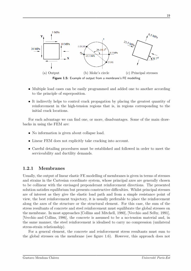
(a) Output (b) Mohr’s circle (c) Principal stressesFigure 1.5: Example of output from a membrane’s FE modelling

• Multiple load cases can be easily programmed and added one to another accordingto the principle of superposition.

• It indirectly helps to control crack propagation by placing the greatest quantity ofreinforcement in the high-tension regions that is, in regions corresponding to theinitial crack locations.

For each advantage we can find one, or more, disadvantages. Some of the main draw-backs in using the FEM are:

• No information is given about collapse load.

• Linear FEM does not explicitly take cracking into account.

• Careful detailing procedures must be established and followed in order to meet theserviceability and ductility demands.

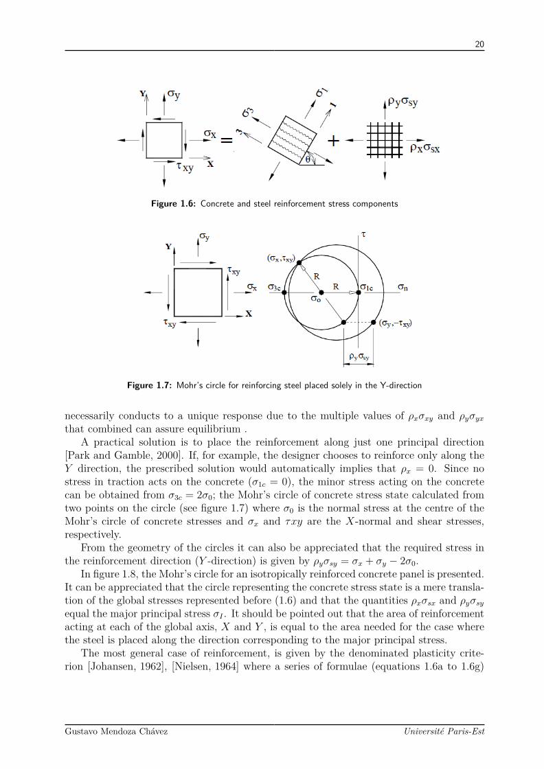
1.2.1 MembranesUsually, the output of linear elastic FE modelling of membranes is given in terms of stressesand strains in the Cartesian coordinate system, whose principal axes are generally chosento be collinear with the envisaged preponderant reinforcement directions. The presentedsolution satisfies equilibrium but presents constructive difficulties. Whilst principal stressesare of interest as they give the elastic load path and from a simple resistance point ofview, the best reinforcement trajectory, it is usually preferable to place the reinforcementalong the axes of the structure or the structural element. For this case, the sum of thestress resultants of concrete and steel reinforcement must equilibrate the global stresses onthe membrane. In most approaches [Collins and Mitchell, 1980], [Vecchio and Selby, 1991],[Vecchio and Collins, 1986], the concrete is assumed to be a no-tension material and, inthe same manner, the steel reinforcement is idealised to carry no compression (unilateralstress-strain relationship).

For a general element, the concrete and reinforcement stress resultants must sum tothe global stresses on the membrane (see figure 1.6). However, this approach does not


20

Figure 1.6: Concrete and steel reinforcement stress components

Figure 1.7: Mohr’s circle for reinforcing steel placed solely in the Y-direction

necessarily conducts to a unique response due to the multiple values of ρxσxy and ρyσyxthat combined can assure equilibrium .

A practical solution is to place the reinforcement along just one principal direction[Park and Gamble, 2000]. If, for example, the designer chooses to reinforce only along theY direction, the prescribed solution would automatically implies that ρx = 0. Since nostress in traction acts on the concrete (σ1c = 0), the minor stress acting on the concretecan be obtained from σ3c = 2σ0; the Mohr’s circle of concrete stress state calculated fromtwo points on the circle (see figure 1.7) where σ0 is the normal stress at the centre of theMohr’s circle of concrete stresses and σx and τxy are the X-normal and shear stresses,respectively.

From the geometry of the circles it can also be appreciated that the required stress inthe reinforcement direction (Y -direction) is given by ρyσsy = σx + σy − 2σ0.

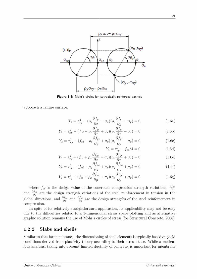
In figure 1.8, the Mohr’s circle for an isotropically reinforced concrete panel is presented.It can be appreciated that the circle representing the concrete stress state is a mere transla-tion of the global stresses represented before (1.6) and that the quantities ρxσsx and ρyσsyequal the major principal stress σI . It should be pointed out that the area of reinforcementacting at each of the global axis, X and Y , is equal to the area needed for the case wherethe steel is placed along the direction corresponding to the major principal stress.

The most general case of reinforcement, is given by the denominated plasticity crite-rion [Johansen, 1962], [Nielsen, 1964] where a series of formulae (equations 1.6a to 1.6g)


21

Figure 1.8: Mohr’s circles for isotropically reinforced pannels

approach a failure surface.

Y1 = τ 2xy − (ρx

∂fyt∂x− σx)(ρy

∂fyt∂y− σy) = 0 (1.6a)

Y2 = τ 2xy − (fcd − ρx

∂fyt∂x

+ σx)(ρx∂fyt∂x− σx) = 0 (1.6b)

Y3 = τ 2xy − (fcd − ρy

∂fyt∂y

+ σy)(ρy∂fyt∂y− σy) = 0 (1.6c)

Y4 = τ 2xy − fcd/4 = 0 (1.6d)

Y5 = τ 2xy + (fcd + ρx

∂fyc∂x

+ σx)(ρx∂fyc∂x

+ σx) = 0 (1.6e)

Y6 = τ 2xy + (fcd + ρy

∂fyc∂y

+ σy)(ρy∂fyc∂y

+ σy) = 0 (1.6f)

Y7 = τ 2xy + (fcd + ρx

∂fyc∂y

+ σx)(ρx∂fyc∂y

+ σy) = 0 (1.6g)

where fcd is the design value of the concrete’s compression strength variations, ∂fyt

∂x

and ∂fyt

∂yare the design strength variations of the steel reinforcement in tension in the

global directions, and ∂fyc

∂xand ∂fyc

∂yare the design strengths of the steel reinforcement in

compression.In spite of its relatively straightforward application, its applicability may not be easy

due to the difficulties related to a 3-dimensional stress space plotting and as alternativegraphic solution remains the use of Mohr’s circles of stress [for Structural Concrete, 2008].

1.2.2 Slabs and shellsSimilar to that for membranes, the dimensioning of shell elements is typically based on yieldconditions derived from plasticity theory according to their stress state. While a meticu-lous analysis, taking into account limited ductility of concrete, is important for membrane


22

elements design, there is much less concern with shells since such structures are typicallyunder-reinforced [for Structural Concrete, 2008]. In other words, the failure of this kindof elements is governed by yielding of the reinforcement bars and not by crushing at theconcrete section. An important exception can be mentioned about concentrated trans-verse forces, that may result in brittle punching failures without transverse reinforcement[Unnikrishna and Devdas, 2003].

As expressed before, placing the steel bars aligned with the principal (major) stressdirection could minimise the quantity of required reinforcement for shell elements. Theso-called “trajectory reinforcement” has been applied to several slab and shell structuresin the past [?]. However, if several different load-cases must be considered, the principalstress directions may vary from one case to another thus, making impossible to align thereinforcement. For these and other constructibility reasons mentioned before, orthogonalreinforcement is provided in almost all slabs and shell structures.

The output of a shell element consists in eight independent stress resultants: bendingand twisting moments (Mxx, Myy Mxy, and Myx), transverse shear forces (Txz and Tyz)and membrane forces (Nxx, Nyy, and Nxy) 1.10a. By applying equilibrium equations overthe body, it can be stated that:

∂Txz∂x

+ ∂Tyz∂y

+ q = 0 (1.7a)

∂Mxx

∂x+ ∂Mxy

∂y− Txz = 0 (1.7b)

∂Myy

∂y+ ∂Myx

∂x− Tyz = 0 (1.7c)

Moment equilibrium equations yields to:

Mn = Mxx cos2 φ+Myy sin2 φ+Mxy sin 2φ (1.8a)Mt = Mxx sin2 φ+Myy cos2 φ−Mxy sin 2φ (1.8b)Mnt = (Myy −Mxx) sinφ cosφ+Mxy cos 2φ (1.8c)

This last group equations can be interpreted as the transformation of bending andtwisting moments acting on any boundary perpendicular to the direction n, where theorientation is determined by the angle φ. Analogously, the equations for the equilibriumof the forces acting on the slab elements yields to the transformation of transverse shearforces perpendicular to n are given by equations 1.9.

Vn = Txz cosφ+ Tyz sinφ (1.9a)Vt = −Txz sinφ+ Tyz cosφ (1.9b)

1.2.2.1 Normal moment yield criterion

For a given simply supported concrete slab, subjected to a distributed service load, theresponse is expected to remain within the elastic domain with the maximum level of stresses


23

(a) Onset of yielding of bottom reinforce-ment at point of maximum deflection (b) The formation of a mechanism

Figure 1.9: Simply supported two-way slab with the bottom steel having yielded along the yield lines

at steel reinforcement and maximum deflection occurring at the centre of the element. Atthis stage, negligible cracking may occur at the lower layer, zone where the concrete’stensile capacity will be exceed due to the forces carried out by flexural behaviour (figureA.6c). Increasing the load beyond the service limit, will increase the size and depth of thecracks and may induce the yielding of the reinforcement. Increasing the load still further,will propagate the cracks to the free edges of the element generating the yielding lines tocross all reinforcing bars. At this ultimate state, the yield lines form boundaries and allowrotation between the rigid or "intact" parts, thus creating mechanisms and the instabilityof the element (figure 1.9b).

The ultimate load of concrete slabs and shells has been investigated by consideringlocal stresses and strains within the element and their corresponding yield conditions underthe basis of plasticity theory and flow rules for concrete and for the inner reinforcement[Nilson, 1997]. This approach gives accurate results for almost any case but its applicationis rarely justified.

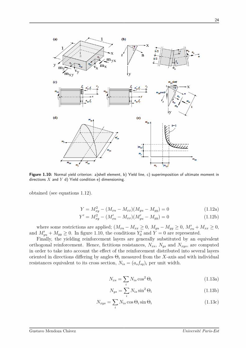
By superimposing the ultimate shell’s moments Mxu and Myu along the global rein-forcement directions and setting Mxy, Nxx, and Nyy equal to zero, a simplified staticallyadmissible state of stress is obtained. Now, for an arbitrary direction n, and based onequations 1.8, it can be stated that Nn = Ntn = 0, Mn = Mxu cos2 φ + Myu sin2 φ andMtn = (Myu −Mxu) sinφ cosφ. For most cases, the resultant depths of the compressionzone in the concrete section do not coincide for the two orthogonal directions, cx 6= cy. Asa result, there is no development of compatible mechanism (figure 1.10c). The differencebetween the value obtained for Mn and the value of Mnu for cx 6= cy have been found of anegligible order leading to:

Mnu = Mxu cos2 φ+Myu sin2 φ (1.10)

M ′nu = M ′

xu cos2 φ+M ′yu sin2 φ (1.11)

From equations 1.8, a state of stress in terms of Mxx, Myy, and Mxy corresponds tobending and twisting moments in direction n is given by Mn = Mxx cos2 φ + Myy sin2 φ +Mxy sin(2φ). From combining these previous expressions with the inequality condition,−Myu ≤Mn ≤Myu, the yield conditions for orthogonally reinforced shell elements can be


24

Figure 1.10: Normal yield criterion: a)shell element, b) Yield line, c) superimposition of ultimate moment indirections X and Y d) Yield condition e) dimensioning.

obtained (see equations 1.12).

Y = M2xy − (Mxu −Mxx)(Myu −Myy) = 0 (1.12a)

Y ′ = M2xy − (M ′

xu −Mxx)(M ′yu −Myy) = 0 (1.12b)

where some restrictions are applied; (Mxu−Mxx ≥ 0, Myu−Myy ≥ 0, M ′xu +Mxx ≥ 0,

and M ′yu +Myy ≥ 0. In figure 1.10, the conditions Y ′0 and Y = 0 are represented.

Finally, the yielding reinforcement layers are generally substituted by an equivalentorthogonal reinforcement. Hence, fictitious resistances, Nxs, Nys and Nxys, are computedin order to take into account the effect of the reinforcement distributed into several layersoriented in directions differing by angles Θi measured from the X-axis and with individualresistances equivalent to its cross section, Nis = (asfsy)i per unit width.

Nxs =∑i

Nis cos2 Θi (1.13a)

Nys =∑i

Nis sin2 Θi (1.13b)

Nxys =∑i

Nis cos Θi sin Θi (1.13c)


25

N

xx

N

xy

T

xz

T

yz

N

yx

N

yy

M

xx

M

yy

d

v

(a) Shell element

d

v

T

xz

T

yz

M

xx

N

xx

d

v

2

+

M

yy

N

yy

d

v

2

+

M

xy

N

xy

d

v

2

+

M

xy

N

xy

d

v

2

-

M

xx

N

xx

d

v

2

+-

(b) Shell element

d

v

V

0

1

V

0

cotq2

V

0

cotq2

q

d

v

cotq

V

0

cotq

V

0

cotqV

0

(c) Shell elementFigure 1.11: Sandwich model.

Due to its simplicity, the normal yield criterion is widely used for the design of concreteslabs in current practice [Kennedy and Goodchild, 2004]. Nevertheless, this method is notconceived for elements presenting excessive reinforcement ratios [Marti, 1978].

1.2.2.2 Sandwich model for shell elements

This model idealises the behaviour of a slab, or a shell, section as the interaction of threecomplementary elements [Marti, 1990]. The covers withstand the bending and twistingmoments (Mxx,Myy,Mxy) as well as the in-plane forces (Nxx, Nyy, Nxy) while the transverseshear forces (Txz, Tyz) are resisted by the core as depicted in figure 1.11.

The middle planes of the covers are taken to coincide with the middle planes of thereinforcing meshes close to the element surfaces. Assuming equal cover thickness, c, atboth sides of the element, the resultant lever arm of the developed inplane forces at thecovers, d, is equal to the effective shear depth of the core, dv.

In general, the model considers the principal transverse shear force to be transferredonly by core, V0 =

√Txz + Tyz along direction φ0 = tan−1(Txz/Tyz). If the nominal shear

stress, Vo/dv is below the nominal concrete’s shear cracking, τC,red, the core is consideredto be uncracked and the forces at the covers are given by:

Nx inf,sup = ±Mxx

dv+ Nxx

2 (1.14a)

Ny inf,sup = ±Myy

dv+ Nyy

2 (1.14b)

Nxy inf,sup = ±Mxy

dv+ Nxy

2 (1.14c)

On the contrary, if the shear stress exceeds the nominal concrete’s shear cracking resis-tance, the core fissures and is treated as the web of a girder of flanged cross-section alongdirection φ0 (figure 1.11). The inclination produces tensile forces that must be resisted bythe covers modifying equations 1.14 as follows:


26

Nx inf,sup = ±Mxx

dv+ Nxx

2 + Txz2V0 tan θ (1.15a)

Ny inf,sup = ±Myy

dv+ Nyy

2 + Tyz2V0 tan θ (1.15b)

Nxy inf,sup = ±Mxy

dv+ Nxy

2 + TxzTyz2V0 tan θ (1.15c)

For cases where the concrete remains elastic and the failure is governed by yielding ofthe reinforcement, the force per unit width acting at the reinforcement in the X and Ydirections can be determined by:

aSXσy ≥Mxx

dv+ Nxx

2 + Txz2V0 tan θ + k

∣∣∣∣Mxy

dv+ Nxy

2 + TxzTyz2V0 tan θ

∣∣∣∣ (1.16a)

aSY σy ≥Myy

dv+ Nyy

2 + Tyz2V0 tan θ + k−1

∣∣∣∣Mxy

dv+ Nxy


∣∣∣∣ (1.16b)

a′SXσy ≥−Mxx

dv+ Nxx

2 + Txz2V0 tan θ + k′

∣∣∣∣−Mxy

dv+ Nxy


∣∣∣∣ (1.16c)

a′SY σy ≥−Myy

dv+ Nyy

2 + Tyz2V0 tan θ + k′−1

∣∣∣∣−Mxy

dv+ Nxy


∣∣∣∣ (1.16d)

where a k and k′ are arbitrary positive factors (normally taken equal to 1), θ is theinclination of the diagonal compression, as and a′s are the bottom and top reinforcementareas per unit width.

For the case where the core is cracked, the need of transverse reinforcement ratio iscomputed by ρ = V0 tan θ

dvσy. For the opposite case, the terms containing Txz or Tyz can be

ignored from equations 1.16 and it is assumed that no transverse shear reinforcement isneeded.

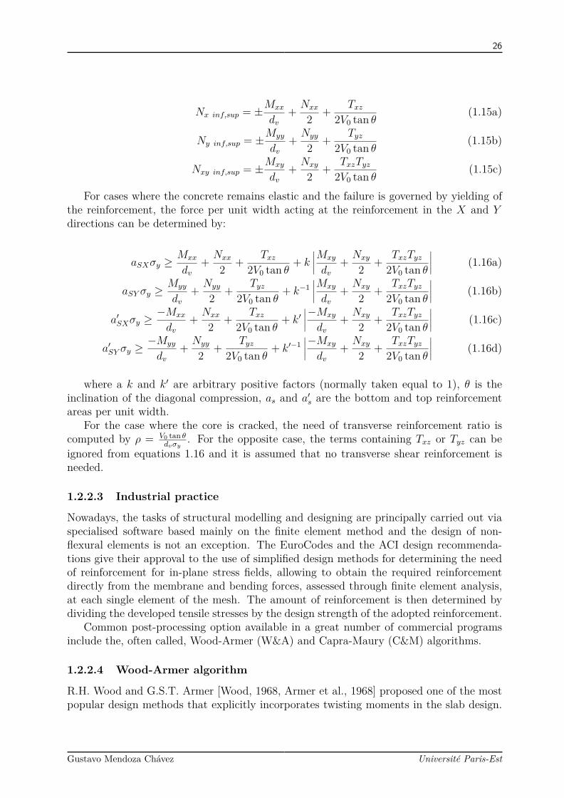
1.2.2.3 Industrial practice

Nowadays, the tasks of structural modelling and designing are principally carried out viaspecialised software based mainly on the finite element method and the design of non-flexural elements is not an exception. The EuroCodes and the ACI design recommenda-tions give their approval to the use of simplified design methods for determining the needof reinforcement for in-plane stress fields, allowing to obtain the required reinforcementdirectly from the membrane and bending forces, assessed through finite element analysis,at each single element of the mesh. The amount of reinforcement is then determined bydividing the developed tensile stresses by the design strength of the adopted reinforcement.

Common post-processing option available in a great number of commercial programsinclude the, often called, Wood-Armer (W&A) and Capra-Maury (C&M) algorithms.

1.2.2.4 Wood-Armer algorithm

R.H. Wood and G.S.T. Armer [Wood, 1968, Armer et al., 1968] proposed one of the mostpopular design methods that explicitly incorporates twisting moments in the slab design.


27

Aiming to prevent yielding in all directions, this method considers the Johansen’s yieldcriterion (normal moment yield criterion); at any point in the slab, the moment normal toany given direction, n, due to design moments Mx, My, and Mxy (figure 1.12), must notexceed the ultimate normal resisting moment in that same direction. The ultimate normalresisting moment is typically provided by ultimate resisting momentsMux andMuΘ relatedto the reinforcement in the X and Θ directions.

M

M

M

xy

M

xx

yx

yy

Z

Y

X

Figure 1.12: Reinforced plate moments

Based on the principles of the plate-type behaviour and the consideration of solid con-crete elements reinforced with unidirectional layers of reinforcement oriented along theglobal axis, the W&A method considers a regular geometry element subjected to a mo-ment field (Mx, My, Mxy). The reinforcement is considered to undergo only tensile forcesdeveloping a resistant stress σs while the compressive forces are taken by the concrete.

Figure 1.13: Orthogonal reinforcement

The procedure attempts to find a feasible solution to reinforce along the principal axis.For this purpose, a transformation of the moments over the principal axes is needed andthen, the requirement is ensured by calculating the resisting momentM∗ and the actuatingmoment as a function of the triad of acting moments according to equations 1.17 to 1.22for the top and the bottom reinforcement [Wood, 1961]. Two types of design moments M∗

are calculated then calculated. The lower (positive) and the upper (negative) moments(respectively causing mainly tension in the bottom parts and in the upper parts).

Based on these concepts, the reinforcement at the bottom of the slab in both directionsmust be designed to provide positive bending moment resistance in an X-Y system and


28

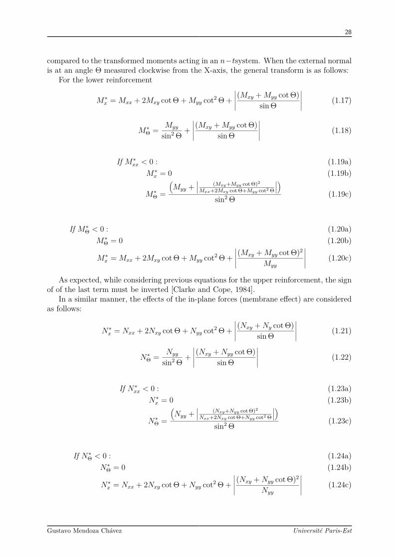
compared to the transformed moments acting in an n−tsystem. When the external normalis at an angle Θ measured clockwise from the X-axis, the general transform is as follows:

For the lower reinforcement

M∗x = Mxx + 2Mxy cot Θ +Myy cot2 Θ +

∣∣∣∣∣(Mxy +Myy cot Θ)sin Θ

∣∣∣∣∣ (1.17)

M∗Θ = Myy

sin2 Θ +∣∣∣∣∣(Mxy +Myy cot Θ)

sin Θ

∣∣∣∣∣ (1.18)

If M∗xx < 0 : (1.19a)

M∗x = 0 (1.19b)

M∗Θ =

(Myy +

∣∣∣ (Mxy+Myy cot Θ)2

Mxx+2Mxy cot Θ+Myy cot2 Θ

∣∣∣)sin2 Θ (1.19c)

If M∗Θ < 0 : (1.20a)

M∗Θ = 0 (1.20b)

M∗x = Mxx + 2Mxy cot Θ +Myy cot2 Θ +

∣∣∣∣∣(Mxy +Myy cot Θ)2

Myy

∣∣∣∣∣ (1.20c)

As expected, while considering previous equations for the upper reinforcement, the signof of the last term must be inverted [Clarke and Cope, 1984].

In a similar manner, the effects of the in-plane forces (membrane effect) are consideredas follows:

N∗x = Nxx + 2Nxy cot Θ +Nyy cot2 Θ +∣∣∣∣∣(Nxy +Ny cot Θ)

sin Θ

∣∣∣∣∣ (1.21)

N∗Θ = Nyy

sin2 Θ +∣∣∣∣∣(Nxy +Nyy cot Θ)

sin Θ

∣∣∣∣∣ (1.22)

If N∗xx < 0 : (1.23a)N∗x = 0 (1.23b)

N∗Θ =

(Nyy +

∣∣∣ (Nxy+Nyy cot Θ)2

Nxx+2Nxy cot Θ+Nyy cot2 Θ

∣∣∣)sin2 Θ (1.23c)

If N∗Θ < 0 : (1.24a)N∗Θ = 0 (1.24b)

N∗x = Nxx + 2Nxy cot Θ +Nyy cot2 Θ +∣∣∣∣∣(Nxy +Nyy cot Θ)2

Nyy

∣∣∣∣∣ (1.24c)


29

Mn = Mxx cos2 Θ +Myy sin2 Θ− 2Mxy sin Θ cos Θ (1.25)Mxx, Myy and Mxy are bending and twisting moments, usually obtained from a finite

element analysis program. Θ is the angle corresponding to the disposition of the transversesteel, measured clockwise, from the Mx axis (see figure 1.13).

Following this procedure the required resisting moments M∗xx, M∗

yy as well as the re-quired resisting normal forces N∗xx, N∗yy can be computed and common flexure theory forRC can be applied.

1.2.2.5 Capra-Maury algorithm

A method used for the calculation of reinforcement in hull elements subjected to a systemof axial forces and bending moments is based on the design presented by A. Capra and J.Maury [Capra and Maury, 1978]. This method has been implemented in some specializedstructural calculation software such as Code_Aster [Delmas, 2011] and AutoDesk Robot[RoboBat, 2002].

Considering a reinforced concrete shell where the steel layers are disposed along twoorthogonal directions X and Y , the state of forces is produced by the value of the threedensities of moments Mxx, Myy, Mxy and the three membrane tensions Nxx, Nyy, Nxy.

N

N

xx

yy

N

yx

N

xy

T

xz

T

yz

M

M

M

xy

M

xx

yx

yy

Z

Y

X

Figure 1.14: Reinforced shell element

This method acts as a post-processing step conducted over the state of generalisedstresses previously obtained on a FE calculation. The problem is to determine the optimaleconomic values of the longitudinal reinforcement sections, as in the upper layer, U , andthe lower one, L. In order to attain that result, the algorithm is based on the principle ofthe equilibrium of different facets centred at the point of calculation whose normal rotatesin the plane tangent to the average sheet.

For each one of these facets, the bending moment (M) and the membrane tension(N) are applied according to the current stress state tensors and are evaluated using thefollowing equations:

M = Mxx cos2 θ +Myy sin2 θ − 2Mxy sin θ cos θ (1.26)

N = Nxx cos2 θ +Nyy sin2 θ − 2Nxy sin θ cos θ (1.27)


30

Taking into account the resultant bending moment and the membrane forces, the mo-ment of service which steel must take can be evaluated. By a combined compression-and-bending calculation, it is now possible to determine the lower tensile forces Φ(θ) and higherΦ′(θ), perpendicular to the section, which must be balanced by the bottom and top layersof reinforcement.

The resisting forces, Φ′∗, in the direction θ of the two plies can be evaluated using thefollowing expressions:

Φ∗(Θ) =(aXL cos2 θ + aY L sin2 θ

)σy (1.28)

for the lower layer

Φ′∗(Θ) =(aXU cos2 θ + aY U sin2 θ

)σy (1.29)

for the upper layerwhere σy represents the maximal admissible stress in the steel (identical for both direc-

tions).Considering that the resisting forces Φ∗(Θ) and Φ′∗(Θ) must be greater than the applied

ones, Φ(Θ) and Φ′(Θ) respectively, the optimum of the reinforcement corresponds to theminimum quantities of:

(aXU + aY U) for the top layer

(aXL + aY L) for the bottom layer

Normally, the problem is solved numerically by checking the resistance of the section fora finite number n of values of Θ regularly spaced [Capra and Maury, 1978, Delmas, 2011,RoboBat, 2002]. The computed bending calculations are carried out in a typical mannerand, for the calculation of the upper reinforcement, we must solve:

minimise: (aXL + aY L) (1.30)

subject to: aXL cos Θ + aY L sin Θ ≥ Φ′(Θi)σ

(1.31a)

aXL ≥ 0 (1.31b)aY L ≥ 0 (1.31c)

(1.31d)

A graphical representation of the previous inequalities (equation 1.31) gives a validitydomain defined in figure 1.15. Considering an orthonormed plane defined by the requiredsteel area along the X and Y directions (aXL and aY L), the inequalities given in equations1.31 define a semi-space of the feasible design.

By exploring different values of Θ, a general domain of validity of the imposed conditionscan be obtained (figure 1.16).

C&M assumes that the compression of the concrete is acceptable and that the reinforce-ments are strained to the limit constraint σy. A verification of these hypotheses, by goingthrough a rigorous or simplified calculation in combined compression-and-bending, is then


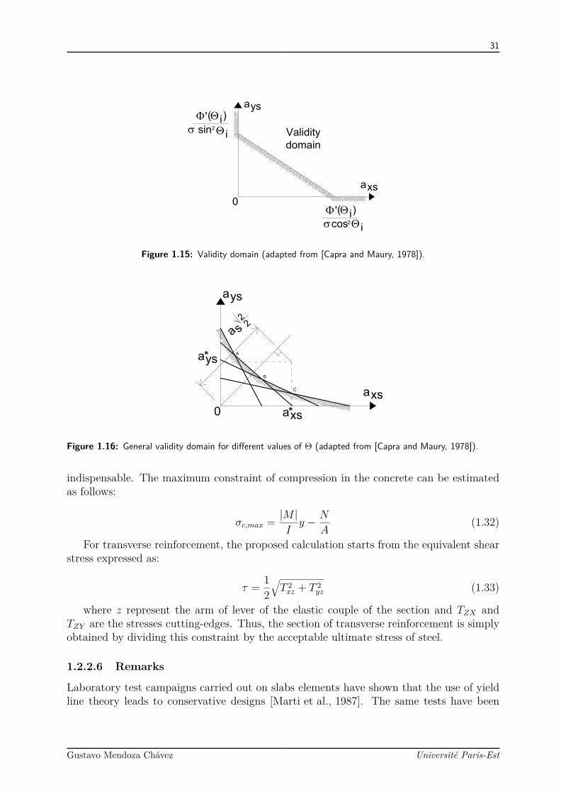
31

0

a

ys

a

xs

F Q

s

'

i

( )

sin

cos

2

F Q

si

( )

2

'

Validity

domain

Qi

Qi

Figure 1.15: Validity domain (adapted from [Capra and Maury, 1978]).

0

a

ys

a

xs

a

s

A

B

C

2

2

a

xs

a

ys

*

*

Figure 1.16: General validity domain for different values of Θ (adapted from [Capra and Maury, 1978]).

indispensable. The maximum constraint of compression in the concrete can be estimatedas follows:

σc,max = |M |Iy − N

A(1.32)

For transverse reinforcement, the proposed calculation starts from the equivalent shearstress expressed as:

τ = 12√T 2xz + T 2

yz (1.33)

where z represent the arm of lever of the elastic couple of the section and TZX andTZY are the stresses cutting-edges. Thus, the section of transverse reinforcement is simplyobtained by dividing this constraint by the acceptable ultimate stress of steel.

1.2.2.6 Remarks

Laboratory test campaigns carried out on slabs elements have shown that the use of yieldline theory leads to conservative designs [Marti et al., 1987]. The same tests have been


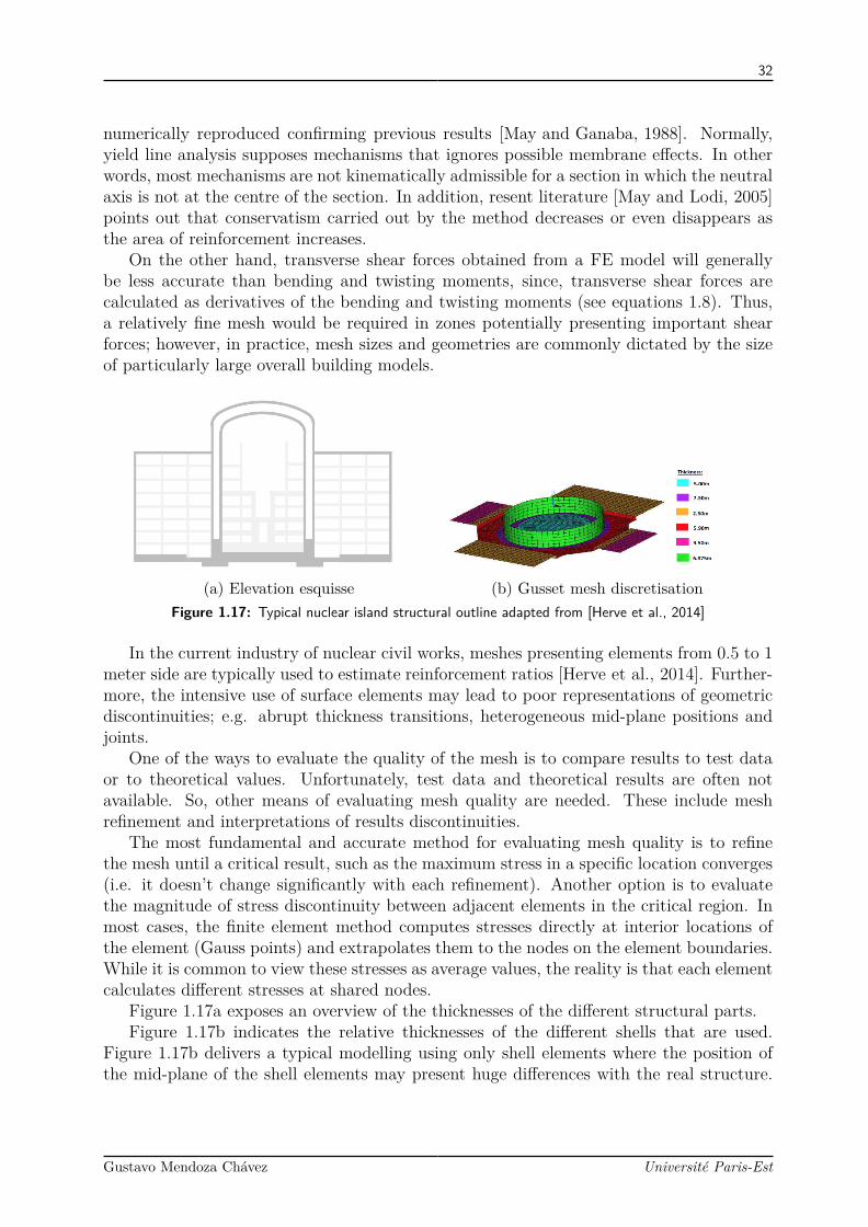
32

numerically reproduced confirming previous results [May and Ganaba, 1988]. Normally,yield line analysis supposes mechanisms that ignores possible membrane effects. In otherwords, most mechanisms are not kinematically admissible for a section in which the neutralaxis is not at the centre of the section. In addition, resent literature [May and Lodi, 2005]points out that conservatism carried out by the method decreases or even disappears asthe area of reinforcement increases.

On the other hand, transverse shear forces obtained from a FE model will generallybe less accurate than bending and twisting moments, since, transverse shear forces arecalculated as derivatives of the bending and twisting moments (see equations 1.8). Thus,a relatively fine mesh would be required in zones potentially presenting important shearforces; however, in practice, mesh sizes and geometries are commonly dictated by the sizeof particularly large overall building models.

(a) Elevation esquisse (b) Gusset mesh discretisationFigure 1.17: Typical nuclear island structural outline adapted from [Herve et al., 2014]

In the current industry of nuclear civil works, meshes presenting elements from 0.5 to 1meter side are typically used to estimate reinforcement ratios [Herve et al., 2014]. Further-more, the intensive use of surface elements may lead to poor representations of geometricdiscontinuities; e.g. abrupt thickness transitions, heterogeneous mid-plane positions andjoints.

One of the ways to evaluate the quality of the mesh is to compare results to test dataor to theoretical values. Unfortunately, test data and theoretical results are often notavailable. So, other means of evaluating mesh quality are needed. These include meshrefinement and interpretations of results discontinuities.

The most fundamental and accurate method for evaluating mesh quality is to refinethe mesh until a critical result, such as the maximum stress in a specific location converges(i.e. it doesn’t change significantly with each refinement). Another option is to evaluatethe magnitude of stress discontinuity between adjacent elements in the critical region. Inmost cases, the finite element method computes stresses directly at interior locations ofthe element (Gauss points) and extrapolates them to the nodes on the element boundaries.While it is common to view these stresses as average values, the reality is that each elementcalculates different stresses at shared nodes.

Figure 1.17a exposes an overview of the thicknesses of the different structural parts.Figure 1.17b indicates the relative thicknesses of the different shells that are used.

Figure 1.17b delivers a typical modelling using only shell elements where the position ofthe mid-plane of the shell elements may present huge differences with the real structure.


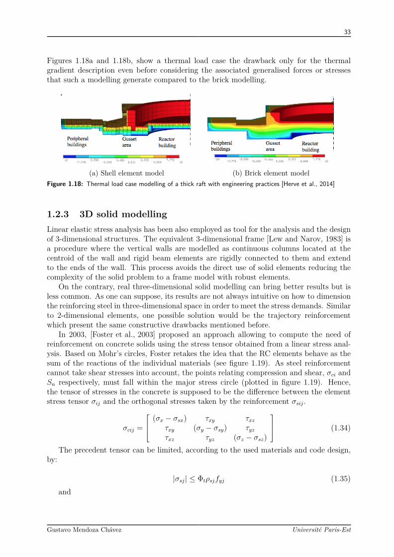
33

Figures 1.18a and 1.18b, show a thermal load case the drawback only for the thermalgradient description even before considering the associated generalised forces or stressesthat such a modelling generate compared to the brick modelling.

(a) Shell element model (b) Brick element modelFigure 1.18: Thermal load case modelling of a thick raft with engineering practices [Herve et al., 2014]

1.2.3 3D solid modellingLinear elastic stress analysis has been also employed as tool for the analysis and the designof 3-dimensional structures. The equivalent 3-dimensional frame [Lew and Narov, 1983] isa procedure where the vertical walls are modelled as continuous columns located at thecentroid of the wall and rigid beam elements are rigidly connected to them and extendto the ends of the wall. This process avoids the direct use of solid elements reducing thecomplexity of the solid problem to a frame model with robust elements.

On the contrary, real three-dimensional solid modelling can bring better results but isless common. As one can suppose, its results are not always intuitive on how to dimensionthe reinforcing steel in three-dimensional space in order to meet the stress demands. Similarto 2-dimensional elements, one possible solution would be the trajectory reinforcementwhich present the same constructive drawbacks mentioned before.

In 2003, [Foster et al., 2003] proposed an approach allowing to compute the need ofreinforcement on concrete solids using the stress tensor obtained from a linear stress anal-ysis. Based on Mohr’s circles, Foster retakes the idea that the RC elements behave as thesum of the reactions of the individual materials (see figure 1.19). As steel reinforcementcannot take shear stresses into account, the points relating compression and shear, σci andSn respectively, must fall within the major stress circle (plotted in figure 1.19). Hence,the tensor of stresses in the concrete is supposed to be the difference between the elementstress tensor σij and the orthogonal stresses taken by the reinforcement σsij.

σcij =

(σx − σsx) τxy τxzτxy (σy − σsy) τyzτxz τyz (σz − σsz)

(1.34)

The precedent tensor can be limited, according to the used materials and code design,by:

|σsj| ≤ Φtρsjfyj (1.35)and


34

Figure 1.19: Compression field for 3-dimensional stresses

Figure 1.20: Idealised 3-dimensional reinforcement

− σcIII ≤ βΦcρsjfcp (1.36)

where Φs and Φc are reduction factors associated with their respective materials, β is thefactor to account the triaxial effect on concrete, and ρsj (j = x, y, z) are the reinforcementratios along the global axis X, Y and Z.

Making and analogy between the tensor in equation 1.36 and figure 1.19, it can beobserved that there are six unknowns: σsx, σsy, σsz, σcI , σcII , and σcIII but only threeequations: Ic1 +Is1 = I1, Ic2 +Is2 = I2, Ic3 +Is3 = I3 which produce an infinity of solutions.Hence, the designer must chose to determine constrains over the variables in order to obtaina unique solution for the system of above equations [Hoogenboom and De Boer, 2010].

1.2.4 Structural analysis and design using non-linear modellingThe results provided by linear-elastic finite element analysis represent a practical way tosafely dimension common structures for serviceability limit states. And have become thebasis of the structural design.

For some design problems, however, a linear analysis may not be sufficient. Specialcases can be mentioned when existent structures may need analysis that take into accountcracking and ageing. Another example is for new structures may require a non-linear revi-sion of the dimensioning using a plasticity-based design procedure. In addition, nonlinear


35

analysis can also be used for evaluating complex geometries or poorly detailed structurespresenting effects of localised cracking.

One common application of non-linear analysis is the confirmation of safety for complexdesign details.

In the industrial practice, and due to the associated cost, this type of analyses areimplemented in situations specific situations:

• large deformations are expected

• sensible materials are used

• coupled effects may occur

Specifically speaking for RC structures, the implementation of non-linear analysis cor-responds to situations when

• verification of the pattern is needed

• the amount/distribution of the reinforcement may considerable modify the linearstress distribution.

1.3 Strut-and-Tie modelsIn the presence of structural members subjected to important punctual loads or possessingabrupt changes in their cross-section and geometry, conventional methods of plane sectionanalysis seems to be no longer sufficient [Thompson, 2002]. Such locations are generallydetailed using good practice rules based on experience or based on empirical guidelines.Strut-and-Tie Method (STM) arises as a rational in-between design procedure for complexstructural detailing; the procedure has a basis in mechanics but it is simple enough to bereadily applied in design.

First proposed by [Ritter, 1899], Strut-and-Tie models represent a simplification tovisualise the path of internal forces in cracked elements. First models were the basis forthe design of concrete beams [Mörsch, 1902]. Years later, the theory continued to be refinedwith the contributions of [Marti, 1985] who created the basis of the rational applicationof the STM. At the same time, [Collins and Mitchell, 1980] derived a rational criteria forshear and torsion. Meanwhile, [Schlaich et al., 1987] extended the beam truss models toall parts of structure in the form of generalised ST systems.

Generally speaking, STM involves the idealisation of a complex structural memberinto a simple truss able to represent the flow of stress paths within the member. Thetruss is composed of struts that model concrete compression fields, ties that model tensilesteel reinforcement, and nodes which represent the localised zones where the elementsinterconnect one another or the zones where the tensile steel is anchored into the concrete.The struts and ties carry only uniaxial forces. This truss mechanism must be stable andproperly balance the applied loads. Failure of the truss is dictated by yielding of oneor more ties or also defined by excessive compressive stresses within the struts or nodes.Ideally, only the first failure mode should occur.


36

Even if the principle can be directly applied to elements resisting flexion with a lineardistribution of stresses [Hsu, 1992], this document will focus only on its application fordetailing discontinuity regions undergoing no-linear distribution of the stresses throughthe member depth.

1.3.1 Discontinuity regionsThe primary tenets of beam theory imply that a linear distribution of strains occurs throughthe member depth: plane sections are assumed to remain plane. The element is thereforedominated by sectional behaviour, and the design can proceed on a section-by-section basis.For the design of elements in flexion, the compressive stresses are conventionally assumedto act over a rectangular stress block, while the tensile stresses are assumed to be carriedby the longitudinal steel reinforcement.

On the other hand, D-regions ("D" standing for discontinuity or disturbed) occur inthe vicinity of load or geometric discontinuities. The applied loads, support reactions andabrupt geometric changes are discontinuities that "disturb" the stress distribution withinthe member near the locations where they act. Corners, openings, and corbels are examplesof geometric discontinuities that correspond to the existence of D-regions.

As a characteristic of D-regions, it is considered that the distribution of the strainsthrough the member depth presents a non-linear profile, therefore, the assumptions thatunderlie the sectional design procedure are invalidated. According to Saint Venant’s prin-ciple, an elastic stress analysis indicates that the stresses due to axial forces and bending,are approaching a linear distribution at a distance approximately equal to the depth of themember, h, away from the discontinuity. In other words, a nonlinear stress distributionexists within one member depth from the location where the discontinuity is introduced[Schlaich et al., 1987]. Following this, it can be stated that D-regions are therefore assumedto extend up to a distance h from the applied load and support reactions.

In general, a region of a structural member is assumed to be dominated by nonlinearbehaviour, or a D-region, when the span/depth ratio, a/h, is less than 2 or 2.5. The shearspan, a, is defined as the distance between the applied load and the closest support insimple members.

1.3.2 FundamentalsA ST model design adheres to two principles: 1) the resultant truss model must be inequilibrium with the external force system and, 2) the concrete element has enough defor-mation capacity to accommodate the assumed distribution of forces [Schlaich et al., 1987].Proper anchorage length of the reinforcement is an implicit requirement in order to assurethe needed ductility. Complementary, the compressive stresses developed in the concretemust not exceed the factored concrete strengths, and the tensile stresses the factored steelcapacities. If all of the mentioned above requirements are satisfied, the application of theSTM should result in a conservative design [Williams et al., 2012].

As mentioned before, the STM consists of three principal components: struts, ties, andnodes. The compression members, referred as struts, are considered to be made out ofconcrete Cc; the tension members, referred to as ties, may be made of concrete withoutreinforcement Tc (case not considered within this work) or reinforced by layers of mild steel


37

reinforcement or prestessing steel Ts. The struts and the ties intersect at regions referred toas nodes. Due to the concentration of stresses from intersecting truss members, the nodesare the most highly stressed regions of a structural member and their revision should beconsidered during the overall analysis.

1.3.3 Design procedureST modelling is suitable for use in a wide range of design problems and has been incorpo-rated into several design codes. Among others, the method is referred in the EuroCode2[Eurocode2, 2008], the Appendix A of ACI 318-02 [ACI-318, 2008] and, the InternationalFederation for Structural Concrete [for Structural Concrete, 2008]. These account for de-sign conditions using the same equations with exception of notation and minor differencesin the value of safety factors.

Typically, the design procedure points out a sequence of steps as follows.

1.3.3.1 Region discrimination

The first step in the STM design process is to define whether the STM is a good alternativeto solve the problem. Based on the Saint-Venant’s principle, the structure can be dividedinto B- and D-regions. The STM design process should be used to design the sections thatare found as D-regions while regions expected to be dominated by sectional behaviour canbe designed using the sectional design approach. If the structure results in a combination ofB- an D-regions, the designer may decide to treat the structure by sections, substructures,or to decide if using only one approach for the whole structure is reasonable and will resultin a suitable design.

1.3.3.2 Defining load case

The second step is to determine the critical load cases that the structure shall withstand. Ifthe structural component consists of both B- and D-regions, only the discontinuity parts ofthe component will be designed using strut-and-tie modelling. Each D-region found shouldbe processed as an isolated element where the nodal boundary conditions originate fromthe interaction with the adjacent elements and global support reaction of the structureunder the design system of loads (figures 1.22): the forces acting at the boundaries of theD-region become the boundary conditions for the further ST analysis.

The internal forces and moment at the interface of the B- and D-regions can be assumedlinearly distributed and should be applied at the boundary of the isolated D-region (figure1.22c). The definition of the boundary forces between D- and B-regions are applied to theSTM in order to 1) determine the forces carried by the truss and 2) determine the geometryof the model by defining the position of some nodes. As it can be inferred, an overall elasticanalysis of the structure should be performed in order to determine the support reactionsand the interface loads for the different D-regions.

Considering that the truss elements are unable to withstand specific loads (eg. moment,distributed loads) some modifications may be necessary to produce an equivalent loadsystem. The most current modification can be resumed as follows:


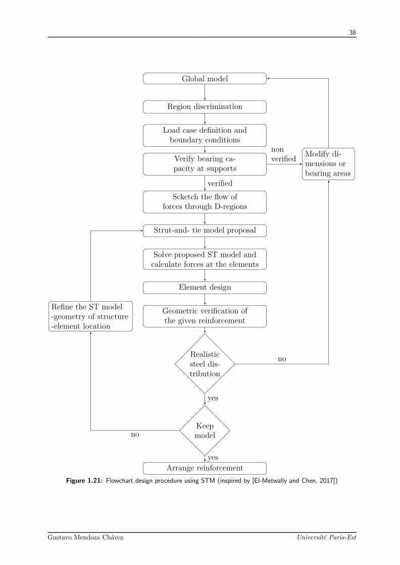
38

Global model

Region discrimination

Load case definition andboundary conditions

Verify bearing ca-pacity at supports

Scketch the flow offorces through D-regions

Strut-and- tie model proposal

Solve proposed ST model andcalculate forces at the elements

Element design

Geometric verification ofthe given reinforcement

Realisticsteel dis-tribution

Keepmodel

Arrange reinforcement

Modify di-mensions orbearing areas

Refine the ST model-geometry of structure-element location

verified

yes

no

yes

no

nonverified

Figure 1.21: Flowchart design procedure using STM (inspired by [El-Metwally and Chen, 2017])


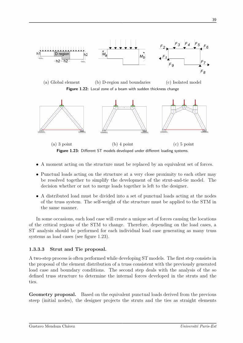
39

D regionh1

h2

h2h2

(a) Global element

M

M

a

b

(b) D-region and boundaries

F

1

F

2

F

3

F

4

F

5

F

6

F

7

F

8

F

9

(c) Isolated modelFigure 1.22: Local zone of a beam with sudden thickness change

(a) 3 point (b) 4 point (c) 5 pointFigure 1.23: Different ST models developed under different loading systems.

• A moment acting on the structure must be replaced by an equivalent set of forces.

• Punctual loads acting on the structure at a very close proximity to each other maybe resolved together to simplify the development of the strut-and-tie model. Thedecision whether or not to merge loads together is left to the designer.

• A distributed load must be divided into a set of punctual loads acting at the nodesof the truss system. The self-weight of the structure must be applied to the STM inthe same manner.

In some occasions, each load case will create a unique set of forces causing the locationsof the critical regions of the STM to change. Therefore, depending on the load cases, aST analysis should be performed for each individual load case generating as many trusssystems as load cases (see figure 1.23).

1.3.3.3 Strut and Tie proposal.

A two-step process is often performed while developing ST models. The first step consists inthe proposal of the element distribution of a truss consistent with the previously generatedload case and boundary conditions. The second step deals with the analysis of the sodefined truss structure to determine the internal forces developed in the struts and theties.

Geometry proposal. Based on the equivalent punctual loads derived from the previoussteep (initial nodes), the designer projects the struts and the ties as straight elements


40

from one node to another with the aim of developing a stable structure within the solidelement. This process may or may not include the interaction of all the initial nodesand, in addition, it may include secondary nodes depending on the designer’s criteria. Forthis step, a linear finite element model is commonly used in order to visualise the flow offorces within the member; and align the truss elements according to the stress trajectories[Schlaich et al., 1987].

Analyse ST models and member design. At this point, the ST model correspondsto a planar (or spatial) truss depicted by a nodal list, an element list and, an inter-connectivity table. Using these three items, a mathematical model can be then built andsolved. The forces developed in the elements are determined by solving a model includingthe previously determined boundary conditions and factored system of loads. The areaof material needed for each element in the STM should be sufficient to safely resist thecomputed force without surpassing the yield strength of the steel nor the limit resistancein the concrete. In a conventionally reinforced structure, the area of reinforcement neededfor a tie, Ast, is determined from the following equation:

Ast = FuφR

(1.37)

where:

Fu corresponds to the largest force in the element for all load combinations considered,

R the material’s resistance (σy for steel, σc the resistance for concrete material) and,

φ the safety factor (0.9 for traction [Eurocode2, 2008, ACI-318, 2008])

Additionally, the Eurocodes requires the diminution of the design strength for struts incracked compression zones:

σc = 0.6(1− fc/250)fcd [Eq. (6.56) and (6.57N) of EUC2] (1.38)

1.3.3.4 Nodal verification

Due to the level of stresses that must be equilibrated within a small volume of concrete, thenodes are the most highly stressed regions of a structural component. As a consequence, alogical step on the design process is the verification of the resistance of the zones generatedby the intersection of different elements.

Briefly said, the nodes are a mere simplified idealisation of a more complex reality andthe definition of their geometry lies also on the designer’s criteria. Ideally, nodes may beconceived such that the stresses on all faces are equal. If the stresses are equal, the ratioof the area of the side face is proportional to the applied force. In this case, the node isreferred as a hydrostatic node: principal stresses are equal on all sides and shear stressesdisappear. In the other hand, if a node is conceived in a manner where unequal stressesexist on each face, then, the node is referred to non-hydrostatic 1.24.

Based on the nature of the elements that converges to a connection zone, anotherclassification can be made. According to the sign of converging forces, the node may be


41

Figure 1.24: Nodal proportioning techniques - hydrostatic versus non-hydrostatic nodes [Birrcher et al., 2009]

Figure 1.25: Representative node types [Birrcher et al., 2009]

referred as CCC, CCT, CTT or TTT (C standing for compression forces and T standingfor tension ones). Due to geometric complications, it is highly recommended to mergegroups of forces in order to reduce their number If more than three elements intersect atone node. However, this is not always possible and often generates other possible type ofnodal combinations as showed in figure 1.25.

For hydrostatic nodes, the faces are perpendicular to the attached elements and thelength sides are proportional to the strut forces. In the presence of ties, position of thefaces are proposed by assuming the tie forces act from behind the node to compress thenodal region.

Table 1.1: ACI and Eurocode values for nodal zones resistance

Nodal zones, σRd,maxσRd,max

ACI EurocodesCCC type nodes 0.85(1)βsf ′c (A.5.2.1) 1ν ′fEcd (6.5.4)Nodal zones anchoring a tie 0.85(0.8)βsf ′c (A.5.2.2) 0.85ν ′fEcd (6.5.4)In nodal zones anchoring two or more ties. 0.85(0.6)βsf ′c (A.5.2.3) 0.75ν ′fEcd (6.5.4)


42

(a) Orthogonal mesh of steel (b) Generic modelFigure 1.26: Bottle-shaped strut (adapted from [Singh et al., 2018]).

Non-hydrostatic nodes are proportioned based on the origin of the applied stress. In thecase of CCC non-hydrostatic nodes, the approach is to set the back face dimension as theeffective depth of the compression block. In the presence of a CCT, the back face dimensionis taken as twice the distance from the centroid of the longitudinal reinforcement to theextreme tension fibre of the beam. Regarding the nodes located at the boundary conditionsand supports, the dimension of the bearing face is determined by the dimensions of thebearing plate. This proportioning technique allows the geometry of the nodes to closelycorrespond to the actual stress concentrations at the nodal regions. In contrast, the useof hydrostatic nodes can sometimes result in unrealistic nodal geometries and impracticalreinforcement layouts [Birrcher et al., 2009].

1.3.3.5 Transverse reinforcement

One of the most frequent assumptions is to idealise the struts as prismatic elements. How-ever, according to Birrcher et al [Birrcher et al., 2009], this simplification does not elim-inate the fact that most struts in two dimensions are bottle-shaped struts. The lateralspreading of bottle-shaped struts introduces tensile stresses transverse to the element,stresses that could cause longitudinal cracking along the length of the strut resulting inpremature failure; hence, transverse reinforcement should be provided in order to controlthe cracking.

Ideally, reinforcement placed inside the strut and aligned with the transverse tensionforces would be the best to resist the transverse tension and to control crack widths.However, in practice, the resistance to "splitting" may derive from the orthogonal mesh ofsteel typically detailed in such elements 1.13.

Even though reinforced bottle-shaped struts seem to represent a more realistic distri-bution of stress then prismatic elements, its real behaviour has been little studied and itsapplication seem not to be standardised among different codes. While codes such as theAASHTO LRFD Bridge Design Specifications required to the bottle shaped struts to bedetailed with reinforcement ratio of 0.003, the Eurocodes present the elements as regionsof partial and full discontinuity (see figure 1.27) proposing two equations.


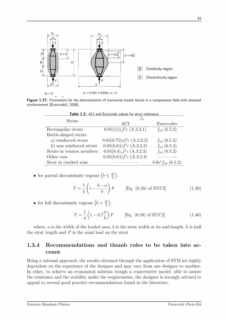
43

Figure 1.27: Parameters for the determination of transverse tensile forces in a compression field with smearedreinforcement [Eurocode2, 2008].

Table 1.2: ACI and Eurocode values for strut resistance

Struts βsACI Eurocodes

Rectangular struts 0.85(1)βsf ′c (A.3.2.1) fcd (6.5.2)Bottle-shaped strutsa) reinforced struts 0.85(0.75)sf ′c (A.3.2.2) fcd (6.5.2)b) non reinforced struts 0.85(0.6λ)f ′c (A.3.2.2) fcd (6.5.2)

Struts in tension members 0.85(0.4)sf ′c (A.3.2.3) fcd (6.5.2)Other case 0.85(0.6λ)f ′c (A.3.2.4) ————-Strut in cracked zone —————- 0.6ν ′fcd (6.5.2)

• for partial discontinuity regions(b ≤ H

2

):

T = 14

(1− b− a

b

)F [Eq. (6.58) of EUC2] (1.39)

• for full discontinuity regions(b > H

2

):

T = 14

(1− 0.7a

h

)F [Eq. (6.59) of EUC2] (1.40)

where, a is the width of the loaded area, b is the strut width at its mid-length, h is halfthe strut length and P is the axial load on the strut

1.3.4 Recommendations and thumb rules to be taken into ac-count

Being a rational approach, the results obtained through the application of STM are highlydependent on the experience of the designer and may vary from one designer to another.In other, to achieve an economical solution trough a conservative model, able to assurethe resistance and the stability under the requirements, the designer is strongly advised toappeal to several good practice recommendations found in the literature;


44

• The distribution of the truss elements can be based on the stress distribution of aprior elastic FEM analysis [Schlaich et al., 1987], [Eurocode2, 2008].

• Align the struts with ±15o of the stress trajectories to represent the nature of theelement [Ramirez and Breen, 1991].

• The most efficient ST models are typically those with the fewest and shortest ties[Williams et al., 2012].

• The ties should coincide in position and direction with the corresponding reinforce-ment [Eurocode2, 2008].

• According to [Eurocode2, 2008], all strut-and-tie models may be optimised by energycriteria .

1.3.5 RemarksThe most important benefit of ST modelling is its versatility. Almost any structure canbe treated with this method in order to obtain a conservative design. In contrast, theflexibility of its application is granted by the lack of explicit guidance and consistency inthe current codes [Barton et al., 1991].

1.4 Non-Linear strut-and-tie model approachThis approach proposes the development of a classic ST model and its further revisionthrough a non-linear model [Yun and Lee, 2005].

The ST initial model can be formulated from experience, from a linear elastic FEmodel or from experimental information such as crack patterns and recorded strains andthe process continues as depicted in figure 1.21.

To evaluate the behaviour and ultimate resistance of the selected ST model, a non-linear FE analysis is carried out of the model. This model needs to consider the final (real)dimensions of the proposed struts and ties as well as an accurate representation of theirrespective materials. The process allows to verify the resistance at the nodal zones byevaluating the developed stresses according to a failure failure. If the bearing capacitiesare not sufficient or the considered load produces failure or mechanisms, the original STmodel is modified and the process is repeated.

1.5 SummaryIn the field of engineering practice, the construction codes allow the analysis and designof non-flexural RC elements trough 3 principal approaches: recommendations based onempirical relations, FEM based algorithms and also rational methods.

Even if several campaigns have been carried out with the aim of determine the behaviourand the resistance of elements such nibs and deep beams, the results remain valid for asmall range of cases where the geometry of analysed element as well of the load systemand steel disposition resembles to those studied restricting its application for particular


45

cases. When a special case is confronted, a FE analysis is, probably, the first alternativeto manual calculation.

As expressed before most structural designs are performed using FEM software andpost-processed trough automatic algorithms. Most of the applied methodologies were con-ceived to treat elements where the effects carried out by a flexural behaviour predominateover those produced by shear, limiting their range of validity if no special considerationsare implemented. It is also worth to mention the fact that, in the most popular methods,W&A nor C&M, no explicit check of the assumed failure mode is made at the elements de-signed. These methodologies implicitly assume that the reinforcement ratios obtained aresmall enough to avoid concrete crushing. While this condition is usually satisfied in slabs,a check of the assumed failure mode should always be carried out for shells, particularlyfor elements subjected to significant axial compression or cases with high reinforcementratios.

Despite the fact of the existence of some other FE-based methods such as the sandwichor a full three-dimensional solid design do indeed take into account a verification on theconcrete, their application has not been included within the construction codes until thisday.

Other alternative is the use of the rational methods that can be seen as an intermediatepoint between structural mechanics and the empirical methods. The main drawbacks ofthe use of such methods has been their lack of explicit guidance and consistency in thecurrent codes, aspects that propitiate a strong dependency on the designer’s expertise.

The guidance provided by the elastic stress field, result of a prior FE analysis, ensuresa good behaviour at the serviceability limit state and can also be used to study its ultimatelimit state response. The procedure seems to be straightforward for cases where the tiesare aligned to the orthogonal reinforcement; for cases where this does not occur, the finalreinforcement may not present the desired behaviour

The performance of a model developed through rational methods is totally dependenton the intuition and practice of the structural engineer as well as the expertise on theproblem to solve. The modifications and decisions taken within the design process becomesa repetitive and logic task for common geometries and load cases but, it can also be a ratherdifficult task when facing unusual cases.

The modification of a model in order to adapt it to different requirements, or just inorder to improve it response, requires a knowledge on the relation of the mechanical char-acteristics and the evolution on the structural behaviour. In a conventional process, anymodification is dictated by preexisting codes and construction recommendations. For STMthese rules can sometimes depend on the typology of the problem and even be subjectiverules presenting guidance for a series of solved recurrent examples but needing a sort ofextrapolations for different problems.

In recent years, the development of Computational Aided Design (CAD) tools allowsto include rational techniques intended guide the engineer through the design process. Dif-ferent techniques adapting mathematical methods have been proposed in order to achieveoptimal solutions for automatically computing the reinforcement of concrete structuresthough ST models. Next chapter intents to make an overall revision of the most commonoptimisation techniques and algorithms that have been applied to propose and to justifythe trajectory of ST models.


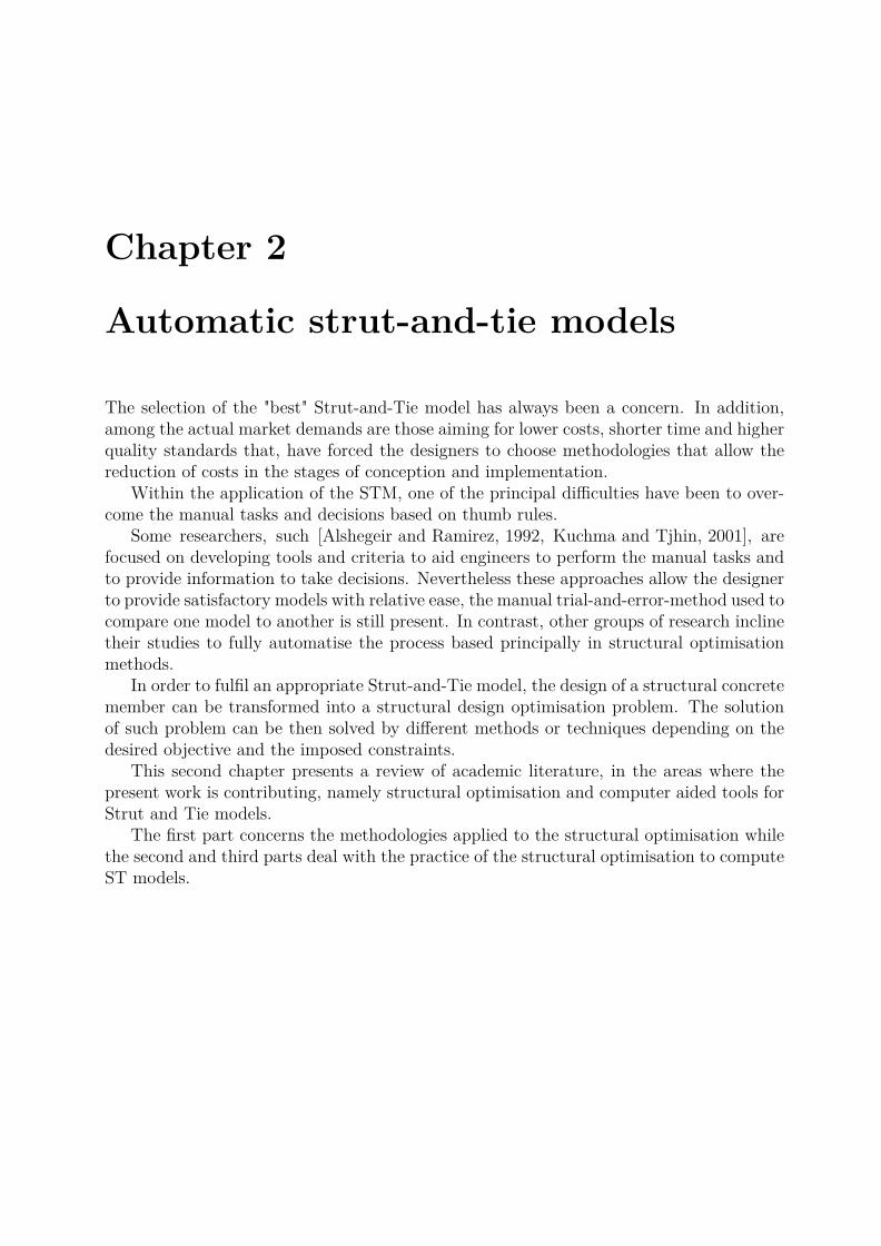
Chapter 2

Automatic strut-and-tie models

The selection of the "best" Strut-and-Tie model has always been a concern. In addition,among the actual market demands are those aiming for lower costs, shorter time and higherquality standards that, have forced the designers to choose methodologies that allow thereduction of costs in the stages of conception and implementation.

Within the application of the STM, one of the principal difficulties have been to over-come the manual tasks and decisions based on thumb rules.

Some researchers, such [Alshegeir and Ramirez, 1992, Kuchma and Tjhin, 2001], arefocused on developing tools and criteria to aid engineers to perform the manual tasks andto provide information to take decisions. Nevertheless these approaches allow the designerto provide satisfactory models with relative ease, the manual trial-and-error-method used tocompare one model to another is still present. In contrast, other groups of research inclinetheir studies to fully automatise the process based principally in structural optimisationmethods.

In order to fulfil an appropriate Strut-and-Tie model, the design of a structural concretemember can be transformed into a structural design optimisation problem. The solutionof such problem can be then solved by different methods or techniques depending on thedesired objective and the imposed constraints.

This second chapter presents a review of academic literature, in the areas where thepresent work is contributing, namely structural optimisation and computer aided tools forStrut and Tie models.

The first part concerns the methodologies applied to the structural optimisation whilethe second and third parts deal with the practice of the structural optimisation to computeST models.

47

Approches automatiques de calcul de modeles bielletirantLa sélection du «meilleur» modèle Bielle-Tirant a toujours été une préoccupation. Enoutre, parmi les demandes réelles du marché figurent celles qui visent à réduire les coûts,à raccourcir les délais et à améliorer les normes de qualité, ce qui a forcé les concepteursà choisir des méthodologies permettant de réduire les coûts de conception et de mise enoeuvre.

Dans l’application de la méthode BT, l’une des principales difficultés a été de surmonterles tâches manuelles et les décisions basées sur les règles du pouce.

Certains chercheurs, tels que [Alshegeir and Ramirez, 1992, Kuchma and Tjhin, 2001],se concentrent sur le développement d’outils et de critères pour aider les ingénieurs à ef-fectuer les tâches manuelles et à fournir des informations pour prendre des décisions.Néanmoins, ces approches permettent au concepteur de fournir des modèles satisfaisantsrelativement facilement, la méthode manuelle d’essai et d’erreur utilisée pour comparer unmodèle à un autre est toujours présente. En revanche, d’autres groupes de recherche ori-entent leurs études pour automatiser entièrement le processus basé principalement sur desméthodes d’optimisation structurelle.

Afin de réaliser un modèle BT approprié, la conception d’un élément en béton armépeut être transformée en un problème d’optimisation structurale. La solution d’un tel prob-lème peut alors être résolue par différentes méthodes ou techniques en fonction de l’objectifrecherché et des contraintes imposées.

Ce deuxième chapitre présente une revue de la littérature académique, structurée pourconsidérer les domaines auxquels cette thèse contribue: l’optimisation structurelle et lesoutils assistés par ordinateur pour les modèles BT.

La première partie présente les méthodologies appliquées à l’optimisation structurelletandis que les deuxième et troisième parties traitent de la pratique de l’optimisation struc-turelle pour calculer les modèles BT.


48

2.1 Structural optimisationIn mechanics, a structure is defined by J.E. Gordon [Gordon, 2009] as "any assemblageof materials which is intended to sustain loads". Optimisation is a process concernedwith achieving the best possible outcome of a given system satisfying certain restrictions.Thus structural optimisation can be understood as the subject dealing with obtaining thebest outcome from an assemble of materials and elements that shall respect pre-establishedrestrictions. From the early years of the structural optimisation, the outcome of a structurehas been commonly measured trough the volume and/or the mass of the element itself,while the restrictions are generally, but not limited, expressed in terms of the displacementsand the stresses [Haftka and Gürdal, 2012].

2.1.1 General problem definitionAs any other optimisation problem, the standard form of a structural optimisation (seeequations 2.1 and 2.2) consists in the minimisation (or maximisation) of an objective func-tion, F (X), in terms of design variables, Xi and restricted by one or more constraintsfunctions, gj(X). The objective function can be interpreted as the mathematical represen-tation of characteristics that are meant to be minimised or maximised.

The notion of improving the objective function implies a freedom of change. Thischange is commonly expressed in terms of ranges of permissible modifications of one singleparameter or a group of them. Such parameters are referred to design variables and canrepresent geometric aspects of a structure such as cross-section or length of some elementsor material parameters like resistance or Young’s modulus. Design variables can takecontinuous or discrete values according to realistic constraints. Continuous variables cantake any value within a range while discrete variables are subjected to a permissible list.In practice, the discrete nature of design variables is commonly disregarded while theoptimisation process and the final results are adjusted to the nearest available discretevalue.

With no restrictions, the result of most optimisation problems would approach to theinfinity or a zero value. Constraints are given in order to keep the results within a feasi-ble domain and are commonly given by restrictions in terms of budget (quantity of usedmaterial), available space (boundary conditions and geometry), serviceability (displace-ments, frequency requirements) and/or intrinsic material properties (permissible strainsand stresses) among others. Generally speaking, there are 3 types of constraints:

• inequality constraints

• equality constraints

• side constraints

Inequality constraints are those which impose either a lower or an upper limit on somequantities. Equality constraints represent specific requirements of a quantity taking aselected value while, the third type, the side constraints, impose at the same time anupper and a lower restriction.


49

minimise F (X) (2.1)

subject to: gj(X) ≥ 0, j = l,m inequality constraints (2.2a)hk(X) = 0, k = l, l equality constraints (2.2b)X li ≤ Xi ≤ Xm

i , i = l, n side constraints (2.2c)

with

X =

x1x2...xn

where X denotes the vector containing the design variables. Commonly, minimisation

problems are preferred to maximisation ones. However, a maximisation problem can besolved indirectly by minimising the problem with opposite value. In a similar way, theless-than constraints can be transformed into greater-than ones by multiplying them by−1 affecting only the sign convention in some of the final results.

When using constraints that do not correspond to the same order of magnitude (e.g.displacements and lengths) it results advantageous to represent them in a normalised form:

xi ≤ xmi becomes xmi − xixmi

≤ 1 (2.3)

2.1.1.1 Variables of structural optimisation problems

Any structural system can be globally described by a set of quantities (lengths, number ofelements, etc.). Some of these quantities such as loads or spans may be preassigned by thetype of structure itself but any other quantity subject to modifications can be taken as avariable.

The selection of variables and preassigned parameters is made for a variety of reasons. Itmay be that the designer is not free to choose certain parameters, or it may be known fromexperience that a particular value of the parameter produces good results [Kirsch, 2012].

For real problems, design variables must consider plausible modifications of the struc-ture. Such modifications can be divided into three types: [Christensen and Klarbring, 2008]:

• Sizing optimisation: the design variables are the thicknesses or the cross sections ofthe elements of a predefined structure. Generally, the design variables are governedby an inferior constraint of non-zero values or replaced by a greater-than relation(see figure 2.1a).

• Shape optimisation: in this case the structure is intended to be improved throughmodifications in the form, the contour of some part of the boundary of the structuraldomain. Shape optimisation does not alter the connectivity of the structure: newboundaries are not formed (see figure 2.1b).


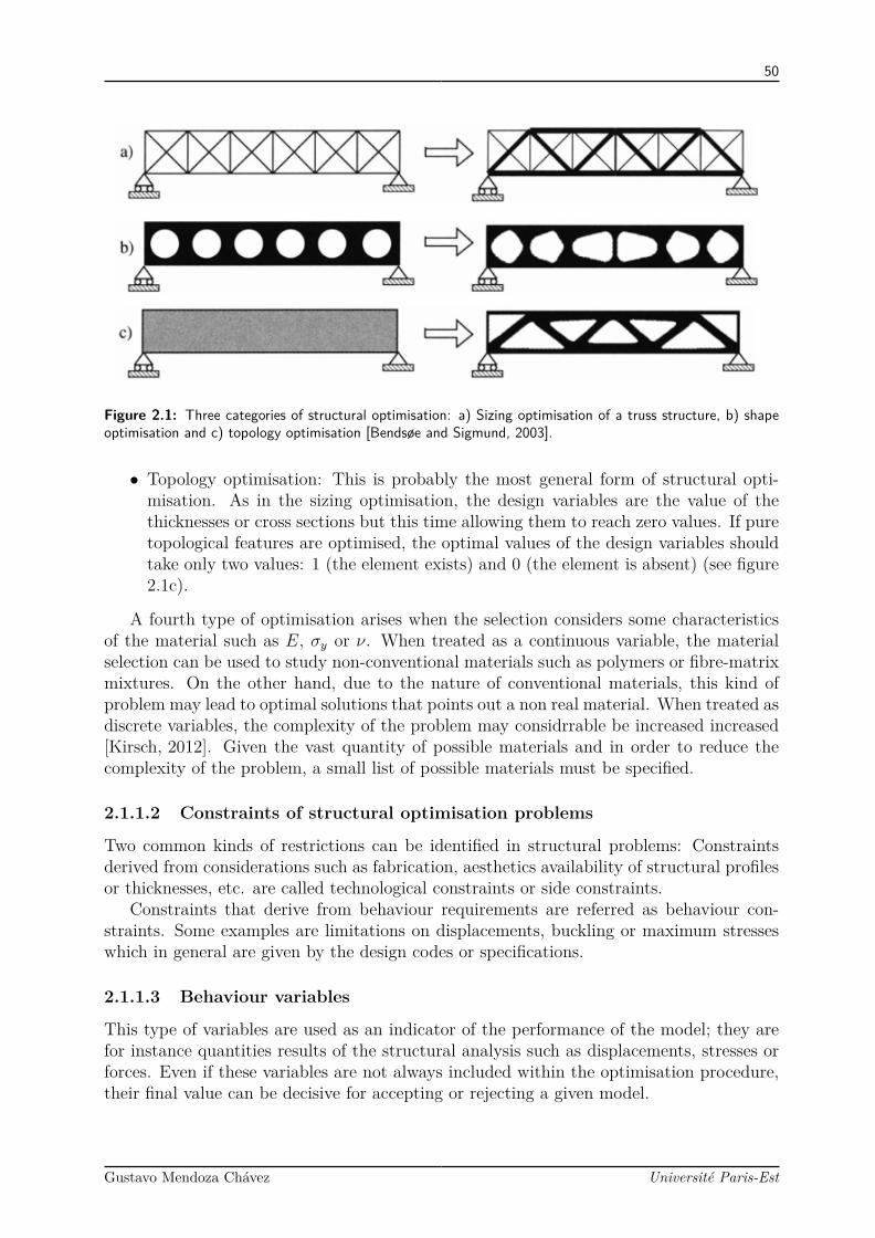
50

Figure 2.1: Three categories of structural optimisation: a) Sizing optimisation of a truss structure, b) shapeoptimisation and c) topology optimisation [Bendsøe and Sigmund, 2003].

• Topology optimisation: This is probably the most general form of structural opti-misation. As in the sizing optimisation, the design variables are the value of thethicknesses or cross sections but this time allowing them to reach zero values. If puretopological features are optimised, the optimal values of the design variables shouldtake only two values: 1 (the element exists) and 0 (the element is absent) (see figure2.1c).

A fourth type of optimisation arises when the selection considers some characteristicsof the material such as E, σy or ν. When treated as a continuous variable, the materialselection can be used to study non-conventional materials such as polymers or fibre-matrixmixtures. On the other hand, due to the nature of conventional materials, this kind ofproblem may lead to optimal solutions that points out a non real material. When treated asdiscrete variables, the complexity of the problem may considrrable be increased increased[Kirsch, 2012]. Given the vast quantity of possible materials and in order to reduce thecomplexity of the problem, a small list of possible materials must be specified.

2.1.1.2 Constraints of structural optimisation problems

Two common kinds of restrictions can be identified in structural problems: Constraintsderived from considerations such as fabrication, aesthetics availability of structural profilesor thicknesses, etc. are called technological constraints or side constraints.

Constraints that derive from behaviour requirements are referred as behaviour con-straints. Some examples are limitations on displacements, buckling or maximum stresseswhich in general are given by the design codes or specifications.

2.1.1.3 Behaviour variables

This type of variables are used as an indicator of the performance of the model; they arefor instance quantities results of the structural analysis such as displacements, stresses orforces. Even if these variables are not always included within the optimisation procedure,their final value can be decisive for accepting or rejecting a given model.


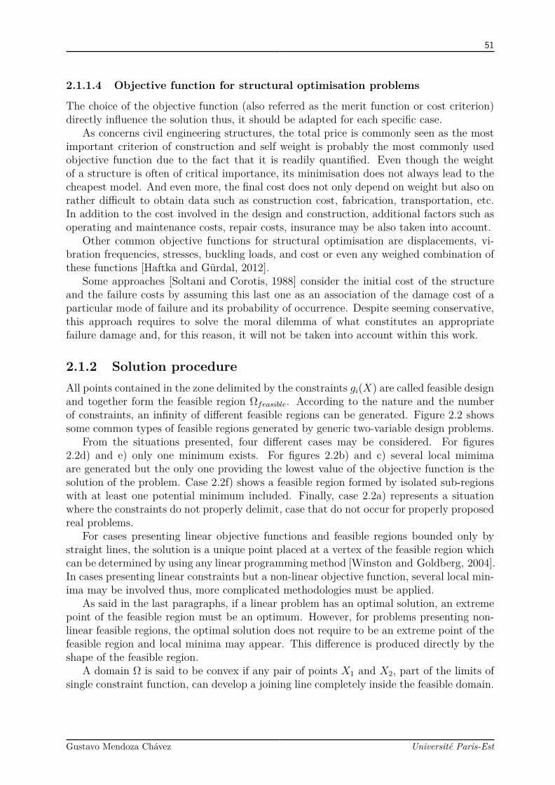
51

2.1.1.4 Objective function for structural optimisation problems

The choice of the objective function (also referred as the merit function or cost criterion)directly influence the solution thus, it should be adapted for each specific case.

As concerns civil engineering structures, the total price is commonly seen as the mostimportant criterion of construction and self weight is probably the most commonly usedobjective function due to the fact that it is readily quantified. Even though the weightof a structure is often of critical importance, its minimisation does not always lead to thecheapest model. And even more, the final cost does not only depend on weight but also onrather difficult to obtain data such as construction cost, fabrication, transportation, etc.In addition to the cost involved in the design and construction, additional factors such asoperating and maintenance costs, repair costs, insurance may be also taken into account.

Other common objective functions for structural optimisation are displacements, vi-bration frequencies, stresses, buckling loads, and cost or even any weighed combination ofthese functions [Haftka and Gürdal, 2012].

Some approaches [Soltani and Corotis, 1988] consider the initial cost of the structureand the failure costs by assuming this last one as an association of the damage cost of aparticular mode of failure and its probability of occurrence. Despite seeming conservative,this approach requires to solve the moral dilemma of what constitutes an appropriatefailure damage and, for this reason, it will not be taken into account within this work.

2.1.2 Solution procedureAll points contained in the zone delimited by the constraints gi(X) are called feasible designand together form the feasible region Ωfeasible. According to the nature and the numberof constraints, an infinity of different feasible regions can be generated. Figure 2.2 showssome common types of feasible regions generated by generic two-variable design problems.

From the situations presented, four different cases may be considered. For figures2.2d) and e) only one minimum exists. For figures 2.2b) and c) several local mimimaare generated but the only one providing the lowest value of the objective function is thesolution of the problem. Case 2.2f) shows a feasible region formed by isolated sub-regionswith at least one potential minimum included. Finally, case 2.2a) represents a situationwhere the constraints do not properly delimit, case that do not occur for properly proposedreal problems.

For cases presenting linear objective functions and feasible regions bounded only bystraight lines, the solution is a unique point placed at a vertex of the feasible region whichcan be determined by using any linear programming method [Winston and Goldberg, 2004].In cases presenting linear constraints but a non-linear objective function, several local min-ima may be involved thus, more complicated methodologies must be applied.

As said in the last paragraphs, if a linear problem has an optimal solution, an extremepoint of the feasible region must be an optimum. However, for problems presenting non-linear feasible regions, the optimal solution does not require to be an extreme point of thefeasible region and local minima may appear. This difference is produced directly by theshape of the feasible region.

A domain Ω is said to be convex if any pair of points X1 and X2, part of the limits ofsingle constraint function, can develop a joining line completely inside the feasible domain.


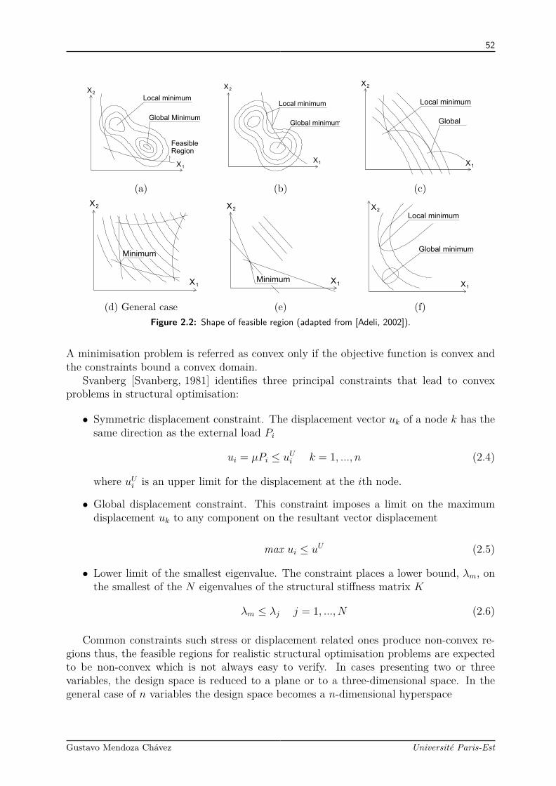
52

X

2

X

1

Local minimum

Global Minimum

Region

Feasible

(a)

X

2

X

1

Local minimum

Global minimum

(b)

X

2

X

1

Local minimum

Global

(c)

Minimum

X

2

X

1

(d) General case

X

2

X

1

Minimum

(e)

X

2

X

1

Local minimum

Global minimum

(f)Figure 2.2: Shape of feasible region (adapted from [Adeli, 2002]).

A minimisation problem is referred as convex only if the objective function is convex andthe constraints bound a convex domain.

Svanberg [Svanberg, 1981] identifies three principal constraints that lead to convexproblems in structural optimisation:

• Symmetric displacement constraint. The displacement vector uk of a node k has thesame direction as the external load Pi

ui = µPi ≤ uUi k = 1, ..., n (2.4)

where uUi is an upper limit for the displacement at the ith node.

• Global displacement constraint. This constraint imposes a limit on the maximumdisplacement uk to any component on the resultant vector displacement

max ui ≤ uU (2.5)

• Lower limit of the smallest eigenvalue. The constraint places a lower bound, λm, onthe smallest of the N eigenvalues of the structural stiffness matrix K

λm ≤ λj j = 1, ..., N (2.6)

Common constraints such stress or displacement related ones produce non-convex re-gions thus, the feasible regions for realistic structural optimisation problems are expectedto be non-convex which is not always easy to verify. In cases presenting two or threevariables, the design space is reduced to a plane or to a three-dimensional space. In thegeneral case of n variables the design space becomes a n-dimensional hyperspace


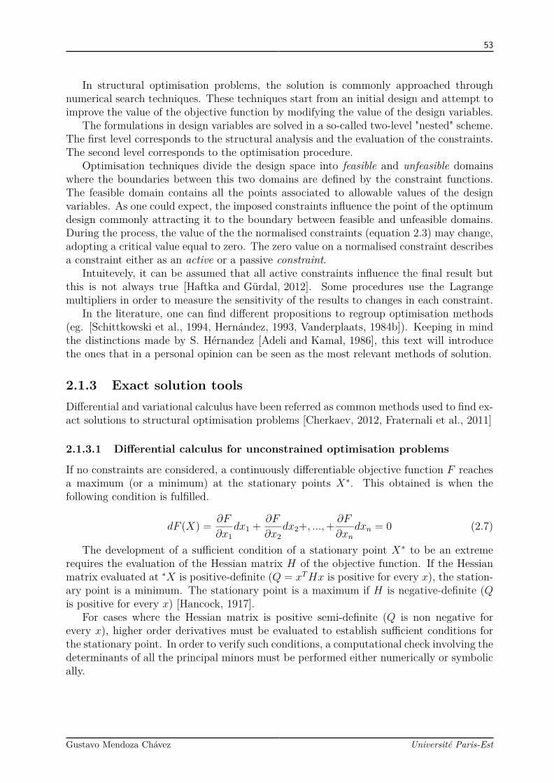
53

In structural optimisation problems, the solution is commonly approached throughnumerical search techniques. These techniques start from an initial design and attempt toimprove the value of the objective function by modifying the value of the design variables.

The formulations in design variables are solved in a so-called two-level "nested" scheme.The first level corresponds to the structural analysis and the evaluation of the constraints.The second level corresponds to the optimisation procedure.

Optimisation techniques divide the design space into feasible and unfeasible domainswhere the boundaries between this two domains are defined by the constraint functions.The feasible domain contains all the points associated to allowable values of the designvariables. As one could expect, the imposed constraints influence the point of the optimumdesign commonly attracting it to the boundary between feasible and unfeasible domains.During the process, the value of the the normalised constraints (equation 2.3) may change,adopting a critical value equal to zero. The zero value on a normalised constraint describesa constraint either as an active or a passive constraint.

Intuitevely, it can be assumed that all active constraints influence the final result butthis is not always true [Haftka and Gürdal, 2012]. Some procedures use the Lagrangemultipliers in order to measure the sensitivity of the results to changes in each constraint.

In the literature, one can find different propositions to regroup optimisation methods(eg. [Schittkowski et al., 1994, Hernández, 1993, Vanderplaats, 1984b]). Keeping in mindthe distinctions made by S. Hérnandez [Adeli and Kamal, 1986], this text will introducethe ones that in a personal opinion can be seen as the most relevant methods of solution.

2.1.3 Exact solution toolsDifferential and variational calculus have been referred as common methods used to find ex-act solutions to structural optimisation problems [Cherkaev, 2012, Fraternali et al., 2011]

2.1.3.1 Differential calculus for unconstrained optimisation problems

If no constraints are considered, a continuously differentiable objective function F reachesa maximum (or a minimum) at the stationary points X∗. This obtained is when thefollowing condition is fulfilled.

dF (X) = ∂F

∂x1dx1 + ∂F

∂x2dx2+, ...,+ ∂F

∂xndxn = 0 (2.7)

The development of a sufficient condition of a stationary point X∗ to be an extremerequires the evaluation of the Hessian matrix H of the objective function. If the Hessianmatrix evaluated at ∗X is positive-definite (Q = xTHx is positive for every x), the station-ary point is a minimum. The stationary point is a maximum if H is negative-definite (Qis positive for every x) [Hancock, 1917].

For cases where the Hessian matrix is positive semi-definite (Q is non negative forevery x), higher order derivatives must be evaluated to establish sufficient conditions forthe stationary point. In order to verify such conditions, a computational check involving thedeterminants of all the principal minors must be performed either numerically or symbolically.


54

2.1.3.2 Lagrange multipliers

As always, in order to find the minimum of an objective function F depending on n designvariables, the differential change must vanish

dF = ∂F

∂x1dx1 + ∂F

∂x2dx2 + ...+ ∂F

∂xndxn = 0 (2.8)

In the same manner, the differential changes in the constraints are verifyed:

dh = ∂h

∂x1dx1 + ∂h

∂x2dx2 + ...+ ∂h

∂xndxn = 0 (2.9)

Multiplying equation 2.9 by an arbitrary constant, λ, and adding the result to equation2.8 leads to:

(∂F

∂x1+ λ

∂h

∂x1

)dx1 +

(∂F

∂x2+ λ

∂h

∂x2

)dx2 + ...+

(∂F

∂xn+ λ

∂h

∂xn

)dxn = 0 (2.10)

In order to vanish the elements inside each parenthesis one must determine λ whichleads to a system of n equations and n + 1 unknowns (the n design variables plus theLagrange multiplier). The additional equation needed to solve the system is given by theconstraint relation (h(x) = 0). If multiple constraints must be treated, additional Lagrangemultipliers shall be added for each of the constraint functions. The general formulationof an optimisation problem of one objective function, n design variables and, ne equalityconstraints is thus equivalent to a n unconstrained problem with an auxiliary function(equation 2.11). Then the optimum design can be found by solving the system formed byequations 2.12.

L(X,λ) = F (X) +ne∑j

λjhj (2.11)

∂L

∂xi= 0, i = 1, ..., n (2.12a)

∂L

∂λj= 0, j = 1, ..., ne (2.12b)

2.1.4 Optimality Criteria (OC) based methodsConsidering a general structure discretised into m finite elements, the load-displacementrelation is expressed in the framework of linear elasticity as:

[K]U = F (2.13)

where [K] is the global stiffness matrix, U is the displacements and, F the appliedload vector.

The total weight, W , of a structure composed of m elements, can be calculated as:


55

W (ai) =m∑i=1

ρiaili (2.14)

where ρ is the mass density and aili the volume of the ith element. The element length,li, is considered constant while the cross sections, ai, are taken as the design variables. Thegeneralised constraints gj(X) applying to the structure can be written as:

gj(ai) = Cj(ai)− Cj ≤ 0 j = l, ..., p (2.15)

where Cj is the actual value of the jth constrained value and Cj is the upper limitvalue.

When treating displacement constraints, it is convenient to express the generalisedconstraints (equation 2.15) as a function of the flexibility coefficient Eij:

Fj(Ai) =m∑i=1

Eijaj− Cj ≤ 0 j = 1, ..., p (2.16)

with Eij = ri[k]isjai (or Eij = FiUji li/Ei for truss structures). In the previous

expressions ri and sj are the displacement vectors generated at the ith element by thea vector R and a virtual load vector Sj associated to the jth constraint, Fi is the forcein the ith bar.

Given the objective function to minimise, W (ai), and the constraints, gj(ai), the La-grange multipliers can be applied to the minimisation in the form:

W (ai, λj) =m∑i=1

ρiliai +p∑j=1

λjgj(ai) (2.17)

where λj are the Lagrangian parameters. Now, the local constrained optimum is ob-tained by differentiating the previous equation (2.17) with respect to the design variablesai resulting in equation 2.18.

∂

∂aiW (ai, λj) = ρili +

p∑j=1

λj∂

∂aigj(ai) = 0 i = 1, ...,m (2.18)

with λj ≥ 0 and λjgj = 0.Substituting equation 2.16 into 2.18 leads to:

p∑j=1

λjEijpiliA2

i

= 1 i = 1, ...,m (2.19)

The optimal structure must satisfy the optimality condition (equation 2.19) and theconstraints (equation 2.15). When solving problems whith only one constraint, the La-grange multiplier can be explicitly defined and used to derive the recurrence relation forthe design variable. When there is more than one constraint, the problem becomes morecomplex.

Since the obtained equations are non-linear, the solution schemes are based on the useof recurrence relations iterative in nature. In few words, the optimality criterion is usedto derive a relation to modify the design variables while the constraints equations are used


56

Figure 2.3: Graphical explanation of KKT conditions as seen in [Kirsch, 2012]

to obtain relations for the evaluation of the Lagrange parameters [Khot and B., 1979]. Fortruss structures, the allowable stress constraint can be directly replaced by a constraint onthe deformation of each element.

2.1.4.1 Karush-Kuhn-Tucker based methods

Karush-Kuhn–Tucker conditions (KKT), sometimes referred as Kuhn–Tucker conditions,establish that the vector ∇F must have negative components for all gradients ∇gi at alocal minimum point. In other words, when some components of λi are non-positive, thecurrent point cannot be a minimum.

∂F

∂xi+

J∑j=1

λj∂gj∂xi

= 0 i = 1, ..., n (2.20)

and

λj ≥ 0 j = 1, ..., J (2.21)A 2D graphical representation of the KKT conditions is given in figure 2.3. In the first

situation, where −∇F is not within the zone delimited by ∇gi, the value of F can stillbe improved without violating the constraints. Thus the point is not a minimum. In thesecond situation, the vector −∇F lies in the zone defined by the constraints.

Based on equation 2.20, and knowing that the first term of the left-hand side cannotbe zero ( ∂F

∂xi6= 0), it can be stated that an equivalent expression for finding the minimum

based on an iterative process is obtained by:

−m∑j=1

λjk∂gjk∂xi

/∂Fk∂xi

= Tik (2.22)

where Tik will take a value of 1 at the minimumEquation 2.22 is used as an indicator of proximity to the point of minimum and, ac-

cording to the value of Tik, a recurrence relation can be established of any element xi of


57

design variables kX and k+1X at two consecutive iterations. A common recurrence rela-tion [Khot and B., 1979] and expression to compute the Lagrange multipliers are shown inequations 2.23 and 2.24.

k+1xi = [α + (1− α)(kTi)]kxi i = 1, ..., n (2.23)

n∑i=1

∂(kgj)∂xi

(kxi)m∑j=1

λj∂(kgj)∂xi

/∂(kF )∂xi

=kgj

1− α −n∑i=1

∂(kgj)∂xi

(kxi) (2.24)

where α is the relaxation factor that limits the step size between iterations. The usualvalue of α oscillates between 0.5 to 0.75 [Adeli, 2002].

Equation 2.24 represents a system of linear equations with non-negative solutions forall λi associated to the active constraints.

As it can be inferred, finding the values of the Lagrange multipliers is trivial to solvethe optimisation problem and this task that can be achieved through an iterative process.A general process can be summarised in four steps:

1. Definition of an initial design 0X.

2. Computation of the Lagrange multipliers λi, task that can be achieved through equa-tion 2.24

3. Computation of values Tik (see equation 2.22)

4. Update of the system using a recurrence relation (such as equation 2.23)

A first estimate or starting point 0X of each design variables 0xi is needed. Thisstarting point gets the iterative procedure improved by a loop generated by points 2 to 4until the relative or absolute convergence is achieved. If the initial point is very far fromthe minimum, the procedure may present difficulties to converge. The same difficultiesare expected if the subset of active constraints changes frequently from one iteration toanother.

2.1.5 Methods based on mathematical programming2.1.5.1 Linear programming

A large variety of types of optimisation problems can be found in almost any book ofoptimisation techniques [Foulds, 2012] or Operational research [Hillier, 2012]. Despite itsversatility, its applicability in the field of structural design can sometimes be reduced.The standard form of LP problems is defined by a linear objective function with lin-ear equality constraints and non-negative design variables defining altogether a (possiblyunbounded) convex polytope. Although structural design problems are rarely linear, lin-earisation strategies can be introduced to fit some special cases.

The general LP statement is:

minimise F = CTX (2.25)


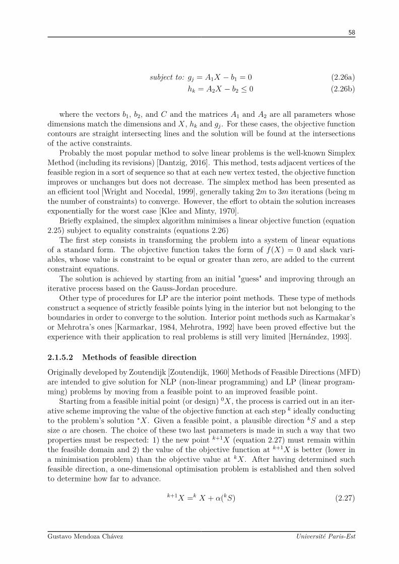
58

subject to: gj = A1X − b1 = 0 (2.26a)hk = A2X − b2 ≤ 0 (2.26b)

where the vectors b1, b2, and C and the matrices A1 and A2 are all parameters whosedimensions match the dimensions and X, hk and gj. For these cases, the objective functioncontours are straight intersecting lines and the solution will be found at the intersectionsof the active constraints.

Probably the most popular method to solve linear problems is the well-known SimplexMethod (including its revisions) [Dantzig, 2016]. This method, tests adjacent vertices of thefeasible region in a sort of sequence so that at each new vertex tested, the objective functionimproves or unchanges but does not decrease. The simplex method has been presented asan efficient tool [Wright and Nocedal, 1999], generally taking 2m to 3m iterations (being mthe number of constraints) to converge. However, the effort to obtain the solution increasesexponentially for the worst case [Klee and Minty, 1970].

Briefly explained, the simplex algorithm minimises a linear objective function (equation2.25) subject to equality constraints (equations 2.26)

The first step consists in transforming the problem into a system of linear equationsof a standard form. The objective function takes the form of f(X) = 0 and slack vari-ables, whose value is constraint to be equal or greater than zero, are added to the currentconstraint equations.

The solution is achieved by starting from an initial "guess" and improving through aniterative process based on the Gauss-Jordan procedure.

Other type of procedures for LP are the interior point methods. These type of methodsconstruct a sequence of strictly feasible points lying in the interior but not belonging to theboundaries in order to converge to the solution. Interior point methods such as Karmakar’sor Mehrotra’s ones [Karmarkar, 1984, Mehrotra, 1992] have been proved effective but theexperience with their application to real problems is still very limited [Hernández, 1993].

2.1.5.2 Methods of feasible direction

Originally developed by Zoutendijk [Zoutendijk, 1960] Methods of Feasible Directions (MFD)are intended to give solution for NLP (non-linear programming) and LP (linear program-ming) problems by moving from a feasible point to an improved feasible point.

Starting from a feasible initial point (or design) 0X, the process is carried out in an iter-ative scheme improving the value of the objective function at each step k ideally conductingto the problem’s solution ∗X. Given a feasible point, a plausible direction kS and a stepsize α are chosen. The choice of these two last parameters is made in such a way that twoproperties must be respected: 1) the new point k+1X (equation 2.27) must remain withinthe feasible domain and 2) the value of the objective function at k+1X is better (lower ina minimisation problem) than the objective value at kX. After having determined suchfeasible direction, a one-dimensional optimisation problem is established and then solvedto determine how far to advance.

k+1X =k X + α(kS) (2.27)


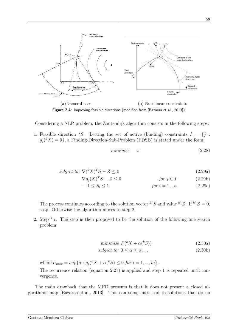
59

(a) General case

First constraint

Second

constraint

Fourth

constraint

Improving feasible

directions

Contours of the

objective function

Third

constraint

g3

(x) g4

(x)

f(x)

x

(b) Non-linear constraintsFigure 2.4: Improving feasible directions (modified from [Bazaraa et al., 2013]).

Considering a NLP problem, the Zoutendijk algorithm consists in the following steps:

1. Feasible direction kS. Letting the set of active (binding) constraints I = j :gj(kX) = 0, a Finding-Direction-Sub-Problem (FDSB) is stated under the form:

minimise z (2.28)

subject to: ∇(kX)TS − Z ≤ 0 (2.29a)∇gj(X)TS − Z ≤ 0 for j ∈ I (2.29b)− 1 ≤ Si ≤ 1 for i = 1, ..n (2.29c)

The process continues according to the solution vector k∗S and value k∗

Z. If k∗Z = 0,

stop. Otherwise the algorithm moves to step 2

2. Step kα. The step is then proposed to be the solution of the following line searchproblem:

minimise F (kX + α(kS)) (2.30a)subject to: 0 ≤ α ≤ αmax (2.30b)

where αmax = supα : gj(kX + α(kS) ≤ 0 for i = 1, ...,m.The recurrence relation (equation 2.27) is applied and step 1 is repeated until con-vergence.

The main drawback that the MFD presents is that it does not present a closed al-gorithmic map [Bazaraa et al., 2013]. This can sometimes lead to solutions that do no


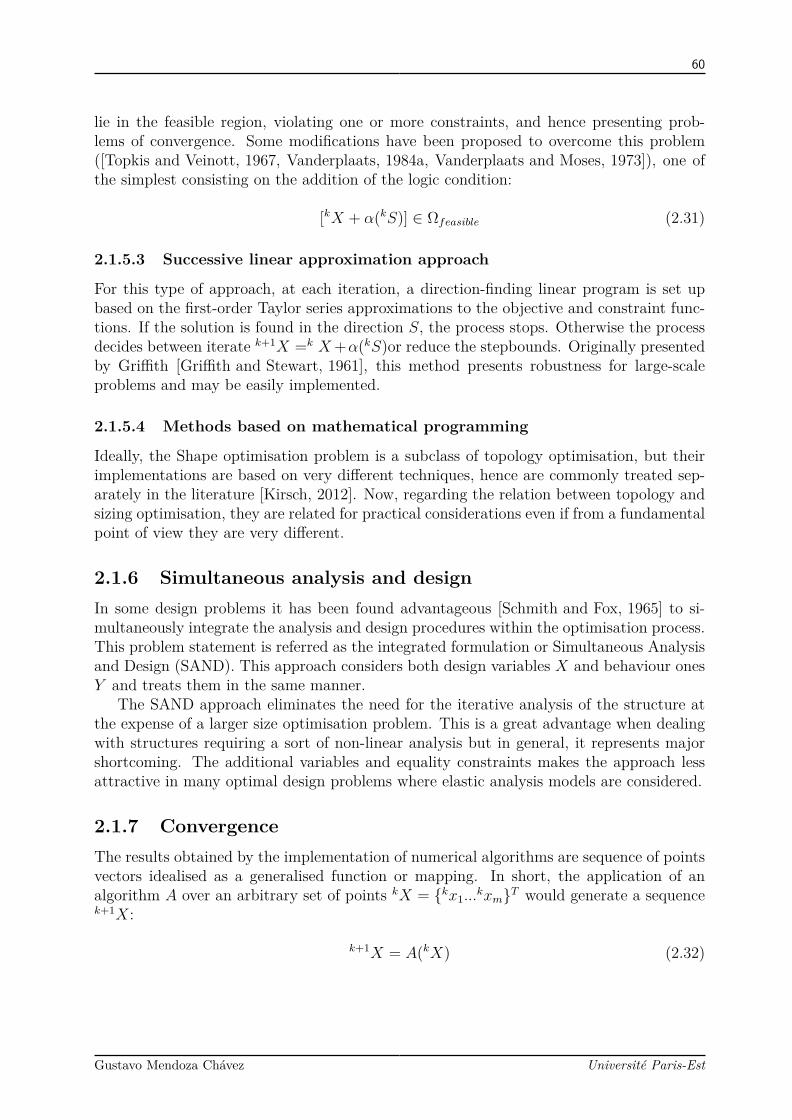
60

lie in the feasible region, violating one or more constraints, and hence presenting prob-lems of convergence. Some modifications have been proposed to overcome this problem([Topkis and Veinott, 1967, Vanderplaats, 1984a, Vanderplaats and Moses, 1973]), one ofthe simplest consisting on the addition of the logic condition:

[kX + α(kS)] ∈ Ωfeasible (2.31)

2.1.5.3 Successive linear approximation approach

For this type of approach, at each iteration, a direction-finding linear program is set upbased on the first-order Taylor series approximations to the objective and constraint func-tions. If the solution is found in the direction S, the process stops. Otherwise the processdecides between iterate k+1X =k X+α(kS)or reduce the stepbounds. Originally presentedby Griffith [Griffith and Stewart, 1961], this method presents robustness for large-scaleproblems and may be easily implemented.

2.1.5.4 Methods based on mathematical programming

Ideally, the Shape optimisation problem is a subclass of topology optimisation, but theirimplementations are based on very different techniques, hence are commonly treated sep-arately in the literature [Kirsch, 2012]. Now, regarding the relation between topology andsizing optimisation, they are related for practical considerations even if from a fundamentalpoint of view they are very different.

2.1.6 Simultaneous analysis and designIn some design problems it has been found advantageous [Schmith and Fox, 1965] to si-multaneously integrate the analysis and design procedures within the optimisation process.This problem statement is referred as the integrated formulation or Simultaneous Analysisand Design (SAND). This approach considers both design variables X and behaviour onesY and treats them in the same manner.

The SAND approach eliminates the need for the iterative analysis of the structure atthe expense of a larger size optimisation problem. This is a great advantage when dealingwith structures requiring a sort of non-linear analysis but in general, it represents majorshortcoming. The additional variables and equality constraints makes the approach lessattractive in many optimal design problems where elastic analysis models are considered.

2.1.7 ConvergenceThe results obtained by the implementation of numerical algorithms are sequence of pointsvectors idealised as a generalised function or mapping. In short, the application of analgorithm A over an arbitrary set of points kX = kx1...

kxmT would generate a sequencek+1X:

k+1X = A(kX) (2.32)


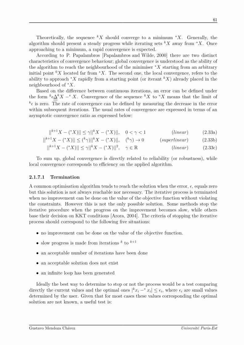
61

Theoretically, the sequence kX should converge to a minimum ∗X. Generally, thealgorithm should present a steady progress while iterating sets kX away from ∗X. Onceapproaching to a minimum, a rapid convergence is expected.

According to P. Papalambros [Papalambros and Wilde, 2000] there are two distinctcharacteristics of convergence behaviour; global convergence is understood as the ability ofthe algorithm to reach the neighbourhood of the minimiser ∗X starting from an arbitraryinitial point 0X located far from ∗X. The second one, the local convergence, refers to theability to approach ∗X rapidly from a starting point (or iterant kX) already placed in theneighbourhood of ∗X.

Based on the difference between continuous iterations, an error can be defined underthe form kε∆kX −∗ X. Convergence of the sequence kX to ∗X means that the limit ofkε is zero. The rate of convergence can be defined by measuring the decrease in the errorwithin subsequent iterations. The usual rates of convergence are expressed in terms of anasymptotic convergence ratio as expressed below:

||k+1X − (∗X)|| ≤ γ||kX − (∗X)||, 0 < γ < 1 (linear) (2.33a)||k+1X − (∗X)|| ≤ (kγ)||kX − (∗X)||, (kγ)→ 0 (superlinear) (2.33b)||k+1X − (∗X)|| ≤ γ||kX − (∗X)||2, γ ∈ R (linear) (2.33c)

To sum up, global convergence is directly related to reliability (or robustness), whilelocal convergence corresponds to efficiency on the applied algorithm.

2.1.7.1 Termination

A common optimisation algorithm tends to reach the solution when the error, ε, equals zerobut this solution is not always reachable nor necessary. The iterative process is terminatedwhen no improvement can be done on the value of the objective function without violatingthe constraints. However this is not the only possible solution. Some methods stop theiterative procedure when the progress on the improvement becomes slow, while othersbase their decision on KKT conditions [Arora, 2004]. The criteria of stopping the iterativeprocess should correspond to the following five situations:

• no improvement can be done on the value of the objective function.

• slow progress is made from iterations k to k+1

• an acceptable number of iterations have been done

• an acceptable solution does not exist

• an infinite loop has been generated

Ideally the best way to determine to stop or not the process would be a test comparingdirectly the current values and the optimal ones |kxi −∗ xi| ≤ εi, where εi are small valuesdetermined by the user. Given that for most cases these values corresponding the optimalsolution are not known, a useful test is:


62

|kxi −k+1 xi| ≤ εi, i = 1...m (2.34)

Many algorithms are also constructed in such a manner that ∇kf → 0T indicating astationary point that is most of the times (a exception for hidden saddles) also a minimiser.

||∇kf || ≤ ε (2.35)

Precedent equation (2.35), together with a satisfactory positive-definiteness of the Hes-sian evaluated at kX, seems to be a reliable index for the termination with the disadvantageof the restiveness of its application to problems with large numbers of variables.

When solving constrained problems, apart from convergence tests, an acceptable con-straint violation is allowed by setting:

||gj|| ≤ ε (2.36)

being gj the vector off all active constraints.In reality, determining the proper termination criteria seems to be a matter of experience

and expertise and is itself a subject of study [Kirsch, 2012].

2.2 Continuum optimisationWithin the structural design, three typical problems can be defined: namely sizing, shapeand topology optimisation problems. The goal of sizing problems is to determine theoptimal distribution of thicknesses or cross sections of the elements conforming an existentlinear elastic structure. The optimal "size" minimises or maximises the objective functionnormally expressed as a physical quantity such as the peak stress, displacement, externalwork (compliance), etc. For the case of shape optimisation, the domain of the structure istaken as the design variable. The goal here is to find the optimum shape. Finally, topologyoptimisation may redefine the connectivity of the domain.

Within the structural optimisation domain, two types of optimisation can be definedaccording to the treated structure: discrete and continuous. For inherently discrete struc-tures (skeletal structures), finding the optimum design consists in determining the optimumnumber, positions, mutual connectivity and individual cross section of the structural mem-bers.

For continuum structures, the shape of both internal and external boundaries as well asinner cavities may be simultaneously optimised following a predefined objective functionand constraints. According to [Eschenauer and Olhoff, 2001], two sub-classes of continuumoptimisation can be distinguished :

1. Material optimisation or Microapproach. For this type of approach, a fixed FE(finite element) mesh is used to describe the initial geometry (or the admissibledesign domain). Typically, the mesh has a rectangular shape with elements evenlydistributed and the constraints are assumed to attain constant values at the nodes ofthe mesh. For the analysis, the characteristics of the FE such as Young modulus Eand material density ρ are based on the physical modelling of a porous microstructure(made up of solid material and void) whose orientation and density are described by


63

continuous variables along the admissible domain. The optimisation consists in thedeciding whether each element should contain material or not. To achieve this, thematerial within each element is associated to a design variable defined between 0and 1; 0 considers a void or a very weak material while 1 represents a solid material[Bendsøe and Sigmund, 2003].The final result can be graphically represented showing a rough description of theoptimum outer and inner boundaries (see figure 2.5).

2. Geometrical continnum optimisation or Macroapproach. This class of optimisationproceeds with a FE analysis considering fixed characteristics for the materials of theelements associated to a non-fixed mesh. The topology of the optimum structure isachieved by growing/reducing material or inserting holes. The first method startsfrom the hypothesis that the optimal design is obtained as a subset of the designdomain. The second method iteratively proposes holes at specific points on thestructure continuously modifying the boundaries of the geometry.

Even if some articles have been published showing Strut-and-Tie models found troughcontinuum-type optimal topology, [Almeida et al., 2013, Shobeiri, 2016] this practice re-mains controversial. From the point of view of mechanics, the characteristics of the dis-crete and continuum structures are very different, and from the point of view of the prac-tical implementation, there is no criteria for constructing truss topologies from the resultsof optimal finite element solutions [Starčev-Ćurčin et al., 2013]. In addition, due to thecharacteristics presented by the interaction concrete-reinforcement and according to somestudies [Swan et al., 1999], a more adequate ST model would be found through a discreteoptimisation purely based on truss structures.

2.3 Discrete optimisation: ground structure approachPast decades can be considered to be the apogee for the development of algorithms forstructural optimisation, mainly for weight minimisation problems. Most of generated algo-rithms have been initially developed for truss cases and then generalised for the treatmentof more complex structures [Farshi and Alinia-Ziazi, 2010].

The objective functions presented in truss optimisation are usually dependant on thedesign variables, while constraints can be expressed in both behaviour and design variablesleading to a non-linear relation that normally requires Non-Linear Programming (NLP)approaches for a direct mathematical solution.

Initially proposed by Dorn [Dorn, 1964], the ground structure approach reduces thecomplexity of a topology optimisation problem by considering a truss with a preexistingquantity of potential elements, m, linked at the nodes, n, of a fixed grid. The initial,or ground structure, is characterised by a high degree of connectivity that in some casesproduces an element for the combination of any two nodes on the grid, having a quantityof elements m equal to n(n− 1)/2, while the degree of freedom N is only of the order 2nor 3n (for planar and 3-D trusses) (see figure 2.6).

The ground structure approach arises as a simplification of the optimisation problem.Once the initial truss has been proposed, its solution depends on the type of the addressedproblem.


64

Figure 2.5: Conceptual processes of optimisation of continuum structures (as seen in[Eschenauer and Olhoff, 2001])

(a) Minimal connection(m = 106)

(b) Intermediate case(m = 183)

(c) Fully connected(m = 595)

Figure 2.6: Three possible ground structures for a 4x6 grid (n = 35)


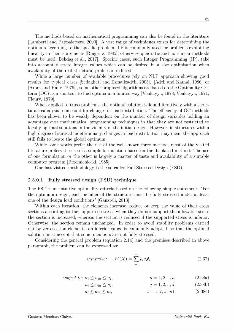
65

The methods based on mathematical programming can also be found in the literature[Lamberti and Pappalettere, 2000]. A vast range of techniques exists for determining theoptimum according to the specific problem. LP is commonly used for problems exhibitinglinearity in their statements [Ringertz, 1985], otherwise quadratic and non-linear methodsmust be used [Bekdaş et al., 2017]. Specific cases, such Integer Programming (IP), takeinto account discrete integer values which can be desired in a size optimisation whenavailability of the real structural profiles is reduced.

While a large number of available procedures rely on NLP approach showing goodresults for typical cases [Sedaghati and Esmailzadeh, 2003], [Adeli and Kamal, 1986] or[Arora and Haug, 1976] , some other proposed algorithms are based on the Optimality Cri-teria (OC) as a shortcut to find optima in a limited way [Venkayya, 1978, Venkayya, 1971,Fleury, 1979].

When applied to truss problems, the optimal solution is found iteratively with a struc-tural reanalysis to account for changes in load distribution. The efficiency of OC methodshas been shown to be weakly dependent on the number of design variables holding anadvantage over mathematical programming techniques in that they are not restricted tolocally optimal solutions in the vicinity of the initial design. However, in structures with ahigh degree of statical indeterminacy, changes in load distribution may mean the approachstill fails to locate the global optimum.

While some works prefer the use of the well known force method, most of the visitedliterature prefers the use of a simple formulation based on the displaced method. The useof one formulation or the other is largely a matter of taste and availability of a suitablecomputer program [Przemieniecki, 1985].

One last visited methodology is the so-called Full Stressed Design (FSD).

2.3.0.1 Fully stressed design (FSD) technique

The FSD is an intuitive optimality criteria based on the following simple statement: "Forthe optimum design, each member of the structure must be fully stressed under at leastone of the design load conditions" [Ganzreli, 2013].

Within each iteration, the elements increase, reduce or keep the value of their crosssections according to the supported stress: when they do not support the allowable stressthe section is increased, whereas the section is reduced if the supported stress is inferior.Otherwise, the section remain unchanged. In order to avoid stability problems carriedout by zero-section elements, an inferior gauge is commonly adopted, so that the optimalsolution must accept that some members are not fully stressed.

Considering the general problem (equation 2.14) and the premises described in aboveparagraph, the problem can be expressed as:

minimise: W (X) =m∑i=1

ρiaili (2.37)

subject to: σi ≤ σin ≤ σi, n = 1, 2, .., n (2.38a)ui ≤ uin ≤ ui, j = 1, 2, .., J (2.38b)ai ≤ ain ≤ ai, i = 1, 2, ..,m1 (2.38c)


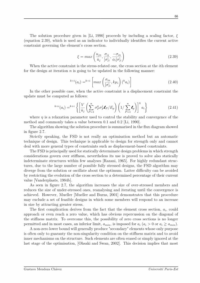
66

The solution procedure given in [Li, 1990] proceeds by including a scaling factor, ξ(equation 2.39), which is used as an indicator to individually identifies the current activeconstraint governing the element’s cross section.

ξ = max

(ujnuj,σij[σ]i

,−σinφi[σ]i

)(2.39)

When the active constraint is the stress-related one, the cross section at the ith elementfor the design at iteration n is going to be updated in the following manner:

k+i(ai) =k+i[max

(σin[σ]i

, kµi

)(kai)

](2.40)

In the other possible case, when the active constraint is a displacement constraint theupdate must be computed as follows:

k+i(ai) =k+i[

V

uj

(n∑

P=1σqPσ

jP lP/Ep

)(1/

n∑P=1lp

)]ηai

(2.41)

where η is a relaxation parameter used to control the stability and convergence of themethod and commonly takes a value between 0.1 and 0.2 [Li, 1990].

The algorithm showing the solution procedure is summarised in the flux diagram showedin figure 2.7.

Strictly speaking, the FSD is not really an optimisation method but an automatictechnique of design. This technique is applicable to design for strength only and cannotdeal with more general types of constraints such as displacement-based constraints.

The FSD is principally used for statically determinate design problems in which strengthconsiderations govern over stiffness, nevertheless its use is proved to solve also staticallyindeterminate structures within few analyses [Razani, 1965]. For highly redundant struc-tures, due to the large number of possible fully stressed designs, the FSD algorithm maydiverge from the solution or oscillate about the optimum. Latter difficulty can be avoidedby restricting the evolution of the cross section to a determined percentage of their currentvalue [Vanderplaats, 1984b].

As seen in figure 2.7, the algorithm increases the size of over-stressed members andreduces the size of under-stressed ones, reanalysing and iterating until the convergence isachieved. However, Mueller [Mueller and Burns, 2001] demonstrates that this proceduremay exclude a set of feasible designs in which some members will respond to an increasein size by attracting greater stress.

The first complication derives from the fact that the element cross section, ai, couldapproach or even reach a zero value, which has obvious repercussion on the diagonal ofthe stiffness matrix. To overcome this, the possibility of zero cross sections is no longerpermitted and in most cases, an inferior limit, amin, is imposed for ai (ai > 0 or ai ≥ amin).

A non-zero lower bound will generally produce "secondary" elements whose only purposeis often only to guaranty the non-singularity condition on the stiffness matrix and to avoidinner mechanisms on the structure. Such elements are often erased or simply ignored at thelast stage of the optimisation, [Ohsaki and Swan, 2002]. This decision implies that most


67

Starting design 0ai

Solve for ku, kσ and W

Compute the scaling fac-tor ξ (equation 2.39)

Activeconstraint

Stress constraint.Apply equation 2.40

Displacement con-straint.Apply equation 2.41

Verify limit values of the variables

∣∣∣ kW−k−1WkW

∣∣∣ ≤ε

Stop

Updatek+1ai = (kai)

ξ = max(σij

[σ]i ,−σik

φi[σ]i

)ξ = max

(ujk

uj

)

yes

no

Figure 2.7: Flowchart design procedure using FSD (inspired from [Li, 1990]).

optimal designs have a singular matrix and present potential mechanisms when describedas a part of the ground structure leading to the second listed complication.

The third complication is related to the choice of the ground structure. The groundstructure approach may or may not lead to the optimal structure according to the group ofnodes proposed (quantity and position) and the set of allowed elements; the optimal struc-ture appears to be limited by the original geometrical restrictions and possible connections(figure 2.8).


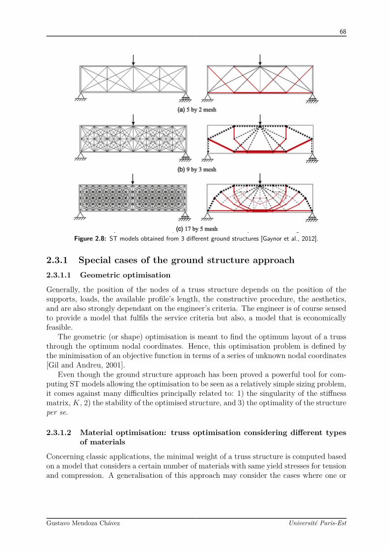
68

Figure 2.8: ST models obtained from 3 different ground structures [Gaynor et al., 2012].

2.3.1 Special cases of the ground structure approach2.3.1.1 Geometric optimisation

Generally, the position of the nodes of a truss structure depends on the position of thesupports, loads, the available profile’s length, the constructive procedure, the aesthetics,and are also strongly dependant on the engineer’s criteria. The engineer is of course sensedto provide a model that fulfils the service criteria but also, a model that is economicallyfeasible.

The geometric (or shape) optimisation is meant to find the optimum layout of a trussthrough the optimum nodal coordinates. Hence, this optimisation problem is defined bythe minimisation of an objective function in terms of a series of unknown nodal coordinates[Gil and Andreu, 2001].

Even though the ground structure approach has been proved a powerful tool for com-puting ST models allowing the optimisation to be seen as a relatively simple sizing problem,it comes against many difficulties principally related to: 1) the singularity of the stiffnessmatrix, K, 2) the stability of the optimised structure, and 3) the optimality of the structureper se.

2.3.1.2 Material optimisation: truss optimisation considering different typesof materials

Concerning classic applications, the minimal weight of a truss structure is computed basedon a model that considers a certain number of materials with same yield stresses for tensionand compression. A generalisation of this approach may consider the cases where one or


69

(a) General case (b) No-compression materialFigure 2.9: Piece-wise linear stress-strain relations (modified from [Achtziger, 1996])

more of the considered materials present different properties for negative and positivestresses.

Figure 2.9 depicts a material where the absolute yield stress σc and σt (stresses ofcompression and traction) are different, in the same manner Ec and Et may be different[Achtziger, 1996]. This "equivalent" behaviour considers the case where two materials arepresent in a structure. One branch of the stress-strain relation represent the behaviour ofthe bars in compression while the other concerns the elements in compression.

A key point of this kind of optimisation must be the correct handling of the property-assignation scheme. However, the nature of the forces at each element is not available atthe beginning of the process. Thus, this difficulty must be stated on the formulation of theproblem.

2.4 SummaryMost optimal design studies applied on skeletal structures deal with cross-sectional designvariables. However, due to the weight reductions that can be gained by modifications ofthe structural configuration [Gil and Andreu, 2001], a growing quantity of scientific papersinterested in shape optimisation have been published in recent years. Yet, there are somebasic difficulties involved in this type of optimisation. One major complication is related tothe need of declare the existence or absence of structural elements. Another complication,and probably the most important, involves the choice of the starting selection of nodes andelements; the selection of the ground structure.

So far, the procedure to select a ground structure seems to relay on the designer experi-ence. Intuitively, if the nodal positions are fixed, the choice of a saturated ground structurewould lead to the best results. In this manner, the geometric optimisation is "replaced"by a large quantity of potential (fixed) nodes in the ground structure. The selection ofthe "best nodal coordinates" is indirectly made by vanishing those nodes only attached toelements whose cross section approximates to 0. From an opposed point of view, if nodalpositions are also implicitly included in the variable vector, a sparse ground structure ispreferred.

From a practical point of view, optimisation formulations that simultaneously improvetopology and geometry may lead to reasonable structures presenting the disadvantage ofbeing a highly non-linear problem and, in some cases, with disjointed design spaces. On the


70

other hand, pure ground structure optimisation generally its simple performed. However,it has been shown that such approach frequently leads to singular unstable structures orto structures with a considerable high quantity of secondary elements.

In an attempt to obtain reasonable structures through a simple algorithm, avoidingthe complications related with mixed design vectors, some methodologies are presented as2-part optimisation problems.

The optimum solution can be obtained by the application of a stress-ratio method overa fixed geometry followed by a geometric optimisation. In the first instance, this processwill allow to "reduce" the structure by decreasing the section of non-trivial elements. Oncethe sizing procedure is completed, the optimisation of the geometry is implemented.

The proposed procedure combines the ground structure approach with a subsequentiteration procedure that alternates between the member sizing optimisation (cross sectionsas variables) and the shape modification (node coordinates as variables).

In addition, [Vanderplaats, 1984a] developed a technique where the stress-ratio methodwas used to size the structure while keeping the topology fixed and the steepest descentmethod was used to move the nodal coordinates while keeping the sections fixed. Using twoseparate design spaces reduces the design variables at each sub-problem and simplifyingthe global optimisation. The main drawback was that the algorithm was not able toautomatically to add or delete members or joints during the design process frequentlyproducing ill-conditioning problems.

According to the reviewed literature, a suitable way to threat truss optimisation problemswould be an hybrid algorithm able to sequentially threat the structure and a subroutinecapable of delete or insert elements without compromising the stability of the Stiffnessmatrix and the whole structure.


Chapter 3

Computational aided approachthrough locally weighted regressions

In recent years, several approaches have been proposed in order to ease the application ofthe Strut-and-Tie method. While some methodologies threat the problem as a continuousoptimisation, some others prefer the ground structure and truss optimisation to create anacceptable reinforcement layout.

One of the main difficulties of this last approach, based on the truss optimisation, ishow to define the initial structure: the initial number of elements, connectivity and, themost important, how to determine the number and position of the nodes.

The objective of this chapter is to present in detail the proposed computer aidedprocess to acquire Strut-and-Tie models for the reinforcement bi-dimensional and three-dimensional concrete structures.

This chapter contains two important sections. The first one presents and describes thealgorithm of the proposed method. The second section intends to clear out some points ofthe behaviour and the performance of the process seen on the test campaign.

Approche assistée par ordinateur par régressions lo-calement pondéréesAu cours des dernières années, plusieurs approches ont été proposées afin de faciliterl’application de la méthode Bielle-Tirant. Alors que certaines méthodologies abordent leproblème en tant qu’une optimisation continue, d’autres préfèrent la structure de base etl’optimisation du treillis pour créer un schéma de ferraillage acceptable.

L’un des principales difficultés de la dernière méthodologie, basée sur l’optimisationd’une ferme, est de définir la structure initiale : le nombre initial d’éléments, la connectivitéet, surtout, la façon de déterminer le nombre et la position des noeuds.

L’objectif de ce chapitre est de présenter en détail le l’algorithme proposée pour l’acquisitionde modèles Bielle-Tirant pour des structures planes ou tridimensionnellles en béton armé.

Ce chapitre consiste en deux sections. La première présente et décrit l’algorithme de laméthode proposée. La deuxième section vise à eclairer certains points du comportement etla performance du processus vu sur la campagne de tests.

72

3.1 Basis and description of the algorithmThe procedure here presented has three main purposes:

• to ease the generation of ST models based on the linear-elastic stress field distribution

• to propose both a fully automatic approach and a rational one based on the experienceof the engineer

• to present a fast and low cost (in terms of computational effort) option to assess theneed of steel reinforcement respecting the EuroCodes

Despite the previously discussed limitations that a ST based on its linear elastic stressfield may have. It was decided that, according to some sources such as [Chae and Yun, 2016],[Schlaich et al., 1987] and the [British Standards Institution, 2005], a strut-and-tie modelcan be developed for a given element based on its linear elastic (uncracked) stress field, usedto identify from it a possible resisting truss model. Accepting that plausible ST modelscan be produced through the application of structural optimisation techniques, the projectproposed a scheme based on weight minimisation. Within this work, discrete representa-tions (FE models including only bar-type elements) have been preferred over the so-calledcontinuous optimisation. This decision was principally based on the structural behaviourof a ST system (according to the EuroCodes) and also, based on the advantages that thistype of representation have in terms of its simplicity of treatment and the direct extractionof the final results.

Since the beginning, the construction of the initial ground structure was one of themajor difficulties to overcome. In order to automatise the process, the selection of thenodes, as well as the construction of the ground structure, is based on the linear elasticstress field of a FE analysis of the structure. This selection allows to generate an initialtruss structure and proceed to optimise it.

The algorithm has been divided in five subroutines that include the analysis and thepost-process of a model. The included subroutines proceed to fulfil different tasks:

1. input of the geometry and the boundary conditions

2. analysis of an initial continuous model of the structure and post-processing of theresults

3. construction of the ground structure based on the trajectories of the principal stressesproduct of the previous subroutine

4. reduction of the truss optimisation

5. construction of the resultant ST model and reinforcement proposition

These five subroutines will allow the user to determine a ST model


73

Input.Mechanical properties,

mesh, boundary conditions.

Linear-elastic FE analysis.Principal stresses andassociated directions.

Ground Structure.Division of the geometry, initialstrut path, linking elements.

Truss optimisation.

• Size

• Topology

• Geometric

kε ≤ ∗ε

Strut-and-tie model.Nodal revision, secondary struts,steel projection to the global axis.

Update

Iterative process

yes

no

Figure 3.1: Flowchart showing proposed the design procedure

3.1.1 InputThe input required for the algorithm depends on whether an initial FE analysis is neededor, the user already posses the results of an analysis carried out on a specialised software.

For the case where the initial finite element analysis is desired to be treated by thealgorithm, the input data matches the requirements of any other FE solver: the geometrydepicted by a nodal list and a connectivity matrix, the list of materials, and the bound-ary conditions. On the other hand, the algorithm can post-treat the results obtained bysoftware such as ANSYS and Code-Aster. For this case, additionally to the previous lists,the input must contain the resultant principal stresses computed at the element’s Gausspoints.

The subroutine reads the available information and stocks it as matrices and vectors inMatlab environment and inside a file where further results are also saved.


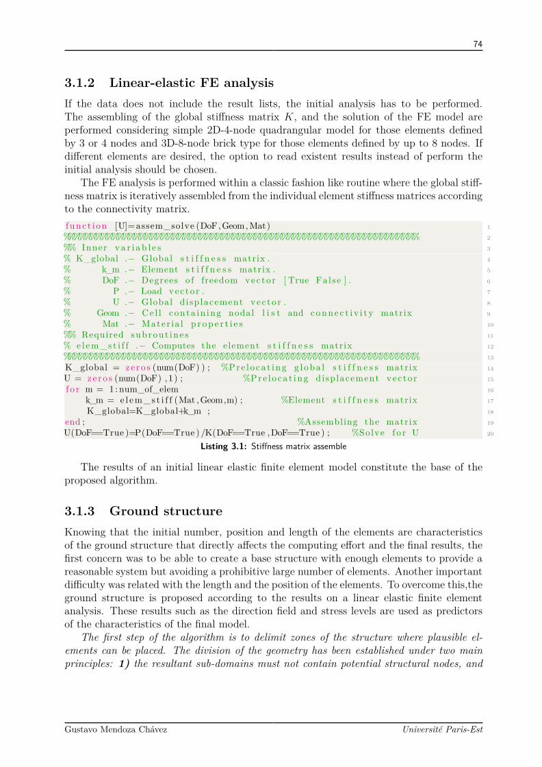
74

3.1.2 Linear-elastic FE analysisIf the data does not include the result lists, the initial analysis has to be performed.The assembling of the global stiffness matrix K, and the solution of the FE model areperformed considering simple 2D-4-node quadrangular model for those elements definedby 3 or 4 nodes and 3D-8-node brick type for those elements defined by up to 8 nodes. Ifdifferent elements are desired, the option to read existent results instead of perform theinitial analysis should be chosen.

The FE analysis is performed within a classic fashion like routine where the global stiff-ness matrix is iteratively assembled from the individual element stiffness matrices accordingto the connectivity matrix.

1f unc t i on [U]=assem_solve (DoF,Geom,Mat)2%%%%%%%%%%%%%%%%%%%%%%%%%%%%%%%%%%%%%%%%%%%%%%%%%%%%%%%%%%%%%%%%%3%% Inner v a r i a b l e s4% K_global .− Global s t i f f n e s s matrix .5% k_m .− Element s t i f f n e s s matrix .6% DoF .− Degrees o f freedom vecto r [ True Fa l se ] .7% P .− Load vec to r .8% U .− Global d i sp lacement vec to r .9% Geom .− Ce l l conta in ing nodal l i s t and conne c t i v i t y matrix10% Mat .− Mater ia l p r op e r t i e s11%% Required subrout ine s12% e l em_s t i f f .− Computes the element s t i f f n e s s matrix13%%%%%%%%%%%%%%%%%%%%%%%%%%%%%%%%%%%%%%%%%%%%%%%%%%%%%%%%%%%%%%%%%14K_global = ze ro s (num(DoF) ) ; %Pre l o ca t ing g l oba l s t i f f n e s s matrix15U = ze ro s (num(DoF) ,1 ) ; %Pre l o ca t ing disp lacement vec tor16f o r m = 1 : num_of_elem17k_m = e l em_s t i f f (Mat ,Geom,m) ; %Element s t i f f n e s s matrix18K_global=K_global+k_m ;19end ; %Assembling the matrix20U(DoF==True )=P(DoF==True ) /K(DoF==True ,DoF==True ) ; %Solve f o r U

Listing 3.1: Stiffness matrix assemble

The results of an initial linear elastic finite element model constitute the base of theproposed algorithm.

3.1.3 Ground structureKnowing that the initial number, position and length of the elements are characteristicsof the ground structure that directly affects the computing effort and the final results, thefirst concern was to be able to create a base structure with enough elements to provide areasonable system but avoiding a prohibitive large number of elements. Another importantdifficulty was related with the length and the position of the elements. To overcome this,theground structure is proposed according to the results on a linear elastic finite elementanalysis. These results such as the direction field and stress levels are used as predictorsof the characteristics of the final model.

The first step of the algorithm is to delimit zones of the structure where plausible el-ements can be placed. The division of the geometry has been established under two mainprinciples: 1) the resultant sub-domains must not contain potential structural nodes, and


75

Figure 3.2: Polynomial interpolation over 8 random XY Z triplets (second degree function of two variables ofthe form f(x, y) = α1x

2i + α2xiyi + α3y

2i + α4xi + α5yi + α6).

2) the principal direction of the minor stresses at each sub-domain must be developed alonga remarkable preponderant direction.

3.1.3.1 Local maximum of stress fields

Based on existent recommendations (principally found in [Schlaich et al., 1987, ACI-318, 2008,Davidovici et al., 2013, El-Metwally and Chen, 2017]) and some previous results found indocuments such [Wahlgren and Bailleul, 2016, Shah et al., 2011], the nodes of the ST modelare initially placed on the stress concentrations of the FE model. Among the different meth-ods to compute the local maxima and minima two options are available in the algorithm:

• Differentiation via interpolation. After having constructed an interpolating poly-nomial from the data, an approximation of the derivative at any point can be obtainedby a direct differentiation of the interpolant.For the differentiation via interpolation, the first stage is to construct an interpolatingpolynomial from the data. An approximation of the derivative at any point can bethen obtained by a direct differentiation of the interpolant.Based on a formula presented by Saniee [Saniee, 2008], the differentiation proceedsthrough the construction of a polynomial function approximately describing the stressfield along axis X and Y . The locals are the computed through the Hessian matrix.Besides its questionable application over stress fields of real structures, its principallimitation lies in the computational effort required to construct the polynomial. Beingn the quantity of triplets on the available data, the procedure requires the solutionof n+ 1 square matrices of nxn elements.

• Grid based numerical differentiation. After having performed a linear inter-polation of the data to approximate the values at the intersections of the grid, thelocal maxima/minima are searched over parallel planes along the and axis through anumerical algorithm.


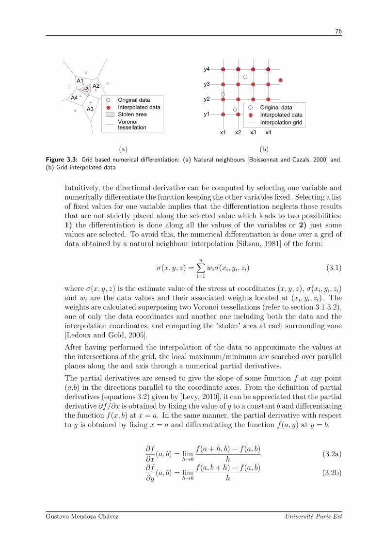
76

A4

A1

A2

A3

x

Original data

Interpolated data

Voronoi

Stolen area

tessellation

(a)

x1 x2 x3 x4

y1

y2

y3

y4

Original data

Interpolated data

Interpolation grid

(b)Figure 3.3: Grid based numerical differentiation: (a) Natural neighbours [Boissonnat and Cazals, 2000] and,(b) Grid interpolated data

Intuitively, the directional derivative can be computed by selecting one variable andnumerically differentiate the function keeping the other variables fixed. Selecting a listof fixed values for one variable implies that the differentiation neglects those resultsthat are not strictly placed along the selected value which leads to two possibilities:1) the differentiation is done along all the values of the variables or 2) just somevalues are selected. To avoid this, the numerical differentiation is done over a grid ofdata obtained by a natural neighbour interpolation [Sibson, 1981] of the form:

σ(x, y, z) =n∑i=1

wiσ(xi, yi, zi) (3.1)

where σ(x, y, z) is the estimate value of the stress at coordinates (x, y, z), σ(xi, yi, zi)and wi are the data values and their associated weights located at (xi, yi, zi). Theweights are calculated superposing two Voronoi tessellations (refer to section 3.1.3.2),one of only the data coordinates and another one including both the data and theinterpolation coordinates, and computing the "stolen" area at each surrounding zone[Ledoux and Gold, 2005].After having performed the interpolation of the data to approximate the values atthe intersections of the grid, the local maximum/minimum are searched over parallelplanes along the and axis through a numerical partial derivatives.The partial derivatives are sensed to give the slope of some function f at any point(a,b) in the directions parallel to the coordinate axes. From the definition of partialderivatives (equations 3.2) given by [Levy, 2010], it can be appreciated that the partialderivative ∂f/∂x is obtained by fixing the value of y to a constant b and differentiatingthe function f(x, b) at x = a. In the same manner, the partial derivative with respectto y is obtained by fixing x = a and differentiating the function f(a, y) at y = b.

∂f

∂x(a, b) = lim

h→0

f(a+ h, b)− f(a, b)h

(3.2a)

∂f

∂y(a, b) = lim

h→0

f(a, b+ h)− f(a, b)h

(3.2b)


77

3.1.3.2 Division of the geometry

Within a manual application of the STM, the structural engineer must decide the length,inclination and position of each structural element. With the same spirit, here, the algo-rithm is intended to identify potential zones of development of a single compressive element(strut). To this purpose, a division of the geometry was proposed under few premises:

1. The resultant division must be influenced by the coordinates of potential structuralnodes (local maximum of stress fields).

2. Each subdivision must be big enough to be able to contain one straight elementwithin its limits.

3. At the same time, it must be small enough to present a clearly preponderant directionof σIII (considering only the results of the initial FE model located at the interior ofeach division).

The Voronoi diagram, also known as Voronoi tessellation, is the partition of an spaceinto a finite number of regions based on the distance between points in a specific subset ofknown data; the "seeds" xi (i = 1, ..., n). Each seed, xi, is surrounded by a convex polygonV (xi) delimiting a Voronoi cell, which is defined as a set of points x that are closer to xithan to any other seed xj (j 6= i) (see equation 3.3).

V (xi) = x ∈ σ : d(x, xj) < d(x, xj), ∀ j 6= i (3.3)

where, for this case, d(x1, x2) represents the Eucledian distance measured between pointx1 and x2.

The Voronoi cells corresponding to the seeds at the boundary of the convex hull of allthe sites are infinite. However, for the purpose of this work, only the parts of the Voronoiwithin the analysed structure (feasible domain), Ωfeasible, are needed. Hence, the Voronoidiagram with respect to the given domain can be defined as the intersection of the Voronoidiagram and the domain, Ω, referred as of the clipped Voronoi diagram [Park et al., 2006].

V (xi)clipped = V (xi) ∩ Ωfeasible (3.4)

Computing the clipped Voronoi diagram in a convex domain requires to compute theintersection of each Voronoi cell and Ωfeassible.

An important number of algorithms for computing clipped Voronoi divisions are avail-able. For this project, the Multi-Parametric Toolbox [Kvasnica et al., 2004] was used andnested into Matlab functions in order to achieve the desired diagrams on the geometry ofthe analised structure.

Based on the clipped Voronoi tessellation, the division of the geometry is performed.Considering the coordinates of the local maxima and minima of the principal stresses asthe seeds, the division allows to delimit zones where the direction field of the principalminor stress of the contained nodes tends to present a preponderant unique direction.In order to make sure that these seeds will be placed at the limits of a region and not


78

inside a sub-domain, a small disturbance is introduced over the position of the seeds. Thisdisturbance is included by replacing the original selected seeds by two new seeds resultfrom the intersection of a circle, of an arbitrary infinitesimal radius and centred at theoriginal seed’s coordinates, with the boundaries of the geometry.

3.1.3.3 Initial struts’ direction assessment

Previous step is intended to directly delimit the length and distribution of the compressiveelements of the skeletal structure. In this work, the inclination of each individual elementis assumed parallel to the principal stress directions and their values are obtained fromthem (this hypothesis is classical in the development of STM).

Considering that the struts shall approach the distribution and direction of the minorprincipal elastic stress, θIII , the inclination of each strut, θs,i, is approximated taking intoaccount a weighted contribution of the principal direction, θIII,j, of the finite elementsincluded in the current Voronoi cell.

The chosen approximation, equation 3.9, is based on a Locally Weighted Least SquareRegression (loess). The estimate of θs at the centred of the cell, C(XY Z), uses the nobservations whose distance d is closest to C. That is, starting from the previouslydefined neighbourhood (Vx,i), each included point is weighted according to its distancefrom C; points close to C have large weight, and points far from C have small weight[Cleveland and Devlin, 1988].

θs = f(θIII,j) + ε, j ∈ V (xi) (3.5)

Fit A to minimise: ε =1∑j=1

wi(θs(X, Y )− AT θIII,j

)2(3.6)

a bT = (PT [W ]P)−1(PT [W ][θIII,j]), j ∈ Vx,i (3.7)

Where wi is the local weight assigned to the data xi, [W ] is the diagonal weight matrix,P is the data set vector containing the explanatory variables and a bT corresponds tothe vector containing the coefficients of the regression.

For this case, the weight is given by a parabolic kernel function (equations 3.8). Thisfunction is intended to reduce (or eliminate) the reliance on the values laying at boundariesof the cells; principally, those nodal results near the mechanic raisers that could bring"noise" to the regression.

Wi =WX,iWY,iWZ,i (3.8a)

WX,i =1− 3(d(xj, C)X

lX

)2

− 2∣∣∣∣∣d(xj, C)X

lX

∣∣∣∣∣3

(3.8b)

WY,i =1− 3(d(xj, C)Y

lY

)2

− 2∣∣∣∣∣d(xj, C)Y

lY

∣∣∣∣∣3

(3.8c)

WZ,i =1− 3(d(xj, C)Z

lZ

)2

− 2∣∣∣∣∣d(xj, C)Z

lZ

∣∣∣∣∣3

(3.8d)


79

Additionally to the kernel function, the loess also requires a specification of neighbour-hood size. The chosen neighbourhoods, Ωi, are selected as cuboids whose maximum interiordiagonal connects the minimum and the maximum of the coordinates of the current cell.

Placing the kernel function over a cuboid zone of dimensions lX , lY and lZ (sidesmeasured along X, Y and Z respectively) and centred at the coordinates (CX , CY and CZ)the local weight of the data subsets within the zone Ωi is given, according to their spatialpositions on the geometry (X, Y and Z) by the product of the parabolic distributions.

θs,i = a(θIII) + b, j ∈ V (xi) (3.9)

For this approximation to be implemented there are some conditions that the data mustsatisfy:

• Cuboid-base sub-domains. Since the base-shape of the chosen kernel functionpresents a cuboid projection, this function is ideally applied on this type of zones.

• Singularities located at the boundaries of the regression zones. Regardingthe kernel function as a filter, the aim of this filter is to reduce the weight that thesingularities could have on the regression, which can be only done if those points areat the boundaries.

• Small angular dispersion coefficient. A small angular dispersion allows applyingthe current model of regression over the selected angular data. This aspect resultsadvantageous inasmuch as is not necessary to apply a sort of angular regression thatcould imply a heavy iterative procedure [Fisher, 1995].

Within this step, the subroutine implemented to approach the initial strut inclinationwhich is computed based on the direction of the major principal stresses of the elementsfound in the subdomain through the loes. This approach is adopted for subdomains pre-senting a small angular dispersion and a significant quantity of available data. The initialstrut at subdomains presenting either a large angular dispersion or a small quantity of data(less than 10) is then associated to the mean value of the circular directions Θ.

Θ = arctan 2 n∑j=1

sin Θj,n∑j=1

cos Θj

(3.10)

where Θj represents the angle of the principal direction of the n elements found insidethe subdomain.

3.1.3.4 Branch-like generation of struts

Last sub-routines propose and distribute the struts within the structure but the connectionbetween the elements is not done yet.

Once the inclination of the struts have been computed at each zone, Ωi, an iterative"branch-like" algorithm is implemented for the generation of the struts.

Starting from the coordinates of the seeds that correspond to the local maximum stress,the algorithm takes an initial node, Ni, and projects a straight line, following the slope


80

calculated for the contouring zone. The projected line is cut at the limits of the currentzone generating an ending node Nf . The next iteration takes the previous final node asthe new initial one, and proceeds in the same manner to calculate another final node. Theprocedure continues for all the seeds until the boundaries of the geometry have been reachedby the generated “branches”. Hence, the strut generation algorithm produces branches thatstart at the coordinates of concentrated loads and compressive stress concentrations, anddiffuses throughout design domain. Even though two or more branches could pass throughcommon zones, until this step, these branches do not necessarily share common nodes.Therefore, a nodal merging procedure has been implemented at this state.

3.1.3.5 Linking elements

Similarly to the case of struts, the ties are expected to approximate the distribution of themajor principal elastic stress σI . Besides, these elements should also be adapted to thealready existing strut path.

Starting from the premise that the punctual concentration of major stress provides areliable index of the position of the ST nodes in pure traction, the distribution of the tiesis obtained by considering each concentration point as a birth node which is attached bya straight line to every existent node contained by the closest local minima.

Considering all possible connections may produce a structure with a high degree ofpotential trusses hence, a reduction of the quantity of potential elements is a desirable stepbefore the optimisation.

Starting from the premise that the principal struts have been already created duringthe branch-like procedure, the linking elements will produce principally potential tractionelements. A simple way to reduce the quantity of elements on the ground structure hasbeen found to apply a restriction on the "linking" phase: an elements is created betweentwo existent nodes if the resultant element is inside the the feasible region but outside thezones delimited by the α-shape defined by the local minima of σI .

[Edelsbrunner et al., 1983] introduced α-shapes as the shape of a point set at a givenlevel of detail, α. With this definition and assuming that any loading system will gen-erate at least one zone where the behaviour is dominated by the minor principal stressover the major one. The algorithm constructs a zone bounded by straight line segmentsdefined between 2 coordinates of local minimum. The constructed zone does not requireto be connected, but points that are close together are in the same component of theshape. Conversely, a component of the shape cannot contain a large region void of points[Van Kreveld et al., 2011].

3.1.4 Optimisation procedureThe three first sub-routines depicted in figure 3.1 are meant to propose the ground struc-ture. The proposed structure is characterised by presenting the structural nodes at thecoordinates (or nearby) the coordinates where the ST nodes are expected to be. At thispoint, the quantity of potential elements do not allow to clearly identify a feasible STmodel. Furthermore, the straight elements lack of fundamental characteristics such as thearea.


81

Ground structure

Ku = P

Sizing optimisation

∗ε

Topology optimisation Geometry optimisation

Stability control

∗ε

Strut-and-tie model

dono

tup

date

upda

te

Iterative process

Figure 3.4: Flowchart of the proposed truss optimisation

In order to decrease highlight a ST model from the ground structure it was implementeda optimisation scheme able to reduce the quantity of elements, to choose the material ofeach member (steel or concrete) and most important, to assess cross sections.

3.1.4.1 Initialisation

An initial configuration built by a total of m elements can be now stated based on thestrut path and the tie distribution.

At the very early stages of the Thesis, the initial cross section of the elements wasintended to be based on an energetic equivalence between the initial FE model and theground structure. The equivalence was made by computing the strain energy associated tothe compressive stresses only, Ψ−EF , within the FE model and calibrate it with the energyof the deformation of the proposed struts ∑Ψ−S .


82

considering that for a general body the strain energy to a compressive state of stresscan be computed as:

Ψ− = A

2

[λ(ε−I + ε

−II

)2+ 2µ

((ε−I )2 + (ε−II )2

)](3.11)

Analogously, in the case of a straight element undergoing an axial compressive force,the strain energy can be easily expressed in terms of the force, F, cross section, ai , length,l, strain, ε , and its Young’s modulus, E as:

Ψ− = 12E(ε−)2 (3.12)

Considering that the struts are proposed and delimited within an individual Voronoizone, Ωi, the equilibrium is made individually for each strut; the strain energy from theFE considers only the nodal results from the n nodes contained inside the limits of thecurrent zone leading to:

n∑j=1

A

2

[λ(ε−I + ε

−II

)2+ 2µ

((ε−I )2 + (ε−II )2

)]Ωj

= 12Eal(ε

−)2S,Ωj

(3.13)

So far, the axial strain of the struts ε−S,Ωjis unknown but, looking for the compatibility of

displacements between the FE model and the ST one, the strain of each strut is estimatedas the nodal displacement between the 2 nodes closest to the strut edges divided by theirinitial Euclidean distance leaving the cross section, a, as the only unknown.

a =

∑nj=1

A2

[λ(ε−I + ε

−II

)2+ 2µ

((ε−I )2 + (ε−II )2

)]Ωj

El(ε−)2S,Ωj

(3.14)

This attempt to predict the cross section of the struts was rapidly discarded for twomain reasons: 1) the operations needed involved three-dimensional nodal research whichrequires high computational efforts and 2) the results were, for most of the cases, too farfrom the final result which was translated into the need of more iterations or even thenon-convergence.

For instance, the guess value of cross sections is proposed as a constant vector of valueainitial. Considering the fact that the selection of the initial cross sections may affect theperformance, or even the solution of the optimisation, ainitial may consider a realistic steeldistribution. The user should chose a value that produce elements that individually fit intothe boundaries of the geometry.

The initial model considers that all elements are made out of steel. This considerationis only made once. During the iterative process, the selection of the material is done basedon the sign of the force obtained at previous iterations. The material models correspondto linear-elastic hypothesis whose behaviour law is assumed with Young’s moduli, Ei, andPoisson’s ratio, ν, assigned according to the idealised selected materials.


83

3.1.4.2 Optimisation scheme

At this point, the problem has been reduced to a quite simple topology optimisation ofa truss model with a relatively low number of potential structural elements where theobjective function is to reduce the volume of the sum of the elements V = ∑m

i=1 aili. Thetreatment of the problem is proposed to be done through a tree-part truss optimisation:

• Sizing problem. Cross-section area of each element is applied as a design variablewith a non-zero lower bound condition, [Li, 1990].Taking into account that, in general, the elements withstanding compression possesa small slenderness ratio, the effects of buckling are neglected. Thus, the previouslypresented FSD (fully stressed design) can be simplified. At each iteration, the equi-librium is verified trough the relation Ku = P , and the cross sections are replacedwith values according to the axial stress ratio.The optimised cross sections are bounded by a maxima and a minima values. Whilethe maximum value commonly depends on available cross sections, the choice of theminimum value does not only relies on manufacturing limitations. As said before,due to the nature of the stiffness matrix, the minimum cross section cannot attain azero value but neither an arbitrary "small" one. Depending on the solving procedureand the available numerical precision, the difference between the smallest and thelargest root of a matrix may be used to determine its singularity. Matrices with largecondition numbers are difficult to invert accurately [Greene, 2003].

Condition number = κ(A) =(maximum root

minimum root

)1/2(3.15)

Although there is not a specific limit on the condition number to determine thesingularity of a matrix [Pyzara et al., 2011], for practical purposes some restrictionswere imposed. The minimum value that a cross section may take at the k-th iterationis equal to the value of the largest cross section, computed at iteration k−1 divided by106. This value has found to be significantly small to represent a neglectable elementbut to be sufficiently large to avoid numerical problems providing an inexpensivedamping to the inversion.

• Topology optimisation. A dichotomous optimisation is applied to the elements in-cluded in the percentile with the less important cross section. The elements includedin this percentile that are not required to maintain equilibrium for that particulargeometry and loaded condition are eliminated, [Kirsch, 1989].The sizing optimisation allows the selection of a group of elements presenting activeconstraints; the elements whose cross-section is equal to the minimum permitted.The basic combinatorial problem of topology design is applied over this group ofelements. Similarly to the case of a lower zero bound, removing all the elementswith active constraints may imply that the stiffness matrix is not necessarily positivedefinite and the state of displacement vector U cannot be computed accurately.To overcome this difficulty, the solution procedure is proposed in two phases: 1) thefirst phase assembles the stiffness matrix with all the elements whose cross-section


84

Random sort of the remaining elements

Stiffness matrix for the i-th elementke = aiEi

li

Ki = Ki−1 + ke

ill-conditioned

matrix

K = Ki

i = i + 1

no

yes

Figure 3.5: Element suppression flowchart

is superior to the minimum, and 2) the second phase randomly adds the rest ofthe elements verifying that the stability of the stiffness matrix. The second phasecontinues until the algorithm determines that no ill-condition is presented in theproblem and eliminates the reminder elements . The process is achieved throughthe modification to the assembling subroutine (see flowchart 3.5) by adding a logicaloperation that verifies the section of the current element and the conditioning of thematrix once the current element has been added.Even though suppressing all the elements presenting active constraints have littlerepercussion on the conditioning of a stiffness matrix associated to a fully populatedstructure, for a problem with sparsity and bandedness, erasing elements becomes atrivial task. The presented subroutine guaranties the invertibility of the matrix anderases non-trivial elements reducing the quantity of elements in the final structureand also reducing the need of computational effort for further iterations.

• Geometric optimisation. As stated before and according to [Bendsøe et al., 1994],the resultant topologies can be very sensitive to the layout of nodal points. Thismakes it natural to consider an extension of the ground structure approach and toinclude the optimisation of the nodal point location for a given number and connec-tivity of nodal points.The optimisation of the nodal coordinates is based on the feasible direction method.The algorithm is intended to find a step and a direction, within the limits of theoriginal structure, and updating the vector x of nodal coordinates.In general, the displacement of the nodal coordinates leads to two complications:

– nodal coordinates found outside the geometry the considered geometry– bars with infinitesimal lengths or "melting nodes"


85

To overcome the first complication logical restrictions were imposed. The algorithmlimits the final position of the nodes accepting the optimised coordinates if and onlyif they are included within the geometry. For cases where the optimum coordinatesare found outside the geometry, the algorithm retains the computed direction α andscales the step S to fit the structure. This allows keeping a classic formulation fora geometric optimisation and, at the same time, it allows to directly include spatialrestrictions.The second complication is linked with bar elements whose length is or approachesto zero thus, their stiffness K = Ea/l approaches to the, computationally speaking,infinite or is simply undefined.According to [Achtziger, 2007], melting nodes can be frequently observed; in somezones, the nodes tend to approach to the supports avoiding long elements with im-portant stresses. Nevertheless, the melting nodes can cause ill-conditioning, theirpresence can also be useful to control the number of elements in the structure.From a practical point of view, one solution to threat this problem is to definea minimum for the length of the elements. Another solution to work-around thisproblem is to formally exclude the melting nodes from the structure.For this work an alternative process was stated. An element presenting both, aninfinite stiffness and an infinitesimal length suggest that the initial and ending nodeof such element may be merged into one single node. According to a distance specifiedby the user or by the used precision (h), a subroutine selects the melting nodes andevaluates if they can or cannot be merged. If the geometry considering the mergeleads to a stable structure, the suppression of the element proceeds and the modelis updated. Alternately, if the merge leads to an unstable structure at the currentiteration, the length of the element is increased.

3.1.5 TerminationThe termination of the algorithm can occur in two different manners:

1. the current error, kε attains the prescribed threshold εi

2. the number of iterations has reached the prescribed maximum

3.1.6 Acquiring the strut-and-tie model and reinforcementAt this point, the cross sections and the associated material of each element are known.A skeletal structure has already been defined from the reduction of the initial groundstructure but this reduced structure sometimes possesses "repeated" elements; elementsthat share both initial and final nodes one another. Even if those elements do not affectthe model, their existence may produce interpretation errors as they represent differentbodies occupying the same space. This is simply avoided by searching those groups ofelements sharing nodes and, if it is the case, merge each group into one single elementwhose area equals the sum of the group. This step provides a skeletal structure with areduced quantity of elements that correspond to the specifications for a ST model prescribedby the Eurocode.


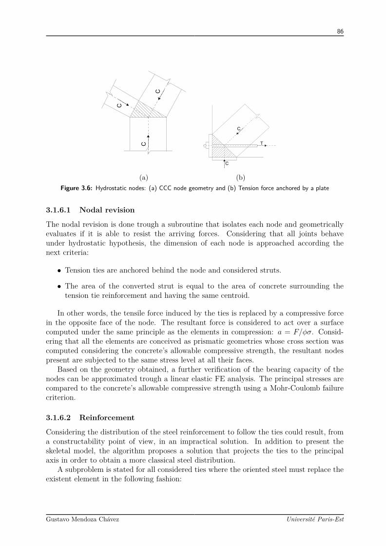
86

C

C

C

(a)

T

C

C

(b)Figure 3.6: Hydrostatic nodes: (a) CCC node geometry and (b) Tension force anchored by a plate

3.1.6.1 Nodal revision

The nodal revision is done trough a subroutine that isolates each node and geometricallyevaluates if it is able to resist the arriving forces. Considering that all joints behaveunder hydrostatic hypothesis, the dimension of each node is approached according thenext criteria:

• Tension ties are anchored behind the node and considered struts.

• The area of the converted strut is equal to the area of concrete surrounding thetension tie reinforcement and having the same centroid.

In other words, the tensile force induced by the ties is replaced by a compressive forcein the opposite face of the node. The resultant force is considered to act over a surfacecomputed under the same principle as the elements in compression: a = F/φσ. Consid-ering that all the elements are conceived as prismatic geometries whose cross section wascomputed considering the concrete’s allowable compressive strength, the resultant nodespresent are subjected to the same stress level at all their faces.

Based on the geometry obtained, a further verification of the bearing capacity of thenodes can be approximated trough a linear elastic FE analysis. The principal stresses arecompared to the concrete’s allowable compressive strength using a Mohr-Coulomb failurecriterion.

3.1.6.2 Reinforcement

Considering the distribution of the steel reinforcement to follow the ties could result, froma constructability point of view, in an impractical solution. In addition to present theskeletal model, the algorithm proposes a solution that projects the ties to the principalaxis in order to obtain a more classical steel distribution.

A subproblem is stated for all considered ties where the oriented steel must replace theexistent element in the following fashion:


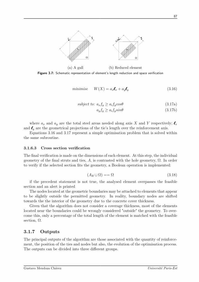
87

W

A

(a) A gull

0

.

6

W

A

R

(b) Reduced elementFigure 3.7: Schematic representation of element’s length reduction and space verification

minimise W (X) = axlx + ayly (3.16)

subject to: axfy ≥ aifycosθ (3.17a)ayfy ≥ aifysinθ (3.17b)

where ax and ay are the total steel areas needed along axis X and Y respectively; lxand ly are the geometrical projections of the tie’s length over the reinforcement axis.

Equations 3.16 and 3.17 represent a simple optimisation problem that is solved withinthe same subroutine.

3.1.6.3 Cross section verification

The final verification is made on the dimensions of each element. At this step, the individualgeometry of the final struts and ties, A, is contrasted with the hole geometry, Ω. In orderto verify if the selected section fits the geometry, a Boolean operation is implemented:

(AR ∪ Ω) == Ω (3.18)if the precedent statement is not true, the analysed element overpasses the feasible

section and an alert is printedThe nodes located at the geometric boundaries may be attached to elements that appear

to be slightly outside the permitted geometry. In reality, boundary nodes are shiftedtowards the the interior of the geometry due to the concrete cover thickness.

Given that the algorithm does not consider a coverage thickness, most of the elementslocated near the boundaries could be wrongly considered "outside" the geometry. To over-come this, only a percentage of the total length of the element is matched with the feasiblesection, Ω.

3.1.7 OutputsThe principal outputs of the algorithm are those associated with the quantity of reinforce-ment, the position of the ties and nodes but also, the evolution of the optimisation process.The outputs can be divided into three different groups.


88

The first type, and maybe the most important, groups the results of each iteration ofthe geometry from the ground structure to the final ST model. Available on list format(.txt) and on Visualization Toolkit (VTK), the results include the geometry (nodal listand connectivity matrix); geometric characteristics of the elements such as length andcross section; and the force developed at each bar. Additionally, data related to the nodalrevision is also included: geometry of the nodes and type of node (CCC, CTC, etc.). Theseresults are saved at each iteration into file named OUTPUT.

The second type corresponds to results that are stocked only in form of text such asthe reinforcement computed from the projection of the ties over the principal axis. If aFE analysis was performed, the initial mesh, global displacements, stresses and principalstresses can also be found in the OUTPUT file. Other intermediate results are also asso-ciated to this group. Useful data of the iterative process such as the convergence rate andthe evolution of the total volume are also presented in text format.

The last type has been associated to results that are contained only in a non-interactivevisual representation. This information such as the Voronoi division, the subdomainsand the local maximum/mminimum of the principal stresses is only depicted in a JointPhotographic Experts Group format (.jpeg). Although, the backup of this informationwas not considered important, the data can be directly read and saved from the Matlab’sinterface.

3.2 Illustrative exampleIn this section, the proposed approach is used to find the ST model of a first planar exampleinspired by the work of [Zhong et al., 2016]. For simplicity and for illustrative purposesthe algorithm is applied over 3 idealised anchorage zones shown in figure 3.8.

Different cases have been chosen. Whether the geometry is the same for the threecases, the load location changes from one case to another as seen in figure 3.8. The lengthof the structures is L = 6m, the width is b = 3m and the considered thickness of theelements is t = 0.2 m . The effect of the prestressing tendons has been simplified into oneconcentrated load F = 5 KN. The considered eccentricities, e, are 0, 0.75, and 1.35 meters.The three models are considered fixed at the opposite side of the force. Regarding thematerial, the Young’s modulus, E, and the Poisson’s ratio, ν, were specified according to aconcrete of fck = 35MPa: E = 34.5GPa and ν = 0.3 (values extracted from the reference[Zhong et al., 2016]).

For this example, a simple linear-elastic finite element model was built and evaluatedin software ANSYS (ANSYS R© Academic Research Mechanical, Release 18.1). In the men-tioned software, a planar representation of the structure was built up using a regular meshconsisting in 1800 4-node plane stress elements (figure 3.9a). The load was represented by aunique punctual force. Concerning the support, all degrees of freedom were suppressed forthe nodes at the base zone. Plane stress hypothesis were considered during the procedure.

3.2.1 InputAfter having imposed the respective boundary conditions and solving some results wereextracted. The information extracted from ANSYS software was the nodal list (NLIST in


89

(a) (b) (c)Figure 3.8: Anchorage zone models [Zhong et al., 2016]

ANSYS environment), the connectivity matrix (ELIST), the principal stresses computedat the Gauss points and also smoothed at the nodes (PRESOL and PRNSOL respectively)and the direction field of the principal stresses (PVSOL). This information, schematisedin figures 3.9 and 3.10, is the starting point to develop the ground structure.

3.2.2 Ground structureAs mentioned in precedent paragraphs, the picks and the valleys presented in the prin-cipal stress fields are taken as indicators of the presence of the nodes of a suitable STmodel. For the current test, the grid based numerical differentiation was preferred overthe differentiation via interpolation and the results.

In figure 3.11 they are shown the principal stress fields all over the structural elementdeveloped under the specified boundary conditions and in subfigure 3.11a the peaks andvalleys detected by the code are also shown.

Taking the local maximum and minimum as seeds for the Voronoi division and thegeometry as the feasible region, the division is performed. For this case, 20 cells wherefound during the performed division (refer to subfigure 3.12a).

Following the presented methodology, the loess was applied at the centre of every cell.Considering the principal directions of the all the elements found in the cell, the regressionwas applied and the results are schematised in figure 3.12b.

The initial strut path (subfigure 3.11d was achieved through the sub routine describedin the previous chapter. An initial node is selected (node containing a maximum of σIII)and a straight line is developed until finding the limits of a cell).


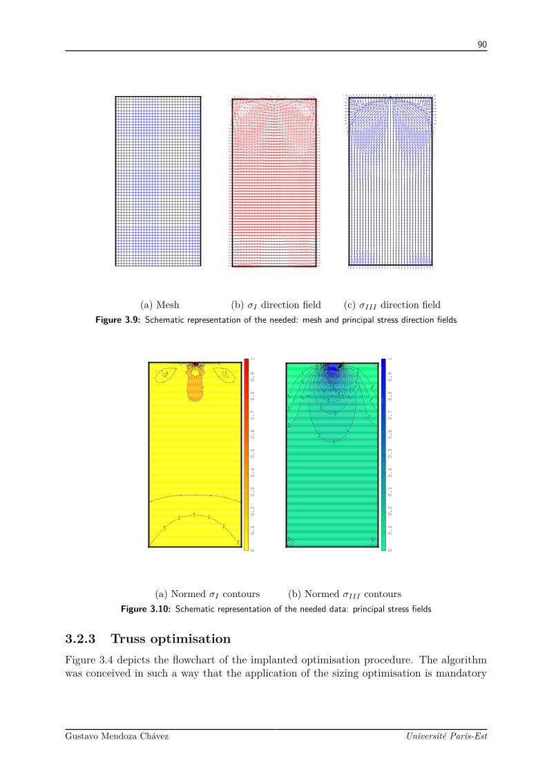
90

(a) Mesh (b) σI direction field (c) σIII direction fieldFigure 3.9: Schematic representation of the needed: mesh and principal stress direction fields

-0.0

4

-0.0

4 -0.0

4

-0.0

4

-0.0

4

-0.0

4

-0.0

4

-0.0

4

-0.0

4

0

0

0 0 0

0

0

0

0

0

0

0

0

0

000.3

0.3

0.3

0.3

0.3 0.3

0.3

0.3 0.65

00.1

0.2

0.3

0.4

0.5

0.6

0.7

0.8

0.9

1

(a) Normed σI contours

00

0.03

0.03

0.03

0.03

0.03

0.03

0.08

0.08

0.08

0.08

0.08

0.08

0.13

0.13

0.13

0.13

0.13

0.13

0.18

0.18

0.18

0.18

0.18

0.18

0.18

0.18

0.18

0.23

0.23

0.23

0.23

0.23

0.28

0.28

0.28

0.28

0.32

0.32

0.32

0.37

0.37

0.37

0.42

0.42

0.42

0.47

0.47

0.52

0.52

0.57

0.57

0.61

0.61

0.66

0.66

0.71 0.760.810.86 0.9

0.95

00.1

0.2

0.3

0.4

0.5

0.6

0.7

0.8

0.9

1

(b) Normed σIII contoursFigure 3.10: Schematic representation of the needed data: principal stress fields

3.2.3 Truss optimisationFigure 3.4 depicts the flowchart of the implanted optimisation procedure. The algorithmwas conceived in such a way that the application of the sizing optimisation is mandatory


91

(a) (b) (c) (d)Figure 3.11: Strut path generation: (a) Computed Voronoi seeds, (b) Clipped Voronoi division, (c) Associateddirection strut direction and (c) Initial strut path

while the application of topology and geometry optimisation is optional. In other words,the algorithm gives the possibility to the user to apply a simply sizing optimisation ormixed schemes; sizing-topology, sizing-geometry, or sizing-topology-geometric.

Figure 3.13 shows the results obtained through the application of 2 mixed schemes:sizing-topology and sizing-topology-geometric. The principal difference between the resultsobtained by the two different mixed schemes lies in the quantity of elements conformingthe final Strut-and-Tie model. More subtile differences are found in the nodal coordinates.A mean distance of 5.8cm was found in the position of the nodes from a model to theother.


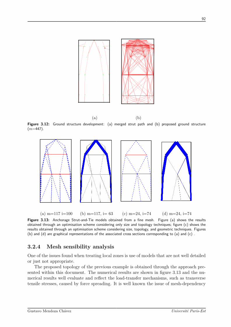
92

(a) (b)Figure 3.12: Ground structure development: (a) merged strut path and (b) proposed ground structure(m=447).

(a) m=117 i=100 (b) m=117, i= 63 (c) m=24, i=74 (d) m=24, i=74Figure 3.13: Anchorage Strut-and-Tie models obtained from a fine mesh. Figure (a) shows the resultsobtained through an optimisation scheme considering only size and topology techniques; figure (c) shows theresults obtained through an optimisation scheme considering size, topology, and geometric techniques. Figures(b) and (d) are graphical representations of the associated cross sections corresponding to (a) and (c) .

3.2.4 Mesh sensibility analysisOne of the issues found when treating local zones is use of models that are not well detailedor just not appropriate.

The proposed topology of the previous example is obtained through the approach pre-sented within this document. The numerical results are shown in figure 3.13 and the nu-merical results well evaluate and reflect the load-transfer mechanisms, such as transversetensile stresses, caused by force spreading. It is well known the issue of mesh-dependency


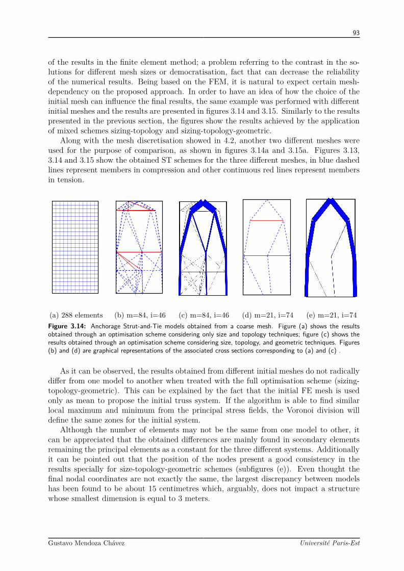
93

of the results in the finite element method; a problem referring to the contrast in the so-lutions for different mesh sizes or democratisation, fact that can decrease the reliabilityof the numerical results. Being based on the FEM, it is natural to expect certain mesh-dependency on the proposed approach. In order to have an idea of how the choice of theinitial mesh can influence the final results, the same example was performed with differentinitial meshes and the results are presented in figures 3.14 and 3.15. Similarly to the resultspresented in the previous section, the figures show the results achieved by the applicationof mixed schemes sizing-topology and sizing-topology-geometric.

Along with the mesh discretisation showed in 4.2, another two different meshes wereused for the purpose of comparison, as shown in figures 3.14a and 3.15a. Figures 3.13,3.14 and 3.15 show the obtained ST schemes for the three different meshes, in blue dashedlines represent members in compression and other continuous red lines represent membersin tension.

(a) 288 elements (b) m=84, i=46 (c) m=84, i=46 (d) m=21, i=74 (e) m=21, i=74Figure 3.14: Anchorage Strut-and-Tie models obtained from a coarse mesh. Figure (a) shows the resultsobtained through an optimisation scheme considering only size and topology techniques; figure (c) shows theresults obtained through an optimisation scheme considering size, topology, and geometric techniques. Figures(b) and (d) are graphical representations of the associated cross sections corresponding to (a) and (c) .

As it can be observed, the results obtained from different initial meshes do not radicallydiffer from one model to another when treated with the full optimisation scheme (sizing-topology-geometric). This can be explained by the fact that the initial FE mesh is usedonly as mean to propose the initial truss system. If the algorithm is able to find similarlocal maximum and minimum from the principal stress fields, the Voronoi division willdefine the same zones for the initial system.

Although the number of elements may not be the same from one model to other, itcan be appreciated that the obtained differences are mainly found in secondary elementsremaining the principal elements as a constant for the three different systems. Additionallyit can be pointed out that the position of the nodes present a good consistency in theresults specially for size-topology-geometric schemes (subfigures (e)). Even thought thefinal nodal coordinates are not exactly the same, the largest discrepancy between modelshas been found to be about 15 centimetres which, arguably, does not impact a structurewhose smallest dimension is equal to 3 meters.


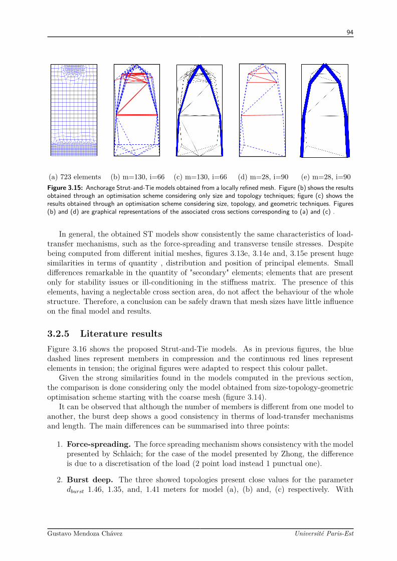
94

(a) 723 elements (b) m=130, i=66 (c) m=130, i=66 (d) m=28, i=90 (e) m=28, i=90Figure 3.15: Anchorage Strut-and-Tie models obtained from a locally refined mesh. Figure (b) shows the resultsobtained through an optimisation scheme considering only size and topology techniques; figure (c) shows theresults obtained through an optimisation scheme considering size, topology, and geometric techniques. Figures(b) and (d) are graphical representations of the associated cross sections corresponding to (a) and (c) .

In general, the obtained ST models show consistently the same characteristics of load-transfer mechanisms, such as the force-spreading and transverse tensile stresses. Despitebeing computed from different initial meshes, figures 3.13e, 3.14e and, 3.15e present hugesimilarities in terms of quantity , distribution and position of principal elements. Smalldifferences remarkable in the quantity of "secondary" elements; elements that are presentonly for stability issues or ill-conditioning in the stiffness matrix. The presence of thiselements, having a neglectable cross section area, do not affect the behaviour of the wholestructure. Therefore, a conclusion can be safely drawn that mesh sizes have little influenceon the final model and results.

3.2.5 Literature resultsFigure 3.16 shows the proposed Strut-and-Tie models. As in previous figures, the bluedashed lines represent members in compression and the continuous red lines representelements in tension; the original figures were adapted to respect this colour pallet.

Given the strong similarities found in the models computed in the previous section,the comparison is done considering only the model obtained from size-topology-geometricoptimisation scheme starting with the coarse mesh (figure 3.14).

It can be observed that although the number of members is different from one model toanother, the burst deep shows a good consistency in therms of load-transfer mechanismsand length. The main differences can be summarised into three points:

1. Force-spreading. The force spreading mechanism shows consistency with the modelpresented by Schlaich; for the case of the model presented by Zhong, the differenceis due to a discretisation of the load (2 point load instead 1 punctual one).

2. Burst deep. The three showed topologies present close values for the parameterdburst 1.46, 1.35, and, 1.41 meters for model (a), (b) and, (c) respectively. With


95

P

d

burst

Q

(a) [Zhong et al., 2016]

P

(-)

(+)

(b) [Schlaich et al., 1987]

P

(c) Computed modelFigure 3.16: Different Strut-and-Tie model propositions

respect to the angle Θ, the proposed model presents a value of 37 degrees; inclination10o greater than the presented by the cited authors (26o reported by Zhong and 28oby Schlaich).

3. Transverse tensile elements. Beyond the burst deep is where the most remark-able differences arise. Whether the literature models show just two straight struts,the computed model propose a continuity of the of the load-transfer mechanism pre-senting short elements following a natural spreading of the force.

The differences presented in the first and second point of the previous list refer to smallvariations that, given the size of the analysed element, are acceptable in actual structures.For the third point, the literature results propose long strut elements (more than 4 meterslong) that, according to the EuroCodes, may need further detailing an even secondarystrut and ties.

3.2.6 Different load casesSimilar analysis were performed for the load cases (b) and (c) showed in figure 3.8. Inter-mediate results can be found in the annexes and the final ST models are presented in thesubsequent figures.

It can be observed that this is so far the model that differs the most from the literatureexamples. Even though the models present strong similarities in terms of load-transfermechanisms, the mere existence of some elements in the proposed model brings effects ofcompression in a zone that do not consider struts in the other two models (right supportin figures 3.17 (a) to (c)).

The differences presented in this model come from the fact that, for this case, the au-tomatically obtained Voronoi seeds did not allow a satisfactory geometry division (clippedVoronoi division) and some seeds were need to be added manually to the algorithm tocontinue the procedure. The present results permit to state that the present approach ishighly sensitive to the number and position of the Voronoi seeds. In case of not being


96

P


P

(b) [Aashto L.R.F.D., 1998]

P

(c) Computed modelFigure 3.17: Comparison of different Strut-and-Tie model propositions(anchorage e=0.75m)

satisfied with the final results, it was decided to let the user the liberty to add, erase ormodify the proposed Voronoi seed hence adapting a computer aided scheme over a fullyautomatic one.

3.3 Behaviour of the algorithm

3.3.1 Linear-elastic FE analysisThe included solving procedure is a very basic algorithm that assembles the matrix K andthen solves for Ku = P . The assemble follows an iterative scheme that do not present anycomplications if the inputs follow the predefined format. Similarly, the available solutionsubroutines are simple and show good performance.

3.3.2 Ground structureFrom the different steep needed to arrive to the ground structure, two of them should bementioned.

Is worth to mention that the subroutine that computes the maxima/minima is highlydependant on the difference of the "peaks" and their surroundings. Given that the mesh-size directly affects this difference, the selection of the threshold defining a peak or valleyis given to the user. Despite this, the tests show that selecting a threshold between 5% and10%, in addition to the change in the sign of numerical derivative, provides good results.

3.3.3 Truss optimisationWhen applying the topology and the geometric subroutines, the algorithm presents a goodperformance and a fast convergence. However, when the vector of design variables alsoincludes nodal coordinates, the algorithm may become unstable and, according to theexperience, a solution may or may not be found.


97

Aiming to stabilise the algorithm, three parameters should be carefully controlled.Firstly, small values of S (step) are preferred. Based on the hypothesis that the nodal

coordinates of the ground structure are close to the optimal coordinates, it results naturalthat just a small variation on the position of the nodes is expected. Thus according tothe tests, limiting S to attain values inferior to 10cm (depending on the dimensions of theanalysed geometry) can be considered as a reasonable limit step.

An aspect worth to point out is the effect that the random elimination of bar elementsduring the topology optimisation, produce a light disparity of the results found when"running" multiple times the exact same example. Even though this can be seen as a hugedrawback concerning the robustness of the algorithm, the difference found between twodifferent runs of the same example do not significantly affect the final results.

3.4 SummaryAs it was pointed out, the proposed methodology is based on an organised list of subroutinesthat allow to automatically obtain feasible ST models from common linear-elastic FEanalysis. The initial FE planar analysis intends to serve as a link between the structuralengineer, used to this type of analysis, and the rational approach ST.

The performed analyses show that:

1. the proposed methodology keeps the "spirit" of the manual ST models being obtainedthrough linear-elastic stress fields

2. the obtained results approach to the geometries obtained by different methods andauthors

3. the use of different mesh sizes have little influence on the final model and results

So far the results clearly show the capabilities for finding feasible ST systems but thegains in terms of reinforcement still remain unsaid. Next chapter addresses to this issueand compares usual practice techniques to compute the reinforcement of a D-region.


Chapter 4

Comparative example

In previous chapter, the proposed approach was described and a simple bi-dimensionalliterature case was used to compare the obtained results.

Even though the automatic generation of feasible planar Strut-and-Tie Models can beadvantageous, a wide variety of structures present geometries or boundary conditions thatcan limit the application of planar models. Besides, due to the graphical limitations, clas-sical reinforcement schemes based on ST models remain applicable only to considered 2Dstructures where the effects in a third direction are just omitted. When facing 3D prob-lems, within the industrial context, the geometries are commonly reduced to mere surfacerepresentations based on shell or plate type elements and the need of steel reinforcement isdirectly computed though an algorithm based on generalised forces such as Capra-Maury.

Specifically, within the nuclear civil works, industrial constraints have imposed an im-moderate use of plate and shell formulations. The size of the buildings, its structuralbehaviour as well as the need of efficient auditable methods, are just some aspects thathave encouraged this practice.

This chapter is intended to compare results from the industrial practice and thosepossibly achieved through the use of the rational approach STM while applied on localzones; pointing out the advantages of the implementation of detailing stages during thedesign procedure. To this purpose a literature example treated from three points of view:

1. ST model computed a from a planar representation

2. Capra-Maury algorithm applied over a surface model representation

3. ST model computed from a full 3D solid element representation

It is worth to mention that in no case the computation time will be a subject of study.This decision has been taken under two premises: 1) the main purpose is to evaluatethe viability of the proposed algorithm and, 2) the code was written in MATLAB that,arguably, may induced a slow execution [Aruoba and Fernández-Villaverde, 2015].

99

Exemple comparativeDans le chapitre précédent, l’approche proposée a été décrite et un simple cas de littératurebidimensionnelle a été utilisé pour comparer les résultats obtenus.

Même si la génération automatique de modèles planaires Strut-and-Tie réalisables peutêtre avantageuse, une grande variété de structures présentent des géométries ou des con-ditions aux limites qui peuvent limiter l’application de modèles planaires. En outre, enraison des limitations graphiques, les schémas de renforcement classiques basés sur lesmodèles ST restent applicables uniquement aux structures 2D considérées où les effets dansune troisième direction sont simplement omis. Face aux problèmes 3D, dans le contexteindustriel, les géométries sont souvent réduites à de simples représentations surfaciquesbasées sur des éléments de type coque ou plaque et le besoin de ferraillage est directementcalculé par un algorithme basé sur des forces généralisées comme Capra-Maury.

Plus précisément, dans les travaux de génie civil nucléaire, les contraintes industriellesont imposé une utilisation immodérée des formulations de plaques et de coques. La taille desbâtiments, son comportement structurel ainsi que le besoin de méthodes auditables efficacesne sont que quelques aspects qui ont encouragé cette pratique.

Ce chapitre vise à comparer les résultats de la pratique industrielle et ceux éventuelle-ment obtenus grâce à l’utilisation d’une approche rationnelle appliquée aux zones locales;souligner les avantages de la mise en œuvre des étapes de détail au cours de la procédurede conception. A cet effet, un exemple de littérature traité de trois points de vue:

1. algorithme Capra-Maury appliqué sur une représentation de surfacique du model

2. BT calculé à partir d’une représentation planaire du modèle

3. BT calculé à partir d’une représentation d’un modèle solide 3D

Il est important de mentionner que le temps de calcul ne sera en aucun cas un sujetd’étude. Cette décision a été prise sous deux prémisses: 1) le but principal est d’évaluer laviabilité de l’algorithme proposé et, 2) le code a été écrit dans MATLAB qui, sans doute,peut induire une exécution lente [Aruoba and Fernández-Villaverde, 2015].


100

4.1 Example selectionWith the aim of having a direct comparison with existent approaches, it was chosen toapply the proposed algorithm to the classical problem of a corbel withstanding a punctualload. The example was inspired by [Almeida et al., 2013] where a 2D FE model of thegeometry was treated by a Smooth Evolutionary Structural Optimisation (SESO). Thestructure was conceived to support a concentrated load, P of 0.5 MN, being fixed at bothends of the column. An initial thickness of 30 cm, along the third direction, was assumedfor the element. The Young’s modulus, Ec, of 28.5 GPa and the Poisson’s ratio, ν, wastaken equal to 0.15.

0.50 m 0.60 m

1.00 m

0.70 m

1.00 m

P

0.15 m

Figure 4.1: Planar corbel initial model

Table 4.1: Considered materials

Material Young’s modulus Poisson’s ratio Compressive strength Tensile strength[GPa] [MPa] [MPa]

Steel 210 0.3 434 434Concrete 28.5 0.15 25 0

4.2 2D planar modelThe first performed analysis is based on a planar model of the structure where a ST modelis aimed to be obtained using the proposed approach.

For this case, a relatively coarse mesh consisting in 708 planar four-node elements(figure 4.2a) was preferred over the original one creating a model. Nodal displacementsconstraints were placed in the zones of the supports, and finally, a concentrated load, P ,was placed according to figure 4.1. The material constants were also directly taken fromthe original model and are shown in table 4.1.

Similar to the previous examples, the procedure was applied and graphical resultsassociated to the soubroutines are shown in figures 4.2. As mentioned in the precedentchapter, the picks and the valleys presented in the principal stress fields are taken asindicators of the presence of the nodes of a suitable ST model.


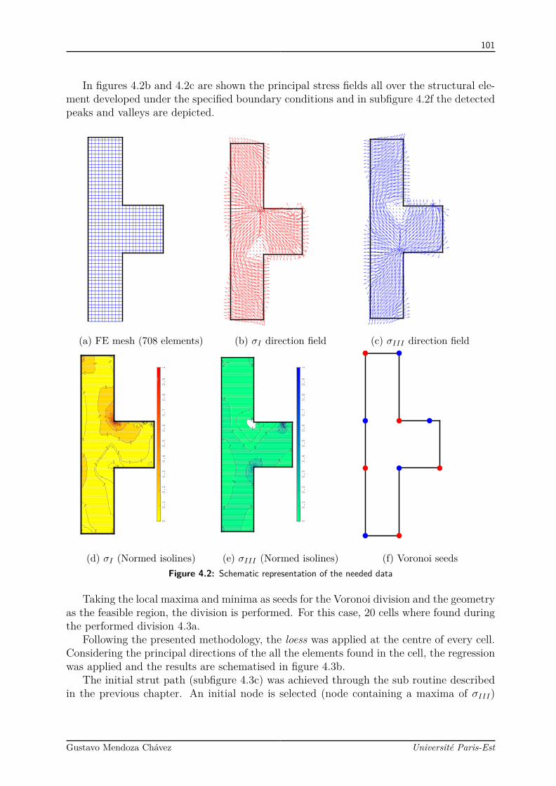
101

In figures 4.2b and 4.2c are shown the principal stress fields all over the structural ele-ment developed under the specified boundary conditions and in subfigure 4.2f the detectedpeaks and valleys are depicted.

(a) FE mesh (708 elements) (b) σI direction field (c) σIII direction field

-0.1

2

0 0

0

00

0

0

0

0

0

0

00

0.02

0.02

0.02

0.02

0.02 0.

02

0.02

0.02

0.02

0.02

0.02

0.02

0.02

0.02

0.16

0.16

0.16

0.16

0.16

0.16

0.16

0.16

0.16

0.16

0.3

0.3

0.3

0.3

0.44

0.440.

580.720.86

00.1

0.2

0.3

0.4

0.5

0.6

0.7

0.8

0.9

1

(d) σI (Normed isolines)

-0.0

5-0

.05

0

0

0

0

00

0

0 0

0

00

0.05

0.05

0.05

0.05

0.05

0.05

0.05

0.050.

05

0.05

0.05

0.05

0.16

0.16

0.16

0.16

0.16

0.26

0.26

0.37

0.370.48

00.1

0.2

0.3

0.4

0.5

0.6

0.7

0.8

0.9

1

(e) σIII (Normed isolines) (f) Voronoi seedsFigure 4.2: Schematic representation of the needed data

Taking the local maxima and minima as seeds for the Voronoi division and the geometryas the feasible region, the division is performed. For this case, 20 cells where found duringthe performed division 4.3a.

Following the presented methodology, the loess was applied at the centre of every cell.Considering the principal directions of the all the elements found in the cell, the regressionwas applied and the results are schematised in figure 4.3b.

The initial strut path (subfigure 4.3c) was achieved through the sub routine describedin the previous chapter. An initial node is selected (node containing a maxima of σIII)


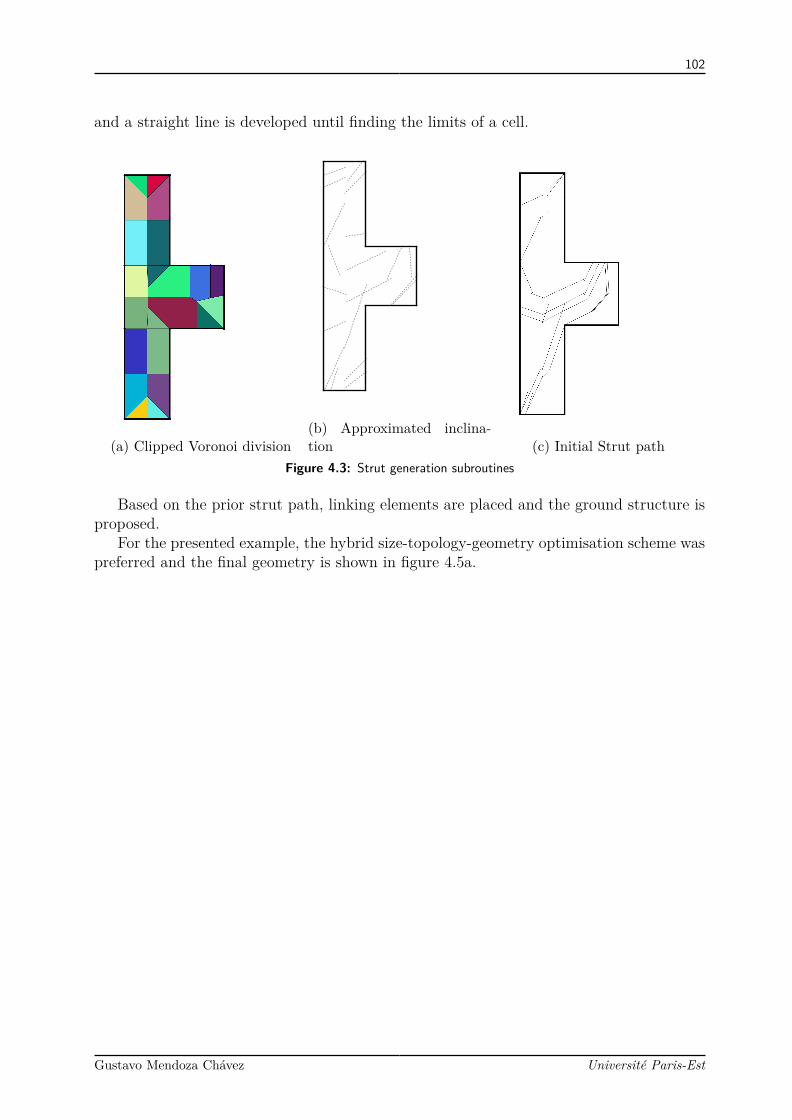
102

and a straight line is developed until finding the limits of a cell.

(a) Clipped Voronoi division(b) Approximated inclina-tion (c) Initial Strut path

Figure 4.3: Strut generation subroutines

Based on the prior strut path, linking elements are placed and the ground structure isproposed.

For the presented example, the hybrid size-topology-geometry optimisation scheme waspreferred and the final geometry is shown in figure 4.5a.


103

(a) Initial strut path (b) Merged strut path(c) Ground structure(m=572)

Figure 4.4: Ground structure

T1

T2

T3

T4

T5

T6

T7

T8

T9

T10

T11

T12

T13

T14

T15

T16

(a) Proposed ST model (b) Optimum ST [Almeida et al., 2013]Figure 4.5: Different ST models for the corbel case. Figure (a) depicts the ties in red and the struts in blue;figure (b) is presented with shifted colours


104

The nodal revision consist in a graphical projection of the element considering their ac-tual cross section. While elements in compression (struts) are directly considered, elementsin tension are replaced by an equivalent strut arriving at the opposite face of the node.Being all elements designed at full stress, and being the geometry of the nodes directlycomputed from the intersection of the elements, the stress attained at nodal zones equalsthe concrete’s strength design.

Figure 4.6 depicts the geometry of a CCT node produced by the intersection of threeelements of the final ST model.

Intersection

Nodal zone

Cross section

Strut

Tie

limit

T4

S2

S6

E

q

u

i

v

a

l

e

n

t

f

o

r

c

e

o

f

:

T

4

Node vertex

Figure 4.6: Nodal geometry

As it can be appreciated, the proposed model (4.5a) present a good geometry in termsof repetition of members and nodal position compared to the optimal design achieved bythe SESO approach (4.5b). Both models, also present strong similarities with the modelproposed by Schlaich and similar repetition of tensile elements.

Tables 4.2 and 4.3 contain the information of the ties for the model depicted in figure4.5a. The first table presents the needed steel considering the Strut-and-Tie model asa skeletal structure. The second output, table 4.3, corresponds to the results of a morerealistic model that considers the cross sections distributed along the principal axis X andY as it is usually done in the construction field. This last result is achieved through theoptimisation subproblem stated in section 3.1.6.2.


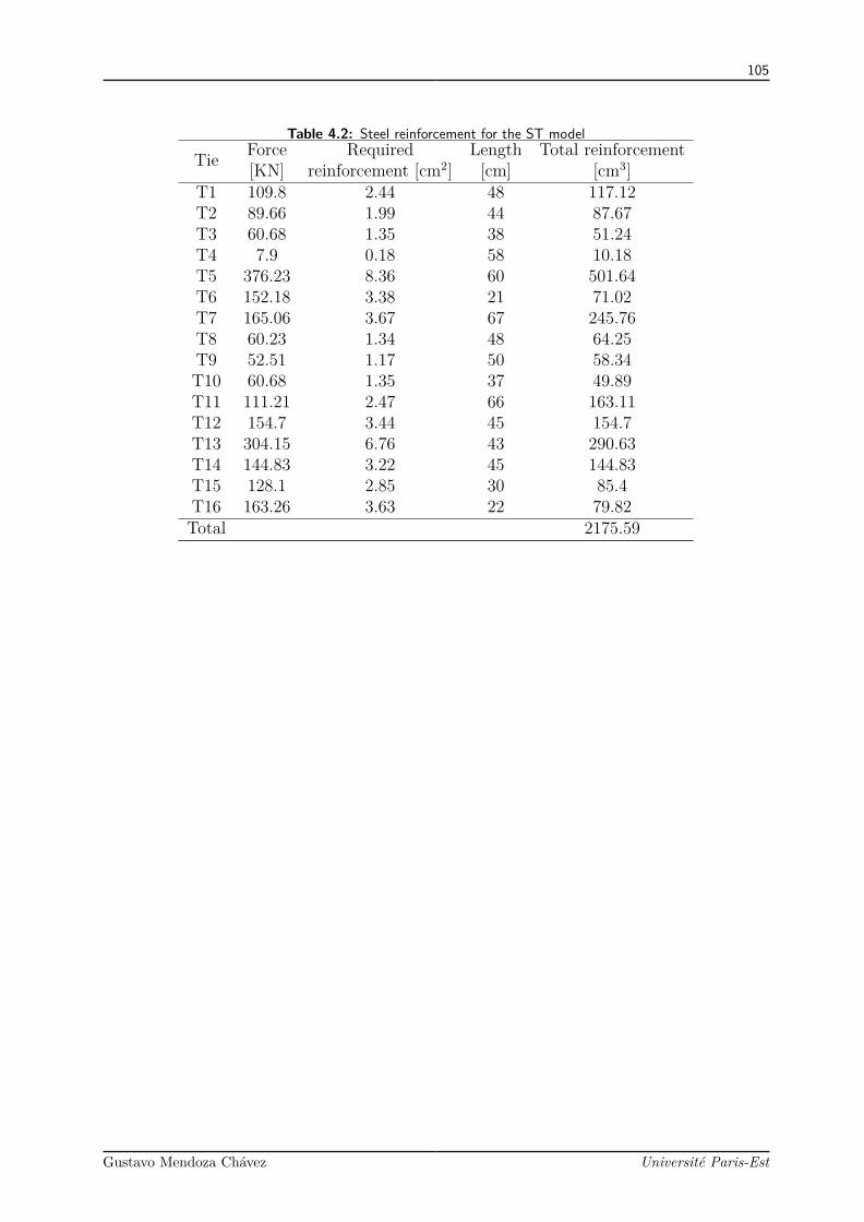
105

Table 4.2: Steel reinforcement for the ST model

Tie Force Required Length Total reinforcement[KN] reinforcement [cm2] [cm] [cm3]

T1 109.8 2.44 48 117.12T2 89.66 1.99 44 87.67T3 60.68 1.35 38 51.24T4 7.9 0.18 58 10.18T5 376.23 8.36 60 501.64T6 152.18 3.38 21 71.02T7 165.06 3.67 67 245.76T8 60.23 1.34 48 64.25T9 52.51 1.17 50 58.34T10 60.68 1.35 37 49.89T11 111.21 2.47 66 163.11T12 154.7 3.44 45 154.7T13 304.15 6.76 43 290.63T14 144.83 3.22 45 144.83T15 128.1 2.85 30 85.4T16 163.26 3.63 22 79.82Total 2175.59


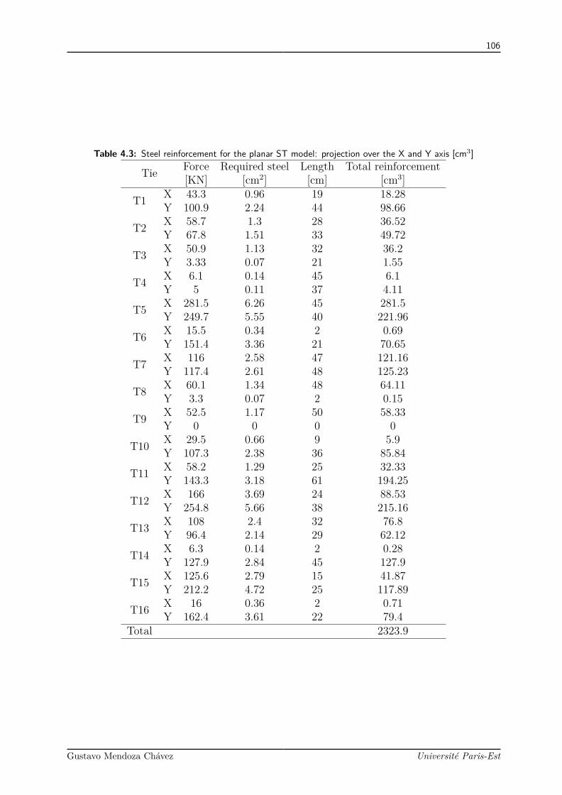
106

Table 4.3: Steel reinforcement for the planar ST model: projection over the X and Y axis [cm3]

Tie Force Required steel Length Total reinforcement[KN] [cm2] [cm] [cm3]

T1 X 43.3 0.96 19 18.28Y 100.9 2.24 44 98.66

T2 X 58.7 1.3 28 36.52Y 67.8 1.51 33 49.72

T3 X 50.9 1.13 32 36.2Y 3.33 0.07 21 1.55

T4 X 6.1 0.14 45 6.1Y 5 0.11 37 4.11

T5 X 281.5 6.26 45 281.5Y 249.7 5.55 40 221.96

T6 X 15.5 0.34 2 0.69Y 151.4 3.36 21 70.65

T7 X 116 2.58 47 121.16Y 117.4 2.61 48 125.23

T8 X 60.1 1.34 48 64.11Y 3.3 0.07 2 0.15

T9 X 52.5 1.17 50 58.33Y 0 0 0 0

T10 X 29.5 0.66 9 5.9Y 107.3 2.38 36 85.84

T11 X 58.2 1.29 25 32.33Y 143.3 3.18 61 194.25

T12 X 166 3.69 24 88.53Y 254.8 5.66 38 215.16

T13 X 108 2.4 32 76.8Y 96.4 2.14 29 62.12

T14 X 6.3 0.14 2 0.28Y 127.9 2.84 45 127.9

T15 X 125.6 2.79 15 41.87Y 212.2 4.72 25 117.89

T16 X 16 0.36 2 0.71Y 162.4 3.61 22 79.4

Total 2323.9


107

For comparative purposes, in this and further examples, the considered geometry isdivided into four regions according to table 4.4: the arm, the forehead, the joint and thefoot.

Table 4.4: Steel reinforcement for the planar ST model: need of steel reinforcement per zone [cm3]X reinforcement Y reinforcement Total

Arm 345.61 222.1 567.71Forehead 274.88 803.17 1078.05Joint 157.11 199.99 357.1Foot 91.71 229.33 321.04∑ =869.31 ∑ =1454.59 ∑ =2323.9

Figure 4.7 shows the PI history attained by the structure along the the optimisationprocess. The PI decreases with the removal of lowly stressed elements from the corbel atthe same time that the error measured between continuous iterations, ε, also is reduced.

Number of iteration0 5 10 15 20 25 30 35 40

PIin

dex

0

0.5

1

erro

r[%

]

0

10

20

T1

T2

T3

T4

T5

T6

T7

T8

T9

T10

T11

T12

T13

T14

T15

T16

Figure 4.7: Optimisation evolution


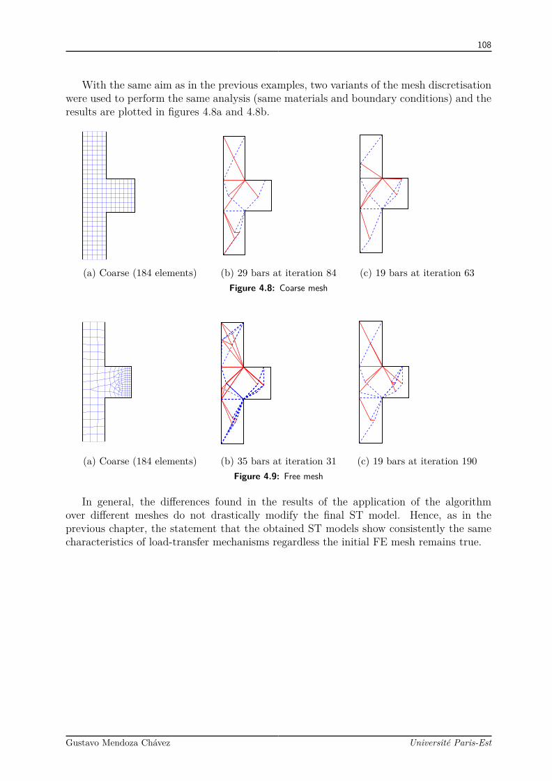
108

With the same aim as in the previous examples, two variants of the mesh discretisationwere used to perform the same analysis (same materials and boundary conditions) and theresults are plotted in figures 4.8a and 4.8b.

(a) Coarse (184 elements) (b) 29 bars at iteration 84 (c) 19 bars at iteration 63Figure 4.8: Coarse mesh

(a) Coarse (184 elements) (b) 35 bars at iteration 31 (c) 19 bars at iteration 190Figure 4.9: Free mesh

In general, the differences found in the results of the application of the algorithmover different meshes do not drastically modify the final ST model. Hence, as in theprevious chapter, the statement that the obtained ST models show consistently the samecharacteristics of load-transfer mechanisms regardless the initial FE mesh remains true.


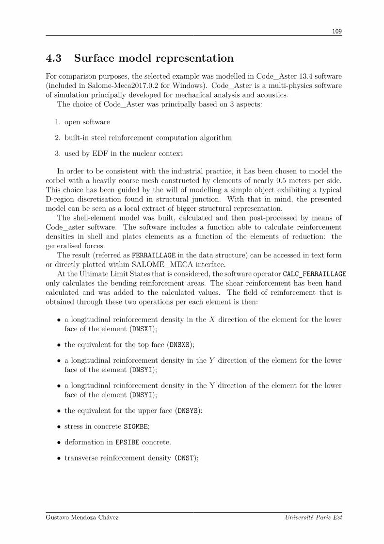
109

4.3 Surface model representationFor comparison purposes, the selected example was modelled in Code_Aster 13.4 software(included in Salome-Meca2017.0.2 for Windows). Code_Aster is a multi-physics softwareof simulation principally developed for mechanical analysis and acoustics.

The choice of Code_Aster was principally based on 3 aspects:

1. open software

2. built-in steel reinforcement computation algorithm

3. used by EDF in the nuclear context

In order to be consistent with the industrial practice, it has been chosen to model thecorbel with a heavily coarse mesh constructed by elements of nearly 0.5 meters per side.This choice has been guided by the will of modelling a simple object exhibiting a typicalD-region discretisation found in structural junction. With that in mind, the presentedmodel can be seen as a local extract of bigger structural representation.

The shell-element model was built, calculated and then post-processed by means ofCode_aster software. The software includes a function able to calculate reinforcementdensities in shell and plates elements as a function of the elements of reduction: thegeneralised forces.

The result (referred as FERRAILLAGE in the data structure) can be accessed in text formor directly plotted within SALOME_MECA interface.

At the Ultimate Limit States that is considered, the software operator CALC_FERRAILLAGEonly calculates the bending reinforcement areas. The shear reinforcement has been handcalculated and was added to the calculated values. The field of reinforcement that isobtained through these two operations per each element is then:

• a longitudinal reinforcement density in the X direction of the element for the lowerface of the element (DNSXI);

• the equivalent for the top face (DNSXS);

• a longitudinal reinforcement density in the Y direction of the element for the lowerface of the element (DNSYI);

• a longitudinal reinforcement density in the Y direction of the element for the lowerface of the element (DNSYI);

• the equivalent for the upper face (DNSYS);

• stress in concrete SIGMBE;

• deformation in EPSIBE concrete.

• transverse reinforcement density (DNST);


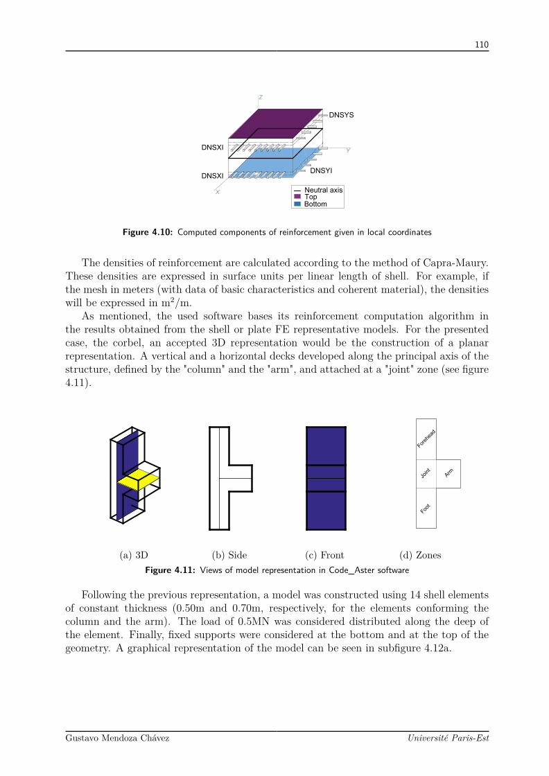
110

Z

Y

X

DNSYS

DNSYI

DNSXI

DNSXI

Neutral axis

Top

Bottom

Figure 4.10: Computed components of reinforcement given in local coordinates

The densities of reinforcement are calculated according to the method of Capra-Maury.These densities are expressed in surface units per linear length of shell. For example, ifthe mesh in meters (with data of basic characteristics and coherent material), the densitieswill be expressed in m2/m.

As mentioned, the used software bases its reinforcement computation algorithm inthe results obtained from the shell or plate FE representative models. For the presentedcase, the corbel, an accepted 3D representation would be the construction of a planarrepresentation. A vertical and a horizontal decks developed along the principal axis of thestructure, defined by the "column" and the "arm", and attached at a "joint" zone (see figure4.11).

(a) 3D (b) Side (c) Front

A

r

m

F

o

r

e

h

e

a

d

J

o

i

n

t

F

o

o

t

(d) ZonesFigure 4.11: Views of model representation in Code_Aster software

Following the previous representation, a model was constructed using 14 shell elementsof constant thickness (0.50m and 0.70m, respectively, for the elements conforming thecolumn and the arm). The load of 0.5MN was considered distributed along the deep ofthe element. Finally, fixed supports were considered at the bottom and at the top of thegeometry. A graphical representation of the model can be seen in subfigure 4.12a.


111

X

Y

Z

Distributed loadFixed supports

(a) Mesh (16 elements)

Req

uire

d st

eel r

einf

orce

men

t [m

2/m

]

#10-4

0

1

2

3

4

5

6

7

8

(b) Top layer along X

Req

uire

d st

eel r

einf

orce

men

t [m

2/m

]

#10-5

0

1

2

3

4

5

6

7

(c) Bottom layer along X

Req

uire

d st

eel r

einf

orce

men

t [m

2/m

]

#10-4

0

1

2

3

4

5

6

7

(d) Top layer along Y

Req

uire

d st

eel r

einf

orce

men

t [m

2/m

]

#10-4

0

0.5

1

1.5

2

2.5

3

3.5

(e) Bottom layer along Y

#10-4

0

1

2

3

4

5

6

7

8

9

(f) ShearFigure 4.12: Capra-Maury computed required steel reinforcement (Coarse mesh).


112

The quantities of computed steel reinforcement were distributed into 4 zones and theresults are presented in the next table.

Table 4.5: Computed need of steel reinforced per zone (coarse model) [cm3]XS XI YS YI SW Total

Arm 55.11 0 0 3555.56 154 3764.67Forehead 0 98 239.22 607.11 0 944.33Joint 35 230.22 29.44 508 125.22 927.89Foot 17.81 111.11 0 0 0 128.92Total 107.92 439.33 268.67 4670.67 279.22 5765.81

Precedent results are attained via a model representation that intends to mimic acommon mesh discretisation found in overall structural models. Assuming no singularitiesare present, meshes dictated by overall models present an acceptable accuracy and mightbe costly efficient for global behaviour objectives, yet their use for local zones and detailingis highly questionable.

Following the good practices, in this context, a coarse model can be used for pre-designpurposes and after, local zones must be isolated and refined in order to proceed with thedetailing stage. Nevertheless, the coarse representation would be kept.

Worthy to mention is the fact that even if the selected discretisation may probably notbe the most appropriated for the problem, due to the size of nuclear facilities and theircorrespondent buildings, the FE mesh herein used represents a common case industriallyused. Further, the selection of Finite Element representation may not be the best optionneither for local zones.

In order to decide when to use shell elements, there exist different thumb rules pre-sented by several authors; [Johnson, 1986] presents three criteria to justify the use of shellelements:

1. By observation (surface area / thickness ratio)

2. By failing to create a useful, or accurate, 3D solid model

3. By discovering that the shell assumptions are wrong

The selected corbel presents surface area / thickness ratios of 1.21 and 2.7 respectivelyfor the arm and the column. These values remain far from the application of shell elements(being 10 the minimum acceptable value for surface area / thickness ratio [Johnson, 1986]).Additionally, due to the geometry, shell elements can "overlap" at corners affecting theprecision of the results. Stiffness is still quite good, but stress at joints is not accurate evenfor thin elements [Moaveni, 2011].

4.4 RemarksDue to its relative ease of implementation, most of the structures are analysed and designedin similar fashion as the one presented. The advantages of the use of shell elements tomodel structural elements, results mainly from time-saving due to reduced number of


113

finite elements (and consequently the equations to solve). However, the shell elements arelimited to thinner features. There is not an specific limit of the application of surfaceelements but a good approximate would be the ratio span / thickness [Bisch, 2013]. If theratio is at least 20 times, the bodies are candidates for surface elements otherwise, the useof this type of elements need further justifications.

In an oversimplified definition, a shell addresses to a solid that presents a dimensionconsiderably smaller than the other two dimensions. Physically, and according to thetheory of structures, this fundamental characteristic allows the allusion to the hypothesesthat entail the simplification of the behaviour of three-dimensional bodies into the one ofa 2D body. Seldom, when modelling local zones, questionable simplifications are done.Shell elements are used to model entire geometries indiscriminately. Whether it resultsreasonable for static analysis of planar elements such as slabs or walls, its implementationfor regions presenting weak span/thickness ratios or geometric discontinuities is debatable.

For structural elements where the third direction cannot be neglected, solid elementdiscretisations are preferred.


114

4.5 3D brick modelAs showed by [Shobeiri, 2016], due to the relatively small thickness of the element, thedevelopment of a strut-and-tie model over a three-dimensional representation of the studiedcase would not be influenced by transverse effects (see figure 4.13).

(a) 3D model representation (b) Obtained ST modelFigure 4.13: ST model found through Bi-directional Evolutionary Structural Optimisation [Shobeiri, 2016]

In order to increase the effects of the load along the third direction, it was decidedto modify the thickness of the original model according to figure 4.14. The corbel wasassumed to present a one-meter thickness instead of the original 0.3m. Regarding the load,an equivalent linearly distributed pattern was preferred over then punctual one.

1.0

01

.0

00

.7

0

0.50 0.60

0.15

P

(a) Side view

1.0

01

.0

00

.7

0

1.00

(b) Front view

1.0

01

.0

00

.7

0

0

.

5

0

0

.

1

5

1

.

0

0

0

.

6

0

P

(c) 3D viewFigure 4.14: Three-dimensional model representation

A linear-elastic model consisting of 4200 8-node brick elements was built (figure 4.15a),the boundary conditions and the load were applied and, finally, the stresses were found.With the associated results, the algorithm was run and the obtained results are shown.


115

Figures 4.15 and 4.16 show some intermediate results product of the different steepsthat conform the algorithm.

(a) Mesh (b) Seeds(c) 86 ClippedVoronoi division

Figure 4.15: Caption

(a) (b) (c) (d)Figure 4.16: (a) directions associated to the Voronoi zones, (b) initial strut path, (c) merged strut path and(d) ground structure (m =1919)

As in previous examples, two types of optimisation schemes were performed: size-topology and size-topology-geometry optimisation schemes.

After 260 iterations, the output of the first optimisation scheme shows a highly pop-ulated structure. Even though the algorithm reduced to almost 35% the quantity of theelements (690 elements) in the structure, it seems not to be sufficient to directly obtain asuitable ST model. In order to visualise the results, a filter needed to be applied. All theelements whose cross section results inferior to the arbitrary value of 0.6cm2 were erasedfrom the plotted images.


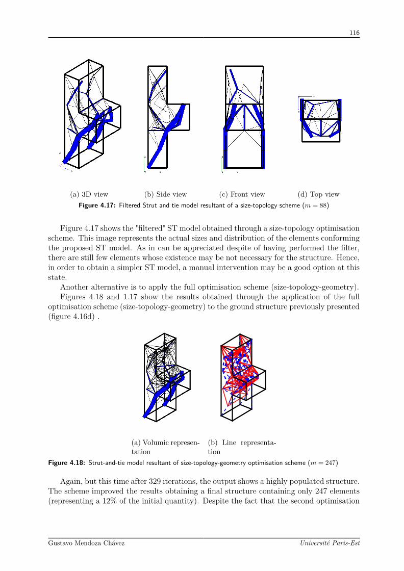
116

(a) 3D view (b) Side view (c) Front view (d) Top viewFigure 4.17: Filtered Strut and tie model resultant of a size-topology scheme (m = 88)

Figure 4.17 shows the "filtered" ST model obtained through a size-topology optimisationscheme. This image represents the actual sizes and distribution of the elements conformingthe proposed ST model. As in can be appreciated despite of having performed the filter,there are still few elements whose existence may be not necessary for the structure. Hence,in order to obtain a simpler ST model, a manual intervention may be a good option at thisstate.

Another alternative is to apply the full optimisation scheme (size-topology-geometry).Figures 4.18 and 1.17 show the results obtained through the application of the full

optimisation scheme (size-topology-geometry) to the ground structure previously presented(figure 4.16d) .

(a) Volumic represen-tation

(b) Line representa-tion

Figure 4.18: Strut-and-tie model resultant of size-topology-geometry optimisation scheme (m = 247)

Again, but this time after 329 iterations, the output shows a highly populated structure.The scheme improved the results obtaining a final structure containing only 247 elements(representing a 12% of the initial quantity). Despite the fact that the second optimisation


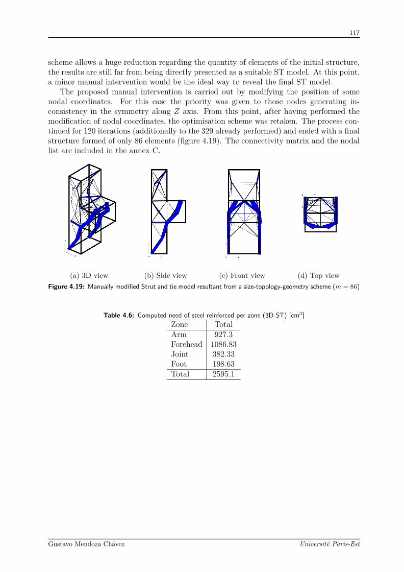
117

scheme allows a huge reduction regarding the quantity of elements of the initial structure,the results are still far from being directly presented as a suitable ST model. At this point,a minor manual intervention would be the ideal way to reveal the final ST model.

The proposed manual intervention is carried out by modifying the position of somenodal coordinates. For this case the priority was given to those nodes generating in-consistency in the symmetry along Z axis. From this point, after having performed themodification of nodal coordinates, the optimisation scheme was retaken. The process con-tinued for 120 iterations (additionally to the 329 already performed) and ended with a finalstructure formed of only 86 elements (figure 4.19). The connectivity matrix and the nodallist are included in the annex C.

(a) 3D view (b) Side view (c) Front view (d) Top viewFigure 4.19: Manually modified Strut and tie model resultant from a size-topology-geometry scheme (m = 86)

Table 4.6: Computed need of steel reinforced per zone (3D ST) [cm3]Zone TotalArm 927.3Forehead 1086.83Joint 382.33Foot 198.63Total 2595.1


118

4.6 ResultsThe following table presents the total need of steel reinforcement per zone for the four differ-ent models presented: the surface representations where the steel reinforcement was com-puted using the Capra-Maury algorithm, the planar and the solid representations treatedthrough the computer aided ST approach.

Table 4.7: Comparative table of need of steel reinforcement per zone [cm3]Zone CM (coarse) ST (2D) ST (3D)Arm 3764.67 567.72 927.3

Forehead 944.33 1078.05 1086.83Joint 927.89 357.1 382.33Foot 128.92 321.04 198.63Total 5765.81 2323.9 2595.1

Table 4.8: Comparative table of need of steel reinforcement per zone. kg of steel per cubic meter of concreteZone Volume [m3] CM (coarse) ST (2D) ST (3D)Arm 0.42 70.36 10.61 17.33

Forehead 0.50 14.83 16.93 17.06Joint 0.35 20.81 8.01 8.58Foot 0.50 2.02 5.04 3.12∑ =1.77 X =27.01 X =10.15 X =11.52

∗The density of steel was taken as 7.85 g/cm3

As it can be inferred, the quantities herein presented, are raw results and should bearranged and smoothed before going to the blueprints. These arrangements may slightlyincrease the shown reinforcement densities.

4.7 DiscussionFrom the results obtained several conclusions can be done. The comments will be dividedinto two topics:

1. the capabilities of the algorithm

2. the quantity of reinforcement

4.7.1 Capabilities of the algorithmSo far, the developed algorithm fulfils the most important criteria established for this work

• Standard FE modelling. Described before, the application of the approach startswith a normal linear-elastic finite element model (bi- or three-dimensional). Fromthe results obtained, the algorithm is able to propose and to design a suitable STmodel.


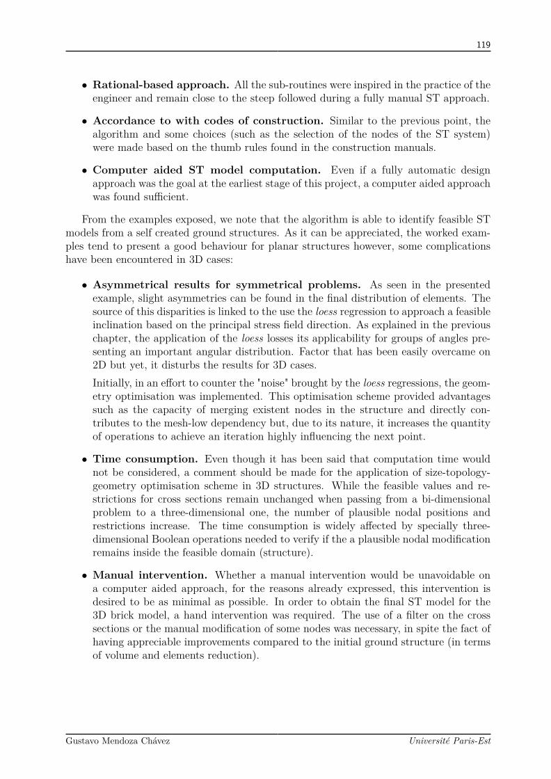
119

• Rational-based approach. All the sub-routines were inspired in the practice of theengineer and remain close to the steep followed during a fully manual ST approach.

• Accordance to with codes of construction. Similar to the previous point, thealgorithm and some choices (such as the selection of the nodes of the ST system)were made based on the thumb rules found in the construction manuals.

• Computer aided ST model computation. Even if a fully automatic designapproach was the goal at the earliest stage of this project, a computer aided approachwas found sufficient.

From the examples exposed, we note that the algorithm is able to identify feasible STmodels from a self created ground structures. As it can be appreciated, the worked exam-ples tend to present a good behaviour for planar structures however, some complicationshave been encountered in 3D cases:

• Asymmetrical results for symmetrical problems. As seen in the presentedexample, slight asymmetries can be found in the final distribution of elements. Thesource of this disparities is linked to the use the loess regression to approach a feasibleinclination based on the principal stress field direction. As explained in the previouschapter, the application of the loess losses its applicability for groups of angles pre-senting an important angular distribution. Factor that has been easily overcame on2D but yet, it disturbs the results for 3D cases.Initially, in an effort to counter the "noise" brought by the loess regressions, the geom-etry optimisation was implemented. This optimisation scheme provided advantagessuch as the capacity of merging existent nodes in the structure and directly con-tributes to the mesh-low dependency but, due to its nature, it increases the quantityof operations to achieve an iteration highly influencing the next point.

• Time consumption. Even though it has been said that computation time wouldnot be considered, a comment should be made for the application of size-topology-geometry optimisation scheme in 3D structures. While the feasible values and re-strictions for cross sections remain unchanged when passing from a bi-dimensionalproblem to a three-dimensional one, the number of plausible nodal positions andrestrictions increase. The time consumption is widely affected by specially three-dimensional Boolean operations needed to verify if the a plausible nodal modificationremains inside the feasible domain (structure).

• Manual intervention. Whether a manual intervention would be unavoidable ona computer aided approach, for the reasons already expressed, this intervention isdesired to be as minimal as possible. In order to obtain the final ST model for the3D brick model, a hand intervention was required. The use of a filter on the crosssections or the manual modification of some nodes was necessary, in spite the fact ofhaving appreciable improvements compared to the initial ground structure (in termsof volume and elements reduction).


120

4.7.2 Quantity of reinforcementFrom table 4.7 it can be appreciated that current practices may lead to an importantincrease in the quantity of need of steel when detailing D-regions. Steel reinforcementquantity drops to half when using a more appropriated approach such as the Strut-and-TieMethod.

The validity and, in consequence, the results of a surface-element-based model suchas the one presented here is debatable, yet it represents a quotidian engineering practice.Besides, it has been shown that the shear strength of reinforced concrete local elementscomputed using STM, predicts good accuracy judged from comparison with test results[Zechmann and Matamoros, 2002, Hofer and McCabe, 1998]. Thus a rational approachwould be preferred over a design trough CM algorithm or similar.

Another advantage that the Strut-and-Tie Method presents over CM is the easiness topass the steel need to the blueprints. While the results of CM often need a smoothingprocess, the ties can be directly proposed as a steel reinforcement pattern.


Concluding remarks

Review of contributionsChapter 1 presents a summary of the current practice engineering design addressed toreinforcement computation. In this chapter, efforts were made to point out the benefitsof rational approaches, specifically the strut-and-tie approach, to threat local members.These techniques present the advantage of allowing a designer to follow the forces througha structure with discontinuities (either static or geometric) which formerly were beyondthe scope of engineering practice based on the flexural theory. So far, one of the maindrawbacks of its application is the need of highly skilled structural engineers for a manualapproach or, the need of important resources in terms of computational effort for an,arguably, less appropriate continuous optimisation.

Within Chapter 2, the ground structure approach arises as a suitable option to extractfeasible ST models from solid structures. The inconveniences of the ground structurelie in the fact that a low populated ground structure itself needs to be proposed basedon experience leading again to the need of highly skilled structural engineers. Anotherpossibility is to initially propose high populated ground structures and introduce powerfuloptimisation algorithms.

Chapter 3 proposes an alternative algorithm able to automatically propose and designground structures from the results of bi- or three-dimensional linear elastic analysis.• Strut pattern search. The fashion developed to construct the initial strut pattern

structures was directly inspired from the recommendations made by Schlaich and alsothe thumb rules found principally in the Eurocodes and the ACI. This aspect allowedto keep the methodology as close as possible to the manual approach. The division ofthe geometry based on the Voronoi tessellation, as well as the application of the loessregression over the direction of the stress fields, are original ideas developed duringthis work.

• Construction of ground structures. Even though the use of ground structureshas been applied before to find ST models, the definition of such structures is prede-fined by the user and automatically developed as in the approach proposed.

• Optimised ST models. The selected optimisation scheme is presented as an ad-vantageous tool for weight (cost) reduction in the engineering domain. Despite ofthe benefits that the inclusion of optimisation techniques may have in the industrialfield, its application remain mostly for research purposes. This project examines theapplication of this type of techniques to cases commonly encountered in the buildingindustry.

122

• Capabilities in 2D and 3D. The advantages of having computer aided ST ap-proaches become clearer when facing three-dimensional problems. For some cases,the distribution of stress in volume structures may not always be evident and at firstglance a ST model may appear to be nearly impossible. Computer aided approachestend to reduce the complexity of the problem by predefining whether load-transfermechanisms, element distributions, nodal positions, cross sections or, as in this case, asuitable ST model. This capability opens the door for the analysis and reinforcementof complex tree-dimensional problems an place it beyond surface-like FE models.

Referring to the objectives, this work attained to merge the rational approach known asStrut-and-Tie with an automatic optimisation. The central hypothesis was confirmed giventhat the proposed methodology and the implemented algorithm allow to obtain suitableground structures based on the direction fields of principal stresses. The results show thatit is also plausible to automatically obtain a optimum ST pattern from the proposed groundstructure.

Future workThis work represents a first stage of a potential future project that intends to develop anopen-source analysis tool.

Given the results attained within these three years, the author presents the tasks where,according to the experience, future work should focus.

• Numerical computing environment and programming language. In the au-thor’s experience, MATLAB is an excellent numerical computing environment andprogramming language adapted to the research and the development of prototypetools. Besides owning a wide range of specific libraries, MATLAB is intuitive andeasy to learn. However, licensing for industry may be seen as a significant inconve-nient (specially small companies or free-lancers) Free open-source alternatives suchas C++, Java or even Python are available and some of them are potentially con-siderably more powerful than MATLAB for general programming purposes. Theseprogramming languages are arguably better suited to development of full-scale sys-tems.

• 3D cases. As it was stated, the algorithmic advances attained in this work areperfectible and can be optimised to reduce the manual intervention. Even if the pro-cedure can lead to ST models, for three-dimensional cases, the implemented algorithmpresents minor drawbacks that were not encountered for bi-dimensional structures.

• Optimisation procedure. Given the vast quantity of optimisation procedures, itwould be impossible to test all of them. As it was mentioned before, the selection ofthe used optimisation scheme was based on literature review. It would be worthy todesign a campaign of numerical tests to select a more appropriated procedure, singleor a combination.

• Non-linear capabilities. One of the main practical issues in the practice of RC isthat almost any methodology present is that the design is performed on two steps:


123

the computation of the internal forces developed on an idealised linear-elastic homo-geneous material and, 2) the equilibrium of such forces through the inclusion a tensileresistant material. Within the real element, the inclusion of reinforcement bars coulddeviate the stress distribution for which it was designed.A non-linear revision of the final ST model could help to validate the models byglimpse the strut formation and the developpement of the inner elements.

• Application in practice. Being based on a full stress design, the proposed algo-rithm suits a serviceability limit state. Further modifications may have be done inorder to be used for ultimate limit state.

Projected trendsIn recent years it can be observed a trend to develop ST models for steel concrete. Fromthe point of view of the mechanics, a truss-like reinforcement would be preferred over thetraditional grids. For decades the use of steel reinforcement has been aligned to principalconstructive axis mainly due to technical (economical) constraints. With the developmentof industrial 3D printings this may change. Potential advantages of this process includefaster construction, lower labour costs and the production of less waste.

The reinforcement of real structures according to strut-and-tie models can representan suitable alternative. Truss-like reinforcement following stress trajectories would help toreduce the existent gap between the linear-elastic models (commonly used for the design)and the real structures.

Closing notesIn summary, it has been shown that this research has satisfied the objective of reducing theevident gap between the rational approach known as Strut-and-Tie and automatic appliedmethodologies based on finite element analysis industrially applied.

The algorithm developed within this work can be seen as one more alternatives that thestructural engineer has to safely design specific zones of the reinforced concrete structures.

Even if some algorithmic challenges, specially in terms of process optimisation, are stillto be addressed, the proposed methodology could guide the structural engineer throughthe design of D-regions using strut-and-tie models.


Bibliography

[Aashto L.R.F.D., 1998] Aashto L.R.F.D. (1998). Bridge design specifications.

[Achtziger, 1996] Achtziger, W. (1996). Truss topology optimization including bar proper-ties different for tension and compression. Structural and Multidisciplinary Optimization,12(1):63–74.

[Achtziger, 2007] Achtziger, W. (2007). On simultaneous optimization of truss geometryand topology. Structural and Multidisciplinary Optimization, 33(4-5):285–304.

[ACI-318, 2008] ACI-318 (2008). Building code requirements for structural concrete : (aci318-95) ; and commentary (aci 318r-95). American Concrete Institute.

[Adeli, 2002] Adeli, H. (2002). Advances in design optimization. CRC Press.

[Adeli and Kamal, 1986] Adeli, H. and Kamal, O. (1986). Efficient optimization of spacetrusses. Computers & structures, 24(3):501–511.

[Aguilar et al., 2002] Aguilar, G., Matamoros, A. B., Parra-Montesinos, G. J., Ramírez,J. A., and Wight, J. K. (2002). Experimental evaluation of design procedures for shearstrength of deep reinfoced concrete beams.

[Almeida et al., 2013] Almeida, V. S., Simonetti, H. L., and Neto, L. O. (2013). Compara-tive analysis of strut-and-tie models using smooth evolutionary structural optimization.Engineering Structures, 56:1665–1675.

[Alshegeir and Ramirez, 1992] Alshegeir, A. and Ramirez, J. (1992). Computer graphicsin detailing strut-tie models. Journal of computing in civil engineering, 6(2):220–232.

[Armer et al., 1968] Armer, G., Mills, H., and Wood, R. (1968). Reinforcement of slabs inaccordance with a pre-determinated field of moments. Concrete, 2(8):319.

[Arora, 2004] Arora, J. (2004). Introduction to optimum design. Academic Press.

[Arora and Haug, 1976] Arora, J. and Haug, E. (1976). Efficient optimal design of struc-tures by generalized steepest descent programming. International Journal for NumericalMethods in Engineering, 10(4):747–766.

[Aruoba and Fernández-Villaverde, 2015] Aruoba, S. B. and Fernández-Villaverde, J.(2015). A comparison of programming languages in macroeconomics. Journal of Eco-nomic Dynamics and Control, 58:265–273.

125

[Baldock and Shea, 2006] Baldock, R. and Shea, K. (2006). Structural topology optimiza-tion of braced steel frameworks using genetic programming. In Intelligent Computing inEngineering and Architecture, pages 54–61. Springer.

[Barton et al., 1991] Barton, D., Anderson, R., Bouadi, A., Jirsa, J., and Breen, J. (1991).An investigation of strut-and-tie models for dapped beam details.

[Bathe, 2006] Bathe, K.-J. (2006). Finite element procedures. Klaus-Jurgen Bathe.

[Bazaraa et al., 2013] Bazaraa, M. S., Sherali, H. D., and Shetty, C. M. (2013). Nonlinearprogramming: theory and algorithms. John Wiley & Sons.

[Bekdaş et al., 2017] Bekdaş, G., Nigdeli, S. M., and Türkakin, O. H. (2017). Non-linearprograming for sizing optimization of truss structures.

[Bendsøe et al., 1994] Bendsøe, M. P., Ben-Tal, A., and Zowe, J. (1994). Optimizationmethods for truss geometry and topology design. Structural optimization, 7(3):141–159.

[Bendsøe and Kikuchi, 1988] Bendsøe, M. P. and Kikuchi, N. (1988). Generating optimaltopologies in structural design using a homogenization method. Computer methods inapplied mechanics and engineering, 71(2):197–224.

[Bendsøe and Sigmund, 2003] Bendsøe, M. P. and Sigmund, O. (2003). Topology optimiza-tion: theory, methods and applications. 2003. Springer.

[Birrcher et al., 2009] Birrcher, D., Tuchscherer, R., Huizinga, M., Bayrak, O., Wood,S. L., and Jirsa, J. O. (2009). Strength and serviceability design of reinforced concretedeep beams. Technical report.

[Bisch, 2013] Bisch, P. (2013). Mécanique des coques: théorie et applications. Presses desPonts.

[Blaauwendraad and Hoogenboom, 2002] Blaauwendraad, J. and Hoogenboom, P. C.(2002). Design instrument spancad for shear walls and d-regions. In FIB Congress,volume 1, page 2002.

[Boissonnat and Cazals, 2000] Boissonnat, J.-D. and Cazals, F. (2000). Natural neighbourcoordinates of points on a surface. PhD thesis, INRIA.

[British Standards Institution, 2005] British Standards Institution (2005). Eurocode 8:Design of structures for earthquake resistance-.

[Capra and Maury, 1978] Capra, A. and Maury, J. (1978). Calcul automatique du ferrail-lage optimal des plaques ou coques en béton armé. Annales de l’insitut technique dubâtiment et des travaux publics, 367.

[Chae and Yun, 2016] Chae, H.-S. and Yun, Y. M. (2016). Strut-tie models and loaddistribution ratios for reinforced concrete beams with shear span-to-effective depth ratioof less than 3 (ii) validity evaluation. Journal of the Korea Concrete Institute, 28(3):267–278.


126

[Cherkaev, 2012] Cherkaev, A. (2012). Variational methods for structural optimization,volume 140. Springer Science & Business Media.

[Christensen and Klarbring, 2008] Christensen, P. W. and Klarbring, A. (2008). An intro-duction to structural optimization, volume 153. Springer Science & Business Media.

[Clarke and Cope, 1984] Clarke, L. and Cope, R. (1984). Concrete slabs: analysis anddesign. CRC Press.

[Cleveland and Devlin, 1988] Cleveland, W. S. and Devlin, S. J. (1988). Locally weightedregression: an approach to regression analysis by local fitting. Journal of the Americanstatistical association, 83(403):596–610.

[Collins and Mitchell, 1980] Collins, M. P. and Mitchell, D. (1980). Shear and torsiondesign of prestressed and non-prestressed concrete beams. PCI journal, 25(5):32–100.

[Cuevas and Villegas, 2006] Cuevas, O. M. G. and Villegas, F. R. F. (2006). Aspectosfundamentales del concreto reforzado. Limusa Noriega.

[Dammika and Anwar, 2013] Dammika, A. and Anwar, N. (2013). Extraction of strut andtie model from 3d solid element mesh analysis.

[Dantzig, 2016] Dantzig, G. (2016). Linear programming and extensions. Princeton uni-versity press.

[Davidovici et al., 2013] Davidovici, V. et al. (2013). Pratique du calcul sismique: guided’application de l’Eurocode 8. Editions Eyrolles.

[Delmas, 2011] Delmas, J. (2011). Calculation algorithm of the densities of reinforcement.Code_ Aster.

[Devadas, 2003] Devadas, M. (2003). Reinforced concrete design. Tata McGraw-Hill Edu-cation.

[Dorn, 1964] Dorn, W. S. (1964). Automatic design of optimal structures. Journal demecanique, 3:25–52.

[Edelsbrunner et al., 1983] Edelsbrunner, H., Kirkpatrick, D., and Seidel, R. (1983). Onthe shape of a set of points in the plane. IEEE Transactions on information theory,29(4):551–559.

[El-Metwally and Chen, 2017] El-Metwally, S. and Chen, W.-F. (2017). Structural Con-crete: Strut-and-Tie Models for Unified Design. CRC Press.

[Eschenauer and Olhoff, 2001] Eschenauer, H. A. and Olhoff, N. (2001). Topology opti-mization of continuum structures: a review. Applied Mechanics Reviews, 54(4):331–390.

[Eurocode2, 2008] Eurocode2 (2008). Design of concrete structures.

[Farshi and Alinia-Ziazi, 2010] Farshi, B. and Alinia-Ziazi, A. (2010). Sizing optimizationof truss structures by method of centers and force formulation. international Journal ofSolids and Structures, 47(18):2508–2524.


127

[Fisher, 1995] Fisher, N. I. (1995). Statistical analysis of circular data. Cambridge Uni-versity Press.

[Fleury, 1979] Fleury, C. (1979). A unified approach to structural weight minimization.Computer Methods in Applied Mechanics and Engineering, 20(1):17–38.

[for Structural Concrete, 2008] for Structural Concrete, I. F. (2008). Practitioners’ guideto finite element modelling of reinforced concrete structures. State-of-Art Report.

[Foster et al., 2003] Foster, S. J., Marti, P., and Mojsilovic, N. (2003). Design of reinforcedconcrete solids using stress analysis. Structural Journal, 100(6):758–764.

[Foulds, 2012] Foulds, L. R. (2012). Optimization techniques: an introduction. SpringerScience & Business Media.

[Fraternali et al., 2011] Fraternali, F., Marino, A., Sayed, T. E., and Cioppa, A. D. (2011).On the structural shape optimization through variational methods and evolutionaryalgorithms. Mechanics of Advanced Materials and Structures, 18(4):225–243.

[Ganzreli, 2013] Ganzreli, S. (2013). Direct fully stressed design for displacement con-straints. In 10th World Congress on Structural and Multidisciplinary Optimization, pages19–24.

[Gaynor et al., 2012] Gaynor, A. T., Guest, J. K., and Moen, C. D. (2012). Reinforcedconcrete force visualization and design using bilinear truss-continuum topology opti-mization. Journal of Structural Engineering, 139(4):607–618.

[Gil and Andreu, 2001] Gil, L. and Andreu, A. (2001). Shape and cross-section optimisa-tion of a truss structure. Computers & Structures, 79(7):681–689.

[Gordon, 2009] Gordon, J. E. (2009). Structures: or why things don’t fall down. Da CapoPress.

[Grandić et al., 2015] Grandić, D., Šćulac, P., and Grandić, I. Š. (2015). Shear resistanceof reinforced concrete beams in dependence on concrete strength in compressive struts.Technical Gazette, 22(4):925–934.

[Greene, 2003] Greene, W. H. (2003). Econometric analysis. Pearson Education India.

[Griffith and Stewart, 1961] Griffith, R. E. and Stewart, R. (1961). A nonlinear program-ming technique for the optimization of continuous processing systems. Managementscience, 7(4):379–392.

[Haftka and Gürdal, 2012] Haftka, R. T. and Gürdal, Z. (2012). Elements of structuraloptimization, volume 11. Springer Science & Business Media.

[Hancock, 1917] Hancock, H. (1917). Theory of maxima and minima.

[Hernández, 1993] Hernández, S. (1993). Del diseño convencional al diseño óptimo. posi-bilidades y variantes. parte i. análisis de sensibilidad y optimización local y global.


128

[Herve et al., 2014] Herve, G., Cloitre, L., El Kadiri, S., Secourgeon, E, Mennela, D., andCarême, C. (2014). Comparative study of shell element and brick element models fornpp structures. In Proceedings of TINCE 2014 Conference, pages –.

[Hillier, 2012] Hillier, F. S. (2012). Introduction to operations research. Tata McGraw-HillEducation.

[Hofer and McCabe, 1998] Hofer, A. A. and McCabe, S. L. (1998). Comparison of shearcapacity of t-beams using strut and tie analysis. Technical report, University of KansasCenter for Research, Inc.

[Hoogenboom and De Boer, 2010] Hoogenboom, P. and De Boer, A. (2010). Computationof optimal concrete reinforcement in three dimensions. In Proceedings of EURO-C, pages639–646.

[Hrennikoff, 1941] Hrennikoff, A. (1941). Solution of problems of elasticity by the frame-work method. J. appl. Mech.

[Hsu, 1992] Hsu, T. T. (1992). Unified theory of concrete concrete, volume 5. CRC press.

[Johansen, 1962] Johansen, K. W. (1962). Yield-line theory. Cement and Concrete Asso-ciation.

[Johnson, 1986] Johnson, D. (1986). Advanced structural mechanics: an introduction tocontinuum mechanics and structural dynamics. Collins.

[Karmarkar, 1984] Karmarkar, N. (1984). A new polynomial-time algorithm for linearprogramming. In Proceedings of the sixteenth annual ACM symposium on Theory ofcomputing, pages 302–311. ACM.

[Kennedy and Goodchild, 2004] Kennedy, G. and Goodchild, C. (2004). Practical yieldline design. The concrete centre, Riverside house, 4.

[Khot and B., 1979] Khot, N. S., B. L. and B., V. V. (1979). Comparison of optimalitycriteria algorithms for minimum weight design of structures. AIAA Journal, 17(2):182–190.

[Kirsch, 1989] Kirsch, U. (1989). Optimal topologies of truss structures. Computer Methodsin Applied Mechanics and Engineering, 72(1):15–28.

[Kirsch, 2012] Kirsch, U. (2012). Structural optimization: fundamentals and applications.Springer Science & Business Media.

[Klee and Minty, 1970] Klee, V. and Minty, G. J. (1970). How good is the simplex algo-rithm. Technical report, WASHINGTON UNIV SEATTLE DEPT OF MATHEMAT-ICS.

[Kuchma and Tjhin, 2001] Kuchma, D. A. and Tjhin, T. N. (2001). Cast (computer aidedstrut-and-tie) design tool. In Structures 2001: A Structural Engineering Odyssey, pages1–7.


129

[Kvasnica et al., 2004] Kvasnica, M., Grieder, P., Baotic, M., and Morari, M. (2004). Multi-parametric toolbox (mpt). In HSCC, pages 448–462. Springer.

[Lamberti and Pappalettere, 2000] Lamberti, L. and Pappalettere, C. (2000). Comparisonof the numerical efficiency of different sequential linear programming based algorithmsfor structural optimisation problems. Computers & Structures, 76(6):713–728.

[Ledoux and Gold, 2005] Ledoux, H. and Gold, C. (2005). An efficient natural neighbourinterpolation algorithm for geoscientific modelling. Developments in spatial data han-dling, pages 97–108.

[Levy, 2010] Levy, D. (2010). Introduction to numerical analysis. Department of Mathe-matics and Center for Scientific Computation and Mathematical Modeling (CSCAMM)University of Maryland, pages 2–2.

[Lew and Narov, 1983] Lew, I. P. and Narov, F. (1983). Three-dimensional equivalentframe analysis of shearwalls. Concrete International, 5(10):25–30.

[Li, 1990] Li, X. (1990). Truss structure optimum design and its engineering application.Computers & Structures, 36(3):567–573.

[MacGregor, 1992] MacGregor, J. G. (1992). Reinforced concrete: Mechanics and design.

[Marti, 1978] Marti, P. (1978). Plastic analysis of reinforced concrete shear walls.Birkhäuser.

[Marti, 1985] Marti, P. (1985). Basic tools of reinforced concrete beam design. In JournalProceedings, volume 82, pages 46–56.

[Marti, 1990] Marti, P. (1990). Design of concrete slabs for transverse shear. StructuralJournal, 87(2):180–190.

[Marti et al., 1987] Marti, P., Leesti, P., and Khalifa, W. U. (1987). Torsion tests onreinforced concrete slab elements. Journal of Structural Engineering, 113(5):994–1010.

[Mattock et al., 1976] Mattock, A. H., Chen, K., and Soongswang, K. (1976). The behaviorof reinforced concrete corbels. PCI Journal, 21(2):52–77.

[May and Ganaba, 1988] May, I. and Ganaba, T. (1988). A full range analysis of reinforcedconcrete slabs using finite elements. International Journal for Numerical Methods inEngineering, 26(4):973–985.

[May and Lodi, 2005] May, I. and Lodi, S. H. (2005). Deficiencies of the normal momentyield criterion for rc slabs. Proceedings of the Institution of Civil Engineers-Structuresand Buildings, 158(6):371–380.

[Mehrotra, 1992] Mehrotra, S. (1992). On the implementation of a primal-dual interiorpoint method. SIAM Journal on optimization, 2(4):575–601.

[Moaveni, 2011] Moaveni, S. (2011). Finite element analysis theory and application withANSYS, 3/e. Pearson Education India.


130

[Mörsch, 1902] Mörsch, E. (1902). Der eisenbetonbau, seine anwendung und theorie. Wayssand Freytag, AG, Im selbstverlag der Firma, Neustadt ad Haardt, May.

[Mueller and Burns, 2001] Mueller, K. M. and Burns, S. A. (2001). Fully stressed framestructures unobtainable by conventional design methodology. International Journal forNumerical Methods in Engineering, 52(12):1397–1409.

[Muttoni et al., 2015] Muttoni, A., Ruiz, M. F., and Niketic, F. (2015). Design versus as-sessment of concrete structures using stress fields and strut-and-tie models. ACI Struc-tural Journal, 112(5):605.

[Nagarajan et al., 2010] Nagarajan, P., Jayadeep, U., and Pillai, T. M. (2010). Applicationof micro truss and strut and tie model for analysis and design of reinforced concretestructural elements. Sonklanakarin Journal of Science and Technology, 31(6):647.

[Nawy, 2000] Nawy, E. (2000). Reinforced concrete: A fundamental approach.

[Nielsen, 1964] Nielsen, M. P. (1964). Limit analysis of reinforced concrete slabs. DanishAcad. of Technical Sciences.

[Nilson, 1997] Nilson, A. (1997). Design of concrete structures. Number 12th Edition.

[Ohsaki and Swan, 2002] Ohsaki, M. and Swan, C. (2002). Topology and geometry opti-mization of trusses and frames. Recent advances in optimal structural design, 46.

[Papalambros and Wilde, 2000] Papalambros, P. Y. and Wilde, D. J. (2000). Principles ofoptimal design: modeling and computation. Cambridge university press.

[Park and Gamble, 2000] Park, R. and Gamble, W. L. (2000). Reinforced concrete slabs.John Wiley & Sons.

[Park et al., 2006] Park, S. W., Linsen, L., Kreylos, O., Owens, J. D., and Hamann, B.(2006). Discrete sibson interpolation. IEEE Transactions on Visualization and ComputerGraphics, 12(2):243–253.

[Przemieniecki, 1985] Przemieniecki, J. S. (1985). Theory of matrix structural analysis.Courier Corporation.

[Pyzara et al., 2011] Pyzara, A., Bylina, B., and Bylina, J. (2011). The influence of amatrix condition number on iterative methods’ convergence. In Computer Science andInformation Systems (FedCSIS), 2011 Federated Conference on, pages 459–464. IEEE.

[Ramirez and Breen, 1991] Ramirez, J. A. and Breen, J. E. (1991). Evaluation of a modi-fied truss-model approach for beams in shear. Structural Journal, 88(5):562–572.

[Rao et al., 2007] Rao, G. A., Kunal, K., and Eligehausen, R. (2007). Shear strength of rcdeep beams. In Proceedings of the 6th International Conference on Fracture Mechanicsof Concrete and Concrete Structures, volume 2, pages 693–699.

[Razani, 1965] Razani, R. (1965). Behavior of fully stressed design of structures and itsrelationship to minimum-weight design. AIAA Journal, 3(12):2262–2268.


131

[Ringertz, 1985] Ringertz, U. T. (1985). On topology optimization of trusses. Engineeringoptimization, 9(3):209–218.

[Ritter, 1899] Ritter, W. (1899). Die bauweise hennebique (the hennebique constructionmethod). Die Bauweise Hennebique, Schweizerische Bauzeitung, 33(7):41–61.

[RoboBat, 2002] RoboBat (2002). Manuel d’utilisation Robot Béton Armé.

[Saniee, 2008] Saniee, K. (2008). A simple expression for multivariate lagrange interpola-tion.

[Schittkowski et al., 1994] Schittkowski, K., Zillober, C., and Zotemantel, R. (1994). Nu-merical comparison of nonlinear programming algorithms for structural optimization.Structural and Multidisciplinary Optimization, 7(1):1–19.

[Schlaich et al., 1987] Schlaich, J., Schäfer, K., and Jennewein, M. (1987). Toward a con-sistent design of structural concrete. PCI journal, 32(3):74–150.

[Schmith and Fox, 1965] Schmith, L. and Fox, R. (1965). An integrated approach to struc-tural synthesis and analysis. AIAA JOURNAL, 3(6).

[Sedaghati and Esmailzadeh, 2003] Sedaghati, R. and Esmailzadeh, E. (2003). Optimumdesign of structures with stress and displacement constraints using the force method.International journal of mechanical sciences, 45(8):1369–1389.

[Shah et al., 2011] Shah, A., Haq, E., and Khan, S. (2011). Analysis and design of dis-turbed regions in concrete structures. Procedia Engineering, 14:3317–3324.

[Shobeiri, 2016] Shobeiri, V. (2016). Topology optimization using bi-directional evolution-ary structural optimization based on the element-free galerkin method. EngineeringOptimization, 48(3):380–396.

[Sibson, 1981] Sibson, R. (1981). A brief description of natural neighbor interpolation.Interpreting multivariate data, pages 21–36.

[Singh et al., 2018] Singh, B., Vimal, A., and Gaurav, G. (2018). Whither transversereinforcement in bottle-shaped struts? In Structures. Elsevier.

[Soltani and Corotis, 1988] Soltani, M. and Corotis, R. B. (1988). Failure cost design ofstructural systems. Structural safety, 5(4):239–252.

[Starčev-Ćurčin et al., 2013] Starčev-Ćurčin, A., Rašeta, A., and Brujić, Z. (2013). Auto-matic generation of planar rc strut-and-tie models. Facta universitatis-series: Architec-ture and Civil Engineering, 11(1):1–12.

[Svanberg, 1981] Svanberg, K. (1981). On local and global minima in structural optimiza-tion. Technical report, ROYAL INST OF TECH STOCKHOLM (SWEDEN).

[Swan et al., 1999] Swan, C. C., Arora, J. S., and Kocer, F. Y. (1999). Continuum andground structure topology methods for concept design of structures. In 1999 New OrleansStructures Congress.


132

[Thompson, 2002] Thompson, K. (2002). The anchorage behavior of headed reinforcementin CCT nodes and lap splices. PhD thesis.

[Topkis and Veinott, 1967] Topkis, D. M. and Veinott, Jr, A. F. (1967). On the conver-gence of some feasible direction algorithms for nonlinear programming. SIAM Journalon Control, 5(2):268–279.

[Turmo et al., 2009] Turmo, J., Ramos, G., and Aparicio, A. (2009). Shear truss analogyfor concrete members of solid and hollow circular cross section. Engineering Structures,31(2):455–465.

[Unnikrishna and Devdas, 2003] Unnikrishna, P. and Devdas, M. (2003). Reinforced con-crete design.

[Van Kreveld et al., 2011] Van Kreveld, M., Van Lankveld, T., and Veltkamp, R. C.(2011). On the shape of a set of points and lines in the plane. In Computer Graph-ics Forum, volume 30, pages 1553–1562. Wiley Online Library.

[Vanderplaats, 1984a] Vanderplaats, G. N. (1984a). An efficient feasible directions algo-rithm for design synthesis. AIAA Journal(ISSN 0001-1452), 22:1633–1640.

[Vanderplaats, 1984b] Vanderplaats, G. N. (1984b). Numerical optimization techniques forengineering design: with applications, volume 1. McGraw-Hill New York.

[Vanderplaats and Moses, 1973] Vanderplaats, G. N. and Moses, F. (1973). Structuraloptimization by methods of feasible directions. Computers & Structures, 3(4):739–755.

[Vecchio and Selby, 1991] Vecchio, F. and Selby, R. (1991). Toward compression-field anal-ysis of reinforced concrete solids. Journal of Structural Engineering, 117(6):1740–1758.

[Vecchio and Collins, 1986] Vecchio, F. J. and Collins, M. P. (1986). The modifiedcompression-field theory for reinforced concrete elements subjected to shear. In JournalProceedings, volume 83, pages 219–231.

[Venkayya, 1971] Venkayya, V. (1971). Design of optimum structures. Computers & Struc-tures, 1(1-2):265–309.

[Venkayya, 1978] Venkayya, V. B. (1978). Structural optimization: a review and some rec-ommendations. International Journal for Numerical Methods in Engineering, 13(2):203–228.

[Wahlgren and Bailleul, 2016] Wahlgren, M. and Bailleul, N. (2016). Experimental analy-sis of limitations in the strut-and-tie method.

[Williams et al., 2012] Williams, C., Deschenes, D., and Bayrak, O. (2012). Strut-and-tiemodel design examples for bridges: Final report. Center for Transportation Research,Report No. FHWA/TX-12/5-5253-01-1, Austin, Texas.

[Winston and Goldberg, 2004] Winston, W. L. and Goldberg, J. B. (2004). Operationsresearch: applications and algorithms, volume 3. Thomson Brooks/Cole Belmont.


133

[Wood, 1968] Wood, R. (1968). Reinforcement of slabs in accordance with a pre-determined field of moments. Concrete, 2(2):69.

[Wood, 1961] Wood, R. H. (1961). Plastic and elastic design of slabs and plates: withparticular reference to reinforced concrete floor slabs. Thames and Hudson.

[Wright and Nocedal, 1999] Wright, S. J. and Nocedal, J. (1999). Numerical optimization.Springer Science, 35(67-68):7.

[Yun and Lee, 2005] Yun, Y. and Lee, W. (2005). Nonlinear strut-tie model analysis ofpre-tensioned concrete deep beams. Advances in Structural Engineering, 8(1):85–98.

[Zechmann and Matamoros, 2002] Zechmann, R. and Matamoros, A. B. (2002). Use ofstrut-and-tie models to calculate the strength of deep beams with openings. Technicalreport, University of Kansas Center for Research, Inc.

[Zhong et al., 2016] Zhong, J., Wang, L., Li, Y., and Zhou, M. (2016). A practical ap-proach for generating the strut-and-tie models of anchorage zones. Journal of BridgeEngineering, 22(4):04016134.

[Zoutendijk, 1960] Zoutendijk, G. (1960). Methods of feasible directions: a study in linearand non-linear programming. Elsevier.


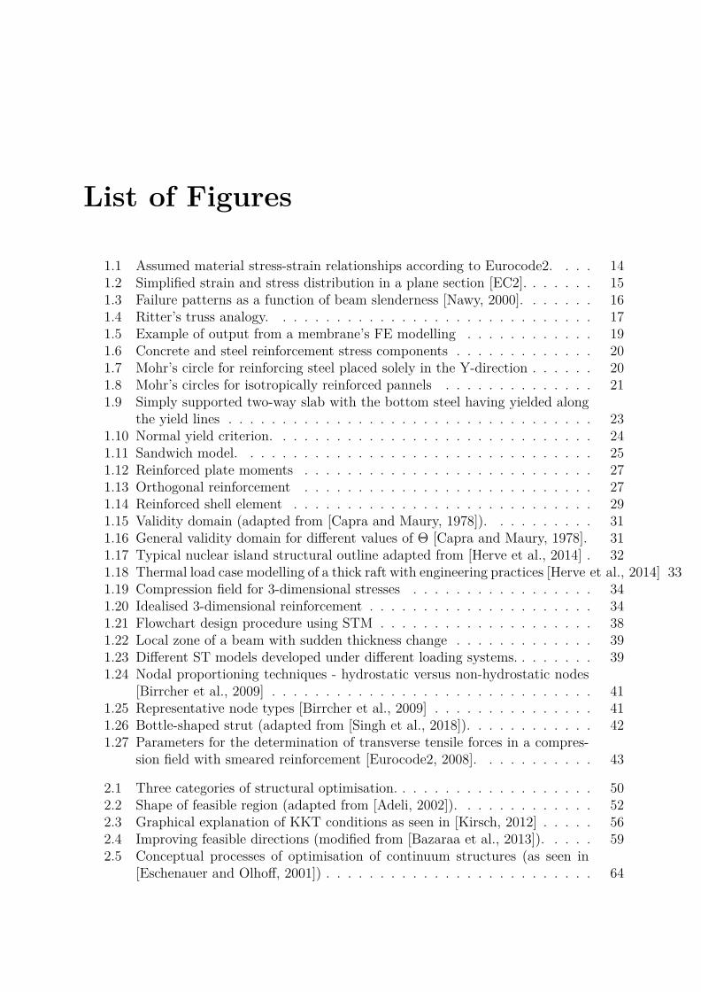
List of Figures

1.1 Assumed material stress-strain relationships according to Eurocode2. . . . 141.2 Simplified strain and stress distribution in a plane section [EC2]. . . . . . . 151.3 Failure patterns as a function of beam slenderness [Nawy, 2000]. . . . . . . 161.4 Ritter’s truss analogy. . . . . . . . . . . . . . . . . . . . . . . . . . . . . . 171.5 Example of output from a membrane’s FE modelling . . . . . . . . . . . . 191.6 Concrete and steel reinforcement stress components . . . . . . . . . . . . . 201.7 Mohr’s circle for reinforcing steel placed solely in the Y-direction . . . . . . 201.8 Mohr’s circles for isotropically reinforced pannels . . . . . . . . . . . . . . 211.9 Simply supported two-way slab with the bottom steel having yielded along

the yield lines . . . . . . . . . . . . . . . . . . . . . . . . . . . . . . . . . . 231.10 Normal yield criterion. . . . . . . . . . . . . . . . . . . . . . . . . . . . . . 241.11 Sandwich model. . . . . . . . . . . . . . . . . . . . . . . . . . . . . . . . . 251.12 Reinforced plate moments . . . . . . . . . . . . . . . . . . . . . . . . . . . 271.13 Orthogonal reinforcement . . . . . . . . . . . . . . . . . . . . . . . . . . . 271.14 Reinforced shell element . . . . . . . . . . . . . . . . . . . . . . . . . . . . 291.15 Validity domain (adapted from [Capra and Maury, 1978]). . . . . . . . . . 311.16 General validity domain for different values of Θ [Capra and Maury, 1978]. 311.17 Typical nuclear island structural outline adapted from [Herve et al., 2014] . 321.18 Thermal load case modelling of a thick raft with engineering practices [Herve et al., 2014] 331.19 Compression field for 3-dimensional stresses . . . . . . . . . . . . . . . . . 341.20 Idealised 3-dimensional reinforcement . . . . . . . . . . . . . . . . . . . . . 341.21 Flowchart design procedure using STM . . . . . . . . . . . . . . . . . . . . 381.22 Local zone of a beam with sudden thickness change . . . . . . . . . . . . . 391.23 Different ST models developed under different loading systems. . . . . . . . 391.24 Nodal proportioning techniques - hydrostatic versus non-hydrostatic nodes

[Birrcher et al., 2009] . . . . . . . . . . . . . . . . . . . . . . . . . . . . . . 411.25 Representative node types [Birrcher et al., 2009] . . . . . . . . . . . . . . . 411.26 Bottle-shaped strut (adapted from [Singh et al., 2018]). . . . . . . . . . . . 421.27 Parameters for the determination of transverse tensile forces in a compres-

sion field with smeared reinforcement [Eurocode2, 2008]. . . . . . . . . . . 43

2.1 Three categories of structural optimisation. . . . . . . . . . . . . . . . . . . 502.2 Shape of feasible region (adapted from [Adeli, 2002]). . . . . . . . . . . . . 522.3 Graphical explanation of KKT conditions as seen in [Kirsch, 2012] . . . . . 562.4 Improving feasible directions (modified from [Bazaraa et al., 2013]). . . . . 592.5 Conceptual processes of optimisation of continuum structures (as seen in

[Eschenauer and Olhoff, 2001]) . . . . . . . . . . . . . . . . . . . . . . . . . 64

135

2.6 Three possible ground structures for a 4x6 grid (n = 35) . . . . . . . . . . 642.7 Flowchart design procedure using FSD (inspired from [Li, 1990]). . . . . . 672.8 ST models obtained from 3 different ground structures [Gaynor et al., 2012]. 682.9 Piece-wise linear stress-strain relations (modified from [Achtziger, 1996]) . 69

3.1 Flowchart showing proposed the design procedure . . . . . . . . . . . . . . 733.2 Polynomial interpolation over 8 random XY Z triplets. . . . . . . . . . . . 753.3 Grid based numerical differentiation . . . . . . . . . . . . . . . . . . . . . . 763.4 Flowchart of the proposed truss optimisation . . . . . . . . . . . . . . . . . 813.5 Element suppression flowchart . . . . . . . . . . . . . . . . . . . . . . . . . 843.6 Hydrostatic nodes . . . . . . . . . . . . . . . . . . . . . . . . . . . . . . . . 863.7 Schematic representation of element’s length reduction and space verification 873.8 Anchorage zone models [Zhong et al., 2016] . . . . . . . . . . . . . . . . . . 893.9 Schematic representation of the needed: mesh and principal stress direction

fields . . . . . . . . . . . . . . . . . . . . . . . . . . . . . . . . . . . . . . . 903.10 Schematic representation of the needed data: principal stress fields . . . . . 903.11 Strut path generation: (a) Computed Voronoi seeds, (b) Clipped Voronoi

division, (c) Associated direction strut direction and (c) Initial strut path . 913.12 Ground structure development: (a) merged strut path and (b) proposed

ground structure (m=447). . . . . . . . . . . . . . . . . . . . . . . . . . . . 923.13 Anchorage Strut-and-Tie models obtained from a fine mesh . . . . . . . . . 923.14 Anchorage Strut-and-Tie models obtained from a coarse mesh . . . . . . . 933.15 Anchorage Strut-and-Tie models obtained from a locally refined mesh . . . 943.16 Different Strut-and-Tie model propositions . . . . . . . . . . . . . . . . . . 953.17 Comparison of different Strut-and-Tie model propositions(anchorage e=0.75m) 96

4.1 Planar corbel initial model . . . . . . . . . . . . . . . . . . . . . . . . . . . 1004.2 Schematic representation of the needed data . . . . . . . . . . . . . . . . . 1014.3 Strut generation subroutines . . . . . . . . . . . . . . . . . . . . . . . . . . 1024.4 Ground structure . . . . . . . . . . . . . . . . . . . . . . . . . . . . . . . . 1034.5 Different ST models for the corbel case. Figure (a) depicts the ties in red

and the struts in blue; figure (b) is presented with shifted colours . . . . . 1034.6 Nodal geometry . . . . . . . . . . . . . . . . . . . . . . . . . . . . . . . . . 1044.7 Optimisation evolution . . . . . . . . . . . . . . . . . . . . . . . . . . . . . 1074.8 Coarse mesh . . . . . . . . . . . . . . . . . . . . . . . . . . . . . . . . . . . 1084.9 Free mesh . . . . . . . . . . . . . . . . . . . . . . . . . . . . . . . . . . . . 1084.10 Computed components of reinforcement given in local coordinates . . . . . 1104.11 Views of model representation in Code_Aster software . . . . . . . . . . . 1104.12 Capra-Maury computed required steel reinforcement (Coarse mesh). . . . . 1114.13 ST model found through Bi-directional Evolutionary Structural Optimisa-

tion [Shobeiri, 2016] . . . . . . . . . . . . . . . . . . . . . . . . . . . . . . . 1144.14 Three-dimensional model representation . . . . . . . . . . . . . . . . . . . 1144.15 Caption . . . . . . . . . . . . . . . . . . . . . . . . . . . . . . . . . . . . . 1154.16 (a) directions associated to the Voronoi zones, (b) initial strut path, (c)

merged strut path and (d) ground structure (m =1919) . . . . . . . . . . 1154.17 Filtered Strut and tie model resultant of a size-topology scheme (m = 88) . 116


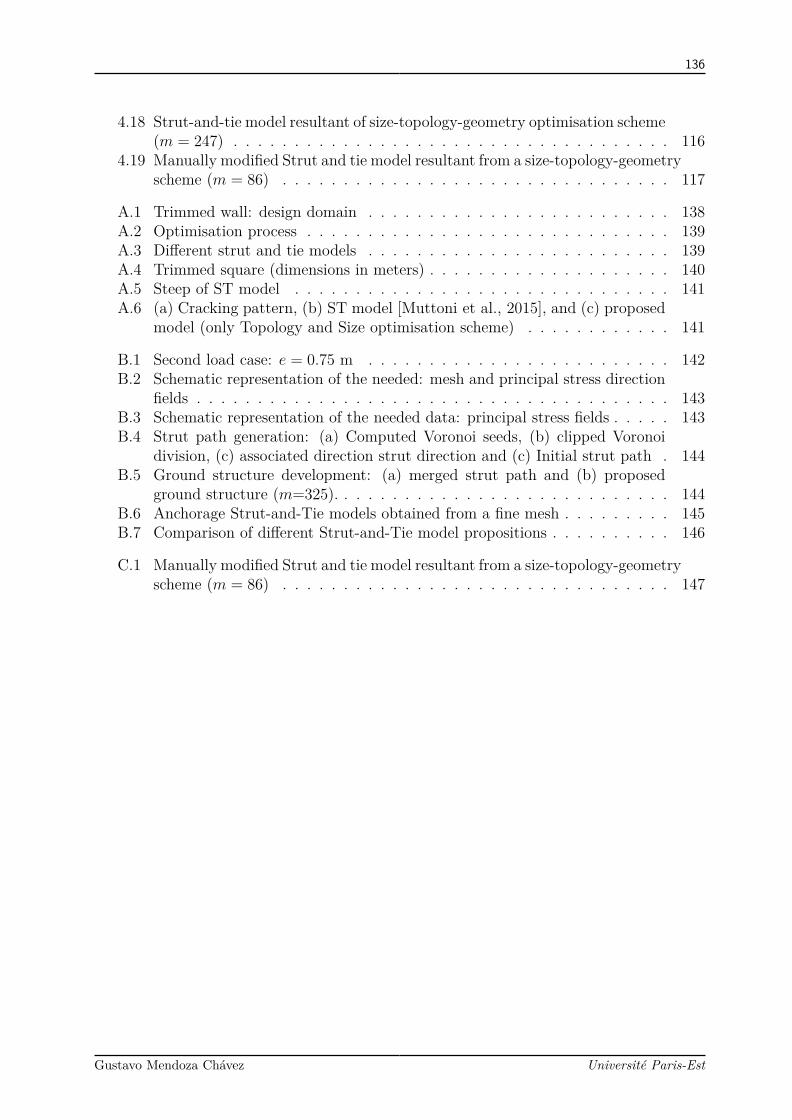
136

4.18 Strut-and-tie model resultant of size-topology-geometry optimisation scheme(m = 247) . . . . . . . . . . . . . . . . . . . . . . . . . . . . . . . . . . . . 116

4.19 Manually modified Strut and tie model resultant from a size-topology-geometryscheme (m = 86) . . . . . . . . . . . . . . . . . . . . . . . . . . . . . . . . 117

A.1 Trimmed wall: design domain . . . . . . . . . . . . . . . . . . . . . . . . . 138A.2 Optimisation process . . . . . . . . . . . . . . . . . . . . . . . . . . . . . . 139A.3 Different strut and tie models . . . . . . . . . . . . . . . . . . . . . . . . . 139A.4 Trimmed square (dimensions in meters) . . . . . . . . . . . . . . . . . . . . 140A.5 Steep of ST model . . . . . . . . . . . . . . . . . . . . . . . . . . . . . . . 141A.6 (a) Cracking pattern, (b) ST model [Muttoni et al., 2015], and (c) proposed

model (only Topology and Size optimisation scheme) . . . . . . . . . . . . 141

B.1 Second load case: e = 0.75 m . . . . . . . . . . . . . . . . . . . . . . . . . 142B.2 Schematic representation of the needed: mesh and principal stress direction

fields . . . . . . . . . . . . . . . . . . . . . . . . . . . . . . . . . . . . . . . 143B.3 Schematic representation of the needed data: principal stress fields . . . . . 143B.4 Strut path generation: (a) Computed Voronoi seeds, (b) clipped Voronoi

division, (c) associated direction strut direction and (c) Initial strut path . 144B.5 Ground structure development: (a) merged strut path and (b) proposed

ground structure (m=325). . . . . . . . . . . . . . . . . . . . . . . . . . . . 144B.6 Anchorage Strut-and-Tie models obtained from a fine mesh . . . . . . . . . 145B.7 Comparison of different Strut-and-Tie model propositions . . . . . . . . . . 146

C.1 Manually modified Strut and tie model resultant from a size-topology-geometryscheme (m = 86) . . . . . . . . . . . . . . . . . . . . . . . . . . . . . . . . 147


List of Tables

1.1 ACI and Eurocode values for nodal zones resistance . . . . . . . . . . . . . 411.2 ACI and Eurocode values for strut resistance . . . . . . . . . . . . . . . . . 43

4.1 Considered materials . . . . . . . . . . . . . . . . . . . . . . . . . . . . . . 1004.2 Steel reinforcement for the ST model . . . . . . . . . . . . . . . . . . . . . 1054.3 Steel reinforcement for the planar ST model: projection over the X and Y

axis [cm3] . . . . . . . . . . . . . . . . . . . . . . . . . . . . . . . . . . . . 1064.4 Steel reinforcement for the planar ST model: need of steel reinforcement per

zone [cm3] . . . . . . . . . . . . . . . . . . . . . . . . . . . . . . . . . . . . 1074.5 Computed need of steel reinforced per zone (coarse model) [cm3] . . . . . . 1124.6 Computed need of steel reinforced per zone (3D ST) [cm3] . . . . . . . . . 1174.7 Comparative table of need of steel reinforcement per zone [cm3] . . . . . . 1184.8 Comparative table of need of steel reinforcement per zone. kg of steel per

cubic meter of concrete . . . . . . . . . . . . . . . . . . . . . . . . . . . . 118

C.1 3D corbel ST nodal list . . . . . . . . . . . . . . . . . . . . . . . . . . . . . 148C.2 3D corbel ST tie table . . . . . . . . . . . . . . . . . . . . . . . . . . . . . 149

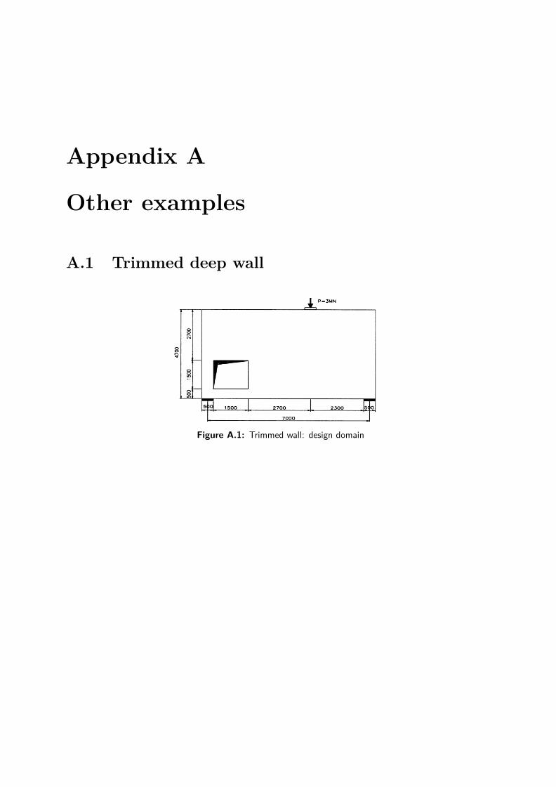
Appendix A

Other examples

A.1 Trimmed deep wall

Figure A.1: Trimmed wall: design domain

139

(a) ground structure (b) iteration 18 (c) iteration 36

(d) iteration 54 (e) iteration 62 (f) iteration 78Figure A.2: Optimisation process

(a) [Almeida et al., 2013] (b) [Schlaich et al., 1987](c) proposed (Full optimisa-tion scheme)

Figure A.3: Different strut and tie models


140

A.2 Trimmed square

1.00

1.00

0.25

0.25

P

P

Figure A.4: Trimmed square (dimensions in meters)


141

(a) Voronoi division (b) Direction field of σI (c) Direction field of σIII

(d) Initial strut path (e) Merged strut path

31

32

37

1

28

19

33

4

3

26

2

39

24

6

23

25

17

5

7

30

14

38

15

13

10

1216

27

9

20

29

1118

36

22

21

8

(f) Ground structureFigure A.5: Steep of ST model

(a) (b)

0 0.2 0.4 0.6 0.8 1

1

0.9

0.8

0.7

0.6

0.5

0.4

0.3

0.2

0.1

0

(c)Figure A.6: (a) Cracking pattern, (b) ST model [Muttoni et al., 2015], and (c) proposed model (only Topologyand Size optimisation scheme)


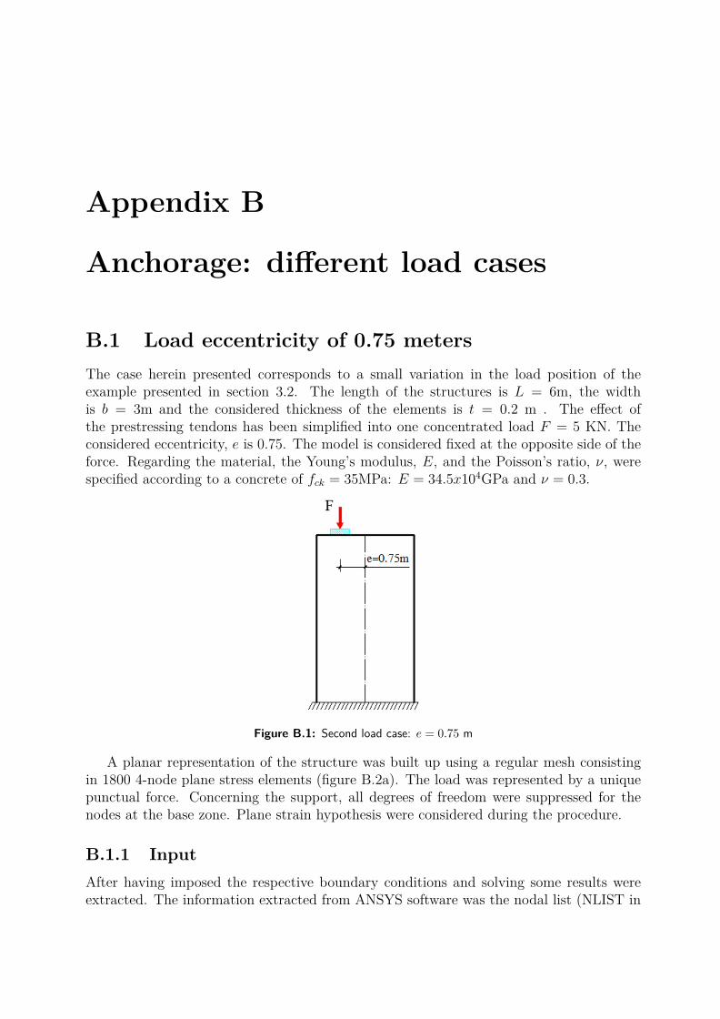
Appendix B

Anchorage: different load cases

B.1 Load eccentricity of 0.75 metersThe case herein presented corresponds to a small variation in the load position of theexample presented in section 3.2. The length of the structures is L = 6m, the widthis b = 3m and the considered thickness of the elements is t = 0.2 m . The effect ofthe prestressing tendons has been simplified into one concentrated load F = 5 KN. Theconsidered eccentricity, e is 0.75. The model is considered fixed at the opposite side of theforce. Regarding the material, the Young’s modulus, E, and the Poisson’s ratio, ν, werespecified according to a concrete of fck = 35MPa: E = 34.5x104GPa and ν = 0.3.

Figure B.1: Second load case: e = 0.75 m

A planar representation of the structure was built up using a regular mesh consistingin 1800 4-node plane stress elements (figure B.2a). The load was represented by a uniquepunctual force. Concerning the support, all degrees of freedom were suppressed for thenodes at the base zone. Plane strain hypothesis were considered during the procedure.

B.1.1 InputAfter having imposed the respective boundary conditions and solving some results wereextracted. The information extracted from ANSYS software was the nodal list (NLIST in

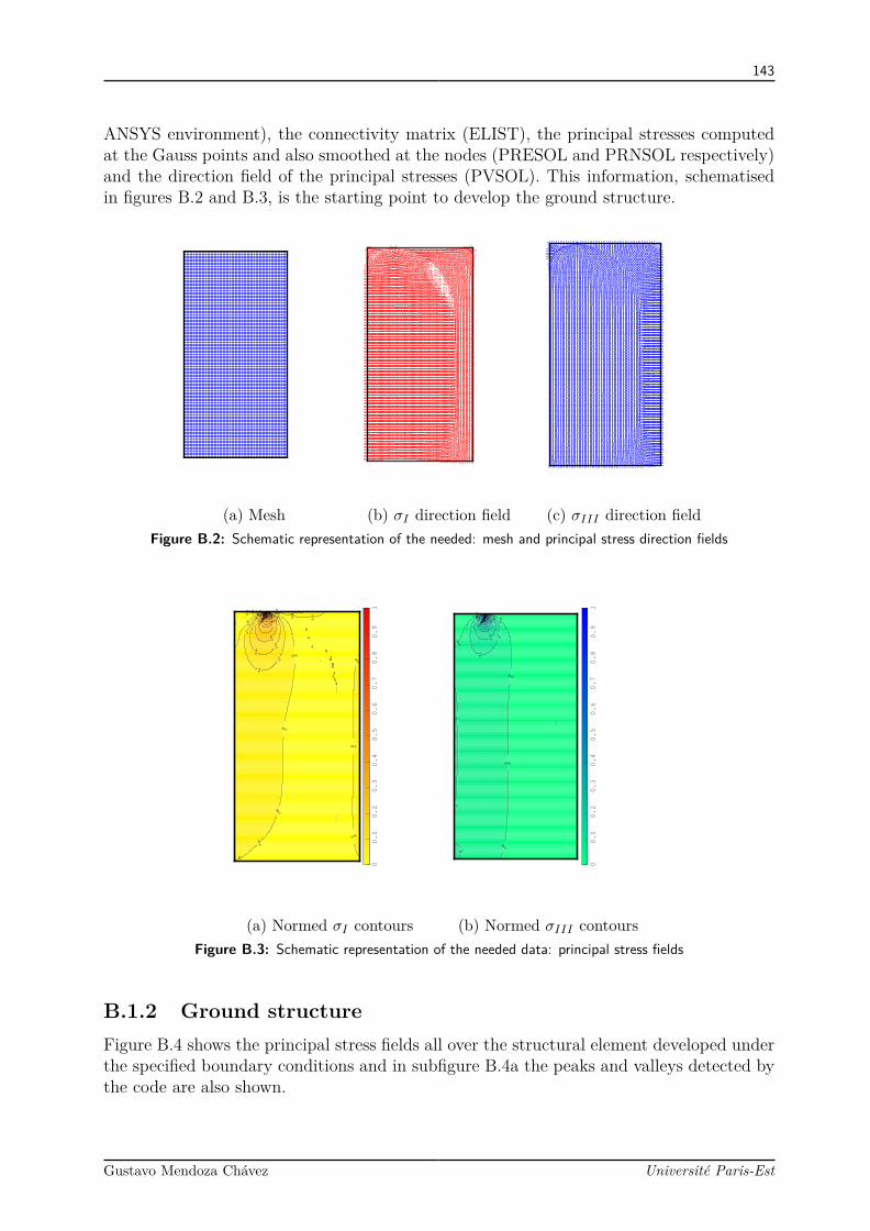
143

ANSYS environment), the connectivity matrix (ELIST), the principal stresses computedat the Gauss points and also smoothed at the nodes (PRESOL and PRNSOL respectively)and the direction field of the principal stresses (PVSOL). This information, schematisedin figures B.2 and B.3, is the starting point to develop the ground structure.

(a) Mesh (b) σI direction field (c) σIII direction fieldFigure B.2: Schematic representation of the needed: mesh and principal stress direction fields

00

000

00

0

0

0

0

0

0.05

0.05

0.05

0.05

0.05

0.05

0.05

0.05

0.05

0.05

0.05

0.05

0.05

0.1

0.1

0.1

0.1

0.1 0.

1

0.14

0.14

0.14

0.14

0.19

0.19

0.24

0.24

0.290.

330.380.430.48

0.52

0.57

0.62

0.67

0.71

0.76

0.81 0.91

00.1

0.2

0.3

0.4

0.5

0.6

0.7

0.8

0.9

1

(a) Normed σI contours

0.05

0.05

0.05

0.05

0.05

0.05

0.1

0.1

0.1

0.1

0.1

0.1

0.14

0.14

0.19

0.19

0.240.290.330.38

0.43

0.48

0.52

0.57

0.62

0.67

0.71

00.1

0.2

0.3

0.4

0.5

0.6

0.7

0.8

0.9

1

(b) Normed σIII contoursFigure B.3: Schematic representation of the needed data: principal stress fields

B.1.2 Ground structureFigure B.4 shows the principal stress fields all over the structural element developed underthe specified boundary conditions and in subfigure B.4a the peaks and valleys detected bythe code are also shown.


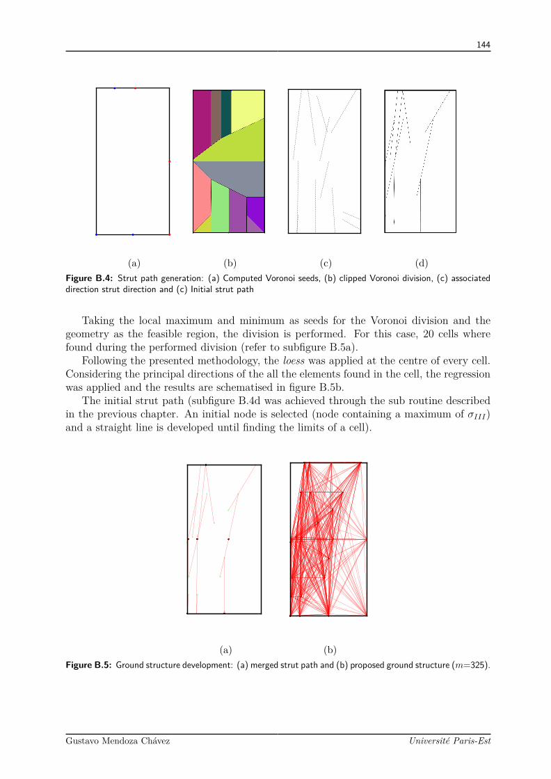
144

(a) (b) (c) (d)Figure B.4: Strut path generation: (a) Computed Voronoi seeds, (b) clipped Voronoi division, (c) associateddirection strut direction and (c) Initial strut path

Taking the local maximum and minimum as seeds for the Voronoi division and thegeometry as the feasible region, the division is performed. For this case, 20 cells wherefound during the performed division (refer to subfigure B.5a).

Following the presented methodology, the loess was applied at the centre of every cell.Considering the principal directions of the all the elements found in the cell, the regressionwas applied and the results are schematised in figure B.5b.

The initial strut path (subfigure B.4d was achieved through the sub routine describedin the previous chapter. An initial node is selected (node containing a maximum of σIII)and a straight line is developed until finding the limits of a cell).

(a) (b)Figure B.5: Ground structure development: (a) merged strut path and (b) proposed ground structure (m=325).


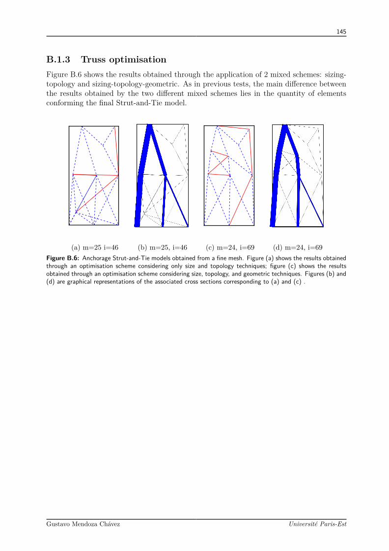
145

B.1.3 Truss optimisationFigure B.6 shows the results obtained through the application of 2 mixed schemes: sizing-topology and sizing-topology-geometric. As in previous tests, the main difference betweenthe results obtained by the two different mixed schemes lies in the quantity of elementsconforming the final Strut-and-Tie model.

(a) m=25 i=46 (b) m=25, i=46 (c) m=24, i=69 (d) m=24, i=69Figure B.6: Anchorage Strut-and-Tie models obtained from a fine mesh. Figure (a) shows the results obtainedthrough an optimisation scheme considering only size and topology techniques; figure (c) shows the resultsobtained through an optimisation scheme considering size, topology, and geometric techniques. Figures (b) and(d) are graphical representations of the associated cross sections corresponding to (a) and (c) .


146

P


P

(b) [Schlaich et al., 1987]

P

(c) Computed modelFigure B.7: Comparison of different Strut-and-Tie model propositions

B.1.4 Literature resultsFigure B.7 shows the proposed Strut-and-Tie models. As in previous figures, the bluedashed lines represent members in compression and the continuous red lines representelements in tension; the original figures were adapted to respect this colour pallet.

It can be observed that this is so far the model that differs the most from the literatureexamples. Even though the models present strong similarities in terms of load-transfermechanisms, the mere existence of some elements in the proposed model brings effects ofcompression in a zone that do not consider struts in the other two models (right supportin figures B.7).

The differences presented in this model come from the fact that, for this case, theobtained the automatically obtained Voronoi seeds did not allow a satisfactory geometrydivision (clipped Voronoi division) and some seeds were need to be added manually to thealgorithm to continue the procedure. The present results permit to state that the presentapproach is highly sensitive to the number and position of the Voronoi seeds. In case ofnot being satisfied with the final results, it was decided to let the user the liberty to add,erase or modify the proposed Voronoi seed hence adapting a computer aided scheme overa fully automatic one.


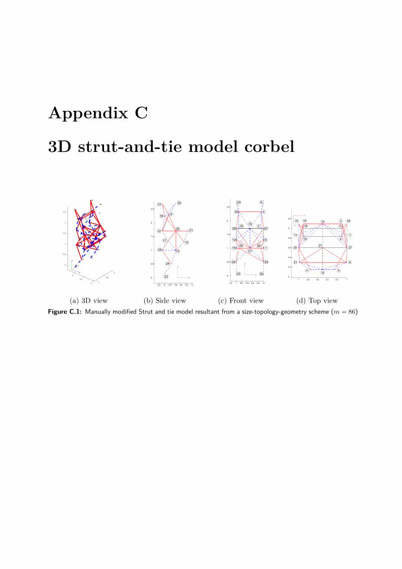
Appendix C

3D strut-and-tie model corbel

0

0.5

6

910

27

8

1

5

25

1

11

7

4

21

22

28

3

12

5

26

2

13

30

15

20

14

24

19

5.5

17

X

18

Y

29

16

23

31

6

Z

0

1

1.5

2

2.5

0.5

(a) 3D view

21

15

29

30

31

20

9

18

17

24

23

12

12

6.2 6 5.8 5.6 5.4 5.2 5

0

0.5

1

1.5

2

2.5

X

Z

(b) Side view

20

20

10

16

30

12

15

29

21

24

23

8

4

2

27

6

1

26

25

22

1

0

0.5

1

1.5

2

2.5

0.8 0.6 0.4 0.2 01.2

X

Z

(c) Front view

3116

18

19

17

30

21

11

10

21

14

282

3

4

7

27

6

9

1 0.8 0.6 0.4 0.2 1

5

5.2

5.4

5.6

5.8

6

6.2

Y

X

(d) Top viewFigure C.1: Manually modified Strut and tie model resultant from a size-topology-geometry scheme (m = 86)

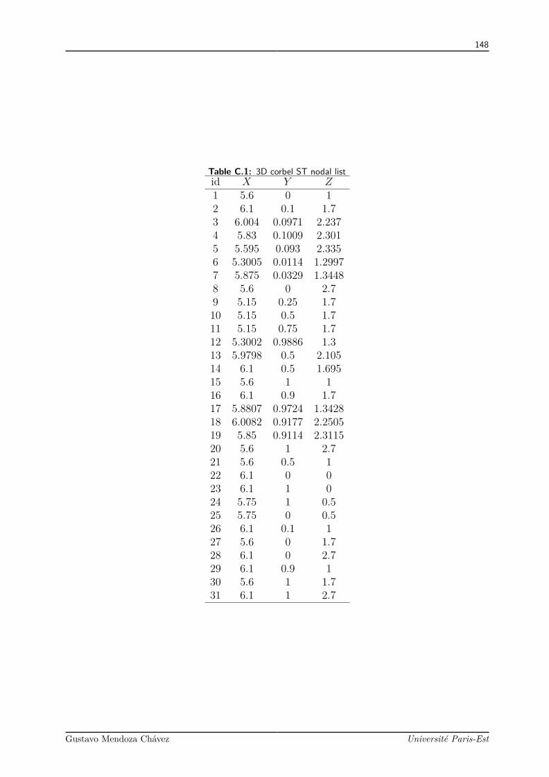
148

Table C.1: 3D corbel ST nodal listid X Y Z1 5.6 0 12 6.1 0.1 1.73 6.004 0.0971 2.2374 5.83 0.1009 2.3015 5.595 0.093 2.3356 5.3005 0.0114 1.29977 5.875 0.0329 1.34488 5.6 0 2.79 5.15 0.25 1.710 5.15 0.5 1.711 5.15 0.75 1.712 5.3002 0.9886 1.313 5.9798 0.5 2.10514 6.1 0.5 1.69515 5.6 1 116 6.1 0.9 1.717 5.8807 0.9724 1.342818 6.0082 0.9177 2.250519 5.85 0.9114 2.311520 5.6 1 2.721 5.6 0.5 122 6.1 0 023 6.1 1 024 5.75 1 0.525 5.75 0 0.526 6.1 0.1 127 5.6 0 1.728 6.1 0 2.729 6.1 0.9 130 5.6 1 1.731 6.1 1 2.7


149

Table C.2: 3D corbel ST tie tableTie i j length force area volumeT1 1 14 99.15 2.27 0.05 5T2 1 15 100 16.26 0.36 36.12T3 1 21 50 7.2 0.16 8.01T4 2 27 50.99 36.43 0.81 41.28T5 3 4 18.54 8.77 0.19 3.61T6 3 18 82.07 21.62 0.48 39.43T7 3 27 67.9 84.71 1.88 127.81T8 3 28 48.27 98.1 2.18 105.23T9 4 19 81.08 39.95 0.89 71.97T10 4 27 65.14 98.94 2.2 143.23T11 4 28 49.22 74.3 1.65 81.26T12 6 12 97.72 173.05 3.85 375.78T13 6 21 64.67 11.45 0.25 16.45T14 6 27 50.01 105.65 2.35 117.41T15 7 14 62.57 6.01 0.13 8.36T16 7 26 41.72 0.11 0 0.1T17 7 27 45.04 4.64 0.1 4.65T18 9 27 51.48 71.68 1.59 82T19 10 14 95 79.71 1.77 168.28T20 11 30 51.48 71.59 1.59 81.9T21 12 30 50 102.39 2.28 113.77T22 15 21 50 21.82 0.48 24.25T23 15 30 70 13.05 0.29 20.3T24 16 17 42.54 0.16 0 0.15T25 16 19 66.07 0.19 0 0.27T26 17 29 41.33 64.35 1.43 59.11T27 17 30 45.51 62.76 1.39 63.47T28 18 30 69.03 69.75 1.55 107T29 18 31 46.61 69.15 1.54 71.63T30 19 30 66.65 96.64 2.15 143.13T31 19 31 47.04 103.42 2.3 108.1T32 21 27 86.02 18.5 0.41 35.37T33 21 30 86.02 0.09 0 0.17T34 24 29 61.85 63.35 1.41 87.07T35 25 26 61.85 68.61 1.52 94.3T36 25 29 108.74 4.69 0.1 11.33T37 26 27 86.6 68.51 1.52 131.85T38 26 29 80 3.33 0.07 5.93Total 2595.1


Strut-and-Tie models for the design of non-flexural elements

Documents

Transcript of Strut-and-Tie models for the design of non-flexural elements