IOP PUBLISHING JOURNAL OF PHYSICS: CONDENSED MATTER

J. Phys.: Condens. Matter 19 (2007) 086224 (14pp) doi:10.1088/0953-8984/19/8/086224

Structure and thermodynamics of discrete potentialfluids in the OZ–HMSA formalism

I Guillen-Escamilla1, M Chavez-Paez1 and R Castaneda-Priego2

1 Instituto de Fısica, Universidad Autonoma de San Luis Potosı, Alvaro Obregon 64, 78000San Luis Potosı, SLP, Mexico2 Instituto de Fısica, Universidad de Guanajuato, Loma del Bosque 103, Lomas del Campestre,37150 Leon, Mexico

E-mail: mchavez@ifisica.uaslp.mx

Received 1 November 2006, in final form 29 December 2006Published 9 February 2007Online at stacks.iop.org/JPhysCM/19/086224

AbstractWe study the structural and thermodynamic properties of three discrete potentialfluids: the square well (SW), the square well–barrier (SWB), and the squarewell–barrier–well (SWBW) fluids by means of the Ornstein–Zernike (OZ)integral equation and the HMSA (hybrid mean spherical approximation) closurerelation. The radial distribution functions, structure factors, and pressure of thesystems are calculated as a function of the strength of the attractive and repulsiveparts of the potential in an extended range of densities, mainly covering therange 0.1 � ρ∗ � 0.9. We find that far away from the liquid–vapour coexistenceregion the HMSA theory is an accurate approach that compares well with MonteCarlo simulations. We also find that when the attractive parts of the potentialdominate over the repulsive part the structure factor at low q values shows aconsiderable increase, which suggests the formation of large-scale domains thatlocally exhibit fluid-like structure.

1. Introduction

Structural and thermodynamic properties of both simple and complex fluids depend on thenature of the interaction potential between particles. While simple fluids can be modelledthrough a simple potential, in complex fluids one has often to resort to simplified schemes andintroduce effective interactions between the main constituents of the fluid. In this process theeffective potential is devised, from first principles or from experimental evidence, such thatit captures enough features to reproduce the properties of the system it is supposed to model.Examples of such potentials are the Lennard-Jones and the DLVO potentials [1, 2]. The formerdescribes very well the properties of many simple liquids and the latter is commonly used todescribe the interaction between charged colloidal particles. Qualitatively, the DLVO potentialis formed by a hard core followed by a short-range attractive well and a long-range repulsivebarrier. For colloidal particles at interphases, the effective interaction can include a secondary

0953-8984/07/086224+14$30.00 © 2007 IOP Publishing Ltd Printed in the UK 1

J. Phys.: Condens. Matter 19 (2007) 086224 I Guillen-Escamilla et al

minimum [3]. The stability of colloidal systems depends crucially on the presence of such anenergetic barrier, whereas the second attractive component modifies drastically the propertiesof the systems. In this work we use a simplified interaction model, a discrete potential (DP),that incorporates attractive and repulsive parts. Due to its simplicity, a DP allows us to studyseparately the effects produced by the different attractive and repulsive components of thepotential, which typically cannot be done with continuous potentials, where only global effectscan be distinguished.

During the last few decades, discrete potentials have been used as simple models toinvestigate properties of continuous potential systems. They have been used, for example,to model the interactions of colloids and protein solutions [4, 5]. Despite its simplicity, aDP fluid can exhibit rather complex and interesting behaviours. Recently, for instance, it hasbeen established that such fluids exhibit both liquid–vapour and liquid–liquid transitions [6].Discrete potentials have been incorporated in a variety of statistical mechanics theories such asthermodynamic perturbation-like theories to describe associating fluids and polar fluids [7, 8].In addition, their bulk properties can be used as inputs in the study of model inhomogeneoussystems, i.e. for fluids in external fields such as porous media or confined systems [9]. All theseaspects make DP systems interesting to explore.

The simplest and most investigated DP system is the well known square-well (SW) fluid.This model system can reproduce the behaviour of a large variety of real fluids by only varyingthe interaction range of the SW potential. The structural properties, as well as the liquid–vapour (LV), solid, and glass transitions of the SW fluid, have been studied by means ofcomputer simulations, perturbation theory, and integral equation theory [4, 10–28]. Recently,within the framework of the self-consistent Ornstein–Zernike approximation (SCOZA), its LVcoexistence has been reinvestigated and described with high accuracy [29]; a similar study onthe liquid–solid transition within the SCOZA approach is in progress [30]. Although it hasbeen shown that SCOZA yields globally accurate structural and thermodynamic properties ofSW fluids and other systems, even near phase transitions and in the critical region, it becomesunstable for systems with potentials that include a second repulsive part (the problem resides inthe diffusion-like coefficient of the associated partial differential equation (PDE), equation (9)in [29], which becomes negative when a repulsive barrier is considered, severely limiting theconvergence of the PDE). It is therefore desirable to investigate other theoretical approachesthat can handle this kind of potentials. In this paper we investigate one of these approaches,namely, the Ornstein–Zernike (OZ) equation in the HMSA approach [31].

The aim of this paper is to investigate the structural and thermodynamic properties of dis-crete potential fluids using the OZ–HMSA formalism. In particular, we investigate three differ-ent discrete potential fluids: the square well (SW), square well–barrier (SWB), and square well–barrier–well (SWBW) fluids. We analyse their radial distribution functions and structure factorsas a function of the density and the energetic strength of the wells and barriers. In particularwe focus our study on systems outside the liquid–vapour coexistence region. The theoreticalpredictions are contrasted with Monte Carlo simulations performed in the canonical ensemble.

After the present introduction, in section 2 we provide a detailed description of the discretepotentials, the theoretical approach, and the simulation method. In section 3 the structurefunctions and the pressure far away from the binodal are analysed. Finally, in section 4 weclose the paper with a section of remarks and conclusions.

2. Model system and theoretical approach

Our system is formed by spherical particles of bulk density ρ and hard-core diameter σ inthermal equilibrium with a heat bath at absolute temperature T . The particles in this fluid

2

J. Phys.: Condens. Matter 19 (2007) 086224 I Guillen-Escamilla et al

1 2 3r/σ

-1

0

1

2

u(r)

ε

ε2

ε3

λλ2

λ3

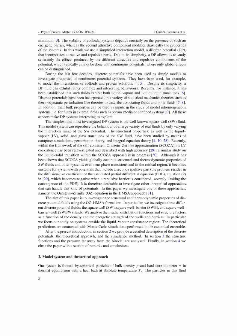
Figure 1. Cartoon of the discrete potential used in this work.

interact through a discrete potential that sequentially includes a hard sphere, a square well, asquare barrier, and a second square well. This pair potential takes the form

u(r) =

⎧⎪⎪⎪⎪⎪⎪⎨

⎪⎪⎪⎪⎪⎪⎩

∞, r < σ ;

−ε, σ � r < λσ ;

ε2, λσ � r < λ2σ ;

−ε3, λ2σ � r < λ3σ ;

0, r � λ3σ .

(1)

The parameters λ, λ2, and λ3 define the discontinuity points of the potential, and delimit thedifferent regions of the potential. The parameters ε, ε2, and ε3, on the other hand, characterizethe strength of the potential in those regions. A cartoon of the potential is presented in figure 1.Appropriate reduced quantities can be defined by scaling with the energy depth ε and the sizeof the particles σ , which leads to the reduced density ρ∗ = ρσ 3 and the reduced temperatureT ∗ = kBT/ε, where kB is the Boltzmann’s constant. From equation (1) several cases can beconsidered, depending on the parameters; in particular, equation (1) reduces to the hard-sphere(HS) potential when only the first part is considered. We will consider the three followingcases of equation (1): (a) the SW potential, defined by ε �= 0 and ε2 = ε3 = 0; (b) the SWBpotential, defined by ε �= 0, ε2 �= 0, and ε3 = 0; and (c) the SWBW potential, defined by thefull equation (1). In this way, SW fluids are characterized by a single well, SWB fluids by awell and a barrier, and SWB fluids by two wells with a barrier in between.

From a theoretical point of view, we have selected the Ornstein–Zernike equationcomplemented with HMSA, a closure proposed by Zerah and Hansen that combines thehypernetted chain (HNC) and the soft mean spherical approximation (SMSA) [31]. This is atheoretical approach that has been applied with success in a large variety of simple and complexsystems with both attractive and repulsive interactions [32–37]. However, its applicability toDP systems has not been explored yet. We also use the so-called mean spherical approximation(MSA), which has been used to study several kinds of simple fluids, in particular the SW fluid,but it has not been used to study SWB and SWBW fluids. Although other closure relations likePercus–Yevick (PY) could be used [11, 33, 38], here we shall focus only on the HMSA andMSA closures.

3

J. Phys.: Condens. Matter 19 (2007) 086224 I Guillen-Escamilla et al

The homogeneous OZ equation is given by [39]

h(r) = c(r) + ρ

∫

h(∣∣r − r′∣∣)c(r′) dr′, (2)

where h(r) = g(r) − 1 and c(r) are the total and direct correlation functions, respectively,and g(r) is the radial pair distribution function. Alternatively, the OZ equation can be writtenin terms of the indirect correlation function γ (r) = h(r) − c(r) by eliminating h(r) fromequation (2). In this work, the OZ equation is numerically solved by using a five-parameterversion of the Ng iterative method [40]. Since the OZ equation defines c(r) in terms of h(r),an additional relation between c(r) and h(r) (or γ (r)) has to be provided to close the system.Many closure relations can be found in the literature of simple fluids and colloidal suspensions.The simplest one is the mean spherical approximation, which can be written as

c(r) ={

−γ (r) − 1, r < σ ;

−βu(r), r � σ ,(3)

where β = 1/kBT is the inverse of the thermal energy. On the other hand, the HMSA closurerelation can be written as [31]

c(r) = exp [−βur(r)][

1 + exp [(γ (r) − βua(r)) f (r)] − 1

f (r)

]

− γ (r) − 1 (4)

for r � σ , supplemented by the exact hard-sphere condition c(r) = −γ (r) − 1 for r < σ .In this equation, the total potential u(r) between particles is split into two parts accordingto the HMSA recipe: ur(r) is the repulsive part of the potential, and ua(r) is the attractivepart. The function f (r) = 1 − exp(−αr) is a mixing function and α the mixing parameter.The isothermal compressibility χ of the system (normalized with the ideal gas compressibilityχ0 = β/ρ) can be obtained through the relations χ−1

v = (∂β P/∂ρ)T (the virial route) and byχ−1

c = 1 − ρc(q = 0), where P is the pressure of the system and c(q) is the Fourier transformof the direct correlation function. The OZ–HMSA approach enforces both routes to give thesame compressibility (χv = χc) by adjusting the mixing parameter, imposing therefore partialthermodynamic consistency. The HMSA closure relation is an extension of an original relationproposed by Rogers and Young (RY) [41]. Although the RY relation works very well forsystems with pure repulsive interactions, its applicability to systems with attractive interactionsis rather restricted [31, 42], which led Zerah and Hansen to develop their closure relation.

Once the OZ equation has been solved, the pressure P of the system can be determinedfrom the virial equation, which for the potential in equation (1) takes the form

β P

ρ= 1 + 2

3πρσ 3

[3∑

i=0

λ3i �g(λi )

]

, (5)

where λi denotes the discontinuity points of the potential, and �g(λi ) = g(λ+i ) − g(λ−

i ) is thedifference in contact values of the radial distribution function at the discontinuity. For a HS fluidi = 0 and the summation only involves the term �g(σ ) = g(σ+). The SW fluid additionallyinvolves �g(λ) = g(λ+) − g(λ−), the SWB involves also the term �g(λ2) = g(λ+

2 ) − g(λ−2 ),

and finally the SWBW includes the contribution �g(λ3) = g(λ+3 ) − g(λ−

3 ).The theoretical calculations are compared to Monte Carlo simulations in the canonical

(N V T ) ensemble [43, 44]. In all our simulations we used periodic boundary conditions, witha minimum of N = 1024 particles and a minimum simulation box length L = 10σ , dependingon the density of the systems. The particles in the simulation box are initially placed in aregular configuration at the prescribed density; this configuration is equilibrated for at least 105

Monte Carlo cycles, where each MC cycle consist of N attempts to displace randomly selected

4

J. Phys.: Condens. Matter 19 (2007) 086224 I Guillen-Escamilla et al

0

0.5

1

1.5

2

g(r)

0

0.5

1

1.5

2

1 2 3r/σ

0

0.5

1

1.5

2

g(r)

1 2 3r/σ

0

1

2

3

ρ∗ = 0.3

ρ∗ = 0.5

ρ∗ = 0.1

ρ∗ = 0.8

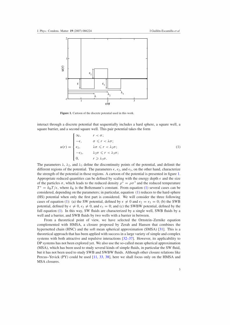
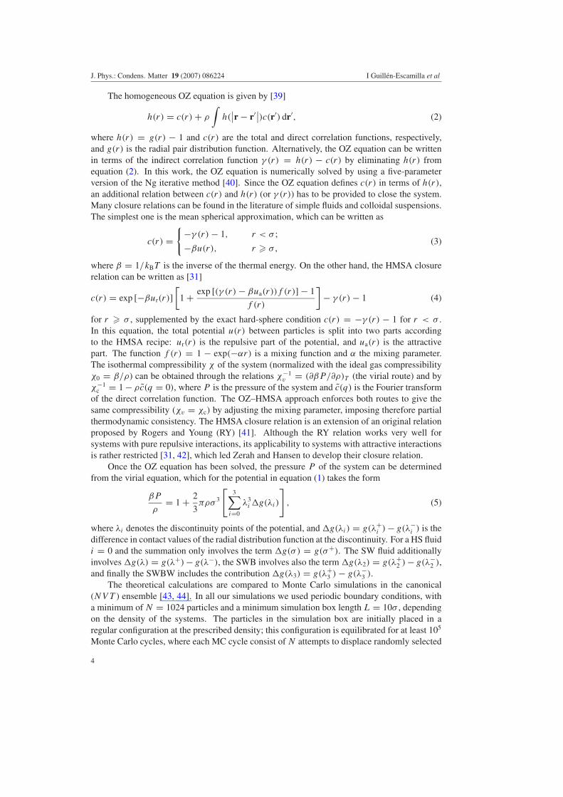
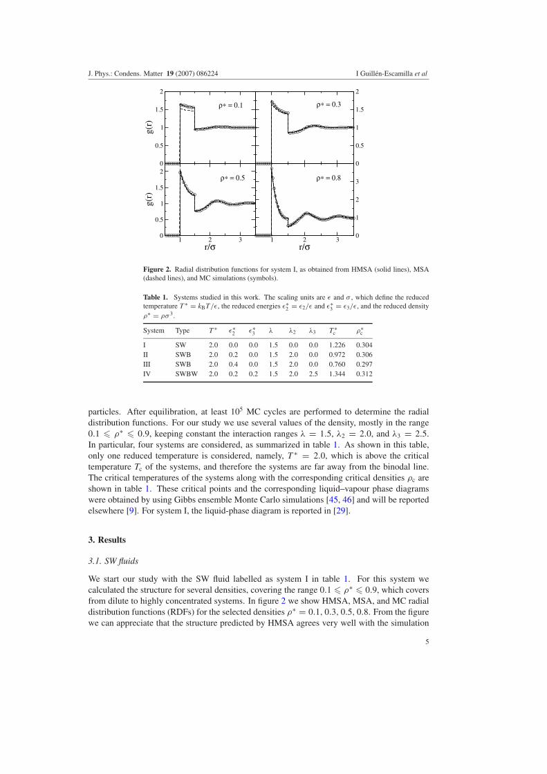
Figure 2. Radial distribution functions for system I, as obtained from HMSA (solid lines), MSA(dashed lines), and MC simulations (symbols).

Table 1. Systems studied in this work. The scaling units are ε and σ , which define the reducedtemperature T ∗ = kBT/ε, the reduced energies ε∗

2 = ε2/ε and ε∗3 = ε3/ε, and the reduced density

ρ∗ = ρσ 3.

System Type T ∗ ε∗2 ε∗

3 λ λ2 λ3 T ∗c ρ∗

c

I SW 2.0 0.0 0.0 1.5 0.0 0.0 1.226 0.304II SWB 2.0 0.2 0.0 1.5 2.0 0.0 0.972 0.306III SWB 2.0 0.4 0.0 1.5 2.0 0.0 0.760 0.297IV SWBW 2.0 0.2 0.2 1.5 2.0 2.5 1.344 0.312

particles. After equilibration, at least 105 MC cycles are performed to determine the radialdistribution functions. For our study we use several values of the density, mostly in the range0.1 � ρ∗ � 0.9, keeping constant the interaction ranges λ = 1.5, λ2 = 2.0, and λ3 = 2.5.In particular, four systems are considered, as summarized in table 1. As shown in this table,only one reduced temperature is considered, namely, T ∗ = 2.0, which is above the criticaltemperature Tc of the systems, and therefore the systems are far away from the binodal line.The critical temperatures of the systems along with the corresponding critical densities ρc areshown in table 1. These critical points and the corresponding liquid–vapour phase diagramswere obtained by using Gibbs ensemble Monte Carlo simulations [45, 46] and will be reportedelsewhere [9]. For system I, the liquid-phase diagram is reported in [29].

3. Results

3.1. SW fluids

We start our study with the SW fluid labelled as system I in table 1. For this system wecalculated the structure for several densities, covering the range 0.1 � ρ∗ � 0.9, which coversfrom dilute to highly concentrated systems. In figure 2 we show HMSA, MSA, and MC radialdistribution functions (RDFs) for the selected densities ρ∗ = 0.1, 0.3, 0.5, 0.8. From the figurewe can appreciate that the structure predicted by HMSA agrees very well with the simulation

5

J. Phys.: Condens. Matter 19 (2007) 086224 I Guillen-Escamilla et al

0 5 10 15 20qσ

0

0.5

1

1.5

2

2.5

3

S(q)

ρ∗ = 0.9ρ∗ = 0.8ρ∗ = 0.6ρ∗ = 0.5ρ∗ = 0.4ρ∗ = 0.3ρ∗ = 0.2ρ∗ = 0.1

Figure 3. Structure factor of SW fluids (system I) for several reduced densities, as obtained fromHMSA.

data and with previous reference hypernetted-chain (RHNC) calculations [47]. MSA, on theother hand, fails to reproduce the structure in the region of the attractive well for low densities,but the agreement improves greatly for ρ∗ � 0.4. From the figure it can be seen that, asexpected, the structure is enhanced when the density is increased. We note, however, that forall densities the agreement of HMSA and MSA with simulations is very good beyond the wellof the potential. It is in the region of the well of the potential where discrepancies between thetwo theories are revealed.

The radial distribution function g(r) is directly connected to the so-called structure factorS(q) through the relation S(q) = 1 + ρh(q), where h(q) is the Fourier transform of the totalcorrelation function [39]. The structure factor describes the isothermal compressibility of thesystem since S(q = 0) = χc [39], as can be easily checked from the definition of both S(q)

and χc. S(q) also gives structural information in the Fourier space and allows us to determinethe main length scales present in the system. For SW fluids three length scales determinethe structure, namely, the size of the particles σ , the range of the SW potential λσ , and themean distance between particles dm, which is defined as dm = ρ−1/3. In figure 3 we showthe structure factors of the SW fluid for several densities, as calculated by using HMSA; MSAresults are not included to avoid an overloaded figure. For large wavevectors (qσ > 2π/d∗

m)the structure factor S(q) exhibits a main peak located at qσ ≈ 2π , which means that animportant length scale of the SW fluid is the diameter of the particles. As the density of thesystem increases this peak increases and shifts slightly to larger wavevectors, which reflects theincreasing correlations between the particles in the fluid.

The behaviour of S(q) at small wavevectors is interesting. Since S(q = 0) = χc

and S(q = 0) decreases when the density of the system increases, this means that thecompressibility of the system decreases. For low densities we observe that S(q = 0) > 1,which means that the compressibility of the SW fluid is larger than its ideal gas counterpart.On the other hand, we notice that the structure factor develops a distinct peak around q = 0for densities ρ∗ < 0.4. For low enough densities (for example ρ∗ = 0.1), this peak is ofsimilar or larger height than that of the principal peak of S(q) located at qσ ≈ 2π . Thisindicates that at low densities the system develops another important length scale that is muchlarger than the diameter of the particles or the mean distance between particles. This suggests

6

J. Phys.: Condens. Matter 19 (2007) 086224 I Guillen-Escamilla et al

0

0.5

1

1.5

2

g(r)

0

0.5

1

1.5

2

1 2 3r/σ

0

0.5

1

1.5

2

g(r)

1 2 3r/σ

0

1

2

3

ρ∗=0.3

ρ∗=0.5

ρ∗=0.1

ρ∗=0.8

Figure 4. Radial distribution functions for system II, as obtained from HMSA (solid lines), MSA(dashed lines), and MC simulations (symbols).

that at small densities the attractive well induces the formation of domains whose size is muchlarger than the diameter of the particles; the local structure of these domains, however, wouldbe liquid-like, as indicated by the behaviour of the corresponding radial distribution functionsand structure factors shown in figures 2 and 3. Recently, similar trends have been observed inmodel colloidal suspensions and protein solutions with attractive interactions [48, 49].

Included in figure 3 is the structure factor for ρ∗ = 0.9. For this density the height ofthe main peak is slightly above the critical value Sc = 2.85, where Sc signals the solidificationof the system, according to the Hansen–Verlet criterion [50]. Thus, according to HMSA theSW fluid reaches the solid phase close to this density, which is smaller than the correspondingdensity of hard-sphere fluids (ρ∗ = 0.935). Note, however, that the radial structure of the SWsystem is liquid-like because the underlying theoretical framework describes correlations in thefluid phase.

3.2. SWB fluids

For SWB fluids the pair potential includes one square well and one square barrier. Each partof the potential plays a role in the structure of the fluid, and many combinations are possiblefor the relative strength of the well and the barrier. Here we only consider two cases, namely,system II and system III presented in table 1. These two systems differ by the height of thebarrier. In one case ε∗

2 = 0.2 and in the other ε∗2 = 0.4; in both cases λ = 1.5, λ2 = 2.0,

and T ∗ = kBT/ε = 2.0. Figures 4 and 5 show HMSA, MSA, and MC RDFs for the selecteddensities ρ∗ = 0.1, 0.3, 0.5, 0.8. For ε∗

2 = 0.2 the structure of the fluid predicted by theHMSA approach compares very well to the simulation data throughout the range of densities,especially at low densities, where the simulation–theory agreement is excellent. This agreementdeteriorates slightly for very high densities (ρ∗ > 0.8). For a higher barrier, as illustrated infigure 5 for ε∗

2 = 0.4, the overall simulation–theory agreement is still good, especially atlow densities. Although the contact values are in general well reproduced, HMSA slightlyoverestimates the main contact value for ρ∗ > 0.5. We find that for larger values of ε∗

2 thesimulation–theory agreement increasingly deteriorates (data not shown), especially the contactvalues, although the main features of the radial distribution functions are captured by the HMSA

7

J. Phys.: Condens. Matter 19 (2007) 086224 I Guillen-Escamilla et al

0

0.5

1

1.5

2

g(r)

0

0.5

1

1.5

2

1 2 3r/σ

0

0.5

1

1.5

g(r)

1 2 3r/σ

0

1

2

3

ρ∗ = 0.3

ρ∗ = 0.5

ρ∗ = 0.1

ρ∗ = 0.8

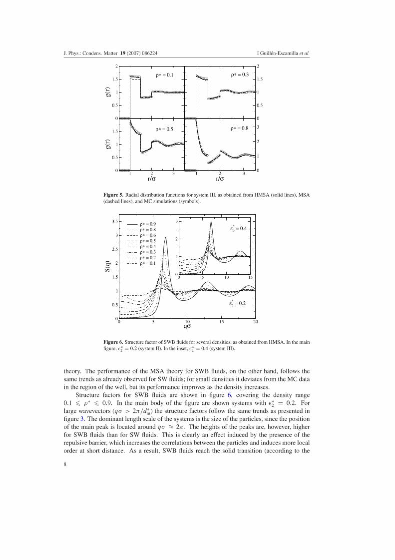
Figure 5. Radial distribution functions for system III, as obtained from HMSA (solid lines), MSA(dashed lines), and MC simulations (symbols).

0 5 10 15 20qσ

0

0.5

1

1.5

2

2.5

3

3.5

S(q)

ρ∗ = 0.9ρ∗ = 0.8ρ∗ = 0.6ρ∗ = 0.5ρ∗ = 0.4ρ∗ = 0.3ρ∗ = 0.2ρ∗ = 0.1

0 5 10 150

1

2

3

ε∗2 = 0.2

ε∗2 = 0.4

Figure 6. Structure factor of SWB fluids for several densities, as obtained from HMSA. In the mainfigure, ε∗

2 = 0.2 (system II). In the inset, ε∗2 = 0.4 (system III).

theory. The performance of the MSA theory for SWB fluids, on the other hand, follows thesame trends as already observed for SW fluids; for small densities it deviates from the MC datain the region of the well, but its performance improves as the density increases.

Structure factors for SWB fluids are shown in figure 6, covering the density range0.1 � ρ∗ � 0.9. In the main body of the figure are shown systems with ε∗

2 = 0.2. Forlarge wavevectors (qσ > 2π/d∗

m) the structure factors follow the same trends as presented infigure 3. The dominant length scale of the systems is the size of the particles, since the positionof the main peak is located around qσ ≈ 2π . The heights of the peaks are, however, higherfor SWB fluids than for SW fluids. This is clearly an effect induced by the presence of therepulsive barrier, which increases the correlations between the particles and induces more localorder at short distance. As a result, SWB fluids reach the solid transition (according to the

8

J. Phys.: Condens. Matter 19 (2007) 086224 I Guillen-Escamilla et al

0

0.5

1

1.5

2

g(r)

0

0.5

1

1.5

2

1 2 3r/σ

0

0.5

1

1.5

2

g(r)

1 2 3r/σ

0

1

2

3

ρ∗ = 0.3

ρ∗ = 0.5

ρ∗ = 0.1

ρ∗ = 0.8

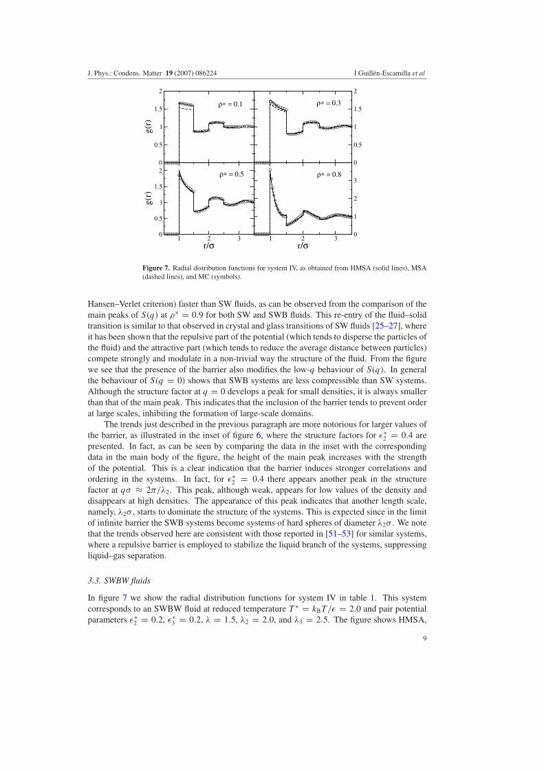
Figure 7. Radial distribution functions for system IV, as obtained from HMSA (solid lines), MSA(dashed lines), and MC (symbols).

Hansen–Verlet criterion) faster than SW fluids, as can be observed from the comparison of themain peaks of S(q) at ρ∗ = 0.9 for both SW and SWB fluids. This re-entry of the fluid–solidtransition is similar to that observed in crystal and glass transitions of SW fluids [25–27], whereit has been shown that the repulsive part of the potential (which tends to disperse the particles ofthe fluid) and the attractive part (which tends to reduce the average distance between particles)compete strongly and modulate in a non-trivial way the structure of the fluid. From the figurewe see that the presence of the barrier also modifies the low-q behaviour of S(q). In generalthe behaviour of S(q = 0) shows that SWB systems are less compressible than SW systems.Although the structure factor at q = 0 develops a peak for small densities, it is always smallerthan that of the main peak. This indicates that the inclusion of the barrier tends to prevent orderat large scales, inhibiting the formation of large-scale domains.

The trends just described in the previous paragraph are more notorious for larger values ofthe barrier, as illustrated in the inset of figure 6, where the structure factors for ε∗

2 = 0.4 arepresented. In fact, as can be seen by comparing the data in the inset with the correspondingdata in the main body of the figure, the height of the main peak increases with the strengthof the potential. This is a clear indication that the barrier induces stronger correlations andordering in the systems. In fact, for ε∗

2 = 0.4 there appears another peak in the structurefactor at qσ ≈ 2π/λ2. This peak, although weak, appears for low values of the density anddisappears at high densities. The appearance of this peak indicates that another length scale,namely, λ2σ , starts to dominate the structure of the systems. This is expected since in the limitof infinite barrier the SWB systems become systems of hard spheres of diameter λ2σ . We notethat the trends observed here are consistent with those reported in [51–53] for similar systems,where a repulsive barrier is employed to stabilize the liquid branch of the systems, suppressingliquid–gas separation.

3.3. SWBW fluids

In figure 7 we show the radial distribution functions for system IV in table 1. This systemcorresponds to an SWBW fluid at reduced temperature T ∗ = kBT/ε = 2.0 and pair potentialparameters ε∗

2 = 0.2, ε∗3 = 0.2, λ = 1.5, λ2 = 2.0, and λ3 = 2.5. The figure shows HMSA,

9

J. Phys.: Condens. Matter 19 (2007) 086224 I Guillen-Escamilla et al

0 5 10 15 20qσ

0

1

2

3

S(q)

ρ∗ = 0.9ρ∗ = 0.8ρ∗ = 0.6ρ∗ = 0.5ρ∗ = 0.4ρ∗ = 0.3ρ∗ = 0.2ρ∗ = 0.1

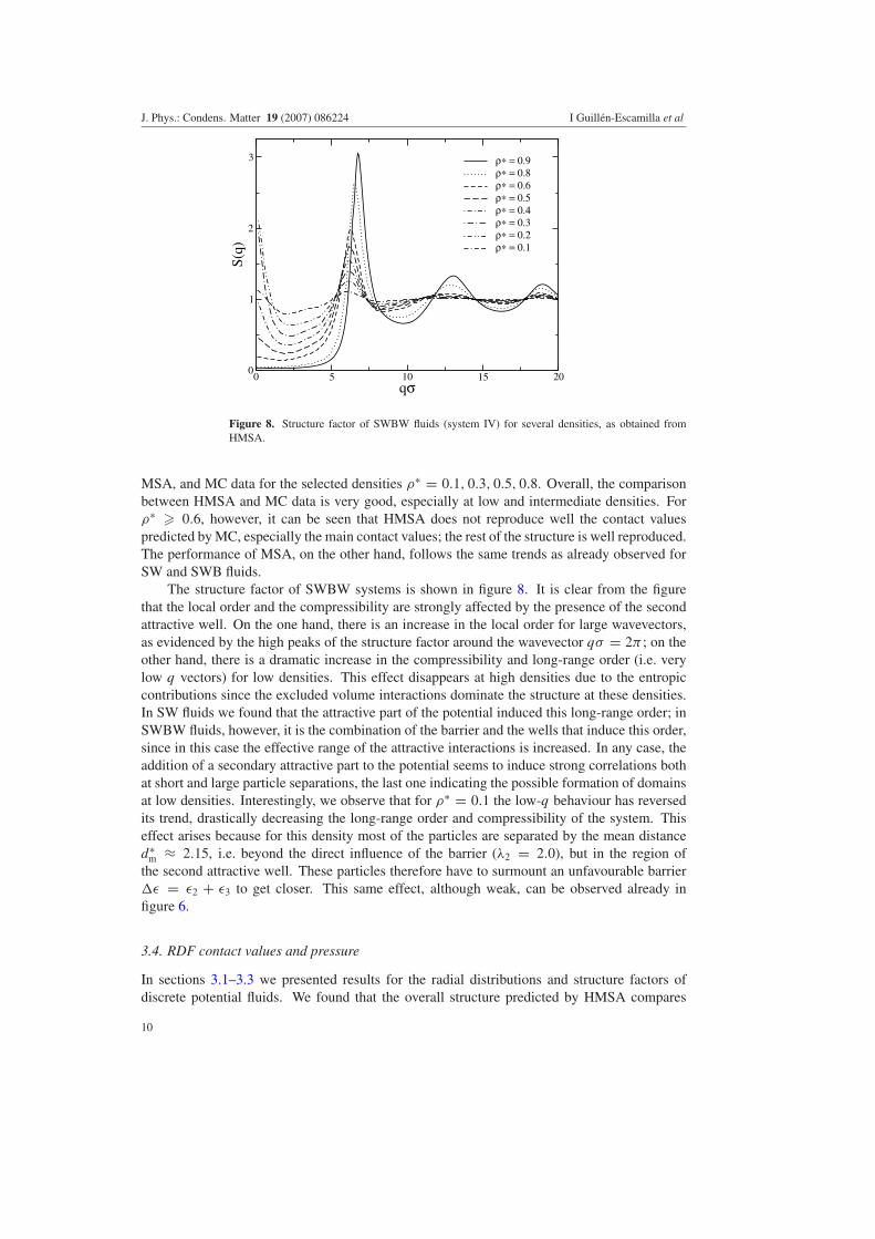
Figure 8. Structure factor of SWBW fluids (system IV) for several densities, as obtained fromHMSA.

MSA, and MC data for the selected densities ρ∗ = 0.1, 0.3, 0.5, 0.8. Overall, the comparisonbetween HMSA and MC data is very good, especially at low and intermediate densities. Forρ∗ � 0.6, however, it can be seen that HMSA does not reproduce well the contact valuespredicted by MC, especially the main contact values; the rest of the structure is well reproduced.The performance of MSA, on the other hand, follows the same trends as already observed forSW and SWB fluids.

The structure factor of SWBW systems is shown in figure 8. It is clear from the figurethat the local order and the compressibility are strongly affected by the presence of the secondattractive well. On the one hand, there is an increase in the local order for large wavevectors,as evidenced by the high peaks of the structure factor around the wavevector qσ = 2π ; on theother hand, there is a dramatic increase in the compressibility and long-range order (i.e. verylow q vectors) for low densities. This effect disappears at high densities due to the entropiccontributions since the excluded volume interactions dominate the structure at these densities.In SW fluids we found that the attractive part of the potential induced this long-range order; inSWBW fluids, however, it is the combination of the barrier and the wells that induce this order,since in this case the effective range of the attractive interactions is increased. In any case, theaddition of a secondary attractive part to the potential seems to induce strong correlations bothat short and large particle separations, the last one indicating the possible formation of domainsat low densities. Interestingly, we observe that for ρ∗ = 0.1 the low-q behaviour has reversedits trend, drastically decreasing the long-range order and compressibility of the system. Thiseffect arises because for this density most of the particles are separated by the mean distanced∗

m ≈ 2.15, i.e. beyond the direct influence of the barrier (λ2 = 2.0), but in the region ofthe second attractive well. These particles therefore have to surmount an unfavourable barrier�ε = ε2 + ε3 to get closer. This same effect, although weak, can be observed already infigure 6.

3.4. RDF contact values and pressure

In sections 3.1–3.3 we presented results for the radial distributions and structure factors ofdiscrete potential fluids. We found that the overall structure predicted by HMSA compares

10

J. Phys.: Condens. Matter 19 (2007) 086224 I Guillen-Escamilla et al

0 0.2 0.4 0.6 0.8ρ∗

0

2

4

6

8

P*

0 0.2 0.4 0.6 0.8ρ∗

0

1

2

3

4

5

g(σ+)g(λ−)g(λ+)

Figure 9. Reduced pressure P∗ = β P/ρ of SW fluids (system I) as a function of density. Solidlines correspond to HMSA, dashed lines to MSA, and symbols to MC. In the inset, HMSA and MCcontact values as a function of density.

well with Monte Carlo simulation data. However, another comparison between theory andsimulations can be done at the level of the thermodynamic pressure of the systems. Since thepressure of DP fluids depends on the contact values of the RDF (see equation (5)), it is importantto predict accurately the contact values. In this section we present comparisons between HMSAand Monte Carlo for the pressure and contact values of the radial distribution functions for thesystems described in table 1.

Figure 9 shows the pressure of the SW fluids studied previously for HMSA (solid line),MSA (dashed line), and MC (symbols). The HMSA results are in very good agreement withthe simulation data up to very high densities. The only point in the curve that is not wellreproduced by the HMSA theory corresponds to ρ∗ = 0.9. The good theory–simulationagreement observed in the figure is the consequence of a good prediction of the contact valuesof the radial distribution functions at the discontinuities of the potential, as illustrated in theinset of the figure. In this inset we present results for the HMSA and MC contact valuesg(σ+), g(λ−), and g(λ+) as a function of the density of the fluid. Here we see that all thecontact values are well predicted. The mayor deviations are observed at ρ∗ = 0.9, whichleads to the underestimation of the theoretical pressure observed in the figure. We note thatthe contact value g(σ+) is a strongly increasing function of the density, which is the typicalbehaviour of hard-sphere fluids. The other contact values decrease with density. Since �g(λ)

decreases slightly, the strong increase of the pressure as a function of density is dominated bythe contributions of the main contact value.

Figure 10 shows the pressure of SWB fluids with interaction parameter ε∗2 = 0.4. Both

theory and simulations are included. The behaviour here is similar to that observed in theprevious figure. In this case, however, HMSA deviates from the simulation data for ρ∗ > 0.75.This is due to the inability of the theory to predict correctly the contributions of the severalcontact values of the radial distribution function at high densities. In contrast to the SW casewhere only three contact values contribute to the pressure, for SWB fluids five contact valueshave to be predicted accurately to maintain good theory–simulation agreement. The inset ofthe figure shows, for ε∗

2 = 0.4, the contact values predicted by HMSA and those obtainedby simulations. From this inset we see that the main contact value increases with density,

11

J. Phys.: Condens. Matter 19 (2007) 086224 I Guillen-Escamilla et al

0 0.2 0.4 0.6 0.8ρ∗

0

2

4

6

8

10

12

P*

0 0.2 0.4 0.6 0.8ρ∗

0

1

2

3

4

5

g(σ+)

g(λ−)g(λ+

)g(λ2

−)

g(λ2

+)

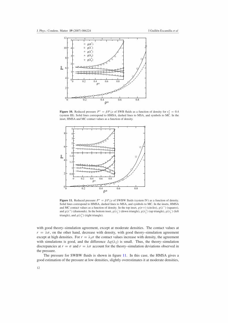
Figure 10. Reduced pressure P∗ = β P/ρ of SWB fluids as a function of density for ε∗2 = 0.4

(system III). Solid lines correspond to HMSA, dashed lines to MSA, and symbols to MC. In theinset, HMSA and MC contact values as a function of density.

0 0.2 0.4 0.6 0.8ρ∗

0

2

4

6

8

P*

0

1

2

3

4

5

0 0.2 0.4 0.6 0.8ρ∗

0.8

1

1.2

1.4

Figure 11. Reduced pressure P∗ = β P/ρ of SWBW fluids (system IV) as a function of density.Solid lines correspond to HMSA, dashed lines to MSA, and symbols to MC. In the insets, HMSAand MC contact values as a function of density. In the top inset, g(σ+) (circles), g(λ−) (squares),and g(λ+) (diamonds). In the bottom inset, g(λ−

2 ) (down triangle), g(λ+2 ) (up triangle), g(λ−

3 ) (lefttriangle), and g(λ+

3 ) (right triangle).

with good theory–simulation agreement, except at moderate densities. The contact values atr = λσ , on the other hand, decrease with density, with good theory–simulation agreementexcept at high densities. For r = λ2σ the contact values increase with density, the agreementwith simulations is good, and the difference �g(λ2) is small. Thus, the theory–simulationdiscrepancies at r = σ and r = λσ account for the theory–simulation deviations observed inthe pressure.

The pressure for SWBW fluids is shown in figure 11. In this case, the HMSA gives agood estimation of the pressure at low densities, slightly overestimates it at moderate densities,

12

J. Phys.: Condens. Matter 19 (2007) 086224 I Guillen-Escamilla et al

and underestimates it at higher densities. Overall, the agreement with simulations is goodfor densities up to ρ∗ ≈ 0.75. Beyond this density the discrepancies are important. Thecomparison between HMSA and MC contact values is presented in the two insets. The topinset shows the contact values at r = σ and λσ , and the bottom inset at r = λ2σ and λ3σ .The behaviour of the contact values is clearly seen in these insets: the contact values at r = σ

and λ2σ (which define the repulsive parts of the potential) increase with density, whereas thecontact values at λσ and λ3σ (which define the attractive parts of the potential) decrease withdensity. All these trends are confirmed by the simulations. From the comparisons in the insetswe see that the main contact value predicted by HMSA agrees well with simulations for lowdensities, but overestimates it at intermediate densities, which is reflected in the correspondingcomparison of the pressure. At high densities the secondary contact values show discrepancieswith simulation. These discrepancies lead to the theoretical underestimation of the pressureobserved in the figure.

MSA results for the pressure are also included in figures 9–11. As shown in these figures,MSA predicts very well the pressure of the systems up to densities ρ∗ ≈ 0.5. For largerdensities MSA clearly deviates from the MC and HMSA data, underestimating the pressuresystematically as the density increases.

4. Summary

In this work, we have studied both structural and thermodynamic properties of discrete potentialfluids by using the Ornstein–Zernike equation together with the HMSA closure relation. Theresults were compared with the mean spherical approximation theory and with N V T MonteCarlo computer simulations. We found that far away from the coexistence region HMSAprovides an accurate description of the system properties, and that HMSA is a better approachthan MSA.

We also found that, in the regime of applicability of HMSA, the inclusion of attractive andrepulsive components in the potential promotes dramatic changes in the local and long-rangeorder of the systems. We observed that the attractive components induce higher compressibilityand the possible formation of clusters or domains, which locally show a fluid-like structure. Onthe other hand, the repulsive part of the potential tends to stabilize the systems, inhibiting theformation of these domains and lowering the compressibility. Also, we found that, in general,the (virial) equation of state provided by the HMSA relation describes well the pressure of thesystems.

Finally, we conclude that this work allows us to identify regions of applicability of theHMSA closure relation when it is applied to simple fluids with both attractive wells and repul-sive barriers. This information becomes useful for inhomogeneous systems or dynamic theorieswhere accurate knowledge of the bulk properties is required [4, 25, 27, 51, 52, 54–56].

Acknowledgments

We acknowledge financial support from CONACYT, Mexico, grants 46373/A-1, J37530E andU47611-F, and PROMEP (SEP, Mexico).

References

[1] Barker J A and Henderson D 1976 Rev. Mod. Phys. 48 587[2] Derjaguin B V and Johnston R K 1989 Theory of Stability of Colloids and Thin Films (New York: Consultants

Bureau)[3] Ruiz-Garcıa J, Gamez-Corrales J R and Ivlev B I 1998 Mol. Phys. 95 371

13

J. Phys.: Condens. Matter 19 (2007) 086224 I Guillen-Escamilla et al

[4] Bergenholtz J and Fuchs M 1999 Phys. Rev. E 59 5706[5] Lutsko J F and Nicolis G 2005 J. Chem. Phys. 122 244907[6] Malescio G, Franzese G, Pellicane G, Skibinsky A, Buldyrev S V and Stanley H E 2002 J. Phys.: Condens.

Matter 14 2193[7] Benavides A L and Gil-Villegas A 1999 Mol. Phys. 97 1225[8] Vidales A, Benavides A L and Gil-Villegas A 2001 Mol. Phys. 99 703[9] Guillen-Escamilla I and Chavez-Paez M 2007 at press

[10] Baxter R J 1968 J. Chem. Phys. 49 2770[11] Smith W R, Henderson D and Barker J A 1971 J. Chem. Phys. 55 4027[12] Henderson D, Barker J A and Smith W R 1976 J. Chem. Phys. 64 4244[13] Nezbeda I 1977 Czech. J. Phys. B 27 247[14] Benavides A L and Gil-Villegas A 1999 Mol. Phys. 97 1225[15] Henderson D, Scalise O H and Smith W R 1980 J. Chem. Phys. 72 2431[16] Largo J, Solana J R, Yuste S B and Santos A 2005 J. Chem. Phys. 122 084510[17] Smith W R and Henderson D 1978 J. Chem. Phys. 69 319[18] Smith W R, Henderson D and Tago Y 1977 J. Chem. Phys. 67 5308[19] Henderson D, Maden W G and Fitts D D 1976 J. Chem. Phys. 64 5026[20] Tago Y 1974 J. Chem. Phys. 60 1531[21] Largo J, Solana J R and Santos A 2003 Mol. Phys. 101 2981[22] Davies L A, Gil-Villegas A and Jackson G 1999 J. Chem. Phys. 111 8659[23] Smith W R, Henderson D and Murphy R D 1974 J. Chem. Phys. 61 2911[24] Alder G J, Young D A and Mark M A 1980 J. Chem. Phys. 56 3013[25] Dawson K, Foffi F, Fuchs M, Gotze W, Sciortino F, Sperl M, Tartaglia P, Voigtmann Th and Zaccarelli E 2000

Phys. Rev. E 63 11401[26] Bolhuis P, Hagen M and Frenkel D 1994 Phys. Rev. E 50 4880[27] Fabbian L, Gotze W, Sciortino F, Tartaglia P and Thiery F 1999 Phys. Rev. E 59 R1347[28] Foffi G, McCullagh G D, Lawlor A, Zaccarelli E, Dawson K, Sciortino F, Tartaglia P, Pini D and Stell G 2002

Phys. Rev. E 65 031407[29] Scholl-Paschinger E, Benavides A L and Castaneda-Priego R 2005 J. Chem. Phys. 123 234513[30] Benavides A L 2006 private communication[31] Zerah G and Hansen J P 1986 J. Chem. Phys. 84 2336[32] Caccamo C, Giaquinta P V and Giunta G 1993 J. Phys.: Condens. Matter 5 B75[33] Caccamo C 1996 Phys. Rep. 274 1[34] Gonzalez-Mozuelos P and Carbajal-Tinoco M D 1998 J. Chem. Phys. 109 11074[35] Coluzzi B, Parisi G and Verrochio P 2000 Phys. Rev. Lett. 84 306[36] Pastore G, Santin R, Taraphder S and Colonna F 2005 J. Chem. Phys. 122 181104[37] Kunor T R and Taraphder S 2006 Phys. Rev. E 74 11201[38] Zaccarelli E, Foffi G, Dawson K A, Buldyrev S V, Sciortino F and Tartaglia P 2003 J. Phys.: Condens. Matter

15 S367[39] Hansen J P and McDonald I R 1986 Theory of Simple Liquids (New York: Academic)[40] Ng K C 1974 J. Chem. Phys. 61 2680[41] Rogers F J and Young D A 1984 Phys. Rev. A 30 999[42] Lang A, Kahl G, Likos C N, Lowen H and Watzlawek M 1999 J. Phys.: Condens. Matter 11 10143[43] Allen M P and Tildesley D J 1987 Computer Simulation of Liquid (New York: Clarendon)[44] Frenkel D and Smit B 2002 Understanding Molecular Simulation: From Algorithms to Applications (San Diego,

CA: Academic)[45] Panagiotopoulos A Z 1987 Mol. Phys. 61 813[46] Smit B, de Smedt P H and Frenkel D 1989 Mol. Phys. 68 931[47] Gil-Villegas A, Vega C, del Rıo F and Malijevsky A 1995 Mol. Phys. 86 857[48] Liu Y, Chen W R and Chen S H 2005 J. Chem. Phys. 122 044507[49] Broccio M, Costa D, Liu Y and Chen S H 2006 J. Chem. Phys. 124 084501[50] Hansen J P and Verlet L 1969 Phys. Rev. 184 151[51] Puertas A M, Fuchs M and Cates M E 2002 Phys. Rev. Lett. 88 98301[52] Puertas A M, Fuchs M and Cates M E 2003 Phys. Rev. E 67 31406[53] Cates M E, Fuchs M, Kroy K, Poon W C and Puertas A M 2004 J. Phys.: Condens. Matter 16 S4861[54] Yeomans-Reyna L, Acuna-Campa H and Medina-Noyola M 2000 Phys. Rev. E 62 3395[55] Yeomans-Reyna L and Medina-Noyola M 2001 Phys. Rev. E 64 66114[56] Chavez-Rojo M A and Medina-Noyola M 2005 Phys. Rev. E 72 31107

14