Structural Dynamics

Structural Dynamics(CEGEM071/CEGEG071)

Tutorial 3 – Student: Carmine Russo – 141031061.Introduction

In general, the system hassix degrees of freedom (ifthe beams CD and EF are notrigid, then they are eight)but neglecting the axialdeformations of columns (EA→∞) they become two. We choose as lagrangiancoordinates the horizontaldisplacements of CD and EF.Collecting these variables inthe vector, we have:

u={u1u2}={uCDuEF}In order to write the equilibrium equations, we have to find thestiffness of each element for each displacement. In this case, we canuse the direct method by solving the differential equation of theelastic beam:

UCL – Civil, Environmental and Geomatic EngineeringStructural Dynamics – 2014 – Tutorial 3 – Carmine Russo – 14103106 page 1 of 16

Initial data:L=4,5 [m ]

EI=65∙105 [Nm2 ]=¿

¿6500 [kNm2 ]

m1=3,5 [t ]=3500 [kg ]

m2=4 [t ]=4000 [kg ]

ηIV=0η'''=C1

η''=C1s+C2η'=12C1s2+C2s+C3

η=16C1s3+

12C2s2+C3s+C4

With the boundary conditions:η(A )=0;M(A )=−EIη(A)

''=0;η(C )' =0;η(C )=u

We get the constants of integration:

C1=−3LAC3 u;C2=0;C3=

32LAC

u;C4=0;

Finally:

TC=−EIη'''=3EILAC3 uMC=−EIη''=3EI

LAC2 u

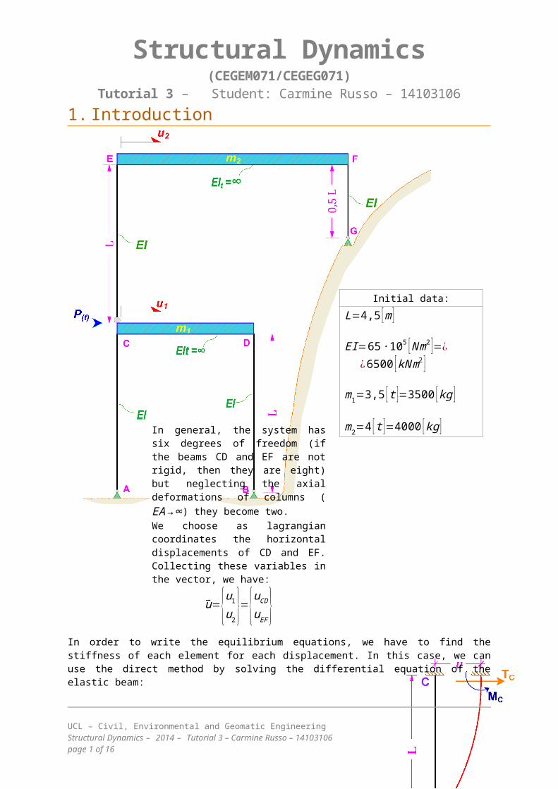
Since there’s no lateral load applied to the columns, the shear forceis constant along their length.It is convenient to indicate with k the quantity:

k= EILAC3 =EI

L3=65∙105 [Nm2 ]

(4,5 [m] )3=71,33059[ kNm ]

Then, the generic expression of the shear force become:T=3k∙u

Where “3k” represent the stiffness.We can assemble the stiffness matrix, column by column, simply imposingone deformation at time, while keeping the other one equal to zero, andfinding the equilibrium forces.

Displacement u1:In this case we have the massm1 (that is the one who moves)subjected to the displacementu1.

The beam CD is subjected tothe horizontal forces TAC,TBD

and TCE;

the beam EF, in this case,just to the horizontal forceEF generate by the deformationof the column EC.

The total forces for each mass


are:

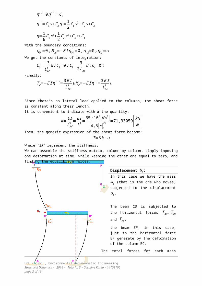
FCD=TCE+TAC+TBD=(3k+3k+3k)∙u1

FEF=−TEC=−3k∙u1

We can summarize these relationsas:

{FCDFEF}=[ 9k−3k ]∙u1

Displacement u2:In this case we have the mass m2(that is the one who moves)subjected to the displacement u2.

In this case we first define theshear on the column FG that is:

TFG=3EI

(L2)3=24

EIL3

=24k

The total forces for each massare:

FCD=−TCE=−3k∙u2

FEF=TCE+TGF=(3k+24k )∙u2

We can summarize these relationsas:

{FCDFEF}=[−3k27k ]∙u2

Thus the static equilibrium isrepresented by the equations:


{FCDFEF}=[ 9k −3k−3k 27k ]∙{u1

u2}The stiffness matrix

[K ]=[ 9k −3k−3k 27k ]=[ 9 −3

−3 27 ]EIL3 =[ 641,975 −213,992−213,992 1925,926 ] [kNm ]

The mass matrix

[M ]=[m1 00 m2]=[3500 0

0 4000] [kg ]

The energetic approachInstead of following the equilibrium approach, we can find the equationby calculating the total energy of the system:

Kinetic Energy

T=12m1u1

2+12m2 u22

The mass matrix can be found simply by calculating the Jacobian:

[M ]=[ ∂2T∂ui∂uj ]=[ ∂2T

∂u12

∂2T∂u1∂u2

∂2T∂u2∂u1

∂2T∂u2∂u2

]=[m1 00 m2]

Potential EnergyIn this exercise the potential elastic energy is given by thehorizontal displacements of the beams, therefore by using thestiffnesses already calculated above, we can directly write theexpression of this energy without calculate the integrals. Simplyremembering that the potential energy of a single spring is:

Vspring=12k∙Δx2

we just have to sum the potential energies of each deformedelement:

V=∑ 12k∙ui2=

12 [kACu12+kBDu12+kCE (u1−u2)

2+kFGu22 ]=¿

¿12 [kACu1

2+kBDu12+kCEu1

2+kCEu22−2kCEu1u2+kFGu22 ]=¿

¿ 12 [3ku1

2+3ku12+3ku12+3ku2

2−6ku1u2+24ku22 ]=¿


¿12 [9ku1

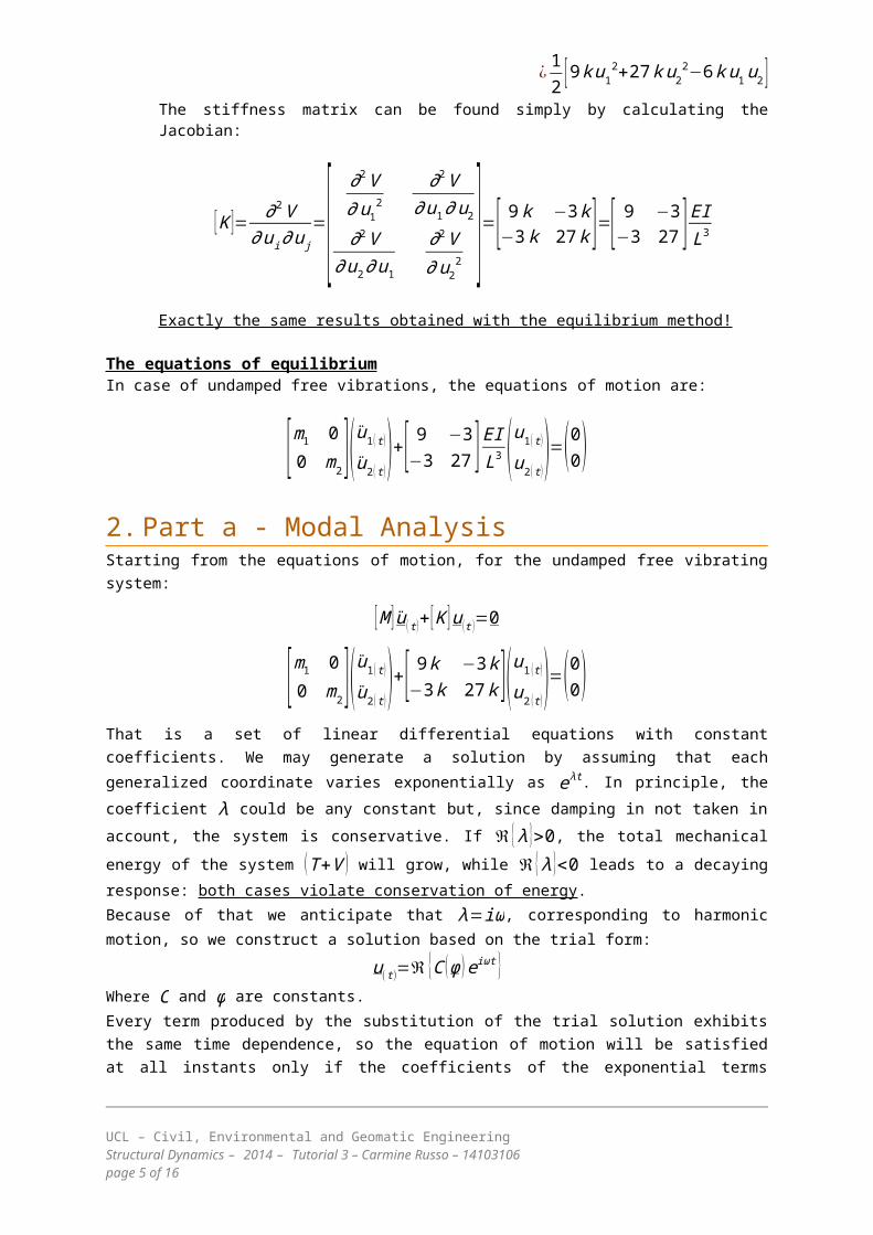
2+27ku22−6ku1u2 ]The stiffness matrix can be found simply by calculating theJacobian:

[K ]= ∂2V∂ui∂uj

=[ ∂2V∂u12

∂2V∂u1∂u2

∂2V∂u2∂u1

∂2V∂u22

]=[ 9k −3k−3k 27k ]=[ 9 −3

−3 27 ]EIL3

Exactly the same results obtained with the equilibrium method!

The equations of equilibriumIn case of undamped free vibrations, the equations of motion are:

[m1 00 m2](u1(t)

u2(t))+[ 9 −3−3 27 ]EIL3 (u1(t)

u2(t))=(00)

2.Part a - Modal AnalysisStarting from the equations of motion, for the undamped free vibratingsystem:

[M ]u(t)+[K ]u(t )=0

[m1 00 m2](u1(t)

u2(t))+[ 9k −3k−3k 27k ](u1 (t)

u2 (t))=(00)That is a set of linear differential equations with constantcoefficients. We may generate a solution by assuming that eachgeneralized coordinate varies exponentially as eλt. In principle, thecoefficient λ could be any constant but, since damping in not taken inaccount, the system is conservative. If ℜ {λ }>0, the total mechanicalenergy of the system (T+V ) will grow, while ℜ {λ }<0 leads to a decayingresponse: both cases violate conservation of energy.Because of that we anticipate that λ=iω, corresponding to harmonicmotion, so we construct a solution based on the trial form:

u(t)=ℜ {C (ϕ )eiωt }Where C and ϕ are constants.Every term produced by the substitution of the trial solution exhibitsthe same time dependence, so the equation of motion will be satisfiedat all instants only if the coefficients of the exponential terms


match. Furthermore, the constant factor C is common to every term, soit cancels. Therefore, we have:

−[M ]C (ϕ )ω2eiωt+[K ]C (ϕ )eiωt=0⟹ {[K ]−ω2 [M ] }(ϕ)=0The nontrivial solution of this system can exist only if the value of ωis such that { [K ]−ω2 [M ] } is not invertible. We must find the value of ωfor which the determinant of this matrix is equal to zero (generaleigenvalue problem):

det ( [K ]−λ [M ] )=0⟹det|(9k−λm1) −3k−3k (27k−λm2)|=0

where we set ω2=λ. From this condition we get the characteristicequation:

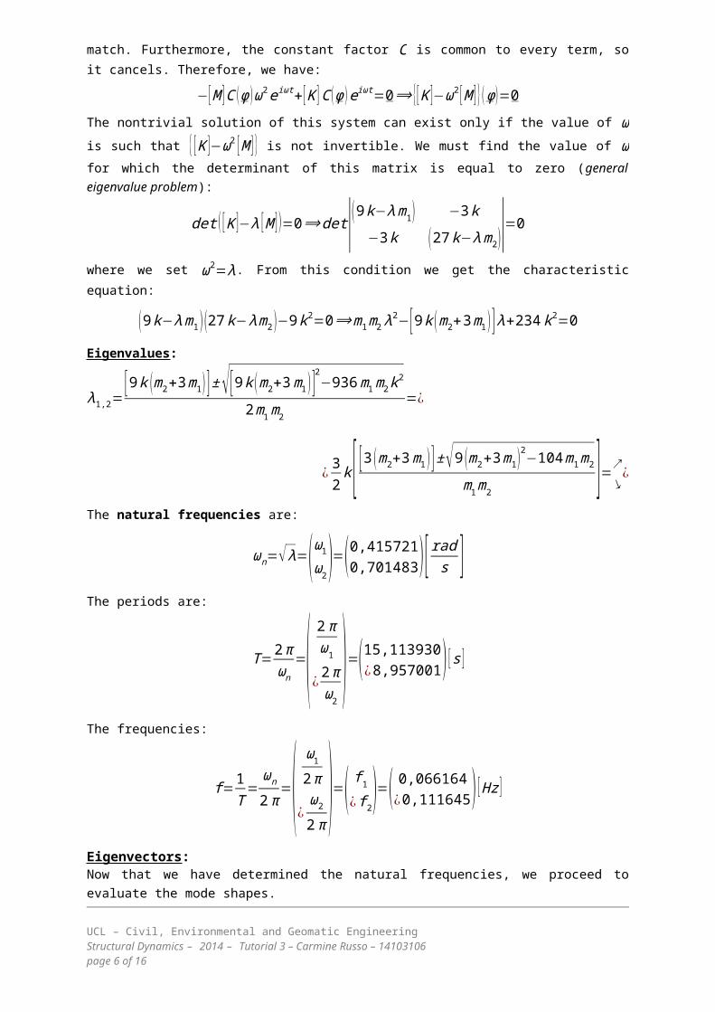
(9k−λm1 )(27k−λm2 )−9k2=0⟹m1m2λ2−[9k (m2+3m1 ) ]λ+234k2=0

Eigenvalues:

λ1,2=[9k (m2+3m1) ]±√[9k (m2+3m1 ) ]2−936m1m2k2

2m1m2=¿

¿32k [ [3 (m2+3m1 ) ]±√9 (m2+3m1)

2−104m1m2

m1m2]=↗

↘¿

The natural frequencies are:

ωn=√λ=(ω1ω2)=(0,4157210,701483)[rads ]The periods are:

T=2πωn

=(2πω1

¿2πω2

)=(15,113930¿8,957001) [s ]

The frequencies:

f=1T

=ωn

2π=(

ω12π

¿ω2

2π)=( f1

¿f2)=( 0,066164¿0,111645) [Hz ]

Eigenvectors:Now that we have determined the natural frequencies, we proceed toevaluate the mode shapes.


When ω=ω1 or ω2, at least one of the scalar equations described by

{[K ]−ωi2 [M ]}(ϕ )=0 is not independent of the other. We can retain one of

the two conditions (for instance the first one), and add a condition onthe norm of the first eigenvector.

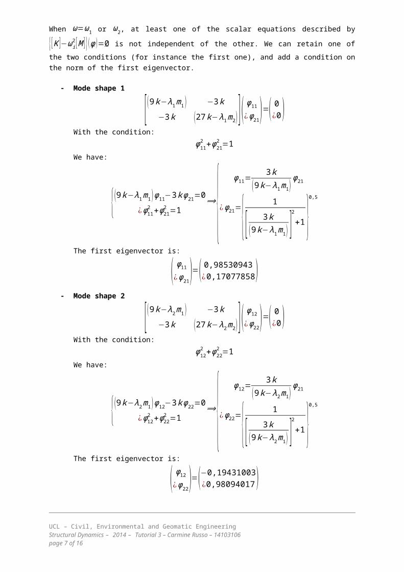
Mode shape 1

[(9k−λ1m1 ) −3k−3k (27k−λ1m2)]( ϕ11

¿ϕ21)=( 0¿0)With the condition:

ϕ112 +ϕ21

2 =1We have:

{(9k−λ1m1 )ϕ11−3kϕ21=0¿ϕ112 +ϕ212 =1

⟹ { ϕ11=3k

(9k−λ1m1)ϕ21

¿ϕ21={ 1

[ 3k(9k−λ1m1) ]

2

+1 }0,5

The first eigenvector is:

( ϕ11¿ϕ21)=( 0,98530943¿0,17077858) Mode shape 2

[(9k−λ2m1 ) −3k−3k (27k−λ2m2)]( ϕ12

¿ϕ22)=( 0¿0)With the condition:

ϕ122 +ϕ22

2 =1We have:

{(9k−λ2m1 )ϕ12−3kϕ22=0¿ϕ122 +ϕ222 =1

⟹ { ϕ12=3k

(9k−λ2m1)ϕ21

¿ϕ22={ 1

[ 3k(9k−λ2m1) ]

2

+1 }0,5

The first eigenvector is:

( ϕ12¿ϕ22)=(−0,19431003¿0,98094017 )


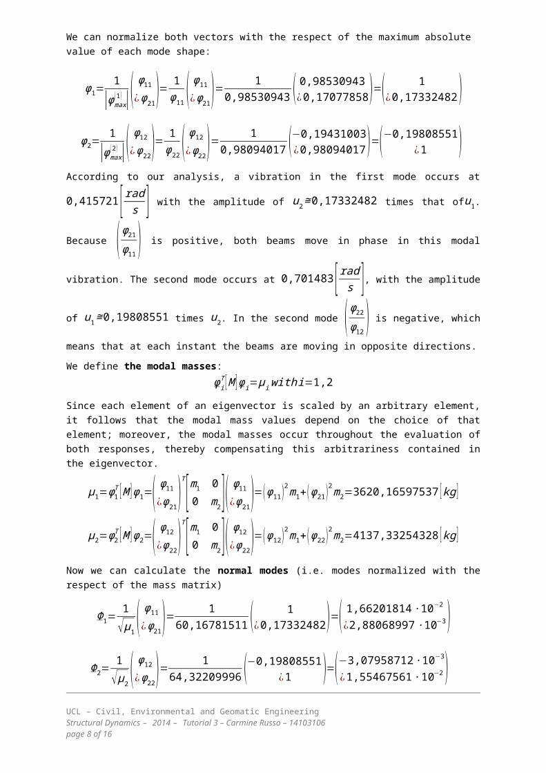
We can normalize both vectors with the respect of the maximum absolute value of each mode shape:

ϕ1=1

|ϕmax(1) |(

ϕ11¿ϕ21)= 1

ϕ11 ( ϕ11

¿ϕ21)= 10,98530943 ( 0,98530943¿0,17077858)=( 1

¿0,17332482)

ϕ2=1

|ϕmax(2) |(

ϕ12¿ϕ22)= 1

ϕ22 ( ϕ12

¿ϕ22)= 10,98094017 (−0,19431003¿0,98094017)=(−0,19808551¿1 )

According to our analysis, a vibration in the first mode occurs at

0,415721 [rads ] with the amplitude of u2≅0,17332482 times that ofu1.

Because (ϕ21ϕ11 ) is positive, both beams move in phase in this modal

vibration. The second mode occurs at 0,701483 [rads ], with the amplitudeof u1≅0,19808551 times u2. In the second mode (ϕ22ϕ12 ) is negative, whichmeans that at each instant the beams are moving in opposite directions.

We define the modal masses:ϕiT [M ]ϕi=μiwithi=1,2

Since each element of an eigenvector is scaled by an arbitrary element,it follows that the modal mass values depend on the choice of thatelement; moreover, the modal masses occur throughout the evaluation ofboth responses, thereby compensating this arbitrariness contained inthe eigenvector.

μ1=ϕ1T [M ]ϕ1=( ϕ11¿ϕ21)T[m1 00 m2]( ϕ11¿ϕ21)=(ϕ11)

2m1+(ϕ21)2m2=3620,16597537 [kg ]

μ2=ϕ2T [M ]ϕ2=( ϕ12¿ϕ22)T[m1 00 m2]( ϕ12¿ϕ22)=(ϕ12)

2m1+(ϕ22)2m2=4137,33254328 [kg ]

Now we can calculate the normal modes (i.e. modes normalized with therespect of the mass matrix)

Φ1=1

√μ1( ϕ11

¿ϕ21)= 160,16781511 ( 1

¿0,17332482)=( 1,66201814∙10−2

¿2,88068997∙10−3)Φ2=

1√μ2

( ϕ12

¿ϕ22)= 164,32209996 (−0,19808551¿1 )=(−3,07958712∙10−3

¿1,55467561∙10−2 )UCL – Civil, Environmental and Geomatic EngineeringStructural Dynamics – 2014 – Tutorial 3 – Carmine Russo – 14103106 page 8 of 16

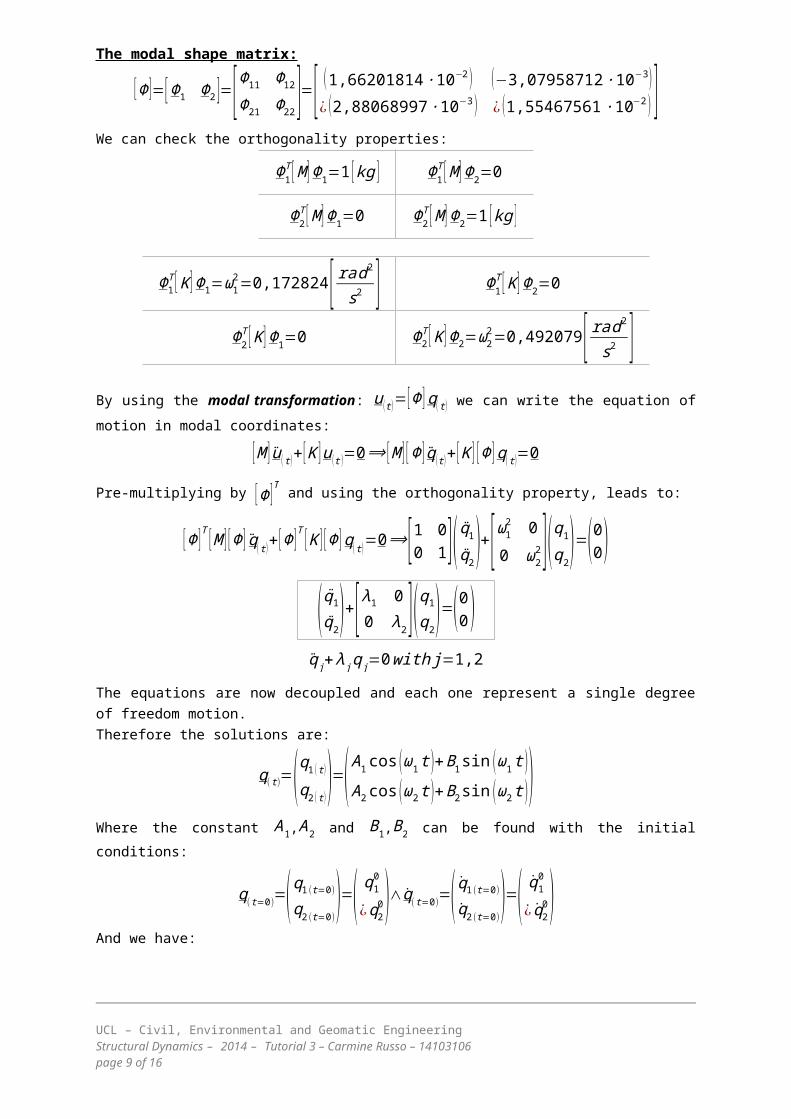
The modal shape matrix:

[Φ ]=[Φ1 Φ2 ]=[Φ11 Φ12Φ21 Φ22 ]=[ (1,66201814∙10−2 )

¿ (2,88068997∙10−3 )(−3,07958712∙10−3)¿ (1,55467561∙10−2 ) ]

We can check the orthogonality properties:

Φ1T [M]Φ1=1 [kg ] Φ1

T [M]Φ2=0

Φ2T [M]Φ1=0 Φ2

T [M]Φ2=1 [kg ]

Φ1T [K]Φ1=ω12=0,172824[ rad2

s2 ] Φ1T [K]Φ2=0

Φ2T [K]Φ1=0 Φ2

T [K]Φ2=ω22=0,492079[ rad2

s2 ]By using the modal transformation: u(t)=[Φ ]q(t) we can write the equation ofmotion in modal coordinates:

[M ]u(t)+[K ]u(t )=0⟹ [M ] [Φ ]q(t)+[K ] [Φ ]q(t)=0

Pre-multiplying by [Φ ]T and using the orthogonality property, leads to:

[Φ ]T [M ] [Φ ] q(t)+[Φ ]T [K ] [Φ ]q(t)=0⟹[1 00 1](q1q2)+[ω12 0

0 ω22](q1

q2)=(00)

(q1

q2)+[λ1 00 λ2](q1

q2)=(00)qj+λjqj=0withj=1,2

The equations are now decoupled and each one represent a single degreeof freedom motion. Therefore the solutions are:

q(t)=(q1 (t)

q2 (t))=(A1cos (ω1t )+B1sin (ω1t )A2cos (ω2t )+B2sin (ω2t ))

Where the constant A1,A2 and B1,B2 can be found with the initialconditions:

q(t=0)

=(q1 (t=0)

q2 (t=0))=( q1

0

¿q20)∧q(t=0)=(q1 (t=0)

q2 (t=0))=( q1

0

¿ q20)And we have:


(A )=(A1

A2)=q(t=0)=( q1

0

¿q20)∧(B )=[ω1 0

0 ω2]−1

( q10

¿ q20)= 1

ω1ω2 [ω2 00 ω1]( q1

0

¿ q20)=[ 1ω1

0

0 1ω2

]( q10¿ q20)

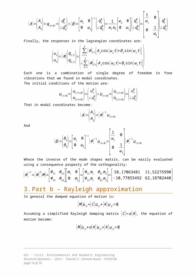
Finally, the responses in the lagrangian coordinates are:

(u1

u2)= [Φ ](q1 (t)

q2 (t))=( ∑i=1

2

[Φ ]1i [Aicos (ωit )+Bisin (ωit )]¿∑i=1

2

[Φ ]2i [Aicos (ωit)+Bisin (ωit) ])Each one is a combination of single degree of freedom in freevibrations that we found in modal coordinates. The initial conditions of the motion are:

u(t=0)

=(u1 (t=0)

u2 (t=0))=( u1

0

¿u20)∧u(t=0)=(u1 (t=0)

u2 (t=0))=( u1

0

¿ u20)That in modal coordinates become:

(A )=(A1

A2)=[Φ ]−1u(t=0)

And

(B )=(B2

B2)=[ω1 00 ω2]

−1

[Φ ]−1u(t=0)=[ 1ω1

0

0 1ω2

] [Φ ]−1u(t=0)

Where the inverse of the mode shapes matrix, can be easily evaluatedusing a consequence property of the orthogonality:

[Φ ]−1= [Φ ]T [M ]=[Φ11 Φ21

Φ12 Φ22 ][m1 00 m2]=[Φ11m1 Φ21m2

Φ12m1 Φ22m2]=[ 58,17063481 11,52275990−10,77855492 62,18702440 ]

3.Part b – Rayleigh approximationIn general the damped equation of motion is:

[M ]u(t)+[C ]u(t )+ [K ]u(t)=0

Assuming a simplified Rayleigh damping matrix [C ]=α [K ], the equation ofmotion become:

[M ]u(t)+α [K ] u(t)+[K ]u(t)=0


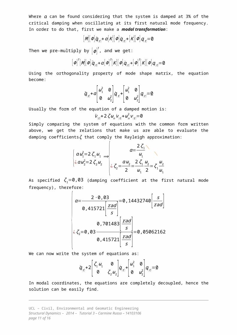
Where α can be found considering that the system is damped at 3% of thecritical damping when oscillating at its first natural mode frequency.In order to do that, first we make a modal transformation:

[M ] [Φ ]q(t )+α [K ] [Φ ]q(t )+ [K ] [Φ ]q(t)=0

Then we pre-multiply by [Φ ]T, and we get:

[Φ ]T [M ] [Φ ] q(t)+α [Φ ]T [K ] [Φ ]q(t )+ [Φ ]T [K ] [Φ ]q(t)=0

Using the orthogonality property of mode shape matrix, the equationbecome:

q(t)+α [ω12 00 ω22]q(t)+[ω12 0

0 ω22]q(t )=0

Usually the form of the equation of a damped motion is:v(t )+2ζωn v(t)+ωn

2v(t )=0Simply comparing the system of equations with the common form writtenabove, we get the relations that make us are able to evaluate thedamping coefficientsζ that comply the Rayleigh approximation:

{ αω12=2ζ1ω1

¿αω22=2ζ2ω2

⟹{ α=2ζ1

ω1

¿ζ2=αω22

=2ζ1ω1

ω22

=ζ1

ω2

ω1

As specified ζ1=0,03 (damping coefficient at the first natural modefrequency), therefore:

{ α=2∙0,03

0,415721[ rads ]=0,14432740 [ s

rad ]

¿ζ2=0,030,701483[ rads ]0,415721[ rads ]

=0,05062162

We can now write the system of equations as:

q(t)+2 [ζ1ω1 00 ζ2ω2]q(t )+[ω1

2 00 ω22]q(t)=0

In modal coordinates, the equations are completely decoupled, hence thesolution can be easily find.


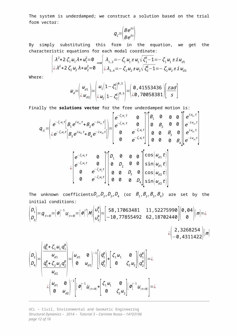
The system is underdamped; we construct a solution based on the trialform vector:

qC=(Beλt

Beλt)By simply substituting this form in the equation, we get thecharacteristic equations for each modal coordinate:

{ λ2+2ζ1ω1λ+ω12=0¿λ2+2ζ2ω2λ+ω2

2=0⟹{ λ1,2=−ζ1ω1±ω1√ζ1

2−1=−ζ1ω1±iωd1

¿λ3,4=−ζ2ω2±ω2√ζ22−1=−ζ2ω2±iωd2Where:

ωd=( ωd1¿ωd2)=( ω1 (1−ζ12)0,5

¿ω2 (1−ζ22)0,5)=( 0,41553436¿0,70058381)[rads ]Finally the solutions vector for the free underdamped motion is:

q(t)=( e−ζ1ω1t [B1e

iωd1t+B2e−iωd1t]

¿e−ζ2ω2t [B3eiωd2t+B4e

−iωd2t ])=[e−ζ1ω1t

e−ζ1ω1t

00

00

e−ζ2ω2t

e−ζ2ω2t]T

[B1 00 B2

0 00 0

0 00 0

B3 00 B4

][ eiωd1t

e−iωd1t

eiωd2t

e−iωd2t]¿ [e

−ζ1ω1t

e−ζ1ω1t

00

00

e−ζ2ω2t

e−ζ2ω2t]T

[D1 00 D2

0 00 0

0 00 0

D3 00 D4

][cos (ωd1t )sin (ωd1t )cos (ωd2t )sin (ωd2t )]

The unknown coefficientsD1,D2,D3,D4 (or B1,B2,B3,B4) are set by theinitial conditions:

(D1

D3)=q(t=0)=[Φ ]−1u(t=0)= [Φ ]T [M ](u1

0

u20)=[ 58,17063481 11,52275990

−10,77855492 62,18702440 ](0,040 ) [m ]=¿

¿( 2,3268254−0,4311422) [m ]

(D2

D4)=(q10+ζ1ω1q1

0

ωd1q20+ζ2ω2q2

0

ωd2)=(ωd1 0

0 ωd2)−1[(q10q20)+[ζ1ω1 0

0 ζ2ω2](q10

q20)]=¿

¿(ωd1 00 ωd2)

−1[[Φ ]−1u(t=0)+[ζ1ω1 00 ζ2ω2] [Φ ]−1u(t=0)]=¿


¿(1ωd1

0

0 1ωd2

)[ [Φ ]T [M ]( u10

¿ u20)+[ζ1 0

0 ζ2] [ω1 00 ω2] [Φ ]T [M ]( u1

0

¿u20)]=( 0,11784071−0,01295087)[m ]

The response in lagrangian coordinates

In matrix form:

u(t)=[Φ ]q(t)=[Φ11 Φ12

Φ21 Φ22 ][e−ζ1ω1t

e−ζ1ω1t

00

00

e−ζ2ω2t

e−ζ2ω2t]T

[D1 00 D2

0 00 0

0 00 0

D3 00 D4

] [cos (ωd1t)sin (ωd1t)cos (ωd2t)sin (ωd2t)]

u(t)=[Φ ]( e−ζ1ω1t [D1cos (ωd1t )+D2sin (ωd1t) ]

¿e−ζ2ω2t [D3cos (ωd2t)+D4sin (ωd2t ) ]) Explicit form:

u(t)=( Φ11e−ζ1ω1t [D1cos (ωd1t )+D2sin (ωd1t )]+Φ12e

−ζ2ω2t [D3cos (ωd2t )+D4sin (ωd2t )]¿Φ21e

−ζ1ω1t [D1cos (ωd1t)+D2sin (ωd1t) ]+Φ22e−ζ2ω2t [D3cos (ωd2t)+D4sin (ωd2t) ])

We can plot the response for each beam (see next page)


¿0 in this case, becauseu

(t=0)=0

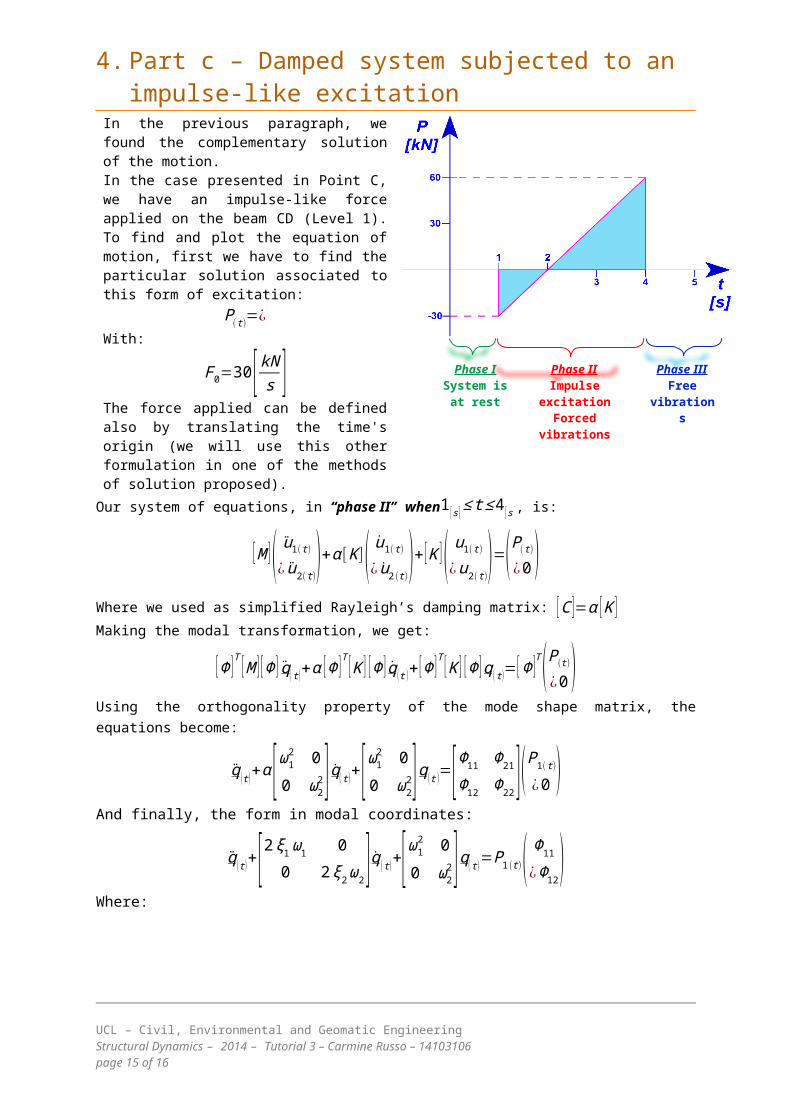
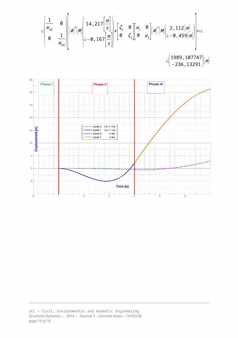
4.Part c – Damped system subjected to an impulse-like excitation

In the previous paragraph, wefound the complementary solutionof the motion.In the case presented in Point C,we have an impulse-like forceapplied on the beam CD (Level_1).To find and plot the equation ofmotion, first we have to find theparticular solution associated tothis form of excitation:

P(t)

=¿With:

F0=30[kNs ]The force applied can be definedalso by translating the time'sorigin (we will use this otherformulation in one of the methodsof solution proposed).

Phase ISystem isat rest

Phase IIImpulse

excitationForced

vibrations

Phase IIIFree

vibrations

Our system of equations, in “phase II” when1[s]≤t≤4[s ], is:

[M ]( u1(t)

¿ u2(t))+α [K]( u1(t)

¿ u2 (t))+[K ]( u1(t)

¿u2(t))=(P(t)

¿0 )Where we used as simplified Rayleigh’s damping matrix: [C ]=α [K ]Making the modal transformation, we get:

[Φ ]T [M ] [Φ ] q(t)+α [Φ ]T [K ] [Φ ]q(t )+[Φ ]T [K ] [Φ ]q(t)=[Φ ]T(P(t)

¿0 )Using the orthogonality property of the mode shape matrix, theequations become:

q(t)+α[ω12 00 ω22]q(t)+[ω12 0

0 ω22]q(t )=[Φ11 Φ21

Φ12 Φ22 ](P1(t)

¿0 )And finally, the form in modal coordinates:

q(t)+[2ξ1ω1 00 2ξ2ω2]q(t)+[ω1

2 00 ω22]q(t)=P1 (t)( Φ11

¿Φ12)Where:


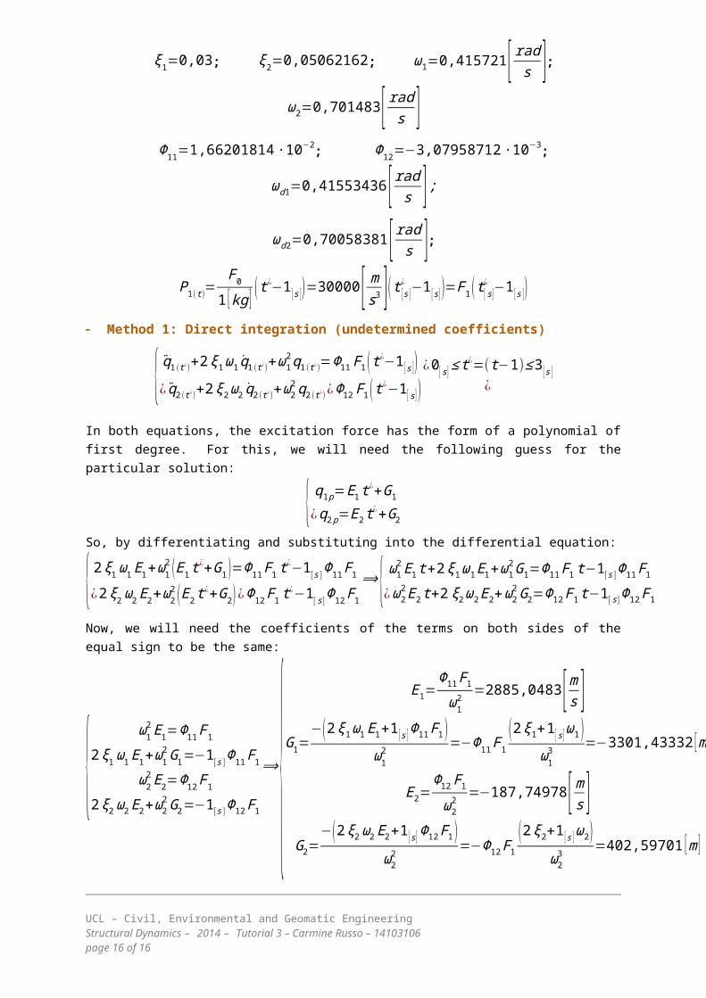
ξ1=0,03; ξ2=0,05062162; ω1=0,415721[ rads ];ω2=0,701483[ rads ]

Φ11=1,66201814∙10−2; Φ12=−3,07958712∙10−3;

ωd1=0,41553436[rads ];ωd2=0,70058381[rads ];

P1(t)=

F0

1 [kg ] (t¿−1[s ])=30000[ ms3 ](t[s ]

¿ −1[s] )=F1(t[s]¿ −1[s ])

Method 1: Direct integration (undetermined coefficients)

{ q1 (t¿)+2ξ1ω1q1 (t¿)+ω12q1 (t¿)=Φ11F1 (t¿−1[s ])

¿ q2 (t¿)+2ξ2ω2 q2 (t¿)+ω22q2 (t¿)¿Φ12F1(t¿−1[s] )¿0[s]≤t

¿=(t−1)≤3[s ]¿

In both equations, the excitation force has the form of a polynomial offirst degree. For this, we will need the following guess for theparticular solution:

{ q1p=E1t¿+G1

¿q2p=E2t¿+G2So, by differentiating and substituting into the differential equation:

{2ξ1ω1E1+ω12 (E1t¿+G1 )=Φ11F1t

¿−1[s ]Φ11F1¿2ξ2ω2E2+ω22 (E2t¿+G2) ¿Φ12F1t¿−1

[s]Φ12F1

⟹ { ω12E1t+2ξ1ω1E1+ω12G1=Φ11F1t−1[s ]Φ11F1

¿ω22E2t+2ξ2ω2E2+ω22G2=Φ12F1t−1[s]Φ12F1

Now, we will need the coefficients of the terms on both sides of theequal sign to be the same:

{ ω12E1=Φ11F1

2ξ1ω1E1+ω12G1=−1

[s ]Φ11F1

ω22E2=Φ12F1

2ξ2ω2E2+ω22G2=−1[s ]Φ12F1

⟹{E1=

Φ11F1ω12 =2885,0483[ms ]

G1=−(2ξ1ω1E1+1[s ]Φ11F1 )

ω12 =−Φ11F1

(2ξ1+1[s]ω1)ω13 =−3301,43332 [m ]

E2=Φ12F1ω22 =−187,74978[ ms ]

G2=−(2ξ2ω2E2+1[s]Φ12F1)

ω22=−Φ12F1

(2ξ2+1[s ]ω2)ω23

=402,59701 [m ]


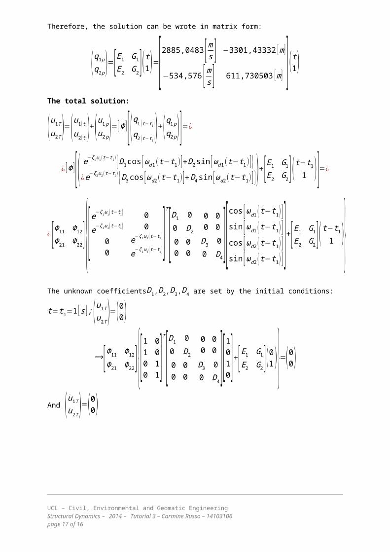
Therefore, the solution can be wrote in matrix form:

(q1p

q2p)=[E1 G1

E2 G2](t1)=[2885,0483[ms ] −3301,43332 [m]

−534,576 [ms ] 611,730503 [m] ](t1)

The total solution:

(u1T

u2T)=(u1(t)

u2(t))+(u1p

u2p)=[Φ ][(q1 (t−t1)

q2 (t−t1))+(q1pq2p)]=¿

¿ [Φ ][( e−ζ1ω1(t−t1){D1cos [ωd1(t−t1)]+D2sin [ωd1(t−t1)]}¿e−ζ2ω2(t−t1) {D3cos [ωd2(t−t1)]+D4sin [ωd2(t−t1)] })+[E1 G1

E2 G2](t−t11 )]=¿

¿ [Φ11 Φ12

Φ21 Φ22]{[e−ζ1ω1(t−t1)

e−ζ1ω1(t−t1)

00

00

e−ζ2ω2(t−t1)

e−ζ2ω2(t−t1)]T

[D1 00 D2

0 00 0

0 00 0

D3 00 D4

][cos [ωd1 (t−t1) ]sin [ωd1 (t−t1) ]cos [ωd2 (t−t1) ]sin [ωd2 (t−t1) ] ]+[E1 G1

E2 G2](t−t11 )}

The unknown coefficientsD1,D2,D3,D4 are set by the initial conditions:

t=t1=1 [s ];(u1T

u2T)=(00)

⟹[Φ11 Φ12

Φ21 Φ22]{[1100 0011]

T

[D1 00 D2

0 00 0

0 00 0

D3 00 D4

][1010]+[E1 G1E2 G2](01)}=(00)

And (u1T

u2T)=(00)


⟹[Φ11 Φ12

Φ21 Φ22]{[−ζ1ω1−ζ1ω100

00

−ζ2ω2

−ζ2ω2]T

[D1 00 D2

0 00 0

0 00 0

D3 00 D4

] [1010 ]+¿

¿+[11000011]

T

[D1 00 D2

0 00 0

0 00 0

D3 00 D4

][ 0ωd1

0ωd2

]+(E1E2) }=(00)

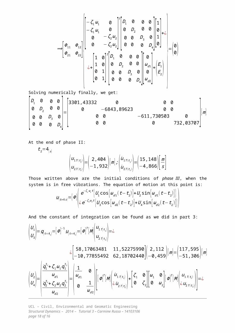
Solving numerically finally, we get:

[D1 00 D2

0 00 0

0 00 0

D3 00 D4

]=[3301,43332 00 −6843,89623

0 00 0

0 00 0

−611,730503 00 732,03707] [m]

At the end of phase II:t2=4[s]

(u1T (t2)

u2T (t2))=( 2,404−1,932) [m ];(u1T (t2)

u2T (t2))=(15,148−4,866)[ ms ]

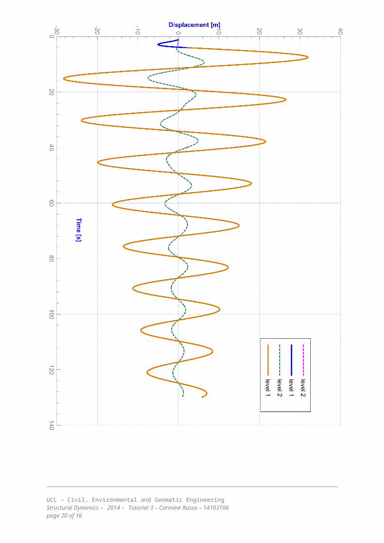
Those written above are the initial conditions of phase III, when thesystem is in free vibrations. The equation of motion at this point is:

u(t>4s)=[Φ ]( e−ζ1ω1t{U1cos [ωd1(t−t2) ]+U2sin [ωd1(t−t2)] }

¿e−ζ2ω2t {U3cos [ωd2(t−t2)]+U4sin [ωd2(t−t2)]})And the constant of integration can be found as we did in part 3:

(U1

U3)=q(t=4s)=[Φ ]−1u(t=4s)=[Φ ]T [M](u1T(t2)

u2T(t2))=¿

¿ [ 58,17063481 11,52275990−10,77855492 62,18702440]( 2,112−0,459) [m ]=(117,595−51,306) [m ]

(U2

U4)=(q1t2+ζ1ω1q1

t2

ωd1q2t2+ζ2ω2q2

t2

ωd2)=(

1ωd1

0

0 1ωd2

) [[Φ ]T [M ]( u1T(t2)¿ u2T (t2))+[ζ1 0

0 ζ2] [ω1 00 ω2] [Φ ]T [M ]( u1T(t2)

¿u2T (t2))]=¿


¿(1ωd1

0

0 1ωd2

)[ [Φ ]T [M ]( 14,217 [ms ]¿−0,167[ms ])+[ζ1 0

0 ζ2][ω1 00 ω2] [Φ ]T [M ]( 2,112 [m ]

¿−0,459 [m ])]=¿

¿(1989,107747−236,13291 ) [m ]


Method 2: Convolution integral (Duhamel)The solution in phase II can be found as solution of the convolutionbetween the generic response to the single impulse (Dirac delta) attimeτ, and the affective force applied:

{ q1(t¿)=∫

0

3s Φ11F1(t¿−1[s] )ω1d

e−ζ1ω1(t¿−τ)sin [ω1d (t¿−τ )]dτ

¿q2 (t¿)=∫0

3s Φ12F1(t¿−1[s ])ω2d

e−ζ2ω2(t¿−τ)sin [ω2d (t¿−τ) ]dτ

Note that the solution is the difference between a ramp forces, minus aconstant force:

{ q1 (t¿)=Φ11F1

ω1d[∫03s

t¿e−ζ1ω1(t¿−τ)sin [ω1d (t¿−τ) ]dτ−∫0

3s

1[s]∙e−ζ1ω1 (t¿−τ)sin [ω1d (t¿−τ) ]dτ]

¿q2 (t¿)=Φ12F1ω2d [∫0

3s

t¿e−ζ2ω2(t¿−τ )sin [ω2d (t¿−τ )]dτ−∫

0

3s

1[s ]∙e−ζ2ω2(t

¿−τ)sin [ω2d (t¿−τ )]dτ ]Integrating by parts:

q1(t¿)=Φ11F1

ω1d { e−ζ1ω1(t¿−τ )

(ω1d2 +ζ12ω1

2)2 [ (−2ζ1ω1ω1d+(ω1d2 +ζ12ω12)ω1dτ)cos [ω1d (t¿−τ )]+¿

¿ (ω1d2 −ζ1

2ω12+(ω1d2 +ζ1

2ω12 )ζ1ω1τ)sin [ω1d (t¿−τ )] ]

¿

−1[s]∙e−ζ1ω1(t¿−τ )[ω1d

ω12 cos [ω1d (t¿−τ )]+ζ1ω1sin [ω1d (t¿−τ ) ]] }|

t1¿=0 [s ]

t2¿=3 [s ]

q2(t¿)=Φ12F1

ω2d { e−ζ1ω1(t¿−τ )

(ω1d2 +ζ12ω1

2)2 [ (−2ζ1ω1ω1d+(ω1d2 +ζ12ω12)ω1dτ)cos [ω1d (t¿−τ )]+¿

¿ (ω1d2 −ζ1

2ω12+(ω1d2 +ζ1

2ω12 )ζ1ω1τ)sin [ω1d (t¿−τ )] ]

¿

−1[s]∙e−ζ1ω1(t¿−τ )[ω1d

ω12 cos [ω1d (t¿−τ )]+ζ1ω1sin [ω1d (t¿−τ ) ]] }|

t1¿=0 [s ]

t2¿=3 [s ]

The total solution in phase II, in terms of the lagrangian u1 and u2,in this case is going to be a combination of the two modal solution,scaled by the eigenvectors.


(u1(t¿)

u2(t¿))=[Φ ]( q1 (t¿ )

¿q2 (t¿))for0≤t¿=(t−1)≤3 [s ]

Apparently simpler than the previous one, but just more compact. Infact, the convolution integral holds inside the complete base of thevector space of solutions.

After phase II, the solution has the same form we found with the directintegration:

u(t>4s)=[Φ ]( e−ζ1ω1t{U1cos [ωd1(t−t2) ]+U2sin [ωd1(t−t2)] }

¿e−ζ2ω2t {U3cos [ωd2(t−t2)]+U4sin [ωd2(t−t2)]})With the constant of integration determined by the initial conditions.

Method 4: Discrete formulation (Newmark)To verify the quality of solutions found, we can try a discreteapproach, performing a numerical integration with the Newmark method(constant average acceleration):Starting from the decoupled system of equations:

{ q1 (t¿)+2ξ1ω1q1 (t¿)+ω12q1 (t¿)=Φ11F1(t¿−1[s ])

¿ q2 (t¿)+2ξ2ω2 q2 (t¿)+ω22q2 (t¿)¿Φ12F1 (t¿−1[s] )¿0[s]≤t

¿=(t−1)≤3[s ]¿

With the initial conditions:q1(0)

=q2(0 )=0∧q1 (0)

=q2 (0¿)=0

we can integrate numerically simply following the steps:1) q1(0)=−2ξ1ω1q1(0)−ω12q1 (0)+Φ11F1 (−1 [s ])

2) ∆q1(∆ti)=1C1

[Φ11F1 (∆ti¿−1[s ])+C2q1 (∆ti)

+2q1(∆ti)]

3) ∆ q1(∆ti)=2( ∆q1(∆ti)

∆ti−q1(∆ti ))

4) ∆ q1(∆ti)=4 [∆q1(∆ti)−∆ q1(∆ti)

∙∆ti]∆ti

2 −2q1(ti+1 )

The update the initial condition for the new iteration:

qi+1=qi+∆qi


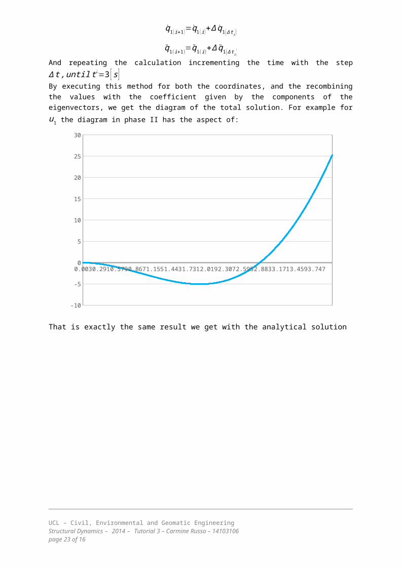
q1(i+1)=q1 (i)+∆ q1(∆ti)

q1(i+1)=q1(i)

+∆ q1(∆ti)And repeating the calculation incrementing the time with the step∆t,untilt¿=3 [s]By executing this method for both the coordinates, and the recombiningthe values with the coefficient given by the components of theeigenvectors, we get the diagram of the total solution. For example foru1 the diagram in phase II has the aspect of:

0.0030.2910.5790.8671.1551.4431.7312.0192.3072.5952.8833.1713.4593.747

-10

-5

0

5

10

15

20

25

30

That is exactly the same result we get with the analytical solution


Structural Dynamics

Documents

Transcript of Structural Dynamics