Should Welding Be Used to Repair Structural Steel - CiteSeerX
Upload
khangminh22Category
view
6download
0
CHAPTER 2Structural Steel
2.1 IntroductionFor the first half of the 20th century, there was essentially only one type of structural steel widely available in North America: Grade A-7 steel. (Although the names A-7 and A-9 were used for bridges and buildings before 1939, the two steels were virtually identical.) By the early 1960s, engineers needed to be familiar with five different types of structural steel, but they were likely to use only one or two for all practical purposes. However, with today’s exponential growth of technology (and opening to the world’s global market), the engineer is offered a “smorgasbord” of steel grades, and many engineers in some parts of North America already do not hesitate to commonly use two or more different steel grades for the main structural mem-bers in a given project.
Despite this growth in available products, the minimum require-ments specified for structural steel grades remain relatively simple. They generally consist of a few limits on chemical composition, limits on some mechanical properties such as minimum yield and tensile strengths, and minimum percentage elongation prior to failure (defi-nitely not very challenging for metallurgical engineers accustomed to dealing with the comprehensive lists of performance requirements specified for the steels needed in some specialty applications). As a result, in the last few decades, a wide variety of steel grades that meet the simple set of minimum requirements for structural steel has been produced. These steels will be adequate in many applications, but from the perspective of ductile response, the structural engineer is cautioned against hastily using unfamiliar steel grades without being fully aware of how these steels perform under a range of extreme conditions.
To increase this awareness, as well as to provide some funda-mental material-related information for the design of ductile struc-tures, this chapter reviews some of the lesser known properties of steel, along with information on the modeling of plastic material behavior.
7
02_Bruneau_Ch02_p007-110.indd 7 6/13/11 3:07:16 PM

8 C h a p t e r T w o S t r u c t u r a l S t e e l 9
2.2 Common Properties of Steel Materials
2.2.1 Engineering Stress-Strain CurveMost engineers will remember testing a standard steel coupon in ten-sion as part of their undergraduate studies and obtaining results sim-ilar to those presented in Figure 2.1, where the stress-strain curves for various structural steel grades tested at ambient temperature are plotted. For reference, engineering stress, s, is calculated as the ratio of the applied force, P, to the cross-sectional area, A, and engineering strain, e, is equal to ΔL/L, where ΔL is the elongation measured over a specified gauge length, L. As shown in Figure 2.1, the operations nec-essary to achieve higher yield strengths [such as alloying or quench-ing and tempering (Van Vlack 1989)] generally reduce the maximum elongation at failure and the length of the plastic plateau. For the structural steels used in rolled shapes today, these side-effects are negligible as sizable plastic deformation capacity remains beyond yield. The stress-strain curve for a uniaxially loaded steel specimen can therefore be schematically described as shown in Figure 2.2, with
A514 heat-treatedconstructional alloy steel
A852 heat-treatedHSLA steel
A588 HSLA steel
120
100
80
60
40
20
00 0.04 0.08 0.12 0.16 0.20 0.24
Strain, in per in
A36 carbon steel
Str
ess,
ksi
Figure 2.1 Stress-strain curves for some commercially available structural steel grades at ambient temperature. (From R.L. Brockenbrough and F.S. Merritt, Structural Steel Designer’s Handbook, 2nd ed, 1994, with permission of the McGraw-Hill Companies.)
02_Bruneau_Ch02_p007-110.indd 8 6/13/11 3:07:22 PM

8 C h a p t e r T w o S t r u c t u r a l S t e e l 9
an elastic range up to a strain of ey, followed by a plastic plateau between strains ey and esh, and a strain-hardening range between esh and eult, where ey, esh, and eult are the strains at the onset of yielding, strain-hardening, and necking, respectively. Depending on the steel used, esh generally varies between 5 to 15 ey, with an average value of 10 ey typically used in many applications. For all structural steels, the mod-ulus of elasticity can be taken as 200,000 MPa (29,000 ksi), and the tangent modulus at the onset of strain-hardening, Esh, is roughly 1/30th of that value, or approximately 6700 MPa (970 ksi); AISC (1971) reports Esh values ranging from 4827 to 5655 MPa (700 to 820 ksi) for various steels (i.e., E/40 to E/35) , whereas Horne and Morris (1981) and Neal (1977), respectively cite values of E/20 and E/25. More recently, Byfield et al. (2005) computed an average value of 2700 MPa (i.e., E/75) from the stress-strain curves of 50 mill tests from UK steel producers, which is practically equal to the value of 2552 MPa (370 ksi) used by Lay and Smith (1965).
The Poisson’s ratio, u, which relates a material’s transverse strain contraction under an applied axial strain elongation, is 0.3 for steel in the elastic range. When metals behave in a purely plastic manner, they preserve their volume (as first observed by Bridgman 1923, 1949a, 1949b), corresponding to a Poisson’s ratio of 0.5 (i.e., incompressible materials). Following the stress strain curve for steel, Poisson’s ratio in the plastic range, u p, is given by (Khan and Huang 1995):
u up E
E= - -
′12
12
(2.1)
σ
σult
σy upperσy static
εy εsh εult
ε
E Plasticplateau
Elastic range
Strain-hardening
rangeNeckingrange
Failure
Ultimatestrength
Esh
Figure 2.2 Schematic representation of stress-strain curve of structural steel.
02_Bruneau_Ch02_p007-110.indd 9 6/13/11 3:07:24 PM

10 C h a p t e r T w o S t r u c t u r a l S t e e l 11
where E′ is the effective tangent modulus (see Section 2.4). Per this equation, in the elastic range, E′ = E, and up = u = 0.3, and for E′ = E/30 at the onset of strain-hardening, up = 0.49, approaching 0.5 as E′ fur-ther decreases at larger strains.
Note that some applications (such as nonlinear finite elements analysis programs) require that the material properties be described in terms of true stress and strains (i.e., calculating stresses using the actual cross-section taking into account the Poisson effect, and strains using the actual length after elongation), rather than engineering stresses and strains (calculated using the initial cross-sectional area and length). These values can be obtained by the following relationships:
s e sTrue Engineering Engineering= +( )1 (2.2a)
e eTrue Engineering= +ln( )1 (2.2b)
by assuming that the volume of steel under consideration remains the same, such that the product of the initial length and area equals that of the instantaneous length and area. The resulting true stress versus true strain relationship is not symmetric, because the cross-section increases in compression and decreases in tension. Furthermore, these equations are only valid until the onset of neck-ing, beyond which they would need to be corrected using actual measurements of cross-section measured during coupon tests. Hence, unless unavoidable due to the requirements of a specific appli-cation, and because reduction of cross-section is small until necking, engineering stresses and strains are generally used for most practical purposes.
2.2.2 Effect of Temperature on Stress-Strain CurveThe shape of the stress-strain curve varies considerably at very high and very low temperatures. The yield and ultimate strengths of steel, as well as its modulus of elasticity, drop (while maximum elongation at failure marginally increases) as temperature increases, as shown in Figures 2.3 and 2.4. This drop is relatively slow and not too signifi-cant up to 500°F (260°C), and is almost linear until these properties reach approximately 80% of their initial value, at a temperature of approximately 800°F (425°C). Beyond that point, weakening and soft-ening of the steel accelerates significantly.
A number of equations that capture this behavior for different types of structural steel are presented in documents concerned with fire resistance (AISC 2005, ASCE 1992, ECCS 2001, NIST 2010). Finite element nonlinear analyses simultaneously accounting for fire spread within a structure and high-temperature degradation of the struc-tural system require rigorous modeling of the steel properties. Such analyses can be simplified by assuming a constant coefficient of ther-mal expansion, α, of 7.8 × 10⁻⁵/°F = 1.4 × 10⁻⁵/°C (exact value varies
02_Bruneau_Ch02_p007-110.indd 10 6/13/11 3:07:25 PM

10 C h a p t e r T w o S t r u c t u r a l S t e e l 11
A514 steelA588 steel
A572 steelA36 steel
1.2
1.0
0.8
0.6
0.4
0.2
0
Typi
cal r
atio
of e
leva
ted-
tem
pera
ture
to r
oom
-tem
pera
ture
yie
ld s
tren
gths
0 200 400 600 800 1,000 1,200 1,400 1,600 1,800 2,000
Temperature, °F(a)
A514 steelA588 steel
A572 steelA36 steel
1.2
1.0
0.8
0.6
0.4
0.2
0
Typi
cal r
atio
of e
leva
ted-
tem
pera
ture
to r
oom
-tem
pera
ture
tens
ile s
tren
gths
0 200 400 600 800 1,000 1,200 1,400 1,600 1,800 2,000
Temperature, °F(b)
Temperature, °F(c)
1.0
0.8
0.6
0.4
0.2
0.0
Typi
cal r
atio
of e
leva
ted-
tem
pera
ture
to r
oom
-te
mpe
ratu
re m
odul
us o
f ela
stic
ity
0 200 400 600 800 1,000
Figure 2.3 Effect of temperature on (a) yield strength, (b) tensile strength, and (c) modulus of elasticity of structural steels. (From R.L. Brockenbrough and B.G. Johnston, USS Steel Design Manual, with permission of U.S. Steel.)
02_Bruneau_Ch02_p007-110.indd 11 6/13/11 3:07:30 PM

S t r u c t u r a l S t e e l 13
Tensile
Yield
Engineering yield and tensile strengths - A 572 Grade 50
100
90
80
70
60
50
40
Str
engt
h, k
si
–150 –100 –50 0 50 100 150 200 250
Temperature, °F(a)
0°F
+75°F
Monotonic tensile tests - A 572 Grade 50
0 10 20 30Engineering strain, %
(b)
Eng
inee
ring
stre
ss, k
si
100
90
80
70
60
50
40
30
20
10
0
–100°F
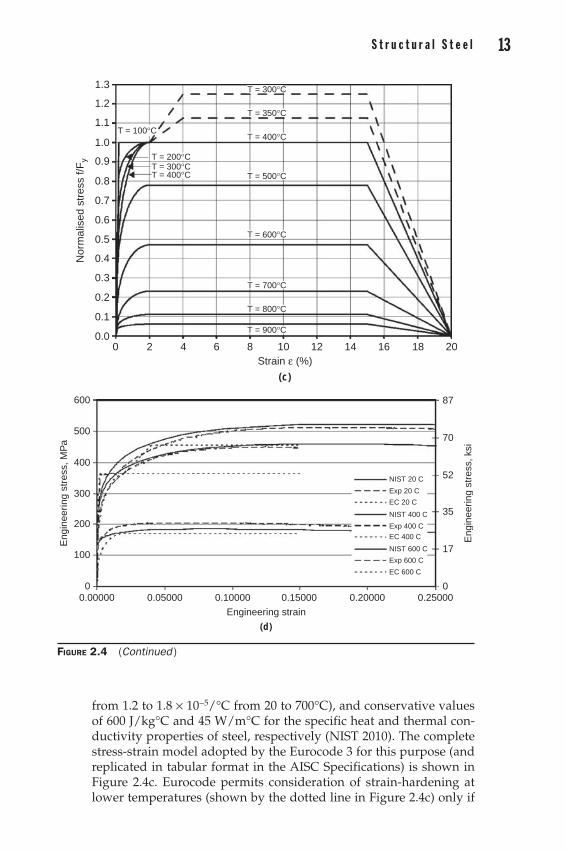
Figure 2.4 Examples of (a) yield and tensile strength and (b) stress-strain curves versus temperature. Composite curves constructed from data taken from several heats of ASTM A572 Grade 50 plate on the order of 1 in thick. (c) Elevated temperature stress-strain relationships of Eurocode 3. (d) Comparison of engineering stress-strain relationships proposed by NIST and by Eurocode 3 with data generated by NIST for the World Trade Center forensic investigation (NIST 2010). (Figures a and b courtesy of H.S. Reemsnyder, Homer Research Laboratory, Bethlehem Steel Corporation, with permission. Note: The data in Figure 2.4 (a) and (b) should not be considered typical, maxima, or minima for all plates and rolled sections of this grade. Properties will vary with chemistry, thermomechanical processing, thickness, and product form.)
12
02_Bruneau_Ch02_p007-110.indd 12 6/13/11 3:07:31 PM
S t r u c t u r a l S t e e l 13
from 1.2 to 1.8 × 10⁻⁵/°C from 20 to 700°C), and conservative values of 600 J/kg°C and 45 W/m°C for the specific heat and thermal con-ductivity properties of steel, respectively (NIST 2010). The complete stress-strain model adopted by the Eurocode 3 for this purpose (and replicated in tabular format in the AISC Specifications) is shown in Figure 2.4c. Eurocode permits consideration of strain-hardening at lower temperatures (shown by the dotted line in Figure 2.4c) only if
T = 350°C
T = 400°C
T = 500°C
T = 200°CT = 300°CT = 400°C
T = 600°C
T = 700°C
T = 800°C
T = 900°C
T = 300°C1.3
1.2
1.1
1.0
0.9
0.8
0.7
0.6
0.5
0.4
0.3
0.2
0.1
0.0
Nor
mal
ised
str
ess
f/Fy
0 2 4 6 8 10 12 14 16 18 20Strain ε (%)
(c)
T = 100°C
87
70
52
35
17
0
Eng
inee
ring
stre
ss, k
siNIST 20 C
Exp 20 C
Exp 400 C
Exp 600 C
EC 400 C
EC 600 C
EC 20 C
NIST 400 C
NIST 600 C
0.250000.200000.150000.100000.050000.00000
Engineering strain
(d)
600
500
400
300
200
100
0
Eng
inee
ring
stre
ss, M
Pa
Figure 2.4 (Continued )
02_Bruneau_Ch02_p007-110.indd 13 6/13/11 3:07:33 PM

14 C h a p t e r T w o S t r u c t u r a l S t e e l 15
advanced finite element models that reflect the state-of-the-art in fire analysis are used.
In its forensic study of the collapses of the World Trade Center towers, the National Institute of Standards and Technology (NIST) also developed the following equation by best fit to experimental data on steels having specified yield stresses ranging from 250 MPa (36 ksi) to 450 MPa (100 ksi), in which temperature is expressed in °C.
s eη= K (2.3)
where
K F
T= + -
( . )exp
.
734 0 315575
4 92
Y (2.4)
and
η = - × -
-( . . )exp
.
0 329 4 23 10637
44 51
FT
Y (2.5)
The resulting stress-strain diagrams for the two models for a A572 Grade 50 steel are compared in Figure 2.4d. The testing procedure used to obtain these curves implicitly accounts for the creep of steel under sustained loading at elevated temperatures (NIST 2010). Although neither models included data from A992 steel, later tests revealed similar behavior (Hu et al. 2009).
Protecting steel from such extreme temperature is obviously the first line of defense against structural collapse during an uncontrolled fire. This is done by application of one of various types of coatings that will enhance fire resistance by delaying the rise of steel tempera-ture, using either insulating, energy absorbing, or intumescent mate-rials (e.g., Buchanan 2001, Gewain et al. 2003, Ruddy et al. 2003). A few specially alloyed steels have also been developed to experience no more than a 33% loss of their yield strength at 600°C—circumvent-ing in some instances the need for such coatings when fire exposure can be controlled or ensured to not exceed this heat intensity—but their properties drop more rapidly beyond that point, back to match-ing that of other steels when temperatures reach 800°C (Mizutani et al. 2004, Sakumoto et al. 1992).
Beyond analyses of the fire resistance of structures having exposed or thermally insulated steel members (or having damaged insulation as the case in NIST 2005), information on properties at elevated tem-peratures may be necessary in other specialty applications. For exam-ple, given that special high-temperature heat treatments [up to 1000°F (540°C)] are often specified to reduce the residual stresses introduced
02_Bruneau_Ch02_p007-110.indd 14 6/13/11 3:07:33 PM

14 C h a p t e r T w o S t r u c t u r a l S t e e l 15
by welding in industrial steel pressure vessels (particularly when a new steel plate is welded in place of an existing damaged or corroded one), a good knowledge of the high-temperature properties of struc-tural steel is crucial to prevent collapse of these vessels under their own weight during the heat treatment.
2.2.3 Effect of Temperature on Ductility and Notch-Toughness
Temperatures below room temperature do not have an adverse impact on the yield strength of steel, as shown in Figure 2.4, but lower temperatures can have a substantial impact on ductility. Indeed, the ultimate behavior of steel will progressively transform from ductile to brittle when temperatures fall below a certain threshold and enter the appropriately labeled “ductile-to-brittle-transition-temperature” (DBTT) range. This undesirable property of structural steel led to a few notable failures in the late 1800s and early 1900s, but began to be fully appreciated only in the 1940s and 1950s when large cracks were discovered in more than 1000 all-welded U.S. steel ships built in that period. These included more than 200 cases of severe fractures and 16 ships lost at sea when their hulls unexpectedly “snapped” in two while they were cruising the Arctic sea.
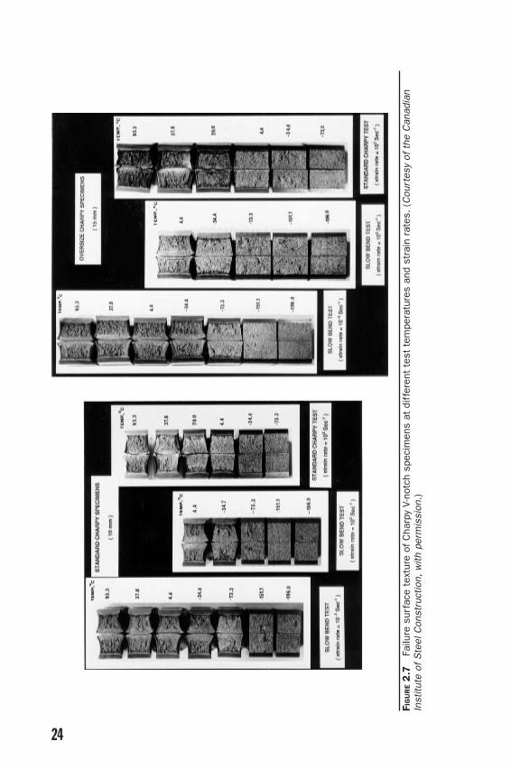
The Charpy V-notch test (also known as a notch-toughness test) was developed to determine the DBTT range. In this test, a standard notched steel specimen is broken by a falling pendulum hammer fitted with a standard striking edge (Figures 2.5a and b). In princi-ple, the energy absorbed by the specimen during its failure will translate into a loss of potential energy of the pendulum. Thus, a rough measure of this absorbed energy can be calculated from the difference between the initial height (h1) of the pendulum when released and the maximum height (h2) it reaches on the far side after breaking the specimen. A typical plot of the absorbed energy of a Charpy specimen as a function of temperature is shown in Figures 2.5c and d for a standard structural steel. Corresponding changes in fracture appearance and lateral expansion at failure are shown in Figures 2.5e and f.
Generally, structural engineering standards and codes will allow the use of only steels that exhibit a minimum energy absorption capa-bility at a predetermined temperature—for example, 15 ft-lb at 40°F (20 Nm at 4.5°C). Although it may first appear to the reader, from the Charpy data of Figure 2.5, that a level of energy dissipation of 15 ft-lb corresponds to a nearly brittle material behavior and is insufficient to ensure ductile response, it must be recognized that the Charpy V-notch test produces failures at very high strain rates. As shown in Figure 2.5c for A572 Grade 50 steel, there exists a shift of 125°F between the DBTT range obtained from the Charpy V-notch tests and that range obtained from failure tests conducted at an intermediate
02_Bruneau_Ch02_p007-110.indd 15 6/13/11 3:07:33 PM

16 C h a p t e r T w o
(a)
55 mmB
B
45°
2 mmSection B-B
0.25-mm R10 mm
10 mm
Figure 2.5 Charpy V-notch impact tests: (a) typical specimen, (b) schematic of testing procedure, (c) energy absorption behavior for impact loading and intermediate strain-rate loading for standard specimens for A572 Grade 50 steel.
W
h1
C
h2
D
(b)
A572 Grade 50 steelImpactIntermediate-strain-ratebehavior predicted byshifting the impact dataIntermediate–strain-rate behaviorpredicted from KXC dataTested at ε =10–3 s–1
75 75
NDT
50
40
30
20
10
0
Temperature, °F(c)
–200 –150 –100 –50 0 50 100 150
Ene
rgy
abso
rptio
n, ft
-lb
02_Bruneau_Ch02_p007-110.indd 16 6/13/11 3:07:36 PM

16 C h a p t e r T w o
Figure 2.5 Composite plots of: (d) energy absorption, (e) fracture appearance, and (f) lateral expansion constructed from data taken from several heats of ASTM A572 Grade 50 plate on the order of 1 in thick. (Figures a, b, and c from J.M. Barsom and S.T. Rolfe, Fracture and Fatigue Control in Structures—Applications of Fracture Mechanics, with permission from J.M. Barsom and S.T. Rolfe; Figures d, e, and f courtesy of H.S. Reemsnyder, Homer Research Laboratory, Bethlehem Steel Corporation, with permission. Note: The data in Figure 2.5 should not be considered typical, maxima, or minima for all plates and rolled sections of this grade. Properties will vary with chemistry, thermomechanical processing, thickness, and product form.)
250
200
150
100
50
0–150 –100 –50 0 50 100 150 200
Charpy V-notch tests
A 572 Grade 50A
bsor
bed
ener
gy, f
t-lb
(d)
–150 –100 –50 0 50 100 150 200
Frac
ture
app
eara
nce,
%
50% FATT
100
80
60
40
20
0
(e)
17
Temperature, °F–150 –100 –50 0 50 100 150 200
Late
ral e
xpan
sion
, mil
100
80
60
40
20
0
(f)
02_Bruneau_Ch02_p007-110.indd 17 6/13/11 3:07:37 PM

18 C h a p t e r T w o
strain rate of 0.001/s, with more ductile behavior obtained at lower strain rates (see ASTM 1985a for details on tests at slower strain rates, and Rolfe and Barsom 1999 for techniques to compare different mea-sures of fracture toughness obtained from different testing proce-dures). Hence, compliance with the specified Charpy V-notch 15 ft-lb energy absorption at 40°F should ensure ductile behavior over the practical range of service temperatures for structural elements sub-jected to such a strain rate. Tables 2.1 and 2.2, as well as Figure 2.6, summarize the Charpy V-notch test results for a number of com-monly used steel grades and show that most comply with the above example specified Charpy limit. However, it should be noted from those tables that structural shapes having large flange and web thick-nesses [such as those formerly known as AISC Groups 4 and 5 (AISC 1994)] generally have lower energy absorption capabilities. For spe-cialty applications that require better performance than that which is commonly available, the structural engineer should request steel spe-cially alloyed to provide the needed material properties at low tem-peratures, high strain rates, or both.
Beyond the energy absorption measure, a large number of descriptive indices exist in the literature to capture and quantify this ductile-to-brittle behavior. The nil-ductility-transition (NDT) tem-perature, defined as the highest temperature at which a specimen fails in a purely brittle manner (or alternatively as the temperature at which a small crack will propagate to failure in a specimen loaded exactly to the yield stress), can also be obtained from the ASTM E208 test (ASTM 1985b). The fracture appearance transition temperature (FATT) is the temperature at which 50% of the fracture surface cor-responds to a cleavage failure (i.e., a flat crystalline surface charac-teristic of brittle failure), with the remaining 50% showing shear-lips of fibrous appearance typical of ductile failures. Figure 2.7 illustrates that this transition in texture of the failure surface is a function of both temperature and strain rate. Further, it shows that alignment of the surfaces exhibiting similar texture, but tested at different strain rates, provides a striking visual expression of the aforementioned temperature shift of the DBTT range.
Although notch toughness and ductility for a given steel are closely related, it is important to realize that notch toughness is not related to yield strength. In fact, in very thick steel sections, the notch toughness of some steels is known to vary quite significantly throughout the cross-section of members, even when a variation in yield strength is not observed. This is particularly true at the core of the web-flange intersection of very thick sections in which a larger steel grain structure exists as a consequence of a lesser amount of cold forming achieved there during the rolling process. For this reason, AISC (2010) specifies that samples for Charpy V-notch tests be taken from the core area, by reference to Supplement S30 of the ASTM A6 standard.
02_Bruneau_Ch02_p007-110.indd 18 6/13/11 3:07:38 PM

18 C h a p t e r T w o
19
Ste
el G
rade
Test
Te
mp
(çF)
ASTM
Sha
pe
Gro
upSam
ple
Siz
eM
ode
(ft-
lb)
Min
imum
(f
t-lb
)M
ean
(ft-
lb)
Max
imum
(f
t-lb
)
Firs
t Q
uart
ile
(ft-
lb)
Med
ian
(ft-
lb)
Thir
d Q
uart
ile
(ft-
lb)
A3
6 Q
ST
32
ALL
21
162
91
151
204
137
16
01
68
A3
6 H
R32
ALL
73
130
91
150
241
124
14
51
69
A3
6 H
R40
ALL
2011
66
16
112
286
65
98
14
7
1421
100
20
116
272
79
11
31
46
21057
239
16
130
286
77
11
71
76
3315
36
19
86
240
63
77
98
4218
54
16
54
193
41
51
62
A3
6 H
R70
ALL
426
239
22
95
253
43
70
12
4
1262
43
25
59
177
36
50
75
259
69
59
122
253
83
97
13
8
324
239
25
200
240
235
23
92
39
481
240
22
158
240
99
17
72
21
A5
72
Gr
50 Q
ST
32
ALL
24
N/A
101
136
182
122
13
81
49
A5
72
Gr
50 H
R32
ALL
15
N/A
106
140
170
135
14
21
47
HR
= H
ot R
olle
d; Q
ST =
Que
nche
d S
elf-
Tem
pere
d
(Fro
m A
mer
ican
Inst
itute
of S
teel
Con
stru
ctio
n, S
tatis
tical
Ana
lysi
s of
Cha
rpy
V-N
otch
Tou
ghne
ss fo
r St
eel W
ide
Flan
ge S
truc
tura
l Sha
pes,
with
per
mis
sion
)
Tab
le 2
.1
Com
pila
tion
of C
harp
y V-N
otch
Tes
t R
esul
ts f
or V
ario
us S
truc
tura
l Ste
el G
rade
s, f
rom
Dat
a Pro
vide
d by
Nor
th A
mer
ican
Pro
duce
rs
02_Bruneau_Ch02_p007-110.indd 19 6/13/11 3:07:38 PM

S t r u c t u r a l S t e e l 21
Ste
el G
rade
Test
Te
mp
(çF)
ASTM
Sha
pe
Gro
upSam
ple
Siz
eM
ode
(ft-
lb)
Min
imum
(f
t-lb
)M
ean
(ft-
lb)
Max
imum
(f
t-lb
)
Firs
t Q
uart
ile
(ft-
lb)
Med
ian
(ft-
lb)
Thir
d Q
uart
ile
(ft-
lb)
A5
72
Gr
50 H
R40
ALL
3930
79
16
91
288
64
80
97
1400
58
16
84
259
58
73
95
22181
80
18
93
288
71
85
10
23
813
86
16
83
280
65
82
96
4453
60
17
66
155
53
63
77
583
49
29
62
155
47
59
71
A5
72
Gr
50 H
R70
ALL
598
47
15
61
241
31
51
74
237
124
31
135
237
89
13
41
94
390
74
31
76
202
56
68
91
4364
50
17
57
241
34
51
68
5104
26
15
33
116
23
27
32
A5
88
HR
40
ALL
223
21
16
140
290
71
12
92
04
2182
54
18
148
290
82
14
52
15
341
N/A
16
103
249
58
75
15
5A9
13
Gr6
5 Q
ST
32
ALL
87
156
92
141
212
122
14
21
58
A9
13
Gr6
5 Q
ST
70
ALL
34
48
33
61
108
45
57
79
Dua
l Cer
tifie
d40
ALL
202
43
17
53
121
37
51
67
1142
38
17
51
121
35
48
63
255
43
24
59
116
43
58
74
Dua
l Cer
tifie
d70
ALL
368
65
15
59
131
41
55
74
1322
53
15
55
131
37
53
69
246
65
60
86
123
67
91
99
Tab
le 2
.1
Com
pila
tion
of C
harp
y V-N
otch
Tes
t R
esul
ts f
or V
ario
us S
truc
tura
l Ste
el G
rade
s, f
rom
Dat
a Pro
vide
d by
Nor
th A
mer
ican
Pro
duce
rs
(Con
tinue
d)
20
02_Bruneau_Ch02_p007-110.indd 20 6/13/11 3:07:38 PM

S t r u c t u r a l S t e e l 21
Steel Grade
Test Temp (°F)
ASTM Shape Group
Observed Probability of Exceedance 15 ft-lb (%)
Observed Probability of Exceedance 20 ft-lb (%)
A36 QST 32 ALL 100 100
A36 HR 32 ALL 100 100
A36 HR 40 ALL
1
2
3
4
99
100
100
100
96
97
97
99
99
95
A36 HR 70 ALL
1
2
3
4
100
100
100
100
100
95
95
100
94
97
A572 Gr 50 QST 32 ALL 100 100
A572 Gr 50 HR 32 ALL 100 100
A572 Gr 50 HR 40 ALL
1
2
3
4
5
100
99
100
98
100
100
99
99
99
98
99
99
A572 Gr 50 HR 70 ALL
2
3
4
5
95
100
100
96
85
87
100
100
89
60
A588 HR 40 ALL
2
3
98
99
97
97
98
95
A913 Gr65 QST 32 ALL 100 100
HR Rolled; QST = Quenched Self-Tempered(From American Institute of Steel Construction, Statistical Analysis of Charpy V-Notch Toughness for Steel Wide Flange Structural Shapes, with permission.)
Table 2.2 Probability of Exceedance of Two Commonly Specified Charpy V-Notch Energy Absorption Material Requirements for Various Structural Steel Grades, from Data Provided by North American Producers
02_Bruneau_Ch02_p007-110.indd 21 6/13/11 3:07:38 PM

22 C h a p t e r T w o S t r u c t u r a l S t e e l 23
2.2.4 Strain Rate Effect on Tensile and Yield StrengthsStrain rate is another factor that affects the shape of the stress-strain curve. Typically, the tensile and yield strengths will increase at higher strain rates, as shown in Figure 2.8, except at high tempera-tures for which the reverse is true. Consideration of this phenom-enon is crucial for blast-resistant design in which very high strain rates are expected, but of little practical significance in earthquake-engineering applications. Past studies have repeatedly demon-strated that, for the steel grades commonly used, the expected increases of roughly 5 to 10% in yield strength at typical earth-quake-induced strain rates is negligible compared with the much greater uncertainties associated with the earthquake input. The effect of strain rate on notch toughness, as described above, is also considerably more significant.
Blast-resistant design manuals and guides typically specify charts or tables of the factors by which the static yield and tensile stresses should be magnified to obtain the corresponding dynamic values to use in calculations, such as Figure 2.8e. Strain rates are a function of the blast pressures and structural system properties, and calculated values for common blast-resistant design scenarios vary between 0.02 to 0.3 in/in/s.
2.2.5 Probable Yield StrengthIn seismic design, as will be demonstrated later, knowledge of the maximum probable yield strength is equally important as knowl-edge of the minimum reliable yield strength. Recent studies have reported that the margin between the actual average yield strength
Steel Grade
Test Temp (°F)
ASTM Shape Group
Observed Probability of Exceedance 15 ft-lb (%)
Observed Probability of Exceedance 20 ft-lb (%)
A913 Gr65 QST 70 ALL 100 100
Dual Certified 40 ALL
1
2
99
98
100
94
94
99
Dual Certified 70 ALL
1
2
98
98
100
94
93
100
Table 2.2 Probability of Exceedance of Two Commonly Specified Charpy V-Notch Energy Absorption Material Requirements for Various Structural Steel Grades, from Data Provided by North American Producers (Continued )
02_Bruneau_Ch02_p007-110.indd 22 6/13/11 3:07:38 PM

22 C h a p t e r T w o S t r u c t u r a l S t e e l 23
A572 Gr50 hot rolled @ 40°F all ASTM groups shapes:Deviation of individual test resultsfrom reported average test result
A572 Gr50 hot rolled @ 40°F all ASTM groups shapes:Cummulative frequency distribution
A572 Gr50 hot rolled @ 40°F all ASTM groups shapes:Relative frequency distribution
40
30
20
10
0
Freq
uenc
y (p
erce
nt)
Freq
uenc
y (p
erce
nt)
34.0
23.5
15.2
9.4
4.2
2.8
1.8
1.0
0.5
0.4
0.2
0.3
0.2
0.2
0.2
0.3
5.9
Sample size: 11790Mode: N/AMinimum: 0%Mean: 9.5%Maximum: 112.8%
Sample size: 3930Mode: 79.0 ft IbsMinimum: 16.3 ft IbsMean: 90.5 ft IbsMaximum: 288.3 ft Ibs
1st quartile (25%): 63.7 ft IbsMedian (50%): 80.3 ft Ibs3rd quartile (75%): 97.3 ft Ibs
2 6 10 14 18 22 26 30 34 38 42 46 50 54 58 62Percent deviation from average
20
15
10
5
0
1
0.9
0.8
0.7
0.6
0.5
0.4
0.3
0.2
0.1
0
0.0
0.5
1.0 2.
36.
010
.7 12.7
16.4
16.2
12.5
6.9
3.6
2.5
1.8
1.1
1.0
0.8
0.4
0.5
0.6
0.7
0.4
0.4
0.4
0.4
0.1
0.1
0.1
0.1
0.0
0.0
5 25 45 65 85 105 125 145 165 185 205 225 245 265 285CVN (ft Ibs)
Cum
mul
ativ
e fr
eque
ncy
10 20 30 40 50 60 70 80 90 100
110
120
130
140
150
160
170
180
190
200
210
220
230
240
250
260
270
280
290
3000
CVN (ft Ibs)
Figure 2.6 Compilation of Charpy V-notch test results for A572 Grade 50 structural steel, from data provided by North American producers. (From American Institute of Steel Construction, Statistical Analysis of Charpy V-Notch Toughness for Steel Wide Flange Structural Shapes, with permission.)
02_Bruneau_Ch02_p007-110.indd 23 6/13/11 3:07:40 PM
S t r u c t u r a l S t e e l 25
Fig
ur
e 2
.7
Failu
re s
urfa
ce t
extu
re o
f C
harp
y V-n
otch
spe
cim
ens
at d
iffe
rent
tes
t te
mpe
ratu
res
and
stra
in r
ates
. (C
ourt
esy
of t
he C
anad
ian
Inst
itut
e of
Ste
el C
onst
ruct
ion,
with
perm
issi
on.)
24
02_Bruneau_Ch02_p007-110.indd 24 6/13/11 3:07:42 PM

S t r u c t u r a l S t e e l 25
A514 A514
A242
A242A515
A515
Tensile strengthYield strength
A242
A515A242
A515
A514
A242
A515
A242 A515
140
130
120
110
100
90
80
70
60
50
40
30
20
10
Str
ess,
ksi
10–510–4 10–3 10–2 10–1 1 10–510–4 10–3 10–2 10–1 1 10–510–4 10–3 10–2 10–1 1Strain rate, in/in/s
–50°FStrain rate, in/in/sroom temperature
Strain rate, in/in/s600°F
(a) (b) (c)
σ yσ y
(2
× 10
–4)
= 0.973 + 0.45 0.33.
10–5 10–4 10–3 10–2 10–1
1.2
1.1
1.0
0.9
Strain rate (1/s)(d)
σy
σy (2 × 10⁻⁴)ε
Figure 2.8 Yield stress as a function of strain rate and temperature for some structural steels. [Figures a, b, and c from R.L. Brockenbrough and B.G. Johnston, USS Steel Design Manual, with permission from U.S. Steel; Figure d from Moncarz, P.D. and Krawinkler H., Theory and Application of Experimental Model Analysis in Earthquake Engineering, Report No. 50, John A. Blume Earthquake Engineering Research Center, Department of Civil Engineering, Stanford University, with permission. Figure e from Unified Facilities Criteria (UFC 2008).]
02_Bruneau_Ch02_p007-110.indd 25 6/13/11 3:07:43 PM

26 C h a p t e r T w o S t r u c t u r a l S t e e l 27
and specified yield strength has progressively increased over the years for some structural steels, even though the steel specification itself remained unchanged. For example, a few decades ago, yield strengths of 255 to 270 MPa (37 to 39 ksi) were typically reported for ASTM-A36 steel by researchers studying the behavior of struc-tural members and connections (e.g., Galambos and Ravindra 1978, NBS 1980, Popov and Stephen 1971), whereas similar tests con-ducted 20 years later (e.g., Englehardt and Husain 1993) using the very same steel grade revealed a substantial increase of the yield strength, with values ranging from 325 to 360 MPa (47 to 52 ksi). Yield stress values in excess of 420 MPa (60 ksi) have also occasion-ally been reported for that steel grade (SAC 1995). In fact, some steel mills have apparently adopted a dual-certification procedure for steel conforming to both the ASTM-A36 and A572 specifica-tions. Although this higher strength translates into safer structures for nonseismic design, an unexpectedly higher yield strength can be disadvantageous for seismic design. For example, a specific structural component can be designed to yield, absorb energy, and prevent adjacent elements from being loaded above a predeter-mined level during an earthquake, thus acting much like a “struc-tural fuse.” An yield strength much higher than expected could prevent that structural fuse from yielding and overload the adja-cent structural components (such as the welded joints in moment-resisting frames), with drastic consequences on the ultimate behavior of the structure (see Chapter 8).
0.00
1
0.00
2
0.00
5
0.01
0.02
0.03
0.05 0.1
0.2
0.3
0.5
0.7 1 2 3 4 6 8 10 20 30 40 50 70 1005 7
Strain rate (in/in/s)
(e)
ASTM A36ASTM A514Plate thickness ≤ 2 1/2''Plate thickness > 2 1/2''
1.8
1.6
1.4
1.2
1
Dyn
amic
incr
ease
fact
or, C
Figure 2.8 (Continued )
02_Bruneau_Ch02_p007-110.indd 26 6/13/11 3:07:44 PM

26 C h a p t e r T w o S t r u c t u r a l S t e e l 27
To address this concern, the ASTM A992 steel was introduced by North American structural shape producers in the late 1990s, and became the de-facto preferred grade for rolled wide-flange shapes. It is effectively an “enhanced” ASTM A572 Grade 50 steel with a maxi-mum yield strength of 448 MPa (65 ksi) in addition to the traditionally specified minimum yield strength of 345 MPa (50 ksi). Furthermore, ASTM A992 has special requirements limiting its carbon equivalent (CE) to 0.47, to improve weldability (see Section 2.5.3), and limiting its yield-to-tensile ratio to a maximum of 0.85, to ensure ductile behavior (AISC 1997a, 1997b, Bartlett et al. 2003, Carter 1997, Cattan 1997, SAC 1995, Zoruba and Grubb 2003). Incidentally, the same maximum yield strength and yield-to-tensile ratio can also be delivered by ASTM A913 Grade 50 steel, but only if such optional supplementary requirements are explicitly specified as a special order.
Note, however, that greater-than-expected yield strength can also simply be the result of an inadvertent but well-intentioned sub-stitution, by a supplier, from the originally requested steel grade to one of higher yield strength, to compensate, for example, for a tem-porary stock shortage. Therefore, in those circumstances that war-rant it, the engineer should indicate on all construction documents the key members for which substitution to a higher strength material is not acceptable.
Special steels targeted for specific purposes have also been introduced in the construction market. For example, intended for use in applications that require greater ductility and energy dissipa-tion more than strength, Japanese steel mills developed and started producing in the 1990s special ductile steels having more than 40% elongation at failure and well-controlled maximum yield values (Saeki et al. 1998, Yamaguchi et al. 1998). As shown in Figure 2.9, low yield point (LYP) steel rolled plates having a specified nominal yield strength as low as 100 MPa (17.5 ksi) have been produced, but the substantial strain-hardening (of 2 to 3 times the yield strength) of those lower strength steels must be considered in the design of their connections and surrounding frames. Low yield steel pro-duced by Chinese mills have exhibited similar elongations, for yield strengths as low as 165 MPa (24 ksi) (Vian et al. 2009). Seismic design applications have already been found for that material (e.g., Dusicka et al. 2004, Matteis et al. 2003, Nakashima et al. 1994, Susanthaa et al. 2005, Vian et al. 2009).
Incidentally, also in the 1990s but with different goals in mind, high-performance steels (HPS) have been developed in North America (Wright 1996) for plates to meet the following specifications: (a) high strength, with yield strengths of 350 MPa (50ksi), 480 MPa (70 ksi), and 690 MPa (100 ksi); (b) excellent weldability due to improved resistance against heat-affected zone cracking, resulting in reduced requirements for preheating (see Section 2.5), provided cautious electrode selection and weld execution procedures are taken (AASHTO 2003, Miller 2000);
02_Bruneau_Ch02_p007-110.indd 27 6/13/11 3:07:44 PM

28 C h a p t e r T w o S t r u c t u r a l S t e e l 29
(c) extremely high toughness, with Charpy V-notch values of roughly 200 ft-lb (270 N-m) at −10°F (−23°C), compared with the current bridge design requirements of 15 ft-lb (20 N-m) at −10°F (−23°C); and (d) cor-rosion resistance comparable to that of weathering steel. Designated as ASTM A709 Grades HPS 50W, 70W, and 100W steels (“W” following the yield strength indicating weathering steel), they have already been implemented as plate girders in hundreds of bridges across North America (Lwin 2002, Wilson 2006). Although these new steels have been developed for bridge applications, as beams intended to remain elastic, their outstanding properties might also make them appealing for general ductile design applications. For HPS 70W, Dusicka et al. (2007) reported stable hysteretic energy dissipation up to cyclic inelas-tic strains of 7% and low cycle fatigue life comparable to that of con-ventional constructional steels. However, research on this topic has been limited.
Finally, a number of special alloys have been the subject of research for potential structural engineering applications where duc-tile performance and good energy dissipation capacity are required, including superelastic nickel-titanium (NiTi) shape memory alloys (SMA) that are appealing for their ability to recover their original shape upon unloading after plastic deformations (e.g., Desroches et al. 2004, McCormick et al. 2007, Van de Lindt and Potts 2008, Wilson and Wesolowsky 2005, Youssef et al, 2008). However, actual implementa-tions have been constrained by the high cost of such advanced mate-rials and, in some instances, the maximum size of shapes/wires that can be produced.
500
400
300
200
100
0
Str
ess
σ (N
/mm
2 )
0 10 20 30 40 50
Strain ε (%)
Pure iron
LYP100
LYP235
SS400
Figure 2.9 Stress-strain curves for low-yield steel grade plates (LYP) compared with regular Japanese JIS SS440 steel with 235 MPa specified yield strength. (Yamaguchi et al. 1998, Courtesy of Nippon Steel.)
02_Bruneau_Ch02_p007-110.indd 28 6/13/11 3:07:45 PM

28 C h a p t e r T w o S t r u c t u r a l S t e e l 29
2.3 Plasticity, Hysteresis, Bauschinger EffectsAfter steel has been stressed beyond its elastic limit and into the plastic range, a number of phenomena can be observed during repeated unloading, reloading, and stress reversal. First, unloading to s = 0 and reloading to the previously attained maximum stress level will be elastic with a stiffness equal to the original stiffness, E, as shown in Figure 2.10. Then, as also shown, upon stress reversal (to s = − sy), a sharp “corner” in the stress-strain curve is not found at the onset of yielding; instead, stiffness softening occurs gradually with yielding initiating earlier than otherwise predicted. This behav-ior, known as the Bauschinger effect, is a natural property of steel—its cause is explained in the next section. If the stress reversal is initiated prior to attainment of the strain-hardening range when the steel is loaded in one direction, a yield plateau will eventually be found in the reversed loading direction as shown in Figure 2.10a. However, once the strain-hardening range has been entered in one loading direction, the yield plateau effectively disappears in both loading directions (Figure 2.10b).
A most important property of steels subjected to large cyclic inelastic loading is their ability to dissipate hysteretic energy. The energy needed to plastically elongate or shorten a steel specimen can be calculated as the product of the plastic force times the plastic dis-placement (i.e., the work done in the plastic range) and is called the hysteretic energy. Unlike kinetic and strain energy, hysteretic energy is a nonrecoverable dissipated energy. As shown in Figure 2.11a, under a progressively increasing loading, followed by subsequent unloading, the hysteretic energy, EH, can be expressed as:
E PH Y MAX Y= -( )d d (2.6)
that is, the shaded area in this figure. For a full cycle of load rever-sal, the hysteretic energy will simply be the area enclosed by the
σ σ
+σy +σy
+σ1
–σ1
–σy–σy
Bauschinger effect
Bauschinger effect
Bauschinger effect
Bauschingereffect
E
E E E
ε εE
E E
E
E
Figure 2.10 Cyclic stress-strain relationship of structural steel.
02_Bruneau_Ch02_p007-110.indd 29 6/13/11 3:07:46 PM

30 C h a p t e r T w o S t r u c t u r a l S t e e l 31
loop of the force-displacement curve, as shown in Figure 2.11b, and approximately expressed as:
E PH Y MAX Y MAX MIN Y≅ - + - -[( ) ( )]d d d d d2 (2.7)
A more accurate calculation of hysteretic energy in this case would recognize the small loss of hysteretic energy at the rounded corners of the force-displacement curve due to the Bauschinger effect.
Under repeated cycles of loading, the energy dissipated in each cycle is simply summed to calculate the total energy dissipated. This cumulative energy dissipation capacity is a most important property that makes possible the survival of steel structures to rare but rather severe loading conditions, such as blast loading or earth-quake loading.
Within the framework of this book, the above description of inelastic cyclic behavior is certainly adequate. However, it is note-worthy that a few additional minor phenomena also develop as steel undergoes numerous cycles of severe hysteretic behavior. For example, the threshold beyond which strain-hardening starts to develop, as well as the extent of the elastic range prior to onset of the Bauschinger effect, is a function of the prior plastic loading his-tory. Mizuno et al. (1992), Dafalias (1992), and Lee et al. (1992) pro-vide a good overview of these phenomena and progress on the development of constitutive relationships that can capture the com-plex behavior of structural steels subjected to arbitrary cyclic load-ing histories.
P PP
+Py +Py
–Py
δ
δ δ
δmax δmax
δmin
δmax – δy δmax – δy
δy
EH EH
(a) (b)
Figure 2.11 Hysteretic energy of structural steel: (a) half cycle and (b) full cycle.
02_Bruneau_Ch02_p007-110.indd 30 6/13/11 3:07:46 PM

30 C h a p t e r T w o S t r u c t u r a l S t e e l 31
2.4 Metallurgical Process of Yielding, Slip PlanesAs mentioned earlier, steel coupons tested axially exhibit a well-defined plastic plateau. In principle, the tangent modulus of elasticity of steel (i.e., the slope of the stress-strain curve) is effectively zero along this plateau, as shown in Figure 2.2. As a result, one may wonder how a steel member can ever reach the strain-hardening range in compression, knowing that the maximum stress that can be resisted by a steel plate prior to buckling is given by (Popov 1968):
s π
crk
b tE
v=
-
( ) ( )/ 2
2
212 1 (2.8)
Indeed, according to Eq. (2.8), buckling should occur as soon as the strain exceeds ey and the tangent modulus drops to zero (i.e., E = 0). To resolve this paradox, an understanding of the metallurgical pro-cess of yielding is needed.
Steel is a polycrystalline material that, when loaded beyond its elastic limit, develops slip planes at 45°. These visible yield lines, also known as Lüder lines, are a consequence of the development of slip planes within the material as yielding develops. A schematic representation of a slip plane is shown in Figure 2.12. By analogy, Figure 2.12d shows slip planes in a copper aluminum single crystal specimen (Elam 1935, van Vlack 1989).
At the precise location of the slip plane, the strains can be thought of as having “slipped” from ey to esh in one single jump. Following this first slip, other planes will subsequently slip, one after the other in a random sequence as a function of the random distribution of various weaknesses and dislocations in the steel’s crystalline structure, as their respective slip resistances are reached. Thus, under no perceptible variation in the applied stress, the number of sections that have jumped from ey to esh will progressively increase until the entire length of member subjected to the yield stress has strain-hardened to a strain equal to esh. Assuming for convenience that at any given time during this process, all slip planes can be grouped together over a length fL, where L is the length of the specimen subjected to the yield stress as shown in Figure 2.12b, and, knowing that all slipped segments have reached esh while the others are still at ey, the average strain over the specimen length can be expressed as:
ee f fe
f e fe
f e
avy sh
y sh
LL
L L L
L= Δ =
- +
= - +
= -
( )
( )
( )
1
1 yy ys+ f e
(2.9)
02_Bruneau_Ch02_p007-110.indd 31 6/13/11 3:07:47 PM

32 C h a p t e r T w o S t r u c t u r a l S t e e l 33
Slip plane
σ = σy σ = σy
σ = σy σ = σy
ε = εsh
εy
εy
εshεy
ε
Lφ
L(a) (b)
σ
σYu
σYA
A'
C B
dσdε
= Ep
Average values:E = 29.6 × 10³ ksiσY = 34.1 ksiεp = 1.4 × 10⁻²
Ep = 0.7 × 10³ ksiεe = 0.114 × 10⁻²
dσdε
= E0
Et
E
0 ε
εe 0.3 0.5 εp 1.5 ε2
E =
30,
000
ksi
Et =
478
0 ks
i
Et =
250
0 ks
i
Et =
114
0 ks
i
Ep
= 8
00 k
si
in 10–2
(A7 structural steel)
(c)
Figure 2.12 Slip planes during yielding: (a) schematic representation of single slip plane, (b) cumulative effect of multiple slip planes, (c) Effective modulus throughout development of slip planes in Grade A-7 steel, (d) Slip planes in single cooper-aluminium crystal, and (e) Movement of a dislocation along a slip plane in a metal crystal. [Figure c from Massonnet, C. E. and Save, M. A., Plastic Analysis and Design, vol. 1: Beams and Frames; Figure d from C.F. Elam 1935, “Dislocation of Metal Crystals (Oxford Engineering Science Series),” by permission of Oxford University Press—www.oup.com; Figure e from Résistance des Matériaux, A. Bazergui et al. 1987, with permission from Presses Internationales Polytechniques, Montreal).]
02_Bruneau_Ch02_p007-110.indd 32 6/13/11 3:07:49 PM

32 C h a p t e r T w o S t r u c t u r a l S t e e l 33
where s (>1.0) is the ratio of esh to ey. This clearly illustrates how the average strain can increase progressively without any apparent increase in the applied stress, while the actual stiffness of the steel material during this yield process varies from E (when f = 0 0. ) to Esh (when f = 1.0), but never zero. Defining the effective stiffness as sy/eav in the yield plateau, Figure 2.12c shows the variation of this effective stiffness over the range 0 0 1 0. . .< <f
Therefore, the plastic plateau on the stress-strain curve is simply a consequence of standard testing methods for which yielding must
(d)
τ
τ τ
τ
τ
τ τ
τ
A1 A1
B1 B2 B3 B4 B5
A2 A3 A4
B1 B2 B3 B4 B5 B6 B7 B8
A2 A3 A4 A5 A6 A7 A8 A9
A1
B1 B2 B3 B4 B5 B6 B7 B8
A2 A3 A4 A5 A6 A7 A8 A9 A9A8A7A6A5A4A3A2A1
B1 B2 B3 B4 B5 B6 B7 B8
A5 A6 A7 A8 A9
B6 B7 B8
A B
C D
(e)
Figure 2.12 (Continued )
02_Bruneau_Ch02_p007-110.indd 33 6/13/11 3:07:52 PM

34 C h a p t e r T w o S t r u c t u r a l S t e e l 35
spread over a specified gage length (e.g., 100 or 200 mm) before higher loads can be applied to a given specimen. This also explains why strain-hardening is usually reached before local buckling and other instabilities develop in a structural member (see Chapter 15).
An understanding of the slip plane phenomenon is also helpful in explaining the Bauschinger effect illustrated in Figure 2.10, recogniz-ing that a piece of steel is actually an amalgam of randomly oriented steel crystals (Timoshenko 1983). Thus, a slip plane contains a large number of steel grains in which sliding has occurred along definite crystallographic planes of weakness (and hence contributed to the yield plateau) and others that have not. If a specimen is unloaded after yielding in tension but prior to attainment of esh, the crystals that have slid are locked in their elongated position while others try to elastically return to their undeformed position. Because of continuity of the metal, this action generates internal residual stresses, with the slipped crystals compressed as they prevent the others from fully recovering their elastic deformations. If, after unloading, the speci-men is subjected to a reversed loading (i.e., compression in this exam-ple), slipping of the most detrimentally oriented crystals triggers at a load much smaller than would have otherwise been necessary on a virgin specimen. This is logical because, prior to the application of the external compression load, these crystals are already in compression because of the residual stresses created upon unloading from the ear-lier tension yielding excursion. This could be illustrated following a step-by-step analysis analogous to the example in Section 2.8, in essence replacing the structure having multiple bars by a slip plane with multiple crystals, and substituting yielding in the bilinear material model in Section 2.8 for crystal slippage in the case at hand. As such, the softening shown in Figure 2.46h in Section 2.8 would represent earlier development of slip planes upon load reversal, instead of ear-lier yielding—hence, the Bauschinger effect.
From a more rigorous metallurgical engineering approach (e.g., Abbaschian and Reed-Hill 2008, van Vlack 1989), slip effectively occurs due to the movement of dislocations across the crystal lattice of the material, and plastic deformations are the result of sequential breakage and rearrangements of interatomic bonds from the slippage of these dislocations. This dislocation creep movement, one lattice point at the time along a crystal plane, occurs along a glide plane. Figure 2.12e illustrates how the atoms in a crystal along a glide plane successively shift under shear, resulting in movement of the dislocation (at atomic forces orders of magnitude less than what would be required other-wise in a perfect crystal).
The quantity and density of dislocations increases with the extent of plastic deformations, up to a saturation point where their number and entanglement start to interfere with the nucleation and
02_Bruneau_Ch02_p007-110.indd 34 6/13/11 3:07:52 PM
34 C h a p t e r T w o S t r u c t u r a l S t e e l 35
movement of other dislocations. Consequently to this congestion, a greater force is required to overcome the resistance against further dislocation motions, resulting in the strain-hardening phenomena. “Bubble raft” models, created by clustering small soap bubbles on a flat control surface that can be distorted, can be effective to illus-trate the formation and propagation of dislocations through the atomic structure of solids (DoITPoMS 2009, Wikipedia Contributors 2009a).
This also partly explains why, on an experimentally obtained stress-strain curve, the yield stress corresponding to the observed yield plateau (denoted sy-static in Figure 2.2) is sometimes preceded by a slightly higher yield value (denoted sy-upper in Figure 2.2) in specimens machined to a very high tolerance to have a uniform cross-section over the gauge length where yielding is expected and tested on high precision equipment (see Lay 1965 for more details). A simplistic analogy between the development of slip planes and the actual physical behavior of friction between solids makes clear that it takes more energy to initiate a slip plane (or to start sliding a body whose only resistance against motion is provided by friction) than to maintain it once it has initiated. In any case, sy-static is the yield value of engineering significance.
2.5 Brittleness in Welded SectionsBrittleness can occur as a result of a variety of influences, as discussed in the following sections.
2.5.1 Metallurgical Transformations During Welding, Heat-Affected Zone, Preheating
The welding process can embrittle the steel material located in the vicinity of the weld. Simple solutions exist to circumvent most problems, although these become more difficult to implement when extremely thick heavy rolled sections are welded.
An important first step in avoiding brittle failures in welded members is to recognize that welding is a complex metallurgical pro-cess (and not a “gluing” operation that performs miracles). Not only is new material deposited during welding, but sound fusion with the base metal is necessary to provide the desired continuity between the welded components (AWS 1976).
The topology of a welded area consists of three important zones: the fusion zone, the heat-affected zone (HAZ), and the base metal (see Figure 2.13). The fusion zone consists of all the metal that is effec-tively melted during welding. Good penetration of the fusion zone into the base metal will generally provide a better-quality weld. This is one reason flux-cored arc welding (FCAW) provides better quality
02_Bruneau_Ch02_p007-110.indd 35 6/13/11 3:07:52 PM

36 C h a p t e r T w o S t r u c t u r a l S t e e l 37
(a)
Heat-affectedzone (HAZ)
Base metal
Fusion zone
Figure 2.13 Topology of a welded area: (a) schematic illustration; (b) fillet welds by shielded metal arc welding (SMAW) on the left, and flux-cored arc welding (FCAW) on the right, in A36 steel (note the increased penetration of FCAW). (Figure b from F.R. Preece and A.L. Collin, Steel Tips: Structural Steel Construction in the ‘90s, with permission from the Structural Steel Education Council.)
(b)
02_Bruneau_Ch02_p007-110.indd 36 6/13/11 3:07:53 PM

36 C h a p t e r T w o S t r u c t u r a l S t e e l 37
welds than shielded metal arc welding (SMAW) for a given filler metal.
Immediately adjacent to the fusion zone lies the heat-affected zone, which, as the name implies, consists of steel whose grain struc-ture has been modified by the high heat imparted during the welding process. The crystalline constitution of the HAZ will depend on the metallurgical content of the base metal and on the speed of cooling of the metal (Van Vlack 1989). Generally, if cooling is too rapid in high-strength steel, the metal in the HAZ will become a hard and brittle martensite layer that is highly susceptible to cracking in the presence of stress raisers or concentrations. Rapid cooling can be a significant problem in thicker steel sections because the heat introduced by welding will be more rapidly dissipated into larger volumes of colder steel, resulting in rapid cooling rates. To avoid introducing brittle martensite in the HAZ, it is generally recommended to preheat the base metal to a specified temperature prior to welding and to main-tain that temperature (termed the interpass temperature) throughout the execution of the weld.
Table 2.3 provides information on heating requirements. Higher preheating and interpass temperatures are specified for thicker steels, in accordance with the above logic regarding heat dissipation. Addi-tional and more extensive requirements are specified by the American Welding Society (AWS 2010, referenced by AISC 2010) and this docu-ment should be consulted for more details on this matter. A welding engineer can help determine the preheating, interpass, and postweld-ing heating needs for specialty applications and unusually congested details.
2.5.2 Hydrogen EmbrittlementAn important distinction is made in Table 2.3 as to whether low hydrogen electrodes are used. Indeed, the introduction of hydrogen into the fusion or heat-affected zones increases the risk of embrittle-ment. Although the molten metal created during welding has a great propensity to absorb the surrounding hydrogen, much of this hydrogen is rejected during normal cooling. However, if cooling is too rapid, the hydrogen gas does not have sufficient time to escape and becomes entrapped at a high pressure within the steel, with the risk that micro-cracks will develop. Low-hydrogen electrodes have been developed to lessen this problem. Combined with preheating, they can generally eliminate hydrogen embrittlement. Nonetheless, it must be recognized that hydrogen may originate from other sources, the most common being water. For that reason, low-hydrogen elec-trodes must be stored in a dry environment. Preheating is also use-ful to evaporate moisture at the surface of the base metal before welding.
02_Bruneau_Ch02_p007-110.indd 37 6/13/11 3:07:53 PM

Ste
el G
rade
Wel
d P
roce
ss
AW
S D
1.1
/D
1.1
M-2
010 M
inim
um T
empe
ratu
re
Req
uire
men
t in
çC
(çF
) fo
r Va
riou
s M
axim
um T
hick
ness
of
Par
ts a
t W
eldi
ng L
ocat
ion
AS
TMS
MAW
w
/o L
HE
SM
AW
w/L
HE
SAW
GM
AWFC
AW3 t
o 20 m
m20 t
o 38 m
m38 t
o 6
5 m
m6
5 m
m o
r m
ore
A3
6a
A5
3b
A5
00
c A5
01
A7
09
d A1
01
1 S
Se
X0 (
32)
65 (
150)
110 (
22
5)
15
0 (
30
0)
A3
6
A5
3b
A4
41
A5
00
c A5
01
A5
29
f A5
72
g A5
88
A6
18
h A7
09
i A9
13
j A9
92
A1
01
1k
XX
XX
0 (
32)
10 (
50)
65 (
15
0)
11
0 (
22
5)
38
02_Bruneau_Ch02_p007-110.indd 38 6/13/11 3:07:53 PM

A5
72
l
A9
13
A7
09
mn
A8
52
nX
XX
X10 (
50)
65 (
150)
110
(2
25
)1
50
(3
00
)
FCA
W =
Flu
x-C
ored
Arc
Wel
din
g; G
MA
W =
Gas
Met
al A
rc W
eld
ing;
LH
E =
Low
Hyd
roge
n E
lect
rod
es; S
AW
= S
ubm
erge
d A
rc W
eld
ing;
SM
AW
=
Shie
lded
Met
al A
rc W
eld
ing
(com
mon
ly r
efer
red
to a
s “s
tick
” or
man
ual w
eld
ing)
.a L
HE
onl
y pe
rmit
ted
for
stee
l thi
ckne
sses
less
than
20
mm
(3/
4")
b Gra
des
Bc G
rad
es A
, B, a
nd C
dG
rad
e 36
e G
rad
es 3
0, 3
3, 3
6 Ty
pe 1
, 40,
45,
50,
and
55
f Gra
des
50
and
55
g G
rad
es 4
2, 5
0, a
nd 5
5h G
rad
es Ib
, II,
and
III
i Gra
des
36,
50,
50S
, and
50W
j Gra
de
50k H
SLA
S G
rad
es 4
5 (C
lass
1 a
nd 2
), 50
(Cla
ss 1
and
2),
and
55
(Cla
ss 1
and
2),
and
HSL
AS-
F G
rad
e 50
l Gra
des
60
and
65
mH
PS70
W (h
igh
perf
orm
ance
ste
el)
n Max
imum
pre
heat
and
inte
rpas
s te
mpe
ratu
re s
hall
not e
xcee
d 2
00°C
(400°F
) for
thic
knes
ses
up to
40
mm
(1.5
"), i
nclu
sive
, and
230°C
(450°F
) for
gre
ater
th
ickn
esse
s.
Tab
le 2
.3
Min
imum
Pre
heat
and
Int
erpa
ss T
emper
atu
re R
equ
irem
ents
39
02_Bruneau_Ch02_p007-110.indd 39 6/13/11 3:07:54 PM

40 C h a p t e r T w o S t r u c t u r a l S t e e l 41
2.5.3 Carbon EquivalentThe “carbon equivalent” concept has been developed to convert into equivalent carbon content the effect of other alloys known to increase the hardness of steel. Although numerous compounds are added to increase the hardness of steel without causing much loss of ductility, increases in strength are always accompanied by a cor-responding increase in hardness, some loss of ductility, and a reduced weldability. Most structural steels are generally alloyed to ensure their weldability, but some steels on the market still have rather high carbon equivalent content. The AWS (2010) mentions that for an equivalent carbon content above 0.40, there is a poten-tial for cracking in the heat-affected zones near flame-cut edges and welds. Various formulas have been proposed to calculate the carbon equivalent content of certain steels. For structural steels, the American Welding Society (AWS 2010) recommends the following formula:
CE C
Mn Si Cr Mo V Ni Cu= + + + + + + +( ) ( ) ( )6 5 15
(2.10)
where CE is the carbon equivalent measure; and C, Mn, Si, Cr, Mo, V, Ni, and Cu are the percentage of carbon, manganese, silicon, chro-mium, molybdenum, vanadium, nickel, and copper, respectively, alloyed in the steel.
Interestingly, structural engineering standards do not specify carbon content equivalent limits for structural steels. Instead, control of their weldability is indirectly achieved through limit-ing the maximum percentage of certain alloys. This practice has endured largely because of the generally satisfactory performance of welded structures constructed with the weldable structural steels currently available on the market, even though some of those steels have a CE in excess of 50 and therefore a high crack-ing potential. However, as high-strength steels come into much greater use and reported instances of brittle failures continue to increase (e.g., Fisher and Pense 1987, Tuchman 1986), an aware-ness of the significance of the carbon content equivalent of steels is essential.
Finally, it is interesting that, although structural steel used to be produced directly from pig iron in the 1960s and 1970s, steel is now often produced from scrap metal. As a result of this change in prac-tice, a large number of “foreign” metals such as aluminum are now found in trace amounts in these steels. There is no evidence that this metallurgical variance could have undesirable consequences on the physical properties of steel, but some structural engineers have expressed concerns regarding the unknown consequences of this practice (SAC 1995).
02_Bruneau_Ch02_p007-110.indd 40 6/13/11 3:07:54 PM
40 C h a p t e r T w o S t r u c t u r a l S t e e l 41
2.5.4 Flame CuttingSome structural details can also introduce brittle conditions in steel structures. For example, weld-access holes are frequently flame-cut in the webs of beams near their flanges to facilitate welding. The weld-access hole may also relieve stresses by reducing the transverse restraint on the flange welds. However, flame-cutting generally cre-ates an irregular surface along these holes and modifies the metal-lurgy of the steel into a brittle martensite up to a depth of 3 mm (0.12 in) along the edge of the hole. This martensite transformation along the roughened surface promotes crack formation. Therefore, when these holes must be flame-cut, it has been recommended that the martensite region be ground smooth prior to welding (Bjor-hovde 1987, Fisher and Pense 1987).
2.5.5 Weld RestraintsAbsorbed hydrogen, high carbon content, and flame cutting can all create an environment favorable for crack initiation and propagation, but an active external factor is usually needed to trigger fracture. The residual stresses induced by restrained weld shrinkage can some-times provide this necessary additional factor (AISC 1973). The choice of welding sequence and weld configuration can severely restrain weld shrinkage.
To understand the nature and impact of these restraints, it is helpful to visualize welds as molten steel that solidifies when cooled. If unrestrained, the hot weld metal will shrink as it cools. It is well known that important distortions will occur as a result of this shrinkage in nonsymmetrical welds, as shown in Figure 2.14. Many examples of such distortions and information on their expected magnitude are available in the literature (e.g., Blodgett 1977a). How-ever, if existing restraints prevent this distortion, internal stresses in self-equilibrium must develop. As shown in Figure 2.15 for single-pass welds, the weld metal will generally be in tension and the pieces being connected will generally be in compression where they are in contact. In multipass welds, some of the weld metal first deposited (usually at the root of the weld) will initially be in ten-sion as it cools, but could eventually end up in compression after all the subsequently deposited weld material has cooled and com-pressed the previously deposited material. The weld material deposited last will generally be subjected to the largest residual tension stresses. Complex residual stress patterns will obviously exist in all but the simplest details. An example of how the residual stress condition in a detail can be qualitatively assessed is pre-sented at the end of this section.
To minimize the tensile residual stresses in welds, at least for sim-ple weld details such as those shown in Figure 2.15, it has been sug-gested (Blodgett 1977b) that a few soft wires could be inserted
02_Bruneau_Ch02_p007-110.indd 41 6/13/11 3:07:54 PM

42 C h a p t e r T w o S t r u c t u r a l S t e e l 43
between the pieces to be welded. During welding, these wires will simply crush with little resistance, allowing the welds to shrink without restraints, thus preventing the development of residual stresses.
Assuming invariant material properties, it is generally preferable to choose a weld configuration that minimizes internal residual stresses. However, there are instances in which large residual stresses are bound to be present. For example, if a beam-to-column fully
(a) Transverse shrinkage
(b) Angular distortion
(e) Pulling effect of welds above neutral axis
(f) Pulling effect of welds below neutral axis
(c) Longitudinal shrinkage
(d) Angular distortion
Neutral axis
Figure 2.14 Examples of distortion and dimensional changes in assemblies due to unsymmetrical welds. (From The Lincoln Electric Company, The Procedure Handbook or Arc Welding, 12th Edition, with permission.)
02_Bruneau_Ch02_p007-110.indd 42 6/13/11 3:07:55 PM

42 C h a p t e r T w o S t r u c t u r a l S t e e l 43
welded connection must be performed at both ends of a beam located between two braced frames, as shown in Figure 2.16, shrinkage of the welds is prevented by the rigid braced frames, and the likelihood of yielding (or cracking) these welds or the adjacent base metal is rather high. In such a case, preheating and postheating may be necessary, along with a stringent inspection program to check the integrity of the resulting welds. Alternatively, changes to the construction sequence should be contemplated.
Potentiallamellartearing
Potentiallamellartearing
Potentiallamellartearing
1. Weld contraction vs. tight fit-up
2. Weld contraction vs. previously deposited weld metal
(a)
T T TC C
CC
T T T T
C
C
C
C C
T
C
Soft wire
Preset before welding
(b)
Weld free to shrink;stress-free
Figure 2.15 (a) Examples of internal stresses due to weld restraints. (b) Example of measure to reduce the magnitude of such stresses. (Figure a from F.R. Preece and A.L. Collin, Steel Tips: Structural Steel Construction in the ‘90s, with permission from the Structural Steel Education Council; figure b from O.W. Blodgett, Special Publication G230 of The Lincoln Electric Company: Why Do Welds Crack, How Can Weld Cracks Be Prevented, with permission from The Lincoln Electric Company.)
02_Bruneau_Ch02_p007-110.indd 43 6/13/11 3:07:58 PM

44 C h a p t e r T w o S t r u c t u r a l S t e e l 45
2.5.6 Lamellar TearingSteel is usually treated as an isotropic material. However, the avail-able test data on steel plates generally demonstrates a significant anisotropy of strength and ductility (Figure 2.17a) because the prop-erties of steel plates tested in the through-thickness direction vary significantly from those in any of the plane directions. The presence of small microscopic nonmetallic compounds (termed “inclusions”) in the metal and flattened during the rolling process explains this difference. These flattened inclusions act as microcracks, of no con-sequence when a steel plate is stressed in its plane directions, but that can grow and link when stresses are applied in the through-thickness direction (z-direction), as shown in Figure 2.17b, producing a brittle failure mechanism known as lamellar tearing. However, this phe-nomenon has been observed only in thick steel plates with highly restrained weld details (thicker steel sections generally have more nonmetallic inclusions). An effective solution to the problem of lamel-lar tearing is to detail the welded connection with bevels that pene-trate deep into the cross-sections to be welded, thereby engaging the full thickness of the plates in the resistance mechanism instead of relying on through-thickness strength to resist the tension force at the surface of the plate. Examples of alternative weld details are pre-sented in Figure 2.17c. The engineer can visualize, in each of these
Closing welds
Fill-inmembers
Closing welds
Braced bay Fill-in bay Braced bay
When final closure welds are made between rigid assemblies they are underhigh restraint. Weld metal and base metal contraction upon cooling must beaccommodated either by yielding or cracking or elongation of the full member.
Figure 2.16 Closing welds for members between rigid assemblies as an example of poor construction sequence, leading to highly restrained welds. (From F.R. Preece and A.L. Collin, Steel Tips: Structural Steel Construction in the ‘90s, with permission from the Structural Steel Education Council.)
02_Bruneau_Ch02_p007-110.indd 44 6/13/11 3:07:59 PM

44 C h a p t e r T w o S t r u c t u r a l S t e e l 45
Angle of specimen fromplate surface.
Ultimate strength
Yield strength(0.20% offset)
Reduction area
Elongation
Angle of specimen from plate surface - φ(a)
0 10 20 30 40 50 60 70 80 90
130
120
110
100
90
80
70
60
50
40
30
20
10
0
Duc
tility
- %
and
str
engt
hs -
100
0 P
SI
φ
Figure 2.17 Lamellar tearing: (a) anisotropic proper ties of structural steel; (b) Photo of 0.07 to 0.10”planar inclusions (laminations); (c) schematic of mechanism of lamellar tearing, star ting with microfissures initiation at flattened nonmetallic par ticle inclusions, growth of cracks due to cross-thickness tension forces, and rupture by interconnecting tears between cracks on dif ferent planes, resulting in a stepped rupture sur face; (d) details prone to development of lamellar tearing and corresponding improved details. (Figures a and c from F.R. Preece and A.L. Collin, Steel Tips: Structural Steel Construction in the ‘90s, with permission from the Structural Steel Education Council; Figure b from Barsom and Pellegrino 2000, copyright © American Institute of Steel Construction. Reprinted with permission. All rights reserved )
02_Bruneau_Ch02_p007-110.indd 45 6/13/11 3:08:00 PM

S t r u c t u r a l S t e e l 47
ZDirection
Microcracks
Flattened non-metallics
Tears
Interconnecting shear
(c)
(b)
Figure 2.17 (Continued )
46
02_Bruneau_Ch02_p007-110.indd 46 6/13/11 3:08:02 PM

S t r u c t u r a l S t e e l 47
improved details, the weld pulling on all “layers” of the thick steel plate rather than on its surface.
2.5.7 Thick Steel SectionsMost of the aforementioned factors contributing to brittle fail-ures will not lead to such failures in most cases. However, special care must be taken with very thick high-strength steel sections, roughly defined as 60 mm (2.4 in) and thicker, because these are known to be more prone to lamellar tearing and other fracture problems.
Likewise, the complex triaxial stresses induced by highly restrained weld details are of greater consequence for heavy thick steel sections. For example, brittle failures of fully welded heavy rolled wide-flange beam splices have been reported (Fisher and
Potentiallamellartear
Questionabledetail
Improveddetail
Questionabledetail
Improveddetail
Questionabledetail
Improveddetail
(d)
Figure 2.17 (Continued )
02_Bruneau_Ch02_p007-110.indd 47 6/13/11 3:08:03 PM
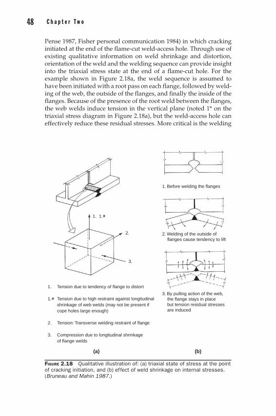
48 C h a p t e r T w o S t r u c t u r a l S t e e l 49
Pense 1987, Fisher personal communication 1984) in which cracking initiated at the end of the flame-cut weld-access hole. Through use of existing qualitative information on weld shrinkage and distortion, orientation of the weld and the welding sequence can provide insight into the triaxial stress state at the end of a flame-cut hole. For the example shown in Figure 2.18a, the weld sequence is assumed to have been initiated with a root pass on each flange, followed by weld-ing of the web, the outside of the flanges, and finally the inside of the flanges. Because of the presence of the root weld between the flanges, the web welds induce tension in the vertical plane (noted 1* on the triaxial stress diagram in Figure 2.18a), but the weld-access hole can effectively reduce these residual stresses. More critical is the welding
1. Before welding the flanges
2. Welding of the outside of flanges cause tendency to lift
3. By pulling action of the web, the flange stays in place but tension residual stresses are induced
Tension due to tendency of flange to distort
Tension due to high restraint against longitudinalshrinkage of web welds (may not be present ifcope holes large enough)
Tension: Transverse welding restraint of flange
Compression due to longitudinal shrinkageof flange welds
1.
1.*
2.
3.
1. 1.*
2.
3.
(b)(a)
Figure 2.18 Qualitative illustration of: (a) triaxial state of stress at the point of cracking initiation, and (b) effect of weld shrinkage on internal stresses. (Bruneau and Mahin 1987.)
02_Bruneau_Ch02_p007-110.indd 48 6/13/11 3:08:04 PM

48 C h a p t e r T w o S t r u c t u r a l S t e e l 49
of the outside of the flanges prior to the inside of the flanges. As shown on Figure 2.18b, this creates a tendency of the flanges to rotate (bow) away from the web. Therefore, the web-flange region at the end of the hole is stressed in tension, and any initial crack or microcracks in this region could propagate further. Assuming that a crack has formed, crack propagation will reduce the flange curvature, which in turn should lower the tensile force at the end of the hole, and the crack will stop propagating once it reaches a finite length. The final path followed by the crack will depend on the magnitude of all the compo-nents of the triaxial stress state shown on Figure 2.18a. A crack may rest in a stable position until external loads applied to the structure raise the stresses to the threshold whereupon crack propagation will resume. Whether total fracture of flange will occur can be determined through use of fracture mechanics.
2.5.8 Fracture MechanicsFracture mechanics (i.e., the study of the behavior and strength of solids having crack discontinuities) is a field of engineering unto itself. A comprehensive presentation of this topic is beyond the scope of this book, and the interested reader is referred to the literature (e.g., Rolfe and Barsom 1999). However, although fracture mechanics has become part of the design process in some applications of engineer-ing (e.g., in ships and airplane hull design and pressure vessels design), it is seldom used at this time for the design of mainstream civil engineering structures such as buildings and bridges (although fatigue, which is an extension of fracture mechanics, is obviously con-sidered in many design situations). However, once brittle failures are encountered, investigators frequently resort to fracture mechanics to explain the observed behavior.
This state-of-practice is partly a consequence of the difficulty and limitations inherent in the currently available fracture mechanics analysis methods. For example, one simple and effective fracture mechanics approach requires comparison of a stress intensity factor, KI, with the fracture toughness, KIC, of the material (also termed criti-cal stress intensity factor). Calculation of KI for a given specimen and crack geometry requires resorting to empirically developed available solutions (Rooke and Cartwright 1976). KIC must be determined by special fracture toughness tests (ASTM 1985a).
For cracks that propagate through base steel, fracture mechanics has proved to be an effective analytical tool. However, for fractures through welds, KIC of the adjacent steel is irrelevant; KIC of the weld itself is needed, a property sensitive to workmanship. This is a prob-lem in postfailure investigations because the KIC of a weld that has failed cannot be inferred from the other welds that have not frac-tured. Furthermore, KIC values obtained on small standard welded
02_Bruneau_Ch02_p007-110.indd 49 6/13/11 3:08:04 PM

50 C h a p t e r T w o S t r u c t u r a l S t e e l 51
specimens may be difficult to reliably extrapolate to large multipass welds; cracks tend to simply propagate through the weakest link between the passes in those welds. An example application of frac-ture mechanics principles to describe the brittle fracture of a high-strength heavy steel section splice with partial penetration welds is presented by Bruneau and Mahin (1987).
2.5.9 Partial Penetration WeldsPartial penetration welds should be avoided whenever ductile response is required (or implied) by design. When structural mem-bers connected by partial penetration welds are loaded to their ulti-mate strength in tension or flexure, only yielding of the weld is possible at best because the cross-sectional area of the weld is smaller than that of the adjacent base metal. As a result, because the weld’s length is rather small, particularly at the root, large ductility of the weld metal translates into small or no ductility at the compo-nent level. Moreover, from a fracture mechanics perspective, the unwelded part of the connected metal can act as an initial crack; this cracklike effect at the toe of a typical partial penetration weld can be clearly seen in Figure 2.19 for a partial penetration weld executed on an 89-mm-thick (3.5-in) flange (cut, polished, and etched to allow visual observation of the weld).
The discontinuity of the base metal produced by the partial penetration weld also introduces a significant stress concentration at the toe of the weld. This is a problem particularly in heavy rolled steel sections because their metallurgy suffers from a reduced frac-ture toughness (KIC), especially in the web-flange core area where the higher stresses occur as a result of this stress concentration. The web-flange core area of a heavy steel section does not get worked to the degree that thinner sections do during the rolling process. It has a “castlike” structure with large grains and inher-ently less fracture toughness. A higher fracture toughness is obtained away from this core area, closer to the outer surface of the flanges, the flange tips, and the bottom surface of flanges. This is in spite of adequate and constant yield stress properties through-out the flange.
2.5.10 K-Area FracturesEven when a structural shape created by the hot rolling process has a fine grain structure, ductile properties, and excellent toughness, some amount of cold working after it has cooled down is often applied to ensure that it meets its specified geometric tolerances. This is achieved by a process called rotary straightening conducted at the mill itself. During rotary straightening, the shape is run through a series of roll-ers to give it its final geometry by removing the undesirable distor-tions that were created by residual stresses during the cooling process.
02_Bruneau_Ch02_p007-110.indd 50 6/13/11 3:08:05 PM

50 C h a p t e r T w o S t r u c t u r a l S t e e l 51
However, such cold working conducted to strengthen a wide-flange shape locally strain hardens the steel and increases its yield and ulti-mate strengths, its hardness, and its ratio of yield-to-ultimate strength, as well as decreases its ductility. These combined effects can have a detrimental affect on the Charpy-V notch toughness over an area where the web meets the flanges—commonly known as the “k-area” (Barsom and Pellegrino 2000, Kaufmann et al. 2001a, Iwankiv and Zoruba 2002, Tide 2000).
More specifically, the k-area in the web starts at the midpoint of the flange-to-web radius and extends approximately 1.5 in beyond the
Figure 2.19 Polished and etched partial penetration weld on a 90-mm-thick (3.5-in) flange.
02_Bruneau_Ch02_p007-110.indd 51 6/13/11 3:08:05 PM

52 C h a p t e r T w o S t r u c t u r a l S t e e l 53
point of tangency between the curved fillet and the web (Figure 2.20); that region roughly corresponds to the part of the web that is cold worked to realign the flanges perpendicular to the web during rotary straightening. The term “k-area” is defined by reference to the dis-tance, k, in wide-flange shapes, which is measured from the top of the flange to the point were the constant-thickness part of the web starts. This k distance is not uniform depending on mill practices. Typically, design manuals list both a minimum and a maximum value of k encompassing the products of the mills they represent—the lower value for calculating web compactness/stability and the high one for detailing purposes (AISC 2001).
Material studies on A572 and A913 Grade 50 steel shapes con-firmed that pre-straining increased the yield and tensile strengths by 20 to 60% and 5 to 20%, respectively (Kaufmann et al. 2001a), as shown in Figure 2.21—a behavior consistent with the idealized behavior illustrated in Figure 2.10 when reloading occurs after an excursion in the strain-hardening range (cold forming), but in this case exceeding the monotonic curve envelope upon reloading. A lower toughness was measured and prestrains of 0.15 to 0.20 were found to initiate cracks within 5 to 10 cycles of hysteretic behavior. Okazaki and Engelhardt (2007) also observed fractures initiating in the k-area of many tested links of the types used in eccentrically braced frames after a few cycles of hysteretic behavior, along with higher tensile strength and reduced toughness and ductility in the k-area of the links. Yet, beam-to-column connections specimens tested by Chi and Uang (2004), with holes drilled in the k-area to act as crack initiator with intent of triggering early fractures, actually performed satisfactorily, with substantial hysteretic behavior.
In light of the above observed possible impact of rotary straight-ening and limited statistical data on expected levels of prestrains,
k
k
1 in to 1 1/2 in (25 to 38 mm)
1 in to 1 1/2 in (25 to 38 mm)
Area of potentially lowernotch toughness in
rotary-straightened W-shapes
Figure 2.20 Typical k-area for a wide-flange shape. (AISC 2010, copyright © American Institute of Steel Construction. Reprinted with permission. All rights reserved.)
02_Bruneau_Ch02_p007-110.indd 52 6/13/11 3:08:06 PM
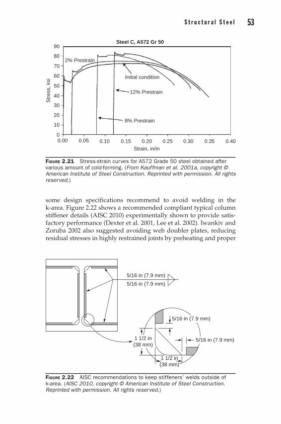
52 C h a p t e r T w o S t r u c t u r a l S t e e l 53
some design specifications recommend to avoid welding in the k-area. Figure 2.22 shows a recommended compliant typical column stiffener details (AISC 2010) experimentally shown to provide satis-factory performance (Dexter et al. 2001, Lee et al. 2002). Iwankiv and Zoruba 2002 also suggested avoiding web doubler plates, reducing residual stresses in highly restrained joints by preheating and proper
Steel C, A572 Gr 5090
80
70
60
50
40
30
20
10
0
Str
ess,
ksi
0.00 0.05 0.10 0.15 0.20 0.25 0.30 0.35 0.40Strain, in/in
8% Prestrain
12% Prestrain
Initial condition
2% Prestrain
Figure 2.21 Stress-strain curves for A572 Grade 50 steel obtained after various amount of cold-forming. (From Kauffman et al. 2001a, copyright © American Institute of Steel Construction. Reprinted with permission. All rights reserved.)
5/16 in (7.9 mm)
5/16 in (7.9 mm)
5/16 in (7.9 mm)
5/16 in (7.9 mm)
1 1/2 in(38 mm)
1 1/2 in(38 mm)
Figure 2.22 AISC recommendations to keep stiffeners’ welds outside of k-area. (AISC 2010, copyright © American Institute of Steel Construction. Reprinted with permission. All rights reserved.)
02_Bruneau_Ch02_p007-110.indd 53 6/13/11 3:08:07 PM

54 C h a p t e r T w o S t r u c t u r a l S t e e l 55
sequencing of welding, and magnetic particle or dye penetrant inspection of the welds in the k-area.
Note that while embrittlement of the k-area was found likely to have a critical impact on steel structures that require highly ductile behavior at the component level (such as in seismic-resistant design applications), it was also occasionally reported to be problematic in some nonyielding applications where cracking in the k-area of galva-nized beams was attributed to liquid metal embrittlement (BCSA 2005, Kinstler 2005), a phenomena whose definitive atomic mecha-nism is still being investigated.
2.5.11 Strain AgingWhen unloaded after an excursion into the strain-hardening range, steels left unstressed for a period of time will experience a modifica-tion in their molecular structure that will translate, upon reloading, into an increase of their yield and tensile strengths as well as a decrease in ductility and fracture toughness (Barsom and Korvink 1998, Pense 2004), as illustrated in Figure 2.23. This phenomenon, known as static strain aging, is attributed to the filling of material dislocations by migrating nitrogen and carbon atoms. Dislocations are defects in the crystals structure of steel that facilitate the develop-ment of slip planes (i.e., yielding), and that are “locked” when filled by the migrating atoms (Baird 1963, 1971; Cottrell and Bilby 1949;
Pre-strain
Ductility of virgin material
Ductility after strain-hardening and strain aging
Strain
Strain-hardening rangeInitial lower yield
extention
Str
ess
Decreased elongationdue to strain aging
Increase in tensile strengthdue to strain aging
Increase in yield strengthdue to strain aging
Figure 2.23 Effect of Strain Aging. (Barsom and Korwink 1998—with permission from SAC Joint Venture, a Partnership of the Structural Engineers Association of California, Applied Technology Council, and Consortium of Universities for Research in Earthquake Engineering.)
02_Bruneau_Ch02_p007-110.indd 54 6/13/11 3:08:07 PM

54 C h a p t e r T w o S t r u c t u r a l S t e e l 55
Pense 2004). Although some industries working with deformed sheet steel (such as the automotive industry) have had to contend with strain-aging issues, structural steels used in construction have more carbon and alloys and a more complex microstructure that has pre-vented strain aging at ambient temperature. However, at a tempera-ture of 400°F (200°C), substantial strain aging can develop in those structural steel within a few hours. Caution is thus warranted when cold forming at relatively high temperatures. Incidentally, Barsom and Korvink (1998) indicated that if rotary straightening operations are conducted at less than 200°F (93°C), the degradation of properties in the k-area attributable to strain-hardening will be more significant than the secondary effects of strain aging.
2.5.12 Stress CorrosionMany guides and documents address the topic of corrosion, provid-ing engineering advice on how to protect steel against corrosive envi-ronments and detail structures such as to avoid trapping liquids or solids that could trigger or accelerate the corrosion process (e.g., Koch et al. 2002). Engineering procedures also exist to calculate the residual strength of structural members that have lost cross-sectional area due to severe corrosion, or to predict such losses as a function of time (e.g., Kayser and Novak 1989, Kulicki et al. 1990).
Stress corrosion is a less familiar phenomenon that is known to happen in various metals, such as certain steels and copper alloys, as well as numerous types of polymers. It can transform ductile steel into a brittle material without substantial visible evidence of this process taking place. Stress corrosion cracking can develop unex-pectedly when materials under tensile stresses are exposed to spe-cific chemicals (hydrogen embrittlement is sometimes considered a subset of stress corrosion). The process is accelerated at higher tem-peratures. Under these conditions, small surface cracks propagate inside the steel, even when exposed to low stress levels considered not critical per fracture mechanics models (e.g., stress corrosion cracks have been reported to propagate in conditions corresponding to less than 1% of the critical stress intensity factor, KIC). Although this phenomenon is of obvious impact to chemical and petrochemi-cal industries, it has also occasionally had adverse effects on conven-tional public infrastructures.
Certain types of stainless steel used structurally are known to be highly sensitive to stress corrosion if exposed to water or vapors con-taining traces of chlorides. Such a chloride attack led to the collapse of a concrete roof supported by stainless steel tension bars over a swimming pool at Uster near Zurich in 1985 (Faller and Richner 2003). Similar structures in Europe collapsed, or were found at imme-diate risk of failure and retrofitted with galvanized steel or stainless steel bars of a different grade having greater resistance to stress
02_Bruneau_Ch02_p007-110.indd 55 6/13/11 3:08:07 PM

56 C h a p t e r T w o S t r u c t u r a l S t e e l 57
corrosion cracking. Although stainless steel has a history of satisfactory performance in multiple applications in which it is either unstressed or intermittently stressed, corrosion cracking can become a threatening failure mode under sustained tensile stresses of any magnitude.
Stress corrosion cracks in regions of large residuals stresses, together with other factors, led to the fracture of a critical eye-bar joint and the ensuing collapse of the Point Pleasant “Silver” Bridge in Ohio, in December 1967 (Fisher 1984, NTSB 1971). Sulphur, an ele-ment not belonging to the metal itself, was detected in the critical crack (and other subcritical cracks) during the forensic investigation, possibly diffused as a consequence of the sulphur dioxide emissions of a local power station using high-sulphur West Virginia coal and/or a foundry close to the east side of the bridge. Tests as part of the investigation indicated that exposure to hydrogen sulphide produced stress corrosion and reduced the fatigue resistance of the material used in the eyebars that fractured.
Figure 2.24 illustrates typical “branches” of stress corrosion cracks having penetrated inside the flange of a structural steel shape, virtually undetectable from the un-attacked steel surface (Ahluwalia 2003).
Stress corrosion due to the diffusion of atomic hydrogen at the tips of cracks in the wires used in cable-supported bridges has been
(a)
Figure 2.24 Chloride stress corrosion cracks developing in stainless steel Grade 304L, in region of residual tensile stresses due to welding. (Courtesy of Dr. Hira Ahluwalia, Material Selection Resources Inc., www.doctormetals .com.)
02_Bruneau_Ch02_p007-110.indd 56 6/13/11 3:08:08 PM
56 C h a p t e r T w o S t r u c t u r a l S t e e l 57
reported to explain the observed ductility losses in such wires (Mahmoud 2003a, 2003b). Figure 2.25 shows the relatively brittle fracture, without cross-sectional necking, of a wire affected by such hydrogenation, by contrast to a regular wire, underlining the need to consider this condition in structural safety evaluations.
Avoidance of stress-corrosion cracking can be best achieved by selection of materials not susceptible to such degradation when exposed to specific chemical or aqueous environments (e.g., using data compiled by NPL 1982), although this is not always possible. Other approaches include heat treatment to relieve residual stresses introduced by welding, avoiding details that induce stress raisers (e.g., using full penetration welds instead of fillet welds), avoiding cold work, or shot peening (Marsh 1993). That latter metal treatment consists of bombarding the surface of the steel at risk with spherical projectiles to plastically deform it into a layer of compression stresses, eliminating the tensile stresses at the surface (see MIC 2005 for details).
2.5.13 Corrosion FatigueCorrosion fatigue is another type of environmentally assisted crack-ing known to have led to structural failures—for example, it contrib-uted to the collapse of Kinzua Viaduct in Pennsylvania during a wind
(b)
Figure 2.24 (Continued )
02_Bruneau_Ch02_p007-110.indd 57 6/13/11 3:08:09 PM

58 C h a p t e r T w o S t r u c t u r a l S t e e l 59
storm in July 2003 (DCNR 2003). By contrast with stress corrosion cracking, it develops in uniformly corroded materials, with cracks that could be visible, if exposed, as for regular fatigue cracks. The detrimental consequence of corrosion fatigue is that it substantially reduces fatigue life of steel details, connections, and members under
Lab file no. 91–23 Specimen no. 4–1
240
200
160
120
80
40
00.0 0.2 0.4 0.6 0.8 1.0 1.2 1.4 1.6 1.8 2.0
Strain, %
Str
ess,
ksi
Hydrogenembrittlementshowing
Top: Tension specimenside view with minimalnecking and low ductility
Right: Stress-straincurve
(a)
Figure 2.25 Fracture and force displacement response of wires taken from a suspension bridge cable, showing: (a) relatively brittle response and (b) ductile response. (Courtesy of Khaled M. Mahmoud of Bridge Technology Consulting (BTC), New York.)
02_Bruneau_Ch02_p007-110.indd 58 6/13/11 3:08:10 PM

58 C h a p t e r T w o S t r u c t u r a l S t e e l 59
cyclic loading, and that it eliminates the fatigue limit (i.e., the stress below which high-cycle fatigue life is theoretically infinite for a spec-ified detail). In stress corrosion the period of crack nucleation is sub-stantially shorter, with crack propagation initiating sooner with sustained growth in stress regimes below the critical stress intensity factor (KIC). However, given that high-cycle fatigue is beyond the scope of this book (as described in Section 2.6), so is a detailed exposé
Lab file no. 91–23 Specimen no. 3–N240
200
160
120
80
40
00.0 0.2 0.4 0.6 0.8 1.0 1.2 1.4 1.6 1.8 2.0
Strain, %
Str
ess,
ksi
Stress corrosioncracking showing:
Top: Tension specimenside view with appreciablenecking
Right: Stress-straincurve
(b)
Figure 2.25 (Continued )
02_Bruneau_Ch02_p007-110.indd 59 6/13/11 3:08:11 PM

60 C h a p t e r T w o S t r u c t u r a l S t e e l 61
of the effects of corrosion fatigue. Corrosion fatigue can be prevented through the same mechanisms and procedures adopted to prevent regular fatigue and corrosion.
2.5.14 Ductility of Corroded SteelIt is recognized that the presence of severe corrosion can typically result in increased stress levels for a given load or in larger stress ranges under fatigue-type cyclic loading, as well as some notable shifts in the type of ultimate failure expected as some geometric prop-erties and failure modes are related to the square or cube of member dimensions (Kayser and Nowak 1989). However, experimental stud-ies on the behavior of corroded members, although few, indicate that the monotonic structural ductility of steel is not detrimentally affected by corrosion. For example, Fisher et al. (1990) conducted ultimate strength tests on two severely corroded bridge hangers having approximately 40% area loss and taken from an actual bridge. They found that the hangers could resist maximum axial loads correspond-ing to the tensile strength calculated using the effective net area of the most rusted region of the member, while exhibiting no considerable reduction in the monotonic structural ductility of the specimens. Sim-ilar behavior was observed by Bruneau and Zahrai (1997) for cor-roded A7 steel coupons taken from an existing bridge, although a 30% reduction in the elongation at failure was noted, as shown in Figure 2.26.
500
400
300
200
100
00.00 0.04 0.08 0.12 0.16 0.20 0.24
Strain
G40.4 (A7) SteelRusted flangeRusted web 1Rusted web 2
Tens
ile s
tres
s (M
Pa)
Figure 2.26 Experimentally obtained stress-strain relationship for rusted coupons (normalized by area computed using minimum thickness of rusted coupon), compared with typical stress-strain curve of unrusted A7 steel (Zahrai and Bruneau 1998).
02_Bruneau_Ch02_p007-110.indd 60 6/13/11 3:08:12 PM

60 C h a p t e r T w o S t r u c t u r a l S t e e l 61
Knowledge on the cyclic ductility of corroded steel is limited, but important given that the hysteretic behavior of steel members may be relied upon to dissipate earthquake energy. These members would need to perform as intended even if rusted by the time a major earth-quake strikes (in a distant future). Cyclic inelastic flexural on struc-tural members revealed that, although stable hysteretic behavior comparable with that of unrusted specimens is possible, fracture under alternating plasticity (i.e., low-cycle fatigue) will typically develop sooner than for comparable unrusted members. However, the considerable cumulative hysteretic energy dissipated in those tests prior to the development of fatal cracking was deemed sufficient to provide adequate seismic resistance in most applications, as shown in Figure 2.27. However, the impact of large corrosion notches or more severe levels and types of corrosion than considered by Bruneau and Zahrai (1997) deserve further experimental study.
x
Loadingpoint
Rigid base
343
686
350 (mm) I 27" × 10" @91(1940)
Critical section SW-II
Critical section SW-I
Actuator
Reaction column
10
5
0
–5
–10
Late
ral l
oad,
kN
–80 –60 –40 –20 0 20 40 60 80Displacement, mm
4553
56
13, 41
Figure 2.27 Cyclic ductility of corroded steel: (a) test set-up, (b) resulting hysteretic behavior (Zahrai and Bruneau 1998).
02_Bruneau_Ch02_p007-110.indd 61 6/13/11 3:08:12 PM

62 C h a p t e r T w o S t r u c t u r a l S t e e l 63
2.6 Low-Cycle versus High-Cycle Fatigue
2.6.1 High-Cycle FatigueCrystal imperfection, dislocations, and other micro cracks in steel can grow into significant cracks in structural components subjected to the action of repeated loads. For example, various components in bridges subjected to heavy traffic loading and offshore structures subjected to wave loading will be subjected to millions of cycles of load during their service life. These components must be detailed with proper care to provide adequate resistance against crack initiation and crack propagation. The ability of metals and specific welded details to resist many hundreds of thousand cycles of strain below the yield level is termed “high-cycle fatigue resistance.” One accomplishes design to ensure this resistance by limiting the maximum stress range due to cyclic loading to values that are usually much below the yield stress and by selecting details that minimize stress concentrations (Rolfe and Barsom 1999, Stephens et al. 2001). The design of these members can be accomplished according to traditional steel design methods, with stress ranges presented in various standards, and is therefore beyond the scope of this book.
2.6.2 Low-Cycle FatigueAnybody who has ever destroyed paper clips knows that these can be bent back and forth only a limited number of times. Some may even have noticed that the maximum number of cycles these paper clips can resist is a function of the severity of their postyield plastic deforma-tions. The ability of metals to resist a limited and quantifiable number of strain cycles above the yield level is termed “low-cycle fatigue resis-tance” or “resistance to alternating plasticity.” Although both low-cycle fatigue and high-cycle fatigue failures result from similar crack initia-tion and crack growth mechanisms, only low-cycle fatigue resistance characterizes the cyclic response of components and connections deformed beyond the yield limit and is thus related to ductile design.
There is also a significant difference between the low-cycle fatigue resistance of the material obtained by tests on coupons of the base metal and that of actual structural members. This difference principally arises as a result of the rather large inelastic strains that develop upon local buckling. For example, although tests of coupons indicate that mild steel can resist more than 400 cycles at a strain of 0.025 (ASM 1986), Bertero and Popov (1965) showed that local buckling in a steel beam of compact cross-section in bending started after half a cycle at that strain and that fracture occurred after the 16th cycle. Indeed, in steel sections that can develop their plastic moment capacity (see Chap-ter 3), local buckling due to cyclic loading will occur at smaller strains than predicted for monotonic loads, because the inelastic curvatures
02_Bruneau_Ch02_p007-110.indd 62 6/13/11 3:08:12 PM

62 C h a p t e r T w o S t r u c t u r a l S t e e l 63
introduced in the flanges of beams subjected to flexural moments above the yield moment will typically act as initial imperfections and help trigger local buckling upon reversal of loading. This explains why smaller maximum width-to-thickness ratios are required by codes for members subjected to cyclic loading (as will be shown later). Fortu-nately, low-cycle fatigue resistance increases rapidly with reductions in the maximum cyclic strain (Figure 2.28). Steel structures detailed for ductile response must be able to resist the expected cyclic inelastic deformation demands without prematurely failing by low-cycle fatigue—usually an implicit goal of design specifications.
The low-cycle fatigue life of a material is established by conduct-ing axial tests on standard coupons subjected to fully reversed cycles of constant strain amplitudes. By repeating such tests for various values of strain amplitude, it is possible to correlate strain ampli-tude, ea, to the number of cycles, Nf , or the number of load reversals, 2Nf , applied before fracture. Such a curve is schematically shown in Figure 2.29, and is asymptotic to two straight lines of slopes b and c: one for high-cycle fatigue in the elastic range, and one at large inelas-tic cyclic plastic strains, respectively. The total strain range, Δe, being equal to twice the strain amplitude (i.e., ranging from −ea to +ea), can be expressed in terms of elastic and plastic ranges, Δee and Δep, respectively, such that:
e e e e s
eae p f
fb
f fc
EN N= = + =
′+ ′
Δ Δ Δ2 2 2
2 2( ) ( ) (2.11)
where sf′/E and ef′ are the intersects of the elastic and plastic asymp-totic lines with the vertical axis of the graph in Figure 2.29, sf′ and ef′ are defined as the fatigue strength coefficient and fatigue ductility coefficient, and b and c are respectively known as the fatigue strength exponent and the fatigue ductility exponent.
The later half of that equation, concerned with low-cycle fatigue at large inelastic strains, is the original Coffin-Manson relationship (Coffin 1954, Manson 1953), namely:
Δeep
f fcN
22= ′ ( ) (2.12)
Regression analysis on experimental data is performed to obtain the values of sf′, ef′, b, and c. For example, these values derived for A572 Gr. 50 rolled shapes (Kaufmann et al. 2001b) and for four grades of steel plates (Dusicka et al. 2007) are summarized in Table 2.4 for the data shown in Figure 2.30.
In most applications, however, the cycles of inelastic strains applied to a structure are of variable amplitudes. To calculate low-cycle fatigue life, a procedure is required to convert the irregular cycles of variable strain amplitude into sets of equivalent regular
02_Bruneau_Ch02_p007-110.indd 63 6/13/11 3:08:13 PM
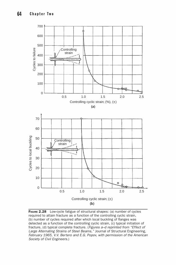
64 C h a p t e r T w o S t r u c t u r a l S t e e l 65
Controllingstrain
70
60
50
40
30
20
10
00.5 1.0 1.5 2.0 2.5
Controlling cyclic strain; (±)(b)
Cyc
les
to lo
cal b
uckl
ing
Cyc
les
to fa
ilure
700
600
500
400
300
200
100
0
Controllingstrain
0.5 1.0 1.5 2.0 2.5
Controlling cyclic strain; (%), (±)(a)
Figure 2.28 Low-cycle fatigue of structural shapes: (a) number of cycles required to attain fracture as a function of the controlling cyclic strain, (b) number of cycles required after which local buckling of flanges was detected as a function of the controlling cyclic strain, (c) typical initiation of fracture, (d) typical complete fracture. (Figures a–d reprinted from “Effect of Large Alternating Strains of Steel Beams,” Journal of Structural Engineering, February 1965, V.V. Bertero and E.G. Popov, with permission of the American Society of Civil Engineers.)
02_Bruneau_Ch02_p007-110.indd 64 6/13/11 3:08:15 PM

64 C h a p t e r T w o S t r u c t u r a l S t e e l 65
Edge ofclamping block
(c)
Edge ofclamping block
(d)
Figure 2.28 (Continued )
02_Bruneau_Ch02_p007-110.indd 65 6/13/11 3:08:17 PM

66 C h a p t e r T w o S t r u c t u r a l S t e e l 67
cycles of constant amplitude, and a combination rule must be used to establish how these sets of cycles at different constant amplitudes can be added. Such a procedure can also be used to assess “damage accu-mulation,” that is, the percentage of the total fatigue life that has been used during a given strain history.
rf (MPa/ksi) b df c
A572 Grade 501 – – 0.03 −0.515
A709M Grade 345W2
894/130 −0.082 0.535 −0.590
A709M HPS 4852
886/129 −0.072 0.432 −0.575
BT-HT-440C2 1000/145 −0.101 0.422 -0.524
BT-LP1002 475/68.8 −0.081 0.275 −0.459
GT-LP2252 507/73.6 −0.063 0.446 −0.612
[1From Kaufmann et al. (2001b); 2from Dusikca et al. (2007).]
Table 2.4 Estimated Coffin-Manson Parameters for Low-Cycle Fatigue of Various Steels
∆ε
∆εp
ε′f
c
b
1
1
Totalstrain
Plasticstrain
1 2Nt
Reversals to failure, 2Nt (log scale)
Elasticstrain
α′f /E
Str
ain
ampl
itude
(lo
g sc
ale)
Figure 2.29 Strain amplitude versus number of load reversals to failure. (Stephens et al. 2001, reprinted with permission of John Wiley & Sons, Inc.)
02_Bruneau_Ch02_p007-110.indd 66 6/13/11 3:08:18 PM
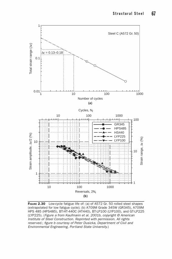
66 C h a p t e r T w o S t r u c t u r a l S t e e l 67
1
0.1
0.011 10 100 1000
Number of cycles(a)
∆ε = 0.13–0.18
Steel C (A572 Gr. 50)To
tal s
trai
n ra
nge
(∆ε)
100
10
1
Str
ain
rang
e, ∆
ε (%
)
100010010Reversals, 2Nf
(b)
10 100 1000
Cycles, Nf
10
1
GR345HPS485HS440LYP225LYP100
Str
ain
ampl
itude
, ∆ε/
2 (%
)
Figure 2.30 Low-cycle fatigue life of: (a) of A572 Gr. 50 rolled steel shapes (extrapolated for low fatigue cycle); (b) A709M Grade 345W (GR345), A709M HPS 485 (HPS485), BT-HT-440C (HT440), BT-LP100 (LYP100), and GT-LP225 (LYP225). (Figure a from Kaufmann et al. 2001b, copyright © American Institute of Steel Construction. Reprinted with permission. All rights reserved.; figure b courtesy of Peter Dusicka, Department of Civil and Environmental Engineering, Portland State University.)
02_Bruneau_Ch02_p007-110.indd 67 6/13/11 3:08:19 PM

68 C h a p t e r T w o S t r u c t u r a l S t e e l 69
The rainflow method (Matsuishi and Endo 1968) is the most fre-quently used technique to count the number of cycles of various amplitudes in an arbitrary strain history (although other equivalent approaches are also encountered in the literature, such as the range-pair, the racetrack counting, the level-crossing, and the peak counting methods). The rainflow-counting algorithm has been widely imple-mented in various software and freeware.
Figure 2.31 illustrates how the procedure is used to count cycles (which are strain cycles for the case of low-cycle fatigue calculations,
A (25)
C (14)E (16)
G (7)
F (2)B (5)
D (–14)H (–12)
I (25)
Time
25
20
15
10
5
0
–5
–10
–15
Load
, str
ess,
or
stra
in
(a)
Time
2520151050–5–10–15
Load, stress, or strain
A
C
E
B
B¢
F¢
F
E¢H
D
G
I
(b)
Figure 2.31 Rainflow counting procedure: (a) original stress or strain history, (b) rainflow analysis on rotated history, and (c) resulting cycles. (Stephens et al. 2001, reprinted with permission of John Wiley & Sons, Inc.)
02_Bruneau_Ch02_p007-110.indd 68 6/13/11 3:08:20 PM
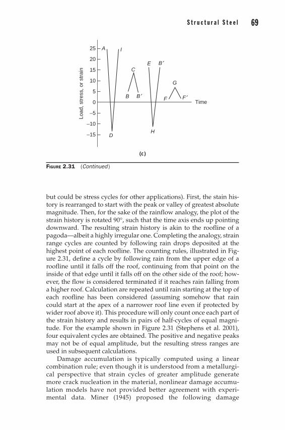
68 C h a p t e r T w o S t r u c t u r a l S t e e l 69
but could be stress cycles for other applications). First, the stain his-tory is rearranged to start with the peak or valley of greatest absolute magnitude. Then, for the sake of the rainflow analogy, the plot of the strain history is rotated 90°, such that the time axis ends up pointing downward. The resulting strain history is akin to the roofline of a pagoda—albeit a highly irregular one. Completing the analogy, strain range cycles are counted by following rain drops deposited at the highest point of each roofline. The counting rules, illustrated in Fig-ure 2.31, define a cycle by following rain from the upper edge of a roofline until it falls off the roof, continuing from that point on the inside of that edge until it falls off on the other side of the roof; how-ever, the flow is considered terminated if it reaches rain falling from a higher roof. Calculation are repeated until rain starting at the top of each roofline has been considered (assuming somehow that rain could start at the apex of a narrower roof line even if protected by wider roof above it). This procedure will only count once each part of the strain history and results in pairs of half-cycles of equal magni-tude. For the example shown in Figure 2.31 (Stephens et al. 2001), four equivalent cycles are obtained. The positive and negative peaks may not be of equal amplitude, but the resulting stress ranges are used in subsequent calculations.
Damage accumulation is typically computed using a linear combination rule; even though it is understood from a metallurgi-cal perspective that strain cycles of greater amplitude generate more crack nucleation in the material, nonlinear damage accumu-lation models have not provided better agreement with experi-mental data. Miner (1945) proposed the following damage
A
C
I
B B¢ F¢
B¢E
G
FTime
25
20
15
10
5
0
–5
–10
–15
Load
, str
ess,
or
stra
in
DH
(c)
Figure 2.31 (Continued )
02_Bruneau_Ch02_p007-110.indd 69 6/13/11 3:08:21 PM

70 C h a p t e r T w o
accumulation model, also known as the Palmgren-Miner linear damage rule:
D
nN
nN
nN
i
ii
j
= = + + ==∑
1
1
1
2
2
1 (2.13)
where Ni is the number of cycles that can be resisted at a single given constant amplitude strain level Si (this being essentially the data used to plot low-cycle fatigue life curves such as in Figure 2.30), ni is the number of cycles in the strain history under consideration applied at this constant amplitude level (obtained from the rainflow method), and D is a damage index, assumed to be equal to 1.0 when median fatigue life is reached. Likewise, Miner’s rule is commonly used to assess the expended percentage of fatigue life, that is, when the dam-age index calculated per the above equation is less than 1.0.
2.7 Material ModelsOnce an appropriately ductile steel material has been chosen for a specific application, suitable stress-strain or moment-curvature mod-els must be adopted for the purpose of calculations. Because increases in model complexity often translate into additional computational difficulties, simple models may provide, in many cases, sufficiently accurate representations of behavior. Some of the simpler models commonly used are described below.
2.7.1 Rigid Plastic ModelAs the name implies, the rigid plastic model neglects elastic deforma-tions. The material is assumed to experience no strain until the yield stress is reached, and flexural components modeled with rigid plastic behavior undergo no curvature until the plastic moment is reached. This rudimentary model, illustrated in Figure 2.32a, can be useful, for example, when the plastic collapse load capacity of a structure is sought, as will be seen in Chapter 4. It has been used to model nonlin-ear friction hysteretic energy dissipation, in terms of forces versus displacement, in structures wherein this behavior could be relied upon to resist extreme dynamic lateral loads (e.g., Dicleli and Bruneau 1995). However, because this model implies infinite stiffness until plastification is reached and null stiffness thereafter, it is best suited for hand calculations and can be difficult to implement in structural analysis programs based on the stiffness-matrix method.
2.7.2 Elasto-Plastic ModelsWhen response under progressive loading until collapse is desired, or when an accurate calculation of nonlinear deflections is needed,
02_Bruneau_Ch02_p007-110.indd 70 6/13/11 3:08:21 PM

70 C h a p t e r T w o
σ or
Mσ
or M
σ or
M
E o
r E
I = 0
E o
r E
I = ∞
E o
r E
I = 0
E o
r E
IE
or
EI
E o
r E
I
E o
r E
IE
or
EI
E o
r E
I
ε or
ϕε
or ϕ
ε or
ϕ
(a)
(b)
(c)
(d)
(e)
(f)
E =
0E
= 0
σσ
σ
Esh
Esh
EE
E
EE O
ptio
nally
mod
elin
gB
ausc
hing
er e
ffect
E
εε
ε
ε max
A2
A1
Fig
ur
e 2
.32
Som
e cy
clic
mat
eria
l mod
els
for
stru
ctur
al s
teel
: (a
) bi
linea
r rigi
d-pe
rfec
tly
plas
tic,
(b)
bili
near
ela
sto-
perf
ectly
plas
tic,
(c)
bili
near
el
asto
-pla
stic
with
stra
in-h
arde
ning
, (d
) tr
iline
ar e
last
o-pl
astic
with
stra
in-h
arde
ning
, (e
) cy
clic
mod
el fro
m m
onot
onic
-load
ing
stre
ss-s
trai
n cu
rve,
an
d (f
) bi
linea
r el
asto
-pla
stic
with
stra
in-h
arde
ning
slo
pe b
ased
on
equa
l ene
rgy
diss
ipat
ion.
71
02_Bruneau_Ch02_p007-110.indd 71 6/13/11 3:08:21 PM

72 C h a p t e r T w o S t r u c t u r a l S t e e l 73
an elasto-perfectly plastic model is generally used. This hysteretic model considers two possible stiffness states: elastic or plastic, as shown in Figure 2.32b. The choice of zero postyield stiffness is suitable for many applications in which strain-hardening is not anticipated, and conservative for predicting the plastic collapse load and deforma-tions whenever strain-hardening would be expected to develop.
A computer is generally needed to take advantage of the features of this bilinear model, so one can easily consider the effect of strain-hardening by assigning a nonzero postyielding stiffness; in fact, for numerical analysis reasons, nonzero positive stiffness is often desir-able. Such an elasto-plastic model with nonzero postyield stiffness to account for strain-hardening is illustrated in Figure 2.32c. Various methods can be used to determine an appropriate postyield stiffness to model material or member behavior. One such reasonable approach, shown in Figure 2.32f, consists of finding the slope of the straight line that would bisect the true stress-strain diagram in the plastic range such that an equal amount of plastic energy is dissipated before fail-ure. To equate the energy, however, iterative procedures are generally needed to determine the maximum strains, emax, of all the yielded members in the structure, which is by no means a simple task. There-fore, values ranging between 0.005 and 0.05 times elastic stiffness are commonly used for the strain-hardening (postyield) stiffness in bilin-ear models. Lower strain-hardening stiffness values will generally produce larger maximum plastic strains and curvatures, whereas higher values will translate into larger stresses and moments.
As reflected in the available literature, the bilinear elasto-plastic model has been widely used to model the cyclic hysteretic behavior of steel frame structures (although in some ways, this has often been constrained by the limitations of computer programs capable of cyclic hysteretic analysis). More complex piece wise linear stress-strain models (Figure 2.32d) or other models (Figure 2.32e) have sometimes been used for analysis. However, the presumed additional benefit gained from the use of such models must always be weighed against all of the uncertainties associated with the design process, particu-larly when earthquakes are responsible for these hysteretic cycles.
2.7.3 Power, Ramberg-Osgood, and Menegotto-Pinto Functions
Another class of material models, known as power functions, is par-ticularly useful to analytically describe the experimentally obtained stress-strain relationships of various alloys. Although these functions complicate the characterization of the stress-strain relationship of low-grade steels having a well-defined yield plateau, they can effec-tively describe the inelastic moment-curvature relationships of mem-bers made with these steels, and even the inelastic shear force versus shear strain relationships in some other applications. Therefore, it is worthwhile to be familiar with these power function models.
02_Bruneau_Ch02_p007-110.indd 72 6/13/11 3:08:22 PM

72 C h a p t e r T w o S t r u c t u r a l S t e e l 73
To remove some of the mathematical abstraction associated with power function models, the discussion is presented within the con-text of a numerical example. The data tabulated in Table 2.5, obtained from a standard tensile test of an aluminum specimen, is used for this purpose. Although this example is expressed in terms of stresses and strains, note that power functions can also be developed to model other behaviors expressed by a pair of related parameters, such as moments and curvatures, with only minor modifications.
Before a demonstration of how power functions can be used to model the stress-strain behavior of this aluminum alloy, it is worth-while to note that, in this particular example, an elasto-perfectly plas-tic model of this material would provide a reasonably accurate
Experimental DataPower Function Ramberg-Osgood Menegotto-Pinto
r (ksi) d d d r (ksi)
0 0 0.0 0.0 0.0
5 0.0005 0.0005 5.0
10 0.00102 0.0010 0.0010 10.2
15 0.00151 0.0015 15.1
20 0.00202 0.0020 0.0020 20.1
25 0.00251 0.0025 24.8
30 0.00301 0.0030 0.0030 29.2
31 0.00311 0.0031 30.0
32 0.00321 0.00321 30.7
33 0.00333 0.00333 31.6
34 0.00345 0.00348 32.4
35 0.0037 0.00371 34.0
36 0.0042 0.0041 0.00416 36.3
37 0.0052 0.0051 0.00516 38.8
38 0.008 0.0074 0.00748 40.1
39 0.015 0.01297 40.4
40 0.0265 0.0258 40.5
41 0.056 0.056 0.0555 41.0
42 0.122 0.123 42.0
1 ksi = 6.895 MPa
Table 2.5 Stress-Strain Data for Aluminum Alloy Tensile Test and Results from Various Models
02_Bruneau_Ch02_p007-110.indd 73 6/13/11 3:08:22 PM

74 C h a p t e r T w o S t r u c t u r a l S t e e l 75
representation of the material behavior. Through a graphical method and the traditional 0.2% offset rule, the yield stress, sy, is calculated to be 37 ksi (255 MPa), and the corresponding yield strain, ey , is 0.0037. The resulting elasto-perfectly plastic material curve could be drawn by joining the following three stress-strain (s, e) points: (0, 0), (37, 0.0037), and (37, ∞). Likewise, an elasto-plastic strain-hardening model could be developed after some trial and error to define an appropriate strain-hardening stiffness.
2.7.3.1 Power Functions The fundamental tenet of a power function is that the strain-stress relationship can be divided into an elastic part and a plastic part as shown:
e e e s s
total elastic plastic Ea
E
n= + = +
(2.14)
Terms for this equation are defined in Figure 2.33a. The task therefore lies in determining the parameters a and n that will provide best fit to the data. From the above expression, it transpires that the plastic strain can be expressed as a function of the elastic strain if Eq. (2.14) is manipulated, to obtain:
e s eplastic a
Ea
n
elasticn=
= (2.15)
or, taking the logarithm of both sides of this equation,
log log log log(e e eplastic elastic
nelaa a n= ( ) = + sstic ) (2.16)
Elastic
ETotal
εelastic εplastic
σ
(a) (b)
Log εplastic
Log εelastic
Pt. 1
Pt. 2
Figure 2.33 Power function material models for structural steel.
02_Bruneau_Ch02_p007-110.indd 74 6/13/11 3:08:24 PM

74 C h a p t e r T w o S t r u c t u r a l S t e e l 75
As illustrated in Figure 2.33b, Eq. (2.16) is the equation of a straight line of slope n in a logarithmic space—that is, a straight line when plotted on log-log paper. Because all experimentally obtained data points will not always fall on a straight line, a least-squares solution could be used to find the best approximation to the true stress-strain curve. However, in most practical cases, this level of refinement is not necessary. A reasonably accurate result can be obtained if one takes two strain data points as far apart as possible, but not on the linear branch of the stress-strain curve where eplastic would be zero, and calcu-lates the values of a and n using the following relationships:
n plastic plastic
elastic
=--
- -
-
log log
log
e ee
2 1
2 llogeelastic-
1
(2.17)
and
log log loga nplastic elastic= -- -e e1 1 (2.18)
For the current example, assuming an elastic modulus of 10,000 ksi and arbitrarily taking for the two strain data points e = 0.0037 (at s = 35 ksi, for which eelastic = 0.0035 and eplastic = 0.0002) and e = 0.1220 (at s = 42 ksi, for which eelastic = 0.0042 and eplastic = 0.1178), Eq. (2.17) and (2.18) give n = 35.0 and a = 1.66 × 1082, respectively, which can be substituted in the general power function expression. This gives the following result:
e s s= + ×
0 0001 1 66 1010000
8235 0
. ..
(2.19)
The accuracy of this solution could be verified if it were plotted against the experimental data. However, because the resulting differ-ence is rather small, results are instead compared through use of Table 2.5, and judged to be satisfactory.
Although the resulting expression may appear awkward to manipulate for hand calculations, the ability to express the entire stress-strain relationship by a single continuous function can be advantageous, particularly for computer programming purposes.
2.7.3.2 Ramberg-Osgood FunctionsIn earthquake engineering, Ramberg-Osgood functions are often used to model the behavior of structural steel materials and compo-nents. These functions are obtained when the above power function is normalized by an arbitrary strain, e0, for which the plastic compo-nent of strain, eplastic, is not zero. Generally, the yield strain, ey, pro-vides a good choice for this normalizing strain, but other choices are
02_Bruneau_Ch02_p007-110.indd 75 6/13/11 3:08:24 PM

76 C h a p t e r T w o S t r u c t u r a l S t e e l 77
also possible and equally effective. Therefore, the Ramberg-Osgood function is expressed as:
ee
ss e
s0 0
= +
aE
n
0 (2.20)
where E is the initial elastic modulus, and s0 is equal to Ee0. To define a Ramberg-Osgood model, one must evaluate a, n, and e0. Note that, when plotted in a parametric manner, normalized stresses as a func-tion of the normalized strain give curves that meet at the point (1 + a, 1), as shown in Figure 2.34a. In that figure, the physical significance of increasing n is also evident: curves with progressively larger values of n will gradually converge toward the elasto-perfectly-plastic curve.
Because the Ramberg-Osgood function is a power function, the cal-culation of n and a proceeds as described previously: two points must be selected to calculate the slope n of a straight line in the log-log space, from which the constant a can then be calculated. However, taking advantage of the normalized form of the Ramberg-Osgood function, it is possible to derive close-formed expressions for this purpose.
If point A is defined as the point on the real data curve where s = s0 (Figure 2.34b), substituting known values in the above equation at point A and defining mA as the slope of the secant joining point A with the origin, produces the following expression:
ee e
s
sA
n
A
A AaE m
am m
E0 0
0
0
11 1
= +
= ⇒
-
( )/
-n 1 (2.21)
1
1 11 + a ε/ε0 εA/ε0 ε/ε0
σ/σ0 σ/σ0
(a) (b)
n = 1n = 2
n = 3
n = 5n = 10n = 20n = ∞
1
1
1
A
mA
mB
B1
1
(Not to scale)
Figure 2.34 Ramberg-Osgood material model for structural steel.
02_Bruneau_Ch02_p007-110.indd 76 6/13/11 3:08:25 PM

76 C h a p t e r T w o S t r u c t u r a l S t e e l 77
Similarly, taking a point B sufficiently far removed from point A along the experimentally obtained stress-strain curve (and preferably the last data point of increasing stress), Eq. (2.21) becomes:
eess
es
s
B
B
B
na
E0
0
0
= +
1BB Bm
s0
1
= (2.22)
Substituting a from Eq. (2.21) into Eq. (2.22) and solving for n, gives:
n
m mm m
A B
B A
B
= +
--
1
11
0
log( )( )
logss
(2.23)
where s0 and sA have been constrained to be equal by this procedure. Once the slope n is known, the value a can be directly obtained from Eq. (2.21), and the Ramberg-Osgood function is completely defined.
To summarize, a systematic procedure to define a Ramberg-Osgood function can be outlined as follows:
1. Draw the stress-strain diagram (or moment-curvature dia-gram, or whatever other force-deformation diagrams of inter-est) for the data and determine the initial elastic modulus, E [or EI, or other parameter relating the selected force and deformation terms per an expression similar to Eq. (2.14)]. If good confidence exists in the accuracy and reliability of the first data points, this value can be determined analytically as the slope to the first data point from the origin. (For the exam-ple here, E = 10,000.)
2. The yield strain can be selected as e0. Therefore, use the 0.2% offset method to first determine s0, and then calculate e0 = s0/E. For the example here, the yield stress of 37 ksi and strains of 0.0037 as previously calculated are used.
3. Select point A as the point on the data curve for which s = s0, and calculate the slope, mA, of the secant joining point A with the origin. Note that for this secant modulus mAE, mA is always less than unity. Also, when s0 is graphically obtained through the 0.2% offset method, the intersect of the data curve and the 0.2% curve directly gives point A. For the example at hand, eA = 0.0052 and mA = 0.711.
4. Select a second point (point B) along the experimentally obtained stress-strain curve as one of the last points for which
02_Bruneau_Ch02_p007-110.indd 77 6/13/11 3:08:26 PM

78 C h a p t e r T w o S t r u c t u r a l S t e e l 79
an increase in stress was measured and calculate the secant modulus mBE.
5. Solve for n using Eq. (2.23).
6. Solve for a using Eq. (2.21).
For this example, mB = 0.0344, n = 34.7, and a = 3.53 × 1081. The resulting Ramberg-Osgood equation becomes:
e s s0 0037 37
3 53 100 0037 10000
81 34 7
..
.
.
= + ×
(2.24)
which can be simplified to:
e s s= + ×
0 0001 3 53 1010000
8134 7
. ..
(2.25)
The slight difference between this result and that obtained using power functions [Eq. (2.19)] can be attributed to the choice of different data points to derive the expressions. However, for all intents and pur-poses, the two equations give identical results, as shown in Table 2.5.
2.7.3.3 Menegotto-Pinto Functions One can derive a class of normalized equations, known as Menegotto-Pinto functions, following an approach similar to that presented above, to express stresses as a function of strains, instead of strains as a function of stresses per the Ramberg-Osgood functions. The general form of the Menegotto-Pinto functions is as follows:
ss
ee
ee
ee
0 0 0
0
1
=
+ =
+
-
b d bb( )1
++0
ee
n n1/ (2.26)
where b is the ratio of the final to initial tangent stiffnesses, and d is a value that is graphically defined in Figure 2.35. In the normalized space of stress and strain, the initial stiffness has a slope of 1, the slope of the final tangent stiffness is b, and d varies from zero to (1 - b) as e/e0 progressively increases from zero to a maximum value at the last data point.
To use Eq. (2.26), one must evaluate the values of e0, s0, b, and n. A simple procedure to determine this needed information is outlined below:
1. Draw the initial and final tangent slopes to the data curves. The intersection of these two curves gives e0 and s0, which
02_Bruneau_Ch02_p007-110.indd 78 6/13/11 3:08:27 PM
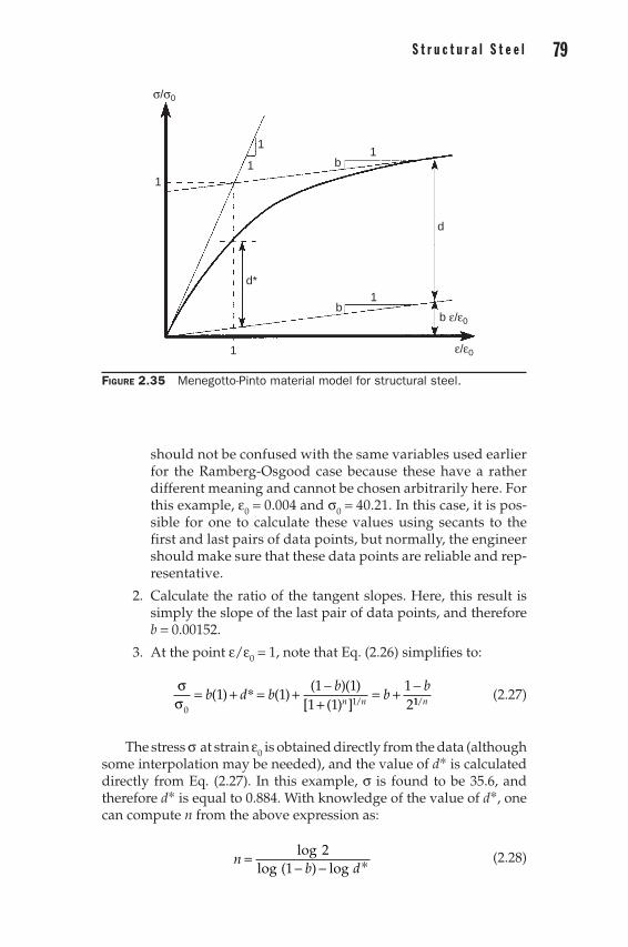
78 C h a p t e r T w o S t r u c t u r a l S t e e l 79
should not be confused with the same variables used earlier for the Ramberg-Osgood case because these have a rather different meaning and cannot be chosen arbitrarily here. For this example, e0 = 0.004 and s0 = 40.21. In this case, it is pos-sible for one to calculate these values using secants to the first and last pairs of data points, but normally, the engineer should make sure that these data points are reliable and rep-resentative.
2. Calculate the ratio of the tangent slopes. Here, this result is simply the slope of the last pair of data points, and therefore b = 0.00152.
3. At the point e/e0 = 1, note that Eq. (2.26) simplifies to:
ss0
= + = + -+
= + -b d b
bb
bn n( ) ( )
( )( )[ ( ) ] /1 1
1 11 1
121
*11/n (2.27)
The stress s at strain e0 is obtained directly from the data (although some interpolation may be needed), and the value of d* is calculated directly from Eq. (2.27). In this example, s is found to be 35.6, and therefore d* is equal to 0.884. With knowledge of the value of d*, one can compute n from the above expression as:
n
b d=
- -log
log ( ) log2
1 * (2.28)
1
1
11
b
d
σ/σ0
d*
b1
1
b ε/ε0
ε/ε0
Figure 2.35 Menegotto-Pinto material model for structural steel.
02_Bruneau_Ch02_p007-110.indd 79 6/13/11 3:08:28 PM

80 C h a p t e r T w o S t r u c t u r a l S t e e l 81
Here, this gives n = 5.68. The resulting Menegotto-Pinto expression becomes:
s e e
e= +
+15 17 9985
1 249 5 68 1 5 68.[ ]. / .
(2.29)
This model is slightly less accurate than the power models presented earlier, as evidenced by the results summarized in Table 2.5, but dif-ferences are not of practical significance.
2.7.4 Smooth Hysteretic ModelsThe multilinear and continuous models presented above to describe monotonic response can be extended to capture cyclic behavior. The concepts and equations are similar, with the difference that “mem-ory” must be introduced in the models to keep track of the strength level and extent of yielding (or accumulated plastic deformation his-tory) at each point of load reversal. Such models are typically formu-lated to also account for strain-hardening effects. Constitutive models relating stresses to strains are used in non linear inelastic finite ele-ment analyses (from a computational mechanics perspective), but similar relationships can be used at the element level to relate forces to deformations in nonlinear inelastic analyses of structural systems constructed of beams, columns, and other discrete elements, for example, in terms of moment-curvature or force-deformation rela-tionships. In the latter case structural element models may need to capture complex physical behaviors, such as global or local buckling effects, in addition to material behavior, and numerous customized models of cyclic inelastic element behavior have been developed to account for such complex multiple phases of plastic behavior.
The following provides general information on some of the mod-els commonly encountered in making modeling decisions. Extensive literature provides details on the mathematical formulations under-lying these models, both from a computational mechanics perspec-tive (e.g., Chakrabarty 2006, Lubliner 1990) or a structural analysis one (e.g., Carr 2004, Sivaselvan and Reinhorn 1999). Note that because these models require a definition of yielding in complex 2-D or 3-D stress conditions, and rules to model strain-hardening behavior in that space, the engineering mechanics principles underlying com-monly used yield criteria are first reviewed. Readers already familiar with this information can proceed directly to Section 2.7.4.2 on cyclic hysteretic models.
2.7.4.1 Yield Criteria Given that yielding is effectively a translational movement of dislo-cations along slip planes in crystals, as described in an earlier sec-tion, the criterion that define yielding in steel elements subjected to
02_Bruneau_Ch02_p007-110.indd 80 6/13/11 3:08:28 PM

80 C h a p t e r T w o S t r u c t u r a l S t e e l 81
multi axial stress conditions are explicitly tied to the magnitude of shear stresses. Contrary to single crystals which have preferential planes along which slippage develops (analogous to cleavage planes in brittle materials), steel is an isotropic material consisting of ran-domly oriented crystals, and yielding develops where the maximum shear stresses are reached.
Recognizing that the maximum shear, tmax, cannot exceed the value reached when a uniaxial coupon yields, Tresca used this cali-brated shear stress value and basic stress transformations (that are conventionally illustrated using Mohr circles) to postulate the first classic yield criteria. Illustrating this for the simpler case of plane stresses, using the well-known fundamental equations from mechan-ics of materials (e.g., Popov 1968):
s ss s s s
tmax = =+
+-
+1
2
2 2x y x y
xy (2.30a)
s ss s s s
tmin = =+
--
+2
2
2 2x y x y
xy (2.30b)
ts s
ts s
max =-
+ =
-x yxy2 2
2
1 2 (2.30c)
where s1 and s2, respectively are the maximum and minimum nor-mal principal stresses, and tmax is the maximum shear stress acting on the principal planes for a general condition of stresses expressed in an arbitrary x-y space, one can obtain that when s1 = sy and s2 = 0, then tmax is sy/2.
For the more general three-dimensional case, the stress transfor-mation equations become substantially more complex, but it remains that:
s s s smax = MAX of [ , , ]1 2 3 (2.31a)
t
s smax
max min=-2
(2.31b)
As a result, still in plane stresses, considering the additional principal stress s3 = 0, three possible scenarios are possible:
(a) s1 > s2 > 0 in which case tmax = sy/2 when s1 = sy
(b) s1 > 0 > s2 in which case tmax = sy/2 when (s1 - s2) = sy
(c) 0 > s1 > s2 in which case tmax = sy/2 when s2 = sy
02_Bruneau_Ch02_p007-110.indd 81 6/13/11 3:08:29 PM

82 C h a p t e r T w o S t r u c t u r a l S t e e l 83
This is illustrated using Mohr circles in Figure 2.36. Three similar expressions can be derived when s2 > s1. The resulting Tresca yield surface is shown in Figure 2.37.
While the Tresca yield condition is simple, and Mohr circles pro-vide a convenient vehicle to assess when yielding under three-dimensional stress states approach the yield criterion set by tmax, it is slightly inaccurate in predicting yielding for steel and other metals. The Von Mises yield condition (also known as the Huber/Von Mises/Hencky criterion), based on energy concepts, provides better results.
The Von Mises criterion is best understood from a three- dimensional state of stresses. For a differential element of size dx, dy, and dz, and volume dV, shown in Figure 2.38, the normal and shear stresses acting on each face of that element can be expressed in the following matrix (known as the Cauchy stress tensor):
ss t tt s tt t s
ij
x xy xz
yx y yz
zx zy z
=
(2.32)
τmax = σ1 + σ2
Slip planes
σ1
σ2
σ1
σ1σ2
= σ1
σ2
τ
σ
2
Slip planes
σ1
σ2
σ2 σ1
σ1
σ2
τ
σ
2
(a)
(b)
τmax
Figure 2.36 Stress conditions and slip planes for Tresca yield criterion, and corresponding Mohr circle, for: (a) s1 > s2 > 0 and (b) s1 > 0 > s2.
02_Bruneau_Ch02_p007-110.indd 82 6/13/11 3:08:29 PM

82 C h a p t e r T w o S t r u c t u r a l S t e e l 83
Knowing that for an elastic system, the strain energy, U, produced by a force, F, over a distance, Δ, is U = ½ (FΔ), the strain energy pro-duced by each stress component can be calculated independently, and summed to get the total stain energy. For example, for the shear strain acting in the x-z plane, the force equal the shear stress times the area on which it is acting (F = txy dxdz) and the “distance” traveled by that force is Δ = ½ g xy dy. As a result:
dU dxdz dy dydxdz dVxy xy xy xy xy xy= = =1
212
12
t g t g t g
(2.33)
For the normal stress on that same x-z plane, F = sy dx dz and Δ = ½ eydy, and dU = ½ sy ey. Summing for all stresses, the total energy for the element becomes:
dUdV
Uo
x x y y z z xy xy yz
=
= + + + +12
12
12
12
12
s e s e s e t g t gg t gyz zx zx+ 12
(2.34)
Y
σ2 = Y
σ 2 –
σ 1 = Y
σ 1 –
σ 2 = Y
σ1 = Y
σ1O
σ2
Y
Tresca hexagon
σ1 = –Y
σ2 = –Y
Mises ellipse
Figure 2.37 Tresca and Von Mises yield surfaces in the s1 - s2 space. (From Theory of Plasticity, J. Chakrabarty 2006. Copyright Elsevier Limited. Reprinted with permission.)
02_Bruneau_Ch02_p007-110.indd 83 6/13/11 3:08:31 PM

84 C h a p t e r T w o S t r u c t u r a l S t e e l 85
Substituting in this equation the mechanics of materials relation-ships:
e s u s s
e s u s s
e s
x x y z
y y z x
z
E
E
E
= - +
= - +
=
1
1
1
[ ( )]
[ ( )]
[ zz z zx- +u s s( )]
and
gt
gt
gt
xyxy
yzyz
zxzx
G
G
G
=
=
=
∆x
∆y
σ′z
σx
τ′zy τ′xy
τzy
τyzτyx
σ′y
σz
τ′yz
τzx
τ′yx
σ′x
σy
τ′zx
τ′xz
τxy
τxz
D
F
H
B
E
A ∆z
G
x
y
z
C
Figure 2.38 Three-dimensional state of stress on a differential element. (From Résistance des Matériaux, A. Bazergui et al. 1987, with permission from Presses Internationales Polytechniques, Montreal.)
(2.35a)
(2.35b)
(2.35c)
(2.35d)
(2.35e)
(2.35f)
02_Bruneau_Ch02_p007-110.indd 84 6/13/11 3:08:32 PM
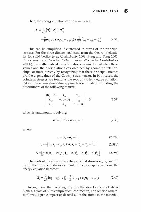
84 C h a p t e r T w o S t r u c t u r a l S t e e l 85
Then, the energy equation can be rewritten as:
UE
E G
o x y z
x y y z z x
= + +( )- + + +
12
12
2 2 2s s s
u s s s s s s t( ) xxy yz zx2 2 2+ +( )t t (2.36)
This can be simplified if expressed in terms of the principal stresses. For the three-dimensional case, from the theory of elastic-ity for solid bodies (e.g., Chakrabarty 2006, Fung and Tong 2001, Timoshenko and Goodier 1934, or even Wikipedia Contributors 2009b), the mathematical transformations required to calculate these values and their orientations can obtained by geometric relation-ships, or more directly by recognizing that these principal stresses are the eigenvalues of the Cauchy stress tensor. In both cases, the principal stresses are found as the root of a third degree equation. Taking the eigenvalue value approach is equivalent to finding the determinant of the following matrix:
( )( )
( )
s s t tt s s tt t s s
x xy xz
yx y yz
zx zy z
--
-= 0 (2.37)
which is tantamount to solving:
s s s3
12
2 3 0- - - =I I I (2.38)
where
I x y z1 = + +s s s (2.39a)
I x y y z z x xy yz zx2
2 2 2= - + + - - - s s s s s s t t t (2.39b)
I x y z xy yz zx x yz y zx z xy3
2 2 22= + - - -s s s t t t s t s t s t (2.39c)
The roots of the equation are the principal stresses s1, s2, and s3. Given that the shear stresses are null in the principal directions, the energy equation becomes:
U
E Eo = + +( ) - + +12 1
222
32
1 2 2 3 3 1s s s u s s s s s s( ) (2.40)
Recognizing that yielding requires the development of shear planes, a state of pure compression (contraction) and tension (dilata-tion) would just compact or distend all of the atoms in the material,
02_Bruneau_Ch02_p007-110.indd 85 6/13/11 3:08:33 PM

86 C h a p t e r T w o S t r u c t u r a l S t e e l 87
without the development of any shear planes. Therefore, all of the strain energy related to such a uniform stress condition doesn’t con-tribute to yielding and must be subtracted from the above equation if one wishes to calculate the strain energy that produces yielding.
By analogy, a condition of equal principal stresses would exist if the differential element dV was submerged in water, and the aver-age stress applied in this case, that would correspond to a volume change (but no shear distortions), is called the “hydrostatic” stress, expressed as:
s
s s s=
+ +1 2 3
3 (2.41)
As shown below for the Cauchy stress tensor in the principal directions, each principal stress can be expressed as the sum of the hydrostatic stress and the remaining balance. In classic mechanics, the corresponding matrices are called the spherical (dilatational) stress tensor and the deviatoric (distortional) stress tensor, respec-tively contributing to volume change or pure distorsion without vol-ume changes. Only the latter of the two can produce yielding:
ss
s
ss
s
s1
2
3
10 00 00 0
0 00 00 0
=
+
---
-
ss s
s s
0 00 00 0
2
3
(2.42)
This decomposition of stresses is shown in Figure 2.39. The bot-tom half of this figure illustrates the case corresponding to uniaxial tension. Note in parts (f) and (g) of that figure, that equal compres-sion and tension acting on perpendicular planes produced a pure shear stress along a plane at 45°—hence, slip planes.
As a result, the total energy, U0, can be calculated as the sum of the dilatation and distortion energy. For the first term, setting s1 = s2 = s3 = s, and expanding back to express s in terms of principal stresses, one obtains:
UE E EDilatation = - = -
=
12
3 33 1 2
22 2 2( ) ( )
( )( )s u s u s
(( )( )
1 26 1 2 3
2- + +u s s sE
(2.43)
The distortion energy, obtained by subtracting the dilatation energy from the total energy, and substituting E = 2G(1 + n), is:
U
GDistortion = - + - + -112 1 2
22 3
23 1
2[( ) ( ) ( )s s s s s s ]] (2.44)
02_Bruneau_Ch02_p007-110.indd 86 6/13/11 3:08:34 PM

86 C h a p t e r T w o S t r u c t u r a l S t e e l 87
As done earlier for the Tresca yield condition, the results from uniaxial testing are used for “calibration,” to establish the critical yield condition. Hence, when s2 = s3 = 0 and s1 = sYield = sY (not to be confused with sy above), the distortional energy at yield is:
U
G GDistortion Y Y YY
- = + + - =112
06
2 2 22
[( ) ( ) ( ) ]s ss
(2.45)
Equating the general distortion energy equation to this maxi-mum, on can obtain the following Von Mises Yield criterion:
s s s s s s sY = - + - + -
12 1 2
22 3
23 1
2( ) ( ) ( ) (2.46)
σ2
σ
σ2
σ3
σ1
σ3
σ1
= +
σ
σ
σ
σ
σ σ1 – σ
σ3 – σ
σ2 – σ
σ1 – σ
σ2 – σσ3 – σ
(a)
Figure 2.39 Decomposition of principal stresses into dilatational and distortional stresses: (a) general state of stress and (b) uniaxial state of stress.
+
=
+
σ1
σ1
σ1
3
σ1
3 σ1
3
σ1
3
σ13
σ13
σ1
3
σ1
3
σ1
3
σ1
3 σ1
3
σ13σ1
3σ13
(b)
02_Bruneau_Ch02_p007-110.indd 87 6/13/11 3:08:35 PM

88 C h a p t e r T w o S t r u c t u r a l S t e e l 89
which, for the two-dimensional case in which s3 = 0, can be simplified into
s s s s s s sY = - + + = + -1
2 1 22
22
12
22
12( ) ( ) ( ) ( ) ( ) (ss s1 2)
(2.47)
This is effectively draws an ellipse in the s1 - s2 plane, as shown in Figure 2.37, normalized by sY. Note that for the pure shear case, s1 = −s2, and t = s1 (from Mohr circle), the equation gives sY = 3t2, and equivalently t2 = 0.58 sY ≈ 0.6 sY , which is typically used as the shear yield strength.
The corresponding Von Mises yield surface in three-dimensional, when s3 ≠ 0, is shown in Figure 2.40. Note that an element only sub-jected to hydrostatic pressure (e.g., s1 = s2 = s3) would never yield, but rather crush or fracture without developing yielding, which is why the main axis of the three-dimensional yield surface is oriented in that direction. As such, the cylinder shown in Figure 2.40 shouldn’t be misinterpreted—although shown to be of infinite length as an expression of the above yielding limit state, in reality it would be intersected by another critical surface for the brittle limit state (frac-ture or crushing) that would eventually develop under critical tri-axial stress conditions. Incidentally, the same would also be true for the Tresca yield surface developed for an element under triaxial stress conditions (as could also be demonstrated using Mohr circles), which is circumscribed by the Von Mises yield surface as shown in Figure 2.40. Note that the two yield criteria intersect a number of times, and that the largest difference between the Tresca and Von Mises surfaces is approximately 16%. However, experiments on var-ious metals have demonstrated a better agreement with the Von Mises criterion, as shown in Figure 2.41, and it is the one used in structural steel design.
120°
σ1
σ3
σ2
σ2
σ1
σ3
VonMisesTresca
Figure 2.40 Von Mises and Tresca yield surfaces in three-dimensional principal stress space and corresponding intersect in s1 - s2 plane.
02_Bruneau_Ch02_p007-110.indd 88 6/13/11 3:08:36 PM
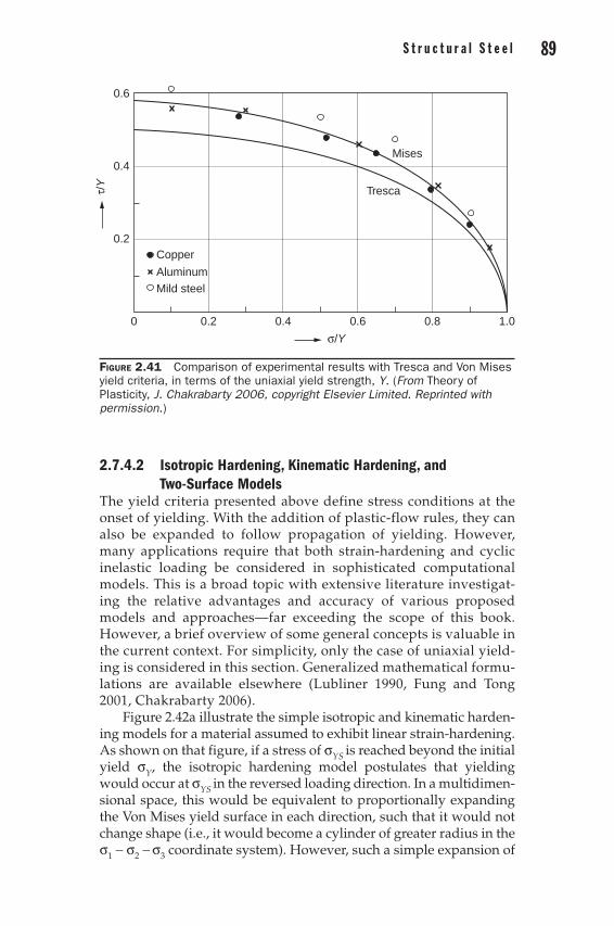
88 C h a p t e r T w o S t r u c t u r a l S t e e l 89
2.7.4.2 Isotropic Hardening, Kinematic Hardening, and Two-Surface Models
The yield criteria presented above define stress conditions at the onset of yielding. With the addition of plastic-flow rules, they can also be expanded to follow propagation of yielding. However, many applications require that both strain-hardening and cyclic inelastic loading be considered in sophisticated computational models. This is a broad topic with extensive literature investigat-ing the relative advantages and accuracy of various proposed models and approaches—far exceeding the scope of this book. However, a brief overview of some general concepts is valuable in the current context. For simplicity, only the case of uniaxial yield-ing is considered in this section. Generalized mathematical formu-lations are available elsewhere (Lubliner 1990, Fung and Tong 2001, Chakrabarty 2006).
Figure 2.42a illustrate the simple isotropic and kinematic harden-ing models for a material assumed to exhibit linear strain-hardening. As shown on that figure, if a stress of sYS is reached beyond the initial yield sY, the isotropic hardening model postulates that yielding would occur at sYS in the reversed loading direction. In a multidimen-sional space, this would be equivalent to proportionally expanding the Von Mises yield surface in each direction, such that it would not change shape (i.e., it would become a cylinder of greater radius in the s1 - s2 - s3 coordinate system). However, such a simple expansion of
Mises
Tresca
1.00.80.60.40.20
0.2
0.4
0.6τ/
Y
σ/Y
Copper
AluminumMild steel
Figure 2.41 Comparison of experimental results with Tresca and Von Mises yield criteria, in terms of the uniaxial yield strength, Y. (From Theory of Plasticity, J. Chakrabarty 2006, copyright Elsevier Limited. Reprinted with permission.)
02_Bruneau_Ch02_p007-110.indd 89 6/13/11 3:08:37 PM

90 C h a p t e r T w o S t r u c t u r a l S t e e l 91
the yield surface due to work hardening does not correctly represent the behavior of steel (and other metals), failing to account for the Bauschinger effects.
By contrast, the kinematic hardening model postulates that the yield surface translates in space without changing volume. For the uniaxial yielding case shown in Figure 2.42b, this implies that if a stress of sYS is reached beyond the initial yield sY, yielding in the reversed loading direction would occur at sYS
* = |sYS − 2sY |. In other words, the distance between yield points in opposite loading direc-tions remains constant—which, in some measures, accounts for the Bauschinger effect and is more appropriate for materials that exhibit linear strain-hardening.
In spite of their respective shortcomings, both the isotropic and kinematic models are appealing for hand calculations when esti-mates of complex response are desirable. However, a better repre-sentation of stress-strain behavior for steel and other metals is achieved using a two-surface model that combines both the isotro-pic and kinematic effects. The Dafalias-Popov (1975) two-surface model, shown in Figure 2.43, is a set of rules that characterize how the yield surface varies as a function of past loading history, while remaining within two linear bounding surfaces (also known as memory surfaces). It is well suited for materials that exhibit a smooth transition into the strain-hardening range and that approach the straight line asymptotes that define the bounding surfaces. Although many researchers have expanded the model to enhance its ability to capture particular hysteretic steel behaviors or expand its range of applicability (e.g., Cofie and Krawinkler 1985, Mizuno et al.
2σYS
–σY–σYS
σσ
σY
σYS
2σY
Kinematic hardeningIsotropic hardening
–σYS*
ε ε
Figure 2.42 Uniaxial expression of: (a) isotropic hardening (expansion of yield surface) and (b) kinematic hardening (translation of yield surface).
02_Bruneau_Ch02_p007-110.indd 90 6/13/11 3:08:37 PM

90 C h a p t e r T w o S t r u c t u r a l S t e e l 91
1992, Petersson and Popov 1977, Tseng and Lee 1983, to name a few), the main features of the original Dafalias and Popov two-surface model are summarized here.
Working from the assumption that, for any given increment of stress, ds, on a stress-strain curve, the corresponding increment of strain, de, can be separated into its elastic and plastic components, dee and dep, respectively, the following relationship can be derived between the total tangent modulus, Et, and the elastic and plastic moduli, Ee and Ep, respectively:
∂ = ∂ + ∂
∂ = ∂ + ∂
= +
e e e
s s s
e p
t p
t p
E E E
E E E1 1 1
(2.48)
The Dafalias-Popov then postulates that:
E E hp p
o
in
= +-
1d
d d (2.49)
2κ
Epo
Ep
κ
δ
σ
2κ
Epo
δin
σr
εp
Figure 2.43 Uniaxial expression of plastic strains, ep, as a function of stress in two-surface model with bounding lines X-X′ and Y-Y′.
02_Bruneau_Ch02_p007-110.indd 91 6/13/11 3:08:38 PM

92 C h a p t e r T w o S t r u c t u r a l S t e e l 93
where Epo is the modulus of the asymptote, d is the distance between
the stress at the point of interest and the boundary curve, din is the value of d at the yield stress for a specific loading path, and h is a fac-tor chosen to fit the experimental data. As the strain increases, d decreases, and Ep varies from infinity at din to the asymptote modu-lus. Knowing the tangent modulus, the complete hysteretic curve can be plotted for any value of strain (Dafalias 1992). Such an exam-ple is shown in Figure 2.44 against experimental data–more general-ized elements also exist that can integrate the yield plateau with kinematic hardening rules into a single for constitutive model (Mahan et al. 2011).
Note that calibration to experimental results also reveal that the elastic range of the curve during any loading excursion is usually less than 2sY; Mizuno et. al (1992) reported a progressive reduction of that range as a function of accumulated plastic strain, down to 30% of that value after 1% of accumulated plastic strain, although others have reported good results using a constant reduced value (e.g., Cofie and Krawinkler 1985 considered it to be 1.2sY). Other refinements to the model, together with comparison to various versions of it, are pre-sented by Mizuno et al. (1992).
2.7.4.3 Smooth Hysteretic Power FunctionsAnother general class of models, proposed by Wen (1976) expanding on the work of Bouc (1971), has been used in the literature—for
0 1 2 3 4Strain %
TheoryExperiment
800
600
400
200
–200
–400
–600
–800
0
Str
ess
(MP
a)
Plastic modulus: Ep = 1 + 1641 + 46 (δin/σ0)3
δδin –δ
Ep0
Figure 2.44 Comparison of stress-strain curve for a randomly loaded Grade 60 steel specimen and results obtained using a two-surface model. (Courtesy of Professor Yannis Dafalias, University of California at Davis and National Technical University of Athens.)
02_Bruneau_Ch02_p007-110.indd 92 6/13/11 3:08:39 PM

92 C h a p t e r T w o S t r u c t u r a l S t e e l 93
example, to express the hysteretic behavior of buckling restrained braces (Andrews et al. 2008, Black et al. 2004), which are axially loaded members whose hysteretic behavior is directly proportional to its material stress-strain relationship, as described Chapter 11). A Bouc-Wen model for hysteretic stress-strain behavior states:
s α e α e= + -E E z( )1 (2.50)
where all terms have been defined earlier, except α which is the ratio of postyielding to elastic stiffness, Et/E, and z is a variable controlled by a differential equation expressed as:
e g e b e eY
n nz z z z + + - =
-10 (2.51)
where eY is the yield strain, b, g, and n are parameters that define the shape of the hysteretic curves. Given the additional constraint that b + g = 1, the values of b and n are left to calibrate the model by curve fitting. Large values of n give results that approach bilinear behavior. For example, for buckling restrained brace, in which the above equa-tion would be identical but instead expressed in terms of axial force, P, versus axial deformation, x, and in which E would be replaced by K = EA/L, a good match with experimental results was obtained for values of b = 0.55 and n = 1, and artificially increasing the calculated value of eY by 25% (Black et al. 2004).
Note that many researchers have expanded the Bouc-Wen model to address various forms of more complex hysteretic behavior (e.g., as summarized in Song and Der Kiureghian 2006), often in attempts to address structural element behavior, rather than material behavior. However, the Bouc-Wen model is only one member of a broad family of Smooth Hysteretic Models (SHM) that have been developed and widely used, for example to model the plastic hinge moment-rotation behavior of structural elements made of various materials, while accounting for all potential physical phenomena that can degrade the strength, stiffness, and fullness of hysteretic curves, such as cracking, gap opening, debonding, slippage, local buckling, local fractures, and other effects. A general purpose SHM model able to integrate all these phenomena behaviors was developed and implemented by Sivaselvan and Reinhorn (1999). These more complex models are either phenom-enological (i.e., fitted to experimental data) or physical (i.e., able to replicate experimental results from simple knowledge of geometry and fundamental material properties, on the basis of recognized physical principles).
Finally, other power models have also been used to capture the stabilized strain-hardened behavior of commonly used structural steel. For example, Kaufmann et al. (2001b) obtained reasonable accu-racy in replicating the cyclic behavior of A572, A913, and A36 steels at 2%, 4%, 6%, and 8% strains, using the power equation s = Ke n, as
02_Bruneau_Ch02_p007-110.indd 93 6/13/11 3:08:39 PM

94 C h a p t e r T w o
shown in Figure 2.45, where n is the work-hardening exponent. Val-ues of K and n obtained by Kaufmann et al. for A572 steels are shown in Figure 2.45. Such an equation can be obtained from the Ramberg-Osgood relationship presented earlier if the inelastic deformations dominates and elastic response can be neglected, and by solving the resulting simplified Ramberg-Osgood for s in terms of e. However, if interested in the entire stress-strain range, including the elastic range, this approach is grossly incorrect because it gives an infinite initial stiffness and incorrect results in the elastic range. This can be cor-rected by breaking the stress-strain curve into a linear segment for which s = Ee up to the yield strength limiting, and the power equa-tion beyond that point (Lubliner 1990).
2.8 Advantages of Plastic Material BehaviorTo illustrate some of the advantages of plastic material behavior, the three-bar truss of Figure 2.46a is subjected to an increasing statically applied load, F, up to its ultimate capacity. Incidentally, two- or
–0.05 –0.04 –0.03 –0.02 –0.01 0 0.01 0.02 0.03 0.04 0.05
Strain (in/in) Strain (in/in)
100
80
60
40
20
0
Str
ess
(ksi
)
0.00 0.01 0.02 0.03 0.04 0.05
Steel A (A572 Gr.50)
Monotonic stress-straincurveStabilized cyclic test data
σ = Kεn
K = 112.5 n = 0.105
100
8060
4020
0–20
–40–60
–80
–100
Str
ess
(ksi
)
(a)
(b)
10080604020
0–20–40–60–80
–100
Str
ess
(ksi
)
Str
ess
(ksi
)
–0.05 –0.04 –0.03 –0.02 –0.01 0 0.01 0.02 0.03 0.04 0.05
Strain (in/in)
0.00 0.01 0.02 0.03 0.04 0.05
Strain (in/in)
100
80
60
40
20
0
Steel C (A572 Gr.50)
Monotonic stress-straincurveStabilized cyclic test data
σ = Kεn
K = 104.4 n = 0.111
Figure 2.45 Smooth hysteretic behavior of A572 Grade steel at 2%, 4%, 6%, and 8% strain ranges and corresponding calibrated power model parameters: (a) sample “A” and (b) sample “C.” (Courtesy of Alan W, Pense, Department of Materials Science and Engineering, Lehigh University.)
02_Bruneau_Ch02_p007-110.indd 94 6/13/11 3:08:41 PM

94 C h a p t e r T w o
1
B
P/P
y
F/P
yF
/Py
P/P
y
P/P
y
∆/∆
y∆
/∆y
CD
A (
typ.
) =
650
mm
2
45°
45°
L = 2500 mm
Mat
eria
l mod
el
A∆
F(a
)(b
)
(g)
(h)
(f)
(c)
(d)
(e)
1.0
Mem
ber
2
Mem
ber
1 an
d 3
0.5
σ
σ y
ε yε
σ y =
250
MP
aE
= 2
0000
0 M
Pa
Cas
e I
Cas
e II
22
11
33
∆/∆
y∆
/∆y
∆/∆
y
∆/∆
y
21
33
42
1
4Unl
oadi
ng/r
eloa
ding
alon
g sa
me
path
2.41
4
1.70
7
(i)(ii
)(ii
i)
KP
KK
∆ Res
idua
l
Unl
oadi
ng/r
eloa
ding
alon
g sa
me
path
AE
/L
AE
/L
AE
/L
AE
/2L
AE
/2L
AE
/2L
32 K
P
K
K
K
32
1
AE
/L AE
/2L
Mem
ber
forc
es v
ersu
s gl
obal
def
lect
ion
Str
uctu
re lo
ad v
ersu
s gl
obal
def
lect
ion
(i) E
last
ic r
ange
(ii)
Con
tain
ed p
last
ic fl
ow(ii
i) U
nres
tric
ted
plas
tic fl
ow
= p
last
ic g
loba
l
stru
ctur
al s
tiffn
ess
KP
K =
initi
al e
last
ic g
loba
l
stru
ctur
al s
tiffn
ess
K
P2
resi
dual
P1
resi
dual
F/P
y
2
13
P2
resi
dual
P1
resi
dual
Fig
ur
e 2
.46
Sim
ple
exam
ple
to il
lust
rate
cyc
lic p
last
ic b
ehav
ior
of in
dete
rmin
ate
stru
ctur
e.
95
02_Bruneau_Ch02_p007-110.indd 95 6/13/11 3:08:44 PM
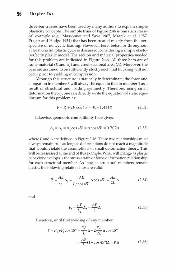
96 C h a p t e r T w o S t r u c t u r a l S t e e l 97
three-bar trusses have been used by many authors to explain simple plasticity concepts. The simple truss of Figure 2.46 is one such classi-cal example (e.g., Massonnet and Save 1967, Mrazik et al. 1987, Prager and Hodge 1951) that has been treated mostly from the per-spective of noncyclic loading. However, here, behavior throughout at least one full plastic cycle is discussed, considering a simple elasto-perfectly plastic model. The section and material properties needed for this problem are indicated in Figure 2.46. All three bars are of same material (E and sy ) and cross-sectional area (A). Moreover, the bars are assumed to be sufficiently stocky such that buckling will not occur prior to yielding in compression.
Although this structure is statically indeterminate, the force and elongation in member 3 will always be equal to that in member 1 as a result of structural and loading symmetry. Therefore, using small deformation theory, one can directly write the equation of static equi-librium for this problem as:
F P P P P= + = +2 1 2 12 45 1 414cos . (2.52)
Likewise, geometric compatibility here gives:
Δ = Δ = Δ = Δ = Δ1 3 2 45 45 0 707cos cos . (2.53)
where F and Δ are defined in Figure 2.46. These two relationships must always remain true as long as deformations do not reach a magnitude that would violate the assumptions of small deformation theory. This will be reassessed at the end of this example. What will change as plastic behavior develops is the stress-strain or force-deformation relationship for each structural member. As long as structural members remain elastic, the following relationships are valid:
P
AEL
AE
L
AEL1
11
4545
2= Δ = Δ = Δ
/coscos
(2.54)
and
P
AEL
AEL2
22= Δ = Δ (2.55)
Therefore, until first yielding of any member:
F P PEAL
EAL
AEL
= + ° = + °
= +
2 1 45 22
45
1
cos cos
( cos
Δ Δ
445° =)Δ ΔK (2.56)
02_Bruneau_Ch02_p007-110.indd 96 6/13/11 3:08:45 PM

96 C h a p t e r T w o S t r u c t u r a l S t e e l 97
where K is the elastic stiffness for this structure. The equation above shows that member 2 reaches its yield strength (Py) first, when mem-bers 1 and 3 are stressed to only half their capacity (i.e., 0.5 Py). The yield displacement of the structure (Δy) could be defined in terms of the truss bar’s properties and geometry:
Δ =y
yP L
AE (2.57)
where all terms have been previously defined. The state of member forces and applied load as a function of the vertical deflection at point A are presented in a normalized format in Figures 2.46c and d. At Δ = Δy, the structure has been loaded to F = 1.707 Py. This case reflects the current standard structural engineering practice worldwide, in which linear elastic analyses are conducted to determine the maximum load that can be applied to a structure until the capacity of a single mem-ber is reached. Here, the capacity of member 2 is reached first, and members 1 and 3 are underutilized. Note that although one could conclude from elastic analysis that having bars of the same size is inefficient and likely propose a solution with bars of different cross-sections, this type of optimization based on minimum weight is often at odds with practical considerations, where architectural, manufac-turing, or construction concerns may dictate equal size bars. Hence, in this problem, it is reasonable to constrain the bars to be of identical cross-section.
Even though truss bar 2 has yielded, the load applied to the struc-ture can be increased beyond 1.707 Py because members 1 and 3 have not reached their ultimate capacity. In the process, member 2 will undergo plastic elongation while sustaining its capacity. Therefore, for Δ > Δy:
P
AEL
P Py1 22= Δ =and (2.58)
and
F P P P
AELy= + = + Δ2 12 45 45cos cos (2.59)
This condition of further loading beyond the elastic range, called contained plastic flow, is illustrated in Figures 2.46c and d. Note that the stiffness of the structure has decreased as a result of this partial yielding. Eventually, when the applied load reaches 2.414 Py, all three truss bars yield, and a condition of unrestrained plastic flow develops. In this example, the ultimate capacity calculated by toler-ating plastification of the structure is 41% larger than the elastic limit, providing some evidence that it is generally worthwhile to take
02_Bruneau_Ch02_p007-110.indd 97 6/13/11 3:08:46 PM

98 C h a p t e r T w o S t r u c t u r a l S t e e l 99
advantage of the existing plastic strength available beyond the elastic range.
It is also important to realize that the maximum plastic capacity of a structure can be calculated directly through use of static equilib-rium alone, without knowledge of prior elastic or plastic loading his-tory. A logical conclusion from this observation is that lack-of-fit and other displacement-induced forces have no influence on the magni-tude of the maximum load a structure can support, termed the plastic capacity. No supporting calculations are presented here, but the reader may wish to verify this remark by redoing the example assum-ing that member 2 was constructed 25 mm too short and forced to fit into the frame during construction before any loads were applied. Although doing so would reduce the value of the maximum load that can be applied if the structure is to remain elastic, it does not change the plastic capacity of the structure.
The behavior of this plastified truss-bar structure upon unloading is investigated next. As described in an earlier section of this chapter, steel unloads at a stiffness equal to the original elastic stiffness (as also shown in Figure 2.46b). However, in this example, two scenarios are evaluated, considering various states of plastification prior to unload-ing. In both cases, because the principle of superposition is not valid beyond the elastic range (as evidenced by Figure 2.46d), calculations must proceed following basic principles.
First, if unloading to F = 0 starts before all three truss bars have yielded (shown as Case I in Figures 2.46e and f), it can be shown that:
PAE
LAE
L
P PAEL
MAX
y
MAX
1
2
2 2= Δ - Δ
= - Δ
Δ = Δ - Δ
d
d
d
(2.60)
where dΔ is the incremental displacement imposed by the unloading, and Δ is the resulting displacement after unloading. The above approach also recognizes that only member 2 had plastified prior to unloading. Because the objective is to unload to F = 0, the equilibrium condition developed earlier can be used to solve for all other vari-ables. As a result:
FAE
LAE
L
PA
MAX MAX
y
= = Δ - Δ - Δ
+ -
0 22 2
45( ) cos
EEL MAX( )Δ - Δ
(2.61)
02_Bruneau_Ch02_p007-110.indd 98 6/13/11 3:08:46 PM
98 C h a p t e r T w o S t r u c t u r a l S t e e l 99
and solving for Δ:
Δ =Δ -
+ °=
Δ - Δ+ °
AEL
P
AEL
MAX y MAX y
( cos )( cos )
1 451 45
== Δ - Δ0 586. ( )MAX y (2.62)
This residual displacement after unloading is shown in Figures 2.46e and f. Based on Figure 2.46g, it could be demon-strated that the residual displacement is also equal to:
Δ = Δ -MAX
MAXFK
(2.63)
where K is the global elastic structural stiffness defined earlier. Numerical examples would confirm the expediency of this alterna-tive procedure.
Moreover, as shown in Figure 2.46e, residual member forces remain after unloading and exist simultaneously to that state of resid-ual deformations. Because no external loads are applied to the struc-ture, these member forces must be self-equilibrating. Numerical values can be obtained through simple substitution in the above equations.
In the second scenario considered here, unloading to F = 0 starts after all members have yielded (shown as Case II in Figures 2.46e and f). The approach remains the same, with slightly different results, as:
F P
AEL
PAELy MAX y M= = - Δ - Δ
° + - Δ0 22
45( ) cos ( AAX - Δ
) (2.64)
and:
Δ =
Δ + ° - Δ °++ °
= ΔMAX yM
( cos ) ( cos )
( cos )
1 45 2 45 1
1 45 AAX y- Δ1 414. (2.65)
Again, this result could be obtained directly (and more easily) through use of the alternative method suggested above.
Note that substantial residual member forces develop in this sec-ond example (Figure 2.46e). Calculations would show that these reach approximately 30% and 40% of the yield force, Py, in members 1 and 2, respectively.
As a result of the residual stresses left after unloading in cases I and II, the truss bars would follow their elastic path until the previ-ously applied maximum load is reached anew if the structure is reloaded in the same direction (Figures 2.46e and f). This has a num-ber of practical implications, as shown in the following chapters. However, this extended elastic range exists only as long as the state of residual stresses in the bars at F = 0 remains unchanged; cyclic load-ing is one factor that can alter these residual stresses.
02_Bruneau_Ch02_p007-110.indd 99 6/13/11 3:08:47 PM

100 C h a p t e r T w o S t r u c t u r a l S t e e l 101
When the loading cycle for this example structure is completed, the elastic range for the reversed loading is reduced because of the residual compression force in member 2, as shown in Figure 2.46h. The resulting hysteretic curve exhibits a shape similar, in principles, to a Bauschinger effect—and would be formally one if this example dealt with slip planes of crystals instead of yielding of bars. Formal analytical expressions to demonstrate this behavior, completing a full cycle of loading with yielding in both directions, can be derived from the same basic principles presented above, but it should be obvious that complex calculations and formulations are not necessary, given the clear graphical relationship already established in this example between the load-deformation relation of the structure and that of the members, as shown in Figure 2.46. Therefore, Figures 2.46g and h can be drawn directly as extensions of parts e and f, through use of simple trigonometric calculations to obtain numerical values. Note that the same structural plastic capacity is reached at F = 2.414Py in the reverse direction despite the earlier threshold of yielding, but this required greater contained plastic deformations.
More in-depth observations on the behavior of structural members subjected to inelastic cyclic loading are reserved for later chapters. Nonetheless, it is worthwhile to emphasize at this point that the plastic analysis presented above is possible only if connections of the struc-tural members are stronger than the members themselves. Although this may sound obvious in the context of this simple example, this log-ical requirement sometimes become controversial when the severity of the expected ultimate loads is hidden in more simple static loading models or design philosophies (such as working stress design).
Finally, it is instructive to review the assumption of small defor-mations. For mild steels typically used in structural engineering applications, strains of up to 20% are possible. However, in this prob-lem, calculations show that near this extreme level of deformations (corresponding to 100ey), the angle of members 1 and 3 to the vertical is approximately 40°. Equilibrium in the deformed configuration gives a maximum value of F barely 5% greater. Such a gain in strength is hardly sufficient to warrant the consideration of large deformations theory, especially in the more practical range of 2% strains. A more important issue is the development of strain-hardening in the truss bars and its tangible impact on member strength. The effect of strain-hardening is addressed as necessary in this book.
2.9 Self-Study Problems Problem 2.1 A simple structural system consists of the three pin-ended bars shown in Figure 2.46. All bars have a cross-section of 1 in2 (645 mm2). The material is a ductile structural steel which can be idealized as having elasto-perfectly plastic properties, with E of 29000 ksi and sy of 36 ksi (200,000 MPa and 250 MPa, respectively).
02_Bruneau_Ch02_p007-110.indd 100 6/13/11 3:08:47 PM

100 C h a p t e r T w o S t r u c t u r a l S t e e l 101
For that structure:
(a) What is the allowable load, Pall, which can be applied to that struc-ture such that stresses in the bars do not exceed 0.66 Fy (i.e., allow-able stress method)?
(b) What is the elastic limit load, Pu, which can be applied to that struc-ture such that stresses do not exceed Fy anywhere (i.e., limit states design, with elastic analysis)? How would this change if the central member was constructed 1 in (25.4 mm) too short and forced to fit? Is a solution in the elastic range possible? Does it matter if member AC is elongated, or if members AB and AD are shortened, to achieve this fit (support answers by calculations)?
(c) What is the ultimate load capacity, Pplast, that the structure can carry accounting for plastic behavior (i.e., plastic design philosophy)?
(d) Draw the force-displacement (P-Δ) graph for the structure up to a maximum displacement of 1 in (25.4 mm) and followed by unload-ing to zero load. Express the vertical axis of this graph in a ratio of Pstructure over Pym, where Pym is the ultimate capacity of a single member, and the horizontal axis as a ratio of Δ/Δy, where Δy is defined at the occurrence of first yielding in the structure. Calculate and indicate on this plot all important numerical values.
(e) For the loading history described in (d), also plot the force displace-ment relation of all three members, superposed on a single graph, the vertical axis of this graph being the ratio of Pmember over Pym, the horizontal axis being the actual structural displacement in inches (mm). Calculate and indicate on this plot all important numerical values; in particular, indicate what are the forces in each bar follow-ing the above displacement history.
(f) If the central member was constructed 1 in (25.4 mm) too short and forced to fit during construction, plot the force displacement relation of all three members corresponding to the following two construction sequences: first, if the central member is elongated by 1 in (25.4 mm), connected to the other two members, and released; second, if the two inclined members are compressed to connect to the central member, and released. Does it matter if member AC is elongated, or if members AB and AD are shortened, to achieve this fit (support answers by calculations)?
(g) Comment on the differences between elastic and plastic behavior for analysis and design. In particular, comment on whether the prin-ciple of superposition is applicable for plastic design (i.e., whether usual computer programs could be used to assess plastic strength), whether lack-of-fit and other displacement-induced forces seem critical to the ultimate strength of the structure, and whether an extremely slender member could buckle under residual stresses upon unloading.
Problem 2.2 A simple structural system consists of three pin-ended bars, as shown in the figure below. All bars have the same cross-section A. The material is a ductile structural steel which can be idealized as having elasto-perfectly plastic properties, with E and sy .
02_Bruneau_Ch02_p007-110.indd 101 6/13/11 3:08:47 PM

102 C h a p t e r T w o S t r u c t u r a l S t e e l 103
For that structure, plot the force-displacement (F-Δ) for the structure on one graph, and the force-displacement relation of all three members on another graph (as done in the previous problem), for the displacement histo-ries described below. Write parametric equations (in terms of E and sy, A, L, F, Δ, P, etc.) applicable at the various stages along the curve, clearly indicating the range of their applicability and key values along the graphs. For the cases of unloading (cases I and II below), also derive expressions for the structural residual displacements after unloading.
(a) Step 1: elastic behavior(b) Step 2: post-elastic behavior up to full plastic capacity (also show
unrestrained plastic flow)(c) Step 3: unloading prior to reaching maximum plastic load (i.e., case I)(d) Step 4: unloading after reaching of maximum plastic load and at
Δmax > 2Δy (i.e., case II) (e) Step 5: for both case I and II above, complete the plot until yielding
in the reversed direction is achieved. The key values on the graphs can be derived graphically (i.e., closed-form solutions are not neces-sary)
F
L
L
Rigid beam ∆
CL
Problem 2.3 Using simple plastic analysis, what is be the maximum load, P (in kips), that can be applied to the structure shown here. This structure consists of seven steel bars, each having a cross-section of 1.5 in2 (1450 mm2).
30'
6 @ 10'
P
02_Bruneau_Ch02_p007-110.indd 102 6/13/11 3:08:48 PM

102 C h a p t e r T w o S t r u c t u r a l S t e e l 103
Problem 2.4 Experimental data has been obtained for the normalized moment-curvature relationship of a steel beam (see below). Use both the Menegotto-Pinto method and the Ramberg-Osgood method to define ana-lytical expressions relating the normalized moments and curvatures for that steel beam.
M/My i/iy M/My i/iy M/My i/iy
0 0 1.204 1.3 1.42 2.5
0.5 0.5 1.245 1.4 1.434 2.75
0.75 0.75 1.278 1.5 1.444 3
1 1 1.337 1.75 1.469 4
1.087 1.1 1.375 2 1.48 5
1.153 1.2 1.401 2.25 1.486 6
Problem 2.5 Provide clear and brief answers (five lines of text or less) to the following questions:
(a) What property of steel does the Charpy-V test measure, and what non-metallurgical parameter affects this property?
(b) What is the Carbon Equivalent Formula, and what practical infor-mation does it provide?
(c) What is a slip plane?(d) What is lamellar tearing? Draw a sketch to give an example of when
such a problem could occur, and another one to show how to design to prevent that potential tearing.
(e) What is a typical value of the modulus of elasticity at the onset of strain-hardening?
(f) What does calculation of KI for a given specimen requires?(g) How can the percentage of manganese, silicon, chromium, molyb-
denum, vanadium, nickel, and copper in steel be quantified in a useful way with respect to their impact on brittleness?
(h) What is the difference between the steel grades ASTM A572 Gr. 50 and ASTM A993 Gr. 50?
(i) What is the heat-affected zone (HAZ)?(j) What is a “contained plastic flow”?(k) What are residual stresses (i.e., a definition of what they are, not
why they exist)?(l) Name three sources of residual stresses in structural members.
Problem 2.6 A very short specimen is tested in pure compression until failure. It is observed that, at failure, the whole specimen is undergoing consider-able strain-hardening. Describe why there has been no buckling on the plastic plateau in spite of the fact that the tangent modulus of elasticity, Et, is zero in theory on this plateau. How will this specimen eventually fail?
Problem 2.7 Some seismic design codes and standards specify that steels “shall have a minimum Charpy-V notch toughness of 20 ft-lb (27 J) at 0ºF
02_Bruneau_Ch02_p007-110.indd 103 6/13/11 3:08:48 PM

104 C h a p t e r T w o S t r u c t u r a l S t e e l 105
(-18ºC).” Yet, looking at Charpy-V experimental results (Figure 2.5), 20 ft-lb seems to be in the brittle behavior range. Explain in a few sentences why a 20 ft-lb value is deemed acceptable in such applications, given that brittle steels are not acceptable in seismic applications.
Problem 2.8 A structural steel T-shape must be constructed from plates 4-inches-thick, as illustrated below:
(a) Indicate what might be a potential problem with this weld design. (b) Propose an alternative weld design which will eliminate this
problem.
4"
4"
CP
ReferencesAASHTO. 2003. Guide Specification for Highway Bridge Fabrication with HPS 70W
(HPS 485W) Steel, 2nd ed., Washington, D. C.: American Association of State Highway and Transportation Officials, p. 19.
Abbaschian, R., and Reed-Hill, R. E. 2008. Physical Metallurgy Principles, 4th ed. CL-Engineering.
Ahluwalia, H. 2003. “Combating Plate Corrosion—Improving Corrosion Resistance Through Welding, Fabrication Methods.” The Fabricator, October 2003, http://www.thefabricator.com/MetalsMaterials/MetalsMaterials_Article.cfm?ID=731
Andrews, B. M., Fahnestock, L. A., and Song, J. 2008. “Performance-Based Engineering Framework and Ductility Capacity Models for Buckling-Restrained Braces,” NSEL Report Series, Report No. NSEL-012. University of Illinois at Urbana-Champaign: Department of Civil and Environmental Engineering.
AISC. 1971. “Plastic Design I Steel—A Guide and Commentary,” ASCE Manual and Reports on Engineering Practice No.41. New York: American Society of Civil Engineers.
AISC. 1973. “Commentary on Highly Restrained Welded Connections.” Engineering Journal, vol. 10, no. 3, 61–73.
AISC. 1994. “Load and Resistance Factor Design Manual of Steel Construction, 2nd ed.” American Institute of Steel Construction, Chicago.
AISC. 1997a. “Steel Industry Announces Improved Structural Grade for Buildings.” Modern Steel Construction, vol. 37, no. 4, 18.
02_Bruneau_Ch02_p007-110.indd 104 6/13/11 3:08:49 PM

104 C h a p t e r T w o S t r u c t u r a l S t e e l 105
AISC. 1997b. Technical Bulletin #3—New Shape Material. Chicago: American Institute of Steel Construction.
AISC. 2001. “Changes to the T, k, and k1 Dimensions for W-Shapes,” AISC Advisory, February 14, 2001. Chicago: American Institute of Steel Construction.
AISC. 2005. “Seismic Provisions for Structural Steel Buildings (ANSI/AISC 341-05)”, American Institute of Steel Construction, Chicago, IL.
AISC. 2010. “Specification for Structural Steel Building—ANSI/AISC 360–05.” Chicago: American Institute of Steel Construction.
ASCE. 1992. “Structural Fire Protection,” ASCE Manuals and Reports on Engineering Practice No. 78, T. T. Lie, editor. New York: ASCE Committee on Fire Protection, American Society of Civil Engineers.
ASM. 1986. Atlas of Fatigue Curves, H. E. Boyer, editor. Materials Park, OH: American Society for Metals.
ASTM. 1985a. “Standard Method of Test for Plane-Strain Fracture Toughness of Metallic Materials—ASTM Designation E399-83,” vol. 03.01, ASTM Annual Standards. West Conshohocken, PA: American Society for Testing and Materials.
ASTM. 1985b. “Standard Method for Conducting Drop Weight Test to Determine Nil-Ductile Transition Temperature of Ferric Steels—ASTM Designation E208,” ASTM Annual Standards. West Conshohocken, PA: American Society for Testing and Materials.
AWS. 2010. “AWS D1.1/D1.1M-2010 Structural Welding Code—Steel”. Miami: American Welding Society.
AWS. 1976, “Fundamentals of Welding,” Welding Handbook, vol. 1, 7th ed. Miami: American Welding Society.
Baird, J. D. 1963. “Strain Aging of Steel; A Critical Review,” Iron Steel, vol. 36, 186–192, 368–374.
Baird, J. D. 1971. “The Effects of Strain Aging due to Interstitial Solutes on Mechanical properties of Metals,” Met. Rev., vol. 5, 1–18.
Bartlett, M. F., Dexter, R. J., Graeser, M. D., Jelinek, J. J., Schmidt, B. J., and Galambos, T. V. 2003. “Updating Standard Shape Material Properties Database for Design and Reliability,” AISC Engineering Journal, vol. 40, no. 1, 3–14.
Barsom, J., and Korvink, S. 1998. “Effect of Strain-hardening and Strain Aging on the k-Region of Structural Shapes,” Report No. SACIBD·98/02. San Francisco, SAC Joint Venture, 47 pp.
Barsom, J. M., and Pellegrino, J. V. 2000. “Failure Analysis of a Column k-Area Fracture,” Modern Steel Construction. Chicago: American Institute of Steel Construction.
Bazergui, A., Bui-Quoc, T., Biron, A., McIntyre, G., and Laberge, C. 1987. “Résistance des matériaux,” Editions de l’Ecole Polytechnique de Montreal, Montreal, Canada, 477 pp.
BCSA. 2005. “Galvanizing Structural Steel Works—An Approach to the Management of Liquid Metal Assisted Cracking,” Publication No.40/06. London: British Constructional Steel Association, 22 pp.
Bertero, V. V., and Popov, E. P. 1965. “Effect of Large Alternating Strains of Steel Beams.” Journal of the Structural Division, American Society of Civil Engineers, vol. 91, no. ST1.
Bjorhovde, R. 1987. “Welded Splices in Heavy Wide-Flange Shapes,” National Engineering Conference and Conference of Operating Personnel. New Orleans.
Black, C. J., Makris, N., and Aiken, I. D. 2004. “Component Testing, Seismic Evaluation, and Characterization of Buckling-Restrained Braces.” Journal of Structural Engineering, ASCE, vol. 130, no. 6, 880–894.
Blodgett, O. W. 1977a. “Distortion … How to Minimize It with Sound Design Practices and Controlled Welding Procedures plus Proven Methods for Straightening Distorted Members,” Publication G261. Cleveland: The Lincoln Electric Co.
Blodgett, O. W. 1977b. “Why Welds Crack—How Cracks Can Be Prevented,” Publication G230. Cleveland: The Lincoln Electric Co.
Bouc, R. 1971. Modèl mathématique d’hysteresis. Acustica, vol. 24, 16–25.
02_Bruneau_Ch02_p007-110.indd 105 6/13/11 3:08:49 PM

106 C h a p t e r T w o S t r u c t u r a l S t e e l 107
Bridgman, P. W. 1923. “The compressibility of thirty metals as a function of pres-sure and temperature.” Proceedings of the American Academy of Arts and Sciences, vol. 58, 165.
Bridgman, P. W. 1949a. The physics of high pressure. London: Bell and Sons.Bridgman, P. W. 1949b. “Linear compressions to 30,000 kg/cm2, including rela-
tively incompressible substances. Proceedings of the American Academy of Arts and Sciences, vol. 77, 189.
Bruneau, M., Mahin, S. A., and Popov, E. P. 1987. “Ultimate Behavior of Butt Welded Splices in Heavy Rolled Steel Sections,” EERC Report No. 87-10. Earthquake Engineering Research Center. Berkeley, CA: University of California at Berkeley.
Bruneau, M., and Zahrai, S. M. 1997. “Some Observations on Effect of Severe Corrosion on the Cyclic Ductility of Steel.” ASCE Journal of Structural Engineering, vol. 123, no.11, 1478–1486.
Buchanan, A. H. 2001. “Structural Design for Fire Safety.” West Sussex, England: John Wiley & Sons, 415 pp.
Byfield, M. P., Davies, J. M., and Dhanalakshmi, M. 2005. “Calculation of the strain-hardening behaviour of steel structures based on mill tests.” Journal of Constructional Steelwork Research, vol. 61, no. 2, 133–150.
Carr, A. C. 2004. Ruaumoko Manual, vols. 1 & 2. Department of Civil Engineering. Christchurch, New Zealand: University of Canterbury.
Carter, C. 1997. “Are you Properly Specifying Structural Steel,” Modern Steel Construction, January 1997.
Cattan, J. 1997. “Steel Industry Embraces A992,” Modern Steel Construction, April 1997.
Chakrabarty, J. 2006. Theory of Plasticity. Oxford, UK: Butterworth-Heinermann, 882 pp.
Chi, B., and Uang., C. M. 2004. “Effect of Straightening Method on the Cyclic Behavior of k-Area in Steel Rolled Shapes,” Engineering Journal, American Institute of Steel Construction, first quarter, 2004, 15–22.
Cofie, N. G., and Krawinkler, H. 1985. “Uniaxial Cyclic Stress-Strain Behavior of Structural Steel,” Proceedings of ASCE, vol. 111, no. EM9, 1105–1120.
Coffin, L. F. 1954. “A Study of the Effects of Cyclic Thermal Stresses on a Ductile Metal.” Transaction of the ASME, vol. 76, 931–950.
Cottrell, A. H., and Bilby, B. A. 1949. “Dislocation Theory of Yielding and Strain Aging of Iron.” Proceedings of the Physical Society, vol. 62, 49–62.
Dafalias, Y. F., and Popov, E.P. 1975. “A Model of Nonlinear Hardening Materials for Complex Loading.” Acta Mechanica, vol. 21, 173–192.
Dafalias, Y. F. 1992. “Bounding Surface Plasticity Models for Steel under Cyclic Loading,” Stability and Ductility of Steel Structures Under Cyclic Loading. Fukomoto, Y., and Lee, G., editors. Boca Raton, Florida: CRC Press.
DesRoches, R., McCormick, J., and Delemont, M. A. 2004. “Cyclic Properties of Superelastic Shape Memory Alloys.” ASCE Journal of Structural Engineering, vol. 130, no. 1, 38–46
Dexter, R. J., Hajjar, J. F., Prochnow, S. D., Graeser, M. D., Galambos, T. V., and Cotton, S. C. 2001. “Evaluation of the Design Requirements for Column Stiffeners and Doublers and the Variation in Properties in Properties of A992 Shapes.” Proceedings, North American Steel Construction Conference. Chicago: AISC, pp. 14-1–17-21.
Dicleli, M., and Bruneau, M. 1995. “An Energy Approach to Sliding of Single-Span Simply Supported Slab-on-Girder Steel Highway Bridges with Damaged Bearings,” Earthquake Engineering and Structural Dynamics. vol. 24, 395–409.
DNCR. 2003. “Report on the July 21st Collapse of the Kinzua Viaduct,” Board of Inquiry investigation report. Pennsylvania Department of Conservation and Natural Resources.
DoITPoMS. 2009. “Dislocation motions.” Dissemination of IT for the Promotion of Materials Science (DoITPoMS). Cambridge, UK: Department of Materials Science
02_Bruneau_Ch02_p007-110.indd 106 6/13/11 3:08:49 PM
106 C h a p t e r T w o S t r u c t u r a l S t e e l 107
and Metallurgy, University of Cambridge. http://www.doitpoms.ac.uk/tlplib/dislocations/dislocation_motion.php
Dusicka, P., Itani, A. M., and Buckle, I. G. 2004. “Shear Link Energy Dissipators Utilizing High Performance and Low Yield Point Steels,” 4th National Seismic Conference and Workshop on Bridges. Memphis, TN.
Dusicka, P., Itani, A. M., and Buckle, I. G. 2007. “Cyclic response of plate steels under large inelastic strains.” Journal of Constructional Steel Research, vol. 63, no. 2 , 156–164
ECCS Technical Committee 3. 2001. Model Code on Fire Engineering, Brussels: European Convention for Constructional Steelwork.
Elam, C. F., 1935. The Distortion of Metal Crystals New York, Oxford. Englehardt, M. D., and Husain, A. S. 1993. “Cyclic Loading Performance of Welded
Flange Bolted Web Connections.” ASCE Structural Engineering Journal, vol. 119, no. 12, 3537–3550.
Faller, M., and Richner, P. 2003. “Material selection of safety-relevant components in indoor swimming pools,” Materials and Corrosion, vol. 54, S. 331–338. (in German).
Fisher, J. W. 1984. Fatigue and Fracture in Steel Bridges—Case Studies. New York:Wiley Interscience, 315 pp.
Fisher, J. W., and Pense, A. W. 1987. “Experience with Use of Heavy W Shapes in Tension,” AISC. Engineering Journal, vol. 24, no. 2, 63–77.
Fisher, J. W., Yen. B. T., and Wang, D. 1990. “Fatigue strength of riveted bridge members.” Journal of Structure and Infrastructure Engineering ASCE, vol. 116, no. 11, 2968–2981.
Fung, Y. C., and Tong, P. 2001. “Classical and Computational Solid Mechanics.” Singapore: World Scientific Publishing, 930 pp.
Galambos, T. V., and Ravindra, M. K. 1978. “Properties for Steel Used in LRFD,” Journal of the Structural Division, ASCE, vol. 104, no. 9, 1459–1468.
Gewain, R. G., Iwankiw, N. R., and Alfawakhiri, F. 2003. “Facts for Steel Buildings—Fire.” Chicago: American Institute of Steel Construction.
Horne, M. R., and Morris, L. J. 1981. Plastic design of low-rise frames. Cambridge, MA: MIT Press.
Hu., G., Morivat, M. A., Lee, J., Schell, E., and Engelhardt, M. 2009. “Elevated Temperature Properties of ASTM A992 Steel,” ASCE Structures Congress. Austin, TX.
Iwankiv, N., and Zoruba, S. 2002. “Steel moment frames: resolution of recent seismic detailing and material shape issues.” Journal of Constructional Steel Research, vol. 58, 495–510.
Kaufmann, E. J., Metrovich, B., Pense, A. W., and Fisher, J. W. 2001a. “Effect of Manufacturing Process on k-Area Properties and Service Performance,” Proceedings of the North American Steel Construction Conference. Fort Lauderdale, FL, May 9–12, 2001. Chicago, IL: American Institute of Steel Construction, Inc., pp. 17.1–17.24.
Kaufmann, E. J., Metrovich, B., and Pense, A. W. 2001b. “Characterization of Cyclic Inelastic Strain Behavior on Properties of A572 Gr. 50 and A913 Gr. 50 Rolled Sections,” ATLSS Report No. 01-13, Lehigh University.
Kayser. J. R., and Nowak, A. S. 1989. “Capacity loss due to corrosion in steel-girder bridges.” J. Struct. Engrg., ASCE, vol. 115, no. 6, 1525–1537.
Khan, A. S., and Huang, S. 1995. Continuum Theory of Plasticity. Wiley-Interscience, New York, 431p.
Koch, G. H., Brongers, P. H., Thompson, N. G., Virmani, Y. P., and Payer, J. H. 2002. “Corrosion Costs and Prevention Strategies in the United States,” Report No. FHWA-RD-01-156. Washington, D. C.: Federal Highway Administration, March 2002.
Kinstler, T. J. 2005. Current Knowledge of the Cracking of Steels During Galvanizing—A Synthesis of the Available Technical Literature and Collective Experience for the American Institute of Steel Construction. Springville, AL, GalvaScience LLC, 79 pp.
02_Bruneau_Ch02_p007-110.indd 107 6/13/11 3:08:49 PM

108 C h a p t e r T w o S t r u c t u r a l S t e e l 109
Kulicki, J. M., Prucz. Z., Sorgenfrei, D. E., Mertz. D. R., and Young. W. T. 1990. “Guidelines for Evaluating Corrosion Effects in Existing Steel Bridges,” NCHRP Rep. No. 333. Washington, D. C.: Transportation Research Board, National Research Council.
Lay, M. G. 1965. “Yielding of Uniformly Loaded Steel Members,” Journal of the Structural Division, Proceedings of the ASCE, vol. 91, no. ST6, 49–66.
Lay, G., and Smith, P. D. 1965. Role of strain-hardening in plastic design. Journal of Structural Divison, ASCE, vol. 93, no. ST3, 25–43.
Lee, D., Cotton, S., Dexter, R. J., Hajjar, J. F., Ye, Y., and Ojard, S. D. 2002. “Column Stiffener Detailing and Panel Zone Behavior of Steel Moment Frame Connections,” Report No. ST-01-3.2, Minneapolis, MN: Department of Civil Engineering, University of Minnesota.
Lee, G. C., Chang, K. C., and Sugiura, K. 1992. “The Experimental Basis of Material Constitutive Laws of Structural Steel under Cyclic and Nonproportional Loading,” Stability and Ductility of Steel Structures Under Cyclic Loading. Fukomoto, Y., and Lee, G., editors. CRC Press: Boca Raton, FL.
Lubliner, J. 1990. Plasticity Theory. NY: Macmillan Publishing, 495 pp. Lwin, M. 2002. High Performance Steel Designers’ Guide. San Francisco: Federal
Highway Administration, U.S. Department of Transportation, 28p.Mahan, M., Dafalias, Y. F., Taiebat, M., Hoe, Y. A., and Kunnath, S. K. 2011.
“SANISTEEL: Simple ANIsotropic STEEL Plasticity Model.” ASCE Journal of Structural Engineering, vol. 137, no. 2, 185–194.
Mahmoud, K. M. 2003a. “Hydrogen Embrittlement of Suspension Bridge Cable Wires,” System-Based Vision for Strategic and Creative Design, pp. 947–950.
Mahmoud, K. M. 2003b. “An Absorbing Process.” Bridge Design and Engineering, no. 31, 2–4.
Manson, S. S. 1953. “Behavior of Materials under Conditions of Thermal Stress,” Heat Transfer Symposium, University of Michigan Engineering Research Institute.
Marsh, K. J. 1993. Shot Peening: Techniques and Applications. London: Engineering Materials Advisory Services Ltd., Chamelion Press Ltd, 320 pp.
Massonnet, C., and Save, M. 1967. “Calcul Plastique des Constructions—Volume 1: Structures Dépendant d’un Paramètre,” Deuxième Édition. Bruxelles: Centre Belgo-Luxembourgeois d’information de l’Acier, 547 pp.
Matsuishi, M., and Endo, T. 1968. Fatigue of metals subjected to varying stress. Fukuoka, Japan: Japan Soc. Mech. Engineering,
Matteis G. D., Landolfo, R., and Mazzolani, F. M. 2003. “Seismic response of MR steel frames with low-yield steel shear panels.” Engineering Structures, vol. 25, 155–168.
McCormick, J., DesRoches, R., Fugazza, D., and Auricchio, F. 2007. “Seismic Assessment of Concentrically Braced Steel Frames with Shape Memory Alloy Braces,” ASCE J. Struct. Engrg, vol. 133, no. 6, 862–870.
MIC. 2005. “Shot Peening Applications, Ninth Edition,” Metal Improvement Company, Paramus, NJ.
Miller, D. K. 2000. “Welding HPS70W Steel,” Proceedng Conference on Steel Bridge Design and Construction for the New Millennium with Emphasis on High Performance Steel, Lincoln, NE, pp. 107–114.
Miner, M. A. 1945. “Cumulative Damage in Fatigue.” Journal of Applied Mechanics, Transaction of ASME, vol. 67, A159.
Mizuno, E., Tanaka, Y., Shen, C., and Usami, T. 1992. “A Uniaxial Stress-Strain Model for Structural Steels under Cyclic Loading,” Stability and Ductility of Steel Structures under Cyclic Loading. Fukomoto, Y., and Lee, G., editors. Boca Raton, FL: CRC Press, pp. 37–48.
Mrazik, A., Skaloud, M., and Tochacek, M. 1987. Plastic Design of Steel Structures. New York: Halsted Press, John Wiley and Sons, p. 637.
Mizutani, Y., Ishibashi, K., Yoshii, K., Watanabe, Y., Chijiiwa, R., and Yoshida, Y. 2004. “590MPa Class Fire-Resistant Steel for Buildings Structural Use,” Nippon Steel Technical Report No. 90. Tokyo, pp. 45–52.
02_Bruneau_Ch02_p007-110.indd 108 6/13/11 3:08:49 PM

108 C h a p t e r T w o S t r u c t u r a l S t e e l 109
Nakashima, M., Iwai, S., Iwata, M., Takeuchi, T., Konomi, S., Akazawa, T., and Saburi, K. 1994. “Energy Dissipation Behavior of Shear Panels Made of Low Yield Steel.” Earthquake Engineering and Structural Dynamics, vol. 23, 1299–1313.
Neal, G. G. 1977. The Plastic Methods of Structural Analysis, 3rd ed. London: Science Paperbacks, Chapman and Hall.
NIST. 2010. “Best Practice Guidelines for Structural Fire Resistance Design of Concrete and Steel Buildings,” National Institute of Standards and Technology, Technical Note 1681. Phan, L.T. McAllister, T. P. Gross, J. L., and Hurley, M. J., editors. 217 pp.
NIST. 2005. “Collapse of the World Trade Center Towers. Final Report. Federal Building and Fire Safety Investigation of the World Trade Center Disaster,” Report NIST NCSTAR1. National Institute of Standards and Technology, National Construction Safety Team, 298p.
NBS. 1980. “Development of a Probability-Based Criterion for American National Standard A58 Building Code Requirements for Minimum Design Loads in Buildings and Other Structures,” NBS Special Publication 577. National Bureau of Standards, U.S. Department of Commerce.
NPL. 1982. Stress Corrosion Cracking—Guides to Good Practice in Corrosion Control. Middlesex, UK: National Physical Laboratory.
NTSB. 1971. “Highway Accident Report—Collapse of U.S. 35 Highway Bridge, Point Pleasant, West Virginia, December 15, 1967,” NTSB/HAR-71/01. US National Transportation Safety Board.
Okazaki, T., and Engelhardt, M. D. 2007. “Cyclic Loading Behavior of EBF Links Constructed of ASTM A992 Steel,” Journal of Constructional Steel Research, vol. 63, 751–765.
Pense, A. 2004. “HPS Corrugated Web Girder Fabrication Innovations Final Report–Part 4: Literature And Experimental Study Of Strain Aging In Hps And Other Bridge Steels,” Center for Advanced Technology for Large Structural Systems, Lehigh University.
Petersson, H., and Popov, E. P. 1977. “Constitutive Relation for Generalized Loadings.” Proceedings of ASCE, vol.104, no. EM4, 611–627.
Popov, E. P. 1968. Introduction to Mechanics of Solids. Prentice Hall: Englewood Cliffs, NJ.
Popov, E. P., and Stephen, R. M. 1971. “Cyclic Loading of Full Size Steel Connections,” Bulletin No. 21. Washington, D. C.: American Iron and Steel Institute.
Prager, W., and Hodge, P. G. 1951. Theory of Perfectly Plastic Solids. New York: John Wiley and Sons, 265.
Rolfe, S. T., and Barsom, J. M. 1999. Fracture and Fatigue Control in Structures—Application of Fracture Mechanics, 3rd ed. West Conshohocken, PA: ASTM International.
Rooke, D. P., and Cartwright, D. J. 1976. Compendium of Stress Intensity Factors. London: Procurement Executive, Ministry of Defense, Her Majesty’s Stationery Office.
Ruddy, J. L., Mario, J. P., Ioannides, S. A., and Alfawakhiri, F. 2003. Fire Resistance of Structural Steel Framing—AISC Steel Design Guide 19. Chicago: American Institute of Steel Construction.
SAC. 1995. “Advisory No. 3—Steel Moment Frame Connections,” Report SAC-95-01. Sacramento, CA: SAC Joint Venture.
Saeki, E., Sugisawa, M., Yamaguchi, T., and Wada, A. 1998. “Mechanical Properties of Low Yield Point Steels.” ASCE Journal of Materials in Civil Engineering, vol. 10, no. 3, 143–152.
Sakumoto, Y., Yamaguchi, T., Ohashi, M., and Saito, H. 1992. “High-temperature properties of fire-resistant steel for buildings.” ASCE Journal of Structural Engineering, vol. 118, no. 1, 392–407.
Sivaselvan, M. V., and Reinhorn, A. M. 1999. “Hysteretic Models for Cyclic Behavior of Deteriorating Inelastic Structures,” Technical Report MCEER-99-0018. Multidisciplinary Center for Earthquake Engineering Research, University at Buffalo, NY, 99p.
Song, J., and Der Kiureghian, A. 2006. “Generalized Bouc-Wen model for highly asymmetric hysteresis.” Journal of Engineering Mechanics, ASCE, vol. 132, no. 6, 610–618.
02_Bruneau_Ch02_p007-110.indd 109 6/13/11 3:08:50 PM

110 C h a p t e r T w o
Stephens, R. I., and Fuchs, H. O. 2001. Metal Fatigue in Engineering. New York: John Wiley and Sons,, 472p.,
Susanthaa, K. A. S., Aokia, T., Kumanob, T., and Yamamotoa, K. 2005. “Applicability of low-yield-strength steel for ductility improvement of steel bridge piers.” Engineering Structures, vol. 27, 1064–1073.
Tide, R. H. R. 2000. “Evaluation of Steel Properties and Cracking in “k”-area of W shapes.” Engineering Structures, vol. 22, no. 2, 128–134.
Timoshenko, S. P., and Goodier, J. N. 1934. Theory of Elasticity. New York: McGraw-Hill, 567pp.
Timoshenko, S. P. 1983. History of Strength of Materials. New York: Dover Publications.
Tseng, N. T., and Lee, G. C. 1983. “Simple Plasticity Model of Two-Surface Type,” Proceedings of ASCE, vol. 109, no. EM3, 795–810.
Tuchman, J. L. 1986. “Cracks, Fractures Spur Study.” Engineering News Record, August 21.
UFC. 2008. “UFC 3-340-02 Structures to Resist the Effects of Accidental Explosions,” Unified Facilities Criteria. Department of Defense, United States, 1867 pp.
Van de Lindt, J. W., and Potts. A. 2008. “Shake Table Testing of a Superelastic Shape Memory Alloy Response Modification Device in a Wood Shearwall,”ASCE Journal of Structural Engineering, vol. 134, no. 8, 1343–1352.
Van Vlack, L. H. 1989. “Elements of Materials Science and Engineering.” Addison-Wesley: Reading, MA:
Vian D., Bruneau, M., Tsai, K. C., and Lin, Y. C. 2009. “Special Perforated Steel Plate Shear Walls with Reduced Beam Section Anchor Beams I: Experimental Investigation.” ASCE Journal of Structural Engineering, vol. 135, no. 3, 211–220.
Wen, Y.-K. 1976. Method for random vibration of hysteretic systems. Journal of Engineering Mechanics vol. 102, no. EM2, 249–263.
Wilson, A. 2006. “Advances in High Performance Steels for Highway Bridges,” National Steel Bridge Alliance White Paper, Omaha, Nebraska, 9 pp.
Wilson, J. C., and Wesolowsky, M. J. 2005. “Shape Memory Alloys for Seismic Response Modification: A State-of-the-Art Review,” EERI Earthquake Spectra, vol. 21, no. 2, 569–601.
Wikipedia contributors. 2009b. “Stress (mechanics),” Wikipedia, The Free Encyclopedia, http://en.wikipedia.org/w/index.php?title=Stress_(mechanics)&oldid= 291524785 (accessed May 26, 2009).
Wikipedia contributors. 2009a. “Bubble rafts,” Wikipedia, The Free Encyclopedia, http://en.wikipedia.org/w/index.php?title=Bubble_rafts&oldid=286258585 (accessed April 26, 2009).
Wright, W. 1996. “High Performance Steels for Highway Bridges,” Proceedings 4th National Workshop on Bridge Research in Progress. Buffalo, NY, pp. 191–194.
Yamaguchi, T., Nakata, Y., Takeuchi, T., Ikebe, T., Nagao, T., Minami, A., and Suzuki, T. 1998. “Seismic Control Devices Using Low-Yield-Point SteeL” Nippon Steel Technical Report No. 77, Tokyo, pp. 65–72.
Youssef, M. A., Alam., M. S., and Nehdi, M. 2008. “Experimental Investigation on the Seismic Behavior of Beam-Column Joints Reinforced with Superelastic Shape Memory Alloys,” Journal of Earthquake Engineering, vol. 12, 1205–1222.
Zahrai, Z. M., and Bruneau, M. 1998. “Seismic Evaluation and Retrofit of Slab-on-Girder Steel Highway Bridges.” Ottawa Carleton Earthquake Engineering Research Centre report OCEERC 98-20, Ottawa, March 1998.
Zoruba, S., and Grubb, K. A. 2003. “Do you 992?” Modern Steel Construction, January 2003.
02_Bruneau_Ch02_p007-110.indd 110 6/13/11 3:08:50 PM
Copyright © 2022 FDOKUMEN