Department of Economics

Department Discussion Paper DDP0902

ISSN 1914-2838

WP0604

ISSN 1485-6441 Strict and Flexible Inflation Forecast Targets: An Empirical Investigation

Glenn Otto

University of New South Wales, Sydney, Australia

and

Graham Voss

University of Victoria, Victoria, Canada

David E. Giles

June 2009

Author Contact: G Voss, Dept. of Economics, University of Victoria, P.O. Box 1700, STN CSC, Victoria, B.C., Canada V8W 2Y2; e-mail: gvoss@uvic.ca; Voice: (250) 721-8545; FAX: (250) 721-6214

V8W 2Y2; e-mail: dgiles@uvic.ca; FAX: (250) 721-6214

Abstract We examine whether models of inflation forecast targeting are consistent with the observed behaviour of the central banks of Australia, Canada, and the United States. The target criteria from these models restrict the conditionally expected paths of variables targeted by the central bank, in particular inflation and the output gap. We estimate various moment conditions, providing a description of monetary policy for each central bank under different maintained hypotheses. We then test whether these estimated conditions satisfy the predictions of models of optimal monetary policy. The overall objective is to examine the extent to which and the manner in which these central banks successfully balance inflation and output objectives over the near term. For all three countries, we obtain reasonable estimates for both the strict and flexible inflation forecast targeting models, though with some qualifications. Most notably, for Australia and the United States there are predictable deviations from forecasted targets, which is not consistent with models of inflation targeting. In contrast, the results for Canada lend considerable support to simple models of flexible inflation forecast targeting. Keywords: Monetary policy; inflation; inflation targeting; central banks

JEL Classifications: E31, E58 Acknowledgements: We thank Aarti Singh, Gregor Smith and James Yetman, as well as seminar participants at the Hong Kong Institute for Monetary Research, the RBA Workshop on Monetary Policy in Open Economies, Griffith University, and ESAM 2008 for their comments.

1 Introduction

Inflation targeting, the practice of specifying a numerical target for inflation and implement-

ing forward-looking policy decisions to achieve the target, was initially developed by central

banks as a transparent means of implementing credible monetary policy.1 Subsequent the-

oretical work by Svensson (1997, 1999), Woodford (2003, 2004), Svensson and Woodford

(2005), and Woodford and Giannoni (2005), recasts inflation targeting as an optimal target-

ing rule, that is as the outcome of a central bank setting monetary policy to minimize social

welfare losses. A key emphasis of this theoretical work is inflation forecast targeting, where

the central bank uses its policy instrument to ensure that the bank’s projections or forecasts

for its target variables satisfy criteria consistent with minimizing social welfare loss.2

In this paper, we use inflation forecast targeting framework as a means of investigating the

actual behaviour of three central banks, those of Australia, Canada, and the United States.

The target criteria from this framework provide restrictions on the conditionally expected

paths of variables targeted by the central bank; they are in fact the Euler conditions from

the linear quadratic optimization problem for the central bank. We estimate these condi-

tions, providing a description of monetary policy for each central bank under the maintained

hypothesis that monetary policy has been implemented as if they were operating within the

inflation forecast targeting framework. General specification tests then allow us to determine

whether the conditions are satisfied. A distinct advantage of the approach is that we need

not concern ourselves with how the policy instrument is adjusted to achieve these conditions,

which would require a structural representation of the entire economy.

1For a summary of the international experience with inflation targeting, see Roger and Stone (2005) andthe earlier work by Bernanke, Laubach, Mishkin, and Posen (1998).

2Woodford (2007). Svensson (1997) is the seminal theoretical treatment of inflation forecast targeting.Earlier work by King (1994) discusses the idea as a practical description of monetary policy in the UK.

1

Australia and Canada, as two early adopters and to date successful practitioners of inflation

targeting, are natural choices for our purposes. The Federal Reserve in the United States

(US), in contrast, is not a declared inflation targeting central bank. Nonetheless, it is of

considerable interest to include it in our analysis as its behaviour has been described as

being implicitly consistent with inflation targeting and our analysis provides an assessment

of the accuracy of this description.3 Moreover, the Federal Reserve, with its lack of an explicit

inflation target, provides a useful point of comparison with the explicit inflation targeting

behaviour of the Reserve Bank of Australia and the Bank of Canada.4

A number of issues motivate our analysis. In the first instance, we are interested in whether

there is a close correspondence between inflation targeting as it is practiced, explicitly or

implicitly, and as it is prescribed by theory. If actual behaviour is consistent with theory,

then models of inflation forecast targeting are arguably useful tools for analysis, in the same

way that policy instrument rules, such as the Taylor rule, are used in policy analysis (see,

Clarida, Galı and Gertler, 1998 or the more general discussion in McCallum, 1999). Both

Svensson (2003) and Woodford (2004, 2007) argue that central banks should move more

explicitly to inflation forecast targeting; our results provide information as to how far past

behaviour has been from these prescriptions for monetary policy.

An additional motivation is to examine directly the issue of flexible versus pure inflation

targeting, or more simply the trade-off between inflation and output pursued by central

banks. Svensson (1999) defines pure inflation targeting as a regime where the target criteria

involve only the projected path of inflation. Such a target arises when the central bank

places no weight on variation in any variable other than inflation in its loss function. Flexible

3See the discussion in Kuttner (2004).4Other candidates that could be usefully examined in the framework here are the United Kingdom, New

Zealand, and Sweden, all having inflation targeting central banks.

2

inflation targeting, in contrast, includes other variables in the target criteria, most commonly

the projected path of the output gap.5 The general consensus is that most inflation targeting

central banks practise flexible inflation targeting.6 Despite this consensus, there is not much

direct empirical evidence in support of flexible inflation targeting nor, consequently, is there

much evidence of the trade-offs central banks pursue. One reason for this is that most

empirical descriptions of inflation targeting central banks are based upon policy instrument

rules, which do not provide a direct means of discriminating between flexible and pure

inflation targeting.7 In contrast, our approach provides evidence on the actual balance

between inflation and cyclical variation in output that central banks have pursued over the

short term horizon.

Related to this balance in the near term between inflation and output is a further forecast

targeting criteria that is of interest to us here. As Woodford (2004, 2007) notes, inflation

forecast targets should be consistent across different horizons. So, for example, a pure

inflation targeting regime should restrict the conditional expectations of inflation from the

near term horizon out through to the end of the policy horizon. Similarly, the balance or

trade-off between inflation and output variation under a flexible inflation forecast targeting

rule should be the same across all horizons. The only relevant restriction is that the horizons

must be ones for which monetary policy has some effect on the target variable. Our empirical

framework allows us to examine this criteria.

5Giannoni and Woodford (2005) consider in detail a variety of theoretical structures and their implicationsfor target criteria, which in some instances include variables in addition to inflation and the output gap.While theoretically appealing, our focus here on inflation and the output is, we believe, more likely to beconsistent with central bank practice.

6See for example Svensson (1999) and Bernanke et al (1999). Buiter (2007), however, is critical of theflexible inflation targeting approach, arguing that most central banks have mandates that are lexicographicin their targets. Price stability is ordered above other objectives. Thus output gap stability is not to betraded-off against price stability, but considered only once inflation is at its target value.

7Policy instrument rules in most instances will include measures of output even if the loss function itselfdoes not include output stabilization. See for example Svensson (2003).

3

Finally, there is a substantive debate in the optimal monetary policy literature as to whether

central banks should specify targeting rules — rules that specify paths for target variables

— or policy instrument rules — rules that specify paths for policy instrument rules, such as

Taylor rules.8 Our analysis, which focuses exclusively on targeting rules, does not address

this debate directly but it does go some way to demonstrating the usefulness of interpreting

and assessing the outcomes of central bank behaviour in terms of targeting rules. McCallum

(2000), for instance, argues that the observed behaviour of inflation targeting central banks

is best characterized as following policy instrument rules rather than the targeting rules of

Svensson, not least of which because there is no evidence that they are optimizing in a manner

consistent with targeting rules. Our analysis attempts to provide some such evidence.

Ours is not the first empirical study to consider the Euler conditions associated with op-

timal inflation forecast targeting. Favero and Rovelli (2003) estimate and test the Euler

conditions associated with a particular structural model of central bank behaviour and the

aggregate economy using US data. Their objective is to identify the preference parameters

of the Federal Reserve, notably the targeted inflation rate, and determine whether there

was a significant change in these preferences after the high inflation period of the 1970s.

Similarly, Dennis (2004, 2006) and Giannoni and Woodford (2005) also provide estimates

for the United States for very general models of an optimizing central bank pursuing flexible

inflation targeting.

Our approach is much simpler than these general models; we focus exclusively on the Euler

conditions alone. The benefit of doing so is twofold. First, these conditions are easily

comparable across countries and we can admit alternative specifications for the behaviour

8See Svensson (2003, 2005) and McCallum and Nelson (2005) for different perspectives. See also Woodford(2007) and the comments in Taylor (2007). Kuttner (2004) provides a good discussion contrasting targetingand policy rules.

4

of aggregate supply and demand. Second, ours is a limited information approach, imposing

relatively little economic structure on the estimation. This can lead to less efficient estimation

relative to full information methods applied to a complete structural model; however, we are

much less danger of estimating a mis-specified model. This is particularly relevant in the

current context because of well known difficulties with estimating different parts of the New

Keynesian monetary model (see Henry and Pagan, 2004).

The other study that examines the forecast target conditions and which comes closest to

ours in approach is Rowe and Yetman (2002). These authors examine whether the Bank of

Canada has targeted either inflation or output in recent decades by asking whether there

are predictable deviations from target values. The principles of our approach are identical

to theirs. The difference is that we estimate and test flexible targets, weighted averages of

inflation and output, as well as strict inflation targets, whereas Rowe and Yetman focus on

single target variables: either inflation or output. Where our results overlap will be our

estimates of strict inflation targets for Canada and these can be usefully compared to these

authors’ results.

Our study is also closely related to Kuttner (2004) though in this instance we share similar

objectives rather than methods. His analysis is based upon a simple interpretation of the

Euler conditions restricting inflation and output in an optimal inflation forecasting frame-

work. In most (but not all) cases, optimal policy should ensure that deviations of inflation

from target should be unconditionally correlated with either the output gap or changes in the

output gap. (The sign of the correlation depends upon the underlying structure of the econ-

omy, as we discuss below). Kuttner, using data for New Zealand, the United Kingdom, and

the United States, considers the unconditional correlations between deviations of inflation

from target and output gap measures at different horizons. There are two critical differences

5

between this study and Kuttner’s. First, we consider conditional rather than unconditional

correlations and do so in a formal manner, allowing us to both estimate the inflation fore-

cast parameters and to test the predictions of inflation forecast targeting. Second, Kuttner

focuses on central bank forecasts in the target conditions. In contrast, we use the paths of

actual data. The distinction is important. Kuttner is looking at the behaviour of central

bank’s projections and the trade-offs they imply. In contrast, we are asking whether cen-

tral banks manage to achieve the outcomes predicted by inflation forecast targeting models.

Ours is a more demanding question of central banks. While central bank projections may be

consistent with inflation targeting we are asking whether and how they are able to manage

the economy and if this is in line with inflation targeting models.

In the next section, we provide a simple set of conditions drawn from the theoretical litera-

ture. These conditions are used to guide the empirical analysis that follows and to provide

a basis for interpreting the results. The empirical analysis considers the three countries,

Australia, Canada and the United States, over samples starting in the early 1990s through

to the end of 2007. The first stage of the analysis estimates the strict and flexible inflation

targeting conditions. The second stage considers how well these estimated conditions satisfy

the predictions of the model.

2 Monetary Targeting Conditions

2.1 Strict Inflation Targeting

We initially consider the simplest case of a central bank that uses its policy instrument to

target only inflation — a strict inflation target (SIT). Given its model of the underlying

6

economy and forecasts, the central bank will adjust the policy instrument to ensure that

inflation does not deviate from target. Since in general the central bank’s instrument only

affects inflation with a lag, it will operate to ensure that expected inflation — at a horizon

for which it can influence inflation — does not differ from target. If we suppose that relative

to time t, the horizon under its control is t + h, h ≥ h, then optimal policy under strict

inflation targeting requires;

Et(πt+h − π∗) = 0, h ≥ h (1)

where πt+h is inflation at time t + h and π∗ is the target rate of inflation. An optimality

condition or Euler equation like (1) can be derived using the standard New Keynesian model

of optimal monetary policy for a central bank that is concerned only about inflation, Galı

(2008).

In most presentations of conditions such as (1), the focus is on the first horizon that is under

the control of the central bank, that is for projections of πt+h. But properly, the condition

should hold for all horizons beyond h, a point emphasized by Woodford (2004, 2007). Note

that the choice of h in general depends upon the underlying model for aggregate demand. For

our purposes, we need not specify a particular model of aggregate demand just a reasonable

choice for h, which we discuss in the following section.

It is straight-forward to perform an empirical test of condition (1). Let ηt+h = (πt+h− π∗)

then we have

Etηt+h = 0, h ≥ h

which implies that for any horizon greater than or to equal to h, deviations of inflation from

target should be unpredictable using information available at time t. If the value of π∗ is

7

known, possibly because it has been publicly announced by a central bank, it can be imposed

and there are no parameters that need to be estimated. This is one of the approaches of

Rowe and Yetman (2002).

Here, though, we treat π∗ as unknown at each horizon and simultaneously estimate and test

the restrictions implied by the forecast targeting model. That is, we estimate the following

generalization of condition (1):

Et(πt+h − π∗h) = 0, h ≥ h (2)

Given the estimates, we can then test the restriction that the parameters are consistent

across horizons, π∗h = π∗,∀h ≥ h. We can also test whether the orthogonality conditions

are satisfied. An advantage of this approach is the estimation of the inflation target π∗.

This allows us to consider countries such as the United States, where there is no announced

target, or countries that have an announced target band with no clear specification of a point

target.9 Most importantly, though, by estimating rather than imposing the inflation target,

we are able to identify what central banks have achieved rather than what they announce

as policy.

2.2 Flexible Inflation Targeting

Few if any central banks claim to be strict inflation targeters and more general or flexible

targets are likely to be a better characterization of central bank behaviour. The two flexible

9The Bank of Canada does stipulate that its goal is the mid-point of its target band of 1–3 percent. TheReserve Bank of Australia does not identify a point target.

8

inflation targets commonly discussed in the literature on monetary policy are:

Et

(πt+h + φxt+h − π∗

)= 0 h ≥ h (3)

Et

(πt+h + φ(xt+h − xt+h−1)− π∗

)= 0 h ≥ h (4)

where xt is the output gap, the difference between the logarithms of output and potential

output. Both of these conditions are associated with models of monetary policy when the

central bank’s loss function depends upon variation in both inflation and output gaps but

arise under different assumptions of central bank behaviour; see Svensson (2003).

Condition (3) arises in a model with a forward-looking New Keynesian aggregate supply

curve and the assumption that the central bank pursues discretionary monetary policy —

that is, it re-optimzes monetary policy every period.10 The condition has been referred to

as a leaning against the wind approach since for inflation to be above its target the bank

must ensure output is below capacity to minimize social welfare loss. The condition, which

is the Euler equation from the bank’s optimization problem, simply captures how the central

bank trades off variation in inflation and output. Svensson (2003) refers to conditions such

as these as a specific inflation forecast targeting rule. Here we use the terminology flexible

to distinguish from the strict inflation forecast rules of preceding section (which is also a

specific inflation forecasting target rule, though one based on a different objective function).

An alternative means of viewing this condition is as a conditional or state contingent inflation

target, as discussed in Woodford (2003). This comes about from re-organizing the condition

10Svensson (2003) provides an exact treatment of this condition when there are lags associated withmonetary policy. The basic principle is outlined in Clardia, Galı, and Gertler (1999), among other places.See also Galı(2008) for a straightforward treatment.

9

to read as follows

Etπt+h = −φEtxt+h + π∗ h ≥ h

This emphasizes that in the near term, when expectations of the output gap are possibly

non-zero, the bank will be targeting a state-contingent inflation rate rather than the strict

target of π∗. Of course, for horizons sufficiently far in the future when the output gap has

expectation zero, this state contingent inflation forecast target is simply π∗.

The parameter φ plays an important role in conditions (3) and (4) in that it captures the

relative weight the output gap variable receives in the flexible inflation target. If we can

obtain stable empirical values for this parameter then we have a description of monetary

policy which is of general practical interest since it will capture the manner in which central

banks balance their objectives over the near term.

One could also attempt to use the underlying theoretical model to further interpret this

parameter. Under certain assumptions about the structure of the underlying economy and

preferences of the central bank, φ will be a simple function of the slope of the Phillips curve

(α) and the weight on output in the central bank loss function (λ); specifically, φ = λ/α (see

Svensson, 2003). Consequently, if we have a value of α then we could infer a value for λ.

For this paper, we leave such considerations aside, largely because there are many empirical

studies of Phillips curves and it is not clear how to select an appropriate value of α. Moreover,

the theoretical models that provide the simple decomposition of φ rely on Phillips curve

representations very much simpler than those that are estimated, which further complicates

choosing an appropriate value for α. We can provide some arguments though that suggest

the value for φ is likely to be small, certainly less than one. First, empirical work for the US

10

that has estimated λ finds it to be essentially zero (Favero and Rovelli, 2003; Dennis, 2004,

2006) while we certainly expect α to be positive.11 Second, Giannoni and Woodford (2005)

provide estimates of φ using US data that are around 0.1; their environment is much richer

than that considered here so the comparison is not exact but this does provide a general

guide. Finally, if λ arises from strict welfare theoretic considerations, then φ reduces further

to be inversely related to the elasticity of substitution among alternative goods in the agent’s

welfare function, which using standard calibrations implies φ should be somewhere around

0.1.12

Condition (4) also arises in a model with a forward-looking New Keynesian aggregate supply

curve but in this case under the assumption that the central bank is able to commit to a time

invariant optimal path for current and future monetary policy) Without going into detail, the

reason the conditions differ can be summarized quite easily. With discretionary optimization,

the central bank need not concern itself with the dynamic structure of the aggregate supply

relation; it need only focus on the contemporaneous trade-off between the current output

gap and inflation. Under commitment, the central bank’s optimization problem does need

to take into account the dynamic structure of the aggregate supply relation, in particular

the dependence of current inflation on future inflation (with a forward-looking aggregate

supply curve). Hence the trade-off between inflation and output will itself have a dynamic

structure, as in condition (4).13

Condition (4) can also be motivated under different circumstances. It arises for a central

bank committing to set monetary policy optimally while facing a backward looking aggregate

supply curve. The difference in this case, though, is that the φ parameter will be negative,

11Other US studies also provide evidence that λ is very small; see the discussion in Dennis (2004).12Woodford (2003, p.527).13For the derivation of the condition and a full discussion of the trade-offs, see Svensson (2003).

11

that is φ = −λ/α so that inflation is positively related to changes in the output gap (Svens-

son, 2003). The reason we get this alternative relationship arises from the different dynamics

of the backward looking relative to the forward looking aggregate supply curve. See Svensson

(2003) for details.

Conditions (3) and (4), our flexible inflation targets, can be generalized for estimation in the

same manner as we did for the strict inflation targets. In this case, we have

Et

(πt+h + φhxt+h − π∗h

)= 0, h ≥ h

or

Et

(πt+h + φh∆xt+h − π∗h

)= 0, h ≥ h

And as with the strict inflation targeting model, theory predicts that φh = φ and π∗h = π∗

for all h.

Setting aside the underlying theory, these conditions as written here are intuitively plausible.

Both imply a leaning against the wind interpretation for describing central bank policy. We

add a further similar condition that uses output growth to capture cyclical variation in

output rather than the output gap:

Et

(πt+h + φh∆yt+h − π∗h

)= 0, h ≥ h

The advantage of this forecast target is its transparency and consistency with much central

bank practice, which often focuses on output growth rather measures of output gaps.

12

3 Empirical Results

3.1 Data Sources and Methods

For the three countries, we use quarterly data with samples chosen specifically for each

country based upon the period in which inflation targeting was adopted or, in the case of

the US, a comparable period. Canada effectively adopted its current inflation target of 1–3

percent in December 1993, so the Canadian sample is 1994:1–2007:4.14 Australia adopted

an inflation target of 2–3 percent in 1993, so the Australian sample is 1993:1-2007:4.15 The

sample for the United States is 1990:1–2007:4. Since we are not restricted to a specific

period in this case, we start somewhat earlier to include the recession of the early 1990s in

our sample. Details on source and construction of the series used in estimation are provided

in Table 1.16

For all three countries, we use a headline measure of consumer price inflation, constructed

as a year on year measure, consistent with the definitions of inflation targets at both the

Bank of Canada and the Reserve Bank of Australia. These are presented in Figures 1–3. An

alternative measure would be to use an inflation rate that has had volatile items such as food

and energy, as well as tax changes, removed. Such measures are certainly used by the central

banks as intermediate targets to guide policy. Our choice of headline is, however, consistent

with what the banks are in fact targeting and ultimately responsible for controlling over the

14Bank of Canada webpage: www.bank-banque-canada.ca/en/backgrounders/bg-i3.html.15Reserve Bank of Australia webpage: www.rba.gov.au/MonetaryPolicy/about monetary policy.html.

The formal inflation target commenced in 1996; however, inflation targeting has in practice been in effectsince 1993.

16We have investigated monthly data, which is readily available for Canada and, to some extent, for theUnited States. The quality of estimation, however, is poor and we suspect this is due to weaker instruments.There are also difficulties constructing a meaningful measure of the output gap on a monthly basis. Nonethe-less, a monthly frequency has the advantage of being more closely aligned with monetary policy decisionsand probably merits further investigation. We leave this for future work.

13

policy horizon.17

For the output gap, we use the Hodrick-Prescott filter to calculate potential GDP. This is a

relatively crude means of identifying the output gap but does have the advantage of being

easily applied across the three countries in a systematic manner. All inflation rates, growth

rates, and deviations from trend are measured in annual percentage terms.

Two practical issues arise when estimating the theoretical moment conditions in equations

(2)–(4). The first concerns the instruments used in estimation; the second concerns the

output gap measures used in the objective function.

The instruments used in estimation, zt, must be observable at time t. For quarterly national

accounts data, and any series derived from them, this means using measures for t − 1 and

earlier, since there is a two to three month delay in the production of these series. Similarly,

consumer price inflation numbers are not available until after the end of the quarter, though

in the case of Canada and the United States, which report monthly numbers, there is consid-

erable information within the quarter about current inflation. Nonetheless, for consistency

across countries, we only consider inflation and output measures at t− 1 to be valid instru-

ments at time t. Where we use other instruments, such as interest rates and commodity

price inflation, that are consistently available on a monthly basis, we use time t values.

We will also use as instruments measures of the output gap, either in levels or quarterly

differences. For these to be valid instruments, they need to be constructed using only current

(time t − 1) information. To achieve this, we construct a sequence of recursive output gap

series using the HP filter. We begin with a series for GDP (in logarithms), yt, for each country

over the sample 1981:1–2007:4. Denote this full sample as t = −p + 1, . . . , 0, 1, . . . , T . Let

17We do make one adjustment here along these lines. Australian CPI is adjusted to remove the one offeffects of the introduction of the goods and services tax in 2000. Details are in Table 1.

14

HP(yi, i = −p+ 1, . . . , t) be the HP filter over the first t+ p observations and the associated

output gap series is {xi,t}ti=−p+1 = HP(yi, i = −p + 1, . . . , t). Then for each observation

t = 1...T , we use the last element of each of these T series as our recursive output gap

measure: xRt = {xt,t}Tt=1. For the change in the output gap, which we also use as an

instrument, we have the series: ∆xRt = {xt,t − xt−1,t}Tt=1. Finally, because of the timing

of the national accounts data, we use {xRt−1, ∆xR

t−1} as instruments for time t. The full

sample and recursive level output gaps for each country, along with the inflation measures,

are presented in Figures 1–3. Inspection of these show that the difference between the two

is largely one of levels. Once differenced, the full sample and recursive output gap measures

are highly correlated for each country.

With these considerations in mind, we choose the following variables as instruments: the

current and first two lags of commodity price inflation; the first two lags of CPI inflation; the

(recursive) output gap and its first difference both lagged one period; lagged output growth

and the change in a short term interest rate. These are denoted as,

zt = {1, πcxt , π

cxt−1, π

cxt−2, πt−1, πt−2, x

Rt−1,∆x

Rt−1,∆yt−1,∆it}.

Details of the series are in Table 1. We further discuss the choice and quality of these

instruments below.

The second practical issue that arises is the measure used in the objective function for the

output gap (or its difference). To facilitate discussion of this point, consider the restricted

version of equation (3):

Et

(πt+h + φxt+h − π∗

)= 0, h ≥ h.

15

One way to interpret these equations is that the bank is attempting to steer the economy as

close as possible to its projections of inflation and the output gap for these horizons. With

this interpretation in mind, one might then wish to use the bank’s own time t projections in

the above conditions to estimate φ and π, giving an indication of the balance between these

objectives, and examine the consistency of this balance across horizons. This is not, however,

a test of the optimizing framework since that requires that the bank achieve this balance

with actual inflation and output gap, not the bank’s projections for these variables. To put

it somewhat differently, the bank’s projections are its stated preferences; we are interested in

whether we can use the forecast targeting framework to uncover its revealed preferences and

its ability to control the economy.18 This same argument applies to the suggestion that the

recursive output gap measures be used in the objective function as these measures are likely

to be much closer to what the bank believes will be the output gap in the near future. Again,

however, the optimizing framework is not concerned with these artificial evolving measures

but the actual path for inflation and output.

Following this logic, the variables required in the objective function are the correct or true

values for these variables, which of course we do not have. But our best measure using the

HP filter is arguably that constructed from the full sample of data, which in terms of the

notation above, means using xt,T and ∆xt,T . This then is how we proceed. For simplicity,

though, we use the notation xt and ∆xt for these full sample measures.19

18Kuttner (2004) evaluates these conditions, somewhat less formally than we do, but using central bankforecasts as discussed in the text. This is still an interesting exercise, particularly if one is interested primarilyin the central bank’s preferences concerning the balance between objectives. But for reasons noted, our viewis that this is not a complete test of the optimizing framework. Moreover, as Kuttner notes, there areconsiderable difficulties with backing out output gap forecasts from central bank forecasts, which typicallyonly involve output growth. Finally, and critically, the forecasts must be conditioned on the proposed pathfor the policy instrument that will deliver these forecasts. In many instances, central bank forecasts are notso constructed. These latter two concerns do not arise with the approach we follow.

19The same arguments in favour of using the full sample output gap can be further used to support the

16

By proceeding this way, we are really adding another layer onto the optimizing framework:

not only are we asking whether the bank is following — to some approximation — an optimal

forecasting framework but we are asking whether it is any good at identifying the goals with

which it is concerned (in this case, the output gap).

The final aspect we need to specify is the horizons that we focus on. The only issue here

is that we need to consider horizons for which monetary policy has an effect on inflation

and output. To this end, we consider horizons two quarters ahead or more (so h = 2).

While empirically this would be generally regarded as too early for the main or maximum

effects of monetary policy on inflation and output, that is not the issue here. As Woodford

(2004) stresses, what matters is that there is some ability for the central bank to affect these

variables and two quarters is certainly consistent with most empirical studies on the effects

of monetary policy (see for example Christiano, Eichenbaum, and Evans, 2005). Moreover, it

is the near term horizons that are potentially the most interesting since it is here where there

will be meaningful trade offs between inflation and output. At longer horizons the there will

be much less expected cyclical variation in output and in inflation around its target.

3.2 Strict Inflation Forecast Targets

Table 2 presents single equation estimates for h = 2, 4, 6, 8 and system equation estimates for

h = 2, 4 for each of the three countries. All models are estimated using generalized method

of moments (GMM). We follow the usual procedure of iterating the estimation using as the

weighting matrix the inverse of successive estimates of the covariance matrix. The covariance

use of current (full sample) vintage GDP data, as we do, versus real time GDP data. Technically, though,we should use real time data for output measures when we use these in the instrument sets — though we donot anticipate that the effects would be substantive. We leave this for future work.

17

matrix is estimated following Newey and West (1987) with truncation parameters indicated

in the table.20

For the single equation estimates for each of the three countries, the estimates of the inflation

target are all statistically significant and reasonably uniform over the different horizons.

Canada’s are the lowest, ranging from 1.7 to 2.1 percent while Australia and the US are

fairly similar, ranging from 2.6 to 2.7 percent and 2.7 to 2.9 percent respectively. For all

horizons and for each country, we cannot reject the over-identifying restrictions, based on

Hansen’s (1982) J-statistic, at usual significance levels. These results do not provide any

direct evidence against the strict inflation forecast targeting model, including the requirement

that the inflation target be stable across different horizons. It is also worth noting that in

the case of Canada, there is a tendency to target (based on these estimates) inflation slightly

below the mid-point of the published target of 1–3 percent. In contrast, for Australia, there

is a tendency to target inflation at the high end of the published target of 2–3 percent. As

for the United States, these estimates suggest that its actual behaviour over this period is

comparable to explicit inflation targeting countries.

Table 2 also presents system based estimates for the strict inflation targeting model. Because

of difficulties with estimation, we limit the system to the first two horizons.21 From a policy

perspective, this is not unreasonable since the two and four quarter horizon are clearly focal

when setting monetary policy. The systems are estimated both as an unrestricted form,

where the inflation targets are allowed to vary across horizons, and in a form where they

20The choice of truncation parameter reflects the fact that for a forecast horizon of h, there is likely tobe a moving average structure of h− 1; Hansen and Hodrick (1980). For the single equation estimates, thisis our choice of h. For the system estimates, we choose h to be one less than the maximum horizon. Allestimation programmes, in GAUSS, are available upon request.

21We limit the horizon to four for the system estimates because of difficulty in getting the estimation toconverge, which we conjecture may be due to weak instruments. Instrument quality is discussed furtherbelow.

18

targets are restricted to be equal. The advantage of the system estimates is that we can now

test formally whether the inflation targets are stable across horizons.

For each of the three countries, the estimates of π∗ are comparable to the single equation

estimates. And as before, we cannot reject the over-identifying restrictions. As far as

parameter constancy is concerned, for Canada the two estimates are virtually identical at

1.8 percent and we cannot reject the hypothesis that the two targets are equal. When the

model is estimated subject to these restrictions, we again obtain an inflation target of 1.8

percent.

These results are similar to those reported in Rowe and Yetman (2002) for the inflation

targeting sample they focus on, 1992-2001. Their estimate for the inflation target for this

period is 1.6 percent. This number can be compared to our single equation estimate for

h = 8, π∗8 = 2.1, as this is the horizon they use for their estimation. Our estimate is

somewhat higher, which may be because we use headline inflation rather than core inflation

as they do, or the different sample, or both. Of more relevance though is that they also fail

to reject the over-identifying restrictions as we do here, finding evidence in favour of a simple

inflation targeting model. This is in fact the principal conclusion of their study.

For Australia and the United States, we reject the restriction the coefficients are equal across

the two and four quarter horizon. In the case of Australia, the rejection is very strong with

a p-value of 0.00. For the United States, the p-value is 0.07 (throughout, we focus on a ten

percent significance level). For Australia, the difference is perhaps economically meaningful

as well; the two coefficients are 2.8 and 3.1 percent. For the United States, however, the

difference is smaller, 2.7 versus 2.8 percent, and perhaps not economically meaningful.

These results provide some support for the strict inflation forecast targeting model for all

19

three countries, though with some qualifications about parameter constancy over different

horizons for Australia and possibly for the United States. We find these results quite sur-

prising, largely because our priors are that central banks do care about cyclical variations in

aggregate demand in the short run and as such, we would anticipate that the test of over-

identifying restrictions would provide evidence against the model. It is possible, though, that

the Hansen’s J-test is not sufficiently powerful to identify mis-specification of the model and

so we now turn to richer targeting models.

3.3 Flexible Inflation Forecast Targets

Table 3 reports the estimates of the first of the flexible target conditions, equation (3), which

uses the output gap xt in the objective function. Recall that this condition can be motivated

as arising from discretionary optimization by a central bank facing a forward-looking Phillips

curve and in this instance we expect φ to be positive and less than one.

For Australia, the single equation estimates of φ are positive at all four horizons though only

h = 2 and h = 6 are statistically significant (using a two-sided t-test with a ten percent

significance level). The point estimates range from roughly 0.1 to 0.2, magnitudes that are

consistent with expectation and without too much variation across the horizons. For the

inflation target, π∗, the estimates are again statistically significant, consistent with prior

expectations, and relatively stable across the horizons. When we estimate the model as a

system over h = 2, 4, a similar pattern emerges: all but φ4 are statistically significant. When

we test for stability of the coefficients across the two horizons, we cannot reject a common

value for the inflation target coefficient but we do strongly reject a common weight on the

output gap. In summary, for Australia, this is a plausible model of flexible inflation forecast

20

targeting with two qualifications: the insignificant coefficient estimate on the h = 4 horizon

and, relatedly, the lack of parameter constancy across horizons. If we have strong prior beliefs

in the restrictions of the model then we could simply use the restricted estimates reported

in Table 3, which provide a φ coefficient of 0.11 and an inflation target of 2.9 percent, which

is also a plausible model of flexible inflation forecast targeting.22

In contrast to Australia, the estimates for Canada and the US in Table 3 provide little

support for this type of flexible inflation target. For Canada, the φ coefficients are negative

and in all but one instance (single equation, h = 4) statistically significant. Taken at face

value, these estimates suggest that monetary policy in Canada is leaning with the wind rather

than leaning against the wind. For the United States, the single equation estimates of the φ

parameter are in all but one instance statistically insignificant — suggesting that the output

gap could be dropped from these equations implying a strict inflation forecast target (which

would be consistent with the studies mentioned previously that found a zero value for λ).

The system estimates, in contrast, give rise to statistically significant coefficients for φ at

both the two and four quarter horizon; however, one coefficient is negative the other positive,

which seems an implausible description of monetary policy. On balance, a flexible inflation

target using the output gap does not appear to be a useful description of monetary policy

in either Canada or the US.

Table 4 reports the estimates for a flexible inflation forecast target using the change in the

output gap. As previously discussed, this can be motivated either as the outcome of a central

22A comparison of the single equation and system estimates in these tables reveals that the unrestrictedsystem estimates can differ significantly from the single equation estimates for the same horizons — as theydo for Australia in Table 2. This may at first seem puzzling since the single equation models are presentin the system estimates. The source of the difference is the weighting matrix used in the GMM estimation,which is proportional to inverse of the covariance matrix. With the system estimates, the weighting matrixdepends upon the entire system rather than the single equation and so the parameter estimates may differ.

21

bank facing a purely backward looking Phillips curve, in which case φ will be negative, or as

the outcome of a central bank, faced with a forward looking Phillips curve, able to commit

to optimal monetary policy. In this latter case, φ will be positive.

An immediate conclusion from Table 4 is that across all three countries, all of the φ coeffi-

cients are positive or not statistically different from zero (at the ten percent level) with one

exception, the coefficient for Canada in the single equation estimates for h = 6. These pos-

itive coefficients are consistent with forward looking rather than backward looking Phillips

curves.23

The single equation estimates are somewhat mixed; while the inflation target coefficients are

consistent with earlier results and prior expectations, the φ parameters do vary considerably.

If we focus on only the first two horizons, where instrument quality is better, then the

estimates for φ tend to be positive or statistically insignificant. Matters look considerably

better, however, if we consider the system estimates. In this case, the φ parameters for each

of the three countries are statistically significant, positive, and again take on small values

as expected. The estimates of π∗ are also consistent with expectations and line up roughly

with what we observed in Table 2 under strict inflation targeting. And as before, we cannot

reject the over-identifying restrictions for any of the models.

Looking at each country individually, the unrestricted estimates for Australia have φ co-

efficients of 0.10 and 0.16 for h = 2, 4 and inflation targets of 2.7 and 2.8. When we test

whether these coefficients are equal across the two horizons, we fail to reject these hypotheses

at usual significance levels. The associated restricted estimates are 0.13 and 2.7, providing

23Whether or not Phillips curves are backward or forward looking, or some combination of both, has beenthe focus of a considerable literature, see Rudd and Whelan (2005). Our results provide only very limitedindirect evidence in this respect. To explore this issue in a substantive manner requires a structural modelof the economy in contrast to our limited focus on inflation targets.

22

a very plausible model of flexible inflation forecast targeting for Australia. Recall that for

Australia we were also able to obtain a plausible model using the level of the output gap,

though with inconsistency in coefficient estimates across horizons. As the results in Table

4 more closely accord with the theoretical model, we view this as our preferred model for

Australia. Either way, of course, we have evidence of a flexible inflation target, one where

the Australian authorities are leaning against the wind.

For Canada, we have estimates for φ of 0.20 and 0.16 for h = 2, 4 and estimates for the

inflation targets of 1.9 and 1.6 percent. In this case, we reject the hypothesis that the

two inflation targets are common across horizons; we do not reject the hypothesis, though,

that the two φ coefficients are common. For comparison purposes, we also report the fully

restricted estimates, giving a φ coefficient of 0.14 and an inflation target of 1.8 percent. For

the United States, we have estimates for φ of 0.16 and 0.07 for h = 2, 4 and estimates for

the inflation targets of 2.7 and 2.7 percent. In contrast to Canada, though, we cannot reject

the hypothesis of a common inflation target across horizons but do reject the hypothesis of

a common φ parameter. Again, for comparison purposes, we report the restricted estimates,

which in this case are 0.09 and 2.7.

There are two points of comparison with the related empirical literature. First, our results

suggest that all three countries have inflation and output paths consistent with flexible infla-

tion targets, implying that each puts positive weight on output variation in their objective

functions (recall that φ can be decomposed to be proportional to λ, the weight on output

variation in the central bank’s objective function). We are unable to provide an estimate

of the weight but our results do suggest that it is non-zero. This contrasts with Dennis’s

(2004, 2006) results for the United States. Second, we can loosely compare our φ estimates

with those of Giannoni and Woodford (2005), which are very close in magnitude to those

23

reported here.

Table 5 reports estimates of the model where output growth is used rather than the output

gap or the change in the output gap. In part, this provides a check on our previous results

but may also be interpreted as an alternative model in its own right, where the central bank

focuses on the readily available and interpretable output growth measure to guide policy. It

also has the practical advantage of not relying on calculations of the output gap. Because

output growth and changes in the output gap are highly correlated for all countries, the

results in Table 5 closely accord with those in Table 4. Focusing on the system estimates

for brevity, we see that across the three countries the φ estimates are essentially the same as

are the conclusions from the restriction tests. The same conclusion holds for the estimates

of the inflation target once one realizes that it now combines the target for inflation as well

as the ‘target’ for output growth.

To clarify this last point, it is helpful to change the notation somewhat from that in the

tables. The condition we are estimating is,

Et

(πt+h + φ∆yt+h − τ

)= 0

where τ is the combined target. This can be reinterpreted as follows:

Et

(πt+h + φ(∆yt+h −∆y)− π∗

)= 0

where ∆y is the output growth target and τ = φ∆y + π∗. If, by way of example, we use the

Australian restricted estimates from Table 4 for π∗ and the restricted estimates from Table 5

for τ (reported as π∗ in the table), we can back out an estimate of the output growth target.

24

In this case, it is 3.4 percent. This is very close, as we would hope, to average quarterly

growth rates over this sample, which is 3.7 percent (annual terms). Similar conclusions hold

for Canada and the United States. Using the methods outlined above and the restricted

estimates in Tables 3 and 4, we obtain ∆y = 3.6 for Canada and ∆y = 2.2 for the United

States. These compare to quarterly average growth rates of 3.3 and 2.9 percent (annual

terms).

In summary, we have plausible general descriptions of flexible inflation forecast targets for all

three countries though for two of these countries, Canada and the United States, we observe

significant variation in coefficients across horizons. And in both of these cases, the difference

in estimates is also, arguably, significant in economic terms. It is possible to plausibly

interpret the pattern of variation. For Canada, we observe that its near term (two quarter)

inflation target is higher, or less strict if you will, than its longer horizon (four quarter)

target. This might be explained by greater concerns or uncertainty about output costs of a

tighter near term target relative to the four quarter horizon. The United States can also be

interpreted as being less stringent in the short run with its inflation target though in this

case it shows up as a greater weight on the near term change in the output gap. Whatever

the explanation, these variations are still departures from the model, suggesting either the

forecast targeting model may be too simple or, if we accept the model’s prescriptions, that

these central banks could improve their targeting behaviour.

There is a further point worth making based on these estimates of flexible inflation targets

— they are entirely dominated by the behaviour of inflation, even allowing for a statistically

significant coefficient on the change in the output gap term. Figure 4 presents the residuals

or deviations from target for the unrestricted system estimates reported in Table 4 for each of

the three countries for the two quarter horizon. Also included in the Figure are the inflation

25

rate and the scaled change in the output gap, φ2∆xt. Together these two series make up the

flexible inflation target. The dominant role of inflation in the residual series is immediately

apparent, arising because the scaled change in the output gap is, relative to the variation in

output, much smaller. A very similar picture emerges if one uses the output growth and the

coefficient estimates from Table 5.

There are two implications from this conclusion. The first concerns whether the flexible

inflation targeting model fits the data better than the strict inflation targeting model. The

results tend to favour the flexible target model in so far as when we include the change in

the output gap it is statistically significant. But this is, so far, the only substantive support.

When we estimate the strict inflation targeting model we do not find any direct evidence

against the model. This latter conclusion may seem surprising; given that the change in the

output gap is significant we might expect the strict inflation target model to be rejected based

on Hansen’s J-statistic. But when we consider that the contribution to the residual from the

change in the output gap is very small, the failure to reject is perhaps understandable. The

consequence of this is that it is going to be difficult empirically to discriminate between these

two models. Below, we further test the predictions of the model by considering whether the

deviations from the targets, strict or flexible, are predictable over the sample; as we shall

again see, it is still difficult to discriminate between the two models.

The second implication of these results concerns how we might evaluate central bank be-

haviour or, more particularly, how we might evaluate a flexible inflation targeting central

bank. One way to think about this is to re-organize the flexible inflation target condition,

as Woodford (2003) does, into a state-contingent target for inflation (at the two quarter

horizon):

πt+2 = π∗ − φ∆xt+2

26

With φ estimates around 0.1 to 0.2, only fairly large changes in the output gap are going to

substantially affect the conditional inflation target. Of course, in theoretical presentations,

π∗ is usually taken to be zero and in this case output gap changes would play a larger role.

But for empirically relevant inflation targets of close to two percent, their role is significantly

diminished.

Before we consider further specification tests of the models, we briefly discuss our choice of

instruments and instrument quality. We selected a consistent set of instruments across all

three countries. As a guide to instrument choice, we refined the instrument set to ensure that

the system equation estimates, which are demanding to estimate because of the number of

moments, are consistent with the single equation estimates. Further, because we have strong

prior information on the magnitude of the π∗ parameter, we focused on sets that provided

estimates consistent with these priors. Within these limits, our parameter estimates are

reasonably robust.24 A further robustness concern is the choice of horizon for the system

estimates. Looking at sets of moment conditions at different horizons than we do here can

give rise to significantly different results, which we suspect is due to instrument quality.

The quality of instrumental variables estimation depends greatly upon the quality of the

instruments. In Table 6, we report instrument quality measures for each of the endogenous

variables. In the weak instruments literature, an F -statistic of 10 or higher is considered an

indication of a good instrument (Stock, Wright, and Yogo, 2002). Unfortunately, none of

our measures are this high though in some instances at the two quarter horizon the statistics

are close, values around 8 or 9. The relative weakness of instruments here is obviously an

24An example of the sensitivity to instrument choice is the estimate of π∗ for Australia for h = 8 reportedin Table 5. As noted in the table, we introduce an additional instrument, it, for this model. With theinstrument set in use for the other models, we obtain an estimate of π∗ = 10.15, which is not consistentwith our priors or indeed any of the other estimates. If we use this expanded instrument set for the otherhorizons the results are essentially unchanged.

27

important qualification to our results. The difficulty arises in part from the nature of the

estimation problem — it is always going to be difficult to find instruments for these variables

because of the lags involved. And this of course makes it particularly difficult for the longer

horizons and explains our focus on the two and four quarter horizon.

3.4 Further Tests of the Models

While all of the models presented so far are not rejected based on Hansen’s J−test of over-

identifying restrictions, it is possible that this is not a very powerful test of the model.

As noted, we have already seen that it fails to discriminate between the strict and flexible

inflation target despite the statistically significant coefficients on various output measures. To

pursue this further, we ask whether residuals from either the strict or flexible inflation targets

are predictable; theoretically, any variable known at time t should not predict deviations from

the targets.

For the strict inflation target models, we use the single equation estimates for h = 2, 4. We

chose the single equation estimates because they are relatively stable across horizons. For

the flexible inflation target models, we use the unrestricted system estimates based on the

change in the output gap (Table 4). For each model, we regress the two and four quarter

horizon residual on the following sets of variables: (1) lagged inflation; (2) lagged output

gaps (recursive); (3) lagged changes in output gaps (recursive); (4) lagged changes in output;

(5) current and lagged changes in the policy nominal interest rate; and (6) current and lagged

changes in the nominal exchange rate (except for the United States). Details of the series

are provided in Table 1.

The results for Australia are presented in Table 7. Significant coefficients (ten percent two-

28

sided t-test) are indicated in bold. A first immediate conclusion is that the predictability

of deviations from the strict inflation target is the same as that for the flexible target,

which reinforces our previous point that the output gap contributes relatively little to the

deviations. At the two quarter horizon, we find lagged inflation predicts deviations from

the either target and, summing the coefficients, the effect is positive. One interpretation of

this, and this will be true for any instance where we observe predictability, is that the target

is mis-specified: we are missing some objective of the central bank or we are treating the

objectives too simply.25 Another interpretation is the Reserve Bank has not been aggressive

enough in its control of inflation over the entire course of the inflation targeting experience.26

At the two and four quarter horizon, again for both models, we also find changes in policy

interest rates predict deviations from targets. On balance, the relationship is positive. Again,

this may point to mis-specification of the target. Alternatively, it may mean that policy

interest rate rises, associated with excess inflation, have not been sufficiently aggressive.

The results for Canada, presented in Table 8, look quite good. One or two variables are

statistically significant but the information in them is relatively small. In no instances do

the R2s exceed 0.1 and in most instances they are much lower than that. So there is relatively

little predictability in the Canadian inflation target, strict or flexible. As far as comparing

the two models, if anything the strict inflation targeting regime fairs slightly better (based

on goodness of fit), though there is really very little increase in predictability. On balance,

25As these models are enriched, either by refinements to the economic environment or to the objectivefunctions of the central bank, the targeting conditions become more complicated. See Woodford (2003).This is a real and important possibility and an obvious direction for further work. Our objective, however,is to ask whether the simple targets used here, and that could be easily used in practice by central banks,have any empirical relevance.

26This role for lagged inflation is strongly influenced by the early part of the sample, where there aresignificant swings in inflation. If we restrict the forecast regressions to the latter part of the sample, deviationsfrom target are no longer predictable by lagged inflation.

29

we would argue that Bank of Canada’s behaviour over the inflation targeting period has

been quite consistent with either a strict or flexible inflation targeting model.

For the United States, presented in Table 9, we see the same key result that we saw for

Australia: considerable persistence in inflation. Again, the total effect is positive leading

to similar conclusions that we put forward for Australia. There is also some evidence of

policy interest rates predicting deviations from the strict inflation target, notably at the

four quarter horizon. This goes away for the flexible inflation target providing some limited

support for this model.

4 Conclusions

We examine strict and flexible inflation targets for two inflation targeting countries — Aus-

tralia and Canada — as well as the United States. These targets can be motivated from

standard theoretical models of monetary policy in New Keynesian environments though they

also have a fairly simple intuitive interpretation, representing the near term balance between

inflation and cyclical variations in output that a central bank wishes to achieve. For all three

countries, we obtain plausible estimates of the weight on output variations in the flexible

inflation forecast target that captures this balance. Remarkably, the parameter estimates

for this weight are very similar across the three countries.

Although the parameter estimates are plausible, we do identify a number of qualifications

to the results. First, for our preferred models there is evidence that the weights in the

forecast targets for Canada and the United States are not constant across different horizons

as we would expect. Of greater importance, however, is that for Australia and the United

States deviations from the forecast targets are predictable, suggesting possible problems with

30

the specification of the simple forecast targeting model for these countries. For Canada, in

contrast, these specification issues do not arise and, on balance, we think the simple forecast

targeting model works quite well in this instance.

There are a number of lessons from the exercise that are worth emphasizing. First, despite a

number of qualifications including some concerns about instrument quality, we see the results

as generally quite supportive of the forecast targeting approach. One way to interpret what

we have done is that it is analogous to the empirical literature on fitting Taylor rules as

a description of monetary policy and a possible rule to which central banks might commit.

Svensson (2003) and Woodford (2007) strongly advocate commitment by central banks to the

sorts of forecast targets considered here. Our results demonstrate that the actual behaviour

of these central banks, particularly Canada, is broadly consistent with such targets and that

a formal commitment would be a practical possibility.

The second lesson from our analysis is that the difference between strict and flexible inflation

forecast targeting is, empirically, quite subtle. Discriminating between the two types of

targeting, for the outside observer, is going to be difficult. The reason for this is that

the targets — weighted average of inflation and output variation — are dominated by the

behaviour of inflation. To our minds, this strengthens the arguments for central banks to

be more transparent about the near term objectives since reading the entrails of their policy

may not be sufficient to assess and judge policy objectives.

The third lesson is simply a practical one. As far as specifying forecast targets are concerned,

we find essentially no difference in our results between using changes in the output gap —

as prescribed by theory — and output growth. This points to the possibility of using output

growth — which is readily measured and easily explained — in forecast targets rather than

31

measures of the output gap that rely on measures of potential output.

As a final broad point, we attempt to fit very simple models of strict and flexible inflation

targeting. Obviously, there are many possible policy considerations that are absent from

these models; central banks may have significantly richer set of objectives than we have

considered here. Interest rate and exchange smoothing are two such possible directions that

could be considered for future research.

32

References

Bernanke, B.S., T. Laubach, F.S. Mishkin, and A.S. Posen, 1999, Inflation Targeting:Lessons from the International Experience, Princeton University Press, Princeton, NJ.

Christiano, L.J., M. Eichenbaum, and C.L. Evans (2005), Nominal Rigidities and the Dy-namic Effects of a Shock to Monetary Policy, Journal of Political Economy 113(1), 1–45.

Clarida, R., J. Galı, and M. Gertler, 1998, Monetary policy rules in practice: some interna-tional evidence, European Economic Review 42, 1033–67.

Clarida, R., J. Galı, and M. Gertler, 1999, The Science of Monetary Policy: A New KeynesianPerspective, Journal of Economic Literature 37(4), 1661–1707

Dennis, R., 2004, Inferring policy Inferring Policy Objectives from Economic Outcomes,Oxford Bulletin of Economics and Statistics 66 Supplement, 735–64.

Dennis, R., 2006, The policy preferences of the U.S. Federal Reserve, Journal of AppliedEconometrics 21, 55–77.

Favero, C.A. and R. Rovelli, 2003, Macroeconomic stability and the preferences of the Fed:a formal analysis, 1961–98, Journal of Money, Credit and Banking 35, 545–56.

Galı, J, 2008, Monetary Policy, Inflation and the Business Cycle, Princeton University Press,Princeton, NJ.

Giannoni, M.P. and M. Woodford, 2005, Optimal inflation targeting rules, in B.S. Bernankeand M. Woodford, eds., The Inflation Targeting Debate, University of Chicago Press, Chicago,IL.

Hansen, L.P., 1982, Large sample properties of generalized-method of moments estimators,Econometrica 50, 1029–54.

Hansen, L.P. and R.J. Hodrick (1980), Forward exchange rates as optimal predictors of futurespot rates: an econometric analysis, Journal of Political Economy 88, 829–53.

Henry, S. and A. Pagan (2004), The Econometrics of the New Keynesian Policy Model:Introduction, Oxford Bulletin of Economics and Statistics 66 Supplement, 581–607.

King, M., 1994, Monetary policy in the UK, Fiscal Studies 15(3), 109–208.

Kuttner, K.N., 2004, The role of policy rules in inflation targeting, Federal Reserve Bank ofSt Louis Review 86(4), 89–111.

McCallum, B. T., 1999, Issues in the design of monetary policy rules, in J.B. Taylor and M.Woodford, eds., Handbook of Macroeconomics, North-Holland, Amsterdam.

McCallum, B. T., 2000, The present and future of monetary policy rules, InternationalFinance 3(2), 273–86.

McCallum, B. T. and E. Nelson, 2005, Targeting vs.instrument rules for monetary policy,

33

Federal Reserve Bank of St Louis Review 87, 597–611.

Newey, W. and K. West, 1987, A simple, positive-definite, heteroskedasticity and autocorre-lation consistent covariance matrix,Econometrica 55, 703–08.

Rowe, N. and J. Yetman (2002), Identifying a policy-makers’ target: an application to theBank of Canada, Canadian Journal of Economics 35(2), 239–56.

Rudd, J. and K. Whelan (2005), Modelling inflation dynamics: a critical review of recentresearch, Board of Governors of the Federal Reserve System FEDS Working Paper No 2005-06.

Stock, J. H., Wright, J. H. and Yogo, M. (2002), A survey of weak instruments and weakidentification in generalised methods of moments, Journal of Business and Economic Statis-tics 20, 518–29.

Svensson, L.E.O., 1997, inflation forecast targeting: Implementing and monitoring inflationtargets, European Economic Review 41, 1111–46.

Svensson, L.E.O., 1999, Inflation targeting as a monetary policy rule, Journal of MonetaryEconomics 43, 607–54.

Svensson, L.E.O., 2003, What is wrong with Taylor rules? Using judgement in monetarypolicy through targeting rules, Journal of Economic Literature 41, 426–27.

Svensson, L.E.O., 2005, Targeting verses instrument rules for monetary policy: What iswrong with McCallum and Nelson, Federal Reserve Bank of St Louis Review 87, 613–25.

Svensson, L.E.O. and M. Woodford, 2005, Implementing optimal monetary policy throughinflation forecast targeting, in B.S. Bernanke and M. Woodford, eds., The Inflation TargetingDebate, University of Chicago Press, Chicago, IL.

Taylor, J. B., 1993, Discretion verses policy rules in practice, Carnegie-Rochester ConferencesSeries on Public Policy 39, 195–214.

Taylor, J.B. 2007, The Dual Nature of Forecast Targeting and Instrument Rules: A Commenton Michael Woodfords ‘Forecast Targeting as a Monetary Policy Strategy: Policy Rules inPractice’, mimeo, Federal Reserve Bank of Dallas Conference 2007.

Woodford, M., 2003, Interest and Prices: Foundations of a Theory of Monetary Policy,Princeton University Press, Princeton, NJ.

Woodford, M., 2004, Inflation targeting and optimal monetary policy, Federal Reserve Bankof St Louis Review 86(4), 15–41.

Woodford, M., 2007, Forecast targeting as a monetary policy strategy: policy rules in prac-tice, mimeo, Columbia University.

34

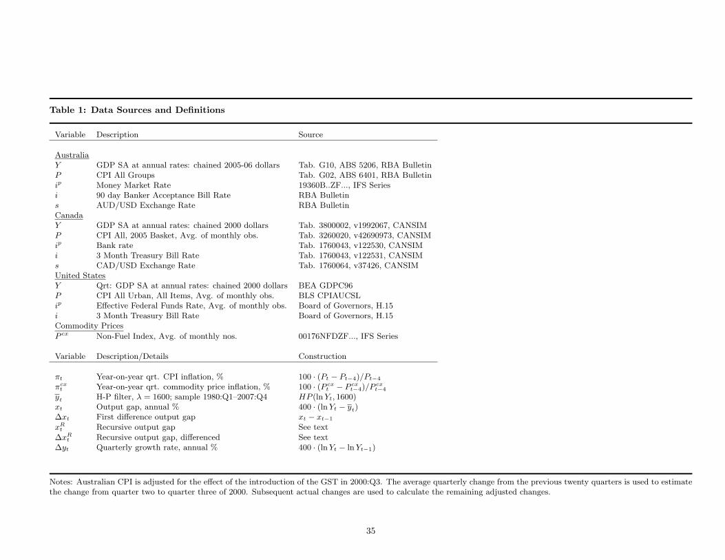
Table 1: Data Sources and Definitions

Variable Description Source

AustraliaY GDP SA at annual rates: chained 2005-06 dollars Tab. G10, ABS 5206, RBA BulletinP CPI All Groups Tab. G02, ABS 6401, RBA Bulletinip Money Market Rate 19360B..ZF..., IFS Seriesi 90 day Banker Acceptance Bill Rate RBA Bulletins AUD/USD Exchange Rate RBA BulletinCanadaY GDP SA at annual rates: chained 2000 dollars Tab. 3800002, v1992067, CANSIMP CPI All, 2005 Basket, Avg. of monthly obs. Tab. 3260020, v42690973, CANSIMip Bank rate Tab. 1760043, v122530, CANSIMi 3 Month Treasury Bill Rate Tab. 1760043, v122531, CANSIMs CAD/USD Exchange Rate Tab. 1760064, v37426, CANSIMUnited StatesY Qrt: GDP SA at annual rates: chained 2000 dollars BEA GDPC96P CPI All Urban, All Items, Avg. of monthly obs. BLS CPIAUCSLip Effective Federal Funds Rate, Avg. of monthly obs. Board of Governors, H.15i 3 Month Treasury Bill Rate Board of Governors, H.15Commodity Prices

P cx Non-Fuel Index, Avg. of monthly nos. 00176NFDZF..., IFS Series

Variable Description/Details Construction

πt Year-on-year qrt. CPI inflation, % 100 · (Pt − Pt−4)/Pt−4

πcxt Year-on-year qrt. commodity price inflation, % 100 · (P cx

t − P cxt−4)/P cx

t−4

yt H-P filter, λ = 1600; sample 1980:Q1–2007:Q4 HP (lnYt, 1600)xt Output gap, annual % 400 · (lnYt − yt)∆xt First difference output gap xt − xt−1

xRt Recursive output gap See text

∆xRt Recursive output gap, differenced See text

∆yt Quarterly growth rate, annual % 400 · (lnYt − lnYt−1)

Notes: Australian CPI is adjusted for the effect of the introduction of the GST in 2000:Q3. The average quarterly change from the previous twenty quarters is used to estimatethe change from quarter two to quarter three of 2000. Subsequent actual changes are used to calculate the remaining adjusted changes.

35

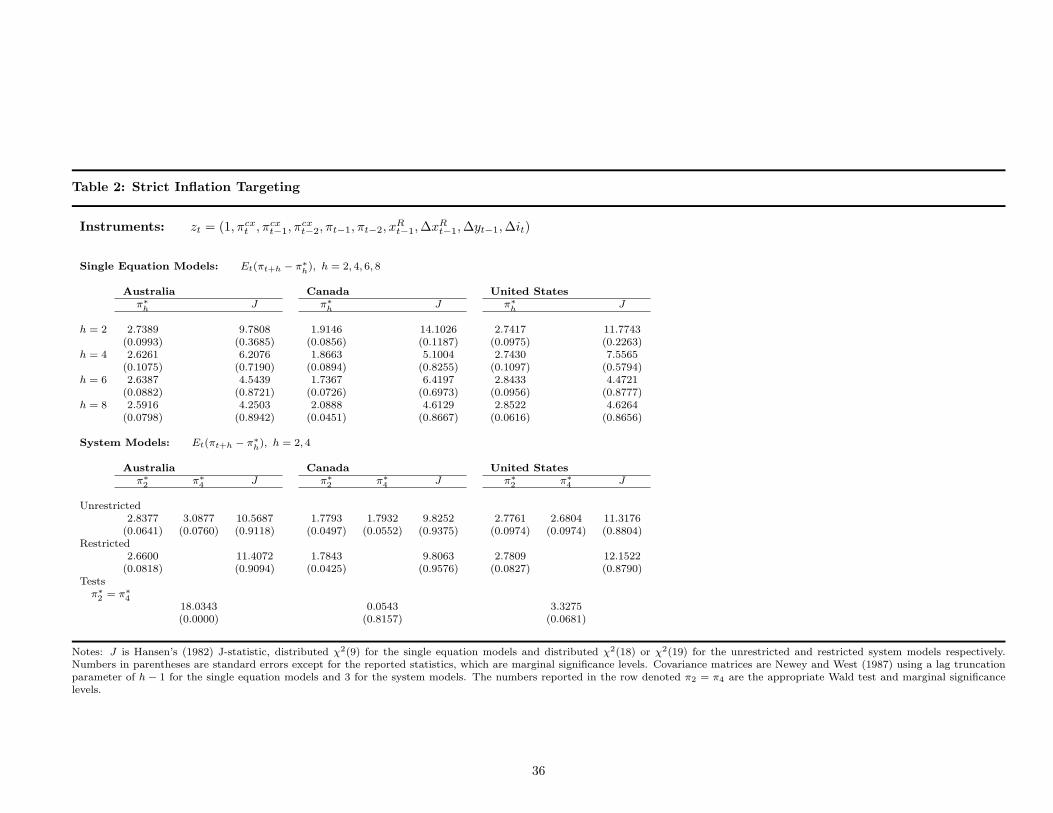
Table 2: Strict Inflation Targeting

Instruments: zt = (1, πcxt , πcx

t−1, πcxt−2, πt−1, πt−2, x

Rt−1,∆x

Rt−1,∆yt−1,∆it)

Single Equation Models: Et(πt+h − π∗h), h = 2, 4, 6, 8

Australia Canada United Statesπ∗h J π∗h J π∗h J

h = 2 2.7389 9.7808 1.9146 14.1026 2.7417 11.7743(0.0993) (0.3685) (0.0856) (0.1187) (0.0975) (0.2263)

h = 4 2.6261 6.2076 1.8663 5.1004 2.7430 7.5565(0.1075) (0.7190) (0.0894) (0.8255) (0.1097) (0.5794)

h = 6 2.6387 4.5439 1.7367 6.4197 2.8433 4.4721(0.0882) (0.8721) (0.0726) (0.6973) (0.0956) (0.8777)

h = 8 2.5916 4.2503 2.0888 4.6129 2.8522 4.6264(0.0798) (0.8942) (0.0451) (0.8667) (0.0616) (0.8656)

System Models: Et(πt+h − π∗h), h = 2, 4

Australia Canada United Statesπ∗2 π∗4 J π∗2 π∗4 J π∗2 π∗4 J

Unrestricted2.8377 3.0877 10.5687 1.7793 1.7932 9.8252 2.7761 2.6804 11.3176

(0.0641) (0.0760) (0.9118) (0.0497) (0.0552) (0.9375) (0.0974) (0.0974) (0.8804)Restricted

2.6600 11.4072 1.7843 9.8063 2.7809 12.1522(0.0818) (0.9094) (0.0425) (0.9576) (0.0827) (0.8790)

Testsπ∗2 = π∗4

18.0343 0.0543 3.3275(0.0000) (0.8157) (0.0681)

Notes: J is Hansen’s (1982) J-statistic, distributed χ2(9) for the single equation models and distributed χ2(18) or χ2(19) for the unrestricted and restricted system models respectively.Numbers in parentheses are standard errors except for the reported statistics, which are marginal significance levels. Covariance matrices are Newey and West (1987) using a lag truncationparameter of h − 1 for the single equation models and 3 for the system models. The numbers reported in the row denoted π2 = π4 are the appropriate Wald test and marginal significancelevels.

36

Table 3: Flexible Inflation Targeting with the Output Gap

Instruments: zt = (1, πcxt , πcx

t−1, πcxt−2, πt−1, πt−2, x

Rt−1,∆x

Rt−1,∆yt−1,∆it)

Single Equation Models: Et(πt+h + φhxt+h − π∗h), h = 2, 4, 6, 8

Australia Canada United Statesφh π∗h J φh π∗h J φh π∗h J

h = 2 0.1815 2.7004 7.8536 -0.0552 1.9639 14.000 -0.0547 2.8352 10.5104(0.0778) (0.0987) (0.4479) (0.0244) (0.0898) (0.0818) (0.0338) (0.0951) (0.2310)

h = 4 0.1576 2.7169 4.7614 -0.0404 1.9313 5.0855 0.0878 2.6576 4.3857(0.1042) (0.1124) (0.7827) (0.0424) (0.1008) (0.7484) (0.0447) (0.1194) (0.8208)

h = 6 0.1737 2.6685 3.1672 -0.0805 1.8988 5.9857 -0.0325 2.8847 4.0447(0.0962) (0.0797) (0.9234) (0.0227) (0.0501) (0.6488) (0.0299) (0.1018) (0.8531)

h = 8 0.0935 2.6276 4.4243 -0.1172 2.2038 4.5251 -0.0132 2.8699 4.4524(0.0639) (0.0623) (0.8170) (0.0404) (0.0562) (0.8069) (0.0350) (0.0648) (0.8142)

System Models: Et(πt+h + φhxt+h − π∗h), h = 2, 4

Australia Canada United Statesφ2 φ4 π∗2 π∗4 J φ2 φ4 π∗2 π∗4 J φ2 φ4 π∗2 π∗4 J

Unrestricted0.1503 -0.0641 2.6355 2.6377 8.6445 -0.0359 -0.0488 1.8755 1.9042 9.4706 -0.0678 0.1128 2.9300 2.6869 8.4032

(0.0271) (0.0511) (0.0766) (0.0833) (0.9273) (0.0144) (0.0260) (0.0546) (0.0481) (0.8928) (0.0222) (0.0215) (0.0786) (0.0830) (0.9359)Restricted

0.1124 2.8909 10.6699 -0.0332 1.8735 9.5200 -0.0421 2.9751 11.2359(0.0291) (0.0545) (0.9078) (0.0133) (0.0429) (0.9465) (0.0159) (0.0690) (0.8841)

Testsφ2 = φ4 19.5145 (0.0000) 0.5296 (0.4668) 28.5170 (0.0000)π∗2 = π∗4 0.0007 (0.9796) 0.2123 (0.6450) 6.1142 (0.0134)π∗2 = π∗4 φ2 = φ4 20.0076 (0.0000) 0.6184 (0.7340) 29.4302 (0.0000)

Notes: J is Hansen’s (1982) J-statistic, distributed χ2(9) for the single equation models and distributed χ2(16) or χ2(18) for the unrestricted and restricted system models respectively.Numbers in parentheses are standard errors except for the reported statistics, which are marginal significance levels. Covariance matrices are Newey and West (1987) using a lag truncationparameter of h−1 for the single equation models and 3 for the system models. The numbers reported in the rows denoted Tests are the appropriate Wald test and marginal significance levels.

37

Table 4: Flexible Inflation Targeting with Output Gap Changes

Instruments: zt = (1, πcxt , πcx

t−1, πcxt−2, πt−1, πt−2, x

Rt−1,∆x

Rt−1,∆yt−1,∆it)

Single Equation Models: Et(πt+h + φh∆xt+h − π∗h), h = 2, 4, 6, 8

Australia Canada United Statesφh π∗h J φh π∗h J φh π∗h J

h = 2 0.1364 2.7141 7.9893 0.1981 1.9988 12.0305 0.0567 2.7500 11.6872(0.0919) (0.1081) (0.4345) (0.0640) (0.0928) (0.1498) (0.0927) (0.0951) (0.1657)

h = 4 0.0899 2.6608 5.3000 0.1356 1.9003 4.1614 0.1512 2.8073 4.2270(0.1260) (0.1152) (0.7251) (0.0663) (0.1063) (0.8423) (0.0748) (0.0977) (0.8361)

h = 6 0.0516 2.6429 4.6064 -0.1492 1.6920 4.8825 -0.0208 2.8428 4.4190(0.1646) (0.0946) (0.7987) (0.0791) (0.0736) (0.7701) (0.0840) (0.0931) (0.8175)

h = 8 -0.0208 2.5957 4.1797 0.4735 1.8101 4.4523 0.1413 2.8456 3.9060(0.1065) (0.0835) (0.8406) (0.1087) (0.0604) (0.8142) (0.0661) (0.0601) (0.8655)

System Models: Et(πt+h + φh∆xt+h − π∗h), h = 2, 4

Australia Canada United Statesφ2 φ4 π∗2 π∗4 J φ2 φ4 π∗2 π∗4 J φ2 φ4 π∗2 π∗4 J

Unrestricted0.1021 0.1642 2.7557 2.8010 6.8504 0.1999 0.1589 1.8827 1.5985 8.9696 0.1569 0.0670 2.7142 2.6603 9.1183

(0.0445) (0.0484) (0.0891) (0.0933) (0.9760) (0.0250) (0.0498) (0.0484) (0.0604) (0.9147) (0.0397) (0.0393) (0.0715) (0.0611) (0.9085)Restricted

0.1275 2.7617 7.4509 0.1410 1.8038 10.2404 0.0887 2.6993 10.9035(0.0145) (0.0781) (0.9857) (0.0233) (0.0374) (0.9238) (0.0351) (0.0665) (0.8984)

Testsφ2 = φ4 0.4896 (0.4841) 0.7231 (0.3951) 5.3570 (0.0206)π∗2 = π∗4 0.3070 (0.5795) 15.6699 (0.0001) 1.1793 (0.2775)π∗2 = π∗4 φ2 = φ4 0.6910 (0.7079) 22.1686 (0.0000) 8.0775 (0.0176)

Notes: J is Hansen’s (1982) J-statistic, distributed χ2(9) for the single equation models and distributed χ2(16) or χ2(18) for the unrestricted and restricted system models respectively.Numbers in parentheses are standard errors except for the reported statistics, which are marginal significance levels. Covariance matrices are Newey and West (1987) using a lag truncationparameter of h−1 for the single equation models and 3 for the system models. The numbers reported in the rows denoted Tests are the appropriate Wald test and marginal significance levels.

38

Table 5: Flexible Inflation Targeting with Output Growth

Instruments: zt = (1, πcxt , πcx

t−1, πcxt−2, πt−1, πt−2, x

Rt−1,∆x

Rt−1,∆yt−1,∆it)

Single Equation Models: Et(πt+h + φh∆yt+h − π∗h), h = 2, 4, 6, 8

Australia Canada United Statesφh π∗h J φh π∗h J φh π∗h J

h = 2 0.1646 3.2557 7.8030 0.1647 2.5040 11.8667 0.1069 3.0882 11.5811(0.0906) (0.3456) (0.4529) (0.0536) (0.1613) (0.1573) (0.0861) (0.2917) (0.1709)

h = 4 0.1332 3.1330 4.8031 0.1486 2.3565 3.7643 0.1414 3.2428 4.1055(0.1164) (0.4242) (0.7784) (0.0606) (0.2114) (0.8777) (0.0672) (0.2234) (0.8475)

h = 6 0.1260 3.0811 4.5472 -0.0828 1.3898 5.5353 -0.0367 2.7323 4.3116(0.1631) (0.6003) (0.8047) (0.0788) (0.2913) (0.6991) (0.0840) (0.2639) (0.8280)

h = 8 0.0270 2.6871 4.3975 0.3498 2.9793 4.2420 0.1076 3.1801 4.3633(0.1129) (0.3968) (0.8834) (0.0532) (0.1848) (0.8347) (0.0522) (0.1510) (0.8229)

System Models: Et(πt+h + φh∆yt+h − π∗h), h = 2, 4

Australia Canada United Statesφ2 φ4 π∗2 π∗4 J φ2 φ4 π∗2 π∗4 J φ2 φ4 π∗2 π∗4 J

Unrestricted0.1156 0.1605 3.1363 3.3303 7.0622 0.1630 0.1463 2.4233 2.1109 8.9252 0.1550 0.0676 3.2122 2.8789 8.7215

(0.0464) (0.0447) (0.1976) (0.1610) (0.9720) (0.0223) (0.0436) (0.0765) (0.1351) (0.9165) (0.0366) (0.0388) (0.1262) (0.1325) (0.9244)Restricted

0.1332 3.2026 7.4322 0.1369 2.2722 9.8882 0.0900 2.9840 10.7207(0.0159) (0.0926) (0.9859) (0.0199) (0.0688) (0.9355) (0.0328) (0.1108) (0.9058)

Testsφ2 = φ4 0.2712 (0.6025) 0.1626 (0.6868) 6.5089 (0.0107)π∗2 = π∗4 0.3751 (0.5402) 5.5635 (0.0183) 10.7951 (0.0010)π∗2 = π∗4 φ2 = φ4 0.4525 (0.7975) 13.6977 (0.0011) 11.3560 (0.0034)

Notes: J is Hansen’s (1982) J-statistic, distributed χ2(9) for the single equation models and distributed χ2(16) or χ2(18) for the unrestricted and restricted system models respectively.Numbers in parentheses are standard errors except for the reported statistics, which are marginal significance levels. Covariance matrices are Newey and West (1987) using a lag truncationparameter of h−1 for the single equation models and 3 for the system models. The numbers reported in the rows denoted Tests are the appropriate Wald test and marginal significance levels.Single equation estimates for Australia for h = 8 include an additional instrument, it. See text for details.

39

Table 6: Instrument Quality

Instruments: zt = (1, πcxt , πcx

t−1, πcxt−2, πt−1, πt−2, x

Rt−1,∆x

Rt−1,∆yt−1,∆it)

Australia Canada United States

πt+h xt+h ∆xt+h ∆yt+h πt+h xt+h ∆xt+h ∆yt+h πt+h xt+h ∆xt+h ∆yt+h

h = 2 8.200 3.159 1.605 1.795 5.673 7.144 3.246 4.674 8.839 9.446 2.291 2.949h = 4 4.530 2.846 0.919 1.232 1.532 2.767 1.858 2.447 1.820 8.254 1.259 1.651h = 6 5.957 1.181 0.217 0.258 1.538 2.593 1.036 1.293 0.979 7.159 0.653 0.857h = 8 5.583 0.851 0.202 0.324 1.520 2.343 0.515 1.210 1.020 3.848 1.041 1.270

Notes: Numbers are F -tests for the joint hypothesis that all instruments (except the constant term) have coefficients zero when regressed against each of theinstruments.

40

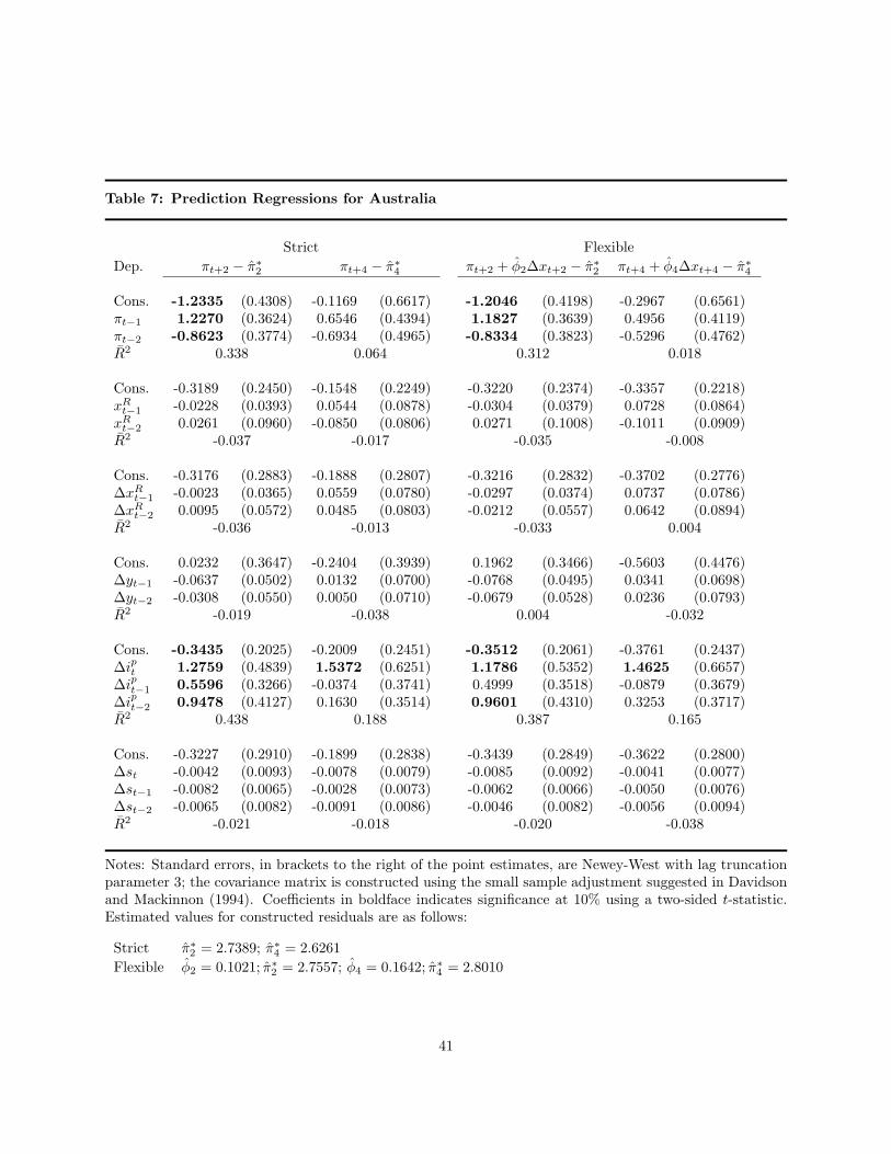
Table 7: Prediction Regressions for Australia

Strict FlexibleDep. πt+2 − π∗2 πt+4 − π∗4 πt+2 + φ2∆xt+2 − π∗2 πt+4 + φ4∆xt+4 − π∗4

Cons. -1.2335 (0.4308) -0.1169 (0.6617) -1.2046 (0.4198) -0.2967 (0.6561)πt−1 1.2270 (0.3624) 0.6546 (0.4394) 1.1827 (0.3639) 0.4956 (0.4119)πt−2 -0.8623 (0.3774) -0.6934 (0.4965) -0.8334 (0.3823) -0.5296 (0.4762)R2 0.338 0.064 0.312 0.018

Cons. -0.3189 (0.2450) -0.1548 (0.2249) -0.3220 (0.2374) -0.3357 (0.2218)xR

t−1 -0.0228 (0.0393) 0.0544 (0.0878) -0.0304 (0.0379) 0.0728 (0.0864)xR

t−2 0.0261 (0.0960) -0.0850 (0.0806) 0.0271 (0.1008) -0.1011 (0.0909)R2 -0.037 -0.017 -0.035 -0.008

Cons. -0.3176 (0.2883) -0.1888 (0.2807) -0.3216 (0.2832) -0.3702 (0.2776)∆xR

t−1 -0.0023 (0.0365) 0.0559 (0.0780) -0.0297 (0.0374) 0.0737 (0.0786)∆xR

t−2 0.0095 (0.0572) 0.0485 (0.0803) -0.0212 (0.0557) 0.0642 (0.0894)R2 -0.036 -0.013 -0.033 0.004

Cons. 0.0232 (0.3647) -0.2404 (0.3939) 0.1962 (0.3466) -0.5603 (0.4476)∆yt−1 -0.0637 (0.0502) 0.0132 (0.0700) -0.0768 (0.0495) 0.0341 (0.0698)∆yt−2 -0.0308 (0.0550) 0.0050 (0.0710) -0.0679 (0.0528) 0.0236 (0.0793)R2 -0.019 -0.038 0.004 -0.032

Cons. -0.3435 (0.2025) -0.2009 (0.2451) -0.3512 (0.2061) -0.3761 (0.2437)∆ipt 1.2759 (0.4839) 1.5372 (0.6251) 1.1786 (0.5352) 1.4625 (0.6657)∆ipt−1 0.5596 (0.3266) -0.0374 (0.3741) 0.4999 (0.3518) -0.0879 (0.3679)∆ipt−2 0.9478 (0.4127) 0.1630 (0.3514) 0.9601 (0.4310) 0.3253 (0.3717)R2 0.438 0.188 0.387 0.165

Cons. -0.3227 (0.2910) -0.1899 (0.2838) -0.3439 (0.2849) -0.3622 (0.2800)∆st -0.0042 (0.0093) -0.0078 (0.0079) -0.0085 (0.0092) -0.0041 (0.0077)∆st−1 -0.0082 (0.0065) -0.0028 (0.0073) -0.0062 (0.0066) -0.0050 (0.0076)∆st−2 -0.0065 (0.0082) -0.0091 (0.0086) -0.0046 (0.0082) -0.0056 (0.0094)R2 -0.021 -0.018 -0.020 -0.038

Notes: Standard errors, in brackets to the right of the point estimates, are Newey-West with lag truncationparameter 3; the covariance matrix is constructed using the small sample adjustment suggested in Davidsonand Mackinnon (1994). Coefficients in boldface indicates significance at 10% using a two-sided t-statistic.Estimated values for constructed residuals are as follows:

Strict π∗2 = 2.7389; π∗4 = 2.6261Flexible φ2 = 0.1021; π∗2 = 2.7557; φ4 = 0.1642; π∗4 = 2.8010

41

Table 8: Prediction Regressions for Canada

Strict FlexibleDep. πt+2 − π∗2 πt+4 − π∗4 πt+2 + φ2∆xt+2 − π∗2 πt+4 + φ4∆xt+4 − π∗4

Cons. 0.2889 (0.3605) 0.0687 (0.2559) 0.3390 (0.3493) 0.2206 (0.3067)πt−1 0.1984 (0.1530) -0.2361 (0.2095) 0.0606 (0.1389) -0.1917 (0.1940)πt−2 -0.2896 (0.0951) 0.2946 (0.2241) -0.1712 (0.1275) 0.3024 (0.2295)R2 0.018 0.022 -0.014 0.029

Cons. 0.1553 (0.1669) 0.2235 (0.1710) 0.1940 (0.1447) 0.4835 (0.1555)xR

t−1 0.0677 (0.0485) -0.0188 (0.0539) 0.0842 (0.0513) -0.0503 (0.0523)xR

t−2 -0.1033 (0.0674) -0.0194 (0.0508) -0.1448 (0.0606) 0.0091 (0.0519)R2 0.010 0.010 0.082 0.049

Cons. 0.1114 (0.1641) 0.1942 (0.1629) 0.1286 (0.1514) 0.4500 (0.1500)∆xR

t−1 0.0376 (0.0579) 0.0311 (0.0525) 0.0758 (0.0582) -0.0049 (0.0528)∆xR

t−2 0.0178 (0.0520) -0.1099 (0.0851) -0.0366 (0.0517) -0.1054 (0.0782)R2 -0.023 0.026 -0.014 0.054

Cons. -0.3300 (0.1376) 0.2464 (0.3455) -0.2545 (0.1781) 0.6152 (0.3185)∆yt−1 0.0797 (0.0509) 0.0604 (0.0601) 0.1165 (0.0570) 0.0271 (0.0616)∆yt−2 0.0574 (0.0585) -0.0803 (0.0927) 0.0020 (0.0556) -0.0776 (0.0877)R2 0.054 -0.012 0.050 -0.011

Cons. 0.1319 (0.1720) 0.1702 (0.1669) 0.1369 (0.1605) 0.4211 (0.1554)∆ipt 0.3165 (0.1950) -0.1124 (0.1951) 0.1837 (0.2207) -0.1505 (0.1806)∆ipt−1 -0.0704 (0.1191) -0.1398 (0.1989) -0.0660 (0.1113) -0.2282 (0.1756)∆ipt−2 -0.0828 (0.2117) -0.1446 (0.1769) -0.1855 (0.1929) -0.0594 (0.1720)R2 -0.003 -0.012 -0.017 0.013

Cons. 0.1061 (0.1852) 0.1612 (0.1872) 0.1041 (0.1651) 0.4123 (0.1791)∆st -0.0052 (0.0127) -0.0027 (0.0090) -0.0096 (0.0110) -0.0028 (0.0094)∆st−1 -0.0038 (0.0115) 0.0032 (0.0074) -0.0051 (0.0114) -0.0009 (0.0085)∆st−2 0.0000 (0.0094) -0.0104 (0.0072) -0.0026 (0.0104) -0.0068 (0.0070)R2 -0.056 -0.047 -0.039 -0.055

Notes: Standard errors, in brackets to the right of the point estimates, are Newey-West with lag truncationparameter 3; the covariance matrix is constructed using the small sample adjustment suggested in Davidsonand Mackinnon (1994). Coefficients in boldface indicates significance at 10% using a two-sided t-statistic.Estimated values for constructed residuals are as follows:

Strict π∗2 = 1.9146; π∗4 = 1.8663Flexible φ2 = 0.1999; π∗2 = 1.8827; φ4 = 0.1589; π∗4 = 1.5985

42

Table 9: Prediction Regressions for the United States

Strict FlexibleDep. πt+2 − π∗2 πt+4 − π∗4 πt+2 + φ2∆xt+2 − π∗2 πt+4 + φ4∆xt+4 − π∗4

Cons. -1.0924 (0.3024) -0.3200 (0.3243) -0.9134 (0.2777) -0.2206 (0.3148)πt−1 0.7889 (0.1554) 0.0362 (0.1878) 0.7465 (0.1683) 0.0535 (0.1885)πt−2 -0.4506 (0.1780) 0.0549 (0.2054) -0.4148 (0.1746) 0.0337 (0.2087)R2 0.297 -0.014 0.248 -0.016

Cons. 0.0054 (0.1597) -0.0558 (0.1433) 0.0334 (0.1539) 0.0304 (0.1411)xR

t−1 -0.0245 (0.0705) 0.0398 (0.0497) -0.0191 (0.0683) 0.0372 (0.0513)xR

t−2 0.0359 (0.0638) -0.0475 (0.0490) 0.0253 (0.0626) -0.0476 (0.0495)R2 -0.025 -0.015 -0.028 -0.016

Cons. 0.0007 (0.1575) -0.0528 (0.1389) 0.0307 (0.1534) 0.0344 (0.1372)∆xR

t−1 -0.0390 (0.0696) 0.0342 (0.0455) -0.0371 (0.0649) 0.0298 (0.0466)∆xR

t−2 0.0568 (0.0479) 0.0105 (0.0401) 0.0626 (0.0521) 0.0134 (0.0423)R2 -0.006 -0.016 -0.002 -0.017

Cons. -0.0016 (0.3648) -0.0878 (0.2501) 0.0467 (0.3755) 0.0185 (0.2621)∆yt−1 -0.0471 (0.0717) 0.0190 (0.0469) -0.0521 (0.0647) 0.0119 (0.0465)∆yt−2 0.0477 (0.0493) -0.0074 (0.0405) 0.0461 (0.0524) -0.0070 (0.0415)R2 -0.008 -0.029 -0.005 -0.030

Cons. 0.0260 (0.1524) -0.0420 (0.1331) 0.0511 (0.1483) 0.0427 (0.1323)∆ipt 0.0422 (0.3202) 0.5595 (0.2983) 0.1282 (0.3574) 0.4913 (0.3114)∆ipt−1 0.4145 (0.2549) -0.1142 (0.1887) 0.2603 (0.2680) -0.0441 (0.1803)∆ipt−2 0.0487 (0.1792) -0.1199 (0.2456) 0.0220 (0.2295) -0.1716 (0.2467)R2 0.041 0.050 0.001 0.037

Notes: Standard errors, in brackets to the right of the point estimates, are Newey-West with lag truncationparameter 3; the covariance matrix is constructed using the small sample adjustment suggested in Davidsonand Mackinnon (1994). Coefficients in boldface indicates significance at 10% using a two-sided t-statistic.Estimated values for constructed residuals are as follows:

Strict π∗2 = 2.7417; π∗4 = 2.7430Flexible φ2 = 0.1569; π∗2 = 2.7142; φ4 = 0.0670; π∗4 = 2.6603

43

AUSTRALIA: INFLATION

-1.0

0.0

1.0

2.0

3.0

4.0

5.0

6.0

7.0

1990

.25

1991

.25

1992

.25

1993

.25

1994

.25

1995

.25

1996

.25

1997

.25

1998

.25

1999

.25

2000

.25

2001

.25

2002

.25

2003

.25

2004

.25

2005

.25

2006

.25

2007

.25

An

nu

al %

AUSTRALIA: OUTPUT GAP

-15.0

-10.0

-5.0

0.0

5.0

10.0

15.0

1990

.25

1991

.25

1992

.25

1993

.25

1994

.25

1995

.25

1996

.25

1997

.25

1998

.25

1999

.25

2000

.25

2001

.25

2002

.25

2003

.25

2004

.25

2005

.25

2006

.25

2007

.25

An

nu

al %

Solid: Recursive

Dashed: Full Sample

Figure 1: Australian Inflation and HP Output Gaps

44

CANADA INFLATION

-1.0

0.0

1.0

2.0

3.0

4.0

5.0

6.0

7.0

1990.25

1991.25

1992.25

1993.25

1994.25

1995.25

1996.25

1997.25

1998.25

1999.25

2000.25

2001.25

2002.25

2003.25

2004.25

2005.25

2006.25

2007.25

An

nu

al %

Figure 2: Canadian Inflation and HP Output Gaps

45

US INFLATION

-1.0

0.0

1.0

2.0

3.0

4.0

5.0

6.0

7.0

1990

.25

1991

.25

1992

.25

1993

.25

1994

.25

1995

.25

1996

.25

1997

.25

1998

.25

1999

.25

2000

.25

2001

.25

2002

.25

2003

.25

2004

.25

2005

.25

2006

.25

2007

.25

An

nu

al %

UNITED STATES: OUTPUT GAP

-15.0

-10.0

-5.0

0.0

5.0

10.0

15.0

1990

.25

1991

.25

1992

.25

1993

.25

1994

.25

1995

.25

1996

.25

1997

.25

1998

.25

1999

.25

2000

.25

2001

.25

2002

.25

2003

.25

2004

.25

2005

.25

2006

.25

2007

.25

An

nu

al %

Solid: Recursive

Dashed: Full Sample

Figure 3: United States Inflation and HP Output Gaps

46

Australia

-4.0

-3.0

-2.0

-1.0

0.0

1.0

2.0

3.0

4.0

5.0

6.0

1990.25 1991.25 1992.25 1993.25 1994.25 1995.25 1996.25 1997.25 1998.25 1999.25 2000.25 2001.25 2002.25 2003.25 2004.25 2005.25 2006.25 2007.25

Date

Annual

Per

cent

Dashed: InflationSolid Light: ResidualSolid Dark: Scaled Change in Output Gap

Canada

-4.0

-3.0

-2.0

-1.0

0.0

1.0

2.0

3.0

4.0

5.0

1990.25 1991.25 1992.25 1993.25 1994.25 1995.25 1996.25 1997.25 1998.25 1999.25 2000.25 2001.25 2002.25 2003.25 2004.25 2005.25 2006.25 2007.25

Date

Annual

Per

cent

Dashed: InflationSolid Light: ResidualSolid Dark: Scaled Change in Output Gap

United States

-4.0

-3.0

-2.0

-1.0

0.0

1.0

2.0

3.0

4.0

5.0

6.0

1990.25 1991.25 1992.25 1993.25 1994.25 1995.25 1996.25 1997.25 1998.25 1999.25 2000.25 2001.25 2002.25 2003.25 2004.25 2005.25 2006.25 2007.25

Date

Annual

Per

cent

Dashed: InflationSolid Light: ResidualSolid Dark: Scaled Change in Output Gap

Figure 4: Estimated Deviations from Flexible Inflation Targets and Scaled Change in OutputGap

47