Strength of Materials WORK-BOOK
76
Strength of Materials W ORK -B OOK RM Nkgoeng
Transcript of Strength of Materials WORK-BOOK

Strength of MaterialsWORK-BOOK
RM Nkgoeng

Copyright c© 2013 Mashilo Nkgoeng
SELF-PUBLISHED
WWW.MASHILONKGOENG.CO.ZA
Licensed under the Creative Commons Attribution-Non-commercial 3.0 Unported License (the“License”). You may not use this file except in compliance with the License. You may obtain acopy of the License at http://creativecommons.org/licenses/by-nc/3.0. Un-less required by applicable law or agreed to in writing, software distributed under the Licenseis distributed on an “AS IS” BASIS, WITHOUT WARRANTIES OR CONDITIONS OFANY KIND, either express or implied. See the License for the specific language governingpermissions and limitations under the License.
First printing, December 2013

Contents
1 Deflection of Beams . . . . . . . . . . . . . . . . . . . . . . . . . . . . . . . . . . . . . . . . . 5
1.1 What is a Beam? 51.1.1 Beam terminology . . . . . . . . . . . . . . . . . . . . . . . . . . . . . . . . . . . . . . . . . . . . . . . 51.1.2 Mathematical Models . . . . . . . . . . . . . . . . . . . . . . . . . . . . . . . . . . . . . . . . . . . . . 51.1.3 Assumption of Classical Beam Theory . . . . . . . . . . . . . . . . . . . . . . . . . . . . . . . . 61.1.4 Beam Loading . . . . . . . . . . . . . . . . . . . . . . . . . . . . . . . . . . . . . . . . . . . . . . . . . . 61.1.5 Support Conditions . . . . . . . . . . . . . . . . . . . . . . . . . . . . . . . . . . . . . . . . . . . . . . 61.1.6 Stresses, strains and bending moments . . . . . . . . . . . . . . . . . . . . . . . . . . . . . . . 6
1.2 Notation 7
1.3 Second Order Method for Beam Deflections 7
1.4 Double Integration Using Bracket Functions 7
1.5 Examples 9
1.6 Exercises 16
2 Continuous Beams . . . . . . . . . . . . . . . . . . . . . . . . . . . . . . . . . . . . . . . . . 19
2.1 Introduction 192.1.1 Point Load . . . . . . . . . . . . . . . . . . . . . . . . . . . . . . . . . . . . . . . . . . . . . . . . . . . . 192.1.2 Uniformly Distributed Load . . . . . . . . . . . . . . . . . . . . . . . . . . . . . . . . . . . . . . . . 21
2.2 Exercise 22
2.3 Examples 23
2.4 Exercises 23
3 Energy Methods . . . . . . . . . . . . . . . . . . . . . . . . . . . . . . . . . . . . . . . . . . . . 25
3.1 Introduction 25
3.2 Strain Energy of Bars 26
3.3 Castigliano’s Theorem 26
3.4 Structures 27
3.5 Castigliano’s theorem applied to Curved Beams 27
3.6 Castigliano’s theorem applied to Beams 273.6.1 Cantilever beam with a Point Load at the free end . . . . . . . . . . . . . . . . . . . . . . . 273.6.2 S/S beam with a Point Load at mid-point . . . . . . . . . . . . . . . . . . . . . . . . . . . . . . 28
3.7 Examples 29
3.8 Exercises 34

4 Unsymmetrical Bending of Beams . . . . . . . . . . . . . . . . . . . . . . . . . . . 39
4.1 Symmetric Member in Pure Bending 39
4.2 Unsymmetrical Bending 40
4.3 Alternative procedure for stress determination 42
4.4 Deflection 44
4.5 Notation 44
4.6 xxx 444.6.1 Point Load . . . . . . . . . . . . . . . . . . . . . . . . . . . . . . . . . . . . . . . . . . . . . . . . . . . . 444.6.2 Uniformly Distributed Load . . . . . . . . . . . . . . . . . . . . . . . . . . . . . . . . . . . . . . . . 44
4.7 Examples 44
4.8 Exercises 47
5 Inelastic Bending . . . . . . . . . . . . . . . . . . . . . . . . . . . . . . . . . . . . . . . . . . . 49
5.1 Plastic Bending of Rectangular Beams 49
5.2 Plastic Bending of Symmetrical (I-Section) Beam 52
5.3 Partially plastic Bending of Unsymmetrical Sections 53
5.4 Limit Analysis-Bending 565.4.1 Bending . . . . . . . . . . . . . . . . . . . . . . . . . . . . . . . . . . . . . . . . . . . . . . . . . . . . . . 565.4.2 The principle of Virtual Work . . . . . . . . . . . . . . . . . . . . . . . . . . . . . . . . . . . . . . . 58
5.5 Solid Shaft 65
5.6 Hollow shaft 67
5.7 Exercises 69

What is a Beam?Beam terminologyMathematical ModelsAssumption of Classical Beam TheoryBeam LoadingSupport ConditionsStresses, strains and bending moments
NotationSecond Order Method for Beam DeflectionsDouble Integration Using BracketFunctionsExamplesExercises 1 — Deflection of Beams
IntroductionThis lecture notes starts the presentation of methods for computed lateral deflections of planebeams undergoing symmetric bending. The workbook just summarises the topic, but thetextbook1 covers in detail this topic in chapter 9 and 10. We assume that as a student you arefamiliar with the following:
1. integration of Ordinary Differential Equations2. Statics of plane beams under symmetric bending. This is also covered in Chapter 5 and 6
of the prescribed textbook.
1.1 What is a Beam?Beams are the most common type of structural component, particularly in Civil and MechanicalEngineering. A beam is a bar-like structural member whose primary function is to supporttransverse loading and carry it to the supports. By bar-like, we mean that one of the dimensionsis considered larger than the other two. This dimension is called the longitudinal dimensionor beam axis. The intersection of planes normal to the longitudinal dimension with the beammember are called cross sections. A longitudinal plane is one that passes through the beam axis.A beam resist transverse loads mainly through bending action. Bending produces compressivelongitudinal stresses in one side of the beam and tensile stresses in the other. the two regionsare separated by a neutral surface of zero stress. The combination of tensile and compressivestresses produces an internal bending moment. This moment is the primary mechanism thattransports loads to the supports. This is illustrated by Fig. #
1.1.1 Beam terminologyGeneral Beam –it is a bar like member designed to resist a combination of loading actions such
as biaxial bending, transverse shears, axial stretching or compression, possibly torsion. Ifthe internal axial force is compressive, the beam has also to be designed to resist buckling.If the beam is subject primarily to bending and axial forces, it is called a beam-column. Ifit is subjected primarily to bending forces, it is called simply a beam. A beam is straight ifits longitudinal axis is straight. It is prismatic if its cross section is constant.
Spatial Beam –it supports transverse loads that can act on arbitrary directions along the crosssection.
Plane Beam –it resists primarily transverse loading on a preferred longitudinal plane.
1.1.2 Mathematical ModelsOne-dimensional mathematical models of structural beams are constructed on the basis of beamtheories. Since beams are actually three-dimensional bodies, all models necessarily involvesome form of approximation to the underlying physics. The simplest and best known model forstraight, prismatic beams are based on the Bernoulli-Euler theory as well as the Timoshenko
1Mechanics of Materials by Gere and Goodno

6 Deflection of Beams
beam theory. The B-E theory is the one that is taught in SOM3602 and is the only one that wewill be dealing with in SOM401M. The Timoshenko model incorporates a first order kinematiccorrection for transverse shear effects. This model assumes additional importance in dynamicsand vibration.
1.1.3 Assumption of Classical Beam Theory
The classical beam theory for plane beams rests on the following assumptions:1. Planar symmetry: The longitudinal axis is straight and the cross section of the beam has
a longitudinal plane of symmetry. The resultant of the transverse loads acting on eachsection lies on that plane. The support conditions are also symmetric about this plane.
2. Cross section variation: The cross section is either constant or varies smoothly.3. Normality: Plane sections originally normal to the longitudinal axis of the beam remain
plane and normal to the deformed longitudinal axis upon bending.4. Strain energy: The internal strain energy of the member accounts only for bending
moment deformations. All other contributions, notably transverse shear and axial force,are ignored.
5. Linearisation: Transverse deflections, rotations and deformations are considered so smallthat the assumptions of infinitesimal deformations apply.
6. Material model: The material is assumed to be elastic and isotropic. Heterogeneousbeams fabricated with several isotropic materials, such as reinforced concrete, are notexcluded.
1.1.4 Beam Loading
The transverse force per unit length that acts on the beam in the y+ direction is denoted byf (x) as shown in Figure #Point loads and moments acting on isolated beam sections can berepresented with Discontinuity Functions (DF’s).
1.1.5 Support Conditions
Support conditions for beams exhibit far more variety than for bar members. Two cases are oftenencountered in engineering practice: simple support and cantilever support. These are shownin Figs. # and # respectively. Beams often appear as components of skeletal structures calledframeworks, in which case the support conditions are of more complex type. Easily solved usingfinite element methods.
1.1.6 Stresses, strains and bending moments
The Bernoulli-Euler model assumes that the internal energy of beam member is entirely due tobending strains and stresses. Bending produces axial stresses σx which is just abbreviated σ andaxial strains εx which is just ε . The strains can be linked to the displacements by differentiatingthe axial displacement u(x):
ε =∂u∂x
=−yd2vdx2 =−yv′′ =−yκ (1.1)
where κ denotes the deformed beam axis curvature. The bending stress is linked to e throughone-dimensional Hooke’s law
σ = Ee =−Eyd2vdx2 =−Eyκ (1.2)

1.2 Notation 7
The most important stress resultant in classical beam theory is the bending moment Mx, which isdefined as the cross sectional integral
Mx =∫
A−yσ dA = E
d2vdx2
∫A
y2dA = EIxxκ (1.3)
The bending moment is considered positive if it compresses the upper portion: y > 0. the productEIxx is called the bending rigidity of the beam with respect to flexure about the x axis.
1.2 Notation
Quantity SymbolGeneric load for ODE Work f (x)Transverse Shear Force V (x)Bending Moment M(x)Slope of deflection curve dv(x)
dx = v′(x)Deflection Curve v(x)
Table 1.1: Notation
1.3 Second Order Method for Beam DeflectionsThe second-order method to find beam deflections gets its name from the order of the ODE to beintegrated: EIxxv′′(x) = M(x) is a second order ODE. The procedure can be broken down intothe following steps:
1. Find the bending moment M(x) = d2v(x)dx2 directly. i.e. by cutting the beam at distance x
and taking moments about x.2. Integrate M(x) once to get the slope v′(x) = dv(x)
dx3. Integrate the slope v′(x) once to get the deflection v(x)4. If there are no continuity conditions, the above steps will produce two integration constants
C1 and C2. Apply kinematics boundary conditions to determine the values of the integrationconstants. If there are continuity conditions, more than two constants of integration mayappear and are solved the same way, i.e. by using boundary conditions.
5. Substitute the constants of integration into the deflection function to get v(x)6. Evaluate v(x) at points of interest on the beam.
1.4 Double Integration Using Bracket FunctionsWhen the loads on a beam do not conform to standard cases, the solution for slope and deflectionmay be found from first principles. Macaulay developed a method for making the integrationsimpler. The basic equation governing the slope and deflection of beams is:
EId2ydx2 = M : Where M is a function of x (1.4)
When a beam has a variety of loads it is difficult to apply this theory because some loads maybe within the limits of x during the derivation but not during the solution of a particular point.Macaluay’s method makes it possible to do the integration necessary by placing all the termscontaining x within a square bracket and integrating the bracket, not x. During evaluation, any

8 Deflection of Beams
bracket with a negative value is ignored because a negative means that the load it refers to isnot within the limit of x. The general method of solution is conducted as follows. Refer to Fig.#. In a real example, the loads and reactions would have numerical values but for the sake ofdemonstrating the general method we will use algebraic symbols. This has only point loads.
1. Write down the bending moment equation placing x on the extreme right hand end of thebeam so that it contains all the loads. Write all terms containing x in a square bracket.
EId2ydx2 = M = RA[x]−P1[x−a]−P2[x−b]−P3[x− c]
2. Integrate once treating the square bracket as the variable.
EIdydx
= RA[x]2
2−P1
[x−a]2
2−P2
[x−b]2
2−P3
[x− c]2
2+C1
3. Integrate again using the same rules.
EIy = RA[x]3
6−P1
[x−a]3
6−P2
[x−b]3
6−P3
[x− c]3
6+C1x+C2
4. Use boundary conditions to solve constants C1 and C2.5. Solve slope and deflection by putting in appropriate value of x. IGNORE any brackets
containing negative values.Evaluating the constants of integration that arise in the double-integration method can becomevery involved if more than two beam segments must be analysed. We can simplify the calculationsby expressing the bending moment in terms of discontinuity functions, also known as Macaulaybracket functions. Discontinuity functions enable us to write a single expression for the bendingmoment that is valid for the entire length of the beam, even if the loading is discontinuous. Byintegrating a single, continuous expression for the bending moment, we obtain equations forslopes and deflections that are also continuous everywhere. As an illustration let us consider asimply supported beam with three segments as shown in Fig. 1.1. I have already determined thereactions. All we need to do is to segment it nicely and take moments about X−X as follows:
Mxx = 480x−500〈x−2〉− 4502〈x−3〉2 Nm (1.5)
Note that a bracket function is zero by definition if the expression in the brackets–namely (x−a)
A B
q0 = 450N/m500N
480N 920N
X
X
5m
2m 1m
x
Figure 1.1: Macaulay’s Method

1.5 Examples 9
is negative; otherwise, it is evaluated as written. A bracket function can be integrated by thesame rule as an ordinary function–namely,∫
〈x−a〉n = 〈x−a〉n+1
n+1+C (1.6)
This is called the global bending moment equation and it can be integrated to obtain the slopeand the deflection equations for the entire beam. The two constants of integration as mentionedbefore can be computed from the boundary conditions. When you use this method ensure thatyou include every load on the beam and leave the last reaction if the beam is simply supported.If the beam is a cantilever, you can obtain the global bending moment equation by starting fromthe free end or by starting from the fixed end. If you choose to start from the fixed end, calculatethe reaction first so that you can be able to include it in the global bending moment equation. Atthe end of the day, you have the choice to use any method that you feel comfortable with. Wehave not included other methods, simply because in practice we have found that we hardly usethe other methods in solving deflection of beam problems.
1.5 Examples� Example 1.1 Determine the equation for the deflection curve as well as the slope in Fig. 1.2. �
q N/m
L
Figure 1.2: Cantilever Beam with UDL
Solution 1.1 Still to be done
� Example 1.2 Determine the equation for the deflection curve as well as the slope in Fig. 5.25.�
P
L
Figure 1.3: Cantilever Beam with UDL
Solution 1.2 Still to be done
� Example 1.3 Determine the equation for the deflection curve as well as the slope in Fig.1.4 . �

10 Deflection of Beams
A B
P
L
L/2
Figure 1.4: SS Beam with Point Load
Solution 1.3 Still to be done
� Example 1.4 For the cantilever beam, Fig. 1.5 under triangular distributed loading or variablydistributed loading, determine the equation for the deflection curve as well as the slope. �
q0X
X
A
C
DB
L
x
Figure 1.5: Cantilever with VDL
Solution 1.4 We will use the same figure, Fig. 1.5 as the free-body diagram. Let the heightCD = q and use the law of triangles to get the expression of q in terms of the maximum heightor intensity q0, i.e.
qx=
q0
L∴ q =
q0xL
The moment about X−X is as follows:
EIv′′(x) =−12
q× x× x3=−q0x3
6L
We need to integrate the above twice to get two constants of integration
EIv′(x) =−q0x4
24L+C1
EIv(x) =− q0x5
120L+C1x+C2
1.5 Examples 11
The kinematic boundary conditions are v′(L) = 0 and v(L) = 0
EIv′(L) = 0 =−q0L4
24L+C1; ∴C1 =
q0L3
24
EIv(L) = 0 =− q0L5
120L+
q0L4
24+C2; ∴C2 =−
q0L4
30The equation of interest are:
v(x) =1
EI
[− q0x5
120L+
q0L3x24− q0L4
30
](1.7)
and
v′(x) =1
EI
[−q0x4
24L+
q0L3
24
](1.8)
� Example 1.5 For a given beam shown below:1. derive the equation of the elastic curve2. determine the point of maximum deflection3. determine ymax
Before one could jump in and provide a solution, it is advisable to do the following:• Develop an expression for M(x) and derive a differential equation for the elastic curve.• Integrate the differential equation twice and apply boundary conditions to obtain the elastic
curve equation• Locate a point of zero slope or point of maximum deflection• Evaluate corresponding maximum deflection
P
L a
A B C
Figure 1.6: SS Beam with an Overhang
�
Solution 1.5 The reactions are found to be RA = PaL and RB = P
(1+ a
L
). Taking moments about
X−X we get
M(x) =−PaxL
(0 < x < L)
EId2ydx2 =−Pax
L
EIdydx
=−Pax2
2L+C1
EIy =−Pax3
6L+C1x+C2

12 Deflection of Beams
The boundary conditions are simply: x = 0 : y = 0 and x = L : y = 0. The first boundary conditionleads to C2 = 0 and the second boundary condition leads to C1 =
PaL6 . The resulting equations
are therefore
EIdydx
=−Pax2
2L+
PaL6
(1.9)
and
EIy =−Pax3
6L+
PaL6
x (1.10)
Determining the position of maximum deflection is relatively easy, set y′(x) = 0
dydx
= 0 =PaL6EI
[1−3
(xm
L
)2]
∴ xm =L√3= 0.577L
ymax =PaL2
6EI
(0.577−0.5773)= 0.0642PaL2
6EI� Example 1.6 For the uniform beam shown below,
1. Determine the reaction at A2. Derive the equation for the elastic curve3. Determine the slope at A (Note that the beam is statically indeterminate to the first degree)
A B
L
Figure 1.7: LHS SS and RHS Fixed
�
Solution 1.6 The solution will include the following:• develop differential equation for the elastic curve. (this will be functionally dependent on
reaction A)• Integrate twice and apply boundary conditions to solve for the reaction at A and to obtain
the equation for the elastic curve.• Evaluate slope at A
Taking moments about D, i.e. Σ MD = 0
M = RAx− 12
(w0x2
L
)x3
M = RAx− w0x3
6L= EI
d2ydx2

1.5 Examples 13
We need to integrate EI d2ydx2 twice to get the equation for the elastic curve.
EId2ydx2 = RAx− w0x3
6L
EIdydx
=RAx2
2− w0x4
24L+C1
EIy =RAx3
6− w0x5
120L+C1x+C2
The boundary conditions are as follows:
x = 0 : y = 0 C2 = 0
x = L :dydx
= 0 C1 =w0L3
24− RAL2
2
x = L :dydx
= 0 C1 =w0L3
120− RAL2
6
From the above we find that the reaction at A is
RA =w0L10
The resulting two equations were:
y =w0
120EI
(−x5 +2L2x3−L4x
)(1.11)
θ =w0
120EI
(−5x4 +6L2x2−L4) (1.12)
� Example 1.7 A cantilever beam is 4m long with a flexural stiffness of 20MNm2. It has a pointload of 1kN at the free end and a u.d.l of 300N/m along its entire length. Calculate the slope anddeflection at the free end. �
Pq N/m
L
Figure 1.8: Cantilever Beam with UDL and Point Load
Solution 1.7 This problem can be solved by using various method. The first one that will beused is Theory of Superposition for Combined loads and the second one is double integrationmethod from first principles.For the point load only we will use the following equations todetermine the slope as well as the deflection:
1. Superposition Method for Combined Loads
y =−PL3
3EI(1.13)
14 Deflection of Beams
dydx
=PL2
2EI(1.14)
y =− 1000×43
3×20×106 =−1.06mm
dydx
=1000×42
2×20×106 = 400×10−6
For the U.D.L we will use the following equations:
y =− qL4
48EI(1.15)
dydx
=qL3
6EI(1.16)
y =− 300×44
48×20×106 =−0.48mm
dydx
=300×43
6×20×106 = 160×10−6 rad
The total deflection and slope are y =−1.54mm and dydx = 560×10−6 rad
2. Double Integration Method from 1st Principles
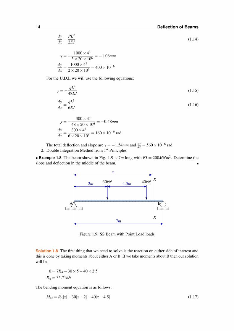
� Example 1.8 The beam shown in Fig. 1.9 is 7m long with EI = 200MNm2. Determine theslope and deflection in the middle of the beam. �
A B
30kN 40kN
7m
2m 4.5mX
X
x
Figure 1.9: SS Beam with Point Load loads
Solution 1.8 The first thing that we need to solve is the reaction on either side of interest andthis is done by taking moments about either A or B. If we take moments about B then our solutionwill be:
0 = 7RA−30×5−40×2.5
RA = 35.71kN
The bending moment equation is as follows:
Mxx = RA[x]−30[x−2]−40[x−4.5] (1.17)

1.5 Examples 15
EId2ydx2 = 35.71[x]−30[x−2]−40[x−4.5]
EIdydx
= 35.71[x]2
2−30
[x−2]2
2−40
[x−4.5]2
2+C1
EIy = 35.71[x]3
6−30
[x−2]3
6−40
[x−4.5]3
6+C1x+C2
The boundary conditions are at x = 0 we have y = 0 and this leads to C2 = 0. At x = L we havey = 0 and C1 needs to be worked out
0 = 35.71[7]3
6−30
[7−2]3
6−40
[7−4.5]3
6+C1(7)
C1 =−187.4
We are now able to write the required expressions as
EIdydx
= 35.71[x]2
2−30
[x−2]2
2−40
[x−4.5]2
2−187.4
EIy = 35.71[x]3
6−30
[x−2]3
6−40
[x−4.5]3
6−187.4x
From the above, it becomes easy to determine the deflection and rotation at the distance x = 3.5m.
� Example 1.9 The beam shown in Fig. 1.10 is 6m long with EI = 300MNm2. Determine theslope at the left hand end and the deflection at the middle of the beam. �
A B
30kN
2kN/m
7m
2mX
X
x
Figure 1.10: SS Beam with UDL and Point Load
Solution 1.9 The reaction is determine by first taking moments about the right hand support.
0 = 6RA−30×4−2×62/2
RA = 26kN
Mxx = RA[x]−30[x−2]− qx2
2
EIy′′ = 26[x]−30[x−2]− 2[x]2
2
EIy′ =26[x]2
2− 30[x−2]2
2− 2[x]3
6+C1
EIy =26[x]3
6− 30[x−2]3
6− 2[x]4
24+C1x+C2
16 Deflection of Beams
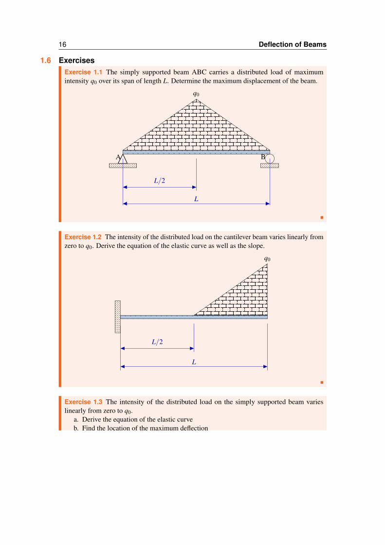
1.6 ExercisesExercise 1.1 The simply supported beam ABC carries a distributed load of maximumintensity q0 over its span of length L. Determine the maximum displacement of the beam.
A B
q0
L
L/2
�
Exercise 1.2 The intensity of the distributed load on the cantilever beam varies linearly fromzero to q0. Derive the equation of the elastic curve as well as the slope.
q0
L
L/2
�
Exercise 1.3 The intensity of the distributed load on the simply supported beam varieslinearly from zero to q0.
a. Derive the equation of the elastic curveb. Find the location of the maximum deflection

1.6 Exercises 17
A B
q0
L
L/2
�
Exercise 1.4 Determine the maximum displacement of the simply supported beam due tothe distributed loading shown below. (Hint: Utilize symmetry and analyse the right of thebeam only.) �
Exercise 1.5 Determine the deflection at the free end for the cantilever beam below with avariably distributed loaded. EI = 10MNm2
�
Exercise 1.6 A 203mm × 133mm × 25kg/m I-section (parallel flange) is used as a can-tilever with a span of 6m. It carries a point load of 6kN at 2m from the fixed end and auniformly distributed load of 2kN/m from the free end to a point 1m from the fixed end. Thecantilever is propped at a point 2m from the free end, such that the load in the prop is 9.7kN.Calculate the deflection at the free end and under the 6kN load. Neglect the mass of the beam.�
Exercise 1.7 A cantilever 3m long carries a point load of 22kN at 1m from the fixed end aswell as a uniformly distributed load of 12kN/m from the free end to a point 1m from the freeend. If the deflection at the free end is limited to 16mm, calculate the minimum necessaryvalue of I for the cross-section, neglecting the mass of the beam. A prop is now introduced1m from the free end to reduce the deflection at the free end by half. What is the magnitudeof the load in the prop. �
Exercise 1.8 Calculate the deflection 2m from the left-hand end and the slope at the left-handsupport of the beam shown below. EI = 10MNm2
�
Exercise 1.9 Calculate the slope and deflection 1m from the left-hand support of the beamshown below. EI = 10MNm2
�
Exercise 1.10 Calculate the slope and deflection 1m from the left-hand support of the beamshown below. EI = 10MNm2
�

18 Deflection of Beams
Exercise 1.11 A beam AB of constant section, depth 400mm and Imax = 250×10−6m4, ishinged at A and simply supported on a non-yielding support at C. The beam is subjected tothe given loading as shown in the figure. Determine:
a. The vertical deflection of Bb. The slope of the tangent to the bent centre line at C
E = 80GPa �
Exercise 1.12 # �
Exercise 1.13 # �

IntroductionPoint LoadUniformly Distributed Load
ExerciseExamplesExercises
2 — Continuous Beams
2.1 Introduction
Definition 2.1.1 — Continuous Beams. -are beams that are supported on more than twosupports. These beams are statically indeterminate.
We will not dwell much on the derivation of the Three Moment Theorem also known as Clapey-ron’s theorem. The following equations is what you will be using when dealing with continuousbeams.
MAL1−2MB(L1 +L2)−MCL2 = 6[
A1x1
L1+
A2x2
L2
](2.1)
A highway bridge shown in Fig. 2.1 is a clear example of a continuous beam
Figure 2.1: A continuous beam acting as a highway bridge
2.1.1 Point Load
Let us take a look at the span AB in Fig. 2.2 and tackle the two triangles ∆ACD and ∆CDB.

20 Continuous Beams
A B
P
L
a b
• •
A
C
DB
x = a3
x = a+ 2b3
MA
B=
Pab L
Figure 2.2: Span with Point Load
6AxL
=6L
[(12×a× Pab
L
)× 2a
3+
(12×b× Pab
L
(a+
b3
))]6AxL
=6L
[Pa3b3L
+Pab2
2L
(a+
b3
)]6AxL
=6L
[Pa3b3L
+Pa2b2
2L+
Pab3
6L
]6AxL
=Pab2
6L2 (2a+b)(a+b) BUT a+b = L
=PabL
(2a+b) BUT b = L−a
=PaL(L−a)(2a+L−a) =
PaL(L2−a2)

2.1 Introduction 21
2.1.2 Uniformly Distributed LoadWe take a look at Fig. #. The centroid of the parabola is at the centre of the semi-circle and it isx = L/2.
6AxL
=6L× 2L
3× qL2
8× L
26AxL
=qL3
4
� Example 2.1 The uniform beam shown in fig. 2.3 carries the loads as indicated. Determinethe B.M at B and hence draw the S.F. and the B.M diagrams for the beam. �
A B C
30 kN/m
20kN
2m 2m
0.5m
Figure 2.3:
Solution 2.1 Still to be done
� Example 2.2 A beam ABCDE is continuous over four supports and carries the loads as shownin fig 2.4. Determine the values of the fixing moment at each support and hence draw the S.F.and B.M. diagrams for the beam. �
10 kN/m
20kN
10 kN/m
A B C D E
5m 4m
2m
5m 2m
Figure 2.4:
Solution 2.2 Still to be done
� Example 2.3 A beam ABCDE is continuous over four supports (A, B, C and D) and fixed atone the other end E. Span AB carries a point of 10kN at 0.5m from A, Span CD carries a pointload 20kN at 0.5m from C. Span BC carries a udl of 30kN/m while span DE carries a 20kN/mudl. Determine the values of the fixing moment at each support and hence draw the S.F. and B.M.diagrams for the beam. �
Solution 2.3 Still to be done
22 Continuous Beams
� Example 2.4 A uniform continuous beam ABC is built-in at support C and simply supportedat A and B. AB is loaded with a udl of 20kN/m magnitude and BC has a point load of 10kNlocated at 1m from point B. Distance for AB = 2m and BC = 2m. Determine the reactions at thesupports and draw the bending moment diagrams as well as the shear force diagrams. �
Solution 2.4 Still to be done
� Example 2.5 Still to be done �
Solution 2.5 Still to be done
2.2 ExerciseExercise 2.1 A uniform continuous beam is built-in at one end.
a. Determine the moments as well as reactions forces.b. Sketch the shear force and bending moment (True moment and correcting moment)
diagrams.c. Determine the position of the point of contra-flexure nearest to the free end.
�
Exercise 2.2 For the continuous beam shown below, calculate the reactions at the supports.IxxAB = 20×10−6m4 = IxxBC and IxxCD = 40×10−6m4. Also, calculate the moments and sketchshear force as well as bending moment diagrams. �
Exercise 2.3 A continuous beam ABCD is simply supported over three spans AB = 1m,BC = 2m and CD = 2m. The first span carries a central load of 20kN and the third span auniformly distributed load of 30kN/m. The central span remains unloaded. Calculate thebending moments at B and C; draw S.F. and B.M. diagrams. The supports remain at the samelevel when the beam is loaded. �
Exercise 2.4 Calculate the magnitude of the reactions at the supports of the continuous beamshown below as well as the true bending moment and and correcting moment diagrams.
�
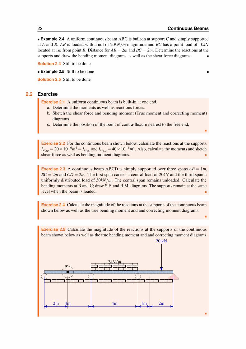
Exercise 2.5 Calculate the magnitude of the reactions at the supports of the continuousbeam shown below as well as the true bending moment and and correcting moment diagrams.
20 kN
2kN/m
4m2m 4m 1m 2m
�

2.3 Examples 23
2.3 Examples
� Example 2.6 # �
Solution 2.6 #
� Example 2.7 # �
Solution 2.7 #
� Example 2.8 # �
Solution 2.8 #
� Example 2.9 # �
Solution 2.9 #
2.4 Exercises
Exercise 2.6 # �
Exercise 2.7 A beam is continuous over four supports and are loaded as shown in Fig. ??.1. Calculate the magnitude of the forces in the supports2. Draw the shear force and bending moment diagrams.
20kN 30kN
10 kN/m
A B
1m
4m 4m 3m 1m
�
Exercise 2.8 A beam is continuous over four supports and are loaded as shown in Fig. ??.1. Calculate the magnitude of the forces in the supports2. Draw the shear force and bending moment diagrams.
8 kN/m 5 kN/m
30kN 10kN
A B C D
4m 3m 1m 4m 1m
�

24 Continuous Beams
Exercise 2.9 # �
Exercise 2.10 # �
Exercise 2.11 # �
Exercise 2.12 # �

IntroductionStrain Energy of BarsCastigliano’s TheoremStructuresCastigliano’s theorem applied to CurvedBeamsCastigliano’s theorem applied to Beams
Cantilever beam with a Point Load at the freeendS/S beam with a Point Load at mid-point
ExamplesExercises 3 — Energy Methods
3.1 Introduction
The energy stored within a material when work has been done is called the strain energy. Energyis normally defined as the capacity to do work and it may exist in many forms such as mechanical,thermal, nuclear, electrical, etc. The potential energy of a body is the form of energy whichis stored by virtue of the work which has previously been done on that body. Strain energyis a particular form of potential energy (PE) which is stored within materials which has beensubjected to strain, i.e. to some change in dimension.
Definition 3.1.1 Strain energy is defined as the energy which is stored within a materialwhen work has been done on the material.
Strain Energy U = Work Done (3.1)
When an axial force P is applied gradually to an elastic body that is rigidly fixed (nodisplacement, rotation permitted), the force does work as the body deforms. We can see thisclearly in Fig. 3.1
L δ
P
Figure 3.1: Elastic Bar
P
δO
B
C
Area=U
Figure 3.2: Load vs Displacement
26 Energy Methods
This work can be calculated from U =∫
δ
0 P dδ , where δ is the work absorbing displacementof the application of the load.
U =12
Pδ (3.2)
where U is the area under the force-displacement diagram. The work of several loads, i.e. P1,P2, P3,..., Pn acting on an elastic body is independent of the order in which the loads are applied.The work is thus
U =12 ∑Piδi (3.3)
where the same U is actually the energy (strain) stored in an elastic body. The unshaded areaabove the line ’OB’ is called the complimentary energy, a quantity which is utilised in someadvanced energy methods of solution, [dro]. [dro]
3.2 Strain Energy of BarsLet us consider a bar of constant cross-sectional area A, length L and Young’s modulus E asshown in Fig. #. If the axial load P is applied gradually to result in displacement δ , the strainenergy of the bar is
U =12
Pδ =P2L2AE
(3.4)
This can be better expressed as follows:
U =12
∫ L
0
P2
2AEdx (3.5)
3.3 Castigliano’s Theorem
Theorem 3.3.1 — Castigliano’s First Theorem. Castigliano’s theorem states that if anelastic body is in equilibrium under the external loads P1, P2, P3,..., Pn then
δi =∂U∂Pi
(3.6)
where δi is the displacement associated with load Pi and U is the strain energy of the body.
The other way of writing Castigliano’s first theorem is as follows:
Theorem 3.3.2 — Castigliano’s First Theorem. If the total strain energy expressed in termsof the external loads is partially differentiated with respect to one of the loads the result is thedeflection of the point of application of that load and in the direction of that load. Deflectionin direction of Pi will be
δPi =∂U∂Pi
(3.7)
In applications where bending provided practially all of the strain energy,
δPi =∫
A
MEI
∂M∂Pi
dA (3.8)
Castigliano’s theorem for angular movements states:

3.4 Structures 27
Theorem 3.3.3 — Castigliano’s theorem for angular movements. If the total strain energyexpressed in terms of the external moments be partially differentiated with respect to one ofthe moments, the result is the angular deflection in radians of the point of application of thatmoment and in its direction
θ =∫
A
MEI
∂M∂Mi
dA (3.9)
where Mi is the actual or dummy moment at the point where θ is required.
3.4 Structures
Displacement in the direction of the applied load is found using the following equation:
δ =n
∑i=1
FiLi∂Fi
AiEi∂P(3.10)
There would be plenty of examples for trusses/structures in the example section
Statically Indeterminate/determinate
Pin jointed structures can either be statically determinate or indeterminate. The challenge iswhen the structure is indeterminate. The following steps should be followed when approaching apin jointed structure:• Count the number of joints, members and reactions. m+ r−2 j = 1. If 2 j < m+ r, the
structure is indeterminate. There is one redundant member on the structure.• The number of redundant members is equal to the degree of indeterminacy of the structure.
Release the redundant members to render the structure statically determinate.• Calculate the forces in the statically determinate structure, subjected to any external loads
plus the redundant reaction forces, using methods of joints of sections.• Use Castigliano’s method to calculate the required deflections and also slopes.
3.5 Castigliano’s theorem applied to Curved Beams
The theorem can be applied to all types of beams, cantilever with point load or udl, simplysupported beam with point load or udl, etc. I will leave you to derive the rest of the beams. Youcan confirm your answer by using first principles.
3.6 Castigliano’s theorem applied to Beams
3.6.1 Cantilever beam with a Point Load at the free end
When given any type of beam, follow this procedure:1. Cut an elemental strip of width dx2. Measure distance x from the free-end or the fixed-end. If it is from the fixed end, make
sure that you calculate the reaction first3. Take moments about X−X line, i.e. distance from free-end to where the strip starts, Mxx
4. Determine partial derivative of moment with respect to the load applied, i.e. ∂Mxx/∂PFor a cantilever given, Fig. 3.6.1, this is what you do:
28 Energy Methods
P
L
xdx
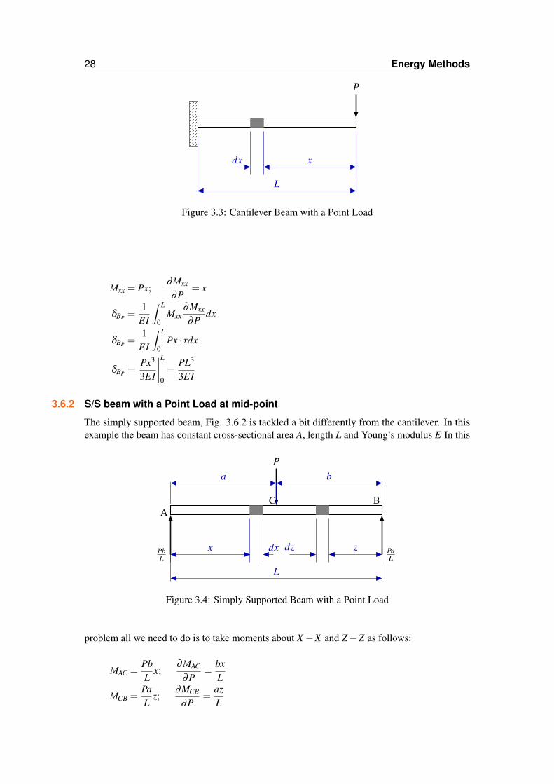
Figure 3.3: Cantilever Beam with a Point Load
Mxx = Px;∂Mxx
∂P= x
δBP =1
EI
∫ L
0Mxx
∂Mxx
∂Pdx
δBP =1
EI
∫ L
0Px · xdx
δBP =Px3
3EI
∣∣∣∣L0=
PL3
3EI
3.6.2 S/S beam with a Point Load at mid-point
The simply supported beam, Fig. 3.6.2 is tackled a bit differently from the cantilever. In thisexample the beam has constant cross-sectional area A, length L and Young’s modulus E In this
AC B
P
PbL
PaL
L
a b
x dx zdz
Figure 3.4: Simply Supported Beam with a Point Load
problem all we need to do is to take moments about X−X and Z−Z as follows:
MAC =PbL
x;∂MAC
∂P=
bxL
MCB =PaL
z;∂MCB
∂P=
azL

3.7 Examples 29
The deflection is thus
δ =1
EI
∫ a
0
PbL
x× bxL
dx+1
EI
∫ b
0
PaL
z× azL
dz
δ =Pb2
L2EIx3
3
∣∣∣∣a0+
Pa2
L2EIz3
3
∣∣∣∣b0
δ =Pb2a3
3L2EI+
Pa2b3
3L2EI
δ =Pb2a2(a+L)
3L2EI
But since a = L/2 = b then
δ =PL3
48EI
3.7 Examples
� Example 3.1 Calculate the vertical displacement at point B on the pin-jointed structure shownin Fig. #. The cross-sectional area of both members is 2000mm2 and E = 200GPa �
Solution 3.1 We start by determining what the length of AB and BC is, i.e. LAB = 2m andLBC = 2m. The only joint that we will deal with is Joint ’B’.
R The structure is statically determinate. j = 3, m = 2 and r = 4. 2 j = m+ r
Σ F ↑= 0 = FAB sin30◦−FBC sin30◦−Q
FBC = FBA−2Q . . .Eq. 1
Σ F →= 0 = R−FAB cos30◦−FBC cos30◦
FBC = 1.155R−FBA . . .Eq. 2
FAB = Q+0.577R with∂FBA
∂Q= 1;
∂FBA
∂R= 0.577
FBC = 0.577R−Q with∂FBC
∂Q=−1;
∂FBC
∂R= 0.577
Member Length (m) Load ∂F∂Q
∂F∂R
FLAE
∂F∂Q
FLAE
∂F∂R
AB 2m Q+0.577R 1 0.577 50×10−6 28×10−6
BC 2m −Q+0.577R -1 0.577 50×10−6 −28×10−6
100µm 0
Table 3.1: Table caption
� Example 3.2 A Plate 5mm thick and 30mm wide is bent into the shape shown below. �

30 Energy Methods
Solution 3.2 Taking moments about z− z
Mzz = Fr sinθ ;∂Mzz
∂P= r sinθ
δ =1
EI
∫ 3π
2
0(Fr sinθ)(r sinθ)rdθ
δ =Fr3
EI
(θ
2− sin2θ
4
)∣∣∣∣3π
2
0
δ =3πFr3
4EI=
(200)(0.2)3(3π)
4×62.5= 60.3mm
� Example 3.3 The structure shown below is made from a pipe with inner and outer diametersof 80mm and 100mm respectively. Calculate the resultant deflection at A due to bending.E = 200GPa. �
Solution 3.3 #
� Example 3.4 Determine the vertical deflection of point A on the bent cantilever as shownbelow, Fig. 3.5, when loaded at A with a vertical load of 25N. The cantilever is built-in at B andEI is constant throughout and is equal to 450Nm2. What would be the horizontal deflection atpoint A? �
P = 25N
r =125mm
200mm
A
B
Figure 3.5: Castigliano-Semicircular
Solution 3.4 We now look at Fig. 3.6 and we let R become a dummy load.
Mxx = Px ,∂Mxx
∂P= xXX
Mzz = (0.2+ r sinθ)P+Rr(1− cosθ),∂Mzz
∂P= (0.2+ r sinθ),
∂Mzz
∂R= r(1− cosθ)XX

3.7 Examples 31
P = 25N
R = 0N
r =125mm
200mmr sinθ
rcos
θ X
X
x
A
B
Figure 3.6: Castigliano-Semicircular
The deflections are calculated as follows:
δP =1
EI
∫ 0.2
0Px · xdx+
1EI
∫π
0(0.2+ r sinθ)P(0.2+ r sinθ)rdθ
δP =
[Px3
3EI
]0.2
0+
PEI
(0.04r+0.4r2 sinθ + r3 sin2θ)dθ
δP =0.0667
EI+
PEI
[0.04rθ −0.4r2 cosθ + r3
(θ
2− sin2θ
4
)]π
0X
δP =0.0667
EI+
PEI
(0.0157+0.0125+0.003068)
δP =0.8484
EIXX
δR =1
EI
∫π
0(0.2+ r sinθ)Pr(1− cosθ)rdθ
δR =Pr2
EI
∫π
0(0.2−0.2cosθ + r sinθ − r sinθ cosθ)dθX
δR =Pr2
EI
[0.2θ −0.2sinθ − r cosθ +
r cos2 θ
2
]π
0
δR =Pr2
EI
(0.2π− r(−2)+
r2(0))
δR =0.3431
EIXX
� Example 3.5 The steel truss (Fig. 3.7) supports the load P = 30kN. Determine the horizontaland vertical displacements of joint E. Use E = 200GPa. The cross-sectional area for all membersis 500mm2. �
Solution 3.5 Referring to Fig. 3.8 We are given A = 500mm2, P = 30kN and E = 200GPa. Wewill use a JOINT method starting with Joint E, D and C. Let us introduce a dummy load R atpoint E.
Joint E

32 Energy Methods
• •
• ••
P
2m
2m
2m
A
B
C
D E
Figure 3.7: Castigliano Truss Structure
• •
• •• R(Dummy)
P
2m
2m
2m
A
B
C
D E
Figure 3.8: Solution Castigliano Truss Structure
ΣFv = 0 = P+0.707FEC
∴ FEC =−1.414PXX∂FEC
∂P=−1.414
ΣFH = FED +0.707FEC−R
∴ FED = P+RXX∂FED
∂P= 1
∂FED
∂R= 1

3.7 Examples 33
Joint D
ΣFV = 0 = FDCXX
ΣFH = FDE −FDB +R
∴ FDB = P+RXX∂FDB
∂P= 1
∂FDB
∂R= 1
Joint C
ΣFv = 0.707FCE +0.707FCB
ΣFv =−P+0.707FCB
∴ FCB = 1.414PXX∂FCB
∂P= 1.414
ΣFH = 0 = 0.707FCE −0.707FCB−FCA
ΣFH =−P−P−FCA
∴ FCA = 2PXX∂FCA
∂P= 2
Member L(mm) Load ∂F∂P
∂F∂R
FLAE
∂F∂P
FLAE
∂F∂R
AC 2000 2P 2 0 1.2 0BC 2828 1.414P 1.414 0 1.696 0BD 2000 P+R 1 1 0.6 0.6CD 2000 0 0 0 0 0DE 2000 P+R 1 1 0.6 0.6CE 2828 -1.414P -1.414 0 -1.696 0
δP = 2.4mm δR = 1.2mm
� Example 3.6 For the simply supported beam (Fig. 3.9) loaded with a uniformly distributedload, determine the maximum deflection in the middle of the beam. Let the udl be q N/m. �
Solution 3.6 We can solve this problem by concentrating on half the length of the beam. Sincewe need to calculate the maximum deflection which occurs in the middle, we need to place adummy load at the middle of the beam. We then need to cut the beam at distance x from the lefthand support and take moments about X−X section as follows:
RA =qL2
+P2= RB
Mxx = RAx− qx2
2=
qLx2
+Px2− qx2
2∂Mxx
∂P=
x2
Since deflection is determined using the following
δP =1
EI
∫A
M∂M∂P
dA (3.11)

34 Energy Methods
A B
q N/m
L
L/2
Figure 3.9: SS Beam with UDL
δP =2
EI
∫ L/2
0
[qLx
2+
Px2− qx2
2
]x2
dx
=1
EI
∫ L/2
0
[qLx2
2+
Px2
2− qx3
2
]dx
=1
EI
[qLx3
6+
Px3
6− qx4
8
]∣∣∣∣L/2
0
=1
EI
[qL(L
2
)3
6+
P(L
2
)3
6−
q(L
2
)4
8
]
=1
EI
[PL3
48+
qL4
48− qL4
128
]=
1EI
[PL3
48+
5qL4
384
]
3.8 ExercisesExercise 3.1 Calculate the vertical displacement as well as the horizontal displacement atpoint B on the pin jointed structure shown in the figure below. The cross-sectional area ofboth members is 2000 mm2 and E = 200GPa.

3.8 Exercises 35
•
•
•
10 kN
C
B
A
2m
2m
2m
�
Exercise 3.2 Calculate the magnitude of the force R on the pin-jointed structure, shown inthe figure below, if the vertical deflection at node E is zero. The cross-sectional area of all themembers is the same.
•
•
• •
•• •
R
AB
C
FED
10 kN3m 3m
4m
�
Exercise 3.3 Calculate the resultant displacement at point E on the pin-jointed structureshown in the figure below. The cross-sectional area for all members is 200mm2 and E =200GPa.

36 Energy Methods
•
•
••
•
•
60◦
60◦60◦
90◦
20 kN
2m�
Exercise 3.4 Calculate the vertical displacement at point D and the horizontal displacementat C on the pin-jointed structure shown in the figure below. The cross-sectional area for allmembers is 1200mm2 and E = 200GPa.
•
•
•
3m
•
20 kN
A CD
B
4m 4m
�
Exercise 3.5 Calculate the resultant deflection at point A on the pin-jointed structure shownin the figure below.
•
• • •
10 kN
2m
3m

3.8 Exercises 37
�
Exercise 3.6 Calculate the vertical deflection at point B on the pin-jointed structure shownbelow. The cross-sectional are of the members in tension is 30mm2 and for those in compres-sion is 200mm2. E = 200GPa
•
•
••
0.6m
0.8m
0.5m
10 kN
1m
�
Exercise 3.7 Calculate the resultant deflection at point D on the pin-jointed structure shownbelow. The cross-sectional area of the members in tension is 1000mm2 and for those incompression is 2000mm2. E = 200GPa
•
•
•
•
8 kN
0.6m
1m
�


Symmetric Member in Pure BendingUnsymmetrical BendingAlternative procedure for stressdeterminationDeflectionNotationxxx
Point LoadUniformly Distributed Load
ExamplesExercises
4 — Unsymmetrical Bending of Beams
IntroductionThe most common type of structural member is a beam. I actual structures beams can be foundin an infinite variety of:• sizes• shapes• orientations
Definition 4.0.1 — Beam. A beam may be defined as a member whose length is relativelylarge in comparison with its thickness and depth, and which is loaded with transverse loadsthat produce significant bending effects as oppose to twisting or axial effects.
Beams are generally classified according to their geometry and the manner in which they aresupported. Geometrical classification includes such features as the shape of the cross sectionwhether the beam is straight, curved, tapered or has constant cross-section.
Beams can also be classified according to the manner in which they are supported. Sometypes that occur in ordinary practice are shown in the figures below, Fig. 4.1 and 4.2. There aremany other types not shown.
Figure 4.1: Cantilever Beam
4.1 Symmetric Member in Pure Bending• Internal forces in any cross section are equivalent to a couple. The moment of the couple
is the section bending moment.• From statics, a couple M consist of two equal and opposite forces.• The sum of the components of the forces in any direction is zero.• The moment is the same about any axis perpendicular to the plane of the couple and zero
about any axis contained in the plane.

40 Unsymmetrical Bending of Beams
Figure 4.2: Continuous Beam-Bridge Support
• These requirements may be applied to the sums of the components and moments of thestatically indeterminate elementary internal forces
4.2 Unsymmetrical Bending
Simple bending theory applies when bending takes place about an axis which is perpendicularto a plane of symmetry. If such an axis is drawn through the centroid of a section, and anothermutually perpendicular to it also through the centroid, then these axes are principal axes. Thus aplane of symmetry is automatically a principal axis. Second moments of area of a cross-sectionabout its principal axes are found to be maximum and minimum values, while the product secondmoment of area,
∫xy dA, is found to be zero. All plane sections, whether they have an axis of
symmetry or not, have two perpendicular axes about which the product second moment of areais zero. Principal axes are thus defined as the axes about which the product second moment ofarea is zero. Simple bending can then be taken as bending which takes place about a principalaxis, moments are being applied in a plane parallel to one such axis.
In general, however, moments are applied about a convenient axis in the cross-section; theplane containing the applied moment may not then be parallel to a principal axis. Such cases aretermed unsymmetrical bending1.
The most simple type of unsymmetrical bending problem is that of skew loading of thesections containing at least one axis of symmetry as shown in Fig. #. This axis and the axisperpendicular to it are then principal axes and the term skew loading implies load applied atsome angle to these principal axes. The method of solution in this case is to resolve the appliedmoment MA into Muu and Mvv
How to approach an Unsymmetrical Bending problem:1. Determine the position of the centroid (if not already known)2. Calculate values of Ixx, Iyy and Ixy
3. Calculate angle θp using
tan 2θ =2Ixy
Ixx− Iyy(4.1)
1Mechanics of Materials, EJ Hearn

4.2 Unsymmetrical Bending 41
4. Calculate principal second moments of area
I11,22 =Ixx + Iyy
2±
√(Ixx− Iyy
2
)2
+ I2xy (4.2)
5. Calculate the moment M and resolve it into components of Muu = M cosθ and Mvv =M sinθ
6. Calculate combined bending stress
σ =Muu× v
Iuu+
Mvv×uIvv
(4.3)
Figure 4.3: Asymmetrical Bending
7. Find position of neutral axis on cross-section (through centroid): σ = 08. Identify points on cross-section which are greatest distance from the neutral axis(one
tensile and one compressive) and determine x,y coordinates of each point.9. Use the following two equations to determine the distances u and v which are both positive
in the quadrant UGV.
u = xcosθ + ysinθ (4.4)
v = ycosθ − xcosθ (4.5)
10. Determine the maximum bending stress using Eqn. 4.3
Moment applied along the principal axis
The conditions that one should consider when working with this type of a problem are:• Stress distribution acting over entire cross-sectional area to be a zero force resultant.• Resultant internal moment about y- axis to be zero.• Resultant internal moment about z- axis to be equal to M.
42 Unsymmetrical Bending of Beams
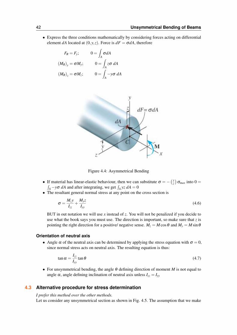
• Express the three conditions mathematically by considering forces acting on differentialelement dA located at (0,y,z). Force is dF = σdA, therefore
FR = Fy; 0 =∫
AσdA
(MR)y = σMy; 0 =∫
Azσ dA
(MR)z = σMz; 0 =∫
A−yσ dA
Figure 4.4: Asymmetrical Bending
• If material has linear-elastic behaviour, then we can substitute σ =−( y
c
)σmax into 0 =∫
A−yσ dA and after integrating, we get∫
A yz dA = 0• The resultant general normal stress at any point on the cross section is
σ =MzyIzz
+MyzIyy
(4.6)
BUT in out notation we will use x instead of z. You will not be penalized if you decide touse what the book says you must use. The direction is important, so make sure that z ispointing the right direction for a positive/ negative sense. Mz = M cosθ and My = M sinθ
Orientation of neutral axis• Angle α of the neutral axis can be determined by applying the stress equation with σ = 0,
since normal stress acts on neutral axis. The resulting equation is thus:
tanα =Izz
Iyytanθ (4.7)
• For unsymmetrical bending, the angle θ defining direction of moment M is not equal toangle α , angle defining inclination of neutral axis unless Izz = Iyy
4.3 Alternative procedure for stress determinationI prefer this method over the other methods.Let us consider any unsymmetrical section as shown in Fig. 4.5. The assumption that we make

4.3 Alternative procedure for stress determination 43
Figure 4.5: Alternative Procedure
as we start this is that the stress at any point on the unsymmetrical section us given by
σ = Px+Qy (4.8)
where P and Q are constants; in other words it is assumed that bending takes place about the Xand Y axes at the same time, stresses resulting from each effect being proportional to the distancefrom the respective axis of bending. Let there be a tensile stress σ on the element of area dA.Then the force F acting on the element is F = σdA. The moment of this force about the X axisis then σdAy
Mxx =∫
σdAy
=∫(Px+Qy)ydA =
∫PxydA+
∫Qy2dA
but we know from statics that
Ixx =∫
y2dA
Iyy =∫
x2dA
Ixy =∫
xydA
therefore substituting the above in the moment equation, we get
Mxx = PIxy +QIxx (4.9)
In a similar manner the moments about the Y axis is
Myy =−∫
σdAx
Myy =−∫(Px+Qy)xdA =−
∫PxydA−
∫Qy2dA
∴Myy =−PIyy−QIxy (4.10)
Since the stresses resulting from bending are zero on the neutral axis, the equation of the neutralaxis is derived by setting the stress to zero, i.e.
0 = Px+Qyyx=−P
Q= tan αN.A

44 Unsymmetrical Bending of Beams
4.4 DeflectionThe deflections of unsymmetrical sections in the directions of the principal axes may always bedetermined by application of the standard deflection formulae, i.e.
δ =FL3
3EI(4.11)
and this we know because it is the maximum deflection of a cantilever with a point load F at thefree end. The vertical deflection is determined as follows:
δv =(Fyy)L3
3EIxx(4.12)
and the horizontal deflection
δh =(Fxx)L3
3EIyy(4.13)
4.5 Notation
Quantity SymbolGeneric load for ODE Work f (x)Transverse Shear Force V (x)Bending Moment M(x)Slope of deflection curve dv(x)
dx = v′(x)Deflection Curve v(x)
Table 4.1: Notation
4.6 xxx#
4.6.1 Point Load#
4.6.2 Uniformly Distributed Load4.7 Examples
� Example 4.1 A z-section shown in Fig.# is subjected to bending moment of M = 20kNm. Theprincipal axes y and z are oriented as shown such that they represent the maximum and minimumprincipal moments of inertia, Iyy = 900× 10−6mm4 and Izz = 7540× 10−6mm4 respectively.Determine the normal stress at point P and orientation of the neutral axis.
�
Solution 4.1 #
� Example 4.2 Due to load misalignment, the bending moment acting on the channel sectionsis inclined at an angle of 3◦ with respect to the y axis. If the allowable flexural stress for thisbeam is σal = 150MPa, what is the maximum moment, Mmax that may be applied. �

4.7 Examples 45
Solution 4.2 We start the solution by determining the components of the moment
Myy =−M sin 3◦
Mxx = M cos 3◦
The normal stresses due to the moment components are
σzz1 =Myy× x
Iyy=−(M sin 3◦)× x
Iyy
σzz2 =Mxx× y
Ixx=
(M cos 3◦)× yIxx
The combines stress is
σzz = σzz1 +σzz2
=−(M sin 3◦)× xIyy
+(M cos 3◦)× x
Ixx
A1 = A3 = 500mm2
A2 = 800mm2
AT = 1800mm2
Ixx = 2(
10×503
12+500(8.9)2
)+
(80×103
12+800(11.1)2
)= 0.3927×106mm4
Iyy = 2(
50×103
12+500(45)2
)+
10×803
12= 2.46×106mm4
−100×106 =−(M sin 3◦)× (−50)2.46×10⁶ +
(M cos 3◦)× (−33.9)0.3927×10⁶
M = 1.17MNm
NB: I am not quite happy with the answer.
� Example 4.3 A rectangular-section beam 80 mm ×50 mm is arranged as a cantilever 1.3mlong and loaded at its free end with a point load of 5kN inclined at an angle of 60◦ to thehorizontal axis as shown in Fig. #. Determine the position and magnitude of the greatest tensilestress in the section. What would be the vertical deflection at the end? E = 210GPa �
Solution 4.3 The moments of inertia are simple to calculate and are as follows:
Ixx =50×803
12= 2.133×106mm4
Iyy =80×503
12= 0.833×106mm4
Mxx = 5000×1300cos30◦ = 5629×103Nmm
Myy =−5000×1300sin30◦ =−3250×103Nmm
Using the general method of determining stress at any point, i.e.
σ =MxxyIxx±
MyyxIyy

46 Unsymmetrical Bending of Beams
Y
X•
C B
AD P
50mm
80m
m
Figure 4.6: Rectangular section
We will determine the stresses at points A(25,40), B(25,−40), C(−25,−40) and D(−25,40)
σA =MxxyIxx±
MyyxIyy
=(5629)(40)(1000)
2.133×10⁶ − (−3250)(25)(1000)0.833×106 = 203.1MPa
σB =MxxyIxx±
MyyxIyy
=(5629)(−40)(1000)
2.133×10⁶ − (−3250)(25)(1000)0.833×106 =−8.021MPa
Using the alternative method, we must determine the constants P and Q. Since the section issymmetric about both axes, we know that Ixy = 0.
Mxx = 5629×106 = 2.133Q ∴ Q = 2639×106
Myy =−3250×106 =−0.833Q ∴ P = 3901.56×106×106
The stresses at various points are
σA = 3901.56(25)+2639(40) = 203.1MPa
σB = 3901.56(25)+2639(−40) = 8.021MPa
σC = 3901.56(−25)+2639(−40) =−203.1MPa
σD = 3901.56(−25)+2639(40) =−8.021MPa
� Example 4.4 A cantilever if length 1.2m and of the cross-section shown in Fig. 4.7 carries avertical load of 10kN at its outer end, the line of action being parallel with the longer leg andarranged to pass through the shear centre of the section (i.e. there is no twisting of the section).Working from first principles, find the stress set up in the section at points A, B and C, given thatthe centroid is located as shown. Determine also the angle of inclination of the neutral axis αNA.Given: Ixx = 4×10⁻⁶m4 and Iyy = 1.08×10⁻⁶m4
�
Solution 4.4 #
� Example 4.5 # �
Solution 4.5 #
� Example 4.6 �
4.8 Exercises 47
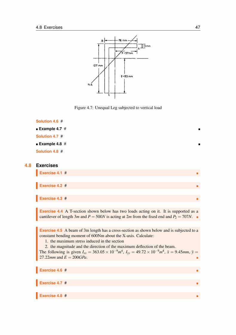
Figure 4.7: Unequal Leg subjected to vertical load
Solution 4.6 #
� Example 4.7 # �
Solution 4.7 #
� Example 4.8 # �
Solution 4.8 #
4.8 ExercisesExercise 4.1 # �
Exercise 4.2 # �
Exercise 4.3 # �
Exercise 4.4 A T-section shown below has two loads acting on it. It is supported as acantilever of length 3m and P = 500N is acting at 2m from the fixed end and P2 = 707N. �
Exercise 4.5 A beam of 3m length has a cross-section as shown below and is subjected to aconstamt bending moment of 600Nm about the X-axis. Calculate:
1. the maximum stress induced in the section2. the magnitude and the direction of the maximum deflection of the beam.
The following is given Ixx = 363.05× 10⁻⁹m4, Iyy = 49.72× 10⁻⁹m4, x = 9.45mm, y =27.22mm and E = 200GPa. �
Exercise 4.6 # �
Exercise 4.7 # �
Exercise 4.8 # �

48 Unsymmetrical Bending of Beams
Exercise 4.9 # �
Exercise 4.10 # �
Exercise 4.11 # �
Exercise 4.12 # �
Exercise 4.13 # �
Exercise 4.14 # �
Exercise 4.15 # �
Exercise 4.16 # �

Plastic Bending of Rectangular BeamsPlastic Bending of Symmetrical (I-Section)BeamPartially plastic Bending of UnsymmetricalSectionsLimit Analysis-Bending
BendingThe principle of Virtual Work
Solid ShaftHollow shaftExercises
5 — Inelastic Bending
Introduction
When the design of components is based upon the elastic theory, i.e. the simple bending ortorsion theory, the dimensions of the components are arranged in such a way that the maximumstresses which are likely to result do not exceed the allowable working stress. This is obtainedby taking the yield stress and dividing it by the applicable safety factor.
Under normal service conditions, we want to present yielding because the resulting permanentdeformation is generally undesirable. However, permanent deformation does not necessarily leadto catastrophic failure; it may only make the structure or component undesirable and consideredunsafe or unfit for further use. At the outer fibres yield stress may have been exceeded but someportion of the component may be found to be still elastic and capable of carrying the load. Thestrength of a component will normally be much greater than that assumed on the basis of initialyielding at any position. To take advantage of the inherent additional strength, a different designprocedure is used which is often referred to as plastic limit design.
Definition 5.0.1 — Inelastic Bending. Inelastic materials are materials which followHooke’s law up to the yield stress σY and then yield plastically under constant stress (see Fig.5.1).
The figure below, Fig. 5.1, assumes material behaviour which:1. Ignores the presence of upper and lower yields and suggests only a single yield point2. takes the yield stress in tension and compression to be equal3. When a plastic hinge has developed at one point, the moment of resistance at that point
remains constant until collapse of the whole structure takes place due to the formation ofthe required number of plastic hinges at other points.
4. transverse sections of beams in bending remain in plane throughout the loading process,i.e. strain is proportional to distance from the neutral axis.
It is now possible on the basis of assumption (4) to determine the moment which must be appliedto produce:• maximum or limiting elastic condition in the beam material with yielding just initiated at
the outer fibres.• yielding to a specific depth.• yielding across the complete section, i.e. fully plastic state or plastic hinge. Depending
on the support and loading conditions, one or more plastic hinges may be required beforecomplete collapse of the beam or structure occurs and the load required to produce thissituation is called the collapse load.
5.1 Plastic Bending of Rectangular Beams
Let us consider a cantilever beam loaded at the tip with a point load P which is large enoughto cause yielding in the shaded area. At section a-a, the stresses on the outer fibres have justreached yield stress, but the distribution is elastic as shown in Fig. 5.3. Applying the flexure

50 Inelastic Bending
ε
σ
O εY
σY
εY
σY
Figure 5.1: Idealized Stress-Strain Diagram
Figure 5.2: Cantilever Beam subjected to load P
formula
Mmax = σmaxS
= σmaxbh2
6we find that the magnitude of the bending moment at this section is
MY =bh2
6σY (5.1)
This moment is called yield moment because it is the moment responsible for yielding.At section b-b, the cross section is elastic over the depth of 2yi but plastic outside this depth asshown in Fig. 5.4 The stress is constant at σY over the plastic portion and varies linearly overthe elastic region. The bending moment carried by this elastic region is given by the followingformula
Mpp =Ii
yi(5.2)
5.1 Plastic Bending of Rectangular Beams 51
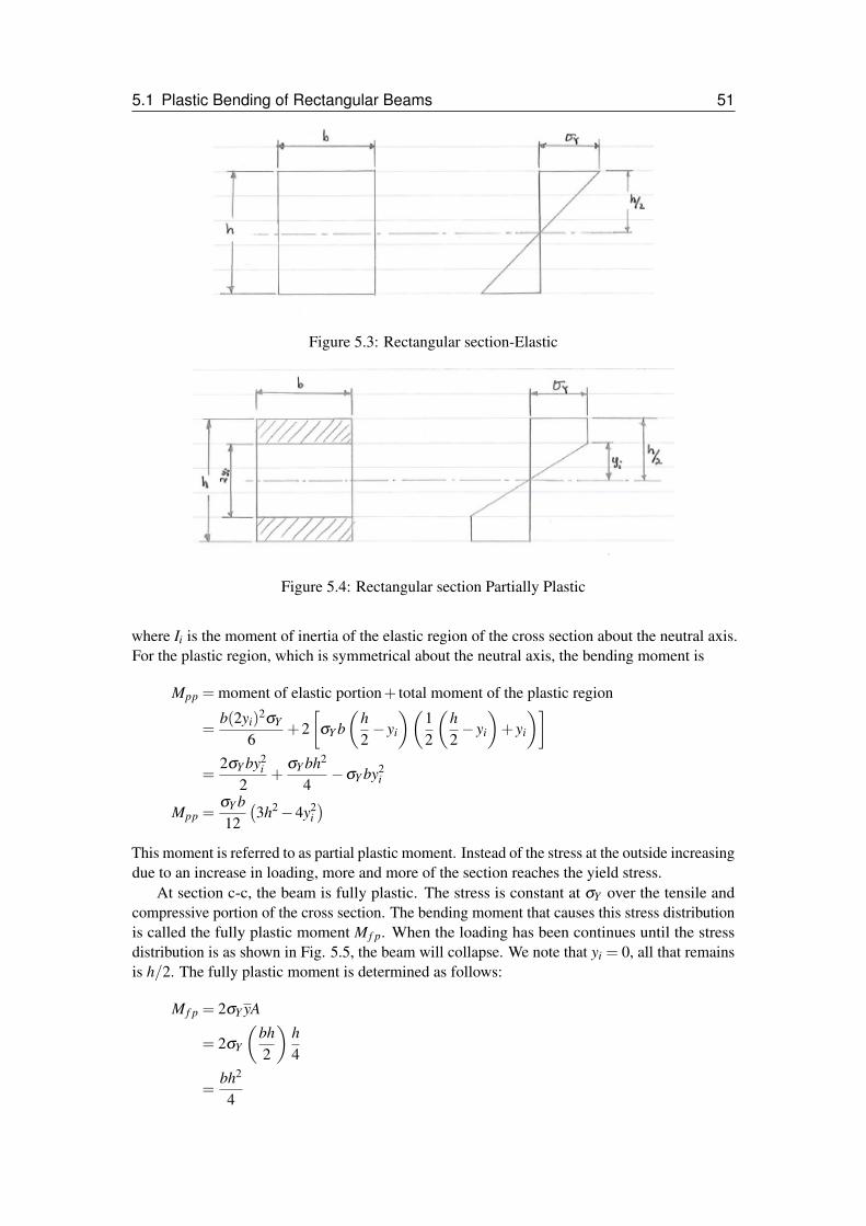
Figure 5.3: Rectangular section-Elastic
Figure 5.4: Rectangular section Partially Plastic
where Ii is the moment of inertia of the elastic region of the cross section about the neutral axis.For the plastic region, which is symmetrical about the neutral axis, the bending moment is
Mpp = moment of elastic portion+ total moment of the plastic region
=b(2yi)
2σY
6+2[
σY b(
h2− yi
)(12
(h2− yi
)+ yi
)]=
2σY by2i
2+
σY bh2
4−σY by2
i
Mpp =σY b12(3h2−4y2
i)
This moment is referred to as partial plastic moment. Instead of the stress at the outside increasingdue to an increase in loading, more and more of the section reaches the yield stress.
At section c-c, the beam is fully plastic. The stress is constant at σY over the tensile andcompressive portion of the cross section. The bending moment that causes this stress distributionis called the fully plastic moment M f p. When the loading has been continues until the stressdistribution is as shown in Fig. 5.5, the beam will collapse. We note that yi = 0, all that remainsis h/2. The fully plastic moment is determined as follows:
M f p = 2σY yA
= 2σY
(bh2
)h4
=bh2
4

52 Inelastic Bending
Figure 5.5: Rectangular section Fully plastic
It is worth noticing that M f p = 2/3MY and this is valid for beams of rectangular cross-section.This ratio is also called the shape factor. Other shape factors for various cross sections are shownin the table below, Tab. 5.1 For a rectangular section, this shape factor means that the beam can
Cross Section M f p/MY
Solid Rectangle 1.5Solid Circle 1.7Thin-walled Circular Tube 1.27Thin-walled Wide-flange Beam 1.1
Table 5.1: Shape factors of different sections
carry 50% additional moment to that which is required to produce initial yielding at the edge ofthe beam section before a fully plastic hinge is formed.
5.2 Plastic Bending of Symmetrical (I-Section) Beam
Figure 5.6: I-section Elastic and Fully Plastic

5.3 Partially plastic Bending of Unsymmetrical Sections 53
The elastic moment or yield moment MY is determined as follows
MY =Iy
σY
I =
(BH3
12−
2 b2 h3
12
)=
BH3
12− bh3
12
y =H2
MY = σY
[BH3
12− bh3
12
]2H
=σY
6H
(BH3−bh3)
The fully plastic moment is found to be:
M f p =σY
4(BH2−bh2) (5.3)
The value of the shape factor is 1.18 for the I-beam indicating that only an 18% increase instrength capacity using plastic design procedures.
5.3 Partially plastic Bending of Unsymmetrical SectionsLet us consider a T-section beam shown below in Fig. 5.7 and 5.8. Whilst stresses remain withinthe elastic limit the position of the neutral axis can be obtained by taking moment of are aboutthe neutral axis.
Figure 5.7: T section-Elastic
It does not matter what state this section is in, i.e. elastic, partially plastic or fully plastic,equilibrium of forces must always be maintained. At any section the tensile forces on one side ofthe neutral axis must equal the compressive forces on the other side of the neutral axis.
Summation of stresses ×area above the N.A= Summation of stresses ×area below the N.A
In the fully plastic condition, the stresses σY will be equal throughout the section, the equationthen becomes:
ΣAabove = ΣAbelow =Atotal
2
For partially plastic condition we will have
F1 +F2 = F3 +F4
54 Inelastic Bending
Figure 5.8: T section Fully Plastic
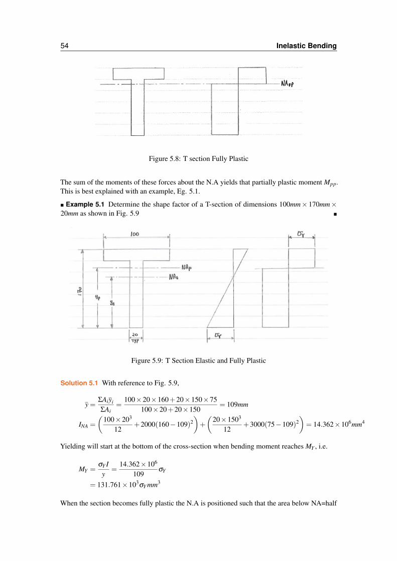
The sum of the moments of these forces about the N.A yields that partially plastic moment Mpp.This is best explained with an example, Eg. 5.1.
� Example 5.1 Determine the shape factor of a T-section of dimensions 100mm× 170mm×20mm as shown in Fig. 5.9 �
Figure 5.9: T Section Elastic and Fully Plastic
Solution 5.1 With reference to Fig. 5.9,
y =ΣAiyi
ΣAi=
100×20×160+20×150×75100×20+20×150
= 109mm
INA =
(100×203
12+2000(160−109)2
)+
(20×1503
12+3000(75−109)2
)= 14.362×106mm4
Yielding will start at the bottom of the cross-section when bending moment reaches MY , i.e.
MY =σY I
y=
14.362×10⁶
109σY
= 131.761×10³σY mm3
When the section becomes fully plastic the N.A is positioned such that the area below NA=half

5.3 Partially plastic Bending of Unsymmetrical Sections 55
the total area. We now must locate the plastic neutral axis, i.e. yp above the base
20× yp = 100×20+20(150− yp)
20× yp = 2000+3000−20× yp
40× yp = 5000
yp = 125mm
The fully plastic moment is then obtained by considering the moments of forces on convenientrectangular parts of the section, each being subjected to a uniform stress σY
M f p = σY (100×20)(45−10)+σY (45−20)(20)× 12(45−20)+σ(125×20)(
1252
)
= 70000σY +6250σY +156250σY
= 232.5×10³σY mm3
∴ f =232.5×10³
131.761×103
= 1.765
� Example 5.2 A cantilever is to be constructed from a T-section beam of Example 5.1 andis designed to carry a udl over its entire length of 2m. Determine the maximum udl that thecantilever beam can carry if yielding is permitted over the lower part of the web to a depth of25mm. The yield stress of the material is σY = 225MPa. �
Figure 5.10: T-section Fully Plastic

56 Inelastic Bending
Solution 5.2
σY
y=
σYi
145− y∴ σYi =
σY
y(145− y)
F1 = σY (20×25) = 500σY
F2 =σY
2(20× y) = 10yσY i.e. Average stress for the triangle
F3 =σY
2
(125− y
y
)×20(125− y) =
10σY
y(125625−250y+ y2)
F4 =σY
2
[(125− y
y
)+
(145− y
y
)](100×20) = 1000σY
(270−2y
y
)F1 +F2 = F3 +F4
500σY +10yσY =10σY
y(125625−250y+ y2)+1000σY
(270−2y
y
)y = 85.25mm
We are now able to calculate the values for the forces and we find them to be F1 = 112.5kN,F2 = 191.8kN, F3 = 41.7kN and F4 = 262.6kN. The moment of resistance MR that the beamcarry can now be obtained by taking moments about the neutral axis.
MR = F1(y+12.5)+F2×23
y+F323(125− y)+F4 [(125− y)+10]
= 112.5(85.25+12.5)+191.8×2×85.25
3+
41.7×2× (125−85.25)3
+262.6 [(125−85.25+10)]
= 10996.875+10901.34+1105.05+12065
= 36068.265Nm
The maximum bending moment present on the beam will occur at the fixed end and it will becalculated using the following formula
Mmax =qL2
2= 18.034kN/m
5.4 Limit Analysis-BendingLimit analysis is a method of determining the loading that causes a statically indeterminatestructure to collapse. This method applies only to ductile materials, which in this simplifieddiscussion are assumed to be elastic, perfectly plastic. The method is straightforward, consistingof two steps. The first step is a kinematic study of the structure to determine which parts mustbecome fully plastic to permit the structure as a whole to undergo large deformations. Thesecond step is an equilibrium analysis to determine the external loading that creates these fullyplastic parts. We will be presenting only bending in the form of examples.
5.4.1 BendingRevisiting Fig. 5.2, as the load P is increased, section c-c at the fixed end goes through elastic andpartially plastic states until it becomes fully plastic, whereas the rest of the beam remains elastic.The fully plastic section is called a plastic hinge because it allows the beam to rotate about thesupport without an increase in the bending moment. The bending moment at the plastic hinge iscalled the limiting moment MP. Once the plastic hinge has formed the beam will collapse.

5.4 Limit Analysis-Bending 57
The collapse mechanism of a beam depends on the supports. Each extra support constrainrequires an additional plastic hinge in the collapse mechanism. A plastic hinge on the beam isshown by a solid circle. A simply supported beam requires only one plastic hinge whereas abeam with built-in ends will require three plastic hinges, that is if there is only one point loadacting on the beam. See Figs. 5.11, 5.12 and 5.13.
A B
WL/3 2L/3
•y
Figure 5.11: Simply Supported Beam
WL/3 2L/3
•
•
y
Figure 5.12: Simply Supported and Fixed
WL/3 2L/3
•
•
•
y
Figure 5.13: Fixed on both ends
In general, plastic hinges form where the bending moment is a maximum, which excludesbuilt-in supports and sections with zero shear force. The location is usually obvious for beamssubjected to concentrated loads. With statically indeterminate beams carrying distributed loads,the task tends to become difficult. Sometimes there is more than one collapse mechanism in

58 Inelastic Bending
which case we must compute the collapse load for each mechanism and choose the smallestcollapse load as the actual limiting load.
5.4.2 The principle of Virtual Work
Virtual Displacement
Definition 5.4.1 Virtual Work: states that for a structure that is in equilibrium and that isgiven a small virtual displacement, the sum of the work done by the internal forces is equal tothe work done by the external force.
Virtual displacement either linear or rotational is an imaginary or hypothetical displacementgiven to a mechanism or a structure and has no relation to the actual displacements produced bythe real loads. The work done by the real loads acting through a virtual displacement is calledvirtual work. If a structure or mechanism is to remain in equilibrium the work-done by the actualloads acting through a virtual displacement must be zero. See more explanation in Examples, Eg.5.3 and 5.4.
Virtual work method on Plastic Hinges
Let us consider the following simply supported loaded beam in Fig. 5.14 Let AB have a virtual
A B
W
L/2 L/2
θ θ
2θ•
y
Figure 5.14: Simply Supported Beam-Collapse Mechanism
rotation of θ radians producing a virtual linear displacement of θL/2 at B through which it acts.The bending moment at B MP, just before a plastic hinge is formed is considered to be negativesince it opposes the work done by Wc which is the collapse load. This energy is then dissipatedthrough till a plastic hinge is formed. So in simple terms,
Work done by the load = Energy dissipated

5.4 Limit Analysis-Bending 59
Wc×θL2
= 2MPθ
Wc =4MP
L=
4 f MY
LOR
MP =WcL
4
� Example 5.3 The simply supported beam ABC shown in Fig. 5.15 has a cantilever overhangand supports two loads 4W and W . Determine the value of W at collapse in terms of the plasticmoment, MP, of the beam. �
A D B C
4W W
X
x
L/2 L/2 L/2
Figure 5.15: Simply Supported Beam with an overhang
Solution 5.3 Referring to Fig. 5.16 We start by taking moments about B, and we don this asfollows:
0 = RAL−4W × L2+
WL2
RA =3W2
Mxx =3Wx
2−4W
[x− L
2
]At x = L/2 we have MD = 3WL/4 and at x = L we have MB = −WL/2. This means that themoment that will cause collapse is MP = MD = 3WuL/4 because it is lowest of the two moments.The bending moment diagram for the beam has been constructed. Clearly as W is increased, aplastic hinge will form first at D, the point of application of the load 4W . Thus at collapse
MP =3WuL
4
Wu =4MP
3L
where Wu is the value of W that will cause collapse.The formation of a plastic hinge in a statically determinate beam produces large, increasing
deformation which ultimate result in failure with no increase in load. In this condition the beambehaves as a mechanism with different lengths of beam rotating relative to each other about theplastic hinge.
In a statically indeterminate system the formation of a single plastic hinge doesn’t necessarilymean collapse. We can demonstrate this by an example, in which a propped cantilever beam isshown in example 5.4. The bending moment diagram may be drawn after the reaction at C hasbeen determined.

60 Inelastic Bending
3WL4
WL2
Figure 5.16: Bending Moment Diagram
� Example 5.4 A propped cantilever beam shown in Figure 5.17 is loaded at mid-point with apoint load W . Determine the load that will cause the collapse. �
W
L/2 L/2
Figure 5.17: Propped Cantilever with W
Solution 5.4 Using the virtual work method, let us refer to Fig. 5.18,
Wuy = MP(θ)+MP(2θ)
WuLθ
2= 3MPθ
Wu =6MP
L
As the value of W is increased a plastic hinge will form first at A where the bending momentis greatest. This doesn’t mean that the beam will collapse. Instead, it behaves as a staticallydeterminate beam with a point load at B and a moment MP at A. Further increases in W willeventually result in the formation of a second plastic hinge at B when the bending moment Breaches the value of MP. The beam now behaves as a mechanism and failure occurs with nofurther increase in the load.
The elastic bending moment diagram has a maximum at point A. After the formation ofthe plastic hinge at A, the bending moment remains constant while the bending moment at B

5.4 Limit Analysis-Bending 61
•
•
θ θ
2θ
y
Figure 5.18: Virtual Work Method-Propped Cantilever
increases until the second plastic hinge forms. This distribution of moments tends to increase theultimate strength of statically indeterminate structures since failure at one section leads to otherportions of the structure supporting additional load.
It must be noted that in this example, it is unnecessary to determine the elastic bendingmoment diagram to solve for the ultimate load which we obtained by using virtual work method.Plastic hinges forms at beam sections where the bending moment diagram attains a peak value.It then follows that for beams carrying a series of point loads, plastic hinges are located at theload positions. This will be shown by a figure and subsequent figures showing mechanisms. Apropped cantilever that supports two point loads is shown in Fig. 5.19 below. Three possiblemechanisms (see Figs. 5.20, 5.21 and 5.22) are possible and each possible mechanism should beanalysed and the lowest ultimate load gets selected.
W1 W2
L1 L2 L3
Figure 5.19: Propped Cantilever with a series of loads
•
•
y 1
y 2
Figure 5.20: Possible Mechanism No. 1

62 Inelastic Bending
•
•
y 1
y 2
Figure 5.21: Possible Mechanism No. 2
•
•
y 1Figure 5.22: Possible Mechanism No. 3
� Example 5.5 A propped cantilever beam of Fig. 5.4 is 10m long and is required to carry aload of 100kN at mid-span. If the yield stress of mild steel is 300MPa, suggest a suitable sectionusing a load factor against failure of 1.5. �
Solution 5.5 The required ultimate load of the beam is 1.5×100 = 150kN. The required plasticmoment, MP is calculated as follows
MP =WuL
6= 250kN
The minimum plastic modulus of the beam section is
ZP =MP
σY= 833,300 mm3
A universal beam 406×140×46kg/m is found to have a plastic modulus of 886.3cm3> Thissection therefore possesses the required ultimate strength and includes a margin to allow for itsself-weight. Note that unless some allowance has been made for self-weight in the estimate ofthe working loads, the design should be rechecked to include this effect.
� Example 5.6 Determine the force P required to maintain equilibrium on the following lever. �
Solution 5.6 Let θ be a small virtual rotational displacement. Then −θ will be a lineardisplacement of A and 3θ a linear displacement of B. The work done by real loads through thesedisplacements must be zero
0 = 400×3θ −Pθ
∴ P = 1200N
� Example 5.7 The beam shown in the figure below, Fig. # is pin-jointed at point C. Determinethe value of P for equilibrium. �

5.4 Limit Analysis-Bending 63
•
P 400N
1m 3m
Figure 5.23: Equilibrium-Lever
Solution 5.7 Let y be a virtual displacement at C. Then
yB = y× 14
and yE = y× 0.50.8
0 = PyB−60yE
0 = P× y4−60× 0.5y
0.8P = 150N
� Example 5.8 A double symmetric hollow box shown below in Fig. 5.24 has a yield stressσY = 220MPa. It is subjected to a bending moment M of such magnitude that the flangesyield but the webs remain linearly elastic. Determine the magnitude of the moment M if thedimensions of the cross section are B = 150mm, b = 130mm, H = 200mm and h = 160mm. �
B
b
H h
Figure 5.24: Box Section
Solution 5.8 #
� Example 5.9 A rectangular steel beam 120mm by 60mm is simply supported at its ends 2mapart, and supports a central point load. If the 120mm side is vertical and the yield stress for thematerial is 260MPa, determine:
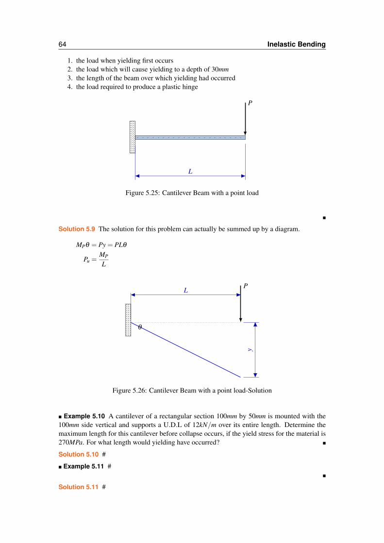
64 Inelastic Bending
1. the load when yielding first occurs2. the load which will cause yielding to a depth of 30mm3. the length of the beam over which yielding had occurred4. the load required to produce a plastic hinge
P
L
Figure 5.25: Cantilever Beam with a point load
�
Solution 5.9 The solution for this problem can actually be summed up by a diagram.
MPθ = Py = PLθ
Pu =MP
L
P
θ
y
L
Figure 5.26: Cantilever Beam with a point load-Solution
� Example 5.10 A cantilever of a rectangular section 100mm by 50mm is mounted with the100mm side vertical and supports a U.D.L of 12kN/m over its entire length. Determine themaximum length for this cantilever before collapse occurs, if the yield stress for the material is270MPa. For what length would yielding have occurred? �
Solution 5.10 #
� Example 5.11 #�
Solution 5.11 #

5.5 Solid Shaft 65
� Example 5.12 # �
Solution 5.12 #
� Example 5.13 �
Solution 5.13 #
� Example 5.14 # �
Solution 5.14 #
5.5 Solid ShaftLet us consider a solid shaft shown in Fig. 5.27. Let us recap on the equations that are useful inthis section:
J =πd4
32(5.4)
T =τJr
=πd3τ
16(5.5)
When the torque is applied in the elastic core, the shear stress reaches τY , then we will have
TE =πd3
E16
τY (5.6)
When the torque is beyond TE then plasticity will result and we will use the following equationto calculate the plastic torque
TP =πτY
12(d3−d3
E)
(5.7)
The above was obtained as follows:
TP =∫ r
RE
πr2τY dr
=2πτY
3(r3− r3
E)
but note that: r = d/2
=2πτY
3
(d3
8− d3
E8
)=
πτY
12(d3−d3
E)
The total torque is obtained by adding the elastic and plastic torques together
T =πd3
E16
τY +πτY
12(d3−d3
E)
=τY πd3
12− τY πd3
E48
=τY π
12
(d3− d3
E4
)For a fully plastic condition, dE = 0 and the equation simplifies to
TFP =τY πd3
12(5.8)

66 Inelastic Bending
τ
dE
d
τY
Figure 5.27: Solid Shaft
The shape factor is obtained the same way we did with other cross-sections, which is simply aratio of the two torques
f =TFP
TE=
16πτY d3
12πτY d3
=43
� Example 5.15 A Steel shaft of φ = 100mm, 1m long is under 30kNm torque in the elasticcore. Determine the diameter of the elastic core of the shaft and the angle of twis. What is thevalue of the fully plastic torque of the shaft. Given: τY = 120MPa and G = 80GPa �
Solution 5.15 Let us start by determining the easiest part which is the diameter of the elasticcore
T =τY π
12
(d3− d3
E4
)−d3
E = 4(
30,000×12π(120×106)
−0.13)
d3E = 180.281×10⁻⁴
dE = 56.49mm

5.6 Hollow shaft 67
The polar moment of intertia
J =πd4
32
=0.1×π
32= 9.817×10⁻⁶m4
The elastic torque is therefore
TE =πτY d3
E16
=π(0.05649)3(120×106)
16= 4,247Nm
The plastic torque is determined as follows:
TP =πτY
12(d3−d3
E)
=π(120×106)(0.13−0.056493)
12= 25,753Nm
The total torque can be confirmed as follows
T = TE +TP
= 4,247+25,753
= 30,000Nm
The fully plastic torque can be determined as follows:
TFP =πτY d3
12
=π(120×106)(0.1)3
12= 31,416Nm
How do we then determine the angle of twist? It’s very easy
γ =τ
G
φ =T LJG
=30,000×1
(9.817×10⁻⁶)(80×109)
= 0.0382 rad
5.6 Hollow shaftLet us consider a hollow shaft with an internal radius R1 and external radius R subjected to atorque large enough to produce yielding to a radius R2, see Fig. 5.28. Now if we ignore thecentral hole
T =πτY
6(4R3−R3
2)
(5.9)

68 Inelastic Bending
τ
τY
τ
R1
R2
R
Figure 5.28: Hollow Shaft
Consider now an imaginary shaft of radius R1. Now, the torque on it will be
T =πR3
1τ
2(5.10)
From the law of triangles
τ
R1=
τY
R2
τ =R1
R2τY
Therefore the torque on the imaginary shaft is given by
T =πR3
12× R1
R2τY
=πR4
12R2
τY
T =πR4
12R2
τY (5.11)

5.7 Exercises 69
Now, the partially plastic torque can be determined as follows
TPP =πτY
6(4R3−R3
2)− πR4
12R2
τY
=πτY
6R2
(4R3R2−R4
2−3R41)
TPP =πτY
6R2
(4R3R2−R4
2−3R41)
(5.12)
The fully plastic torque occurs when R2 = R1, i.e.,
TFP =πτY
6(4R3R1−4R4
1)
=πτY
6(4R3−4R3
1)
=2πτY
3(R3−R3
1)
TFP =2πτY
3(R3−R3
1)
(5.13)
Tips when Working with Shafts
Description Formula to Use
Total Torque T =πτY
(d3− d3
E4
)12
Torque in Elastic core TE =πτY d3
E16
Torque in Plastic condition TP =πτY(d3−d3
E)12
Slope of deflection curve dv(x)dx = v′(x)
Deflection Curve v(x)
Table 5.2: Tips when Working with Shafts
5.7 ExercisesExercise 5.1 Determine the plastic moment and shape factor of a beam of solid circularcross-section having a radius r and yield stress σY . �
Exercise 5.2 Determine the plastic moment and shape factor for a thin-walled box girderwhose cross-section has a breadth b and depth d and a constant wall thickness t. Calculatethe shape factor f for b = 200mm and h = 300mm �
Exercise 5.3 A beam having the cross section shown below is fabricated from mild steelwhich has a yield stress of 300MPa. Determine the plastic moment of the section and itsshape factor. The cross-section has a common thickness of 15mm.

70 Inelastic Bending
250mm
75mm
300m
m
�
Exercise 5.4 A cantilever beam of length 6m has an additional support at a distance of 2mfrom its free end as shown in the figure below. Determine the minimum value of W at whichcollapse occurs if the section of the beam is identical to the section above. State clearly theform of the collapse mechanism corresponding to this ultimate load.
A B C D
2W W
2m 2m 2m
�
Exercise 5.5 A beam of length L is rigidly built-in t each end and carries a uniformlydistributed load of intensity w along its complete span. Determine the ultimate strength of thebeam in terms of the plastic moment, MP, of its cross- section. �
Exercise 5.6 A simply supported beam has a cantilever overhang and supports loads asshown below. Determine the collapse load of the beam, stating the position of the correspond-ing plastic hinge.
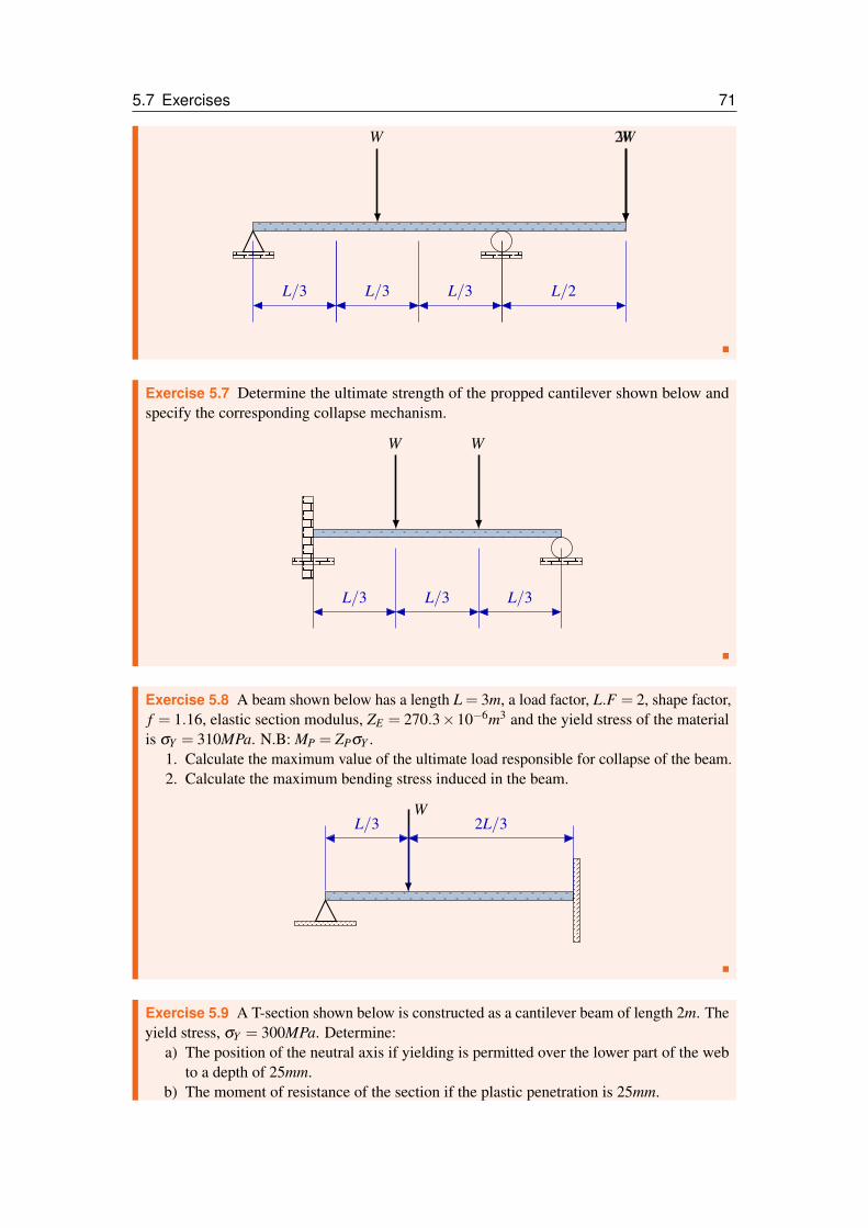
5.7 Exercises 71
W 2WW
L/3 L/3 L/3 L/2
�
Exercise 5.7 Determine the ultimate strength of the propped cantilever shown below andspecify the corresponding collapse mechanism.
W W
L/3 L/3 L/3
�
Exercise 5.8 A beam shown below has a length L = 3m, a load factor, L.F = 2, shape factor,f = 1.16, elastic section modulus, ZE = 270.3×10⁻⁶m3 and the yield stress of the materialis σY = 310MPa. N.B: MP = ZPσY .
1. Calculate the maximum value of the ultimate load responsible for collapse of the beam.2. Calculate the maximum bending stress induced in the beam.
WL/3 2L/3
�
Exercise 5.9 A T-section shown below is constructed as a cantilever beam of length 2m. Theyield stress, σY = 300MPa. Determine:
a) The position of the neutral axis if yielding is permitted over the lower part of the webto a depth of 25mm.
b) The moment of resistance of the section if the plastic penetration is 25mm.

72 Inelastic Bending
c) The uniformly distributed load over the whole span that will cause a plastic penetrationof 25mm.
�
Exercise 5.10 For the beam shown in the figure below, determine the mode of collapse andthe value of the collapse load.
•
W
3m 3m
1m
�
Exercise 5.11 The two beams shown below both have a shape factor, f = 1.5, yield stress,σY = 200MPa but different cross sections. The Beam AC has a rectangular cross-section75mm×40mm with 75mm lying vertically while beam CD has a rectangular cross-section100mm×60mm with 75mm lying vertically. Hint:
MP = f ME = f σY ZP = f σYbd2
6
Determine the value of the load Wu that will cause collapse of the beam
•A BC D
W
2m 3m
1m
�
Exercise 5.12 A mild steel coupling in a metal working process has a diameter of 40mmand length L = 250mm. It is subjected to a torque of 1800Nm which is known to have causedshear yielding in the shaft. τY = 120MPa and G = 80GPa �
Exercise 5.13 A beam is fixed at both ends and loaded with a point load at B. The shapefactor is 1.18 and the load factor is 2.2. If the yield stress is 300MPa and ZE = 305×10−6m4,determine the permissible load as well as the maximum stress. �

5.7 Exercises 73
Exercise 5.14 # �
Exercise 5.15 # �
Exercise 5.16 # �


Bibliography
[1] D.L. Logan, "A First Course in Finite Element Method, 4th Ed.”
[2] P. P. Chandrupatla and R. J. Belegundu, "Introduction to Finite Elements in engineering”,4th, Pearson-Prentice Hall."
[3] M.J. Fagan, "Finite Element Analysis, Theory and practice,Pearson-Prentice Hall."
[4] J. Drotsky, "Strength of Materials for Technologists, Self-published."
[5] P.P. Benham, et.al, "Mechanics of Engineering Materials, Prentice Hall."