Eliciting a human understandable model of ice adhesion strength for rotorblade leading edge materials from uncertain experimental data

Ana M. Palacios a, José L. Palacios b, Luciano Sánchez a,⇑

aDepartamento de Informática, Universidad de Oviedo, 33071 Gijón, Asturias, SpainbDepartment of Aerospace Engineering, The Pennsylvania State University, University Park, PA 16802, USA

a r t i c l e i n f o

Keywords:

Genetic Fuzzy Systems

Fuzzy rule-based classifiers

Vague data

Isotropic materials

Ice-phobic materials

Shear adhesion strength

a b s t r a c t

The published ice adhesion performance data of novel ‘‘ice-phobic’’ coatings varies significantly, and

there are not reliable models of the properties of the different coatings that help the designer to choose

the most appropriate material. In this paper it is proposed not to use analytical models but to learn

instead a rule-based system from experimental data. The presented methodology increases the level of

post-processing interpretation accuracy of experimental data obtained during the evaluation of ice-

phobic materials for rotorcraft applications. Key to the success of this model is a possibilistic representa-

tion of the uncertainty in the data, combined with a fuzzy fitness-based genetic algorithm that is capable

to elicit a suitable set of rules on the basis of incomplete and imprecise information.

Ó 2012 Elsevier Ltd. All rights reserved.

1. Introduction

Helicopter rotors are more susceptible to icing than fixed-wing

vehicles. Rotors impact more super-cooled water particles per sec-

ond than the rest of the fuselage. The higher collection efficiency of

rotor airfoils makes them accrete ice at a higher rate than thicker

fixed-wing airfoils. While fixed wing aircraft usually cruise at alti-

tudes above icing conditions, rotorcraft vehicles operate in atmo-

spheric conditions where super-cooled water particles are found.

Ice accretion can be critically dangerous, as it can modify the

vehicles aerodynamics, create excessive vibration, increase drag

(Withington, 2010), and introduce ballistic concerns as thick ice

layers sheds off.

1.1. Electro-thermal de-icing systems and ice-phobic coatings

To date, the only de-icing systems qualified by the Federal Avi-

ation Administration are based on electro-thermal energy. Electro-

thermal systems melt the ice interface between accreted ice and

the leading edge erosion protection cap of the rotor. Such a system

requires large amounts of energy (3.9 W/cm2) and contributes to

an undesired increase in the overall weight of the system and cost

of the blade. The weight related to the required electrical power

can be as large as 112 kg on a 4300 kg gross weight helicopter

(Coffman, 1987; Zumwalt, 1985). Normally, a secondary electrical

system with redundant, dual alternator features is required when

installing electrothermal de-icing on helicopters (Coffman, 1987;

Zumwalt, 1985). The thermal de-icing mechanism is turned on

cyclically to limit power consumption or introduce excessive heat-

ing of the leading edge structure (which could cause composite

delamination). Those areas not protected during de-icing continue

to accumulate ice until the heating mats under that specific leading

edge region are turned on. During some occasions, melted ice

might flow to the aft portion of the blade (where there are no heat-

ing mats) to refreeze. Since the electro-thermal de-icing system

sublimates the ice interface, ice shedding occurs under centrifugal

loading. Released ice patches could reach up to 7.6 mm in thick-

ness (Coffman, 1987; Zumwalt, 1985) and are a ballistic concern

for some vehicles. The system relies on the thermal conductivity

of isotropic materials that protect the leading edge of the blade

from erosion. For this reason, electro-thermal de-icing is not ideal

for new high erosion resistant polymer based leading edge protec-

tion materials because they have lower thermal conductivity than

isotropic materials.

Due to mentioned drawbacks, particularly power generation,

weight, and system cost constrains, medium and small size vehi-

cles avoid the installation of electro-thermal de-icing systems, also

limiting operation in icing environments. A passive ice-phobic

coating that prevents ice formation would be the ideal solution

to helicopter rotor blade ice accretion.

1.2. Variability of the experimental data for ice-phobic coatings

The search for ice-phobic materials for rotorcraft applications is

ongoing. To quantify the ice adhesion performance of novel ‘‘ice-

phobic’’ coatings, many researchers have attempted to measure

0957-4174/$ - see front matter Ó 2012 Elsevier Ltd. All rights reserved.

doi:10.1016/j.eswa.2012.02.155

⇑ Corresponding author.

E-mail addresses: palaciosana@uniovi.es (A.M. Palacios), jlp324@psu.edu

(J.L. Palacios), luciano@uniovi.es (L. Sánchez).

Expert Systems with Applications 39 (2012) 10212–10225

Contents lists available at SciVerse ScienceDirect

Expert Systems with Applications

journal homepage: www.elsevier .com/locate /eswa

the shear adhesion strength of ice to these materials. The published

data varies significantly, even for isotropic materials, as it is shown

in Table 1 (Brouwers, Peterson, Palacios, & Centolanza, 2011). In

this table, ‘‘Freezer ice’’ is ice accumulated slowly on a substrate,

while ‘‘impact ice’’ would be that formed as a body travels through

an icing cloud at a certain velocity.

Impact ice better represents the physics involved in ice forma-

tion on helicopter rotors. Even though some authors have studied

ice accretion and shedding with impact ice, critical icing conditions

governing ice accretion physics are not reported. These conditions

are: liquid water concentration (LWC) of the cloud, median volume

diameter (MVD) of the super-cooled water droplets in the cloud,

ambient temperature and impact velocity. It is also important to

know the surface conditions of the coatings being tested, especially

surface roughness. Scavuzzo and Chu (1987) have demonstrated

the effect of surface roughness on ice adhesion strength. Surface

roughness issues are particularly important for rotorcraft, which

may operate in both erosive sand/rain environments and icing con-

ditions. An eroded blade leading edge will have an effect on the

shedding performance of the rotor. The discrepancies reported on

ice adhesion strength testing are attributed to the different test

procedures adopted, to the ice adhesion process, and to the variant

environmental conditions triggered during shedding.

1.3. Rule-based empirical models of ice creation

Computer models of rotorcraft icing are based on empirical data

that is gathered in experiments under controlled conditions. The

numerical experiments that will be discussed in this work are

based on experimental knowledge gained by the Vertical Lift Re-

search Center of Excellence at the Pennsylvania State University.

This center has developed a new icing facility for rotorcraft icing

research (Palacios, Brouwers, Han, & Smith, 2010).

The creation of ice is influenced by different parameters, whose

interrelationship is complex (see Section 2). Furthermore, the con-

trol that the experts exert over these parameters is not complete,

and thus the experiments are not fully repeatable. Significantly dif-

ferent outcomes can be produced for the same set of controlling

parameters and to our best knowledge there is not a reliable math-

ematical model relating the experimental conditions with the ice

adhesion performance of novel ‘‘ice-phobic’’ coatings.

In this study a rule-based model of the experimental data is

proposed, whose knowledge base is to be automatically obtained

by means of a computer algorithm. This system inputs the environ-

mental and icing conditions and predicts whether the coating is

suitable or not, considering the shear adhesion strength of ice to

this material. There are advantages related to the use a of rule-

based model against a statistical decision system for the applica-

tion at hand. To name some:

� A rule-based system has a human understandable structure

comprising sentences of the type ‘‘IF the control parameters

are in certain set, THEN the adhesion strength is [. . .]’’. By direct

examination of the rules, the experts can gain knowledge about

the coating that is not evident from the raw experimental data.

� The subset of rules taking part in every prediction is known.

These rules can be tracked down to these experiments where

they originated. Ultimately this allows for assigning a degree

of reliability to each prediction.

� In case that the control parameters are much different from

those of any past experiment, a rule-based system can produce

the output ‘‘unknown response’’, while regression models will

generate a possibly wrong extrapolation.

On the other hand, obtaining rules from data is a computation-

ally hard problem (Cordón, Gomide, Herrera, Hoffmann, & Magda-

lena, 2004; Herrera, 2008; Kuncheva, 2000), which is further

complicated by mentioned uncertainty in the data. In this paper,

those decisions taken for solving this learning problem will be

detailed:

� The use of fuzzy logic, as it reduces the complexity of the

knowledge base (Cordón, 2001).

� A possibilistic representation of the uncertainty in the data,

since it is better suited than stochastic models for ‘‘epistemic

uncertainty’’ (Dubois & Prade, 1987). This is the variability that

is not related to random deviations but to an insufficient knowl-

edge of the parameters governing the experiment.

� The use of genetic algorithms for obtaining fuzzy rules from

uncertain data (Palacios, Sánchez, & Couso, 2010; Palacios, Sán-

chez, & Couso, 2011; Sánchez, Couso, & Casillas, 2007; Sánchez,

Couso, & Casillas, 2009).

In Section 2, the rotorcraft icing facility and shedding testing

procedures developed by the Pennsylvania State University is

introduced. The characteristics of available experimental data

regarding shear adhesion strength of ice to material are shown in

Section 3, along with the use of possibility distributions for repre-

senting the uncertainty in this data. In Section 4, the structure of

the fuzzy rule based system is detailed along with an overview

of a novel learning algorithm able to elicit a knowledge base from

possibilistic data. Section 5 contains the experimental validation of

the proposed system, whose outcomes are compared with that of

real experiments, and also with subjective predictions taken by hu-

man experts in the field. In Section 6 the paper finishes with the

concluding remarks.

2. Icing system model

The Vertical Lift Research Center of Excellence at the Pennsylvania

State University has developed a new icing facility for rotorcraft

icing research. Achieving an initial operational capability in

November 2009, the Adverse Environment Rotor Test Stand

(AERTS) is designed to generate an accurate icing cloud around test

rotor. The AERTS facility is formed by an industrial 6 m by 6 m by

6 m cold chamber where temperatures between ÿ25 °C and 0 °C

can be achieved. The chamber floor is waterproofed with marine

lumber covered by aluminum plating, and a drainage system in

the perimeter of the room collects melted ice during the post-test

Table 1

Shear adhesion strength (SAT) for Aluminum with a temperature of ÿ11 °C.

Author Ice Test SAT-kPa

Loughborough and Hass (1946) Freezer ice Pull 558

Stallabrass et al. (1962) Impact ice Rotating instrumented beam 97

Itagaki (1983) Impact ice Rotating rotor 27–157

Scavuzzo and Chu (1987) Impact ice Shear Window 90–290

Reich (1994) Freezer ice Pull 896

A.M. Palacios et al. / Expert Systems with Applications 39 (2012) 10212–10225 10213

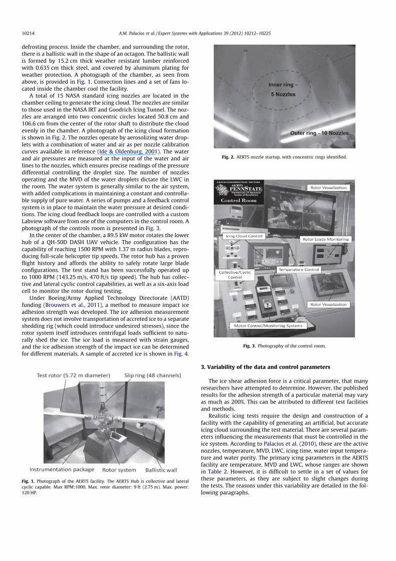
defrosting process. Inside the chamber, and surrounding the rotor,

there is a ballistic wall in the shape of an octagon. The ballistic wall

is formed by 15.2 cm thick weather resistant lumber reinforced

with 0.635 cm thick steel, and covered by aluminum plating for

weather protection. A photograph of the chamber, as seen from

above, is provided in Fig. 1. Convection lines and a set of fans lo-

cated inside the chamber cool the facility.

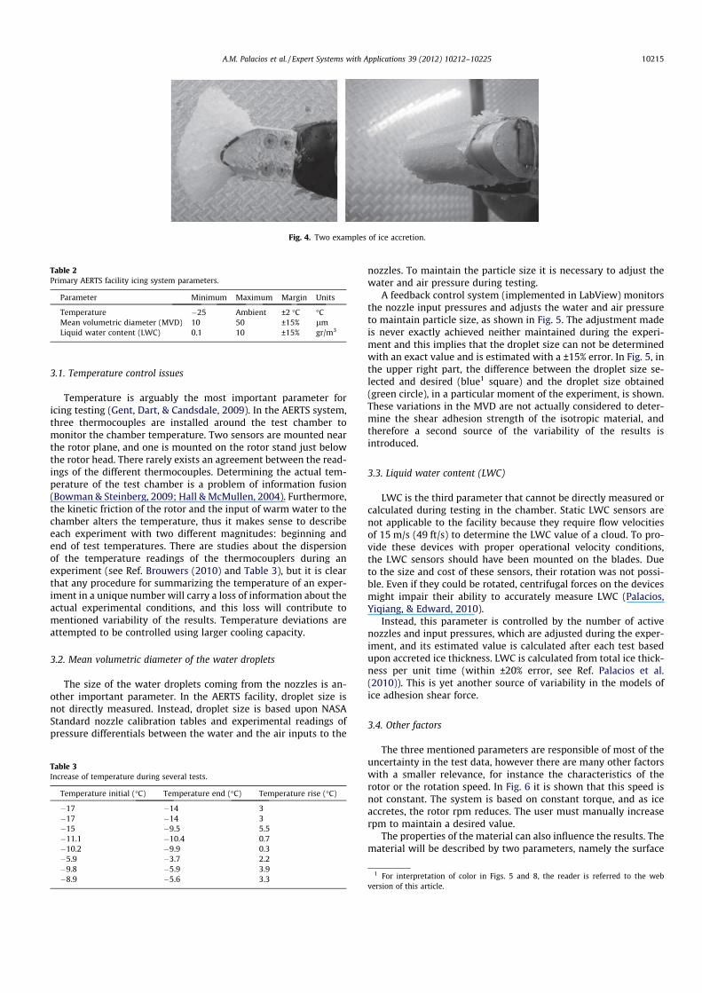
A total of 15 NASA standard icing nozzles are located in the

chamber ceiling to generate the icing cloud. The nozzles are similar

to those used in the NASA IRT and Goodrich Icing Tunnel. The noz-

zles are arranged into two concentric circles located 50.8 cm and

106.6 cm from the center of the rotor shaft to distribute the cloud

evenly in the chamber. A photograph of the icing cloud formation

is shown in Fig. 2. The nozzles operate by aerosolizing water drop-

lets with a combination of water and air as per nozzle calibration

curves available in reference (Ide & Oldenburg, 2001). The water

and air pressures are measured at the input of the water and air

lines to the nozzles, which ensures precise readings of the pressure

differential controlling the droplet size. The number of nozzles

operating and the MVD of the water droplets dictate the LWC in

the room. The water system is generally similar to the air system,

with added complications in maintaining a constant and controlla-

ble supply of pure water. A series of pumps and a feedback control

system is in place to maintain the water pressure at desired condi-

tions. The icing cloud feedback loops are controlled with a custom

Labview software from one of the computers in the control room. A

photograph of the controls room is presented in Fig. 3.

In the center of the chamber, a 89.5 kWmotor rotates the lower

hub of a QH-50D DASH UAV vehicle. The configuration has the

capability of reaching 1500 RPM with 1.37 m radius blades, repro-

ducing full-scale helicopter tip speeds. The rotor hub has a proven

flight history and affords the ability to safely rotate large blade

configurations. The test stand has been successfully operated up

to 1000 RPM (143.25 m/s, 470 ft/s tip speed). The hub has collec-

tive and lateral cyclic control capabilities, as well as a six-axis load

cell to monitor the rotor during testing.

Under Boeing/Army Applied Technology Directorate (AATD)

funding (Brouwers et al., 2011), a method to measure impact ice

adhesion strength was developed. The ice adhesion measurement

system does not involve transportation of accreted ice to a separate

shedding rig (which could introduce undesired stresses), since the

rotor system itself introduces centrifugal loads sufficient to natu-

rally shed the ice. The ice load is measured with strain gauges,

and the ice adhesion strength of the impact ice can be determined

for different materials. A sample of accreted ice is shown in Fig. 4.

3. Variability of the data and control parameters

The ice shear adhesion force is a critical parameter, that many

researchers have attempted to determine. However, the published

results for the adhesion strength of a particular material may vary

as much as 200%. This can be attributed to different test facilities

and methods.

Realistic icing tests require the design and construction of a

facility with the capability of generating an artificial, but accurate

icing cloud surrounding the test material. There are several param-

eters influencing the measurements that must be controlled in the

ice system. According to Palacios et al. (2010), these are the active

nozzles, temperature, MVD, LWC, icing time, water input tempera-

ture and water purity. The primary icing parameters in the AERTS

facility are temperature, MVD and LWC, whose ranges are shown

in Table 2. However, it is difficult to settle in a set of values for

these parameters, as they are subject to slight changes during

the tests. The reasons under this variability are detailed in the fol-

lowing paragraphs.

Fig. 1. Photograph of the AERTS facility. The AERTS Hub is collective and lateral

cyclic capable. Max RPM:1000. Max. rotor diameter: 9 ft (2.75 m). Max. power:

120 HP.

Fig. 2. AERTS nozzle startup, with concentric rings identified.

Fig. 3. Photography of the control room.

10214 A.M. Palacios et al. / Expert Systems with Applications 39 (2012) 10212–10225

3.1. Temperature control issues

Temperature is arguably the most important parameter for

icing testing (Gent, Dart, & Candsdale, 2009). In the AERTS system,

three thermocouples are installed around the test chamber to

monitor the chamber temperature. Two sensors are mounted near

the rotor plane, and one is mounted on the rotor stand just below

the rotor head. There rarely exists an agreement between the read-

ings of the different thermocouples. Determining the actual tem-

perature of the test chamber is a problem of information fusion

(Bowman & Steinberg, 2009; Hall & McMullen, 2004). Furthermore,

the kinetic friction of the rotor and the input of warm water to the

chamber alters the temperature, thus it makes sense to describe

each experiment with two different magnitudes: beginning and

end of test temperatures. There are studies about the dispersion

of the temperature readings of the thermocouplers during an

experiment (see Ref. Brouwers (2010) and Table 3), but it is clear

that any procedure for summarizing the temperature of an exper-

iment in a unique number will carry a loss of information about the

actual experimental conditions, and this loss will contribute to

mentioned variability of the results. Temperature deviations are

attempted to be controlled using larger cooling capacity.

3.2. Mean volumetric diameter of the water droplets

The size of the water droplets coming from the nozzles is an-

other important parameter. In the AERTS facility, droplet size is

not directly measured. Instead, droplet size is based upon NASA

Standard nozzle calibration tables and experimental readings of

pressure differentials between the water and the air inputs to the

nozzles. To maintain the particle size it is necessary to adjust the

water and air pressure during testing.

A feedback control system (implemented in LabView) monitors

the nozzle input pressures and adjusts the water and air pressure

to maintain particle size, as shown in Fig. 5. The adjustment made

is never exactly achieved neither maintained during the experi-

ment and this implies that the droplet size can not be determined

with an exact value and is estimated with a ±15% error. In Fig. 5, in

the upper right part, the difference between the droplet size se-

lected and desired (blue1 square) and the droplet size obtained

(green circle), in a particular moment of the experiment, is shown.

These variations in the MVD are not actually considered to deter-

mine the shear adhesion strength of the isotropic material, and

therefore a second source of the variability of the results is

introduced.

3.3. Liquid water content (LWC)

LWC is the third parameter that cannot be directly measured or

calculated during testing in the chamber. Static LWC sensors are

not applicable to the facility because they require flow velocities

of 15 m/s (49 ft/s) to determine the LWC value of a cloud. To pro-

vide these devices with proper operational velocity conditions,

the LWC sensors should have been mounted on the blades. Due

to the size and cost of these sensors, their rotation was not possi-

ble. Even if they could be rotated, centrifugal forces on the devices

might impair their ability to accurately measure LWC (Palacios,

Yiqiang, & Edward, 2010).

Instead, this parameter is controlled by the number of active

nozzles and input pressures, which are adjusted during the exper-

iment, and its estimated value is calculated after each test based

upon accreted ice thickness. LWC is calculated from total ice thick-

ness per unit time (within ±20% error, see Ref. Palacios et al.

(2010)). This is yet another source of variability in the models of

ice adhesion shear force.

3.4. Other factors

The three mentioned parameters are responsible of most of the

uncertainty in the test data, however there are many other factors

with a smaller relevance, for instance the characteristics of the

rotor or the rotation speed. In Fig. 6 it is shown that this speed is

not constant. The system is based on constant torque, and as ice

accretes, the rotor rpm reduces. The user must manually increase

rpm to maintain a desired value.

The properties of the material can also influence the results. The

material will be described by two parameters, namely the surface

Fig. 4. Two examples of ice accretion.

Table 2

Primary AERTS facility icing system parameters.

Parameter Minimum Maximum Margin Units

Temperature ÿ25 Ambient ±2 °C °C

Mean volumetric diameter (MVD) 10 50 ±15% lm

Liquid water content (LWC) 0.1 10 ±15% gr/m3

Table 3

Increase of temperature during several tests.

Temperature initial (°C) Temperature end (°C) Temperature rise (°C)

ÿ17 ÿ14 3

ÿ17 ÿ14 3

ÿ15 ÿ9.5 5.5

ÿ11.1 ÿ10.4 0.7

ÿ10.2 ÿ9.9 0.3

ÿ5.9 ÿ3.7 2.2

ÿ9.8 ÿ5.9 3.9

ÿ8.9 ÿ5.6 3.31 For interpretation of color in Figs. 5 and 8, the reader is referred to the web

version of this article.

A.M. Palacios et al. / Expert Systems with Applications 39 (2012) 10212–10225 10215

roughness and the Young’s modulus. The surface roughness is

measured by hand with a profilometer. The assumed value of this

parameter is the average of the maximum and minimum of the

measurements taken at the stagnation point of the coating. Lastly,

the Young’s modulus is the ratio between the linear stress and the

linear strain for a given material. This value is not experimentally

determined at AERTS facilities.

3.5. Attribution of values to the uncertain parameters

From the preceding discussion it is clear that almost none of the

values of parameters governing a test can be accurately described

by means of a single number. Former attempts to do this are a

plausible origin of the discrepancies between the published results

regarding the ice shear adhesion force of different materials.

According to our own experience, it is not needed to attribute

numerical values to the uncertain parameters for interpreting the

dependence between the input data (the temperature, the mean

volumetric diameter of the droplets, the LWC, roughness and

Young’s modulus) and the output data (the ice shear adhesion

force measured for a material). Consequently, in the next section

it is proposed that the uncertain parameters are not assigned pre-

cise numbers but distributions of values, whose nature is discussed

in the following paragraphs. Later in the same section, it will be

shown how to actually build these models from datasets compris-

ing a mix of numerical measurements and distributions of values.

4. Obtaining models from imprecisely known data

In the preceding sections, it has been shown that the available

knowledge about the parameters governing an experiment is, at

most, partial. It is presumed that the inability for accurately deter-

mining the value of some parameters is, in part, accountable for the

large differences between the experimental results found in the lit-

erature. For example, imagine that a shear adhesion strength (SAT)

of 100 kPa was measured in an experiment for which the initial

temperature was ÿ14 degrees and the final temperature was

ÿ10°. In this case, it is not correct to write ‘‘SAT = 100 kPa at a tem-

perature of ÿ12 °C’’ neither it is to state ‘‘SAT = 100 kPa for temper-

atures between ÿ14 and ÿ10 °C’’; our knowledge is restricted to

the fact ‘‘SAT = 100 kPa at an unknown temperature between

ÿ14 and ÿ10 °C.’’

In this study it is proposed not to discard the information about

the variability in the parameters when deriving a model. This is

easier to do if rule-based models are adopted. In other words, for-

mulae like ‘‘SAT = a � TEMP + b �MWD + c � LWC + d,’’ will not be

sought but the imprecision in the results of the experimentation

will be taken into account for producing rule-based models com-

prising expressions such that ‘‘if the temperature is higher than

ÿ10 °C then the ice shear adhesion force is always lower than

150 kPa.’’

Lastly, the purpose of this paper is to derive a rule-based model

with which it can be determined whether a given material fulfills

or not the requirements for being used in a helicopter blade.

According to the usual nomenclature in machine learning, this kind

of models can be regarded as binary classification systems. Some

other artificial intelligence-related terms need to be introduced:

the misclassification rate is the proportion of prediction failures

committed by the model in a certain corpus of experimental data,

Fig. 5. Labview monitor: to adjust the water and air pressure to maintain particle size.

Fig. 6. Rotor tip without and with accreted ice.

10216 A.M. Palacios et al. / Expert Systems with Applications 39 (2012) 10212–10225

or ‘‘training set’’. The term ‘‘learning’’ will be used in the sense of

‘‘numerical optimization of the parameters defining the model’’,

and the terms ‘‘instance’’ or ‘‘example’’ indistinctly denote one of

the experiments that measure the ice accretion for a certain set

of environmental conditions. An instance is comprised of an ‘‘input

part’’ (these environmental conditions) which is a list of numbers,

intervals or fuzzy sets, that will be called ‘‘features’’, and an ‘‘out-

put part’’ or ‘‘class label’’, which is the number 1 if the experiment

was successful (the material is adequate for its use) or 0 if it is not.

In the remainder of this section the representation of imprecise

data will be discussed, along with the combination of this data

with fuzzy rule-base classifiers, the assessment of the quality of a

classifier on a sample of imprecisely perceived data, and two differ-

ent numerical methods for finding the rule-based model that opti-

mizes the mentioned quality.

4.1. Possibilistic representation of imprecise values

In this paper a technique for modeling the imprecision which is

based in the possibility theory (Couso & Sánchez, 2008; Sánchez

et al., 2009) will be adopted. This possibilistic framework encloses

interval-valued data as a particular case, and easily accommodates

other cases where more precise information is available.

In particular, those situations where one or more confidence

intervals for a parameter can be determined are well suited for this

technique. For example, suppose that there is a broad range of

extreme values, but a smaller typical range: ‘‘99% of times the

temperature was between ÿ18 °C and ÿ8 °C, but 95% of times it

was between ÿ13 °C and ÿ11 °C.’’ Such a nested family of confi-

dence intervals is compatible with a possibility distribution (Couso

& Sánchez, 2008). These, in turn, can also be described by means

of fuzzy membership functions. In this case, these functions are

chosen so that their each level cut is one of the available confi-

dence intervals, at the level 1 ÿ a (see Sánchez et al. (2007, 2009)

and Fig. 7). In short, a fuzzy representation for imprecise data will

be used, which is often used in fuzzy statistics (Couso, Sánchez, &

Gil, 2004; Gil, 1987).

4.2. Rule-based classification systems with fuzzy inputs

The binary rule-based systems mentioned in the preceding par-

agraph will be given an structure similar to that of the following

example:

if x1 is HIGH and x2 is LOW then class is 1

if x1 is MEDIUM and x2 is MEDIUM then class is 0

if x2 is HIGH then class is 1:

ð1Þ

Let x = (x1, . . . ,xd) be a vector of features, and let us consider that a

rule-based classifier system is a list of M ‘‘IF–THEN’’ rules, compris-

ing an antecedent, a consequent and sometimes a weight:

If ðx is eAiÞ then class is Ci ½with weight wi� ð2Þ

where eAi is a fuzzy subset of Rd, and the expression ‘‘x is eAi’’ is a

combination of asserts of the form ‘‘xp is eAiq’’ by means of different

logical connectives, often the ‘‘AND’’ or minimum connective. The

terms eAiq are, in turn, subsets of R that have been assigned a linguis-

tic meaning, and the membership function of eAi models the degree

of truth of this combination. Ci 2 {0,1} are the labels of the different

classes. wi are degrees of credibility that may be given to each rule,

wi 2 [0,1]. In the last example, eA11 ¼HIGH, eA12 ¼LOW, and the

membership functions of these two sets define the compatibility

between the values of x1 and x2 and the linguistic terms ‘‘HIGH’’

and ‘‘LOW’’. The fuzzy set eA1 ¼minðeA11; eA12Þ define the compatibil-

ity of each pair (x1,x2) and the antecedent of the first rule.

Given a rule-based classifier system and a vector x comprising a

list of experimental parameters or features (temperature, MWD,

LWC, etc.), the output of the model is determined by a voting pro-

cedure, where each rule is assigned a number of votes equal to the

compatibility between x and its antecedent, multiplied by its

weight. The mechanisms for choosing the winner alternative are

two:

1. The class of the object is given by the consequent of the most

voted rule:

classðxÞ ¼ Ck where k ¼ argmaxifwi

eAiðxÞg: ð3Þ

2. The votes of all rules with the same consequent are added, and

the option with a higher number of votes is chosen:

classðxÞ ¼ argmaxi

X

j¼1...;M

djCiwj

eAjðxÞ

( ); ð4Þ

where dba is Kronecker’s delta; dba ¼ ½a ¼ b�.

In this case, some of the features are not precisely known, thus a

fuzzy setwill be used for describing the inputs: eX ¼ ðeX1; eX2; . . . ; eXdÞ.

When the input is imprecise, the output is no longer a class label but

a fuzzy set of classes denoted by classðeXÞ. Themembership function

of this set is

classðeXÞðcÞ ¼maxfeXðxÞjc ¼ classðxÞg: ð5Þ

This last expression is made clear with two additional examples:

1. A classification system is defined by three interval rules:

if x < 3 then class is B

if x 2 ½3;4:5� then class is A

if x > 4:5 then class is C

ð6Þ

The input x is an unknown point in [3.2,5]. What is the class of x?

Answer: Since xP 3, the truth of the antecedent of the first rule is

zero. If x 2 [3.2,4.5] the output is A, or else x 2 [4.5,5], and in this

last case the output is C, therefore

classð½3:2;5�Þ ¼ fA;Cg: ð7Þ

2. A classification system is defined by three fuzzy rules:

if x is LOW then class is B

if x is MEDIUM then class is A

if x is HIGH then class is C

ð8Þ

where the meanings of ‘‘LOW’’, ‘‘MEDIUM’’ and ‘‘HIGH’’ are given in

Fig. 8.

The input is the fuzzy set eX , plotted in red in the same figure

(observe that the 0.5-cuts of these sets are the same intervals in

the antecedents and the input of the preceding example). What is

the class of eX?

Fig. 7. Fuzzy representation of vague data. Left: the only information is the range of

the variable, or P([min,max]) = 1. Right: a compound value (in this example, a set of

five different measurements of the variable) can be summarized by a fuzzy

membership, such that each a-cut contains the true value of the variable with

probability at least 1-a.

A.M. Palacios et al. / Expert Systems with Applications 39 (2012) 10212–10225 10217

Answer: For each level a, an interval classifier is obtained (for

a = 0.5 that classifier is identical to that described in the last exam-

ple.) The output of each one of these interval classifiers is a set of

classes; these sets are nested, as the width of all the intervals grows

when a decreases. If these sets are regarded as the level cuts of the

fuzzy output, the corresponding membership is

classðeXÞ ¼ f1jA;0:4jB;0:7jCg ð9Þ

depicted in the same figure. In other words, classðeXÞðAÞ ¼ 1,

classðeXÞðBÞ ¼ 0:4, classðeXÞðCÞ ¼ 0:7.

4.2.1. Assessing the misclassification rate with imprecise data

If the input to a classifier is imprecise and its output is set-

valued, the same can be said about its misclassification rate. Let

fðci; classðeX iÞÞgi¼1...N , be a list of N pairs, where ci is the true class

of the ith object, and classðeX iÞ is the set valued output of the clas-

sifier. According to Sánchez and Couso (2007), the misclassification

rate is computed as follows for a generic classification problem

with Nc classes: let

p ¼ arg maxc¼1;...;Nc

classðeX iÞðcÞ ð10Þ

be the class label with higher membership value in the classifier

output at the ith object, and be

q ¼ arg maxc¼1;...;Nc ; c–p

classðeX iÞðcÞ ð11Þ

the second largest one. The number of errors that the classifier com-

mits at the ith object is either 0 or 1, however the knowledge about

this number is a fuzzy set

~ei ¼f1j0; classðeX iÞðqÞj1g if ci ¼ p

fclassðeX iÞðciÞj0;1j1g if ci – p:

(ð12Þ

Finally, the total misclassification rate is a fuzzy subset of

0; 1N; 2N; . . . ;1

� :

eðcÞ ¼1

N� �N

i¼1~ei; ð13Þ

where the meaning of the fuzzy arithmetic operators is

ð~a� ~bÞðxÞ ¼maxfminð~aðuÞ; ~bðvÞÞjuþ v ¼ xg; ð14Þ

ðk � ~aÞðxÞ ¼ ~aðx=kÞ: ð15Þ

4.3. Obtaining rule bases from fuzzy data

Some of the most effective numerical techniques for obtaining

fuzzy rule bases from data are based on genetic algorithms, so

called ‘‘Genetic Fuzzy Systems’’ (Cordón, 2001). A recent branch

of these algorithms studies how to obtain rules from imprecise

data, as happens in this study (Sánchez & Couso, 2007). Two differ-

ent state-of-the art GFSs will be used. Both are able to exploit the

information in vague data for eliciting a human readable, knowl-

edge base comprising fuzzy rules. The first of these GFSs is called

Genetic Cooperative-Competitive Learning (GCCL) (Palacios,

Sánchez, & Couso, 2010; Palacios et al., 2010) and evolves a popu-

lation of rules so that the misclassification rate in the experimental

data (see Eq. (13)) is minimum. The second one is a generalization

of the Adaboost algorithm, that determines the weights of a set of

rules optimizing the expectation of the misclassification rate

(Palacios, Sánchez, & Couso, in press). A comprehensive description

of these algorithms can be found in the mentioned references. An

outline of the algorithms is included for the convenience of the

reader.

4.3.1. Requisites

Both algorithms make use of a set of empirical measurements,

as described in the first part of this paper. These comprise the

(maybe vague) parameters defining the experimental conditions,

and the results of the tests; that is to say, whether the material

fulfills the conditions, or not.

In addition to this, the membership functions associated to the

linguistic terms that appear in the rules must be defined in ad-

vance. Although there exist numerical procedures for automati-

cally producing these memberships (Bastian, 1994; Karr, 1991),

in our opinion, a human readable model must be based on a prior

consensus about the meaning of the linguistic terms, and thus the

determination of these membership functions will not be a part of

the numerical algorithm presented here.

4.3.2. Genetic Cooperative-Competitive Learning

GCCL is designed for finding a set of rules optimizing the fuzzy

expression described in Eq. (13). Since the search space is very

large, an exhaustive search is not feasible. Unfortunately, the prop-

erties of the objective function do not allow for significant short-

cuts either, thus GCCL is based in two heuristic simplifications:

� The number M of rules in the knowledge base is assumed

known.

� Given the antecedent part of a rule (‘‘If (x is eAi)’’), the best con-

sequent and weight for this antecedent only depend on those

experimental cases for which this last expression is true.

As a consequence of these two assumptions, the search space is

reduced to the free parameters of the M fuzzy sets describing the

antecedents; the consequents and weights are not part of the

search, as they will be computed from the experimental cases

matching their corresponding antecedents (the calculations are de-

scribed later). The output of the classifier is computed as shown in

see Eq. (3), Section 4.2.

In turn, each chain can be formed as a combination of the sym-

bols in a finite catalog of linguistic terms and connectives (for in-

stance: ‘‘x1 is SMALL and x2 is LARGE and . . .’’). Following the

binary representation system described in González and Pérez

(2001), all the antecedents of a knowledge base can be represented

in a bit chain, allowing for the exploration of the different rule-

based classifier systems by means of a genetic algorithm.

The genetic search consists therefore in finding the bit chain

that minimizes the misclassification rate defined in Eq. (13). There

are some problems that must be addressed before this search can

take place:

1. The concept of ‘‘minimum’’ depends on the definition of a total

order among the fuzzy values of the misclassification rate, some

of which cannot be directly compared. For example: which is

lower, the interval error [0.01,0.1] or [0.02,0.05]?

2. How the best consequent and weight of a rule are produced for

a given antecedent.

3. How to alleviate the computational complexity of determining

the fuzzy set in Eq. (13), and in particular the intermediate step

in Eq. (5).

Fig. 8. Fuzzy sets used in the second example in Section 4.2.

10218 A.M. Palacios et al. / Expert Systems with Applications 39 (2012) 10212–10225

The first issue is solved by redefining the objective of the

problem: it is acknowledged that a minimum cannot be obtained,

but a set of non dominated classifiers can be produced: for instance,

given three classifiers with misclassification rates of [0.06,0.08],

[0.01,0.1] and [0.02,0.05], it is known that the minimum must be

either the second or the third classifiers, because any value in

[0.06,0.08] is higher than any value in [0.01,0.1] or [0.02,0.05].

The second problem is solved by embracing and extending the

definition in Ishibuchi, Nakashima, and Murata (1995), which con-

sists in selecting the consequent for which the number of misclas-

sifications is the lowest, constrained to the elements that fulfill the

condition ‘‘x is eA’’. When the experimental data fðeX i; ciÞgNi¼1 com-

prises fuzzy numbers, our knowledge about this number of correct

classifications is

ghitsðeA; cÞðtÞ ¼max minfeX iðxiÞgNi¼1jt ¼

X

i

dccieAðxiÞ

( ): ð16Þ

where dcci ¼ ½c ¼ ci�. The best class is selected by means of a fuzzy

ranking (Teich, 2001) on the elements of the set fghitsðeA; cÞgNc

c¼0.

The pseudocode of this numerical procedure has been included in

Appendix A.1.

Lastly, two computer efficient approximations to Eq. (13) are

shown, in turn, in Appendices A.2 and A.3. The second one is based

on a Monte-Carlo sampling and it is more accurate, albeit slower,

thus it has been used only to assess the final results.

4.3.3. Boosting fuzzy rules from LQD

A second technique for obtaining fuzzy rule based classifiers

from data consists in regarding each fuzzy rule as a weak learner,

and the knowledge base as an ensemble of learners. In other words,

each rule

If ðx is eAiÞ then class is Ci with weight wi ð17Þ

is understood as a simple classifier. For an input x, the output of this

classifier comprises a class label (which is always the same, Ci) and a

degree of certainty in the classification, whose value is wi � eAiðxÞ.

These classifiers are not very useful as isolated entities, but they

can be combined in an ensemble that performs better than its con-

stituent parts. In this case, the boosting (Hoffman, 2001; Schapire,

2001) technique can be applied for obtaining the best set of weights

fwigMi¼1 for any given set of fuzzy rules. This is because the output of

boosting-based ensemble is identical to the voting inference de-

scribed in Section 4.2 (see Eq. (4)). It is expected that this procedure

improves the accuracy of the preceding approach, however the

results are less understandable (Schapire, Freund, Bartlett, & Lee,

1998). This will be further discussed in the next section.

It is remarked that the combined output of this ensemble of

classifiers is not intended to directly minimize the misclassification

rate on a training set, as was the case with the GCCL algorithm.

Boosting optimizes instead the exponential loss

XN

i¼1

exp 1ÿ 2dci

classðxiÞ

� �ð18Þ

where dba ¼ ½a ¼ b�. The ensemble for which this last value is

minimum is also expected to have the least overall misclassification

rate over the universe, avoiding the so called overtraining (Amari,

Murata, Muller, Finke, & Yang, 1997; Sjoberg et al., 1994).

The Adaboost algorithm (Freund et al., 1996) solves this optimi-

zation problem iteratively. Let z be an instrumental variable, for

simplifying the notation:

zðx; x;wÞ ¼ x exp weAðxÞ 1ÿ 2dcj

Ci

� �� �: ð19Þ

Firstly, a weightxj = 1/N is assigned to each of the N instances. Sec-

ondly, a fuzzy set eAi and a class label Ci, constituents of a weak clas-

sifier of the form

If ðx is eAiÞ then class is Ci with weight 1 ð20Þ

is searched, such that its exponential loss

Zð1Þ ¼XN

j¼1

zðxj; xj;1Þ ð21Þ

is minimum. A genetic algorithm is well suited for this task, using

the same binary representation mentioned in the preceding section.

The weight wi of this rule is determined afterwards, as the value wi

minimizing

ZðwÞ ¼XN

j¼1

zðxj; xj;wÞ: ð22Þ

Thirdly, the weights of the N instances are updated according to the

results of this classifier,

xjðtþ1Þ ¼

z xjðtÞ; x

j;wi

� �

PNj¼1z xj

ðtÞ; xj;wi

� � : ð23Þ

The process jumps to the second step, and loops until the desired

number of fuzzy rules is eventually obtained.

When the training set comprises imprecise data, these steps are

altered as follows:

1. Weight and loss of a rule: Given a set of fuzzy weights feXjgNj¼1,

the weight of a rule is obtained by finding the minimum of the

fuzzy-valued function eZðwÞ defined below (see Appendix B for a

pseudocode of the computer implementation):

eZðwÞðzÞ¼max minN

j¼1feX jðxjÞ; eXjðxjÞg such that z¼

XN

j¼1

zðxj ;xj;wÞ andXN

j¼1

wj¼1

( ):

ð24Þ

A fuzzy ranking is used to define an order among the values of eZðwÞ,whose minimal element wi is found with a genetic algorithm, as

done in the preceding section. The loss of a rule, used for searching

the best unweighted rules, is the fuzzy set eZð1Þ.2. The weights of the instances are updated after the inclusion of

the ith rule as follows:

eXjðtþ1ÞðxÞ ¼max min eX jðxÞ; eXj

ðtÞðuÞn o

jx ¼ Kzðwi; x;uÞn o

ð25Þ

where K is a normalization factor chosen so that the distance

between the (fuzzy arithmetic-based) sum of all the weights

Xjðtþ1Þ and the value 1 is as low as possible.

5. Numerical results

In this section some experimental results obtained by means of

the methodology introduced in this paper will be discussed. The

algorithms for eliciting human readable models are assessed with

data based on testing knowledge at the Vertical Lift Research Cen-

ter of Excellence at the Pennsylvania State University (Palacios

et al., 2010). A set of rules describing the ice accretion strength

of nickel, titanium and stainless steel, for different environmental

conditions, will be derived. The same procedure will be applied

to ice-phobic coating testing in the future. A detailed description

regarding how to reproduce the results is given, thus other

researchers can apply the algorithms proposed here to their own

experimental data. An statistical comparison of the outcomes of

some different numerical algorithms is provided, that substanti-

ates our recommendations about the use of rule-based models,

and in particular about the benefits of using a fuzzy representation

for describing the uncertainty in the data.

A.M. Palacios et al. / Expert Systems with Applications 39 (2012) 10212–10225 10219

The remaining part of this section is divided as follows: first, the

properties of the different sets of data2 are detailed, along with

some information about the parameters governing the numerical

optimization algorithm. Second, the mentioned benefits of the use

of fuzzy data are assessed, by applying the same algorithms to both

fuzzy and numerical data, and comparing the results. Third, the same

statistical comparison is adopted for deciding whether the rules de-

rived by the boosting algorithm are preferred to those of GCCL, and

the relevance of the human-readable models in the design of heli-

copter blades is discussed.

5.1. Properties of the set of data

The set of data describing the ice adhesion strength of helicop-

ter rotor blades materials3 has been produced after repeated exper-

iments with nickel, titanium and stainless steel. A threshold of

34.4 kPa (5 psi) has been selected for the ice adhesion strength.

There are seven variables, some of which are imprecisely perceived,

whose description follows:

1. Initial temperature (°C): This is the temperature measured by a

thermocouple prior to the start of the icing cloud that promotes

ice accretion. This temperature is read three times: when the

experiment begins, when the rotor reaches the desired revolu-

tions per minute (rpm) and before turning on the icing cloud

(dry room). These three measurements of the initial tempera-

ture are combined into a fuzzy value, as mentioned in Section 3.

2. Final temperature (°C): This is the temperature read at the end

of the test, once the ice sheds off from the rotor. The increase in

temperature during testing is due to inability of the chamber to

compensate for the increase in temperature provided by kinetic

friction of the rotor. Again, this temperature is defined by a

fuzzy term provided by the several thermocouples.

3. Median volume diameter (MVD) of the water particle (lm):

This is the size of the water droplets in the cloud (measured

in micrometers). The size is calculated from calibration tables

provided by NASA (NASA icing nozzles used). The nozzles work

via atomization of water. The water and air pressure provided

determine the water droplet size. Both water and air pressure

are measured by pressure sensors located at the water and air

input to the nozzles. Acceptable variability of MVD is ±15%, thus

an interval-valued variable is used. The width of these intervals

is determined by a human expert.

4. Liquid water concentration (LWC) (g/m3): This is the severity of

the icing cloud. LWC quantifies how much water is there in an

icing cloud. This quantity is not measured or directly calculated

during testing. Test procedures for determinimg LWC are based

on the measurement of ice thickness at the stagnation location

of a blade for a given time interval. Acceptable variability of

LWC is ±20% which implies again an interval-valued input

whose width is determined by the expert.

5. Revolutions per minute (rpm) (cycles/minute): This is the

velocity of rotation of the rotor. The RPM of the rotor is mea-

sured by a Hall sensor that quantifies the rotational speed of

the shaft. The measurements obtained from this sensor are

combined into a fuzzy value. Shedding tests are usually con-

ducted at 350 rpm to avoid severe imbalance issues when shed-

ding is not symmetric, so the rotor rpm was limited to 350

(170 ft/s or 51.86 m/s tip speed) for safety reasons. The rotor

was designed to achieve 800 rpm (380 ft/s or 115.82 m/s tip

speed), but shedding rotor imbalance concerns limited opera-

tional RPM.

6. Surface roughness of tested material (lin): this is the surface

roughness of the coating being tested. The surface roughness

is measured by hand with a profilometer. The quantity provided

is a fuzzy value obtained from the values measured at the stag-

nation point of the coating.

7. Young’s modulus (Pa): this is the ratio of the linear stress to the

linear strain for a given material, a crisp value.

5.1.1. Parameters governing the numerical optimization

The genetic algorithms (see references Palacios et al., 2010, in

press) have been run with a population size of 100, probabilities

of crossover and mutation of 0.9 and 0.1, respectively, and limited

to 150 generations. The fuzzy partitions of the labels are uniform

and their size is 5 (see Fig. 9). All the imprecise experiments were

repeated 100 times with bootstrapped resamples of the training

set. Each test set contains 1000 bootstrap resamples.

5.2. Benefits of the use of fuzzy data

According to the discussion in Section 4.2.1, the results cannot

be described by a number but a fuzzy set (or an interval, where

applicable). The statistical comparison between samples of fuzzy

data is not a mature field yet (Couso & Sánchez, 2009) and still ex-

ist some controversy in the definition of the most appropriate sta-

Fig. 9. Fuzzy sets defining the meaning of the linguistic terms in the knowledge

base.

2 The datasets are available online at the site http://ccia35.edv.uniovi.es/datasets.3 The corresponding file is called ‘‘Ice_shedding’’ in the online site.

10220 A.M. Palacios et al. / Expert Systems with Applications 39 (2012) 10212–10225

tistical tests for this problem. Therefore, a graphical representation

is provided, where boxplots for interval-valued data are used, as

defined in Palacios et al. (2010). These boxplots are used for com-

paring selected level-cuts of the fuzzy misclassification rate, and

show the 75% percentile of the maximum and the 25% percentile

of the minimum error. Moreover, the interval-valued median of

the maximum and minimum rate are represented, as well as the

mean of the minimum and maximum fitness by dotted lines (this

last is not a part of an standard boxplot).

To compare crisp and low quality data-based algorithms a

method for removing the imprecision in observation of the data

is needed. It is clear that a removal or substitution of data can

distort the actual (unknown) value. For this reason, the steps first

proposed in Palacios et al. (2010) for mitigating this problem were

followed. To remove the uncertainty of an input variable in the

training stage, intervals are replaced by its midpoint and fuzzy sets

are replaced by their center of gravity. When the fuzzy value has

been obtained by an aggregation of different measurements (for in-

stance, this happens with the temperatures) this amounts to using

the mean value of all these measurements, discarding its disper-

sion. Each imprecise variable, when used in the validation stage,

is replaced by 1000 different values, with Monte Carlo simulation.

A uniform sampling has been used, although the results do not de-

pend on this distribution, because only the minimum and the max-

imum are relevant for the analysis.

5.3. Decision about the best numerical algorithm for eliciting rule-

based models

In Fig. 9 the membership functions of the fuzzy sets associated

to each linguistic term in the knowledge bases are plotted, as

agreed with the human expert, and in Table 4 a selection of rule-

based models, based upon these terms, is shown for the ice accre-

tion strength problem. These models are labeled ‘‘crisp data’’ when

Table 4

Rule base obtained for the dataset ‘‘Ice_shedding’’ with the algorithms ‘‘p-LQD_Boos’’ and ‘‘LQD_GCCL’’, when the imprecise data in all the input fields is replaced by the mean of

the measurements in conflict. Interval-valued errors are understood as the margin between the prediction errors in the best and worst cases.

Algorithm and error Rules

p-LQD_Boos R1: If Inital temp. is Low and Final temp. is Low and RPM is Medium then Class is No

Imprecise data R2: If Final temp. is Low and RPM is Fairly High and Roughness is Fairly Low then Class is No

R3: If LWC is Fairly Low and RPM is Fairly High and Roughness is Fairly High and Young’s modulus is Low then Class is No

error ¼ ½0:228;0:297� R4: If Final temp. is Low and Roughness is Fairly High and Young’s modulus is Low then Class is No

R5: If Final temp. is High and MVD is Low and LWC is Fairly Low and Roughness is Medium and Young’s modulus is High then Class is No

R6: If Inital temp. is Medium and Final temp. is High and LWC is Medium and RPM is Medium and Roughness is Fairly Low then Class is Yes

R7: If MVD is Medium and Roughness is Fairly Low then Class is Yes

R8: If Final temp. is Fairly High and LWC is Medium and RPM is Medium and Young’s modulus is Fairly High then Class is Yes

R9: If Final temp. is Fairly Low and MVD is Medium and LWC is Medium and Young’s modulus is Fairly High then Class is Yes

R10: If Final temp. is High and MVD is Fairly High and LWC is Fairly Low and Young’s modulus is Low then Class is Yes

p-LQD_Boos R1: If Final temp. is Low and LWC is Fairly High and RPM is Fairly High and Young’s modulus is High then Class is No

Crisp data R2: If Inital temp. is Fairly High and Final temp. is Fairly High and LWC is High and RPM is High and Young’s modulus is High then Class is No

R3: If Inital temp. is Low and MVD is Fairly Low then Class is No

error ¼ ½0:292;0:361� R4: If RPM is Fairly High and Roughness is Low and Young’s modulus is High then Class is No

R5: If Final temp. is Medium and RPM is Fairly High and Young’s modulus is High then Class is No

R6: If Final temp. is Fairly High and Roughness is Fairly Low then Class is Yes

R7: If Inital temp. is Fairly Low and LWC is High and RPM is High and Roughness is High and Young’s modulus is Fairly High then Class is Yes

R8: If Inital temp. is Fairly Low and Final temp. is Failry Low and MVD is Fairly High and RPM is and High then Class is Yes

R9: If Final temp. is Medium and LWC is Fairly Low and RPM is High and Roughness is Low and Young’s modulus Low is then Class is Yes

R10: If Inital temp. is Fairly High and Final temp. is Fairly High and MVD is Fairly Low and Roughness is High then Class is Yes

LQD_GCCL R1: If Inital temp. is Fairly Low and Final temp. is Fairly High and MVD is Low and

LWC is Medium and RPM is Medium and Roughness is Fairly Low and Young’s modulus is Medium then Class is Yes

Imprecise data R2: If Inital temp. is Medium and Final temp. is Fairly High and MVD is Fairly High and

LWC is Medium and RPM is Medium and Roughness is Fairly High and Young’s modulus is Medium then Class is No

R3: If Inital temp. is Fairly Low and Final temp. is Medium and MVD is Medium and LWC is Fairly Low and

RPM is Medium and Roughness is Fairly Low and Young’s modulus is Medium then Class is Yes

error ¼ ½0:470;0:545� R4: If Inital temp. is High and Final temp. is High and MVD is Fairly Low and LWC is Medium and

RPM is Fairly Low and Roughness is Medium and Young’s modulus is Low then Class is No

R5: If Inital temp. is Medium and Final temp. is Fairly High and MVD is Fairly High and LWC is Medium and

RPM is Medium and Roughness is Fairly Low and Young’s modulus is Medium then Class is Yes

R6: If Inital temp. is Low and Final temp. is Low and MVD is Low and LWC is Medium and

RPM is Medium and Roughness is Fairly Low and Young’s modulus is Medium then Class is No

R7: If Inital temp. is Fairly Low and Final temp. is Failry Low and MVD is Medium and LWC is Medium and

RPM is Medium and Roughness is Fairly Low and Young’s modulus Medium is then Class is Yes

R8: If Inital temp. is Fairly Low and Final temp. is Medium and MVD is Medium and LWC is Fairly Low and

RPM is Medium and Roughness is Fairly High and Young’s modulus is Medium then Class is No

LQD_GCCL R1: If Inital temp. is High and Final temp. is High and MVD is Fairly Low and LWC is Fairly High and

RPM is Fairly Low and Roughness is Medium and Young’s modulus is Low then Class is No

Crisp data R2: If Inital temp. is Fairly Low and Final temp. is Medium and MVD is Medium and LWC is Fairly High and

RPM is Medium and Roughness is Fairly Low and Young’s modulus is Medium then Class is Yes

R3: If Inital temp. is Medium and Final temp. is Medium and MVD is Medium and LWC is Fairly High and

RPM is Failry Low and Roughness is High and Young’s modulus is Medium then Class is No

error ¼ ½0:507;0:576� R4: If Inital temp. is Low and Final temp. is Low and MVD is Fairly Low and LWC is Fairly High and

RPM is Medium and Roughness is Fairly Low and Young’s modulus is Medium then Class is No

R5: If Inital temp. is Fairly High and Final temp. is Fairly High and MVD is Fairly High and LWC is Fairly High and

RPM is Fairly Low and Roughness is Fairly Low and Young’s modulus is Medium then Class is Yes

R6: If Inital temp. is Low and Final temp. is Low and MVD is Fairly High and LWC is Fairly High and

RPM is Medium and Roughness is Fairly Low and Young’s modulus is Medium then Class is No

R7: If Inital temp. is Fairly Low and Final temp. is Medium and MVD is Medium and LWC is Fairly High and

RPM is Medium and Roughness is Low and Young’s modulus is Medium then Class is Yes

A.M. Palacios et al. / Expert Systems with Applications 39 (2012) 10212–10225 10221

they have been obtained after discarding the dispersion of the con-

flicting measurements, as discussed in the preceding section. The

following conclusions can be drawn:

1. The use of boosting is preferred over GCCL, as the misclassifi-

cation rate of the former algorithm is better for both crisp and

fuzzy data and the readability of both GCCL and boosting is sim-

ilar for the problem at hand. In Fig. 10 there is a boxplot show-

ing that the accuracy of the model produced by the p-LQD_Boos

algorithm is better than that of LQD_GCCL, in both crisp and

fuzzy data.

2. The results are better when fuzzy data is used, in both accuracy

(as shown in the preceding boxplot) and understandability of

the model (5.12% less linguistic terms, on average).

For supporting this last claim, in Table 5 two examples are

includedwhere the informationprovidedby the fuzzy data-based

approach about temperature and roughness is preferred. In these

cases, the use of fuzzy data allows concluding that the nickel is a

valid material when the temperature is fairly low, independently

of the roughness (rules #9 of the fuzzy model and #7 of the crisp

model). On the contrary, if crisp data is used, the roughness

appears as a relevant factor, when it is not (Brouwers et al.,

2011). In turn, if rules #9 of the fuzzy model and #8 of the crisp

model are compared, the fuzzy model predicts that any material

is valid when the final temperature is fairly low, again indepen-

dently of the roughness. The crisp model wrongly predicts that

this behavior only happens with nickel.

Considering the rule base produced by the best classifier found

with the algorithm ‘‘p-LQD_Boos’’ (see the first group of rules in

Table 4), the extracted knowledge can be summarized as follows:

1. According to the first rule, if the initial temperature is low

(between ÿ25.75 °C and ÿ18.25 °C, with a characteristic value

of ÿ22 °C), and this temperature is kept until the final of the

experiment, for a normal speed of the rotor (‘‘medium’’, about

350 rpm or 170 ft/s tip speed) none of the studied materials

(nickel, titanium, stainless steel) can be used with a 100% confi-

dence. The same happens, according to the second rule, if the

surface roughness is not too high (‘‘fairly low’’), the temperature

is low and the speed is high. Because of these two rules (and also

in concordance with the results in Brouwers et al. (2011)) it can

be concluded that under these conditions the roughness is not

relevant when the temperature is ‘‘low’’ because the ice adhe-

sion strength is over the selected threshold of 34.4 kPa (5 psi)

and that renders nickel, stainless steel and titanium unusable.

2. If the titanium (as well as other materials whose Young’s mod-

ulus is ‘‘Low’’, between 97.5 and 142.5, characteristic value of

120), has a fairly high surface roughness (between 120 and

170), then it is not usable (confidence degree of 61%) indepen-

dently of the temperature. If the study is restricted to the cases

where the temperature is low, this confidence degree is

increased up to 94%. With roughness values between 110 and

120 (lower than ‘‘fairly high’’) it can still be conclude that the

titanium is not valid for low temperatures.

3. For high temperatures (between ÿ9.3 °C and ÿ2.3 °C, with a

characteristic value of ÿ5.8 °C) and MVD and LWC not too high

(between 1 and 9.25, and between 3 and 6.5, respectively), the

stainless steel is not valid when the surface roughness is med-

ium, but nickel and titanium can be used.

4. All the materials are valid if the temperature is fairly high, LWC

and RMP are medium and the roughness is between 70 and 120.

The weight of this assert is 73%, since the stainless steel can ful-

fill this properties and at the same time those of the preceding

rule, in which case it is not a valid material.

Fig. 10. Behaviour of ‘‘p-LQD_Boost’’ and ‘‘LQD_GCCL’’ in the dataset ‘‘Ice_Shed-

ding’’ with fuzzy and crisp data.

Table 5

Comparison between rules obtained with ‘‘p-LQD_Boos’’ fuzzy and crisp data.

Imprecise data Crisp data

R9: If Final temp. is Fairly Low and

MVD is Medium and LWC is

R7: If Inital temp. is Fairly Low and

LWC is High and RPM is High and

Medium and Young’s modulus is

Fairly High then Class is Yes

Roughness is High and Young’s

modulus is Fairly High then Class is Yes

R9: If Final temp. is Fairly Low and

MVD is Medium and LWC

R8: If Inital temp. is Fairly Low and

Final temp. is Failry Low

is Medium and Young’s modulus is

Fairly High then Class is Yes

and MVD is Fairly High and RPM is and

High then Class is Yes

Fig. 11. Ice adhesion strength comparison: nickel and titanium (taken from Brouwers et al. (2011)).

10222 A.M. Palacios et al. / Expert Systems with Applications 39 (2012) 10212–10225

5. When the temperature is fairly high, MVD and LWC are medium

and for any roughness in the surface, the nickel is suitable for its

use (adhesion strength lower than 5 psi). This metal is also suit-

able when the temperature is fairly low (between ÿ19.8 °C and

ÿ12.8 °C, with a characteristic value of ÿ16.3 °C), even when

the roughness is high.

6. Regarding the titanium, for any roughness between 45 and 195,

this material is apt when the final temperature is between

ÿ9.3 °C and ÿ2.3 °C. It is no longer valid for temperatures in

the range [ÿ9.3 °C, ÿ2.3 °C].

Summarizing these results, the ice shear adhesion strength

grows when either the temperature decreases or the roughness is

higher. Stainless steel should be discarded unless the temperature

is very high and the roughness is low. Nickel is the most appropri-

ate material, improving titanium, and therefore it should become

the baseline for all future tests. Interestingly enough, some of the

results obtained by the learning algorithm agree with previous

works in the field (see (Brouwers et al., 2011) and Fig. 11). There

are facts that have been discovered by the artificial intelligence

method proposed herein that were not noticed by the experts in

these studies. For example, the following facts about the use of

titanium were known in previous works:

1. Titanium is valid (less than 5 psi of adhesion force) when the

temperature is about ÿ5 °C, and the roughness is between

110 and 210 lin.

2. If the temperature is between ÿ10 °C and ÿ15 °C and the

roughness is higher than 110 lin, the material is not valid.

The same set of data is better exploited by the algorithm

‘‘p_LQD_Boos’’:

1. Titanium is valid for ‘‘high’’ temperatures (about ÿ5.8 °C) if the

roughness of the surface is ‘‘medium’’ (about 120). If the rough-

ness id ‘‘fairly-high’’ or worse, this material cannot be used.

2. The same is partially true if the temperature decreases to ‘‘med-

ium’’ values (about ÿ12.8 °C) the material is still valid as long as

the roughness is ‘‘fairly-low’’ (about 95).

3. If the temperature is ‘‘low’’ (around ÿ19.8 °C), the same mate-

rial is not valid for roughness higher or equal than ‘‘fairly-low’’.

6. Concluding remarks

Predicting the ice accretion strength is relevant in the design of

helicopter rotors leading edge protective materials, however the

published data regarding the different coatings is arguably unreli-

able because there are significant differences among the reported

ice adhesion strength of the same materials. In this paper, it has

been proposed to use artificial intelligence techniques for learning

a rule-based model from empirical data. The model can predict

whether a material is suitable or not as a function of the desired

environmental and icing conditions. By means of certain numerical

algorithms, customized to this problem, a human readable, fuzzy

rule-based model has been obtained. The model allows the de-

signer to better grasp the ice adhesion strength properties of the

different materials. The numerical algorithms involved in this

study can extract knowledge from imprecise data; this kind of data

arises when there are readings of different sensors in mild conflict

or indirect measurements with high tolerance, to name some. The

data collected in 42 experiments, involving baseline isotropic

materials (not ice-phobic), has been used to validate this method-

ology, proving that the outcomes of the models may be used to for-

mulate more accurate predictions that those brought out by

statistical and machine learning techniques that ignore the impre-

cision in the data.

Acknowledgements

This study has been supported by the Spanish Ministry of Sci-

ence and Technology and by European Fund FEDER (projects

TIN2008-06681-C06-04 and TIN2011-24302).

Appendix A. Pseudocode of thegenetic cooperative competitive

learning (GCCL) algorithm

A.1. Assignment of consequents

function assignImpreciseConsequent (rule)

1 for c in {1, . . . ,C}

2 grade = 0

3 compExample = 0

4 for k in {1, . . . ,D}

5 m = fuzMembership (Antecedent,k,c)

6 grade = grade �m

7 end for K

8 weight[c] = grade

9 end for c

10 mostFrequent = {1, . . . ,C}

11 for c in {1, . . . ,C}

12 for c1 in {c + 1, . . . ,C}

13 if (weight[c] dominates weight[c1]) then

14 mostFrequent = mostFrequent ÿ {c1}

15 end if

16 end for c117 end for c

18 Consequent = select (mostFrequent)

return rule

A.2. Fast approximated evaluation of the fuzzy fitness function

function assignImpreciseFitnessApprox (population,dataset)

1 for k in {1, . . . ,D}

2 setWinnerRule = ;

3 for r in {1, . . . ,M}

4 dominated = FALSE

5 r. ~m = fuzMembership (Antecedent[r],example)

6 for sRule in setWinnerRule

7 if (sRule dominates r) then

8 dominated = TRUE

9 end if

10 end for sRule

11 if (not dominated and r. ~m > 0) then

12 for sRule in setWinnerRule

13 if (r. ~m dominates sRule) then

14 setWinnerRule = setWinnerRule ÿ {sRule }

15 end if

16 end for sRule

17 setWinnerRule = setWinnerRule [ {r}

18 end if

19 end for r

20 if (setWinnerRule == ;) then

21 setWinnerRule = setWinnerRule [ {rule_freq_class}

22 setOfCons = ;

23 for sRule in setWinnerRule

24 setOfCons = setOfCons [ {consequent (sRule)}

25 end for sRule

(continued on next page)

A.M. Palacios et al. / Expert Systems with Applications 39 (2012) 10212–10225 10223

26 deltaFit = 0

27 if ({class (example)} == setOfCons and size

(setOfCons) == 1) then

28 deltaFit = {1}

29 else

30 if ({class (example)} \ setOfCons – ;) then

31 deltaFit = {0,1}

32 end if

33 end if

34 Select winnerRule 2 setWinnerRule

35 fitness[winnerRule] = fitness[winnerRule] � deltaFit

36 end for k

return fitness

A.3. Accurate computation of the fuzzy fitness function

function Evaluation_test_Exhaustive (rules,tests)

1 for dataset in {1, . . . ,1000}

2 fitness[dataset] = 0

3 for example in {1, . . . ,N}

4 bestMatch = 0

5 WRule = ÿ1

6 for r in {1, . . . ,M}

7 m = membership (Antecedent[r],example)

8 if (m > bestMatch) then

9 WRule = r

10 bestMatch = m

11 end if

12 end for r

13 if (WRule == ÿ1) then

14 WRule = rule_fre_class

15 end if

16 if (consequent (WRule) == class (example)) then

17 score = 1

18 else

19 if consequent (WRule) � class (example) then

20 score = {0,1}

21 end if

22 end if

23 fitness[dataset] = fitness[dataset] � score

24 end for example

25 end for dataset

26 fitness = 0

27 for dataset in {1, . . . ,1000}

28 fitness = fitness � fitness[dataset]

29 end for dataset

30 fitness = mean (fitness)

return mean (fitness)

Appendix B. Pseudocode of the Adaboost algorithm

Input data:

1 Low quality training set

ð eX 1; eZ1Þ; . . . ; ð eXm; eZmÞ; eX i 2 FðRnÞ and eZ i 2 Fðf1; . . . ;CgÞ

2 Number of fuzzy rules H � {1, . . . ,N}

3 Number of partitions E

Local Variables:

1 fW 2 FðRmÞ: weights of the instances in the low quality

training set

2 a 2 RH⁄C: votes of the weak hypotheses

3 y # {ÿ1,1}m: consequents of the weak hypotheses

4 s 2 [0,1]H⁄C: confidence of the consequents of rules

5 eA 2 Fð½0;1�m�n�EÞ: fuzzy membership

Local Procedures:

1 Generate a new fuzzy rule (k) (by means an

evolutionary algorithm): begin

2 Initialize population

3 gfitnessi AssignImpreciseFitness (population,k) (see

Appendix B.1)

4 for iter = 1 until Iterations

5 Select parents Tournament (precedence operators)

6 Crossover and mutation

7 Replace the worst individuals Precedence

operators

8 gfitnessi AssignImpreciseFitness (population,k) (see

Appendix B.1)

9 end-for

10 Rj minimizes gfitness Precedence operators

11 return Rj

12 end

begin of main p-LQD_Boosting:

1 for k = 1 until C

2 for i = 1 until m

3 Initialize fW i: fW i ¼ 1=m

4 end-for

5 repeat H/C times

6 Generate a new fuzzy rule (k): ‘‘Rj: if x is Aj then cj’’

! gfitnessRj

7 Calculate the number of votes of the rule: votes (if x is

Aj then cj) = ajk

8 Update the weights of the instances: fW i

9 end-repeat

10 end-for

11 Convert votes into confidences: sjk

12 Emit rules: for all j, if any sjk – 0

13 Errortrain: Evaluate the training set Inference from low

quality data

14 Errortest: Evaluate the test files

end of main p-LQD_Boosting

B.1. Computation of the fitness function

1 AssignImpreciseFitness (population,k): begin

2 for j = 1 until population

3 ffit j ¼ 0

4 for i = 1 until m

5 if (eZ i=k) yi = 1

6 else if ðeZ i \ k ¼ ;Þ yi = ÿ1

7 else if ðeZ i – k and eZ i \ k– ;Þ yi = {1,ÿ1}

8 ffit j ¼ ffit j � fW j {exp({ÿ(yi) Aj(x)}jx 2 [Xi]a)}

9 end-for

10 end-for

11 end

10224 A.M. Palacios et al. / Expert Systems with Applications 39 (2012) 10212–10225

References

Amari, S., Murata, N., Muller, R., Finke, M., & Yang, H. H. (1997). Asymptoticstatistical theory of overtraining and cross-validation. IEEE Transactions onNeural Networks, 8(5), 985–996.

Bastian, A. (1994). How to handle the flexibility of linguistic variables withapplications. International Journal of Uncertainty, Fuzziness Knowledge-BasedSystems, 3(4), 463–484.

Bowman, C. L., & Steinberg, A. N. (2009). Systems engineering approach forimplementing data fusion systems. In M. E. Liggins, D. L. Hall, & J. Llinas (Eds.),Handbook of multisensor data fusion: Theory and practice. Boca Raton: CRC Press.

Brouwers, E. W. (2010). The experimental investigation of a rotor icing model withshedding. A thesis in aerospace engineering. The Pennsylavinia State University.

Brouwers, E. W., Peterson, A. A., Palacios, J. L., & Centolanza, L. (2011). Ice adhesionstrength measurements for rotor blade edge materials. In 67th annual forumproceedings. American Helicopter Society.

Coffman, H. J. (1987). Helicopter rotor icing protection methods. Journal of theAmerican Helicopter Society, 32, 34–39.

Cordón, O., Gomide, F., Herrera, F., Hoffmann, F., & Magdalena, L. (2004). Ten yearsof genetic fuzzy systems: current framework and new trends. Fuzzy Sets andSystems, 141, 5–31.

Cordón, O., Herrera, F., Hoffmann, F., & Magdalena, L. (Eds.). (2001). Genetic fuzzysystems: Evolutionary tuning and leaning of fuzzy knowledge bases. Singapore:World Scientific Publishing Company.

Couso, I., & Sánchez, L. (2008). Higher order models for fuzzy random variables.Fuzzy Sets and Systems, 159, 237–258.

Couso, I., & Sánchez, L. (2009). Defuzzification of fuzzy p-values. Advances in SoftComputing: Soft Methods for Handling Variability and Imprecision, 48, 26–132.

Couso, I., Sánchez, L., & Gil, P. (2004). Imprecise distribution function associated to arandon set. Information Sciences, 159(1–2), 109–123.

Dubois, D., & Prade, H. (1987). The mean value of a fuzzy number. Fuzzy Sets andSystems, 24(3), 279–300.

Freund, Y., & Schapire, R. (1996). Experiments with a new boosting algorithm. InProceedings of the 13th international conference machine learning (pp. 148–156).

Gent, R. W., Dart, N. P., & Candsdale, J. T. (2009). Aircraft icing. PhilosophicalTransactions of the Royal Society of London Series A, 358, 2873–2911.

Gil, M. A. (1987). Fuzziness and loss of information in statistical problems. IEEETransactions of SMC, 17, 1012–1025.

González, A., & Pérez, R. (2001). Selection of relevant features in a fuzzy geneticlearning algorithm. IEEE Transactions on Systems, Man, and Cybernetics, 31(3),417–425.

Hall, D. l., & McMullen, . S. A. H. (2004). Mathematical techniques in multisensor datafusion (second ed.). Northwood: Artech House.

Herrera, F. (2008). Genetic fuzzy systems: taxonomy, current research trends andprospects. Evolutionary Intelligence, 1, 27–46.

Hoffman, F. (2001). Boosting a genetic fuzzy classifier. In Proceedings of the joint 9thIFSA world congress 20th NAFIPS international conference (Vol. 3, p. 1564).

Ide, R., & Oldenburg, J. (2001). Icing cloud calibration of the NASA Glenn IcingResearch Tunnel, AIAA-2001-0234.

Ishibuchi, H., Nakashima, T., & Murata, T. (1995). A fuzzy classifier system thatgenerates fuzzy ifthen rules for pattern classification problems. In

Proceedings of 2nd IEEE international conference on evolutionary computation(pp. 759–764).

Itagaki, K. (1983). Self-shedding of accreted ice from high speed rotors. US ArmyCold Regions Research and Engineering Laboratory, ASME 83-WA/HT-68.

Karr, C. (1991). Genetic algorithms for fuzzy controllers. AI Expert, 6(2), 26–33.Kuncheva, L. (2000). Fuzzy classifier designs. Berlin: Springer.Loughborough, D., & Hass, E. (1946). Reduction of adhesion of ice to de-icer surfaces.

Journal of Aeronautical Sciences, 13.Palacios, J. L., Brouwers, E. W., Han, Y., & Smith, E. C. (2010). Adverse environment

rotor tests stand calibration and ice shape correlation. In 66th annual forumproceedings. American Helicopter Society.

Palacios, J. L., Yiqiang, H., & Edward, W. B. (2010). Icing Environment rotor test standliquid water content measurement procedures and ice shape correlation.Journal AHS. JAHS-1562-Jun-2010.

Palacios, A., Sánchez, L., & Couso, I. (in press) Boosting of fuzzy rules with lowquality data. Journal of Multiple-Valued Logic and Soft Computing.

Palacios, A., Sánchez, L., & Couso, I. (2010). Extending a simple cooperative-competitive learning fuzzy classifier to low quality datasets. EvolutionaryIntelligence, 2(1–2), 73–84.

Palacios, A., Sánchez, L., & Couso, I. (2010). Diagnosis of dyslexia with low qualitydata with genetic fuzzy systems. International Journal on Approximate Reasoning,51, 993–1009.

Palacios, A., Sánchez, L., & Couso, I. (2011). Linguistic cost-sensitive learning ofgenetic fuzzy classifiers from imprecise data. International Journal onApproximate Reasoning, 56, 841–862.

Reich, A. (1994). Interface influences upon ice adhesion to airfoil materials. In 32ndaerospace sciences meeting and exhibit [Paper AIAA 94-0714].

Sánchez, L., & Couso, I. (2007). Advocating the use of imprecisely observed data ingenetic fuzzy systems. IEEE Transactions of Fuzzy Systems, 15(4), 551–562.

Sánchez, L., Couso, I., & Casillas, J. (2009). Genetic learning of fuzzy rules based onlow quality data. Fuzzy Sets and Systems, 160(17), 2524–2552.

Sánchez, L., Couso, I., & Casillas, J. (2007). Modelling vague data with genetic fuzzysystems under a combination of crisp and imprecise criteria. In Proceedings 2007IEEE symposium on computational intelligence in multicriteria decision making (pp.30–37).

Scavuzzo, R. J., & Chu, M. L. (1987). Structural properties of impact ices accreted onaircraft structures. NASA CR 179580.

Schapire, R. (2001). The boosting approach to machine learning: An overview. In:MSRI Workshop on Nonlinear Estimation and Classification.

Schapire, R., Freund, Y., Bartlett, P., & Lee, W. S. (1998). Boosting the margin: A newexplanation for the effectiveness of voting methods. The Annals of Statistics,26(5), 1651–1686.

Sjoberg, J., & Ljung, L. (1994). Overtraining, regularization and searching forminimum with application to neural networks. LiTH-ISY-R-1567.

Stallabrass, J. R., & Price, R. D. (1962). On the adhesion of ice to various materials.National Research Laboratory, LR-350.

Teich, J. (2001). Pareto-front exploration with uncertain objects. EMO, 314–328.Withington, T. (2010). Bad vibrations. Aerosafety World Magazine, Helicopter Safety,

Flight Safety Foundation, 26–28.Zumwalt, G. W. (1985). Icing tunnel tests of electro-impulse de-icing of engine inlet

and high-speed wings. In AIAA 23rd aerospace science meeting.

A.M. Palacios et al. / Expert Systems with Applications 39 (2012) 10212–10225 10225