Mechanics of soil-blade interaction A Thesis ... - CORE

Mechanics of soil-blade interaction

A Thesis Submitted to the College of

Graduate Studies and Research

In Partial Fulfillment of the Requirements

For the Degree of Doctoral of Philosophy

In the Department of Mechanical Engineering

University of Saskatchewan

Saskatoon

By

Ahad Armin

© Copyright Ahad Armin, August, 2014. All rights reserved

i

Permission to use

In presenting this thesis/dissertation in partial fulfillment of the requirements for a Postgraduate

degree from the University of Saskatchewan, I agree that the Libraries of this University may

make it freely available for inspection. I further agree that permission for copying of this

thesis/dissertation in any manner, in whole or in part, for scholarly purposes may be granted by

the professor or professors who supervised my thesis/dissertation work or, in their absence, by

the Head of the Department or the Dean of the College in which my thesis work was done. It is

understood that any copying or publication or use of this thesis/dissertation or parts thereof for

financial gain shall not be allowed without my written permission. It is also understood that due

recognition shall be given to me and to the University of Saskatchewan in any scholarly use

which may be made of any material in my thesis/dissertation.

Requests for permission to copy or to make other uses of materials in this thesis/dissertation in

whole or part should be addressed to:

Head of the Department of Mechanical Engineering

University of Saskatchewan, College of Engineering

57 Campus Dr.

Saskatoon, Saskatchewan, S7N5A9, Canada

ii

Abstract

The main objective of this research work is to develop a simulation procedure for modeling the

soil-tool interaction for a blade of arbitrary shape. The primary motivation for this study is

developing agricultural robots with limited power and pulling force to help farmers in crop

production.

In this thesis, a finite element (FE) investigation of soil-blade interaction is presented. The soil is

considered as an elastic-plastic material with the non-associated Drucker-Prager constitutive law.

A separation procedure to model the cutting of soil and a method of calculating the forces acting

on the blade are proposed and discussed in detail. The procedure uses a separation criterion that

becomes active at consecutive nodes on the predefined separation surfaces. In order to mimic

soil-blade sliding and soil-soil cutting phenomena contact elements with different properties are

applied. To verify correctness of the FE model developed and the procedures used, the FE results

are first compared with analytical results available for straight rectangular blades from classical

soil mechanics theories; and then the FE results are compared with the experimental ones. Also

the effects of blade width, depth and rake angle on blade’s draft force were studied by simulating

soil-blade interaction with different blade’s dimensions.

After the analytical and experimental validation of the results for straight rectangular blade, the

rectangular curved shape blade was modeled in order to investigate the effects of changing the

blade’s radius of curvature on the blade’s draft force.

The soil interaction with straight triangular blade in different rake angles was simulated next.

Since the analytical solutions are limited to rectangular blades, calculated draft forces for

iii

triangular blade were verified only experimentally. The triangular and rectangular blades with

the same width and depth of interaction were also investigated. The results showed that

triangular blade draft force is around half of the amount of force acting on the rectangular blade

with the same rake angle.

Also the effect of triangular blade’s sharpness and changing the blade’s radius of curvature on

draft force was discussed. By changing the blade’s sharpness, the draft forces of triangular blade

were calculated in two conditions of constant blade’s width and constant blade’s contact length.

The approach presented in this thesis can be used to investigate the soil-tool interactions for real

and more complex blade geometries and soil conditions, and ultimately for improving design of

blades to be used in tillage operations.

iv

Acknowledgement

I would like to express my earnest and heartfelt gratitude and appreciation to my supervisors

Prof. Reza Fotouhi and Prof. Walerian Szyszkowski whose guidance, support and patience

during all stages of this study enabled me to achieve success. I am also grateful for the help of

my graduate advisory committee, Professors Jerzy A. Szpunar, James (J.D.) Johnston, and

Mohamed Boulfiza for their helpful suggestions in general.

Financial support of this work provided by the University of Saskatchewan Graduate Scholarship

and NSERC discovery grant is gratefully acknowledged. I am thankful to the Department of

Mechanical Engineering for providing me a comfortable research environment.

I also want to thank my colleagues, Dr. Mohammad Vakil, Mr. Reza Aminzadeh, Mr. Ashkan

Oghabi who helped me with my experiments and analysis. Also the help of departmental

assistants, Mr. Douglas Bitner and Mr. Louis Ruth are greatly appreciated for helping me to

setup the experiment setups and tests.

I would like to thank my dear mom and dad, and my brothers who have been a great emotional

support for me from miles away. They are the people who have shaped me as a person that I am,

and never stopped encouraging me through ups and downs.

Last but definitely not the least; I would like to express my deepest gratitude and appreciation to

my dear wife, Nazanin. She is my whole life and as graceful as can be. I owe her for every bit of

success I have had from the moment that she came into my life. She is the most important

motivation for me to move forward and to be a better person each day passes by. Endless thank

to her and her family.

v

Dedication

This thesis is dedicated to my father Naser Armin, my mother Mahdokht Mirhosseini and my

dear wife Nazanin Samadi

vi

TableofContentsPermission to use ............................................................................................................................. i

Abstract ........................................................................................................................................... ii

Acknowledgement ......................................................................................................................... iv

Dedication ....................................................................................................................................... v

Introduction and objectives ............................................................................................................. 1

1.1. Introduction ...................................................................................................................... 2

1.2. Objectives ......................................................................................................................... 4

Literature review ............................................................................................................................. 5

1.3. Soil Properties .................................................................................................................. 6

1.3.1. Soil physical properties ............................................................................................. 6

1.3.2. Soil dynamic properties ............................................................................................ 7

1.3.3. Soil shear strength ..................................................................................................... 8

1.4. Analytical approach .......................................................................................................... 9

1.4.1. Two-Dimensional Models ...................................................................................... 10

1.4.2. Three-Dimensional Models .................................................................................... 11

vii

1.5. FE Method literatures ..................................................................................................... 16

1.5.1. Constitutive law for FE soil modeling .................................................................... 16

1.5.2. FE Soil-blade interaction models ............................................................................ 17

1.6. Experimental approach ................................................................................................... 22

1.6.1. Force measurement instruments ............................................................................. 23

1.6.2. Externally located transducers: ............................................................................... 23

1.6.3. Instrumented Tillage Tools: .................................................................................... 28

Finite element simulation .............................................................................................................. 31

1.7. The FE formulation and constitutive law for soil .......................................................... 32

1.8. Soil-tool interaction including separation ...................................................................... 42

1.8.1. Tow-Dimensional (2-D) FE modeling .................................................................... 42

1.8.2. General solution procedure ..................................................................................... 44

1.8.3. The separation criterion .......................................................................................... 45

1.8.4. Calculating forces on the blade ............................................................................... 49

1.9. Three-Dimensional (3-D) FE modeling ......................................................................... 54

1.9.1. FE model, geometry and boundary conditions ....................................................... 55

Experimental method .................................................................................................................... 66

viii

1.10. Soil-bin facility ........................................................................................................... 67

4.2 . Tools specifications ...................................................................................................... 73

4.3 . Soil preparation ............................................................................................................ 76

Results and discussions ................................................................................................................. 79

1.11. Effect of the compacting strain limit on the draft force ............................................. 80

1.12. Effect of soil internal friction angle on compacting strain limit ................................. 81

1.13. Effects of meshing ...................................................................................................... 84

1.14. Model verifications ..................................................................................................... 88

1.14.1. Analytical validation ........................................................................................... 88

1.14.2. Experimental validation ...................................................................................... 93

1.15. Comparison of rectangular and triangular blades ..................................................... 103

1.16. Effect of blade width, depth and rake angle on draft force for rectangular blades .. 107

1.17. Force results and discussion for curved shape blade ................................................ 110

1.17.1. Effects of changing blade’s radius of curvature (at a constant rake angle) ....... 110

1.17.2. Effects of changing blade’s radius of curvature with constant cα ................... 116

1.18. Effects of blade’s sharpness on blade force in soil interaction ................................. 123

1.18.1. Changing blade’s sharpness while keeping the blade’s contact length constant

123

ix

1.18.2. Changing the blade’s sharpness while keeping blade’s width constant ............ 125

1.19. Deformation patterns ................................................................................................ 127

1.19.1. 2D model ........................................................................................................... 127

1.19.2. 3D model ........................................................................................................... 130

6. Conclusion and Future Work .............................................................................................. 136

6.1. Summary and Conclusion ............................................................................................ 137

6.2. Future Work ................................................................................................................. 141

7. References: .......................................................................................................................... 143

Appendix A ................................................................................................................................. 152

Appendix B ................................................................................................................................. 155

Appendix C ................................................................................................................................. 158

x

ListofFigures

Figure 2.1: Logarithmic spiral failure method [35] ...................................................................... 10

Figure 2.2: Payne’s failure model [35] ......................................................................................... 11

Figure 2.3: O’Callaghan-Farrely three-dimensional soil failure model [35] ................................ 12

Figure 2.4: Hettiaratchi-Reece three-dimensional soil failure model [44] ................................... 13

Figure 2.5: Godwin-spoor three-dimensional soil failure model [44] .......................................... 14

Figure 2.6: Three-dimensional soil failure model in front of a tool [8] ........................................ 15

Figure 2.7: FE soil-blade interaction model [47] .......................................................................... 18

Figure 2.8: a typical 3D soil-blade interaction model shows interface element and mesh density

[54]. ............................................................................................................................................... 19

Figure 2.9: Tool’s shape used in soil test [59] .............................................................................. 21

Figure 2.10: Six s-shape load cell arrangement [62]. ................................................................... 25

Figure 2.11: A schematic of soil box and the blade system [26]. ................................................. 25

Figure 2.12: Extended Octagonal Ring showing applied forces, moments, and strain gauge

bridges [64] ................................................................................................................................... 26

Figure 2.13: A schematic of extended octagonal ring dynamometer attachment on the implement

framework [64] ............................................................................................................................. 27

xi

Figure 2.14: A, B, C, D, and E are the extended octagonal ring dynamometers which are located

between frame and shank [66] ...................................................................................................... 28

Figure 2.15: A schematic view of the instrumented tool used in [68] .......................................... 29

Figure 2.16: load cells located inside a narrow soil-cutting blade [72]. ....................................... 30

Figure 3.1: Elastic plastic stress-strain relation and iteration pattern ........................................... 33

Figure 3.2: The Drucker-Prager material law with non-associated flow rule. .............................. 39

Figure 3.3: Details of modeling the blade-soil interaction ........................................................... 40

Figure 3.4: 2D soil-tool model for wide blade; vL is contact surface between blade-soil, hL is

separation surface between soil particles. ..................................................................................... 43

Figure 3.5: Finite element mesh for a typical 3D soil-tool interaction model .............................. 44

Figure 3.6: (a) The soil yielding function for the Drucker-Prager criterion at various stages of the

cutting process. (b) Details of the stress state at different phases of the separation procedure. ... 48

Figure 3.7: The force developed on the blade using the first six elements in front of the blade . 51

Figure 3.8: The soil deformation after three separations (note the opening in front of the blade's

tip). ................................................................................................................................................ 52

Figure 3.9: Hexahedral SOLID45 element which has 8 nodes and 3 translational degree of

freedoms in x, y, and z directions at each node [23]..................................................................... 54

Figure 3.10: 3D soil-tool model dimensions for narrow blade ..................................................... 56

xii

Figure 3.11: Finite element mesh for a typical 3D soil-tool interaction model ............................ 57

Figure 3.12: The surfaces with contact elements (bonding and sliding on surfaces 1, 2, 3, sliding

on surface 4). ................................................................................................................................. 58

Figure 3.13: 3D soil-tool model dimensions for narrow blade ..................................................... 59

Figure 3.14: Parameters characterizing a curved blade ................................................................ 60

Figure 3.15: Finite element mesh for a typical 3D soil-tool interaction model ............................ 61

Figure 3.16: 3D Soil-blade model with contact surfaces. (1, 2, 3: contact surfaces with bonding

and sliding option, 4: contact surface with sliding option) ........................................................... 62

Figure 3.17: 3D soil-tool model dimensions for triangular narrow blade .................................... 63

Figure 3.18: Finite element mesh for 3D soil-tool interaction model ........................................... 64

Figure 3.19: 3D Soil-blade model with contact surfaces. (1, 2, 3, 4: contact surfaces with bonding

and sliding option, 5, 6: contact surfaces with sliding option) ..................................................... 65

Figure 4.1: The monorail system at the University of Saskatchewan (12 m long and 1.8 m wide)

....................................................................................................................................................... 68

Figure 4.2: control panel for motion of carriage and attachments ................................................ 69

Figure 4.3: The monorail system with six S-type load cells arrangement shown in (a) and (b) .. 70

Figure 4.4: General load system of the monorail .......................................................................... 71

Figure 4.5: The steel rectangular blade shape which is used in experiments (units are in mm) ... 74

xiii

Figure 4.6: The steel rectangular blade shape which is used in experiments ............................... 74

Figure 4.7: Blade holder with the ability of changing the rake angle of blades. .......................... 75

Figure 4.8: Roto-tiller used to loosen hard soil and mix dry and wet soil. ................................... 76

Figure 4.9: Scraper blade with the same width as the frame in order to level the soil ................. 77

Figure 4.10: Sheep-foot packer and roller packer used to pack the soil ....................................... 78

Figure 5.1: Effect of compacting strain limit on the calculated force for soil with o35=ϕ ........ 81



Figure 5.4: Effect of soil internal friction angle on the limiting compacting strain ..................... 84

Figure 5.5: The draft force F for different element size e (and different mesh density) .............. 85

Figure 5.6: Effect of e (and the mesh density) on the average draft force F . .............................. 86

Figure 5.7: Variation of the draft force F with element size (for o60=α ) ..................................... 87

Figure 5.8: Variation of the averaged drag force F with the element size (for o60=α ). ............... 88

Figure 5.9: The blade (draft) force versus blade displacement for 2D blade with rake angle of

o90 . Draft force produced NFD 10404= .................................................................................... 89

Figure 5.10: The force acting on the blade and its mean value (draft force DF ) .......................... 92

xiv

Figure 5.11: Unfiltered horizontal (draft) force on the blade when moving with o60 rake angle 95

Figure 5.12: The spectrum of natural frequencies of the system (the signal from accelerometer,

A=21.06, B=38.09 Hz) ................................................................................................................. 95

Figure 5.13: The spectrum of natural frequencies of the system (the signal from horizontal load

cells, A=21.97, B=38.45 Hz) ........................................................................................................ 96

Figure 5.14: The spectrum of frequencies of the moving system (the signal from accelerometer,

A=1.1, B=21.7, C=41.2 Hz) .......................................................................................................... 96

Figure 5.15: The spectrum of frequencies of the moving system (the signal from horizontal load

cells A=1.8, B=19.5, C=39.0 Hz) ................................................................................................. 97

Figure 5.16: Unfiltered and filtered horizontal blade (draft) force on the blade when the blade

moves through soil ........................................................................................................................ 97

Figure 5.17: Variation of blade (draft) forces for different triangular blade’s rake angles. ....... 100

Figure 5.18: Variation of the averaged blade (draft) forces for different triangular blade’s rake

angles .......................................................................................................................................... 100

Figure 5.19: Unfiltered and filtered horizontal blade (draft) force on the blade for o45 rake angle

and o53=Sα ................................................................................................................................ 101

Figure 5.20: Unfiltered and filtered horizontal blade (draft) force on the blade of o60 rake angle

and o53=Sα ................................................................................................................................ 101

xv


and o53=Sα ................................................................................................................................ 102

Figure 5.22: Unfiltered and filtered horizontal (draft) force on the blade of o90 rake angle and

o53=Sα ....................................................................................................................................... 102

Figure 5.23: 3D model dimensions for rectangular and triangular narrow blades (these

parameters are defined in Sec. 3.3.1.1 and 3.3.1.3) .................................................................... 104

Figure 5.24: Comparing draft forces of rectangular vs. triangular blades (different blade’s rake

angle)........................................................................................................................................... 105

Figure 5.25: Soil deformation patterns for the rectangular (a) and the triangular (b) blades (for

blade’s rake angle o60=α , o53=Sα ) ......................................................................................... 106

Figure 5.26: Displacement pattern in soil for the rectangular (a) and the triangular (b) blades (for

blade’s rake angle o60=α ) ......................................................................................................... 106

Figure 5.27: The draft force ( DF ) for constant depth and different ratio1

1d

w .......................... 108

Figure 5.28: The draft force ( DF ) for constant depth and differing blade width. ....................... 109

Figure 5.29: FEA results: The blade force for constant width and different depth. .................. 110

Figure 5-30: FE models for o60=α and differing cα : (a) o60=cα , (b) o75=cα , (c) o90=cα ,

(d) definition of α and cα (taken from Fig. 3.13) ...................................................................... 111

xvi

Figure 5.31: Variation of blade (draft) forces for differing cα and the rake angle o60=α . ....... 112

Figure 5.32: Variation of the average blade (draft) forces for different cα and the rake

angle o60=α ............................................................................................................................... 112

Figure 5.33: Variation of the blade (draft) forces with differing blade’s average rake angles

for o60=α . .................................................................................................................................. 113

Figure 5.34: FE model for 3D soil interaction with the triangular blade while rake angle is

constant, o60=α and blade’s curvature angles are different, (a) o60=cα , (b) o75=cα , (c)

o90=cα ...................................................................................................................................... 114

Figure 5.35: Variation of blade (draft) forces for different curvature angles cα with constant rake

angle o60=α . .............................................................................................................................. 115

Figure 5.36: Variation of the average blade (draft) forces for different curvature angles cα with

constant rake angle o60=α . ....................................................................................................... 115

Figure 5.37: FE models for o60=cα and different rake angles, (a) o60=α , (b) o45=α , (c)

o35=α . ...................................................................................................................................... 117


o45=α . ...................................................................................................................................... 117


o60=α . ...................................................................................................................................... 118

xvii

Figure 5.40: Variation of the draft force DF with the rake angles α for different cα . .............. 119

Figure 5.41: Variation of the draft force DF with the blade’s average rake angles )( avgα ....... 120

Figure 5.42: FE soil-triangular blade interaction model with three different blade’s rake angles

..................................................................................................................................................... 121

Figure 5.43: Variation of blade (draft) forces for different rake angles α with constant curvature

angle o60=cα . ............................................................................................................................ 122

Figure 5.44: Variation of the average blade (draft) forces for different rake angles α with

constant curvature angle o60=cα . ............................................................................................. 122

Figure 5.45: Comparing draft forces of rectangular and triangular shapes blade for different

blade’s average rake angles )( avgα ............................................................................................. 123

Figure 5.46: 3D model dimensions of triangular narrow blades with constant depth )50( 1 mmd = ,

blade contact length )60( mmLs = , blade rake angle )90( o=α , and different sharpness angle

(a) o301 =sα , (b) o402 =sα , (c) o533 =sα , (d) o754 =sα , (e) o905 =sα ...................................... 124

Figure 5.47: Draft forces ( DF ) of the triangular blade with different blade’s sharpness angles

)( Sα ............................................................................................................................................ 125

Figure 5.48: 3D model dimensions of triangular narrow blades with constant interaction

depth )50( 1 mmd = , blade height )100( 1 mmh = , blade’s width )50( 1 mmw = , blade rake

xviii

angle )90( o=α and different sharpness angle (a, d) o531 =sα , (b, e) o902 =sα , (c, f) o1203 =sα .

(d), (e), and (f) are top views of the triangular blades of (a), (b), and (c) respectively. ............. 126

Figure 5.49: Non dimensional draft forces ratio (o120D

DF

F ) of the triangular blade with constant

blade’s width and different blade’s sharpness angles. ................................................................ 127

Figure 5.50: Displacement of soil for the blade with o90=α . .................................................. 128

Figure 5.51: Displacement vector plot of soil ............................................................................. 129

Figure 5.52: plastic strain distribution of soil in front of the blade and angle of failure plane;

A=1.608, B=0.189, C=0, D=0.0133 (FEA o29=θ , analytical o5.27=θ ) .................................. 129

Figure 5.53: The deformed shape and the displacement of soil in the horizontal direction ....... 131

Figure 5.54: Displacement of soil (in front of the blade only) ................................................... 131

Figure 5.55: Displacement of soil without the blade (blade moved 16mm) ............................... 132

Figure 5.56: plastic strain distribution on the surrounding soil (blade moved 16mm) ............... 132

Figure 5.57: Displacement patterns of the soil at u=7mm: (a) in front of the blade, (b) at the top

surface. ........................................................................................................................................ 133

Figure 5.58: Details of displacement of soil in front of the blade at u=7mm. ............................ 133

Figure 5.59: Interaction between soil and blade with o60==αα c (a) Displacement of soil in front

of the blade, (b) soil-blade configuration at u=8.5mm. ............................................................... 134

xix

Figure 5.60: The displacement of soil with the frontal segment removed at u=8.5mm. ............. 135

xx

ListofTables

Table 3.1: Soil and blade parameters that are used in the present analysis. ................................. 42

Table 3.2: Soil-tool model dimensions that used in first model analysis ..................................... 60

Table 3.3: Soil-tool model dimensions that used in FEA ............................................................. 63

Table 5.1: Horizontal component of K’s for obtaining the blade force. ....................................... 91

Table 5.2: Soil and blade parameters that are used in the present analysis. ................................. 93

Table 5.3: Comparing the experimental, analytical, and FE results. ............................................ 98

Table 5.4: Comparing the experimental and FE results. ............................................................. 103

Table 5.5: Blade model dimensions that are used in FEA .......................................................... 104

Table 5.6: comparing analytical and FEA results for 8 different models (blade’s rake

angle o60=α ) ............................................................................................................................. 107

Table 5.7: Comparing analytical and FE results for 3 different models (effect of rake angles) . 110

Table 5.8: Draft forces DF for nine different FE models with different rake angles (α ) and three

constant curvature angles ( cα ). .................................................................................................. 119

xxi

ListofSymbols

B Strain-displacement matrix for the element

c Soil cohesion

PC Convergence parameter

sd Depth of soil block

1d Depth of cut soil

D Material matrix

e Element size on the separation plane

E Modulus of elasticity

)(σf yield function

F FEM blade’s draft force

F FEM average force

peF Fictitious plastic force

eF Vector of external forces

DF FEM blade’s draft force for particular conditions assumed in

the simulation

xxii

ViF Experimental vertical forces measured by load cells

DiF Experimental horizontal forces measured by load cells

1SF Experimental side force measured by side load cell

ADF Analytical blade force

ADHF Analytical horizontal blade force

g Gravitational acceleration

1h Blade's total height

1I First invariant of the stress tensor

2J Second invariant of the stress deviator tensor

k First material constants

eK Element stiffness matrix

),,( qca KKK Dimensionless cutting factors for wide blade

eL Length of additional soil

fL Maximum length of blade’s motion

vL Soil-blade sliding surface

xxiii

hL Soil-soil separation surface

sL Length of soil block

zyx MMM ,, Moments about, x , y, z axis

N Matrix of the element's shape function

),,( qc NNNγ Dimensionless cutting factors for narrow blade

),,( qHcHH NNN γ Horizontal components of cutting factors for narrow blade

XP , YP , ZP Components of blade force

eq Nodal displacements

)(σQ Plastic potential function

Bearing pressure

R Radius of blade’s curvature

u Distance traveled by the blade's tip

eu Displacement field of element

eV Volume of the element

1w Width of cut soil (also the width of blade)

bQ

xxiv

2w Side widths of soil

sw Width of soil block

α Blade rake angle

cα Angle of blade at the soil surface

avgα Average slope of blade

sα Sharpness angle of blade

β Arc angle of blade

cβ Second material constants

Uδ Virtual change of total internal work

Wδ Virtual change of external force work

Teqδ Arbitrary virtual increments

ε Total strain vectors

elε Elastic strain vectors

Pε plastic strain vectors

xε Strain component (in the direction of the blade's motion)

xxv

cε Limiting compacting strain

μ Poisson’s ratio

ρ Density

σ Stress vector

nσ Normal stress

mσ Mean stress or hydrostatic pressure

iσ Principal stresses

τ Shear stress

1

Introduction and objectives

2

1.1. Introduction

According to [1], about half of the energy used in farming for crop production is consumed by

tillage operation because of the high draft force generated when breaking and loosening the soil.

In the past five decades, most soil-blade interaction research works were focused on developing

models to predict the draft force for different soil conditions, tool geometry, and operating

parameters such as depth of operation and tool direction [2]. Rather significant effects of these

conditions and parameters on the force prediction have been demonstrated experimentally in

several research works [3-6].

Analytical considerations of soil-blade interaction are typically restricted to straight blades and

are based on a simplified limit analysis; nevertheless, when combined with experimental

findings, they are widely used in design. The resulting formulas defining forces on blades during

tillage operation can be found in [7] for two dimensional problems, and in [8] for three

dimensional problems.

The blade shape obviously affects the form and size of the soil failure zone and consequently

forces on the blade. In particular, it is known that curved blades work better than straight blades.

Therefore, blades of more complicated geometries should be considered in optimization of the

tillage operation. However, as already mentioned, any prediction of forces using analytical

models would be limited to only a straight rectangular blade shape, and therefore not particularly

useful in improving efficiency of tillage operations.

The Finite Element (FE) method has obviously a potential of modeling the interaction between

soil and blades of arbitrary shapes and to find the blade force during this interaction. Also, such

techniques can be used to obtain information about the failure zone, field of stress, soil

3

deformation, acting forces, and other parameters for any soil condition. Several models based on

FE analysis to simulate soil-tool interaction and to obtain response of tools during these

interactions have been presented in [9-18].

Two major challenges to be considered in the FE approach are the mechanical behavior of soil

and the criteria for soil separation due to the cutting action of the blade [19]. Several models

were proposed for simulating the constitutive law for soil; one of them is the Drucker-Prager’s

model that assumes a non-associated elastic plastic behavior [1]. From the numerical viewpoint

soil separation is somewhat similar to the problem of cutting chips in machining operations [20-

22], where various geometrical and physical separation criteria were developed based on critical

values of displacements, strains, stresses, or strain energy to estimate the beginning of

separation. A new criterion that uses the limit compacting strains in the direction of cutting is

proposed here. When using this criterion to the FE model the soil particles are separated

'discreetly' at consecutive nodes starting from the node that is nearest to the cutting edge of the

blade.

The overall objective of this research work is to develop a simulation procedure for modeling the

soil-tool interaction for a blade of arbitrary shape. Developing limited power agricultural robots

to help farmers in cultivation is the motivation of this study. Customized tillage tools which

require less draft force and the same efficiency compared to existing ones should be designed so

that they can be pulled by a robot.

Here the proposed procedure is tested on the straight blades in order to compare it with available

analytical/experimental results from [7-8]. In particular, the use of contact elements modeling

sliding and cutting as the blade moves through the soil is explained in detail, and the method of

4

calculating the draft force for the separation process that takes place discretely at successive

nodes.

1.2. Objectives

In this research work a FE investigation of soil-blade interaction is presented. The general

objective of this thesis is to propose a simulation procedure for modeling the soil-tool interaction

for arbitrary shapes of a blade; this is done by verifying the amount of soil resistance force on

blade of different shapes by comparing results from theoretical, experimental and FE Analysis. It

is believed that the approach presented can be used to investigate the soil-tool interactions of real

and more complex blade geometries, soil conditions and ultimately for improving design of

blades used in tillage operations. A potential future plan can be to extend the procedure's

applications to the analysis of blades of arbitrary shapes, which in turn can be used in developing

software for optimization of the tillage operations.

This general objective has 5 distinct sub-objective defined as follows:

1. FE modeling and simulation procedure for modeling the soil-tool interaction

2. Developing a two-dimensional (2D) Finite Element Model of soil-blade interaction.

3. Developing a three-dimensional (3D) FE model of soil interaction with blades of rectangular

and triangular shapes.

4. Validating the model by analytical and experimental results using tests performed in a soil bin

facility.

5. Finding the effects of blade’s dimensions, rake angle and curvature on the draft force during

the soil-blade interaction.

5

Literature review

6

1.3. Soil Properties

Amount of draft force acting on the blade during interaction with soil, is affected by the soil’s

physical and mechanical parameters. In this section the soil’s physical and dynamic properties

and their influence on draft force are discussed.

1.3.1. Soil physical properties

Soil physical properties include soil texture or structure that is associated with soil water content.

Soil texture is one of the most important factors that may change the mechanical behavior and

strength of soil. Soil texture classifies soils in several groups such as gravel, sand, silt and clay

based on the size of individual grains [27]. Based on the “US Department of Agriculture”

(USDA) standard, soil particles with diameter between 2-75mm are classified as gravel;

consequently particles with finer diameters between 0.05-2mm are considered as sand and

between 0.002-0.05mm considered as silt. The last group is clay in which the particle’s

diameters are less than 0.002mm. Based on [27], most soils do not fall in one specific category

that is mentioned above and may be a mixture of two or more groups. Soils are classified based

on the percentage of each category. It should be mentioned that by changing the soil texture, soil

behavior will change, even though the mechanical condition stays same.

Another parameter that affects mechanical behavior of soil is its water content. Soil water

content is the amount of water in the pore spaces of the soil particles calculated by:

“Dried mass of soil” is the mass of soil after being dried for 24 hours in the temperature of

Co105 [27]. By changing the water content of soil, soil changes from a brittle solid (dry soil) to

7

viscous liquid (mud). By increasing the soil water content, soil strength is decreased from the

lubricating effect of moisture layers on soil particles [3]. As [28, 29] concluded, the draft force

for a dry bulk of soil would be much greater than moist soil.

1.3.2. Soil dynamic properties

As [30] stated, dynamic properties of soil are defined as those properties which appear through

soil motion. Base on this definition, soil friction angle, soil cohesion and soil strength which are

the operative factors during soil motion and interactions, are considered as dynamic properties of

soil.

Since soil dynamic properties change during the soil motion, measuring dynamic properties of

soil is very difficult. Moreover, placing the measuring devices in the soil may change soil

reaction. As [30] mentioned, the results of similar experiments on the specific soil cannot be

compared if the tests were performed under different soil conditions. The reason is based on

different strength of soil for each condition. Therefore a typical way to handle this problem is

assuming constant dynamic properties during soil interaction.

1.3.2.1. Soil Cohesion

Soil cohesion (c) is considered as a bonding force between soil particles per unit area [31] and is

measured in (Pa). Soil cohesion is the force independent strength of soil. As mentioned above,

physical properties such as soil texture and soil water content can affect cohesion which results

from electrostatic bonds between clay and silt particles. Therefore, soils in the absence of clay or

silt are not cohesive [32]. In soil mechanics, clays are classified as cohesive soils, whereas sand

is considered as a non-cohesive soil. The relation between soil cohesion with soil texture and soil

8

water content is reported in [33, 34]. It is concluded that the more fine grained a soil is (high clay

content), the greater the cohesion value.

1.3.2.2. Internal friction angle

Angle of internal friction )(φ is representing the existence of friction force between soil particles.

Based on this definition, part of tillage energy is used to break the cohesive bonds between

particles and their rolling and sliding on each other [2]. Same as soil cohesion, internal friction

angle is affected by physical properties such as soil texture and soil water content. As [33, 34]

concluded, normally coarse grained soils (high sand fraction) exhibit higher friction angles.

Thus, sandy soils are considered as frictional soils because of their larger angle of internal

friction in comparison with the clays. Internal friction angle mostly varied from o25 for moist

and fine soil particles to about o45 for dry, dense, coarse soil particles [31].

1.3.3. Soil shear strength

According to [30] soil strength is the capability of soil to sustain an applied force. However soil

strength may be affected by soil texture combination, but soil water content and bulk density are

the most effective factors on soil strength changes. By expanding the volume of soil, the density

of particles or bulk density decreases and subsequently strength will decrease. During tillage, soil

can fail based on several effects such as shear, compression and tension. The shear effect on

failure zone is higher than the other two. For years, many research works have been carried out

in this field, but finally Coulomb proposed a general form of shear strength as shown below

which is known as Mohr-Coulomb criteria.

φστ tanmax nc += (2.1)

9

This criterion is used with triaxial test (shear strength test) to determine soil cohesion (c) and

internal friction angle )(φ . By drawing Mohr’s circles based on triaxial test results on cylindrical

soil sample and soil-failure line (a line tangent to Mohr’s circles), soil cohesion (c) and internal

friction angle of soil )(φ are determined (see Fig 3.2 in chapter 3.1). Cohesion is the intercept of

the soil-failure line on the shear stress line and internal friction angle is the slope of the soil-

failure line.

1.4. Analytical approach

Analytical approaches in soil tool interaction are based on limit analysis. As [35] stated, the

concept of this method is to consider soil in the limit state, i.e. satisfying the condition (2.1). The

other assumption is considering soil as a rigid body (non-deformable). Based on these

assumptions, analytical approaches may be used to obtain information on the forces during soil-

tool interaction. In the past five decades, several research studies were done in the area of soil-

tool interaction in order to calculate the resultant forces on the soil and blade analytically [35].

The most practical research works which are focused on this topic are classified in two groups;

two-dimensional and three-dimensional. When the width of the blade moving through the soil is

ten times wider than its depth, the blade is considered a wide blade and approach is classified as

two-dimensional; otherwise the blade is considered a narrow blade and a three-dimensional

approach is more suitable [27]. The difference between wide and narrow blades is based on edge

effects of soil movement outside of the width of blade [36]. In the narrow blade, considerable

amount of soil moves sideways near edges of the moving soil zone, while in the wide blade the

edge effect is negligible.

10

1.4.1. Two-Dimensional Models

Several equations were proposed to calculate soil resistance and forces acting on a wide blade

during two-dimensional soil-blade interaction based on the logarithmic spiral method, which

originally was developed by [37]. This logarithmic spiral method assumed that the soil in front of

the tool consists of the Rankine passive zone [38] and the shear zone is limited by the

logarithmic spiral curve as shown in Fig.2.1. Based on these assumptions, [37] proposed general

two-dimensional equations as:

21 1 1 1( )s c b qP d N cd N Q d N wγγ= + + (2.2)

where sγ is the soil specific weight, c is soil cohesion, bQ is bearing pressure (due to soil

accumulation), 1d is cutting depth of the blade and ),,( qc NNNγ are dimensionless cutting

factors that depend on the soil friction angle φ , and the blade rake angle α . This equation has

been widely used for calculating forces acting on wide blades during interaction with the soil.

Figure 0.1: Logarithmic spiral failure method [35]

11

1.4.2. Three-Dimensional Models

As mentioned above, interaction between the soil and narrow blade is considered as a three-

dimensional problem because of the edge effects of soil motion on the side of blade. Several

three-dimensional soil cutting models were proposed to calculate the forces required for soil

failure based upon empirical observations as follows.

1.4.2.1. Payne model

Based on soil mechanics theories and several experiments on soil failure shapes, [39] derived a

three-dimensional soil failure model. Based on experimentally detected upward motion of soil in

front of the blade during soil interaction, this model was developed as shown in Fig.2.2. The

failure model was included by triangular center wedge, two side and one center crescent. By

applying limited analysis on this model, resultant forces were derived, however solving these

equations are fairly complicated and time consuming [35]. Authors of [40] showed

experimentally that the shape of the failure zone is changed by changing the blade’s geometry

such as blade width and blade-soil interaction parameters including depth of interaction and

blade’s rake angle.

Figure 0.2: Payne’s failure model [35]

12

1.4.2.2. O’Callaghan-Farrely model

Following Payne’s soil failure model, [41] did several experiments on three different soils with

vertical flat tines. Based on experimental observation, the soil failure formation was proposed as

shown in Fig.2.3, which consisted of a forward failure section above critical depth and two

horizontal crescents below the critical depth. Based on this model assumption, critical depth is

equal to 0.6 of the tine width. The soil section above critical depth and in front of the tine is

defined by two-dimensional logarithmic spiral method. The force results obtained from this

model force equations are usually close to the test data except the force prediction when a very

hard soil is interacted [42]. The main shortcoming of this model is related to its assumption as

neglecting two side crescents above the critical depth. Also all tested tine plates were vertical and

flat, and mass of the soil crescent below the critical depth was neglected [35].

Figure 0.3: O’Callaghan-Farrely three-dimensional soil failure model [35]

13

1.4.2.3. Hettiaratchi-Reece model

A three-dimensional soil failure model, partially similar to the O’Callaghan-Farrely model was

proposed by [42]. Same as previous model, Hettiaratchi and Reece assumed a critical depth for

the blade and two horizontal transverse sections below the critical depth. A forward failure zone,

in front of the soil-blade interface was also assumed as shown in Fig.2.4. Same as O’Callaghan-

Farrely’s model, the force related to the forward failure zone was determined by the two-

dimensional equations. For transverse sections, three-dimensional equations were used in the

same way as O’Callaghan-Farrely’s model except that the gravitational component was counted

in this model. However the effects of soil properties and tool geometries are included in the

equations of this model, but this model is found to overestimate the blade force for vertical

blades and under-predict for inclined blades [43].

Figure 0.4: Hettiaratchi-Reece three-dimensional soil failure model [44]

14

1.4.2.4. Godwin-spoor model

In this soil failure model, six separate failure parts are assumed by [45]. Three sections include

center wedge and two circular side crescents are located above the critical depth and three soil

failure zones similar to Hettiaratchi-Reece’s model are placed below the critical depth as shown

in Fig.2.5. The total length of soil failure on the soil surface is defined by r, where this length

would be changed by changing the soil strength or ratio of width to depth of blade [40]. However

[40] performed several tests to estimate this rupture length (r), but according to [35], the

determination of this length is still difficult.

Figure 0.5: Godwin-spoor three-dimensional soil failure model [44]

1.4.2.5. McKyes-Ali model

A three-dimensional soil failure model without a need for experimental data such as rupture

length, r, in Godwin-spoor’s model was proposed by [8]. This model failure configuration is

15

almost similar to Godwin-spoor’s model. The only difference is the assumption of flat planes for

the bases of center wedge and circular side crescents in McKeys-Ali model in order to define the

force direction at the base of failure zone as shown in Fig. 2.6. Since this model doesn’t need

prior information of the rupture length, using this model is much easier than the Godwin-spoor

model. A set of graphs to determine dimensionless factors in the equations based on internal

friction angle )(φ and external friction angle )(δ in order to make the equations more

convenient to use was proposed by [25]. According to [46], the best correlation between

analytical and experimental results can be achieved by using McKeyes approach.

Figure 0.6: Three-dimensional soil failure model in front of a tool [8]

16

1.5. FE Method literatures

The previous section reveals that the limit analysis methods that are based on passive earth

pressure theory have some serious restrictions. The major drawback of analytical methods is that

they cannot provide enough information about soil deformations and displacements. This

shortcoming is covered by developing numerical approaches such as FE method instead of

conventional limit analysis methods.

The FE methods have led to the development of highly efficient numerical techniques that permit

a more realistic simulation of the soil–tool interactions. These methods, if applied properly, can

be used to predict the failure zone, field stress and deformation in the soil, and forces acting on

blades without limitation on the shape of blades. Several Finite Element models have been

presented to simulate soil-tool interactions as described in this chapter.

1.5.1. Constitutive law for FE soil modeling

The mechanical behavior, or stress-strain behavior of soil is the main challenge in the FE

method. This constitutive equations, highly affect the accuracy of FE model results. Since soil is

a non-linear material, the mechanical behavior of soil is very complex and cannot define the

stress-strain behavior with a simple relationship [2]. Most of FE method research works can be

classified in two groups based on types of their constitutive equations: nonlinear elastic and

elasto-plastic models. Several studies performed based on considering soil as nonlinear elastic

model [47-50]. These research works showed satisfactory results for some specific cases such as

soil hydrostatic compression, but still more accurate soil behavior description is needed

especially for soil deformation during soil interaction. Although during the soil cutting or soil-

blade interaction, soil goes through extensive plastic deformations; but these models assumed the

soil deformations as being totally recoverable.

17

Therefore, it is required to utilize elastic-plastic constitutive model to describe the soil behavior

before and after soil failure more precisely. Several models were proposed for simulating the

elastic-plastic constitutive law for soil; [52] is the most practical among them that assumes a

non-associated elastic-plastic behavior. In this model, soil is considered as linear elastic material

before soil failure and plastic deformation occurs after stresses reach the yield criteria.

1.5.2. FE Soil-blade interaction models

Improvement in computers and computational techniques has led to the development of a new

generation of highly efficient numerical approaches to solve complicate engineering problems

which are involved with both geometric and material nonlinearities [53].

Several research works investigated the soil-tool interaction by using a FE method that [14]

classifies and tabulates them based on their significant features. Use of the FE method in soil-

tool interaction has several advantages such as obtaining strain–stress information inside the

entire soil; also there is no need to assume failure-zone geometry [35].

The first 2D FE soil-blade interaction was modeled by [47]. Using the plane strain assumption,

the blade was considered a wide blade. Soil was divided in three sections, soil, soil-tool and soil-

soil interfaces. The soil part was modeled with three-noded linear triangular elements whereas

the soil-tool and soil-soil interfaces were modeled with 1D joint element with four-nodes as

shown in Fig. 2.7.

18

Figure 0.7: FE soil-blade interaction model [47]

These joint elements are attached to both triangular elements above and below of the interface

that allow for large displacements. They modeled a blade with two different rake angles of o40

and o80 by assuming the soil as a nonlinear elastic material. They also performed several

experiments to measure the forces and observe the soil deformations. The predicted force results

and experimental blade forces had a good correlation [54].

The works in [55] developed a 3D soil-blade interaction model by considering the soil with

Drucker-Prager material model. They also used artificial soil which is combined of sand, clay

and spindle oil in order to decrease the effects of changing the moisture on the soil constitutive

behavior. Soil-blade interface section was modeled with smooth 3D interface element. The soil

was modeled with 8-noded brick element as shown in Fig.2.8. The force was applied at soil-tool

interface nodes. By comparing to the experimental values, using interface element was being

19

necessary to make a correlation between force results. The FE force results were in agreement

with experimental ones for the blade’s rake angle of o30 and o45 . However the FE model under-

predicted the draft force for a o75 rake angle. In general, their model prediction seemed to be

stiffer compared with experimental results because of not considering the proper fracture

propagation [54].

Figure 0.8: a typical 3D soil-blade interaction model shows interface element and mesh density

[54].

A 3D soil-interaction with a narrow blade using material and geometrical nonlinearities was

proposed by [56]. In this research work, soil was modeled as elastic-plastic with yield surface

similar to the Mohr-Coulomb failure criterion. They simulated the soil-blade interface by using

friction elements which connected nodes in the soil zone to corresponding nodes on blade. The

novelty part of this study was on using frictional elements and considering specific stiffness for

them. This element stiffness was selected based on the results of direct shear test data. [54] Did

several tests to observe the soil deformation pattern and finding the blade’s force.

20

Another 3D soil interaction model for narrow blade with o90 blade’s rake angle was proposed by

[48]. Soil constitutive relation was modeled based on Duncan and Chang hyperbolic model [12].

Also the Mohr-Coulomb criterion was assumed for soil failure. They compare their FE results

with two analytical approaches, [8] and [57] which are based on limited analysis. As they

claimed, their results were in reasonable agreement with calculated results from both two

analytical models.

A 2D FE model in order to study the dynamic effect of soil-blade interaction was proposed by

[58]. Similar to [48], Duncan and Chang’s hyperbolic model was used for soil constitutive

relation and soil failure was based on the Mohr-Coulomb criterion. Although [58] mentioned the

presence of interface elements in the FE model, additional information was not provided [54].

Another issue that relates to the accuracy of this FE model was using 2D plain strain assumption

for modeling a narrow blade (with 18 mm width); this may under-predict the blade force. By

using this FE model, [58] compared the predicted draft forces for a vertical blade in soil-blade

interaction with experimental results. These comparisons were indicated that during soil-blade

interaction, blade draft force gradually increased with increase of blade’s speed when this speed

was less than 9km/h. But for a speed of more than 9km/h, draft force increased up to a peak

value and then slowly dropped when blade moved further.

A dynamic soil-blade interaction to study high speed tillage for a narrow blade was proposed by

[6]. The blade’s speed was between 0.5 m/s to 10 m/s. Same as [58], soil constitutive equations

followed the Duncan and Chang hyperbolic model. A special test facility was used to perform

high speed soil-blade interaction for three different shapes the of blade: flat, triangular and

elliptical shapes as shown in Fig. 2.9. It should be noted that the soil used for these experiments

were Saskatchewan sandy clay loam soil. The blade’s force was about 1% over-predicted for

21

blade’s speed of 2.8m/s and 25% over-predicted for 8.4m/s speed. [6] Concluded that draft force

of the triangular-shaped blade is less than the flat blade; it was also noted that the draft force of

the elliptical-shaped blade is less than the triangular-shaped blade at higher speed. They believe

that these results show the similarity of remolded soil and viscous fluid and that drag effects have

more influence on draft force in comparison to soil strength [54].

Figure 0.9: Tool’s shape used in soil test [59]

[60] Proposed a 3D FE soil-blade interaction model in order to investigate the effect of non-

homogenous sandy loam soil on the blade’s force. The soil was modeled with an 8-noded brick

element and considered as elastic-plastic materials with associated Drucker-Prager constitutive

law. In order to verify the simulated results, they used four different subsoiler shanks and chisels

with different angels and cutting depth. COSMOS, FE software was used to analyze this soil-

blade interaction model. The FE results were over-predicted for both homogeneous and non-

homogeneous soil in comparison with experimental results. This over estimation ranged from

11% to 16.8% for non-homogeneous soils and about 15% to 18.4% for homogeneous soils.

22

A 3D FE model for interaction between narrow blade and sandy soil was proposed by [9]. The

effects of blade’s speed and rake angle on the blade’s draft force were investigated. The soil was

modeled using an 8-noded brick element and considered as a hypo-plastic material. In this

research work, two predefined failure surfaces were considered: a horizontal plane in direction of

blade’s motion and parallel to the tool tip and a vertical plane corresponding to the blade’s edge.

They performed several soil-blade simulations with different blade’s speed and acceleration.

Since non-cohesion sandy soil was used for simulation, the effect of speed on the draft force was

minimal. They indicated that the force results for high blade speed has a short lived spike due to

the rapid change of soil momentum and by further blade motion. The results show their

independence from speed as [54] stated. Although [9] did not compare their results with

analytical or other researcher work measured values, it was shown that the novelty of applying

predefined failure surfaces in the soil-blade interaction modeling was very useful.

1.6. Experimental approach

Force comparison is the only viable testing approach in literatures that are used to validate

analytical and simulation models of soil - tillage interaction. In this approach, the forces applied

on several types of blades obtained by sensors are compared with simulation results in order to

verify the simulation model. Experimentally, comparison of force results to validate the

simulation model has 2 primary applications: first, it helps in design of tools, second, it helps to

measure the dynamic properties of soil in the study of tillage mechanics. In this section, several

types of field dynamometers and load cells that have been developed to sense the force acting on

a tillage from the soil are introduced and discussed. Also, the soil bin facility, which used to

validate our simulation results is described.

23

1.6.1. Force measurement instruments

A basic part of instruments which are used for draft-force measurements are force or pressure

transducers. Dynamometers and load cells are instruments which are used for force

measurements. Load cells can be categorized by the device that generates the output signal

(pneumatic, hydraulic, electric) or by the way they detect force (bending, shear, compression,

tension, torsion)

The operation of the load cells and dynamometers in agricultural and other applications are based

on a single concept: force applied on the device creates a voltage proportional to the stress

generated on the structure itself, which is translated into an electrical signal through the use of

strain gauges.

Strain gauges are bonded onto a beam or structural member where it is deformed by applying

load. In most cases, four strain gauges are connected in the form of a full Wheatstone bridge to

obtain maximum sensitivity. Two of the gauges are usually in tension, while the other two are in

compression, and all are wired with compensation adjustments. When a load is applied, the strain

changes electrical resistance of the gauges proportional to the load.

Review of literature shows that several types of field dynamometers and load cells have been

developed to sense the forces acting on the tillage from the soil; these devices can be divided into

two main groups: first, externally located transducers and second, instrumented tillage tools, as

[61] noted.

1.6.2. Externally located transducers:

Reports in this area include the design of two types of instruments: S-shape load cells and

Extended Octagonal Ring dynamometer. Although the type of instrument that is used in soil-

24

tillage interaction has the main role in the accuracy of finding the loads, the location of these

instruments is another factor that affects the accuracy of the resultant force.

The analysis of force in the soil tillage interaction system reveals that the complex set of forces

and moments can be reduced to reactions in three principal axes: longitudinal, vertical, and

lateral. Force instruments for such systems consist of individual strain gauges or load cells

mounted on specific locations of the frame that support the tool, enabling the measurement of

resultant forces. S-shape load cells are the most common load cells which are used in the soil-

bins for measuring the forces during soil-tillage interaction. This type of load cell can provide an

output if under tension or compression. When load is applied, the strain changes the electrical

resistance of the gauges in proportion to the load that converts the force into measurable

electrical signals. An S-shape six-load cell system that measures forces in three directions was

used by [62]. The arrangement of the load cells was such that two load cells in the direction of

tillage motion, measured the draft, three measured the vertical force, and one measured the side

force. This arrangement of load cells is shown in Fig.2.10. The tool was attached to the bottom

of the load frame, while the top of the frame was attached to the carriage. The forces from the

tool were transmitted through six load cells to the carriage frame. This tool-force measuring

system has been in use at the soil bin facility at the Department of Mechanical Engineering

(formerly Agriculture and Bio resource Eng.), University of Saskatchewan since 1978. The

details of how draft, vertical and lateral loads are generated from these load cells are explained in

Sec. 4.1. The simulation results were validated based on this approach.

25

Figure 0.10: Six s-shape load cell arrangement [62].

Figure 0.11: A schematic of soil box and the blade system [26].

Using one s-shape load cell in the horizontal direction and one load cell in vertical direction is

another approach of using s-shape load cells. The issue with this approach is its low accuracy

compared with the previous one. The soil-tool interaction model with discrete element method

was simulated and the resultant draft forces were verified in the simple laboratory soil box by

[26] as shown in Fig.2.11. The other deficiency of this method is ignoring the bending moment

on vertical load cell. The problems with such an approach (using s-shape load cells for externally

located transducer) include safety of the strain gauges which are exposed in s-shape load cells,

26

and inaccurate force prediction due to system frequencies that this causes low performance of the

load cells in most of the soil bin tests [63]. These problems can be eliminated by use of the

Extended Octagonal Ring (EOR) dynamometer as [61] noted.

EOR dynamometers that use strain gauges (usually connected in two full Wheatstone bridge

circuits for high sensitivity) have been applied in many studies for measuring force acting on soil

engaging implements as shown in Fig.2.12. EOR was led to Extended Multiple Octagonal Ring

(EMOR) dynamometer that can measure force and moment much more accurately [64]. This

type of dynamometer, based on mounting two EOR dynamometers “back-to-back”, is able to

attach to the carriage of the soil bin or framework for field measurements, as shown in Fig.2.13.

In a follow-up research [65] tried to identify the optimal locations of the strain gauges on a

double extended octagonal ring (DEOR) dynamometer which led in utilizing different strain

gauge locations in order to increase the sensitivity of the dynamometer.

Figure 0.12: Extended Octagonal Ring showing applied forces, moments, and strain gauge

bridges [64]

27

Figure 0.13: A schematic of extended octagonal ring dynamometer attachment on the implement

framework [64]

Another approach that can be used for the soil bin purposes is to place instruments (both S-type

load cell and Octagonal rings dynamometer) in the interface between the frame and tools which

are engaged with soil. This approach removes the complexity of soil-tillage systems of forces

which affect the measured forces. This approach is designed by [66] and used an extended

octagonal load cell located in the beam as shown in Fig.2.14 and followed by [67] who used an

S-type load cell between the shank and the frame.

28

Figure 0.14: A, B, C, D, and E are the extended octagonal ring dynamometers which are located

between frame and shank [66]

1.6.3. Instrumented Tillage Tools:

A more recent approach to measure the blade force during soil-tillage interaction is use of

instrumented tillage-tools with transducers which are in direct contact with the soil. This method

decreases noise signals which affect resultant forces and consequently increases the accuracy.

Another feature of these devices is that they were designed to measure horizontal (draft) forces

through several sensing elements located at different depths, thus it is possible to determine

distribution of the soil resistance during interaction. This can be done in two different

arrangements: using strain gauges or using force measuring instruments (load cells and

dynamometers). [68] and [69] designed models by using sets of strain gauges mounted on the

back side of a blade to measure moments and deformation of the beam caused by the soil during

29

blade motion. Using several strain gages along and back of the tool allowed [68] to interpret

force distribution on the tool and consequently measured the tool’s bending moment during soil-

tool interaction, as shown in Fig. 2.15. On the other hand [70], [71], and [72] used load cells

directly attached to the tools (cutting elements) in the direction of travel. In this arrangement, load

cells were located inside a narrow soil-cutting blade and were extended in front of the blade edge, as

shown in Fig. 2.16. In addition to its high accuracy, this approach is also used to find soil strength

profile (SSP) at multiple depths.

Figure 0.15: A schematic view of the instrumented tool used in [68]

30

Figure 0.16: load cells located inside a narrow soil-cutting blade [72].

31

Finite element simulation

32

In this section, first FE formulation and the plasticity based constitutive law for soil are briefly

outlined. Then the FE meshing and handling of the soil-blade interaction is explained. In

particular, the procedure of simulating the cutting process (which is continuous) through the soil

(described by a discrete FE mesh) is discussed in more details.

1.7. The FE formulation and constitutive law for soil

The strain vector (the vector formed by six components of the strain tensors, as defined in

Mechanics of Solids) in an inelastic behavior is composed of:

,Pel εεε += (3.1)

whereε , elε , and Pε are the total, elastic and plastic strain vectors respectively as indicated in

Fig. 3.1.

The stress vector σ is defined as

)( Pel DD εεεσ −== (3.2)

Where D is the material matrix ( E , Young’s modulus in 1-D)

33

Figure 0.1: Elastic plastic stress-strain relation and iteration pattern

Elastic-plastic response of material is analyzed incrementally in which the following apply

,Pel εεε Δ+Δ=Δ (3.3)

and

),( PD εεσ Δ−Δ=Δ (3.4)

Material plastic behavior is governed by the yielding function, 0)( ≤σf (or the yield criterion,

the behavior is elastic if 0)( <σf and plastic if 0)( =σf ) and the plastic flow rule which

determine the plastic strain increments by

,σ

λε∂∂

Δ=ΔQ

P (3.5)

34

where λΔ is a scalar related to magnitude of plastic strain increment and )(σQ is the plastic

potential function. Equation (3.5) indicate that vector PεΔ is normal to the surface

.)( ConstQ =σ

In FE the displacement field of element,u , is assumed in the form

ee qNu ⋅= , (3.6)

where N is matrix of the element's shape function and eq is the corresponding vector of degrees

of freedom (for the elements used in this thesis eq are the nodal displacements).

Then the virtual incremental displacement will be

ee qNu δδ ⋅= (3.7)

The strain of element is related to the nodal displacement by this formula

eqB ⋅=ε , (3.8)

where B is the strain-displacement matrix for the element.

Then the virtual incremental strain is derived as

eqB δδε ⋅= (3.9)

The basic formulas of FE can be derived by applying the principal of virtual work which states

that the virtual (incremental) change of total internal work (strain energy) Uδ is equal to change

of work of external force Wδ i.e.:

,WU δδ = (3.10)

35

The internal work Uδ is defined as

,∫=eV

T dVU σδεδ (3.11)

where eV is the volume of the element. By applying Eq. (3.2) in (3.11), the strain energy is

derived as

[ ]Peee

TeV P

TeV

TTeV Pe

TTe FqKqdVDBqDBdVBqdVBqDBqU

ee

−=⎥⎦⎤

⎢⎣⎡ −⎟

⎠⎞⎜

⎝⎛=−= ∫∫∫ δεδεδδ )( (3.12)

where eK is the element stiffness matrix specified as

∫=eV

Te DBdVBK (3.13)

and peF is the fictitious plastic force defined as

∫=eV p

Tpe dVDBF ε (3.14)

Note that as a result of inelastic strains, both eK and PeF become dependent on vector eq .

On the other hand the virtual work of external force eF can be written in the form

,eTe FqW ⋅= δδ (3.15)

where eF is the vector of external forces applied to the element. By combining Eqs. (3.10),

(3.12) and (3.15), one arrives at:

,0)( =−−⋅ eP

eeeTe FFqKqδ (3.16)

36

For arbitrary virtual increments Teqδ the following is true

eeP

eeee FqFqqK =−⋅ )()( (3.17)

Where notations )( ee qK and )( eP

e qF are used to indicate that matrix eK and vector PeF are both

dependent on vector eq .

Eq. (3.17) is referred to as the element equilibrium equation. Assembling all the elements

equilibrium equations for the whole model results in

FqFqqK P =−⋅ )()( (3.18)

where )(qK and PF represent the stiffness material and vector of plastic force for the whole

model ( q and F are vectors of DOFs and nodal forces respectively). Clearly these equations are

nonlinear with respect to q .

Equations (3.18) are solved iteratively for each incremental step which symbolically can be

represented by

,...2,1,0)),()((11 =+= −+ kqFFqKq k

Pkk (3.19)

Where 0q is known from the previous step and the iterations (referred to as equilibrium iteration)

are repeated until

Pkk Cqq <−+1 (3.20)

at the end of the current step, where PC is the convergence parameter.

37

In the FEA software ANSYS a more sophisticated Newton-Raphson iteration procedure (details

can be found in [73]) was used.

If the plastic potential is the same as the yield function, then the plastic flow rule is called

associated, with the increments of plastic strains normal to the yield surface. Otherwise, the flow

rule is called non-associated with the direction of increments of plastic strains normal to the

surface representing the plastic potential, but not to the yield function.

The Drucker-Prager yield function (also referred to as extended/modified Drucker-Prager

criteria, for example in [23]) is pressure dependent, which makes it applicable for geotechnical

materials. This function can be expressed as follows:

0)( 21 =−+= kJIf cβσ (3.21)

Where k and cβ are material constants, and 1I is the first invariant of the stress tensor

(also mI σ31 = , where mσ is mean or hydrostatic pressure) while 2J is the second invariant of the

stress deviator tensor defined using the principal stresses ),,( 321 σσσ defined by:

=1I 321 σσσ ++ (3.22)

=2J ( ) ( ) ( )[ ]223

231

2216

1 σσσσσσ −+−+− (3.23)

For soil the constants k and β are specified in terms of c andφ , the soil cohesion and the angle

of internal friction respectively, as:

)sin3(3

cos6φ

φ−

=ck (3.24)

38

)sin3(3sin2

φφβ

−= (3.25)

The values of c and φ can be determined from triaxial test, in which the maximum shear

stressτ ′ in the presence of normal stress σ ′ is recorded and graphed as sketched in Fig. 3.2. The

stresses τ ′ andσ ′ , which are shown in the insert, are often related to the minimum and maximum

principal stresses ( 1σ and 3σ respectively) via 2D stress transformations. In our case these

stresses will typically be in the plane of the blade's motion. The limit values of τ ′ and σ ′ , which

are usually related linearly, can be interpreted as 2J and 1I− respectively. The direction of

inelastic sliding θ is dependent on the internal friction through the relationship 2/45 φθ −≈ o . It

should be noticed that the thick-solid line represents the yield criterion (3.21) for the mean stress

in compression.

In this research, the soil- blade interaction is modeled by the Drucker-Prager criteria with a non-

associate flow rule. The numerical procedure available in FE software allows the use of the same

functions for the plastic flow rule and for the yield surface, i.e. )()( σσ fQ = and then rotate the

vector PεΔ by the angle ν as indicated in Fig. 3.2. The angleν represents the volumetric

expansion and frictional-dilatancy behavior of the material (therefore it is also referred to as the

dilatancy angle).

For the flow rule associated with criterion (3.21) the increments of plastic strains would have

direction 1 that contains shear deformation and dilatations characterized by the dilatancy

angle φν = . On the other hand, if there is no volumetric expansion, then 0=ν (shear type of

deformation only), which corresponds the direction 3 (vertical) of the increments of plastic

strain. According to [19] for real soil value of dilatancy angle ν is usually less than φ and

39

should be within the limits φν <<0 as indicated by direction 2 (the values of parameters used

in the paper are listed in Table 3.1).

Figure 0.2: The Drucker-Prager material law with non-associated flow rule.

In the FE standard analysis, the material body analyzed is assumed as a continuum. However in

the soil-tool interaction the soil besides being compressed by the motion of the tool (see in Fig.

3.3) is sliding on the tool interfaces, and is separated by the lower tip of the tool. In particular,

modeling of the separation is a challenge (the sliding is modeled with the help of contact

elements). In order to overcome this challenge, separation surfaces are actually modeled by two

surfaces connected via the contact elements (and initially the nodes belonging to these two

surfaces coincide). Such a configuration is indicated in Fig 3.3 (this picture is not to scale and

only the line representing the horizontal separation surface is shown). Any relative soil motion

40

takes place on these surfaces during the soil-blade interaction. By entering the tool through the

soil, these contact elements are turned off on correlated nodes and consequently the separation

between soil elements is modeled.

Figure 0.3: Details of modeling the blade-soil interaction

It should be noted that the yield criterion is not related to separation, which should be defined

independently (but the stresses must be on the yield surface for the separation to happen). Since

the separation status in FE analysis can only be defined at nodes, the simulated separation

process is 'discrete' in the sense that there would be some stress relief when the status at a

particular node is changed from initially connected to separated. For example if just before the

first separation the stress state is defined by 1T then just after separation it will be lowered and

back to elastic region (see Fig. 3-2). In this region the highest stress state, defined by 1B , will be

typically at the opening's tip, i.e. at the node to be separated next. Then after a further load

increase (controlled here by the forced blade's displacement) the stress state is observed at the

node that would separated next. This stress state must first reach the yield surface again and then

41

follow it until arriving at point 2T where the separation criterion is met again. After separating at

the subsequent node the stress state drops to 2B , and so on (points 1B , 2B .. are further

interpreted and discussed in sections 3.2.2 and 3.2.3 and shown in Fig. 3.6 and Fig 3.7).

Therefore in our FE analysis the constitutive law for soil being cut is represented by a line

coinciding with the yield line but with elastic 'incisions' inwards (such as 11BT in Fig.3.2)

representing separation at the consecutive nodal point. More details of the separation procedure

are explained in the next section after the geometry of the FE model.

In the numerical analysis for such a soil model with the external load increasing, a typical

material behavior defined by this constitutive law is plotted with dotted curve in Fig.3.2. It starts

with elastic deformations until the yield criterion is reached and then the curve lines up with the

yield surface (points iT are on this surface). Plastic deformations generated along the yield

surface may be considered as compacting.

The properties of soil, as given by [24] and also used in this study, are listed in Table 3.1. The

elastic–plastic behavior of soil is defined by the cohesion, internal friction angle, dilatancy angle,

modulus of elasticity, specific weight, and Poisson’s ratio.

42

Table 0.1: Soil and blade parameters that are used in the present analysis.

1.8. Soil-tool interaction including separation

1.8.1. Tow-Dimensional (2-D) FE modeling

In order to explain the soil separation in detail, this description is illustrated with the simplest

model. The so-called wide blades (with width about 10 times greater than the cutting height) can

be represented by 2-D models that obviously are much more numerically efficient and easier to

interpret as shown in Fig.3.4. In such models quadrilateral PLANE42 elements from the ANSYS

[23] library of elements, have 4 nodes and 2 degree of freedoms (DOF) at each node with the

plane strain option. As mentioned in the previous section during soil-blade interaction, soil is

sliding on the blade interface besides being compressed by the motion of the blade, and is

separated by the lower tip of the blade between soil particles which are shown in the Fig.3.4

as vL and hL respectively.

Properties Soil

c- Cohesion 20 KPa

φ - Soil internal friction angle o35

ν - Dilatancy angle o20

E - Modulus of elasticity 5 MPa

μ - Poisson’s ratio 0.36

ρ - Density 12203/ mkg

43

Figure 0.4: 2D soil-tool model for wide blade; vL is contact surface between blade-soil, hL is

separation surface between soil particles.

In order to model the sliding and the separating, 2D surface-surface contact element,

CONTA171 and TARGET169 elements were used. However for soil-blade sliding these contact

elements with sliding options are used along vL , but for the modeling soil-soil separation these

elements with bonding options are used along hL . The separation process is similar to the

process of cutting chips in machining operations [20-22] or to the crack propagation process, i.e.

there is always a small crack moving in front of the blade that allows the blade to travel through

the soil (such a crack can be observed on the deformation pattern shown in Fig. 3.8). The nodes

on the separation surface can move apart if a specified separation criterion is met. The distance u

traveled by the blade's tip is measured from eL , and its maximum value is fL .

44

A 2D typical meshing pattern is indicated in Fig.3.5 and boundary conditions of the model can

be listed as follows:

1. Bottom nodes, at Y=0, are fixed.

2. Nodes on vertical boundaries X=0 and X= sL are fixed.

3. The blade is fixed in Y direction in order to limit blade motion in the X direction.

The meshing shown in Fig. 3.5 (which can be considered typical) uses a total number of 408

quadrilateral elements and 36 contact elements

Figure 0.5: Finite element mesh for a typical 3D soil-tool interaction model

1.8.2. General solution procedure

As mentioned in sec. 3.1, an iteration procedure starts with the prior step results to update the

equation (3.18) and resolve it again by applying the Newton-Raphson method.

45

Based on elastic-plastic material type and employing contact elements in this study, we are

dealing with material and contact nonlinearities, which make equilibrium iteration harder to

converge.

In the present study based on the motion of blade, the increments of u are assumed in steps

(representing the 'load' steps in FE software that define the load history) in order to represent all

the evaluation sets at the end of each step. The values of such steps are quite important from the

numerical viewpoint since too small steps may result in a substantial increase of the time of

calculations and large steps may result in divergence of the nonlinear solution. In this study, the

length of each load step is fixed manually to balance calculation time and result convergence

which are larger between the separation instances (approximately one tenth of element size) and

smaller around the separation (around one twentieth of element size). After each load step,

results are observed to check if they reach the separation criterion. This criterion is discussed in

the next section.

A solution within a load step is acquired by applying the load incrementally (signifying the 'Sub'

steps in FE software). Within each sub step, the program carries out several equilibrium

iterations to achieve a converged solution. Based on the balance between the calculation time

and the result convergence, FE software sets the number of sub steps of each load step in the

automatic time stepping algorithm.

1.8.3. The separation criterion

The elements above and below the expected separation surface are connected at nodes using the

contact elements that allow to activate or deactivate the bonding forces between them. The

highest stress/deformation level is observed always in the element which is at the tip of the

46

opening and it is of a particular interest during the whole simulation. At the beginning all

bonding forces are active and this element (to be referred as to the tip element) is adjacent to the

tip of blade. As the blade starts to move the stresses go through the elastic phase (see the broken

line in Fig. 3.2) until the solid line representing the yielding condition Eq.(3.21) is reached

(where the Drucker-Prager plasticity rules are followed). In the tip element the strain component

xε (in the direction of the blade's motion) is monitored continuously. The elasto-plastic process

will continue until xε reaches a predefined magnitude of cε (which may be referred to as the

limiting compacting strain) with the stress state reaching point 1T in Fig. 3.2. At this instant the

force bonding the nodes at the opening's tip (of the tip element) is deactivated, and the separated

nodes generate the first opening of length equal to the size of the element's side. This is also

associated with the stresses being relieved to the state denoted by point 1B , which will again be

inside the elastic range (i.e. inside the surface defined by the yielding condition), and a drop in

the value of xε below cε . With the blade moving forward the stress state will be increasing to

reach the yielding condition again but at the new tip of opening that is now away from the

blade's tip. The strain xε will become equal to cε at 2T and the node separate at this tip

increasing the opening's length by the size of element and causing the stress (and strain) relieve

indicated by point 2B , and so on.

As discussed in the next sections, the numerical experimentations indicate that if 3.0≈cε then

the resultant draft force was best matching the results obtained from the 'engineering' formulas

presented in [7-8], and often used by the designers of tools for tillage operations.

47

Since the continuous process of cutting the soil is modeled 'discretely' (by disjoining consecutive

nodes on the separation surface), the local stiffness in the vicinity of the opening's tip changes

abruptly with the system appearing to be slightly stiffer before the separation and slightly softer

after. Such effects will be taken into account in the next section that presents the method of

calculating the draft force required to move the blade through soil.

The separation procedure also affects how the stress state in soil follows the Drucker-Prager

criterion Eq.(3.21), which in the 31,σσ coordinates (i.e. in maxmin ,σσ respectively and assuming

2σ as at the instant of separation) can be represented by ellipsoidal yielding curves growing or

shrinking dependently on the magnitude of the current pressure. Such curves for soil are

significantly affected by the internal frictionφ , and generally shift towards compressive stress

components.

For the case of the rake angle o60=α , and for the tip element at the nodes about to be separated

(i.e. corresponding to points 4321 ,,, TTTT in Fig. 3.2) such curves are plotted in Fig. 3.6a. Only

a relatively small portion of the curves in the location A-A which is redrawn in Fig. 3.6b was

used in this case. For comparison the curve for 0=φ (independent of the pressure and

intersecting the 31,σσ coordinates at c2± ) is also indicated. The figure shows some details of

the stress state history for particular material points due to a continuous quasi-static motion of

the blade.

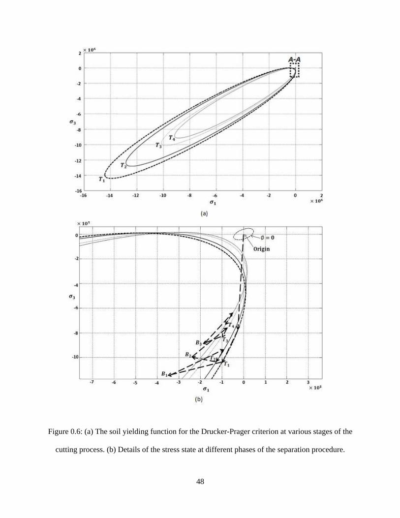
48

Figure 0.6: (a) The soil yielding function for the Drucker-Prager criterion at various stages of the

cutting process. (b) Details of the stress state at different phases of the separation procedure.

49

For the point that initially is at the blade's tip, the history starts at 0B (no stress) and ends at

1T (just before the first separation). Then for the next point to separate, the history starts at 1B

(just after the first separation) and ends at 2T (just before the second separation, and so on).

It should be noted that the curves for the states iT are in general relatively close to each other

(especially in the range shown in Fig. 3.6b), and are getting closer with consecutive separations.

Such curves essentially coincide after about the fifth separation indicating that the simulation of

the cutting process stabilizes, i.e. it becomes independent of the preliminary phase that starts

from the unloaded state (this will be used in calculating the draft force from the plots as

discussed in Fig. 3.7).

From the numerical point of view, the simulation with such stress histories demands a larger

number of equilibrium iterations (we used the standard updated Newton-Raphson method) and a

very careful monitoring of the convergence at each load step.

1.8.4. Calculating forces on the blade

As already mentioned the analysis is quasi-static, the stress-strain states in the whole FE model is

calculated for increasing horizontal distance traveled by the blade (denoted by u in Fig. 3.3).

The forces (draft and lift) acting on the blade are determined by properly integrating the stress

components. As mentioned before, the size of each subsequent step can be estimated from the xε

readings of the previous step. If xε is near cε , the step size is decreased to approach the

separation criterion smoothly.

For an assumed mesh size a typical calculated draft force depends on the distance traveled as

plotted in Fig. 3.7. The calculations start as elastic (OE range) with all the bonding forces active

50

(and therefore all the soil elements still connected), enter the plastic deformation at some point E,

and then go to inelastic phase until deformation in the vicinity of the tip of the blade (point A)

measured as xε , reaches the value cε . This happens when the blade's displacement and the

corresponding draft force reaches the level defined by point 1T .

Then the bonding force in the first node is deactivated (or the elements above and below the

separation plane closest to the blade are allowed to separate) which brings about a drop in the

magnitude of the draft force to the value corresponding to point 1B .

51

Figure 0.7: The force developed on the blade using the first six elements in front of the blade

The opening equal to the element size along the separation surface is created and the stresses and

deformation in its vicinity are reduced enough (see the explanations in the previous section) for

the analysis to start at 1B from an elastic level. First the yielding condition is reached, and next

xε increases to cε , which takes place at the blade's displacement and the draft force is denoted by

point 2T . Deactivating the bonding force in the second node brings the draft force to the level

52

indicated by point 2B (in the elastic range), and so on. The elements separated in the first and

second deactivations are indicated with the broken lines.

The plot in Fig. 3.7 represents a typical relationship for the draft force vs. the blade's

displacement covering five separations (i.e. the cutting/opening runs through five elements) as

obtained from the simulation.

Some details of the meshing and opening after three separations are shown in Fig. 3.8. One can

note in the enlarged picture that the elements above the separation line have shrunk about 30% in

the horizontal direction, which is the consequence of assuming cε =0.3.

Figure 0.8: The soil deformation after three separations (note the opening in front of the blade's

tip).

The separation simulated by the FE model takes place sequentially at the nodes on the separation

surfaces, as already discussed. When the bonding force at a particular node is deactivated the

53

system suddenly changes its overall stiffness resulting in the draft force drop indicated by a

jump ii BT − . It should be noted that the 'discrete' modeling of the separation force )( iTF is

calculated for an underestimated length of the opening in front of the blade and for an

overestimated bonding force in the node to separate. Similarly, force )( iBF is calculated for an

overestimated length of the opening and for an underestimate bonding force at the same node.

Also, the elements in configuration iT are connected by one node more than in configuration iB

(at the same distance u). Therefore one may interpret )( iTF as an upper limit of the draft force

calculated continuously, while )( iBF as a lower limit of that force.

How much the draft force is over- and underestimated (or the difference )()( ii BFTF − ) depends

on the element size e on the separation plane (see Fig. 3.8). However, as our numerical

experimentations indicate (to be presented in the next section), the average force

[ ] 2/)()(( ii BFTFF += for e small enough appears to be essentially independent of meshing.

Therefore it can be considered as an approximation of the draft force for the blade's displacement

u at the instant of a particular separation. This force is plotted as a broken line in Fig. 3.6; note

that it becomes almost constant even after one or two separations. Such a force is denoted by DF ,

and it represents the draft force characterizing the soil-tool interaction for particular conditions

assumed in the simulation.

Since the shape of nonlinear portions 1TE − and then 1+− ii TB of the draft force-displacement

are of less importance, the plots in the next sections will be simplified to show only points iT and

iB (to demonstrate how they are getting closer with smaller e), and then the plot of F and the

value of DF .

54

1.9. Three-Dimensional (3-D) FE modeling

In the FE general 3D model both soil and blade are represented by the hexahedral elements

SOLID45 from the ANSYS [23] library of elements, which has 8 nodes and 3 degrees of

freedom (DOF) at each node as shown in Fig.3.9 (translations in the nodal x, y, and z directions).

The soil-blade sliding is modeled by the 3-D surface to surface contact elements CONTACT173

and TARGET170 with sliding option placed along the intersection of soil and blade surfaces.

The same contact elements were used with both bonding and sliding options for simulating

separation surfaces. The model with the elasto-plastic constitutive law, the separation procedure,

and with elastic incisions (see Fig. 3.2) require a relatively large number of equilibrium iterations

for convergence, thus the calculations are generally long (typically lasting several hours).

Therefore a number of meshing patterns with higher density near the contact areas were tried for

balancing the computational effort with accuracy of calculations. The effects of the elements'

sizes on accuracy and convergence are discussed in the section presenting the results. In general

only the models that can be considered converged are shown in this study.

Figure 0.9: Hexahedral SOLID45 element which has 8 nodes and 3 translational degree of

freedoms in x, y, and z directions at each node [23]

55

1.9.1. FE model, geometry and boundary conditions

1.9.1.1. Straight Rectangular blade

After illustrating the separation procedure by the 2-D FE model, this section is continued by

simulation of interaction between soil and narrow blades or 3-D soil-blade interaction. Geometry

of the 3D straight rectangular model is sketched in Fig. 3.10. The model is parametric with

several parameters defining the geometry of soil and tool. The soil block is sL = 300mm long,

sw = 300mm wide, and sd = 150mm deep. These dimensions were selected in such a way that

the solution in the vicinity of the blade is not sensitive to the block’s size. The block is divided

into sub-blocks that can be meshed with different mesh densities. The maximum distance blade

can travel while cutting the soil, also the length of contacts between upper and lower blocks of

soil, is fL = 50mm. Parameter 1w is the width of cut soil (also the width of blade), 2w is the side

widths of soil block (and swww =+ 21 2 ). The depth of cut soil is 1d ; which is also the cutting

depth of blade. Tilting of the blade with respect to the soil is defined byα , the rake angle.

56

Figure 0.10: 3D soil-tool model dimensions for narrow blade

The starting point of the blade’s travel inside the soil block is denoted by eL = 50mm+ αcos1d .

The blade's total height is 1h = 100mm, this parameter does not affect the cutting process. The

ranges of =1d 25- 50mm, =1w 20-160mm, and =α 30- o90 were examined.

A typical meshing pattern is indicated in Fig.3.11. Boundary conditions for such a model are as

follows:

1. Bottom nodes, at 0=Y , are fixed.

2. Nodes on vertical boundaries parallel to the Y–X plane, at 0=Z and )2( 12 wwZ +−= , are

fixed.

3. Nodes on vertical boundaries parallel to the Y–Z plane, at 0=X except cutting soil area are

fixed.

4. Nodes on vertical boundaries parallel to the Y–Z plane and sLX = are fixed.

57

5. The blade is fixed in Y and Z directions in order to limit blade motion in the X direction.

The meshing shown in Fig. 3.11 (which can be considered typical) uses a total number of 3548

hexagonal elements and 392 contact elements. For comparison, the corresponding 2D model uses

408 quadrilateral elements and 36 contact elements.


As mentioned in the previous section, the separation surfaces between soil-soil surfaces are

predefined to simulate separation and motion of soil particles after interaction with blade.

However in 2-D soil-blade interaction only one separation line was predefined, in 3-D interaction

of soil with a rectangular blade three separation surfaces have to be predefined. As shown in Fig.

3.12, the soil is in contact with the blade on four surfaces. The soil separation takes place along

surfaces 1 and 3 (the vertical cuts) and along surface 2 (the horizontal cut). These surfaces will

58

be referred to as the separation surfaces, and the contact elements with bonding and sliding

options are used to model these connections. On surface 4, however, the soil should be allowed

to slide along the blade without separation, therefore the contact elements with only the sliding

option should be used there. This surface will be referred to as the sliding surface.

Figure 0.12: The surfaces with contact elements (bonding and sliding on surfaces 1, 2, 3, sliding

on surface 4).

It should be noted that the separation surfaces are parallel to the direction of the blade’s motion,

while the sliding surface is parallel to the front of the blade.

1.9.1.2. Curved Rectangular blade

The second 3-D FE model is interaction between soil and curved rectangular blade. Geometry of

this FE model is sketched in Fig. 3.13. The geometrical parameters sL , sw , sd and 1h are the

same as first FE model. The start point of blade’s travel inside the soil block is denoted by eL =

59

115mm and fL = 50mm is maximum distance blade can travel while cutting the soil (also length

of contacts between upper and lower blocks of soil). The cutting portion of the blade is defined

by three parametersα , cα and 1d , where α is the angle of the blade's tip (the rake angle), and

cα is the angle of blade at the soil surface. The other parameters shown in Fig.3.14, such as avgα ,

the average slope,β , the arc angle, and R, the blade's radius of curvature can be calculated from:

cc

cavg

dR

ααααβ

ααα

coscos,,

21

−=−=

+= (3.27)

Table 3.2 lists the values of the above parameters used in first phase of the study. In the results

section, the effects of the anglesα , and cα on the force acting on the blade are examined (which

through (3.27) can be interpreted as the effect of blade's curvature).

Figure 0.13: 3D soil-tool model dimensions for narrow blade

60

Table 0.2: Soil-tool model dimensions that used in first model analysis

)(1 mmw )(1 mmd )(mmL f

50 50 50

)(mmLe )(oα )( ocα

115 60-75-90 35, 45, 60, 75, 90

Figure 0.14: Parameters characterizing a curved blade

A typical meshing pattern is indicated in Fig.3.15 and boundary conditions of the model are the

same as first FE model

61


The same as first FE model, the FE model for interaction between soil and curved rectangular

blade has three predefined separation surfaces (two vertical cuts and one horizontal cut) parallel

to the direction of the blade’s motion and one sliding surface which is parallel to the front of

blade as shown in Fig. 3.16.

62

Figure 0.16: 3D Soil-blade model with contact surfaces. (1, 2, 3: contact surfaces with bonding

and sliding option, 4: contact surface with sliding option)

1.9.1.3. Blades of triangular shapes

The last FE model is a general triangular model with the ability to change blade’s rake angle and

blade’s curvature. Geometry of this FE model is sketched in Fig. 3.17. The model is parametric

with several parameters defining the geometry of soil and tools same as for rectangular blade.

Parameters and dimensions for the triangular blade model are almost same as the rectangular

blade model. The only difference between these two models is the way of defining blade

configuration. For defining the triangular blade configuration, five parameters are needed instead

of four parameters that were used for rectangular blade shape modeling. The cutting portion of

the blade is defined by five parametersα , cα , sα , 1w and 1d , where sα is the sharpness angle of

blade. The curvature of the triangular blade is the same as the rectangular blade model which is

shown in Fig. 3.17.

63

Figure 0.17: 3D soil-tool model dimensions for triangular narrow blade

Table 0.3: Soil-tool model dimensions that used in FEA

)(1 mmw )(1 mmd )(mmL f )(mmLe

50 50 50 100

)(oα )(ocα )(osα

45-60-75-90 45-60-75-90 30-40-52-75-90

The meshing pattern for the 3D triangular model is indicated in Fig.3.18 and the boundary

conditions of the model are the same as the previous 3-D FE models.

64

Figure 0.18: Finite element mesh for 3D soil-tool interaction model

The meshing shown in Fig. 3.18 uses a total number of 2358 hexagonal elements and 480 contact

elements.

The other difference of this FE model with the previous ones is soil-blade and soil-soil

contacting surfaces. Six contact surfaces are existed in this model, four bonding surfaces and two

sliding. The same as the previous models, the two sliding surfaces are parallel to the front of the

blade. However, based on the shape of the cut soil, four separation surfaces (two vertical and two

horizontal cuts) parallel to the direction of the blade’s motion are predefine as shown in Fig. 3.19

65

Figure 0.19: 3D Soil-blade model with contact surfaces. (1, 2, 3, 4: contact surfaces with

bonding and sliding option, 5, 6: contact surfaces with sliding option)

66

Experimental method

67

Analytical and simulation models of soil - tool interaction are typically validated by

experimentally measuring required forces to move the tool through the soil. In this chapter, Soil

bin facility and devices engaged for my experimental procedure are presented. Load cells

arrangement is discussed in detail. At the end, blades specifications and soil preparation is also

explained.

1.10. Soil-bin facility

The Department of Mechanical Engineering (formerly Agriculture and Bio resource Eng.) at the

University of Saskatchewan has an instrumented soil bin which was used in this research. The

soil bin is 1.8 m wide and 12 m long with a movable length of 9 m. Experiments were performed

using a linear monorail system in this soil bin. This monorail system, shown in Fig. 4.1 is

capable of moving tools inside the soil at different speeds. There are two rails on each side of the

soil bin which hold a tool carriage set by four wheels attached to the carriage at four corners.

Also there is an 11.2kW electric motor equipped with speed control, electric clutch and break

with the ability to change the speed from 1.2 km/h to 7.5 km/h. It should be mentioned that the

carriage has a stationary control panel which is located beside the soil bin in order to control the

motion of the carriage and attachments (roto-tiller, roller and sheep-foot packers) as shown in

Fig.4.2.

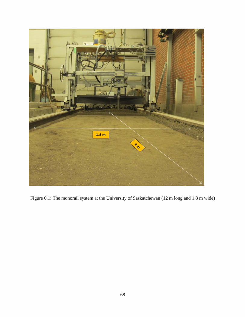
68

Figure 0.1: The monorail system at the University of Saskatchewan (12 m long and 1.8 m wide)

69

Figure 0.2: control panel for motion of carriage and attachments

As shown in Fig. 4.3(a, b), this tool carriage is equipped with six S-type load cells (SSM-1000);

two horizontal to measure blade forces in direction of the blade motion through the soil, three

vertical to measure the blade force in vertical direction and one side load cell to measure the

lateral blade force. As [74] explained, this load cell arrangement makes it possible to measure the

blade forces in three directions. During motion of the blade inside the soil, the load cells

collected data at 2.5 millisecond intervals and sent them to a data recorder.

70

(a)

(b)

Figure 0.3: The monorail system with six S-type load cells arrangement shown in (a) and (b)

71

As shown in Fig. 4.4, the load cells measure the forces 1VF , 2VF , 3VF , 1DF , 2DF , 1SF . The total

blade force is with the components XP , YP , ZP is applied to point A of the blade.

Figure 0.4: General load system of the monorail

In terms of the load cell, the three components of the blade force are

21 DDX FFP += (4.1)

1SY FP = (4.2)

321 VVVZ FFFP ++= (4.3)

The measuring system can also provide information about location of point A .

The moment equilibrium about the x axis is

ZAYAx PyPzM −= (4.4)

Where

72

))(2

( 32 VVx FFaM −= (4.5)

Similarly the moment equilibrium about the y axis is

XAZAy PzPxM −= (4.6)

where

)()( 132 VVVy FcFFbM −+= (4.7)

And the moment about the z axis is

YAXAz PxPyM −= (4.8)

where

)())(2

( 121 SDDz FbFFaM −−= (4.9)

Equations (4.4), (4.6) and (4.8) in the matrix form are

⎥⎥⎥

⎦

⎤

⎢⎢⎢

⎣

⎡=

⎥⎥⎥

⎦

⎤

⎢⎢⎢

⎣

⎡

⎥⎥⎥

⎦

⎤

⎢⎢⎢

⎣

⎡

−−

−

z

y

x

A

A

A

XY

XZ

YZ

MMM

zyx

PPPP

PP.

00

0 (4.10)

The determinant of the LHS matrix is zero, which reflects the fact that the force P can be moved

along the line of action without changing the moment about a point. Mathematically it means

that the coordinates AAA zyx ,,, cannot be defined from Eq. (4.10).

73

However if one of these components is known, then the remaining components can be

determined from the measurements. Based on the symmetric shape of the blades over the

xz − plane, it is reasonable to assume 0=Ay . Then

Y

xA P

Mz = , (4.11)

Y

zA P

Mx −= (4.12)

Substituting in the third equation results in

0=++ zZyYxX MPMPMP (4.13)

This equation can be used to verify correctness of the measuring system.

4.2 . Tools specifications

Two types of blades (rectangular and triangular cross section) were made in order to validate the

FE simulation results. As shown in Figs. 4.5 and 4.6, the steel rectangular blade has 480 mm

length, 40 mm width and 20 mm depth where the steel triangular blade has the same length with

50 mm depth. These blades were attached to the main frame with special holder (Fig. 4.7) that

enables the blades to change their position across the soil bin width. Also this holder has the

ability of changing the rake angle of blades which were used during the experiments in order to

validate simulation results. To ensure the accuracy of the equipment, load cells were calibrated

by the dead weight method in advance of measuring by CNH group who used the equipment

before me.

74

Figure 0.5: The steel rectangular blade shape which is used in experiments (units are in mm)

Figure 0.6: The steel rectangular blade shape which is used in experiments

As mentioned above, by using the linear monorail system the interaction speed can be managed.

According to Godwin and O’Dogherty [75], the effect of blade speed on the blade force is

75

negligible for narrow blades if the speed is less than )6.0(5 1dwg + ; where g , 1d and w

represents gravitational acceleration and depth and width of the blade respectively. For the

experiments, blades (rectangular and triangular) with mw 04.01 = for the rectangular blade and

mw 05.01 = for the triangular blade, 281.9 smg = and md 05.01 = for both of the blades, has

the speed limit of )66.6(85.1 hkmsm and )128.7(98.1 hkmsm respectively. All tests

were performed at a speed of 0.56 m/s (2 km/h) in order to ignore the effect of the interaction

speed and conform with theoretical results consequently.

Figure 0.7: Blade holder with the ability of changing the rake angle of blades.

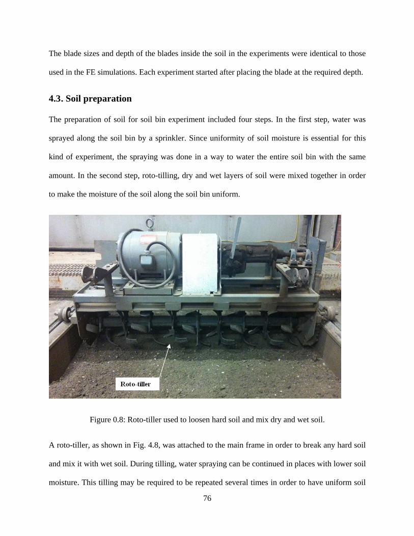
76

The blade sizes and depth of the blades inside the soil in the experiments were identical to those

used in the FE simulations. Each experiment started after placing the blade at the required depth.

4.3 . Soil preparation

The preparation of soil for soil bin experiment included four steps. In the first step, water was

sprayed along the soil bin by a sprinkler. Since uniformity of soil moisture is essential for this

kind of experiment, the spraying was done in a way to water the entire soil bin with the same

amount. In the second step, roto-tilling, dry and wet layers of soil were mixed together in order

to make the moisture of the soil along the soil bin uniform.

Figure 0.8: Roto-tiller used to loosen hard soil and mix dry and wet soil.

A roto-tiller, as shown in Fig. 4.8, was attached to the main frame in order to break any hard soil

and mix it with wet soil. During tilling, water spraying can be continued in places with lower soil

moisture. This tilling may be required to be repeated several times in order to have uniform soil

77

in all parts of the soil bin. After tilling, the soil was levelled by scraper blade. This blade, which

has the same width as the frame, was attached to the back of the main frame with the ability to

move up and down as shown in Fig. 4.9. Soil compacting is the last step of soil preparation. In

this step packers (sheep-foot packer and roller packer) shown in Fig. 4.10, were attached in front

of the main frame to compact the soil. It was necessary to level the soil again after using sheep-

foot packer which distributed the soil before using the roller packer.

Figure 0.9: Scraper blade with the same width as the frame in order to level the soil

78

Figure 0.10: Sheep-foot packer and roller packer used to pack the soil

Different soil compaction levels can be obtained by varying the number of packer passes. A low

compaction level can be achieved by two passes of the sheep-foot packer and four passes of the

roller packer. A hard compaction level which is similar to most agricultural field conditions can

be obtained by ten passes of sheep-foot packer and four passes of roller packer as Rosa [59]

stated. During the experiments, a hard compaction level was used to simulate the field condition

and compared with FE results. Also the soil selected for this experiment is the type of soil

commonly found in Saskatchewan, which is silty clay loam (47.5% sand, 24.2% silt and 28.3%

clay). The soil properties with 7% water content are given in Table 3.1 as Bankole [24]

calculated.

79

Results and discussions

80

In this section the FE models and procedure proposed are tested for convergence and accuracy.

The main focus is on accuracy of calculating the draft force. First the effects of the compacting

strain limit and the soil internal friction angle on the calculated draft force are presented. Then

the effect of meshing is discussed. Finally, the results are validated by comparing them with the

formulas that for straight blades are available in the literature. Also, the FE results were validated

experimentally by testing several soil blade interactions in the soil bin facility (see chapter 4).

The effects of blade width, blade depth and rake angles on the blade force are also investigated.

Then, the effects of curved blade and changing the shape of blade are examined.

1.11. Effect of the compacting strain limit on the draft force

The magnitude of the strain component in the direction of the blade's motion to initiate

separation (refer to as the compacting strain limit, cε in Sec. 3.2.3) is crucial in this analysis. In

particular, the draft force is affected by the choice of the magnitude of cε . In order to examine

this, the numerical experiment was performed on the blade with 1d = 50mm, 1w = 50mm, o60=α

and the soil with properties that are listed in Table.3.1 (in particular for the friction

angle o35=ϕ ). The draft forces that were calculated assuming different values of cε are shown in

Fig. 5.1. As can be seen, the calculated draft forces increase sharply until the strain limit, cε is

around 0.3. Then the force stays almost constant (for 3.0≥cε ) which means that further

distortion of the monitored element does not have significant effects on the calculated force. It

should be mentioned that the number of the load steps required in this analysis increases quite

fast with an increasing value of cε . For example by assuming 45.0=cε (instead of 3.0=cε ), the

time required to calculate the correspondent force increases by more than 40%. However, the

difference between blade (draft) forces with compacting strain limit 0.3 and its constant final

81

value (which here corresponds to compacting strain of 0.45) is around 3% ( NF 458= at

45.0=cε and NF 446= at 3.0=cε ). Thus for the computational efficiency and to make a

balance between computational efforts and accuracy, 3.0=cε was selected to initiate separation

for this type of soil. This 3% is considered as a settling value of blade (draft) force for this

analysis.

Figure 0.1: Effect of compacting strain limit on the calculated force for soil with o35=ϕ

1.12. Effect of soil internal friction angle on compacting strain limit

It turned out that the cF ε− curves such as shown in Fig. 5.1 are somewhat affected by the type

of soil characterized by friction angleϕ . In order to examine this effect, the draft force was

calculated for a straight rectangular blade with 1d = 50mm, 1w = 50mm, o60=α and using the

soil internal friction angles varying from o20 to o40 . For example, for the internal friction

82

angle o20=ϕ , the draft forces calculated for different cε are shown in Fig. 5.2. These forces

increase sharply until for 2.0<cε and then stay almost constant for 2.0≥cε . The difference

between forces with compacting strain limit 0.2 and 0.35 is around 3% ( NF 221= at 35.0=cε

and NF 215= at 2.0=cε ), therefore for computational efficiency 2.0=cε should be selected in

any further analysis of this type of soil. With the same procedure, 35.0=cε was selected to

initiate soil separation for the soil with o40=ϕ as shown in Fig. 5.3.


83


This procedure was applied for several analyses with oo 4020 ≤≤ϕ and the relationship between

the soil internal friction angle and compacting strain limit was established as shown in Fig. 5.4.

As can be seen for the soil internal friction angle analysed here, the compacting strain limit

varies almost linearly within the range 35.02.0 ≤≤ cε . Also it should be mentioned that the soil

cohesion does not seem to have any meaningful effect on the cF ε− curve.

84

Figure 0.4: Effect of soil internal friction angle on the limiting compacting strain

1.13. Effects of meshing

As discusses in Section 3.2.4 the choice of the size of elements on the separation surface in the

vicinity of the blade's tip, denoted by e in Fig. 3.8, affects the calculated relationship between the

draft force and the displacement of the blade. Typical results for the 3D soil blade interaction

model with different e and for 1d = 50mm, 1w = 50mm, and o90=α (vertical blade) are shown in

Fig. 5.5. Clearly, smaller e reduces the difference )()( ii BFTF − , but also makes the mesh more

dense that in turn increases the computation time.

85

Figure 0.5: The draft force F for different element size e (and different mesh density)

For example, if e = 8.7mm (low mesh density, 1876 elements) then the calculation time to obtain

the F-u plot for u up to 16mm is about 15 hours (computer with Intel core i5 4 GH processor and

3.2 GB of RAM) . If the mesh size is reduced to e = 7.8mm (regular mesh density, 2472

elements) then the time increases to 19 hours, and to 22 hours if e = 6.7mm (high mesh density,

2854 elements).

The effect of e on the average force [ ] 2/)()(( ii BFTFF += is shown in Fig. 5.6. As can be

seen, results for the regular and high mesh patterns are practically indistinguishable; therefore for

computational efficiency the regular mesh density was selected for this case. For the low mesh

density the force NFD 915= (see the definition in Fig. 3.7), then it drops by 2% to NFD 896=

for the regular mesh density, and drops 0.3% further to NFD 893= for the high mesh density.

86

Figure 0.6: Effect of e (and the mesh density) on the average draft force F .

Similar results for another 3D soil-blade interaction model with 1d = 50mm, 1w = 50mm, and

o60=α are presented in Fig. 5.7 and 5.8, where e = 8.4, 7.0, 5.8 were used.

87

Figure 0.7: Variation of the draft force F with element size (for o60=α )

The corresponding average draft force F is shown in Fig. 5.8. For e = 8.4mm (low density

meshing, 2186 elements) the draft force NFD 485= . This force drops by 7.8% to NFD 446= if

the mesh size is reduced to e = 7mm (regular mesh density, 3548 elements), and further by 1.3%

to NFD 441= if e = 5.8mm (high mesh density, 4982 elements). The results for the regular and

high mesh patterns are practically indistinguishable; for computational efficiency the regular

mesh density could be selected to analyze this case.

88

Figure 0.8: Variation of the averaged drag force F with the element size (for o60=α ).

1.14. Model verifications

1.14.1. Analytical validation

1.14.1.1. Validation of 2D model

2D elements can be used to simulate action of wide blades. In order to model separation between

elements above and below separation surface, hL , (Fig. 3.4) the nodes representing soil are

connected using contact elements that allow to activate or deactivate the bonding contact

between them. In this process the blade force F (output) is calculated as a function of distance

traveled u (input) by the blade through the soil.

Using the procedure discussed in 3.2.4, draft force acting on the blade can be determined. A

typical plot is shown in Fig. 5.9 representing blade force as the blade moves through the soil. For

89

this 2D typical simulation, the blade was vertical )90( o=α and the required soil-blade

parameters were listed in Table 3.1. The draft force is the sum of all horizontal nodal forces on

the blade at a specified displacement. This force increases from zero to about 10 KN around the

blade displacement of mm6 and stays almost constant. The average force,

[ ] 2/)()(( ii BFTFF += reaches the value of N10404 , and is considered as the draft force DF as

obtained from the simulation.

Figure 0.9: The blade (draft) force versus blade displacement for 2D blade with rake angle of

o90 . Draft force produced NFD 10404=

Prediction of the draft force in soil-blade interaction have been proposed by many researchers.

Onwualu and Watts [46] reported that the best correlation between analytical and experimental

results can be achieved by using McKeyes approach. In this study we used the McKeys

90

analytical approach [25] to compare forces acting on a blade with FE results for both wide and

narrow blades.

He proposed the following expression for a wide blade:

21 1 1 1( )A

D a c b qF d K Cd K Q d K wλ= + + (5.1)

Where ADF is the total force, λ is the soil’s specific weight, C is soil cohesion, bQ is bearing

pressure, 1d is depth of blade inside soil (interaction), ),,( qca KKKK are force factors for

wide blade and 1w is width of the blade which should be at least ten times of the depth of

interaction )10( 1d to be considered as wide blade. Force factors ),,( qca KKKK , depend on the

soil friction angle φ , the blade rake angleα , angle of soil failure planeθ and soil-blade friction

angleδ . The horizontal components of the total blade force ADF , can be derived as

)sin( δα += AD

ADH FF (5.2)

In the present study, the value of Q is negligible, thus qK in eq. (5.1) is not needed.

aK and cK were derived by [8] as

)sin()sin()cot(cot

δφθαφθθα

+++++

=aK (5.3)

)sin(sincos

δφθαβφ

+++=cK (5.4)

Where θ is

91

⎥⎥⎥⎥⎥

⎦

⎤

⎢⎢⎢⎢⎢

⎣

⎡

++

++−++

=)sin(

)cos(sinsin

)sin()sin(

cotφδα

φδαφα

φδδα

θ arc (5.5)

By using variables from Table 5.1 and using eq. (5.3-5.5), values of ( aK , )cK are calculated as

reported in Table 5.1.

Table 0.1: Horizontal component of K’s for obtaining the blade force.

Variables

ooo 35,23,90 === φδα 4.88 10.85

By using equation (5.1) and (5.2) and using values in Tables 5.1 and 3.1, the force on the blade

can be determined as,

[ ] NwKCdKdF caA

DH 8.10121))(sin( 112

1 =++= λδα (5.6)

The difference in the total blade force between FE result ( NFD 10404= , see Fig. 5.9), and

analytical value NF ADH 8.10121= is found to be about 2.7%; this can be considered as validation

of the FE results.

1.14.1.2. Determining the blade force and model validation in 3D

A typical plot of the blade force calculated by the procedure presented in section 3.3.2 is shown

in Fig.5.10 for 3D soil-blade interaction. This is the case with o60=α and 1d = 50mm, and

1w = 40mm, modeled by the mesh with the element size e = 7mm (as discussed in Sec. 5.3). As

shown in Fig. 5.10, the average force F is almost horizontal after the first iteration already, and

the corresponding blade force is NFD 408= .

92

Figure 0.10: The force acting on the blade and its mean value (draft force DF )

This force can be validated by comparing it with the analytical results. McKyes and Ali [8]

proposed the following expression for a narrow blade:

1112

1 )( wNQdNCdNdF qcA

D ++= γλ (5.7)

Where parameters are the same as a 2D case (Eq. 5.1) except the narrow blade considers the

effects of soil motion at the edges of blade that is ignored for wide blade. These factors depend

on the soil friction angle, φ and the blade rake angleα . In the present study, the value of Q is

negligible and the parameters ),,( qHcHH NNN γ in Eq. 5.7 take the values as shown in Table 5.2.

Based on negligible effects of bearing pressure on results of this research work, qHN is

neglected in the calculation.

93

Table 0.2: Soil and blade parameters that are used in the present analysis.

Rake

angle )(o )(1 mw )(1 md )( 3m

Nλ )(Kpac HN γ cHN

60 0.04 0.05 12000 20000 5.27 10.48

Therefore Eq. 5.7 takes the simplified form:

NwNCdNdF cHHA

DH 425)( 112

1 =+= γλ (5.8)

The difference in total horizontal blade force between FE results (using regular mesh density

model, NFD 408= ), and analytical result is found to be about 4%; this can be considered as

validation of our FE results.

1.14.2. Experimental validation

1.14.2.1. Filtering and Validating results for the rectangular blade

During motion of the blade through the soil, load cells collected data at a 2.5 millisecond interval

and sent them to a data recorder. The recorded signal from load cells is shown in Fig. 5.11.

Based on the effect of all the higher natural frequencies of the whole monorail system, the signal

was noisy. These recorded signals represent dynamic forces based on the location of load cells as

shown in Fig.4.3; however FE results are based on static analysis. Therefore, these signals should

be filtered to exclude all system natural frequencies (dynamic effects) which do not effect the

draft force and include force frequency (static effects).These recorded signals were related to the

experiment with the same rectangular blade dimension as shown in Fig. 4.5 and the rake

angle o60=α .

94

It should be mentioned that the filtered signal must include all forced frequencies on the blade. In

order to find the filtering range, the natural frequencies of the blade attached to the monorail

(with its tip inside the soil) were determined by applying Fast Fourier Transform (FFT) to two

different measurements (the first signal from horizontal load cells, and the second signal using an

accelerometer attached to the monorail system). These natural frequencies were excited by

hitting the hammer to the blade. The frequency spectra of the system using FFT of the signals

from accelerometer and from horizontal load cells are plotted in Fig. 5.12 and 5.13 respectively.

As it can be seen the first two natural frequencies are about 21 and 38 Hz, respectively. Then, the

spectra of frequency of the system (monorail and frame) were determined using similar

measurements and FFT when the blade was moving through the soil with speed of 2 km/h and

were plotted in Figures 5.14 and 5.15 using signals from accelerometer and horizontal load cells,

respectively. As can be seen from these plots, the first three frequencies are about 1.5, 21 and 40

Hz. Comparing these forced frequencies with the natural frequencies (21 and 38 Hz), it can be

concluded that 1.5 Hz is the forced frequency and the other two (21 and 40) are natural

frequencies of the system that should be filtered out. Therefore this signal was filtered to exclude

all frequencies above 2 HZ. The result is shown in Fig. 5.16 with a solid line. As can be seen,

beyond the initial phase, the draft force stayed almost constant at a value of 415 N.

95

Figure 0.11: Unfiltered horizontal (draft) force on the blade when moving with o60 rake angle

Figure 0.12: The spectrum of natural frequencies of the system (the signal from accelerometer,

A=21.06, B=38.09 Hz)

96

Figure 0.13: The spectrum of natural frequencies of the system (the signal from horizontal load

cells, A=21.97, B=38.45 Hz)

Figure 0.14: The spectrum of frequencies of the moving system (the signal from accelerometer,

A=1.1, B=21.7, C=41.2 Hz)

97

Figure 0.15: The spectrum of frequencies of the moving system (the signal from horizontal load

cells A=1.8, B=19.5, C=39.0 Hz)

Figure 0.16: Unfiltered and filtered horizontal blade (draft) force on the blade when the blade

moves through soil

98

The experimental results are compared with the analytical and FE results as shown in Table 5.3.

The difference between analytical and experimental results is 2.3%, and the difference between

FE and experimental results is 1.6% which shows good correlations between these three

methods. Therefore our FE model is validated with both analytical and experimental ones.

Table 0.3: Comparing the experimental, analytical, and FE results.

)(1 md )(1 mw Analytical force, )(NFD

FE force, )(NFD

Experimental Force, )(NFD

50 40 425.0 408.0 415 Difference between analytical and

experimental (%) Difference between FE and

experimental (%) 2.3 1.6

1.14.2.2. Validating results for the triangular blade

In order to validate the FE model for triangular blades, the draft forces of such a blade with four

different rake angles ooo 75,60,45=α and o90 are calculated. It should be noted that blades in

these models are straight, which means cαα = , and the sharpness angles in all models

were o53=α . These four cases are modeled with the element size e = 7.5mm which is obtained

the same way as in Sec. 5.1. A typical plot of the blade forces calculated by the procedure

presented in the previous section and the average forces plot F are shown in Figs. 5.17 and 5.18.

The average forces F are almost horizontal after the second iterations already, and the

corresponding draft forces are NNNFD 326,275,172= and N425 for rake angles

ooo 75,60,45=α and o90 respectively. Based on Fig. 5.18, one can conclude that a more

inclined blade (with smaller rake angleα ) has less draft force which is similar to the behavior of

rectangular shaped blades. Since the available analytical solutions are limited to rectangular

blades, these results are verified only experimentally.

99

Same as in the experiments for rectangular blade, all the tests were performed at a speed of 0.56

m/s (2 km/h). The blade size and depth of blade inside the soil in the experiments were identical

to those used in the FE simulations as shown in Figs. 3.17 and 4.6. As mentioned before, each

experiment started after placing the blade at the required depth )5( 1 cmd = . The horizontal forces

on the blade for four different blade’s rake angle ( ooo 75,60,45=α and o90 plotted in Figs. 5-

19) were measured by summing the results from two horizontal load cells. During motion of the

blade, the load cells collected data at 2.5 millisecond intervals and sent them to a data recorder.

Based on what was discussed in previous section (Sec.5.4.2.1), the recorded signal (dotted line in

Figs. 5.19-5.22) was noisy because all the higher natural frequencies of the monorail system

were registered; therefore this signal was filtered to exclude all frequencies above 2 Hz to

eliminate natural frequencies and keep the forced frequency. As can be seen, beyond the initial

phase, the blade forces in Figs. 5.19-5.22 which are shown as a solid line, stayed almost constant

at values of around 181 N, 289 N, 337 N, and 431 N respectively.

The experimental results are compared with FE results as shown in Table 5.4. The difference

between FE and experimental results are less than 5% in all cases that shows good correlations

between these methods. It should be mentioned that by increasing compacting strain limit cε , the

FE draft force results will increase and the difference between FE and experimental results will

decrease. Also as shown in Figs.5.19- 5.22, the more inclined blade has more vibration which the

error of finding average draft force will increase consequently that is shown in Table 5.4.

Therefore the FE model for triangular blade is validated with the experimental method.

100

Figure 0.17: Variation of blade (draft) forces for different triangular blade’s rake angles.

Figure 0.18: Variation of the averaged blade (draft) forces for different triangular blade’s rake

angles

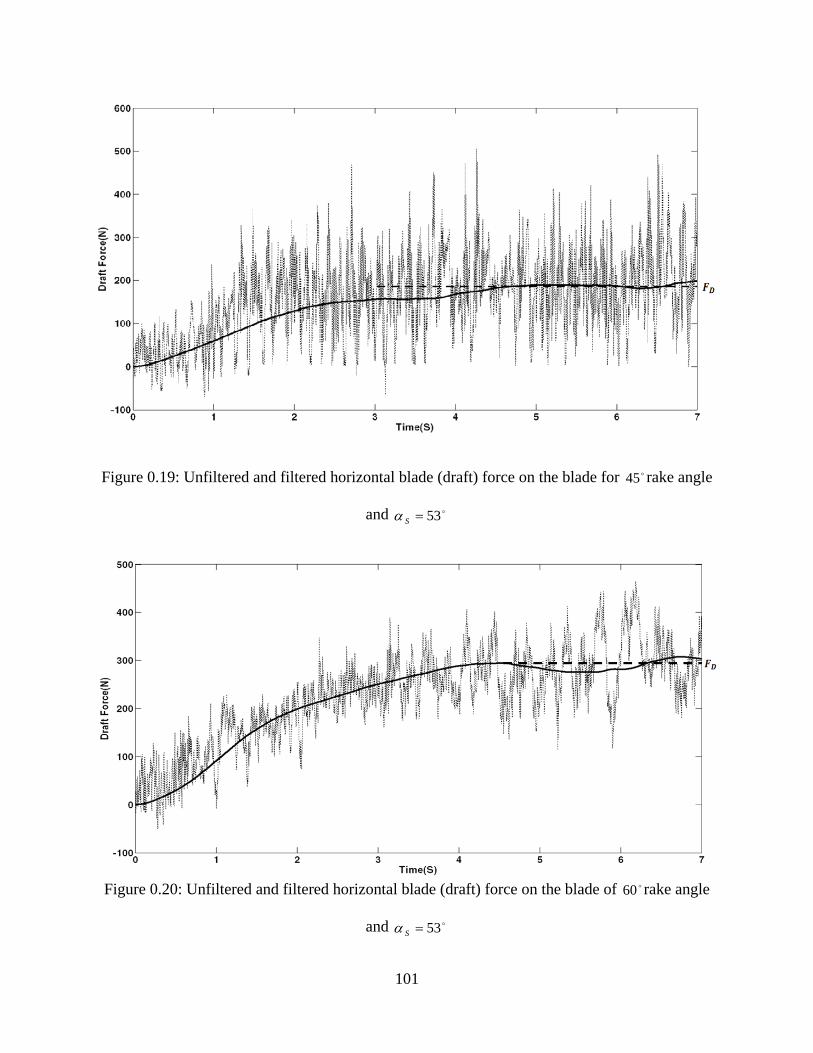
101

Figure 0.19: Unfiltered and filtered horizontal blade (draft) force on the blade for o45 rake angle

and o53=Sα


and o53=Sα

102


and o53=Sα

Figure 0.22: Unfiltered and filtered horizontal (draft) force on the blade of o90 rake angle and

o53=Sα

103

Table 0.4: Comparing the experimental and FE results.

Sα cα α FE force,

)(NFD Experimental force, )(NFD

Difference (%)

o53

o45 o45 172 181 4.9

o60 o60 275 289 4.8

o75 o75 326 337 3.2

o90 o90 425 431 1.3

1.15. Comparison of rectangular and triangular blades

In order to compare the triangular blade with the rectangular one, FE results for the rectangular

blade with the same width and depth of interaction as shown in Fig. 5.23 and listed in Table 5.5

are calculated. Results for the rectangular blade were verified analytically based on the analytical

method which is limited to a straight rectangular blade, and results for the triangular blade were

verified experimentally.

In Fig. 5.24, the FE draft force results of the rectangular blade are compared with analytical

results. The maximum difference between these two methods is less than 5% (at )60o=α which

generally indicates good correlations. Also the FE force results for the triangular blade are

compared with the experimental results for which the maximum differences between the forces

are around 8%. As shown in Fig. 5.24, the difference between horizontal forces acting on the

triangular blade is around half of the amount of force which acts on the rectangular blade with

the same rake angle (i.e. at o45=α , triangular blade force is NFDT 172= and rectangular blade

force is NFDR 368= or at o90=α , NFDT 425= while NFDR 900= ). This means that for the

104

same width of groove through the soil, triangular blade need much less force than the blade with

rectangular shape.

The soil deformation patterns of these two shapes of blades are compared in Fig. 5.25. Also the

displacements of soil in front of these two types of blades were compared in Fig. 5.26. For the

rectangular blade, the soil is accumulated in front of the blade and tends to swell up in an upward

direction and lateral directions with respect to its original configuration in a pattern similar to

that indicated in Shmulevich et al. [26]. However for the triangular blade, the soil is pushed

mostly in lateral directions and slightly accumulated in front of the blade as shown in Figs. 5.26.

Figure 0.23: 3D model dimensions for rectangular and triangular narrow blades (these

parameters are defined in Sec. 3.3.1.1 and 3.3.1.3)

Table 0.5: Blade model dimensions that are used in FEA

parameters )(1 mmw )(1 mmh )(1 mmd )(oα )(oSα

Values 50 100 50 45, 60, 75, 90 53

105

Figure 0.24: Comparing draft forces of rectangular vs. triangular blades (different blade’s rake

angle)

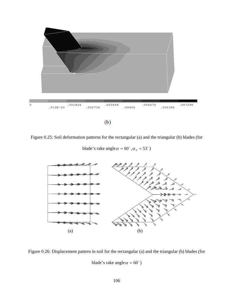
106

Figure 0.25: Soil deformation patterns for the rectangular (a) and the triangular (b) blades (for

blade’s rake angle o60=α , o53=Sα )

Figure 0.26: Displacement pattern in soil for the rectangular (a) and the triangular (b) blades (for

blade’s rake angle o60=α )

(a) (b)

107

1.16. Effect of blade width, depth and rake angle on draft force for

rectangular blades

The FE model for the rectangular blade was used to investigate the effects of the depth of blade

in the soil )( 1d and width of blade )( 1w on the draft force DF . The geometrical parameters and

the results are listed in Table 5.6. Also the analytical results calculated from Eq. 5.7 are shown

for comparison. As can be seen the agreement is within about 5%, which should be considered

acceptable.

Table 0.6: comparing analytical and FEA results for 8 different models (blade’s rake

angle o60=α )

)(1 mmd )(1 mmw 1

1d

w

Analytical force,

)(NFD

FEA force, )(NFD

Percentage Difference (%)

25 6.3 0.25 90.00 87.00 3.3

25 20 0.8 105.0 109.0 3.6

25 25 1.0 116.0 121.0 4.1

25 75 3.0 231.0 242.0 4.5

50 12.5 0.25 364.0 351.0 3.5

50 40 0.8 425.0 408.0 3.9

50 50 1.0 470.0 446.0 4.8

50 150 3.0 933.0 965.0 3.3

The FE results are also plotted in Fig. 5.27. The blade force increases with increasing1

1d

w ,

Also, by doubling the blade depth in soil, and keeping 1

1d

w constant, the blade force increases

108

approximately 4 times (e.g. F increases from 87 N to 351 N for 1

1d

w =0.25 when 1d increased

from mm25 to mm50 ).

Fig. 5.28 shows the blade’s force for eight different cases with two different blade’s depths. As

can be seen by doubling the working depth of the blade ( 1d ) and keeping its width ( 1w ) constant

the blade force triples (e.g. F increases from 142 N to 408 N for mmw 401 = and 1d changing

from mm25 to mm50 ).

Figure 0.27: The draft force ( DF ) for constant depth and different ratio1

1d

w

109

Figure 0.28: The draft force ( DF ) for constant depth and differing blade width.

In order to investigate effects of the blade’s rake angle on the draft force the procedure was used

for oo 60,90=α and o30 with the results listed in Table 5.7 and plotted in Fig. 5.29. By

increasing the blade’s rake angle, the effect of sliding between soil and blade decreases; but on

the other hand the effects of compression and cohesion between soil particles increases which is

resulted in increasing blade’s draft force.

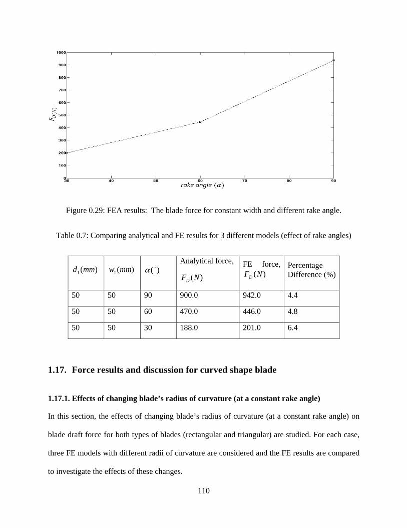
110

Figure 0.29: FEA results: The blade force for constant width and different rake angle.

Table 0.7: Comparing analytical and FE results for 3 different models (effect of rake angles)

)(1 mmd )(1 mmw )(oα Analytical force,

)(NFD

FE force, )(NFD

Percentage Difference (%)

50 50 90 900.0 942.0 4.4

50 50 60 470.0 446.0 4.8

50 50 30 188.0 201.0 6.4

1.17. Force results and discussion for curved shape blade

1.17.1. Effects of changing blade’s radius of curvature (at a constant rake angle)

In this section, the effects of changing blade’s radius of curvature (at a constant rake angle) on

blade draft force for both types of blades (rectangular and triangular) are studied. For each case,

three FE models with different radii of curvature are considered and the FE results are compared

to investigate the effects of these changes.

111

1.17.1.1. Rectangular blade

Three FE models are studied in order to investigate the effects of changing the radius of

curvature of the blade while keeping the rake angle constant. The shapes of curved blades are

indicated in Figs. 5.30(a) - 5.30(c) and are controlled by the angle cα that increases from

o60 to o90 . As shown in Fig. 5.31 and 5.32, variation and average draft forces for these three

models are obtained based on the previous FE procedure. From these figures it is obvious that by

decreasing the radius (or increasing the curvature) while keeping the rake angle constant the

blade force increases. It should be noted that also the blade’s average rake angle avgα is

increasing from o60 to o75 . Fig. 5.33 depicts how this parameter affects the blade force that

increases from 440 N to 605 N; a more inclined blade requires less draft force.

Figure 0-30: FE models for o60=α and differing cα : (a) o60=cα , (b) o75=cα , (c) o90=cα ,

(d) definition of α and cα (taken from Fig. 3.13)

112

Figure 0.31: Variation of blade (draft) forces for differing cα and the rake angle o60=α .

Figure 0.32: Variation of the average blade (draft) forces for different cα and the rake

angle o60=α

113

Figure 0.33: Variation of the blade (draft) forces with differing blade’s average rake angles

for o60=α .


Same as the rectangular case, three FE models were studied for the triangular blade in order to

investigate the effects of changing the radius of curvature of the blade while keeping the rake

angle constant. The shapes of curved blades as shown in Fig. 5.34 are controlled by the angle

cα that increases from o60 to o90 , while the rake angle o60=α is constant. From Figs. 5.35, and

5.36, it is obvious that by decreasing the radius (or increasing the curvature) while keeping the

rake angle constant the blade force increases, which is similar to the rectangular blade case.

Same as what is concluded from curved rectangular blades, this increase in draft force is

significantly related to the blade’s average rake angle avgα , by increasing this angle, the draft

force increase. As shown in Fig. 5.36, by increasing avgα from o60 to o5.67 , the draft force

114

increase from 275N to 295N, and by increasing avgα from o5.67 to o75 , the draft force increases

from 295N to 326N; a more inclined blade requires less draft force. By comparing Fig. 5.33 for

the rectangular blade and Fig 5.36 for the triangular blade, it seems that the curved force results

for triangular blades are almost half of the force results for rectangular ones which mean that for

the same width of groove, the triangular curved blade needs need less force than rectangular

ones.

Figure 0.34: FE model for 3D soil interaction with the triangular blade while rake angle is

constant, o60=α and blade’s curvature angles are different, (a) o60=cα , (b) o75=cα , (c)

o90=cα

115

Figure 0.35: Variation of blade (draft) forces for different curvature angles cα with constant rake

angle o60=α .

Figure 0.36: Variation of the average blade (draft) forces for different curvature angles cα with

constant rake angle o60=α .

116

1.17.2. Effects of changing blade’s radius of curvature with constant cα

In this section, the effects of changing blade’s radius of curvature with constant cα on blade

draft force for both types of blades (rectangular and triangular shape blades) are studied. For the

rectangular case, nine FE models, and for triangular one, three the FE models with different

radius of curvature are considered. Subsequently the FE results are compared to investigate the

effects of these changes.


The effects of changing rake angle while keeping the angle cα constant are investigated using the

FE models shown in Figs. 5.37, 5.38, and 5.39. Variation and average draft forces for these three

models are obtained based on the discussed FE procedure and draft forces for these nine models

are listed in Fig. 5.40 and listed in Table 5.8.

As shown in Fig. 5.40, by increasing the rake angle α at the angle cα constant, the blade draft

force increases in all three cases with constant cα . Same as in the previous section, it can be

explained by the increase of the blade’s average rake angle, avgα or by the increase in the

blade’s curvature. The relationship of the draft forces to the angle avgα are plotted in Fig. 5.41.

As shown in this figure, by increasing avgα from o5.47 to o90 , the draft force increase from

268N to 920N which indicate that more inclined curved blade requires less draft force.

117


o35=α .


o45=α .

118


o60=α .

119

Table 0.8: Draft forces DF for nine different FE models with different rake angles (α ) and three

constant curvature angles ( cα ).

cα α )(NFD from FE models

60

60 440

45 317

35 268

75

75 640

60 540

45 440

90

90 920

75 753

60 640

Figure 0.40: Variation of the draft force DF with the rake angles α for different cα .

120

Figure 0.41: Variation of the draft force DF with the blade’s average rake angles )( avgα


The effects of changing rake angle while keeping the angle cα constant (in order to study the

effect of changing radius of curvature) on the blade draft forces, are investigated using the FE

models shown in Fig. 5.42. As shown in this figure, three FE models with different rake angles

oo 45,60=α , and o30 with same angle o60=cα are simulated to increase the curvature and

investigate its effect on the blade force. By decreasing the blade’s rake angle, the blade’s average

rake angle avgα decreases from o60 to o5.47 . Figs. 5.43 and 5.44 represent the FE results for

blade (draft) force and averaged force acting on the blade of different rake angleα with constant

curvature angle cα . From these Figures, it is clear that by increasing the blade’s curvature

(decreasing the blade shape radius R), forces on the blades decrease with the same trend of

121

rectangular cases. As shown in Fig 5.44, by decreasing avgα from o60 to o5.52 , the draft force

( DF ) increases from 275N to 220N ; and by decreasing avgα from o5.52 to o5.47 , the draft force

( DF ) decreases from 220N to 180N which means a more inclined blade shape has less draft

force.

As shown in Fig. 5.45, draft forces of the rectangular blade are plotted based on blade’s average

rake angle, avgα in comparison with the draft forces of the blade with the triangular shape. From

this figure, it is clear that by increasing the blade’s average rake angle avgα , the difference

between the draft forces of the rectangular blade and the triangular blade is increasing.

Figure 0.42: FE soil-triangular blade interaction model with three different blade’s rake angles

(a) o60=α , (b) o45=α , (c) o35=α and constant o60=cα

122

Figure 0.43: Variation of blade (draft) forces for different rake angles α with constant curvature

angle o60=cα .

Figure 0.44: Variation of the average blade (draft) forces for different rake angles α with

constant curvature angle o60=cα .

123

Figure 0.45: Comparing draft forces of rectangular and triangular shapes blade for different

blade’s average rake angles )( avgα

1.18. Effects of blade’s sharpness on blade force in soil interaction

1.18.1. Changing blade’s sharpness while keeping the blade’s contact length constant

Five FE models with different sharpness angles were used in order to investigate the effects of

the blade’s sharpness on the blade’s draft force ( DF ) when keeping the contact length constant.

As shown in Fig. 5.46, in order to study this effect, the interaction depth 1d , blade height 1h ,

blade’s contact length sL and blade’s rake angle α are kept constant in all models. The only

difference in these models is their sharpness angle )( Sα which varies from o30 to o90

124

Figure 0.46: 3D model dimensions of triangular narrow blades with constant depth )50( 1 mmd = ,

blade contact length )60( mmLs = , blade rake angle )90( o=α , and different sharpness angle

(a) o301 =sα , (b) o402 =sα , (c) o533 =sα , (d) o754 =sα , (e) o905 =sα

The FE results are given and plotted in Fig. 5.47. As expected, the blade’s draft force )( DF

increases with increasing sharpness angle sα and this increasing rate is almost constant. So by

decreasing the blade’s sharpness angle or in other words by increasing blade’s sharpness, the

average draft force decreases considerably.

125

Figure 0.47: Draft forces ( DF ) of the triangular blade with different blade’s sharpness angles

)( Sα

1.18.2. Changing the blade’s sharpness while keeping blade’s width constant

In order to study effects of the blade’s sharpness on draft force ( DF ) while the blade’s width is

constant )( 1w , three FE models with different sharpness angles )( Sα were used. As shown in Fig.

5.48, in order to study this effect, the interaction depth 1d , blade height 1h , blade width 1w and

blade rake angle α , are kept constant in all models. The only difference in these models is their

sharpness angle )( Sα which varies from o53 to o120 .

In order to examine the effects of sα , the calculated draft force for 120sα = o is denoted as

120DF o and is assumed as a reference. Then the ratios of

120

D

D

FF o

for siα are plotted in Fig 5.49.

126

It is clear from this Figure that by decreasing the sharpness angle Sα from o120 to o90 or

increasing the blade’s sharpness, the draft force decreasing 22% from N697 to N547 . By

further decreasing to o53 , the original draft force decreases 40% to N425 ; that means that for a

constant width of groove, and a sharper blade, the less draft force ( DF ) is applied to the blade.

Figure 0.48: 3D model dimensions of triangular narrow blades with constant interaction

depth )50( 1 mmd = , blade height )100( 1 mmh = , blade’s width )50( 1 mmw = , blade rake

angle )90( o=α and different sharpness angle (a, d) o531 =sα , (b, e) o902 =sα , (c, f) o1203 =sα .

(d), (e), and (f) are top views of the triangular blades of (a), (b), and (c) respectively.

127

Figure 0.49: Non dimensional draft forces ratio (o120D

DF

F ) of the triangular blade with constant

blade’s width and different blade’s sharpness angles.

1.19. Deformation patterns

1.19.1. 2D model

It was shown that the FE model as described in the Sec.3.2.1 is capable of simulating soil-wide

blade interaction. By moving the blade in the horizontal direction (about 11mm), the soil is

swelled up in front of the blade as shown in Fig. 5.50. For example the maximum soil

displacement upward is about 16 mm (the depth of cut soil is 50 mm) and is immediately at the

blade as shown, and then decreases with the distance away from it.

128

Figure 0.50: Displacement of soil for the blade with o90=α .

The vector displacement plot of soil as shown in Fig. 5.51, indicates the swelled up soil in front

of the blade due to the soil particles sliding upward with respect to the blade.

Fig. 5.52 shows the equivalent plastic strain of the soil. As shown, the maximum plastic strain of

soil is located at the blade’s lower tip (point D). The strain is decreased approximately in a line

from D to B. This forms a wedge shape (triangle ABD) as also indicated in McKeyes [25]. The

angle of this line with respect to horizontal line (direction of motion of the blade), is called soil

plane failure angle, θ (as shown in Fig.5.52). The FEA result for this angle is o29=θ whereas

the analytical value is about o5.27 ; this is a good agreement, only 5% difference, and is support

for validating our FE model.

129

Figure 0.51: Displacement vector plot of soil

Figure 0.52: plastic strain distribution of soil in front of the blade and angle of failure plane;

A=1.608, B=0.189, C=0, D=0.0133 (FEA o29=θ , analytical o5.27=θ )

130

1.19.2. 3D model


Figures 5.53-5.55 show same deformation results for vertical rectangular blade after the blade

has been moved by about 9mm.As shown in Fig. 5.53, by moving the blade in the horizontal

direction after 16mm, the disturbed soil is accumulated in front of the blade and tends to swell in

upward and lateral directions with respect to its original configuration. Observation of the FE

results revealed that the failure curve could be reasonably described by a straight line, as

indicated by Shmulevich et al. [26]. Also as observed in [26], by moving the blade through the

soil in a horizontal direction, each layer of soil (above the separation surface) is pushed upward

and the accumulated soil can be described as a convex curve; this is similar to the FE results

shown in Fig. 5.54

As shown in Fig. 5.55 by moving the blade, the soil around the moving blade also goes upward

to make an eliptical shape. By increasing soil accumulation, the plastic strain on the surrounding

soil increases as well. The increased plastic strains based on soil accumulation are shown in Fig.

5.56 after the blade moved 16mm in the horizontal direction. As it is shown in Fig. 5.56, the

maximum plastic strain is on the top of the soil adjacent to the blade; this location of maximum

plastic strain is because of the soil deformation due to motion of the blade.

131

Figure 0.53: The deformed shape and the displacement of soil in the horizontal direction

Figure 0.54: Displacement of soil (in front of the blade only)

132

Figure 0.55: Displacement of soil without the blade (blade moved 16mm)

Figure 0.56: plastic strain distribution on the surrounding soil (blade moved 16mm)

133

As seen in Figs. 5.57 (a), (b) and 5.58 for curved rectangular blade, after 7mm displacement of

the blade, the soil has swelled in upward and lateral directions with respect to its original

configuration in a pattern similar to non-curved rectangular blade.

Figure 0.57: Displacement patterns of the soil at u=7mm: (a) in front of the blade, (b) at the top

surface.

Figure 0.58: Details of displacement of soil in front of the blade at u=7mm.

134

1.19.2.2. Triangular blade

Figures 5.59-5.60 show same deformation results for the straight triangular blade after the blade

has been moved by about 8.5mm. As seen in Fig. 5.59 (a) and (b), the soil has accumulated in

front of the blade and tends to swell up in lateral directions with respect to its original

configuration as mentioned in Sec. 5.4. Also as observed in Shmulevich et al. [26] for a

rectangular blade, by moving blade through the soil in the horizontal direction, each layer of soil

(above the separation surface) is pushed in upward and lateral directions and accumulated soil

can be described as a convex curve; this is similar to the FE results shown in Fig.5.59(a).

Also according to Fig. 5.60, by moving the blade, the surronding soil goes upward to make an

elliptical shape predicted in [26] as well.

Figure 0.59: Interaction between soil and blade with o60==αα c (a) Displacement of soil in front

of the blade, (b) soil-blade configuration at u=8.5mm.

135

Figure 0.60: The displacement of soil with the frontal segment removed at u=8.5mm.

136

6. Conclusion and Future Work

137

6.1. Summary and Conclusion

The main objective of this thesis was to propose a simulation procedure for soil-tool interaction

modeling for arbitrary blade configurations in order to show how the blade’s shape affects the

blade draft force. It is believed that the presented approach can be used to study the soil-tool

interactions of real and more complex blade geometries and soil conditions and eventually used

in developing software for optimization of tillage operations and improving design of blades

used in tillage operations.

The thesis started with a literature review in the field of soil mechanics and soil interaction to

study about previous research works. Then a new procedure for simulating the soil-blade

interaction by the FE method was presented. The procedure combines the non-associated

Drucker-Prager constitutive law with a compacting strain based separation criterion to describe

the behavior of soil while being cut by the blade. Several separation and sliding surfaces were

defined and utilized in the analysis. The elements on these surfaces were bonded to each other by

special use of contact elements. During motion of the blade through soil, the bonding along the

separation surfaces was allowed to break resulting in separation of the soil elements in front of

the blade. The sliding surfaces allowed the soil to slide upward and sideways of the blade. A

method of calculating the draft force that essentially eliminates the effects of 'discrete' disjoining

particular nodes was proposed and tested for convergence.

First the procedure was applied on the straight rectangular blades, mainly for the purpose of

validation. Effects of compacting strain limit on the draft force were studied. For the

computational efficiency and to make a balance between computational efforts and accuracy,

138

3.0=cε were selected to initiate separation for the type of soil used in this research work (i.e.

for o35=ϕ ). Then the effects of soil internal friction angle, ϕ on the compacting strain limit, cε

were investigated. The procedure was applied for oo 4020 ≤≤ϕ with the conclusion that by

increasing internal friction angle, the compacting strain limit should be also increasing almost

linearly within the range 35.02.0 ≤≤ cε .

In the next step, the choice of element size on the separation surface in the vicinity of blade was

investigated. The effect of mesh density on the draft force for the straight rectangle blade with

rake angles o60=α and o90=α were discussed and selected based on computational efficiency.

Then the simulation force results for both wide (2D model) and narrow (3D model) blades were

compared with the semi-analytical formulas of the classical soil mechanics which showed good

correlation between simulation and analytical results.

Plastic strain distribution of soil in front of the 2D blade model was shown. The failure plane

angle of the FE model was compared with the analytical one that showed only a 5% difference,

and was another check for validating our FE model. Also deformation results for the 3D vertical

rectangular blade were presented that showed the accumulated disturbed soil in front of the blade

and its tendency to swell in upward and lateral directions with respect to its original

configuration. These FE results revealed that the failure curve could be reasonably described by

a straight line, as indicated by previous analytical works. Furthermore the maximum plastic

strain was on the top of the soil, adjacent to the blade.

After analytical validation, the FE force results were compared with experimental ones. The

rectangular blade draft forces with several rake angles were recorded and the results for

139

o60=α was shown in this study. Because of sensitivity of the monorail’s measuring system to all

the natural frequencies, the recorded signals were noisy. Therefore these signals were filtered to

exclude all those frequencies which have no effect on the force results. Natural frequencies were

determined and verified by applying FFT to the signals from the horizontal load cells and the

attached accelerometer. The experimental results were compared with the analytical and

simulation results. The difference between the analytical and experimental results is 2.3% and

the difference between the FE and experimental results is 1.6%; this shows good correlations

between these three methods.

The effects of blade width, depth and rake angle on blade draft force were investigated by

simulating soil-blade interaction with different blade dimensions. It was concluded that by

doubling the blade depth in the soil ( 1d ), the blade force increases approximately 4 times when

1

1d

w keeps constant and approximately 3 times when blade width ( 1w ) remains constant. It was

also demonstrated that generally by increasing the rake angle, the force increases almost linearly.

After validating the FE results for straight rectangular blades both analytically and

experimentally, the rectangular curved blade was simulated in order to investigate the effects of

changing the blade’s radius of curvature on the draft force. These effects were studied in two

different cases, with constant rake angleα and then with constant angle cα . It was concluded that

by decreasing the radius (or increasing the curvature), the blade force increases while keeping

the angleα constant, and decreases when angle cα remains constant, which in the other words

means that a more inclined blade requires less draft force.

140

Next the soil interaction with the straight triangular blade in different rake angles was simulated.

Since the analytical solution is limited to only rectangular blades, force results for triangular

blade were verified experimentally. Therefore, a triangular blade with the ability of changing its

rake angle was fabricated and tested in four different rake angles at the soil bin facility. After

filtering the draft force signals, the difference between FE and experimental results were less

than 9% in all cases that showed good correlations between these methods. Therefore the FE

model for triangular blade was validated experimentally.

Then the triangular blade was compared with the rectangular one with the same width and depth

of interaction. It was shown that the triangular blade draft force is around half of the amount of

force acting on the rectangular blade with the same rake angle; which means that for the same

width of groove through the soil, the triangular blade needs much less force than the rectangular

one. Also soil distributions of these two shapes of blades were compared with each other. For

rectangular blade, the soil is accumulated in front of the blade and tends to swell in upwards and

lateral directions with respect to its original configuration. However for the triangular blade, the

soil is pushed mostly in lateral directions and slightly accumulated in front of the blade.

After the comparison of two shapes of blades, the effects of changing the blade’s radius of

curvature on the draft force were also studied on the triangular blade which came to the same

deduction as the rectangular blade that the more inclined blade requires less draft force.

Next, the effect of the triangular blade’s sharpness on draft force was discussed. By changing the

blade’s sharpness, the draft forces of the triangular blade were calculated in two conditions of

constant blade width and constant blade contact length. The draft force increased almost linearly

with increasing sharpness angle in both conditions. As showed, by decreasing the blade’s

141

sharpness angle or in other words by increasing blade’s sharpness, the draft force decreased

considerably. For a constant width of groove, the sharper the blade, the less draft force applied

on the blade.

6.2. Future Work

Suggestions arising from the presented study to improve future research works are divided into

the three following categories:

1) On the FE modeling with automatic strain monitoring and turn off/on contact elements on

the separation line:

During the soil-blade simulation in the presented study, the strain component in the direction of

the blade's motion, xε was monitored manually after each step until it reached the predefined

compacting strain limit, cε . At this instant, the contact elements of the correspondent element

were turned off manually to generate the separation. Surely it will improve the study if this

monitoring process and activating / deactivating the contact elements are done automatically.

This automation will be useful in shape optimization of blade.

2) On optimizing the shape of blade:

In the presented study, the proposed simulation procedure was applied on two common shapes of

narrow blades (rectangular and triangular) and the effects of all dimensional aspects on draft

force were investigated. For continuing this study and finding the best shape of blade to

minimize the consumed energy during tillage, this procedure should be applied on more arbitrary

shape and eventually used to develop software for shape optimization.

142

3) On improving the experimental instruments:

As noted earlier, the FE simulation force results were validated by tool-force measuring systems

with externally located load cells. Although the results from these load cells are accurate enough

to validate the simulation models, there are some suggestions to improve this system for future

tillage interaction tests.

The S shape load cell, SM1000 (Super-Mini), used in the soil bin is a low-cost, yet accurate cell

with a straight-through loading design. This system has two weaknesses; one is that the S-shape

load cells work poorly in compression which affects the accuracy of measuring the side loads

and the second is the sensitivity to natural vibrations that produce noisy signals and require

filtering the force results. These two weaknesses should be resolved in order to improve accuracy

of results.

Substituting S-shape load cells by low profile load cells is one way to increase precision in draft

force results. Since low profile series of load cells have the advantages of moment cancellation,

they are better suited to applications that may apply side loads or moment loads into the cells.

Also employing instrumented tillage where load cells or strain gauges are attached to the tillage

will decrease the effect of system vibration in the force result. Combination of these two

suggestion methods will increase the accuracy of force results and remove all the drawbacks.

143

7. References:

144

[1] S. Davoudi, R., Alimardani, A. Keyhani, R. Atarnejad. A two dimensional finite element

analysis of a plane tillage tool in soil using a non-linear elasto-plastic model. American-Eurasian

J. Agric.& Environ. Sci. 3 (2008) 498-505.

[2] S. Karmakar. Modeling of soil-tool interaction in tillage. Transworld research network, India,

2008.

[3] S.R. Ashrafizadeh. Modeling of energy requirements by a narrow tillage tool. Doctoral

Thesis at the University of Saskatchewan, Saskatoon, Canada, 2006.

[4] Y. Qinsen, S. Shuren. A soil–tool interaction model for bulldozer blades. Journal of

Terramechanics. 31 (1994) 55–65.

[5] A.M. Mouazen, M. Nemenyi. Tillage Tool Design by the Finite Element Method: Part 1.

Finite Element Modelling of Soil Plastic Behaviour. J. Agric. Engng Res. 72 (1999) 37-51

[6] UA. Rosa, D. Wulfsohn. Constitutive model for high speed tillage using narrow tools.

Journal of Terramechanics. 36 (1999) 221–234.

[7] D.R.P. Hettiaratchi, A.R., Reece. The calculation of passive soil resistance. Computers and

Geotechnique. 24 (1974) 280-310.

[8] E. McKyes, O.S. Ali. The cutting of soil by a narrow blade. Journal of Terramechanics. 14

(1977) 43-58.

[9] M. Abo-Elnor, R. Hamilton, J.T. Boyle. Simulation of soil-blade interaction for sandy soil

using advanced 3D finite element analysis. Soil & Tillage Research. 75 (2004) 61-73.

145

[10] J. Su, Y. Wang. Equivalent dynamic in finite element for soil–structure interaction. Finite

elements in analysis and design. 63 (2013) 1-7.

[11] L. Yu, J. Liu, X.J. Kong, Y. Hu. Three-dimensional RITSS large displacement finite

element method for penetration of foundations into soil. Computers and Geotechnics. 35 (2008)

372-382.

[12] J. M. Duncan, C. Y. Chang. Non-linear analysis of stress and strain in soils. J. Soil Mech. 96

(1970) 1629-1653.

[13] D. Sheng, K.D. Eigenbrod, P. Wriggers. Finite element analysis of pile installation using

large-slip frictional contact. Computers and Geotechnics. 32 (2005) 17-26.

[14] S.K Upadhyaya, U.A. Rosa, D. Wulfsohn. Application of the finite element method in

agricultural soil mechanics. advances in soil Dynamics. 2 (2002) 117-153.

[15] A. J. Mao. Finite element approach to solve contact problems in geotechnical engineering.

Int. J. Numer. Anal. Meth. Geomech. 29 (2005) 525–550.

[16] K. S. Kazakov. Elasto dynamic in finite elements with united shape functions for soil -

structure interaction. Finite element in analysis and design. 46 (2010) 936-942.

[17] Y. Liu, C. Wang, Q. Yang. Stability analysis of soil slope based on deformation

reinforcement theory . Finite elements in analysis and design. 58 (2012) 10-19.

[18] A. A. Javadi, A. Faramarzi, A. Ahangar-Asr. Analysis of behaviour of soils under cyclic

loading using EPR-based finite element method. Finite elements in analysis and design. 58

(2012) 53-65.

146

[19] Y. Chen, L. J. Munkholm, T. A. Nyord. Discrete element model for soil-sweep interaction

in three different soils. Soil & Tillage Research. 126 (2013) 34-41.

[20] J. M. Huang, J. T. Black. An evaluation of chip separation criteria for the fem simulation of

machining. J. Manufacturing science and Engineering. 118 (1996) 461-469

[21] E. G. Ng, D.K. Aspinwall. Modeling of hard part machining. J. Material processing

technology. 127 (2002) 222-229.

[22] A.P. Markopoulos. Finite element method in machining process. Springer, London, 2013.

[23] Ansys version 11.0: Standard user’s manual, 2008. Available from www.ansys.com

[24] A. Bankole. Critical State Behaviour Of An Agricultural Soil. Doctoral Thesis at the

University of Saskatchewan, Saskatoon, Canada, 1996.

[25] E. McKeyes. Soil cutting and tillage. Elsevier Science Publishing Company, New York,

1985.

[26] I. Shmulevich, Z. Asaf, D. Rubinstein. Interaction between soil and a wide cutting blade

using the discrete element method. Soil & Tillage Research. 97 (2007) 37–50

[27] E. McKyes. Agricultural Engineering Soil Mechanics. Elsevier Science Publishing

Company, New York, 1989.

[28] E. McKyes, J. Maswaure. Effect of design parameters of flat tillage tools on loosening of a

clay soil. Soil and Tillage Research, 43 (1997): 197-206.

147

[29] M. Rashidi, I. Najjarzadeh, B. Jaberinasab,S. M. Emadi, M. Fayyazi. Effect of Soil Moisture

Content, Tillage Depth and Operation Speed on Draft Force of Moldboard Plow. Middle-East

Journal of Scientific Research 16 (2013): 245-249

[30] W.R. Gill, G.E. Vanden Berg. Soil Dynamics in Tillage and Traction. USDAARS

Agricultural Handbook No. 316. U.S., Washington DC, 1968.

[31] A.J. Koolen, H. Kuipers. Agricultural soil mechanics. Berlin, Germany. Library of Congress

Cataloging in Publication Data, 1983

[32] F.V. Blasio. Introduction to the physics of landslides. Springer, 2011

[33] J. Mulqueen, J.V. Stafford, D.W. Tanner. Evaluation of penetrometers for measuring soil

shear strength. Journal of Terramechanics 14 (1977): 137-151.

[34] J.H. Schmertmann. Measurement of insitu shear strength. In Proceedings of the Conference

on insitu measurement of soil properties, 2 (1975) 57-138.

[35] J. Shen, R.L. Kushwaha. Soil-machine interactions. Marcel Dekker INC., New York, 1998.

[36] A.R. Reece. The fundamental equation of earth-moving mechanics. Proceedings of the

IMechE, 179 (1965): 16-22

[37] K. Terzaghi. Theoretical soil mechanics. J. Wiley & Sons Inc., N.Y. 1959

[38] W.J.M. Rankine. On the stability of loose earth. Philosophical transaction of the royal

society. 147 (1857): 9-27.

[39] P. C. J. Payne. The relationship between the mechanical properties of soil and the

performance of simple cultivation implements. Journal of agricultural engineering research, 1

(1956): 23-50.

[40] P. C. J Payne, D. W. Tanner. The relationship between rake angle and the performance of

simple cultivation implements. Journal of agricultural engineering research, 4 (1959): 312-325.

148

[41] J.R. O’Callaghan, K. M. Farrelly. Cleavage of soil by tined implements. Journal of

agricultural research, 9 (1964): 259-270.

[42] D. R. P. Hettiaratchi, A. R. Reece. Symmetrical three-dimensional soil failure. Journal of

Terramechanics. 4 (1967): 45-67

[43] R. D. Grisso, J. V. Perumpral. Review of model for predicting performance of narrow

tillage tool. Transactions of the ASAE 28 (1985): 1062-1067

[44] S. K. Upadhyaya, W.J. Chancellor. Tillage mechanics. Advances in Soil Dynamics. 3

(2009): 275-320.

[45] R. J. Godwin, G. Spoor. Soil failure with narrow tines. Journal of agricultural engineering

research, 22 (1977): 213-228.

[46] A. P. Onwualu, K. C. Watts. Draught and vertical forces obtained from dynamic soil cutting

by plane tillage tools. Soil and Tillage, 48 (1998): 239-253.

[47] R. N. Yong, A. W. Hanna. Finite element analysis of plane soil cutting. Journal of

Teramechanics. 14 (1977): 103-125.

[48] L. Chi, R. L. Kushwaha. Finite element analyisis of forces on a plane soil blade. Canadian

Agricultural engineering. 31 (1989): 135-140.

[49] D. Pollock, J. V. Perumpral, T. Kuppusamy. Finite element analysis of multipass effects of

vehicles on soil compaction. Transaction of the ASAE. 29(1986):45-50.

[50] L. Chi, R. L. Kushwaha. Three-dimensional, finite element interaction between the soil and

simple tillage tool. Transaction of the ASAE. 34 (1991): 361-365.

[51] S. László, K. Attila. A new exact integration method for the Drucker–Prager elastoplastic

model with linear isotropic hardening. International journal of solids and structures, 49 (2012):

170–190.

149

[52] D.C. Drucker, W. Prager. Soil mechanics and plastic analysis or limit design. Quaterly of

Applied Mathematics, 10 (1952): 157-165.

[53] D. Wulfsohn, B. A. Adams. Critical-state soil mechanics for unsaturated agricultural soils.

In Advances in Soil Dynamics, 2 (2002): 71-116.

[54] S. K. Upadhyaya. Finite element analysis of soil-tillage tool interaction. Advances in Soil

Dynamics. 3 (2009): 323-334.

[55] C. S. Desai, H. V. Phan, J. V. Perumpral. Mechanics of three-dimensional soil structure

interaction. J. Eng. Mech. Division, Proc. of ASCE, 108 (1982): 731-747.

[56] Y. Liu, Z. M. Hou. Three dimensional nonlinear finite element analysis of soil cutting by

narrow blades. In Soil Dynamics as Related to Tillage Machinery Systems. Proc. of the Intl.

Conf. on Soil Dynamics, 2 (1985): 322-337.

[57] J. V. Perumpral, R. D. Grisso, C. S. Desai. A soil tool model based on limit equilibrium

analysis. Trans. ASAE 26 (1983): 991-995.

[58] J. Shen, R. L. Kushwaha. Investigation of an algorithm for non-linear and dynamic

problems in soil-machine systems. Computers and Electronics in Agric. 13 (1995): 51-66.

[59] U.A. Rosa. Performance of narrow tillage tools with inertial and strain rate effects. Doctoral

Thesis at the University of Saskatchewan, Saskatoon, Canada, 1997.

[60] A. M. Mouazen, M. Nemenyi. Finite element analysis of subsoiler cutting in

nonhomogeneous sandy loam soil. Soil and Tillage Res. 51 (1999): 1-15.

150

[61] S.K. Upadhyaya, W.J. Chancellor, J.V. Perumprai, D.L. Wulfsohn, T.R. Way. Advances in

soil dynamics. American Society of Agricultural and Biological Engineers. 3 (2009).

[62] K. Chandon, R.L. Kushwaha. Soil Forces on Deep Tillage Tools. In: AIC Meeting

CSAE/ESGR. Program Saskatoon, Saskatchewan, 2002.

[63] A. P. Onwualu. An extended octagonal ring dynamometer for measurement of forces on a

simple tillage tool. Nigerian Journal of Technology. 21 (2002): 46-59

[64] R. J. Godwin, A. J. Reynolds, M. J. O’Dogherty, A. A. Al-Ghazal. A triaxial dynamometer

for force and moment measurements on tillage implements. J. Agric. Eng. Res. 55(1993) 189-

205.

[65] Y. Chen, N.B. McLaughlin, S. Tessier. Double extended octagonal ring (DEOR) draba

dynamometer. Soil and tillage. Res. 93(2007) 462-471.

[66] G. Girma. Multicomponent dynamometer for measurement of forces on plough bodies. J.

Agric. Eng. Res. 42 (1989): 85-96.

[67] R. Berntsen, B. Berre, T. Torp, H. Aasen. Tine forces established by a two-level model and

the draught requirement of rigid and flexible tines. Soil and Tillage Res. 90 (2006): 230-241.

[68] J. L. Glancey, S. K. Upadhyaya, W. J. Chancellor, J. W. Rumsey. An instrumented chisel

for the study of soil-tillage dynamics. Soil and Tillage Res. 14 (1989): 1-24.

[69] V. I. Adamchuk, M. T. Morgan, H. Sumali. Application of a strain gauge array to estimate

soil mechanical impedance on-the-go. Trans. ASAE 44 (2001): 1377-1383.

151

[70] P. Andrade-Sanchez, S.K Upadhyaya, B. Jenkins, J. Agüera. Evaluation of a capacitance

based soil moisture sensor for real-time applications. Trans. ASAE 47 (2004): 1281-1287.

[71] E. Chukwu, C. G. Bowers. Instantaneous multiple-depth soil mechanical impedance sensing

from a moving vehicle. Trans. ASABE 48 (2005): 885-894.

[72] S. O. Chung, K. A. Sudduth, J. W. Hummel. Design and validation of an on-the-go soil

strength profile sensor. Trans. ASABE 49 (2006): 5-14.

[73] K. J. Bathe. Finite Element Procedures. Prentice Hall, (1996)

[74] R. A. Kepner, R. Bainer, E.L. Barger. Principles of farm machinery Westport, CT. The Avi

publishing Co. (1972)

[75] R.J. Godwin, M.J. O’Dogherty. Integrated soil tillage force prediction models. Journal of

Terramechanics. 44 (2007): 3-14

152

Appendix A

153

Figure A.1: Parameters characterizing a curved blade

2βαα −= cavg (1)

αβα +=2avg (2)

2αα

α+

= cavg (3)

ααβ −= c (4)

)2

sin(2 βRAB = (5)

)2

sin(1 αβ+= ABd (6)

)2

sin()2

sin(21 αββ+×= Rd (7)

154

⎥⎦⎤

⎢⎣⎡ +×= ))sin()

2(cos())cos()

2(sin()

2sin(21 αβαββRd (8)

⎥⎦⎤

⎢⎣⎡ +×= ))sin()

2cos()

2(sin())cos()

2((sin2 2

1 αββαβRd (9)

)2

(sin21)2

(sin)2

(cos)cos( 222 ββββ −=−= (10)

)2

cos()2

sin(2)sin( βββ = (11)

⎥⎦⎤

⎢⎣⎡ +

−×= )

2)sin()sin(()

2)cos(1)(cos(21

αββαRd (12)

[ ])sin()sin()cos()cos()cos(1 αββαα +−×= Rd (13)

[ ])cos()cos(1 αβα +−×= Rd (14)

By combining Eqs. (14) and (4), one arrives at:

[ ])cos()cos(1 cRd αα −×= (15)

)cos()cos(1

c

dR

αα −= (16)

155

Appendix B

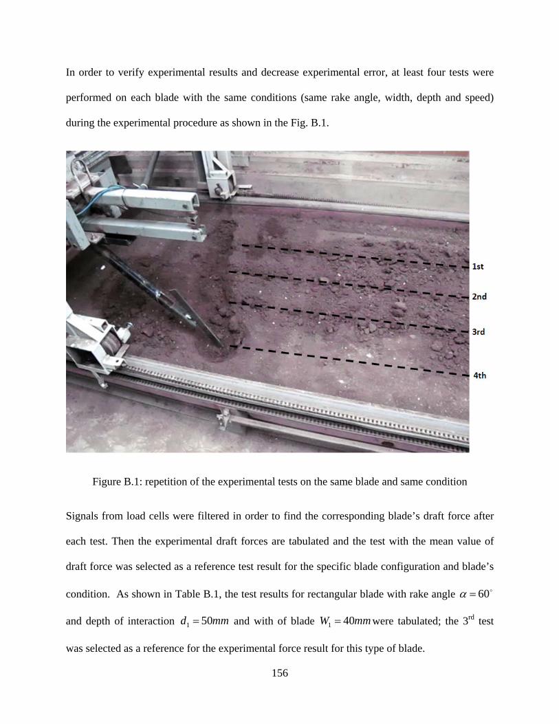
156

In order to verify experimental results and decrease experimental error, at least four tests were

performed on each blade with the same conditions (same rake angle, width, depth and speed)

during the experimental procedure as shown in the Fig. B.1.

Figure B.1: repetition of the experimental tests on the same blade and same condition

Signals from load cells were filtered in order to find the corresponding blade’s draft force after

each test. Then the experimental draft forces are tabulated and the test with the mean value of

draft force was selected as a reference test result for the specific blade configuration and blade’s

condition. As shown in Table B.1, the test results for rectangular blade with rake angle o60=α

and depth of interaction mmd 501 = and with of blade mmW 401 = were tabulated; the 3rd test

was selected as a reference for the experimental force result for this type of blade.

157

Table B.1: experimental tests results on the rectangular blade with o60=α , mmd 501 = and

mmW 401 =

Test Number Final Draft Force

1 427

2 409

3 415

4 406

5 413

6 419

158

Appendix C

A Sample of Ansys program for Curved rectangular blade with o45=α and o90=cα

159

Finish

/clear

/prep7

/title,soil

!mat 1(Blade)

Mp,ex,1,2e11

Mp,prxy,1,.3

Mp,dens,1, 7850

!Mat2(soil)

Mp,ex,2,5e6

Mp,prxy,2,.36

Mp,dens,2,1200

TB,DP,2

TBDATA,1,2e4,35,20

!--------- -------------------Modeling of Soil-----

Et,1,solid45

Keyopt,1,1,1

Keyopt,1,2,0

Type,1

Mat,1

r,1

!---------- Blade & soil bin parameter------------

h1=.05

w1=(.05)

d=.02

H=2*h1

W=(.24)

LS=.2

Lb=.05

LE=.05

HS=.1

HS1=HS-h1

R=.07

alp=77

HM=.26

Q=1.3

PI = 4*ATAN(1)

l=cos(alp*(PI/180))

m=sin(alp*(PI/180))

t=tan(alp*(PI/180))

!------------Modeling of blade--------------------------

k,400,-(H/t),((.7)*H+HS1),((W-w1)/2)

k,401,0,HS1,((W-w1)/2)

KK=-(sqrt((H*H)+((H/t)*(H/t))))

k,402,KK,HS1,((W-w1)/2)

k,403,(d-(H/t)),((.7)*H+HS1),((W-w1)/2)

k,404,d,HS1,((W-w1)/2)

k,405,(KK+.05),HS1,((W-w1)/2)

LARC,400,401,402,-R

LARC,403,404,405,-R

k,500,-(H/t),((.7)*H+HS1),((W+w1)/2)

k,501,0,HS1,((W+w1)/2)

k,502,KK,HS1,((W+w1)/2)

k,503,(d-(H/t)),((.7)*H+HS1),((W+w1)/2)

k,504,d,HS1,((W+w1)/2)

k,505,(KK+.05),HS1,((W+w1)/2)

LARC,500,501,502,-R

LARC,503,504,505,-R

!-------- -----------check HM here-------------------------

KL,1,HM,2,

kl,2,HM,5

l,504,501

l,503,500

l,401,404

l,400,403

l,400,500

l,403,503

l,404,504

160

l,401,501

type,1

mat,1

al,9,10,8,6

al,1,2,8,7

al,12,11,7,5

al,3,4,5,6

al,1,12,3,9

al,10,2,11,4

va,1,2,3,4,5,6

Lesize,1,,,7,

Lesize,2,,,7,

Lesize,3,,,7,

Lesize,4,,,7,

Lesize,9,,,6

Lesize,10,,,6

Lesize,11,,,6

Lesize,12,,,6

Lesize,5,,,3

Lesize,6,,,3

Lesize,7,,,3

Lesize,8,,,3

MSHKEY,1

MSHAPE,0,3d

vmesh,1

!--------------- Modeling of soil--------------------

type,1

mat,2

!----------------Modeling of lines--------------

k,100,0,0,0

k,101,LS,0,0

k,102,LS,HS,0

k,103,LS,HS,W

k,104,LS,0,W

k,105,LS,HS1,0

k,106,LS,HS1,W

k,107,LS,HS,(W-w1)/2

k,108,LS,HS,(W+w1)/2

k,109,LS,HS1,(W-w1)/2

k,110,LS,HS1,(W+w1)/2

k,111,LS,0,(W-w1)/2

k,112,LS,0,(W+w1)/2

k,113,Lb,0,0

k,114,Lb,HS,0

k,115,Lb,HS1,0

k,116,Lb,HS,(W-w1)/2

k,117,Lb,HS1,(W-w1)/2

k,118,Lb,0,(W-w1)/2

k,119,Lb,HS,(W+w1)/2

k,120,Lb,HS1,(W+w1)/2

k,121,Lb,0,(W+w1)/2

k,122,Lb,HS,W

k,123,Lb,HS1,W

k,124,Lb,0,W

k,125,d,0,W

k,126,d,0,(W+w1)/2

k,127,d,0,(W-w1)/2

k,128,d,0,0

k,129,d,HS1,0

k,130,d,HS1,((W-w1)/2)

k,131,d,HS1,((W+w1)/2)

k,132,d,HS1,W

!-----first arc------------------------

k,601,(d-(H/t)),((.7)*H+HS1),((W+w1)/2)

k,602,d,HS1,((W+w1)/2)

k,603,(KK+.05),HS1,((W+w1)/2)

LARC,601,602,603,-R

KL,13,HM,604

161

LARC,604,602,603,-R

!-----second arc------------

k,701,(d-(H/t)),((.7)*H+HS1),((W-w1)/2)

k,702,d,HS1,((W-w1)/2)

k,703,(KK+.05),HS1,((W-w1)/2)

LARC,701,702,703,-R

KL,15,HM,704

LARC,704,702,703,-R

!-----Third arc------------

k,801,(d-(H/t)),((.7)*H+HS1),0

k,802,d,HS1,0

k,803,(KK+.05),HS1,0

LARC,801,802,803,-R

KL,17,HM,804

LARC,804,802,803,-R

!-----forth arc------------

k,901,(d-(H/t)),((.7)*H+HS1),W

k,902,d,HS1,W

k,903,(KK+.05),HS1,W

LARC,901,902,903,-R

KL,19,HM,904

LARC,904,902,903,-R

!-----doublicate first arc------------

k,1001,(d-(H/t)),((.7)*H+HS1),((W+w1)/2)

k,1002,(KK+.05),HS1,((W+w1)/2)

LARC,1001,131,1002,-R

KL,13,HM,1003

LARC,1003,131,1002,-R

!-----doublicate second arc------------

k,1004,(d-(H/t)),((.7)*H+HS1),((W-w1)/2)

k,1005,(KK+.05),HS1,((W-w1)/2)

LARC,1004,130,1005,-R

KL,15,HM,1006

LARC,1006,130,1005,-R

!----------------Modeling of Volumes------

!-------Volume 2 ------

l,904,604

l,602,902

l,122,904

l,123,902

l,119,604

l,120,602

l,122,119

l,123,120

l,119,120

l,122,123

al,31,29,25,27

al,32,30,28,26

al,20,34,27,28

al,31,32,33,34

al,30,14,33,29

al,14,25,20,26

va,7,8,9,10,11,12

Lesize,25,,,4,.2

Lesize,26,,,4,5

Lesize,31,,,4,.2

Lesize,32,,,4,.2

Lesize,33,,,6,

Lesize,14,,,6,Q

Lesize,20,,,6,Q

Lesize,34,,,6,

Lesize,30,,,6

Lesize,29,,,6

Lesize,28,,,6

Lesize,27,,,6

MSHKEY,1

MSHAPE,0,3d

vmesh,2

162

!------Volume 3 ------

l,1006,1003

l,119,116

l,120,131

l,120,117

l,131,130

l,117,130

l,116,1006

l,116,117

l,119,1003

al,41,35,36,43

al,37,38,40,39

al,22,37,33,43

al,38,33,36,42

al,40,42,41,24

al,24,39,22,35

va,13,14,15,16,17,18

Lesize,35,,,6

Lesize,36,,,6

Lesize,39,,,6

Lesize,38,,,6

Lesize,33,,,6,

Lesize,22,,,6,Q

Lesize,24,,,6,Q

Lesize,42,,,6,

Lesize,37,,,6

Lesize,40,,,6

Lesize,41,,,6

Lesize,43,,,6

MSHKEY,1

MSHAPE,0,3d

vmesh,3

!-------Volume 4 ------

l,704,804

l,702,802

l,704,116

l,702,117

l,117,115

l,116,114

l,114,115

l,114,804

l,115,802

al,51,44,49,46

al,45,52,47,48

al,46,42,47,16

al,42,48,50,49

al,50,51,18,52

al,18,44,16,45

va,19,20,21,22,23,24

Lesize,44,,,4,5

Lesize,49,,,4,5

Lesize,48,,,4,5

Lesize,45,,,4,5

Lesize,50,,,6,

Lesize,18,,,6,Q

Lesize,16,,,6,Q

Lesize,51,,,6

Lesize,52,,,6

Lesize,40,,,6

Lesize,46,,,6

MSHKEY,1

MSHAPE,0,3d

vmesh,4

!-------Volume 5 ------

l,123,124

l,120,121

l,124,121

l,125,124

163

l,125,126

l,126,121

l,902,125

l,602,126

al,57,55,56,58

al,28,56,53,59

al,55,32,54,53

al,54,30,60,58

al,26,60,57,59

va,8,25,26,27,28,29

Lesize,54,,,3,5

Lesize,60,,,3,5

Lesize,53,,,3,5

Lesize,59,,,3,5

Lesize,57,,,4,.2

Lesize,55,,,4,.2

Lesize,56,,,6

Lesize,58,,,6

MSHKEY,1

MSHAPE,0,3d

vmesh,5

!-------Volume 6 ------

l,121,118

l,117,118

l,127,118

l,127,126

l,127,702

l,602,702

al,47,38,30,66

al,61,58,64,63

al,54,61,62,38

al,62,47,65,63

al,66,60,64,65

va,28,30,31,32,33,34

Lesize,66,,,6

Lesize,64,,,6

Lesize,61,,,6

Lesize,63,,,6

Lesize,62,,,3,5

Lesize,65,,,3,.2

MSHKEY,1

MSHAPE,0,3d

vmesh,6

!-------Volume 7 ------

l,118,113

l,128,113

l,128,127

l,115,113

l,128,802

al,67,68,69,63

al,70,67,62,48

al,70,52,71,68

al,45,71,69,65

va,33,20,35,36,37,38

Lesize,67,,,4,5

Lesize,69,,,4,.2

Lesize,68,,,6

Lesize,70,,,3,5

Lesize,71,,,3,.2

MSHKEY,1

MSHAPE,0,3d

vmesh,7

!-------Volume 8 ------

l,123,106

l,124,104

l,120,110

l,121,112

l,110,106

164

l,106,104

l,104,112

l,110,112

al,74,32,72,76

al,55,73,78,75

al,72,53,73,77

al,76,77,78,79

al,74,79,75,54

va,27,39,40,41,42,43

Lesize,74,,,5,10

Lesize,75,,,5,10

Lesize,72,,,5,10

Lesize,73,,,5,10

Lesize,76,,,4,5

Lesize,78,,,4,.2

Lesize,77,,,3,5

Lesize,79,,,3,5

MSHKEY,1

MSHAPE,0,3d

vmesh,8

!-------Volume 9 ------

l,109,110

l,111,112

l,117,109

l,118,111

l,109,111

al,82,74,38,80

al,75,81,83,61

al,80,84,81,79

al,84,82,83,62

va,32,43,44,45,46,47

Lesize,82,,,5,10

Lesize,83,,,5,10

Lesize,80,,,6

Lesize,81,,,6

Lesize,84,,,3,5

MSHKEY,1

MSHAPE,0,3d

vmesh,9

!-------Volume 10 ------

l,105,109

l,101,105

l,101,111

l,101,113

l,105,115

al,89,48,82,85

al,87,88,67,83

al,85,86,87,84

al,89,70,88,86

va,36,47,48,49,50,51

Lesize,89,,,5,.1

Lesize,88,,,5,.1

Lesize,85,,,4,.2

Lesize,87,,,4,.2

Lesize,86,,,3,.2

MSHKEY,1

MSHAPE,0,3d

vmesh,10

!-------Volume 11 ------

l,108,110

l,103,106

l,122,103

l,103,108

l,119,108

al,94,31,92,93

al,92,91,72,34

al,93,90,76,91

al,94,90,74,33

165

va,10,39,52,53,54,55

Lesize,92,,,5,10

Lesize,94,,,5,10

Lesize,91,,,6,

Lesize,90,,,6,

Lesize,93,,,4,.2

MSHKEY,1

MSHAPE,0,3d

vmesh,11

!-------Volume 12 ------

l,108,107

l,107,109

l,116,107

al,97,94,95,36

al,95,96,80,90

al,97,96,82,42

va,16,55,44,56,57,58

Lesize,97,,,5,10

Lesize,95,,,6

Lesize,96,,,6,

MSHKEY,1

MSHAPE,0,3d

vmesh,12

!-------Volume 13 ------

l,105,102

l,102,107

l,102,114

al,100,49,97,99

al,99,98,85,96

al,100,98,89,50

va,22,58,48,59,60,61

Lesize,100,,,5,.1

Lesize,99,,,4,.2

Lesize,98,,,6,2

MSHKEY,1

MSHAPE,0,3d

vmesh,13

!-------Volume 14 ------

k,1100,-LE,0,W

k,1101,-LE,0,((W+w1)/2)

k,1102,-LE,HS1,W

k,1103,-LE,HS1,((W+w1)/2)

l,1102,902

l,1102,1103

l,1103,602

l,125,1100

l,126,1101

l,1100,1101

l,1100,1102

l,1101,1103

al,102,101,26,103

al,104,106,105,57

al,107,101,59,104

al,103,60,105,108

al,102,107,106,108

va,62,63,64,65,66,29

Lesize,108,,,3,.2

Lesize,107,,,3,.2

Lesize,106,,,4,.2

Lesize,102,,,4,.2

Lesize,105,,,3,10

Lesize,104,,,3,10

Lesize,101,,,3,.1

Lesize,103,,,3,.1

MSHKEY,1

MSHAPE,0,3d

vmesh,14

!-------Volume 15 ------

166

k,1200,-LE,HS,W

k,1201,-LE,HS,((W+w1)/2)

l,1200,1201

l,1200,1102

l,1201,1103

l,1200,904

l,1201,604

al,109,112,25,113

al,112,110,101,20

al,113,111,103,14

al,109,110,102,111

va,12,62,67,68,69,70

Lesize,110,,,6,

Lesize,111,,,6,

Lesize,112,,,3

Lesize,113,,,3

Lesize,109,,,4,.2

MSHKEY,1

MSHAPE,0,3d

vmesh,15

!-------Volume 16 ------

k,1300,-LE,0,((W-w1)/2)

k,1301,-LE,HS1,((W-w1)/2)

l,1103,1301

l,1301,1300

l,1300,1101

l,1301,702

l,1300,127

al,114,115,116,108

al,115,117,65,118

al,117,114,103,66

al,118,116,105,64

va,34,65,71,72,73,74

Lesize,115,,,3,5

Lesize,116,,,6

Lesize,114,,,6

Lesize,118,,,3,.1

Lesize,117,,,3,.1

MSHKEY,1

MSHAPE,0,3d

vmesh,16

!-------Volume 17 ------

k,1400,-LE,0,0

k,1401,-LE,HS1,0

l,1401,1400

l,1401,802

l,1400,128

l,1400,1300

l,1401,1301

al,120,123,117,45

al,122,121,69,118

al,119,123,115,122

al,120,119,121,71

va,72,38,75,76,77,78

Lesize,119,,,3,5

Lesize,122,,,4,.2

Lesize,121,,,3,.1

Lesize,120,,,3,.1

Lesize,123,,,4,.2

MSHKEY,1

MSHAPE,0,3d

vmesh,17

!-------Volume 18 ------

k,1500,-LE,HS,0

k,1501,-LE,HS,((W-w1)/2)

l,1501,1500

l,1500,1401

l,1500,804

167

l,1501,704

l,1501,1301

al,124,126,127,44

al,124,125,123,128

al,126,125,120,18

al,127,128,117,16

va,24,75,79,80,81,82

Lesize,126,,,3

Lesize,124,,,4,5

Lesize,125,,,6,

Lesize,128,,,6,

Lesize,127,,,3

MSHKEY,1

MSHAPE,0,3d

vmesh,18

/pnum,area,1

/pnum,kp,1

!---- -----------Contact element-------------------

Et,2,conta173

Et,3,targe170

KEYOPT,2,1,0

KEYOPT,2,10,2

KEYOPT,2,12,2

Et,4,conta173

KEYOPT,4,1,0

KEYOPT,4,10,2

KEYOPT,4,12,3

Et,5,targe170

!-------------- blade contact--------

ASEL,S,,,6

NSLA,S,1

real,1

TYPE,2

mat,1

ESURF

ALLSEL,all

ASEL,S,,,18

NSLA,S,1

TYPE,3

mat,2

ESURF

ALLSEL,ALL

!------------- soil contact(above volume) --------

ASEL,S,,,14

NSLA,S,1

real,2

TYPE,3

mat,2

ESURF

ALLSEL,all

ASEL,S,,,30

NSLA,S,1

TYPE,4

mat,2

ESURF

ALLSEL,ALL

!----- -----------soil contact(left volume) --------

ASEL,S,,,15

NSLA,S,1

real,2

TYPE,3

mat,2

ESURF

ALLSEL,all

ASEL,S,,,11

NSLA,S,1

TYPE,4

mat,2

168

ESURF

ALLSEL,ALL

!------------ soil contact(right volume) ----

ASEL,S,,,17

NSLA,S,1

real,2

TYPE,3

mat,2

ESURF

ALLSEL,all

ASEL,S,,,21

NSLA,S,1

TYPE,4

mat,2

ESURF

ALLSEL,ALL

!----------------- soil contact(above volume) ----

ASEL,S,,,14

NSLA,S,1

real,1

TYPE,2

mat,2

ESURF

ALLSEL,all

ASEL,S,,,30

NSLA,S,1

TYPE,5

mat,2

ESURF

ALLSEL,ALL

!----- ----------------soil contact(left) ----

ASEL,S,,,15

NSLA,S,1

real,1

TYPE,2

mat,2

ESURF

ALLSEL,all

ASEL,S,,,11

NSLA,S,1

TYPE,5

mat,2

ESURF

ALLSEL,ALL

!-------- -------------soil contact(right) ----

ASEL,S,,,17

NSLA,S,1

real,1

TYPE,2

mat,2

ESURF

ALLSEL,all

ASEL,S,,,21

NSLA,S,1

TYPE,5

mat,2

ESURF

ALLSEL,ALL

*do,k,1,216

ekill,2076+k

*enddo

!---------------solution------------

/solu

Antype,0

SOLCONTROL,ON

Autots,on

Nlgeom,on

neqit,100

169

ACEL,,9.8

!------------Boundary Constrain

ASEL,S,,,64

NSLA,S,1

d,all,all

nsel,all

ASEL,S,,,68

NSLA,S,1

d,all,all

nsel,all

ASEL,S,,,9

NSLA,S,1

d,all,all

nsel,all

ASEL,S,,,26

NSLA,S,1

d,all,all

nsel,all

ASEL,S,,,53

NSLA,S,1

d,all,all

nsel,all

ASEL,S,,,41

NSLA,S,1

d,all,all

nsel,all

ASEL,S,,,54

NSLA,S,1

d,all,all

nsel,all

ASEL,S,,,57

NSLA,S,1

d,all,all

nsel,all

ASEL,S,,,42

NSLA,S,1

d,all,all

nsel,all

ASEL,S,,,46

NSLA,S,1

d,all,all

nsel,all

ASEL,S,,,60

NSLA,S,1

d,all,all

nsel,all

ASEL,S,,,50

NSLA,S,1

d,all,all

nsel,all

ASEL,S,,,61

NSLA,S,1

d,all,all

nsel,all

ASEL,S,,,51

NSLA,S,1

d,all,all

nsel,all

ASEL,S,,,37

NSLA,S,1

d,all,all

nsel,all

ASEL,S,,,23

NSLA,S,1

d,all,all

nsel,all

ASEL,S,,,78

NSLA,S,1

170

d,all,all

nsel,all

ASEL,S,,,81

NSLA,S,1

d,all,all

nsel,all

ASEL,S,,,49

NSLA,S,1

d,all,all

nsel,all

ASEL,S,,,45

NSLA,S,1

d,all,all

nsel,all

ASEL,S,,,40

NSLA,S,1

d,all,all

nsel,all

ASEL,S,,,35

NSLA,S,1

d,all,all

nsel,all

ASEL,S,,,25

NSLA,S,1

d,all,all

nsel,all

ASEL,S,,,31

NSLA,S,1

d,all,all

nsel,all

ASEL,S,,,74

NSLA,S,1

d,all,all

nsel,all

ASEL,S,,,76

NSLA,S,1

d,all,all

nsel,all

ASEL,S,,,63

NSLA,S,1

d,all,all

nsel,all

ASEL,S,,,70

NSLA,S,1

d,all,all

nsel,all

ASEL,S,,,66

NSLA,S,1

d,all,all

nsel,all

ASEL,S,,,71

NSLA,S,1

d,all,all

nsel,all

ASEL,S,,,80

NSLA,S,1

d,all,all

nsel,all

ASEL,S,,,77

NSLA,S,1

d,all,all

nsel,all

ASEL,S,,,1

NSLA,S,1

d,all,uy,0

d,all,uz,0

nsel,all

171

ASEL,S,,,30

NSLA,S,1

d,all,uy,0

nsel,all

!------------- ----------Do loop--------

*do,i,1,10

*if,i,eq,1,then

!-------- motion of the blade--------

*do,j,1,7

time,j/2

aSEL,S,,,5

NSLa,S,1

d,all,ux,((0)+((j)*0.00045))

nsel,all

nsub,800

solve

*enddo

*elseif,i,eq,2,then

*do,j,8,11

time,j/2

aSEL,S,,,5

NSLa,S,1

d,all,ux,((.00315)+((j-8)*0.0004))

nsel,all

nsub,800

solve

*enddo

*elseif,i,eq,3,then

*do,j,12,15

time,j/2

aSEL,S,,,5

NSLa,S,1

d,all,ux,((.00435)+((j-12)*0.0004))

nsel,all

nsub,800

solve

*enddo

*elseif,i,eq,4,then

*do,j,16,30

time,j/2

aSEL,S,,,5

NSLa,S,1

d,all,ux,((.00555)+((j-16)*0.0003))

nsel,all

nsub,800

solve

*enddo

*elseif,i,eq,5,then

*do,j,18,50

time,j/2

aSEL,S,,,5

NSLa,S,1

d,all,ux,((.0087)+((j-18)*0.0006))

nsel,all

nsub,800

solve

*enddo

*elseif,i,eq,6,then

*do,j,28,80

time,j/2

aSEL,S,,,5

NSLa,S,1

d,all,ux,((.0143)+((j-28)*0.0005))

nsel,all

nsub,800

solve

*enddo

*endif

172

!-- killing the contact element between ( Above and Below)

!-------------above

ekill,(1896-(6*i)+1)

ekill,(1896-(6*i)+2)

ekill,(1896-(6*i)+3)

ekill,(1896-(6*i)+4)

ekill,(1896-(6*i)+5)

ekill,(1896-(6*i)+6)

!-------------below

ekill,(1903-i)

ekill,(1909-i)

ekill,(1915-i)

ekill,(1921-i)

ekill,(1927-i)

ekill,(1933-i)

ealive,(2112-(6*i)+1)

ealive,(2112-(6*i)+2)

ealive,(2112-(6*i)+3)

ealive,(2112-(6*i)+4)

ealive,(2112-(6*i)+5)

ealive,(2112-(6*i)+6)

!-------------below

ealive,(2119-i)

ealive,(2125-i)

ealive,(2131-i)

ealive,(2137-i)

ealive,(2143-i)

ealive,(2149-i)

!----- killing the contact element between (Above and left)

!-------------above

ekill,(1939-i)

ekill,(1945-i)

ekill,(1951-i)

ekill,(1957-i)

ekill,(1963-i)

ekill,(1969-i)

!-------------left

ekill,(1975-i)

ekill,(1981-i)

ekill,(1987-i)

ekill,(1993-i)

ekill,(1999-i)

ekill,(2005-i)

!-------------above

ealive,(2155-i)

ealive,(2161-i)

ealive,(2167-i)

ealive,(2173-i)

ealive,(2179-i)

ealive,(2185-i)

!-------------left

ealive,(2191-i)

ealive,(2197-i)

ealive,(2203-i)

ealive,(2209-i)

ealive,(2215-i)

ealive,(2221-i)

!-- -- killing the contact element between (Above and right)

!-------------above

ekill,(2011-i)

ekill,(2017-i)

ekill,(2023-i)

ekill,(2029-i)

ekill,(2035-i)

ekill,(2041-i)

!-------------right

ekill,(2047-i)

ekill,(2053-i)

173

ekill,(2059-i)

ekill,(2065-i)

ekill,(2071-i)

ekill,(2077-i)

!-------------above

ealive,(2227-i)

ealive,(2233-i)

ealive,(2239-i)

ealive,(2245-i)

ealive,(2251-i)

ealive,(2257-i)

!-------------right

ealive,(2263-i)

ealive,(2269-i)

ealive,(2275-i)

ealive,(2281-i)

ealive,(2287-i)

ealive,(2293-i)

!------------------------

*enddo

Mechanics of soil-blade interaction A Thesis ... - CORE

Documents

Transcript of Mechanics of soil-blade interaction A Thesis ... - CORE