Advances in strength theories for materials under complex ...
Upload
khangminh22Category
view
0download
0
Indiana University – Purdue University Fort WayneOpus: Research & Creativity at IPFWManufacturing and Construction EngineeringTechnology and Interior Design FacultyPublications
Department of Manufacturing and ConstructionEngineering Technology and Interior Design
8-2014
Applied Strength of Materials for EngineeringTechnologyBarry DupenIPFW, [email protected]
Follow this and additional works at: http://opus.ipfw.edu/mcetid_facpubsPart of the Applied Mechanics Commons
This Book is brought to you for free and open access by the Department of Manufacturing and Construction Engineering Technology and InteriorDesign at Opus: Research & Creativity at IPFW. It has been accepted for inclusion in Manufacturing and Construction Engineering Technology andInterior Design Faculty Publications by an authorized administrator of Opus: Research & Creativity at IPFW. For more information, please [email protected].
Opus CitationBarry Dupen (2014). Applied Strength of Materials for Engineering Technology. 6 ed.http://opus.ipfw.edu/mcetid_facpubs/35

Applied Strength of Materials for Engineering TechnologyBarry Dupen
Associate Professor, Mechanical Engineering Technology, Indiana University – Purdue University Fort Wayne
v.6 Revised August 2014. This work is licensed under Creative Commons Attribution-ShareAlike 4.0 International (CC BY-SA 4.0) See creativecommons.org for license details.
1
Table of ContentsPreface...............................................................................................3
Purpose of the Book....................................................................3Editors.........................................................................................4Cover Photos...............................................................................4
Terminology......................................................................................5Definitions.........................................................................................7Chapter 1: Introduction to Strength of Materials.............................9
What is Strength of Materials?...................................................9The Factor-Label Method of Unit Conversion........................10
Chapter 2: Stress and Strain............................................................14Normal Stress and Strain..........................................................14Sign Convention.......................................................................17Shear Stress and Strain.............................................................17
Chapter 3: Poisson's Ratio and Thermal Expansion......................20Poisson's Ratio..........................................................................20Thermal Expansion and Thermal Stress..................................22
Chapter 4: Pressure Vessels and Stress Concentrations................25Thin-Walled Pressure Vessels..................................................25Stress Concentration in Tension...............................................27
Chapter 5: Bolted and Welded Joints.............................................30Bolted Lap Joints Loaded in Tension......................................30Welded Lap Joints....................................................................35
Chapter 6: Properties of Areas........................................................38Dimensions and Area................................................................38Centroid and Centroidal Axes..................................................38Moment of Inertia of a Rectangle............................................38Compound Beams Sharing a Centroidal Axis.........................39Hollow Beams Sharing a Centroidal Axis...............................40The Transfer Formula...............................................................41Compound Beams With Different Neutral Axes.....................42Hollow Beams With Different Neutral Axes...........................45Moment of Inertia about the y-y Neutral Axis........................48Shortcuts....................................................................................51Radius of Gyration....................................................................51Polar Moment of Inertia...........................................................51
Chapter 7: Torsion in Round Shafts...............................................52Shear Stress in a Round Shaft..................................................52Angle of Twist in a Round Shaft..............................................53Stress Concentration in Torsion...............................................54
Chapter 8: Beam Reactions, Shear Diagrams, and Moment Diagrams..........................................................................................56
Loads on Beams........................................................................56Reactions for Simply-Supported Simple Beams.....................57Reactions for Overhanging and Cantilever Beams..................60Shear Diagrams.........................................................................61Moment Diagrams....................................................................67
Chapter 9: Stresses in Beams..........................................................73Bending Stress in Beams..........................................................73
Bending Stress in Steel Beams.................................................75Shear Stress in Beams...............................................................77Allowable Load.........................................................................82
Chapter 10: Beam Deflection.........................................................84Radius of Curvature..................................................................84The Formula Method for Simple Cases...................................85Formula Method Hints..............................................................87The Formula Method for Complex Cases: Superposition.......87Visualizing the Deflection Curve.............................................89
Chapter 11: Beam Design...............................................................90Wide-Flange Steel Beam Design in Six Easy Steps................90Timber Beam Design in Six Easy Steps..................................96
Chapter 12: Combined Stresses......................................................99Tension + Bending....................................................................99Bending in Two Directions......................................................99Eccentric Loading...................................................................101
Chapter 13: Statically Indeterminate Beams................................104Defining Determinate and Indeterminate Beams..................104Method of Superposition........................................................104
Chapter 14: Buckling of Columns................................................108Types of Columns...................................................................108Ideal Slender Columns...........................................................108Structural Steel Columns........................................................110Steel Machine Parts................................................................111
Chapter 15: Visualizing Stress and Strain....................................114Measuring Stress.....................................................................114Stress at the Base of a Short Block........................................114Mohr's Circle...........................................................................115
Bibliography..................................................................................128Textbooks................................................................................128Other Reading Material..........................................................128
Appendix A: Units........................................................................129SI System of Units..................................................................129US Customary System of Units.............................................129
Appendix B: Materials Properties................................................130Metals, Concrete, & Stone.....................................................130
Appendix C: Properties of Areas..................................................134Center of Gravity, Area, Moment of Inertia, and Radius of Gyration..................................................................................134
Appendix D: Properties of Steel Beams and Pipes......................137W-beams.................................................................................137Steel Pipes...............................................................................141Copper Tubing........................................................................142
Appendix E: Mechanical and Dimensional Properties of Wood.143Mechanical Properties of Air-Dried Boards and Timber......143Softwood Lumber and Timber Sizes.....................................144
Appendix F: Beam Equations.......................................................146Index..............................................................................................151
2

Preface
PrefacePurpose of the Book
1.8 million bachelors degrees are awarded annually in the US.1 About 80 thousand are Engineering degrees, and about 17 thousand are Engineering Technology degrees and Technician degrees. The number of Mechanical, Civil, and Construction Engineering Technology graduates is only about 2 thousand per year, so the market for algebra-based Strength of Materials textbooks for Engineering Technology is a small fraction of the market for calculus-based Engineering textbooks.
Since I attended college in the 1980s, textbook prices have risen about twice as fast as inflation. The internet did not exist when I was in college, so all textbooks were printed. Now we have another option: low-cost or free online e-books which are revised more frequently than printed books. While traditional textbooks are revised every 4 to 10 years based on input from experts in the topic, this e-book is revised every semester based on input from experts in learning: the students.
Students complain that the explanations in many Engineering Technology textbooks are too theoretical, too wordy, and too difficult to understand. They also complain about the lack of complete unit conversions in example problems, and inconsistent use of symbols between related courses. For example, some authors use sn, ss, and e for normal stress, shear stress, and strain, instead of the standard Greek symbols σ, τ, and ε. This use of Latin characters with multiple subscripts confuses students because the Greek symbols are used in other textbooks, and because capital S is used for section modulus later in the course. Students have trouble distinguishing between s and S on the chalkboard and in their notes.
Professors complain that too many students copy answers from online solution manuals or college fraternity homework filesinstead of learning to solve problems from scratch, then fail exams. Probably 10% of the learning in Strength of Materials occurs in class, and 90% occurs as students solve problems. Therefore, the problem set for this book is not available online, and is changed every semester.
I teach Strength of Materials to Mechanical, Civil, and Architectural Engineering Technology students. In conversation and by their work, these students tell me they want help with algebra skills, unit conversions, and problem-solving approaches. The problem set that accompanies this book contains problems requiring an algebraic answer as well as traditional problemsrequiring a numerical answer. The Factor-Label Method of Unit Conversion is emphasized from the first chapter, and is used in all example problems.
Summarizing, the goals of this book are:
• Free distribution over the internet
• Frequent revisions based on student input
• Concise explanations
• Examples with complete unit conversions
• Standard Greek symbols for stress and strain
• Problems requiring algebraic answers as well as problems requiring numerical answers
• Problems requiring answers in sentences to show reasoning and understanding of the topics
This e-book is a living document, and is revised on an ongoing basis. Please send suggestions for improvement to me at [email protected].
Barry Dupen
Indiana University – Purdue University Fort Wayne
Fort Wayne, Indiana
August, 2014
1 Data from 2011-2012. You can find the current numbers online in the Digest of Educational Statistics, published by the National Center for Educational Statistics, U.S. Department of Education, at nces.ed.gov.
3

Preface
Editors
These IPFW students edited the text and contributed to improving this book:
Jacob Ainsworth, George Allwein, Matthew Amberg, Mark Archer, Justin Arnold, Stuart Aspy, Caleb Averill, Alex Baer, Jacob Beard, John Blankenship, Crystal Boyd, Aaron Bryant, Nicholas Burchell, Justin Byerley, Danny Calderon, Brody Callaghan, Esperanza Castillo, Brian Chaney, Zachary Clevenger, Ryan Clingenpeel, Uriel Contreras, Logan Counterman, Daniel Cummings, Christopher Davis, Patrick Davis, Stephen England, Cameron Eyman, Tyler Faylor, Austin Fearnow, John Fisher, Charles Foreman, Michael Friddle, Brett Gagnon, Carl Garringer, Shane Giddens, Almario Greene, Ryan Guiff, Charles Hanes, Cody Hepler, Ben Hinora, Kaleb Herrick, James Hoppes, Bradley Horn, Sujinda Jaisa-Ard, Ariana Jarvis, Daniel Johns, Jason Joyner, Adam Kennedy, Joseph Kent, Hannah Kiningham, Nate Kipfer, Andrew Kitrush, Rachael Klopfenstein, Branden Lagassie, Doug Lambert, Brandon Lane, Justin Lantz, Venus Lee, Christopher Leek, DaltonMann, David MarcAurele, Alex Mason, La Keisha Mason, Michael McLinden, Angela Mendoza, Derek Morreale, Senaid Mrzljak, Travis Mullendore, Michael Nusbaum, Jordan Owens, John Pham, Braxton Powers, Nathan Pratt, Trey Proper, Justin Reese, Shawn Reuille, Daniel Reynolds, Charles Rinehart, Connor Ruby, Austin Rumsey, Billie Saalfrank, Zachary Saylor, John Schafer, Zackory Schaefer, Zeke Schultz, Ryan Sellers, Philip Sheets, Keith Shepherd, Scott Shifflett, Brad Shamo, Matthew Shimko, Trenton Shrock, Travis Singletary, Eric Shorten, Jacob Smarker, Jonas Susaraba, Troy Sutterfield, Kyle Tew, Zach Thorn, Jason Tonner, Chandler Tracey, Cody Turner, Jason Vachon, Thadius Vesey, Dakota Vogel, Scott Vorndran, Charles Wadsworth, Jay Wehrle, Travis Weigold, Scott Wolfe, Michael Woodcock, Lyndsay Wright, and Matthew Young.
Cover Photos
Cover photos by the author. British Columbia ferry boat; interior of a Churrascaria restaurant in Brazil, showing the clay roof tiles; interior of a tourist kiosk near Squamish, British Columbia; 8 mile long Confederation Bridge between New Brunswick and Prince Edward Island (in winter, the world's longest bridge over ice); J.C. Van Horne bridge between Campbellton, New Brunswick, and Point à la Croix, Québec; Spillway gate at Itaipu Dam, between Ciudad del Este, Paraguay, and Foz do Iguaçu, Brazil.
This book was created with the Apache Software Foundation's Open Office software v. 4.0.0
4

Terminology
TerminologySymbols used in this book, with typical units
Because the Roman and Greek alphabets contain a finite number of letters, symbols are recycled and used for more than oneterm. Check the context of the equation to figure out what the unit means in that equation.
Other science and engineering disciplines use different symbols for common terms. For example, P is used for point load here; in Physics classes, F is commonly used for point load. Some older Strength of Materials texts use µ for Poisson's ratio,s for stress, and e for strain; the formulas are the same, but the labels differ.
Symbol Term U.S. Units SI Units
α Thermal expansion coefficient °F-1 °C-1
γ Shear strain ⋯ ⋯γ Specific weight lb./in.3, lb./ft.3 N/m3
δ Change in dimension (length, diameter, etc.) in. mmΔ Change ⋯ ⋯Δ Beam deflection in. mmε Strain ⋯ ⋯ν Poisson's ratio ⋯ ⋯ρ Density slug/ft.3 kg/m3
σ Normal (perpendicular) stress psi, ksi MPaτ Shear (parallel) stress psi, ksi MPaθ Angle of twist (radians) (radians)
A , a Area in.2 mm2, m2
A' Term in the General Shear Formula in.2 mm2, m2
b Base dimension of a rectangle in. mmc Torsion problem: distance from centroid to outer surface
Beam problem: distance from neutral axis to outer surfacein. mm
d Diameter in. mmd Transfer distance in. mm
d i , d o Inside and outside diameters of a pipe in. mm
d H Hole diameter in. mm
e Eccentricity in. mmE Young's modulus (a.k.a. modulus of elasticity) psi, ksi MPa
F.S. Factor of safety ⋯ ⋯G Shear modulus (a.k.a. modulus of rigidity) psi, ksi MPah Height dimension of a rectangle in. mmh Fillet weld throat in. mmI Moment of inertia in.4 mm4
J Polar moment of inertia in.4 mm4
J.E. Joint efficiency % %K Stress concentration factor ⋯ ⋯K Effective length factor (in column analysis) ⋯ ⋯l Fillet weld leg in. mmL Length (of a tension member or a beam) ft. mL Total weld length in. cmM Moment lb.⋅ft., kip⋅ft. kN⋅mn Number of shear planes ⋯ ⋯N Number of bolts ⋯ ⋯
N F Number of holes in the fracture plane ⋯ ⋯
5

Terminology
Symbol Defnition U.S. Units SI Units
p Fluid pressure psi, ksi kPaP Point load lb., kip kN
Pcr Euler critical buckling load lb., kip kN
PG Bolt load – gross tensile failure of the plate lb., kip kN
PN Bolt load – net tensile failure of the plate lb., kip kN
PP Bolt load – bearing failure of the plate lb., kip kN
PS Bolt load – bolt shear failure lb., kip kN
P weld Weld load (lapped plates loaded in tension) lb., kip kN
Q Term in the General Shear Formula in.3 mm3
r Radius (of a hole, fillet, or groove) in. mmrG Radius of gyration in. mm
R Reaction force lb., kip kNR Radius of curvature in., ft. mm, mS Section modulus in.3 mm3
t Thickness in. mmT Torque lb.⋅ft., kip⋅ft. kN⋅mT Temperature °F °CV Shear load lb., kip kNw Distributed load (weight per unit length) lb./ft., kip/ft. kN/mW Weight lb., kip kN
x, y, z Axes in three-dimensional space: x is horizontal, y is vertical,and z is into the page.
⋯ ⋯
x Distance along the x-axis in., ft. mm, my Distance along the y-axis, such as the distance from the
neutral axis in beam problemsin., ft. mm, m
y Distance from the reference axis to the x-x axis of a composite shape [moment of inertia problems]
in. mm
y Term in the General Shear Formula in. mmz Distance along the z-axis in., ft. mm, mZ Plastic section modulus in.3 mm3
Greek Letters
Upper case Lower case Name Upper case Lower case NameΑ α Alpha Ν ν NuΒ β Beta Ξ ξ XiΓ γ Gamma Ο ο OmicronΔ δ Delta Π π PiΔ ε Epsilon Ρ ρ RhoΖ ζ Zeta Σ σ SigmaΗ η Eta Τ τ TauΘ θ Theta Υ υ UpsilonΙ ι Iota Φ ϕ PhiΚ κ Kappa Χ χ ChiΛ λ Lambda Ψ ψ PsiΜ μ Mu Ω ω Omega
6
Definitions
DefnitionsAllowable (stress, load, etc.)..............Permitted for safe design. Bending moment, M ........................Moment in a beam that is loaded in bending with transverse loads.Bending stress, σ ..............................A normal stress along the length of a beam that develops due to transverse loading.Buckling.............................................Collapse of a long, thin member under longitudinal compressive loading, at a load
much lower than the load that causes yielding in tension.Density, ρ .........................................Mass density is the mass of an object or fluid divided by its volume. See specific
weight entry for weight density.Distributed load, w ...........................Force acting over a length (such as the weight of a beam) or area (such as a snow load
on a roof). Compare point load.Eccentricity, e ...................................Distance between the neutral axis of a part and the location of an applied point load.Effective length of a column..............Portion of the length of a column that bows like a fully pinned column.Elastic deformation.............................Temporary deformation; release the load and the part returns to its original shape.
Compare plastic deformation.Elastic modulus, E ...........................A measure of the stiffness of a material (the resistance to elastically deforming under
a given load.) The slope of the linear elastic portion of the stress-strain curve. Also called Young's modulus or modulus of elasticity.
Euler critical buckling load, P cr .......The load at which an ideal Euler column will fail, assuming perfect material and perfectly aligned loading.
Factor of Safety, F.S...........................The material's strength (typically yield strength) divided by the actual stress in the part. Also called “factor of ignorance” because it includes unknowns such as materials defects, improper installation, abuse by the operator, lack of maintenance, corrosion or rot, temperature variations, etc.
Fillet weld...........................................A weld with a triangular cross section used for joining lapped plates. Unlike solderingor brazing, welding involves melting the base metal as well as the joining material.
General shear formula........................Equation for finding the shear stress within a beam of any shape.Joint efficiency...................................The efficiency of a bolted or welded joint is the lowest allowable load divided by the
allowable load of the weaker of the two plates some distance from the joint.Longitudinal direction........................Along the length of a part, such as a beam or shaft. Compare transverse direction.Longitudinal stress, σ .......................A normal stress that develops in a tensile or compressive member due to longitudinal
loading.Modulus of elasticity, E ...................See elastic modulus.Moment, M .......................................More accurately called a force moment, the product of a length and a transversely
applied force. Used in beam problems. There are other types of moment (such as area moment: the product of a length and an area).
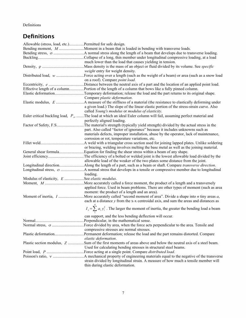
Moment of inertia, I .........................More accurately called “second moment of area”. Divide a shape into n tiny areas a, each at a distance y from the x-x centroidal axis, and sum the areas and distances as
I x=∑1
n
ai yi2 . The larger the moment of inertia, the greater the bending load a beam
can support, and the less bending deflection will occur.Normal................................................Perpendicular, in the mathematical sense.Normal stress, σ ...............................Force divided by area, when the force acts perpendicular to the area. Tensile and
compressive stresses are normal stresses.Plastic deformation.............................Permanent deformation; release the load and the part remains distorted. Compare
elastic deformation.Plastic section modulus, Z ................Sum of the first moments of areas above and below the neutral axis of a steel beam.
Used for calculating bending stresses in structural steel beams.Point load, P .....................................Force acting at a single point. Compare distributed load.Poisson's ratio, ν ..............................A mechanical property of engineering materials equal to the negative of the transverse
strain divided by longitudinal strain. A measure of how much a tensile member will thin during elastic deformation.
7

Definitions
Polar moment of inertia, J ................More accurately called “polar second moment of area”. Divide a shape into n tiny areas a, each at a distance r from the centroid, and sum the areas and distances as
J=∑1
n
a i r i2 . The larger the polar moment of inertia, the greater the torque a shaft can
support, and the less angular twist will be produced.Pressure (of a fluid), p .....................Fluid equivalent of normal stress. A pressurized gas produces a uniform pressure
perpendicular to the walls of the pressure vessel. A pressurized liquid produces a uniform pressure in a small pressure vessel; the pressure is nonuniform in a tall vesseldue to gravity (lower pressure at the top, higher at the bottom).
Radius of curvature, R .....................If a beam segment is bent with a constant bending moment, the segment becomes a circular arc with a radius of curvature, R.
Radius of gyration, rG ......................Concentrate an area at a distance r from the x-x neutral axis. If the moment of inertia of the original area is the same as for the concentrated area, then rGx is the radius of gyration about the x-x axis. The larger the radius of gyration, the more resistant a column is to buckling. Calculate rG=√ I / A .
Reaction moment, M A or M B ........Moment at reaction point A or B which supports a transversely loaded cantilever beam.
Reaction force, RA or RB ................Forces at reaction points A or B which support a transversely loaded beam.Section modulus, S ...........................Moment of inertia divided by the distance from the neutral axis to the surface. The
larger the section modulus, the more resistant a beam is to bending.Shear modulus, G .............................The shear analog to Young's modulus: shear stress divided by shear strain in an elastic
material.Shear load, V ....................................Transverse load on a beam.Shear plane.........................................In a bolted joint with two plates pulling in opposite directions, the shear plane is the
transverse plane within a bolt that lies at the interface of the two plates.Shear strain, γ ..................................Shear deflection divided by original unit lengthShear stress, τ ...................................Force divided area, when the force acts parallel to the area.Specific weight, γ ............................Specific weight, a.k.a. weight density, is the weight of an object or fluid divided by its
volume. The symbol, lower case gamma, is also used for shear strain. In this text, plain gamma means shear strain, while bold gamma means specific weight. See density entry for mass density.
Strain (normal), ε .............................Change in length of a material under normal load divided by initial length.Stress..................................................See normal stress, shear stress, bending stress, torsional stress, longitudinal stress.Stress concentration............................A locally high stress due to a sharp discontinuity in shape, such as a hole or notch
with a small radius. While the overall stress in the part may be at a safe level, the stress at the discontinuity can exceed yield or ultimate strength, causing failure.
Tensile strength, σUTS .......................Maximum stress on the stress-strain diagram. Beyond this point, the material necks and soon breaks.
Thermal expansion coefficient, α ....Materials property that determines how much a material expands or contracts with changing temperature.
Torque, T ..........................................Rotational moment applied to a shaft. Units of moment and torque are the same (force× distance).
Torsion................................................Twisting of a shaft due to an applied torque.Torsional stress, τ ............................A shear stress that develops in a shaft due to torsional loading.Transfer distance, d ..........................Term used in calculating moment of inertia of a compound shape.Transverse direction...........................Perpendicular (crosswise) to the length of a long part, such as a beam or shaft.
Compare longitudinal direction.Ultimate tensile strength, σUTS .........See tensile strength.Yield strength, σYS ............................Below the yield strength, a material is elastic; above it, the material is plastic.Young's modulus, E .........................See elastic modulus.
8

Chapter 1: Introduction to Strength of Materials
Chapter 1: Introduction to Strength of MaterialsWhat is Strength of Materials?
Statics is the study of forces acting in equilibrium on rigid bodies. “Bodies” are solid objects, like steel cables, gear teeth, timber beams, and axle shafts (no liquids or gases); “rigid” means the bodies do not stretch, bend, or twist; and “equilibrium” means the rigid bodies are not accelerating. Most problems in a Statics textbook also assume the rigid bodies are stationary. These assumptions do not match reality perfectly, but they make the math much easier. This model is close enough to reality to be useful for many practical problems.
In Strength of Materials, we keep the assumptions of bodies in equilibrium, but we drop the “rigid” assumption. Real cablesstretch under tension, real floor joists bend when you walk across a wood floor, and real axle shafts twist under torsional load.
Strength of Materials is a difficult course because the topics are cumulative and highly interconnected. If you miss an early topic, you will not understand later topics. This diagram shows how the major topics in Strength are linked to each other andto three topics in Statics (boxes with thick black outlines).
If you want to be successful in a Strength of Materials course, you need the following:
• Attention to Detail. Solve every problem methodically. Make your step-by-step solution easy for the reader (the grader) to understand, with the final solution at the bottom.
• Algebra. Solve every problem algebraically before introducing numbers and units.
9
Beam reactions
Normal strain
Yield strength Young'smodulus
Poisson's ratio
Thermal strain
Shear stress
Shearmodulus
Shaft torque, shearstress, & angle of twist
Shear strain
Thermal stress
Strain from multiaxial loads
Pressurevessels
Bolted & riveted joints
Stressconcentration
Mom. of inertia of a complex shape
Column buckling
Radius ofgyration
Moment diagram
Bending stress in a beam
Sectionmodulus
Beam designEccentric loading Superposition (combined stress)
Formula methodYoung's modulus & moment of inertia (fromabove)
Polar mom.of inertia
Young'smodulus
(fromabove)
Factor ofsafety
Mom. of inertia of asimple shape
Shear stress(from above)
Normal stress(from above)
Yield strength(from above)
Shear stress in a beam
Shear diagram
Normal stress

Chapter 1: Introduction to Strength of Materials
• Unit Conversions. Use the Factor-Label Method of Unit Conversion, the standard in Engineering and Chemistry. The convention in Physics is to convert everything into SI units, plug numbers into the equation, and hope the units come outOK. In engineering and chemistry, we introduce the actual units into the equation, and add the unit conversions at the end of the equation. The reason is that real objects are dimensioned in more than one unit. For example, in the U.S., steelbeam lengths are in feet, depths are in inches; in Canada, steel beam lengths are in meters, depths are in millimeters. You might be able to convert inches to feet in your head, but it is easy to make mistakes when the unit is exponential (converting in.3 to ft.3 or mm4 to m4), so use the Factor-Label Method and avoid simple mistakes.
• Strong Work Ethic. If you copy someone else’s homework solutions instead of working them out, you will fail the exams, and you will have to repeat the course. The only way to learn this material is by practicing. For every hour of class time, expect to spend at least three hours doing homework. A good estimate is 10% of the learning occurs in the classroom; 90% of the learning occurs while you are solving the problems. Start the homework the same day as class (while your memory is fresh), work with other students in study groups, go to the professor’s office hours if you do not understand something, and turn in every homework assignment on time.
• Engineering Paper. It comes in light green or light yellow, with a grid printed on the back. Write on the front only; the printed grid on the back side helps you align graphics and text. With Engineering Paper, you can sketch beam problems to scale. The graphical result will tell you if the calculated numbers are in the ballpark.
Strength of Materials is one of the most useful courses in an Engineering Technology education. It is the foundation for advanced Structures courses in Civil Engineering Technology, and the foundation for Machine Elements in Mechanical Engineering Technology.
The Factor-Label Method of Unit Conversion
Three Simple Steps
In Engineering disciplines, we use the three-step Factor-Label Method of Unit Conversion to solve algebraic problems with mixed units.
Step 1 Write the algebraic equation so the desired quantity is on the left of the equals sign, and an algebraic expression is on the right of the equals sign.
Step 2 Draw a horizontal line on the page, and enter numbers and units above and below the line according to the algebraic expression.
Step 3 Draw a vertical line to show the separation between each unit conversion, and enter all unit conversions necessary to solve the problem. If the unit is raised to a power, then the conversion factor and unit must be raised to that power. Consider memorizing the most common conversion factors, like the ones at the right. See Appendix A for more unit conversionsand metric prefixes, and Appendix B for materials properties such as thermal expansion coefficient and Young's modulus. Table B1 gives these properties in U.S. Customary units, while Table B2 gives them in S.I. units.
1ft. = 12 in.1m = 100cm = 103 mm
1kip = 103 lb.1 Pa = 1 N /m2
Metric prefixes
milli- (m) = 10−3
centi- (c) = 10−2
kilo- (k) = 103
Mega- (M ) = 106
Giga- (G) = 109
The units in the final answer must appear in the equation, and all other units must cancel.
Example #1
The area of a rectangle is A=b⋅h . Given a base b=83in. and a height h=45 ft. , calculate the area insquare feet.
Step 1 The algebraic equation does not need to be manipulated.
Step 2 Draw a horizontal line. Enter 83 in. and 45 ft. in the numerator. A=b⋅h=83in.⋅45 ft.
Step 3 We want to eliminate inches to obtain a final result insquare feet. Therefore, put 12 inches in the denominator of the unit conversion, and 1 ft. in the numerator.
A=b⋅h=83in.⋅45ft.∣ ft.12 in.
=311.25ft.2
10
b
h

Chapter 1: Introduction to Strength of Materials
Example #2
Stress is force divided by area. If the stress is 1 N/mm2, what is the stress in MPa?
Step 1 There is no algebra to solve here because we are converting one unit to another.
Step 2 Draw a horizontal line. Enter 1 N in the numerator, and mm2 in the denominator.
1 Nmm2
Step 3 A pascal is defined as Pa=N/m2, so enter Pa in the numerator. Instead of writing in N/m2 the denominator, put N in the denominator and m2 in the numerator.
1 N
mm2∣Pa m2
N
Now enter the unit conversions to eliminate the two area terms: m2 and mm2. There are 103 mm in a meter, so use parentheses to square the number and the unit.
1 Nmm2∣Pa m2
N ∣(103mm)2
m2
Finally, 1MPa=106Pa. Put MPa in the numerator and 106 Pa in the denominator. If you write the equation without
numbers, it looks like N
mm2∣Pa m2
N ∣mm2
m2 ∣MPaPa
. Cross out
duplicate terms, and all terms cancel except for MPa. If you
write the equation without units, it looks like 1∣(103)2∣106 .
1 Nmm2∣Pa m2
N ∣(103mm)2
m2 ∣MPa106 Pa
Nmm2∣Pa m2
N ∣(mm)2
m2 ∣MPaPa
Solving the equation with numbers and units, we get1N /mm2=1 MPa . This is a useful conversion factor in SI
Strength of Materials problems.
1 Nmm2∣Pa m2
N ∣(103mm)2
m2 ∣MPa106 Pa
=1MPa
Example #3
Deflection due to thermal expansion is δ=α⋅L⋅ΔT . The upper-case Greek letter delta means “change”, so ΔT means “change in temperature.” Given a deflectionδ=0.06in. , a length L=8ft. , and a thermal expansion coefficient α=5×10⁶ °F−1 ,
calculate the change in temperature in degrees Fahrenheit.
Step 1 Rewrite the equation algebraically to solve for ΔT. δ=α⋅L⋅ΔTΔT= δ
α L
Step 2 Draw a horizontal line. Enter 0.06 in. in the numerator; enter 5×10⁶ °F−1 and 8 ft. in the denominator.
Since °F is to the power -1, write it in the numerator to the power +1.
ΔT=0.06in.
5×10⁻⁶°F−1 8ft.
ΔT=0.06in. °F
5×10⁻⁶ 8ft.
Step 3 Convert feet to 12 inches so the length units to cancel, and the result is in °F. ΔT=0.06in. °F
5×10⁻⁶ 8ft.∣ft12 in.=125° F
11
T1
L δ
T2

Chapter 1: Introduction to Strength of Materials
Example #4
Stress is force divided by area: σ= PA
. Given a force P = 7000 lb. acting on an area A = 3 ft.2, calculate the stress in units
of pounds per square inch (psi).
Step 1 The equation does not need to be manipulated.
Step 2 Draw a horizontal line. Enter 7000 lb. in the numerator, and 3 ft.2 in the denominator. σ= P
A=7000 lb.
3ft.2
Step 3 The stress is in units of pounds per square foot. Thereare 12 inches in a foot, but we need to convert square feet, so square the number and the unit: (12 in.)2 . Square feet cancel, and the answer is in pounds per square inch, also written psi.
σ= PA=7000lb.
3ft.2 ∣ ft.2
(12 in.)2=16.2lb.
in.2 =16.2 psi
Example #5
A tensile bar stretches an amount δ= P⋅LA⋅E
where P is the applied load, L is the length of the bar, A is
the cross-sectional area, and E is Young’s Modulus. The bar has a circular cross section. Given a load of30 kN, a length of 80 cm, a diameter of 6 mm, and a Young’s Modulus of 207 GPa, calculate thedeflection in mm.
Step 1 In math class, the area of a circle is given byA=π r2 . In real life, we measure diameter using calipers; it
is much easier to measure a diameter than a radius on most objects. Convert radius to diameter, and the area equation becomes more useful. This is a good equation to memorize.
A=π r2=π(d2)
2
=π d 2
4=π
4d 2
Combine the two equations to obtain a single algebraic equation. δ= P⋅L
A⋅E= 4 P Lπd 2 E
Step 2 Draw a horizontal line and enter the numbers and units. δ= 4⋅30 kN⋅80cm
π (6mm)2 207GPa
Step 3 The SI unit of stress or pressure is the pascal, where
Pa=Nm2 , so GPa=
109 N
m2 . Since 1kN=103 N , we can
write GPa= 106 kN
m2 . Three conversion factors are needed:
one to cancel GPa and kN; a second to cancel mm2 and m2; and a third to put the final answer in mm.
δ= 4⋅30 kN⋅80 cmπ(6 mm)2 207GPa∣GPa m2
106kN ∣(103 mm)2
m2 ∣10 mmcm
=4.1 mm
12
P
P
L

Chapter 1: Introduction to Strength of Materials
Example #6
The weight of a solid object is the specific weight of the material times the volume of the object: W=γV . The volume ofa rod, pipe, or bar is the cross-sectional area times the length: V=A L . Calculate the weight of a 2 inch diameter, 3 foot long bar of steel. From Appendix B, the specific weight of steel is 0.284 lb./in.3
Step 1 Combine the two equations to solve for weight: W=γ A L . Since the rod is round, the cross-sectional area is
A=π4
d2, therefore W=γπ d 2 L
4
Step 2 Draw a horizontal line and enter the numbers and units. W=γπ d2 L
4=0.284 lb.
in.3
π(2in.)23 ft.4
Step 3 The only unit conversion is feet to inches.W=γπ d 2 L
4=0.284 lb.
in.3
π(2 in.)23ft.4 ∣12 in.
ft.=32.1lb.
Example #7
Calculate the weight of a 5 cm diameter, 2 meter long bar of steel. From Appendix B, the density of steel is 7.85 g/cm3
Step 1 Use W= γπ d 2 L4
from Example #6. Specific weight is density times gravity: γ=ρg , so W=ρg πd 2 L4
.
Step 2 Draw a horizontal line and enter the numbers and units. W=
ρg πd 2 L4
= 7.85g
cm3
9.81 m
s2
π(5cm)2 2 m4
Step 3 The SI unit of weight is the newton: N=kg m
s2 .
Notice the unit “g” for grams and the term “g” for gravity. In science and engineering, we tend to use romantype for units, and italic type for variables. Another example is a block sliding on an inclined plane, where “N”stands for newtons and “N” stands for normal force.
W=7.85 g
cm3
9.81 m
s2
π(5cm )22 m4 ∣ kg
103g∣100cmm ∣N s2
kg m=302 N
Example #8
A 50 mm thick wood board is planed to a thickness of 38 mm. Calculate how much material was removed, in percent.
Calculate the percent change by subtracting the initial value from the final value, then dividing by the initial value. This method works whether you are calculating thickness change, weight change, price change, or any other kind of change. The word “percent” means “per hundred”, so a result of 0.36 is 36%.
t f− t o
t o
= 38mm−50mm50mm
=−0.24 or −24% The minus sign means the value decreased.
13

Chapter 2: Stress and Strain
Chapter 2: Stress and StrainNormal Stress and Strain
The words “stress” and “strain” are used interchangeably in popular culture in apsychological sense: “I’m feeling stressed” or “I’m under a lot of strain.” In engineering,these words have specific, technical meanings. If you tie a steel wire to a hook in theceiling and hang a weight on the lower end, the wire will stretch. Divide the change inlength by the original length, and you have the strain in the wire. Divide the weighthanging from the wire by the wire’s cross sectional area, and you have the tensile stressin the wire. Stress and strain are ratios.
The symbol for tensile stress is σ, the lower case Greek letter sigma. If the weight is 25lb. and the cross-sectional area of the wire is 0.002 in.2, then the stress in the wire is
σ=WA= 25 lb.
0.002 in.2=12,700lb.
in.2=12,700 psi .
The symbol for strain is ε, the lower case Greek letter epsilon. If the original length of the wire L=40in. and the change in
length Δ L=0.017 in. (also written δ=0.017 in. ), then strain ε=Δ LL= δ
L=0.017 in.
40in.=0.000425 . This is a small number,
so sometimes the strain number is multiplied by 100 and and reported as a percent: 0.000425=0.0425% . You may also see strain reported in microstrain: 0.000425×106=425 microstrain. Strain is usually reported as a percent for highly elasticmaterials like rubber.
Example #1
A 6 inch long copper wire is stretched to a total length of 6.05 inches. What is the strain?
Solution The change in anything is the final dimension minus the initial dimension. Here, the change in length is the final
length minus the initial length: Δ L=L f−Lo=6.05in.−6.0 in.=0.05 in. . Strain is ε=Δ LL=0.05 in.
6.0 in.=0.0083 .
If we hang a bucket from the wire and gradually fill the bucket with water, the weight will gradually increase along with thestress and the strain in the wire, until finally the wire breaks. We can plot the stress vs. strain on an x-y scatter graph, and the result will look like this:
This graph shows the stress-strain behavior of a low-carbon sheet steel specimen. Stress is in units of ksi, or kips per square inch, where 1 kip = 103 lb. (1 kilopound). The points at the left end of the curve (left of the red dashed line) are so close together that they are smeared into a line. This straight part of the stress-strain curve is the elastic portion of the curve. If you fill the bucket with only enough water to stretch the wire in the elastic zone, then the wire will return to its original
14
L
ΔL or δ
W
0.00 0.02 0.04 0.06 0.08 0.10 0.12 0.14 0.16 0.18 0.200
10
20
30
40
50
60
70
Strain
Stress(ksi)

Chapter 2: Stress and Strain
length when you empty the bucket.
We can change the range of the strain axis from 0.0-0.2 to 0.000-0.002, to show the elastic data only:
This graph shows the leftmost 1% of the previous graph. The dashed red line is in the same position on both graphs. Now the individual data points are visible, and the curve is almost perfectly straight up to a strain of about 0.0018. The straight line has a slope, called Young’s Modulus,2 or Elastic Modulus, E. The slope of a straight line is the rise over run, so within
this elastic zone, E= σε
. Since strain is unitless, Young’s modulus has the same units as stress. Young’s modulus is a
mechanical property of the material being tested: 30×106 psi or 207 GPa for steels, 10×106 psi or 70 GPa for aluminum alloys. See Appendix B for materials properties of other materials.
Example #2
What tensile stress is required to produce a strain of 8×10⁻⁵ in aluminum? Report the answer in MPa.
Solution Aluminum has a Young’s modulus of E = 70 GPa. Rewrite E=σε , solving for stress:
σ=E ε=8×10−5⋅70 GPa∣ 103 MPaGPa
=5.6 MPa
2 Named for Thomas Young, an English physics professor, who defined it in 1807.
15
0.0000 0.0002 0.0004 0.0006 0.0008 0.0010 0.0012 0.0014 0.0016 0.0018 0.00200
10
20
30
40
50
60
70
Strain
Stress(ksi)

Chapter 2: Stress and Strain
This cartoon of a stress-strain curve illustrates the elastic and plasticzones. If you hang a light weight to the wire hanging from the ceiling, thewire stretches elastically; remove the weight and the wire returns to itsoriginal length. Apply a heavier weight to the wire, and the wire willstretch beyond the elastic limit and begins to plastically3 deform, whichmeans it stretches permanently. Remove the weight and the wire will be alittle longer (and a little skinnier) than it was originally. Hang asufficiently heavy weight, and the wire will break.
Two stress values are important in engineering design. The yield strength,σYS, is the limit of elastic deformation; beyond this point, the material“yields,” or permanently deforms. The ultimate tensile strength, σUTS (alsocalled tensile strength, σTS) is the highest stress value on thestress-strain curve. The rupture strength is the stress at finalfracture; this value is not particularly useful, because once thetensile strength is exceeded, the metal will break soon after.Young’s modulus, E, is the slope of the stress-strain curve beforethe test specimen starts to yield. The strain when the testspecimen breaks is also called the elongation.
Many manufacturing operations on metals are performed at stresslevels between the yield strength and the tensile strength.Bending a steel wire into a paperclip, deep-drawing sheet metalto make an aluminum can, or rolling steel into wide-flangestructural beams are three processes that permanently deform the metal, so σYS<σApplied . During each forming operation, the metal must not be stressed beyond its tensile strength, otherwise it would break, so σYS<σApplied<σUTS . Manufacturers need to know the values of yield and tensile strength in order to stay within these limits.
After they are sold or installed, most manufactured products and civil engineering structures are used below the yield strength, in the elastic zone.4 In this Strength of Materials course, almost all of the problems are elastic, so there is a linear relationship between stress and strain.
Take an aluminum rod of length L, cross-sectional area A, and pull on it with a load P.The rod will lengthen an amount δ. We can calculate δ in three separate equations, or wecan use algebra to find a simple equation to calculate δ directly. Young’s modulus is
defined as E= σε
. Substitute the definition of stress, σ= PA
, and E= σε= P
A⋅ε.
Substitute the definition of strain, ε= δL , and E= PA⋅ε
= PLAδ
. Rewrite this equation to
solve for deflection: δ= PLAE
. Now we have a direct equation for calculating the change
in length of the rod.
3 Here, the word plastic is used in its 17th century sense “capable of being deformed” rather than the 20th century definition “polymer.”4 One exception is the crumple zones in a car. During an auto accident, the hood and other sheet metal components yield, preventing
damage to the driver and passengers. Another exception is a shear pin in a snow blower. If a chunk of ice jams the blades, the shear pin exceeds its ultimate strength and breaks, protecting the drivetrain by working as a mechanical fuse.
16
Stressσ
Strain ε
plastic zoneelasticzone
Stressσ
Strain ε
Elon-gation
Yield strength Rupturestrength
Tensile strength
Young'sModulus
P
P
A
L L+δ
Chapter 2: Stress and Strain
Example #3
A 6 foot long aluminum rod has a cross-sectional area of 0.08 in.2. How much does the rod stretch under an axial tensile load of 400 lb.? Report the answer in inches.
Solution Aluminum has a Young’s modulus of E=10×106 psi .
Deflection δ=PLAE= 400lb. 6ft.
0.08 in.2in.2
10×106lb.∣12in.ft.
=0.036 in.
Note Young's modulus is in units of psi, but when you write it in an equation, split up the lb. and the in.2 between numerator and denominator to avoid unit confusion.
Sign Convention
A load that pulls is called a tensile load. If the load pushes, we call it a compressive load. The equations are the same: compressive stress σ=P /A , compressive strain ε=δ/ L , and compressive deflection δ=PL/AE . We need a way to differentiate between compression and tension, so we use a sign convention. Tensile loads and stresses are positive; compressive loads and stresses are negative. Increases in length are positive; decreases in length are negative.
Example #4
A 70 kN compressive load is applied to a 5 cm diameter, 3 cm tall, steel cylinder. Calculate stress, strain, and deflection.
Solution The load is –70 kN, so the stress is . σ=PA=
4Pπd 2=
4 (−70 kN)π (5cm)2 ∣MPa m2
103 kN ∣(100cm)2
m2 =−35.6 MPa
The negative sign tells us the stress is compressive.
Young's modulus E=σε . Rewrite the equation to solve for strain: ε= σE=−35.6MPa
207GPa ∣ GPa103 MPa
=−0.000172
Strain is defined as ε= δL . Rewrite to solve for deflection: δ=ε L=−0.000172⋅3cm∣10 mmcm
=−0.0052 mm .
The negative signs tell us that the cylinder is shrinking along the direction of the load.
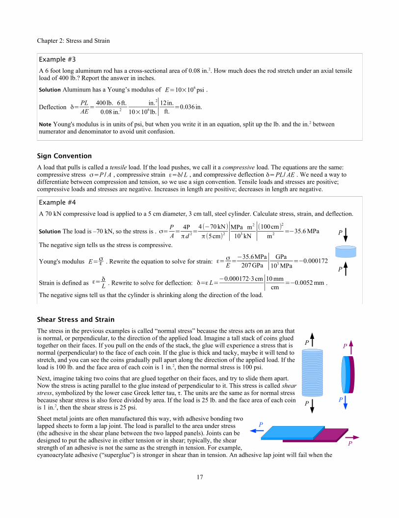
Shear Stress and Strain
The stress in the previous examples is called “normal stress” because the stress acts on an area thatis normal, or perpendicular, to the direction of the applied load. Imagine a tall stack of coins gluedtogether on their faces. If you pull on the ends of the stack, the glue will experience a stress that isnormal (perpendicular) to the face of each coin. If the glue is thick and tacky, maybe it will tend tostretch, and you can see the coins gradually pull apart along the direction of the applied load. If theload is 100 lb. and the face area of each coin is 1 in.2, then the normal stress is 100 psi.
Next, imagine taking two coins that are glued together on their faces, and try to slide them apart.Now the stress is acting parallel to the glue instead of perpendicular to it. This stress is called shearstress, symbolized by the lower case Greek letter tau, τ. The units are the same as for normal stressbecause shear stress is also force divided by area. If the load is 25 lb. and the face area of each coinis 1 in.2, then the shear stress is 25 psi.
Sheet metal joints are often manufactured this way, with adhesive bonding twolapped sheets to form a lap joint. The load is parallel to the area under stress(the adhesive in the shear plane between the two lapped panels). Joints can bedesigned to put the adhesive in either tension or in shear; typically, the shearstrength of an adhesive is not the same as the strength in tension. For example,cyanoacrylate adhesive (“superglue”) is stronger in shear than in tension. An adhesive lap joint will fail when the
17
P
P
P
P
P
P
P
P

Chapter 2: Stress and Strain
shear strength of the adhesive is exceeded.
If the sheet metal is held together with rivets instead of glue, theneach rivet is loaded in shear across its cross-section. The shearplane passes through the rivet where the two sheets meet. In abolted joint, use a bolt with a smooth shank instead of a bolt that isthreaded along its entire length. This way, the shear plane can passthrough the smooth shank, which has a larger cross-sectional areathan the root of a thread, and therefore can handle a higher applied load. Later in the book, we will see that the thread root also acts as a stress concentration site; yet another reason for keeping threads out of shear planes.
One way to produce holes in sheet metal is by punching them out with a punch and die set. The punch shears the sheet metal, so we can use shear stress calculations to figure out the stress in the sheet metal. The sheared area is perimeter of the shape that is punched times the thickness of the sheet metal t. The shear stress is the punch force divided by the sheared
surface: τ= PA
.
Example #5
A 3 mm thick aluminum sheet is cut with a 4 cm diameter round punch. Ifthe punch exerts a force of 6 kN, what is the shear stress in the sheet?Report the answer in MPa.
Solution The punch will create a round slug, where the cut edge is aroundthe circumference of the slug. Think of the cut edge as the wall of acylinder with a height of 3 mm and a diameter of 4 cm. The area equalsthe circumference of the circle times the thickness of the sheet metal:A=π dt .
Shear stress
τ= PA= Pπ dt
= 6kNπ⋅4cm⋅3 mm∣MPa m2
103 kN∣100 cmm ∣103 mm
m=15.9 MPa
A process engineer in a stamping plant will rewrite this equation to solve for P in order to find out whether a press is capable of punching out blanks of a given size in a sheet metal of known shear strength.
Shear stress controls the design of torsion members. Think of around shaft as a series of disks glued together on their faces. Ifyou twist the shaft with a torque T, the glue will be loaded inshear because the load is parallel to the face of each disk.
Consider a rectangular block loaded in shear. The block will distort as aparallelogram, so the top edge moves an amount δ. Divide the distortion bylength L perpendicular to the distortion, and you have the shear strain,γ= δ
L . Like normal strain, shear strain is unitless.
Consider the angle formed between the initial and loaded positions of the
block. From trigonometry, we know that tan ϕ= δL The amount of strain in the cartoon is exaggerated. For metals, concrete,
wood, and most polymers, angle ϕ is so small that tan ϕ≈ϕ if we measure the angle in radians, therefore ϕ≈γ= δL .
Key Equations
18
P
Pshearplane
punch
P
d
t slug
P
δ
Lϕ
TT

Chapter 2: Stress and Strain
Normal stress in a tensile or compressive member is the load divided by the cross-sectional area: σ= PA
Normal strain is the change in length parallel to the load divided by initial length: ε=Δ LL= δ
L
Young's modulus is the ratio of stress over strain within the elastic zone of the stress-strain diagram: E=σε
The change in length of a tensile or compressive member is derived from the three previous equations: δ= PLAE
Shear stress is the load divided by the area parallel to the load: τ= PA
Shear strain is the deformation parallel to the load divided by initial length perpendicular to the load: γ= δL .
19

Chapter 3: Poisson's Ratio and Thermal Expansion
Chapter 3: Poisson's Ratio and Thermal ExpansionPoisson's Ratio
Stretch a thick rubber band, and you notice the material gets thinner as it gets longer. This effect occurs in metals, plastics, concrete, and many other materials. We can predict how much the thickness changes with a materials property called Poisson’s ratio,5 which relates the strain along the tensile axis with the strain in the transverse (crosswise) direction. The symbol for Poisson’s ratio is ν, the lower case Greek letter nu, which looks similar to the lower case Roman letter v.
Poisson’s ratio is defined as ν=−εtransverse
εlong
, where εtransverse is the strain in the transverse
(crosswise) direction, and εlong is the strain along the longitudinal axis (sometimes called εaxial ). The sign convention for strain is positive for expansion, negative for shrinkage. Typical values of Poisson’s ratio are 0.25 for steel, 0.33 for aluminum, and 0.10 to 0.20 for concrete. We can
calculate the change in length of a rod by taking the definition of strain, εlong=δlong
L, and
rewriting it as δlong=εlong L . In the same way, we can calculate the change in diameter by substituting εtransverse for εaxial , and diameter d for length L: δtransverse=εtransverse L .
Example #1
An aluminum rod has a cross-sectional area of 0.19635 in.2. An axial tensile load of 6000 lb. causes the rod to stretch along its length, and shrink across its diameter. What is the diameter before and after loading? Report the answer in inches.
Solution The rod has a circular cross section, so the cross-sectional area before the rod is loaded is A= π4
d 2. Rewrite to
solve for the initial diameter, d=√ 4 Aπ =√ 4⋅0.19635 in.2
π =0.50000 in. .
When the rod is loaded, the axial strain is εlong=σE= P
AE= 6000 lb.
0.19635 in.2
in.2
10×106 lb.=0.00306 .
Poisson’s ratio ν=−εtransverse
εlong, so εtransverse=−ν⋅εlong=−0.33⋅0.00306=−0.00101
The change in diameter is δtransverse=εtransverse⋅d=−0.00101⋅0.50000in.=−0.000504 in.
The final diameter d f=d o+δtransverse=0.50000in.−0.000504 in.=0.4995 in.
In a civil engineering structure, a dimensional change of half a thousandth of aninch is insignificant, but in a machine it could affect performance. Imagine amachine part that slides in a slot: if the part is loaded axially in tension orcompression, Poisson’s effect could change a part that slides (slip fit) into a partthat sticks (press fit).
You can feel the effect of Poisson's ratio when you insert a rubber stopper or acork in a bottle. The Poisson's ratio of rubber is about 0.5, while cork is about0.0. If you try to push a rubber stopper into the neck of a bottle, the materialabove the neck will shorten and thicken, making it difficult to insert into thebottle. The harder you push, the more the stopper will expand in the transversedirection, and this expansion is about 50% of the compression in the axialdirection. Natural cork is made from the bark of the cork oak tree, and does not expand transversely when you push on it. The only resistance comes from compressing the cork in the bottle neck, and friction.
5 Named for Siméon Poisson, a French mathematician and physicist.
20
corkrubber
PP
shrinks
expands
P
εaxial
εtransverse

Chapter 3: Poisson's Ratio and Thermal Expansion
Consider a block that is pulled in two directions by forces Px and Py. The strain in the x
direction due to the axial stress from Px is εx axial=σ x
E . If Px is positive (tension), then
the strain is also positive...the bar is stretching along the x axis due to the action of Px.However, tensile load Py is acting to shrink the bar in the x direction; the strain due to
this transverse load is εx transverse=−νσ y
E. Add these two strains to find the total strain
in the x direction, εx=σ x
E−νσ y
E= 1
E(σ x−νσ y) . Similarly, the total strain in the y
direction is εy=σ y
E−νσ x
E= 1
E(σ y−νσ x) .
Real blocks, of course, are three-dimensional. If the block is loaded in all three directions, calculate the strain in the x, y, and
z directions as εx=1E(σ x−νσ y−νσ z) , εy=
1E(σ y−νσ x−νσ z) , and εz=
1E(σ z−νσ x−νσ y ) .
Example #2
Calculate the strains in the x, y, and z directions for the steel block loaded asshown.
Solution First, calculate the normal stress in the x, y, and z directions as the forcedivided by the perpendicular surface that it acts on.
The stress in the x direction acts on the right face of the block, so the normal
stress is σ x=3kN
2cm×4cm∣MPa m2
103 kN ∣(100cm)2
m2 =3.75 MPa . The stress in the y
direction acts on the top of the block, so the normal stress is
σ y=5kN
2cm×3cm∣MPa m2
103 kN ∣(100cm)2
m2 =8.33 MPa . The stress in the z direction
acts on the front face of the block, so the normal stress is σ z=−2 kN
3cm×4cm∣MPa m2
103kN ∣(100cm)2
m2 =−1.67 MPa . The load
and stress are negative because they are compressive.
Next, calculate the strains. Since the block is steel, Young's modulus is 207 GPa and Poisson's ratio is 0.25.
ε x=1E[σ x−νσ y−νσz ]=
1
207×103 MPa[3.75MPa−0.25(8.33MPa )−0.25 (−1.67 MPa)]=1.01×10⁻⁵
ε y=1E[σ y−νσx−νσz ]=
1
207×103 MPa[8.33 MPa−0.25 (3.75 MPa )−0.25(−1.67 MPa )]=3.77×10⁻⁵
ε z=1E[σz−νσx−νσ y]=
1
207×103MPa[−1.67 MPa−0.25(3.75 MPa )−0.25(8.33MPa )]=−2.26×10⁻⁵
21
Px
Py
Py = 5 kN
Px = 3 kN
Pz = 2 kN
4 cm
3 cm2 cm

Chapter 3: Poisson's Ratio and Thermal Expansion
Thermal Expansion and Thermal Stress
Heat a piece of steel, wood, or concrete, and it expands. Cool the same piece, and it shrinks.Plot the strain as a function of temperature change, and for most materials, you get arelatively straight line. The slope of the line is called the thermal expansion coefficient,Greek letter α. It tells us how much strain we can expect for a given temperature change.From the graph, the slope α=ε/ΔT . The units of α are strain divided by temperature:in./ in.
°F or
mm /mm°C
, which we can write as °F-1 or °C-1. Substitute the definition of
strain, ε=δ/ L , and we have α=δ
L(ΔT ) . Rewrite the equation to solve for thermal
deflection: δ=α L(ΔT ) .
The thermal expansion coefficient is a materials property; different materials expand at differentrates. For example, aluminum expands about twice as much as steel for a given temperature change, becauseαAluminum=23×10−6°C−1 and αSteel=12×10−6°C−1 . One reason we use steel as a reinforcement in concrete isαConcrete=11×10−6°C−1 , so the steel and concrete expand and contract at roughly the same rate. If the matrix and
reinforcement in a composite expand at different rates, then the matrix and reinforcement may separate under repeated thermal cycles.
The change in temperature can be positive or negative, and is defined as the final temperature minus the original temperature: ΔT=T f−T o . If the material is cooled from 70°F to 40°F, the change in temperature isΔT=40 °F−70°F=−30 °F . If the material is heated from 70°F to 90°F, the change in temperature isΔT=90 °F−70 °F=+20 °F .
Example #3
A 5 m aluminum flagpole is installed at 20°C. Overnight, the temperature drops to -5°C. How much does the height change, in millimeters? What is the final height of the flagpole, in meters?
Solution First, calculate the change in length using δ=α L(ΔT ) . From the Appendix, the thermal expansion coefficient for aluminum is αAluminum=23×10−6°C−1 . Next, calculate the final length by adding the change in length to the original length.
Change in length δ=αL (ΔT )=23×10−6
°C5 m(−5°C−20°C)∣103 mm
m=−2.88 mm . The negative sign indicates the
flagpole is getting shorter.
Final length L f=L+δ=5 m−2.88 mm∣ m
103 mm=4.997 m
Two cantilever beams made of different materials have a measurable gap between their ends.As the bars heat up, they grow towards each other and eventually meet if the temperaturerises enough. Each bar has a different thermal coefficient of expansion. How do we calculatethe temperature Tf at which they meet? Consider that the gap between the two bars equalsδtotal=δsteel+δbrass . Substitute the equation for thermal expansion, and we getδtotal=αsteel Lsteel (ΔT steel )+αbrass Lbrass(ΔT brass) . The change in temperature is the same for
both materials, so δtotal=ΔT (αsteel Lsteel+αbrass Lbrass) . Rewrite the equation to solve for
temperature change: ΔT=δtotal
αsteel Lsteel+αbrass Lbrass. The temperature change ΔT=T f−T o ,
so we can solve for the final temperature: T f=T o+δtotal
αsteel Lsteel+αbrass Lbrass.
22
Δ Temperature
Strainε α
steelTo brass
Lsteel
Lbrass
Tf
δthermal (steel)
+ δthermal (brass)
Chapter 3: Poisson's Ratio and Thermal Expansion
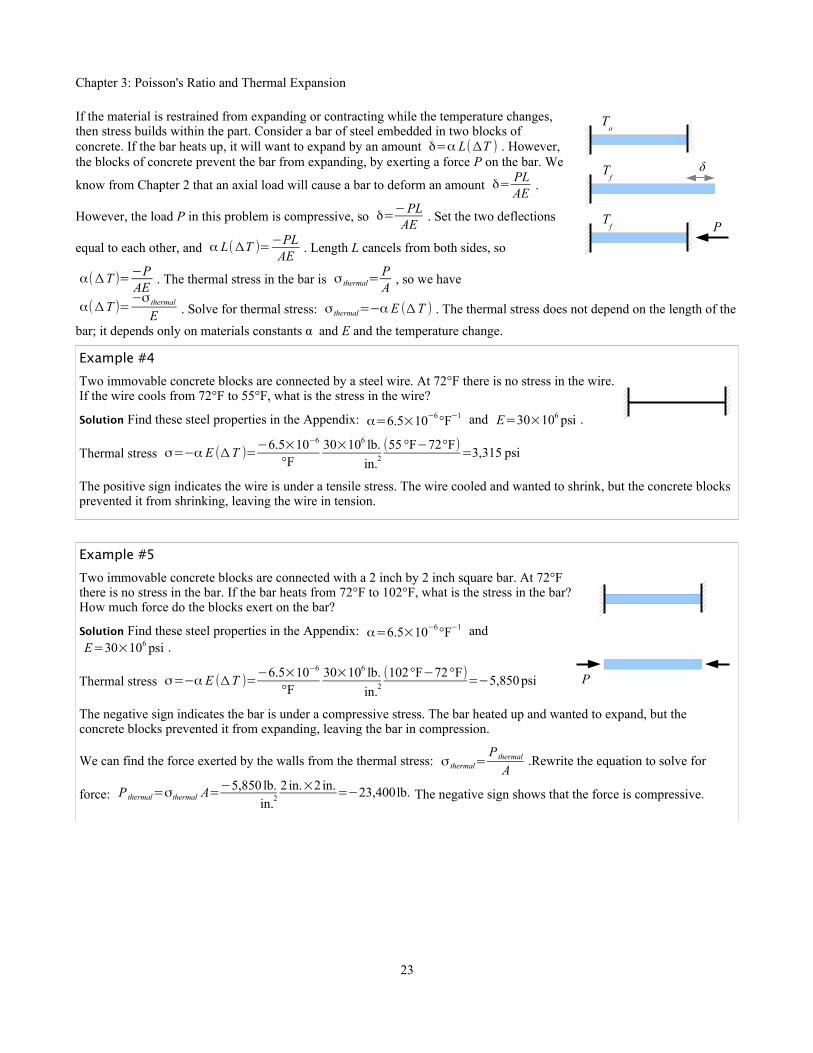
If the material is restrained from expanding or contracting while the temperature changes,then stress builds within the part. Consider a bar of steel embedded in two blocks ofconcrete. If the bar heats up, it will want to expand by an amount δ=α L(ΔT ) . However,the blocks of concrete prevent the bar from expanding, by exerting a force P on the bar. We
know from Chapter 2 that an axial load will cause a bar to deform an amount δ= PLAE
.
However, the load P in this problem is compressive, so δ=−PLAE
. Set the two deflections
equal to each other, and α L(ΔT )=−PLAE
. Length L cancels from both sides, so
α(ΔT )=−PAE
. The thermal stress in the bar is σ thermal=PA
, so we have
α(ΔT )=−σ thermal
E . Solve for thermal stress: σ thermal=−α E (ΔT ) . The thermal stress does not depend on the length of the
bar; it depends only on materials constants α and E and the temperature change.
Example #4
Two immovable concrete blocks are connected by a steel wire. At 72°F there is no stress in the wire.If the wire cools from 72°F to 55°F, what is the stress in the wire?
Solution Find these steel properties in the Appendix: α=6.5×10⁻⁶°F−1 and E=30×106 psi .
Thermal stress σ=−α E (ΔT )=−6.5×10⁻⁶
°F30×106 lb.
in.2(55 °F−72°F)=3,315 psi
The positive sign indicates the wire is under a tensile stress. The wire cooled and wanted to shrink, but the concrete blocks prevented it from shrinking, leaving the wire in tension.
Example #5
Two immovable concrete blocks are connected with a 2 inch by 2 inch square bar. At 72°Fthere is no stress in the bar. If the bar heats from 72°F to 102°F, what is the stress in the bar?How much force do the blocks exert on the bar?
Solution Find these steel properties in the Appendix: α=6.5×10⁻⁶°F−1 andE=30×106 psi .
Thermal stress σ=−α E (ΔT )=−6.5×10⁻⁶
°F30×106 lb.
in.2(102°F−72 °F)=−5,850 psi
The negative sign indicates the bar is under a compressive stress. The bar heated up and wanted to expand, but the concrete blocks prevented it from expanding, leaving the bar in compression.
We can find the force exerted by the walls from the thermal stress: σ thermal=P thermal
A.Rewrite the equation to solve for
force: P thermal=σthermal A=−5,850 lb.in.2
2in.×2in.=−23,400lb. The negative sign shows that the force is compressive.
23
P
To
P
Tf
Tf
δ

Chapter 3: Poisson's Ratio and Thermal Expansion
Some thermal expansion problems require both the deflection and the stress equations. Forexample, if this cantilever beam heats up sufficiently, it will meet the right-hand wall. If thetemperature continues to rise, stress will build up in the beam. If you know the initial length,material, and temperatures To and T2 (but not temperature T1), how do you find the thermalstress? Use the thermal deflection equation and the temperature change ΔT=T 1−T o to figureout temperature T1, then use the thermal stress equation and the temperature changeΔT=T 2−T 1 to figure out σthermal at temperature T2.
Key Equations
Poisson's ratio is the decrease in transverse strain to the increase in longitudinal strain: ν=−εtransverseεlong
Calculate the strains in an elastic block loaded in the x, y, and z directions as εx=1E(σ x−νσ y−νσ z) ,
εy=1E(σ y−νσ x−νσ z) , and εz=
1E(σ z−νσx−νσ y ) . If a load does not exist in one of the directions, then the stress term
for that direction is zero, and the equations become simpler.
Change in length due to a change in temperature is a function of the thermal expansion coefficient, the initial length, and thechange in temperature: δ=α L(ΔT )
Stress due to a change in temperature is a function of the thermal expansion coefficient, Young's modulus, and the change intemperature: σ thermal=−α E (ΔT )
24
To
T1 >T
o
no contact, σ = 0
contact, σ = 0
contact, σ > 0T2 >T
1

Chapter 4: Pressure Vessels and Stress Concentrations
Chapter 4: Pressure Vessels and Stress ConcentrationsThin-Walled Pressure Vessels
A pressure vessel is a container that holds a fluid (liquid or gas) under pressure. Examples include carbonated beverage bottles, propane tanks, and water supply pipes. Drain pipes are not pressure vessels because they are open to the atmosphere.
In a small pressure vessel such as a horizontal pipe, we can ignore the effects of gravity on the fluid.In the 17th century, French mathematician and physicist Blaise Pascal discovered that internal fluidpressure pushes equally against the walls of the pipe in all directions, provided the fluid is not moving.The SI pressure and stress unit, the pascal (Pa), is named after Pascal because of his work with fluidpressure. The symbol for pressure is lower-case p, not to be confused with upper-case P used for pointloads.
If the thickness of the wall is less than 10% of the internal radius of the pipe or tank, then the pressurevessel is described as a thin-walled pressure vessel. Because the wall is thin, we can assume that thestress in the wall is the same on the inside and outside walls. (Thick-walled pressure vessels have a higher stress on the inner wall than on the outer wall, so cracks form from the inside out.)
Imagine cutting a thin-walled pipe lengthwise through the pressurized fluid andthe pipe wall: the force exerted by the fluid must equal the force exerted by thepipe walls (sum of the forces equals zero). The force exerted by the fluid isp⋅A= p di L where di is the inside diameter of the pipe, and L is the length of
the pipe. The stress in the walls of the pipe is equal to the fluid force divided bythe cross-sectional area of the pipe wall. This cross-section of one wall is thethickness of the pipe, t, times its length. Since there are two walls, the totalcross-sectional area of the wall is 2 t L . The stress is around the circumference
or the “hoop” direction, so σhoop=p d i L2 t L
. Notice that the length cancels: hoop
stress is independent of the length of the pipe, so σhoop=p d i
2 t.
Example #1
A pipe with a 14 inch inside diameter carries pressurized water at 110 psi. What is the hoop stress if the wall thickness is 0.5 inches?
Solution First, check if the pipe is thin-walled. The ratio of the pipe wall thickness to the internal radius istri
= 0.5 in.12(14 in.)
=0.071<0.10, so the pipe is thin-walled.
Hoop stress σhoop=p d i
2 t=110 psi⋅14in.
2⋅0.5 in.=1,540 psi
What if the pipe has a cap on the end? If the cap were loose, pressure would push the cap off theend. If the cap is firmly attached to the pipe, then a stress develops along the length of the pipe toresist pressure on the cap. Imagine cutting the pipe and pressurized fluid transversely. The forceexerted by the fluid equals the force along the length of the pipe walls. Pressure acts on a circular
area of fluid, so the force exerted by the fluid is P fluid=p⋅A= p π4
d i2
. The cross-sectional area
of the pipe wall A= π4
d o2−π
4d i
2=π4(d o
2−d i2) . We can estimate the cross-sectional area of a thin-walled pipe pretty closely
by multiplying the wall thickness by the circumference, so A≈π di t . The stress along the length of the pipe is
σ long=P fluid
Apipe
=pπ d i
2
4π di t. Simplify by canceling π and one of the diameters: σ long=
pd i
4 t.
25
p
p
L
di
p

Chapter 4: Pressure Vessels and Stress Concentrations
Compare the hoop stress and longitudinal stress equations: in a thin-walled pipe, hoop stress is twice as large as longitudinalstress. If the pressure in a pipe exceeds the strength of the material, then the pipe will split along its length (perpendicular to the hoop direction).
Does the shape of the cap affect the longitudinal stress in thepipe? No, because only the cross-sectional area of the pipematters. Typically, pressure vessels have concave or convexdomes, because flat caps tend to deflect under pressure, but theshape has no effect on longitudinal stress in the pipe walls.
A welded steel outdoor propane tank typically consists of a tube with twoconvex hemispherical caps (right). Hoop stress controls the design in thetube portion. Where the caps are welded to the tubes, longitudinal stresscontrols the design. If the steel is all the same thickness (and the welds areperfect), then the tank will fail in the tube section because hoop stress istwice the longitudinal stress. A spherical tank (far right) only haslongitudinal stress, so it can handle twice the pressure of a tubular tank.Think of a spherical tank as two hemispheres welded together; the weldprevents the two halves from separating.
In conclusion, if you have a pipe or a tubular tank, use σhoop=p d i
2 t. If you
have a spherical tank, use σ long=pd i
4 t.
The ASME Boiler Code recommends using an allowable stress σallowable=14σUTS or σallowable=
23σYS , whichever is smaller.
Example #2
What is the minimum thickness of a spherical steel tank if the diameter is 10 feet, internal pressure is 600 psi, the tensile strength of the steel is 65ksi, and the yield strength of the steel is 30 ksi?
Solution First, calculate the allowable stress. Next, rewrite the stress equation for longitudinal stress (because this is a sphere, not a pipe) to solve for wall thickness.
Based on tensile strength, σallowable=14σUTS=
65 ksi4
=16.25 ksi . Based on yield strength,
σallowable=23σYS=
2⋅30 ksi3
=20 ksi ; therefore, use 16.25 ksi because it is the smaller number.
Longitudinal stress σ long=pd i
4 t. Rewrite the equation for thickness, t=
p d i
4σallowable
=600psi⋅10 ft4⋅16.25ksi ∣ ksi
103 psi∣12in.ft
=1.11in.
The welds in real steel tanks contain defects, which reduce the strength of the welds. We can measure the strength of weldedjoints in the lab and compare them with the strength of the base metal. If the strengths match, we say the joint is 100% efficient. If the weld strength is 80% of the base metal strength, we say the joint is 80% efficient. In the previous example, the allowable stress was 16.25 ksi. Multiply this value by 0.80 to get the allowable stress of an 80% efficient joint. The wall
thickness would be t=p d i
4σallowable
= 600 psi⋅10 ft4(0.8×16.25 ksi)∣ ksi
103 psi∣12 in.ft
=1.38 in.
26
p p
p
longitudinal stress
hoop stress
p

Chapter 4: Pressure Vessels and Stress Concentrations
Stress Concentration in Tension
Pull a bar in tension, and the tensile stress in the bar will be uniform
within the bar: σ=P
Agross where Agross is the gross cross-sectional area
of the bar. If the bar has a hole in it, we would expect the stress to be
higher because there is less material: σnet=P
Anet where Anet is the net
cross-sectional area of the bar (gross area minus the area of the hole). Experiments show the stress is not uniform within the remaining solid material; instead, it is highest next to the hole, and lower as you move away from the hole. We say that the stress is concentrated next to the hole.
The maximum stress adjacent to the hole is σmax=K σnet=K PAnet
, where K is a stress concentration factor that depends on
the size of the bar and the diameter of the hole. In general, the smaller the radius, the higher the stress. For example, cracks have very high stress concentrations at their tips, exceeding the tensile strength of the material, even though the average stress in the part is well below the yield strength; this explains why cracks grow. One way to prevent a crack from growing in a material is to drill a hole at its tip.
Stress concentrations can occur anywhere there is a change in geometry with a small radius, such as holes, fillets, and grooves. In the 1930s, M.M. Frocht6 published a series of graphs relating K to the dimensions of the bar and hole (or fillet or groove), and R.E. Peterson published scientific papers on fatigue cracks which start at stress concentrations. Peterson's book on stress concentration factors7 is stillin print.
This graph is based on Frocht's original work. Use a four-step process to solve stress concentration problems:
Step 1 Divide the hole diameter by the gross width of the bar to find the ratiod /h gross .
Step 2 Find the value of K from the graph.
Step 3 Calculate the net cross-sectional area (gross cross-sectional area minus the cross-sectional area of the hole). The easiest way to find this value is to multiply the net width by the thickness.
Step 4 Calculate the maximum stress using σmax=K PAnet
6 M.M. Frocht, “Photoelastic Studies in Stress Concentration,” Mechanical Engineering, Aug. 1936, 485-489. M.M. Frocht, “Factors ofStress Concentration Photoelastically Determined", ASME Journal of Applied Mechanics 2, 1935, A67-A68.
7 Walter D. Pilkey & Deborah F. Pilkey, Peterson's Stress Concentration Factors, 3rd ed., Wiley, 2008.
27
P
σ
P
σ
Pd
0.0 0.1 0.2 0.3 0.4 0.5 0.6 0.72.0
2.2
2.4
2.6
2.8
d / hgross
K
hgross
Circular hole in a rectangular cross-section bar loaded in tension

Chapter 4: Pressure Vessels and Stress Concentrations
Example #3
A bar measuring 80 mm wide by 16 mm thick has a 20 mm diameter hole in the center. The tensile load on the bar is 900 N. Calculate the maximum stress in the bar due to the stress concentration. Report the result in MPa.
Solution Divide the hole diameter by the gross cross-sectional width of the bar: d
h gross
= 20 mm80 mm
=0.25 . Use the graph to
find K≈2.36 . The net cross-sectional area of the bar is the net width times the thickness. The net width is the gross widthminus the hole diameter, so Anet=(80 mm−20 mm)16 mm=960mm2
Maximum stress is σmax=KP
Anet
=2.36900 N
960mm2∣MPa mm2
N=2.2 MPa
Use a similar four-step process to solve stress concentration problems in tensile bars having fillets or semicircular grooves.
Step 1 Divide the groove or fillet radius by the net width of the bar to find the ratio r /hnet .
Step 2 Find the value of K from the graph on the following page. Be sure to use the right curve!
Step 3 Calculate the net cross-sectional area at the groove or fillet.
Step 4 Calculate the maximum stress using σmax=K PAnet
Example #4
A 1/4 in. thick, 2 in. wide bar has two semicircular 3/8 in. radius grooves. The tensile load on the bar is 1 ton. Find the maximum stress in the bar due to the stress concentration. Report the result inksi.
Solution Net width hnet=2in.−2(0.375in.)=1.25 in.
Calculate r
hnet
=0.375in.1.25 in.
=0.30 .
From the graph, K≈1.82 . The net cross-sectional area is the net width times the thickness:
Anet=1.25 in.×0.25 in.=0.3125in.2 . Maximum stress is σmax=KP
Anet
=1.821 ton
0.3125 in 2∣2kipston
=11.6 ksi
28
P = 900 N
d = 20 mm
hgross
= 80 mm
r = 3/8 in.
hnet
hgross
= 2in.P = 1 ton

Chapter 4: Pressure Vessels and Stress Concentrations
Key Equations
Hoop stress in a pressure vessel is equal to the internal pressure times the inside diameter divided by twice the wall
thickness: σhoop=p d i
2 t. This equation is used for pipes.
Longitudinal stress in a pressure vessel is equal to the internal pressure times the inside diameter divided by the wall
thickness: σ long=pd i
4 t. This equation is used for spherical pressure vessels.
For welded tanks, the ASME Boiler Code recommends using σall=14σUTS or σall=
23σYS , whichever is smaller.
Stress at a stress concentration equal to the stress concentration factor times the average stress at the net cross-sectional area: σ=Kσnet . Use stress concentration graphs to find the value of K.
29
σ
0.0 0.1 0.2 0.3 0.4 0.5 0.6 0.71.2
1.4
1.6
1.8
2.0
r / hnet
K
Semicircular grooves and quarter-circle fillets in a rectangularcross-section bar loaded in tension
0.8 0.9 1.0
2.2
2.4
2.6
2.8
P
r
hnet
Fillets
Grooves
Fillets
P
rGrooves
hnet
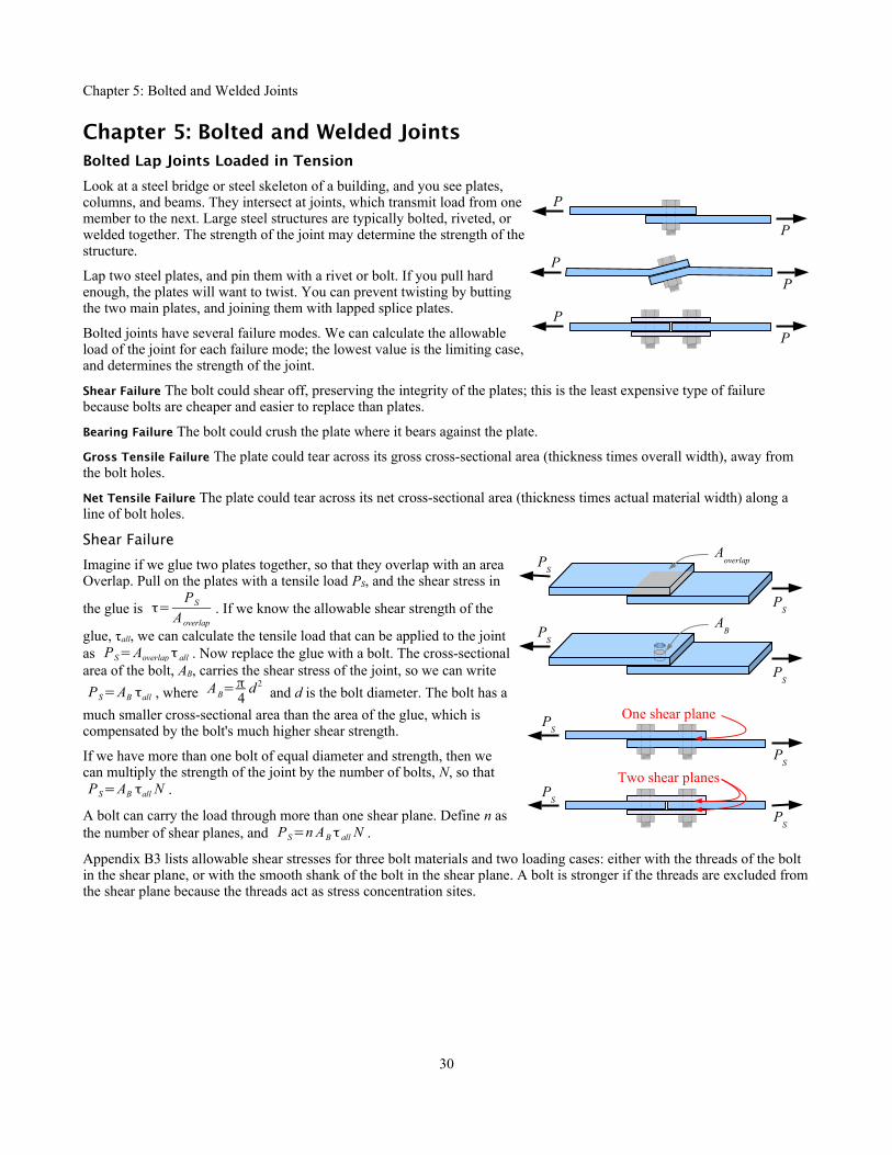
Chapter 5: Bolted and Welded Joints
Chapter 5: Bolted and Welded JointsBolted Lap Joints Loaded in Tension
Look at a steel bridge or steel skeleton of a building, and you see plates,columns, and beams. They intersect at joints, which transmit load from onemember to the next. Large steel structures are typically bolted, riveted, orwelded together. The strength of the joint may determine the strength of thestructure.
Lap two steel plates, and pin them with a rivet or bolt. If you pull hardenough, the plates will want to twist. You can prevent twisting by buttingthe two main plates, and joining them with lapped splice plates.
Bolted joints have several failure modes. We can calculate the allowableload of the joint for each failure mode; the lowest value is the limiting case,and determines the strength of the joint.
Shear Failure The bolt could shear off, preserving the integrity of the plates; this is the least expensive type of failure because bolts are cheaper and easier to replace than plates.
Bearing Failure The bolt could crush the plate where it bears against the plate.
Gross Tensile Failure The plate could tear across its gross cross-sectional area (thickness times overall width), away from the bolt holes.
Net Tensile Failure The plate could tear across its net cross-sectional area (thickness times actual material width) along a line of bolt holes.
Shear Failure
Imagine if we glue two plates together, so that they overlap with an areaOverlap. Pull on the plates with a tensile load PS, and the shear stress in
the glue is τ=PS
Aoverlap
. If we know the allowable shear strength of the
glue, τall, we can calculate the tensile load that can be applied to the jointas PS=Aoverlap τ all . Now replace the glue with a bolt. The cross-sectionalarea of the bolt, AB, carries the shear stress of the joint, so we can write
PS=AB τall , where AB=π4
d 2 and d is the bolt diameter. The bolt has a
much smaller cross-sectional area than the area of the glue, which iscompensated by the bolt's much higher shear strength.
If we have more than one bolt of equal diameter and strength, then wecan multiply the strength of the joint by the number of bolts, N, so thatPS=AB τall N .
A bolt can carry the load through more than one shear plane. Define n asthe number of shear planes, and PS=n AB τ all N .
Appendix B3 lists allowable shear stresses for three bolt materials and two loading cases: either with the threads of the bolt in the shear plane, or with the smooth shank of the bolt in the shear plane. A bolt is stronger if the threads are excluded fromthe shear plane because the threads act as stress concentration sites.
30
P
P
P
P
P
P
PS
PS
Aoverlap
PS
PS
AB
PS
PS
PS
PS
One shear plane
Two shear planes

Chapter 5: Bolted and Welded Joints
Example #1
Two A-36 steel plates are joined with two splice plates andeight 3/4 in. diameter A325 bolts. The plates are 6 in. wide and1.5 in. thick; the splice plates are the same width, and 0.8 in.thick. Bolt threads are excluded from the shear plane. Calculatethe load that the joint can support in order to resist shearfailure. Report the result in kips.
Solution From Appendix B3, A325 bolts with threads excludedfrom the shear plane have a shear strength of 30 ksi. The problem is symmetrical,so either the four bolts in the left plate will fail in shear first, or the four bolts in theright plate will fail first. Therefore, we can erase half of the diagram, and focus onfour bolts, and N = 4.
The load is carried by two shear planes per bolt, so n = 2.
P S=n AB τ all N=2 shear planesbolt
⋅
π4(0.75in.)2
shear plane⋅30
kips
in.2 ⋅4 bolts=106 kips
Bearing Failure
If one or more of the plates is crushed by the bolt, then the area that is crushed equals the bolt diameter, d, times the platethickness, t. Multiply this area by the bearing strength of the plate, and we have the allowable bearing load for a joint with one bolt: PP=d t σ P−all .
The allowable bearing load for a joint with multiple bolts isPP=d t σ P−all N .
If the main plate is thicker than the sum of the thicknesses of two splice plates, then use the sum of the splice plate thicknesses for t.
The allowable bearing stress is listed in Appendix B4; it is 1.5 times the ultimate tensile strength of the plate material.
Example #2
Calculate the load that the joint in Example #1 can support in order to resist bearing failure. Report the result in kips.
Solution From the Allowable Plate Stress table, A-36 steel plates have an allowable bearing strength of 87 ksi. The two splice plates have a combined thickness of 1.6 in., which is greater than the main plate thickness of 1.5 in. Using the smaller of the two numbers, t = 1.5 in.
P P=d t σP−all N=0.75in.bolt
⋅1.5in.⋅87 kips
in.2 ⋅4 bolts=392 kips
Gross Tensile Failure
The gross cross-sectional area of the plate some distance away from the bolt holes is the width, b, times the thickness, t. Check the gross cross-sectional areas of both the main plate and the splice plates, and use the smaller of the two. Multiply this area by the gross tensile strength of the plate to find the allowable gross tensile load for the joint: PG=b t σG−allowable . The allowable gross tensile strength is 60% of the yield strength of the plate material, listed in Appendix B4.
31
PP
PP
PP
PP
Zones where the plate is crushed by the bolt
PS
PS
PS
PS
6"
1.5"
0.8"
PS
PS
PS
PS

Chapter 5: Bolted and Welded Joints
Example #3
Calculate the load that the joint in Example #1 can support in order to resist gross tensile failure. Report the result in kips.
Solution From Appendix B4, A-36 steel plates have an allowable gross tensile strength of 21.6 ksi.
P G=bt σG−all=6.0 in.⋅1.5 in.⋅21.6 kips
in.2 =194 kips
Net Tensile Failure
The net cross-sectional area of the plate at the bolt holes is the gross cross-sectional area, AG, minus the cross-sectional area of the holes, AH. Each hole has a cross-sectional area perpendicular to the direction of the load equal to the hole diameter, dH, times the plate thickness, t: AH=d H t . As a rule of thumb for structural applications, use a hole diameter 1/8 inch or 3 mm larger than the nominal bolt diameter.
The plate will fail along the line of one set of holes. Defining the number of holes in the fracture plane as NF, the net cross-sectional area is AN=AG−AH=bt−N F d H t . The allowable net tensile load is this area times the allowable net tensile strength: PN=(bt−N F d H t )σN −all . The allowable net tensile strength, listed in Appendix B4, is half of the ultimate tensilestrength of the plate material.
Both joints have six bolts per symmetrical half, but the joint on the left has three holes in the fracture plane, while the joint on the right has two holes in the fracture plane.
Example #4
Calculate the load that the joint in Example #1 can support in order to resist net tensile failure. Report the result in kips.
Solution From Appendix B4, A-36 steel plates have an allowable net tensile strength of 29 ksi. The hole diameter is 1/8 in.larger than the nominal bolt diameter, so d H=3 /4in+1/8in.=7 /8 in.
P N=(6in.⋅1.5 in.−2 holes7 /8in.⋅1.5in.
hole )29kips
in.2=185 kips
32
PN
PN
PN
PN
Fracture
PN
PN
PN
PN
FractureNF = 2N
F = 3
PG
PG
PG
PG
Fracture
b
t/2PG
PG
PG
PG
Fracture
b
t

Chapter 5: Bolted and Welded Joints
Joint Efciency
Punching holes in steel causes it to weaken, so a joint may be weaker than the base material. Analysis of the roof of the Hartford Civic Center, which collapsed in January 1978 under a load of heavy wet snow, showed that some joint plates consisted of 85% holes, 15% steel! This flaw was one of several design and construction errors that led to the roof collapse.
We can calculate the efficiency of the joint by dividing the minimum joint strength by the gross strength of the plate some distance away from the joint.
Example #5
Calculate the efficiency of the joint in the previous Examples. Report the result in percent.
Solution The minimum joint strength is 144 kips (bolt shear failure). The gross tensile load of the plate is 194 kips. Joint
efficiency is J.E.=106 kips194 kips
=0.55=55% .
J.E.<100 indicates an overloaded joint will fail before the structure does. This is the better failure mode for repairability, because it is easier to replace a bolt than to replace an I-beam. J.E.≪100 indicates a poorly designed joint, which could be improved with stronger bolts, more bolts, or a better hole pattern.
J.E.>100 indicates an overdesigned joint – the structure will fail before the joint.
Solution Method for Bolted Joints
Use all of the previous steps. Solve for P based on bolt shear failure, bearing failure, gross tensile failure, and net tensile failure. The lowest value of P is the limiting case. Divide this result by PG to find the efficiency of the joint.
33

Chapter 5: Bolted and Welded Joints
Example #6
Two A-36 steel plates are joined with two splice plates and twelve 25 mm diameter A325-X high strength bolts. The main plates are 150 mm wide and 10 mm thick; the splice plates are 125 mm wide and 7 mm thick. Calculate the load that the joint can support; report the result in kN. Calculate the joint efficiency; report the result in percent.
Solution Solve for P based on shear, bearing, gross tensile, and net tensile; the lowest value is the limiting case. Divide this result by PG to find the efficiency of the joint.
Shear The “X” in A325 -X means bolts with threads excluded from the shear plane. From the Bolt Shear Strengthtable, these bolts have a shear strength of 207 MPa.
The problem is symmetrical, so we can erase half of the diagram, and N = 6. The load is carried by two shear planes per bolt, so n = 2.
P S=n AB τallowable N=2 shear planesbolt
π4(25 mm)2
shear plane207MPa ⋅6 bolts∣ 103 kN
MPa m2∣ m2
(103 mm)2=1220 kN
Bearing From Appendix B4, the allowable bearing stress in the plates is 600 MPa. The two splice plates have a total thickness of 14 mm, which is thicker than the 10 mm thick main plate, therefore t = 10 mm.
P P=d t σP−allowable N= 25 mmbolt
10 mm⋅600 MPa 6 bolts∣ 103 kNMPa m2∣ m2
(103mm)2=900 kN
Gross Tensile From Appendix B4, the allowable gross tensile stress is 150 MPa. The splice and main plates have different thicknesses and widths, so calculate PG both ways. Note the splice plate total thickness t=7mm+7mm=14 mm .
Splice plates: PG=bt σG−allowable=125mm⋅14 mm⋅150MPa∣ 103kN
MPa m2 ∣ m2
(103 mm)2=263kN
Main plate: PG=bt σG−allowable=150mm⋅10 mm⋅150 MPa∣ 103 kN
MPa m2∣ m2
(103 mm)2=225kN . Use this lower value for PG.
Net Tensile From Appendix B4, the allowable net tensile stress is 200 MPa. Calculate PN both ways.
Splice plates:
P N=(b t−N F d H t )σN−allowable=(125 mm⋅14 mm−2holes28 mm⋅14 mm
hole )200MPa ∣ 103kNMPa m2 ∣ m2
(103 mm)2=193kN
Main plate:
P N=(bt−N F d H t )σN−allowable=(150 mm⋅10 mm−2holes28 mm⋅10 mm
hole )200MPa ∣ 103 kNMPa m2∣ m2
(103 mm)2=188kN
The lowest value is 188 kN, so the joint will fail first by fracturing across a line of bolt holes.
Joint Efciency Pmin=188kN and PG−main plate=225kN . J.E.=188 kN225 kN
=0.84=84 %
34
10 mm
P
P
P
P
P
P
P
P
150 mm125 mm
7 mm

Chapter 5: Bolted and Welded Joints
Welded Lap Joints
Bolted and riveted joints contain holes which may act as stressconcentration sites. If joined plates have to be watertight, such as theplates in a tank or a ship, then welding is a better choice. Welding isalso a good choice for parts that will not be disassembled in the future.If you have ever soldered copper pipes together, you have melted thesolder but not the pipes. In welding, the weld metal and the base metalmelt together. In electric arc welding, an electric arc is struck betweenan electrode and the base metal. The arc melts the metals, and theelectrode is gradually consumed. Welding problems in this chapterfocus on continuous electric-arc fillet welds in lapped steel joints.
In cross-section, a fillet weld looks roughly like a right triangle. The size l of a fillet weld is the length of a leg of the triangle. Overloadedfillet welds fail by shearing along the throat h. Using trigonometry,h≈l sin 45° . The weld supports shear load PS over and area h×L ,
where L is the total length of the weld. The allowable shear strength ofthe weld metal is τallowable=0.3σUTS . Combining these equations, the load that the welded joint can support isP weld=τ allowable×area=0.3σUTS l sin 45° L=0.212⋅l⋅L⋅σUTS
Weld strength is proportional to weld size, weld length, and the strength of the electrode. E60 electrodes have an ultimate tensile strength of 60 ksi, while E70 electrodes have a tensile strength of 70 ksi. Appendix B5 shows joint strengths for common plate thicknesses. The values come from P weld=0.212⋅l⋅L⋅σUTS . Use Appendix B5 for common weld and plate sizes; use the equation for a different electrode such as E90, or for a nonstandard plate size.
The strengths in the table are given as load per unit length; multiply this value by the total length of the weld to find the shear load capacity of the welded joint. For example, a 6 in. long, 7/16 in. weld, using an E60 electrode, has a strength of
5.57 kips/in. The weld can support a load of P weld=6 in. 5.57kips
in.=33.4 kips .
Weld strength is not the only consideration when you design a welded joint. AISC recommends the following practices:
End Return The end of a fillet weld creates a stress concentration. Run the weld around the end of the top plate to minimize this effect. The length of the end return should be at least twice the nominal weld size:, a 3/8 in. weld should wrap around the end at least 0.75 in. End returns are included in the total weld length, L.
Lap Based on Thickness Two plates in a lap joint should lap at least five times the thickness of the thinner plate, and no lessthan 1 inch. For example, a 3/8 in. thick plate welded to a 1/2 in. thick plate should lap at least 3/8 in.×5=1.875 in. ; an 1/8in. plate welded to a 1/4 in. plate should lap at least 1 in. because 1/8 in.×5=0.625 in. , which is less than an inch.
Lap Based on Width This rule applies to welds that are parallel to the loading direction. Two plates in a lap joint should lap at least the width b of the narrower plate, unless the weld wraps fully around the end of the plate (i.e., the end returns meet at the centerline). For example, a 3/8 in. thick, 6 in. wide plate welded along its sides to a 1/2 in. thick, 8 in. wide plate should lap at least 6 in.
Weld Size The leg of a fillet weld can be made as large as the thickness of the top plate, or smaller; AISC recommends ranges of size according to Appendix B6. If the top plate is less than 1/4 in. thick, then the leg can be as large as the thickness; for thicker plates, the leg should be no larger than 1/16 in. less than the plate thickness.
Joint Efciency
Calculate the efficiency of a welded joint the same way as for a bolted joint: divide the joint load by the gross tensile load inthe plate with the smaller cross-section.
35
Pweld
end return
A A
Section A-Adetailleg size, l
throat, h
Pweld
b
t
lap

Chapter 5: Bolted and Welded Joints
Example #7
Two 3/8 in. thick, 6 in. wide plates made of A36 steel are welded asshown. Select the maximum size weld, and using an E70 electrode,determine the joint strength, reporting the result in kips. Also,calculate the efficiency of the joint.
Solution From Appendix B6, the maximum weld size is 5/16 in. FromAppendix B5, a 5/16 in. weld made with an E70 electrode cansupport a load of 4.63 kips/in. Each weld can support a load of
PS=4.63 kips
in.6 in.=27.78 kips . Since there are two welds, the joint
strength is PS=2×27.78kips=55.56kips
From Appendix B4, A36 steel has an allowable gross tensile strength of 21.6 ksi. The gross plate strength is
PG=bt σG−allowable=6in.⋅3/8in.⋅21.6 ksi=48.6 kips . J.E.=55.56 kips48.60 kips
=1.14=114 % , which means that the joint is
stronger than the base metal. If the structure fails, the plate will crack while the joint remains intact.
Example #8
A 3/8 in. thick, 6 in. wide plate made of A992 high-strength steel is welded to a 1/2 in. thick, 8 in. wide plate using a 3/16 in. weld with an E90 electrode. Determine the joint strength, reporting the result in kips. Also, calculate the efficiency of the joint.
Solution Appendix B5 does not include data for the E90 electrode; instead, use the weld strength equation. The length of each weld is 7 in. plus the 1 in. end return, or 8 in. The total weld lengthL=2(8in.)=16 in. The tensile strength of an E90 weld is 90 ksi.
The joint can support a load of
PS=0.212⋅l⋅L⋅σUTS=0.212⋅ 316
in.⋅16 in.⋅90 kipsin.2 =57.2 kips .
From Appendix B4, A992 steel has an allowable gross tensile strength of 30.0 ksi. Use the smaller plate cross-sectional area (the top plate). The gross plate strength is
PG=bt σG−allowable=6in.⋅ 38
in.⋅30.0 kipsin.2 =67.5kips .
J.E.=57.2 kips67.5 kips
=0.85=85 % , which means that the joint is 15%
weaker than the 6 in. plate. The joint could be strengthened in several ways: a larger weld bead, a stronger weld electrode, a continuous bead around the end of the top plate, or a weld bead underneath.
Key Equations
Check bolted joints for shear, bearing, gross tensile, and net tensile failure; the lowest result is the limiting case. With a symmetrical spliced joint, erase half of the joint and solve.
The allowable shear load for a bolted joint is PS=n AB τ allowable N where n is the number of shear planes per bolt, AB is the cross-sectional area of the bolt (calculated from its nominal diameter), τallowable is the allowable shear stress of the bolt (see
36
Pweld
Pweld
3/8 in.
Pweld
Pweld
6 in.
3/8 in.
Pweld
Pweld
6 in.
7 in.
1 in.
3/8 in.
Pweld
Pweld
1/2 in.
Pweld
Pweld
Pweld
Pweld

Chapter 5: Bolted and Welded Joints
Appendix B3), and N is the number of bolts being considered.
The allowable bearing load for a bolted joint is PP=d t σ P−allowable N where d is the nominal bolt diameter, t is the plate thickness (either the thickness of the main plate, or the combined thicknesses of the splice plates, whichever is smaller), and σP-allowable is the allowable bearing stress in the plate (see Appendix B4).
The allowable gross tensile load for a bolted joint is PG=bt σG−allowable where b is the plate width and σG-allowable is the allowable gross tensile stress in the plate.
The allowable net tensile load for a bolted joint is PN=(bt−N F d H t )σN−allowable where NF is the number of holes in the fracture plane, dH is the nominal hole diameter (1/8 inch or 3 mm larger than d), and σN-allowable is the allowable net tensile stress in the plate.
The allowable tensile load of a fillet-welded joint is PS=0.212⋅l⋅L⋅σUTS . If standard plates are used with E60 or E70 electrodes, then use Appendix B5 to find the allowable tensile load.
The efficiency of a bolted or welded joint equals the lowest allowable load divided by the allowable load of the weaker of the two plates some distance from the joint.
37
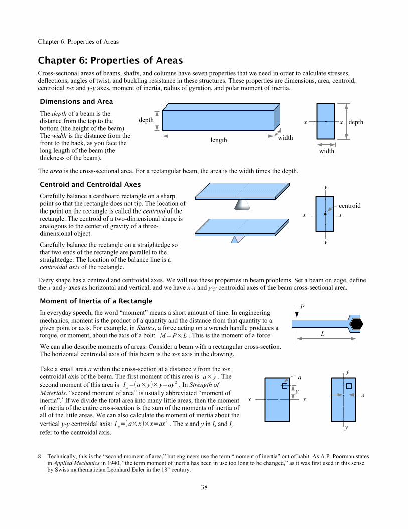
Chapter 6: Properties of Areas
Chapter 6: Properties of AreasCross-sectional areas of beams, shafts, and columns have seven properties that we need in order to calculate stresses, deflections, angles of twist, and buckling resistance in these structures. These properties are dimensions, area, centroid, centroidal x-x and y-y axes, moment of inertia, radius of gyration, and polar moment of inertia.
Dimensions and Area
The depth of a beam is the distance from the top to the bottom (the height of the beam). The width is the distance from thefront to the back, as you face the long length of the beam (the thickness of the beam).
The area is the cross-sectional area. For a rectangular beam, the area is the width times the depth.
Centroid and Centroidal Axes
Carefully balance a cardboard rectangle on a sharp point so that the rectangle does not tip. The location ofthe point on the rectangle is called the centroid of the rectangle. The centroid of a two-dimensional shape is analogous to the center of gravity of a three-dimensional object.
Carefully balance the rectangle on a straightedge so that two ends of the rectangle are parallel to the straightedge. The location of the balance line is acentroidal axis of the rectangle.
Every shape has a centroid and centroidal axes. We will use these properties in beam problems. Set a beam on edge, define the x and y axes as horizontal and vertical, and we have x-x and y-y centroidal axes of the beam cross-sectional area.
Moment of Inertia of a Rectangle
In everyday speech, the word “moment” means a short amount of time. In engineering mechanics, moment is the product of a quantity and the distance from that quantity to a given point or axis. For example, in Statics, a force acting on a wrench handle produces a torque, or moment, about the axis of a bolt: M=P×L . This is the moment of a force.
We can also describe moments of areas. Consider a beam with a rectangular cross-section. The horizontal centroidal axis of this beam is the x-x axis in the drawing.
Take a small area a within the cross-section at a distance y from the x-x centroidal axis of the beam. The first moment of this area is a×y . The second moment of this area is I x=(a×y)× y=ay 2 . In Strength of Materials, “second moment of area” is usually abbreviated “moment of inertia”.8 If we divide the total area into many little areas, then the momentof inertia of the entire cross-section is the sum of the moments of inertia ofall of the little areas. We can also calculate the moment of inertia about thevertical y-y centroidal axis: I y=(a×x)×x=ax2 . The x and y in Ix and Iy refer to the centroidal axis.
8 Technically, this is the “second moment of area,” but engineers use the term “moment of inertia” out of habit. As A.P. Poorman statesin Applied Mechanics in 1940, “the term moment of inertia has been in use too long to be changed,” as it was first used in this sense by Swiss mathematician Leonhard Euler in the 18th century.
38
x xdepth
widthlength
width
depth
P
L
x xcentroid
y
y
x xy
a
y
y
x

Chapter 6: Properties of Areas
This rectangular beam cross-section has a depth of 16 cm and a width of 5 cm. We can divide the beam into 8 equal segments 2 cm deep, 5 cm wide, so that each segment has an area a=2cm×5cm=10 cm 2 . The centroidal axis of segment #1 is 7 cm from the x-x axis(y1=7cm) ; the centroidal axis of segment #2 is 5 cm from the x-x axis (y 2=5cm) ; and
so on. We can estimate the moment of inertia for the entire area as the sum of the moments
of inertia of the segments, written as I x=∑1
n
ai yi2 where n = the total number of
segments, and i = the number of each segment (from 1 to n), or:I x=a1 y1
2+a2 y22+a3 y 3
2+a 4 y42+a5 y5
2+a6 y62+a7 y7
2+a8 y82
With numbers and units, we have:
I x=10 cm2(7cm)2+10 cm2(5cm)2+10 cm2(3cm)2+10 cm2(1cm)2
+10 cm2(1cm)2+10 cm2(3cm)2+10 cm2(5cm)2+10 cm2(7cm)=1,680cm4
We can take the same beam and split it into 16 segments 1 cm deep.
I x=a1 y 12+a 2 y2
2+a3 y32+a4 y 4
2+a5 y 52+a6 y 6
2+a7 y72+a8 y8
2
+a 9 y92+a10 y10
2 +a11 y112 +a12 y 12
2 +a13 y132 +a 14 y 14
2 +a15 y 152 +a16 y16
2
We can estimate the moment of inertia as:
I x=5cm2(7.5 cm)2+5cm2(6.5cm)2+5cm2(5.5 cm)2+5cm2(4.5cm)2
+5cm 2(3.5cm)2+5cm 2(2.5 cm)2+5cm2(1.5 cm)2+5cm 2(0.5cm)+5cm 2(0.5cm)2+5cm 2(1.5cm)2+5cm2(2.5 cm)2+5cm 2(3.5cm)2
+5cm 2(4.5 cm)2+5cm2(5.5 cm)2+5cm2(6.5 cm)2+5cm 2(7.5cm)=1,704.5 cm4
As the segment size drops, the estimates converge on a solution. Split the beam into an infinite
number of infinitely-small segments to get the actual solution, derived from calculus: I x=bh3
12,
where b is the width and h is the depth. See Appendix C for moments of inertia of other simple shapes.
Example #1
A rectangular beam has a depth of 16 cm and a width of 5 cm. What is the moment of inertia about the x-x centroidal axis?Report the answer in cm4.
Solution I x=bh3
12=5cm(16 cm)3
12=1,706.7cm4 The estimated Ix based on 8 segments was within 2% of the exact
answer; the estimated Ix based on 16 segments is within 0.1%. Estimates can get us close to the exact solution, but in this case, the math for the exact solution is less time-consuming (one equation instead of 16).
Compound Beams Sharing a Centroidal Axis
Laminated structural wood beams are manufactured by glueing planks together. If we stand the planks vertically and glue them along their facing surfaces, we can increase the moment of inertia. Since bending strength is directly proportional I, if you double the moment of inertia you double the strength of the beam.
39
x x
1
5 cm
16cm
2
3
4
5
6
7
8
y1
x x
12345678910111213141516
5 cm
16cm
x xh
b

Chapter 6: Properties of Areas
Example #2
Two 5cm×16 cm rectangular planks are glued together as shown. What is the moment of inertia about the x-x centroidal axis? Report the answer in cm4.
Solution The moment of inertia is
I x=bh3
12=
10 cm(16cm)3
12=3,413.3cm4 , which is twice the
moment of inertia of a single beam. Therefore, we can add the
moments of inertia of two cross-sections as long as they share the same centroidal axis: I xtotal= I x1+ I x2 . A laminated
beam made of n parallel planks would have a moment of inertia of I xtotal=∑1
n
I x n .
You can use this method even if the planks are not the same size, as long as they share the same centroidal axis.
Example #3
A 5cm×16 cm rectangular plank is glued to an 8cm×3cm as shown, so they share the same neutral x-x axis. What is the moment of inertia about the centroidal axis? Report the answer in cm4.
Solution Add the moments of inertia of the individual planks:
I x=b1h1
3
12+
b2h 23
12=
b1 h13+b2h 2
3
12=5cm(16 cm)3+3cm(8cm)3
12=1,834.7 cm4
A compound beam shape may be made by welding or glueing two beams together, or it may be made by extruding or rolling. Aluminum extrusions are widely used in architecture, machine parts, furniture, automotive components, and other consumer goods. Steel is hot-rolled into railroad rails and wide-flange structural steel beams, channels, and angles. Draw construction lines on a cross-section and analyze it as if it were glued togetherwith rectangles sharing a common centroidal axis.
The moment of inertia for the entire shape is I xtotal= I x1+ I x2+I x3=b1h1
3+b2 h23+b3 h3
3
12.
Hollow Beams Sharing a Centroidal Axis
If a beam is hollow and the hollow space shares the same centroidal axis as the beam, then we can subtract the moment of inertia of the hollow area from the moment of inertia ofan equivalent solid beam. For a rectangular beam with a rectangular hollow section,
I xtotal= I x1− I x2=b1h1
3
12−
b2h 23
12=
b1 h13−b2h 2
3
12
40
5 cm
16 cm
x x
3 cm
8 cm
5 cm
16 cmx x
5 cm
=
10 cm
16 cmx x
b1
b2
=– x xx xx x
h1 h
2
1
x x
3
2x x =
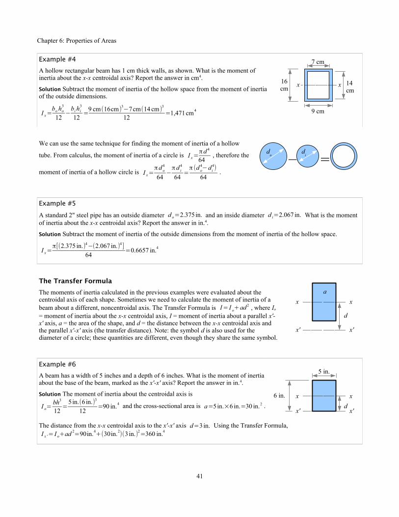
Chapter 6: Properties of Areas
Example #4
A hollow rectangular beam has 1 cm thick walls, as shown. What is the moment of inertia about the x-x centroidal axis? Report the answer in cm4.
Solution Subtract the moment of inertia of the hollow space from the moment of inertia of the outside dimensions.
I x=bo ho
3
12−
bi hi3
12=9 cm(16cm)3−7cm(14 cm)3
12=1,471cm4
We can use the same technique for finding the moment of inertia of a hollow
tube. From calculus, the moment of inertia of a circle is I x=πd 4
64, therefore the
moment of inertia of a hollow circle is I x=πd o
4
64−πd i
4
64=π(d o
4−di4)
64.
Example #5
A standard 2" steel pipe has an outside diameter d o=2.375 in. and an inside diameter d i=2.067 in. What is the moment of inertia about the x-x centroidal axis? Report the answer in in.4.
Solution Subtract the moment of inertia of the outside dimensions from the moment of inertia of the hollow space.
I x=π[(2.375 in.)4−(2.067 in.)4]
64=0.6657 in.4
The Transfer Formula
The moments of inertia calculated in the previous examples were evaluated about the centroidal axis of each shape. Sometimes we need to calculate the moment of inertia of a beam about a different, noncentroidal axis. The Transfer Formula is I= I o+ad 2 , where Io = moment of inertia about the x-x centroidal axis, I = moment of inertia about a parallel x'-x' axis, a = the area of the shape, and d = the distance between the x-x centroidal axis and the parallel x'-x' axis (the transfer distance). Note: the symbol d is also used for the diameter of a circle; these quantities are different, even though they share the same symbol.
Example #6
A beam has a width of 5 inches and a depth of 6 inches. What is the moment of inertiaabout the base of the beam, marked as the x'-x' axis? Report the answer in in.4.
Solution The moment of inertia about the centroidal axis is
I o=bh3
12=
5in.(6in.)3
12=90 in.4 and the cross-sectional area is a=5in.×6 in.=30 in.2 .
The distance from the x-x centroidal axis to the x'-x' axis d=3 in. Using the Transfer Formula,I x '= I o+ad 2=90in.4+(30in.2)(3in.)2=360 in.4
41
x x
d
a
x' x'
x x
d
5 in.
x' x'
6 in.
x x16cm
9 cm
7 cm
14cm
–d
od
i =
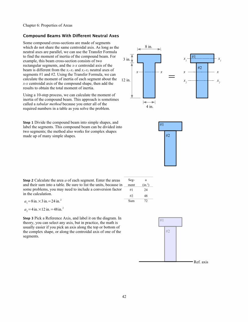
Chapter 6: Properties of Areas
Compound Beams With Diferent Neutral Axes
Some compound cross-sections are made of segmentswhich do not share the same centroidal axis. As long as theneutral axes are parallel, we can use the Transfer Formulato find the moment of inertia of the compound beam. Forexample, this beam cross-section consists of tworectangular segments, and the x-x centroidal axis of thebeam is different from the x1-x1 and x2-x2 neutral axes ofsegments #1 and #2. Using the Transfer Formula, we cancalculate the moment of inertia of each segment about the x-x centroidal axis of the compound shape, then add theresults to obtain the total moment of inertia.
Using a 10-step process, we can calculate the moment ofinertia of the compound beam. This approach is sometimescalled a tabular method because you enter all of therequired numbers in a table as you solve the problem.
Step 1 Divide the compound beam into simple shapes, and label the segments. This compound beam can be divided into two segments; the method also works for complex shapes made up of many simple shapes.
Step 2 Calculate the area a of each segment. Enter the areas and their sum into a table. Be sure to list the units, because in some problems, you may need to include a conversion factor in the calculation.
a1=8in.×3in.=24 in.2
a2=4in.×12 in.=48in.2
Seg- a
ment (in.2)
#1 24
#2 48
Sum 72
Step 3 Pick a Reference Axis, and label it on the diagram. In theory, you can select any axis, but in practice, the math is usually easier if you pick an axis along the top or bottom of the complex shape, or along the centroidal axis of one of the segments.
42
x x
x2
x2
x x
x1
x1
12 in.
3 in.
8 in.
4 in.
=
#1
#2
Ref. axis
#1
#2
#1
#2

Chapter 6: Properties of Areas
Step 4 Draw the distance from the Reference Axis to the centroidal axes of the segments, x1-x1 and x2-x2. Label these distances y1, y2, etc. Enter these values into the table.
Seg- a y
ment (in.2) (in.)
#1 24 13.5
#2 48 6
Sum 72
Step 5 Calculate the product a×y for each segment, and enter these values and their sum in the table.
Seg- a y ay
ment (in.2) (in.) (in.3)
#1 24 13.5 324
#2 48 6 288
Sum 72 612
Step 6 Draw the distance from the Reference Axis to the x-x centroidal axis of the complex shape. Calculate this distance as
y=∑ ay
∑ a=
612in.3
72 in.2=8.5in.
43
x x
x2
x2
x1
x1
Ref. axis
#1
#2
yy
2y
1
x2
x2
x1
x1
Ref. axis
#1
#2
y2
y1

Chapter 6: Properties of Areas
Step 7 Draw the Transfer Distance d for each segment. This isthe distance from the centroidal axis of the segment to the centroidal axis of the complex shape. Given the way this beam is drawn, d 1= y1− y and d 2=y−y2 . For other compound beams, you will have to figure out the formulas ford1, d2, d3, etc. based on the drawing. Enter the results into the table.
Seg- a y ay d
ment (in.2) (in.) (in.3) (in.)
#1 24 13.5 324 5
#2 48 6 288 2.5
Sum 72 612
Step 8 Calculate the product a×d 2 for each segment, and enter the results and their sum in the table. Be sure to calculate a×d 2 , not a×d ...it’s an easy error to make.
Segment 1: a×d 2=24 in.2(5in.)2=600 in.4
Segment 2: a×d 2=48 in.2(2.5in.)2=300in.4
Enter these values and their sum into the table.
Seg- a y ay d ad2
ment (in.2) (in.) (in.3) (in.) (in.4)
#1 24 13.5 324 5 600
#2 48 6 288 2.5 300
Sum 72 612 900
Step 9 Calculate I for each segment about its centroidal axis:
I o1=bh3
12=
8in. (3 in.)3
12=18in.4
I o2=bh3
12=
4 in.(12 in.)3
12=576in.4
Enter these values and their sum into the table.
Seg- a y ay d ad2 Io
ment (in.2) (in.) (in.3) (in.) (in.4) (in.4)
#1 24 13.5 324 5 600 18
#2 48 6 288 2.5 300 576
Sum 72 612 900 594
Step 10 Use the Transfer Formula to calculate I for the compound shape.
I=∑ I o+∑ ad 2=594 in.4+900in.4=1494 in.4
44
x x
x2
x2
d1
x1
x1
Ref. axis
#1
#2
d2
yy
2y
1

Chapter 6: Properties of Areas
Hollow Beams With Diferent Neutral Axes
If the beam is hollow and the cavity does not share the same neutral axis as the outline of the solid shape, then we need theTransfer Formula. Let Segment #1 be the solid shape (with nohole), and Segment #2 be the hole. In all calculations, the areaof the hole and the moment of inertia of the hole are negative numbers. Thus a1, a1y1, a1d1
2, and I1 are positive numbers; a2, a2y2, a2d1
2, and I2 are negative numbers.
Step 1 Divide the compound beam into simple shapes, and label the segments. Segment #1 is a solid rectangle measuring8 cm wide by 6 cm deep; Segment #2 is a hole measuring 6 cm wide by 2 cm deep.
Step 2 Calculate the area a of each segment.
a1=8cm×6cm=48 cm2
a2=−(6cm×2 cm)=−12 cm2
Seg- a
ment (cm2)
#1 48
#2 -12
Sum 36
Step 3 Pick a Reference Axis, and label it on the diagram.
45
#2
#1
6 cm
8 cm
3.5 cm
2 cm
6 cm
Ref. axis
#2
#1

Chapter 6: Properties of Areas
Step 4 Draw the distance from the Reference Axis to the centroidal axes of the segments, x1-x1 and x2-x2. Label these distances y1, y2, etc. Enter these values into the table.
Seg- a y
ment (cm2) (cm)
#1 48 3
#2 -12 4.5
Sum 36
Step 5 Calculate the product a×y for each segment, and enter these values and their sum in the table.
Seg- a y ay
ment (cm2) (cm) (cm3)
#1 48 3 144
#2 -12 4.5 -54
Sum 36 90
Step 6 Draw the distance from the Reference Axis to the x-x centroidal axis of the complex shape. Calculate this distance as
y=∑ ay
∑ a=
90 cm3
36cm 2=2.5cm
46
x1
x1
Ref. axis
#2
#1y
1y
2
x2
x2
x1
x1
Ref. axis
#2
#1yy
1y
2
x2
x2
x x

Chapter 6: Properties of Areas
Step 7 Draw the Transfer Distance d for each segment. This isthe distance from the centroidal axis of the segment to the centroidal axis of the complex shape. Enter the results into thetable.
Placing a hole in the upper part of this beam shifts the centroidal axis downward, to where more of the material lies. Since d 1=0.5 cm , the centroidal axis of this hollow beam is 0.5 cm below the centroidal axis of a solid 6 cm × 8 cm solid beam.
Seg- a y ay d
ment (cm2) (cm) (cm3) (cm)
#1 48 3 144 0.5
#2 -12 4.5 -54 2
Sum 36 90
Step 8 Calculate the product a×d 2 for each segment, and enter the results and their sum in the table. Be sure to calculate a×d 2 , not a×d ...it’s an easy error to make.
Segment 1: a×d 2=48 cm2(0.5cm)2=12 cm4
Segment 2: a×d 2=−12 cm 2(2cm)2=−48cm4
Seg- a y ay d ad2
ment (cm2) (cm) (cm3) (cm) (cm4)
#1 48 3 144 0.5 12
#2 -12 4.5 -54 2 -48
Sum 36 90 -36
Step 9 Calculate I for each segment about its centroidal axis. Note that I is negative for the hole.
I o1=bh3
12=
8cm (6cm)3
12=144cm4
I o2=−bh3
12=−
6cm(2cm)3
12=−4cm4
Enter these values and their sum into the table.
Seg- a y ay d ad2 Io
ment (cm2) (cm) (cm3) (cm) (cm4) (cm4)
#1 48 3 144 0.5 12 144
#2 -12 4.5 -54 2 -48 -4
Sum 36 90 -36 140
Step 10 Use the Transfer Formula to calculate I for the compound shape.
I=∑ I o+∑ ad 2=140 cm4−36 cm4=104cm4
Some compound beams have more than two segments; the 10-step procedure is the same, with more rows in the table.
47
x1
x1
Ref. axis
#2
#1
d2
yy1
y2
x2
x2
x xd
1

Chapter 6: Properties of Areas
Moment of Inertia about the y-y Neutral Axis
The solution method for Iy is the same as for Ix, turned 90°. Instead of y terms in the table, we have x terms.
Step 1 Divide the compound beam into three rectangles.
Step 2 Calculate the area a of each segment.
a1=4in.×1 in.=4 in.2
a2=6in.×1 in.=6 in.2
a3=4in.×2in.=8in.2
Seg- a
ment (in.2)
#1 4
#2 6
#3 8
Sum 18
Step 3 Pick a Reference Axis (easiest along the left edge or along the right edge).
48
y1
y2
#2#1
#3
y1
y2
4 in.
2 in.
1 in.
3 in.
1 in.
y1
y2
#2#1
#3
Ref. axis

Chapter 6: Properties of Areas
Step 4 Draw the distance from the Reference Axis to the centroidal axes of the segments, y1-y1, y2-y2., and y3-y3. Label these distances x1, x2, etc. In this problem, the y1-y1 and y3-y3 centroidal axes are the same.
Seg- a x
ment (in.2) (in.)
#1 4 2
#2 6 4.5
#3 8 2
Sum 18
Step 5 Calculate the product a×x for each segment, and enter these values and their sum in the table.
Seg- a x ax
ment (in.2) (in.) (in.3)
#1 4 2 8
#2 6 4.5 27
#3 8 2 16
Sum 18 51
Step 6 Draw the distance from the Reference Axis to the y-y centroidal axis of the complex shape. Calculate this distance as
x=∑ ax
∑ a= 51in.3
18 in.2=2.833 in.
49
y1&3
y1
y2
y2
#2#1
#3
x1
x3
Ref. axis y1&3
y2
x2
y1&3
x
y1
y2
y2
y
#2#1
#3
x1
x3
Ref. axis y1&3
y2
y
x2

Chapter 6: Properties of Areas
Step 7 Draw the Transfer Distance d for each segment. This isthe distance from the centroidal axis of the segment to the centroidal axis of the complex shape. For this drawing,d1=x− x1=d3 and d2=x2− x .
Seg- a x ax d
ment (in.2) (in.) (in.3) (in.)
#1 4 2 8 0.83
#2 6 4.5 27 1.67
#3 8 2 16 0.83
Sum 18 51
Step 8 Calculate the product a×d 2 for each segment. Seg- a x ax d ad2
ment (in.2) (in.) (in.3) (in.) (in.4)
#1 4 2 8 0.83 2.78
#2 6 4.5 27 1.67 16.67
#3 8 2 16 0.83 5.56
Sum 18 51 38.89
Step 9 Calculate I for each segment about its centroidal axis:
I o1=bh3
12=1 in.(4 in.)3
12=5.333 in.4
I o2=bh3
12=6in.(1 in.)3
12=0.5 in.4
I o3=bh3
12= 2in.(4in.)3
12=10.667in.4
Seg- a x ax d ad2 Io
ment (in.2) (in.) (in.3) (in.) (in.4) (in.4)
#1 4 2 8 0.83 2.78 5.33
#2 6 4.5 27 1.67 16.67 0.5
#3 8 2 16 0.83 5.56 10.67
Sum 18 51 38.89 50.06
Step 10 Use the Transfer Formula to calculate Iy for the compound shape.
I y=∑ I o+∑ ad 2=38.89 in.4+50.06 in.4=88.95 in.4
50
d3
y1&3
x
y1
y2
y2
y
#2#1
#3
d1
x1
x3
d2
Ref. axis y1&3
y2
y
x2
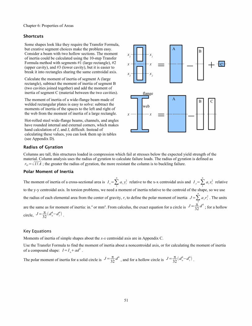
Chapter 6: Properties of Areas
Shortcuts
Some shapes look like they require the Transfer Formula, but creative segment choices make the problem easy. Consider a beam with two hollow sections. The moment of inertia could be calculated using the 10-step Transfer Formula method with segments #1 (large rectangle), #2 (upper cavity), and #3 (lower cavity), but it is easier to break it into rectangles sharing the same centroidal axis.
Calculate the moment of inertia of segment A (large rectangle), subtract the moment of inertia of segment B (two cavities joined together) and add the moment of inertia of segment C (material between the two cavities).
The moment of inertia of a wide-flange beam made of welded rectangular plates is easy to solve: subtract the moments of inertia of the spaces to the left and right of the web from the moment of inertia of a large rectangle.
Hot-rolled steel wide-flange beams, channels, and angles have rounded internal and external corners, which makes hand calculation of Ix and Iy difficult. Instead of calculating these values, you can look them up in tables (see Appendix D).
Radius of Gyration
Columns are tall, thin structures loaded in compression which fail at stresses below the expected yield strength of the material. Column analysis uses the radius of gyration to calculate failure loads. The radius of gyration is defined asrG=√ I / A ; the greater the radius of gyration, the more resistant the column is to buckling failure.
Polar Moment of Inertia
The moment of inertia of a cross-sectional area is I x=∑1
n
ai yi2 relative to the x-x centroidal axis and I y=∑
1
n
ai xi2 relative
to the y-y centroidal axis. In torsion problems, we need a moment of inertia relative to the centroid of the shape, so we use
the radius of each elemental area from the center of gravity, r, to define the polar moment of inertia J=∑1
n
a i r i2 . The units
are the same as for moment of inertia: in.4 or mm4. From calculus, the exact equation for a circle is J= π32
d 4; for a hollow
circle, J= π32(d o
4−d i4) .
Key Equations
Moments of inertia of simple shapes about the x-x centroidal axis are in Appendix C.
Use the Transfer Formula to find the moment of inertia about a noncentroidal axis, or for calculating the moment of inertia of a compound shape: I= I o+ad2 .
The polar moment of inertia for a solid circle is J= π32
d 4, and for a hollow circle is J= π
32(d o
4−d i4) .
51
x x
x2
x2
x1
x1
=
A
–
B
+
x x = –
AB C
web
flange
C

Chapter 7: Torsion in Round Shafts
Chapter 7: Torsion in Round ShaftsShear Stress in a Round Shaft
Many machine parts are loaded in torsion, either to transmit power(like a driveshaft or an axle shaft in a vehicle) or to support adynamic load (like a coil spring or a torsion bar). Powertransmission parts are typically circular solid shafts or circularhollow shafts because these shapes are easy to manufacture andbalance, and because the outermost material carries most of thestress. For a given maximum size, more material is available along theentire surface of a circle than at the four corners of a square.
Apply a torque T to a round shaft, and the shaft will twist through anangle θ. Twisting means the material is deforming, so we have strainin the material. The greatest strain is at the surface, while strain iszero at the center of the shaft. The strain varies linearly from thecenter to the surface of the shaft. We saw in Chapter 2 that materialslike steel and aluminum follow Hooke's law: the ratio of stress/strainis Young's modulus, a constant. Therefore, the stress in the shaft alsovaries linearly from the center to the surface of the shaft. We also saw in Chapter 2 that this stress is a shearing stress, soτ=0 at the center, and τ=τmax at the surface.
Consider a small area a at a distance r from the center of the circle. If we define c = the distance from the
centroid to the surface of the circle, then the shear stress at r is τ= rcτ surface . Since shear stress is force
divided by area, the shear force acting on area a is P shear(a )=τ a=r τsurface a
c. The torque on area a is
the force times the distance from the centroid: T (a)=P shear r=r2 τ surfacea
c=τ surface
ca r2 . The total torque
on the entire circular area about the centroid is the sum of the torques on all the small areas that comprise the
circle, so T=τ surface
c ∑ a r2. We've seen the last part of this equation before: the polar moment of inertia of a circle is
J=∑ a r2 , therefore T=τ surface J
c. For design purposes, only the maximum stress matters, so we usually drop the
subscript from the shear stress, understanding that we mean the stress at the surface, so we write T= τ Jc
. In many
problems, we know the applied torque and dimensions; we need the stress. Rewrite the equation to solve for stress: τ=TcJ
.
Example #1
The torque on a ¼ inch diameter circular shaft is 5 ft.⋅lb. What is the shear stress? Report the answer in ksi.
Solution The distance from the centroid to the surface is c=d2= 0.25in.
2=0.125 in. . The polar moment of inertia of a
circle is J=πd 4
32. Shear stress τ=
TcJ=5ft.⋅lb. 0.125 in. 32
π(0.25 in.)4∣12in.1ft. ∣kip
103 lb.=19.6 ksi
Once we have the shear stress, we can compare it with the allowable shear stress for this material. If the calculated stress ishigher than the allowable stress, then we can either select a stronger material or use a larger diameter shaft.
52
εmax
εmax
τmax
τmaxε = 0 τ = 0
r
carea a
θ T
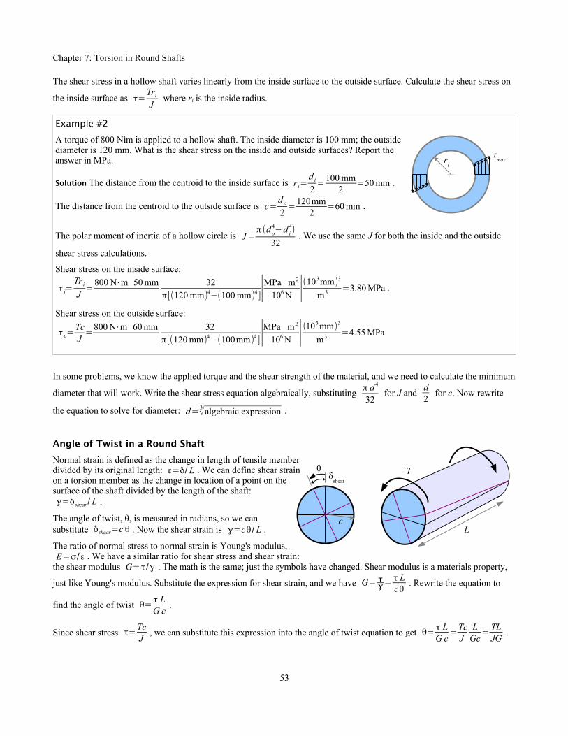
Chapter 7: Torsion in Round Shafts
The shear stress in a hollow shaft varies linearly from the inside surface to the outside surface. Calculate the shear stress on
the inside surface as τ=Tri
J where ri is the inside radius.
Example #2
A torque of 800 N⋅m is applied to a hollow shaft. The inside diameter is 100 mm; the outsidediameter is 120 mm. What is the shear stress on the inside and outside surfaces? Report theanswer in MPa.
Solution The distance from the centroid to the inside surface is r i=d i
2=100 mm
2=50 mm .
The distance from the centroid to the outside surface is c=d o
2=120mm
2=60 mm .
The polar moment of inertia of a hollow circle is J=π(d o
4−d i4)
32. We use the same J for both the inside and the outside
shear stress calculations.
Shear stress on the inside surface:
τ i=Tr i
J=
800 N⋅m 50 mm 32
π[(120 mm)4−(100 mm)4]∣MPa m2
106 N ∣(103mm)3
m3 =3.80 MPa .
Shear stress on the outside surface:
τ o=TcJ=800 N⋅m 60 mm 32
π[(120 mm)4−(100mm)4]∣MPa m2
106 N ∣(103mm)3
m3 =4.55 MPa
In some problems, we know the applied torque and the shear strength of the material, and we need to calculate the minimum
diameter that will work. Write the shear stress equation algebraically, substituting π d 4
32 for J and
d2
for c. Now rewrite
the equation to solve for diameter: d= 3√algebraic expression .
Angle of Twist in a Round Shaft
Normal strain is defined as the change in length of tensile memberdivided by its original length: ε=δ/ L . We can define shear strainon a torsion member as the change in location of a point on thesurface of the shaft divided by the length of the shaft:γ=δshear/ L .
The angle of twist, θ, is measured in radians, so we cansubstitute δshear=c θ . Now the shear strain is γ=cθ/ L .
The ratio of normal stress to normal strain is Young's modulus,E=σ/ε . We have a similar ratio for shear stress and shear strain:
the shear modulus G=τ/γ . The math is the same; just the symbols have changed. Shear modulus is a materials property,
just like Young's modulus. Substitute the expression for shear strain, and we have G= τγ=
τ Lcθ
. Rewrite the equation to
find the angle of twist θ= τ LG c
.
Since shear stress τ=TcJ
, we can substitute this expression into the angle of twist equation to get θ= τ LG c
=TcJ
LGc= TL
JG.
53
ri
τmax
θ
c
δshear
L
T

Chapter 7: Torsion in Round Shafts
Example #3
A solid round aluminum shaft has a maximum allowable shear stress of 80 MPa. The shaft is 10 cm in diameter and 1 m long. What is the angle of twist? Report the answer in radians and in degrees.
Solution From Appendix B, the shear modulus of aluminum is G=28×103MPa . The angle of twist is
θ= τ LGc
= 80 MPa 1 m
28×103 MPa12(10cm)∣100cm
m=0.057 rad
Convert to degrees using the conversion button on your calculator, or use the Factor-Label Method of Unit Conversion:
0.057rad∣180°π rad
=3.3°
Example #4
A hollow round steel shaft has a torque of 600 ft.lb. The shaft has an outside diameter of 1.25 in., an inside diameter of 1.10 in., and a length of 36 in. What is the angle of twist? Report the answer in radians and in degrees.
Solution From Appendix B, the shear modulus of steel is G=12,000 ksi . The angle of twist is
θ=T LJG
=32 T L
π d 4 G= 32⋅600 ft.lb.⋅36 in. in.2
π[(1.25in.)4−(1.10in.)4 ]12,000 kip∣ kip
103 lb.
12 in.ft.
=0.225 rad
Convert to degrees using the conversion button on your calculator, or use the Factor-Label Method of Unit Conversion:
0.225 rad∣180°π rad
=12.9°
Looking at the equations, you can see that the angle of twist is directly proportional to length: if you double the length of theshaft, the angle of twist doubles. In a tensile member, if you double the length the elongation doubles. Shear stress is independent on length, just as normal stress is independent of the length of a tensile member.
Stress Concentration in Torsion
If a shaft has a uniform diameter along its length, then the maximum shear stress at the
surface is τ=TcJ
. Many shafts in machines have different diameters in different
locations, such as at the flange of an axle shaft, or adjacent to a bearing surface. Asudden change in diameter creates a stress concentration. The maximum stress in the
smaller diameter section, at the base of the fillet, is τ=K TcJ
where K is the stress
concentration factor. Other dimensional changes, such as keyways and transversethrough-holes, also create stress concentrations in shafts.
54
r
d D
location ofmaximum stress
T

Chapter 7: Torsion in Round Shafts
Look at the diagram of the shaft: thefillet radius meets the flat face of thelarge diameter portion of the shaft. Thetwo shaft diameters and fillet radius areall independent variables, so the stressconcentration graph has several curves,each for a different ratio of shaftdiameters. Use a five-step process forcalculating the maximum shear stress atthe stress concentration site:
Step 1 Divide the fillet radius by thesmaller shaft diameter find the ratio r/d.
Step 2 Divide the larger shaft diameterby the smaller shaft diameter find theratio D/d.
Step 3 Using these two values, find thevalue of K from the graph. If yourcalculated D/d does not match the valueson the graph, interpolate. For example, ifr/d = 0.06 and D/d = 1.15, then K≈1.35.
Step 4 Calculate c and J using thesmaller shaft diameter.
Step 5 Calculate the maximum stress
using τ=K TcJ
.
Example #5
A 2¼ inch diameter shaft is welded to a 3 inch diameter shaft. The weld bead is ground to a radius of 0.125 inches. If the torque is 600 ft.lb., what is the maximum shear stress? Report the answer in ksi.
Solution Calculate the ratios Dd= 3in.
2.25in.=1.33 and
rd=0.125 in.
2.25in.=0.056 . Use the 1.33 line on the graph to find the
stress concentration factor K≈1.65
The maximum shear stress at the fillet is τ=KTcJ=K T
d2
32
πd 4=16 K T
π d 3 =16⋅1.65⋅600ft.⋅lb.
π(2.25in.)3 ∣12 in.ft. ∣ kip
103 lb.=5.31 ksi
Key Equations
Shear stress on the surface of a round solid or hollow shaft is the torque times the distance from the center to the outside
surface, divided by the polar moment of inertia: τ=TcJ
The angle of twist of a round solid or hollow shaft can be calculated with θ= τ LG c
or with θ= TLJG
, depending on the
available input variables. With a stepped shaft, the maximum stress is τ=K TcJ
where K is the stress concentration factor.
55
σ
0.0 0.02 0.04 0.06 0.08 0.10 0.121.0
1.2
1.4
1.6
1.8
r / d
K
Fillet in a stepped shaft loaded in torsion
2.0
2.2
2.4
2.6
1.09
2.00
1.50
1.20
1.33
r
d DT
D/d

Chapter 8: Beam Reactions, Shear Diagrams, and Moment Diagrams
Chapter 8: Beam Reactions, Shear Diagrams, and Moment DiagramsLoads on Beams
The way a part is loaded determines whether it is called a tensile or compressivemember, a torsional shaft, or a beam. If you take a ½ inch diameter steel rod and pullit lengthwise with a load P, the rod will develop a tensile stress σ=P /A where A isthe cross-sectional area of the rod. Loading the rod in tension parallel to its axismakes the rod a tensile member; loading it in compression parallel to its axis makes it acompressive member. If you twist the steel rod with torque T, then we call it atorsional shaft.
If loading is perpendicular (transverse) to its axis so that the rod bends, then the rod iscalled a beam. You can load a beam with point loads, uniformlydistributed loads, or nonuniformly distributed loads. A swimmer standingon the end of a diving board is an example of a point load: a force appliedat a single point on the beam. This point load P could be the weight of anobject on the beam, or it could be a load applied by a cable or rodattached to the beam at that point. Typically, the left end of the beam ismarked “A” and the right end is marked “B”. For each loaded beam wedraw beam reactions: reaction forces RA and RB for a simply supportedbeam; reaction force RB and reaction moment MB for a cantilever beam.
The symbols for supports indicate the reactions that develop at thesupport. For example, support “A” is pinned, like a hinge, so the symbolfor the support is a triangle. A pinned support may have vertical andhorizontal reaction forces. The beam at the right has no applied horizontal loads,therefore RAx = 0. In the beam problems in this chapter, there are no appliedhorizontal forces, so the horizontal reaction force is zero, and the verticalreaction forces RAy and RBy are abbreviated RA and RB.
A roller support allows the beam to move freely horizontally; the symbol is acircle. A roller support has only a vertical reaction force. A beam supported by apin at one end and a roller at the other end is called a simply-supported beam.
A cantilever beam is embedded in a wall, so the beam has reaction forces as wellas a reaction moment. The horizontal reaction force RBx=0 if there are nohorizontal applied forces, so the vertical reaction force RBy is abbreviated RB.
The weight of a beam is a uniform distributed load. The weight per unit length, w,typically has units of lb./ft., kips/ft., or kN/m. Consider a wide-flange beam, or“W-beam,” having a cross-section that looks like a Courier font capital letter I.The U.S. Customary W-beam designation system has two numbers: the first isthe nominal depth, and the second is the weight per unit length. For example, aW24×162 beam has a nominal depth of 24 inches and a weight per unit lengthw=162 lb./ft. . If the beam is 10 feet long, then the total weight, W, of the beam
is W=wL=162lb.ft.
10 ft.=1,620 lb.
In Canada, W-beams are specified in SI (metric) units. These beams are designated by mass, not weight: a W250×115 wide flange beam has a nominal depth of 250 mm and a mass per unit length of 115 kg/m. From Newton’s Second Law,force=mass×acceleration , or in this case, weight=mass×acceleration of gravity . The SI unit of force and weight is the
newton (N), defined as 1N=1 kg ms2 , and the acceleration of gravity is 9.81 m/s2 . The weight per unit length of a
W250×115 wide-flange beam is w=115 kgm
9.81ms2 ∣N s2
kg m ∣ kN103 N
=1.13kN/m . If the beam is 4 m long, then the total
weight of the beam is W=wL=1.13kNm
4 m=4.51 kN .
56
P
P
T
=P
RB
MB
=P
RB
RA
P
RBy
MB
P
RBy
RAy
RAx
RBx
A B
A B
A B
A B
w
RB
RA
A B

Chapter 8: Beam Reactions, Shear Diagrams, and Moment Diagrams
You can also calculate the weight per unit length from the cross-sectional area and the specific weight of the material. Specific weight is weight divided by volume: γ=W /V . The volume of a beam of uniform cross-section is the cross-
sectional area times the length: V=A⋅L . Combining, γ=WV= W
A⋅L or γ⋅A=W
L. Weight per unit length w=W
L=γ⋅A .
Example #1
What is the weight per unit length of a 1 inch diameter steel rod? Report the answer in lb./ft.
Solution The cross-sectional area of a circle A= π4
d 2. The specific weight of steel is 490 lb./ft.3.
Weight per unit length w=ρ⋅A=γ πd 2
4=490lb.
ft.3π(1in.)2
4 ∣ ft.2
(12 in.)2=2.67lb./ft.
A distributed load may run the length of the beam (likethe beam's weight), may run along a portion of thebeam, or may be nonuniform.
Reactions for Simply-Supported SimpleBeams
You can calculate the reaction forces for a symmetrically-loaded, simply-supported beam by dividing the total load by 2, because each end of the beam carries half the load. The reactions for the beam with a point load are RA=RB=P /2 .
Example #2
Calculate the reaction forces RA and RB for a beam with a 30 kN load at the midspan.
Solution Divide the total load by 2 to obtain the reaction forces,
RA=RB=P2=30 kN
2=15 kN
A simply-supported beam with a uniform distributed load also has a symmetrical loading pattern. Divide the total load on the beam by 2 to find the reaction forces.
Example #3
Calculate the reaction forces RA and RB for a 10-ft. beam with a 480 lb./ft. uniformlydistributed load. Report the answer in kips.
Solution Multiply the uniform distributed load by the length to find the total load on thebeam: W=wL . Divide the total load by 2 to obtain the reaction forces,
RA=RB=W2=
wL2=
480lb.ft.
10 ft. 12∣ kip
1000 lb.=2.4 kips
57
w
RB
RA
A B
w
RB
RA
A B
30 kN
RB
RA
A B
4 m 4 m
480 lb./ft.
RB
RA
A B
10 ft.

Chapter 8: Beam Reactions, Shear Diagrams, and Moment Diagrams
For beams with nonsymmetrical loading, we need two equations from Statics: the sum of the vertical forces equals zero, and the sum of themoments about a point equals zero. The moment about a point is theforce acting on an object times the perpendicular distance from theforce to the pivot point. Whether the object is a blob or a beam, themoment about point A is M A=P⋅x .
You can pick a pivot point at either end of a simply-supported beam. Moststudents find it easier to select the left end of the beam, point A. Since moment has amagnitude and a direction (clockwise or counterclockwise), we need to establish aconvention for positive and negative moments. We’ll select counterclockwise as positive,symbolized as , and start adding up the moments about point A. The load acts at adistance x from point A. Think of point A as a hinge point…the load causes the beam torotate clockwise about point A, so the moment is negative. The reaction force RB acts at adistance L from point A, and causes the beam to rotate counterclockwise about point A, sothe moment is positive. The moment about point A is ∑M A=0=−Px+RB L . Now solve for the reaction force
RB=PxL
. Use the sum of the forces in the vertical direction to calculate the other reaction force. Forces have magnitude
and direction; pick upwards as positive, so ∑ F y=0=RA−P+RB . Now solve for the reaction force RA=P−RB .
Example #4
Calculate the reaction forces RA and RB for this simply-supported beam.
Solution Redraw the diagram, marking the distances to all loads and reactions from pointA.
The moment about point A is ∑M A=0=−40 kN⋅3 m+RB⋅10 m .
Rewrite the equation to find the reaction force RB=40 kN⋅3 m
10 m=12 kN .
Use the sum of the forces in the vertical direction to calculate the other reaction force:
∑ F y=0=RA−40 kN+12 kN .
Rewrite the equation to find the reaction force RA=40 kN−12 kN=28 kN .
You can check the answer by solving the sum of the moments about point B.
Most of the applied load is supported by the left end of thebeam. Intuitively, this makes sense because the load is closerto the left end of the beam. Flip the beam upside down and itlooks like two children on a see-saw: the pivot point has tobe closer to the heavier child in order to balance the see-saw.
Use the same technique for a simply-supported beam with multiple point loads.
58
P
RA
MA
A B
x
P
xA
MA
P
RB
RA
A B
x
L
40kN
RB
RA
A B
3m 7m
40kN
A B
3m10m
40kN
RA
A B
RB
12kN
40kN
A B
12kN28kN12kN
28kN

Chapter 8: Beam Reactions, Shear Diagrams, and Moment Diagrams
Example #5
Calculate the reaction forces RA and RB for a beam with two point loads.
Solution Redraw the diagram, marking the distances to all loads and reactions from pointA. This step may seem to be a waste of time, but as the loading conditions become morecomplicated, it becomes more important to redimension the drawing, in order to keeptrack of the distances used in the Sum of the Moments calculation.
The moment about point A is ∑M A=0=−5 lb.⋅3 in.−12 lb.⋅6 in.+RB⋅10 in.
Rewrite the equation to find the reaction force RB=5lb.⋅3in.+12 lb.⋅6 in.
10 in.=8.7 lb.
Sum of the forces ∑ F y=0=RA−5lb.−12 lb.+8.7lb.
Rewrite the equation to find the reaction force RA=5lb.+12 lb.−8.7 lb.=8.3 lb.
If a uniformly distributed load is not symmetrical, thenwe need to convert the distributed load into a point loadequivalent to the total load W=wL1 where L1 is thelength of the distributed load. The equivalent point loadis located at the centroid of the distributed load…thecenter of the rectangle. Use the equivalent load diagramfor calculating the reaction forces.
Example #6
Calculate the reaction forces RA and RB for a beam with auniform distributed load of 800 N/m. Report the resultin N.
Solution Draw an equivalent load diagram, placing theequivalent load at the centroid of the distributed load.Use the equivalent load diagram to find the reactionforces.
The distributed load runs for 2m, so the location of the equivalent load is 1m from the left end of the distributed load, or
1.8m from point A. The equivalent load W=wL=800 N⋅2 mm
=1600 N .
The moment about point A is ∑M A=0=−1600 N⋅1.8 m+RB⋅6 m .
Rewrite the equation to find the reaction force RB=1600 N⋅1.8 m
6 m=480 N .
Sum of the forces ∑ F y=0=RA−1600 N+480 N . Solve for the reaction force RA=1600 N−480 N=1120 N .
Use the same approach for a nonuniformly distributedload. Again, the location of the equivalent load is at thecentroid of the distributed load. The centroid of a triangleis one third of the distance from the wide end of thetriangle, so the location of the equivalent load is onethird of the distance from the right end of this beam, ortwo thirds of the distance from the left end.
59
5 lb.
RB
RA
A B
3"
A B
RB
3" 4"
12 lb.
RA
5 lb. 12 lb.
3"6"
10"
w
RB
RA
A B =L1
W
RB
RA
A B
L2
Load diagram Equivalent load diagram
800 N/m
RB
RA
A B =R
BR
A
A B
Load diagram Equivalent load diagram
0.8 m 2 m 3.2 m
1.8 m6 m
1600 N
RB
RA
A B =R
BR
A
A B
Load diagram Equivalent load diagram
L 2L/3
w W
L

Chapter 8: Beam Reactions, Shear Diagrams, and Moment Diagrams
The load varies from 0 at the left end to w at the right end; therefore, the total load is the average of these loads times the
beam length: W=(0+w2 ) L=wL
2.
If the beam has point loads and distributed loads, draw an equivalent load diagram with the applied point loads and the equivalent point loads, then solve like Example #5.
Reactions for Overhanging and Cantilever Beams
A simply-supported beam is supported by a pinned connection at one end and a roller support at the other; all applied loads lie between these two points. An overhanging beam extends beyond one or both supports. The solution method is the same as for simply-supported beams: use the sum of the moments about one of the support points to find the reaction at the other support point.
Example #7
Calculate the reaction forces RA and RB for an overhanging beam with two point loads.
Solution Redraw the diagram, marking the distances to all loads and reactions frompoint A.
The moment about point A is ∑M A=0=50 kN⋅5 m−30 kN⋅11m+RB⋅15 m .Notice the 50 kN load produces a positive (counterclockwise) moment about point A,while the 30 kN load produces a negative (clockwise) moment about point A.
Rewrite the equation to find the reaction force
RB=−50 kN⋅5 m+30 kN⋅11m
15 m=5.33 kN
Sum of the forces ∑ F y=0=RA−50 kN−30 kN+5.33 kN . Solve for the reactionforce RA=50 kN+30 kN−5.33 N=74.67kN .
Solve for the reactions to a distributed load on an overhanging beam the same way as for a distributed load on a simply-supported beam: draw an equivalent load diagram, then use the sum of the moments and the sum of the forces to find the reactions.
Example #8
Calculate the reaction forces RA and RB for anoverhanging beam with a uniform distributed load.
Solution Draw an equivalent load diagram, markingthe distances to all loads and reactions from point A.We do not need the dimensions to the ends of theoverhangs, because there are no loads outside of thetwo supports.
The distributed load runs for 9 ft., so the location of the equivalent load is 4.5 ft. from the left end of the distributed load,
or 1.5 ft. to the right of point A. The equivalent load W=wL=60lb.⋅9ft.ft.
=540lb.
The moment about point A is ∑M A=0=−540lb.⋅1.5 ft.+RB⋅6ft.
Rewrite the equation to find the reaction force RB=540lb.⋅1.5 ft.
6 ft.=135lb.
Sum of the forces ∑ F y=0=RA−540lb.+135lb. . Solve for the reaction force RA=540lb.−135lb.=405lb. .
60
A B
RB
RA
50 kN 30 kN
5 m 11 m 4 m
A B
50 kN 30 kN
RB
RA5 m 11 m
15 m
A B
RB
RA
3 ft. 6 ft. 2 ft.
60 lb./ft.
= A B
RB
RA 1.5 ft.
6 ft.
540 lb.
Load diagram Equivalent load diagram

Chapter 8: Beam Reactions, Shear Diagrams, and Moment Diagrams
A cantilever beam with a single support has a reaction force and a reaction moment. The reaction force RB equals the sum of the applied forces on the beam, soRB=P=5 kips .
The moment reaction equals the sum of the moments about point B – the applied load times its distance from the wall – so M B=P⋅x=5kips⋅7ft.=35kip ft. .
Shear Diagrams
When we calculate reaction forces and torques on tension members, torsion members, and beams, we are calculating external forces and torques. Unless the material has no strength at all, the material resists these external loads by developinginternal loads. Apply a torque of 25 ft.lb. to each end of a ½ inch diameter rod, and a resisting torque of 25 ft.lb. exists within the rod all along its length. Apply a tensile force of 400 N to each end of a 2 cm diameter rod, and a resisting tensile force of 400N exists within the rod all along its length. Beams in bending also develop internal forces to resist external forces. Since the external forces on beams are transverse (perpendicular to the axis of the beam), the internal resisting forcesare also transverse forces.
Imagine a simply-supported beam with a point load at themid-span. Cut the beam to the left of the point load, anddraw a free-body diagram of the beam segment. In a free-body diagram, forces must balance. Therefore, a downwardforce at the cut edge balances the support reaction RA. Wecall this shear force V. It is a shear force because the forceacts parallel to a surface (the cut edge of the beam).
The forces RA and V are in balance (equal in value; opposite in sign), but our segmentwants to spin clockwise about point A. To counteract this tendency to spin, a moment Mdevelops within the beam to prevent this rotation. The moment equals the shear force timesits distance from point A.
Cut the beam to the right of the point load, and draw the free-body diagram. Since P islarger than RA, force V points upwards.
Example #9
Calculate the shear forces in this beam to the left and to the right of the 30 kN point load.
Solution The loading is symmetrical, so RA=RB=P2=30 kN
2=15 kN .
Use the sum of the forces to find V.
Between support A and point load P, ∑ F y=0=RA−V 1 .
Solving for shear load, V 1=−RA=−15 kN .
Between point load P and support B, ∑ F y=0=RA−P+V 2 .
Solving for shear load, V 2=−RA+P=−15 kN+30 kN=15 kN .
61
5 kips
RB
MB
A B
7 ft.
P
RB
RA
A B
L/2 L/2
V
RA
A
RA
A M
V
RA
A M
VP
30 kN
RB
RA
A B
4 m 4 m
V1
RA
A M
RA
A M
V2
P

Chapter 8: Beam Reactions, Shear Diagrams, and Moment Diagrams
We can sketch V as a function of location along the beam using a ShearDiagram. Draw vertical construction lines below the load diagramwherever the applied loads and reactions occur. Draw a horizontalconstruction line, indicating zero shear load. Next, draw the value of Valong the length of the beam, as follows:
Step 1 Starting at the left side of the shear diagram, go up 15 kN,because RA is 15 kN upwards.
Step 2 There are no additional loads on the beam until you get to themidspan, so the shear value remains at 15 kN.
Step 3 The applied load at the midspan is 30 kN downwards, thereforethe shear load is 15 kN−30 kN=−15 kN .
Step 4 There are no additional loads on the beam until you get to pointB, so the shear value remains at -15kN.
Step 5 At point B, the reaction force RB = 15 kN upwards, therefore theshear load is −15 kN+15 kN=0 . If you don’t get to 0, you know youmade a mistake someplace.
Finish the shear diagram by shading the areas between your line and thehorizontal zero shear line. Mark all significant points (anywhere theshear line changes direction). In the next chapter, we will use themaximum absolute value of shear load, ∣V∣max , to calculate themaximum shear stress in the beam.
A point load at the midspan of a simply-supported beam produces identical reaction forces and a symmetric shear diagram with two rectangles. If the point load is not at the midspan, use sum of the moments and sum of the forces to calculate the reaction forces. Draw vertical construction lines below the applied loads and reaction forces, draw a horizontal line at zero shear, then draw the shear value along the length of the beam.
Example #10
Draw a complete shear diagram for a simply-supported 8 ft. beam with a 100 lb.point load 2 ft. to the right of point A.
Solution Use sum of the moments and sum of the forces to find the reaction forces RA and RB.
Starting the shear diagram at zero shear, go up RA=75lb. at point A. There are noloads between point A and the applied point load, so the shear load does notchange. Draw a horizontal line to the right, until you reach the point load. Draw avertical line down 100 lb., reaching a value V=−25lb. There are no loads betweenthe point load and point B, so the shear load does not change. Draw a horizontalline to the right, until you reach point B. The reaction force at B is 25 lb. upwards,so draw a vertical line up 25 lb., reaching a value V=0 . Again we have two rectangles, but they are not symmetric; the beam carries three times as much shear load to the left of the point load than it does to the right.
Multiple point loads produce a stepped shear diagram.
62
100 lb.
A B
6 ft.75 lb. 25 lb.
75 lb.
-25 lb.V
2 ft.
30 kN
A B
4 m 4 m15 kN 15 kN
15 kN
-15 kN
V Step 5
15 kN
-15 kN
VFinishedsheardiagram
15 kN
-15 kN
V Step 4
15 kN
-15 kN
V Step 3
15 kN
V
15 kN
V
Step 2
Step 1

Chapter 8: Beam Reactions, Shear Diagrams, and Moment Diagrams
Example #11
Draw a complete shear diagram for a simply-supported 8 ft. beam with 100 lb.point loads every 2 ft. along the length.
Solution The loading is symmetrical, so the reaction forces equal half the totalapplied load.
Calculate the shear values as:
V 1=RA=150lb.
V 2=V 1−100 lb.=50 lb.
V 3=V 2−100 lb.=−50lb.
V 4=V 3−100 lb.=−150lb.
V 5=V 4+RB=−150lb.+150 lb.=0
In this problem, ∣V∣max=150lb.
A uniformly distributed load is like an infinite number of small point loads along the length of the beam, so the shear diagram is like a stepped multiple point load shear diagram with infinitely small steps.
Example #12
Draw a complete shear diagram for a simply-supported 4 m beam with auniformly distributed load of 3 kN/m.
Solution The loading is symmetrical, so the reaction forces equal half the total
applied load. RA=RB=W2= wL
2= 3kN⋅4 m
m 2=6 kN .
A complete shear diagram includes the values of the shear at locations of appliedpoint loads and reaction forces.
V 1=RA=6kN
V 2=V 1−3kN
m4m=−6kN
V 3=V 2+RB=−6kN+6 kN=0
In this problem, ∣V∣max=6kN
If the uniformly distributed load does not extend along the entire length of the beam, then draw an equivalent load diagram to find the reaction forces. Go back to the original load diagram to draw the shear diagram; do not use the equivalent load diagram to draw the shear diagram.
63
A B
6 kN 6 kN
V1=6 kN
V V3= 0
V2= -6 kN
3 kN/m
4 m
100 lb.
A B
150 lb. 150 lb.
V1=150 lb.
V
2 ft.
100 lb. 100 lb.
2 ft. 2 ft. 2 ft.
V2=50 lb.
V3= -50 lb.
V4= -150 lb.

Chapter 8: Beam Reactions, Shear Diagrams, and Moment Diagrams
Example #13
Draw a complete shear diagram for a simply-supported 20 ft. beam which has a uniform distributed load of 2 kips/ft. running from the left end for 6 feet.
Solution Draw an equivalent load diagram, placing the equivalent load at the centroid of the distributed load. Use the equivalent load diagram to find the reaction forces.
The distributed load runs for 6 ft., so the location of the equivalent load is 3 ft. from the left end of the beam.
The equivalent load W=wL=2 kips⋅6ft.ft.
=12 kips .
The moment about point A is ∑M A=0=−12 kips⋅3ft.+RB⋅20 ft. .
Rewrite the equation to find the reaction force RB=12 kips⋅3ft.
20 ft.=1.8 kips .
Sum of the forces ∑ F y=0=RA−12 kips+1.8kips . Solve for the reaction force RA=12 kips−1.8 kips=10.2 kips .
Draw construction lines down from the original load diagram wherever a point load or reaction exists, and wherever a distributed load starts or stops. Calculate the shear loads at these points.
V 1=RA=10.2 kips
V 2=V 1−2 kips
ft.6 ft.=−1.8 kips
V 3=V 2+RB=−1.8 kips+1.8 kips=0
In this problem, ∣V∣max=10.2kips
Multiple point loads of increasing load will give you an asymmetric stepped shear diagram.
Example #14
Draw a complete shear diagram for a simply-supported 4 m beam which has athree different point loads as shown in the load diagram.
Solution Use sum of the moments and sum of the forces to find the reactionforces RA and RB.
Calculate the shear loads as follows:
V 1=RA=250 N
V 2=V 1−100 N=150 N
V 3=V 2−200lb.=−50 N
V 4=V 3−300 N=−350 N
V 5=V 4+RB=−350 N+350 N=0
In this problem, ∣V∣max=350kN
64
100 N
A B
250 N 350 N
V1=250 N
V
1m
200 N 300 N
1m 1m 1m
V2=150 N
V3= -50 N
V4= -350 N
V5= 0
2 kips/ft.
RB
RA
A B =R
BR
A
A B
Load diagram Equivalent load diagram
6 ft. 14 ft.
3 ft.20 ft.
12 kips
V1=10.2 kips
V V3= 0
V2= -1.8 kips

Chapter 8: Beam Reactions, Shear Diagrams, and Moment Diagrams
A nonuniformly distributed load produces two different reaction forces. Draw an equivalent load diagram to find the reaction forces. Go back to the original load diagram to draw the shear diagram. A wedge-shaped nonuniformly distributed load is like an infinite number of small point loads of increasing magnitude along the length of the beam, so the shear diagram is like the previous stepped multiple point load shear diagram in which the slope of the curve increases parabolically.
Example #15
Draw a complete shear diagram for a simply-supported 6 m beam which has a wedge-shapednonuniformly distributed load of 0 kN/m at the leftend of the beam to 5 kN/m at the right end of thebeam.
Solution Draw an equivalent load diagram, placingthe equivalent load at the centroid of the distributedload. The centroid of a triangle lies two-thirds of thedistance from the point of the triangle. Use theequivalent load diagram to find the reaction forces.
The centroid is located at x= 23
L=2⋅6 m3
=4m ,
measuring from the left end of the beam. The equivalent load is the average of the minimum and maximum distributed
loads times the length of the distributed load: W=(0+5)kN2 m
6m=15 kN .
The moment about point A is ∑M A=0=−15 kN⋅4m+RB⋅6 m . Rewrite the equation to find the reaction force
RB=15 kN⋅4m
6 m=10 kN . Sum of the forces ∑ F y=0=RA−15 kN+10 kN . Solve for RA=15kN−10 kN=5kN .
Draw construction lines down from the original load diagram at the two reaction forces. Calculate the shear loads at these points.
V 1=RA=5kN
V 2=V 1−15 kN=−10 kN
V 3=V 2+RB=−15 kN+15 kN=0
The shear line crosses the axis where the area of the distributed load equals RA. The area of the
distributed load is one half the base times the height of the triangle, or a= xh2
. By similar
triangles, the height of the little triangle h= xL
w , so a=x2 w2 L
=RA . Solving,
x=√ 2 LRA
w=√2⋅6 m⋅5 kN m
5 kN=3.46 m . The shear line crosses the axis 3.46 m from the
left end of the beam.
Look at the shear diagrams, and you can see that point loads create rectangles, uniform distributed loads create triangles, and wedge-shaped (triangular) distributed loads create parabolas.
Shear diagrams for cantilever beams follow the same rules as for simply supported beams. First, find the reactions; next, draw the shear diagram using construction lines wherever a point load occurs or a distributed load starts or stops.
65
hw
Lx
a
5 kN
A B =R
BR
A
A B
Load diagram Equivalent load diagram
6 m 4 m
15 kN
6 mV
1=5 kN
V
V2= -10 kN
V3= 0
5 kN/m
10 kN

Chapter 8: Beam Reactions, Shear Diagrams, and Moment Diagrams
Example #16
Draw a complete shear diagram for a 10 foot cantilever beam having a 5 kip point load 7 feet from the wall.
Solution Since there is no reaction force at the left end, there is no shear load until we get to the applied load. Then, the shear load is negative (downward) until we get to the support, where RB is positive (upward).
The moment about point B is ∑M B=0=5 kips⋅7ft.=35 kip ft. . Sum of the
forces ∑ F y=0=RB−5 kips therefore RB=5kips .
Draw construction lines down from the original load diagram at the point load and the reaction force. Calculate the shear loads at these points.
V 1=P=−5 kips
V 2=V 1+5 kips=0
With a shear diagram, we can identify the location and size of the largest shear load in a beam. Therefore, we know the location of the largest shear stress, and we can calculate the value of this stress. Once we know the actual stress in the material, we can compare this values with the shear strength of the material, and we can know whether the beam will fail in shear. Shear diagrams are necessary for drawing bending moment diagrams (“moment diagrams”, for short), which we can use to identify the location and size of bending stresses that develop within beams. We can compare the actual bending stresses with the yield strength of the material, and we can know whether the beam will fail in bending.
66
5 kips
RB
MB
A B
7 ft.
VV
3= -50 N
V1= -5 kips
V2= 0
10 ft.

Chapter 8: Beam Reactions, Shear Diagrams, and Moment Diagrams
Moment Diagrams
The moment about a point along a beam is defined as the distance from that point to a force acting perpendicular to the beam, so the units are force × distance: lb.⋅ft. (orft.⋅lb. – the order does not matter), lb.⋅in. , kip⋅ft. , N⋅m ,or kN⋅m . We can graph the value of the bending moment along a beam by drawing a moment diagram.
To draw a moment diagram, sketch the value of the momentproduced by the shear force V times the distance from the left end of the beam. At the first meter, V = 15 kN, so moment M 1=15 kN×1m=15 kN⋅m .
At 2 m, M 2=M 1+15 kN×1 m=30 kN⋅m
At 3 m, M 3=M 2+15 kN×1 m=45 kN⋅m
At 4 m, M 4=M 3+15 kN×1 m=60 kN⋅m
At 5 m, M 5=M 4−15 kN×1 m=45 kN⋅m
At 6 m, M 6=M 5−15 kN×1 m=30 kN⋅m
At 7 m, M 7=M 6−15 kN×1 m=15 kN⋅m
At 8 m, M 8=M 7−15 kN×1m=0 kN⋅m
Shade the finished diagram, marking all significant points (places where the moment line changes direction). The mostimportant point is the maximum absolute value of M; this is where the maximum bending stress occurs in the beam.
The value of the moment diagram at any point equals the area of the shear diagram up to that point. The shear diagram has positive areas above the zero line, and negative areas below the zero line. When the shear area is positive, the moment increases; when the shear area is negative, the moment decreases.
You can draw the moment diagram faster by calculating the area of the left-hand rectangle in the shear diagram:M max=15 kN×4 m=60 kN⋅m . Verify that M 8=0 by
subtracting the area of the second rectangle in the shear diagram: M 8=M max−15 kN×4 m=0 kN⋅m .
It is a good idea to check the moment at point B. If you end up with a value otherthan 0, then you know there is a mistake someplace. Most likely, the error is in thereaction forces. You can draw a shear diagram that works with the wrong reactionforces, but you cannot draw a good moment diagram if RA and RB are wrong. Thisis an amazing feature of moment diagrams – they tell you if your solution is right!
If the point load is not at the midspan, then the maximum moment will also beoffset. In this example, the maximum moment is the area of the shear diagram upto the point load: M max=RA⋅L1 .
Multiple point loads will give you multiple rectangles on the shear diagram, andmultiple triangles on the moment diagram.
67
P
A B
L1
RA
V
Mmax
M
RB
RA
L2
RB
30 kN
A B
4 m 4 m15 kN 15 kN
-15 kN
Finished momentdiagram with max.labeled
M1M
15 kN
V
Moment atx = 1 m
Sheardiagram
M
M
M
M
M
M
M8M
Mmax
= 60 kN⋅m
M
M7
M6
M5
M4
M3
M2 Moment at
x = 2 m
Moment atx = 3 m
Moment atx = 4 m
Moment atx = 5 m
Moment atx = 6 m
Moment atx = 7 m
Moment atx = 8 m
Loaddiagram

Chapter 8: Beam Reactions, Shear Diagrams, and Moment Diagrams
Example #17
Draw complete shear and moment diagrams for an 8 foot long, simply-supported beam having 100 lb. point loads every 2 feet.
Solution The loading is symmetrical, therefore the reaction forces RA and RB are each equal to half the total applied load.R A=RB=(100lb.+100 lb.+100lb.)/2=150lb.
Draw construction lines down from the load diagram at each reaction force and applied load. The shear diagram is a series of rectangles.
Calculate the values on the moment diagram as follows:
M 1=2ft.×150lb.=300 ft.⋅lb.
M 2=M 1+2ft.×50 lb.=400ft.⋅lb.
M 3=M 2−2ft.×50 lb.=300 ft.⋅lb.
M 4=M 3−2 ft.×150 lb.=0ft.⋅lb.
A uniformly distributed load produces a parabolic moment diagram. Close to point A, a large shear produces a steep slope in the moment diagram. As you approach the midspan, the smaller shear produces a shallower slope in the moment diagram.Beyond the midspan, an increasingly negative shear produces an increasingly steeper slope downwards.
The maximum moment equals the area of the left-hand triangle. Subtract the area of the right-hand triangle to get the moment at point B.
Example #18
Draw complete shear and moment diagrams for an 8 meter long, simply-supported beam having a uniform distributed load of 3 kN/m.
Solution The loading is symmetrical, therefore the reaction forces RA and RB
are each equal to half the total applied load. RA=RB=3kN
m8m2=12 kN
Draw construction lines down from the load diagram at each reaction force . The shear diagram is two triangles. Draw a construction line down from where the shear line crosses the zero axis.
The max. moment is equal to the area of the left-hand triangle: the base timesthe height divided by 2. The base of the triangle is half the beam length, 4 m.
M max=12 kN×4m
2=24 kN⋅m The moment at point B is the moment at the
midspan minus the area of the right-hand triangle.
M B=M max−12 kN×4 m
2=0kN⋅m
We’ve seen that a nonuniform wedge-shaped distributed load produces a parabolic shear diagram. The moment diagram looks like a parabola skewed to the right, with the maximum moment at the point where the shear diagram crosses the zero-load axis.
68
100 lb.
A B
150 lb. 150 lb.
V1=150 lb.
V
2 ft.
100 lb. 100 lb.
2 ft. 2 ft. 2 ft.
V2=50 lb.
V3= -50 lb.
V4= -150 lb.
M1=300 ft.lb.
M M4= 0 ft.lb.
M2=400 ft.lb.
M3=300 ft.lb.
A B
12 kN 12 kN
V1=12 kN
V V3= 0
V2= -12 kN
3 kN/m
8 m
Mmax
=24 kN⋅m
M
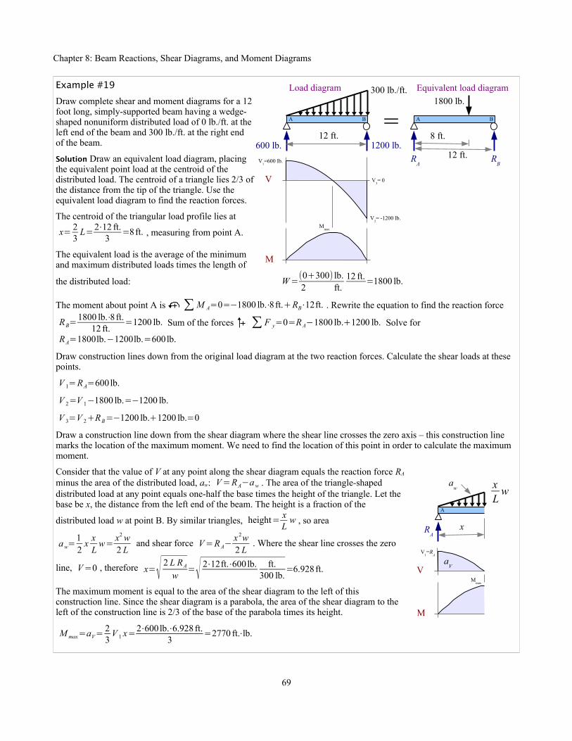
Chapter 8: Beam Reactions, Shear Diagrams, and Moment Diagrams
Example #19
Draw complete shear and moment diagrams for a 12foot long, simply-supported beam having a wedge-shaped nonuniform distributed load of 0 lb./ft. at theleft end of the beam and 300 lb./ft. at the right endof the beam.
Solution Draw an equivalent load diagram, placingthe equivalent point load at the centroid of thedistributed load. The centroid of a triangle lies 2/3 ofthe distance from the tip of the triangle. Use theequivalent load diagram to find the reaction forces.
The centroid of the triangular load profile lies at
x= 23
L=2⋅12 ft.3
=8ft. , measuring from point A.
The equivalent load is the average of the minimumand maximum distributed loads times the length of
the distributed load: W=(0+300) lb.2 ft.
12 ft.=1800 lb.
The moment about point A is ∑M A=0=−1800 lb.⋅8ft.+RB⋅12ft. . Rewrite the equation to find the reaction force
RB=1800 lb.⋅8ft.
12 ft.=1200 lb. Sum of the forces ∑ F y=0=RA−1800 lb.+1200 lb. Solve for
RA=1800lb.−1200lb.=600lb.
Draw construction lines down from the original load diagram at the two reaction forces. Calculate the shear loads at these points.
V 1=RA=600lb.
V 2=V 1−1800 lb.=−1200 lb.
V 3=V 2+RB=−1200 lb.+1200 lb.=0
Draw a construction line down from the shear diagram where the shear line crosses the zero axis – this construction line marks the location of the maximum moment. We need to find the location of this point in order to calculate the maximum moment.
Consider that the value of V at any point along the shear diagram equals the reaction force RA
minus the area of the distributed load, aw: V=RA−a w . The area of the triangle-shapeddistributed load at any point equals one-half the base times the height of the triangle. Let thebase be x, the distance from the left end of the beam. The height is a fraction of the
distributed load w at point B. By similar triangles, height= xL
w , so area
a w=12
xxL
w= x2 w2 L
and shear force V=RA−x 2w2 L
. Where the shear line crosses the zero
line, V=0 , therefore x=√ 2 L RA
w=√ 2⋅12ft.⋅600lb. ft.
300 lb.=6.928ft.
The maximum moment is equal to the area of the shear diagram to the left of thisconstruction line. Since the shear diagram is a parabola, the area of the shear diagram to theleft of the construction line is 2/3 of the base of the parabola times its height.
M max=aV=23
V 1 x=2⋅600lb.⋅6.928 ft.3
=2770 ft.⋅lb.
69
600 lb.
A B =R
BR
A
A B
Load diagram Equivalent load diagram
12 ft. 8 ft.
1800 lb.
12 ft.V
1=600 lb.
V
V2= -1200 lb.
V3= 0
300 lb./ft.
1200 lb.
Mmax
M
RA
x
V1=R
A
VM
max
M
xL
w
A
aV
aw

Chapter 8: Beam Reactions, Shear Diagrams, and Moment Diagrams
So far, all of the examples have shown moment diagrams with positive areas. A cantilever beam with a point load has a negative area in the moment diagram.
Example #20
Draw complete shear and moment diagrams for a cantilever beam having a pointload of 5 kips, located 7 feet from the wall.
Solution By inspection, the reaction force RB=5kips . The reaction momentM B=5 kips×7ft.=35 kip⋅ft. The shear diagram is a rectangle, so the moment
diagram will be a triangle. The area of the shear diagram equals the value of themoment diagram, so
M 1=−5 kips×7ft.=−35kip⋅ft.
M 2=−35 kip⋅ft.+M B=0kip⋅ft.
In this problem, ∣M∣max=35 kip⋅ft.
The shear diagram of a cantilever beam with a uniform distributed load is a triangle. Use an equivalent load diagram to find the reaction force and reaction moment, then draw shear and moment diagrams below the original load diagram.
Example #21
Draw complete shear and moment diagramsfor a 3 m long cantilever beam having auniform distributed load of 2 kN/m along itslength.
Solution Draw an equivalent load diagram,placing the equivalent point load at thecentroid of the distributed load. The centroidof a rectangle lies at the halfway point. Use theequivalent load diagram to find the reactionforce and reaction moment.
RB=2 kN
m3 m=6kN
M B=6 kN×1.5 m=9 kN⋅m
The shear diagram is a triangle, so the moment diagram is a parabola with ∣M∣max=9 kN⋅m .
Follow the same procedures to draw the shear and moment diagrams of an overhanging beam with a distributed load and a two point loads.
70
5 kips
RB
MB
A B
7 ft.
VV
3= -50 N
V1= -5 kips
V2= 0
10 ft.
M
M1= -35 kip⋅ft.
M2= 0
2 kN/m
RB
A B =R
B
A B
Load diagram Equivalent load diagram
3 m 1.5 m
6 kN
V V2= 0
V1= -6 kN
MB
MB
M M2= 0
M1= -9 kN⋅m
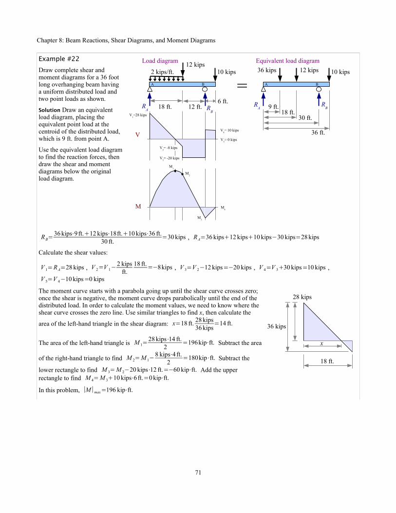
Chapter 8: Beam Reactions, Shear Diagrams, and Moment Diagrams
Example #22
Draw complete shear andmoment diagrams for a 36 footlong overhanging beam havinga uniform distributed load andtwo point loads as shown.
Solution Draw an equivalentload diagram, placing theequivalent point load at thecentroid of the distributed load,which is 9 ft. from point A.
Use the equivalent load diagramto find the reaction forces, thendraw the shear and momentdiagrams below the originalload diagram.
RB=36 kips⋅9ft.+12 kips⋅18ft.+10 kips⋅36 ft.
30 ft.=30 kips , RA=36 kips+12 kips+10 kips−30 kips=28 kips
Calculate the shear values:
V 1=RA=28 kips , V 2=V 1−2 kips
ft.18 ft.=−8kips , V 3=V 2−12 kips=−20 kips , V 4=V 3+30 kips=10 kips ,
V 5=V 4−10 kips=0 kips
The moment curve starts with a parabola going up until the shear curve crosses zero;once the shear is negative, the moment curve drops parabolically until the end of thedistributed load. In order to calculate the moment values, we need to know where theshear curve crosses the zero line. Use similar triangles to find x, then calculate the
area of the left-hand triangle in the shear diagram: x=18 ft. 28 kips36 kips
=14 ft.
The area of the left-hand triangle is M 1=28 kips⋅14 ft.
2=196kip⋅ft. Subtract the area
of the right-hand triangle to find M 2=M 1−8 kips⋅4ft.
2=180kip⋅ft. Subtract the
lower rectangle to find M 3=M 2−20 kips⋅12 ft.=−60 kip⋅ft. Add the upperrectangle to find M 4=M 3+10 kips⋅6ft.=0kip⋅ft.
In this problem, ∣M∣max=196 kip⋅ft.
71
x
18 ft.
28 kips
36 kips
2 kips/ft.
RB
RA
A B =
Load diagram
18 ft. 12 ft.V
1=28 kips
VV
4= 10 kips
V5= 0 kips
10 kips12 kips
6 ft. RB
RA
A B
Equivalent load diagram
9 ft.
30 ft.
10 kips12 kips
36 ft.
36 kips
18 ft.
V2= -8 kips
V3= -20 kips
M
M3
M4
M2
M1
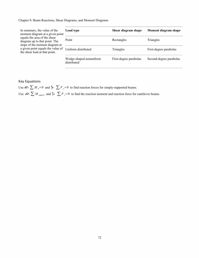
Chapter 8: Beam Reactions, Shear Diagrams, and Moment Diagrams
In summary, the value of the moment diagram at a given pointequals the area of the shear diagram up to that point. The slope of the moment diagram at a given point equals the value of the shear load at that point.
Load type Shear diagram shape Moment diagram shape
Point Rectangles Triangles
Uniform distributed Triangles First-degree parabolas
Wedge-shaped nonuniform distributed
First-degree parabolas Second-degree parabolas
Key Equations
Use ∑M A=0 and ∑ F y=0 to find reaction forces for simply-supported beams.
Use ∑M support and ∑ F y=0 to find the reaction moment and reaction force for cantilever beams.
72

Chapter 9: Stresses in Beams
Chapter 9: Stresses in BeamsIn the last chapter, we learned how to draw shear and bending momentdiagrams for beams. These diagrams tell us the location and magnitudeof the maximum shear load and maximum bending moment. We can use Vmax and Mmax to calculate the maximum shear stress and max. bendingstress in a beam, then we can compare these results with the allowableshear stress and bending stress of the material. If the actual value is lessthan the allowable value, then the beam is safe; if the actual value isgreater than the allowable, then we need to select a different beam.
Bending Stress in Beams
A point load at the midspan of a beam makes the beam bend. We cansketch a deflection diagram to show this bending. The deflectiondiagram shows the beam as if it had no depth, because it is easier to drawa curve than to draw a double curve with shading. A real beam hasdepth, and when it is bent, the top surface shortens while the bottomsurface lengthens...the top surface has a negative strain, while the bottomsurface has a positive strain. Plot strain vs. depth: the strain varieslinearly from top to bottom, and is zero at the centroidal axis.
We saw in Chapter 2 that materials like steel andaluminum follow Hooke's law: the ratio of stress/strainis Young's modulus, a constant. Therefore, the stress inthe beam also varies linearly from top to bottom, and iszero at the centroidal axis of the beam. We call this axisthe neutral axis, where stress is zero.9 This bendingstress acts perpendicular to the cross-sectional area ofthe beam, so the stress is a normal stress; it is negativeon the top and positive on the bottom.
We can calculate the bending stress at any position yfrom the neutral axis: the stress is proportional to the distance from the neutral
axis, so σ=σmaxyc
where c is the distance from the neutral axis to the surface of
the beam. This is the same meaning of c that we used in torsion problems.
Think about a very small area a at a distance y from the neutral axis. Since stress isforce divided by area, the force acting on this area is equal to the stress times the
area: P=σ⋅a=σmax a y
c. The moment of this force with respect to the neutral axis is M=P⋅y=
σmax a y2
c. If we sum up
the moment for all values of a and y, M=σmax
c ∑1n
ai y i2 . Recall from Chapter 5, the moment of inertia of a cross-sectional
area relative to the x-x centroidal axis is I x=∑1
n
ai yi2 , therefore M=
σmax I x
c.
Rewrite this equation to solve for bending stress at the surface: σ=McI x
. This equation is called the Flexure Formula.
We can use the moment equation if we want to know how much bending moment the beam can support. The allowable
moment M allowable=σallowable I x
c.
9 The centroidal axis and the neutral axis are the same if the beam is made of a single material that obeys Hooke's law. The centroidal and neutral axes are often different in beams made of composite materials, like steel-reinforced concrete, or glass/epoxy composite.
73
P
A B
L/2 L/2R
AR
B
Momentdiagram
V Sheardiagram
Mmax
M
Loaddiagram
Vmax
Deflectiondiagram
ΔΔ
max
Vmax
+εmax
–εmax
neutral axis
+σmax
–σmax
+σmax
–σmax
σ yca
Side views of the beam
End view

Chapter 9: Stresses in Beams
Example #1
A 4×6 timber beam, 8 feet long, is loaded with a uniform distributed load of54.65 lb./ft. The beam itself has a weight per unit length of 5.35 lb./ft. What isthe maximum bending stress, and where does it occur? Report the answer in psi.
Solution The total uniform distributed load is the applied load plus the weight of
the beam, wtotal=wapplied+wweight=54.65lb.
ft.+5.35 lb.
ft.=60 lb.
ft.
The load is symmetrical, so the reaction forces are equal to half of the applied
load. RA=RB=W2=wL
2= 60lb.
ft.8 ft.2=240 lb.
The maximum moment equals the area of the left-hand triangle in the shear
diagram: one half the base times the height. M max=240lb.⋅4ft.
2=480ft.⋅lb.
The actual dimensions of a 4×6 timber are 3.5"×5.5". Since the cross-section is a rectangle, the moment of inertia is
I x=bh3
12=
3.5 in.(5.5 in.)3
12=48.53 in.4 The value of c is half the height: c=5.5in.
2=2.75 in. The maximum bending
stress occurs at the midspan, and is σ=McI x
=480ft.⋅lb.(2.75 in.)48.53in.4 ∣12 in.
ft.=326 psi . Bending stress tapers off to zero at the
end supports.
What happens if you use the nominal dimensions instead of actual dimensions for the timber? I x=4in.(6 in.)3
12=72in.4 ,
c= 6in.2=3in. , and σ= 480ft.⋅lb.(3in.)
72in. ∣12in.ft.
=240psi , which is 26% lower than the actual stress.
Tables in the Appendix list values for Ix and Iy for many shapes, but no values for c. Instead, the tables give the section
modulus, defined as S x=I x
c and S y=
I y
c. Section modulus makes the stress calculation easier, because it combines two
terms into one. Bending stress σ=McI x
=MS x
, and allowable moment M allowable=σallowable I x
c=σallowable S x .
In Example #1, the section modulus of a 4×6 timber is 17.6 in.3. Bending stress is σ=MS x
=480 ft.⋅lb.17.6 in.3 ∣12in.
ft.=327 psi .
Simple shapes like rectangles and circles are symmetrical about theneutral axis, so the distance c from the neutral axis to the top surfaceis the same as the distance c from the neutral axis to the bottomsurface. Compound shapes like a T are not symmetrical about the x-xneutral axis, so there are two values to consider: ctop and cbottom. From
the flexure formula, σ=McI x
, the largest stress occurs on
the surface with the largest value of c. In the case of a T-shaped beam loaded on the top flange as shown, the largeststress is the tensile stress along the bottom surface of the
beam: σ=M cbottom
I x
.
74
A B
240 lb. 240 lb.
V1=240 lb.
V V3= 0
V2= -240 lb.
wapplied
8 ft.
Mmax
= 480 ft.⋅lb.
M
wweight
c
c
cbottom
ctop
c
c
End viewSide viewP

Chapter 9: Stresses in Beams
Example #2
What is the allowable moment of a 2×4 Douglas fir beam? Report the answer in ft.⋅lb.
Solution The allowable moment is the largest bending moment that a beam can support. From the Appendix, the section modulus of a 2×4 timber is 3.06 in.3, and the allowable bending stress is 900 psi.
The allowable moment is M allowable=σallowable S x=900lb.
in.23.06in.3∣ ft.
12in.=230 ft.⋅lb.
Bending Stress in Steel Beams
Stress-strain diagrams formany materials aresimplified as a cartoonshowing a straight linesegment for elastic behaviorfollowed by an arc forplastic behavior. In theelastic zone, stress isproportional to strain; theratio is Young's modulusE=σε . Almost all
equations in this book applyonly to the elastic zone. In the plastic zone, the stress required to stretch the material increases due to strain hardening (also called work hardening) until the stress reaches a peak at the tensile strength of the material. After the peak, the material begins to thin, and the cross-sectional area shrinks, so there is less material to support the load, and eventually the material breaks.
Low-carbon steel usedfor wide-flange beamshas an elastic zonefollowed by a horizontalplastic zone in whichthe stress does notchange, so there is nostrain hardening. Thestress-strain curve forlow-carbon sheet steelin Chapter 2 shows thiseffect clearly. As thestrain builds up, eventually strain hardening begins, and thestress-strain curve arcs upwards. In steel beam design, we canuse the horizontal part of the stress-strain curve to extend theload-carrying capacity of the beam. Let's look at the strainand stress profiles in a steel beam as the load is increased:
Point #1 Strain and stress are in the elastic zone. They areboth zero at the neutral axis, and we have maximumcompressive and tensile values at the top and bottomsurfaces.
Point #2 Strain and stress have reached the yield point, soε2=εY and σ2=σYS , the yield strength of the material.
Point #3 Strain continues to increase, but the stress does notexceed the yield strength. Material below the surface reaches the yield point, down to a certain depth. Below this depth, the
75
+ε1
–ε1
neutral axis
+σ1
–σ1
#1Stress
σ
Strain ε
εY
εP
σYS
1 2 3 4 5
+ε2
–ε2
+σYS
–σYS
#2
+ε3
–ε3
+σYS
–σYS
#3
+ε4
–ε4
+σYS
–σYS
#4
+ε5
–ε5
+σYS
–σYS
#5
Strain profile Stress profile
Stressσ
plastic zoneelastic zone
Strain ε
σYS
σTS
Stressσ
Strain ε
plastic zone
εY
εP
σYS strain hardening
elastic zone
Wood, concrete,titanium, aluminum,
alloy steels, etc.Low-carbonsteels only

Chapter 9: Stresses in Beams
interior bending stress remains in the elastic zone.
Point #4 Strain continues to increase. More of the material below the surface reaches the yield point, but the core is in the elastic zone.
Point #5 Strain reaches the point of strain hardening, ε5=εP . All of the material has reached the yield point, becoming fullyplastic. Any additional load on the beam will cause the beam to fail by bending at this location, like two hinged bars.
We can draw an equivalent load diagram for thefully-plastic beam at Point #5. The compressiveforce acting above the neutral axis equals the yieldstrength times the cross-sectional area of the beamin compression (the area above the neutral axis):PC=σYS⋅AC . Likewise, the tensile force below
the neutral axis is PT=σYS⋅AT . The beamdevelops an internal moment to counteract theseforces, equal to each force times the distance fromthe neutral axis of the beam to the centroidal axis of each area. Since this moment iscounteracting fully-plastic loading, we call it the plastic moment, MP., given asM P=PC yC+PT yT=σYS AC yC+σYS AT yT .
If we define a new variable Z=AC yC+AT yT , then M P=σYS Z . This new variable is thesum of the first moments of the areas above and below the neutral axis; we call it the plasticsection modulus. Like section modulus, S, the plastic section modulus is calculated withreference to either the x-x or the y-y neutral axis. The example in the diagram is Zx. Beamsloaded in the strong direction will use Zx; beams that are either loaded from the side ortipped on the side will use Zy.
We can easily calculate Z for simple shapes; you can find Zx and Zy
for complex shapes like wide-flanged beams in the Appendix.
Rectangle Each area is half the area of the rectangle. Each momentarm is half the height of each area, or a quarter of the height of theentire rectangle.
AC=AT=bh/2
yC= yT=h /4
Z x=AC yC+AT yT=bh2
h4+b h
2h4= bh2
4and Z y=
h b2
4
Circle Each area is half the area of a circle. Find the moment arm in the Appendix.
AC=AT=πd 2
4×1
2=πd 2
8
yC= yT=2 d3π
Z x=Z y=AC yC+AT yT=π d 2
82d3π+πd 2
82d3π=
d 3
6
While ideal beams follow the ideal stress-strain curves in the preceding section, real beams vary in strength due to defects inmanufacturing and handling. AISC recommends using a factor of safety of 1.67 in steel beam design, so
σallowable=σYS
1.67=0.6σYS . If we let the moment in a beam equal the plastic moment, then M allowable=σallowable Z=0.6σYS Z .
76
Stress profile
+σYS
–σYS
=
Equivalent load profile End view
PT
PC
centroid oftop half
centroid ofbottom half
yT
yC
area AC
area AT
h/4h
b
h/4d
2d / 3π
2d / 3π

Chapter 9: Stresses in Beams
Example #3
What is the allowable moment of a W200×59 wide-flange beam? Report the answer in kN⋅m.
Solution From Appendix D, the plastic section modulus is 652×103 mm3. From Appendix B, the yield strength is 345 MPa.
The allowable moment is M allowable=0.6σYS Z x=0.6 345 MPa 652×103 mm3∣ m3
(103 mm)3∣ 103kN
MPa m2 =135 kN⋅m
The bending stress in a low-carbon steel beam is σ=MZ x
.
Shear Stress in Beams
Bending stress is a normal stress, acting perpendicularly to the cross-sectional area of the beam. Apply a downward load on top of a simply-supported beam, and the bending stress on the top surface is horizontal andcompressive; along the bottom surface it is horizontal and tensile.
Beams also have a horizontal shear stress which acts parallel to the neutralaxis of the beam. Take a deck of playing cards and flex it in your hand; thecards slide past each other. Think of this sliding as strain; if the cards hadbeen glued together, then a corresponding shear stress would havedeveloped in the adhesive.
Glue all but one of the cards on their faces, then place the free card on top ofthe glued deck. Bend the deck, and the top card slides very little withrespect to the rest of the deck. Now take a second deck having the samenumber of cards as the first deck, and glue all of the cards in the seconddeck together. Place one deck on the other and bend them; the two decksslide with respect to each other – more so than if the decks were differentthicknesses. This experiment shows that the shear stress is zero at thesurface of a beam, and maximum at the neutral axis.
Bend a simply-supported beam with a point load at the midspan, and themoment diagram is an isosceles triangle. Select two points on the beam thatare separated by a small distance Δx. On the moment diagram, M 1<M 2 .Since bending stress is proportional to bending moment, σ1<σ2 . Pick ahorizontal plane within the beam where you want to calculate theshear stress. In this example, the shear plane is above the neutralaxis. The cross-sectional area between the shear plane and the topof the beam is A'.
Draw a free-body diagram of the beam above the shear plane. Thehorizontal force acting on this area at point 1 is P1=σ1 A' .Likewise, the horizontal force acting on this area at point 2 isP2=σ2 A' . Since σ1<σ2 , P1<P2 . The sum of the forces in the x
direction equals zero, so the difference between these forces is ahorizontal shear force, V H=P2−P1 .
The normal stress acting on area A' at point 1 varies with depth: it ishighest on the top surface of the beam, and lower at the shear plane. Wecan break up area A' into many tiny areas, where each tiny area a is a distancey from the neutral axis. The average normal stress acting on area A' at point 1 is
the sum of the normal stresses acting on all of the tiny areas, so σ1avg=∑y
c M 1 yI
.
77
Loose cards
1 card onglued deck
2 glued decksP
P
P
P
A B
RA
RB
V
MM
1
End view
yarea A'shear plane
Free-bodydiagramof area A'
Δx
1 2
Δx
P1
VH
P2
M2
x
c
area A'
yyshear planearea a
centroid of area A'

Chapter 9: Stresses in Beams
The normal force acting on area A' at point 1 is the average stress times the sum of these tiny areas, so
P1=∑y
c M 1 y aI
=M 1
I ∑y
c
y a . Since ∑y
c
y a=y A' , P1=M 1 y A'
I. Similarly, the normal force acting on area A' at point 2
is P2=M 2 y A '
I. The shear force V H=P2−P1=
(M 2−M 1) y A 'I
.
The value of the bending moment at any point along a beam equals the area of the shear diagram up to that point, soM 1=V x and M 2=V (x+Δ x) . The difference of the two moments is M 2−M 1=V (x+Δ x)−V x=V⋅Δ x . Substitute
this result into the shear force equation, and we have V H=V Δ x y A'
I.
The shear stress acting in the shear plane equals the shear force VH divided by the area it acts on: the thickness of the beam
in the shear plane times the length of beam between points 1 and 2: τ=V H
t Δ x=V Δ x y A'
I t Δ x=V y A'
I t. The product y A' is
the first moment of area A' about the neutral axis, defined as the variable Q= y A' . Substituting, we have the General
Shear Formula for beams: τ=V QI t
.
Example #4
Calculate the shear stress in a rectangular beam at five locations: at the neutral axis, ¼ of the way between the neutral axis and the top of the beam, ½ way, ¾ of the way, and at the top of the beam.
Case 1 When the shear plane is at the neutral axis, y= h4
and A'=bh2
, so Q= y A'= h4
bh2=bh2
8. The moment of
inertia of a rectangle is I=bh3
12 and the thickness of the beam at the shear plane is t=b . The shear stress is
τ=VQI t=V bh2
812
bh3 b= 3V
2bh
Case 2 y= 516
h and A'=38
bh , so Q= y A'=5h16
3bh8= 15bh2
128. The other two variables in the General Shear Equation,
I and t, are the same as before, so the shear stress is τ=VQI t=V 15 bh2
12812
bh3 b= 45 V
32 bh
Case 3 y=38
h and A'=14
bh , so Q= y A'=3 h8
bh4=
3bh2
32 and τ=
VQI t=V 3bh2
3212
bh3 b= 9V
8bh
Case 4 y= 716
h and A'=18
bh , so Q= y A'=7 h16
bh8=
7bh2
128 and τ=
VQI t=V 7bh2
12812
bh3 b= 21V
32 bh
Case 5 y=12
h and A'=0 , so Q= y A'=0 and τ=VQI t=0
78
h
b
area A'
y
shearplane
centroid ofarea A'
area A'
yh/4
area A'
yh/8
area A'
y3h/8
area A' = 0
yh/2
Case 1 Case 2 Case 3 Case 4 Case 5

Chapter 9: Stresses in Beams
We can plot the results from this Example problem as a function of depth (red dots atthe right). The shear stress profile for a rectangular beam looks like a parabola. Theshear stress is a maximum at the neutral axis, diminishing to zero at the top andbottom surfaces. The profile looks different for wide-flange beams because the area isdistributed differently, but the maximum shear stress will still be at the core and thesurface will have zero shear stress.
Example #5
A round 1.5 cm diameter rod is loaded in bending with a point load of 300 N atthe midspan. Calculate the shear stress at the neutral axis. Report the result inMPa.
Solution The loading is symmetrical, so the reaction forces equal half the
applied load: RA=RB=300 N
2=150 N . Draw the shear diagram to find the
maximum shear load, V max=RA=150 N .
From the Appendix, the centroid of area A' is at y= 4 r3π
where r is the radius
of the circle. Substitute diameter for radius, and y= 2d3π
.
Area A' is half the area of the circle: A'=12πd 2
4=πd 2
8.
Calculate Q= y A'=2d3π
πd 2
8=
d 3
12. The moment of inertia of a circle is I=
π d 4
64, and the thickness of the beam at the
shear plane is d.
Combine terms to find shear stress, τ=VQI t=
V d 3
1264πd 4 d
=16V3π d 2=
16⋅150 N3 π(1.5 cm)2∣MPa m2
106 N ∣(100 cm)2
m2 =1.13 MPa
Another way to solve this problem is to calculate numerical answers for y , A', Q, and I, with appropriate unit conversions, then calculate τ. Try it both ways, and you will find that the algebraic solution is shorter and requires fewer keystrokes on the calculator, which means fewer opportunities for error.
The General Shear Formula works well for simple shapes where y and A' are easy to calculate. Wide-flange beams have a more complicated shape, so we can approximate the shear stress at the neutral axis
using the Average Web Shear Approach: τ=V
d t w where d is the depth of the beam and tw is the thickness
of the web.
79
dtw
P = 300 N
A B
L/2 L/2150 N 150 N
V
150 N
-150 N
shearplane
area A'
y
Shear stress profile End view

Chapter 9: Stresses in Beams
Example #6
A W4×13 wide-flange beam is loaded in bending with a point load of 6 kips at the midspan. Calculate the shear stress at the neutral axis. Report the result in ksi.
Solution The loading is symmetrical, so the reaction forces equal half the
applied load: RA=RB=6kips
2=3kips . From the shear diagram, the
maximum shear load V max=RA=3 kips . Use the Average Web Shear Approach to find the shear stress at the neutral axis:
τ= Vd t w
= 3kips4.16 in.×0.280 in.
=2.58 ksi .
How does the calculated shear stress compare with the actual shear strength of the material? While yield and ultimate strengths are easy to find in reference books and on the internet, shear strengths are rarely reported. A good estimate for steels is τallowable=0.4σYS . If the beam in the previous Example is made of A36 steel with a yield strength of 36 ksi, the allowable shear stress is τallowable=0.4 (36 ksi)=14.4 ksi>τ applied , therefore the beam will not fail in shear.
In most of the problems so far, we have assumed that the beams are weightless. Real beams have real weight, so we need to include the weight as a uniform distributed load along the length of the beam.
80
P = 6 kips
A B
3 kips 3 kips
V
3 kips
-3 kips
L/2 L/2

Chapter 9: Stresses in Beams
Example #7
A 36 foot long W12×30 wide-flange beam is loaded in bending with a point load of 5 kips located 24 feet from the leftend. The beam also has weight. Calculate the allowable bending moment in the beam. Calculate the maximum bending stress and maximum shear stress, and report the result in ksi. Report the locations of these maximum points.
Solution The loading is not symmetrical, so use an equivalent load diagram, sum ofthe moments and sum of the forces to findthe reaction forces. A W12×30 beam has a weight per unit length w=30 lb./ ft. , so the equivalent point load
W =30lb.ft.
36ft.∣ kip103 lb.
=1.08 kips at the midspan.
The moment about point A is ∑M A=0=−1.08 kips⋅18ft.−5kips⋅24ft.+RB⋅36ft.
Rewrite the equation to find the reaction force RB=1.08 kips⋅18ft.+5kips⋅24ft.
36 ft.=3.873 kips
Sum of the forces ∑ F y=0=RA−1.08 kips−5kips+3.873 kips . Solve for the reaction forceRA=1.08kips+5 kips−3.873kips=2.207 kips . Calculate the inflection points on the shear diagram.
V 1=RA=2.207kips , V 2=V 1−0.030kips
ft.24 ft.=1.487 kips , V 3=V 2−5 kips=−3.5133 kips ,
V 4=V 3−0.030kips
ft.12 ft.=−3.873 kips , V 5=V 4+RB=0 kips
The maximum moment is the area of the left-hand trapezoid in the shear diagram:
M max=2.207 kips+1.487 kips
224ft.=44.3 kip⋅ft.
The allowable bending moment M allowable=0.6σYS Z=0.6⋅50 kips⋅43.1 in.3
in.2 ∣ ft.12 in.
=107.8kip⋅ft.
Since M allowable>M applied , the beam is strong enough to support the existing loads in bending.
The maximum bending stress in the beam is σ=MZ=
44.3 kip⋅ft.43.1 in.3 ∣12in.
ft.=12.34ksi , and it occurs at the point load.
From the shear diagram, the maximum shear load ∣V max∣=3.5133kips . Use the Average Web Shear Approach to find the
maximum shear stress τ=V
d t w
= 3.5133 kips12.34 in.×0.260 in.
=1.10 ksi , which occurs at point B.
81
wbeam
= 30 lb./ft.
= 0.030 kips/ft.
RB
RA
A B
24 ft. 12 ft.
V1=2.207 kips
V
V4= -3.873 kips
V5= 0 kips
P = 5 kips
V3= -3.513 kips
M
Mmax
=
=R
BR
A
A B
Equivalent load diagram
18 ft.
W = 1.08 kips
24 ft.
P = 5 kips
V2= 1.487 kips

Chapter 9: Stresses in Beams
Allowable Load
Design engineers select beams that will support known loads. However, in many cases the structure already exists, and will be used with a different loading condition than it was originally intended. A manufacturing plant may bring in a larger piece of equipment, so the engineer calculates whether the existing floor will support the machine.
A simply-supported timber beam carries a uniform distributed load; how large a load can the beam support? Since the loading is symmetrical, the reaction
forces equal half the applied load: RA=RB=w L2
. The maximum shear load is
V 1=RA=w L
2. The maximum moment equals the area of the left-hand triangle
in the shear diagram, or one half the base times the height:
M max=12
L2
w L2=
w L2
8. If we look at bending stress, then σ=
MS=
w L2
8 S.
Rewrite the equation to solve for the load, w=8σallowable S
L2 . If we look at shear stress, τ=V QI t=w L Q
2 I t. Rewrite the
equation to solve for the load, w=2 τallowable I t
L Q.
Example #8
A simply-supported, 8 foot long, 4×8 southern yellow pine timber supports auniform distributed load. Calculate the maximum load the beam can support.Report the result in lb./ft.
Solution From the previous discussion, based on bending stress the beam can
support a total load of wtotal=8σallowable S
L2 . From the Appendix, the allowable
bending stress of southern yellow pine is 1400 psi and the section modulusS x=30.7in.3 .
The total load is wtotal=8
(8ft.)2
1400lb.in.2
30.7in.3∣ ft.12 in.
=448lb./ ft. . The total
load includes the beam's weight per unit length: wtotal=wapplied+wbeam . From theAppendix, a 4×8 timber has a weight of 7.05 lb./ft., sowapplied=wtotal−wbeam=448lb. /ft.−7.05lb./ ft.=441lb./ ft.
Also from the previous discussion, based on shear stress the beam can support a
total load of wtotal=2 τallowable I t
L Q. From the Appendix, I x=111in.4 and
τallowable=175 psi . Based on the dimensions, y=7.25 in.4
=1.8125 in. ,
t=3.5in. , and A'=3.5 in.⋅7.25 in.2
=12.6875 in.2 , so Q=A' y=12.6875 in.2⋅1.8125in.=22.9961 in.3 . The total load is
wtotal=2 τallowable I t
L Q= 2
8ft.175lb.
in.2
111in.4
22.9961 in.3
3.5in.=739lb. / ft. . The applied load is
wapplied=739lb./ ft.−7.05lb./ ft.=732 lb./ ft.
The beam can support an applied load of 441 lb./ft. before it fails in bending, and a load of 732 lb./ft. before it fails in shear. Pick the lower of the two numbers because this is where failure will occur first.
82
A B
wL/2 wL/2
V1=wL/2
V V3= 0
V2= –wL/2
w
8 ft.
Mmax
= wL2/8
M
7.25 in.
3.5 in.
area A'
y
shearplane
centroid ofarea A'
A B
wL/2 wL/2
V1=wL/2
V V3= 0
V2= –wL/2
w
L
Mmax
= wL2/8
M

Chapter 9: Stresses in Beams
Key Equations
Use the Flexure Formula to find the bending stress in a beam: σ=McI x
or σ=MS x
The allowable moment of a beam is M allowable=σallowable I x
c or M allowable=σallowable S x
For low-carbon steel beams, the allowable moment is M allowable=0.6σYS Z x and the bending stress is σ=MZ x
Use the General Shear Formula to find the maximum shear stress in a beam: τ=V QI t
where Q= y A'
Use the Average Web Shear Approach to find the maximum shear stress in a wide-flange beam: τ=V
d t w
For steels, use τallowable=0.4σYS
83

Chapter 10: Beam Deflection
Chapter 10: Beam DefectionRadius of Curvature
A weightless beam with no loads hasa horizontal elastic curve. Pick twopoints C and D that are a smalldistance x apart. If we add a load, thebeam deflects, and the elastic curvebows downward. Points C and D nowlie on an arc with a radius ofcurvature, labeled R on the diagram.At the bottom of the beam, points Cand D are now x+δ apart, becausethe bottom of the beam has stretcheda little. Draw a vertical line throughpoint D, and we have a little trianglewith height c and base δ. We can usethe principle of similar triangles tocompare the little triangle with thebig triangle having a height R and
base x: δc= x
R. Rewrite the equation
to solve for δx= c
R. Along the
bottom surface of the beam, the strain is ε=δx , so ε= cR
. As long as the beam is elastic, E= σε
, which we can rewrite as
ε= σE
. Set the strain equations equal to each other, and σE= c
R. Solving for stress, σ= E c
R. We know another equation
for bending stress in a beam: σ=M cI
. Set the stress equations equal to each other, and E cR=M c
I→ E
R=M
I. Now
solve for radius of curvature, R= E IM
.
This equation helps us calculate the radius of curvature at a given point along the length of a beam. There are some special cases where the moment M is constant over a long length, so the elastic curve is a circular arc along this length.
Example #1
A 2 m long titanium beam is made of 1 cm square barstock. Two 50 N pointloads lie 0.25 meters from each end. What is the radius of curvature of thebeam between the two point loads? Report the answer in meters.
Solution Draw the elastic curve, shear diagram, and moment diagram. Theloading is symmetrical, so the reaction forces RA=RB=50 N . The value ofthe moment diagram between the point loads equals the area of the left-handrectangle in the shear diagram: M=0.25 m⋅50 N=12.5 N⋅m .
The moment of inertia of a square I=b h3
12=
b4
12.
The radius of curvature of the beam between the two point loads is
R= E IM= E b4
12 M=
114 GPa (1 cm)4
12⋅12.5 N⋅m ∣ 109 N
GPa m2∣ m4
(100cm )4=7.6 m
84
A B
RA
RB
C
P
A BD
Elasticcurve
C D
R
c
δ
x+δ
A B
RA
RB
CA BD
Elasticcurve
C D
c
x
Beam with no load Loaded beam
R
xc
δx
Elasticcurve
A B
50 N 50 N
V
Mmax
= 12.5 N⋅m
0.25 m
50 N
0.25 m
1.5 m
M
V1= 50 N
50 N
V2= 0
V3= –50 N
V4= 0

Chapter 10: Beam Deflection
The blade on a bandsaw obeys the radius of curvature equation because the blade flexes elastically, and forms a semicircular arc at each bandsaw wheel.
In a few rare cases, we can calculate the maximum deflection of a beam using the radius of curvature, as in the following example.
Example #2
A 2 m long titanium beam is made of 1 cm squarebarstock. Two 50 N point loads lie at the ends, and thesupports lie 0.25 meters from each end. What is themaximum deflection at the midspan? Report the answerin cm.
Solution This problem is like Example #1 but flippedupside down. Draw the elastic curve with its radius ofcurvature and the center of curvature (cross at thebottom of the figure). The distance from the center ofcurvature to the beam is R; the beam deflects adistance Δmax at the midspan; and the distance fromthe center of curvature to the undeflected beam isR−Δmax . The base of the shaded triangle is half the
distance between the supports, 0.75 m. Use thePythagorean Theorem to find the height of the triangle,R−Δmax=√R2−(0.75m)2=√(15.2 m)2−(0.75 m)2=15.182 m . Deflection at the midspan
Δmax=R−(R−Δmax)=15.200 m−15.182 m∣100cm
m=1.8 cm
The Formula Method for Simple Cases
We can use the Radius of Curvature Method to calculate deflection as long as the moment is constant. From the examples inprevious chapters, we know that the moment usually changes along the length of a beam. There are a number of geometricaland calculus-based techniques for calculating deflection in these cases. Engineers have compiled these solutions in handbooks, so future engineers can use a worked-out algebraic solution, instead of deriving the solution from scratch. The most useful compilation is Roark's Formulas for Stress and Strain, which contains many hundreds of formulas for beams, shells, membranes, pressure vessels, and columns.
Look in the Appendix for Formula Method solutions for various beam problems. Each case includes a load diagram, shear diagram, moment diagram, reaction forces and moments, and formulas for shear, moment, the slope at the ends, and deflection at various positions along the beam. Use the Appendix to find values for E and I, then solve.
Example #3
Use the Formula Method to calculate the maximum deflection of a simply-supported 8-foot 4×4 Southern yellow pine timber loaded with a 200 lb. pointload at the midspan. Report the result in inches.
Solution From Appendix F, the deflection at the midspan Δmax=P L3
48 E I,
where Young's modulus is 1700 ksi and the moment of inertia is 12.5 in.4.
Δmax=200lb.(8ft.)3
48⋅12.5in.4
in.2
1700 kip∣(12 in.)3
ft.3 ∣ kip
103 lb.=0.17in.
85
Elasticcurve
A B
50 N 50 N
V
M= –6.25 N⋅m
0.25 m
50 N
0.25 m1.5 m
M
V1= –50 N
50 N
V2= 0 V
3= 50 N
V4= 0
RR
R–Δmax
0.75 m
Δmax
P = 200 lb.
A B
4 ft. 4 ft.100 lb. 100 lb.
Elasticcurve
Δmax

Chapter 10: Beam Deflection
Example #4
Use the Formula Method to calculate the maximum deflection of a cantilever8-foot 4×4 Southern yellow pine timber loaded with a 200 lb. point load at theend. Report the result in inches.
Calculate the slope at the end of the beam; report the result in degrees.
Solution From the Appendix, the deflection at the free end Δmax=P L3
3E I. The
moment of inertia and Young's modulus are the same as in the previousExample.
Δmax=200lb.(8ft.)3
3⋅12.5 in.4in.2
1700 kip∣(12 in.)3
ft.3 ∣ kip103 lb.
=2.78in.
The equation for the slope at the free end is in radians, so include a conversion factor for degrees:
θ= P L2
2 E I=
200lb. (8ft.)2
2⋅12.5 in.4in.2
1700 kip∣(12 in.)2
ft.2 ∣ kip103 lb.∣180°
rad=7.81°
When the point load on a cantilever beam is at the end of the beam, the elastic curve is an arc. If the point load is located away from the end, then the elastic curve is an arc from the wall to the point load, and a straight line between the point load and the end of the beam. This portion of the beam is sloped but straight.
Example #5
A cantilever 8-foot 4×4 Southern yellow pine timber loaded with a 200 lb.point load 2 feet from the end. Use the Formula Method to calculate thedeflection at the point load. Calculate the deflection at the point load and themaximum deflection at the end. Report the results in inches.
Solution From Appendix F, the deflection at point C is ΔC=P b3
3 E I, where b
is the distance from the point load to the wall. The moment of inertia andYoung's modulus are the same as in the previous two Examples.
ΔC=200lb.(6 ft.)3
3⋅12.5in.4
in.4
1700 kip∣(12 in.)3
ft.3kip
103 lb.=1.17 in.
The slope of the straight portion of the beam from point C to the left end is
θ= P b2
2 E I=
200lb. (6ft.)2
2⋅12.5in.4
in.2
1700 kip∣(12 in.)2
ft.2 ∣ kip103 lb.∣180°
rad=4.39° .
The portion of the beam to the left of the point load is a straight line. Use trigonometry
to find the maximum deflection: tan θ= y2ft.
so y=2ft. tan (4.39° )∣12in.ft.
=1.84 in. and
Δmax=y+ΔC=1.84 in.+1.1 in.=3.01 in.
86
1600 ft.⋅lb.P = 200 lb.
A B
8 ft.200 lb.
Elasticcurve
Δmax
θ
1200 ft.⋅lb.P = 200 lb.
A B
6 ft.200 lb.
2 ft.
Elasticcurve
Δmax
θarcline
ΔC
C
Δmax
ΔC
θyline
2 ft.

Chapter 10: Beam Deflection
Formula Method Hints
Some Formula Method equations haveconditions. Consider a simply-supported beamwith a single point load located at a distance afrom the left end. The deflection at a distance x
from the left end is Δx=P b x
6 E I L(L2−b2−x2)
when x<a , so this equation is restricted tothe portion of the beam to the left of the pointload. What if we want the deflection at alocation to the right of the point load? Redrawthe beam as a left-to-right mirror image,swapping dimensions a and b, and solve forthe deflection.
Example #6
A simply-supported 36 cm long steel beam is loaded with a 6.5 kN point load 8 cm from the left end. The beam is made of 1.2 cm square barstock. Use the Formula Method to calculate the deflection 24 cm from the left end. Report the results in mm.
Solution From Appendix F, the
deflection at a distance x from the left end
is Δx=P b x
6 E I L(L2−b2−x2) when x<a .
Since x>a , we have to draw a mirror image of the loading case.
The moment of inertia is I=bh3
12= b4
12=(1.2 cm)4
12=0.1728 cm4
Δ x=6.5 kN⋅8cm⋅12cm
6⋅207GPa⋅0.1728 cm4⋅36cm∣GPa m2
106kN ∣(100cm )2
m2 ×((36cm )2−(8 cm)2−(12cm)2)∣10 mm
cm=8.79mm
The Formula Method for Complex Cases: Superposition
The Formula Method equations in the Appendixapply to simple loading cases. Many loadingconditions are more complex, but you canseparate a complex loading condition into itsparts, solve for V, M, or Δ at any location alongthe beam, then add the results together to find thetotal V, M, or Δ at that location:Δ total=Δ1+Δ2+Δ3+...Δn for n cases.
87
P
A B
a bR
AR
BL
Elasticcurve
Δx
x
P
A B
a bR
AR
BL
Elasticcurve
Δx
x
Original Mirror image
6.5 kN
A B
8 cm28 cm
RA
RB36 cm
Elasticcurve
Δx = 24 cm
24 cm
6.5 kN
A B
RA
RB36 cm
Elasticcurve
Δx = 12 cm
Original Mirror image
12 cm
28 cm8 cm
P
A B
w
=P
A B + A B
w
x x xC C C

Chapter 10: Beam Deflection
Example #7
A simply-supported 200 cm long, 51 mm standard steel pipe is loaded with a uniform distributed load of 400 N/m and a point load of 8 kN located 25 cm from the right end. Use the Formula Method and Superposition to calculate the deflection at the midspan (atx=1m ). Report the results in mm.
Solution From Appendix F, the deflection due to the point load at a distance x from the left end is
Δ1=P b x
6 E I L(L2−b2−x2) . At the midspan, x= L
2, so Δ1=
P b L6 E I L 2 (L2−b2−( L
2 )2
)= P b12 E I (34 L2−b2) . In this
equation, b is 25 cm. Also from the Appendix, a 51 mm standard steel pipe has a moment of inertia I=0.276×106mm 4
Δ1=8kN⋅25 cm
12⋅207GPa⋅0.276×106 mm4∣GPa m2
106 kN ∣(103mm )2
m2 ∣10mmcm
×(0.75(200 cm )2−(25cm )2)∣(10 mm)2
cm 2 =8.57 mm
The deflection due to the distributed load at the midspan is Δ2=5w L4
384 E I
Δ2=5
384400 N
m(200 cm)4
207GPa⋅0.276×106 mm4∣GPa m2
109 N ∣103 mmm ∣(10 mm)4
cm4 =1.46 mm
Δtotal=Δ1+Δ2=8.57 mm+1.46 mm=10.03 mm
In the previous Example, the maximum deflection due to the uniform distributed load is at the midspan (x = 1 m), but the
maximum deflection due to the point load is located at x=√ a (a+2b)3
=√ 175 cm(175 cm+2 (25 cm))3
=114.5 cm , to the
right of the midspan. Using the Method of Superposition, you can add the shear, moment, or deflection at a given point along the beam, but you cannot add the maximum shear, moment, or deflection, unless they occur at the same point along the beam. One example is a simply-supported beam with a point load at the midspan and a uniform distributed load; both loading conditions have the maximum deflection and maximum moment at the midspan.
Example #7 does not consider the weight of the pipe. From Appendix D, the mass per unit length is 5.44 kg/m. The SI unit of weight is the newton, equal to a kilogram meter per second squared. Multiply mass by gravity to get weight.
WL=m g
L=5.44kg
m9.81m
s2 ∣N s2
kg m=53.4 N/m
88
P = 8 kN
A B
w = 400 N/m
= A B + A B
25 cm200 cm
8 kN 400 N/m

Chapter 10: Beam Deflection
Visualizing the Defection Curve
We can use the Formula Method for calculating the deflection of a beam at many points along its length, then graphing the result to see the deflection curve.
Example #9
Plot the deflection curve for a W16×100 steel beam due to the applied load. Ignore the weight of the beam.
Solution From Appendix F, the deflection equation for this loading condition is
Δx=wmax x
360 E I L(3x4−10L2 x2+7L4) . From Appendix D, Ix=1490 in.4 Calculate
the deflection at 0.5 foot intervals.
Δ0.5ft.=0.3 kip
ft.0.5ft.360
in.2
30 kips
[3(0.5 ft.)4−10(14ft.)2(0.5ft.)2+7(14 ft.)4 ]1490in.414 ft.
(12 in.)3
ft.3 =0.31in.
Δ1.0ft.=0.3 kip
ft.1.0 ft.360
in.2
30 kips[3(1.0 ft.)4−10(14 ft.)2(1.0 ft.)2+7(14ft.)4 ]
1490in.414ft.
(12in.)3
ft.3=0.61in.
Δ1.5ft.=0.3 kip
ft.1.5 ft.360
in.2
30 kips
[3(1.5 ft.)4−10(14ft.)2(1.5 ft.)2+7(14 ft.)4]1490in.414 ft.
(12 in.)3
ft.3 =0.91 in.
For a repetitive equation like this, it's easiest to use a spreadsheet to calculate the rest of the points:
Δ2.0ft. = 1.20 in.
Δ2.5ft. = 1.48 in.
Δ3.0ft. = 1.74 in.
Δ3.5ft. = 1.98 in.
Δ4.0ft. = 2.19 in.
Δ4.5ft. = 2.39 in.
Δ5.0ft. = 2.55 in.
Δ5.5ft. = 2.69 in.
Δ6.0ft. = 2.79 in.
Δ6.5ft. = 2.86 in.
Δ7.0ft. = 2.90 in.
Δ7.5ft. = 2.90 in.
Δ8.0ft. = 2.87 in.
Δ9.5ft. = 2.80 in.
Δ10.0ft. = 2.69 in.
Δ10.5ft. = 2.16 in.
Δ11.0ft. = 1.92 in.
Δ11.5ft. = 1.65 in.
Δ12.0ft. = 1.35 in.
Δ12.5ft. = 1.03 in.
Δ13.0ft. = 0.70 in.
Δ13.5ft. = 0.35 in.
Δ14.0ft. = 0.00 in.
Graphing the numbers, we get:
The curve looks like a parabola, but the numbers in the table show that the arc is skewed to the right (where the load is greatest).
Key Equations
If a beam segment has a constant moment, then the radius of curvature of that segment of beam is R= E IM
. The bending
stress in this segment of the beam is σ= E cR
.
89
A B
0.3 kip/ft.
14 ft.
x
0 2 4 6 8 10 12 140
1
2
3
Distance from the left end (ft.)
Deflection(in.)

Chapter 11: Beam Design
Chapter 11: Beam DesignWide-Flange Steel Beam Design in Six Easy Steps
In the previous three chapters, we learned how to calculate reaction forces and moments, how to draw shear and moment diagrams, how to calculate deflection, and how to calculate bending and shear stresses for a given beam size and shape. When you design a beam, you start with the applied loads, beam length, allowable stresses (and sometimes allowable deflection), and you must figure out what size beam to use. Use these six steps, and you can design a wide-flange steel beam.
Step 1 Identify all applied loads and design constraints (beam length, yield strength, and maximum deflection if specified).
Step 2 Draw the load diagram and calculate the reactions. Draw an equivalent load diagram if necessary.
Step 3 Draw shear and moment diagrams, and calculate Vmax and Mmax.
Step 4 Select the lightest beam from Appendix D that will support Mmax, or has enough stiffness to limit Δmax. The allowable
moment in a steel beam M allowable=0.6σYS Z x , so the required plastic section modulus is Z required=M
0.6σYS
=1.67 MσYS
. Solve
for Zrequired, then find the lightest W-beam that has a slightly larger value of Z.
U.S. Customary beams are identified by nominal depth and weight per unit length. For example, W12×40 is about 12 in. deep, and weighs 40 lb./ft.
Metric beams are identified by nominal depth and mass per unit length. For example, W360×110 is about 360 mm deep, andhas a mass of 110 kg/m; convert to weight per unit length by multiplying by gravity (9.81 m/s2), using the definition of a
newton, N=kg⋅ms2 , to convert units: w=m
Lg=110 kg
m9.81 m
s2 ∣N s2
kg m ∣ kN
103 N=1.08 kN/m
If the maximum deflection is specified, write the equation for Δmax, solve it for Irequired, then find the lightest W-beam that hasa slightly larger value of I.
Step 5 Add the beam weight to the load diagram, and recheck moment and deflection. You may have to draw completely new shear and moment diagrams. If Z beam>Z required , the beam is OK in bending, and if I beam> I required , the beam is OK in deflection. If either of these conditions is not met, pick a larger beam and recalculate.
Step 6 Check shear. For steel W-beams, V applied≤0.4σYS d t w where d is the beam depth and tw is the thickness of the web. As long as this inequality is true, the beam is OK in shear.
The rule of thumb in these calculations is to use a beam that has more than you need (more I, more Z, more shear strength). Just like in real life, having more than you need is usually better than having less than you need (money, food, education, happiness, etc.)
90
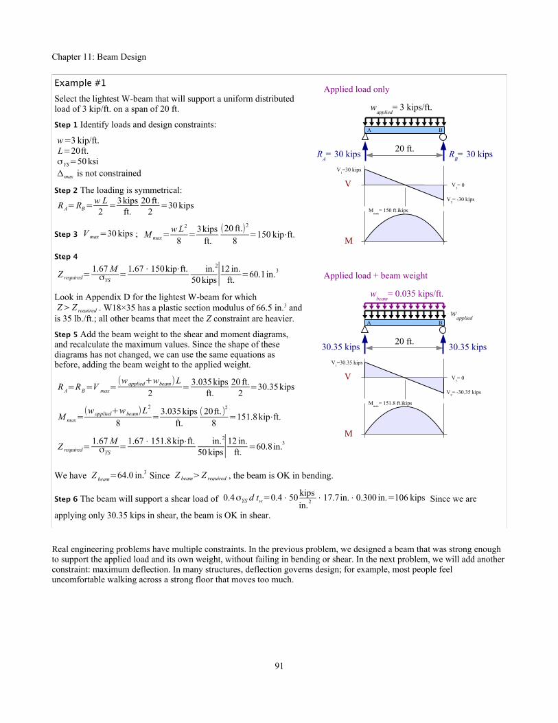
Chapter 11: Beam Design
Example #1
Select the lightest W-beam that will support a uniform distributed load of 3 kip/ft. on a span of 20 ft.
Step 1 Identify loads and design constraints:
w=3 kip/ft.L=20ft.σYS=50 ksiΔmax is not constrained
Step 2 The loading is symmetrical:
RA=RB=w L2=3kips
ft.20 ft.
2=30 kips
Step 3 V max=30 kips ; M max=w L2
8=3kips
ft.(20 ft.)2
8=150 kip⋅ft.
Step 4
Z required=1.67 MσYS
=1.67⋅150kip⋅ft. in.2
50 kips∣12 in.ft.
=60.1in.3
Look in Appendix D for the lightest W-beam for whichZ>Z required . W18×35 has a plastic section modulus of 66.5 in.3 and
is 35 lb./ft.; all other beams that meet the Z constraint are heavier.
Step 5 Add the beam weight to the shear and moment diagrams, and recalculate the maximum values. Since the shape of these diagrams has not changed, we can use the same equations as before, adding the beam weight to the applied weight.
RA=RB=V max=(w applied+wbeam)L
2= 3.035 kips
ft.20 ft.
2=30.35kips
M max=(w applied+w beam)L
2
8=3.035 kips
ft.(20ft.)2
8=151.8 kip⋅ft.
Z required=1.67 MσYS
=1.67⋅151.8kip⋅ft. in.2
50 kips∣12 in.ft.
=60.8in.3
We have Z beam=64.0 in.3 Since Z beam>Z required , the beam is OK in bending.
Step 6 The beam will support a shear load of 0.4σYS d tw=0.4⋅50 kipsin.2 ⋅17.7in.⋅0.300 in.=106 kips Since we are
applying only 30.35 kips in shear, the beam is OK in shear.
Real engineering problems have multiple constraints. In the previous problem, we designed a beam that was strong enough to support the applied load and its own weight, without failing in bending or shear. In the next problem, we will add anotherconstraint: maximum deflection. In many structures, deflection governs design; for example, most people feel uncomfortable walking across a strong floor that moves too much.
91
A B
RA= 30 kips
V1=30 kips
V V3= 0
V2= -30 kips
20 ft.
Mmax
= 150 ft.⋅kips
M
RB= 30 kips
wapplied
= 3 kips/ft.
A B
30.35 kips
V1=30.35 kips
V V3= 0
V2= -30.35 kips
20 ft.
Mmax
= 151.8 ft.⋅kips
M
30.35 kips
wbeam
= 0.035 kips/ft.
wapplied
Applied load + beam weight
Applied load only

Chapter 11: Beam Design
Example #2
Select the lightest W-beam that will support a uniform distributed load of 3 kip/ft. on a span of 20 ft., and deflects no more than 0.6 in.
Step 1 Identify loads and design constraints:
w=3 kip/ft.L=20 ft.
σYS=50 ksiΔmax=0.6 in.
Steps 2 & 3 These steps are identical to Example #1:RA=RB=30 kips , V max=30 kips , and M max=150 kip⋅ft.
Step 4 Z required=60.1in.3 as in Example #1, therefore we should try W16×36 which has a plastic section modulus of 64.0 in.3
For this loading case, Δmax=5w L4
384 E I. The moment of inertia
required to support the deflection constraint is
I required=5w L4
384 E Δmax
=5
3843kips
ft.(20ft.)4 in.2
30×103kip 0.6 in.∣(12 in.)3
ft.3 =600in.4 .
The moment of inertia of a W16×36 beam is 448 in.4... not enough. The lightest W-beam with I>600in.4 is W18×40, which hasI x=612 in.4 and S x=78.4in.3
Step 5 Add beam weight to shear and moment diagrams; recalculate the max. values. The shape of the diagrams is unchanged; use the same equations as before, adding beam weight to applied weight.
RA=RB=V max=(wapplied+w beam)L
2=3.04 kips
ft.20ft.
2=30.4 kips
M max=(wapplied+wbeam) L2
8=3.04 kips
ft.(20ft.)2
8=152kip⋅ft.
Z required=1.67 MσYS
=1.67⋅152kip⋅ft. in.2
50 kips∣12 in.ft.
=60.9in.3
We have Z beam=78.4 in.3 Since Z beam>Z required , the beam is OK in bending.
I required=5(wapplied+wbeam)L
4
384 EΔmax
= 5384
3.04 kipsft.
(20 ft.)4 in.2
30×103 kip 0.6 in.∣(12 in.)3
ft.3 =608in.4
We have I beam=612in.4 . Since I beam> I required , the beam is OK in deflection.
Step 6 The beam will support a shear load of 0.4σYS d tw=0.4⋅50 kipsin.2 ⋅17.9in.⋅0.315 in.=113 kips Since we are
applying only 30.4 kips in shear, the beam is OK in shear.
In these two Examples, the shear and moment diagrams retained their shapes when we added the weight of the beam. In most loading cases, we need to draw new shear and moment diagrams, as in Example #3.
92
A B
30.4 kips
V1=30.40 kips
V V3= 0
V2= -30.40 kips
20 ft.
Mmax
= 152 ft.⋅kips
M
30.4 kips
wbeam
= 0.040 kips/ft.
wapplied
Applied load + beam weight
A B
RA= 30 kips
V1=30 kips
V V3= 0
V2= -30 kips
20 ft.
Mmax
= 150 ft.⋅kips
M
RB= 30 kips
wapplied
= 3 kips/ft.
Applied load only

Chapter 11: Beam Design
Example #3
Select the lightest W-beam that will support a point load of 6 kips located 4 feet from the left end of a 12 ft. span.
Step 1 Identify loads and design constraints:
P=6 kipsL=12ft.
σYS=50 ksiΔmax is not constrained
Step 2 For this loading case, RA=P bL= 6kips⋅8ft.
12 ft.=4 kips and
RB=P aL=6 kips⋅4 ft.
12 ft.=2 kips
Step 3 From the shear and moment diagrams, V max=4kips andM max=4kips⋅4ft.=16 kip⋅ft.
Step 4 Z required=1.67 MσYS
=1.67⋅16 kip⋅ft. in.2
50 kips∣12 in.ft.
=6.41 in.3
From Appendix D, the best choice is W6×12 which has a S x=8.3in.3 and a weight per unit length of 12 lb./ft.
Step 5 Add beam weight to the load diagram; redraw shear & moment diagrams. Use the Method of Superposition to add the effects of the point load and the beam weight to find the reactions.
RA=P bL+
wbeam L2
=6kips⋅8ft.12 ft.
+0.012 kipsft.
12ft.2=4.072 kips
RB=P aL+
wbeam L2
=6 kips⋅4ft.12 ft.
+ 0.012 kipsft.
12 ft.2=2.072 kips
V 1=RA=4.072 kips
V 2=V 1−wbeam 4ft.=4.024 kips
V 3=V 2−6 kips=−1.976 kips
V 4=V 3−wbeam8ft.=−2.072 kips
V 5=V 4+RB=0 kips
Since the maximum moment for the point load occurs at the point load, and the maximum moment for the beam weight occurs at the midspan, we cannot add the Mmax equations for each case. Instead, use the area of the first trapezoid in the
shear diagram to find M max=(4.072 kips+4.024 kips2 )⋅4ft.=16.192 kip⋅ft.
Z required=1.67 MσYS
=1.67⋅16.192kip⋅ft. in.2
50 kips∣12in.ft.
=6.49 in.3 We have Z beam=8.3 in.3 Since Z beam>Z required , the beam
is OK in bending.
Step 6 The beam will support a shear load of 0.4σYS d tw=0.4⋅50 kipsin.2 ⋅6.03in.⋅0.23in.=27.7 kips Since we are
applying only 4.024 kips in shear, the beam is OK in shear.
93
A B
RA=
4.072 kipsV
1=4.072 kips
V V5= 0
V4= -2.024 kips
L = 12 ft.
Mmax
= 16.192 ft.⋅kips
M
RB= 2.024
kips
P = 6 kips
Applied load + beam weight
a = 4 ft. b = 8 ft.
wbeam
= 0.012 kips/ft.
V2=4.024 kips
V3=-1.976 kips
A B
RA= 4 kips
V1=4 kips
V V3= 0
V2= -2 kips
L = 12 ft.
Mmax
= 16 ft.⋅kips
M
RB= 2 kips
P = 6 kips
Applied load only
a = 4 ft. b = 8 ft.

Chapter 11: Beam Design
Example #4
Select the lightest W-beam that will support the point loads shown.
Step 1 Identify loads and design constraints.
σYS=345 MPaΔmax is not constrained
Step 2 Use Sum of the Moments and Sum of the Forces to find thereaction forces.
R B=−40 kN⋅1m+180 kN⋅3m
5 m=100 kN
R A=40 kN+180 kN−100 kN=120 kN
Step 3 Calculate the values for shear and moment diagrams.
V 1=−40 kN
V 2=V 1+R A=80 kN
V 3=V 2−180 kN=−100 kN ,
V 4=V 3+RB=0
M 1=−40 kN⋅1m=−40kN⋅m
M 2=M 1+80kN⋅3 m=200 kN⋅m=M max
M 3=M 2−10kN⋅2m=0
Step 4 Z required=1.67 MσYS
=1.67⋅200 kN⋅m345 MPa ∣MPa m2
103 kN ∣(103 mm)3
m3 =968×103mm3 From Appendix D, the best choice is
W460×52 which has a plastic section modulus of 1090×103 mm3 and a mass per unit length of 52 kg/m. Multiply by
gravity to get the weight per unit length, w=52 kgm
9.81 m
s2∣N s2
kg m ∣ kN
103 N=0.510 kN
m
Step 5 Add beam weight to the loaddiagram, then draw an Equivalent LoadDiagram to find the reactions.
The equivalent point load for the beamweight per unit length is
W=w⋅L=0.510 kNm
6 m=3.06kN
It acts at the center of the beam, 2 m to theright of reaction RA. Use Sum of theMoments and Sum of the Forces to findthe reaction forces.
R B=−40 kN⋅1m+3.06kN⋅2 m+180 kN⋅3m
5 m=101.2kN
R A=40 kN+3.06 kN+180 kN−101.2 kN=121.8kN
94
A B
RA= 100 kN
V V4= 0
V3= -100 kN
M2= 200 kN⋅m
M
RB= 120 kN
40 kN
Applied load only
1 m 2 m
180 kN
3 m
V2=80 kN
V1=-40 kN
M1= -40 kN⋅m
M3= 0
A B
RA
RB
40 kN
Applied load + beam weight
1 m 2 m
180 kN
3 m
wbeam
= 0.510 kN/m
A B
RB
40 kN
1 m2 m
180 kN
3 m
W= 3.06 kN
5 mR
A

Chapter 11: Beam Design
Example #4, continued
Now draw the shear and moment diagrams
V 1=−40 kN
V 2=V 1−0.51 kNm⋅1m=−40.5kN
V 3=V 2+R A=81.3 kN
V 4=V 3−0.51 kNm⋅3m=79.8kN
V 6=V 5−0.51kNm
⋅2 m=−101.2 kN
V 5=V 4−180 kN=−100.2 kN
V 7=V 6+RB=0
M 1=−( 40kN+40.5kN2 )⋅1 m=−40.3 kN⋅m
M 2=M 1+(81.3 kN+79.8 kN2 )⋅3 m=201.4 kN⋅m
M 3=M 2−(100.2 kN+101.2 kN2 )⋅2 m=0
Z required=1.67 MσYS
=1.67⋅201.4 kN⋅m345 MPa ∣MPa m2
103 kN ∣(103mm )3
m3=975×103 mm3
We have Z beam=1090×103 mm3 Since Z beam>Z required , the beam is OK in bending.
Step 6 The beam will support a shear load of
0.4σYS d tw=0.4 345MPa 450 mm 7.62mm∣ 103 kN
MPa m2 ∣ m2
(103mm )2=473 kN Since we are applying only 101.2 kN in
shear, the beam is OK in shear.
95
A B
RA
V V7= 0
V6= -101.2 kN
M2= 201.4 kN⋅m
M
RB
40 kN
Applied load + beam weight
1 m 2 m
180 kN
3 m
V4=79.8 kN
V1=-40 kN
M1= -40.3 kN⋅m
M3= 0
wbeam
= 0.510 kN/m
V2=-40.5 kN
V3=81.3 kN
V5=-100.2 kN

Chapter 11: Beam Design
Timber Beam Design in Six Easy Steps
Rectangular cross-section timber beam design is similar to wide-flange steel beam design, except we use section modulus S instead of plastic section modulus Z. Otherwise, the steps are the same:
Step 1 Identify all applied loads and design constraints.
Step 2 Draw the load diagram and calculate the reactions. Draw an equivalent load diagram if necessary.
Step 3 Draw shear and moment diagrams, and calculate Vmax and Mmax.
Step 4 Select the lightest beam from Appendix E that will support Mmax, or has enough stiffness to limit Δmax. The allowable
moment in a timber beam M allowable=σ S x , so the required section modulus is S required=M
σallowable bending. Solve for Srequired,
then find the lightest timber beam that has a slightly larger value of S.
If the maximum deflection is specified, write the equation for Δmax, solve it for Irequired, then find the lightest timber beam thathas a slightly larger value of I, just like we did for steel beams previously.
Step 5 Add the beam weight to the load diagram, and recheck moment and deflection. You may have to draw completely new shear and moment diagrams. If S beam>S required , the beam is OK in bending, and if I beam> I required , the beam is OK in deflection. If either of these conditions is not met, pick a larger beam and recalculate.
Step 6 Check shear. For rectangular cross-section timbers, τ=3V2 A
. Therefore, as long as V applied<2 A τallowable
3, the beam
is OK in shear.
96

Chapter 11: Beam Design
Example #5
Select the lightest Douglas fir timber beam for this load.
Step 1 Identify loads and design constraints:
P=800 lb.L=14 ft.b=12ft.σallowable bending=900psiτallowable=180 psiΔmax is not constrained
Step 2 RB=P=800 lb.
Step 3 V max=800 lb. , M max=P b=800 lb.× 12ft.=9600ft.⋅lb.
Step 4 S required=M
σall. bending
=9,600 ft.⋅lb. in.2
900lb.∣12 in.ft.
=128 in.3
Look in Appendix E for the lightest Douglas fir beam for whichS>S required . A 4×16 beam has S=136in.3 and w=11.12 lb./ft. ;
all other beams that meet the S constraint are heavier.
Step 5 Add the beam weight to the load diagram, and redraw theshear and moment diagrams. Using the Method of Superposition,we can add the effects of the point load and the distributed load tofind the reaction force and reaction moment.
RB=V max=P+w L=800 lb.+11.12 lb./ft.× 14 ft.=956lb.
M B=M max=P b+wbeam L2
2
=800 lb. × 12ft.+11.12 lb.ft.
(14ft.)2
2=10,690ft.⋅lb.
S required=M
σall. bending
=10,690 ft.⋅lb. in.2
900lb.∣12in.ft.
=143in.3
We have S beam=136in.3 Since S beam<S required , the beam is notOK in bending, and we need to find a stronger beam. Try a 6×14beam with S=167in.3 and w=15.5lb./ft.
RB=V max=P+w L=800 lb.+15.5lb./ft. × 14 ft.=1,020 lb.
M B=M max=800lb.× 12ft.+15.5 lb.ft.
(14 ft.)2
2=11,120ft.⋅lb.
S required=11,120 ft.⋅lb. in.2
900 lb.∣12 in.ft.
=148in.3 We have
S beam=136in.3 Since S beam>S required , the beam is OK in bending.
Step 6 The beam supports a shear load of 2 A τallowable
3=2⋅74.3 in.2
3180lb.
in.2=8,920 lb. Since we are applying only 1,020
lb. in shear, the beam is OK in shear.
97
A B
VV
max= -800 lb.
b =12 ft.
M
RB= 800 lb.
P= 800 lb.
Applied load only
Applied load + beam weight, 4×16 timber
wbeam
= 11.12 lb./ft.
Applied load + beam weight, 6×14 timber
MB= 9,600 ft.lb.
L =14 ft.
Mmax
= -9,600 ft.⋅lb.
A B
VV
max= -956 lb.
M
RB= 956 lb.
P= 800 lb.M
B= 10,690 ft.lb.
Mmax
= -10,690 ft.⋅lb.
wbeam
= 15.5 lb./ft.
A B
VV
max= -1020 lb.
M
RB= 1,020 lb.
P= 800 lb.M
B= 11,120 ft.lb.
Mmax
= -11,120 ft.⋅lb.

Chapter 11: Beam Design
Key Equations
Steel beam design
Follow the 6-step method for steel beams, using Z required=1.67 MσYS
and V applied≤0.4σYS d t w .
Timber beam design
Follow the 6-step method for timber beams, using S required=M
σallowable bending and V applied<
2 A τallowable
3.
98

Chapter 12: Combined Stresses
Chapter 12: Combined StressesTension + Bending
Previous chapters discussed how to solve bending, torsion, tension, thermal, and pressure problems independently. Many real problems combine states of stress: a steam pipe restrained at both ends (pressure + thermal stress), horizontal beams in a tall building (vertical bending due to gravity + horizontal bending due to wind loads), or a bolt as it is tightened (torsion + tension). We can use the Method of Superposition to solve these problems. Calculate the stresses at a given point due to each loading condition, then add the stresses. We use the same method to calculate deflections.
Example #1
A 2 meter long, 51 mm diameter standard pipe is loaded axially in tension with a load of 60 kN. The bar is also a simply-supported beam, loaded transversely at the midspan with a load of 250 kN. Calculate the maximum stress in the bar. Report the results in MPa.
Solution Using the Method of Superposition, add the maximum tensile stresses resulting from the axial load and the bending load. The tensile stress in the bar due to the axial load is
σaxial=Paxial
A= 60 kN
658 mm2∣103 NkN ∣MPa mm2
N=91.2 MPa
From the Formula Method (Appendix F), the maximum bending stress due to the transverse load at the midspan is
σbending=P transverse L
4 S= 250 kN⋅2m
4⋅9160 mm3∣103 NkN ∣MPa mm2
N=13.6 MPa .
The combined maximum stress is σcombined=σaxial+σbending=91.2 MPa+13.6 MPa=104.8 MPa . This maximum occurs on the bottom side of the pipe at the midspan. (On the top side of the pipe at the midspan, the combined stress isσcombined=σaxial−σbending=91.2 MPa−13.6 MPa=77.6MPa .)
Bending in Two Directions
Consider a square cross-section beam loaded vertically at the midspan: the maximum bending stress occurs on the top and bottom surfaces. If the beam is loaded horizontally at the midspan, the maximum bending stress occurs on the side surfaces. We can add the stresses at the corners to find the extremes.
The beam deflects down and to the left; we can calculate these deflections, then combine them using trigonometry.
99
+σbending
–σbending
Bending stress
A B
RA
2 mR
B
Ptransverse
= 250 kNP
axial= 60 kN
σmax
= σaxial
+ σbending
Combined stress+ =
+σaxial
Axial stressσ
min= σ
axial- σ
bending

Chapter 12: Combined Stresses
Example #2
A simply supported Douglas fir 2×4 timber is 84 inches long. It has a vertical load of 50 lb. and a horizontal load of30 lb., both at the midspan. Calculate the combined stresses at the edges of the beam, at the midspan. Report the results in psi. Also, vertical, horizontal, and total deflections. Report the results in inches.
Stress Solution From the Formula Method, the bending stress at the midspan due to the vertical load is
σ y=M y
S x
=P y L4 S x
. This stress is positive (tension) at
points C and D, because they are on the far side of the beam from the applied load. The stress is negative (compression) at points A and B, because they are on the same side of the beam as the applied load.
σ y=P y L4 S x
=50 lb.⋅84in.4⋅3.06 in.3
=343 psi , therefore σ y(C)=σ y (D)=+343 psi and σ y(A)=σ y(B)=−343 psi .
The bending stress at the midspan due to the horizontal load is σ x=M x
S y
=P x L4 S y
. This stress is positive (tension) at points
A and C, negative (compression) at points B and D. Calculate S y=I y
c= bd 3
12(0.5d )=b d 2
6=
3.5in. (1.5in.)2
6=1.313 in.3
σx=P x L4 S y
=30 lb.⋅84 in.4⋅1.313 in.3=480psi , therefore σx (A)=σ x (C )=+480 psi and σx (B)=σ x (D)=−480 psi .
The final step is to add the stresses at each location. The maximum tensile stressis 823 psi at point C; the maximum compressive stress is -823 psi at point B.
Defection Solution From the Appendix, deflection due to a point load at the
midspan is Δmax=P L3
48 E I.
Vertical deflection is
Δvert.=P y L3
48 E I x
=50 lb.(84 in.)3
48in.2
1700 kips 5.36 in.4∣ kip103lb.
=0.068 in. downward. Horizontal deflection is Δhoriz.=P x L3
48 E I y
,
but the Appendix does not list Iy for timber beams, so we have to calculate it. I y=h b3
12=3.5 in.(1.5in. )3
12=0.984 in.4 so
Δhoriz.=Px L3
48 E I y
=30lb. (84in.)3
48in.2
1700 kips 0.984 in.4∣ kip103 lb.
=0.221 in. to the left.
Use trigonometry to find the combined deflection and its direction.Δcombined=√Δhoriz.
2 +Δvert.2 =√(0.221 in.)2+(0.068 in.)2=0.231 in.
θ=tan−1 Δvert.
Δhoriz.=tan−1 0.068 in.
0.221 in.=17.1°
100
Point σ y (psi) σ x (psi) σtotal (psi)A −343 480 137B −343 −480 −823C 343 480 823D 343 −480 −137
Δhoriz.
= 0.221 in.
Δvert.
= 0.068 in.
Δcombined
θ
D
Py= 50 lb.
Px= 30 lb.
C
BA
D
BA
Py= 50 lb.
Px= 30 lb.x x
y
y
h
b

Chapter 12: Combined Stresses
Eccentric Loading
Consider an axial member loaded intension or compression. If the load path isnot along the neutral axis, then a bendingmoment develops in addition to the axialload.
The weight of a traffic light hanging froma cantilever arm creates an axial stressσaxial=−P /A in the vertical support pole
(negative because the load is compressive),while the weight times the moment armcreates a bending moment in the supportpole, causing a bending stress. Moment isforce times perpendicular distance; if we
define this eccentric distance as e, the moment M=P e . The bending stress at points A and B is σbending=±M c
I=±P e c
I.
The combined stress in the pole is σcombined=σaxial+σbending=−P
A± P e c
I. At point A, the bending stress is compressive, so
σA=−P
A− P ec
I. At point B, the bending stress is tensile, so σB=
−PA+ P e c
I.
Some problems that look like axial loadingproblems are actually eccentric loading problems.Consider this link in a conveyer belt chain. To findthe stresses at points A and B, cut the link as shown.The total stress at these points is
σcombined=σaxial+σbending=PA± P e c
I where I is the moment of inertia in the link at the cut section.
A C-clamp or an arbor press is an eccentric load problem: the frame is eccentrically loaded with respect to the workpiece clamped between the anvils.
Consider a short masonry block with a verticalpoint load. If the load is centric, then the stressat the base of the block is due to the point load
and the weight of the block: σ=−WA− P
A.
Both terms are negative because they are bothcompressive loads.
If the load is offset from the center, we have aneccentric load problem. The combined stress atthe base of the block is the axial term plus thebending moment term. The weight (a centricload) adds to the axial term, but not to thebending moment term.
The combined stress at the base of aneccentrically loaded short block is
σ=−WA− P
A± P e c
I y where I y=
b d 3
12.
101
Centric loading P
R
P
R
e
Eccentric loading
W W
d c
b
Axialstress
+Bending
stress=
Combinedstress
x x
y
y
x x
y
y
Axial stress
P
Axialstress
ec
A B
+Bending
stressCombined
stress=
R R
P
M = Pe
=
P
A
B =P
A
Be
c

Chapter 12: Combined Stresses
Example #3
A stone block measuring 2.5 ft. × 4 ft. × 3 ft. has an eccentricload of 12 kips placed 1.5 ft. to the right of center as shown.The specific gravity of the stone is 200 lb./ft.3. Calculate thestresses at corners A, B, C, and D. Report the results in psi.
Solution The weight of the block is the density times the
volume: W=γV=200lb.
ft.32.5ft.×4 ft.×3ft.∣ kip
103 lb.=6 kips .
Axial stress due to the weight is
σW=−W
A= −6kips
2.5 ft.×4ft.∣103 lb.kip ∣ ft.2
(12 in.)2=−4.17 psi
Axial stress due to the point load is
σP=−P
A= −12 kips
2.5ft.×4ft.∣103 lb.kip ∣ ft.2
(12 in.)2=−8.33 psi
The moment of inertia of the plan-view of the block with
respect to the y-y axis is I y=b d 3
12=
2.5ft. (4ft.)3
12=13.3ft.4
Bending stress due to the eccentric load is
σbending=±P e c
I y
=±12 kips⋅1.5 ft.⋅2ft.13.3ft.4 ∣103lb.
kip ∣ ft.2
(12 in.)2=±18.75 psi .
This stress is positive (tension) at points A and C, negative(compression) at points B and D.
Create a table to add up the stresses. Along the left edge of theblock, the stress is 6.25 psi in tension; along the right edge, thestress is 31.25 psi in compression.
In a masonry structure, tensile stress leads to cracks because stone andunreinforced concrete tend to be many times stronger in compression thanin tension. One type of short block problem is to find the optimumlocation of P such that no tensile stress develops. We want the stress at the
left edge of this diagram to equal zero, so σ=0=−WA−P
A+ P e c
I y.
Rewrite the equation to solve for e, then calculate the answer.
102
P = 12 kips
W
d = 4 ft.Axialstress
+Bending
stress=
Combinedstress
A B
DCh = 3 ft.
b = 2.5 ft.c = 2 ft.
x x
y
ye = 1.5 ft.
Point σW (psi) σP (psi) σ bending (psi) σtotal (psi)A −4.17 −8.33 18.75 6.25B −4.17 −8.33 −18.75 −31.25C −4.17 −8.33 18.75 6.25D −4.17 −8.33 −18.75 −31.25
Axialstress
+Bending
stress=
Combinedstress
σ = 0

Chapter 12: Combined Stresses
Another type of short block problem involves a load that is eccentric with respect toboth the x-x and y-y neutral axes. Use the same technique as before, but add another
term for the new eccentricity: σ=−WA− P
A±
P e1c1
I y
±P e2c2
I x
where I y=b d 3
12 as
before, and I x=d b3
12. Now the short block problem starts to look like an
Accounting problem. The way this block is drawn, eccentricity e1 will create apositive stress as A and C, a negative stress at B and D. Eccentricity e2 will create apositive stress as C and D, a negative stress at A and B. The maximum compressivestress occurs at point B because the bending stresses due to both eccentricities arenegative at that corner; the maximum tensile stress (or smallest compressive stress,if we don't achieve tension) is at point C, because the bending stresses due to botheccentricities are positive at that corner.
Example #4
The stone block from Example #3 has an eccentric load of12 kips placed 1.5 ft. to the right of center and 0.5 ft. to thefront of center. Calculate the corner stresses in psi.
Solution Axial stress due to the weight and the point load arethe same as before: σW=−4.17 psi and
σP=−8.33 psi . The moment of inertia with respect to the
y-y axis is the same as before: I y=b d 3
12=13.3ft.4 The
moment of inertia with respect to the x-x axis is
I x=d b3
12=
4ft.(2.5 ft.)3
12=5.21 ft.4 .
Bending stress due to eccentricity e1 is the same as before:
σbending 1=±P e1 c1
I y
=±12 kips⋅1.5 ft.⋅2ft.
13.3 ft.4 ∣103 lb.kip ∣ ft.2
(12 in.)2=±18.75psi . Bending stress due to eccentricity e2 is
σbending 2=±P e2c2
I x
=±12 kips⋅0.5 ft.⋅1.25ft.
5.21 ft.4 ∣103 lb.kip ∣ ft.2
(12 in.)2=±10 psi .
Create a table to add up the stresses. The maximum compressive stress is at the front right corner; the rear left is the only corner with a tensile stress.
Key Equations
Combine stresses due to multiple loads by adding the individual stresses.
Solve short block problems with σ=−WA− P
A±
P e1c1
I y
±P e2c2
I x
103
P = 12 kipsWx x
y
y
e1 = 1.5 ft.
c2 = 1.25 ft.
A B
DC
d = 4 ft.
h = 3 ft.
b = 2.5 ft.
c1 = 2 ft.
e2 = 0.5 ft.
Point σW (psi) σ P (psi) σbending 1(psi) σbending 2(psi) σ total (psi)A −4.17 −8.33 +18.75 −10.00 −3.75B −4.17 −8.33 −18.75 −10.00 −41.25C −4.17 −8.33 +18.75 +10.00 +16.25D −4.17 −8.33 −18.75 +10.00 −21.25
PW
d
c1
b
x x
y
y
e2e
1
c2
A B
DC

Chapter 13: Statically Indeterminate Beams
Chapter 13: Statically Indeterminate BeamsDefning Determinate and Indeterminate Beams
We know how to calculate deflection, reactions, shear stresses, and bending stresses in beams that have two reactions (either two reaction forces, or a reaction force and a reaction moment). These problems have two unknowns and two equations (sum of the moments, sum of the forces). Since the number of unknowns equals the number of equations, we can solve the problems directly with simple algebra, and we call these problems staticallydeterminate.
From a design perspective, a statically determinate structure is risky; if one of the supports fails, the entire structure collapses. If you are building a deck, adding extra supports will preserve the deck even if one support is damaged. However, each additional support adds an unknown without adding an equation, so we cannot solve the problem directly; it is a statically indeterminate beam.
Method of Superposition
We can split a statically indeterminate problem into two statically determinate problems. Consider a propped cantilever beam: if we remove the prop, the end of the beam will deflect downward by an amount Δ1 . If instead we remove the applied load and leave the prop in place, reaction force RA will cause the end of the beam to deflect upward by an amountΔ2 . Since the end of the propped cantilever beam does not deflect, Δ1=Δ2 . Use the Formula Method to find expressions
for deflection, set them equal, and solve for reaction force RA.
104
P
A B
ElasticcurveΔ
1
C
RB
MB
RA
+= A B
RB
MB
Elasticcurve
Δ2
P
A BC
RB
MB
RA
P
RB
MB
P
RB
RA
A B A B
P
RB
MB
P
RB
RA
A B A B
RC
C
RA
Statically determinate beams
Statically indeterminate beams
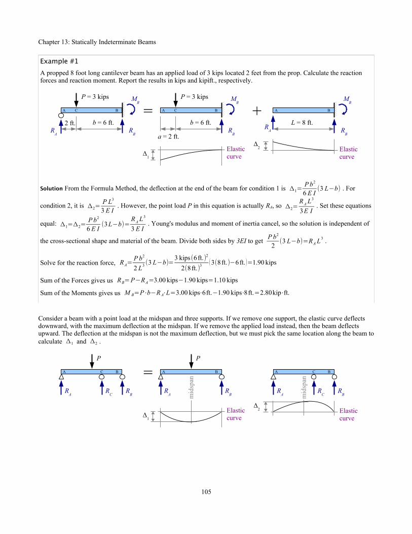
Chapter 13: Statically Indeterminate Beams
Example #1
A propped 8 foot long cantilever beam has an applied load of 3 kips located 2 feet from the prop. Calculate the reaction forces and reaction moment. Report the results in kips and kip⋅ft., respectively.
Solution From the Formula Method, the deflection at the end of the beam for condition 1 is Δ1=P b2
6 E I(3 L−b) . For
condition 2, it is Δ2=P L3
3 E I. However, the point load P in this equation is actually RA, so Δ2=
RA L3
3E I. Set these equations
equal: Δ1=Δ2=P b2
6 E I(3L−b)=
RA L3
3 E I. Young's modulus and moment of inertia cancel, so the solution is independent of
the cross-sectional shape and material of the beam. Divide both sides by 3EI to get P b2
2(3 L−b)=RA L3 .
Solve for the reaction force, RA=P b2
2 L3 (3 L−b)=3 kips(6ft.)2
2(8ft.)3(3(8ft.)−6ft. )=1.90 kips
Sum of the Forces gives us RB=P−RA=3.00 kips−1.90 kips=1.10 kips
Sum of the Moments gives us M B=P⋅b−R A⋅L=3.00 kips⋅6ft.−1.90 kips⋅8ft.=2.80kip⋅ft.
Consider a beam with a point load at the midspan and three supports. If we remove one support, the elastic curve deflects downward, with the maximum deflection at the midspan. If we remove the applied load instead, then the beam deflects upward. The deflection at the midspan is not the maximum deflection, but we must pick the same location along the beam tocalculate Δ1 and Δ2 .
105
ElasticcurveΔ
1
=
Elasticcurve
Δ2
RB
RA
A B
RC
C
P
RB
RA
A B
P
RB
RA
A B
RC
C
mid
span
mid
span
P = 3 kips
A B
b = 6 ft.
a = 2 ft.
ElasticcurveΔ
1
C
RB
MB
RA
+= A B
L = 8 ft.R
B
MB
Elasticcurve
Δ2
P = 3 kips
A B
b = 6 ft.2 ft.
C
RB
MB
RA

Chapter 13: Statically Indeterminate Beams
Example #2
A 3 meter long beam has an applied load of 300 kN located at the midspan. The beam is supported at the ends and with a third support 1 meter from the right end. Calculate the three reaction forces. Report the results in kN.
Solution From the Formula Method, the deflection at the midspan for condition 1 is Δ1=P L3
48 E I. For condition 2, the
deflection at a distance x from the left end is Δ2=P b x
6 E I L(L2−b2−x2) . However, the point load P in this equation is
actually RC, and the distance x is L/2, so Δ2=RC b L
6 E I L⋅2 (L2−b2−( L2 )
2)= RC b
12 E I(0.75L2−b2) .
Set these equations equal: Δ1=Δ2=P L3
48 E I=
RC b12 E I
(0.75L2−b2) . Once again, E and I cancel. Divide both sides by 12EI
to get P L3
4=RC b(0.75L 2−b2) .
Solve for the reaction force, RC=P L3
4b(0.75L 2−b2)=
300kN (3m)3
4⋅1m [0.75(3 m)2−(1 m)2]=352.2 kN
Sum of the Moments about point A gives us M B=0=−300kN⋅1.5 m+352kN⋅2 m+RB⋅3m . Solve for
RB=300 kN⋅1.5 m−352.2 kN⋅2m
3 m=−84.8 kN . The negative sign means RB acts downward.
Sum of the Forces gives us RA=P−RB−RC=300 kN−(−84.8kN)−352.2 kN=32.6 kN , positive, therefore acting upward.
Once you have solved for the reactions, you can draw shear and moment diagrams to find maximum bending and shear stresses.
106
ElasticcurveΔ
1
=
Elasticcurve
Δ2
RB
RA
A B
RC
C
P = 300 kN
RB
RA
A B
RB
RA
A B
RC
C
1 m1.5 m
3 m
P = 300 kN
b = 1 mL = 3 m
x mid
span
mid
span
mid
span
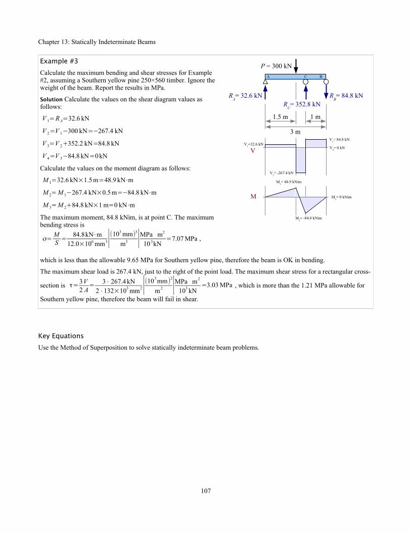
Chapter 13: Statically Indeterminate Beams
Example #3
Calculate the maximum bending and shear stresses for Example #2, assuming a Southern yellow pine 250×560 timber. Ignore the weight of the beam. Report the results in MPa.
Solution Calculate the values on the shear diagram values as follows:
V 1=RA=32.6 kN
V 2=V 1−300 kN=−267.4 kN
V 3=V 2+352.2 kN=84.8 kN
V 4=V 3−84.8 kN=0kN
Calculate the values on the moment diagram as follows:
M 1=32.6 kN×1.5 m=48.9 kN⋅m
M 2=M 1−267.4 kN×0.5 m=−84.8 kN⋅m
M 3=M 2+84.8 kN×1 m=0 kN⋅m
The maximum moment, 84.8 kN⋅m, is at point C. The maximum bending stress is
σ=MS= 84.8kN⋅m
12.0×106 mm3∣(103 mm)3
m3 ∣MPa m2
103kN=7.07 MPa ,
which is less than the allowable 9.65 MPa for Southern yellow pine, therefore the beam is OK in bending.
The maximum shear load is 267.4 kN, just to the right of the point load. The maximum shear stress for a rectangular cross-
section is τ=3V2 A
= 3⋅ 267.4 kN2⋅132×103 mm2∣(103mm )2
m2 ∣MPa m2
103 kN=3.03 MPa , which is more than the 1.21 MPa allowable for
Southern yellow pine, therefore the beam will fail in shear.
Key Equations
Use the Method of Superposition to solve statically indeterminate beam problems.
107
RB= 84.8 kNR
A= 32.6 kN
A BC
P = 300 kN
1 m1.5 m
3 m
V1=32.6 kN
V V4= 0 kN
V2= -267.4 kN
V3= 84.8 kN
M M3= 0 kN⋅m
RC= 352.8 kN
M1= 48.9 kN⋅m
M2= -84.8 kN⋅m

Chapter 14: Buckling of Columns
Chapter 14: Buckling of ColumnsTypes of Columns
Squeeze a short cylindrical blockelastically, and the normal stressis σ=P /A . Squeeze hardenough to exceed the yieldstrength, and the block will eitherfail by distorting (if it is ductile)or by fracturing (if it is brittle). Aductile short block will yield atthe same load, whether it is intension or in compression.
Change the dimensions of thecylinder so it is very long andthin, and push on the ends: it willform a gentle bow at a normalstress less than the yield strengthof the material. We call this a slender column. You can make a slender column bycutting out the longest straight segment of a steel wire coat hanger. Put one end on akitchen scale and press on the other end; the wire will bow under a force of a couple of pounds.If we measure a wire diameter of 0.087 in. and assume a yield strength of 30 ksi, the wire will not
yield in tension until the load reaches P tension=σ A=30 kipsin.2
π(0.087 in.)2
4 ∣103 lb.kip
=178 lb. In tension,
it takes almost 200 lb. to permanently deform the wire, while in compression it takes about 2 lb. – a difference of two ordersof magnitude! The extreme example of a slender column is a rope or cable: high tensile strength; no compressive strength.
Between the short block and the slender column is the intermediate column, not as skinny as the slender column, but longer and thinner than the short block. Push on the ends, and an intermediate column forms a kink about halfway up, at a normal stress less than the yield strength of the material. You can make an intermediate column with a thick piece of solder about 10 in. long.
Ideal Slender Columns
Euler Critical Load
Leonhard Euler, the Swiss mathematician who gave us the ex button on the calculator, studied the mathematics of columns. He derived an equation for the critical load that causes buckling in an ideal
slender column that is pinned at both ends. The Euler critical load P cr=π2 E I
L2 where I is the smallest
moment of inertia for the cross-sectional area of the column. For example, if the column is a wide-flange beam, I y< I x , so use Iy. Euler's equation tells us the critical load for a 16.5 in. long coat hanger wire is
P cr=π2 E I
L2 =π2 E
L2
πd 4
64= π2
(16.5in.)2
30×106lb.
in.2π(0.087in.)4
64=3.1 lb. , which is pretty close to, but not the
same as, the 2 lb. measured in the kitchen. Why are the numbers different? Euler's equation assumes the wire is perfectly straight, the loads are applied in perfect alignment with the axis of the column, there are no materials defects in the steel, the cross-section is perfect and uniform along the length of the wire, there are no scratches on the wire's surface, and the ends can rotate freely with no friction.
What if you know the applied load, and have to select a round rod to support that load? Rewrite the Euler critical load
equation, solving for diameter: P cr=π2 E I
L2 =π2 EL2
πd 4
64→ d= 4√ 64 P L2
π3 E.
108
PP
σ < σYS
P
Short blockP
P
Slendercolumn
P P
Intermediatecolumn
σ > σYS
ductilefailure
σ > σYS
brittlefailure
σ < σYS
bow
σ < σYS
kink
Pcr
L

Chapter 14: Buckling of Columns
Example #1
An aluminum column made of 2 cm square barstock is loaded as a pin-connected column. Calculate the Euler critical load for this column if the length is 3 m. Report theresult in kN.
Solution The moment of inertia of a solid square is I=bh3
12= b4
12.
From the Appendix, E = 70 GPa.
P cr=π2 E I
L2 =π2b4 E
12 L2 =π2(2cm)4 70 GPa
12 (3m)2 ∣ 106 kNGPa m2 ∣ m4
(100cm)4=1.02kN
Euler Stress
Recall the definition for radius of gyration of an area: rG=√ I /A . Square both sides to get rG2= I /A . The Euler critical
load divided by the cross-sectional area of the column gives us the stress in the column:Pcr
A=σcr=
π2 E I
L2 A=π2 E rG
2
L2 = π2 E
(L / rG)2 . The quantity L/rG is called the slenderness ratio of the column; the larger this value,
the slenderer the column.
Support Conditions
The end of a column can have one of threesupport conditions. It can be pinned: free torotate, but prevented from sliding sideways. Itcan be fixed, like the wall-end of a cantileverbeam: prevented from rotating or sliding. It canbe free to rotate and slide, like the free end of acantilever beam.
If both ends are pinned, the column bows in anarc equal to the length of the column. Theeffective length of the column is its own length.
If both ends are fixed, then the column cannotrotate at its ends. It bows in the center relative totwo inflection points located L/4 from each end,so the effective length of the bow is half thecolumn length, and Leff=0.5 L .
If one end is fixed while the other is pinned, thenthe column can rotate about the pinned connection. The column bows over an effective length Leff=0.7 L .
A fixed & free column looks like a flagpole; a pteranodon landing on the tip will cause the flagpole tosway. The column bows over an effective length that is twice its actual length: Leff=2 L .
We can modify Euler's critical load equation to include these support conditions: P cr=π2 E I
(KL)2 where K is
the effective length factor 1, 0.5, 0.7, or 2, as appropriate. Likewise, the Euler stress is σcr=π2 E
(KL / rG)2 .
109
PinnedK = 1
FixedK = 0.5
Fixed & pinnedK = 0.7
Fixed & freeK = 2
Leff
=0.5 LLeff
= LL
eff=0.7 L
Leff
=2 L
Pcr P
cr
Pcr
Pcr
Pcr
3 m
2 cm
2 cm
crosssection

Chapter 14: Buckling of Columns
These equations help us find the load and stress when buckling first starts, assuming perfect loading conditions and
materials. In real life, we need to include a Factor of Safety, so P cr=π2 E I
(KL)2 F.S. and σcr=
π2 E(KL / rG)
2 F.S..
Example #2
A standard 4 inch pipe 35 feet long is used as an Ideal fixed column. Using a factor of safety of 2, calculate the load that the pipe can support; report the result in kips. Calculate the stress in the pipe; report the result in ksi.
Solution Since the column is fixed, K=0.5 . From Appendix D, a standard 4 inch pipe has a moment of inertia I=6.82 in.4 , a radius of gyration rG=1.51 in. , and a cross-sectional area of 2.96 in.2.
Pcr=π2 E I
(KL)2 F.S.= π2
(0.5⋅35ft.)2 230×106 lb.
in.2
6.82 in.4∣ kips103 lb.∣ (ft.)2
(12 in.)2=24.3kips
σcr=π2 E
(KLrG)
2
F.S.
= π2
(0.5⋅35ft.1.51 in. ∣12 in.
ft. )2
⋅2
30×106 lb.in.2∣kips
103 lb.=7.65 ksi
Structural Steel Columns
W-beams are often used as columns in steel structures. AISC recommends using the following formulas for calculating the allowable load.
If KLrG
>200 then the column is too slender for safe use; pick a shorter or deeper column.
If KLrG
>4.71√ EσYS
then Pall=0.525σ cr A
If KLrG
<4.71√ EσYS
then Pall=0.658(σYS /σcr )σYS A
1.67
Solve Structural Steel Column problems in four steps:
1. Calculate KL /rG and 4.71√E/σYS . Since rGy<rGx for W-beams, use rGy
2. Calculate σcr
3. Use the appropriate formula to calculate Pall
4. Use σ=Pall /A to find the stress in the column
110
crosssection
30 ft.
Pcr

Chapter 14: Buckling of Columns
Example #3
A 30 m long W200×59 wide-flange beam made from A36 steel is used as a fixed and pinned column with a Factor of Safety of 2.5. Calculate the allowable load; report the result in kN. Calculate the stress in the column; report the result in MPa.
Solution Since the column is fixed and pinned, K=0.7 . From Appendix D, rGx=89 mm andrGy=52 mm . Use the smaller of these numbers. From Appendix B, the yield strength of A36 steel
is 250 MPa.
KLrG
=0.7⋅30 m52mm ∣103 mm
m=404
Since KLrG
>200 , the column is too slender for safe use.
Example #4
Solve Example #3 using a 12 m long W200×59 wide-flange beam.
Solution The material and dimensional properties are the same as in Example #3.
KLrG
=0.7⋅12 m52 mm ∣103 mm
m=161.5
4.71 √ EσYS
=4.71 √ 207GPa250 MPa∣103 MPa
GPa=136
Since KLrG
>4.71√ EσYS
, use Pall=0.525σ cr A where σcr=π2 E
(KL / rG)2 F.S.
. We can plug in the
calculated value of KL/rG from above.
σcr=π2 207GPa(161.5)2⋅2.5∣103 MPa
GPa=31.3MPa
Pall=0.525σ cr A=0.525⋅31.3 MPa ⋅7550 mm2∣ 103kNMPa m2 ∣ m2
(103 mm)2=124 kN
The actual stress in the column is σ=Pall
A=
124 kN
7550 mm2∣MPa m2
103kN∣(103 mm)2
m2 =16.4 MPa
Steel Machine Parts
Structural columns are large – several feet to dozens of feet tall. Machines also use long, thin compression members, such as
connecting rods in internal combustion engines. If KLrG
≥√ 2π2 EσYS
then the column is slender, and the allowable stress is
σall=π2 E
(KL /rG)2F.S.
. This is the Euler equation for ideal columns.
111
35 m
Pcr
12 m
Pcr

Chapter 14: Buckling of Columns
On the other hand, if KLrG
<√ 2π2 EσYS
then the column is intermediate. Based on empirical data from real machine parts, J.B.
Johnson developed a formula for the allowable stress: σall=[1−σYS (KL / rG)2
4 π2 E ] σYS
F.S..
Calculate the allowable load of a steel machine part by multiplying the allowable stress by the cross-sectional area.
Example #5
A 20 inch long , 1 inch diameter steel rod with a yield strength of 35 ksi is used as a fixed and pinned column with a Factor of Safety of 2. Calculate the allowable stress in the machine part; report the result in ksi. Calculate the the allowable load in the machine part; report the result in kips.
Solution Since the column is fixed and pinned, K=0.7 . The radius of gyration of a solid circle is one quarter the diameter, so rG = 0.25 in.
KLrG
=0.7⋅20 in.0.25in.
=56
√ 2π2 EσYS
=KLrG
<√2π2⋅30×103 ksi35ksi
=130
Since KLrG
<√ 2π2 EσYS
, the column is intermediate.
σall=[1−σYS (KL / rG)2
4π2 E ] σYS
F.S.=[1− 35ksi (56)2
4π230×103ksi ] 35 ksi2
=15.9ksi
Pall=σall A=15.9 kips
in.2π(1 in.)2
4=12.5 kips
Some machine design problems start with a known load and column length; your job is to calculate the minimum diameter of a solid round rod to allow the column to survive buckling. Remember that the radius of gyration of a solid round rod is
d/4 and the allowable stress is σall=PA= P(π/4 )d 2 , then follow these six steps:
Step 1 Assume the column is slender (because the math is easier): σall=π2 E
(KL /rG)2F.S.
= P(π /4)d 2
Step 2 Rewrite the equation to solve for diameter.
Step 3 Check that the column really is slender.
Step 4 If the column is not slender, then σall=[1−σYS (KL / rG)2
4π2 E ] σYS
F.S.= P
(π /4)d 2
Step 5 Rewrite the equation to solve for diameter. This is a little tricky because of the number of terms.
Step 6 Check that the column really is intermediate; if it isn't, you made a mistake someplace.
112
35 m
Pcr

Chapter 14: Buckling of Columns
Key Equations
Ideal Slender Columns
The Euler critical load is P cr=π2 E I
(KL)2 F.S., and the Euler critical stress is σcr=
π2 E(KL / rG)
2 F.S.
Structural Steel Columns
If KLrG
>200 then the column is too slender for safe use.
If KLrG
>4.71√ EσYS
then Pall=0.525σ cr A
If KLrG
<4.71√ EσYS
then Pall=0.658(σYS /σcr )σYS A
1.67
Steel Machine Columns
If KLrG
≥√ 2π2 EσYS
then the column is slender, and the allowable stress is σall=π2 E
(KL /rG)2F.S.
.
If KLrG
<√ 2π2 EσYS
then the column is intermediate, and σall=[1−σYS (KL /rG)2
4π2 E ] σYS
F.S..
Calculate Pall=σall A
To find the smallest allowable diameter of a round solid rod, follow the 6-step procedure described above.
113

Chapter 15: Visualizing Stress and Strain
Chapter 15: Visualizing Stress and StrainMeasuring Stress
We can see deformation, if it's large enough, but we cannot see stress, and in most cases we cannot measure it directly. Instead, we can use a strain gauge to measure the strain on the surface of an object that is being elastically deformed, and use Young's Modulus to estimate the stress.
The earliest strain gauges in the 1930s were made of fine wire. If you glue a very thin wire along the bottom surface of a beam, then load the beam in bending, the wire will stretch and become thinner. The thinner the wire becomes, the higher its electrical resistance. By measuring this resistance you can determine strain, then
calculate stress as σ= E ε
, provided the object is being
strained elastically.
Modern strain gauges use the same principal, but are made of thin metal foil instead of wire. The foil is embedded in a pad that is easy to glue to the part being tested.
The longer the conductor, the more sensitive the gauge. With a foil strain gauge, the conductor loops back on itself many times. The total wire length is the loop length times twice the number of loops; in this cartoon, the total length is 14 times the loop length.
Stress at the Base of a Short Block
Consider the short block in Chapter 12, Example #4. A point load is offset from both neutral axes. The total stress at the four corners is -3.75 psi, -41.25 psi, +16.25 psi, and -21.25 psi.
In plan view, point C has a tensile stress, while points A, B, and D have compressive stresses.
We can calculate the stress at any point along the edges by interpolating from the corner stresses, because the stress varies linearly from one corner to the next. Likewise we can calculate the stresses within the area of the block by interpolating from the edge stresses.
114
A
4 ft.
B
C DPlan view
2.5 ft.
σA= -3.75 psi σ
B= -41.25 psi
σC= +16.25 psi σ
D= -21.25 psi
Point loadlocation
12 kipsWx x
y
y
1.5 ft.
A B
DC
4 ft.
3 ft.
2.5 ft.
0.5 ft.
loop length

Chapter 15: Visualizing Stress and Strain
One way to visualize these stresses is with a grid pattern in plan view, identifying the stress at each location, or node. In the diagram, the nodes are at half-foot intervals.
Alternatively, we can calculate contour lines of stress (a.k.a. isostress lines), coloring the spaces between the lines. The pattern shows that the pink areas are in tension,while the blue areas are in compression. The picture helpsus see that the isostress lines are diagonals, and there is a zero stress line stretching from the AC edge to the CD edge.
Mohr's Circle
Normal and shear stresses in uniaxial tension
Take a tensile bar, cut it in half transversely to the axis, and glue the bar back together. If you pull on the bar
along the x-axis, a normal stress σ x=PA
develops in the
adhesive. Area A is the cut surface area of the bar (the cross-sectional area). There is no shear stress, because theadhesive is not loaded in shear. Consider a little square piece of adhesive: it has a normal stress σx acting on the left and right faces, but no normal stress on the top or bottom faces, and no shear stresses.
115
P σx
y
x
cut
A B
C D+16.25
+7.56
-3.75
-21.25
-41.25
+2.88 -1.81 -6.50 -11.19 -15.88 -20.56 -25.25+12.25
+3.56 -1.13 -5.81 -10.50 -15.19 -19.88 -24.56 -29.25+8.25
-0.44 -5.13 -9.81 -14.50 -19.19 -23.88 -28.56 -33.25+4.25
-4.44 -9.13 -13.81 -18.50 -23.19 -27.88 -32.56 -37.25+0.25
-8.44 -13.13 -17.81 -22.50 -27.19 -31.88 -36.56
+11.56 +6.88 +2.19 -2.50 -7.19 -11.88 -16.56
A B
C D
0 psi-5
-10-15
-20-25
-30
510
-35-40
15
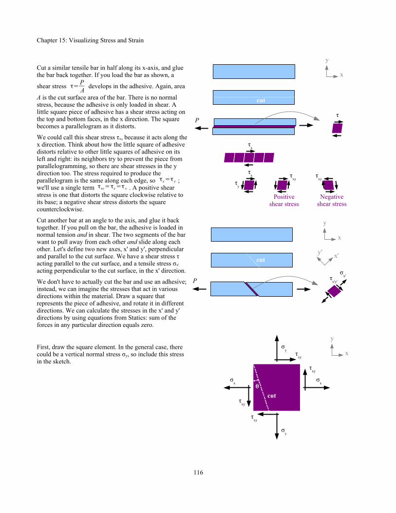
Chapter 15: Visualizing Stress and Strain
Cut a similar tensile bar in half along its x-axis, and glue the bar back together. If you load the bar as shown, a
shear stress τ= PA
develops in the adhesive. Again, area
A is the cut surface area of the bar. There is no normal stress, because the adhesive is only loaded in shear. A little square piece of adhesive has a shear stress acting on the top and bottom faces, in the x direction. The square becomes a parallelogram as it distorts.
We could call this shear stress τx, because it acts along thex direction. Think about how the little square of adhesive distorts relative to other little squares of adhesive on its left and right: its neighbors try to prevent the piece from parallelogramming, so there are shear stresses in the y direction too. The stress required to produce the parallelogram is the same along each edge, so τx=τ y ; we'll use a single term
τxy=τx=τ y . A positive shear stress is one that distorts the square clockwise relative to its base; a negative shear stress distorts the square counterclockwise.
Cut another bar at an angle to the axis, and glue it back together. If you pull on the bar, the adhesive is loaded in normal tension and in shear. The two segments of the bar want to pull away from each other and slide along each other. Let's define two new axes, x' and y', perpendicular and parallel to the cut surface. We have a shear stress τ acting parallel to the cut surface, and a tensile stress σx' acting perpendicular to the cut surface, in the x' direction.
We don't have to actually cut the bar and use an adhesive;instead, we can imagine the stresses that act in various directions within the material. Draw a square that represents the piece of adhesive, and rotate it in different directions. We can calculate the stresses in the x' and y' directions by using equations from Statics: sum of the forces in any particular direction equals zero.
First, draw the square element. In the general case, there could be a vertical normal stress σy, so include this stress in the sketch.
116
Pτ
y
x
cut
τx
τx
τy
τxy
τxy
Negativeshear stress
Positiveshear stress
y
x
cut
P τx'y'
σx'
y'x'
y
x
cut
σx
σx
σy
σy
τxy
τxy
τxy
τxy
θ
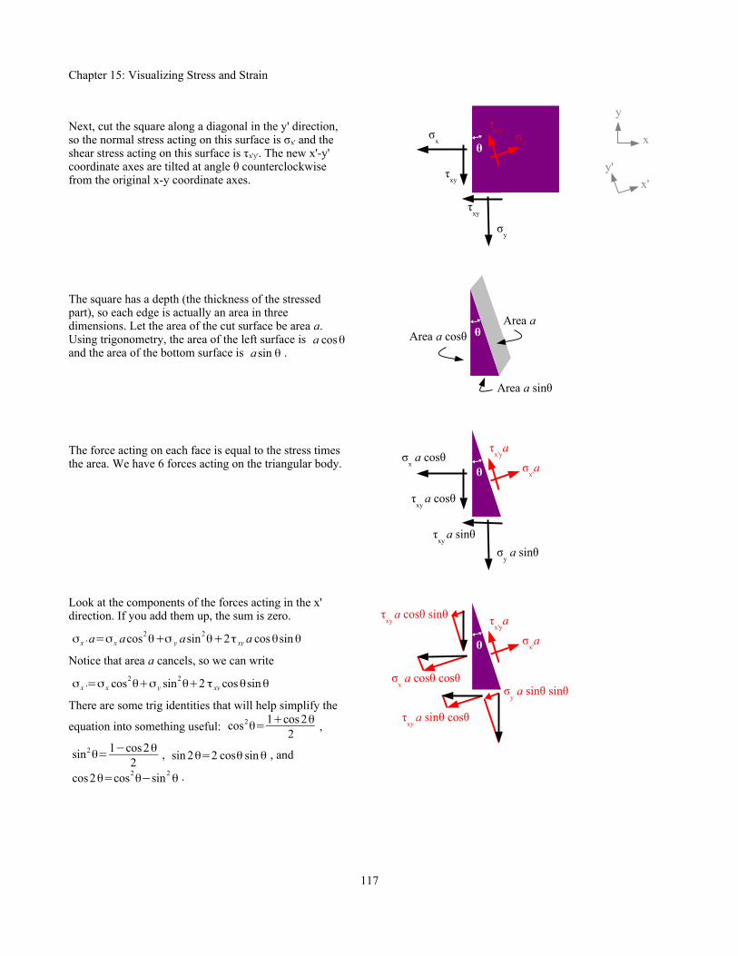
Chapter 15: Visualizing Stress and Strain
Next, cut the square along a diagonal in the y' direction, so the normal stress acting on this surface is σx' and the shear stress acting on this surface is τx'y'. The new x'-y' coordinate axes are tilted at angle θ counterclockwise from the original x-y coordinate axes.
The square has a depth (the thickness of the stressed part), so each edge is actually an area in three dimensions. Let the area of the cut surface be area a. Using trigonometry, the area of the left surface is a cosθ and the area of the bottom surface is asin θ .
The force acting on each face is equal to the stress times the area. We have 6 forces acting on the triangular body.
Look at the components of the forces acting in the x' direction. If you add them up, the sum is zero.
σx ' a=σ x acos2θ+σ y asin2θ+2τ xy a cosθsinθ
Notice that area a cancels, so we can write
σ x '=σ x cos2θ+σ y sin2θ+2 τ xy cosθsinθ
There are some trig identities that will help simplify the
equation into something useful: cos2θ=1+cos 2θ2
,
sin2θ=1−cos2θ2
, sin 2θ=2 cosθ sinθ , and
cos2θ=cos2θ−sin2 θ .
117
y
xτ
x'y'σx
y'
x'
σx'
σy
τxy
τxy
θ
τx'y
a
σx'a
σy a sinθ
τxy
a cosθ
τxy
a sinθ
θσ
x a cosθ
τx'y
a
σx'a
σy a sinθ sinθ
τxy
a cosθ sinθ
τxy
a sinθ cosθ
θ
σx a cosθ cosθ
θ
Area a sinθ
Area a cosθArea a

Chapter 15: Visualizing Stress and Strain
Now we get
σ x '=σx
1+cos 2θ2
+σ y
1−cos 2θ2
+τ xysin 2θ
=σx+σx cos 2 θ+σ y+σ y cos 2θ
2+τxy sin 2θ
=σx+σ y
2+σx−σ y
2cos 2θ+τxy sin 2θ
Following the same procedure, we can calculate the sum of the forces in the y' direction.
τ x ' y ' a=−σ x a cosθsin θ+σ y a sinθ cosθ−τ xy asin 2θ+τ xy a cos2θ
Area a cancels. Using the trig identities, we can simplify the equation:
τx ' y '=(−σ x+σ y )cosθsinθ+τ xy(cos2θ−sin2 θ)
=−(σ x−σ y)sin 2θ
2+τ xy cos 2θ
=−(σ x−σ y)
2sin 2θ+τ xy cos 2θ
We can calculate the stress in the y' direction by taking angle θ+90° . Using free-body diagrams and trig identities, we get:
σ y '=σx+σ y
2−σx−σ y
2cos 2θ−τ xy sin 2θ
Now we have three equations that are functions of σx, σy, and τxy, and θ. Let's pick values of normal and shear stresses, and see how σx', σy', and τx'y' vary by plotting stress vs. angle θ. The graph at the right shows σx' as a function of angle θ if we pick σ x=1ksi , σ y=0.5 ksi , and τxy=1.2 ksi . The graph is a sine wave, with peaks, valleys, and zero values. Picking different values of σx, σy, and τxy will change the amplitude and vertical positionof the sine wave, but not the period.
Notice that the maximum values of σx' occur at θ=40 ° and 220°, the minimum values occur at θ=130° and 310°, and σ x '=0 at θ=100° , 155°, 283°, and 385°.
118
τx'y
a
σx'a
σy a sinθ cosθ
τxy
a cosθ cosθ
τxy
a sinθ sinθ
θσx a cosθ sinθ
y
xτ
x'y'
σx
y'
x'
σy'
σy
τxy
τxy
θ+90°
Stress(ksi)
2.0
1.0
0.0
-1.0
-2.0
0 120 180 240 300 36060
Angle θ (degrees)
σx'
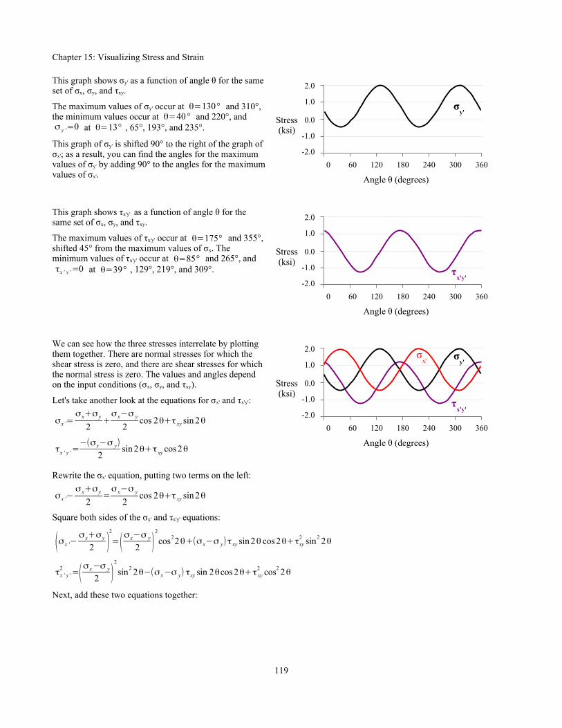
Chapter 15: Visualizing Stress and Strain
This graph shows σy' as a function of angle θ for the sameset of σx, σy, and τxy.
The maximum values of σy' occur at θ=130° and 310°, the minimum values occur at θ=40 ° and 220°, andσ y '=0 at θ=13° , 65°, 193°, and 235°.
This graph of σy' is shifted 90° to the right of the graph of σx'; as a result, you can find the angles for the maximum values of σy' by adding 90° to the angles for the maximumvalues of σx'.
This graph shows τx'y' as a function of angle θ for the same set of σx, σy, and τxy.
The maximum values of τx'y' occur at θ=175° and 355°, shifted 45° from the maximum values of σx. The minimum values of τx'y' occur at θ=85° and 265°, andτx ' y '=0 at θ=39° , 129°, 219°, and 309°.
We can see how the three stresses interrelate by plotting them together. There are normal stresses for which the shear stress is zero, and there are shear stresses for which the normal stress is zero. The values and angles depend on the input conditions (σx, σy, and τxy).
Let's take another look at the equations for σx' and τx'y':
σx '=σ x+σ y
2+σ x−σ y
2cos 2θ+τ xy sin 2θ
τx ' y '=−(σ x−σ y)
2sin 2θ+τ xy cos2θ
Rewrite the σx' equation, putting two terms on the left:
σx '−σ x+σ y
2=σ x−σ y
2cos 2θ+τ xy sin 2θ
Square both sides of the σx' and τx'y' equations:
(σ x '−σ x+σ y
2 )2
=(σ x−σ y
2 )2
cos22θ+(σ x−σ y) τ xy sin 2θ cos 2θ+τxy2 sin2 2θ
τx ' y '2 =(σ x−σ y
2 )2
sin2 2θ−(σ x−σ y) τxy sin 2θcos 2θ+τ xy2 cos2 2θ
Next, add these two equations together:
119
Stress(ksi)
2.0
1.0
0.0
-1.0
-2.0
0 120 180 240 300 36060
Angle θ (degrees)
σy'
Stress(ksi)
2.0
1.0
0.0
-1.0
-2.0
0 120 180 240 300 36060
Angle θ (degrees)
τx'y'
Stress(ksi)
2.0
1.0
0.0
-1.0
-2.0
0 120 180 240 300 36060
Angle θ (degrees)
τx'y'
σy'
σx'

Chapter 15: Visualizing Stress and Strain
(σ x '−σ x+σ y
2 )2
+τ x' y'2 =( σ x−σ y
2 )2
cos22θ+(σ x−σ y ) τ xysin 2θcos 2θ+τ xy2 sin22θ
+(σ x−σ y
2 )2
sin2 2θ−(σ x−σ y) τ xy sin 2θ cos2θ+τ xy2 cos2 2θ
We can eliminate two terms because (σ x−σ y) τ xy sin 2θcos 2θ−(σ x−σ y) τ xy sin 2θ cos 2θ=0 . Rewriting the equation, we have:
(σ x '−σ x+σ y
2 )2
+τ x' y'2 =( σ x−σ y
2 )2
(cos2 2θ+sin 22θ)+τ xy2 (sin 22θ+cos2 2θ)
Using the trig identity cos22θ+sin2 2θ=1 , the equation simplifies to (σ x '−σ x+σ y
2 )2
+τ x' y'2 =( σ x−σ y
2 )2
+τ xy2 .
The term σ x+σ y
2 is an average of two stress values, so let's call it σavg. Now the equation is even simpler:
(σ x '−σavg)2+τ x ' y '
2 =(σ x−σ y
2 )2
+τ xy2 . If we define the right side of the equation as R=√(σ x−σ y
2 )2
+τ xy2 then
(σ x '−σavg)2+τ x ' y '
2 =R2 . This is the equation of a circle with a radius R and a center at coordinates (σavg ,0) . In 1880, OttoMohr developed this method for visualizing stresses in two-dimensional and three-dimensional objects. His graphical method is also used for diagramming strains. We can use Mohr's Circle to determine the value and direction of maximum stresses within a loaded part.
Follow this 6-step process for drawing Mohr's circle for the stresses acting at a point within a stressed object. For best results, use a compass and straightedge on graph paper. In this example, use the same stresses as before: σx=1ksi ,σy=0.5 ksi , and τxy=1.2 ksi .
Step 1 Draw two axes. Label the horizontal axis σ and thevertical axis τ.
Step 2 Mark the center of the circle at coordinates(σavg ,0) and label it C for center. In this case,
σ avg=σx+σ y
2=1 ksi+0.5 ksi
2=0.75ksi .
120
τ
σ
τ
σC

Chapter 15: Visualizing Stress and Strain
Step 3 Mark point (σ x ,−τ xy) on the graph; in this case,(1ksi ,−1.2 ksi) . Label this point A.
Step 4 Placing your compass point at the center of the circle, draw a circle passing through this point. The radiusof Mohr's circle is:
R=√(σ x−σ y
2 )2
+τ xy2
=√(1 ksi−0.5 ksi2 )
2
+(1.2 ksi )2=1.226 ksi
Notice the circle also passes through point (σ y , τ xy) , which is (0.5 ksi ,1.2 ksi) . Mark this point and label it B. A line passing through points A and B is the diameter of Mohr's circle.
Step 5 The maximum normal stress occurs at point D; we call it σ1. The minimum normal stress occurs at point E; we call it σ2. The maximum shear stress occurs at point F;we call this τmax.These three stresses are called Principal Stresses.
You can measure these values off the graph, or you can calculate them:
σ1=σavg+R=0.75ksi+1.226 ksi=1.976ksi
σ2=σavg−R=0.75 ksi−1.226 ksi=−0.476 ksi
τmax=R=1.226ksi
Step 6 Starting on line segment A-C, measure the angle counterclockwise about point C to line segment C-D. Thisangle is 2θ.
tan 2θ=τ xy
(σ x−σ y)/2=
2τ xy
σ x−σ y
=2(1.2 ksi)
1ksi−0.5 ksi=4.8
2θ=tan−14.8=78.2°
θ=78.2°2
=39.1°
This is the angle of the principal stress σ1. The angle of principal stress σ2 is θ=90°+39.1°=129.1° .
121
τ
σ
(σx, -τxy)A
C
τ
σ
(σx, -τxy)
R
(σy, τxy)
A
C
B
τ
σ
(σx, -τxy)
σ1
R
τmax
σ2
(σy, τxy)
A
C
B
E D
F
τ
σ
(σx, -τxy)
σ1
R
τmax
2θσ
2
(σy, τxy)
A
C
B
E D
F
2θ-τxy
(σ x−σ y
2 )
σ x−σ y
A
B

Chapter 15: Visualizing Stress and Strain
Going back to the original stress element, we hadσ x=1ksi , σ y=0.5 ksi , and τxy=1.2 ksi . If we rotate
the element counterclockwise 39.1°, in this orientation there are no shear stresses, and the principal stresses areσ1=1.976 ksi tension and σ2=−0.476 ksi
compression. The maximum shear stress τmax=1.226 ksiis oriented 45° from the maximum normal stress, atθ=45°+39.1 °=84.1° .
Example #1
An aluminum rod with a diameter of 0.5 inches is pulled with a load of 2000 lb. as shown. Calculate the applied stresses σx, σy, and τxy. Use Mohr's circle to find the principal stresses σ1 and σ2, angle θ, and the maximum shear stress τmax at point A.
Solution
The applied normal stress is in the y direction; there is no applied shear stress.
σx=0
σ y=PA= 4 P
π d 2=4⋅2000 lb.
π(0.5in.)2∣ kip
103 lb.=10.2 ksi
τ xy=0
σ avg=σx+σ y
2=0 ksi+10.2ksi
2=5.09 ksi
R=√(σ x−σ y
2 )2
+τ xy2
=√(0 ksi−10.2ksi2 )
2
+(0 ksi)2 = 5.09 ksi
σ1=σavg+R=5.09 ksi+5.09 ksi=10.2 ksi
σ2=σavg−R=5.09 ksi−5.09 ksi=0ksi
τmax=R=5.09ksi
Angle θ=0 , by inspection.
122
y
x
σx=1 ksi
τxy=1.2 ksi
σy=0.5 ksi
y'
σ2= -0.476 ksi
σ1=1.976 ksi
x'
θ = 39.1°
P
y
x
A
τ
σ(σx, -τxy)
σ1
τmax= 5.1 ksi
σ2
(σy, τxy)CA B
F
(10.2 ksi, 0)(0, 0)
(σavg, 0)
(5.1 ksi, 0)

Chapter 15: Visualizing Stress and Strain
Example #2
The rod in Example #1 is pulled as before, and also twisted with a torque of 45 ft.⋅lb.
Solution
Once again the applied normal stress is in the y direction, but the torque creates an applied shear stress.
σ x=0
σ y=PA= 4 P
π d 2=4⋅2000 lb.
π(0.5in.)2∣ kip
103 lb.=10.2 ksi as before
τxy=T cJ
where c= d2
and J=πd 4
32 (see Chapter 7 – torsion in a round shaft produces a shear
stress at the surface)
Substituting, τ xy=T d
232
πd 4=16 T
πd 3=16 45ft⋅lb.
π(0.5 in.)3 ∣12in.ft. ∣ kip
103 lb.=22.0 ksi
σ avg=σx+σ y
2=0 ksi+10.2ksi
2=5.09 ksi
R=√(σ x−σ y
2 )2
+τ xy2
=√(0 ksi−10.2ksi2 )
2
+(22.0 ksi)2 = 22.6ksi
σ1=σavg+R=5.09 ksi+22.6 ksi=27.1 ksi
σ2=σavg−R=5.09 ksi−22.6ksi=−16.9ksi
τmax=R=22.6 ksi
tan 2θ=2τ xy
σ x−σ y
= 2(22.0ksi )0ksi−10.2 ksi
=−4.32
2θ=tan−1−4.32=−77.0°
θ=−77.0 °2
=−38.5° ; −38.5°+90 °=51.5°
We can also use Mohr's circle to find out the stress in a plane at any angle α. Rotate counterclockwise through angle 2α from line segment A-C to a new line segment A'-C to find the shear and normal stresses acting in this direction.
123
P
T
y
x
A
τ
σ
(σx, -τxy)
σ1=27.1 ksiR
τmax=22.6 ksi
2θσ2
(σy, τxy)
A
C
B
E D
F(10.2 ksi, 22.0 ksi)
(0 ksi, -22.0 ksi)
-16.9 ksi-77°

Chapter 15: Visualizing Stress and Strain
Example #3
A 20" diameter cylindrical tank with a ¼" wall thickness is pressurized to 700 psi. If the barrel of the tank is made from a strip of steel welded in a spiral at 65°, what are the normal and shear stresses acting on the weld?
Solution
From Chapter 4,
σ x=σ long=p d i
4 t=700 psi 20 in.
4 0.25 in. ∣ksi
103psi=14ksi
σ y=σ hoop=p d i
2 t=700 psi 20 in.
2 0.25in. ∣ksi
103 psi=28 ksi
τ xy=0
Now solve the Mohr's circle equations.
σavg=σ x+σ y
2=14 ksi+28ksi
2=21ksi
R=√( σx−σ y
2 )2
+τ xy2 = √(14 ksi−28 ksi
2 )2
+(0 ksi)2 = 7ksi
σ1=σavg+R=21 ksi+7 ksi=28ksi
σ2=σavg−R=21ksi−7 ksi=14ksi
τmax=R=7ksi
Angle θ=0 , by inspection.
Rotate counterclockwise through angle 2α=2⋅65°=130 ° from line segment A-C to a new line segment A'-C. The normalstresses acting perpendicular and parallel to the weld are σ avg±Rcos 2α=21 ksi±7 ksi cos(130° )=16.5 ksi &25.5 ksi . The shear stress acting along the weld R sin 2α=7 ksi sin(130° )=5.4 ksi .
Since the normal stress acting on the spiral weld is 91% of the maximum normal stress (the hoop stress), the weld efficiency can be as low as 91% before the tank will fail at a weld.
If the tank were manufactured like welded pipe, with a longitudinal weld instead of a spiral weld, then anything less than 100% weld efficiency would cause the tank to fail at the weld instead of splitting in the base metal from excessive hoop stress.
The end cap welds can have as little as 50% weld efficiency and still survive, because the longitudinal stress is 50% of the hoop stress.
Chapter 9 discussed normal and shear stresses in beams. We can use Mohr's circle to look at the normal and shear stresses atany location within a beam.
124
y
x
α = 65°
τ
σ(σx, -τxy)
σ1
τmax= 7 ksi
σ2
(σy, τxy)B A
F
(28 ksi, 0)(14 ksi, 0)
(σavg, 0)
2α=130°(16.5 ksi, 5.4 ksi)
A'
RC
(21 ksi, 0)
B'(25.5 ksi, -5.4 ksi)

Chapter 15: Visualizing Stress and Strain
Example #4
A 4 cm × 12 cm titanium bar is loaded as a beam and as a compression member. Find the stresses in the bar 1 cm above the neutral axis, at the midspan.
Solution
First, determine whether the bar will fail in buckling. From
Chapter 14, P cr=π2 E I
L2 .
If the load is greater than Pcr, then the bar fails in buckling. The moment of inertia about the weak axis is
I=12 cm (4cm )3
12=64 cm 4 , therefore Pcr=
π2114GPa 64cm4
(3m)2 ∣ 106 kN
GPa m 2∣ m4
(100 cm )4=80 kN . Since the applied axial load
is less than 80 kN, the bar does not buckle.
The axial stress in the bar is
σ xaxial=PA= −25kN
4cm⋅12 cm∣MPa m2
103 kN ∣(100cm )2
m2 =−5.2 MPa
The bending stress in the bar at the top or bottom surface is
σx bending=M c
I, but we need the bending stress at a location 1 cm
above the neutral axis, so σx bending=M y
I where y=1cm . The
beam is being bent in the strong direction, so
I=4 cm (12cm )3
12=576 cm4
σ xbending=7.5 kN⋅m 1 cm
576cm 4 ∣MPa m2
103kN ∣(100cm )3
m3 =13.0MPa
Add the axial and bending stresses together to find the total stress in the x direction.
σx total=σx axial+σx bending=−5.2 MPa+13.0 MPa=7.8 MPa
σ y=0
Shear stress in the beam is τ xy=V QI t
where
Q=A' y=(4cm×5cm )3.5 cm=70cm3
τ xy=5kN 70cm3
576cm 4 4cm∣MPa m2
103 kN ∣(100 cm)2
m2=1.5 MPa
125
A B
RA
3 mR
B
10 kN25 kN
4 cm
12cm
A B
RA= 5 kN
V1=5 kN
V
V2= -5 kN
3 m
Mmax
= 7.5 kN⋅m
M
RB= 5 kN
10 kN
Bending load only
A B
Axial load only
25 kN
A'=20 cm2
4 cm
12cm
y=3.5 cm
1 cm

Chapter 15: Visualizing Stress and Strain
Example #4, continued
Now solve the Mohr's circle equations.
σavg=σ x+σ y
2=7.8 MPa+0 MPa
2=3.9 MPa
R=√(σ x−σ y
2 )2
+τ xy2 = √(7.8 MPa−0MPa
2 )2
+(1.5 MPa)2 = 4.2 MPa
σ1=σavg+R=3.9 MPa+4.2 MPa=8.1 MPa
σ2=σavg−R=3.9 MPa−4.2 MPa=−0.2 MPa
τmax=R=4.2 MPa
tan 2θ=2 τ xy
σx−σ y
=2(1.5 MPa)7.8 MPa−0
=0.385
2θ=tan−1(0.385)=21.0°
θ=21.0°2
=10.5° ; 10.5°+90 °=100.5 °
Theories of Failure
Design engineers don't prevent failure, they manage it by designing products and structures so that when they fail due to old age, abuse, or ordinary service, nobody is injured. How do we define failure? It depends on the product or structure. A bridge deck could be described as a failure if it deflects too far, even though it does not break. A shear pin in a snowblower fails if it does not break when the blades are overloaded by ice, or does break under ordinary snow load.
In Strength of Materials, elastic formulas do not work in the plastic zone, and usually we do not want plastic deformation during service, therefore we can define failure as yielding for most products or structures.
William Rankine, a 19th century Scottish engineer, developed the Maximum Normal Stress Theory. He considered materials having the same strength in tension and compression (such as steel, not cast iron). He proposed a failure stress criterion σ f=σP max where σf is the failure stress and σPmax is the maximum principal stress. If we plot principal stresses σ1 and σ2 on x and y coordinates, the part is “safe” if the combined stress pointis within the square.
126
τ
σ
(σx, -τ
xy)
σ1
R
τmax
=4.2 MPa
2θ = 21°σ
2
(σy, τ
xy)
A
C
B
E D
F
-0.2 MPa 8.1 MPa
(0, 1.5 MPa)
(7.8 MPa,1.5 MPa)
3.9 MPa
σ1
σ2
Safe
Notsafe
σf
σf
-σf
-σf

Chapter 15: Visualizing Stress and Strain
Charles-Augustin de Coulomb, a 19th century French physicist, and Henri Tresca, a 19th century French engineer, developed the Maximum Shear Stress Theory (also known as the Tresca Theory), which defines failure
as τ f =τmax=σmax−σmin
2 . This theory is more
conservative than the Maximum Normal Stress Theory, asit cuts off the upper left and lower right corners of the square “safe” zone.
In metals, we have a linear elastic curve on the stress-strain diagram. The area under the curve equals the strain
energy per unit volume, u=σε2 . Richard Edler von
Mises was a Jewish mathematician who escaped Austria when the Nazis rose to power, and later joined the facultyat Harvard. He developed the most widely-used failure criterion. From the energy per unit volume equation, he derived: σ f =√σ1
2−σ1σ2+σ22 where σ1 and σ2 are the
principal stresses. The von Mises or Maximum Distortion Energy Theory produces an elliptical “safe zone”.
Notice on all three stress graphs, the “safe” envelopes all pass through the same four points on the two axes, marked in red.
A number of other failure theories apply to special cases, such as the Maximum Strain Theory of Barré de Saint-Venant, andthe Internal Friction Theory. However, von Mises is used widely in finite element programs because it fits more data than other methods.
Key Equations
The average normal stress (center of Mohr's circle) is σavg=σx+σ y
2, and the radius is R=√(σ x−σ y
2 )2
+τ xy2
The principal stresses are σ1=σavg+R and σ2=σavg−R . The maximum shear stress τmax=R
Find the angle of principal stresses with
tan 2θ=[ τ xy
(σ x−σ y
2 ) ] → 2θ=tan−1[ τ xy
(σ x−σ y
2 ) ] → θ=[2θ]2
and 90 °+[2θ]2
127
Notsafe
σ2 σf
σ1
Safe
σf
-σf
-σf
Notsafe
σ2
σ1
Safe
ε
σarea=σε
2

Bibliography
BibliographyTextbooks
Sometimes when you are learning a new topic, it's helpful to look at other textbooks. The Engineering Technology textbooks focus on algebraic and trigonometric solutions, while Engineering textbooks also use calculus. Symbols used in these textbooks vary; authors use different symbols for force (F, P), normal stress (σ, s, S), shear stress (τ, ss, Ss), Poisson's ratio (ν, μ), section modulus (S, Z), length (L, l), temperature (T, t), pressure (p, R), radius of curvature (R, ρ), radius of gyration (r, k, q), and stress concentration (k, K, Kconc, Kt). Check the table of terminology before using the equations.
The basic theory of Strength of Materials has not changed in the years since the oldest textbooks on this list were published. Material properties have improved – structural steel is better than it used to be – and some industry standards for Factors of Safety have changed. Newer textbooks have full-color diagrams and online resources, including videos and animations.
Engineering Technology Textbooks
George Limbrunner & Leonard Spiegel, Applied Statics and Strength of Materials, 5th ed., Pearson Prentice Hall, 2009.
Fa-Hwa Cheng, Statics and Strength of Materials, 2nd ed., Glencoe/McGraw-Hill, 1997.
Lawrence J. Wolf, Statics and Strength of Materials: A Parallel Approach to Understanding Structures, Merrill, 1988.
Ottmar W. Eckardt, Strength of Materials, Holt, Rinehart and Winston, 1969.
Alfred Jensen, Statics and Strength of Materials, McGraw-Hill, 1962.
Engineering Textbooks
R.C. Hibbeler, Statics and Mechanics of Materials, 3rd ed., Pearson Prentice Hall, 2011.
Madhukar Vable, Intermediate Mechanics of Materials, Oxford University Press, 2008.
William Riley, Leroy Sturges, & Don Morris, Mechanics of Materials, 6th ed., John Wiley & Sons, 2007.
Ferdinand P. Beer, E. Russell Johnston, Jr., & John T. DeWolf, Mechanics of Materials, 4th ed., McGraw-Hill, 2006. Beer and Johnston pioneered the design of modern mechanics textbooks, using many examples and drawings.
Joseph Edward Shigley, Applied Mechanics of Materials, McGraw-Hill, 1976.
Other Reading Material
A textbook is usually written for a specific course. Other books that are not course-specific are still useful in engineering practice; these include histories of technology, handbooks of design specifications, anthologies of mechanism designs, etc.
Warren Young, Richard Budynas, & Ali Sadegh, Roark's Formulas for Stress and Strain, 8th ed., McGraw-Hill, 2011.
Wood Handbook – 2010 Centennial Edition, General Technical Report FPL-GTR-190. Madison, WI: U.S. Department of Agriculture, Forest Service, Forest Products Laboratory. Available online at www.fpl.fs.fed.us.
Walter Pilkey & Deborah Pilkey, Peterson's Stress Concentration Factors, 3rd ed., Wiley, 2008. The original edition of 1953 contains hundreds of 7"×10" hand-drawn graphs. Most of the data was developed experimentally using photoelastic tests; some graphs are based on mathematical models. Rudolph Peterson was the manager of the Mechanics department at Westinghouse Research Laboratories.
Eugene Avallone, Theodore Baumeister III, & Ali Sadegh, Mark's Standard Handbook for Mechanical Engineers, 11th ed., McGraw-Hill, 2006.
J.E. Gordon, Structures: Or Why Things Don't Fall Down, Da Capo Press, 2003
Stephen P. Timoshenko, History of Strength of Materials, Dover, 1983 (reprint from McGraw-Hill, 1953).
128

Appendix A: Units
Appendix A: UnitsSI System of Units
The SI system of units (Système International), also commonly called the metric system, uses prefixes toindicate scale. Learn the prefixes, and unit conversion will become easy. For example, 1 kN is 103 newtons, 1 MPa is 106 pascals, and 1 Pa is 1 N/m2. If you are converting 600 kN/m2 to MPa, you can either convert everything to the lowest level of meters and newtons:
600kNm2 ∣103 N
kN ∣MPa m2
106 N=0.6 MPa
or you can recognize that 1 MPa is 103 kPa and takefewer steps:
600kN
m2 ∣MPa m2
103 kN=0.6 MPa
Prefix Abbrev. Multiplier Literal meaningnano- n = 10−9 dwarf (Greek)
micro- μ = 10−6 small (Greek)milli- m = 10−3 thousand (Latin)centi- c = 10−2 hundred (Latin)kilo- k = 103 thousand (Greek)
Mega- M = 106 great (Greek)Giga- G = 109 giant (Greek)
Tera- T = 1012 monster (Greek)
Quantity Unit Symbol DefinitionLength meter mMass gram g
Force or Weight newton N kg⋅m/s2
Stress or Pressure pascal Pa N /m2
Moment or Torque newton meter N⋅m
A very useful SI conversion factor for stress: 1MPa=1N /mm2
US Customary System of Units
The US Customary system of units, also commonly called the English system, does not uses prefixes to indicate scale, except for “kips” for “kilopounds” (1000 lb.). Instead, we use conversion factors to go from one scale to the next. Most customary unit symbols are abbreviations with periods: “ft.” not “ft”, “in.” not “in”; exceptions include “psi” and “ksi” which have no periods.
In the construction trades, the term “yard” is an abbreviation for “cubic yard”, so 3 yards of concreteis actually 3 cubic yards, or 27 cubic feet.
Quantity Unit Symbol DefinitionLength foot ft.Mass slug S
Force or Weight pound lb.Stress or Pressure pounds per sq. in. psi lb./ in.2
Moment or Torque foot pound ft.⋅lb.
Unit Equivalent1 ft. = 12 in.1 yd. = 3 ft.1 kip = 1,000 lb.1 ksi = 1,000 psi1 ton = 2,000 lb.
129

Appendix A: Units
Appendix B: Materials PropertiesApply a load to a material and measure the response to obtain Mechanical Properties such as yield strength, Young's modulus, elongation, hardness, impact resistance, and fatigue life. All other properties are called Physical Properties, including thermal expansion, electrical conductivity, density, color, corrosion resistance, and specific heat. Some properties vary very little, while others have large ranges. For example, published values of Young's modulus for steels vary less than ±1½% because this property is related to bond strength at the atomic level. On the other hand, the yield strength of a particular grade of steel can vary ±15% or more due to variations in composition and processing. The weakest, softest steelshave a yield strength below 25 ksi, while the strongest have a yield strength greater than 300 ksi.
The numbers in the tables below are either typical or minimum values, for use in homework problems only. Use standards published by ASTM, SAE, et al., for materials property values before designing anything.
Metals, Concrete, & Stone
Table B1: Materials Properties at Room Temperature (U.S. Customary units)
Material Specificweight
Yieldstrength(tension)
Ultimatestrength(tension)
Ultimatestrength
(compression)
Ultimatestrength(shear)
Young'smodulus
Shearmodulus
Thermalexpansioncoefficient
Poisson'sratio
γ σYS σUTS σUCS τult E G α ν
(lb./in.3) (ksi) (ksi) (ksi) (ksi) (106 psi) (106 psi) (10-6 in./(in.°F))
-
SteelsASTM A36 0.284 36 58 - - 30 12 6.5 0.25ASTM A992 (HSLA) 0.284 50 65 - - 30 12 6.5 0.25AISI 80X (HSLA) 0.284 80 100 - - 30 11.6 6.5 0.28AISI 1020, annealed 0.284 43 57 - - 30 12 6.8 0.25AISI 1020, cold rolled 0.284 48 65 - - 30 12 6.8 0.25AISI 1040, annealed 0.284 51 75 - - 30 12 6.3 0.25AISI 1040, cold rolled 0.284 60 90 - - 30 12 6.3 0.25AISI 4140, annealed 0.284 61 95 - - 30 12 6.8 0.25AISI 8620, annealed 0.284 56 78 - - 30 12 6.2 0.25Stainless steelsType 304, annealed 0.290 30 75 - - 28 12.5 9.6 0.29Type 304, cold rolled 0.290 110 150 - - 28 12.5 9.6 0.29Type 409, annealed 0.280 30 55 - - 29 11.3 6.5 0.28Cast ironsGrade 4 austempered ductile iron 0.260 155 200 - - 24.4 9.4 5.9 0.25Class 35 gray cast iron 0.260 - 35 125 48.5 10.9 6.4 7.2 0.29Aluminum alloys2024-T4 0.101 47 68 - 41 10.6 4.0 12.9 0.336061-T6 0.098 40 45 - 30 10.0 3.8 13.1 0.337075-T6 0.101 73 83 - 48 10.4 3.9 13.1 0.33Magnesium alloysAZ80A, as extruded 0.065 36 49 - 22 6.5 2.4 14.0 0.35AZ80A, T5 temper 0.065 40 55 - 24 6.5 2.4 14.0 0.35Copper alloysC26000 cartridge brass, annealed 0.308 16 48 - 34 16.0 6.0 11.1 0.38C26000 cartridge brass, rolled 0.308 52 70 - 42 16.0 6.0 11.1 0.38C63000 aluminum bronze, annealed 0.274 53 111 - - 17.0 6.4 9.0 0.33Titanium alloysTi-6Al-4V, annealed 0.160 120 130 - 80 16.5 6.1 8.6 0.34Ti-6Al-4V, heat treated 0.160 160 170 - - 16.5 6.1 8.6 0.34Concrete & StoneUnreinforced concrete (range of grades)
0.0868 0.1× σUCS 3 to 4 0.5× σUCS 2.5 to 4 5.5 0.1 to0.20
Granite (typical) 0.0972 25 7.0 3.6 0.28Limestone (typical) 0.0961 8 to 16 6.0 2.8 0.21Sandstone (typical) 0.0903 6 2.5 5.2 0.28
130

Appendix A: Units
Table B2: Materials Properties at Room Temperature (SI units)
Material Density Yieldstrength(tension)
Ultimatestrength(tension)
Ultimatestrength
(compression)
Ultimatestrength(shear)
Young'smodulus
Shearmodulus
Thermalexpansioncoefficient
Poisson'sratio
ρ σYS σUTS σUCS τult E G α ν
(g/cm3) (MPa) (MPa) (MPa) (MPa) (GPa) (GPa) (10-6 mm/(mm°C))
-
SteelsASTM A36 7.85 250 400 - - 207 83 11.7 0.25ASTM A992 (HSLA) 7.85 345 450 - - 207 83 11.7 0.25AISI 80X (HSLA) 7.85 550 690 - - 207 80 11.7 0.28AISI 1020, annealed 7.85 295 395 - - 207 83 11.7 0.25AISI 1020, cold rolled 7.85 330 450 - - 207 83 11.7 0.25AISI 1040, annealed 7.85 350 520 - - 207 83 11.3 0.25AISI 1040, cold rolled 7.85 415 620 - - 207 83 11.3 0.25AISI 4140, annealed 7.85 420 655 - - 207 83 12.3 0.25AISI 8620, annealed 7.85 385 540 - - 207 83 11.1 0.25Stainless steelsType 304, annealed 8.00 205 515 - - 193 86 17.2 0.29Type 304, cold rolled 8.00 760 1035 - - 193 86 17.2 0.29Type 409, annealed 7.80 205 380 - - 200 78 11.7 0.28Cast ironsGrade 4 austempered ductile iron 7.1 1100 1400 - - 168 65 10.6 0.25Class 35 gray cast iron 7.1 241 855 334 110 44 13.0 0.29Aluminum alloys2024-T4 2.78 325 470 - 285 73 28.0 23.2 0.336061-T6 2.70 275 310 - 205 69 26.0 23.6 0.337075-T6 2.80 505 570 - 330 72 26.9 23.6 0.33Magnesium alloysAZ80A, as extruded 1.80 250 340 - 150 45 17 26.0 0.35AZ80A, T5 temper 1.80 275 380 - 165 45 17 26.0 0.35Copper alloysC26000 cartridge brass, annealed 8.53 110 330 - 235 110 40 19.9 0.38C26000 cartridge brass, rolled 8.53 360 480 - 290 110 40 19.9 0.38C63000 aluminum bronze, annealed 7.58 370 766 115 44 16.2 0.33Titanium alloysTi-6Al-4V, annealed 4.43 830 900 - 550 114 42 4.8 0.34Ti-6Al-4V, heat treated 4.43 1100 1170 - - 114 42 4.8 0.34Concrete & StoneUnreinforced concrete (range of grades)
2.40 0.1× σUCS 21 to 28 0.5× σUCS 17 to 28 9.9 0.1 to0.20
Granite (typical) 2.69 170 48 6.5 0.28Limestone (typical) 2.66 55 to 110 40 5.0 0.21Sandstone (typical) 2.50 40 17 9.4 0.28
For most metals, the ultimate strength in compression is equal to the ultimate strength in tension.
Concrete, stone, and gray cast iron are significantly stronger in compression than in tension. The elastic portion of their stress-strain curves are not linear, so Young's modulus is not clearly defined for these materials.
131

Appendix A: Units
Table B3: Materials Properties of Bolts in Bolted Joints
Bolt Specification τall τall
(ksi) (MPa)ASTM A307 low-carbon steel 12.0 82.5ASTM A325N, threads in the shear plane 24.0 165ASTM A325X, threads excluded from the shear plane 30.0 207ASTM A490N, threads in the shear plane 30.0 207ASTM A490X, threads excluded from the shear plane 37.5 260
Table B4: Materials Properties of Plates in Bolted Joints or Welded Joints
Plate Material σYS σYS σUTS σUTS σP-all σP-all σG-all σG-all σN-all σN-all
(ksi) (MPa) (ksi) (MPa) (ksi) (MPa) (ksi) (MPa) (ksi) (MPa)
ASTM A36 low-carbon steel
36 250 58 400 87 600 21.6 150 29 200
ASTM A992 high-strength low-alloy steel
50 345 65 448 97.5 672 30 207 32.5 224
Table B5: Unit Strengths for Fillet Welds Table B6: AISC Recommended Weld Sizes
Weld Size E70 electrode E60 electrode Plate Thickness Weld Size(in.) (kip/in.) (kip/in.) (in.) (in.)1/16 0.925 0.795 1/8 1/81/8 1.85 1.59 3/16 1/8 to 3/163/16 2.78 2.39 1/4 1/8 to 3/161/4 3.70 3.18 5/16 3/16 to 1/45/16 4.63 3.98 3/8 3/16 to 5/163/8 5.55 4.77 7/16 3/16 to 3/87/16 6.48 5.57 1/2 3/16 to 7/161/2 7.40 6.36 9/16 1/4 to 1/29/16 8.33 7.16 5/8 1/4 to 9/165/8 9.25 7.95 11/16 1/4 to 5/8
11/16 10.18 8.75 3/4 1/4 to 11/163/4 11.10 9.54 13/16 5/16 to 3/4
13/16 12.03 10.34 7/8 5/16 to 13/167/8 12.95 11.13
132

Appendix A: Units
Table B7: Descriptions of Materials and their Common Uses
SteelsASTM A36 Low-carbon, low-strength, low-cost rolled structural steel used for W-beams, I-beams, C-channels, etc.ASTM A992 (HSLA)AISI 80X (HSLA)
High-strength, low-alloy steels contain grain-refining elements such as boron which create very small grains. The smaller the grain, the stronger the steel. Reheating to welding temperatures causes grains to grow, ruining the strength of the steel. Used for structural steel applications in buildings and large trucks. Must be bolted or riveted, never welded. By definition, few alloying elements are added, keeping costs low.
AISI 1020 Low-carbon steel containing 0.20% carbon, 0.45% manganese. Cold rolling increases strength & decreases ductility.AISI 1040 Medium-carbon steel containing 0.40% carbon, 0.75% manganese. Added carbon makes the alloy stronger than AISI
1020. Cold rolling further increases strength and decreases ductility.AISI 4140 Add 0.95% chromium, 0.20% molybdenum, and a little manganese to AISI 1040 steel. Cost and strength increase.
Quench & temper heat treatment can raise yield strength above 230 ksi. Used for machine parts.AISI 8620 Add 0.55% nickel, 0.50% chromium, 0.20% molybdenum, and a little manganese to AISI 1020 steel. Cost and
strength increase. Used for gears and bearings which are carburized to create a hard, wear-resistant high-carbon surface.
Stainless steelsType 304 Most common stainless steel, with 18% Cr, 8% Ni for corrosion resistance. Used for food handling equipment
(cutlery, pots and pans), tubing, cryogenic equipment. Not magnetic. Hardenable by cold work (rolling, drawing, etc), but not through heat treatment.
Type 409, annealed Contains 11% Cr, ½% Ni, therefore cheaper than type 304, with less corrosion resistance. Widely used for stainless exhaust pipes on cars and trucks. Magnetic.
Cast ironsGrade 4 austempered ductile iron Contains 3 to 4% carbon in the form of spherical graphite particles which reduce stress concentrations within the
alloy. Austempering heat treatment further strengthens the material, giving it the strength and wear resistance of steels with the low cost and castability of cast irons. Used for crankshafts and other machine parts.
Class 35 gray cast iron Contains 2.5 to 4% carbon in the form of graphite flakes which help absorb vibration, but create stress concentrationswhich reduce strength. Widely used for engine blocks and machinery bases. Gray cast iron does not have a linear elastic stress-strain curve, so yield strength is not reported. The stress-strain curve is a continuous arc.
Aluminum alloys2024-T4 Contains 4.4% copper, 1.5% magnesium, 0.6% manganese. Used widely in the aircraft industry owing to its high
strength to weight ratio. T4 heat treatment quadruples yield strength of the soft annealed condition.6061-T6 Contains 1% magnesium, 0.6% silicon, 03% copper, 0.2% chromium. Used in canoes, trucks, pipelines, and other
structural applications where good strength to weight ratio, corrosion resistance, and weldability are needed. T6 heat treatment increases yield strength 2½ times that of the soft annealed condition.
7075-T6 Contains 5.6% zinc, 2.5% magnesium, 1.6% copper, 0.23% chromium. Used widely in the aircraft industry owing to its high strength to weight ratio and corrosion resistance. T6 heat treatment quadruples yield strength of the soft annealed condition.
Magnesium alloysAZ80A Contains 8.5% aluminum, 0.5% zinc. Commonly used as an extrusion. T5 heat treatment increases strength about
10%.Copper alloysC12200 phosphorus deoxidized copper
Contains a mininum of 99.9% copper. Used for copper tube for domestic water, medical gas, air conditioning, and refrigeration. Allowable stress depends on the amount of cold work, from 6 ksi (annealed) to 10 ksi (as-drawn condition) at room temperature.
C26000 cartridge brass Contains 70% copper, 30% zinc. Cold work (rolling) and heat treatment can substantially change mechanical properties. Widely used in electrical, hardware, ammunition (hence the name), plumbing, and automotive industries. Susceptible to stress-corrosion cracking in the presence of ammonia.
C63000 aluminum bronze Contains 82% copper, 10% aluminum, 5% nickel, 3% iron. Used for pump parts, valve seats, faucet balls, gears, cams, and steam condensers.
Titanium alloysTi-6Al-4V Titanium alloys are expensive to produce, in part because liquid titanium is explosive in air. Ti-6-4 is widely used in
the aerospace industry because it has half the density of steel, but higher strength and stiffness (Young's modulus andshear modulus) than aluminum aerospace alloys.
Concrete & StoneUnreinforced concrete 10 times stronger in compression than in tension; commonly reinforced with steel to improve tensile strength. Wet
curing increases strength as the concrete ages; 90% of strength reached within 28 days of pouring.Granite Igneous rock. Hard, strong, durable material used for building exteriors and curbstones. Resistant to acid rain.Limestone Sedimentary rock. Softer than granite, used for building exteriors and gravel for paving. Sensitive to acid rain.Sandstone Sedimentary rock. Easier to carve than other rock. Used for paving and building exteriors.
For more information, consult ASTM Standards, SAE Standards, the ASM Handbook series published by ASM International, the Copper Tube Handbook, and other engineering handbooks.
133

Appendix C: Properties of Areas
Appendix C: Properties of AreasCenter of Gravity, Area, Moment of Inertia, and Radius of Gyration
In these diagrams, the polar moment of inertia, J, is about the center of gravity (the small circle marked“CG”).
The moments of inertia, Ix and Iy, and radii of gyration, rGx and rGy, are about the x-x and y-y neutral axes(horizontal and vertical magenta lines).
Rectangle Hollow rectangle Circle Hollow circle Thin-walled hollowcircle
x= b2
, y= h2
A=b h
I x=bh3
12
I y=h b3
12
J=b h12(h2+b2)
rGx=h√12
rGy=b
√12
x=bo
2, y=
ho
2
A=bo ho−bi hi
I x=boho
3−bi hi3
12
I y=h obo
3−hi bi3
12
J= I x+ I y
rGx=√ bo ho3−bi hi
3
12 A
rGy=√ hobo3−hi bi
3
12 A
x= y=d2
A=πd 2
4
I x=I y=πd 4
64
J=πd 4
32
rGx=rGy=d4
x= y=d o
2
A=π(d o
2−d i2)
4
I x=I y=π(d o
4−d i4)
64
J=π(d o
4−d i4)
32
rGx=rGy=√do
2−d i2
4
If a hollow circle has athin wall of thickness t, then the area is equal to the circumference times the wall thickness. Thecross-section of a copper water pipe is a good example of thin-walled hollow circle.
x= y=d2
A=π d t
I x=I y=πd 3 t
8
rGx=rGy=√d t
2
134
x x
y
y
CG
b
hCG
y
x bo
ho
bi
hi
CG
y
x
dCG
y
x
do
di
CG
y
x
dCG
t
y
x

Appendix C: Properties of Areas
Ellipse Half circle Quarter circle Segment of a circle 2nd degree parabola
A=πa b
I x=πa b3
4
I x=πba3
4
J=πa b4
(a2+b2 )
rGx=b2
, rGy=a2
y= 2d3π
A=πd 2
8
I x=πd 4
128 [1−( 83π )
2]= d 4
145.78
I y=π d 4
128, J=
d 4
31.84
rGx=d
60.51, rGy=
d4
x= y=2d3π
A=πd 2
16
I x=I y=d 4
291.4
J= d 4
145.7
rGx=rGy=d
7.564
x= d sinθ3θ
(θ in radians)
A=θ d 2
4
I x=d 4(2θ−sin 2θ)
128
I y=d 4(2θ+sin 2θ)
128
y= 2h5
A= 4bh3
I x=0.914 b h3
I y=4 hb3
15
Trapezoid, parallel topand bottom edges
Trapezoid, parallel leftand right edges
Right triangle General triangle
y=h3 (2 a+b
a+b )A=h ( a+b
2 )x= b
3 ( h1+2 h2
h1+h2)
A=b (h1+h 2
2 )
x= b3
, y= h3
A= bh2
I x=bh3
36
rGx=h
√18
x= a+b3
, y= h3
A= bh2
I x=bh3
36
rGx=h
√18
135
bCG
a d
CGy
d/2
CG
yx
2b
CG
hy
b
hCG
a
y
b
h2
CGh1
x
d/2
CGθ
x
θ
b
h
y
x
a
CG
b
h
y
x
CG

Appendix C: Properties of Areas
2nd degree halfparabola, vertex at the
top
nth degree halfparabola, vertex at the
top
2nd degree halfparabola, vertex at the
left
nth degree halfparabola, vertex at the
left
x= 38
b , y= 25
h
A= 23
bh
x=b (n+1)2(n+2)
y= h n2n+1
A= n bhn+1
x= b4
, y= 310
h
A=13
bh
x= bn+2
y=h n+14 n+2
A= b hn+1
136
b
hCG
y
x
vertex
b
hCG
y
x
vertex
b
hCG
y
xvertexb
hCG
y
xvertex

Appendix D: Properties of Steel Beams and Pipes
Appendix D: Properties of Steel Beams and PipesW-beams
Steel is hot-rolled to manufacture beams in shapes that look like the letters I or L. In this diagram, theflanges are the top and bottom horizontal portions of the beam; the web is the vertical portion. I-shaped steel beams with wide flanges are called W-beams.
The tables below list geometric properties of hot-rolled steel beams.
U.S. Customary W-beams are designated by the nominal depth and the weight per unit length: aW18×40 beam has a depth of about 18 inches and a weight per unit length of 40 lb./ft.
Table D1: U.S. Customary W-Beams
Beam Area Depth Flangewidth
Flangethickness
Webthickness
Properties with respect to the x-x neutral axis(moment of inertia, section modulus, radius of
gyration, and plastic section modulus)
Properties with respect tothe y-y neutral axis
w A d bf tf tw Ix Sx rGx Zx Iy Sy rGy
(in.)×(lb./ft.) (in.2) (in.) (in.) (in.) (in.) (in.4) (in.3) (in.) (in.3) (in.4) (in.3) (in.)W44×335 98.5 44.0 15.9 1.77 1.03 31100 1410 17.8 1620 1200 150 3.49W44×290 85.4 43.6 15.8 1.58 0.865 27000 1240 17.8 1410 1040 132 3.49W44×262 77.2 43.3 15.8 1.42 0.785 24100 1110 17.7 1270 923 117 3.47W44×230 67.8 42.9 15.8 1.22 0.710 20800 971 17.5 1100 796 101 3.43W40×397 117 41.0 16.1 2.20 1.22 32000 1560 16.6 1800 1540 191 3.64W40×297 87.3 39.8 15.8 1.65 0.930 23200 1170 16.3 1330 1090 138 3.54W40×199 58.8 38.7 15.8 1.07 0.650 14900 770 16.0 869 695 88.2 3.45W40×149 43.8 38.2 11.8 0.830 0.630 9800 513 15.0 598 229 38.8 2.29W36×395 116 38.4 16.8 2.20 1.22 28500 1490 15.7 1710 1750 208 3.88W36×302 89.0 37.3 16.7 1.68 0.945 21100 1130 15.4 1280 1300 156 3.82W36×194 57.0 36.5 12.1 1.26 0.765 12100 664 14.6 767 375 61.9 2.56W36×150 44.3 35.9 12.0 0.940 0.625 9040 504 14.3 581 270 45.1 2.47W36×135 39.9 35.6 12.0 0.790 0.600 7800 439 14.0 509 225 37.7 2.38W33×387 114 36.0 16.2 2.28 1.26 24300 1350 14.6 1560 1620 200 3.77W33×201 59.1 33.7 15.7 1.15 0.715 11600 686 14.0 773 749 95.2 3.56W33×130 38.3 33.1 11.5 0.855 0.580 6710 406 13.2 467 218 37.9 2.39W33×118 34.7 32.9 11.5 0.740 0.550 5900 359 13.0 415 187 32.6 2.32W30×391 115 33.2 15.6 2.44 1.36 20700 1250 13.4 1450 1550 198 3.67W30×292 86.0 32.0 15.3 1.85 1.02 14900 930 13.2 1060 1100 144 3.58W30×211 62.3 30.9 15.1 1.32 0.775 10300 665 12.9 751 757 100 3.49W30×148 43.6 30.7 10.5 1.18 0.650 6680 436 12.4 500 227 43.3 2.28W30×90 26.3 29.5 10.4 0.610 0.470 3610 245 11.7 283 115 22.1 2.09W27×368 109 30.4 14.7 2.48 1.38 16200 1060 12.2 1240 1310 179 3.48W27×281 83.1 29.3 14.4 1.93 1.06 11900 814 12.0 936 953 133 3.39W27×194 57.1 28.1 14.0 1.34 0.750 7860 559 11.7 631 619 88.1 3.29W27×146 43.2 27.4 14.0 0.975 0.605 5660 414 11.5 464 443 63.5 3.20W27×114 33.6 27.3 10.1 0.930 0.570 4080 299 11.0 343 159 31.5 2.18W27×84 24.7 26.7 10.0 0.640 0.460 2850 213 10.7 244 106 21.2 2.07W24×370 109 28.0 13.7 2.72 1.52 13400 957 11.1 1130 1160 170 3.27W24×279 81.9 26.7 13.3 2.09 1.16 9600 718 10.8 835 823 124 3.17W24×192 56.5 25.5 13.0 1.46 0.810 6260 491 10.5 559 530 81.8 3.07W24×104 30.7 24.1 12.8 0.750 0.500 3100 258 10.1 289 259 40.7 2.91W24×76 22.4 23.9 8.99 0.680 0.440 2100 176 9.69 200 82.5 18.4 1.92W24×55 16.2 23.6 7.01 0.505 0.395 1350 114 9.11 134 29.1 8.30 1.34W21×201 59.3 23.0 12.6 1.63 0.910 5310 461 9.47 530 542 86.1 3.02W21×166 48.8 22.5 12.4 1.36 0.750 4280 380 9.36 432 435 70.0 2.99W21×147 43.2 22.1 12.5 1.15 0.720 3630 329 9.17 373 376 60.1 2.95W21×83 24.4 21.4 8.36 0.835 0.515 1830 171 8.67 196 81.4 19.5 1.83W21×62 18.3 21.0 8.24 0.615 0.400 1330 127 8.54 144 57.5 14.0 1.77W21×50 14.7 20.8 6.53 0.535 0.380 984 94.5 8.18 110 24.9 7.64 1.30
137
tw
xd
tf
bf
x
y
y
flange
web

Appendix D: Properties of Steel Beams and Pipes
Table D1: U.S. Customary W-Beams (continued)
Beam Area Depth Flangewidth
Flangethickness
Webthickness
Properties with respect to the x-x neutral axis(moment of inertia, section modulus, radius of
gyration, and plastic section modulus)
Properties with respect tothe y-y neutral axis
w A d bf tf tw Ix Sx rGx Zx Iy Sy rGy
(in.)×(lb./ft.) (in.2) (in.) (in.) (in.) (in.) (in.4) (in.3) (in.) (in.3) (in.4) (in.3) (in.)W18×311 91.6 22.3 12.0 2.74 1.52 6970 624 8.72 754 795 132 2.95W18×211 62.3 20.7 11.6 1.91 1.06 4330 419 8.35 490 493 85.3 2.82W18×130 38.3 19.3 11.2 1.20 0.670 2460 256 8.03 290 278 49.9 2.70W18×86 25.3 18.4 11.1 0.770 0.480 1530 166 7.77 186 175 31.6 2.63W18×60 17.6 18.2 7.56 0.695 0.415 984 108 7.47 123 50.1 13.3 1.68W18×35 10.3 17.7 6.00 0.425 0.300 510 57.6 7.04 66.5 15.3 5.12 1.22W16×100 29.4 17.0 10.4 0.985 0.585 1490 175 7.10 198 186 35.7 2.51W16×67 19.6 16.3 10.2 0.665 0.395 954 117 6.96 130 119 23.2 2.46W16×40 11.8 16.0 7.00 0.505 0.305 518 64.7 6.63 73.0 28.9 8.25 1.57W16×31 9.13 15.9 5.53 0.440 0.275 375 47.2 6.41 54.0 12.4 4.49 1.17W16×26 7.68 15.7 5.50 0.345 0.250 301 38.4 6.26 44.2 9.59 3.49 1.12W14×159 46.7 15.0 15.6 1.19 0.745 1900 254 6.38 287 748 96.2 4.00W14×99 29.1 14.2 14.6 0.780 0.485 1110 157 6.17 173 402 55.2 3.71W14×82 24.0 14.3 10.1 0.855 0.510 881 123 6.05 139 148 29.3 2.48W14×38 11.2 14.1 6.77 0.515 0.310 385 54.6 5.87 61.5 26.7 7.88 1.55W14×22 6.49 13.7 5.00 0.335 0.230 199 29.0 5.54 33.2 7.00 2.80 1.04W12×152 44.7 13.7 12.5 1.40 0.870 1430 209 5.66 243 454 72.8 3.19W12×106 31.2 12.9 12.2 0.990 0.610 933 145 5.47 164 301 49.3 3.11W12×72 21.1 12.3 12.0 0.670 0.430 597 97.4 5.31 108 195 32.4 3.04W12×50 14.6 12.2 8.08 0.640 0.370 391 64.2 5.18 71.9 56.3 13.9 1.96W12×40 11.7 11.9 8.01 0.515 0.295 307 51.5 5.13 57.0 44.1 11.0 1.94W12×30 8.79 12.3 6.52 0.440 0.260 238 38.6 5.21 43.1 20.3 6.24 1.52W12×19 5.57 12.2 4.01 0.350 0.235 130 21.3 4.82 24.7 3.76 1.88 0.822W12×14 4.16 11.9 3.97 0.225 0.200 88.6 14.9 4.62 17.4 2.36 1.19 0.753W10×100 29.3 11.1 10.3 1.12 0.680 623 112 4.60 130 207 40.0 2.65W10×60 17.7 10.2 10.1 0.680 0.420 341 66.7 4.39 74.6 116 23.0 2.57W10×49 14.4 10.0 10.0 0.560 0.340 272 54.6 4.35 60.4 93.4 18.7 2.54W10×39 11.5 9.92 7.99 0.530 0.315 209 42.1 4.27 46.8 45.0 11.3 1.98W10×30 8.84 10.5 5.81 0.510 0.300 170 32.4 4.38 36.6 16.7 5.75 1.37W10×19 5.62 10.2 4.02 0.395 0.250 96.3 18.8 4.14 21.6 4.29 2.14 0.874W10×12 3.54 9.87 3.96 0.210 0.190 53.8 10.9 3.90 12.6 2.18 1.10 0.785
W8×67 19.7 9.00 8.28 0.935 0.570 272 60.4 3.72 70.1 88.6 21.4 2.12W8×40 11.7 8.25 8.07 0.560 0.360 146 35.5 3.53 39.8 49.1 12.2 2.04W8×31 9.13 8.00 8.00 0.435 0.285 110 27.5 3.47 30.4 37.1 9.27 2.02W8×24 7.08 7.93 6.50 0.400 0.245 82.7 20.9 3.42 23.1 18.3 5.63 1.61W8×10 2.96 7.89 3.94 0.205 0.170 30.8 7.81 3.22 8.87 2.09 1.06 0.841W6×25 7.34 6.38 6.08 0.455 0.320 53.4 16.7 2.70 18.9 17.1 5.61 1.52W6×15 4.43 5.99 5.99 0.260 0.230 29.1 9.72 2.56 10.8 9.32 3.11 1.45W6×9 2.68 5.90 3.94 0.215 0.170 16.4 5.56 2.47 6.23 2.20 1.11 0.905W4×13 3.83 4.16 4.06 0.345 0.280 11.3 5.46 1.72 6.28 3.86 1.90 1.00
138
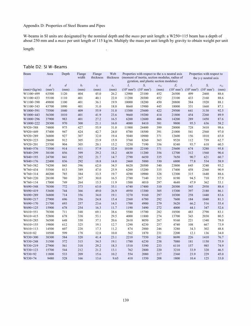
Appendix D: Properties of Steel Beams and Pipes
W-beams in SI units are designated by the nominal depth and the mass per unit length: a W250×115 beam has a depth of about 250 mm and a mass per unit length of 115 kg/m. Multiply the mass per unit length by gravity to obtain weight per unit
length: .
Table D2: SI W-Beams
Beam Area Depth Flangewidth
Flangethickness
Webthickness
Properties with respect to the x-x neutral axis(moment of inertia, section modulus, radius of
gyration, and plastic section modulus)
Properties with respect tothe y-y neutral axis
A d bf tf tw Ix Sx rGx Zx Iy Sy rGy
(mm)×(kg/m) (mm2) (mm) (mm) (mm) (mm) (106 mm4) (103 mm3) (mm) (103 mm3) (106 mm4) (103 mm3) (mm)W1100×499 63500 1120 404 45.0 26.2 12900 23100 452 26500 499 2460 88.6W1100×433 55100 1110 401 40.1 22.0 11200 20300 452 23100 433 2160 88.6W1100×390 49800 1100 401 36.1 19.9 10000 18200 450 20800 384 1920 88.1W1100×343 43700 1090 401 31.0 18.0 8660 15900 445 18000 331 1660 87.1W1000×591 75500 1040 409 55.9 31.0 13300 25600 422 29500 641 3130 92.5W1000×443 56300 1010 401 41.9 23.6 9660 19200 414 21800 454 2260 89.9W1000×296 37900 983 401 27.2 16.5 6200 12600 406 14200 289 1450 87.6W1000×222 28300 970 300 21.1 16.0 4080 8410 381 9800 95.3 636 58.2W920×588 74800 975 427 55.9 31.0 11900 24400 399 28000 728 3410 98.6W920×449 57400 947 424 42.7 24.0 8780 18500 391 21000 541 2560 97.0W920×289 36800 927 307 32.0 19.4 5040 10900 371 12600 156 1010 65.0W920×223 28600 912 305 23.9 15.9 3760 8260 363 9520 112 739 62.7W920×201 25700 904 305 20.1 15.2 3250 7190 356 8340 93.7 618 60.5W840×576 73500 914 411 57.9 32.0 10100 22100 371 25600 674 3280 95.8W840×299 38100 856 399 29.2 18.2 4830 11200 356 12700 312 1560 90.4W840×193 24700 841 292 21.7 14.7 2790 6650 335 7650 90.7 621 60.7W840×176 22400 836 292 18.8 14.0 2460 5880 330 6800 77.8 534 58.9W760×582 74200 843 396 62.0 34.5 8620 20500 340 23800 645 3240 93.2W760×434 55500 813 389 47.0 25.9 6200 15200 335 17400 458 2360 90.9W760×314 40200 785 384 33.5 19.7 4290 10900 328 12300 315 1640 88.6W760×220 28100 780 267 30.0 16.5 2780 7140 315 8190 94.5 710 57.9W760×134 17000 749 264 15.5 11.9 1500 4010 297 4640 47.9 362 53.1W690×548 70300 772 373 63.0 35.1 6740 17400 310 20300 545 2930 88.4W690×419 53600 744 366 49.0 26.9 4950 13300 305 15300 397 2180 86.1W690×289 36800 714 356 34.0 19.1 3270 9160 297 10300 258 1440 83.6W690×217 27900 696 356 24.8 15.4 2360 6780 292 7600 184 1040 81.3W690×170 21700 693 257 23.6 14.5 1700 4900 279 5620 66.2 516 55.4W690×125 15900 678 254 16.3 11.7 1190 3490 272 4000 44.1 347 52.6W610×551 70300 711 348 69.1 38.6 5580 15700 282 18500 483 2790 83.1W610×415 52800 678 338 53.1 29.5 4000 11800 274 13700 343 2030 80.5W610×285 36500 648 330 37.1 20.6 2610 8050 267 9160 221 1340 78.0W610×155 19800 612 325 19.1 12.7 1290 4230 257 4740 108 667 73.9W610×113 14500 607 228 17.3 11.2 874 2880 246 3280 34.3 302 48.8W610×82 10500 599 178 12.8 10.0 562 1870 231 2200 12.1 136 34.0W530×300 38300 584 320 41.4 23.1 2210 7550 241 8690 226 1410 76.7W530×248 31500 572 315 34.5 19.1 1780 6230 238 7080 181 1150 75.9W530×219 27900 561 318 29.2 18.3 1510 5390 233 6110 157 985 74.9W530×123 15700 544 212 21.2 13.1 762 2800 220 3210 33.9 320 46.5W530×92 11800 533 209 15.6 10.2 554 2080 217 2360 23.9 229 45.0W530×74 9480 528 166 13.6 9.65 410 1550 208 1800 10.4 125 33.0
139

Appendix D: Properties of Steel Beams and Pipes
Table D2: SI W-Beams (continued)
Beam Area Depth Flangewidth
Flangethickness
Webthickness
Properties with respect to the x-x neutral axis(moment of inertia, section modulus, radius of
gyration, and plastic section modulus)
Properties with respect tothe y-y neutral axis
A d bf tf tw Ix Sx rGx Zx Iy Sy rGy
(mm)×(kg/m) (mm2) (mm) (mm) (mm) (mm) (106 mm4) (103 mm3) (mm) (103 mm3) (106 mm4) (103 mm3) (mm)W460×464 59100 566 305 69.6 38.6 2900 10200 221 12400 331 2160 74.9W460×315 40200 526 295 48.5 26.9 1800 6870 212 8030 205 1400 71.6W460×193 24700 490 284 30.5 17.0 1020 4200 204 4750 116 818 68.6W460×128 16300 467 282 19.6 12.2 637 2720 197 3050 72.8 518 66.8W460×89 11400 462 192 17.7 10.5 410 1770 190 2020 20.9 218 42.7W460×52 6650 450 152 10.8 7.62 212 944 179 1090 6.37 83.9 31.0W410×149 19000 432 264 25.0 14.9 620 2870 180 3240 77.4 585 63.8W410×100 12600 414 259 16.9 10.0 397 1920 177 2130 49.5 380 62.5W410×60 7610 406 178 12.8 7.75 216 1060 168 1200 12.0 135 39.9W410×46.1 5890 404 140 11.2 6.99 156 773 163 885 5.16 73.6 29.7W410×38.8 4950 399 140 8.76 6.35 125 629 159 724 3.99 57.2 28.4W360×237 30100 381 396 30.2 18.9 791 4160 162 4700 311 1580 102W360×147 18800 361 371 19.8 12.3 462 2570 157 2830 167 905 94.2W360×122 15500 363 257 21.7 13.0 367 2020 154 2280 61.6 480 63.0W360×57.8 7230 358 172 13.1 7.87 160 895 149 1010 11.1 129 39.4W360×32.9 4190 348 127 8.51 5.84 82.8 475 141 544 2.91 45.9 26.4W310×226 28800 348 318 35.6 22.1 595 3420 144 3980 189 1190 81.0W310×158 20100 328 310 25.1 15.5 388 2380 139 2690 125 808 79.0W310×107 13600 312 305 17.0 10.9 248 1600 135 1770 81.2 531 77.2W310×74 9420 310 205 16.3 9.40 163 1050 132 1180 23.4 228 49.8W310×60 7550 302 203 13.1 7.49 128 844 130 934 18.4 180 49.3W310×44.5 5670 312 166 11.2 6.60 99.1 633 132 706 8.45 102 38.6W310×28.3 3590 310 102 8.89 5.97 54.1 349 122 405 1.57 30.8 20.9W310×21 2680 302 101 5.72 5.08 36.9 244 117 285 0.982 19.5 19.1W250×149 18900 282 262 28.4 17.3 259 1840 117 2130 86.2 655 67.3W250×89 11400 259 257 17.3 10.7 142 1090 112 1220 48.3 377 65.3W250×73 9290 254 254 14.2 8.64 113 895 110 990 38.9 306 64.5W250×58 7420 252 203 13.5 8.00 87.0 690 108 767 18.7 185 50.3W250×44.8 5700 267 148 13.0 7.62 70.8 531 111 600 6.95 94.2 34.8W250×28.4 3630 259 102 10.0 6.35 40.1 308 105 354 1.79 35.1 22.2W250×17.9 2280 251 101 5.33 4.83 22.4 179 99.1 206 0.907 18.0 19.9W200×100 12700 229 210 23.7 14.5 113 990 94.5 1150 36.9 351 53.8W200×59 7550 210 205 14.2 9.14 60.8 582 89.7 652 20.4 200 51.8W200×46.1 5890 203 203 11.0 7.24 45.8 451 88.1 498 15.4 152 51.3W200×35.9 4570 201 165 10.2 6.22 34.4 342 86.9 379 7.62 92.3 40.9W200×15 1910 200 100 5.21 4.32 12.8 128 81.8 145 0.870 17.4 21.4W150×37.1 4740 162 154 11.6 8.13 22.2 274 68.6 310 7.12 91.9 38.6W150×22.5 2860 152 152 6.60 5.84 12.1 159 65.0 177 3.88 51.0 36.8W150×13.5 1730 150 100 5.46 4.32 6.83 91.1 62.7 102 0.916 18.2 23.0W100×19.3 2470 106 103 8.76 7.11 4.70 89.5 43.7 103 1.61 31.1 25.4
140

Appendix D: Properties of Steel Beams and Pipes
Steel Pipes
In the 1920s, iron and steel pipes were available in three thickness grades: Standard Weight, Extra Strong (XS), and Double Extra Strong (XXS). Subsequently, the “schedule” designation system was developed to cover other pipe wall thicknesses. Schedule 40 is the same as Standard Weight; Schedule 80 is the same as Extra-Strong. Pipes are available from Schedule 5 to Schedule 160. Regardless of the Schedule, the OD is identical between nominal sizes, so pipes of different Schedules can thread into the same fittings. The heavier Schedules have thicker walls, therefore smaller IDs.
Table D3: US Customary Steel Pipes
Nominaldiameter
Insidediameter
Outsidediameter
Wallthickness
Area Moment ofinertia
Sectionmodulus
Radius ofgyration
Polarmoment of
inertia
Weight perunit length
di do t A I S rG J w(in.) (in.) (in.) (in.) (in.2) (in.4) (in.3) (in.) (in.4) (lb./ft.)
Schedule 40pipes
(StandardWeight)
1 1.05 1.32 0.133 0.469 0.0830 0.126 0.423 0.166 1.682 2.07 2.38 0.154 1.02 0.627 0.528 0.791 1.25 3.663 3.07 3.50 0.216 2.07 2.85 1.63 1.17 5.69 7.584 4.03 4.50 0.237 2.96 6.82 3.03 1.51 13.6 10.85 5.05 5.56 0.258 4.01 14.3 5.14 1.88 28.6 14.66 6.07 6.63 0.280 5.20 26.5 7.99 2.25 52.9 19.08 7.98 8.63 0.322 7.85 68.1 15.8 2.95 136 28.6
Schedule 80pipes
(Extra-Strong)
1 0.957 1.32 0.179 0.602 0.101 0.154 0.410 0.202 2.172 1.94 2.38 0.218 1.40 0.827 0.696 0.771 1.65 5.033 2.90 3.50 0.300 2.83 3.70 2.11 1.14 7.40 10.34 3.83 4.50 0.337 4.14 9.12 4.05 1.48 18.2 15.05 4.81 5.56 0.375 5.73 19.5 7.02 1.85 39.0 20.86 5.76 6.63 0.432 7.83 38.3 11.6 2.20 76.6 28.68 7.63 8.63 0.500 11.9 100 23.1 2.89 199 43.4
Table D4: SI Steel Pipes
Nominaldiameter
Insidediameter
Outsidediameter
Wallthickness
Area Moment ofinertia
Sectionmodulus
Radius ofgyration
Polarmoment of
inertia
Mass perunit length
di do t A I S rG J(mm) (mm) (mm) (mm) (mm2) (106 mm4) (103 mm3) (mm) (103 mm.4) (kg/m)
Schedule 40pipes
(StandardWeight)
25 26.7 33.5 3.38 303 0.0345 2.06 10.7 69.1 2.5051 52.5 60.5 3.91 658 0.261 8.65 20.1 520 5.4476 78.0 88.9 5.49 1340 1.19 26.7 29.7 2370 11.3102 102 114 6.02 1910 2.84 49.7 38.4 5660 16.1127 128 141 6.55 2590 5.95 84.2 47.8 11900 21.7152 154 168 7.11 3350 11.0 131 57.2 22000 28.3203 203 219 8.18 5060 28.3 259 74.9 56600 42.5
Schedule 80pipes
(Extra-Strong)
25 24.3 33.5 4.55 388 0.0420 2.52 10.4 84.1 3.2351 49.3 60.5 5.54 903 0.344 11.4 19.6 687 7.4876 73.7 88.9 7.62 1830 1.54 34.6 29.0 3080 15.3102 97.3 114 8.56 2670 3.80 66.4 37.6 7580 22.3127 122 141 9.53 3700 8.12 115 47.0 16200 30.9152 146 168 11.0 5050 15.9 190 55.9 31900 42.5203 194 219 12.7 7680 41.6 379 73.4 82800 64.5
Additional data on steel beams and pipes are freely available online from the American Institute of Steel Construction (AISC).
141
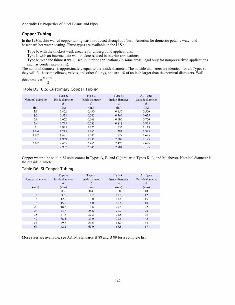
Appendix D: Properties of Steel Beams and Pipes
Copper Tubing
In the 1930s, thin-walled copper tubing was introduced throughout North America for domestic potable water and baseboard hot water heating. Three types are available in the U.S.:
Type K with the thickest wall, useable for underground applications.Type L with an intermediate wall thickness, used in interior applications.Type M with the thinnest wall, used in interior applications (in some areas, legal only for nonpressurized applications such as condensate drains).
The nominal diameter is approximately equal to the inside diameter. The outside diameters are identical for all Types so they will fit the same elbows, valves, and other fittings, and are 1/8 of an inch larger than the nominal diameters. Wall
thickness t=d o−d i
2.
Table D5: U.S. Customary Copper Tubing
Type K Type L Type M All TypesNominal diameter Inside diameter Inside diameter Inside diameter Outside diameter
di di di do
(in.) (in.) (in.) (in.) (in.)3/8 0.402 0.430 0.450 0.5001/2 0.528 0.545 0.569 0.6255/8 0.652 0.668 0.690 0.7503/4 0.745 0.785 0.811 0.8751 0.995 1.025 1.055 1.125
1 1/4 1.245 1.265 1.291 1.3751 1/2 1.481 1.505 1.527 1.625
2 1.959 1.985 2.009 2.1252 1/2 2.435 2.465 2.495 2.625
3 2.907 2.945 2.981 3.125
Copper water tube sold in SI units comes in Types A, B, and C (similar to Types K, L, and M, above). Nominal diameter is the outside diameter.
Table D6: SI Copper Tubing
Type A Type B Type C All TypesNominal diameter Inside diameter Inside diameter Inside diameter Outside diameter
di di di do
(mm) (mm) (mm) (mm) (mm)10 8.2 8.4 8.8 1012 9.6 10.2 10.8 1215 12.6 13.0 13.6 1518 15.6 16.0 16.6 1822 18.8 19.8 20.4 2228 24.8 25.6 26.2 2835 31.8 32.2 32.8 3542 38.4 39.0 39.6 4254 49.8 50.6 51.0 6467 62.2 63.0 63.8 57
More sizes are available; see ASTM Standards B 88 and B 89 for a complete list.
142

Appendix E: Mechanical and Dimensional Properties of Wood
Appendix E: Mechanical and Dimensional Properties of WoodMechanical Properties of Air-Dried Boards and Timber
Wood is a natural material which varies in mechanical properties. Factors affecting strength and stiffness include defects (knots, insect and woodpecker holes), moisture content, service temperature, age of the tree at cutting, direction within the wood (along the grain, tangential, and radial), and geographic source ofthe tree. For example, this graph from the Forest Products Laboratory of the U.S. Department of Agriculture* shows variation in the same visual grade of lumber (same quality & equivalent species), cut from a wide geographical area.
The Allowable Stress Design method (ASD) sets the design stress at the bottom 5th percentile of wood within a stress grade. In theory, 5% of the wood used in any structure is weaker than the required strength...so use a Factor of Safety to preventfailure.
Table E1: U.S. Customary Materials Properties of Timber
Tree species Allowable StressesBending Horizontal shear Tension
parallel to grainCompression
parallel to grainSpecific weight Young's modulus
γ E(psi) (psi) (psi) (psi) (lb./ft.3) (ksi)
Eastern white pine 600 135 275 725 22 1100Southern yellow pine 1400 175 825 1250 34 1700Hem-fir 1000 150 500 1300 25 1400Douglas fir 900 180 625 1050 30 1700Redwood 1000 160 600 1050 25 1300
Table E2: SI Materials Properties of Timber
Tree species Allowable StressesBending Horizontal shear Tension
parallel to grainCompression
parallel to grainDensity Young's modulus
ρ E(MPa) (MPa) (MPa) (MPa) (kg/m3) (GPa)
Eastern white pine 4.1 0.93 1.9 5.0 350 7.6Southern yellow pine 9.7 1.2 5.7 8.6 550 11.7Hem-fir 6.9 1.0 3.4 9.0 400 9.7Douglas fir 6.2 1.2 4.3 7.2 480 11.7Redwood 6.9 1.1 4.1 7.2 400 9.0
Additional data on timber are freely available online from the U.S. Forest Products Laboratory of the U.S. Department of Agriculture at http://www.fpl.fs.fed.us.
* General Technical Report FPL GTR 190, Chapter 7, p. 7-6.
143
1.0 1.8 2.6Young's modulus, E
(106 psi)
0
8
16
Frequency(%)

Appendix E: Mechanical and Dimensional Properties of Wood
Softwood Lumber and Timber Sizes
Softwood is “dressed” or planed from nominal size to the sizes listed below. These sizes are S4S (surfaced four sides). Weight per unit length depends on the density of the wood. Dried softwoods range in specific weight from 20 to 40 lb./ft.3 (320 to 640 kg/m3). If a 2×4 is made of wood with a specific weight of 30 lb./ft.3, its weight per unit length is 1.09 lb./ft.
Table E3: U.S. Customary Timber Sizes
Designation Width Depth Area Moment ofinertia
Sectionmodulus
Weight per unitlength
γ = 20 lb/ft.3
Weight per unitlength
γ = 30 lb/ft.3
Weight per unitlength
γ = 40 lb/ft.3
b d A Ix Sx w w w(in.) (in.) (in.2) (in.4) (in.3) (lb./ft.) (lb./ft.) (lb./ft.)
2×2 1.5 1.5 2.25 0.422 0.563 0.313 0.469 0.6252×3 1.5 2.5 3.75 1.95 1.56 0.521 0.781 1.042×4 1.5 3.5 5.25 5.36 3.06 0.729 1.09 1.462×6 1.5 5.5 8.25 20.8 7.56 1.15 1.72 2.292×8 1.5 7.25 10.9 47.6 13.1 1.51 2.27 3.022×10 1.5 9.25 13.9 98.9 21.4 1.93 2.89 3.852×12 1.5 11.25 16.9 178 31.6 2.34 3.52 4.694×4 3.5 3.5 12.3 12.5 7.1 1.70 2.55 3.404×6 3.5 5.5 19.3 48.5 17.6 2.67 4.01 5.354×8 3.5 7.25 25.4 111 30.7 3.52 5.29 7.054×10 3.5 9.25 32.4 231 49.9 4.50 6.74 8.994×12 3.5 11.25 39.4 415 73.8 5.47 8.20 10.94×14 3.5 13.25 46.4 678 102 6.44 9.66 12.94×16 3.5 15.25 53.4 1034 136 7.41 11.12 14.86×6 5.5 5.5 30.3 76.3 27.7 4.20 6.30 8.406×8 5.5 7.5 41.3 193 51.6 5.73 8.59 11.56×10 5.5 9.5 52.3 393 82.7 7.26 10.9 14.56×12 5.5 11.5 63.3 697 121 8.78 13.2 17.66×14 5.5 13.5 74.3 1130 167 10.3 15.5 20.66×16 5.5 15.5 85.3 1710 220 11.8 17.8 23.76×18 5.5 17.5 96.3 2460 281 13.4 20.1 26.76×20 5.5 19.5 107 3400 349 14.9 22.3 29.88×8 7.5 7.5 56.3 264 70.3 7.81 11.7 15.68×10 7.5 9.5 71.3 536 113 9.90 14.8 19.88×12 7.5 11.5 86.3 951 165 12.0 18.0 24.08×14 7.5 13.5 101 1540 228 14.1 21.1 28.18×16 7.5 15.5 116 2330 300 16.1 24.2 32.38×18 7.5 17.5 131 3350 383 18.2 27.3 36.58×20 7.5 19.5 146 4630 475 20.3 30.5 40.610×10 9.5 9.5 90.3 679 143 12.5 18.8 25.110×12 9.5 11.5 109 1200 209 15.2 22.8 30.310×14 9.5 13.5 128 1950 289 17.8 26.7 35.610×16 9.5 15.5 147 2950 380 20.5 30.7 40.910×18 9.5 17.5 166 4240 485 23.1 34.6 46.210×20 9.5 19.5 185 5870 602 25.7 38.6 51.510×22 9.5 21.5 204 7870 732 28.4 42.6 56.710×24 9.5 23.5 223 10300 874 31.0 46.5 62.012×12 11.5 11.5 132 1460 253 18.4 27.6 36.712×14 11.5 13.5 155 2360 349 21.6 32.3 43.112×16 11.5 15.5 178 3570 460 24.8 37.1 49.512×18 11.5 17.5 201 5140 587 28.0 41.9 55.912×20 11.5 19.5 224 7110 729 31.1 46.7 62.312×22 11.5 21.5 247 9520 886 34.3 51.5 68.712×24 11.5 23.5 270 12400 1060 37.5 56.3 75.1
144

Appendix E: Mechanical and Dimensional Properties of Wood
Timber beams in SI units are listed by their mass per unit length, not by their weight per unit length. A 200×360 timber beam made of wood with a density of 320 kg/m3 has a mass per unit length of 21 kg/m. Multiply by the mass per unit length
by gravity to obtain weight per unit length: .
Table E4: SI Timber Sizes
Designation Width Depth Area Moment ofinertia
Sectionmodulus
Mass per unitlength
ρ = 320 kg/m3
Mass per unitlength
ρ = 480 kg/m3
Mass per unitlength
ρ = 640 kg/m3
b d A Ix Sx m/L m/L m/L(mm) (mm) (103 mm2) (106 mm4) (103 mm3) (kg/m) (kg/m) (kg/m)
50×100 38.1 88.9 3.39 2.23 50.2 1.09 1.63 2.1750×150 38.1 140 5.33 8.71 124 1.71 2.56 3.4250×200 38.1 184 7.01 19.8 215 2.25 3.37 4.4950×250 38.1 235 8.95 41.2 351 2.87 4.30 5.7450×300 38.1 286 10.9 74.3 519 3.49 5.24 6.9850×360 38.1 337 12.8 122 721 4.12 6.17 8.2350×410 38.1 387 14.7 184 951 4.73 7.09 9.45
100×100 88.9 88.9 7.90 5.21 117 2.53 3.80 5.07100×150 88.9 140 12.4 20.3 290 3.99 5.98 7.98100×200 88.9 184 16.4 46.2 502 5.24 7.86 10.5100×250 88.9 235 20.9 96.1 818 6.70 10.0 13.4100×300 88.9 286 25.4 173 1212 8.15 12.2 16.3100×360 88.9 337 30.0 284 1683 9.60 14.4 19.2100×410 88.9 388 34.5 433 2230 11.1 16.6 22.1150×150 140 140 19.6 32.0 457 6.28 9.42 12.6150×200 140 191 26.7 81.3 851 8.57 12.9 17.1150×250 140 241 33.7 163 1360 10.8 16.2 21.6150×300 140 292 40.9 290 1990 13.1 19.7 26.2150×360 140 343 48.0 471 2750 15.4 23.1 30.8150×410 140 394 55.2 714 3620 17.7 26.5 35.4150×460 140 445 62.3 1030 4620 20.0 30.0 39.9150×510 140 496 69.4 1420 5740 22.3 33.4 44.5200×200 191 191 36.5 111 1160 11.7 17.5 23.4200×250 191 241 46.0 223 1850 14.8 22.1 29.5200×300 191 292 55.8 396 2710 17.9 26.8 35.7200×360 191 343 65.5 642 3750 21.0 31.5 42.0200×410 191 394 75.3 974 4940 24.1 36.2 48.2200×460 191 445 85.0 1400 6300 27.2 40.9 54.5200×510 191 496 94.7 1940 7830 30.4 45.5 60.7250×250 241 241 58.1 281 2330 18.6 27.9 37.2250×300 241 292 70.4 500 3420 22.6 33.8 45.1250×360 241 343 82.7 810 4730 26.5 39.7 53.0250×410 241 394 95.0 1230 6240 30.4 45.7 60.9250×460 241 445 107 1770 7950 34.4 51.6 68.7250×510 241 495 119 2440 9840 38.2 57.4 76.5250×560 241 546 132 3270 12000 42.2 63.3 84.3250×610 241 597 144 4270 14300 46.1 69.2 92.2300×300 292 292 85 606 4150 27.3 41.0 54.7300×360 292 343 100 982 5730 32.1 48.2 64.2300×410 292 394 115 1490 7550 36.9 55.3 73.7300×460 292 445 130 2140 9640 41.6 62.5 83.3300×510 292 495 145 2950 11900 46.3 69.5 92.7300×560 292 546 159 3960 14500 51.1 76.7 102300×610 292 597 174 5180 17300 55.9 83.8 112
145

Appendix F: Beam Equations
Appendix F: Beam EquationsRA and RB are the reaction forces at points A and B. MB is the reaction moment at point B.
Vx, Mx and Δx are the shear load, bending moment, and deflection at a distance x from the left end of the beam.
Ma and Δa are the bending moment and deflection at a distance x = a from the left end of the beam.
Point load at the midspan of a simply-supported beam
RA=RB=V max=P2
M max=P L4
at the point load
M x=P x2
for x< L2
Δmax=P L3
48 E I at the point load
Δx=P x
48 E I(3 L2−4 x2) for x≤ L
2
Point load at any location on a simply-supported beam
RA=P bL
, RB=P aL
, Vmax is the greater of the two
M max=P a b
L at the point load
M x=P b x
L for x < a
Δmax=P a b(a+2b)√3 a(a+2b )
27 E I L at x=√ a (a+2b)
3 when a > b
Δa=P a 2b2
3E I L at the point load
Δx=P b x
6 E I L(L2−b2−x2) for x < a
146
P
A B
RA
V
RA
RB
L/2 L/2R
B
M
Mmax
Elasticcurve
x
Δmax
P
A B
RA
V
RA
RB
a bR
B
M
Mmax
Elasticcurve
x
Δmax

Appendix F: Beam Equations
Two identical point loads, symmetrically placed on a simply-supported beam
RA=RB=V max=P
M max=P a between the point loads
M x=P x for x < a
Δmax=P a
24 E I(3 L2−4a 2) at the midspan
Δx=P x
6 E I(3 L a−3a 2−x2) for x < a
Δx=P a
6 E I(3 L x−3 x2−a2) between the point loads
Uniform distributed load along the entire length of a simply-supported beam
RA=RB=V max=w L2
V x=w( L2−x)
M max=w L2
8 at the midspan
M x=w x2(L−x)
Δmax=5w L4
384 E I at the midspan
Δx=w x
24 E I(L3−2 L x2+x3)
Uniform distributed load on a simply-supported beam
RA=V max=w a2 L
(2 L−a ) , RB=w a2
2 L
V x=RA−w x for x < a
M max=RA
2
2w at x=
RA
w
M x=RA x−w x2
2 for x < a; M x=RB(L−x) for x > a
Δx=w x
24 E I L[a2(2 L−a )2−2 a x 2(2 L−a)+L x 3] for x < a
Δx=w a2(L−x)
24 E I L(4 x L−2 x 2−a2) for x > a
147
P
A B
RA
V
RA
RB
a aR
B
M
Mmax
Elasticcurve
x
Δmax
P
L/2
A B
RA
VR
B
w
b
Mmax
M
ElasticcurveΔ
max
x
a
A B
RA
VR
B
w
L
Mmax
M
ElasticcurveΔ
max
x

Appendix F: Beam Equations
Nonuniform distributed load, tapered along the length
RA=wmax L
6, RB=
wmax L3
V x=wmax L
6−
wmax x2
2 L
M max=wmax L2
9√3 at x= L
√3 M x=
wmax L x
6 L2 (L2−x 2)
Δmax=0.00652wmax L4
E I at x=L√1−√ 8
15
Δx=wmax x
360 E I L(3 x4−10 L2 x2+7L4)
Nonuniform distributed load on a simply-supported beam, tapering from the midspan to the ends
RA=RB=V max=w L
V x=w
4 L(L2−4 x 2) for x< L
2
M max=w L2
12 at the midspan
M x=w L x
2 (12−2 x2
3 L2 ) for x< L2
Δmax=w L3
120 E I at the midspan
Δx=w x
960 E I L(5 L2−4 x2 )2 for x< L
2
Point load at the end of a cantilever beam
RB=V max=P
M B=M max=P L
M x=P x
Δmax=P L3
3E I at the free end
Δx=P
6 E I(2L3−3 L2+x3)
148
A B
RA
VR
B
wmax
L
Mmax
M
ElasticcurveΔ
max
x
A B
RA
VR
B
wmax
L
Mmax
M
ElasticcurveΔ
max
x
P
A B
VR
B
LR
B
MM
max
Elasticcurve
x
Δmax
MB

Appendix F: Beam Equations
Point load at any location on a cantilever beam
RB=V max=P
M B=M max=P b
M x=P (x−a ) for x > a
Δmax=P b2
6 E I(3 L−b) at the free end
Δa=P b3
3E I at the point load
Δx=P b2
6 E I(3 L−3 x−b) for x < a
Δx=P (L−x)2
6 E I(3b−L+x) for x > a
The beam bends in an arc between the support and the point load. To theleft of the point load, the beam is straight.
Uniform distributed load along the entire length of a cantilever beam
RB=V max=wL
V x=w x
M B=M max=w L2
2
M x=w x 2
2
Δmax=w L4
8E I at the free end
Δx=w
24 E I(x4−4 L3 x+3 L4)
149
P
A B
VR
B
bR
B
MM
max
Elasticcurve
x
Δmax
MB
a
Δa
straightsegment
curved segment
A B
VR
B
LR
B
MM
max
Elasticcurve
x
Δmax
MB
w

Appendix F: Beam Equations
Nonuniform distributed load along the entire length of a cantilever beam, tapering from the support to the free end
RB=V max=wmax L
2
V x=wmax x 2
2 L
M B=M max=wmax L2
6
M x=wmax x3
6 L
Δmax=wmax L4
30 E I at the free end
Δx=wmax
120 E I L(x5−5 L4 x+4 L5)
150
A B
VR
B
LR
B
M
Mmax
Elasticcurve
xΔ
max
MB
wmax

Appendix F: Beam Equations
IndexAllowable moment in a beam.........................................................73Allowable stress in welded tanks....................................................26Angle of twist in a round shaft.......................................................53Average web shear approach..........................................................79Beam deflection...............................................................................84Beam design, steel...........................................................................90Beam design, wood.........................................................................96Beam reactions................................................................................56Bending moment diagrams.............................................................67Bending stress in beams..................................................................73Bending stress in steel beams.........................................................75Bolted joints....................................................................................30Buckling of columns.....................................................................108Cantilever beams.............................................................................56Centroid ..........................................................................................38Centroidal axis.................................................................................38Column buckling...........................................................................108Columns, ideal slender..................................................................108Columns, steel...............................................................................110Columns, steel machine parts.......................................................111Columns, support conditions........................................................109Combined stresses...........................................................................99Deflection diagrams........................................................................73Eccentric loading...........................................................................101Effective length of a column.........................................................109Efficiency, bolted & welded joints.................................................33Elastic deformation.........................................................................16Elastic modulus...............................................................................15Equivalent load diagram.................................................................59Euler critical load..........................................................................108Euler stress....................................................................................109Factor-label method of unit conversion..........................................10Failure theories..............................................................................126Flexure formula...............................................................................73Formula method of beam analysis..................................................85Hollow shafts...................................................................................53Hoop stress......................................................................................25Ideal slender columns....................................................................108Isostress lines.................................................................................115Joint efficiency in bolted & welded joints......................................33Load diagrams.................................................................................57Longitudinal stress in a pipe...........................................................25Microstrain......................................................................................14Modulus of elasticity.......................................................................15Modulus, shear................................................................................53Mohr's circle..................................................................................115Moment diagrams............................................................................67Moment of inertia............................................................................38
Neutral axis......................................................................................73Overhanging beams.........................................................................60Pipes.................................................................................................25Plastic deformation..........................................................................16Plastic moment................................................................................76Plastic section modulus...................................................................76Poisson's ratio..................................................................................20Polar moment of inertia..................................................................51Pressure vessels...............................................................................25Radius of curvature of a beam........................................................84Radius of gyration...........................................................................51Reference axis.................................................................................42Rupture strength..............................................................................16S4S.................................................................................................144Section modulus..............................................................................74Shafts in torsion...............................................................................52Shear diagrams................................................................................61Shear stress......................................................................................17Shear stress in beams......................................................................77Shear stress in round shafts.............................................................52Short block....................................................................................101Simply-supported beams.................................................................56Statically indeterminate beams.....................................................104Steel beam design............................................................................90Steel columns................................................................................110Steel machine part columns..........................................................111Strain................................................................................................14Stress concentration in tension.......................................................27Stress concentration in torsion........................................................54Stress-strain curve...........................................................................14Stress, tensile...................................................................................14Stress, thermal.................................................................................23Superposition....................................................................87, 99, 104Tensile strength...............................................................................16Terminology......................................................................................5Thermal expansion..........................................................................22Thin-walled pipe.............................................................................25Timber beam design........................................................................96Torsion in round shafts...................................................................52Transfer formula..............................................................................41Ultimate tensile strength.................................................................16Unit systems & conversions.........................................................129Visualizing Stress and Strain........................................................114Welded lap joints.............................................................................35Wood beam design..........................................................................96Yield strength..................................................................................16Young's modulus.............................................................................15
151
Copyright © 2022 FDOKUMEN