Centre forEconomicand FinancialResearchatNew Economic School

Strategic Asset Allocation in MoneyManagement

Suleyman Basak

Dmitry Makarov

Working Paper o 158

CEFIR / ES Working Paper series

August 2009

Strategic Asset Allocationin Money Management∗

Suleyman Basak Dmitry MakarovLondon Business School and CEPR New Economic School

Regents Park Nakhimovsky pr. 47London NW1 4SA Moscow 117418

United Kingdom RussiaTel: 44 (0)20 7000-8256 Tel: 7 495 129-3911Fax: 44 (0)20 7000-8201 Fax: 7 495 129-3722

E-mail: sbasak@london.edu E-mail: dmakarov@nes.ru

This version: August 2009

∗We are grateful to Tomas Bjork, Anthony Neuberger, Anna Pavlova, Guilllaume Plantin, Larry Samuel-son, and the seminar participants at London Business School, New Economic School, Stockholm School ofEconomics, University of Lausanne, University of Toronto, and European Finance Association meetings forhelpful comments. Earlier version of this work was circulated in the manuscript entitled “Strategic AssetAllocation with Relative Performance Concerns.” All errors are our responsibility.

Strategic Asset Allocation in Money Management

Abstract

This article analyzes the dynamic portfolio choice implications of strategic interaction

among money managers. The strategic interaction emerges as the managers compete for

money flows displaying empirically documented convexities. A manager gets money flows

increasing with performance, and hence displays relative performance concerns, if her relative

return is above a threshold; otherwise she receives no (or constant) flows and has no relative

concerns. We provide a tractable formulation of such strategic interaction between two risk

averse managers in a continuous-time setting, and solve for their equilibrium policies in

closed-form. When the managers’ risk aversions are considerably different, we do not obtain

a Nash equilibrium as the managers cannot agree on who loses (getting no flows) in some

states. We obtain equilibria, but multiple, when the managers are similar since they now

care only about the total number of losing states. We recover a unique equilibrium, however,

when a sufficiently high threshold makes the competition for money flows less intense. The

managers’ unique equilibrium policies are driven by chasing and contrarian behaviors when

either manager substantially outperforms the opponent, and by gambling behavior when

their performances are close to the threshold. Depending on the stock correlation, the

direction of gambling for a given manager may differ across stocks, however the two managers

always gamble strategically in the opposite direction from each other in each individual stock.

JEL Classifications: G11, G20, D81, C73, C61.

Keywords: Money Managers, Strategic Interaction, Portfolio Choice, Relative Perfor-

mance, Incentives, Risk Shifting, Fund Flows, Tournaments.

1. Introduction

This paper analyzes the dynamic portfolio strategies of money managers in the presence of

strategic interactions, arising from each manager’s desire to perform well relative to the other

managers. There are several reasons why managers may care about relative performance.

First, given the prevalent finding in money management that the money flows to relative

performance relationship is increasing and convex (Chevalier and Ellison (1997), Sirri and

Tufano (1998)) for individual mutual funds, Gallaher, Kaniel, and Starks (2006) for mutual

fund families, Agarwal, Daniel, and Naik (2004), Ding, Getmansky, Liang and Wermers

(2007) for hedge funds), a fund manager has incentives to outperform the peers so as to

increase her assets under management, and hence, her compensation.1 Relative concerns

may also arise within fund families as funds with high relative performance are likely to be

advertised more (Jain and Wu (2000)) and also to be cross-subsidized at the expense of other

family members (Gaspar, Massa, and Matos (2006)). Moreover, money managers may care

about their relative standing due to psychological aspects of human behavior, such as envy

or crave for higher social status.

When discussing the interaction of fund managers in the presence of relative performance

concerns, Brown, Harlow, and Starks (1996) appeal to the notion of a tournament in which

managers are the competitors and money flows are the prizes awarded based on relative rank-

ing. Since then, a rapidly growing empirical literature (Busse (2001), Qiu (2003), Goriaev,

Nijman, and Werker (2005), Reed and Wu (2005)) address the tournament hypothesis by

looking at how risk taking behavior responds to relative performance. While several recent

theoretical studies attempt to analyze mutual fund tournaments, their results are obtained

under fairly specialized economic settings (as discussed below). To our best knowledge, ours

is the first comprehensive analysis of the portfolio choice effects of strategic interactions

within a workhorse dynamic asset allocation framework, allowing us to derive a rich set of

implications. The effects of strategic considerations are likely to be the strongest when there

is a small number of funds competing against each other. One natural real-life case is when

several top-performing funds compete for the leadership. Another example is the strategic

interaction of money managers within a fund family comprised of a small number of funds,

as documented by Kempf and Ruenzi (2008).

We consider two risk averse money managers, interpreted as either mutual fund man-

agers, hedge fund managers, or simply traders.2 We adopt a familiar Merton (1969)-type

1A standard explanation for a positive relation between money flows and relative performance is thatinvestors respond to widely published fund rankings (MorningStars, Business Week, Forbes, Institutional

Investor) when choosing which fund to invest into.2In addition to the money management industry, our analysis can also be applied to study the behavior

of traders working in the same investment bank. Indeed, while it may not be explicitly written in a contract,it is common knowledge that promotion of traders much depends on their relative (to colleagues) success.Hence, a trader concerned about her career is likely to have relative performance considerations as one of

1

continuous-time economy for investment opportunities with multiple correlated risky stocks,

and assume constant relative risk aversion (CRRA) preferences for a normal manager with

no relative performance concerns. We model relative performance concerns by postulating

that a manager’s objective function depends (positively) on the ratio of her horizon invest-

ment return over the other manager’s return, in addition to her own horizon wealth. Our

interpretation for the presence of these relative performance concerns is based on money

flows, which capture the desire of a money manager to attract new money by outperforming

the other manager. We formally justify this in our analysis by considering an option-like

flow-performance specification that exhibits a convexity, consistent with the above-cited em-

pirical evidence on fund flows. If the manager’s relative performance is above a certain

threshold, she receives money flows increasing with performance, and hence displays relative

performance concerns. Otherwise if she performs relatively poorly, she receives no (or con-

stant) flows and her objectives are as for a normal manager with no relative concerns. The

presence of the threshold captures inertia whereby investors respond to relative performance

and award a fund with money flows only after this fund outperforms the opponent by a cer-

tain margin (Huang, Wei, and Yan (2007)). In characterizing managers’ behavior, we appeal

to the pure-strategy Nash equilibrium concept, in which each manager strategically accounts

for the dynamic investment policies of the other manager, and the equilibrium policies of

the two managers are mutually consistent.

Solving for the managers’ best responses reveals that a manager only chooses two out-

comes at the horizon: “winning” by outperforming the other manager and attracting flows,

or “losing” by underperforming and getting no flows, and never opting for a “draw.” This

is due to the local convexity around the performance threshold, inducing the manager to

gamble so as to end up either a winner or a loser, thus avoiding a draw. Moreover, we show

that an important feature of a manager when outperforming, and hence displaying relative

performance concerns, is that she either “chases” the opponent, increasing her investment

policy in response to the opponent’s increasing hers, or acts as a “contrarian,” decreasing her

investments in response to the opponents’s increasing hers. In our formulation, a manager

is a chaser if her risk aversion coefficient is greater than unity (more empirically plausible),

and is a contrarian otherwise.

Moving to equilibrium, we demonstrate that the gambling behavior caused by local con-

vexities leads to the potential non-existence of a pure-strategy Nash equilibrium, since when

both managers’ performances are close to their thresholds (in the convex region), they cannot

agree on who the winner is. Such a situation occurs when the managers’ attitude towards

risk are considerably different, where one manager may want to outperform the other by

just a little to become a winner, while the other manager wants to underperform by a lot

her objectives.

2

to be content with being a loser. If on the other hand, the managers’ risk aversions are

sufficiently similar, an equilibrium obtains, with one manager emerging as a winner and the

other as a loser. However, since the managers are very similar, the opposite outcome may

also occur, where the earlier winner and loser positions are switched, giving rise to multiplic-

ity. We show that both of these non-existence and multiplicity issues are resolved when the

performance threshold is sufficiently high. This is because with a high threshold, the two

managers cannot both be close to their thresholds and gamble at the same time, which is

the main cause for the non-existence and multiplicity. This unique equilibrium is more likely

to exist for higher values of risk aversions or lower money flow elasticities as this dampens

the gambling incentives.

It is recognized in other economic settings that strategic interactions may lead to out-

comes such as multiplicity or non-existence of equilibrium. However, the economic mech-

anisms and factors determining which of the outcomes occur seem to be specific to our

framework.3 In particular, we believe that our analysis is the first to identify an important

economic role played by the performance threshold and risk aversion heterogeneity in deter-

mining whether unique or multiple equilibrium exists. It is also worth noting that in related

non-strategic works where the gambling behavior is present the optimal portfolios are unique

(Carpenter (2000), Basak, Pavlova, and Shapiro (2007)), and hence the possibility of mul-

tiple equilibria or no equilibrium at all is not anticipated in the existing finance literature.

We discuss the possible multiplicity and non-existence in detail because the client investors

and regulators may find these outcomes problematic given the resulting behavior of money

managers.4

When equilibrium is unique, we provide a full characterization of the equilibrium invest-

ment policies. The investments of the two managers at any interim point in time depend on

their performance relative to each other. If a manager significantly outperforms the oppo-

nent, both managers are far from the convex region of their objectives and so the chasing and

contrarian behaviors dominate the gambling incentives. In particular, when outperforming a

chaser moves her investment policy towards the opponent’s normal policy, while a contrarian

tilts her policy away from the opponent’s normal policy. For the underperforming manager,

the relative concerns are weak since the likelihood of her attracting money flows at year-end

is low, and hence her equilibrium policy is close to the normal policy. When both managers’

3In other words, the important question of when multiplicity or non-existence occurs cannot be addressedby relying on the intuition or formal conditions developed in other strategic settings where these featuresare also present. For example, given the complexity of our framework it does not appear possible to checkwhether the conditions for existence (Baye, Tian, and Zhou (1993)) or multiplicity (Cooper and John (1988))of pure-strategy equilibrium are satisfied in our setting.

4Indeed, if pure-strategy equilibrium does not exist the managers are likely to resort to mixed strategies,implying that investor returns are subject to an additional randomness on top of the stock price uncertainty.Under multiplicity, investors cannot reliably predict their returns for a given realization of stock prices, whichagain implies the presence of an additional risk.

3

performance is close to the threshold, the gambling incentives dominate the chasing and

contrarian behaviors, inducing the two managers to gamble in the opposite direction from

each other in each individual stock. The exact direction of a manager’s gambling in each

stock is determined by the relation between the managers’ risk aversions and the Sharpe

ratios of the risky stocks.

Considering a setting with two risky stocks and looking at the effect of stock correlation,

we show that the managers’ policies are driven by the interaction of a diversification effect,

the extent of benefits to diversification, and a substitution effect, the extent of the stocks

acting as a substitute to each other. A higher stock correlation reduces the diversification

benefits and so the managers tend to decrease their investments in both stocks. As the

correlation increases further, the substitution effect kicks in leading to a decrease in the

managers’ investments in the less favorable stock (with a relatively low Sharpe ratio) and

an increase in the more favorable stock (with a relatively high Sharpe ratio). As a result,

the managers’ investments in the more favorable stock are non-monotonic in correlation.

Moreover, as the substitution effect grows stronger for high correlation values, each manager

strategically changes the direction of gambling in the less favorable stock in order to amplify

the gambling in the opposite direction in the more favorable stock.

Above equilibrium investments determine whether a manager ends up as a winner or as

a loser at the investment horizon depending on economic conditions. In good states, the

more risk averse manager performs worse (consistent with normal behavior) and hence is a

loser, while the less risk averse manager with the better performance is a winner, getting the

money flows. In bad states, the opposite holds, with the more risk averse manager emerging

as the winner, and the less risk averse as the loser. In intermediate states, around their

performance thresholds, both managers are losers, not getting any flows. Multiple equilibria

obtains when the performance threshold is low, which rules out the unique equilibrium

outcome of both managers being losers in intermediate states. Each manager now wants to

differentiate herself from the opponent, and so both outcomes, with either manager being a

winner and the other a loser, constitute a (multiple) equilibrium. The reason why a manager

may be content with being a loser in a certain state is that choosing a relatively low wealth

and losing in that state allows the manager to choose a relatively high wealth and win in

another state. In good and bad states the multiple equilibrium outcomes are as in the unique

equilibrium.

Our paper is related to several strands of literature. First is the literature on the effects

of strategic considerations on portfolio managers’ choices. Most of these works adopt single-

or two-period settings and often assume risk neutrality (Goriaev, Palomino and Prat (2003),

Taylor (2003), Palomino (2005), Li and Tiwari (2005), Chiang (1999), Loranth and Sciubba

(2006)). Our goal is to characterize optimal portfolios in a standard dynamic asset allocation

4

setting with risk averse managers. We find risk aversion to be the critical driving factor

in much of our analysis, including chasing/contrarian behavior, risk shifting, existence of

equilibrium. In a dynamic setting like ours, Browne (2000) investigates a portfolio game

between two managers. He primarily focuses on the case when the managers face different

financial investment opportunities and have practical objectives (maximizing the probability

of beating the other manager, minimizing the expected time of beating the other manager).

None of these objective functions display local convexities, which we find to have important

implications for equilibrium investment policies as well as for the number of equilibria.

If a peer group consists of a large number of competing funds, strategic interactions

are likely to be less pronounced. In this case, the behavior of each fund manager is better

described by assuming that she seeks to perform well relative to an exogenous benchmark.

The manager’s behavior in this case has been recently investigated in Basak, Shapiro, and

Tepla (2006), van Binsbergen, Brandt, and Koijen (2007), Cuoco and Kaniel (2007). Several

works, including Carpenter (2000), Basak, Pavlova, and Shapiro (2007), have demonstrated

that convexities in managers’ objective functions have significant implications for the optimal

portfolios, leading to risk shifting behavior. We contribute to this literature by investigating

how the risk shifting motives interact with strategic considerations and recover novel eco-

nomic implications. First, strategic interactions can lead to non-existence or multiplicity of

equilibrium. Second, the economic mechanism behind the chasing and contrarian behavior,

which drives the equilibrium policies across the whole range of relative performance apart

from the gambling region, is not present in the above non-strategic studies. Third, our two

managers always gamble in the opposite direction from each other in each individual stock,

and it is the manager’s risk aversion relative to that of the opponent that determines the

direction of gambling. This is notably different from the related works which find that the

direction of gambling is either determined by the absolute value of the manager’s risk aver-

sion or is always the same. Fourth, we reveal that changing the correlation between risky

stock returns leads to rich patterns in the behavior of strategic managers, which are not

present in the existing non-strategic works.

Finally, our paper is related to the literature that examines the role of relative wealth

concerns in finance. DeMarzo, Kaniel, and Kremer (2007, 2008) show that relative wealth

concerns may play a role in explaining financial bubbles and excessive real investments.

These papers are close in spirit to our work since they also demonstrate how relative wealth

concerns may arise endogenously. However, their mechanism for the emergence of relative

concerns is a general equilibrium one, and so is notably different from ours. In DeMarzo et al.,

there is a scarce consumption good whose price increases with the cohort’s wealth, implying

that an investor’s relative wealth determines the quantity of the good she can afford. Abel

(1990), Gomez, Priestley, and Zapatero (2008), among many others, demonstrate that models

with the “catching-up-with-the-Joneses” feature can explain various empirically observed

5

asset pricing phenomena. Goel and Thakor (2005) investigate how envy leads to corporate

investment distortions.

Remainder of the paper is organized as follows. Section 2 presents the economic set-

up and provides the money flows justification for relative performance concerns. Section 3

describes the managers’ objective functions and characterizes their best responses. Section

4 analyzes the issues of non-existence, uniqueness, and multiplicity of equilibrium. Section

5 characterizes the unique and multiple equilibrium and investigates the properties of the

equilibrium investment policies. Section 6 concludes. Proofs are in the Appendix.

2. Economy with Strategic Asset Allocation

2.1. Economic Set-Up

We adopt a familiar dynamic asset allocation framework along the lines of Merton (1969). We

consider a continuous-time, finite horizon [0, T ] economy, in which the uncertainty is driven

by an N -dimensional standard Brownian motion ω = (ω1, . . . , ωN)⊤. Financial investment

opportunities are given by a riskless bond and N correlated risky stocks. The bond provides

a constant interest rate r. Each stock price, Sj , follows a geometric Brownian motion

dSjt = Sjtµjdt + Sjt

N∑

k=1

σjkdωkt, j = 1, . . . , N,

where the stock mean returns µ ≡ (µ1, . . . , µN)⊤ and the nondegenerate volatility matrix

σ ≡ σjk, j, k = 1, . . . N are constant,5 and the (instantaneous) correlation between stock

j and ℓ returns is given by ρjℓ =∑N

k=1 σjkσℓk/√

∑

k σ2jk

∑

k σ2ℓk.

Each money manager i in this economy dynamically chooses an investment policy φi,

where φit ≡ (φi1, . . . , φiN)⊤ denotes the vector of fractions of fund assets invested in each

stock, or the risk exposure, given initial assets of Wi0. The investment wealth process of

manager i, Wi, follows

dWit = Wit[r + φ⊤it(µ − r1)]dt + Witφ

⊤itσdωt, (1)

where 1 = (1, . . . , 1)⊤. Dynamic market completeness (under no-arbitrage) implies the

existence of a unique state price density process, ξ, with dynamics dξt = −ξtrdt − ξtκ⊤dωt,

5While it may be of interest to consider a more general setting with a stochastic investment opportunityset, the analytical tractability in the current framework would be lost (as would also be the case for non-strategic models). To characterize the dynamic equilibrium portfolio policies in such a setting, one wouldneed to resort to numerical methods, such as those proposed by Detemple, Garcia, and Rindisbacher (2003)and Cvitanic, Goukasian, and Zapatero (2003). We leave this for future work.

6

where κ ≡ σ−1(µ − r1) is the constant N -dimensional market price of risk in the economy.

The state-price density serves as the driving economic state variable in a manager’s dynamic

investment problem absent any market imperfections. The quantity ξt(ω) is interpreted as

the Arrow-Debreu price per unit probability P of one unit of wealth in state ω ∈ Ω at time

t. In particular, each manager’s dynamic budget constraint (1) can be restated as (e.g.,

Karatzas and Shreve (1998))

E[ξTWiT ] = Wi0. (2)

This allows us to equivalently define the set of possible investment policies of managers as

being the managers’ horizon wealth, WiT , subject to the static budget constraint (2).

2.2. Modeling Strategic Interaction

We envision a money manager, interpreted either as a mutual fund manager, a hedge fund

manager or a trader, who seeks to increase the terminal value of her portfolio. This is

consistent with maximizing her own compensation given the widespread use of the linear

fee structure in the money management industry. The key feature of our setting is that

the manager experiences money flows which depend on her relative performance within a

peer group – we formalize this idea below. In this paper, we look at the scenario when all

fund managers within this peer group have relative performance concerns driven by money

flows, leading to the strategic interaction among the managers. We expect the effects of

such interaction to be most pronounced when the peer group is comprised of a small number

of funds. In this case, each manager is a major player in the competition for money flows

implying that her decisions may significantly affect the other managers’ actions. One natural

real-life example is when the few very top funds attempt to become year-end top-performers.

Another example is the competition of fund managers within fund families. Kempf and

Ruenzi (2008) document the presence of strategic interactions in families that are comprised

of a small number of funds.

In the presence of relative concerns, the objective function of manager i has the general

form

vi(WiT , RiT ), (3)

where vi is increasing in horizon wealth, WiT , and horizon relative return, RiT . We consider

a framework with two fund managers, indexed by i = 1, 2. The relative returns of managers

1 and 2, R1T and R2T , capture the relative performance concerns and are defined as the ratio

of the two managers’ time-T investment returns:

R1T =W1T /W10

W2T /W20, R2T =

W2T /W20

W1T /W10. (4)

7

We normalize both managers’ initial assets to be equal, W10 = W20, without loss of generality

(see Remark 3).

We now provide a rational justification for the objective function (3) by showing that it

arises naturally in a setting where managers care directly only about their own wealth and

that its specific form used in this paper corresponds to the empirically observed fund-flows to

relative performance relation. Towards this, the economic setting is extended as follows. The

manager continues to invest beyond date T up until an investment horizon T ′. Motivated by

the empirical evidence for both mutual funds and hedge funds (Chevalier and Ellison (1997),

Sirri and Tufano (1998), Agarwal, Daniel, and Naik (2004), Ding, Getmansky, Liang and

Wermers (2007)), we assume that the manager experiences money flows at a rate fT . The

flow-performance relationship fT is (weakly) increasing and convex in the manager’s relative

performance over the period [0,T ], with fT > 1 denoting an inflow and fT < 1 an outflow.

The manager’s investment horizon T ′ (e.g., expected tenure, compensation date), of course,

need not coincide with the money flows date T (e.g., quarter- or year-end). So, the objective

function (3) is interpreted as the manager’s indirect utility of post-flows horizon wealth.6

Manager i, i = 1, 2, is assumed to have CRRA preferences defined over the overall value

of assets under management at time T ′ > T :

ui (WT ′) =(WT ′)1−γi

1 − γi

, γi > 0, γi 6= 1. (5)

Chevalier and Ellison (1997) document that for top-performing mutual funds the flow-

performance relation is roughly flat until a certain threshold and then increases sharply.

Similarly, Ding, Getmansky, Liang, and Wermers (2007) find that for a certain group of

hedge funds, comprised to a large extent of top-performers, the flows sensitivity shoots up

in the region of high past performance.7 Based on this, we consider a flow-performance

relation that resembles the convex payoff profile of a call option – it is flat until a cer-

tain performance threshold η and then increases with relative performance – given by fT =

k1RiT <η + k(RiT /η)α1RiT ≥η. In this specification, α denotes the flow elasticity, the elas-

ticity of money flows with respect to manager’s relative performance when it is above the

6Alternatively, the objective specification (3) could be interpreted as capturing the well-known psycholog-ical feature that people care about their relative standing in the society or in their profession. Furthermore,we note from (3) that a manager only cares about her relative performance at the investment horizon T,even though when choosing a fund some client investors may additionally take into account the relativeperformance at interim dates. We do not incorporate such a feature in our model in order to better reflectthe prevailing view that ”the most critical rankings are based on annual performance” (Brown, Harlow, andStarks (1996)).

7While Ding et al. find a linear relationship between flows and past performance for the universe of hedgefunds, they document a convex relationship once they look at the so-called defunct database. One of themain reasons why a hedge fund becomes defunct is when it had an exceptionally good past performance and,as a result, no longer needs to advertise itself to potential investors by reporting the information to datavendors. Given that we focus on top-performing hedge funds, this evidence supports our assumption thatthe flow-performance relation is convex.

8

performance threshold η. The parameter k reflects the idea that a manager, being a top-

performer, is likely to experience money inflows even when her relative performance is below

the threshold η. This feature can be captured by setting k > 1. The performance threshold

η ≥ 1 captures the potential inertia of individual investors who do not respond to relative

performance unless a manager outperforms the opponent by a certain margin. The case of

η = 1 corresponds to the absence of inertia, where investors immediately reward manager

i with money flows once her performance RiT exceeds that of the opponent. The stronger

the inertia the higher the performance threshold η. For completeness, we comment on the

case of η < 1 in Remark 1. It should be noted that the presence of the inertia does not

imply any sort of investors’ irrationality. On the contrary, Huang, Wei, and Yan (2007)

formally show that performance thresholds endogenously arise when rational investors face

information acquisition costs or transaction costs.8

The original optimization problem of maximizing the expected value of (5) is equivalent

to maximizing the time-T indirect utility function viT , defined as

viT ≡ maxφi

ET [ui (WiT ′)]

subject to the dynamic budget constraint (1) for t ∈[T, T ′], given the time-T assets value

augmented by money flows, WiT fT . Lemma 1 presents the time-T indirect utility function

for our flow-performance specification.

Lemma 1. For the flow-performance function fT = k1RiT <η + k(RiT /η)α1RiT ≥η, α > 0,

the time-T indirect utility function is

viT =

k1−γi

1−γiW 1−γi

iT RiT < η

k1−γiη−θ(1−γi)

1−γi

(

W 1−θiT Rθ

iT

)1−γiRiT ≥ η,

(6)

where

θ =α

1 + α, (7)

γi = γi + α(γi − 1), (8)

with the properties that θ ∈ [0, 1), γi > γi if and only if γi > 1.

Lemma 1 provides a rational justification for managers’ having relative performance con-

8A real-life example of the use of thresholds is provided by the following description of the investmentstrategy of DAL Investment Company with 2 billion under management: “We rank them [mutual funds]based on the average performance ... Then we review the rankings to select the funds that are in the top 10%of their risk category for the portfolio. We have specific sell thresholds, and when they reach the threshold,we replace them with the current leaders.”

9

cerns, and quantifies the link between the shape of the flow-performance relation and the

parameters of the manager’s objective function. When the manager performs relatively

poorly, she gets performance-insensitive money flows, and so inherits the objectives of a nor-

mal manager with no relative performance concerns. When the manager’s relative return is

above the performance threshold however, she gets money flows increasing with performance,

and hence displays relative concerns, with the parameter θ capturing the manager’s relative

performance bias, the extent to which she biases her objectives towards relative performance

concerns. The special case of θ = 0 (or equivalently α = 0) corresponds to a normal man-

ager. From (6), we also observe that the manager’s attitude towards risk changes in the

presence of money flows. Indeed, while γi represents the manager’s intrinsic risk aversion

(over terminal wealth WiT ′), the parameter γi captures her effective risk aversion (over the

composite W 1−θiT Rθ

iT ) in the presence of relative performance concerns.9 Moreover, the man-

ager’s attitude towards risk is increased (γi > γi) by the presence of money flows (α > 0)

for intrinsic risk aversions greater than unity (γi > 1), and is decreased for intrinsic risk

aversions less than unity.

We note that for our subsequent maximization problems to be well-defined, we will assume

that the indirect utility function (6) is concave in the region RiT ≥ η. This is true if and only

if γi > 1−1/(1+α), which always holds for a relatively risk averse manager γi > 1. We also

note that a local convexity in our flow-performance specification leads to a local convexity

in the resulting objective function (6), which will be shown to have important implications

for many of our results. In addition to the fact the local convexities arise endogenously for

a realistic flow-performance specification, Koijen (2008) provides an alternative supporting

evidence for the presence of convexities in managers’ objective functions. He derives the

optimal portfolios of mutual fund managers for several different specifications of the objective

function and then uses the portfolio data to back out the managers’ risk aversions implied by

each specification. Koijen uncovers that the only specification leading to plausible estimates

of risk aversion is the one featuring local convexities.

2.3. Nash Equilibrium Policies

In this paper, we appeal to the Nash equilibrium notion to characterize managers’ behavior

in their strategic interaction via relative performance concerns.10 In what follows, we assume

9The difference between the two risk aversion parameters stems from the fact that manager i assesses agamble (WiT +ǫ, WiT −ǫ) differently in cases with and without money inflows. In the latter case, ǫ representsan actual change in wealth . In the former case, changing wealth by ǫ leads to money in- or outflows and soeffectively the manager faces a different gamble.

10As we employ the concept of Nash equilibrium, we assume that the managers act non-cooperatively. Inprinciple, it is possible that other types of behavior, such as herding (Scharfstein and Stein (1990)), cantake place. However, the empirical literature largely fails to find evidence of herding among fund managers(Grinblatt, Titman, and Wermers (1995), Dass, Massa, and Patgiri (2008)).

10

that managers have common knowledge of the flow-performance relation and each other’s

objectives, in particular attitude towards risk γi. In reality, an average fund manager may

not know precisely her peers’ risk aversions. However, this seems to be less of a concern in

our setting given that we focus on the very top managers. Indeed, their portfolio strategies

are often in the spotlight attracting a lot of attention from the analysts and financial media.

Moreover, the managers’ risk aversions can be estimated from the past performance data,

as demonstrated by Koijen (2008). In order to define a Nash equilibrium, we first introduce

the best response policies. Throughout the paper, a symbol with a hatˆdenotes an optimal

best response quantity, while one with an asterisk ∗ denotes an equilibrium quantity.

Definition 1. For a given manager 2’s dynamic policy φ2, manager 1’s best response φ1 is

the solution to the following maximization problem:

maxφ1

E [v1(W1T , R1T )] (9)

subject to dW1t = W1t[r + φ⊤1t(µ − r1)]dt + W1tφ

⊤1tσdωt.

Similarly, for a given manager 1’s dynamic policy φ1, manager 2’s best response φ2 is the

solution to the problem:

maxφ2

E [v2(W2T , R2T )] (10)

subject to dW2t = W2t[r + φ⊤2t(µ − r1)]dt + W2tφ

⊤2tσdωt

Definition 2. A pure-strategy Nash equilibrium is a pair of investment policies (φ∗1t, φ∗

2t,

t ∈ [0, T ]) such that:

(i) φ∗1 is manager 1’s best response to φ∗

2,

(ii) φ∗2 is manager 2’s best response to φ∗

1.

In a Nash equilibrium, each manager strategically accounts for the actions of the other

manager, and the pure-strategy equilibrium policies of the two managers are mutually con-

sistent. As discussed previously, in our set-up, for a given horizon wealth WiT satisfying

the budget constraint (2) there exists a unique portfolio policy φit, t ∈ [0, T ], replicating it.

Hence, for an equilibrium outcome in investment policies (φ∗1t, φ∗

2t, t ∈ [0, T ]), there is always

an equivalent outcome in terms of horizon wealth policies (W ∗1T ,W ∗

2T ). We make use of this

duality by solving for the equilibrium horizon wealth, and then deriving the corresponding

equilibrium investment policies. As the subsequent analysis demonstrates, the equilibrium

horizon wealth profiles do not depend on time. Hence, the managers’ equilibrium investment

policies are time-consistent.11

11To solve for equilibrium, we conjecture that the managers’ equilibrium horizon wealth profiles are fixedfunctions of the state variable ξT . It is then straightforward to verify that the resulting equilibrium strategies

11

3. Managers’ Objectives and Best Responses

In our analysis, we investigate a setting in which manager 1 is guided by the objective

function

v1(W1T , W2T ) =

k1−γ1

1−γ1W 1−γ1

1T W1T < ηW2T

k1−γ1

1−γ1

(

W 1−θ1T ( W1T

ηW2T)θ)1−γ1

W1T ≥ ηW2T ,(11)

as given by Lemma 1, where η ≥ 1 is the performance threshold, and manager 2’s ob-

jective function is as in (11) with subscripts 1 and 2 switched. Here, the convexity of

flow-performance relation leads to an asymmetric perception of outperformance and under-

performance by the manager, whereby only the former affects her normal objectives.12 For

ease of discussion, we henceforth refer to the manager with a below-threshold performance

as not getting any flows (instead of getting constant flows), since all our subsequent results

are not affected by the magnitude of constant flows k (Propositions 1–4).

Before proceeding with the formal analysis, we provide some basic intuition regarding how

the optimal horizon wealth of manager 1 may be affected by manager 2’s choice of horizon

wealth in the presence of relative performance concerns when outperforming (W1T ≥ ηW2T ).

Suppose that manager 2’s horizon wealth increases. This has the following two effects on

manager 1. First, higher manager 2’s wealth implies lower money flows for manager 1. As

a result, manager 1 wants to increase her wealth so as to restore the previous level of flows.

Second, higher W2T reduces the incremental effect of a unit change in manager 1’s wealth,

making it costlier for manager 1 to increase her wealth. In the pivotal logarithmic case

(γ1 = 1), the two effects exactly offset each other. For a relatively risk averse manager,

γ1 > 1, the first effect dominates and manager 1 increases her wealth W1T . For a relatively

risk tolerant manager, γ1 < 1, the second effect dominates and manager 1 decreases her

wealth. Note that for γ1 > 1, manager 1’s response essentially means that manager 1 is

chasing manager 2. On the other hand, for γ1 < 1 manager 1 is a contrarian to manager

2. Chetty (2006), in different economic settings, and Koijen (2008), specifically for fund

managers, document a substantial heterogeneity in the estimates of relative risk aversion,

which suggests that both types of behavior – chasing and contrarian – are likely to be present

in our money management context. The latter study also finds the average risk aversion of

fund managers to be above unity, implying that one can expect the average real-life manager

to be a chaser.

will also constitute an equilibrium if the managers can choose path-dependent wealth profiles. It remainsto be investigated whether there are other equilibria with path-dependent wealth profiles, in which casetime-consistency is not ensured.

12An alternative psychological interpretation is that that such an asymmetry can be due to the well-documented fact that people tend to attribute their success to skill and failure to bad luck (Zuckerman(1979)).

12

To highlight further features of the objective function (11), we plot in Figure 1 its typical

shape. From Figure 1, there are three distinct regions of the objective function, depend-

v1(W1T , W2T )

W1TηW2T

“Winner” region,risk aversion γ1

“Loser” region,risk aversion γ1

Figure 1: Manager 1’s objective function.

ing on manager 1’s relative performance at the horizon T , or equivalently on the relation

between manager 1’s wealth and the threshold level ηW2T . When her wealth is above the

threshold, the manager gets money flows, and hence we label her as the winner. In this case,

she is in the region of objectives augmented by relative performance concerns, driven by her

effective risk aversion γ1. When manager 1’s wealth is below the threshold, she does not get

money flows, and so is labelled as the loser. In this case, the manager finds herself in the

region of normal objectives with no relative performance concerns, driven by her intrinsic

risk aversion γ1. Finally, when the performance is around the threshold level, the manager

is in the region of local convexity. Consequently, there are two main differences from the

conventional CRRA objective function. The first is that now both intrinsic and effective

risk aversions directly enter the objective specification, and thus have distinct effects on the

optimal policies. The second, and a major, difference is the presence of the local convexity in

(11) which, as established in the existing literature (Basak, Pavlova, and Shapiro (2007) and

Carpenter (2000)), leads to risk shifting behavior. We show that such convexities coupled

with strategic interactions can result in multiple equilibria or no pure-strategy equilibrium.

Given the novelty of these phenomena, we provide a detailed analysis of the economic condi-

tions under which they may occur in the next Section 4. In Section 5, we fully characterize

the equilibrium policies when an equilibrium (unique or multiple) exists and also investigate

the effects of various parameters on the equilibrium policies.

We now determine the managers’ best responses. The managers’ optimization problems

are non-standard since their objective functions are not globally concave. Nevertheless,

interior solutions turn out to exist since the managers’ risk aversions limit the sizes of their

gambles over the locally convex regions. In Proposition 1 we report the managers’ best

responses explicitly in closed form.

13

Proposition 1. The best responses of managers 1 and 2 are given by

W1T =

(y1ξT )−1/γ1 y1ξT > b1(ηW2T ) (loser) (12)

(1 + α)1/γ1(y1ξT )−1/γ1(ηW2T )θ(γ1−1)/γ1 y1ξT ≤ b1(ηW2T ) (winner), (13)

W2T =

(y2ξT )−1/γ2 y2ξT > b2(ηW1T ) (loser) (14)

(1 + α)1/γ2(y2ξT )−1/γ2(ηW1T )θ(γ2−1)/γ2 y2ξT ≤ b2(ηW1T ) (winner), (15)

where the boundary functions bi(·) are given by

bi(W ) = (1 + α)γi/θ (γi/γi)γiγi/(γi−γi) W−γi (16)

and yi > 0 solves E[ξT WiT ] = Wi0, i = 1, 2. Moreover, when manager i is a winner, her

associated relative performance RiT is bounded from below by the minimum outperformance

margin, ηi, given by ηi = (1 + α)−1/α(γi/γi)−γi/(γi−γi)η > η. When manager i is a loser, her

relative performance RiT is bounded from above by the maximum underperformance margin,

ηi, given by η

i= (1 + α)−(1+α)/α(γi/γi)

−γi/(γi−γi)η < η.

Focusing on manager 1, she chooses whether to be a winner or a loser depending on the

level of the threshold wealth, ηW2T , relative to the cost of wealth in that state, ξT , where

the threshold wealth affects manager 1 through the decreasing boundary function b1(·). For

a relatively low threshold wealth (low manager 2’s wealth or performance threshold), man-

ager 1 optimally becomes a winner, outperforming the threshold ηW2T , in which case her

best response (13) is given by by a normal policy, (y1ξT )−1/γ1 , augmented by the component

Wθ1(γ1−1)/γ1

2T , accounting for relative performance concerns. The additional component for-

malizes the basic intuition offered previously. When a chaser (γ1 > 1), manager 1 increases

her optimal wealth in response to manager 2’s increasing hers. Vice versa, if a contrarian

(γ1 < 1), manager 1 decreases her wealth in response to manager 2’s increasing hers. Other-

wise, for a relatively high threshold wealth, manager 1 opts to be a loser, in which case her

best response (12) follows the normal policy.

An important feature here is that a manager only considers two outcomes: winning or

losing, never opting for a “draw” by choosing her relative performance RiT to be equal or

close to the threshold η. This is due to the convexity of her the objective function around the

threshold, inducing her to gamble so as to end up either a winner or a loser, thus avoiding

a draw. As presented in Proposition 1, formally, there exists a manager-specific minimum

outperformance margin ηi, greater than η, so that a winner’s relative performance can never

be below this margin. Similarly, there is a maximum underperformance margin ηi, less than

η, so that a loser’s relative performance can never be above this margin.

14

4. Existence and Uniqueness of Pure-Strategy

Equilibrium

As we demonstrate below, the managers’ risk-shifting motives, together with their strategic

interaction, may prevent an equilibrium to occur. In this Section, we investigate the under-

lying economic mechanisms and establish the conditions for the existence and uniqueness of

a Nash equilibrium.

To find a Nash equilibrium, we look for mutually consistent best responses of the two

managers. Since for a given state of nature, represented by a realization of ξT , a manager is

either a winner or a loser, there are four possibilities for an equilibrium with two managers.

However, both managers cannot be winners as the performance threshold η is greater or equal

to 1, and so at most one manager can get money flows. Hence, for each ξT there are three

possible Nash equilibrium outcomes, denoted by (manager 1 outcome, manager 2 outcome):

(winner, loser), (loser, winner), or (loser, loser). Note that the condition for the (loser, loser)

outcome is 1/η < W1T /W2T < η, which is only possible if η > 1. A Nash equilibrium exists

if the three possible outcomes fully cover the interval (0, +∞), which represents all possible

states of the world ξT . There are multiple equilibria whenever any two intervals of ξT over

which two outcomes occur overlap, meaning that for some ξT the outcome is not uniquely

defined.

The existence of an equilibrium, however, is not always possible in this setting. To see

how non-existence may arise, assume for ease of exposition that the performance threshold

η equals one, ruling out the potential (loser, loser) outcome. Consider a situation when

manager 1’s minimum outperformance margin η1 is close to one (her relative performance

has to exceed η1 for winning (Proposition 1)), while manager 2’s maximum underperformance

margin η2

is much lower than one (her relative performance has to be below η2

for losing). In

this situation, in some states manager 1 may want to outperform manager 2 by just a little,

while manager 2, whenever she decides to be a loser, wants to underperform by a lot. Hence,

the managers cannot agree on the winning/losing margin, resulting in the non-existence of

equilibrium.

This non-existence issue would be resolved if the two managers had (sufficiently) similar

risk aversions, and hence similar performance margins. Indeed, an equilibrium would now

exist because the winner’s outperformance margin η1 is consistent with the loser’s underper-

formance margin η2. However, if in a certain state of the world the outcome with manager

1 a winner and manager 2 a loser constitutes an equilibrium, the opposite outcome is also

likely to be an equilibrium as the managers are (almost) symmetric – in other words, the

multiplicity of equilibrium arises. Intuitively, since each manager is aware of her own and

the other’s budget constraint, a manager is indifferent between being a winner and a loser

15

in a particular state since choosing a relatively low wealth (being a loser) in one state will

allow her to have a relatively high wealth (be a winner) in another state.

Proposition 2 formalizes the discussion above by providing conditions on the model’s

parameters for the existence and uniqueness of an equilibrium.

Proposition 2.

(i) A unique pure-strategy Nash equilibrium occurs when

η > max[

(B/A)1/(2γ1 γ2) , (C/A)1/(2γ1γ2), (B/D)1/(2γ1γ2)]

; (17)

(ii) multiple pure-strategy Nash equilibria occur when

max[

Aηγ1γ2 , Cη−γ2(γ1+θ(γ1−1))]

≤ min[

Bη−γ1γ2 , Dηγ1(γ2+θ(γ2−1))]

; (18)

(iii) if neither (17) nor (18) is satisfied, there is no pure-strategy Nash equilibrium.

In the above, the constants A, B, C, D are given by

A = (1 + α)−γ1γ2/θ (γ1/γ1)−γ1γ1γ2/(γ1−γ1) , B = (1 + α)γ1γ2/θ (γ2/γ2)

γ1γ2γ2/(γ2−γ2) , (19)

C = (1 + α)γ1γ2/θ−γ2 (γ2/γ2)γ1γ2γ2/(γ2−γ2) , D = (1 + α)γ1−γ2γ1/θ (γ1/γ1)

−γ1γ1γ2/(γ1−γ1) . (20)

Proposition 2 reveals that a unique equilibrium occurs when the performance threshold η

is above a certain critical value.13,14 As discussed, the non-existence arises when a potential

equilibrium is destroyed by a loser who, after observing that the winner’s performance is

only slightly higher, increases her performance in an attempt to become the winner. When

η increases, it is less likely that the loser would try to become the winner, since it would

require a larger increase in performance. As for the multiplicity, it occurs when in some

states the managers may switch their ranking, with the winner becoming the loser, and vice

versa. When the performance threshold is high, both managers optimally choose to be losers

in some states of the world. In this case, the mechanism behind multiplicity – switching

rankings – does not work since the rankings are the same, and so the unique equilibrium

13To see that the unique- and multiple-equilibria conditions, (17) and (18), cannot hold simultaneously,

note that from (17) it follows that η > (B/A)1/(2γ1γ2), or equivalently, Aηγ1γ2 > Bη−γ1γ2 , while (18) impliesthat Aηγ1γ2 < Bη−γ1γ2 , contradicting (17).

14When the performance threshold η is equal (or close) to 1, the outcome (loser, loser) cannot happen inequilibrium. Hence, for an equilibrium to exist, the conditions for the two remaining outcomes have to coverthe interval (0, +∞). As shown in the Appendix, the outcome (winner, loser) is an equilibrium when ξT ishigher than the left-hand side in the multiple-equilibria condition (18), while (loser, winner) is an equilibriumwhen ξT is lower than the right-hand side in (18). Hence, if (18) is satisfied, for every ξT ∈ (0, +∞) at leastone of the two outcomes is an equilibrium. In the region where ξT is between the left- and right-hand side of(18), any of the two outcomes can occur in equilibrium, giving rise to multiple equilibria. The condition foruniqueness where the performance threshold η is above a certain critical value (17) admits the outcome (loser,loser) for some states ξT . It turns out that in this case the regions corresponding to the three equilibriumoutcomes cover all possible states of the world and do not overlap. Hence, a unique equilibrium occurs.

16

γ1

γ2

1 3 5 7

1

3

5

7

(a) α = 0.7, η = 1.05

γ1

γ2

1 3 5 7

1

3

5

7

(b) α = 0.7, η = 1.1

γ1

γ2

1 3 5 7

1

3

5

7

(c) α = 1, η = 1.05

γ1

γ2

1 3 5 7

1

3

5

7

(d) α = 1, η = 1.1

γ1

γ2

1 3 5 7

1

3

5

7

(e) α = 1.3, η = 1.05

γ1

γ2

1 3 5 7

1

3

5

7

(f) α = 1.3, η = 1.1

Figure 2: Unique Nash equilibrium. The filled area corresponds to the pairs of man-agers’ intrinsic risk aversions (γ1, γ2) for which the unique pure-strategy Nash equilibriumoccurs. The flow elasticity α increases as we go down the plots. The relative performancethreshold η increases as we go from the left to the right.

obtains. Given the convoluted nature of conditions for uniqueness and multiplicity, (17) and

(18), we investigate when they are likely to be satisfied numerically.

Figure 2 depicts the values of the managers’ intrinsic risk aversions, γ1 and γ2, for which

the unique equilibrium occurs, i.e. when (17) is satisfied. For a given flow elasticity α and

performance threshold η, the unique equilibrium is likely to exist for higher values of the risk

aversions. The reason is that in states of the world when both managers are losers, high risk

aversions prevent each manager from gambling that would destroy the equilibrium. As we

have just discussed, increasing the performance threshold η works against both non-existence

17

γ1

γ2

1 3 5 7

1

3

5

7

(a) α = 0.7, η = 1

γ1

γ2

1 3 5 7

1

3

5

7

(b) α = 0.7, η = 1.05

γ1

γ2

1 3 5 7

1

3

5

7

(c) α = 0.7, η = 1.1

γ1

γ2

1 3 5 7

1

3

5

7

(d) α = 1, η = 1

γ1

γ2

1 3 5 7

1

3

5

7

(e) α = 1, η = 1.05

γ1

γ2

1 3 5 7

1

3

5

7

(f) α = 1, η = 1.1

γ1

γ2

1 3 5 7

1

3

5

7

(g) α = 1.3, η = 1

γ1

γ2

1 3 5 7

1

3

5

7

(h) α = 1.3, η = 1.05

γ1

γ2

1 3 5 7

1

3

5

7

(i) α = 1.3, η = 1.1

Figure 3: Multiple Nash Equilibria. The filled area corresponds to the pairs of man-agers’ intrinsic risk aversions (γ1, γ2) for which multiple Nash equilibria obtain. The flowelasticity α increases as we go down the plots. The performance threshold η increases as wego from the left to the right.

and multiplicity, hence the region (γ1, γ2) where the unique equilibrium exists expands when

η increases, as seen by comparing the right panels to the left ones in Figure 2. Finally,

increasing the flow elasticity α (moving from the top to bottom plots in Figure 2) amplifies

the incentives to gamble for both managers, leading to a smaller region of (γ1, γ2) for which

the equilibrium exists.

Figure 3 plots the values of the managers’ intrinsic risk aversions for which multiple

equilibria occur, i.e., when (18) is satisfied. When the performance threshold is low – plots

18

(a), (d), (g) on the left – multiple equilibria obtain provided that the risk aversions are

not very different, so that the winner’s outperformance margin is consistent with the loser’s

underperformance margin. As the flow elasticity increases, moving from plot (a) down to

(g), the gambling behavior becomes more pronounced, and so the set of risk aversions for

which equilibria obtain shrinks. As the performance threshold η increases, we get the unique

equilibrium for high risk aversions, as depicted in Figure 2. Hence, we no longer have multiple

equilibria in the region of high risk aversion, as evident in Figure 3, plots (c), (f), and (i)

on the right. Finally, we note that increasing the flow elasticity α has a larger effect when

the performance threshold is low (plots (a), (d), and (g)) than when the threshold is high

(plots (c), (f), and (i)). This is explained by recalling that the non-existence arises when both

managers are in the convex region and cannot agree on who the winner is. If the threshold

η is high, only one manager can be in her risk-shifting region in a given state. For example,

manager 1 is in her risk-shifting region when her relative performance R1T is close to η,

meaning that the relative performance of manager 2, R2T = 1/R1T , is close to 1/η, which

is far from her gambling level η when η is high. As a result, increasing the flow elasticity α

has little impact on the existence of equilibrium when η is high.

Given the novelty of our results pertaining to multiplicity and non-existence within a

standard workhorse asset allocation framework, it is natural to address their robustness. In

parallel work, we investigate a strategic game among money managers in a similar setting but

when local convexities are absent and show that a pure-strategy equilibrium always obtains

and is unique. Hence, the key assumption that leads to multiplicity and non-existence is the

convexity of the flow-performance relationship, and consequently the local convexities in the

managers’ objective functions. As discussed earlier, there is extensive empirical literature

supporting this assumption.

Remark 1. Low performance threshold, η < 1. While in our setting the assumption that

the performance threshold η is higher than or equal to unity seems justified (see discussion

of investor inertia in Section 2.2), it is possible to envision settings in which the threshold

is lower than one. For example, Murphy (1999) documents that the prevalent executive

compensation contract in the U.S. is the so called 80/120 plan, whereby the manager receives

a fixed base salary plus a bonus if her performance exceeds 80% of a pre-specified performance

standard. If we take an industry with a few large companies, it may well be that the

CEOs of these companies behave strategically, and our framework could be applied once the

performance threshold is set at 0.8. It turns out the condition for multiplicity (18) equally

applies to this case. However, unlike the case of η > 1, unique equilibrium is not possible.

When η drops below a certain value, (18) is no longer satisfied and the equilibrium does

not exist. To understand why low performance threshold leads to non-existence, we note

that there emerges an additional outcome when both managers are winners. In this (winner,

winner) outcome, both managers’ objective functions are augmented by relative concerns,

19

and so each manager’s actions affect the other’s marginal utility. This imposes an additional

restriction on the managers’ behavior, as compared to the case η > 1, where we always

have at least one loser whose marginal utility is not affected by the winner’s actions. This

restriction leads to the non-existence of equilibrium.

5. Equilibrium Investment Policies and Properties

In this Section, we describe the (possibly multiple) equilibrium policies and investigate their

properties. When a pure-strategy equilibrium does not exist, it is likely that the managers

will resort to mixed strategies. Given that our strategy space is infinite-dimensional, it

appears that characterizing mixed-strategy equilibrium can be done only numerically, and

so is left for future research.

5.1. Characterization of Unique Equilibrium

We start with the case of the unique equilibrium that admits a more comprehensive analysis.

Proposition 3 fully characterizes the unique investment policies and horizon wealth profiles.

Proposition 3. Assume the condition for the existence and uniqueness of a Nash equilib-

rium (17) is satisfied. The equilibrium investment policy of manager 1, φ∗1, is given by

φ∗1t = (σ⊤)−1κ

(1 − N(d(γ, β)))y1Z(γ, t)ξ−1/γt /γ

− n(d(γ, β))y1Z(γ, t)ξ−1/γt /(‖κ‖

√T − t) + N(d(γ1, β))y

−1/γ1

1 Z(γ1, t)ξ−1/γ1

t /γ1

+ n(d(γ1, β))y−1/γ1

1 Z(γ1, t)ξ−1/γ1

t /(‖κ‖√

T − t)

/W ∗1t, (21)

where N(·) is the standard-normal cumulative distribution function, n(·) is the corresponding

probability density function, ‖·‖ denotes the norm and

y1 = y−1/γ1

1 y−α(γ1−1)/(γ1 γ2)2 ((1 + α)−1η−α(γ1−1))−1/γ1 , γ =

γ1γ2

γ2 + α(γ1 − 1),

Z(z, t) = e((1−z)/z)(r+‖κ‖2/(2z))(T−t), d(z, x) =ln(x/ξt) + (r + (2 − z)‖κ‖2/(2z)) (T − t)

‖κ‖√

T − t,

β =[

ηγ1γ2y−γ12 yγ2

1 (1 + α)−γ1γ2/θ (γ1/γ1)−γ1γ1γ2/(γ1−γ1)

]1/(γ1−γ2)

,

yi > 0 solves E[ξTW ∗iT ] = Wi0, and W ∗

1t is given in the Appendix. The equilibrium portfolio

policy of manager 2, φ∗2t, is as in (21) with subscripts 1 and 2 switched.

The associated equilibrium outcomes and wealth profiles (W ∗1T , W ∗

2T ) at the horizon are

as follows.

20

When ξγ1−γ2

T ≥ yAηγ1γ2, the managers are in (winner, loser) and

W ∗1T = y1ξ

−(γ2+θ(γ1−1))/(γ1 γ2)T , W ∗

2T = (y2ξT )−1/γ2 .

When yBη−γ1γ2 ≤ ξγ1−γ2

T < yAηγ1γ2, the managers are in (loser, loser) and

W ∗1T = (y1ξT )−1/γ1 , W ∗

2T = (y2ξT )−1/γ2 .

When ξγ1−γ2

T < yBη−γ1γ2, the managers are in (loser, winner) and

W ∗1T = (y1ξT )−1/γ1 , W ∗

2T = y2ξ−(γ1+θ(γ2−1))/(γ2 γ1)T .

where A and B are as given in (19) of Proposition 2, y = y−γ12 yγ2

1 , and

y2 = y−1/γ2

2 y−α(γ2−1)/(γ2 γ1)1 ((1 + α)−1η−α(γ2−1))−1/γ2 .

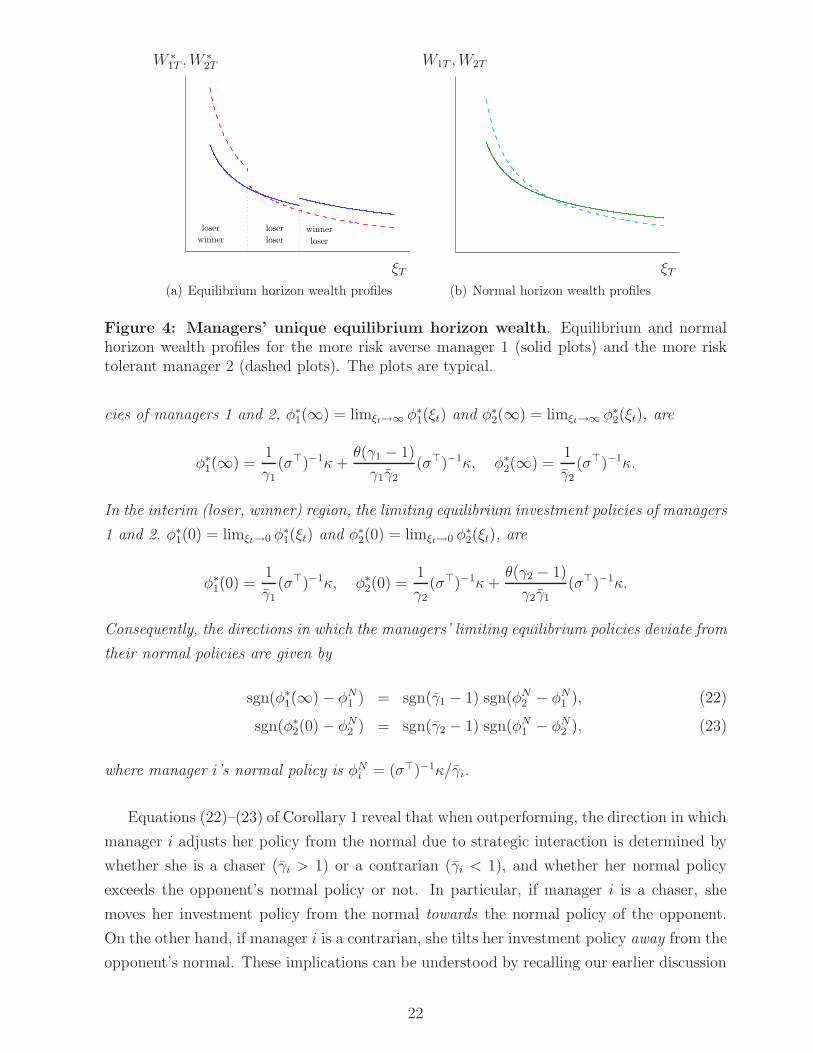
We first look at the managers’ equilibrium horizon wealth. Figure 4 plots the equilibrium

(latter part of Proposition 3), as well as the normal wealth profiles, as a function of the state

price density ξT . From Figure 4(a), in good states (low ξT ), the less risk averse manager 2

has a higher equilibrium wealth than manager 1, in line with the normal wealth profiles as

depicted in Figure 4(b). In these states, manager 1 is a loser and manager 2 is a winner,

getting the money flows. As we move into intermediate states (middle-ξT region), manager

2’s relative performance decreases, and after hitting her minimum outperformance margin η2,

jumps down as manager 2 optimally becomes a loser, no longer getting any flows. Finally, as

economic conditions deteriorate (high ξT ), manager 1’s relative performance increases, and

after reaching the maximum underperformance margin η1, it jumps upwards as manager 1

becomes a winner and receives money flows. From the viewpoint of potential fund investors,

Figure 4 illustrates the importance of accounting for the managers’ relative performance

concerns. The effect is most pronounced in good and bad states, where the presence of

strategic interactions strongly amplifies the difference between the returns on the managers’

portfolios.

Turning to the equilibrium investment policies, we first investigate the managers’ behavior

in the deep outperformance and underperformance regions at an interim point in time t < T .

Corollary 1 characterizes the managers’ limiting behavior in the interim bad (high ξt) and

good (low ξt) states, henceforth referred to as the interim (winner, loser) and (loser, winner)

regions, respectively.

Corollary 1. In the interim (winner, loser) region, the limiting equilibrium investment poli-

21

winner

loser

loser

loser

loser

winner

v

(a) Equilibrium horizon wealth profiles

W ∗1T , W ∗

2T

ξT

(b) Normal horizon wealth profiles

W1T , W2T

ξT

Figure 4: Managers’ unique equilibrium horizon wealth. Equilibrium and normalhorizon wealth profiles for the more risk averse manager 1 (solid plots) and the more risktolerant manager 2 (dashed plots). The plots are typical.

cies of managers 1 and 2, φ∗1(∞) = limξt→∞ φ∗

1(ξt) and φ∗2(∞) = limξt→∞ φ∗

2(ξt), are

φ∗1(∞) =

1

γ1(σ⊤)−1κ +

θ(γ1 − 1)

γ1γ2(σ⊤)−1κ, φ∗

2(∞) =1

γ2(σ⊤)−1κ.

In the interim (loser, winner) region, the limiting equilibrium investment policies of managers

1 and 2, φ∗1(0) = limξt→0 φ∗

1(ξt) and φ∗2(0) = limξt→0 φ∗

2(ξt), are

φ∗1(0) =

1

γ1(σ⊤)−1κ, φ∗

2(0) =1

γ2(σ⊤)−1κ +

θ(γ2 − 1)

γ2γ1(σ⊤)−1κ.

Consequently, the directions in which the managers’ limiting equilibrium policies deviate from

their normal policies are given by

sgn(φ∗1(∞) − φN

1 ) = sgn(γ1 − 1) sgn(φN2 − φN

1 ), (22)

sgn(φ∗2(0) − φN

2 ) = sgn(γ2 − 1) sgn(φN1 − φN

2 ), (23)

where manager i’s normal policy is φNi = (σ⊤)−1κ/γi.

Equations (22)–(23) of Corollary 1 reveal that when outperforming, the direction in which

manager i adjusts her policy from the normal due to strategic interaction is determined by

whether she is a chaser (γi > 1) or a contrarian (γi < 1), and whether her normal policy

exceeds the opponent’s normal policy or not. In particular, if manager i is a chaser, she

moves her investment policy from the normal towards the normal policy of the opponent.

On the other hand, if manager i is a contrarian, she tilts her investment policy away from the

opponent’s normal. These implications can be understood by recalling our earlier discussion

22

of the chasing and contrarian behavior in the presence of relative performance concerns.

For example, consider the case where manager 1 is a chaser (γ1 > 1) while manager 2 is

a contrarian (γ2 < 1). Here, the normal policy of the more risk averse manager 1 is less

risky than that of the more risk tolerant manager 2, φN1 < φN

2 . Being a chaser, manager 1

moves her policy towards the normal policy of manager 2, leading to a higher than normal

risk exposure, as predicted by (22). Manager 2 is a contrarian and so moves her policy away

from the normal policy of manager 1, leading to a higher than normal risk exposure, as

implied by (23).

To best highlight the managers’ overall asset allocation behavior, Figure 5 plots managers’

equilibrium investments (equation (21)) as a function of manager 1’s relative performance

at time t, R1t = W1t/W2t, with a relatively high R1t (> η) corresponding to the interim

(winner, loser) region and a relatively low R1t (< 1/η) to the interim (loser, winner) region.

For expositional clarity, we specialize the economy to feature two risky stocks, 1 and 2, and

without loss of generality let the stock return volatility matrix to be

σ =

(

σ1 0

ρσ2

√

1 − ρ2σ2

)

where ρ is the correlation between stock 1 and 2 returns. Here, the market prices of risk are

κ1 = (µ1 − r)/σ1 and κ2 = [(µ2 − r)/σ2 − ρ(µ1 − r)/σ1]/√

1 − ρ2. For the parameter values

in Figure 5, stock 1 is the more favorable of the two stocks in the sense that the Sharpe ratio

of the stock 1 ((µ1 − r)/σ1) is relatively high as compared to the Sharpe ratio of stock 2

((µ2 − r)/σ2). As a result, both managers tend to invest a larger share of wealth in stock 1

than in stock 2. Apart from this, the profiles of the equilibrium investments in stocks 1 and

2 are similar, as seen by comparing the left panels of Figure 5, (a) and (c), with the right

panels, (b) and (d). Hence, in our discussion we focus only on the equilibrium investments

in stock 1 (Figure 5(a), (c)).

Figure 5(a) corresponds to the case when both managers are chasers. In the interim

(winner, loser) region manager 1 chases manager 2, which from Corollary 1 implies that

manager 1 increases her risk exposure as compared to normal and moves her policy towards

manager 2’s normal policy. For manager 2, the relative performance concerns are weak in

the interim (winner, loser) region since the likelihood of attracting money flows at year-end

is low. As a result, the equilibrium policy of manager 2 is close to her normal policy. In the

interim (loser, winner) region, manager 2, a chaser, decreases her risk exposure relative to

normal as she tilts her investment policy towards manager 1’s normal policy. The equilibrium

policy of manager 1 is close to normal since the effect of relative performance concerns is

small. In Figure 5(c), manager 1 is a chaser but manager 2 is a contrarian. In the interim

(winner, loser) region, the outcome of the strategic interaction is as in Figure 5(a): manager

23

Managers 1 and 2 both chasers

Η1ΗR1 t

Φ21N

Φ11N

Φ11 t* ,Φ21 t

*

(a) More favorable stock 1

Η1ΗR1 t

Φ22N

Φ12 t* ,Φ22 t

*

Φ12N

(b) Less favorable stock 2

Manager 1 a chaser, manager 2 a contrarian

Η1ΗR1 t

Φ21N

Φ11N

Φ11 t* ,Φ21 t

*

(c) More favorable stock 1

Η1ΗR1 t

Φ22N

Φ12N

Φ12 t* ,Φ22 t

*

(d) Less favorable stock 2

Figure 5: The managers’ unique equilibrium investment policies. The time-t in-vestment policies of the more risk averse manager 1 (solid lines) and the more risk tolerantmanager 2 (dashed lines) in stock 1 and stock 2. In each panel, the lower dotted line is thenormal policy of manager 1 φN

1 = (σ⊤)−1κ/γ1, the upper dotted line is the normal policy ofmanager 2 φN

2 = (σ⊤)−1κ/γ2. Stock 1 is more favorable than stock 2 as it has a relativelyhigher Sharpe ratio. In panels (a) and (b), the two managers are chasers, and the param-eter values are: r = 0.05, µ1 = 0.1, µ2 = 0.12, σ1 = 0.15, σ2 = 0.3, ρ = 0.3, γ1 = 4, γ2 =2, α = 1.5, η = 1.2, t = 0.8, T = 1, and hence θ = 0.6, γ1 = 8.5, γ2 = 3.5. In panels (c) and(d), manager 1 is a chaser and manager 2 is a contrarian, and the parameter values are:γ1 = 2, γ2 = 0.5, α = 0.3, η = 1.35, t = 0.95, and hence θ = 0.23, γ1 = 2.3, γ2 = 0.35, and theremaining parameters are as in panels (a) and (b).

1 increases her risk exposure while manager 2 chooses a policy close to her normal. In the

interim (loser, winner) region, Corollary 1 implies that manager 2, a contrarian, increases

her risk exposure relative to the normal as she moves her policy away from the manager 1’s

normal policy. For manager 1, the effect of relative considerations is weak and so she chooses

a policy close to the normal.

In the interim (loser, loser) region, the economic mechanism underlying the chasing and

contrarian behavior is dominated by the gambling incentives as each manager is in the convex

24

region of her (conditional) objective function. Hence, the behavior of managers in this region

is similar in Figures 5(a) and (c). Each manager gambles in order to avoid a situation where

her relative performance is close to the threshold level, which is achieved by following a

policy that is sufficiently different from that of the opponent. As a result, the managers

always gamble in the opposite directions from each other in each individual stock. The more

risk averse manager 1 optimally decreases her stock holding when gambling while the more

risk tolerant manager 2 gambles by increasing hers, as seen in Figures 5(a) and (c).15

5.2. Effects of Stock Correlation on Unique Equilibrium

Figure 6 illustrates the impact of the correlation between the two stocks, ρ, on the man-

agers’ equilibrium investment policies. Several noteworthy features arise. First, changing

the correlation can affect the equilibrium policies in a non-monotonic way, as in Figures

6(a)-(c), as well as monotonically, as in Figure 6(d). Second, Figures 6(a) and (b) reveal

that the equilibrium investment profiles may cross for different values of correlation. Third,

as correlation increases the direction of humps in the interim (loser, loser) region can invert,

as depicted in Figures 6(b) and (d).

Above rich patterns arise due to the interaction of a diversification effect, the extent of

benefits to diversification, and a substitution effect, the extent of the two stocks acting as

a substitute to each other. The diversification effect dominates for low correlation values,

while the substitution effect dominates for high values of correlation. When the correlation

is low, both sources of stock return uncertainty matter considerably and so the two stocks

compliment each other by providing a hedge against a specific source of risk. Increasing the

correlation reduces the diversification benefits from holding a portfolio of the two stocks,

leading the managers to reduce their investments in both stocks. When the correlation is

high, the two stocks become close substitutes, in which case the more favorable stock 1 (with

a relatively high Sharpe ratio) becomes the primary security through which the managers

achieve their desired risk exposures. As the correlation increases further, the managers

substitute away from the less favorable stock 2 (with a relatively low Sharpe ratio) into the

more favorable stock 1.

Going back to Figure 6, when the correlation increases from −0.25 to 0.3 (moving from

the dotted to dashed lines in all panels of Figure 6), the diversification effect dominates

and both managers reduce their investments in each stock across all three regions of interim

15We note that mutual fund managers are often not allowed to go short, while according to Figure 5 itmay be optimal for a manager to short risky assets in a certain range of interim relative performance. Fortractability, we do not explicitly introduce a no-short-sale constraint. We believe that incorporating such aconstraint is not going to significantly change our main insights, because if the constraint were present, itwould likely lead to less pronounced gambling by the more risk averse manager in the relevant range of theinterim relative performance.

25

More risk averse manager 1

ΗΗR1 t

Φ11 t*

(a) More favorable stock 1

ΗΗR1 t

Φ12 t*

(b) Less favorable stock 2

Less risk averse manager 2

1Η1ΗR1 t

Φ21 t*

(c) More favorable stock 1

1Η1ΗR1 t

Φ22 t*

(d) Less favorable stock 2

Correlation

ρ=0.85

ρ=0.3

ρ=−0.25

Figure 6: Effect of stock correlation on the managers’ unique equilibrium in-vestment policies. The managers’ time-t equilibrium policies for varying levels of thecorrelation, ρ, between stock 1 and 2 returns. In all panels, dotted line corresponds toρ = −0.25, dashed line to ρ = 0.3, solid line to ρ = 0.85. The other parameter values are asin Figure 5(a) and (b).

relative performance.16 As the correlation rises further from ρ = 0.3 to ρ = 0.85 (moving

from dashed to solid lines in Figure 6), in the interim (winner, loser) and (loser, winner)

regions the substitution effect induces the managers to increase their investments in the more

favorable stock 1 and to finance this by decreasing their holdings in the less favorable stock

2. Hence, the substitution effect works in the opposite direction from the diversification

effect for stock 1, leading the equilibrium policies to being non-monotonic in the correlation

(Figures 6(a) and (c)). In the interim (loser, loser) region, the more risk averse manager 1

gambles by decreasing her risk exposure. Since the more favorable stock 1 is the primary

16While not explicitly highlighted in Figure 6, we note that the intensity of the chasing behavior, asmeasured by the magnitude of the deviation of the equilibrium policy from normal, is also reduced with theincrease in correlation. The reason is that the managers’ normal policies are scaled down proportionally asthe correlation increases due to the diversification effect, and so the absolute difference between them, whichaffects the intensity of chasing, decreases.

26

means to changing her risk exposure, the downward hump becomes more pronounced, as

seen in Figure 6(a). The substitution effect implies that this decrease in stock 1 holdings

is mirrored by an increase in the less favorable stock 2 holdings. This leads to the inverted

shape of the equilibrium policy for stock 2, as depicted in Figure 6(b). The more risk tolerant

manager 2 follows the opposite strategy to that of manager 1 and gambles by increasing her

risk exposure. Consequently, the size of the upward hump in the primary stock 1 holdings

increases (Figure 6(c)). This larger position in stock 1 is financed by a decrease in the less

favorable stock 2 holdings, leading to the inverted hump in Figure 6(d).17

Having fully described the unique equilibrium investment policies of the managers in a

strategic setting, we may now compare our results to those obtained in frameworks where a

manager competes against an exogenous benchmark (Basak, Pavlova, and Shapiro (2007),

Carpenter (2000)). The main similarity between our work and non-strategic studies is the

presence of the gambling behavior in one of the three interim regions of our unique equilib-

rium and their optimal investment policies. On the other hand, there are several important

differences. First, strategic interactions can lead to non-existence or multiplicity of equilib-

rium, as we have elaborated on in Section 4. Second, the economic mechanism behind the

chasing and contrarian behavior, which drives the equilibrium policies in the interim (win-

ner, loser) and (loser, winner) regions, is not present in Basak et al. or Carpenter. Third,

in the interim (loser, loser) region, where the gambling behavior prevails, the two managers

always gamble in the opposite direction from each other in each individual stock, and it is

the manager’s risk aversion relative to that of the opponent that determines the direction

of gambling. This is notably different from Basak et al., where for given market parameter

values the direction of gambling is determined by the absolute value of the manager’s risk

aversion. In Carpenter, the direction of gambling is always the same. Fourth, by considering

a setting with multiple correlated risky stocks we uncover novel patterns of the managers’

behavior for varying levels of correlation.

5.3. Characterization of Multiple Equilibria

We now turn to the case of multiple equilibria, which obtains under the multiplicity condition

(18). Proposition 4 provides the full characterization of all horizon wealth profiles that can

occur in equilibrium.18

17Given that the managers care about the overall risk of their portfolios and that they are heterogeneous intheir risk preferences, one could have expected that the mechanism that leads to the shape inversion does notnecessarily kick in simultaneously for the two managers. However as discussed earlier, the managers alwaysgamble strategically against each other in the opposite direction in each individual stock. So, manager 1optimally inverts her equilibrium policy in the less favorable stock 2 if and only if manager 2 inverts hers,reflecting the strategic nature of the managers’ interaction.

18Due to the nature of multiplicity, describing the corresponding investment policies is not straightfor-ward. Loosely, the number of terms in the expressions for equilibrium policies depend on the number of

27

Proposition 4. Assume the condition for the multiplicity of Nash equilibrium (18) is sat-

isfied. The equilibrium outcomes and horizon wealth profiles (W ∗1T , W ∗

1T ) are as follows.

When ξγ1−γ2

T > y min[

Bη−γ1γ2 , Dηγ1(γ2+θ(γ2−1)]

, the managers are in (winner, loser) and

W ∗1T = y1ξ

−(γ2+θ(γ1−1))/(γ1 γ2)T , W ∗

2T = (y2ξT )−1/γ2 .

When ξγ1−γ2

T < y max[

Aηγ1γ2 , Cη−γ2(γ1+θ(γ1−1)]

, the managers are in (loser, winner) and

W ∗1T = (y1ξT )−1/γ1 , W ∗

2T = y2ξ−(γ1+θ(γ2−1))/(γ2 γ1)T .

When y max[

Aηγ1γ2 , Cη−γ2(γ1+θ(γ1−1))]

< ξγ1−γ2

T < y min[

Bη−γ1γ2 , Dηγ1(γ2+θ(γ2−1))]

, both

outcomes, (winner, loser) and (loser, winner), can occur in equilibrium. Here, the constants

A, B, C, D are as in Proposition 2, and y, y1, y2 as in Proposition 3.

winner

loser

multiplicity

region

loser

winner

I

II

II

AAAAAAAAAAAAAAAAAAAAAAAAAAAAI

W ∗1T , W ∗

2T

ξT

Figure 7: Managers’ multiple equilibrium horizon wealth. Multiple equilibriumhorizon wealth profiles of the more risk averse manager 1 (solid plot) and the more risktolerant manager 2 (dashed plot). The plots are typical.

Figure 7 plots the multiple equilibrium wealth profiles. Looking at Figures 4 and 7, we

observe that the multiple equilibrium wealth profiles and the unique ones differ only in the

middle-ξT region. When the equilibrium is unique, both managers are losers in the middle

region, choosing similar horizon wealth profiles (Figure 4). Now, since the performance

threshold is relatively low, such wealth profiles are no longer optimal as both managers have

incentives to gamble. So, one of the managers must be a winner, implying that her wealth will

be considerably higher than the other manager’s wealth, preventing the latter from gambling.

As discussed in Section 4, in some states the managers are indifferent to switching their

rankings. Since now the rankings are different in all states, with neither (winner, winner)

discontinuities in the horizon wealth profiles, which can be infinite.

28

nor (loser, loser) outcomes being possible, switching rankings leads to multiple equilibria.

Unlike the middle region, when ξT is either relatively low or high, the difference between

the managers’ wealth levels is substantial in the unique equilibrium (Figure 4). So, even

with a low performance threshold η neither of the two managers has incentives to gamble

in these regions, leading to the multiple equilibria wealth profiles being the same as the

unique-equilibrium ones, as seen by comparing Figures 4 and 7.

A natural question is whether we can narrow down the set of multiple equilibria and rule

out some that are not likely to occur in the real world. While an in-depth investigation of this

issue is beyond the scope of this paper, we may put forward the following simple selection

criterion. Since real-life money managers incur trading costs, which we have abstracted away

from for tractability, the managers would favor the equilibrium with the minimal swings in

investments so as to minimize the transaction costs. Since the most pronounced swings are

associated with discontinuities in horizon wealth profiles, a natural selection criterion is to

pick an equilibrium with the minimum number of the discontinuities, which in our setting

amounts to the equilibrium with just one discontinuity. Indeed, inspecting Figure 7 we

observe that such an equilibrium is obtained by dividing the middle-ξT multiplicity region

into two parts, with (loser, winner) outcome occurring in the left part and (winner, loser)

outcome occurring in the right part. One can easily see that the structure of the resulting

equilibrium wealth profiles is similar to that obtained in the unique equilibrium (Proposition

3), and so the investment policies underlying this selected equilibrium have the same profile

as the unique equilibrium investment policies depicted in Figure 4.

Remark 2. Interim Performance. Starting from the study by Brown, Harlow, and Starks

(1996), it has become common in both theoretical and empirical works to consider the

interim performance as a pertinent factor that affects risk taking incentives in tournament

settings. In our analysis, we can easily accommodate this factor in by introducing an interim

performance parameter, R10 > 1, which gives manager 1 an initial advantage. The time-

t performance of manager 1 is now given by R10W1t/W10. As a result, manager 1 and

2’s relative performances become R10R1t and R2t/R10, respectively, where as before R1t =

W1t/W2t and R2t = W2t/W1t. In Figures 5–6, we simply need to put manager 1’s new

relative performance in place of R1t. Alternatively, if one wants to keep the old ones, the

graphs should be appropriately scaled along the x-axis by a factor of R10. All our results

pertaining to equilibrium existence and multiplicity remain unchanged, and so Figures 2–3

are not affected. This is in contrast to a static risk-neutral setting where the difference in

the managers’ interim performance is found to be critical for the existence of a pure-strategy

Nash equilibrium (Taylor (2003)). The only additional implication of the introduction of

interim performance is the possibility of a new equilibrium, in which manager 1 is a winner

at the horizon T with certainty, across all states. We do not present this analysis since such

an equilibrium can only occur in a knife-edge case when both managers have identical risk

29

aversions.

Remark 3. Managers with different initial wealth. If the managers’ initial wealth are dif-

ferent, the expressions for best responses in Proposition 1 are augmented by the ratio of the

initial wealths. However, all the subsequent results pertaining to equilibrium are virtually

unchanged. In particular, the conditions for existence and uniqueness of equilibrium are

unaffected (Proposition 2), and the structures of the unique and multiple equilibria and the

shapes of the unique equilibrium investment policies are preserved (Propositions 3–4). The

reason is that the fund flows are driven by relative returns, and changing initial wealth does

not give a manager any kind of advantage or disadvantage in the competition for fund flows.

6. Conclusion

In this paper, we analyze the equilibrium portfolios of money managers in presence of strate-

gic interactions driven by relative performance concerns with local convexities. We discover

the possibility of three distinct results: multiple equilibria, unique equilibrium, or no equi-

librium at all. When the equilibrium is unique, we analyze the properties of the equilibrium

investment policies. In the other two cases, we elaborate on the underlying economic mecha-

nisms that lead to non-existence or multiplicity, most of which are driven by the risk shifting

incentives combined with the strategic interaction of the managers.

Given the novelty of our analysis, we believe there are various promising directions for

future research. While we assume that money managers have a perfect knowledge of each

other’s attitude towards risk, it would be valuable to investigate a perfect Bayesian equi-

librium in a more realistic framework where the managers do not have such knowledge but

can learn about each other’s traits by observing the investment policies. It would also be

of interest to extend our framework to investigate the possible strategic interactions among

CEOs, whose contracts often include a bonus part for high relative performance (Murphy

(1999)). Considering a setting where managers compete against each other and at the same

time against an exogenous peer-group benchmark could be an interesting generalization. An-

other natural extension of our framework would be to incorporate flow-performance relations

where money flows depend on discrete rankings, leading to discontinuities of the managers’

objective functions. Finally, analyzing the case when the investment opportunities of the

managers are not perfectly correlated would be worthwhile.

30

Appendix: Proofs

Proof of Lemma 1. Employing martingale methods, given the CRRA preferences (5),

manager i’s optimal time-T ′ wealth profile WiT ′ is given by the first order condition

WiT ′ = (yiT ξT ′)−1/γi , (A1)

where yiT > 0 is the Lagrange multiplier attached to her time-T static budget constraint

ET [ξT ′WiT ′ ] = ξT WiT fT . The Lagrange multiplier is found by substituting (A1) into the

budget constraint, which yields

y−1/γi

iT =ξTWiT fT

ET [ξ1−1/γi

T ′ ]. (A2)

Plugging (A2) into (A1), we find manager i’s optimal time-T ′ wealth profile:

WiT ′ =ξTWiT fT

ET [ξ1−1/γi

T ′ ]ξ−1/γi

T ′ (A3)

Combining (6) and (A3) yields the time-T indirect utility function

viT ≡ ET [ui(WiT ′)] =1

1 − γi(ξT WiT fT )1−γi(ET [ξ

1−1/γi

T ′ ])γi. (A4)

Since ξt follows a geometric Brownian motion with constant drift and volatility, we have that

ET [ξ1−1/γi

T ′ ] = aξ1−1/γi

T where a is some constant depending on r, κ, and T ′−T , and we drop it

without loss of generality since it does not affect the optimal behavior. Finally, substituting

the expectation into (A4), we get

viT =1

1 − γi(WiT fT )1−γi . (A5)

The indirect utility function (6) follows by plugging the flow-performance function into (A5)

after some manipulation. The stated properties of θ and γi are immediate.

Q.E.D.

Proof of Proposition 1. We consider only manager 1; for manager 2 the analysis is

analogous. Fixing the horizon wealth profile of manager 2, W2T (ξT ), we look for the manager

1’s optimal horizon wealth profile W1T . Although manager 1’s objective function has a region

of local convexity, we can still use standard optimization techniques once we concavify the

objective function (see Basak, Pavlova, and Shapiro (2007) for a more formal proof in a

similar setting). Concavification involves finding the range [W, W ] and the coefficients a

and b1 such that replacing v1(·) within the range [W, W ] with a chord a + b1W1T will result

31

in a globally concave objective function. Noting that the chord must be tangent to v1(·) at

W and W , we have the following system of equations to solve for:

a + b1W =W1−γ1

1 − γ1

(A6)

a + b1W =1

1 − γ1

(

W1−θ(

WηW2

)θ)1−γ1

(A7)

b1 = W−γ1 = (1 + α)W−γ1

Wθ(γ1−1)2 , (A8)

where we have dropped k1−γ1 from the objective function since it does not affect the opti-

mization problem. Subtracting (A6) from (A7) yields

b1(W − W) =1

1 − γ1

(

W1−γ1

(ηW2)θ(γ1−1) − W1−γ1

)

. (A9)

Expressing W and W in terms of b1 and W2 (from (A8)) and plugging into (A9) gives

b1(b−1/γ1

1 (1 + α)1/γ1Wθ(γ1−1)/γ1

2 − b−1/γ1

1 )

=1

1 − γ1

(

b(γ1−1)/γ1

1 (1 + α)(γ1−1)/γ1W−θ(γ1−1)2/γ1

2 (ηW2)θ(γ1−1) − b

(γ1−1)/γ1

1

)

,

which after some algebra yields the boundary function (16). If y1ξT is higher that the slope

of the concavification line b1, the optimal wealth is to the left from W, i.e., manager 1 chooses

to be a loser and her normal-type policy (12) obtains. Otherwise, she becomes a winner and

(13) obtains, accounting for relative concerns.

Manager 1’s relative performance is closest to the threshold ηW2T when she is indifferent

between being a winner and a loser, i.e., when

y1ξT = b1(ηW2T ) = (1 + α)γ1/θ (γ1/γ1)γ1γ1/(γ1−γ1) (ηW2T )−γ1 . (A10)

If manager 1 chooses to be a winner, her “minimum outperformance margin” η1 is obtained

by plugging (A10) into (13) and dividing the resulting wealth by W2T . This yields

η1 = (1 + α)1/γ1

(

(1 + α)γ1/θ (γ1/γ1)γ1γ1/(γ1−γ1) (ηW2T )−γ1

)−1/γ1

(ηW2T )θ(γ1−1)/γ1/W2T

= (1 + α)(1−γ1/θ)/γ1 (γ1/γ1)−γ1/(γ1−γ1) (ηW2T )(γ1+θ(γ1−1))/γ1/W2T

= (1 + α)−1/α (γ1/γ1)−γ1/(γ1−γ1) η,

where in the last equality we use (7)–(8) to simplify the expressions. If manager 1 chooses to

be a loser, her “maximum underperformance margin” η1

is obtained by substituting (A10)

32

into (12) and dividing the result by W2T , which yields

η1

=(

(1 + α)γ1/θ (γ1/γ1)γ1γ1/(γ1−γ1) (ηW2T )−γ1

)−1/γ1

/W2T = (1 + α)−1/θ (γ1/γ1)−γ1/(γ1−γ1) η.

Q.E.D.

Proof of Proposition 2. For a given realization of ξT , we can have one of the three

outcomes: (winner, loser), (loser, winner), or (loser, loser). From the best responses (12)–

(15), we can determine the regions of ξT for which these outcomes can occur.

(winner, loser). From (13), manager 1 chooses to be a winner if y1ξT ≤ b1(ηW2T ). Plugging

manager 2’s wealth, given by (14) as she is a loser, and using the definition of b1(·) (16),

yields

y1ξT ≤ (1 + α)γ1/θ (γ1/γ1)γ1γ1/(γ1−γ1) (ξT y2)

γ1/γ2η−γ1 .

Rearranging, we get

ξγ1−γ2

T ≥ yγ21 y−γ1

2

(

(1 + α)γ1/θ (γ1/γ1)γ1γ1/(γ1−γ1)

)−γ2

ηγ1γ2 ≡ yAηγ1γ2 , (A11)

where y ≡ yγ21 y−γ1

2 and A is as given in (19).

From (13), manager 2 chooses to be a loser if y2ξT > b2(ηW1T ). Plugging manager 1’s

wealth W1T , given in (13), and expanding b2 yields

y2ξT > (1 + α)γ2/θ (γ2/γ2)γ2γ2/(γ2−γ2) (η(1 + α)1/γ1(y1ξT )−1/γ1(ηW2T )θ(γ1−1)/γ1)−γ2 .

After some algebra, we get

ξγ1−γ2

T > yγ2

1 y−γ1

2 (1 + α)γ1γ2/θ−γ2 (γ2/γ2)γ1γ2γ2/(γ2−γ2) η−γ2(γ1+θ(γ1−1)) ≡ yCη−γ2(γ1+θ(γ1−1)),

(A12)

where C is as given in (20). The outcome (winner, loser) can occur provided that both (A11)

and (A12) are satisfied, which means ξT satisfies:

ξγ1−γ2

T > y max[

Aηγ1γ2 , Cη−γ2(γ1+θ(γ1−1))]

. (A13)

(loser, winner). The expressions are obtained from (A11) and (A12) by switching sub-

scripts 1 and 2, leading to the conditions on ξγ2−γ1

T . For ease of comparison with (winner,

loser) case, we then invert the obtained inequalities to get the conditions on ξγ1−γ2

T :

ξγ1−γ2

T ≤ yγ21 y−γ1

2

(

(1 + α)γ2/θ (γ2/γ2)γ2γ2/(γ2−γ2)

)γ1

η−γ1γ2 ≡ yBη−γ1γ2 , (A14)

ξγ1−γ2

T < yγ21 y−γ1

2 (1 + α)γ1−γ2γ1/θ (γ1/γ1)−γ2γ1γ1/(γ1−γ1) ηγ1(γ2+θ(γ2−1)) ≡ yDηγ1(γ2+θ(γ2−1)),

where B and D are given by (19) and (20), respectively. Combining the two conditions,

33

(loser, winner) can occur for ξT satisfying

ξγ1−γ2

T < y min[

Bη−γ1γ2 , Dηγ2(γ2+θ(γ2−1))]

. (A15)

(loser, loser). The conditions for this outcome follow from the observation that manager

i wants to be a loser in those states in which she does not want to be a winner. Hence,

manager 1 wants to be a loser for ξT such that (A11) is not satisfied. Similarly, manager 2

chooses to be a loser when (A14) does not hold. So, (loser, loser) can occur for ξT given by

yBη−γ1γ2 < ξγ1−γ2

T < yAηγ1γ2 . (A16)

Inspection of (A13), (A15), and (A16) reveals that if (loser, loser) region is not empty,

i.e., if

Bη−γ1γ2 < Aηγ1γ2 , (A17)

the three regions can never overlap, meaning that multiple equilibria are not possible. For

the unique equilibrium to exist, i.e., for the three regions to fully cover the interval (0, +∞),

it must be the case that

Aηγ1γ2 ≥ Cη−γ2(γ1+θ(γ1−1)), Bη−γ1γ2 ≤ Dηγ2(γ2+θ(γ2−1)), (A18)

in which case the unique equilibrium has the following structure. (winner, loser) occurs for

ξγ1−γ2

T > yAηγ1γ2 , (loser, loser) for yBη−γ1γ2 ≤ ξγ1−γ2

T ≤ yAηγ1γ2 , and (loser, winner) for

ξγ1−γ2

T < yBη−γ1γ2 . Combining (A17) and (A18) yields the condition for the existence and

uniqueness of equilibrium (17).

If (loser, loser) region is empty, i.e., if (A17) is not satisfied, then for an equilibrium to

exist it must be the case that the remaining two outcomes fully cover (0, +∞). Hence, from

(A13) and (A15), we get the multiple equilibria condition (18). In a knife-edge case when

(18) holds as an equality, the equilibrium is unique. In this case, (winner, loser) occurs for

ξT satisfying (A13), (loser, winner) occurs for the other ξT . In all other cases, when (18)

holds as a strict inequality, multiple equilibria obtains. The structure of the equilibria is as

follows. (winner, loser) occurs for ξγ1−γ2

T > y min[

Bη−γ1γ2 , Dηγ1(γ2+θ(γ2−1)]

, (loser, winner)

occurs for ξγ1−γ2

T < y max[

Aηγ1γ2 , Cη−γ2(γ1+θ(γ1−1)]

. The region

y max[

Aηγ1γ2 , Cη−γ2(γ1+θ(γ1−1))]

< ξγ1−γ2

T < y min[

Bη−γ1γ2 , Dηγ1(γ2+θ(γ2−1))]

is consistent with both (winner, loser) and (loser, winner) outcomes, hence for such ξT we

get the multiplicity of equilibria with these two outcomes. Other structures of equilibrium

are not possible, hence there is no pure-strategy Nash equilibrium if neither (17) nor (18) is

34

satisfied.

Q.E.D.

Proof of Proposition 3. From Proposition 2, an equilibrium exists and is unique if the

uniqueness condition (17) is satisfied. In the proof of Proposition 2, we have established

the structure of the managers’ equilibrium wealth profiles – for each realization of ξT we

identified whether manager i, i = 1, 2, is a winner or a loser. We now determine the

associated equilibrium horizon wealth profiles corresponding to these two outcomes. Focusing

on manager 1, from (12) her optimal wealth is (y1ξT )−1/γ1 when she is a loser, i.e., when

ξγ1−γ2

T ≤ yAηγ1γ2 . Otherwise, when ξγ1−γ2

T > yAηγ1γ2 , manager 1 is a winner, and her best

response wealth is given in (13). As the performance threshold η is greater than one, manager

2 is a loser whenever manager 1 is a winner, and so in equilibrium chooses W ∗2T = (y2ξT )−1/γ2 .

Plugging this into (13) yields the equilibrium manager 1’s wealth when she is a winner:

W ∗1T = y

−1/γ1

1 y−θ(γ1−1)/(γ1 γ2)2 (1 + α)1/γ1ηθ(γ1−1)/γ1ξ

−(γ2+θ(γ1−1))/(γ1 γ2)T .

To derive the associated equilibrium investment policy of manager 1, φ∗1t, we first de-

termine the time-t value of the equilibrium wealth W ∗1t. Since ξtW

∗1t is a martingale, we

have

ξtW∗1t = Et[ξTW ∗

1T ] = y−1/γ1

1 Et[ξ(γ1−1)/γ1

T 1ξT <β] + y1Et[ξ(γ−1)/γT 1ξT ≥β], (A19)

where β and y1 are as defined in Proposition 3. To evaluate the two conditional expectations,

we use the following property of the truncated log-normal distribution. If x is a log-normally

distributed random variable such that ln x is normal with mean m and variance v2, then

E[xn1x<a] = enm+n2v2/2 N(

(ln a − m − nv2)/v)

. (A20)

Given that as of time t ln ξT has mean ln ξt − (r + ‖κ‖2/2)(T − t) and variance ‖κ‖2(T − t),

applying (A20) to (A19) yields

W ∗1t = N(d(γ1, β))y

−1/γ1

1 Z(γ1, t)ξ−1/γ1

t + (1 − N(d(γ, β)))y1Z(γ, t)ξ−1/γt , (A21)

where N, d, Z, γ, y1 are as defined in Proposition 3. From Ito’s Lemma, the coefficient of the

Brownian motion ω in the dynamic process for W ∗1t is equal to

−κjξt∂W ∗

1t

∂ξt,

where κj is the j-th component of the market price of risk vector κ. Equating each of these

coefficients to the corresponding diffusion term in (1), we obtain the following system of

35

linear equations:

ξt∂W ∗

1t

∂ξtκ = W ∗

1tσ⊤φ∗

1t.

Solving the system and substituting the derivative of (A21) with respect to ξt into the

solution yields manager 1’s equilibrium investment policy. For manager 2, the analysis is

analogous.Q.E.D.

Proof of Corollary 1. The limiting equilibrium policies of manager 1 is straightforwardly

obtained by letting ξt tend to 0 or ∞ in (21), and similarly for manager 2.

Substituting the equilibrium limiting policies into (22) and multiplying both parts by the

inverse of (σ⊤)−1κ, we obtain that (22) is equivalent to

sgn

(

1

γ1+

θ(γ1 − 1)

γ1γ2− 1

γ1

)

= sgn(γ1 − 1) sgn

(

1

γ2− 1

γ1

)

. (A22)

Rearranging the argument of sgn(·) on the left-hand side of (A22) yields

γ1γ2 + γ1α(γ1 − 1) − γ2(γ1 + α(γ1 − 1))

γ1γ1γ2=

γ1α(γ1 − 1) − γ2α(γ1 − 1)

γ1γ1γ2

=α

γ1

(γ1 − 1)

(

1

γ2

− 1

γ1

)

.

Since α and γ1 are positive, (A22) obtains. Switching subscripts 1 and 2 in (22) gives (23).

Q.E.D.

Proof of Proposition 4. In Proposition 2 we show that multiple equilibria occur if the

multiplicity condition (18) is satisfied. In the proof of Proposition 2, we describe the structure

of the multiple equilibria, i.e., the states in which outcome (winner, loser) or outcome (loser,

winner) occurs in equilibrium, and the states in which either of the two outcomes is possible.

In Proposition 3, we describe what horizon wealth manager i, i = 1, 2, chooses in equilibrium

when she is a winner and when she is a loser. Combining the results of these two Propositions,

we obtain the horizon wealth profiles that can occur in the case of multiple equilibria.

Q.E.D.

36

References

Abel, A., 1990, “Asset Prices under Habit Formation and Catching Up with the Joneses,”

American Economic Review, 80, 38–42.

Agarwal, V., N. Daniel, and N. Naik, 2004, “Flows, Performance, and Managerial Incentives

in Hedge Funds,” working paper, LBS.

Baye, M., G. Tian, and J. Zhou, 1993, “Characterizations of the Existence of Equilibria

in Games with Discontinuous and Non- Quasiconcave Payoffs,” Review of Economic

Studies, 60, 935–948.

Basak, S., A. Pavlova, and A. Shapiro, 2007, “Optimal Asset Allocation and Risk Shifting

in Money Management,” Review of Financial Studies, 20, 1583–1621.

Basak, S., A. Shapiro, and L. Tepla, 2006, “Risk Management with Benchmarking, ” Man-

agement Science, 52, 542–557.

van Binsbergen, J., M. Brandt, and R. Koijen, 2008, “Optimal Decentralized Investment

Management,” Journal of Finance, 63, 1849–1895.

Brown, K., W. Harlow, and L. Starks, 1996, “On Tournaments and Temptations: An

Analysis of Managerial Incentives in the Mutual Fund Industry,” Journal of Finance,

51, 85–110.

Browne, S., 2000, “Stochastic Differential Portfolio Games,” Journal of Applied Probability,

37, 126–147.

Busse, J., 2001, “Another Look at Mutual Fund Tournament,” Journal of Financial and

Quantative Analysis, 36, 53–73.

Carpenter, J., 2000, “Does Option Compensation Increase Managerial Risk Appetite?,”

Journal of Finance, 55, 2311–2331.

Chetty, R., 2006, “A New Method of Estimating Risk Aversion,” American Economic

Review, 96, 1821–1834.

Chevalier, J., and G. Ellison, 1997, “Risk Taking by Mutual Funds as a Response to Incen-

tives,” Journal of Political Economy, 105, 1167–1200.

Chiang, K., 1999, “Survival, Tournament, and Asset Allocation Strategy in the Mutual

Fund Industry,” working paper, Louisiana State University.

Cooper, R., and A. John, 1988, “Coordinating Coordination Failures in Keynesian Models,”

Quarterly Journal of Economics, 103, 441–463.

Cox, J., and C. Huang, 1989, “Optimal Consumption and Portfolio Policies when Asset

Prices Follow a Diffusion Process,” Journal of Economic Theory, 49, 33–83.

Cuoco, D., and R. Kaniel, 2007, “Equilibrium Prices in the presence of Delegated Portfolio

Management,” working paper, University of Pennsylvania.

37

Cvitanic, J., L. Goukasian, and F. Zapatero, 2003, “Monte-Carlo Computation of Optimal

Portfolios in Complete Markets,” Journal of Economic Dynamics and Control, 27,

971–986.

Dass, N., M. Massa, and R. Patgiri, 2008, “Mutual Funds and Bubbles: The surprising role

of contractual incentives,” Review of Financial Studies, 21, 51–99.

DeMarzo, P., R. Kaniel, and I. Kremer, 2007, “Technological Innovation and Real Invest-

ment Booms and Busts,” Journal of Financial Economics, 85, 735–754.

DeMarzo, P., R. Kaniel, and I. Kremer, 2008, “Relative Wealth Concerns and Financial

Bubbles,” Review of Financial Studies, 21, 19–50.

Detemple, J., R. Garcia, and M. Rindisbacher, 2003, “A Monte-Carlo Method for Optimal

Portfolios,” Journal of Finance, 58, 401–446.

Ding, B., M. Getmansky, B. Liang, and R. Wermers, 2007, “Investor Flows and Share

Restrictions in the Hedge Fund Industry,” working paper, University of Massachusetts.

Gallaher, S., R. Kaniel, and L. Starks, 2006, “Madison avenue meets wall street: Mutual

fund families, competition, and advertising,” working paper, University of Texas.

Gaspar, J.-M., M. Massa, and P. Matos, 2006, “Favoritism in Mutual-Fund Families? Evi-

dence on Strategic Cross-Fund Subsidization,” Journal of Finance, 61, 33-71.

Goel, A., and A. Thakor, 2005, “Green with Envy: Implications for Corporate Investment

Distortions,” Journal of Business, 78, 2255–2287.

Gomez, J.P., R. Priestley, and F. Zapatero, 2008, “Implications of Keeping Up with the

Joneses Behavior for the Equilibrium Cross-Section of Stock Returns: International

Evidence,” Journal of Finance, forthcoming.

Goriaev, A., T. Nijman, and B. Werker, “Yet Another Look at Mutual Fund Tournaments,”

Journal of Empirical Finance, 12, 127–137.

Goriaev, A., F. Palomino, and A. Prat, 2003, “Mutual fund tournament: Risk taking

incentives induced by ranking objectives,” working paper, NES, HEC, and LSE.

Grinblatt, M., S. Titman, and R. Wermers, 1995, “Momentum Investment Strategies, Port-

folio Performance, and Herding: A Study of Mutual Fund Behavior,” American Eco-

nomic Review, 85, 1088–1105.

Huang, J., K. Wei, and H.Yan, 2007, “Participation Costs and the Sensitivity of Fund Flows

to Past Performance,” Journal of Finance, 62, 1273–1311.

Jain, P., and J. Wu, 2000, “Truth in Mutual-Fund Advertising: Evidence on Future Per-

formance and Fund Flows,” Journal of Finance, 55, 937-958.

Karatzas, I., J. Lehoczky, and S. Shreve, 1987, “Optimal Portfolio and Consumption De-

cisions for a ‘Small Investor’ on a Finite Horizon,” SIAM Journal of Control and

Optimization, 25, 1157–1186.

38

Karatzas, I., and S. Shreve, 1998, Methods of Mathematical Finance, Springer-Verlag, New

York.

Kempf, A., and S. Ruenzi, 2008, “Tournaments in Mutual-Fund Families,” Review of Fi-

nancial Studies, 21, 1013–1036.

Koijen, R., 2008, “The Cross-Section of Managerial Ability and Risk Preferences,” working

paper, University of Chicago.

Li, W., and A. Tiwari, 2005, “On the Consequences of Mutual Fund Tournaments,” working

paper, University of Iowa.

Loranth, G., and E. Sciubba, 2006, “Relative Performance, Risk and Entry in The Mutual

Fund Industry,” B.E. Journal of Economic Analysis & Policy, 6, article 19.

Merton, R., 1969, “Lifetime Portfolio Selection under Uncertainty: The Continuous-Time

Case,” Review of Economic and Statistics, 51, 247–257.

Murphy, K., 1999, “Executive Compensation,” in O. Ashenfelter and D. Card, eds., Hand-

book of Labor Economics, 2485–2561.

Palomino, F., 2005, “Relative Performance Objectives in Financial Markets,” Journal of

Financial Intermediation, 14, 351–375.

Qiu, J., 2003, “Termination Risk, Multiple Managers and Mutual Fund Tournaments,”

European Finance Review, 7, 161–190.

Reed, A., and L. Wu, 2005, “Racing the Clock: Benchmarking or Tournaments in Mutual

Fund Risk-Shifting?,” working paper, UNC.

Scharfstein, D., and J. Stein, 1990, “Herd Behavior and Investment,” American Economic

Review, 80, 465–479.

Sirri, E., and P. Tufano, 1998, “Costly Search and Mutual Funds Flows,” Journal of Fi-

nance, 54, 359–375.

Taylor, J., 2003, “A Role for the Theory of Tournaments in Studies of Mutual Fund Be-

havior,” Journal of Economic Behavior and Organization, 50, 373–383.

Zuckerman, M., 1979, “Attribution of Success and Failure Revisited, or: the Motivational

Bias is Alive and Well in Attribution Theory,” Journal of Personality, 47, 245–287.

39