Tactical Asset Allocation: Australian Evidence*

by Robert Faff a

David R. Gallagher † b

Eliza Wu b

Abstract: This paper evaluates the tactical asset allocation (TAA) capabilities, strategies and behaviour of Australian investment managers who invest assets across multiple asset classes. Specifically, we analyse the behaviour of balanced, growth and capital stable fund managers with regard to their asset allocation activity across defensive (cash, domestic bonds, overseas bonds) and growth (domestic equities, international equities, property) asset classes, over the period December 1989 to February 2001. Overall, our evidence suggests that active managers have been unable to deliver investors with superior returns through tactical asset allocation. While the most successful asset class, domestic equities, has been value enhancing, international shares and domestic fixed interest have generally detracted value. Finally, across all asset classes examined, our findings suggest that asset allocation into domestic equities is the most influenced by public economic information variables, with short-term interest rates, the term structure and dividend yield all having a significant explanatory role. Keywords: TACTICAL ASSET ALLOCATION; MULTI-SECTOR FUNDS; STRATEGIC BENCHMARKS; PERFORMANCE ATTRIBUTION

a Department of Accounting and Finance, Monash University, Clayton, VIC 3800, Australia b School of Banking and Finance, The University of New South Wales, Sydney, NSW 2052, Australia

* We thank an anonymous referee and Garry Twite (Finance Editor) for helpful comments on an earlier version of the manuscript. The authors also gratefully thank Mercer Investment Consulting for the provision of the asset allocation dataset. David R. Gallagher gratefully acknowledges research funding from Mercer Investment Consulting. † Corresponding author. Mail: P.O. Box H58, Australia Square, Sydney, NSW 1215, Australia. Telephone (+61 2 9236 9106). Email: david.gallagher@unsw.edu.au

2

Tactical Asset Allocation: Australian Evidence

Abstract: This paper evaluates the tactical asset allocation (TAA) capabilities, strategies and behaviour of Australian investment managers who invest assets across multiple asset classes. Specifically, we analyse the behaviour of balanced, growth and capital stable fund managers with regard to their asset allocation activity across defensive (cash, domestic bonds, overseas bonds) and growth (domestic equities, international equities, property) asset classes, over the period December 1989 to February 2001. Overall, our evidence suggests that active managers have been unable to deliver investors with superior returns through tactical asset allocation. While the most successful asset class, domestic equities, has been value enhancing, international shares and domestic fixed interest have generally detracted value. Finally, across all asset classes examined, our findings suggest that asset allocation into domestic equities is the most influenced by public economic information variables, with short-term interest rates, the term structure and dividend yield all having a significant explanatory role. Keywords: TACTICAL ASSET ALLOCATION; MULTI-SECTOR FUNDS;

STRATEGIC BENCHMARKS; PERFORMANCE ATTRIBUTION

1

1. Introduction

The asset allocation decision is the most fundamental issue facing portfolio managers

who invest across multiple asset classes. It has been demonstrated in a number of

studies that the mix of assets between equities, bonds, property and cash is a critical

factor affecting the performance of diversified funds. Indeed, Brinson, Hood and

Beebower (1986), Brinson, Singer and Beebower (1991), and Blake, Lehmann and

Timmerman (1999) all find that asset allocation policy decisions explain more than 90

percent of the variation in pension fund returns. While the asset allocation decision is

clearly important for multiple sector portfolios, the literature is surprisingly sparse in

terms of understanding the process by which active investment managers allocate

assets across the spectrum of securities and analyzing their ability to fine-tune the

portfolio’s asset allocation from a fund’s strategic benchmark position in an attempt to

capture active returns.

Brinson et al. (1986) and Brinson et al. (1991) represents the first papers to

address the topic in the US, and Blake et al. (1999) provide an important contribution

to the literature with respect to the performance of UK pension funds invested across

multiple asset classes. However, in Australia the literature is largely absent. While

Sinclair (1990) evaluated market timing and stock selection for Australian pooled

superannuation funds invested in multiple asset-classes (using an equity market proxy

as the market portfolio), his sample was very small and he did not address the

question of their tactical asset allocation (TAA) capabilities. Recently, Gallagher

(2001) evaluated the performance of Australian pooled superannuation funds with

respect to the contribution of stock selection and market timing to total portfolio

returns where a manager’s portfolio allocations were used to decompose the source of

portfolio performance. Overall, Gallagher’s (2001) performance attribution results

indicated that active managers were unable to earn superior returns through either

stock selection or market timing on a before expenses basis at the total portfolio level,

as well as across the three largest asset classes. Using an expanded sample over a

longer time frame of 135-months, the current study provides the most comprehensive

analysis (to date) of asset allocation in the Australian funds management performance

evaluation literature.

To permit appropriate assessment of performance, investment managers

offering managed funds with exposure to a number of different asset classes must first

define their strategic or long-term passive benchmark weights in each asset sector.

2

This entails identifying strategic benchmarks across both ‘growth’ assets (equities and

property securities) and ‘defensive’ assets (bonds and cash). An investment

manager’s strategic benchmark is derived with reference to the collective set of risk

and return assumptions across multiple asset classes, and is ultimately designed to

provide investors with diversified portfolios that achieve the highest expected return

per unit of risk over time. Typically, the diversified portfolio’s strategic benchmark

allocation to each of the asset classes is determined using quantitative models (i.e.

asset-liability modeling) that incorporate historical (ex-post) asset class returns data to

determine the behaviour of asset class returns (correlations) and predict the likely

returns and behaviour of asset class returns and risks into the future (ex-ante). Once

the investment manager’s strategic asset allocation has been determined, active

managers may attempt to earn additional return above the fund’s stated investment

policy by altering the fund’s asset class exposures over time. These deviations from

the fund’s long-term strategic portfolio weights represent the fund’s dynamic

(tactical) asset allocation strategy. Tactical asset allocation is described by Arnott and

Fabozzi (1988, p. 4) as:

“…active strategies which seek to enhance performance by opportunistically shifting

the asset mix of a portfolio in response to changing patterns of reward available in

capital markets. Notably, tactical asset allocation tends to refer to disciplined

processes for evaluating prospective rates of return on various asset classes and

establishing an asset allocation response intended to capture higher rewards.”

The primary motivation for our paper is to provide unique coverage of tactical

asset allocation in an Australian setting, where little is known about how dynamic

asset allocation is implemented and the magnitude of value-added/detracted relative to

strategic benchmarks. The literature is relatively scarce in the attention provided to

the dynamic asset allocation decisions made by portfolio managers, and such evidence

is largely non-existent in Australia. It is important to stress that this research void

exists due to limited access by researchers to the long-term data necessary for such a

study. Indeed, the body of literature dedicated to the performance evaluation of

multiple asset class portfolios represents a very small proportion of all studies, where

performance is principally examined in sector specific asset classes, namely equities.

Our ability to gain authorized access to such data from a proprietary source not only

3

makes our work unique in a domestic setting, but it presents a worthy extension,

triangulation and enhancement to a very exclusive literature on the global stage.

Moreover, a unique feature of our study that warrants particular emphasis is

the superiority (relative to Blake et al., 1999) of the strategic benchmark for ‘normal’

returns that we employ, since our database provides actual information regarding this

strategic benchmark. Such a direct measure of the benchmark weights contrasts the

indirect approximations used by Blake et al. (1999), thereby providing us with a

much less noisy framework for assessing the tactical asset allocation performance of

our sample. This feature of our study constitutes an extension to this literature.

In addition, our paper makes the following important contributions to the

performance evaluation literature. First, a sample of active Australian investment

managers’ pooled superannuation funds are evaluated to determine the importance of

the asset allocation decision in terms of explaining the variation in fund returns. We

examine diversified funds (Balanced and Growth) that have a majority of assets

invested in growth assets, as well as Capital Stable funds that predominantly exhibit

defensive asset class exposures. Second, the paper extends Gallagher (2001) by using

a larger sample of investment managers as well as over a longer time horizon. Third,

the paper evaluates the extent to which pooled superannuation funds are able to

correctly predict asset class returns through tactically varying the fund’s strategic

asset allocation. The paper attempts to identify the determinants of an active

manager’s tactical asset allocation decision and their reliance on public information

variables as a means of altering the portfolio’s configuration in anticipation of

capturing excess returns.

The remainder of this paper is structured as follows. Section 2 describes the

data employed. Section 3 outlines the empirical framework and analysis of tactical

asset allocation strategies adopted by Australian investment managers and discusses

the empirical results. The final section concludes.

2. Data

2.1 Description of Institutional Fund Dataset

This study uses monthly fund and benchmark returns as well as both strategic

benchmark and asset allocation data for a sample of 51 institutional Australian growth

and balanced funds and 29 capital stable funds provided by Mercer Investment

Consulting (hereafter Mercer IC). The Mercer IC Manager Performance Analytics

4

(MPA) database is extensive and includes all institutional pooled superannuation

investment vehicles available to investors in the Australian market.1 The data

represent funds classified into three broad style categories: ‘Balanced’, ‘Growth’ and

‘Capital Stable’ and the total assets under management existing at February 2001 was

$A35.44 billion, $A4.36 billion and $A4.13 billion, respectively. The evaluation

period covers 135 months from December 1989 to February 2001 for Growth and

Balanced funds (hereafter referred to as ‘Diversified funds’) and 122 months from

January 1991 to February 2001 for Capital Stable funds. The time horizon covered by

this database includes a number of economic cycles which we can examine.

Investment managers report performance to Mercer IC net of management expenses

and taxes (in Australian dollar terms). The analysis is not affected by survivorship

bias as the Mercer IC MPA database retains all records of non-surviving funds, which

permits analysis of the non-survivors that have closed, merged into other funds or

ceased to continue operating as at February 2001. Given that Brown et al. (1992) find

truncating by survivorship gives rise to the appearance of predictability in mutual

funds performance studies, this aspect of our study makes an important contribution to

the existing literature.2, 3

The total fund-years for the diversified funds and capital stable funds included

in the sample are 406 and 224 years, respectively. Mercer IC provided detailed

information from the Mercer IC MPA database which monitors fund performance

across the entire Australian institutional funds market. In particular, the data used in

this study were derived from two specific datasets: (1) the Diversified funds sample

was derived from the Pooled Funds Survey database and (2) the Capital Stable funds

sample came from the Capital Stable Fund Survey database. Summary statistics

showing the performance and characteristics of the funds are presented in Tables 1

and 2.4

1 Mercer IC does not limit its coverage by manager. The only limitation is that the funds are wholesale, are public funds (i.e. unit trust type vehicles) as well as superannuation products (i.e. for their tax status for the type of investors who access them). 2 Grinblatt and Titman (1992) argue the converse case, namely, that induced performance reversals or non-persistence is more likely (see Hallahan and Faff, 2001). 3 An analysis of funds with unequal lives helps to ensure the analysis is not biased in favour of funds with sufficient longevity, or those funds that by virtue of their success remain in existence at February 2001. The data is not subject to any material survivorship bias, since all funds ceasing to exist and meeting the minimum data criterion of 36 months are included in the analysis. 4 Due to the small sample size, the Growth fund category is not reported in these tables.

5

<<INSERT TABLES 1 & 2>>

Table 1 shows that the mean multi-sector fund does not outperform the market

and is consistent with Bird et al. (1983) and Gallagher (2001). The diversified sample

comprises funds with both ‘Growth’ and ‘Balanced’ investment strategies, whereas

the Capital Stable sample includes funds identified as ‘low-risk diversified’ and

‘capital protected’.

Diversified funds and Capital Stable funds invest across a number of different

asset classes, however the number of asset classes to which these funds have exposure

and their relative weights to these asset classes is greatly dependent upon a fund’s

specific investment objective. The broad asset class spectrum includes investment in

domestic and international equities, domestic and international bonds, direct property

holdings and/or listed property securities, and cash. A small number of funds in the

sample also have portfolio exposures (albeit, relatively low) to private equity or direct

investments5 and international liquid assets (cash). However, as reflected in Table 2,

the major difference between diversified funds and capital stable funds is that the

latter type fund has significantly lower benchmark asset allocation exposures to

growth-oriented assets, namely equities and property. This is so because the

investment objective of capital stable funds requires the investment manager to

minimise the chance of the fund’s assets being eroded by negative returns over time.

As we will see shortly, growth asset classes over the period 1989-2000 generally

reveal both higher returns and higher volatilities than other asset classes in the period.

This translates into growth assets having a higher probability of earning a negative

return in the period than is the case for the defensive asset classes. Therefore, capital

stable funds generally invest higher proportions of fund assets in cash and fixed

income securities.

The Mercer IC MPA database includes monthly fund performance across

individual sectors and for the total portfolio. Average asset allocations of each fund

and across each month are also recorded, which allows inferences to be made

concerning the asset allocation positions of investment managers relative to each

fund’s unique strategic benchmark. The investment managers provide these strategic

benchmark weights for each of their pooled funds to asset consulting firms such as

6

Mercer IC in order to better understand the investment strategy to be implemented.6

Strategic benchmarks are generally fixed across time and represent a fund’s long-term

investment objective. They are also publicly available to investors, and provide them

with information concerning the relative aggressiveness of the investment strategy.

Over the short-term, managers may implement dynamic asset allocation strategies

whereby the manager uses economic and capital markets forecasts as a predictor of

future returns. This involves the manager under- or over-weighting a fund’s asset

allocation relative to their own strategic benchmark in an attempt to enhance portfolio

performance via their chosen tactical asset allocation strategy.

Table 3 reports in summary form, annual average deviations from the strategic

benchmarks across major asset classes (in percentage terms). For example, we see that

in the case of Balanced funds (Panel A), over the years 1993-1996 managers were

relatively ‘bullish’ with regard to Australian equities, on average taking over-weight

bets of around 4% above their strategic benchmarks. In contrast, for the years

following this period, they deviated negligibly from their domestic equities

benchmark. A second feature evident for the Balanced funds sample is a consistent

‘under-weight’ strategy in the Australian Fixed Interest (AFI) sector – particularly, in

the latter half of our period, wherein on average they took bets against AFI in the

region of 2.5 to 5%. Interestingly, this negative AFI tilt was even more pronounced

for the Capital Stable funds (Panel B), which on average were typically 4 to 7%

under-weight. This contrasts their bullish view of AFI in 1991-1992, wherein

managers over-weighted by around 8%. A third feature worthy of comment in Table 3

is the Cash allocation deviations from benchmark. Mostly, we see over-weighting in

cash which in part might reflect a fund flow issue. The literature finds evidence

consistent with new money flows ‘chasing’ past period performance, and when these

managers are performing well, new money flows will tend to be attracted to the fund.

Over the latter part of our sample period (post mid 1990s), fund managers

experienced very high absolute returns, particularly sourced from domestic and

international equities asset classes. However, the late 1990s also exhibited significant

liquidity entering the investment industry, and primarily sourced from superannuation

5 That is, non-listed shares representing ownership in, for example, biotechnology or information technology companies or infrastructure assets, e.g. electricity, airports or toll roads. 6 These independent strategic benchmark weights provided by the investment managers have been used in the attribution analysis performed below.

7

contributions. In addition to liquidity reasons, the overweight positions to Cash might

also be explained by managers acting defensively given the long bull run in equity

securities, climaxing in the Technology boom of 2000.

<<INSERT TABLE 3>>

2.2 Historical Asset Class Returns, Risks and Correlations

The evaluation of performance of investment managers investing across multiple asset

classes first requires the identification of appropriate market proxies that represent a

passive, market-capitalisation-weighted investment in a universe of securities. In

theory there are numerous asset classes that may exist, however in investment

markets, asset classes are typically defined in broad terms on the basis that the

securities comprising the asset class have some degree of commonality in terms of

their characteristics. In the Australian investment markets, the six largest and easily

identifiable asset classes are Australian equities, International equities, Australian

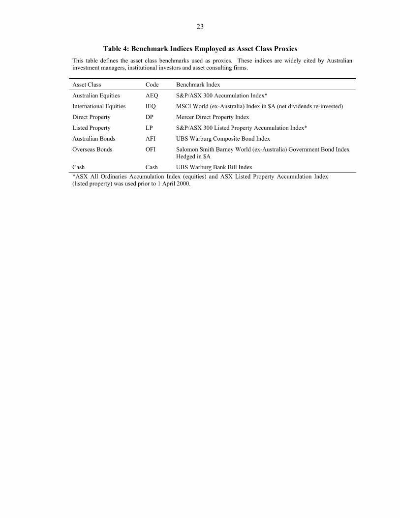
Bonds, International Bonds, Property and Cash. The market indices used as proxies

for each of the asset classes are outlined in Table 4 and represent passive investment

strategies across each asset sector.7

<<INSERT TABLE 4>>

Asset classes may be dichotomised into two broad categories - growth assets

or defensive assets. Growth assets include equity and property investments, whereby

returns derived from such investments comprise income and changes in capital value.

Defensive assets on the other hand are defined as income returns from investments in

bonds and liquid securities. Defensive asset classes exhibit a degree of stability in the

underlying value of an investor’s initial investment. That is, highly liquid money

market securities and bonds derive interest income from the underlying capital value,

wherein the capital value remains stable. In the case of bonds held to maturity, the

principal component or initial investment is redeemable at maturity. Debt instruments

provide the investor with a legal claim to repayment of the principal value at a future

date. In addition, growth and defensive asset classes may be generally distinguished in

8

terms of their historical returns, ex-post volatility and the level of asset class

correlation existing between sectors. To this end, Table 5 presents the returns (income

plus capital changes), volatilities and correlations between asset classes using data

provided by Mercer Investment Consulting. The asset class proxies used rely on the

standard industry benchmarks widely referenced in the Australian investment

management industry and are defined as per Table 4. While future returns and future

volatility of asset classes are unknown, historical data provides investors with some

degree of insight into the level of returns derived and the risks associated with each of

the asset classes.

Table 5 shows that across all asset class sectors, international equities recorded

both the highest return and standard deviation in the 13-year period. As expected, the

growth asset classes exhibit higher standard deviations (or risk) than is the case for

defensive asset classes. An important point also needs to be identified in relation to

direct property. Direct property valuations do not occur as frequently as other asset

classes. That is, other asset classes are more easily priced given their relative liquidity

benefits. In many cases, direct property requires valuers to estimate prices. Given the

‘staleness’ of direct property as an asset class, standard deviation measures should be

expected to be understated – where a closer approximation would be to the risk/return

attributes of listed property.

<<INSERT TABLE 5>>

3. Evaluating Performance and Tactical Asset Allocation

3.1 Sources of Change in Aggregate Portfolio Weights

While Tables 2 and 3 provide an interesting picture regarding some possible trends in

asset allocation dynamics across our sample, they do not allow us to deduce to what

extent this reflects ex-ante manager decisions (i.e. changes in the strategic asset

allocation) versus ex-post rewards (i.e. due to successful market timing). In this

context, as a preliminary step in their analysis, Blake et al. (1999) develop a

procedure to decompose these sources of change in aggregate portfolio weights.

Accordingly, we also apply their decomposition technique to our sample as follows.

7 These market proxies are the most commonly used/cited indexes in the Australian investment industry during the period evaluated.

9

Two forms of decomposition are examined. First, the mean change in portfolio

weights are decomposed according to Blake et al. (1999)’s equation (4):8

ptjtptjtjt NCFNCFrr −+−≈∆ )log(ω (1)

where: ωjt is the total portfolio holding in asset class j at the end of month t; rjt is the

rate of return on fund holdings of asset class j; rpt is the rate of return on the total

portfolio at time t; NCFjt is the rate of net cash flow into asset class j in month t; and

NCFpt is the value-weighted net cash flow into the total fund portfolio in month t.

Equation (1) states that the mean change in portfolio weights are disentangled into: (a)

a passive strategy, i.e. that part due to differential returns across asset classes (rjt – rpt)

and (b) an active strategy, i.e. that part due to net cash flow differentials across asset

classes by rebalancing the portfolio (NCFjt – NCFpt).

In the second form of the decomposition, the variance of changes in portfolio

weights are decomposed according to Blake et al. (1999)’s equation (5):

),cov(2)var()var())log(var( ptjtptjtptjtptjtjt NCFNCFrrNCFNCFrr −−+−+−≈∆ ω (2)

As such, this decomposition states that the short-term variation in aggregate asset

allocations can be disentangled into: (a) variations in return differentials across asset

classes; (b) variations in net cash flow differentials across asset classes; and (c) the

covariance between differential returns and net cash flow differentials across asset

classes.

The results for this analysis are reported in Table 6, wherein Panel A (Panel B)

presents the outcome for Diversified funds (Capital Stable funds). We first consider

Diversified funds and the decomposition of the mean change in portfolio weight

(Panel A.1). Several features are evident. First, the slight increase in weight for

Australian Equities (1.21%) is mostly due to passive differential returns. Second, the

2.15% increase in portfolio weight into International Equities is driven exclusively by

return differential, offset slightly by some (active) net selling. Third, the decline in

average asset allocation to AFI is totally due to net sales. Fourth, the net increased

portfolio allocation in OFI occurs despite a (4.25%) fall in weighting induced by

8 See Blake et al. (1999) for a derivation of this equation.

10

passive differential returns – hence, there was considerable (7.1%) active net

purchases for this asset class. Fifth, Listed Property experienced a considerable

increase in portfolio weighting of 8.3%, almost exclusively explained by active net

purchases. Sixth, Direct Property saw the largest decline in average asset allocation (-

13.3%) approximately equally induced by both passive and active strategies. In

relation to listed and direct property, we cannot rule out that managers simply re-

configured their property portfolios as a means of achieving improved diversification

and liquidity benefits from listed property trusts.

<<INSERT TABLE 6>>

Now consider Capital Stable funds and the decomposition of the mean change

in portfolio weight (Panel B.1). First, Australian Equities exhibited a 4% increase

average asset allocation which, similar to the Diversified funds counterpart, is mostly

due to passive differential returns. Second, International Equities experienced a

considerable increase in portfolio weight of over 19%, exclusively due to active net

purchases. This result contrasts the counterpart case for Diversified funds. Third, the

5.6% decline in average asset allocation to AFI is totally due to net sales (similar to

the counterpart case for Diversified funds). Fourth, International Fixed Interest and

Listed Property both experienced massive asset allocation increases in excess of 30%

which are almost exclusively explained by active net purchases. Fifth, Direct Property

showed a relatively neutral change (of around 2%) in portfolio weights, driven by

strategic purchases despite the relatively poor performance of passive strategies

(leading to a reduced allocation of 4%).

Next consider Diversified funds and the decomposition of the variance of

changes in portfolio weight (Panel A.2). Most notably we see that in the case of the

International Equities, Australian Fixed Interest, International Fixed Interest and

Listed Property asset classes; return differentials largely explain the monthly variation

in portfolio weights. For Australian Equities, the variance is driven by both

differential returns and net cash flow differentials, while being considerably reduced

by the covariance between them.

Finally in the context of Table 6, consider Capital Stable funds and the

decomposition of the variance of changes in portfolio weight (Panel B.2). Across all

asset classes it is seen that return differentials are the dominant force (though slightly

11

less so for Australian Equities).9 In summary, the full set of findings displayed in

Table 6, are broadly consistent with their counterparts reported in Blake et al. (1999).

3.2 Measuring Tactical Asset Allocation Ability

Tactical asset allocation performance can be assessed using the performance

attribution framework proposed by Brinson et al. (1986 and 1991). Performance

attribution measures the effect of the portfolio manager’s active investment decisions

across asset sectors and their respective contribution to aggregate portfolio

performance. Indeed, Brinson et al. (1986) and Blake et al. (1999) document the

overwhelming significance of the asset allocation policy in determining the fund’s

overall performance. The seminal paper by Brinson et al. (1986) proposes an

attribution framework allowing a decomposition of the active return (differential

return from the benchmark return) derived through security selection and tactical asset

allocation management. This approach assumes the fund manager’s portfolio

management objective is to outperform the fund’s strategic benchmark return (or

investment policy) without reference to whether the manager predominantly employs

a ‘top-down’ approach in portfolio construction, ‘bottom-up’ strategy or some

combination of both methodologies.

The attribution approach begins with a simple decomposition of the active raw

(unadjusted for risk) return of a fund in period t: If we define rpt as the portfolio

return at time t, rbt as the return on the asset class market proxy or benchmark index,

then the return difference between rpt and rbt can be decomposed into security

selection (rst), tactical asset allocation (rat) and residual or interaction (rrt)

components. The residual of active performance is not strictly attributable to either

stock selection or asset allocation, and represents the interaction between both sources

of active management decision-making. Tactical asset allocation, security selection

and interaction components, respectively, over a single time period t can be expressed

as:

∑ −=i

itititat rR ))(( ωω (3)

9 Readers should note that the variance results need to be interpreted with some caution, due to the considerable variation in the length of available data across the funds. This factor meant that the sample of funds was often changing, particularly in the case of Capital Stable funds.

12

∑ −=i

itititst rrR ))((ω (4)

∑ −−=i

itptititrt rrR ))(( ωω (5)

where:

iω = average actual weight in asset class i;

iω = benchmark weight in asset class i;

ir = return earned by the fund in asset class i;

pr = fund return for the total portfolio;

ir = benchmark return representing a passive investment strategy in asset class i;

br = benchmark return for the total portfolio.

Burnie et al. (1998) also propose a modified equation from (3) that measures

tactical asset allocation with respect to the difference in value-added between the

individual asset class’ benchmark return and the total portfolio’s overall benchmark

return. In this respect, the Burnie et al. (1998) methodology accounts for timing

ability with respect to the fund’s overall investment policy and is expressed as:

∑ −−=i

btitititat rrR ))(( ωω (6)

At the aggregate portfolio level, the summation across asset classes ensures

the contribution of tactical asset allocation to total performance is identical for both

(3) and (6). Given that this study is concerned with tactical asset allocation, we

evaluate the performance of diversified funds and their ability to earn incremental

returns above their strategic asset allocation benchmark with respect to equation (3).

Consistent with Brinson et al. (1986) and Blake et al. (1999), the returns captured by

13

the residual term are attributed to security selection,10 such that the decomposition of

returns can be simply expressed in terms of the funds’: (a) investment policy (or

strategic benchmark), (b) tactical asset allocation and (c) stock selection.

A unique feature of our study that warrants strong emphasis is the superiority

(relative to Blake et al., 1999) of the strategic benchmark for ‘normal’ returns, iω ,

that we employ. Specifically, our study exhibits a major advantage, in that our

database provides actual information regarding this strategic benchmark, as supplied

by Australian fund managers to Mercer IC. Such a direct measure contrasts the

indirect approximations used by Blake et al. (1999), namely, (a) a ‘constant’

benchmark based on average ex-post portfolio weights and (b) a ‘trended’ benchmark

in which weights are arbitrarily modeled to linearly increase or decrease over time

between initial and terminal weights. As stated by Blake et al. (1999, p. 451):

“The choice of normal portfolio weights is more problematic. Genuine performance measures should reflect investors’ ex ante information on future asset returns. However, we only observe actual portfolio weights, and these reflect realized returns. So information on ex post returns and portfolio weights will permit only noisy performance measurement. In the absence of any information on the funds’ asset-liability modeling exercises that might enable us to draw inferences about their associated strategic asset allocations, we were reduced to experimenting with a few simple, empirically plausible models.”

As such, our direct measure of the benchmark weights provides a less noisy

framework for assessing the tactical asset allocation performance of our sample. This

feature of our study constitutes an improvement in this literature.

The results for fund tactical asset allocation ability are presented in Table 7.

Overall, the evidence suggests that active managers investing across multiple asset

classes have been unable to deliver investors with superior returns through tactical

asset allocation over the period examined. The most successful asset class across all

fund types has been domestic equities (AEQ), with an average monthly TAA return of

around 0.01% and 0.02% for Capital Stable and Diversified funds, respectively. These

averages are statistically different from zero based on a non-parametric sign test (at

the 5% level) in both cases, and this significance is also reinforced by the test in the

case of Diversified funds. Indeed with the latter category, AEQ asset allocation

10 The assumption is that the residual term is small relative to the returns attributable to timing, selection and investment policy.

14

returns are positive in all but 6 of the 45 funds, 17 cases of which are individually

significant at the 5% level. In contrast, Table 7 reveals that tactical asset allocation in

international shares (IEQ) and domestic fixed interest (AFI) has generally been value

detracting. Specifically, in the case of AFI an average monthly TAA return of –

0.027% is observed for Capital Stable funds and this value is statistically significant

according to the parametric t-test (at the 5% level). With regard to the asset class of

IEQ, the average monthly TAA return of –0.015% (–0.028%) for the Capital Stable

(Diversified) funds is statistically significant for both the parametric and non-

parametric tests (at the 5% level).11, 12

<<INSERT TABLE 7>>

3.3 Manager’s TAA Strategy Given Publicly Available Information

A major goal of this study is to examine the potential determinants of tactical asset

allocation decisions by managed funds in Australia. To this end we investigate

whether, and to what extent, a set of public information or macroeconomic variables

predict shifts in TAA behaviour. The selection of market and macroeconomic

indicators is somewhat arbitrary, and to keep the analysis manageable we confine our

analysis to a set of three lagged variables that previous return predictability studies

have identified – the 1-month treasury bill yield (Ztnote), dividend yield (Zdivy), and

the term structure premium (between 10-year Treasury bond yields and the 3-month

treasury bill yields) (Zterm).13 Our data source was the Reserve Bank of Australia’s

(RBA) Electronic database. We also employ the dividend yield of the MSCI World

(ex-Australia) Index for our examination of the determinants of asset allocation

dynamics for international equities.

Following Blake et al.’s (1999) decomposition on the cross-sectional aspects

of asset allocation dynamics, shifts in relative net cash flows across asset classes (net

of the liquidity component) are used in this paper to proxy active decisions in asset

11 Jonathan Shead at SSgA has also reported evidence at the sector level which shows that Australian managers have been successful overall in Australian equities, while unsuccessful in International shares. This research is available on the SSgA website www.ssga.com. 12 One final issue based on unreported analysis, is worthy of comment. We found that funds which failed within our sample period have weaker tactical asset allocation performance than the surviving ones. Further, the distributions of their tactical asset allocation performance across asset classes were more peaked and positively skewed indicating a higher degree of consistency in their ability to add value to fund performance. 13 See Ferson and Schadt (1996), Sawicki and Ong (2000) and Flannery and Protopapadakis (2002).

15

allocation and thus, market timing ability. This captures the fund managers’ active

strategy of rebalancing the portfolio by redirecting cash flows across asset groups

instead of that due to cash flow (liquidity) shocks or due to return differentials

between sectors. Relative net cash flows (RNCF) for each individual asset class are

defined as:

[ ]{ } 1,1,,1,1,,, /)1( −−−− +−= titijtijtitijtitijijt FwrFwFwRNCF (7)

where i = fund manager

j = asset class

t = month

F = fund’s total asset value

r = return

w = proportion of fund i’s total asset value (F)

For the main fund types, a fixed effects14 unbalanced panel data regression was run

with the relative net cashflows (dependent variable) against the vector of lagged

public information variables Zt-1: Ztnote, Zterm and Zdivy.15

ijttijijt ZRNCF εβα ++= −1' (8)

3.3.1 Diversified Fund Manager’s TAA Strategy Given Publicly Available

Information

In the case of Diversified funds, Panel A of Table 8 reports the outcome of estimating

this model. Generally, we observe that across the six asset classes, economic variables

appear most important in determining the appropriate level of asset allocation for

Australian Equities. Specifically, coefficients on Ztnote and Zterm are both significant

at the 1% level, and exhibit positive coefficients, suggesting that fund managers

increase their asset allocation to Australian shares when the economy is both

performing well and is expected to continue to do so (upward sloping yield curve).

14 The fixed effects model is consistent with the error structure of the model used by Blake et al. (1999) for analyzing UK pension fund behaviour. 15 Observations that were more than two standard deviations away from the mean have been excluded.

16

That is, it seems that asset class shifts enacted by fund managers follow a type of

momentum pattern.16, 17

<<INSERT TABLE 8>>

Similar to the AEQ case, for Listed Property both Ztnote and Zterm are

significant (though at the 5% level this time), and also reveal positive coefficients.18

This suggests that fund managers increase their asset allocation to Listed Property

during normal economic conditions, and when the economy is struggling (but

expected to perform better in the future) due to an expected ‘re-rating’ (i.e. when the

yield curve is upward sloping). The positive coefficient on Ztnote suggests that fund

managers also increase their asset allocation to Listed Property when short-term

interest rates are higher.

In the case of Overseas Fixed Interest (OFI), the coefficient on Zdivy is

positive and significant at the 5% level, while the Zterm coefficient is negative and

significant at the 10% level. The positive Zdivy coefficient potentially suggests that

fund managers increase their allocation to OFI when the domestic equity market is in

decline and dividend yields are increasing (since when equity markets ‘correct’,

companies tend to smooth dividends, inducing a rise in percentage yields). In contrast

to OFI, for the Australian Fixed Interest (AFI) sector, the coefficient on Zterm is

positive (and significant at the 10% level). This suggests that fund managers increase

their domestic fixed interest asset allocation and decrease their overseas fixed interest

allocation when (domestic) long-term interest rates are higher.

For International Equities (IEQ) only Zdivy produced a significant, positive

coefficient, at the 1% level. This is not surprising, since it potentially suggests that

fund managers increase their asset allocation in foreign equities when domestic

dividend yields are increasing – a situation likely to coincide with a decline in the

domestic share market.

16 Strong price momentum has been documented in the Australian equity market. Hurn and Pavlov (2003) show evidence of medium-term momentum prevalent in the Australian equity market. Similarly, Demir et al. (2004) find evidence of a very strong momentum anomaly (at both short and intermediate horizons) which is robust to size, liquidity, and risk-adjustment techniques. 17 The authors are aware of some unpublished research which investigates momentum strategies in a TAA setting. Generally, this research shows that asset class shifts follow a momentum pattern – managers reallocate to sectors based on past sector returns, and this phenomenon is more pronounced among funds with poor market timing skill. 18 This is not entirely unexpected, given Table 4 shows Listed Property and Australian Equities asset classes are highly correlated in terms of their performance.

17

Finally, it is noted that no economic variables were significant in determining

fund managers asset allocation to Cash. It is likely that cash has relatively small

weights in Diversified funds, and as a consequence its asset allocation may be

determined as a residual from the larger asset classes, thereby explaining the generally

lower importance of economic variables. Indeed, cash also has an important role in

managing liquidity between the fund and investors.

3.3.2 Capital Stable Fund Manager’s TAA Strategy Given Publicly Available

Information

Panel B of Table 8 reports the results for the Capital Stable sample of funds. Similar

to the case of Diversified funds, economic variables seem best at explaining asset

allocation for Australian Equities. Once again, coefficients on Ztnote (1% level) and

Zterm (10% level) are positive and significant for Australian equities, while the Zdivy

coefficient is now also significant at the 10% level and shows a negative sign. This

latter result suggests that (unlike their Diversified fund counterparts) there is weak a

tendency for Capital Stable fund managers to reduce their asset allocation to

Australian equities when the sharemarket is in decline and dividend yields are

increasing. Presumably this differential response to the dividend-based public

information variable reflects the more cautious/conservative nature of Capital Stable

managers.

For International Equities the pattern mimics the counterpart case for

Diversified funds – only the coefficient on Zdivy is positive and significant (this time

only at the 10% level), again suggesting an increased allocation to foreign equity

when the domestic market is in decline. In the case of Australian Fixed Interest, only

the coefficient on Ztnote is positive and significant at the 1% level. This suggests that

asset allocation to domestic fixed interest increases with higher short-term interest

rates.

For the remaining asset classes very little evidence is forthcoming that Capital

Stable fund managers base asset allocation decisions on this set of economic

variables. Arguably, this reflects that for Overseas Fixed Interest; Listed Property and

Cash, the conservative nature of this type of manager sees them adopting some type of

‘immunity’ strategy on asset allocation with regard to economic conditions.

4. Summary and Conclusion

18

This paper provides both an original and comprehensive analysis of tactical asset

allocation abilities and strategies employed by Australian investment managers who

invest assets across multiple asset classes. Consistent with the literature concerning

U.S. and U.K. funds investing in multiple asset classes, the strategic asset allocation

adopted by superannuation funds represents the single most important determinant of

portfolio returns. We analyse the behaviour of Balanced, Growth and Capital Stable

fund managers with regard to their asset allocation activity across defensive (cash,

domestic bonds, overseas bonds) and growth (domestic equities, international

equities, property) asset classes, over the period 1990 to 2001.

It is worthy of emphasis that the literature on dynamic asset allocation

decisions made by portfolio managers is generally sparse and largely non-existent

outside the US. Such a research void exists due to limited access by researchers to the

data necessary for such a study. Our ability to gain authorized access to such data

from a proprietary source ensures that our study enhances a very exclusive literature

on the global stage. Moreover, a unique feature of our study that warrants strong

emphasis is the superiority (relative to Blake et al., 1999) of the strategic benchmark

for ‘normal’ returns that we employ, since our database provides actual fund

information regarding this strategic benchmark. Such a direct measure of the

benchmark weights contrasts the indirect approximations used by Blake et al. (1999),

thereby providing us with a much cleaner experimental framework for assessing the

tactical asset allocation performance of our sample.

Overall, our evidence suggests that active managers have been unable to

deliver investors with superior returns through tactical asset allocation. While the

most successful asset class, domestic equities, has been value enhancing, international

shares and domestic fixed interest have generally detracted value. Finally, across all

asset classes examined, our findings suggest that in terms of factors that might

influence changes in asset allocations over time, domestic equities is most influenced

by public economic information variables, with short-term interest rates, the term

structure and dividend yields all having a significant explanatory role.

Given the inability of managers to add value through tactical asset allocation,

this leads researchers to speculate as to the reasons why dynamic asset mix strategies

detract from aggregate portfolio returns. Blake et al. (1999) postulate that in the UK

the evidence might be explained due to the overall structure of the pension fund

industry, including competition levels amongst investment providers, trustee

19

governance, as well incentive arrangements in existence in the market. Given the

empirical evidence, the debate will continue to be waged regarding the role of

dynamic asset allocation strategies, and whether Plan sponsors should maintain static

asset class exposures in line with their strategic benchmarks. Future research should

examine why tactical asset allocation has failed to deliver superior returns above

strategic benchmark weights. Indeed, the extent to which portfolio construction is a

significant determinant should be empirically examined, such that a comparison can

be made between portfolios which exercise a ‘top-down’ approach to asset allocation

relative to ‘bottom-up’ portfolio construction. How the investment manager

ultimately achieves the fund’s aggregate asset mix, coupled with the research and

investment process executed by chief investment officers represents important

avenues for future research.

20

Table 1: The Cross-sectional Performance of 59 Diversified and 29 Capital Stable Funds existing in the period 1990-2001

This table presents cross sectional statistics at the overall fund level using monthly total fund return data across diversified funds and capital stable funds. Excess fund return measures the performance difference of the fund relative to the fund’s appropriate benchmark (where the benchmark accounts for the fund’s specific strategic benchmark asset allocation to the various sectors). Alpha measures the risk adjusted return of the fund. All performance measures are expressed in percentage terms per month.

Panel A: Diversified Funds Total Overall Fund Performance 0.827 Excess Fund Return to Benchmark 0.004

t-statistic 0.43 Alpha (risk-adjusted return) -0.011

t-statistic -1.05 Panel B: Capital Stable Funds Total Overall Fund Performance 0.683 Excess Fund Return to Benchmark -0.016

t-statistic -1.68 Alpha (risk-adjusted return) -0.010

t-statistic -0.86

21

Table 2: Descriptive Statistics of the Sample’s Asset-Weighted Asset Allocation by Sector (in %) and Total Fund Sizes as at December for the years 1989-2000

1989 1990 1991 1992 1993 1994 1995 1996 1997 1998 1999 2000 Panel A: Balanced Funds No. Funds 8 29 29 30 33 34 36 37 35 36 33 33 Total Size ($A Billion) 1.38 11.01 13.85 15.05 20.58 20.82 24.43 28.27 32.29 35.78 34.41 35.44 Australian Equities 31.0 31.1 36.2 35.9 39.2 37.2 39.1 39.0 36.1 34.8 36.8 36.7 International Equities 20.1 14.9 18.7 17.9 20.2 15.9 18.6 17.1 17.6 18.6 20.2 21.9 Direct Property 12.0 12.5 9.0 8.2 5.8 8.7 8.5 6.7 5.7 4.9 2.6 2.3 Listed Property 2.2 1.9 1.7 1.9 2.8 2.8 3.3 4.8 4.8 5.9 6.2 7.1 Australian Fixed Interest 18.8 21.8 18.4 20.3 15.2 19.4 16.4 16.1 14.9 17.5 16.9 16.7 International Fixed Interest 3.7 5.0 8.7 9.4 8.4 3.6 4.8 4.3 5.6 6.4 4.9 5.6 Index-Linked Bonds - - 0.4 0.9 3.1 3.1 3.2 2.9 2.3 2.0 1.6 1.5 Cash 9.7 10.0 4.8 3.6 4.0 7.9 5.1 7.8 11.3 8.5 9.8 7.2 Other 2.5 2.7 2.4 2.8 4.4 4.5 4.3 4.3 3.9 3.4 2.6 2.5 Panel B: Capital Stable Funds No. Funds - - 17 19 23 23 25 26 24 22 21 21 Total Size ($A Billion) - - 1.79 3.39 5.67 5.10 5.80 6.04 6.56 5.96 5.10 4.13 Australian Equities - - 17.3 16.1 18.8 14.3 17.1 17.2 14.8 13.7 13.8 13.7 International Equities - - 4.4 2.3 4.7 3.6 5.0 4.0 4.3 5.0 5.8 6.5 Direct Property - - 1.3 1.8 2.4 4.2 4.5 3.7 3.7 2.8 1.8 1.9 Listed Property - - 1.3 1.9 3.4 2.1 2.7 3.2 3.2 4.0 3.6 3.4 Australian Fixed Interest - - 58.5 58.5 43.6 41.9 41.9 42.5 39.4 43.2 31.1 32.6 International Fixed Interest - - 3.1 3.9 6.8 2.8 4.2 3.7 6.3 6.8 8.8 9.8 Index-Linked Bonds - - 0.1 0.9 6.6 4.7 3.5 3.0 2.7 2.5 2.7 2.6 Cash - - 13.8 14.6 13.7 26.2 21.1 22.6 25.5 21.8 32.4 29.6 Other - - 0.2 0.0 0.0 0.1 0.0 0.0 0.1 0.2 0.0 0.0

22

Table 3: Descriptive Statistics of the Asset-Weighted Average Fund’s Tactical Asset Allocation Strategy Relative to Strategic Benchmark for the Major Asset Classes

1989 1990 1991 1992 1993 1994 1995 1996 1997 1998 1999 2000 Panel A: Balanced Funds Australian Equities -2.6 -2.6 1.7 1.5 4.3 2.4 4.2 4.3 0.9 -0.7 -0.7 -0.2 International Equities 0.8 -4.5 -0.8 -1.7 0.8 -3.4 -0.7 -1.9 -1.9 -1.0 -0.4 0.1 Direct Property -2.1 -1.6 -4.1 -3.1 -3.9 -0.3 -0.7 -0.5 -1.1 -1.7 -2.3 -1.5 Listed Property 0.8 0.5 0.4 -0.4 0.2 0.0 0.6 1.1 0.8 1.9 1.2 2.3 Australian Fixed Interest -1.0 1.8 -0.6 0.7 -4.8 -0.5 -3.5 -3.7 -5.0 -2.5 -2.5 -2.4 International Fixed Interest 1.2 1.9 4.4 4.6 3.4 -1.7 -0.4 -1.1 0.4 1.7 0.3 -0.1 Index-Linked Bonds 0.0 0.0 0.0 0.0 1.4 0.0 0.1 0.2 -0.4 -0.8 -0.4 0.0 Cash 2.6 3.7 -1.2 -2.1 -1.2 2.8 0.0 2.5 6.2 3.3 4.8 2.6 Other 0.5 0.8 0.2 0.5 -0.1 0.6 0.2 -0.7 0.0 -0.2 0.0 -1.0 Panel B: Capital Stable Funds Australian Equities - - 3.9 3.1 5.7 0.8 3.2 3.4 0.8 -0.1 -1.1 -0.9 International Equities - - -0.4 -1.8 0.3 -1.4 -0.5 -1.3 -1.3 -0.3 -0.2 -0.4 Direct Property - - -1.9 -1.9 -1.5 1.5 1.4 0.9 0.7 0.4 0.0 0.2 Listed Property - - -1.5 -1.6 -0.2 -1.7 -0.5 0.0 -0.6 0.1 0.5 0.6 Australian Fixed Interest - - 7.5 8.4 -5.3 -7.1 -5.0 -4.5 -6.2 -3.7 -5.6 -3.8 International Fixed Interest - - -1.8 -0.3 2.4 -2.8 -1.8 -2.7 0.3 0.9 -0.4 0.0 Index-Linked Bonds - - 0.0 0.1 5.2 3.0 1.8 1.4 0.2 -0.2 -0.2 0.3 Cash - - -6.0 -6.1 -6.7 7.6 1.5 2.8 6.0 3.0 7.1 4.4 Other - - 0.2 0.0 0.0 0.0 -0.2 0.0 0.1 0.1 -0.1 -0.3

The figures reported in this table are based as at December for the years 1989-2000. Deviations from strategic benchmark expressed in percentage terms. Positive (negative) values indicate above (below) benchmark exposures.

23

Table 4: Benchmark Indices Employed as Asset Class Proxies This table defines the asset class benchmarks used as proxies. These indices are widely cited by Australian investment managers, institutional investors and asset consulting firms. Asset Class Code Benchmark Index

Australian Equities AEQ S&P/ASX 300 Accumulation Index*

International Equities IEQ MSCI World (ex-Australia) Index in $A (net dividends re-invested)

Direct Property DP Mercer Direct Property Index

Listed Property LP S&P/ASX 300 Listed Property Accumulation Index*

Australian Bonds AFI UBS Warburg Composite Bond Index

Overseas Bonds OFI Salomon Smith Barney World (ex-Australia) Government Bond Index Hedged in $A

Cash Cash UBS Warburg Bank Bill Index *ASX All Ordinaries Accumulation Index (equities) and ASX Listed Property Accumulation Index (listed property) was used prior to 1 April 2000.

24

Table 5: Historical Annual Returns, Volatility and Correlations: Period December 1989 – February 2001

This table shows the per annum returns, volatilities and correlations (Pearson) across asset classes in the period December 1989 to February 2001, where the asset classes are defined in Table 4. The Consumer Price Index (CPI), as a measure of inflation and Average Weekly (Male) Ordinary-Time Earnings is also presented for comparison purposes in the period December 1989 to December 2000. Correlation (%)

Asset Class

Return % pa

SD % pa

AEQ IEQ DP LP AFI OFI Cash

AEQ 11.0 13.2 100.0 43.5* -1.2 54.2* 41.4* 22.4 * -3.5

IEQ 12.3 14.9 - 100.0 -5.8 29.8* 18.3* 30.0 * -6.1

DP 3.0 4.2 - - 100.0 -1.4 -13.6 -22.2 * -10.9

LP 12.1 10.2 - - - 100.0 47.5* 30.8 * 6.2

AFI 11.6 4.8 - - - - 100.0 65.2 * 32.3*

OFI 10.5 3.2 - - - - - 100.0 24.1*

Cash 7.3 0.9 - - - - - - 100.0

CPI 2.7 1.9 - - - - - - -

AWE 3.4 2.4 - - - - - - - * Significant at 5% level.

25

Table 6: Identifying the Sources of Changes to Aggregate Portfolio Weights across Asset Classes Australian

equities International

equities Australian

fixed interest International fixed interest

Listed property

Direct property

(AEQ) (IEQ) (AFI) (OFI) (LP) (DP) Panel A: Diversified Funds A.1 Mean change in portfolio weight (annualized) 1.21 2.15 -3.32 2.89 8.30 -13.30 - due to differential returns 0.97 2.83 -0.32 -4.25 0.82 -6.30 - due to net cash flow differentials 0.25 -0.68 -3.00 7.14 7.48 -7.00 A.2 Percentage of monthly variance in portfolio weights - due to differential returns 93.47 84.25 90.11 99.45 84.26 59.31 - due to net cash flow differentials 75.70 28.50 17.70 2.21 35.33 23.11 - due to covariance between these -69.18 -12.75 -7.81 -1.66 -19.59 17.58 Panel B: Capital Stable Funds B.1 Mean change in portfolio weight (annualized) 4.02 19.65 -5.58 32.24 35.31 1.77 - due to differential returns 3.32 0.08 -0.47 -3.46 1.37 -4.03 - due to net cash flow differentials 0.70 19.58 -5.12 35.70 33.94 5.80 B.2 Percentage of monthly variance in portfolio weights - due to differential returns 61.33 101.16 88.88 112.14 87.96 108.76 - due to net cash flow differentials 27.27 8.19 7.56 0.59 10.72 4.01 - due to covariance between these 11.40 -9.35 3.56 -12.73 1.32 -12.77

The results in this table are based on the procedure developed in Blake et al. (1999).

26

Table 7: Empirical Tests of Tactical Asset Allocation Performance This table summarizes tactical asset allocation performance in the six major asset classes (defined in Table 4) for Diversified funds (Panel A) and Capital Stable funds (Panel B). The mean and standard deviations are recorded in percentage terms per month. Sectors AEQ IEQ DP LP AFI OFIPanel A: Diversified funds Mean 0.021 -0.028 0.004 0.005 -0.004 -0.004 Standard Deviation (Average) 0.206 0.170 0.061 0.071 0.088 0.027 Median 0.008 -0.015 -0.003 0.004 -0.006 -0.003 No. Funds Significant* and Positive 17 3 9 6 11 2 No. Funds Insignificant* and Positive 22 5 7 14 9 9 No. Funds Significant* and Negative 0 12 2 5 16 12 No. Funds Insignificant* and Negative 6 25 6 10 9 6 No. Funds with Sector Exposures 45 45 24 35 45 29 Cross-sectional parametric test 2.92* -3.68* -0.87 1.48 -1.00 -0.96 Cross-sectional non-parametric test 4.77* -4.47* 1.43 0.68 -0.89 -1.49 Panel B: Capital Stable funds Mean 0.009 -0.015 0.009 -0.001 -0.027 -0.005 Standard Deviation (Average) 0.135 0.075 0.023 0.063 0.135 0.028 Median 0 -0.008 0.004 0.001 -0.013 -0.003 No. Funds Significant* and Positive 8 1 9 4 4 3 No. Funds Insignificant* and Positive 13 5 3 9 8 1 No. Funds Significant* and Negative 1 9 4 5 8 8 No. Funds Insignificant* and Negative 5 11 1 5 9 4 No. Funds with Sector Exposures 27 26 17 23 29 16 Cross-sectional parametric test 1.43 -4.44* 2.30* -0.28 -2.10* -1.65 Cross-sectional non-parametric test 2.69* -2.94* 1.46 0.42 -1.11 -2.25* * Significant at the 5% level.

Note: The non-parametric sign test, tests whether there are a significantly greater number of positive than negative cases across our sample of funds. The statistic is calculated as:

P)P(NEA

Statt

it

−

−±=

1)5.0(

where, A is the actual number of positive cases. If A< 1/2N, the expression (At + 0.5) is applied and if A > 1/2N, the expression (At - 0.5) is applied. E i = expected number of positive cases, Nt = total number of observations, P = expected percentage of positive cases under the null hypothesis, i.e. p = 0.5.

27

Table 8: Economic Conditions and Asset Allocation This table presents in panel A, the panel data regression results for the sample of Diversified Funds (i.e. Balanced and Growth Funds) and in Panel B, the results for Capital Stable Funds. Direct Property is excluded from the analysis due to relative illiquidity of the asset class for a fund manager to quickly shift their asset class exposure. The model specification is defined in equation (8) as follows:

ijttijijt ZRNCF εβα ++= −1' (8)

where RNCF is the relative net cash flows defined as:

[ ]{ } 1,1,,1,1,,, /)1( −−−− +−= titijtijtitijtitijijt FwrFwFwRNCF (7)

i = fund manager j = asset class t = month F = fund balance r = return w = proportion of fund i’s total asset value (F)

and 1−tZ = the vector of public information variables lagged one period (treasury note rate, term spread and dividend yield).

AEQ IEQ AFI OFI LP Cash Panel A: Diversified funds Constant -0.0292

(0.1856) -0.0308 (0.3440)

0.0754** (0.0476)

-0.0750 (0.2239)

0.0082 (0.5146)

0.2409 (0.3789)

Ztnote 0.0543*** (0.0004)

-0.0767 (0.1591)

-0.0364 (0.1684)

-0.0490 (0.7353)

0.0244** (0.0355)

0.1751 (0.4385)

Zterm 0.0928*** (0.0000)

-0.0423 (0.5476)

0.0429* (0.0954)

-0.3214* (0.0509)

0.0241** (0.0108)

0.0262 (0.9153)

Zdivy -0.0296 (0.5330)

0.3515*** (0.0025)

0.0510 (0.5315)

0.6931** (0.0156)

-0.0243 (0.5653)

-1.0195 (0.1343)

F-statistic 3.91*** (0.0000)

4.36*** (0.0000)

1.55** (0.0202)

1.88*** (0.0071)

3.35*** (0.0001)

1.17 (0.2281)

No. Funds 36 35 37 24 31 35 R2. Adj. 0.0579 0.0572 0.0220 0.0455 0.0614 0.0226 Panel B: Capital Stable funds Constant -0.0104

(0.7744) -0.1911*** (0.0032)

0.0360 (0.2860)

-0.0630 (0.4501)

0.0174** (0.0481)

-0.0656 (0.4681)

Ztnote 0.2180*** (0.0000)

0.0388 (0.8407)

0.1271*** (0.0003)

-0.0246 (0.9213)

-0.0043 (0.6777)

0.1298 (0.1693)

Zterm 0.0652* (0.0734)

-0.0228 (0.9200)

0.0345 (0.3044)

-0.3790 (0.1573)

-0.0112 (0.1860)

0.0748 (0.4187)

Zdivy -0.2765* (0.0608)

0.7050* (0.0733)

-0.1737 (0.1877)

0.8616* (0.0705)

-0.0217 (0.5655)

-0.3079 (0.3682)

F-statistic 2.62*** (0.0000)

1.04 (0.4117)

2.40*** (0.0002)

0.96 (0.4949)

1.69** (0.0434)

0.93 (0.5436)

No. Funds 26 27 25 17 17 19 R2. Adj. 0.0672 0.0277 0.0482 0.0303 0.0393 0.0180 Notes: p-values are shown in brackets. *,**,*** denote significance at the 10, 5 and 1% level, respectively. The F-test is for the null hypothesis of no fixed effects.

28

References

Arnott R., Fabozzi, F. (1988), Asset Allocation: A Handbook of Portfolio Policies, Strategies and Tactics, Probus Professional Publishers, U.S.A.

Becker, C., Ferson, W., Myers, D., Schill, M. (1999), Conditional Market Timing with Benchmark Investors, Journal of Financial Economics, Vol. 52, pp. 119-48. Bird, R., Chin, H., McCrae, M. (1983), The Performance of Australian Superannuation Funds, Australian Journal of Management, Vol. 8, pp. 49-69. Blake, C.R., Elton, E.J., Gruber M.J. (1993), The Performance Of Bond Mutual Funds, Journal of Business, Vol. 66, pp. 371-403. Blake, C.R., Elton, E.J, Gruber, M.J. (1996), Survivorship Bias and Mutual Fund Performance, Review of Financial Studies, Vol.9, pp. 1097-1120. Blake, D., Lehmann, B., Timmerman, A. (1999), Asset Allocation Dynamics and Pension Fund Performance, Journal of Business, Vol. 72, pp. 429-61. Brinson, G.P., Hood, L.R., Beebower, G.L. (1986), Determinants of Portfolio Performance, Financial Analysts Journal, Vol. 42, pp. 39-44. Brinson, G.P., Singer, B.D., Beebower, G.L. (1991), Determinants of Portfolio Performance II: An Update. Financial Analysts Journal, Vol. 47, pp. 40-48. Brown, S., Goetzmann, W., Ibbotson, R., Ross, S. (1992), Survivorship Bias in Performance Studies, Review of Financial Studies, Vol. 2, pp. 553-80. Burnie, J., Knowles J., Teder, T. (1998), Arithmetic and Geometric Attribution, Journal of Performance Measurement, Vol. 3, pp. 59-68. Chang, E., Llewellen, W. (1984), Market Timing and Mutual Fund Investment Performance, Journal of Business, Vol. 57, pp. 57-72. Chen, N., Roll, R., Ross, S.A. (1986), Economic Forces and the Stock Market, Journal of Business, Vol. 59, pp. 383-403. Daniel, K., Grinblatt, M., Titman, S., Wermers, R. (1997), Measuring Mutual Fund Performance with Characteristic-Based Benchmarks, Journal of Finance, Vol. 52, pp.1035-58. Demir, I., Muthuswamy, J., Walter, T. (2003), Momentum Returns in Australian Equities: The Influences of Size, Risk, Liquidity, and Return Computation, Pacific-Basin Finance Journal, Vol. 12(2): pp. 143-158. Elton, E., Gruber, M., Das, S., Hlavka, M. (1993), Efficiency with Costly Information: A Reinterpretation of Evidence from Managed Portfolios, Review of Financial Studies Vol. 6, pp.1-22.

29

Ferson, W., Schadt, R. (1996), Measuring Fund Strategy and Performance in Changing Economic Conditions, Journal of Finance, Vol. 51, pp. 425-61. Ferson, W., Warther, V. (1996), Evaluating Fund Performance in a Dynamic Market, Financial Analysts Journal, Vol. 52, pp. 20-28. Finn, F., Koivurinne, T. (2000), The Ex-Ante Efficiency of Australian Stock Market Benchmarks, Australian Journal of Management, Vol. 25, pp. 1-15. Flannery, M.J., Protopapadakis, A.A. (2002), Macroeconomic Factors Do Influence Aggregate Stock Returns, Review of Financial Studies, vol. 15, pp. 751-82. Gallagher, D.R. (2001), Attribution of Investment Performance: An Analysis of Australia Pooled Superannuation Funds, Accounting and Finance, Vol. 41, pp. 41-62. Grant, D. (1977), Portfolio Performance and the Cost of Timing Decisions, Journal of Finance, Vol. 32, pp. 837-846. Grinblatt, M., Titman, S. (1989), Mutual Fund Performance: An Analysis of Quarterly Portfolio Holdings, Journal of Business, Vol. 62, pp. 393-416. Grinblatt, M., Titman, S. (1992), The Persistence of Mutual Fund Performance, Journal of Finance, Vol. 47, pp. 1977-84. Grinblatt, M., Titman, S., Wermers, R. (1995), Momentum Investment Strategies, Portfolio Performance and Herding: A Study of Mutual Fund Behavior, American Economic Review, Vol. 85, pp. 1088-1105. Hallahan, T., Faff, R. (1999), An Examination of Australian Equity Trusts for Selectivity and Market Timing Performance, Journal of Multinational Financial Management, Vol. 9, pp. 387-402. Hallahan, T., Faff, R., (2001), Induced Persistence or Reversals in Fund Performance?: The Effect of Survivorship Bias, Applied Financial Economics, Vol. 11, pp. 119-26. Henriksson, R. (1984), Market Timing and Investment Performance: An Empirical Investigation, Journal of Business, Vol. 57, pp. 73-96. Hurn, S., Pavlov, V. (2003), Momentum in Australian Stock Returns, Australian Journal of Management, Vol. 28(2): pp. 141-155. Ippolito, R. (1989), Efficiency with Costly Information: A Study of Mutual Fund Performance, Quarterly Journal of Economics, Vol. 104, pp. 1-23. Jagannathan, R., Korajczyk, R. (1986), Assessing the Market Timing Performance of Managed Portfolios, Journal of Business, Vol. 59, pp. 217-35. Jegadeesh, N., Titman, S. (1993), Returns to Buying Winners and Selling Losers: Implications for Stock Market Efficiency, Journal of Finance, Vol. 48, pp. 65-91.

30

Jegadeesh, N., Titman, S. (2001), Profitability of Momentum Strategies: An Evaluation of Alternative Explanations, Journal of Finance, Vol. 56, pp. 699-720. Kon, S. (1983), The Market-Timing Performance of Mutual Fund Managers, Journal of Business, Vol. 56, pp. 323-47. Lee, C., Rahman, S. (1990), Market Timing, Selectivity, and Mutual Fund Performance: An Empirical Investigation, Journal of Business, Vol. 63, pp. 261-78. Robson, G. (1986), The Investment Performance of Unit Trusts and Mutual Funds in Australia for the Period 1969 to 1978, Accounting and Finance, Vol. 26, pp. 55-79. Sawicki, J., Ong, F. (2000), Evaluating Managed Fund Performance Using Conditional Measures: Australian Evidence, Pacific-Basin Finance Journal, Vol. 8, pp. 505-28. Sharpe, W. (1964), Capital Asset Prices: A Theory of Market Equilibrium Under Conditions of Risks, Journal of Finance, Vol. 19, pp. 425-42. Sinclair, N. (1990), Market Timing Ability of Pooled Superannuation Funds January 1981 to December 1987, Accounting and Finance, Vol. 30, pp. 511-65. Wermers, R. (2000), Mutual Fund Performance: An Empirical Decomposition into Stock Picking Talent, Style, Transaction Costs and Expenses, Journal of Finance, Vol. 55, pp. 1655-95.