1

Strategic approaches to targeting technology generation: Assessing the coincidence 1

of poverty and drought-prone crop production 2

3

Glenn Hymana, Sam Fujisakaa, Peter Jonesa, Stanley Woodb, Carmen de Vicentec and 4

John Dixond 5

6

a International Center for Tropical Agriculture (CIAT) 7

b International Food Policy Research Institute (IFPRI) 8

c Generation Challenge Programme (GCP), International Maize and Wheat Improvement 9

Center (CIMMYT) 10

d International Maize and Wheat Improvement Center (CIMMYT) 11

12

13

Abstract 14

15

The world’s poorest and most vulnerable farmers on the whole have not benefited from 16

international agricultural research and development. Past efforts have tried to increase the 17

production of countries in more favourable environments; farmers with relatively higher 18

potential for improvement benefited most from these advances. This study prioritizes 19

areas of high poverty, the key problem of high drought risk and the crops grown and 20

consumed in these areas. We used global spatial data on crop production, climate and 21

poverty (as proxied by child stunting) to identify geographic areas of high priority for 22

crop improvement. Using spatial overlay, drought modelling and descriptive statistics, we 23

* Manuscript

2

identified where best to target technology generation to achieve its intended human 1

welfare goals. Analysis showed that drought coincides with high levels of poverty in 15 2

major farming systems, especially in South Asia, the Sahel and eastern and southern 3

Africa, where high diversity in drought frequency characterizes the environments. 4

Twelve crops make up the bulk of food production in these areas. We developed a 5

database for use in agricultural research and development targeting and priority setting to 6

raise the productivity of crops on which the poor in marginal environments depend. 7

8

Keywords: Farming systems; Child stunting; Drought; Staple food crops; Risk 9

10

11

1. Introduction 12 13

Over the last 50 years, progress in reducing poverty and malnutrition has been mixed 14

(World Bank, 2004, FAO, 2005). A reduction in the proportion of the poor and 15

undernourished has been achieved in most regions of the world. But the absolute numbers 16

of poor people continues to grow across sub-Saharan Africa and, between 1991 and 2002, 17

the number of hungry has grown by over 40 million people in central and eastern Africa 18

and South Asia. These negative trends exacerbate a situation in which many regions are 19

already projected to fall short of international poverty and hunger goals (UNDP, 2006). 20

Given the importance of agriculture in the food security and livelihoods of the poor, any 21

strategy to address poverty in such regions must pay particular attention to raising the 22

productivity, profitability and sustainability of agricultural enterprises (Gryseels et al., 23

1992, Dixon et al., 2001). 24

3

1

Unfortunately, most farmers in marginal environments have had little benefit from 2

agricultural research and development (Freebairn, 1995, CGIAR, 2000, Evenson and 3

Gollin, 2003). The dominant humanitarian goal of early international research and 4

development efforts, including that of the Consultative Group on International 5

Agricultural Research, was to “increase the pile of rice” in poor and famine-prone 6

countries (Shah and Strong 1999). But, while the new Green Revolution technologies 7

succeeded in raising overall levels of food security, they were primarily adopted by 8

relatively well-off farmers with access to resources and capital. There is now a growing 9

commitment to the notion that accelerating progress in reducing poverty and hunger 10

requires an urgent refocusing of development efforts on resource-poor farmers in 11

marginal environments. 12

13

In the past it has proved difficult to respond to this challenge because the necessary layers 14

of information and the tools to analyse them in an integrated fashion, were not available. 15

In this study we bring together a unique combination of new spatial data and analyses that 16

allows research investors and scientists to take a broad, strategic perspective of the most 17

important geographical regions, farming systems and crops for which development of 18

drought-tolerant traits would likely bring major benefits to the poorest people. 19

20

Specifically, this study identifies the coincidence of poor populations in developing 21

countries, the production of key food staple crops on which the poor depend and drought-22

prone production environments. We used farming systems as our geographic units of 23

4

analysis (Fig. 1, Dixon et al., 2001). Our study used malnutrition, identified by childhood 1

stunting, as a proxy for poverty (FAO, 2003). We developed a model to appraise the 2

susceptibility of regions more and less prone to drought. We assessed the relative 3

importance of different crops in the farming systems using a global database of harvested 4

area and production for the main food staples (You and Wood, 2006). 5

6

Fifteen farming systems have between 2.5 and 28 million stunted children each, 7

accounting for over 70% of the world’s stunted children. High average crop production 8

losses from drought are found in these systems. They have evolved largely to support the 9

production of 12 food staple crops, with at least 5% of the global harvested area of the 10

dominant food staples in each system. They include a large area in Mesoamerica, the 11

African Sahel, parts of eastern and southern Africa and large areas of South Asia, 12

Southeast Asia and East Asia. Our study ranks the farming systems according to the total 13

scale of poverty, the average drought frequency and the total area of food staple crops. 14

The derived information base is intended to support priority setting for research and 15

development on raising the productivity of food staple cropping systems targeted to 16

addressing the needs of poor people in marginal environments. 17

18

2. Materials and Methods 19

20

2.1. Population, poverty and crop production 21

22

5

We developed a spatial database to support assessments of poverty and crop production 1

and acquired global data sets with estimates for grid cells of 1-km2 to 400-km2 spatial 2

resolution. The database includes population information from the Gridded Population of 3

the World (GPW) Version 3 project (CIESIN et al., 2004). We used infant mortality rates 4

and the prevalence and absolute number of underweight and stunted children as measures 5

of poverty (FAO, 2003, CIESIN, 2005, CIESIN, 2006). The data sets of underweight and 6

stunted children are based on health surveys such as the Demographic and Health Survey 7

(FAO, 2003, Balk et al., 2005). The data report the percentage and absolute number of 8

children under 5 years of age that are -2 standard deviations from the international growth 9

reference standard. We linked tabular data for administrative units to maps in a 10

geographic information system (GIS). 11

12

We chose to use stunting as our principle poverty indicator because: 13

• Stunting occurs in households that cannot provide sufficient food or income for 14

healthy nutrition; 15

• Poor families first try to improve their food and nutrition with greater income or crop 16

production; 17

• Income or wealth as indicators are difficult to elicit or standardize in a way that allows 18

comparison and are highly variable as a contributing factor to well-being; and 19

• Only 20 to 30 countries in the world have detailed mapping of income or consumption 20

that is sufficiently reliable and of significant resolution; while 21

• The measurement of stunting is straightforward and comparable globally. 22

23

6

A full table of population and stunting by farming system is given in the Appendix (Table 1

A1). We derived estimates of the spatial distribution and productivity of crops for 10-km 2

grids using a novel allocation approach involving the fusion of sub-national crop 3

production statistics (You and Wood, 2006). This we combined with an array of digitally 4

mapped data on the distribution of rainfed and irrigated cropland, the potential 5

biophysical yield of each crop and population density. We derived sub-national crop 6

production data from agricultural censuses and surveys and scaled all values so as to 7

obtain national production estimates that were compatible with the annual average FAO 8

national crop statistics for 1999-2001. The prototype crop distribution database used in 9

this study is available from the authors upon request but is currently being regenerated 10

using newer and additional data sources (including revisions based on expert validation) 11

and an enhanced allocation algorithm. A large share of the sub-national crop production 12

can be downloaded directly from FAO’s (2006) Agromaps site at 13

http://www.fao.org/landandwater/agll/agromaps/interactive/index.jsp. The following 14

digital crop maps in GIS formats were used in our analysis: 15

• Barley • Millet • Sorghum

• Bean • Musa • Soybean

• Cassava • Other pulses • Sweet potato

• Groundnut • Potato • Wheat

• Maize • Rice

16

Three of the crop maps in the list above are combined categories. “Other pulses” include 17

cowpea, chickpea, pigeon pea and lentils. Musa includes banana and plantain. Millet 18

7

includes pearl millet and finger millet. These three maps combined crops because of 1

difficulties in reporting them separately at the global scale. Accounting for the combined 2

categories, the list above includes 19 crops. 3

4

Irrigated areas are obviously less susceptible to weather variability and drought (albeit 5

lower than normal rainfall may reduce ground and surface water needed for irrigation). A 6

focus on poor farmers in marginal environments largely excludes the targeting of 7

irrigated areas. Our analysis excluded irrigated areas based on estimates from the global 8

digital crop maps (You and Wood, 2006). 9

10

2.2. Farming systems 11

12

We used the farming system region (Fig. 1) as the geographical unit of analysis. Dixon et 13

al. (2001) mapped 72 farming systems in the developing countries. The map includes 14

Latin America and the Caribbean; sub-Saharan Africa, the Middle East and North Africa; 15

South Asia, East Asia and the Pacific; and Eastern Europe and Central Asia. The map 16

was based on the knowledge of agricultural experts of these regions at local, regional and 17

global scales. The regions were defined based on the dominant pattern of the natural 18

resources base, farm activities and household livelihoods. The expert panels used about 19

12 to 15 spatial surfaces including agro-ecological zones, rainfall, irrigation, slope, 20

human population, cultivated extents, livestock systems and livestock distributions where 21

available. Factors such as climate, water availability, land cover, tenure and organization, 22

farm size, dominant crop types, off-farm activities, technologies that determine 23

8

production intensity and integration of crops, livestock and other activities were used in 1

drawing the boundaries of the farming systems. 2

3

(Fig. 1 near here) 4

5

Using these factors as criteria, Dixon et al. (2001) identified eight broad categories: 6

7

• Irrigated farming systems, 8

• Wetland rice-based farming systems, 9

• Rainfed farming systems in humid areas of high resource potential, 10

• Rainfed farming systems in steep and highland areas, 11

• Rainfed farming systems in dry or cold areas of low potential areas, 12

• Dualistic (mixed large commercial and smallholder) farming systems, 13

• Coastal artisanal fishing and 14

• Urban-based farming systems. 15

16

Urban-based farming systems are excluded from the global map because of their 17

relatively small size. This leaves 63 systems, which had average agricultural populations 18

of 40 million, ranging from less than one million to several hundred million people. 19

20

Our analysis relies on comparing the 63 farming systems according to their levels of 21

poverty, crop production and drought. We converted the data to grid cells with 10-km 22

spatial resolution within the 63 farming systems shown in Fig. 1. We then used zonalstats 23

9

in ArcInfo to calculate population, poverty and crop production statistics for each 1

agricultural region. The algorithm considers each 10-km grid cell falling within an 2

agricultural region. The method can calculate the mean, median, maximum, minimum, 3

standard deviation, sum and other statistics for each region. 4

5

2.3. Assessing the frequency of drought by farming system 6

7

In order to map drought risk, we estimated the probability of a failed growing season. At 8

a conceptual level, a failed season is one in which the harvest was not worth the costs of 9

producing the crop, one in which less food has been harvested than the human effort 10

expended. What we need here is a simple surrogate measurement for this concept that 11

might apply across a number of crops. There is no hard-and-fast rule for these 12

assumptions, so we have designated a failed season as that which has rainfall at the start 13

sufficient for germination and establishment, less than 50 growing days and a clearly 14

defined end. This definition is clearly generic and does not apply to any specific crop. 15

Thus the failed-season approach depends upon the use of a reliable means to assess the 16

water- and temperature-constrained length of growing period in each locale. 17

18

Rainfed crops rely on soil water available to their roots to support growth and yield. The 19

amount of water available depends upon rainfall, the water-holding capacity of the soil 20

profile, the rooting depth of the crop and the potential and actual rates at which a crop can 21

consume soil water during its growth cycle. Although reasonably accurate soil maps are 22

available for most of the world, it is difficult to determine the actual soil water-holding 23

10

capacity of any given square metre of soil. Our analysis assumed that all soils were 1

capable of storing 100 mm of available soil water—a value that holds true for most of the 2

agricultural areas in the drought-prone regions of the tropics. Where the storage capacity 3

is larger, this assumption will lead to the under prediction of growing season lengths. For 4

example, Fluvisols (flood plain soils) by definition are likely to have extra soil water 5

resources within rooting depth for which this analysis cannot account. 6

The actual rate at which a crop consumes water (actual evapotranspiration, Ea) can often 7

be less than the potential rate at which the crop could consume water if it was in abundant 8

supply (potential evapotranspiration, Et). This happens, for example, when soil water 9

content is low and it becomes more difficult for the roots to extract water. Thus the ratio 10

Ea/Et is a well-established index of the water stress a plant experiences during its growth. 11

Ea/Et ratios of between 0.8 and 1.0 imply little or no yield-reducing water stress. An 12

Ea/Et ratio of less than 0.4 is, for most crops, an indication that severe drought stress is 13

being experienced and that the ability of the crop to deliver an economic level of yield is 14

severely compromised. The soil water accounting model (WATBAL, see below) uses the 15

ratio internally to determine the dynamics of the water balance and the extent of drought 16

stress on a daily basis. 17

18

Our method establishes rules for defining a growing season. To have a reasonable chance 19

of seed germination, certain minimum levels of soil water and temperature must prevail. 20

Thus we stipulate that a growing season cannot start until at least 5 days have occurred 21

with an Ea/Et greater than 0.8 and that the mean temperature during those days is above 8 22

oC. Conversely, we define the end of a growing season for annual crops such as maize or 23

11

beans as following 12 consecutive days with Ea/Et less than 0.4 (stress days) or any 1

sequence of 12 consecutive days with temperatures less than 4 ºC. Crop physiologists 2

will differ on the meaning of water stress for relevant crops but we used these rules to 3

enable us to define a generic growing season. Some crops such as cassava would easily 4

tolerate this stress, where beans would be deeply stressed—folding their leaves and 5

closing their stomata, thus shutting down photosynthesis. The temperature criteria are 6

aimed at tropical and subtropical crops. They do not represent truly temperate crops and 7

will not reflect the correct situation for cold-adapted, temperate cereals. 8

9

To implement the length of growing period analysis, we used the model WATBAL (Kieg 10

and McAlpine, 1974), which directly assesses available soil moisture in each time period 11

based on the factors highlighted above. WATBAL assumes that the Ea/Et ratio is 12

proportional to the ground cover; thus a wet soil surface and/or a complete cover of an 13

unstressed growing crop have a value of 1.0 and a completely dry soil open surface will 14

have a ratio close to 0. This is termed the CROP FACTOR. For simplicity we have 15

assumed a value of 0.8 during a crop cycle. 16

17

We simulated 100 years of daily rainfall, temperature and radiation data for 30 arc-18

second pixels within the study area using MarkSim® (Jones and Thornton, 2000, Jones et 19

al., 2002). We used Linacre’s (1977) method to calculate potential evapotranspiration and 20

WATBAL (originally Keig and McAlpine, 1974, here applied as a FORTRAN subroutine 21

as in Jones, 1987) to calculate daily water balance. 22

23

12

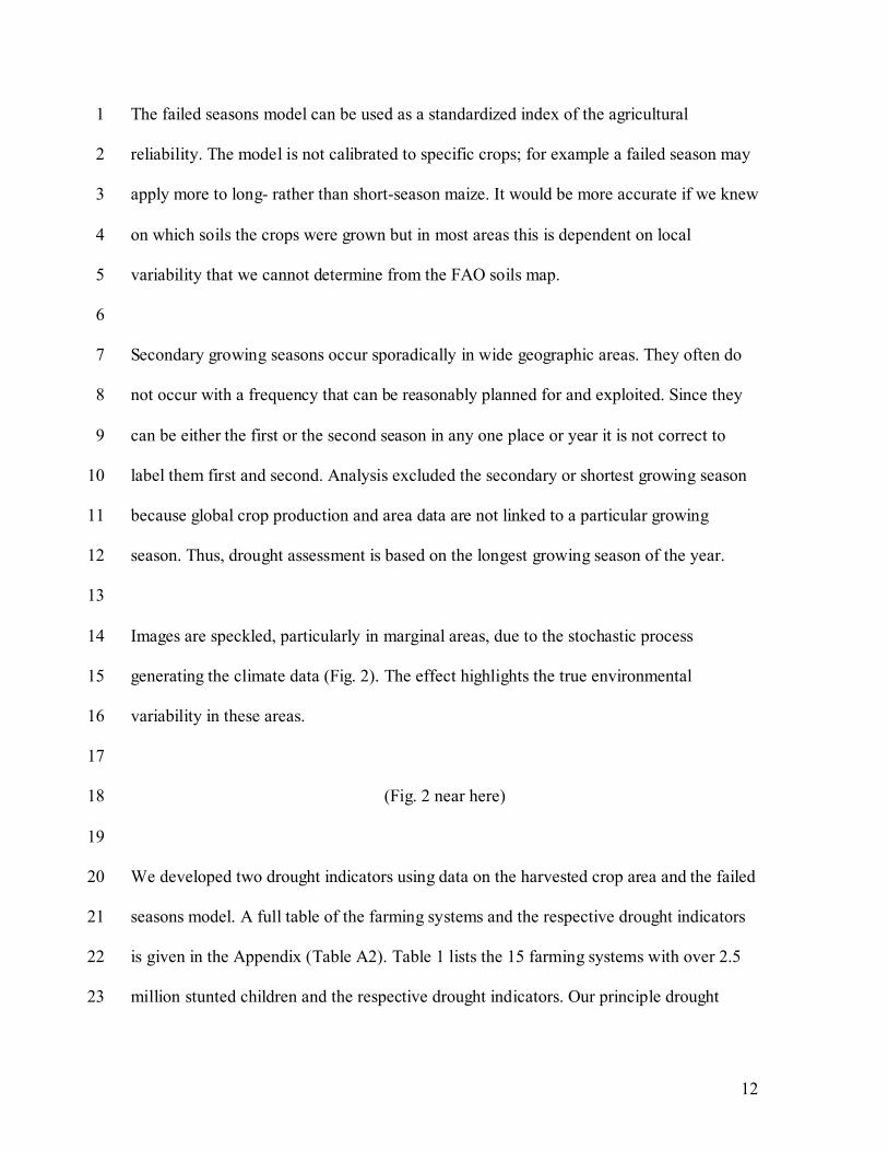
The failed seasons model can be used as a standardized index of the agricultural 1

reliability. The model is not calibrated to specific crops; for example a failed season may 2

apply more to long- rather than short-season maize. It would be more accurate if we knew 3

on which soils the crops were grown but in most areas this is dependent on local 4

variability that we cannot determine from the FAO soils map. 5

6

Secondary growing seasons occur sporadically in wide geographic areas. They often do 7

not occur with a frequency that can be reasonably planned for and exploited. Since they 8

can be either the first or the second season in any one place or year it is not correct to 9

label them first and second. Analysis excluded the secondary or shortest growing season 10

because global crop production and area data are not linked to a particular growing 11

season. Thus, drought assessment is based on the longest growing season of the year. 12

13

Images are speckled, particularly in marginal areas, due to the stochastic process 14

generating the climate data (Fig. 2). The effect highlights the true environmental 15

variability in these areas. 16

17

(Fig. 2 near here) 18

19

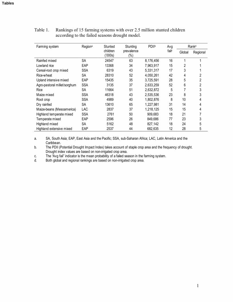
We developed two drought indicators using data on the harvested crop area and the failed 20

seasons model. A full table of the farming systems and the respective drought indicators 21

is given in the Appendix (Table A2). Table 1 lists the 15 farming systems with over 2.5 22

million stunted children and the respective drought indicators. Our principle drought 23

13

indicator, labelled “Potential Drought Impact Index” in the table, is a reflection of the 1

expected loss of production due to drought. This indicator is derived by multiplying the 2

area of rainfed food staple crops by the probability of a failed season. An example of two 3

hypothetical grid cells illustrate its calculation: 4

Rainfed staple

crop area

(ha)

Mean probability of

a failed season

(%)

Potential drought

impact index

Grid cell no.1 1000 60 600

Grid cell no. 2 3000 40 1200

5

(Table 1 near here) 6

7

The index accounts for the scale of staple food crop production weighted by the 8

probability of a failed season. Some form of drought can occur in all farming systems. In 9

systems where the probability of drought is low, the index may still be high if the 10

cultivated area is large. For example, the intensive mixed system in Latin America covers 11

relatively well-watered areas that are less prone to drought. But because the cultivated 12

area of this system is extensive, the potential impacts of droughts when they do occur can 13

be severe. 14

15

The mean probability of a failed season within the farming system region is a second 16

drought indicator, labelled “Avg fail” in Table 1. The value was derived by averaging the 17

probability of a failed season (Fig. 2) over all the pixels in each of the 63 farming systems 18

14

(Fig. 1). Within some systems, some areas are very dry or experience temperature 1

extremes that render them unsuitable for crop growth. Those pixels falling into this 2

category we excluded from the calculation of the mean probability of a failed season. 3

This indicator locates the most drought-prone and marginal environments. As might be 4

expected, many of the systems with high values have very little cultivated area. 5

6

Our study also assessed the distribution of drought frequencies within the farming 7

systems to better understand the heterogeneity of drought conditions across those regions 8

and where the mean probability of failed seasons could be biased by a few large or small 9

drought frequency values. The assessment also allowed us to identify the mix of crops 10

under different drought frequency conditions across the farming systems. We developed 11

cumulative frequency curves that show the extent of areas under all probabilities of failed 12

seasons. The curves are discussed below in the results section. 13

14

3. Results 15

16

3.1. Population and stunted children by farming system 17

18

The study area includes 5 billion of the planet’s 6 billion people (see Appendix, Table 19

A1). About 60% of these 5 billion people live in rural areas and 40% in urban areas. The 20

total number of stunted children is 184.3 million, a figure that corresponds well with the 21

World Health Organization’s estimate of 181.9 million stunted children in developing 22

countries in the year 2000 (WHO, 2000). 23

15

Table A1 (see Appendix) shows the average prevalence of stunting within the farming 1

systems. Since this figure combines all the sub-national administrative districts in a 2

farming system, high prevalence values reflect serious malnutrition throughout the 3

region. Of the top 20 systems, in terms of the absolute number of stunted children, only 4

one has a stunting prevalence below 34% (i.e., the temperate mixed system of East Asia 5

and the Pacific, 26%). 6

7

Rural population data also indicate that the systems with high numbers of stunted 8

children have high rural populations. Unfortunately, no global data set distinguishes 9

between urban and rural stunting, potentially biasing our results towards farming systems 10

that include large cities. 11

12

The total number and the prevalence (or percentage) of stunted children agree reasonably 13

well. High stunting prevalence coincides with high absolute numbers of stunted children. 14

Farming systems with high prevalence of stunting, however, have a wide range of 15

absolute figures. Of the top 10 farming systems according to absolute numbers of stunted 16

children, four systems are in South Asia; and three each are in sub-Saharan Africa and 17

East Asia and the Pacific. In terms of stunting prevalence, 8 of the top 10 systems are in 18

South Asia, with the remaining two in sub-Saharan Africa. 19

20

16

3.2. Drought 1

2

The 10 systems in which the potential impact of drought on the production of staple crops 3

is the largest are found in South Asia (3), sub-Saharan Africa (4), East Asia (2) and Latin 4

America (1) (Table A2, Appendix). The next group of 10 systems is dominated by five 5

Latin American systems, added to four other systems from the three regions in the first 6

group and an additional system in Eastern Europe and Central Asia. The remaining 43 7

systems in the ranking are varied in their regional composition. Systems in the Middle 8

East and North Africa tend to be found in the lower half of the ranking, reflecting the 9

smaller cultivated area in these regions. The bottom third of the list is made up of systems 10

that are marginal for cropping. Although these areas are drought prone, they have 11

insufficient cultivated area to rank high on the list. In other words, people usually 12

cultivate very little where drought is a frequent problem; because of this we emphasized 13

target areas where many people can and do grow crops and where drought is a major 14

problem affecting food security. 15

16

The values for mean probability of a failed season show a wide distribution throughout 17

the list of 63 systems. The top third of Table A2, sorted by the potential drought impact 18

index, includes a wide range of values. Some systems in the top third of the table have 19

relatively low mean values of the probability of a failed season. For example, the root 20

crop system in sub-Saharan Africa has a high potential drought impact index, indicating 21

large areas susceptible to drought but a relatively low drought intensity value (mean 22

failure) of eight. Even though droughts may be relatively infrequent compared to other 23

17

systems, the large cultivated area of the root crop system in sub-Saharan generates higher 1

losses to production. The middle and bottom thirds of the table have higher probability of 2

failed seasons, including a few farming systems with very high values. The highest values 3

in these two groups are associated with arid farming systems with a small aggregate of 4

cultivated areas. For example, the sparse arid system in sub-Saharan Africa has a 94% 5

probability of failed seasons. This system occurs in the Kalahari Desert and has very little 6

area under cultivation. 7

8

3.3.The spatial variability of drought frequencies within farming systems 9

10

The incidence and frequency of drought varies within individual farming systems, 11

ranging from completely absent to always present. Figs. 3 and 4 show the distribution of 12

drought in four important regions of the developing world. (Cumulative frequency curves 13

for each of the 63 farming systems in the entire developing world can be found at 14

http://gisweb.ciat.cgiar.org/drought/freqcurves.htm.) The driest systems have large areas 15

where the probability of a failed season is high. Well-watered systems have small areas 16

with a high probability of a failed season. At these two extremes, the farming systems 17

rely on fewer crops. Not surprisingly, high value and perennial systems are all found in 18

well-watered areas, while pastoral systems are found in the drier areas. Farming systems 19

that have values with a wide range of failed seasons rely on a greater number of crops. 20

These high poverty, priority systems all show moderate to severe drought risk in between 21

the extremes. 22

23

18

Figs. 3 and 4 show the cumulative frequencies of failed seasons of selected highest-1

poverty farming systems in the context of their respective regions. With the exception of 2

the South Asian rice system, all show a wide range of drought frequency as evidenced by 3

the gently sloping curves. The curves closer to 45 degrees show more varied 4

environments. Farmers in these high-poverty systems are therefore attempting to cope 5

with a range of drought regimes; and this is probably the reason for the diversity of 6

cropping in these systems. 7

8

(Figs. 3 and 4 near here) 9

10

3.4. Combination of poverty, crops and drought indicators 11

12

Poverty and drought are a combined problem in Latin America and the Caribbean, sub-13

Saharan Africa, South Asia and East Asia (Table A2). These regions are discussed in 14

greater detail below. Farming systems in Eastern Europe and Central Asia and in the 15

Middle East and North Africa, generally have fewer poor and less cultivated areas 16

susceptible to drought. While these regions do suffer from drought combined with 17

poverty, they are relatively less important in the context both of population and cultivated 18

area. 19

20

Table 2 shows poverty and drought in the farming systems of the region of Latin America 21

and the Caribbean. The maize-bean system in Mexico and Central America stands out, 22

with 2.8 million stunted children, global drought ranking of 15 and regional drought 23

19

ranking of 4. The second in the ranking is coastal plantation mixed, a system that follows 1

much of the coast of northern South America, Central America and Mexico. This system 2

has high numbers of urban population related to the port cities on the coast. The third, the 3

irrigated system, is found in northern Mexico and along the Peruvian coast. This system 4

also has high urban population, including one of the region’s largest cities, Lima, Peru. 5

The fourth, dryland mixed, is often considered to be particularly drought prone but it 6

ranks in the middle third of the global ranking of farming systems according to drought. 7

While some of the remaining systems in Latin America have high drought rankings, they 8

all have relatively fewer numbers of stunted children compared to other farming systems. 9

Overall, Latin America and the Caribbean conforms to the accepted view that the region 10

is less poor than Africa and Asia and suffers less from drought. 11

12

(Table 2 near here) 13

14

Sub-Saharan Africa, the Middle East and North Africa suffer more from poverty and 15

drought: each of the poorest top 10 systems has more than 2 million stunted children 16

(Table 3). Four of these systems are in the top 10 globally in the crop drought rankings. 17

The cereal root crop and maize mixed systems, each with 6.3 million stunted children, 18

span the southern portion of the Sahel and a large part of East Africa and have high rural 19

populations. The root crop system has a high number of stunted children (5 million), even 20

though drought intensity is relatively low. The other notable system in this region is agro-21

pastoral millet-sorghum, a Sahel system with more than 3 million stunted children and 22

high drought intensity. 23

20

1

(Table 3 near here) 2

3

Areas of high drought risk in Asia have even higher numbers of stunted children (Table 4

4). Five of these systems each has more than 10 million stunted children. Five of the top 5

six drought systems are also the top five systems with stunted children. The rainfed 6

mixed system in South Asia stands out, with the second highest stunting value and the 7

highest global drought ranking. The rice-wheat system in South Asia has the highest 8

number of stunted children and the fourth highest drought ranking. The lowland rice 9

system in East Asia and the Pacific has the second highest drought index but less than 10

half as many stunted children compared to the South Asian rice-wheat system. These 11

three Asian systems are marked by large populations with large cultivated areas. The 12

upland intensive mixed system of East Asia and the Pacific has somewhat lower poverty 13

and drought figures compared to the top two South Asian systems but these are still 14

among the top rankings of the 63 systems. The Asian systems rank very high for poverty 15

and drought throughout their top 10. 16

17

(Table 4 near here) 18

19

Poverty and drought are more severe in the farming systems of Asia and Africa, with 20

notably lower severity in Latin America. Table 5 shows the top 15 farming systems 21

ranked by the absolute number of stunted children. Each of these systems has more than 22

2.5 million stunted children, a number we chose as a threshold for inclusion here because 23

21

these systems rely more heavily on staple crops. The values just below 2.5 million in 1

Table A1 are mostly livestock-based systems. Below these, the number of stunted 2

children begins to decrease substantially. 3

4

(Table 5 near here) 5

6

The main crops of the farming systems with high levels of poverty and drought are also 7

shown in Table 5. Each of these crops covers at least 5% of the total cultivated area in 8

each respective farming system (Table 6). This list suggests that poor farmers in drought-9

prone areas rely largely on 12 crops: 10

11

• Rice • Millet • Cassava

• Wheat • Sorghum • Sweet potato

• Chickpea • Groundnut • Bean

• Maize • Cowpea • Barley

12

The drought ranking of the 15 systems shown in Table 5 are all within or near the top 13

third of the 63 farming systems globally. Nine of these 15 systems are in the top 10 in 14

terms of their drought ranking. Only the East Asia temperate mixed system (drought rank 15

= 23) and the East Asia highland extensive mixed system (drought rank = 28) did not fall 16

into the top third of the 63 systems. 17

18

22

4. Conclusions 1

2

This assessment of poverty, crops and drought suggests that 15 farming systems should 3

be given high priority for agricultural research and development (Table 5 and Fig. 5). 4

These systems account for substantial populations of the poor, including over 70% of 5

stunted children in the world. The 15 systems have large areas of cultivated lands 6

susceptible to drought. Land use and the agricultural economy in these systems rely 7

largely on just 12 crops. 8

9

(Fig. 5 near here) 10

11

With few exceptions, the poorest, most drought-susceptible systems have diverse 12

environments and farmers have developed effective mechanisms to cope with risk. These 13

farmers cope through diversity of livelihoods, including livestock. Judicious employment 14

of improved crops may well be successful if the varieties can fit into such diverse and 15

risky systems. 16

17

The databases used and developed in this study have great potential for research and 18

priority-setting for developing country agriculture. Our assessment used criteria that 19

would help focus on a reasonable number of regions and crops that could be given 20

priority for investment in agricultural research and development. These criteria could be 21

easily modified to reflect other priorities than those developed in the study to date. 22

23

23

The aggregate scale of the analysis limits the results of this study. Future work could 1

include other poverty indicators and poverty analysis at finer geographic resolutions 2

within the farming systems. Further work should develop crop-specific drought models 3

that distinguish the main drought types according to the crop cycle (establishment, around 4

flowering and terminal) in order to provide more detailed information to crop 5

improvement programmes. This analysis excluded assessment of factors within farming 6

systems such as variety adoption and the potential to use agricultural technology. Nor did 7

we make economic assessments to estimate the potential impact of focusing on the 8

priority crops and systems identified in the study. While further research could 9

complement the results obtained here, this study provides an initial assessment of the 10

previously bypassed poor that face high drought risk and the principal crops on which 11

they depend. 12

13

Acknowledgments 14

15

We thank Elizabeth Barona and German Lema for their assistance in developing the 16

spatial database used in this analysis. 17

18

References 19

20

Balk, D., Storeygard, A., Levy, M., Gaskell, J., Sharma, M., Flor, R., 2005. Child hunger 21

in the developing world: An analysis of environmental and social correlates. Food Policy. 22

30, 568-583. 23

24

CGIAR (Consultative Group on Internacional Agricultural Research), 2000. Charting the 1

CGIAR’s future: A new vision for 2010. URL: 2

http://www.Rimisp.lc/cg2010b/doc4.html#_ftnl. Accessed on 15 August 2005. 3

4

CIESIN (Center for International Earth Science Information Network), 2005. Global 5

subnational infant mortality rates [dataset]. Columbia University, Palisades, NY. URL: 6

http://www.ciesin.columbia.edu/povmap/ds_global.html. Accessed on 1 November 2006. 7

8

CIESIN (Center for International Earth Science Information Network), 2006. Where the 9

poor are: An atlas of poverty. Columbia University, Palisades, NY. URL: 10

http://www.ciesin.columbia.edu/povmap/. Accessed on 1 November 2006. 11

12

CIESIN (Center for International Earth Science Information Network), Columbia 13

University and CIAT (Centro Internacional de Agricultura Tropical), 2004. Gridded 14

Population of the World (GPW), Version 3. Columbia University, Palisades, NY. URL: 15

http://beta.sedac.ciesin.columbia.edu/gpw. Accessed on 1 November 2006. 16

17

Dixon, J., Gulliver, A., Gibbon, D., 2001. Farming Systems and Poverty: Improving 18

Farmers’ Livelihoods in a Changing World. FAO and World Bank, Rome and 19

Washington DC. 20

21

Evenson R., Gollin, D., 2003. Assessing the impact of the Green Revolution, 1960-2000. 22

Science 300, 758-762. 23

25

FAO (Food and Agriculture Organization), 2003. Chronic undernutrition among children: 1

An indicator of poverty. Poster and unpublished data set. FAO, Rome. 2

3

FAO (Food and Agriculture Organization), 2005. The State of Food Insecurity in the 4

World. FAO, Rome. 5

6

FAO (Food and Agriculture Organization), 2006. Agro-MAPS: A global spatial database 7

of agricultural land-use statistics aggregated by sub-national administrative districts. 8

URL: http://www.fao.org/landandwater/agll/agromaps/interactive/index.jsp. FAO, Rome. 9

10

Freebairn, D., 1995. Did the Green Revolution concentrate incomes? A quantitative study 11

of research reports. World Develop. 23(2), 265-279. 12

13

Gryseels, G., De Wit, C.T., McCalla, A., Monyo, J., Kassam, A., Crasswell, E., 14

Collinson, M., 1992. Setting agricultural research priorities for the CGIAR. Agric. Syst. 15

40, 59-103. 16

17

Jones, P.G., 1987. Current availability and deficiencies data relevant to agro-ecological 18

studies in the geographical area covered in IARCS. In: Bunting, A.H. (Ed.), Agricultural 19

Environments: Characterisation, Classification and Mapping. CAB International, 20

Wallingford, Great Britain, pp. 69-82. 21

22

26

Jones, P.G., Thornton, P.K., 2000. MarkSim: Software to generate daily weather data for 1

Latin America and Africa. Agron. J. 93, 445-453. 2

3

Jones, P.G., Thornton, P.K., Diaz, W., Wilkens, P.W., 2002. MarkSim, Version 1. A 4

computer tool that generates simulated weather data for crop modelling and risk 5

assessment. Centro Internacional de Agricultura Tropical (CIAT) CD-ROM series. Cali, 6

Colombia: CD-ROM + Guide, 87 pp. 7

8

Keig, G., McAlpine, J.R., 1974. A computer system for analysis of soil moisture regimes 9

from simple climatic data. Tech. Memo 74/4. Division of Land Research, Commonwealth 10

Scientific and Industrial Research Organisation, Canberra, Australia. 11

12

Linacre, E., 1977. A simple formula for estimating evaporation rates in various climates, 13

using temperature data alone. Agric. Meteorol. 18, 409-424. 14

15

Shah, M., Strong, M., 1999. Food in the 21st Century: From Science to Sustainable 16

Agriculture. World Bank, Washington DC. 17

18

UNDP (United Nations Development Programme), 2006. Human development report, 19

2006. Beyond scarcity: Power, poverty and the global water crisis. URL: 20

http://hdr.undp.org/hdr2006/ Accessed on 16 April 2007. 21

22

27

You, L., Wood, S., 2006. An entropy approach to spatial disaggregation of agricultural 1

production. Agric. Syst. 90, 329-347. 2

3

WHO (World Health Organization), 2000. Global database on child growth and 4

malnutrition: Forecast of trends. Document WHO/NHD/00.3, Geneva. 5

6

World Bank, 2004. Dramatic decline in global poverty, but progress uneven. URL: 7

http://web.worldbank.org/WBSITE/EXTERNAL/TOPICS/EXTPOVERTY/-8

0,,contentMDK:20195240~pagePK:148956~piPK:216618~theSitePK:336992,00.html. 9

Accessed on 7 September 2006. 10

1

Figure Legends Fig. 1. The sixty-three farming systems used for the analysis (from Dixon et al., 2001). Fig. 2. Modelled percentage of failed seasons due to drought in the study areas. Fig. 3. The proportion of area within each farming system experiencing at least a given

number of failed seasons in a 100-year period for (A) Latin America and the Caribbean and (B) sub-Saharan Africa. Systems represented by solid lines are among the 15 systems of the world with more than 2.5 million stunted children.

Fig. 4. The proportion of area within each farming system experiencing at least a given

number of failed seasons in a 100-year period for (A) South Asia and (B) East Asia and the Pacific. Systems represented by solid lines are among the 15 systems of the world with more than 2.5 million stunted children.

Fig. 5. Priority systems in Latin America and the Caribbean (LAC), sub-Saharan Africa

(SSA), South Asia (SA) and East Asia (EA) with over 70% of all stunted children and substantial drought.

All figures

2

Fig. 1.

3

Fig. 2.

4

(A) Latin America and the Caribbean

0.0

0.1 0.2

0.3

0.4

0.5

0.6

0.7

0.8

0.9

1.0

0 10 20 30 40 50 60 70 80 90 100 x = failed seasons in 100 years

Prop

ortio

n of

farm

ing

syste

ms e

xper

ienc

ing

at le

ast x

faile

d se

ason

s in

100 y

r

Irrigated F orest-based Maize-bean

Extens ive dryland mixed Intensive mixed

(B) Sub-Saharan Africa

0.0 0.1 0.2 0.3 0.4 0.5 0.6 0.7 0.8 0.9 1.0

0 20 40 60 80 100 x = failed seasons in 100 years

Prop

ortio

n of

farm

ing

syst

ems e

xper

iencin

g at

lea

st x

faile

d se

ason

s in

100

yr

Tree crop Sparse arid Highland temperate mixed Root crop Cereal root crop Maize mixed Agropastoral millet/sorghum Pastoral Highland perennial

Figs. 3A and 3B.

5

(A) South Asia

0.0 0.1 0.2 0.3 0.4 0.5 0.6 0.7 0.8 0.9 1.0

0 20 40 60 80 100 x = failed seasons in 100 years

Prop

ortio

n of

farm

ing

syst

em ex

perie

ncin

g at

le

ast x

faile

d se

ason

s in

100

yr

Rice Coastal artisanal fishing Rice wheat Highland mixed Rainfed mixed Dry rainfed Pastoral Sparse arid

(B) East Asia and the Pacific

0.0 0.1 0.2 0.3 0.4 0.5 0.6 0.7 0.8 0.9 1.0

0 10 20 30 40 50 60 70 80 90 100 x = failed seasons in 100 years

Prop

ortio

n of f

armi

ng sy

stem

s exp

erien

cing

at lea

st x

failed

seas

ons i

n 10

0 yr

Lowland rice Tree crop mixed Root tuber Upland intensive mixed Highland extensive mixed Pastoral Sparse arid

Figs. 4A and 4B.

6

Fig. 5.

1

Table 1. Rankings of 15 farming systems with over 2.5 million stunted children according to the failed seasons drought model.

Rankd Farming system Regiona Stunted

children (’000s)

Stunting prevalence

(%)

PDIIb Avg failc Global Regional

Rainfed mixed SA 24547 63 8,176,456 16 1 1 Lowland rice EAP 13368 34 7,963,917 15 2 1 Cereal-root crop mixed SSA 6319 43 5,331,317 17 3 1 Rice-wheat SA 28310 52 4,050,261 42 4 2 Upland intensive mixed EAP 15435 35 3,725,591 28 5 2 Agro-pastoral millet/sorghum SSA 3135 37 2,633,259 52 6 2 Rice SA 11664 51 2,632,872 5 7 3 Maize mixed SSA 46318 43 2,535,536 23 8 3 Root crop SSA 4989 40 1,802,876 8 10 4 Dry rainfed SA 13610 65 1,227,981 31 14 4 Maize-beans (Mesoamerica) LAC 2837 37 1,218,125 15 15 4 Highland temperate mixed SSA 2761 50 909,683 18 21 7 Temperate mixed EAP 2596 26 849,686 77 23 3 Highland mixed SA 5162 48 827,142 18 24 5 Highland extensive mixed EAP 2537 44 682,635 12 28 5

a. SA, South Asia; EAP, East Asia and the Pacific; SSA, sub-Saharan Africa; LAC, Latin America and the

Caribbean. b. The PDII (Potential Drought Impact Index) takes account of staple crop area and the frequency of drought.

Drought index values are based on non-irrigated crop area. c. The “Avg fail” indicator is the mean probability of a failed season in the farming system. d. Both global and regional rankings are based on non-irrigated crop area.

Tables

2

Table 2. The top 10 systems in Latin America, both regional and global, by stunted children and failed season rankings based on expected loss to production for non-irrigated areas.

Failed Farming system Regiona Stunted children

(’000s) Global Regional Maize-beans CA 2837 15 4 Plantation mixed Coastal 1692 9 1 Irrigated LAC 809 38 10 Dryland mixed LAC 684 22 7 High altitude mixed Central Andes 600 42 11 Forest-based LAC 464 31 8 Intensive highland mixed N. Andes 380 37 9 Intensive mixed LAC 309 11 2 Extensive mixed Cerrados-llanos 225 19 6 Cereal-livestock Campos 221 16 5

a. CA, Central America; LAC, Latin America and the Caribbean.

3

Table 3. The top 10 systems in sub-Saharan Africa (SSA) and the Middle East and North Africa (MENA) by stunted children and both regional and global failed seasons rankings, based on expected loss to production for non-irrigated areas.

Failed Farming system Region Stunted children

(’000s) Global Regional Cereal-root crop SSA 6319 3 1 Maize mixed SSA 6318 8 3 Root crop SSA 4989 10 4 Forest-based SSA 3243 18 6 Pastoral SSA 3230 27 9 Agro-pastoral millet-sorghum SSA 3135 6 2 Highland temperate mixed SSA 2761 21 7 Highland perennial SSA 2625 26 8 Sparse arid MENA 2417 56 5 Tree crop SSA 2291 13 5

4

Table 4. The top 10 systems in South Asia (SA) and East Asia and the Pacific (EAP) by stunted children and both regional and global failed seasons rankings.

Failed Farming system Region Stunted children

(’000s) Global Regional Rice-wheat SA 28310 4 2 Rainfed mixed SA 24547 1 1 Upland intensive mixed EAP 15435 5 2 Lowland rice EAP 13368 2 1 Rice SA 11664 7 3 Highland mixed SA 5162 24 5 Sparse (forest) EAP 4360 36 6 Dry rainfed SA 3610 14 4 Tree crop mixed EAP 3106 25 4 Temperate mixed EAP 2596 23 3

5

Table 5. Fifteen farming systems with over 2.5 million stunted children, with global (fsg) and regional (fsr) farming systems rankings according to potential drought impact index.

Farming systema Stunted

children (’000s) Cropsa fsg fsr

SA rice wheat 28310 Rice, pulses (chickpea) millet, wheat, maize, bean 4 2 SA rainfed mixed 24547 Rice, millet, sorghum, chickpea, bean, groundnut,

maize, wheat 1 1

EAP upland intensive mixed 15435 Maize, rice, wheat, sweet potato, potato, bean 5 2 EAP lowland rice 13368 Rice, maize, wheat, sweet potato, groundnut 2 1 SA rice 11668 Rice, pulses (chickpea) 7 3 SSA cereal-root 6319 Sorghum, millet, pulses (cowpea), maize, groundnut,

cassava 3 1

SSA maize mixed 6318 Maize, cassava, sorghum, pulses, groundnut, millet, bean, sweet potato

8 3

SA highland mixed 5162 Rice, maize, wheat, potato, groundnut, pulses (chickpea)

24 5

SSA root 4989 Maize, cassava, rice, sweet potato, cowpea, sorghum, groundnut, bean

10 4

SA dry rainfed 3610 Sorghum, millet, chickpea, groundnut, bean 14 4 SSA agro-pastoral millet/sorghum 3135 Millet, sorghum, pulses groundnut, maize 6 2 LAC maize-beans 2837 Maize, bean, sorghum 15 4 SSA highland temperate mixed 2761 Maize, wheat, sorghum, barley, millet, pulses 21 7 EAP temperate mixed 2596 Maize, wheat, potato, groundnut, millet 23 3 EAP highland extensive mixed 2486 Rice, maize, wheat, potato, groundnut, pulses 28 5 a. SA, South Asia; SSA, sub-Saharan Africa; LAC, Latin America and the Caribbean; EAP, East Asia and the

Pacific. b. Crops appearing for the first time in the list are in italics.

6

Table 6. The proportional area (%) of each crop in the agricultural systems with more than 2.5 million stunted children. Areas shaded in grey have more than 5% of the area in their respective system.

Farming system Regiona BANPb Barley Bean Cassava Groundnut Maize Millet OPULc Potato Rice Sorghum SWPd Wheat Maize-beans (Mesoamerica) LAC 0.017 0.008 0.161 0.002 0.007 0.668 0.000 0.009 0.005 0.009 0.098 0.000 0.016 Cereal-root crop mixed SSA 0.007 0.001 0.032 0.052 0.093 0.125 0.224 0.126 0.004 0.045 0.255 0.033 0.002 Maize mixed SSA 0.000 0.004 0.057 0.091 0.063 0.461 0.059 0.073 0.023 0.024 0.075 0.056 0.016 Root crop SSA 0.004 0.000 0.060 0.222 0.074 0.275 0.030 0.027 0.002 0.117 0.074 0.117 0.000 Agro-pastoral millet/sorghum SSA 0.003 0.002 0.010 0.018 0.125 0.065 0.377 0.146 0.001 0.009 0.238 0.006 0.001 Highland temperate mixed SSA 0.000 0.166 0.040 0.009 0.008 0.251 0.062 0.051 0.008 0.003 0.168 0.016 0.218 Rice-wheat SA 0.002 0.009 0.053 0.000 0.011 0.101 0.109 0.118 0.023 0.428 0.038 0.001 0.106 Rainfed mixed SA 0.002 0.002 0.109 0.001 0.071 0.066 0.170 0.150 0.001 0.205 0.166 0.001 0.056 Rice SA 0.015 0.001 0.011 0.011 0.020 0.009 0.038 0.100 0.021 0.722 0.023 0.003 0.026 Highland mixed SA 0.009 0.023 0.026 0.007 0.007 0.196 0.081 0.117 0.021 0.281 0.013 0.002 0.217 Dry rainfed SA 0.001 0.000 0.053 0.000 0.064 0.021 0.327 0.132 0.001 0.020 0.358 0.000 0.023 Upland intensive mixed EAP 0.012 0.009 0.060 0.035 0.045 0.267 0.017 0.021 0.062 0.249 0.005 0.080 0.137 Lowland rice EAP 0.012 0.012 0.043 0.041 0.060 0.166 0.004 0.009 0.026 0.379 0.004 0.097 0.148 Temperate mixed EAP 0.000 0.010 0.037 0.005 0.070 0.532 0.057 0.026 0.080 0.002 0.041 0.049 0.093 Highland extensive mixed EAP 0.004 0.008 0.041 0.012 0.056 0.144 0.022 0.055 0.094 0.427 0.002 0.015 0.119 a. LAC, Latin America and the Caribbean; SSA, sub-Saharan Africa; SA, South Asia; EAP, East Asia and the Pacific. b. BANP, combined category of bananas and plantain. c. OPUL, combined category of cowpea, chickpea, lentils and other pulses. d. SWP, sweet potato.

Appendices, for posting additional data to web siteClick here to download Supplementary material for on-line publication only: Appendix, Targeting PovDrou_Apr25.doc