1

Photoelectron-Auger electron coincidence spectroscopy of free molecules Volker Ulrich1, Silko Barth1, Toralf Lischke1, Sanjeev Joshi1, Tiberiu Arion1, Melanie Mucke1, Marko

Förstel1,2, Alex M. Bradshaw1,3, and Uwe Hergenhahn1,*

1. Max-Planck-Institut für Plasmaphysik, Euratom Association, Boltzmannstr. 2, 85741 Garching, Germany

2. Max-Planck-Institut für Kernphysik, Saupfercheckweg 1, 69117 Heidelberg, Germany

3. Fritz-Haber-Institut der Max-Planck-Gesellschaft, Faradayweg 4-6, 14195 Berlin, Germany

Dedicated to the memory of Professor Kai Siegbahn

Abstract

Photoelectron-Auger electron coincidence spectroscopy probes the dicationic states produced by

Auger decay following the photoionization of core or inner valence levels in atoms, molecules or

clusters. Moreover, the technique provides valuable insight into the dynamics of core hole decay. This

paper serves the dual purpose of demonstrating the additional information obtained by this technique

compared to Auger spectroscopy alone as well as of describing the new IPP/FHI apparatus at the

BESSY II synchrotron radiation source. The distinguishing feature of the latter is the capability to

record both the photoelectron and Auger electron with good energy and angle resolution, for which

purpose a large hemispherical electrostatic analyser is combined with several linear time-of-flight

spectrometers. Results are reported for the K-shell photoionization of oxygen (O2) and the subsequent

K-VV Auger decay. Calculations in the literature for non-coincident O2 Auger spectra are found to be

in moderately good agreement with the new data.

PACS

07.81.+a, 07.85.Qe, 29.30.Dn, 32.80.Hd, 33.80.Eh

* Corresponding author, Mail address: c/o Helmholtz-Zentrum Berlin, Albert-Einstein-Str. 15, 12489 Berlin,

Germany. Electronic address: uwe.hergenhahn@ipp.mpg.de.

2

I. Introduction

Auger decay is widely used as an element-specific probe of material composition, in particular, in

surface analysis [1]. In molecules, the Auger spectrum also contains information about the electronic

and nuclear structure of the final (dicationic) states of the radiationless decay process. Some of the

very first high resolution Auger spectra of molecules can be found in Kai Siegbahn’s second book [2].

The Auger spectrum of an atom of a particular element, characterized by its nuclear charge Z, has a

specific appearance according to the molecular environment in which the atom finds itself. However, a

detailed understanding of the spectra is difficult because of the large number of dicationic states that

are relevant in a molecule [3] and because of the influence of the nuclear dynamics in the decay

process [4][5]. Moreover, the question arises as to whether Auger decay in molecules is a local

process, i.e., whether the initial inner shell vacancy is filled only by valence electrons originating from

the same atom [6][7][8]. A further complication arises for all but the simplest molecules, since the

Auger emission from different atoms of the same sort (i.e. with identical Z) – should they be present –

will overlap. Conventional (non-coincident) electron spectroscopy is typically not able to disentangle

the contributions of such atoms, or of different vibrational levels associated with the same final state.

Electron-electron coincidence spectroscopy has the potential to greatly enhance the amount of

information which can be extracted from photoelectron and Auger electron spectroscopy. In the

following we consider such processes after excitation with small bandwidth soft X-radiation as

provided by undulators at an electron storage ring. Early photoelectron-Auger electron coincidence

experiments were concerned with bulk and adsorbate systems [9][10]; more recent work on bulk

systems has been reviewed by Stefani et al. [11]. Useful comments on the technique and some

pioneering results for free atoms can be found in Ref. [12]. Application of the electron-electron

coincidence technique to free molecules demonstrated the possibility of identifying the contributions

of satellite autoionization to the main KVV Auger spectrum in N2 [13]. Moreover, a study by Viefhaus

et al. [14] showed how the resolution barrier in core level photoelectron spectroscopy dictated by the

natural lifetime broadening can be overcome. This can be understood as follows: the energy balance of

the process reads Efi = hν + E0 − εph − εau, where Efi and E0 are the final (dicationic) and the initial

3

(neutral ground) state energies, εph and εau kinetic energies of the photo- and the Auger electron, and

hν the photon energy. Thus, if the final state is long lived and the bandwidth, with which hν, εph and

εau are selected, is sufficiently low, structures can be discerned in the coincidence spectrum below the

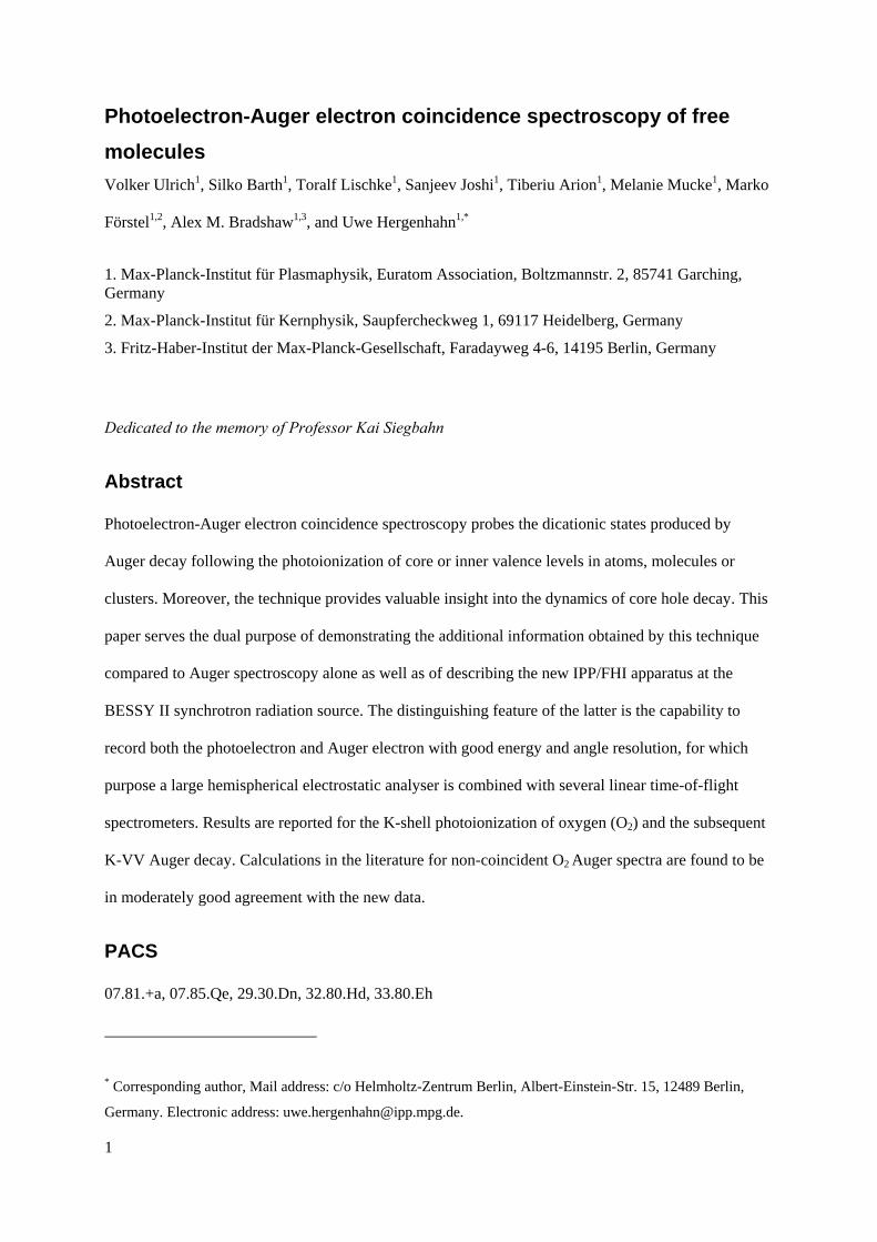
limit of the lifetime broadening (Fig. 1). This may in future enable detailed studies of the nuclear

dynamics in the intermediate (core ionized) state [15][16]; this topic has been of great interest in the

analogous situation of resonant Auger decay. In the latter case, due to the fact that only one electron is

escaping from the molecule, sub-natural resolution has been achieved [17][18] without the need of a

coincidence set-up.

In this article we discuss not only the technique of photoelectron-Auger electron coincidence

spectroscopy but also describe a new apparatus for the detection of electron-electron pairs with

superior energy resolution. The design of the latter is based on the combination of a large electrostatic

hemispherical electron analyser with several medium-sized linear time-of-flight (TOF) spectrometers.

The construction of the apparatus and the details of the data acquisition procedure are first explained,

some principal features of the spectra are then described , and finally some new experimental data for

molecular oxygen are shown. First results obtained with this apparatus (for CO) have been published

elsewhere [19]. Together with the description of our apparatus we also include a critical comparison

with other spectrometers for coincident electron detection.

II. Experimental Set-up

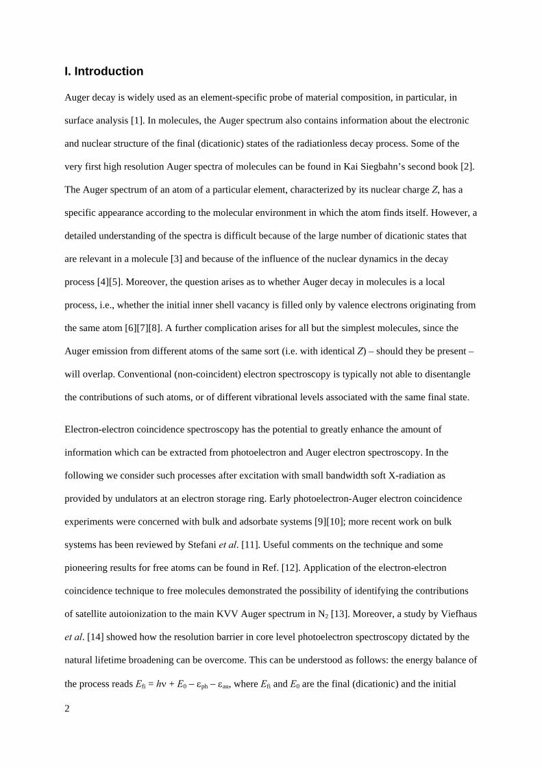
A sketch of the main apparatus parts is shown in Fig. 2. A spherical vacuum chamber [20] holds a

hemispherical analyser of 200 mm nominal radius (Scienta ES 200, [21]) and several TOF

spectrometers. The Scienta analyser has been fitted with a fast position-resolving anode based on a

delay line (Roentdek, Frankfurt, Germany), in order to make it capable of performing coincidence data

acquisition. The properties of this system have been discussed [22]. The Scienta analyser is positioned

at the so-called magic angle of 54.7° with respect to the horizontal. Therefore, with horizontally

linearly polarized radiation, the non-coincident differential cross sections recorded are proportional to

the total cross section within the electric dipole approximation. No such analogous pair of angles is

4

known for two-electron emission. The TOF analysers therefore have been placed at positions which

are convenient from the point of view of the chamber geometry.

All data covered here were recorded at the BESSY II synchrotron radiation source (Berlin, Germany).

The oxygen spectra shown in section IV were measured at the UE52-SGM beamline [23]. This

beamline is equipped with an undulator of the Apple-II type [24], which was set to produce vertically

linearly polarized radiation. The 1200 l/mm grating was used with a resolution selected as 140 meV

(estimated from ray-tracing calculations). The photon energy was set at 551.85 eV, with about ±0.2 eV

calibration uncertainty. Sample gas was leaked into the chamber up to a background pressure of

3 x 10-6 mbar, limited in the first instance by the ratio of true to random coincidences (see below).

A. Time­of­Flight Analysers 

Time-of-flight analysers (TOFs) for electron spectroscopy have been described e.g. by Hemmers et al.,

Feulner et al. and Becker et al. [25][26][27][28]. The decision to use this principle in our set-up was

made because TOFs allow a range of energies to be covered in parallel, with modest construction

effort and at a good energy resolution. Our design consists of a conical drift tube of 110 mm length

which is followed by a second, cylindrical drift tube. The entrance is formed by a spherical diaphragm

(4 mm diameter) at a distance of 30 mm to the interaction zone. Both drift regions can be set to

different electric potentials in order to improve the resolution by retarding or, alternatively, the

transmission for low kinetic energy electrons by accelerating. Often, voltages can be selected such that

electron lens effects formed in the transit regions between the different potentials increase the angular

acceptance, and by that the detected intensity for an energy region of interest. The cylindrical drift

tube is terminated by a copper mesh, and electrons are then accelerated onto a triple microchannel

plate (MCP) stack (MCP outer diameter 34.5 mm). The holder for the MCPs is a simplified version of

the design by Snell et al. [29]. The MCPs can be dismounted from the vacuum chamber independently

of the TOFs themselves. Most conducting parts are made of aluminum, insulating parts of PEEK.

The total length of the drift section (centre of interaction to mesh) can be varied, and amounts to either

228.5 or 268.5 mm. From geometrical considerations of a point-like interaction region a solid angle of

5

acceptance of about 14 msR follows, which is determined both by the MCP active area and the

entrance aperture. In all measurements shown here the shorter drift section was used.

For these analysers, we have demonstrated an energy resolution of 70 meV for photoelectrons of 8 eV

kinetic energy, retarded with -4.5/-7.6 V in the conical and cylindrical section, resp. If detection of

electrons with low kinetic energy is of interest, a positive (acceleration) voltage can be used in the drift

tube, and we have demonstrated a flat transmission function down to at least 0.3 eV with acceleration

values of +1/+2 V. The energy resolution of the analysers is strongly influenced by the effective size

and shape of the interaction region. From geometrical considerations, electrons produced by the

synchrotron radiation (SR) beam along a path length of the order of 10 mm are accepted in the TOFs,

which leads to a degradation of the resolution as electron trajectories from non-central source points

differ in length. This effect is the worse the smaller the angle formed by the TOF and the SR beam.

For an analyser at 45°, a difference of about 4 % in length is estimated. On the other hand, the sample

is formed by an effusive gas jet leaking in via a d = 0.8 mm copper capillary, which leads to a strong

peaking of the gas density at the point where the TOF middle axes intersect [30].

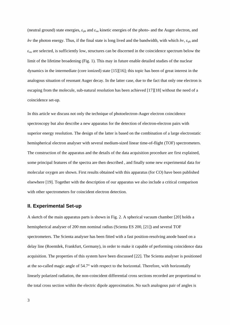
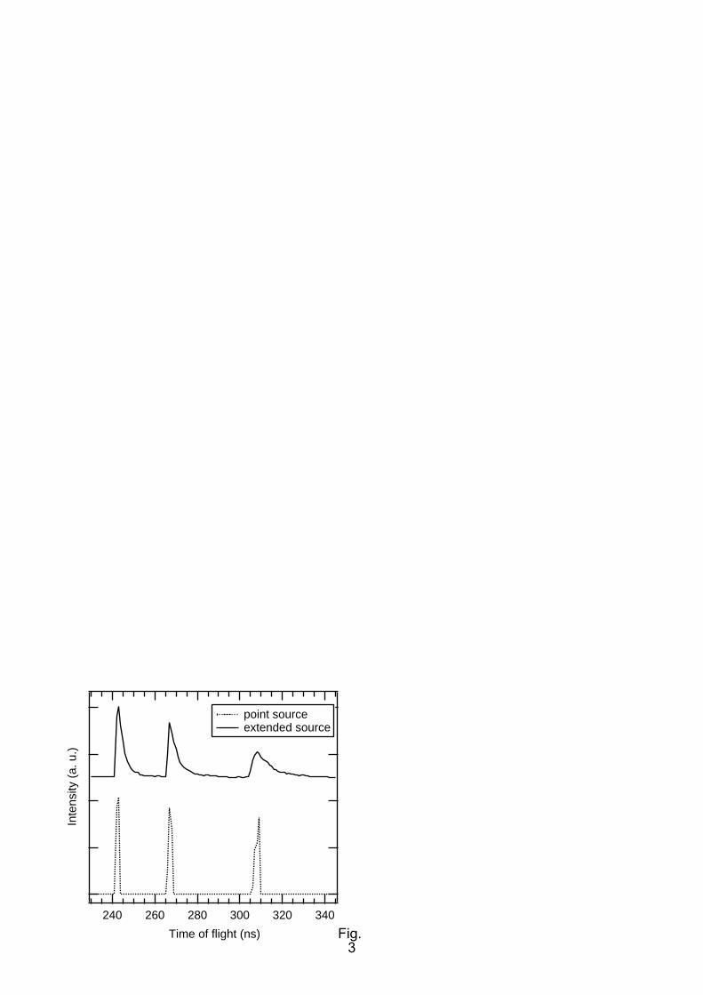
A conservative estimate of the true TOF resolution can be found from ray-tracing simulations of the

electron trajectories, which are presented in Fig. 3. Simulations where carried out with the SimIon 8.0

programme (SIS, Ringoes, NJ. USA). For the simulations, electrons with kinetic energies of 7.7 eV,

8.0 eV and 8.3 eV were considered. Trajectories for 90000 electrons were calculated for each source

point and each kinetic energy, distributed homogeneously in a filled cone with a half angle of 20°. For

consistency, the retarding voltages of the two stages of the spectrometer were set to -4.5/-7.6 V,

similar to the experiment. The simulated spectra present the ideal case of a point-like interaction

region (dotted curve), and the more realistic case of a pencil shaped electron source of 10 mm length,

2 mm diameter and an inclination of the spectrometer with respect to the TOF middle axis of 44.4°

(solid curve). As expected, the resolution of the spectrometer worsens on moving from the ideal case

to realistic conditions, but even then remains better than 70 meV approx. Electronic contributions to

the resolution, such as jitter of the timing signals, were not taken into account in the simulation.

6

The simultaneous operation of several TOF analysers is advantageous, since the true coincidence rate

scales with the solid angle (TOF-Scienta coincidences) or the square of the solid angle (TOF-TOF

coincidences) covered. From geometrical constraints given by the vacuum recipient, including the

Scienta analyser and an expansion chamber to produce free molecular jets and cluster jets [20], the

TOF analysers had to be mounted in a vertical plane, pointing downward (see Fig. 2). Some remarks

concerning angular effects by this choice are in order. Photoelectrons excited by linearly polarized

light normally have a propensity for emission along the polarization axis (positive β parameter) [28].

Synchrotron radiation from conventional beamlines is linearly polarized in the storage ring plane,

which leads to unfavorable detection efficiencies in our geometry. However, the flexibility of the

Apple-II undulator design allows to also produce vertically linearly polarized radiation [24]. In all

studies reported here, this setting was used to increase the number of registered photoelectrons. The

hemispherical analyser by that is not placed at the magic angle anymore. Since it typically is used to

detect the Auger electrons, which in a non-coincident experiment have a rather isotropic angular

distribution, this is less of a concern. For the triply differential cross section in sequential photo-

double-ionization no general picture has emerged so far. Photoelectron-Auger electron coincidence

experiments on atoms suggest that back-to-back emission of the two electrons is favourable when the

photoelectron is emitted along the (linear) polarization axis, but chiral, more complicated angular

correlation patterns have been observed when the photoelectron analyser is moved away from the

polarization direction [12][31][32]. Contrary to those experiments, our apparatus does not allow a

relative rotation of the analysers. Detection of the photoelectrons under a variable angle with respect to

the polarization direction could be achieved by rotating the polarization ellipse of the synchrotron

radiation however, which is possible at some undulators [33]. As our analysers, except for the central

one, are placed outside of the dipole plane, they are sensitive to angular distribution terms from higher

multipole orders in the photon-molecule interaction. Most recent studies for two systems found an

only small influence from this mechanism [34][35].

In the measurements shown here the signals of all TOF analysers were added to increase the

coincidence rate. The 66.6° analyser was not used.

7

B. Data acquisition 

Electron-electron coincidence signals in the two types of analyser could be recorded in a straight-

forward manner when the separation of two successive synchrotron radiation pulses was larger than

the typical time-of-flight for low kinetic energy electrons in the TOF analyser. The latter is of the

order of 300 ns. The use of the single bunch mode of BESSY would then be required to meet this

condition. Due to the small solid angle accepted by the detectors, however, either the number of

accidental coincidences would then be unacceptably large or the time required for data acquisition

would be unpractical. We have therefore chosen to record coincidences during multi-bunch (normal)

operation. Under these conditions, synchrotron radiation is delivered in pulses of 20-30 ps length with

a spacing of 2 ns [36]. A train of 350 electron bunches is followed by a dark gap of 100 ns length, in

the middle of which a single electron bunch is injected, resulting in the so-called hybrid peak [37].

Thus, the non-coincident electron time-of-flight spectra excited by the different bunches overlap and

cannot be disentangled in a simple time-of-flight measurement. Only the spectrum excited by the

hybrid peak can often be separated, and is seen either in the dark gap or on top of a diffuse background

of slow electrons. This serves as a valuable calibration. Typical non-coincident time-of-flight data (for

C 1s emission in CO) are shown in Fig. 4, and will be discussed in the next section.

A schematic diagram of the data acquisition electronics is shown in Fig. 5. In the first version of the

electronics, shown in the figure, only four TDC channels were available. Therefore, signals from all

TOF analysers were multiplexed by OR gates. Signal path lengths for the different analysers were

adjusted to within one ns. In the same way, the four signals from the delay line anode were collected

in two TDC channels. Signal pairs were separated by use of a cable delay in two of the four signal

paths.

For the coincident detection of an electron pair by one of the TOFs and the hemispherical analyser, the

problem of implicit convolution with the BESSY fill pattern can be overcome by referring the TOF

arrival time not to the bunch clock of BESSY, but to the time of electron detection in the

8

hemispherical analyser. Since the latter filters electrons with a selected energy, it can be expected that

these have an approximately fixed time-of-flight in this instrument. In practice, the hemispherical

analyser is set to detect (fast) Auger electrons, such that comparatively large pass energies (typically

75-300 eV) can be used. This helps in the reduction of the time-of-flight spread for the trajectories

within the analyser, as discussed in detail below (see also [22][38][39]). Thus, referring the

photoelectron arrival times to the Auger arrival times allows the experiment to be carried out in multi-

bunch mode, with a greatly improved true-to-random ratio, but at the expense of a slight reduction of

time resolution, and thus energy resolution of the photoelectron.

C. Typical time­of­flight data 

It is instructive to examine some typical data sets. To demonstrate the resolution achieved in the TOF

detectors, we refer first to the C 1s spectrum of CO, as recorded in the first experiments with the new

apparatus [19]. Carbon K-shell photoionization of CO, at a threshold energy of 296.07 eV [40], leads

to a photoelectron spectrum characterized by an easily observed, single vibrational progression with an

energy separation of 304 meV [41]. In our non-coincident TOF spectrum of Fig. 4, the first two

vibrational states are readily separated. The separation of the v' = 2 state is difficult because of the

background from fast electrons in this type of spectrum. A least squares fit of PCI (Post Collision

Interaction) profiles [41][42] to the CO C 1s spectrum in panel 4b) results in a Gaussian (apparatus)

contribution to the linewidth of approx. 100 meV. (A fixed natural linewidth of 95 meV was assumed

[43].) Deconvolution of the monochromator bandpass [19] then results in a spectrometer resolution of

ca. 50 meV only. This resolution can, however, only be achieved in an experiment where the BESSY

bunch clock is used as the stop signal. For coincidence data acquisition, with the Auger arrival times

serving as a stop signal, an additional apparatus broadening for the photoelectron arises, which for the

data shown amounts to about 150 meV. These contributions recombined are in reasonable agreement

with the total photoelectron linewidth of 200 meV quoted in [19].

Due to the higher photon energy and slightly less stringent retardation voltages applied, our new data

on O2 O 1s photoionization and subsequent KVV Auger decay reported below, as well as in Section

IV, show a poorer energy resolution of 260 meV for the non-coincident time-of-flight data and 350

9

meV total photoelectron energy resolution for the coincidence data. Data were recorded in 69000 s of

subsequent acquisition time. Non-coincident count rates were approx. 800 Hz for the Auger spectrum

and 60000 Hz in all TOF analysers added up. Approximately 47000 true coincident events have been

detected, which corresponds to a rate of true coincidences of about 0.7 Hz.

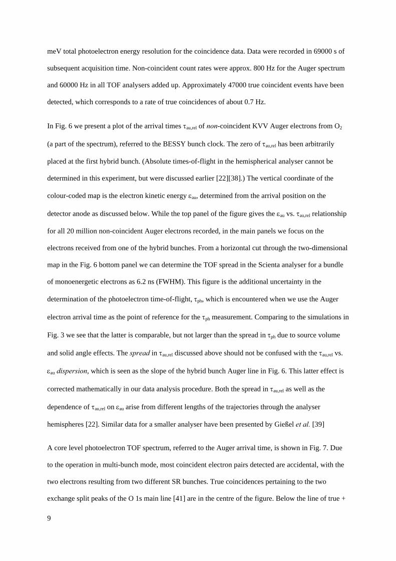
In Fig. 6 we present a plot of the arrival times τau,rel of non-coincident KVV Auger electrons from O2

(a part of the spectrum), referred to the BESSY bunch clock. The zero of τau,rel has been arbitrarily

placed at the first hybrid bunch. (Absolute times-of-flight in the hemispherical analyser cannot be

determined in this experiment, but were discussed earlier [22][38].) The vertical coordinate of the

colour-coded map is the electron kinetic energy εau, determined from the arrival position on the

detector anode as discussed below. While the top panel of the figure gives the εau vs. τau,rel relationship

for all 20 million non-coincident Auger electrons recorded, in the main panels we focus on the

electrons received from one of the hybrid bunches. From a horizontal cut through the two-dimensional

map in the Fig. 6 bottom panel we can determine the TOF spread in the Scienta analyser for a bundle

of monoenergetic electrons as 6.2 ns (FWHM). This figure is the additional uncertainty in the

determination of the photoelectron time-of-flight, τph, which is encountered when we use the Auger

electron arrival time as the point of reference for the τph measurement. Comparing to the simulations in

Fig. 3 we see that the latter is comparable, but not larger than the spread in τph due to source volume

and solid angle effects. The spread in τau,rel discussed above should not be confused with the τau,rel vs.

εau dispersion, which is seen as the slope of the hybrid bunch Auger line in Fig. 6. This latter effect is

corrected mathematically in our data analysis procedure. Both the spread in τau,rel as well as the

dependence of τau,rel on εau arise from different lengths of the trajectories through the analyser

hemispheres [22]. Similar data for a smaller analyser have been presented by Gießel et al. [39]

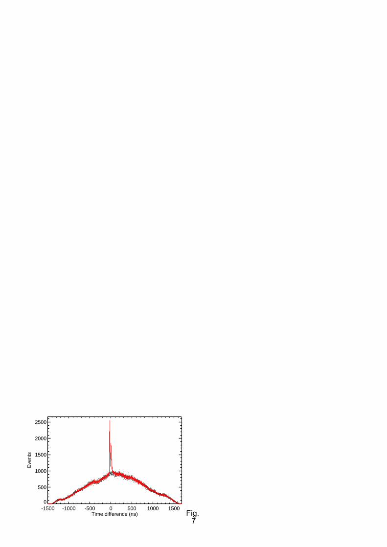
A core level photoelectron TOF spectrum, referred to the Auger arrival time, is shown in Fig. 7. Due

to the operation in multi-bunch mode, most coincident electron pairs detected are accidental, with the

two electrons resulting from two different SR bunches. True coincidences pertaining to the two

exchange split peaks of the O 1s main line [41] are in the centre of the figure. Below the line of true +

10

random coincidences we show an estimate of the random contribution to the signal (dots). This we

calculate from event pairs, in which the two electrons were produced within different revolution

periods of BESSY.

The details of Fig. 7 depend on the settings of the data acquisition hardware. In our experiments, the

BESSY bunch marker signal was used as 'start' for a time-of-flight measurement. Events were then

collected for a period of two full revolutions of the electron beam in the storage ring (approx.

1600 ns). This time is dictated by hardware limitations. If any events were detected, they were then

processed by the TDC firmware while a new measurement cycle was initiated. Thus the measurement

process is practically dead-time free. The true coincidences recorded such appear at small values of the

arrival time difference (independent axis in Fig. 7). The accidental coincidences ideally form a smooth

triangle with a baseline length of twice the revolution period. Its remnant structure results from the

time structure of the BESSY fill pattern. Detailed discussion of the true and accidental coincidence

spectra have been given for similar acquisition schemes [44][45]. Two facts we have experienced in

our work are corroborated in [45]: (i). The net acquisition time cannot be reduced by increasing the SR

flux, or the target density, since the accidental coincidence rate scales quadratically with these factors,

while the true coincidence rate has a linear dependence. The true-to-random ratio therefore becomes

worse, such that the statistical quality of the data recorded in a certain total time T is invariant. A

reasonable trade-off between count rate and true-to-random ratio (RT/RAcc) for the experiments shown

here was found at RT/RAcc of 0.5-2. (ii). Performing our experiment in multi-bunch as opposed to

single-bunch data acquisition reduces the random coincidence count rate perceived for a given rate of

true coincidences by a factor of τbb/( τe F) = 800/20*350/400 = 35, where τbb is the single bunch

period, τe the width of the photoelectron part of the TOF spectrum, and F a factor which corrects for

the incomplete filling of the ring in multibunch operation. F can be written as the number of electron

bunches in a completely filled ring, divided by the actual number of electron bunches.

D. Data analysis 

Due to the use of a position-sensitive anode in our hemispherical analyser, a band of energies centred

around the pass energy (the energy of the central, concentric trajectory) can be monitored

11

simultaneously. Its full width is roughly 10 % of the pass energy. For calibration purposes the Ar

L2,3M2,3M2,3 Auger spectrum was recorded with the same settings as the O2 Auger spectrum, fitted by a

least squares program, and compared to literature data [46]. We have thus been able to correct small

non-linearities of the Scienta energy axis and have determined the energy resolution as 182(10) meV

under the conditions used (pass energy 75 eV, 500 µm curved slit). The relative peak areas of the

spectrum recorded on the analyser MCP were found to agree with [46] within 6 %. Therefore, no

correction for differing transmission functions for the electrons within the analyser window was made.

For the photoelectron spectra, a time-to-energy (t-E) conversion is necessary. An empirical t-E relation

is used, as analytical expressions were not found in sufficient agreement with calibration data.

Empirical relations can be found either from calibration measurements with the TOF analysers in

single bunch mode, or by analysis of the time-of-flight of an isolated photoline excited by the hybrid

bunch. Here, the latter was used. It is desirable to perform the time-to-energy conversion such that the

total area of the spectra is conserved in a mathematical sense. That is, the integral over the transformed

spectrum )(~ Ef should equal the integral over the channel spectrum )(tf . This necessitates

multiplication of the transformed data by a Jacobian factor dEdtj =: , since

∫ ∫= )/))(((d)(d dEdtEtfEtft . We calculate j from our t-E relationship, multiply all points

of the original data set by it and resample the resulting function jff =~

on a grid which is equally

spaced in energy. As the width of a TDC bin is much lower than the effective time resolution, the

original spectrum )(tf typically contains much more data points than are meaningful for )(~ Ef .

The width of the energy grid is therefore chosen such that it implies an averaging over several time

channels. (A mathematically equivalent procedure would consist of collecting for each bin in energy

space Ei all counts of the bins in t space, which after t-E conversion fall within the scope of Ei. For

(necessarily imperfect) experimental data this leads to more noisy energy spectra though.)

12

E. Comparison with other systems 

To close this Section we briefly compare our set-up with other systems for electron-electron

coincidence spectroscopy which have been described in the literature. We restrict this discussion to

instruments that have been used for synchrotron radiation studies, since a complete review of the

subject including (e,2e) experiments is outside the scope of this article. The set-ups used with SR

excitation can be grouped in three categories: 1. Time-of-flight spectrometers, 2. Conventional

dispersive instruments, 3. Projecting spectrometers, aka. reaction microscopes.

Linear time-of-flight spectrometers have been used for atomic and molecular coincidence studies

[14][27][47]. They combine good to moderate energy resolution with the capability to record a band of

energies in parallel. Their prime use is therefore in the investigation of simultaneous photo-double-

ionisation, where both ejected electrons can share the excess energy arbitrarily. For molecular

photoelectron - Auger electron coincidences (CO C 1s, K-VV), an estimated resolution of 200 meV

for the photoelectron and 500 meV for the Auger electron has been achieved [48][49]. Experiments so

far were conducted such that all electron flight times were shorter than the synchrotron radiation bunch

period, which necessitates use of a single or few bunch mode. The acceptance angle of such analysers

is small, comparable to hemispherical electron analysers at best. This can be overcome by using an

inhomogeneous magnetic field to guide the electrons first into a linear drift tube, and after some flight

path onto a detector ('magnetic bottle spectrometer' [50]). Application of this principle for

photoelectron, Auger electron coincidence studies has been described [51]. The solid angle accepted

by the spectrometer can be greatly enhanced, up to nearly 4π sR. This is at the cost of energy

resolution however. In a study of Xe N4,5 Auger decay at hν = 110 eV [51] the energy resolution of

photoelectrons was approx. 500 meV, compared to better than 100 meV for a linear TOF [14]. A

better energy resolution has been found for slow electrons, and very useful results have been obtained

for near-to-threshold photo-double-ionization [52][53][54].

Various combinations of two electrostatic analysers for coincidence acquisition have been described

[10][11][12][32][45][55][56][57]. Of these, however, only the instruments which employ

hemispherical analysers seem to be capable to retard fast (several hundred eV of kinetic energy)

electrons efficiently to a pass energy which allows high resolution detection [45][57]. The solid angle

13

accepted is then small. A combination of a cylindrical mirror analyser with a linear TOF spectrometer

has been described by Wehlitz et al. [58].

Finally, projecting electron spectrometers employing electric fields only ('velocity map imaging

spectrometers') have found their place in synchrotron radiation based electron spectroscopy, but are

not capable of detecting coincident electron pairs resolved by energy, as the inversion of the projected

spectrum into energy space cannot be performed on an event by event basis. This can be overcome by

overlaying a magnetic field ('reaction microscope'). However, various trade-offs in practice have

hitherto limited this technique to the low resolution detection of electrons below some tens of eV

kinetic energy [59][60]. In addition, the analysis of data from these experiments is non-trivial.

III. Molecular photoelectron-Auger electron coincidence spectra: typical

features

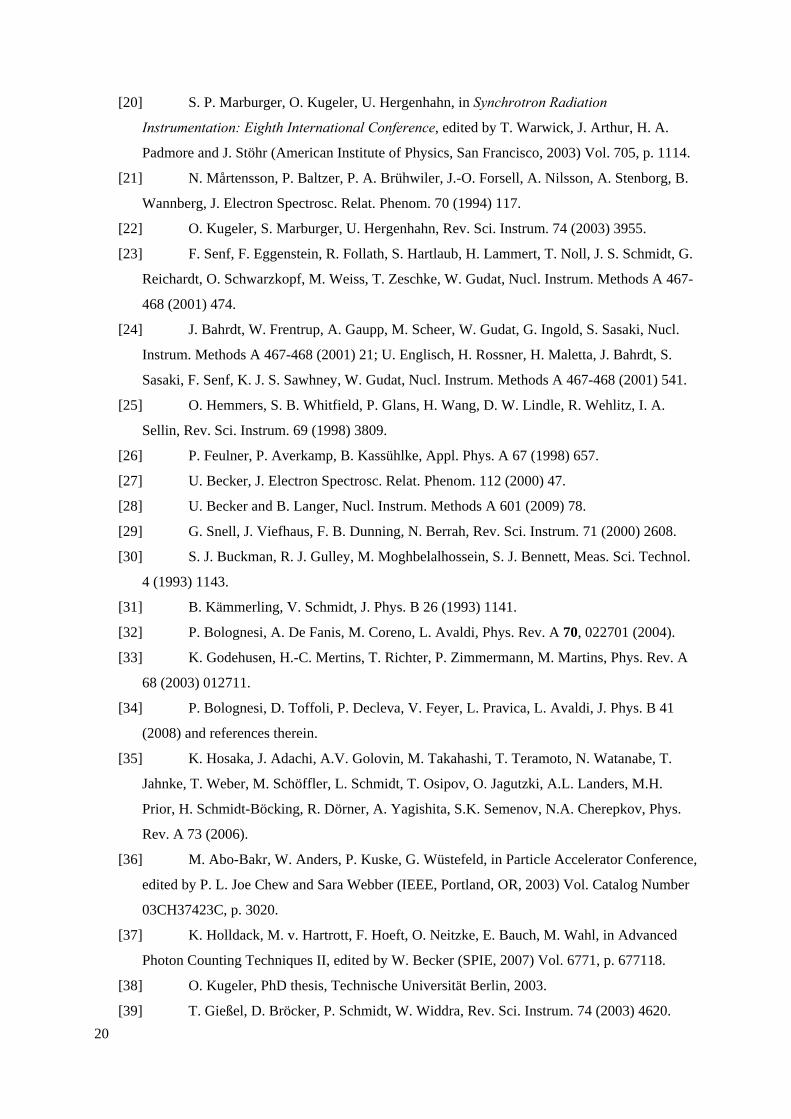
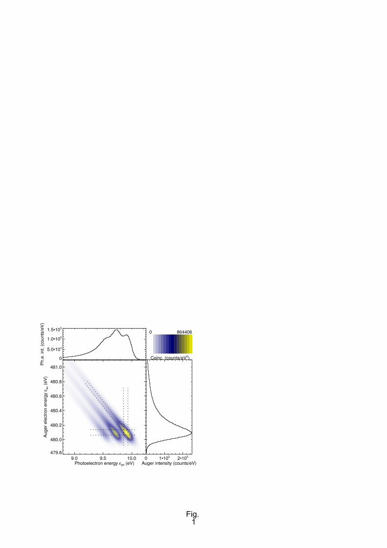
Here we highlight some general features of molecular photoelectron-Auger electron coincidence

spectra using the simulated spectrum of Fig. 1. Details of the figure are as follows: An inner shell

photoelectron main line with a nominal adiabatic kinetic energy of 10 eV is emitted, followed by a

subsequent KVV Auger decay of the core hole at a nominal kinetic energy of 480 eV, and a lifetime

broadening of 150 meV. Two vibrationally excited core-hole states, with a (harmonic) vibrational

quantum energy of ħω = 200 meV, and intensities according to a Poisson distribution with a parameter

(I(v' = 1)/I(v' = 0)) of 0.8 [41] are seen at lower kinetic energy. The same nominal Auger energy is

assumed for all vibrational states, which is the case when the potential curves of the singly and doubly

excited states are parallel (within the range of nuclear coordinates which can be accessed by the

intermediate state). Apparatus broadening effects are modelled by convolution with Gaussian profiles,

the width (FWHM) of which were set to 50 meV (photon bandpass) and 80 meV (photoelectron and

Auger electron analyser). Intensities of the colour-coded map are given as counts/eV2, and of the non-

coincident plots as counts/eV. Integration of these in a mathematical sense leads to an assumed

intensity of approx. 100,000 coincidence counts. The Coulomb interaction of the two electrons in the

continuum (PCI) is taken into account [42].

14

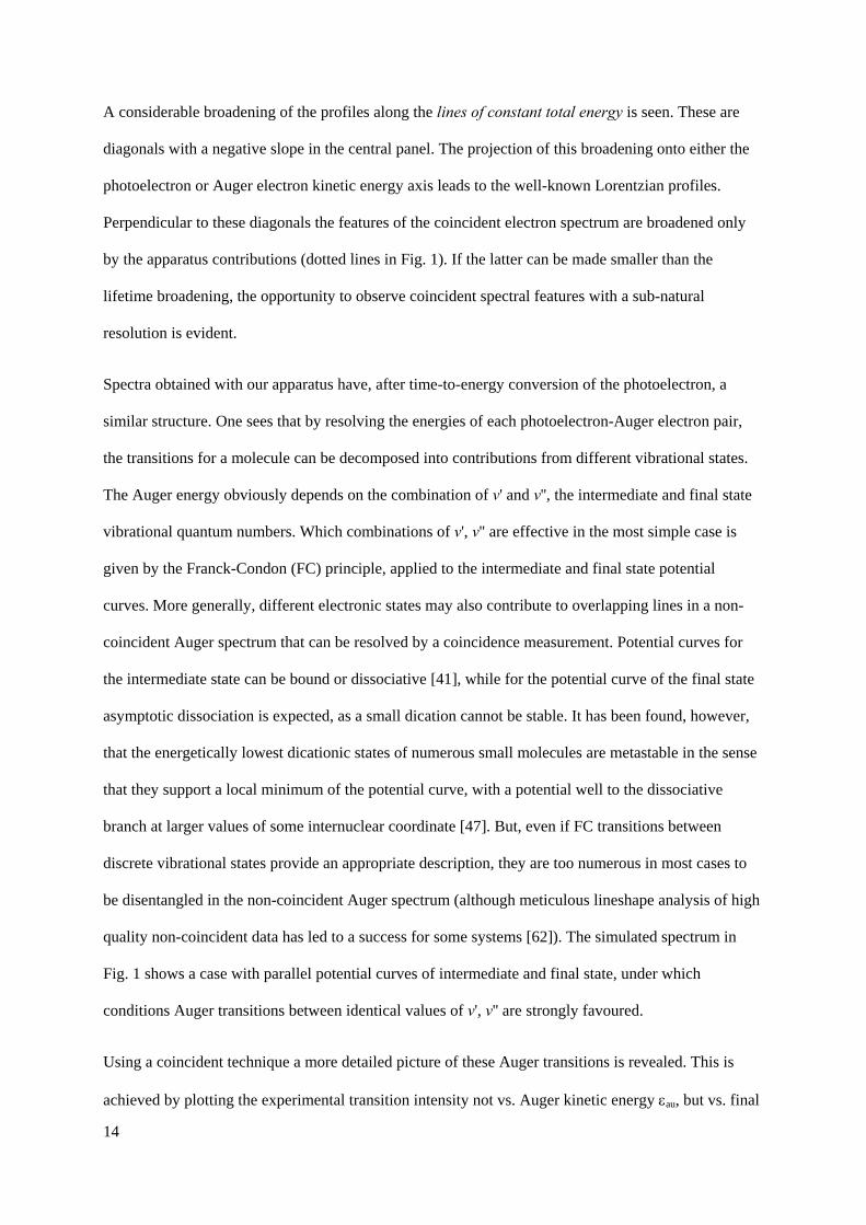
A considerable broadening of the profiles along the lines of constant total energy is seen. These are

diagonals with a negative slope in the central panel. The projection of this broadening onto either the

photoelectron or Auger electron kinetic energy axis leads to the well-known Lorentzian profiles.

Perpendicular to these diagonals the features of the coincident electron spectrum are broadened only

by the apparatus contributions (dotted lines in Fig. 1). If the latter can be made smaller than the

lifetime broadening, the opportunity to observe coincident spectral features with a sub-natural

resolution is evident.

Spectra obtained with our apparatus have, after time-to-energy conversion of the photoelectron, a

similar structure. One sees that by resolving the energies of each photoelectron-Auger electron pair,

the transitions for a molecule can be decomposed into contributions from different vibrational states.

The Auger energy obviously depends on the combination of v' and v'', the intermediate and final state

vibrational quantum numbers. Which combinations of v', v'' are effective in the most simple case is

given by the Franck-Condon (FC) principle, applied to the intermediate and final state potential

curves. More generally, different electronic states may also contribute to overlapping lines in a non-

coincident Auger spectrum that can be resolved by a coincidence measurement. Potential curves for

the intermediate state can be bound or dissociative [41], while for the potential curve of the final state

asymptotic dissociation is expected, as a small dication cannot be stable. It has been found, however,

that the energetically lowest dicationic states of numerous small molecules are metastable in the sense

that they support a local minimum of the potential curve, with a potential well to the dissociative

branch at larger values of some internuclear coordinate [47]. But, even if FC transitions between

discrete vibrational states provide an appropriate description, they are too numerous in most cases to

be disentangled in the non-coincident Auger spectrum (although meticulous lineshape analysis of high

quality non-coincident data has led to a success for some systems [62]). The simulated spectrum in

Fig. 1 shows a case with parallel potential curves of intermediate and final state, under which

conditions Auger transitions between identical values of v', v'' are strongly favoured.

Using a coincident technique a more detailed picture of these Auger transitions is revealed. This is

achieved by plotting the experimental transition intensity not vs. Auger kinetic energy εau, but vs. final

15

state energy Efi. As these two quantities are connected by Efi = IP − εau, with IP denoting the core level

ionization potential, mathematically the conversion corresponds to a shear of the recorded coincidence

map by 45°. Then, all transitions populating a certain final state line up along one of the coordinate

axes (Fig. 8). This resembles experiments in molecular photo-double-ionization by electron-electron

coincidence methods (e.g. [52]), but we see the population of one electronic final state over a wider

range of its potential curve, because an intermediate state is involved in the transition. One point

apparent from Fig. 8 is the non-trivial shape which the coincident intensity regions acquire due to the

combined effect of the finite electron analyser resolution, monochromator bandwidth and the shear

transformation [19].

The lifetime of Auger decay and the time-span of a molecular vibrational period are of the same order

of magnitude. One therefore expects an influence of the molecular dynamics during the decay on the

radiationless de-excitation spectrum. In a time-independent picture a simple model of such effects is

known as lifetime vibrational interference (LVI) [16][63]; there is also some experimental evidence

for this effect in normal Auger spectra [62]. With the new set-up we expect to be able to isolate the

effect of LVI in normal Auger spectra better than is currently possible.

IV. The photoelectron-Auger electron coincidence spectrum of molecular

oxygen: Results and discussion

As an instructive example, we report here new data for oxygen (O2). The non-coincident photoelectron

and Auger spectra both have been reported a number of times (e.g. [2]). For the O 1s spectrum, most

recent data are by Sorensen et al. [64]. Earlier work has been reviewed in Ref. [41]. The spectrum is

characterized by the exchange splitting between the 2Σ and 4Σ states of the cation, which amounts to

1.06 eV. This splitting is due to the spin coupling of the core hole with the triplet spin of the open,

outermost valence shell of O2. The two resulting photoelectron lines differ in width, with the 2Σ line

about 1.5 times as wide as the 4Σ line. This can be rationalized by the smaller influence of relaxation in

the latter state. The exact decomposition of the observed profiles into vibrational contributions and a

g/u splitting of the core hole (26 meV in theory [65]) is as yet unknown. The KVV Auger spectrum

16

has been discussed in detail by Sambe and Ramaker [66], Larsson et al. [67] and most recently by Bao

et al. [68]. The dicationic states of the O2 molecule (and of a molecule in general) can also be accessed

by direct photo-double-ionisation with detection of both photoelectrons. This method has proven to be

useful for characterizing the energies and vibrational progressions of the doubly charged states in

numerous species, and has been applied to O2 by Dawber et al. and by Eland [69][52].

In the following we will present some of our experimental results. By our data acquisition scheme,

coincident and non-coincident spectra are recorded simultaneously. We present the conventional, non-

coincident KVV Auger spectrum in the right hand side panel of Fig. 6. Compared to earlier work the

structures are very similar [66][67] and the experimental resolution equals the one of Larsson et al.

[67].

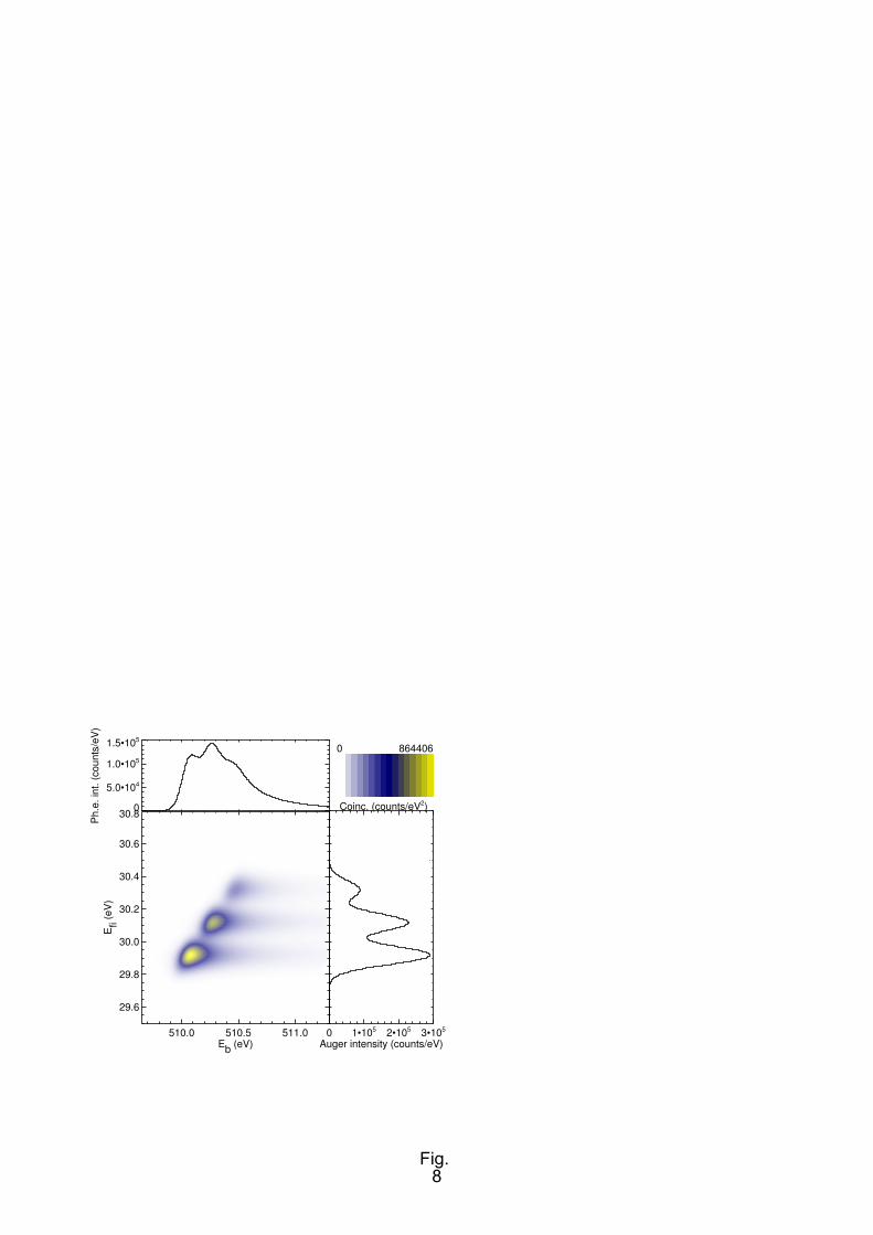
The Auger spectrum acquired in coincidence with the core level electrons is shown in Fig. 9. A

transformation of the coincidence data into a binding energy vs. final state energy representation has

been carried out as discussed above. Here, we present the binding energy region of the lowest three

dicationic states which are populated by Auger decay. Statistical errors of the data were propagated

throughout the analysis procedure. The relative error of the intensity represented by a single pixel in

the central panel of Fig. 9 lies between 10 and 30 %, for pixels exceeding 10000 counts/eV2. Error

bars on the one-dimensional sums are shown in the Figure.

The lowest dicationic states seen in our experiment have been assigned as W 3∆u, B 3Πg and B 3Σu−,

while two energetically lower states, which have been detected in a zero-kinetic-energy electron-

electron coincidence measurement [69], hardly receive intensity by Auger decay. The assignment is

taken from earlier work [66][68]. The population of three final states can be easily seen in the summed

spectrum. While two of them obviously receive intensity from both the 2Σ and the 4Σ intermediate

states, our coincidence map suggests that the middle one, assigned to B 3Πg, can be populated only

from the 4Σ state. The Auger spectra separated with respect to the core-ionized state are presented

again in Fig. 10, where the intensity for intermediate states in the binding energy intervals [543.1,

543.7] and [544.2, 544.7] eV has been summed up.

17

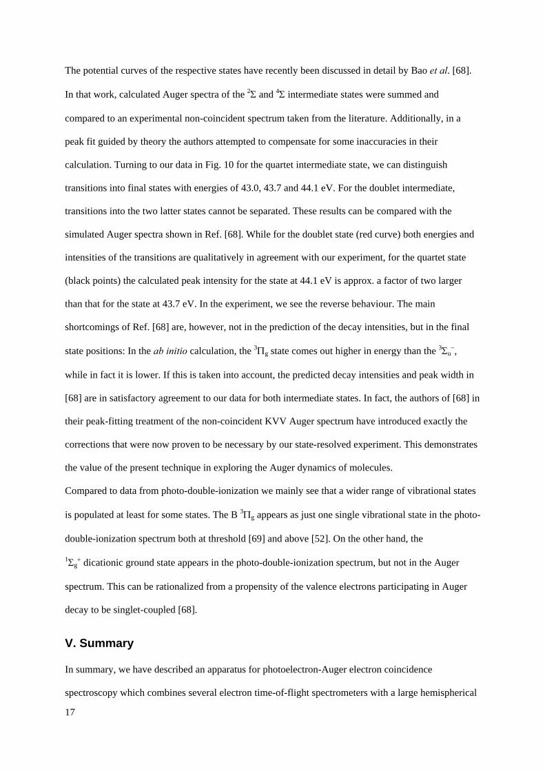
The potential curves of the respective states have recently been discussed in detail by Bao et al. [68].

In that work, calculated Auger spectra of the 2Σ and 4Σ intermediate states were summed and

compared to an experimental non-coincident spectrum taken from the literature. Additionally, in a

peak fit guided by theory the authors attempted to compensate for some inaccuracies in their

calculation. Turning to our data in Fig. 10 for the quartet intermediate state, we can distinguish

transitions into final states with energies of 43.0, 43.7 and 44.1 eV. For the doublet intermediate,

transitions into the two latter states cannot be separated. These results can be compared with the

simulated Auger spectra shown in Ref. [68]. While for the doublet state (red curve) both energies and

intensities of the transitions are qualitatively in agreement with our experiment, for the quartet state

(black points) the calculated peak intensity for the state at 44.1 eV is approx. a factor of two larger

than that for the state at 43.7 eV. In the experiment, we see the reverse behaviour. The main

shortcomings of Ref. [68] are, however, not in the prediction of the decay intensities, but in the final

state positions: In the ab initio calculation, the 3Πg state comes out higher in energy than the 3Σu−,

while in fact it is lower. If this is taken into account, the predicted decay intensities and peak width in

[68] are in satisfactory agreement to our data for both intermediate states. In fact, the authors of [68] in

their peak-fitting treatment of the non-coincident KVV Auger spectrum have introduced exactly the

corrections that were now proven to be necessary by our state-resolved experiment. This demonstrates

the value of the present technique in exploring the Auger dynamics of molecules.

Compared to data from photo-double-ionization we mainly see that a wider range of vibrational states

is populated at least for some states. The B 3Πg appears as just one single vibrational state in the photo-

double-ionization spectrum both at threshold [69] and above [52]. On the other hand, the

1Σg+ dicationic ground state appears in the photo-double-ionization spectrum, but not in the Auger

spectrum. This can be rationalized from a propensity of the valence electrons participating in Auger

decay to be singlet-coupled [68].

V. Summary

In summary, we have described an apparatus for photoelectron-Auger electron coincidence

spectroscopy which combines several electron time-of-flight spectrometers with a large hemispherical

18

electron analyser. We have described and discussed the general features of this form of electron

spectroscopy applied to free molecules and clusters and, in particular, we illustrate its potential for the

investigation of molecular Auger decay with high resolution. Moreover, we show the first data for the

diatomics CO [68] and O2 (hitherto unpublished). The latter are compared to existing calculations.

Acknowledgements

UH would like to thank Jens Viefhaus and Georg Prümper for valuable discussions on various aspects

of this project. This work was partially funded by the Deutsche Forschungsgemeinschaft (He 3060/4)

and the Fonds der chemischen Industrie. The expertise of BESSY in running the storage ring and

maintaining the beamlines is gratefully acknowledged.

19

References

[1] R.E. Weber, W.T. Peria, J. Appl. Phys. 38 (1967) 4355.

[2] K. Siegbahn, C. Nordling, G. Johansson, J. Hedman, P.F. Héden, K. Hamrin, U. Gelius, T.

Bergmark, L.O. Werme, R. Manne, Y. Baer: ESCA applied to free molecules, North-Holland,

Amsterdam, 1969.

[3] F.P. Larkins, J. Electron Spectrosc. Relat. Phenom. 51 (1990) 115.

[4] A. Cesar, H. Ågren, V. Carravetta, Phys. Rev. A 40 (1989) 187.

[5] L. S. Cederbaum and F. Tarantelli, J. Chem. Phys. 98 (1993) 9691; J. Chem. Phys. 99 (1993)

5871.

[6] F. Tarantelli and L. S. Cederbaum, Phys. Rev. Lett. 71 (1993) 649.

[7] T. X. Carroll, J. Hahne, T. D. Thomas, L. J. Sæthre, N. Berrah, J. Bozek, E. Kukk, Phys. Rev.

A 61 (2000) 042503 and references therein.

[8] T. D. Thomas, C. Miron, K. Wiesner, P. Morin, T. X. Carroll, L. J. Sæthre, Phys. Rev. Lett. 89

(2002) 223001.

[9] H. W. Haak, G. A. Sawatzky, T. D. Thomas, Phys. Rev. Lett. 41 (1978) 1825.

[10] E. Jensen, R. A. Bartynski, S. L. Hulbert, E. D. Johnson, R. Garrett, Phys. Rev. Lett.

62 (1989) 71.

[11] G. Stefani, R. Gotter, A. Ruocco, F. Offi, F. Da Pieve, S. Iacobucci, A. Morgante, A.

Verdini, A. Liscio, H. Yao, R. A. Bartynski, J. Electron Spectrosc. Relat. Phenom. 141 (2004)

149.

[12] V. Schmidt: Electron Spectrometry of Atoms using Synchrotron Radiation, University

Press, Cambridge, 1997.

[13] M. Neeb, J.-E. Rubensson, M. Biermann, W. Eberhardt, J. Phys. B 29 (1996) 4381.

[14] J. Viefhaus, G. Snell, R. Hentges, M. Wiedenhöft, F. Heiser, O. Gessner, U. Becker,

Phys. Rev. Lett. 80 (1998) 1618.

[15] E. Pahl, H.-D. Meyer, L. S. Cederbaum, Z. Phys. D 38 (1996) 215; Z. W. Gortel, R.

Teshima, D. Menzel, Phys. Rev. A 58 (1998) 1225.

[16] F. Gelmukhanov and H. Ågren, Phys. Rep. 312 (1999) 87.

[17] A. Kivimäki, A. Naves de Brito, S. Aksela, H. Aksela, O.-P. Sairanen, A. Ausmees, S.

J. Osborne, L. B. Dantas, S. Svensson, Phys. Rev. Lett. 71 (1993) 4307.

[18] A. Kivimäki, K. Maier, U. Hergenhahn, M. N. Piancastelli, B. Kempgens, A. Rüdel,

A. M. Bradshaw, Phys. Rev. Lett. 81 (1998) 301.

[19] V. Ulrich, S. Barth, S. Joshi, T. Lischke, A. M. Bradshaw, U. Hergenhahn, Phys. Rev.

Lett. 100 (2008) 143003.

20

[20] S. P. Marburger, O. Kugeler, U. Hergenhahn, in Synchrotron Radiation

Instrumentation: Eighth International Conference, edited by T. Warwick, J. Arthur, H. A.

Padmore and J. Stöhr (American Institute of Physics, San Francisco, 2003) Vol. 705, p. 1114.

[21] N. Mårtensson, P. Baltzer, P. A. Brühwiler, J.-O. Forsell, A. Nilsson, A. Stenborg, B.

Wannberg, J. Electron Spectrosc. Relat. Phenom. 70 (1994) 117.

[22] O. Kugeler, S. Marburger, U. Hergenhahn, Rev. Sci. Instrum. 74 (2003) 3955.

[23] F. Senf, F. Eggenstein, R. Follath, S. Hartlaub, H. Lammert, T. Noll, J. S. Schmidt, G.

Reichardt, O. Schwarzkopf, M. Weiss, T. Zeschke, W. Gudat, Nucl. Instrum. Methods A 467-

468 (2001) 474.

[24] J. Bahrdt, W. Frentrup, A. Gaupp, M. Scheer, W. Gudat, G. Ingold, S. Sasaki, Nucl.

Instrum. Methods A 467-468 (2001) 21; U. Englisch, H. Rossner, H. Maletta, J. Bahrdt, S.

Sasaki, F. Senf, K. J. S. Sawhney, W. Gudat, Nucl. Instrum. Methods A 467-468 (2001) 541.

[25] O. Hemmers, S. B. Whitfield, P. Glans, H. Wang, D. W. Lindle, R. Wehlitz, I. A.

Sellin, Rev. Sci. Instrum. 69 (1998) 3809.

[26] P. Feulner, P. Averkamp, B. Kassühlke, Appl. Phys. A 67 (1998) 657.

[27] U. Becker, J. Electron Spectrosc. Relat. Phenom. 112 (2000) 47.

[28] U. Becker and B. Langer, Nucl. Instrum. Methods A 601 (2009) 78.

[29] G. Snell, J. Viefhaus, F. B. Dunning, N. Berrah, Rev. Sci. Instrum. 71 (2000) 2608.

[30] S. J. Buckman, R. J. Gulley, M. Moghbelalhossein, S. J. Bennett, Meas. Sci. Technol.

4 (1993) 1143.

[31] B. Kämmerling, V. Schmidt, J. Phys. B 26 (1993) 1141.

[32] P. Bolognesi, A. De Fanis, M. Coreno, L. Avaldi, Phys. Rev. A 70, 022701 (2004).

[33] K. Godehusen, H.-C. Mertins, T. Richter, P. Zimmermann, M. Martins, Phys. Rev. A

68 (2003) 012711.

[34] P. Bolognesi, D. Toffoli, P. Decleva, V. Feyer, L. Pravica, L. Avaldi, J. Phys. B 41

(2008) and references therein.

[35] K. Hosaka, J. Adachi, A.V. Golovin, M. Takahashi, T. Teramoto, N. Watanabe, T.

Jahnke, T. Weber, M. Schöffler, L. Schmidt, T. Osipov, O. Jagutzki, A.L. Landers, M.H.

Prior, H. Schmidt-Böcking, R. Dörner, A. Yagishita, S.K. Semenov, N.A. Cherepkov, Phys.

Rev. A 73 (2006).

[36] M. Abo-Bakr, W. Anders, P. Kuske, G. Wüstefeld, in Particle Accelerator Conference,

edited by P. L. Joe Chew and Sara Webber (IEEE, Portland, OR, 2003) Vol. Catalog Number

03CH37423C, p. 3020.

[37] K. Holldack, M. v. Hartrott, F. Hoeft, O. Neitzke, E. Bauch, M. Wahl, in Advanced

Photon Counting Techniques II, edited by W. Becker (SPIE, 2007) Vol. 6771, p. 677118.

[38] O. Kugeler, PhD thesis, Technische Universität Berlin, 2003.

[39] T. Gießel, D. Bröcker, P. Schmidt, W. Widdra, Rev. Sci. Instrum. 74 (2003) 4620.

21

[40] V. Myrseth, J. D. Bozek, E. Kukk, L. J. Sæthre, T. D. Thomas, J. Electron Spectrosc.

Relat. Phenom. 122 (2002) 57.

[41] U. Hergenhahn, J. Phys. B 37 (2004) R89.

[42] M. Y. Kuchiev and S. A. Sheinerman, Soviet Physics-JETP 63 (1986) 986.

[43] T. X. Carroll, K. J. Børve, L. J. Sæthre, J. D. Bozek, E. Kukk, J. A. Hahne, T. D.

Thomas, J. Chem. Phys. 116 (2002) 10221.

[44] E. Jensen, R. A. Bartynski, S. L. Hulbert, E. D. Johnson, Rev. Sci. Instrum. 63 (1992)

3013.

[45] P. Calicchia, S. Lagomarsino, F. Scarinci, C. Martinelli, V. Formoso, Rev. Sci.

Instrum. 70 (1999) 3529.

[46] H. Pulkkinen, S. Aksela, O.-P. Sairanen, A. Hiltunen, H. Aksela, J. Phys. B 29 (1996)

3033.

[47] J. Viefhaus, S. Cvejanovic, B. Langer, T. Lischke, G. Prümper, D. Rolles, A. V.

Golovin, A. N. Grum-Grzhimailo, N. M. Kabachnik, U. Becker, Phys. Rev. Lett. 92 (2004)

083001.

[48] J. Viefhaus, U. Hergenhahn, R. Hentges, A. Rüdel, U. Becker, (Hasylab Annual

Report, 1998).

[49] J. Viefhaus, U. Hergenhahn, R. Hentges, A. Rüdel, U. Becker in ICPEAC XXI, Abstr.

of Contrib. Papers, ed. by Y. Itikawa, reprinted in [27].

[50] P. Kruit and F. H. Read, J. Phys. E 16 (1983) 313.

[51] F. Penent, P. Lablanquie, R. I. Hall, J. Palaudoux, K. Ito, Y. Hikosaka, T. Aoto, J. H.

D. Eland, J. Electron Spectrosc. Relat. Phenom. 144-147 (2005) 7.

[52] J. H. D. Eland, Chem. Phys. 294 (2003) 171.

[53] J. H. D. Eland, O. Vieuxmaire, T. Kinugawa, P. Lablanquie, R. I. Hall, F. Penent,

Phys. Rev. Lett. 90 (2003) 053003.

[54] P. Lablanquie, L. Andric, J. Palaudoux, U. Becker, M. Braune, J. Viefhaus, J. H. D.

Eland, F. Penent, J. Electron Spectrosc. Relat. Phenom. 156-158 (2007) 51.

[55] T. J. Reddish, G. Richmond, G. W. Bagley, J. P. Wightman, S. Cvejanovic, Rev. Sci.

Instrum. 68 (1997) 2685.

[56] R. Gotter, A. Ruocco, A. Morgante, D. Cvetko, L. Floreano, F. Tommasini, G.

Stefani, Nucl. Instrum. Methods A 467-468 (2001) 1468.

[57] P. Bolognesi, R. Püttner, L. Avaldi, Chem. Phys. Lett. 464 (2008) 21.

[58] R. Wehlitz, L. S. Pibida, J. C. Levin, I. A. Sellin, Rev. Sci. Instrum. 70 (1999) 1978.

[59] R. Dörner, V. Mergel, O. Jagutzki, L. Spielberger, J. Ullrich, R. Moshammer, H.

Schmidt-Böcking, Phys. Rep. 330 (2000) 95.

[60] J. Ullrich, R. Moshammer, A. Dorn, R. Dörner, L. P. H. Schmidt, H. Schmidt-

Böcking, Rep. Prog. Phys. 66 (2003) 1463.

22

[61] D. Schröder and H. Schwarz, J. Phys. Chem. A 103 (1999) 7385.

[62] R. Püttner, X.-J. Liu, H. Fukuzawa, T. Tanaka, M. Hoshino, H. Tanaka, J. Harries, Y.

Tamenori, V. Carravetta, K. Ueda, Chem. Phys. Lett. 445 (2007) 6 and references therein.

[63] F. Kaspar, W. Domcke, L. S. Cederbaum, Chem. Phys. 44 (1979) 33; F. Gelmukhanov

and H. Ågren, Phys. Rep. 312 (1999) 87.

[64] S. L. Sorensen, K. J. Børve, R. Feifel, A. de Fanis, K. Ueda, J. Phys. B 41 (2008)

095101.

[65] N. Kosugi, Chem. Phys. 289 (2003) 117.

[66] H. Sambe and D. E. Ramaker, Chem. Phys. 104 (1986) 331.

[67] M. Larsson, P. Baltzer, S. Svensson, B. Wannberg, N. Mårtensson, A. Naves de Brito,

N. Correia, M. P. Keane, M. Carlsson-Göthe, L. Karlsson, J. Phys. B 23 (1990) 1175.

[68] Z. Bao, R. F. Fink, O. Travnikova, D. Céolin, S. Svensson, M. N. Piancastelli, J. Phys.

B 41 (2008) 125101.

[69] G. Dawber, A. G. McConkey, L. Avaldi, M. A. MacDonald, G. C. King, R. I. Hall, J.

Phys. B 27 (1994) 2191.

23

Figure captions

FIG. 1. (Colour online) Simulated sketch of a molecular photoelectron, Auger electron coincidence

spectrum measured with high energy resolution. The colour-coded map shows the simulated intensity

of electron pairs for the respective combinations of energies; the one-dimensional plots on the top and

left-hand side show the coincident intensity integrated along one of the energy axes. These correspond

to conventionally measured photoelectron and Auger electron spectra, respectively, Dotted lines

indicate the full width at half maximum (FWHM) of the analyser bandpass and photon bandpass used

in the simulation. See text for details (beginning of Section III).

FIG. 2. (Colour online) Set-up for electron-electron coincidence measurements. The synchrotron

radiation propagates towards the observer. The hemispherical detector is mounted at a downward

angle of 54.7° to the horizontal and within the plane perpendicular to the photon beam ('dipole plane').

The gas cell is mounted atop of an expansion chamber for cluster experiments (not drawn, see [20]).

An array of six identical time-of-flight spectrometers is mounted in a vertical plane containing the

radiation propagation axis, and at angles of 0°, ±22.2°, ±44.4° and 66.6° with respect to the vertical

axis. (Positive sign = backward scattering direction.) Magnetic fields are actively compensated by a set

of Helmholtz coils (not shown).

FIG. 3. Ray-tracing simulation of the time-of-flight (TOF) spectrometers with a flight path of

228.5 mm from the interaction region to the mesh. A total number of 2.7 x 105 (for the point source

case, dotted curve) and 8.1 x 105 electrons (for the 44.4° tilted line source, solid line) have been used

to simulate the two spectra (see text for details).

FIG. 4. Electron spectra of CO excited with a photon energy of 304 eV, sum over all TOF analysers.

The flight time in the TOF is referred to the BESSY bunch clock. The spectra are therefore a

convolution of a TOF spectrum, including photo- and Auger electrons, with the time structure of the

BESSY fill pattern (panel a). The vibrationally resolved, non-coincident CO C 1s photoelectron

spectrum excited by the hybrid bunch can be recognized on-top of a background of fast electrons from

other bunches (the C 1s region is expanded in panel b).

24

FIG. 5. Schematic of the data acquisition electronics. The MCP pulses are amplified by pairs of

commercial, inverting GHz amplifiers (Minicircuits), and further shaped by constant fraction

discriminators (TOFs: Ortec, Scienta: Roentdek). A four channel multi-hit-capable time-to-digital

converter (TDC) with 60 ps bin width and 16 bit signal depth collects the timing information for the

norm pulses (GPTA, Berlin, Germany). The TDC start signal is provided by the BESSY bunch

marker, a clock with the frequency of the inverse electron revolution time. All electron hits are used as

stop signals, and, by the TDC firmware, are tagged with a bit pattern, which is incremented with the

bunch marker pulses. For the hemispherical analyser, timing and energy information can be retrieved

from the TDC signals as described in Ref. [22][38]. Coincident events involving detection of more

than one electron can be separated in an off-line analysis of the data, and non-coincident data are

extracted from the same set.

FIG. 6. (Colour online) Arrival times of electrons emitted by O2 molecules in the hemispherical

analyser, τau,rel, vs. Auger electron energy εau. The gross structure of the arrival time spectrum reflects

the BESSY fill pattern [37], see top panel and Fig. 4. A zoom into the Auger electrons received from

the hybrid bunch (colour coded map in bottom panel) allows the TOF spread in the hemispherical

analyser to be determined for monoenergetic electrons (middle panel). For the middle panel, electrons

between the two dotted lines in the bottom panel have been taken into account. On the right-hand side

the non-coincident Auger spectrum (sum over all events shown in the top panel) is shown. The

numbering of the lines follows Larsson et al. [67].

FIG. 7. (Colour online) Time-of-flight spectrum of O2 O 1s photoelectrons detected in coincidence

with K-VV Auger electrons. The flight time in the TOF is referred to the time of Auger electron

detection. In the centre, the true coincidence signal with the two oxygen 1s main lines can be seen.

Other events pertain to accidental coincidences, which have the shape of approximately a triangle in

this plot. The line spectrum is the true + accidental signal; the points represent a spectrum of

accidental coincidences only.

25

FIG. 8. (Colour online) Simulated sketch of a molecular photoelectron-Auger electron coincidence

spectrum plotted as a function of intermediate (Eb) and final state (Efi) binding energy. Same

parameters as in Fig. 1. See text for details.

FIG. 9. (Colour online) Experimental photoelectron-Auger electron coincidence spectrum of O 1s

photoionization in O2, followed by K-VV Auger decay. The photon energy is 551.85 eV. The colour-

coded map gives the intensity of electron pairs with the respective combinations of intermediate and

final state binding energy. The top panel and the right-hand side panel contain the photoelectron

intensity and the Auger electron intensity, respectively, summed over all energies of the other electron.

Final state designations on the right-hand side follow the literature [68][52]. Intensities of the colour-

coded map are given as counts/eV2, and of the non-coincident plots as counts/eV.

FIG. 10. (Colour online) Experimental Auger spectra of the O 1s-1 4Σ and the 2Σ core-ionized states,

plotted as a function of final state energy. Error bars of characteristic size are shown for two data

points.

0 864406

Coinc. (counts/eV2)

9.0 9.5 10.0Photoelectron energy εph (eV)

479.8

480.0

480.2

480.4

480.6

480.8

481.0

Auger

ele

ctr

on e

nerg

y ε

au (

eV

)

0

5.0•104

1.0•105

1.5•105

Ph

.e.

int.

(co

un

ts/e

V)

0 1•105 2•105

Auger intensity (counts/eV)

Fig. 1

Drift tubesGas cell

Expansion chamberElectric lens section

Hemispherical electron analyzer

Adjustable holder

MCP holder

Synchrotron radiation

Fig. 2

Inte

nsity

(a.

u.)

340320300280260240

Time of flight (ns)

point source extended source

Fig. 3

600x103

500

400

300

200

100

Co

un

ts

8006004002000

ns

K-VV Auger (hybrid bunch)

C 1s(hybrid bunch)

CO C 1s

hν = 304 eV

a)

3.5x106

3.0

2.5

2.0

Co

un

ts

460440420400380360340

ns

C 1s(hybrid bunch)

b)

Fig. 4

TOF1...

TOF6

BunchmarkerNIM

BunchmarkerTTL

Roe

ntde

kC

FD

CFD

CFD

CFD

Counter

CFD

3

4 ∆t

5

6

or

4 ch

anne

l mul

ti-hi

t T

DC

T1

T2

T3

T4

start

Time

Bunchmarker

Status

bm

or

or

2byte

2byte

4byte

dela

y

Amp

20 bit Bunchmarker Identification

ScientaDelayline

Anode

Scienta MCP

PC

Control

∆t

Fig. 5

0 35

-10 0 10Time-of-flight τau,rel (ns)

496

497

498

499

500

501

502

503A

uger

ele

ctro

n en

ergy

εau

(eV

)

050

100150200250

Eve

nts

6.2 ns

0 4.0•104 8.0•104 1.2•105

Events

9

10

1112

-200 0 200 400 600 800 1000496

498

500

502

ε au

(eV

)

Fig. 6

-1500 -1000 -500 0 500 1000 1500Time difference (ns)

0

500

1000

1500

2000

2500

Eve

nts

Fig. 7

0 864406

Coinc. (counts/eV2)

510.0 510.5 511.0E

b (eV)

29.6

29.8

30.0

30.2

30.4

30.6

30.8

Efi (

eV

)

0

5.0•104

1.0•105

1.5•105

Ph

.e.

int.

(co

un

ts/e

V)

0 1•105 2•105 3•105

Auger intensity (counts/eV)

Fig. 8

5000 30000

Coincidences (counts/eV2)

543 544 545Eb (eV)

42.5

43.0

43.5

44.0

44.5

45.0

Efi

(eV

)

0

1•104

2•104

3•104

4•104

Ph.

e. In

t. (c

ount

s/eV

)

4Σ2Σ

0 1•104 2•104 3•104

Auger Intensity (counts/eV)

W3∆

u

B3Π

g

B3Σ

u -

Fig. 9

16x103

14

12

10

8

6

4

2

0

Inte

nsity

(C

ount

s/eV

)

47464544434241Efi (eV)

O 1s−1

4Σ

O 1s−1

2Σ

W 3∆u B

3Πg

B 3Σu

−

Fig. 10