The Pierre Auger Observatory IV: Operation and Monitoring
42
32ND I NTERNATIONAL COSMIC RAY CONFERENCE,BEIJING 2011 The Pierre Auger Observatory IV: Operation and Monitoring THE PIERRE AUGER COLLABORATION Observatorio Pierre Auger, Av. San Mart´ ın Norte 304, 5613 Malarg¨ ue, Argentina 1 Long Term Performance of the Surface Detectors of the Pierre Auger Observatory presented by Ricardo Sato 1 2 Remote operation of the Pierre Auger Observatory presented by Julian Rautenberg 5 3 Atmospheric Monitoring at the Pierre Auger Observatory – Status and Update presented by Karim Louedec 9 4 Implementation of meteorological model data in the air shower reconstruction of the Pierre Auger Ob- servatory presented by Martin Will 13 5 Night Sky Background measurements by the Pierre Auger Fluorescence Detectors and comparison with simultaneous data from the UVscope instrument presented by Alberto Segreto 17 6 Observation of Elves with the Fluorescence Detectors of the Pierre Auger Observatory presented by Aurelio S. Tonachini 21 7 Atmospheric Super Test Beam for the Pierre Auger Observatory presented by Lawrence Wiencke 25 8 Multiple scattering measurement with laser events presented by Pedro Assis 29 9 Education and Public Outreach of the Pierre Auger Observatory presented by Gregory R. Snow 33
-
Upload
independent -
Category
Documents
-
view
1 -
download
0
Transcript of The Pierre Auger Observatory IV: Operation and Monitoring

32ND INTERNATIONAL COSMIC RAY CONFERENCE, BEIJING 2011
The Pierre Auger Observatory IV: Operation andMonitoring
THE PIERRE AUGER COLLABORATION
Observatorio Pierre Auger, Av. San Martın Norte 304, 5613 Malargue, Argentina
1 Long Term Performance of the Surface Detectors of the Pierre Auger Observatorypresented by Ricardo Sato 1
2 Remote operation of the Pierre Auger Observatorypresented by Julian Rautenberg 5
3 Atmospheric Monitoring at the Pierre Auger Observatory – Status and Updatepresented by Karim Louedec 9
4 Implementation of meteorological model data in the air shower reconstruction of the Pierre Auger Ob-servatorypresented by Martin Will 13
5 Night Sky Background measurements by the Pierre Auger Fluorescence Detectors and comparison withsimultaneous data from the UVscope instrumentpresented by Alberto Segreto 17
6 Observation of Elves with the Fluorescence Detectors of the Pierre Auger Observatorypresented by Aurelio S. Tonachini 21
7 Atmospheric Super Test Beam for the Pierre Auger Observatorypresented by Lawrence Wiencke 25
8 Multiple scattering measurement with laser eventspresented by Pedro Assis 29
9 Education and Public Outreach of the Pierre Auger Observatorypresented by Gregory R. Snow 33

32ND INTERNATIONAL COSMIC RAY CONFERENCE, BEIJING 2011
The Pierre Auger Collaboration
P. ABREU74 , M. AGLIETTA57, E.J. AHN93, I.F.M. ALBUQUERQUE19 , D. ALLARD33, I. ALLEKOTTE1,J. ALLEN96, P. ALLISON98, J. ALVAREZ CASTILLO67 , J. ALVAREZ-MUNIZ84, M. AMBROSIO50 , A. AMINAEI 68 ,L. A NCHORDOQUI109 , S. ANDRINGA74 , T. ANTICIC27 , A. ANZALONE56, C. ARAMO50 , E. ARGANDA81 ,F. ARQUEROS81 , H. ASOREY1 , P. ASSIS74 , J. AUBLIN35 , M. AVE41, M. AVENIER36, G. AVILA 12, T. BACKER45 ,M. BALZER40 , K.B. BARBER13 , A.F. BARBOSA16 , R. BARDENET34 , S.L.C. BARROSO22 , B. BAUGHMAN98 ,J. BAUML 39 , J.J. BEATTY98, B.R. BECKER106 , K.H. BECKER38 , A. BELLETOILE37, J.A. BELLIDO13,S. BENZVI108 , C. BERAT36, X. BERTOU1 , P.L. BIERMANN42 , P. BILLOIR35 , F. BLANCO81 , M. BLANCO82 ,C. BLEVE38, H. BLUMER41, 39, M. BOHACOVA29, 101 , D. BONCIOLI51 , C. BONIFAZI25, 35 , R. BONINO57 ,N. BORODAI72 , J. BRACK91 , P. BROGUEIRA74 , W.C. BROWN92 , R. BRUIJN87 , P. BUCHHOLZ45 , A. BUENO83 ,R.E. BURTON89 , K.S. CABALLERO-MORA99 , L. CARAMETE42, R. CARUSO52 , A. CASTELLINA57, O. CATALANO 56,G. CATALDI 49, L. CAZON74 , R. CESTER53, J. CHAUVIN 36 , S.H. CHENG99 , A. CHIAVASSA57 , J.A. CHINELLATO20,A. CHOU93, 96, J. CHUDOBA29 , R.W. CLAY 13 , M.R. COLUCCIA49 , R. CONCEICAO74 , F. CONTRERAS11 , H. COOK87 ,M.J. COOPER13 , J. COPPENS68, 70, A. CORDIER34 , U. COTTI66 , S. COUTU99 , C.E. COVAULT89 , A. CREUSOT33, 79,A. CRISS99 , J. CRONIN101 , A. CURUTIU42 , S. DAGORET-CAMPAGNE34 , R. DALLIER37, S. DASSO8, 4,K. DAUMILLER 39, B.R. DAWSON13, R.M. DE ALMEIDA 26, M. DE DOMENICO52 , C. DE DONATO67, 48, S.J. DE
JONG68, 70, G. DE LA VEGA10 , W.J.M. DE MELLO JUNIOR20 , J.R.T.DE MELLO NETO25, I. DE M ITRI49 , V. DE
SOUZA18 , K.D. DE VRIES69 , G. DECERPRIT33 , L. DEL PERAL82, O. DELIGNY32, H. DEMBINSKI41 , N. DHITAL 95,C. DI GIULIO47, 51, J.C. DIAZ95 , M.L. D IAZ CASTRO17 , P.N. DIEP110, C. DOBRIGKEIT 20, W. DOCTERS69 ,J.C. D’OLIVO67, P.N. DONG110, 32, A. DOROFEEV91 , J.C.DOS ANJOS16, M.T. DOVA7, D. D’URSO50 , I. DUTAN42,J. EBR29 , R. ENGEL39, M. ERDMANN43 , C.O. ESCOBAR20 , A. ETCHEGOYEN2, P. FACAL SAN LUIS101 , I. FAJARDO
TAPIA67 , H. FALCKE68, 71, G. FARRAR96 , A.C. FAUTH20, N. FAZZINI 93, A.P. FERGUSON89 , A. FERRERO2 ,B. FICK95 , A. FILEVICH2 , A. FILIPCIC78, 79, S. FLIESCHER43 , C.E. FRACCHIOLLA91 , E.D. FRAENKEL69,U. FROHLICH45 , B. FUCHS16 , R. GAIOR35 , R.F. GAMARRA2 , S. GAMBETTA46, B. GARCIA10 , D. GARCIA
GAMEZ83, D. GARCIA-PINTO81 , A. GASCON83 , H. GEMMEKE40, K. GESTERLING106, P.L. GHIA35, 57,U. GIACCARI49 , M. GILLER73, H. GLASS93 , M.S. GOLD106 , G. GOLUP1, F. GOMEZ ALBARRACIN7 , M. GOMEZ
BERISSO1 , P. GONCALVES74, D. GONZALEZ41, J.G. GONZALEZ41, B. GOOKIN91 , D. GORA41, 72, A. GORGI57 ,P. GOUFFON19 , S.R. GOZZINI87, E. GRASHORN98 , S. GREBE68, 70, N. GRIFFITH98 , M. GRIGAT43 , A.F. GRILLO58,Y. GUARDINCERRI4 , F. GUARINO50 , G.P. GUEDES21, A. GUZMAN67, J.D. HAGUE106, P. HANSEN7, D. HARARI1 ,S. HARMSMA69, 70, J.L. HARTON91, A. HAUNGS39 , T. HEBBEKER43 , D. HECK39 , A.E. HERVE13, C. HOJVAT93,N. HOLLON101, V.C. HOLMES13, P. HOMOLA72, J.R. HORANDEL68, A. HORNEFFER68 , M. HRABOVSKY30, 29,T. HUEGE39, A. INSOLIA52, F. IONITA101, A. ITALIANO 52, C. JARNE7 , S. JIRASKOVA68 , M. JOSEBACHUILI2 ,K. K ADIJA27 , K.-H. KAMPERT38, P. KARHAN28 , P. KASPER93 , B. KEGL34, B. KEILHAUER39 , A. KEIVANI 94 ,J.L. KELLEY68, E. KEMP20, R.M. KIECKHAFER95 , H.O. KLAGES39, M. KLEIFGES40, J. KLEINFELLER39,J. KNAPP87, D.-H. KOANG36, K. KOTERA101 , N. KROHM38 , O. KROMER40 , D. KRUPPKE-HANSEN38 ,F. KUEHN93 , D. KUEMPEL38, J.K. KULBARTZ44, N. KUNKA40, G. LA ROSA56 , C. LACHAUD33 , P. LAUTRIDOU37 ,M.S.A.B. LEAO24, D. LEBRUN36 , P. LEBRUN93 , M.A. L EIGUI DE OLIVEIRA 24 , A. LEMIERE32, A. LETESSIER-SELVON35 , I. LHENRY-YVON32, K. L INK41, R. LOPEZ63, A. LOPEZ AGUERA84 , K. LOUEDEC34 , J. LOZANO
BAHILO83 , A. LUCERO2, 57 , M. LUDWIG41 , H. LYBERIS32, M.C. MACCARONE56 , C. MACOLINO35 , S. MALDERA57,D. MANDAT29, P. MANTSCH93 , A.G. MARIAZZI 7 , J. MARIN11, 57, V. MARIN37 , I.C. MARIS35 , H.R. MARQUEZ
FALCON66 , G. MARSELLA54, D. MARTELLO49, L. MARTIN37 , H. MARTINEZ64, O. MARTINEZ BRAVO63 ,

H.J. MATHES39, J. MATTHEWS94, 100, J.A.J. MATTHEWS106, G. MATTHIAE51, D. MAURIZIO53 , P.O. MAZUR93,G. MEDINA-TANCO67 , M. MELISSAS41, D. MELO2, 53 , E. MENICHETTI53, A. MENSHIKOV40, P. MERTSCH85,C. MEURER43 , S. MI CANOVIC27 , M.I. M ICHELETTI9, W. MILLER106, L. M IRAMONTI48 , S. MOLLERACH1,M. M ONASOR101 , D. MONNIER RAGAIGNE34 , F. MONTANET36, B. MORALES67, C. MORELLO57, E. MORENO63,J.C. MORENO7 , C. MORRIS98 , M. MOSTAFA91, C.A. MOURA24, 50, S. MUELLER39, M.A. M ULLER20,G. MULLER43, M. M UNCHMEYER35, R. MUSSA53 , G. NAVARRA57 †, J.L. NAVARRO83 , S. NAVAS83 , P. NECESAL29,L. NELLEN67, A. NELLES68, 70, J. NEUSER38, P.T. NHUNG110, L. NIEMIETZ38, N. NIERSTENHOEFER38,D. NITZ95, D. NOSEK28, L. NOZKA29, M. NYKLICEK 29 , J. OEHLSCHLAGER39, A. OLINTO101, V.M. OLMOS-GILBAJA84 , M. ORTIZ81, N. PACHECO82 , D. PAKK SELMI -DEI20, M. PALATKA 29, J. PALLOTTA 3, N. PALMIERI 41 ,G. PARENTE84 , E. PARIZOT33 , A. PARRA84 , R.D. PARSONS87 , S. PASTOR80 , T. PAUL97 , M. PECH29 , J. PEKALA 72,R. PELAYO84 , I.M. PEPE23, L. PERRONE54 , R. PESCE46, E. PETERMANN105 , S. PETRERA47 , P. PETRINCA51 ,A. PETROLINI46 , Y. PETROV91, J. PETROVIC70 , C. PFENDNER108, N. PHAN106 , R. PIEGAIA4 , T. PIEROG39 ,P. PIERONI4 , M. PIMENTA74, V. PIRRONELLO52 , M. PLATINO2, V.H. PONCE1 , M. PONTZ45, P. PRIVITERA101 ,M. PROUZA29 , E.J. QUEL3, S. QUERCHFELD38 , J. RAUTENBERG38 , O. RAVEL37, D. RAVIGNANI 2 , B. REVENU37,J. RIDKY 29 , S. RIGGI84, 52, M. RISSE45 , P. RISTORI3 , H. RIVERA48 , V. RIZI47 , J. ROBERTS96 , C. ROBLEDO63 ,W. RODRIGUES DE CARVALHO84, 19, G. RODRIGUEZ84 , J. RODRIGUEZ MARTINO11, 52, J. RODRIGUEZ ROJO11 ,I. RODRIGUEZ-CABO84 , M.D. RODRIGUEZ-FRIAS82 , G. ROS82 , J. ROSADO81 , T. ROSSLER30 , M. ROTH39 ,B. ROUILL E-D’ORFEUIL101, E. ROULET1, A.C. ROVERO8 , C. RUHLE40 , F. SALAMIDA 47, 39, H. SALAZAR 63,G. SALINA 51 , F. SANCHEZ2 , M. SANTANDER11 , C.E. SANTO74, E. SANTOS74, E.M. SANTOS25 , F. SARAZIN90 ,B. SARKAR38 , S. SARKAR85 , R. SATO11, N. SCHARF43 , V. SCHERINI48 , H. SCHIELER39, P. SCHIFFER43 ,A. SCHMIDT40 , F. SCHMIDT101 , O. SCHOLTEN69, H. SCHOORLEMMER68, 70 , J. SCHOVANCOVA29 , P. SCHOVANEK29 ,F. SCHRODER39 , S. SCHULTE43, D. SCHUSTER90 , S.J. SCIUTTO7 , M. SCUDERI52 , A. SEGRETO56, M. SETTIMO45,A. SHADKAM 94 , R.C. SHELLARD16, 17, I. SIDELNIK 2 , G. SIGL44, H.H. SILVA LOPEZ67, A. SMIAŁKOWSKI 73 ,R. SMIDA39, 29, G.R. SNOW105 , P. SOMMERS99 , J. SOROKIN13 , H. SPINKA88, 93 , R. SQUARTINI11 , S. STANIC79 ,J. STAPLETON98, J. STASIELAK72, M. STEPHAN43, E. STRAZZERI56, A. STUTZ36, F. SUAREZ2 , T. SUOMIJARVI32 ,A.D. SUPANITSKY8, 67 , T. SUSA27 , M.S. SUTHERLAND94, 98, J. SWAIN97 , Z. SZADKOWSKI73 , M. SZUBA39,A. TAMASHIRO8 , A. TAPIA2, M. TARTARE36 , O. TASCAU38 , C.G. TAVERA RUIZ67 , R. TCACIUC45 ,D. TEGOLO52, 61, N.T. THAO110 , D. THOMAS91, J. TIFFENBERG4 , C. TIMMERMANS70, 68, D.K. TIWARI66 ,W. TKACZYK 73 , C.J. TODEROPEIXOTO18, 24, B. TOME74, A. TONACHINI53 , P. TRAVNICEK29 , D.B. TRIDAPALLI 19 ,G. TRISTRAM33 , E. TROVATO52, M. TUEROS84, 4, R. ULRICH99, 39 , M. UNGER39 , M. URBAN34 , J.F. VALD ES
GALICIA 67 , I. VALI NO84, 39 , L. VALORE50, A.M. VAN DEN BERG69, E. VARELA63 , B. VARGAS CARDENAS67 ,J.R. VAZQUEZ81, R.A. VAZQUEZ84, D. VEBERIC79, 78 , V. VERZI51, J. VICHA29 , M. V IDELA10, L. V ILLASENOR66,H. WAHLBERG7 , P. WAHRLICH13 , O. WAINBERG2 , D. WALZ43, D. WARNER91 , A.A. WATSON87, M. WEBER40 ,K. WEIDENHAUPT43 , A. WEINDL39 , S. WESTERHOFF108 , B.J. WHELAN13, G. WIECZOREK73 , L. WIENCKE90 ,B. WILCZY NSKA72 , H. WILCZY NSKI72 , M. WILL 39, C. WILLIAMS 101 , T. WINCHEN43 , L. WINDERS109 ,M.G. WINNICK13 , M. WOMMER39 , B. WUNDHEILER2 , T. YAMAMOTO101 a, T. YAPICI95 , P. YOUNK45 , G. YUAN94 ,A. Y USHKOV84, 50 , B. ZAMORANO83 , E. ZAS84, D. ZAVRTANIK 79, 78, M. ZAVRTANIK 78, 79, I. ZAW96, A. ZEPEDA64,M. Z IMBRES-SILVA 20, 38 M. Z IOLKOWSKI45
1 Centro Atomico Bariloche and Instituto Balseiro (CNEA- UNCuyo-CONICET), San Carlos de Bariloche, Argentina2 Centro Atomico Constituyentes (Comision Nacional de Energıa Atomica/CONICET/UTN-FRBA), Buenos Aires,Argentina3 Centro de Investigaciones en Laseres y Aplicaciones, CITEFA and CONICET, Argentina4 Departamento de Fısica, FCEyN, Universidad de Buenos Aires y CONICET, Argentina7 IFLP, Universidad Nacional de La Plata and CONICET, La Plata, Argentina8 Instituto de Astronomıa y Fısica del Espacio (CONICET- UBA), Buenos Aires, Argentina9 Instituto de Fısica de Rosario (IFIR) - CONICET/U.N.R. and Facultad de Ciencias Bioquımicas y FarmaceuticasU.N.R., Rosario, Argentina10 National Technological University, Faculty Mendoza (CONICET/CNEA), Mendoza, Argentina11 Observatorio Pierre Auger, Malargue, Argentina12 Observatorio Pierre Auger and Comision Nacional de Energıa Atomica, Malargue, Argentina13 University of Adelaide, Adelaide, S.A., Australia16 Centro Brasileiro de Pesquisas Fisicas, Rio de Janeiro, RJ,Brazil17 Pontifıcia Universidade Catolica, Rio de Janeiro, RJ, Brazil

32ND INTERNATIONAL COSMIC RAY CONFERENCE, BEIJING 2011
18 Universidade de Sao Paulo, Instituto de Fısica, Sao Carlos, SP, Brazil19 Universidade de Sao Paulo, Instituto de Fısica, Sao Paulo, SP, Brazil20 Universidade Estadual de Campinas, IFGW, Campinas, SP, Brazil21 Universidade Estadual de Feira de Santana, Brazil22 Universidade Estadual do Sudoeste da Bahia, Vitoria da Conquista, BA, Brazil23 Universidade Federal da Bahia, Salvador, BA, Brazil24 Universidade Federal do ABC, Santo Andre, SP, Brazil25 Universidade Federal do Rio de Janeiro, Instituto de Fısica, Rio de Janeiro, RJ, Brazil26 Universidade Federal Fluminense, EEIMVR, Volta Redonda, RJ, Brazil27 Rudjer Boskovic Institute, 10000 Zagreb, Croatia28 Charles University, Faculty of Mathematics and Physics, Institute of Particle and Nuclear Physics, Prague, CzechRepublic29 Institute of Physics of the Academy of Sciences of the Czech Republic, Prague, Czech Republic30 Palacky University, RCATM, Olomouc, Czech Republic32 Institut de Physique Nucleaire d’Orsay (IPNO), Universite Paris 11, CNRS-IN2P3, Orsay, France33 Laboratoire AstroParticule et Cosmologie (APC), Universite Paris 7, CNRS-IN2P3, Paris, France34 Laboratoire de l’Accelerateur Lineaire (LAL), Universite Paris 11, CNRS-IN2P3, Orsay, France35 Laboratoire de Physique Nucleaire et de Hautes Energies (LPNHE), Universites Paris 6 et Paris 7, CNRS-IN2P3,Paris, France36 Laboratoire de Physique Subatomique et de Cosmologie (LPSC), Universite Joseph Fourier, INPG, CNRS-IN2P3,Grenoble, France37 SUBATECH,Ecole des Mines de Nantes, CNRS-IN2P3, Universite de Nantes, Nantes, France38 Bergische Universitat Wuppertal, Wuppertal, Germany39 Karlsruhe Institute of Technology - Campus North - Institutfur Kernphysik, Karlsruhe, Germany40 Karlsruhe Institute of Technology - Campus North - Institutfur Prozessdatenverarbeitung und Elektronik, Karlsruhe,Germany41 Karlsruhe Institute of Technology - Campus South - Institutfur Experimentelle Kernphysik (IEKP), Karlsruhe,Germany42 Max-Planck-Institut fur Radioastronomie, Bonn, Germany43 RWTH Aachen University, III. Physikalisches Institut A, Aachen, Germany44 Universitat Hamburg, Hamburg, Germany45 Universitat Siegen, Siegen, Germany46 Dipartimento di Fisica dell’Universita and INFN, Genova, Italy47 Universita dell’Aquila and INFN, L’Aquila, Italy48 Universita di Milano and Sezione INFN, Milan, Italy49 Dipartimento di Fisica dell’Universita del Salento and Sezione INFN, Lecce, Italy50 Universita di Napoli ”Federico II” and Sezione INFN, Napoli, Italy51 Universita di Roma II ”Tor Vergata” and Sezione INFN, Roma, Italy52 Universita di Catania and Sezione INFN, Catania, Italy53 Universita di Torino and Sezione INFN, Torino, Italy54 Dipartimento di Ingegneria dell’Innovazione dell’Universita del Salento and Sezione INFN, Lecce, Italy56 Istituto di Astrofisica Spaziale e Fisica Cosmica di Palermo(INAF), Palermo, Italy57 Istituto di Fisica dello Spazio Interplanetario (INAF), Universita di Torino and Sezione INFN, Torino, Italy58 INFN, Laboratori Nazionali del Gran Sasso, Assergi (L’Aquila), Italy61 Universita di Palermo and Sezione INFN, Catania, Italy63 Benemerita Universidad Autonoma de Puebla, Puebla, Mexico64 Centro de Investigacion y de Estudios Avanzados del IPN (CINVESTAV), Mexico, D.F., Mexico66 Universidad Michoacana de San Nicolas de Hidalgo, Morelia,Michoacan, Mexico67 Universidad Nacional Autonoma de Mexico, Mexico, D.F., Mexico68 IMAPP, Radboud University Nijmegen, Netherlands69 Kernfysisch Versneller Instituut, University of Groningen, Groningen, Netherlands70 Nikhef, Science Park, Amsterdam, Netherlands71 ASTRON, Dwingeloo, Netherlands72 Institute of Nuclear Physics PAN, Krakow, Poland

73 University of Łodz, Łodz, Poland74 LIP and Instituto Superior Tecnico, Lisboa, Portugal78 J. Stefan Institute, Ljubljana, Slovenia79 Laboratory for Astroparticle Physics, University of Nova Gorica, Slovenia80 Instituto de Fısica Corpuscular, CSIC-Universitat de Valencia, Valencia, Spain81 Universidad Complutense de Madrid, Madrid, Spain82 Universidad de Alcala, Alcala de Henares (Madrid), Spain83 Universidad de Granada & C.A.F.P.E., Granada, Spain84 Universidad de Santiago de Compostela, Spain85 Rudolf Peierls Centre for Theoretical Physics, Universityof Oxford, Oxford, United Kingdom87 School of Physics and Astronomy, University of Leeds, United Kingdom88 Argonne National Laboratory, Argonne, IL, USA89 Case Western Reserve University, Cleveland, OH, USA90 Colorado School of Mines, Golden, CO, USA91 Colorado State University, Fort Collins, CO, USA92 Colorado State University, Pueblo, CO, USA93 Fermilab, Batavia, IL, USA94 Louisiana State University, Baton Rouge, LA, USA95 Michigan Technological University, Houghton, MI, USA96 New York University, New York, NY, USA97 Northeastern University, Boston, MA, USA98 Ohio State University, Columbus, OH, USA99 Pennsylvania State University, University Park, PA, USA100 Southern University, Baton Rouge, LA, USA101 University of Chicago, Enrico Fermi Institute, Chicago, IL, USA105 University of Nebraska, Lincoln, NE, USA106 University of New Mexico, Albuquerque, NM, USA108 University of Wisconsin, Madison, WI, USA109 University of Wisconsin, Milwaukee, WI, USA110 Institute for Nuclear Science and Technology (INST), Hanoi, Vietnam† Deceaseda at Konan University, Kobe, Japan

32ND INTERNATIONAL COSMIC RAY CONFERENCE, BEIJING 2011
Long Term Performance of the Surface Detectors of the Pierre Auger Observatory.
RICARDO SATO1 FOR THEPIERRE AUGER COLLABORATION1
1Observatorio Pierre Auger, Av. San Martin Norte 304, 5613 Malargue, Argentina(Full author list: http://www.auger.org/archive/authors 201105.html)auger [email protected]
Abstract: The Surface Array Detector of the Pierre Auger Observatory consists of about 1600 water Cherenkov detectors.The operation of each station is continuosly monitored withrespect to its individual components like batteries and solarpanels, aiming at the diagnosis and the anticipation of failures. In addition, the evolution with time of the response andof the trigger rate of each station is recorded. The behaviorof the earliest deployed stations is used to predict the futureperformance of the full array.
Keywords: Long term, surface detector, Pierre Auger Observatory
1 Introduction
The Surface Detector (SD) of the Pierre Auger Observa-tory [1] consists of about 1600 stations based on cylindri-cal tanks of1.2 m × 10 m2 volume filled with ultra purewater of 8 to 10 MΩ-cm [1]. Each station is autonomousand uses two12 V batteries and two solar panels.
Particles of extensive air showers generated by primarycosmic rays produce Cherenkov radiation in the tank wa-ter. This light is reflected by a material (TyvekR©1) whichcovers the inside of the water-containing liner and is ob-served by 3 photomultiplier tubes (PMT) of 9” diameter.The nominal operating gain of the PMTs is2 × 105 andcan be extended to106. Stations in the main array are dis-tributed in a triangular grid of 1.5 km spacing, coveringabout 3000 km2. This design has a full efficiency for pri-mary cosmic rays with energies above about3×1018eV [2]and is intended to be operational for at least 20 years.
An important issue is the signal stability which is related tothe PMT gain, water transparency and the reflection coeffi-cient of the TyvekR©.
It is important for the station to be able to measure both thecurrent I and the charge Q (time-integrated current) pro-duced by the PMTs in response to an extensive air shower.The charge is used to determine the energy deposited in thetank by the shower, and the time distribution of the currentis used to form the trigger in each station. The charge andmaximum current due to a single vertical muon,QV EM
andIV EM , respectively, referred to in this paper as Areaor A and Peak orP , respectively, are constantly monitoredby the calibration and monitoring system and provide thebasis for calibration of each station [2, 3].
These quantities together with others such as the baselinevalues and the dynode/anode ratio (the ratio of the outputsignal from the last PMT dynode to that of the anode) areavailable to evaluate the behavior of the stations. Althoughthe calibration system provides continuously updated val-ues of all these signals, it is important to model the underly-ing changes in detector performance in order to determinethe long term effectiveness of the performance and calibra-tion of the detectors. In this work we provide a methodfor the phenomenological understanding of the signal evo-lution allowing us to predict the long term performance ofthe detector. The model has been shown to be reliable pre-viously [4, 5]. In this work we review the model presentedearlier after more years of operational experience and ap-ply it to the full SD array, which was completed in 2008.This allows us to predict the array lifetime.
In section 2 we will examine the power system of the sta-tions as it is an important system for the stable operationof the stations. In section 3 we quantify and predict howmuch the signal properties will change in the next decadeof operation, mainly through the Area over Peak ratio ofthe muon signals (A/P ) as will be described. In section 4we show the evolution of the the trigger rate of the arrayand of individual stations.
2 Power system
Each station has its power supply running autonomouslywith solar panels and batteries. Two important issues thenare the battery lifetime and solar panel efficiency loss overtime. The main power system design consists of two solar
1. TyvekR© is a registered trademark of DuPont corporation.
1

R.SATO, et al. LONG TERM - SD - PIERRE AUGER
panels of 53 Wp each connected in series and two batter-ies2 of 12 V and 100 Ah also connected in series. A stationwith fully charged batteries can operate 7-10 days withoutfurther charging during a cloudy period. During all the op-eration of the observatory there has not been any generalloss of operation due to extended cloudiness.
The current provided by the solar panels is monitored con-stantly and the information obtained is useful to determinewhen solar panels need attention. Because of modulationof the solar panel current by the solar power regulator itis challenging to remotely measure performance of solarpanels that are working properly. So far, we do not iden-tify a significant solar panel efficiency loss, though we havefound apparent cell damage to many of the solar panelsdue to some not-yet-understood manufacturing problem.We are currently studying these solar panels to estimatewhether or not this will adversely affect long term perfor-mance.
As the daily discharge is quite small (about 10% of therated capacity), we estimate the end of battery life in thiswork to be when the battery voltage drops below 11V if thedrop is not generated by a very long cloudy period or an ap-parent problem related to other part of the system. Note thatit is quite different from the definition normally used in theindustry which considers the lifetime to have been reachedwhen the battery can not accumulate more that 80% of itsrated capacity.
Figure 1 is a histogram of the time interval between initialbattery operation and the time at which the battery volt-age goes below 11V. In total, 808 pairs of batteries havesatisfied this criterion. Some failures are observed in op-eration before reaching the expected lifetime in one of thetwo batteries, mostly for newer ones, populating the lowervalues of the histogram. From our experience we find thatthe quality of the batteries have not been constant.
Many batteries in the array have operated for more than 3years with no sign of failure. As a consequence, they arenot included in the histogram of figure 1 and their inclusionwould have raised the overall apparent lifetime.
In most cases, a station can still operate for more than 3months without data acquisition interruption even thoughwe have considered the battery dead in this way. Therefore,the battery lifetime might be considered to be a little higherthan obtained here. The average lifetime is then between4.5 and 6 years.
3 VEM Signal: Area over Peak
The output signal from the PMTs of a single vertical muonhas a fast rise and decays exponentially with time. The fastrise is dominated by the Cherenkov radiation which is onlyreflected once at the TyvekR©, while the exponential decayis dominated by multiple reflections. As a consequence,the exponential decay has a strong dependence on the re-flection coefficient of the tank wall and the transparency ofthe water.
0
20
40
60
80
100
0 1 2 3 4 5 6 7 8
time(years)
Figure 1: Histogram of the battery lifetime (see text).
0
2000
4000
6000
8000
10000
12000
14000
16000
2.5 3 3.5 4 4.5
A/P(25ns)
1.5
2
2.5
3
3.5
Dec
ay T
ime(
25ns
)
Figure 2: Histogram of correlation between the area to peakratio (A/P ) and signal decay constant for muon signals inSD array.
In figure 2 we can see a good correlation between the expo-nential decay constant and the parameter area/peak (A/P )ratio. As theA andP are directly available in the onlinemonitoring of each station, we are going to look theA/Pratio, instead of the exponential decay constant.
The proper description of theA/P evolution with timemight be very complicated, taking into account the dailyand seasonal temperature variation, maintenance and hard-ware replacement of the stations for example. In this workwe examine the main long term trend of theA/P . We con-sider that it might be described by an exponential behavioras:
A
P= s(t) ×
[
1 − p1 · (1 − e−t
p2 )]
(1)
wheres(t) takes into account the seasonal variations andinitial value,p1 is the fractional loss and is a dimensionlessquantity that varies between 0 and 1, andp2 is the char-acteristic time in units of years. This decay assumes thattheA/P will stabilize at1 − p1 combined with a seasonalvariations.
We propose theA/P seasonal variation as:
2. Moura Clean model 12MC105, a flooded lead acid batterywith a selectively permeable membrane to reduce water loss.www.moura.com.br
2

32ND INTERNATIONAL COSMIC RAY CONFERENCE, BEIJING 2011
s(t) = p0 ×[
1 + p3 · sin(2π(t
T− φ))
]
(2)
wherep0 is the overall normalization factor,p3 quantifiesthe strength of the seasonal variation and is a dimension-less quantity that varies between 0 and 1. TheT will beconsidered to be 1 year and theφ is just a phase parameterto adjust the annual temperature variation.
As the analog signal from the PMT is digitized at a40 MHzrate (one sample every25 ns), which is fast enough to havea good idea of the muon signal shape,A is basically calcu-lated as the sum of digitized information around the regionwhere the main signal appears and theP is the maximumvalue of this signal. To simplify this analysis, the ratioA/Pas well as the parameterp0 will be given in units of25 ns.We calculate the mean and deviation ofA/P over 7 days.We use these values to find the parameters of equation 1using a least square fit.
For long term operation station maintenance may be re-quired which might involve PMTs or general electronicsreplacement. This might adjust the voltage of the PMTs[3] and generate a slight gain change and, consequently,the values of Peak and Area. However, it is expected thatmost of these changes generate an almost unchangedA/Pratio. Some residual effects may remain and, in many ofthe cases, it is a little difficult to treat them properly.
The parameters which are expected to have big effects onA/P are mostly the water transparency and the coefficientof reflection of the tank wall. In particular what we aremost interested in is the variation of theA/P with time andits correlation with possible degradation of the station. Theanalysis is thus rather complex and, to try to avoid bias, weconsidered only well operating stations that were installedbefore 2007 so as to have a long term operational period,and PMTs which also pass the following restriction:1 ≤
p0 ≤ 5.5, in units of 25ns;0 ≤ p2 ≤ 500 yr; χ2/ν ≤ 2000,whereν > 40 is the number of degree of freedom.
The last constraint is much weaker than acceptable statisti-cally. This is because there are many short term effects inthe data which are not taken into account in a simple ex-pression as considered in equation 1, although it describesquite well the general behavior, as shown in figure 3. Inthe local winter of 2007 we observed a deviation fromthe steady trend due to extreme low temperatures (below−15oC). This weather generated a10 cm thick ice layerin the stations, which produced an extra drop, at a level of1-3%, in A/P . Reasons for that drop are being studied.
In total we found approximately 1500 PMTs which pass theabove restrictions. We obtain the characteristic time aroundfew years, an overall normalizationp0 ≈ 3.5 × 25 ns andless than 1% for the seasonal amplitude.
In figure 4 we show an example histogram for the param-etersp1 of equation 1. We can see that the fractional lossfactor (p1) is below 20% in general.
In figure 5 there is an estimation of theA/P loss usingequation 1 and the parameters predicted for the next 10
/ ndf 2χ 1.256e+05 / 300
p0 0.000± 3.581
p1 0.0001± 0.1392
p2 0.005± 3.066
p3 0.00002± 0.01013
φ 0.000± 2.487
Time [years]2005 2006 2007 2008 2009 2010
A/P
[25
ns]
3.1
3.2
3.3
3.4
3.5
3.6
/ ndf 2χ 1.256e+05 / 300
p0 0.000± 3.581
p1 0.0001± 0.1392
p2 0.005± 3.066
p3 0.00002± 0.01013
φ 0.000± 2.487
Station 437: PMT 1
/ ndf 2χ 1.738e+05 / 300
p0 0.000± 3.638
p1 0.0001± 0.1427
p2 0.005± 3.102
p3 0.000019± 0.006969
φ 0.000± 2.516
Time [years]2005 2006 2007 2008 2009 2010
A/P
[25
ns]
3.2
3.3
3.4
3.5
3.6
3.7
/ ndf 2χ 1.738e+05 / 300
p0 0.000± 3.638
p1 0.0001± 0.1427
p2 0.005± 3.102
p3 0.000019± 0.006969
φ 0.000± 2.516
PMT 2
/ ndf 2χ 1.409e+05 / 300
p0 0.000± 3.658
p1 0.0001± 0.1421
p2 0.005± 3.248
p3 0.000021± 0.007424
φ 0.000± 2.494
Time [years]2005 2006 2007 2008 2009 2010
A/P
[25
ns]
3.2
3.3
3.4
3.5
3.6
3.7
/ ndf 2χ 1.409e+05 / 300
p0 0.000± 3.658
p1 0.0001± 0.1421
p2 0.005± 3.248
p3 0.000021± 0.007424
φ 0.000± 2.494
PMT 3
Figure 3: A/P as a function of time for station 437. The dotsare the average of the A/P over 7 day and the continuousline is the fit of the equation 1.
Fractional Loss0 0.1 0.2 0.3 0.4 0.5 0.6 0.7 0.8
1
10
210
Fractional Loss (p1)Fractional Loss (p1)
Figure 4: Values of the fractional lossp1 1.
years. We can see that the finalA/P will be larger than85% in most cases. There are a few cases for which thisvalue is much smaller that may require some interventionin the near future. However, they are few and would notgreatly affect the general operation of the surface detectorarray.
TheA/P would be affected by growth of microorganismsin the water which could produce some turbidity. Bacterio-logical testing of the water and the surface of the TyvekR©
is carried out regularly in some stations, but until nowthere has been no identification of relevant microorganismgrowth.
3

R.SATO, et al. LONG TERM - SD - PIERRE AUGER
Fraction0 0.1 0.2 0.3 0.4 0.5 0.6 0.7 0.8 0.9 1
1
10
210
Figure 5: Estimated relative values (Fraction) ofA/P after10 years of operation with respect to its initial value.
4 Trigger
It is also important to monitor the trigger rates of the ar-ray. As an example we show the trigger rate of one par-ticular station (see figure 6). The T1 and T2 triggers [2],which are just simple threshold triggers, are quite stablewith time. On the contrary, the ToT (Time over Threshold)rate [2] which follows theA/P evolution, with an initialdecay time followed by a stable operation in time. TheToT trigger requires thirteen 25 nsec FADC bins in a largertime window of 3µs to be above a 0.2 VEM threshold, sothis trigger is sensitive to a broad time distribution of lowenergy showers and sensitive to the individual pulse width.
Time [years]2005 2006 2007 2008 2009 2010
T1
Rat
e [H
z]
107
107.5
108
108.5
109
Station 437
Time [years]2005 2006 2007 2008 2009 2010
T2
Rat
e [H
z]
21.2
21.4
21.6
21.8
22
Time [years]2005 2006 2007 2008 2009 2010
To
T R
ate
[Hz]
0.4
0.6
0.8
1
1.2
1.4
1.6
1.8
2
Figure 6: Trigger rate T1, T2 and ToT for the station 437as function of time.
The figure 7 shows the highest SD level trigger (T5) eventrate normalized by the number of active hexagons in thearray. T5 which is sometimes also called as 6T5 requestthat the station with the largest signal is surrounded by 6working stations at the time of shower impact and have al-ready passed the previous trigger levels (T3 and T4) [2].We can see that the physical event rate above the thresholdfor SD full efficiency, was unaffected by the decrease ofToT trigger rate of individual stations.
0.01
0.015
0.02
0.025
0.03
0.035
0.04
0.045
0.05
0 500 1000 1500 2000 2500Julian time since Jan 2004
Rat
e (6
T5/
Hex
agon
s/da
ys)
2004 2005 2006 2007 2008 2009 2010
Figure 7: Event rate as function of time.
5 Conclusions
With the experience of more than 6 years of operation ofthe detector, the studies of power system and single muonssignals has shown a perfectly normal behavior.
As the lifetime of the batteries obtained in the presentanalysis confirms initial expectations, the maintenance costshould be consistent with the programmed one.
The study carried out on single muons shows that the Areaover Peak reduction will be less than 15% in the nextdecade. The reasons for the decay of A/P with time are aconvolution of water transparency, TyvekR© reflection andelectronic response of the detectors. The proportion of eachof these three causes has not yet been determined. Theoverall event rate above the threshold for SD full efficiencyhave not been so far affected by the evolution of the signalsdescribed in this work.
References
[1] I. Allekotte et al. [Pierre Auger Collaboration], Nucl.Instrum. Meth. A586 (2008) 409-420
[2] J. Abrahamet al. [Pierre Auger Collaboration], Nucl.Instrum. Meth. A613 (2010) 29-39.
[3] X. Bertouet al.[Pierre Auger Collaboration], Nucl. In-strum. Meth. A568 (2006) 839-846.
[4] I. Allekotte et al., Proc. 29th ICRC, Pune, India8(2005) 287-290.
[5] T. Suomijarviet al., Proc. 30th ICRC, Merdia, Mexico4 (2007) 311-314.
4

32ND INTERNATIONAL COSMIC RAY CONFERENCE, BEIJING 2011
Remote operation of the Pierre Auger Observatory
JULIAN RAUTENBERG1 FOR THEPIERRE AUGER COLLABORATION2
1Bergische Universitat Wuppertal, Gaußstr. 20, D-42119 Wuppertal, Germany2Observatorio Pierre Auger, Av. San Martın Norte 304, 5613 Malargue, Argentina(Full author list: http://www.auger.org/archive/authors_2011_05.html)[email protected]
Abstract: The different components of the Pierre Auger Observatory, the surface detectors (SD) and the fluorescencetelescopes (FD), are operated and maintained mainly by operators on site. In addition, the FD data-acquisition has to besupervised by a shift crew on site to guarantee a smooth operation. To provide access to the detector-systems for expertsfrom remote sites not only increases the knowledge available for the maintenance, but opens the possibility to operatethe detector from remote sites. Establishing remote shift operation has the benefit of saving substantial travelling timeand cost, but also offers the possibility of remote support for shifters,increasing the quality of the data and the safety ofthe detector. The monitoring of the Pierre Auger Observatory has been designed with the server and replication schemefor remote availability. In addition, grid based technology has been used toimplement the access to the control of thedetector to make remote shift operation possible.
Keywords: Pierre Auger Observatory, UHECR, detector operation, monitoring, remote control, remote shift
1 Introduction
The Pierre Auger Observatory measures cosmic rays at thehighest energies. The southern site in the province of Men-doza, Argentina, was completed during the year 2008. Theinstrument [1] was designed to measure extensive air show-ers with energies ranging from1 − 100EeV and beyond.It combines two complementary observational techniques,the detection of particles on the ground using an array of1660 water Cherenkov detectors distributed on an area of3000 km2 and the observation of fluorescence light gener-ated in the atmosphere above the ground by a total of 27wide-angle Schmidt telescopes positioned at four sites onthe border around the ground array. Routine operation ofthe detectors has started in 2002.
2 Shift operation
The data-acquisition system of the surface detector array isnot operated manually. It runs continuously without start-ing and stopping discrete runs. The duty cycle of the SDreaches almost 100%. The fluorescence telescopes operateon clear, moonless, nights and are sensitive to environmen-tal factors such as rain, strong winds and lightning. There-fore, the telescopes have to be operated manually and thedata-acquisition is organized in runs. The operation of theFD is controlled by a shift-crew from a control room withinthe Pierre Auger campus building. A total of 61 shifters per
year are required to cover the shift operation of up to 13hours per night in dark periods of up to 18 days per lunarcycle. These shifters have to travel long distances to be onsite.
3 Monitoring
A monitoring system [2] has been developed to help theshifter judge the operation of the FD on the basis of theavailable information. The overview page for one FD-siteis shown in fig.1. An alarm-system has been implementedto notify the shifter in case of occurrences that require im-mediate action. The monitoring system overviews the op-eration and maintenance of the SD. Daily checks on themonitoring data of the single surface detectors can iden-tify the onset of failures. This starts a maintenance processwhich typically leads to an intervention of a crew visitingthe surface detector in the field. The maintenance and in-tervention system realized within the monitoring system ofthe Pierre Auger Observatory covers the whole work-flowfrom the alarm being raised to the intervention in the fieldand finally resolving the alarm. It represents a tailored tick-eting system which has been developed for the SD, but isextended to other components like the monitoring systemitself.
Technically, the monitoring system is based on a set ofdatabases that store all monitoring information availableand a web-interface that is used to display the information
5

J. RAUTENBERG et al. REMOTE OPERATION OF THEPIERRE AUGER OBSERVATORY
Figure 1: Overview page of the monitoring showing the statusof one FD-site, Coihueco.
using mainly PHP, JavaScript, JPGraph and gnuplot. In thecase of the FD, the databases are partially filled locally atthe FD sites. The mysql build-in mechanism of replicationis used to transport the data to the central database serveron the campus. Replication guarantees the completeness ofthe data in the case of lost connections between the campusand the FD-sites.
An authentication schema and a sophisticated role modelallow the user to interact with the monitoring system ac-cording to their privileges. These interactions include notonly the acknowledgement of an alarm, but also adminis-trative tasks like the configuration of alarms or the assign-ment of roles to users. The maintenance and interventionsystem is highly interactive and thus relies on the properassignment of roles to users.
In addition, replication is used to transport the informationto a database on a server in Europe. This server containsthe monitoring information in quasi real-time, as long asthe internet-connection between the observatory and Eu-rope is stable. The mirror site in Europe can provide theweb-interface without additional traffic to the observatory.The problem of an unstable internet connection with lim-ited bandwidth has been addressed by the AugerAccessproject [3] that involved the installation of an optical fibreconnecting the observatory with the internet backbone.
4 Remote control
The possibility of connecting via internet to the inner con-trol systems of the detector allows the expert for a specificsystem to inspect it, in case of failure, from all over theworld. This supports the local staff who are trained forthe operation of the systems, but which cannot have all the
knowledge of the experts that developed it. Previously, thelow bandwidth of the internet connection to the observatoryprevented the knowledge of experts being available on site,leading in the worst case to expensive and time consum-ing travel to the detector with consequential severe delay inthe processing of problems. With AugerAccess the internetconnection now provides the required reliability to connectremotely to the system for debugging purposes. Experts(e.g. from Europe) can inspect the system and share theirknowledge in understanding the symptom of a problem andits possible cure.
The operation of the FD [4] is secured by a slow-controlsystem. The slow-control system works autonomously andcontinuously monitors detector and weather conditions.Commands from operators are accepted only if they do notviolate safety rules. Data-acquisition takes place withintherun-control. These two systems, the slow-control and therun-control, are the main components of the operation ofthe FD.
The security of a connection to the sensitive inner systemof the observatory is established by using grid technolo-gies for the authentication and encrypted protocols. Forthe access an X.509 certificate obtaining by a national cer-tificate authority is used. These certificates are valid foronly one year. Both, a valid certificate and a password arerequired for authentication, and the user has to be regis-tered on site at the observatory through authorization by anadministrator. The remote client alleviate certificate han-dling includes a single-sign-on with the passphrase to bevalid only 24 hours. The graphical user interface allowsthe renewal of the decryption. The decrypted certificateis checked on every operation, on the DAQ as well as theslow-control. The system handles the slow-control for op-eration of the FD system by connecting to the slow-control
6

32ND INTERNATIONAL COSMIC RAY CONFERENCE, BEIJING 2011
Figure 2: Example of the slow-control as it is displayed thesame way on the campus as in the remote control room.
server on the campus via a Grid secured SSH connectionand port forwarding. This server in turn is connected to thesystems at each FD-site. In this way, the remote operatorsees the same interface as the operator in the control roomon the campus. An example is given in fig.2. The topologyof the services and the connections is illustrated in fig.3.
5 Remote shift
The Pierre Auger Collaboration established a task force tostudy the feasibility of operating the observatory remotely.The task force was especially concerned with the opera-tion of the FD shifts from a remote control room. Thisis not necessary for the SD, which operates continuously.In that case, off-site work uses monitoring information todetect malfunctioning detectors as part of the maintenanceprocess. No special arrangements are then needed for off-site SD work, which is part of the monitoring programand can be performed from any site at any time. Sincethe Auger Collaboration has not had a program of regu-lar on-site shifts for SD, off-site SD shifts do not reducethe workload but do improve maintenance efficiency and,thus, detector performance.
The remote FD-shift aims at reducing the load on the col-laborators, since travelling to the site is time-consumingand expensive. Even with the more reliable internet con-nection via the optical fibre installed as the main part ofAugerAccess the connection to the observatory from a re-mote site, even including other cities in Argentina, is notguaranteed. Therefore, even with shifters operating the ob-servatory remotely, we need to have two shifters on sitefor safety reasons. Those shifters need not stay focusedall the night and can rest while being on call in case ofalarms. This way, the number of shifters needed for opera-tion might be reduced in the end by 60%. This is not only a
Figure 3: Topology of the services and the connections forthe remote access of the DAQ and the slow-control.
relief for the collaborators, but could also open the possibil-ity of running shifts on nights with even smaller fractionsof observing time, thus increasing the scientific output ofthe observatory.
Shift operation is a good experience, especially for new oryoung collaborators to get familiar with the detector. Run-ning the shifts remotely prevents the collaborators fromgetting on-site experience of shifts. On the other hand, itopens the possibility of “dropping in” for just some hoursor nights, if no travelling is needed. In addition, the shiftmight even be partially in normal working time instead ofnight time making it more attractive to follow the opera-tion. Therefore, remote control rooms open the prospect ofgetting more people in close contact with the operation ofthe observatory.
For the operation of the FD, i. e. the data-acquisition, therun-control of the FD has been extended to a client serverconfiguration where the communication is done throughgrid-authenticated connections using SOAP, a platform andlanguage independent specification that allows one to cou-ple the existing DAQ software [5] with the new remotesoftware components via a message based communication.The client has been developed to cover the same function-ality as the previous stand alone run-control running ona central server on the campus. For the development andevaluation phase, before the internet connection of Auger-Access is available, a virtual testbed has been set up at theKarlsruhe Institute of Technology in Germany. This testbedsimulates the real systems including firewalls. Only thelong connection to Malargue and its reliability cannot besimulated realistically.
7

J. RAUTENBERG et al. REMOTE OPERATION OF THEPIERRE AUGER OBSERVATORY
Figure 4: The control room at the observatory.
6 Remote control rooms
Ideally a remote control room offers the same functionalityas the control room at the observatory, shown in fig.4. But,with the introduction of remote operation, additional com-munication measures have to be taken in the control roomas well. The task force established requirements for mak-ing the remote control rooms functional. As at the obser-vatory, two desktop systems, together with one spare sys-tem, have to be available for operation of the FD and theLidar system. In addition, five screens on the wall showthe status of each FD site with its telescopes. With oneadditional screen summarizing the status of the SD, we re-quire at least six screens on the wall to present an overviewof the detector systems. The remote control room has tohave a prioritized internet connection. This can also beused for video-conferencing with the observatory controlroom. EVO [6] has been established to be used for video-conferencing within the Auger Collaboration, and we fol-low its recommendations for the necessary room micro-phone and video camera. If a network connection is lost,a regular phone with the ability to call international to Ar-gentina has to be available in the remote control room. Analarm will be raised at the observatory if the connectionto the remote control room is broken, thus notifying theon-site shifter on call to take over responsibility for the op-eration. As a first test, a remote control room has beeninstalled at the Bergische Universitat Wuppertal, Germany.From here, the first tests of passive shifts, i.e. initially with-out intervention from the remote control room, are beingmade. Once the technique is established, it is foreseen toinstall several remote control rooms distributed all over theworld at the major collaborator sites.
7 Summary
The Pierre Auger Observatory and especially the FD data-acquisition is operated on site to guarantee a smooth oper-ation. Access to the detector-systems for experts at remotesites increases the knowledge available for the observatorymaintenance. Further, establishing remote shift operationcan save substantial travelling time and cost by reducingthe number of shifters by up to 60% and offers the possibil-ity of supervising shifters by persons off site, increasingthequality of the data and the safety of the detector. The mon-itoring program of the Pierre Auger Observatory has beendesigned for a remote availability. Grid based technologyhas been used to implement the access to the run-control.Requirements for remote shift rooms have been establishedand the first passive tests are being performed.
References
[1] The Pierre Auger Collaboration, Nucl. Instrum. Meth.,2004,A523, 50–95.
[2] J. Rautenberg, for the Pierre Auger Collaboration,Proc. 30th ICRC (Merida, Mexico), 2007,5, 993–996.
[3] AugerAccess, http://www.augeraccess.net[4] The Pierre Auger Collaboration, Nucl. Instrum. Meth.,
2010,A620, 227–251.[5] H.-J. Mathes, S. Argiro, A. Kopmann and O. Mar-
tineau, The DAQ system for the Fluorescence De-tectors of the Pierre Auger Observatory, CHEP 2004(http://indico.cern.ch/event/0).
[6] The EVO (Enabling Virtual Organizations) System,http://evo.caltech.edu
8

32ND INTERNATIONAL COSMIC RAY CONFERENCE, BEIJING 2011
Atmospheric Monitoring at the Pierre Auger Observatory – Status and Update
KARIM LOUEDEC1 FOR THEPIERRE AUGER COLLABORATION2
1Laboratoire de l’Accelerateur Lineaire, Univ Paris Sud, CNRS/IN2P3, Orsay, France2Observatorio Pierre Auger, Av. San Martın Norte 304, 5613 Malargue, Argentina(Full author list: http://www.auger.org/archive/authors 201105.html)auger [email protected]
Abstract: Calorimetric measurements of extensive air showers are performed with the fluorescence detector of the PierreAuger Observatory. To correct these measurements for the effects introduced by atmospheric fluctuations, the Observa-tory operates several instruments to record atmospheric conditions across and above the detector site. New developmentshave been made in the study of the aerosol optical depth, the aerosol phase function and cloud identification. Also,for cosmic ray events meeting certain criteria, a rapid monitoring program has been developed to improve the accuracyof the reconstruction. We present an updated overview of performed measurements and their application to air showerreconstruction.
Keywords: Pierre Auger Observatory, ultra-high energy cosmic rays, air fluorescence technique, atmospheric monitor-ing, aerosols, clouds
1 Introduction
The Pierre Auger Observatory detects the highest energycosmic rays with over1600 water-Cherenkov detectors. Itis surrounded by the fluorescence detector (FD) which con-sists of27 telescopes grouped at four locations. The tele-scopes measure UV light emitted by atmospheric nitrogenmolecules after having been excited by electrons producedin the extensive air showers. Since the fluorescence lightis proportional to the energy deposited by the shower, theprimary cosmic ray energy can be estimated if the fluores-cence yield is known [1]. The FD telescopes are also usedto reconstruct the slant depth of shower maximum (Xmax)which is sensitive to the mass composition of cosmic rays.
The Auger Observatory uses the atmosphere as a giantcalorimeter. Light is produced and transmitted to theFD detector through an atmosphere with properties whichchange through the day. Thus, it is necessary to developa sophisticated atmospheric monitoring program [2]. Theproduction of fluorescence and Cherenkov photons in ashower depends on the atmospheric state variables such astemperature, pressure and humidity. When a photon travelsfrom the shower to the observing telescopes, it can be scat-tered from its original path by molecules (Rayleigh scatter-ing) and/or aerosols (Mie scattering).
In Fig. 1, the different experimental setups installed atMalargue to monitor the atmosphere are listed. The statevariables of the atmosphere are recorded at ground levelusing five weather stations. Above the Pierre Auger Obser-
FD Los Leones:Lidar, HAM, FRAM
IR Camera Weather Station
FD Los Morados:Lidar, APFIR Camera
Weather Station
FD Loma Amarilla:Lidar
IR Camera Weather Station FD Coihueco:
Lidar, APFIR Camera
Weather Station
eu Malarg
Central Laser Facility Weather Station
eXtreme Laser Facility
BalloonLaunchStation
10 km
Figure 1:Map of the Pierre Auger Observatory locatedclose to Malargue, in Argentina.Each FD site hosts sev-eral atmospheric monitoring facilities.
vatory, the height-dependent profiles have been measuredusing meteorological radio-sondes launched from a heliumballoon station. The balloon flight program ended in De-cember 2010 after having been operated331 times. Themost recent monthly models of atmospheric state variablesderived from these flights were developed from data be-tween August 2002 and December 2008. Additionaly, a
9

K. L OUEDECet al. ATMOSPHERICMONITORING AT THE PIERRE AUGER OBSERVATORY – STATUS AND UPDATE
meteorological model has been implemented by the AugerCollaboration for air shower reconstruction [3] based onthe Global Data Assimilation System (GDAS) developedby the National Oceanic and Atmospheric Administration(NOAA) which combines observations with results from anumerical weather prediction model.
Aerosol monitoring is performed using two central lasers(CLF / XLF), four elastic scattering lidar stations, twoaerosol phase function monitors (APF) and two opticaltelescopes (HAM / FRAM). Also, a Raman lidar currentlytested in Colorado (USA) is scheduled to be moved to theAuger Observatory for the Super-Test-Beam project [4].For cloud detection, a Raytheon 2000B infrared cloud cam-era (IRCC) is installed on the roof of each FD building.
2 Extracting the Aerosol properties
Most of the aerosols are present only in the first few kilo-meters above the ground level. The aerosol component ishighly variable in time and location. Two main physicalquantities have to be estimated to correct the effect of theaerosols on the number of photons detected by the tele-scopes. These are the aerosol attenuation length, linked tothe aerosol optical depth, and the aerosol scattering phasefunction.
2.1 Aerosol attenuation
Unlike molecular scattering, aerosol attenuation does nothave an analytical solution. Aerosol optical depths aremeasured in the field at a fixed wavelengthλ0, chosen moreor less in the centre of the nitrogen fluorescence spectrum.To evaluate the aerosol extinction at another incident wave-length, we use the power law
τa(h, λ) = τa(h, λ0) × (λ0/λ)γ
, (1)
parameterized empirically, whereτa(h, λ) is the verticalaerosol optical depth between the ground level and an al-titudeh, andγ is known as theAngstrom coefficient. Itsvalue was estimated at the Auger Observatory by two fa-cilities. The Horizontal Attenuation Monitor (HAM) pro-vides a wavelength dependence withγ = 0.7±0.5 [5]. Thesmall value of the exponent suggests a large component oflarge aerosols, i.e. aerosols larger than about1 µm at least.This result is confirmed by the FRAM, the (F/Ph)otometricRobotic Atmospheric Monitor, a robotic optical telescopelocated about30 m from the FD building at Los Leones [6].In addition, an aerosol sampling program at ground level isbeing developed to study chemical composition and sizedistribution [7]. When enough statistics are accumulated,crosschecks between optical and direct measurements willbe possible.
During FD operating shifts, vertical aerosol optical depthprofiles are measured hourly by two lasers, the CLF andthe XLF, located at sites towards the centre of the Augerarray (see Fig. 2(a)). The incident wavelength is fixed at
λ0 = 355 nm and the mean energy per pulse is around7 mJ, more or less the amount of fluorescence light pro-duced by an air shower with an energy of1020 eV. Onlyduring FD data taking, more than six years of hourly dataaccumulated with the CLF is currently used to correctevents for aerosol attenuation. The four lidars can also beused to estimate the optical depth and the horizontal atten-uation for the four FD sites.
2.2 Angular dependence of aerosol scattering
The FD reconstruction of the cosmic ray energy must ac-count not only for light attenuation between the shower andthe telescopes, but also for direct and indirect Cherenkovlight contributing to the recorded signal. Therefore, thescattering properties of the atmosphere need to be well es-timated. The angular dependence of scattering is describedby a phase functionP (θ), defined as the probability of scat-tering per unit solid angle out of the beam path through anangleθ. Whereas the molecular component is described an-alytically by the Rayleigh scattering theory, the Mie scatter-ing cannot be described by a basic equation for the aerosolcomponent. At the Auger Collaboration, the aerosol phasefunction (APF) is usually parameterized by the Henyey-Greenstein function
Pa(θ|g) =1 − g2
4π
1
(1 + g2 − 2 g cos θ)3/2, (2)
whereg = 〈cos θ〉 is the asymmetry parameter. It quanti-fies the scattered light in the forward direction: a largergvalue corresponds to a stronger forward-scattered light.
At the Auger Observatory, the goal is to monitor the APFby estimating theg parameter. Up to now, the phasefunction was measured by the APF monitors located atCoihueco and Los Morados [8]. Recently, a new methodbased on very inclined shots fired by the CLF was devel-oped (laser shots with zenith angles higher than86o). Fol-lowing the same idea as before, knowing the geometry ofthe laser shot and the signal recorded by the pixels, it ispossible to extract theg parameter. The advantage of thistechnique is that ag parameter can be estimated for eachFD site, and it can cover lower scattering angles (the an-gular range where larger aerosols could be detected). Thetwo techniques give, on average, a similar value for thegparameter, around0.55 (see Fig. 2(b)).
3 Cloud Detection
Cloud coverage has an influence on the FD measurements:it biases the estimation of theXmax by producing bumpsor dips in the longitudinal profiles and it decreases the realflux of cosmic ray events. Thus, an event is reconstructedonly if the cloud fraction is lower than25%. Around30%of the events are rejected due to cloudy conditions. Duringthe recent years, the Auger Collaboration has developedseveral methods to monitor the clouds all through the night.
10

32ND INTERNATIONAL COSMIC RAY CONFERENCE, BEIJING 2011
(3.5 km,355 nm)aτ0 0.02 0.04 0.06 0.08 0.1 0.12 0.14 0.16 0.18 0.2
Ent
ries
0
100
200
300
400
500
600
700
Aerosol optical depth @ 3.5 km
> = 0.040aτLos Leones <
> = 0.042aτLos Morados <
> = 0.038aτCoihueco <
> 90 %aT
Quality cut for data
Clear nights Dirty nights
>θAsymmetry parameter g = < cos 0 0.1 0.2 0.3 0.4 0.5 0.6 0.7 0.8 0.9 1
0
0.05
0.1
0.15
0.2
0.25
0.3APF monitors
0.10± g = 0.57
Inclined CLF shots (preliminary) 0.16± g = 0.54
Distribution of the Asymmetry parameter
Figure 2:Aerosol measurements.(a) Vertical aerosol optical depth at3.5 km above the fluorescence telescopes measuredbetween January 2004 and December 2010. The transmission coefficient is defined asTa = exp (−τa). (b) Asymmetryparameter distribution measured by the APF monitor betweenJune 2006 and June 2008, and the inclined CLF shotsduring 2008.
During FD data acquisition, each IRCC records5 picturesof the FD field-of-view every 5 minutes: the raw image isconverted into a binary image (white: cloudy / black: clearsky), then the fraction of cloud coverage for each pixel ofthe FD cameras is calculated producing the so-called FDpixels coverage mask. Different filters are applied in suc-cession to remove camera artifacts and to get the clear skybackground as uniform as possible. The cloud informationfor each pixel is updated every5-15 minutes. These cloudmasks are stored in a database and are now used as qual-ity cuts after the air shower reconstruction. Fig. 3(a) givesan example of cloud mask ontop of on a telescope camerascheme, with the corresponding longitudinal profile show-ing dips and bumps typical for cloudy conditions.
A new method of identifying clouds over the Auger Ob-servatory using infrared data from the imager instrumenton the GOES-12/13 geostationary satellite is also used [9].It obtains images using four infrared bands every30 min-utes. A brightness temperatureTi is assigned to thei-thband. The whole array is described by360 pixels: the in-frared pixels projected on the ground have a spatial reso-lution of ∼ 2.4 km horizontally and∼ 5.5 km vertically.The cloud identification algorithm uses the combination ofT2 − T4 and T3 to produce cloud probability maps (seeFig. 3(b)). Data from the satellite indicate clear conditions(cloud probability lower than20%) during∼ 50% of FDdata acquisition and cloudy (cloud probability higher than80%) during∼ 20%.
Thanks to the IRCC and the data satellite, cloud coveragecan be followed through the night. However, they cannotdetermine the cloud heights. At the Auger Observatory,this information is provided by the CLF / XLF and the li-dars. The maximum height of clouds detected by these twotechniques is between12 km and14 km, depending on theFD site. A cloud positioned along the vertical laser trackscatters a higher amount of light, producing a peak in therecorded light profile. On the other hand, a cloud located
between the laser and the FD site produces a local decreasein the laser light profile. Finally, the lidar telescopes sweepthe sky during a10-min scan every hour. Clouds are de-tected as strong light scatter regions in the backscatteredlight profiles recorded by the mirrors. The height of a cloudis deduced from the arrival time of the detected photons.These measurements have identified two cloud populationslocated at about2.5 km and8.0 km above sea level.
4 Rapid Atmospheric Monitoring
During FD data acquisition, showers meeting certain cri-teria are used to trigger dedicated measurements by theweather balloon, lidar and FRAM to get a detailed descrip-tion of the atmosphere, partly in the vicinity of the showertrack. The rapid monitoring system occurs as follows: ahybrid reconstruction using all the detectors and calibra-tion data available is performed on shower data measuredat most10 min after their detection. Only events passingcustomized quality cuts activate subsystems of the rapidmonitoring procedure.
The Balloon-the-Shower(BtS) program was dedicated toperform an atmospheric sounding within about three hoursafter the detection of a high-energy event. The measure-ments obtained by launching weather balloons provide al-titude profiles of the air temperature, pressure and humid-ity up to about23 km above sea level. Such a delay isexpected to be compatible with the temporal variation ofthese atmospheric state variables. Between March 2009and December 2010,53 launches were performed cov-ering 63 selected events. Using monthly models insteadof BtS profiles introduces an uncertainty on the energy∆E/E = (0.43±2.38)% and on the position of the showermaximumXmax = (0.60±5.93) g cm−2, for showers withenergies between1019.3 eV and1019.9 eV [10]. The bal-loon program, including BtS, was terminated in December
11

K. L OUEDECet al. ATMOSPHERICMONITORING AT THE PIERRE AUGER OBSERVATORY – STATUS AND UPDATE
Auger Easting [km]0 10 20 30 40 50 60 70
Aug
er N
orth
ing
[km
]
-10
0
10
20
30
40
50
60
70
80
90
0
10
20
30
40
50
60
70
80
90
100
Cloud probability map @ 17/07/2007
Figure 3: Cloud coverage. (a) Display of an event recorded by a FD camera, with index of cloud coverage for eachpixel (lighter pixels mean higher cloud coverage). Pixels with no cloud are in black. The associated longitudinal profileis also shown.(b) Cloud probability map for 17/07/2007 at 01:09:24 UT. Pixelsand their cloud probability are colored inaccordance with the scale to the right of the map.
2010 and is now replaced by numerical meteorological pro-files [3].
The motivation of theShoot-the-Shower(StS) program isto identify non-uniformities – especially clouds or aerosollayers – that affect light transmission between the showerand detector. The StS sequence, or lidar scan, goes fromthe ground to the top of the FD field of view, all along theshower track. Each shooting direction is separated fromthe previous one by1.5o. Between January 2009 and July2010,70 hybrid events passed the online quality cuts andtriggered a StS scan.9 out of 70 StS were aborted be-cause of various hardware issues, reducing the sample to61 events. The StS scans were analyzed and clouds weredetected in20 of the61 events.
FRAM can be programmed to scan the shower path,recording images with a wide-field CCD camera mountedon the telescope. For each event passing the different cutsand being close to Los Leones, a sequence of10 to 20 CCDimages is produced. The CCD images can be analyzed au-tomatically, and an atmospheric attenuation is obtained foreach image. This goal is achieved using the photometricobservations of selected standard, i.e. non-variable, stars.From January 2010 to July 2010,173 successful observa-tions were done. These observations permitted detection ofthe presence of clouds or aerosol layers and images corre-sponding to an attenuation coefficient higher than expectedfor a clear sky.
5 Conclusion & Future Plans
Thanks to a collection of atmospheric monitoring data, theAuger Collaboration has accumulated a large database ofatmospheric measurements. This effort significantly re-duced the systematic uncertainties in the air shower recon-struction. The rapid monitoring, focused on the highest en-ergy events, also reduced uncertainties due to atmospheric
effects. The program can be easily extended to incorpo-rate new instruments as the Raman lidar, expected to beinstalled close to the CLF in 2011 for the Super-Test-Beamproject. Also, a design study for new elastic scattering li-dars has been undertaken. The goals are a more compactlidar with better mechanical stability and weatherproofing.
Recently, a public conference took place at Cambridge,UK, where interdisciplinary science at the Pierre AugerObservatory (IS@AO) was discussed [11]. During thismeeting, scientists from a variety of disciplines talkedabout the potential of the Observatory site and to ex-changed ideas exploiting it further. Among them, we cancite the possible connection between clouds, thunderstormsand cosmic rays, a larger aerosol sampling program and thedetection of atmospheric gravity waves.
References
[1] AIRFLY Collaboration, NIM A, 2008,597: 46-51[2] The Pierre Auger Collaboration, Astropart. Phys.,
2010,33: 108-129[3] M. Will, for the Pierre Auger Collaboration, paper
0339, these proceedings[4] L. Wiencke, for the Pierre Auger Collaboration, paper
0742, these proceedings[5] S. BenZvi et. al., for the Pierre Auger Collaboration,
Proc. 30th ICRC, Merida, Mexico, 2007,4: 355-358[6] P. Travnıcek, for the Pierre Auger Collaboration,
Proc. 30th ICRC, Merida, Mexico, 2007,4: 347-350[7] M.I. Micheletti et. al.,private communication[8] S. BenZvi et. al., Astropart. Phys., 2007,28: 312-320[9] https://events.icecube.wisc.edu/indico/contribution
Display.py?contribId=22&sessionId=11&confId=30[10] B. Keilhauer, for the Pierre Auger Collaboration, As-
trophys. Space Sci. Trans., 2010,6: 27-30[11] http://www.ncas.ac.uk/isATao
12

32ND INTERNATIONAL COSMIC RAY CONFERENCE, BEIJING 2011
Implementation of meteorological model data in the air shower reconstructionof the Pierre Auger Observatory
MARTIN WILL 1 FOR THEPIERRE AUGER COLLABORATION2
1Karlsruher Institut fur Technologie, Institut fur Kernphysik, Karlsruhe, Germany2Observatorio Pierre Auger, Av. San Martın Norte 304, 5613 Malargue, Argentina(Full author list: http://www.auger.org/archive/authors_2011_05.html)[email protected]
Abstract: The Global Data Assimilation System (GDAS) provides altitude-dependent profiles of the main state variablesof the atmosphere. The original data and their application to the air shower reconstruction of the Pierre Auger Observatoryare described. By comparisons with radiosonde and weather station measurements obtained on-site at the observatoryand averaged monthly mean profiles, the informative value of the data is shown.
Keywords: cosmic rays, extensive air showers, atmospheric monitoring, atmospheric models
1 Introduction
The Pierre Auger Observatory [1, 2] is located nearMalargue in the province Mendoza, Argentina. Extensiveair showers are measured using a hybrid detector, con-sisting of a Surface Detector (SD) array and five Fluores-cence Detector (FD) buildings. For the reconstruction ofair showers, the atmospheric conditions at the site have tobe known quite well. This is particularly true for recon-structions based on data obtained by the FD [3]. Weatherconditions near the ground and height-dependent profilesof temperature, pressure and humidity are relevant.
Atmospheric conditions over the observatory are measuredby intermittent meteorological radio soundings. Ground-based weather stations measure surface data continuously.The profiles from the ascents of weather balloons wereaveraged to obtain local models, called (new) MalargueMonthly Models (nMMM) [3]. However, performing ra-dio soundings imposes a large burden on the collaboration.
Here, we investigate the possibility of using data from theGlobal Data Assimilation System (GDAS), a global atmo-spheric model, for the site of the Auger Observatory [4].The data are publicly available free of charge via READY(Real-time Environmental Applications and Display sYs-tem). Each data set contains all the main state variables asa function of altitude.
2 Global Data Assimilation System
In the field of Numerical Weather Prediction, data assimi-lation is the process by which the development of a model
incorporates the real behavior of the atmosphere as found inmeteorological observations [5]. The atmospheric modelsdescribe the atmospheric state at a given time and position.Three steps are needed to perform a full data assimilation:
1. Collect data from meteorological measuring instru-ments placed all over the world.
2. Forecast the atmospheric state from the current stateusing numerical weather prediction.
3. Use data assimilation to adjust the model output tothe measured atmospheric state, resulting in a 3-dimensional image of the atmosphere.
At a given timet0, the observations provide the value ofa state variable. A model forecast for this variable from aprevious iteration exists for the same time. The data assim-ilation step combines observation and forecast. This anal-ysis is the initial point for the weather prediction model tocreate the forecast for a later timet1.
The Global Data Assimilation System [6] is an atmosphericmodel developed at NOAA’s1 National Centers for Envi-ronmental Prediction (NCEP). The numerical weather pre-diction model used is the Global Forecast System (GFS).
Data are available for every three hours at 23 constantpressure levels – from 1000 hPa (≈ sea level) to 20 hPa(≈ 26 km) – on a global 1-spaced latitude-longitude grid(180 by 360). Each data set is complemented by data forthe surface level. The data are made available online [6].
1. National Oceanic and Atmospheric Administration
13

M. W ILL et al. IMPLEMENTATION OF METEOROLOGICAL MODEL DATA IN AIR SHOWER RECONSTRUCTIONS
For the site of the observatory, applicable GDAS data areavailable starting June 2005. Because of the lateral homo-geneity of the atmospheric variables across the Auger ar-ray [3], only one location is needed to describe the atmo-spheric conditions. The grid point at 35 S and 69 W waschosen, at the north-eastern edge of the SD array.
Our database used for air shower analyses describing themain state variables of the atmosphere contains values fortemperature, pressure, relative humidity, air density, and at-mospheric depth at several altitudes. The first three quan-tities are directly available in the GDAS data. Air densityand atmospheric depth can be calculated. The surface datacontain height and pressure at the ground, as well as rela-tive humidity and temperature 2 m above the ground.
3 GDAS vs. Local Measurements
To validate the quality of GDAS data and to verify theirapplicability to air shower reconstructions for the AugerObservatory, we compare the GDAS data with local mea-surements – atmospheric soundings with weather balloonsand ground-based weather stations. The nMMM are alsoshown in some comparisons as a reference since they werethe standard profiles used in reconstructions until recently.
3.1 GDAS vs. Soundings with Weather Balloons
Local radio soundings are performed above the array of theAuger Observatory since 2002, but not on a regular basis.To provide a set of atmospheric data for every measuredevent, data were averaged to form monthly mean profiles.
The nMMM have been compiled using data until the endof 2008. The uncertainties for each variable are given bythe standard error of the differences within each month to-gether with the absolute uncertainties of the sensors mea-suring the corresponding quantity. For atmospheric depthprofiles, a piecewise fitting procedure is performed to en-sure a reliable application of these parameterizations to airshower simulation programs. An additional uncertainty isincluded which covers the quality of the fitting procedure.
Comparing the monthly models with ascent data until theend of 2008 shows, by construction, only small devia-tions [3]. In the comparison displayed in Fig. 1, only ra-diosonde data from 2009 and 2010 are used to illustratethe strength of the GDAS model data – the data set of localsoundings is independent of the nMMM. The error bars de-note the RMS of the differences at each height. These un-certainties are larger for the nMMM than for GDAS data,the latter describe the conditions of the years 2009 and2010 better. In contrast, the GDAS data represent the lo-cal conditions much better and the intrinsic uncertainty isconsistently small. For earlier years, the GDAS data fitthe measured data equally well or better than the nMMMwhich were developed using the data from these years.
The GDAS data fit the radiosonde data in the upper partof the atmosphere, especially in the field of view of the
Height a.s.l. [km]2 4 6 8 10 12 14 16 18 20
C]
oTe
mpe
ratu
re (
Dat
a -
Mod
el)
[
-2
-1
0
1
2
3
Height a.s.l. [km]2 4 6 8 10 12 14 16 18 20V
apor
Pre
s. (
Dat
a -
Mod
el)
[hP
a]
-1
-0.5
0
0.5
1
1.5
2
Height a.s.l. [km]2 4 6 8 10 12 14 16 18 20
]-2
Atm
. Dep
th (
Dat
a -
Mod
el)
[g c
m
-2.5
-2
-1.5
-1
-0.5
0
0.5
1
1.5
2
2.5
Figure 1: Difference between measured individual radiosondedata and the corresponding GDAS data (black dots) and nMMM(gray squares) versus height for all ascents performed in 2009 and2010.
fluorescence detectors. Possible inconsistencies betweenlocal measurements and GDAS data close to the surfaceare investigated using weather station data.
3.2 GDAS vs. Ground Weather Stations
Five ground weather stations continuously monitor atmo-spheric values, at about 2 to 4 m above surface level. Fourare located at the FD stations, one was set up near thecenter of the array at the Central Laser Facility (CLF). Tomake sure that the GDAS data describe the conditions at theground reasonably well, the values provided by the GDASdata set are compared to all available weather station data.The GDAS data are interpolated at the height of the station.
In Fig. 2, the differences between measured weather sta-tion data and GDAS data are shown for the stations closeto the CLF and the FD station Loma Amarilla (LA). Alldata measured in 2009 were used. Temperature, pressure(not shown), and vapor pressure are in similar agreementas GDAS data with local sounding data close to ground.The mean difference in temperature for the CLF station is1.3 K and−0.3 K for the LA station. For vapor pressure,the means are−0.2 hPa (CLF) and−0.7 hPa (LA). Thedifferences between the GDAS and the weather station dataare of the same order as the difference in data of two dif-ferent stations [4]. The GDAS data fit the measured data
14

32ND INTERNATIONAL COSMIC RAY CONFERENCE, BEIJING 2011
T [K]∆-15 -10 -5 0 5 10 15
entr
ies
0
2000
4000
6000
8000
10000
e [hPa]∆-10 -5 0 5 10
entr
ies
0
2000
4000
6000
8000
10000
12000
14000
16000
18000
20000
22000
Figure 2: Difference between data measured at weather sta-tions and from GDAS, all data of 2009 are used. The difference(‘GDAS’ minus ‘weather station’) in temperature and water vaporpressure is shown for the weather station at the CLF (dashed line)and the station at Loma Amarilla (solid line).
at the observatory very well and are a suitable replacementfor the nMMM and subsequently for radiosonde ascents.
4 Air Shower Reconstruction
To study the effects caused by using the GDAS data inthe air shower reconstruction, all air shower data betweenJune 1, 2005 and the end of 2010 were used. The changeof the atmosphere’s description will mainly affect the re-construction of the fluorescence data. Varying atmosphericconditions alter the fluorescence light production and trans-mission [3]. The fluorescence model we use determinesthe fluorescence light as a function of atmospheric condi-tions [7], parameterized using results from the AIRFLY flu-orescence experiment [8, 9].
4.1 Data Reconstruction
The following analysis is based on three sets of reconstruc-tions. The first set,FY, is the reconstruction applying anatmosphere-dependent fluorescence yield calculation with-out temperature-dependent collisional cross sections andhumidity quenching [10]. The nMMM are used in the cal-culations. For the second set,FYmod, all atmospheric ef-fects in the fluorescence calculation are taken into account.Again, the nMMM are used. For the third set,FYGDAS
mod, the
nMMM are exchanged with the new GDAS data in combi-nation with the modified fluorescence calculation. Com-paring the reconstruction sets with each other, the variationof the reconstructed primary energyE and the position ofshower maximumXmaxcan be determined, see Fig. 3.
E/<E>∆-0.05 0 0.05 0.1
-3 1
0×
entr
ies
0
2
4
6
8
10
12
14
[km a.s.l.]max
Height X1 2 3 4 5 6 7 8 9 10
E/<
E>
∆
0
0.01
0.02
0.03
0.04
0.05
0.06
0.07
0.08
]-2 [g cmmaxX∆-10 0 10
-3 1
0×
entr
ies
0
1
2
3
4
5
6
[km a.s.l.]max
Height X1 2 3 4 5 6 7 8 9 10
]-2
[g c
mm
axX∆
-8
-6
-4
-2
0
2
4
6
8
10
Figure 3: Difference of reconstructedE (top) andXmax (bot-tom), plotted versus geometrical height ofXmaxin the right pan-els. Dashed black line or black dots forFYGDAS
mod minusFYmod,and solid red line or open red squares forFYGDAS
mod minusFY.
Using GDAS data in the reconstruction instead of nMMMaffects E only slightly. The mean of the differenceFYGDAS
modminusFYmod is 0.4% with an RMS of 1.4%. For
the reconstructedXmax, only a small shift of−1.1 g cm−2
is found with an RMS of 6.0 g cm−2. Comparing the fullatmosphere-dependent reconstructionFYGDAS
modwith FY, a
clear shift inE can be seen: an increase inE by 5.2%(RMS 1.5%) and a decrease ofXmax by −1.9 g cm−2
(RMS 6.3 g cm−2). These modified fluorescence settingsare now used in the Auger reconstruction, in conjunctionwith other improvements to the procedure, see [11].
The difference in reconstructedE vs. meanE reveals anegligible effect for small energies, increasing slightlyto-wards higher energies [4]. ForXmax differences, the de-pendence on meanE is of minor importance. The descrip-tion of atmospheric conditions close to ground is very diffi-cult in monthly mean profiles since the fluctuations in tem-perature and humidity are larger below 4 km than in the up-per layers of the atmosphere. Consequently, a more precisedescription of actual atmospheric conditions with GDASthan with nMMM will alter the reconstruction for thoseair showers which penetrate deeply into the atmosphere.The full atmosphere-dependent fluorescence calculation al-ters the light yield for conditions with very low tempera-tures, corresponding to higher altitudes. Showers reachingtheir maximum in the altitude range between 3 and 7 kmshow a difference inE around 5%, see Fig. 3, upper right.However, showers with very shallow or very deepXmaxare reconstructed with a 7–8% higher energy than using
15
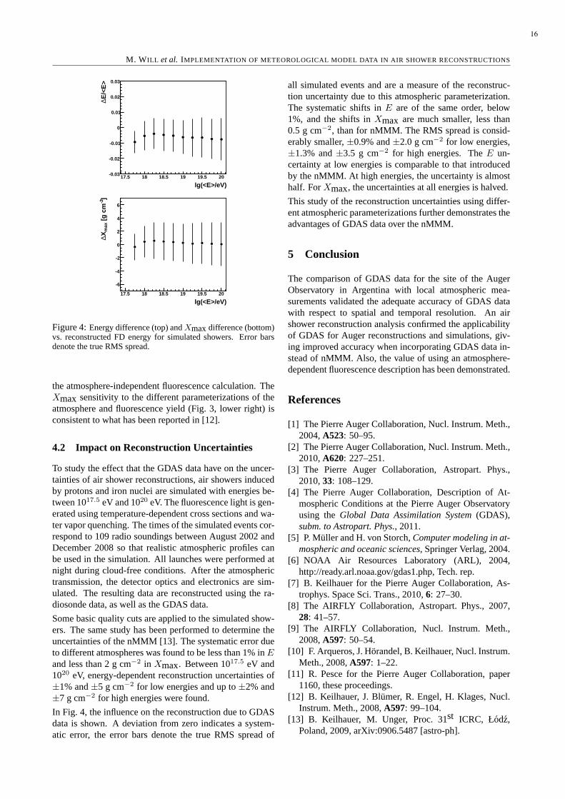
M. W ILL et al. IMPLEMENTATION OF METEOROLOGICAL MODEL DATA IN AIR SHOWER RECONSTRUCTIONS
lg(<E>/eV)17.5 18 18.5 19 19.5 20
E/<
E>
∆
-0.03
-0.02
-0.01
0
0.01
0.02
0.03
lg(<E>/eV)17.5 18 18.5 19 19.5 20
]-2
[g c
mm
axX∆
-6
-4
-2
0
2
4
6
Figure 4:Energy difference (top) andXmaxdifference (bottom)vs. reconstructed FD energy for simulated showers. Error barsdenote the true RMS spread.
the atmosphere-independent fluorescence calculation. TheXmax sensitivity to the different parameterizations of theatmosphere and fluorescence yield (Fig. 3, lower right) isconsistent to what has been reported in [12].
4.2 Impact on Reconstruction Uncertainties
To study the effect that the GDAS data have on the uncer-tainties of air shower reconstructions, air showers inducedby protons and iron nuclei are simulated with energies be-tween 1017.5 eV and 1020 eV. The fluorescence light is gen-erated using temperature-dependent cross sections and wa-ter vapor quenching. The times of the simulated events cor-respond to 109 radio soundings between August 2002 andDecember 2008 so that realistic atmospheric profiles canbe used in the simulation. All launches were performed atnight during cloud-free conditions. After the atmospherictransmission, the detector optics and electronics are sim-ulated. The resulting data are reconstructed using the ra-diosonde data, as well as the GDAS data.
Some basic quality cuts are applied to the simulated show-ers. The same study has been performed to determine theuncertainties of the nMMM [13]. The systematic error dueto different atmospheres was found to be less than 1% inEand less than 2 g cm−2 in Xmax. Between 1017.5 eV and1020 eV, energy-dependent reconstruction uncertainties of±1% and±5 g cm−2 for low energies and up to±2% and±7 g cm−2 for high energies were found.
In Fig. 4, the influence on the reconstruction due to GDASdata is shown. A deviation from zero indicates a system-atic error, the error bars denote the true RMS spread of
all simulated events and are a measure of the reconstruc-tion uncertainty due to this atmospheric parameterization.The systematic shifts inE are of the same order, below1%, and the shifts inXmax are much smaller, less than0.5 g cm−2, than for nMMM. The RMS spread is consid-erably smaller,±0.9% and±2.0 g cm−2 for low energies,±1.3% and±3.5 g cm−2 for high energies. TheE un-certainty at low energies is comparable to that introducedby the nMMM. At high energies, the uncertainty is almosthalf. ForXmax, the uncertainties at all energies is halved.
This study of the reconstruction uncertainties using differ-ent atmospheric parameterizations further demonstrates theadvantages of GDAS data over the nMMM.
5 Conclusion
The comparison of GDAS data for the site of the AugerObservatory in Argentina with local atmospheric mea-surements validated the adequate accuracy of GDAS datawith respect to spatial and temporal resolution. An airshower reconstruction analysis confirmed the applicabilityof GDAS for Auger reconstructions and simulations, giv-ing improved accuracy when incorporating GDAS data in-stead of nMMM. Also, the value of using an atmosphere-dependent fluorescence description has been demonstrated.
References
[1] The Pierre Auger Collaboration, Nucl. Instrum. Meth.,2004,A523: 50–95.
[2] The Pierre Auger Collaboration, Nucl. Instrum. Meth.,2010,A620: 227–251.
[3] The Pierre Auger Collaboration, Astropart. Phys.,2010,33: 108–129.
[4] The Pierre Auger Collaboration, Description of At-mospheric Conditions at the Pierre Auger Observatoryusing theGlobal Data Assimilation System(GDAS),subm. to Astropart. Phys., 2011.
[5] P. Muller and H. von Storch,Computer modeling in at-mospheric and oceanic sciences, Springer Verlag, 2004.
[6] NOAA Air Resources Laboratory (ARL), 2004,http://ready.arl.noaa.gov/gdas1.php, Tech. rep.
[7] B. Keilhauer for the Pierre Auger Collaboration, As-trophys. Space Sci. Trans., 2010,6: 27–30.
[8] The AIRFLY Collaboration, Astropart. Phys., 2007,28: 41–57.
[9] The AIRFLY Collaboration, Nucl. Instrum. Meth.,2008,A597: 50–54.
[10] F. Arqueros, J. Horandel, B. Keilhauer, Nucl. Instrum.Meth., 2008,A597: 1–22.
[11] R. Pesce for the Pierre Auger Collaboration, paper1160, these proceedings.
[12] B. Keilhauer, J. Blumer, R. Engel, H. Klages, Nucl.Instrum. Meth., 2008,A597: 99–104.
[13] B. Keilhauer, M. Unger, Proc. 31st ICRC, Łodz,Poland, 2009, arXiv:0906.5487 [astro-ph].
16

32ND INTERNATIONAL COSMIC RAY CONFERENCE, BEIJING 2011
Night Sky Background measurements by the Pierre Auger Fluorescence Detectors and compar-ison with simultaneous data from the UVscope instrument
ALBERTO SEGRETO1 FOR THE PIERRE AUGER COLLABORATION2
1Ist. Astrofisica Spaziale e Fisica Cosmica, IASF-Pa/INAF, Via La Malfa 153, 90146, Palermo, Italy2Observatorio Pierre Auger, Av. San Martın Norte 304, 5613 Malargue, Argentina(Full author list: http://www.auger.org/archive/authors 2011 05.html)[email protected]
Abstract: Due to the AC coupling of PMTs in the Pierre Auger Fluorescence Detectors, the slowly varying currentinduced by the Night Sky Background cannot be directly measured. Estimate of the Night Sky Background is howeverindirectly obtained by the statistical analysis of the current fluctuations, whose variance is recorded every 30 s for eachpixel. We present the procedure used to convert the raw background data of the Fluorescence Detector to an absolute cal-ibrated Night Sky Background flux and compare the results with data taken simultaneously with the UVscope instrument(a single photon counting UV detector) placed on the roof of one of the Fluorescence Detector buildings. We also showhow the measurements of Night Sky Background flux can effectively be used as a general non-invasive tool to verify theend-to-end calibration of a large aperture telescope with multi-pixel cameras.
Keywords: Pierre Auger Observatory,fluorescence detector, calibration, night sky background
1 Introduction
The Pierre Auger Observatory includes 27 FluorescenceDetector (FD) telescopes in 4 sites [1]. In brief, a singleFD telescope is composed by an aperture system with aUV filter, a spherical mirror (13 m2) and a camera formedby an array of 440 hexagonal photomultipliers (PMTs), ar-ranged in a matrix of 20× 22 pixels in the focal surface.Each pixel has a hexagonal field of view of 1.5 .The signals from the PMTs are amplified, filtered and con-tinuously digitized by 10 MHz (20 MHz for the latest tele-scopes named HEAT) 12 bit Flash Analog to Digital Con-verters (FADCs). Signals from the PMTs are AC coupledto the analog electronics, so the slowly varying anode cur-rent proportional to the Night Sky Background (NSB) lightcannot be directly observed in the FADC traces.However, due to the random nature of the process involved,there is a direct relation between the average anode currentand its statistical fluctuations that, being fast varying sig-nals, are not entirely blocked by the AC coupling. For thisreason, the variances of the FADC traces are continuouslycomputed and recorded for each pixel, in background files.In this paper we report on the procedure to convert therecorded FD variance signal to an absolute calibrated pho-ton flux and compare the results with measurements per-formed with an independent detector, named UVscope, ob-serving, in Single Photon Counting mode, the same regionof the sky. We also show how the NSB flux measurements
can effectively be used as a general non-invasive tool to ver-ify the end-to-end calibration of large aperture telescopeswith multi-pixel cameras.
2 The FADC Variance
The statistical analysis of the FADC traces has been im-plemented in the FPGA logic on the FD first level triggerboards. The FADC variance and pedestal for each pixelare usually recorded with a sampling time of 30 s. In-dicating with σ2
FADC the variance of the FADC trace inADC-counts2, and with IFADC the mean anode current inADC-counts, the direct proportionality existing betweenthese two variables can be expressed by the constant KV,given by [2] :
KV.=
IFADC
σ2FADC
=10
2 ·G · (1+νG) ·F(1)
where G is the PMT gain (FADC-counts/photoelectron),νG is the gain variance factor of the PMT, and F is the noiseequivalent bandwidth (MHz) from the complete analog sig-nal chain. Of course the electronic noise gives a small ad-ditional contribution to the measured FADC variance. Forsake of simplicity, we will omit this term in the formula.In the following sections we explain the procedure used toconvert the recorded FADC variance values to an absolutecalibrated photon flux.
17

A. SEGRETO et al. NIGHT SKY BACKGROUND MEASUREMENTS
3 The FD absolute calibration costants
The FD absolute end-to-end calibrations [3] provide, foreach camera pixel, the scaling factors to convert any pulsedsignal observed in the FADC traces to the correspondingphoton flux at the telescope aperture. This calibration isperformed periodically by placing in front of the FD tele-scope diaphragm an extended (2.5 m diameter) uniformlight source that, for its shape, is called ”Drum”.The ”Drum calibration constants”, KD, are provided inunits of photons/FADC-counts, being conventionally de-fined so that, for a monochromatic source at the refer-ence wavelength λD = 375 nm, they enable one to con-vert the FADC signal to the number of photons arrivingat the FD diaphragm in the FADC integration time. Theflux in photons/m2/sr/s of a pulsed monochromatic sourceat wavelength λD, fully illuminating the pixel, is then ob-tained by:
ΦλD =KD
∆T ·A ·Ω· IFADC (2)
where IFADC is the pulse amplitude (in FADC-counts), andthe parameters have the following fixed numerical values:
• ∆T = 100 ns (FADC Integration Time, 50 ns for theHEAT telescope)
• A = 3.8 m2 (Area of FD telescope diaphragm)
• Ω = 5.94 ×10⁻⁴ sr (Pixel Solid Angle Acceptance)
For a non-monochromatic source with spectral distributionΦλ, the number of equivalent photons at λD must be ob-tained by:
ΦλD =
∫ ∞
0Φλ ·Fλ ·dλ (3)
where Fλ is the pixel spectral response normalized to thereference wavelength λD (FλD = 1).Of course, Eq. 2 can be applied only to fast (µs time scale)pulsed signals observed in the FADC traces, while theslowly varying component of the illuminating photon fluxcan only be derived from the variance of the FADC trace asexplained in the following section.
4 Calibration of the FADC variance
Combining Eq. 1, 2, and 3, the end-to-end conversion for-mula to obtain the average flux (in photons/m2/sr/ns/nm)of a slow-varying, non-monochromatic source fully illumi-nating the pixel, is expressed by:
< Φλ >.=
∫ ∞0 Φλ ·Fλ dλ∫ ∞
0 Fλ dλ=
=KD ·KV
∆T ·A ·Ω ·∫ ∞
0 Fλ dλ·σ2
FADC (4)
This formula then allows one to convert the variance signalrecorded in the FD background files (after subtraction of
Figure 1: Upper panel: FADC average trace of 400 Cal. Apulses; Bottom panel: residuals after fitting an analyticalmodel to the pulse. The delayed response of afterpulses(not included in the model) and the increase of fluctuationsassociated to the illuminating photons are evident.
the electronic noise) to the absolute calibrated value of thediffuse component of the NSB flux.In addition to the uncertainty associated with the absolutecalibration constant KD, the accuracy of the flux measure-ments obtained from this equation is also affected by pixel-to-pixel variations in the spectral response Fλ and by theuncertainty in the variance scaling factor KV.Multi-wavelength calibration [4] has shown that pixel-to-pixel dispersion of the spectral response is of the order offew percent so, as a first approximation, we use the aver-age spectral response of the FD pixels (reported in [4]), toobtain a common scaling factor:∫ ∞
0Fλ dλ = 73.5nm (5)
The uncertainty in the constant KV, is affected (Eq. 1) bythe cumulative indetermination in all the three physical pa-rameters G, νG and F. Since the values of these parametersmay change significatively from pixel to pixel and no accu-rate measurements are available for every pixel, the overallindeterminacy in KV, (computed, e.g., by adopting the typ-ical mean values) would be unacceptably high.Rather than deriving KV from the pixel physical parame-ters, it is possible to directly obtain its value, with a muchbetter statistical accuracy, from analysis of the relative cali-bration runs ”Cal. A” as explained in the following section.
5 Cal. A calibrations
To follow the short term behavior of the FD photomultipli-ers, three relative calibrations, Cal. A, B, C are performedeach night of data taking. In the Cal. A, a sequence ofsquare-type light pulses (57 µs) are produced at a rate of1/3 Hz with a very stable bright LED source (at 470 nm)and transmitted with light guides to a Teflon diffuser lo-cated in the center of the mirror, thus illuminating directlythe camera photomultipliers [5].
18
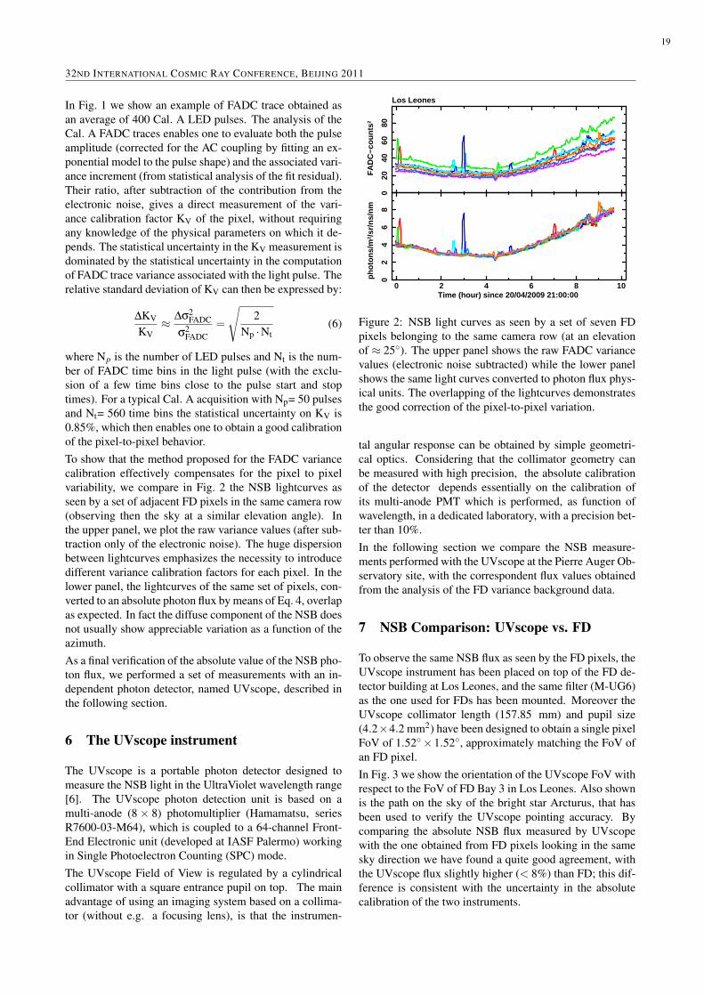
32ND INTERNATIONAL COSMIC RAY CONFERENCE, BEIJING 2011
In Fig. 1 we show an example of FADC trace obtained asan average of 400 Cal. A LED pulses. The analysis of theCal. A FADC traces enables one to evaluate both the pulseamplitude (corrected for the AC coupling by fitting an ex-ponential model to the pulse shape) and the associated vari-ance increment (from statistical analysis of the fit residual).Their ratio, after subtraction of the contribution from theelectronic noise, gives a direct measurement of the vari-ance calibration factor KV of the pixel, without requiringany knowledge of the physical parameters on which it de-pends. The statistical uncertainty in the KV measurement isdominated by the statistical uncertainty in the computationof FADC trace variance associated with the light pulse. Therelative standard deviation of KV can then be expressed by:
∆KV
KV≈
∆σ2FADC
σ2FADC
=
√
2Np ·Nt
(6)
where Np is the number of LED pulses and Nt is the num-ber of FADC time bins in the light pulse (with the exclu-sion of a few time bins close to the pulse start and stoptimes). For a typical Cal. A acquisition with Np= 50 pulsesand Nt= 560 time bins the statistical uncertainty on KV is0.85%, which then enables one to obtain a good calibrationof the pixel-to-pixel behavior.To show that the method proposed for the FADC variancecalibration effectively compensates for the pixel to pixelvariability, we compare in Fig. 2 the NSB lightcurves asseen by a set of adjacent FD pixels in the same camera row(observing then the sky at a similar elevation angle). Inthe upper panel, we plot the raw variance values (after sub-traction only of the electronic noise). The huge dispersionbetween lightcurves emphasizes the necessity to introducedifferent variance calibration factors for each pixel. In thelower panel, the lightcurves of the same set of pixels, con-verted to an absolute photon flux by means of Eq. 4, overlapas expected. In fact the diffuse component of the NSB doesnot usually show appreciable variation as a function of theazimuth.As a final verification of the absolute value of the NSB pho-ton flux, we performed a set of measurements with an in-dependent photon detector, named UVscope, described inthe following section.
6 The UVscope instrument
The UVscope is a portable photon detector designed tomeasure the NSB light in the UltraViolet wavelength range[6]. The UVscope photon detection unit is based on amulti-anode (8 × 8) photomultiplier (Hamamatsu, seriesR7600-03-M64), which is coupled to a 64-channel Front-End Electronic unit (developed at IASF Palermo) workingin Single Photoelectron Counting (SPC) mode.The UVscope Field of View is regulated by a cylindricalcollimator with a square entrance pupil on top. The mainadvantage of using an imaging system based on a collima-tor (without e.g. a focusing lens), is that the instrumen-
0 2 4 6 8 10
02
46
8
phot
ons/
m2 /
sr/n
s/nm
Time (hour) since 20/04/2009 21:00:00
020
4060
80
FA
DC
−cou
nts
2
Los Leones
Figure 2: NSB light curves as seen by a set of seven FDpixels belonging to the same camera row (at an elevationof ≈ 25). The upper panel shows the raw FADC variancevalues (electronic noise subtracted) while the lower panelshows the same light curves converted to photon flux phys-ical units. The overlapping of the lightcurves demonstratesthe good correction of the pixel-to-pixel variation.
tal angular response can be obtained by simple geometri-cal optics. Considering that the collimator geometry canbe measured with high precision, the absolute calibrationof the detector depends essentially on the calibration ofits multi-anode PMT which is performed, as function ofwavelength, in a dedicated laboratory, with a precision bet-ter than 10%.In the following section we compare the NSB measure-ments performed with the UVscope at the Pierre Auger Ob-servatory site, with the correspondent flux values obtainedfrom the analysis of the FD variance background data.
7 NSB Comparison: UVscope vs. FD
To observe the same NSB flux as seen by the FD pixels, theUVscope instrument has been placed on top of the FD de-tector building at Los Leones, and the same filter (M-UG6)as the one used for FDs has been mounted. Moreover theUVscope collimator length (157.85 mm) and pupil size(4.2×4.2 mm2) have been designed to obtain a single pixelFoV of 1.52×1.52, approximately matching the FoV ofan FD pixel.In Fig. 3 we show the orientation of the UVscope FoV withrespect to the FoV of FD Bay 3 in Los Leones. Also shownis the path on the sky of the bright star Arcturus, that hasbeen used to verify the UVscope pointing accuracy. Bycomparing the absolute NSB flux measured by UVscopewith the one obtained from FD pixels looking in the samesky direction we have found a quite good agreement, withthe UVscope flux slightly higher (< 8%) than FD; this dif-ference is consistent with the uncertainty in the absolutecalibration of the two instruments.
19

A. SEGRETO et al. NIGHT SKY BACKGROUND MEASUREMENTS
Figure 3: Left panel: orientation of the UVscope FoV withrespect to the FD telescope in Los Leones Bay 3. Rightpanel: the UVscope Field of View with the bright star Arc-turus in the center.
In Fig. 4 we compare (by using a scaling factor for therelative calibration) the NSB lightcurves as observed by asingle UVscope pixel and the correspondent FD pixel. Inthe upper panel we have not applied any correction for thenightly evolution of the FD PMT gain, so a relative drift be-tween the two lightcurves is expected. In fact, comparisonbetween the Cal. A runs performed at the beginning and atthe end of the night, always shows the presence of system-atic nightly evolution (few percent) in the PMT gains.In Fig. 4, lower panel, we have corrected the FD lightcurveby assuming a linear drift of the PMT gain between thevalues measured from Cal. A runs at the beginning and atthe end of the night. In this case the match between thetwo NSB measurements is so good that the two lightcurvescan hardly been distinguished.Note that in the comparison of NSB lightcurves, the emis-sion associated to point sources (stars and planets) are notexpected to match exactly as the scaling factors used arevalid only for the diffuse emission.
0 2 4 6 8 10
05
10
ph
oto
ns/
m2 /
sr/n
s/n
m
Time (hour) since 20/04/2009 21:00:00
05
10
ph
oto
ns/
m2 /
sr/n
s/n
m
Arcturus
FD UVscope
Figure 4: NSB lightcurves by single UVscope and FDpixels looking in the same sky direction. Upper panel:lightcurve obtained without correcting for the FD PMTgain drift. Lower panel: The FD PMT gain drift has beencorrected assuming a linear evolution between the gain val-ues measured from the Cal. A at start and stop times.
The example shows how independent measurements ofNSB flux can be effectively used as a general non-invasivetool to verify the end-to-end calibration of telescopes withlarge fields of view and multi-pixel cameras without inter-fering at all with the normal operation of the telescopes.This gives the possibility of monitoring the gain of individ-ual camera pixels in the real working condition (the back-ground flux can induce a shift of the PMT gain with re-spect to dark condition). Moreover the method can be usedto easily verify the flat-fielding of the telescope responseby comparing all the telescope pixels, in turn, to the samereference detector.
8 Conclusions
We have shown how to convert the variance of the FADCtraces, provided in the FD background files, to an absolutecalibrated measurement of the NSB flux and that the re-sulting lightcurves are in excellent agreement with directmeasurements obtained with an independent photon count-ing detector.This opens up the possibility to use the huge FD Augerdatabase for a scientific study of the NSB evolution as afunction of time (short and long term) on an extremelylarge field of view. Moreover the spatial dependence (inparticular with elevation) of the NSB flux can be correlatedwith atmospheric parameters provided by the several at-mospheric monitoring devices installed at the Pierre AugerObservatory site.We have also shown as the UVscope instrument can beused in support of the absolute end-to-end (camera + op-tics + electronics) calibration of telescopes with a cameracomposed by a mosaic of numerous independent photondetectors. This kind of application would be particularlyuseful when, due to the large telescope aperture, the useof a uniform extended illumination source, like the Drum,may not be feasible. This could make it an attractive optionfor future projects such as CTA [7] with a large number oftelescopes distributed over a large area.
References
[1] J. Abraham et al., for the Pierre Auger Collaboration,Nucl. Instrum. Meth., 2010, A620: 227–251.
[2] M. Kleifges et al., IEEE Trans. Nucl. Sci., 2003, 50:1204–1207.
[3] J. Brack, R. Meyhandan, G. Hofman, J. Matthews, As-troparticle Physics, 2004, 20: 653–659.
[4] A. Rovero et al., for the Pierre Auger Collaboration,Astroparticle Physics, 2009, 31: 305–311.
[5] C. Aramo et al., for the Pierre Auger Collaboration,Proc. 29th ICRC, Pune, India, 2005, 8:101-104
[6] M. C. Maccarone et al., paper 0148, these proceedings.[7] G. Hermann, for the CTA collaboration, Nucl. Instrum.
Meth., 2010, A623: 408–409.
20
32ND INTERNATIONAL COSMIC RAY CONFERENCE, BEIJING 2011
Observation of Elves with the Fluorescence Detectors of the Pierre Auger Observatory
AURELIO S. TONACHINI1 FOR THEPIERRE AUGER COLLABORATION2
1Universita degli Studi di Torino and INFN Sezione di Torino, Via PietroGiuria 1, 10125 Torino, Italy2Observatorio Pierre Auger, Av. San Martın Norte 304, 5613 Malargue, Argentina(Full author list: http://www.auger.org/archive/authors 201105.html)auger [email protected]
Abstract: We report the observation of elves using the Fluorescence Detectors of the Pierre Auger Observatory inMalargue, Argentina. Elves are transient luminous phenomena originating in the D layer of the ionosphere, high abovethunderstorm clouds, at an altitude of approximately 90 km.With a time resolution of 100 ns and a space resolution ofabout 1 degree, the Fluorescence Detectors can provide an accurate 3D measurement of elves for thunderstorms whichare below the horizon. Prospects for the implementation of adedicated trigger to improve detection efficiency and plansto perform multi-wavelength studies on these rare atmospheric phenomena will be given.
Keywords: elves, lightnings, ionosphere, thunderstorms, fluorescence detectors, Pierre Auger Observatory
1 Introduction
There is an electrodynamic coupling between electromag-netic fields produced by lightning discharges and the lowerionosphere. This coupling gives rise to distinct sets of ob-served phenomena, including various transient luminousevents (TLEs) such as the so-called “Sprites” and “Elves”.Sprites are luminous discharges located at altitudes be-tween 40 and 90 km. They are due to the heating of am-bient electrons, and last a few to tens of milliseconds. Thischaracteristic makes them easily detectable with high speedcameras. Elves are optical flashes produced by heating,ionisation, and subsequent optical emissions due to intenseelectromagnetic pulses (EMPs) radiated by both positiveand negative lightning discharges. Elves are confined to80-95 km altitudes, and extend laterally up to 600 km [1].Their duration, much shorter (< 1ms) than that of sprites,made them somewhat harder to study. The first clear ob-servation of elves was made using a high speed photometerpointed at altitudes above those of sprites [2]. More sophis-ticated instruments, such as “Fly’s Eye” [3] and PIPER [4],consisting of linear arrays of horizontal and vertical pho-tometers with a time resolution of∼ 40µs, have been usedin the last decade to study the rapid lateral expansion ofthese high altitude optical emissions, and to test the excita-tion mechanism. Data from space on elves were acquiredby the ISUAL/Formosat-2 mission, from 2004 to 2007 [5].These data allowed one to conclude that elves develop onoceans or coastal regions ten times more frequently than onland. The satellite data were acquired with six PMTs and
two 16-channel multi-anode PMTs, with time resolutionsof 100 and 50µs, respectively.
Further advancements in the understanding of these phe-nomena may be achieved using the fluorescence detector(FD) of the Pierre Auger Observatory [6]. The FD com-prises four observation sites located atop small hills at theboundaries of the Auger surface array. Each FD build-ing contains six independent telescopes, each with a fieldof view (FOV) of 30 × 30
in azimuth and elevation.The combination of the FOV of the six telescopes cov-ers180 in azimuth. Incoming light enters through a UV-transmitting filter window, and is focused by a mirror ontoa camera, which is formed by22 × 20 hexagonal photo-multiplier tubes (PMTs). The wavelength of detected lightranges from 300 to 420 nm. Light pulses in each photo-multiplier are digitized every 100 ns. The PMT processeddata are passed through a flexible multi-stage trigger sys-tem, which is implemented in firmware and software. Theresulting data are stored in100µs-long traces.
The FD geometry and time resolution are ideal for study-ing fast developing TLEs. However, the trigger chain con-tains a dedicated selection algorithm for rejecting light-ning, which makes the FD a rather inefficient elve detec-tor. Nevertheless, a few events which accidentally passedthe rejection have been detected while searching for non-conventional cosmic ray shower events.
21

A. S. TONACHINI et al. OBSERVATION OF ELVES
2 Observations
The first event was noticed serendipitously during an FDdata taking shift. This unusual event presented a well de-fined space-time structure: a luminous ring starting from acluster of pixels, and expanding in all directions.
A search for events with a similar space-time evolution inthe data collected by the Pierre Auger Observatory since2004 has identified two more events. These events arelisted in the Table 1. The presence of dust and poor localweather conditions, recorded by local atmospheric moni-toring devices [7], complicate the reconstruction of the firstand the last event, but do not prevent one from recognizingthe same overall features of the phenomenon. Most of thedetails which are given in this paper refer to the analysisof the second event. In Fig. 1, the photon time distribu-tions for the three events are shown. Events which do notpass the whole trigger selection, but trigger a minimum of
s)µTime (0 10 20 30 40 50 60 70 80 90 100
Sig
nal (
phot
on c
ount
s)
020406080
100120140160180200
310×
s)µTime (0 10 20 30 40 50 60 70 80 90 100
Sig
nal (
phot
on c
ount
s)
0
20
40
60
80
100
120
140
310×
s)µTime (0 10 20 30 40 50 60 70 80 90 100
Sig
nal (
phot
on c
ount
s)
0
20
40
60
80
100
120
140
310×
Figure 1: Photon counts at 370 nm obtained from the sumof all photomultiplier ADC traces of the three events in Ta-ble 1. Since these events are not totally contained inside thecamera FOV, the gray areas denote a region with possiblesignal losses.
Site-Bay GPS time GMT timeLM − 6 800414142 18 May 2005 01:15:29CO − 3 860806213 17 April 2007 00:49:59LL− 1 861081389 20 April 2007 05:16:15
Table 1: Three elve candidates seen by Auger fluorescencedetectors and their arrival times.
Figure 2: Schematic view of an EMP generated by a thun-derstorm inS, which interacts with the D region of theionosphere. The light emitted by the ionosphere (in red)is detected by the fluorescence detector atO. The observedsignal timet is the combination of the time needed by thepulse to move fromS to the interaction pointP and thetime needed by the emitted light to travel fromP to O.
adjacent PMTs (second level trigger, or T2) leave some ba-sic information in a log file, such as the GPS time and thenumber of PMTs hit. From these logs it is found that allthe selected events last much longer than 70µs, and are ac-tually detected in adjacent FD bays, or even in other eyes,as summarized in Table 2. The number of buffered pagesshows, in units of 0.1 ms, the time duration of the detectedevent.
Site-Bay N buffered pages Time delay (µ s)LM-6 7 0LM-5 7 38CO-3 9 0CO-2 7 9.5LL-1 4 56.3LL-1 2 0LL-2 3 34.1CO-3 5 59.1
Table 2: FD telescope, number of T2 pages, and time delayfor the three elve events.
3 Front propagation reconstruction
If the events observed are elves, the signals recorded cor-respond to the optical emission of the D region of the iono-sphere, as a consequence of its interaction with a lightning-launched electromagnetic pulse (EMP).
22

32ND INTERNATIONAL COSMIC RAY CONFERENCE, BEIJING 2011
s)µTime (10 20 30 40 50 60
Sig
nal (
phot
on c
ount
s)
-100
0
100
200
300
400
500
σ3
Figure 3: A signal measured with a single photomulti-plier (gray graph). To reduce noise fluctuations, a mov-ing average is performed on the original trace (black thickgraph). The start point (blue square point) is defined fromthis graph when the signal is5σ above the baseline (dottedline).
3.1 Geometrical model
The EMP source is confined inside the troposphere, whilethe optical emission takes place at 80-95km altitudes. Theobserved light develops over times comparable with thetime needed to travel from the sourceS to a point in theD region, and from there to the observerO at the speed oflight (see Fig. 2). In fact, the light detected at timet maycome from any of the points belonging to the intersectionof the D region with an ellipsoid whose foci areO andS.
The first light arrives at a timet0 defined by the ellipsoidtangent to the D region. The tangent pointP is found fromobservations, and puts constraints on the location of thesourceS. Indeed, it can be demonstrated geometricallythat the line tangent atP to an ellipse with fociO andSforms equal angles with the linesOP andPS. Thus, oncedefinedP , the locus of the fociSi is a line.
At a time ti > t0 the intersection of the ellipsoid with theD region corresponds to a closed curve: this is actually ob-served by the fluorescence detectors. The lateral expansionof this curve is expected to be symmetric, while the frontmoving towards the FD is expected to move faster than thatmoving in the opposite direction.
3.2 Signal treatment
The pixels considered in each event are the ones which havean FD first level trigger trace. Each trace is formed by 1000time bins of 100 ns each. Signal bounds are searched ineach trace by maximizing the signal to noise ratio. This al-lows one to roughly estimate the pulse start and stop times.Afterwards the signal is smoothed by applying a2.1µs run-ning average in order to decrease short time signal fluctu-ations. The pulse start position is then moved back untilthe signal is less than5σ above the noise. The error asso-ciated with this point is determined by searching the time
where the signal is less than3σ, and then taking the timedifference with respect to the start point (see Fig. 3).
The pulse start times measured by each photomultiplier areplotted in Fig. 4 as a function of PMT pointing directions.This development has been compared with the geometricalmodel discussed before. Once the pixel which recordedthe minimum pulse start time was found, the direction ofthe start pointP was varied by±2
in both elevation andazimuth angles. For eachP the altitude of the D regionand the direction of the EMP source with respect to the FDhave been variated within 80 to 100 km and+5
and−5
respectively, in order to find the parameters which better fitthe elve development.
4 Results
The best fit to the pulse start times of the event studiedis obtained for a source elevation angle of−1.15 and aD layer altitude of 92 km a.s.l.. The direction (elevation,azimuth) of the first light is (14.6,−52.1). The sourcelinear distance from the fluorescence detector of the AugerObservatory is about 580 km. A comparison of the timesexpected from a theoretical model with these parametersand the real data is shown in Fig. 5. The time residuals areplotted in Fig. 6.
The location of the event is strengthened by the presenceof a large cloud perturbation seen by GOES geostation-ary satellites in the same region [8]. Moreover, a coinci-dence with a strong lightning pulse detected by the WorldWide Lightning Location Network (WWLLN) [9] has beenfound.
Elevation (deg)8 10 12 14 16 18 20 22 24 26 28
Azimuth (deg)-58
-56-54
-52-50
-48-46
-44-42
-40
s)µTi
me
(
2030405060708090
Figure 4: Interpolated tridimensional curve representingthe time of arrival of photons at the FD diaphragm as afunction of elevation and azimuth angle. Pulse start timesbelong to the event detected at GPS 860806213. This eventtriggered 143 pixels.
23

A. S. TONACHINI et al. OBSERVATION OF ELVES
Elevation (deg)
10 12 14 16 18 20 22 24 26
s)
μt
(δ
0
5
10
15
20
25
30
(deg)φδ
-6 -4 -2 0 2 4 6 8 10
s)
μt
(δ
0
5
10
15
20
25
30
Figure 5: Best fit (red curve) compared to real data (blacksquares) for the column and the row of pixels passingthrough the centre of the event.δφ is the azimuth direc-tion of the pixel with respect to the centre.
Azimuth (deg)-58 -56 -54 -52 -50 -48 -46 -44
Ele
vatio
n (d
eg)
10
12
14
16
18
20
22
24
-4
-2
0
2
4
6
8
Figure 6: Difference between measured pulse start timesand simulated ones as a function of the pixel pointing di-rections (µs). Differences are confined within2µs, withthe exception of one pixel which recorded a trace delayedby 7µs.
5 Final remarks
It has been shown that the fluorescence detector of thePierre Auger Observatory may represent an interesting op-portunity to study the elve evolution with an unprecedentedtime resolution. However, in order to transform the FD inan efficient elve detector it is necessary to design a dedi-cated software trigger. This would allow one not only toincrease the FD efficiency, but to record subsequent sig-nal traces up to the expected length of these optical flashes(∼ 1ms).
Longitude(degrees)-72 -70 -68 -66 -64 -62 -60
Latit
ude(
degr
ees)
-42
-41
-40
-39
-38
-37
-36
-35
-34
-33
Figure 7: The position of the reconstructed elve (blacksquare) is compared to that of lightning occurring at thesame GPS second (black circle). Lightning recorded byWWLLN stations during the same day are plotted as graycircles. Lightning close in time (within 5 s) is representedby filled circles. Black stars mark the locations of Augerfluorescence detectors. Dotted lines define the six bays ofthe FD at Coihueco (CO).
6 Acknowledgements
We would like to thank Prof. R. Holzworth for having madeavailable the list of lightnings recorded by WWLLN, andthe GOES organization for having made public GOESsatellite data.
References
[1] U. S. Inan, T. F. Bell, J. V. Rodriguez, Geophys. Res.Lett., 1991,18: 705-708
[2] H. Fukunishi et al., Geophys. Res. Lett., 1996,23:2157-2160
[3] U. S. Inan et al., Geophys. Res. Lett., 1997,24: 583-586
[4] R.T.Newsome and U.T.Inan, J.Geophys.Res., 2010,113: A00E41
[5] Chen et al. J.Geophys.Res., 2008,113: A08306[6] The Pierre Auger Collaboration, NIM A, 2010,620:
227-251[7] The Pierre Auger Collaboration, Astropart. Phys.,
2010,33: 108-129[8] http://www.oso.noaa.gov/goes/[9] http://webflash.ess.washington.edu/
24

32ND INTERNATIONAL COSMIC RAY CONFERENCE, BEIJING 2011
Atmospheric ”Super Test Beam” for the Pierre Auger Observatory
L. W IENCKE1 , FOR THE PIERRE AUGER COLLABORATION2 AND A. BOTTS1, C. ALLAN 1, M. CALHOUN1 ,B. CARANDE1 , M. COCO1,5 , J. CLAUS1 , L. EMMERT1, S. ESQUIBEL1, L. HAMILTON 1, T.J. HEID1,F. HONECKER1,3, M. IARLORI4 , S. MORGAN1, S. ROBINSON1 , D. STARBUCK1 , J. SHERMAN1 , M. WAKIN 5 ,O. WOLF1
1 Colorado School of Mines, Department of Physics, 1523 Illinois St., Golden CO, USA2 Observatorio Pierre Auger, Av. San Martin Norte 304, 5613 Malargue, Argentina3 Karlsruhe Institute of Technology (KIT), 76131 Karlsruhe,Germany4 CETEMPS and INFN, Dep. di Fisica Universita Degli Studi dell’Aquila, via Vetoio, I-67010, L’Aquila, Italy5 Colorado School of Mines, Division of Engineering, 1500 Illinois St., Golden CO, USA(Full author list: http://www.auger.org/archive/authors_2011_05.html)[email protected]
Abstract: We present results from 200 hours of operation of an atmospheric super test beam system developed forthe Pierre Auger Observatory. The approximate optical equivalence is that of a 100 EeV air shower. This new systemcombines a Raman backscatter LIDAR receiver with a calibrated pulsed UV laser system to generate a test beam inwhich the number of photons in the beam can be determined at ground level and as a function of height in the atmospherewhere high energy air showers develop. The data have been recorded simultaneously by the Raman receiver and by asingle mirror optical cosmic ray detector that tested the new system by measuring the side-scattered laser light acrossahorizontal distance of 39 km. The new test beam instrument will be moved from the R&D location in southeast Coloradoto the Pierre Auger Observatory location in Argentina to effect a major upgrade of the central laser facility.
Keywords: Atmosphere, LIDAR, Pierre Auger Observatory, Calibration, Raman Scattering
1 Introduction
The Pierre Auger Observatory uses the atmosphere as a gi-ant calorimeter to measure properties of the highest energyparticles known to exist. Test beams of particles with theseextreme energies (1-100 EeV) do not exist. However lightscattered out of UV laser beams directed into the atmo-sphere from the Central and eXtreme Laser Facilities (CLF[1] & XLF) generate tracks that are recorded by the AugerObservatory fluorescence detector (FD) [2] telescopes thatalso record tracks from extensive air showers. There is anapproximate effective optical equivalence between a 5 mJUV laser track and that of a 100 EeV air shower.
Atmospheric clarity, specifically the aerosol optical depthprofile, τ(z, t), is the largest and most variable calibrationterm, especially for the highest energy air showers. Themethod to obtainτ(z, t) that was pioneered by HiRes [3]and extended to the Auger Observatory uses FD measure-ments of side-scattered light from UV laser pulses [4] [5].The relatively large light collecting power of the telescopesmeans that relatively few laser pulses are required. Thesepulses also provide a means to monitor detector calibration,performance, and aperture [6].
38.9 kmAMT
1.54 km Lase
r B
eam
10.8 km
LIDAR
AMT Field of View
Figure 1: Geometrical arrangement, viewed from the side,of the laser and the two independent optical detectors.
To improve detector monitoring andτ(z, t) measurements,an upgrade is planned for the CLF. This will add a RamanLIDAR receiver, replace the flash lamp laser with a solidstate laser, add an automated beam calibration system [8]as used at the XLF, and improve critical infrastructure.
Key components for the upgrade have been tested at thePierre Auger North R&D site [9] in Southeast Colorado.Data collected have been used to measureτ(z, t) by twoindependent methods: elastic side scattering and inelastic(Raman) backscattering from N2 molecules. The arrange-ment of instruments (Fig. 1) includes the solid state laserthat generates a vertical pulsed beam (355 nm 7 ns pulsewidth), the collocated LIDAR receiver and a simplified FD
25

WIENCKE et al. ATMOSPHERIC“SUPERTEST BEAM”
Figure 2: Scanning electron images of aerosols sampledat ground level at the Pierre Auger Observatory [10] (left:2.5µm filter right:10.0µm filter).
telescope 38.9 km distant. Dubbed the atmospheric moni-toring telescope (AMT), this instrument records side scat-tered light from the laser in the same way that the AugerObservatory FD telescopes record light from the CLF andthe XLF in Argentina. Data collected also include tem-perature, pressure and humidity profiles recorded by 27 ra-diosonde weather balloons launched from the LIDAR siteduring 2009 to 2011.
2 The Raman LIDAR
In measuringτ(z, t) with elastically scattered laser light aninherent ambiguity is encountered. The measured quantity,i.e. the amount of light reaching the detector at a particu-lar time bin (height) depends on several unknowns. Theseinclude the fraction of light transmitted to the scatteringre-gion, the fraction of light scattered in the direction of thedetector by the molecular component and aerosols at theparticular height, and the fraction of light transmitted backto the detector. The transmission terms can be combinedif the atmosphere is assumed to be horizontally uniform,or if the receiver and laser are collocated. The molecularpart of the scattering term can be determined to good accu-racy from radiosonde measurements and molecular scatter-ing theory. However the aerosol scattering term can not bemodeled well because aerosol particles span a wide rangeof sizes and irregular shapes [10] (Fig. 2) and these prop-erties typically vary with height.
Raman LIDARs evade this ambiguity by measuring lightRaman scattered by N2 molecules. The Raman scatteringcross section for N2 is well understood. The N2 densityprofile can be derived from radiosonde data or through theGlobal Data Assimilation System (GDAS) [14] [15]. Overthe past few decades, Raman LIDAR has become the stan-dard method to measureτ(z, t).
The Raman LIDAR receiver used in these tests features a50 cm diameter f/3 parabolic mirror pointing vertically be-neath a UV transmitting window and motorized roof hatch.A liquid light guide couples the reflected light from the mir-ror focus to a three channel receiver (Fig. 3). Dichroicbeam splitters direct this light onto 3 photomultiplier tubes(PMTs) that are located behind narrow band optical fil-ters. These isolate the three scattered wavelengths of in-
Figure 3: The three channel LIDAR receiver. Light re-flected from the parabolic mirror (not shown) enters vialiquid light guide seen near the lower left corner of thispicture.
terest: 355 nm (Elastic scattering), 386.7 nm (Raman N2
backscattering), and 407.5 nm (Raman H2O backscatter-ing). The data acquisition system uses fast photon counting(250 MHz) modules. The LIDAR receiver and solid stateUV laser were deployed 15 km south of Lamar, Colorado.
3 The AMT detector
The AMT (Fig. 4) is a modified HiRes II type telescope.The 3.5 m2 mirror, camera, photomultiplier tube assem-blies, and UV filter are all housed in a custom-built shel-ter with a roll-up door across the aperture. For these tests,the central 4 columns of1 pixels were instrumented. TheAMT is mounted on four concrete posts and aligned so thatthe vertical laser track passed near the center of the fieldof view (FOV). The FOV at the vertical laser spans 1.54to 10.8 km above the ground. A precipitation and ultra-sonic wind sensor ensure the door was closed during rainyor windy conditions. The AMT is pointed toward the northso that direct sunlight could not damage the camera if thedoor is open during the day. The door and field of view canbe observed remotely through a network video camera.
The PMTs were gain sorted prior to installation. Data froma temperature controlled UV LED system at the mirror cen-ter and from a vertical nitrogen laser scanned across thefield of view were used to flat field and debug the cam-era. During routine nightly operation, the relative calibra-tion was monitoried using the LED system.
The readout of the PMT current is performed by pulseshaping and digitization system electronics that are also im-plemented in the High Elevation Auger Telescope (HEAT)[11] [12] extension to the Auger Observatory. The sam-pling period is 50 ns. The readout is triggered externally,either by pulses from the UV LED system, or from a GPSdevice [13]. The laser is also triggered by the same modelGPS device. The AMT GPS pulse output is delayed by130 µs to allow for light travel time between the two in-struments.
26

32ND INTERNATIONAL COSMIC RAY CONFERENCE, BEIJING 2011
Figure 4: The remotely operated Atmospheric Monitoring Telescope (left) and its camera (right) with the central 4columns instrumented. A rectangular UV transmitting filter(not shown) normally covers the camera surface.
Figure 5: The hourly sequence of operations.
Sep 2010
Oct 2010
Nov 2010
Dec 2010
Jan 2011
Feb 2011
Mar 2011
0
50
100
150
200
250
Hours
Figure 6: Accumulation of data when the AMT and theRaman LIDAR operated on the same hour
4 Operations and Data Analysis
The AMT, LIDAR, laser and various subsystems are alloperated under computer control. Their nightly operationis sequenced by automation scripts initiated on moonlessnights from the Colorado School of Mines campus. Oper-ation and data collection are then monitored remotely bycollaborators in Colorado, Germany, and Italy. The hourlysequence (Fig. 5) interleaves sets of 200 laser shots at 4 Hzfor AMT measurements, sets of 120 UV LED shots forAMT relative calibration, and 12 minute sets of 100 Hzlaser shots for LIDAR measurements. Between October2010 and March 2011, more than 200 hours of data havebeen accumulated for which the AMT and LIDAR mea-sured laser light during the same hour (Fig. 6).
The Raman LIDAR was benchmarked against the Euro-pean LIDAR network EARLINET [7] prior to shipment
Height a.s.l. [km]2 4 6 8 10 12 14 16 18 20
]-3
Air
Den
sity
(G
DA
S -
dat
a) [k
g m
-6
-5
-4
-3
-2
-1
0
1
2
3
4-310×
Figure 7: Average difference in atmospheric density as de-termined from the GDAS model and measured from 27 ra-diosondes launches.
from Italy. The algorithm used in this benchmark was alsoused to retrieve aerosol profiles in Colorado from the N2
channel. The N2 density was obtained from the GDASmodel. The model agreed well with the radiosonde datacollected at the site (Fig. 7).
The measurement ofτ(z, t) from the AMT data used thedata normalized retrieval algorithm adapted from the ver-sion used in Argentina to obtainτ(z, t) from FD measure-ments of vertical CLF laser pulses. Two reference nightswere selected in the Colorado sample. The analysis in-cluded corrections for variations in the laser output and inthe relative calibration of the AMT. Systematic errors of3% were assigned to these terms and an equivalent errorwas assigned for the choice of reference night.
5 Results
A correlation is observed between the two independentmeasurements of aerosol optical depth (Fig. 8). Periods ofobvious cloud were removed from this analysis. The small-est differences in absolute terms are observed during loweraerosol conditions, i.e.τ(4.5 km) < 0.05. Horizontal non-uniformity of the aerosol distribution across the 39 km be-tween detectors can be expected to contribute to the broad-
27

WIENCKE et al. ATMOSPHERIC“SUPERTEST BEAM”
Figure 8: Comparison between the vertical aerosol opticaldepth at 4.5 km as measured by the AMT and the RamanLIDAR systems.
ening of the correlation under hazier conditions. Furtheranalysis is in progress. We note this work represents thefirst systematic comparison between these methods as ap-plied to astroparticle detectors.
6 Targeted applications of the CLF upgrade
Because of the relatively small size of the Raman scatter-ing cross section, thousands of laser shots are needed toaccumulate sufficient photon statistics. This has potentialto interfere significantly with FD operation. However, anumber of specific physics targets have been identified forwhich one set of Raman LIDAR measurements per night isexpected to provide a valuable supplement to current meth-ods.
1. Systematically compare the aerosol optical depthprofiles measured by the Raman LIDAR and by theside-scatter method. This comparison is motivatedby the elongation rate for hybrid data that suggeststhe particle composition may transition to heavierprimaries above 10 EeV.
2. Better identify periods of extremely low aerosol con-centration to reduce uncertainty in the data normal-ized aerosol analysis.
3. Use the super test beam to crosscheck the end-to-end photometric calibration of the FD which setsthe energy scale for the observatory. The differencebetween the energy spectra measured by the AugerObservatory and by other experiments could be ex-plained by a systematic difference in energy scales.
4. Precision measurement of aerosols shortly after de-tection of especially interesting air showers. TheRaman receiver will make an independent precisionmeasurement of the aerosol optical depth profile and
Figure 9: Water vapor profile measured by a radiosonde(smoother line) and by the LIDAR on the same evening.
water vapor profile. An example water vapor profileas measured by the LIDAR and by a radiosonde isshown in Fig. 9.
References
[1] B. Fick et al. JINST, 2006,1 11003.[2] The Pierre Auger Collaboration, Nucl. Instr. And
Meth., 2010,A620, 227-251.[3] HiRes Collaboration, Astropart. Phys., 2006,25, 74-
83.[4] L. Valore for the Pierre Auger Collaboration, Proc.
31st ICRC, Łodz, Poland, 2009 (arXiv:0906.2358[astro-ph]).
[5] The Pierre Auger Collaboration, Astropart. Phys, 201033, 108-129.
[6] The Pierre Auger Collaboration, Astropart. Phys.,2011,A34, 368-381.
[7] www.earlinet.org.[8] L. Wiencke, F. Arqueros, J. Compton, M. Monasor, D.
Pilger and J. Rosado, Proc. 31st ICRC, Łodz, Poland,2009 (arXiv:1105.4016 [astro-ph]).
[9] F. Sarazin for the Pierre Auger Collaboration, contri-bution 0944 in these proceedings.
[10] M. Micheletti (private communication).[11] M. Kleifges for the Pierre Auger Collaboration, Proc.
31st ICRC, Łodz, Poland, 2009 (arXiv:0906.2354[astro-ph]).
[12] H.J. Mathes for the Pierre Auger Collaboration, con-tribution 0761 in these proceedings.
[13] J. Smith, J. Thomas, S. Thomas, and L. Wiencke,Proc. 30th ICRC, Merida, Mexico 2007,5 997-1000.US Patent 7,975,160.
[14] NOAA Air Resources Laboratory (ARL),Global Data Assimilation System (GDAS1)Archive Information, Tech. rep. 2004. URLhttp://ready.arl.noaa.gov/gdas1.php
[15] M. Will for the Pierre Auger Collaboration, contribu-tion 0339 in these proceedings.
28

32ND INTERNATIONAL COSMIC RAY CONFERENCE, BEIJING 2011
Multiple scattering measurement with laser events
PEDRO ASSIS1 FOR THE PIERRE AUGER COLLABORATION2
1LIP - Laboratorio de Instrumentacao e Fısica Experimental de Partıculas, Av. Elias Garcia, 14-1, 1000-149 Lisboa,Portugal2Observatorio Pierre Auger, Av. San Martın Norte 304, 5613 Malargue, Argentina(Full author list: http://www.auger.org/archive/authors 201105.html)auger [email protected]
Abstract: The Fluorescence Detector of the Pierre Auger Observatory performs a calorimetric measurement of theprimary energy of cosmic ray showers. The level of accuracy of this technique is determined by the uncertainty in severalparameters, including the fraction of the fluorescence and Cherenkov light reaching the detector after being scatteredinthe atmosphere through Rayleigh and Mie processes. A new method to measure this multiple scattering is presented.It relies on the analysis of the image of laser tracks observed by the fluorescence telescopes at various distances tocharacterize the scattering of light and its dependence on the atmospheric conditions. The laser data was systematicallycompared with a dedicated Geant4 simulation of the laser light propagation, allowing for any number of scatterings dueto both Rayleigh and Mie processes, followed by a detailed simulation of the telescopes optics also based on Geant4.
Keywords: Laser; Multiple Scattering; Pierre Auger Observatory; Fluorescence detector
1 Introduction
The Pierre Auger Observatory [1] in Argentina has1660surface detectors in a3000 km2 array that is overlooked by27 fluorescence telescopes at four locations on its periph-ery. The Fluorescence Detector (FD) [2] telescopes mea-sure the shower development in the air by observing thefluorescence light. The FD offers optical shower detectionin a calorimetric way and can be calibrated with very littledependence on shower models.
The accuracy of the fluorescence technique is determinedby the uncertainty in several parameters [3], among them,the fraction of shower light (both from fluorescence andCherenkov processes) that reaches the detector after beingmultiply scattered in the atmosphere. The multiple scat-tering (MS) component, which has to be estimated and in-cluded in the reconstruction analysis to correctly derive thecosmic ray properties, depends on the atmospheric condi-tions, in particular on the Rayleigh and Mie scattering pro-cesses.
The atmospheric conditions at the Auger site are monitoredby several devices [4]. In particular, the observatory isequipped with a set of laser systems that can shoot laserpulses into the atmosphere to be seen by the FD, allow-ing us to measure atmospheric conditions and monitor theperformance of the telescopes. One of them is the CentralLaser Facility (CLF) [5], a unit placed about30 km fromthe FD sites emitting energy calibrated pulses of wave-
lengthλ = 355 nm. In addition, a roving laser system,emitting vertical laser pulses atλ = 337 nm, can be posi-tioned in front of the telescopes at distances of a fewkm.
Using the large amount of laser data and profiting from thenegligible width of the beam we have developed a methodto extract the transverse distribution of light in the FD cam-eras, from which it is possible to access the MS parameters.Data is compared to a dedicated Geant4 simulation of lightpropagation in the atmosphere.
2 Extraction of the transverse light profile
The emitted laser pulses propagate upwards in the atmo-sphere. The direct light seen by the telescopes results froma first Rayleigh scattering, as illustrated in figure 1. Thelight from the first scattering can suffer additional scatter-ings and contribute to the signal recorded at large angleswith respect to the direct light component. The methodemployed to extract this transverse light profile from laserdata relies on the principle that identical laser events canbeaveraged to extract information inaccessible on an event-by-event basis.
For each acquisition time slot, the recorded image is trans-lated into a distribution of the number of detected photonsas a function of the angular distance,ζ, to the direction ofthe direct light.
29

P. ASSISet al. MS MEASUREMENT WITH LASER EVENTS
Figure 1: Schematic representation of the propagation oflaser photons from the CLF to the FD site. In this model,there is an aerosol band in the area below thehS horizontalline. Rayleigh and Mie scattering dominated regions are,respectively, above and below the scale height parameter,hS .
In figure 2, a single time bin (100 ns) from the averageof several CLF shots (almost one thousand) seen at LosLeones with a full camera acquisition is shown, for the casewhen the laser spot is atα ∼ −4.9 andβ ∼ −8, whereα andβ are, respectively, the elevation and azimuthal an-gle in the camera coordinates. Here the full FD camera isrepresented by the440 hexagonal pixels and the color scalerepresents the number of photons detected during this timeperiod, normalized to the maximum signal value at the spotcentre. Additional structures are observed surrounding thehottest pixel: a first crown of (yellow/light-orange) pixelsfollowed by second crown made of a bigger group of (or-ange) pixels, and an almost flat distribution for the rest ofthe camera with an intensity of∼ 10−3 with respect to themaximum. The first crown is connected with the detectorpoint spread function (PSF) while the farther regions aredominated by multiple scattered light. Another feature inthe image are the darker pixels (corresponding to fewer de-tected photons) just below the spot centre. These are thefirst pixels crossed by the laser, for which the signal at-tained the largest values, and were removed from the anal-ysis. The small signal in these pixels, some time bins afterbeing hit by the laser direct light, is consistent with an un-dershoot effect: large signals affect the baseline (pullingit down), which then takes a fewµs to recover. Cloudscan cause serious distortions to the light profile. Therefore,events in which clouds are identified during the reconstruc-tion are removed from the analysis.
To build theζ profile, dN
dΩ(ζ), the number of photons in
pixel i and in time binj, ∆Ni,j , corrected by the pixelsolid angle∆Ωi is obtained as a function ofζ and averagedaccording to
Figure 2: Camera image for a single time bin built by av-eraging over several CLF shots seen at Los Leones FD sitewith a full camera acquisition. Colors represent the accu-mulated charge normalized to the maximum.
dN
dΩ(ζ) =
∑
Nt
j=1
∑Np
i=1
∆Ni,j
∆Ωi(ζ)
Nt · Np
,
whereNt is the number of time bins andNp is the numberof acquired pixels in the camera (440 for a full camera ac-quisition). This method allows us to obtain transverse lightprofiles, as shown in figure 3.
The observed transverse light profile is the convolutionof those of the light source (point-like at the current dis-tances), the multiple scattering in the atmosphere and thedetector PSF. The direct light convoluted with the detectorPSF is expected to dominate at smallζ angles, while themultiply scattered light should dominate at largeζ (espe-cially for a far away source like the CLF). Although someruns were performed with full camera acquisition, as in theexample shown in figure 2, most available CLF data weretaken with partial camera acquisition. In this case, dataare taken for a small group of pixels neighbouring the pix-els triggered by the laser. For vertical CLF shots the dataavailable are contained within a band of pixels with approx-imately 8 degrees inβ. Even in this case, the describedmethod can be used up to values ofζ = 15.
3 Geant4 laser simulation
A realistic simulation capable of reproducing the featuresof the multiply scattered photons from production to detec-tion was developed to support the data analysis presentedin this paper. This simulation is based on Geant4[6] andperforms the tracking of photons in the atmosphere. Simu-lation of both Rayleigh and Mie scattering processes wereimplemented according to [4]. Photons are individually
30

32ND INTERNATIONAL COSMIC RAY CONFERENCE, BEIJING 2011
]°[ζ0 2 4 6 8 10 12 14 16 18 20
Sig
nal [
Arb
. uni
ts]
210
310
410
510
610
Figure 3: Transverse light profile seen at Los Lones FD siteusing CLF shots (full camera acquisition runs).
followed through the atmosphere, allowing for any num-ber of scatterings from both processes. The atmospherewas parametrized in layers of constant depth,20 g cm−2,and different atmospheric profiles can be selected. In or-der to simulate the camera aperture and inclination, and toimprove the efficiency of the simulation, the detector wasimplemented as a full2π, 2 meter high cone section. Thelaser photons are generated at the centre of the cone sectionwith the cone radius corresponding to the distance betweenthe laser and the detector.
The contribution to the light transverse profile from the de-tector was evaluated by using a full simulation of the fluo-rescence telescopes [2] based on Geant4. To reduce com-putation time maps of the optical spot at several positionson the camera were produced with this simulation. The di-rection of each photon at the entrance window of the tele-scope was smeared according to these maps.
4 Dependence on aerosol concentration
The multiple scattering processes occur in the interactionof photons with the atmosphere and therefore depend onthe atmospheric conditions. In particular these processesdepend on atmospheric depth but also on the quantity ofaerosols. The latter is quantified in terms of the VerticalAerosol Optical Depth profile, VAOD(h, t), which is mea-sured using CLF shots [4]. In this work the VAOD willbe evaluated at a fixed reference height (h = 3 km, aboveground level), allowing the event characterization with asingle number.
To access the parameters characterizing multiple scatter-ing processes, two distributions were considered: the totallight detected by the FD as a function ofα and the trans-verse light profile. The distributions were obtained withthe method described in section 2, using 18 months of CLFshots recorded at the Coihueco FD site.
Figure 4: Average light measured at Coihueco FD site asa function ofα for different VAOD ranges. The Mie andRayleigh dominated regions are labeled.
[deg]ζ2 4 6 8 10 12 14
]-1
[sr
Ω d
N/d
° 1.
51/
N
1
10
210
310 ]0.00;0.03[∈VAOD
]0.03;0.06[∈VAOD
]0.06;0.10[∈VAOD
]0.10;0.20[∈VAOD
Figure 5: Average transverse light profile seen at CoihuecoFD site as a function ofζ for different VAOD ranges.
In figure 4 the average total light flux as a function ofαis shown for different VAOD ranges where the expectedlaser attenuation dependence on the elevation angleα isobserved. The total light flux was obtained integrating thelight in ζ ∈ [0, ζopt], whereζopt is the angle that maxi-mizes the signal to noise ratio. The curves were normal-ized in the regionα ∈ [5, 12] to the one with the low-est VAOD. The oscillations on the light curves are due tothe FD camera non-uniformities and, since the curves re-sult from averaging over several hundreds of thousand oflaser events, the distributions show structures with highdefinition and small statistical errors. The normalisationand shape of the curves shows sensitivity to the aerosolcontent and distribution, allowing us to extract informationconcerning the Mie scattering process. As illustrated in fig-ure 1, aerosols are mostly concentrated near the ground andtheir density can be modeled by an exponential function
31

P. ASSISet al. MS MEASUREMENT WITH LASER EVENTS
[deg]α-15 -10 -5 0 5 10 15
opt
ζN
orm
ligh
t in
0
0.05
0.1
0.15
0.2
0.25
Data (VAOD = 0.015)
Sim (VAOD = 0.015)
Data (VAOD = 0.15)
Sim Low (VAOD = 0.15)
Figure 6: Average light profile seen at Coihueco FD siteas a function ofα for VAOD = 0.015 and VAOD =0.15.Comparison between data and simulation.
decreasing with a vertical scaling factor,hs. Thus, photonspropagating in the lower part of the atmosphere(. hs) aremore likely to suffer from Mie scattering than at higher al-titudes. The profiles in figure 4 are in agreement with thismodel, where the effect of Mie scattering can be observedfor low values ofα.
The parameters describing Mie scattering can also beconstrained by the analysis of the transverse light pro-file. The transverse light profile distributions correspond-ing to different VAOD ranges are shown in figure 5.The distributions were normalized to the total signal inζ < 1.5 (N1.5). As described in section 2, the multi-ple scattering component of the signal should dominate thelight transverse profile distribution for values ofζ largerthan the size of the direct signal convoluted with the de-tector PSF (ζ . 1.5). Therefore, the dependence of themultiple scattered light component on the atmospheric con-ditions should be visible in the transverse profile distribu-tions for different VAOD ranges. This is observed in figure5, where the differences between the profiles for differentVAOD ranges are clearly visible for bigger values ofζ. Thedistributions show, as expected, that the higher the VAOD,the higher is the multiple scattering component.
The available data on the transverse light distribution fromlaser shots is being explored to assess the MS parameters.Both the total light profile (fig. 6) and the transverse lightprofile (fig. 7) show a reasonable agreement between dataand simulation if the average Auger Mie parameters, whichdepend on the aerosol type and concentration, are used.The observed effect of higher aerosol concentrations on thelight profile is well described by the simulation. For thetransverse light profile, a deviation between simulation anddata is observed forζ < 2. Such effect is expected to
[deg]ζ0 2 4 6 8 10 12 14 16 18 20
]-1
[sr
Ω d
N/d
° 1.
51/
N
1
10
210
310Sim
Data
Figure 7: Average transverse light profile from CLF shotsseen at FD for low VAOD. Comparison between data andsimulation.
arise from the use of a finite set of spot maps, as describedin section 3.
5 Conclusions
A method to extract the transverse light profile using CLFlaser shots was developed. The method enables the assess-ment of atmospheric parameters relevant for both Rayleighand Mie scattering processes. A dedicated laser simula-tion based on Geant4 was developed to attain a better un-derstanding of multiply scattered light in the atmosphere.A first comparison between data and simulation shows al-ready a reasonable agreement. Further studies exploringthe evolution of the multiple scattering component with al-titude, time and distance from the FD are in progress.
References
[1] The Pierre Auger Collaboration, Nucl. Instrum. Meth.,2004,A523: 50-95.
[2] The Pierre Auger Collaboration, Nucl. Instrum. Meth.,2010,A620: 227-251.
[3] Unger, M., Dawson, B. R., Engel, R., Schussler, F., andUlrich, R., Nucl. Instrum. Meth., 2008,A588: 433-441.
[4] The Pierre Auger Collaboration, Astropart. Phys.,2010,33: 108-129.
[5] Fick, B. et. al., JINST, 2006,1: 11003.[6] Agostinelli, S. et. al., Nucl. Instrum. Meth., 2003,506:
250-303.
32
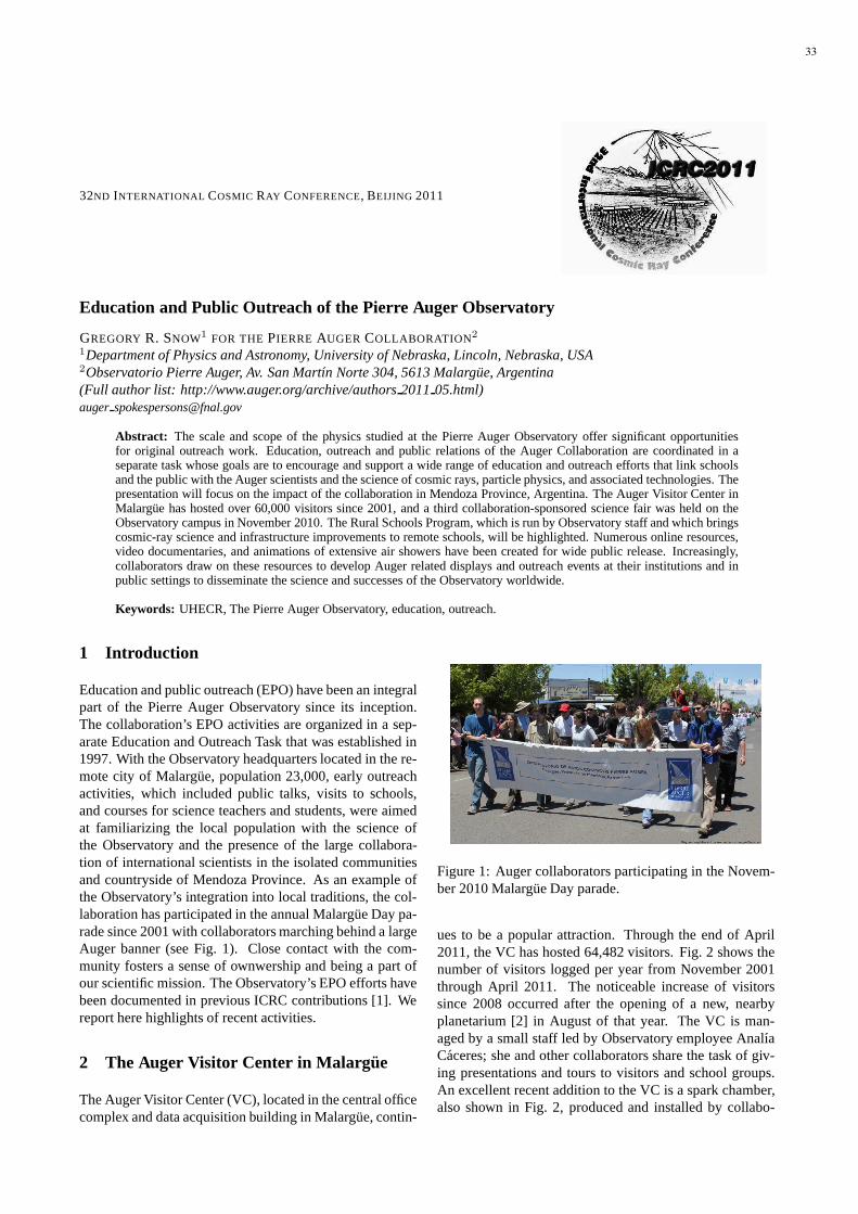
32ND INTERNATIONAL COSMIC RAY CONFERENCE, BEIJING 2011
Education and Public Outreach of the Pierre Auger Observatory
GREGORYR. SNOW1 FOR THEPIERRE AUGER COLLABORATION2
1Department of Physics and Astronomy, University of Nebraska, Lincoln, Nebraska, USA2Observatorio Pierre Auger, Av. San Martın Norte 304, 5613 Malargue, Argentina(Full author list: http://www.auger.org/archive/authors 201105.html)auger [email protected]
Abstract: The scale and scope of the physics studied at the Pierre AugerObservatory offer significant opportunitiesfor original outreach work. Education, outreach and publicrelations of the Auger Collaboration are coordinated in aseparate task whose goals are to encourage and support a widerange of education and outreach efforts that link schoolsand the public with the Auger scientists and the science of cosmic rays, particle physics, and associated technologies.Thepresentation will focus on the impact of the collaboration in Mendoza Province, Argentina. The Auger Visitor Center inMalargue has hosted over 60,000 visitors since 2001, and a third collaboration-sponsored science fair was held on theObservatory campus in November 2010. The Rural Schools Program, which is run by Observatory staff and which bringscosmic-ray science and infrastructure improvements to remote schools, will be highlighted. Numerous online resources,video documentaries, and animations of extensive air showers have been created for wide public release. Increasingly,collaborators draw on these resources to develop Auger related displays and outreach events at their institutions and inpublic settings to disseminate the science and successes ofthe Observatory worldwide.
Keywords: UHECR, The Pierre Auger Observatory, education, outreach.
1 Introduction
Education and public outreach (EPO) have been an integralpart of the Pierre Auger Observatory since its inception.The collaboration’s EPO activities are organized in a sep-arate Education and Outreach Task that was established in1997. With the Observatory headquarters located in the re-mote city of Malargue, population 23,000, early outreachactivities, which included public talks, visits to schools,and courses for science teachers and students, were aimedat familiarizing the local population with the science ofthe Observatory and the presence of the large collabora-tion of international scientists in the isolated communitiesand countryside of Mendoza Province. As an example ofthe Observatory’s integration into local traditions, the col-laboration has participated in the annual Malargue Day pa-rade since 2001 with collaborators marching behind a largeAuger banner (see Fig. 1). Close contact with the com-munity fosters a sense of ownwership and being a part ofour scientific mission. The Observatory’s EPO efforts havebeen documented in previous ICRC contributions [1]. Wereport here highlights of recent activities.
2 The Auger Visitor Center in Malarg ue
The Auger Visitor Center (VC), located in the central officecomplex and data acquisition building in Malargue, contin-
Figure 1: Auger collaborators participating in the Novem-ber 2010 Malargue Day parade.
ues to be a popular attraction. Through the end of April2011, the VC has hosted 64,482 visitors. Fig. 2 shows thenumber of visitors logged per year from November 2001through April 2011. The noticeable increase of visitorssince 2008 occurred after the opening of a new, nearbyplanetarium [2] in August of that year. The VC is man-aged by a small staff led by Observatory employee AnalıaCaceres; she and other collaborators share the task of giv-ing presentations and tours to visitors and school groups.An excellent recent addition to the VC is a spark chamber,also shown in Fig. 2, produced and installed by collabo-
33

G.R. SNOW et al. AUGER OUTREACH
rators from the Laboratory of Instrumentation and Experi-mental Particle Physics (LIP) in Portugal.
Figure 2: Top: Number of visitors logged by year at theAuger Visitor Center. Bottom: New spark chamber allowsvisitors to view cosmic ray muon tracks.
3 The Rural Schools Program and Educa-tion Fund
Many schools in the Department of Malargue, some over100 km away, have difficulty bringing their students to theObservatory and the Visitor Center. A dedicated team ofObservatory staff members has initiated a Rural SchoolsProgram which brings information about the Observatoryand needed infrastructure improvements to remote schools.Infrastructure improvements include attention to electricaland heating systems, fences, providing school supplies, etc.The Rural Schools team consists of physicists, engineers,technicians, and office staff members who volunteer theirown time. As an example, the team visited students andteachers at schools in the cities of Bardas Blancas (60 km)and Las Loicas (150 km) southwest of Malargue on a 2-day trip in December 2010 (see Fig. 3). Analıa Caceres isshown leading a presentation and discussion with the stu-dents about cosmic ray physics and the Observatory. Otherstaff members are shown donating an electric heater foruse in the school. The team also made personal dona-tions which provided small Christmas gifts to the students.These efforts to reach out to the non-local community havebeen received with great enthusiasm. The personal contactwith those involved in the Observatory has been one of the
best features of the school visits. Financial support for thisongoing program is provided by contributions from collab-orating institutions and generous individuals to an Educa-tion Fund managed by the Observatory staff.
Figure 3: Top: Analıa Caceres talking to Bardas Blan-cas students about the Observatory, December 2010. Bot-tom: Observatory staff members Mario Rodrıguez (left)and GualbertoAvila (center) presenting an electric heaterfor use in the school.
4 The 2010 Auger Science Fair
Following successful Science Fairs held in November 2005and 2007, the Collaboration sponsored a third Fair onNovember 19-21, 2010, that attracted the exhibition of 22science projects in the areas of natural science and technol-ogy (see Fig. 4). This Science Fair featured the youngestgroup of students to date (4 first graders), as well as theteam which traveled the longest distance to date to partic-ipate (from the Province of Catamarca, over 800 km northof Malargue). The 2010 Fair spanned 3 days, which al-lowed participants to enjoy more activities than in previousyears – a presentation in the Auger Visitor Center, a visitto Malargue’s planetarium, and an evening dinner with livemusic and dancing.
A team of 15 Auger collaborators judged the projects on thebasis of science content, oral and visual presentation, andthe written report that accompanied each project. First and
34

32ND INTERNATIONAL COSMIC RAY CONFERENCE, BEIJING 2011
second prizes were awarded in four age categories (grades1-3, 4-7, 8-9, and 10-12), and new award categories wereintroduced this year: the most innovative project and aprize for the teacher whose students received the highestscore. A new Challenge Cup trophy was presented to thehighest-ranked team to be displayed at their school, withthe expectation that a team from this school will return tothe next Science Fair, foreseen to be held in November2012. All participants received Science Fair T-shirts, andeach school received a one-year subscription toNationalGeographicmagazine in Spanish. The collaboration is in-debted to the Observatory staff, the local organizing teamof three science teachers, and the city of Malargue for help-ing to make the Science Fair a success.
Figure 4: Participants in the 2010 Auger Science Fair, withJim Cronin (bottom panel).
5 The New Auger Video Documentary
During the last year, collaborators Ingo Allekotte and Beat-riz Garcıa worked with professional film producer CristinaRaschia to make a new video documentary about the Ob-servatory entitled “Voces del Universo”. The 26-minutevideo features interviews with collaborators from manycountries speaking in their native languages, plus extensive
footage of detectors and activities around the Observatorysite. Several collaborating groups provided clips show-ing Auger activities at their home institutions. The videowas produced with a choice of Spanish or English subti-tles. The first public viewing of the documentary was heldin Malargue during the March 2011 collaboration meeting,and it was made available to the collaboration for dissemi-nation in DVD format. Fig. 5 shows two still images fromthe video.
Figure 5: Sample still images from the “Voces del Uni-verso” video. Top: Dr. Carlos Hojvat from Fermilabexplaining cosmic ray particles detected with a Geigercounter. Bottom: A surface detector station and signagealong Route 40 in Mendoza Province.
6 Other Outreach Activities
The Observatory was a co-sponsor of the 95th meetingof the Argentinean Physics Association held in MalargueSeptember 28-October 1, 2010, with several Auger collab-orators serving on the Organizing Committee. Observatorystaff offered tours of the Observatory campus and the flu-orescence detector and HEAT installations at the Coihuecosite to the 700 meeting participants.
The online release of extensive air shower data [3] forinstructional purposes continues to draw attention fromaround the world. Between May 1, 2010, and April 30,2011, the web site hosting the growing data set had 3920unique visitors from 81 countries, although the bulk of thetraffic is from the U.S., Argentina, and a few Europeancountries. A number of collaborators are working on lessonplans to instruct teachers and students in the use of the dataset, suggesting various plots students can make and hintson interpreting, for example, energy and arrival directiondistributions.
35

G.R. SNOW et al. AUGER OUTREACH
Randy Landsberg and colleagues at the Kavli Institute forCosmological Physics have posted high-resolution, inter-active panoramas of a number of locations at the Observa-tory on theGigapanonline system [4]. Views from the LosLeones fluorescence detector building, at the central cam-pus office building, and on the Pampa Amarilla are avail-able.
The scholarship program which brings top Malargue stu-dents to Michigan Technical University (MTU) has en-joyed continued success. The fifth student enrolled at MTUin the fall semester 2010. The first four students havegraduated with degrees in either Mechanical Engineeringor Materials Science. The first three students have em-barked on engineering careers, one in the U.S. and two inArgentina.
In Madrid, Spain, the Auger Observatory and cosmic rayswere featured during the Science Week held in November2010. Visitors to the physics building at the UniversidadComplutense de Madrid witnessed cosmic ray muons de-tected with Geiger counters and with a spark chamber likethe Auger VC spark chamber shown in Fig. 2, producedby collaborators from Portugal. Visitors were filmed as amuon track passed through their hand held above the cham-ber. A selected still photo was copied into a take-homecertificate stamped with the time and location, giving eachvisitor his or her personal cosmic ray to remember.
Collaborators in the Netherlands remain active in educa-tion and outreach via projects like the HiSPARC network[5], which employs high-school based scintillator detec-tors on school rooftops, and cosmic ray displays at openhouse events at NIKHEF, the National Institute for Nu-clear and High Energy Physics in Amsterdam. Notably, aDutch team that included Auger collaborators was awardedthe 2008-09 Annual Academic Prize for the best trans-lation of scientific research to the public. The generousaward funded the construction of a large “Cosmic Sensa-tion” dome (Fig. 6) [6] in a park near the Radboud Univer-sity in Nijmegen. Lights and music in the dome were trig-gered by random cosmic ray hits detected by scintillators.Music and dance evenings held on September 30-October2, 2010, attracted thousands of visitors and extensive presscoverage.
A highlight of recent outreach activities in the CzechRepublic was the “Science for the World” exhibition,September-October, 2009, which featured research activ-ities and results from the institutes of the Academy of Sci-ences. Fig. 7 shows a segment of a Czech-made fluores-cence detector mirror which was part of an Auger exhibitin the main building of the Academy. The exhibit attractedover 15,000 visitors and media coverage. High school stu-dents have also had the opportunity to participate in re-search experiences with Auger collaborators, drawing onthe Auger data set released to the public, as part of the“Open Science” initiative that involves several Academyinstitutes and universities.
Figure 6: The Cosmic Sensation dome in Nijmegen, NL.
Figure 7: One-fifth size fluorescence detector mirror proto-type on display at the Academy of Sciences in Prague.
References
[1] G. Snow, for the Pierre Auger Collaboration, Proc.27th ICRC, Hamburg, Germany, 2001,2: 726-729;B. Garcıa and G. Snow, for the Pierre Auger Col-laboration, Proc. 29th ICRC, Pune, India, 2005,8:1-4; G. Snow, for the Pierre Auger Collaboration,Proc. 30th ICRC, Merida, Mexico, 2007,4: 295-298,arXiv:0707.3656 [astro-ph]; G. Snow, for the PierreAuger Collaboration, Proc. 31st ICRC, Łodz, Poland,2009, arXiv:0906.2354v2 [astro-ph].
[2] See http://www.malargue.gov.ar/planetario.php.[3] See http://auger.colostate.edu/ED/.[4] See http://www.gigapan.org/gigapans/xxxxx/, and sub-
stitute 59328, 59256, 59253, or 59258 for xxxxx.[5] See http://www.hisparc.com.[6] See http://www.experiencetheuniverse.nl.
36

32ND INTERNATIONAL COSMIC RAY CONFERENCE, BEIJING 2011
AcknowledgmentsThe successful installation, commissioning and operationof the Pierre Auger Observatory would not have been possiblewithout the strong commitment and effort from the technicaland administrative staff in Malargue.
We are very grateful to the following agencies and organizations for financial support:
Comision Nacional de Energıa Atomica, Fundacion Antorchas, Gobierno De La Provincia de Mendoza, Municipali-dad de Malargue, NDM Holdings and Valle Las Lenas, in gratitude for their continuing cooperation over land ac-cess, Argentina; the Australian Research Council; Conselho Nacional de Desenvolvimento Cientıfico e Tecnologico(CNPq), Financiadora de Estudos e Projetos (FINEP), Fundac¸ao de Amparo a Pesquisa do Estado de Rio de Janeiro(FAPERJ), Fundacao de Amparo a Pesquisa do Estado de SaoPaulo (FAPESP), Ministerio de Ciencia e Tec-nologia (MCT), Brazil; AVCR AV0Z10100502 and AV0Z10100522, GAAV KJB100100904, MSMT-CR LA08016,LC527, 1M06002, and MSM0021620859, Czech Republic; Centrede Calcul IN2P3/CNRS, Centre National de laRecherche Scientifique (CNRS), Conseil Regional Ile-de-France, Departement Physique Nucleaire et Corpusculaire(PNC-IN2P3/CNRS), Departement Sciences de l’Univers (SDU-INSU/CNRS), France; Bundesministerium fur Bildungund Forschung (BMBF), Deutsche Forschungsgemeinschaft (DFG), Finanzministerium Baden-Wurttemberg, Helmholtz-Gemeinschaft Deutscher Forschungszentren (HGF), Ministerium fur Wissenschaft und Forschung, Nordrhein-Westfalen,Ministerium fur Wissenschaft, Forschung und Kunst, Baden-Wurttemberg, Germany; Istituto Nazionale di Fisica Nu-cleare (INFN), Ministero dell’Istruzione, dell’Universita e della Ricerca (MIUR), Italy; Consejo Nacional de Cienciay Tecnologıa (CONACYT), Mexico; Ministerie van Onderwijs, Cultuur en Wetenschap, Nederlandse Organisatie voorWetenschappelijk Onderzoek (NWO), Stichting voor Fundamenteel Onderzoek der Materie (FOM), Netherlands; Min-istry of Science and Higher Education, Grant Nos. 1 P03 D 014 30, N202 090 31/0623, and PAP/218/2006, Poland;Fundacao para a Ciencia e a Tecnologia, Portugal; Ministry for Higher Education, Science, and Technology, SlovenianResearch Agency, Slovenia; Comunidad de Madrid, Consejer´ıa de Educacion de la Comunidad de Castilla La Mancha,FEDER funds, Ministerio de Ciencia e Innovacion and Consolider-Ingenio 2010 (CPAN), Xunta de Galicia, Spain; Sci-ence and Technology Facilities Council, United Kingdom; Department of Energy, Contract Nos. DE-AC02-07CH11359,DE-FR02-04ER41300, National Science Foundation, Grant No. 0450696, The Grainger Foundation USA; ALFA-EC /HELEN, European Union 6th Framework Program, Grant No. MEIF-CT-2005-025057, European Union 7th FrameworkProgram, Grant No. PIEF-GA-2008-220240, and UNESCO.