STRASHEIM 2011

38 Management Dynamics Volume 20 No 4, 2011

ABSTRACT

_____________________________________________

The methodology for invariance testing for a first-orderconfirmatory factor analysis is well documented in theliterature. However, it is not the case for a second-orderconfirmatory factor analysis model. In addition, it is veryoften of interest to include means in the analyses, usingmeans and covariance structure analysis (MACS) toinvestigate differences between groups in the structuralpart and between the means of latent variables. Mostmethodological papers on this topic are not very clear onhow means should be treated in confirmatory factoranalysis models. Also, the mathematical model thatunderlies a second-order model is not well documented.This study addresses all these issues, and uses empiricalexamples to provide the syntax for two software packagesthat are frequently used for invariance testing, namelyLISREL 8.8 and AMOS 19. The study further sets out theprocedure so that readers that are less familiar with matrixalgebra can link the equations with the symbols used on thepath diagram, and correspond these to the syntax providedin the appendices.

The issue of the need to test for measurement equivalencein confirmatory research, especially when measurementinstruments with clearly defined sub-dimensions are used,is a matter that has become an increasingly important topicin leading international journals. However, in SouthAfrica, although researchers often make use of instrumentsdeveloped elsewhere and apply them across differentcultural groups or other subgroupings, these studies rarelyevaluate the measurement invariance of the instruments.This situation may lead to invalid findings, which maylimit the usefulness of our studies to international scholars.

In addition, during data collection, some bias may havebeen introduced for reasons that are beyond the control ofthe researcher. An example of this type of bias could beacquiescence bias or extreme response styles, which maybe an artefact of the cultural tendencies of one or moregroups being studied in the target population. Method biascould also be introduced, for example, when differentmethods of data collection have been used. Wheneverthere is reason to be concerned about the presence of bias, itis necessary for the researcher to test for measurementequivalence to establish whether it would be valid toproceed with further analyses.

The methodology for invariance testing for first-orderconfirmatory factor analysis models (1CFA) within astructural equation modelling (SEM) framework is clearlyset out in the statistical and applied literature. Theapplication of the technique and its value in cross-culturalstudies is well established, and more recently, themethodology is also applied in South African studies.Second-order confirmatory factor analysis models areappealing (2CFA) when several first-order factors arepresent in the model. The robustness of 2CFA models,given that they are plausible higher-level explanations ofthe covariances between the first-order factors, are veryuseful for empirical testing of theory. Although themethodology and software for fitting 2CFA models areavailable, the method is not often used in situations whereit could be beneficial. Except for a methodological paperby Chen, Sousa and West (2005), invariance testing of2CFA models is also very seldomly applied, probablybecause the methodology is not always clearly described.The mathematical exposition of the 2CFA model has alsonot been well-documented, and the treatment of means andintercepts in invariance testing is also often very vaguelytreated in the literature. This study seeks to address allthese issues.

INTRODUCTION

Testing the invariance of second-orderconfirmatory factor analysis models thatinclude means and intercepts

Arien StrasheimUniversity of Pretoria

FIRST-ORDER AND SECOND-ORDERCONFIRMATORY FACTOR ANALYSIS

OBJECTIVES OF THE STUDY

Confirmatory factor analysis models are concerned withexamining the factorial structure and relationshipsbetween factors or latent variables (Bollen, 1989), and it isparticularly useful to examine the psychometric propertiesof an instrument (Shiu, Pervan, Bove and Beatty, 2011;Van de Vijver and Leung, 1997).

Many researchers using confirmatory factor analysis(CFA) in a structural equation modelling (SEM)framework, have in their models several first-order factorsthat are interrelated. When more than four of the first-orderlatent variables are part of the model, it may be possiblethat higher-order factors explain the relationships betweenthe first-order factors in a way that is simpler thaninterpreting all the covariances between the first-orderlatent variables. From a modelling perspective, theadvantage of a second-order confirmatory factor analysismodel (2CFA) is the simplification that it achieves fromthe first-order confirmatory factor analysis model (1CFA).When it is correctly specified, the 2CFA model always hasfewer or the same number of parameters as the 1CFAmodel. The advantage of the 2CFA model is that it modelsthe structure of the covariances between the first-orderlatent variables as emanating from correlated second-orderfactors.

From a theoretical viewpoint, the existence of higher-orderfactors is often suggested by studies, but rarely doresearchers test or apply the higher-order models that are inmost instances more parsimonious than the 1CFA model.The limitation of the 1CFA model is that it only models therelationships (covariances) between the first-orderconstructs, whereas the 2CFA model implies the existenceof possible structural relationships between the first-orderlatent variables. When several first-order latent variablesare involved, the interpretation of all the relationships maybe simplified by using a 2CFA model. However, thereshould always be sufficient substantive reason for theexistence of the unobserved second-order latent variablethat has an effect on the first-order constructs.

One of the possible reasons that 2CFA models are avoided,or that invariance testing of 2CFA models is not alwaysapplied, may be that the procedure for testing higher-ordermodels is not described in much detail in themethodological literature, and certain aspects of theprocedure are not always covered in sufficient detail. Inaddition, after measurement invariance is found to hold,many studies do not proceed to MACS analyses to estimatethe model-implied means and variances of the latentvariables, in order to draw substantive conclusions fromthese estimates. The advantage of the invariance testing isthereby lost, since the measurement invariant model is

“corrected” for measurement artefacts through theinvariance testing procedure. One possible reason for theavoidance of MACS analyses could be that the proceduresused for model identification could lead to inconsistentfindings for the same set of data, based on the fact thatscaling methods are arbitrary. Thus, although the samemodel fit is achieved by different scaling methods, theselection of a specific scaling indicator could lead todifferent estimated means for the same model, when thescaling indicator is changed to use a different observedvariable for scaling a latent variable.

Another factor contributing to the infrequent use of 2CFAmodels, is that the methodology for testing the invarianceof a 2CFA model is not thoroughly covered in theliterature, and the application of multi-group 2CFA forequivalence/invariance testing seldom sheds light on howthe invariance testing is approached.Although a procedurefor higher-order models is suggested in the psychologyliterature by Marsh and Hocevar (1985), where the higher-order dimensions of self-concept were measured andtested across groups, very few studies that apply themethod are available outside the discipline of psychology.The procedure of Marsh and Hocevar (1985) seems inessence the same as suggested by this paper, but their studymentioned the method for invariance testing only verybriefly. Although their study did not include how meansshould be treated, the inclusion of means often makessubstantive sense in multigroup testing. More recently,essentially the same approach followed by Marsh andHocevar (1985) was suggested by Chen (2005), andalthough their study did cover the testing of means, itunfortunately only considers a second-order model with asingle second-order latent variable, which therefore doesnot cover the covariances between second-order latentvariables. In addition, the mathematical treatment of themodel is also not covered in the paper by Chen(2005). Therefore, this study attempts to formally set outthe mathematics underlying the invariance testing for a2CFA model, and illustrates the method with empiricalexamples. In addition, the Simplis (LISREL 8.8) andAMOS 19 syntax for the examples are provided.

This study contributes to the methodological literature byfirstly showing mathematically how the 2CFA modelextends from the 1CFA model, and how the matrixelements are linked to the parameters of a path diagram inexamples of both models. The matrix algebra is extendedto show all the matrix elements for the specific examples,thereby making it more accessible to those less familiarwith matrix algebra. Secondly, an empirical example of theprocedure is provided for both the 1CFAand 2CFAmodels.Lastly, the appropriate syntax for both AMOS- andLISREL-users is included.

et al.

et al.

Management Dynamics Volume 20 No 4, 2011 39

MULTI-GROUP CONFIRMATORY FACTORANALYSIS (MG CFA)

EXAMPLE 1

Multi-group confirmatory factor analysis in a first-orderconfirmatory factor analyis (1CFA) context is adequatelydescribed in the literature. In the field of education andpsychology, Rensvold and Cheung (1998) suggest asystematic approach to invariance testing. In the marketingdiscipline, the paper by Steenkamp and Baumgartner(1998) for testing measurement invariance of aninstrument has introduced and popularised the approach tomarketing scholars, while the paper by Vandenberg andLance (2000) and Vandenberg (2002) may be morefamiliar to researchers within organisational and humanresources context. There are virtually no differences in theapproaches suggested by all these authors – and the workmainly appeared during the same period. All these papersare based on the seminal contributions by Jöreskog (1971),Jöreskog, Anderson, Laake and Cox (1981) as well asMeredith (1993) who formally set out the multi-groupconfirmatory factor analysis method (MG CFA).The origins of the terminology used in this study are thoseof Steenkamp and Baumgartner (1998), and to a lesserextent, that of Byrne (1998).

When CFA is used, the purpose is to model therelationships between observed variables and theconstructs assumed to underlie them, and the correlationalrelationships among the constructs. CFA within a SEMframework is congruent with classical test theory, whichallows error terms in the model. Therefore, one of themajor advantages of CFA within the SEM approach, is thatmeasurement error (which could be both systematic andrandom error) for each observed variable, forms part of themodel.

Usually, the first step in the MG CFA method is to fit CFAmodels of the same form (with matching fixed and freeparameters across the groups) on each of the groupssimultaneously in a single analysis. It then becomespossible to evaluate different levels of invariance of theinstrument by introducing sequential restrictions on sets ofparameters in the model, and by evaluating the fit of thesemodels at each sequential step.

the errors

–

, which

(1)

(2)

This section briefly revisits the MG CFA approach for afirst-order confirmatory factor analysis model (1CFA)using matrix notation, and then explains how the multi-group confirmatory factor analysis approach can beextended from the 1CFA model to a second-orderconfirmatory factor analysis model (2CFA).

Example 1 is a 1CFA model as reported by Ungerer andStrasheim (2011), with three indicator or observedvariables that emanate from F ; four indicators from F ;three from F and two from F , as shown in Figure 1.

The model is very similar to most other models in the SEMliterature, except that it includes means and intercepts withthe path diagram showing how these form part of themodel. As discussed by Little (2000), there are two levelsof parameters, namely parameters at the measurementlevel and parameters at the structural level, and within eachlevel, there are three types of parameters for the 1CFAmodel, in total six types of parameters.

First, at the measurement level, the three sets of parametersare: (1) the regression slopes or measurement weights fromeach factor to the observed variables (labelled a to a );and (2) the corresponding intercepts shown as i to i ;and (3) the measurement error or residual variancesv to v that are the parameters that estimate the unknownor non-relevant terms e to e that have an effect on theobserved scores. The means of the error terms are assumedto be equal to zero, and are uncorrelated(therefore there are no two-headed arrows between theerror terms). The error terms are often referred to as theunique factors or unreliability in the indicators (Little,2000). At least the measurement weights (a to a ) andintercepts (i to i ) need to be equivalent across groups,before it is valid to proceed to the analysis of the structuralparameters which is at the next level of analysis.

At the second level or structural part of the model, the threesets of parameters involved are: (4) the means (labelledm to m ) of the latent factors F1 to F4, and (5) thecorresponding factor variances of F1 to F4, labelledvv to vv in Figure 1. Lastly (6), the four factors or latentvariables F to F are correlated in the model, (therefore thedouble-headed arrows between them) and thecorresponding covariance parameters are cc to cc asshown in Figure 1.

The last three sets of parameters, (4), (5) and (6) arerelevant in a MACS analysis assumes that at leastthe measurement weights (a to a ) and measurementintercepts (i to i ) are equal across the groups beingstudied, before it is valid to proceed with a MACS analysis.

In order to be consistent with other authors (Bollen andBiesanz, 2002), the -notation is used to avoid confusionwhen the 2CFA model is specified later in this study.When means and intercepts are part of the model, the 1CFAmeasurement model for the -th indicator, ( = 1, ..., )or observed variable is

with the slope of the regression of on ,.

In matrix notation, the model in equation (1) is representedas

1 2

3 4

1 121

1 12

1 12

1 12

1 12

1 12

1 4

1 4

1 4

1 6

1 12

1 12

,

Y

i i p

y

y +

= + +

i i ij j i

ij i j

i i

= +α λ η ε

λ η an interceptterm α , and a stochastic error term ε

y α Λη ε


where is a x 1 vector of observed variables or items;

is a x 1 vector of intercepts of the observedvariables;

is a x matrix of factor loadings;

is a x 1 vector of latent variables;

is a x 1 vector of error terms; and

where the model has latent variables. It is assumed that, and are normally distributed. For our example,= 12 and = 4. The model-implied mean vector (which

is the vector of estimated indicator means) of the observedvariables , ..., is given by

y

y

p

p

p m

m

p

m

p m

y y

α

Λ

η

ε

η ε

1 12

μ θ α Λμ( ) + (3)= η

e1

e2

e3

e4

e5

e6

e7

e8

e9

e10

e11

e12

V1

V2

V3

V4

V5

V6

V7

V8

V9

V10

V11

V12

0, v11

a1

a20, v2

1

0, v31

0, v41

0, v51

0, v61

0, v71

0, v81

0, v91

0, v101

0, v111

0, v121

F1

F2

F3

F4

mm1, vv1

mm2, vv2

mm3, vv3

mm4, vv4

a3

a4

a5

a6

a8

a9

a10

a7

a11

a12

cc1

cc2

cc3cc4

cc5

cc6

i1

i2

i3

i4

i5

i6

i7

i8

i9

i10

i11

i12

FIGURE 1EXAMPLE 1: A 1CFA MODEL


Note that is the general convention used in the SEMliterature to refer to all the model parameters. Equation (3)essentially says: “the model-implied means of theobserved indicators based on the parameter estimates areexpressed as ...”. The estimated means in (3) exclude theerror term, since the expected mean error is , and thereforethe estimated means represent only the “reliable part” ofthe measured variables. The matrices in equation (3) areexpanded as in equation (4):

The model-implied mean vector for the observed variablesof Example 1 is shown in equation (5), and the

corresponding parameters of this matrix on the pathdiagram in Figure 1 are given after the arrow .These are provided explicitly in order to follow the AMOSsyntax that is provided in the appendices, and to enablereaders who are less familiar with matrix algebra to matchthe mathematics and the path diagram, and eventually thesyntax coding.

In order for the following sections to make sense, it isnecessary to cover different methods of modelidentification that are helpful for the different approachesfor MACS analyses that have a role in how modelparameters, and more specifically latent means, areinterpreted.

Little, Slegers and Card (2006) outlined three differentmethods that can be used for model identification purposesin mean and covariance structure analysis. All threemethods, as well as their variants within a method,produce the same measures of fit, but the estimatedmodel parameters are different, and carry differentinterpretations.

The first method described by Little (2006) involvessetting the means of the latent variables equal to 0 and to fixthe variance of the latent variables equal to 1. With thisapproach, the estimated means of the observed variablesreduces to the estimated intercepts as shown in (6).

The second commonly used identification methoddescribed by Little . (2006) sets the path of oneindicator per latent variable equal to 1, and thecorresponding intercept is then set equal to zero.The choice of scaling parameter is arbitrary – but its choicemay have an effect on the estimated model parameters.If the items are closely related, the choice will not have adrastic effect on the estimated parameters. For the secondtype of identification method, the vector of model-impliedmeans simplifies to the format in (7), when the firstindicator of each latent variable is used as the scalingindicator.

θ

0

y

(4)

(5)

(6)

(7)

et al.

et al

μ(θ)

μ

α λ μ

F

F

1

2 2 1

3

+

α λ μ

μ

α λ μ

α λ μ

α λ μ

μ

α λ μ

α λ μ

μ

α λ μ

+

+

+

+

+

+

+

3 1

2

5 5 2

6 6 2

7 7 2

3

9 9 3

10 10 3

4

12 12 4

F

F

F

F

F

F

F

F

F

F

mm

i + a mm

1

2 2 1

3 3

2

5 5 2

6 6 2

7 7 2

3

9 9 3

10 10 3

4

1 1 4

i + a mm

mm

i + a mm

i + a mm

i + a mm

mm

i + a mm

i + a mm

mm

i + a mm

1

2 2


The third method – called the effects coding method byLittle (2006) – is non-arbitrary and seems to havedesirable properties. This method constrains the interceptterms to sum to zero, and the measurement weights areconstrained so that their average is equal to 1. For thecurrent example, it requires that the constraints shown inTable 1 are imposed for the purpose of modelidentification.

Since this method can be cumbersome in complex models,the resulting detailed matrices are not provided forExample 1, although this method seems to be very useful(see Table 8 for a more detailed discussion about the threemethods.)

et al.

TABLE 1EFFECTS CODING IDENTIFICATION CONSTRAINTS FOR EXAMPLE 1


Φ

Model parameters Parameters matched on path diagram

λ λ λ α α α1 2 3 1 2 3= – and = 0 – – a i1 2 3 1 2 3= 3 – and = 0– – –a a i i

λ λ λ α α α4 5 6 4 5= 4 – and = 0– – – – –λ α7 7 8 a a a a i i i i– – = 0 – – –7 4 5 6 74 5 6= 4 – and

λ λ λ α α α8 9 10 8 9 10= 3 – and = 0– – – a a a i i i8 9 10 8 9 10= 3 – – and = 0 – –

λ λ α α11 12 11 12= 2 – and = 0 – a a i i11 12 11 12= 2 – and = 0 –

For the model-implied covariance matrix

Two additional parameter matrices, namely and areof importance in Example 1:

The variance covariance matrix between the first-orderfactors in (9) is symmetrical, with the factor variances on

the diagonal and the covariances between the factorsprovided off the diagonal. Note that since the matrix issymmetrical, = ; = ; = and so on.The corresponding parameters on the path diagram areshown after the arrow in equation (9), where thesymmetry is more clearly visible.

The matrix that contains the residuals of the observedvariables, , is a diagonal matrix (only the diagonalelements are defined, and the off-diagonal elements arezero) because the model in Example 1 has no correlatederrors. The corresponding parameters on the path diagramare shown after the arrow in equation (10).

Σ θ ΛΦΛ Θ( ) = + (8)

(9)

΄

Φ Θ

Φ

Θ

,

12 21 13 31 32 23

The model-implied covariance matrix for the 1CFAmodel for Example 1 is ( ) = + and is given in

equation (11). The matrix dimensions are ( ) (12x12);(12x4); (4x4); (4x12); an .Σ θ ΛΦΛ́ Θ

Σ θΛ Φ Λ́ε

→

→ → → d →(12x12)Θ

(10)Θ

Using matrix algebra, the model-implied covariancematrix for Example 1 is then given in equation (12).

( )=Σ θ


(11)

The corresponding symbols (non-redundant elementsonly) for the parameters on the 1CFApath diagram for eachelement of the matrix in (12) are provided in (13):

(12)

(13)

12124121241112610126912681257125612551254123312321231 vavvaavvaaccaaccaaccaaccaaccaaccaaccaaccaaccaacca

111141111610116911681157115611551154113311321131 vavvaaccaaccaaccaaccaaccaaccaaccaaccaaccaacca

1010310103910381047104610451044102310221021 vavvaavvaavvaaccaaccaaccaaccaaccaaccaacca

9939938947946945944923922921 vavvaavvaaccaaccaaccaaccaaccaaccaacca

8838847846845844823822821 vavvaaccaaccaaccaaccaaccaaccaacca

7727726725724713712711 vavvaavvaavvaavvaaccaaccaacca

6626625624613612611 vavvaavvaavvaaccaaccaacca

5525524513512511 vavvaavvaaccaaccaacca

4424413412411 vavvaaccaaccaacca

3313312311 vavvaavvaavva

2212211 vavvaavva

1111 vavva

Using the first method of model identification describedby Little (2006), which sets the variances of each

factor equal to 1, results in the variance covariancematrix shown in equation (14):et al.

(14)


With the second method of model identification describedby Little . (2006), where one indicator per latentvariable is constrained to 1; and the correspondingintercept is constrained to 0, results in a model-impliedcovariance matrix as shown in (15). If the first indicator foreach latent variable selected to be the scaling indicator,(that is, = = = = 1), the matrix is simplified to theform shown in (15):

When LISREL 8.8 is used to fit a 1CFA model, the outputwill refer to certain matrices that are mostly consistent withthe notation used here the matrix is referred to asLAMBDA-X and the matrix as PHI. However, there area few differences that may cause confusion. The vector ofintercepts, = ( , ... ) is referred to as TAU-X; thevector of latent means as KAPPA; and the matrix oferror terms is referred to as THETA-DELTA.

et al

a a a a1 4 8 11

– ΛΦ

α΄μ

Θ

α α1 12

η

EXAMPLE 2

For a second-order factor analysis model, (Figure 2) theobserved response to an item ( = 1, ..., ) is representedas a linear function of a latent construct ( = 1, ...

and a stochastic error term . Thus the 1CFApart of the model is

with the slope of the regression of on . Since the first

order latent construct is in itself a function of a secondorder latent construct ( = 1, ... ), an intercept andan error term related to the first order latent construct, the2CFApart of the model is

Substituting (17) into (16) yields the 2CFA-model in (18)

y i i pj m

y

k n

i

j

yi i

ij i j

k j

j

η anintercept α ε

λ η

ξ αζ

),

y

j= + +

y + + + +

i i ij j i

j jk k j

i yi ij j jk k j i=

= α λ η ε

η α γ ξ ζ

α λ α γ ξ ζ ε

+ +

[ ]

(16)

(17)

(18)

η

η

η

In matrix notation, the 2CFA model contains second-order factors , that are determined by the first-orderfactors , and that are in turn indicated by the observedvariables, . The second-order factor measurement modelis therefore given by

where

is an x 1 vector of intercepts of the first-order latentvariables;

is an x matrix of second-order factor loadings on thefirst-order factors;

is an x 1 vector of second-order latent variables;

is an x 1 vector of errors, residuals or disturbances inthe first-order factors or latent disturbances;

The vectors , , , and , as well as the matrix aredefined as in the 1CFAmodel.

In the 2CFA model it is assumed that ( ) = , ( ) = andfurther that

is uncorrelated with and ; and is uncorrelated withand .

nm

p

m

m n

n

m

E E

ξη

ξ

ζ

α η ε Λ

ζ ε

ζ ξ ε εξ η

y

y

y = + [ + + ] +α Λ α Γ ξ ζ εη (19)

αη

Г

y

0 0

FIGURE 2EXAMPLE 2: A 2CFA MODEL

e1

e2

e3

e4

e5

e6

e7

e8

e9

e10

e11

e12

V1

V2

V3

V4

V5

V6

V7

V8

V9

V10

V11

V12

0, v11

a1

a20, v2

1

0, v31

0, v41

0, v51

0, v61

0, v71

0, v81

0, v91

0, v101

0, v111

0, v121

FF1

F2

F3

F4

ii1

a3

a4

a5

a6

a8

a9

a10

a7

a11

a12

ccc1

i1

i2

i3

i4

i5

i6

i7

i8

i9

i10

i11

i12

mmm1, vvv1

mmm2, vvv2

ef2

ef1

ef4

ef3

FF2

ii2

ii3

ii4

0, vv1

0, vv2

0, vv3

0, vv4

aa1

aa2

aa3

aa4


F1

It is assumed that , , , and are normally distributed.In Example 2, = 12; = 4 and = 2. This 2CFAmodel hastwo correlated second-order latent variables FF and FF ,with two first-order latent variables emanating from eachof them. The 2CFA model “replaces” or models the

between the first-order latent variables, asemanating from a higher-order level.

The 2CFA model has three layers of parameters, and ineach layer there are three types of parameters, in total 9types of parameters. Similar to the 1CFA model, at themeasurement level or layer in the model, the three types ofparameters that refer to the measurement part of the modelare: (1) the regression coefficients or measurementweights, a to a and (2) the corresponding interceptsi to i ; and (3) the error variances depicted as lowercasev to v on the path diagram in Figure 2. At the first-orderstructural level, or second layer, the three sets ofparameters are: (4) the measurement weights from thesecond-order latent variable to the first-order latentvariable, labelled aa to aa (5) the intercepts ii to ii ofthe second at the first-order latent variables, and (6) thedisturbance error variances of the first order latentvariables named vv to vv . At the third layer, theparameters involved are (7) the means of the second-orderlatent variables, labelled mmm to mmm ; (8) the variances

and of the second-order latent variables labelled asvvv to vvv ; and (9) the covariance between the second-order latent variables labelled as ccc .

y η ξ ζ εp m n

1 2

1 12

1 12

1 12

1 4; 1 4

1 4

1 2

1 2

1 2

1

ζ ζ

covariances

On the path diagram, the error terms or structural residualsor disturbances ef1 to ef4 of the first-order factor terms arerequired, since F1 to F4 are endogenous variables in a2CFAmodel. The structural residuals ef1 to ef4 are definedto have zero mean with corresponding variances vv to vv .

The regression paths or structural weights from the second-order latent variables to the first-order latent variables areaa to aa with their corresponding intercepts ii to ii . Inaddition, the mean parameters of the second-order latentvariables are mmm and mmm , with the correspondingvariances vvv and vvv . The covariance between the twosecond-order latent variables is denoted by ccc .These names are arbitrary (and different users may havedifferent names for the same parameters), and they are used

to assist non-mathematical readers to make the leap to theAMOS syntax and output provided later in this study.

The model-implied mean vector that is required to estimatethe means of the observed variables ... , for the 2CFAmodel is

In this equation, the additional vectors and matricesthat have not been defined in the 1CFA model are theintercept terms of the regression coefficients from thesecond-order latent variables to the first-order latentvariables shown in equation (21), with the correspondingparameters from the path diagram in Figure 2 shown afterthe arrow ,

and the matrix which is provided in equation (22) withthe regression coefficients from the second order latentvariables to the first-order latent variables, and with thecorresponding elements on the path diagram given after thearrow .

The mean vector of the second-order latent variables withthe corresponding parameters on the path diagram aregiven in equation (23).

,

1 4

1 4 1 4

1 2

1 2

1

1 12y y

μ θ α Λ α Γμ

μ θ α Λ α Γμ

y y

y y

( ) + ( + ). (20)

(21)

(22)

(23)

Based on the matrices in (21) to (23), it is possible to writethe elements of the model-implied mean vector,

( ) + ( + ). The elements and parameters fromthe path diagram in Figure 2 are given in equation (24) afterthe arrow

=

=

η ξ

η

η ξ

α

Г

4

3

2

1

4

3

2

1

0

0

0

0

0

0

0

0

aa

aa

aa

aa

Γ

(24)


1

2

3

4

1 1

2 2

1

2

3

4

1

1

1

1

1

1

1

2

2 2

2 2

2

2

2

2

2

2

2 2

2 2

3 3

4 4

4 4

55

66

77

9 9

10 10

1111

12 12

α λ α γ μ1 1 1 1 1+ ( + )F FF

α λ α γ μ

α λ α γ μ

α λ α γ μ

α λ α γ μ

α λ α γ μ

α λ α γ μ

α λ α γ μ

α λ α γ μ

α λ α γ μ

α λ α γ μ

α λ α γ μ

2 2 1 1 1

3 3 1 1 1

4 4 2 2 1

5 5 2 2 1

6 6 2 2 1

7 7 2 2 1

8 8 3 3 1

9 9 3 3 2

10 10 3 3 2

11 11 4 4 2

12 12 4 4 2

+ ( + )

+ ( + )

+ ( + )

+ ( + )

+ ( + )

+ ( + )

+ ( + )

+ ( + )

+ ( + )

+ ( + )

+ ( + )

F FF

F FF

F FF

F FF

F FF

F FF

F FF

F FF

F FF

F FF

F FF

1

2

3

4

5

6

7

8

9

10

11

12

1

2

3

4

5

6

7

8

9

10

11

12

1

1

1

2

2

2

2

3

3

3

4

4

1

1

1

2

2

2

2

3

3

3

4

4

1

1

1

1

1

1

1

2

2

2

2

2

μ θ( ) =

If the first method of identification scaling described byLittle (2006) is used, where the latent means areconstrained equal to zero, and the latent variances areconstrained equal to unity, the estimated means of theobserved variables reduce to the corresponding interceptsas in equation (6).

When the second method of scaling identification is used,one of the measurement weights per latent variable isconstrained equal to 1, with the corresponding interceptconstrained equal to zero. In addition, in the second-orderpart of the model, in order to identify the second-order

factors, one indicator for each second-order latent variableis also constrained equal to 1, and the correspondingintercepts are constrained equal to 0. Therefore, = == = = = 1 and = = = = = = 0 in ourexample. Using this method of identification leads to thesimplification of the expression in (24) as given in the lastmatrix, after the second arrow .

et al.a a a

a aa aa i i i i ii ii1 4 8

11 1 3 1 8 11 1 34

Although not shown in expanded notation, if the thirdmethod described by Little . (2006) is used inExample 2, the parameter constraints for the purpose ofidentification are provided in Table 2.

et al

TABLE 2EFFECTS CODING IDENTIFICATION CONSTRAINTS FOR EXAMPLE 2

(29)


The third method of constraints has the advantage that theaverage of the measurement weights will be equal to 1 andthe average of the measurement intercepts is equal to 0.

The model-implied covariance matrix for the 2CFA modelis

with as in equation (4) and as in equation (10). Thematrices that were not specified in the 1CFA model aregiven in (27) and (28). The matrix of the variances andcovariances between the second-order latent variablesand the corresponding parameters on the path diagram inFigure 2 are shown after the arrow in equation (27).When the first identification method described by Little

. (2006) is used, the equation reduces to the last matrix in

equation (27), where the variances of the latent variablesare constrained equal to 1.

The structural residuals or disturbances, is a diagonalmatrix, and the corresponding parameters are given afterthe arrow in (28).

The non-redundant elements of + are given inequation (29), with the corresponding elements on the pathdiagram given after the arrow .

Σ θ Λ Γ Φ Γ΄ Ψ Λ Θ(g)( ) = ( + ) + (26)

(27)

(28)

΄

Λ Θ

Φ

Ψ

Γ Φ Γ΄ Ψetal

When the first method of model identification of Little. (2006) is used, the variances and on the

diagonal of equation (27) are constrained to be equal to

one, and then the matrix + in (29) is simplied asshown in equation (30) after the arrow .et al ζ ζ11 22

Γ Γ΄ ΨΦ

44434214114

333213113

22212

111

4443422141214

33322131213

22212

111

vvaaaaaaaaaacccaaaacccaa

vvaaaaaacccaaaacccaa

vvaaaaaaaa

vvaaaa

ΨΓ'ΦΓ

(30)


44224322422141214

3322322131213

221121112

11111

ΨΓ'ΦΓ

(31)

If the second identification method of Little (2006)is used, that is where the scaling indicators and areset equal to 1, + in (29) reduces to equation (31).

When LISREL is used to fit a 2CFA model, the output willrefer to certain matrices that are mostly consistentwith the notation used here. The matrix is referred to as

et al.aa aa1 3

Γ Γ΄ Ψ ΛΦ

LAMBDA-Y; the matrix as GAMMA; the vector offirst-order intercepts as ALPHA; the matrix as PHI;the matrix as PSI; and the matrix of error terms

is referred to as THETA-EPS. The ones that maybe confusing are the vector of indicator intercepts,

that are referred to as TAU-Y and the vector of latentmeans that are named KAPPAin LISRELoutput.

This discussion follows the default multi-group method ofthe later versions of AMOS (version 19) fairly closely,which is also the method and sequence that Steenkamp andBaumgartner (1998) and Byrne (1998) have followed.However, the methods that these authors have proposed,have had a stronger focus on invariance testing, and paidlittle attention to the means and covariances differences (orMACS analysis) in the model. When the work ofSteenkamp and Baumgartner (1998), as well the defaultmulti-group models approach inAMOS 19 is used, the MGCFA method in the case of a first-order CFA model, can beviewed as a hierarchy of five increasingly restrainedmodels.

For the multiple group case, assuming that the same factorstructure apply to groups, the model-implied momentmatrices of the multiple group 1CFA invariance testinganalyses are then provided in (32) and (33). In theseequations, the superscript ( ) indicates that the matrix orvector is unique for each group. When means are includedin the model, two sets of equations are relevant, one for themeans part of the model as shown in (32) and one for thecovariance part of the model (33).

Invariance testing involves the specification of a modelthat is of the same form for each of groups.The parameter matrices from which the model-impliedcovariance matrix is derived, is therefore unique for eachgroup with = 1, ..., , as shown in Table 3.

The initial model M0, tests for(Steenkamp and Baumgartner, 1998) by testing whetherthe different groups have a similar factorial structure.Unless the configuration of salient and nonsalient factor

Γα Φ

ΨΘ

αμ

η

ξ

η

η

INVARIANCE TESTING APPROACH FOR THE1CFA MODEL

G

g

G

g, g G

configural invariance

μ θ α Λ μ

Σ θ Λ Φ Λ Θ

( ) ( ) ( ) ( )

( ) ( ) ( ) ( ) ( )

gy

g g g

g g g g g

( ) = + (32)

( )= + (33)΄

loadings is the same for the groups analysed, theinstrument will not have configural invariance. In this casethe best option for the researcher is to analyse the resultsseparately for each group, but comparisons betweengroups would be invalid. Only when M0, an unconstrainedmodel, fits the data very well, would it make sense to moveon to the more restrictive models, such as the model ofmetric invariance (as referred to by Steenkamp andBaumgartner, 1998). The decision whether a model fits thedata well is based on an interpretation of the fit indices ofthe model, and the guidelines by Hu and Bentler (1999) arefollowed for the purpose of this study.

With M1, or the metric invariance model, the questionimplicit is: “Does a one unit change in the latent variableresult in the same amount of average change in theresponses to the items associated with the latent variable?”

Expressed as M1, it corresponds to testing whether thevalues of the factor loadings or measurement weights areinvariant; in other words, whether the descriptors andintervals on a scale are understood in the same way acrossgroups. If so, observed item differences indicate realdifferences in the underlying construct and can bemeaningfully compared across the groups.

To test for metric invariance or M1, the factor loadings ormeasurement weights can be constrained to be equal forthe groups. If the fit for this constrained model is poor, M1is rejected, from which it can be inferred that certain points

or intervals on the scale in certain items are understooddifferently across groups, and that comparisons betweenthe groups would be invalid.

When M1 fits poorly, modification indices (Bollen, 1989)of the measurement weights could be examined to identifythe specific factor loadings that are different.These parameters could be set free, and the model could berefitted. If the model fits well with some measurementweights allowed to be unique across groups, the instrumentcould be seen as partially metric invariant. Byrne,Shavelson and Muthén (1989) provide an excellentguideline for testing partial invariance. If these efforts donot lead to a satisfactory fit, the last resort for the researcheris to analyse the groups separately, but group comparisonswould not make much sense.

M2 is the model that is testing for scalar invariance, orequal measurement intercepts. If this model does not fitwell, it would not make sense to compare mean scores onitems or on latent variables, although it would still bepossible to only focus on the covariance structures acrossgroups. Where M1, the metric invariance model tests thatthe scales are using the same units, M2 tests whether thescales have the same origin or offset. If M2 does not fit thedata well, bias or systematic error may be present in thedata, rendering means comparisons to be invalid. Onepotential source of such systematic bias could bedifferences in response styles as has been explained in

TABLE 3NESTED MODELS FOR INVARIANCE TESTING FOR THE 1CFA MODEL

Configural invariance (or similar factor structure)

Unconstrained model of same form over groups

Metric invariance

Measurement weights equal over groups

Scalar invariance

Measurement intercepts equal over groups

Means invariance

Latent means equal over groups

Factor variance and covariance invarianceStructural covariances equal over groups - means free or means equal

Error variance invariance - means free or means equal

Measurement residuals equal over groups

–

Covariance Matrices Means

M0:

M1:

M2:

M3:

M4:

M5:


Σ θ Λ Φ Λ Θ( ) ( ) ( ) ( ) ( )g g g g g( ) = +η ́

Σ θ Λ Φ Λ Θ( ) ( ) ( )g g g( ) = +η ́

Σ θ Λ Φ Λ Θ( ) ( ) ( )g g g( ) = +η ́

Σ θ Λ Φ Λ Θ( ) ( ) ( )g g g( ) = +η ́

Σ θ Λ Φ Λ Θ( ) ( )g g( ) = +η ́

Σ θ Λ Φ Λ Θ( )g ( ) = +η ́

μ θ α Λ μ( ) ( ) ( ) ( )g g g g( ) = +y η

μ θ α Λ μ( ) ( ) ( )g g g( ) = +y η

μ θ α Λ μ( ) ( )g g( ) = +y η

μ θ α Λ μy( )g ( ) = +y η

μ θ α Λ μ μ θ α Λ μ( ) ( )y( )g g g( ) = + or ( ) = +y yη η

μ θ α Λ μ μ θ α Λ μ( ) ( ) ( )g g g( ) = + or ( ) = +y yη η

detail by Baumgartner and Steenkamp (2001). The modelM2 for the scalar invariance test requires that themeasurement intercepts are constrained equally acrossgroups, once metric invariance has been established:

Only if metric and scalar invariance has been established,will it be valid to proceed to MACS analyses, therebyconstraining the means of the latent variables equal acrossgroups (M3), and thereby testing whether the latent meansare equal across groups. This hypothesis is of interestwhen it is of substantive interest to compare themeans of groups, but it is not a required hypothesis toproceed to M4. The reason for this is that the equation ofthe model-implied covariance matrix of the 1CFA-model,

( ) = + and the implied mean vector( ) = + , only have the matrix ,which represents the

measurement weights in common, and this is not anadditional constraint in M3.

It is therefore possible to proceed further with the restrictedmodels M4 and M5 on the model-implied covariancematrix, even if M2 and M3 do not hold.

Therefore, if M0, M1 and M2 fit the data well, it is possibleto assume that the sets of items are understood equivalentlyacross the groups, and that the scale for each item isunderstood in the same way across the groups and wouldyield comparable means.

M4 is concerned with the covariances between latentvariables and the variances of the latent variables by askingwhether factor variances and covariances between thelatent variables are equivalent. This level of invariance canbe tested by setting the covariances and variances equalacross groups in the model. If the fit for this veryconstrained model is poor for all groups, M4 is rejected,implying that at least one of the covariances or variances ofthe latent variances is not equal. In this case it would beappropriate to identify the specific pair of latent variablesfor which the covariance or variance is different acrossgroups. When these parameters are subsequentlyset free, and a good fit is obtained, it can be inferredthat the instrument is partially structural invariant(see Byrne , 1989)

M5 is the final invariance test that can be applied to themeasurement model, and is concerned with the invarianceof the measurement errors across groups. In thishypothesis, indicator error variances are set equal acrossgroups, which implies that the measurement errors of itemsare constrained to be equal for each variable across groups.In M5, configural, metric, scalar, structural and errorinvariance are forced by means of imposed constraints.Complete invariance is supported if M5 fits the data well inall groups, and then it can be concluded that themeasurement instrument is completely structurallyinvariant (and by implication completely equivalent)across cultural groups. According to Steenkamp and

Baumgartner (1998), if M5 is tenable, it can be inferredthat the measurement is equally reliable across groups.Although M5 seems to be necessary, it is widelyacknowledged (see Byrne 1998) that this model is overlyrestrictive in invariance testing, and could be ignored ininvariance testing. The minimal requirement in a 1CFAinvariance testing approach is that models M0, M1 and M2should fit the data well, in order to assume that theinstrument has measurement invariance across groups.Table 4 summarises the invariance testing procedure for a1CFAmodel.

When the interest is to investigate the invariance of asecond-order CFA(2CFA) model with means, it is ‒due tothe method followed with the notation – easy to extend to a2CFA model. In order to distinguish the different types ofhierarchical models in the 2CFA model to those in the1CFA model, the models are numbered from MM0 toMM8 for the key models, compared to M0 to M5 for the1CFA invariance approach. The method for invariancetesting of a 2CFAmodel is an extension of the approach forthe 1CFAmodel with a number of additional steps:

In the 2CFA model, the model-implied mean vector is

Σ θ Λ Φ Λ΄ Θμ θ α Λμ Λ

et al. .

INVARIANCE TESTING OF A SECOND-ORDERCONFIRMATORY FACTOR ANALYSIS MODEL(2CFA)

MM0: Configural invariance (or similar second-order

factor structure);

MM1: Metric invariance, or equal measurement weights

at the first-order level;

MM2: Scalar invariance, or equal measurement intercepts

at the first-order level;

MM3: Equal regression weights between the second-order

latent variables and the first-order latent variables;

MM4: Equal intercepts at the first-order latent variables;

MM5: Equal latent means of the second-order latent

variables;

MM6: Structural variances and covariances of the second-

order latent variables equal;

MM7: Structural residuals (or disturbances) of the first-

order latent variables equal; and

MM8: Error variance invariance, which constrains the

measurement residuals as equal.

μ θ α Λ α Γ μ( ) ( ) ( ) ( ) ( ) ( )g g g g g g( ) = + ( + ) (34)η ξ

and the model-implied covariance matrix is

Σ θ Λ Γ Φ Γ Ψ Λ Θ( ) ( ) ( ) ( ) ( ) ( ) ( ) )g g g g g g g g( ) = ( + ) + (35)ξ ΄ ΄ (


In a 2CFA model, the covariances and variances of thefirst-order latent variables are modelled as emanating fromthe second-order latent variables, with error terms on thefirst-order latent variables.

The covariance hypotheses for the 2CFA model can besummarised as shown in Table 5.

As in the procedure followed for the 1CFA model, themodels provided in MM1 and MM2 test for and

or for equal measurement weights andequal measurement intercepts across groups. MM3 is amodel that further restricts the second-order factorloadings equal across groups, and MM4 imposes furtherrestrictions by setting the corresponding intercepts of theweights from the second-order latent variables to the first-order latent variables equal across groups. Only whenMM4 fits the data well, would it be valid to compare themeans of the second-order latent variables, as in MM5.

MM5 is a hypothesis that involves the means of thesecond-order latent variables, and is of interest when it isnecessary to test whether the latent variables have

In the 2CFA invariance testing approach, MM0 also testsfor , and it is similar to the approachin the 1CFAmodel, an unconstrained model with fixed andfree parameters in the same places across groups.This model tests whether the 2CFAfactor structure has thesame form across groups.

configural invariance

metricscalar invariance

TABLE 4INVARIANCE HYPOTHESES IN FIRST-ORDER MEANS AND

COVARIANCE STRUCTURE ANALYSES

Type of invariance Covariance hypotheses Means hypotheses

Configural invariance (or similar factor structure)

Similar factor structure

Unconstrained model Necessary for M1 to be valid Necessary for M1 to be valid

Metric invariance

Equal measurement weights

Necessary for M2 to be valid Necessary for M2 to be valid

Scalar invariance

Measurement scales have the same offset

Necessary for M3 to be valid Necessary for M3 to be valid

Means invariance (Means in MACS analysis)

Latent variables have equal means

as implied by the model Optional – Substantive interest Optional – Substantive interestTests whether first-order latent meansare equal

M4: Factor variance and factor covariance invariance (Covariance in MACS analysis)

Variances of latent variables andbetween latent variables

groupscovariancesare equal over

Optional – Substantive interest Tests whether first-order latent meansare equal

M5: Error variance invariance

Equal measurement errors across groups

Deemed overly strict Tests whether first-order latent meansare equal

M6: M4 and means free

Variances of latent variables andbetween latent variables are

groupscovariancesequal over

Optional – Substantive interest Means allowed to be free

M7: M5 and means free

Equal measurement errors across groups

Deemed overly strict Means allowed to be free

M0:

M1:

M2:

M3:


Σ θ Λ Φ Λ Θ( ) ( ) ( ) ( ) ( )g g g g g( ) = +́

Σ θ Λ Φ Λ Θ( ) ( ) ( )g g g( ) = +́

Σ θ Λ Φ Λ Θ( ) ( ) ( )g g g( ) = +́

Σ θ Λ Φ Λ Θ( ) ( ) ( )g g g( ) = +́

Σ θ Λ Φ Λ Θ( ) ( )g g( ) = +́

Σ θ Λ Φ Λ Θ( )g ( ) = +́

Σ θ Λ Φ Λ Θ( ) ( )g g( ) = +́

Σ θ Λ Φ Λ Θ( )g ( ) = +η ́

μ θ α Λ μ( ) ( ) ( ) ( )g g g g( ) = +y η

μ θ α Λ μ( ) ( ) ( )g g g( ) = +y η

μ θ α Λ μ( ) ( )g g( ) = +y η

μ θ α Λ μ( )g ( ) = +y η

μ θ α Λ μ( )g ( ) = +y η

( )μ θ α Λ μg ( ) = +y η

μ θ α Λ μ( ) ( )g g( ) = +y η

μ θ α Λ μ( ) ( )g g( ) = +y η

Λ Λ Λ(1) (2) ( )== ... = G

α α αy y yG(1) (2) ( )= = ... =

μ μ μη η η(1) (2) ( )= = ... = G

Φ Φ Φ(1) (2) ( )= = ... = G

Θ Θ Θ(1) (2) ( )= = ... = G

Φ Φ Φ(1) (2) ( )= = ... = G

Θ Θ Θ(1) (2) ( )= = ... = G

significant different means across the groups as in a MACSanalysis. Very often this hypothesis is rejected. Thishypothesis is not required to hold before it is possible toproceed to MM6, which states that the structuralcovariances and variances are equal across groups. MM7 isconcerned with the structural residuals of the first-orderlatent variables. Finally MM8 restricts all the measurementresiduals equal across groups. If MM8 fits the data well, itcan be inferred the 2CFA model is completely invariantacross groups. As before, MM8 is overly restrictive, andnot required for the purposes of invariance testing. It is alsopossible to relax the restrictions in MM6 and MM7 infurther analyses, since it is seldom that these will holdacross groups. Therefore, the minimal requirement in a2CFA invariance testing approach is that models MM0,

MM1, MM2, MM3 and MM4 should fit the data well, inorder to assume that a research instrument hasmeasurement invariance across groups.

The advantage of using matrix algebra is that it clearlyshows which matrix and corresponding parameters areinvolved at each step of the hypothesis testing procedure,and it also shows how it affects both the hypothesisedmeans and the covariance structures of both the 1CFA and2CFAmodels.

Table 6 provides a summary and further explanations of thevarious measurement invariance models for a 2CFAmodel, and whether they are required for invariance tohold.

TABLE 5NESTED MODELS FOR INVARIANCE TESTING FOR THE 2CFA MODEL


Covariance Matrices Means

MM0: Configural invariance (or similar second-order factor structure)unconstrained model of same form over groups

MM1: Metric invariance, or equal measurement weights at the first order level-measurement weights equal overgroups

MM2: Scalar invariance, or equal measurement intercepts at the first-order level measurement intercepts equalover groups

MM3: Equal regression weights between the second-order latent variables and the first-order latent variables

MM4: Equal intercepts at the first-order latent variables

MM5: Equal latent means of the second-order latent variables

MM6: Structural variances and covariances of the second-order latent variables equal

MM7: Structural residuals of the first-order latent variables equal

MM8: Error variance invariance, which constrains themeasurement residuals equal

Σ θ Λ Γ Φ Γ Ψ Λ Θ( ) ( ) (g) (g) ( )g g g( ) = ( +́( ) ( ) ( ) +g g g) ́ μ θ α Λ μ( ) ( ) ( ) ( )g g g g( ) = + ( )y α Γη +( ) ( )g g

Σ θ Λ Γ Φ Γ Ψ Λ Θ( ) ( ) ( ) (g) ( ) + ( )g g g g g( ) = ( + )́ ́

Σ θ Λ Γ Φ Γ Ψ Λ Θ( ) ( ) ( ) ( ) ( ) + ( )g g g g g g( ) = ( + )́ ́

Σ θ Λ Γ Φ Γ Ψ Λ Θ( ) ( ) ( ) + ( )g g g g( ) = ( + )́ ́

Σ θ Λ Γ Φ Γ Ψ Λ Θ( ) ( ) ( ) + ( )g g g g( ) = ( + )́ ́

Σ θ Λ Γ Φ Γ Ψ Λ Θ( ) ( ) ( ) + ( )g g g g( ) = ( + )́ ́

Σ θ Λ Γ Φ Γ Ψ Λ Θ( ) ( ) ( )g g g( ) = ( + )́ ́

Σ θ Λ Γ Φ Γ Ψ Λ Θ( ) + ( )g g( ) = ( + )́ ́

Σ θ Λ Γ Φ Γ Ψ Λ Θ( ) +g ( ) = ( + )́ ́

μ θ α Λ α Γ μ( ) ( ) ( ) ( ) ( )g g g g g( ) = + ( + )y η

μ θ α Λ α Γ μ( ) ( ) ( ) ( )g g g g( ) = + ( + )y η ξ

μ θ α Λ α Γ μ( ) ( ) ( )g g g( ) = + ( + )y η ξ

μ θ α Λ α Γ μ( ) ( )g g( ) = + ( + )y η ξ

μ θ α Λ α Γ μ( )g ( ) = + ( + )y η ξ

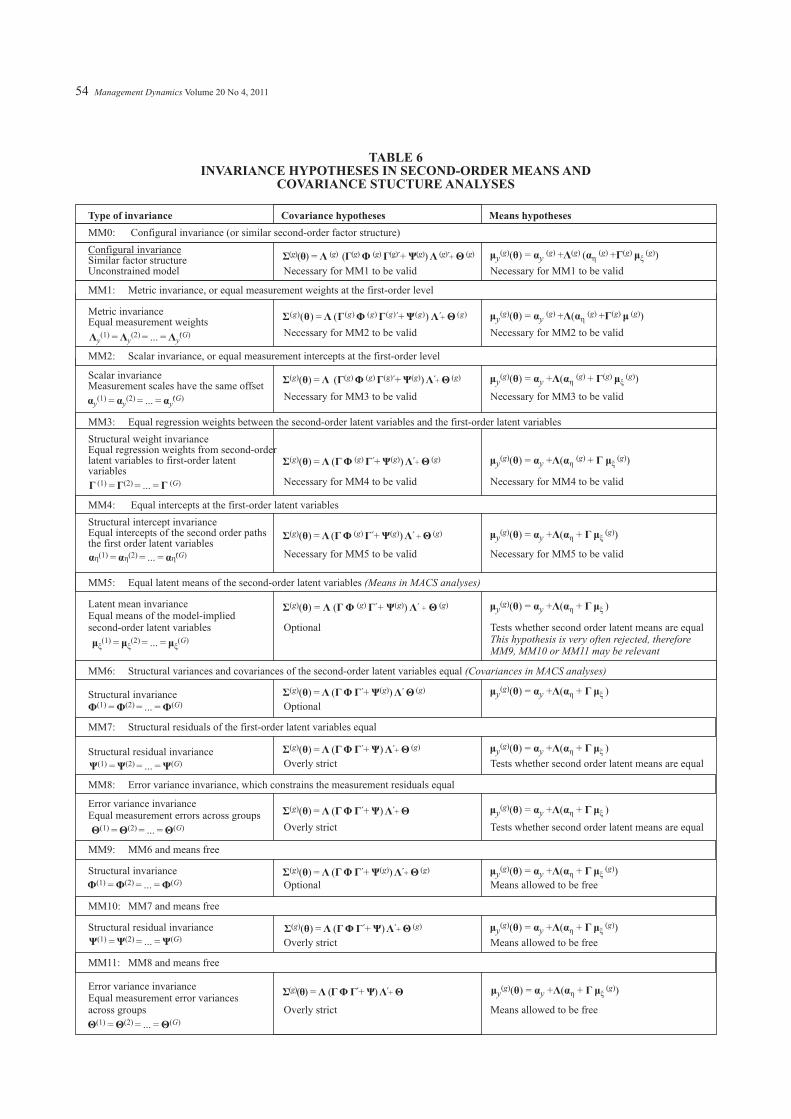
TABLE 6INVARIANCE HYPOTHESES IN SECOND-ORDER MEANS AND

COVARIANCE STUCTURE ANALYSES

Type of invariance Covariance hypotheses Means hypotheses

MM0: Configural invariance (or similar second-order factor structure)

Similar factor structureUnconstrained model Necessary for MM1 to be valid Necessary for MM1 to be valid

MM1: Metric invariance, or equal measurement weights at the first-order level

Metric invarianceEqual measurement weights

Necessary for MM2 to be valid Necessary for MM2 to be valid

MM2: Scalar invariance, or equal measurement intercepts at the first-order level

Scalar invarianceMeasurement scales have the same offset


MM3: Equal regression weights between the second-order latent variables and the first-order latent variables

Structural weight invarianceEqual regression weights from second-orderlatent variables to first-order latentvariables


MM4: Equal intercepts at the first-order latent variables

Structural intercept invarianceEqual intercepts of the second order pathsthe first order latent variables


MM5: Equal latent means of the second-order latent variables

Latent mean invarianceEqual means of the model-implied

-order latent variables Optional

MM6: Structural variances and covariances of the second-order latent variables equal

Structural invarianceOptional

MM7: Structural residuals of the first-order latent variables equal

Structural residual invarianceOverly strict Tests whether second order latent means are equal

MM8: Error variance invariance, which constrains the measurement residuals equal

Error variance invarianceEqual measurement errors across groups

Overly strict Tests whether second order latent means are equal

MM9: MM6 and means free

Structural invariance

Optional Means allowed to be free


Structural residual invariance

Overly strict Means allowed to be free


Error variance invarianceEqual measurement error variancesacross groups Overly strict Means allowed to be free

Configural invariance

(Means in MACS analyses)

This hypothesis is very often rejected, thereforeMM9, MM10 or MM11 may be relevant

(Covariances in MACS analyses)

second Tests whether second order latent means are equal


Σ θ Λ Γ Φ Γ Ψ Λ Θ( ) ( ) ( ) ( ) (g) ( ) ( ) + ( )g g g g g g g( ) = ( + )́ ́

Σ θ Λ Γ Φ Γ Ψ Λ Θ( ) ( ) ( ) ( ) ( ) + ( )g g g g g g( ) = ( + )́ ́

Σ θ Λ Γ Φ Γ Ψ Λ Θ( ) ( ) ( ) (g) ( ) + ( )g g g g g( ) = ( + )́ ́

Λ Λ Λy y yG(1) (2) ( )= = ... = ́

α α αy y yG(1) (2) ( )= = ... = ́

α α αη η η(1) (2) ( )= = ... = ́G

μ μ μξ ξ ξ(1) (2) ( )= = ... = G

Φ Φ Φ(1) (2) ( )= = ... = G

Ψ Ψ Ψ(1) (2) ( )= = ... = G

Θ Θ Θ(1) (2) ( )= = ... = G

Φ Φ Φ(1) (2) ( )= = ... = G

Ψ Ψ Ψ(1) (2) ( )= = ... = G

Θ Θ Θ(1) (2) ( )= = ... = G

Γ Γ Γ(1) (2) ( )= = ... = G

Σ θ Λ Γ Φ Γ Ψ Λ Θ( ) ( ) ( ) + ( )g g g g( ) = ( + )́ ́

Σ θ Λ Γ Φ Γ Ψ Λ Θ( ) ( ) ( ) + ( )g g g g( ) = ( + )́ ́

Σ θ Λ Γ Φ Γ Ψ Λ Θ( ) ( ) ( ) + ( )g g g g( ) = ( + )́ ́

Σ θ Λ Γ Φ Γ Ψ Λ Θ( ) ( ) ( )g g g( ) = ( + )́ ́

Σ θ Λ Γ Φ Γ Ψ Λ Θ( ) + ( )g g( ) = ( + )́ ́

Σ θ Λ Γ Φ Γ Ψ Λ Θ( ) +g ( ) = ( + )́ ́

Σ θ Λ Γ Φ Γ Ψ Λ Θ( ) ( ) + ( )g g g( ) = ( + )́ ́

( ) + ( )Σ θ Λ Γ Φ Γ Ψ Λ Θg g( ) = ( + )́ ́

Σ θ Λ Γ Φ Γ Ψ Λ Θ( ) +g ( ) = ( + )́ ́

μ θ α Λ μ( ) ( ) ( ) ( )g g g g( ) = + ( )yy α Γη ξ+( ) ( )g g

μ θ α Λ α Γ μy y( ) ( ) ( ) ( ) ( )g g g g g( ) = + ( + )η

μ θ α Λ α Γ μy y( ) ( ) ( ) ( )g g g g( ) = + ( + )η ξ

μ θ α Λ α Γ μy y( ) ( ) ( )g g g( ) = + ( + )η ξ

μ θ α Λ α Γ μy y( ) ( )g g( ) = + ( + )η ξ

μ θ α Λ α Γ μy y( )g ( ) = + ( + )η ξ

μ θ α Λ α Γ μy y( )g ( ) = + ( + )η ξ

μ θ α Λ α Γ μy y( )g ( ) = + ( + )η ξ

μ θ α Λ α Γ μy y( )g ( ) = + ( + )η ξ

μ θ α Λ α Γ μy y( ) ( )g g( ) = + ( + )η ξ

μ θ α Λ α Γ μy y( ) ( )g g( ) = + ( + )η ξ

μ θ α Λ α Γ μy y( ) ( )g g( ) = + ( + )η ξ

Consequences of non-invariance

The use of three different identification methods inmulti-group CFAanalyses

The diagram in Figure 3 illustrates the consequences ofnon-invariance for different types of parameters that arenot equal. In this diagram, the latent variable is depicted onthe horizontal or x-axis, which predicts the indicatorvariable that is displayed on the vertical or y-axis. Cheungand Rensvold (2000) provide an explanation of the use ofstructural equation models to assess different types ofresponse biases, and their methods were used as a base forthe explanation offered in Figure 3.

The three most common methods to constrain models foridentification purposes are described in Table 8, and arebased on the proposals of Little (2006). These authorshave built their discussion on essentially congenericmeasures, which assumes that all the constructs havemultiple indicators, there is a simple structure in the sensethat no indicator loads on more than one factor, and that allthe indicators are measured on the same response scale,and measurement errors are not correlated. All theseconditions are met in the examples discussed in this study.

In order to explain the consequences of non-invariance, itis easier to over-simplify the situation where we have fourlatent variables , , and , each indicated by a single

observed variable, , , and . The four situations arefurther explained in Table 7.

F F F F

y y y y

1 2 3 4

1 2 3 4

et al.

y1(1)

α1(1)

λ1(1)

μF1(1)

y1(2)

α1(2)

λ1(2)

μF1(2)

y2(1)

α2(1)

λ2(1)

μF2(1)

y2(2)

α2(2)

λ2(2)

μF2(2)

y3(1)

α3(1)

λ3(1)

μF3(1)

y3(2)

α3(2)

λ3(2)

μF3(2)

y4(1)

α (1)4

λ4(1)

μF4(1)

y4(2)

α4(2)

λ4(2)

μF 4(2)

Group 1 Group 2

FIGURE 3GRAPHICAL ILLUSTRATION OF THE CONSEQUENCES OF NON-INVARIANCE


Situation 1:

Situation 2:

Situation 3:

Situation 4:

The scaling indicator sets the slope = 1 and the intercept equal to 0 inboth groups.This results in the latent variables to assume the same scale as themarker variable.

The items in the two groups have equal slopes and equal intercepts.The result is that if two individuals have equal latent means across thegroups, the corresponding indicator values or responses on the itemsalso have equal values.

The items in the two groups have different slopes but equal intercepts.If a person in one group is equal to another person in the other group interms of the latent variable, their item responses will not have equalvalues.

The items in the two groups have equal slopes but different intercepts.If a person in group 1 is equal to another person in group 2, theirresponses will be different on the indicator items, due to thedifferences in the intercepts. There seems to be an off-set differenceacross the two groups.

TABLE 7ILLUSTRATION OF FOUR SITUATIONS TO EXPLAIN THE

CONSEQUENCES OF NON-INVARIANCE

Situation 1: Marker variable set so that slope=1 and intercept =0

Group1: y1(1) = α1

(1) + 1(1)

1(1) + ε1

(1) Group 2: y1(2) = α1

(2) + 1(2)

1(2) + ε1

(2)

The mean of the latent variable in group 1 is equal to the mean of the latent variable in group 2, and it is equal to the indicator

variable mean since the constraints mposed, namely thati forces the model-implied observed

groups means to be equal. Therefore,

α1(1) = α1

(2) = 0 and 1(1) = 1

(2) = 1

F1(1) = F1

(2) .

Situation 2: Invariant items with equal slopes and intercepts

Group 1: y2(1) = α2

(1) + 2(1)

2(1) + ε2

(1) Group 2: y2(2) = α2

(2) + 2(2)

2(2) + ε2

(2)

The mean of the latent variable in group 1 will be equal to the mean of the latent variable in group 2, if and only if

therefore Therefore, only if the model with these constraints fit the data well, it is safe to assume

that an observed indicator value in one group carries the same meaning in the second group. Not only does the item measure with the same

intensity (meaning slope), it also seems not to differ in terms of the level (there seems to be absense of bias, which is so because the intercepts

are not different). Equals intercepts also suggest that it is acceptable to assume that the offset of the scales are equal across groups

α2(1) = α2

(2) = α2 and 2(1)

= 2(2) = 2 F2

(1) = F2(2) = α2 + 2 2

Situation 3: Non -invariant items due to differences in slopes

Group 1: y3(1) = α3 + 3

(1)3

(1) + ε3(1) Group 2: y3

(2) = α3+ 3(2)

3(2) + ε3

(2)

Even though the intercepts (or offset of the scale) are equal across the groups , when the slopes in the two groups are not equal,

two individuals with equal levels of the latent variable, will not have the same observed indicator values. Therefore, although,

it is not possible for to be equal to , since . It can therefore be inferred that the items seem to indicate the

underlying latent variable with different levels of intensities (or slopes).

α3(1) = α3

(2) = α3

3(1)

3(2),

F3(1)= F3

(2)y3

(1) y3(2)

3(1)

3(2)

Situation 4: Non -invariant items due to differences in intercepts

Group 1: y4(1) = α4

(1) + 4 4(1) + ε4

(1) Group 2: y4(2) = α4

(2) + 4 4(2) + ε4

(2)

α4(1) α4

(2), two

F4(1)= F4

(2)

y4(1) y4

(2)α4

(1) α4(2)


TABLE 8PROPERTIES OF THREE MODEL IDENTIFICATION METHODS

Scaling method Properties*

Method 1:(reference group method)

Setting latent means = 0Setting latent variances =1

In the multigroup context, a reference group is used, and the latent means of this group isconstrained equal to zero, and the latent variance is constrained equal to one. The latent means inthe remaining groups are allowed to be estimated freely. The estimated means on the remaininggroups are expressed as relative mean-level differences. When the variances are constrainedequal to one, the relationships in the reference groups are no longer covariances, but areexpressed as correlations – which is useful for the purpose of interpreting the parameters.

Method 2:(marker variable method)

Set one indicator per latentvariable equal to 1.

Set the corresponding interceptequal to 0.

This method constrains the same marker variables equal to one in each group, and thecorresponding intercept equal to zero. The advantage of this method, is that it is not necessary tofree parameters in the model at a later stage, since each group contain free parameters. The majordisadvantage of this method is that the estimates of the means and the variances are dependent onwhich marker variable was chosen. Further, if invariant items are chosen as marker variables, itmay influence the evaluation of the invariance properties of the remaining indicators. Methods 1and 3 are better at identifying the indicator variables that are not invariant. However, if the itemsare not problematic, it remains a very practical and easy method that produces estimates that areinterpretable in the original scale of the measurement indicators.

Method 3:(effects coding method)

Constrain measurement weightsso that their average is 1.

Constrain measurement interceptsso that their average is 0.

This method is similar to effects coding in analysis of variance. An optimal balance is obtainedbetween the relative regression weights, thereby allowing the estimate of the latent means to be aweighted average of the set of indicators of the construct, and the estimated variances of thelatent variables to the average of the variances of the indicators. The major advantage of thismethod is the ease of interpreting the estimated parameters. It is also possible to compare therelative importance of constructs among one another within the scale with this method.

* The properties provided here were summarised by the author from Little . (2006)et al

EMPIRICALEXAMPLES

The examples presented here correspond to the modelstested in Ungerer and Strasheim (2011). The Schwartz’svalues theory (Schwartz 2006; 1992) consists of tenmotivational drives that are believed to be present atdifferent levels in all individuals, and the motivationalvalues are useful to explain human attitudes, preferencesand behaviours. The measurement instrument used was thePortrait Values Questionnaire (PVQ) developed bySchwartz, Melech, Lehmann, Burgess, Harris and Owens(2001). These authors adapted and validated the PortraitValues Questionnaire (PVQ) in a South African context,and developed a set of 29 items to determine valueproperties in a situation where all the respondents are notnecessarily literate. Only 12 items representing four valueconstructs of the original 29-item PVQ were used in thisstudy to indicate four personal value constructs ofrespondents (see Annexure 1). All the PVQ statements andmore detail are provided in Ungerer and Strasheim (2011).

A reputable market research organisation collected thedata, and the respondents were representative in terms ofmajor demographic characteristics in the population.The invariance testing for both the 1CFA model and the2CFA model across race groups is used for illustration.Since the cultural value orientation of individuals tends tobe influenced by their cultural heritage, race is a keyvariable in the study of individual values. It is thereforeimportant to investigate the measurement invariance of thePVQ instrument over race groups, before it would be validto proceed with further analyses of the data. Therefore, theresults reported in this study focus only on the invariancetesting and MACS analysis across the race groups.The sample (2 566 in total) consisted mainly of blackpeople, while the other ethnic groups were not representedas strongly – 69% of respondents were black (1 769), 16%white (408), 11% coloured (282) and 4% Indian (107). Thisprofile closely resembles the general ethnic profile of theSouthAfrican population.

Race group All

Black White Indian ColouredGroups

Benevolence 0.601 0.559 0.618 0.766 0.629

Universalism 0.558 0.726 0.768 0.762 0.622

Achievement 0.575 0.695 0.608 0.657 0.613

Power 0.468 0.573 0.515 0.478 0.503

Race group All

Black White Indian ColouredGroups

Allocentrism 0.736 0.778 0.823 0.854 0.766

Idiocentrism 0.604 0.715 0.706 0.655 0.643

TABLE 9CRONBACH'S ALPHA COEFFICIENT FOR THE 1CFA MODEL IN EXAMPLE 1


While the 1CFA model (see Figure 4) was not explicitlyreported by Ungerer and Strasheim (2011), the model wastested, and the procedure is briefly provided here for thesake of demonstrating the similarities and differencesbetween a 1CFA and a 2CFA approach. The internalconsistency reliability of the first-order constructs is

provided in Table 9. Although the Cronbach’s coefficientalpha is lower than normally accepted, Schwarz andBoehnke (2004) reported similar values for this scale.In addition, since only a few items measure eachconstruct, lower alpha values were tolerated in this study.

TABLE 10CRONBACH'S ALPHA COEFFICIENT

e8

e15

e28

e5

e18

e22

e26

e3

e20

e27

e9

e13

PVQ8

PVQ15

PVQ28

PVQ5

PVQ18

PVQ22

PVQ26

PVQ3

PVQ20

PVQ27

PVQ9

PVQ13

0, v11

a1

a20, v2

1

0, v31

0, v41

0, v51

0, v61

0, v71

0, v81

0, v91

0, v101

0, v111

0, v121

Benevolence

Universalism

Achievement

Power

mm1, vv1

mm2, vv2

mm3, vv3

mm4, vv4

a3

a4

a5

a6

a8

a9

a10

a7

a11

a12

cc1

cc2

cc3cc4

cc5

cc6

i1

i2

i3

i4

i5

i6

i7

i8

i9

i10

i11

i12

FIGURE 4EMPIRICAL EXAMPLE OF A FIRST-ORDER CONFIRMATORY FACTOR

ANALYSIS MODEL


FIGURE 5EMPIRICAL EXAMPLE OF A SECOND-ORDER CONFIRMATORY

FACTOR ANALYSIS MODEL

e8

e15

e28

e5

e18

e6

e22

e3

e20

e27

e9

e13

PVQ8

PVQ15

PVQ28

PVQ5

PVQ18

PVQ22

PVQ26

PVQ3

PVQ20

PVQ27

PVQ9

PVQ13

0, v11

a1

a20, v2

1

0, v31

0, v41

0, v51

0, v61

0, v71

0, v81

0, v91

0, v101

0, v111

0, v121

Benevolence

Universalism

Achievement

Power

a3

a4

a5

a6

a8

a9

a10

a7

a11

a12

i1

i2

i3

i4

i5

i6

i7

i8

i9

i10

i11

i12

ii1

ef2

ef1

ef4

ef3

ii2

ii3

ii4

0, vv1

0, vv2

0, vv3

0, vv4

Allocentrism

ccc1

mmm1, vvv1

mmm2, vvv2

Idiocentrism

aa1

aa2

aa3

aa4


The internal consistency of the higher-order factors inExample 2 5 are provided in Table 10. Most ofthese values are above 0.7, the generally accepted cut-offcriterion for reliability, with two below 0.7. This is to beexpected since the number of items that collectivelyindicate the higher-order constructs is more, therebyresulting in higher alpha values.

The results of the fit measures (usingAMOS 19.0) for boththese models are provided in Tables 11 and 13.

(See Figure )From the fit measures in Table 11 it is clear that the modelsfit increasingly worse as one proceeds from M0 to M5.

This is to be expected, since the models becomeincreasingly restrictive. When the means are restricted inmodel M3, the fit measures decline when all the fitmeasures are evaluated, and therefore it is appropriate torelax this constraint, as was done in models M6 and M7.The results indicate that configural, metric and scalarinvariance can be assumed for the 1CFA model. In model

Model NPAR CMIN DF P CMIN/DF

>0.05 <3.0

M0: Unconstrained 168 508.0 192 0.000 2.65

M1: Measurement weights 144 561.3 216 0.000 2.60

M2: Measurement intercepts 120 673.1 240 0.000 2.81

M3: Structural means 108 953.3 252 0.000 3.78

M4: Structural covariances 78 1134.5 282 0.000 4.02

M5: Measurement residuals 42 1629.2 318 0.000 5.12

M6: M4 and means free 90 814.6 270 0.000 3.02

M7: M5 and means free 54 1324.1 306 0.000 4.33

Model IFI TLI CFI PCFI

>0.90 >0.90 >0.90 >0.90

M0: Unconstrained 0.947 0.927 0.947 0.688

M1: Measurement weights 0.942 0.929 0.942 0.771

M2:Measurement intercepts 0.927 0.920 0.927 0.843

M3: Structural means 0.882 0.876 0.882 0.842

M4: Structural covariances 0.856 0.865 0.856 0.915

M5: Measurement residuals 0.777 0.816 0.779 0.938

M6: M4 and means free 0.908 0.910 0.908 0.929

M7: M5 and means free 0.827 0.852 0.828 0.960

RMSEA LO 90 HI 90 PCLOSE

<0.05 <0.05 <0.08 1.0

M0: Unconstrained 0.025 0.023 0.028 1.000

M1: Measurement weights 0.025 0.022 0.028 1.000

M2: Measurement intercepts 0.027 0.024 0.029 1.000

M3: Structural means 0.033 0.031 0.035 1.000

M4: Structural covariances 0.034 0.032 0.036 1.000

M5:Measurement residuals 0.040 0.038 0.042 1.000

M6:M4 and means free 0.028 0.026 0.030 1.000

M7: M5 and means free 0.036 0.034 0.038 1.000

TABLE 11FIT MEASURES FOR THE 1CFA EXAMPLE


1 See Hu and Bentler (1999)

Criteria for good fit1


Model


M6, the covariances are constrained to be equal.This model seems to be the most appropriate choice whenall the fit measures are considered.

The estimated parameters for model M6 are provided inTable 12, and the corresponding parameters on the pathdiagram are also shown.

Slope Estimate p

p

Slope Estimate p

Intercept Estimate p

PVQ8 Benevolence 1.000 – 0.000 –

Benevolence 0.985 *** 0.177 0.402

Benevolence 1.108 *** -0.633 0.006

Universalism 1.000 – 0.000 –

Universalism 0.978 *** -0.191 0.440

Universalism 0.906 *** 0.092 0.702

Universalism 1.171 *** -0.997 ***

Achievement 1.000 – 0.000 –

Achievement 1.080 *** -0.269 0.301

Achievement 1.178 *** -0.857 0.002

Power 1.000 – 0.000 –

Power 1.329 *** -1.154 ***

Covariances Slope Estimate

Universalism 0.327 ***

Achievement

Achievement

0.256 ***

Power 0.026 0.092

0.267 ***

Power 0.035 0.016

Power 0.300 ***

Variances

0.340 ***

0.468 ***

0.541 ***

Estimated means

Black White Indian Coloured

4.965 5.226 5.305 5.413

5.110 5.234 5.362 5.434

4.612 4.431 4.405 4.484

3.838 3.442 3.250

Variable

Benevolence

Universalism

Achievement

Power

PVQ15

PVQ28

PVQ5

PVQ18

PVQ22

PVQ26

PVQ3

PVQ20

PVQ27

PVQ9

PVQ13

Benevolence

Benevolence

Benevolence

Universalism

Universalism

Achievement

Benevolence

Universalism

Achievement

Power

3.141

TABLE 12ESTIMATED PARAMETERS OF MODEL M6 OF 1CFA MODEL

a

a

a

a

a

a

a

a

a

a

a

a

cc

cc

cc

cc

cc

cc

vv

vv

vv

vv

1

2

3

4

5

6

7

8

9

10

11

12

1

2

3

4

5

6

1

2

3

4

i1

i2

i3

i4

i5

i6

i7

i8

i9

i10

i11

i12

mm1 _1

mm 2_1

mm 3_1

mm 4_1

mm1 _2

mm 2_2

mm 3_2

mm 4_2

mm1 _3

mm 2_3

mm 3_3

mm 4_3

mm1 _4

mm 2_4

mm 3_4

mm 4_4


0.334

*** p < 0.001- the parameters are constrained, and therefore there are no standard errors or significance tests for them

***

NPAR CMIN DFp CMIN/DF

>0.05 <3.0

164 521.7 196 0.000 2.66

140 573.3 220 0.000 2.61

116 687.2 244 0.000 2.82

110 708.6 250 0.000 2.83

104 866.8 256 0.000 3.39

98 1010.6 262 0.000 3.86

89 1074.7 271 0.000 3.97

77 1136.6 283 0.000 4.02

41 1630.0 319 0.000 5.11

95 916.3 265 0.000 3.46

83 982.0 277 0.000 3.55

47 1485.1 313 0.000 4.75

IFI TLI CFI PCFI

>0.90 >0.90 >0.90 >0.90

0.946 0.926 0.945 0.702

0.941 0.928 0.940 0.784

0.925 0.919 0.925 0.855

0.923 0.918 0.923 0.874

0.897 0.894 0.897 0.870

0.874 0.873 0.874 0.867

0.864 0.868 0.864 0.887

0.856 0.866 0.856 0.918

0.777

0.777

0.777

0.817

0.817

0.817

0.779

0.779

0.779

0.941

0.941

0.941

0.801 0.833 0.802 0.951

RMSEA

<0.05

LO 90

<0.05

HI 90

<0.08

PCLOSE

1.0

0.025 0.02 0.028 1.000

0.025 0.02 0.028 1.000

0.027 0.02 0.029 1.000

0.027 0.02 0.029 1.000

0.031 0.02 0.033 1.000

0.033 0.03 0.036 1.000

0.034 0.03 0.036 1.000

0.034 0.03 0.036 1.000

0.040 0.03 0.042 1.000

MM0: Unconstrained

MM1: Measurement weights

MM2: Measurement intercepts

MM3: Structural weights

MM4: Structural intercepts

MM5: Structural means

MM6: Structural covariances

MM7: Structural residuals

MM8: Measurement residuals




Model

Model



MM0: Unconstrained












Model


MM0: Unconstrained









0.031 0.02 0.033 1.000

0.032

0.038

0.02

0.03

0.034

0.040

1.000

1.000




TABLE 13FIT MEASURES OF THE 2CFA MODEL


1 See Hu and Bentler (1999)

The fit measures of the 2CFA model in Figure 5 areprovided in Table 13. When these are examined, it isevident that the fit measures also decline with eachincreasingly restrictive model. Models MM0 to MM3 stillmeet the minimum fit criteria, but for model MM4, the fitmeasures are just below the recommended threshold.

Since this model is required before it is valid to proceedwith means comparisons, and since the RMSEA is stillvery acceptable, it will be marginally acceptable to assumethat the 2CFA model has configural, metric and scalarinvariance on both the 1CFAand 2CFAlevel.

Since the fit decreases more dramatically when modelMM5 is tested, which constrains the second-order latentvariable means to be equal, it is appropriate to relax thisconstraint. The most appropriate model to interpret takingall fit measures and parsimony into consideration, is MM9– which constrains the covariances and variances of thesecond-order model equal, but the means are freely

estimated. The estimated parameters of model MM9 withthe corresponding parameters shown on Figure 5 are givenin Table 14.

The estimated mean parameters show the differences in themean allocentric and idiocentric values across the fourcultural groups.

TABLE 14ESTIMATED PARAMETERS OF MODEL M9 OF 2CFA MODEL


*** p < 0.001- the parameters are constrained, and therefore there are no standard errors or significance tests for them

SUMMARY

This methodological study showed in matrix notation howa 2CFA model extends from a 1CFA model, and showedhow invariance testing can be done for the 2CFA model.The method provided is similar to ones reported so far, andprovides the matrices that can be used for eachincreasingly restrictive hypothesis. In addition, thecorresponding parameters on the path diagrams are shown,thereby offering researchers not familiar with matrixalgebra and the procedure, a more accessible approach.Lastly, the constraints and method to implement thesemodels are provided for the 1CFA and 2CFA model usingAMOS 19.0 in Annexures 2 and 3 respectively, and when

LISREL8.8 is used, the reader is referred toAnnexure 4 forthe 1CFA model and Annexure 5 for the 2CFA model.The examples are only provided for the second scalingidentification method, which sets one indicator path perlatent variable equal to 1, and the corresponding interceptequal to 0._____________________________________________

End Note:

The intercepts are, as in simple regression, similar to the value on they-axis where the “regression line” cuts into the observed y-variablewhen the corresponding x-variable (or in this case factor value) is equalto zero.

1

Slope Estimate p Intercept Estimate p

Covariances Estimate p

Variances

Estimated means

Variable Black White Indian Coloured

Benevolence Allocentrism aa 1.000 – ii 0.000 –

Universalism Allocentrism aa 0.950 *** ii 0.354 0.153

Achievement Idiocentrism aa 1.000 – ii 0.000 –

Power Idiocentrism aa 0.206 *** ii 2.740 ***

PVQ8 Benevolence a 1.000 – i 0.000 –

PVQ15 Benevolence a 0.988 *** i 0.160 0.454

PVQ28 Benevolence a 1.119 *** i -0.691 0.003

PVQ5 Universalism a 1.000 – i 0.000 –

PVQ18 Universalism a 0.999 *** i -0.298 0.232

PVQ22 Universalism a 0.918 *** i 0.026 0.913

PVQ26 Universalism a 1.172 *** i -1.007 ***

PVQ3 Achievement a 1.000 – i 0.000 –

PVQ20 Achievement a 1.070 *** i -0.224 0.380

PVQ27 Achievement a 1.186 *** i -0.893 0.001

PVQ9 Power a 1.000 – i 0.000 –

PVQ13 Power a 1.040 *** i -0.086 0.774

Idiocentrism Allocentrism ccc 0.272 ***

Allocentrism vvv 0.342 ***

Idiocentrism vvv 1.780 ***

Allocentrism mmm 4.991 mmm 5.190 mmm 5.297 mmm 5.383

Idiocentrism mmm 4.587 mmm 4.457 mmm 4.463 mmm 4.548

1 1

2 2

3 3

4 4

1 1

2 2

3 3

4 4

5 5

6 6

7 7

8 8

9 9

10 10

11 11

12 12

1

1

2

1_1 1_2 1_3 1_4

2_1 2_2 2_3 2_4

Estimate p

REFERENCES

Baumgartner. H. and Steenkamp, J.E.M. 2001. Responsestyles in marketing research: A cross-nationalinvestigation. , 38(2)May: 143-156.

Journal of Marketing Research

cross-cultural research: A critique of Cheung and Rensvold,

, 31(2): 213-219.

Little, T.D., Slegers D.W. and Card, N.A. 2006. A non-arbitrary method of identifying and scaling latentvariables in SEM and MACS models.

, 13(1): 59-72.

Marsh, H.W. and Hocevar, D. 1985. Application ofconfirmatory factor analysis to the study of self-concept:First and higher-order factor models and their invarianceacross groups. , 97(3): 562-582.

Meredith, W. 1993. Measurement invariance, factoranalysis and factorial invariance.58(4): 525-543.

Rensvold, R.B. and Cheung, G.W. 1998. Testingmeasurement models for factorial invariance:A systematic approach.

, 58(6): 1017-1034.

Schwartz, S.H. 1992. Universals in the content and structureof values: Theory and empirical tests in 20 countries.In:Volume 25. Zanna, M. (Ed.). New York: AcademicPress, 1-65.

Schwartz, S.H. 2006. Les valeurs de base de la personne:Théorie, mesures et applications [Basic human values:Theory, measurement, and applications].

, 45 (4): 926-968.

Schwartz, S.H. and Boehnke, K. 2004. Evaluation of thestructure of human values with confirmatory factoranalysis. ,38: 230-255.

Schwartz, S.H., Melech, G., Lehmann, A., Burgess, S.M.,Harris, M. and Owens, V. 2001. Extending the cross-cultural validity of the theory of basic human valueswith a different method of measurement.

, 32 (5): 519-542.

Shiu, E., Pervan, S.J., Bove, L.L. and Beatty, S.E. 2011.Reflections on discriminant validity: Re-examining theBove (2009) findings.

, 64: 497-500.

Steenkamp, J.E.M. and Baumgartner, H.B. 1998. Assessingmeasurement invariance in cross-national consumerresearch, 25(June):78-90.

Ungerer, L. and Strasheim, A. 2011. The moderating effect ofliving standards on the relationship between individual-level culture and life satisfaction: A value segmentationperspective. 20(3): 25-50.

Van de Vijver, F. and Leung, K. 1997., London: Sage.

Vandenberg, R.J. 2002. Toward a further understanding ofand improvement in measurement invariance methodsand procedures. ,5(2): 139-158.

Vandenberg, R.J. and Lance, C.E. 2000. A review andsynthesis of the measurement invariance literature:Suggestions, practices and recommendations fororganisational research.

3(1): 4-69.

Journal of Cross-Cultural Psychology

StructuralEquation Modeling

Psychological Bulletin

Psychometrika,

Educational and PsychologicalMeasurement

Advances in Experimental Social Psychology

RevueFrançaise De Sociologie

Journal of Research in Personality

Journal ofCross-Cultural Psychology

Journal of BusinessResearch

Journal of Consumer Research

Management Dynamics,

Methods and DataAnalysis for Cross-Cultural Research

Organizational Research Methods

Organizational ResearchMethods

.

et al.

,

,

Bollen, K.A. 1989., NewYork: John Wiley and Sons.

Bollen, K.A. and Biesanz, J.C. 2002. A note on two-stageleast squares estimator for higher-order factor analyses.

, 30(4): 568-579.

Byrne, B.M. 1998.

, London: LawrenceErlbaumAssociates, Publishers.

Byrne, B.M., Shavelson, R.J. and Muthén, B. 1989. Testingfor the equivalence of factor covariance and meanstructures: The issue of partial measurement invariance,

105(May): 456-466.

Chen, F.F., Sousa, K.H. and West, S.G. 2005. Testingmeasurement invariance of second-order factor models.

, 12(3): 471-492.

Cheung, G.W. and Rensvold, R.B. 2000. Assessing extremeand aquiescence response sets in cross-cultural researchusing Structural Equation Modelling,

, 31(2): 187-212.

Hu, L-T. and Bentler, P.M. 1999. Cut-off criteria for fit indicesin covariance structure analysis: Conventional criteriaversus new alternatives. ,6(1): 1-55.

Jöreskog, K. G. 1971. Simultaneous factor analysis in severalpopulations. , 36: 409-426.

Jöreskog, K.G., Andersen, E.B., Laake, P. and Cox, D.R.,1981.Analysis of covariance structures [with discussionand reply]. , 8(2):65-92. Stable URL:

Little, T.D. 2000. On the comparability of constructs in

Structural Equations with LatentVariables

Sociological Methods and Research

Structural Equation Modelling withLISREL, PRELIS and SIMPLIS: Basic Concepts,Applications and Programming

Psychological Bulletin

Structural Equation Modelling

Journal of Cross-Cultural Psychology

Structural Equation Modelling

Psychometrika

Scandanawian Journal of Statisticshttp://www.jstor.org/

stable/4615818

,

All correspondence should be addressed to Arien Strasheim, Department of Marketing and Communication Management, University of Pretoria,[email protected]


PVQ8 She always wants to help the people who are close to her. It is very important to her to care for the people she knows and likes.

PVQ15 Honesty is very important to her. She believes she must be honest in any situation and always tell the truth.

PVQ28 It is important to her that her friends can always trust her. She wants to be loyal to them and always to look out for their interests.

PVQ5 She thinks it is important that every person in the world should be treated equally. She wants justice for everybody, even for peopleshe does not know.

PVQ18 She strongly believes that people should care for nature. Looking after an environment is important to her.

PVQ22 It is important to her to listen to people who are different from her. Even when she disagrees with them she still wants to understandthem and to get along with them.

PVQ26 She thinks everyone should work to get people in the world to live together peacefully. Peace everywhere in the world is importantto her.

PVQ3 Being very successful is important to her. She likes to stand out and to impress other people.

PVQ20 She likes people to know that she can do well. She is ambitious and ready to work hard to get ahead.

PVQ27 It is very important to her to show her abilities. She want people to admire what she does.

PVQ9 She likes to be in charge and tell others what to do. She wants people to do what she says.

PVQ13 It is important to her to be rich. She wants to have a lot of money and expensive things.

ANNEXURE 1THE PVQ ITEMS AND THEIR CONSTRUCTS USED IN THIS STUDY

Higher-order dimension PVQ first-order dimension Items

Self-transcendence Benevolence PVQ8; PVQ15; PVQ28

Allocentrism Universalism PVQ5; PVQ18; PVQ22; PVQ26

Self-enhancement Achievement PVQ3; PVQ20; PVQ27

Idiocentrism Power PVQ9; PVQ13

Response categories are: 1 = “very much like me”; 2 = “like me”; 3=”somewhat like me”; 4=”a little like me”; 5 = “not like me”; 6 = “not at all likeme”; and 7 = “do not know”

PVQ ITEMS

*Note: Both male and female versions of the PVQ were used, in accordance with recommended measurement practice


M0 No constraints

M1 a1_1=a1_2=a1_3=a1_4=1 Scaling indicators = 1

Measurement weights a2_1=a2_2=a2_3=a2_4

a3_1=a3_2=a3_3=a3_4

a4_1=a4_2=a4_3=a4_4=1 Scaling indicators = 1

a5_1=a5_2=a5_3=a5_4

a6_1=a6_2=a6_3=a6_4

a7_1=a7_2=a7_3=a7_4


a9_1=a9_2=a9_3=a9_4

a10_1=a10_2=a10_3=a10_4


a12_1=a12_2=a12_3=a12_4

M2 i1_1=i1_2=i1_3=i1_4=0 Intercepts = 0

Measurement intercepts i2_1=i2_2=i2_3=i2_4

i3_1=i3_2=i3_3=i3_4

i4_1=i4_2=i4_3=i4_4=0 Intercepts = 0

i5_1=i5_2=i5_3=i5_4

i6_1=i6_2=i6_3=i6_4

i7_1=i7_2=i7_3=i7_4

i8_1=i8_2=i8_3=i8_4=0 Intercepts = 0

i9_1=i9_2=i9_3=i9_4

i10_1=i10_2=i10_3=i10_4

i11_1=i11_2=i11_3=i11_4=0 Intercepts = 0

i12_1=i12_2=i12_3=i12_4

M3 m1_1=m1_2=m1_3=m1_4 Leave out for M6 and M7

Latent means m2_1=m2_2=m2_3=m2_4

m3_1=m3_2=m3_3=m3_4

m4_1=m4_2=m4_3=m4_4

M4 c1_1=c1_2=c1_3=c1_4

Variances and covariances c2_1=c2_2=c2_3=c2_4

c3_1=c3_2=c3_3=c3_4

c4_1=c4_2=c4_3=c4_4

c5_1=c5_2=c5_3=c5_4

c6_1=c6_2=c6_3=c6_4

vv1_1=vv1_2=vv1_3=vv1_4

vv2_1=vv2_2=vv2_3=vv2_4

vv3_1=vv3_2=vv3_3=vv3_4

vv4_1=vv4_2=vv4_3=vv4_4

M5 v1_1=v1_2=v1_3=v1_4

Measurement residuals v2_1=v2_2=v2_3=v2_4

v3_1=v3_2=v3_3=v3_4

v4_1=v4_2=v4_3=v4_4

v5_1=v5_2=v5_3=v5_4

v6_1=v6_2=v6_3=v6_4

v7_1=v7_2=v7_3=v7_4

v8_1=v8_2=v8_3=v8_4

v9_1=v9_2=v9_3=v9_4

v10_1=v10_2=v10_3=v10_4

v11_1=v11_2=v11_3=v11_4

V12_1=v12_2=v12_3=v12_4

ANNEXURE 2:AMOS GRAPHICS SYNTAX

MODEL CONSTRAINTS FOR 1CFA MODELS USING AMOS 19.0


ANNEXURE 3MODEL CONSTRAINTS FOR 2CFA MODELS USING AMOS 19.0

MM0 No constraints

MM1 a1_1=a1_2=a1_3=a1_4=1 Scaling indicators = 1

Measurement weights a2_1=a2_2=a2_3=a2_4

a3_1=a3_2=a3_3=a3_4


a5_1=a5_2=a5_3=a5_4

a6_1=a6_2=a6_3=a6_4

a7_1=a7_2=a7_3=a7_4


a9_1=a9_2=a9_3=a9_4

a10_1=a10_2=a10_3=a10_4


a12_1=a12_2=a12_3=a12_4

MM2 i1_1=i1_2=i1_3=i1_4=0 Intercepts = 0

Measurement intercepts i2_1=i2_2=i2_3=i2_4

i3_1=i3_2=i3_3=i3_4

i4_1=i4_2=i4_3=i4_4=0 Intercepts = 0

i5_1=i5_2=i5_3=i5_4

i6_1=i6_2=i6_3=i6_4

i7_1=i7_2=i7_3=i7_4

i8_1=i8_2=i8_3=i8_4=0 Intercepts = 0

i9_1=i9_2=i9_3=i9_4

i10_1=i10_2=i10_3=i10_4

i11_1=i11_2=i11_3=i11_4=0 Intercepts = 0

i12_1=i12_2=i12_3=i12_4

MM3 aa1_1=aa1_2=aa1_3=aa1_4=1 Scaling indicators = 1

Structural or second-order weights aa2_1=aa2_2=aa2_3=aa2_4

aa3_1=aa3_2=aa3_3=aa3_4=1 Scaling indicators = 1

aa4_1=aa4_2=aa4_3=aa4_4

MM4 ii1_1=ii1_2=ii1_3=ii1_4=0 Intercepts = 0

Structural intercepts ii2_1=ii2_2=ii2_3=ii2_4

ii3_1=ii3_2=ii3_3=ii3_4=0 Intercepts = 0

ii4_1=ii4_2=ii4_3=ii4_4

MM5 mmm1_1=mmm1_2=mmm1_3=mmm1_4 Leave out for MM9,

Second-order latent means mmm2_1=mmm2_2=mmm2_3=mmm2_4 MM10 and MM11

MM6 ccc1_1=ccc1_2=ccc1_3=ccc1_4

Variances and covariances vvv1_1=vvv1_2=vvv1_3=vvv1_4

vvv2_1=vvv2_2=vvv2_3=vvv2_4

MM7 vv1_1=vv1_2=vv1_3=vv1_4

Structural residuals vv2_1=vv2_2=vv2_3=vv2_4

vv3_1=vv3_2=vv3_3=vv3_4

vv4_1=vv4_2=vv4_3=vv4_4

MM8 v1_1=v1_2=v1_3=v1_4

Measurement residuals v2_1=v2_2=v2_3=v2_4

v3_1=v3_2=v3_3=v3_4

v4_1=v4_2=v4_3=v4_4

v5_1=v5_2=v5_3=v5_4

v6_1=v6_2=v6_3=v6_4

v7_1=v7_2=v7_3=v7_4

v8_1=v8_2=v8_3=v8_4

v9_1=v9_2=v9_3=v9_4

v10_1=v10_2=v10_3=v10_4

v11_1=v11_2=v11_3=v11_4

V12_1=v12_2=v12_3=v12_4


ANNEXURE 4LISREL SIMPLIS SYNTAX FOR INVARIANCE TESTING OF 1CFA MODEL

Leave all statements as is for all themodels M0 to M7 for the first groupanalysed

PVQ8 = 1*BENEVOL

PVQ15 PVQ28 = BENEVOL

PVQ5 = 1*UNIVERS

PVQ18 PVQ22 PVQ26 = UNIVERS

PVQ3 = 1*ACHIEVE

PVQ20 PVQ27 = ACHIEVE

PVQ9 = 1*POWER

PVQ13 = POWER

PVQ15 PVQ28 PVQ18 PVQ22 PVQ26 PVQ20 PVQ27 PVQ13 = CONST

BENEVOL UNIVERS ACHIEVE POWER = CONST

Set the Covariance between BENEVOL and UNIVERS Free

Set the Covariance between BENEVOL and ACHIEVE Free

Set the Covariance between BENEVOL and POWER Free

Set the Covariance between UNIVERS and ACHIEVE Free

Set the Covariance between UNIVERS and POWER Free

Set the Covariance between ACHIEVE and POWER Free

Set the Variance of BENEVOL Free

Set the Variance of UNIVERS Free

Set the Variance of ACHIEVE Free

Set the Variance of POWER Free

Set the Error Variance of PVQ8 Free












GROUP1: BLACK

BLACK.PSF

! INVARIANCE 1CFA

Observed Variables: NR PVQ1-PVQ29

Raw Data from file

Latent Variables: BENEVOL UNIVERS ACHIEVE POWER

Relationships:


PVQ8 = 1*BENEVOL


PVQ5 = 1*UNIVERS


PVQ3 = 1*ACHIEVE


PVQ9 = 1*POWER

PVQ13 = POWER

























Leave in for M0Delete for models M1, M2, M3, M4,M5, M6, M7

Leave in for M0, M1Delete for models M2, M3, M4, M5,M6, M7

Leave in for M0, M1, M2Delete for models M3, M4, M5

Leave in for M0, M1, M2, M3Delete for models M4, M5, M6, M7

Leave in for M0, M1, M2, M3Delete for models M4, M5, M6, M7

Leave in for M0, M1,M2, M3, M4, M6

Delete for models M5, M7

GROUP2: WHITE

WHITE.PSF


Raw Data from file


Relationships:

ANNEXURE 4 (Cont.)LISREL SIMPLIS SYNTAX FOR INVARIANCE TESTING OF 1CFA MODEL


PVQ8 = 1*BENEVOL


PVQ5 = 1*UNIVERS


PVQ3 = 1*ACHIEVE


PVQ9 = 1*POWER

PVQ13 = POWER

























Delete for models M1, M2, M3, M4,M5, M6, M7

Delete for models M2, M3, M4, M5,M6, M7

Delete for models M3, M4, M5

Delete for models M4, M5, M6, M7



GROUP3: INDIAN

INDIAN.PSF


Raw Data from file


Relationships:




PVQ8 = 1*BENEVOL


PVQ5 = 1*UNIVERS


PVQ3 = 1*ACHIEVE


PVQ9 = 1*POWER

PVQ13 = POWER

























Path Diagram

LISREL OUTPUT: ND=3 SC AD=OFF

End of Problem

Delete for models M1, M2, M3, M4,M5, M6, M7

Delete for models M2, M3, M4, M5,M6, M7

Delete for models M3, M4, M5




GROUP4 COLOURED

COLOURED.PSF

:

Observed variables: NR PVQ1-PVQ29

Raw data from file

Latent variables: BENEVOL UNIVERS ACHIEVE POWER

Relationships:


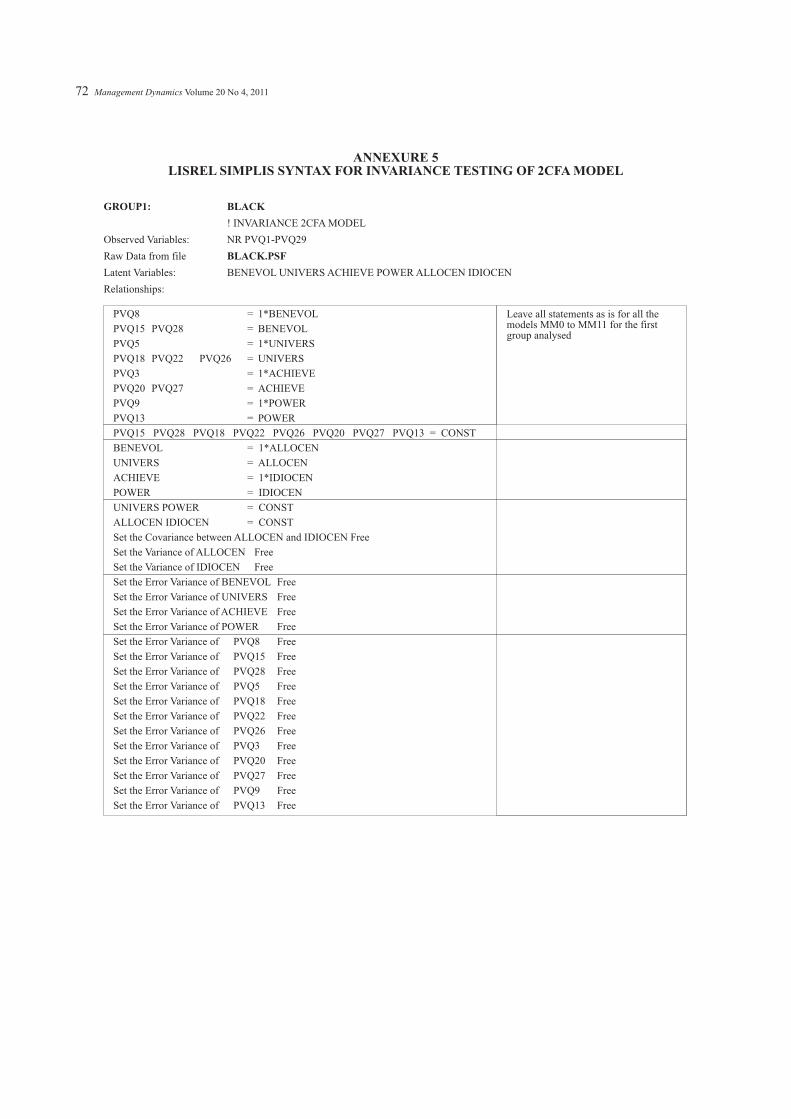
ANNEXURE 5LISREL SIMPLIS SYNTAX FOR INVARIANCE TESTING OF 2CFA MODEL

GROUP1: BLACK

BLACK.PSF

! INVARIANCE 2CFA MODEL


Raw Data from file

Latent Variables: BENEVOL UNIVERS ACHIEVE POWER ALLOCEN IDIOCEN

Relationships:

PVQ8 = 1*BENEVOL


PVQ5 = 1*UNIVERS


PVQ3 = 1*ACHIEVE


PVQ9 = 1*POWER

PVQ13 = POWER


BENEVOL = 1*ALLOCEN

UNIVERS = ALLOCEN

ACHIEVE = 1*IDIOCEN

POWER = IDIOCEN

UNIVERS POWER = CONST

ALLOCEN IDIOCEN = CONST

Set the Covariance between ALLOCEN and IDIOCEN Free

Set the Variance of ALLOCEN Free

Set the Variance of IDIOCEN Free

Set the Error Variance of BENEVOL Free

Set the Error Variance of UNIVERS Free

Set the Error Variance of ACHIEVE Free

Set the Error Variance of POWER Free













Leave all statements as is for all themodels MM0 to MM11 for the firstgroup analysed


PVQ8 = 1*BENEVOL


PVQ5 = 1*UNIVERS


PVQ3 = 1*ACHIEVE


PVQ9 = 1*POWER

PVQ13 = POWER


BENEVOL = 1*ALLOCEN

UNIVERS = ALLOCEN

ACHIEVE = 1*IDIOCEN

POWER = IDIOCEN






















Leave in for model MM0

Delete for models MM1, MM2, MM3,MM4, MM5, MM6, MM7, MM8,MM9, MM10, MM11

Leave in for MM0, MM1\\

Delete for models MM2, MM3, MM4,MM5, MM6, MM7, MM8, MM9,MM10, MM11

Leave in for MM0, MM1, MM2

Delete for models MM3, MM4, MM5,MM6, MM7, MM8, MM9, MM10,MM11

Leave in for MM0, MM1, MM2, MM3

Delete for models MM4, MM5, MM6,MM7, MM8, MM9, MM10, MM11

Leave in for MM0, MM1, MM2, MM3,MM4, MM9, MM10, MM11

Delete for models MM5, MM6, MM7,MM8

Leave in for MM0, MM1, MM2, MM3,MM4, MM5

Delete for models MM6, MM7, MM8,MM9, MM10, MM11



Leave in for MM0, MM1, MM2, MM3,MM4, MM5, MM6, MM7, MM9,MM10

Delete for models MM8, MM11


GROUP2: WHITE

WHITE.PSF


Raw Data from file

Latent Variables: BENEVOL UNIVERS ACHIEVE POWER ALLOCEN IDIOCEN

Relationships:


PVQ8 = 1*BENEVOL


PVQ5 = 1*UNIVERS


PVQ3 = 1*ACHIEVE


PVQ9 = 1*POWER

PVQ13 = POWER


BENEVOL = 1*ALLOCEN

UNIVERS = ALLOCEN

ACHIEVE = 1*IDIOCEN

POWER = IDIOCEN
























Leave in for MM0, MM1















GROUP3: INDIAN

INDIAN.PSF


Raw data from file

Latent variables: BENEVOL UNIVERS ACHIEVE POWER ALLOCEN IDIOCEN

Relationships:



GROUP4:


Raw data from file

Latent variables: BENEVOL UNIVERS ACHIEVE POWER ALLOCEN IDIOCEN

Relationships:

COLOURED

COLOURED.PSF

PVQ8 = 1*BENEVOL


PVQ5 = 1*UNIVERS


PVQ3 = 1*ACHIEVE


PVQ9 = 1*POWER

PVQ13 = POWER


BENEVOL = 1*ALLOCEN

UNIVERS = ALLOCEN

ACHIEVE = 1*IDIOCEN

POWER = IDIOCEN






















Path Diagram

LISREL OUTPUT: ND=3 SC AD=OFF

End of Problem



Leave in for MM0, MM1















STRASHEIM 2011

Documents

Transcript of STRASHEIM 2011