Strained graphene: tight-binding and density functional calculations

arX

iv:0

905.

1573

v1 [

cond

-mat

.mes

-hal

l] 1

1 M

ay 2

009 Strained graphene: tight-binding and density

functional calculations

R. M. Ribeiro1, Vitor M. Pereira2, N. M. R. Peres1, P. R.

Briddon3, and A. H. Castro Neto2

1Department of Physics and Center of Physics, University of Minho, Campus de

Gualtar, 4710-057 Braga, Portugal,

E-mail: [email protected], [email protected] of Physics, Boston University, 590 Commonwealth Avenue, Boston, MA

02215, USA,

E-mail: [email protected], [email protected] of Natural Sciences, University of Newcastle upon Tyne, Newcastle upon

Tyne, NE1 7RU, United Kingdom

Abstract. We determine the band structure of graphene under strain using density

functional calculations. The ab-initio band strucure is then used to extract the best

fit to the tight-binding hopping parameters used in a recent microscopic model of

strained graphene. It is found that the hopping parameters may increase or decrease

upon increasing strain, depending on the orientation of the applied stress. The fitted

values are compared with an available parametrization for the dependence of the orbital

overlap on the distance separating the two carbon atoms. It is also found that strain

does not induce a gap in graphene, at least for deformations up to 10%.

New J. Phys.

PACS numbers: 81.05.Uw, 62.20.-x, 73.90.+f

1. Introduction

Graphene currently gathers and enormous amount of interest from many fronts. This

stems, mostly, from it being a rare example of a system whose phenomenology spans

a broad specrum of fields. For example, graphene exhibits many uncommon transport

signatures — as was established during the earliest experiments following its isolation

[1, 2, 3] — and is an unexpectedly good conductor, despite being a strictly two-

dimensional system. While graphene has many properties typical of hard condensed

matter systems [4], it is simultaneously a soft membrane from a structural point of view

[5, 6]. In fact, since reliable empirical potentials for carbon are generally available, and

graphene isolation is now widely practiced, this system can become a new paradigm

in membrane physics because both accurate microscopic modelling [7], and direct

comparison with experiments are possible

http://arxiv.org/abs/0905.1573v1

Strained graphene: tight-binding and density functional calculations 2

The simple fact that graphene is an atomically-thick membrane has a high import

for the interplay between its electronic and mechanical structures. One particular aspect

of this interplay is the extent to which in-plane strain can modify graphene’s electronic

structure and, consequently, its transport characteristics. Strain-induced modifications

of the electronic structure are usually negligible in conventional systems because of their

three dimensional nature. Even in the thinnest films grown epitaxially on a mismatched

substrate, strain is generally irrelevant for the bulk properties, insofar as it is rapidly and

efficiently relieved from layer to layer above the substrate, either elastically, or by the

intervention of defects [8]. Graphene, on the other hand, is a single-layer membrane,

made out of sp2 hybridized carbon bonds [9], which are the strongest in nature. If

buckling is disregarded, strain cannot be relived in the third direction, nor in plane

through the generation of defects, which are energetically costly. This tallies with

recent experiments that place graphene as the strongest material ever measured, when

it comes to the elastic response in the plane of the carbon atoms [10]. Graphene can

sustain reversible (elastic) deformations of the order of 20%, as shown from ab-initio

calculations [11] and recent experiments [12].

Despite these facts, the question of strain and its influence in the electronic structure

of graphene has remained much unexplored until very recently. From the experimental

point of view, important initial steps came from a series of investigations in the context of

Raman spectroscopy [13]. Under in-plane strain the Raman peaks shift considerably, and

can be split under anisotropic deformations. Their dependence with strain can be used

to extract the Gruneissen parameters of graphene, which can be potentially quite usefull,

for one can use a simple Raman measurement to directly identify and quantify strain

profiles in graphene. Another seminal step was given by Kim and collaborators, who

have investigated transport properties of graphene under strain, achieved by depositing

samples on stretchable substrates [12].

From the theoretical front, a vital question is whether small and easily achievable

strain can induce a bulk spectral gap in graphene’s spectrum. If so, this would have

enormous consequences in the context of a graphene device with tunable electronic

structure. An early density functional theory calculation (DFT) [14] advanced that any

arbitrarily small amount of uniaxial strain opens a gap in graphene’s spectrum, whose

magnitude varies non-monotonically with the amount of strain. These findings were

apparently seconded by another ab-initio calculation [15], although there was strong

disagreement between the magnitude of the gap among those two calculations, for

the same amount of strain. Recently, however, Pereira and collaborators [17], using

a tight-binding approach and treating deformations within linear continuum elasticity,

challenged those conclusions. They showed that a spectral gap is achievable only for

uniaxial deformations in excess of 20%, and that the effect strongly depends on the

direction of the deformation with respect to the underlying lattice. These results are

consistent with the investigations of Hasegawa et al which show that the gappless Dirac

spectrum is robust with respect to arbitrary (and not exceedingly large) changes in the

nearest-neighbor hoppings [18]. Recent developments from the ab-initio front [16, 19]


have shown results in agreement with the gappless scenario put forth in reference [17].

The apparent contradiction among different ab-initio calculations can be traced to the

peculiarities of the electronic spectrum in graphene. In particular, the fact that, under

strain, the Dirac point drifts away from the high-symmetry points of the lattice [17]

was overlooked in the interpretation of the earliest results, and led to the erroneous

conclusion that a gap seemed possible for any amount of strain.

Given that strain is now perceived as a new avenue of research in the physics of

graphene, and given the importance of simple microscopic models that reliably describe

the evolution of the electronic system under strain, we intend to further clarify these

issues by pursuing two complimentary goals. We perform an ab-initio calculation of

the band structure of graphene under uniaxial strain, for deformations up to 10%.

The calculated bandstructure allows us to establish the absence of a spectral gap in

the spectrum. Subsequently, we fit the tight-binding model used in reference [17] to

the bandstructure obtained here ab-initio, in order to ascertain its range of validity,

and to extract the model parameters. We conclude that the parameterization for the

hopping integrals used in the cited reference is generally applicable in the entire range

of deformations used in our study.

This paper is organized as follows. We start the next section by discussing

the general features of strain in the honeycomb lattice, and the tight-binding

parameterization that will be fit to our ab-initio bandstructure. In Sec. 3 we present

the details of our DFT calculations, followed, in Sec. 4, by the procedure used here

to study the electronic structure as a function of strain. The calculated banstructures

and their fitting to the tight-binding dispersion are shown and discussed in Sec. 5. In

Sec. 6 we analyse the variation in the tight-binding hopping integrals, as fitted to the

ab-initio bands, and compare their strain dependence with the analytical form proposed

in reference [17].

2. General considerations on deformed graphene

In Fig. 1 we represent the unit cell of graphene, depicting the next nearest-neighbor

vectors, δi (i = 1, 2, 3), and the hopping parameters, ti. The primitive vectors, a and b,

used in the DFT calculations are also shown. In this study we consider only two types

of uniaxial strain: (i) along the x direction – corresponding to strain parallel to the

zig-zag edge of the ribbon; (ii) along the y direction – corresponding to strain along the

armchair edges of the ribbon. These correspond to two particular orientations of the

more general uniaxial case discussed in Ref. [17], where an arbitrary orientation with

respect to the lattice was considered. For small strain (appropriate for our study), the

length of the vectors δi (in units of a0) is given by [17]

|δ1| = |δ3| = 1 +3

4ε − 1

4εσ , |δ2| = 1 − εσ

|δ1| = |δ3| = 1 +1

4ε − 3

4εσ , |δ2| = 1 + ε , (1)


Figure 1. (Color online) Illustration of the honeycomb lattice with the A and B

sublattices, the lattice vectors δi (i = 1, 2, 3), and the hopping parameters t1, t2 and

t3. The abscissas are along the zig-zag edge (horizontally in the figure). Also shown are

the primitive vectors a and b used in the DFT calculation, and a0 is the equilibrium

carbon-carbon distance.

for zig-zag and armchair deformations, respectively. In our notation, ε represents the

longitudinal strain and σ = 0.165 is the Poisson ratio, as measured for graphite [20], or

σ = 0.10−0.14 for graphene as calculated in Ref. [19]. It is clear from Eq. (1) that both

t1 and t3 will change upon stress by the same value, since the corresponding change in

δ1 and δ3 is the same. In Ref. [17] it was found that:

(i) For stress along the zig-zag edge, t1 and t3 decrease and t2 increase upon increasing

strain.

(ii) For stress along the armchair edge, all ti decrease, with t2 being smaller than t1

and t3.

These findings result from a combination of Eq. (1) with a parametrization for the

change of the hopping parameters with the bond length given by [21]

Vppπ = t0e−βi(l/a0−1) , (2)

where t0 is the hopping integral in free-standing graphene, l the bond length, and βi a

number of order βi ∼ 3. One of our goals is to verify to which extent this parametrization

(2) is valid, starting from a full DFT calculation of graphene’s bands under stress.

With that purpose, we shall compare quantitatively the above parametrization for the

variation of ti with the values of ti obtained from adjusting the tight-binding and DFT

bands. For our DFT calculations it is convenient to write the primitive vectors of the

unit cell as (see Fig. 1):

a = a ex , (3)

b = − a

2ex +

√3

2b ey , (4)

The parameter a was varied when stress was applied along the x axis, and likewise for

b, when stress is applied along the y direction.


3. Details of the DFT calculations

In our study of the spectrum of graphene under stress, density functional (DFT)

calculations were performed with an ab-initio spin-density functional code (aimpro)[22],

along with the local density approximation (LDA).

The Brillouin-zone (BZ) was sampled for integrations according to the scheme

proposed by Monkhorst-Pack[23]. A grid of 12 × 12 × 1 k-points was generated and

folded according to the symmetry of the BZ. An increase in the number of points did

not result in a significant total energy change. However, a careful choice of the sampled

k-points is necessary in this study (see more below).

We use pseudo-potentials to describe the ion cores. Lower states (core states)

are accounted for by using the dual-space separable pseudo-potentials by Hartwigsen,

Goedecker, and Hutter[24]. The valence states are expanded over a set of s-, p-,

and d-like Cartesian-Gaussian Bloch atom-centered functions, and the states are filled

according to the Fermi-Dirac distribution using a value of kBT = 0.01 eV, a procedure

known to accelerate the convergence of the calculations. Kohn-Sham states are expressed

as linear combinations of these basis functions, which were optimized for graphite.

Graphene was modeled in a slab geometry by including a vacuum region in a unit

cell containing 2 carbon atoms. In the normal direction (z-direction), the vacuum

separating repeating slabs has more than 30 A(c = 31.75 A). The size of the cell in the

z-direction was optimized to make sure there was no interaction between repeating slabs.

The size of the unit cell in the plane direction was optimized, and the lattice parameter

after relaxation is a = 2.4426 A. The tolerance for stopping structural optimization was

10−6 Ha. The tolerance for self-consistency was 10−6 Ha.

4. Bandstructure calculations under strain

Our calculations implement the deformation of the lattice along the following steps: the

unit cell of graphene was first strained in the x direction and no relaxation was first

allowed in the y direction, which is at first sight a reasonable approximation if the strain

is small (this hypothesis is confirmed by the DFT calculations). This is validated by

the small Poisson ratio for graphene, σ ∼ 0.10 − 0.14, calculated in Ref. [19] for much

larger strains. Latter, we have allowed the lattice to relax along the y axis, probing

the energy landscape as a function of different bond lengths along y thus locating in

this way the energy minimum of the relaxed lattice. The reasons for studying both the

relaxed and unrelaxed lattice are given below. This allowed us to extract a Poisson

ratio of σ ∼ 0.13 − 0.15, in agreement with the calculations of Ref. [19]. The band

structure of strained graphene was then calculated using DFT, for a fixed value of ǫ.

The resulting DFT valence band around the K−point was subsequently used to find

the best values of ti that fit the tight-binding bandstructure. Our choice of the valence

band to fit the hopping parameters is motivated by the documented lack of accuracy of

DFT in describing empty states. In the fitting procedure the bands were cut-off at 0.2


momentum -0.2

-0.1

0

0.1

0.2

ene

rgy

(eV

)

-6 -4 -2 0 2 4 6 energy (eV)

0

0.2

0.4

0.6

0.8

1

DO

S (

1/eV

)

K point

Figure 2. (Color online) Fitting of the DFT data (circles) to the tight-binding

expression in Eq. (5) (solid line), for 1% strain (deformation along the x-direction).

The fit is performed around the K point in the BZ, and along the Γ − K direction.

Note, however, that under strain the bands do not touch at the K point anymore [17].

The system remains gapless, as can be seen on the right panel, where the density of

states (DOS), as computed from DFT data for the same strain as in the left panel,

is given. Also depicted in the right panel are the positions of the two Van Hove

singularities in unstrained graphene (dashed lines).

eV, well inside the validity of the Dirac cone approximation for unstrained graphene. A

fit for the values of ti valid over the full energy range of the DFT graphene bands was

found to be unsatisfactory using the simple Eq. (5). This is not surprising because Eq.

(5) neglects details like the overlap factors of the orbitals, and other details discussed

in Ref. [25]. In addition, the expression used for the tight-binding energy includes only

hopping to the first neighbors, albeit with different values for the parameters t1, t2 and

t3[4]:

E = ±|t2 + t3e−ik·(a+b) + t1e

−ik·b| . (5)

If the lattice is strained only along the two chosen directions – x and y –, symmetry

imposes that t3 = t1. The above procedure was then repeated for stress along the

armchair direction.

5. DFT versus tight-binding

Figure 2 presents a fitting of Eq. (5) to the DFT results (points), together with the

fitting (solid line) of the tight-binding Eq. (5). The fit of the numerical data to Eq. (5)

was done for momenta around the K point for all the values of strain. As can be seen

in Fig. 2, for finite strain the touching of the valence and conducting bands does not

happen at the K point. This was shown explicitly in Ref. [17] and, as a result, any


plot of the bandstructure in the close vicinity of K will inevitably show a fictitious gap.

In reality the system remains gapless, as can be seen from the DFT density of states

plotted in Fig. 2.

To fit the tight-binding dispersion we used twenty LDA points from each side of the

K point in the direction Γ–K. As mentioned earlier, the fit was done only for the valence

band, although Fig. 2 also shows the DFT data for the conduction band together with

the tight-binding spectrum using the values of ti from the fit to the valence band. The

agreement is excellent. The 41 momentum points used for the fitting span a reciprocal

length in momentum space of the order of 0.08 rad/bohr. A few notes are worth to be

cast here. As strain is induced in graphene, the hexagonal symmetry is lost and the K

points do not retain their original position in the Brillouin zone. As an example, one of

those symmetry points lies at the position given by the general expression:

K =

(

c1y

2

c22x + c2

2y − c1xc2x − c1yc2y

c1yc2x − c1xc2y

+c1x

2,

− c1x

2

c22x + c2

2y − c1xc2x − c1yc2y

c1yc2x − c1xc2y+

c1y

2

)

, (6)

where

c1 = (c1x, c1y) , (7)

c2 = (c2x, c2y) (8)

are the primitive vectors of the Brillouin zone, associated with the distorted unit cell

(see Fig. 1). We have calculated the coordinates of the K point for each value of the

strain, and verified that the valence and conduction bands do not touch each other at

this point. As found previously in [17] using a tight-binding approach, the K point

and the point in momentum space where the valence and conduction bands touch do

not coincide. Our calculations show no gap opening in graphene, which agrees with the

calculations of the cited reference, and also the DFT calculations of Ref. [19].

This point is indeed crucial for the discussion of the bandstructure under strain,

since computing the spectrum around the K point only may lead to the erroneous

conclusion that strain opens a spectral gap [15], a fact not supported by a more detailed

analysis [16, 19], and our current results. DFT methods, inevitably use a finite grid of

momentum values over the Brillouin zone, which are used to sample the spectrum and

the corresponding density of states. Using a too coarse sampling of the Brillouin zone

is most likely bound to miss the precise momenta at which the valence and conduction

bands touch. This would produce a density of states featuring an artificial non-existing

gap, a consequence of an aliasing effect [15].

6. Tight-binding hopping parameterization

Figure 3 shows the variation of the hopping parameters as graphene endures stress

along the zig-zag direction (upper panel). We have strained graphene’s unit cell up to

10%, although experiments seem to indicate that the material can support reversible


0 1 2 3 4 5 6 7 8 9 102

2.2

2.4

2.6

2.8

hopp

ing

(eV

) t1=t3t2

0 1 2 3 4 5 6 7 8 9 10percentage of strain ε

1.8

2

2.2

2.4

2.6

hopp

ing

(eV

)

t1=t3t2

Figure 3. (Color online) Variation of hopping parameters, t1 = t3 and t2, as function

of the strain ε determined from fitting Eq. (5) to the DFT valence band (points). The

upper panel shows the case where the lattice is deformed along the zig-zag direction,

while the lower panel refers to strain along the armchair direction. The solid lines

represent the hopping computed using Eqs. (1) and (2) and the parametrization given

in Table 6. The dashed line with triangles in the upper panel is the value of t2 when

the length of the corresponding bond is kept constant. The maximum amount of strain

was 10%. The error bars are of the size of the points.

strains up to 20% [26]. The hopping parameter t2 is perpendicular to this direction, and

according to Eqs. (1) should have, in this case, a small variation due to the small value

of the Poisson coefficient. Consequently, we have studied two cases for stress along

the zig-zag direction: (i) keeping constant the bond distance associated with t2; (ii)

allowing this distance to vary, such that the energy of the strained lattice is minimum.

The study (i) allow us to discuss whether the change in t2 is only due to the bonding

length modification or is also controlled by the redistribution of the electronic density

around the carbon atoms. It is worth noticing that, according to the simple tight binding

description of Eqs. (1) and (2), the change in the value of t2 is due to the modification

of the bond length alone, a result not observed in our DFT calculations, where t2 varies

with strain, even under the approximation of keeping the corresponding bond length

constant (the variation of t2 is, nevertheless, very small). Additionally, as graphene is

strained along the zig-zag direction the hopping parameters t1 and t3 decrease, certainly

due to the change of the bond length associated with these parameters. The overall

results can be understood as follows: strain along the zig-zag direction increases the

bond length along t1 and t3 directions and reduces the electronic density along these

same bonds, additionally it increases the electronic density on the bond length associated

with t2, even if no deformation is allowed for this bond. Consequently, t1 and t3 are

reduced and t2 increases slightly. This redistribution of electronic density among the


Stress ti βi

x-direction t1 = t3 3.15

t2 4.0

y-direction t1 = t3 2.6

t2 3.3

Table 1. Results for the parameter βi in Eq. (2) for stress along the zig-zag

(x−direction) and armchair (y−direction) directions, both considered in the text.

several bonds is effectively included in the tight binding description by allowing a change

of all bond lengths, but this is not strictly necessary to observe the effect. We are then

forced to conclude that the change in t2 stems from a combination of the two effects:

electronic density redistribution among the bonds and change in the bond length. This

is in line with the fact that the relative orientation of the orbitals is also affected by the

deformation and the resulting re-hybridization alone contributes to a modification of

the effective hopping, even if the bond length remains unmodified. It is worth noticing

that the values of t2 for the relaxed and unrelaxed lattice are essentially the same for

strain up 3%, as seen in the upper panel of Fig. 2. The points for strains below 1% were

obtained without relaxation in the direction perpendicular to the strain. The agreement

of these points to the parametrization confirms our assumption that the relaxation is

not important for small values of strain.

The situation is different for strain applied along the armchair direction (see lower

panel of Fig. 3), because in this case all three bonds are deformed, up to first order in

ε without any contribution from the Poisson coefficient, as can be seen from Eq. (1).

Since the bond associated with t2 decreases considerably more than the other two, this

hopping decreases faster upon strain, an effect seen in Fig. 3.

In either the zig-zag or armchair cases, the bandstructure in the neighborhood of

the neutrality point is seen to be well described by the parametrization used in the

tight-binding analysis of Ref. [17], and given by Eq. (2). This fact is documented by

the agreement between the solid lines and points in both panels of Fig. 3 In Table 1 we

present the values of the parameter βi [Eq. (2)] associated with each bond, extracted

for the different cases studied here.

7. Conclusions

We have calculated the bandstructure of graphene under uniaxial strain ab-initio, within

the LDA approximation. The spectrum remains gapless for all strain configurations

studied, and up to the maximum value of longitudinal deformation (10%) used in

our calculations, tallying with recent similar investigations [16, 19]. The ab-initio

bandstructures were used to fit a tight-binding parametrization of the dispersion,

from where we extracted the effective nearest-neighbor hopping parameters, and their

dependence with the magnitude of deformation. As is generally known, hopping


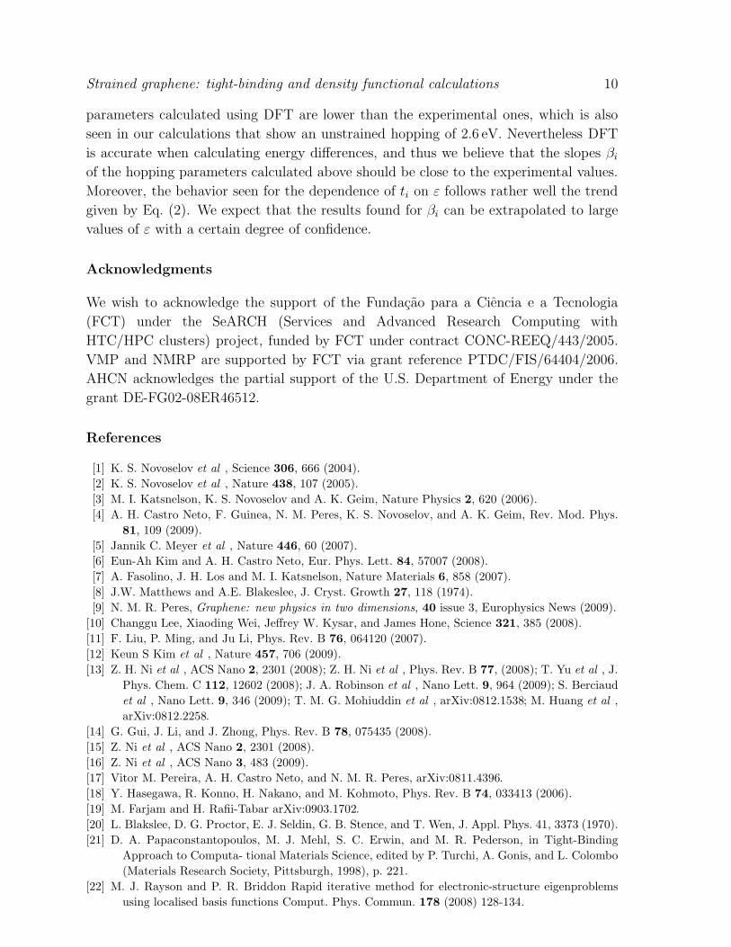
parameters calculated using DFT are lower than the experimental ones, which is also

seen in our calculations that show an unstrained hopping of 2.6 eV. Nevertheless DFT

is accurate when calculating energy differences, and thus we believe that the slopes βi

of the hopping parameters calculated above should be close to the experimental values.

Moreover, the behavior seen for the dependence of ti on ε follows rather well the trend

given by Eq. (2). We expect that the results found for βi can be extrapolated to large

values of ε with a certain degree of confidence.

Acknowledgments

We wish to acknowledge the support of the Fundacao para a Ciencia e a Tecnologia

(FCT) under the SeARCH (Services and Advanced Research Computing with

HTC/HPC clusters) project, funded by FCT under contract CONC-REEQ/443/2005.

VMP and NMRP are supported by FCT via grant reference PTDC/FIS/64404/2006.

AHCN acknowledges the partial support of the U.S. Department of Energy under the

grant DE-FG02-08ER46512.

References

[1] K. S. Novoselov et al , Science 306, 666 (2004).

[2] K. S. Novoselov et al , Nature 438, 107 (2005).

[3] M. I. Katsnelson, K. S. Novoselov and A. K. Geim, Nature Physics 2, 620 (2006).

[4] A. H. Castro Neto, F. Guinea, N. M. Peres, K. S. Novoselov, and A. K. Geim, Rev. Mod. Phys.

81, 109 (2009).

[5] Jannik C. Meyer et al , Nature 446, 60 (2007).

[6] Eun-Ah Kim and A. H. Castro Neto, Eur. Phys. Lett. 84, 57007 (2008).

[7] A. Fasolino, J. H. Los and M. I. Katsnelson, Nature Materials 6, 858 (2007).

[8] J.W. Matthews and A.E. Blakeslee, J. Cryst. Growth 27, 118 (1974).

[9] N. M. R. Peres, Graphene: new physics in two dimensions, 40 issue 3, Europhysics News (2009).

[10] Changgu Lee, Xiaoding Wei, Jeffrey W. Kysar, and James Hone, Science 321, 385 (2008).

[11] F. Liu, P. Ming, and Ju Li, Phys. Rev. B 76, 064120 (2007).

[12] Keun S Kim et al , Nature 457, 706 (2009).

[13] Z. H. Ni et al , ACS Nano 2, 2301 (2008); Z. H. Ni et al , Phys. Rev. B 77, (2008); T. Yu et al , J.

Phys. Chem. C 112, 12602 (2008); J. A. Robinson et al , Nano Lett. 9, 964 (2009); S. Berciaud

et al , Nano Lett. 9, 346 (2009); T. M. G. Mohiuddin et al , arXiv:0812.1538; M. Huang et al ,

arXiv:0812.2258.

[14] G. Gui, J. Li, and J. Zhong, Phys. Rev. B 78, 075435 (2008).

[15] Z. Ni et al , ACS Nano 2, 2301 (2008).

[16] Z. Ni et al , ACS Nano 3, 483 (2009).

[17] Vitor M. Pereira, A. H. Castro Neto, and N. M. R. Peres, arXiv:0811.4396.

[18] Y. Hasegawa, R. Konno, H. Nakano, and M. Kohmoto, Phys. Rev. B 74, 033413 (2006).

[19] M. Farjam and H. Rafii-Tabar arXiv:0903.1702.

[20] L. Blakslee, D. G. Proctor, E. J. Seldin, G. B. Stence, and T. Wen, J. Appl. Phys. 41, 3373 (1970).

[21] D. A. Papaconstantopoulos, M. J. Mehl, S. C. Erwin, and M. R. Pederson, in Tight-Binding

Approach to Computa- tional Materials Science, edited by P. Turchi, A. Gonis, and L. Colombo

(Materials Research Society, Pittsburgh, 1998), p. 221.

[22] M. J. Rayson and P. R. Briddon Rapid iterative method for electronic-structure eigenproblems

using localised basis functions Comput. Phys. Commun. 178 (2008) 128-134.

http://arxiv.org/abs/0812.1538





[23] H. J. Monkhorstand J. D. Pack, Phys. Rev. B 13, 5188 (1976).

[24] C. Hartwigsen, S. Goedecker, and J. Hutter, Phys. Rev. B 58, 3641(1998).

[25] S. Reich, J. Maultzsch, C. Thomsen, and P. Ordejon, Phys. Rev. B 66, 035412 (2002).

[26] F. Liu, P. Ming, and J. Li, Phys. Rev. B 76, 064120 (2007)

Strained graphene: tight-binding and density functional calculations

Documents

Transcript of Strained graphene: tight-binding and density functional calculations