Stochastic Power Control for Time-Varying Long-Term Fading Wireless Networks

Hindawi Publishing CorporationEURASIP Journal on Applied Signal ProcessingVolume 2006, Article ID 89864, Pages 1–13DOI 10.1155/ASP/2006/89864

Stochastic Power Control for Time-Varying Long-Term FadingWireless Networks

Mohammed M. Olama,1 Seddik M. Djouadi,1 and Charalambos D. Charalambous2

1 Department of Electrical and Computer Engineering, University of Tennessee, Knoxville, TN 37996, USA2 Department of Electrical and Computer Engineering, University of Cyprus, 1678 Nicosia, Cyprus

Received 1 June 2005; Revised 4 March 2006; Accepted 7 April 2006

A new time-varying (TV) long-term fading (LTF) channel model which captures both the space and time variations of wirelesssystems is developed. The proposed TV LTF model is based on a stochastic differential equation driven by Brownian motion. Thismodel is more realistic than the static models usually encountered in the literature. It allows viewing the wireless channel as adynamical system, thus enabling well-developed tools of adaptive and nonadaptive estimation and identification techniques to beapplied to this class of problems. In contrast with the traditional models, the statistics of the proposed model are shown to be TV,but converge in steady state to their static counterparts. Moreover, optimal power control algorithms (PCAs) based on the newmodel are proposed. A centralized PCA is shown to reduce to a simple linear programming problem if predictable power controlstrategies (PPCS) are used. In addition, an iterative distributed stochastic PCA is used to solve for the optimization problem usingstochastic approximations. The latter solely requires each mobile to know its received signal-to-interference ratio. Generalizationsof the power control problem based on convex optimization techniques are provided if PPCS are not assumed. Numerical resultsshow that there are potentially large gains to be achieved by using TV stochastic models, and the distributed stochastic PCAprovides better power stability and consumption than the distributed deterministic PCA.

Copyright © 2006 Mohammed M. Olama et al. This is an open access article distributed under the Creative Commons AttributionLicense, which permits unrestricted use, distribution, and reproduction in any medium, provided the original work is properlycited.

1. INTRODUCTION

Power control (PC) is important to improve the perfor-mance of wireless communication systems. The benefits ofpower minimization are not just increased battery life, butalso increased overall network capacity. Users only need toexpand sufficient power for acceptable reception, as deter-mined by their quality of service (QoS) specifications, thatis usually characterized by the signal-to-interference ratio(SIR) [1]. The majority of research papers in this field usetime-invariant (static) models for the wireless channels. Intime-invariant models, channel parameters are random butdo not depend on time, and remain constant throughout theobservation and estimation phase. This contrasts with time-varying (TV) models, where the channel dynamics becomeTV stochastic processes [2–6]. TV models take into accountthe relative motion between transmitters and receivers andtemporal variations of the propagating environment such asmoving scatterers [1].

Radio channels experience both long-term fading (LTF)and short-term fading (STF). LTF is modelled by lognor-mal distributions and STF is modelled by Rayleigh or Ricean

distributions [7]. In general, LTF and STF are consideredsuperimposed and may be treated separately [7, 8]. In thispaper, we consider dynamical modeling and power controlfor LTF channels that predominate in suburban areas. TheSTF case has been considered in [2]. In particular, we de-velop a TV model based on a stochastic differential equa-tion (SDE) driven by Brownian motion for LTF channels.The proposed SDE model is a generalization of the standardlognormal model. In particular, it is shown that the statis-tics of the SDE model are TV and converge in steady state totheir static lognormal counterparts. The proposed model ex-hibits more realistic behaviors of wireless channels than thecurrent LTF models. It allows viewing the wireless channelas a dynamical system that shows how the channel evolves intime and space. In addition, it allows well-developed tools ofadaptive and nonadaptive estimation and identification (toestimate the model parameters) to be applied to this class ofproblems [9–11]. Finally, based on the proposed TV model,centralized and iterative distributed PCAs are developed.

Power control algorithms (PCAs) can be classified ascentralized and distributed. The centralized PCAs requireglobal out-of-cell information available at base stations. The

2 EURASIP Journal on Applied Signal Processing

distributed PCAs require base stations to know only in-cellinformation, which can be easily obtained by local measure-ments. The power allocation problem has been studied ex-tensively as an eigenvalue problem for nonnegative matrices[12, 13], resulting in iterative PCAs that converge each user’spower to the minimum power [14–17], and as optimization-based approaches [18]. Much of these previous works dealwith static time-invariant channel models. The scheme is in-troduced in [18], whereby the statistics of the received SIRare used to allocate power, rather than an instantaneous SIR.Therefore, the allocation decisions can be made on a muchslower time scale. Previous attempts at capacity determina-tions in CDMA systems have been based on a “load balanc-ing” view of the PC problem [19]. This reflects an essentiallystatic or at best quasistatic view of the PC problem, whichlargely ignores the dynamics of channel fading as well as usermobility.

Stochastic PCAs (SPCAs) that use noisy interference es-timates have been introduced in [20], where conventionalmatched filter receivers are used. There, it is shown that theiterative stochastic PCA, which uses stochastic approxima-tions, converges to the optimal power vector under certainassumptions on the stepsize sequence. These results werelater extended to the cases where a nonlinear receiver or adecision feedback receiver is used [21]. However, the chan-nel gains are assumed to be fixed ignoring the effects of time-variations on the performance of the system. In this paper,the proposed distributed stochastic PCA is different fromthose in [20–22] in that these algorithms are based on theassumption that two parameters are assumed to be knownat each transmitter, namely, the received matched filter out-put (received SIR) at its intended receiver and the channelgain between the transmitter and its intended receiver. In theproposed algorithm, only the received SIR at its intended re-ceiver is required.

Other results that attempt to recognize the time-correlat-ed nature of signals are proposed in [23], where blocking isdefined via the sojourn time of global interference above agiven level. Downlink PC for fading channels is studied in[24] by a heavy traffic limit where averaging methods areused. Stochastic control approach for uplink lognormal fad-ing channels is studied in [25], in which a bounded ratepower adjustment model is proposed. Recent work on dy-namic PC with stochastic channel variation can be found in[26–28]. However, in our proposed approach, the modelingand analysis of PC strategies investigated here employ wire-less models which are TV and subject to fading.

Two different PCAs are proposed. The first one is cen-tralized and based on predictable power control strategies(PPCS) that were first introduced in [2]. PPCS simply meanupdating the transmitted powers at discrete times and main-taining them fixed until the next power update begins. ThePPCS algorithm is proven to be effectively applicable to suchdynamical models for an optimal PC. The outage probability(OP) is used as a performance measure. A distributed versionof this algorithm is derived along the lines of [15–17]. Thelatter helps in allowing autonomous execution at the nodeor link level, requiring minimal usage of network communi-

cation resources for control signaling. The second one is aniterative and distributed SPCA based on stochastic approx-imations. It requires less information than the SPCAs pro-posed in [20–22]. Numerical results are provided to evaluatethe performance of the proposed PCAs. Since few temporalor even spatiotemporal dynamical models have so far beeninvestigated with the application of any PCA, the suggesteddynamical models and PCAs will thus provide a far more re-alistic and efficient optimum control of wireless channels.

The paper is organized as follows. In Section 2, a TV LTFchannel model in which the evolution of the channel is de-scribed by an SDE is introduced. In Section 3, several PCAsare discussed. In Section 3.1, a centralized deterministic PCAis proposed in which the solution is obtained through linearprogramming using PPCS, and then an iterative version isintroduced to simplify the implementation of the proposedPCA. A distributed SPCA is proposed in Section 3.2. Moregeneral PC cases are presented in Section 3.3. In Section 4,numerical results are presented. Finally, Section 5 providesthe conclusion.

2. TIME-VARYING LOGNORMAL FADINGCHANNEL MODEL

Wireless communication networks are subject to time-spread (multipath), Doppler spread (time variations), pathloss, and interference seriously degrading their performance.In addition to the exponential power path loss, wireless chan-nels suffer from stochastic STF due to multipath, and LTFdue to shadowing depending on the geographical area. If amobile happens to be in some less populated area with fewbuildings, vehicles, mountains, and so forth, its signal under-goes LTF (lognormal shadowing) [7], which must be com-pensated in any design. Before introducing the dynamicalTV LTF channel model that captures both space and timevariations, we first summarize and interpret the traditionallognormal shadowing model, which serves as a basis in thedevelopment of the subsequent TV model. The traditional(time-invariant) power loss (PL) in dB for a given path isgiven by [7]

PL(d)[dB] := PL(d0)[dB] + 10α log

(d

d0

)+ Z, d ≥ d0,

(1)

where PL(d0) is the average PL in dB at a reference distanced0 from the transmitter, the distance d corresponds to thetransmitter-receiver separation distance, α is the path loss ex-ponent which depends on the propagating medium, and Zis a zero-mean Gaussian distributed random variable, whichrepresents the variability of PL due to numerous reflectionsand possibly any other uncertainty of the propagating envi-ronment from one observation instant to the next. The aver-age value of the PL described in (1) is

PL(d)[dB] := PL(d0)[dB] + 10α log

(d

d0

), d ≥ d0. (2)

In the traditional models the statistics of the PL do notdepend on time t, therefore these models treat PL as static

Mohammed M. Olama et al. 3

(time invariant). They do not take into consideration therelative motion between the transmitter and the receiver, orvariations of the propagating environment due to mobility,appearance, and disappearance of various scatters along theway from one instant to the next. Such spatial and time vari-ations of the propagating environment are captured hereinby modeling the PL and the envelop of the received signalas random processes that are functions of space and time.Moreover, and perhaps more importantly, traditional modelsdo not take into consideration the correlation properties ofthe PL in space and at different observation times. In reality,such correlation properties exist, and one way to model themis through stochastic processes, which obey specific type ofstochastic differential equations (SDEs).

In transforming the static model to a dynamical model,the random PL in (1) is relaxed to become a random process,denoted by {X(t, τ)}t≥0, τ≥τ0 , which is a function of both timet and space represented by the time delay τ, where τ = d/c,d is the path length, c is the speed of light, τ0 = d0/c, andd0 is the reference distance. The signal attenuation is definedby S(t, τ) � ekX(t,τ), where k = − ln(10)/20. For simplic-ity, we first introduce the TV lognormal model for a fixedtransmitter-receiver separation distance d (or τ) that cap-tures the temporal variations of the propagating environ-ment. After that we generalize it by allowing both t and τto vary, as the transmitter and receiver, as well as scatters, areallowed to move at variable speeds. This induces spatiotem-poral variations in the propagating environment.

When τ is fixed, the proposed model captures the depen-dence of {X(t, τ)}t≥0, τ≥τ0 on time t. This corresponds to ex-amining the time-variations of the propagating environmentfor fixed transmitter-receiver separation distance. The pro-cess {X(t, τ)}t≥0, τ≥τ0 represents how much power the signallooses at a particular location as a function of time. However,since for a fixed distance d, the PL should be a function ofdistance, we choose to generate {X(t, τ)}t≥0, τ≥τ0 by a mean-1reverting version of a general linear SDE given by [3]

dX(t, τ) = β(t, τ)(

( γ(t, τ)− X(t, τ))dt + δ(t, τ)dW(t),

X(t0, τ

) = N(PL(d)[dB]; σ2

t0

),

(3)

where {W(t)}t≥0 is the standard Brownian motion (zerodrift, unit variance) which is assumed to be independent ofX(t0, τ), N(μ; κ) denotes a Gaussian random variable withmean μ and variance κ, and PL(d)[dB] is the average pathloss in dB. The parameter γ(t, τ) models the average time-varying PL at distance d from the transmitter, which corre-sponds to PL(d)[dB] at d indexed by t. This model tracks andconverges to this value as time progresses. The instantaneousdrift β(t, τ)(γ(t, τ)− X(t, τ)) represents the effect of pullingthe process towards γ(t, τ), while β(t, τ) represents the speedof adjustment towards this value. Finally, δ(t, τ) controls theinstantaneous variance or volatility of the process for the in-stantaneous drift. The initial condition of X(t, τ) can be ob-tained from a geometric Brownian motion model which cal-culates X(t0, τ) for a fixed t = t0 as a function of τ.

Let {θ(t, τ)}t≥0 � {β(t, τ), γ(t, τ), δ(t, τ)}t≥0. If the ran-dom processes in {θ(t, τ)}t≥0 are measurable and bounded,then (3) has a unique solution for every X(t0, τ) given by [4]

X(t, τ) = e−β([t,t0],τ)(X(t0, τ

)+∫ t

t0eβ([u,t0],τ)(β(u, τ)γ(u, τ)du

+ δ(u, τ)dW(u)))

,

(4)

where β([t, t0], τ) �∫ tt0 β(u, τ)du. Moreover, using Ito’s

stochastic differential rule on S(t, τ) = ek X(t,τ) the attenua-tion coefficient obeys the following SDE:

dS(t, τ) = S(t, τ)[(

kβ(t, τ)[γ(t, τ)− 1

kln S(t, τ)

]

+12k2δ2(t, τ)

)dt + kδ(t, τ)dW(t)

],

S(t0, τ

) = ekX(t0,τ).(5)

This model captures the temporal variations of the prop-agating environment as the random parameters {θ(t, τ)}t≥0

can be used to model the TV characteristics of the channelfor the particular location τ. A different location is charac-terized by a different set of parameters {θ(t, τ)}.

Now, let us consider the special case when the parametersθ(t, τ) = θ(τ) � {β(τ), γ(τ), δ(τ)} are time-invariant. In thiscase we need to show that the expected value of the dynamicPLX(t, τ), denoted by E[X(t, τ)], converges to the traditionalaverage PL in (2). In this case, the solution of the SDE (3) isgiven by

X(t, τ) = e−β(τ)(t−t0)(

X(t0, τ

)+ γ(τ)

(eβ(τ)(t−t0) − 1

)

+ δ(τ)∫ t

t0eβ(τ)(u−t0)dW(u)

),

(6)

where for a given set of time-invariant parameters θ(τ) andif the initial X(t0, τ) is Gaussian or fixed, the distribution ofX(t, τ) is Gaussian with mean and variance given by

E[X(t, τ)

]=e−β(τ)(t−t0)(E[X(t0, τ

)]+γ(τ)

(eβ(τ)(t−t0)−1

)),

Var[X(t, τ)

] = δ(τ)2(

1− e−2β(τ)(t−t0)

2β(τ)

)

+ e−2β(τ)(t−t0) Var(X(t0, τ

)).

(7)

Expression (7) of the mean and variance shows that thestatistics of the communication channel vary as a function ofboth time t and space τ. As the observation instant t becomeslarge, the random process {X(t, τ)} converges to a Gaussianrandom variable with mean γ(τ) = PL(d)[dB] and varianceδ(τ)2/2β(τ). Therefore, the traditional lognormal model (1)is a special case of the general TV LTF model (3). Moreover,the distribution of S(t, τ) = ekX(t,τ) is lognormal with mean


90

80

70

60

50

4020

x(t)

(dB

)

1510

50

Distance (m) 01

23

�10�4

γ(t, τ)

X(t, τ)

Time (s)

Figure 1: Mean-reverting power path loss as a function of t and τ,for the time-varying γ(t, τ) in Example 1.

and variance given by

E[S(t, τ)

] = exp

(2kE

[X(t, τ)

]+ k2 Var

[X(t, τ)

]

2

)

,

Var[S(t, τ)

] = exp(

2kE[X(t, τ)

]+ 2k2 Var

[X(t, τ)

])

− exp(

2kE[X(t, τ)

]+ k2 Var

[X(t, τ)

]).

(8)

Now, let us go back to the more general case in which{θ(t, τ)}t≥0 � {β(t, τ), γ(t, τ), δ(t, τ)}t≥0. At a particular lo-cation τ, the mean of the PL process E[X(t, τ)] is required totrack the time variations of the average PL. This can be seenin the following example.

Example 1. Let

γ(t, τ) = γm(τ)(

1 + 0.15e−2t/T sin(

10πtT

)), (9)

where γm(τ) is the average PL at a specific location τ, T isthe observation interval, δ(t, τ)= 1400, and β(t, τ)= 225000(these parameters are determined from experimental mea-surements as will be shown at the end of this section), wherefor simplicity δ(t, τ) and β(t, τ) are chosen to be constant,but in general they are functions of both t and τ. The vari-ations of X(t, τ) as a function of distance and time are rep-resented in Figure 1. The temporal variations of the environ-ment are captured by a TV γ(t, τ) which fluctuates arounddifferent average PLs γ′ms, so that each curve correspondsto a different location. It is noticed in Figure 1 that as timeprogresses, the process X(t, τ) is pulled towards γ(t, τ). Thespeed of adjustment towards γ(t, τ) can be controlled bychoosing different values of β(t, τ).

Next, the general spatiotemporal lognormal model is in-troduced by generalizing the previous model to capture both

Rx Txd

θ

��υ

d(t)

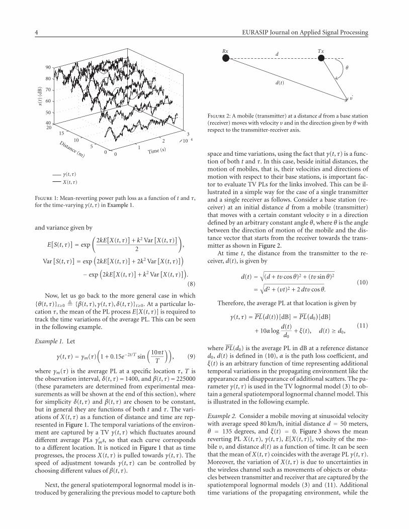
Figure 2: A mobile (transmitter) at a distance d from a base station(receiver) moves with velocity υ and in the direction given by θ withrespect to the transmitter-receiver axis.

space and time variations, using the fact that γ(t, τ) is a func-tion of both t and τ. In this case, beside initial distances, themotion of mobiles, that is, their velocities and directions ofmotion with respect to their base stations, is important fac-tor to evaluate TV PLs for the links involved. This can be il-lustrated in a simple way for the case of a single transmitterand a single receiver as follows. Consider a base station (re-ceiver) at an initial distance d from a mobile (transmitter)that moves with a certain constant velocity υ in a directiondefined by an arbitrary constant angle θ, where θ is the anglebetween the direction of motion of the mobile and the dis-tance vector that starts from the receiver towards the trans-mitter as shown in Figure 2.

At time t, the distance from the transmitter to the re-ceiver, d(t), is given by

d(t) =√

(d + tυ cos θ)2 + (tυ sin θ)2

=√d2 + (υt)2 + 2dtυ cos θ.

(10)

Therefore, the average PL at that location is given by

γ(t, τ) = PL(d(t)

)[dB] = PL

(d0)[dB]

+ 10α logd(t)d0

+ ξ(t), d(t) ≥ d0,(11)

where PL(d0) is the average PL in dB at a reference distanced0, d(t) is defined in (10), α is the path loss coefficient, andξ(t) is an arbitrary function of time representing additionaltemporal variations in the propagating environment like theappearance and disappearance of additional scatters. The pa-rameter γ(t, τ) is used in the TV lognormal model (3) to ob-tain a general spatiotemporal lognormal channel model. Thisis illustrated in the following example.

Example 2. Consider a mobile moving at sinusoidal velocitywith average speed 80 km/h, initial distance d = 50 meters,θ = 135 degrees, and ξ(t) = 0. Figure 3 shows the meanreverting PL X(t, τ), γ(t, τ), E[X(t, τ)], velocity of the mo-bile υ, and distance d(t) as a function of time. It can be seenthat the mean of X(t, τ) coincides with the average PL γ(t, τ).Moreover, the variation of X(t, τ) is due to uncertainties inthe wireless channel such as movements of objects or obsta-cles between transmitter and receiver that are captured by thespatiotemporal lognormal models (3) and (11). Additionaltime variations of the propagating environment, while the


95

90

85

80

75X(t

,τ)

�

E(t

,τ)

(dB

)

0 1 2 3 4 5 6

Time (s)

X(t, τ) as a function of t

γ(t, τ)

E[X(t, τ)]X(t, τ)

80

60

40

20

0d(t

)(m

),v(t)

(m/s

)

0 1 2 3 4 5 6

Time (s)

Variable speed v(t) and distance d(t)

d(t)v(t)

Figure 3: Mean-reverting power path loss X(t, τ) for the TV LTFwireless channel model in Example 2.

mobile is moving, can be captured by using the TV PL co-efficient α(t) in (1) in addition to the TV parameters β(t, τ)and δ(t, τ), or simply by ξ(t).

Before we finish this section, we want to show that thespatial correlation of the lognormal mean-reverting modelof (3) agrees with the experimental spatial correlation [29–31]. In particular, it is reported that the spatial correlation forshadow fading in mobile communications, which comparessuccessfully with experimental data, can be modeled using anexponentially decreasing function multiplied by the varianceof the PL process as follows:

CovX(Δt) � σ2X e

−Δd/Xc = σ2Xe−(v/Xc)Δt, (12)

where σ2X is the covariance of the PL process, Δd is the dis-

tance between two consecutive samples, and v is the velocityof the mobile. Xc is the effective correlation distance which isproportional to the density of the propagating environmentcorresponding to the distance when the normalized corre-lation falls to e−1 [31]. To show that our spatial dynami-cal model captures these correlation properties, consider thespace-time mean-reverting lognormal model in (3). With-out loss of generality, consider the particular case where theparameters {θ(t, τ)}t≥0 = {β(τ), γ(t, τ), δ(τ)}t≥0. Let X(t, τ)� X(t, τ)−E[X(t, τ)], then we have the mobile starts movingcloser to the base station from point 50 meters with an an-gle of 135 degrees and sinusoidal speed with average 80 km/h

(22.2 m/s):

dX(t, τ) = −β(τ)X(t, τ)dt + δ(τ)dW(t),

X(t0, τ

) = N(0; σ2

t0

).

(13)

The solution of (13) is given by

X(t, τ) = e−β(τ)(t−t0)(X(t0, τ

)+∫ t

t0eβ(τ)(u−t0)δ(τ)dW(u)

).

(14)

The mean of the process X(t, τ) is zero, and its covarianceis given by

CovX(t, v)=e−β(τ)(t+v)e2β(τ)t0

[σ2t0 +

δ2(τ)2β(τ)

(e2β(τ)(t∧v−t0) − 1

)],

(15)

where t ∧ v � min(t, v). Letting v = t + Δt, then

CovX(t, t + Δt)

= e−2β(τ)(t−t0)−β(τ)Δt[σ2t0 +

δ2(τ)2β(τ)

(e2β(τ)(t−t0) − 1

)].

(16)

The covariance of the overall dynamical model indicateswhat proportion of the environment remains constant fromone observation instant or location to the next, separatedby the sampling interval. Since the mobile is in motion, itimplies that this corresponds to a spatial covariance. If wechoose the variance of the initial condition such that σ2

t0 =δ2(τ)/2β(τ), then

CovX(t, t + Δt) = δ2(τ)2β(τ)

e−β(τ)Δt = σ2t0e−β(τ)Δt � CovX(Δt).

(17)

Expression (17) indicates that the spatial covariance ofour overall dynamical model corresponds to the reportedexperimental spatial covariance given by (12). The compar-ison further indicates that β(τ) is a characteristic of boththe propagating environment and the separation distance oftwo consecutive samples, that is, β(τ) is inversely propor-tional to the density of the propagating environment, and di-rectly proportional to the sample separation distance. Notethat the spatial covariance is an important characteristic forour dynamical mean-reverting shadow fading model sinceit can be clearly used in order to identify the random pa-rameters {β(τ), δ(τ)}. This could be accomplished by us-ing experimental data of CovX(Δt). Therefore, the parame-ters {β(τ), δ(τ)} can be estimated on-line from experimentalmeasurements. Finally, we note that the variance of the ini-tial condition of the PL process σ2

t0 should inevitably increasewith distance, or equivalently δ(τ) should increase and/orβ(τ) decrease.

Subsequently, we consider the uplink channel of a cel-lular network. We assume that users are already assigned totheir base stations and therefore we do not consider the base


station assignment case. Let M be the number of mobiles(users), and N the number of base stations. The received sig-nal of the ith mobile at its assigned base station at time t canbe expressed as

yi(t) =M∑

j=1

√pj(t)s j(t)Si j(t) + ni(t), (18)

where pj(t) is the transmitted power of mobile j at time t,which acts as a scaling on the information signal s j(t), ni(t)is the channel disturbance or noise at the base station of mo-bile i, and Si j(t) is the signal attenuation coefficient betweenmobile j and the base station assigned to mobile i. Therefore,in a cellular network the spatiotemporal model described in(3) for M mobiles and N base stations can be described as

dXij(t, τ)=βi j(t, τ)(γi j(t, τ)− Xij(t, τ)

)dt+ δi j(t, τ)dWij(t),

Xij(t0, τ

) = N(PL(d)[dB]i j ; σ2

t0

), 1 ≤ i, j ≤M,

(19)

and the signal attenuation coefficients Si j(t) are generatedusing the relation Si j(t, τ) = ekXij (t,τ), where k = − ln(10)/20.Moreover, correlation between the channels in a multiuser/multiantenna model can be induced by letting the dif-ferent Brownian motions Wij ’s to be correlated, that is,

E[W(t)W(t)T] = Q(τ) · t, where W(t) � (Wij(t)), and Q(τ)is some (not necessarily diagonal) matrix that is a functionof τ and dies out as τ becomes large.

The TV LTF channel models in (19) are used to generatethe link gains for the proposed PCAs introduced in the nextsection.

3. POWER CONTROL ALGORITHMS

In this section, different PCAs are introduced based on theTV lognormal channel model derived in the previous sec-tion. A deterministic PCA (DPCA) is introduced first, andthen a stochastic PCA (SPCA) is presented. Both centralizedand distributed PCAs are considered.

3.1. Deterministic power control schemes

The aim of the PCAs described here is to minimize the totaltransmitted power of all users while maintaining acceptablequality of service (QoS) for each user. The measure of QoScan be defined by the signal-to-interference ratio (SIR) foreach link to be larger than a target SIR. Consider a cellularnetwork as described above, then the centralized PC problemfor time-invariant channels can be stated as [2]

min(p1≥0,...,pM≥0)

M∑

i=1

pi subject topigii

∑Mj �=i p jgi j + ηi

≥ εi,

1 ≤ i ≤M,

(20)

where pi is the power of mobile i, gi j > 0 is the time-invariantchannel gain between mobile j and the base station assignedto mobile i, εi > 0 is the target SIR of mobile i, and ηi > 0is the noise power level at the base station of mobile i. Theconstraint in (20) for the TV lognormal channel models de-scribed using path-wise QoS of each user over a time interval[0,T] is given by

∫ T0 pi(t)s2

j (t)S2ii(t)dt

∑Mj �=i∫ T

0 pj(t)s2j (t)S

2i j(t)dt +

∫ T0 n2

i (t)dt≥ εi, i = 1, . . . ,M.

(21)

Consequently, a natural generalization of the PC problemin (20) with respect to the TV lognormal models in (19) canbe written as

min(p1≥0,...,pM≥0)

{ M∑

i=1

∫ T

0pi(t)dt

}

, subject to

M∑

j �=i

∫ T

0pj(t)s2

j (t)S2i j(t)dt −

1εi

∫ T

0pi(t)s2

i (t)S2ii(t)dt

+∫ T

0n2i (t)dt ≤ 0, i = 1, . . . ,M.

(22)

A solution to (22) is presented by first introducingthe communication meaning of predictable power controlstrategies (PPCS). In wireless cellular networks, it is prac-tical to observe and estimate channels at base stations andthen send the information back to the mobiles to adjusttheir power signals {pi(t)}Mi=1. Since channels experience de-lays, and power control is not feasible continuously in timebut only at discrete time instants, the concept of predictablestrategies is introduced [2]. Consider a set of discrete timestrategies {pi(tk)}Mi=1, where 0 = t0 < t1 < · · · < tk < tk+1 <· · · ≤ T . At time tk−1, the base stations observe or estimatethe channel information {Si j(tk−1), si(tk−1)}Mi, j=1. Using theconcept of predictable strategy, the base stations determinethe control strategy {pi(tk)}Mi=1 for the next time instant tk.The latter is communicated back to the mobiles, which holdthese values during the time interval [tk−1, tk). At time tk,a new set of channel information {Si j(tk), si(tk)}Mi, j=1 is ob-served at the base stations and the time tk+1 control strate-gies {pi(tk+1)}Mi=1 are computed and communicated backto the mobiles which hold them constant during the timeinterval [tk, tk+1). Such decision strategies are called pre-dictable. More specifically, we say that a discrete time signal{ϕ(k); k = 0, 1, . . .} is predictable with respect to a filtration{Zk} if ϕ(k) is Zk−1 measurable. Using the concept of PPCSover any time interval [tktk+1], (22) is equivalent to

minp(tk+1)>0

M∑

i=1

pi(tk+1

), subject to p

(tk+1

)

≥ ΓG−1I

(tk, tk+1

)× (G(tk, tk+1

)p(tk+1

)+ η

(tk+1

)),

(23)


where

gi j(tk, tk+1

):=∫ tk+1

tks2j (t)S

2i j(t)dt,

ηi(tk, tk+1

):=∫ tk+1

tkn2i (t)dt, 1 ≤ i, j ≤M,

GI(tk, tk+1

) = diag(g11(tk, tk+1

), . . . , gMM

(tk, tk+1

)),

G(tk, tk+1

) =⎧⎨

⎩

0 if i = j,

gi j(tk, tk+1

)if i �= j,

j(tk, tk+1

) = (η1(tk, tk+1

), . . . ,ηM

(tk, tk+1

))tr,

p(tk+1

) = (p1(tk+1

), . . . , pM

(tk+1

))tr,

Γ = diag(ε1, . . . , εM

),

(24)

diag(·) denotes a diagonal matrix with its argument as diag-onal entries, and “tr” stands for matrix or vector transpose.The optimization in (23) is a linear programming problemin M × 1 vector of unknowns p(tk+1). Here [tk, tk+1] is a timeinterval such that the channel model does not change signifi-cantly, that is, [tk, tk+1] should be smaller than the coherencetime of the channel.

Next, we consider an iterative distributed version of thecentralized PCA in (23). This is convenient for on-line imple-mentation since it helps autonomous execution at the nodeor link level, requiring minimal usage of network commu-nication resources for control signaling. The iterative dis-tributed PCA proposed in [15–17] can be used to find a dis-tributed version to the centralized PCA in (23). The con-straint in (23) can be rewritten as

(I−ΓG−1

I

(tk, tk+1

)G(tk, tk+1

))p(tk+1

)

≥ΓG−1I

(tk, tk+1

)η(tk+1

).

(25)

Defining F(tk, tk+1)�ΓG−1I (tk, tk+1)G(tk, tk+1) and u(tk,

tk+1)Δ= ΓG−1

I (tk, tk+1)η(tk+1), then (25) can be rewritten as

(I− F

(tk, tk+1

))p(tk+1

) ≥ u(tk, tk+1

). (26)

If channel gains are time invariant, that is, F(tk, tk+1) = Fand u(tk, tk+1) = u, then the power control problem is fea-sible if ρF < 1, where ρF is the Perron-Frobenius eigenvalueof F [15]. It is shown in [15–17] that the following iterativePCA converges to the minimal power vector when ρF < 1:

p(tk+1

) = Fp(tk)

+ u. (27)

However, our channel gains are time varying, thus a“time-varying version” of the deterministic PCA (DPCA) in(27) can be defined as

p(tk+1

) = F(tk, tk+1

)p(tk)

+ u(tk, tk+1

). (28)

Clearly, in general the power vector p(tk) will not con-verge to some deterministic constant as it does in (27). Rath-er, in a time-varying (random) propagation environment, it

is required that the power vector p(tk) converges in distri-bution to a well-defined random variable. Since F(tk, tk+1) isa random matrix-valued process, the key convergence con-dition is the Lyapunov exponent λF < 0 [32], where λF isdefined as

λF = limk→∞

1k

log∥∥F(t0, t1

)F(t1, t2

) · · ·F(tk, tk+1

)∥∥. (29)

Throughout this section, we assume that the PC problemis feasible, that is, there exists a power vector p(tk) that sat-isfies the inequality in (23) for all tk. The distributed versionof (28) can be written as

pi(tk+1

) = εi(tk)

Ri(tk) pi

(tk), i = 1, . . . ,M, (30)

where Ri(tk) is instantaneous SIR defined by

Ri(tk)= pi

(tk)gii(tk, tk+1

)

∑Mj �=i p j

(tk)gi j(tk, tk+1

)+ ηi

(tk, tk+1

) , i = 1, . . . ,M.

(31)

It is shown in [22] that the performance of the DPCA in(30) in terms of power consumption is not optimal when thechannel environment is time varying (random). Actually, theperformance can be severely degraded when PCAs that aredesigned for deterministic channels are applied to TV chan-nels [22]. Therefore, stochastic PCAs (SPCAs) must be usedin order to ensure stable optimal power consumption. Thelatter is introduced in the following section.

3.2. Stochastic power control schemes

A distributed SPCA similar to the one described in [20] isused in this section, where the transmit powers are updatedbased on stochastic approximations. Let us define the instan-taneous interference at time tk by

Ii(tk) =

M∑

j �=ipi(tk)gi j(tk, tk+1

)+ ηi

(tk, tk+1

), i = 1, . . . ,M,

(32)

then the SPCA proposed in [20], which uses the concept ofinterference averaging as introduced in [33], can be used toupdate the transmitted power recursively as

pi(tk+1

) = (1− a(tk))pi(tk)

+ a(tk) εi

(tk)

gii(tk, tk+1

)[Ii(tk)]

, i = 1, . . . ,M,(33)

where a(tk) is the stepsize at time tk, which satisfies certainconditions as explained later. Substituting (32) into (33) and


using (31) yield

pi(tk+1

) = (1− a(tk))pi(tk)

+ a(tk) εi(tk)

Ri(tk) pi

(tk), i = 1, . . . ,M.

(34)

If the PC problem in (22) is feasible, the distributedSPCA in (34) converges to the optimal power vector whenthe stepsize sequence satisfies certain conditions. Two dif-ferent types of convergence results are shown in [34] underdifferent choices of the stepsize sequence. If the stepsize se-quence satisfies

∑∞k=0 a(tk) = ∞ and

∑∞k=0 a(tk)2 < ∞, then

the SPCA in (34) converges to the optimal power vector withprobability one. However, due to the requirement for theSPCA to track TV environments, the iteration stepsize se-quence is not allowed to decrease to zero. So we considerthe case where the condition

∑∞k=0 a(tk)2 < ∞ is violated.

This includes the situation when the stepsize sequence de-creases slowly to zero, and the situation when the stepsize isfixed at a small constant. In the first case when a(tk) → 0slowly, the SPCA in (34) converges to the optimal power vec-tor in probability. While in the second case the power vec-tor clusters around the optimal power. In fact, the error be-tween the power vector and the optimal value does not van-ish for nonvanishing stepsize sequence; this is the price paidin order to make the algorithm in (34) able to track TV en-vironments. This algorithm is fully distributed in the sensethat each user iteratively updates its power level by estimat-ing the received SIR of its own channel. It does not requireany knowledge of the link gains and state information ofother users. The remaining three parameters of (34): the userpower value in the previous iteration pi(tk

), its SIR target

value εi(tk), and stepsize sequence a(tk), are trivially knownby the user. It is worth mentioning that the proposed dis-tributed SPCA in (34) is different from the algorithm pro-posed in [22] where two parameters, namely, the receivedSIRs Ri(tk) and the channel gains gii(tk, tk+1), are required tobe known. In contrast, here only the received SIRs Ri(tk) arerequired in (34).

The received SIRs Ri(tk) can be estimated at the base sta-tions every L bits, and then transmitted back to the users.Each user keeps its transmitted power level fixed until thefeedback from its base station arrives and then updates itstransmitted power according to (34). This process occursduring the time interval [tk, tk+1] which should be chosensuch that the channel model does not change significantly,that is, [tk, tk+1] should be smaller than the coherence timeof the channel. For small [tk, tk+1], the power control up-dates will be more frequent and thus convergence will befaster. However, frequent transmission of the feedback on thedownlink channel will effectively decrease the capacity of thesystem since more system resources (bandwidth) will have tobe used for power control.

3.3. More generalizations

Without predictable power control strategies, two formu-lations in terms of convex optimization using linear pro-gramming techniques and stochastic control with integral

or exponential-of-integral constraints are introduced in thissection. Moreover, an alternative stochastic power controlformulation that meets outage constraints is also discussed.

The first problem is formulated in terms of convex opti-mization and linear programming as follows:

min(p1≥0,...,pM≥0)

{ M∑

i=1

∫ tk+1

tkpi(t)dt

}, subject to

M∑

j �=i

∫ tk+1

tkp j(t)s2

j (t)S2i j(t)dt −

1εi

∫ tk+1

tkpi(t)s2

i (t)S2ii(t)dt

+∫ tk+1

tkn2i (t)dt ≤ 0, i = 1, . . . ,M.

(35)

According to the above formulation using predictablestrategies, this is a convex optimization problem. In addition,any interval [0, T] can be considered as 0 = t0 < t1 < t2 . . . <tk < tk+1 < . . . ≤ T , and by approximating the integrals byRiemann sums as close as desired, it can be shown that (35)reduces to a linear programming problem again.

The second problem is formulated in terms of stochasticcontrol with integral or exponential-of-integral constraintsas

min(p1≥0,...,pM≥0)

{ M∑

i=1

E∫ T

0pi(t)dt

}, subject to

J i0,T(p)Δ=E

{ M∑

j �=i

∫ T

0pj(t)s2

j (t)S2i j(t)dt−

1εi

∫ T

0pi(t)s2

i (t)S2ii(t)dt

+∫ T

0n2i (t)dt

}

≤ 0, i = 1, . . . ,M.

(36)

If there exists a set of {εi}Mi=1 such that the QoS are feasi-ble, by employing Lagrange multipliers λi for each J i0,T(p) wecan introduce

Lλ(u∗, λ

) = min(p1≥0,...,pM≥0)

×{ M∑

i=1

E

[∫ T

0pi(t)dt

+ λi

[ M∑

j �=i

∫ T

0pj(t)s2

j (t)S2i j(t)dt

− 1εi

∫ T

0pi(t)s2

i (t)S2ii(t)dt

+∫ T

0n2i (t)dt

]]}

(37)

and then solve the problem l (λ∗,u∗) = supλ≥0Lλ (u∗, λ).

Further, it can be shown that Lλ (u∗, λ) satisfies a dynamicprogramming equation of the Hamilton-Jacobi-Bellmantype [35].


Similarly, the QoS can be considered as point-wise con-straints and pursue the problem

min(p1≥0,...,pM≥0)

{ M∑

i=1

E∫ T

0pi(t)dt

}

, subject to

M∑

j �=ip j(t)s2

j (t)S2i j(t)−

1εipi(t)s2

i (t)S2ii(t) + n2

i (t) ≤ 0,

t ∈ [0,T], i = 1, . . . ,M.

(38)

Optimizations (36) and (38) are convex optimizationproblems, since their objective functions and constraints areconvex.

An alternative stochastic power control formulation canbe stated in terms of outage probability (OP). It is definedas the probability that a randomly chosen link fails due toexcessive interference [12]. Therefore, smaller OP implieslarger capacity of the wireless network. A link with a re-ceived SIR Ri, less than or equal to a target SIR εi, is con-sidered a communication failure. The OP O(εi) is expressedas O(εi) = Prob{Ri ≤ εi}. The stochastic PC problem thatmeets outage constraints can be formulated as

min(p1≥0,...,pM≥0)

{ M∑

i=1

∫ T

0pi(t)dt

}, subject to

Pr{(∑

j �= iM∫ T

0pj(t)s2

j (t)S2i j(t)dt

− 1εi

∫ T

0pi(t)s2

i (t)S2ii(t)dt +

∫ T

0n2i (t)dt

)≥ 0

}≤ Oi,

(39)

where t ∈ [0,T], Oi is the target OP of user i, and i =1, . . . ,M. The probabilities in the constraint of (39) are verydifficult to compute. Therefore, Chernoff bounds [36] can beused to evaluate the probability of failure to achieve a desiredQoS requirement as follows:

Pr

{( M∑

j �=i

∫ T

0pj(t)s2

j (t)S2i j(t)dt

− 1εi

∫ T

0pi(t)s2

i (t)S2ii(t)dt +

∫ T

0n2i (t)dt

)

≥ 0

}

≤ E

{

exp

(

ci

( M∑

j �=i

∫ T

0pj(t)s2

j (t)S2i j(t)dt

− 1εi

∫ T

0pi(t)s2

i (t)S2ii(t)dt+

∫ T

0n2i (t)dt

))}

,

(40)

where ci > 0, i = 1, . . . ,M. The Chernoff bound associatedwith (40) subject to (18) and (19) can be computed in [2]using a version of the backward Kolmogorov equation; the

right-hand side of (40) is given by [2]

E

{

exp

(

ci

( M∑

j �=i

∫ T

0pj(t)s2

j (t)S2i j(t)dt

− 1εi

∫ T

0pi(t)s2

i (t)S2ii(t)dt +

∫ T

0n2i (t)dt

))}

= exp

[c2i

2σ2T

]

Vi(0, x),

(41)

where σ2 is the variance of the noise ni(t), and Vi(t, x) is de-fined by

Vi(t, x) � E

{

exp

(

ci

( M∑

j �=i

∫ T

tp j(t)s2

j (t)S2i j(t)dt

− 1εi

∫ T

tpi(t)s2

i (t)S2ii(t)dt

+∫ T

tn2i (t)dt

)

− ci

∫ T

tn2i (t)dt

)∣∣Xij(0)

}

.

(42)

Thus, the Chernoff bound is computed explicitly in (41),and then has to be minimized over ci ≥ 0.

To illustrate the efficiency of the various PCAs proposedin this paper, numerical results are presented in the next sec-tion.

4. NUMERICAL RESULTS

In this section, we provide two numerical examples to deter-mine the performance of the various PCAs under the pro-posed TV LTF channel models. In Example 1, we comparethe performance of the centralized DPCA using PPCS de-scribed in (23) under two different types of TV LTF chan-nel models; the stochastic TV models in (3) and the staticTV models in (1). In the second example, the performanceof the distributed DPCA (30) and the distributed SPCA (34)under the proposed stochastic TV LTF channel models is de-termined.

The cellular model has the following features: the num-ber of transmitters (mobiles) is M = 24, the informationsignal si(t) = 1 for i = 1, . . . ,M, the number of bits L ineach power update period is one, initial distances of all mo-biles with respect to their own base stations dii are generatedas uniformly independent identically distributed (i.i.d.) ran-dom variables (r.v.’s) in (10–100) meters, cross initial dis-tances of all mobiles with respect to other base stations di j ,i �= j, are generated as uniformly i.i.d. r.v.’s in (250–550) me-ters, the angle θi j between the direction of motion of mo-bile j and the distance vector passes through base station iand mobile j are generated as uniformly i.i.d. r.v.’s in (0–180) degrees, the average velocities of mobiles are generatedas uniformly i.i.d. r.v.’s in (40–100) km/h, all mobiles move at


1

0.8

0.6

0.4

0.2

0

Ou

tage

prob

abili

ty

5 10 15 20 25 30 350

2

4

6

Target SIR (dB)

Tim

e(s

)

0.8

0.7

0.6

0.5

0.4

0.3

0.2

0.1

0

(a)

1

0.8

0.6

0.4

0.2

0

Ou

tage

prob

abili

ty

5 10 15 20 25 30 350

2

4

6

Target SIR (dB)

Tim

e(s

)

0.8

0.7

0.6

0.5

0.4

0.3

0.2

(b)

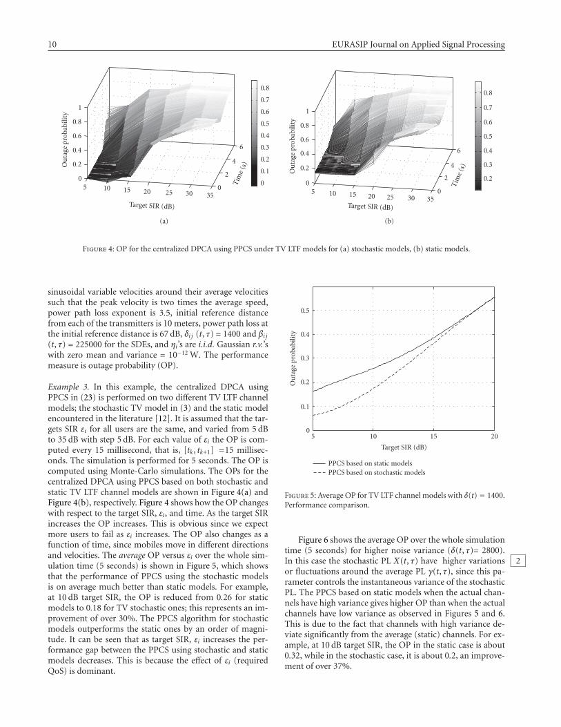
Figure 4: OP for the centralized DPCA using PPCS under TV LTF models for (a) stochastic models, (b) static models.

sinusoidal variable velocities around their average velocitiessuch that the peak velocity is two times the average speed,power path loss exponent is 3.5, initial reference distancefrom each of the transmitters is 10 meters, power path loss atthe initial reference distance is 67 dB, δi j (t, τ) = 1400 and βi j(t, τ) = 225000 for the SDEs, and ηi’s are i.i.d. Gaussian r.v.’swith zero mean and variance = 10−12 W. The performancemeasure is outage probability (OP).

Example 3. In this example, the centralized DPCA usingPPCS in (23) is performed on two different TV LTF channelmodels; the stochastic TV model in (3) and the static modelencountered in the literature [12]. It is assumed that the tar-gets SIR εi for all users are the same, and varied from 5 dBto 35 dB with step 5 dB. For each value of εi the OP is com-puted every 15 millisecond, that is, [tk, tk+1] =15 millisec-onds. The simulation is performed for 5 seconds. The OP iscomputed using Monte-Carlo simulations. The OPs for thecentralized DPCA using PPCS based on both stochastic andstatic TV LTF channel models are shown in Figure 4(a) andFigure 4(b), respectively. Figure 4 shows how the OP changeswith respect to the target SIR, εi, and time. As the target SIRincreases the OP increases. This is obvious since we expectmore users to fail as εi increases. The OP also changes as afunction of time, since mobiles move in different directionsand velocities. The average OP versus εi over the whole sim-ulation time (5 seconds) is shown in Figure 5, which showsthat the performance of PPCS using the stochastic modelsis on average much better than static models. For example,at 10 dB target SIR, the OP is reduced from 0.26 for staticmodels to 0.18 for TV stochastic ones; this represents an im-provement of over 30%. The PPCS algorithm for stochasticmodels outperforms the static ones by an order of magni-tude. It can be seen that as target SIR, εi increases the per-formance gap between the PPCS using stochastic and staticmodels decreases. This is because the effect of εi (requiredQoS) is dominant.

0.5

0.4

0.3

0.2

0.1

0

Ou

tage

prob

abili

ty

5 10 15 20

Target SIR (dB)

PPCS based on static modelsPPCS based on stochastic models

Figure 5: Average OP for TV LTF channel models with δ(t) = 1400.Performance comparison.

Figure 6 shows the average OP over the whole simulationtime (5 seconds) for higher noise variance (δ(t, τ)= 2800).In this case the stochastic PL X(t, τ) have higher variations 2or fluctuations around the average PL γ(t, τ), since this pa-rameter controls the instantaneous variance of the stochasticPL. The PPCS based on static models when the actual chan-nels have high variance gives higher OP than when the actualchannels have low variance as observed in Figures 5 and 6.This is due to the fact that channels with high variance de-viate significantly from the average (static) channels. For ex-ample, at 10 dB target SIR, the OP in the static case is about0.32, while in the stochastic case, it is about 0.2, an improve-ment of over 37%.


0.5

0.4

0.3

0.2

0.1

0

Ou

tage

prob

abili

ty

5 10 15 20

Target SIR (dB)

PPCS based on static modelsPPCS based on stochastic models

Figure 6: Average OP for TV LTF channel models with δ(t) = 2800.Performance comparison.

102

101

100

10�1

Tota

lpow

er

0 0.15 0.3 0.45 0.6 0.75 0.9 1.05 1.2 1.35 1.5

Time (s)

Distributed DPCADistributed SPCA

Figure 7: Sum of transmitted power of all mobiles for the dis-tributed DPCA and the distributed SPCA under TV LTF channels.

Example 4. In this example, the performance of the dis-tributed DPCA (30) is compared with the distributed SPCA(34) under stochastic TV LTF channels. With the same pa-rameters as Example 3, in addition to the target SIRs, εi = 5for all users and ak = 0.1. The total transmitted powersof all mobiles using the distributed DPCA in (30) and theSPCA in (34) under stochastic TV LTF channels are shown inFigure 7. Note that the power axis is logarithmic. Clearly, thedistributed SPCA using stochastic approximations providesbetter power stability and consumption than the distributedDPCA described in [15–17].

5. CONCLUSION

In this paper, a TV LTF wireless channel model, which cap-tures both the space and time-variations of TV LTF wirelesschannels, is developed. The dynamics of the TV LTF chan-nels are described by an SDE, which essentially captures thespatiotemporal variations of wireless communication links.The proposed model is more realistic than the standard staticmodels encountered in the literature. The SDE model pro-posed allows viewing the wireless channel as a dynamicalsystem, which shows how the channel evolves in time andspace. In addition, it allows well-developed tools of estima-tion and identification to be applied to this class of problems[9–11]. An optimal DPCA based on the developed model isproposed. The optimal DPCA is shown to reduce to a sim-ple linear programming problem if predictable power con-trol strategies (PPCS) are used. Iterative distributed DPCAsand SPCAs are used to solve for the optimization problem.The proposed distributed SPCA requires less informationthan the distributed SPCAs encountered in the literature.Generalizations to PC problems based on convex optimiza-tion techniques are provided if PPCS are not assumed, to-gether with outage constraints. These optimizations are thesubject of on-going research. Numerical results show thatthere are potentially large gains to be achieved by using TVstochastic models, and the distributed SPCA provides betterpower stability and consumption than the distributed DPCA.It should be noted that channel models based on SDEs forSTF (Rayleigh and Ricean environments) have been consid-ered in [2, 5], by approximating the Doppler power spectraldensity of wireless channels.

REFERENCES

[1] M. Huang, P. E. Caines, C. D. Charalambous, and R. P. Mal-hame, “Power control in wireless systems: a stochastic controlformulation,” in Proceedings of the American Control Confer-ence, vol. 2, pp. 750–755, Arlington, Va, USA, June 2001.

[2] C. D. Charalambous, S. M. Djouadi, and S. Z. Denic, “Stochas-tic power control for wireless networks via SDEs: probabilis-tic QoS measures,” IEEE Transactions on Information Theory,vol. 51, no. 12, pp. 4396–4401, 2005.

[3] C. D. Charalambous and N. Menemenlis, “Stochastic modelsfor long-term multipath fading channels and their statisticalproperties,” in Proceedings of the 38th IEEE Conference on De-cision and Control (CDC ’99), vol. 5, pp. 4947–4952, Phoenix,Ariz, USA, December 1999.

[4] C. D. Charalambous and N. Menemenlis, “General non-stationary models for short-term and long-term fading chan-nels,” in Proceedings of IEEE/AFCEA Conference on InformationSystems for Enhanced Public Safety and Security (EUROCOMM’00), pp. 142–149, Munich, Germany, May 2000.

[5] M. M. Olama, S. M. Shajaat, S. M. Djouadi, and C. D. Char-alambous, “Stochastic power control for time-varying short-term flat fading wireless channels,” in Proceedings of the 16thIFAC World Congress, Prague, Czech Republic, July 2005.

[6] M. M. Olama, S. M. Shajaat, S. M. Djouadi, and C. D. Char-alambous, “Stochastic power control for time-varying long-term fading wireless channels,” in Proceedings of the AmericanControl Conference, pp. 1817–1822, Portland, Ore, USA, June2005.


[7] T. S. Rappaport, Wireless Communications: Principles and Prac-tice, Prentice-Hall, Upper Saddle River, NJ, USA, 1996.

[8] J. Zhang, E. K. P. Chong, and I. Kontoyiannis, “Unified spatialdiversity combining and power allocation for CDMA systemsin multiple time-scale fading channels,” IEEE Journal on Se-lected Areas in Communications, vol. 19, no. 7, pp. 1276–1288,2001.

[9] L. Ljung and T. Sodestrom, Theory and Practice of RecursiveEstimation, MIT Press, Cambridge, Mass, USA, 1983.

[10] A. Benveniste, M. Metivier, and P. Priouet, Adaptive Algorithmsand Stochastic Approximations, Springer, New York, NY, USA,1990.

[11] M. A. Kouritzin, “Inductive methods and rates of rth-meanconvergence in adaptive filtering,” Stochastic and Stochastic Re-ports, vol. 51, pp. 241–266, 1994.

[12] J. Zander, “Performance of optimum transmitter power con-trol in cellular radio systems,” IEEE Transactions on VehicularTechnology, vol. 41, no. 1, pp. 57–62, 1992.

[13] J. M. Aein, “Power balancing in systems employing frequencyreuse,” COMSAT Technical Review, vol. 3, no. 2, pp. 277–299,1973.3

[14] S. A. Grandhi, J. Zander, and R. Yates, “Constrained powercontrol,” Wireless Personal Communications, vol. 1, no. 4, pp.257–270, 1994.

[15] N. Bambos and S. Kandukuri, “Power-controlled multiple ac-cess schemes for next-generation wireless packet networks,”IEEE Wireless Communications, vol. 9, no. 3, pp. 58–64, 2002.

[16] X. Li and Z. Gajic, “An improved SIR-based power control forCDMA systems using Steffensen iterations,” in Proceedings ofthe Conference on Information Science and Systems, pp. 287–290, Princeton, NJ, USA, March 2002.

[17] G. J. Foschini and Z. Miljanic, “Simple distributed au-tonomous power control algorithm and its convergence,” IEEETransactions on Vehicular Technology, vol. 42, no. 4, pp. 641–646, 1993.

[18] S. Kandukuri and S. Boyd, “Optimal power control ininterference-limited fading wireless channels with outage-probability specifications,” IEEE Transactions on Wireless Com-munications, vol. 1, no. 1, pp. 46–55, 2002.

[19] A. M. Viterbi and A. J. Viterbi, “Erlang capacity of a powercontrolled CDMA system,” IEEE Journal on Selected Areas inCommunications, vol. 11, no. 6, pp. 892–900, 1993.

[20] S. Ulukus and R. D. Yates, “Stochastic power control for cel-lular radio systems,” IEEE Transactions on Communications,vol. 46, no. 6, pp. 784–798, 1998.

[21] M. K. Varanasi and D. Das, “Fast stochastic power control al-gorithms for nonlinear multiuser receivers,” IEEE Transactionson Communications, vol. 50, no. 11, pp. 1817–1827, 2002.

[22] T. Holliday, A. J. Goldsmith, and P. Glynn, “Distributed powercontrol for time-varying wireless networks: optimality andconvergence,” in Proceedings of 41st Annual Allerton Conferenceon Communications, Control, and Computing, Monticello, Ill,USA, October 2003.

[23] N. B. Mandayam, P.-C. Chen, and J. M. Holtzman, “Minimumduration outage for cellular systems: a level crossing analysis,”in Proceedings of 46th IEEE Vehicular Technology Conference,vol. 2, pp. 879–883, Atlanta, Ga, USA, April 1996.

[24] R. Buche and H. J. Kushner, “Control of mobile communica-tions with time-varying channels in heavy traffic,” IEEE Trans-actions on Automatic Control, vol. 47, no. 6, pp. 992–1003,2002.

[25] M. Huang, P. E. Caines, and R. P. Malhame, “Uplink power ad-justment in wireless communication systems: a stochastic con-

trol analysis,” IEEE Transactions on Automatic Control, vol. 49,no. 10, pp. 1693–1708, 2004.

[26] J.-F. Chamberland and V. V. Veeravalli, “Decentralized dy-namic power control for cellular CDMA systems,” IEEE Trans-actions on Wireless Communications, vol. 2, no. 3, pp. 549–559,2003.

[27] L. Song, N. B. Mandayam, and Z. Gajic, “Analysis of anup/down power control algorithm for the CDMA reverse linkunder fading,” IEEE Journal on Selected Areas in Communica-tions, vol. 19, no. 2, pp. 277–286, 2001.

[28] C. W. Sung and W. S. Wong, “Performance of a cooperativealgorithm for power control in cellular systems with a time-varying link gain matrix,” Wireless Networks, vol. 6, no. 6, pp.429–439, 2000.

[29] F. Graziosi, M. Pratesi, M. Ruggieri, and F. Santucci, “Multi-cell model of handover initiation in mobile cellular networks,”IEEE Transactions on Vehicular Technology, vol. 48, no. 3, pp.802–814, 1999.

[30] F. Graziosi and F. Santucci, “A general correlation model forshadow fading in mobile radio systems,” IEEE Communica-tions Letters, vol. 6, no. 3, pp. 102–104, 2002.

[31] P. Taaghol and R. Tafazolli, “Correlation model for shadowfading in landmobile satellite systems,” Electronics Letters,vol. 33, no. 15, pp. 1287–1289, 1997.

[32] A. I. Mees, Nonlinear Dynamics and Statistics, Birkhauser,Boston, Mass, USA, 2001.

[33] R. D. Yates, “A framework for uplink power control in cellularradio systems,” IEEE Journal on Selected Areas in Communica-tions, vol. 13, no. 7, pp. 1341–1347, 1995.

[34] J. Luo, S. Ulukus, and A. Ephremides, “Standard and quasi-standard stochastic power control algorithms,” IEEE Transac-tions on Information Theory, vol. 51, no. 7, pp. 2612–2624,2005.

[35] B. Oksendal, Stochastic Differential Equations: An Introductionwith Applications, Springer, Berlin, Germany, 1998.

[36] R. Nelson, Probability, Stochastic Processes, and Queuing The-ory: The Mathematics of Computer Performance Modeling,Springer, New York, NY, USA, 3rd edition, 2000.

Mohammed M. Olama received his B.S.and M.S. (with first class honors) degreesin electrical engineering from Universityof Jordan, in 1998 and 2001, respectively.From 2001 to 2003, he completed 33 credithours towards his Ph.D. degree in the Ap-plied Science Department, University ofArkansas at Little Rock (UALR). Since Au-gust 2003, he has been a Ph.D. candidatein the Electrical and Computer EngineeringDepartment at the University of Tennessee, Knoxville. His researchinterests include channel modeling, power control, and mobile lo-cation estimation for wireless networks.


Seddik M. Djouadi received his Ph.D. de-gree from McGill University, his M.A.Sc.degree from Ecole Polytechnique, both inMontreal, his B.S. (with first class honors)from Ecole Nationale Polytechnique, Al-giers, all in electrical engineering, respec-tively, in 1999, 1992, and 1989. He is cur-rently an Assistant Professor in the Electri-cal and Computer Engineering Departmentat the University of Tennessee. He was anAssistant Professor in UALR, and held postdoctoral positions inthe Air Force Research Laboratory and Georgia Institute of Tech-nology, where he was also with American Flywheel Systems Inc.He received the Ralph E. Powe Junior Faculty Enhancement Award2005, four US Air Force Summer Faculty Fellowships, the TibbetAward with AFS Inc. in 1999, the ACC Best Student Paper Certifi-cate (best five in competition) in 1998. He was selected by Automat-ica as an outstanding reviewer for 2003–2004. His research interestsare modeling and power control for wireless networks, robust con-trol, control under communication limitations, active vision, andidentification.

Charalambos D. Charalambous joined theDepartment of Electrical and ComputerEngineering at the University of Cyprus in2003. He accepted his first tenure-track fac-ulty position at the rank of Associate Pro-fessor with the University of Ottawa, Schoolof Information Technology and Engineer-ing, in 1999. He has served at the faculty ofMcGill University, Department of Electri-cal and Computer Engineering, as a VisitingProfessor, from 1995 to 1999; from 1993 to 1995 he was a Postdoc-toral Fellow with Idaho State University, Engineering Department.His teaching and research interests span topics in the followingareas: stochastic systems: estimation, identification, and decision;games theory: robustness and optimization of uncertain stochas-tic systems; control subject to communication constraints, queu-ing systems, large deviations, and information theory. He served asan Associate Editor of the IEEE Transactions on Automatic Con-trol, 2001-2004, and he was a Member of the Control System So-ciety Conference Editorial Board. He was a member of the Cana-dian Centres of Excellence through the mathematics of informationtechnology and complex systems (MITACS), 1998–2001. In 2001,he received the Premier’s Research Excellence Award of the OntarioProvince of Canada.

Composition Comments

1. There is an extra left delimiter or a missing right one.Please check.

2. We made keys for Figures 5, 6, and 7. Please check

3. Comment on ref. [14]: We changed the year. Pleasecheck.

Stochastic Power Control for Time-Varying Long-Term Fading Wireless Networks

Documents

Transcript of Stochastic Power Control for Time-Varying Long-Term Fading Wireless Networks