arX

iv:0

711.

1161

v1 [

cs.IT

] 7

Nov

200

71

Joint Source-Channel Codes for MIMO Block

Fading ChannelsDeniz Gunduz, Elza Erkip

Abstract

We consider transmission of a continuous amplitude source over anL-block Rayleigh fadingMt × Mr MIMO

channel when the channel state information is only available at the receiver. Since the channel is not ergodic, Shannon’s

source-channel separation theorem becomes obsolete and the optimal performance requires a joint source -channel

approach. Our goal is to minimize the expected end-to-end distortion, particularly in the high SNR regime. The figure

of merit is the distortion exponent, defined as the exponential decay rate of the expected distortion with increasing

SNR. We provide an upper bound and lower bounds for the distortion exponent with respect to the bandwidth ratio

among the channel and source bandwidths. For the lower bounds, we analyze three different strategies based on

layered source coding concatenated with progressive, superposition or hybrid digital/analog transmission. In each

case, by adjusting the system parameters we optimize the distortion exponent as a function of the bandwidth ratio.

We prove that the distortion exponent upper bound can be achieved when the channel has only one degree of freedom,

that isL = 1, andmin{Mt, Mr} = 1. When we have more degrees of freedom, our achievable distortion exponents

meet the upper bound for only certain ranges of the bandwidthratio. We demonstrate that our results, which were

derived for a complex Gaussian source, can be extended to more general source distributions as well.

Index Terms

Broadcast codes, distortion exponent, diversity-multiplexing gain tradeoff, hybrid digital/analog coding, joint

source-channel coding, multiple input- multiple output (MIMO), successive refinement.

I. I NTRODUCTION

Recent advances in mobile computing and hardware technology enable transmission of rich multimedia

contents over wireless networks. Examples include digitalTV, voice and video transmission over cellular

and wireless LAN networks, and sensor networks. With the high demand for such services, it becomes

The material in this paper was presented in part at the 39th Asilomar Conference on Signals, Systems, and Computers, Pacific Grove, CA,

Nov. 2005, at the IEEE Information Theory Workshop, Punta del Este, Uruguay, March 2006, and at the IEEE International Symposium on

Information Theory (ISIT), Seattle, WA, July 2006.

This work is partially supported by NSF grants No. 0430885 and No. 0635177.

Deniz Gunduz was with Department of Electrical and Computer Engineering, Polytechnic University. He is now with the Department of

Electrical Engineering, Princeton University, Princeton, NJ, 08544, and also with the Department of Electrical Engineering, Stanford University,

Stanford, CA, 94305. Elza Erkip is with the Department of Electrical and Computer Engineering, Polytechnic University, Brooklyn, NY, 11201.

Email: dgunduz@princeton.edu, elza@poly.edu.

2

crucial to identify the system limitations, define the appropriate performance metrics, and to design

wireless systems that are capable of achieving the best performance by overcoming the challenges posed

by the system requirements and the wireless environment. Ingeneral, multimedia wireless communica-

tion requires transmitting analog sources over fading channels while satisfying the end-to-end average

distortion and delay requirements of the application within the power limitations of the mobile terminal.

Multiple antennas at the transceivers have been proposed asa viable tool that can remarkably improve

the performance of multimedia transmission over wireless channels. The additional degrees of freedom

provided by multiple input multiple output (MIMO) system can be utilized in the form of spatial

multiplexing gain and/or spatial diversity gain, that is, either to transmit more information or to increase

the reliability of the transmission. The tradeoff between these two gains is explicitly characterized as the

diversity-multiplexing gain tradeoff (DMT) in [1]. How to translate this tradeoff into an improved overall

system performance depends on the application requirements and limitations.

In this paper, we consider transmission of a continuous amplitude source over a MIMO block Rayleigh

fading channel. We are interested in minimizing the end-to-end average distortion of the source. We

assume that the instantaneous channel state information isonly available at the receiver (CSIR). We

consider the case whereK source samples are to be transmitted overL fading blocks spanningN

channel uses. We define thebandwidth ratioof the system as

b =N

Kchannel uses per source sample, (1)

and analyze the system performance with respect tob. We assume thatK is large enough to achieve

the rate-distortion performance of the underlying source,andN is large enough to design codes that can

achieve all rates below the instantaneous capacity of the block fading channel.

We are particularly interested in the highSNR behavior of the expected distortion (ED) which is

characterized by thedistortion exponent[2]:

∆ = − limSNR→∞

log ED

log SNR. (2)

Shannon’s fundamental source-channel separation theoremdoes not apply to our scenario as the channel

is no more ergodic. Thus, the optimal strategy requires a joint source-channel coding approach. The

minimum expected end-to-end distortion depends on the source characteristics, the distortion metric, the

power constraint of the transmitter, the joint compression, channel coding and transmission techniques

used.

Since we are interested in the average distortion of the system, this requires a strategy that performs

‘well’ over a range of channel conditions. Our approach is tofirst compress the source into multiple layers,

where each layer successively refines the previous layers, and then transmit these layers at varying rates,

3

hence providing unequal error protection so that the reconstructed signal quality can be adjusted to the

instantaneous fading state without the availability of thechannel state information at the transmitter

(CSIT). We consider transmitting the source layers either progressively in time,layered source coding

with progressive transmission(LS), or simultaneously by superposition,broadcast strategy with layered

source(BS). We also discuss a hybrid digital-analog extension of LS calledhybrid-LS(HLS).

The characterization of distortion exponent for fading channels has recently been investigated in several

papers. Distortion exponent is first defined in [2], and simple transmission schemes over two parallel

fading channels are compared in terms of distortion exponent. Our prior work includes maximizing

distortion exponent using layered source transmission forcooperative relay [3], [4], [5], for SISO [6],

for MIMO [7], and for parallel channels [8]. Holliday and Goldsmith [9] analyze high SNR behavior of

the expected distortion for single layer transmission overMIMO without explicitly giving the achieved

distortion exponent. Hybrid digital-analog transmission, first proposed in [10] for the Gaussian broadcast

channel, is considered in terms of distortion exponent for MIMO channel in [11].

Others have focused on minimizing the end-to-end source distortion for general SNR values [15], [16].

Recently, the LS and BS strategies introduced here have beenanalyzed for finite SNR and finite number

of source layers in [17]-[22].

This paper derives explicit expressions for the achievabledistortion exponent of LS, HLS and BS

strategies, and compares the achievable exponents with an upper bound derived by assuming perfect

channel state information at the transmitter. Our results reveal the following:

• LS strategy, which can easily be implemented by concatenating a layered source coder with a

MIMO channel encoder that time-shares among different coderates, improves the distortion exponent

compared to the single-layer approach of [9] even with limited number of source layers. However,

the distortion exponent of LS still falls short of the upper bound.

• While the hybrid digital-analog scheme meets the distortion exponent upper bound for small band-

width ratios as shown in [11], the improvement of hybrid extension of LS (HLS) over pure progressive

layered digital transmission (LS) becomes insignificant asthe bandwidth ratio or the number of digital

layers increases.

• Transmitting layers simultaneously as suggested by BS provides the optimal distortion exponent for

all bandwidth ratios when the system has one degree of freedom, i.e., for single block MISO/SIMO

systems, and for high bandwidth ratios for the general MIMO system. Hence, for the mentioned

cases the problem of characterizing the distortion exponent is solved.

• There is a close relationship between the DMT of the underlying MIMO channel and the achievable

distortion exponent of the proposed schemes. For LS and HLS,we are able to give an explicit

4

characterization of the achievable distortion exponent once the DMT of the system is provided. For

BS, we enforce successive decoding at the receiver and the achievable distortion exponent closely

relates to the ‘successive decoding diversity-multiplexing tradeoff’ which will be rigorously defined

in Section V.

• The correspondence between source transmission to a singleuser with unknown noise variance

and multicasting to users with different noise levels [10] suggests that, our analysis would also

apply to the multicasting case where each receiver has the same number of antennas and observes

an independent block fading Rayleigh channel possibly witha different mean. Here the goal is to

minimize the expected distortion of each user. Alternatively, each user may have a static channel, but

the channel gains over the users may be randomly distributedwith independent Rayleigh distribution,

where the objective is to minimize the source distortion averaged over the users.

• While minimizing the end-to-end distortion for finite SNR isstill an open problem, in the high SNR

regime we are able to provide a complete solution in certain scenarios. Using this high SNR analysis,

it is also possible to generalize the results to non-Gaussian source distributions. Furthermore, LS and

BS strategies motivate source and channel coding strategies that are shown to perform very well for

finite SNRs as well [17]-[22].

We use the following notation throughout the paper.E[·] is the expectation,f(x).= g(x) is the

exponential equality defined aslimx→∞log f(x)log g(x) = 1, while ≥ and ≤ are defined similarly. Vectors and

matrices are denoted with bold characters, where matrices are in capital letters.[·]T and [·]† are the

transpose and the conjugate transpose operations, respectively. tr(A) is the the trace of matrixA. For

two Hermitian matricesA � B means thatA − B is positive-semidefinite.(x)+ is x if x ≥ 0, and0

otherwise. We denote the set{[x1, . . . , xn] : xi ∈ R+,∀i} by Rn+.

II. SYSTEM MODEL

We consider a discrete time continuous amplitude (analog) source{sk}∞k=1, sk ∈ R available at the

transmitter. For the analysis, we focus on a memoryless, i.i.d., complex Gaussian source with independent

real and imaginary components each with variance 1/2. We usethe distortion-rate function of the complex

Gaussian sourceD(R) = 2−R whereR is the source coding rate in bits per source sample, and consider

compression strategies that meet the distortion-rate bound. Although in Sections III-VI we use properties

of this complex Gaussian source (such as its distortion-rate function and successive refinability), in Section

VIII we prove that our results can be extended to any complex source with finite second moment and

finite differential entropy, with squared-error distortion metric. As stated in Section I, we assume thatK

source samples are transmitted inN channel uses which corresponds to a bandwidth ratio ofb = N/K.

5

In all our derivations we allow for an arbitrary bandwidth ratio b > 0.

We assume a MIMO block fading channel withMt transmit andMr receive antennas. The channel

model is

y[i] =

√

SNR

MtH[i]x[i] + z[i], i = 1, . . . , N (3)

where√

SNRMt

x[i] is the transmitted signal at timei, Z = [z1, . . . , zN ] ∈ CMr×N is the complex Gaussian

noise with i.i.d entriesCN (0, 1), andH[i] ∈ CMr×Mt is the channel matrix at timei, which has i.i.d.

entries withCN (0, 1). We have anL-block fading channel, that is, the channel observesL different i.i.d.

fading realizationsH1, . . . ,HL each lasting forN/L channel uses. Thus we have

H

[

kN

L+ 1

]

= H

[

kN

L+ 2

]

= . . . = H

[

(k + 1)N

L

]

= Hk+1, (4)

for k = 0, . . . , L−1 assumingN/L is integer. The realization of the channel matrixHi is assumed to be

known by the receiver and unknown by the transmitter, while the transmitter knows the statistics ofHi.

The codeword,X =

[

x[1], . . . ,xL

]

∈ CMt×N is normalized so that it satisfiestr(E[X†X]) ≤ MtN .

We assume Gaussian codebooks which can achieve the instantaneous capacity of the MIMO channel.

We defineM∗ = min{Mt,Mr} andM∗ = max{Mt,Mr}.

The source is transmitted through the channel using one of the joint source-channel coding schemes dis-

cussed in this paper. In general, the source encoder matchestheK-length source vectorsK = [s1, . . . , sK ]

to the channel inputX. The decoder maps the received signalY =

[

y[1], . . . ,y[N ]

]

∈ CMr×N to an

estimates ∈ CK of the source. Average distortionED(SNR) is defined as the average mean squared

error betweens and s at average channel signal-to-noise ratioSNR, where the expectation is taken

with respect to all source samples, channel realizations and the channel noise. The exact expression of

ED(SNR) for the strategies introduced will be provided in the respective sections.

As mentioned in Section I, we are interested in the high SNR behavior of the expected distortion. We

optimize the system performance to maximize thedistortion exponentdefined in Eqn. (2). A distortion

exponent of∆ means that the expected distortion decays asSNR−∆ with increasing SNR whenSNR

is high.

In order to obtain the end-to-end distortion for our proposed strategies, we will need to characterize

the error rate of the MIMO channel. Since we are interested inthe high SNR regime, we use the outage

probability, which has the same exponential behavior as thechannel error probability [1]. For a family

of codes with rateR = r log SNR, r is defined as the multiplexing gain of the family, and

d(r) = − limSNR→∞

log Pout(SNR)

log SNR(5)

as the diversity advantage, wherePout(SNR) is the outage probability of the code. The diversity

gain d∗(r) is defined as the supremum of the diversity advantage over allpossible code families with

6

multiplexing gain r. In [1], it is shown that there is a fundamental tradeoff between multiplexing

and diversity gains, also known as the diversity-multiplexing gain tradeoff (DMT), and this tradeoff

is explicitly characterized with the following theorem.

Theorem 2.1:(Corollary 8, [1]) For anMt ×Mr MIMO L-block fading channel, the optimal tradeoff

curved∗(r) is given by the piecewise-linear function connecting the points (k, d∗(k)), k = 0, 1, . . . ,M∗,

where

d∗(k) = L(Mt − k)(Mr − k). (6)

III. D ISTORTION EXPONENT UPPERBOUND

Before we study the performance of various source-channel coding strategies, we calculate an upper

bound for the distortion exponent of the MIMOL-block fading channel, assuming that the transmitter

has access to perfect channel state information at the beginning of each block. Then the source-channel

separation theorem applies for each block and transmissionat the highest rate is possible with zero outage

probability.

Theorem 3.1:For transmission of a memoryless i.i.d. complex Gaussian source over anL-block Mt ×

Mr MIMO channel, the distortion exponent is upper bounded by

∆UB = LM∗∑

i=1

min

{bL

, 2i − 1 + |Mt − Mr|

}

. (7)

Proof: Proof of the theorem can be found in Appendix I.

Note that, increasing the number of antennas at either the transmitter or the receiver by one does

not provide an increase in the distortion exponent upper bound for b < L(1 + |Mt − Mr|), since the

performance in this region is bounded by the bandwidth ratio. Adding one antenna to both sides increases

the upper bound for all bandwidth ratios, while the increaseis more pronounced for higher bandwidth

ratios. The distortion exponent is bounded by the highest diversity gainLMtMr.

In the case ofM × 1 MISO system, and alternatively1 × M SIMO system, the upper bound can be

simplified to

∆UBMISO/SIMO = min{b, LM}. (8)

We next discuss how a simple transmission strategy consisting of single layer digital transmission per-

forms with respect to the upper bound. In single layer digital transmission, the source is first compressed

at a specific ratebR, the compressed bits are channel coded at rateR, and then transmitted over the

channel. This is the approach taken in [2] for two-parallel channels, in [3] for cooperative relay channels,

and in [9] for the MIMO channel to transmit an analog source over a fading channel. Even though

7

y = br

∆ = d∗(r∗)

r∗r

d∗(r)

Multiplexing gain

Div

ersi

tyga

in

MIMO DMT curve

Fig. 1. A geometric interpretation illustrating the optimal multiplexing gain for a single layer source-channel coding system. The intersection

point of the DMT curve and the liney=br gives the optimal multiplexing gain- distortion exponent pair.

compression and channel coding are done separately, the rate is a common parameter that can be chosen

to minimize the end-to-end distortion. Note that the transmitter choses this rateR without any channel

state information.

The expected distortion of single layer transmission can bewritten as

ED(R,SNR) = (1 − Pout(R,SNR))D(bR) + Pout(R,SNR), (9)

wherePout(R,SNR) is the outage probability at rateR for givenSNR, andD(R) is the distortion-rate

function of the source. Here we assume that, in case of an outage, the decoder simply outputs the mean

of the source leading to the highest possible distortion of1 due to the unit variance assumption. At fixed

SNR, there is a tradeoff between reliable transmission overthe channel (through the outage probability),

and increased fidelity in source reconstruction (through the distortion-rate function). This suggests that

there is an optimal transmission rate that achieves the optimal average distortion. For any given SNR this

optimal R can be found using the exact expressions forPout(R,SNR) andD(R).

In order to study the distortion exponent, we concentrate onthe high SNR approximation of Eqn. (9).

To achieve a vanishing expected distortion in the high SNR regime we need to increaseR with SNR.

ScalingR faster thanO(log SNR) would result in an outage probability of1, since the instantaneous

channel capacity of the MIMO system scales asM∗ log SNR. Thus we assignR = r log SNR, where

0 ≤ r ≤ M∗. Then the high SNR approximation of Eqn. (9) is

ED.= D(bR) + Pout(R),

.= SNR−br + SNR−d∗(r). (10)

8

0 1 2 3 4 50

0.5

1

1.5

2

2.5

3

3.5

4

Bandwidth ratio (b)

Dis

tort

ion

expo

nent

(∆)

Upper bound(2 x 2 MIMO)Upper bound(4 x 1 MISO)Single rate (2 x 2 MIMO)Single rate (4 x 1 MISO)

Fig. 2. Upper bound and single layer achievable distortion exponents for2 × 2 and4 × 1 MIMO systems.

Of the two terms, the one with the highest SNR exponent would be dominant in the high SNR regime.

Maximum distortion exponent is achieved when both terms have the same SNR exponent. Then the

optimal multiplexing gainr∗ satisfies

∆ , br∗ = d∗(r∗), (11)

where∆ is the corresponding distortion exponent. Eqn. (11) suggests an optimal operating point on the

DMT curve to maximize the distortion exponent of the single layer scheme.

Figure 1 shows a geometric illustration of the optimal multiplexing gain and the corresponding distortion

exponent. A similar approach was taken in [9] for single layer transmission with the restriction of integer

multiplexing gains, and later extended to all multiplexinggains in [11]. However, as we argue next,

even when all multiplexing gains are considered, this single layer approach is far from exploiting all the

resources provided by the system.

In Figure 2, we illustrate the distortion exponent upper bound and the distortion exponent of the single

layer scheme for4×1 MISO and2×2 MIMO systems. We observe a significant gap between the upper

bounds and the single layer distortion exponents in both cases for all bandwidth ratios. This gap gets

larger with increasing degrees of freedom and increasing bandwidth ratio.

The major drawback of the single layer digital scheme is thatit suffers from the threshold effect, i.e.,

error probability is bounded away from zero or an outage occurs when the channel quality is worse

than a certain threshold, which is determined by the attempted rate. Furthermore, single layer digital

transmission cannot utilize the increase in the channel quality beyond this threshold. Lack of CSIT

9

makes only a statistical optimization of the compression/transmission rate possible. To make the system

less sensitive to the variations in the channel quality, we will concentrate on layered source coding

where the channel codewords corresponding to different layers are assigned different rates. Using the

successive refinability of the source, we transmit more important compressed bits with higher reliability.

The additional refinement bits are received when the channelquality is high. This provides adaptation to

the channel quality without the transmitter actually knowing the instantaneous fading levels. We argue

that, due to the exponential decay of the distortion-rate function in general, layering increases the overall

system performance from the distortion exponent perspective. Our analysis in the following sections

proves this claim.

IV. L AYERED SOURCE CODING WITH PROGRESSIVE TRANSMISSION ANDHYBRID DIGITAL -ANALOG

EXTENSION

The first source-channel coding scheme we consider is based on compression of the source in layers,

where each layer is a refinement of the previous ones, and transmission of these layers successively in

time using channel codes of different rates. We call this schemelayered source coding with progressive

transmission(LS). This classical idea, mostly referred as progressive coding, has been used to various

extents in the image and video standards such as JPEG2000 andMPEG-4. After analyzing the distortion

exponent of LS in Section IV-A, in Section IV-B we consider a hybrid digital-analog extension called

hybrid LS(HLS) where the error signal is transmitted without coding.In this section we analyze single

block fading, i.e.,L = 1, for clarity of presentation. Generalization to the multiple block case(L > 1)

will be a straightforward extension of the techniques presented here and will be briefly discussed in

Section VI.

A. Layered Source Coding with Progressive Transmission (LS)

We assume that the source encoder hasn layers with each layer transmitted over the channel at rate

Ri bits per channel use intiN channel uses fori = 1, 2, . . . , n, with∑n

i=1 ti = 1. This is illustrated in

Fig. 3(a). We assume thattiN is large enough to approach the instantaneous channel capacity. For each

layer this corresponds to a source coding rate ofbtiRi bits per sample, whereb is the bandwidth ratio

defined in (1). Theith layer is composed of the successive refinement bits for thepreviousi− 1 layers.

The transmission power is kept constant for each layer, so the optimization variables are the rate vector

R = [R1, . . . , Rn] and the channel allocation vectort = [t1, . . . , tn].

Let P iout denote the outage probability of layeri, i.e., P i

out = Pr{C(H) < Ri}. Using successive

refinability of the complex Gaussian source [23], the distortion achieved when the firsti layers are

10

R1 R2 Rn

N channel uses

t1N t2N tnN(a) LS strategy with n layers.

R1 R2 Rn

t1(N −K

M∗

) t2(N −K

M∗

) tn(N −K

M∗

)

Analog transmission

K/M∗

(b) HLS strategy with n layers for b > 1/M∗.

R1, SNR1

Rn, SNRn

(c) BS strategy with n layers. Layers are transmitted simultaneouslywith total power allocated among them.

Fig. 3. Channel and power allocation for different transmission strategies explored in the paper.

successfully decoded is

DLSi = D

(

bi∑

k=1

tkRk

)

,

= 2−bP

i

k=1tkRk , (12)

with DLS0 = 1. Note that due to successive refinement source coding, a layer is useless unless all the

preceding layers are received successfully. This imposes anon-decreasing rate allocation among the

layers, i.e.,Ri ≤ Rj for any j > i. Then the expected distortion (ED) for such a rate allocation can be

written as

ED(R, t, SNR) =n∑

i=0

DLSi ·

(P i+1

out − P iout

), (13)

where we defineP 0out = 0 andPn+1

out = 1.

The minimization problem to be solved is

minR,t

ED(R, t, SNR)

s.t.∑n

i=1 ti = 1,

ti ≥ 0, for i = 1, . . . , n

0 ≤ R1 ≤ R2 ≤ · · · ≤ Rn.

(14)

11

This is a non-linear optimization problem which can be untractable for a given SNR. An algorithm solving

the above optimization problem for finite SNR is proposed in [17]. However when we focus on the high

SNR regime and compute the distortion exponent∆, we will be able to obtain explicit expressions.

In order to have a vanishing expected distortion in Eqn. (13)with increasing SNR, we need to

increase the transmission rates of all the layers with SNR asargued in the single layer case. We let

the multiplexing gain vector ber = [r1, . . . , rn]T , henceR = r log SNR. The ordering of rates is

translated into multiplexing gains as0 ≤ r1 ≤ · · · ≤ rn. Using the DMT of the MIMO system under

consideration and the distortion-rate function of the complex Gaussian source, we get

ED(R, SNR).=

n∑

k=0

[

SNR−d∗(rk+1) − SNR−d∗(rk)]

SNR−bP

k

i=1tiri

.=

n∑

k=0

SNR−d∗(rk+1)SNR−bP

k

i=1tiri

.= SNRmax0≤k≤n{−d∗(rk+1)−b

P

k

i=1tiri}, (15)

whered∗(rn+1) = 0, and the last exponential equality arises because the summation will be dominated

by the slowest decay in high SNR regime. Then the optimal LS distortion exponent can be written as

∆LSn = max

r,tmin

0≤k≤n

{

d∗(rk+1) + bk∑

i=1

tiri

}

(16)

s.t.n∑

i=1

ti = 1,

ti ≥ 0, for i = 1, . . . , n

0 ≤ r1 ≤ r2 ≤ · · · ≤ rn ≤ M∗.

Assuming a given channel allocation amongn layers, i.e.,t is given, the Karush-Kuhn-Tucker (KKT)

conditions for the optimization problem of (16) lead to:

btnrn = d∗(rn), (17)

d∗(rn) + btn−1rn−1 = d∗(rn−1), (18)

. . .

d∗(r2) + bt1r1 = d∗(r1), (19)

where the corresponding distortion exponent is∆LSn = d∗(r1).

The equations in (17)-(19) can be graphically illustrated on the DMT curve as shown in Fig. 4. This

illustration suggests that, for given channel allocation,finding the distortion exponent inn-layer LS can

be formulated geometrically: We haven straight lines each with slopebti for i = 1, . . . , n, and each line

12

rn−1 rn

r

d∗(r)

d∗(rn) y = btnr

y = d∗(r2) + bt1r

r1

d∗(rn−1)

MIMO DMT curve

y = d∗(rn) + btn−1r

∆ = d∗(r1)

Fig. 4. Rate allocation for the source layers of LS illustrated on DMT curve of the MIMO channel.

intersects they-axis at a point with the same ordinate as the intersection ofthe previous line with the

DMT curve. Although the total slope is always equal tob, the more layers we have, the higher we can

climb on the tradeoff curve and obtain a larger∆.

The distortion exponent of LS in the limit of infinite layers provides a benchmark for the performance

of LS in general. The following lemma will be used to characterize the optimal LS distortion exponent

in the limit of infinite layers.

Lemma 4.1:In the limit of infinite layers, i.e., asn → ∞, the optimal distortion exponent for LS can

be achieved by allocating the channel equally among the layers.

Proof: Proof of the lemma can be found in Appendix II.

The next theorem provides an explicit characterization of the asymptotic optimal LS distortion exponent

∆LS (in the case of infinite layers) for anMt × Mr MIMO system.

Theorem 4.2:Let the sequence{ci} be defined asc0 = 0, ci = ci−1+(|Mr−Mt|+2i−1) ln(

M∗−i+1M∗−i

)

for i = 1, . . . ,M∗ − 1 andcM∗= ∞. The optimal distortion exponent of infinite layer LS is given by:

∆LS =∑p−1

i=1 (|Mr − Mt| + 2i − 1)

+(M∗ − p + 1)(|Mr − Mt| + 2p − 1)(1 − e−

b−cp−1

|Mr−Mt|+2p−1 ),

for cp−1 ≤ b < cp, p = 1, . . . ,M∗.

13

Proof: Proof of the theorem can be found in Appendix III.

Corollary 4.3: For a MISO/SIMO system, we have

∆LSMISO/SIMO = M∗(1 − e−b/M∗

). (20)

Illustration of ∆LS for some specific examples as well as comparison with the upper bound and other

strategies is left to Section VII. However, we note here that, although LS improves significantly compared

to the single layer scheme, it still falls short of the upper bound. Nevertheless, the advantage of LS is the

simple nature of its transceivers. We only need layered source coding and rate adaptation among layers

while power adaptation is not required.

Another important observation is that, the geometrical model provided in Fig. 4 and Theorem 4.2

easily extends to any other system utilizing LS once the DMT is given. This is done in [4], [5] for a

cooperative system, and will be carried out to extend the results to multiple block fading(L > 1) and

parallel channels in Section VI.

B. Hybrid Digital-Analog Transmission with Layered Source(HLS)

In [11], the hybrid digital-analog technique proposed in [10] is analyzed in terms of the distortion

exponent, and is shown to be optimal for bandwidth ratiosb ≤ 1/M∗. For higher bandwidth ratios,

while the proposed hybrid strategy improves the distortionexponent compared to single layer digital

transmission, its performance falls short of the upper bound. Here, we show that, combining the analog

transmission with LS further improves the distortion exponent for b > 1/M∗. We call this technique

hybrid digital-analog transmission with layered source(HLS). We will show that, introduction of the

analog transmission will improve the distortion exponent compared to LS with the same number of digital

layers, however; the improvement becomes insignificant as the number of layers increases.

For b ≥ 1/M∗, we divide theN channel uses into two portions. In the first portion which is composed

of N −K/M∗ channel uses,n source layers are channel coded and transmitted progressively in time in

the same manner as LS. The remainingK/M∗ channel uses are reserved to transmit the error signal in

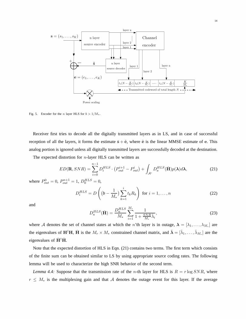
an analog fashion described below. Channel allocation for HLS is illustrated in Fig. 3(b).

Let s ∈ CK be the reconstruction of the sources upon successful reception of all the digital layers.

We denote the reconstruction error ase ∈ CK wheree = s − s. This error is mapped to the transmit

antennas where each component of the error vector is transmitted without coding in an analog fashion,

just by scaling within the power constraint. Sincerank(H) ≤ M∗, degrees of freedom of the channel is

at mostM∗ at each channel use. Hence, at each channel use we utilizeM∗ of the Mt transmit antennas

and inK/M∗ channel uses we transmit allK components of the error vectore. HLS encoder is shown

in Fig. 5.

14

layer 1

layer 2

layer n

n layer

source encoder

s = (s1, . . . , sK)

−

+n layer

source decoder

e = (e1, . . . , eK)

Channel

encoder

t1(N −

K

M∗

) t2(N −

K

M∗

) tn(N −

K

M∗

)K

M∗

layer 1

layer 2

layer n

Power scaling

s

Transmitted codeword of total length N

Fig. 5. Encoder for then layer HLS forb > 1/M∗.

Receiver first tries to decode all the digitally transmittedlayers as in LS, and in case of successful

reception of all the layers, it forms the estimates + e, wheree is the linear MMSE estimate ofe. This

analog portion is ignored unless all digitally transmittedlayers are successfully decoded at the destination.

The expected distortion forn-layer HLS can be written as

ED(R, SNR) =

n−1∑

i=0

DHLSi ·

(P i+1

out − P iout

)+

∫

Ac

DHLSa (H)p(λ)dλ, (21)

whereP 0out = 0, Pn+1

out = 1, DHLS0 = 0,

DHLSi = D

(

(b−

1

M∗

)i∑

k=1

tkRk

)

for i = 1, . . . , n (22)

and

DHLSa (H) =

DHLSn

M∗

M∗∑

i=1

1

1 + SNRM∗

λi

, (23)

whereA denotes the set of channel states at which then’th layer is in outage,λ = [λ1, . . . , λM∗] are

the eigenvalues ofH†H, H is theMr × M∗ constrained channel matrix, andλ = [λ1, . . . , λM∗] are the

eigenvalues ofH†H.

Note that the expected distortion of HLS in Eqn. (21) contains two terms. The first term which consists

of the finite sum can be obtained similar to LS by using appropriate source coding rates. The following

lemma will be used to characterize the high SNR behavior of the second term.

Lemma 4.4:Suppose that the transmission rate of then-th layer for HLS isR = r log SNR, where

r ≤ M∗ is the multiplexing gain and thatA denotes the outage event for this layer. If the average

15

signal-to-noise ratio for the analog part isSNR, we have∫

Ac

1

M∗

M∗∑

i=1

1

1 + SNRM∗

λi

p(λ)dλ ≤ SNR−1. (24)

Proof: Proof of the lemma can be found in Appendix IV.

Then the second term of the expected distortion in (21) can beshown to be exponentially less than or

equal to

SNR−

h

1+(b− 1

M∗)

P

n

k=1tk

i

. (25)

Note that at high SNR, both LS and HLS have very similar ED expressions. Assuming the worst SNR

exponent for the second term, the high SNR approximation of Eqn. (21) can be written as in Eqn. (15),

except for the following: i) the bandwidth ratiob in (15) is replaced byb − 1M∗

, and ii) then-th term

in (15) is replaced by (25). Hence, for a given time allocation vectort, we obtain the following set of

equations for the optimal multiplexing gain allocation:

1 +

(

b −1

M∗

)

tnrn = d∗(rn), (26)

d∗(rn) +

(

b −1

M∗

)

tn−1rn−1 = d∗(rn−1), (27)

. . .

d∗(r2) +

(

b −1

M∗

)

t1r1 = d∗(r1), (28)

where the corresponding distortion exponent is again∆HLSn = d∗(r1). Similar to LS, this formulation

enables us to obtain an explicit formulation of the distortion exponent of infinite layer HLS using the

DMT curve. For brevity we omit the general MIMO HLS distortion exponent and only give the expression

for 2 × 2 MIMO and general MISO/SIMO systems for comparison.

Corollary 4.5: For 2× 2 MIMO, HLS distortion exponent with infinite layers forb ≥ 1/2 is given by

∆HLS = 1 + 3[1 − e−1

3(b− 1

2)].

Corollary 4.6: For a MISO/SIMO system utilizing HLS, we have (forb ≥ 1)

∆HLSMISO/SIMO = M∗ − (M∗ − 1)e−(b−1)/M∗

. (29)

Proof: For MISO/SIMO, we haveM∗ = 1. For n layer HLS with equal time allocation, using

Lemma 3.1 in Appendix III we obtain the distortion exponent

∆HLSMISO/SIMO,n = M∗ − (M∗ − 1)

(

1

1 + b−1nM∗

)n

. (30)

Since equal channel allocation in the limit of infinite layers is optimal, taking the limit asn → ∞, we

obtain (29).

16

Comparing∆HLSMISO/SIMO with ∆LS

MISO/SIMO in Corollary 4.3, we observe that

∆HLSMISO/SIMO − ∆LS

MISO/SIMO = e−b/M∗

[M∗ − (M∗ − 1)e1/M∗

]. (31)

For a given MISO/SIMO system with a fixed number ofM∗ antennas, the improvement of HLS

over LS exponentially decays to zero as the bandwidth ratio increases. Since we haveb ≥ 1/M∗,

the biggest improvement of HLS compared to LS is achieved when b = 1/M∗ = 1, and is equal to

e−1/M∗

[M∗ − (M∗ − 1)e1/M∗

]. This is a decreasing function ofM∗, and achieves its highest value at

M∗ = 1, i.e., SISO system, atb = 1, and is equal to1/e. Illustration of∆HLS for some specific examples

as well as a comparison with the upper bound and other strategies is left to Section VII.

V. BROADCAST STRATEGY WITH LAYERED SOURCE (BS)

In this section we consider superimposing multiple source layers rather than sending them successively

in time. We observe that this leads to higher distortion exponent than LS and HLS, and is in fact optimal

in certain cases. This strategy will be called ‘broadcast strategy with layered source’ (BS).

BS combines broadcasting ideas of [24] -[27] with layered source coding. Similar to LS, source

information is sent in layers, where each layer consists of the successive refinement information for

the previous layers. As in Section IV we enumerate the layersfrom 1 to n such that theith layer is the

successive refinement layer for the precedingi−1 layers. The codes corresponding to different layers are

superimposed, assigned different power levels and sent simultaneously throughout the whole transmission

block. Compared to LS, interference among different layersis traded off for increased multiplexing gain

for each layer. We consider successive decoding at the receiver, where the layers are decoded in order

from 1 to n and the decoded codewords are subtracted from the received signal.

Similar to Section IV we limit our analysis to single block fading (L = 1) scenario and leave the

discussion of the multiple block case to Section VI. We first state the general optimization problem

for arbitrary SNR and then study the high SNR behavior. LetR = [R1, R2, . . . , Rn]T be the vector of

channel coding rates, which corresponds to a source coding rate vector ofbR as each code is spread

over the wholeN channel uses. LetSNR = [SNR1, . . . , SNRn]T denote the power allocation vector

for these layers with∑n

i=1 SNRi = SNR. Fig. 3(c) illustrates the channel and power allocation forBS.

For i = 1, . . . , n we define

SNRi =n∑

j=i

SNRj . (32)

The received signal overN channel uses can be written as

Y = H

n∑

i=1

√

SNRi

MtXi + Z, (33)

17

whereZ ∈ CMr×N is the additive complex Gaussian noise. We assume eachXi ∈ CMt×N is generated

from i.i.d. Gaussian codebooks satisfyingtr(E[XiX†i ]) ≤ MtN . Here

√SNRi

MtXi carries information for

the i-th source coding layer. Fork = 1, . . . , n, we define

Xk =n∑

j=k

√

SNRj

MtXj , (34)

and

Yk = HXk + Z. (35)

Note thatYk is the remaining signal at the receiver after decoding and subtracting the firstk− 1 layers.

DenotingI(Yk;Xk) as the mutual information betweenYk andXk, we can define the following outage

events,

Ak = {H : I(Yk;Xk) < Rk} , (36)

Bk =k⋃

i=1

Ai, (37)

and the corresponding outage probabilities

P kout = Pr {H : H ∈ Ak} , (38)

P kout = Pr {H : H ∈ Bk} . (39)

We note thatP kout denotes the probability of outage for layerk given that the decoder already has access

to the previousk − 1 layers. On the other hand,P kout is the overall outage probability of layerk in

case of successive decoding, where we assume that if layerk cannot be decoded, then the receiver will

not attempt to decode the subsequent layersi > k. Then the expected distortion forn-layer BS using

successive decoding can be written as

ED(R,SNR) =

n∑

i=0

DBSi (P i+1

out − P iout), (40)

where

DBSi = D

(

bi∑

k=1

Rk

)

,

P 0out = 0, Pn+1

out = 1, andDBS0 = 1. Various algorithms solving this optimization problem areproposed

in [15],[18]-[22].

The following definition will be useful in characterizing the distortion exponent of BS.

Definition 5.1: The ‘successive decoding diversity gain’ for layer k of the BS strategy is defined as

the high SNR exponent of the outage probability of that layerusing successive decoding at the receiver.

18

The successive decoding diversity gain can be written as

dsd(rk) , − limSNR→∞

log P kout

log SNR

Note that the successive decoding diversity gain for layerk depends on the power and multiplexing gain

allocation for layers1, . . . , k − 1 as well as layerk itself. However, we drop the dependence on the

previous layers for simplicity.

For any communication system with DMT characterized byd∗(r), the successive decoding diversity

gain for layerk satisfiesdsd(rk) ≤ d∗(r1 + . . . + rk). Concurrent work by Diggavi and Tse [28], coins

the term ‘successive refinability of the DMT curve’ when this inequality is satisfied with equality, i.e.

multiple layers of information simultaneously operate on the DMT curve of the system. Our work, carried

out independently, illustrates that combining successiverefinability of the source and the successive

refinability of the DMT curve leads to an optimal distortion exponent in certain cases.

From (40), we can write the high SNR approximation forED as below.

ED.=

n∑

i=0

P i+1out DBS

i ,

.=

n∑

i=0

SNR−dsd(ri+1)SNR−bP

i

j=1rj . (41)

Then the distortion exponent is given by

∆BSn = min

0≤i≤n

dsd(ri+1) + b

i∑

j=1

rj

. (42)

Note that, while the DMT curve for a given system is enough to find the corresponding distortion exponent

for LS and HLS, in the case of BS, we need the successive decoding DMT curve.

Next, we propose a power allocation among layers for a given multiplexing gain vector. For a general

Mt×Mr MIMO system, we consider multiplexing gain vectorsr = [r1, . . . , rn]such thatr1 + · · ·+rn ≤

1. This constraint ensures that we obtain an increasing and nonzero sequence of outage probabilities

{P kout}

nk=1. We impose the following power allocation among the layers:

SNRk = SNR1−(r1+···+rk−1+ǫk−1), (43)

for k = 2, . . . , n and0 < ǫ1 < · · · < ǫn−1.

Our next theorem computes the successive decoding diversity gain obtained with the above power

allocation. We will see that the proposed power allocation scheme results in successive refinement of

the DMT curve for MISO/SIMO systems. By optimizing the multiplexing gainr we will show that the

optimal distortion exponent for MISO/SIMO meets the distortion exponent upper bound.

19

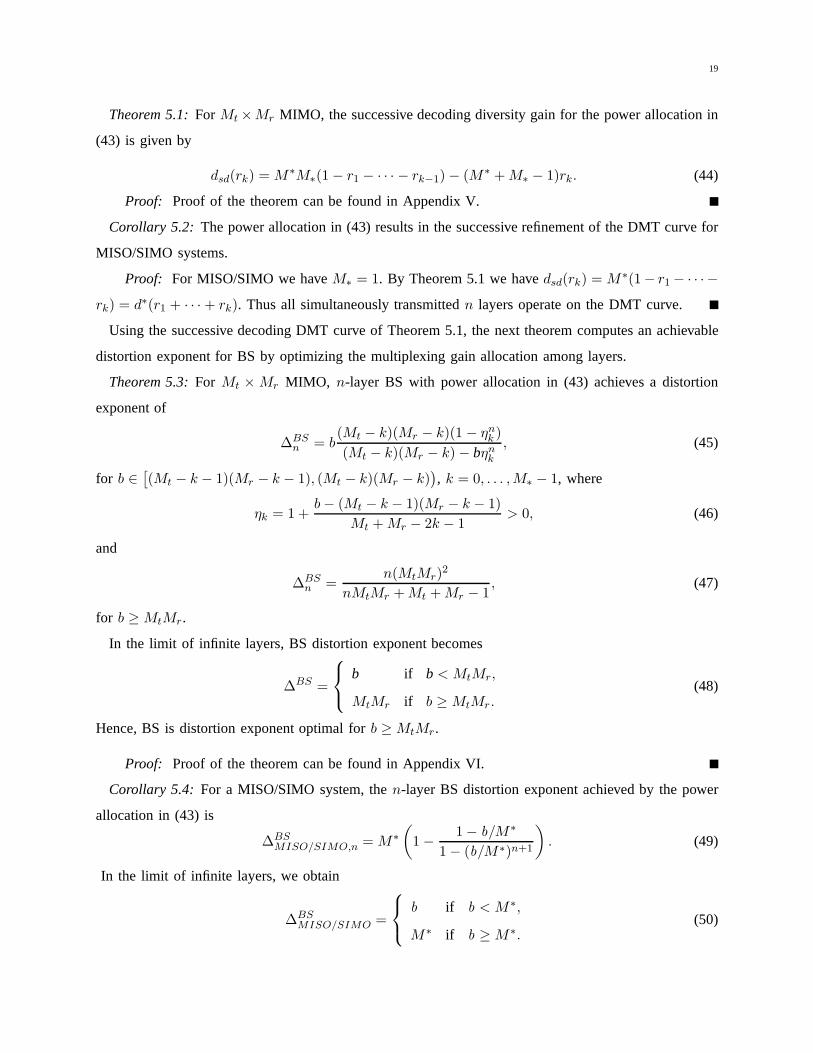
Theorem 5.1:For Mt ×Mr MIMO, the successive decoding diversity gain for the power allocation in

(43) is given by

dsd(rk) = M∗M∗(1 − r1 − · · · − rk−1) − (M∗ + M∗ − 1)rk. (44)

Proof: Proof of the theorem can be found in Appendix V.

Corollary 5.2: The power allocation in (43) results in the successive refinement of the DMT curve for

MISO/SIMO systems.

Proof: For MISO/SIMO we haveM∗ = 1. By Theorem 5.1 we havedsd(rk) = M∗(1− r1 − · · · −

rk) = d∗(r1 + · · · + rk). Thus all simultaneously transmittedn layers operate on the DMT curve.

Using the successive decoding DMT curve of Theorem 5.1, the next theorem computes an achievable

distortion exponent for BS by optimizing the multiplexing gain allocation among layers.

Theorem 5.3:For Mt × Mr MIMO, n-layer BS with power allocation in (43) achieves a distortion

exponent of

∆BSn = b

(Mt − k)(Mr − k)(1 − ηnk )

(Mt − k)(Mr − k) − bηnk

, (45)

for b ∈[(Mt − k − 1)(Mr − k − 1), (Mt − k)(Mr − k)

), k = 0, . . . ,M∗ − 1, where

ηk = 1 +b − (Mt − k − 1)(Mr − k − 1)

Mt + Mr − 2k − 1> 0, (46)

and

∆BSn =

n(MtMr)2

nMtMr + Mt + Mr − 1, (47)

for b ≥ MtMr.

In the limit of infinite layers, BS distortion exponent becomes

∆BS =

b if b < MtMr,

MtMr if b ≥ MtMr.(48)

Hence, BS is distortion exponent optimal forb ≥ MtMr.

Proof: Proof of the theorem can be found in Appendix VI.

Corollary 5.4: For a MISO/SIMO system, then-layer BS distortion exponent achieved by the power

allocation in (43) is

∆BSMISO/SIMO,n = M∗

(

1 −1 − b/M∗

1 − (b/M∗)n+1

)

. (49)

In the limit of infinite layers, we obtain

∆BSMISO/SIMO =

b if b < M∗,

M∗ if b ≥ M∗.(50)

20

0 0.5 1 1.5 2 2.5 3 3.5 40

0.1

0.2

0.3

0.4

0.5

0.6

0.7

0.8

0.9

1

SISO, L = 1

Bandwidth ratio, b

Dis

tort

ion

expo

nent

, ∆

Upper boundBS (infinite layers)HLS (1 layer)BS (10 layers)LS (infinite layer)LS (1 layer)

Fig. 6. Distortion exponent vs. bandwidth ratio for SISO channel, L = 1.

BS with infinite source layers meets the distortion exponentupper bound of MISO/SIMO given in (8)

for all bandwidth ratios, hence is optimal. Thus, (50) fullycharacterizes the optimal distortion exponent

for MISO/SIMO systems.

Recently, [12], [13] reported improved BS distortion exponents for general MIMO by a more advanced

power allocation strategy. Also, while a successively refinable DMT would increase the distortion ex-

ponent, we do not know whether it is essential to achieve the distortion exponent upper bound given

in Theorem 3.1. However, successive refinement of general MIMO DMT has not been established [28],

[29].

As in Section IV, the discussion of the results is left to Section VII.

VI. M ULTIPLE BLOCK FADING CHANNEL

In this section, we extend the results forL = 1 to multiple block fading MIMO, i.e.,L > 1. As we

observed throughout the previous sections, the distortionexponent of the system is strongly related to

the maximum diversity gain available over the channel. In the multiple block fading scenario, channel

experiencesL independent fading realizations duringN channel uses, so we haveL times more diversity

as reflected in the DMT of Theorem 2.1. The distortion exponent upper bound in Theorem 3.1 promises a

similar improvement in the distortion exponent for multiple block fading. However, we note that increasing

L improves the upper bound only if the bandwidth ratio is greater than|Mt − Mr| + 1, since the upper

bound is limited by the bandwidth ratio, not the diversity atlow bandwidth ratios.

Following the discussion in Section IV, extension of LS to multiple block fading is straightforward.

21

0 5 10 15 20 25 3010

−4

10−3

10−2

10−1

100

SNR(dB)

Exp

ecte

d di

stor

tion

SISO, L = 1, b = 2

LS, BS (1 layer)LS (2 layers)BS (2 layers)Analog transmissionUpper Bound

Fig. 7. Expected distortion vs. SNR plots forb = 2. The topmost curve LS, BS (1 layer) corresponds to single layer transmission.

As before, each layer of the successive refinement source code should operate on a different point of

the DMT. This requires us to transmit codewords that span allchannel realizations, thus we divide each

fading block amongn layers and transmit the codeword of each layer over itsL portions.

Without going into the details of an explicit derivation of the distortion exponent for the multiple block

fading case, as an example, we find the LS distortion exponentfor 2× 2 MIMO channel withL = 2 as

∆LS =

4(1 − exp(−b/2)) if 0 < b ≤ 2 ln 2,

2 + 6[1 − exp

(−( b

6 − ln 23 ))]

if b > 2 ln 2.(51)

For HLS, the threshold bandwidth ratio1/M∗ is the same as single block fading as it depends on the

channel rank per channel use, not the number of different channel realizations. Forb ≥ 1/M∗, extension

of HLS to multiple blocks can be done similar to LS. As an example, for 2-block Rayleigh fading2× 2

MIMO channel, the optimal distortion exponent of HLS forb ≥ 1/2 is given by

∆HLS =

1 + 3[1 − exp

(−1

2(b− 12))]

if 1/2 ≤ b ≤ 12 + 2 ln 3

2 ,

2 + 6[1 − exp

(−1

6(b− 12 − 2 ln 3

2))]

if b > 12 + 2 ln 3

2 .(52)

For BS over multiple block fading MIMO, we use a generalization of the power allocation introduced

in Section V in (43). ForL-block fading channel and fork = 2, . . . , n let

SNRk = SNR1−L(r1+···+rk−1−ǫk−1), (53)

with 0 < ǫ1 < · · · < ǫn−1 and imposing∑n

i=1 ri ≤ 1/L. Using this power allocation scheme, we obtain

the following distortion exponent for BS overL-block MIMO channel.

22

Theorem 6.1:For L-block Mt ×Mr MIMO, BS with power allocation in (53) achieves the following

distortion exponent in the limit of infinite layers.

∆BS =

b/L if b < L2MtMr,

LMtMr if b ≥ L2MtMr.(54)

This distortion exponent meets the upper bound forb ≥ L2MtMr.

Proof: Proof of the theorem can be found in Appendix VII.

The above generalizations to multiple block fading can be adapted to parallel channels through a scaling

of the bandwidth ratio byL [8]. Note that, in the block fading model, each fading block lasts forN/L

channel uses. However, forL parallel channels with independent fading, each block lasts for N channel

uses instead. Using the power allocation in (43) we can get achievable BS distortion exponent for parallel

channels. We refer the reader to [8] for details and comparison. Detailed discussion and comparison of

the L-block LS, HLS and BS distortion exponents are left to Section VII.

Distortion exponent for parallel channels has also been studied in [2] and [14] both of which consider

source and channel coding for two parallel fading channels.The analysis of [2] is limited to single

layer source coding and multiple description source coding. Both schemes perform worse than the upper

bound in Theorem 3.1 and the achievable strategies presented in this paper. Particularly, the best distortion

exponent achieved in [2] is by single layer source coding andparallel channel coding which is equivalent to

LS with one layer. In [14], although 2-layer successive refinement and hybrid digital-analog transmission

are considered, parallel channel coding is not used, thus the achievable performance is limited. The hybrid

scheme proposed in [14] is a repetition based scheme and cannot improve the distortion exponent beyond

single layer LS.

VII. D ISCUSSION OF THERESULTS

This section contains a discussion and comparison of all theschemes proposed in this paper and the

upper bound. We first consider the special case of single-input single-output (SISO) system. For a SISO

single block Rayleigh fading channel, the upper bound for optimal distortion exponent in Theorem 3.1

can be written as

∆ =

b if b < 1,

1 if b ≥ 1.(55)

This optimal distortion exponent is achieved by BS in the limit of infinite source coding layers (Corollary

5.2) and by HLS [11]. In HLS, pure analog transmission is enough to reach the upper bound whenb ≥ 1

[6], while the hybrid scheme of [11] achieves the optimal distortion exponent forb < 1.

23

0 1 2 3 4 50

0.5

1

1.5

2

2.5

3

3.5

4

Bandwidth ratio, b

Dis

tort

ion

expo

nent

, ∆

Mt = 4, M

r = 1, L = 1

Upper boundBS (infinite layers)HLS (infinite layers)LS (infinite layers)HLS (1 layer)LS/BS (1 layer)

Fig. 8. Distortion exponent vs. bandwidth ratio for4 × 1 MIMO, L = 1.

The distortion exponent vs. bandwidth ratio of the various schemes for the SISO channel,L = 1 are

plotted in Fig. 6. The figure suggests that while BS is optimalin the limit of infinite source layers, even

with 10 layers, the performance is very close to optimal for almost all bandwidth ratios.

For a SISO channel, when the performance measure is the expected channel rate, most of the im-

provement provided by the broadcast strategy can be obtained with two layers [30]. However, our results

show that when the performance measure is the expected end-to-end distortion, increasing the number

of superimposed layers in BS further improves the performance especially for bandwidth ratios close to

1.

In order to illustrate how the suggested source-channel coding techniques perform for arbitrarySNR

values for the SISO channel, in Fig. 7 we plot the expected distortion vs. SNR for single layer

transmission (LS, BS with 1 layer), LS and BS with2 layers, analog transmission and the upper bound

for b = 2. The results are obtained from an exhaustive search over allpossible rate, channel and power

allocations. The figure illustrates that the theoretical distortion exponent values that were found as a result

of the highSNR analysis hold, in general, even for moderateSNR values.

In Fig. 8, we plot the distortion exponent versus bandwidth ratio of 4 × 1 MIMO single block

fading channel for different source-channel strategies discussed in Section IV-V as well as the upper

bound. As stated in Corollary 5.2, the distortion exponent of BS coincides with the upper bound for all

bandwidth ratios. We observe that HLS is optimal up to a bandwidth ratio of 1. This is attractive for

practical applications since only a single coded layer is used, while BS requires many more layers to be

superimposed. However, the performance of HLS degrades significantly beyondb = 1, making BS more

24

0 1 2 3 4 50

0.5

1

1.5

2

2.5

3

3.5

4

Bandwidth ratio, b

Dis

tort

ion

expo

nent

, ∆

Mt = 2, M

r = 2, L = 1

Upper boundBS (infinite layers)HLS (infinite layers)LS (infinite layers)HLS (1 layer)LS (1 layer)

Fig. 9. Distortion exponent vs. bandwidth ratio for2 × 2 MIMO, L = 1.

0 2 4 6 8 10 12 14 16 180

1

2

3

4

5

6

7

8

Bandwidth ratio, b

Dis

tort

ion

expo

nent

, ∆

2−block 2x2 MIMO channel

Upper boundBS (infinite layers)HLS (infinite layers)LS (infinite layers)LS (1 layer)

Fig. 10. Distortion exponent vs. bandwidth ratio for 2x2 MIMO, L = 2.

advantageous in this region. Pure analog transmission of the source samples would still be limited to a

distortion exponent of1 as in SISO, since linear encoding/decoding can not utilize the diversity gain of

the system. More advanced nonlinear analog schemes which would take advantage of the diversity gain

and achieve an improved distortion exponent may be worth exploring. While LS does not require any

superposition or power allocation among layers, and only uses a digital encoder/decoder pair which can

transmit at variable rates, the performance is far below BS.Nevertheless, the improvement of infinite

layer LS compared to a single layer strategy is significant.

We plot the distortion exponent versus bandwidth ratio for2 × 2 MIMO with L = 1 in Fig. 9. We

25

observe that BS is optimal forb ≥ 4 and provides the best distortion exponent forb > 2.4. For bandwidth

ratios1/2 < b < 4, none of the strategies discussed in this paper achieves theupper bound.

Note that, both for4× 1 MISO and2× 2 MIMO, when b ≥ 1/M∗ the gain due to the analog portion,

i.e., gain of HLS compared to LS, is more significant for one layer and decreases as the number of layers

goes to infinity. Furthermore, at any fixed number of layers, this gain decays to zero with increasing

bandwidth ratio as well. We conclude that for general MIMO systems, when the bandwidth ratio is

high, layered digital transmission with large number of layers results in the largest improvement in the

distortion exponent.

In Figure 10 we plot the distortion exponent for a2-block 2 × 2 MIMO channel. We observe that

the improvement of HLS over LS, both operating with infinite number of layers, is even less significant

than the single block case. However, HLS can still achieve the optimal distortion exponent forb < 1/2.

Although BS is optimal forb ≥ L2MtMr = 16, both this threshold ofL2MtMr and the gap between

the upper bound and BS performance below this threshold increases asL increases.

VIII. G ENERALIZATION TO OTHER SOURCES

Throughout this paper, we have used a complex Gaussian source for clarity of the presentation. This

assumption enabled us to use the known distortion-rate function and to utilize the successive refinable

nature of the complex Gaussian source. In this section we argue that our results hold for any memoryless

source with finite differential entropy and finite second moment under squared-error distortion.

Although it is hard to explicitly obtain the rate-distortion function of general stationary sources, lower

and upper bounds exist. Under the mean-square error distortion criteria, the rate-distortion functionR(D)

of any stationary continuous amplitude sourceX is bounded as [31]

RL(D) ≤ R(D) ≤ RG(D), (56)

whereRL(D) is the Shannon lower bound andRG(D) is the rate-distortion function of the complex

Gaussian source with the same real and imaginary variances.

Further in [32] it is shown that the Shannon lower bound is tight in the low distortion(D → 0), or,

the high rate(R → ∞) limit when the source has a finite moment and finite differential entropy. We

have

limR→∞

D(R) −e2h(X)

2πe2−R = 0. (57)

The high rate approximation of the distortion-rate function can be written asD(R) = 2−R+O(1), where

O(1) term depends on the source distribution but otherwise independent of the compression rate. Since in

our distortion exponent analysis we consider scaling of thetransmission rate, hence the source coding rate,

26

logarithmically with increasing SNR, the high resolution approximations are valid for our investigation.

Furthermore theO(1) terms in the above distortion-rate functions do not change our results since we are

only interested in the SNR exponent of the distortion-rate function.

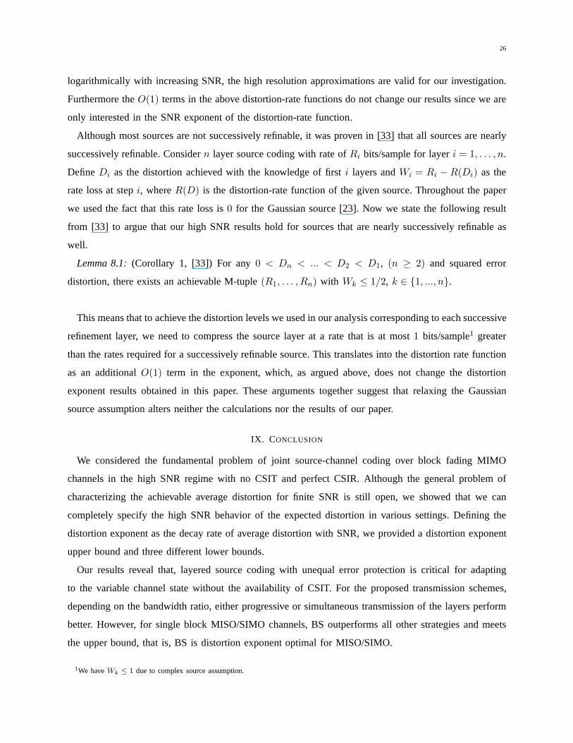
Although most sources are not successively refinable, it wasproven in [33] that all sources are nearly

successively refinable. Considern layer source coding with rate ofRi bits/sample for layeri = 1, . . . , n.

DefineDi as the distortion achieved with the knowledge of firsti layers andWi = Ri − R(Di) as the

rate loss at stepi, whereR(D) is the distortion-rate function of the given source. Throughout the paper

we used the fact that this rate loss is0 for the Gaussian source [23]. Now we state the following result

from [33] to argue that our high SNR results hold for sources that are nearly successively refinable as

well.

Lemma 8.1:(Corollary 1, [33]) For any0 < Dn < ... < D2 < D1, (n ≥ 2) and squared error

distortion, there exists an achievable M-tuple(R1, . . . , Rn) with Wk ≤ 1/2, k ∈ {1, ..., n}.

This means that to achieve the distortion levels we used in our analysis corresponding to each successive

refinement layer, we need to compress the source layer at a rate that is at most1 bits/sample1 greater

than the rates required for a successively refinable source.This translates into the distortion rate function

as an additionalO(1) term in the exponent, which, as argued above, does not changethe distortion

exponent results obtained in this paper. These arguments together suggest that relaxing the Gaussian

source assumption alters neither the calculations nor the results of our paper.

IX. CONCLUSION

We considered the fundamental problem of joint source-channel coding over block fading MIMO

channels in the high SNR regime with no CSIT and perfect CSIR.Although the general problem of

characterizing the achievable average distortion for finite SNR is still open, we showed that we can

completely specify the high SNR behavior of the expected distortion in various settings. Defining the

distortion exponent as the decay rate of average distortionwith SNR, we provided a distortion exponent

upper bound and three different lower bounds.

Our results reveal that, layered source coding with unequalerror protection is critical for adapting

to the variable channel state without the availability of CSIT. For the proposed transmission schemes,

depending on the bandwidth ratio, either progressive or simultaneous transmission of the layers perform

better. However, for single block MISO/SIMO channels, BS outperforms all other strategies and meets

the upper bound, that is, BS is distortion exponent optimal for MISO/SIMO.

1We haveWk ≤ 1 due to complex source assumption.

27

APPENDIX I

PROOF OFTHEOREM 3.1

Here we find the distortion exponent upper bound under short-term power constraint assuming avail-

ability of the channel state information at the transmitter(CSIT)2. Let C(H) denote the capacity of the

channel with short-term power constraint when CSIT is present. Note thatC(H) depends on the channel

realizationsH1, . . . ,HL. The capacity achieving input distribution at channel realizationHj is Gaussian

with covariance matrixQj. We have

C(H) =1

L

L∑

j=1

supQj�0,

P

L

j=1tr(Qj)≤LMt

log det

(

I +SNR

MtHjQjH

†j

)

,

≤1

L

L∑

j=1

supQj�0,tr(Qj)≤LMt

log det

(

I +SNR

MtHjQjH

†j

)

,

≤1

L

L∑

j=1

log det(I + L · SNRHjH†j), (58)

where the first inequality follows as we expand the search space, and the second inequality follows from

the fact thatLMtI − Qj � 0 when tr(Qj) ≤ LMt and log det(·) is an increasing function on the cone

of positive-definite Hermitian matrices. Then the end-to-end distortion can be lower bounded as

D(H) = 2−bC(H) ≥L∏

j=1

[det(I + L · SNRHjH†j)]

−b/L. (59)

We consider expected distortion, where the expectation is taken over all channel realizations and analyze

its high SNR exponent to find the corresponding distortion exponent. We will follow the technique used

in [1]. Assume without loss of generality thatMt ≥ Mr. Then from Eqn. (59) we have

D(H) ≥L∏

j=1

[det(I + L · SNRHjH†j)]

−b/L, (60)

≥L∏

j=1

Mr∏

i=1

(1 + L · SNRλji)−b/L, (61)

where λj1 ≤ λj1 ≤ · · · ≤ λjMrare the ordered eigenvalues ofHjH

†j for block j = 1, . . . , L. Let

λji = SNR−αji . Then we have(1 + L · SNRλji).= SNR(1−αji)+ .

2We note that a similar upper bound forL = 1 is also given in [11]. We derive it for theL-block channel here for completeness.

28

The joint pdf ofαj = [αj1, . . . , αjMt] for j = 1, . . . , L is

p(αj) = K−1Mt,Mr

(log SNR)Mr

Mr∏

i=1

SNR−(Mt−Mr+1)αji

·

[∏

i<k

(SNRαji − SNRαjk)2

]

exp

(

−Mr∑

i=1

SNRαji

)

, (62)

whereKMt,Mris a normalizing constant. We can write the expected end-to-end distortion as

E[D(H)].=

∫

D(H)p(α1) . . . p(αL)dα1 . . . dαL, (63)

≥

[∫ Mr∏

i=1

(1 + SNRλ1i)−b/Lp(α1)dα1

]L

, (64)

where we used the fact thatαj ’s are i.i.d. forj = 1, . . . , L and that the constant multiplicative term in

front of SNR does not affect the exponential behavior. Sincewe are interested in the distortion exponent,

we only need to consider the exponents of SNR terms. Following the same arguments as in [1] we can

make the following simplifications.∫ Mr∏

i=1

(1 + SNRλ1i)−b/Lp(α1)dα1

.=

∫

Rn+

Mr∏

i=1

(1 + SNR1−α1i)−b/L

·Mr∏

i=1

SNR−(Mt−Mr+1)α1i ·∏

i<k

(SNR−α1i − SNR−α1k)2dα1.

.=

∫

Rn+

Mr∏

i=1

SNR− b

L(1−α1i)+

Mr∏

i=1

SNR−(2i−1+Mt−Mr)α1idα1.

.=

∫

Rn+

Mr∏

i=1

SNR−(2i−1+Mt−Mr)α1i−bL

(1−αi)+dα,

.= SNR−∆1

Again following the arguments of the proof of Theorem 4 in [1], we have

∆1 = infα∈Rn+

Mr∑

i=1

(2i − 1 + Mt − Mr)α1i +bL

(1 − α1i)+. (65)

The minimizingα1 can be found as

α1i =

0 if b

L < 2i − 1 + Mt − Mr

1 if b

L ≥ 2i − 1 + Mt − Mr.

(66)

Letting E[D(H)]≥SNR−∆UB

, we have∆UB = L∆1, and

∆UB = L

Mr∑

i=1

min

{b

L, 2i − 1 + Mt − Mr

}

. (67)

Similar arguments can be made for theMt < Mr case, completing the proof.

29

APPENDIX II

PROOF OFLEMMA 4.1

Let t∗ be the optimal channel allocation vector andr∗ be the optimal multiplexing gain vector forn

layers. For anyε > 0 we can findt with ti ∈ Q and∑n

i=1 ti = 1 where |t∗i − ti| < ε. Let ti = γi/ρi

where γi ∈ Z, ρi ∈ Z and θ = LCM(ρ1, . . . , ρn) is the least common multiple ofρ1, . . . , ρn. Now

consider the channel allocationt = [1/θ, . . . , 1/θ]T , which divides the channel intoθ equal portions and

the multiplexing gain vector

r = [r∗1, . . . , r∗1

︸ ︷︷ ︸

θt1 times

, r∗2 , . . . , r∗2

︸ ︷︷ ︸

θt2 times

, . . . , r∗n, . . . , r∗n︸ ︷︷ ︸

θtn times

]T (68)

Due to the continuity of the outage probability and the distortion-rate function, this allocation which

consists ofθn layers achieves a distortion exponent arbitrarily close tothen-layer optimal one asε → 0.

Note that{∆LSn }∞n=1 is a non-decreasing sequence since withn layers it is always possible to assign

tn = 0 and achieve the optimal performance ofn − 1 layers. On the other hand, using Theorem 3.1,

it is easy to see that{∆LSn } is upper bounded byd∗(0), hence its limit exists. We denote this limit by

∆LS . If we define∆LSn as the distortion exponent ofn-layer LS with equal channel allocation, we have

∆LSn ≤ ∆LS

n . On the other hand, using the above arguments, for anyn there existsm ≥ n such that

∆LSm ≥ ∆LS

n . Thus we conclude that

limn→∞

∆LSn = lim

n→∞∆LS

n = ∆LS

Consequently, in the limit of infinite layers, it is sufficient to consider only the channel allocations that

divide the channel equally among the layers.

APPENDIX III

PROOF OFTHEOREM 4.2

We will use geometric arguments to prove the theorem. Using Lemma 4.1, we assume equal channel

allocation, that is,t = [ 1n , . . . , 1

n ]. We start with the following lemma.

Lemma 3.1:Let l be a line with the equationy = −α(x −M) for someα > 0 andM > 0 and letli

for i = 1, . . . , n be the set of lines defined recursively fromn to 1 asy = (b/n)x + di+1, whereb > 0,

dn+1 = 0 anddi is they−component of the intersection ofli with l . Then we have

d1 = Mα

[

1 −

(α

α + b/n

)n]

. (69)

with

limn→∞

d1 = Mα(

1 − e−b/α)

. (70)

30

r

d∗(r)

M∗ − i

slope=|Mr − Mt| + 2i − 1

|Mr − Mt| + 2i − 1

M∗ − i + 1

Fig. 11. DMT curve of anMt × Mr MIMO system is composed ofM∗ = min{Mt, Mr} line segments, of which thei’th one is shown in

the figure.

Proof: If we solve for the intersection points sequentially we easily find

dk − dk+1 = Mb

n

(α

α + b/n

)n−k+1

, (71)

for k = 1, . . . , n, wheredn+1 = 0. Summing up these terms, we get

dk = Mα

[

1 −

(α

α + b/n

)n−k+1]

. (72)

In the case of a DMT curve composed of a single line segment, i.e., M∗ = 1, using Lemma 3.1 we

can find the distortion exponent in the limit of infinite layers by lettingM = 1 andα = M∗. However,

for a generalMt × Mr MIMO system the tradeoff curve is composed ofM∗ line segments where the

ith segment has slope|Mr −Mt|+ 2i− 1, and abscissae of the end pointsM∗ − i andM∗ − i + 1 as in

Fig. 11. In this case, we should consider climbing on each line segment separately, one after another in

the manner described in Lemma 3.1 and illustrated in Fig. 4. Then, each break point of the DMT curve

corresponds to a threshold onb, such that it is possible to climb beyond a break point only ifb is larger

than the corresponding threshold.

Now let M = M∗ − i + 1, α = |Mr −Mt|+ 2i− 1 in Lemma 3.1 and in the limit ofn → ∞, let kin

be the number of lines with slopesb/n such that we havedn = |Mr −Mt|+ 2i− 1. Using the limiting

form of Eqn. (72) we can find that

ki =|Mr − Mt| + 2i − 1

bln

(M∗ − i + 1

M∗ − i

)

. (73)

31

This gives us the proportion of the lines that climb up thepth segment of the DMT curve. In the general

MIMO case, to be able to go up exactly to thepth line segment, we need to have∑p−1

j=1 kj < 1 ≤∑p

j=1 kj .

This is equivalent to the requirementcp−1 < b ≤ cp in the theorem.

To climb up each line segment, we needkin lines (layers) fori = 1, . . . , p−1, and for the last segment

we have(1 −∑p−1

j=1 kj)n lines, which gives us an extra ascent of

(M∗ − p + 1)(|Mr − Mt| + 2p − 1)(1 − e−

bkp

|Mr−Mt|+2p−1 )

on the tradeoff curve. Hence the optimal distortion exponent, i.e., the total ascent on the DMT curve,

depends on the bandwidth ratio and is given by Theorem 4.2.

APPENDIX IV

PROOF OFLEMMA 4.4

As in the proof of Theorem 3.1 in Appendix I, we letλi = SNR−αi and λi = SNR−βi for i =

1, . . . ,M∗. The probability densities ofλ and λ and their exponentsα andβ are given in Appendix I.

Note that sinceH is a submatrix ofH, λ and λ as well asα andβ are correlated. Letp(α, β) be the

joint probability density ofα andβ. If Mt ≤ Mr, H andH coincide andλ = λ, α = β.

We can write∫

α∈Ac

1

M∗

M∗∑

i=1

1

1 + SNRM∗

λi

p(λ)dλ.=

∫

α∈Ac

M∗∑

i=1

SNR−(1−βi)+p(α)dα, (74)

.=

∫

α∈Ac

SNR−(1−βmax)+p(α)dα, (75)

.=

∫

α∈Ac

SNR−(1−βmax)+∫

βp(α,β)dβdα, (76)

.=

∫

βSNR−(1−βmax)+

∫

α∈Ac

p(α,β)dαdβ, (77)

≤

∫

βSNR−(1−βmax)+p(β)dβ, (78)

.= SNR−µ, (79)

where

µ = infβ∈RM∗+

(1 − βmax)+ +M∗∑

i=1

(2i − 1)βi. (80)

The minimizingβ satisfiesβ1 ∈ [0, 1] and β2 = · · · = βM∗= 0, and we haveµ = 1.

32

APPENDIX V

PROOF OFTHEOREM 5.1

The mutual information betweenYk andXk defined in (35) can be written as

I(Yk;Xk) = I(Yk;Xk, Xk+1) − I(Yk; Xk+1|Xk), (81)

= log det

(

I +SNRk

MtHH†

)

− log det

(

I +SNRk+1

MtHH†

)

,

= logdet(

I + SNRk

MtHH†

)

det(

I + SNRk+1

MtHH†

) . (82)

For layersk = 1, . . . , n − 1, and the multiplexing gain vectorr we have

P kout = Pr

H : log

det(

I + SNRk

MtHH†

)

det(

I + SNRk+1

MtHH†

) < rk log SNR

= Pr

H :

∏M∗

i=1(1 + SNRk

Mtλi)

∏M∗

i=1(1 + SNRk+1

Mtλi)

< SNRrk

, (83)

and

Pnout =

{

H :

M∗∏

i=1

(

1 +SNRn

Mtλi

)

< SNRrn

}

. (84)

where λ1 ≤ λ2 ≤ · · · ≤ λM∗are the eigenvalues ofHH† (H†H) for Mt ≥ Mr (Mt < Mr). Let

λi = SNR−αi . Then for the power allocation in (43), conditions in Eqn. (83) and Eqn. (84) are,

respectively, equivalent to

M∗∑

i=1

(1 − r1 − · · · − rk−1 − ǫk−1 − αi)+ −

M∗∑

i=1

(1 − r1 − · · · − rk − ǫk − αi)+ < rk,

andM∗∑

i=1

(1 − r1 − · · · − rn−1 − ǫn−1 − αi)+ < rn.

Using Laplace’s method and following the similar argumentsas in the proof of Theorem 4 in [1] we

show that, fork = 1, . . . , n,

P kout

.= SNR−dk , (85)

where

dk = infα∈Ak

M∗∑

i=1

(|Mt − Mr| + 2i − 1) αi. (86)

For k = 1, . . . , n − 1

33

Ak =

{

α = [α1, . . . , αM∗] ∈ RM∗+ : α1 ≥ · · · ≥ αM∗

≥ 0,

∑M∗

i=1(1 − r1 − · · · − rk−1 − ǫk−1 − αi)+ −

∑M∗

i=1(1 − r1 − · · · − rk − ǫk − αi)+ < rk

}

.

whileAn = { α = [α1, . . . , αM∗

] ∈ RM∗+ : α1 ≥ · · · ≥ αM∗≥ 0,

∑M∗

i=1 (1 − r1 − · · · − rn−1 − ǫn−1 − αi)+ < rn}.

The minimizingα for each layer can be explicitly found as

αi = 1 − r1 − · · · − rk−1 − ǫk−1, for i = 1, . . . ,M∗ − 1,

and

αM∗= 1 − r1 − · · · − rk−1 − rk − ǫk−1.

Letting ǫk → 0 for k = 1, . . . , n − 1, we have

dk = M∗M∗(1 − r1 − · · · − rk−1) − (M∗ + M∗ − 1)rk. (87)

Note that the constraint∑n

i=1 ri ≤ 1 makes the sequence{1−r1−· · ·−rk}nk=1 decreasing and greater

than zero. ThusP kout constitutes an increasing sequence. Therefore, using (37)and (39), in the high SNR

regime we haveP kout

.= P k

out, anddsd(rk) = dk.

APPENDIX VI

PROOF OFTHEOREM 5.3

Using the formulation of∆BSn in (41) and successive decoding diversity gains of the proposed power

allocation in Theorem 5.1, we find the multiplexing gain allocation that results in equal SNR exponents

for all the terms in (41).

We first consider the caseb ≥ (Mt − 1)(Mr − 1). Let

η0 =b− (Mt − 1)(Mr − 1)

Mt + Mr − 1≥ 0. (88)

For 0 ≤ η0 < 1, we set

r1 =MtMr(1 − η0)

MtMr − bηn0

, (89)

ri = ηi−10 r1, for i = 2, . . . , n. (90)

If η0 ≥ 1, we set

r1 = · · · = rn =MtMr

nMtMr + Mt + Mr − 1. (91)

34

Next, we show that the above multiplexing gain assignment satisfies the constraint∑n

i=1 ri ≤ 1. For

η0 < 1, b ≤ MtMr and

r1 + · · · + rn = r1

(1 + η0 + · · · + ηn−1

0

),

=MtMr(1 − ηn

0 )

MtMr − bηn0

,

≤ 1. (92)

On the other hand, whenη0 ≥ 1, we have∑n

i=1 ri = nMtMr

nMtMr+Mt+Mr−1 < 1.

Then the corresponding distortion exponent can be found as

∆BSn =

bMtMr(1−ηn0 )

MtMr−bηn0

if (Mt − 1)(Mr − 1) ≤ b < MtMr,

n(MtMr)2

nMtMr+Mt+Mr−1 if b ≥ MtMr.(93)

For (Mt − k − 1)(Mr − k − 1) ≤ b < (Mt − k)(Mr − k), k = 1, . . . ,M∗ − 1, we can consider the

(Mt − k) × (Mr − k) antenna system and following the same steps as above, we obtain a distortion

exponent of

b(Mt − k)(Mr − k)(1 − ηn

k )

(Mt − k)(Mr − k) − bηnk

,

whereηk is defined in (46).

In the limit of infinite layers, it is possible to prove that this distortion exponent converges to the

following.

∆BS = limn→∞

∆BSn =

b if 0 ≤ b < MtMr,

MtMr if b ≥ MtMr.(94)

APPENDIX VII

PROOF OFTHEOREM 6.1

We transmit codewords of each layer across all fading blocks, which means thatP kout in Eqn. (83)

becomes

P kout = Pr

(H1, . . . ,HL) :

1

L

L∑

i=1

logdet(

I + SNRk

MtHiH

†i

)

det(

I + SNRk+1

MtHiH

†i

) < rk log SNR

,

for k = 1, . . . , n − 1, andPnout can be defined similarly.

For the power allocation in (53), above outage event is equivalent toL∑

j=1

M∗∑

i=1

(1 − Lr1 − · · · − Lrk−1 − Lǫk−1 − αj,i)+ − (1 − Lr1 − · · · − Lrk − Lǫk − αj,i)

+ < Lrk.

Following the same steps as in the proof of Theorem 5.1, we have

P kout

.= SNR−dk , (95)

35

where

dk = infα∈Ak

L∑

j=1

M∗∑

i=1

(|Mt − Mr| + 2i − 1) αj,i. (96)

For k = 1, . . . , n − 1

Ak =

{

α = [α1, . . . , αLM∗] ∈ RLM∗+ : αj,1 ≥ · · · ≥ αj,M∗

≥ 0 for j = 1, . . . , L

∑Lj=1

∑M∗

i=1(1 − Lr1 − · · · − Lrk−1 − Lǫk−1 − αj,i)+

−(1 − Lr1 − · · · − Lrk − Lǫk − αj,i)+ < Lrk

}

.

The minimizingα for each layer can be explicitly found as

αj,i = 1 − Lr1 − · · · − Lrk−1 − Lǫk−1, for j = 1, . . . , L, and i = 1, . . . ,M∗ − 1,

and

αj,M∗= 1 − Lr1 − · · · − Lrk−1 − rk − Lǫk−1, for j = 1, . . . , L.

Then, lettingǫn−1 → 0, the diversity gaindk is obtained as

dk = L

[

M∗M∗(1 − Lr1 − · · · − Lrk−1) − (M∗ + M∗ − 1)rk

]

. (97)

We skip the rest of the proof as it closely resembles the proofof Theorem 5.3 in Appendix VI.

REFERENCES

[1] L. Zheng, D. Tse, “Diversity and multiplexing: A fundamental tradeoff in multiple antenna channels,” IEEE Transactions on Information

Theory, May 2003.

[2] J. N. Laneman, E. Martinian, G. W. Wornell, and J. G. Apostolopoulos, “Source-Channel Diversity for Parallel Channels,” IEEE Transactions

on Information Theory, vol. 51, no. 10, pp. 3518-3539, Oct. 2005.

[3] D. Gunduz, E. Erkip, “Joint source-channel cooperation: Diversity versus spectral efficiency,” Proceedings of 2004 ISIT, Chicago, June

2004.

[4] D. Gunduz, E. Erkip, “Source and channel coding for cooperative relaying,” Proceedings of SPAWC, New York City, June 2005.

[5] D. Gunduz, E. Erkip, “Source and channel coding for cooperative relaying,”, IEEE Transactions on Information Theory, Special Issue on

Models, Theory and Codes for Relaying and Cooperation in Communication Networks, Oct. 2007.

[6] D. Gunduz, E. Erkip, “Source and channel coding for quasi-static fading channels,” Proceedings of 39th Asilomar Conf., Pacific Grove,

California, November 2005.

[7] D. Gunduz, E. Erkip, “Distortion exponent of MIMO fading channels,” Proceedings of IEEE Information Theory Workshop, Punta del Este,

Uruguay, March 2006.

[8] D. Gunduz, E. Erkip, “Distortion exponent of parallelchannels,” Proceedings of ISIT 2006, Seattle, WA, July 2006.

[9] T. Holliday and A. Goldsmith, “Joint source and channel coding for MIMO systems,” Proc. of Allerton Conference on Communications,

Control, and Computing, Oct. 2004, Allerton, IL.

[10] U. Mittal, N. Phamdo, “Hybrid digital-analog joint source-channel codes for broadcasting and robust communications,” IEEE Transactions

on Information Theory, May 2002.

[11] G. Caire, K. Narayanan , “On the SNR exponent of hybrid digital-analog space time coding,” Proceedings of Allerton Conference, Allerton,

IL, September 2005.

36

[12] K. Bhattad, K. R. Narayanan, G. Caire, “On the distortion exponent of some layered transmission schemes,” AsilomarConference, Nov.

2006.

[13] K. Bhattad, K. R. Narayanan, G. Caire, “On the distortion SNR exponent of some layered transmission schemes,” submitted to IEEE

Transactions on Information Theory.

[14] B. P. Dunn and J. N. Laneman, “Characterizing source-channel diversity approaches beyond the distortion exponent,” in Proc. Allerton

Conf. Communications, Control, and Computing, Monticello, IL, Sept. 2005.

[15] K. Zachariadis, M. L. Honig, A. K. Katsaggelos, “Sourcefidelity over fading channels: Erasure codes versus scalable codes”, submitted

to IEEE Transactions on Communications, July 2006.

[16] S. Sesia, G. Caire, G. Vivier, “Lossy transmission overslow-fading AWGN channels: a comparison of progressive, superposition and

hybrid approaches,” in Proc. of IEEE International Symposium on Information Theory (ISIT), Adelaide, Australia, Sept. 2005. C. Tian,

[17] F. Etemadi, H. Jafarkhani, “Optimal layered transmission over quasi-static fading channels,” Proc. of IEEE International Symposium on

Information Theory (ISIT), Seattle, WA, July 2006.

[18] F. Etemadi, H. Jafarkhani, “Optimal rate and power allocation for layered transmission with superposition coding,” IEEE Data Compression

Conference (DCC ‘07), Salt Lake City, UT, March 2007.

[19] C. T. K. Ng, D. Gunduz, A. J. Goldsmith and E. Erkip, “Minimum expected distortion in Gaussian joint source-channel layered broadcast

coding,” in the Proc. of IEEE International Symposium on Information Theory (ISIT 2007), Nice, France, June 2007.

[20] C. T. K. Ng, D. Gunduz, A. J. Goldsmith and E. Erkip, “Recursive power allocation in Gaussian joint source-channellayered broadcast

coding,” in the Proceedings of IEEE International Conference on Communications (ICC 2007), Glasgow, Scotland, June 2007.

[21] C. T. K. Ng, D. Gunduz, A. J. Goldsmith, and E. Erkip, “Optimal power distribution and minimum expected distortionin Gaussian layered

broadcast coding with successive refinement,” Submitted toIEEE Transactions on Information Theory, May 2007.

[22] C. Tian, A. Steiner, S. Shamai, S. Diggavi, “Expected distortion for Gaussian source with a broadcast transmissionstrategy over a fading

channel,” in Proc. of IEEE Inform. Theory Workshop, Bergen,Norway, Sept. 2007.

[23] W. Equitz, T. Cover, “Successive refinement of information,” IEEE Transactions on Information Theory, 37(2): 269-275, Mar. 1991.

[24] I. Kozintsev, K. Ramchandran, “Multiresolution jointsource-channel coding using embedded constellations for power-constrained time-

varying channels,” In Proceedings of 1996 IEEE International Conference on Acoustics, Speech, and Signal Proc. (ICASSP), Atlanta, GA,

May 1996.

[25] I. Kozintsev, K. Ramchandran, “Robust image transmission over energy-constrained time-varying channels using multiresolution joint

source-channel coding,” IEEE Transactions on Signal Processing, Volume: 46 Issue: 4, April 1998.

[26] S. Shamai, “A broadcast strategy for the Gaussian slowly fading channel,” Proceedings of ISIT, p. 150, June 1997.

[27] S. Shamai, A. Steiner, “A broadcast approach for a single-user slowly fading MIMO channel,” IEEE Transactions on Information Theory,

October 2003.

[28] S. Diggavi, D. Tse, “Fundamental limits of diversity-embedded codes over fading channels,” Proceedings ISIT, Adelaide, Australia,

September 2005.

[29] S. Diggavi, D. Tse, “On opportunistic codes and broadcast codes with degraded message set,” in Proc. 2006 IEEE Information Theory

Workshop (ITW 2006), Punta del Este, Uruguay, March 13-17, 2006.

[30] Y. Liu, K. N. Lau, O. Y. Takeshita, M. P. Fitz, “Optimal rate allocation for superposition coding in quasi-static fading channels,” In

Proceedings of ISIT, Lausanne, Switzerland, June 2002.

[31] T. Berger,Rate Distortion Theory: A Mathematical Basis for Data Compression, Prentice-Hall, 1971.

[32] T. Linder, R. Zamir, “On the asymptotic tightness of theShannon lower bound”, IEEE Transactions on Information Theory, pp. 2026-2031,

Nov. 1994.

[33] L. Lastras, T. Berger, “All sources are nearly successively refinable,” IEEE Transactions on Information Theory, 47(3): 918-926, March

2000.