Stochastic Multicriteria Acceptability Analysis (SMAA)
429
-
Upload
independent -
Category
Documents
-
view
1 -
download
0
Transcript of Stochastic Multicriteria Acceptability Analysis (SMAA)


Trends in Multiple Criteria Decision Analysis

International Series in Operations Research& Management Science
Volume 142
Series Editor:
Frederick S. HillierStanford University, CA, USA
Special Editorial Consultant:
Camille C. PriceStephen F. Austin State University, TX, USA
For other volumes:http://www.springer.com/series/6161

Matthias Ehrgott � Jose Rui FigueiraSalvatore GrecoEditors
Trends in Multiple CriteriaDecision Analysis
123

EditorsAssoc. Prof. Matthias EhrgottThe University of AucklandDepartment of Engineering ScienceAuckland 1142New [email protected]
Assoc. Prof. Jose Rui FigueiraInstituto Superior TecnicoDepartamento de Engenharia e GestaoTagus Park, Av. Cavaco Silva2780-990 Porto [email protected]
Prof. Salvatore GrecoUniversita di CataniaFacolta di EconomiaCorso Italia 5595129 [email protected]
ISSN 0884-8289ISBN 978-1-4419-5903-4 e-ISBN 978-1-4419-5904-1DOI 10.1007/978-1-4419-5904-1Springer New York Dordrecht Heidelberg London
Library of Congress Control Number: 2010932006
c� Springer Science+Business Media, LLC 2010All rights reserved. This work may not be translated or copied in whole or in part without the writtenpermission of the publisher (Springer Science+Business Media, LLC, 233 Spring Street, New York,NY 10013, USA), except for brief excerpts in connection with reviews or scholarly analysis. Use inconnection with any form of information storage and retrieval, electronic adaptation, computer software,or by similar or dissimilar methodology now known or hereafter developed is forbidden.The use in this publication of trade names, trademarks, service marks, and similar terms, even if they arenot identified as such, is not to be taken as an expression of opinion as to whether or not they are subjectto proprietary rights.
Printed on acid-free paper
Springer is part of Springer Science+Business Media (www.springer.com)

Contents
List of Figures . . . . . . . . . . . . . . . . . . . . . . . . . . . . . . . . . . . . . . . . . . . . . . . . . . . . . . . . . . . . . . . . . . . . . . vii
List of Tables . . . . . . . . . . . . . . . . . . . . . . . . . . . . . . . . . . . . . . . . . . . . . . . . . . . . . . . . . . . . . . . . . . . . . . . . ix
Introduction . . . . . . . . . . . . . . . . . . . . . . . . . . . . . . . . . . . . . . . . . . . . . . . . . . . . . . . . . . . . . . . . . . . . . . . . xiMatthias Ehrgott, Jose Rui Figueira, and Salvatore Greco
1 Dynamic MCDM, Habitual Domains and CompetenceSet Analysis for Effective Decision Makingin Changeable Spaces . . . . . . . . . . . . . . . . . . . . . . . . . . . . . . . . . . . . . . . . . . . . . . . . . . . . . . . . 1Po-Lung Yu and Yen-Chu Chen
2 The Need for and Possible Methods of Objective Ranking . . . . . . . . . . . . . . 37Andrzej P. Wierzbicki
3 Preference Function Modelling: The MathematicalFoundations of Decision Theory . . . . . . . . . . . . . . . . . . . . . . . . . . . . . . . . . . . . . . . . . . . . 57Jonathan Barzilai
4 Robustness in Multi-criteria Decision Aiding . . . . . . . . . . . . . . . . . . . . . . . . . . . . . 87Hassene Aissi and Bernard Roy
5 Preference Modelling, a Matter of Degree . . . . . . . . . . . . . . . . . . . . . . . . . . . . . . . . .123Bernard De Baets and Janos Fodor
6 Fuzzy Sets and Fuzzy Logic-Based Methodsin Multicriteria Decision Analysis . . . . . . . . . . . . . . . . . . . . . . . . . . . . . . . . . . . . . . . . . .157Radko Mesiar and Lucia Vavrıkova
7 Argumentation Theory and Decision Aiding . . . . . . . . . . . . . . . . . . . . . . . . . . . . . .177Wassila Ouerdane, Nicolas Maudet, and Alexis Tsoukias
v

vi Contents
8 Problem Structuring and Multiple Criteria DecisionAnalysis . . . . . . . . . . . . . . . . . . . . . . . . . . . . . . . . . . . . . . . . . . . . . . . . . . . . . . . . . . . . . . . . . . . . . . . .209Valerie Belton and Theodor Stewart
9 Robust Ordinal Regression . . . . . . . . . . . . . . . . . . . . . . . . . . . . . . . . . . . . . . . . . . . . . . . . . .241Salvatore Greco, Roman Słowinski, Jose Rui Figueira,and Vincent Mousseau
10 Stochastic Multicriteria Acceptability Analysis (SMAA) . . . . . . . . . . . . . . . .285Risto Lahdelma and Pekka Salminen
11 Multiple Criteria Approaches to Group Decisionand Negotiation . . . . . . . . . . . . . . . . . . . . . . . . . . . . . . . . . . . . . . . . . . . . . . . . . . . . . . . . . . . . . . .317D. Marc Kilgour, Ye Chen, and Keith W. Hipel
12 Recent Developments in Evolutionary Multi-ObjectiveOptimization . . . . . . . . . . . . . . . . . . . . . . . . . . . . . . . . . . . . . . . . . . . . . . . . . . . . . . . . . . . . . . . . . .339Kalyanmoy Deb
13 Multiple Criteria Decision Analysis and GeographicInformation Systems . . . . . . . . . . . . . . . . . . . . . . . . . . . . . . . . . . . . . . . . . . . . . . . . . . . . . . . . .369Jacek Malczewski
Contributors . . . . . . . . . . . . . . . . . . . . . . . . . . . . . . . . . . . . . . . . . . . . . . . . . . . . . . . . . . . . . . . . . . . . . . . .397
Index . . . . . . . . . . . . . . . . . . . . . . . . . . . . . . . . . . . . . . . . . . . . . . . . . . . . . . . . . . . . . . . . . . . . . . . . . . . . . . . . .407

List of Figures
1.1 The behavior mechanism . . . . . . . . . . . . . . . . . . . . . . . . . . . . . . . . . . . . . . . . . . . . . . . . . . 51.2 The interrelationships among four elements of competence set . . . . . . . . . 211.3 Two domains of competence set analysis . . . . . . . . . . . . . . . . . . . . . . . . . . . . . . . . . 221.4 Innovation dynamics . . . . . . . . . . . . . . . . . . . . . . . . . . . . . . . . . . . . . . . . . . . . . . . . . . . . . . . 251.5 Decision blinds . . . . . . . . . . . . . . . . . . . . . . . . . . . . . . . . . . . . . . . . . . . . . . . . . . . . . . . . . . . . . 311.6 Decision blind is reducing as we move from A to B then to C. . . . . . . . . . . 322.1 The general OEAM spiral of evolutionary knowledge creation .. . . . . . . . . 418.1 The process of MCDA (from [8]) . . . . . . . . . . . . . . . . . . . . . . . . . . . . . . . . . . . . . . . . .2118.2 An illustration of the process of “dynamic decision
problem structuring” suggested by Corner et al. [24] . . . . . . . . . . . . . . . . . . . .2158.3 Combining problem structuring and multicriteria modelling . . . . . . . . . . . .2198.4 Causal map from Hawston workshops . . . . . . . . . . . . . . . . . . . . . . . . . . . . . . . . . . . .2238.5 Overall value tree for fisheries rights allocation . . . . . . . . . . . . . . . . . . . . . . . . . .2248.6 Synthesized map which provided the starting point for the
visual thinking workshop . . . . . . . . . . . . . . . . . . . . . . . . . . . . . . . . . . . . . . . . . . . . . . . . . .2268.7 SSM process and tools . . . . . . . . . . . . . . . . . . . . . . . . . . . . . . . . . . . . . . . . . . . . . . . . . . . . .2288.8 Rich picture for King Communications and Security Ltd .. . . . . . . . . . . . . . .2298.9 Multicriteria model for King Communications and
Security Ltd .. . . . . . . . . . . . . . . . . . . . . . . . . . . . . . . . . . . . . . . . . . . . . . . . . . . . . . . . . . . . . . . .2318.10 NRF value tree. . . . . . . . . . . . . . . . . . . . . . . . . . . . . . . . . . . . . . . . . . . . . . . . . . . . . . . . . . . . . .2328.11 Example of the use of scenarios to define performance levels . . . . . . . . . . .2339.1 Necessary partial ranking at the first iteration . . . . . . . . . . . . . . . . . . . . . . . . . . . .2789.2 Necessary partial ranking at the second iteration . . . . . . . . . . . . . . . . . . . . . . . . .2789.3 Necessary partial ranking at the third iteration. . . . . . . . . . . . . . . . . . . . . . . . . . . .27910.1 Traditional approach: decision model determines
the “best” solution based on criteria measurements andDMs’ preferences.. . . . . . . . . . . . . . . . . . . . . . . . . . . . . . . . . . . . . . . . . . . . . . . . . . . . . . . . . .286
10.2 Inverse approach: identify preferences that are favourablefor each alternative solution. . . . . . . . . . . . . . . . . . . . . . . . . . . . . . . . . . . . . . . . . . . . . . . .287
10.3 Favourable weights and acceptability indices indeterministic 2-criterion case with linear utility function . . . . . . . . . . . . . . . .291
10.4 Favourable rank weights and rank acceptability indices indeterministic 2-criterion case with linear utility function . . . . . . . . . . . . . . . .292
vii

viii List of Figures
10.5 Rank acceptability indices in deterministic 2-criterion problem .. . . . . . . .29310.6 Examples of simulated cardinal values for four ranks . . . . . . . . . . . . . . . . . . . .29910.7 Feasible weight space in the 3-criterion case . . . . . . . . . . . . . . . . . . . . . . . . . . . . .30010.8 Uniform distribution in the weight space in the 3-criterion
case (projected into two dimensions) . . . . . . . . . . . . . . . . . . . . . . . . . . . . . . . . . . . . . .30110.9 Uniformly distributed weights with interval constraints for weights . . . .30210.10 Uniformly distributed weights with two constraints for
trade-off ratios . . . . . . . . . . . . . . . . . . . . . . . . . . . . . . . . . . . . . . . . . . . . . . . . . . . . . . . . . . . . . .30310.11 Uniformly distributed weights with importance order . . . . . . . . . . . . . . . . . . . .30310.12 With an additive utility/value function holistic preference
statements correspond to general linear constraints in theweight space . . . . . . . . . . . . . . . . . . . . . . . . . . . . . . . . . . . . . . . . . . . . . . . . . . . . . . . . . . . . . . . .304
11.1 DMs and stakeholders in Ralgreen BR . . . . . . . . . . . . . . . . . . . . . . . . . . . . . . . . . . . .32911.2 Feasible states in the Elmira conflict model. . . . . . . . . . . . . . . . . . . . . . . . . . . . . . .33111.3 Option prioritizing for MoE . . . . . . . . . . . . . . . . . . . . . . . . . . . . . . . . . . . . . . . . . . . . . . .33211.4 Evolution of the Elmira conflict . . . . . . . . . . . . . . . . . . . . . . . . . . . . . . . . . . . . . . . . . . .33212.1 A set of points and the first non-dominated front are shown .. . . . . . . . . . . .34112.2 Schematic of a two-step multi-criteria optimization and
decision-making procedure . . . . . . . . . . . . . . . . . . . . . . . . . . . . . . . . . . . . . . . . . . . . . . . .34312.3 A posteriori MCDM methodology
employing independent single-objectiveoptimizations . . . . . . . . . . . . . . . . . . . . . . . . . . . . . . . . . . . . . . . . . . . . . . . . . . . . . . . . . . . . . . .344
12.4 Schematic of the NSGA-II procedure . . . . . . . . . . . . . . . . . . . . . . . . . . . . . . . . . . . . .34612.5 The crowding distance calculation . . . . . . . . . . . . . . . . . . . . . . . . . . . . . . . . . . . . . . . .34712.6 NSGA-II on ZDT2 . . . . . . . . . . . . . . . . . . . . . . . . . . . . . . . . . . . . . . . . . . . . . . . . . . . . . . . . .34812.7 NSGA-II on KUR . . . . . . . . . . . . . . . . . . . . . . . . . . . . . . . . . . . . . . . . . . . . . . . . . . . . . . . . . .34812.8 Non-constrained-domination fronts . . . . . . . . . . . . . . . . . . . . . . . . . . . . . . . . . . . . . . .34912.9 Obtained nondominated solutions using NSGA . . . . . . . . . . . . . . . . . . . . . . . . . .35112.10 Four trade-off trajectories . . . . . . . . . . . . . . . . . . . . . . . . . . . . . . . . . . . . . . . . . . . . . . . . . .35113.1 Vector and raster data models in GIS . . . . . . . . . . . . . . . . . . . . . . . . . . . . . . . . . . . . . .37113.2 Cumulative numbers of the GIS-MCDA articles published
in refereed journals, 1990–2004 [996] . . . . . . . . . . . . . . . . . . . . . . . . . . . . . . . . . . . .375

List of Tables
1.1 A structure of goal functions . . . . . . . . . . . . . . . . . . . . . . . . . . . . . . . . . . . . . . . . . . . . . . 81.2 Eight methods for expanding and enriching habitual
domains . . . . . . . . . . . . . . . . . . . . . . . . . . . . . . . . . . . . . . . . . . . . . . . . . . . . . . . . . . . . . . . . . . . . 171.3 Nine principles of deep knowledge . . . . . . . . . . . . . . . . . . . . . . . . . . . . . . . . . . . . . . . 182.1 Data for an example on international business management
(Empl. D employees) . . . . . . . . . . . . . . . . . . . . . . . . . . . . . . . . . . . . . . . . . . . . . . . . . . . . . . 512.2 An example of objective ranking and classification for the
data from Table 2.1 . . . . . . . . . . . . . . . . . . . . . . . . . . . . . . . . . . . . . . . . . . . . . . . . . . . . . . . . 522.3 Four different types of reference profile distributions . . . . . . . . . . . . . . . . . . . . 544.1 Performance matrix of potential actions . . . . . . . . . . . . . . . . . . . . . . . . . . . . . . . . . .1184.2 Efficient set of actions for b D 190. . . . . . . . . . . . . . . . . . . . . . . . . . . . . . . . . . . . . . . .1184.3 Efficient set of actions for b D 180. . . . . . . . . . . . . . . . . . . . . . . . . . . . . . . . . . . . . . . .1185.1 Parametric families of continuous distributions.. . . . . . . . . . . . . . . . . . . . . . . . . .1525.2 Cycle-transitivity for the continuous distributions in Table 5.1 . . . . . . . . . .1527.1 Fox and Parsons’ argument scheme . . . . . . . . . . . . . . . . . . . . . . . . . . . . . . . . . . . . . . .1957.2 Atkinson’s argument scheme . . . . . . . . . . . . . . . . . . . . . . . . . . . . . . . . . . . . . . . . . . . . . .1968.1 Problem structuring methods and the link to MCDA . . . . . . . . . . . . . . . . . . . . .2188.2 Consideration of MCDA in the light of Rosenhead and
Minger’s characteristics of problem structuring methods . . . . . . . . . . . . . . . .2359.1 The set A of Pareto optimal solutions for the illustrative
MOO problem . . . . . . . . . . . . . . . . . . . . . . . . . . . . . . . . . . . . . . . . . . . . . . . . . . . . . . . . . . . . . .27710.1 Problem with four alternatives and two criteria to be maximized.. . . . . . .29110.2 SMAA applications . . . . . . . . . . . . . . . . . . . . . . . . . . . . . . . . . . . . . . . . . . . . . . . . . . . . . . . .30711.1 Condorcet paradox: Preference orderings of 1, 2, and 3
over A, B, and C . . . . . . . . . . . . . . . . . . . . . . . . . . . . . . . . . . . . . . . . . . . . . . . . . . . . . . . . . . . .32111.2 Satisfaction of screening criteria. . . . . . . . . . . . . . . . . . . . . . . . . . . . . . . . . . . . . . . . . . .33013.1 Classification of the GIS-MCDA articles according to the
GIS data model, the spatial dimension of the evaluationcriteria (EC), and the spatial definition of decisionalternatives (DA) . . . . . . . . . . . . . . . . . . . . . . . . . . . . . . . . . . . . . . . . . . . . . . . . . . . . . . . . . . .377
ix

x List of Tables
13.2 Classification of the GIS-MCDA articles according to themulticriteria decision rule; multiattribute decision analysis(MADA) and multiobjective decision analysis (MODA).Some articles presented more than one combination rule . . . . . . . . . . . . . . . .378
13.3 Classification of GIS-MCDA papers according to the typeof multicriteria decision method for individual decision maker. . . . . . . . . .379
13.4 Classification of GIS-MCDA papers according to the typeof multicriteria decision methods for group decision making .. . . . . . . . . . .379

Introduction
Matthias Ehrgott, Jose Rui Figueira, and Salvatore Greco
1 Introduction
When 5 years ago we edited the book “Multiple Criteria Decision Analysis: Stateof the Art Surveys” with 24 chapters written by 49 international leading experts, webelieved that the book would cover the research field for several years. But over thelast 5 years Multiple Criteria Decision Analysis (MCDA) has received an increas-ing interest and has experienced a development faster than we expected. Thus, whatlooked like a comprehensive collection of state-of-the-art surveys appears clearlypartial and incomplete a few years later. New approaches and new methodologieshave been developed which even contribute to change the paradigm of MCDA. Aresearcher who does not take into account the new contributed risks to be discon-nected from the main trends of the discipline and to have a misleading conceptionof it. These thoughts convinced us to explore the map of the new trends in MCDAin order to recognize the most promising new contributions. This book comprises13 chapters, once again written by leading international experts, that summarizetrends in MCDA that were not covered in our previous book and that describe thedevelopment of rapidly evolving sub-fields of MCDA.
Po-Lung Yu and Yen-Chu Chen present the theory of dynamic multiple criteriadecision analysis, habitual domains, and competence set analysis. In real life, mostdecisions are dynamic with multiple criteria. Even though most of the MCDA lit-erature assumes that the parameters involved in decision problems – such as the setof alternatives, the set of criteria, the preference structures of the decision makers– are more or less fixed and steady, in reality – for most nontrivial decision prob-lems – these parameters can change dynamically. In fact, satisfactory solutions areobtained only when those parameters are properly structured. To analyze the deci-sion process in a dynamic context the concepts of habitual domain and competenceset are of fundamental importance. A habitual domain is the set of ideas and con-cepts which we encode and store in our brain, gradually stabilized over a periodof time. The competence set is a collection of ideas, knowledge, resources, skills,and effort for the effective solution of a decision problem. Competence set analy-sis and habitual domain theory suggest how to expand and enrich our competence
xi

xii M. Ehrgott et al.
set and how to maximize the value of our competence set. In this perspective, anydecision problem can be dealt with by restructuring its elements and environmentalfacets in order to gain a broader and richer perception permitting to derive effectivesolutions.
Andrzej P. Wierzbicki discusses the need for and possible methods of objectiveranking after observing that the classical approach in decision analysis and multiplecriteria theory concentrates on subjective ranking. However, in many practical situ-ations, the decision maker might not want to use personal preferences, but prefersto have some objective ranking. One reason for objectivity is that decisions of agiven class might influence other people, e.g., some decision situations dominatingin technology creation, such as constructing a safe bridge or a safe car. Thus, tech-nologists stress objectivity but real managers also know well that there are manymanagerial situations where stressing objectivity is necessary. Therefore, even if itcan be agreed that an absolute objectivity is not attainable, it is reasonable to treat theconcept of objectivity as a useful ideal worth striving for, looking for objective rank-ing interpreted as an approach to ranking that is as objective as possible. Betweenmany possible multiple criteria approaches, the reference point approach (alreadyintroduced in the literature to deal with interactive multiple criteria optimization) ismentioned as the best suited methodology for rational objective ranking, becausereference levels needed in this approach can be established to some extent objec-tively – statistically from the given data set.
Jonathan Barzilai in his provocative chapter discusses preference function mod-elling, i.e., the mathematical foundations of decision theory. He formulates theconditions that must be satisfied for the mathematical operations of linear alge-bra and calculus to be applicable and claims that the mathematical foundations ofdecision theory and related theories depend on these conditions, which have notbeen correctly identified in the classical literature. He argues that Operations Re-search and Decision Analysis Societies should act to correct fundamental errors inthe mathematical foundations of measurement theory, utility theory, game theory,mathematical economics, decision theory, mathematical psychology, and relateddisciplines. Consequences of this approach to some MCDA methodologies suchas AHP or value theory are also discussed.
Hassene Aissi and Bernard Roy discuss robustness in MCDA. The term robustrefers to a capacity for withstanding “vague approximations” and/or “zones of igno-rance” in order to prevent undesirable impacts. Robustness concerns are related tothe observation that an action is made, executed, and judged in a real-life context thatmay not correspond exactly to the model on which the decision analysis is based.The gap between formal representation and real-life context originates frailty pointsagainst which the robustness concern attempts to protect. Robustness concerns canbe dealt with using approaches involving a single robustness criterion, completinga preference system that has been defined previously, or using several criteria. Ro-bustness can be considered other than by using one or several criteria to compare thesolutions in approaches that involve one or several properties designed to character-ize the robust solution or to draw robust conclusions. The considerations developed

Introduction xiii
in this chapter show that the use of multiple criteria for apprehending robustnessin MCDA is a field of research open to future development, both theoretically andpractically.
Bernard De Baets and Janos Fodor consider preferences expressed in a gradualway. The key concept is that the application of two-valued (yes or-no) preferences,regardless of their sound mathematical theory, is not satisfactory in everyday situ-ations. Therefore, it is desirable to consider a degree of preference. There are twomain frameworks in which gradual preferences can be modeled: fuzzy preferences,which are a generalization of Boolean (2-valued) preference structures, and recip-rocal preferences, also known as probabilistic relations, which are generalization ofthe three-valued representation of complete Boolean preference relations. The au-thors consider both frameworks. Since the whole exposition makes extensive use of(logical) connectives, such as conjunctors, quasi-copulas and copulas, the authorsprovide an appropriate introduction on the topic.
Radko Mesiar and Lucia Vavrıkova present fuzzy set and fuzzy logic-based meth-ods for MCDA. Alternatives are evaluated with respect to each criterion on a scalebetween 0 and 1, which can be seen as membership function of fuzzy sets. There-fore, alternatives can be seen as multidimensional fuzzy evaluations that have to beordered according to the decision maker’s preferences. This chapter considers sev-eral methodologies developed within fuzzy set theory to obtain this preference order.After discussion of integral-based utility functions, a transformation of vectors offuzzy scores x into fuzzy quantity U.x/ is presented. Orderings on fuzzy quantitiesinduce orderings on alternatives. Special attention is paid to defuzzification-basedorderings, in particular, the mean of maxima method. Moreover, a fuzzy logic-basedconstruction method to build complete preference structures over the set of alterna-tives is given.
Wassila Ouerdane, Nicolas Maudet, and Alexis Tsoukias discuss argumentationtheory in MCDA. The main idea is that decision support can be seen as an activityaiming to construct arguments through which a decision maker will convince firstherself and then other actors involved in a problem situation that “that action” is thebest one. In this context the authors introduce argumentation theory (in an ArtificialIntelligence oriented perspective) and review a number of approaches that indeeduse argumentative techniques to support decision making, with a specific emphasison their application to MCDA.
Valerie Belton and Theodor Stewart introduce problem structuring methods(PSM) in MCDA providing an overview of current thinking and practice with re-gard to PSM for MCDA. Much of the literature on MCDA focuses on methods ofanalysis that take a well-structured problem as a starting point with a well-definedset of alternatives from which a decision has to be made and a coherent set of criteriaagainst which the alternatives are to be evaluated. It is an erroneous impression thatarriving at this point is a relatively trivial task, while in reality this is not so simpleeven when the decision makers believe to have a clear understanding of the problem.Thus, PSM provides a rich representation of a problematic situation in order to en-able effective multicriteria analysis or to conceptualize a decision, which is initiallysimplistically presented, in order for the multicriteria problem to be appropriately

xiv M. Ehrgott et al.
framed. The chapter outlines the key literature, which explores and offers sugges-tions on how this task might be approached in practice, reviewing several suggestedapproaches and presenting a selection of case studies.
Salvatore Greco, Roman Słowinski, Jose Rui Figueira, and Vincent Mousseaupresent robust ordinal regression. Within the disaggregation–aggregation approach,ordinal regression aims at inducing parameters of a preference model, for example,parameters of a value function, which represent some holistic preference compar-isons of alternatives given by the decision maker. Usually, from among many sets ofparameters of a preference model representing the preference information given bythe DM, only one specific set is selected and used to work out a recommendation.For example, while there exist many value functions representing the holistic pref-erence information given by the DM, only one value function is typically used torecommend the best choice, sorting, or ranking of alternatives. Since the selectionof one from among many sets of parameters of the preference model compatiblewith the preference information given by the DM is rather arbitrary, robust ordinalregression proposes taking into account all the sets of parameters of the preferencemodel compatible with the preference information, in order to give a recommenda-tion in terms of necessary and possible consequences of applying all the compatiblepreference models on the considered set of alternatives. For example, the necessaryweak preference relation holds for any two alternatives a and b if and only if allcompatible value functions give to a a value greater than or equal to the value pro-vided to b, and the possible weak preference relation holds for this pair if and onlyif at least one compatible value function gives to a a value greater than or equal tothe value given to b. This approach can be applied to many multiple criteria decisionmodels such as multiple attribute utility theory, fuzzy integral modeling interactionbetween criteria, and outranking models. Moreover, it can be applied to interactivemultiple objective optimization and can be used within an evolutionary multiple ob-jective optimization methodology to take into account preferences of the decisionmaker. Finally, robust ordinal regression is very useful in group decisions where itpermits to detect zones of consensus for decision makers.
Risto Lahdelma and Pekka Salminen present Stochastic Multicriteria Acceptabil-ity Analysis (SMAA). SMAA is a family of methods for aiding multicriteria groupdecision making in problems with uncertain, imprecise, or partially missing infor-mation. SMAA is based on simulating different value combinations for uncertainparameters, and computing statistics about how the alternatives are evaluated. De-pending on the problem setting, this can mean computing how often each alternativebecomes most preferred, how often it receives a particular rank, or obtains a partic-ular classification. Moreover, SMAA proposes inverse weight space analysis, usingsimulation with randomized weights in order to reveal what kind of weights makeeach alternative solution most preferred. After discussing several variants of SMAAthe authors describe several real-life applications.
D. Marc Kilgour, Ye Chen, and Keith W. Hipel discuss multiple criteria ap-proaches to Group Decision and Negotiation (GDN). After explaining group deci-sion and negotiation, and the differences between them, the applicability of MCDAtechniques to problems of group decision and negotiation is discussed. Application

Introduction xv
of MCDA to GDN is problematic because – as shown by the well-known Condorcetparadox and by Arrow’s theorem on collective choices – collective preferences maynot exist. While ideas and techniques from MCDA are directly applicable to GDNonly rarely, it is clear that many successful systems for the support of negotiators,or the support of group decisions, have borrowed and adapted ideas and techniquesfrom MCDA. The paper presents a review of systems for Group Decision Supportand Negotiation Support, then highlights the contributions of MCDA techniques andsome suggestions for worthwhile future contributions from MCDA are put forward.
Kalyanmoy Deb presents recent developments in Evolutionary Multi-objectiveOptimization (EMO). EMO deals with multiobjective optimization using algorithmsinspired by natural evolution mechanisms using a population-based approach inwhich more than one solution participates in an iteration and evolves a new pop-ulation of solutions at each iteration. This approach is a growing field of researchwith many applications in several fields. The author discusses the principles of EMOthrough an illustration of one specific algorithm (NSGA-II) and an application to aninteresting real-world bi-objective optimization problem. Thereafter, he provides alist of recent research and application developments of EMO to paint a picture ofsome salient advancements in EMO research such as hybrids of EMO algorithmsand mathematical optimization or multiple criterion decision-making procedures,handling of a large number of objectives, handling of uncertainties in decisionvariables and parameters, solution of different problem-solving tasks by convert-ing them into multi-objective problems, runtime analysis of EMO algorithms, andothers.
Jacek Malczewski introduces MCDA and Geographic Information Systems(GIS). Spatial decision problems typically involve sets of decision alternatives, ofmultiple, conflicting, and incommensurate evaluation criteria, and, very often, ofindividuals (decision makers, managers, stakeholders, interest groups). The criticalaspect of spatial decision analysis is that it involves evaluation of the spatiallydefined decision alternative and the decision maker’s preferences. This impliesthat the results of the analysis depend not only on the geographic pattern of deci-sion alternatives, but also on the value judgments involved in the decision-makingprocess. Accordingly, many spatial decision problems give rise to GIS-MCDA,being a process that combines and transforms geographic data (input maps) andthe decision maker’s preferences into a resultant decision (output map). The majoradvantage of incorporating MCDA into GIS is that a decision maker can introducevalue judgments (i.e., preferences with respect to decision criteria and/or alterna-tives) into GIS-based decision making enhancing a decision maker’s confidencein the likely outcomes of adopting a specific strategy relative to his/her values.Thus, GIS-MCDA helps decision makers to understand the results of GIS-baseddecision-making procedures, permitting the use of the results in a systematic anddefensible way to develop policy recommendations.
The spectrum of arguments, topics, methodologies, and approaches presentedin the chapters of this book is surely very large and quite heterogeneous. IndeedMCDA is developing in several directions that probably in the near future wouldneed to be reorganized in a more systematic theoretical scheme. We know that not

xvi M. Ehrgott et al.
all new proposals currently discussed in the field are represented in the book andwe are sure that new methodologies will appear in the next years. However, webelieve that the book represents the main recent ideas in the field and that, togetherwith the above quoted book “Multiple Criteria Decision Analysis – State of the ArtSurveys,” it gives sufficient resources for an outline of the field of MCDA permittingto understand the most important and characterizing debates in the area being whollyaware of their origins and of their implications.
Acknowledgements A book like this involves many people and we would like to thank everyonewho was involved in the publication of this book. Thanks go to Fred Hillier, the series editor, andNeil Levine from Springer for their encouragement and support. The authors of the chapters haveto be thanked not only for writing their own chapters, but also for reviewing other chapters inorder to ensure the high standard of the book. In addition, Michael Doumpos, Sebastien Damart,Tommi Tervonen, Yves De Smet, and Karim Lidouh acted as reviewers for some of the chaptersand Tommi Tervonen as well as Augusto Eusebio assissted with the translation of some chaptersfrom Word to Latex.

Chapter 1Dynamic MCDM, Habitual Domainsand Competence Set Analysis for EffectiveDecision Making in Changeable Spaces
Po-Lung Yu and Yen-Chu Chen
Abstract This chapter introduces the behavior mechanism that integrates thediscoveries of neural science, psychology, system science, optimization theory andmultiple criteria decision making. It shows how our brain and mind works anddescribes our behaviors and decision making as dynamic processes of multicrite-ria decision making in changeable spaces. Unless extraordinary events occur orspecial effort exerted, the dynamic processes will be stabilized in certain domains,known as habitual domains. Habitual domains and their expansion and enrichment,which play a vital role in upgrading the quality of our decision making and lives,will be explored. In addition, as important consequential derivatives, concepts ofcompetence set analysis, innovation dynamics and effective decision making inchangeable spaces will also be introduced.
Keywords Dynamic MCDM � Dynamics of human behavior � Habitual domains� Competence set analysis � Innovation dynamics � Decision making in changeablespaces
1.1 Introduction
Humans are making decisions all the time. In real life, most decisions are dynamicwith multiple criteria. Take “dining” as an example. There are many things we,consciously or subconsciously, consider when we want to dine. Where shall we go?
P.-L. Yu (�)Institute of Information Management, National Chiao Tung University,1001, Ta Hsueh Road, HsinChu City, TaiwanandSchool of Business, University of Kansas, Lawrence, Kansas, USAe-mail: [email protected]
Y.-C. ChenInstitute of Information Management, National Chiao Tung University,1001, Ta Hsueh Road, HsinChu City, Taiwane-mail: [email protected]
M. Ehrgott et al. (eds.), Trends in Multiple Criteria Decision Analysis,International Series in Operations Research and Management Science 142,DOI 10.1007/978-1-4419-5904-1 1, c� Springer Science+Business Media, LLC 2010
1

2 P.-L. Yu and Y.-C. Chen
Will we eat at home or dining out? What kind of meal shall we have? Location,price, service, etc. might be the factors that affect our decision of choosing the placeto eat. Nutrition, flavor and the preference to food might influence our choices, too.Eating, an ordinary human behavior, is a typical multiple criteria decision problemthat we all have to face in our daily life. Its decision changes dynamically as time andsituation change. Dynamic multiple criteria decision making (MCDM) is, therefore,not unusual.
Indeed, human history is full of literature recording dynamic MCDM events.However, putting MCDM into mathematical analysis started in the nineteenth cen-tury by economists and applied mathematicians including Pareto, Edgeworth, VonNeumann, Morgenstern and many more.
Typically, the studies of MCDM are based on the following three patterns oflogic. The first is “simple ordering” which states that a good decision should besuch that there is no other alternative that can be better in some aspects and notworse in every aspect of consideration. This concept leads to the famous Paretooptimality and nondominated solutions [42] and quotes therein. The second oneis based on human goal-setting and goal-seeking behavior, which leads to satisfic-ing and compromise solution [42] and quotes therein. The third pattern is based onvalue maximization, which leads to the study of value function. The three types oflogic lead to an abundant literature of MCDM [12, 37] and quotes therein. Most lit-erature of MCDM assume that the parameters involved in decision problems suchas the set of alternatives, the set of criteria, the outcome of each choice, the pref-erence structures of the decision makers, and the players are, more or less, fixedand steady. In reality, for most nontrivial decision problems, these parameters couldchange dynamically. In fact, great solutions are located only when those parametersare properly restructured. This observation prompts us to study decision making inchangeable spaces [38, 43, 48].
Note that the term “dynamic” could have diverse meanings. From the viewpointof social and management science sense, it carries the implication of “change-able, unpredictable”; however, from the hard science and technological sense, itmay also mean “changing according to inner laws of a dynamic process,” whichmight, but not necessarily, imply unpredictability. Much works in MCDM were mo-tivated by applying multiple criteria analysis to dynamic processes (in the secondtype of meaning), for example, see the concept of ideal point, nondominated de-cision, cone convexity and compromise solutions in dynamic problems of Yu andLeitmann [50, 51] and in technical control science of Salukvadze [31, 32]. In thisarticle, we use “dynamic” to imply “changes with time and situation.” The dimen-sions and structures of MCDM could dynamically change with time and situations,consistent with the changes of psychological states of the decision makers and newinformation.
As a living system, each human being has a set of goals or equilibrium pointsto seek and maintain. Multiple criteria decision problems are part of the prob-lems that the living system must solve. To broaden our understanding of humandecision making, it is very important for us to have a good grasp of human behav-ior. In order to facilitate our presentation, we first briefly describe three nontrivial

1 Effective Decision Making in Changeable Spaces 3
decision problems which involve changeable parameters in Section 1.2. The exam-ples will be used to illustrate the concepts introduced in the subsequent sections. InSection 1.3 we shall present a dynamic behavioral mechanism to capture how ourbrain and mind work. The mechanism is essentially a dynamic MCDM in change-able spaces. In Section 1.4, the concepts and expansion of habitual domains (HDs)and their great impact on decision making in changeable spaces will be explored.As important applications of habitual domains, concepts of competence set Analy-sis and innovation dynamics will be discussed in Section 1.5. Decision parametersfor effective decision making in changeable spaces and decision traps will be de-scribed in Section 1.6. Finally in Section 1.7 conclusion and further researches willbe provided.
1.2 Three Decision Makings in Changeable Spaces
In this section, three nontrivial decision problems in changeable spaces are brieflydescribed in three examples. The examples illustrate how the challenge problemsare solved by looking into the possible changes of the relevant parameters. Theexamples will lubricate our presentation of the concepts to be introduced in thesubsequent sections.
Example 1.1. Alinsky’s Strategy (Adapted from [1]) During the days of theJohnson-Goldwater campaign (in 1960s), commitments that were made by cityauthorities to the Woodlawn ghetto organization of Chicago were not being met.The organization was powerless. As the organization was already committed tosupport the Democratic administration, the president’s campaign did not bring themany help. Alinsky, a great social movement leader, came up with a unique solvablesituation. He would mobilize a large number of supporters to legally line up andoccupy all the restroom facilities of the busy O’Hare Airport. Imagine the chaoticsituation of disruption and frustration that occurred when thousands of passengerswho were hydraulically loaded (very high level of charge or stress) rushed forrestrooms but could not find the facility to relieve the charge or stress.
How embarrassing when the newspapers and media around the world (France,England, Germany, Japan, Soviet Union, Taiwan, China, etc.) headlined and dra-matized the situation. The supporters were extremely enthusiastic about the project,sensing the sweetness of revenge against the City. The threat of this tactic was leakedto the administration, and within 48 hours the Woodlawn Organization was meetingwith the city authorities, and the problem was, of course, solved graciously witheach player releasing a charge and claiming a victory.
Example 1.2. The 1984 Olympics in LAThe 1984 Summer Olympics, officially known as the Games of the XXIII
Olympiad, were held in 1984 in Los Angeles, CA, United States of America. Fol-lowing the news of the massive financial losses of the 1976 Summer Olympics inMontreal, Canada, and that of 1980s Games in Moscow, USSR, few cities wished to

4 P.-L. Yu and Y.-C. Chen
host the Olympics. Los Angeles was selected as the host city without voting becauseit was the only city to bid to host the 1984 Summer Olympics.
Due to the huge financial losses of the Montreal and that of the MoscowOlympics, the Los Angeles government refused to offer any financial support tothe 1984 Games. It was then the first Olympic Games that was fully financed bythe private sector in the history. The organizers of the Los Angeles Olympics, ChiefExecutive Officer Peter Ueberroth and Chief Operating Officer Harry Usher, decidedto operate the Games like a commercial product. They raised fund from corporationsand a great diversity of activities (such as the torch relay) and products (for example,“Sam the Eagle,” the symbol and mascot of the Games), and cut operating cost byutilizing volunteers. In the end, the 1984 Olympic Games produced a profit of over$ 220 million.
Peter Ueberroth, who was originally from the area of business, created thechances to let ordinary people (not just the athletes) and corporations to take part inthe Olympic Games, and alter people’s impression of hosting Olympic Games.
Example 1.3. Chairman Ingenuity (adapted from [43])A retiring corporate chairman invited to his ranch two finalists (A and B) from
whom he would select his replacement using a horse race. A and B, equally skillfulin horseback riding, were given a black and white horse, respectively. The chairmanlaid out the course for the horse race and said, “Starting at the same time now,whoever’s horse is slower in completing the course will be selected as the nextChairman!” After a puzzling period, A jumped on B’s horse and rode as fast as hecould to the finish line while leaving his horse behind. When B realized what wasgoing on, it was too late! Naturally, A was the new Chairman.
In the first two examples, new players, such as the passengers and the mediain Example 1.1 and all the potential customers to the Olympic Games besides theathletes in Example 1.2, were introduced into the decision problem. In the thirdexample, new rule/criteria were introduced, too. These examples show us that in re-ality, the players, criteria and alternatives (part of decision parameters) are not fixed;instead, they are dynamically changed. The dynamic changes of the relevant param-eters play an important role in nontrivial decision problems. To help us understandthe dynamic changes, let us introduce first the dynamics of human behavior, whichbasically is a dynamic MCDM in changeable spaces.
1.3 Dynamics of Human Behavior
Multicriteria decision making is only a part of human behaviors. It is a dynamic pro-cess because human behaviors are undoubtedly dynamic, evolving, interactive andadaptive processes. The complex processes of human behaviors have a commondenominator resulting from a common behavior mechanism. The mechanism de-picts the dynamics of human behavior.

1 Effective Decision Making in Changeable Spaces 5
In this section, we shall try to capture the behavior mechanism through eightbasic hypotheses based on the findings and observations of psychology and neuronscience. Each hypothesis is a summary statement of an integral part of a dynamicsystem describing human behavior. Together they form a fundamental basis for un-derstanding human behavior. This section is a summary sketch of Yu [40–43, 48].
1.3.1 A Sketch of the Behavior Mechanism
Based on the literature of psychology, neural physiology, dynamic optimization the-ory, and system science, Yu described a dynamic mechanism of human behavior aspresented in Fig. 1.1.
Comparation
CHARGESTRUCTURE
Attention Allocation
SolutionObtained?
Uns
olic
ited
Info
rmat
ion
Solic
ited
Info
rmat
ion
External
StateEvaluation
Internal InformationProcessing Center
Phy
siol
ogic
al M
onitor
ing
GoalSetting
Self-s
ugge
stio
n
Actions/Discharges
(1)(11)
(3) (2)
(4)
(5)
(6)
(8)(7)
(12)
(13)
(9)
(10)
Experience/Reinforcement
BeingObserved
Pro
blem
Sol
ving
or
Avo
idan
ce J
ustifica
tion
(14)
Fig. 1.1 The behavior mechanism

6 P.-L. Yu and Y.-C. Chen
Although Fig. 1.1 is self-explanatory, we briefly explain it as follows:
1. Box (1) is our brain and its extended nerve systems. Its functions may be de-scribed by the first four hypotheses (H1–H4) shortly.
2. Boxes (2)–(3) describe a basic function of our mind. We use H5 to explain it.3. Boxes (4)–(6) describe how we allocate our attention to various events. It will be
described by H6.4. Boxes (8)–(9), (10) and (14) describe a least resistance principle that humans
use to release their charges. We use H7 to describe it.5. Boxes (7), (12)–(13) and (11) describe the information input to our information
processing center (Box (1)). Box (11) is internal information inputs. Boxes (7)and (12)–(13) are for external information inputs, which we use H8 to explain.
The functions described in Fig. 1.1 are interconnected, meaning that through timethey can be rapidly interrelated. The outcome of one function can quickly becomean input for other functions, from which the outcomes can quickly become an inputfor the original function.
Observe that the four hypotheses related to Box (1) which describe the infor-mation processing functions of the brain are four basic abstractions obtained fromthe findings of neuron science and psychology. The other Boxes (2)–(14) and hy-potheses describe the input, output and dynamics of charges, attention allocationand discharge. They form a complex, dynamic multicriteria optimization systemwhich describes a general framework of our mind. These eight hypotheses will bedescribed in the following subsection.
1.3.2 Eight Hypotheses of Brain and Mind Operation
While the exact mechanism of how the brain works to encode, store and pro-cess information is still largely unknown, many neural scientists are still workingon the problem with great dedication. We shall summarize what is known intofour hypotheses to capture the basic workings of the brain. They are Circuit Pat-tern Hypothesis (H1), Unlimited Capacity Hypothesis (H2), Efficient RestructuringHypothesis (H3) and Analogy/Association Hypothesis (H4).
The existence of life goals and their mechanism of ideal setting and evaluationlead to dynamic charge structures which not only dictate our attention allocation oftime, but also command the action to be taken. This part of the behavior mechanismis related to how our mind works. We shall use another four hypotheses to sum-marize the main idea: Goal Setting and State Evaluation Hypothesis (H5), ChargeStructure and Attention Allocation Hypothesis (H6), Discharge Hypothesis (H7) andInformation Inputs Hypothesis (H8).
1. Circuit Pattern Hypothesis (H1): Thoughts, concepts or ideas are represented bycircuit patterns of the brain. The circuit patterns will be reinforced when the cor-responding thoughts or ideas are repeated. Furthermore, the stronger the circuit

1 Effective Decision Making in Changeable Spaces 7
patterns, the more easily the corresponding thoughts or ideas are retrieved in ourthinking and decision making processes.Each thought, concept or message is represented as a circuit pattern or a se-quence of circuit patterns. Encoding is accomplished when attention is paid.When thoughts, concepts or messages are repeated, the corresponding circuitpatterns will be reinforced and strengthened. The stronger the circuit patternsand the greater the pattern redundancy (or the greater the number of the circuitpatterns), the easier the corresponding thoughts, concepts or messages may beretrieved and applied in the thinking and interpretation process.
2. Unlimited Capacity Hypothesis (H2): Practically, every normal brain has thecapacity to encode and store all thoughts, concepts and messages that one in-tends to.In normal human brains, there are about 100 billion neurons that are intercon-nected by trillions of synapses. Each neuron has the potential capacity to activateother neurons to form a pattern. To simplify the situation for the moment andto ease computations, let us neglect the number of possible synapses betweenneurons and simply concentrate on only activated neurons. Since each neuroncan be selected or not selected for a particular subset, mathematically the num-ber of possible patterns that can be formed by 100 billion neurons is 2109
.To appreciate the size of that number, consider the fact that 2100 is equal to1,267,650,600,228,329,401,496,703,205,376 (or 100 neurons). It suggests thatthe brain has almost infinite capacity, or for practical purposes, all the capacitythat will ever be needed to store all that we will ever intend to store. According toneural scientists (see [2, 3, 27, 30]), certain special messages or information maybe registered or stored in special sections of the brain, and only a small part ofhuman brain (about percent) is activated and working for us at any moment intime. Therefore, the analogy described above is not a totally accurate representa-tion of how the brain works. However, it does show that even a small section ofthe brain, which may contain a few hundred to a few million neurons, can createan astronomical number of circuit patterns which can represent an astronomi-cal number of thoughts and ideas. In this sense, our brain still has a practicallyunlimited capacity for recording and storing information.
3. Efficient Restructuring Hypothesis (H3): The encoded thoughts, concepts andmessages (H1) are organized and stored systematically as data bases for efficientretrieving. Furthermore, according to the dictation of attention they are contin-uously restructured so that relevant ones can be efficiently retrieved to releasecharges.Our brain puts all concepts, thoughts and messages into an organizational struc-ture represented by the circuit patterns discussed earlier as H1. Because of chargestructure, a concept to be discussed later, the organizational structure within ourbrain can be reorganized rapidly to accommodate changes in activities and eventswhich can arise rapidly. This hypothesis implies that such restructuring is accom-plished almost instantaneously so that all relevant information can be retrievedefficiently to effectively relieve the charge.

8 P.-L. Yu and Y.-C. Chen
4. Analogy/Association Hypothesis (H4): The perception of new events, subjectsor ideas can be learned primarily by analogy and/or association with what isalready known. When faced with a new event, subject or idea, the brain first in-vestigates its features and attributes in order to establish a relationship with whatis already known by analogy and/or association. Once the right relationship hasbeen established, the whole of the past knowledge (preexisting memory structure)is automatically brought to bear on the interpretation and understanding of thenew event, subject or idea.Analogy/Association is a very powerful cognitive ability which enables the brainto process complex information. Note that there is a preexisting code or memorystructure which can potentially alter or aid in the interpretation of an arrivingsymbol. For example, in language use, if we do not have a preexisting code fora word, we have no understanding. A relationship between the arriving symboland the preexisting code must be established before the preexisting code can playits role in interpreting the arriving symbol.
5. Goal Setting and State Evaluation (H5): Each one of us has a set of goal func-tions and for each goal function we have an ideal state or equilibrium point toreach and maintain (goal setting). We continuously monitor, consciously or sub-consciously, where we are relative to the ideal state or equilibrium point (stateevaluation). Goal setting and state evaluation are dynamic, interactive, and aresubject to physiological forces, self-suggestion, external information forces, cur-rent data bank (memory) and information processing capacity.There exist a set of goal functions in the internal information processing centerwhich are used to measure the many dimensional aspects of life. Basically ourmind works with dynamic multicriteria. A probable set is given in Table 1.1.Goal functions can be mutually associated, interdependent and interrelated.
Table 1.1 A structure of goal functions
1 Survival and Security: physiological health (correct blood pressure, body temperature andbalance of biochemical states); right level and quality of air, water, food, heat, clothes, shelterand mobility; safety; acquisition of money and other economic goods
2 Perpetuation of the Species: sexual activities; giving birth to the next generation; family love;health and welfare
3 Feelings of Self-Importance: self-respect and self-esteem; esteem and respect from others;power and dominance; recognition and prestige; achievement; creativity; superiority; accu-mulation of money and wealth; giving and accepting sympathy and protectiveness
4 Social Approval: esteem and respect from others; friendship; affiliation with (desired)groups; conformity with group ideology, beliefs, attitudes and behaviors; giving and accept-ing sympathy and protectiveness
5 Sensuous Gratification: sexual; visual; auditory; smell; taste; tactile6 Cognitive Consistency and Curiosity: consistency in thinking and opinions; exploring and
acquiring knowledge, truth, beauty and religion7 Self-Actualization: ability to accept and depend on the self, to cease from identifying with
others, to rely on one’s own standard, to aspire to the ego-ideal and to detach oneself fromsocial demands and customs when desirable

1 Effective Decision Making in Changeable Spaces 9
6. Charge Structures and Attention Allocation Hypothesis (H6): Each event isrelated to a set of goal functions. When there is an unfavorable deviation of theperceived value from the ideal, each goal function will produce various levelsof charge. The totality of the charges by all goal functions is called the chargestructure and it can change dynamically. At any point in time, our attention willbe paid to the event which has the most influence on our charge structure.The collection of the charges on all goal functions created by all current eventsat one point in time is the charge structure at that moment in time. The chargestructure is dynamic and changes (perhaps rapidly) over time. Each event caninvolve many goal functions. Its significance on the charge structure is measuredin terms of the extent of which its removal will reduce the levels of charges.Given a fixed set of events, the priority of attention to events at a moment in timedepends on the relative significance of the events on the charge structure at thatmoment in time. The more intense the remaining charge after an event has beenremoved, the less its relative significance and the lower its relative priority. Thusattention allocation is a dynamic multicriteria optimization problem.
7. Discharge Hypothesis (H7): To release charges, we tend to select the actionwhich yields the lowest remaining charge (the remaining charge is the resistanceto the total discharge) and this is called the least resistance principle.Given the charge structure and the set of alternatives at time t , the selected al-ternative for discharge will be the one which can reduce the residual charge tothe lowest level. This is the least resistance principle which basically is a conceptof dynamic multicriteria optimization. When the decision problem involves highstakes and/or uncertainty, active problem solving or avoidance justification canbe activated depending on whether or not the decision maker has adequate confi-dence in finding a satisfactory solution in due time. Either activity can restructurethe charge structure and may delay the decision temporarily.
8. Information Input Hypothesis (H8): Humans have innate needs to gather exter-nal information. Unless attention is paid, external information inputs may not beprocessed.In order to achieve life goals, humans need to continually gather information.Information inputs, either actively sought or arriving without our initiation, willnot enter the internal information processing center unless our attention is al-lotted to them. Allocation of attention to a message depends on the relevancyof the message to the charge structures. Messages which are closely related tolong lasting events which have high significance in the charge structures cancommand a long duration of attention, and can, in turn, impact our charge struc-tures and decision/behavior. Thus information inputs play an important role indynamic MCDM.
1.3.3 Paradoxical Behavior
The following are some observations of human paradoxical behavior described in[43, 48]. They also appear in the decision making process regularly. We can verify

10 P.-L. Yu and Y.-C. Chen
them in terms of H1–H8 and specify under what conditions these statements may ormay not hold.
� Each one of us owns a number of wonderful and fine machines – our brain andbody organs. Because they work so well, most of the time we may be unawareof their existence. When we are aware of their existence, it is very likely we arealready ill. Similarly, when we are aware of the importance of clean air andwater, they most likely have already been polluted.This is mainly because when they work well, the charge structures are low andthey will not cause our attention (H6). Once we are “aware” of the problems,the charge structure must be high enough so that we will pay attention to it. Thereader may try to explore the charge structures and attention allocation of thosepeople involved in Examples 1.1–1.3. The high levels of charges and dissolutionmake the examples interesting to us because they go beyond our habitual waysof thinking.
� Dr. H. Simon, a Nobel Prize laureate, states that people have a bounded ratio-nality. They do not like information overload. They seek satisfying solutions, andnot the solution which maximizes the expected utility (see [35, 36]).People gather information from different sources and channels, these messagesmay have significance in the charge structures and impact our decision mak-ing behavior (H8). They do not like information overload because it will createcharges (H6). To release charges, people tend to follow the least resistanceprinciple (H7) and seek for satisfying solutions instead of the solution whichmaximizes the expected utility (because the latter may create high charge struc-ture!) Solutions that make people satisfied are those ones that meet people’s goalsetting and state evaluations (H5), they might not be the best answers but they arefair enough to solve the problems and make people happy. Again, here we clearlysee the impact of the charge structure and attention allocation hypothesis (H6).Note that the challenging problems of Examples 1.1–1.3 were solved by jumpingout of our habitual ways of thinking, no utility or expected utility were used.
� Uncertainty and unknown are no fun until we know how to manage them. If peo-ple know how to manage uncertainty and unknown, they do not need probabilitytheory and decision theory.Uncertainty or unknown comes from messages that we are not able to judge orrespond by our previous experiences or knowledge (H8). These experiences andknowledge form old circuit patterns (H1) in our brain/mind. When facing deci-sion problems, we do not like the uncertainty and unknown which are new tous and we are unable to find matching circuit patterns to deal with them. Thismight create charges and makes us feel uncomfortable (H6). However, our brainhas unlimited capacity (H2), by restructuring the circuit patterns (H1, H3) andthe ability of analogy/association (H4), we can always learn new things andexpand our knowledge and competence sets (the concept will be discussed inSection 1.5) to manage uncertainty/unknown. Examples 1.1–1.3 illustrate thatmuch uncertainty and unknown are solved by expanding our competence for gen-erating effective concepts and ideas, rather by using probability or utility theory.

1 Effective Decision Making in Changeable Spaces 11
� Illusions and common beliefs perpetuate themselves through repetition and wordof mouth. Once deeply rooted they are difficult to change (see [15]).Illusions and common beliefs are part of the information inputs people receiveeveryday (H8) and they will form the circuit patterns in our brain. Through repeti-tion and word of mouth, these circuit patterns will be reinforced and strengthenedbecause the corresponding ideas are repeated (H1). Also, the stronger the circuitpatterns, the more easily the corresponding thoughts are retrieved in our thinkingand decision making processes, this explains why illusions, common beliefs orrumors can usually be accepted easier than the truth. In history, many famouswars were won by creating effective illusions and beliefs. Such creation in fact isan important part of war games.
� When facing major challenges, people are charged, cautious, exploring, andavoiding making quick conclusions. After major events, people are less chargedand tend to take what has happened for granted without careful study and explo-ration.This is a common flaw when we are making decisions. Major challenges or seri-ous problems are information that have high significance in the charge structuresand can command our attention, so we will be cautious and avoiding makingrough diagnostic (H6, H8). After major events, the decision maker’s stake is lowso that his/her attention will be paid to other problems that cause higher chargestructures. As we read Examples 1.1–1.3, we are relaxed and enjoying. Thosepeople involved in the examples might, most likely, be fully charged, nervousand exploring all possible alternatives for solving their problems.
For more paradoxical behaviors, please refer to [43, 48].
1.4 Habitual Domains
Our behavior and thinking are dynamic as described in the previous section. Thisdynamic change of charge makes it difficult to predict human behavior. Fortunately,these dynamic changes will gradually stabilize within certain domains. Formerly,the set of ideas and concepts which we encode and store in our brain can overa period of time gradually stabilize in certain domain, known as habitual domains,and unless there is an occurrence of extraordinary events, our thinking processes willreach some steady state or may even become fixed. This phenomenon can be provedmathematically [4, 42] as a natural consequence of the basic behavior mechanism(H1–H8) described in Section 1.3. As a consequence of this stabilization, we canobserve that every individual has his or her own set of habitual ways of thinking,judging and responding to different problems, events and issues. Understanding thehabitual ways of making decisions by ourselves and others is certainly important forus to make better decisions or avoid expensive mistakes. Habitual domains was firstsuggested in 1977 [38] and further developed [4, 40–44, 48] and quotes therein byYu and his associates.

12 P.-L. Yu and Y.-C. Chen
In this section, we shall discuss the stability and concepts of habitual domainsand introduce the tool boxes for their expansion and enrichment so that we canmake good use of our habitual domains to improve the quality of decision makingand upgrade our lives. In fact, the concept of habitual domains is the underlyingconcept of competence set analysis to be introduced subsequently.
1.4.1 Definition and Stability of Habitual Domains
By the habitual domain at time t, denoted by HDt , we mean the collection ofideas and actions that can be activated at time t . In view of Fig. 1.1, we see thathabitual domains involve self-suggestion, external information, physiological mon-itoring, goal setting, state evaluation, charge structures, attention allocation anddischarges. They also concern encoding, storing, retrieving and interpretation mech-anisms (H1–H4). When a particular aspect or function is emphasized, it will bedesignated as “habitual domain on that function.” Thus, habitual domain on self-suggestion, habitual domains on charge structures, habitual domain on attention,habitual domain on making a particular decision, etc. all make sense. When theresponses to a particular event are of interest, we can designate it as “habitual do-mains on the responses to that event,” etc. Note that conceptually habitual domainsare dynamic sets which evolve with time.
Recall from H1 that each idea (thought, concept, and perception) is representedby a circuit pattern or a sequence of circuit patterns; otherwise, it is not encoded andnot available for retrieving. From H2, we see that the brain has an infinite capac-ity for storing encoded ideas. Thus, jHDt j, the number of elements in the habitualdomain at time t , is a monotonic nondecreasing function of time t .
From H4 (analogy and association), new ideas are perceived and generated fromexisting ideas. The larger the number of existing ideas, the larger the probability thata new arriving idea is one of them; therefore, the smaller the probability that a newidea can be acquired. Thus, jHDt j, although increasing, is increasing at a decreasingrate. If we eliminate the rare case that jHDt j can forever increase at a rate abovea positive constant, we see that jHDt j will eventually level off and reach its steadystate. Once jHDt j reaches its steady state, unless extraordinary events occur, habitualways of thinking and responses to stimuli can be expected.
Theoretically our mind is capable of almost unlimited expansion (H2) and withsufficient effort one can learn almost anything new over a period of time. However,the amount of knowledge or ideas that exist in one’s mind may increase with time,but the rate of increment tends to decrease as time goes by. This may be due to thefact that the probability of learning new ideas or concepts becomes lower as a num-ber of ideas or actions in the habitual domain are larger. These observations enableus to show that the number of ideas in one’s HDt converges when suitable con-ditions are met. The followings are mathematically precise models which describeconditions for stability on the number of elements in habitual domains.

1 Effective Decision Making in Changeable Spaces 13
Let us introduce the following notation:
1. Let at be the number of additional new ideas or concepts acquired during theperiod .t � 1; t �. Note that the timescale can be in seconds, minutes, hours, ordays, etc. Assume that at � 0, and that once an idea is registered or learned, itwill not be erased from the memory, no matter whether it can be retrieved easilyor not. When a particular event is emphasized, at designates the additional ideasor concepts acquired during .t � 1; t � concerning that event.
2. For convenience, denote the sequence of at throughout a period of time by at .Note that due to the biophysical and environmental conditions of the individuals,at is not necessarily monotonic. It can be up or down and subject to certainfluctuation. For instance, people may function better and more effectively in themorning than at night. Consequently, the at in the morning will be larger thanthat at night. Also observe that at may display a pattern of periodicity (day/nightfor instance) which is unique for each individual. The periodicity can be a resultof biophysical rhythms or rhythms of the environment.
The following can readily be proved by applying the ratio test of power series.The interested readers please refer to [4, 42] for further proof.
Theorem 1.1. Suppose there exists T such that whenever t > T; at C1at
� r < 1.Then as t ! 1;
P1tD0 at converges.
Theorem 1.2. Assume that (i) there exists a time index s, periodicity con-stant m > 0, and constants D and M, such that
P1nD0 asCnm � D, where
asCnm is a subsequence of at with periodicity m, and (ii) for any period n,�PmiD1 asCnmCi
�=masCnm � M . Then
P1tD0 at converges.
Note that for habitual domain to converge, Theorem 1.2 does not require at tobe monotonically decreasing as required in Theorem 1.1. As long as there existsa convergent subsequence, and the sum of at within a time period of length m isbounded, then at can fluctuate up and down without affecting the convergence ofHDt . Thus the assumptions in Theorem 1.2 are a step closer to reality than those inTheorem 1.1.
Another aspect of the stability of habitual domains is the “strength” of the ele-ments in HDt to be activated, which is called activation probability.
Define xi .t/; i 2 HDt , to be the activation probability of element i at time t . Forsimplicity let HDt D 1; 2; : : : ; n and x D .x1; : : : ; xn/. Note that n, the number ofelements in HDt , can be very large. As xi .t/ is a measurement of the force for ideai to be activated, we can assume that xi .t/ � 0. Also xi .t/ D 0 means that ideai cannot be activated at time t , by assigning xi .t/ D 0 we may assume that HDt
contains all possible ideas of interest that may be acquired now and in the future.Similar to charge structure, xi .t/ may be a measurement of charge or force for
idea i to occupy the “attention” at time t . Note that xi .t/=P
i xi .t/ will be a mea-surement of relative strength for idea i to be activated. If all xi .t/ become stableafter some time, the relative strength of each i to be activated will also be stable.For stability of xi .t/, the interested reader may refer to [4, 42] for mathematicalderivation and further discussion.

14 P.-L. Yu and Y.-C. Chen
1.4.2 Elements of Habitual Domains
There are two kinds of thoughts or memory stored in our brain or mind: (1) the ideasthat can be activated in thinking processes; and (2) the operators which transformthe activated ideas into other ideas. The operators are related to thinking processesor judging methods. In a broad sense, operators are also ideas. But because of theirability to transform or generate (new) ideas, we call them operators. For instance,let us consider the numerical system. The integers 0; 1; 2; : : : are ideas, but the op-eration concepts of C; �; �; �, are operators, because they transform numbers intoother numbers.
Habitual domains at time t; HDt , have the following four subconcepts:
1. Potential domain, designated by PDt , which is the collection of all ideas andoperators that can be potentially activated with respect to specific events or prob-lems by one person or by one organization at time t . In general, the larger thePDt , the more likely that a larger set of ideas and operators will be activated,holding all other things equal.
2. Actual domain, designated by ADt , which is the collection of ideas and operatorswhich actually occur at time t . Note that not all the ideas and operators in thepotential domain can actually occur. Also note that the actual domain is a subsetof the potential domain. That is ADt � PDt .
3. Activation probability, designated by APt , which is defined for each subset ofPDt and is the probability that a subset of PDt is actually activated or is in ADt .For example, people who emphasize profit may have a greater frequency to ac-tivate the idea of money. Similarly, people who study mathematics may have agreater frequency to generate equations.
4. Reachable domain, designated by R.It ; Ot /, which is the collection of ideas andoperators that can be generated from the initial idea set .It / and the initial oper-ator set .Ot /. In general, the larger the idea set and/or operator set, the larger thereachable domain.
At any point in time, without specification, habitual domains .HDt / will meanthe collection of the above four subsets. That is HDt D fPDt ; ADt ; APt ; R.It ; Ot /g.In general, the actual domain is only a small portion of the reachable domain, whilethe reachable domain is only a small portion of the potential domain, and only asmall portion of the actual domain is observable. This makes it very difficult for usto observe other people’s habitual domains and/or even our own habitual domains.A lot of work and attention is therefore needed in order to accomplish that. Forfurther discussion, see [42, 43, 48].
As a mental exercise, it might be of interest for the reader to answer: “Withrespect to the players or rules of games, how the PDt ; ADt and RDt evolve overtime in Examples 1.1–1.3?” Note that it is the expansion of the relevant HDt thatget the challenge problems solved. We will further discuss this later.

1 Effective Decision Making in Changeable Spaces 15
1.4.3 Expansion and Enrichment of Habitual Domains
As our habitual domains expand and enrich, we tend to have more ideas andoperators to deal with problems. As a consequence, we could be more effective insolving problems, routine or challenges, and more capable to release the pains andfrustrations of our own and others. In Example 1.1, Alinsky could solve the chal-lenging problem graciously because he could see through people’s charge structurein their potential domains. To be able to do so, his habitual domains must be verybroad, rich and flexible as to find the solution that could release everyone’s charge.In Example 1.2, Peter Ueberroth also owns a large habitual domain, so he could in-corporate the potential domains of potential players as to create the winning strategyto solve the challenge problems of the Olympic. Thus, it is important to expand andenrich our habitual domains. By doing so, we can understand the problems better,and make decisions more effectively and efficiently. Without doing so, we mightunwillingly get stuck and trapped in the process, feel powerless and frustrated.
There are three Toolboxes coined by Yu [43,45,48] to help us enrich and expandour potential domain and actual domain:
� Toolbox 1: “Seven Self-Perpetuating Operators” to change our minds in posi-tive ways
� Toolbox 2: Eight Methods for expanding the habitual domains� Toolbox 3: Nine Principles of Deep Knowledge
We will briefly introduce them in the following three subsections.
1.4.3.1 Seven Self-Perpetuating Operators
Just as the plus and minus operators in mathematics help us to arrive at anotherset of numbers, the following seven operators, the circuit patterns, are not right orwrong, but they can help us reach another set of ideas or concepts. These operatorsare self-perpetuating because once they are firmly implanted in our habitual domainand used repetitively, they will continuously grow and help us continuously expandand enrich our habitual domains.
1. Everyone is a priceless living entity. We all are unique creations who carry thespark of the divine. (Goal setting for self-image)Once this idea of the pricelessness of ourselves and every other living personbecomes such a strong circuit pattern as to be a core element of our belief system,it will be the source of tremendous power. If we are all sparks of the divine, wewill have high level of self-respect and respect others. We can try to be polite andhumble to others, to listen to their ideas and problems. Our habitual domain willbecome absorbing, continuously being expanded and enriched.
2. Clear, specific and challenging goals produce energy for our lives. I am totallycommitted to doing and learning with confidence. This is the only way I can reachthe goals. (Self-empowering)

16 P.-L. Yu and Y.-C. Chen
Goals energize us. They fill us with vitality. But to be effective they must be clear,specific, measurable, reachable and challenging. Without clear, specific and chal-lenging goals, in the rush of daily events, we may find ourselves being attracted torandomly arriving goals and desires. We may even be controlled by them. With aclear, specific and challenging goal, we create a high level of charge that focusesour efforts. Through positive problem solving, the charge becomes a strong driveto reach our goal. The accomplishment will enhance our confidence, competenceand courage to undertake further challenges. In the process, our habitual domainwill continuously be expanded and enriched.
3. There are reasons for everything that occurs. One major reason is to help usgrow and develop. (Meaning of events (state evaluation))Because we carry the divine spark (since we are transformed from God orBuddha), everything that happens to us has a reason; i.e., to help us grow andmature. Therefore we must pay close attention to the events in our lives. Wemust be concerned and look for understanding. As a consequence, our habitualdomain will be expanded and enriched.
4. Every task is part of my life’s mission. I have the enthusiasm and confidence toaccomplish this mission. (Meaning of works)All the work we do is important. In fact, everything we do matters. Basically,there is no such thing as an unimportant task. We must regard every task as im-portant to our lives. Whatever we are doing at a given moment is occupying 100%of our lives at that time. We must learn to say, “All my life is being given rightnow to what I am doing. I must do this as though it were worth taking up mylife. The work I do has value when I bring to it my best efforts.” Once this op-erator has taken root in your habitual domain, you will find yourself approacheach job with a total dedication of mind and effort, and you will experience feel-ings of accomplishment and satisfaction. As a result your habitual domain willbe expanded and enriched.
5. I am the owner of my living domain. I take responsibility for everything thathappens in it. (Attitude toward living domain)We are the masters of the domains wherein we live, act and connect with theoutside world. Therefore, we must take responsibility – that is, agree to be a pos-itive force – in everything within our world. We cannot simply let things happenaround us and expect to succeed at reaching our own potential. When this circuitpattern or belief becomes strong, it will push us on to a keener understanding ofthe habitual domain of ourselves and others with whom we interact. We will bewilling to take the initiative to be our best self. Our habitual domain, as a result,will be expanded and enriched.
6. Be appreciative and grateful, and do not forget to give back to society. (Attitudetoward the world)Appreciation, gratification and making contributions are all circuit patterns,modes of behavior which can be cultivated until they become second nature.They benefit us first, because such circuit patterns make us feel good. But theyalso benefit others. Through reciprocation, by making a contribution and givingback some of what we have gained we will assure that our circuit patterns create

1 Effective Decision Making in Changeable Spaces 17
an upward spiral of joy and satisfaction that affects not only ourselves but thosearound us. In the process, we expand and enrich our habitual domains.
7. Our remaining lifetime is our most valuable asset. I want to enjoy it 100% andmake a 100% contribution to society in each moment of my remaining life. (Atti-tude toward life)When we say to ourselves that we want to enjoy our lifetime here and now andmake a 100% contribution to society in each moment of our remaining life, ourbrain will restructure the circuit patterns, allowing us more likelihood to do so.Our life and habitual domain will consequently be expanded and enriched. Soenjoy our life and make our contributions here and now.
1.4.3.2 Eight Methods for Expanding the Habitual Domains
The followings are eight basic methods for expanding the habitual domains, shownin Table 1.2.
Each can be extremely useful when used alone. Their power is only multipliedwhen we combine two or more. Let us briefly discuss three of them, the interestedreaders please refer to [43, 45, 48] for more.
1. Learning ActivelyBy active learning we mean obtaining those concepts, ideas and thoughts fromvarious channels including consultations with experts, reading relevant booksand following the radio, television, journals, etc. Libraries are filled with litera-tures which contain human wisdom, experiences and thoughts. As long as we arewilling to study, we certainly can learn from this abundant literature contributedby our ancestors and current scholars (refer to Unlimited Capacity Hypothesis(H2) in Section 1.3). According to the Circuit Pattern Hypothesis (H1), to ef-fectively acquire new knowledge, we must first pay attention to new ideas andinformation and then repeatedly rehearse them, so that the new correspondingcircuit patterns will become strong and numerous. This will make the ideas andinformation easily retrievable so that they can be integrated systematically intoour existing memory and become part of our knowledge.
2. Projecting from a Higher PositionProjecting from a higher position in the hierarchy of living systems is an effec-tive way to expand our habitual domains because it permits us to see those things
Table 1.2 Eight methodsfor expanding and enrichinghabitual domains
1. Learning Actively2. Take the Higher Position3. Active Association4. Changing the Relative Parameters5. Changing the Environment6. Brainstorming7. Retreat in Order to Advance8. Praying or Meditation

18 P.-L. Yu and Y.-C. Chen
which we could not see otherwise. It is very useful especially when we are facingmultiple criteria decision making problems. By standing and projecting from ahigher position, we could make better observations and comparisons and see intothe future more clearly. One of the consequences is that we may be less satisfiedwith our current abilities and achievements. This will prompt us to be humbleand willing to work hard and to learn more. This process usually, through self-suggestion, will force us to generate new ideas, new concepts and, consequently,to expand our habitual domains. In observing, thinking or projecting from thehigher hierarchical position, we must again first try to dissolve our prejudicesand wishful thinking. Otherwise, our view or projection could be strongly influ-enced by them. This would prevent us from seeing things objectively and fromgenerating good ideas.
3. Changing the Relevant ParametersThere are many parameters which are involved in a particular problem or event.If we are willing to change the parameters, we may be able to obtain new ideas.Recall Example 1.1, the passengers, the toilets in the airport, the medias, etc.were the parameters. Alinsky made good use of them and therefore could solvethe problem. Many of us have a habitual way of looking at a particular problemwith a fixed parameter value (for instance, our assumption that the recovery timeof an investment is 7 years), which can fix our mind, perhaps unconsciously,in dealing with our problems. Being willing to search for the parameters andchange their values can usually help us expand our view of the problem. In manyimportant decision problems, our criteria, alternatives, possible outcomes andpreferences can all be changed over time. Allowing the parameters to change inour thinking process will allow us to reconsider what a good decision should beand to construct better strategies for the problems.
1.4.3.3 Nine Principles of Deep Knowledge
The following nine principles, shown in Table 1.3, can help us sharpen our mindand, in the process, expand our habitual domains.
We shall briefly discuss two of them here, the interested readers please refer to[43, 45, 48] for more.
Table 1.3 Nine principlesof deep knowledge
1. Deep and Down Principle2. Alternating Principle3. Contrasting and Complementing Principle4. Revolving and Cycling Principle5. Inner Connection Principle6. Changing and Transforming Principle7. Contradiction Principle8. Cracking and Ripping Principle9. Void Principle

1 Effective Decision Making in Changeable Spaces 19
1. Deep and Down PrincipleThis principle has two meanings. First, every so often one needs to reduce his/hercharges to as low as possible. When we are very busy and deeply concentrating,only ideas carrying high activation probability will occupy our mind. We willbe too preoccupied with those situations to consider anything else. By reducingour charges, we can attend to those ideas with low activation probability. Thus,our actual domain will be expanded. The second is to take “the humble position”when dealing with others. By being sincerely humble, we could make other peo-ple to offer their ideas and operators to us more willingly and absorb new ideasmore easily and effectively. Consequently our habitual domain will be expandedand enriched.
2. The Alternating PrincipleSometimes we have to omit or change our combined assumptions so that we cancreate new ideas from different sets of assumptions. It is easy to think of exam-ples of how varying the combination of elements can create beneficial results.By combining 0 and 1 in different orders, mathematicians can create numericalsystems and digital systems upon which electronic devices and computers arebased. Different combinations of the three primary colors (red, blue and yellow)can create an unlimited variety of colors and patterns. By alternating seven ba-sic tones, one can compose an infinite number of songs. Recall in Example 1.3,speed of riding horses has been alternated. If the candidate can utilize this princi-ple, he would have known how to solve the problem. In multiple criteria decisionmaking, the decision maker can alternate the parameters (as combining with the“Changing the Relevant Parameters” we mentioned above) or assumptions to seeif new ideas or solutions are produced. By doing so, the habitual domains will beexpanded and enriched, and the decision makers can make better decisions.
Stable habitual domains exist for every living system including individuals, or-ganizations, societies and nations. Wherever we go, our habitual domains go withus and have a great impact on our behaviors and decisions. The three tool boxes wehave explored in this section will help us expand and enrich our habitual domainsas to find and/or create great ideas to solve problems, routines or challenges, moreeffectively and efficiently. For more detailed applications, see [43, 45–48].
1.5 Competence Set Analysis
We have explored the essence and relationship of the dynamics of decision makingand habitual domains. Generally, decision making is a manifestation of habitualdomains, and expanding and enriching the habitual domains will help people makedecisions more effectively. Now, if we are facing a particular problem, how do wehandle it? Recall Example 1.2, why was there no city other than Los Angeles willingto hold the 1984 Summer Olympics? Because they were threatened by the previousfinancial disastrous experience of Olympic Games at Montreal and Moscow (beingaffected by the corresponding circuit patterns), and they were afraid of not beingable to bear the possible financial loss.

20 P.-L. Yu and Y.-C. Chen
Why could the Los Angeles Olympics be so successful and produced a profit ofover $220 million? Because Peter Ueberroth, the Chief Executive Officer, effectivelymade use of all potential resources and integrated all competences in the potentialdomains.
For each decision problem there is a competence set of ideas, knowledge, skillsand resources for its effective solution. Such a set, denoted by CS�, like habitualdomain, implicitly contains potential domain, actual domain, activation probability,and reachable domain as discussed in Section 1.4. When the decision maker thinkshe/she has already acquired and mastered the CS� as perceived, he/she would feelcomfortable making the decision and/or undertaking the challenge.
In this section, based on [43, 48], we shall discuss the concept and elementsof competence sets, and the relationship among them. Several important researchissues will be described. In the last subsection we shall introduce the concept ofinnovation dynamics as an integration of habitual domains theory and competenceset analysis.
1.5.1 Concept of Competence Set Analysis
The concept of competence set has been prevailing in our daily life. In order toincrease our competence, we go to schools to study and get diplomas or degreeswhen we graduate from schools with satisfactory performance. Diplomas or degreessymbolize that we have certain set of competence. In order to help people reduceuncertainty and unknown, or verify that certain professionals or organizations havecertain competence sets, various certificates through examinations are issued to cer-tify the qualifications. Hundreds of billions of dollars annually have been spent inthis acquiring and in verifying competence sets.
Given a problem, different people might see the needed competence set differ-ently. Indeed, competence set for a problem is a habitual domain projecting to theproblem. Note that competence sets are dynamic and can change with time t . Forease of presentation, without confusion, in the following discussion we shall not uset as a subscript to signify the time dynamics. In order to more precisely understandCS, we shall distinguish “perceived” and “real” CS, and “perceived” and “real” skillset Sk that we have acquired. Thus, there are four basic elements of competence setfor a given problem E , described as follows:
1. The true competence set .Tr.E//: consists of ideas, knowledge, skills, informa-tion and resources that are truly needed for solving problem E successfully.
2. The perceived competence set .Tr�.E//: the true competence set as perceived bythe decision maker (DM).
3. The DM’s acquired skill set .Sk.E//: consists of ideas, knowledge, skills, infor-mation and resources that have actually been acquired by the DM.
4. The perceived acquired skill set .Sk�.E//: the acquired skill set as perceived bythe DM.

1 Effective Decision Making in Changeable Spaces 21
Tr(E)The True
Competence Set
Tr*(E)The Percieved
Competence Set
Sk(E)The DM's Acquired
Skill Set
Sk*(E)The Percieved
Acquired Skill Set
IgnoranceUncertainty
Illusion
DecisionQuality
Confidence,Risk Taking
Illusion
IgnoranceUncertainty
Fig. 1.2 The interrelationships among four elements of competence set
Note that each of the above sets inherently involves with actual, reachable andpotential domains, and activation probabilities. This fact makes competence setanalysis rich, interesting and complex. Without special mention, in the followingdiscussion we shall focus on actual domains of the competence sets. The interrela-tionships of the above four elements are shown in Fig. 1.2.
Note that the above four elements are some special subsets of the habitual do-main of a decision problem E . Without confusion, we shall drop E in the followinggeneral discussion. According to the different relations among the four elements,we have the following observations:
1. The gaps between the true competence set (Tr or Sk) and perceived competenceset (Tr� or Sk�) are due to ignorance, uncertainty and illusion.
2. If Tr� is much larger than Sk� (i.e. Tr� Sk�), the DM would feel uncomfort-able and lack of confidence to make good decisions; conversely, if Sk� is muchlarger than Tr� (i.e. Sk� Tr�), the DM would be fully confident in makingdecisions.
3. If Sk is much larger than Sk� (i.e. Sk Sk�), the DM underestimates his owncompetence; conversely, if Sk� is much larger than Sk (i.e. Sk� Sk), the DMoverestimates his own competence.
4. If Tr is much larger than Tr� (i.e. Tr Tr�), the DM underestimates the diffi-culty of the problem; conversely, if Tr� is much larger than Tr (i.e. Tr� Tr),the DM overestimates the difficulty of the problem.
5. If Tr is much larger than Sk (i.e. Tr Sk), and decision is based on Sk, thenthe decision can be expected to be of low quality; conversely, if Sk is much largerthan Tr (i.e. Sk Tr), then the decision can be expected to be of high quality.
The following observations are worth mentioning (for further discussion, pleasesee Chapter 8 of [48]):
First, core competence is the collection of ideas or skills that would almost surelybe activated when problem E is presented. To be powerful, the core competenceshould be flexible and adaptable.

22 P.-L. Yu and Y.-C. Chen
Next, the ideal competence set (similar to ideal habitual domain, see [43,45,48])is the one that can instantly retrieve a subset of it to solve each arriving problemsuccessfully and instantaneously.
Finally, a competence is competitive if it is adequately flexible, adaptable, andcan be easily integrated or disintegrated as needed to solve the arriving problemsfaster and more effectively than that of the competitors.
1.5.2 Research Issues of Competence Set Analysis
Competence set analysis has two inherent domains: competence domain and prob-lem domain. Like habitual domain, each domain has its actual domain and potentialdomain, as depicted in Fig. 1.3.
From these two domains, there are two main research directions:
1. Given a problem or set of problems, what is the needed competence set? and howto acquire it?For example, how to produce and deliver a quality product or service to satisfycustomers’ needs is a main problem of supply chain management. To success-fully solve this problem, each participant in a supply chain including suppliers,manufacturers, distributors, and retailers must provide the chain with its own setof competence, so that the collected set of competence can effectively achievethe goal of satisfying customers’ needs.To analyze the competence sets of individuals or corporations, we can decomposethe CS as follows:
CSt D �CSt
t ; CS2t ; CS3
t ; : : : ; CS4t
�; (1.1)
where CSkt denotes the kth item of the CS at time t . Note that CS will be dynam-
ically changed as time goes by. When confronting a decision problem, one canevaluate its current CS to see if the problem can be solved by the CS. If the CSis not adequate to solve the problem, one should try to expand or transform thecompetence set:
CStC1 D Tt .CSt ; Et / ; (1.2)
(ii) To create value effectively
CompetenceDomain
potential competence domain
ProblemDomain
potential problem domain
(i) To acquire needed CSefficiently and effectively
Fig. 1.3 Two domains of competence set analysis

1 Effective Decision Making in Changeable Spaces 23
where Et denotes the event or decision problem that the corporation or individualis confronted. After transforming by the function Tt , the original competence setCSt is expanded into a new one, CStC1.The expansion of competence set can be achieved internally or externally.Through internal adjustment or development on the resources, time and pro-cesses, corporations can improve or transform the existent competence set soas to solve the problems or achieve the goal [8, 21]. On the other hand, by in-tegrating with external competence, corporations can expand their competencesets. Outsourcing, strategic alliance, merging, acquisition, and utilization of in-formation technology and consulting services are means to expand competenceset externally [9, 10, 33].How to expand the existent competence set to the needed competence set in mosteffective and efficient way? A mathematical foundation for such competenceanalysis is provided by Yu and Zhang [53]. Under some suitable assumptions,the problem can be formulated and solved by decision tree, graph theory, span-ning trees, spanning tables and mathematical programming [13,19,23–25,34,52].Most earlier researches have focused only on the deterministic situation. How-ever, one could remove this assumption to include uncertainty, fuzziness andunknowns. In the recent studies, some heuristic methods, such as genetic algo-rithm (GA), hybrid genetic algorithm (hGA), multicriteria genetic algorithm,multiobjective evolutionary algorithm (MOEA), data mining technology andforest learning technique have also been incorporated into the analysis of com-petence set expansion [7, 16, 20, 26, 28, 29].
2. Given a competence set, how to locate a set of problems to solve as to maximizethe value of the competence?Given a competence set, what is the best set of problems that can be solved bythe competence set as to maximize its value? If someone has already acquireda particular competence set, what are the problems he/she should focus to solveas to maximize its value? For instance, if we get a doctoral degree from certainuniversity, which symbolize we have a certain set of competence, how do wemaximize the value of this degree? Think of the opportunities in actual domainsand potential domains. There are lots of studies of competence set analysis work-ing in this direction. For example, Chen [6] established several indices that haveimpact on consumers decision making and provided a framework for helpingfirms in expanding the benefits of their products to fully address the consumer’sneeds. Hu et al. [17,18] generate learning sequences for decision makers throughcompetence set expansion to help them make better decisions. Chang and Chen[5] develop an analytical model of competence sets to assist drivers in routingdecisions. Chiang-Lin et al. [8] studied the change of value when competencesets are changed in linear patterns so that the corporations can create value bytaking loss at the ordering time and making profit at the delivery time.The products and/or services that corporations provide, in abstract, could be re-garded as main results of competence set transformation. Their value depends ontwo major factors:

24 P.-L. Yu and Y.-C. Chen
(a) Targets: who are the customers? Whom will the products or services be servedto, currently and potentially?
(b) Functions: what kind of pains and frustrations, both in actual and potentialdomains, can the products and/or services help release?
For simplicity, we can use a value function to represent the above idea:
V�
CSk�
D Qf .x; u/ ; (1.3)
where k denotes the kth products and/or services provided by the corpo-rations, and CSk represents the competence set of the kth products and/orservices. The value created by the products or services could be a fuzzy setfunction of the targets (x) and the functions (utilities) (u). Note that both x
and u have actual domains, reachable domains and potential domains. To cre-ate maximum value, one should not only look for the target customers andunderstand their problems, pains or frustrations from actual domains, but alsodiscover the customers and their problems, pains, and frustrations hidden inthe potential domains and reachable domains (for illustration, see Example1.4: YouTube – Broadcast Yourself to be described in Section 1.5.3).
1.5.3 Innovation Dynamics
Without innovation, corporations will stand still and eventually get out of busi-ness. Without creating value, corporations cannot realize their meaning of existenceand cannot sustain their continued growth. Innovation indeed is the key factor forthe corporate sustained growth and is the key activity for value creation. Corpo-rate innovation itself is a dynamic process involving corporate goal setting, stateevaluation, understanding customers’ need, output of products and services and cre-ating values for the targeted customers and the stakeholders. Innovation dynamics(see Fig. 1.4), based on habitual domains theory and competence set analysis, is acomprehensive and integrated framework to help people understand corporate inno-vation and creation on maximal values for the targeted customers and themselves.
The dynamics can be interpreted clockwise, according to the index of Fig. 1.4,as follows:
(i) According to habitual domain Theory, when there exist unfavorable discrepan-cies (for instance, the corporations are losing money instead of making money,or they are technologically behind, instead of ahead of the competitors) be-tween the current states and the ideal goals of individuals or organizations, itwill create charges which can prompt the individuals or corporations to workharder to reach their ideal goals (see Section 1.3). During this stage, the corpo-rations will evaluate their current competence sets to see if the sets are sufficientto solve the problems. If the problems cannot be solved or the goals cannot bereached by the current competence sets, the corporations will tend to transform

1 Effective Decision Making in Changeable Spaces 25
(i)
(D)(A)
(E)
(B)(C)
(vi)
(iv)
(ii)
(iii)
individual /organizations
participants: employees,stock holders, suppliers,society…
create value
products /services
pain/frustration oftargeted customers
InternalCharge
(v)
CStransformation
relieve /release
valuedistribution
reinvestment
create or releasechargesExternal
Charge
Fig. 1.4 Innovation dynamics
their competence sets by internal adjustment or development (such as reengi-neering) or integrate with external competence (e.g., outsourcing or strategicalliance) to expand the competence sets (see Eq. 1.2 of Section 1.5.2)
(ii) The transformation of competence sets will be presented in visible or invisibleways, which results in a new set of the products or services produced by thecorporations.
(iii) The products or services produced by corporations must carry the capability torelieve / release the pain and frustration of targeted customers. Note that thereare actual domains, reachable domains and potential domains for the targetedcustomers, their pains, frustrations and problems.
(iv) Besides discharge, corporations or organizations can create charges to the tar-geted customers by means of marketing, advertisement or promotion.
(v) The targeted customers will experience the change of charges. When their painsand frustrations are relieved, by buying our products or services, the customersbecome happy, and the products and services create their value.
(vi) The value will be distributed to the participants such as employees, stock hold-ers, suppliers, society, etc. In addition, to gain the competitive edge, productsand services have to be continuously upgraded and improved. The reinvestmenttherefore is needed in order to develop or produce new products and services.
In contrast to the clockwise cycle, the innovation dynamics can be interpretedcounter-clockwise, according to the indexing of Fig. 1.4, as follows:
(A) To create values, the corporations must consider who will be the targeted cus-tomers, and what kind of pain and frustration they have, both in actual andpotential domains.

26 P.-L. Yu and Y.-C. Chen
(B) In order to ease the pains and frustrations for the targeted customers, what prod-ucts or services, in actual and potential domains, are needed? Competitivenessbecomes an important issue in the final selection of the products and servicesto produce.
(C) How do the corporations transform their internal and external competence andresource to develop or provide the selected products and services effectivelyand efficiently?
(D) When the transformation of competence sets succeed, the corporation’s internaland external charge will be released.
(E) New goals as to create new values can be reestablished. The innovation cycle:(A) ! (B) ! (C) ! (D) ! (E) ! (A) will go round and round.
The concept of innovation dynamics describes the dynamics of how to solve aset of problems with our existent or acquired competence (to relieve the pains orfrustrations of “targeted customers or decision makers” at certain situations) as tocreate value, and how to distribute this created value so that we can continuously ex-pand and enrich the competence set to solve more challenging problems and createmore value.
Note, while we describe innovation dynamics in terms of corporation, it can alsobe applied to individual person as to continuously expand and enrich his/her habitualdomains and maximize the value of his/her life.
Let us use the following example to illustrate innovation dynamics further.
Example 1.4. YouTube – Broadcast YourselfYouTube is a video sharing web site where users can upload, view and
share video clips. It was created in mid-February 2005 by three former Pay-Pal employees, Steve Chen, Chad Hurley and Jawed Karim. Its service usesAdobe Flash technology to display a wide variety of user-generated video con-tent, including movie clips, TV clips and music videos, as well as amateurcontent such as videoblogging and short original videos. In November 2006,YouTube was acquired by Google Inc. for US$1.65 billion. (Adopted fromhttp://en.wikipedia.org/wiki/YouTube.)
At the very beginning, all these young men wanted to do was to share somevideos from a dinner party with a half-dozen friends in San Francisco, but theycould not figure out a good solution. Sending the clips by e-mail kept getting re-jected because they were too big. Posting the videos online was a headache, too.So the buddies decided to work in Hurley’s garage, determined to design somethingsimpler. It was YouTube.
When the platform was built up, the founders intended to offer their services tothe sellers in eBay (a popular auction web site) so that those sellers could introduceand demonstrate their goods through video clips instead of photos and text. In thisstage, the value YouTube created could be represented as
V .CSt / DX
xj 2XeBay
cj xj ;

1 Effective Decision Making in Changeable Spaces 27
where xj denotes the seller j in eBay, cj is the expected payoff that YouTube couldobtain from seller j and XeBay is the set of the customers of eBay.
Unfortunately the eBay sellers did not like the idea. The founders of YouTubesearched for potential customers in their potential domains. They found that manyinternet users have strong desire to create video clips and share with others of in-terest. This discovery prompts the founders to expand their target customers to allinternet users and provide their service free to them. Since then, YouTube allowspeople to upload their video clips to the internet and share them with friends world-wide. By sharing and viewing these video clips, more and more people know thisweb site. The shift of YouTube’s target customers from the eBay sellers (actual do-main) to the internet users worldwide (potential domain) indeed is a key factor ofits major success.
As described in the last subsection, the target customers and the functions (util-ities) have their actual domains, potential domains and reachable domains. Theoriginal idea of YouTube is to solve the problem of video sharing, which is theactual domain of YouTube’s function. To enhance its competence, each video isaccompanied by a full HTML markup for linking to it and/or embedding it withinanother page, unless the submitter of a video chooses to disable the embedding fea-ture. By adding an embeddable markup, the video provider can have his/her videoplay automatically when his/her webpage is loaded. These simple cut-and-paste op-tions are especially popular with users of social-networking sites. By offering thisembedding function, YouTube not only solves the problem of video sharing by pro-viding a web site, but also releases the charges and frustrations of those users whowant to play the video directly on their webpage. The former is the need existingin the actual domain of the internet users, while the latter is the desire and anxi-ety hidden in the potential domain. The value created by this enhancement can berepresented as follows:
V .CStC1/ D V .CSt ˚ �/ ;
where � D fu1; u2; u3; : : : ; ung represents the enhanced functions or the compe-tences in terms of utilities newly added. Similar to Eq. 1.3, the value created byYouTube after the transformation of its competence set could be described by afuzzy set function:
V .CStC1/ DX
xj 2X
Qfj
�xj ; uj
�; (1.4)
where X is the set of all the potential users, xj is the j th user/target customer, anduj is a vector that represents the functions and/or utilities provided to user (or targetgroup) xj .
It is worth noting that a successful value creation is a virtuous cycle. The morepeople’s pain and frustration is released, the more value the product or servicecan create; the more value it creates, the more people can be served and the morepain and frustration can be relieved or released. As time and situation dynamicallychange, both sides of Eq. 1.4 can be a function of time t as expressed in (1.5).

28 P.-L. Yu and Y.-C. Chen
VtC1 .CStC1/ DX
xjt 2Xt
Qft
�xjt ; ujt
�; (1.5)
where Xt represents the set of all the potential users at time t; xjt is the j thuser/target customer at time t , and ujt is the utilities and/or functions provided tothe user (or target group) xjt at time t . Note that usually VtC1 is increasing as ujt
expands, which leads to the resource reinvestment to CStC1, so ujtC1 and xjtC1 willalso be expanded, which, in turn, will increase VtC2. In the YouTube example, xjt
and VtC1 are expanded exponentially.Innovation can be defined as the work and process to transform the creative
ideas into reality as to create the value expected. It includes planning, executing(building structures, organization, processes, etc.) and adjustment. It could demandhard working, perseverance, persistence and competences. The innovation dynamicsprovides us a comprehensive and integrated framework, which can help the corpo-rations create value as to realize their meaning of existence. The framework can alsobe applied to individuals because everyone owns competence sets. By active apply-ing the framework, one can continuously expand and enrich his/her competence setand habitual domains, and make best use (create maximum value) of his/her com-petence and life.
1.6 Decision Making in Changeable Spaces
Recall that for most nontrivial decision problems, there are a number of parame-ters that could be changeable in the process of decision making. As the parameterschange, the features of the decision problems change. Treating these parameters ascontrol variable, looking into their reachable domains and potential domains (habit-ual domains), the challenging problems may be solved more effectively. Otherwise,we may get trapped in the process without satisfying solution.
Consider Example 1.1. Before Alinsky got involved, the relevant parametersof the problem had no much change and the Woodlawn Organization got trappedand was powerless. With Alinsky’s involvement, the decision situation changeddramatically. Alinsky’s habitual domain penetrated into the potential domains ofthe problem, and changed the rule, the strategies and the minds of the potentialplayers (these are part of the relevant parameters). The challenging problem wassolved gracefully with all players claiming victory after the parameters changed.The readers are invited to explore those changes of the relevant parameters inExamples 1.2–1.4.
A superior strategist restructures the decision situations by changing the value ofrelevant parameters to find a solution that all players can claim victory, not justto find an optimal solution with the parameters fixed at certain values. Makingdecision for the problems with changeable parameters will be called “Decision Mak-ing in Changeable Spaces.” As pointed out before, knowing the potential domains,reachable domains of the decision problems play a key role for solving challenging

1 Effective Decision Making in Changeable Spaces 29
problem. In Section 1.6.1, we will briefly list those parameters that have great im-pact in decision making. By understanding their potential domains, we will be morecapable of knowing and solving the problems. In Section 1.6.2, we will discuss de-cision blinds and decision traps and how to overcome them using competence setanalysis discussed in Section 1.5.
1.6.1 Parameters in Decision Processes
We will list those parameters that are changeable and can shape up the decisionsituations in terms of Decision Elements and Decision Environments. For each de-cision maker there are five basic elements involved in decision processes. These aredecision alternatives, decision criteria, decision outcomes, decision preference anddecision information inputs. For further details, see [38, 43, 48].
1. Decision AlternativesAlternatives are those choices which we can select or control in order to achieveour decision goals. It can be regarded as a habitual domain which may varywith time and situation. Therefore, the set of alternatives may not be a fixed set,contrary to the implicit assumption that the set is fixed in decision science. Inmany high-stake decision problems, such as those discussed in Examples 1.1–1.4, the set is usually not fixed, especially when the decision problems are in theirtransition state. New alternatives can and should continuously be generated andsuggested. As a habitual domain, the set tends to be stable over time. Being ableto create new and innovative alternatives outside of the existing habitual domainis very important in solving nontrivial decision problems. See Examples 1.1–1.4.
2. Decision CriteriaEach decision problem involves a set of criteria for measuring the effectivenessor efficiency of the decision. To be effective, the chosen decision criteria shouldbe able to create a high level of charge in our charge structure. Toward this end,the criteria, ideally, should be clear, measurable and specific.Note that the set of criteria used to measure the performance or effectiveness ofa decision maker can be a function of time and situation and will depend on thehabitual domains of the individual decision makers.
3. Decision OutcomesThe measurement of decision outcomes in terms of the criteria can be determin-istic, probabilistic, fuzzy or unknown. When our decision criteria change, theperceptions of the possible outcomes of our decisions also change. Such changescan have important effects on the final decision. Note that the outcomes may beinvisibly hidden in the potential domains. This includes trusting or grudging,which has great impact on the execution of the decision.
4. PreferencesImplicitly or explicitly, we have preferences over the possible decision outcomesof our decisions. Preferences may be represented by numerical orderings. One

30 P.-L. Yu and Y.-C. Chen
may also define a value function for each possible outcome such that the out-come with a higher value is better than that with a lower value. There are a largernumber of methods for constructing numerical ordering for preferences. The in-terested reader is referred to [11, 14, 42]. Note that the preference may vary overtime. The shift from the sellers of eBay to the internet users as target customersof YouTube (Example 1.4) is an obvious example.
5. Information InputsEach information input can potentially affect our perception of the decision el-ements described above. Observe that information inputs can be regarded ashabitual domains. Although they can vary with time and situations, they canbe stabilized. In order to maintain effective decision making, we need to pur-posely be aware of whether or not our information inputs are adequate and alive(not stagnant) to prevent ourselves from being trapped in a stagnant habitualdomain. Observe that information input can shape up the decision situationsand be a powerful control variable in decision making as implicitly shown inExamples 1.1–1.2 and 1.4.
Decision environments may be described by four facets:
1. Decisions as a Part of the Behavior MechanismDecision itself is a part of our behavior mechanism, as we described inSection 1.3. Decision problems may be regarded as events which can catchour attention. Because we have to attend to a number of events over time, thesame decision problem cannot occupy our attention all of the time. The complexand important problems which do not have satisfactory solutions may create arelatively high level of charge on us. Our attention is caught more often and forlonger periods of time by these kinds of problems until their final solutions arefound. Recall in Example 1.1, Alinsky understood that decision as a part of hu-man behavior, so he could artfully utilize “human hydraulic load and restrooms”to design its grand winning strategy. In this respect, we encourage the readersto review dynamics of human behavior as to become more capable of using theconcepts to solve challenging problems.
2. Stages of Decision ProcessesDecision processes may take time to complete. In order to facilitate analysis,the entire process may be decomposed into subprocesses; or instead of one largeprocess, we may solve the problem in a number of substages. Once we start todecompose the processes into substages, we begin to get a more concrete feelingand gain more control over the decision processes. In Examples 1.1–1.2, 1.4, wecould see the stages of decision processes when key players or key events occur.
3. Players in the Decision ProcessesPlayers play an important role in the decision process. People make decisionsand interact with others continuously through the interaction of different habit-ual domains. This can make the decision process very interesting and complex.In Examples 1.1–1.2 and 1.4, we see that more potential players (participants orcustomers) were introduced into the problems, which eventually changed the de-cision situations and solved the problems. Note, in Example 1.1, Alinsky planed

1 Effective Decision Making in Changeable Spaces 31
to get the whole world into the game through media, which made city authoritycomply with the agreement graciously.
4. Unknowns in Decision ProcessesUnknowns can create charge and excitement in our decision processes. If weknow the unknowns and how to manage them, they add satisfaction to our de-cision processes; otherwise, they can create fear, frustration and bitterness. Theunknowns could exist in any decision element. When our habitual domain ex-panded, outside of our habitual domain (unknown) will be reduced. As long aswe are aware these decision elements are habitual domain and can be stabilizedand expanded, our perception of the decision problems will be changed.
These five decision elements and four decision environmental facets not onlyvary with time, but also interact with each other through time. This can make the pro-cesses of decision making quite dynamic, complex and interesting. The dynamics ofhuman behaviors and three toolboxes of Habitual Domains described in Sections 1.3and 1.4 can help us understand how these elements and facets can be changed andinteract over time, and how to use them to ensure high quality decisions.
1.6.2 Decision Blinds and Decision Traps
Recall that given a decision problem .E/, there is a competence set for its satisfac-tory solution. Competence set is a projection of our habitual domain on that partic-ular problem. It also has actual, reachable and potential domain (see Section 1.5).Recall that the truly needed competence set for a problem E is denoted by Tr.E/,while our perceived competence set for E is by Tr�.E/. For simplicity of presen-tation, let us assume that the perceived true competence sets Tr�.E/ D Sk�.E/ DSk.E/. Then Tr.E/nTr�.E/ would be the decision blind, the set of competenceneeded for solving problem E and we do not see it. See Fig. 1.5.
Note that the larger the decision blind, the more likely to make dangerousmistakes.
As Tr�.E/ and Tr.E/ are dynamic, we may denote them as Tr�t .E/ and Trt .E/.
Suppose that Tr�t .E/ is fixed or trapped in a certain domain, while Trt .E/ changes
with time and Trt .E/nTr�t .E/ gets large. Obviously the decision blinds get larger
Decision BlindsTr(E)\Tr*(E)
Tr*(E)
Tr(E)
Fig. 1.5 Decision blinds

32 P.-L. Yu and Y.-C. Chen
A
BC
RD (A)
RD (B) RD (C)
Tr (E)
RD: Reachable Domain
Fig. 1.6 Decision blind is reducing as we move from A to B then to C
and the probability to make dangerous mistake would get larger, too. When we arein this kind of situations we say we are in decision traps.
Note that Tr�t .E/ is fixed or trapped in a certain domain is equivalent to that the
corresponding actual domain and reachable domain are fixed or trapped in a cer-tain domain. This situation can occur when we are in a very highly charged stateof mind or we are over confident, respond quickly, and unwittingly and habituallycommit the behavior of decision traps. In Example 1.1, before Alinsky got involved,the Woodlawn organization might get in a decision trap. So were the Olympic orga-nizers at Montreal (1976) and Moscow (1980) as to have disastrous financial loss.
By changing our actual domain, we can change and expand our reachabledomain. As actual domains and their corresponding reachable domains can bechanged, we can avoid decision traps and reduce the decision blinds by system-atically changing the actual domains. As an illustration, in Fig. 1.6, if Tr.E/ andRDs are given, as depicted, then as we move actual domain from A to B, then toC : : :, our decision blind reduces step by step. If we could systematically move ourconsideration over the five decision elements and four facets of decision environ-ment discussed in Section 1.6.1, we could systematically reduce our decision blindand avoid dangerous decision traps.
Finally, the three tool boxes for expanding and enriching our habitual domaincan let us tap those ideas in the potential domains of our own and others. They areeffective tools for us to expand our competence set as to reduce decision blinds andavoid decision traps. For further discussion, see [43, 46–48].
1.7 Conclusion
In this chapter, we introduce the dynamics of human behavior, the concepts of ha-bitual domains, competence set analysis and decision making in changeable spaces.We first explore the dynamics of human behavior through eight basic hypotheses,which is a dynamic MCDM in changeable spaces. The stability of this behaviordynamics leads to the concept of habitual domains. Habitual domains follow us

1 Effective Decision Making in Changeable Spaces 33
whenever we go and have a great impact on our decision making and lives. In orderto improve the quality and effectiveness of decisions and upgrade our lives, we needto expand and enrich our habitual domains. Three tool boxes for expanding and en-riching our habitual domains are introduced so that we can have better ideas to dealwith problems, routine or challenge, and enjoy the process of solving the problems.
Decision problems implicitly have their habitual domains. For each decisionproblem, there is a collection of ideas, knowledge, resource, skills and effort forits effective solution. This collection is called “Competence Sets.” We described theconcept of competence set analysis. Based on competence set analysis and habitualdomains theory, a framework of innovation dynamics is introduced. It describes thedynamics of how we can expand and enrich our competence set on one hand andmaximize the value of our competence set on the other hand.
Finally, we describe decision making in changeable spaces. The parameters ofdecision problems, including the five elements and four environmental facets of de-cision problems, are explored. These parameters, like habitual domains, have theirown actual, reachable and potential domains, and can be changing with time and sit-uation. By restructuring the parameters, we may gain a broader and richer perceptionto the decision problems as to be able to derive effective solutions for challengingdecision problem in changeable spaces. In the process we also introduce decisionblinds and traps and how to deal with them using competence set analysis and ha-bitual domain concept.
Many research problems remain open. For instances, in competence set analysis,the interaction among Tr; Tr�; Sk and Sk� and their impact on decision makingin changeable spaces need to be further explored. Effective and concrete means tomaximize the value of our competence sets need further studies. For innovationdynamics, mathematical analysis for specific cases would be of great interest to ex-plore. How to early detect decision traps and decision blinds, and to locate effectivemethods to deal with them certainly, would bring value to practical decision makingin changeable spaces and to academic research in decision science. In second ordergames [39] in which relevant parameters and players’ state of mind can change withtime and situation, how to restructure the games so that each player can declare avictory? Some significant results based on habitual domains theory can be found in[22, 49].
Acknowledgments This research is partially supported by National Science Council, Taiwan,NSC 97-2410-H009-036, NSC 96-2416-H009-013 and NSC 95-2416-H009-026.
References
1. S. D. Alinsky. Rules for Radicals. Vintage Books, New York, NY, 1972.2. F. E. Bloom, A. Lazerson, and L. Hofstadter. Brain, Mind, and Behavior. W. H. Freeman and
Company, New York, NY, 1985.3. N. R. Carlson. Physiology of Behavior. Allyn and Bacon, Newton, MA, 1986.4. S. J. Chan and P. L. Yu. Stable habitual domains: Existence and implication. Journal of Math-
ematical Analysis and Application, 110(2):469–482, 1985.

34 P.-L. Yu and Y.-C. Chen
5. H. L. Chang and P. C. Chen Expanding the competence sets of drivers to alter their habitualdomains when addressing the route choice problem. Technical report, Department of Trans-portation Technology and Management, National Chiao Tung University, 2007.
6. T. Y. Chen. Using competence sets to analyze the consumer decision problem. European Jour-nal of Operational Research, 128:98–118, 2001.
7. T. Y. Chen. Expanding competence sets for the consumer decision problem. European Journalof Operational Research, 138:622–648, 2002.
8. C. Y. Chiang-Lin, C. C. Lai, and P. L. Yu. Programming models with changeable parameters –theoretical analysis on taking loss at the ordering time and making profit at the delivery time.International Journal of Information Technology and Decision Making, 6(4):577–598, 2007.
9. C. Y. Chiang-Lin and P. L. Yu. Calculation of created values through cooperation using linearprogramming. Technical report, Institute of Information Management, National Chiao TungUniversity, 2008.
10. D. K. Datta and P. L. Yu. Corporate acquisitions, the merging of habitual domains. HumanSystems Management, 10:47–60, 1991.
11. G. Debreu. Theory of Value. Wiley, New York, NY, 1956.12. J. S. Dyer, P. C. Fishburn, R. E. Steuer, J. Wallenius, and S. Zionts. Multiple criteria deci-
sion making, multiattribute utility theory: The next ten years. Management Science, 38(5):645–654, 1992.
13. J. W. Feng and P. L. Yu. Minimum spanning table and optimal expansion of competence set.Journal of Optimization Theory and Applications, 99:655–679, 1998.
14. P. C. Fishburn. Utility Theory for Decision Making. Wiley, New York, NY, 1970.15. R. Hogarth. Judgment and Choice. John Wiley and Sons, New York, NY, 1987.16. Y. C. Hu, R. S. Chen, G. H. Tzeng, and Y. J. Chiu. Acquisition of compound skills and learn-
ing costs for expanding competence sets. Computers and Mathematics with Applications, 46(5–6):831–848, 2003.
17. Y. C. Hu, G. H. Tzeng and C. M. Chen. Deriving two-stage learning sequences from knowledgein fuzzy sequential pattern mining. Information Sciences, 159:69–86, 2004.
18. Y. C. Hu, R. S. Chen, and G. H. Tzeng Generating learning sequences for decision makersthrough data mining and competence set expansion. IEEE Transactions on Systems, Man, andCybernetics, 32(5):679–686, 2002.
19. G. T. Huang, H. F. Wang, and P. L. Yu. Exploring multiple optimal solutions of competence setexpansion using minimum spanning table method. In Proceedings of the 11th Conference onHabitual Domains, pages 163–175. Hsin Chu, Taiwan, 2004.
20. J. J. Huang, C. S. Ong, and G. H. Tzeng. Optimal fuzzy multi-criteria expansion of compe-tence sets using multi-objectives evolutionary algorithms. Expert Systems with Applications,30(4):739–745, 2006.
21. C. C. Lai, C. Y. Chiang-Lin, and P. L. Yu. Optimal competence set adjustment with linearprogramming. Taiwanese Journal of Mathematics, 12(8):2045–2062, 2007.
22. M. Larbani and P. L. Yu. Two-person second-order games, part 2: Restructuring opera-tions to reach a win-win profile. Journal of Optimization Theory and Applications, 141(3):641–659, 2009.
23. H. L. Li and P. L. Yu. Optimal competence set expansion using deduction graphs. Journal ofOptimization Theory and Applications, 80:75–91, 1994.
24. J. M. Li, C. I. Chiang, and P. L. Yu. Optimal multiple state expansion of competence set.European Journal of Optimization Research, 120:511–524, 2000.
25. C. C. Lin. Competence set expansion using an efficient 0–1 programming model. EuropeanJournal of Operational Research, 170:950–956, 2006.
26. C. M. Lin. Multiobjective fuzzy competence set expansion problem by multistatedecision-based hybrid genetic algorithms. Applied Mathematics and Computation, 181:1402–1416, 2006.
27. P. H. Lindsay and D. A. Norman. Human Information Processing, An Introduction toPsychology. Academic Press, New York, NY, 1972.

1 Effective Decision Making in Changeable Spaces 35
28. S. Opricovic and Tzeng G. H. Competence set expansion: Multicriteria routing model and com-promise solution. Technical report, Institute of Management of Technology, National ChiaoTung University; Department of Information Management, Kainan University, 2009.
29. S. Opricovic and G. H. Tzeng. Multicriteria expansion of a competence set using geneticalgorithm. In T. Tanino, T. Tanaka, and M. Inuiguchi, editors, Multi-Objective Program-ming and Goal-Programming: Theory and Applications, pages 221–226. Springer, Berlin,Germany, 2003.
30. W. Penfield. The Mystery of the Mind. Princeton University Press, Princeton, NJ, 1975.31. M. E. Salukvadze. Optimization of vector functionals, i. the programming of optimal trajecto-
ries. Automation and Remote Control, 32:1169–1178, 1971.32. M. E. Salukvadze. Optimization of vector functionals, ii. the analytic construction of optimal
controls. Automation and Remote Control, 32:1169–1178, 1971.33. Y. Shee Daniel. An analytic framework for competence set expansion: Lessons learned from
an sme. Total Quality Management & Business Excellence, 17(8):981–997, 2006.34. D. S. Shi and P. L. Yu. Optimal expansion and design of competence set with asymmetric
acquiring costs. Journal of Optimal Theory and Applications, 88:643–658, 1996.35. H. A. Simon. Models of Man: Social and Rational. Wiley, New York, NY, 1957.36. H. A. Simon. Administrative Behavior. The Macmillan Company, New York, NY, 1958.37. J. Wallenius, J. Dyer, P. Fishburn, R. Steuer, S. Zionts, and K. Deb. Multiple criteria decision
making; multiattribute utility theory: Recent accomplishments and what lies ahead. Manage-ment Science, 54(7):1336–1349, 2008.
38. P. L. Yu. Decision dynamics, with an application to persuasion and negotiation. In M.K. Starrand M. Zeleny, editors, Multiple Criteria Decision Making, number 6 in TIMS Studies in theManagement Sciences, pages 159–177. North Holland, 1977.
39. P. L. Yu. Second-order game problem: Decision dynamics in gaming phenomena. Journal ofOptimization Theory and Applications, 27(1):147–166, 1979.
40. P. L. Yu. Behavior bases and habitual domains of human decision/behavior – concepts andapplications. In G. Fandel and T. Gal, editors, Multiple Criteria Decision-Making, Theory andApplications, pages 511–539. Springer-Verlag, New York, NY, 1980.
41. P. L. Yu. Behavior bases and habitual domains of human decision / behavior – an integrationof psychology, optimization theory and common wisdom. International Journal of Systems,Measurement and Decisions, 1(1):39–62, 1981.
42. P. L. Yu. Multiple Criteria Decision Making: Concepts, Techniques and Extensions. PlenumPress, New York, NY, 1985.
43. P. L. Yu. Forming Winning Strategies – An Integrated Theory of Habitual Domains. SpringerVerlag, Berlin, Germany, 1990.
44. P. L. Yu. Habitual domains. Operations Research, 39(6):869–876, 1991.45. P. L. Yu. Habitual Domains: Freeing Yourself from the Limits on Your Life. Highwater Editions,
Kansas City, Kansas, 1995.46. P. L. Yu. HD: Habitual Domains – The Human Software, Beyond IQ and EQ, That Determines
Our Life. Reading Times Publishing Company, Taipei, Taiwan, 1998.47. P. L. Yu. Are You Overwhelmed? Let Habitual Domains Solve Your Problems. Reading-Times
Publishing Company, Taipei, Taiwan, 2002.48. P. L. Yu. Habitual Domains and Forming Winning Strategies. NCTU Press, Hsin Chu, Taiwan,
2002.49. P. L. Yu and M. Larbani. Two-person second-order games, part 1: Formulation and transition
anatomy. Journal of Optimization Theory and Applications, 141(3):619–639, 2009.50. P. L. Yu and G. Leitmann. Compromise solutions, domination structures and Salukvadze’s
solution. Journal of Optimization Theory and Applications, 13(3):362–378, 1974.51. P. L. Yu and G. Leitmann. Nondominated decisions and cone convexity in dynamic multicrite-
ria decision problems. Journal of Optimization Theory and Applications, 14(5):573–584, 1974.52. P. L. Yu and D. Zhang. Competence set analysis for effective decision making. Control –
Theory and Advanced Technology, 5(4):523–547, 1989.53. P. L. Yu and D. Zhang. A foundation for competence set analysis. Mathematical Social
Sciences, 20:251–299, 1990.


Chapter 2The Need for and Possible Methods of ObjectiveRanking
Andrzej P. Wierzbicki
Abstract The classical approach in decision analysis and multiple criteria theoryconcentrates on subjective ranking, at most including some aspects of intersubjec-tive ranking (ranking understood here in a wide sense, including the selection ora classification of decision options). Intuitive subjective ranking should be distin-guished here from rational subjective ranking, based on the data relevant for thedecision situation and on an approximation of personal preferences. However, inmany practical situations, the decision maker might not want to use personal pref-erences, but prefers to have some objective ranking. This need of rational objectiveranking might have many reasons, some of which are discussed in this chapter. De-cision theory avoided the problem of objective ranking partly because of the generaldoubt in objectivity characteristic for the twentieth century; the related issues arealso discussed. While an absolute objectivity is not attainable, the concept of objec-tivity can be treated as a useful ideal worth striving for; in this sense, we characterizeobjective ranking as an approach to ranking that is as objective as possible. Betweenpossible multiple criteria approaches, the reference point approach seems to be mostsuited for rational objective ranking. Some of the basic assumptions and philosophyof reference point approaches are recalled in this chapter. Several approaches to de-fine reference points based on statistical data are outlined. Examples show that suchobjective ranking can be very useful in many management situations.
Keywords Rational subjective ranking � Rational objective ranking � Objectivity� Reference point approaches
2.1 Introduction
While there exists a need for objective ranking in some management situations,the classical approach in decision analysis and multiple criteria theory concentratessolely on subjective ranking, at most including some aspects of intersubjective
A.P. Wierzbicki (�)National Institute of Telecommunications, Szachowa 1, 04-894 Warsaw, Polande-mail: [email protected]
M. Ehrgott et al. (eds.), Trends in Multiple Criteria Decision Analysis,International Series in Operations Research and Management Science 142,DOI 10.1007/978-1-4419-5904-1 2, c� Springer Science+Business Media, LLC 2010
37

38 A.P. Wierzbicki
ranking. This is because, in a popular belief of management science, decisionmaking is usually based on personal experience, memory, thoughts, thinkingparadigms and the psychological states (sometimes called habitual domains, see[35]) of the decision maker. Management science maintains that all individual de-cisions are subjective; it might be only admitted that there are situations where thedecision may have impact on many other people, in which case, showing a kind ofobjectivity is needed. Objectivity might be considered desirable but, since the truestate of nature and the perceived state of nature usually are not the same, and peopleuse their perceived state of nature to make decisions, it is not possible to achievefull objectivity and thus not essential to seek objectivity.
While correct in basic arguments and dominating in management science, theabove described perception is far from completeness. There are classes of individualdecision situations where objectivity is needed, because practically all decisions ofa given class might influence other people. Such kind of decision situations is dom-inating in technology creation, because all creation of technological tools assumesimpacts on many other people; consider, for example, the issue of constructing asafe bridge or a safe car. Thus, technologists stress objectivity much more thanmanagement scientists – while real managers also know well that there are manymanagerial situations where stressing objectivity is necessary. Technologists alsoknow, since the works of Heisenberg [9] discussed in more detail later, that a fullprecision of measurement is impossible, thus the concept of a true state of naturecan be an approximation only and full objectivity is not attainable. However, theyinterpret this fact quite differently than social scientists, seeing in this fact not areason to dismiss objectivity, but a constraint to objectivity. We see that differentdisciplines perceive the issue of objectivity versus subjectivity quite differently andthat an interdisciplinary, even philosophical discussion of these concepts is needed;we shall return to such a discussion in the next section.
We must also stress to use here the concept of ranking in a wide sense, includingthe selection of one or several best, or worst decision options, or a classificationof all decision options. All classical approaches of multi-attribute decision analy-sis – whether presented in [12], or in [24], or in [11] – concentrate on subjectiveranking. By this we do not mean intuitive subjective ranking, which can be done byany experienced decision maker based on her/his intuition, but rational subjectiveranking, based on the data relevant for the decision situation – however, using anapproximation of personal preferences in aggregating multiple criteria.
And therein is the catch: in many practical situations, if the decision maker wantsto have a computerized decision support and rational ranking, she/he does not wantto use personal preferences, prefers to have some objective ranking. This is, assuggested above both from social science and technological perspectives, usuallybecause the decision is not only a personal one, but affects many people – and it isoften very difficult to achieve an intersubjective rational ranking, accounting for per-sonal preferences of all people involved. We shall discuss in more detail the reasonsfor the need of objective ranking in the next section.
Decision theory avoided – to some extent, we comment on this issue later –the problem of objective ranking partly because of the general doubt in objectivity

2 The Need for and Possible Methods of Objective Ranking 39
characteristic for the twentieth century. Thus, we recall also some of philosophicalfoundations and contemporary approaches to the issue of objectivity. While it canbe agreed that an absolute objectivity is not attainable, the concept of objectivitycan be treated as a goal, a higher-level value, a useful ideal worth striving for; inthis sense, we characterize objective ranking as an approach to ranking that is asobjective as possible.
Several multiple criteria decision analysis approaches are recalled in relationto the problem of objective ranking. Between such possible multiple criteria ap-proaches, the reference point approach seems to be most suited for rational objectiveranking, because reference levels needed in this approach can be established – tosome extent objectively – statistically from the given data set. Some of the basic as-sumptions and philosophy of reference point approaches are recalled, stressing theirunique concentration on the sovereignty of the subjective decision maker. However,precisely this sovereignty makes it possible also to postulate a proxy, virtual objec-tive decision maker that is motivated only by statistical data. Several approaches todefine reference points based on statistical data are outlined. Examples show thatsuch objective ranking can be very useful in many management situations.
2.2 The Need for Objective Ranking and the Issue of Objectivity
Objectivity as a goal and objective ranking are needed not only in technology cre-ation, but also – as we show here – in management. For an individual decisionmaker, this might mean that she/he needs some independent reasons for ranking,such as a dean cannot rank the laboratories in her/his school fully subjectively, musthave some reasonable, objective grounds that can be explained to entire faculty, seeone of further examples. For a ranking that expresses the preferences of a group,diverse methods of aggregating group preferences might be considered; but theymust be accepted as fair – thus objective in the sense of intersubjective fairness –by the group, and the task of achieving a consensus about the fairness might be dif-ficult. One of acceptable methods of such aggregation might be the specification ofa proxy, virtual decision maker that is as objective as possible, e.g., motivated onlyby statistical data.
The need for objective ranking is expressed also in business community by theprevalent practice of hiring external consulting companies to give independent ad-vice, including ranking, to the chief executive officer (CEO) of a company. TheCEO obviously could use her/his detailed, tacit knowledge about the company andintuition to select a solution or ranking (either intuitive or rational); but she/he ap-parently prefers, if the situation is serious enough, not to use personal preferencesand to ask for an independent evaluation instead.
There are many other situations where we need ranking, broadly understoodthus including also classification and selection of either best or worst options (de-cisions, alternatives, etc.), performed as objectively as possible. This particularlyconcerns the task of selecting the worst options, often encountered in management

40 A.P. Wierzbicki
(some opinions suggest that best management is concentrated on patching the worstobserved symptoms); if we have to restructure the worst parts of an organization, weprefer to select them possibly objectively. These obvious needs have been neglectedby decision theory that assumed subjectivity of a decision maker because of manyreasons, partly paradigmatic, partly related to the anti-positivist and antiscientismturn in the philosophy of twentieth century.
Here we must add some philosophical comments on subjectivity and objectivity.The industrial era episteme – sometimes called not quite precisely positivism orscientism – valued objectivity; today we know that absolute objectivity does notexist. The destruction of this episteme started early, e.g., since Heisenberg [9] hasshown that not only a measurement depends on a theory and on instruments, but alsothe very fact of measurement distorts the measured variable. This was followed bydiverse philosophical debates, summarized, e.g., by Van Orman Quine [21] who hasshown that the logical empiricism (neo-positivism) is logically inconsistent itself,that all human knowledge “is a man-made fabric that impinges on existence onlyalong the edges”. This means that there is no absolute objectivity; however, this wasquite differently interpreted by hard sciences and by technology, which neverthelesstried to remain as objective as possible, and by social sciences which, in some cases,went much further to maintain that all knowledge is subjective – results from adiscourse, is constructed, negotiated, relativist, depends on power and money, thatthe very concept of “Nature” is only a construction of our minds, see, e.g., [14]. Thishas led to a general divergence of the episteme – understood after Michel Foucaultas the way of constructing and justifying knowledge, characteristic for a historicalera or a cultural sphere, see [41] – of the three different cultural spheres of hard andnatural sciences, of technology, and of social sciences and humanities, see [27].
Full objectivity is obviously – after Heisenberg and Quine – not attainable; butin many situations we must try to be as much objective as possible. This concernsnot only technology that cannot advance without trying to be objective and, infact, pursues Popperian falsificationism [20] in everyday practice when submittingtechnological artifacts to destructive tests in order to increase their reliability –while postmodern social sciences ridicule falsificationism as an utopian descriptionhow science develops. However, objectivity is needed also – as indicated above – inmanagement.
In order to show that the postmodern episteme is not the only possible one, wepresent here another description of the relation of human knowledge to nature [32].First, from a technological perspective we do not accept the assumption of post-modern philosophy that “Nature” is only a construction of our minds and has onlylocal character. Of course, the word nature refers both to the construction of ourminds and to something more – to some persisting, universal (to some degree) as-pects of the world surrounding us. People are not alone in the world; in addition toother people, there exists another part of reality, that of nature, although part of thisreality has been converted by people to form human-made, mostly technologicalsystems. There are aspects of reality that are local and multiple, there are aspectsthat are more or less universal. To some of our colleagues who believe that there isno universe, only a multiverse, we propose the following hard wall test: we position

2 The Need for and Possible Methods of Objective Ranking 41
ourselves against a hard wall, close our eyes and try to convince ourselves that thereis no wall before us or that it is not hard. If we do not succeed in convincing our-selves, it means that there is no multi-verse, because nature apparently has someuniversal aspects. If we succeed in convincing ourselves, we can try to verify orfalsify this conviction by running ahead with closed eyes.
Second, the general relation of human knowledge to reality might be describedas follows. People, motivated by curiosity and aided by intuition and emotions, ob-serve reality and formulate hypotheses about properties of nature, of other people,of human relations; they also construct tools that help them to deal with nature (suchas cars) or with other people (such as telephones); together, we call all this knowl-edge. People test and evaluate the knowledge constructed by them by applying it toreality: perform destructive tests of tools, devise critical empirical tests of theoriesconcerning nature, apply and evaluate theories concerning social and economic re-lations; in general, we can consider this as a generalized principle of falsification,broader than defined by Popper even in his later works [20].
Such a process can be represented as a general spiral of evolutionary knowledgecreation, see Fig. 2.1. We observe reality (either in nature or in society) and itschanges, compare our observations with human heritage in knowledge (the transi-tion Observation). Then our intuitive and emotive knowledge helps us to generatenew hypotheses (Enlightenment) or to create new tools; we apply them to existingreality (Application), usually with the goal of achieving some changes, modifica-tions of reality (Modification); we observe them again.
Fig. 2.1 The general OEAM spiral of evolutionary knowledge creation

42 A.P. Wierzbicki
It is important, however, to note that many other transitions enhance this spiral.First is the natural evolution in time: modified reality becomes existing realitythrough Recourse. Second is the evolutionary selection of tested knowledge: mostnew knowledge might be somehow recorded, but only the positively tested knowl-edge, resilient to falsification attempts, remains an important part of human heritage(Evaluation); this can be interpreted as an objectifying, stabilizing feedback. Natu-rally, there might be also other transitions between the nodes indicated in the spiralmodel, but the transitions indicated in Fig. 2.1 are the most essential ones.
Thus, nature is not only the effect of construction of knowledge by people, noris it only the cause of knowledge: it is both cause and effect in a positive feedbackloop, where more knowledge results in more modifications of nature and more mod-ifications result in more knowledge. As in most positive feedback loops, the overallresult is an avalanche-like growth; and this avalanche-like growth, if unchecked bystabilizing feedbacks, beside tremendous opportunities creates also diverse dangers,usually not immediately perceived but lurking in the future. Thus, the importanceof selecting knowledge that is as objective as possible relates also to the fact thatavalanche-like growth creates diverse threats: we must leave to our children bestpossible knowledge in order to prepare them for dealing with unknown future.
This description of a spiral-like, evolutionary character of knowledge creationpresented in Fig. 2.1 was proposed first in [31] as consistent with our technologicalcognitive horizon, and different than presented in [10] from a position of an eco-nomic cognitive horizon; we are aware that there are many theories and schools ofthought concerning philosophy of life and development of science, but we presentthis description as an extension of one of them. It is an extension of the concept ofobjective knowledge as presented in [20] which, however, admits relativistic inter-pretations. It only postulates objectivity as a higher level value, similar to justice:both absolute justice and absolute objectivity might be not attainable, but are im-portant, worth striving for, particularly if we take into account uncertainty aboutfuture (see also [22]). This description is, however, concentrating not on individualknowledge creation, but on the evolutionary value of well-tested, as objectively aspossible, knowledge for human societies and for humanity as a whole, includingfuture generations.
2.3 Basic Formulations and Assumptions
We turn now to the main subject of this paper. We assume that we have a deci-sion problem with n criteria, indexed by i D 1; : : : ; n (also denoted by i 2 I ),and m alternative decisions called also alternatives, indexed by j D 1; : : : ; m orj D A; B; : : : ; H (also denoted by j 2 J ). The corresponding criteria valuesare denoted by qij; we assume that all are maximized or converted to maximizedvariables. The maximal values maxj 2J qij D q
upi are called upper bounds for
criteria and are often equivalent to the components of so called ideal or utopiapoint quto D qup D �
qup1 ; : : : ; q
upi ; : : : ; q
upn
�– except for cases when they were

2 The Need for and Possible Methods of Objective Ranking 43
established a priori as a measurement scale, see further comments. The minimalvalues minj 2J qij D qlo
i are called lower bounds and, generally, are not equivalentto the components of so called nadir point qnad � qlo D �
qlo1 ; : : : ; qlo
i ; : : : ; qlon
�; the
nadir point qnad is defined similarly as the lower bound point qlo, but with mini-mization restricted to Pareto optimal or efficient or nondominated alternatives, see,e.g., [3]. An alternative j � 2 J is Pareto optimal (Pareto-nondominated or shortlynondominated, also called efficient), if there is no other alternative j 2 J that dom-inates j �, that is, if we denote qj D .q1j ; : : : ; qij; : : : ; qnj/, there is no j 2 J suchthat qj � qj � ; qj ¤ qj � .
While there is an extensive literature how to select the best alternative (usuallybetween nondominated ones) or to rank or classify all alternatives in response to thepreferences of a decision maker, this literature usually makes several tacit assump-tions:
1. A standard and usually undisputed assumption is that there is a decision maker(DM) that does not mind to reveal her/his preferences – either a priori, beforethe computer system proposes her/his supposedly best decision (in this case,we should actually not speak about decision support, only about decision au-tomation), or interactively, exchanging information with a computerized decisionsupport system (in this case, truly supporting decisions). In group decision mak-ing, it is often assumed that the group members do not mind discussing theirpreferences. However, highly political decision makers might intuitively (usingtheir experience in political negotiations) refuse to discuss their preferences, anddo not have time for a long interaction with the decision support system. More-over, as discussed above, there are also many rational reasons why a decisionmaker might want to obtain an advice on the best decision or ranking of deci-sions that is as objective as possible, thus independent from her/his preferences,particularly if the final decision will be highly political, or there is actually a largegroup of decision makers or stakeholders in the decision situation.
2. Another standard and usually undisputed assumption is that there is an ana-lyst (AN) that knows well decision theory and practice, interacts with decisionmakers on the correct definition and modeling of the decision situation, thus in-fluences, e.g., the choice of criteria, further programs or fine-tunes the decisionsupport system, etc. (even if the role of the analyst might be hidden just by anassumed approach used for constructing the decision support system). However,the role of an analyst is essential even if it should not be dominant; for example,the choice of criteria might be a result of a political process, and even if the an-alyst would know the extensive literature how to select criteria reasonably fromdecision theoretical point of view, she/he has just to accept even unreasonablecriteria.
In further discussions, we assume that there are decision makers and analysts,but their roles should be interpreted more broadly than usually.

44 A.P. Wierzbicki
2.4 Why Classical Approaches Are Not Applicable in This Case
We discuss here two classes of methods taught usually – for historical reasons – as“the basic approach” to multiple criteria decision making. The first of them is theweighted sum aggregation of criteria: determining by diverse approaches, betweenwhich the AHP [24] is one of the most widely known, weighting coefficients wi forall i 2 I , with the additional requirement on the scaling of weighting coefficientsthat
Pi2I wi D 1, and then using them to aggregate all criteria by a weighted sum:
�jsum DX
i2I
wi qij : (2.1)
We use the aggregated values �jsum to select the best alternative (maximizing�jsum between j 2 J ) or to rank alternatives (ordering them from the largest to thelowest value of �jsum). Such an aggregation might be sometimes necessary, but ithas several limitations, particularly for the problem of objective ranking. The mostserious between them are the following:
1. The weighted sum is based on a tacit (unstated) assumption that a compensatorytrade-off analysis is applicable to all criteria: a worsening of the value of onecriterion might be compensated by the improvement of the value of another one.While often encountered in economic applications, this compensatory characterof criteria is usually not encountered in interdisciplinary applications.
2. Changes of weighting coefficients in interactive decision processes with morethan two criteria often lead to counter-intuitive changes of criteria values [69]explained below.
3. The linear aggregation of preferences expressed by the weighted sum tends topromote decisions with unbalanced criteria, as illustrated by the Korhonen para-dox quoted below; in order to accommodate the natural human preference forbalanced solutions, a nonlinear aggregation is necessary.
4. In the weighted sum approach, it is not easy to propose a way of defining weight-ing coefficients that are as objective as possible (except if all criteria have thesame importance and we assume simply equal weighting coefficients).
The Korhonen paradox can be illustrated by the following example. Supposewe select a product and consider two criteria: quality and cost, while using anassessment scale 0–10 points for both criteria (0 points for cost means very ex-pensive, 10 points means very cheap products). Suppose we have three alternativedecisions. Alternative A has 10 points for quality, 0 points for cost. Alternative B has0 points for quality, 10 points for cost. Alternative C has 4.5 points for quality and4.5 points for cost. It is easy to prove that when using a weighted sum for rankingthe alternatives, alternative C will be never ranked first – no matter what weightingcoefficients we use. Thus, weighted sum indeed tends to promote decisions with un-balanced criteria; in order to obtain a balanced solution (the first rank for alternativeproduct C), we have either to use additional constraints or a nonlinear aggregationscheme.

2 The Need for and Possible Methods of Objective Ranking 45
Educated that weighting coefficients methods are basic, the legislators in Polandintroduced a public tender law. This law requires that any institution preparing a ten-der using public money should publish beforehand all criteria of ranking the offersand all weighting coefficients used to aggregate the criteria. This legal innovationbackfired: while the law was intended to make public tenders more transparent andaccountable, the practical outcome was opposite because of effects similar to theKorhonen paradox. Organizers of the tenders soon discovered that they are forcedeither to select the offer that is cheapest and worst in quality or the best in qual-ity but most expensive one. In order to counteract, they either limited the solutionspace drastically by diverse side constraints (which is difficult but consistent withthe spirit of the law) or added additional poorly defined criteria such as the degreeof satisfaction (which is simple and legal but fully inconsistent with the spirit of thelaw, since it makes the tender less transparent and opens hidden door for graft).
The example of counter-intuitive effects of changing weighting coefficients givenby Nakayama [16] is simple: suppose n D 3 and the criteria values for many alter-natives are densely (or continuously) spread over the positive part of the surface of asphere, q2
1 Cq22 Cq2
3 D 1. Suppose we select first w1 D w2 D w3 D 0:3333, whichresults in the best alternative with criteria values q1 D q2 D q3 D 0:577. Supposewe want next to increase the values of q1 strongly and of q2 slightly, while agreeingto decrease q3; what modifications of weighting coefficients would do the job? If wechoose w1 D 0:55; w2 D 0:35 and w3 D 0:1, the result will be a strong increase ofq1 D 0:8338 accompanied by a decrease of both q2 D 0:5306 and q3 D 0:1516; inorder to increase q1 strongly and q2 slightly we must increase w2 almost as stronglyas w1. If we have more criteria, it might be sometimes very difficult to choose achange of weighting coefficients resulting in a desired change of criteria values.
Both such theoretical examples and recent practical experience presented aboveshow that we should be very careful when using weighted sum aggregation. In shortsummary, a linear weighted sum aggregation is simple mathematically but too sim-plistic in representing typical human preferences that are usually nonlinear; usingthis simplistic approach resulted in practice in adverse and unforeseen side-effects.For objective ranking, weighted sum aggregation is not applicable, except in themost simplest case of equal weighting coefficients.
Thus, we should rather look for nonlinear approximations of the preferences ofdecision makers. There are many highly developed methods of the elicitation of non-linear utility or value functions, see, e.g., [11,12]. However, these classical methodsare not directly applicable for objective ranking, because they are developed pre-cisely in order to express the subjectivity of the decision maker. As noted above, indecisions involving political processes such elicitations of utility or value functionsmight be not applicable because of several reasons:
1. Politically minded decision makers might be adverse to a disclosure and detailedspecifications of their preferences.
2. Such elicitations of utility or value functions require a large number of pairwisecomparisons of alternatives, done in the form of questions addressed to the de-cision maker and her/his answers; this number is nonlinearly growing with thenumber of criteria.

46 A.P. Wierzbicki
For these and other reasons, we should further look for more ad hoc and roughnonlinear approximations of preferences of decision makers, which do not requiremuch time nor a detailed specification or identification of preferences. However,it is not obvious how to define the grounds of an objective selection or ranking.In multiple criteria optimization, one of similar issues was to propose compromisesolutions, see, e.g., [5, 34, 36]; however, such solutions might depend too stronglyon the assumed metric of the distance from the utopia or ideal point. In [28] it isproposed to define objective selection and ranking as dependent only on a givenset of data, agreed upon to be relevant for the decision situation (generally, for anyselected data information system, see [19]), and independent of any more detailedspecification of personal preferences than that given by defining criteria and thepartial order in criteria space. The specification of criteria and their partial order(whether to minimize, or maximize them) can be also easily be agreed upon, beobjective in the sense of intersubjective fairness.
It is also not obvious how an objective selection and ranking might be achieved,because almost all the tradition of aggregation of multiple criteria concentratedon rational subjective aggregation of preferences and thus subjective selection andranking. While we could try, in the sense of intersubjective fairness, identify grouputility functions or group weighting coefficients, both these concepts are too ab-stract to be reasonably debated by an average group (imagine a stockholder meetingtrying to define their aggregate utility function under uncertainty). Thus, neither ofthese approaches is easily adaptable for rational objective selection or ranking. Theapproach that can be easily adapted for rational objective selection and ranking, alsoclassification, is reference point approach as described below, because reference lev-els needed in this approach can be either defined subjectively by the decision maker,or established objectively statistically from the given data set.
2.5 Reference Point Approaches for Objective Ranking
A rough approximation of decision maker preferences is provided by reference pointapproaches. In these approaches, we note that:
1. The preferences of decision maker can be approximated using several degreesof specificity, and the reference point approaches assume that this specificationshould be as general as possible, since a more detailed specification violates thesovereign right of a decision maker to change her/his mind.
2. The most general specification of preferences contains a selection of outcomesof a model of decision situation that are chosen by the decision maker (or ana-lyst) to measure the quality of decisions, called criteria (quality measures, qualityindicators) or sometimes objectives (values of objective functions) and denotedhere by qi ; i 2 I . This specification is accompanied by defining a partial order inthe space of criteria – simply asking the decision maker which criteria should bemaximized and which minimized, while another option, stabilizing some criteriaaround given reference levels, is also possible in reference point approaches, see

2 The Need for and Possible Methods of Objective Ranking 47
[30]. Here we consider – in order to simplify presentation – the simplest casewhen all criteria are maximized.
3. The second level of specificity in reference point approaches is assumed to con-sist of specification of reference points – generally, desired levels of criteria.These reference points might be interval-type, double, including aspiration lev-els, denoted here by ai (levels of criteria values that the decision maker wouldlike to achieve) and reservation levels ri (levels of criteria values that shouldbe achieved according to the decision maker). Specification of reference levelsis treated as an alternative to trade off or weighting coefficient information thatleads usually to linear representation of preferences and unbalanced decisions asdiscussed above, although some reference point approaches – see, e.g., [16,23] –combine reference levels with trade-off information.
4. While the detailed specification of preferences might include full or gradual iden-tification of utility or value functions, as shortly indicated above, this is avoidedin reference point approaches that stress learning instead of value identification –according to the reference point philosophy, the decision maker should learnduring the interaction with a decision support system, hence her/his preferencesmight change in the decision making process and she/he has full, sovereign rightor even necessity to be inconsistent.
5. Thus, instead of a nonlinear value function, reference point approaches approxi-mate the preferences of the decision maker by a nonlinear achievement functionwhich is an ad hoc, easily adaptable nonlinear approximation of the value func-tion of decision maker consistent with the information contained in criteriaspecification, their partial order and the position of reference point (or points)between the lower and upper bounds for criteria. As opposed to goal program-ming, similar in approach to reference point methods but using distance conceptsinstead of achievement functions, the latter functions preserve strict monotonicitywith respect to the partial order in criteria space – because they are not equivalentto distances, see later comments.
6. The particular form of this nonlinear approximation of value function is de-termined essentially by max–min terms that favor solutions with balanced de-viations from reference points and express the Rawlsian principle of justice(concentrating the attention on worst off members of society or on issues worstprovided for, see [22]; these terms are slightly corrected by regularizing terms,resulting in nondomination (Pareto optimality) of alternatives that maximizeachievement functions. It can be shown [26] that such achievement functionshave the property of full controllability, independently of convexity assumptions.This means that, also for discrete decision problems, any nondominated (Paretooptimal) alternative can be selected by the decision maker when modifying refer-ence points and maximizing the achievement function; this provides for the fullsovereignty of the decision maker.
While there are many variants of reference point approaches, see [15, 23], weconcentrate here on a reference point approach that requires the specification ofinterval-type reference, that is, two reference levels (aspiration and reservation) for

48 A.P. Wierzbicki
each criterion. After this specification, the approach uses a nonlinear aggregation ofcriteria by an achievement function that is performed in two steps:
1. We first count achievements for each individual criterion or satisfaction with itsvalues by transforming it (strictly monotonically and piece-wise linearly), e.g.,in the case of maximized criteria as shown in Eq. 2.2. For problems with a con-tinuous (nonempty interior) set of options, for an easy transformation to a linearprogramming problem, such a function needs additional specific parameters se-lected to assure the concavity of this function, see [10]. In a discrete decisionproblem, however, we do not necessarily need concavity and can choose thesecoefficients to have a reasonable interpretation of the values of the partial (orindividual) achievement function:
�i .qi ; ai ; ri / D
8ˆ<
ˆ:
˛�qi � qlc
i
�=�ri � qlo
i
�if qlo
i � qi < ri ;
˛ C .ˇ � ˛/ .qi � ri / =.ai � ri / if ri � qi < ai ;
ˇ C .10 � ˇ/ .qi � ai / =�q
upi � ai
�if ai � qi � q
upi :
(2.2)
Since the range of [0; 10] points is often used for eliciting expert opinions aboutsubjectively evaluated criteria or achievements, we adopted this range in Eq. 2.2for the values of a partial achievement function �i .qi ; ai ; ri /. The parameters˛ and ˇ; 0 < ˛ < ˇ < 10, in this case denote correspondingly the valuesof the partial achievement function for qi D ri and for qi D ai . The value�ij D �i .qij; ai ; ri / of this achievement function for a given alternative j 2 J
signifies the satisfaction level with the criterion value for this alternative. Thus,the above transformation assigns satisfaction levels from 0 to ˛ (say, ˛ D 3) forcriterion values between qlo
i and ri , from ˛ to ˇ (say, ˇ D 7) for criterion valuesbetween ri and ai , from ˇ to 10 for criterion values between ai and q
upi .
2. After this transformation of all criteria values, we might use then the followingform of the overall achievement function:
� .q; a; r/ D mini2I
�i .qi ; ai ; ri / C "=nX
i2I
�i .qi ; ai ; ri / ; (2.3)
where q D .q1; : : : ; qi ; : : : ; qn/ is the vector of criteria values, a D.a1; : : : ; ai ; : : : ; an/ and r D .r1; : : : ; ri ; : : : ; rn/ are the vectors of aspira-tion and reservation levels, while " > 0 is a small regularizing coefficient.The achievement values �j D �.qj ; a, r/ for all j 2 J can be used either toselect the best alternative, or to order the options in an overall ranking list orclassification list, starting with the highest achievement value.The formulae (2.2), (2.3) do not express the only form of an achievement func-tion; there are many possible forms of such functions as shown in [30]. Allof them, however, are not equivalent to a distance: a distance, say, from theaspiration point a has the value 0 when q D a and looses its monotonicitywhen crossing this point, while the overall achievement function maintains itsstrict monotonicity as a strictly monotone function of strictly monotone partial

2 The Need for and Possible Methods of Objective Ranking 49
achievement functions. Moreover, all of them have an important property ofpartial order approximation: their level sets approximate closely the positive conedefining the partial order in criteria space (see [26]). As indicated above, theachievement function has also a very important theoretical property of control-lability, not possessed by utility functions nor by weighted sums: for sufficientlysmall values of ", given any point q� in criteria space that is ("-properly)Pareto-nondominated and corresponds to some alternative decision (such as thealternative C in the Korhonen paradox), we can always choose such referencelevels – in fact, it suffices to set aspiration levels equal to the components ofq� – that the maximum of the achievement function (3) is attained precisely atthis point. Conversely, if " > 0, all maxima of achievement function (2.3) corre-spond to Pareto-nondominated alternatives – because of the monotonicity of thisfunction with respect to the partial order in the criteria space, mentioned above,similarly as in the case of utility functions and weighted sums, but not in the caseof a distance norm used in goal programming, since the norm is not monotonewhen passing zero. As noted above, precisely the controllability property resultsin a fully sovereign control of the decision support system by the user.
We turn now to the question how to use reference point approaches for objec-tive ranking. Since an achievement function models a proxy decision maker, it issufficient to define – as objectively as possible – the corresponding aspiration andreservation levels. Several ways of such definition were listed in [6]: neutral, sta-tistical, voting; we shall concentrate here on statistical determination. A statisticaldetermination of reference levels concerns values qav
i that would be used as basicreference levels, a modification of these values to obtain aspiration levels ai , andanother modification of these values to obtain reservation levels ri ; these might bedefined (for the case of maximization of criteria) as follows:
qavi D
X
j 2J
qij =mI ri D 0:5�qlo
i C qavi
� I ai D 0:5�q
upi C qav
i
�: (2.4)
Recall that m is just the number of alternative decision options, hence qavi is
just an average criterion value between all alternatives, and aspiration and reser-vation levels – just averages of these averages and the lower and upper bounds,respectively. However, as shown by examples presented later, there are no essentialreasons why we should limit the averaging to the set of alternative options ranked;we could use as well a larger set of data in order to define more adequate (say, his-torically meaningful) averages, or a smaller set, e.g., only the Pareto-nondominatedalternatives.
Thus, we are ready to propose one basic version of an objectified reference pointapproach for discrete decision alternatives. Here are our advices for the analyst:
1. Accept the criteria and their character (which to maximize, which to minimize)proposed by decision maker(s), but insist on a reasonable definition of their upperand lower bounds.

50 A.P. Wierzbicki
2. Gather (the evaluation of) all criteria values for all alternative decisions. In thecase that some criteria have to be assessed by expert opinions, organize an ob-jectifying process for these assessments (e.g., voting on these assessments asif judging ski-jumping, with deleting extreme assessments or even with usingmedian score, allowing for a dispute and a repeated vote in cases of divergentassessments).
3. Compute the averages of criteria values, the statistically objective reservation andaspiration points as in Eq. 2.4. Assuming ˛ D 3 and ˇ D 7 for all criteria andusing the achievement functions as defined by (2.2), (2.3), compute achievementfactors �j for all alternatives and order alternatives in a decreasing fashion ofthese factors (say, randomly if �j D �j 0 for some j and j 0; we shall suggest inthe next section a way of improving such ordering). Use this ordering either for asuggested (objective and neutral) selection of the best alternative, or a classifica-tion of alternatives (say, into projects accepted and rejected), or an objective andneutral ranking.
4. Discuss with decision maker(s) the suggested objective and neutral outcome. Ifshe/he wants to modify it, several ways of interaction are possible, starting withsubjective modifications of reference levels, or an intersubjective definition ofimportance factors for every criterion (see [29]).
2.6 Examples
The first example concerns international business management. Suppose an inter-national corporation consists of six divisions A; : : : ; F. Suppose these units arecharacterized by diverse data items, such as name, location, number of employees,etc. However, suppose that the CEO of this corporation is really interested in rank-ing or classification of these divisions taking into account the following attributesused as criteria:
1. Profit (p., in percent of revenue)2. Market share (m.s., in percent of supplying a specific market sector, e.g., global
market for a type of products specific for this division)3. Internal collaboration (i.t., in percent of revenue coming from supplying other
divisions of the corporation)4. Local social image (l.s.i., meaning public relations and the perception of this
division – e.g., of its friendliness to local environment – in the society where it islocated, evaluated on a scale 0–100 points)
All these criteria are maximized, improve when increased. An example of deci-sion table of this type is shown in Table 2.1 (with data distorted for privacy reasons),while Pareto-nondominated divisions are distinguished by mark �.
The CEO obviously could propose an intuitive, subjective ranking of thesedivisions – and this ranking might be even better than a rational one resultingfrom Table 2.1, if the CEO knows all these divisions in minute detail. However,

2 The Need for and Possible Methods of Objective Ranking 51
Table 2.1 Data for an example on international business management (Empl. D employees)
Division Name Location Empl. q1: p. q2: m.s. q3: i.t. q4: l.s.i.
A Alpha USA 250 11% 8% 10% 40B� Beta Brasilia 750 23% 40% 34% 60C� Gamma China 450 16% 50% 45% 70D� Delta Dubai 150 35% 20% 20% 44E� Epsilon C. Europe 350 18% 30% 20% 80F Fi France 220 12% 8% 9% 30
when preparing a discussion with her/his stockholders, (s)he might prefer to ask aconsulting firm for an objective ranking.
Thus, we first illustrate the issue of objective ranking and statistical determina-tion of reservation and aspiration levels. The principle that all criteria improve whenincreasing is easy to agree upon; similarly, the stockholders would easily acceptthe principle that the details of ranking should be determined mostly by the datacontained in Table 2.1 and not by any personal preferences. The question how tostatistically define reservations and aspirations is actually technical, but interestingfor illustration. There are no essential reasons why we should limit the averaging tothe set of alternatives ranked; we could use as well a larger set of data in order todefine more adequate (say, historically meaningful) averages, or a smaller set – forexample, only the Pareto-nondominated alternatives denoted by � in Table 2.1 – inorder to define, say, more demanding averages and aspirations. For the data fromTable 2.1, we can thus present two variants of objective ranking: A – based on aver-ages of data from this table; B – based on averages from Pareto optimal options – seeTable 2.2. We use here the achievement function from Eq. 2.3 with " D 0:4.n D 4/.
We do not observe changes of ranking and classification when shifting from av-erage A to more demanding B aspirations and reservations; this is confirmed byother applications and shows that objective ranking gives – at least, on the exam-ples considered – rather robust results. Generally, we might expect rank reversals,although usually not very significant, when shifting to more demanding aspirations.This is, however, a natural phenomenon: average aspirations favor standard thoughgood solutions, truly interesting solutions result from demanding aspirations. Notethat we did not change the estimates of the lower and upper bounds and thus mea-surement ranges when averaging over Pareto-nondominated solutions; although thelower bounds for Pareto-nondominated alternatives (so called nadir point) are in thiscase different than the lower bounds for all alternatives, a change of ranges wouldmean a change of measurement units and should be avoided, see also [11].
The second example concerns knowledge management at a university. It il-lustrates a management application where the worst ranked options are the mostinteresting, because they indicate the need of a corrective action. Objective rank-ing was actually motivated originally by this specific application when evaluatingscientific creativity conditions in a Japanese research university, JAIST, see [25].The evaluation was based on survey results. The survey included 48 questionswith diverse answers and over 140 respondents with diverse characteristics: school

52 A.P. Wierzbicki
Table 2.2 An example of objective ranking and classification for the data from Table 2.1
Criterion q1 q2 q3 q4
Upper bound 35% 50% 45% 80Lower bound 11% 8% 9% 30
Reference A(average) 19.2% 26% 23% 54Aspiration A 27.1% 38% 34% 67Reservation A 15.1% 17% 16% 42
Reference B(Pareto average) 23% 35.0% 29.7% 63.5Aspiration B 29% 42.5% 37.4% 71.7Reservation B 17% 17% 19.4% 46.7
Ranking A: Division �1 �2 �3 �4 � Rank Class
A 0.00 0.00 0.37 2.50 0.29 5 IIIB 5.63 7.50 7.00 5.88 8.23 1 IC 3.30 10.0 10.0 7.62 6.39 2 IID 10.0 3.57 3.89 3.32 5.40 4 IIE 3.97 5.48 3.89 10.0 6.30 3 IIF 0.73 0.00 0.00 0.00 0.07 6 III
Ranking B: Division
A 0.00 0.00 0.29 1.80 0.21 5 IIIB 5.00 6.61 6.24 5.13 7.30 1 IC 2.50 10.0 10.0 6.73 5.42 2 IID 10.0 3.47 3.13 2.51 4.42 4 IIE 3.33 5.04 3.13 10.0 5.28 3 IIF 0.50 0.00 0.00 0.00 0.05 6 III
attachment (JAIST consists of three schools), nationality (Japanese or foreign – thelatter constitute over 10% of young researchers at JAIST), research position (masterstudents, doctoral students, research associates, etc.). In total, the data base was notvery large, but large enough to create computational problems.
The questions were of three types. The first type was assessment questions,assessing the situation between students and at the university; the most critical ques-tions of this type might be selected as those that correspond to worst responses.The second type was important questions, assessing importance of a given subject;the most important questions might be considered as those that correspond to bestresponses. For those two types of questions, responders were required to tick ap-propriate responses in the scale vg (very good), g (good), a (average), b (bad), vb(very bad) – sometimes in an inverted scale if the questions were negatively formu-lated. The third type was controlling questions, testing the answers to the first twotypes by indirect questioning revealing responder attitudes or asking for a detailedexplanation.
Answers to all questions of first two types were evaluated on a common scale, asa percentage distribution (histogram) of answers vg – g – a – b – vb. It is good if

2 The Need for and Possible Methods of Objective Ranking 53
there are many answers specifying positive evaluations very good and good, and ifthere are only few answers specifying negative evaluations bad and very bad. Theinterpretation of the evaluation average was almost bad; if we want most answersto be very good and good, we admit only a few answers to be average. Therefore,in this case I D G [ B; G D fvg; gg; B D fa; b; vbg; the statistical distributions(percentage histograms) of answers were interpreted in the sense of multiple criteriaoptimization, with i 2 G D fvg; gg counted as positive outcomes (quality indicatorsthat should be maximized) and i 2 B D fa; b; vbg counted as negative outcomes(quality indicators to be minimized).
A reference point approach (similar as described here, only using single referencepoint r) was proposed for this particular case of ranking probability distributions;other approaches are usually more complicated (see, e.g., [18]). However, when thedean of the School of Knowledge Science in JAIST, himself a well-known specialistin multiple criteria decision support, was asked to define his preferences or preferredaspiration levels, the reality of the managerial situation overcome his theoreticalbackground: he responded “in this case, I want the ranking to be as objective aspossible – I must discuss the results with the deans of other schools and with allprofessors”. This was the origin of reflection on objective versus subjective rationalranking.
Thus, a statistical average of the percentages of answers in the entire data set wastaken as the reference distribution or profile. Since it was realized that such a ref-erence profile might result in good but standard answers, some artificial referencedistributions were also constructed as more demanding than the average one; aver-ages over Pareto optimal options were not computed because of the complexity ofthe data set.
The reference distribution called Average above .rD/ represents the actual aver-age of percentages of answers for all questions (of the first and second type) andall responders. This distribution might be taken as the basic one, because it resultsfrom the experimental data and might be considered as independent from the pref-erences of the decision maker, thus resulting in a ranking of questions that is asobjective as possible – although, theoretically, average aspirations result only in av-erage, not necessarily interesting answers (actually, this theoretical conclusion waslater confirmed in practice). Truly interesting results might correspond to more de-manding aspirations, hence beside the average distribution we postulated syntheticusers and considered three more demanding ones, which were characterized by thetypes of neutral reference distributions. The one called Regular .rA/ was almost lin-early decreasing; the one called Stepwise .rC / was almost uniform for positive andfor negative outcomes; while the one called Demanding .rB/ was almost hyperbol-ically decreasing and actually the most demanding (Table 2.3).
The detailed results of the survey were not only very interesting theoretically,but also very useful for university management, see [25]. It was found that sevenquestions of the first (assessment) type ranked as worst practically did not dependon the variants of reference distributions and ranking, on the schools or on the char-acteristics of respondents; thus, the objective ranking gave robust results as to theproblems that required most urgent intervention by the university management. The

54 A.P. Wierzbicki
Table 2.3 Four different types of reference profile distributions
Name Symbol vg (%) g (%) a (%) b (%) vb (%)
Regular rA 36 28 20 12 4Demanding rB 48 26 14 8 4Stepwise rC 42 42 7 5 4Average rD 21 38 22 14 5
best ranked questions of the second (importance) type were more changeable, onlythree of them consistently were ranked among the best ones in diverse ranking pro-files. Moreover, a rank reversal phenomenon was observed: if the average referencedistribution was used, best ranked were questions of rather obvious type, more in-teresting results were obtained when using more demanding reference profile. Thisrank reversal, however, influenced more the best ranked questions than worst rankedquestions, more significant for university management.
In [25], the more demanding reference distributions or profiles were constructedby an arbitrary modification of the statistical average reference profile. However,can we construct them more objectively? The answer is positive, as shown in thepreceding example, provided we have a good algorithm for finding all Pareto opti-mal (nondominated) options in a complex data set. In classical approaches, Paretooptimal points in complex data sets are found by envelope analysis using appropri-ate linear and mixed integer programming formulations. However, envelope analysisresults only in the envelope – a convex hull of Pareto optimal points, while discretealternative problems are known to possess many Pareto optimal points in the inte-rior of the convex hull. Thus, EMO algorithms are a natural candidate to resolve theproblem of a sufficiently fine approximation of the Pareto set (that can have manyelements for complex data sets) to estimate well the averages of criteria values overPareto set. Naturally, because of the discrete character of the problem, the geneticvariant of the evolutionary algorithms should be also considered, see, e.g., [2].
2.7 Conclusions and Further Research
While absolute objectivity is known not to be attainable, postmodern sociology ofscience is wrong in reducing scientific objectivity to power and money: we musttransfer knowledge that is as objective as possible to future generations, becauseonly this way we can help them in facing uncertain future. In the same sense, weuse the concept of objective ranking as such a ranking (including classification andselection of decision options) that is not absolutely objective, but as objective aspossible.
We define here objective ranking as dependent only on a given set of data, rele-vant for the decision situation, and independent of any more detailed specificationof personal preferences than that given by defining criteria and the partial order incriterion space.

2 The Need for and Possible Methods of Objective Ranking 55
Rational objective ranking can be based on reference point approach, becausereference levels needed in this approach can be established statistically from thegiven data set.
Examples show that such objective ranking can be very useful in many manage-ment situations. A technical problem of finding objective but demanding referencelevels can be solved by averaging over Pareto set and using, e.g., EMO algorithmsfor this purpose.
The concept of objective ranking opens many avenues of possible future re-search, such as: the use of equitable aggregation, see [13,17] and the use of orderedweighted averaging (OWA, see [36]), both in objective ranking; possible extensionsof rough set theory [8, 19] for objective ranking; multiobjective comparison of em-pirical statistical profiles [7], and many other possibilities.
Acknowledgments The author thanks a reviewer who provided many very helpful comments,even more valuable because of their debatable character.
References
1. J. Barzilai. A new theory of measurement – correcting the classical errors – preference func-tion modelling. In Proceedings of MCDM 2004 – 17th International Conference on MultipleCriteria Decision Making, Whistler, Canada. Simon Fraser University, 2004.
2. K. Deb. Multi Objective Optimization Using Evolutionary Algorithms. J. Wiley and Sons, NewYork, 2001.
3. M. Ehrgott and D. Tenfelde-Podehl: Computation of ideal and nadir values and implica-tions for their use in MCDM methods. European Journal of Operational Research, 151(1):119–131, 2003.
4. M. Foucault. The Order of Things: An Archeology of Human Sciences. Routledge, NewYork, 1972.
5. M. Freimer and P.L. Yu. Some new results on compromise solutions for group decision prob-lems. Management Science, 22:688–693, 1976.
6. J. Granat, M. Makowski, and A.P. Wierzbicki. Hierarchical reference ap-proach to multicriteria analysis of discrete alternatives. In Proceedings ofCSM’06: 20th Workshop on Methodologies and Tools for Complex SystemModeling and Integrated Policy Assessment. IIASA, Laxenburg, Austria, 2006.http://www.iiasa.ac.at/pub/mda/Pubs/csm06/pres/granat.ppt.
7. J. Granat and A.P. Wierzbicki. Objective classification of empirical probability dis-tributions and the issue of event detection. In Proceedings of 23rd IFIP TC 7Conference on System Modelling and Optimization. AGH, Cracow, Poland, 2007.http://ifip2007.agh.edu.pl/abstracts/232.pdf.
8. S. Greco, B. Matarazzo, and R. Slowinski. Rough sets theory for multicriteria decision analysis.European Journal of Operational Research, 129:1–47, 2001.
9. W. Heisenberg. uber den anschaulichen Inhalt der quantentheoretischen Kinematik undMechanik. Zeitschrift fur Physik, 43:172–198, 1927.
10. H.S. Jensen, L.M. Richter, and M.T. Vendelo. The Evolution of Scientific Knowledge. EdwardElgar, Cheltenham, UK, 2003.
11. R. Keeney. Value Focused Thinking, a Path to Creative Decision Making. Harvard UniversityPress, Cambridge, MA, 1992.
12. R. Keeney and H. Raiffa. Decisions with Multiple Objectives: Preferences and Value Tradeoffs.J. Wiley and Sons, New York, 1976.
13. M.M. Kostreva, W. Ogryczak, and A. Wierzbicki. Equitable aggregations and multiple criteriaanalysis. European Journal of Operational Research, 158:362–377, 2004.

56 A.P. Wierzbicki
14. B. Latour. Science in Action. Open University Press, Milton Keynes, UK, 1987.15. K. Miettinen. Nonlinear Multiobjective Optimization. Kluwer Academic Publishers,
Boston, 1999.16. H. Nakayama. Aspiration level approach to multi-objective programming and its applications.
In P.M. Pardalos, Y. Siskos, and C. Zopounidis, editors, Advances in Multicriteria Analysis,pages 147–174. Kluwer Academic Publishers, Dordrecht, 1995.
17. W. Ogryczak. On multicriteria optimization with fair aggregation of individualachievements. In Proceedings of CSM’06: 20th Workshop on Methodologies andTools for Complex System Modelling and Integrated Policy Assessment. Interna-tional Institute for Applied Systems Analysis (IIASA), Laxenburg, Austria, 2006.http://www.iiasa.ac.at/pub/mda/Pubs/csm06/pres/ogryczak pap.pdf.
18. W. Ogryczak and A. Ruszczynski. On consistence of stochastic dominance and mean-semideviation models. Mathematical Programming, 89:217–232, 2001.
19. Z. Pawlak. Rough Sets – Theoretical Aspects of Reasoning about Data. Kluwer AcademicPublishers, Dordrecht, 1991.
20. K.R. Popper. Objective Knowledge. Oxford University Press, Oxford, 1972.21. W.V. Quine. Two dogmas of empiricism. In P. Benacerraf and H. Putnam, editors, Philosophy
of Mathematics, pages 346–365. Prentice-Hall, Englewood Cliffs, 1953.22. J. Rawls. A Theory of Justice. Belknap Press, Cambridge, MA, 1971.23. F. Ruiz, M. Luque, and J.M. Cabello. The weight factor in reference point procedures: From
objective normalization to subjective information. Journal of the Operational Research Society,60:544–553, 2009.
24. T. Saaty. Decision Making for Leaders: The Analytical Hierarchy Process for Decisions in aComplex World. Lifetime Learning Publications, Belmont, CA, 1982.
25. J. Tian, A.P. Wierzbicki, H. Ren, and Y. Nakamori. A study on knowledge creation support ina Japanese research institute. In Proceedings of First International Conference on KnowledgeScience, Engineering and Management (KSEM06), pages 405–417. Springer Verlag, Berlin,Heidelberg, 2006.
26. A.P. Wierzbicki. On the completeness and constructiveness of parametric characterizations tovector optimization problems. OR Spektrum, 8:73–87, 1986.
27. A.P. Wierzbicki. Technology and change – the role of technology in knowledge civilization.In J. Gu and G. Chroust, editors, Proceedings of the First World Congress of the Interna-tional Federation for Systems Research. Japan Advanced Institute of Science and Technology(JAIST), Nomi, Japan, 2005.
28. A.P. Wierzbicki. Reference point approaches and objective ranking. Seminar report, SchlossDagstuhl Seminar 06501 – Practical Approaches to Multi-Objective Optimization, 2006.http://drops.dagstuhl.de/opus/volltexte/2007/1121/pdf/06501.WirzbickiAndrzej.Paper.1121.pdf.
29. A.P. Wierzbicki, J. Granat, and M. Makowski. Discrete decision problems with large num-bers of criteria. Working paper, International Institute for Applied Systems Analysis (IIASA),Laxenburg, Austria. http://www.iiasa.ac.at/Admin/PUB/Documents/IR-07-025.pdf.
30. A.P. Wierzbicki, M. Makowski, and J. Wessels. Model-Based Decision Support Methodologywith Environmental Applications. Kluwer, Dordrecht, 2000.
31. A.P. Wierzbicki and Y. Nakamori. The episteme of knowledge civilization. International Jour-nal of Knowledge and Systems Sciences, 4:8–20, 2007.
32. A.P. Wierzbicki and Y. Nakamori, editors. Creative Environments: Creativity Support for theKnowledge Civilization Age. Springer Verlag, Berlin, Heidelberg, 2007.
33. R.R. Yager. On ordered weighted averaging aggregation operators in multicriteria decisionmaking. IEEE Transactions on Systems, Man and Cybernetics, 18:183–190, 1988.
34. P.L. Yu. A class of solutions for group decision problems. Management Science, 19:936–946, 1973.
35. P.L. Yu. Forming Winning Strategies, An Integrated Theory of Habitual Domains. SpringerVerlag, Berlin, Heidelberg, 1990.
36. M. Zeleny. A concept of compromise solutions and the method of displaced ideal. Computersand Operations Research, 1:479–496, 1974.

Chapter 3Preference Function Modelling:The Mathematical Foundationsof Decision Theory
Jonathan Barzilai
Abstract We establish the conditions that must be satisfied for the mathematicaloperations of linear algebra and calculus to be applicable. The mathematical founda-tions of decision theory and related theories depend on these conditions which havenot been correctly identified in the classical literature. Operations Research and De-cision Analysis Societies should act to correct fundamental errors in the mathemat-ical foundations of measurement theory, utility theory, game theory, mathematicaleconomics, decision theory, mathematical psychology, and related disciplines.
Keywords Foundations of science � Measurement theory � Decision theory � Socialchoice � Group decision making � Utility theory � Game theory � Economic theory� Mathematical psychology
3.1 Introduction
The construction of the mathematical foundations of any scientific discipline re-quires the identification of the conditions that must be satisfied to enable theapplication of the mathematical operations of linear algebra and calculus. We iden-tify these conditions and show that classical measurement and evaluation theories,including utility theory, cannot serve as the mathematical foundation of decisiontheory, game theory, economics, or other scientific disciplines because they do notsatisfy these conditions.
The mathematical foundations of social science disciplines, including economictheory, require the application of mathematical operations to non-physical vari-ables, i.e., to variables such as preference that describe psychological or subjectiveproperties. Whether psychological properties can be measured (and hence whether
J. Barzilai (�)Department of Industrial Engineering, Dalhousie University,Halifax, Nova Scotia, B3J 2X4 Canadae-mail: [email protected]
M. Ehrgott et al. (eds.), Trends in Multiple Criteria Decision Analysis,International Series in Operations Research and Management Science 142,DOI 10.1007/978-1-4419-5904-1 3, c� Springer Science+Business Media, LLC 2010
57

58 J. Barzilai
mathematical operations can be applied to psychological variables) was debated bya Committee that was appointed in 1932 by the British Association for the Ad-vancement of Science but the opposing views in this debate were not reconciled inthe Committee’s 1940 Final Report.
In 1944, game theory was proposed as the proper instrument with which to de-velop a theory of economic behavior where utility theory was to be the means formeasuring preference. We show that the interpretation of utility theory’s lottery op-eration which is used to construct utility scales leads to an intrinsic contradictionand that the operations of addition and multiplication are not applicable on utilityscale values. We present additional shortcomings of utility theory which render itunsuitable to serve as mathematical foundations for economics or other theories andwe reconstruct these foundations.
3.2 Measurement of Preference
The applicability of mathematical operations is among the issues implicitly ad-dressed by von Neumann and Morgenstern in [53, ��3.2–3.6] in the context ofmeasurement of individual preferences. Preference, or value, or utility, is not aphysical property of the objects being valued, that is, preference is a subjective,i.e. psychological, property. Whether psychological properties can be measured wasan open question in 1940 when the Committee appointed by the British Associationfor the Advancement of Science in 1932 “to consider and report upon the possibilityof Quantitative Estimates of Sensory Events” published its Final Report (Fergusonet al. [30]). An Interim Report, published in 1938, included “a statement arguingthat sensation intensities are not measurable” as well as a statement arguing thatsensation intensities are measurable. These opposing views were not reconciled inthe Final Report.
The position that psychological variables cannot be measured was supported byCampbell’s view on the role of measurement in physics [24, Part II] which elab-orated upon Helmholtz’s earlier work on the mathematical modelling of physicalmeasurement [35]. To re-state Campbell’s position in current terminology the fol-lowing is needed.
By an empirical system E we mean a set of empirical objects together with op-erations (i.e. functions) and possibly the relation of order which characterize theproperty under measurement. A mathematical model M of the empirical system E
is a set with operations that reflect the empirical operations in E as well as the orderin E when E is ordered. A scale s is a mapping of the objects in E into the ob-jects in M that reflects the structure of E into M (in technical terms, a scale is ahomomorphism from E into M ).
The purpose of modelling E by M is to enable the application of mathematicaloperations on the elements of the mathematical system M : As Campbell eloquentlystates [24, pp. 267–268], “the object of measurement is to enable the powerfulweapon of mathematical analysis to be applied to the subject matter of science.”

3 Preference Function Modelling: The Mathematical Foundations of Decision Theory 59
In terms of these concepts, the main elements of Campbell’s view aresummarized by J. Guild in Ferguson et al. [30, p. 345] in the context of mea-surement of sensation where he states that for psychological variables it is notpossible to construct a scale that reflects the empirical operation of addition becausesuch an empirical (or “practical”) addition operation has not been defined; if theempirical operation does not exist, its mathematical reflection does not exist as well.
The framework of mathematical modelling is essential. To enable the applica-tion of mathematical operations, the empirical objects are mapped to mathematicalobjects on which these operations are performed. In mathematical terms, these map-pings are functions from the set of empirical objects to the set of mathematicalobjects (which typically are the real numbers for the reasons given in Section 3.7.2).Given two sets, a large number of mappings from one to the other can be con-structed, most of which are not related to the characterization of the propertyunder measurement: A given property must be characterized by empirical operationswhich are specific to this property and these property-specific empirical operationsare then reflected to corresponding operations in the mathematical model. Mea-surement scales are those mappings that reflect the specific empirical operationswhich characterize the given property to corresponding operations in the mathe-matical model. Therefore, the construction of measurement scales requires that theproperty-specific empirical operations be identified and reflected in the mathemati-cal model. Moreover, the operations should be chosen so as to achieve the goal ofthis construction which is the application of mathematical operations in the mathe-matical model.
3.2.1 Empirical Addition – Circumventing the Issue
Accordingly, von Neumann and Morgenstern had to identify the empirical oper-ations that characterize the property of preference and construct a correspondingmathematical model. As we shall see in Section 3.5, the operations of addition andmultiplication are not enabled in their mathematical model and their empirical op-eration requires an interpretation that leads to an intrinsic contradiction.
The task of constructing a model for preference measurement is addressed by vonNeumann and Morgenstern in [53, �3.4] indirectly in the context of measurement ofindividual preference. While the operation of addition as applies to length and massresults in scales that are unique up to a positive multiplicative constant, physicalvariables such as time and potential energy to which standard mathematical oper-ations do apply are unique up to an additive constant and a positive multiplicativeconstant. (If s and t are two scales then for time or potential energy t D pCq�s forsome real numbers p and q > 0 while for length or mass t D q �s for some q > 0.)This observation implies that Guild’s argument against the possibility of measure-ment of psychological variables is not entirely correct. It also seems to indicate theneed to identify an empirical – “natural” in von Neumann and Morgenstern’s termi-nology – operation for preference measurement for which the resulting scales are

60 J. Barzilai
unique up to an additive constant and a positive multiplicative constant. Seeking anempirical operation that mimics the “center of gravity” operation, they identified thenow-familiar utility theory’s operation of constructing lotteries on “prizes” to servethis purpose.
Von Neumann and Morgenstern’s uniqueness argument and center of gravityoperation are the central elements of their utility theory which is formalized inthe axioms of [53, �3.6]. This theory is the basis of game theory which, in turn,was to serve as the mathematical foundation of economic theory. Elaborating uponvon Neumann and Morgenstern’s concepts, Stevens [62] proposed a uniqueness-based classification of “scale type” and the focus on the issues of the possibility ofmeasurement of psychological variables and the applicability of mathematical oper-ations to scale values has moved to the construction of “interval” scales, i.e. scalesthat are unique up to an additive constant and a positive multiplicative constant.
3.2.2 Applicability of Operations on Scale Values VersusScale Operations
Consider the applicability of the operations of addition and multiplication to scalevalues for a fixed scale, that is, operations that express facts such as “the weightof an object equals the sum of the weights of two other ones” (which correspondsto addition: s.a/ D s.b/ C s.c/) and “the weight of a given object is two anda half times the weight of another” (which corresponds to multiplication: s.a/ D2:5 � s.b/).
It is important to emphasize the distinction between the application of theoperations of addition and multiplication to scale values for a fixed scale (e.g.,s.a/ D s.b/ C s.c/) as opposed to what appears to be the same operations whenthey are applied to an entire scale whereby an equivalent scale is produced (e.g.,t D p C q � s where s and t are two scales and p, q are numbers). In the caseof scale values for a fixed scale, the operations of addition and multiplication areapplied to elements of the mathematical system M and the result is another ele-ment of M . In the case of operations on entire scales, addition or multiplication bya number is applied to an element of the set S D fs; t; : : :g of all possible scalesand the result is another element of S rather than M . These are different operationsbecause operations are functions and functions with different domains or ranges aredifferent.
In the case of “interval” scales where the uniqueness of the set of all possiblescales is characterized by scale transformations of the form t D p C q � s, it can-not be concluded that the operations of addition and multiplication are applicableto scale values for a fixed scale such as s.a/ D s.b/ C s.c/. It might be claimedthat the characterization of scale uniqueness by t D p C q � s implies the ap-plicability of addition and multiplication to scale values for fixed scales, but thisclaim requires proof. There is no such proof, nor such claim, in the literature be-cause this claim is false: Consider the automorphisms of the group of integers under

3 Preference Function Modelling: The Mathematical Foundations of Decision Theory 61
addition. The group is a model of itself .E D M /, and scale transformations aremultiplicative: t D .˙1/ � s. However, by definition, the operation of multiplica-tion which is defined on the set of scales is not defined on the group M .
3.3 The Principle of Reflection
Consider the measurement of length and suppose that we can only carry out ordinalmeasurement on a set of objects, that is, for any pair of objects we can determinewhich one is longer or whether they are equal in length (in which case we canorder the objects by their length). This may be due to a deficiency with the stateof technology (appropriate tools are not available) or with the state of science (thestate of knowledge and understanding of the empirical or mathematical system isinsufficient). We can still construct scales (functions) that map the empirical objectsinto the real numbers but although the real numbers admit many operations andrelations, the only relation on ordinal scale values that is relevant to the propertyunder measurement is the relation of order. Specifically, the operations of additionand multiplication can be carried out on the range of such scales since the range isa subset of the real numbers, but such operations are extraneous because they donot reflect corresponding empirical operations. Extraneous operations may not becarried out on scale values – they are irrelevant and inapplicable; their applicationto scale values is a modelling error.
The Principle of Reflection is an essential element of modelling that states thatoperations within the mathematical system are applicable if and only if they reflectcorresponding operations within the empirical system. In technical terms, in orderfor the mathematical system to be a valid model of the empirical one, the mathe-matical system must be homomorphic to the empirical system (a homomorphismis a structure-preserving mapping). A mathematical operation is a valid element ofthe model only if it is the homomorphic image of an empirical operation. Otheroperations are not applicable on scale values.
By The Principle of Reflection, a necessary condition for the applicability of anoperation on scale values is the existence of a corresponding empirical operation(the homomorphic pre-image of the mathematical operation). That is, The Principleof Reflection applies in both directions and a given operation is applicable in themathematical image only if the empirical system is equipped with a correspondingoperation.
3.4 The Ordinal Utility Claim in Economic Theory
Preference theory, which plays a fundamental role in decision theory, plays the samerole under the name utility theory (see Section 3.9.4) in economic theory. We nowshow that in the context of economic theory, utility theory is founded on errors that

62 J. Barzilai
have not been detected by decision theorists or other scholars. In his Manual of Po-litical Economy, Pareto claims that “the entire theory of economic equilibrium isindependent of the notions of (economic) utility” [54, p. 393]. More precisely, it isclaimed that ordinal utility scales are sufficient to carry out Pareto’s developmentof economic equilibrium. This claim is surprising considering that Pareto’s Manualis founded on the notions of differentiable utility scales (by different names suchas “ophelimity” and “tastes”). This claim is also surprising because a parallel claimstating that ordinal temperature scales are sufficient to carry out partial differentia-tion in thermodynamics is obviously false. It is even more surprising that this falseclaim has escaped notice for so long and is repeated in current economic literature.
Relying on Pareto’s error, Hicks [36, p. 18] states that “The quantitative conceptof utility is not necessary in order to explain market phenomena.” With the goalof establishing a Logical foundation of deductive economics – having identified theNeed for a theory consistently based upon ordinal utility – (see the titles of ChapterI’s sections in Value and Capital [36]) he proceeds “to undertake a purge, rejectingall concepts which are tainted by quantitative utility” [36, p. 19]. In essence, Hicksclaims that wherever utility appears in economic theory, and in particular in Pareto’stheory which employs partial differentiation, it can be replaced by ordinal utility (seealso the title The ordinal character of utility [36, Chapter I, �4]).
Neither Pareto, who did not act on his claim, nor Hicks, who did proceed topurge “quantitative utility” from economic theory, provide rigorous mathemati-cal justification for this claim and it seems that authors who repeat this claimrely on an incorrect argument in Samuelson’s Foundations of Economic Analysis[58, pp. 94–95].
3.4.1 Ordinal Utility
An ordinal empirical system E is a set of empirical objects together with the relationof order, which characterize a property under measurement. A mathematical modelM of an ordinal empirical system E is an ordered set where the order in M reflectsthe order in E . A scale s is a homomorphism from E into M , i.e. a mapping ofthe objects in E into the objects in M that reflects the order of E into M . In gen-eral, the purpose of modelling E by M is to enable the application of mathematicaloperations on the elements of the mathematical system M and operations that arenot defined in E are not applicable in M . In the case of ordinal systems the math-ematical image M of the empirical system E is equipped only with order and theoperations of addition and multiplication are not applicable in M . In other words,since, by definition, in ordinal systems only order is defined (explicitly – neither ad-dition nor multiplication is defined), addition and multiplication are not applicableon ordinal scale values and it follows that the operation of differentiation is not ap-plicable on ordinal scale values because differentiation requires that the operationsof addition and multiplication be applicable.

3 Preference Function Modelling: The Mathematical Foundations of Decision Theory 63
In summary, if u.x1; : : : ; xn/ is an ordinal utility function it cannot bedifferentiated and conversely, a utility function that satisfies a differential conditioncannot be an ordinal utility scale.
3.4.2 Optimality Conditions on Indifference Surfaces
In [36, p. 23] Hicks says that “Pure economics has a remarkable way of producingrabbits out of a hat” and that “It is fascinating to try to discover how the rabbits gotin; for those of us who do not believe in magic must be convinced that they got insomehow.” The following is treated with only that minimal degree of rigor which isnecessary to discover how this observation applies to the use of, supposedly ordinal,utility functions in the standard derivation of elementary equilibrium conditions.(A greater degree of rigor is necessary if other errors are to be avoided.)
Consider the problem of maximizing a utility function u.x1; : : : ; xn/ subject to aconstraint of the form g.x1; : : : ; xn/ D b where the variables x1; : : : ; xn representquantities of goods. Differentiating the Lagrangean L D u � �.g � b/ we have
@u
@xi
� �@g
@xi
D 0 for i D 1; : : : ; n
which implies @u@xi
� @g@xi
D � D @u@xj
� @g@xj
for all i; j , and therefore
@u
@xj
� @u
@xi
D @g
@xj
� @g
@xi
: (3.1)
Equation 3.1 is a tangency condition because, in common notation,
@xi
@xj
D ��
@f
@xj
� @f
@xi
�
(3.2)
holds on a surface where a function f .x1; : : : ; xn/ is constant. Since applying thisnotation to Eq. 3.1 yields
@xi
@xj
D @xi
@xj
;
it is preferable to use the explicit notation
@xi
@xj
ˇˇˇˇ
u
x
to indicate that the differentiation is performed on an indifference surface of thefunction u at the point x. This derivative depends on the function u as well asthe point x; the function u is not “eliminated” in this expression. In general, at anarbitrary point x we expect

64 J. Barzilai
@xi
@xj
ˇˇˇˇ
u
x
¤ @xi
@xj
ˇˇˇˇ
g
x
but at the solution point x� Eq. 3.1 implies
@xi
@xj
ˇˇˇˇ
u
x�
D @xi
@xj
ˇˇˇˇ
g
x�
for all i; j; (3.3)
which, together with the constraint g.x1; : : : ; xn/ D b, is a system of equations forthe n unknowns x� D �
x�1 ; : : : ; x�
n
�.
In the special case of a budget constraint p1x1 C � � �C pnxn D b where pi is theprice of good i ,
� @xi
@xj
ˇˇˇˇ
g
x
D @g
@xj
� @g
@xi
D pj
pi
and the solution satisfies
p1x�1 C� � �Cpnx�
n D b and � @xi
@xj
ˇˇˇˇ
u
.x�
1;��� ;x�
n/D pj
pi
for all i; j: (3.4)
When the number of variables is greater than two, this system of equations can-not be solved by the method of indifference curves, i.e. by using two-dimensionaldiagrams, because the left hand sides of the equations in (3.4) depend on all then unknowns. For example, we can construct a family of indifference curves in the.x1; x2/ plane where the variables x3; : : : ; xn are fixed, but x3; : : : ; xn must be fixedat the unknown solution values x�
3 ; : : : ; x�n . To emphasize, with each fixed value of
the variables x3; : : : ; xn is associated a family of .x1; x2/ indifference curves. Tosolve for x�
1 ; x�2 by the method of indifference curves, it is necessary to construct
the specific family of indifference curves that corresponds to the solution valuesx�
3 ; : : : ; x�n , but these values are not known. Noting again that the utility function u
is not eliminated in Eq. 3.4 and that this equation was derived using the operationof differentiation which is not applicable on ordinal utility functions, we concludethat Hicks’s “Generalization to the case of many goods” [36, �9] has no basis.
Returning to Eq. 3.2, we note that f .x1; : : : ; xn/ and F.f .x1; : : : ; xn// have thesame indifference surfaces (but with different derivatives) and, by the chain rule, ifF and f .x1; � � � ; xn/ are both differentiable then
@xi
@xj
ˇˇˇˇ
F .f /
x
D @xi
@xj
ˇˇˇˇ
f
x
(3.5)
so that this partial derivative is independent of F . However, since both F and f areassumed to be differentiable, Eq. 3.5 does not imply that f is ordinal.

3 Preference Function Modelling: The Mathematical Foundations of Decision Theory 65
3.4.3 Pareto’s Claim
In the Appendix to his Manual of Political Economy [54, pp. 392–394] Paretoconsiders the indifference surfaces of the utility I D ‰.x; y; z; : : :/ of the goodsx; y; z; : : :. Taking for granted the applicability of the operation of differentiation, ifI D F.‰/ “is differentiated with I taken as a constant,” Pareto obtains the equation(numbered (8) in his Appendix) 0 D ‰xdx C ‰ydy C ‰zdz C � � � independentlyof F . This equation is followed by the statement that “An equation equivalent to thelast mentioned could be obtained directly from observation.” Pareto then says thatthe latter equation (numbered (9) in his Appendix), 0 D qxdx C qydy C qzdz C � � � ,“contains nothing which corresponds to ophelimity, or to the indices of ophelimity”(where he uses the term ophelimity for utility) and concludes that “the entire theoryof economic equilibrium is independent of the notions of (economic) utility” [54,p. 393].
This conclusion has no basis: “direct observation” does not constitute mathemat-ical proof; Pareto does not define the variables qx; qy ; qz; : : :; and it is not clear whatit is which he directly observes. On the contrary, if Pareto’s equation
0 D qxdx C qydy C qzdx C � � �
contains nothing which corresponds to utility, it cannot be equivalent to his equation
0 D ‰xdx C ‰ydy C ‰zd z C � � � ;
which characterizes utility indifference surfaces. As pointed out in Section 3.4.1,since ‰ satisfies a differential condition it cannot be an ordinal utility scale.
3.4.4 Samuelson’s Explanation
Samuelson defines an ordinal utility scale '.x1; : : : ; xn/ in Eqs. 6–8 of [58, p. 94]and states, correctly, that any function U D F.'/ where F 0.'/ > 0 reflects the sameorder. However, this observation does not imply that ' is ordinal. On the contrary,since this observation is based on differentiating both F and ', it is only valid if '
is differentiable in which case it cannot be ordinal.The paragraph that follows this observation in [58, p. 94] consists of one sen-
tence: “To summarize, our ordinal preference field may be written [here Samuelsonrepeats his Eq. 9 as Eq. 10] where ' is any one cardinal index of utility.” RecallingHicks’s comment that “It is fascinating to try to discover how the rabbits got in,” thissentence is remarkable, for “those of us who do not believe in magic” will note thatthe ordinal utility at the beginning of the sentence has metamorphosed into cardinalutility at the sentence’s end. Note that Samuelson does not define the concept of“cardinal” utility, nor does it appear to be defined elsewhere in the literature.

66 J. Barzilai
The concepts of tangents, partial derivatives, and differentials that follow on thenext page (Samuelson [58, p. 95]) are applicable only if the utility scales in questionare differentiable in which case they cannot be ordinal. Additional analysis of therest of Samuelson’s explanation is not necessary, except that it should be noted thatthe marginal utilities that appear in Eq. 25 that follows on [58, p. 98] are par-tial derivatives of a utility function. If the derivatives of this utility function, i.e.the marginal utilities, exist it cannot be ordinal. Finally, we note that Samuelson’suse of preference and utility as synonyms is consistent with the observations inSection 3.9.4 of this chapter.
3.4.5 Counter-Examples
Define an ordinal utility function of two variables by u.x; y/ D xy if x or y is arational number, and u.x; y/ D x3y otherwise. Under the budget constraint p1x Cp2y D b the tangency condition
�@y
@x
ˇˇˇˇ
u
D p1
p2
does not hold because (regardless of how the “or” in the definition of u.x; y/ isinterpreted) the left hand side of this equation is undefined – the derivative doesnot exist.
More generally, given any finite ordinal system, there exist smooth ordinal utilityscales u1 and u2 such that
@xi
@xj
ˇˇˇˇ
u1
x
D ��
@u1
@xj
� @u1
@xi
�
¤ ��
@u2
@xj
� @u2
@xi
�
D @xi
@xj
ˇˇˇˇ
u2
x
; (3.6)
which means that the marginal substitution rate @xi
@xjis undefined at x. These
counter-examples show that ordinal utility scales are not sufficient for the deriva-tion of the standard equilibrium conditions of consumer demand theory. In currenteconomic theory (see, e.g., Chapter 3 in Mas-Colell et al. [46]), the claim that ordi-nal utility theory is sufficient to establish the existence of the partial derivatives thatdefine marginal substitution rates is based on errors. Ordinal systems do not con-stitute vector spaces; vector differences and norms are undefined in such systems;and there is no basis for the concepts of convexity, continuity, and differentiation inordinal systems (see, e.g., Definition 3.B.3 in Mas-Colell et al. [46, p. 42]).
3.5 Shortcomings of Utility Theory
Campbell’s argument against the possibility of measurement of psychological vari-ables can be rejected on the basis of von Neumann and Morgenstern’s uniquenessargument but constructing utility scales that are immune from Campbell’s argument

3 Preference Function Modelling: The Mathematical Foundations of Decision Theory 67
is not equivalent to establishing that psychological variables can be measured. Infact, as we show in Section 3.5.2, the operations of addition and multiplication donot apply to utility scale values. This and additional shortcomings of utility theoryrender it unsuitable to serve as the foundation for the application of mathematicalmethods in decision theory or in economic theory.
3.5.1 Von Neumann and Morgenstern’s Utility Theory
The fundamental role of preference modelling in game theory was recognized byvon Neumann and Morgenstern (see [53, ��3.5–3.6]) but their treatment of this dif-ficult problem which is the basis for latter developments in “modern utility theory”(cf. Fishburn [31, �1.3] and Coombs et al. [25, p. 122]) suffers from multiple flawsand this theory cannot serve as a foundation for any scientific theory.
In essence, von Neumann and Morgenstern study a set of objects A equippedwith an operation (i.e. a function) and the relation of order (which is not an op-eration) that satisfy certain assumptions. The operation is of the form f .˛; a; b/,where a and b are objects in A; ˛ is a real number, and c D f .˛; a; b/ is an objectin A. Their main result is an existence and uniqueness theorem for scales (homo-morphisms) that reflect the structure of the set A into a set B equipped with orderand a corresponding operation g.˛; s.a/; s.b// where a ! s.a/; b ! s.b/, andf .˛; a; b/ ! g.˛; s.a/; s.b//.
3.5.2 Addition and Multiplication Are Not Applicableto Utility Scales
The Principle of Reflection implies that the operations of addition and multiplicationare not applicable to utility scales despite their “interval” type. These operations arenot applicable to von Neumann and Morgenstern’s utility model because their ax-ioms include one compound empirical ternary operation (i.e. the “center of gravity”operation which is a function of three variables) instead of the two binary operationsof addition and multiplication (each of which is a function of two variables). Addi-tion and multiplication are not enabled on utility scale values in latter formulationsas well because none of these formulations is based on two empirical operationsthat correspond to addition and multiplication. It should be noted that the goal ofconstructing the utility framework was to enable the application of mathematicaloperations rather than to build a system with a certain type of uniqueness.
Although modern utility models (e.g., Luce and Raiffa [45, �2.5], Fishburn [31,pp. 7–9], Coombs et al. [25, pp. 122–129], French [32, Ch. 5]) are not equivalent tovon Neumann and Morgenstern’s model, The Principle of Reflection implies that allutility models are weak: despite the fact that they produce “interval” scales, none ofthese models enables the operations of addition and multiplication.

68 J. Barzilai
3.5.3 Barzilai’s Paradox: Utility’s Intrinsic Contradiction
As an abstract mathematical system, von Neumann and Morgenstern’s utility ax-ioms are consistent. However, while von Neumann and Morgenstern establish theexistence and uniqueness of scales that satisfy these axioms, they do not addressutility scale construction. This construction requires a specific interpretation of theempirical operation in the context of preference measurement (in terms of lotteries)and although the axioms are consistent in the abstract, the interpretation of the em-pirical utility operation creates an intrinsic contradiction. Utility theory constrainsthe values of utility scales for lotteries while the values of utility scales for prizesare unconstrained. The theory permits lotteries that are prizes (cf. Luce and Raiffa’s“neat example” [45, pp. 26–27]) and this leads to a contradiction since an objectmay be both a prize, which is not constrained, and a lottery which is constrained. Inother words, utility theory has one rule for assigning values to prizes and a differ-ent, conflicting, rule for assigning values to lotteries. For a prize which is a lotteryticket, the conflicting rules are contradictory. For a numerical example see Barzilai[11] or [14].
3.5.4 Utility Theory Is Neither Prescriptive Nor Normative
Coombs et al. [25, p. 123]) state that “utility theory was developed as a prescrip-tive theory.” This claim has no basis since von Neumann and Morgenstern’s utilitytheory as well as its later variants (e.g., Luce and Raiffa [45, �2.5], Fishburn [31,pp. 7–9], Coombs et al. [25, pp. 122–129], French [32, Ch. 5], Luce [43, p. 195])are mathematical theories. These theories are of the form P ! Q, that is, if theassumptions P hold then the conclusions Q follow. In other words, these theoriesare not of the form “Thou Shalt Assume P” but rather “if you assume P .” Sincemathematical theories do not dictate to decision makers what sets of assumptionsthey should satisfy, the claim that utility theory is prescriptive has no basis in math-ematical logic nor in modern utility theory.
Howard says that a normative theory establishes norms for how things shouldbe (In Praise of the Old Time Religion [38, p. 29]) and appears to suggest thatdecision theory says how you should act in compliance with von Neumann andMorgenstern’s assumptions [53, p. 31]. His comments on “second-rate thinking”and education [38, p. 30] seem to indicate that he believes that those who do notshare his praise for the old time utility religion need to be re-educated. In the contextof logic and science this position is untenable – mathematical theories do not dictateassumptions to decision makers. Furthermore, educating decision makers to followflawed theories is not a remedy for “second-rate thinking.” Flawed theories shouldbe corrected rather than be taught as the norm.
Unfortunately, according to Edwards [28, pp. 254–255], Howard is not alone.Edwards reports as editor of the proceedings of a conference on utility theoriesthat the attendees of the conference unanimously agreed that the experimental and

3 Preference Function Modelling: The Mathematical Foundations of Decision Theory 69
observational evidence has established as a fact the assertion that people do not max-imize “subjective expected utility” and the attendees also unanimously stated thatthey consider “subjective expected utility” to be the appropriate normative rule fordecision making under risk or uncertainty. These utility theorists are saying that al-though decision makers reject the assumptions of the mathematical theory of utility,they should accept the conclusions which these assumptions imply. This position islogically untenable.
3.5.5 Von Neumann and Morgenstern’s StructureIs Not Operational
The construction of utility functions requires the interpretation of the operationf .˛; a1; a0/ as the construction of a lottery on the prizes a1; a0 with probabil-ities ˛; 1 � ˛, respectively. The utility of a prize a is then assigned the value ˛
where u.a1/ D 1; u.a0/ D 0 and a D f .˛; a1; a0/.In order for f .˛; a1; a0/ to be an operation, it must be a single-valued function.
Presumably with this in mind, von Neumann and Morgenstern interpret the relationof equality on elements of the set A as true identity: in [53, A.1.1–A.1.2, p. 617]they remark in the hope of “dispelling possible misunderstanding” that “[w]e donot axiomatize the relation D, but interpret it as true identity.” If equality is inter-preted as true identity, equality of the form a D f .˛; a1; a0/ cannot hold whena is a prize since a lottery and a prize are not identical objects. Consequently, vonNeumann and Morgenstern’s interpretation of their axioms does not enable the prac-tical construction of utility functions.
Possibly for this reason, later variants of utility theory (e.g., Luce and Raiffa[45]) interpret equality as indifference rather than true identity. This interpretationrequires the extension of the set A to contain the lotteries in addition to the prizes.In this model, lotteries are elements of the set A rather than an operation on A sothat this extended set is no longer equipped with any operations but rather with therelations of order and indifference (see, e.g., Coombs et al. [25, p. 122]). This utilitystructure is not homomorphic (and therefore is not equivalent) to von Neumann andMorgenstern’s structure and the utility functions it generates are weak (i.e. do notenable the operations of addition and multiplication) and only enable the relation oforder despite their “interval” type of uniqueness.
3.6 Shortcomings of Game Theory
As a branch of decision theory, game theory is an operations research discipline thatwas founded by von Neumann and Morgenstern [53] with the aim of serving as theproper instrument with which to develop a theory of economic behavior. Unfortu-nately, game theory is founded on multiple errors and while its utility foundations

70 J. Barzilai
can be replaced with proper ones, other fundamental game theory errors must becorrected if it is to serve as the mathematical foundation of economic theory (seeBarzilai [12–14]). In particular, preference measurement plays a fundamental role,and is necessary in order to introduce the real numbers and operations on them, ingame theory and economics and it is not possible to escape the need to constructpreference functions by assuming that payoffs are in money units and that eachplayer has a utility function which is linear in terms of money. The mathematicaloperations of game theory are performed on preferences for objects rather than onempirical objects, preference scales are not unique, and preference spaces are notvector spaces. See Barzilai [15–18].
3.6.1 Undefined Sums
The expression v.S/ C v.T / which represents the sum of coalition values in vonNeumann and Morgenstern’s definition of the characteristic function of a game hasno basis since, by The Principle of Reflection, addition is undefined for utility orvalue scales. The sum of points on a straight line in an affine geometry, which is thecorrect model for preference measurement (see Section 3.7.1), is undefined as well.For the same reasons, the sum of imputations, which are utilities, is undefined. Inconsequence, throughout the literature of game theory, the treatment of the topic ofthe division of the “payoff” among the players in a coalition has no foundation.
3.6.2 The Utility of a Coalition
The definition of the characteristic function of a game depends on a reduction to“the value” of a two-person (a coalition vs. its complement) game. In turn, the con-struction of a two-person-game value depends on the concept of expected utility ofa player. The reduction treats a coalition, i.e. a group of players, as a single playerbut there is no foundation in the theory for the utility of a group of players.
3.6.3 “The” Value of a Two-Person Zero-Sum Game Is Ill-Defined
To construct von Neumann and Morgenstern’s characteristic function, a coalitionand its complement are treated as players in a two-person zero-sum game, and thecoalition is assigned its “single player” value in this reduced game. However, theconcept of “the” value of two-person zero-sum game theory is not unique and con-sequently is ill-defined.
The minimax theorem which states that every two-person zero-sum game withfinitely many pure strategies has optimal mixed strategies is a cornerstone of gametheory. Given a two-person zero-sum game, denote by x� and y� the minimax

3 Preference Function Modelling: The Mathematical Foundations of Decision Theory 71
optimal strategies and by u the utility function of player 1. Utility functions arenot unique and for any p and positive q; u is equivalent to p C q � u but since theminimax optimal strategies do not depend on the choice of p and q; x� and y� arewell defined. However, the value of the game varies when p and q vary so that itdepends on the choice of the utility function u and given an arbitrary real number v,the numbers p and q can be chosen so that the value of the game equals v. As aresult, the concept of “the” value of a game is ill-defined and any game theoreticconcept that depends on “the” value of a game is ill-defined as well.
3.6.4 The Characteristic Function of Game Theory is Ill-Defined
The construction of the characteristic function of a game is ignored in the literaturewhere it is assumed that a characteristic function is “given” and conclusions aredrawn from its numerical values. This is not surprising since without specifyingwhose values are being measured the characteristic function of a game cannot beconstructed.
The assignment of values to objects such as outcomes and coalitions, i.e. theconstruction of value functions, is a fundamental concept of game theory. Value(or utility, or preference) is not a physical property of the objects being valued,that is, value is a subjective (or psychological, or personal) property. Therefore, thedefinition of value requires specifying both what is being valued and whose valuesare being measured.
Game theory’s characteristic function assigns values to coalitions but vonNeumann and Morgenstern do not specify whose values are being measured inthe construction of this function. Since it is not possible to construct a value (orutility) scale of an unspecified person or a group of persons, game theory’s char-acteristic function is not well defined. All game theory concepts that depend onvalues where it is not specified whose values are being measured are ill-defined (seealso Barzilai [21]). This includes the concept of imputations, von Neumann andMorgenstern’s solution of a game, and Shapley’s value [33, 60] and [5, Chapter 3]in all its variants and generalizations (e.g., McLean [47], Monderer and Samet[52], and Winter [63]). Moreover, since the current definition of an n-person gameemploys the ill-defined concept of the characteristic function (see, e.g., Mondererand Samet [52, p. 2058]), the very definition of a game has no foundation.
3.6.5 The Essential Role of Preference
Under the heading “The Mathematical Method in Economics” von Neumann andMorgenstern state in Theory of Games and Economic Behavior [53, �1.1.1] that thepurpose of the book was “to present a discussion of some fundamental questions ofeconomic theory.” The role of preference measurement in game theory is essential

72 J. Barzilai
because the outcomes of economic activity are empirical objects rather than realnumbers such as
p� and the application of mathematical operations such as addi-
tion and multiplication requires the mathematical modelling of economic systemsby corresponding mathematical systems. In other words, the purpose of preferencemeasurement is to introduce the real numbers and operations on them in order toenable the application of The Mathematical Method.
Consider Guild’s statement in support of the position that mathematical op-erations are not applicable to non-physical variables (his position as well as theopposing position were based on incorrect arguments concerning the applicabilityof mathematical operations to non-physical variables – see Section 3.7.1) as sum-marized in [30, p. 345] in the context of measurement of sensation:
I submit that any law purporting to express a quantitative relation between sensation inten-sity and stimulus intensity is not merely false but is in fact meaningless unless and until ameaning can be given to the concept of addition as applied to sensation. No such meaninghas ever been defined. When we say that one length is twice another or one mass is twiceanother we know what is meant: we know that certain practical operations have been de-fined for the addition of lengths or masses, and it is in terms of these operations, and in noother terms whatever, that we are able to interpret a numerical relation between lengths andmasses. But if we say that one sensation intensity is twice another nobody knows what thestatement, if true, would imply.
Note that the property (length, mass, etc.) of the objects must be specified inorder for the mathematical operations to be applicable and that addition and mul-tiplication are applied on lengths and masses of objects. It is not possible to “addobjects” without knowing whether what is being added is their mass, length, temper-ature, etc. Observing that preference is the only property of relevance in the contextof the mathematical foundations of game theory, we conclude that preference mea-surement is not a cosmetic issue but a fundamental one in this context.
3.6.6 Implications
The fact that preference modelling is of the essence in game theory implies thatmuch of the theory is in error. Under the title “What is game theory trying to accom-plish?” Aumann [3] says that game theory is not a branch of abstract mathematicsbut is rather motivated by and related to the world around us. As pointed out above,economic transactions are not performed in order to attain as an outcome the numberp
� . Stated differently, the outcome of a real-world economic transaction is seldoma real number. One therefore cannot simply “assume” (see, e.g., Definition 2.3 inAumann [5]) that the outcome of an economic transaction which is modelled as aplay of a game is a numerical payoff function. The only way to introduce the realnumbers, and thereby The Mathematical Method, into game theory is through theconstruction of preference functions which represent preference for empirical ob-jects including outcomes of games. As we shall see in Section 3.6.7, it is not possibleto escape the need to construct preference functions by “assuming that payoffs are

3 Preference Function Modelling: The Mathematical Foundations of Decision Theory 73
in money units and that each player has a utility function which is linear in termsof money” (Aumann [5, p. 106]). Note that this statement implies that utility is aproperty of money so that in the fundamental structure of preference modelling (seeSection 3.2), money, in the form of a $20 bill, or 20 coconuts, cocoa beans, driedfish, salt bars, or a beaver pelt (cf. Shubik [61, p. 361]), is an object rather than aproperty of empirical objects. In the context of mathematical modelling the distinc-tion between objects and properties of objects is fundamental. (In addition to theseconsiderations, the mathematical operations of game theory must be performed onthe preferences of the players because what matters to them is their preferences forthe outcomes rather than the physical outcomes.)
Having concluded that the mathematical operations of game theory are per-formed on preferences for objects rather than on empirical objects, recall that (1)preference functions are not unique (they are unique up to affine transformations)and (2) the sum of values of a preference function is undefined (see Section 3.7.1).
3.6.7 On “Utility Functions That Are Linear in Money”
Consider again the assumption that “payoffs are in money units and that each playerhas a utility function which is linear in terms of money” (Aumann [5, p. 106]). Inaddition to the obvious reasons for rejecting this assumption (e.g., the St. PetersburgParadox which implies that this is an unrealistic assumption; it is also necessaryto make the even more unrealistic assumption that the additive and multiplicativeconstants in the players’ utility scales are all identical) we re-emphasize that moneyis not a property of objects and preference functions are unique up to affine ratherthan linear transformations. This implies that in the case of monetary outcomes it isstill necessary to construct the decision maker’s preference function for money.
It is correct to say that a given decision maker (who must be identified sincepreference is a subjective property) is indifferent between the objects A and B whereB is a sum of money, which means that f .A/ D f .B/ where f is the decisionmaker’s preference function. However, the statement that the outcome of a play isthe object A and f .A/ D f .B/ requires the determination of the preference valuef .A/ and, in addition, f .B/ as well as the identification of the object B for whichf .A/ D f .B/. It follows that this indirect and more laborious procedure does noteliminate the need to construct the decision maker’s preference function and gametheory cannot be divorced from preference modelling. It follows that there is noescape from the fact that utility sums are undefined.
3.6.8 The Minimax Solution of Two-Person Zero-Sum Games
In [22, 23] we give examples that show that even for repeated games, the minimaxsolution of two-person zero-sum game theory prescribes to the players “optimal”strategies that cannot be described as conservative or rational. In addition, since

74 J. Barzilai
the minimax probabilities do not depend on the outcomes of the game (they onlydepend on the numerical payoffs which are associated with the outcomes), they areinvariant with respect to a change of payoff unit. For example, denote the outcomesof a two-person zero-sum game by
�A B
C D
�
; (3.7)
where player 1 can choose between R1 and R2 (rows) and player 2 between C1
and C 2 (columns) and consider the case where player 1’s utility values for theseoutcomes are given by �
1 2
3 0
�
: (3.8)
According to the minimax rule, player 1 is to play R1 or R2 with probabilities (0.75,0.25) regardless of whether the numbers in this game represent the payoffs in cents,dollars, euros, millions of dollars, billions of dollars, or any other unit. Probabilitiescannot be assigned to scale values on an indefinite scale; when the scale is changed,the probabilities assigned to scale values must change. Denote by x the probabilitythat the temperature in a given process will reach 20ı. Then x must depend on thechoice of the temperature scale – it cannot be the case that the temperature willreach 20ı on the Celsius scale, the Fahrenheit scale, and any arbitrary other scalewith the same probability. In the minimax solution of two-person zero-sum gameschoice probabilities are divorced from choice consequences because probabilitiesare assigned to indefinite scale values. This is a fundamental error which indicatesthat this problem is formulated incorrectly.
The following should be noted: Aumann tells us in the General Summary andConclusions of his 1985 paper entitled “What Is Game Theory Trying to Accom-plish?” [3, p. 65] that “Game-theoretic solution concepts should be understood interms of their applications, and should be judged by the quantity and quality of theirapplications.” More recently, in their paper entitled “When All Is Said and Done,How Should You Play and What Should You Expect?” Aumann and Dreze [6, p. 2]tell us that 77 years after it was born in 1928, strategic game theory has not gottenbeyond the optimal strategies which rational players should play according to vonNeumann’s minimax theorem of two-person zero-sum games; that when the gameis not two-person zero-sum none of the equilibrium theories tell the players how toplay; and that the “Harsanyi-Selten selection theory does choose a unique equilib-rium, composed of a well-defined strategy for each player and having a well-definedexpected outcome. But nobody – least of all Harsanyi and Selten themselves – wouldactually recommend using these strategies.”
This implies that while the meaning of n-person “solutions” is in question, gametheorists universally accept the minimax strategy as a reasonable (in fact, the only)solution for rational players in two-person zero-sum games. Consistent with thisview is Aumann’s characterization of the minimax theorem as a vital cornerstone ofgame theory in his survey of game theory [4, p. 6], yet this solution, too, is a flawedgame theory concept.

3 Preference Function Modelling: The Mathematical Foundations of Decision Theory 75
3.6.9 Errors Not Corrected
It has been suggested that the errors uncovered here have been corrected in recenttimes, but this is not the case. In the Preface to his 1989 Lectures on Game Theory[5], Aumann states that its material has not been superseded. This material includesa discussion of game theory without its preference underpinning, the use of unde-fined sums, ill-defined concepts, and additional errors.
For example, the “payoff functions” hi in part (3) of Definition 2.3 in Aumann[5] are not unique and there is no basis for assuming that the outcomes of games arereal numbers. Moreover, these functions are unique up to additive and multiplicativeconstants which are not independent of the index i . As a result, the very definitionof a game has no basis even in the simplest two-person case. In the absence ofthe property of preference, no operations are applicable in game theory but whenpreference is modelled the sum of values of a preference function is undefined. Suchsums appear in Aumann [5] (Definition 3.9 p. 28, Definitions 4.3 and 4.6, p. 38) andthroughout game theory’s literature.
While Aumann’s discussion of Shapley’s value ignores utility theory altogether,Hart introduces his 1989 Shapley Value [33] as an evaluation, “in the [sic] partici-pant’s utility scale,” of the prospective outcomes. He then refers explicitly to utilitytheory and to measuring the value of each player in the game. Note that in additionto the use of undefined sums and ill-defined concepts in the context of Shapley’svalue, it is not clear whether Shapley’s value is intended to represent the evaluationof prospective outcomes of a game by a player or the evaluation of the players them-selves (not surprisingly, the question who evaluates the players is not addressed inthe literature).
More recently Hart (2004, [34, pp. 36–37]), denoting by xi the utility of an out-come to player i , refers to the set of utilities as the set of feasible payoff vectors anduses the undefined sum of these utilities †i2Sxi in the definition of a “transferableutility” game. As pointed out earlier, utility spaces are not vector spaces and utilitysums are undefined.
3.7 Reconstructing the Foundations
3.7.1 Proper Scales – Straight Lines
In order to enable the “powerful weapon of mathematical analysis” to be appliedto any scientific discipline it is necessary, at a minimum, to construct models thatenable the operations of addition and multiplication, for without these operations thetools of linear algebra and elementary statistics cannot be applied. This construction,which leads to the well-known geometrical model of points on a straight line, isbased on two observations:

76 J. Barzilai
� If the operations of addition and multiplication are to be enabled in the mathe-matical system M , these operations must be defined in M . The empirical systemE must then be equipped with corresponding operations in order for M to be amodel of E .
� Mathematical systems with an absolute zero or one are not homogeneous: thesespecial, distinguishable, elements are unlike others. On the other hand, sincethe existence of an absolute zero or one for empirical systems that characterizesubjective properties has not been established, they must be modelled by homo-geneous mathematical systems.
Sets that are equipped with the operations of addition and multiplication, includ-ing the inverse operations of subtraction and division, are studied in abstract algebraand are called fields. The axioms that define fields are listed in Section 3.7.3. A fieldis a not a homogeneous system since it contains two special elements, namely anabsolute zero and an absolute one which are the additive and multiplicative identi-ties of the field (in technical terms, they are invariant under field automorphisms).It follows that to model a subjective property by a mathematical system where theoperations of addition and multiplication are defined we need to modify a field inorder to homogenize its special elements, i.e. we need to construct a homogeneousfield. To homogenize the multiplicative identity, we construct a one-dimensionalvector space which is a partially homogeneous field (it is homogeneous with re-spect to the multiplicative identity but not with respect to the additive identity)where the elements of the field serve as the set of scalars in the vector space. Tohomogenize the additive identity as well, we combine points with the vectors andscalars and construct a one-dimensional affine space, which is a homogeneous field,over the previously constructed vector space. The axioms characterizing vector andaffine spaces are listed in Section 3.7.3. The end result of this construction, the one-dimensional affine space, is the algebraic formulation of the familiar straight line ofelementary (affine) geometry so that for the operations of addition and multiplica-tion to be enabled on models that characterize subjective properties, the empiricalobjects must correspond to points on a straight line of an affine geometry. For detailssee Section 3.7.3, or the equivalent formulations in [2, p. 79], and [55, pp. 46–47].
In an affine space, the difference of two points is a vector and no other operationsare defined on points. In particular, it is important to note that the ratio of two pointsas well as the sum of two points are undefined. The operation of addition is definedon point differences, which are vectors, and this operation satisfies the group axiomslisted in Section 3.7.3. Multiplication of a vector by a scalar is defined and the resultis a vector. In the one-dimensional case, and only in this case, the ratio of a vectordivided by another non-zero vector is a scalar.
It follows that Campbell’s argument is correct with respect to the application ofThe Principle of Reflection and the identification of addition as a fundamental op-eration, but that argument does not take into account the role of the multiplicationoperation and the modified forms of addition and multiplication when the modelscorrectly account for the degree of homogeneity of the relevant systems. Note alsothat it is not sufficient to model the operation of addition since, except for the natural

3 Preference Function Modelling: The Mathematical Foundations of Decision Theory 77
numbers, multiplication is not repeated addition: In general, and in particular forthe real numbers, multiplication is not defined as repeated addition but through fieldaxioms.
Since the purpose of modelling is to enable the application of mathematical op-erations, we classify scales by the type of mathematical operations that they enable.We use the terms proper scales to denote scales where the operations of additionand multiplication are enabled on scale values, and weak scales to denote scaleswhere these operations are not enabled. This partition is of fundamental importanceand we note that it follows from The Principle of Reflection that all the models inthe literature are weak because they are based on operations that do not correspondto addition and multiplication.
3.7.2 Strong Scales – the Real Numbers
Proper scales enable the application of the operations of linear algebra but are notnecessarily equipped with the relation of order which is needed to indicate a direc-tion on the straight line (e.g., to indicate that an object is more preferable, or heavier,or more beautiful than another). To construct proper ordered scales the underlyingfield must be ordered (e.g., the field of complex numbers is unordered while thefield of the rational numbers is ordered). For a formal definition of an ordered fieldsee Section 3.7.3.1.
Physics, as well as other sciences, cannot be developed without the mathematical“weapons” of calculus. For example, the basic concept of acceleration in Newton’sSecond Law is defined as a (second) derivative; in statistics, the standard devia-tion requires the use of the square root function whose definition requires the limitoperation; and marginal rates of change, defined by partial derivatives, are used ineconomics. If calculus is to be enabled on ordered proper scales, the underlying fieldmust be an ordered field where any limit of elements of the field is itself an elementof the field. In technical terms, the underlying field must be complete (see McShaneand Botts [48, Ch. 1, �5] for a formal definition). Since the only ordered completefield is the field of real numbers, in order to enable the operations of addition andmultiplication, the relation of order, and the application of calculus on subjectivescales, the objects must be mapped into the real, ordered, homogeneous field, i.e. aone-dimensional, real, ordered, affine space, and the set of objects must be a subsetof points on an empirical ordered real straight line. We use the term strong models todenote such models and strong scales to denote scales produced by strong models.
The application of the powerful weapon of mathematical analysis requires a sys-tem in which addition and multiplication, order, and limits are enabled. The reasonfor the central role played by the real numbers in science is that the field of realnumbers is the only ordered complete field.

78 J. Barzilai
3.7.3 The Axioms of an Affine Straight Line
3.7.3.1 Groups and Fields
A group is a set G with an operation that satisfies the following requirements (i.e.axioms or assumptions):
� The operation is closed: the result of applying the operation to any two elementsa and b in G is another element c in G. We use the notation c D a ı b and sincethe operation is applicable to pairs of elements of G, it is said to be a binaryoperation.
� The operation is associative: .a ı b/ ı c D a ı .b ı c/ for any elements in G.� The group has an identity: there is an element e of G such that a ı e D a for any
element a in G.� Inverse elements: for any element a in G, the equation a ı x D e has a unique
solution x in G. If a ı x D e; x is called the inverse of a.
If a ı b D b ı a for all elements of a group, the group is called commutative. Were-emphasize that a group is an algebraic structure with one operation and we alsonote that a group is not a homogeneous structure because it contains an element,namely its identity, which is unlike any other element of the group since the identityof a group G is the only element of the group that satisfies a ı e D a for all a in G.
A field is a set F with two operations that satisfy the following assumptions:
� The set F with one of the operations is a commutative group. This operation iscalled addition and the identity of the additive group is called zero (denoted ‘0’).
� The set of all non-zero elements of F is a commutative group under the otheroperation on F . That operation is called multiplication and the multiplicativeidentity is called one (denoted ‘1’).
� For any element a of the field, a � 0 D 0.� For any elements of the field the distributive law a �.b C c/ D .a � b/ C .a � c/
holds.
Two operations are called addition and multiplication only if they are related toone another by satisfying the requirements of a field; a single operation on a setis not termed addition nor multiplication. The additive inverse of the element a isdenoted �a, and the multiplicative inverse of a non-zero element is denoted a�1 or1=a. Subtraction and division are defined by a � b D a C .�b/ and a=b D a � b�1.
A field F is ordered if it contains a subset P such that if a; b 2 P , then aCb 2 P
and a�b 2 P , and for any a 2 F exactly one of a D 0, or a 2 P , or �a 2 P holds.
3.7.3.2 Vector and Affine Spaces
A vector space is a pair of sets .V; F / together with associated operations as follows.The elements of F are termed scalars and F is a field. The elements of V are termedvectors and V is a commutative group under an operation termed vector addition.

3 Preference Function Modelling: The Mathematical Foundations of Decision Theory 79
These sets and operations are connected by the additional requirement that for anyscalars j; k 2 F and vectors u; v 2 V the scalar product k � v 2 V is defined and sat-isfies, in the usual notation, .j C k/v D jv C kv; k.u C v/ D ku C kv; .jk/v D j.kv/
and 1 � v D v.An affine space (or a point space) is a triplet of sets (P, V, F) together with asso-
ciated operations as follows (see also Artzy [2] or Postnikov [55]). The pair (V, F) isa vector space. The elements of P are termed points and two functions are definedon points: a one-to-one and onto function h W P ! V and a “difference” function� W P 2 ! V that is defined by �.a; b/ D h.a/ � h.b/. Note that this differencemapping is not a closed operation on P : although points and vectors can be iden-tified through the one-to-one correspondence h W P ! V , the sets of points andvectors are equipped with different operations and the operations of addition andmultiplication are not defined on points. If �.a; b/ D v, it is convenient to say thatthe difference between the points a and b is the vector v. Accordingly, we say that apoint space is equipped with the operations of (vector) addition and (scalar) multi-plication on point differences. Note that in an affine space no point is distinguishablefrom any other.
The dimension of the affine space (P, V, F) is the dimension of the vector space V .By a homogeneous field we mean a one-dimensional affine space. A homogeneousfield is therefore an affine space (P, V, F) such that for any pair of vectors u; v 2 V
where v ¤ 0 there exists a unique scalar ˛ 2 F so that u D ˛v. In a homogeneousfield (P, V, F) the set P is termed a straight line and the vectors and points are saidto be collinear. Division in a homogeneous field is defined as follows. For u; v 2 V;
u=v D ˛ means that u D ˛v provided that v ¤ 0. Therefore, in an affine space,the expression �.a; b/=�.c; d/ for the points a; b; c; d 2 P where �.c; d/ ¤ 0 isdefined and is a scalar:
�.a; b/
�.c; d/2 F (3.9)
if and only if the space is one-dimensional, i.e. it is a straight line or a homogeneousfield. When the space is a straight line, �.a; b/=�.c; d/ D ˛ (where a; b; c; d 2 P )means by definition that �.a; b/ D ˛�.c; d/.
3.8 Measurement Theory
Beginning with Stevens [62] in 1946, measurement theory (which only deals withthe mathematical modelling of measurement) has centered on issues of scale unique-ness rather than applicability of operations. As a result of the shift of focus fromapplicability of operations to uniqueness, the operations of addition and multiplica-tion are not applicable on scale values for any scale constructed on the basis of thistheory regardless of their “scale type” including “ratio” scales and “interval” scales(see Section 3.2.2 and Barzilai [13]).
The focus of this theory was further narrowed when Scott and Suppes [59] in1958 adopted a system with a single set of objects as the foundation of the the-ory. Vector and affine spaces cannot be modelled by such systems because the

80 J. Barzilai
construction of vector and affine spaces requires two or three sets, respectively (thesets of scalars, vectors, and points). The operations on points, vectors, and scalarsare not closed operations: the difference of two points in an affine space is a vec-tor rather than a point and, in a one-dimensional space, the ratio of two vectors isa scalar rather than a vector. Because proper scales for psychological variables areaffine scales that are based on three sets, the operations of addition and multipli-cation are not enabled on scales constructed on the basis of classical measurementtheory for any psychological variable for in this theory no model is based on threesets. In particular, this is the case for preference which is the fundamental variableof decision theory. In consequence, the mathematical foundations of decision the-ory must be replaced in order to enable the application of mathematical operationsincluding addition and multiplication.
The mathematical models in Foundations of Measurement (Krantz et al. [41] andLuce et al. [44]) and Roberts [56] are incorrect even for the most elementary variableof physics – position of points on an affine straight line. Derived from the model ofposition, the correct model for length of segments (position differences) on this lineis a one-dimensional vector space. Likewise, “extensive measurement” (see, e.g.,Roberts [56, �3.2]) is not the correct model for the measurement of mass, anotherelementary physical variable. In essence, “extensive measurement” is the “vectorhalf” of a one-dimensional vector space where multiplication and the scalars arelost. Not surprisingly, the second half of a one-dimensional affine space is then lostin the classical theory’s “difference measurement” where the scalars and vectorsare both lost together with vector addition and scalar multiplication (see Roberts[56, �3.2–3.3]). In his 1992 paper [42, p. 80], Luce acknowledges the inadequacyof the models of the classical theory: “Everybody involved in this research has beenaware all along that the class of homogeneous structures fails to include a numberof scientifically important examples of classical physical measurement and, quitepossibly, some that are relevant to the behavioral sciences.” But despite the evidenceof inadequacy, these models have not been corrected in the classical theory.
In summary, the fundamental problem of applicability of mathematical opera-tions to scale values has received no attention in the classical theory of measurementafter 1944; the theory does not provide the tools and insight necessary for identifyingshortcomings and errors of evaluation and decision methodologies including utilitytheory and the Analytic Hierarchy Process; the basic model of Scott and Suppes[59] is flawed; and the operations of addition and multiplication are not applicableto scale values produced by any measurement theory model.
3.9 Classical Decision Theory
3.9.1 Utility Theory
Barzilai’s paradox (see Section 3.5.3, [14, �6.4.2] and [11, �4.2]) and the inapplica-bility of addition and multiplication on utility scale values imply that utility theorycannot serve as a foundation for any scientific discipline. In addition, von Neumann

3 Preference Function Modelling: The Mathematical Foundations of Decision Theory 81
and Morgenstern’s utility theory was not developed as, and is not, a prescriptive the-ory neither is it a normative theory (see [14, �6.4.3]). Moreover, the interpretationby von Neumann and Morgenstern of utility equality as a true identity precludesthe possibility of indifference between a prize and a lottery which is utilized in theconstruction of utility scales while under the interpretation of utility equality as in-difference the construction of lotteries is not single-valued and is therefore not anoperation (see [14, �6.4.4]).
In the context of decision theory, despite the evidence to the contrary (e.g.,Barzilai [14, �6.4.3] and [11]), utility theory is still treated by some as the founda-tion of decision theory and is considered a normative theory. Howard in particularrefers to utility theory in the non-scientific term “The Old Time Religion” [38] whileelsewhere he refers to “Heathens, Heretics, and Cults: The Religious Spectrum ofDecision Aiding” [37]. A recent publication entitled “Advances in Decision Analy-sis” [29] does not contribute to correcting these errors.
3.9.2 Undefined Ratios and Pairwise Comparisons
In order for the operations of addition and multiplication to be applicable, the math-ematical system M must be (1) a field if it is a model of a system with an absolutezero and one, (2) a one-dimensional vector space when the empirical system has anabsolute zero but not an absolute one, or (3) a one-dimensional affine space whichis the case for all non-physical properties with neither an absolute zero nor abso-lute one. This implies that for proper scales, scale ratios are undefined for subjectivevariables including preference. In particular, this invalidates all decision methodolo-gies that apply the operations of addition and multiplication to scale values and arebased on preference ratios. For example, in the absence of an absolute zero for time,it must be modelled as a homogeneous variable and the ratio of two times (the ex-pression t1=t2) is undefined. For the same reason, the ratio of two potential energiese1=e2 is undefined while the ratios of the differences �t1=�t2 and �e1=�e2 areproperly defined. We saw that the sum of von Neumann and Morgenstern’s utilityscale values is undefined. Since the sum of two points in an affine space is undefined,the sum of proper preference scale values is undefined as well.
The expression .a � b/=.c � d/ D k where a, b, c, d are points on an affinestraight line and k is a scalar is used in the construction of proper scales. The numberof points in the left hand side of this expression can be reduced from four to three(e.g., if b D d ) but it cannot be reduced to two and this implies that pairwisecomparisons cannot be used to construct preference scales where the operations ofaddition and multiplication are enabled.
3.9.3 The Analytic Hierarchy Process
The Analytic Hierarchy Process (AHP, see Saaty [57]) is not a valid methodology.More than 30 years after the publication of Miller’s work in the 1960s [49–51], there

82 J. Barzilai
is still no acknowledgement in the AHP literature (or elsewhere) of his contributionto decision theory in general and the AHP in particular. Miller was not a mathe-matician and his methodology is based on mathematical errors although some of itsnon-mathematical elements are valuable. The AHP is based on these mathematicalerrors and additional ones (see Barzilai [7–10, 19] and the references there).
Not surprisingly, these errors have been mis-identified in the literature and someof these errors appear in decision theory. For example, Kirkwood [40, p. 53] relieson Dyer and Sarin which repeats the common error that the coefficients of a linearvalue function correspond to relative importance [27, p. 820]. Furthermore, “differ-ence measurement” which is the topic of Dyer and Sarin is not the correct modelof preference measurement. More specifically, in his Remarks on the Analytic Hi-erarchy Process [26, p. 250] Dyer’s major focus is in Section 3 where he arguesthat the AHP “generates rank orderings that are not meaningful” and states that “[a]symptom of this deficiency is the phenomenon of rank reversal” but his argument iscircular since the only AHP deficiency presented in Section 3 of his paper is rankreversal. Moreover, the AHP suffers from multiple methodological flaws that can-not be corrected by “its synthesis with the concepts of multiattribute utility theory”(which suffers from its own flaws) as stated by Dyer [26, p. 249].
The AHP is a method for constructing preference scales and, as is the case forother methodologies, the operations of addition and multiplication are not applica-ble on AHP scale values. The applicability of addition and multiplication must beestablished before these operations are used to compute AHP eigenvectors and, aswe saw in Section 3.2.2, the fact that eigenvectors are unique up to a multiplicativeconstant does not imply the applicability of addition and multiplication.
In order for addition and multiplication to be applicable on preference scalevalues, the alternatives must correspond to points on a straight line in an affine ge-ometry (see Section 3.7.1 or Barzilai [11, 12]). Since the ratio of points on an affinestraight line is undefined, preference ratios, which are the building blocks of AHPscales, are undefined. In addition, pairwise comparisons cannot be used to constructaffine straight lines.
The fundamental mathematical error of using inapplicable operations to con-struct AHP scales renders the numbers generated by the AHP meaningless. OtherAHP errors include the fact that the coefficients of a linear preference function can-not correspond to weights representing relative importance and therefore cannotbe decomposed using Miller’s criteria tree; the eigenvector method is not the cor-rect method for constructing preference scales; the assignment of the numbers 1–9to AHP’s “verbal scales” is arbitrary, and there is no foundation for these “verbalscales” (see Barzilai [7–10, 19, 20]).
3.9.4 Value Theory
Scale construction for physical variables requires the specification of the empiricalobjects and the property under measurement. For example, if the property under

3 Preference Function Modelling: The Mathematical Foundations of Decision Theory 83
measurement is temperature, the construction results in a temperature scale and,clearly, the measurement of length does not produce a mass scale. In the case ofsubjective measurement too, the property under measurement must be explicitlyspecified. If the property under measurement is preference, the resulting scales arepreference scales. Noting that von Neumann and Morgenstern’s measurement ofpreference [53, �3.1] results in utility scales, we conclude that preference and utility(and, for the same reason, value, worth, ophelimity, etc.) are synonyms for the sameunderlying subjective property. It follows that the distinction between utility theoryand value theory has no foundation in logic and science. For example, Keeney andRaiffa’s notion of “the utility of value” of an object (uŒv.x/�, in [39, p. 221]) is asmeaningless as “the temperature of the temperature of water” or “the length of thelength of a pencil” are.
Likewise, although the notions of “strength of preference” (Dyer and Sarin [27])and “difference measurement” (e.g., Krantz et al. [41], Roberts [56]) are intuitivelyappealing, these measurement models of value, utility, priorities, etc., are based onmeasurement theory errors as shown above. Similarly, the utility theories in Edwards[28] are founded on errors as well and, although the issues have been known for afew years, the more recent “Advances in Decision Analysis” (Edwards et al. [29])does not contribute to correcting these methodological errors.
3.9.5 Group Decision Making
The common view in the classical literature concerning group decision making isbased on a misinterpretation of the implications of Arrow’s Impossibility Theorem[1] which is a negative result. Constructive theories cannot be founded on negativeresults and, in addition, this theorem deals with ordinal scales which enable therelation of order but do not enable the operations of addition and multiplication.The concepts of trade-off and cancellation are not applicable to ordinal scales – seeBarzilai [14, �6.5] for details.
3.10 Summary
Classical decision and measurement theories are founded on errors which have beenpropagated throughout the literature and have led to a large number of methodolo-gies that are based on flawed mathematical foundations and produce meaninglessnumbers. The fundamental issue of applicability of the operations of addition andmultiplication to scale values was not resolved by von Neumann and Morgenstern’sutility theory and the literature of classical decision and measurement theory offersno insight into this and other fundamental problems. Decision theory is not a pre-scriptive theory and decision analysis will not be a sound methodology until theseerrors are corrected.

84 J. Barzilai
We identified the conditions that must be satisfied in order to enable the applica-tion of linear algebra and calculus, and established that there is only one model forstrong measurement of subjective variables. The mathematical foundations of thesocial sciences need to be corrected to account for these conditions. In particular,foundational errors in utility theory, game theory, mathematical economics, decisiontheory, measurement theory, and mathematical psychology need to be corrected. Itis hoped that the leaders of INFORMS and its Decision Analysis Society, who havebeen aware of these errors for the last few years, will act to bring these errors to theattention of their followers and correct the educational literature.
This chapter includes the results of very recent research. The development ofthe theory, methodology, and software tools continues and updates will be posted atwww.scientificmetrics.com.
Acknowledgments This chapter has benefited from discussions and comments by referees,editors, and colleagues including Professor Sergiu Hart. The author thanks Mr. Augusto Eusebiofor translating this chapter into LaTeX format.
References
1. K. J. Arrow. Social Choice and Individual Values. Wiley, 1951.2. R. Artzy. Linear Geometry. Addison-Wesley, 1965.3. R. J. Aumann. What is game theory trying to accomplish? In K. Arrow and S. Honkapohja,
editors, Frontiers of Economics, pages 28–76. Basil Blackwell, 1985.4. R. J. Aumann. Game theory. In J. Eatwell, M. Milgate, and P. Newman, editors, The New
Palgrave: Game Theory, pages 1–53. W. W. Norton & Co Inc., 1989.5. R. J. Aumann. Lectures on Game Theory. Westview Press, 1989.6. R. J. Aumann and J. Dreze. When All is Said and Done, How Should You Play and What Should
You Expect? Department des Sciences Economiques de l’Universite Catholique de Louvain,2005. Discussion Paper 2005–21.
7. J. Barzilai. Deriving weights from pairwise comparison matrices. Journal of the OperationalResearch Society, 48(12):1226–1232, 1997.
8. J. Barzilai. On the decomposition of value functions. Operations Research Letters, 22(4–5):159–170, 1998.
9. J. Barzilai. Understanding hierarchical processes. In Proceedings of the 19th Annual Meetingof the American Society for Engineering Management, pages 1–6, 1998.
10. J. Barzilai. Notes on the analytic hierarchy process. In Proceedings of the NSF Designand Manufacturing Research Conference, pages 1–6, Tampa, Florida, 2001. Posted atwww.ScientificMetrics.com.
11. J. Barzilai. Notes on utility theory. In Proceedings of the IEEE International Conference onSystems, Man, and Cybernetics, pages 1000–1005. IEEE Press, 2004.
12. J. Barzilai. Measurement and preference function modelling. International Transactions in Op-erational Research, 12:173–183, 2005.
13. J. Barzilai. On the Mathematical Modelling of Measurement, 2006. Posted atwww.ScientificMetrics.com.
14. J. Barzilai. Preference modeling in engineering design. In K. E. Lewis, W. Chen, and L. C.Schmidt, editors, Decision Making in Engineering Design, pages 43–47. ASME Press, 2006.
15. J. Barzilai. Game theory foundational errors – part I. Technical report, Department of IndustrialEngineering, Dalhousie University, 2007. Posted at www.ScientificMetrics.com.

3 Preference Function Modelling: The Mathematical Foundations of Decision Theory 85
16. J. Barzilai. Game theory foundational errors and the mathematical foundations ofoperations research. CORS-SCRO Bulletin, 41(4):42–43, November 2007. Posted atwww.ScientificMetrics.com.
17. J. Barzilai. A game theory pitfall – “the value of a game”. CORS-SCRO Bulletin, 41(3):44,July. Posted at www.ScientificMetrics.com.
18. J. Barzilai. On the mathematical foundations of economic theory. Technical re-port, Department of Industrial Engineering, Dalhousie University, 2007. Posted atwww.ScientificMetrics.com.
19. J. Barzilai. Pairwise comparisons. In N.J. Salkind, editor, Encyclopedia of Measurement andStatistics, volume II, pages 726–727. Sage Publications, 2007.
20. J. Barzilai. Avoiding MCDA evaluation pitfalls. In I. Linkov, E. Ferguson, and V. S. Magar,editors, Real Time and Deliberative Decision Making, NATO Science for Peace and SecuritySeries C – Environmental Security, pages 349–353. Springer, 2008.
21. J. Barzilai. Value of a game. Notices of the American Mathematical Society, 55(4):446, April2008. Posted at http://www.ams.org/notices/200804/tx080400446p.pdf.
22. J. Barzilai. Game theory foundational errors – part III. Technical report, Department of Indus-trial Engineering, Dalhousie University, 2009. Posted at www.ScientificMetrics.com.
23. J. Barzilai. Game theory foundational errors – part VI. Technical report, Department of Indus-trial Engineering, Dalhousie University, 2009. Posted at www.ScientificMetrics.com.
24. N. R. Campbell. Physics: The Elements. Cambridge University Press, 1920.25. C. H. Coombs, R. M. Dawes, and A. Tversky. Mathematical Psychology: An Elementary In-
troduction. Prentice-Hall, 1970.26. J. S. Dyer. Remarks on the analytic hierarchy process. Management Science, 36(3):
249–258, 1990.27. J. S. Dyer and R. K. Sarin. Measurable multiattribute value functions. Operations Research,
27(4):810–822, 1979.28. W. Edwards. Utility Theories: Measurements and Applications. Kluwer, 1992.29. W. Edwards, R. F. Miles, and D. von Winterfeldt, editors, Advances in Decision Analysis.
Cambridge University Press, 2007.30. A. Ferguson, C. S. Myers, R. J. Bartlett, H. Banister, F. C. Bartlett, W. Brown, N. R. Campbell,
K. J. W. Craik, J. Drever, J. Guild, R. A. Houstoun, J. O. Irwin, G. W. C. Kaye, S. J. F. Philpott,L. F. Richardson, J. H. Shaxby, T. Smith, R. H. Thouless, and W. S. Tucker. Quantitative esti-mates of sensory events. Advancement of Science, 2:331–349, 1940.
31. P. C. Fishburn. Decision and Value Theory. Wiley, 1964.32. S. French. Decision Theory. Ellis Horwood, 1988.33. S. Hart. Shapley value. In J. Eatwell, M. Milgate, and P. Newman, editors, The New Palgrave:
Game Theory, pages 210–216. W. W. Norton & Co Inc., 1989.34. S. Hart. A comparison of non-transferable values. Theory and Decision, 56:35–46, 2004.35. H. von Helmholtz. Zahlen und Messen erkenntnis-theoretisch betrachet. Philosophische
Aufsatze, pages 17–52, 1887. English translation by C. L. Bryan, Counting and Measuring,van Nostrand, 1930.
36. J. R. Hicks. Value and Capital. Oxford University Press, 1946.37. R. A. Howard. Heathens, heretics, and cults: The religious spectrum of decision aiding. Inter-
faces, 22(6):15–27, 1992.38. R. A. Howard. In praise of the old time religion. In W. Edwards, editor, Utility Theories:
Measurements and Applications, pages 27–55. Kluwer, 1992.39. R. L. Keeney and H. Raiffa. Decisions with Multiple Objectives. Wiley, 1976.40. C. W. Kirkwood. Strategic Decision Making. Duxbury, 1996.41. D. H. Krantz, R. D. Luce, P. Suppes, and A. Tversky. Foundations of Measurement, volume 1.
Academic Press, 1971.42. R. D. Luce. Singular points in generalized concatenation structures that otherwise are homo-
geneous. Mathematical Social Sciences, 24:79–103, 1992.43. R. D. Luce. Utility of Gains and Losses. Erlbaum, 2000.44. R. D. Luce, D. H. Krantz, P. Suppes, and A. Tversky. Foundations of Measurement, volume 3.
Academic Press, 1990.

86 J. Barzilai
45. R. D. Luce and H. Raiffa. Games and Decisions. Wiley, 1957.46. A. Mas-Colell, M. D. Whinston, and J. R. Green. Microeconomic Theory. Oxford University
Press, 1995.47. R. P. McLean. Values of non-transferable utility games. In R. J. Aumann and S. Hart, editors,
Handbook of Game Theory, pages 2077–2120. Elsevier, 2002.48. E. J. McShane and T. A. Botts. Real Analysis. van Nostrand, 1959.49. J. R. Miller. The Assessment of Worth: A Systematic Procedure and Its Experimental Validation.
PhD thesis, M.I.T., 1966.50. J. R. Miller. Assessing Alternate Transportation Systems. Memorandum RM-5865-DOT, The
RAND Corporation, 1969.51. J. R. Miller. Professional Decision-Making. Praeger, 1970.52. D. Monderer and D. Samet. Variations on the Shapley value. In R. J. Aumann and S. Hart,
editors, Handbook of Game Theory, volume 3, pages 2055–2076. Elsevier, 2002.53. J. von Neumann and O. Morgenstern. Theory of Games and Economic Behavior. Princeton
University Press, 1944.54. V. Pareto. Manual of Political Economy. A. M. Kelley, 1971.55. M. M. Postnikov. Analytic Geometry (Lectures in Geometry, Semester I). Mir Publishers, 1982.56. F. S. Roberts. Measurement Theory. Addison-Wesley, 1979.57. T. L. Saaty. The Analytic Hierarchy Process. McGraw-Hill, 1980.58. P. A. Samuelson. Foundations of Economic Analysis. Harvard University Press, 1948.59. D. Scott and P. Suppes. Foundational aspects of theories of measurement. Journal of Symbolic
Logic, 23(2):113–128, 1958.60. L. Shapley. A value for n-person games. In H. W. Kuhn and A. W. Tucker, editors, Contribu-
tions to the Theory of Games, volume II, pages 307–317. Princeton University Press, 1953.61. M. Shubik. Game Theory in the Social Sciences. MIT Press, 1982.62. S. S. Stevens. On the theory of scales of measurement. Science, 103:677–680, 1946.63. E. Winter. The Shapley value. In R. J. Aumann and S. Hart, editors, Handbook of Game Theory,
volume 3, pages 2025–2054. Elsevier, 2002.

Chapter 4Robustness in Multi-criteria Decision Aiding
Hassene Aissi and Bernard Roy
Abstract After bringing precisions to the meaning we give to several of the termsused in this chapter (e.g., robustness, result, procedure, method, etc.), we highlightthe principal characteristics of most of the publications about robustness. Subse-quently, we present several partial responses to the question, “Why is robustness amatter of interest in Multi-Criteria Decision Aiding (MCDA)?” (see Section 4.2).Only then do we provide an outline for this chapter. At this point, we introduce theconcept of variable setting, which serves to connect what we define as the formalrepresentation of the decision-aiding problem and the real-life decisional context.We then introduce five typical problems that will serve as reference problems in therest of the chapter. Section 4.3 deals with recent approaches that involve a single ro-bustness criterion completing (but not replacing) a preference system that has beendefined previously, independently of the robustness concern. The following sectiondeals with approaches in which the robustness concern is modelled using several cri-teria. Section 4.5 deals with the approaches in which robustness is considered otherthan by using one or several criteria to compare the solutions. These approachesgenerally involve using one or several properties destined to characterize the robustsolution or to draw robust conclusions. In the last three sections, in addition to de-scribing the appropriate literature, we suggest some avenues for new developmentand in some cases, we present some new approaches.
Keywords Robustness � Multi-criteria methods � Decision aiding � MAUT� ELECTRE methods � Mathematical programming
H. Aissi (�) and B. RoyLAMSADE, Universite Paris-Dauphine, Place du Marechal de Lattre de Tassigny,75116, Paris, Francee-mail: [email protected]; [email protected]
M. Ehrgott et al. (eds.), Trends in Multiple Criteria Decision Analysis,International Series in Operations Research and Management Science 142,DOI 10.1007/978-1-4419-5904-1 4, c� Springer Science+Business Media, LLC 2010
87

88 H. Aissi and B. Roy
4.1 Introduction
In the field of Multi-Criteria Decision Aiding (MCDA), the subject of robustness isincreasingly present in scientific journals. This subject is also present more and morein much of the less formal works done by companies applying operational researchtools about concrete decision-aiding problems. In MCDA, the multiple meaningsaccorded to the term “robust” are open to debate. This subject is discussed in detailin the Newsletter of the European Working Group “Multiple Criteria Decision Aid-ing” [25] in the contributions of Aloulou et al. (nı 12, 2005), Dias (nı 13, 2006),Fernandez Barberis (nı 13, 2006), Pictet (nı 15, 2007), Rios Insua (nı 9, 2004),Rosenhead (nı 6, 2003), Roy (nı 6, 2002), Roy (nı 8, 2003), Sayin (nı 11, 2005),Sevaux, Sorensen (nı 10, 2004) and Vincke (nı 8, 2003). This series of perspectiveshighlights the polysemic character of the notion of robustness. This polysemic char-acter is primarily due to the fact that, depending on the situation, this notion can besimilar to, and sometimes compared to, the notion of flexibility, stability, sensitivityand even equity.
In this chapter, we use the term robust as a qualifier meaning a capacity forwithstanding “vague approximations” and/or “zones of ignorance” in orderto prevent undesirable impacts, notably the degradation of the properties thatmust be maintained (see Roy Roy [29]). The research on robustness seeks to insurethis capacity to the greatest degree possible. Consequently, robustness stems from aprocess that responds to a concern: a need for resistance or self-protection.
For this reason, we prefer to use the expression robustness concern, rather thanrobustness analysis because the latter can give the impression of work done a pos-teriori, as is the case with sensitivity analysis, for example. Robustness more ofteninvolves a concern that must be taken into account a priori, when formulating theproblem. (Of course, this does not exclude the use of sensitivity analysis to respondto such a concern, if necessary.)
In the following section, we will endeavour to explain in detail the multiple rea-sons for the existence of the robustness concern. Our perspective, like that of thisbook, is primarily multi-criteria. We will show that robustness and multiple criteriacan be expressed in a variety of forms. At this point, we will present the outline ofthe rest of the chapter. But, before doing so, it is necessary to provide some impor-tant explanations and call back to memory some basic notions.
First, let us explain briefly the meaning that we assign to certain terms (see RoyRoy [29] for more details). We designate as procedure P a set of instructions usedfor handling a problem. Result is used to refer to the outcome of applying P to a rig-orously formulated problem. This result can have diverse forms: solutions, bundlesof solutions possessing the required properties, or simple statements (e.g., “there isno solution with this property” or “this solution is non-dominated”). Like Vincke[42,43], we use method M to designate a family of OP procedures that have enoughsimilar features (i.e., structure, process, concept, action or hypothesis) that they canonly be differentiated by the value attributed to certain parameters or by diverse op-tions dealing with the way certain rules are formulated (e.g., the role of the differentcriteria).

4 Robustness in Multi-criteria Decision Aiding 89
Most publications dealing with robustness use the term “robust” to characterizesolutions. This term is also used to qualify a statement (or a conclusion), a method(see Billaut et al. [8], Roy [30, 32], Vincke [43], for example).
Among works targeting the search for robust solutions, many of them have thefollowing characteristics (see Roy [32]):
(i) The problem studied is one of the standard OR models: job shop, flow shop,knapsack, spanning tree, shortest path, travelling salesman, maximum flow,maximum stable, p-median and p-centre in location and/or the standard math-ematical programming models, notably linear programming. These problemsare studied in a mono-criterion context.
(ii) A scenario set is defined by considering the value of some parameters asuncertain. These parameters are either those present in the definition of theoptimization criterion, or those that intervene in certain constraints. Such pa-rameters are assumed capable of taking a few or all of the values in one interval.A scenario is defined by attributing one of the possible values to each of theseuncertain parameters.
(iii) Feasible solutions that optimize a criterion r.x/, used to indicate the relativerobustness of solution x, are qualified as robust. Frequently, r.x/ is one of thethree measures introduced by Kouvelis and Yu [23]. Since we will refer to themin the rest of this chapter, the definitions of these indicators are given below.
These measures are based on the unique optimization criterion v of the standardmodel considered. This criterion attributes a value vs.x/ to x in scenario s. Here,optimum is assumed to mean maximum.
� Absolute robustness: The robustness measure that must be maximized is definedby the value of the solution in the worst scenario: r.x/ D minsfvs.x/g.
� Absolute deviation: The robustness measure that must be minimized is definedby the value of the absolute regret in the worst scenario, due to the fact thatthe solution differs from that which would be optimal in this scenario: r.x/ Dmaxs fv�
s � vs.x/g, where v�s is the value of the optimal solution in scenario s.
� Relative deviation: The robustness measure that must be minimized is definedby the value of the relative regret in the worst scenario, due to the fact that the
solution is not optimal in this scenario: r.x/ D maxs
nv�
s �vs.x/
v�
s
o.
Let us underline that these measures correspond to the classical and criteria indecision under uncertainty. The complexity and the approximation of the underlyingproblems are studied in Aissi et al. [1].
4.2 Why Is Robustness of Interest in MCDA?
In our opinion, in decision aiding, the desire to take our own ignorance into ac-count as much as possible explains why the robustness concern exists. From thisperspective, it is important to remember that the decisions for which decision aidingis performed will be:

90 H. Aissi and B. Roy
1. executed in a real-life context that may not correspond exactly to the model onwhich the decision aiding is based; and
2. judged in terms of a system of values that will appear to be pertinent (and notnecessarily stable) for a future that may not be well defined; as a result, thissystem of values may not correspond exactly to the one used to create and exploitthe model.
These are two of the possible reasons for a non-perfect conformity, and thus agap between:
� on the one hand, the formal representation (FR), including the model and theprocessing procedures that are applied to it; and
� on the other hand, the real-life context (RLC) in which decisions will be made,executed and judged.
“State of nature” could be used instead of real-life context, but because the latterexpression refers to real life, it seems more appropriate in the context of decisionaiding than the expression referring to nature.
In decision aiding, it is important to try to take into account the vague ap-proximations and zones of ignorance responsible for the formal representation’snon-perfect conformity to the real-life context: FR ¤ RLC. In this section, we il-lustrate these vague approximations and zones of ignorance, though without anypretence of exhaustivity.
In the formal representation, the vague approximations and zones of ignoranceagainst which the robustness concern attempts to protect appear in the form offrailty points (Roy [29]). To highlight these frailty points, the formal representa-tion, adopted as the problem formalization, can be examined from four differentperspectives:
1. The way that imperfect knowledge is treated: imperfect knowledge may be ig-nored, for example by treating uncertain data as certain, or it may be modelledusing elements of arbitrariness, for example using probability distribution, fuzzynumbers or thresholds. In a third possibility, imperfect knowledge may be incor-porated in the procedure when the latter has been conceived to take into accountimprecise and/or ambiguous data even non-necessarily coherent and complete.
2. The preferential attribution of questionable, even inappropriate, meaning to cer-tain data: preferential attributions of meaning can be made by moving fromqualitative or numerical analysis to quantitative analysis without justification,or by attributing inappropriate meanings to so-called objective measurements,using data generated through a questioning procedure.
3. The modelling of complex aspects of reality (notably introduction of parameters),which are difficult to grasp because imperfectly defined: the choice of modelparameters (e.g., sets of weights, capacity indicators, utility functions, referencelevels or aspiration levels) has a great influence.
4. The way that essentially technical parameters and/or selection rules with little orno concrete meaning are introduced: these parameters are notably those imposedby the processing procedure, for example, the minimum deviation guaranteeing

4 Robustness in Multi-criteria Decision Aiding 91
the strict nature of the inequality, the bounds limiting the domain of investigationor the parameters required by a metaheuristic. These rules can be for instancerelated to the way the selection of a solution among several ones is conceived(solution in the neighbourhood of an optimum).
Taking a robustness concern into account implies first identifying the frailtypoints in FR. These points obviously depend on the way that the decision-aidingproblem was formulated and modelled. They can also depend on the processing pro-cedures that will be used. In general, these frailty points appear to be connected tosources of contingency, uncertainty or arbitrariness (see Roy [29, 32], Section 2.2).We believe that, used in conjunction with these sources (which are on a higher hi-erarchical level), the four perspectives described above can help OR researchersconfronted with real-world problems to inventory these frailty points.
In many cases, establishing an inventory by concentrating only on the elementsin the FR that reflect uncertainty can lead to the exclusion of a certain number offrailty points. In fact, the term “uncertainty” does not cover all the forms of vagueapproximations and zones of ignorance that must be resisted or protected against.For example, approximations due to simplifications, imperfect determinations, orarbitrary options are not uncertain, nor are zones of ignorance due to imperfectknowledge about the complexity of the phenomena or the systems of values.
Limiting robustness concern to considerations of uncertainty generally accompa-nies the use of scenario-based concepts for understanding the relationship betweenthe formal representation and the real-life context (see end of Section 4.1, ii). Fromthis somewhat limited viewpoint, the search for robustness is based on defining a fi-nite or infinite set of scenarios. This set must allow the different real-life contextsthat should be considered to be incorporated into the formal representation: itis the uncertainty with which real values are assigned to certain data or parametersthat makes it necessary to consider these different realities. Each scenario is thusdefined by attributing a precise value to each of the data elements and parameters.
Roy [28, 29] showed that, in order to respond to the reasons for the existence ofrobustness concern, it is preferable to go beyond the limited viewpoint describedabove. To avoid limiting the search for robustness to a simple consideration of un-certainty, the scenario concept must be left behind, especially since this concept hasthe additional disadvantage of causing confusion in certain professional milieus.Roy proposed replacing this scenario view of robustness with a view centred on aversion that is strongly connected to the decision-aiding problem formulation. Eachversion represents a reality that should be considered and is defined using a combi-nation of the options related to the model’s frailty points. In some cases, the versionset thus defined is not enough to clarify the relationship between FR and RLC, pri-marily because the robustness concern can make it necessary to take into account allthe processing procedures in a certain family, and not just a single one. The frailtypoints that make it necessary to take such a family into account can be due bothto the technical parameters that are part of the procedure definition and to the per-sonality of the experts who are in charge of processing the model (see Roy [29]). Itis even possible that the robustness concern relates only to a single version of theproblem formulation, to which the entire procedure family must be applied.

92 H. Aissi and B. Roy
This wider view of the robustness concern can make it appropriate to replacethe scenario set by a set comprised of all the pertinent pairs (procedure, version).Such a pair .p; v/ is defined by a set of values and options that characterize theprocedure p and the version v that are under consideration. In the following, wedenote any pertinent pair as s D .p; v/ and refer to this pair as a variable setting,an expression primarily employed in reliability engineering (see Salazar and Rocco[37] for example).
We denote the set of pertinent variable settings S . When the robustness concernis based on a single procedure, S is simply a set of versions, and in many cases,a set of scenarios. However, when the focus is on the robustness of a method asopposed to a single version v of a problem, S refers to the family OP of proceduresthat characterize this method. In any case, S is the intermediary through which theformal representation (FR) incorporates the different real-life contexts (RLC) thatthe robustness concern requires be taken into account.
8s D .p; v/ 2 S , the procedure p applied to the version v produces a result,R.s/. This result can take extremely varied, non-exclusive forms, as suggested inthe introduction.
Once S is finite, it is possible, in some cases, to associate a subjective probabilityto each element s 2 S . This probability must reflect the chances that this variablesetting s will be able to correctly describe what the RLC will be. In this case, S issaid to be probabilized.
In order to illustrate the robustness concern in multi-criteria decision aiding(MCDA) more concretely, a few problem types, chosen more or less arbitrarily fromthose that exist, are briefly described below.
Problem 1. Choosing a supplier following a Call to Bid for the acquisition andinstallation of new equipment
Suppose that around 15 bids were received and that each one was evaluated ac-cording to the following criteria: cost; deadline; two satisfaction levels, each onerelated to a specific property and a possible veto effect; and the confidence thatthe supplier will respect the deadlines and the specifications. Here, the vague ap-proximations and the zones of ignorance affect the way that the bids received areevaluated in terms of these five criteria, especially the last three. They also affectthe role that each criteria plays in the final decision (i.e., the relative weights andthe possibility of a veto). Thus, for some of the responses, an analyst might retainnot just a single evaluation of given criteria, but two or three. By combining theseevaluations, he/she can define a set V of the versions of the problem. If, for ex-ample, the analyst chooses a decision-aiding method like ELECTRE, he/she mightdecide to take several sets of weights into account, and once a veto threshold crite-rion is justified, to retain two or three values, thus defining a set P of procedures. S
would thus be defined by the Cartesian product P � V . It would also be possible toconsider that the different sets of weights allow differentiating versions instead ofprocedures. The definition of S would be unchanged.
The decision maker may expect the analyst to recommend as few bid proposals asthe vague approximations and zones of ignorance permit, along with the arguments

4 Robustness in Multi-criteria Decision Aiding 93
that justify why each of the bids was selected. These arguments must, for example,allow the decision maker to understand under what conditions (i.e., the hypothesesrelated to the vague approximations and zones of ignorance) the bid in question isat least as acceptable as the others, while also explaining the risks taken if theseconditions are not satisfied.
Problem 2. Setting the structural characteristics of a water treatment system for amunicipality that currently has no system
Determining the optimal value for these structural characteristics requiressufficiently precise knowledge of the needs that will have to be satisfiedthroughout the expected life of the system. These needs are, in fact, not verywell known because they depend on multiple factors, including but not limited tothe evolution of the population, of the population’s use of the system, and of thelaws regulating system discharges, as well as the arrival of new activities in thesector. If the analyst tries to formulate the problem in terms of the optimization of asingle criterion, this criterion must not take into account only the provisional costsof constructing and maintaining the system. It is also necessary to take into accountthe cost of adapting the system if the municipality’s needs were underestimatedand cannot be satisfied without modifying the initial structural characteristics. Inaddition, the analyst must take into account the negative consequences of budgetoverruns for the initial construction and maintenance operations if the munici-pality’s needs were overestimated. This example shows that the formulation of asingle optimization criterion can run up against serious difficulties. Even if the ORresearcher manages to overcome these difficulties and develops a suitable scenarioset, this formulation of the decision-aiding problem may not respond to the decisionmaker’s expectations. Here, the robustness concern stems from a desire to be ableto justify the decision in the future, if necessary, as well to avoid any cases in whichneeds were left critically unsatisfied, except in unforeseeable circumstances. Thisexample shows that, in certain cases, the robustness concern may play a crucialrole in the formulation of the decision-aiding problem, taking into account multiplecriteria.
Problem 3. Scheduling airline flight crews for all the flights of an airline company
The robustness concern in this example is the need to take into account unan-ticipated crew absences (e.g., illnesses, injuries during a mission) and/or flight planmodifications (e.g., a plane type other than the one expected). The question thatmust be answered is how can these risks be handled given the potential conflictsbetween the following two points of view:
� The point of view of the airline company, which seeks an economic optimumin the context of highly complex legislation that leaves very little room forinterpretation;
� The point of view of the crew, which includes the desires that the crew wouldlike to see satisfied while avoiding scheduling perturbations that would make thecrew’s life difficult.

94 H. Aissi and B. Roy
Problem 4. Controlling the execution of a vast projectDiverse software using a variety of methods for establishing a provisional sched-
ule of execution are available. To use these software, it is necessary to take multipledata elements into consideration (e.g., task duration, supply delivery deadlines,skilled worker availability, weather, etc.). However, the real-life context of theproject’s execution may not correspond to the initial values predicted for each ofthese data elements. If this is the case, both the execution cost and the completiontime can undergo tremendous modifications. Thus, execution cost and the comple-tion time are two criteria which should be taken into account when choosing aprovisional schedule liable to best withstand the vague approximations and zonesof ignorance that affect these data, where “best withstand” means “has the potentialto allow acceptable local adaptations”.
Problem 5. Reliability of a complex system
Let us consider the case of a complex system whose reliability depends on thevalues that will be attributed to certain variables during the design phase. In thissystem, the relationship between the values retained and the reliability of each ofthe large system components is highly complex and thus imperfectly known; fur-thermore, the relationship between these values and the reliability of overall systemis even less well known. In these conditions, in order to enlighten the choice of thesevalues during the design phase, it may be appropriate to take into account as manyreliability criteria as there are large system components.
The above examples (to which we will refer later in the chapter) underline theoften multi-criteria character of the preference models that can be used to guide thechoice of a solution. However, in these examples, no criterion for characterizingthe relative robustness of a solution has been considered. This is generally howpreferences of a decision maker are modelled, especially when there is a singlecriterion. To take the robustness concern into account, one of the three followingfamilies of approaches can be considered:
(a) Define a mono-dimensional robustness measure that will make sense of suchstatements as “solution x is at least as robust as solution y”. This measure isthen used to introduce a new criterion linked to a preference model that hasbeen defined previously without taking the robustness concern into account.
(b) Apprehend robustness multi-dimensionally, in such a way that it is expressedthrough several criteria, not just one. These criteria can then constitute the pref-erence model itself, or as in (a) above, they can complete an initial preferencemodel that has no criterion to express the robustness concern.
(c) Apprehend robustness other than by describing one or more criteria designedto allow the solutions to be compared. This last family of approaches leads,more or less explicitly, to make intervene one or more properties intended tocharacterize the solutions that are qualified as robust. These properties can alsoserve to establish robust conclusions. Defining these properties can, in somecases, bring one or more robustness measures into play. Thus, this family ofapproaches serves as a constraint and not as a criterion of comparison.

4 Robustness in Multi-criteria Decision Aiding 95
The three sections that follow deal with each of the above families of approaches.In these last three sections, in addition to describing the appropriate literature, wesuggest some avenues for new development and in some cases, we present somenew approaches.
4.3 Robustness in MCDA: Mono-dimensional Approaches
4.3.1 Characterizing Mono-dimensional Approaches
In this section, we examine the approaches that lead to apprehending the robustnessby completing a preference model that was previously defined with no direct link tothe robustness concern. The robustness measure r.x/ is introduced to give meaningto the statement “solution x is at least as robust as solution y”.
At the end of the introduction, we called back to memory three measures definedby Kouvelis and Yu [23]. These measures are appropriate when the previously de-fined preference model is mono-criterion. Most of the works that have used one ofthese three measures have done so by substituting the robustness criterion inducedby the chosen robustness measure for the initial criterion. This kind of approachremains mono-criterion and consequently is not within the scope of this chapter.
In the following sections, we explore the works or new avenues of research thatuse this robustness measure to define a new criterion, which is added to the ini-tially defined preference model. We first consider two cases, one in which the initialmodel is mono-criterion (see Section 4.3.2) and one in which it is multi-criteria (seeSection 4.3.3). Then, in Section 4.3.4, we present a new approach that, under thespecified conditions, can be applied to both the mono-criterion and multi-criteriacases.
4.3.2 With an Initial Mono-criterion Preference Model
In this kind of approach, two criteria are considered to guide the choice of a solution.In addition to the single preference criterion (e.g., gain, cost, duration), a robustnesscriterion is added to take the different frailty points inherent to the formal represen-tation (FR) into account. Since these two criteria are in conflict, in all but certainparticularly auspicious cases, this naturally leads to a consideration of the efficientfrontier or an approximation of it.
By hypothesis, the preference criterion is intended to attribute a value v.x/
to each solution x by ignoring the vague approximations and the zones of igno-rance against which robustness is supposed to withstand. To define v.x/ in suchconditions, it is possible to use the values vs.x/ that this criterion attributes to so-lution x with the variable setting s 2 S . For example, v.x/ can be the median

96 H. Aissi and B. Roy
or the arithmetic mean of the values vs.x/, or even their expected value if S isprobabilized. It is also possible to set v.x/ D vs0
.x/, where s0 is a variable settingcharacterizing a description of the reality chosen as reference for its high credibility.In these conditions, the robustness measure can be one of the robustness measuresproposed by Kouvelis and Yu (see end of Section 4.1) or any other criterion appro-priate for dealing with the impact of imperfect knowledge.
In the classic mono-criterion approaches that take into account one of the crite-ria proposed by Kouvelis and Yu, robustness focuses on the worst case and assignsno importance to the solution performances in the other variable settings. The ap-proaches presented in this section try to remedy these drawbacks by simultaneouslyconsidering the performance in the worst case and in the median or average case.Thus, these approaches make it possible for decision makers to choose from severalcompromise solutions.
Below, we present several papers from the literature that use this kind ofapproach.
Chen et al. [9] studied the problem of industrial system design. Designers havealways tried to take into account variations in the properties of the object to bedesigned, even when these variations are due to uncontrollable factors, such as tem-perature or humidity. These factors can cause the overall system performance todeteriorate sharply during operation. It is thus important to integrate the possiblevariations as early as possible in the design process, allowing the possible impactof these variations to be anticipated so as to minimize their effect on system per-formance. A solution is qualified as robust if its performance varies little under theinfluence of these variation-provoking factors. The possible variations of a materialproperty are modelled using a set S of probabilized variable settings. A referencevalue and a neighbourhood defined around this value are associated to this prop-erty. The preference criterion of initial model is defined by the expected value of theperformance in this neighbourhood. The added robustness criterion corresponds tothe variance of the performance in this same neighbourhood. Decision makers areattracted to the solutions that offer a compromise between global performance androbustness.
Ehrgott and Ryan [10] studied the robustness of crew schedules at AirNew Zealand. In the current systems for airline planning and management, op-timizing crew schedules involves only a single criterion, the cost criterion. Thiscriterion v.x/ takes into account the costs engendered supposing that a plan x isperfectly respected. However, in reality, the sources of the risks likely to perturbtraffic are numerous. If aircraft downtimes are not sufficient to withstand theseperturbations, plan x will not be respected, which will provoke penalties for theairlines. For this reason, the airlines are also interested in robust solutions that areable to withstand these perturbations. Optimizing the criterion v.x/ yields solutionsthat cannot be considered robust because they also make it necessary to minimizeaircraft downtimes. Ehrgott and Ryan considered that the robustness of a solutionincreased as the total penalties caused by the probable delays decreased. For thisreason, in addition to the criterion v.x/, they introduced a robustness criterionr.x/ based on the sum of the penalties that the “predictable delays” were likely

4 Robustness in Multi-criteria Decision Aiding 97
to provoke. These predictable delays were introduced for each flight based on sta-tistical observations that allowed an average delay and a standard deviation to bedefined. The predictable delay is defined as the average delay increased by threestandard deviations. The set of delays thus constructed constitutes a single variablesetting s that is taken into account when defining r.x/ as the sum of the penaltiesassigned to each flight according to this single variable setting. The efficient frontieris then generated using the "-constraints method.
Salazar and Rocco [37] studied reliable system design (see also Problem 5). Thedesign of a product is often initially limited to finding the characteristics that meetthe required specifications. Nevertheless, product reliability can vary due to uncon-trollable external perturbations (e.g., aging, environmental changes) or due to designvariables, which could have negative consequences. In this context, the stability ofthe reliability plays an important role, as does the design cost. In order to illus-trate the problem, the authors considered the case of a complex system with severalcomponents. In their study, the reliability of the system and the reliability of thedifferent components are related and are expressed with a complex mathematicalformulation. By setting an admissibility interval for overall reliability, it is possibleto determine, exactly or approximately, the feasible domain of the different compo-nents’ reliabilities. Clearly, the points that are close to the borders of this domainare less interesting than those that are near the centre since a small variation in thefrailty point values can push the system out of the acceptable reliability interval.Given a system reliability value, robustness can be apprehended, on the one hand,through the volume of the biggest parallelepiped included in the feasibility domaincontaining this value and, on the other hand, through the cost corresponding to themaximum cost in this volume. Decision makers are naturally interested in solutionsthat offer a compromise between design costs and the stability of the reliability.
Kennington et al. [22] studied Dense Wavelength Division Multiplexing(DWDM) routing and provisioning. DWDM is an optical transmission technol-ogy that allows data from different sources to be circulated over an optical fibreby assigning a wavelength to each source. Thus, in theory, several dozen differentdata flows can be transmitted at the same time. The transmission speeds are thoseof fibre optics: several billion bits per second. Given a network and an estimateddemand, the DWDM routing and provisioning problem seeks to design a low-costfibre optics network that will allow data to be sent to different demand centres.However, the process of estimating demand includes vague approximation andzone of ignorance. Under-estimating the demand, or over-estimating it, can havetroublesome consequences. In this study, the imperfect knowledge of the demandis taken into account through a probabilized scenario set. The robustness concernis taken into account through a penalty measure that avoids the solutions proposinga capacity that is significantly under or over the demand in all the scenarios. Thismeasure is based on the subjective costs corresponding to the positive or negativedeviations from the demand. The installation costs and the robustness criterion helpto enlighten the decision maker’s choices. Since robustness plays an important role,Kennington et al. [22] transformed the bi-criteria problem into a lexicographicalproblem.

98 H. Aissi and B. Roy
These three examples show the degree to which the additional robustnesscriterion can depend on the nature of the problem studied. For this reason, ithardly seems possible to formulate rules to facilitate the criterion’s design. Thus,modellers must use their imagination to make the criterion correspond correctly tothe problem at hand.
To bring this section to a close, we suggest an approach that is different from theones described above. We consider the case in which S is finite and v.x/ is definedeither based on a reference variable setting or on an average or median of S . Inthese conditions, it is possible to adopt one of the robustness criteria proposed byRoy [30]: bw-absolute robustness, bw-absolute deviation, or bw-relative deviation.We present what we think is an especially interesting case of project scheduling(see Problem 4). The robustness criterion can be defined as the proportion or theprobability of the variable setting s 2 S for which vs.x/ � v.x/ C � where �
is a given constant. When controlling the execution of a vast project, the singlepreference criterion may be a cost criterion that includes the penalties engenderedif the project is not completed on time. In this approach, the efficient frontier or anapproximation of this frontier appears to be quite interesting for the decision maker.For this reason, it could be useful to study the sensitivity of this efficient frontier tovariations of �.
4.3.3 With an Initial Multi-criteria Preference Model
In this section, we consider the case in which the initial preference model is multi-criterion, and not mono-criterion as in Section 4.3.2. Let F be a family of n � 2
criteria defined with no reference to a robustness concern. For the i th criterion,the performance can be defined as in Section 4.3.2. Again, we are interested inapproaches that use a single additional criterion to give meaning to the statement“solution x is at least as robust as solution y”.
This criterion must synthesize, in a single dimension expressing robustness, theimpact of the variable settings in S on the performances of each of the n criteriain F . Unfortunately, we were unable to find a single publication in the literatureproposing such a criterion. We describe below one possible approach.
This approach consists of:
1. First to consider each of the n criteria separately, and to assign a specific robust-ness measure to each one (see Section 4.3.2)
2. Second to aggregate these measures in order to define the additional robustnesscriterion
If the n criteria have a common scale, the aggregation can, with a few precau-tions, use the operators Max, OWA (Yager [44]), and even the Choquet integral(Grabisch [16], see also Roy [30]) to differentiate between the roles of each of thedifferent robustness measures. In these conditions, the efficient frontier has n C 1
dimensions. For n � 3, it might be better to try to aggregate the criteria of the initial

4 Robustness in Multi-criteria Decision Aiding 99
preference model in order to reduce the complexity of the calculation and make theresults easier to interpret. It must be pointed out that aggregating all n criteria of theinitial preference model into a single criterion before defining the single robustnesscriterion falls within the framework defined in Section 4.3.2 and thus constitutes adifferent approach from the one presented here.
4.3.4 With an Initial Preference Model That Is EitherMono-criterion or Multi-criteria
The approach presented below is applicable only to a finite set A of actions (theterm “action” is here substituted for “solution”), which are evaluated using one ormore criteria in each of the variable settings in set S , which is also assumed to befinite. In the case of a single criterion v, the values vs.x/ define for A a completepreorder Ps , 8s 2 S . In the case of multiple criteria, the same result can be obtained(except that the preorders may be only partial) by applying an aggregation procedure(e.g., an ELECTRE-type method). Let P be a set of complete or partial preordersthus defined. We propose defining the robustness measure r.x/, associated to anaction x, by the proportion (or the probability if S is probabilized) of the preordersPs in P in which x occupies a rank at least equal to ˛, where ˛ defines an imposedrank. It is also possible to imagine another imposed rank ˇ, penalizing solutions thatare not very well ranked in some variable settings. The robustness measure r.x/ canbe defined by substituting from the previously defined measure the proportion (orprobability) of the Ps in P in which x occupies a rank at least equal to ˇ. Thegreater this measure, the more robust the action x is judged to be. This approachcan be very useful for helping a decision maker to choose a supplier following aCall to Bid (see Problem 1 in Section 4.2). It might also be useful for studying thesensitivity of the results to the values of ˛ and ˇ. The results obtained must be ableto be easily summarized as robust conclusions (see Section 4.5) that decision makerscan easily understand.
4.4 Robustness in MCDA: Multi-dimensional Approaches
4.4.1 Characterizing Multi-dimensional Approaches
In this section, we survey the approaches that involve not a single measure of therobustness concern, but several. Each of these measures is designed to look at ro-bustness from a specific point of view. These measures are used to define a set R
(jRj > 1) of criteria intended to judge the more or less robustness of the solution.In order to present the research pertaining to this kind of approaches, as well as
to propose some new paths to explore, we distinguish the following three cases:

100 H. Aissi and B. Roy
� The family R constitutes a preference model intended to enlighten the decisionin the absence of any other previously defined preference model.
� The family R is substituted for or completes a previously defined mono-criterionpreference model that has no links to the robustness concern.
� The family R is substituted for or completes a previously defined multi-criteriapreference model whose criteria do not represent the robustness concern.
4.4.2 Without Any Initial Preference Model
Surprisingly, our bibliographic search did not reveal any studies about the kind ofapproach discussed in this section. As mentioned above, this kind of approach takespreferences into account directly by defining a priori a family of criteria in whicheach member expresses a different point of view of robustness; these criteria are not,however, based on a multi-criteria preference model initially conceived with no linkto robustness. Nevertheless, one of the authors (see Pomerol et al. [26]) helped todevelop and implement such an approach for dealing with concrete problems. Thefollowing paragraph provides a brief summary of the study by Pomerol et al. [26].
The concrete context was a large Parisian railway station that had to cope withintense rail traffic. Minor perturbations (e.g., a delayed gate closing due to an ob-struction) frequently caused delays. Despite the actions of the dispatchers, whointervened to re-establish normal traffic patterns as quickly as possible, more se-rious accidents (e.g., damaged equipment) provoked a snowballing effect, leadingto cancelled trains. To resolve the problem, new timetables, as well as local im-provements to the rail network and the rolling stock, were envisioned. Combiningthese suggestions led to defining a set X of solutions to be studied. The goal of thestudy was to compare the robustness of these solutions when faced with differentkinds of perturbations, while also taking into account the way that the dispatchersintervened to lessen the negative effects as much as possible. A set S , called the “in-cidence benchmark”, was built; this set contained a set of representative incidences,each of them described precisely with a weight assigned according to its frequency.The family R was composed of the following six criteria:
g0.x/: maximum delay allowed to any train without any perturbation beingprovoked;
g1.x/: total number of trains including timetable concern by a delay from the orig-inal incident to the return to the theoretical schedule;
g2.x/: the total duration of the perturbation;g3.x/: the total number of travellers concern by the perturbation;g4.x/: average delay of the travelling time;g5.x/: the total number of the trains concerned.
The first three criteria essentially reflect the viewpoints of the operator in chargeof train traffic, while the others are directly concerned with traveller satisfaction.The performance g0.x/ is completely determined by the timetable component that

4 Robustness in Multi-criteria Decision Aiding 101
is part of the definition of x. In no way does g0.x/ depend on the different variablesettings s 2 S , which is not true of the other five criteria. In addition, 8x 2 X , thecalculation of gj .x/, where j ¤ 0, requires that the behaviour of the dispatchersfacing each of the incidents in S be taken into account. To calculate these perfor-mances, it was necessary to call upon an expert system to reproduce this type ofbehaviour.
To end this section, let us underline that, in the kind of approach considered here,testing the coherence of family R is essential (i.e., verifying the following proper-ties: exhaustivity, cohesion and non-redundancy; see Roy [27], Roy and Bouyssou[33]) because the preference model here is characterized by the family R.
4.4.3 With an Initial Mono-criterion Preference Model
This kind of approach is characterized by a family R containing several crite-ria to take robustness concern into account, rather than a single criterion as inSection 4.3.2. The criteria in R must reflect different non-correlated points of view.Consequently, if one of them can be chosen from the three proposed by Kouvelisand Yu (see Section 4.1), given the dependencies that exist between these criteria,we do not feel that the intervention of a second one would be pertinent.
Below, we first present an approach that substitutes several robustness criteriafor the initial single preference criterion, and then we describe several approachesin which the robustness criteria complete the initial preference criteria.
Hites et al. [20] studied the connections between the robustness concern andmulti-criteria analysis. Defining the elements in S as scenarios, these authors pro-posed substituting the set R D fvs.x/=s 2 Sg for the single criterion v.x/. Eachof the criteria thus defined provides pertinent information for determining the rela-tive robustness of solution x. By considering this set, these authors showed that anapproach that applies a classic multi-criteria method is not appropriate for identi-fying robust solutions. One of the reasons comes from the cardinality of S : classicmulti-criteria methods are only appropriate for criteria families containing 20 or atmost 30 criteria. When the number of scenarios is small (a few units), consideringthe efficient frontier or an approximation of this frontier can in some cases help torespond to the robustness concern. It is useful to note that in all other approachesto the problem, a solution presented as robust must necessarily be a non-dominatedsolution in the multi-criteria problem defined by the set R considered here.
Let us move on to approaches in which the initial preference criteria are com-pleted by a family R of criteria. The following paragraph briefly presents the onlystudy that we were able to find involving this kind of approach.
Jia and Ierapetritou [21] studied the problem of batch scheduling in the chemicalindustry. The discrete process represents an ideal operational mode for synthesiz-ing chemical products in small or intermediate quantities. This process is able toproduce several composites by batch, using standard equipment and is also able toadapt to the variations in the nature and quality of the primary materials, which is

102 H. Aissi and B. Roy
a major advantage in terms of flexibility. In order to insure that any resource usedin the production process is exploited efficiently, it is important to take a detailedplant schedule into account in the design phase. The design objective is to deter-mine the number and types of equipment to be used and to build a feasible scheduleof the operations that will maximize a performance criterion, given the followingelements:
� The production guidelines (e.g., production time for each task, quantities of ma-terials involved in the manufacturing of the different products)
� The availability and the capacity of the production equipment and storagefacilities
� The production requirements;� The time horizon of the study
In this study, the performance criterion corresponds to the total production time.However, during the design phase, it is almost impossible to obtain precise infor-mation about the production conditions. Thus, the information needed to calculatethe expected performance exactly is not available. To remedy this lack, the variouspossible production conditions are modelled by a set S of variable settings. Theproduction time associated to each of these variable settings can be calculated. Inorder to quantify the effect of the variations in the production conditions, two ad-ditional criteria are considered. The first tends to support feasible solutions in mostof the variable settings by seeking to minimize the expected value of the unmet de-mand. The second attempts to measure the stability of the solution performance byseeking to minimize the expected value of the positive deviation between the realduration and the expected value of that duration. The main advantage of this mea-sure with respect to the variance is its simplicity, since unlike variance, this measurecan be written linearly. The efficient frontier provides the decision maker with a setof interesting compromise solutions.
The work presented above shows that combining a performance criterion and aset of robustness criteria can have numerous practical applications. To conclude thissection, we suggest a new approach of the same type.
This new approach is concerned with the case in which S is finite. We assumethat the initial preference model criterion v.x/ expresses a gain. We assume be-sides that v.x/ is defined by a variable setting s1 judged particularly convincing:v.x/ D vs1
.x/. The value v.x/ could also be defined by the median or the arithmeticaverage of the values vs.x/. The approach proposed here consists of modelling therobustness concern using two criteria. The first is the minimum gain of all the vari-able settings, and the second is defined by the number of variable settings, such asvs.x/ � b, where b corresponds to an objective that the decision maker hopes toreach, and even to exceed with a maximum of chance. Depending on the decision-making context, the second criterion can be replaced by the number of variablesettings in which the absolute or relative regret is limited to b. The presence ofthese two robustness criteria, in addition to the expected gain with the referencevariable setting s1, can help the decision makers to be aware of how subjective thenotion of robustness is. By discussing the value to be attributed to the bound b with

4 Robustness in Multi-criteria Decision Aiding 103
the analyst, the decision maker can clarify the meaning that he/she assigns to theterm “robust solution”. For these reasons, studying the efficient frontier, possiblyparameterized by b, seems to be a useful support tool for the final choice. This newapproach is different than the one described in Section 4.3.2. In fact, in this newapproach, we have retained a gain criterion as such (i.e., a gain in the variable set-ting or an average or median gain), and we have also added a second robustnesscriterion: the minimum gain. Cancelling the gain criterion would create a bi-criteriaapproach similar to the one proposed in Section 4.4.2. The advantages of this newapproach are illustrated in Appendix A.
4.4.4 With an Initial Multi-criteria Preference Model
In this section, we consider the kind of approach in which the initial preferencemodel is a family F containing n � 2 criterion. A criteria family R is introduced;the robustness concern is taken into account either by substituting R for F , or byusing R to complete F . Each criterion in R may refer either to a specific aspectof robustness or to a criterion of the initial preference model. Unlike the approachdescribed in Section 4.3.3, this kind of approach does not seek to aggregate the R
criteria into a single summary criterion, but rather attempts to consider the criteriajointly. The most interesting case is the one in which the set R is substituted for F ,since the case in which the set F is completed by R is difficult to interpret and caninvolve implementing algorithms that require a lot of computer resources and highcalculation times.
In practice, researchers generally use only a single measure to model the robust-ness concern, undoubtedly for reasons of simplicity. Nonetheless, we found twopapers in the literature that deal with the kind of approach considered in this sec-tion. We present them below.
Fernandez et al. [13] examined multi-criteria Weber location problem. The prob-lem dealt with in the paper consists of choosing the location of a super-server in amunicipality where n servers are already in operation. This super-server includesk servers, each with its own individual characteristics. To server i is associated avector with n components. Each of these components pij , called weights, is used totake into account the relative importance that the decision maker assigns to the dis-tance that separates the already established server j from server i . In reality, theseweights are ill-determined, and for this reason, a set Si of vectors with plausibleweights ps
ij is defined for i D 1; : : : ; k. The decision maker’s preference in termsof the choice of location for server i at place h is taken into account for each s 2 S ,by the criterion of the weighted sum d s
ij , defined as d sij D Pn
j D1 psij jjxh � xj jj2,
where xh and xj , respectively, represent the vectors of the coordinates for placeh and those for server j . The servers i D 1; : : : ; k should be located in the sameplace. This location is chosen by finding a compromise between the preference com-ponents referring to the different weighted sums d s
ij . The authors begin by selecting,

104 H. Aissi and B. Roy
as the only possible locations, the places h for which the quantities d sij have an ac-
ceptable value in all the variable settings, where i D 1; : : : ; k. Then, to facilitate thechoice among the selected places, the authors bring into play k robustness criteriarih, i D 1; : : : ; k. Each of these criteria is a maximum regret criterion, defined as
rih D maxs2Si
nd s
ih� minq d s
iq
o. The efficient frontier or the approximation of this
frontier can help the decision maker to choose the best location possible.Besharati and Azarm [7] studied the problem of engineering design optimization.
This problem is similar to the one described in Section 4.3.2 (Chen et al. [9]), butthe approach used is different. The initial preference model has n criteria (and not asingle criterion) fi for which the value i D 1; : : : ; n must be minimized. In order toprevent undesirable consequences due to uncontrollable factors, the authors proposea method based on a generalization of the robustness criteria proposed by Kouvelisand Yu for the case in which the initial preference model is formed by a family F
and for the case in which the values of certain constraint coefficients are imperfectlyknown. More precisely, the imperfect knowledge of the value of the frailty pointsis modelled with a set of variable settings S , where each element characterizes apossible version of criterion fi , and the robustness of a solution is evaluated usingtwo criteria.
The first criterion measures, for the worst variable setting, a p-distance betweena given solution x and a point of reference x�:
maxs2S
"nX
iD1
ˇˇˇˇf s
i .x/ � fi .x�/
fi .xw/ � fi .x�/
ˇˇˇˇ
p# 1
p
;
where xw corresponds to a solution deemed particularly bad for all criteria and allvariable settings. Let us notice that this p-distance insures that all the initial criteriaplay the same role.
The second criterion measures the performance variability of a solution x by cal-culating the p-distance between the points corresponding to the best and the worstvariable setting for solution x, denoted sb and sw, respectively:
"nX
iD1
ˇˇˇˇˇ
f sw
i .x/ � f sb
i .x/
fi .xw/ � fi .x�/
ˇˇˇˇˇ
p# 1p
:
Let us note that in this paper, the frailty points do not affect only the coefficientsof the objective function, but also the coefficients of the constraint matrix. For thisreason, the authors are interested in efficient solutions that remain feasible in all thevariable settings.
These two robustness criteria seem to be interesting since they can be applied inmany contexts. In fact, the first is a generalization of the multi-criteria case of theabsolute regret, and the second can be seen as a dispersion measure.

4 Robustness in Multi-criteria Decision Aiding 105
4.5 Robustness in MCDA: Other Approaches
4.5.1 Preliminaries
The approaches discussed in this section differ from the ones presented above inthe sense that they are not intended to identify the most robust solutions in terms ofone or more previously defined criteria. These approaches have their place in thischapter because they apply to formal representations of decision-aiding problemsinvolving an initial multi-criteria preference model without any link to robustness.
Most of these approaches assign a determinant role to the fact that a solution,a set of solutions, or a method possesses (or does not possess) certain propertiescharacterizing robustness, properties that are formulated in terms other than to max-imize a criterion or to be on the efficient frontier (as was the case in the two sectionsabove). In some cases, these properties make one or more robustness measures andtheir associated thresholds intervene so as to define the conditions under which theproperty(ies) will be judged satisfied. In most cases, these approaches yield resultsthat allow conclusions about the robustness concern to be drawn.
Before presenting some of these approaches, it is necessary to call back to mem-ory what Roy [31, 32] has called robust conclusions. By definition, each variablesetting s 2 S is associated to an exactly defined formal representation of the prob-lem and an exactly defined processing procedure. Applying this procedure to theproblem’s formal representation provides what has been defined under the generalterm result (see Section 4.1). Let us denote this result R.s/.
Definition 4.1. A robust conclusion related to a sub-set OS.S/ is a statement thatsummarizes the result set fR.s/=s 2 OSg.
To illustrate this definition, we give several typical forms of robust conclusionsthat are interesting in the context of decision aiding (in cases when the preferencemodel may or may not be multi-criteria).
(i) 8s 2 OS , x is a solution for which the deviation from the optimum (or from anefficient frontier) never exceeds a given threshold.
(ii) If the variable settings s 2 OS are taken into account, the results that follow(e.g., guaranteed cost, guaranteed completion time) are incompatible.
(iii) The results that follow : : : are validated by the results R.s/ obtained with asample OS of variable settings; since the sample is considered to be representa-tive of S , it can be inferred that these statements are valid for all S .
(iv) For “almost” all s 2 OS , x is a solution for which the deviation from the op-timum (or from an efficient frontier) never exceeds a given threshold. Here,“almost” means that exceptions apply to the variable settings that, withoutnecessarily being completely and perfectly identified, are considered to be neg-ligible in the sense that they bring into play combinations of unlikely frailtypoints options.

106 H. Aissi and B. Roy
(v) The results R.s/ obtained 8s 2 OS highlight a solution set fx1; : : : ; xqg thatresponds to the robustness concern as it was formulated (this formulation maybe relatively imprecise).
These examples show that:
� Stating robust conclusions does not necessarily lead to recommending the imple-mentation of one solution over another (or even the choice of one method overanother, see Section 4.5.4), but simply provides a framework for the decisionmaker’s choices, and even sometimes restricts those choices.
� A robust conclusion may be more or less rigorous depending on whether it isvalidated over a relatively well-defined set and whether its formulation more orless permits interpretation (see Roy [31, 32] for an explanation of the distinctionbetween perfectly-, approximately-, and pseudo-robust conclusions).
In the next section, we present a certain number of approaches that are includedin this chapter either because they are recent, or because, despite being proposed inthe past, they merit further consideration with respect to the above considerations,allowing them to be broadened, thus removing them from the restricted context inwhich they were proposed.
4.5.2 Robustness in Mathematical Programming
In mathematical programming, the search for a solution able to resist to vagueapproximations and zones of ignorance in order to withstand negative impacts isboth a practical concern and a source of interesting theoretical problems. Differentconcepts and methods have been proposed in the literature for organizing and in-tegrating this imperfect knowledge into the decision-making process (Ben-Tal andNemirovski [3,4], Bertsimas and Sim [5], Bertsimas et al. [6], El Ghaoui and Lebret[11], El Ghaoui et al. [12], Soyster [39, 40]). When the objective function coeffi-cients are not known exactly, the classic criteria from decision-making theory (e.g.,worst case, absolute and relative regret) have often been used to define the robust-ness concern in linear programming as well as in integer programming.
When the imperfect knowledge concerns constraint matrix coefficients, themodels studied in the literature primarily deal with the imperfect knowledge abouteither the columns or the lines of the matrix. These models assume that the con-straint matrix columns (or lines) have coefficients able to vary in well-defined sets.
Imperfect knowledge in the constraint matrix columns was initially studied bySoyster [39, 40]. In this model, each column Aj D .aij / of the constraint matrixm � n can have values from a set Kj � Rm. The objective function coefficients,as well as the right-hand members, are assumed to be known exactly. The authordeems robust any solution that is feasible for all the possible values of the vectorsAj chosen from Kj . The search for a robust solution is thus equivalent to solving a

4 Robustness in Multi-criteria Decision Aiding 107
new mathematical program of the same nature for a constraint matrix A0 D�a0
ij
�
defined as follows:
� a0ij D maxaj 2Kj
aij if the constraint is of the type �;� a0
ij D minaj 2Kjaij if the constraint is of the type �.
The Soyster model is very conservative. The new mathematical program does notalways allow feasible solutions although certain robust solutions of the type definedabove may exist. In fact, although for certain j , the vector a0
ij , where i D 1; :::; n,described above does not belong to Kj , the set of feasible solutions of the new linearprogram does not necessarily contain all the robust solutions. In addition, even whenfeasible solutions exist, the one that optimizes the objective function may have anincorrect value and thus not be optimal in the set of robust solutions.
According to Ben-Tal and Nemirovski [3, 4], when the constraint matrix coeffi-cients (and possibly the objective function coefficients) are not exactly known, therobust solution must remain feasible for all possible values of the unknown inputs.In the general case, it is possible that this intersection is empty. In the case thisintersection is not empty, the resulting solution is very conservative.
Bertsimas and Sim [5] presented an approach that allows the degree of conser-vatism of the model’s recommendation to be controlled when the imperfect knowl-edge is related to the lines of the constraint matrix. More specifically, each coeffi-cient in the constraint matrix can have any value in the interval
�aij � ˛ij ; aij C ˛ij
�
and for each line i , a number �i is considered, where �i cannot exceed the numbern of variables. The model is based on the hypothesis that it is not very likely thatall the model parameters will reach the worst values simultaneously. A solution isdeemed �-robust if it respects the constraint i , for all i D 1; : : : ; m, when at most�i coefficients are likely to reach the interval’s higher bound aij C ˛ij in cases witha �-type constraint (or likely to reach the interval’s lower bound aij � ˛ij in caseswith a �-type constraint), and the other coefficient values are set to the average valueof the interval. Bertsimas and Sim showed that, unlike the min–max versions of theabsolute or relative regret, this approach generates a robust version with the samecomplexity as the starting problem. Specifically, the robust version of the shortestpath, spanning tree and assignment problems are solvable in polynomial time. Inaddition, the robust version of the NP-hard problem that is ˇ-approximable is alsoˇ-approximable. Nevertheless, this approach does have limitations. In fact, it gen-erates a program that is parameterized by quantities, and it is not easy to specify theappropriate values for this program in advance. In the absence of information facil-itating the choice of these values, setting �i D n, for all i D 1; : : : ; m, produces amodel similar to Soyster’s conservative model.
In the studies cited above, the robustness concern does not bring into play cri-teria that permit the degree of robustness of the solution to be apprehended. Thisconcern leads to considering any solution that is feasible in the defined conditionsas robust. To conclude this section, we suggest a different approach. Let us considerthe following linear program:

108 H. Aissi and B. Roy
minnX
j D1
cj xj
s.t.nX
j D1
aij xj D bj ; i D 1; : : : ; m
xj � 0; j D 1; : : : ; n:
Let us also suppose that only the objective function coefficients are known ex-actly and that, by hypothesis, all the constraint matrix lines correspond to quantitiesthat are expressed in the same type of unit (e.g., physical, monetary). The values ofthe constraint matrix coefficients are uncertain. A finite set S of variable settingsallows this imperfect knowledge to be modelled. In the general case, it is possiblefor the intersection of the feasible domains of all the variable settings to be empty.In addition, even if this intersection is not empty, the price of robustness, as Soysterrefers to it, can be high. The decision maker might accept an unfeasible robust so-lution in a small subset of S , but only if the cost is relatively low. In fact, it is oftenacceptable in practice to not respect equality; however, in this case, it is importantfor the non-zero deviations between the right and left members to be “small” andfew in number. Thus, an unfeasible mathematical solution may be preferable to amuch more costly solution that perfectly satisfies all the equalities. For a solution x,the deviations that must be taken into account are defined as follows:
esi D bs
i �nX
j D1
asij xj :
A solution may be judged even more robust if these deviations remain small inthe greatest possible number of variable settings. From this perspective, we proposeadding one of the following three robustness criteria to the cost criteria:
� 1jS jP
s2S maxiD1;:::;m jesi j;
� 1mjS j
Ps2S
PmiD1 jes
i j; and
� 1mjS j
Ps2S jes
i j2:
In some cases, it may be appropriate to incorporate weights into these criteriato indicate the importance of the different deviations according to whether they arepositive or negative or whether they are related to one line i or another.
Ultimately, this approach seeks solutions that provide a compromise between, onthe one hand, the value of the objective function and, on the other hand, the devi-ations representing imperfect satisfaction of the constraints. Let us notice that thefrontier can be built using the simplex method by optimizing a linear combinationof the two criteria chosen, unless if the chosen robustness criterion is the third oneabove. This combination is possible because there are no unsupported solutions.

4 Robustness in Multi-criteria Decision Aiding 109
4.5.3 Obtaining Robust Conclusions from a RepresentativeSubset S
At the beginning of the 1980s, two studies were completed in order to obtain robustconclusions. The first examined the execution priorities for extending Metro lines inthe Paris region (see Roy and Hugonnard [34]). The second dealt with choosing acompany to automate the sorting centres in the French Postal Service (see Roy andBouyssou [33], Chapter 8). For these studies, Roy designed and implemented anapproach that, although relatively informal, allowed a series of robust conclusionsto be obtained. These two concrete studies were multi-criteria. Frailty points (notreferred to by this term) appeared for two reasons: on the one hand, the presence ofdiverse data with ill-determined values in a certain interval and, on the other hand,the choice of a method that, due to technical reasons, justified the use of severalprocessing procedures. In both cases, the robust conclusions obtained turned outto be quite interesting. In our opinion, this approach deserves to be broadened andextended within the formal framework described below.
Before describing this framework, we should specify that this type of approach isappropriate only for cases with a finite set A of possibilities, which we call actionsrather than solutions. The results R.s/ which have to be exploited can be thoseobtained by applying (Roy [27], Chapter 6):
� A selection procedure (a choice problematic)� An assignment procedure (a sorting problematic) or� An ordering procedure (a ranking problematic)
We propose to structure this approach into three steps.
Step 1: Moving from S to OS (see Section 4.5.1)
In step 1, S always designates the set of variable settings derived, on the one hand,from the possible versions retained when formulating the problem and, on the otherhand, from the various possible processing procedures that are envisioned. OS desig-nates a finite subset of S fulfilling the following two requirements:
� Calculability requirement: R.s/ must be able to be determined, 8s 2 OS .� Representativity requirement: Studying fR.s/=s 2 OSg permits conclusions to be
drawn, conclusions that can, with a negligible risk of error, be considered as validfor all of S .
Since these two requirements are generally in conflict, elaborating OS means find-ing a compromise. To fulfil the representativity requirement (which in many caseswill be highly subjective), a combinatorial approach or a probabilistic approach, orpossibly a combination of the two, may be used.
The combinatorial approach involves retaining a very limited set f of possi-ble options (e.g., two or three) for each frailty point ef . OS is then defined as the

110 H. Aissi and B. Roy
Cartesian product of these sets or as a part of this Cartesian product, by eliminatingthe least likely combinations in order to respect the calculability requirement.
The probabilistic approach involves choosing a random sorting procedure de-fined on S and applying this procedure repeatedly to gather a number of variablesettings compatible with the calculability requirement. If S is the Cartesian productof a certain number of intervals, the sorting can be done independently for each ofthese intervals according to a uniform law. (For more information about this type ofprocedure, notably its representativity, see for example, Steuer [41].)
Step 2: Moving from OS to OS 0
After calculating R.s/, 8s 2 OS , a preliminary examination of these results is con-ducted in order to highlight two categories of frailty points.
� Category 1 contains the points that can have a significant influence on the results.These are the points that produce a result R.s/ that is greatly influenced by theoption (relative to the points being examined) present in s when a subset of OSis examined. This subset is such that each component is, for every frailty pointother than the one being examined, either identical or very similar.
� Category 2 contains the points with a negligible influence on the results. Theseare the points that produce a result R.s/ that is very little influenced by the option(relative to the points being examined) present in s when a subset of OS is exam-ined. This subset is such that each component is, for every frailty point other thanthe one being examined, either identical or very similar.
To conduct such an examination, it is possible, in some cases, to use classic dataanalysis tools. The presence of reference variable settings s� in OS (that have partic-ular importance to the decision maker) can also be quite useful. This is especiallytrue if all or a part of the variable settings that differ from s� only in terms of asingle component are introduced into OS .
The examination described above is done in order to replace OS with a set OS 0 atleast as representative and, if possible, smaller. In fact, only one option (possiblytwo) can be retained for category 2 frailty points. This case leads to the with-drawal of a certain number of variable settings from OS . Category 1 frailty pointscan nonetheless justify adding certain variable settings to better highlight the influ-ence of these category 1 points.
Step 3: Obtaining robust conclusions
A careful analysis of fR.s/=s 2 OS 0g, possibly facilitated by a systematic procedure,must allow pertinent robust conclusions to be drawn for the problem being studied.Below, we provide several typical examples of conclusions that could be validateddepending on the nature of the procedure that is used to determine R.s/. Thesestudies are inspired from the conclusions obtained for the two concrete examplesgiven at the beginning of this section.

4 Robustness in Multi-criteria Decision Aiding 111
With a selection procedure
� action a1 2 R.s/; 8s 2 OS 0;� action a2 … R.s/; 8s 2 OS 0;� depending on whether the frailty point option f is : : : or : : :, the action a3 be-
longs or does not belong to R.s/; and� actions a4 and a5 are always associated since R.s/ either contains both of the
actions, or neither.
With an assignment procedure
� 8s 2 S , ck is the worst category to which can be assigned, and as soon as, thefrailty point f option is at least equal to : : :, then the worst category is not ck
but ch;� action a2 is always assigned to a higher category than the one to which action a3,
8s 2 OS 0, is assigned, and as soon as the frailty point f option is at least equal to: : :, two categories, at least, separate their assignments.
With an ordering procedure
� none of the actions in B � A is among the first 10 in R.s/, 8s 2 OS 0;� the actions in C � A are the only ones that are always among the first 12 in
R.s/, 8s 2 OS 0.
In many cases, the conclusions that can be validated cannot be formulated asrigorously as the ones above (perfectly robust conclusions). Exceptions could be tol-erated. The latter may not be clearly defined. If these exceptions are due to variablesettings combining the extreme options of several frailty points, they may be judgednegligible since they are not very likely (i.e., approximately-robust or pseudo-robustconclusions). Taking as a starting point a statement similar to the ones proposedabove, it should be possible to design a procedure capable of identifying under whatconditions and for which actions this type of statement can be validated.
4.5.4 Approaches for Judging the Robustness of a Method
As mentioned in the introduction, “method” here refers to a family OP of proceduresthat can be differentiated by the options chosen with respect to some of the method’sfrailty points. This could be, for example,
� the concordance levels or the cut thresholds in the ELECTRE methods;� the thresholds making certain inequalities strict in the MACBETH or UTA
methods; and� the multiple parameters involved in the tabu, simulated annealing or genetic
methods.
In addition to these frailty points, which can be described as techniques, manymulti-criteria methods involve parameters that are supposed to take into account an

112 H. Aissi and B. Roy
aspect of reality without referring to the existence of a true value that they shouldhave in this reality. This is notably the case, for example, with substitution rates,intrinsic weights, indifference, preference and veto thresholds, and the analyticalform of a probability distribution or those defining a fuzzy number. This secondkind of frailty point can be viewed either as part of a method (in this case connectedto the procedure), or as part of a model (in this case connected to the version of theproblem).
Once the frailty points of a method have been defined, a procedure Ps ischaracterized by a variable setting s that describes the option retained for eachof these frailty points. Using a method to either implement a repetitive applicationor simply to enlighten a single decision can lead to consider all the variable settingsin a certain set S (which can leave out certain irrelevant procedures of OP ) as equallylegitimate. Considering the robustness of the method implies a desire to protectoneself from the arbitrariness involved in choosing one element in S rather thananother. Vincke [42,43] proposed basing the evaluation of a method’s robustness onthe relative similarity of the results obtained with the different procedures Ps , s 2 S .
This approach to the robustness of a multi-criteria decision-aiding method re-quires an exact definition of “similarity”. Vincke proposed defining this similarityusing a distance measure applied to result pairs, with the distance obviously depend-ing on the nature of the results produced by the multi-criteria method (e.g., utilityfunctions, action selections, complete or partial preorders, category assignments).The criterion used to evaluate the robustness of a method can thus be defined bythe maximum value of this distance for the set of variable setting pairs belongingto S when the method is applied to a specific version of the problem. Accordingly,a method can be qualified as robust on such basis if this maximum remains un-der a fixed threshold for the set of versions retained for the problem studied. AsVincke underlined, this definition of a method’s robustness should not be used tojudge whether or not a method is “good” or “bad” because, in fact, a method thatsystematically produces the same “bad” results could nonetheless be robust.
These considerations show that it is not easy to assign a meaning to the notion ofrobustness of a multi-criteria method. This notion cannot have an absolute character.The definition depends on both the version set of the problem studied and the waythat the set S is defined. In the approach proposed by Vincke, it also depends on thedistance measure chosen.
The subject of the robustness of a method could lead to interesting theoreticalresearch. It would not be necessary to expect such research to help researchers con-fronted with real-life problems to choose the most robust method for dealing withthese problems. In fact, for a given problem, the way that the version set is definedis frequently influenced by the method. In addition, the set S is strongly conditionedby the method. For these reasons, we cannot see how and on what basis one methodcan be declared more robust than another. The practitioner can nonetheless expectresearch about the robustness of different methods to provide guidance in order:
� to better take into account the frailty point set for the chosen method, no-tably when formulating robust conclusions, when it is necessary to enlighten adecision;

4 Robustness in Multi-criteria Decision Aiding 113
� to decide which option to retain for each of the frailty points chosen, when it isnecessary to implement a method for repeated application (in time or space).
In Roy et al. [34, 35], the interested reader will find a description of a case inwhich the way of assigning numerical values to some parameters for a repetitiveapplication of the ELECTRE III method was based on a comparison of the relativesimilarities of the top ranking elements. The objective of the method was to aiddecision makers to periodically select, from among several hundred Metro stations,a small group of stations (a maximum of eight) whose renovation should be givenpriority. The k stations ranked highest by the method are referred to as the “topranking” stations. The comparison of these top ranking stations (setting k D 20)highlighted, in a first step, the fact that, for most of the frailty points, the choice ofthe option retained had little or no influence (i.e., top ranking highly similar in termsof the symmetric difference). This, in turn, in a second step allowed (setting k D 10)the impact of the options retained for the remaining frailty points to be studied moreprecisely and the additional information to be taken into account when making thefinal choices.
4.5.5 Approach Allowing to Formulate Robust Conclusionsin the Framework of Additive Utility Functions
Figueira et al. [14] have proposed diverse multi-criteria aggregation procedures,based on the principle of ordinal regression, allowing certain statements of robustconclusions to be validated in terms of the concepts of what is “possible” and whatis “necessary” (see also Chapter 9). The subject of these conclusions varies with theaggregation procedure proposed:
� UTADIS (Greco et al. [18]) deals with the category among a set of totally rankedcategories to which an action a can be assigned.
� UTAGMS (Greco et al. [19]) deals with assertions such as “action a outranksaction b”.
� GRIP (Figueira et al. [15]) deals with the intensity with which an action a out-ranks an action b.
� GRIP-MOO (Figueira et al. [14]) deals with the best actions that are not out-ranked by any other feasible action in a particular step of an interactive multi-objective optimization procedure.
These four aggregation procedures were designed to help one or several decisionmaker(s) (DM) (see the extensions presented in Greco et al. [18]) in the followingcircumstances.
The DM is interested in a set A of actions evaluated with n criteria. The DMcan provide preference information for some reference actions, but this informa-tion differs depending on the procedure in question. Essentially, this information

114 H. Aissi and B. Roy
explains how the DM ranks these reference actions from best to worst, how certainactions are compared to others, or, in GRIP, the intensity with which action a is pre-ferred to action b for certain criteria considered separately and/or comprehensively.Let I denote the set of information provided. The envisaged aggregation is additiveas in the UTA procedures (Siskos et al. [38]), yet with various improvements, no-tably in the form of the marginal utility functions, which are no longer piecewiselinear but simply non-decreasing. This means that the authors seek to take the in-formation I into consideration with synthetic utility functions, each interpretableas a weighted sum of n marginal utility functions associated with different criteria.An adjusting algorithm makes it possible to identify a set U.I / of synthetic utilityfunctions said to be “compatible with I ”. The set U is defined by a set of linearconstraints: a compatible utility function is associated to each interior point of thepolyhedron S delimited by these constraints. Here, any point s 2 S constitutes oneof the variable settings taken into account. It is not impossible for S to be empty,which means that the additive utility model considered is inappropriate for takingthe DM’s preferences into account as they were expressed in the set I .
In all cases, each of the aggregation procedures described above leads to presentto the DM conclusions in terms of what is “necessary” and what is “possible” (seeGreco et al. [17]). A conclusion is said to be necessary if it is validated by all thefunctions of U.I /; it is said to be possible if it is validated by at least one of theseU.I / functions. Any conclusion that is necessary is thus possible. Ruling out anysituation of incomparability, this additive utility model identifies as possible anyconclusion of the above types that is not necessary. After showing the results ob-tained to the DM, it can be interesting to ask if I can be enriched either by addingcomplementary information about the same reference set, or by adding other refer-ence actions. The enrichment of I leads to new conclusions that in turn lead to newresponses to the DM’s robustness concern. This enrichment also reduces S , whichmay possibly become empty.
Based on the possible and the necessary, this kind of approaches can be exploitedin other contexts. Let us consider, for example, a set X (not necessarily finite) ofsolutions evaluated with n criteria v1; : : : ; vn or a set S (finite) of variable settingsthat helps to define a performance vis for each solution x, i D 1; : : : ; n. All efficientsolutions, 8s 2 S , can be qualified as necessarily efficient, and all solutions that areefficient for at least one s 2 S can be qualified as possibly efficient. In many cases,it could be predicted that the sets of necessarily efficient solutions will be empty,and the set of possibly efficient solutions will be excessively large. This could leadto considering the greatest value of � for which solutions are efficient for at least �
variable settings s 2 S . Such solutions can, in a certain sense, be qualified as robust.Other approaches for exploiting this approach based on the possible and the nec-
essary have been presented (Greco et al. [17]). These methods primarily concerncertain classic mono-criterion models in OR-DA (e.g., minimal spanning trees) andthe multi-criteria outranking models.

4 Robustness in Multi-criteria Decision Aiding 115
4.5.6 Approaches to Robustness Based on the Conceptof Prudent Order
The concept of prudent order was introduced by Arrow and Raynaud [2]. In thissection, we first provide a brief reminder of what constitutes a prudent order. Then,we highlight the elements of this concept that are appropriate to bring an answer torobustness concern. Our explanations are based on Lamboray’s research [24].
Let A D fa1; : : : ; ang denote a set of actions and F a family of q individu-als (these individuals may be criteria). The individual i (i 2 f1; : : : ; qg) ranks theactions in A with respect to his/her preferences according to a complete ranking Oi .
The concept of prudent order is designed to highlight rankings defined on A
that minimize the oppositions. The meaning of “minimize the oppositions” will beexplained later.
Let S denote a relation that counts the number of rankings that prefer ai over aj
: Sij D jfk 2 f1; : : : ; qg W .ai ; aj / 2 Okgj. Let R�� (R>�) be a cut-relation of S
defined as follows: R�� D f.ai ; aj / W Sij � �g (R>� D f.ai ; aj / W Sij > �g).Clearly, increasing the value of � decreases the cardinality of R��. When � D 1,this relation contains q complete orders (linear order) Oi . So there is a maximumvalue of �, denoted ˛, such that R�˛ contains a complete order (R�.˛C1/ does notcontain any complete order).
The relation R>q is empty. Consequently, it contains no cycle. So thereis also a minimum value of �, denoted ˇ, such that R>ˇ contains no cycle,and as a result, R>.ˇ�1/ contains at least one cycle. In the case of unanimity(O1 D O2 D � � � D Oq), ˇ D z0, and ˛ D q.
By definition, a prudent order O is a complete order verifying R>ˇ � O � R�˛.In the case of unanimity, the common order is a prudent order.
Before interpreting the concept of prudent order, let us provide some results.Arrow and Raynaud showed that ˛ Cˇ D q. In the particular case where ˛ � ˇ,
it is easy to verify that only one prudent order exists. In the opposite case, ˛ < q2
< ˇ
is necessarily verified. Thus, several prudent orders can exist. This number could bevery high when n is large. In the general case, Arrow and Raynaud justify the factthat these orders are said to be prudent as follows (an analogous justification isvalid for the single prudent order in the case ˛ � ˇ).
First of all, an ordered pair .ai ; aj / 2 R>ˇ belongs by definition to all prudentorders. These ordered pairs create no cycle between them, and consequently nocontradiction. For Arrow and Raynaud, a prudent order must highlight elements ofconsensus. From this perspective, not retaining a pair .ai ; aj / 2 R>ˇ would leadto retaining the opposite pair .aj ; ai /, this solution would create a great oppositionwhen the pair .ai ; aj / is supported by a majority at least equal to ˇ > q
2. Let us now
consider a ranking that contains a pair .ai ; aj / … R>ˇ . The number of individualsthat support such a pair is <˛. These pairs in the prudent order are all supportedby at least ˛ individuals. Eliminating the pairs not found in R�˛ leads to qualifyingas prudent only the orders that minimize the greatest opposition, which is equal toq � ˛ in all prudent orders.

116 H. Aissi and B. Roy
In the exceptional case when there is only one prudent order, this order can beviewed as a robust ranking. In the opposite case, Lamboray [24] proposes elaborat-ing robust conclusions based on the multiplicity of the prudent orders.
An initial form of robust conclusions can be obtained by building assertions thatare valid for all the prudent orders. From this perspective, it is possible to examinethe pairs .ai ; aj / that are contained in all the prudent orders. It is also possible tolook at the best and worst ranks of action ai in the entire prudent order set. Lamborayhave shown how these extreme ranks can be computed.
Another form of robust conclusions can be obtained by looking only at theprudent orders that possess a given property, for example, those that contain oneor more pairs .ai ; aj / or those that assign to action ai a rank at least equal or atmost equal to an imposed rank. Looking at only this type of prudent orders leads todrawing conditional robust conclusions. Such conclusions can facilitate a dialoguewhose objective is to find a consensus ranking.
Let us observe that the multiplicity of the prudent orders can be seen as a con-sequence of the difficulties and the ambiguities (i.e., the arbitrariness) that areencountered when attempting to aggregate purely ordinal information. Let us un-derline in conclusion that the concept of prudent orders is defined based on a set ofcomplete orders. It would be interesting to try to generalize this concept for the caseof complete pre-orders or semi-orders. Complete orders guarantee sij C sj i D 1.Unless the definition of sij is modified, this equality is no longer verified if there areties. The verification of this equality, unfortunately, plays an important role in thedefinition and interpretation of prudent orders.
4.6 Conclusion
In MCDA, robustness is a practical and theoretical concern of great importance. Theterm robust refers to a capacity for withstanding “vague approximations” and/or“zones of ignorance” in order to prevent undesirable impacts, notably the degrada-tion of the properties that must be maintained.
The objective of the first two sections of this chapter was to call back to memorya certain number of basic ideas and introduce a few definitions in order to estab-lish the framework for examining the new trends discussed herein. Section 4.3was devoted to an approach in which robustness is considered through a singlecriterion that completes a preference model that has been defined previously, inde-pendently of the robustness concern. In the first part of Section 4.3, we characterizedthis type of approach, and then in the next two sections (4.3.2 and 4.3.3), we de-scribed two sub-types of this approach, presenting several articles dealing with thesetwo sub-types. In the last section, we propose a new approach (Section 4.3.4). InSection 4.4, we examined how robustness can be taken into account using severalcriteria. After characterizing this second type of approach, we broke it down intothree sub-types (see Sections 4.4.2, 4.4.3 and 4.4.4). Very few publications deal-ing with this type of approach were found in the literature, but those that were

4 Robustness in Multi-criteria Decision Aiding 117
available were mentioned in each section. After presenting these three sub-types,we introduced new approaches, one of which is illustrated in the Appendix. In alast section before the conclusion, we presented approaches that allow robustnessto be considered other than with a single criterion or multiple criteria serving tocompare the solutions. Following several preliminary explanations (Section 4.5.1),we described (Section 4.5.2) a new robustness approach in mathematical program-ming. Section 4.5.3 presented a procedure for obtaining robust conclusions froma representative subset of the set S of variable settings. The manner in which therobustness of a method should be apprehended is the focus of Section 4.5.4. Sec-tion 4.5.5 aims to formulate the robust conclusions related to the additive utilityfunctions. Section 4.5.6 examines robustness approaches based on prudent orders.
The considerations developed in this chapter show that the use of multiple cri-teria for apprehending robustness in MCDA is a field of research open to futuredevelopment, both theoretically and practically. These future developments shouldcontribute to increasing the use of operational research tools.
Appendix: A Numerical Example
In this example, we consider 20 actions evaluated in 20 scenarios (see Table 4.3)according to a criterion v used to express a gain.
We suppose that the scenario s1 involves, for each frailty point, a value that thedecision maker (DM) judges particularly plausible. The other scenarios were builtby taking diverse possible combinations of values that deviate significantly fromthose retained in s1. The case that is of interest here is the one in which, to enlightenhis/her choice, the DM would like, in addition to considering the gain solution x
corresponding to scenario s1 (gain denoted v1.x/), to consider two criteria deemedpertinent to determine the robustness of solution x:
� The criterion r1.x/ expressing the worst gain that solution x could yield for the20 scenarios considered
� The criterion r2.x/ indicating the number of scenarios that will guarantee a gainat least equal to the value b D 190, a value that reflects an objective that the DMwould like to have a maximum chance of attaining and, if possible, exceeding
For the three criteria retained, only 6 of the 20 actions are efficient (see Table 4.1).Table 4.1 gives the DM the information necessary to make a responsible choice,while also making the DM aware of the subjectivity that is inherent to any of thechoices made based on the three retained criteria. Depending on the DM’s attitudetowards risk and the way that the likelihood of the different scenarios is evaluated,the DM could:
� Choose x4, which would suppose that he/she accepts the risk of only earning 120,a value that is quite far from the objective of 190. The fact that this objective isnot only attained, but considerably exceeded in all the scenarios except s2 couldconvince the DM to take this risk. However, the DM could also refuse this choice

118 H. Aissi and B. Roy
Table 4.1 Performance matrix of potential actions
Action s1 s2 s3 s4 s5 s6 s7 s8 s9 s10 s11 s12 s13 s14 s15 s16 s17 s18 s19 s20
1 150 180 170 175 165 160 170 175 160 175 170 165 155 160 170 165 170 165 180 180
2 110 145 120 155 165 195 145 150 165 170 155 160 165 170 155 155 170 165 195 90
3 180 130 175 170 175 175 175 175 170 175 190 190 195 190 195 190 195 190 195 190
4 200 120 190 195 190 195 190 195 190 195 190 195 190 195 190 200 190 195 200 210
5 90 90 210 205 200 205 195 200 190 195 195 200 205 210 215 210 210 205 220 210
6 130 125 135 150 145 150 155 160 165 195 155 145 170 155 145 140 145 135 160 185
7 190 125 175 175 175 190 175 170 175 175 190 195 190 195 190 195 190 185 200 210
8 170 140 190 195 190 195 190 195 190 195 180 185 180 185 180 185 180 185 125 100
9 95 125 190 165 165 155 175 160 165 150 150 165 170 165 160 155 165 170 185 120
10 100 130 175 195 160 155 155 150 170 155 145 140 155 160 155 160 155 160 185 110
11 105 135 110 120 195 150 160 155 150 130 145 155 145 160 155 150 135 145 90 190
12 170 140 190 190 170 175 170 160 165 160 190 165 170 190 190 190 190 180 170 190
13 115 150 150 165 160 150 195 145 140 150 165 170 145 160 170 155 170 165 185 120
14 120 125 155 160 155 145 165 195 155 160 155 160 165 170 155 145 165 170 200 110
15 125 130 145 150 165 170 165 160 195 170 155 150 165 160 155 170 165 160 170 185
16 160 140 190 195 200 195 190 195 190 190 195 160 175 160 175 160 150 170 170 175
17 135 130 155 135 130 120 135 150 145 125 195 135 125 155 135 120 110 175 180 190
18 140 135 145 130 125 145 140 135 125 130 135 195 160 155 150 145 140 135 150 185
19 145 130 135 155 150 145 125 155 150 145 135 140 195 150 145 155 145 150 190 160
20 145 125 125 135 155 150 140 145 155 150 145 135 155 195 140 145 160 165 180 170
Table 4.2 Efficient setof actions for b D 190
Action v1 r1 r2
1 150 150 316 160 140 912 170 140 83 180 130 107 190 125 104 200 120 19
Table 4.3 Efficient setof actions for b D 180
Action v1 r1 r2
1 150 150 38 170 140 163 180 130 117 190 125 104 200 120 19
if he/she thinks that scenario s2 is plausible enough and that a gain of only 120would be highly detrimental
� Not choose x4, for the reasons outlined above. This would normally lead the DMto eliminate x7, which, in the scenario s2, could lead to a slightly higher gain than

4 Robustness in Multi-criteria Decision Aiding 119
the one obtained with x4 while producing gains at best equal to the ones for mostof the other scenarios. A desire to maximize the gain would lead to choosing x1.The DM could judge this choice to be “bad” since, in the scenario s1 that the DMappears to favour, the objective is far from being attained (150 instead of 190); inaddition, the objective is not attained in any of the 19 other scenarios. Observingthat, whatever the choice among the 5 other efficient actions, choosing scenarios2 entails running a risk, the DM could decide that the best compromise betweenthe chance of attaining his/her objective and the risks of a mediocre gain wouldbe either x3 or x16, with the latter solution appearing preferable to x12, whichproduces the same result in scenario s2.
The analyst should point out to the DM that lowering the objective b D 190
would allow the set of efficient actions to be modified, thus highlighting other pos-sible compromises. In fact, this is the case if b is set to 180 (see Table 4.2). Actionx8 guarantees a gain of 140, as does x16, but in addition to being better in scenarios1, this action also guarantees a gain of 180 in 16 scenarios, instead of the 9 obtainedwith x16.
Thus, depending on the DM’s ambitions (i.e., the desired objective level) andhis/her attitude towards risk (worst case), the DM may find the choice is between x4
and x8.
References
1. H. Aissi, C. Bazgan, and D. Vanderpooten. Min–max and min–max regret versions of combi-natorial optimization problems: A survey. European Journal of Operational Research, 197(2):427–438, 2009.
2. K. Arrow and H. Raynaud. Social Choice and Multicriteria Decision-Making. MIT Press,1986.
3. A. Ben-Tal and A. Nemirovski. Robust convex optimization. Mathematics of OperationsResearch, 23:769–805, 1998.
4. A. Ben-Tal and A. Nemirovski. Robust solutions of uncertain linear programs. OperationsResearch Letters, 25:1–13, 1999.
5. D. Bertsimas and M. Sim. Robust discrete optimization and network flows. MathematicalProgramming Series B, 98:49–71, 2003.
6. D. Bertsimas, D. Pachamanova, and M. Sim. Robust linear optimization under general norms.Operations Research Letters, 32:510–516, 2004.
7. B. Besharati and S. Azarm. Worst case deterministic feasibility and multiobjective robustnessmeasures for engineering design optimisation. International Journal of Reliability and Safety,1:40–58, 2006.
8. J.C. Billaut, A. Moukrim, and E. Sanlaville, editors. Flexibilite et Robustesse en Ordonnance-ment. Paris, Lavoisier, 2005.
9. W. Chen, J. Allen, K.L. Tsui, and F. Mistree. A procedure for robust design: Minimizingvariations caused by noise factors and control factors. Journal of Mechanical Design, 118:478–493, 1996.
10. M. Ehrgott and D.M. Ryan. Constructing robust crew schedules with bicriteria optimization.Journal of Multi-Criteria Decision Analysis, 11:139–150, 2002.
11. L. El Ghaoui and H. Lebret. Robust solutions to least-squares problems with uncertainty data.SIAM Journal on Matrix Analysis and Applications, 18:1035–1064, 1997.

120 H. Aissi and B. Roy
12. L. El Ghaoui, F. Oustry, and H. Lebret. Robust solutions to uncertain semidefinite programs.SIAM Journal of Optimization, 9:33–52, 1998.
13. F.R. Fernandez, S. Nickel, J. Puerto, and A.M. Rodrıguez-Chıa. Robustness in the Pareto-solutions for the multicriteria Weber location problem. Journal of Multi-Criteria DecisionAnalysis, 10:191–203, 2001.
14. J. Figueira, S. Greco, V. Mousseau, and R. Slowinski. Interactive multiobjective optimizationusing a set of additive value functions. In J. Branke, K. Deb, K. Miettinen, and R. Slowinski,editors, Multiobjective Optimization: Interactive and Evolutionary Approaches, volume 5252of Lecture Notes in Computer Science, pages 97–120. Springer-Verlag, Berlin, 2008.
15. J. Figueira, S. Greco, and R. Slowinski. Building a set of additive value functions representinga reference preorder and intensities of preference: GRIP method. European Journal of Opera-tional Research, 195(2):460–486, 2009.
16. M. Grabisch. The application of a fuzzy integral in multicriteria decision making. EuropeanJournal of Operational Research, 89:445–457, 1996.
17. S. Greco, V. Mousseau, and R. Slowinski. The necessary and the possible in a perspectiveof robust decision aiding. In 66th Meeting of the EURO Working Group “Multiple CriteriaDecision Aiding”, Marrakech, Morroco, October 18–20, 2007.
18. S. Greco, V. Mousseau, and R. Slowinski. Multicriteria sorting with a set of value functions. InJoint Conference FRANCORO V / ROADEF 2007, Grenoble, France, February 20-23, 2007,2007.
19. S. Greco, V. Mousseau, and R. Slowinski. Ordinal regression revisited: Multiple criteria rank-ing with a set of additive value functions. European Journal of Operational Research, 191:416–435, 2008.
20. R. Hites, Y. De Smet, N. Risse, M. Salazar-Neumann, and P. Vincke. About the applicability ofMCDA to some robustness problems. European Journal of Operational Research, 74:322–332,2006.
21. Z. Jia and M.G. Ierapetritou. Generate pareto optimal solutions of scheduling problems usingnormal boundary intersection technique. Computers & Chemical Engineering, 31:268–280,2007.
22. J. Kennington, K. Lewis, E. Olinick, A. Ortynski, and G. Spiride. Robust solutions for theWDM routing and provisioning problem with uncertain demands and single link failure pro-tection. Technical Report 01-EMIS-07, EMIS Departement, SMU, Dallas, 2001.
23. P. Kouvelis and G. Yu. Robust Discrete Optimization and its Applications. Kluwer AcademicPublishers, Boston, 1997.
24. C. Lamboray. Supporting the search for a group ranking with robust conclusions on prudentorders. In B. Roy, M.A. Aloulou, and R. Kalaı, editors, Robustness in OR-DA, pages 145–172.Universite Paris-Dauphine, Annales du LAMSADE nı 7, 2007.
25. Newsletter of the European Working Group “Multiple Criteria Decision Aiding”. Newletter ofthe European Working Group “Multiple Criteria Decision Aiding”. Available online at http://www.inescc.pt/�ewgmcda/Articles.html, 2002-2007.
26. J.C. Pomerol, B. Roy, C. Rosenthal-Sabroux, and A. Saad. An “intelligent” DSS for the mul-ticriteria evaluation of railway timetables. Foundations of Computing and Decision Sciences,20:219–238, 1995.
27. B. Roy. Multicriteria Methodology for Decision Analysis. Kluwer Academic Publishers, 1996.28. B. Roy. Robustesse de quoi et vis-a-vis de quoi mais aussi robustesse pourquoi en aide a la
decision ? In C. Henggeler Antunes, J. Figueira, and J. Clımaco, editors, Aide Multicritere ala Decision- Multiple Criteria Decision Aiding, 56e Journees du Groupe de Travail Europeen“Aide Multicritere a la Decision” – 56th Meeting of the European Working Group “MultipleCriteria Decison Aiding”, Coimbra, Portugal, October 3–5, 2002, Comissao de Coordenacaoe Desenvolvimento Regional do Centro, INESC Coimbra, Faculdade de Economia da Univer-sidade de Coimbra, pages 29–39, 2004.
29. B. Roy. A propos de robustesse en recherche operationnelle et aide a la decision. In J.C.Billaut, A. Moukrim, and E. Sanlaville, editors, Flexibilite et robustesse en ordonnancement,pages 35–50. Paris, Lavoisier, 2005.

4 Robustness in Multi-criteria Decision Aiding 121
30. B. Roy. Robustness in operational research and decision aiding: A multi-faceted issue.European Journal of Operational Research, 200:629–638, 2010. Also in French: La robustesseen recherche operationnelle et aide a la decision: une preoccupation multi-facettes. In Robust-ness in OR-DA, Roy, B. and Aloulou, M.A. and Kalaı, R., editors, pages 209–236, UniversiteParis-Dauphine, Annales du LAMSADE nı 7, 2007.
31. B. Roy. Une lacune en RO-AD: les conclusions robustes. Cahier du LAMSADE 144, Univer-site Paris-Dauphine, 1997.
32. B. Roy. A missing link in OR-DA, robustness analysis. Foundations of Computing and Deci-sion Sciences, 23:141–160, 1998.
33. B. Roy and D. Bouyssou. Aide Multicritere a la Decision : Methodes et Cas. Paris, Economica,1993.
34. B. Roy and J.C. Hugonnard. Ranking of suburban line extension projects on the Paris metrosystem by a multicriteria method. Transportation Research, 16A:301–312, 1982.
35. B. Roy, M. Present, and D. Silhol. Programmation de la renovation des stations du metroparisien : Un cas d’application de la methode ELECTRE III. Document du LAMSADE 24,Universite Paris-Dauphine, 1983.
36. B. Roy, M. Present, and D. Silhol. A programming method for determining which paris metrostations should be renovated. European Journal of Operational Research, 24:318–334, 1986.
37. D.E. Salazar and C.M.S. Rocco. Solving advanced multi-objective robust designs by meansof multiple objective evolutionary algorithms (MOEA): A reliability application. ReliabilityEngineering & System Safety, 92:697–706, 2007.
38. Y. Siskos, E. Grigoroudis, and N.F. Matsatsinis. UTA methods. In J. Figueira, S. Greco, andM. Ehrgott, editors, Multiple Criteria Decision Analysis – State of the Art Surveys, pages 297–343. Springer, Berlin, 2005.
39. L.A. Soyster. Convex programming with set-inclusive constraints and application to inexactlinear programming. Operations Research, 2:1154–1157, 1973.
40. L.A. Soyster. A duality theory for convex programming with set-inclusive constraints. Opera-tions Research, 22:892–898, 1974.
41. R.E. Steuer. Multiple Criteria Optimization: Theory, Computation and Application. JohnWiley, New York, 1986.
42. P. Vincke. Robust and neutral methods for aggregating preferences into an outranking relation.European Journal of Operational Research, 112:405–412, 1999.
43. P. Vincke. Robust solutions and methods in decision-aid. Journal of Multi-Criteria DecisionAnalysis, 8:181–187, 1999.
44. R.R. Yager. On ordered weighted averaging aggregation operators in multi-criteria decisionmaking. IEEE Transactions on Systems, Man and Cybernetics, 18:183–190, 1988.


Chapter 5Preference Modelling, a Matter of Degree
Bernard De Baets and Janos Fodor
Abstract We consider various frameworks in which preferences can be expressedin a gradual way. The first framework is that of fuzzy preference structures as ageneralization of Boolean (two-valued) preference structures. A fuzzy preferencestructure is a triplet of fuzzy relations expressing strict preference, indifference andincomparability in terms of truth degrees. An important issue is the decompositionof a fuzzy preference relation into such a structure. The main tool for doing so isan indifference generator. The second framework is that of reciprocal relations asa generalization of the three-valued representation of complete Boolean preferencerelations. Reciprocal relations, also known as probabilistic relations, leave no roomfor incomparability, express indifference in a Boolean way and express strict pref-erence in terms of intensities. We describe properties of fuzzy preference relationsin both frameworks, focusing on transitivity-related properties. For reciprocal rela-tions, we explain the cycle-transitivity framework. As the whole exposition makesextensive use of (logical) connectives, such as conjunctors, quasi-copulas and cop-ulas, we provide an appropriate introduction on the topic.
Keywords Fuzzy relation � Preference structure � Transitivity � Reciprocal relation� Cycle-transitivity
5.1 Introduction
Most of the real-world decision problems take place in a complex environmentwhere different forms of incompleteness (such as uncertainty, imprecision, vague-ness, partial truth and the like) pervade our knowledge. To face such complexity, aninevitable step is the use of appropriate models of preferences [45, 54].
B. De Baets (�)Department of Applied Mathematics, Biometrics and Process Control, Ghent University,Coupure links 653, B-9000 Gent, Belgiume-mail: [email protected]
J. FodorInstitute of Intelligent Engineering Systems, Obuda University, Becsi ut 96/b,H-1034 Budapest, Hungarye-mail: [email protected]
M. Ehrgott et al. (eds.), Trends in Multiple Criteria Decision Analysis,International Series in Operations Research and Management Science 142,DOI 10.1007/978-1-4419-5904-1 5, c� Springer Science+Business Media, LLC 2010
123

124 B. De Baets and J. Fodor
The key concept in preference modelling is the notion of a preference structure.It represents pairwise comparison in a set of alternatives, and consists of three binaryrelations expressing strict preference, indifference and incomparability. Neverthe-less, the application of two-valued (yes-or-no) preferences, regardless of their soundmathematical theory, is not satisfactory in everyday situations. Therefore, it is desir-able to consider a degree of preference, which can be represented by fuzzy relationsin a natural way.
Thus we face the problem of extending classical preference structures to thefuzzy case. Any proper extension must meet some minimal expectations. For sure, itmust allow preference degrees lying anywhere in the unit interval. Roughly speak-ing, the extension relies mainly on two facts: first, on the right choice of theunderlying logical operations (t-norms and t-conorms); second, on the use of anappropriate form of the completeness condition. These are really new features ofthe extended models since in the Boolean case both the logical operations and thecompleteness condition are unique.
It has been proved (see [51–53]) that even the above minimal condition is vi-olated unless we use a particular class of t-norms. Within the group of continuoust-norms, the only possibility is to use a transform of the Łukasiewicz t-norm [15,53].This case leads to additive fuzzy preference structures, with a rather well-developedtheory [11, 26, 27, 52] on functional equations identifying suitable strict preference,indifference and incomparability generators.
We reconsidered the construction of additive fuzzy preference structures [1], bystarting from the minimal definition of an additive fuzzy preference structure. Wehave shown that a given additive fuzzy preference structure is not necessarily the re-sult of applying monotone generators to a large preference relation. In order to coverall additive fuzzy preference structures, we therefore start all over again, looking forthe most general strict preference, indifference and incomparability generators. Wepinpoint the central role of the indifference generator and clarify that the monotonic-ity of a generator triplet is totally determined by using a commutative quasi-copulaas indifference generator.
Reciprocal relations, satisfyingQ.a; b/CQ.b; a/ D 1, provide another populartool for expressing the result of the pairwise comparison of a set of alternatives [5]and appear in various fields such as game theory [22] and mathematical psychology[24]. Reciprocal relations are particularly popular in fuzzy set theory where they areused for representing intensities of preference [4, 34]. Compared to additive fuzzypreference structures, however, they leave no room for incomparability.
In the context of preference modelling, transitivity is always an interesting, of-ten desirable property. In fuzzy relational calculus, the notion of T -transitivity isindispensable. Some types of transitivity have been devised specifically for recip-rocal relations, such as various types of stochastic transitivity. Although formallyreciprocal relations can be seen as a special kind of fuzzy relations, they are notequipped with the same semantics. One should therefore be careful in consideringT -transitivity for reciprocal relations, as well as in studying stochastic transitivityof fuzzy relations.

5 Preference Modelling, a Matter of Degree 125
Recently, two general frameworks for studying the transitivity of reciprocalrelations have been established, both encompassing various types of T -transitivityand stochastic transitivity. The first framework is that of FG-transitivity, developedby Switalski [48], and is oriented towards reciprocal relations, although formally(but maybe not in a meaningful way) applicable to fuzzy relations. The secondframework was developed in [10] and is restricted to reciprocal relations only. Forvarious reasons, this framework has been coined the cycle-transitivity framework.
All the above issues are touched upon in the present chapter. First we sum-marize some necessary notions and results on fuzzy and probabilistic connectivessuch as t-norms, t-conorms and (quasi-)copulas. In Section 5.3 we present the ba-sics of fuzzy relations, including their fundamental properties and particular classessuch as fuzzy equivalence relations and weak orders. Then we summarize an ax-iomatic approach to fuzzy preference structures. Closing the section, we show howto build up fuzzy preference structures by the help of an indifference generatorand (quasi-)copulas. In Section 5.4 reciprocal relations are introduced. The cycle-transitivity framework is established and studied in considerable detail. Randomvariables are compared on the basis of winning probabilities, which are shown to becharacterizable in the cycle-transitivity framework. They key role played by copulasfor (artificially) coupling random variables is emphasized. We conclude by explain-ing how also mutual ranking probabilities in partially ordered sets fit into this view.
5.2 Fuzzy and Probabilistic Connectives
It is essential to have access to suitable operators for combining the degrees of pref-erence. In this paper, we are mainly interested in two classes of operators: the classof t-norms [37] and the class of (quasi-) copulas [31, 41].
Definition 5.1. A binary operation T W Œ0; 1�2 ! Œ0; 1� is called a t-norm if itsatisfies:
(i) Neutral element 1: .8x 2 Œ0; 1�/ .T .x; 1/ D T .1; x/ D x/.(ii) Monotonicity: T is increasing in each variable.
(iii) Commutativity: .8.x; y/ 2 Œ0; 1�2/ .T .x; y/ D T .y; x//.(iv) Associativity: .8.x; y; z/ 2 Œ0; 1�3/ .T .x; T .y; z// D T .T .x; y/; z//.
The three prototypes of t-norms are the minimum TM.x; y/ D min.x; y/, theproduct TP.x; y/ D xy and the Łukasiewicz t-norm TL.x; y/ D max.xCy�1; 0/.The first one is idempotent, TP is strict, while TL is nilpotent.
The following parametric family of t-norms play a key role in fuzzy preferencestructures. Consider a number s 2 �0; 1Œ[ �1;1Œ, and define a binary operation T F
s
on Œ0; 1� by
T Fs .x; y/ D logs
�
1C .sx � 1/.sy � 1/s � 1
�
:

126 B. De Baets and J. Fodor
Thus defined T Fs is a t-norm for the considered parameter values s. Taking the limits
in the remaining cases, we get
lims!0
T Fs .x; y/ D min.x; y/;
lims!1
T Fs .x; y/ D xy;
lims!1T
Fs .x; y/ D max.x C y � 1; 0/:
Thus, we employ also the following notations: T F0 D TM, T F
1 D TP, T F1 D TL.The parametric family
�T Fs
�s2Œ0;1�
is called the Frank t-norm family, after the
author of [29]. Notice that members are positive (i.e., T Fs .x; y/ > 0 when x; y > 0)
for 0 � s < 1, while T F1 D TL has zero divisors (i.e., there are positive x; y suchthat T F1.x; y/ D 0).
T-conorms are the dual operations of t-norms, in the sense that for a given t-normT , the operation S W Œ0; 1�2 ! Œ0; 1� defined by
S.x; y/ D 1 � T .1� x; 1 � y/;
is a t-conorm. Formally, the only difference between t-conorms and t-norms is thatthe former have neutral element 0, while the latter have neutral element 1.
Concerning the duals of the prototypes, we have SM.x; y/D max.x; y/,SP.x; y/ D x C y � xy, and SL.x; y/ D min.x C y; 1/.
The t-conorm family consisting of duals of members of the Frank t-norm familyis called the Frank t-conorm family:
�SFs
�s2Œ0;1�
. Corresponding pairs�T Fs ; S
Fs
�are
ordinally irreducible solutions of the Frank equation:
T .x; y/C S.x; y/ D x C y:
For more details see [29].Now we turn to the probabilistic connectives quasi-copulas and copulas.
Definition 5.2. A binary operation C W Œ0; 1�2 ! Œ0; 1� is called a quasi-copula if itsatisfies:
(i) Neutral element 1: .8x 2 Œ0; 1�/.C.x; 1/ D C.1; x/ D x/.(i0) Absorbing element 0: .8x 2 Œ0; 1�/.C.x; 0/ D C.0; x/ D 0/.(ii) Monotonicity: C is increasing in each variable.
(iii) 1-Lipschitz property: .8.x1; x2; y1; y2/ 2 Œ0; 1�4/
.jC.x1; y1/� C.x2; y2/j � jx1 � x2j C jy1 � y2j/:
If instead of (iii), C satisfies
(iv) Moderate growth: .8.x1; x2; y1; y2/ 2 Œ0; 1�4/

5 Preference Modelling, a Matter of Degree 127
.x1 � x2 ^ y1 � y2/ imply
C.x1; y1/C C.x2; y2/ � C.x1; y2/C C.x2; y1/;
then it is called a copula.
Note that in case of a quasi-copula condition (i0) is superfluous. For a copula,condition (ii) can be omitted (as it follows from (iv) and (i0)). As implied by theterminology used, any copula is a quasi-copula, and therefore has the 1-Lipschitzproperty; the opposite is, of course, not true. It is well known that a copula is a t-norm if and only if it is associative; conversely, a t-norm is a copula if and only if itis 1-Lipschitz. Finally, note that for any quasi-copulaC it holds that TL � C � TM,where TL.x; y/ D max.x C y � 1; 0/ is the Łukasiewicz t-norm and TM.x; y/ Dmin.x; y/ is the minimum operator.
We consider a continuous De Morgan triplet .T; S;N / on Œ0; 1�, consisting of acontinuous t-norm T , a strong negationN (i.e., a decreasing involutive permutationof Œ0; 1�) and the N -dual t-conorm S defined by
S.x; y/ D N.T .N.x/;N.y///:
Note that a strong negation is uniquely determined by the corresponding automor-phism � of the unit interval, N�.x/ WD ��1.1 � �.x//.
For a t-norm T that is at least left-continuous,
IT .x; y/ D supfu 2 Œ0; 1� j T .x; u/ � yg
denotes the unique residual implication (R-implication) of T . This operation playsan important role in Section 5.3.1.
5.3 Fuzzy Preference Structures
Binary relations, especially different kinds of orderings and equivalence relations,play a central role in various fields of science such as decision making, measurementtheory and social sciences. Fuzzy logics provide a natural framework for extendingthe concept of crisp binary relations by assigning to each ordered pair of elementsa number from the unit interval – the strength of the link between the two elements.This idea was already used in the first paper on fuzzy sets by Zadeh [55].
In the whole section we assume thatA is a given set and .T; S;N / is a continuousDe Morgan triplet interpreting logical operations AND, OR and NOT, respectively.
5.3.1 Fuzzy Relations
Fuzzy relations are introduced naturally in the following way.

128 B. De Baets and J. Fodor
Definition 5.3. A binary fuzzy relation R on the set A is a function R W A � A !Œ0; 1�.
That is, R is a fuzzy subset of A � A. For any a; b 2 A the value R.a; b/ isunderstood as the degree to which the elements a and b are in relation.
For a given � 2 Œ0; 1� the crisp relation R� is defined as the set of ordered pairswith values not less than �:
R� D f.a; b/ 2 A2 j R.a; b/ � �g:
These �-cuts R� form a chain (a nested family) of relations.The complement coN R, the converse Rt and the dual Rd of a given fuzzy rela-
tion R are defined as follows .a; b 2 A/:
coN R.a; b/ WD N.R.a; b//; Rt .a; b/ WD R.b; a/; Rd .a; b/ WD N.R.b; a//:
Notice that Rd D coN Rt D .coN R/t .For two binary fuzzy relationsR andQ on A, we can define their T -intersection
R \T Q and S -unionR [S Q as follows:
.R \T Q/.a; b/ WD T .R.a; b/;Q.a; b//;
.R [S Q/.a; b/ WD S.R.a; b/;Q.a; b//:
Since we deal only with binary fuzzy relations, we often omit the adjective andsimply write fuzzy relation.
5.3.1.1 Properties of Fuzzy Relations
In this section we consider and explain the most basic properties of fuzzy relations.
Definition 5.4. A binary fuzzy relation R on A is called
� reflexive if R.a; a/ D 1 for all a 2 A;� irreflexive if R.a; a/ D 0 for all a 2 A;� symmetric if R.a; b/ D R.b; a/ for all a; b 2 A.
If a fuzzy relation R on A is reflexive (irreflexive) then all crisp relations R� arereflexive (irreflexive for � 2 �0; 1�). It is obvious that R is irreflexive if and only ifRd is reflexive, which holds if and only if coN R is reflexive.
Definition 5.5. A fuzzy relation R on A is called
� T -asymmetric if T .R.a; b/; R.b; a// D 0 holds for all a; b 2 A;� T -antisymmetric if T .R.a; b/; R.b; a// D 0 holds for all a; b 2 A such thata 6D b.

5 Preference Modelling, a Matter of Degree 129
One can prove easily that if a fuzzy relation R on A is TM-antisymmetric(TM-asymmetric) then its cut relations R� are antisymmetric (asymmetric) crisprelations for � 2 �0; 1�.
Obviously, if a fuzzy relation R on A is T -antisymmetric (T -asymmetric) for acertain t-norm T , then R is also T 0-antisymmetric (T 0-asymmetric) for any t-normT 0 such that T 0 � T . Therefore, a TM-antisymmetric relation is T -antisymmetricfor any t-norm T .
If T is a positive t-norm then a fuzzy relation R is T -antisymmetric (T -asymmetric) if and only ifR is TM-antisymmetric (TM-asymmetric). For positive T ,T -asymmetry implies irreflexivity.
Remarkable new definitions (that is, different from the case TM) can only beobtained by using t-norms with zero divisors. In such cases both values R.a; b/and R.b; a/ can be positive, but cannot be too high simultaneously. More ex-actly, if one considers the Łukasiewicz t-norm TL.x; y/ D maxfx C y � 1; 0g,TL-antisymmetry (TL-asymmetry) of R is equivalent to the following inequality:R.a; b/CR.b; a/ � 1.
Definition 5.6. A fuzzy relation R on A is called
� strongly S -complete if S.R.a; b/; R.b; a// D 1 for all a; b 2 A;� S -complete if S.R.a; b/; R.b; a// D 1 for all a; b 2 A such that a 6D b.
Obviously, ifR is S -complete (strongly S -complete) on A then it is S 0-complete(strongly S 0-complete) on A for any t-conorm S 0 such that S 0 � S .
Since .T; S;N / is a De Morgan triplet, S -completeness and T -antisymmetry(strong S -completeness and T -asymmetry) are dual properties. That is, a fuzzy re-lation R on A is S -complete (strongly S -complete) if and only if its dual Rd isT -antisymmetric (T -asymmetric) on A. Using duality, it is easy to prove that whenT is a positive t-norm in the De Morgan triplet .T; S;N / then a fuzzy relationR onA is S -complete (strongly S -complete) if and only if R is SM-complete (stronglySM-complete) on A. Strong S -completeness implies reflexivity if and only if T is apositive t-norm.
If a fuzzy relation R on A is SM-complete (strongly SM-complete) then its cutrelations R� are complete (strongly complete) crisp binary relations.
Now we turn to transitivity, which is certainly one of the most important prop-erties concerning either equivalences or different types of orders. Since classicaltransitivity can be introduced by using the composition of relations, first we definethe corresponding notion of T -composition for binary fuzzy relations.
Definition 5.7. Let R1; R2 be fuzzy relations on A. The T -composition of R1 andR2 is a fuzzy relation denoted as R1 ıT R2, and defined by
.R1 ıT R2/.a; b/ D supc2A
T .R1.a; c/; R2.c; b//: (5.1)
This definition is natural. Indeed, if Q1 and Q2 are crisp binary relations on Athen a.Q1 ıQ2/b if and only if there exists an element c 2 A such that aQ1c andcQ2b. This corresponds to (5.1) in the fuzzy case.

130 B. De Baets and J. Fodor
Consider two fuzzy relations R1; R2 on A. We say that R1 is contained in R2and denote byR1 � R2 if and only if for all a; b 2 Awe haveR1.a; b/ � R2.a; b/.Fuzzy relations R1 and R2 are said to be equal if and only if R1.a; b/ D R2.a; b/
for all a; b 2 A.It is easy to prove that
(a) R1 ıT .R2 ıT R3/ D .R1 ıT R2/ ıT R3(b) R1 � R2 implies R1 ıT R3 � R2 ıT R3 and R3 ıT R1 � R3 ıT R2for all fuzzy relations R1; R2 and R3 on A. In other words, composition of fuzzyrelations is an associative and increasing operation. For proof see [27].
Turning back to transitivity, the idea behind it is that “the strength of the linkbetween two elements must be greater than or equal to the strength of any indirectchain (i.e., involving other elements)”, see [21]. This is expressed in the followingdefinition (see also [56]).
Definition 5.8. A fuzzy relation R on A is called T -transitive if
T .R.a; c/; R.c; b// � R.a; b/ (5.2)
holds for all a; b; c 2 A.
General representation theorems of T -transitive fuzzy relations have been estab-lished in [28]. One of those is recalled now.
Theorem 5.1. [28] Let R be a fuzzy relation on A. Then R is T -transitive if andonly if there exist two families ff�g�2� , fg�g�2� of functions from A to Œ0; 1� suchthat f� .a/ � g� .a/ for all a 2 A, � 2 � and
R.a; b/ D inf�2� IT .f� .a/; g� .b//: (5.3)
It is easy to see that if R is a TM-transitive fuzzy relation on A then each �-cutof R is a transitive relation for � 2 �0; 1�.
NegativeS -transitivity is the dual concept of T -transitivity and vice versa. There-fore, only some main points are explained in detail. The others can be obtained bycorresponding results on T -transitivity.
Definition 5.9. A fuzzy relation R on A is called negatively S -transitive ifR.a; b/ � S.R.a; c/; R.c; b// for all a; b; c 2 A.
It is easily seen that a fuzzy relationR on A is negatively S -transitive if and onlyif its dual Rd is T -transitive, where .T; S;N / is still a De Morgan triplet.
Suppose that R is negatively S -transitive for a given S . Then R is negativelyS 0-transitive for any t-conorm S 0 such that S 0 � S . In particular, a negatively SM-transitive relation is negatively S 0-transitive for any t-conorm S 0.
If R is strongly S -complete and T -transitive on A then R is negativelyS -transitive on A (for the proof see [27]).

5 Preference Modelling, a Matter of Degree 131
5.3.1.2 Special Types of Fuzzy Relations
Fuzzy relations that are reflexive and T -transitive are called fuzzy preorders withrespect to T , short T -preorders. Symmetric T -preorders are called fuzzy equiv-alence relations with respect to T , short T -equivalences. Note that the termT -similarity relation is also used for a T -equivalence relation. Similarity relationshave been introduced and investigated by Zadeh [56] (see also [43, 44]).
The following result is a characterization and representation of T -equivalencerelations (published under the term “indistinguishability” instead of equivalence,see [50]). Compare also with Theorem 5.1.
Theorem 5.2. [50] Let R be a binary fuzzy relation on A. Then R is aT -equivalence relation onA if and only if there exists a family fh�g�2� of functionsfrom A to Œ0; 1� so that for all a; b 2 A
R.a; b/ D inf�2� IT .maxfh� .a/; h� .b/g;minfh� .a/; h� .b/g/; (5.4)
where IT is the R-implication defined by T .
Equivalence classes of a T -equivalence relation consist of elements being closeto each other, and formally are defined as follows. LetR be a T -equivalence relationonA. For any given a 2 A, an equivalence class of a is a fuzzy setRŒa� W A ! Œ0; 1�
defined by RŒa�.c/ D R.a; c/ for all c 2 A. It may happen that RŒa� D RŒb� fordifferent elements a; b 2 A. It is easy to verify that RŒa� D RŒb� holds if and only ifR.a; b/ D 1. Each �-cut of a fuzzy TM-equivalence relation is a crisp equivalencerelation, as one can check it easily.
Strongly complete T -preorders are called fuzzy weak orders with respect to T ,short weak T -orders.
Given a T -equivalenceE W X2 ! Œ0; 1�, a binary fuzzy relation L W X2 ! Œ0; 1�
is called a fuzzy order with respect to T andE , short T -E-order, if it is T -transitiveand additionally has the following two properties:
� E-reflexivity: E.x; y/ � L.x; y/ for all x; y 2 X� T -E-antisymmetry: T .L.x; y/; L.y; x// � E.x; y/ for all x; y 2 X
We are ready to state the first – score function-based – representation theorem ofweak T -orders. For more details and proofs see [3].
Theorem 5.3. [3] A binary fuzzy relation R W X2 ! Œ0; 1� is a weak T -order ifand only if there exists a non-empty domain Y , a T -equivalence E W Y 2 ! Œ0; 1�,a strongly SM-complete T -E-order L W Y 2 ! Œ0; 1� and a mapping f W X ! Y
such that the following equality holds for all x; y 2 X :
R.x; y/ D L.f .x/; f .y//: (5.5)
This result is an extension of the following well-known classical theorem.

132 B. De Baets and J. Fodor
Theorem 5.4. A binary relation . on a non-empty domain X is a weak order ifand only if there exists a linearly ordered non-empty set .Y;�/ and a mappingf W X ! Y such that . can be represented in the following way for all x; y 2 X :
x . y if and only if f .x/ � f .y/: (5.6)
The standard crisp case consists of the unit interval Œ0; 1� equipped with its naturallinear order. Given a left-continuous t-norm T , the canonical fuzzification of thenatural linear order on Œ0; 1� is the residual implication IT [2,32,33]. The followingproposition, therefore, provides us with a construction that can be considered as astraightforward counterpart of (5.6).
Proposition 5.1. Given a function f W X ! Œ0; 1�, the binary fuzzy relation R WX2 ! Œ0; 1� defined by
R.x; y/ D IT�f .x/; f .y/
�(5.7)
is a weak T -order.
The function f is called a score function. Note that there are weak T -orders thatcannot be represented by means of a single score function [3]. Therefore, a weakT -order R W X2 ! Œ0; 1� is called representable if there exists a function f W X !Œ0; 1�, called generating score function, such that Eq. 5.7 holds. A representableweak TM-order is called Godel-representable [12]. The following result is a uniquecharacterization of representable fuzzy weak orders for continuous t-norms.
Theorem 5.5. [3] Assume that T is continuous. Then a weak T -order R is repre-sentable if and only if the following function is a generating score function of R:
Nf .x/ D infz2X R.z; x/:
The following well-known theorem shows that fuzzy weak orders can be repre-sented by more than one score function. Compare also with Theorems 5.1 and 5.2.
Theorem 5.6. [50] Consider a binary fuzzy relation R W X2 ! Œ0; 1�. Then thefollowing two statements are equivalent:
(i) R is a T -preorder.(ii) There exists a non-empty family ofX ! Œ0; 1� score functions .fi /i2I such that
the following representation holds:
R.x; y/ D infi2I IT .fi .x/; fi .y//: (5.8)
Now the following theorem provides us with a unique characterization of weakT -orders.

5 Preference Modelling, a Matter of Degree 133
Theorem 5.7. [3] Consider a binary fuzzy relation R W X2 ! Œ0; 1�. Then thefollowing two statements are equivalent:
(i) R is a weak T -order.(ii) There exists a crisp weak order . and a non-empty family of X ! Œ0; 1� score
functions .fi /i2I that are non-decreasing with respect to . such that represen-tation (5.8) holds.
The following theorem finally characterizes weak T -orders as intersections ofrepresentable weak T -orders that are generated by score functions that are mono-tonic at the same time with respect to the same crisp linear order.
Theorem 5.8. [3] Consider a binary fuzzy relation R W X2 ! Œ0; 1�. Then thefollowing two statements are equivalent:
(i) R is a weak T -order.(ii) There exists a crisp linear order � and a non-empty family of X ! Œ0; 1�
score functions .fi /i2I that are non-decreasing with respect to � such thatrepresentation (5.8) holds.
The interested reader can find further representation and construction results in[3]. This includes inclusion-based representations, and representations by decompo-sition into crisp linear orders and fuzzy equivalence relations, which also facilitatesa pseudo-metric-based construction.
5.3.2 Additive Fuzzy Preference Structures: Bottom-Up Approach
5.3.2.1 Classical Preference Structures
Consider a set of alternatives A and suppose that a decision maker wants to judgethese alternatives by pairwise comparison. Given two alternatives, the decisionmaker can act in one of the following three ways:
(i) He/she clearly prefers one to the other.(ii) The two alternatives are indifferent to him/her.
(iii) He/she is unable to compare the two alternatives.
According to these cases, three binary relations can be defined in A: the strict pref-erence relation P , the indifference relation I and the incomparability relation J .For any .a; b/ 2 A2, we classify:
.a; b/ 2 P , he/she prefers a to b;
.a; b/ 2 I , a and b are indifferent to him/her;
.a; b/ 2 J , he/she is unable to compare a and b.

134 B. De Baets and J. Fodor
One easily verifies that the triplet .P; I; J / defined above satisfies the conditionsformulated in the following definition of a preference structure. For a binary relationR in A, we denote its converse by Rt and its complement by co R.
Definition 5.10. [45] A preference structure on A is a triplet .P; I; J / of binaryrelations in A that satisfy:
(B1) P is irreflexive, I is reflexive and J is irreflexive.(B2) P is asymmetrical, I is symmetrical and J is symmetrical.(B3) P \ I D ;, P \ J D ; and I \ J D ;.(B4) P [ P t [ I [ J D A2.
This definition is exhaustive: it lists all properties of the components P , I and Jof a preference structure. The asymmetry of P can also be written as P \ P t D ;.Condition (B4) is called the completeness condition and can be expressed equiva-lently (up to symmetry) in the following alternative ways: co .P [ I / D P t [ J ,co .P [ P t / D I [ J , co .P [ P t [ I / D J , co .P [ P t [ J / D I andco .P t [ I [ J / D P .
It is possible to associate a single reflexive relation to any preference structure sothat it completely characterizes this structure. A preference structure .P; I; J / onA is characterized by the reflexive binary relation R D P [ I , its large preferencerelation, in the following way:
.P; I; J / D .R \ co Rt ; R \Rt ; co R \ co Rt /:
Conversely, a triplet .P; I; J / constructed in this way from a reflexive binary rela-tionR in A is a preference structure on A. The interpretation of the large preferencerelation is
.a; b/ 2 R , b is considered at most as good as a:
The above definition of a preference structure can be written in the followingminimal way, identifying a relation with its characteristic mapping [13]: I is reflex-ive and symmetrical, and for any .a; b/ 2 A2:
P.a; b/C P t .a; b/C I.a; b/C J.a; b/ D 1:
Thus, classical preference structures can also be considered as Boolean preferencestructures, employing 1 and 0 for describing presence or absence of strict pref-erences, indifferences and incomparabilities. Complement, intersection and unionthen correspond to Boolean negation, conjunction (i.e. minimum) and disjunction(i.e. maximum) on characteristic mappings.
5.3.2.2 The Quest for Fuzzy Preference Structures: The Axiomatic Approach
As preference structures are based on classical set theory and are therefore restrictedto two-valued relations, they do not allow to express degrees of strict preference,

5 Preference Modelling, a Matter of Degree 135
indifference or incomparability. This is seen as an important drawback to their prac-tical use, leading researchers already at an early stage to the theory of fuzzy sets,and in particular to the calculus of fuzzy relations. In that case, preference degreesare expressed on the continuous scale Œ0; 1� and operations from fuzzy logic are usedfor manipulating these degrees.
A fuzzy preference structure (FPS) on A is a triplet .P; I; J / of binary fuzzyrelations in A satisfying:
(F1) P is irreflexive, I is reflexive and J is irreflexive.(F2) P is T -asymmetrical, I and J are symmetrical.(F3) P \T I D ;, P \T J D ; and I \T J D ;.(F4) a completeness condition, such as coN .P [S I / D P t [S J ,
coN .P [S P t [S I / D J or P [S P t [S I [S J D A2.
Invoking the assignment principle: for any pair of alternatives .a; b/ the deci-sion maker is allowed to assign at least one of the degrees P.a; b/, P.b; a/, I.a; b/and J.a; b/ freely in the unit interval, shows that only a nilpotent t-norm T is accept-able, i.e. a �0-transform of the Łukasiewicz t-norm: T .x; y/ WD �0�1.max.�0.x/C�0.y/ � 1; 0// [52]. For the sake of simplicity, we consider � D �0. Conse-
quently, we will be working with a Łukasiewicz triplet�T1� ; S
1� ; N�
�. The latter
notation is used to indicate that the Łukasiewicz t-norm belongs to the Frank t-norm family .T s/s2Œ0;1� (which is also a family of copulas) and corresponds tothe parameter value s D 1 (note that the minimum operator and the algebraicproduct correspond to the parameter values s D 0 and s D 1, respectively). More-
over, in that case, the completeness conditions co��P [1
� I�
D P t [1� J and
co��P [1
� P t�
D I [1� J become equivalent and turn out to be stronger than the
other completeness conditions, with P [1� P t [1
� I [1� J D A2 as weakest con-
dition [52]. Restricting to the strongest completeness condition(s), we then obtainthe following definition.
Definition 5.11. Given a Œ0; 1�-automorphism �, a �-FPS (a �-fuzzy preferencestructure) on A is a triplet of binary fuzzy relations .P; I; J / in A satisfying:
(F1) P is irreflexive, I is reflexive and J is irreflexive.(F2) P is T1
� -asymmetrical, I and J are symmetrical.(F3) P \1
� I D ;, P \1� J D ; and I \1
� J D ;.
(F4) co��P [1
� I�
D P t [1� J .
Moreover, a minimal formulation of this definition, similar to the classical one,exists: a triplet .P; I; J / of binary fuzzy relations in A is a �-FPS on A if and onlyif I is reflexive and symmetrical, and for any .a; b/ 2 A2:
�.P.a; b//C �.P t .a; b//C �.I.a; b//C �.J.a; b// D 1:
In view of the above equality, fuzzy preference structures are also called additivefuzzy preference structures.

136 B. De Baets and J. Fodor
Axiomatic Constructions
Again choosing a continuous de Morgan triplet .T; S;N /, we could transport theclassical construction formalism to the fuzzy case and define, given a reflexive bi-nary fuzzy relation R in A:
.P; I; J / D .R \T coN Rt ; R \T Rt ; coN R \T coN Rt /:
At the same time, we want to keep R as the fuzzy large preference relation of thetriplet .P; I; J /, i.e. R D P [S I and coN R D P t [S J . Fodor and Roubensobserved that the latter is not possible in general, and proposed four axioms fordefining fuzzy strict preference, indifference and incomparability relations [26, 27].According to the first axiom, the independence of irrelevant alternatives, there existthree Œ0; 1�2 ! Œ0; 1� mappings p, i , j such that P.a; b/ D p.R.a; b/; R.b; a//,I.a; b/ D i.R.a; b/; R.b; a// and J.a; b/ D j.R.a; b/; R.b; a//: The second andthird axioms state that the mappings p.x; N.y//, i.x; y/ and j.N.x/;N.y// areincreasing in both x and y, and that i and j are symmetrical. The fourth and mainaxiom requires that P [S I D R and P t [S J D coN R, or explicitly, for any.x; y/ 2 Œ0; 1�2:
S.p.x; y/; i.x; y//D x;
S.p.x; y/; j.x; y//D N.y/:
The latter axiom implies that coN .P [S I / D P t [S J , i.e. the first completenesscondition.
Theorem 5.9. [26,27] If .T; S;N / and .p; i; j / satisfy the above axioms, then thereexists a Œ0; 1�-automorphism � such that
.T; S;N / D �T1� ; S
1� ; N�
�
and, for any .x; y/ 2 Œ0; 1�2:
T1� .x;N�.y// � p.x; y/ � T 0.x;N�.y//;
T1� .x; y/ � i.x; y/ � T 0.x; y/;
T1� .N�.x/;N�.y// � j.x; y/ � T 0.N�.x/;N�.y//:
Moreover, for any reflexive binary fuzzy relation R in A, the triplet .P; I; J / ofbinary fuzzy relations in A defined by
P.a; b/ D p.R.a; b/; R.b; a//;
I.a; b/ D i.R.a; b/; R.b; a//;
J.a; b/ D j.R.a; b/; R.b; a//
is a �-FPS on A such that R D P [1� I and co� R D P t [1
� J .

5 Preference Modelling, a Matter of Degree 137
Although in general the function i is of two variables, and there is no need toextend it for more than two arguments, it might be a t-norm. The following theoremstates that the only construction methods of the above type based on continuoust-norms are the ones using two Frank t-norms with reciprocal parameters.
Theorem 5.10. [26, 27] Consider a Œ0; 1�-automorphism � and two continuoust-norms T1 and T2. Define p and i by p.x; y/ D T1.x;N�.y// and i.x; y/ DT2.x; y/. Then .p; i; j / satisfies the above axioms if and only if there exists a pa-rameter s 2 Œ0;1� such that T1 D T
1=s� and T2 D T s� . In this case, we have that
j.x; y/ D i.N�.x/;N�.y//:
Summarizing, we have that for any reflexive binary fuzzy relation R in A thetriplets
.Ps ; Is; Js/ D�
R \ 1s
� co� Rt ; R \s� Rt ; co� R \s� co� Rt�
;
with s 2 Œ0;1�, are the only t-norm-based constructions of fuzzy preference struc-tures that satisfy R D P [1
� I and co� R D P t [1� J . Consequently, R is again
called the large preference relation. Note that
�.R.a; b// D �.P.a; b//C �.I.a; b//:
In fact, in [27] it was only shown that ordinal sums of Frank t-norms should beused. For the sake of simplicity, only the ordinally irreducible ones were considered.However, we can prove that this is the only option.
Finally, we deal with the reconstruction of a �-FPS from its large preferencerelation. As expected, an additional condition is required. A �-FPS .P; I; J / on Ais called:
(i) an .s; �/-FPS, with s 2 f0; 1;1g, if P \s� P t D I \ 1s
� J ;(ii) an .s; �/-FPS, with s 2 �0; 1Œ[ �1;1Œ, if
s��P\s
�Pt�
C s��
�I\1=s
� J�
D 2:
One can verify that the triplet .Ps ; Is ; Js/ constructed above is an .s; �/-FPS.Moreover, any .s; �/-FPS can be reconstructed from its large preference relationby means of the corresponding construction. The characterizing condition of a.0; �/-FPS, respectively .1; �/-FPS, can also be written as P \0 P t D ;, i.e.min.P.a; b/; P.b; a// D 0 for any .a; b/, respectively. I\0J D ;, i.e. min.I.a; b/;J.a; b// D 0 for any .a; b/.
5.3.2.3 Additive Fuzzy Preference Structures and Indifference Generators
Now we reconsider the construction of additive fuzzy preference structures, not byrephrasing the conclusions resulting from an axiomatic study, but by starting from

138 B. De Baets and J. Fodor
the minimal definition of an additive fuzzy preference structure. For the sake ofbrevity, we consider the case �.x/ D x. For motivation and more details we referto [1].
Definition 5.12. A triplet .p; i; j / of Œ0; 1�2 ! Œ0; 1�mappings is called a generatortriplet compatible with a continuous t-conorm S and a strong negatorN if and onlyif for any reflexive binary fuzzy relationR on a set of alternativesA it holds that thetriplet .P; I; J / of binary fuzzy relations on A defined by:
P.a; b/ D p.R.a; b/; R.b; a//;
I.a; b/ D i.R.a; b/; R.b; a//;
J.a; b/ D j.R.a; b/; R.b; a//
is a FPS on A such that P [S I D R and P t [S J D coN R.
The above conditions P [S I D R and P t [S J D coN R require the re-constructability of the fuzzy large preference relation R from the fuzzy preferencestructure it generates. The following theorem expresses that for that purpose onlynilpotent t-conorms can be used.
Theorem 5.11. If .p; i; j / is a generator triplet compatible with a continuoust-conorm S and a strong negatorN D N� , then S D S1
, i.e. S is nilpotent.
Let us again consider the case .x/ D x. The above theorem implies that wecan omit the specification “compatible with a continuous t-conorm S and strongnegation N ” and simply talk about generator triplets. The minimal definition of afuzzy preference structure then immediately leads to the following proposition.
Proposition 5.2. A triplet .p; i; j / is a generator triplet if and only if, for any.x; y/ 2 Œ0; 1�2:
(i) i.1; 1/ D 1
(ii) i.x; y/ D i.y; x/
(iii) p.x; y/C p.y; x/C i.x; y/C j.x; y/ D 1
(iv) p.x; y/C i.x; y/ D x
From this proposition it follows that a generator triplet is uniquely determinedby, for instance, the generator i . Indeed, for any generator triplet .p; i; j / it holdsthat
p.x; y/ D x � i.x; y/;
j.x; y/ D i.x; y/ � .x C y � 1/:
The fact that p and j take values in Œ0; 1� implies that T1 � i � T 0. Moreover,from any symmetrical i such that T1 � i � T 0 a generator triplet can be built. It is

5 Preference Modelling, a Matter of Degree 139
therefore not surprising that additional properties of generator triplets .p; i; j / arecompletely determined by additional properties of i . In fact, in practice, it would besufficient to talk about a single generator i . We could simply talk about the generatorof the FPS. Note that the symmetry of i implies the symmetry of j .
Firstly, we try to characterize generator triplets fitting into the axiomaticframework of Fodor and Roubens.
Definition 5.13. A generator triplet .p; i; j / is called monotone if:
(i) p is increasing in the first and decreasing in the second argument.(ii) i is increasing in both arguments.
(iii) j is decreasing in both arguments.
Inspired by the paper [37], we can show that monotone generator triplets arecharacterized by a 1-Lipschitz indifference generator, i.e. by a commutative quasi-copula.
Theorem 5.12. A generator triplet .p; i; j / is monotone if and only if i is a com-mutative quasi-copula.
The following theorem shows that when i is a symmetrical ordinal sum of Frankt-norms, j.1� x; 1 � y/ is also a t-norm and p.x; 1 � y/ is symmetrical. Note thatby symmetrical ordinal sum we mean the following: if .a; b; T / is a summand, thenalso .1 � b; 1 � a; T / is a summand.
The associativity of p.x; 1 � y/, however, can only be guaranteed in case of anordinally irreducible i , i.e. a Frank t-norm.
Theorem 5.13. Consider a generator triplet .p; i; j / such that i is a t-norm, thenthe following statements are equivalent:
(i) The mapping j.1 � x; 1 � y/ is a t-norm.(ii) The mapping p.x; 1 � y/ is symmetrical.
(iii) i is a symmetrical ordinal sum of Frank t-norms.
Theorem 5.14. Consider a generator triplet .p; i; j / such that i is a t-norm, thenthe following statements are equivalent:
(i) The mapping p.x; 1 � y/ is a t-norm.(ii) i is a Frank t-norm.
In the latter case, i.e. when i is a Frank t-norm, say i D T s , s 2 Œ0;1�, it holdsthat
p.x; y/ D T 1=s.x; 1 � y/;
j.x; y/ D T s.1 � x; 1 � y/:
This result closes the loop, and brings us back to the conclusions drawn from theaxiomatic study of Fodor and Roubens expressed in Theorem 5.10.
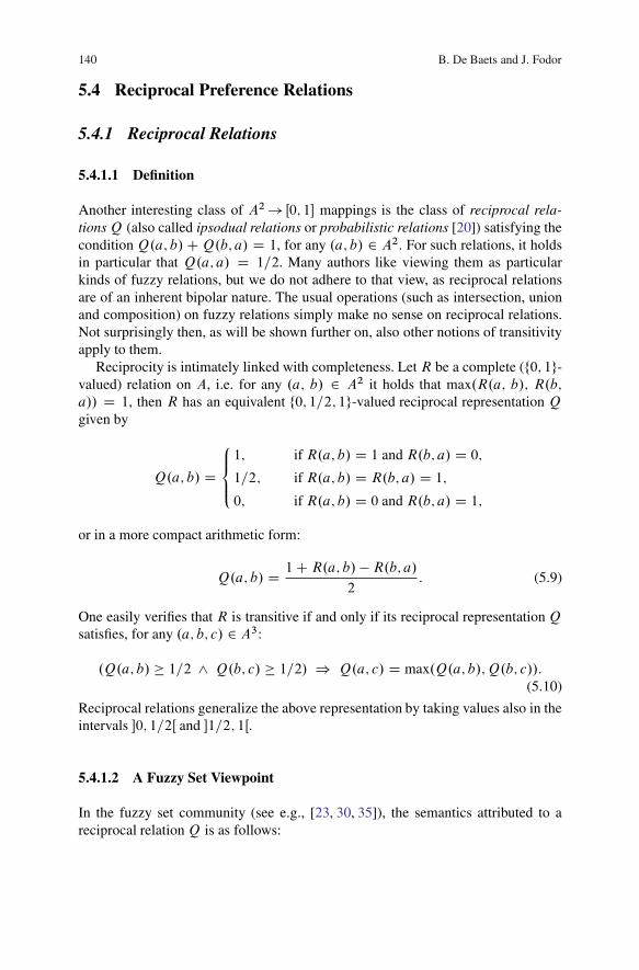
140 B. De Baets and J. Fodor
5.4 Reciprocal Preference Relations
5.4.1 Reciprocal Relations
5.4.1.1 Definition
Another interesting class of A2 ! Œ0; 1� mappings is the class of reciprocal rela-tionsQ (also called ipsodual relations or probabilistic relations [20]) satisfying thecondition Q.a; b/CQ.b; a/ D 1, for any .a; b/ 2 A2. For such relations, it holdsin particular that Q.a; a/ D 1=2. Many authors like viewing them as particularkinds of fuzzy relations, but we do not adhere to that view, as reciprocal relationsare of an inherent bipolar nature. The usual operations (such as intersection, unionand composition) on fuzzy relations simply make no sense on reciprocal relations.Not surprisingly then, as will be shown further on, also other notions of transitivityapply to them.
Reciprocity is intimately linked with completeness. Let R be a complete (f0; 1g-valued) relation on A, i.e. for any .a; b/ 2 A2 it holds that max.R.a; b/; R.b;a// D 1, then R has an equivalent f0; 1=2; 1g-valued reciprocal representation Qgiven by
Q.a; b/ D
8<
:
1; if R.a; b/ D 1 and R.b; a/ D 0;
1=2; if R.a; b/ D R.b; a/ D 1;
0; if R.a; b/ D 0 and R.b; a/ D 1;
or in a more compact arithmetic form:
Q.a; b/ D 1CR.a; b/�R.b; a/2
: (5.9)
One easily verifies that R is transitive if and only if its reciprocal representationQsatisfies, for any .a; b; c/ 2 A3:
.Q.a; b/ � 1=2 ^ Q.b; c/ � 1=2/ ) Q.a; c/ D max.Q.a; b/;Q.b; c//:(5.10)
Reciprocal relations generalize the above representation by taking values also in theintervals �0; 1=2Œ and �1=2; 1Œ.
5.4.1.2 A Fuzzy Set Viewpoint
In the fuzzy set community (see e.g., [23, 30, 35]), the semantics attributed to areciprocal relationQ is as follows:

5 Preference Modelling, a Matter of Degree 141
Q.a; b/ 2
8<
:
�1=2; 1�; if a is rather preferred to b;
f1=2g; if a and b are indifferent;
Œ0; 1=2Œ; if b is rather preferred to a:
Hence, a reciprocal relation can be seen as a compact representation of an additivefuzzy preference structure in which the indifference relation I is a crisp relation,the incomparability relation J is empty and the strict preference relation P and itsconverse P t are fuzzy relations complementing each other. Reciprocal relations aretherefore closely related to fuzzy weak orders.
Note that, similarly as for a complete relation, a weakly complete fuzzy relationR on A can be transformed into a reciprocal representation Q D P C 1=2I , withP and I the strict preference and indifference components of the additive fuzzypreference structure .P; I; J / generated from R by means of the generator i DTL [14, 52]:
P.a; b/ D TM.R.a; b/; 1� R.b; a// D 1 � R.b; a/;
I.a; b/ D TL.R.a; b/; R.b; a// D R.a; b/CR.b; a/� 1;
J.a; b/ D TL.1 �R.a; b/; 1 �R.b; a// D 0:
Note that the corresponding expression for Q is formally the same as (5.9). Thisrepresentation is not equivalent to the fuzzy relation R, as many weakly completefuzzy relationsRmay have the same representation. Recall that, if the fuzzy relationR is also strongly complete, then the generator i used is immaterial.
5.4.1.3 A Frequentist View
However, the origin of reciprocal relations is not to be found in the fuzzy set com-munity. For several decades, reciprocal relations are used as a convenient tool forexpressing the results of the pairwise comparison of a set of alternatives in fieldssuch as game theory [22], voting theory [42] and psychology [20]. A typical use isthat where an individual is asked, in a controlled experimental set-up, to compare thesame set of alternatives multiple times, where each time he can either prefer alterna-tive a to b or b to a. The fraction of times a is preferred to b then yieldsQ.a; b/. Inwhat follows, we will stay close to that frequentist view. However, we prefer to usethe more neutral term reciprocal relation, rather than the term probabilistic relation.
5.4.2 The Cycle-Transitivity Framework
5.4.2.1 Stochastic Transitivity
Transitivity properties for reciprocal relations rather have the conditional fla-vor of (5.10). There exist various kinds of stochastic transitivity for reciprocal

142 B. De Baets and J. Fodor
relations [5, 40]. For instance, a reciprocal relation Q on A is called weaklystochastic transitive if for any .a; b; c/ 2 A3 it holds that Q.a; b/ � 1=2 ^Q.b; c/ � 1=2 implies Q.a; c/ � 1=2. In [10], the following generalization ofstochastic transitivity was proposed.
Definition 5.14. Let g be an increasing Œ1=2; 1�2 ! Œ0; 1� mapping such thatg.1=2; 1=2/ � 1=2. A reciprocal relation Q on A is called g-stochastic transitive iffor any .a; b; c/ 2 A3 it holds that
.Q.a; b/ � 1=2 ^ Q.b; c/ � 1=2/ ) Q.a; c/ � g.Q.a; b/;Q.b; c//:
Note that the condition g.1=2; 1=2/ � 1=2 ensures that the reciprocal representationQ of any transitive complete relation R is always g-stochastic transitive. In otherwords, g-stochastic transitivity generalizes transitivity of complete relations. Thisdefinition includes the standard types of stochastic transitivity [40]:
(i) Strong stochastic transitivity when g D max(ii) Moderate stochastic transitivity when g D min
(iii) Weak stochastic transitivity when g D 1=2
In [10], also a special type of stochastic transitivity was introduced.
Definition 5.15. Let g be an increasing Œ1=2; 1�2 ! Œ0; 1� mapping such thatg.1=2; 1=2/ D 1=2 and g.1=2; 1/ D g.1; 1=2/ D 1. A reciprocal relation Q onA is called g-isostochastic transitive if for any .a; b; c/ 2 A3 it holds that
.Q.a; b/ � 1=2 ^ Q.b; c/ � 1=2/ ) Q.a; c/ D g.Q.a; b/;Q.b; c//:
The conditions imposed upon g again ensure that g-isostochastic transitivity gen-eralizes transitivity of complete relations. Note that for a given mapping g, theproperty of g-isostochastic transitivity obviously is much more restrictive than theproperty of g-stochastic transitivity.
5.4.2.2 FG-Transitivity
The framework of FG-transitivity, developed by Switalski [47,51], formally gener-alizes g-stochastic transitivity in the sense thatQ.a; c/ is bounded both from belowand above by Œ1=2; 1�2 ! Œ0; 1� mappings.
Definition 5.16. Let F and G be two Œ1=2; 1�2 ! Œ0; 1� mappings such thatF.1=2; 1=2/ � 1=2 � G.1=2; 1=2/ and G.1=2; 1/ D G.1; 1=2/ D G.1; 1/ D 1
and F � G. A reciprocal relation Q on A is called FG-transitive if for any.a; b; c/ 2 A3 it holds that

5 Preference Modelling, a Matter of Degree 143
.Q.a; b/ � 1=2 ^ Q.b; c/ � 1=2/
+F.Q.a; b/;Q.b; c// � Q.a; c/ � G.Q.a; b/;Q.b; c//:
5.4.2.3 Cycle-Transitivity
Similarly as the FG-transitivity framework, the cycle-transitivity framework in-volves two bounds. However, these bounds are not independent, and moreover,the arguments are subjected to a reordering before they are applied. More specif-ically, for a reciprocal relation Q, we define for all .a; b; c/ 2 A3 the followingquantities [10]:
˛abc D min.Q.a; b/;Q.b; c/;Q.c; a//;
ˇabc D median.Q.a; b/;Q.b; c/;Q.c; a//;
�abc D max.Q.a; b/;Q.b; c/;Q.c; a//:
Let us also denote� D f.x; y; z/ 2 Œ0; 1�3 j x � y � zg. A function U W � ! R iscalled an if it satisfies:
(i) U.0; 0; 1/ � 0 and U.0; 1; 1/ � 1;(ii) for any .˛; ˇ; �/ 2 �:
U.˛; ˇ; �/C U.1 � �; 1 � ˇ; 1 � ˛/ � 1: (5.11)
The function L W � ! R defined by L.˛; ˇ; �/ D 1 � U.1 � �; 1 � ˇ; 1 � ˛/ iscalled the dual of a given upper bound function U . Inequality (5.11) then simplyexpresses that L � U . Condition (i) again guarantees that cycle-transitivity gener-alizes transitivity of complete relations.
Definition 5.17. A reciprocal relation Q on A is called cycle-transitive w.r.t. anupper bound function U if for any .a; b; c/ 2 A3 it holds that
L.˛abc ; ˇabc ; �abc/ � ˛abc C ˇabc C �abc � 1 � U.˛abc ; ˇabc ; �abc/; (5.12)
where L is the dual lower bound function of U .
Due to the built-in duality, it holds that if (5.12) is true for some .a; b; c/, thenthis is also the case for any permutation of .a; b; c/. In practice, it is therefore suf-ficient to check (5.12) for a single permutation of any .a; b; c/ 2 A3. Alternatively,due to the same duality, it is also sufficient to verify the right-hand inequality (orequivalently, the left-hand inequality) for two permutations of any .a; b; c/ 2 A3
(not being cyclic permutations of one another), e.g., .a; b; c/ and .c; b; a/. Hence,(5.12) can be replaced by

144 B. De Baets and J. Fodor
˛abc C ˇabc C �abc � 1 � U.˛abc ; ˇabc ; �abc/: (5.13)
Note that a value of U.˛; ˇ; �/ equal to 2 is used to express that for the given valuesthere is no restriction at all (as ˛ C ˇ C � � 1 is always bounded by 2).
Two upper bound functionsU1 andU2 are called equivalent if for any .˛; ˇ; �/ 2� it holds that ˛ C ˇ C � � 1 � U1.˛; ˇ; �/ is equivalent to ˛ C ˇ C � � 1 �U2.˛; ˇ; �/.
If it happens that in (5.11) the equality holds for all .˛; ˇ; �/ 2 �, then the upperbound function U is said to be self-dual, since in that case it coincides with its duallower bound function L. Consequently, also (5.12) and (5.13) can only hold withequality then. Furthermore, it then holds that U.0; 0; 1/ D 0 and U.0; 1; 1/ D 1.
The simplest example of a self-dual upper bound function is the median, i.e.UM.˛; ˇ; �/ D ˇ. Another example of a self-dual upper bound function is the func-tion UE defined by
UE .˛; ˇ; �/ D ˛ˇ C ˛� C ˇ� � 2˛ˇ�:
Cycle-transitivity w.r.t. UE of a reciprocal relationQ on A can also be expressed as
˛ijkˇijk�ijk D .1 � ˛ijk/.1 � ˇijk/.1 � �ijk/:
It is then easy to see that cycle-transitivity w.r.t. UE is equivalent to the notion ofmultiplicative transitivity [49]. Recall that a reciprocal relation Q on A is calledmultiplicatively transitive if for any .a; b; c/ 2 A3 it holds that
Q.a; c/
Q.c; a/D Q.a; b/
Q.b; a/� Q.b; c/Q.c; b/
:
The cycle-transitive formulation is more appropriate as it avoids division by zero.
5.4.2.4 Cycle-Transitivity Is a General Framework
Although C -transitivity is not intended to be applied to reciprocal relations, it canbe formally cast quite nicely into the cycle-transitivity framework.
Proposition 5.3. [10] Let C be a commutative conjunctor such that C � TM. A re-ciprocal relation Q on A is C -transitive if and only if it is cycle-transitive w.r.t. theupper bound function UC defined by
UC .˛; ˇ; �/ D min.˛ C ˇ � C.˛; ˇ/; ˇ C � � C.ˇ; �/; � C ˛ � C.�; ˛//:
Moreover, if C is 1-Lipschitz, then UC is given by
UC .˛; ˇ; �/ D ˛ C ˇ � C.˛; ˇ/: (5.14)

5 Preference Modelling, a Matter of Degree 145
This proposition applies in particular to commutative quasi-copulas and copulas.In case of a copula, the expression in (5.14) is known as the dual of the copula.Consider the three basic t-norms/copulas TM, TP and TL:
(i) For C D TM, we immediately obtain as upper bound function the median
UM.˛; ˇ; �/ D ˇ:
(ii) For C D TP, we find
UP.˛; ˇ; �/ D ˛ C ˇ � ˛ˇ:
(iii) For C D TL, we obtain
UL.˛; ˇ; �/ D(˛ C ˇ; if ˛ C ˇ < 1;
1; if ˛ C ˇ � 1:
An equivalent upper bound function is given by U 0L.˛; ˇ; �/ D 1.
Cycle-transitivity also incorporates stochastic transitivity, although the latter fitsmore naturally in the FG-transitivity framework. We list just one interesting propo-sition under mild conditions on the function g.
Proposition 5.4. Let g be a commutative, increasing Œ1=2; 1�2 ! Œ1=2; 1�mappingsuch that g.1=2; x/ � x for any x 2 Œ1=2; 1�. A reciprocal relation Q on A is g-stochastic transitive if and only if it is cycle-transitive w.r.t. the upper bound functionUg defined by
Ug.˛; ˇ; �/ D
8<
:
ˇ C � � g.ˇ; �/; if ˇ � 1=2 ^ ˛ < 1=2;
1=2; if ˛ � 1=2;
2; if ˇ < 1=2:
(5.15)
A final simplification, eliminating the special case ˛ D 1=2 in (5.15), is obtainedby requiring g to have as neutral element 1=2, i.e. g.1=2; x/ D g.x; 1=2/ D x forany x 2 Œ1=2; 1�.Proposition 5.5. Let g be a commutative, increasing Œ1=2; 1�2 ! Œ1=2; 1�mappingwith neutral element 1=2. A reciprocal relation Q on A is g-stochastic transitive ifand only if it is cycle-transitive w.r.t. the upper bound Ug defined by
Ug.˛; ˇ; �/ D(ˇ C � � g.ˇ; �/; if ˇ � 1=2;
2; if ˇ < 1=2:(5.16)
This proposition implies in particular that strong stochastic transitivity (g Dmax) is equivalent to cycle-transitivity w.r.t. the simplified upper bound functionU 0ss defined by

146 B. De Baets and J. Fodor
U 0ss.˛; ˇ; �/ D
(ˇ; if ˇ � 1=2;
2; if ˇ < 1=2:
Note that g-stochastic transitivity w.r.t. a function g � max always implies strongstochastic transitivity. This means that any reciprocal relation that is cycle-transitivew.r.t. an upper bound function Ug of the form (5.16) is at least strongly stochastictransitive. It is obvious that TM-transitivity implies strong stochastic transitivity andthat moderate stochastic transitivity implies TL-transitivity.
One particular form of stochastic transitivity deserves our attention. A prob-abilistic relation Q on A is called partially stochastic transitive [24] if for any.a; b; c/ 2 A3 it holds that
.Q.a; b/ > 1=2 ^ Q.b; c/ > 1=2/ ) Q.a; c/ � min.Q.a; b/;Q.b; c//:
Clearly, it is a slight weakening of moderate stochastic transitivity. Interestingly, alsothis type of transitivity can be expressed elegantly in the cycle-transitivity frame-work [17] by means of a simple upper bound function.
Proposition 5.6. Cycle-transitivity w.r.t. the upper bound function Ups defined by
Ups.˛; ˇ; �/ D �
is equivalent to partial stochastic transitivity.
Finally, not surprisingly, isostochastic transitivity corresponds to cycle-transiti-vity w.r.t. particular self-dual upper bound functions [10]. An interesting way ofconstructing a self-dual upper bound function goes as follows.
Proposition 5.7. Let g be a commutative, increasing Œ1=2; 1�2 ! Œ1=2; 1�mappingwith neutral element 1=2. It then holds that any� ! R function U of the form
U sg .˛; ˇ; �/ D(ˇ C � � g.ˇ; �/; if ˇ � 1=2;
˛ C ˇ � 1C g.1 � ˇ; 1 � ˛/; if ˇ < 1=2;
is a self-dual upper bound function.
Note that the function g in Proposition 5.7 has the same properties as the functiong in Proposition 5.5.
Proposition 5.8. A reciprocal relation Q on A is cycle-transitive w.r.t. a self-dualupper bound function of type U sg if and only if it is g-isostochastic transitive.
In particular, a reciprocal relationQ is TM-transitive if and only if
.Q.a; b/ � 1=2 ^ Q.b; c/ � 1=2/ ) Q.a; c/ D max.Q.a; b/;Q.b; c//;
for any .a; b; c/ 2 A3. Note that this is formally the same as (5.10) with the differ-ence that in the latter case Q was only f0; 1=2; 1g-valued.

5 Preference Modelling, a Matter of Degree 147
If the function g is a commutative, associative, increasing Œ1=2; 1�2 ! Œ1=2; 1�
mapping with neutral element 1=2, then the Œ0; 1�2 ! Œ0; 1� mapping Sg defined by
Sg.x; y/ D 2g
�1C x
2;1C y
2
�
� 1
is a t-conorm. For the self-dual upper bound function UE , the associated t-conormSE is given by
SE .x; y/ D x C y
1C xy;
which belongs to the parametric Hamacher t-conorm family, and is the co-copula ofthe Hamacher t-norm with parameter value 2 [37].
We have shown that the cycle-transitivity andFG-transitivity frameworks cannoteasily be translated into one another, which underlines that these are two essentiallydifferent frameworks [6].
5.4.3 Comparison of Random Variables
5.4.3.1 Dice-Transitivity of Winning Probabilities
Consider three dice A, B and C which, instead of the usual numbers, carry thefollowing integers on their faces:
A D f1; 3; 4; 15; 16; 17g; B D f2; 10; 11; 12; 13; 14g; C D f5; 6; 7; 8; 9; 18g:
Denoting by P.X; Y / the probability that dice X wins from dice Y , we haveP.A;B/ D 20=36, P.B; C / D 25=36 and P.C;A/ D 21=36. It is natural tosay that dice X is strictly preferred to dice Y if P.X; Y / > 1=2, which reflectsthat dice X wins from dice Y in the long run (or that X statistically wins from Y ,denoted X >s Y ). Note that P.Y;X/ D 1 � P.X; Y / which implies that the rela-tion >s is asymmetric. In the above example, it holds that A >s B , B >s C andC >s A: the relation >s is not transitive and forms a cycle. In other words, if weinterpret the probabilities P.X; Y / as constituents of a reciprocal relation on the setof alternatives fA;B;C g, then this reciprocal relation is even not weakly stochastictransitive.
This example can be generalized as follows: we allow the dice to possess anynumber of faces (whether or not this can be materialized) and allow identical num-bers on the faces of a single or multiple dice. In other words, a generalized dice canbe identified with a multiset of integers. Given a collection of m such generalizeddice, we can still build a reciprocal relation Q containing the winning probabilitiesfor each pair of dice [19]. For any two such dice A and B , we define
Q.A;B/ D PfA wins from Bg C 1
2PfA and B end in a tieg:

148 B. De Baets and J. Fodor
The dice or integer multisets may be identified with independent discrete randomvariables that are uniformly distributed on these multisets (i.e. the probability ofan integer is proportional to its number of occurrences); the reciprocal relation Qmay be regarded as a quantitative description of the pairwise comparison of theserandom variables.
In the characterization of the transitivity of this reciprocal relation, a type ofcycle-transitivity, which can neither be seen as a type of C -transitivity, nor as a typeof FG-transitivity, has proven to play a predominant role. For obvious reasons, thisnew type of transitivity has been called dice-transitivity.
Definition 5.18. Cycle-transitivity w.r.t. the upper bound function UD defined by
UD.˛; ˇ; �/ D ˇ C � � ˇ�;
is called dice-transitivity.
Dice-transitivity is closely related to TP-transitivity. However, it uses the quan-tities ˇ and � instead of the quantities ˛ and ˇ, and is therefore less restrictive.Dice-transitivity can be situated between TL-transitivity and TP-transitivity, and alsobetween TL-transitivity and moderate stochastic transitivity.
Proposition 5.9. [19] The reciprocal relation generated by a collection of general-ized dice is dice-transitive.
5.4.3.2 A Method for Comparing Random Variables
Many methods can be established for the comparison of the components (randomvariables, r.v.) of a random vector .X1; : : : ; Xn/, as there exist many ways to extractuseful information from the joint cumulative distribution function (c.d.f.) FX1;:::;Xn
that characterizes the random vector. A first simplification consists in comparing ther.v. two by two. It means that a method for comparing r.v. should only use the infor-mation contained in the bivariate c.d.f. FXi ;Xj
. Therefore, one can very well ignorethe existence of a multivariate c.d.f. and just describe mutual dependencies betweenthe r.v. by means of the bivariate c.d.f. Of course one should be aware that notall choices of bivariate c.d.f. are compatible with a multivariate c.d.f. The problemof characterizing those ensembles of bivariate c.d.f. that can be identified with themarginal bivariate c.d.f. of a single multivariate c.d.f. is known as the compatibilityproblem [41].
A second simplifying step often made is to bypass the information contained inthe bivariate c.d.f. to devise a comparison method that entirely relies on the one-dimensional marginal c.d.f. In this case there is even not a compatibility problem,as for any set of univariate c.d.f. FXi
, the product FX1FX2
� � �FXnis a valid joint
c.d.f., namely the one expressing the independence of the r.v. There are many waysto compare one-dimensional c.d.f., and by far the simplest one is the method thatbuilds a partial order on the set of r.v. using the principle of first order stochastic

5 Preference Modelling, a Matter of Degree 149
dominance [49]. It states that a r.v. X is weakly preferred to a r.v. Y if for all u 2 Rit holds that FX .u/ � FY .u/. At the extreme end of the chain of simplifications arethe methods that compare r.v. by means of a characteristic or a function of somecharacteristics derived from the one-dimensional marginal c.d.f. The simplest ex-ample is the weak order induced by the expected values of the r.v.
Proceeding along the line of thought of the previous section, a random vector.X1; X2; : : : ; Xm/ generates a reciprocal relation by means of the following recipe.
Definition 5.19. Given a random vector .X1; X2; : : : ; Xm/, the binary relation Qdefined by
Q.Xi ; Xj / D PfXi > Xj g C 1
2PfXi D Xj g
is a reciprocal relation.
For two discrete r.v. Xi and Xj , Q.Xi ; Xj / can be computed as
Q.Xi ; Xj / DX
k>l
pXi ;Xj.k; l/C 1
2
X
k
pXi ;Xj.k; k/;
with pXi ;Xjthe joint probability mass function (p.m.f.) of .Xi ; Xj /. For two con-
tinuous r.v. Xi and Xj , Q.Xi ; Xj / can be computed as
Q.Xi ; Xj / DZ C1
�1dx
Z x
�1fXi ;Xj
.x; y/ dy;
with fXi ;Xjthe joint probability density function (p.d.f.) of .Xi ; Xj /.
For this pairwise comparison, one needs the two-dimensional marginal distribu-tions. Sklar’s theorem [41,46] tells us that if a joint cumulative distribution functionFXi ;Xj
has marginals FXiand FXj
, then there exists a copula Cij such that for allx; y:
FXi ;Xj.x; y/ D Cij .FXi
.x/; FXj.y//:
If Xi and Xj are continuous, then Cij is unique; otherwise, Cij is uniquely deter-mined on Ran.FXi
/ � Ran.FXj/.
As the above comparison method takes into account the bivariate marginal c.d.f.it takes into account the dependence of the components of the random vector. Theinformation contained in the reciprocal relation is therefore much richer than if, forinstance, we would have based the comparison ofXi andXj solely on their expectedvalues. Despite the fact that the dependence structure is entirely captured by themultivariate c.d.f., the pairwise comparison is only apt to take into account pairwisedependence, as only bivariate c.d.f. are involved. Indeed, the bivariate c.d.f. do notfully disclose the dependence structure; the r.v. may even be pairwise independentwhile not mutually independent.
Since the copulas Cij that couple the univariate marginal c.d.f. into the bivariatemarginal c.d.f. can be different from another, the analysis of the reciprocal relation

150 B. De Baets and J. Fodor
and in particular the identification of its transitivity properties appear rather cumber-some. It is nonetheless possible to state in general, without making any assumptionson the bivariate c.d.f., that the probabilistic relation Q generated by an arbitraryrandom vector always shows some minimal form of transitivity.
Proposition 5.10. [8] The reciprocal relation Q generated by a random vector isTL-transitive.
5.4.3.3 Artificial Coupling of Random Variables
Our further interest is to study the situation where abstraction is made that the r.v.are components of a random vector, and all bivariate c.d.f. are enforced to dependin the same way upon the univariate c.d.f., in other words, we consider the situationof all copulas being the same, realizing that this might not be possible at all. Infact, this simplification is equivalent to considering instead of a random vector, acollection of r.v. and to artificially compare them, all in the same manner and basedupon a same copula. The pairwise comparison then relies upon the knowledge ofthe one-dimensional marginal c.d.f. solely, as is the case in stochastic dominancemethods. Our comparison method, however, is not equivalent to any known kind ofstochastic dominance, but should rather be regarded as a graded variant of it (seealso [7]).
The case C D TP generalizes Proposition 5.9, and applies in particular to acollection of independent r.v. where all copulas effectively equal TP.
Proposition 5.11. [18, 19] The reciprocal relation Q generated by a collection ofr.v. pairwise coupled by TP is dice-transitive, i.e. it is cycle-transitive w.r.t. the upperbound function given by UD.˛; ˇ; �/ D ˇ C � � ˇ� .
We discuss next the case when using one of the extreme copulas to artificiallycouple the r.v. In case C D TM, the r.v. are coupled comonotonically. Note that thiscase is possible in reality.
Proposition 5.12. [16, 17] The reciprocal relation Q generated by a collection ofr.v. pairwise coupled by TM is cycle-transitive w.r.t. to the upper bound functionU given by U.˛; ˇ; �/ D min.ˇ C �; 1/. Cycle-transitivity w.r.t. the upper boundfunction U is equivalent to TL-transitivity.
In case C D TL, the r.v. are coupled countermonotonically. This assumptioncan never represent a true dependence structure for more than two r.v., due to thecompatibility problem.
Proposition 5.13. [16, 17] The reciprocal relation Q generated by a collection ofr.v. pairwise coupled by TL is partially stochastic transitive, i.e. it is cycle-transitivew.r.t. to the upper bound function defined by Ups.˛; ˇ; �/ D max.ˇ; �/ D � .

5 Preference Modelling, a Matter of Degree 151
The proofs of these propositions were first given for discrete uniformly dis-tributed r.v. [16, 19]. It allowed for an interpretation of the values Q.Xi ; Xj / aswinning probabilities in a hypothetical dice game, or equivalently, as a method forthe pairwise comparison of ordered lists of numbers. Subsequently, we have shownthat as far as transitivity is concerned, this situation is generic and therefore charac-terizes the type of transitivity observed in general [17, 18].
The above results can be seen as particular cases of a more general result.
Proposition 5.14. [8] Let C be a commutative copula such that for any n > 1 andfor any 0 � x1 � � � � � xn � 1 and 0 � y1 � � � � � yn � 1, it holds that
X
i
C.xi ; yi /�X
i
C.xn�2i ; yn�2i�1/�X
i
C.xn�2i�1; yn�2i /
� C
xn CX
i
C.xn�2i�2; yn�2i�1/ �X
i
C.xn�2i ; yn�2i�1/;
yn CX
i
C.xn�2i�1; yn�2i�2/�X
i
C.xn�2i�1; yn�2i /!
; (5.17)
where the sums extend over all integer values that lead to meaningful indices ofx and y. Then the reciprocal relation Q generated by a collection of random vari-ables pairwise coupled by C is cycle-transitive w.r.t. to the upper bound functionUC defined by:
UC .˛; ˇ; �/ D max.ˇ C C.1 � ˇ; �/; � C C.ˇ; 1 � �//:
Inequality (5.17) is called the twisted staircase condition and appears to bequite complicated. Although its origin is well understood [8], it is not yet clearfor which commutative copulas it holds. We strongly conjecture that it holds for allFrank copulas.
5.4.3.4 Comparison of Special Independent Random Variables
Dice-transitivity is the generic type of transitivity shared by the reciprocal relationsgenerated by a collection of independent r.v. If one considers independent r.v. withdensities all belonging to one of the one-parameter families in Table 5.1, then thecorresponding reciprocal relation shows the corresponding type of cycle-transitivitylisted in Table 5.2 [18].
Note that all upper bound functions in Table 5.2 are self-dual. More strikingis that the two families of power-law distributions (one-parameter subfamilies ofthe two-parameter Beta and Pareto families) and the family of Gumbel distribu-tions all yield the same type of transitivity as exponential distributions, namelycycle-transitivity w.r.t. the self-dual upper bound function UE , or, in other words,multiplicative transitivity.

152 B. De Baets and J. Fodor
Table 5.1 Parametric families of continuous distributions
Name Density function f .x/
Exponential �e��x � > 0 x 2 Œ0;1Œ
Beta �x.��1/ � > 0 x 2 Œ0; 1�
Pareto �x�.�C1/ � > 0 x 2 Œ1;1Œ
Gumbel �e��.x��/e�e��.x��/� 2 R; � > 0 x 2 �� 1;1Œ
Uniform 1=a � 2 R; a > 0 x 2 Œ�; �C a�
Laplace .e�jx��j=�//=.2�/ � 2 R; � > 0 x 2 �� 1;1Œ
Normal .e�.x��/2=22 /=p22 � 2 R; > 0 x 2 �� 1;1Œ
Table 5.2 Cycle-transitivity for the continuous distributions in Table 5.1
Name Upper bound function U.˛; ˇ; �/
ExponentialBetaPareto ˛ˇ C ˛� C ˇ� � 2˛ˇ�
Gumbel
Uniform
8ˆ<
ˆ:
ˇ C � � 1C 1
2
hmax.
p2.1� ˇ/Cp
2.1� �/� 1; 0/i2
ˇ � 1=2
˛ C ˇ � 1
2
hmax.
p2˛ Cp
2ˇ � 1; 0/i2; ˇ < 1=2
Laplace
�ˇ C � � 1C f �1.f .1 � ˇ/C f .1� �//; ˇ � 1=2
˛ C ˇ � f �1.f .˛/ C f .ˇ//; ˇ < 1=2
with f �1.x/ D 12
�1C x
2
�e�x
Normal
�ˇ C � � 1Cˆ.ˆ�1.1� ˇ/Cˆ.1� �//; ˇ � 1=2
˛ C ˇ �ˆ.ˆ�1.˛/Cˆ�1.ˇ//; ˇ < 1=2
with ˆ.x/ D .p2/�1
R x�1
e�t2=2dt
In the cases of the unimodal uniform, Gumbel, Laplace and normal distribu-tions we have fixed one of the two parameters in order to restrict the family to aone-parameter subfamily, mainly because with two free parameters, the formulaebecome utmost cumbersome. The one exception is the two-dimensional family ofnormal distributions. In [18], we have shown that the corresponding reciprocal rela-tion is in that case moderately stochastic transitive.
5.4.4 Mutual Ranking Probabilities in Posets
Consider a finite poset .P;�/ with P D fx1; : : : ; xng. A linear extension of P isan order-preserving permutation of its elements (hence, also a ranking of the ele-ments compatible with the partial order). We denote by p.xi < xj / the fraction oflinear extensions of P in which xi precedes xj . If the space of all linear extensionsof P is equipped with the uniform measure, the position of x in a linear exten-sion can be regarded as a discrete random variable X with values in f1; : : : ; ng.
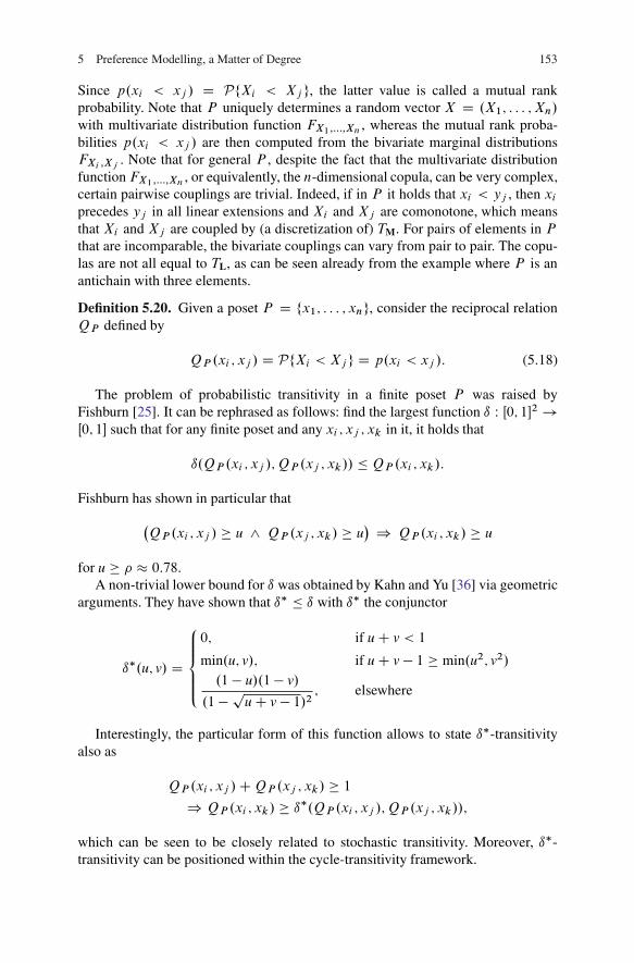
5 Preference Modelling, a Matter of Degree 153
Since p.xi < xj / D PfXi < Xj g, the latter value is called a mutual rankprobability. Note that P uniquely determines a random vector X D .X1; : : : ; Xn/
with multivariate distribution function FX1;:::;Xn, whereas the mutual rank proba-
bilities p.xi < xj / are then computed from the bivariate marginal distributionsFXi ;Xj
. Note that for general P , despite the fact that the multivariate distributionfunction FX1;:::;Xn
, or equivalently, the n-dimensional copula, can be very complex,certain pairwise couplings are trivial. Indeed, if in P it holds that xi < yj , then xiprecedes yj in all linear extensions and Xi and Xj are comonotone, which meansthat Xi and Xj are coupled by (a discretization of) TM. For pairs of elements in Pthat are incomparable, the bivariate couplings can vary from pair to pair. The copu-las are not all equal to TL, as can be seen already from the example where P is anantichain with three elements.
Definition 5.20. Given a poset P D fx1; : : : ; xng, consider the reciprocal relationQP defined by
QP .xi ; xj / D PfXi < Xj g D p.xi < xj /: (5.18)
The problem of probabilistic transitivity in a finite poset P was raised byFishburn [25]. It can be rephrased as follows: find the largest function ı W Œ0; 1�2 !Œ0; 1� such that for any finite poset and any xi ; xj ; xk in it, it holds that
ı.QP .xi ; xj /;QP .xj ; xk// � QP .xi ; xk/:
Fishburn has shown in particular that
�QP .xi ; xj / � u ^ QP .xj ; xk/ � u
� ) QP .xi ; xk/ � u
for u � � 0:78.A non-trivial lower bound for ı was obtained by Kahn and Yu [36] via geometric
arguments. They have shown that ı� � ı with ı� the conjunctor
ı�.u; v/ D
8ˆ<
ˆ:
0; if u C v < 1
min.u; v/; if u C v � 1 � min.u2; v2/.1 � u/.1� v/
.1 � pu C v � 1/2 ; elsewhere
Interestingly, the particular form of this function allows to state ı�-transitivityalso as
QP .xi ; xj /CQP .xj ; xk/ � 1
) QP .xi ; xk/ � ı�.QP .xi ; xj /;QP .xj ; xk//;
which can be seen to be closely related to stochastic transitivity. Moreover, ı�-transitivity can be positioned within the cycle-transitivity framework.

154 B. De Baets and J. Fodor
Proposition 5.15. [9] ı�-Transitivity implies cycle-transitivity w.r.t. the upperbound function UP defined by
UP .˛; ˇ; �/ D ˛ C � � ˛�;
and hence also dice-transitivity.
References
1. B. De Baets and J. Fodor. Generator triplets of additive fuzzy preference structures. In Pro-ceedings of the Sixth International Workshop on Relational Methods in Computer Science,pages 306–315, 2001.
2. U. Bodenhofer. A similarity-based generalization of fuzzy orderings preserving the classi-cal axioms. International Journal of Uncertainty Fuzziness and Knowledge-Based Systems,8(5):593–610, 2000.
3. U. Bodenhofer, B. De Baets, and J. Fodor. A compendium of fuzzy weak orders: representa-tions and constructions. Fuzzy Sets and Systems, 158:811–829, 2007.
4. F. Chiclana, F. Herrera, E. Herrera-Viedma, and L. Martınez. A note on the reciprocity inthe aggregation of fuzzy preference relations using OWA operators. Fuzzy Sets and Systems,137:71–83, 2003.
5. H.A. David. The Method of Paired Comparisons, volume 12 of Griffin’s Statistical Mono-graphs & Courses. Charles Griffin & Co. Ltd., London, 1963.
6. B. De Baets and H. De Meyer. Transitivity frameworks for reciprocal relations: cycle-transitivity versus fg-transitivity. Fuzzy Sets and Systems, 152:249–270, 2005.
7. B. De Baets and H. De Meyer. Toward graded and nongraded variants of stochastic dominance.In I. Batyrshin, J. Kacprzyk, J. Sheremetov, and L. Zadeh, editors, Perception-based Data Min-ing and Decision Making in Economics and Finance, volume 36 of Studies in ComputationalIntelligence, pages 252–267. Springer, Berlin, 2007.
8. B. De Baets and H. De Meyer. Cycle-transitive comparison of artificially coupled randomvariables. International Journal of Approximate Reasoning, 47:306–322, 2008.
9. B. De Baets, H. De Meyer, and K. De Loof. On the cycle-transitivity of the mutual rank prob-ability relation of a poset. Fuzzy Sets and Systems, doi:10.1016/j.fss.2010.05.005, 2010.
10. B. De Baets, H. De Meyer, B. De Schuymer, and S. Jenei. Cyclic evaluation of transitivity ofreciprocal relations. Social Choice and Welfare, 26:217–238, 2006.
11. B. De Baets and J. Fodor. Twenty years of fuzzy preference structures (1978–1997). BelgianJournal of Operations Research Statistics and Computer Science, 37:61–82, 1997.
12. B. De Baets, J. Fodor, and E.E. Kerre. Godel representable fuzzy weak orders. InternationalJournal of Uncertainty, Fuzziness and Knowledge-Based Systems, 7(2):135–154, 1999.
13. B. De Baets and B. Van De Walle. Minimal definitions of classical and fuzzy preferencestructures. In Proceedings of the Annual Meeting of the North American Fuzzy InformationProcessing Society, pages 299–304. Syracuse, New York, 1997.
14. B. De Baets, B. Van de Walle, and E. Kerre. Fuzzy preference structures without incompara-bility. Fuzzy Sets and Systems, 76:333–348, 1995.
15. B. De Baets, B. Van de Walle, and E. Kerre. A plea for the use of łukasiewicz triplets in fuzzypreference structures. Part 2: The identity case. Fuzzy Sets and Systems, 99:303–310, 1998.
16. H. De Meyer, B. De Baets, and B. De Schuymer. Extreme copulas and the comparison ofordered lists. Theory and Decision, 62:195–217, 2007.
17. H. De Meyer, B. De Baets, and B. De Schuymer. On the transitivity of the comonotonicand countermonotonic comparison of random variables. Journal of Multivariate Analysis, 98:177–193, 2007.

5 Preference Modelling, a Matter of Degree 155
18. B. De Schuymer, H. De Meyer, and B. De Baets. Cycle-transitive comparison of independentrandom variables. Journal of Multivariate Analysis, 96:352–373, 2005.
19. B. De Schuymer, H. De Meyer, B. De Baets, and S. Jenei. On the cycle-transitivity of the dicemodel. Theory and Decision, 54:264–285, 2003.
20. J.-P. Doignon, B. Monjardet, M. Roubens, and Ph. Vincke. Biorder families, valued relations,and preference modelling. Journal of Mathematical Psychology, 30:435–480, 1986.
21. D. Dubois and H. Prade. Fuzzy Sets and Systems: Theory and Applications. Academic Press,New York, 1980.
22. B. Dutta and J.F. Laslier. Comparison functions and choice correspondences. Social Choiceand Welfare, 16:513–532, 1999.
23. M. Fedrizzi, M. Fedrizzi, and R. Marques-Pereira. Soft consensus and network dynamics ingroup decision making. International Journal of Intelligent Systems, 14:63–77, 1999.
24. P. Fishburn. Binary choice probabilities: On the varieties of stochastic transitivity. Journal ofMathematical Psychology, 10:327–352, 1973.
25. P. Fishburn. Proportional transitivity in linear extensions of ordered sets. Journal of Combina-torial Theory, 41:48–60, 1986.
26. J. Fodor and M. Roubens. Valued preference structures. European Journal of OperationalResearch, 79:277–286, 1994.
27. J.C. Fodor and M. Roubens. Fuzzy Preference Modelling and Multicriteria Decision Support.Kluwer Academic Publishers, Dordrecht, 1994.
28. J.C. Fodor and M. Roubens. Structure of transitive valued binary relations. MathematicalSocial Sciences, 30:71–94, 1995.
29. M.J. Frank. On the simultaneous associativity of f .x; y/ and x C y � f .x; y/. AequationesMathematicae, 19:194–226, 1979.
30. J.L. Garcia-Lapresta and B. Llamazares. Aggregation of fuzzy preferences: Some rules of themean. Social Choice and Welfare, 17:673–690, 2000.
31. C. Genest, J. Molina, J. Lallena, and C. Sempi. A characterization of quasi-copulas. Journalof Multivariate Analysis, 69:193–205, 1999.
32. S. Gottwald. Fuzzy Sets and Fuzzy Logic. Vieweg, Braunschweig, 1993.33. P. Hajek. Metamathematics of Fuzzy Logic, volume 4 of Trends in Logic. Kluwer Academic
Publishers, Dordrecht, 1998.34. E. Herrera-Viedma, F. Herrera, F. Chiclana, and M. Luque. Some issues on consistency of
fuzzy preference relations. European Journal of Operational Research, 154:98–109, 2004.35. J. Kacprzyk, M. Fedrizzi, and H. Nurmi. Group decision making and consensus under fuzzy
preferences and fuzzy majority. Fuzzy Sets and Systems, 49:21–31, 1992.36. J. Kahn and Y. Yu. Log-concave functions and poset probabilities. Combinatorica, 18:85–99,
1998.37. E. Klement, R. Mesiar, and E. Pap. Triangular Norms, volume 8 of Trends in Logic, Studia
Logica Library. Kluwer Academic Publishers, 2000.38. A. Kolesarova and J. Mordelova. 1-lipschitz and kernel aggregation operators. In Proceedings
of the International Summer School on Aggregation Operators and their Applications, pages71–75. Oviedo, Spain, 2001.
39. H. Levy. Stochastic Dominance. Kluwer Academic Publishers, Boston, MA, 1998.40. B. Monjardet. A generalisation of probabilistic consistency: linearity conditions for valued
preference relations. In J. Kacprzyk and M. Roubens, editors, Non-Conventional PreferenceRelations in Decision Making, volume 301 of Lecture Notes in Economics and MathematicalSystems, pages 36–53, 1988.
41. R. Nelsen. An Introduction to Copulas, volume 139 of Lecture Notes in Statistics. SpringerVerlag, New York, 1998.
42. H. Nurmi. Comparing Voting Systems. Reidel, Dordrecht, 1987.43. S. Ovchinnikov. Structure of fuzzy binary relations. Fuzzy Sets and Systems, 6:169–195, 1981.44. S. Ovchinnikov. Similarity relations, fuzzy partitions, and fuzzy orderings. Fuzzy Sets and
Systems, 40:107–126, 1991.45. M. Roubens and Ph. Vincke. Preference Modeling, volume 250 of Lecture Notes in Economics
and Mathematical Systems. Springer Verlag, Berlin, 1985.

156 B. De Baets and J. Fodor
46. A. Sklar. Fonctions de repartition a n dimensions et leurs marges. Publications de l’Institut deStatistique de l’Universite de Paris, 8:229–231, 1959.
47. Z. Switalski. Transitivity of fuzzy preference relations – an empirical study. Fuzzy Sets andSystems, 118:503–508, 2001.
48. Z. Switalski. General transitivity conditions for fuzzy reciprocal preference matrices. FuzzySets and Systems, 137:85–100, 2003.
49. T. Tanino. Fuzzy preference relations in group decision making. In J. Kacprzyk andM. Roubens, editors, Non-Conventional Preference Relations in Decision Making, volume301 of Lecture Notes in Economics and Mathematical Systems, pages 54–71. Springer Verlag,Berlin/New York, 1988.
50. L. Valverde. On the structure of f -indistinguishability operators. Fuzzy Sets and Systems,17:313–328, 1985.
51. B. Van de Walle, B. De Baets, and E. Kerre. A comparative study of completeness conditionsin fuzzy preference structures. In Proceedings of the Seventh International Fuzzy SystemsAssociation Congress, volume III, pages 74–79. Academia, Prague, Czech Republic, 1997.
52. B. Van de Walle, B. De Baets, and E. Kerre. Characterizable fuzzy preference structures.Annals of Operations Research, 80:105–136, 1998.
53. B. Van de Walle, B. De Baets, and E. Kerre. A plea for the use of Łukasiewicz triplets in fuzzypreference structures. Part 1: General argumentation. Fuzzy Sets and Systems, 97:349–359,1998.
54. Ph. Vincke. Multicriteria Decision Aid. Wiley, New York, 1992.55. L.A. Zadeh. Fuzzy sets. Information and Control, 8:338–353, 1965.56. L.A. Zadeh. Similarity relations and fuzzy orderings. Information Sciences, 3:177–200, 1971.

Chapter 6Fuzzy Sets and Fuzzy Logic-Based Methodsin Multicriteria Decision Analysis
Radko Mesiar and Lucia Vavrıkova
Abstract In this chapter, we discuss some fuzzy sets and fuzzy logic-basedmethods for multicriteria decision aid. Alternatives are identified with score vec-tors x 2 Œ0; 1�n, and thus they can be seen as fuzzy sets, too. After discussionof integral-based utility functions, we introduce a transformation of score x intofuzzy quantity U.x/. Orderings on fuzzy quantities induce orderings on alternatives.A special attention is paid to defuzzification-based orderings, especially to mean ofmaxima method. Our approach allows an easy incorporation of importance of crite-ria. Finally, a fuzzy logic-based construction method to build complete preferencestructures over set of alternatives is given.
Keywords Fuzzy set � Fuzzy quantity � Fuzzy utility � Dissimilarity � Defuzzification
6.1 Introduction
In this chapter we will deal with alternatives x from a set of alternatives A. Eachalternative x � A is characterized by a score vector .x1; : : : ; xn/ and we willnot distinguish x and .x1; : : : ; xn/. Score vector .x1; : : : ; xn/ 2 Œ0; 1�n summa-rizes the information about the degrees of fulfilment of criteria C1; : : : ; Cn bythe alternative x. Here xi D 1 means that x fully satisfies the criterion Ci , whilexj D 0 means that x is completely failed in the criterion Cj . We will not discussany aspect of commensurability nor of vagueness of the degrees of satisfaction (forthis item we recommend Chapter 5 of Bernard De Baets and Janos Fodor in thisedited volume). Hence each alternative x can be seen as a fuzzy subset of the spaceC D fC1; : : : ; Cng of all criteria considered in our decision problems (here n issome fixed integer, the number of all considered criteria). The set A of discussedalternatives is then a subset of the set of all fuzzy subsets of C. Alternatives from
R. Mesiar and L. Vavrıkova (�)Department of Mathematics, Faculty of Civil Engineering, Slovak University of Technology,Radlinskeho 11, 813 68 Bratislava, Slovakiae-mail: [email protected]; [email protected]
M. Ehrgott et al. (eds.), Trends in Multiple Criteria Decision Analysis,International Series in Operations Research and Management Science 142,DOI 10.1007/978-1-4419-5904-1 6, c� Springer Science+Business Media, LLC 2010
157

158 R. Mesiar and L. Vavrıkova
A will be denoted by x, y, z, etc. Note that we did not distinguish fuzzy subsetsand their membership functions. Thus the same letter x is used for an alternativefrom A, for its score vector and for the fuzzy subset of C with membership function.x1; : : : ; xn/ 2 Œ0; 1�n. We hope that this convention will not create any confusion.In some cases, score values from an interval I (e.g., I D R) will be considered too,and then it will be mentioned explicitly.
We recall first some basic notions and notations from the fuzzy set theory [12,46]. For a given non-empty set � (universe), a fuzzy set V (fuzzy subset V of �)is characterized by the membership function �V W � ! Œ0; 1�. In this context,classical sets (subsets of �) are called crisp sets (crisp subsets of �) and they arecharacterized by the corresponding characteristic function. The height hgt.V / of afuzzy set V is given by
hgt.V / D sup!2�
�V .!/:
Evidently, for non-empty crisp set V it holds hgt.V / D 1. Vice versa, on anyfinite universe �, if hgt.V / D 1 then there is a non-empty crisp set V 0 such that�V 0 � �V . For a given constant ˛ 2 Œ0; 1�; the corresponding ˛-cut V .˛/ of a fuzzyset V is given by
V .˛/ D f! 2 � j �V .!/ � ˛g:Fuzzy set V is called normal if V .1/ ¤ ;; i.e., �V .!/ D 1 for some ! 2 �:
Fuzzy subsets of the real line R D ��1; 1Œ (or any real interval I ) are called fuzzyquantities. Moreover, a V is called convex whenever each ˛-cut V .˛/ is a convexsubset of R; i.e., V .˛/ is an interval for all ˛ 2 Œ0; 1�: Equivalently, convexity of afuzzy quantity V can be characterized by the fulfilment of inequality
�V .�r C .1 � �/s/ � min.�V .r/; �V .s//; (6.1)
for all r; s 2 R (r; s 2 I ) and � 2 Œ0; 1�: For more details see [10, 25].The aim of this chapter is to discuss several methods for building (weak) or-
derings on A (in fact, on Œ0; 1�n), based on fuzzy set theory and fuzzy logic. Thechapter will bring in the next section an overview of such methods which can beroughly seen as utility function based methods. In Section 6.3, methods based onsome orderings of fuzzy quantities are introduced. A special case of MOM (meanof maxima) based defuzzification method of ordering fuzzy quantities is related toutility based decisions and it is investigated in Section 6.4. In Section 6.5, we exploitsome fuzzy logic connectives to create a variety of complete preference structures onŒ0; 1�n, which need not be transitive, in general. Finally, some concluding remarksare included.
6.2 Fuzzy Set Based Utility Functions
Global evaluation of a fuzzy event x (measurable fuzzy subset of some measurablespace .�;X /) was first introduced by Zadeh [47] as a fuzzy probability measure P ,P.x/ D R
�x dP , where P is some probability measure on .�;X /, i.e., P is the
expected value, P.x/ D E.x/. In our case this means that

6 Fuzzy Sets and Fuzzy Logic-Based Methods in MCDA 159
P.x/ DnX
iD1
xi pi ; (6.2)
pi � 0,Pn
iD1 pi D 1, i.e., P is a normed additive utility function on Œ0; 1�n.The next step in this direction was done by Klement [19], when discussing normedutility functions M satisfying the valuation property M.x _ y/ C M.x ^ y/ DM.x/ C M.y/. Supposing the lower semicontinuity of M, Klement’s results forour case yield
M.x/ DnX
iD1
Fi .xi /pi ; (6.3)
where Fi W Œ0; 1� ! Œ0; 1� is a (restriction on Œ0; 1�) distribution function of somerandom variable Xi acting on �0; 1Œ, Fi .u/ D P.Xi < u/.
Evidently, (6.3) generalizes (6.2). In fact, (6.2) corresponds to (6.3) in specialcase, when all random variables Xi are uniformly distributed over �0; 1Œ. Utilityfunction M given by (6.3) is a general version of additive (lower semicontinuous)utility function over Œ0; 1�n.
Comonotone additive models are related to [8, 16]. In such a case, instead ofprobability measure P on C (pi is the weight of criterion Ci ) one needs to knowa fuzzy measure M on C [18, 36], M W 2C ! Œ0; 1�, M is non-decreasing andM.;/ D 0, M.C/ D 1 (here M.E/ is the weight of group E of some criteria fromC), and then the corresponding utility function Ch W Œ0; 1�n ! Œ0; 1� is given by
Ch.x/ DnX
iD1
x�.i/.M.Ai / � M.AiC1//; (6.4)
where � is a permutation of .1; : : : ; n/ such that .x�.1/; : : : ; x�.n// is a non-decreasing permutation of .x1; : : : ; xn/, and Ai D ˚
j 2 f1; : : : ; ng jxj � x�.i/
�,
with a convention AnC1 D ;. A trivial generalization of (6.4) can follow the sameline as the way relating (6.2) and (6.3), namely
Chg.x/ DnX
iD1
F�.i/.x�.i//.M.Ai / � M.AiC1//; (6.5)
where � is a permutation of 1; : : : ; n such that .F�.1/.x�.1//; : : : ; F�.n/.x�.n/// isnon-decreasing. Note that if fuzzy measure M is additive (i.e., it is a probabilitymeasure), then (6.2) coincides with (6.4), while (6.3) coincides with (6.5). For dis-cussion of comonotone maxitive models we recommend [29].
Example 6.1. Let n D 2, M.C1/ D M.C2/ D 13
, F1.u/ D u, F2.u/ D u2. Then(6.5) yields the utility function Chg W Œ0; 1�2 ! Œ0; 1� given by Chg.x1; x2/ D2�x1 ^ x2
2
�=3 C �
x1 _ x22
�=3 D �
x1 C x22 C x1 ^ x2
2
�=3.
The most general form of a normed utility function U , i.e., U W Œ0; 1�n ! Œ0; 1� isnon-decreasing and U.0/ D 0, U.1/ D 1, represents aggregation operators discussed,

160 R. Mesiar and L. Vavrıkova
e.g., in [5, 6, 22]. In fact, normed utility functions are exactly n-ary aggregation op-erators, and only expected properties of these functions restrict our possible choiceto some well-known classes (this is, e.g., the case of formulas (6.2), (6.3) and (6.4),while the characterization of normed utility functions C hg introduced in (6.5) is re-lated to the valuation property restricted to comonotone alternatives only). Amongwell-known classes of aggregation operators, we recall (weighted) quasi-arithmeticmeans characterized by the unanimity and the bisymmetry [1, 13], OWA operators[41] characterized by the anonymity and comonotone additivity, triangular norms,triangular conorms and uninorms characterized by the anonymity, associativity andneutral element [21, 43], quasi-copulas and related operators characterized by 1-Lipschitz property and neutral element [32], etc. A deep discussion and state-of-artoverview of aggregation operators is the topic of a forthcoming monograph [17], anda lot of useful material on aggregation operators can be found in recent handbook[3] and monograph [37].
In any case when a normed utility function (an aggregation operator) U WŒ0; 1�n !Œ0; 1� is exploited to build a preference structure on A, this preference structure isevidently transitive and does not possess any incomparable pairs of alternatives, i.e.,it is a weak ordering on A given by x �U y if and only if U.x/ � U.y/. However, wecannot avoid many possible ties in such a case. Among several ways of refining suchkinds of preference structures (recall, e.g., Lorentz [24] approach to the problemhow to refine the standard arithmetic mean), we focus now on a modification of arecent method based on limit approach we have introduced in [23]. The next resultis based on an infinite sequence of U D .Uk/k2N of n-ary aggregation operators.Partial ordering -U induced by U is given as follows: x -U y if and only if there is ak0 2 N such that for all k 2 N , k � k0, it holds Uk.x/ � Uk.y/. Note that denotingby Rk the relation on Œ0; 1�n�Œ0; 1�n given by Rk.x; y/ if and only if x �Uk
y, k 2 N
and R the relation given by R.x; y/ if and only if x -U y then R D lim inf Rk .
Proposition 6.1. Let U D .Uk/k2N be a system of n-ary aggregation operatorswith pointwise limit U . Then U W Œ0; 1�n ! Œ0; 1� is an aggregation operator andthe partial order -U on Œ0; 1�n x Œ0; 1�n is related to the weak order �U as follows:
x <U y ) x �U y;
x U y ) x U y:
Moreover, if -U does not admit incomparable pairs then it is a refinement of�U . Note that the original roots of Proposition 6.1 can be found in [9] where therefinements of �Min and �Max weak orderings were discussed.
Example 6.2.(i) Let B D .Bk/k2N , where
Bk.x1; : : : ; xn/ D k log
PniD1 exp
�xi
k
�
n
!
:

6 Fuzzy Sets and Fuzzy Logic-Based Methods in MCDA 161
Then limk!1Bk D M is the arithmetic mean. Note that for x, y 2 Œ0; 1�n,Bk.x/ < Bk.y/ if and only if
PniD1 exp
�xi
k
�
n<
PniD1 exp
�yi
k
�
n:
By means of Taylor’s series, we see that Bk.x/ � Bk.y/ if and only if
1
k
nX
iD1
xi
!
C 1
2Šk2
nX
iD1
x2i
!
C 1
3Šk3
nX
iD1
x3i
!
C � � �
� 1
k
nX
iD1
yi
!
C 1
2Šk2
nX
iD1
y2i
!
C 1
3Šk3
nX
iD1
y3i
!
C : : : :
Then, for x, y 2 Œ0; 1�n, x -B y if and only if MOFx � MOFy, where MOFx:N! Œ0; 1� is the moment function given by MOFx.m/ D �
1n
� PniD1 xm
i , i.e.,MOFx.m/ is the mth initial moment of a random variable described by theuniform sample x D .x1; : : : ; xn/. Observe that x B y if and only if x is apermutation of y.
(ii) Let MAX D .Mk/k2N be the system of root-power operators [11]
Mk.x1; : : : ; xn/ D
1
n
nX
iD1
xki
! 1k
:
Then limk!C1Mk D Max:
For x 2 Œ0; 1�n, define the occurrence function �x W Œ0; 1� ! N [ f0g,�x.u/ Dcardfi 2 f1; : : : ; ng jxi D ug. Then x -MAX y if and only if �x ı� �Lex �y ı �, where � W Œ0; 1� ! Œ0; 1� is given by �.u/ D 1 � u.Note that though Œ0; 1� is uncountable, the supports of both �x ı � and �y ı �
are finite. The lexicographic relation �x ı � <Lex �y ı � means that there isu 2 Œ0; 1� such that �x.1 � u/ <Lex �y.1 � u/ and for all v 2 Œ0; uŒ it holds�x.1 � v/ D �y.1 � v/. Observe that on Œ0; 1�n, -MAX�LexiMax is just theLexiMax preorder [11].
(iii) Starting from an arbitrary continuous Archimedean t-norm T with an additivegenerator t W Œ0; 1� ! Œ0; 1�, see [21], also tk W Œ0; 1� ! Œ0; 1�, k 2 N , isan additive generator and it generates a continuous Archimedean t-norm Tk .Then limk!1Tk D Min and for MIN D .Tk/k2N , x -MIN y if and only ifMin.x/ D Min.y/ D 0, or �xjŒ0; 1Œ �Lex �yjŒ0; 1Œ:
Note that though we focus in this chapter on the comparison of alternatives de-scribed by score vectors with a fixed dimension (n is fixed), aggregation operatorbased approach allows to compare also the alternatives having score vectors withdifferent dimension. Recall, e.g., classical comparison by means of the arithmeticmean. Interestingly, when applying Proposition 2.1 in such situation, one can obtain

162 R. Mesiar and L. Vavrıkova
different partial orderings -U1 and -U2 of score vectors with non-fixed dimension,though for the fixed dimension n they coincide.
Example 6.3. Taking the system MAX D .Mk/k2N of general root-power opera-tors defined for any arity n, we have seen in Example 2.2(ii) that -MAX on Œ0; 1�n
is the LexiMax preorder, whenever the arity n is fixed. However, when we have tocompare alternatives x 2 Œ0; 1�n and y 2 Œ0; 1�m with m ¤ n, then x -MAX y ifand only if
�x ı �
n�Lex
�y ı �
m;
see [23]. Hence -MAX extends the standard LexiMax preorder in that sense thatthe score vector of x repeated m-timesex D .x; : : : ; x/
„ ƒ‚ …m-t imes
and the score vector of y
repeated n-timesey D .y; : : : ; y/„ ƒ‚ …
n-t imes
are of the same n:m-arity and then we apply the
standard LexiMax to compareex andey, x -MAX y if and only ifex �LexiMaxey:
On the other hand, when modifying the Example 6.2(iii) by duality, we can startfrom an arbitrary continuous Archimedean t-conorm S with an additive generators W Œ0; 1� ! Œ0; 1�, and work with Sk generated by sk , k 2 N . Take, for ex-
ample s.t/ D t , t 2 Œ0; 1�, i.e., Sk.u1; : : : ; un/ D min
�
1;�Pn
iD1 uki
� 1k
�
: Let
S D .Sk/k2N . Then for x, y 2 Œ0; 1Œn it holds x -S y if and only if x �LexiMax y,i.e., -S and -MAX coincide on Œ0; 1Œn for each n 2 N . However, if x 2 Œ0; 1Œn
and y 2 Œ0; 1Œm with n ¤ m, then x -S y if and only if x� �LexiMax y�, where bothx� D .x; 0; : : : ; 0
„ ƒ‚ …m-t imes
/ and y� D .y; 0; : : : ; 0„ ƒ‚ …n-t imes
/ have the same dimension n C m.
Example 6.4. Put x D .0:8; 0:2/ and y D .0:8; 0:3; 0:1/. Then ex D .0:8; 0:2;
0:8; 0:2; 0:8; 0:2/ >LexiMax ey D .0:8; 0:3; 0:1; 0:8; 0:3; 0:1/ and x� D .0:8;
0:2; 0; 0; 0/ <LexiMax y� D .0:8; 0:3; 0:1; 0; 0/, i.e., x �MAX y but x �S y.
6.3 Fuzzy Quantities Based Preference StructuresConstructions
In several decision-making models, the choice of an appropriate alternative is trans-formed to the problem of comparison of some available quantitative information.Recall, e.g., the standard optimization problems arising from the minimal costs orthe maximal profit, several ordering approaches such as leximin or discrimin, see[9], etc. The simplest situation occurs when each alternative is described by a sin-gle real value (say the costs), in which case from two alternatives we choose thecheaper one. From a mathematical point of view, we exploit here the standard or-dering on the real line. Much more complex is the situation when alternatives are

6 Fuzzy Sets and Fuzzy Logic-Based Methods in MCDA 163
described by fuzzy reals [10, 25]. In that case, there are several orderings known sofar. For an exhaustive overview we recommend [39,40]. Because of greater flexibil-ity and modelling power, we focus our attention to the last case, i.e., to the decisionproblems for alternatives characterized by fuzzy quantities.
On the set of alternativesA; let each alternative x be described by the score vector.x1; : : : ; xn/; where n is the number of applied criteria and x1; : : : ; xn 2 I are thesingle score from some prescribed real interval I (usually, I D Œ0; 1� or I D R).In the criterion i; the dissimilarity Di .x; y/ of a score x and another score y; withx; y 2 I; is described by the Di W I 2 ! R; such that
Di .x; y/ D Ki .fi .x/ � fi .y//;
where Ki W R ! R is a convex function with the unique minimum Ki .0/ D 0
(shape function), and fi W I ! R is a strictly monotone continuous function (scaletransformation). Evidently, each Di is then continuous. Observe that this approachto dissimilarity is based on the ideas of verbal fuzzy quantities as proposed anddiscussed in [26–28]. Note also that the concept of dissimilarity functions is closelyrelated to the penalty functions proposed by Yager and Rybalov [44], compare also[4]. Finally, remark that the dissimilarity function D is related to some standardmetric on the interval I whenever it is symmetric, i.e., if K is an even function. Tobe more precise, for any even shape function K; let L be the inverse function toKjŒ0;1Œ: Then for the dissimilarity function D.x; y/ D K.f .x/ � f .y// we haveL ı D.x; y/ D jf .x/ � f .y/j; i.e., L ı D is a metric. Typical examples of suchdissimilarity functions are (on any real interval I ):
� D.x; y/ D .f .x/ � f .y//2
� D.x; y/ D jf .x/ � f .y/j� D.x; y/ D 1 � cos
� arctan x�arctan y2
�
As an example of a dissimilarity D which is not a transformed metric (only thesymmetry is violated) we introduce functions Dc ; with c 2�0; 1Œ; c ¤ 1; given by
Dc.x; y/ D(
c.y � x/ if x � y;
x � y else.(6.6)
The dissimilarity of score .x1; : : : ; xn/ and the unanimous score .r; : : : ; r/ isdescribed by the real vector .D1.x1; r/; : : : ; Dn.xn; r//: The fuzzy utility functionU; compare [14,45], assigns to each alternative x (with score .x1; : : : ; xn/) the fuzzyquantity U.x/ with membership function �x W I ! Œ0; 1�;
�x.r/ D 1
1 CPniD1 Di .xi ; r/
: (6.7)
Proposition 6.2. For each alternative x 2 A; the fuzzy utility function value U.x/
with membership function given by (6.7) is a convex fuzzy quantity with continuousmembership function.

164 R. Mesiar and L. Vavrıkova
Proof. The continuity of �x follows from the continuity of each dissimilarityfunction Di : For arbitrary r; s 2 I and � 2 Œ0; 1�; the convexity of Ki ; i D 1; : : : ; n;
and the strict monotonicity and the continuity of fi ; i D 1; : : : ; n; ensure the follow-ing facts: the function g W I ! R; g.r/ D 1 CPn
iD1 Di .xi ; r/ � 1; is continuousand convex, and thus g.�r C .1 � �/s/ � �g.r/ C .1 � �/g.s/ � max.g.r/; g.s//,compare also [7]. As far as �˛ D 1
g; the inequality (6.1) follows. ut
Note that the convexity of all shapes Ki was crucial in the above proof, justifyingthe restriction of possible shapes to convex ones. Observe that applying the above-described procedures, introduced fuzzy utility function U W I n ! F.R/ assigns ton-tuple x D .x1; : : : ; xn/ 2 I n continuous convex quantity U.x/ with membershipfunction �x described by (6.7).
Example 6.5.(i) Let D1 D � � � D Dn D D; D.x; y/ D .x � y/2 and x D .x1; : : : ; xn/ 2 Rn:
Then U.x/ has membership function
�x.r/ D 1
n.x � r/2 C 1 � nx2 CPniD1 x2
i
D 1
1 C n..x � r/2 C �2/;
which is symmetric w.r.t. point r D x (the arithmetic mean of .x1; : : : ; xn/;
x D 1n
nP
iD1
xi ), where the dispersion �2 D 1n
PniD1 x2
i � x2 (i.e., �x.x � �/ D�.x C�/ for all � 2 R). Moreover, U.x/ is unimodal fuzzy number with height
11Cn�2 attained in the point r D x:
(ii) Let D1 D � � � D Dn D D; D.x; y/ D jx � yj and x D .x1; : : : ; xn/ 2 Rn:
Then
�x.r/ D 1
1 CPniD1 jxi � r j
is symmetric w.r.t. point r D x if and only if for the order statistics x01; : : : ; x0
n
of .x1; : : : ; xn/ it holds x01 C x0
n D x02 C x0
n�1 D � � � D 2x: Moreover, U.x/
always attains its height in the median med.x1; : : : ; xn/ and it is unimodal ifand only if n is odd, or if n is even, n D 2k; and x0
kD x0
kC1:
(iii) Let D1.x; y/ D jx � yj; D2.x; y/ D .x � y/2 and .x1; x2/ 2 R2: Then
�.x1;x2/.r/ D 1
1 C jx1 � r j C .x2 � r/2
is symmetric w.r.t. point r D x if and only if x1 D x2: Moreover, it is unimodaland U.x1; x2/ attains its height in the point r D med
�x1; x2 � 1
2; x2 C 1
2
�:
Remark 6.1. Formula (6.7) arises from the global dissimilarityPn
iD1 Di .xi ; r/ 2Œ0; 1Œ and the decreasing bijection ' W Œ0; 1� ! Œ0; 1� given by '.t/ D 1
1Ct:
Concerning Proposition 6.2, the sum operator can be replaced by any other operatorH W Œ0; 1Œn ! Œ0; 1Œ such that h.r/ D H.D1.x1; r/; : : : ; Dn.xn; r// is a convexfunction. For example, we can take H.t1; : : : ; tn/ D Pn
iD1 t2i : Similarly, ' can be
replaced by any other decreasing bijection � W Œ0; 1� ! Œ0; 1�; not violating thevalidity of Proposition 6.2. For example, we can take �.t/ D e�t :

6 Fuzzy Sets and Fuzzy Logic-Based Methods in MCDA 165
On the set of all fuzzy quantities F ; respectively of all continuous convex fuzzyquantities Q; there were introduced many types of orderings. For an exhaustiveoverview we recommend [10,39,40]. Based on any such ordering �; we can derivea preference relation - on the set A of all alternatives, x - y if and only if U.x/ �U.y/: Obviously, if � is a fuzzy ordering, then - is a fuzzy ordering relation (formore details on fuzzy orderings and fuzzy preference structures see Chapter 5 in thisedited volume). However, in this paper, we will deal with crisp preference relations(crisp orderings) only, i.e., only crisp orderings of fuzzy quantities will be taken intoaccount. In such a case, we can even refine the derived weak ordering relation.
Definition 6.1. Let A be a set of alternatives and let U W A ! F.R/ be a fuzzyutility function given by (6.7). Let � be a crisp ordering on the set of all continuousconvex fuzzy quantities. Then we define a weak ordering relation - on A as follows:x - y whenever U.x/ < U.y/ or U.x/ D U.y/ and hgt.U.x// � hgt.U.x//:
It is evident that - given in the above definition is really a weak ordering re-lation on A: However, it need not fit the Pareto principle, in general, i.e., for twoalternatives x and y characterized by the respective scores x D .x1; : : : ; xn/ andy D .y1; : : : ; yn/ with xi � yi ; i D 1; : : : ; n; we do not have necessarily x - y:
A huge class of crisp orderings on fuzzy quantities (continuous, convex) is linkedto defuzzification methods, see, e.g., [42], i.e., to mappings DF W F ! R or DF WQ ! R. For a defuzzification DF, we simply have then U.x/ � U.y/ if and only ifDF.Ux/ � DF.Uy/ (where the last inequality is the standard inequality among realnumbers). Each such defuzzification method induces an operator ADF W I n ! R,ADF.x1; : : : ; xn/ D DF.Ux/: As already mentioned, the operator ADF need not bemonotone, in general, and thus the Pareto principle may fail.
Example 6.6. We continue Example 6.5. As a defuzzification method DF for a fuzzy
quantity F with .hgt.F //-cut D Œu; v� we take DF.F / D u C .v�u/3
1C.v�u/2 . Then:
(i) if D1 D � � � D Dn D D; D.x; y/ D .x � y/2; we obtain ADF.x1; : : : ;
xn/ D x D M.x1; : : : ; xn/; where M is the standard arithmetic mean oper-ator (acting on R). Evidently, M is a monotone idempotent operator, i.e., thePareto principle is satisfied.
(ii) if D1 D � � � D Dn D D; D.x; y/ D jx � yj; then ADF is an idempotentoperator on R which is not monotone, and thus it violates the Pareto principle.For example ADF.1; 3; 5; 6/ D 23
5but ADF.2; 4; 5; 10/ D 9
2:
Observe, however, that any defuzzification method DF compatible with the fuzzymaximum emax (i.e., DF.Ux/ � DF.Uy/ whenever emax .Ux; Uy/ D Uy) yields anon-decreasing idempotent operator ADF: Recall that
�fmax.Ux;Uy/.r/ D sup�min.Ux.t/; Uy.s// j max.t; s/ D r
�;
see [12].

166 R. Mesiar and L. Vavrıkova
6.4 Mean of Maxima Defuzzification Approach
One of the simplest defuzzification methods is the MOM method [42], i.e., the cen-tre of the .hgt.F //-cut.
Definition 6.2. For the MOM method, the operator AMOM D A W I n ! I is given by
A.x1; : : : ; xn/ D inffr j �x.r/ D hgt.Ux/g C supfr j �x.r/ D hgt.Ux/g2
: (6.8)
For unanimous score x D .x; : : : ; x/ it is obvious that for arbitrary dissimilarityfunctions D1; : : : ; Dn; the membership function �x.r/ D 1
1CnP
iD1
Di .x;r/
of U.x/ is
normal and unimodal with the unique maximum �x.x/ D 1; and hence the operatorA is idempotent, A.x; : : : ; x/ D x for all x 2 I: To show the monotonicity of A(and thus the fitting to the Pareto principle), we need first some lemmas.
Lemma 6.1. Let K W R ! R be a convex function. Then for any u; v; w 2 R;
v � 0; w � 0 it holds
K.u C v/ C K.u C w/ � K.u/ C K.u C v C w/: (6.9)
Proof. If v D 0 or w D 0; (6.9) trivially holds (even with equality). Suppose thatv > 0; w > 0: Then u C v D w
vCw u C vvCw.u C v C w/ and from the convexity of K
it holdsK.u C v/ � w
v C wK.u/ C v
v C wK.u C v C w/:
Similarly,
K.u C w/ � v
v C wK.u/ C w
v C wK.u C v C w/:
Summation of the two last inequalities gives just the desired inequality (6.9). utLemma 6.2. Let K W R ! R be a convex function and let f W I ! R be a strictlymonotone continuous function. Then for any x; y; s; p 2 I; x � y and s � p itholds K.f .y/ � f .p// � K.f .x/ � f .p// � K.f .y/ � f .s// � K.f .x/ � f .s//;
i.e.,D.y; p/ � D.x; p/ � D.y; s/ � D.x; s/: (6.10)
Proof. Applying Lemma 6.1, it is enough to put f .x/�f .p/ D u; f .p/�f .s/ D vand f .y/ � f .x/ D w if f is increasing; in the case when f is decreasing, it isenough to put f .y/ � f .s/ D u; f .s/ � f .p/ D v and f .x/ � f .y/ D w: utTheorem 6.1. Let Di .x; y/ D Ki .fi .x/�fi .y//, i D 1; : : : ; n; x; y 2 I; be givendissimilarity functions. Then the idempotent operator A W I n ! I given by (6.8) ismonotone and thus an aggregation operator fitting the Pareto principle.

6 Fuzzy Sets and Fuzzy Logic-Based Methods in MCDA 167
Proof. For a given score x D .x1; : : : ; xn/ 2 I n and " > 0; i 2 f1; : : : ; ng;suppose that y D .x1; : : : ; xi C "; : : : ; xn/ 2 I n: Denote Px.r/ =
Pnj D1 Dj
.xj ; r/; r 2 I: Then Py.r/ D Px.r/ C Di .xi C "; r/ � Di .xi ; r/: Take an ar-bitrary element p 2 I such that for all r 2 I; Px.r/ � Px.p/; i.e., p is anelement minimizing Px (existence of p follows from the continuity of all dis-similarities Di and the convexity of all shapes Ki ). Then for arbitrary s 2 I;
s � p it holds Px.s/ � Px.p/ and because of Lemma 6.2, inequality (6.10), alsoDi .xi C "; s/ � Di .xi ; s/ � Di .xi C "; p/ � Di .xi ; p/: Summing the two lastinequalities we obtain Py.s/ � Py.p/: However, this means that there is a minimalelement p0 of Py such that p0 � p; and thus the centre of minimal elements ofPx is less or equal to the centre of minimal elements of Py: Observe that the set ofminimal elements of Px is the same as the set of maximal elements of �x D 1
1CPx;
and thus because of (6.8), A.x/ � A.y/: utNote that if all dissimilarity functions Di are equal, D1 D � � � D Dn D D; the
concept of MOM-based aggregation operators coincides with the penalty based ap-proach proposed by Yager and Rybalov [44] and further developed in [4], in whichcase the aggregation operator A is anonymous, i.e., for all x D .x1; : : : ; xn/ 2 I n
and any permutation � of .1; : : : ; n/ it holds A.x1; : : : ; xn/ D A.x�.1/; : : : ; x�.n//:
Observe also that the convexity of function Ki involved in dissimilarities Di is cru-cial to ensure that �x is a quasi-convex membership function and that A is monotone.For example, for K1 D � � � D Kn D K;
K.x/ D(
0 if x D 0;
1 else,and for anyfi W I ! R;
the operator A derived by (6.8) is the modus operator which is not monotone. Indeed,A.0; 0:2; 0:5; 1; 1/ D 1 while A.0:5; 0:5; 0:5; 1; 1/ D 0:5: Note also that followingthe ideas of quantitative weights in aggregation discussed in [4], for any non-zeroweighting vector w D .w1; : : : ; wn/ we can derive the corresponding weightedaggregation operator Aw applying Definition 6.2 to the weighted dissimilarity func-tions w1D1; : : : ; wnDn: For further generalization see [30, 31].
Remark 6.2. Definition 6.1 brings a refinement of the weak ordering �A on the setof alternatives A given by x �A y whenever A.x/ � A.y/, where A is an aggregationoperator given by (6.8), see also Theorem 6.1. Indeed, for the weak ordering - intro-duced in Definition 6.1 and based on MOM fuzzification method and dissimilarityfunctions D1; : : : ; Dn:
x <A y ) x � y;
x y ) x A y:
Moreover, if x <A y, then:
� if min
�nP
iD1
Di .xi ; r/j r 2 I
�
< min
�nP
iD1
Di .yi ; r/j r 2 I
�
then x � y;

168 R. Mesiar and L. Vavrıkova
� if min
�nP
iD1
Di .xi ; r/j r 2 I
�
> min
�nP
iD1
Di .yi ; r/j r 2 I
�
then x � y;
� and if min
�nP
iD1
Di .xi ; r/j r 2 I
�
D min
�nP
iD1
Di .yi ; r/j r 2 I
�
then
x y:
Example 6.7. We continue the previous examples.
(i) For D1 D : : : D Dn D D; D.x; y/ D .x�y/2; the corresponding aggregationoperator A W R ! R is the standard arithmetic mean, A D M: The correspond-ing weighted aggregation operator Aw is the weighted arithmetic mean linkedto the weighting vector w;
Aw.x/ DPn
iD1 wi xiPn
iD1 wi
:
Evidently p D .p1; : : : ; pn/ where pj D wjPniD1 wi
, j D 1; : : : ; n, is a probabil-
ity distribution on the set of criteria C D fC1; : : : ; Cng and then the weightedmean Aw is the expected value operator on the set of alternatives A (comparewith formula (6.2)). Moreover, denoting the corresponding variance operatorby �2
w, we have the next probabilistic interpretation for the weak order - onA as given in Definition 6.1 for this case, namely x - y if and only if eitherAw.x/ < Aw.y/ or Aw.x/ D Aw.y/ and �2
w.x/ � �2w.y/, i.e., - is just the�
Aw; �2w
�– lexicographical ordering as introduced in [23], x - y if and only if�
Aw.x/; �2w.x/
� �Lex
�Aw.y/; �2
w.y/�
:
Modifying D into Df .x; y/ D .f .x/ � f .y//2; the quasi-arithmetic meanMf is recovered, Af .x/ D Mf .x/ D f �1
�1n
PniD1 f .xi /
�: Finally, the
corresponding weighted aggregation operator is the weighted quasi-arithmeticmean,
Af;w.x/ D f �1
�PniD1 wi f .xi /Pn
iD1 wi
�
:
In this case, the weak order - introduced in Definition 6.1 can be represented asfollows: x - y if and only if
�Af;w.x/; �2
w.f .x//� �Lex
�Af;w.y/; �2
w.f .y//�
:
(ii) For D1 D � � � D Dn D D; D.x; y/ D jx � yj; Definition 6.2 leads to thestandard median operator A D med;
A.x/ D med.x1; : : : ; xn/ D8<
:
x0nC1
2
; if n is odd,x0
n2
Cx0
n2
C1
2; if n is even,
where�x0
1; : : : ; x0n
�is a non-decreasing permutation of .x1; : : : ; xn/: Note that
a modification of D into Df ; Df .x; y/ D jf .x/ � f .y/j; has no influenceon the resulting aggregation operator A in this case whenever n is odd. Thecorresponding weighted median Aw D medw corresponds to the weighted me-dian proposed in [4, 44], and in the case of integer weights it is given by

6 Fuzzy Sets and Fuzzy Logic-Based Methods in MCDA 169
medw.x/ D med.x1; : : : ; x1„ ƒ‚ …w1-times
; : : : ; xn; : : : ; xn„ ƒ‚ …wn-times
/:
Denote by w0
i the weight corresponding to x0
i , and by W0
i the cumulative
weight, i.e., W0
i DiP
j D1
w0
j . Define two functions: Cx;w; Dx;w Wh0; W
0
n
i! I
by Cx;w.0/ D 0 and Cx;w.u/ D x0
i whenever W0
i�1 < u � W0
i with conven-
tion W0
0 D 0, and Dx;w.u/ D Cx;w
W
0
n � u
. Denote Rx;w D RW0
n
0jCx;w.u/ �
Dx;w.u/j du.Then the weak order - given by Definition 6.1 and related to this frame-work can be represented in the following form: x - y if and only if.medw.x/; R.x; w// �Lex .medw.y/; R.y; w//:
Note that in the case when w1 D � � � D wn D 1 (i.e., when the standard medianis considered), then R.x/ D R.x; w/ D Pn
iD1 jxi � xnC1�i j and we have anew refinement of the median weak order.
(iii) For D1.x; y/ D jx � yj and D2.x; y/ D .x � y/2 the aggregation operatorA defined by (6.8) is given by A.x1; x2/ D med
�x1; x2 � 1
2; x2 C 1
2
�: The
corresponding weighted aggregation operator Aw is given by
Aw.x1; x2/ D med
�
x1; x2 � w1
2w2
; x2 C w1
2w2
�
:
Finally, observe that if D1 D � � � D Dn D Dc , c 2�0; 1Œ, c ¤ 1 see formula(6.6), then the corresponding aggregation operator Ac is the order statistic corre-sponding to the q D 1
1Cc:100%-quantile, and A1 D A from Example 6.7 (ii).
Remark 6.3. The operator AMOM introduced in Definition 6.2, see (6.8), can be seenalso as a solution of the minimization problem AMOM.x/ D rx, where
nX
iD1
Di .xi ; rx/ D min
(nX
iD1
Di .xi ; r/jr 2 I
)
: (6.11)
This approach leads to minimization problem ofPn
iD1 wi Di .xi ; r/ when theweights w1; : : : ; wn have to be incorporated. Moreover, if weights are input-dependent, i.e., when wi D w.xi / for a given weighting function w W I ! Œ0; 1Œ,then we have to minimize the expression
PniD1 wi .xi /Di .xi ; r/: However, the
resulting operator Aw W I n ! I need not fulfil Pareto principle, in general. Forexample, if D1 D : : : D Dn D D, D.x; y/ D .x � y/2 then
Aw.x/ DPn
iD1 wi .xi /xiPn
iD1 wi .xi /

170 R. Mesiar and L. Vavrıkova
is a mixture operator [33–35]. For I D Œ0; 1� and w D idŒ0;1�, Aw.0; 1/ D 0C10C1
D 1
but Aw.0:5; 1/ D 0:25C10:5C1
D 56
. For deeper discussion of mixture operators andrelated concepts we recommend [30, 31].
6.5 Fuzzy Logic-Based Construction of Preference Relations
Let T W Œ0; 1�2 ! Œ0; 1� be a left-continuous [21], i.e., T is associative, commutative,non-decreasing and T .x; 1/ D x for all x 2 Œ0; 1�, and let IT W Œ0; 1�2 ! Œ0; 1� bethe adjoint residual implication,
IT .x; y/ D supfz 2 Œ0; 1� j T .x; z/ � yg:
Then x � y if and only if IT .x; y/ � IT .y; x/: This fact allows to introducepreference relations on A as follows:
Definition 6.3. Let T W Œ0; 1�2 ! Œ0; 1� be a left-continuous t-norm and let H WŒ0; 1�n ! Œ0; 1� be an aggregation operator. Then the preference relation RT;H �A2 is given by .x; y/ 2 RT;H ; i.e., x �T;H y if and only if
H.IT .x1; y1/; : : : ; IT .xn; yn// � H.IT .y1; x1/; : : : ; IT .yn; xn//: (6.12)
RT;H is a complete preference relation (i.e., there are no incomparable alternativesx and y), but not a weak ordering, in general.
Note that if H has neutral element 1 or if H is strictly monotone then the deci-sion about relation of x and y depends only on those score for which xi ¤ yi ; i.e.,the discriminative approach to decision making as discussed in [11] is applied. Ob-serve that though in some cases �T;H can be represented in the form of a transitivecomplete weak preference relation �Q (Q is an aggregation operator) and thus thepreference relation RT;H is also transitive, in general this is not true. Note also thatH need not be anonymous (symmetric).
Recall that the strongest t-norm TM W Œ0; 1�2 ! Œ0; 1� is given by TM .x; y/ Dmin fx; yg and that the related implication ITM
W Œ0; 1�2 ! Œ0; 1� which is called theGodel implication is given by
ITM.x; y/ D
�1 if x � y;
y else.
An important class of continuous t-norm is the class of continuous Archimedeant-norms T W Œ0; 1�2 ! Œ0; 1� characterized by additive generators t W Œ0; 1� ! Œ0; 1�,which are continuous, strictly decreasing and t.1/ D 0, in such a way that for all.x; y/ 2 Œ0; 1�2 it holds
T .x; y/ D t�1.min ft.0/; t.x/ C t.y/g/: (6.13)

6 Fuzzy Sets and Fuzzy Logic-Based Methods in MCDA 171
Then the corresponding residual implication IT W Œ0; 1�2 ! Œ0; 1� is given by
IT .x; y/ D t�1.max f0; t.y/ � t.x/g/: (6.14)
If t.0/ is finite then T is called a nilpotent t-norm. Prototypical example of nilpo-tent t-norm is the Łukasiewicz t-norm TL W Œ0; 1�2 ! Œ0; 1� given by TL.x; y/ Dmax f0; x C y � 1g with an additive generator tL W Œ0; 1� ! Œ0; 1�, tTL
.x/ D 1�x.The corresponding Łukasiewicz implication ITL
W Œ0; 1�2 ! Œ0; 1� is given byITL
.x; y/ D min f1; 1 � x C yg :
If t.0/ D 1 then the corresponding t-norm T is called a strict t-norm. A pro-totypical example of a strict t-norm is the product t-norm TP W Œ0; 1�2 ! Œ0; 1�,TP .x; y/ D xy, where adjoint residual implication ITP
W Œ0; 1�2 ! Œ0; 1� is calledthe Goguen implication and it is given by
ITP.x; y/ D
�1 if x � y;yx
else.
For more details about t-norms we recommend monographs [2, 20, 21].
Example 6.8.(i) For any nilpotent t-norm T with an additive generator t W Œ0; 1� ! Œ0; 1�;
see [21], and the quasi-arithmetic mean Mt generated by t; see [5], �T;Mtis
exactly �Mt; and x D .x1; : : : ; xn/ �T;Mt
, y D .y1; : : : ; yn/ if and only ifPniD1 t.xi / � Pn
iD1 t.yi /: Thus the transitivity of �T;Mtis obvious.
Note that considering T D TL we have Mt D M the standard arithmeticmean and t W Œ0; 1� ! Œ0; 1� is given by t.x/ D 1 � x. Then
PniD1 t.xi / D
n �nP
iD1
xi � n �nP
iD1
yi DnP
iD1
t.yi / if and only if 1n
PniD1 xi D M.x/ �
M.y/ D 1n
nP
iD1
yi :
(ii) Similarly for any strict t-norm T with an additive generator t W Œ0; 1� !Œ0; 1�, �T;Mt
is transitive, but there is no aggregation operator Q such that�T;Mt
�Q : Observe that now x �T;Mty if and only if
P
xi ¤yi
t.xi / �P
xi ¤yi
t.yi /:
In the particular case T D TP , Mt D G is the geometric mean and t W Œ0; 1� !Œ0; 1� is given by t.x/ D � log x. Then G.x/ > G.y/ implies x >T;Mt
y andG.x/ D G.y/ > 0 implies x T;Mt
y. In the case when G.x/ D G.y/ D 0,we should apply Discri-G comparison, i.e., we omit coordinates i where xi Dyi .D 0/ and then we apply the geometric mean to the remaining scores forboth alternatives. Summarizing, we see that �T;Mt
is now the Discri-Mt weakorder. Due to the isomorphism of strict t-norms with the product t-norm TP ,the same conclusion is true also in general, i.e., for any strict t-norm T with anadditive generator t , the weak ordering �T;Mt
is just the Dicsri-Mt ordering asintroduced in [12].

172 R. Mesiar and L. Vavrıkova
(iii) For any nilpotent t-norm T with an additive generator t; �T;TMis not transi-
tive. Observe that x �T;TMy if and only if
min˚t�1.max.t.y1/ � t.x1/; 0//; : : : ; t�1.max.t.yn/ � t.xn/; 0//
�
� min˚t�1.max.t.x1/ � t.y1/; 0//; : : : ; t�1.max.t.xn/ � t.yn/; 0//
�:
For T D TL (Łukasiewicz t-norm), we have x �TL;TMy if and only if max
fxi � yi ji D 1; : : : ; ng � max fyi � xi ji D 1; : : : ; ng. Let x D .1; 0; 0:5/,y D .0; 0:2; 0:6/ and z D .0:5; 0:6; 0/. Then x >TL; TM
y >TL;TMz >TL;TM
x, visualizing the non-transitivity of �TL;TM:
In some cases, the approach introduced in Definition 6.3 can be related to thebipolar aggregation B of the vector x � y, and then x �T;H y if and only ifB.x � y/ � 0.
Example 6.9. Consider H D Ch the Choquet integral based on a fuzzy measureM , see (6.4), and let T D TL be the Łukasiewicz t-norm. Then for any x; y 2 A,H.IT .x1; y1/; : : : ; IT .xn; yn// D Ch.min.1; 1�xi Cyi //. Considering the [3,6,18,37,38], Si with respect to M , it holds Ch.min.1; 1�xCy// D 1�Si.max.0; x�y//,and thus x �C h;TL
y if and only if 1 � Si.max.0; x � y// � 1 � Si.max.0; y � x//:
However, due to the properties of the Sipos integral, the latest inequality is equiv-alent to the inequality Si.x; y/ � 0, i.e., x �C h;TL
y if and only if Si.x; y/ � 0.
6.6 Concluding Remarks
We have introduced and discussed several methods of multicriteria decision makingbased on the fuzzy set theory and on the fuzzy logic. In some cases, well-establishedmethods were rediscovered, such as the comparison of alternatives by means of theaggregation of the corresponding score vectors, or by means of the discrimina-tive aggregation (i.e., aggregating only those score values where both comparedalternatives differ). Definition 6.1 has brought as a corollary a refinement of aggre-gation based comparison for those cases when Theorem 6.1 applies (note that thereour approach covers a big part of aggregation functions known from multicriteriadecision-making problems). Based on fuzzy logic ideas, also non-transitive pref-erence structure on the set of alternatives A was proposed. Approaches discussedin Sections 6.3 and 6.4 enable an easy implementation of weights/importance ofsingle criteria into the corresponding processing. Evidently, our overview of fuzzyset/logic based methods is only a small part of numerous decision-making methodsproposed in the framework of multicriteria characterization of alternatives. Wehave chosen only some of recently proposed methods, and in some particular casesthis is the first place where the discussed methods appear. In some cases, pre-sented approaches allow to compare also alternatives described by score vectorswith different dimension (i.e., not each criterion was evaluated for all compared

6 Fuzzy Sets and Fuzzy Logic-Based Methods in MCDA 173
alternatives). As a by-product, two different extensions of well-known LexiMax(LexiMin) methods were introduced. Among several new approaches with promis-ing potential for multicriteria decision making, but still to be developed, recall thelevel-dependent fuzzy measures and the related fuzzy integrals, such as the Choquetintegral with respect to the level-dependent fuzzy measures proposed and discussedin [15], or the extended Sugeno integral representing the comonotone maxitiveutility functions proposed in [29].
Acknowledgments Our work on this chapter was supported by the grant APVV-0012-07 andVEGA 1/4209/07.
References
1. J. Aczel. On mean values. Bulletin of the American Mathematical Society, 54:392–400, 1948.2. C. Alsina, M.J. Frank, and B. Schweizer. Associative Functions: Triangular Norms and Cop-
ulas. World Scientific, Singapore, 2006.3. G. Beliakov, T. Calvo, and A. Pradera. Aggregation Functions: A Guide for Practitioners.
Springer Verlag, Berlin, 2007.4. R. Calvo, T. Mesiar and R.R. Yager. Quantitative weights and aggregation. IEEE Transactions
on Fuzzy Systems, 12(1):62–69, 2004.5. T. Calvo, A. Kolesarova, M. Komornıkova, and R. Mesiar. Aggregation operators: Properties,
classes and construction methods. In T. Calvo, G. Mayor, and R. Mesiar, editors, Studies inFuzziness and Soft Computing-Aggregation Operators. New Trends and Applications, pages3–106. Physica-Verlag, Heidelberg, 2002.
6. T. Calvo, G. Mayor, and R. Mesiar, editors. Studies in Fuzziness and Soft Computing-Aggregation Operators. New Trends and Aplications. Physica-Verlag, Heidelberg, 2002.
7. A.C. Chiang. Fundamental Methods of Mathematical Economics. McGraw-Hill, Columbus,OH, third edition, 1984.
8. G. Choquet. Theory of capacities. Annales de l’Institut Fourier, 5:131–292, 1953/54.9. D. Dubois, Ph. Fortemps, M. Pirlot, and H. Prade. Leximin optimality and fuzzy set-theoretic
operations. European Journal of Operational Research, 130:20–28, 2002.10. D. Dubois, E.E. Kerre, R. Mesiar, and H. Prade. Fuzzy interval analysis. In D. Dubois and
H. Prade, editors, Fundamentals of Fuzzy Sets, volume 1 of The Handbook of Fuzzy Set Series,pages 483–582. Kluwer Academic Publishers, Boston, 2000.
11. D. Dubois and H. Prade. Refining aggregation operators in finite ordinal scales. InJ.M. Garibaldi and R.I. John, editors, Proceedings of the 2nd International Conference in FuzzyLogic and Technology, Leicester, United Kingdom, September 5–7, 2001, pages 175–178. Eu-ropean Society for Fuzzy Logic and Technology, 2001.
12. D. Dubois and H. Prade. Fuzzy Sets and Systems: Theory and Applications. Academic Press,New York, 1980.
13. J.C. Fodor and M. Roubens. Fuzzy Preference Modelling and Multicriteria Decision Support.Kluwer Academic Publishers, Dordrecht, 1994.
14. M.A. Gil and P. Jain. Comparison of experiments in statistical decision problems with fuzzyutilities. IEEE Transactions on Systems, Man and Cybernetics, 22:662–670, 1992.
15. S. Giove, S. Greco, and B. Matarazzo. Level dependent capacities and the generalized Choquetintegral. In D. Dubois, E.P. Klement, and R. Mesiar, editors, Proceedings of the 28th LinzSeminar on Fuzzy Set Theory, Linz, Austria, February 6–10, 2007, pages 54–55. JohannesKepler University, Linz, Austria, 2007.
16. M. Grabisch. Fuzzy integral in multicriteria decision making. Fuzzy Sets and Systems, 69:279–298, 1995.

174 R. Mesiar and L. Vavrıkova
17. M. Grabisch, J.-L. Marichal, R. Mesiar, and E. Pap. Aggregation Functions, volume 127 ofEncyclopedia of Mathematics and Its Applications. Cambridge University Press, Cambridge,UK, 2009.
18. M. Grabisch, T. Murofushi, and M. Sugeno, editors. Fuzzy Measures and Integrals, Theoryand Applications. Physica-Verlag, Heidelberg, 2000.
19. E.P. Klement. Characterization of finite fuzzy measures using markoff-kernels. Journal ofMathematical Analysis and Applications, 75:330–339, 1980.
20. E.P. Klement and R. Mesiar, editors. Logical, Algebraic, Analytic, and Probabilistic Aspectsof Triangular Norms. Elsevier, Amsterdam, 2005.
21. E.P. Klement, R. Mesiar, and E. Pap. Triangular Norms. Kluwer Academic Publishers,Dordrecht, 2000.
22. G.J. Klir and T.A. Folger. Fuzzy Sets, Uncertainty and Information. Prentice Hall, EnglewoodCliffs, 1988.
23. D. Kyselova, D. Dubois, M. Komornıkova, and R. Mesiar. Refining aggregation operator-basedorderings in multifactorial evaluation – part i.: Continuous scales. IEEE Transactions on FuzzySystems, 15:1100–1106, 2007.
24. M.O. Lorenz. Methods of measuring concentration of wealth. Journal of the American Statis-tical Association, 9:209–219, 1905.
25. M. Mares. Computation Over Fuzzy Quantities. CRC Press, Boca Raton, 1994.26. M. Mares and R. Mesiar. Composition of shape generators. Acta Mathematica et Informatica
Universitatis Ostraviensis, 4:37–45, 1996.27. M. Mares and R. Mesiar. Calculation over verbal variables. In J. Kacprzyk and L.A. Zadeh,
editors, Computing with Words in Information/Intelligent Systems, pages 409–427. Physica-Verlag, Heidelberg, 1999.
28. M. Mares and R. Mesiar. Verbally generated fuzzy quantities and their aggregation. In T. Calvo,G. Mayor, and R. Mesiar, editors, Aggregation Operators, pages 291–352. Physica-Verlag,Heidelberg, 2002.
29. R. Mesiar, K. Ahmad, and A. Mesiarova Zemankova. Comonotone maxitivity and extendedSugeno integral. In L. Magdalena, M. Ojeda-Aciego, and J.L. Verdegay, editors, Proceedingsof the 12th International Conference on Information Processing and Management of Uncer-tainty in Knowledge-Based Systems IPMU’2008, Malaga, Spain, June 22–27, 2008, pages1484–1489, 2008.
30. R. Mesiar and J. Spirkova. Weighted means and weighted functions. Kybernetika, 42:151–160,2006.
31. R. Mesiar, J. Spirkova, and L. Vavrıkova. Weighted aggregation operators based on minimiza-tion. Information Sciences, 178:1133–1140, 2008.
32. R. Nelsen. An Introduction to Copulas. Lecture Notes in Statistics. Springer Verlag, New York,1999.
33. R.A. Ribeiro and R.A.M. Pereira. Weights as functions of attribute satisfaction values. InB. De Baets, M. Delgado, J. Fodor, F. Herrera, E. Herrera-Viedma, and L. Martinez, edi-tors, Proceedings of the EUROFUSE Workshop on Preference Modelling and Applications,Granada, Spain, April 25–27, 2001, 2001.
34. R.A. Ribeiro and R.A.M. Pereira. Aggregation with generalized mixture operators usingweighting functions. Fuzzy Sets and Systems, 137:43–58, 2003.
35. R.A. Ribeiro and R.A.M. Pereira. Generalized mixture operators using weighting functions: Acomparative study with WA and OWA. European Journal of Operational Research, 145:329–342, 2003.
36. M. Sugeno. Theory of fuzzy integrals and its applications. PhD thesis, Tokyo Institute ofTechnology, Tokyo, Japan, 1974.
37. V. Torra and Y. Narukawa. Modelling Decision: Information Fusion and Aggregation Opera-tors. Springer Verlag, Berlin, 2007.
38. J. Sipos. Integral with respect to a pre-measure. Mathematica Slovaca, 29:141–155, 1979.39. X. Wang and E.E. Kerre. Reasonable properties for the ordering of fuzzy quantities (i). Fuzzy
Sets and Systems, 118:375–385, 2001.

6 Fuzzy Sets and Fuzzy Logic-Based Methods in MCDA 175
40. X. Wang and E.E. Kerre. Reasonable properties for the ordering of fuzzy quantities (ii). FuzzySets and Systems, 118:387–405, 2001.
41. R..R. Yager. On ordered weighted averaging aggregation operators in multicriteria decision-making. IEEE Transactions on Systems, Man and Cybernetics, 18:183–190, 1988.
42. R.R. Yager and D. Filev. Essentials of Fuzzy Modelling and Control. John Wiley & Sons,New York, 1994.
43. R.R. Yager and A. Rybalov. Uninorm aggregation operators. Fuzzy Sets and Systems, 80:111–120, 1994.
44. R.R. Yager and A. Rybalov. Understanding the median as a fusion operator. InternationalJournal of General Systems, 26:239–263, 1997.
45. Ch.-H. Yeh and H. Deng. A practical approach to fuzzy utilities comparison in fuzzy multicri-teria analysis. International Journal of Approximate Reasoning, 35:179–194, 2004.
46. L.A. Zadeh. Fuzzy sets. Information and Control, 8:338–353, 1965.47. L.A. Zadeh. Probability measures of fuzzy events. Journal of Mathematical Analysis and
Applications, 23:421–427, 1968.


Chapter 7Argumentation Theory and Decision Aiding
Wassila Ouerdane, Nicolas Maudet, and Alexis Tsoukias
Abstract The purpose of this chapter is to examine the existent and potential contri-bution of argumentation theory to decision aiding, more specifically to multi-criteriadecision aiding. On the one hand, decision aiding provides a general framework thatcan be adapted to different contexts of decision making and a formal theory aboutpreferences. On the other hand, argumentation theory is a growing field of Arti-ficial Intelligence, which is interested in non-monotonic logics. It is the processof collecting arguments in order to justify and explain conclusions. The chapteris decomposed into three successive frames, starting from general considerationsregarding decision theory and Artificial Intelligence, moving on to the specificcontribution of argumentation to decision-support systems, to finally focus on multi-criteria decision aiding.
Keywords Argumentation theory � Multiple criteria � Decision analysis � Decision-support systems
7.1 Introduction
Decision-support systems aim at helping the user to shape a problem situation, for-mulate a problem and possibly try to establish a viable solution to it. Under such aperspective decision aiding can be seen as the construction of the reasons for whichan action is considered a “solution to a problem” rather than the solution itself [131].Indeed the problem of decisions accountability is almost as important as the deci-sion itself. Decision support can therefore be seen as an activity aiming to constructarguments through which a decision maker will convince first herself and then otheractors involved in a problem situation that “that action” is the best one (we are not
W. Ouerdane, N. Maudet (�), and A. TsoukiasCNRS – LAMSADE, Universite Paris-Dauphine, Place du Marechal de Lattre de Tassigny,75775 PARIS Cedex 16e-mail: [email protected]; [email protected];[email protected]
M. Ehrgott et al. (eds.), Trends in Multiple Criteria Decision Analysis,International Series in Operations Research and Management Science 142,DOI 10.1007/978-1-4419-5904-1 7, c� Springer Science+Business Media, LLC 2010
177

178 W. Ouerdane et al.
going to discuss the rationality hypotheses about “best” here). Decision theory andmultiple criteria decision analysis have focused on such issues for a long time, butmore on how this “best solution” should be established and less on how a decisionmaker should be convinced about that (for exceptions on that see [16, 25]).
On the other hand, in the field of Artificial Intelligence, argumentation has beenput forward as a very general approach allowing to support different kinds of de-cision making [95, 101]. Typically, one will construct for each possible decision(alternative) a set of positive arguments and a set of negative arguments. Adoptingan argumentation-based approach in a decision problem would have some obviousbenefits, as “on the one hand, the user will be provided with a ‘good’ choice andwith the reasons underlying this recommendation, in a format that is easy to grasp.On the other hand, argumentation-based decision making is more akin with the wayhumans deliberate and finally make a choice [2].” Moreover, the arguments allow usto take into account the non-monotonic aspect of a decision process and the prob-lem of incomplete information. Aspects that are, sometimes, poorly controlled indecision theory.
The aim through this chapter is to introduce the reader to some contribution ofargumentation theory to decision aiding. The chapter is organised as follows: inthe next section, we introduce and discuss two main concepts that follow more orless directly from Simon’s criticisms to classical models of rationality. In particular,we shall see what requirements this puts on decision-support approaches. Firstly,decisions result from a complex process which is hardly captured by classical math-ematical languages. Secondly, these languages are not necessarily appropriate tohandle preferential information as it is stated by the client (because it may, for in-stance, involve generic, ambiguous or incomplete statements). The section whichfollows (Section 7.3) advances that argumentation theory is a good candidate tohandle some of the challenging requirements that came out from the previous dis-cussion. To justify this claim, we first offer a brief introduction to argumentationtheory (in an AI oriented perspective). We then review a number of approaches thatindeed use argumentative techniques to support decision making. This section isintended to offer a broad (even though not exhaustive) overview of the range of ap-plicability of argumentation. In fact, the use of argumentation in decision-supportsystems has been greatly encouraged. Such systems have the aim to assist peoplein decision making. The need to introduce arguments in such systems has emergedfrom the demand to justify and to explain the choices and the recommendations pro-vided by them. Section 7.4 focuses more specifically on approaches adopting (moreor less explicitly) a multiple criteria decision analysis perspective. The final sectionpresents some advances on the use of argumentation in a decision-aiding process.
7.2 Decision Theory and AI
The story we are going to tell in this chapter results from a long history that we cantrace back to Simon’s criticisms to traditional “economic” models of rationality (andthus of rational behaviour and decision making, see [126]). Focussing on how real

7 Argumentation Theory and Decision Aiding 179
decision makers behave within real organisations Simon argued that several postu-lates of “classic rationality”: well-defined problems, full availability of information,full availability of computing resources, were utopian and unrealistic. Instead deci-sions (following Simon) are based upon a “bounded rationality” principle which issubjective, local and procedural. A decision is thus “rational” now, under that avail-able information, with that given computing capability, within that precise contextbecause it subjectively satisfies the decision maker.
These ideas can be found at the origin of research conducted both in new direc-tions of Decision Analysis and in Artificial Intelligence (see more in [132]). We arenot going to explore the whole contribution of Simon, we are going to emphasisetwo specific innovations Simon directly or indirectly introduced:
� The concept of decision process� The subjective handling of preferences
7.2.1 Decision Process and Decision Aiding
Decisions are not just an “act of choice”, they are the result of a “decision pro-cess”, a set of cognitive activities enabling to go from a “problem” (a state of theworld perceived as unsatisfactory) to its “solution” (a state of the world perceivedas satisfactory, if any exists). Even if we consider at the place of a human deci-sion maker an automatic device (such as a robot or other device with some sort ofautonomous behaviour) we can observe, describe and analyse the process throughwhich a “decision” is reached. However, it is clear that is not a process only aboutsolving a problem: a decision process implies also understanding and shaping a de-cision problem.
In fact, research conducted in what is known as “Problem Structuring Metho-dologies” [48,111,122] emphasised that decision aiding is not just to offer a solutionto well-established mathematically formulated problem, but to be able to support thewhole decision process, representing the problem situation, formulating a problemand possibly constructing a reasonable recommendation. Thus, to the concept ofdecision process, we can associate the concept of “decision aiding process” wherethe cognitive artefacts representing the modelling of different elements of the de-cision process are described and analysed. A decision aiding context implies theexistence of at least two distinct actors (the decision maker and the analyst) bothplaying different roles; at least two objects, the client’s concern and the analyst’smethodological knowledge, money, time, etc. [113, 115, 132].
A formal model of decision-aiding process, that meets these needs, is the onedescribed by Tsoukias in [131]. The ultimate objective of this process is to comeup with a consensus between the decision maker and the analyst. Four cognitiveartefacts summarise the overall process:

180 W. Ouerdane et al.
� A representation of a problem situation: the first artefact consists in offering arepresentation of the problem situation for which the decision maker has askedthe analyst to intervene.
� A problem formulation: given a representation of the problem situation, the an-alyst may provide the decision maker with one or more problem formulation.The idea is that a problem formulation translates the client’s concern, using thedecision-support language, into a “formal problem”.
� An evaluation model: For a given problem formulation, the analyst may constructan evaluation model, that is to organise the available information in such a waythat it will be possible to obtain a formal answer to a problem statement.
� A final recommendation: The evaluation model will provide an output which isstill expressed in terms of the decision-support language. The final recommenda-tion is the final deliverable which translates the output into the decision-maker’slanguage.
The above process is a dialogue between the analyst and the decision makerwhere the preference statements of the former are elaborated using some metho-dology by the latter, the result expected to be a contextual and subjective modelof the decision-maker’s values as perceived, modelled and manipulated by the an-alyst. Such a process is expected to be understood and validated by the client. In a“human-to-human” interaction the above dialogue is handled through typical humaninteraction, possibly supported by standard protocols (as in the case of constructinga value or a utility function or assessing importance parameters in majority basedprocedures). In any case we can fix some explicit formal rules on how such a pro-cess can be conducted. Consider now the case where the analyst part is played bya device collecting information about some user’s preferences (a typical case beingrecommender systems). We need to be able to structure the dialogue on a formalbasis in order to be able to control and assess what the device concludes as far as theuser preference models are concerned and what type of recommendations (if any) isgoing to reach.
In both the above cases (human-to-human and human-to-machine) we need onthe one hand some formal theory about preferences (and this is basically providedby decision analysis), and on the other hand some formal language enabling torepresent the dialogue, to explain it, to communicate its results, to convince theuser/decision maker that what is happening is both theoretically sound and op-erationally reasonable. Under such a perspective we consider that Argumentationtheory provides a useful framework within which to develop such a dialogue.
7.2.2 Preferences and Decision Aiding
Decision support is based on the elaboration of preferential information. The basicidea in decision-aiding methodology is that, given a decision problem, we collectpreferential information from the decision maker such that his/her system of valuesis either faithfully represented or critically constructed and thus we are able to build

7 Argumentation Theory and Decision Aiding 181
a model which, when applied, should turn a recommendation for action to the deci-sion maker. Then the fundamental step in decision aiding is the modelling and therepresentation of the decision maker’s preferences on the set of actions [26]. Fur-thermore, handling the preferences of a decision maker in a decision aiding processimplies going through the following steps:
1. Preference Learning Acquire from the decision maker preferential informationunder form of preference statements on a set of “alternatives” A. Such statementscan be on single attribute comparisons or assessments (I prefer red shoes to brownshoes; red shoes are nice) or multi-attribute ones (I prefer shoe x to shoe y;x is a nice shoe, x and y being vectors of information on a set of attributes).Possibly such statements can carry some further quantitative information or takea more complex form: my preference of x over y is stronger than the one of zover w or twice stronger, etc. Problems arising here include what to ask, how toask, what rationality hypotheses to do about the decision maker, what degrees offreedom allow to the decision-maker’s replies, how much the interaction protocolinfluence the decision maker (see more in [15,22,37,59,61,62,64,119,120,147]).
2. Preference Modelling Transform the preference statements in models. Thesecan take the form of binary relations on the set of actions A, on the set A � A, onthe set A � P [ P � A (P being a set of reference points) or of functions [46,72,89,110,112]. In this latter case we can talk about “measuring the preferences” onsome appropriate scale. Once again the models may concern single or multipleattributes. An attribute to which we are able to associate a preference model isdenoted as a criterion. There is a very standard theory on how single attribute(or uni-dimensional) preference models can be defined and these concern thewell-known concepts of total order, weak order, semi-order, interval order, partialorder, etc. It is less studied (mainly in conjoint measurement theory) in the caseof multi-attribute preference models. We call representation theorems the resultsproviding necessary and sufficient conditions for numerical representations ofparticular types of preference models. The typical problem is to fit the preferencestatements in one such representation theorem (if any)
3. Preference Aggregation In case we have several attributes on which we con-structed preference models we may consider the problem of aggregating suchpreferences in one single model [116, 117, 138]. It is the typical problem of bothsocial choice and multi-attribute utility theory. There exist several procedures andmethods proposed for this purpose. In case we have global preference statementsand/or a multi-attribute preference model we may consider the inverse problem:obtain preferences on single attributes compatible with such global statementsand/or model.
4. Exploiting Preferences Constructing a preference model (either directly orthrough preference aggregation) does not necessarily imply that we can get an“operational result”. That is we do not necessarily have an “order” such thatwe can identify a subset of maximal elements or at least a partial ranking, etc.It might be that it is necessary to make some further manipulation in order toget such a result. A simple case is to have an acyclic binary relation, but not

182 W. Ouerdane et al.
transitive, and to complete it through transitive closure. There are many proce-dures suggested for these types of problems [27, 137].
However, handling the preferential information provided by the decision makermay seem a simple task but in reality presents two majors problems.
1. From a formal point of view preferences are binary relations applied on a set ofobjects (alternatives, lotteries, combinations of values in a multi-attribute space,etc.). However, not always the decision maker is able to provide the informationunder such a form. She may be able to state that she likes red shoes, but not thatthese are necessarily better than brown shoes, or that she dislikes black shoes, butnot more than that. She may have a target of shoes in mind but not necessarilythese are the maximal elements of a ranking of available shoes in the market. Inother terms the preference statements a decision maker may make do not neces-sarily fit the formal language traditionally used for representing preferences.
2. The way through which preferences are expressed depends on the process thoughwhich they are acquired and on the model expected to be used in order to elab-orate them. However, we do not know a priori what type of method we shoulduse. We also do not know what information is lost or neglected when we makea certain type of question. If we ask somebody what music he likes to hear wedo not consider the option of silence. If we ask somebody how much is readyto pay more in order to increase safety of a certain device we implicitly assumethat costs and safety can compensate one the other (but perhaps we never askedif this makes sense: worse, had we make the question, it is not sure this would beunderstood).
Thus, we can observe that in practice conventional mathematical languages usedin decision theory do not necessarily fit with such requirements, therefore, it is nec-essary to look for languages explicitly allowing to take them into account (see forinstance [130]; an alternative idea, the so called “Decision Rule approach”, has beendeveloped by Greco et al., see [57, 58]). Such idea was emphasised by Doyle andThomason in [40] who suggest that it is essential to formalise the decision-makingprocess more generally than classical decision theory does (where actions and out-comes are assumed to be fixed to start with, for example). Indeed, if you are to senda robot to complete a mission on a remote area, it is of course crucial to cater forthe possibility that some information may be missing, that preferences may change,that goals can be revised, and so on; but also to provide explanations and reasons asto why this particular action has been eventually chosen. In short, many elements ofthe practice of decision analysis need to be incorporated in a model. But this meansthat the formal language used in classical decision theory is maybe not enough ex-pressive, not enough flexible. One distinctive feature of AI approaches is preciselythat they usually base their representation of agents’ preferences on cognitive atti-tudes, like goals or beliefs (see [36]), which are expressive and intelligible to thehuman user. Moving to this type of representations allows to represent and reasonabout the underlying reasons motivating a particular preference statement: for in-stance, it becomes possible to identify conflicting goals or unforeseen consequencesof certain actions to be chosen.

7 Argumentation Theory and Decision Aiding 183
Regarding the issues of expressiveness and ability to deal with contradictionthat we emphasised here, argumentation seems a good candidate. Indeed, theAI literature offers a corresponding argument-based approach to decision making[2,7,23,31,45,55,69,91]. It appears that such approaches have much to offer to de-cision models, because they allow a great expressivity in the specification of agents’preferences, because they naturally cater for partial specification of preferences, andbecause they make explicit many aspects that are usually somewhat hidden in deci-sion models.
7.3 Argumentation for Decision Support
In this section our first aim is to provide an overview of argumentation theory. Asbriefly mentioned before, it may offer several advantages to multi-criteria decisionanalysis, such as the justification and the explanation of the result, the expressivenature of the language used, or the possibility to handle incomplete or even con-tradictory information. Thus, after a brief introduction to argumentation theory, wepresent some decision-support systems that use diverse elements of this theory. Thepurpose is to show the different areas involving both decision and argumentation.
After that, we propose to discuss, in more detail, some approaches that havefocused to what may be an argument for an action (a decision), and this discussionwill be from an MCDA point of view.
7.3.1 Argumentation Theory
Under the classical logical reasoning (propositional, predicate, etc.), we can inferthat a conclusion is true despite the additions in the set of proposition which allowedus to reach this conclusion. That is what we call monotonicity. In other words, no ad-ditional information can cause conclusions to be modified or withdrawn. There areno rules which allow to draw conclusions which may be faulty, but are nonethelessbetter than indecision. This is obvious if our reasoning concerns a mathematicaldemonstration (indeed classic formal logic has been developed mainly for such apurpose [148]). It is far less obvious if we are concerned by more general reasoninglanguages where conclusions are not necessarily definite truths.
For instance, if we look at our daily life reasoning, we can observe that this rea-soning is not necessarily monotonic. Indeed, we can change our minds and movefrom one to another conclusion on the simple fact that new information is availableor not. Besides, we are often faced with decision situations where we are far fromknowing with certainty all data and information necessary to make this decision. Webuild our conclusion on the basis of available information at that moment and wereserve the right to change it at any time. Indeed, we do not have the time or men-tal capacity to collect, evaluate and process all the potentially relevant information

184 W. Ouerdane et al.
before deciding what to do or think. In such cases monotonicity in reasoning is notvery useful. In the sense that it does not offer ways to face this type of reasoning.Another example is where we take into account beliefs. Indeed, a human reasoningis not based solely on facts or action but also on its own beliefs. In this case, classi-cal logic offers no theory about how to deal with beliefs. For instance, which beliefsto prefer given that certain things are known in a particular case.
These limitations of classical logic caused a number of Artificial Intelligenceresearchers to explore the area of non-monotonic logics. The emergence of theselogics was initially developed by McCarthy [81], McDermott and Doyle [82], andReiter [105]. Part of the original motivation was to provide a formal frameworkwithin which to model phenomena such as defeasible inference and defeasibleknowledge representation, i.e., to provide a formal account of the fact that reasonerscan reach conclusions tentatively, reserving the right to retract them in the light offurther information. A familiar example in the literature of this kind of reasoning isthe one of Reiter [106]:
Example 7.1. ([405])
� Birds fly� Tweety is a bird� Therefore, Tweety flies
The problem with this example concerns the interpretation of the first premise“Birds fly”. To infer a valid conclusion, a possible interpretation can be: “for allx, if x is a bird, then x flies”. But what is if Tweety is a penguin, a type of birdthat does not fly? If we add this new information, the conclusion becomes false,but the second premise is true, therefore to maintain the deduction valid, the firstpremise should be false. However, this interpretation is problematic, because thefirst premise, in reality, still seems be true. As Reiter said:
a more natural reading of this premise is one that allows for possible exceptions and allowsfor the possibility that Tweety could be an exceptional type of bird with respect to theproperty of flying, that is, ‘Normally, birds fly’ or ‘typically the birds fly’ or ‘if x is atypical bird, then we can assume by default that x flies’.
The default refers to the fact that we should consider that Tweety flies until wecan say or prove that it is atypical.
Much interest has been brought to non-monotonic reasoning from researchers inArtificial Intelligence, in particular, from those interested in model human intelli-gence in computational terms. The challenge has been to formalise non-monotonicinference, to describe it in terms of a precisely defined logical system which couldthen be used to develop computer programs that replicate everyday reasoning. Dif-ferent non-monotonic reasoning formalism emerged, within AI, such as: defaultlogic [105], autoepistemic logic [83], etc. In this chapter we are interested by onekind of these reasonings which is argumentation theory.
Indeed, argumentation provides an alternative way to mechanise such kind ofreasoning. Specifically, argument-based frameworks view this problem as a process

7 Argumentation Theory and Decision Aiding 185
in which arguments for and against conclusions are constructed and compared. Non-monotonicity arises from the fact that new premises may enable the construction ofnew arguments to support new conclusion, or stronger counter-arguments againstexisting conclusions. Thus, argumentation is a reasoning model based on the con-struction and the evaluation of interacting arguments. Those arguments are intendedto support, explain or attack statements that can be decisions, opinions, preferences,values, etc.
The important motivations that brought argumentation into use in AI drove fromthe issues of reasoning and explanation in the presence of incomplete and uncertaininformation. In the 1960s and 1970s Perelman and Toulmin were the most influ-ential writers on argumentation. Perelman tried to find a description of techniquesof argumentation used by people to obtain the approval of others for their opin-ions. Perelman and Olbrechts-Tyteca called this “new rhetoric” [94]. Toulmin, onthe other hand, developed his theory (starting in 1950s) in order to explain how ar-gumentation occurs in the natural process of an everyday argumentation. He calledhis theory “The uses of argument” [129]. Early studies using argumentation inspiredmethods in AI contexts can be found in the work of Birnbaum et al. [21] in whicha structural model of argument embracing notions of support and attack within agraph-theoretic base. Moreover, the need of some model of argument for commonsense reasoning can be traced to Jon Doyle’s work on truth maintenance systems[39]. Doyle offered a method for representing beliefs together with the justificationsfor such belief, as well as procedures for dealing with the incorporation of newinformation.
In most AI oriented approaches argumentation is viewed as taking place againstthe background of an inconsistent knowledge base, where the knowledge base is aset of propositions represented in some formal logic (classical or non-monotonic).Argumentation in this conception is a method for deducing justified conclusionfrom an inconsistent knowledge base. Which conclusions are justified depends onattack and defeat relations among the arguments which can be constructed fromthe knowledge base. Instantiation of Dung’s [41] abstract argumentation frameworkare typically models of this kind. In such a framework, an argumentation systemis a pair of a set of argument and a relation among the arguments, called an attackrelation.
However, in the decision-making context, it is not always possible to assumethe existence of a fixed knowledge base to start the process. This point has beenemphasised by Gordon and Walton [56], who state:
in decision-making processes, we cannot assume the existence of a knowledge base as inputinto the process. Problems for which all the relevant information and knowledge have beenpreviously represented in formal logic are rare.
Indeed, we are often faced with decision situations where we are far from know-ing with certainty all data and information necessary to make this decision. We buildour conclusion on the basis of available information at that moment and we reservethe right to change it at any time. As a consequence, argumentation can be seen as:

186 W. Ouerdane et al.
a kind of process for making justified, practical decisions [. . . ] The goal of the process is toclarify and decide the issues, and produce a justification of the decision which can withstanda critical evaluation by a particular audience. [56]
On the other hand, argumentation systems formalise non-monotonic reasoning interms of the dialectical interaction between arguments and counterarguments. Theytell us how arguments can be constructed, when arguments are in conflict, how con-flicting arguments can be compared, and which arguments survive the competitionbetween all conflicting arguments. Thus, an argumentation process can be describedas a succession of different steps. Prakken and Sartor [100] suggest to distinguishthe following layers in an argumentation process:
� Logical Layer It is concerned with the language in which information can beexpressed, and with the rules for constructing arguments in that language. Inother terms, it defines what arguments are, i.e., how pieces of information can becombined to provide basic support for a claim. There are many ways to addressthe form of an argument: as trees of inferences [68], as sequences of inferences(deductions) [134], or as simple premise–conclusion pairs. The different formsof arguments depend on the language and on the rules for constructing them[4,18,32,101,141]. The choice between the different options depends on the con-text and the objective sought through the use of argumentation. A general form isthe one of Argument Schemes [142]. These are forms of arguments that capturestereotypical patterns of humans reasoning, especially defeasible ones [87, 143].The first attempt to give an account of scheme was in the work of Aristotle.Indeed, he has introduced schemes in a common form of argumentation calledtopics (places) in Topics [10], On Sophistical Refutations and Rhetoric [9]. Afterthat, argument schemes have been employed by Perelman and Olbrecht-Tyteca[94] in The New Rhetoric, as tools for analysing and evaluating argument used ineveryday and legal discourse. More recently there has been considerable interestin schemes in computer science, especially in AI, where they are increasingly be-ing recognised, in fields like multi-agent system, for their usefulness to refine thereasoning capabilities of artificial agents [102, 136]. For special use in ArtificialIntelligence systems, Pollock’s OSCAR identified some 10 schemes [96]. In ad-dition, Reed and Walton [103] present some examples of application of argumentschemes.
� Dialectical Layer It focuses on conflicting arguments and introduces notionssuch as counter-argument, attack, rebuttal, etc. Pollock [96] drew an importantdistinction between two kinds of arguments that can attack and defeat another ar-gument, calling them rebutting defeaters and undercutting defeaters. A rebuttingattack concerns arguments that have contradictory conclusions. An undercuttingdefeater has a different claim. It attacks the inferential link between the con-clusion and the premise rather than attacking the conclusion. Moreover, recentstudies have proposed to represent another kind of relation between argument,namely a positive relation, called support relation [4, 68, 135]. Indeed, an argu-ment can defeat another argument, but it can also support another one. This newrelation is completely independent of the attack one (i.e., the support relation is

7 Argumentation Theory and Decision Aiding 187
not defined in terms of the defeat relation, and vice versa). This suggests a notionof bipolarity, i.e., the existence of two independent kinds of information whichhave a diametrically opposed nature and which represent contrasting forces [30].Another way to challenge an argument is to use the concept of Critical Questions[63]. The critical questions are associated to an argument scheme. They representattacks, challenges or criticisms which, if not answered adequately, falsify the ar-gument fitting the scheme. In other terms, asking such question throws doubt onthe structural link between the premises and the conclusion. They can be ap-plied when a user is confronted with the problem of replying to that argument orevaluating that argument and whether to accept it [136, 144, 145].
� Procedural Layer It regulates how an actual dispute can be conducted, i.e.,how parties can introduce or challenge new information and state new argument.In other words, this level defines the possible speech acts, and the discourserules governing them. In fact, arguments are embedded in a procedural con-text, in that they can be seen as having been put forward on one side or theother of an issue during a dialogue between human and/or artificial agents. Inother terms, one way to define argumentation logics is in the dialectical form ofdialogue games (or dialogue systems). Such games model interaction betweentwo or more players, where arguments in favour and against a proposition areexchanged according to certain rules and conditions [29]. The information pro-vided by a dialogue for constructing and evaluating argument is richer than justa set of sentences. Indeed, the context can tell us whether some party has ques-tioned or conceded a statement, or whether a decision has been taken acceptingor rejecting a claim [5, 80, 98]. An influential classification of dialogue type isthat of Walton and Krabbe [146]. Indeed, the authors have identified a number ofdistinct dialogue types used in human communication: Persuasion, Negotiation,Inquiry, Information-Seeking, Deliberation, and Eristic Dialogues.
Finally, recent research has shown that argumentation can be integrated in agrowing number of applications. As examples we quote: legal reasoning [100],handling inconsistency in knowledge bases [3, 20], knowledge engineering [28],clustering [53], multi-agent systems [6, 90, 93], decision making [8, 23, 92].
In this chapter, we are interested in presenting the use of argumentation for mul-tiple criteria decision aiding. Thus, the rest of this document is devoted to such apurpose.
7.3.2 Argumentation-Based Decision-Support Systems
Computer based systems are being increasingly used to assist people in decisionmaking. Such systems are known as decision-support systems. The need to intro-duce arguments in such systems has emerged from the demand to justify and toexplain the choices and the recommendation provided by them. Other needs havemotivated the use of argumentation, such as dealing with incomplete information,qualitative information and uncertainty [8, 23, 45, 91]. In what follows we present

188 W. Ouerdane et al.
a range of decision systems involving the use of argumentation. This section doesnot pretend to list all the existing systems but simply to give an overview of thedifferent domains where argumentation has proven to be useful for supporting de-cision making. As we shall see, these different application domains may involvevery different type of decision makers, from experts (medical domains) to potentialbuyers (recommender systems) or simple citizens (public debate); and even largelyautonomous pieces of software that should act on behalf of a user (multi-agent). Ofcourse the contexts of these applications vary a lot, from mediated human interac-tions to human–computer interaction. Our ambition is not to discuss the technicalspecificities of each of these, but merely to illustrate the wide range of applicationof argumentation techniques.
Supporting an Expert Decision Medical applications using argumentation havebeen numerous. We just cite three examples here. Atkinson et al. in [14] describehow to use argumentation in a system for reasoning about the medical treatment ofa patient. The focus of the paper is the Drama (Deliberative Reasoning with Argu-Ments about Actions) agent which deals with a number of information sources (e.g.,medical knowledge) in argumentation terms, and comes to a decision based on anevaluation of the competing arguments. Glasspool et al. in [50] present a softwareapplication (REACT, for Risks, Events, Action and their Consequences over Time),based on argumentation logic, which provides support for clinicians and patientsengaged in a medical planning. The approach may provide a general aid for clini-cians and patients in visualising, customising, evaluating and communicating aboutcare plans. Shankar et al. present the system WOZ [121] as an explanation frame-work of a clinical decision-support system based on Toulmin’s argument structureto define pieces of explanatory information. Initially, WOZ was developed as a partof the EON architecture [86] – a set of software components with which developerscan build robust guideline-based decision-support systems. After that, an extensionof WOZ was realised in order to build the explanation function of ATHENA DSS, adecision-support system for managing primary hypertension [52].
Mediating Public Debate Atkinson [12] presents one particular system – the PAR-MENIDES (Persuasive ArguMENt In DEmocracieS) developed by Atkinson et al. [13].It is designed to encourage public participation and debate regarding the Govern-ment’s justifications for proposed actions. The idea is to enable members of thepublic to submit their opinions about the Government’s justification of a particularaction. Morge [84] presents a computer-supported collaborative argumentation forthe public debate. The framework is based on the Analytic Hierarchy Process (AHP,[118]). The aim is to provide a tool to help the users to build an argumentationschema and to express preferences about it. The “Risk Agora” has been proposed asa system to support deliberations over the potential health and environmental risksof new chemicals and substances, and the appropriate regulation of these substances[78, 79, 104]. The framework is grounded in a philosophy of scientific inquiry anddiscourse, and uses a model of dialectical argumentation. The system is intended toformally model and represent debates in the risk domain.

7 Argumentation Theory and Decision Aiding 189
Acting as a Collaborative Assistant George Ferguson et al. [42] implementeda mixed-initiative planning system for solving routing problems in transportationdomains. By mixed-initiative, they refer to the fact that the computer acts as a col-laborating assistant to the human, anticipating need, performing the tasks it is wellsuited for, and leaving the remaining task to the human. The unifying model ofinteraction was implemented as a form of dialogue. Both the system and humanare participants in a dialogue. The ZENO system was developed to support decisionmaking in urban planning [54, 55, 71, 104]. The system was designed to be usedin a mediation system, an advanced kind of electronic discussion forum with spe-cial support for arguments, negotiation and other structured forms of group decisionmaking. The argumentation model used by ZENO is a formal version of IBIS system(Informal Issue-Based Information) [109] modified for the urban-planning model.The modification allows the expression of preferences. Karacapilidis and Papadiasdescribe an advanced Group Decision Support System [75] for cooperative and non-cooperative argumentative discourse, named HERMES System [68–70]. The systemcan be used for distributed, asynchronous or synchronous collaboration, allowingagents to communicate without constraints of time and space. Moreover, it supportsdefeasible and qualitative reasoning in the presence of ill-structured information.HERMES system is a variant of the informal IBIS model of argumentation [76, 109].
Recommending Novice Web Users Recommender systems are aimed at helpingusers with the problem of information overload by facilitating access to relevantitems [77]. They are programs that create a model of the user’s preferences or theusers task with the purpose of facilitating access to items that the user may finduseful. While in many situations the user explicitly posts a request for recommen-dations in the form of a query, many recommender systems attempt to anticipatethe user’s need and are capable of proactively providing assistance. These sys-tems adopt two different approaches to help predict information needs. The fistone, called user modelling, is based on the use of the user model or user profilewhich is constructed by observing the behaviour of the user. The second approachis based on task modelling, and the recommendations are based on the context inwhich the user is immersed. Consequently, two principles paradigms for comput-ing recommendations have emerged, content-based and collaborative filtering [51].Advanced recommender systems tend to combine collaborative and content-basedfiltering, trying to mitigate the drawbacks of either approach and exploiting syner-getic effect. ArgueNet system is an approach towards the integration of user supportsystems such as critics and recommender systems with a defeasible argumentationframework [31,34,35]. Critiquing and recommendation systems have evolved in thelast years as specialised tools to assist users in a set of computer-mediated tasks byproviding guidelines or hints [51,74,77,108]. ArgueNet provides solutions to prob-lems encountered with existing recommender systems. Indeed, they are unable toperform qualitative inference on the recommendations they offer and are incapableof dealing with defeasible nature of user’s preferences (see [34]). In this context, de-feasible argumentation frameworks [97, 139, 140] have evolved to become a soundsetting to formalise qualitative reasoning. The basic idea in this system is to modelthe preference associated with the active user and a pool of users by means of facts,

190 W. Ouerdane et al.
strict rules and defeasible rules, named a DeLP program [49]. These preferencesare combined with additional background information and used by an argumenta-tion framework to prioritise potential recommendations, thus enhancing the finalresults provided to the active user. An application where such argumentation frame-work is used is the one proposed by Chesnevar et al. [33], where the authors presentan argumentative approach to providing proactive assistance for language usage as-sessment on the basis of usage indices, which are good indicators of the suitabilityof an expression on the basis of the Web Corpus [73].
Autonomous Decision Making In recent years, argumentation has been promotedas a primary technique to support autonomous decision making for agents acting inmulti-agent environment. Kakas and Moraitis [67] present an argumentation basedframework to support the decision making of an agent within a modular architecturefor agents. The proposed framework is dynamic as it allows the agent to adapt hisdecisions in a changing environment. In addition, abduction was integrated withinthis framework in order to enable the agent to operate within an environment wherethe available information may be incomplete. Parsons and Jennings [92] summarisetheir work on mixed-initiative decision making which extends both classical deci-sion theory and a symbolic theory of decision making based on argumentation to amulti-agent domain. One focus of this work is the development of multi-agent sys-tems which deal with real-world problems, an example being the diagnosis of faultsin electricity distribution networks. Sillince [124] has investigated conflict resolu-tion within a computational framework for argumentation. The author analysed howagents attempt to make claims using tactical rules (such as fairness and commit-ment). The system does not require truth propagation or consistency maintenance.Indeed, agents may support inconsistent beliefs until another agent is able to attacktheir beliefs with a strong argument. Parsons et al. in [93] try to link agents andargumentation using multi-context systems [60]. In this approach agents are able todeal with conflicting information, making it possible for two or more agents to en-gage into dialogue to resolve conflicts between them. Sycara [127, 128] developedPERSUADER, a framework for intelligent computer-supported conflict resolutionthrough negotiation and mediation. She advocates persuasive argumentation as amechanism for group problem solving of agents who are not fully cooperative.Construction of arguments is performed by integrating case-based reasoning, graphsearch and approximate estimation of agent’s utilities. The paper of Sierra et al.[123] describes a general framework for negotiation in which agents exchange pro-posals backed by arguments which summarise the reasons why the proposals shouldbe accepted. The framework is inspired by the work of the authors in the domain ofbusiness process management and is explained using examples from that domain.
7.4 Arguing Over Actions: A Multiple Criteria Point of View
The ultimate aim of a multi-criteria decision analysis study is to build a possiblerecommendation that will be considered useful by the users in the decision processwhere they are involved. Such recommendations are based on formal preference

7 Argumentation Theory and Decision Aiding 191
models [89]. Different steps (which can be implicit in a decision process) arerequired in order to obtain a recommendation [117]: formulate and structure theproblem, build an evaluation model which allow us to obtain a formal answer toa given problem and construct a recommendation which translates the output ofthe process into the client’s language. To reach a recommendation, multi-criteriadecision analysis uses different tools for learning and aggregating preferences[25, 43, 138].
In an argumentation context, in general, the whole decision process will be madeexplicit in terms of different steps: construct arguments in favour and against eachalternative; evaluate the strength of each argument [3, 20, 99, 125]; and comparepairs of choices on the basis of the quality of their arguments. The comparison canbe based on different aggregation procedures of arguments (e.g., [24]).
Very broadly speaking, on the one hand, we have an evaluation process and on theother hand an argumentation process. The first is devoted to construct the necessarymechanisms to achieve “the best solution” on the basis of different points of viewand preferences. The second one also leads to the “best solution” but in such amanner that will provide the explanation and the justification for this choice. Bothprocesses appear to borrow two different ways to reach a solution, but in substanceare very complementary.
In this section, we present a set of approaches that attempted to combine bothevaluation and argumentation (or explanation). Before doing that, we start by dis-cussing in general the notions of arguments and criteria. We then provide someexamples of argument schemes proposed in the literature to account for decisionmaking, and more generally to decision-aiding processes.
7.4.1 Arguments, Criteria and Actions
When facing a decision problem, the first step may be to identify the differentobjects submitted to the decision-aiding process. These objects can be potential de-cisions, projects, feasible solutions, items, units, alternatives, candidates, etc. andwill be called the actions. In decision analysis, the concept of criterion is a toolconstructed for evaluating and comparing the actions according to a point of viewwhich must be (as far as possible) well defined. Thus, a criterion plays an importantrole in the process of action evaluation. Indeed, the construction of the set of criteriais a central activity in the decision-aiding process. It can be either the result of adirect process (creating from dimensions through direct questioning of the client)or of an indirect process (establishing criteria “explaining” global preferences ex-pressed by the client on examples or already known cases [26, 59, 64]). A criterioncan be regarded as a point of view against which it is possible to compare differentalternatives. For such a comparison we need the user’s preferences either explicitlystated (through a binary ordering relation) or implicitly associated to “values” (howmuch it is?) and “utilities” (measures or preferences). Therefore, a criterion modelsthe decision-maker’s preferences [26, 132]. On the other hand, the evaluation of an

192 W. Ouerdane et al.
action can be the result of the construction of positive and negative reasons for thataction. In argumentation theory, such reasons are formally represented by the meanof arguments. Thus, we can have both arguments in favour of and against an action.Those arguments are intended to support, explain or attack the action.
Consequently, we have two evaluation tools, but two different practices. An ar-gument is designed more to justify the consequences of an action. The criterion,in turn, is built for purposes of preference representation. Indeed, the structure (ormore precisely the premises) of an argument provides explicit evidence that willbe used to support (or not) a precise action. The criterion, however, does not seemto have this feature. It certainly helps to model the decision-maker’s preferences,which then can be used to justify why we can be in favour of an action. The prob-lem is that this information is not explicit and visible for the decision maker. It isnot easy to guess what is the model (or reasoning) that helped to promote an actionrather than other.
A further difference between an argument and a criterion concerns the way bywhich the actions are compared. Decision analysis allows to identify models of pref-erences which can be used to compare and choose actions, either on the basis of anintrinsic evaluation (the evaluation of an action is based on its comparison to somepre-established norms) or a pairwise comparison (the choice is defined with respectto the comparison of the actions among themselves). In argumentation, however, theevaluation is rather intrinsic and the pairwise comparison of actions only comes asa by-product of the construction of arguments pro/con each alternative. One mayargue that, in decision analysis, it is always possible to retrieve pairwise compari-son on the basis of intrinsic valuations. But this is more than a simple technicality.The hypothesis done in almost all Multiple Criteria Decision Analysis methods(see [72, 116]) is that criteria represent complete preferences (all alternatives be-ing comparable to all the other ones). This is empirically falsifiable as well as otherhypotheses (for instance transitivity of preferences).
Finally, a basic requirement on the criteria set is separability: each criterion aloneshould be able to discriminate the actions, regardless of how these behave on theother criteria (further conditions can apply, that we shall not discuss here; for moredetails the reader is referred to [72, 117, 138]). With arguments, it is not possible toprovide such a result on the set of action on the basis of a single argument. Eachargument constructed concerns a particular action.
To summarise, the concept of criterion is devoted to model the decision-maker’spreferences, and an argument is designed, in general, to explain and justify conclu-sions. From our point of view, argumentation can be seen as a way to make explicitthe reasons justifying each preference ranking among actions. That is, if the deci-sion making were to ask the question “why did you say that you preferred a overb?”, we may give those reasons.
Under such a perspective, what can be the structure of such reasons? In otherterms, what is the structure of an argument for an action? In fact, argumentation isusually conceived as a process for handling (potentially conflicting) beliefs. In AI,many systems have been proposed that allow to capture the defeasible nature of thiskind of reasoning. Thus, the basic building block (the argument) can typically be

7 Argumentation Theory and Decision Aiding 193
defined as a premise/conclusion pair, whereby you state that this conclusion shouldbe reached under these premises. What is discussed here is the truth-value of theconclusion, so an argument supporting a conclusion basically asserts some evidenceto believe that this conclusion holds. When it comes to decision making though, thisrather crude argument scheme needs to be refined. Indeed, as it has been recognisedfor a long-time now, a significant difference exists between argumentation for be-liefs and argumentation for actions [46, 47]. This is better explained by means of asimple example, borrowed to Amgoud [1].
Example 7.2. This example is about having a surgery or not, knowing the patienthas colonic polyps. The knowledge base contains the following information: “hav-ing a surgery has side effects”, “not having a surgery avoids having side-effects”,“when having a cancer, having a surgery avoids loss of life”, “if a patient has cancerand has no surgery, the patient would lose his life”, “the patient has colonic polyps,having colonic polyps may lead to cancer”.
� The first argument: “the patient has a colonic polyps” and “having colonic polypsmay lead to cancer”, is considered as an epistemic argument believing that thepatient may have cancer. While,
� The second argument: “the patient may have cancer”, “when having a cancer,having a surgery avoids loss of life”, is a practical argument for having a surgery.This argument is in favour of (or supports) the option “having a surgery”.
In what follows, we address some of the approaches that have contributed toimprove our understanding on what makes the argumentation about actions cru-cially different from mere epistemic argumentation. The idea is to understand howto judge or evaluate an action in order to conclude that we have an argument inits favour. Moreover, we propose to review these works, taking a decision theoryperspective, more precisely a multi-criteria decision analysis perspective. Thus, theintuitive reading for an argument for an action is that action a will have “good con-sequences”. Then, we must first somehow valuate the outcome of the action. Indecision models, this would typically be done by using an ordered scale definingthe different values that can be used to assess the action (for instance, marks from0 to 20 for students). After that, what counts as a positive or negative outcome isspecific to each decision maker, and depends on its (subjective) preferences. Thatis, we have to classify the outcome of the actions. In decision models, one approachis that the decision maker uses an evaluation scale and specifies a frontier, that is, aneutral point (or zone), thus inducing a bipolar scale. This will in turn allow us todetermine what counts as an argument pro, or against, the action.
The concept of “bipolarity” in scales measuring value is not really new in theliterature. Rescher [107] has been the first to introduce this concept. Roy [114]has introduced the concept of concordance/discordance in multiple criteria decisionanalysis (through the outranking procedures) and Tsoukias and Vincke [133] useda specific logic formalism in order to extend preference models under the presenceof positive and negative reasons, among others. In this work, the concept of bipo-larity refers to the existence of two independent types of information, positive and

194 W. Ouerdane et al.
negative. The first provides support to the action and the second allows to expressa disagreement against this action. Furthermore, in argumentation theory, severalstudies have emphasised the possibility of having this bipolarity (positive vs. nega-tive) between arguments [4, 135]. Thus, we can construct arguments in favour of aconclusion and arguments against that conclusion.
Consequently, considering such aspects of multi-criteria evaluation, what are thebenefits provided by these approaches and what are their limits in this type of con-text? To guide our discussion, for each approach we will try to provide answers tothe following questions:
� How is the notion of criterion (point of view) captured in this model?� How are pro/con arguments constructed?
– How are the user’s preferences represented?– What is the scale used to evaluate outcomes?– Is there an explicit reference to a preference model?
In our view, these issues include the major necessary basic elements to build anargument in favour of an action, by taking into account the different aspects of amulti-criteria evaluation.
7.4.2 Argument Schemes for Action
Our aim in what follows is to present and discuss different approaches that haveattempted to define an argument for an action. we will use the following example toillustrate the different approaches.
Example 7.3. We want to select a candidate for a given position, and we have anumber of candidates applying for it. We need to evaluate the outcome of eachpossible action, that is, how good is the situation induced by accepting each givencandidate. For instance, a desired consequence is to have a strong enough candidateas far as academic level is concerned. Let us suppose that this is assessed by usinga bipolar scale referring to marks, where 12 stands for our neutral point. Then, wecould say that according to “marks”, we have an argument in favour of acceptingthis candidate if its mark is more than 12.
Fox and Parsons [46] is one of the first works that tried to advocate an argu-mentative approach to decision making, building on Fox’s earlier work [42]. Theyrecognise and clearly state what makes argumentation for action different from ar-gumentation for beliefs, and put forward argument schemes as shown in Table 7.1.
This argument can be represented as follows:
A ! C : G : + e1
C : G0 : + v1
A : .e1; v1/ : + ev1

7 Argumentation Theory and Decision Aiding 195
Table 7.1 Fox and Parsons’ argument scheme
We should perform A (A has positive expected value)Whose effects will lead to the condition C
Which has a positive value
where in the general formulae < St W G W Sg >: St (Sentence) represents the claim,G (Grounds) are the formulae used to justify the argument, and Sg (a signe) is anumber or a symbol which indicates the confidence warranted in the conclusion. Asexplained by Fox and Parsons, the advantage of this representation is that it makesexplicit three inference steps:
� e1: that C will indeed result from action A
� v1: that C has some positive value, and eventually� ev1: that A has a positive expected value
Clearly, steps (v1) and (ev1) require additional information in order to be ableto assign values to situations, and to decide whether the action has indeed a posi-tive expected value. The valuation of the condition is subjective (depending on theagent’s preference), and represented here by “labelling the proposition describing C
with a sign drawn from a dictionary”, which can be qualitative or not and plays therole of a scale. Interestingly, different values can be assigned to C from differentpoints of view. However, it is not clear how we can handle these different points ofview in order to reach a conclusion. For instance, one can ask if these points of vieware predefined.
We can apply this approach to Example 7.3, then we can say, for instance, optingfor a given candidate (say a) could lead to an outcome where the chosen candidatehas a mark of 14. This would be captured by the first epistemic step e1 of the scheme,where ga stands for the justification of this step. Together with the two followingsteps, this could be represented with this scheme as follows:
chosea ! mark D 14 : ga : + e1
mark D 14 : va : + v1
chosea : .e1; v1/ : + ev1
(case 1)
The second step (v1) means that the condition mark D 14 is positively evaluatedby our agent (noted by symbol +) (it then counts as a positive argument), whereva is the justification for this value assignment. Although this aspect is not deeplyexplored in the paper, a very interesting feature of this approach is that it makesexplicit the grounds allowing to assign this value to this condition: what may countas obvious candidates to justify this value assignment, if we take the view of themulti-criteria decision approach, would be the user’s preferences (“I consider thatthe mark is good beyond 12”), as well as the preference model used (“a mark is good(or positive) as long as it is beyond the limit previously stated”).
We could also directly encode within this scheme that opting for a given candi-date would lead to an outcome where the condition that the chosen candidate has a

196 W. Ouerdane et al.
mark over 12 is satisfied, a fact that we consider positive. This could be representedas follows:
chosea ! mark � 12 : ga : + e1
mark � 12 : va : + v1(case 2)
meaning that the condition mark � 12 is positively evaluated by our agent (notedby symbol +) (it then counts as a positive argument), where va is the justificationfor this value assignment. In this case, the nature of this justification is less clear, forit leads to support the agent’s preferences.
These two alternative ways of representing argument schemes about actions seemsomewhat unsatisfactory. On the one hand, choosing to directly represent the neu-tral action (here 12) drawn from the agent’s preferences (case 2) drops the relationlinking an action and its consequences. On the other hand, not representing it (case1) assumes it is somehow encoded within a “value assignment” mechanism. Finally,this approach does not really acknowledge that actions themselves can be evaluatedagainst a number of meaningful, predefined, dimensions: in fact, each condition in-duces a new dimension against which the action can be evaluated.
One of the most convincing proposals recently put forward to account forargument-based decision making is the one by Atkinson et al. [12,14]. They proposean extension of the “sufficient condition” argument scheme proposed by Walton[142], called argument scheme for practical reasoning.
The need for practical reasoning has emerged from the recent growth of interestin software agent technologies (see [149]), which puts action at the centre of thestage. Indeed, for software agents to have the capability of interacting with theirenvironment they also need to be equipped with an ability to reason about whatactions are the best to execute in given situations.
To define the scheme of Table 7.2, the authors have taken Walton’s notion of agoal and separated it into three distinct elements: states (a set of propositions aboutthe world to which they can assign a truth value), goals (propositional formulaeon this set of propositions) and values (functions on goals). Therefore, unlike theprevious approach, the notion of value is used here in a different sense. Atkinsonexplains [11] that values should not be confused with goals as “they provide theactual reasons for which an agent wishes to achieve a goal”.
A given action can induce different state of affairs that may satisfy many goals,hence affecting different values. Indeed, a function value maps goals to pairshv; signi where v 2 V , and sign belongs to the scale fC; �; Dg. Thus, the valuationof the consequences of an action is based on a scale, related to v, which expresses
Table 7.2 Atkinson’s argument scheme
In the circumstances R
We should perform A
Whose effects will result in state of affairs S
Which will realise a goal G
Which will promote some value V

7 Argumentation Theory and Decision Aiding 197
the fact the value is promoted or demoted. So, unlike the previous one, this approachaddresses explicitly action’s consequences, and states actually desired by the agent(preferences). We believe this distinction remains important even if there is no dis-crepancy between observed and inferred states [19]. For instance, using our runningexample, we could have
value.mark � 12/ D hacademic level; Ci
meaning that the value (criterion) academic level is promoted when the mark isover 12.
In this approach, values seem to play the role of criteria in the sense that wecan assess the action’s consequences according to a point of view (here v). The par-ticularity of a criterion is its ability to model the agent’s desires. In this approachsuch desires are specified through the goals. However, the declarative nature of goalsallows for more flexible classifications than what we typically have in decision mod-els. For instance, it is possible to easily express that
value.age � 18 ^ age � 32/ D hyouth; Ci
the value “youth” is only promoted when the age falls between 18 and 32. It is alsoimportant to note that this approach does not cater for an explicit representation ofall the justifications of the value assignment (this only relies on the logical satis-faction: a goal reached or not, which justifies the value assignment). In this case, itis not possible to represent or indeed challenge the preference structured used. Wealso refer to Bench-Capon and Prakken [19] for a detailed discussion related to thisscheme.
In Amgoud et al. [2], the authors proposed an approach explicitly linking ar-gumentation to multi-criteria decision making. They see an argument as a 4-tuplehS; x; c; gi where
� S � K: the support of the argument� x 2 X : the conclusion of the argument� c 2 C: is the criterion which is evaluated for x
� g 2 G: represents the way in which c is satisfied by x (goals)
where: K represents a knowledge base gathering the available information about theworld; X is the set of all possible decisions; C is a base containing the differentcriteria and G is the set of all goals.
It is required that S is consistent when we add the fact that the action x hastaken place. Here, in a way that is reminiscent of the previous approach, each goalg is explicitly associated to a criterion by means of a propositional formula g ! c,although the possibility of having goals referring to different criteria is also men-tioned. More precisely, the goal g refers to the satisfaction of criterion c. Indeed,each criterion can be translated into a set of consequences. In turn, the consequencesare associated with the satisfactory level of the corresponding criterion. This satis-faction is measured on the basis of a bipolar scale which has a neutral point that

198 W. Ouerdane et al.
separates the positive and the negative values. Therefore, in this approach, unlikein [11], the use of (bipolar) scale is explicitly mentioned: the goals will fall either onthe negative or on the positive side, which represents two subsets of consequences.In addition, this approach also allows for a quantitative measure of how good arethe attained goals.
To apply this approach to Example 7.3, we may specify that the knowledge basehas several layers
GC2 D fmark � 14gI GC
1 D f14 > mark � 12gI G�1 D fmark < 12g
which means that the marks are considered as “good” from 12, and even “verygood” from 14, while it is insufficient when it is below 12. This comes togetherwith formulae of the form
mark � 14 ! academic level
which explicitly states that the goal GC2 affects the criterion “academic level”. Now
each decision will have some consequences, which will in turn fulfil some goals ornot. An argument is in favour of this decision if this later satisfies positively a cri-terion. In other terms it satisfies positive goals. However, an argument is against adecision if the decision satisfies insufficiently a given criterion. So, it satisfies neg-ative goals. Thus, it is possible to identify arguments pro and cons a given decisionx, by simply scanning the knowledge base and checking which positive (resp. neg-ative) goals are satisfied by the occurrence of a given decision x. For instance, inour example of choosing a candidate a having a mark D 14, we have an argumentin favour of chosea because it satisfies the positive goal GC
2 .In conclusion we can notice that this approach seems to be the first tentative
work that investigates the interest and the question raised by the introduction ofargumentation capabilities in multiple criteria decision making.
To conclude, what we have seen along this section, is that each approach is rathermarginally different from the other ones, but they share the fact that a decision pro-cess can be represented by explicit and distinct steps. Therefore, these approachesallow to focus on the different aspects of this process. Specifically, Fox and Parsons[46] are the only ones to explicitly represent the justification of a value assignment;however, they do not fully explore this avenue; and hardwire the possibility of hav-ing different criteria. Atkinson [11] makes this latter distinction clear, but on theother hand, does not cater for an explicit representation of all the justifications ofthe value assignment (this only relies on the logical satisfaction: a goal is reached ornot, which justifies the value assignment). In this case, it is not possible to representor indeed challenge the preference structures used. Amgoud et al. [2] also rely on thelogical satisfaction of goals to justify the value assignment, but the goals are orderedin a way that indeed allows to refine the preference structure, to express various de-grees of satisfaction of a goal. Still, this is directly encoded in the knowledge baseand cannot be discussed in the process. Also, by using a bipolar scale, they constrain

7 Argumentation Theory and Decision Aiding 199
the syntax of goals and prevent themselves from using the full expressivity providedby the logic.
There are, on the other hand, many similarities between these approaches. First,the evaluation is made possible by an explicit representation of the consequencesof the action. By relying on logic to represent such states of affairs, it is more ex-pressive than the ordered scale that is usually used in decision models. One furtherpossibility that is offered by this representation is that some action evaluation maybe implicit or partial, whereas in decision models you would require each action tobe evaluated on each criterion. The third, perhaps most striking similarity, is thatthey all rely on a method of intrinsic evaluation, and use more or less explicitly aneutral (or fictive) action.
However, if we consider the context of decision-aiding process, such approachesdo not necessarily meet the expectations of such a field. Indeed, most approachesdo not refer explicitly to the criterion which is the main tool to assess and comparealternatives according to a well-defined point of view. This concept does not onlyevaluate actions but reflects the decision-maker’s preferences. Moreover, unlike indecision analysis, where several different problem statements are allowed (such aschoosing, rejecting, ranking, classifying, etc.), the different argumentation-basedapproaches [68,85] assume only one kind of decision problem, namely “choosing”,where the aim is to select the best solution. Other approaches [12,46] rely on the in-trinsic evaluation of the consequences of an action, while many decision problemsinvolve the relative evaluation of actions. Furthermore, they focus much more onthe construction of arguments for and against an action and do not care about theconstruction of the final recommendation. Finally, several approaches [2, 24] usedaggregation procedures based only on the number or the strength of arguments,while in decision analysis there exists a range of aggregation procedures. Regardingthe latter, one can ask the question of how to justify the use of a procedure ratherthan another. Indeed, argument schemes can also be designed to make explicit ag-gregation techniques that can be used on the basis of preferential information.
7.4.3 Argument Schemes for the Decision-Aiding Process
Decision aiding has to be understood as a process, where several different versionsof the cognitive artefacts may be established. Such different versions are due, es-sentially, to the fact that the client does not know how to express clearly, at thebeginning of the process, what is his problem and what are his preferences. Thus,as the model is constructed, the decision maker revises and updates his preferencesand/or objectives. Thus, it is necessary to have a language that enables to:
� capture the feedback loops present in such process,� account for the inconsistencies which may appear during the process,� account for irreducible uncertainties, possibly of qualitative nature and� consider the necessary revisions and updates that may occur along such
processes.

200 W. Ouerdane et al.
Under such a perspective, argumentation, as we have seen throughout thischapter, seems to be a good alternative in order to reply to such needs. A first workthat tried to introduce argumentation within a decision-aiding process is the oneof Dimopoulos et al. [38]. The aim of the authors was, on the one hand, to designautonomous agents able to undertake decision-aiding tasks and on the other handto show why such a theory could be helpful for automatic decision purposes inautonomous agents. Moreover, they claimed to be able to provide a way allowingthe revision and the update of the cognitive artefacts of decision-aiding process. Todo that, they use different elements from Kakas et al. [66, 67]. They establish:
� a number of object level rules showing the relations between problem formula-tion and evaluations models,
� the default context priority rules which help in applying the object level ones and� the specific context rules which will give priority to the exceptional condi-
tions rules.
The idea is to show how argumentation theory can be used in order to modelthe decision-aiding process, besides being a formalism enabling to take in accountthe defeasible character of the outcomes of such a process. It is clear that thisapproach represents a first step towards using argumentation in decision-aiding pro-cess. However, some features remain not clear or unsatisfactory. For instance, adecision-aiding process is an interaction between an analyst and a decision maker,and in this framework it is not very clear how we can model this interaction, eventhrough an automatic system.
In a recent paper, Ouerdane et al. [88] advocated the use of argument schemesto handle the various stages of decision-aiding processes. Following this approach,a hierarchy of schemes can be designed, allowing to make explicit many of the as-sumptions that remain otherwise hidden in the process, for instance: justificationand revision. The idea is to specify in argumentative terms the steps involved in amulti-criteria evaluation process. To do that, they make use of the notion of argu-ment scheme already introduced before. Thus, a hierarchical structure of argumentschemes allows to decompose the process into several distinct steps – and for eachof them the underlying premises are made explicit, which allows in turn to identifyhow these steps can be dialectically defeated.
7.5 Conclusion
This chapter explores the links between decision aiding and argumentation theory.We did a brief introduction to argumentation (in an AI perspective), and discussedhow and why it results to be useful in different contexts of decision aiding. Wehave also discussed several existing approaches to argument-based decision makinginvolving (or at least referring to) more specifically MCDA techniques. In particular,we have seen that argument schemes:

7 Argumentation Theory and Decision Aiding 201
� can be employed to explicitly state what justifies a chosen course of action. Theycan be based on various notions: underlying motivations, goals, or direct compar-ison of alternatives based on user’s preference statement. Note that by relying onunderlying goals, we must then chose a specific criterion to be able to comparetwo possible states of the world (do I prefer a situation where many secondarygoals are satisfied vs. one in which only, but prominent, is?). There are of coursemany possible options here (see [24]) that we shall not discuss further. From ourbrief review, it came out that different approaches make explicit different stepsof the process.
� are of primary importance: by explicitly representing the inference steps of anargument, we also define what counts as valid “critical question”, that is howarguments will interact with each other (how they can be attacked and so on).
� more prospectively, argument schemes can also be designed to make explicit ag-gregation procedures that can be used on the basis of preferential information.For instance, a user may want to challenge the use of a weighted majority prin-ciple. Even more than that, we have seen that in a real decision-aiding process itis possible to modify problem formulations, or other statements.
So far, research has largely focused on the benefits of adopting an argument-based approach in that it allows to ground preferential information on underlyingmotivational attitudes. We want to stress here that we believe it also has muchto contribute when it comes to capture the decision-aiding process. We concludeadding one more research perspective concerning interleaving argument structuresand preferential information. This highly interesting avenue of research is taken by agrowing number of researchers [17, 65], which only provides a further and final ex-ample of the vivid activity blossoming at the interface of MCDA and argumentation.
References
1. L. Amgoud. Argumentation for decision making. In I. Rahwan and G.Simari, editors, Argu-mentation in Artificial Intelligence, pages 301–320. Springer Verlag, Berlin, 2009.
2. L. Amgoud, J.-F. Bonnefon, and H. Prade. An argumentation-based approach to multiplecriteria decision. In Symbolic and Quantitative Approaches to Reasoning with Uncertainty.Proceedings of the 8th European Conference on Symbolic and Quantitative Approaches toReasoning and Uncertainty (ECSQARU’05), Barcelona, Spain, July 6–8, 2005, volume 3571of Lecture Notes in Computer Science, pages 269–280. Springer Verlag, Berlin, 2005.
3. L. Amgoud and C. Cayrol. Inferring from inconsistency in preference-based argumentationframeworks . International Journal of Automated Reasoning, 29(2):125–169, 2002.
4. L. Amgoud, C. Cayrol, and M.-C. Lagasquie Schiex. On the bipolarity in argumentationframeworks. In J.P. Delgrande and T. Schaub, editors, Proceedings of 10th InternationalWorkshop on Non-Monotonic Reasoning (NMR’04). Whistler, Canada, pages 1–9, 2004.
5. L. Amgoud, N. Maudet, and S. Parsons. Modelling dialogues using argumentation. InE. Durfee, editor, Proceedings of the 4th International Conference on Multi-Agent Systems(ICMAS’00), pages 31–38, Boston, USA, 2000.
6. L. Amgoud, N. Maudet, and S. Parsons. An argumentation-based semantics for agent commu-nication languages. In F. Van Harmelen, editor, Proceedings of the 15th European Conferenceon Artificial Intelligence (ECAI’02), pages 38–42, Lyon, France, 2002.

202 W. Ouerdane et al.
7. L. Amgoud and H. Prade. Using arguments for making decisions: A possibilistic logicapproach. In Proccedings of the 20th Conference of Uncertainty in Artificial Intelligence(UAI’04). Banff, Canada, July 7–11, 2004, pages 10–17. AUAI Press, 2003.
8. L. Amgoud and H. Prade. Explaining qualitative decision under uncertainty by argumen-tation. In Y. Gil and R. Moo, editors, Proceedings of the 21st Conference on ArtificialIntelligence (AAAI’06). Boston, USA, July 16–20, 2006. AAAI Press, 2006.
9. Aristotle. On Sophistical Refutations. Harvard University Press, Loeb Classical Library,Cambridge, Mass., 1928.
10. Aristotle. Topics. Harvard University Press, Loeb Classical Library, Cambridge, Mass., 1939.11. K. Atkinson. What Should We Do? Computational Representation of Persuasive Argument in
Practical Reasoning. PhD thesis, Department of Computer Science, University of Liverpool,2005.
12. K. Atkinson. Value-based argumentation for democratic support. In P.E. Dunne and T.J.M.Bench-Capon, editors, Proceedings of the 1st International Conference on ComputationalModels of Natural Argument (COMMA’06). Liverpoool, UK, September 11–12, 2006, vol-ume 144 of Frontiers in Artificial Intelligence and Applications, pages 47–58. IOS Press,Amsterdam, The Netherlands, 2006.
13. K. Atkinson, T.J.M. Bench-Capon, and P. McBurney. PARMENIDES: Facilitating demo-cratic debate. In Proceedings of the 3rd International Conference on Electronic Grovernment.Zaragoza, Spain, August 30 – September 3, 2004, volume 3183 of Lecture Notes in ComputerScience, pages 313–316. Springer Verlag, Berlin, 2004.
14. K. Atkinson, T.J.M. Bench-Capon, and S. Modgil. Argumentation for decision support. InS. Bressan, J. Kung, and R. Wagner, editors, Proceedings of the 17th International Confer-ence on Database and Expert Systems Applications. Krakow, Poland, September 4–8, 2006,volume 4080 of Lecture Notes in Computer Science, pages 822–831. Springer Verlag, Berlin,2006.
15. C.A. Bana e Costa and J.C. Vansnick. Macbeth – an interactive path towards the constructionof cardinal value fonctions. International Transactions in Operational Research, 1:489–500,1994.
16. V. Belton and T. Stewart. Muliple Criteria Decision Analysis: An Integrated Approach.Kluwer Academic, 2002.
17. T.J.M. Bench-Capon. Value-based argumentation frameworks. In S. Benferhat andE. Giunchiglia, editors, Proceedings of the 9th International Workshop on Non-MonotonicReasoning (NMR2002). Toulouse, France, April 19–21, 2002, pages 4436–454, 2002.
18. T.J.M. Bench-Capon and H. Prakken. Argumentation. In A.R. Lodder and A. Oskamp,editors, Information Technology & Lawyers : Advanced Technology in the Legal Domainfrom Challenges to Daily Routine, pages 61–80. Springer Verlag, Berlin, 2006.
19. T.J.M Bench-Capon and H. Prakken. Justifying actions by accruing arguments. In T.J.M.Bench-Capon and P.E. Dunne, editors, Proceedings of the 1st International Conference onComputational Models of Argument (COMMA’06). Liverpoool, UK, September 11–12, 2006,pages 247–258. IOS Press, Amsterdam, 2006.
20. S. Benferhat, D. Dubois, and H. Prade. Argumentative inference in uncertain and incon-sistent knowledge base. In Proceedings of the 9th Conference on Uncertainty in ArtificialIntelligence (UAI93). Providence, USA, July 9–11, 1993, pages 411–419. Morgan Kaufmann,San Mateo, CA, 1993.
21. L. Birnbaum, M. Flowers, and R. McGuire. Towards an artificial intelligence model of ar-gumentation. In R. Balzer, editor, Proceedings of the 1st Annual National Conference onArtificial Intelligence. Stanford University, August 18–21, 1980, pages 313–315. AAAI Press,1980.
22. A. Blum, J. Jackson, T. Sandholm, and M. Zinkevich. Preference elicitation and query learn-ing. Journal of Machine Learning Research, 5:649 – 667, 2004.
23. B. Bonet and H. Geffner. Arguing for decisions: A qualitative model of decision making.In E. Horvitz and F.V. Jensen, editors, Proceedings of the 12th Conference on Uncertaintyin Artificial Intelligence (UAI’96). Portland, USA, August 1–4, 1996, pages 98–105. MorganKaufmann, San Mateo, CA, 1996.

7 Argumentation Theory and Decision Aiding 203
24. J.-F. Bonnefon and H. Fargier. Comparing sets of positive and negative arguments: Empiricalassessment of seven qualitative rules. In G. Brewka, S. Coradeschi, A. Perini, and P. Traverso,editors, Proceedings of 17th European Conference on Artificial Intelligence(ECAI’06). Rivadel Garda, Italy, August 29 – September 1, 2006, pages 16–20, 2006.
25. D. Bouyssou, T. Marchant, M. Pirlot, P. Perny, A. Tsoukias, and Ph. Vincke. Evaluation andDecision Models: A Critical Perspective. Kluwer Academic Publishers, Dordrecht, 2000.
26. D. Bouyssou, T. Marchant, M. Pirlot, A. Tsoukias, and Ph. Vincke. Evaluation and DecisionModels with Multiple Criteria: Stepping Stones for the Analyst. Springer Verlag, Berlin, 2006.
27. D. Bouyssou and Ph. Vincke. Ranking alternatives on the basis of preference relations: Aprogress report with special emphasis on outranking relations. Journal of Multiple CriteriaDecision Analysis, 6:77–85, 1997.
28. D.V. Carbogim, D. Robertson, and J. Lee. Argument-based applications to knowledge engi-neering. The Knowledge Engineering Review, 15(2):119–149, 2000.
29. L. Carlson. Dialogue Games: An Approach to Discourse Analysis. Reidel, Dordrecht, 1983.30. C. Cayrol and M.-C. Lagasquie Schiex. On the acceptability of arguments in bipolar argu-
mentation frameworks. In Proceedings of the 8th European Conference on Symbolic andQuantitative Approaches to Reasoning and Uncertainty (ECSQARU’05), pages 378–389,2005.
31. C.I. Chesnevar and A.G. Maguitman. ArgueNet: An argument-based recommender systemfor solving web search queries. In Proceedings of the 2nd international IEEE Conference onIntelligent Systems, pages 282–287, Varna, Bulgaria, 2004. IEEE Press.
32. C.I. Chesnevar, A.G. Maguitman, and R.P. Loui. Logical models of argument. ACM Com-puting Surveys, 32(4):337–383, 2000.
33. C.I. Chesnevar, A.G. Maguitman, and M. Sabate. An argument-based decision support systemfor assessing natural language usage on the basis of the web corpus. International Journal ofIntelligent Systems, 2006.
34. C.I. Chesnevar, A.G. Maguitman, and G.R. Simari. A first approach to argument-based rec-ommender systems based on defeasible logic programing. In J.P. Delgrande and T. Schaub,editors, Proceedings of the 10th International Workshop on Non Monotonic Reasoning(NMR’04). Whistler, Canada, June 6–8, 2004, pages 109–117, June 2004.
35. C.I. Chesnevar, A.G. Maguitman, and G.R. Simari. Argument-based critics and recom-menders: a qualitative perspective on user support systems. Journal of Data and KnowledgeEngineering, 59(2):293–319, 2006.
36. M. Dastani, J. Hulstijn, and L.W.N. van der Torre. How to decide what to do? EuropeanJournal of Operational Research, 160(3):762–784, 2005.
37. L.C. Dias and V. Mousseau. Inferring Electre’s veto-related parameters from outrankingexamples. European Journal of Operational Research, 170:172–191, 2006.
38. Y. Dimopoulos, P. Morasitis, and A. Tsoukias. Argumentation based modeling of deci-sion aiding for autonomous agents. In Proceedings of the Intelligent Agent TechnologyIEEE/WIC/ACM International Conference (IAT 2004), pages 99–105. IEEE Computer So-ciety, Washington DC, 2004.
39. J. Doyle. A truth maintenance system. Artificial Intelligence, 12:231–272, 1979.40. J. Doyle and R.H. Thomason. Background to qualitative decision theory. AI Magazine,
20:55–68, 1999.41. P.M. Dung. On the acceptability of arguments and its fundamental role in nonmonotonic
reasoning, logic programming and n-person games. Artificial Intelligence, 77(2):321–358,1995.
42. G. Ferguson, J. Allen, and B. Miller. Trains-95 : Towards a mixed-initiative planning assis-tant. In B. Drabble, editor, Proceedings of the 3rd International Conference on AI PlanningSystems. Edinburgh, Scotalnd, May 29–31, 1996, pages 70–77. AAAI Press, 1996.
43. J. Figueira, S. Greco, and M. Ehrgott, editors. Multiple Criteria Decision Analysis: State ofthe Art Surveys. Springer Verlag, Boston, 2005.
44. J. Fox, D. Barber, and K.D. Bardhan. Alternatives to Bayes? A quantitative comparison withrule-based diagnostic inference. Methods of Information in Medicine, 19(4):210–215, 1980.

204 W. Ouerdane et al.
45. J. Fox, P. Krause, and M. Elvang-Gøransson. Argumentation as a general framework foruncertain reasoning. In D. Heckerman and A. Mamdani, editors, Proceedings of the 9thConference on Uncertainty in Artificial Intelligence (UAI’93). Providence, USA, July 9–11,1993, pages 428–434. Morgan Kaufmann, San Mateo CA, 1993.
46. J. Fox and S. Parsons. On using arguments for reasoning about actions and values. In Proceed-ings of the AAAI Spring Symposium on Qualitative Preferences in Deliberation and PracticalReasoning. Stanford, USA, 1997, pages 55–63. AAAI Press, 1997.
47. J. Fox and S. Parsons. Arguing about beliefs and actions. In Applications of UncertaintyFormalisms, volume 1455 of Lecture Notes in Computer Science, pages 266–302, 1998.
48. L.A. Franco, D. Shaw, and M. Westcombe. Special issue: Problem structuring methods.Journal of the Operational Research Society, 57:757 – 883, 2006.
49. A.J. Garcıa and G.R. Simari. Defeasible logic programming: An argumentative approach.Theory and Practice of Logic Programming, 4(2):95–138, 2004.
50. D. Glasspool, J. Fox, A. Oettinger, and J. Smith-Spark. Argumentation in decision supportfor medical care planning for patients and clinicians. In T. Bickmore and N. Green, editors,Proceedings of AAAI Spring Symposium Series 2006. AAAI Press, New York, 2006.
51. D. Goldberg, D. Nichols, B.M. Oki, and D. Terry. Using collaborative filtering to weave aninformation tapestry. Communications of the ACM, 35(12):61–70, 1992.
52. M.K. Goldstein, B.B. Hoffman, R.W. Coleman, M.A. Musen, S.W. Tu, A. Advani,R. Shankar, and M. O’Connor. Implementing clinical practice guidelines while taking ac-count of changing evidence: ATHENA DSS, an easily modifiable decision-support systemfor managingan hypertension in primary care. Proceedings of the American Medical Infor-matics Association Symposium, 20:300–304, 2000.
53. S.A. Gomez and C.I. Chesnevar. A hybrid approach to pattern classification using neuralnetworks and defeasible argumentation. In Proceedings of the 17th International FLAIRSConference. Florida, USA, 2004, pages 393–398. AAAI Press, Stanford CA, 2004.
54. T. Gordon, N.I. Karacapilidis, H. Voss, and A. Zauke. Computer-mediated cooperative spatialplanning. In H. Timmermans, editor, Decision Support Systems in Urban Planning, pages299–309. E & FN Spon, London, 1997.
55. T.F. Gordon and N.I. Karacapilidis. The zeno argumentation framework. In Proceedings ofthe 6th International Conference on Artificial Intelligence and Law (ICAIL’97). Melbourne,Australia, June 30–July 3, 1997, pages 10–18. ACM Press, 1997.
56. T.F. Gordon and D. Walton. Proof burdens and standards. In I. Rahwan and G. Simari, editors,Argumentation in Artificial Intelligence, pages 239–260. Springer Verlag, Berlin, 2009.
57. S. Greco, B. Matarazzo, and R. Slowinski. Rough sets theory for multicriteria decision anal-ysis. European Journal of Operational Research, 129:1–47, 2001.
58. S. Greco, B. Matarazzo, and R. Slowinski. Chapter 13: Decision rule approach. In J. Figueira,S. Greco, and M. Ehrgott, editors, Multiple Criteria Decision Analysis: State of the Art Sur-veys, pages 507–562. Springer Verlag, Boston, 2005.
59. S. Greco, V. Mousseau, and R. Slowinski. Ordinal regression revisited: multiple criteriaranking using a set of additive value functions. European Journal of Operational Research,191:415–435, 2008.
60. F. Guinchiglia. Contextual reasoning. Epistemoligia, 16:345–364, 1993.61. V. Ha and P. Haddawy. Similarity of personal preferences: Theoretical foundations and em-
pirical analysis. Artificial Intelligence, 146:149 – 173, 2003.62. P. Haddaway, V. Ha, A. Restificar, B. Geisler, and J. Miyamoto. Preference elicitation via
theory refinement. Journal of Machine Learning Research, 4:317 – 337, 2003.63. A.C. Hastings. A Reformulation of the Modes of Reasoning in Argumentation. PhD thesis,
Northwestern University, Evanston, Illinois, 1963.64. E. Jacquet-Lagreze and Y. Siskos. Preference disaggregation: 20 years of MCDA experience.
European Journal of Operational Research, 130:233–245, 2001.65. S. Kaci and L. Van der Torre. Preference-based argumentation: Arguments supporting multi-
ple values. International Journal of Approximate Reasoning, pages 730–751, 2008.

7 Argumentation Theory and Decision Aiding 205
66. A.C. Kakas and P. Moraitis. Argumentative agent deliberation, roles and context. InProceedings of CLIMA’2002 Computational Logic in Multi-Agent Systems. Copenhagen,Denmark, August 1, 2002, pages 35–48, 2002. Electronic Notes in Theoretical ComputerScience 70(5).
67. A.C. Kakas and P. Moraitis. Argumentation based decision making for autonomous agents. InProceedings of the 2nd International Joint Conference on Autonomous Agents and MultiagentSystems. Melbourne, Australia, pages 883–890. ACM Press, New York, NY, 2003.
68. N.I. Karacapilidis and D. Papadias. A group decision and negotiation support system forargumentation based reasoning. In Selected Papers from the Workshop on Reasoning withIncomplete and Changing Information and on Inducing Complex Representations (PRICAI’96), volume 1359 of Lecture Notes in Computer Science, pages 188–205. Springer Verlag,Berlin, 1998.
69. N.I. Karacapilidis and D. Papadias. Hermes: Supporting argumentative discourse in multi-agent decision making. In Proceedings of the Fifteenth National/Tenth Conference onArtificial Intelligence/Innovative Applications of Artificial Intelligence, Madison, WI, pages827–832. American Association for Artificial Intelligence, Menlo Park, CA, 1998.
70. N.I. Karacapilidis and D. Papadias. Computer supported argumentation and collaborativedecision making: The HERMES system. Information System, 26:259–277, 2001.
71. N.I. Karacapilidis, D. Papadias, T.F. Gordon, and H. Voss. Collaborative environmental plan-ning with GeoMed. European Journal of Operational Research, 102(2):335–346, 1997.
72. R.L. Keeney and H. Raiffa. Decisions with Multiple Objectives: Preferences and Value Trade-offs. J. Wiley, New York, 1976.
73. A. Kilgarriff and G. Grefenstette. Web as corpus. Introduction to the special issue on the Webas corpus. Computational Linguistics, 29(3):333–347, 2003.
74. J.A. Konstan. Introduction to recommender systems: Algorithms and evaluation. ACM Trans-actions on Information Systems, 22(1):1–4, 2004.
75. K.L. Kraemer and J.L. King. Computer-based systems for cooperative work and group deci-sion making. ACM Computing Surveys, 20(2):115–146, 1988.
76. W. Kunz and H.W. Rittel. Issues as elements of informations systems. Technical Report 131,Institut fur Grundlagen der Planung, Universitat Stuttgart, 1970.
77. P. Maes. Agents that reduce work and information overload. Communications of the ACM,37(7):30–40, 1994.
78. P. McBurney and S. Parsons. Risk agoras: Dialectical argumentation for scientific reasoning.In C. Boutilier and M. Goldszmidt, editors, Proceedings of 16th Conference on Uncertaintyin Artificial Intelligence (UAI’00). Stanford, USA, June 30–July 3, 2000, pages 371–379.Morgan Kaufmann, San Francisco CA, 2000.
79. P. McBurney and S. Parsons. Representing epistemic uncertainty by means of dialecticalargumentation. Annals of Mathematics and Artificial Intelligence, 32(1–4):125–169, 2001.
80. P. McBurney and S. Parsons. Dialogue game protocols. In Communication in Multiagent Sys-tems. Agent Communication Languages and Conversation Policies, volume 2650 of LectureNotes in Computer Science, pages 269–283. Springer Verlag, Berlin, 2003.
81. J.L. McCarthy. Epistemological problems of artificial intelligence. In Proceedings of the 5thInternational Joint Conference on Artificial Intelligence (IJCAI’77). Cambridge MA, USA,August 22–25, 1977, pages 1038–1044, 1977.
82. D. McDermott and J. Doyle. Nonmonotonic logic 1. Artificial Intelligence, 13:41–72, 1980.83. R.C. Moore. Semantical consideration on nonmonotonic logic. Artificial Intelligence, 25:
75–94, 1985.84. M. Morge. Computer supported collaborative argumentation. In F. Grasso, C. Reed, and
G. Caremini, editors, Proceedings of 4th workshop on Computational Models of Natural Ar-gument (CNMA04), pages 1–4, 2004.
85. M. Morge. The hedgehog and the fox. an argumentation-based decision support system.In Proceedings of the 4th International Workshop on Argumentation in Multi-Agent Systems(ArgMas’07), pages 55–68, USA, 2007. Springer Verlag.

206 W. Ouerdane et al.
86. M. Musen, S. Tu, K. Das, and Y. Shahar. EON: A component-based approach to automationof protocol-directed therapy. Journal of the American Medical Informatics Association,3(6):367–388, 1996.
87. T.J. Norman, D.V. Carbogim, E.C. Krabb, and D. Walton. Argument and multi-agent systems.In C. Reed and T.J. Norman, editors, Argumentation Machines: New Frontiers in Argumentand Computation, chapter 2, pages 15–54. Kluwer Academic Publishers, 2003.
88. W. Ouerdane, N. Maudet, and A. Tsoukias. Argument schemes and critical questions fordecision aiding process. In Ph. Besnard, S. Doutre, and A. Hunter, editors, Proceedings of the2nd International Conference on Computational Models of Argument (COMMA’08), pages285–296. IOS Press, Amsterdam, 2008.
89. M. Ozturk, A. Tsoukias, and Ph. Vincke. Preference modelling. In J. Figueira, S. Greco,and M. Ehrgott, editors, Multiple Criteria Decision Analysis: State of the Art Surveys, pages27–72. Springer Verlag, Boston, 2005.
90. S. Parons and P. McBurney. Argumentation-based dialogue for argent coordination. GroupDecision and Negiciation, 12:415–439, 2003.
91. S. Parsons and S. Greene. Argumentation and qualitative decision making. In Proceedingsof the 3rd European Conference on Symbolic and Quantitative Approaches to Reasoning andUncertainty (ECSQARU’99), London, United Kingdom, July 5–9, 1999, volume 1638 of Lec-ture Notes in Computer Science, pages 328–340. Springer Verlag, Berlin, 1999.
92. S. Parsons and N. Jennings. Argumentation and multi-agent decision making. In Proceed-ings of the AAAI Spring Symposium on Interactive and Mixed-Initiative Decision Making,Stanford, USA, pages 89–91. AAAI Press, 1998.
93. S. Parsons, C. Sierra, and N. Jennings. Agents that reason and negotiate by arguing. Journalof Logic and Computation, 8(3):261–292, 1998.
94. C. Perelman and L. Olbrechts-Tyteca. The New Rhetoric: A Treatise on Argumentation.University of Notre Dame Press, Notre Dame, London, 1969.
95. J.L. Pollock. Defeasible reasoning. Cognitive Science, 11:481–518, 1987.96. J.L. Pollock. Cognitive Carpentry : A Blueprint for How to Build a Person. The MIT Press,
Cambridge MA, 1995.97. H. Prakken. A logical framework for modeling legal argument. In G. Carenini, F. Grasso, and
C. Reed, editors, Proceeding of the Fourth International Conference on Artificial Intelligenceand Law, pages 1–9. ACM, New York, 1993.
98. H. Prakken. Coherence and flexibility in dialogue games for argumentation. Journal of Logicand Computation, 15(6):1009–1040, 2005.
99. H. Prakken and G. Sartor. Argument-based logic programming with defeasible priorities.Journal of Applied Non-classical Logics, 7:25–75, 1997.
100. H. Prakken and G. Sartor. The role of logic in computational models of legal argument: Acritical survey. In A.C. Kaks and F. Sadri, editors, Computational Logic: Logic Programmingand Beyond, Essays in Honour of Robert A. Kowalski, Part II, volume 2408 of Lecture Notesin Computer Science, pages 342–381. Springer Verlag, Berlin, 2002.
101. H. Prakken and G. Vreeswijk. Logical systems for defeasible argumentation. In D. Gabbayand F. Guenthner, editors, Handbook of Philosophical Logic, volume 4, pages 219–318.Kluwer Academic Publsihers, Dordrecht, 2001, 2002.
102. C. Reed and T.J. Norman. Argumentation Machines : New Frontiers in Argument and Com-putation. Kluwer Academic Publishers, 2003.
103. C. Reed and D. Walton. Application of argumentation schemes. In H.V. Hansen,C.W. Tindale, J.A. Blair, R.H. Johnson, and R.C. Pinto, editors, Conference of the OntarioSociety for the Study of Argument (OSSA2001), Windsor, Canada, pages 1–8, 2001.
104. W. Rehg, P. McBurney, and S. Parsons. Computer decision-support systems for public argu-mentation: assessing deliberative legitimacy. Artificial Intelligence & Society, 19(3):203–228,2005.
105. R. Reiter. A logic for default reasoning. Artificial Intelligence, 67(1,2):81–132, 1980.106. R. Reiter. Nonmonotonic reasoning. Annual Review of Computer Science, 2:147–186, 1987.107. N. Rescher. Introduction to Value Theory. Prentice Hall, Engleweeod Cliffs, 1969.

7 Argumentation Theory and Decision Aiding 207
108. P. Resnick and H.R. Varian. Recommender systems. Communications of the ACM, 40(3):56–58, 1997.
109. H.W.J. Rittel and M.M. Webber. Dilemmas in a general theory of planning. Policy Sciences,4(2):155–169, 1973.
110. F.S. Roberts. Measurement Theory, with Applications to Decision Making, Utility and theSocial Sciences. Addison-Wesley, Boston, 1979.
111. J. Rosenhead. Rational Analysis of a Problematic World. J. Wiley, New York NY, 1989. 2ndrevised edition in 2001.
112. M. Roubens and Ph. Vincke. Preference Modeling. Springer Verlag, Berlin, 1985.113. B. Roy. Decision-aid and decision-making. European Journal of Operational Research,
45:324–331, 1990.114. B. Roy. The outranking approach and the foundation of ELECTRE methods. Theory and
Decision, 31:49–73, 1991.115. B. Roy. Decision science or decision-aid science? European Journal of Operational Research,
66:184–203, 1993.116. B. Roy. Multicriteria Methodology for Decision Aiding. Kluwer Academic, Dordrecht, 1996.117. B. Roy and D. Bouyssou. Aide Multicriter a la Decision : Methode et Cas. Economica, Paris,
1993.118. T.L. Saaty. The Analytic Hierarchy Process. McGraw-Hill, New York, 1980.119. A.A. Salo and R.P. Hamalainen. Preference ratio in multiattribute evaluation (PRIME) -
elicitation and decision procedures under incomplete information. IEEE Transactions onSystems, Man and Cybertnetics: Part A, 31:533–545, 2001.
120. T. Sandholm and C. Boutilier. Preference elicitation in combinatorial auctions. In P.Cramton,Y. Shoham, and R. Steinberg, editors, Combinatorial Auctions, pages 233 – 264. MIT Press,Boston, 2006.
121. R.D. Shankar, S.W. Tu, and M.A. Musen. Medical arguments in an automated health caresystem. In Proceedings of the AAAI Spring Symposium, Stanford University, USA, March27–29, 2006, pages 55–63. AAAI Press, 2006.
122. D. Shaw, L.A. Franco, and M. Westcombe. Special issue: Problem structuring methods ii.Journal of the Operational Research Society, 58:545–700, 2007.
123. C. Sierra, N.R. Jennings, P. Noriega, and S. Parsons. A framework for argumentation-basednegotiation. In M.P. Singh, A.S. Rao, and M. Wooldridge, editors, Proceedings of the 4th In-ternational Workshop on Intelligent Agents IV, Agent Theories, Architectures, and Languages(ATAL’97), Providence, USA, July 24–26, 1997, volume 1365 of Lecture Notes in ComputerScience, pages 177–192. Springer Verlag, Berlin, 1998.
124. C. Sillince. Multi-agent conflict resolution: a computational framework for an intelligentargumentation program. Knowledge-Based Systems, 7:75–90, 1994.
125. G.R. Simari and R.P. Loui. A mathematical treatment of defeasible reasoning and its imple-mentation. Artificial Intelligence, 53:125–157, 1992.
126. H.A. Simon. Rational decision making in business organisations. American Economic Re-view, 69:493–513, 1979.
127. K. Sycara. Argumentation: Planning other agent’s plans. In Proceedings of the 11th Inter-national Joint Conference on Artificial Intelligence, Detroit, USA, August 20–25, 1989, pages517–523. Morgan Kaufmann, San Francisco CA, 1989.
128. K. Sycara. Persuassive argumentation in negotiation. Theory and Decision, 28(3):203–242,1990.
129. S. Toulmin. The Uses of Arguments. Cambridge University Press, Cambridge, UK, 1958.130. A. Tsoukias. Preference modelling as a reasoning process: a new way to face uncertainty
in multiple criteria decision support systems. European Journal of Operational Research,55:309–318, 1991.
131. A. Tsoukias. On the concept of decision aiding process. Annals of Operations Research,154(1):3–27, 2007.
132. A. Tsoukias. From decision theory to decision aiding methodology. European Journal ofOperational Research, 187:138 –161, 2008.

208 W. Ouerdane et al.
133. A. Tsoukias and Ph. Vincke. Extended preference structures in MCDA. In J. Climaco, editor,Multi-criteria Analysis, pages 37–50. Springer Verlag, Berlin, 1997.
134. B. Verheij. Rules, Reasons, Arguments: Formal Studies of Argumentation and Defeat. PhDthesis, Maastricht University, Holland, 1996.
135. B. Verheij. On the existence and multiplicity of extensions in dialectical argumentation. InS. Benferhat and E. Giunchiglia, editors, Proceedings of the 9th International Workshop onNon-Monotonic Reasoning (NMR’02), Toulouse, France, April 19–21, 2002, pages 416–425,2002.
136. B. Verheij. Artificial argument assistants for defeasible argumentation. Artificial Intelligence,150(1-2):291–324, 2003.
137. Ph. Vincke. Exploitation of a crisp relation in a ranking problem. Theory and Decision,32(3):221–240, 1992.
138. Ph. Vincke. Multicriteria Decision-Aid. J. Wiley, New York, 1992.139. G. Vreeswijk. Studies in Defeasible Argumentation. PhD thesis, Vrije Universiteit
Amsterdam, 1993.140. G. Vreeswijk. Abstract argumentation systems. Artificial Intelligence, 90:225–279, 1997.141. D. Walton. What is reasoning? What is an argument? Journal of Philosophy, 87:399–419,
1990.142. D. Walton. Argumentation Schemes for Presumptive Reasoning. Lawrence Erlbaum,
Mahwah, NJ, 1996.143. D.N. Walton. Justification of argument schemes. Australasian Journal of Logic, 3:1–13,
2005.144. D.N. Walton. Visualization tools, argumentation schemes and expert opinion evidence in law.
Law, Probability and Risk Advance Access, pages 1–22, 2007.145. D.N. Walton and T.F. Gordon. Critical questions in computational models of legal argument.
In P.E. Dunne and T. Bench-Capon, editors, International Workshop on Argumentaiton inArtificial Intelligence and Law, pages 103–111. Wolf Legal publishers, 2005.
146. D.N. Walton and E.C.W. Krabbe. Commitment in Dialogue: Basic Conceptions of Interper-sonal Reasoning. SUNY Press, Albany, NY, 1995.
147. J. Wang. Artificial neural networks versus natural neural networks: a connectionist paradigmfor preference assessment. Decision Support Systems, 11:415–429, 1994.
148. A.N. Whitehead and B. Russell. Principia Mathematica. Cambridge University Press,Cambridge, 1910.
149. M.J. Wooldrdige. Reasoning About Rational Agents. MIT Press, Cambridge MA, 2000.

Chapter 8Problem Structuring and Multiple CriteriaDecision Analysis
Valerie Belton and Theodor Stewart
Abstract This chapter addresses two complementary themes in relation to problemstructuring and MCDA. The first and primary theme highlights the nature and im-portance of problem structuring for MCDA and then reviews suggested ways forhow this process may be approached. The integrated use of problem structuringmethods (PSMs) and MCDA is one such approach; this potential is explored ingreater depth and illustrated by four short case studies. In reflecting on these andother experiences we conclude with a brief discussion of the complementary themethat MCDA can also be viewed as creating a problem structure within which manyother standard tools of OR may be applied, and could therefore also be viewed asa PSM.
Keywords Problem structuring � Decision methodology � Case studies
8.1 Introduction
As the field of MCDA began to develop as a distinctive area of activity in the late1960s and 1970s [6, 23, 42, 46, 53, 95] the initial focus was primarily on developingmethods with relatively little attention to methodology or process, and to a largeextent that emphasis remains strong. As the field became more established in the1980s, consideration of both philosophical and methodological aspects of the useof MCDA started to grow [74, 84, 102] and increasing attention was paid to thestructuring of MCDA models [13, 17, 98, 99]. In parallel with this, growing interest
V. BeltonDepartment of Management Science, The University of Strathclyde, 40 George Street,Glasgow, G1 1QE, Scotlande-mail: [email protected]
T. Stewart (�)Department of Statistical Sciences, University of Cape Town,Rondebosch, 7701, South Africae-mail: [email protected]
M. Ehrgott et al. (eds.), Trends in Multiple Criteria Decision Analysis,International Series in Operations Research and Management Science 142,DOI 10.1007/978-1-4419-5904-1 8, c� Springer Science+Business Media, LLC 2010
209

210 V. Belton and T. Stewart
in the UK in so-called “soft” methods for operational research began to attract theattention of MCDA practitioners [7, 100] who recognized the potential of these ap-proaches, in particular cognitive mapping [32], to support the MCDA process. Theimportance of problem structuring for MCDA is now widely recognised: the Man-ifesto for a New Era of MCDA by Bouyssou et al. [11] stressed the importanceof understanding decision processes and broadening the reach of MCDA; Keeney[51] highlighted the need to pay attention to understanding values – in the sense of“what matters” to decision makers; issues relating to problem structuring in generaland to value elicitation in particular were the focus of the article by Wright andGoodwin [101] and the associated comments [2, 5, 16, 27, 28, 40, 73, 88, 92, 97]; andthe book by Belton and Stewart [8] is the first compendium of MCDA methods toafford significant attention to problem structuring.
We chose to quote Keeney [51, p9], of many possible authors, to reflect the con-cerns of many with regard to MCDA when he wrote:
Invariably, existing methodologies are applied to decision problems once they are structured. . . such methodologies are not very helpful for the ill-defined decision problems where oneis in a major quandary about what to do or even what can possibly be done.
He went on to articulate what could be interpreted as a need for problem struc-turing in the statement [51, p9]:
What is missing in most decision making methodologies is a philosophical approach andmethodological help to understand and articulate values and to use them to identify decisionopportunities and to create alternatives.
The importance of good problem structuring in any context is widely acknowl-edged. Dewey [30] wrote “It is a familiar and significant saying that a problem wellput is half solved. To find out what the problem and problems are which a problem-atic situation presents to be inquired into, is to be well along in inquiry. To mistakethe problem involved is to cause subsequent inquiry to be irrelevant or go astray.”The final sentence identifies what the statistician Kimball [55] labels as an errorof the third kind – or solving the wrong problem – a concept which Mitroff andFeatheringham [64] translate into domain of organisational problem solving andone which is widely recognised. In Belton and Stewart [8] we stress the importanceof problem structuring both as a means of establishing the potential for MCDA andas an integral part of the MCDA process, as illustrated in Fig. 8.1.
The aim of this chapter is to provide an overview of current thinking and prac-tice with regard to problem structuring for MCDA. We begin with a brief discussionof the nature of problems in general, of multicriteria problems in particular andwhat we are seeking to achieve in structuring a problem for multicriteria analysis.In Section 8.3 we outline the key literature which explores and offers sugges-tions on how this task might be approached in practice. Following on from this,in Section 8.4, we discuss the potential to provide integrated support, from prob-lem structuring to evaluation, through the combined use of MCDA and one of the“problem structuring methods” (PSMs) described by Rosenhead and Mingers [83].Section 8.5 reviews some of the practicalities of problem structuring for MCDAbefore a selection of case studies, illustrating the use of different processes and

8 Problem Structuring and Multiple Criteria Decision Analysis 211
Identification ofthe
problem/issue
Problemstructuring
Model building
Using the modelto inform and
challengethinking
Developing anaction plan
Values
Goals
Constraints
Externalenvironment
Key issues
Uncertainties
Alternatives
Stakeholders
Specifyingalternatives
Definingcriteria
Eliciting values
Synthesis ofinformation
Challengingintuition
Creating newalternatives
Robustnessanalysis
Sensitivityanalysis
Fig. 8.1 The process of MCDA (from [8])
methods, is presented in Section 8.6. We conclude in Section 8.7 with reflectionon the extent to which the MCDA process exhibits the characteristics of PSMs andmight itself provide a framework for problem structuring in some situations.
8.2 The Nature of Problems and Problem Structuringfor MCDA
Much has been written about the nature of problems and it is not our intention todelve too deeply into these issues here. Pidd [77], building on Ackoff [1], definespuzzles, problems and messes in terms of whether or not their formulation and so-lution are agreed or arguable. In the case of puzzles both formulation and solutionare agreed (but not necessarily obvious); in the case of problems the formulationis agreed but the solution is arguable; and in the case of messes both are arguable.A mess is a complex and dynamic system of interacting problems, differently per-ceived by many different stakeholders. Other authors have used different labels todescribe such situations, for example: Schon’s [91] swamp, in contrast to the highground; Rittel and Webber’s [79] wicked as opposed to tame problems; or Dewey’s[30] problematic situation.
We describe MCDA as a collection of formal approaches to help individualsor groups explore “decisions that matter” in a way which takes explicit account

212 V. Belton and T. Stewart
of multiple, usually conflicting, criteria [8] and will refer to a decision which meritssuch consideration as a “multicriteria problem”. A multicriteria problem could neverbe described as a puzzle in the above sense, as differing value systems prioritise dif-ferent criteria, leading to a preference for different outcomes, thus the “solution” isalmost always potentially arguable (a rare exception being when all parties agree onthe relevant criteria and there is an option which dominates all others, performingat least as well or better than all others in all respects) . A structured multicriteriaproblem, one for which alternatives and relevant criteria have been defined, fits wellwith Ackoff’s definition of a problem. However, as the above quotation of Keeneyhighlights, multicriteria problems are not “given”, they must be revealed from a sit-uation which, to a greater or lesser degree, is messy. The main focus of this chapteris on ways of facilitating this process, on problem structuring for MCDA, but be-fore going on to discuss how this might be done, in the remainder of this section webriefly review what it is we want to achieve and why it is not straightforward.
Whilst recognising that any investigation or intervention is necessarily a process(Roy [84] in French and translated into English in [86]), as emphasised in Fig. 8.1,the starting point for multicriteria analysis is a well-framed problem in which thefollowing components are clearly stated:
� The set of alternatives or decision space from which a choice (decision) has to bemade
� The set of criteria against which the alternatives are to be evaluated� The model, or method, to be used to effect that evaluation
Much of the literature on MCDA, in particular that focused on methods of analysis,takes a well-structured problem as a starting point. The effect of this is to convey,perhaps unintentionally, the erroneous impression that arriving at this point is a rel-atively trivial task. It is also our experience in practice that some decision makerswho seek to engage in an MCDA process do so in the belief that they have a clearunderstanding of relevant criteria and the options open to them. More often thannot, it is not so simple. Thus, the role for problem structuring for MCDA may beto provide a rich representation of a problematic situation in order to enable effec-tive multicriteria analysis or it may be to problematise a decision which is initiallysimplistically presented. In both cases, the aim is to ensure that the multicriteriaproblem is appropriately framed and to avoid errors of the third kind; to achievethis, attention should be paid to the following, inter-related questions:
Who are the relevant stakeholders? In any decision, whether personal or organi-sational, there are likely to be multiple stakeholders – clients, decision makers, thoseaffected by a decision, those who have to implement it. Who are they? Should theybe involved in the process? What are their views, should they be taken into accountand if so, how?
Are there key uncertainties or constraints and how should these be managed?There are inevitably internal or external uncertainties of some form and it is im-portant to assess whether these should be explicitly incorporated in some way inthe multicriteria model, explored through sensitivity or scenario analysis, or are notjudged to be a significant concern.

8 Problem Structuring and Multiple Criteria Decision Analysis 213
What is the appropriate frame? Different frames may emerge for a number ofreasons, for example: different stakeholder perspectives, or worldviews; the outputof a process of creative thinking; or the consequence of critical reflection on anissue. Differently framed decisions can surface very different alternatives and cri-teria, potentially leading to very different outcomes. Consider the simple situationof a family with two teenage children owning two cars. One of these has just beenwritten off and thus the family is faced with the question of what to do. The problemcould be framed in many different ways, for example:
� What would be the best model of new car to replace the one which has been writ-ten off? This might surface fundamental objectives related to economy, safety,environmental impact, suitability for the users’ needs, etc., and a list of candi-date replacement cars.
� How many cars do the family need and what should these be? Similar objectivesto those identified above might emerge, alongside other considerations whicharise if the number of cars is changed, such as meeting the needs of differentfamily members, and the list of potential options becomes much broader.
� How can the family use this opportunity to minimise its travel-related carbonfootprint? This frame may not change the nature of the fundamental objectives,but by according greater importance to particular ones may encourage the cre-ation of very different options, such as dual-fuel cars, acquisition of bicycles,even consideration of a house move which may lead on to thinking about possi-ble job changes.
Not only do the different frames outlined above suggest problems of varyinglevels of complexity, but associated with that is the need to identify and adopt acommensurate approach to dealing with the issue. This is referred to by Russo andSchoemaker [87] as the metadecision and calls for attention to: process; method;and extent and nature of stakeholder involvement.
The approaches to problem structuring to be discussed in the following sectionsboth encourage and support fuller consideration of the above issues, with the aimof achieving a shared view (i.e. shared by those stakeholders participating in theprocess) of the problem and designing an MCDA model which is characterised by:
� A comprehensive specification of options / alternatives� A set of criteria which is preferentially independent, complete, concise, well de-
fined and operationally meaningful� Identification and incorporation of all relevant stakeholder perspectives� An appreciation of critical uncertainties and how these will be explored
We have previously defined and find helpful, both in teaching and practisingMCDA, the mnemonic CAUSE (Criteria, Alternatives, Uncertainties, Stakehold-ers and External/Environmental factors) as a framework to prompt consideration ofthese aspects. However, SUECA (a Portuguese card game) better reflects the orderin which we consider the elements!

214 V. Belton and T. Stewart
8.3 How Has Problem Structuring for MCDABeen Approached?
Attention to problem structuring for MCDA has developed in a number of ways.One direction has been to put increased emphasis on problem structuring withinthe existing MCDA framework. Keeney’s [51] work on value focused thinking(VFT) exemplifies this. Once a decision problem or opportunity has been recog-nised, VFT emphasises the stages of surfacing and understanding the decisionmakers’ values, and associated objectives and then using these as the basis forcreative generation of alternatives prior to evaluation of selected alternatives and se-lection of a preferred one. Understanding the decision frame, defined by the decisioncontext and associated fundamental objectives, is key to VFT and the set of alter-natives for consideration should only be established, with an emphasis on creativedesign of good candidates, once the frame is clear. Keeney stresses the importanceof ensuring that these three components (frame, objectives and alternatives) are co-herently specified. As we saw earlier, a slight modification of the frame can lead to adifferentiated, albeit overlapping, set of objectives and alternatives and it may makeno sense to evaluate alternatives generated in one frame against the objectives foranother.
Value focused thinking distinguishes the hierarchy of fundamental objectivesrelevant to a decision context (which are ends in themselves and capture “what mat-ters” to those facing the problem, thus are necessarily subjective) from a networkof means-end objectives (which is more objective and indicates how to achieve thefundamental objectives). However, it is important to recognise that fundamental ob-jectives in relation to one decision situation may become means in a higher levelcontext. The reader is referred to Keeney [51] for a full description of VFT and toKeeney and McDaniels [52] and Keeney [49, 50] for further applications.
Keeney contrasted value focused thinking with alternative focused thinking,starting from a specified set of alternatives and using these as the stimulus to identifyvalues; whilst he did not actually advocate that these should be seen as competingapproaches, some authors present them as potentially being so [60, 101]. Wrightand Goodwin [101], recalling March’s “Technology of Foolishness” [62], point todifficulties in identifying values which are potentially relevant to decision makingwith regard to previously unexperienced circumstances; and argue the importanceof experience, real or simulated, in surfacing values. In their commentaries on thisarticle, several authors point to the inter-related nature of the components of a prob-lem and the need to explore these interactions and employ them in the process oflearning about the issue.
The framework proposed by Corner et al. [24] and labelled “dynamic decisionproblem structuring” is one which seeks to do just that. This approach makes explicitand actively encourages a continuing process of iteration between value focusedthinking and alternative focused thinking, as illustrated in Fig. 8.2. Consideration ofvalues prompts creative thinking about possible alternatives, which in turn surfacenew values, and so on. The iterative process encourages decision makers to reflecton and learn about their values and the problem context. It may lead to a reframing

8 Problem Structuring and Multiple Criteria Decision Analysis 215
Identify newobjectives
Identify newalternatives
Alternatives
Objectives
Fig. 8.2 An illustration of the process of “dynamic decision problem structuring” suggested byCorner et al. [24]
of the issue from a simple choice such as the selection of a new model of car, as out-lined in the first example frame described earlier, to the more complex considerationof lifestyle captured in the third frame.
For the approach to be effective, it would seem to be important not to concludethe process prematurely. To some extent, this is a process which informally un-derpins much MCDA in practice, and is in part implicit in adopting an approachto structuring value hierarchies which combines top-down and bottom-up think-ing [17]. Applications of the dynamic decision problem structuring process aredescribed by Henig and Katz [43] and Henig and Weintraub [44].
Brugha’s [14] proposed framework for MCDA, which is founded on principlesof nomology, also recognises the importance of fully accessing a decision maker’srelevant constructs in a comprehensive and convincing manner and advocates theiterative use of value (criteria) focused thinking and alternative focused thinking.In common with others [36, 45, 90] he suggests that the core concepts of Kelly’sPersonal Construct Theory [54], which also underpins cognitive mapping [31], arevery relevant in problem structuring for MCDA.
A second stream of development in problem structuring for MCDA has beenresearch directed towards integration of one of the problem structuring methods de-scribed by Rosenhead and Mingers [83] with a multicriteria approach. The majorityof published applications have combined cognitive / causal mapping [15, 34, 35]with multi-attribute value analysis (for example, [3, 9, 39]) and this combination ofmethods is being used increasingly in the field of environmental management [63].Neves et al. [69] use Checkland’s Soft Systems Methodology (SSM) [18, 19, 21] tostructure thinking and analysis of new initiatives to improve energy efficiency. In-terestingly, the authors define the process of analysis of options, based on multipleperspectives, as a part of the SSM model. They do not go as far as discussing theactual analysis of initiatives but suggest that, as the aim would be a broad categori-sation of options, ELECTRE-TRI [68] would be an appropriate methodology. Losaand Belton [61] describe the integrated use of conflict analysis and multi-attributevalue analysis to help understand a situation of organisational conflict. Daellenbach[26] and Daellenbach and Nilakant [27] also discuss the potential for SSM to sup-port problem structuring for MCDA.
A more recent approach, stimulated both by practical experience and theoreticalconsiderations with regard to the linking of the two distinct methodologies

216 V. Belton and T. Stewart
of cognitive/causal mapping and multi-attribute value analysis, has been thedevelopment of Reasoning Maps [65–67]. Earlier applications combining the use ofthese two approaches (see examples referenced above) proceeded by first workingwith the decision makers, possibly in conjunction with other stakeholders, to de-velop a detailed causal map capturing participants’ broad perspectives on the issueunder consideration. Whilst this provides a rich description of the issue and ensuresa sound basis for MCDA, the complexity and level of detail of the map (whichmay contain tens or hundreds of concepts) typically exceed that appropriate formulticriteria analysis. This necessitates a stage of transition between the causal mapand MCDA model structure, a process facilitated by the analyst in negotiation withparticipants. Reasoning Maps seek to integrate these two phases by developing afocused causal map which enables the qualitative analysis of alternatives within thestructure of the map, removing the need for transition to a simplified multicriteriamodel structure.
In the next section we explore the links between the problem structuring methodsoutlined by Rosenhead and Mingers [83] and MCDA in greater depth.
8.4 Problem Structuring Methods and the Potentialfor Integration with MCDA
The UK “school” of problem structuring methods (PSMs) began to emerge in the1970s in reaction to a perceived failure of traditional, optimisation-based methodsof OR to address messy problems [81]. In their Editorial to the first of two specialissues of the Journal of the Operational Research Society devoted to PSMs, Shawet al. [93] describe PSMs as:
... a collection of participatory modelling approaches that aim to support a diverse collectionof actors in addressing a problematic situation of shared concern. The situation is normallycharacterised by high levels of complexity and uncertainty, where differing perspectives,conflicting priorities and prominent intangibles are the norm rather than the exception..
PSMs have been characterised in a number of ways and we aim to provide aricher sense of the methods by presenting a selection of these. Perhaps the classicalcharacterisation of PSMs is Rosenhead and Mingers’ contrast with the traditionalOR paradigm in which they highlight the following aspects:
� Non-optimising, seeking solutions which are acceptable on separate dimensionswithout trade-offs rather than formulating the problem in terms of a single, quan-tifiable objective
� Reduced data demands, achieved by greater integration of hard and soft data withsocial judgements, thereby seeking to avoid problems of availability, reliabilityand credibility
� Simplicity and transparency aimed at clarifying the terms of conflict� Conceptualising people as active subjects rather than treating them as passive
objects

8 Problem Structuring and Multiple Criteria Decision Analysis 217
� Facilitating planning from the bottom up in contrast to an autocratic, hierarchi-cally implemented process
� Accepting uncertainty and the need to address this through qualitative analysesand aiming to keep options open, rather than pre-taking decisions on the basis ofexpected probabilities
(based on Rosenhead and Mingers [83], p11).
Daellenbach [25, p533] provides a more process oriented description, whichgives a sense of the nature of the methods in practice, as follows:
� Focusing on structuring a problem situation, rather than on solving a problem� Aiming to facilitate a dialogue between stakeholders in order to achieve greater
shared perception of the problem situation, rather than to provide a decision aidto the decision maker
� Initially considering ‘What’ questions, such as: “what is the nature of the issue?”;“what are appropriate objectives given the differing worldviews of stakehold-ers?”; “which changes are systemically desirable and culturally feasible?” andonly then “how could these changes be best achieved?”
� Seeking to elicit resolution of the problem through debate and negotiation be-tween the stakeholders, rather than from the analyst
� Seeing the role of the “analyst” as facilitator and resource person who relies onthe technical subject expertise of the stakeholders.
An additional process requirement specified by Rosenhead and Mingers [83,p14–15] is that the process should be iterative, moving between “analysis of judge-mental inputs and the application of judgement to analytic outputs” [81, p162] andthat it should support partial commitment in the sense that whilst participants aresatisfied that there has been incremental progress with respect to their concerns,there is no requirement for “... commitment to a comprehensive solution of all theinteracting strands that make up the problematic situation” [81, p162].
The descriptions so far have highlighted the nature of the contexts in which PSMsare used and characteristics of the associated processes, but have said very littleabout the methods at the level of what is in the facilitator’s toolbag. Each approachhas its own, specific approach(es) to facilitate the capture, structure and analysis ofrelevant material, but share an emphasis on the use of visual and qualitative repre-sentations of an issue.
Rosenhead and Mingers [83] focus on five principal methods for problem struc-turing, namely Strategic Options Development and An-lysis (SODA) [34], SoftSystems Methodology (SSM) [18], Strategic Choice Approach (SCA) [41], Ro-bustness Analysis [80] and Drama Theory [10], all of which have their roots inthe UK communities of Operational Research or Systems Thinking. The first threeof these approaches – SODA, SSM and SCA – are the most generally applicable,in the sense that they can be used to surface ideas and structure thinking with re-spect to any broadly defined issue, and, as a consequence, the most widely knownand applied [33]. Robustness Analysis has a particular focus on consideration ofuncertainty about the future and Drama Theory on the tensions underlying the po-tential for cooperation or conflict between multiple parties. A participative approach

218 V. Belton and T. Stewart
Table 8.1 Problem structuring methods and the link to MCDA
Method Key features Potential link to MCDA
SODA Beginning with a process of ideageneration, seeks to capture andstructure the complexity of anissue reflected by multipleperspectives
Can be used flexibly with MCDA, asa precursor or in an integratedmanner. Incorporates simple,holistic preferencing
SSM Uses rich pictures, CATWOE, rootdefinitions and conceptualmodels to explore the issue froma number of differentperspectives
Can be used flexibly with MCDA, asa precursor or in an integratedmanner
SCA Four modes – Shaping, Designing,Comparing, Choosing. Focuseson key uncertainties (aboutrelated areas, environment andvalues) and analysis ofinterconnected decision options
Parallels MCDA – shaping anddesigning highlight key choicesand comparing evaluates theseusing a simple form ofmulticriteria evaluation
RobustnessAnalysis
Focuses on identifying optionswhich perform well in allpossible futures
Complementary to MCDA – focuson different aspects of an issue
DramaTheory
Appropriate in multi-party contexts,where the outcome is dependenton the inter-dependent actionsof the parties – seeks to identifystable options
Drama theory requires possiblefutures to be ranked according topreference, which is doneholistically
to MCDA, together with System Dynamics and Viable Systems Modelling are alsobriefly outlined, as “near neighbours” of PSMs [83, Chapter 12]. Other approacheswhich it is felt might lay claim to share the same characteristics [83, p xv] are Ack-off’s Idealized Planning, Mason and Mitroff’s Strategic Assumption Surfacing andTesting and Saaty’s Analytic Hierarchy Process. The key features of the five prin-cipal approaches and the potential for integration with MCDA are summarised inTable 8.1.
In exploring how PSMs and MCDA might be combined it may be helpful to dis-tinguish between process and modelling. Although all PSMs stress the importanceof a participative process, many considerations are general in nature and applicableto many forms of process consultancy, including a participative approach to MCDA[37, 76, 89]. SODA [32, 35, 38] is the only PSM which pays explicit attention toprocess, distinguishing different modes of working. In the first of these, known asSODA I, individual cognitive maps are developed in 1 to 1 interviews with par-ticipants; these maps are then merged to create a group map which provides thestarting point for a facilitated workshop. In SODA II participants are jointly in-volved in creating a shared model in a facilitated workshop, either using a manualOval Mapping process, or a direct entry multi-user system. An intervention usingMCDA, in isolation or in combination with mapping or another PSM, might adoptany of these three processes. The question then becomes one of how the modelling

8 Problem Structuring and Multiple Criteria Decision Analysis 219
MCDAMCDA
Focused PSM
General PSM
MCDA
Focused PSM
MCDA
General PSM
A
B
C
Fig. 8.3 Combining problem structuring and multicriteria modelling
methods which define the different approaches to problem structuring and MCDAcan be effectively combined. The diagrammatic representation of the MCDA pro-cess in Fig. 8.1 suggests a natural way to do so, with the problem structuring phasesupported by one of the more general PSMs and providing a rich description ofthe problem from which an appropriate multicriteria model may be derived. Thisway of working, illustrated in Fig. 8.3A, provides the foundation for an Honoursyear class, entitled “Problem Structuring to Evaluation”, which one of the authorshas taught, together with Fran Ackermann since 2003. Whilst there is rich potentialfor interaction and iteration between models, in reality this is dependent on practicalcircumstances, in particular constraints on time and resource. Figure 8.3B illustratesa way of working which is perhaps more likely if using MCDA with one of the morefocused PSMs (see, for example [61]); however, such an intervention might be fur-ther enhanced if initiated and supported by the use of a general PSM, as shown inFig. 8.3C.
These models for integration of PSMs and MCDA resemble those presented byPidd [78] and Brown et al. [12] for mixing “soft” and “hard” OR. These are furtherdiscussed by Kotiadis and Mingers [56] who explore philosophical issues relatingto paradigm commensurability, cognitive issues regarding inclination and abilityto work across paradigms, and practical challenges associated with mixing hardand soft methods. Rather than “soft” and “hard” we are concerned here with PSMsand MCDA and our intention is not to suggest that MCDA should be seen as a“hard” methodology (it is our view that the philosophical positions of the actorsengaged in an MCDA decision process rather than the adopted method define theparadigm), nevertheless, we believe that the issues raised are ones with which theMCDA community should seek to engage.

220 V. Belton and T. Stewart
8.5 Implementing Problem Structuring for MCDA
In the next section, we illustrate the use of different problem structuring processesand methods in conjunction with MCDA through a number of case studies. It is use-ful, however, to reflect first on some general practicalities in facilitating the processof problem structuring for MCDA.
We have seen that the problem structuring phase of MCDA needs to be directedtowards obtaining a shared view (i.e. shared by those stakeholders participating inthe process) of all of the issues summarised in the CAUSE (or SUECA) check-list mentioned earlier. In order to apply any of the methodologies of MCDA, theoutput from the problem structuring phase needs at very least to include a clearstatement of the alternatives or decision space to be considered, and of the criteriato be used in evaluating or comparing elements of the decision space.
In applying problem structuring in the MCDA context, it will become evidentfrom the case studies in the next section that at least three phases of the process maybe identified.
“Brainstorming” or “Idea Generation” in groups or by one-on-one interviewsbetween analyst and different stakeholders or their representatives, to get as manyissues on to the table as possible. At this stage the process is divergent, and thefacilitator/ analyst needs to encourage unconstrained lateral thinking. The presentauthors have made extensive use of “post-it” sessions (or related methods such asoval mapping) for group brainstorming, the practical implementation of which isdescribed in Section 3.3 of Belton and Stewart [8]. Computer systems for suchbrainstorming are, however, also available, for example Group Explorer or Think-tank (http://www.groupsystems.com/).
Representation of issues (jointly or separately for different stakeholders) in a formwhich facilitates clustering of the generated concepts into categories which even-tually may be associated with all the “CAUSE” issues. The present authors havemade extensive use of causal mapping for this step and this is illustrated in the casestudies.
Apart from providing a succinct summary of issues, such maps can be analysedin order to identify, inter alia:
� Nodes which have outgoing influence or causal arcs, but no incoming arcs: thesesuggest driving forces which may be external constraints or action alternatives.
� Nodes which have incoming influence or causal arcs, but no outgoing arcs: thesesuggest extrinsic goals or consequences, which may be associated with ultimateperformance measures or criteria of evaluation.
� Closed loops of cause–effect relationships (arcs): action may need to be taken tobreak such loops, especially of “vicious” rather than “virtuous” cycles.
Critical evaluation of the emerging structure: The structure which emerges fromthe previous step does still need to be subjected to critical evaluation by analysts andstakeholders (either in further workshops or through individual written submissions)

8 Problem Structuring and Multiple Criteria Decision Analysis 221
before moving to the more conventional analytical processes of MCDA. In particu-lar, as an agreed decision space and criteria emerge from the process, the facilitatorneeds to ensure a continuing and critical reflection on these outputs and their impacton the choice of MCDA methodology to be adopted at the analytical phase.
In our experience, key questions which should be posed include:
� Should the decision space be represented by a discrete set of alternatives, or asa continuous set of possibilities? Have alternatives been comprehensively spec-ified? All too often, in reported applications, it seems that the specification ofdiscrete or continuous sets is dictated more by the authors’ preferred methodol-ogy than by the demands of the problem at hand.
� What are the fundamental points of motivation for the set of criteria used? Arethe criteria complete, while at the same time being non-redundant, preferentiallyindependent and operationally meaningful and well-defined? Such motivation isas critically important to the practice of MCDA as the criteria themselves. Onceagain, it seems that in many reported applications, the criteria are simply listedwith at most a brief statement that the criteria were agreed by all participants.
� Which uncertainties are critical to assessing performance of different alterna-tives and how will consideration of these be incorporated in the analysis?
� Are other worldviews or problem frames still possible?
Whilst problem structuring methods can assist in achieving the critical reflection,they do not guarantee it.
It must be emphasised, however, that there is not a discrete point of movementfrom “structuring” to “analysis”. The analytical phase may well raise additionalunresolved questions which demand a restructuring as illustrated in Fig. 8.1. Forexample:
� The process of evaluating alternatives in terms of identified criteria may generateunexpected conflicts between stakeholders, signifying criteria which are eitherinadequately defined operationally or incomplete in some sense.
� The absence of alternatives which perform at a satisfactory level on all criteriamay leave a feeling of unease or dissatisfaction with the results of the MCDA,leading to a need to seek further alternatives.
We now turn to an illustration of the problem structuring process by means offour case studies.
8.6 Case Studies in Problem Structuring for MCDA
In this section we describe four case studies. The first, concerned with the alloca-tion of fishing rights in the Western Cape of South Africa, provides a brief overviewof cognitive/causal mapping and describes its use with a number of communitygroups as a precursor to the development of a multicriteria model. The second study,

222 V. Belton and T. Stewart
focusing on a critical funding decision for an SME, starts with mapping individuals’ideas in one-to-one interviews and uses this information as the starting point fora group workshop. In this case the use of a very simple multicriteria evaluationserves to crystallise the ideas emerging from the map, but remains strongly linkedto and dependent on it. The third case summarises SSM and outlines its use withanother SME undergoing organisational growth and culture change. In this situa-tion the SSM process provides a broad understanding of the company’s activity andhighlights a specific issue which is explored in detail using a multi-attribute valueanalysis. The fourth intervention also makes use of mapping to structure a valuetree, but sets the scene for the final section of the paper which considers MCDA asproblem structuring.
Case Study 1: Fisheries Rights Allocation in Western Cape(South Africa) – from Group Mapping Sessions to a SharedMulti-attribute Value Tree
This case has been reported in [47,48,94]. The background was that many fisheriesin the Western Cape province of South Africa are under stress, with decreas-ing stocks and increasing poaching of threatened species. Fishing has, however,been the traditional occupation of many poverty stricken communities, providinga source both of food and of financial income. Before the constitutional changesin 1994, fishing quotas were largely allocated to large commercial companies, andtraditional communities were marginalised. With the new constitution, the govern-ment pledged to ensure that the allocation of fishing rights would grant greaterrepresentation to formerly disadvantaged groups. With the new policies, however,there arose a number of substantial conflicts, between goals of transformation andsocio-economic upliftment, of preservation of threatened stocks, and of sustainableeconomic growth.
Three community groups were selected for purposes of analysing and evaluatingpotential strategies for fisheries rights allocation. These groups were judged to berepresentative of the broader fishing community in the province, and included arelatively rural fishing community (Hawston/ Hermanus), located along a stretch ofcoast about 100–150 km east of Cape Town, and two rather more urbanised commu-nities within the boundaries of the City of Cape Town (Kalk Bay and Ocean View).
Workshops were conducted with representatives in each community. Thesestarted with opportunities for free expression of concern, after which a more for-malised brainstorming session using “post-its” was employed in order to captureperceptions of problems, goals and potential courses of action. Results from thepost-it sessions were summarised in the form of causal maps as a basis for furtherinteraction. In other words, a relatively simple “brainstorming” was structured bythe project team into a causal map which could be reflected back to all groupsinvolved (including officials from the relevant government department).

8 Problem Structuring and Multiple Criteria Decision Analysis 223
Fig. 8.4 Causal map from Hawston workshops
As illustration, the causal map extracted from the Hawston/Hermanus commu-nity is shown in Fig. 8.4. A central theme is probably that of concept 103, namelythat the “wrong” people were receiving rights, rather than the traditional fishingcommunities. A number of reasons for this feature are identified, suggesting pos-sible courses of action and external forces. More importantly to the interests ofMCDA, a small number of concepts appear near the top of the map, and whichare at the end of chains of links. These concepts can then be interpreted (atleast tentatively) as the primary objectives of the rights allocation process as per-ceived by the Hawston/Hermanus community, namely (a) reduction of poverty andunemployment in the community, (b) countering of gangsterism and crime, and(c) preservation of stocks.
Although, different structures emerged from the three community groups, it wasevident that there was also a high degree of commonality, especially as regardsthe objectives identified and the key driving forces. The emerging structure fromthe three causal maps, especially as regards the objectives identified from conceptsat the ends of chains of links, almost naturally fell into a value tree (hierarchy ofobjectives). In summary, the upper level of the value tree consisted of the followingcriteria (which had been made more operationally meaningful than the more abstractfundamental criteria such as “community cohesiveness”):
1. Previous involvement in the industry2. Knowledge and skill in the fishery3. Status as a “historically disadvantage person” (HDP)4. History of compliance with previous quotas and conservation regulations

224 V. Belton and T. Stewart
The value tree was presented back to the communities for their consensus.At final workshops with community representatives from two of the communities(Hawston and Ocean View), measures of the relative importance of the above fourprimary criteria were obtained by providing delegates with stickers to place againsteach. Once again a high level of consistency of views between these two communi-ties emerged.
Interaction with the relevant government department, the Marine and CoastalManagement (MCM) directorate of the Department of Environmental Affairs andTourism, was carried out separately from that with community representatives. Theprocess was similar, but also included a deconstruction of effective criteria thatwere in operation in previous rights allocations (even if not explicitly stated at thetime). Similar structures evolved, and the objectives identified with MCM did in-clude those identified by the communities. However, additional criteria emerged,notably those related to concerns for financial stability of the industry and regionaleconomic development. Finally, an aggregate value tree incorporating all concernscould be tabled as a basis for future rights allocation decisions. This tree is presentedin Fig. 8.5.
The problem structuring exercises with the community and MCM can still be de-scribed as “soft OR”. In contentious problems such as the fisheries rights allocations
Goal-directedrights allocation
Economic
Social
Ecosystemprotection
Financialperformance and
viability
Current investmentand commitment
Effective use ofrights
Employmentrecord on
transformation
HDP status ofapplicant
Personalinvolvement
Historicalinvolvement
Link to fishingcommunity
Good fishingpractice
History ofcompliance
Business plans; liquidity; taxcompliance
Investment in industry;involvement in processing
Appropriate equipment;record of filling quotas
Staff numbers and profile;training programmes
HDP status of owners,managers and staff;transformation plan
Risk of “paper quota” (i.e.transferred to others)
Previous involvement as rightsholder or crew; dependence onresource
Residence in the area
Availability of appropriatevessel and gear
Past compliance withregulations; use of officiallanding sites; submission ofcatch-returns
Fig. 8.5 Overall value tree for fisheries rights allocation

8 Problem Structuring and Multiple Criteria Decision Analysis 225
under discussion here, such identification and documentation of community viewsare critical. The process cannot, however, stop there! Eventually, a decision processfor the final identification of those who will or will not be allocated rights has to beput in place. This process needs to be well documented, in a manner which facilitatesauditing and public defence. In practice, this requires some degree of quantification.It is at this point that a formal additive value function model was proposed as abasis for “scoring” applicants. From the value tree, it was possible to develop a sim-ple spreadsheet-based decision support system both to capture relevant informationfrom applicants for rights and to implement the simple value function model.
Case Study 2: To Venture for the Venture Capital or not?From Individual Mapping to Group Workshop
This intervention was to support Visual Thinking, a small UK-based software com-pany in the early development stage of growth, in thinking through a major decisionregarding funding. The company designed, developed and marketed simulation soft-ware, also providing consultancy, training and technical support. The six employeeswere all highly educated, welcomed challenges and were ready to try new ideas,furthermore, the company structure was very flat and the culture open and infor-mal: it fitted De Geus’ [29] description of a learning organisation. The CEO, whowas the majority shareholder, had been seeking venture capital funding to enablethe company to grow and expand internationally and this intervention was broughtabout when an initial offer was received. The offer was less favourable than hadbeen initially hoped for and the aim of the intervention was to help the company de-cide, in the short space of time available, whether to accept the offer or to continueto look for other options. The offer of venture capital was largely premised on theappointment of a senior marketing manager, who would pursue a particular strat-egy, and a larger board with a non-executive chairman who supported that strategy.The decision represented a real dilemma for the company. Key issues were relatedto: the achievable level of growth with and without the funding; the loss of control,together with organisational and cultural changes that would potentially result if thefunding was accepted; and the costs and uncertainties associated with the proposedmarketing strategy.
Although there was a clear decision, with well-defined options, facing the com-pany – i.e. to accept or reject the offer – it was felt that much benefit could bederived from spending time to fully explore the issues surrounding the decision, inorder to ensure that all employees had the opportunity to contribute their views, tounderstand each other’s views and the implications of the decision. Although theculture was an open one, employees had different levels of knowledge about theissue and different perspectives as a consequence of their position and length oftime in the company. It was decided to take an approach which started with one-to-one interviews of all employees, during which their views would be mapped; thematerial from these interviews would then be synthesised and form the basis for aone day workshop which we expected to lead to an evaluation of options open tothe company.

226 V. Belton and T. Stewart
Fig. 8.6 Synthesized map which provided the starting point for the visual thinking workshop
The individual interviews revealed a strong consistency in employee values anddesire to see the company grow in order to realise, eventually, a “pot of gold”. How-ever, different perspectives on how this might be achieved were apparent and theinterview process led one employee to realise that they had more substantial con-cerns about developments that would ensue from accepting the venture capital thanthey had previously thought. The key concepts from the individual maps were con-solidated into one map (Fig. 8.6) by the team of facilitators before the workshop and,as this was of a manageable size, it was manually recreated step-by-step in front ofthe group of employees. As the map unfolded, participants were able to commenton the concepts and links and to further develop these.
When new ideas were no longer being generated the focus was shifted towardscreative thinking about options. Participants were asked to suggest potential futuresthat they had not or would not normally consider and for each of these options tocollectively identify three positive and three negative consequences for the com-pany; as new ideas surfaced these were added to the map. By this time the map hadgrown to include a very large number of concepts and it was judged appropriateto refocus discussion on the decision. The group decided to evaluate four potentialstrategies: the one associated with accepting the venture capital; the status quo (i.e.continue to grow at the current rate); and two intermediate options which reflectedless aggressive approaches to growth. The map was used to identify and prioritisecompany goals and those judged to be most significant for the decision (in termsintrinsic importance and the extent to which they differentiated selected options)were transferred to another whiteboard to create a values/consequences table whichformed the basis for a very simple evaluation using a five-point qualitative scale.This was represented visually as a profile graph and further discussion ensued, butit was felt that no further analysis was necessary (nor was it possible, given theimpending deadline to respond to the offer).

8 Problem Structuring and Multiple Criteria Decision Analysis 227
It was the CEO who had to make the final decision, but he wanted to be able to doso in the knowledge that the whole company was behind it. The workshop enabledthis through the development of greater group cohesiveness, a shared understand-ing of the issues and a common sense of purpose. When the CEO announced thathis decision was to accept the offer everyone was in support, including the personwho had had doubts. The intervention was part of a wider research project, whichinvolved follow up interviews to capture participants’ reflections on the process. Forthe CEO the workshop did not prompt new ideas, but it did provide a framework tothink about the decision, allowed him (and others) to see the links between issuesand to assess their importance and consequence. For the employees, in addition tothis understanding, it generated new ideas about how they could see their roles de-veloping. It was interesting that the participants did not feel that any specific stageof the workshop was in its own right particularly helpful, rather that it worked wellas a whole. It was felt that the final evaluation crystallised the ideas that had beenbuilt up during the day, but could not have been done without the detailed discussionthat developed the map – the specified goals were not completely independent, norwere they comprehensive or clearly defined, nevertheless, the exercise was judgedto be useful. It may have been possible, given more time, to develop a more “robust”or “credible” model; however, or it could be said that in this instance the detailedmap legitimized the sparse, simple multicriteria model, or perhaps that the sum ofthe models was requisite [74].
Case Study 3: Meeting Customer Needs: From SSMto Multi-attribute Value Analysis via CAUSE
This small case study is based on a project which was carried out by a group of stu-dents as part of the class mentioned earlier. Their client was the Managing Director(MD) of King Communications and Security Ltd., a Scotland-based SME providingintegrated security and telecommunications solutions to business. The MD has beenin post for less than a year and is seeking to improve customer service at a time ofsubstantial business growth.
Checkland and Poulter [20], who provide a very accessible explanation of theprocess of SSM, describe it as an “... action-oriented process of inquiry into prob-lematic situations in the everyday world; users learn their way from finding outabout the situation to defining/taking action to improve it. The learning emerges viaan organised process in which the real situation is explored, using as intellectualdevices – which serve to provide structure to discussion – models of purposefulactivity built to encapsulate pure, stated worldviews.” The four elements of theSSM learning cycle are shown at the bottom left of Fig. 8.7, these are: a processof finding out about a problematical situation; exploration of the situation throughthe building of a number of purposeful activity models relevant to the situation, eachcorresponding to a clearly defined worldview; use of the models to prompt questionsand structure discussion about the real situation with a view to identifying changes

228 V. Belton and T. Stewart
3E’s
Monitor & Control
Build models of these systems using:
• What/How/Why (PQR) • Root Definition • CATWOE • 3E’s: efficacy,
efficiency, effectiveness
Perceived real world problematic situation
Define / takeaction toimprove
Discussion anddebate aboutthe situation
Explore the situation usingmodels of purposefulactivity based on differentworldviews
Finding out about the situation
Leads to
Changes
Identify some relevant systems & name the worldview these represent
Rich Pictures
Analysis 1 – the intervention Analysis 2 – social Analysis 3 - political
Informs
Fig. 8.7 SSM process and tools
that are systemically desirable and culturally feasible; and action to improve the sit-uation. Figure 8.7 also illustrates the range of tools, or techniques which might beused to support each element of the SSM process; there is no compulsion to use allof these, or to do so in any particular order.
Rich pictures are probably the most widely known device of SSM; their purposeis visually to represent the main features of a problem situation – the structures, pro-cesses, stakeholders, relationships, culture, conflicts, issues, etc. Figure 8.8 showsthe initial rich picture drawn with KCS Ltd. The picture shows current KCS clientson the right and (below) the nature of the business they bring and associated prod-ucts. The left hand side of the picture shows the company and its operations. Wesee the organisational structure – the management team of father and son, the officestaff, and three teams, each with their own leader, focusing on different elements ofthe business (service & maintenance, installation and nursing jobs). Also shown (atthe top of the picture, towards the right) are the two systems currently used to man-age customer information and jobs (Job Master and Merlin). Reviewing the richpicture at this point seemed to suggest a gap between the resources available andthe customer (jobs). It emerged that this was a key issue for the company as therewas no distinct system for allocating jobs to the staff, compromising the efficiencyof the company’s operations. The middle of the picture, which depicts the systemfor prioritising and allocating work, was then defined as a result of evaluating sys-tems currently in place and ideas in the pipeline. This issue became the focus of thefurther analysis.
The rich picture ensured that the client and consultants had a shared understand-ing of the company’s organisation and focus; gaps in the picture began to highlight

8 Problem Structuring and Multiple Criteria Decision Analysis 229
Fig. 8.8 Rich picture for King Communications and Security Ltd
some of the issues and uncertainties faced. This was complemented by a stakeholderanalysis, which sought to identify and map all stakeholders against the two dimen-sions of interest in the issue and their power to influence outcomes (positively ornegatively). See Eden and Ackermann [35, p121–125] for a more detailed discus-sion of this type of analysis. This power-interest grid groups stakeholders in fourcategories: players (high interest and power) need to be managed closely; subjects(high interest, low power) should be kept informed; context setters (high power butlow interest) need to be kept satisfied; and the crowd (low interest and power) whoshould be monitored.
Following on from this, the PQR formula (do P by Q in order to contribute tothe achievement of R) was used to develop a description of the organisation as apurposeful activity system, leading to an associated root definition (a structured de-scription of the system from a particular perspective), as follows:
To design, install and maintain customer systems (do P) through re-sell and adding valueof products (by Q) to provide a customer solution, in order to maximise profits throughmeeting demand, in order to make a living (in order to R).
The stakeholder analysis and PQR formula surfaced more or less the same issues aswould the use of CATWOE, a checklist which surfaces different perspectives fromwhich the system under consideration can be viewed. Although CATWOE did notform part of the actual intervention, we include an outline here for illustration:

230 V. Belton and T. Stewart
Customers Those organisations that employ KCS to deliver solutions and maintainsystems: KCS suppliers
Actors All staff of KCS
Transformation ptCustomer demand for security/telecoms systems? Installed sys-tems which satisfy customer demand
Worldview That KCS is a viable business model that will generate profits for itsowners
Owners King family, including the Managing Director
Environment Regulatory bodies, competitors
Finally, we consider the performance measures – the 3 E’s – efficacy, efficiency andeffectiveness, against which the corresponding activity system would be evaluated.
Efficacy Does the transformation produce the intended outcome – i.e. are systemsactually being installed?
Efficiency Is the transformation achieved with minimum use of resources – e.g. arecomponents procured as cheaply as possible, are systems designed, installed andmaintained using the appropriate number and level of staff, etc.
Effectiveness Does the transformation help to achieve higher level aims – e.g. arecustomers satisfied with the service received and systems installed? Is new demandcreated? Are profits generated?
From these initial considerations it emerged that an issue of particular concernto the MD was the company’s ability to meet customer demand in a timely manner,given recently generated growth in demand, shortage of skilled staff and a chang-ing organisational culture. In particular, the system in place to schedule and manageprojects was considered to be no longer fit-for-purpose. If time had been available,the group might have developed a more focused root definition and purposeful activ-ity model to represent the project management process, but given the limited natureof the intervention and the time available decided to use the CAUSE framework, asa stepping stone to a multicriteria analysis of options for such a system. The initialanalysis was done using multiattribute value analysis, and ELECTRE III was usedto validate some aspects of this. The value tree used and high-level value profiles ofthe alternatives considered are shown in Fig. 8.9.
In this particular intervention the analysis using SSM served to provide a verygeneral framework to facilitate high level understanding of an issue, from which afocused MCDA problem was identified and structured. However, the flexible natureof SSM permits many different ways in which it might be used in an integratedway with MCDA. For example, Daellenbach and Nilakant [27] write: “The reasonfor exploring several root definitions is to discover and contrast the implications ofeach different worldview, to gain a deeper and more varied understanding of theconflicts between them, and discover opportunities for new choices. If there is morethan one decision maker or active stakeholder, the debate tends to bring about ashared consensus on values and decisions”.

8 Problem Structuring and Multiple Criteria Decision Analysis 231
Fig. 8.9 Multicriteria model for King Communications and Security Ltd
Case Study 4: Research Project Evaluation: UsingMCDA to Guide Problem Structuring
In this case study we describe the use of MCDA to guide the problem structuringprocess (see also Section 8.7). The South African National Research Foundation(NRF) is a statutory organisation, tasked inter alia with distributing state researchfunds to university departments and other research groupings. Our involvementrelated to applications for funding within a number of so-called focus area pro-grammes. Applications could be made by “rated researchers” (those who hadsubmitted themselves to a process of peer review of their research, and had receiveda “rating”), or by unrated researchers who might be given funding for up to 4 yearsin order to raise their research output to a rateable level.
The background to our involvement was an increasing concern that the rankingof project proposals and subsequent funding decisions should be goal-directed, eq-uitable and transparent. We were tasked, however, primarily to develop a processfor ranking of project proposals.
Although researchers themselves are important stakeholders, the project de-scribed here involved only the management of the NRF, with only the final resultsreported back to researchers for final agreement at the end of the process. Never-theless, even within the NRF management there existed a diverse range of interests,between representatives of different areas of research (ranging from engineering tosociology), and between those emphasising the fundamental benefits of research andthose emphasising the need to use state-funded research primarily for purposes oftraining researchers.
Once again we started with a workshop in which participants first made openingstatements after which a “post-it” session addressed the question as to what issuesneed to be taken into consideration when comparing and evaluating research pro-posals. In this case, the “post-its” were immediately grouped into clusters of related

232 V. Belton and T. Stewart
OverallContribution
Human ResourceDevelopment
Student Output:Quality
Student Output:Numbers
Current StudentNumbers
Mentorship
Redress andEquity
Applicant
Race
Gender
Disability
Age
Track Record ofStudents
Race
Gender
Disability
Current Students
Race
Gender
Disability
Rating ofApplicant
Relevance ofProposal toFocus Area
Quality ofProposal
Scientific Merit
Feasibility andRisk
DisseminationStrategy
Fig. 8.10 NRF value tree
concepts. There did not seem to be a need for causal mapping, as the “alterna-tives” were defined by the applicants, and the stakeholders and environment wereself-evident. The MCDA perspective led to using emergent criteria as the rationalefor clustering. In between the first and second workshops a value tree could thusbe structured and circulated to participants, and was broadly accepted in the formdisplayed in Fig. 8.10.
The real structuring challenge lay in creating operationally meaningful and trans-parent definitions of levels of performance for each of the lowest level criteria. Thisstep was achieved by establishing small work groups, each of which was commis-sioned to develop clear verbal descriptions of 3–5 levels of performance for a smallnumber of criteria. These were then reported back to the full workshop for commentand criticism before being reworked.
The discipline of constructing these performance descriptions was perhaps themost critical phase of problem structuring. As groups struggled to reach consensuson the definitions, it became clear that certain criteria were differently understoodby many participants (e.g., contributions to corrective action addressing historicaldisadvantages and their links to rate of student output), while others were fun-damentally non-measurable (e.g., mentorship of other staff in the applicants owninstitution).

8 Problem Structuring and Multiple Criteria Decision Analysis 233
The value tree was thus simplified to some extent, with the following amend-ments arising from the attempted construction of performance measures:
� Relevance to focus area became simply a “hurdle”; projects deemed not to berelevant were excluded, but relevance otherwise was not to be used a criterionfor ranking.
� Three criteria were omitted as not operationally measurable, namely studentquality, mentorship and dissemination strategy.
� Performance in terms of redress and equity was to be described by integrated sce-nario descriptions involving race and gender only for students, and race, genderand age for the applicant. Disability issues were omitted, with a decision to createan opportunity for those with disabilities to apply for supplementary grants.
With these modifications, a broadly acceptable structuring of the remaining cri-teria was achieved. As an example, we display in Fig. 8.11 a set of scenarios agreedto define performance levels for one of the identified criteria (namely numbers ofcurrent postgraduate students).
At this stage, it became relatively simple to construct an additive value functionto provide a means for ranking proposals within focus areas. The clearly definedoperational levels for performance on each criterion (as illustrated in Fig. 8.11) fa-cilitated both within-criterion value scoring (as the categories of performance werewell specified) and elicitation of swing weights (as the ranges on each criterion werespecified). When the results were conveyed to researchers in a series of presentationsround the country, it was in fact the value tree plus the full value scoring that waspresented. Although some comments were received leading to minor modifications,there were no major objections to the scoring system from researchers.
1.2 Current postgraduate students
This criterion addresses the number of doctoral and masters students currently registered under the supervision of the applicant, i.e. students whoregistered for their respective degrees in the last three years, including the present year (i.e. 2005, 2006 and 2007). Only full-time students should be taken into account that are in their 1st, 2nd or 3rd year of doctoral study (i.e. 2005, 2006 and 2007) or in their 1st
or 2nd year of masters study. For
part-time students: 1st, 2nd, 3rd, 4th, 5th year of doctoral, 1st, 2nd or 3rd year masters.
SC
EN
AR
IOS
(a) The number of doctoral students registered undersupervision of the applicant in the last three years is 50%or more than the average number (of doctoral students)per supervisor in the discipline over the same period AND the number of registered doctoral students should at leastbe four.
200Only students in their first three years of registration for a full-timedoctoral degree will be counted. Part-time students in their first fiveyears of registration will be taken into account.
(b) The total number of doctoral and masters studentsregistered under supervision of the applicant in the lastthree years is 25% or more than the average number (ofdoctoral and masters students) per supervisor in thediscipline over the same period AND the number ofregistered doctoral students should at least be two.
150Only students in their first three years of registration for a full-timedoctoral degree and students in their first two years of registration for afull-time masters degree will be counted. In the case of part-time study,doctoral students in their first five years of registration and mastersstudents in their first three years of registration will be taken intoaccount.
(c) The total number of doctoral and masters studentsregistered under supervision of the applicant in the lastthree years is about average per supervisor in thediscipline over the same period.
100As above
(d) The total number of doctoral and masters studentsregistered under supervision of the applicant in the lastthree years is 25% or more below average per supervisorin the discipline over the same period.
50As above
(e) No doctoral or masters students registered in the lastthree years. 0
(f) Score for applicants who are new entrants or museumresearchers
100 Applicants who fall into this category who have students which meet therequirements for scenarios (a) or (b) should be counted in thesescenarios.
Fig. 8.11 Example of the use of scenarios to define performance levels

234 V. Belton and T. Stewart
8.7 MCDA as Problem Structuring
There are strong parallels between PSMs and MCDA. Other writers have oftenstressed the importance of MCDA as a process rather than as a problem solvingtool. For example:
The decision unfolds through a process of learning, understanding, information process-ing, assessing and defining the problem and its circumstances. The emphasis must be on theprocess, not on the act or outcome of making a decision : : : Zeleny [102]
. . . decision analysis helps to provide a structure to thinking, a language for expressingconcerns of the group and a way of combining different perspectives. Phillips [75]
Distinguishing features of a PSM as seen by various authors have been com-mented upon earlier. Fundamentally, these views have stressed the purpose of aPSM as being that of providing alternative views and framings for the situation athand, and a “rich picture” in which hard and soft issues are comprehensively identi-fied. The end result is a structuring of the mess into a problem amenable to analyticsolution.
We may characterize the MCDA approach as providing:
� Identification of a complete, relevant and operational set of criteria� Evaluation and/or comparison of alternatives in terms of each criterion� Aggregation of preferences across criteria
These features of MCDA provide in effect a pro forma structuring template, toguide representation of the “mess” into a problem defined in terms of criteria, alter-natives, uncertainties, stakeholders and environment. Some illustrations of this viewof the MCDA process include:
� Keeney’s Value-Focused Thinking [51] which provides structured guidelines foridentification of criteria, by means of consideration of distinctions between fun-damental or means-ends objectives.
� The construction of performance measures for each criterion (which may be seenby some technocratically as an analytical step) is in fact an important structuringprocess, by means of which stakeholder conflicts, ambiguities and uncertaintiesare revealed.
� Even the seemingly hard analytical step of evaluation and comparison of alter-natives is itself tentative and exploratory in good MCDA practice, leading toimproved perception of available alternatives and of differing world views.
� Roy’s [85] differentiation between “decision making” and “decision aiding”, ac-cording to which the analyst works with a client to co-construct the problem ina mutual learning process, utilising model components which retain a degree ofambiguity, such as partial preference structures. This constructivist perspective ofdecision was further developed by Landry [57], Landry et al. [58, 59], Banvilleet al. [4], Norese [70], Ostanello [71], Ostanello and Tsoukias [72] and morerecently by Tsoukias [96].

8 Problem Structuring and Multiple Criteria Decision Analysis 235
Table 8.2 Consideration of MCDA in the light of Rosenhead and Minger’s characteristics ofproblem structuring methods
Problem Structuring Methods MCDA
Non-optimising – seeks alternativesolutions without trade-offs
Value tradeoffs may emerge, but MCDA startswith incommensurate criteria
Reduced data demands MCDA can (does) operate with subjectivejudgments
Simplicity and transparency, to clarifyconflict
These are the characterizing features of theMCDA process
People as active subjects Absolutely! The need for MCDA to incorporatesubjective judgment necessitates theinvolvement of problem owners
Accepts uncertainty – keeps optionsopen
MCDA can take account of both internal andexternal uncertainties. The inputs and valuejudgments are not viewed as rigid or precisein MCDA
Facilitates bottom-up planning MCDA has been used with grass-rootsstakeholders as well as top management
It is useful to compare the MCDA process as described above with the characteris-tics of problem structuring methods as stated by Rosenhead and Mingers [83, p11].Such a comparison is suggested in Table 8.2.
Of course, MCDA does not end with structuring. On occasions, a good struc-turing may make the solution self-evident, but in most cases the analytical orconvergent phase of MCDA will follow the structuring. The advantage of using theMCDA framework as a template for structuring is that the transition from divergentstructuring to convergent analysis is essentially seamless. The general feature of thecase studies above was that the analytical models (in these cases multiattribute valuefunctions, but the method is not central) flowed out of the structuring as a naturalconsequence.
Acknowledgments Rosie Brawley and Lynn McKay (researchers involved in the Visual Think-ing case study); Mark Elder (CEO of Visual Thinking); Graham McArthur, Kirsty Franks, JenniferRutherford Jeffrey Mott, LinLin Wang, Lewis Boyd, XiaNan Diao (Management Science Hon-ours Year students who conducted the case study for King Communications and Security Ltd)and Martyn King (Managing Director of King Communications and Security Ltd); The Presidentand management of the South African National Research Foundation; Fishing communities ofHawston, Ocean View and Kalk Bay.
References
1. R. L. Ackoff. The future of Operational Research is past. Journal of the Operational ResearchSociety, 30:93–104, 1979.
2. E. Atherton. Comment on ‘Rethinking value elicitation for personal consequential decisions’by G Wright and P Goodwin. Journal of Multi-Criteria Decision Analysis, 8:11–12, 1999.

236 V. Belton and T. Stewart
3. C. A. Bana e Costa, L. Ensslin, E. C. Correa, and J.-C. Vansnick. Decision support systemsin action: integrated application in a multicriteria decision aid process. European Journal ofOperational Research, 113:315–335, 1999.
4. C. Banville, M. Landry, J.-M. Martel, and C. Boulaire. A stakeholder approach to MCDA.Systems Research and Behavioral Science, 15:15–32, 1998.
5. E. Beinat. Comment on ‘Rethinking value elicitation for personal consequential decisions’by G Wright and P Goodwin. Journal of Multi-Criteria Decision Analysis, 8:14–15, 1999.
6. D. E. Bell, R. L. Keeney, and H. Raiffa, editors. Conflicting Objectives in Decisions. JohnWiley & Sons, Chichester, 1977.
7. V. Belton. Multiple criteria decision analysis: practically the only way to choose. In L. Hendryand R. Eglese, editors, Operational Research Tutorial Papers. Operational Research Society,Birmingham, 1990.
8. V. Belton and T. J. Stewart. Multiple Criteria Decision Analysis: An Integrated Approach.Kluwer Academic Publishers, Boston, 2002.
9. V. Belton, F. Ackermann, and I. Shepherd. Integrated support from problem structuringthrough to alternative evaluation using COPE and V�I�S�A. Journal of Multi-Criteria De-cision Analysis, 6:115–130, 1997.
10. P. Bennett, J. Bryant, and N. Howard. Drama theory and confrontation analysis. In J. Rosen-head and J. Mingers, editors. Rational Analysis for a Problematic World Revisited, chapter 10.
11. D. Bouyssou, P. Perny, M. Pirlot, A. Tsoukias, and Ph. Vincke. A manifesto for the newMCDA era. Journal of Multi-Criteria Decision Analysis, 2:125–127, 1993.
12. J. Brown, C. Cooper, and M. Pidd. A taxing problem: the complementary use of hard and softOR in the public sector. European Journal of Operational Research, 172:666–679, 2006.
13. S. A. Brownlow and S. R. Watson. Structuring multi-attribute value hierarchies. Journal ofthe Operational Research Society, 38:309–318, 1987.
14. Bouyssou. Structure of multi-criteria decision-making. Journal of the Operational ResearchSociety, 55:1156–1168, 2004.
15. J. M. Bryson, F. Ackermann, C. Eden, and C. B. Finn. Visible Thinking: Unlocking CausalMapping for Practical Business Results. John Wiley & Sons, Chichester, 2004.
16. J. Buchanan, M. Henig, and J. Corner. Comment on ‘Rethinking value elicitation for personalconsequential decisions’ by G Wright and P Goodwin. Journal of Multi-Criteria DecisionAnalysis, 8:15–17, 1999.
17. D. M. Buede. Structuring value attributes. Interfaces, 16:52–62, 1986.18. P. Checkland. Soft systems methodology. In J. Rosenhead and J. Mingers, editors. Rational
Analysis for a Problematic World Revisited, chapter 4.19. P. Checkland. Systems Thinking, Systems Practice. John Wiley & Sons, Chichester, 1981.20. P. Checkland and J. Poulter. Learning for Action. A Short Definitive Account of Soft Systems
Methodology and Its Use for Practitioners, Teachers and Students. John Wiley & Sons,Chichester, 2006.
21. P. Checkland and J. Scholes. Soft Systems Methodology in Action. John Wiley & Sons,Chichester, 1999.
22. J. Climaco, editor. Multicriteria Analysis. Springer-Verlag, Berlin, 1997.23. J. L. Cochrane and M. Zeleny, editors. Multiple Criteria Decision Making. The University of
South Carolina Press, Columbia, South Carolina, 1973.24. J. Corner, J. Buchanan, and M. Henig. Dynamic decision problem structuring. Journal of
Multi-Criteria Decision Analysis, 10:129–141, 2001.25. H. G. Daellenbach. Systems and Decision Making. A Management Science Approach. John
Wiley & Sons, Chichester, 1994.26. H. G. Daellenbach. Multiple criteria decision making within Checkland’s Soft Systems
Methodology. In J. Climaco, editor. Multicriteria Analysis, pages 51–60.27. H. G. Daellenbach and V. Nilakant. Comment on ‘Rethinking value elicitation for personal
consequential decisions’ by G Wright and P Goodwin. Journal of Multi-Criteria DecisionAnalysis, 8:17–19, 1999.
28. A. David. Comment on ‘Rethinking value elicitation for personal consequential decisions’by G Wright and P Goodwin. Journal of Multi-Criteria Decision Analysis, 8:19–20, 1999.

8 Problem Structuring and Multiple Criteria Decision Analysis 237
29. A. De Geus. Planning as learning. Harvard Business Review, pages 70–74, Mar/Apr 1998.30. J. Dewey. The pattern of inquiry (from Logic The Theory Of Inquiry published by Henry
Holt and Co.), reproduced in: The Essential Dewey (Vol 2): Ethics, Logic and Psychology(1998), Hickman, L. A. and Alexander, T. M. (Eds), pages 169–179, Indiana University Press,Bloomington and Indianapolis, USA, 1938.
31. C. Eden. Cognitive mapping: a review. European Journal of Operational Research, 36:1–13,1988.
32. C. Eden. Using cognitive mapping for strategic options development and analysis (SODA).In J. Rosenhead, editor. Rational Analysis for a Problematic World, pages 21–42.
33. C. Eden and F. Ackermann. Where next for problem structuring methods? Journal of theOperational Research Society, 57:766–768, 2006.
34. C. Eden and F. Ackermann. SODA – the principles. In J. Rosenhead and J. Mingers, editors.Rational Analysis for a Problematic World Revisited, pages 21–41.
35. C. Eden and F. Ackermann. Making Strategy: The Journey of Strategic Management. SAGEPublications, London, 1998.
36. C. Eden and S. Jones. Using repertory grids for problem construction. Journal of the Opera-tional Research Society, 35:779–790, 1984.
37. C. Eden and J. Radford, editors. Tackling Strategic Problems: The Role of Group DecisionSupport. SAGE Publications, London, 1990.
38. C. Eden and P. Simpson. SODA and cognitive mapping in practice. In J. Rosenhead, editor.Rational Analysis for a Problematic World, pages 43–70.
39. L. Ensslin, G. Montibeller, and M. V. Lima. Constructing and implementing a DSS to helpevaluate perceived risk of accounts receivable. In Y. Y. Haimes and R. E. Steuer, editors,Research and Practice in Multi-Criteria Decision Making, pages 248–259. Springer, Berlin,2000.
40. P. C. Fishburn. Comment on ‘Rethinking value elicitation for personal consequential deci-sions’ by G. Wright and P. Goodwin. Journal of Multi-Criteria Decision Analysis, 8:20–21,1999.
41. J. Friend. The strategic choice approach. In J. Rosenhead and J. Mingers, editors. RationalAnalysis for a Problematic World Revisited, chapter 6.
42. Y. Y. Haimes, W. A. Hall, and H. T. Freedman. Multiobjective Optimization in Water Re-sources Systems: The Surrogate Worth Tradeoff Method. Elsevier, Amsterdam, 1975.
43. M. Henig and H. Katz. R& D project selection: a decision process approach. Journal ofMulti-Criteria Decision Analysis, 5:169–177, 1996.
44. M. I. Henig and A. Weintraub. A dynamic objective-subjective structure for forest manage-ment focusing on environmental issues. Journal of Multi-Criteria Decision Analysis, 14:55–65, 2006.
45. P. Humphreys and A. Wishuda. Multi-attribute utility decomposition. Technical Report79-2/2, Brunel University, Decision Analysis Unit, Uxbridge, Middlesex, 1980.
46. C. L. Hwang and A. S. Masud. Multiple Objective Decision Making – Methods andApplications, volume 164 of Lecture Notes in Economics and Mathematical Systems.Springer-Verlag, Berlin, 1979.
47. A. Joubert, T. Stewart, L. Scott, J. Matthee, L. de Vries, A Gilbert, R. Janssen, and M. vanHerwijnen. Fishing rights and small-scale fishers: an evaluation of the rights allocation pro-cess and the utilisation of fishing rights in South Africa. Technical report, PREM, 2005. URLhttp://www.prem-online.org/index.php?p=publications&a=show&id=67.
48. A. R. Joubert, R. Janssen, and T. J. Stewart. Allocating fishing rights in South Africa: aparticipatory approach. Fisheries Management and Ecology, 15:27–37, 2007.
49. R. L. Keeney. Developing a foundation for strategy at Seagate software. Interfaces, 29(6):4–15, 1999.
50. R. L. Keeney. The value of internet commerce to the customer. Management Science, 15:533–542, 1999.
51. R. L. Keeney. Value-Focused Thinking: A Path to Creative Decision Making. HarvardUniversity Press, Cambridge, Massachusetts, 1992.

238 V. Belton and T. Stewart
52. R. L. Keeney and T. L. McDaniels. Value focused thinking about strategic decisions at BChydro. Interfaces, 22(3):269–290, 1992.
53. R. L. Keeney and H. Raiffa. Decisions with Multiple Objectives. John Wiley & Sons, NewYork, 1976.
54. G. A. Kelly. The Psychology of Personal Constructs. Norton, New York, 1955.55. A. W. Kimball. Errors of the third kind in statistical consulting. Journal of the American
Statistical Association, 52:133–142, 1957.56. K. Kotiadis and J. Mingers. Combining PSMs with hard OR methods: the philosophical and
practical challenges. Journal of the Operational Research Society, 57:856–867, 2006.57. M. Landry. A note on the concept of problem. Organization Studies, 16:315–343, 1995.58. M. Landry, D. Pascot, and D. Briolat. Can DSS evolve without changing our view of the
concept of problem? Decision Support Systems, 1:25–36, 1983.59. M. Landry, C. Banville, and M. Oral. Model legitimisation in operational research. European
Journal of Operational Research, 92:443–457, 1996.60. O. G. Leon. Valued-focused thinking versus alternative focused thinking: effects on gener-
ation of objectives. Organizational Behavior and Human Decision Processes, 80:213–227,1999.
61. F. B. Losa and V. Belton. Combining MCDA and conflict analysis: an exploratory applicationof an integrated approach. Journal of the Operational Research Society, 56:1–16, 2005.
62. J. G. March. Decisions and Organisations. Blackwell, Oxford, 1988.63. G. A. Mendoza and H. Martins. Multi-criteria decision analysis in natural resource man-
agement: a critical review of methods and new modelling paradigms. Forest Ecology andManagement, 230:1–22, 2006.
64. I. I. Mitroff and T. R. Featheringham. On systemic problem solving and the error of the thirdkind. Behavioral Science, 19:383–393, 1974.
65. G. Montibeller and V. Belton. Qualitative operators for reasoning maps. European Journalof Operational Research, 195:829–840, 2009.
66. G. Montibeller, V. Belton, and M. V. Lima. Supporting factoring transactions in Brazil us-ing 38 maps: a language-based DSS for evaluating accounts receivable. Decision SupportSystems, 42:2085–2092, 2007.
67. G. Montibeller, V. Belton, F. Ackermann, and L. Ensslin. Reasoning maps for decision aid:an integrated approach for problem-structuring and multi-criteria evaluation. Journal of theOperational Research Society, 59:575–589, 2008.
68. V. Mousseau, R. Slowinski, and P. Zielniewicz. A user-oriented implementation of theELECTRE-TRI method integrating preference elicitation support. Computers and Opera-tions Research, 27:757–777, 199.
69. L. M. P. Neves, A. G. Martins, C. H. Antunes, and L. C. Dias. Using SSM to rethink theanalysis of energy efficiency initiatives. Journal of the Operational Research Society, 55:968–975, 2004.
70. M. F. Norese. A process perspective and multicriteria approach in decision-aiding contexts.Journal of Multi-Criteria Decision Analysis, 5:133–144, 1996.
71. A. Ostanello. Validation aspects of a prototype solution implementation to solve a complexMC problem. In J. Climaco, editor. Multicriteria Analysis, pages 61–74.
72. A. Ostanello and A. Tsoukias. An explicative model of ‘public’ interorganizational interac-tions. European Journal of Operational Research, 70:67–82, 1993.
73. A. Pearman. Comment on ‘Rethinking value elicitation for personal consequential decisions’by G Wright and P Goodwin. Journal of Multi-Criteria Decision Analysis, 8:21–22, 1999.
74. L. D. Phillips. A theory of requisite decision models. Acta Psychologica, 56:29–48, 1984.75. L. D. Phillips. Decision analysis for group decision support. In C. Eden and J. Radford, edi-
tors. Tackling Strategic Problems: The Role of Group Decision Support, pages 142–153.76. L. D. Phillips and M. C. Phillips. Facilitated work groups: theory and practice. Journal of the
Operational Research Society, 44:533–549, 1993.77. M. Pidd. Tools for Thinking. John Wiley & Sons, Chichester, 2nd edition, 2003.78. M. Pidd. Complementarity in systems modelling. In M. Pidd, editor, Systems Modelling:
Theory and Practice, pages 1–19. John Wiley & Sons, Chichester, 2004.

8 Problem Structuring and Multiple Criteria Decision Analysis 239
79. H. W. J. Rittel and M. M. Webber. Dilemmas in a general theory of planning. Policy Science,4:155–169, 1973.
80. J. Rosenhead. Robustness analysis: keeping your options open. In J. Rosenhead andJ. Mingers, editors. Rational Analysis for a Problematic World Revisited, chapter 8.
81. J. Rosenhead. Past, present and future of problem structuring methods. Journal of the Oper-ational Research Society, 57:759–765, 2006.
82. J. Rosenhead, editor. Rational Analysis for a Problematic World. John Wiley & Sons,Chichester, 1989.
83. J. Rosenhead and J. Mingers, editors. Rational Analysis for a Problematic World Revisited.John Wiley & Sons, Chichester, second edition, 2001.
84. B. Roy. Methodologie Multicritere d’Aide a la Decision. Economica, Paris, 1985.85. B. Roy. Decision science or decision-aid science? European Journal of Operational Research,
66:184–203, 1993.86. B. Roy. Multicriteria Methodology for Decision Aiding. Kluwer Academic Publishers, Dor-
drecht, 1996.87. J. E. Russo and P. J. H. Schoemaker. Decision Traps. Fireside, New York, 1989.88. T. L. Saaty. Comment on ‘Rethinking value elicitation for personal consequential decisions’
by G Wright and P Goodwin. Journal of Multi-Criteria Decision Analysis, 8:23–24, 1999.89. E. H. Schein. Process Consultation Revisited: Building the Helping Relationship. Addison
Wesley, MA, 1999.90. R. Scheubrein and S. Zionts. A problem structuring front end for a multiple criteria decision
support system. Computers & Operations Research, 33:18–31, 2006.91. D. A. Schon. Educating the Reflective Practitioner: Towards a New Design for Teaching and
Learning in the Professions. Jossey Bass, San Francisco, 1987.92. B. Schoner, E. U. Choo, and W. C. Wedley. Comment on ‘Rethinking value elicitation for
personal consequential decisions’ by G Wright and P Goodwin. Journal of Multi-CriteriaDecision Analysis, 8:24–26, 1999.
93. D. Shaw, A. Franco, and M. Westcombe. Problem structuring methods: new directions in aproblematic world. Journal of the Operational Research Society, 57:757–758, 2006.
94. T. J. Stewart, A. Joubert, and R. Janssen. MCDA framework for fishing rights allocation inSouth Africa. Group Decision and Negotiation, 2009 (to appear: DOI 10.1007/s10726-009-9159-9).
95. H. Thiriez and S. Zionts, editors. Multiple Criteria Decision Making: Proceedings Jouy-en-Josas, France. Springer-Verlag, Berlin, 1976.
96. A. Tsoukias. On the concept of decision aiding process: an operational perspective. Annalsof Operations Research, 154:3–27, 2007.
97. A. Tsoukias. Comment on ‘Rethinking value elicitation for personal consequential decisions’by G Wright and P Goodwin. Journal of Multi-Criteria Decision Analysis, 8:26–27, 1999.
98. D. von Winterfeldt. Structuring decision problems for decision analysis. Acta Psychologica,45:71–93, 1980.
99. D. von Winterfeldt and W. Edwards. Decision Analysis and Behavioral Research. CambridgeUniversity Press, Cambridge, 1986.
100. S. R. Watson and D. M. Buede. Decision Synthesis. The Principles and Practice of DecisionAnalysis. Cambridge University Press, 1987.
101. G. Wright and P. Goodwin. Rethinking value elicitation for personal consequential decisions.Journal of Multi-Criteria Decision Analysis, 8:3–10, 1999.
102. M. Zeleny. Multiple Criteria Decision Making. McGraw-Hill, New York, 1982.


Chapter 9Robust Ordinal Regression
Salvatore Greco, Roman Słowinski, Jose Rui Figueira, and Vincent Mousseau
Abstract Within disaggregation–aggregation approach, ordinal regression aims atinducing parameters of a preference model, for example, parameters of a value func-tion, which represent some holistic preference comparisons of alternatives given bythe Decision Maker (DM). Usually, from among many sets of parameters of a pref-erence model representing the preference information given by the DM, only onespecific set is selected and used to work out a recommendation. For example, whilethere exist many value functions representing the holistic preference informationgiven by the DM, only one value function is typically used to recommend the bestchoice, sorting, or ranking of alternatives. Since the selection of one from amongmany sets of parameters of the preference model compatible with the preferenceinformation given by the DM is rather arbitrary, robust ordinal regression proposestaking into account all the sets of parameters compatible with the preference in-formation, in order to give a recommendation in terms of necessary and possibleconsequences of applying all the compatible preference models on the consideredset of alternatives. In this chapter, we present the basic principle of robust ordinal
S. Greco (�)Faculty of Economics, University of Catania, Corso Italia 55, 95 129 Catania, Italye-mail: [email protected]
R. SłowinskiInstitute of Computing Science, Poznan University of Technology, Piotrowo 2,60-965 Poznan, Systems Research Institute, Polish Academy of Sciences,00-441 Warsaw, Polande-mail: [email protected]
J.R. FigueiraCEG-IST Center for Management Studies, Instituto Superior Tecnico, Technical Universityof Lisbon and TagusPark, Av. Cavaco Silva, 2780-990 Porto Salvo, PortugalLAMSADE Universite Paris-Dauphine, Francee-mail: [email protected]
V. MousseauLaboratoire de Genie Industriel, Ecole Centrale Paris, Grande Voie des Vignes,92 295 Chatenay-Malabry Cedex, Francee-mail: [email protected]
M. Ehrgott et al. (eds.), Trends in Multiple Criteria Decision Analysis,International Series in Operations Research and Management Science 142,DOI 10.1007/978-1-4419-5904-1 9, c� Springer Science+Business Media, LLC 2010
241

242 S. Greco et al.
regression, and the main multiple criteria decision methods to which it has been ap-plied. In particular, UTAGMS and GRIP methods are described, dealing with choiceand ranking problems, then UTADISGMS, dealing with sorting (ordinal classification)problems. Next, we present robust ordinal regression applied to Choquet integral forchoice, sorting, and ranking problems, with the aim of representing interactions be-tween criteria. This is followed by a characterization of robust ordinal regressionapplied to outranking methods and to multiple criteria group decisions. Finally, wedescribe an interactive multiobjective optimization methodology based on robustordinal regression, and an evolutionary multiobjective optimization method, calledNEMO, which is also using the principle of robust ordinal regression.
Keywords Robust ordinal regression � Multiple criteria � Choice, sorting andranking � Additive value functions � Choquet integral � Outranking methods �Multiple criteria group decisions � Interactive multiobjective optimization �Evolutionary multiobjective optimization
9.1 Introduction
In Multiple Criteria Decision Analysis (MCDA) (for a recent state of theart see [14]), an alternative a, belonging to a finite set of alternatives A Dfa; b; : : :g (jAj D m), is evaluated on the basis of a family of n criteria F Dfg1; g2; : : : ; gi ; : : : ; gng, with gi WA ! R: For example, in a decision problemregarding a recruitment of new employees, the alternatives are the candidates andthe criteria can be a certain number of characteristics useful to give a comprehensiveevaluation of the candidates, such as educational degree, professional experience,age, and interview assessment. From here on, we will use the term criterion gi , orcriterion i interchangeably (i D 1; 2; : : : ; n). For the sake of simplicity, but withoutloss of generality, we suppose that the evaluations on criteria are increasing withrespect to preference, i.e., the more the better, defining a marginal weak preferencerelation as follows:
“a is at least as good as b” with respect to criterion i , gi .a/ � gi .b/:
The purpose of Multi-Attribute Utility Theory (MAUT) [13, 42] is to representthe preferences of the Decision Maker (DM) on a set of alternatives,A, by an overallvalue function U.g1.�/; : : : ; gn.�//W Rn ! R, such that:
� a is indifferent to b , U.g.a// D U.g.b//I� a is preferred to b , U.g.a// > U.g.b//;
where for simplicity of notation, we used U.g.a//, instead of U..g1.a/, : : : ,gn.a///.

9 Robust Ordinal Regression 243
The principal value function aggregation model is the multiple attribute additiveutility [42]:
U.g.a// D u1.g1.a//C u2.g2.a//C � � � C un.gn.a// with a 2 A;
where ui are nondecreasing marginal value functions, i D 1; 2; : : : ; n:
Even if multiple attribute additive utility is the most well-known aggregationmodel, some critics have been advanced to it because it does not permit to representinteractions between the considered criteria. For example, in evaluating a car onecan consider criteria such as maximum speed, acceleration, and price. In this case,very often there is a negative interaction (redundancy) between maximum speedand acceleration of cars: in fact, a car with a high maximum speed has, usually, alsoa good acceleration and thus, even if these two criteria can be very important fora person who likes sport cars, their comprehensive importance is smaller than theimportance of the two criteria considered separately. In the same decision problem,very often there is a positive interaction (synergy) between maximum speed andprice of cars: in fact, a car with a high maximum speed has, usually, also a highprice, and thus a car with a high maximum speed and not so high price is very muchappreciated. So, the comprehensive importance of these two criteria is greater thanthe importance of the two criteria considered separately. To handle the interactionsbetween criteria one can consider nonadditive integrals, such as Choquet integral[11] and Sugeno integral [61] (for a comprehensive survey on the use of nonadditiveintegrals in MCDA, see [21, 25]).
Another interesting decision model permitting representation of interactions be-tween criteria is the Dominance-based Rough Set Approach (DRSA) [29, 59]. InDRSA, the DM’s preference model is a set of decision rules, i.e., easily understand-able “if..., then...” statements, such as “if the maximum speed is at least 200 km/hand the price is not greater than $50,000, then the car is attractive.” In general,we shall call the decision models, which, differently from multiple attribute addi-tive utility, permit to represent the interaction between criteria nonadditive decisionmodels.
Each decision model requires the specification of some parameters. For example,using MAUT, the parameters are related to the formulation of the marginal valuefunctions ui .gi .a//, i D 1; 2; : : : ; n, while using nonadditive integrals, the parame-ters are related to so-called fuzzy measures, which permit to model the importancenot only of each criterion gi 2 F , but also of any subset of criteria R � F . WithinMCDA, many methods have been proposed to determine the parameters character-izing the considered decision model in a direct way, i.e., asking them directly to theDM, or in an indirect way, i.e., inducing the values of such parameters from someholistic preference comparisons of alternatives given by the DM. In general, this isa difficult task for several reasons. For example, it is acknowledged that the DM’spreference information is often incomplete because the DM is not fully aware of themultiple criteria approach adopted, or because the preference structure is not welldefined in DM’s mind [43, 62].

244 S. Greco et al.
Recently, MCDA methods based on indirect preference information and on thedisaggregation approach [40] are considered more interesting, because they requirea relatively smaller cognitive effort from the DM than methods based on direct pref-erence information. In these methods, the DM provides some holistic preferencecomparisons on a set of reference alternatives AR, and from this information theparameters of a decision model are induced using a methodology called ordinal re-gression. Then, a consistent decision model is taken into consideration to evaluatethe alternatives from setA (aggregation approach.) Typically, ordinal regression hasbeen applied to MAUT models, such that in these cases we speak of additive ordinalregression. For example, additive ordinal regression is applied by the well-knownmethod called UTA [39]. The principle of ordinal regression has also been appliedto some nonadditive decision models. In this case, we speak of nonadditive ordinalregression exemplified by some UTA-like methods involving the Choquet integral[1, 47], and by the DRSA methodology [29, 59].
Usually, from among many sets of parameters of a preference model represent-ing the preference information given by the DM, only one specific set is selectedand used to work out a recommendation. For example, while there exist many valuefunctions representing the holistic preference information given by the DM, onlyone value function is typically used to recommend the best choice, sorting, or rank-ing of alternatives. Since the selection of one from among many sets of parameterscompatible with the preference information given by the DM is rather arbitrary,robust ordinal regression proposes taking into account all the sets of parameterscompatible with the preference information, in order to give a recommendation interms of necessary and possible consequences of applying all the compatible pref-erence models on the considered set of alternatives.
The first method of robust ordinal regression is a recent generalization of the UTAmethod, called UTAGMS [34]. The UTAGMS is a multiple criteria method, which, in-stead of considering only one additive value function compatible with the preferenceinformation provided by the DM, as UTA does, takes into consideration the wholeset of compatible additive value functions.
In particular, the UTAGMS method requires from the DM a set of pairwise com-parisons on a set of reference alternatives AR � A as preference information.
Then, using linear programming, one obtains two relations in set A: the nec-essary weak preference relation, which holds for any two alternatives a; b 2 A ifand only if all compatible value functions give to a a value greater than the valueprovided to b, and the possible weak preference relation, which holds for this pairif and only if at least one compatible value function gives to a a value greater thanthe value given to b.
More recently, an extension of UTAGMS has been proposed: the GRIP method[18]. The GRIP method builds a set of additive value functions, taking into accountnot only a set of pairwise comparisons of reference alternatives, but also the inten-sities of preference among reference alternatives.
This kind of preference information is often required in other well-known MCDAmethods such as MACBETH [6] and AHP [54, 55].

9 Robust Ordinal Regression 245
Both UTAGMS and GRIP apply the robust ordinal regression to the MAUTmodels, so we can say that these methods apply the additive robust ordinalregression.
Finally, nonadditive robust ordinal regression has been proposed, applying thebasic ideas of robust ordinal regression to a value function expressed as Choquetintegral in order to represent positive and negative interactions between criteria.More precisely, the disaggregation–aggregation approach used in this context hasbeen inspired by UTAGMS and GRIP methods, but in addition to preference informa-tion required by these methods, it includes some preference information on the signand intensity of interaction between couples of criteria.
The chapter is organized as follows. Section 9.2 is devoted to a presentation of ageneral scheme of the constructive learning interactive procedure. It provides a briefreminder on learning of one compatible additive piecewise-linear value function formultiple criteria ranking problems using the UTA method. In Section 9.3, the GRIPmethod is presented, which is presently the most general of all UTA-like methods.Section 9.4, makes a comparison of GRIP to its main competitors in the field ofMCDA. First GRIP is compared to AHP method, which requires pairwise compar-isons of alternatives and criteria, and yields a priority ranking of solutions. ThenGRIP is compared to MACBETH method, which also takes into account a prefer-ence order of alternatives and intensity of preference for pairs of alternatives. Thepreference information used in GRIP does not need, however, to be complete: theDM is asked to provide comparisons of only those ordered pairs of selected alter-natives on particular criteria for which his/her judgment is sufficiently certain. Thisis an important advantage comparing to methods which, instead, require compar-ison of all possible pairs of alternatives on all the considered criteria. Section 9.5presents robust ordinal regression applied to sorting problems. Section 9.6 presentsthe concept of “most representative” value function. Section 9.7 deals with nonaddi-tive robust ordinal regression considering an application of robust ordinal regressionmethodology to a decision model formulated in terms of Choquet integral. Section9.8 describes an interactive multiobjective optimization method based on robust or-dinal regression. Section 9.9 presents NEMO, being an evolutionary multiobjectiveoptimization method based on robust ordinal regression. Section 9.10 shows howrobust ordinal regression can deal with outranking methods. Section 9.11 deals withrobust ordinal regression applied to multiple criteria group decisions. Section 9.12presents a didactic example relative to an interactive application of the robust ordi-nal regression to a multiple objective optimization problem. In Section 9.13, someconclusions and further research directions are provided.
9.2 Ordinal Regression for Multiple Criteria Ranking Problems
The preference information may be either direct or indirect, depending uponwhether it specifies directly values of some parameters used in the preference model(e.g., trade-off weights, aspiration levels, discrimination thresholds, etc.) or, whether

246 S. Greco et al.
it specifies some examples of holistic judgments from which compatible values ofthe preference model parameters are induced. Eliciting direct preference informa-tion from the DM can be counterproductive in real-world decision-making situationsbecause of a high cognitive effort required. Consequently, asking directly the DM toprovide values for the parameters seems to make the DM uncomfortable. Elicitingindirect preference is less demanding of the cognitive effort. Indirect preferenceinformation is mainly used in the ordinal regression paradigm. According to thisparadigm, a holistic preference information on a subset of some reference ortraining alternatives is known first and then a preference model compatible with theinformation is built and applied to the whole set of alternatives in order to rank them.
The ordinal regression paradigm is concordant with the posterior rationality pos-tulated by March in [46]. It has been known for at least 50 years in the fieldof multidimensional analysis. It is also concordant with the induction principleused in machine learning. This paradigm has been applied within the two mainMCDA approaches mentioned above: those using a value function as preferencemodel [39, 51, 58, 60], and those using an outranking relation as preference model[44, 49, 50]. This paradigm has also been used since mid-1990s in MCDA meth-ods involving a new, third family of preference models – a set of dominancedecision rules induced from rough approximations of holistic preference relations[28, 29, 31, 59].
Recently, the ordinal regression paradigm has been revisited with the aim of con-sidering the whole set of value functions compatible with the preference informationprovided by the DM, instead of a single compatible value function used, for ex-ample, in UTA-like methods [39, 58]. This extension has been implemented in amethod called UTAGMS [34], further generalized in another method called GRIP[18]. UTAGMS and GRIP are not revealing to the DM only one compatible valuefunction, but they are using the whole set of compatible (general, not piecewise-linear only) additive value functions to set up a necessary weak preference relationand a possible weak preference relation in the whole set of considered alternatives.
9.2.1 Concepts: Definitions and Notation
We are considering an MCDA problem where a finite set of alternatives A Dfx; : : : ; y; : : : ;w; : : : ; zg (jAj D m), is evaluated on a family F D fg1; g2; : : : ;
gng of n criteria. Let I D f1; 2; : : : ; ng denote the set of criteria indices. We as-sume, without loss of generality, that the greater gi .x/, the better alternative x oncriterion gi , for all i 2 I , x 2 A. A DM is willing to rank the alternatives of A fromthe best to the worst, according to his/her preferences. The ranking can be completeor partial, depending on the preference information provided by the DM and onthe way of exploiting this information. The family of criteria F is supposed to sat-isfy consistency conditions, i.e., completeness (all relevant criteria are considered),monotonicity (the better the evaluation of an alternative on the considered criteria,the more it is preferable to another), and nonredundancy (no superfluous criteria areconsidered) [53].

9 Robust Ordinal Regression 247
Such a decision-making problem statement is called multiple criteria rankingproblem. It is known that the only information coming out from the formulation ofthis problem is the dominance ranking. Let us recall that in the dominance ranking,alternative x 2 A is preferred to alternative y 2 A, x � y, if and only if gi .x/ �gi .y/ for all i 2 I , with at least one strict inequality. Moreover, x is indifferent toy, x � y, if and only if gi .x/ D gi .y/ for all i 2 I . Hence, for any two alternativesx; y 2 A, one of the four situations may arise in the dominance ranking: x � y,y � x, x � y and x‹y, where the last one means that x and y are incomparable.Usually, the dominance ranking is very poor, i.e., the most frequent situation is x‹y.
In order to enrich the dominance ranking, the DM has to provide preference in-formation, which is used to construct an aggregation model making the alternativesmore comparable. Such an aggregation model is called preference model. It inducesa preference structure on set A, whose proper exploitation permits to work out aranking proposed to the DM.
In what follows, the evaluation of each alternative x 2 A on each criteriongi 2 F will be denoted either by gi .x/ or xi . Let Gi denote the value set (scale)of criterion gi , i 2 I . Consequently,
G D Qi2I Gi
represents the evaluation space, and x 2 G denotes a profile of an alternative in sucha space. We consider a weak preference relation % on A which means, for each pairof vectors, x; y 2 G,
x % y , “x is at least as good as y”:
This weak preference relation can be decomposed into its asymmetric and symmet-ric parts, as follows,
(1) x � y � Œx % y and not y % x� , “x is preferred to y”, and(2) x � y � Œx % y and y % x� , “x is indifferent to y”.
From a pragmatic point of view, it is reasonable to assume that Gi � R, fori D 1; : : : ; n. More specifically, we will assume that the evaluation scale on eachcriterion gi is bounded, such that Gi D Œ˛i ; ˇi �, where ˛i , ˇi , ˛i < ˇi are theworst and the best (finite) evaluations, respectively. Thus, gi W A ! Gi , i 2 I .Therefore, each alternative x 2 A is associated with an evaluation vector denotedby g.x/ D .x1; x2; : : : ; xn/ 2 G.
9.2.2 The UTA Method
In this section, we recall the principle of the ordinal regression via linear program-ming, as proposed in the original UTA method, see [39].

248 S. Greco et al.
9.2.2.1 Preference Information
The preference information is given in the form of a complete preorder on a subsetof reference alternatives AR � A (where jARj D p), called reference preorder.The reference alternatives are usually those contained in set A for which the DM isable to express holistic preferences. Let AR D fa; b; c; : : :g be the set of referencealternatives.
9.2.2.2 Additive Model
The additive value function is defined on A such that for each g.x/ 2 G,
U.g.x// DX
i2I
ui .gi .xi //; (9.1)
where, ui are nondecreasing marginal value functions, ui W Gi ! R, i 2 I . For thesake of simplicity, we shall write .1/ as follows,
U.x/ DX
i2I
ui .xi / or U.x/ DnX
iD1
ui .xi /: (9.2)
In the UTA method, the marginal value functions ui are assumed to be piecewise-linear functions. The ranges Œ˛i ; ˇi � are divided into �i � 1 equal sub-intervals�x0
i ; x1i
�,�x1
i ; x2i
�, : : :,
hx
�i �1i ; x
�i
i
i, where xj
i D ˛i C j�i.ˇi � ˛i /, j D 0; : : : ; �i ,
and i 2 I . The marginal value of an alternative x 2 A is obtained by linearinterpolation,
ui .x/ D ui
�x
ji
�C xi � xj
i
xj C1i � xj
i
�ui
�x
j C1i
�� ui
�x
ji
��; xi 2
hx
ji ; x
j C1i
i: (9.3)
The piecewise-linear additive model is completely defined by the marginal valuesat the breakpoints, i.e., ui
�x0
i
� D ui .˛i /, ui
�x1
i
�, ui
�x2
i
�, � � � , ui
�x
�i
i
� D ui .ˇi /.In what follows, the principle of the UTA method is described as it was recently
presented in [58]. Therefore, a value functionU.x/ D PniD1 ui .xi / is compatible if
it satisfies the following set of constraints.
U.a/ > U.b/ , a � b
U.a/ D U.b/ , a � b
9=
;8 a; b 2 AR
ui
�x
j C1i
�� ui
�x
ji
�� 0; i D 1; :::; n; j D 0; :::; �i � 1
ui .˛i / D 0; i D 1; :::; n
nX
iD1
ui .ˇi / D 1
(9.4)

9 Robust Ordinal Regression 249
9.2.2.3 Checking for Compatible Value Functions ThroughLinear Programming
To verify if a compatible value function U.x/ D PniD1 ui .xi / restoring the refer-
ence preorder % onAR exists, one can solve the following linear programming prob-
lem, where ui
�x
ji
�; i D 1; : : : ; n; j D 1; : : : ; �i , are unknown, and �C.a/; ��.a/
.a 2 AR/ are auxiliary variables:
Min Z DmX
a2AR
��C.a/C ��.a/
�
s.t.U.a/C �C.a/ � ��.a/ �
U.b/C �C.b/ � ��.b/C " , a � b
U.a/C �C.a/ � ��.a/ DU.b/C �C.b/ � ��.b/ , a � b
9>>=
>>;
8a; b 2 AR
ui
�x
j C1i
�� ui
�x
ji
�� 0; i D 1; :::; n; j D 0; :::; �i � 1
ui .˛i / D 0; i D 1; :::; nnX
iD1
ui .ˇi / D 1
�C.a/; ��.a/ � 0; 8a 2 AR;
(9.5)
where " is an arbitrarily small positive value so that U.a/ C �C.a/ � ��.a/ >U.b/C �C.b/� ��.b/ in case of a � b.
If the optimal value of the objective function of program (9.5) is equal tozero (Z� D 0), then there exists at least one value function U.x/ D Pn
iD1 ui
.xi / satisfying (9.4), i.e., compatible with the reference preorder on AR. In otherwords, this means that the corresponding polyhedron (9.4) of feasible solutions for
ui
�x
ji
�; i D 1; :::; n; j D 1; :::; �i , is not empty.
Let us remark that the transition from the preorder % to the marginal value func-tion exploits the ordinal character of the criterion scaleGi . Notice, however, that thescale of the marginal value function is a conjoint interval scale. More precisely, forthe considered additive value function
PniD1 ui .xi /, the admissible transformations
on the marginal value functions ui .xi / have the form u�i .xi / D k ui .xi / C hi ,
hi 2 R; i D 1; : : : ; n, k > 0, such that for all Œx1; :::; xn�; Œy1; :::; yn� 2 QniD1Gi
nX
iD1
ui .xi / �nX
iD1
ui .yi / ,nX
iD1
u�i .xi / �
nX
iD1
u�i .yi /:
An alternative way of representing the same preference model is:
U.x/ DX
i2I
wi Oui .x/; (9.6)

250 S. Greco et al.
where Ou.˛i / D 0; Ou.ˇi / D 1; wi � 0 8i 2 I; andP
i2I wi D 1. Note thatthe correspondence between (9.6) and (2) is such that wi D ui .ˇi /; 8i 2 I . Due tothe cardinal character of the marginal value function scale, the parameters wi can beinterpreted as trade-off weights among marginal value functions Oui .x/. We will use,however, the preference model (2) with normalization constraints boundingU.x/ tothe interval Œ0; 1�.
When the optimal value of the objective function of the program (9.5) is greaterthan zero (Z� > 0), then there is no value function U.x/ D P
i2I ui .xi / compati-ble with the reference preorder on AR. In such a case, three possible moves can beconsidered:
� Increasing the number of linear pieces �i for one or several marginal valuefunction ui could make it possible to find an additive value function compatiblewith the reference preorder on AR.
� Revising the reference preorder onAR could lead to find an additive value func-tion compatible with the new preorder.
� Searching over the relaxed domainZ Z� C � could lead to an additive valuefunction giving a preorder on AR sufficiently close to the reference preorder (inthe sense of Kendall’s �).
9.3 Robust Ordinal Regression for Multiple CriteriaRanking Problems
Recently, two new methods, UTAGMS [34] and GRIP [18], have generalized the or-dinal regression approach of the UTA method in several aspects:
� Taking into account all additive value functions (1) compatible with the prefer-ence information, while UTA is using only one such function.
� Considering marginal value functions of (1) as general nondecreasing functions,and not piecewise-linear, as in UTA.
� Asking the DM for a ranking of reference alternatives, which is not necessarilycomplete (just pairwise comparisons).
� Taking into account additional preference information about intensity of prefer-ence, expressed both comprehensively and with respect to a single criterion.
� Avoiding the use of the exogenous, and not neutral for the result, parameter " inthe modeling of strict preference between alternatives.
UTAGMS and GRIP produce two rankings on the set of alternatives A, such thatfor any pair of alternatives a; b 2 A:
� In the necessary ranking, a is ranked at least as good as b if and only if, U.a/ �U.b/ for all value functions compatible with the preference information.
� In the possible ranking, a is ranked at least as good as b if and only if, U.a/ �U.b/ for at least one value function compatible with the preference information.

9 Robust Ordinal Regression 251
The necessary ranking can be considered as robust with respect to the preferenceinformation. Such robustness of the necessary ranking refers to the fact that any pairof alternatives compares in the same way whatever the additive value function com-patible with the preference information. Indeed, when no preference information isgiven, the necessary ranking boils down to the dominance relation, and the possibleranking is a complete relation. It allows for taking into account the incomparabilitybetween alternatives. Every new pairwise comparison of reference alternatives, forwhich the dominance relation does not hold, is enriching the necessary ranking andit is impoverishing the possible ranking, so that they converge with the growth ofthe preference information.
Moreover, such an approach gives space for interactivity with the DM. Presenta-tion of the necessary ranking, resulting from a preference information provided bythe DM, is a good support for generating reactions from part of the DM. Namely,(s)he could wish to enrich the ranking or to contradict a part of it. Such a reactioncan be integrated in the preference information considered in the next iteration.
The idea of considering the whole set of compatible value functions was orig-inally introduced in UTAGMS. GRIP (Generalized Regression with Intensities ofPreference) can be seen as an extension of UTAGMS permitting to take into accountadditional preference information in the form of comparisons of intensities of pref-erence between some pairs of reference alternatives. For alternatives x; y;w; z 2 A,these comparisons are expressed in two possible ways (not exclusive): (i) compre-hensively, on all criteria, like “x is preferred to y at least as much as w is preferredto z”; and, (ii) partially, on any criterion, like “x is preferred to y at least as much asw is preferred to z, on criterion gi 2 F ”. Although UTAGMS was historically the firstmethod among the two, as GRIP incorporates and extends UTAGMS, in the followingwe shall present only GRIP.
9.3.1 The Preference Information Providedby the Decision Maker
The DM is expected to provide the following preference information:
� A partial preorder % on AR whose meaning is: for x; y 2 AR
x % y , x is at least as good as y:
Moreover, � (preference) is the asymmetric part of % and � (indifference) isthe symmetric part given by % \ %�1. (%�1 is the inverse of %, i.e., for allx; y 2 AR, x %�1 y , y % x).
� A partial preorder %� on AR AR, whose meaning is: for x; y;w; z 2 AR,
.x; y/ %� .w; z/ , x is preferred to y at least as much as wis preferred to z:

252 S. Greco et al.
Also in this case, �� is the asymmetric part of %� and �� is the symmetric partgiven by %� \ %��1
(%��1
is the inverse of %�, i.e., for all x; y;w; z 2 AR,.x; y/ %��1
.w; z/ , .w; z/ %� .x; y/).� A partial preorder %�
i on AR AR, whose meaning is: for x; y;w; z 2 AR,.x; y/ %�
i .w; z/ , x is preferred to y at least as much as w is preferred to z oncriterion gi , i 2 I .
In the following, we also consider the weak preference relation %i being a com-plete preorder whose meaning is: for all x; y 2 A,
x %i y , x is at least as good as y on criterion gi ; i 2 I:Weak preference relations %i , i 2 I , are not provided by the DM, but it is
obtained directly from the evaluation of alternatives x and y on criterion gi , i.e.,x %i y , gi .x/ � gi .y/.
9.3.2 Possible and Necessary Rankings
While the preference information provided by the DM is rather similar to that ofUTA, the output of GRIP is quite different. In GRIP, the preference information hasthe form of a partial preorder in a set of reference alternatives AR � A (i.e., a setof pairwise comparisons of reference alternatives), augmented by information aboutintensities of preferences.
A value function is called compatible if it is able to restore the partial preorder %on AR, as well as the given relation of intensity of preference among ordered pairsof reference alternatives. Each compatible value function induces, moreover, a com-plete preorder on the whole set A. In particular, for any two alternatives x; y 2 A,a compatible value function orders x and y in one of the following ways: x � y,y � x, x � y. With respect to x; y 2 A, it is thus reasonable to ask the followingtwo questions:
� Are x and y ordered in the same way by all compatible value functions?� Is there at least one compatible value function ordering x at least as good as y
(or y at least as good as x)?
Having answers to these questions for all pairs of alternatives .x; y/ 2 AA, onegets a necessary weak preference relation %N (partial preorder), whose semanticsis U.x/ � U.y/ for all compatible value functions, and a possible weak prefer-ence relation %P in A (strongly complete and negatively transitive relation), whosesemantics is U.x/ � U.y/ for at least one compatible value function.
Let us remark that preference relations %N and %P are meaningful only if thereexists at least one compatible value function. Observe also that in this case, for anyx; y 2 AR,
x % y ) x %N y
andx � y ) not
�y %P x
�:

9 Robust Ordinal Regression 253
In fact, if x % y, then for any compatible value function, U.x/ � U.y/ and,therefore, x %N y. Moreover, if x � y, then for any compatible value function,U.x/ > U.y/ and, consequently, there is no compatible value function such thatU.y/ � U.x/, which means not(y %P x).
9.3.3 Linear Programming Constraints
In this section, we present a set of constraints that interprets the preference informa-tion in terms of conditions on the compatible value functions.
The value function U W A ! Œ0; 1� should satisfy the following constraints cor-responding to DM’s preference information,
.a/ U.w/ > U.z/ if w � z
.b/ U.w/ D U.z/ if w � z
.c/ U.w/� U.z/ > U.x/� U.y/ if .w; z/ �� .x; y/.d/ U.w/� U.z/ D U.x/ � U.y/ if .w; z/ �� .x; y/.e/ ui .w/ � ui .z/ if w %i z, i 2 I.f / ui .w/ � ui .z/ > ui .x/ � ui .y/ if .w; z/ ��
i .x; y/, i 2 I.g/ ui .w/ � ui .z/ D ui .x/ � ui .y/ if .w; z/ ��
i .x; y/, i 2 ILet us remark that within UTA-like methods, constraint .a/ is written as U.w/ �
U.z/ C ", where " > 0 is a threshold exogenously introduced. Analogously, con-straints .c/ and .f / should be written as,
U.w/ � U.z/ � U.x/ � U.y/C "
andui .w/ � ui .z/ � ui .x/ � ui .y/C ":
However, we would like to avoid the use of any exogenous parameter and, there-fore, instead of setting an arbitrary value of ", we consider it as an auxiliary variable,and we test the feasibility of constraints .a/, .c/, and .f / (see Section 9.3.4). Thispermits to take into account all possible value functions, even those which satisfy theconstraints for having a very small threshold ". This is safer also from the viewpointof “objectivity” of the selected methodology. In fact, the value of " is not meaning-ful in itself and it is useful only because it permits to discriminate preference fromindifference.
Moreover, the following normalization constraints should also be taken intoaccount:
.h/ ui
�x�
i
� D 0, where x�i is such that x�
i D minfgi .x/ W x 2 Ag.i/
Pi2I ui
�y�
i
� D 1, where y�i is such that y�
i D maxfgi .x/ W x 2 AgIf the constraints from .a/ to .i/ are fulfilled, then the partial preorders % and %�on AR and AR AR can be extended on A and A A, respectively.

254 S. Greco et al.
9.3.4 Computational Issues
In order to conclude the truth or falsity of binary relations %N , %P , %�N
, %�P
,%�N
i and %�P
i , we have to take into account that, for all x; y;w; z 2 A and i 2 I :
.1/ x %N y , infnU.x/ � U.y/
o� 0
.2/ x %P y , infnU.y/ � U.x/
o 0
.3/ .x; y/ %�N.w; z/ , inf
n�U.x/ � U.y/
���U.w/� U.z/
�o� 0
.4/ .x; y/ %�P.w; z/ , inf
n�U.w/� U.z/
���U.x/ � U.y/
�o 0
.5/ .x; y/ %�N
i .w; z/ , infn�
ui .xi / � ui .yi /�
��
ui .wi /� ui .zi /�o
� 0
.6/ .x; y/ %�P
i .w; z/ , infn�
ui .wi /� ui .zi /�
��
ui .xi / � ui .yi /�o
0
with the infimum computed on the set of value functions satisfying constraints from.a/ to .i/. Let us remark, however, that the linear programming is not able to handlestrict inequalities such as the above .a/, .c/, and .f /. Moreover, linear programmingpermits to compute the minimum or the maximum of an objective function and notan infimum. Nevertheless, reformulating properly the above properties .1/ to .6/, aresult presented in [47] permits to use linear programming for testing the truth ofbinary relations, %N , %P , %�N
, %�P, %�N
i and %�P
i .In order to use such a result, constraints .a/, .c/ and .f / have to be reformulated
as follows:
.a0/ U.x/ � U.y/C " if x � y
.c0/ U.x/ � U.y/ � U.w/� U.z/C " if .x; y/ �� .w; z/.f 0/ ui .x/ � ui .y/ � ui .w/ � ui .z/C " if .x; y/ ��
i .w; z/
with " > 0.Then, properties .1/ � .6/ have to be reformulated such that the search of the
infimum is replaced by computing the maximum value of " on the set of valuefunctions satisfying constraints from .a/ to .i/, with constraints .a/, .c/ and .f /transformed to .a0/, .c0/ and .f 0/, plus constraints specific for each point:
.10/ x %P y , "� > 0,where "� D max ", subject to the constraints .a0/, .b/, .c0/, .d/, .e/, .f 0/,plus the constraint U.x/ � U.y/
.20/ x %N y , "� 0,where "� D max ", subject to the constraints .a0/, .b/, .c0/, .d/, .e/, .f 0/,plus the constraint U.y/ � U.x/C "
.30/ .x; y/ %�P.w; z/ , "� > 0,
where "� D max ", subject to the constraints .a0/, .b/, .c0/, .d/, .e/, .f 0/,plus the constraint
�U.x/ � U.y/
���U.w/ � U.z/
�� 0

9 Robust Ordinal Regression 255
.40/ .x; y/ %�N.w; z/ , "� 0,
where "� D max ", subject to the constraints .a0/, .b/, .c0/, .d/, .e/, .f 0/,plus the constraint
�U.w/� U.z/
���U.x/ � U.y/
�� "
.50/ .x; y/ %�P
i .w; z/ , "� > 0,where "� D max ", subject to the constraints .a0/, .b/, .c0/, .d/, .e/, .f 0/,plus the constraint
�ui .xi /� ui .yi /
���
ui .wi / � ui .zi /�
� 0
.60/ .x; y/ %�N
i .w; z/ , "� 0,where "� D max ", subject to the constraints .a0/, .b/, .c0/, .d/, .e/, .f 0/,plus the constraint
�ui .wi /� ui .zi /
���
ui .xi / � ui .yi /�
� ".
9.4 Comparison of GRIP with other MCDA Methods
9.4.1 Comparison of GRIP with the AHP
In AHP (Analytical Hierarchy Process) [54, 55], criteria should be pairwise com-pared with respect to their importance. Alternatives are also pairwise compared onparticular criteria with respect to intensity of preference. The following nine pointscale is used:
1 – Equal importance-preference3 – Moderate importance-preference5 – Strong importance-preference7 – Very strong or demonstrated importance-preference9 – Extreme importance-preference
2, 4, 6, and 8 are intermediate values between the two adjacent judgements. Theratio of importance of criterion gi over criterion gj is the inverse of the ratio ofimportance of gj over gi . Analogously, the intensity of preference of alternative xover alternative y is the inverse of the intensity of preference of y over x. The abovescale is a ratio scale. Therefore, the difference of importance is read as the ratioof weights wi and wj , corresponding to criteria gi and gj , and the intensity ofpreference is read as the ratio of the attractiveness of x and the attractiveness of y,with respect to the considered criterion gi . In terms of value functions, the intensityof preference can be interpreted as the ratio ui .gi .x//
ui .gi .y//. Thus, the problem is how to
obtain values of wi and wj from ratio wi
wj, and values of ui .gi .x// and ui .gi .y//
from ratio ui .gi .x//ui .gi .y//
.In AHP it is proposed that these values are supplied by the principal eigenvectors
of the matrices composed of the ratios wi
wjand ui .gi .x//
ui .gi .y//. The marginal value functions
ui .gi .x// are then aggregated by means of a weighted-sum using the weights wi .

256 S. Greco et al.
Comparing AHP with GRIP, we can say that with respect to single criteria thetype of questions addressed to the DM is the same: express intensity of preferencein qualitative-ordinal terms (equal, moderate, strong, very strong, extreme). How-ever, differently from GRIP, this intensity of preference is translated in AHP intoquantitative terms (the scale from 1 to 9) in a quite arbitrary way. In GRIP, in-stead, the marginal value functions are just a numerical representation of the originalqualitative-ordinal information, and no intermediate transformation in quantitativeterms is exogenously imposed.
Other differences between AHP and GRIP are related to the following aspects.
1. In GRIP, the value functions ui .gi .x// depend mainly on comprehensive pref-erences involving jointly all the criteria, while this is not the case in AHP.
2. In AHP, the weights wi of criteria gi are calculated on the basis of pairwisecomparisons of criteria with respect to their importance; in GRIP, this is notthe case, because the value functions ui .gi .x// are expressed on the same scaleand thus they can be summed up without any further weighting.
3. In AHP, all unordered pairs of alternatives must be compared from the view-point of the intensity of preference with respect to each particular criterion.Therefore, ifm is the number of alternatives, and n the number of criteria, thenthe DM has to answer n m�.m�1/
2questions. Moreover, the DM has to an-
swer questions relative to n�.n�1/2
pairwise comparisons of considered criteriawith respect to their importance. This is not the case in GRIP, which acceptspartial information about preferences in terms of pairwise comparison of somereference alternatives. Finally, in GRIP there is no question about comparisonof relative importance of criteria.
As far as point 2 is concerned, observe that the weights wi used in AHP representtrade-offs between evaluations on different criteria. For this reason it is doubtfulthat if they could be inferred from answers to questions concerning comparison ofimportance. Therefore, AHP has a problem with meaningfulness of its output withrespect to its input, and this is not the case of GRIP.
9.4.2 Comparison of GRIP with MACBETH
MACBETH (Measuring Attractiveness by a Categorical Based Evaluation Tec-Hnique) is a method for MCDA [5,6], which builds a value function from qualitativejudgements obtained from DMs about differences of values quantifying the relativeattractiveness of alternatives or criteria.
When using MACBETH, the DM is asked to provide the following preferenceinformation about every two alternatives from set A:
� First, through an (ordinal) judgement on their relative attractiveness.� Second, (if the two alternatives are not considered to be equally attractive),
through a qualitative judgement about the difference of attractiveness betweenthese two alternatives.

9 Robust Ordinal Regression 257
Seven semantic categories of difference of attractiveness are considered inMACBETH: null, very weak, weak, moderate, strong, very strong, extreme.
The main idea of MACBETH is to build an interval scale from the preferenceinformation provided by the DM. It is, however, necessary that the above cate-gories correspond to disjoint intervals (represented in terms of the real numbers).The bounds for such intervals should not be arbitrarily fixed a priori, but they shouldbe calculated simultaneously with the numerical values of all particular alternativesfromA, so as to ensure compatibility between these values [5]. Linear programmingmodels are used for these calculations. In case of inconsistent judgments, MAC-BETH provides the DM with information permitting to eliminate such inconsistency.
When comparing MACBETH with GRIP the following aspects should beconsidered:
� Both deal with qualitative judgements.� Both need a set of comparisons of alternatives or pairs of alternatives to work
out a numerical representation of preferences, however, MACBETH dependson the definition of two characteristic levels on the original scale, “neutral”and “good,” to obtain the numerical representation of preferences.
� GRIP adopts the disaggregation–aggregation approach and, therefore, it con-siders also comprehensive preferences relative to comparisons involving jointlyall the criteria, which is not the case of MACBETH.
� GRIP is, however, more general than MACBETH since it can take into accountthe same kind of qualitative judgments as MACBETH (the difference of attrac-tiveness between pairs of alternatives) and the intensity of preferences of thetype “x is preferred to y at least as much as z is preferred to w”.
As for the last item, it should be noticed that the intensity of preference consid-ered in MACBETH and the intensity coming from comparisons of the type “x ispreferred to y at least as strongly as w is preferred to z” (i.e., the quaternary relation%�) are substantially the same. In fact, the intensities of preference are equivalenceclasses of the preorder generated by %�. This means that all the pairs .x; y/ and.w; z/, such that x is preferred to y with the same intensity as w is preferred to z,belong to the same semantic category of difference of attractiveness considered inMACBETH. To be more precise, the structure of intensity of preference consid-ered in MACBETH is a particular case of the structure of intensity of preferencerepresented by %� in GRIP. Still more precisely, GRIP has the same structure ofintensity as MACBETH when %� is a complete preorder. When this does not occur,MACBETH cannot be used while GRIP can naturally deal with this situation.
Comparison of GRIP and MACBETH could be summarized in the followingpoints:
1. GRIP is using preference information relative to: (a) comprehensive preferenceon a subset of reference alternatives with respect to all criteria, (b) partial in-tensity of preference on some single criteria, and (c) comprehensive intensity ofpreference with respect to all criteria, while MACBETH requires preference in-formation on all pairs of alternatives with respect to each one of the consideredcriteria.

258 S. Greco et al.
2. Information about partial intensity of preference is of the same nature in GRIPand MACBETH (equivalence classes of relation %�
i correspond to qualitativejudgements of MACBETH), but in GRIP it may not be complete.
3. GRIP is a “disaggregation–aggregation” approach while MACBETH makes useof the “aggregation” approach and, therefore, it needs weights to aggregate eval-uations on the criteria.
4. GRIP works with all compatible value functions, while MACBETHbuilds a single interval scale for each criterion, even if many such scales wouldbe compatible with preference information.
9.5 Robust Ordinal Regression for Multiple CriteriaSorting Problems
Robust ordinal regression has been proposed also for sorting problems [32, 35, 45].In the following, we present the new UTADISGMS method [32,35]. UTADISGMS con-siders an additive value function
U.a/ DnX
iD1
ui .gi .a//
as a preference model (a 2 A). Let us remember that sorting procedures consider aset of p predefined preference ordered classes C1; C2; : : : ; Cp, where ChC1 � Ch
(� a complete order on the set of classes), h D 1; : : : ; p � 1. The aim of a sortingprocedure is to assign each alternative to one class or to a set of contiguous classes.The robust ordinal regression uses a value function U to decide the assignments insuch a way that if U.a/ > U.b/, then a is assigned to a class not worse than b.
We suppose the DM provides preference information in form of possibly impre-cise assignment examples on a reference set A�, i.e., for all a� 2 A� the DM definesa desired assignment a� ! ŒCLDM .a�/; CRDM .a�/�, where ŒCLDM .a�/; CRDM .a�/�
is an interval of contiguous classes CLDM .a�/, CLDM .a�/C1, ..., CRDM .a�/. Eachsuch alternative is called a reference alternative. A� � A is called the set of ref-erence alternatives. An assignment example is said to be precise if LDM .a�/ DRDM .a�/, and imprecise, otherwise.
Given a value function U , a set of assignment examples is said to be consistentwith U iff
8a�; b� 2 A�; U.a�/ � U.b�/ ) RDM .a�/ � LDM .b�/ (9.7)
which is equivalent to
8a�; b� 2 A�; LDM .a�/ > RDM .b�/ ) U.a�/ > U.b�/ (9.8)
On the basis of (9.8), we can state that, formally, a general additive compati-ble value function is an additive value function U.a/ D Pn
iD1 ui .a/ satisfying thefollowing set of constraints:

9 Robust Ordinal Regression 259
U.a�/ > U.b�/ , LDM .a�/ > RDM .b�/ 8a�; b� 2 A�ui .gi .a�i .j ///� ui .gi .a�i .j �1/// � 0; i D 1; :::; n; j D 2; :::; m
ui .gi .a�i .1/// � 0; ui.gi .a�i .m/// ui .ˇi /; i D 1; :::; n;
ui .˛i / D 0; i D 1; :::; nnX
iD1
ui .ˇi / D 1;
9>>>>>>>=
>>>>>>>;
.EA�
/
where ˛i and ˇi are, respectively, the worst and the best evaluations on each crite-rion gi , and �i is the permutation on the set of indices of alternatives from A� thatreorders them according to the increasing evaluation on criterion gi , i.e.,
gi .a�i .1// gi .a�i .2// : : : gi .a�i .m�1// gi .a�i .m//:
Let us observe that the set of constraints .EA�
/ is equivalent to
U.a�/ � U.b�/C " , LDM .a�/ > RDM .b�/ 8a�; b� 2 A�ui .gi .a�i .j /// � ui .gi .a�i .j �1/// � 0; i D 1; :::; n; j D 2; :::; m
ui .gi .a�i .1/// � 0; ui .gi .a�i .m/// ui .ˇi /; i D 1; :::; n;
ui .˛i / D 0; i D 1; :::; nnX
iD1
ui .ˇi / D 1;
9>>>>>>>=
>>>>>>>;
.EA�
/0
with " > 0. Thus, to verify that the set of all compatible value functions UA� is notempty, it is sufficient to verify that "� > 0, where "� D max ", subject to set ofconstraints .EA�
/0.Taking into account a single value function U 2 UA� and its associated assign-
ment examples relative to the reference set A�, an alternative a 2 A can be assignedto an interval of classes ŒCLU .a/; CRU .a/�, in the following way:
LU .a/ D Max�f1g [
nLDM .a�/ W U.a�/ U.a/; a� 2 AR
o�; (9.9)
RU .a/ D Min�fpg [
nRDM .a�/ W U.a�/ � U.a/; a� 2 AR
o�: (9.10)
For each nonreference alternative a 2 A n A� the indices satisfy the followingcondition:
LU .a/ RU .a/: (9.11)
In order to take into account the whole set of value functions one can proceed asfollows. Given a set A� of assignment examples and a corresponding set UA� ofcompatible value functions, for each a 2 A, we define the possible assignmentCP .a/ as the set of indices of classes Ch for which there exist at least one valuefunction U 2 UA� assigning a to Ch, and the necessary assignment CN .a/ as set ofindices of classes Ch for which all value functions U 2 U assign a to Ch, that is:
CP .a/ Dnh 2 H W 9U 2 UA� for which h 2
hLU .a/; RU .a/
io(9.12)
CN .a/ Dnh 2 H W 8U 2 UA� it holds h 2
hLU .a/; RU .a/
io(9.13)

260 S. Greco et al.
To compute the possible and necessary assignments CP .a/ and CN .a/, we canconsider the following indices:
� minimum possible class:
LUP .a/ D Max
�f1g [
nLDM .a�/ W 8U 2 UA� ; U.a�/ U.a/; a� 2 A�o�
(9.14)� minimum necessary class:
LUN .a/ D Max
�f1g [
nLDM .a�/ W 9U 2 UA� for which U.a�/ U.a/; a� 2 A�o�
(9.15)� maximum necessary class:
RUN .a/ D Min
�fpg [
nRDM .a�/ W 9U 2 UA� for which U.a/ U.a�/; a� 2 A�o�
(9.16)� maximum possible class:
RUP .a/ D Min
�fpg [
nRDM .a�/ W 8U 2 UA� ; U.a/ U.a�/; a� 2 A�o�
(9.17)
Using indices LUP .a/, L
UN .a/, R
UN .a/ and RU
P .a/, the possible and necessaryassignments CP .a/ and CN .a/ can be expressed as follows:
CP .a/ D �LU
P .a/; RUP .a/
�
and, if LUN .a/ RU
N .a/, then
CN .a/ D �LU
N .a/; RUN .a/
�
while, if LUN .a/ > R
UN .a/, then
CN .a/ D ;:
As in the methods UTAGMS and GRIP, on the basis of all compatible value functionsUA� , we can define two binary relations on the set of alternatives A:
� Necessary weak preference relation %N , in case U.a/ � U.b/ for all compat-ible value functions
� Possible weak preference relation %P , in case U.a/ � U.b/ for at least onecompatible value function
Using necessary weak preference relation %N and possible weak preference re-lation %P we can redefine indices LU
P .a/, LUN .a/, R
UN .a/ and RU
P .a/ as follows:
� minimum possible class:
LUP .a/ D Max
�f1g [
nLDM .a�/ W a %N a�; a� 2 A�o� ; (9.18)

9 Robust Ordinal Regression 261
� minimum necessary class:
LUN .a/ D Max
�f1g [
nLDM .a�/ W a %P a�; a� 2 A�
o�; (9.19)
� maximum necessary class:
RUN .a/ D Min
�fpg [
nRDM .a�/ W a� %P a; a� 2 A�o� ; (9.20)
� maximum possible class:
RUP .a/ D Min
�fpg [
nRDM .a�/ W a� %N a; a� 2 A�o� : (9.21)
Thus, using necessary weak preference relation %N and possible weak prefer-ence relation %P , it is possible to deal quite simply with the sorting problem.
Therefore, on the basis of the above observations, the following example-basedsorting procedure can be proposed:
1. Ask the DM for an exemplary sorting.2. Verify that the set of compatible value functions UA� is not empty.3. Calculate the necessary and the possible weak preference relations a %N a�,a %P a�, a� %N a and a� %P a, with a� 2 A� and a 2 A.
4. Calculate for each a 2 A the indices LUP .a/, L
UN .a/, R
UN .a/ and RU
P .a/ using(9.18), (9.19), (9.20) and (9.21).
5. Assign to each a 2 A its possible assignment CP .a/ D �LU
P .a/; RUP .a/
�.
6. Assign to each a 2 A its necessary assignment, which is CN .a/ D�LU
N .a/; RUN .a/
�in case LU
N .a/ RUN .a/, and CN .a/ D ; otherwise.
In [16], one can find a proposal how to handle within UTADISGMS an additionalpreference information about intensity of preference.
9.6 The Most Representative Value Function
The robust ordinal regression builds a set of additive value functions compatiblewith preference information provided by the DM and results in two rankings, nec-essary and possible. Such rankings answer to robustness concerns, since they arein general “more robust” than a ranking made by an arbitrarily chosen compatiblevalue function. However, in practice, for some decision-making situations, a score isneeded to assign to the different alternatives, and despite the interest of the rankingsprovided, some users would like to see, and they indeed need to know, the “mostrepresentative” value function among all the compatible ones. This allows assign-ing a score to each alternative.

262 S. Greco et al.
Recently, a methodology to identify the “most representative” value function inGRIP, without loosing the advantage of taking into account all compatible valuefunctions, has been proposed in [17]. The idea is to select among compatible valuefunctions that one which better highlights the necessary ranking maximizing thedifference of values between alternatives for which there is a preference in the nec-essary ranking. As secondary objective, one can consider minimizing the differenceof values between alternatives for which there is no preference in the necessary rank-ing. This comprehensive “most representative” value function can be determined viathe following procedure:
1. Determine the necessary and the possible rankings in the considered set of alter-natives.
2. For all pairs of alternatives .a; b/, such that a is necessarily preferred to b, addthe following constraints to the linear programming constraints of GRIP:U.a/ �U.b/C ".
3. Maximize the objective function ".4. Add the constraint " D "�, with "� D max " from the previous point, to the
linear programming constraints of robust ordinal regression.5. For all pairs of alternatives .a; b/, such that neither a is necessarily preferred tob nor b is necessarily preferred to a, add the following constraints to the linearprogramming constraints of GRIP and to the constraints considered in abovepoint 4): U.a/� U.b/ ı and U.b/� U.a/ ı.
6. Minimize the objective function ı.
This procedure maximizes the minimal difference between values of alternativesfor which the necessary preference holds. If there is more than one such value func-tion, the above procedure selects the most representative compatible value functiongiving the greatest minimal difference between values of alternatives for which thenecessary preference holds, and the smallest maximal difference between values ofalternatives for which the possible preference holds.
Notice that the concept of the “most representative” value function thus defined isstill based on the necessary and possible preference relations, which remain crucialfor GRIP, and, in a sense, it gives the most faithful representation of this necessaryand possible preference relations.
In [27] the concept of the “most representative” value function has been extendedto robust ordinal regression applied to sorting problems within UTADIS GMS.
The idea is to select among all compatible value functions that one which bet-ter highlights the possible sorting considered as the most stable part of the robustsorting obtained by UTADISGMS. In consequence, the selected value function is thatone which maximizes the difference of values between alternatives for which the in-tervals of possible sorting are disjoint. As secondary objective, to tie-breaking, onecan wish to maximize the minimal difference between values of alternatives a and bsuch that for any compatible value functionU a is assigned to a class not worse thanthe class of b and for at least one compatible value function a is assigned to a classwhich is better than the class of b. In case there is still more than one such valuefunction, the “most representative” function minimizes the maximal difference be-

9 Robust Ordinal Regression 263
tween values of alternatives a and b being in the same class for all compatible valuefunctions U or such that the order of classes is not univocal in the sense that forsome compatible value functions U a is assigned to a class better than b and forother compatible value function b is assigned to a class better than a.
The following three-stage procedure for determining the most representativevalue function can be proposed:
1. Determine the possible sorting CP .a/ and the necessary sorting CN .a/ for eachconsidered alternative a 2 A.
2. For all pairs of alternatives .a; b/, such that LUP .a/ > R
UP .b/, add the following
constraint to the linear programming constraints of UTADISGMS, EAR:
U.a/ � U.b/C ":
3. Maximize the objective function " subject to the set of linear constraints frompoint 2.
4. Add the constraint " D "�, with "� D max " from the previous point, to thelinear programming constraints of UTADISGMS, EAR
.5. For all pairs of alternatives .a; b/, such that for any compatible value functionU a is assigned to a class not worse than the class of b and for at least onecompatible value function a is assigned to a class which is better than the classof b, add the following constraint to the linear programming constraints frompoint 4:
U.a/ � U.b/C �:
6. Maximize the objective function � subject to the set of linear constraints frompoint 5.
7. Add the constraint � D ��, with �� D max � from the previous point, to thelinear programming constraints from point 5.
8. For all pairs of alternatives .a; b/, such that they are in the same class for allcompatible value functions U , or such that the order of classes is not univo-cal, add the following constraints to the linear programming constraints frompoint 7:
U.a/� U.b/ ı and U.b/� U.a/ ı:
9. Minimize the objective function ı subject to the set of linear constraints frompoint 8.
Notice that the concept of the “most representative” value function thus definedis based on the possible assignments and supplies the most faithful representation ofthe recommendation given by UTADISGMS. Therefore, it can play a significant rolein supporting the DM to understand the results of the robust sorting. Moreover, themost representative value function UR chosen according to the above principles,can be used along with the assignment examples supplied at the beginning by theDM to drive an autonomous example-based sorting procedure. In such a way themost representative assignment for each alternative a 2 A can be determined.
264 S. Greco et al.
9.7 Nonadditive Robust Ordinal Regression
To take into account interactions between criteria, robust ordinal regression has beenapplied to Choquet integral [2].
Let 2G be the power set of G (i.e., the set of all the subsets of the set of criteriaG); a fuzzy measure onG is defined as a set function� W 2G ! Œ0; 1�which satisfiesthe following properties:
(1a) �.;/ D 0 and �.G/ D 1 (boundary conditions)(2a) 8 T � R � G; �.T / �.R/ (monotonicity condition)
In the framework of multiple criteria decision problems, a fuzzy measure �.R/is related to the importance weight given by the DM to every subset of criteria Rthat can be evaluated by the Shapley value [56], defined later in this section.
Let x 2 A and � be a fuzzy measure on G, then the Choquet integral [11] isdefined by:
C�.x/ DnX
iD1
��g.i/.x/
� � �g.i�1/ .x/
��� .Ai /; (9.22)
where .�/ stands for a permutation of the indices of evaluations of criteria such that:
g.1/ .x/ g.2/ .x/ g.3/ .x/ ::: g.n/ .x/;
with Ai D f.i/; : : : ; .n/g, i D 1; : : : ; n; and g.0/ D 0.One of the main drawbacks of the Choquet integral is the necessity to elicit and
give an adequate interpretation of 2jGj �2 parameters. In order to reduce the numberof parameters to be computed and to eliminate a too strict description of the inter-actions among criteria, which is not realistic in many applications, one can considerthe concept of fuzzy k-additive measure [22].
Given a partial preorder � onAR, a set of fuzzy measures � is called compatibleif the Choquet integral, calculated with respect to it, restores the DM’s ranking onAR, i.e.,
a � b , C�.a/ � C�.b/ 8a; b 2 AR:
The procedure proposed is composed of three successive phases:
(I) Elicitation of preference information on a reference setAR � A of alternatives(II) Evaluation of all the compatible fuzzy measures to establish the preference
relations a �P b and a �N b for every ordered pair of alternatives .a; b/ 2A A
(III) Exploitation of the results obtained to detect possible DM’s inconsistencies orto revise the preference model obtained
In the phase of elicitation of preference information, the DM is asked to providethe following preference information:

9 Robust Ordinal Regression 265
(a) A partial preorder � on AR, i.e., for a; b 2 AR:
a � b , a is at least as good as b:
(b) A partial preorder �� on AR AR, i.e., for a; b; c; d 2 AR
.a; b/ �� .c; d / , a is preferred to b
at least as much as c is preferred to d:
(c) A partial preorder F on G, for i; j 2 G, whose definition is:
i F j , criterion i is more important than criterion j:
(d) A partial preorder F� on G G, whose definition is: for i; j; l; k 2 G .i; j / F�.l; k/ , the difference of importance between criteria i and j is at least asmuch as difference of importance between criteria l and k.
(e) A sign (positive or negative) of interaction of couples of criteria.(f) A partial preorder FInt on G G, whose definition is: for i; j; l; k 2 G,
.i; j / FInt .l; k/ ,
intensity of interaction between criteria i and j is at least as strong as intensityof interaction between criteria l and k.
(g) A partial preorder F�Int on G4, whose definition is: for i; j; l; k; r; s; t;w 2 G,
Œ.i; j /; .l; k/� F�Int Œ.r; s/; .t;w/� ,
difference of intensity of interaction between criteria i and j , and intensity ofinteraction between criteria l and k is at least as strong as difference of intensityof interaction between criteria r and s, and intensity of interaction betweencriteria t and w: In this phase, the DM compares the intensity of interaction forpairs of criteria, both redundant or synergic.
The preference information of type (b), (d), (f) and (g) can be provided by theDM using a semantic scale in a similar way to the approaches of MACBETH [6],AHP [54] and GRIP [18]. More precisely, given an ordinal scale such as “null,”“small,” “medium,” “large,” and “extreme,” the DM can give information of thetype: “the preference of alternative a over alternative b is large” or “the difference ofimportance between criteria gi and gj is medium” or “the synergy between criteriagi and gj is small”.
In Phase II, the set of all compatible fuzzy measures is determined as those fuzzymeasures satisfying a system of linear constraints representing all the preferenceinformation given by the DM in Phase I, plus the monotonicity and boundary con-ditions of fuzzy measures.
In Phase III, the obtained preference model, i.e., the system of linear constraintsdetermining the set of all compatible fuzzy measures, is used to determine the

266 S. Greco et al.
necessary preference relation �N and the possible preference relation �P on A,as follows:
x �N y , C�.x/ � C�.y/
for all compatible sets of fuzzy measures �, with x; y 2 A, and
a �P b , C�.x/ � C�.y/
for at least one compatible set of fuzzy measures �, with x; y 2 A.In [3], nonadditive robust ordinal regression has been proposed to deal with
sorting problems. In simple words, the methodology follows the principle ofUTADISGMS, but considering the Choquet integral, instead of an additive valuefunction. In [4], nonadditive robust ordinal regression has been extended in turnto deal with some generalizations of Choquet integral, such as bipolar Choquetintegral [23, 24, 30] and the level dependent Choquet integral [26].
9.8 Robust Ordinal Regression in Interactive MultiobjectiveOptimization
Classical ordinal regression methods have been applied in Multiobjective Optimiza-tion (MOO) in [38] and in [57], where an additive value function interactively builtusing the UTA method is optimized within the feasible region. In the same spirit,robust ordinal regression has been applied to MOO problems in [15], as explainedbelow. We assume that the Pareto optimal set of an MOO problem is generated priorto an interactive exploration of this set. Instead of the whole and exact Pareto opti-mal set of a MOO problem, one can also consider a proper representation of this set,or its approximation. In any case, an interactive exploration of this set should leadthe DM to a conviction that either there is no satisfactory solution to the consideredproblem, or there is at least one such solution. We will focus our attention on theinteractive exploration, and the proposed interactive procedure will be valid for anyfinite set of solutions to be explored. Let us denote this set by A. Note that suchset A can be computed using evolutionary multiobjective optimization. For a recentstate of the art of interactive and evolutionary approaches to MOO, see [8].
In the course of the interactive procedure, the preference information providedby the DM concerns a small subset of A, called reference or training sample, anddenoted by AR. The preference information is transformed by an ordinal regres-sion method into a DM’s preference model. We propose to use at this stage theGRIP method, thus the preference model is a set of general additive value functionscompatible with the preference information. A compatible value function comparesthe solutions from the reference sample in the same way as the DM. The obtainedpreference model is then applied on the whole set A, which results in possible andnecessary rankings of solutions. These rankings are used to select a new sample ofreference solutions, which is presented to the DM, and the procedure cycles untila satisfactory solution is selected from the sample or the DM comes to conclusionthat there is no satisfactory solution for the current problem setting.

9 Robust Ordinal Regression 267
The proposed interactive procedure is composed of the following steps:
� Step 1. Select a representative reference sample AR of solutions from set A.� Step 2. Present the sample AR to the DM.� Step 3. If the DM is satisfied with at least one solution from the sample, then this
is the satisfactory solution and the procedure stops. The procedure also stops inthis step if the DM concludes that there is no satisfactory solution for the currentproblem setting. Otherwise continue.
� Step 4. Ask the DM to provide information about his/her preferences on set AR
in the following terms:
– Pairwise comparison of some solutions from AR
– Comparison of intensities of comprehensive preferences between somepairs of solutions from AR
– Comparison of intensities of preferences on single criteria between somepairs of solutions from AR
� Step 5. Use the GRIP method to build a set of additive monotonically nonde-creasing value functions compatible with the preference information obtainedfrom the DM in Step 4.
� Step 6. Apply the set of compatible value functions built in Step 5 on the wholeset A, and present the possible and necessary rankings (see Section 9.4.2) re-sulting from this application to the DM.
� Step 7. Taking into account the possible and necessary rankings, let the DMselect a new reference sample of solutions AR � A , and go to Step 2.
In Step 4, the information provided by the DM may lead to a set of constraints,which define an empty polyhedron of the compatible value functions. In this case,the DM gets information about which items of his/her preference information makethe polyhedron empty, so as to enable revision in the next round. This point is ex-plained in detail in [18, 34]. Moreover, information provided by the DM in Step 4cannot be considered as irreversible. Indeed, the DM can retract to one of previousiterations and continue from this point. This feature is concordant with the spirit of alearning oriented conception of multiobjective interactive optimization, i.e., it con-firms the idea that the interactive procedure permits the DM to learn about his/herpreferences and about the “shape” of the Pareto optimal set (see [7]).
Notice that the proposed approach allows to elicit incrementally preferenceinformation from the DM. In Step 7, the “new” reference sample AR is not neces-sarily different from the previously considered, however, the preference informationelicited from the DM in the next iteration is richer than previously, due to the learn-ing effect. This permits to build and refine progressively the preference model: infact, each new item of information provided in Step 4 restricts the set of compatiblevalue functions and defines the DM’s preferences more and more precisely.
Let us also observe that information obtained from the DM in Step 4 and infor-mation given to the DM in Step 6 is composed of very simple and easy to understandstatements: preference comparisons in Step 4, and possible and necessary rankingsin Step 6 (i.e., a necessary ranking that holds for all compatible value functions,

268 S. Greco et al.
and a possible ranking that holds for at least one compatible value function; seeSection 9.4.2). Thus, the nature of information exchanged with the DM during theinteraction is purely ordinal. Indeed, monotonically increasing transformations ofevaluation scales of considered criteria have no influence on the final result.
Finally, observe that a very important characteristic of our method from the pointof view of learning is that the DM can observe the impact of information providedin Step 4 in terms of possible and necessary rankings of solutions from set A.
9.9 Robust Ordinal Regression in Evolutionary InteractiveMultiobjective Optimization
Most of the research in evolutionary multiobjective optimization (EMO) attempts toapproximate the complete Pareto optimal front by a set of well-distributed represen-tatives of Pareto optimal solutions. The underlying reasoning is that in the absenceof any preference information, all Pareto optimal solutions have to be consideredequivalent.
On the other hand, in most practical applications, the DM is eventually interestedin only a single solution. In order to come up with a single solution, it is necessaryto involve the DM. This is the underlying idea of another multiobjective optimiza-tion paradigm: interactive multiobjective optimization (IMO). IMO deals with theidentification of the most preferred solution by means of a systematic dialogue withthe DM. Only recently, the scientific community has discovered the great potentialof combining the two paradigms (for a recent survey, see [41]). From the point ofview of EMO, involving the DM in an interactive manner will allow to focus thesearch on the area of the Pareto front which is most relevant to the DM. This, inturn, may allow to find more appropriate solutions faster. In particular, in the caseof many objectives, EMO has difficulties, because the number of Pareto-optimalsolutions becomes huge, and Pareto-optimality is not sufficiently discriminativeto guide the search into better regions. Integrating user preferences promises toalleviate these problems, allowing to converge faster to the preferred region of thePareto-optimal front.
Robust ordinal regression has been applied to EMO in a methodology calledNEMO (Necessary preference-based Evolutionary Multiobjective Optimization)presented in [9, 10]. NEMO combines NSGA-II [12], a widely used EMO tech-nique, with the IMO methodology based on robust ordinal regression presentedin Section 9.4. The NEMO methodology takes into account the information aboutnecessary preferences, given by the robust ordinal regression, in order to focus thesearch on the most promising parts of the Pareto optimal front. More specifically,robust ordinal regression based on information obtained through interaction withthe DM determines the set of compatible value functions, and an EMO proceduresearches for all nondominated solutions taking into account all compatible valuefunctions in parallel.

9 Robust Ordinal Regression 269
We believe that the integration of robust ordinal regression into EMO isparticularly promising for two reasons:
1. The preference information required by robust ordinal regression is very basicand easy to provide by the DM. All that the DM is asked for is to compare twonondominated solutions, and to reveal whether one is preferred over the other.
2. The resulting set of compatible value functions reveals implicitly an appropriatescaling of the criteria, an issue that is largely ignored by the EMO communityso far.
A crucial step in NSGA-II, is the ranking of solutions (individuals) in a currentpopulation according to two criteria.
The primary criterion is the so-called dominance-based ranking. This criterionranks individuals by iteratively determining the nondominated solutions in the pop-ulation (nondominated front), assigning those individuals the next best rank, andremoving them from the population. The result is a partial ordering, favoring indi-viduals closer to the Pareto optimal front.
According to the secondary criterion, individuals which have the same dominan-ce-rank (primary criterion) are sorted with respect to the crowding distance, whichis defined as the sum of distances between a solution and its neighbors on either sidein each dimension of the objective space. Individuals with a large crowding distanceare preferred, as they are in a less crowded region of the objective space, which isconcordant with the goal of preserving diversity in the population.
NEMO combines the robust ordinal regression with NSGA-II in three differentvariants:
� NEMO-0: a single compatible value function is used to rank solutions in a pop-ulation. For example, one can consider the value function obtained by the UTAmethod.
� NEMO-I: the whole set of compatible value functions is considered and the dom-inance relation used in NSGA-II to rank solutions is replaced by the necessarypreference relation of robust ordinal regression.
� NEMO-II: the whole set of compatible value functions is also considered, butdifferently from NEMO-I, the solutions in the population are ranked accordingto a score calculated as the max–min difference of values between a given solu-tion and other solutions in the population, for the whole set of compatible valuefunctions.
In NEMO-0, NEMO-I, and NEMO-II, the following types of value functions areconsidered:
� Linear value function, i.e.,
U.g.a// D �1.g1.a//C �2.g2.a//C : : :C �n.gn.a// with a 2 A;
�1 � 0; �2 � 0; : : : ; �n � 0; �1 C �2 C : : :C �n D 1
� Piecewise-linear value function, as in the UTA method (see Section 9.3)

270 S. Greco et al.
� General additive value function, as in the UTAGMS and GRIP methods (seeSection 9.4)
Observe that the NEMO-I variant with a linear value function corresponds to themethod proposed in [37].
In the following, we present NEMO-I with a general additive value function,which was the first variant proposed in [9]. The modifications of NEMO-I withrespect to NSGA-II are the following:
1. NEMO-I replaces the dominance-based ranking procedure by the necessaryranking procedure. The necessary ranking procedure works analogously to thedominance-based ranking procedure, but taking into account the preference in-formation by the DM through the necessary preference relations. More precisely,the procedure first puts in the best rank all solutions, which are not preferred byany other solution in the population, then removes them from the population andcreates the second best rank composed of solutions, which are not preferred byany other solution in the reduced population, and so on.
2. NEMO-I replaces the crowding-distance by a distance calculated in the spaceof marginal values, taking into account the multidimensional scaling given bythe “the most representative” value function among the whole set of compatiblevalue functions (see Section 9.7). More precisely, the crowding distance is cal-culated according to the procedure used in NSGA-II with the only difference thatin calculating the average side-length of the cuboid the distance is measured interms of marginal values of the “most representative” value function.
Preferences are elicited by asking the DM to compare pairs of nondominated solu-tions, and specify a preference relation between them.
The overall NEMO-I algorithm is outlined in Algorithm 1. Although the gen-eral procedure is rather straightforward, there are several issues that need to beconsidered:
Algorithm 1: Basic NEMO-IGenerate initial solutions randomlyElicit DM’s preferences fPresent to the DM a pair of nondominated solutions and ask for apreference comparisongDetermine necessary ranking fReplaces dominance ranking in NSGA-IIgDetermine secondary ranking fOrder solutions within the same rank, based on the crowdingdistance measured in terms of the “most representative value function”grepeat
Mating selection and offspring generationif Time to ask the DM then
Elicit DM’s preferencesend ifDetermine necessary rankingDetermine secondary rankingEnvironmental selection
until Stopping criterion metReturn all preferred solutions according to necessary ranking

9 Robust Ordinal Regression 271
1. How many pairs of solutions are shown to the DM, and when? In [9], one pair-wise comparison of nondominated solutions was asked every k generations, i.e.,every k generations, NEMO-I is stopped, and the user is asked to provide pref-erence information about one given pair of individuals. Preliminary experimentsshow that k D 20 in 300 generation runs gives satisfactory results.
2. Which pairs of solutions should be presented to the DM for comparison? In [9],each pair of solutions was picked randomly from among the best solutions notrelated by the necessary preference relation, i.e., from solutions having the bestrank. This avoids that the DM can specify inconsistent information, inverting thenecessary preference relation (including dominance) between two solutions. Tospeed up convergence, it would be reasonable, however, to pick pairs of solutionshaving the best rank and being close with respect to the overall value but diversi-fied on respective marginal values, for “the most representative” value function.
An important remark about the NEMO methodology regards its approximationpower. In fact, NSGA-II can identify all nondominated solutions, even improperones, i.e., nondominated points that allow unbounded trade-off between objectivefunctions [20], in problems where the nondominated frontier has discontinuities orit is nonconvex. From this point of view, NEMO methodology maintains this goodproperty. More precisely, considering linear value functions in NEMO-0 or NEMO-II, one cannot deal with improper solutions and discontinuous or nonconvex frontier,because there can be no linear value function giving the best value to some efficientsolutions. NEMO-I can find, however, all nondominated points because it comparespairs of solutions and, therefore, there can be linear compatible value functionsfor which the considered nondominated solution, possibly improper, is preferredto other nondominated solutions, even in case of discontinuities of nonconvexity.Using a general additive value function in NEMO-0, NEMO-I, or NEMO-II, im-proper efficient points, discontinuous or nonconvex nondominated frontiers can bedealt without any difficulty. To explain this ability, remark that:
(a) The class of value functions, which can be expressed as additive value functionsis very large, including, for instance, value functions of the form
U.g.a// D u1.g1.a//�1 u2.g2.a//
�2 : : : un.gn.a//�n
with a 2 A; �1 � 0; �2 � 0; : : : ; �n � 0; whose logarithm takes the form
U �Œg.a/� D logŒU.g.a//� D �1 logŒu1.g1.a//�C �2 logŒu2.g2.a//�
C : : :C �n logŒun.gn.a//�:
(b) Marginal value functions ui .gi .a//, i D 1; : : : ; n, can be constant in some partsof their domains
Remark (a) explains why NEMO-I and NEMO-II are able to deal with discontinuousand nonconvex nondominated frontiers, while remark (b) explains why NEMO-I andNEMO-II are able to deal with improper points.

272 S. Greco et al.
Piecewise linear value functions have a behavior, which is intermediate betweenthe linear value functions and general additive value functions. One can say, in gen-eral, that the greater the number of linear pieces assumed for each marginal valuefunction, the more similar the final results are to the case of general additive valuefunctions. This means that increasing the number of linear pieces, one improvesthe capacity of dealing with improper solutions, discontinuities and nonconvexities.However, the more flexible the value function model, the more preference informa-tion, and thus more interactions with the DM, is required to focus the search on themost preferred region of the Pareto optimal front.
9.10 Robust Ordinal Regression for Outranking Methods
Outranking relation is a noncompensatory preference model used in the ELECTREfamily of MCDA methods [52]. Its construction involves two concepts known asconcordance and discordance. Outranking relation, usually denoted by S , is a binaryrelation on a setA of alternatives. For an ordered pair of alternatives .a; b/ 2 A, aSbmeans “a is at least as good as b.” The assertion aSb is considered to be true if thecoalition of criteria being in favor of this statement is “strong enough” comparingto the rest of criteria, and if among the criteria opposing to this statement, thereis no one for which a is “significantly worse” than b. The first condition is calledconcordance test, and the second, non-discordance test.
Let us denote by ki the weight assigned to criterion gi , i D 1; : : : ; n; it representsa relative importance of criterion gi within family F of n criteria. The indifference,preference and veto thresholds on criterion gi are denoted by qi , pi and vi , respec-tively. For consistency, vi > pi > qi � 0, i D 1; : : : ; n. In all formulae that follow,we suppose, without loss of generality, that all these thresholds are constant, thatpreferences are increasing with evaluations on particular criteria, and that criteriaare identified by their indices.
The concordance test involves calculation of concordance index C.a; b/. It rep-resents the strength of the coalition of criteria being in favor of aSb. This coalitionis composed of two subsets of criteria:
� Subset of criteria being clearly in favor of aSb, i.e., such that gi .a/ � gi .b/�qi .� Subset of criteria that do not oppose to aSb, while being in an ambiguous po-
sition with respect to this assertion; these are those criteria for which a weakpreference relation bQa holds; i.e., such that gi .b/� pi gi .a/ < gi .b/� qi .
Consequently, the concordance index is defined as
C.a; b/ D
nX
iD1
i .a; b/ ki
nX
iD1
ki
; (9.23)

9 Robust Ordinal Regression 273
where, for i D 1; : : : ; n,
i .a; b/ D
8ˆ<
ˆ:
1; if gi .a/ � gi .b/� qi ,gi .a/ � Œgi .b/ � pi �
pi � qi
; if gi .b/� pi gi .a/ < gi .b/� qi ,
0; if gi .a/ < gi .b/� pi .(9.24)
i .a; b/ is a marginal concordance index, indicating to what extent criterion gi
contributes to the concordance index C.a; b/. As defined by (9.24), i .a; b/ is apiecewise linear function, nondecreasing with respect to gi .a/� gi .b/.
Remark that C.a; b/ 2 Œ0; 1�, where C.a; b/ D 0 if gi .a/ gi .b/ � pi , i D1; : : : ; n (b is strictly preferred to a on all criteria), and C.a; b/ D 1 if gi .a/ �gi .b/� qi , i D 1; : : : ; n (a outranks b on all criteria).
The result of the concordance test for a pair .a; b/ 2 A is positive if C.a; b/� �,where � 2 Œ0:5; 1� is a cutting level, which has to be fixed by the DM.
Once the result of the concordance test has been positive, one can pass to the non-discordance test. Its result is positive for the pair .a; b/ 2 A unless “a is significantlyworse than b” on at least one criterion, i.e., if gi .b/� gi .a/ < vi for i D 1; : : : ; n.
It follows from above that the outranking relation for a pair .a; b/ 2 A is true,and denoted by aSb if both the concordance test and the non-discordance test arepositive. On the other hand, the outranking relation for a pair .a; b/ 2 A is false,and denoted by aScb, either if the concordance test or the non-discordance test isnegative.
KnowingS or Sc for all ordered pairs .a; b/ 2 A, one can proceed to exploitationof the outranking relation in set A, which is specific for the choice, or sorting orranking problem, as described in [19].
Experience indicates that elicitation of preference information necessary for con-struction of the outranking relation is not an easy task for a DM. In particular, theinter-criteria preference information concerning the weights of criteria and the vetothresholds are difficult to be expressed directly.
For this reason, some disaggregation–aggregation procedures have been pro-posed in the past to assist the elicitation of the weights of criteria and all thethresholds required to construct the outranking relation [48–50]. The most generalproposal, however, has been presented in [33,36]. It permits to asses the whole set ofoutranking relations compatible with some exemplary pairwise comparisons of fewreal or fictitious reference alternatives, using a robust ordinal regression approach.Below, we briefly sketch this proposal.
We assume that the preference information provided by the DM is a set of pair-wise comparisons of some reference alternatives. The set of reference alternativesis denoted by AR, and it is usually, although not necessarily, a subset of set A. Thecomparison of a pair of alternatives .a; b/ 2 AR states the truth or falsity of theoutranking relation, denoted by aSb or aScb, respectively. It is worth stressing thatthe DM does not need to provide all pairwise comparisons of reference alternatives,so this comparison can be confined to a small subset of pairs.

274 S. Greco et al.
We also assume that the intra-criterion preference information concerning indif-ference and preference thresholds pi > qi � 0, i D 1; : : : ; n, is given. The lastassumption is not unrealistic because these thresholds are relatively easy to provideby an analyst who is usually aware what is the precision of criteria, and how muchdifference is nonsignificant or relevant.
In order to simplify calculations of the ordinal regression, we assume that theweights of criteria sum up to one, i.e.,
PniD1 ki D 1. Thus, (9.23) becomes
C.a; b/ DnX
iD1
i .a; b/ ki DnX
iD1
i .a; b/; (9.25)
where the marginal concordance index i .a; b/ D i .a; b/ ki is a monotonenondecreasing function with respect to gi .a/�gi .b/, such that i .a; b/ � 0 for all.a; b/ 2 AR AR, i D 1; : : : ; n, i .a; b/ D 0 for all gi .b/ � gi .a/ � pi , i D1; : : : ; n, and
PniD1 i .a; b/ D 1 in case gi .a/ � gi .b/ � �qi for all i D 1; : : : ; n.
The ordinal regression constraints defining the set of concordance indicesC.a; b/, cutting levels � and veto thresholds vi , i D 1; : : : ; n, compatible withthe pairwise comparisons provided by the DM have the following form:
C.a; b/ DnX
iD1
i .a; b/ � � and gi .b/� gi .a/ vi � "; i D 1; : : : ; n;
if aSb; for .a; b/ 2 AR �AR;
C.a; b/ DnX
iD1
i .a; b/ �� "CM0.a; b/ and gi.b/� gi .a/ vi � ıMi .a; b/;
Mi .a; b/ 2 f0; 1g;nX
iD0
Mi .a; b/ n; i D 1; : : : ; n;
if aScb; for .a; b/ 2 AR �AR;
1 � � � 0:5; vi � pi ; i D 1; : : : ; n;
i .a; b/ � 0; for all .a; b/ 2 AR �AR; i D 1; : : : ; n;
i .a; b/ D 0 if gi .b/� gi.a/ � pi ; for all .a; b/ 2 AR � AR; i D 1; : : : ; n;nX
iD1
i .a; b/ D 1 if gi.a/� gi .b/ � �qi for all .a; b/ 2 AR � AR; i D 1; : : : ; n;
i .a; b/ � i.c; d/ if gi.a/� gi .b/ � gi .c/� gi.d/;
for all a; b; c; d 2 AR; i D 1; : : : ; n;
9>>>>>>>>>>>>>>>>>>>>>>>>>>>>>>>>=
>>>>>>>>>>>>>>>>>>>>>>>>>>>>>>>>;
E.AR/
where " is a small positive value and ı is a big positive value. Remark that E.AR/
are constraints of a 0-1 mixed linear program.Given a pair of alternatives .x; y/ 2 A, x necessarily outranks y, which is de-
noted by xSNy, if and only if d.x; y/ � 0, where
d.x; y/ D Min
(nX
iD1
i .x; y/ � �
)
;

9 Robust Ordinal Regression 275
subject to constraints E.AR/, plus constraints i .x; y/ � 0, i .x; y/ D 0 ifgi .y/� gi .x/ � pi ; i .a; b/ � i .c; d / if gi .a/� gi .b/ � gi .c/� gi .d/, for alla; b; c; d 2 AR [fx; yg; i D 1; : : : ; n,
PniD1 i .x; y/ D 1 if gi .x/�gi .y/ � �qi
for all i D 1; : : : ; n, and gi .y/ � gi .x/ vi , i D 1; : : : ; n.d.x; y/ � 0 means that for all compatible outranking models x outranks y.
Obviously, for all .x; y/ 2 AR, xSy ) xSNy.Analogously, given a pair of alternatives .x; y/ 2 A, x possibly outranks y,
which is denoted by xSPy, if and only if D.x; y/ � 0, where
D.x; y/ D Max
(nX
iD1
i .x; y/ � �
)
;
subject to constraints E.AR/, plus constraints i .x; y/ � 0, i .x; y/ D 0 ifgi .y/� gi .x/ � pi ; i .a; b/ � i .c; d / if gi .a/� gi .b/ � gi .c/� gi .d/, for alla; b; c; d 2 AR [fx; yg; i D 1; : : : ; n,
PniD1 i .x; y/ D 1 if gi .x/�gi .y/ � �qi
for all i D 1; : : : ; n, and gi .y/ � gi .x/ vi , i D 1; : : : ; n.D.x; y/ � 0 means that for at least one compatible outranking model x out-
ranks y.Moreover, for any pair of alternatives .x; y/ 2 A:
xSNy , not.xScPy/ and xSPy , not.xScNy/
so, only xSNy and xSPy are to be checked.The necessary and the possible outranking relations are to be exploited as usual
outranking relations in the context of choice, sorting, and ranking problems.
9.11 Robust Ordinal Regression for Multiple CriteriaGroup Decisions
The robust ordinal regression can be adapted to the case of group decisions [36].In this case, several DMs cooperate in a decision problem to make a collective de-cision. DMs share the same “description” of the decision problem (the same set ofalternatives, family of criteria and performance matrix). Each DM provides his/herown preference information, composed of pairwise comparisons of some referencealternatives. The collective preference model accounts for the preference expressedby each DM.
Let us denote the set of DMs by DD fd1; : : : ; dpg.In case of ranking and choice problems, for each DM dh 2 D0 � D, we consider
all compatible value functions. Four situations are interesting for a pair .a; b/ 2 A:
� a �N;ND0 b : a �N b for all dh 2 D0
� a �N;PD0 b : a �N b for at least one dh 2 D0

276 S. Greco et al.
� a �P;ND0 b : a �P b for all dh 2 D0
� a �P;PD0 b : a �P b for at least one dh 2 D0
In case of sorting problems, for each DM dr 2 D0 � D, we consider the set ofall compatible value functions Udr
AR . Given a set AR of assignment examples, foreach a 2 A and for each DM dr 2 D0, we define his/her possible and necessaryassignments as
Cdr
P .a/ Dnh 2 H W 9U 2 Udr
AR assigning a to Ch
o; (9.26)
Cdr
N .a/ Dnh 2 H W 8U 2 Udr
AR assigning a to Ch
o: (9.27)
Moreover, for each subset of DMsD0 � D, we define the following assignments:
CD0
P;P .a/ D Sdr 2D0 C
dr
P .a/; (9.28)
CD0
N;P .a/ D Sdr 2D0 C
dr
N .a/; (9.29)
CD0
P;N .a/ D Tdr 2D0 C
dr
P .a/; (9.30)
CD0
N;N .a/ D Tdr 2D0 C
dr
N .a/: (9.31)
Possible and necessary assignments Cdr
P .a/ and Cdr
N .a/ are calculated foreach decision maker dr 2D using UTADISGMS, and then the four assignmentsCD0
P;P .a/; CD0
N;P .a/; CD0
P;N .a/ and CD0
P;P .a/ can be calculated for all subsets ofdecision makers D0 � D.
In case of application of robust ordinal regression to outranking methods, foreach DM dh 2D0 � D, we consider all compatible outranking models. Four situa-tions are interesting for a pair .x; y/ 2 A:
� x SN;ND0 y : xSNy for all dh 2 D0
� x SN;PD0 y : xSNy for at least one dh 2 D0
� x SP;ND0 y : xSPy for all dh 2 D0
� x SP;PD0 y : xSPy for at least one dh 2 D0.
9.12 An Illustrative Example
In this section, we present a didactic example proposed in [15], illustrating howrobust ordinal regression can support the DM to specify his/her preferences in amultiobjective optimization problem. In this didactic example, we shall imaginean interaction with a fictitious DM so as to exemplify and illustrate the type ofinteraction proposed in our methodology.
We consider an MOO problem involving five objectives that are to be maximized.Let us consider a subset A of the Pareto frontier of the MOO problem consisting of

9 Robust Ordinal Regression 277
Table 9.1 The set A ofPareto optimal solutions forthe illustrative MOO problem
s1 D (14.5, 147, 4, 1014, 5.25)s2 D (13.25, 199.125, 4, 1014, 4)s3 D (15.75, 164.375, 16.5, 838.25, 5.25)s4 D (12, 181.75, 16.5, 838.25, 4)s5 D (12, 164.375, 54, 838.25, 4)s6 D (13.25, 199.125, 29, 662.5, 5.25)s7 D (13.25, 147, 41.5, 662.5, 5.25)s8 D (17, 216.5, 16.5, 486.75, 1.5)s9 D (17, 147, 41.5, 486.75, 5.25)s10 D (15.75, 216.5, 41.5, 662.5, 1.5)s11 D (15.75, 164.375, 41.5, 311, 6.5)s12 D (13.25, 181.75, 41.5, 311, 4)s13 D (12, 199.125, 41.5, 311, 2.75)s14 D (17, 147, 16.5, 662.5, 5.25)s15 D (15.75, 199.125, 16.5, 311, 6.5)s16 D (13.25, 164.375, 54, 311, 4)s17 D (17, 181.75, 16.5, 486.75, 5.25 )s18 D (14.5, 164.375, 41.5, 838.25, 4)s19 D (15.75, 181.75, 41.5, 135.25, 5.25)s20 D (15.75, 181.75, 41.5, 311, 2.75)
20 solutions (see Table 9.1). Note that this set A is to be computed using MOO orEMO algorithms (see [8]). Let us suppose that the reference sample AR of solu-tions from set A is the following: AR D fs1; s2; s4; s5; s8; s10g. For the sake ofsimplicity, we shall consider the set AR constant across iterations (although the in-teraction scheme permitsAR to evolve during the process). For the same reason, wewill suppose that the DM expresses preference information only in terms of pair-wise comparisons of solutions in AR (intensity of preference will not be expressedin the preference information).
The DM does not see any satisfactory solution in the reference sample AR (s1,s2, s4 and s5 have too weak evaluations on the first criterion, while s8 and s10
have the worst evaluation in A on the last criterion), and wishes to find a satisfac-tory solution in A. Obviously, solutions in A are not comparable unless preferenceinformation is expressed by the DM. In this perspective, he/she provides a first pair-wise comparison: s1 � s2.
Considering the provided preference information, we can compute the necessaryand possible rankings on set A. The DM decided to consider the necessary rankingonly, as it has more readable graphical representation than the possible ranking at thestage of relatively poor preference information. The partial preorder of the necessaryranking is depicted in Fig. 9.1 and shows the comparisons that hold for all additivevalue functions compatible with the information provided by the DM (i.e., s1 � s2).It should be observed that the computed partial preorder contains the preferenceinformation provided by the DM (dashed arrow), but also additional comparisonsthat result from the initial information (continuous arrows); for instance, s3 �N s4holds as U.s3/ > U.s4/ holds for all compatible value functions.

278 S. Greco et al.
s1
s2
s3
s4
s5 s6 s7 s8s9
s10
s11
s12 s13
s14 s15 s16
s17 s18 s19 s20
Fig. 9.1 Necessary partial ranking at the first iteration
Fig. 9.2 Necessary partialranking at the second iteration
s1
s2
s3
s4
s5
s6
s7
s8
s9
s10
s11
s12 s13
s14
s15
s16
s17
s18
s19 s20
Analyzing this first result, the DM observes that the necessary ranking is stillvery poor, which makes it difficult to discriminate among the solutions in A. He/shereacts by stating that s4 is preferred to s5. Considering this new piece of preferenceinformation, the necessary ranking is computed again and shown in Fig. 9.2. At thissecond iteration, it should be observed that the resulting necessary ranking has beenenriched as compared to the first iteration (bold arrows), narrowing the set of “bestchoices,” i.e., solutions that are not preferred by any other solution in the necessaryranking: fs1, s3, s6, s8, s10, s14, s15, s17, s18, s19, s20 g.
The DM believes that this necessary ranking is still insufficiently decisive andadds a new pairwise comparison: s8 is preferred to s10. Once again, the necessaryranking is computed and shown in Fig. 9.3.
At this stage, the set of possible “best choices” has been narrowed down to alimited number of solutions, among which s14 and s17 are judged satisfactory by theDM. In fact, these two solutions have a very good performance on the first criterionwithout “dramatically” bad evaluation on the other criteria.
The current example stops at this step, but the DM could then decide to providefurther preference information to enrich the necessary ranking. He/she could alsocompute new Pareto optimal solutions “close” to s14 and s17 to focus the searchin this area. In this example, we have shown that the proposed interactive process

9 Robust Ordinal Regression 279
s1
s2
s3
s4
s5
s6
s7
s8
s9s10 s11
s12 s13
s14 s15
s16
s17s18
s19 s20
Fig. 9.3 Necessary partial ranking at the third iteration
supports the DM in choosing most satisfactory solutions, without imposing anystrong cognitive effort, as the only information required is a holistic information.
9.13 Conclusions and Further Research Directions
In this chapter we presented the basic principle of robust ordinal regression, whichis to take into account all the sets of parameters of a preference model compatiblewith the preference information given by the DM. We recalled the main multiple cri-teria decision methods to which it has been applied, in particular UTAGMS and GRIPdealing with choice and ranking problems, and UTADISGMS dealing with sorting(ordinal classification) problems. We presented also robust ordinal regression ap-plied to Choquet integral for choice, ranking, and sorting problems, with the aimof representing interactions between criteria. Moreover, we described an interactivemultiobjective optimization methodology based on robust ordinal regression, and anevolutionary multiobjective optimization methodology, called NEMO, which is alsousing the principle of robust ordinal regression. In order to show that robust ordi-nal regression is a general paradigm, independent of the type of preference modelinvolved, we described the robust ordinal regression methodology for outrankingmethods, and for multiple criteria group decisions. Finally, we presented an exem-plary application of robust ordinal regression methodology. Future research will berelated to the development of a user friendly software and to specialization of robustordinal regression methodology to specific real-life problems, such us environmen-tal management, financial planning, and bankruptcy risk evaluation.
Acknowledgments The second author wishes to acknowledge financial support from the PolishMinistry of Science and Higher Education, grant N N519 314435. The third author acknowledgesthe FCT/CNRS 2009 Luso-French grant, between CEG-IST and LAMSADE.

280 S. Greco et al.
References
1. S. Angilella, S. Greco, F. Lamantia, and B. Matarazzo. Assessing non-additive utility formulticriteria decision aid. European Journal of Operational Research, 158:734–744, 2004.
2. S. Angilella, S. Greco, and B. Matarazzo. Non-additive robust ordinal regression: a multiplecriteria decision model based on the Choquet integral. European Journal of Operational Re-search, 201:277–288, 2010.
3. S. Angilella, S. Greco, and B. Matarazzo. Sorting decisions with interacting criteria.http://services.economia.unitn.it/AttiAMASES2008/Lavori/angilella.pdf. Presented at theA.M.A.S.E.S. conference, Trento, September 1–4, 2008.
4. S. Angilella, S. Greco, and B. Matarazzo. Non-additive robust ordinal regression with Cho-quet integral, bipolar and level dependent Choquet integrals. In J.P. Carvalho, D. Dubois,U. Kaymak, and J.M.C. Sousa, editors, Proceedings of the Joint 2009 International Fuzzy Sys-tems Association World Congress and 2009 European Society of Fuzzy Logic and TechnologyConference, Lisbon, Portugal, July 20–24, 2009. European Society for Fuzzy Logic and Tech-nology, July 2009.
5. C.A. Bana e Costa, J.M. De Corte, and J.C. Vansnick. On the mathematical foundation ofMACBETH. In J. Figueira, S. Greco, and M. Ehrgott, editors, Multiple Criteria DecisionAnalysis: State of the Art Surveys, pages 409–443. Springer, New York, 2005.
6. C.A. Bana e Costa and J.C. Vansnick. MACBETH: An interactive path towards the con-struction of cardinal value functions. International Transactions in Operational Research,1(4):387–500, 1994.
7. V. Belton, J. Branke, P. Eskelinen, S. Greco, J. Molina, F. Ruiz, and R. Słowinski. In-teractive multiobjective optimization from a learning perspective. In J. Branke, K. Deb,K. Miettinen, and R. Słowinski, editors, Multiobjective Optimization: Interactive and Evo-lutionary Approaches, volume 5252 of Lecture Notes in Computer Science, pages 405–434.Springer, Berlin, 2008.
8. J. Branke, K. Deb, K. Miettinen, and R. Słowinski, editors. Multiobjective Optimization: In-teractive and Evolutionary Approaches, volume 5252 of Letcure Notes in Computer Science.Springer, Berlin, 2008.
9. J. Branke, S. Greco, R. Słowinski, and P. Zielniewicz. Interactive evolutionary multiobjectiveoptimization using robust ordinal regression. In M. Ehrgott, C.M. Fonseca, X. Gandibleux,J.-K. Hao, and M. Sevaux, editors, Proceedings of the 5th International Conference on Evo-lutionary Multi-Criterion Optimization, EMO’09. Nantes, April 07–10, 2009, volume 5467 ofLecture Notes in Computer Science, pages 554–568. Springer, Berlin, 2009.
10. J. Branke, S. Greco, R. Słowinski, and P. Zielniewicz. NEMO-II: integrating evolutionarymultiobjective optimization and decision making. Presented at the 23rd European Conferenceon Operational Research, Bonn, July 5–8, 2009.
11. G. Choquet. Theory of capacities. Annales de l’Institut Fourier, 5:131–295, 1953.12. K. Deb, A. Pratap, A. Agarwal, and T. Meyarivan. A fast and elitist multiobjective genetic
algorithm: NSGA-II. IEEE Transactions on Evolutionary Computation, 6:182–197, 2002.13. J.S. Dyer. Multiattribute utility theory. In J. Figueira, S. Greco, and M. Ehrgott, editors, Multi-
ple Criteria Decision Analysis: State of the Art Surveys, pages 265–295. Springer, New York,2005.
14. J. Figueira, S. Greco, and M. Ehrgott. Multiple Criteria Decision Analysis: State of the ArtSurveys. Springer, New York, 2005.
15. J. Figueira, S. Greco, V. Mousseau, and R. Słowinski. Interactive multiobjective optimizationusing a set of additive value functions. In J. Branke, K. Deb, K. Miettinen, and R. Słowinski,editors, Multiobjective Optimization: Interactive and Evolutionary Approaches, volume 5252of Lecture Notes in Computer Science, pages 97–120. Springer, Berlin, 2008.
16. J. Figueira, S. Greco, V. Mousseau, and R. Słowinski. UTAGMS and GRIP methodology formultiple criteria decision problems. presented at the 19th International Conference on MultipleCriteria Decision Making, Auckland, January 7–12, 2008.

9 Robust Ordinal Regression 281
17. J. Figueira, S. Greco, and R. Słowinski. Identifying the “most representative” value functionamong all compatible value functions in the grip method. Presented at the 68th Meeting of theEuropean Working Group on Multiple Criteria Decision Aiding, Chania, October 2–3, 2008.
18. J. Figueira, S. Greco, and R. Słowinski. Building a set of additive value functions represent-ing a reference preorder and intensities of preference: GRIP method. European Journal ofOperational Research, 195:460 – 486, 2009.
19. J. Figueira, V. Mousseau, and B. Roy. ELECTRE methods. In J. Figueira, S. Greco, andM. Ehrgott, editors, Multiple Criteria Decision Analysis: State of the Art Surveys, chapter 4,pages 133–162. Springer, New York, 2005.
20. A.M. Geoffrion. Proper effciency and the theory of vector maximization. Journal of Mathe-matical Analysis Application, 22:618–630, 1968.
21. M. Grabisch. The application of fuzzy integrals in multicriteria decision making. EuropeanJournal of Operational Research, 89:445–456, 1996.
22. M. Grabisch. k-order additive discrete fuzzy measures and their representation. Fuzzy Setsand Systems, 92:167–189, 1997.
23. M. Grabisch and C. Labreuche. Bi-capacities–I: Definition, Mobius transform and interaction.Fuzzy Sets and Systems, 151:211–236, 2005.
24. M. Grabisch and C. Labreuche. Bi-capacities–II: The Choquet integral. Fuzzy Sets and Sys-tems, 151:237–259, 2005.
25. M. Grabisch and C. Labreuche. Fuzzy measures and integrals in MCDA. In J. Figueira,S. Greco, and M. Ehrgott, editors, Multiple Criteria Decision Analsysis: State of the Art Sur-veys, pages 563–608. Springer, New York, 2005.
26. S. Greco, S. Giove, and B. Matarazzo. The Choquet integral with respect to a level dependentcapacity. Submitted to Fuzzy Sets and Systems, 2009.
27. S. Greco, M. Kadzinski, and R. Słowinski. The most represenative value function for multiplecriteria sorting based on robust ordinal regression. Submitted to Computers & OperationsResearch, 2009.
28. S. Greco, B. Matarazzo, and R. Słowinski. The use of rough sets and fuzzy sets in MCDM.In T. Gal, T. Hanne, and T. T. Stewart, editors, Multicriteria Decision Making: Advances inMCDM Models, Algorithms, Theory and Applications, pages 14.1–14.59. Kluwer, Dordrecht,1999.
29. S. Greco, B. Matarazzo, and R. Słowinski. Rough sets theory for multicriteria decision analysis.European Journal of Operational Research, 129:1–47, 2001.
30. S. Greco, B. Matarazzo, and R. Słowinski. Bipolar Sugeno and Choquet integrals. In B. DeBaets, J. Fodor, and G. Pasi, editors, Proceedins of the EUROFUSE Workshop on InformationsSystems, pages 191–196, Varenna, September 2002.
31. S. Greco, B. Matarazzo, and R. Słowinski. Decision rule approach. In J. Figueira, S. Greco,and M. Ehrgott, editors, Multiple Criteria Decision Analsysis: State of the Art Surveys, pages507–561. Springer, New York, 2005.
32. S. Greco, V. Mousseau, and R. Słowinski. Multiple criteria sorting with a set of additivevalue functions. Presented at the 18th International Conference on Multiple Criteria DecisionMaking, Chania, June 19–23, 2006.
33. S. Greco, V. Mousseau, and R. Słowinski. The necessary and the possible in a perspectiveof robust decision aiding. Presented at the 66th Meeting of the European Working Group onMultiple Criteria Decision Aiding, Marrakech, October 18–20, 2007.
34. S. Greco, V. Mousseau, and R. Słowinski. Ordinal regression revisited: Multiple criteriaranking with a set of additive value functions. European Journal of Operational Research,191:415–435, 2008.
35. S. Greco, V. Mousseau, and R. Słowinski. Multiple criteria sorting with a set of additive valuefunctions. European Journal of Operational Research, in print, doi:10.1016/j.ejor.2010.05.021,2010.
36. S. Greco, V. Mousseau, and R. Słowinski. The possible and the necessary for multiple criteriagroup decision. In F. Rossi and A. Tsoukias, editors, Proceedings of the First InternationalConference on Algorithmic Decision Theory (ADT 2009), volume 5783 of Lecture Notes inArtificial Intelligence, pages 203–214. Springer Verlag, Berlin, 2009.

282 S. Greco et al.
37. G. W. Greenwood, X.S. Hu, and J.G. D’Ambrosio. Fitness functions for multiple objectiveoptimization problems: Combining preferences with pareto rankings. In R.K. Belew and VoseM.D., editors, Foundations of Genetic Algorithms, pages 437–455. Morgan Kaufmann, SanFrancisco, 1997.
38. E. Jacquet-Lagreze, R. Meziani, and R. Słowinski. MOLP with an interactive assessment ofa piecewise-linear utility function. European Journal of Operational Research, 31:350–357,1987.
39. E. Jacquet-Lagreze and Y. Siskos. Assessing a set of additive utility functions for multicriteriadecision-making, the UTA method. European Journal of Operational Research, 10:151–164,1982.
40. E. Jacquet-Lagreze and Y. Siskos. Preference disaggregation: 20 years of MCDA experience.European Journal of Operational Research, 130:233–245, 2001.
41. A. Jaszkiewicz and J. Branke. Interactive multiobjective evolutionary algorithms. In J. Branke,K. Deb, K. Miettinen, and R. Słowinski, editors, Multiobjective Optimization: Interactive andEvolutionary Approaches, volume 5252 of Lecture Notes in Computer Science, pages 179–193.Springer, Berlin, 2008.
42. R.L. Keeney and H. Raiffa. Decision with Multiple Objectives – Preferences and Value Trade-offs. Wiley, New York, 1976.
43. S.H. Kim and B.S. Ahn. Interactive group decision making procedure under incomplete infor-mation. European Journal of Operational Research, 116:498–507, 1999.
44. L. Kiss, J.M. Martel, and R. Nadeau. ELECCALC - an interactive software for modelling thedecision maker’s preferences. Decision Support Systems, 12:757–777, 1994.
45. M. Koksalan and S. Bilgin Ozpeynirci. An interactive sorting method for additive utility func-tions. Computers & Operations Research, 36:2565–2572, 2009.
46. J. March. Bounded rationality, ambiguity and the engineering of choice. Bell Journal ofEconomics, 9:587–608, 1978.
47. J.L. Marichal and M. Roubens. Determination of weights of interacting criteria from a refer-ence set. European Journal of Operational Research, 124:641–650, 2000.
48. V. Mousseau and L. Dias. Valued outranking relations in ELECTRE providing manage-able disaggregation procedures. European Journal of Operational Research, 156:467–482,2004.
49. V. Mousseau and R. Słowinski. Inferring an ELECTRE TRI model from assignment examples.Journal of Global Optimization, 12:157–174, 1998.
50. V. Mousseau, R. Słowinski, and P. Zielniewicz. A user-oriented implementation of theELECTRE-TRI method integrating preference elicitation support. Computers & OperationsResearch, 27:757–777, 2000.
51. D. Pekelman and S.K. Sen. Mathematical programming models for the determination of at-tribute weights. Management Science, 20:1217–1229, 1974.
52. B. Roy. The outranking approach and the foundations of ELECTRE methods. Theory andDecision, 31:49–73, 1991.
53. B. Roy and D. Bouyssou. Aide Multicritere a la Decision : Methodes et Cas. Economica,Paris, 1993.
54. T.L. Saaty. The Analytic Hierarchy Process. McGraw-Hill, New York, 1980.55. T.L. Saaty. The analytic hierarchy and analytic network processes for the measurement of
intangible criteria and for decision-making. In J. Figueira, S. Greco, and M. Ehrgott, editors,Multiple Criteria Decision Analysis: State of the Art Surveys, pages 345–407. Springer, NewYork, 2005.
56. L.S. Shapley. A value for n-person games. In H.W. Kuhn and A.W. Tucker, editors, Contribu-tions to the Theory of Games II, pages 307–317. Princeton University Press, Princeton, 1953.
57. J. Siskos and D.K. Despotis. A DSS oriented method for multiobjective linear programmingproblems. Decision Support Systems, 5:47–55, 1989.
58. Y. Siskos, V. Grigoroudis, and N. Matsatsinis. UTA methods. In J. Figueira, S. Greco, andM. Ehrgott, editors, Multiple Criteria Decision Analysis: State of the Art Surveys, pages 297–343. Springer, New York, 2005.

9 Robust Ordinal Regression 283
59. R. Słowinski, S. Greco, and B. Matarazzo. Rough set based decision support. In E.K.Burke and G. Kendall, editors, Search Methodologies: Introductory Tutorials in Optimiza-tion and Decision Support Techniques, chapter 16, pages 475–527. Springer, New York,2005.
60. V. Srinivasan and A.D. Shocker. Estimating the weights for multiple attributes in a compositecriterion using pairwise judgments. Psychometrika, 38:473–493, 1973.
61. M. Sugeno. Theory of fuzzy integrals and its applications. Ph.D. thesis, Tokyo Institute ofTechnology, 1974.
62. M. Weber. A method of multiattribute decision making with incomplete information. Manage-ment Science, 31(11):1365–1371, 1985.


Chapter 10Stochastic Multicriteria Acceptability Analysis(SMAA)
Risto Lahdelma and Pekka Salminen
Abstract Stochastic multicriteria acceptability analysis (SMAA) is a family ofmethods for aiding multicriteria group decision making in problems with uncertain,imprecise or partially missing information. These methods are based on exploringthe weight space in order to describe the preferences that make each alternative themost preferred one, or that would give a certain rank for a specific alternative. Themain results of the analysis are rank acceptability indices, central weight vectors andconfidence factors for different alternatives. The rank acceptability indices describethe variety of different preferences resulting in a certain rank for an alternative,the central weight vectors represent the typical preferences favouring each alter-native, and the confidence factors measure whether the criteria measurements aresufficiently accurate for making an informed decision. A general approach for ap-plying SMAA in real-life decision problems is to use it repetitively with more andmore accurate information until the information is sufficient for making a decision.Between the analyses, information can be added by making more accurate crite-ria measurements, or assessing the DMs’ preferences more accurately in terms ofvarious preference parameters.
Keywords SMAA � Stochastic multicriteria acceptability analysis � MCDA� Decision support
R. LahdelmaHelsinki University of Technology, Department of Energy Technology, Otakaari 4,FIN-02015 TKK, FinlandandUniversity of Turku, Department of Information Technology, Joukahaisenkatu 3-5,FIN-20520 Turku, Finlande-mail: [email protected]
P. Salminen (�)University of Jyvaskyla, School of Business and Economics, P.O. Box 35, FIN-40014, Finlande-mail: [email protected]
M. Ehrgott et al. (eds.), Trends in Multiple Criteria Decision Analysis,International Series in Operations Research and Management Science 142,DOI 10.1007/978-1-4419-5904-1 10, c� Springer Science+Business Media, LLC 2010
285

286 R. Lahdelma and P. Salminen
10.1 Introduction
10.1.1 Aims and Goals of SMAA Methods
In real-life decision problems, most of the associated information is to some degreeuncertain or imprecise and sometimes relevant information can even be missing[40]. Stochastic multicriteria acceptability analysis (SMAA, pronounced /sma:/) isa family of multicriteria decision-aiding (MCDA) methods for problems where theuncertainty is so significant that it should be considered explicitly.
The central component of any MCDA method is the decision model that com-bines (aggregates) the criteria measurements with decision-makers’ (DMs) prefer-ences in order to evaluate the alternatives. Different MCDA methods use differentdecision models, such as value/utility functions, outranking relations or referencepoint models. SMAA can be applied with any decision model, and it can also beused in different problem settings: for choosing one or a few “best” alternatives,ranking the alternatives, and classifying the alternatives into different categories.
SMAA is based on simulating different value combinations for uncertain param-eters, and computing statistics about how the alternatives are evaluated. Dependingon the problem setting, this can mean computing how often each alternative be-comes most preferred, how often it receives a particular rank or obtains a particularclassification.
SMAA was initially developed for a public real-life MCDA problem where wecould not obtain weight information from a large number of political DMs. Withmissing weight information, it was not possible to apply the traditional MCDA ap-proach where the “best” (most preferred) alternative is identified based on criteriameasurements and DMs’ preferences (Fig. 10.1). This led to the idea of inverse
Fig. 10.1 Traditional approach: decision model determines the “best” solution based on criteriameasurements and DMs’ preferences

10 Stochastic Multicriteria Acceptability Analysis (SMAA) 287
Fig. 10.2 Inverse approach: identify preferences that are favourable for each alternative solution
weight space analysis. Instead of the traditional approach, we applied simulationwith randomized weights in order to reveal what kinds of weights make eachalternative solution most preferred (Fig. 10.2).
The results from inverse analysis are often descriptive, i.e., they characterize whatkinds of preferences correspond to each alternative. Inverse analysis cannot in gen-eral determine a unique best solution. However, often some inferior solutions can beeliminated, because they do not correspond to any possible preferences. Also, it ispossible to identify widely acceptable solutions that are favoured by a large varietyof different preferences.
Although SMAA was originally developed for situations with absence of prefer-ence information, it is not a pure inverse analysis method. In the majority of real-lifedecision making processes, some kind of preference information is available, andalso the criteria measurements can be accurate up to a certain degree. This meansthat the real-life cases fall between the extremes shown in Figs. 10.1 and 10.2. InSMAA, different kinds of uncertain criteria and preference information are mod-elled using suitable probability distributions. The true strength of SMAA is that insuch cases it is able to handle flexibly the whole range of uncertain, imprecise orpartially missing information.
Typically, a real-life decision process will start with very vague and uncertain cri-teria and preference information, and more accurate information is obtained duringthe process. In this kind of process SMAA can be used iteratively after each round ofinformation collection, until the information is accurate enough for making the deci-sion. SMAA can help to determine if the information is accurate enough for makingthe decision, and also pinpoint which parts of the information still need to be mademore accurate. This can (1) protect from making wrong decisions due to insufficientinformation and also (2) cause significant savings in information collection if lessaccurate information can be deemed sufficient for decision making.

288 R. Lahdelma and P. Salminen
10.1.2 Variants of SMAA
A number of different variants of SMAA methods exist. In the original SMAAmethod by Lahdelma et al. [29] inverse weight space analysis was performed basedon an additive utility or value function and stochastic criteria data to identify foreach alternative the weights that made it most preferred. SMAA-2 [34] generalizedthe analysis to apply a general utility or value function, to include various kinds ofpreference information and to consider holistically all ranks. SMAA-3 [35] is basedon pseudocriteria as in the ELECTRE III decision aid (see, e.g., [47, 55, 56, 71]).SMAA-D [36] applies, instead of a value function, the efficiency score of DataEnvelopment Analysis (DEA). The SMAA-O method [32] extended SMAA-2 fortreating mixed ordinal and cardinal criteria in a comparable manner.
Recent developments of SMAA include versions based on different kinds of de-cision models. SMAA-P [38] is based on piecewise linear prospect theory wherealternatives are evaluated with respect to gains and losses from reference points.SMAA-DS is based on Dempster–Shafer theory of evidence trying to represent ab-sence of information in a more consistent way [43]. SMAA-A methods [10, 11, 33]compare the alternatives by applying reference points and Wierzbicki’s achievementscalarizing functions. SMAA-III [64] is based on the full ELECTRE III outrankingprocess with uncertain criteria, weights and thresholds. SMAA-NC [73] is a nominalclassification method that classifies alternatives into unordered pre-defined classes.SMAA-OC [39] is an ordinal classification (sorting) method that classifies alterna-tives into ordered pre-defined classes. SMAA-TRI [67] is an ordinal classificationmethod based on ELECTRE-TRI with uncertain criteria, thresholds and weights.
For a survey on different SMAA methods, see Tervonen and Figueira [66].
10.1.3 Related Research
The idea of weight space analysis was first presented by Charnetski [7] and Char-netski and Soland [8]. They introduced for multicriteria problems the comparativehypervolume criterion, which is based on computing for each alternative the volumeof the multidimensional weight space that makes the alternative the most preferred.This method can handle preference information in the form of linear constraints forthe weights, but is restricted to deterministic criteria measurements and an additiveutility function. Rietveld [53] and Rietveld and Ouwersloot [54] presented similarmethods for problems with ordinal criteria and ordinal preference information. TheQualiflex method [1, 50] approaches similar problems by testing how each possi-ble ranking of alternatives is supported by different criteria. Bana e Costa [2, 3]introduced the Overall Compromise Criterion method for identifying alternativesgenerating the least conflict between several DMs. This method can handle partialpreference information in the form of arbitrary weight distributions. The SMAAmethod was initially developed based on the last-mentioned method.

10 Stochastic Multicriteria Acceptability Analysis (SMAA) 289
The above-mentioned methods tried to analyse the weight space using partlyanalytical methods. Those methods require either some simplifying assumptionsabout decision model or otherwise the decision problem must be very small to allowsufficiently fast solution.
The dramatically increased performance of computers has allowed solving com-plex decision problems with uncertainty efficiently using numerical methods. Inparticular, the Monte-Carlo simulation technique applied in SMAA allows efficientanalysis of arbitrarily detailed models without being forced to make simplifying as-sumptions. Related simulation approaches for analysing multicriteria problems withuncertainty include, e.g., those by Stewart [59–61], Butler et al. [6], Jia et al. [21],Durbach and Stewart [13], and Garcıa et al. [15].
In SMAA, uncertain information is modelled explicitly by probability distribu-tions. Other techniques for modelling such information have also been suggested,such as fuzzy set theory [74] and rough sets [51]. In the context of multicriteriadecision making, Fuzzy Set Theory has been applied, e.g., by Hipel [17] to ag-gregate together subjective criteria data from multiple DMs. Rough sets have beenapplied to multicriteria choice and ranking problems by Greco et al. [16]. From thestated assumptions, the stochastic model is accurate and comprehensive while othertechniques are approximations. Approximate methods may be preferable when theyallow a simpler problem representation, are easier to understand and explain to theusers, are easier to implement or are computationally less expensive.
With the aid of modern computers, the stochastic model of SMAA can be usedsuccessfully in applications where approximate techniques have traditionally beenapplied. As a special case, the stochastic model allows an equally simple problemrepresentation in form of independent, uniform or normal distributions for criteria.When required, it is possible to use more complex dependent distributions with amarginal effect on computational efficiency.
10.2 SMAA Approach
In the following, we first define the problem representation in SMAA as a stochasticMCDA model. Then we illustrate the inverse weight space analysis using graphi-cal examples. Following this, we describe the generic simulation approach for theSMAA computations. After that we describe the basic SMAA-2 method based onutility or value functions.
10.2.1 Problem Representation
In SMAA we consider discrete multicriteria decision problems consisting of a set ofm alternatives fx1; x2; : : : ; xmg that are evaluated in terms of n criteria. SMAA canbe used in different problem settings. The DMs may, e.g., want to choose from the

290 R. Lahdelma and P. Salminen
set one or more of their most preferred alternatives, produce a partial or completeranking of the alternatives or classify the alternatives into pre-defined categories.
We assume that the DMs jointly accept some decision model M.x; w/ that issuitable for the problem setting. Here x D Œxij � is a matrix of criteria measure-ments with i referring to the alternative and j to the criterion. w D Œwj � is a vectorof preference parameters representing the DMs’ subjective preferences. The prefer-ence parameters and their interpretation depend on the preference model. Typicallyw will contain importance weights for the criteria, and possibly other preferenceparameters, such as
� various shape parameters (e.g., risk aversion coefficients) in non-linear utility andvalue function models;
� reference points or aspiration levels in prospect theory and reference point meth-ods; and
� indifference, preference and veto thresholds in outranking models.
With deterministic (precise) x and w, the decision model will produce precise resultsaccording to the problem setting. This means that under perfect information aboutthe criteria measurements and consensus about precise values for the preference pa-rameters, the decision-making problem is trivially solved by applying the decisionmodel and accepting the recommended solution. However, in real-life problems,both criteria and preference information are incomplete and potentially conflicting.To explicitly represent the incompleteness of the information, we extend the deter-ministic MCDA problem into a stochastic MCDA problem.
In a stochastic MCDA problem incomplete criteria and preference informationare represented by suitable (joint) probability distributions fX .x/ and fW .w/. As wewill see later, probability distributions allow very flexible modelling of differentkinds of inaccurate, uncertain, imprecise or partially missing information. Becauseall information is represented uniformly, this allows using efficient simulation tech-niques for analysing the problem and deriving results about prospective solutionsand their robustness based on statistical methods.
10.2.2 Inverse Weight Space Analysis
The idea of inverse weight space analysis is to describe the preferences that makeeach alternative most preferred, or give it a particular rank of classification. Weillustrate weight space analysis assuming a linear value function. However, weightspace analysis works the same way with arbitrarily shaped utility functions and alsowith other decision models that are based on some kind of weights.
A linear utility function defines the overall utility of an alternative as a weightedsum of partial utilities. A linear utility function has thus the form
u.xi ; w/ D w1 � ui1 C w2 � ui2 C � � � C wn � uin: (10.1)

10 Stochastic Multicriteria Acceptability Analysis (SMAA) 291
The partial utilities uij are computed from the actual criteria measurements xij
through linear scaling so that the worst value is mapped to 0 and the best valuebecomes 1. wj are the importance weights (tradeoffs) for criteria. Typicallythe weights should be non-negative and normalized so that their sum is 1. In theabsence or weight information, we assume that any non-negative and normalizedweights are equally possible.
Consider as an example deterministic the 2-criterion problem defined inTable 10.1. The first step is to normalize the criteria measurements into partialutilities uij . Normalization can be done in different ways. The best and worst val-ues can, e.g., be identified among the alternatives or some theoretical ideal andanti-ideal values can be used. In Table 10.1 we have normalized the criteria simplyby dividing the measurements for Criterion 1 by 10 and Criterion 2 by 100. Thenormalized problem is illustrated in Fig. 10.3.
Without weight information the most preferred alternative cannot be determined.However, we can easily see that alternatives x1, x2 and x3 are efficient, i.e., any oneof them could be most preferred, subject to suitable weights. Alternative x4 isinefficient, because it cannot be the most preferred one with any feasible
Table 10.1 Problem with four alternatives and two criteria tobe maximized
Criteria measurements Partial utilities
Alternative Criterion 1 Criterion 2 ui1 ui2
x1 6 80 0.6 0.8x2 9 30 0.9 0.3x3 1 90 0.1 0.9x4 5 40 0.5 0.4
Fig. 10.3 Favourableweights and acceptabilityindices in deterministic2-criterion case with linearutility function

292 R. Lahdelma and P. Salminen
combination of weights. The figure illustrates as grey sectors the sets of favourableweights Wi that make the corresponding alternative xi most preferred one. In SMAAwe characterize the sets of favourable weights by two measures: their relative sizeand midpoint (centre of gravity). The relative size of set Wi in comparison to the setof feasible weights W is the acceptability index ai . The acceptability index of eachefficient alternative is illustrated in the figure and it measures the variety of weightsthat make alternative xi most preferred. The midpoint of Wi is the central weightvector and it describes typical weights that favour alternative xi .
Besides the weights that make an alternative xi most preferred, we can alsoidentify the sets of favourable rank weights W r
i that give a particular rank r foralternative xi . Figure 10.4 illustrates the favourable rank weights for the alterna-tives. We can see that alternative x2 will always obtain either rank 1 or 2 and neverrank 3 or 4, while x4 can only receive either one of the two last ranks. The rela-tive size of set W r
i is the rank acceptability index, and it measures the variety ofweights that give rank r to alternative xi . We can see that the second and third rankfavourable weights are not necessarily connected sets. Therefore the midpoints ofthe favourable rank weights are meaningful only for the first rank.
The weight space analysis is simple to perform graphically or analytically in2-criterion problems with linear (and the more general additive) utility functionsand deterministic criteria measurements. However, in higher dimensions, with morecomplex decision models, and with stochastic criteria, numerical methods for theanalysis are required.
Different visualization techniques are also needed with more complex models.The rank acceptability indices can be presented as a 3D column chart as in Fig. 10.5.
Fig. 10.4 Favourable rank weights and rank acceptability indices in deterministic 2-criterion casewith linear utility function

10 Stochastic Multicriteria Acceptability Analysis (SMAA) 293
Fig. 10.5 Rank acceptability indices in deterministic 2-criterion problem
Sorting the alternatives into lexicographical order according to their rank accept-ability indices makes the chart easy to read. The most acceptable alternatives can beeasily identified as the ones with tall columns for the best ranks and low columnsfor the worst ranks.
10.2.3 Generic Simulation Approach
The generic simulation scheme for analyzing stochastic MCDA problems with dif-ferent variants of SMAA is presented in Algorithm 1.
Algorithm 1: Generic SMAA simulationAssume a decision model M.x; w/ for ranking or classifying the alternatives using preciseinformation (criteria matrix x and preference parameter vector w)fUse Monte-Carlo simulation to treat stochastic criteria and weights:grepeat
Draw < x,w > from their distributionsRank, sort or classify the alternatives using M.x; w/
Update statistics about alternativesuntil Repeated K timesCompute results based on the collected statistics

294 R. Lahdelma and P. Salminen
The simulation scheme is simple to implement and with modern computers veryefficient. Complex distributions could in principle slow down the computation, butwe have never experienced this in real-life MCDA applications. The statistical re-sults from the Monte-Carlo simulation are approximate, but in MCDA applicationsit is not necessary to compute results with greater accuracy than a couple of decimalplaces. Criteria and preference information is typically uncertain, and it is mean-ingless to compute any derived results with greater accuracy than the input data.The computational accuracy of the main results depends on the square root of thenumber of iterations, i.e., increasing the number of iterations by a factor of 100 willincrease the accuracy by one decimal place. See Section 10.4.1 for details on this.Another remarkable property of Monte-Carlo simulation is that the accuracy of theresults does not depend on the dimensions (number of alternatives and criteria) ofthe problem.
10.2.4 The SMAA-2 Method
In SMAA-2 the decision model is a general utility or value function. SMAA-2 canbe used as aid in several different problem settings, such as choosing a single “best”alternative, choosing a set of best alternatives or ranking the alternatives.
The main results of the analysis are rank acceptability indices, central weightvectors and confidence factors for different alternatives. The rank acceptability in-dices describe the variety of different preferences resulting in a certain rank for analternative; the central weight vectors represent the typical preferences favouringeach alternative; and the confidence factors measure whether the criteria data aresufficiently accurate for making an informed decision.
With deterministic criteria measurements and preference parameters, the utilityfunction u.xi ; w/ evaluates how good each alternative is by a real number from0 to 1. The preference parameters and their interpretation depend on the shape ofthe utility function. Often an additive utility function is used, i.e., the utility of eachalternative is expressed as a weighted sum of partial utilities:
u.xi ; w/ D w1u1.xi1/ C w2u2.xi2/ C � � � C wnun.xin/: (10.2)
For conditions that allow additive decomposition of the utility function,see [26]. Here the preference parameters are importance weights for criteriaw D Œw1; w2; : : : ; wn�. The weights are non-negative and normalized so that theirsum is 1. The partial utility functions uj .xij / map the original criteria measurementsinto partial utilities in the range [0,1]. The partial utility functions are typicallymonotonic mappings. If they are linear, then the overall utility function is linear.
Uncertain or imprecise criteria measurements x are represented by a matrix ofstochastic variables [xij ] with distribution fX .x/. Similarly, the DMs’ unknown orpartially known preferences are represented by a weight distribution with densityfunction fW .w/. Unknown preferences are represented by a uniform distribution inthe set of feasible weights
W D fwjwj � 0 and w1 C w2 C � � � C wn D 1g: (10.3)

10 Stochastic Multicriteria Acceptability Analysis (SMAA) 295
The simulation scheme presented in the previous section is then applied. Duringeach iteration, criteria measurements and weights are drawn from their distributionsand the utility function is used to rank the alternatives. Then statistics about theranking is updated. (Observe that this approach differs from traditional utility func-tion methods that compute the expected utility). Based on the ranking, the followingstatistics is collected:
Bir The number of times alternative xi obtained rank r
Cik The number of times alternative xi was more preferred than xk
Wij Sum of the weights that made alternative xi most preferred
Based on the collected statistics, estimates for the descriptive measures of SMAA-2are computed.
The primary descriptive measure of SMAA-2 is the rank acceptability indexbri ,
which measures the variety of different preferences that grant alternative xi rank r .It is the share of all feasible weights that make the alternative acceptable for a par-ticular rank, and it is most conveniently expressed in percent. The rank acceptabilityindex is estimated from the simulation results as
bri � Bir=K: (10.4)
The most acceptable (best) alternatives are those with high acceptabilities for thebest ranks. Evidently, the rank acceptability indices are in the range [0,1] where 0indicates that the alternative will never obtain a given rank and 1 indicates that it willobtain the given rank always with any choice of weights. Graphical examination ofthe rank acceptability indices (see Fig. 10.5) is useful for comparing how differentvarieties of weights support each rank for each alternative. Alternatives with highacceptabilities for the best ranks are taken as candidates for the most acceptablesolution. On the other hand, alternatives with large acceptabilities for the worst ranksshould be avoided when searching for compromises – even if they would have fairlyhigh acceptabilities for the best ranks.
The first rank acceptability index is called the acceptability index ai . The ac-ceptability index is particularly interesting, because it is non-zero for efficientalternatives and zero for inefficient alternatives. The acceptability index not onlyidentifies the efficient alternatives, but also measures the strength of the efficiencyconsidering the uncertainty in criteria and DMs’ preferences. The acceptability in-dex can thus be used for classifying the alternatives into stochastically efficient ones(ai > 0) and inefficient or weakly efficient ones (ai zero or near-zero). The accept-ability index can also be interpreted as the number of DMs voting for an alternative,assuming that the applied weight distribution represents the DMs’ preferences ac-curately. However, in practice, this assumption may not be valid. The acceptabilityindex should thus not in general be used for ranking the alternatives strictly.
SMAA-2 defines also for each alternative a holistic acceptability index whichaims to measure the overall acceptability of the alternative. The holistic acceptabilityindex is defined as a weighted sum of the rank acceptabilities

296 R. Lahdelma and P. Salminen
ahi D
mX
rD1
˛rbri ; (10.5)
where suitable meta-weights 1 D ˛1 � ˛2 � � � � � ˛m � 0 are used to model thatthe best ranks are preferred over the worst ranks. The holistic acceptability index isthus in the interval [0,1] and it is always greater than or equal to the acceptabilityindex. Different ways to choose the meta-weights are discussed in [34].
The pairwise winning index cik is the probability for alternative xi being morepreferred than xk , considering the uncertainty in criteria and preferences [44]. Thepairwise winning index is estimated from the simulation results as
cik � Cik=K: (10.6)
The pairwise winning indices are useful when comparing the mutual performance oftwo alternatives. This information can be used, e.g., when it is necessary to eliminatesome alternatives from further and more detailed analyses.
The central weight vector wci is the expected centre of gravity of the favourable
first rank weights of an alternative. The central weight vector represents the prefer-ences of a “typical” DM supporting this alternative. The central weight vectors ofdifferent alternatives can be presented to the DMs in order to help them understandhow different weights correspond to different choices with the assumed preferencemodel. The central weight vector is estimated from the simulation results as
wcij � Wij =Bi i ; j D 1; : : : ; n: (10.7)
A second simulation is needed to compute additional information, such as con-fidence factors and cross confidence factors. This computation is presented inAlgorithm 2. The following statistics is collected:
Pik The number of times alternative xi was most preferred using weights wck
.
The confidence factor pci is the probability for an alternative to obtain the first
rank when its central weight vector is chosen. The confidence factor is estimatedfrom the simulation results as
pci � Pi i =K: (10.8)
Algorithm 2: Computation of confidence factors and cross confidence factorsin SMAA-2
repeatDraw x from its distributionfor central weight vector wc
i of each alternative doRank the alternatives using u
�xi ; wc
i
�
Update statistics about alternativesend for
until Repeated K times

10 Stochastic Multicriteria Acceptability Analysis (SMAA) 297
The confidence factors measure whether the criteria data are accurate enough todiscern the efficient alternatives. A low confidence factor indicates that even whenapplying the central weight vector, the alternative cannot reliably be considered themost preferred one. The confidence factor can also be used together with the accept-ability index for eliminating weakly efficient alternatives. If the acceptability indexis very low (near-zero, � 1=m) and the confidence factor is low (less than, say,5%), we can argue that such an alternative is very unlikely the most preferred byany DM. In contrast, a very high confidence factor (over 95%) indicates that withsuitable preferences, the alternative is almost certainly the most preferred one.
Observe that confidence factors can be calculated similarly for any given weightvector. The confidence factor can be interpreted as the proportion of the stochas-tic criterion space that makes the alternative most preferred with the given weightvector.
The cross confidence factors pcik
are based on computing confidence factors foralternatives using each other’s central weight vectors. The cross confidence factorsare estimated from the simulation results as
pcik � Pik=K: (10.9)
The cross confidence factor is the probability for an alternative to obtain the firstrank (considering the uncertainty in the criteria measurements) when central weightvector of the target alternative is chosen. Therefore, the non-zero cross confidencefactors identify which alternative’s xi compete about the first rank with a givenalternative’s xk central weight vector and how strongly they do it. Observe that thetarget alternative has to be efficient; otherwise its central weight vector is undefined.In principle, the cross confidence factors can of course be computed using arbitraryweight vectors, e.g., weight vectors specified by the DMs.
10.3 Modelling Uncertain Information
Real-life MCDA problems often involve a considerable amount of uncertainty.Uncertainties arise for a number of different reasons. For example, French [14]identifies 10 different sources of uncertainty. Belton and Stewart [4] suggest thatfor purposes of multicriteria decision aid, differentiating between internal and ex-ternal uncertainty could be useful.
In metrology [62], measurements are treated as stochastic quantities that areapproximations or estimations of reality. Uncertainty is classified into statistical(Type A) and subjective (Type B) uncertainty. The use of probability distributionsto represent statistical uncertainty is mathematically justified. With subjective un-certainty the “true” distribution is not known, and any applied distribution is anapproximation. In some situations this approach can be justified. For example, ifthe uncertainty is small, then different distributions produce almost identical re-sults in the overall analysis, it does not matter which distribution to use. However,

298 R. Lahdelma and P. Salminen
when uncertainty is substantial, assuming one distribution instead of another maycause different results. In such cases, the analyst and DMs should be aware of theuncertainty of the uncertainty modelling, and take this into account when draw-ing conclusions based on the analysis results. To select suitable distributions, it isnecessary to understand how the uncertainty of different parameters is formed.
In the following sections we describe different ways to represent uncertain infor-mation in criteria and in preferences.
10.3.1 Representing Uncertain Criteria
10.3.1.1 Cardinal Criteria
Uncertainty of a measurement can be expressed, e.g., as a confidence interval atgiven confidence level, as the standard deviation of the measurement (so called stan-dard uncertainty in Metrology), or as a specific probability distribution around theexpected value. In SMAA the different representations are transformed into suitableprobability distributions to be used in the simulation. The most commonly used dis-tributions have been simple parametric distributions such as uniform and normaldistributions, but any other distributions can be easily handled in the simulation.
In the absence of information about the true distribution of an uncertain mea-surement, it is necessary to assume some distribution. The uniform distribution is achoice to represent criteria measurements for which a confidence interval has beendefined. The normal distribution is likewise a convenient choice when the measure-ment is expressed by its mean and standard deviation. Our experiences with severalreal-life MCDA problems indicate that, e.g., uniform and normal distributions pro-duce virtually identical recommendations.
When the uncertainties of different measurements are independent, then thejoint distribution or the criteria measurements fX .x/ is the product of independentdistributions fXij
.xij / for each measurement. In some real-life problems, the un-certainties of the criteria measurements may be dependent. In particular, when acommon uncertain external factor affects simultaneously different measurements,the uncertainties of the measurements will be dependent. In these situations it is nec-essary to represent the uncertainties by a multidimensional joint distribution fX .x/.Again, simple parametric representations can be applied. For example, the multi-variate Gaussian (Normal) distribution is convenient if information about the meanof individual measurements and their covariance (or correlation) is available [30].Another approach is convenient when an external simulation model is available tocompute criteria measurements, their uncertainties and dependencies. In that casethe simulated discrete sample can be used directly in SMAA [31].
10.3.1.2 Ordinal Criteria
An ordinal criterion is measured by ranking the alternatives according to the cri-terion. The ranking can be complete or partial. A complete ranking defines for

10 Stochastic Multicriteria Acceptability Analysis (SMAA) 299
each pair of alternatives either that one of them is better than the other, or that thealternatives are equally good. A complete ranking is defined simply by assigning1 to the best alternative(s), 2 to the second best, etc. Equally good alternatives areassigned the same rank and in that case we should actually talk about rank levelsrather than ranks. A partial ranking can for some pairs of alternatives leave unspeci-fied whether one is better than the other or if they are equally good. A partial rankingis represented by a directed acyclic graph between the alternatives.
In SMAA-O, ordinal criteria are treated by simulating corresponding (unknown)cardinal criteria values. The best alternative(s) corresponds to cardinal value 1and the worst alternative(s) corresponds to 0. In the case of a complete ranking,the intermediate ranks correspond to values between 0 and 1. These values aregenerated randomly from a uniform distribution, sorted into descending order, andassigned for the intermediate ranks. Equally good alternatives on the same ranklevel are assigned the same value. In the case of a partial ranking, sorting can beimplemented efficiently using a variant of the topological sorting algorithm [22].Figure 10.6 illustrates random cardinal values generated for a complete rankingwith four different ranks.
The process described converts ordinal criteria into stochastic cardinal criteria.If the problem contains both ordinal and cardinal criteria, the cardinal criteria aredrawn from their distributions. Additional information about the ordinal scales canalso be taken into account. If we know, for example, that the first interval is largerthan the second interval, we simply discard generated mapping not satisfying thiscondition.
As stated previously, the SMAA methods can be used with any form of valuefunction, as long as all the DMs jointly accept it. However, in SMAA-O, we canrelax this requirement if the value function is additive. If the DMs’ partial valuefunctions are unknown, we can, in principle, simulate them in the same way as we
Fig. 10.6 Examples of simulated cardinal values for four ranks

300 R. Lahdelma and P. Salminen
converted ordinal criteria into cardinal. However, such additional simulation is notnecessary for ordinal criteria, because we can interpret the simulated cardinal valuesdirectly as partial values on a linear scale. Therefore, if the DMs accept an additivevalue function, it is not necessary for the DMs to agree on a common shape forthe partial value functions for the ordinal criteria. Nor is it necessary to know theseshapes for the ordinal criteria.
10.3.2 Incomplete Preference Information
Preference information can be incomplete in many different ways. In the followingwe consider different cases of incomplete weight information. However, the sametechniques can be used for other preference parameters, as well.
10.3.2.1 Missing Weight Information
In the extreme case, no weight information is available. However, even in that case,we can assume something about the weights. Normally the MCDA problem can beformulated so that all DMs want to maximize the outcome for each criterion. There-fore, we can assume that the weights should be non-negative. Also, practically alldecision models are insensitive to scaling all weights by a positive factor. There-fore, we can, without loss of generality, assume that the weights are normalizedsomehow, e.g., so that their sum equals 1. This means that the feasible weight spaceis an (n � 1)-dimensional simplex (see Eq. 10.3). Figure 10.7 illustrates the feasi-ble weight space in the 3-criterion case as a triangle with corners (1,0,0), (0,1,0) and(0,0,1). We therefore represent missing weight information by a uniform weight dis-tribution in the feasible weight space. Because the uniform distribution carries theleast amount of information, it is well justified to use it to represent missing weightinformation.
Fig. 10.7 Feasible weightspace in the 3-criterion case

10 Stochastic Multicriteria Acceptability Analysis (SMAA) 301
Fig. 10.8 Uniformdistribution in the weightspace in the 3-criterion case(projected into twodimensions)
Generation of uniformly distributed normalized weights requires a specialtechnique [69]. First we generate n � 1 independent uniformly distributed ran-dom numbers in the interval [0,1] and sort these along with 0 and 1 into ascendingorder to get 0 D r0 � r1 � � � � � rn D 1. Then we compute the weights as theintervals w1 D r1 � r0; w2 D r2 � r1; : : : ; wn D rn � rn�1. Obviously the resultingweights will be non-negative and normalized. That the resulting joint distributionindeed is uniform is proved in [9].
Without going into details of the proof, we make a few observations. In the2-criterion case only a single uniformly distributed random number is generatedand the weights are determined as w1 D r1 and w2 D 1 � r1. Now the weight vec-tors follow a uniform distribution along the line segment from (0,1) to (1,0) and alsothe marginal distribution of each weight is uniform. However, when n > 2 a uniformjoint distribution in the (n�1)-dimensional simplex does not correspond to uniformmarginal distributions for the individual weights. Figure 10.8 illustrates the gener-ated weights in the three-dimensional case. It is easy to see that the marginal densityfunction of w1 is proportional to the height of the triangle. Because the area underthe density function must equal 1, the actual marginal density function is 2.1 � w1/.Due to symmetry the marginal distributions of all weights are identical. In the gen-eral n-dimensional case the marginal density of weight wj is .n � 1/.1 � wj /n�2.
10.3.2.2 Intervals for Weights
Weight intervals can be expressed as wj 2hwmin
j ; wmaxj
i. Weight intervals may
result from DMs’ preference statements of type “the importance weight for cri-terion j is between wmin
j and wmaxj ”. Weight intervals can also be computed to
include precise weights or weight intervals of multiple DMs. The intervals canbe represented as a distribution by restricting the uniform weight distribution with

302 R. Lahdelma and P. Salminen
Fig. 10.9 Uniformlydistributed weights withinterval constraints forweights
linear inequality constraints based on the intervals. Generation of weights from therestricted distributioncan be implemented easily by modifying the above procedureto reject weights that do not satisfy the interval constraints. Upper bounds can betreated efficiently using the rejection technique, but in high-dimensional cases lowerbounds may cause a high rejection rate. A special scaling technique can be appliedto treat lower bounds efficiently [69]. Figure 10.9 illustrates the resulting weightdistribution. The interval constraints are parallel to the sides of the triangle.
10.3.2.3 Intervals for Trade-Off Ratios of Criteria
Intervals for trade-off ratios of criteria can be expressed as wj =wk 2hwmin
jk; wmax
jk
i.
Such intervals may result from preference statements like “criterion j is from wminjk
to wmaxjk
times more important than criterion k”. These intervals can also be deter-mined to include the preferences of multiple DMs. The intervals can be representedas a distribution by restricting the uniform weight distribution with linear constraintsbased on the intervals. The rejection technique applies also for generating weightsfrom this distribution. Constraints for trade-off ratios run through the corners of thetriangle as illustrated in Fig. 10.10.
10.3.2.4 Ordinal Preference Information
Ordinal preference information can be expressed as linear constraints w1 � w2 �� � � � wn. This is consistent with the DMs’ preference statement that “the crite-rion 1 is most important, 2 is second, etc”. It is also possible to allow unspecified

10 Stochastic Multicriteria Acceptability Analysis (SMAA) 303
Fig. 10.10 Uniformlydistributed weights with twoconstraints for trade-off ratios
Fig. 10.11 Uniformlydistributed weights withimportance order
importance ranking for some criteria (wj ? wk) or equal importance (wj D wk). Inthe general case, ordinal preference information means that the DMs’ preferencestatements correspond to a partial importance ranking of the criteria. Multiple DMsmay either agree on a common partial ranking, or they can provide their own rank-ings, which can then be combined into a partial ranking that is consistent with eachDM’s preferences. Without any consensus, the combined order may result into ab-sent preference information.
The rejection technique applies also for generating weights that satisfy a(partial) ranking, but equality constraints must be treated by using the sameweight for the associated criteria thus reducing the dimensionality of theweight space. A more efficient technique for generating ranked weights is based onsorting uniformly distributed weights into consistent order with a minimal numberof adjacent swaps. Figure 10.11 illustrates how the ordinal constraints form mediansfor the triangular weight space.

304 R. Lahdelma and P. Salminen
Fig. 10.12 With an additiveutility/value function holisticpreference statementscorrespond to general linearconstraints in the weightspace
10.3.2.5 Implicit Weight Information
Implicit weight information can result, e.g., from DMs’ holistic preference state-ments “alternative xi is more preferred than xk”. This can be expressed as xi � xk ,and it means that the weights and other possible preference parameters must be suchthat the decision model ranks the alternatives consistent with the preference state-ments. In the case of an additive utility or value model, such holistic constraintsresult into general linear constraints in the weight space, as illustrated in Fig. 10.12.In the general case, with non-additive utility/value function model, outranking mod-els, etc., holistic constraints correspond to non-linear constraints in the weight space.The rejection technique can be used to generate the weights with arbitrary decisionmodels.
10.3.2.6 Non-uniform Distributions
Non-uniform distributions can also be used easily in the simulation scheme. Therejection technique works equally with non-uniform distributions to treat differentkinds of preference information. However, some additional evidence or justificationis necessary to motivate applying non-uniform distribution. For example, if a DMhas expressed precise weights, but we understand that some amount of uncertaintyor impreciseness must be present, it may be justified to apply a distribution withdecreasing density around the expressed weights. Examples of such distributionsare, e.g., triangular distributions and (truncated) normal distributions.
10.3.2.7 Combining Preference Information
The problem with combining preference information from different sources is thatthere is no universally acceptable way to do it. If a number of DMs have provided

10 Stochastic Multicriteria Acceptability Analysis (SMAA) 305
different weights, a commonly used technique is to compute some kind of averageweights, and use them in the decision model. Such average weights may result intoa solution that nobody prefers. The averaging process will also eliminate valuableinformation about potential conflicts.
Different sources may provide information about either consistent or conflictingpreferences. Using distributions to represent preference information allows usinga wide range of different techniques combine preference information. Instead ofhiding the conflict by computing some kind of averages, it may sometimes be betterto represent the conflict by a distribution that preserves the information.
10.4 Implementation Techniques
The efficient implementation and computational efficiency of SMAA methods havebeen described in [69]. The results show that sufficient accuracy for purposes of real-life decision aiding can be obtained very quickly on a standard personal computer.
10.4.1 Accuracy of the SMAA Computations
The accuracy of the results can be calculated by considering the Monte-Carlo sim-ulations as point estimators for rank acceptability indices br
i , pairwise winningindices cik, and confidence factors pc
i . According to the central limit theorem, thestochastic estimates are normally distributed if the number of iterations is largeenough (>25) [49]. In practical SMAA computations the number of iterations istypically from 10,000 up to a million.
To achieve precision d with 95% confidence for bri and cik , the number of
Monte-Carlo iterations needed is [49]:
K D 1:962
4d 2: (10.10)
For example, an error limit of 0.01 can be accomplished with 95% confidence byperforming 9,604 Monte-Carlo iterations. Increasing the number of iterations by afactor of 100 will increase the accuracy by one decimal place. The accuracy of pc
i
depends on the accuracy of the central weight vectors and the criteria distributionin a complex manner. In theory, an arbitrarily small error in a central weight vectormay cause an arbitrarily large error in a confidence factor. If we disregard this errorsource for the confidence factors, then the same accuracy analysis applies for theconfidence factors as for the rank acceptability indices, and the same number ofiterations is sufficient.
The accuracy of central weights wci does not depend on the total number of
Monte-Carlo iterations, but rather on the number of iterations that contribute to the

306 R. Lahdelma and P. Salminen
computation of that central weight vector. To achieve an accuracy of d with 95%confidence for wc
i , the required number of iterations is
K D 1:962
ai � 4d 2: (10.11)
Thus, alternatives with small acceptability indices require more iterations to com-pute their central weight vectors with a given accuracy. In practice, we are normallynot interested in central weight vectors for alternatives with extremely low accept-ability indices.
10.4.2 Efficiency of Computations
The SMAA computations can be implemented efficiently and with sufficient accu-racy using Monte-Carlo simulation. With cardinal criteria, the computation time isnearly proportional to n�m and with ordinal criteria it is proportional to n�m�log.m/.
In a group decision-making process, it is common that new preference informa-tion is received and old information is adjusted as the process evolves. When newinformation is added to the model, the SMAA computations must be repeated. Em-pirical efficiency tests have shown that the required time for computing a typicaldecision-making problem with 10 alternatives and 8 criteria with a personal com-puter is less than a second [69]. Thus, the effect of modified preference informationon the results can be investigated interactively by the decision makers.
The efficiency and low time complexity of the Monte-Carlo implementation al-low using SMAA also for solving continuous multicriteria decision problems bytransforming them into large sets of discrete alternatives.
10.5 Applications
In the following, we describe briefly the real-life applications of SMAA listed inTable 10.2. The majority of these applications contain environmental aspects. Suchproblems are often characterized by multiple DMs and large uncertainty in bothcriteria measurements and preferences.
Helsinki General Cargo Harbour EIA [19, 28] SMAA was originally developedfor this real-life problem, since during the process it turned out that no weight infor-mation is available from the 81 DMs consisting of the members of the City Councilof Helsinki. The problem was to evaluate 25 alternatives: 24 different ways to carryout the development project and one for not carrying out the project. The alternativeactions were evaluated based on 11 criteria. Two types of cardinal scales were usedfor representing the criteria: continuous linear scales for those criteria that could be

10 Stochastic Multicriteria Acceptability Analysis (SMAA) 307
Table 10.2 SMAA applications
Application Methods Publications
Helsinki general cargo harbourEIA
SMAA-1, SMAA-2 [19, 28]
General plan of Kirkkonummi SMAA-3 [18, 27]Technology competition for
cleaning polluted soilSMAA-2 [20]
EIA for locating South-Karelianwaste treatment facility
SMAA-O [41]
Waste storage of Pietarsaarimulti-fuel power plant
SMAA-O [37]
Choosing land-fill reparationmethod at Huuna
SMAA-2, SMAA-O [42]
Land use planning in Oulu region SMAA-2, SMAA-O unpublishedStrategic planning of an electricity
retailerSMAA-2, multivariate criteria [46]
Management of university courses SMAA-DS [55]Elevator planning SMAA-2, SMAA-O [68]Locating a kindergarten in Madrid SMAA-III, SMAA-TRI [63]Nanomaterial risk assessment SMAA-TRI [70]Airport hub for centralizing cargo
in MoroccoSMAA-2, SMAA-O [48]
represented by one specific measurable factor and linear value functions constructedby experts for the remaining more complex criteria. The SMAA analysis resulted infour highly acceptable alternatives including the “not carry out the project”.
General Plan of Kirkkonummi [18,27] The goal was to determine the implemen-tation order of the general plan of Kirkkonummi, Finland. The SMAA-3 method wasdeveloped during this real application. Again, no weight information was availablefrom the DMs consisting of 13 members of the Municipal board of Kirkkonummi.Instead of using the original SMAA, we decided to combine the pseudo criteriamodel of ELECTRE III with the weight space analysis of SMAA. The ELECTREmodel was used without discordance and the exploitation of the outranking relationwas done by Min in Favor choice procedure [52]. The problem consisted of sevendifferent parts of a general plan that were evaluated based on five criteria. The cri-teria were measured similarly to the Helsinki harbour case. The SMAA-3 analysisresulted in a partial implementation order of the alternatives.
Technology Competition for Cleaning Polluted Soil [20] An industrial area inToukolanranta, Helsinki was replanned for residential use, and therefore the areahad to be cleaned before building. The SMAA-2 method was used in choosing threefinalists for test-cleaning a small part of the region considered. The winner of thistest got the contract for cleaning the whole area. The nine competitors were evalu-ated based on five criteria. Initially, each of the eight experts forming the competitionboard defined their own preferences for each criterion, and individual rankings wereformed using SMART and ELECTRE III methods. Because the results were very

308 R. Lahdelma and P. Salminen
conflicting, the SMAA-2 method was then applied for analysing the acceptability ofeach candidate. All criteria except costs were measured with linear value functionsdefined by the competition board. Instead of having no weight information in theSMAA-2 analysis, the uniform distribution for the weights was defined between theDMs’ observed minimum and maximum weights from the earlier individual rank-ing phase. SMAA-2 analysis revealed unambiguously the three best candidates tocontinue the competition.
EIA for Locating South-Karelian Waste Treatment Facility [41] A new solidwaste management area was to be built near Lappeenranta in South-Eastern Fin-land to replace outdated landfills in the region. The DMs in this problem were theboard members of Etela-Karjalan Jatehuolto Oy (South-Karelian Solid Waste Treat-ment Ltd). However, several other decisions had to be made regarding new permitsrequired before a waste treatment area can be established. Four different potentialregions for the new area were evaluated based on 17 ordinal criteria. The reason forusing ordinal criteria only was that the criteria applied could not be measured on nat-ural cardinal scales, and the efforts required for defining linear value functions foreach criterion in consensus were considered too demanding. The SMAA-O anal-ysis of the problems was first carried out with two different ways: using the fullrange of ranks from 1 to 4, and for the shared ranks, using only given ranks. Noremarkable differences were observed between these two analyses. One alternativereceived clearly highest first acceptability index in both analyses (80%). After this,the experts were able to state for some criteria that some rank interval is more orless significant than another. A new SMAA-O analysis with these new constraintswas carried out. This raised the first rank acceptability index of the most acceptablealternative up to 85%. The DMs’ choice was another promising alternative with afirst rank acceptability of 15%.
Waste Storage of Pietarsaari Multi-fuel Power Plant [37] Siting the storage areafor the by-products of a biofuel-based combined heat and power plant was consid-ered in Pietarsaari, on the West-Coast of Finland. Four different siting areas wereevaluated based on 11 criteria. The analysis was done with the SMAA-O method ina similar way than in the previous landfill-siting problem. The result of the analysiscould reveal only one unacceptable alternative thus leaving the choice between thethree remaining acceptable alternatives to the DMs. This time the DMs’ however,decided to choose the alternative with the highest first rank acceptability index.
Choosing Landfill Reparation Method at Huuna [42] A former industrial wastelandfill in Huuna, Tervakoski was to be repaired soon, since it was considered asa so-called risk landfill. Initially six different alternative options for dealing withthe landfill were considered. The evaluation was done with 13 criteria. During theprocess, a new seventh alternative was formed. The difference to earlier SMAAapplications was in this case that both cardinal and ordinal criteria measurementswere used. In addition, some criteria values were re-evaluated during the deci-sion process. For the first time, the (partial) importance order of the criteria wasused as preference information in SMAA. In fact, two different partial importance

10 Stochastic Multicriteria Acceptability Analysis (SMAA) 309
orders were considered, since additional experts did not agree with the importanceorder defined by the other participants. These additional analyses, however, did notchange the results of the analysis: the newly formed alternative received a first rankacceptability of more than 90%.
Land-Use Planning in Oulu Region (2000–2002) A former industrial area inPateniemi, Oulu, Finland was polluted due to past industrial activities. This projectinvolved integration of MCDA methods with a geographical information system(GIS) to compare different alternatives to clean a polluted area and zone it for res-idential, recreational and commercial activities. The results of this study have notbeen published.
Strategic Planning of an Electricity Retailer [46] Liberalization of the electricitymarket, unbundling of vertically integrated businesses, scarcity of natural resourcesand increasing emphasis on the environmental effects of the energy sector have cre-ated for energy companies a new business environment, where complex, interactingdecision problems must be solved in co-ordination [45]. These decision problemsinvolve a large number of variables, multiple criteria, and they are stochastic bynature. In this application, a combination of efficient simulation and optimizationmethods were applied to analyse the effect of different strategic choices, concerningthe pricing policy, risk attitude and environmental inclination. A total of 81 differentalternatives were evaluated in terms of 4 criteria. The alternatives were comparedusing the SMAA-2 method and different ways to represent the uncertain criteria(independent normal distributions, a multivariate Gaussian (joint) distribution and adiscrete sample obtained from simulation).
Management of University Courses [65] The Department of Information Tech-nology at the University of Turku collects course feedback. After each course,students fill in a form where they rate different aspects of the course. During theyears 2003–2004, 10 courses were selected for modelling collective preferencesof the students. The purpose was to reveal possible needs of improvement of theselected courses. The courses were evaluated based on six criteria from lecturingskills to course material. The course criteria measurements were modelled as Gaus-sian distributed. The SMAA-DS method was used for generating recommendationsfor the department. The analysis divided the courses in to three classes: (1) good,(2) small improvements needed and (3) large improvements needed. The personnelof the department obtained valuable support for developing course organization.
Elevator Planning [68] Modern elevator systems in high-rise buildings consistof groups of elevators with centralized control. The goal in elevator planning isto configure a suitable elevator group to be built. The elevator group must satisfyspecific minimum requirements for a number of standard performance criteria. Inaddition, it is desirable to optimize the configuration in terms of other criteria re-lated to the performance, cost and service level of the elevator group. Differentstakeholders involved in the planning phase emphasize different criteria. Most ofthe criteria measurements are by nature uncertain. Some criteria can be estimatedby using analytical models, while others, especially those related to the service

310 R. Lahdelma and P. Salminen
level in different traffic patterns, require simulations. In this application, 10 feasibleelevator group configurations for a 20-floor building were compared. The problemcontained criteria of mixed type. Some criteria were represented by multivariateGaussian distribution, others by deterministic values and ordinal (ranking) informa-tion. SMAA was used to identify the configurations that best satisfy the goals ofdifferent stakeholders.
Locating a Kindergarten in Madrid [63] The largest private university ofMadrid, San Pablo CEU, needed to build a kindergarten for children of the per-sonnel. The problem is to choose between seven different locations evaluatedin terms of five criteria. The criteria measurements, as well as the preferences,contained large uncertainties. Therefore, the problem was analysed by using theSMAA-III method that allows modelling uncertainties through joint probabilitydistributions. The results were also cross-validated by applying a modified versionof the SMAA-3 method. Both methods produced essentially the same results. Basedon the analysis, the DMs were able to identify their most preferred alternative.
Nanomaterial Risk Assessment [70] Nanotechnology is a rapidly growing re-search field with an increasing impact on our everyday lives. Although nanomate-rials are used in common consumer products, the lack of information about humanhealth and environmental risks may hamper the full-scale implementation of thistechnology. To guide scientists and engineers in nanomaterial research and applica-tion as well as to promote the safe handling and use of these materials, SMAA-TRIwas used to construct a generic risk-assessment model for assessing nanomaterialsafety by assigning them into five ordered risk classes. The use of SMAA-TRI al-lowed to include imprecise expert judgements in the model. Although the currentknowledge about nanomaterial risks is very partial, the model allowed to providereasonable recommendations about which nanomaterials may need more precisemeasurements and testing to be safely deployed in consumer products.
Airport Hub for Centralizing Cargo in Morocco [48] The main objective ofthis study was to provide support for the decision on the location of a centralizedair cargo hub at one of the existing airports in Morocco. The hub will serve themultimodal transport of goods between four continents. The decision process wasundertaken by the National Airports Authority of Morocco (ONDA) in coopera-tion with the Civil Aeronautical Department (DAC) and the Air Bases Department(DBA). Nine alternative locations were compared in terms of six criteria (some ofthem assessed on ordinal scales). For this reason, the SMAA-O method that allowsmixed ordinal and cardinal criteria was applied. The results indicated that two of thealternatives were superior and the choice between them depends on how the differ-ent criteria are weighted. Among these, ONDA chose the more widely acceptablealternative and started negotiations with investors about building the hub.
SMAA has been widely applied also in problems in the forest sector, see, e.g.,Kangas et al. [24, 25]. For descriptive use of SMAA, see Durbach [12].

10 Stochastic Multicriteria Acceptability Analysis (SMAA) 311
10.6 Discussion and Future Research
In SMAA uniform distributions are used to represent absence of information both incriteria measurements and preferences. Ordinal criteria are transformed into cardinalmeasurements by simulating consistent ordinal to cardinal mappings. The simula-tion process is equivalent to treating the absence of interval information of ordinalscales as uniform joint distributions. Similarly, absence of weight information istreated as a uniform joint distribution in the feasible weight space.
Representing absence of information through uniform distributions is not abso-lutely correct in theoretical sense. However, we justify this approach by the factthat uniform distributions carry the least amount of information (maximal entropy)among all distributions. Therefore, it makes sense to use them to represent absenceof information.
In particular, when no preference information is available, the scaling of criteriavalues may greatly influence the results given by the method. When weight infor-mation is expressed, the DMs must also consider the scaling and understand howtheir weights affect the overall utilities. Scaling is generally done by using ideal andanti-ideal criteria values. The choice to be made here is whether these values aretaken from the set of alternatives at hand, or whether some information outside theproblem is taken into account when defining these ideals [72].
Although SMAA can be used with arbitrarily shaped utility functions, in real-life applications, simple forms, such as linear or some concave shapes, are the mostlikely ones. Assessing the precise preference structure of DMs can be difficult andtime-consuming in practice. Prospect theory models [23] are a promising alternativeto utility functions due to their descriptive power observed in several studies [57].SMAA can also be used with these decision models [38].
Future research needs comparisons with different types of preference models.These include, for example, the value function based versions, ELECTRE basedversions (e.g., Roy [55, 56]), PROMETHEE (e.g., Brans and Vincke [5]) and refer-ence point methods. All of these procedures have been successfully applied in realdecision making with explicit weights. It would be interesting to study these mod-els in the SMAA sense: how useful information is handled through each technique,how the results differ, and what the DMs’ actual comments are. Another importantresearch topic is the treatment of absence of information in the analysis towards, forexample, the direction of Dempster–Shafer evidence theory [58].
Acknowledgments We thank the referees for valuable comments and PhD Tommi Tervonen fortransforming this chapter into scientific format.
References
1. J.-P. Ancot and J.H.P Paelinck. Recent experiences with the qualiflex multicriteria method.In J.H.P. Paelinck, editor, Qualitative and Quantitative Mathematical Economics. MartinusNijhoff Publishers, The Hague, 1982.

312 R. Lahdelma and P. Salminen
2. C.A. Bana e Costa. A multicriteria decision aid methodology to deal with conflicting situationson the weights. European Journal of Operational Research, 26:22–34, 1986.
3. C.A. Bana e Costa. A methodology for sensitivity analysis in three-criteria problems: a casestudy in municipal management. European Journal of Operational Research, 33:159–173,1988.
4. V. Belton and T.J. Stewart. Multiple Criteria Decision Analysis – An Integrated Approach.Kluwer Academic Publishers, Dordrecht, 2002.
5. J.P. Brans and Ph. Vincke. A preference ranking organization method. Management Science,31:647–656, 1985.
6. J. Butler, J. Dia, and J. Dyer. Simulation techniques for the sensitivity analysis of multi-criteriadecision models. European Journal of Operational Research, 103(3):531–545, 1997.
7. J.R. Charnetski. The multiple attribute problem with partial information: the expected valueand comparative hypervolume methods. PhD thesis, University of Texas at Austin, 1973.
8. J.R. Charnetski and R.M. Soland. Multiple-attribute decision making with partial informa-tion: the comparative hypervolume criterion. Naval Research Logistics Quarterly, 25:279–288,1978.
9. H.A. David. Order Statistics. Wiley and Sons, New York, 1970.10. I. Durbach. A simulation-based test of stochastic multicriteria acceptability analysis using
achievement functions. European Journal of Operational Research, 170(3):923–934, 2006.11. I. Durbach. On the estimation of a satisficing model of choice using stochastic multicriteria
acceptability analysis. Omega, 37(3):497–509, 2009.12. I.N. Durbach. The use of the SMAA acceptability index in descriptive decision analysis.
European Journal of Operational Research, 196(3):1229–1237, 2009.13. I.N. Durbach and T.J. Stewart. Using expected values to simplify decision making under un-
certainty. Omega, 37(2):312–330, 2009.14. S. French. Uncertainty and imprecision: modelling and analysis. The Journal of the Opera-
tional Research Society, 46(1):70–79, 1995.15. R.G. Garcıa, J.A. Araoz, and F. Palacios. Integral analysis method – IAM. European Journal
of Operational Research, 193(3):891–903, 2009.16. S. Greco, B. Matarazzo, and R. Słowinski. Rough set approach to multi-attribute choice
and ranking problems. ICS Research Report 38/95, Institute of Computer Science, WarsawUniversity of Technology, 1995.
17. K.W. Hipel. Fuzzy set techniques in decision making. Resource Management and Optimiza-tion, 2(3):187–203, 1983.
18. J. Hokkanen, R. Lahdelma, K. Miettinen, and P. Salminen. Determining the implementationorder of a general plan by using a multicriteria method. Journal of Multi-Criteria DecisionAnalysis, 7(5):273–284, 1998.
19. J. Hokkanen, R. Lahdelma, and P. Salminen. A multiple criteria decision model for analyzingand choosing among different development patterns for the Helsinki cargo harbor. Socio-Economic Planning Sciences, 33:1–23, 1999.
20. J. Hokkanen, R. Lahdelma, and P. Salminen. Multicriteria decision support in a technologycompetition for cleaning polluted soil in Helsinki. Journal of Environmental Management,60(4):339–348, 2000.
21. J. Jia, G. Fisher, and J. Dyer. Attribute weighting methods and decision quality in the presenceof response error: a simulation study. Journal of Behavioural Decision Making, 11:85–105,1998.
22. A.B. Kahn. Topological sorting of large networks. Communications of the ACM, pages558–562, 1962.
23. D. Kahneman and A. Tversky. Prospect theory: an analysis of decisions under risk. Economet-rica, 47:262–291, 1979.
24. A. Kangas, J. Kangas, R. Lahdelma, and P. Salminen. Using SMAA-2 method with dependentuncertainties for strategic forest planning. Forest Policy and Economics, 9:113–125, 2006.
25. J. Kangas, J. Hokkanen, A. Kangas, R. Lahdelma, and P. Salminen. Applying stochastic mul-ticriteria acceptability analysis to forest ecosystem management with both cardinal and ordinalcriteria. Forest Science, 49(6):928–937, 2003.

10 Stochastic Multicriteria Acceptability Analysis (SMAA) 313
26. R. Keeney and H. Raiffa. Decisions with Multiple Objectives: Preferences and Value Tradeoffs.John Wiley & Sons, New York, 1976.
27. R. Lahdelma, J. Hokkanen, K. Miettinen, and P. Salminen. Determining the implementationorder of a general plan by using a multicriteria method. In K. Miettinen (editor). Proceed-ings of the Second Noon2nooN Seminar on Decision Science and Applications, University ofJyvaskyla, Department of Mathematics, Laboratory of Scientific Computing, Report 5/997,54–64, 1997.
28. R. Lahdelma, J. Hokkanen, and P. Salminen. Stochastic multi-objective acceptability analysisfor development of helsinki cargo harbour. In M. Brannback and M. Kuula, editors, Deci-sion Science and Applications, pages 57–75. Institute for Advanced Management SystemsResearch, Abo Academy University Press, Turku.
29. R. Lahdelma, J. Hokkanen, and P. Salminen. SMAA – stochastic multiobjective acceptabilityanalysis. European Journal of Operational Research, 106(1):137–143, 1998.
30. R. Lahdelma, S. Makkonen, and P. Salminen. Multivariate Gaussian criteria in SMAA.European Journal of Operational Research, 170(3):957–970, 2006.
31. R. Lahdelma, S. Makkonen, and P. Salminen. Two ways to handle dependent uncertainties inmulti-criteria decision problems. Omega, 37(1):79–92, 2009.
32. R. Lahdelma, K. Miettinen, and P. Salminen. Ordinal criteria in stochastic multicriteria ac-ceptability analysis (SMAA). European Journal of Operational Research, 147(1):117–127,2003.
33. R. Lahdelma, K. Miettinen, and P. Salminen. Reference point approach for multiple decisionmakers. European Journal of Operational Research, 164(3):785–791, 2005.
34. R. Lahdelma and P. Salminen. SMAA-2: stochastic multicriteria acceptability analysis forgroup decision making. Operations Research, 49(3):444–454, 2001.
35. R. Lahdelma and P. Salminen. Pseudo-criteria versus linear utility function in stochastic multi-criteria acceptability analysis. European Journal of Operational Research, 141(2):454–469,2002.
36. R. Lahdelma and P. Salminen. Stochastic multicriteria acceptability analysis using the dataenvelopment model. European Journal of Operational Research, 170(1):241–252, 2006.
37. R. Lahdelma and P. Salminen. Ordinal measurements with interval constraints in the EIAprocess for siting a waste storage area. In Real-Time and Deliberative Decision Making:Application to Emerging Stressors, pages 397–414. NATO Science for Peace and SecuritySeries – C: Environmental Security, Springer, Dordrecht, 2008.
38. R. Lahdelma and P. Salminen. Prospect theory and stochastic multicriteria acceptability anal-ysis (SMAA). Omega, 37(5):961–971, 2009.
39. R. Lahdelma and P. Salminen. Simple method for ordinal classification in multicriteria decisionmaking. Technical Report 939, TUCS – Turku Center for Computer Science, Turku, Finland,2009.
40. R. Lahdelma, P. Salminen, and J. Hokkanen. Using multicriteria methods in environmentalplanning and management. Environmental Management, 26(6):595–605, 2000.
41. R. Lahdelma, P. Salminen, and J. Hokkanen. Locating a waste treatment facility by usingstochastic multicriteria acceptability analysis with ordinal criteria. European Journal of Oper-ational Research, 142(2):345–356, 2002.
42. R. Lahdelma, P. Salminen, A. Simonen, and J. Hokkanen. Choosing a reparation method for alandfill using the SMAA-O multicriteria method. In Multiple Criteria Decision Making in theNew Millenium, Lecture Notes in Economics and Mathematical Systems, volume 507, pages380–389. Springer-Verlag, Berlin, 2001.
43. R. Lahdelma, T. Tervonen, P. Salminen, and J. Figueira. Group preference modelling inSMAA using belief functions. In M.H. Hamza, editor, Proceedings of the 23rd IASTED In-ternational Conference on Artificial Intelligence and Applications, pages 361–385, Innsbruck,2005. ACTA Press.
44. P. Leskinen, J. Viitanen, A. Kangas, and J. Kangas. Alternatives to incorporate uncertainty andrisk attitude in multicriteria evaluation of forest plans. Forest Science, 52(3):304–312, 2006.
45. S. Makkonen and R. Lahdelma. Analysis of power pools in the deregulated energy marketthrough simulation. Decision Support Systems, 30(3):289–301, 2001.

314 R. Lahdelma and P. Salminen
46. S. Makkonen, R. Lahdelma, A.M. Asell, and A. Jokinen. Multicriteria decision support in theliberated energy market. Journal of Multi-Criteria Decision Analysis, 12(1):27–42, 2003.
47. L.-Y. Maystre, J. Pictet, and J. Simos. Methodes Multicriteres ELECTRE. Presses Polytech-niques et Universitaires Romandes, Lausanne, 1994.
48. A. Menou, A. Benallou, R. Lahdelma, and P. Salminen. Decision support for centralizing cargoat a moroccan airport hub using stochastic multicriteria acceptability analysis. In Proceedingsof the 67th Meeting of the European Working Group “Multiple Criteria Decision Aiding”.University of Jyvaskyla, Reports of the Department of Mathematical Information Technology,Series A. Collections. No A.1, pages 30–41, 2008.
49. J. S. Milton and J.C. Arnold. Introduction to Probability and Statistics. McGraw-Hill Inc.,New York, 3rd edition, 1995.
50. J.H.P. Paelinck. Qualitative multiple criteria analysis, environmental protection and multire-gional development. Papers of the Regional Science Association, 36:59–74, 1976.
51. Z. Pawlak. Rough sets. International Journal of Computer and Information Sciences, 11:341–356, 1982.
52. M. Pirlot. The characterization of ’min’ as a procedure for exploiting valued preference rela-tions and related results. Journal of Multi-Criteria Decision Analysis, 4(1):37–57, 1995.
53. P. Rietveld. Multiple Objective Decision Methods and Regional Planning. North-Holland,Amsterdam, 1980.
54. P. Rietveld and H. Ouwersloot. Ordinal data in multicriteria decision making, a stochastic dom-inance approach to siting nuclear power plants. European Journal of Operational Research,56:249–262, 1992.
55. B. Roy. Electre III: Un algorithme de classements fonde sur une representation floue despreferences en presence de criteres multiples. Cahiers du CERO, 20(1):3–24, 1978.
56. B. Roy. Multicriteria Methodology for Decision Aiding. Kluwer Academic Publishers, Dor-drecht, 1996.
57. P. Salminen and J. Wallenius. Testing prospect theory in a deterministic multiple criteria deci-sion making environment. Decision Sciences, 24:279–294, 1993.
58. G. Shafer. A Mathematical Theory of Evidence. Princeton University Press, Princeton, NJ,1976.
59. T. Stewart. Use of piecewise linear value functions in interactive multicriteria decision support.Management Science, 39(11):1369–1381, 1993.
60. T. Stewart. Simplified approaches for multicriteria decision making under uncertainty. Journalof Multi-Criteria Decision Analysis, 4(4):246–248, 1995.
61. T. Stewart. Robustness of additive value function methods in mcdm. Journal of Multi-CriteriaDecision Analysis, 5(4):301–309, 1996.
62. B.N. Taylor and C.E. Kuyatt. Guidelines for evaluating and expressing the uncertainty of NISTmeasurement results. NIST Technical Note 1297, National Institute of Standards and Technol-ogy, Washington, 1994.
63. T. Tervonen, G.F. Barberis, J.R. Figueira, and M.E. Rodenas. Siting a university kindergarten inMadrid with SMAA-III. Working paper 12/2007 of CEG-IST, Technical University of Lisbon,Portugal, 2007.
64. T. Tervonen, J. Figueira, R. Lahdelma, and P. Salminen. An inverse approach for ELECTREIII. Research Report 20/2004 of The Institute of Systems Engineering and Computers (INESC-Coimbra), Coimbra, Portugal, 2004.
65. T. Tervonen, J. Figueira, R. Lahdelma, and P. Salminen. Modelling MCDA group preferencesfor public human resource management: evaluating the quality of education at the Departmentof Information Technology, the University of Turku (Finland). Research Report 22/2004 ofThe Institute of Systems Engineering and Computers (INESC-Coimbra), Coimbra, Portugal,2004.
66. T. Tervonen and J.R. Figueira. A survey on stochastic multicriteria acceptability analysis meth-ods. Journal of Multi-Criteria Decision Analysis, 15(1–2):1–14, 2008.
67. T. Tervonen, J.R. Figueira, R. Lahdelma, J. Almeida Dias, and P. Salminen. A stochasticmethod for robustness analysis in sorting problems. European Journal of Operational Re-search, 192(1):236–242, 2009.

10 Stochastic Multicriteria Acceptability Analysis (SMAA) 315
68. T. Tervonen, H. Hakonen, and R. Lahdelma. Elevator planning with stochastic multicriteriaacceptability analysis. Omega, 36(3):352–362, 2008.
69. T. Tervonen and R. Lahdelma. Implementing stochastic multicriteria acceptability analysis.European Journal of Operational Research, 178(2):500–513, 2007.
70. T. Tervonen, I. Linkov, J. Steevens, M. Chappell, J.R. Figueira, and M. Merad. Risk-based clas-sification system of nanomaterials. Journal of Nanoparticle Research, 11(4):757–766, 2009.
71. Ph. Vincke. Multicriteria Decision-Aid. John Wiley & Sons, Chichester, 1992.72. R. von Nitzsch and M. Weber. The effect of attribute ranges on weights in multiattribute utility
measurements. Management Science, 39(8):937–943, 1993.73. I. Yevseyeva. Solving classification problems with multicriteria decision aiding approaches.
PhD thesis, University of Jyvaskyla, Finland, 2007. Jyvaskyla Studies in Computing 84.74. L.A. Zadeh. Fuzzy sets. Information and Control, 8(3):338–353, 1965.


Chapter 11Multiple Criteria Approaches to Group Decisionand Negotiation
D. Marc Kilgour, Ye Chen, and Keith W. Hipel
Abstract Collective decision making, the processes of group decision and nego-tiation, and the differences between them are explained and illustrated. Then theapplicability of techniques of multiple criteria decision analysis (MCDA) to prob-lems of group decision and negotiation (GDN) is discussed. A review of systemsfor Group Decision Support and Negotiation Support then highlights the contribu-tions of MCDA techniques. The roles of decision makers and others in GDN arediscussed, and overall progress in GDN is reviewed. Finally, some suggestions forworthwhile future contributions from MCDA are put forward.
Keywords Collective decisions � Group decision � Negotiation � Multiple criteriadecision analysis � Multiple-party multiple-objective decisions � Multilateral� Bilateral
11.1 Introduction: Group Decision and Negotiation
The ability to reach informed and appropriate collective decisions is probably a pre-requisite for civilization, and is certainly crucial for individuals and organizationstoday. Formal procedures for reaching a decision are often recommended, reflect-ing the belief that collective decision making can be “improved” by a systematic
D.M. Kilgour (�)Department of Mathematics, Wilfrid Laurier University, Waterloo, Ontario, N2L 3C5, Canadae-mail: [email protected]
Y. ChenCollege of Economics and Management, Nanjing University of Aeronauticsand Astronautics, Nanjing, Jiangsu, 210016, Chinae-mail: [email protected]
K.W. HipelDepartment of Systems Design Engineering, University of Waterloo, Waterloo,Ontario, N2L 3G1, Canadae-mail: [email protected]
M. Ehrgott et al. (eds.), Trends in Multiple Criteria Decision Analysis,International Series in Operations Research and Management Science 142,DOI 10.1007/978-1-4419-5904-1 11, c� Springer Science+Business Media, LLC 2010
317

318 D.M. Kilgour et al.
approach. Group Decision and Negotiation (GDN) is an academic and professionalfield that aims to assist groups, or individuals within groups, in interacting and col-laborating to reach a collective decision. The broad aims of the field are to provideprocedures to ensure that collective decisions are as good as possible, and to studythe nature of the structural, strategic, tactical, social, and psychological issues facedby individuals as they narrow in on a collective choice. GDN combines approachesfrom operations research, computer science, psychology, political economy, systemsengineering, social choice theory, game theory, system dynamics, and many otherfields, including Multiple Criteria Decision Analysis (MCDA). In fact, the recentlypublished Handbook of Group Decision and Negotiation [51] contains a full chapteron the contributions of MCDA [84].
The field of GDN boasts a large and growing research literature. Within the Webof Science database, for instance, a search on the keywords “group decision” and“group negotiation” identifies about 20,000 papers, scattered over more than 100 re-search areas including management science, engineering, psychology, neuroscience,political science, and many others [81].
The amount of research is not surprising, given that collective decision making isamong the most important processes carried out by corporations, governmental andnongovernmental organizations (NGOs), and individuals around the world. For ex-ample, negotiations conducted by the United Nations among national governments,regional organizations, NGOs, and other groups, cover a broad range of issues in-cluding international law, international security, economic and social development,and human rights [78]. Meetings aimed at making a group decision are ubiquitous incorporate and governmental organizations; they often follow explicit procedures inorder to obtain information that is as accurate and complete as practicable, therebyreaching appropriate decisions judiciously and quickly.
What is group decision and what is negotiation? Is it useful to distinguish be-tween them? A Group Decision is a decision problem shared by two or moreconcerned parties who must make a choice for which all parties will bear someresponsibility. A Negotiation is a process in which two or more independent, con-cerned parties may make a collective choice, or may make no choice at all. Generallyspeaking, group decision is a generic process and negotiation is a specific one and,as discussed by Walton and MacKersie [91], negotiation often has a distributive di-mension that group decision lacks. The points of difference between group decisionsand negotiations are reflected in the possible outcomes, the process, the numbers ofparticipants, the existence of common ground, and the types of participation. Thedetails are given next.
Difference in outcome: The possibility of disagreement is the major distinction be-tween group decision and negotiation. In a group decision process a decision mustbe made, whereas in negotiation each party has the option of “walking away.” Be-cause of this fundamental fact, negotiating parties are advised to take into accountwhat Fisher et al. [38] and Raiffa [76] call their BATNA, or Best Alternative ToNegotiated Agreement. A party that prefers not to have responsibility for a particu-lar choice need not agree to it.

11 Multiple Criteria Approaches to Group Decision and Negotiation 319
It may seem that group decision could be made similar to negotiation by allowingthe group the option of deferring a decision, or doing nothing. But this similarityis superficial as a group may decide to do nothing because of the numbers andinfluence of those members who prefer that option; other members may disagree,but remain in the group. The fundamental property of negotiation is that all partiesagree with the collective choice. In group decision, by contrast, it is common forthe parties to disagree on what is the best choice, but to select an alternative thatachieves a minimum level of support within the group.
Difference in process: One well-known group decision procedure is voting. In aproperly conducted election, all options are known at the time of voting, and themembers of the group indicate preferences, which are combined according to somestandard systems to obtain a group choice [21]. Voting has some special propertiesthat make it very useful for some decisions but not for others. For instance, mostvoting systems give all voters equal weight in the final decision; tinkering with the“one person, one vote” property usually causes a voting system to lose many of itsother appealing properties [37]. Moreover, provided there are three or more votersand three or more alternatives, every voting system is vulnerable to strategy, andtherefore voting results do not provide a reliable reading of “group preference” [4].Voting is widely used for surveying opinion (a “straw vote”) but rarely consideredsufficient for a group decision in a corporate context, in part because the act ofvoting provides no forum for information search or exchange, for the developmentof preferences, or for the modification of the information or preferences of others. Innegotiation, of course, the opportunity for persuasion is central, and indeed is oftenthe point of the process.
Difference in numbers of participants: Among the less important differences be-tween group decisions and negotiations is the tendency for group decisions toinvolve larger numbers of parties. A group decision or negotiation that involvestwo parties is called bilateral; if it involves more than two parties, it is called mul-tilateral. Almost all group decisions are multilateral, at least in the formal sense ofthe number of parties at the table. By contrast, bilateral negotiations are at least ascommon as multilateral.
Difference in common ground: Group decisions are usually made by a group, i.e.,by parties who have something in common; typically, they are all employees of thesame corporation, and can therefore be assumed to have an interest in the quality ofthe decision, insofar as it contributes to the success of their common enterprise. Thegroup decision ideal is that a “meeting” of individuals with a common interest ina good decision, but different information and perspectives, can be an informativeand even creative process that identifies the choice most consistent with the com-mon interest. Good decisions are certainly the key to success for a business, andit is widely held that even an expert individual is rarely as successful in decisionmaking as a process that canvasses multiple points of view [88]. Negotiations, onthe other hand, often involve parties whose relationship is partially or even entirelyadversarial, and who begin with evaluations of options that differ substantially andeven (in the bilateral case) diametrically.

320 D.M. Kilgour et al.
Difference in types of participation: Another small but significant difference isthat parties in negotiations are often represented by negotiators, who may be com-pensated for their efforts. One reason is that many negotiations, especially thoseinvolving large organizations–labor and management, for example – are rarely lim-ited in the time and resources they use up. Another reason may be the view thattactics and style are important determinants of success in negotiation, causing eachparty to want professionalism on its side.
Despite their differences, group decision and negotiation are often studied to-gether, or in parallel, mainly because of the collective decision aspect that theyshare. For example, group decision and negotiation can and should include searchesfor new alternatives, efforts to repackage existing options to form new alternatives,and detailed assessments and evaluations of alternatives. Many procedures studiedin the field of Group Decision and Negotiation are designed to assist in these en-deavors. Of course, GDN has its own distinctive problems and issues. For instance,the decision environment in GDN is usually ill-structured and dynamic. Moreover,the vague or conflicting perceptions of decision makers often make it difficult topin down exactly which problem each one understands the group to be facing. Forexample, [68] discussed problem structuring in the GDN context; the ability to finda shared vision of a group problem can be crucial in a context of uncertainty, incon-sistent perceptions, and diverging interests. For these and other reasons, it can beextremely difficult to apply standard tools to understand and analyze practical GDNproblems [47].
The development of GDN as a field has been motivated by the need for betterapproaches to collective decision problems. Tools from other fields have often beensuccessful in GDN, even though they may fit only a few GDN problems, and oftennot exactly. However, as will be illustrated later, there remain aspects of collectivedecision making that are not accounted for in GDN. For many of these, adaptationis essential to comprehend the nature of the difficulties, which is often to only wayto achieve a good solution.
11.2 Multiple Criteria Decision Analysis in Group Decisionand Negotiation
Multiple criteria decision analysis (MCDA) is a set of techniques and principlesdesigned to help a decision maker (DM) compare and evaluate alternatives accord-ing to two or more criteria (objectives), which are usually conflicting [10]. MostMCDA procedures are designed to elicit a DM’s preferences, both over the level ofperformance of alternatives according to a particular criterion and over the relativeimportance of criteria, or to combine these preferences according to a procedurethat helps the DM choose the best alternative, rank the alternatives, or sort the fullset of alternatives into a few (ordered) groups of approximately equally preferredalternatives [80].

11 Multiple Criteria Approaches to Group Decision and Negotiation 321
Traditionally, MCDA takes the set of alternatives and the set of criteria as given,and focuses on preference elicitation and aggregation. Recently, though, there hasbeen more attention to problem construction, and greater effort is now recommendedto search out new alternatives, identify objectives more appropriately, and selectcriteria that reflect the DM’s real interests and objectives. This trend began withKeeney’s ideas on value-focused thinking [49], which suggest a systematic methodthat provides an excellent approach to this aspect of MCDA.
MCDA procedures are designed to be applied to data measuring the performanceof each alternative according to each criterion, the so-called performance matrix,plus input from the DM that describes the DM’s preferences. Procedures for choos-ing, ranking, or sorting are different, but clearly they have much in common.
There have been many applications of MCDA to collective decision prob-lems. For example, many participative decision-aiding frameworks implementedin environmental contexts, including Marchi et al. [65], Norese [71], Strager andRosenberg [87], Mustajoki et al. [69], and Adrianto et al. [1], use MCDA method-ologies. But applying an MCDA technique to a collective decision problem posesan unavoidable theoretical problem: Collective preferences may not exist. In otherwords, the “DM’s” preferences are an essential input to any MCDA method, andeach individual in the group may have well-defined preferences, but the notion thatcollective preferences are determined by individual preferences is naive.
The existence of individual preferences does not imply the existence of a collec-tive preference with properties similar to those of the individual preferences, as isillustrated by the well-known Condorcet Paradox [4]. In this example, three individ-uals, 1, 2, and 3, are asked to consider three alternatives, A, B, and C. As shown inTable 11.1, Person 1 prefers A to B to C; Person 2 prefers B to C to A; and Person3 prefers C to A to B. It is obvious that two people prefer A to B, two people preferB to C, and two people prefer C to A.
The existence of a collective preference therefore presents a dilemma: We musteither accept that group preference can be intransitive, or we must make one persona dictator. The first option is to accept that even though A is preferred to B and Bto C, it does not follow that A is preferred to C, as transitivity would require–in thiscase, in fact, the opposite preference holds. The second option is to accept that acollective preference is transitive only because one person is more important thanthe other two combined. If the collective ordering in the Condorcet example A toB to C, for instance, then person 1 is more important than 2 and 3 combined, inthat 1’s preference of A to C outweighs 2’s and 3’s preferences of C to A. Simplyput, person 1 a dictator, so the group preference is the same as 1’s preference, and2 and 3 simply don’t matter. In any case, we must accept that even when individualpreferences are well-behaved, a well-behaved group preference that reflects all in-dividual preferences may not exist.
Table 11.1 Condorcetparadox: Preference orderingsof 1, 2, and 3 over A, B,and C
Individual Preference order
Person 1 A > B > CPerson 2 B > C > APerson 3 C > A > B

322 D.M. Kilgour et al.
The lesson of the Condorcet Paradox is relevant to the application of MCDAprocedures to a “DM” who is really a group, because MCDA procedures require theDM to have a preference with respect to performance on criteria, and with respect tocriteria. A useful group preference may exist in some cases, but in others a transitivenon-dictatorial group preference may simply not be available. Of course there aresituations in which group preference is well-defined and has the expected proper-ties, or in which, even absent a sensible group preference, MCDA procedures givesensible results. Moreover, from a practical point of view, the fact that a decisionhas a shaky theoretical basis does not imply that it is necessarily bad. Nonetheless,the Condorcet Paradox shows that, when the DM is replaced by a group, MCDAprocedures may be inapplicable in principle.
This concern applies whenever MCDA procedures are applied to GDN as ifa group of individuals with an interest in a decision were an individual DM. Insome instances, the group–say, the planning committee for a new building or a re-tail expansion–has the collective power to make a decision. The group is asked toanswer, collectively, the same questions that would be used to elicit the preferencesof a DM in accordance with the MCDA procedure selected. The inferred “collectivepreference” is then used to make a decision, or as input to a decision. But, as notedabove, such an application of an MCDA procedure may be difficult to justify–eventhough it often works well in practice.
A variant of this idea for applying MCDA procedures is based on a consulta-tion meeting or process involving the “stakeholders” affected by a decision to bemade, for example, by a government agency or a corporation. In some instances,the stakeholders have some control over certain aspects of the decision [7, 41]. Butthe process may have other goals, such as making the stakeholders aware of the fullrange of issues entering into the decision, or even making a decision that is politi-cally acceptable. Inasmuch as the stakeholders have the power to make a decision,the techniques of GDN are certainly applicable. The possibility of other roles in agroup decision process is discussed in detail below.
Another “pitfall” for applications of MCDA techniques to GDN problems is theidentification of individuals with criteria. This strategy is simple, and quickly solvesthe problem of identifying the criteria, but it is generally not helpful. One majorobjective of MCDA techniques is to trade criteria off against each other in a con-trolled way and, in extreme cases, to drop or combine criteria. Procedures advisingthat some group members be dropped and that others be combined, or that explainhow to trade one person off against another, are rarely credible or persuasive in agroup setting. MCDA procedures are designed for multiple criteria; they succeedby helping the DM break the problem down into comparisons of performance oneach criterion, and then into weighing the relative importance of the criteria. If the“DM” is a group, it will be more difficult to elicit the DM’s attitude and judgment,but to ignore actual criteria on which alternatives can be measured and compared isto throw away the proven features of MCDA methods [7].
In the end, of course, a group decision process may take on many “political”features, and it may be inevitable that the interests of some are sacrificed in fa-vor of the interests of others [44]. And, while not recommended, the identification

11 Multiple Criteria Approaches to Group Decision and Negotiation 323
of individuals with criteria can produce some useful insights into the process–forinstance, Nurmi [72] provides an assessment of the vulnerability of MCDA to manywell-known voting paradoxes. But in general we recommend that criteria and indi-viduals be treated as separate entities.
We now turn to a general description of the application of MCDA methods togroup decision and negotiation. While we classify this work into the categoriesMCDA and group decision support and MCDA and negotiation, we will make noteof ideas, techniques, and systems that fit into both categories.
11.3 MCDA and Group Decision Support (GDS)
To understand Group Decision and Group Decision Support, it is useful to distin-guish among the possible roles of an individual (or a group of individuals with acommon viewpoint) in a group decision process. In addition, there are a few studiesof actor typologies within decision-aiding processes, including [5, 57].
A DM is a member of the decision-making group; together, the DMs have controlof the decision process, including data collection, data aggregation and assessment,and final implementation. A stakeholder is an individual (often a representative ofa group) who is significantly affected by the final decision, but does not necessarilyhave any control over it. The main difference between DMs and stakeholders is thatalthough stakeholders have preferences over the resolution of a decision problem,their primary concern is not with the full scope of the resolution, and they may haveno significant influence on the decision process. Another role is that of expert, anindividual with special knowledge of the decision problem, but no interest (in thesense of being disinterested–of having nothing to gain or lose) in its resolution.
MCDA provides useful terminology to describe these roles. A stakeholder, typ-ically, is concerned about only a few of the criteria. The expert, because of bothspecial knowledge and disinterest, is often called upon to provide an “unbiased” as-sessment of the performance of alternatives according to one or several criteria, orof the relative weights of the criteria themselves.
Group Decision Support aims to provide formal assistance to a group as it movestoward a decision by encouraging focused communication about the possible al-ternatives, the choice of criteria, the measurement of performance, the weights tobe given to criteria, and the overall evaluation of alternatives. Basic techniques forgroup decision support have been available for many years. They include
� Brainstorming, originally suggested by Osborn [75], is a group creativity tech-nique designed to generate a large number of ideas for the solution to a problem.
� Nominal group technique [48], an approach for use among groups of many sizes,aiming to make a decision quickly, as by a vote, but taking everyone’s opinionstaken into account (as opposed to traditional plurality voting, where the largestgroup prevails).
� Delphi method [79], a systematic interactive method to obtain and integrateknowledge from a panel of independent experts.

324 D.M. Kilgour et al.
� Voting [23], which can be carried out according to various voting procedures andaggregation rules.
Note, for example, that Delphi is designed exclusively to enable a group of expertsto produce a consistent judgment, whereas voting on alternatives or criteria makessense for DMs only.
It is clear that GDS has a role for MCDA, as group decision making must involveassessments of the relevance of performance levels on criteria, and of the relative im-portance of criteria. One of the first applications of MCDA methodologies to groupdecision support was Bui’s [12] discussion of the analysis, design, and implemen-tation of group decision support systems from an MCDA viewpoint. Bui’s systemutilized several MCDA methods for individual preference elicitation and preferenceaggregation to support a group decision process.
As Bui and Jarke [13] suggested, MCDA can provide a systematic frameworkfor tackling three important tasks in GDS: organization of the whole decision pro-cess, preference representation for different DMs, and preference aggregation. Thecombination of MCDA and GDS has generated many important research products.These methods can be divided, roughly, into two categories.
� GDS based on procedures: These MCDA-based methods focus on the design ofeffective procedures through which the DMs can interact in a way that bringsout important information, generates new ideas, minimizes disagreement, andleads to a final choice. Procedure-based MCDA-GDS methods are very close tonegotiation in some sense and have been extensively applied to both GDS andmultilateral negotiation problems. Clearly, the aforementioned “soft-thinking”approaches, such as brainstorming, the nominal group technique, and the Delphimethod already incorporate some multiple-criteria or multiple-objective ideas forGDS. Other procedure-based MCDA-GDS methods that have been developed,refined, and applied to group decision problems are summarized next.
– MEDIATOR is a negotiation support system based on evolutionary systemsdesign and database-centered implementation [46], but it can be used usefullyas a group decision support system.
– Outranking Methods, a family of popular MCDA methodologies that origi-nated in Europe in the mid-1960s [80]. Both ELECTRE and PROMETHEEhave been applied to support group decisions, for example, in [24, 28]and [64].
– Preference disaggregation approaches, which analyze a DM’s global assess-ment in order to identify the criterion aggregation model that underlies thepreferences, have been extended to a group decision context, for example,in [66].
– SCDAS (Selection Committee Decision Analysis and Support) is a systemdesigned to support a group of decision makers working together on selectingthe best alternative from a given finite set of alternatives. The frameworkutilizes aspiration-led and quasi-satisficing paradigms for eliciting user pref-erence, and an achievement function for ranking alternatives [58].
– A topologically based approach to measuring the distance between DMs thatwas used by [14] to formalize the problem of reaching consensus.

11 Multiple Criteria Approaches to Group Decision and Negotiation 325
– Several techniques based on AHP (Analytic Hierarchy Process) [83] havebeen applied to GDS problems in various contexts. These include [2, 29, 56],and [77].
– JUDGES, a descriptive GDS for the cooperative ranking of alternatives [14].– An integrated framework of Drama Theory and MCDA, developed in [61],
exploit their potential for synergy, with a view to providing more effectiveunilateral or multilateral decision support.
– The idea of jointly improving directions is at the basis of a series of re-search initiatives aimed at reaching Pareto optimality in group decisions overmultiple continuous issues, for example, in [30, 31], and [32].
An early book on MCDA-GDS that summarizes many GDS approaches is [43].The impacts of three procedural factors on information sharing and quality ofgroup decision are examined in [42].
� GDS based on optimization and aggregation: These approaches aim to generatethe optimal group decision by designing and employing optimization models.Representative methods include
– Various techniques based on fuzzy logic, such as [18, 73] and [99], have beendeveloped to incorporate multiple experts’ ratings into GDS.
– The Dempster-Shafer evidential reasoning approach [85] has been applied toGDS, for example, by [8, 9, 27] and [97], to effectively aggregate differentDMs’ knowledge.
– Ordered Weighted Average (OWA) operators, initially proposed by Yager[96], constitute convenient ways to average information from multiple sourcesor different DMs for GDS [3, 60] and [94].
– A few optimization aggregation procedures have been designed to integratepreference data in multiple formats, such as fuzzy logic, interval relations,and probability, from different DMs, by [39, 62] and [95].
Many other optimization aggregation approaches, including [45,55], and [92], toname a few, are applicable to GDS problems.
Group Decision Support Systems (GDSS) are computer systems specifically de-signed to guide and assist a group of DMs. Many GDSSs require a special computerinstallation, a special room, or specialized expertise to operate the system, espe-cially if facilitation of the decision process is going on at the same time. The Co-oPsystem [12], one of the earliest GDSSs, incorporated MCDA methods such as AHPand outranking techniques to encourage cooperative multiple criteria group decisionmaking. Another example is Web-HIPRE [70], a Java applet-based MCDA systemthat provides a common platform for individual and GDSS. Virtually all GDSSsencourage communication and contribution by each member of the group; many ofthem aim at the creative generation of additional alternatives and the creation or con-firmation of a group identity and role, and some also include substantial recordingand surveying capabilities, and may be designed for meetings that are distributed inspace and even in time (“non-synchronous”). One well-known GDSS for electronicmeetings is Meetingworks [67].

326 D.M. Kilgour et al.
Even broader than GDSS are Group Collaboration Systems (GCS), which sup-port collaborative processes of strategy-making, process engineering, or productdesign and development [26]. The most ambitious of the GCS can support collabo-ration across several organizations. GCS are a natural extension of GDSS, and areoften classed as Group Decision Support, as they may be used to develop a deci-sion on a specific problem, or a set of linked decisions. Well-known group supportsystems, often called groupware, include Decision Explorer [6] and ThinkLets [11].
Of course, it is difficult to choose among systems using only their specifications.Davey and Olson [25] compared GDSS using laboratory methods. Other compara-tive research includes [20, 22, 40], and [74].
11.4 MCDA and Negotiations
As an area of study, negotiation is much more diffuse than Group Decision. The rea-son is that negotiations can be conducted under fixed rules only if all parties agree,since any party has the option of “walking away” from the process–and can be ex-pected to do so, if it perceives a strategic advantage. Advice on negotiation can befound by following up on advertisements in popular magazines or in popular tradebooks such as Getting to Yes [38]. Among the more serious general academic stud-ies of negotiation is Raiffa et al.’s The Art and Science of Negotiation [76]. Thesetwo works are generally credited with popularizing the concept of a negotiator’sBATNA, or Best Alternative To Negotiated Agreement. To a rational, informed ne-gotiator, the BATNA is a “hard” floor, to which any agreement must be superior.
One important subdivision of negotiation is bilateral (two parties) or multilat-eral (many parties). Negotiations are interest-based or positional – or often both. Ininterest-based negotiations, which may be bilateral or multilateral, the possible al-ternatives are not specified in advance, and the parties typically have some commonpreferences. A win–win solution is possible; efforts to generate new alternatives orcreatively recombine old ones are often repaid with a solution that is better for bothsides. On the other hand, positional (or zero-sum, or fixed-pie) negotiations are gen-erally bilateral; if so, the two sides’ evaluations of the alternatives are diametricallyopposite. There is little room for creativity or even new information, and bargainingproceeds mostly by threatening and holding out. Positional negotiations are widelyunderstood to be the most intractable of negotiations, because there is no possiblewin–win outcome. Of course, most practical negotiations are partly positional; forexample, if there is a fixed list of alternatives, and the parties’ rankings of theirdesirability are the same, then the bargaining must be positional.
Many useful approaches to the study of negotiation, especially at a theoreticallevel, have come from traditional social sciences like economics and political sci-ence, and from the study of mathematical models of negotiation. The examinationof many game-theory models of negotiation, such as the Stahl [86]–Rubinstein [82]alternating-offer bargaining model, reveals that in interest-based negotiations, nego-tiators are most likely to achieve a win–win outcome if they work to learn about the

11 Multiple Criteria Approaches to Group Decision and Negotiation 327
values of others, while slowly revealing their own values. In fact, this idea presumesmultiple-criteria outcomes, where the relative values of criteria (and even the eval-uations of performance on a criterion) may be different for different parties. Inthis context, there is scope to find outcomes that are preferred to the status quofor both parties, or Pareto-superior to it. Bargaining is efficient (in the economicsense) if it achieves a Pareto-optimal outcome, one to which no other outcome isPareto-superior. Political science has contributed some practical studies, often at thediplomatic level, of multilateral negotiation procedures (like the “rolling text” nowcommonly used by the United Nations) and of negotiation ripeness [98].
We now proceed to a brief survey of MCDA-related work on negotiation. Asalready noted, both negotiation and group decision are problems of collective de-cision making, so many procedures have some applicability to both. For example,many of the procedure-based GDS approaches reviewed above can be applied tonegotiation; in fact, some were originally developed to support negotiation. Hence,we do not repeat our discussion of these methods, and focus on procedures that areapplicable mainly or exclusively to negotiation support.
One important and rapidly developing area is e-negotiation, which refers to ne-gotiations using computers–usually the Internet–as the medium of communication.Negotiators may be humans, who may be distant in time and space, electronic ne-gotiating agents, or robots. For a general account of the development of systems,see [50]. The development of the World Wide Web has given great impetus toe-negotiation and its role in e-marketplaces, especially in personalizing and cus-tomizing processes. Clearly, electronic negotiating agents can be used only in acontext in which they can evaluate offers; these agents are now well developed,and e-negotiation systems often offer human negotiators a “wizard” to assist themin evaluating offers. Note that preferences must be input to a negotiating agent orwizard, either explicitly or based on inferences from choices on some test set ofcases. Many ideas for these systems have been imported directly from MCDA.For example, Vetschera [90] examined whether DMs’ preferences embedded ine-negotiation models are actually reflected in the behavior of negotiators, or in ne-gotiation outcomes.
Other computer-related work involves multiagent modeling of negotiation, anarea of study in which autonomous agents carry out a sequence of negotiations,based on some ideas from complexity theory and agent-based models. The param-eters of the agents are set using ideas from MCDA. Some relevant work includes[19, 33, 59], and [93].
An MCDA approach to positional negotiation has been developed using a novelcase-based distance method [15], in which a case set provided by each negotiator isinput to a program to generate criterion weights for a weighted distance representa-tion of the negotiator’s preference. Then negotiation support using these distanceshelps the negotiators to identify and reach an efficient compromise.
Finally, negotiation involves many essentially strategic choices–negotiators mustchoose courses of action (what to offer, whether to accept an offer) that determinehow well their goals and objectives are met. Strategic advice is important, par-ticularly in negotiation preparation, and several systems that assist participants in

328 D.M. Kilgour et al.
strategic conflict are applicable. One is the Graph Model for Conflict Resolution,implementedin the Decision Support System GMCR II [34–36, 52], and [53]. Be-cause preferences are its input, the Graph Model presumes the availability of anMCDA system to evaluate a DM’s preferences for various possible outcomes, whichcan be interpreted as “packages” of features. Thus, the Graph Model goes one stepfurther than MCDA, assisting a DM at planning negotiation strategy and at respond-ing to unexpected developments during a negotiation.
11.5 Examples
We now use two practical examples to illustrate real-world processes that fall be-tween negotiation and group decision, showing that strategic choice and negotiationpreparation play an important part in the determining outcomes. The first exampleincludes the application of MCDA concepts and methods for group decision; thesecond demonstrates analysis and support for a multilateral negotiation using theGraph Model for Conflict Resolution and the associated decision support systemGMCR II [34,53]). The intention here is to raise open issues and suggest directionsfor development.
Example 11.1. Ralgreen Brownfield RedevelopmentBrownfields are abandoned, idle, or underutilized commercial or industrial prop-
erties, with potential for redevelopment, where past activities caused, or may havecaused, environmental contamination [89]. In many countries, interest in brownfieldredevelopment (BR) increased rapidly in the 1990s as it became clear that revitaliza-tion of urban areas was the only way to relieve expansion pressure on the greenfieldssurrounding urban centers. BR often involves multiple DMs and stakeholders, as il-lustrated in the story of the Ralgreen BR project that follows.
The Ralgreen community is located in Kitchener, Ontario, Canada. It now con-tains 101 residential units, including semi-detached and row housing and low-riseapartments. Until the late 1940s, the Ralgreen area was part of a family farm justoutside the city. Around 1948, the property owners and the City of Kitchener hadagreed that a pond on the property could be infilled with organic materials thatincluded cinders and ash from the City’s incinerators. The land was used for agri-cultural purposes until 1965, when the property was sold to a developer who builtthe Ralgreen subdivision.
Beginning in 1996, Ralgreen residents complained to the City of Kitchener aboutgeotechnical issues: settlement and displacement of structures; seepage of liquidsinto basements; methane; and mould. By 1997, investigations by consultants for theRalgreen residents had linked the problems to the infilled pond. In 2000, a medi-ated settlement was reached by residents and the City of Kitchener. The subdivisionwould be cleaned up in accordance with the guidelines of the Ontario Ministry ofEnvironment. Figure 11.1 shows the DMs and stakeholders involved in this issuejust prior to the agreement in 2000.

11 Multiple Criteria Approaches to Group Decision and Negotiation 329
MoE
Consultant
Experts
Ralgreen residentgroup
Kitchener CityHall
PublicCommunity
DMsStakeholder
Fig. 11.1 DMs and stakeholders in Ralgreen BR
The two key DMs in the Ralgreen BR were the City of Kitchener (City Hall)and the Ralgreen residents’ group. Some but not all of their interests were in directconflict [17]. Other participants included in the negotiation were Ontario Ministryof Environment (MoE), a consultant employed by City Hall playing the role of ex-pert, and environmental groups in the broader community, which can be consideredstakeholders. The arrows in Fig. 11.1 show the interactions among the DMs andother participants. For instance, the consultants communicated with City Hall sug-gesting for possible clean-up plans and evaluating them according to several criteria.
The four clean-up plans finalized and presented to Kitchener City Council in2001 are listed below.
� A1: Demolition of 20 houses, structural renovation of nine houses, full-scalewaste removal and building/lot resale to neighborhood density.
� A2: Demolition of 14 houses, structural renovation of 15 houses, full-scale wasteremoval and building/lot resale to neighborhood density.
� A3: Demolition of 18 houses, partial waste excavation, landfill encapsulation,site-specific risk assessment, and parkland construction.
� A4: Demolition of 14 houses, structural renovation of 15 houses, stratified re-moval of waste to 1.5 m below surface, with clean soil fill.
A two-stage decision procedure was conducted including initial screening with se-lection of an option by the group of stakeholders. Options were evaluated accordingto several criteria [16]. The two stages are described next.
Initial Screening: A screening procedure was used to identify and remove infe-rior alternatives, so that further comparisons involved only feasible and promisingoptions. Accordingly, each alternative was assessed for feasibility and evaluated, inaccordance with MoE guidelines, based on the following criteria:
� Construction and field implementation (CFI)� Consistency with the mediated settlement and legal acceptability (CML)� Compatibility of land reuse with residential setting (CLR)
As shown in Table 11.2, A4 failed the CML and CLR tests and was thereforerejected. The remaining three alternatives were carried forward for further inves-tigation.

330 D.M. Kilgour et al.
Table 11.2 Satisfactionof screening criteria
Criteria
Alternatives CFI CML CLR
A1 X X XA2 X X XA3 X X XA4 X � �
Further Investigation: In 2002, after several meetings and public consultations,Kitchener City Council adopted alternative A1. In a study of this project [16], theauthors reanalyzed the decision process by applying MCDA tools to A1, A2, andA3, the three alternatives that survived the screening process. Criteria were selectedfor the evaluation of these alternatives, as follows: C1: protection of human healthand the environment; C2: acceptability to the community; C3: operational and main-tenance costs; C4: expected property tax returns; C5: effect on property values; C6:demolition time; C7: amount of waste to be excavated.
The analysis was conducted using the Analytic Hierarchy Process (AHP) [83].After the establishment of alternatives and criteria, analysis steps included compar-isons of all possible pairs of alternatives on all criteria, followed by evaluations,which produced an overall score for each alternative. For details on the AHP anal-ysis, refer [16]. Alternative A1 had the highest score, confirming its choice in theactual event. In 2005, soil reports confirmed the success of the Ralgreen redevelop-ment, and the project was considered to be complete.
Example 11.2. Elmira Aquifer PollutionThe town of Elmira, with a population of about 7,500, is located within a rich
agricultural region about 100 km west of Toronto in Ontario, Canada. Until 1989,Elmira’s municipal water supply was drawn from the aquifer underlying the town.In late 1989, the Ontario Ministry of Environment (MoE) discovered that this under-ground aquifer had been contaminated by the carcinogen N-nitroso demethylamine(NDMA). Blame fell on the pesticide and rubber products plant of Uniroyal Chemi-cal Ltd. (Uniroyal), which was located in Elmira, had a history of environmentalproblems, and was associated with NDMA-producing processes. MoE issued aControl Order under the Environmental Protection Act of Ontario, requiring thatUniroyal implement a long-term collection and treatment system, undertake stud-ies to assess the need for a cleanup, and execute any necessary cleanup under MoEsupervision. Uniroyal immediately exercised its right to appeal. At the same timevarious interest groups formed and attempted to influence the process through lob-bying and other means. The Regional Municipality of Waterloo and the Townshipof Woolwich (Local Government) adopted common positions in the dispute and,encouraged by MoE, hired independent consultants and procured extensive legal ad-vice at substantial cost. Negotiations among MoE, Uniroyal and Local Governmentcommenced in mid-1991. MoE’s objective was to carry out its mandate as effec-tively as possible; Uniroyal wanted the Control Order rescinded or at least modified;Local Government wanted to protect its citizens and its industrial base.

11 Multiple Criteria Approaches to Group Decision and Negotiation 331
Distinct StatesDMs Options
7 3 4 8 5 1 2 6 9
MoE 1. Modify (Modify the controlorder for Uniroyal) N N Y Y N N Y Y ---
2. Delay (Lengthen the appealprocess) 3. Accept (Accept currentcontrol order)Uniroyal
4. Abandon (Abandon Elmiraoperation)
LocalGovernment
5. Insist (Insist that the originalcontrol should be applied)
N N N N Y Y Y Y ---
Y Y Y Y N N N N ---
N N N N N N N N Y
Y N N Y Y N N Y ---
Fig. 11.2 Feasible states in the Elmira conflict model
This rather typical environmental conflict was studied by Kilgour et al. [54], whoassessed what negotiation support could have been provided by the Graph Modelfor Conflict Resolution and the DSS GMCR II [34, 53]). The application of GMCRII takes into account not only multilateral negotiation, but also the possible benefitsof coalition formation. Essentially, one asks how well each DM can do on his orher own, and then whether some group of DMs would benefit by cooperating in acoalition.
The left column of Fig. 11.2 lists the three DMs in the basic Elmira graph model,followed by the options or courses of action each one controlled. The right portionof Fig. 11.2 shows the nine feasible states, listed in descending order of MoE’spreference. Each column on the right represents a state: “Y” indicates that an optionis selected by the DM controlling it, “N” means that it is not selected, and “-” meanseither Y or N. For example, state 8 is the scenario in which MoE modifies the controlorder, Uniroyal accepts this modification, and Local Government continues to insiston the original control order. In state 9, Uniroyal abandons its Elmira facility, so allother options are irrelevant–the resulting states are considered indistinguishable.
GMCR II contains a procedure called Option Prioritization to input state pref-erences for each DM. (For example, Fig. 11.3 shows MoE’s ranking in descendingorder of preference, with ties allowed.) The hierarchal preference statements usedby GMCR II to order the feasible states are provided in Fig. 11.3; statements areordered from most to least important. (Numbers in the left column refer to op-tions in Fig. 11.2.) Notice that MoE most by prefers that Uniroyal not abandonits Elmira plant, indicated by the initial statement “�4,” which implies that stateswith N opposite option 4 precede those with Y beside option 4. Next in MoE’sorder of priority is that Uniroyal accept the current control order (indicated “3”),so among states with the same status relative to the highest priority statement(�4), states with Y beside option 3 are preferred to those with N. As illustratedin Fig. 11.3, Option Prioritization can handle an if and only if (iff) preference state-ment. In fact, this procedure accommodates any statement in “first-order logic,”and ranks states according to the truth or falsity of these statements, using an al-gorithm that assumes transitivity of preferences. The algorithm for producing apreference ranking based on these priorities is similar to the discrimination method

332 D.M. Kilgour et al.
−4 MoE most prefers that Uniroyal not abandon itsElmira plant.
3 Next, MoE would like Uniroyal to accept thecurrent control order.
−2 MoE then prefers that Uniroyal not delay the appealprocess.
−1 MoE would not like to modify the control order.
5 IFF -1MoE prefers that Local Government insists that theoriginal control order be applied (5), if and only if(iff ) it does not modify the control order (-1) itself.
Less Preferred
More Preferred
Note that “-” represents the option is not chosen.
Preference Statements Explanation
Fig. 11.3 Option prioritizing for MoE
DMs Options StatusQuo
TransitionalNon-cooperative
Equilibrium
CooperativeEquilibrium
Uniroyal
MoE 1. Modify N N Y2. Delay Y Y N3. Accept N N Y4. Abandon N N N
LocalGovernment 5. Insist N Y Y
State Number 1 5 8
Fig. 11.4 Evolution of the Elmira conflict
of MacCrimmon [63]. The ranking of states (entered in a similar way) for Uniroyalis 1 � 4 � 8 � 5 � 9 � 3 � 7 � 2 � 6, and for Local Government it is7 � 3 � 5 � 1 � 8 � 6 � 4 � 2 � 9.
Once a graph model has been constructed by defining DMs, options, allowabletransitions, and relative preferences, GMCR II carries out a stability analysis to de-termine which states are stable for each DM according to a rich range of solutionconcepts describing potential human behavior under conflict. States that are stablefor all DMs according to a particular mode of behavior constitute a possible equi-librium or compromise resolution. Figure 11.4 shows how choices in the Elmiramodel evolved from the status quo state, state 1, via a transitional noncooperativeequilibrium to the final cooperative equilibrium. At the status quo state, MoE is re-fusing to modify its control order, Uniroyal is delaying the negotiation process andLocal Government has not taken a position. As shown, Local Government causedthe conflict to move from state 1 to 5 by insisting that MoE implements the originalcontrol order. Later, MoE and Uniroyal formed a coalition in which MoE modifiedthe control order and Uniroyal accepted the revision, moving the state of the con-flict from 5 to 8, as depicted in Fig. 11.4. Keep in mind that both MoE and Uniroyalprefer state 8 to state 5 and, hence, it was in their joint interest to form a coalition

11 Multiple Criteria Approaches to Group Decision and Negotiation 333
and thereby achieve a result they both preferred. Local Government did not benefit,however. These strategic and coalitional events model very well the actual historicalevolution of the Elmira dispute.
11.6 Conclusions
The need for more and better collective decisions, to address problems such asglobal warming, probably guarantees that systems for the support of group decisionand negotiation have a strong future. Formal procedures have proven successful infacilitating better collective decisions, and have become crucial to many individualsand organizations. As an academic and professional field, GDN has demonstrated itsability to assist groups, or individuals within groups, in interacting and collaboratingto reach a collective decision. It seems very likely that in the future more collectivedecision making and collaboration will take place at a distance, probably using theinternet. If so, the recently developed systems for e-meetings and e-negotiationshave a particularly strong future.
GDN combines approaches from operations research, computer science, psy-chology, political economy, system engineering, social choice theory, game the-ory, system dynamics, and many other fields. Multiple Criteria Decision Analysis(MCDA) has played, and is playing, an important role. While ideas and techniquesfrom MCDA are directly applicable to GDN only rarely (exceptions include sys-tems for the support of two negotiators in a multi-issue positional negotiation, likethe case-based distance approach of [15]), it is clear that many successful systemsfor the support of negotiators, or the support of group decisions, have borrowed andadapted ideas and techniques from MCDA. Since collective decisions are impor-tant, this flow can be expected to continue. To some degree, ideas from GDN willfind application in broader areas of MCDA. One example is Nurmi’s study [72] ofwhether MCDA is vulnerable to voting paradoxes.
Ideas that could improve collective decision making are likely to receive a goodtrial in GDN, simply because the problems are ubiquitous and the issues are oftencrucial. Some of the open issues that we have suggested above include differentdecision roles, strategy, and coalition formation. New methods for addressing theseissues will be helpful, though we should not forget the successes that existing GDNmethods have achieved. Any procedures that will help organizations and individualssearch out useful information, exchange it efficiently, and use it to reach decisionsjudiciously and quickly, are sure to be in demand for a long time.
References
1. L. Adrianto, Y. Matsuda, and Y. Sakuma. Assessing local sustainability of fisheries system:A multi-criteria participatory approach with the case of Yoron Island, Kagoshima prefecture,Japan. Marine Policy, 29(1):9–23, 2005.

334 D.M. Kilgour et al.
2. B.S. Ahn, B.S. Ahn, and S.H. Choi. Erp system selection using a simulation-based ahp ap-proach: A case of Korean homeshopping company. Journal of the Operational ResearchSociety, 69:322–330, 2008.
3. B.S. Ahn and H. Park. Least-squared ordered weighted averaging operator weights. Interna-tional Journal of Intelligent Systems, 23:33–49, 2008.
4. K.J. Arrow. Social Choice and Individual Values. Wiley, New York, 2nd edition, 1963.5. C. Banville, M. Landry, J.M. Martel, and C. Boulaire. A stakeholder approach to mcda. Systems
Research, 15:15–32, 1993.6. Banxia Software Ltd. Decision explorer. Available online at http://www.banxia.com/dexplore/
index.html.7. V. Belton and J. Pictet. A framework for group decision using a mcda model: Sharing, aggre-
gating or comparing individual information. Revue des Systemes de Decision, 6(3):283–303,1997.
8. M. Beynon. A method of aggregation in DS/AHP for group decision-making with the non-equivalent importance of individuals in the group. Computers and Operations Research,32:1881–1896, 2005.
9. M. Beynon. The role of the DS/AHP in identifying inter-group alliances and majority rulewithin group decision making. Group Decision and Negotiation, 15:21–42, 2006.
10. D. Bouyssou, T. Marchant, P. Pirlot, M. amd Perny, A. Tsoukias, and Ph. Vincke. Evaluationand Decision Models: A Critical Perspective. Kluwer, Dordrecht, 2000.
11. R.O. Briggs, G.J. de Vreede, and J.F. Nunamaker Jr. Collaboration engineering with ThinkLetsto pursue sustained success with group support systems. Journal of Management InformationSystems, 19:31–63, 2003.
12. T.X. Bui. Co-oP: A Group Decision Support System for Cooperative Multiple Criteria GroupDecision Making. Springer-Verlag, Berlin, 1987.
13. T.X. Bui and M. Jarke. Communications design for Co-oP: A group decision support system.ACM Transactions on Office Information Systems, 4:81–103, 1986.
14. C. Carlsson, D. Ehrenberg, P. Eklund, M. Fedrizzi, P. Gustafsson, P. Lindholm, G. Merkuryeva,T. Riisanen, and A.G.S. Ventre. Consensus in distributed soft environments. European Journalof Operational Research, 61:165–185, 1992.
15. Y. Chen, D.M. Kilgour, and K.W. Hipel. Bilateral negotiation using case-based distancemethods. International Conference on Group Decision and Negotiation GDN 2006, Universityof Karlsruhe, Germany, 28 June 2006.
16. Y. Chen, J.A. Witmer, K.W. Hipel, and D.M. Kilgour. Strategic decision support for brownfieldredevelopment. In Proceedings of the 2007 IEEE International Conference on Systems, Manand Cybernetics, Montreal, Quebec, pages 1860–1865. IEEE Press, 2007.
17. Y. Chen, J.A. Witmer, K.W. Hipel, and D.M. Kilgour. Systems engineering approach to Brown-field redevelopment: Ralgreen community revitalization in Canada. In M. Lambert, T. Daniell,and M. Leonard, editors, Proceedings of Water Down Under 2008, Adelaide, Australia, pages601–612. Engineers Australia, Mudbury, Australia, 2008.
18. F. Chiclana, F. Herrera, and E. Herrera-Viedma. Integrating three representation models infuzzy multipurpose decision making based on fuzzy preference relations. Fuzzy Sets and Sys-tems, 97:33–48, 1998.
19. A.K. Choudhury, R. Shankar, and M.K. Tiwari. Consensus-based intelligent group decision-making model for the selection of advanced technology. Decision Support Systems, 42:1776–1799, 2006.
20. M.T. Chu, J. Shyu, and G.H. Tzeng. Comparison among three analytical methods for knowl-edge communities group-decision analysis. Expert Systems with Applications: An InternationalJournal, 33:1011–1024, 2007.
21. J.M. Colomer, editor. Handbook of Electoral System Choice. Palgrave-Macmillan, LondonNew York, 2004.
22. G. Colson. The OR’s prize winner and the software ARGOS: How a multi-judge and a multi-criteria ranking GDSS helps a jury to attribute a scientific award. Computers and OperationsResearch, 27:741–755, 2000.

11 Multiple Criteria Approaches to Group Decision and Negotiation 335
23. L.F. Cranor. Declared-Strategy Voting: An Instrument for Group Decision-Making. Ph.D.thesis, Washington University, December 1996.
24. S. Damart, L.C. Dias, and V. Mousseau. Supporting groups in sorting decisions: Methodol-ogy and use of a multi-criteria aggregation-disaggregation DSS. Decision Support Systems,43:1464–1475, 2007.
25. A. Davey and D.L. Olson. Multiple criteria decision making models in group decision support.Group Decision and Negotiation, 7:55–75, 1998.
26. G.J. De Vreede and D.R. Vogel. Group support systems for the collaborative design oforganizational systems: Introduction to the special issue. Group Decision and Negotiation,9:93–96, 2000.
27. A. DeKorvin and M.F. Shipley. A Dempster-Shafer-based approach to compromise decisionmaking with multiattributes applied to product selection. IEEE Transactions on EngineeringManagement, 40:60–67, 1993.
28. L.C. Dias and J. Climaco. ELECTRE TRI and group decision aiding: An analytic study on therobustness of the conclusions. Group Decision and Negotiation, 9:355–377, 2000.
29. R.F. Dyer and E.H. Forman. Group decision support with the analytic hierarchy process. De-cision Support Systems, 8:99–124, 1992.
30. H. Ehtamo and R.P. Hamalainen. Interactive multiple-criteria methods fo reaching Paretooptimal agreements in negoatiations. Group Decision and Negotiation, 10:475–491, 2001.
31. H. Ehtamo, E. Kettunen, and R.P. Hamalainen. Searching for joint gains in multi-party negoti-ations. European Journal of Operational Research, 130:54–69, 2001.
32. H. Ehtamo, M. Verkama, and R.P. Hamalainen. How to select fair improving directions in a ne-gotiation model over continuous issues. IEEE Transactions on Systems, Man and Cybernetics,Part C, 29:26–33, 1999.
33. B. Espinasse, G. Picolet, and E. Chouraqui. Negotiation support systems: A multicriteria andmulti-agent approach. European Journal of Operational Research, 103:389–409, 1997.
34. L. Fang, K.W. Hipel, and D.M. Kilgour. Interactive Decision Making: The Graph Model forConflict Resolution. Wiley, New York, 1993.
35. L. Fang, K.W. Hipel, D.M. Kilgour, and X. Peng. A decision support system for interac-tive decision making, part 1: Model formulation. IEEE Transactions on Systems, Man andCybernetics, Part C, 33:42–55, 2003.
36. L. Fang, K.W. Hipel, D.M. Kilgour, and X. Peng. A decision support system for interactivedecision making, part 2: Analysis and output interpretation. IEEE Transactions on Systems,Man and Cybernetics, Part C, 33:56–66, 2003.
37. D.M. Farrell. Electoral Systems: A Comparative Introduction. St. Martin’s Press, New York,2001.
38. R. Fisher, W.L. Ury, and B.M. Patton. Getting to Yes: Negotiating Agreement Without GivingIn. Penguin, New York, 2nd edition, 1991.
39. E. Herrera-Viedma, F. Herrera, and F. Chiclana. A consensus model for multiperson decisionmaking with different preference structures. IEEE Transactions on Systems, Man and Cyber-netics: Part A, 32:394–402, 2002.
40. B.F. Hobbs and P. Meierm. Multicriteria methods for resource planning: An experimentalcomparison. IEEE Transactions on Power Systems, 9:1811–1817, 1994.
41. B.F. Hobbs and P. Meierm. Energy Decision and the Environment: A Guide to the Use ofMulticriteria Methods. Kluwer, Boston, MA, 2000.
42. A.B. Hollingshead. The rank-order effect in group decision making. Organizational Behaviorand Human Decision Processes, 68:181–193, 1996.
43. C.L. Hwang and M.J. Ling. Group Decision Making Under Multiple Criteria. Springer-Verlag,Berlin, 1987.
44. P. Iz and P. Korhonen. Introduction. Group Decision and Negotiation, 7:1–2, 1998.45. K. Jabeur and J.M. Martel. A collective choice method based on individual preference rela-
tional systems (p.r.s.). European Journal of Operational Research, 177:1549–1565, 2007.46. M.T. Jelassi and R.A. Beauclair. MEDIATOR: Towards a negotiation support system. Euro-
pean Journal of Operational Research, 31:314–333, 1987.

336 D.M. Kilgour et al.
47. M.T. Jelassi, G. Kersten, and S. Zionts. An introduction to group decision and negotiationsupport. In C.A. Bana e Costa, editor, Readings in Multiple Criteria Decision Aid, pages50–58. Springer-Verlag, Berlin, 1990.
48. J. Jones and D. Hunter. Consensus methods for medical and health services research. BritishMedical Journal, 311:376–80, 1995.
49. R.L. Keeney. Value Focused Thinking: A Path to Creative Decision Making. Harvard UniversityPress, Cambridge, MA, 1992.
50. G.E. Kersten. E-negotiation systems: Interaction of people and technologies to resolveconflicts. Interneg working papers, John Molson School of Business, Concordia University,2004. Available online at http://interneg.concordia.ca/interneg/research/papers/2004/08.pdf
51. D.M. Kilgour and C. Eden, Handbook of Group Decision and Negotiation, Springer,Dordrecht, 2010.
52. D.M. Kilgour and K.W. Hipel. The graph model for conflict resolution: Past, present, andfuture. Group Decision and Negotiation, 14:441–460, 2005.
53. D.M. Kilgour, K.W. Hipel, and L. Fang. The graph model for conflicts. Automatica, 23:41–55,1987.
54. D.M. Kilgour, K.W. Hipel, L. Fang, and X. Peng. Coalition analysis in group decision support.Group Decision and Negotiation, 10:159–175, 2001.
55. S.H. Kim, S.H. Choi, and J.K. Kim. An interactive procedure for multiple attribute groupdecision making with incomplete information: Range-based approach. European Journal ofOperational Research, 118:139–152, 1999.
56. V.S. Lai, B.K. Wong, and W.M. Cheung. Group decision making in a multiple criteria environ-ment: A case using the AHP in software selection. European Journal of Operational Research,137:134–144, 2002.
57. M. Landry, C. Banville, and M. Oral. Model legitimisation in operational research. EuropeanJournal of Operational Research, 92:443–457, 1996.
58. A. Lewandowski. SCDAS-decision support system for group decision making: Decision theo-retic framework. Decision Support Systems, 5:403–423, 1989.
59. C. Li, J.A. Giampapa, and K. Sycara. Bilateral negotiation decisions with uncertain dynamicoutside options. IEEE Transactions on Systems, Man, and Cybernetics: Part C, 36:31–44,2006.
60. B. Llamazares. Choosing OWA operator weights in the field of Social Choice. InformationSciences, 177:4745–4756, 2007.
61. F.B. Losa and V. Belton. Combining MCDA and conflict analysis: An exploratory applicationof an integrated approach. Journal of the Operational Research Society, 57:510–525, 2006.
62. J. Ma, Z.P. Fan, Y.P. Jiang, and J.Y. Mao. An optimization approach to multiperson decisionmaking based on different formats of preference information. IEEE Transactions on Systems,Man, and Cybernetics: Part A, 36:876–889, 2006.
63. K.R. MacCrimmon. An overview of multiple objective decision making. In J. Cochrane andM. Zeleny, editors, Multiple Criteria Decision Making, pages 18–44. University of South Car-olina Press, Columbia, USA, 1973.
64. T. Marchant. PROMETHEE and GAIA in a multi-decision maker environment. Ricerca Op-erativa, 26(79):19–43, 1997.
65. B.D. Marchi, S.O. Funtowicz, S.L. Cascio, and G. Munda. Combining participative and insti-tutional approaches with multicriteria evaluation. an empirical study for water issues in Troina,Sicily. Ecological Economies, 34:267–282, 2000.
66. N.F. Matsatsinis and A. Samaras. MCDA and preference disaggregation in group decisionsupport systems. European Journal of Operational Research, 130:414–429, 2001.
67. Meetingworks, Inc. Available online at http://www.meetingworks.com/68. J. Mingers and J. Rosenhead. Problem structuring methods in action. European Journal of
Operational Research, 152:530–554, 2004.69. J. Mustajoki, R.P. Hamalaien, and M. Marttunen. Participatory multicriteria decision analysis
with Web-HIPRE: A case of lake regulation policy. Environmental Modelling & Software,19(6):537–547, 2004.

11 Multiple Criteria Approaches to Group Decision and Negotiation 337
70. J. Mustajoki and R.P. Hamalainen. Web-HIPRE: Global decision support by value tree andAHP analysis. INFOR, 38:208–220, 2000.
71. M.F. Norese. ELECTRE III as a support for participatory decision-making on the localisationof waste-treatment plants. Land Use Policy, 23(1):76–85, 2006.
72. H. Nurmi and T. Meskanen. Voting paradoxes and MCDM. Group Decision and Negotiation,9:297–313, 2000.
73. H. Nurmi. Approaches to collective decision-making with fuzzy preference relations. FuzzySets and Systems, 1:249–259, 1981.
74. D.L. Olson, G. Fliedner, and K. Currie. Comparison of the Rembrandt System with AnalyticHierarchy Process. European Journal of Operational Research, 82:522–539, 1995.
75. A.F. Osborn. Applied Imagination: Principles and Procedures of Creative Problem Solving.Charles Scribner’s Sons, New York, 3rd edition, 1963.
76. H. Raiffa, J. Richardson, and D. Metcalfe. Negotiation Analysis: The Science and Art of Col-laborative Decision Making. Harvard University Press, Cambridge, MA, 2nd edition, 2002.
77. T. Retchless, B. Golden, and E. Wasil. Ranking US army generals of the 20th century: A groupdecision-making application of the Analytic Hierarchy Process. Interfaces, 37:163–175, 2007.
78. H. Rey-Valette, S. Damart, and S. Roussel. A multicriteria participation based methodol-ogy for selecting sustainable development inidcators: An incentive tool for concerted decisionmaking beyond the diagnosis framework. International Journal of Sustainable Development,10(1/2):122–138, 2007.
79. G. Rowe and G. Wright. The Delphi technique as a forecasting tool: Isues and analysis. Inter-national Journal of Forecasting, 15:353–375, 1999.
80. B. Roy. Multicriteria Methodology for Decision Aiding. Kluwer, Dordrecht, 1996.81. B. Roy. Decision-aiding today, What should we expect? In T. Gal, Th. Stewart, and Th. Hanne,
editors, Multicriteria Decision Making Advances in MCDM Models, Algorithms, Theory, andApplications, pages 1–35. Kluwer, Boston, MA, 1999.
82. A. Rubinstein. Perfect equilibrium in a bargaining model. Econometrica, 50:97–110, 1982.83. T. Saaty. The Analytic Hierarchy Process. McGraw-Hill, New York, 1980.84. A. Salo and R.P. Hamalainen, Multicriteria Decision Analysis in Group Decision Processes. In
D.M. Kilgour and C. Eden, editors, Handbook of Group Decision and Negotiation, Springer,Dordrecht, 2010.
85. G. Shafer. A Mathematical Theory of Evidence. Princeton University Press, Princeton, NJ,1976.
86. I. Stahl. Bargaining Theory. Economic Research Institute, Stockholm, 1972.87. M.P. Strager and R.S. Rosenberger. Incorporating stakeholder preferences for land conserva-
tion: Weights and measures in spatial MCA. Ecological Economics, 58(1):79–92, 2006.88. J. Surowiecki. The Wisdom of Crowds: Why the Many Are Smarter Than the Few and
How Collective Wisdom Shapes Business, Economies, Societies and Nations. Random House,New York, 2004.
89. US Environmental Protection Agency (USEPA). Road map to understanding innovative tech-nology options for brownfields investigation and cleanup, 2005. EPA-542-B-05-001.
90. R. Vetschera. Preference structures and negotiator behavior in electronic negotiations. DecisionSupport Systems, 44:135–146, 2007.
91. R.E. Walton and R.B. MacKersie. A Behavioral Theory of Labor Negotiations: An Analysis ofa Social Interaction System. MacGraw Hill, New York, 1965.
92. Y.M. Wang, J.B. Yang, and D.L. Xu. A preference aggregation method through the estimationof utility intervals. Computers and Operations Research, 32:2027–2049, 2005.
93. T. Wanyama and B. Far. A protocol for multi-agent negotiation in a group-choice decisionmaking process. Journal of Network and Computer Applications, 30:1173–1195, 2007.
94. Z.S. Xu. Uncertain linguistic aggregation operators based approach to multiple attribute groupdecision making under uncertain linguistic environment. Information Sciences, 168:171–184,2004.
95. Z.S. Xu. Multiple-attribute group decision making with different formats of preference in-formation on attributes. IEEE Transactions on Systems, Man, and Cybernetics, Part B,37:1500–1511, 2007.

338 D.M. Kilgour et al.
96. R.R. Yager. On ordered weighted averaging aggregation operators in multicriteria decisionmaking. IEEE Transactions on Systems, Man and Cybernetics, 18:183–190, 1988.
97. J.B. Yang and M.G. Singh. An evidential reasoning approach for multiple-attribute decisionmaking with uncertainty. IEEE Transactions on Systems, Man, and Cybernetics, pages 1–18,1994.
98. I.W. Zartman. Ripe for Resolution: Conflict and Intervention in Africa. Oxford UniversityPress, New York, 1989.
99. G.Q. Zhang and J. Lu. An integrated group decision-making method dealing with fuzzy pref-erences for alternatives and individual judgments for selection criteria. Group Decision andNegotiation, 12:501–515, 2003.

Chapter 12Recent Developments in EvolutionaryMulti-Objective Optimization
Kalyanmoy Deb
Abstract By now evolutionary multi-objective optimization (EMO) is anestablished and a growing field of research and application with numerous textsand edited books, commercial software, freely downloadable codes, a biannualconference series running successfully since 2001, special sessions and workshopsheld at all major evolutionary computing conferences, and full-time researchersfrom universities and industries from all around the globe. In this chapter, wediscuss the principles of EMO through an illustration of one specific algorithmand an application to an interesting real-world bi-objective optimization problem.Thereafter, we provide a list of recent research and application developments ofEMO to paint a picture of some salient advancements in EMO research. Some ofthese descriptions include hybrid EMO algorithms with mathematical optimizationand multiple criterion decision-making procedures, handling of a large number ofobjectives, handling of uncertainties in decision variables and parameters, solutionof different problem-solving tasks better by converting them into multi-objectiveproblems, runtime analysis of EMO algorithms, and others. The development andapplication of EMO to multi-objective optimization problems and their continuedextensions to solve other related problems has elevated the EMO research to a levelwhich may now undoubtedly be termed as an active field of research with a widerange of theoretical and practical research and application opportunities.
Keywords Evolutionary optimization � Multi-objective optimization � Evolutionarymulti-objective optimization � EMO
K. Deb (�)Department of Mechanical Engineering, Indian Institute of Technology Kanpur,Kanpur, PIN 208016, Indiae-mail: [email protected] of Business Technology, Helsinki School of Economics, FIN-00101,Helsinki, Finlande-mail: [email protected]
M. Ehrgott et al. (eds.), Trends in Multiple Criteria Decision Analysis,International Series in Operations Research and Management Science 142,DOI 10.1007/978-1-4419-5904-1 12, c� Springer Science+Business Media, LLC 2010
339

340 K. Deb
12.1 Introduction
Since the middle of Nineties, evolutionary multi-objective optimization (EMO) hasbecome a popular and useful field of research and application. In a recent surveyannounced during the World Congress on Computational Intelligence (WCCI) inVancouver 2006, EMO has been judged as one of the three fastest growing fields ofresearch and application among all computational intelligence topics. Evolutionaryoptimization (EO) algorithms use a population-based approach in which more thanone solution participates in an iteration and evolves a new population of solutionsin each iteration. The reasons for their popularity are many. Some of them are: (i)EOs do not require any derivative information, (ii) EOs are relatively simple to im-plement, and (iii) EOs are flexible and have a widespread applicability. For solvingsingle-objective optimization problems or in other tasks focusing on finding a sin-gle optimal solution, the use of a population of solutions in each iteration may atfirst seem like an overkill but they help provide an implicit parallel search ability,thereby making EOs computationally efficient [48, 53], in solving multi-objectiveoptimization problems an EO procedure is a perfect match [19].
Multi-objective optimization problems, by nature, give rise to a set of Pare-to-optimal solutions which need further processing to arrive at a single preferredsolution. To achieve the first task, it becomes quite a natural proposition to use anEO, because the use of a population in an iteration helps an EO to simultaneouslyfind multiple nondominated solutions, which portrays a trade-off among objectives,in a single run of the algorithm.
In this chapter, we begin with a brief description of the principles of an EMOin solving multi-objective optimization problems and then illustrate its workingthrough a specific EMO procedure, which has been popularly and extensivelyused over the past 5–6 years. Besides this specific algorithm, there exist a num-ber of other equally efficient EMO algorithms which we do not describe here forbrevity. Instead, in this chapter, we discuss a number of recent advancements ofEMO research and application which are driving the researchers and practition-ers ahead. Fortunately, researchers have utilized the EMO’s principle of solvingmulti-objective optimization problems in handling various other problem-solvingtasks. The diversity of EMO’s research is bringing researchers and practitioners to-gether with different backgrounds including computer scientists, mathematicians,economists, and engineers. The topics we discuss here amply demonstrate why andhow EMO researchers from different backgrounds must and should collaborate insolving complex problem-solving tasks which have become the need of the hour inmost branches of science, engineering, and commerce.
12.2 Evolutionary Multi-objective Optimization (EMO)
A multi-objective optimization problem involves a number of objective functionswhich are to be either minimized or maximized subject to a number of constraintsand variable bounds:

12 Recent Developments in Evolutionary Multi-Objective Optimization 341
Minimize/Maximize fm.x/; m D 1; 2; : : : ; M Isubject to gj .x/ � 0; j D 1; 2; : : : ; J I
hk.x/ D 0; k D 1; 2; : : : ; KIx
.L/i � xi � x
.U /i ; i D 1; 2; : : : ; n:
9>>>=
>>>;
(12.1)
A solution x 2 Rn is a vector of n decision variables: x D .x1; x2; : : : ; xn/T .The solutions satisfying the constraints and variable bounds constitute a S in thedecision variable space Rn. One of the striking differences between single-objectiveand multi-objective optimization is that in multi-objective optimization the objectivefunction vectors belong to a multidimensional objective space RM . The objectivefunction vectors constitute a feasible set Z in the objective space. For each solutionx in S , there exists a point z 2 Z, denoted by f.x/ D z D .z1; z2; : : : ; zM /T . Tomake the descriptions clear, we refer a decision variable vector as a solution and thecorresponding objective vector as a point.
The optimal solutions in multi-objective optimization can be defined from amathematical concept of partial ordering. In the parlance of multi-objective opti-mization, the term domination is used for this purpose. In this section, we restrictourselves to discuss unconstrained (without any equality, inequality, or bound con-straints) optimization problems. The domination between two solutions is definedas follows [19, 72]:
Definition 12.1. A solution x.1/ is said to dominate the another solution x.2/, if boththe following conditions are true:
1. The solution x.1/ is no worse than x.2/ in all objectives. Thus, the solutions arecompared based on their objective function values (or location of the correspond-ing points (z.1/ and z.2/) in the objective function set Z).
2. The solution x.1/ is strictly better than x.2/ in at least one objective.
For a given set of solutions (or corresponding points in the objective function set Z,for example, those shown in Fig. 12.1a), a pair-wise comparison can be made usingthe above definition and whether one point dominates another point can also beestablished.
14
2
f1(maximize)
6 10 812
1
3
5
f2(minimize)
1
4
5
3
Non−dominatedfront
6
f2(minimize)
14
3
f1(maximize)
6 10 182
1
3
5
4
1 5
2
6
a b
Fig. 12.1 A set of points and the first non-dominated front are shown

342 K. Deb
All points which are not dominated by any other member of the set are calledthe nondominated points of class one, or simply the nondominated points. For theset of six points shown in the figure, they are points 3, 5, and 6. One property ofany two such points is that a gain in an objective from one point to the other hap-pens only due to a sacrifice in at least one other objective. This trade-off propertybetween the non-dominated points makes the practitioners interested in finding awide variety of them before making a final choice. These points make up a frontwhen viewed together on the objective space; hence the non-dominated points areoften visualized to represent a non-dominated front. The theoretical computationaleffort needed to select the points of the non-dominated front from a set of N pointsis O.N log N / for two and three objectives, and O.N logM�2 N / for M > 3 ob-jectives [65], but for a moderate number of objectives, the procedure need not beparticularly computationally effective in practice.
With the above concept, it is now easier to define the Pareto-optimal solutionsin a multi-objective optimization problem. If the given set of points for the abovetask contain all points in the decision variable space, the points lying on the non-domination front, by definition, do not get dominated by any other point in theobjective space; hence are Pareto-optimal points (together they constitute the Pareto-optimal front) and the corresponding pre-images (decision variable vectors) arecalled Pareto-optimal solutions. However, more mathematically elegant definitionsof Pareto-optimality (including the ones for continuous search space problems) existin the multi-objective optimization literature [55, 72].
12.2.1 EMO Principles
In the context of multi-objective optimization, the extremist principle of findingthe optimum solution cannot be applied to one objective alone, when the rest ofthe objectives are also important. This clearly suggests two ideal goals of multi-objective optimization:
Convergence: Find a (finite) set of solutions which lie on the Pareto-optimal front,andDiversity: Find a set of solutions which are diverse enough to represent the entirerange of the Pareto-optimal front.
EMO algorithms attempt to follow both the above principles, similar to a posteri-ori MCDM method. Figure 12.2 shows schematically the principles followed in anEMO procedure.
Since EMO procedures are heuristic based, they may not guarantee finding theexact Pareto-optimal points, as a theoretically provable optimization method woulddo for tractable (e.g., linear or convex) problems. But EMO procedures have es-sential operators to constantly improve the evolving nondominated points (from thepoint of view of convergence and diversity mentioned above) similar to the waymost natural and artificial evolving systems continuously improve their solutions.

12 Recent Developments in Evolutionary Multi-Objective Optimization 343
Multi−objectiveoptimizer
IDEAL
Higher−level
information
Minimize f
Minimize f
Multiple trade−offsolutions found
......Minimize f
subject to constraints
Multi−objectiveoptimization problem
Step 1
Step 2
1
2
M
Choose onesolution
Fig. 12.2 Schematic of a two-step multi-criteria optimization and decision-making procedure
To this effect, a recent study [32] has demonstrated that a particular EMO procedure,starting from random non-optimal solutions, can progress towards the theoreticalKarush-Kuhn-Tucker (KKT) points with iterations in real-valued multi-objectiveoptimization problems. The main difference and advantage of using an EMO com-pared to a posteriori MCDM procedures is that multiple trade-off solutions can befound in a single run of an EMO algorithm, whereas most a posteriori MCDMmethodologies would require multiple independent runs.
In Step 1 of the EMO-based multi-objective optimization and decision-makingprocedure (the task shown vertically downwards in Fig. 12.2), multiple trade-off,nondominated points are found. Thereafter, in Step 2 (the task shown horizontally,towards the right), higher-level information is used to choose one of the obtainedtrade-off points.
12.2.2 A Posteriori MCDM Methods and EMO
In the “a posteriori” MCDM approaches (also known as “generating MCDMmethods”), the task of finding multiple Pareto-optimal solutions is achieved byexecuting many independent single-objective optimizations, each time finding asingle Pareto-optimal solution [72]. A parametric scalarizing approach (such as theweighted-sum approach, �-constraint approach, and others) can be used to convertmultiple objectives into a parametric single-objective function. By simply varyingthe parameters (weight vector or �-vector) and optimizing the scalarized function,

344 K. Deb
f2
f1
Local fronts
Infeasibleregions
Initialpoints
frontPareto−optimal
Fig. 12.3 A posteriori MCDM methodology employing independent single-objectiveoptimizations
different Pareto-optimal solutions can be found. In contrast, in an EMO, multiplePareto-optimal solutions are attempted to be found in a single run of the algorithmby emphasizing multiple non-dominated and isolated solutions in each iteration ofthe algorithm without the use of any scalarization of objectives.
Consider Fig. 12.3, in which we sketch how multiple independent parametricsingle-objective optimizations (through a posteriori MCDM method) may find dif-ferent Pareto-optimal solutions.
It is worth highlighting here that the Pareto-optimal front corresponds to globaloptimal solutions of several problems each formed with a different scalarization ofobjectives. During the course of an optimization task, algorithms must overcomea number of difficulties, such as infeasible regions, local optimal solutions, flat ornon-improving regions of objective landscapes, isolation of optimum, etc., to fi-nally converge to the global optimal solution. Moreover, due to practical limitations,an optimization task must also be completed in a reasonable computational time.All these difficulties in a problem require that an optimization algorithm strikes agood balance between exploring new search directions and exploiting the extent ofsearch in currently-best search direction. When multiple runs of an algorithm needto be performed independently to find a set of Pareto-optimal solutions, the abovebalancing act must be performed in every single run. Since runs are performed inde-pendently from one another, no information about the success or failure of previousruns is utilized to speed up the overall process. In difficult multi-objective optimiza-tion problems, such memory-less, a posteriori methods may demand a large overallcomputational overhead to find a set of Pareto-optimal solutions [85]. Moreover,despite the issue of global convergence, independent runs may not guarantee achiev-ing a good distribution among obtained points by an easy variation of scalarizationparameters.

12 Recent Developments in Evolutionary Multi-Objective Optimization 345
EMO, as mentioned earlier, constitutes an inherent parallel search. When aparticular population member overcomes certain difficulties and makes a progresstowards the Pareto-optimal front, its variable values and their combination must re-flect this fact. When a recombination takes place between this solution and anotherpopulation member, such valuable information of variable value combinations getsshared through variable exchanges and blending, thereby making the overall task offinding multiple trade-off solutions a parallelly processed task.
12.3 A Brief History of EMO Methodologies
During the early years, EA researchers realized the need of solving multi-objectiveoptimization problems in practice and mainly resorted to using weighted-sum ap-proaches to convert multiple objectives into a single goal [40, 78].
However, the first implementation of a real multi-objective evolutionary algo-rithm (vector-evaluated GA or VEGA) was suggested by David Schaffer in the year1984 [84]. Schaffer modified the simple three-operator genetic algorithm [53] (withselection, crossover, and mutation) by performing independent selection cycles ac-cording to each objective. The selection method is repeated for each individualobjective to fill up a portion of the mating pool. Then the entire population is thor-oughly shuffled to apply crossover and mutation operators. This is performed toachieve the mating of individuals of different subpopulation groups. The algorithmworked efficiently for some generations but in some cases suffered from its biastowards some individuals or regions (mostly individual objective champions). Thisdoes not fulfil the second goal of EMO, discussed earlier.
Ironically, no significant study was performed for almost a decade after thepioneering work of Schaffer, until a revolutionary 10-line sketch of a new non-dominated sorting procedure suggested by David E. Goldberg in his seminal bookon GAs [48]. Since an EA needs a fitness function for reproduction, the trick wasto find a single metric from a number of objective functions. Goldberg’s sugges-tion was to use the concept of domination to assign more copies to non-dominatedindividuals in a population. Since diversity is the other concern, he also suggestedthe use of a niching strategy [49] among solutions of a non-dominated class. Get-ting this clue, at least three independent groups of researchers developed differentversions of multi-objective evolutionary algorithms during 1993–1994 [43, 54, 87].These algorithms differ in the way a fitness assignment scheme is introduced to eachindividual.
These EMO methodologies gave a good head-start to the research and applica-tion of EMO, but suffered from the fact that they did not use an elite-preservationmechanism in their procedures. Inclusion of elitism in an EO provides a mono-tonically non-degrading performance [79]. The second generation EMO algorithmsimplemented an elite-preserving operator in different ways and gave birth to elitistEMO procedures, such as NSGA-II [21], Strength Pareto EA (SPEA) [94], Pareto-archived ES (PAES) [60], and others. Since these EMO algorithms are state-of-the-art and commonly used procedures, we describe one of these algorithms in detail.

346 K. Deb
12.4 Elitist EMO: NSGA-II
The NSGA-II procedure [21] is one of the popularly used EMO procedures whichattempt to find multiple Pareto-optimal solutions in a multi-objective optimizationproblem and has the following three features:
1. It uses an elitist principle2. It uses an explicit diversity-preserving mechanism and3. It emphasizes non-dominated solutions
At any generation t , the offspring population (say, Qt ) is first created by using theparent population (say, Pt ) and the usual genetic operators. Thereafter, the two pop-ulations are combined together to form a new population (say, Rt ) of size 2N . Then,the population Rt is classified into different non-dominated classes. Thereafter, thenew population is filled by points of different non-dominated fronts, one at a time.The filling starts with the first non-dominated front (of class one) and continues withpoints of the second non-dominated front, and so on. Since the overall populationsize of Rt is 2N , not all fronts can be accommodated in N slots available for thenew population. All fronts which could not be accommodated are deleted. When thelast allowed front is being considered, there may exist more points in the front thanthe remaining slots in the new population. This scenario is illustrated in Fig. 12.4.Instead of arbitrarily discarding some members from the last front, the points whichwill make the diversity of the selected points the highest are chosen.
The crowded-sorting of the points of the last front which could not be accommo-dated fully is achieved in the descending order of their crowding distance values and
Multi−objectiveoptimizer
IDEAL
Higher−level
information
Minimize f
Minimize f
Multiple trade−offsolutions found
......Minimize f
subject to constraints
Multi−objectiveoptimization problem
Step 1
Step 2
1
2
M
Choose onesolution
Fig. 12.4 Schematic of the NSGA-II procedure

12 Recent Developments in Evolutionary Multi-Objective Optimization 347
Fig. 12.5 The crowdingdistance calculation
Cuboid
f1
f2
i
i-1
i+1
0
l
points from the top of the ordered list are chosen. The crowding distance di of pointi is a measure of the objective space around i which is not occupied by any othersolution in the population. Here, we simply calculate this quantity di by estimatingthe perimeter of the cuboid (Fig. 12.5) formed by using the nearest neighbors in theobjective space as the vertices (we call this the crowding distance).
12.4.1 Sample Results
Here, we show results from several runs of the NSGA-II algorithm on two testproblems. The first problem (ZDT2) is two-objective, 30-variable problem with aconcave Pareto-optimal front:
ZDT2 W
8ˆˆˆ<
ˆˆˆ:
Minimize f1.x/ D x1;
Minimize f2.x/ D s.x/�1 � .f1.x/=s.x//2
�;
where s.x/ D 1 C 929
P30iD2 xi
0 � x1 � 1;
�1 � xi � 1; i D 2; 3; : : : ; 30:
(12.2)
The second problem (KUR), with three variables, has a disconnected Pareto-optimalfront:
KUR W
8ˆ<
ˆ:
Minimize f1.x/ D P2iD1
h�10 exp
��0:2
qx2
i C x2iC1
�i;
Minimize f2.x/ D P3iD1
�jxi j0:8 C 5 sin�x3
i
��;
�5 � xi � 5; i D 1; 2; 3:
(12.3)
NSGA-II is run with a population size of 100 for 250 generations. The variablesare used as real numbers and an SBX recombination operator [20] with pc D 0:9,distribution index of �c D 10, a polynomial mutation operator [19] with pm D1=n (n is the number of variables), and distribution index of �m D 20 are used.

348 K. Deb
Fig. 12.6 NSGA-II on ZDT2
00 0.1 0.2 0.3 0.4 0.5 0.6 0.7 0.8 0.9 1
0.10.20.30.40.50.60.70.80.9
11.1
f1
f2
Fig. 12.7 NSGA-II on KUR
−10
−8
−6
−4
−2
0
2
−12−20 −19 −18 −17 −16 −15 −14
f2
f1
Figures 12.6 and 12.7 show that NSGA-II converges to the Pareto-optimal front andmaintains a good spread of solutions on both test problems.
There also exist other competent EMOs, such as strength Pareto evolutionary al-gorithm (SPEA) and its improved version SPEA2 [93], Pareto-archived evolutionstrategy (PAES) and its improved versions PESA and PESA2 [16], multi-objectivemessy GA (MOMGA) [89], multi-objective-GA [12], neighbourhood constraint GA[69], ARMOGA [80], and others. Besides, there exists other EA-based methodolo-gies, such as particle swarm EMO [19,73], ant-based EMO [50,71], and differentialevolution-based EMO [1].
12.4.2 Constraint Handling in EMO
The constraint handling method modifies the binary tournament selection, wheretwo solutions are picked from the population and the better solution is chosen. Inthe presence of constraints, each solution can be either feasible or infeasible. Thus,there may be at most three situations: (i) both solutions are feasible, (ii) one isfeasible and other is not, and (iii) both are infeasible. We consider each case bysimply redefining the domination principle as follows (we call it the constrained-domination condition for any two solutions x.i/ and x.j /):

12 Recent Developments in Evolutionary Multi-Objective Optimization 349
Definition 12.2. A solution x.i/ is said to ‘constrained-dominate’ a solution x.j / (orx.i/ �c x.j /), if any of the following conditions are true:
1. Solution x.i/ is feasible and solution x.j / is not.2. Solutions x.i/ and x.j / are both infeasible, but solution x.i/ has a smaller con-
straint violation, which can be computed by adding the normalized violation ofall constraints:
CV.x/ DJX
j D1
max�0; � Ngj .x/
�CKX
kD1
abs. Nhk.x//:
The normalization of a constraint gj .x/ � gj;r can be achieved as Ngj .x/ � 0,where Ngj .x/ D gj .x/=gj;r � 1.
3. Solutions x.i/ and x.j / are feasible and solution x.i/ dominates solution x.j / inthe usual sense (Definition 12.1).
The above change in the definition requires a minimal change in theNSGA-II procedure described earlier. Figure 12.8 shows the nondominated frontson a six-member population due to the introduction of two constraints (the mini-mization problem is described as CONSTR elsewhere [19]). In the absence of theconstraints, the nondominated fronts (shown by dashed lines) would have been((1,3,5), (2,6), (4)), but in their presence, the new fronts are ((4,5),(6), (2), (1), (3)).
The first nondominated front consists of the “best” (i.e., nondominated and feasi-ble) points from the population and any feasible point lies on a better nondominatedfront than an infeasible point.
f2
f1
1
3
2
5
6
4
3
4
5
0
2
4
6
8
10
0.1 0.2 0.3 0.4 0.5 0.6 0.7 0.8 0.9 1
Front 1
Front 2
Fig. 12.8 Non-constrained-domination fronts

350 K. Deb
12.5 Applications of EMO
Since the early development of EMO algorithms in 1993, they have been applied tomany challenging real-world optimization problems. Descriptions of some of thesestudies can be found in books [13, 19, 77], dedicated conference proceedings [15,41,76,91], and domain-specific books, journals and proceedings. In this section, wedescribe one case study which clearly demonstrates the EMO philosophy which wedescribed in Section 12.2.1.
12.5.1 Spacecraft Trajectory Design
Coverstone-Carroll et al. [17] proposed a multi-objective optimization techniqueusing the original non-dominated sorting algorithm (NSGA) [87] to find multipletrade-off solutions in a spacecraft trajectory optimization problem. To evaluate asolution (trajectory), the SEPTOP (Solar Electric Propulsion Trajectory Optimiza-tion) software [81] is called, and the delivered payload mass and the total time offlight are calculated. The multi-objective optimization problem has eight decisionvariables controlling the trajectory, three objective functions: (i) maximize the de-livered payload at destination, (ii) maximize the negative of the time of flight, and(iii) maximize the total number of heliocentric revolutions in the trajectory, andthree constraints limiting the SEPTOP convergence error and minimum and maxi-mum bounds on heliocentric revolutions.
On the Earth–Mars rendezvous mission, the study found interesting trade-off so-lutions [17]. Using a population of size 150, the NSGA was run for 30 generations.The obtained nondominated solutions are shown in Fig. 12.9 for two of the threeobjectives and some selected solutions are shown in Fig. 12.10.
It is clear that there exist short-time flights with smaller delivered payloads(solution marked 44 with 1.12 years of flight and delivering 685.28 kg load) andlong-time flights with larger delivered payloads (solution marked 36 with close to3.5 years of flight and delivering about 900 kg load).
While solution 44 can deliver a mass of 685.28 kg and requires about 1.12 years,solution 72 can deliver almost 862 kg with a travel time of about 3 years. In thesefigures, each continuous part of a trajectory represents a thrusting arc and eachdashed part of a trajectory represents a coasting arc. It is interesting to note thatonly a small improvement in delivered mass occurs in the solutions between 73 and72 with a sacrifice in flight time of about 1 year.
The multiplicity in trade-off solutions, as depicted in Fig. 12.10, is what we envis-aged in discovering in a multi-objective optimization problem by using a posterioriprocedure, such as a generating method or using an EMO procedure vis-a-vis a pri-ori approach in which a single scalarized problem is solved with a single preferredparameter setting to find a single Pareto-optimal solution. This aspect was also dis-cussed in Fig. 12.2. Once a set of solutions with a good trade-off among objectivesis obtained, one can analyze them for choosing a particular solution. For example,

12 Recent Developments in Evolutionary Multi-Objective Optimization 351
1 1.5 2 2.5 3 3.50
100
200
300
400
500
600
700
800
900
2236
132
72
Transfer Time (yrs.)
73
44
Mass Delivered to Target (kg.)
Fig. 12.9 Obtained nondominated solutions using NSGA
Fig. 12.10 Four trade-off trajectories

352 K. Deb
in this problem context, it makes sense to not choose a solution between points 73and 72 due to poor trade-off between the objectives in this range, a matter which isonly revealed after a representative set of trade-off solutions are found. On the otherhand, choosing a solution within points 44 and 73 is worthwhile, but which particu-lar solution to choose depends on other mission-related issues. But by first finding awide range of possible solutions and revealing the shape of front in a computation-ally quicker manner, EMO can help a decision maker in narrowing down the choicesand in allowing to make a better decision (e.g., in the above example, focussing tochoose a solution with a transfer time less than 2 years). Without the knowledge ofsuch a wide variety of trade-off solutions, proper decision making may be a difficulttask. The use of a priori approach to find a single solution using for example, the�-constraint method with a particular � vector, the decision maker will always won-der what solution would have been derived if a different � vector was chosen. Forexample, if �1 D 2:5 years is chosen and mass delivered to the target is maximized,a solution in between points 73 and 72 will be found. As discussed earlier, this partof the Pareto-optimal front does not provide the best trade-offs between objectivesthat this problem can offer. A lack of knowledge of good trade-off regions beforea decision is made may allow the decision maker to settle for a solution which,although optimal, may not be a good compromised solution. The EMO procedureallows a flexible and a pragmatic procedure for finding a well-diversified set of solu-tions simultaneously so as to enable picking a particular region for further analysisor a particular solution for implementation.
12.6 Salient Recent Developments of EMO
An interesting aspect regarding research and application of EMO is that soon after anumber of efficient EMO methodologies had been suggested and applied in variousinteresting problem areas, researchers did not waste any time to look for opportuni-ties to make the field broader and more useful by diversifying EMO applications tovarious other problem-solving tasks. In this section, we describe a number of suchsalient recent developments of EMO.
12.6.1 Hybrid EMO Algorithms
Search operators used in EMO are heuristic-based. Thus, these methodologies arenot guaranteed to find Pareto-optimal solutions with a finite number of solutionevaluations in an arbitrary problem. In single-objective EA research, hybridizationof EAs is common for ensuring convergence to an optimal solution, it is not sur-prising that studies on developing hybrid EMOs are now being pursued to ensurefinding of true Pareto-optimal solutions by hybridizing them with mathematicallyconvergent ideas.

12 Recent Developments in Evolutionary Multi-Objective Optimization 353
EMO methodologies provide adequate emphasis to currently non-dominated andisolated solutions so that population members progress towards the Pareto-optimalfront iteratively. To make the overall procedure faster and to perform the task witha more theoretical emphasis, EMO methodologies are combined with mathematicaloptimization techniques having local convergence properties. A simple-minded ap-proach would be to start the process with an EMO and the solutions obtained fromEMO can be improved by optimizing a composite objective derived from multipleobjectives to ensure a good spread by using a local search technique [22]. Anotherapproach would be to use a local search technique as a mutation-like operator in anEMO so that all population members are at least guaranteed to be local optimalsolutions [22, 86]. To save computational time, instead of performing the localsearch for every solution in a generation, a mutation can be performed only aftera few generations. Some recent studies [56, 82, 86] have demonstrated the useful-ness of such hybrid EMOs for a guaranteed convergence.
Although these studies have concentrated on ensuring convergence to thePareto-optimal front, some emphasis should now be placed in providing an adequatediversity among obtained solutions, particularly when a continuous Pareto-optimalfront is represented by a finite set of points. Some ideas of maximizing hypervolumemeasure [39] or maintenance of uniform distance between points are proposed forthis purpose, but how such diversity-maintenance techniques would be integratedwith convergence-ensuring principles in a synergistic way would be interesting anduseful future research. Some relevant studies in this direction exist [4, 56, 66].
12.6.2 Multi-objectivization
Interestingly, the act of finding multiple trade-off solutions using an EMO procedurehas found its application outside the realm of solving multi-objective optimiza-tion problems. The concept of finding near-optimal trade-off solutions is applied tosolve other kinds of optimization problems as well. For example, the EMO conceptis used to solve constrained single-objective optimization problems by convert-ing the task into a two-objective optimization task of additionally minimizing anaggregate constraint violation [14]. This eliminates the need to specify a penaltyparameter while using a penalty based constraint handling procedure. If viewed thisway, the usual penalty function approach used in classical optimization studies isa special weighted-sum approach to the bi-objective optimization problem of min-imizing the objective function and minimizing the constraint violation, for whichthe weight vector is a function of the penalty parameter. A well-known difficulty ingenetic programming studies, called bloating, arises due to the continual increasein the size of evolved “genetic programs” with iteration. The reduction of bloatingby minimizing the size of a program as an additional objective helped find high-performing solutions with a smaller size of the code [3,57]. In clustering algorithms,minimizing the intra-cluster distance and maximizing inter-cluster distance simul-taneously in a bi-objective formulation of a is found to yield better solutions than

354 K. Deb
the usual single-objective minimization of the ratio of the intra-cluster distance tothe inter-cluster distance [51]. An EMO is used to solve minimum spanning treeproblem better than a single-objective EA [75]. A recent edited book [62] describesmany such interesting applications in which EMO methodologies have helped solveproblems which are otherwise (or traditionally) not treated as multi-objective opti-mization problems.
12.6.3 Uncertainty-based EMO
A major surge in EMO research has taken place in handling uncertainties amongdecision variables and problem parameters in multi-objective optimization. Prac-tice is full of uncertainties and almost no parameter, dimension, or property canbe guaranteed to be fixed at a value it is aimed at. In such scenarios, evaluationof a solution is not precise, and the resulting objective and constraint function val-ues becomes probabilistic quantities. Optimization algorithms are usually designedto handle such stochasticities by using crude methods, such as the Monte Carlosimulation of stochasticities in uncertain variables and parameters and by sophis-ticated stochastic programming methods involving nested optimization techniques[24]. When these effects are taken care of during the optimization process, the re-sulting solution is usually different from the optimum solution of the problem andis known as a “robust” solution. Such an optimization procedure will then find asolution which may not be the true global optimum solution, but one which is lesssensitive to uncertainties in decision variables and problem parameters. In the con-text of multi-objective optimization, a consideration of uncertainties for multipleobjective functions will result in a robust frontier which may be different from theglobally Pareto-optimal front. Each and every point on the robust frontier is thenguaranteed to be less sensitive to uncertainties in decision variables and problemparameters. Some such studies in EMO are [2, 23].
When the evaluation of constraints under uncertainties in decision variables andproblem parameters are considered, deterministic constraints become stochastic(they are also known as “chance constraints”) and involves a reliability index (R) tohandle the constraints. A constraint g.x/ � 0 then becomes Prob.g.x/ � 0/ � R.In order to find left side of the above chance constraint, a separate optimizationmethodology [18], is needed, thereby making the overall algorithm a bi-level op-timization procedure. Approximate single-loop algorithms exist [34] and recentlyone such methodology has been integrated with an EMO [24] and shown to find a“reliable” frontier corresponding a specified reliability index, instead of the Pareto-optimal frontier, in problems having uncertainty in decision variables and problemparameters. More such methodologies are needed, as uncertainties is an integral partof practical problem-solving and multi-objective optimization researchers must lookfor better and faster algorithms to handle them.

12 Recent Developments in Evolutionary Multi-Objective Optimization 355
12.6.4 EMO and Decision Making
Searching for a set of Pareto-optimal solutions by using an EMO fulfils only oneaspect of multi-objective optimization, as choosing a particular solution for an im-plementation is the remaining decision-making task which is equally important. Formany years, EMO researchers have postponed the decision-making aspect and con-centrated on developing efficient algorithms for finding multiple trade-off solutions.Having pursued that part somewhat, now for the past couple of years or so, EMOresearchers are putting efforts to design combined algorithms for optimization anddecision making. In the view of the author, the decision-making task can be consid-ered from two main considerations in an EMO framework:
1. Generic consideration: There are some aspects which most practical userswould like to use in narrowing down their choice. We have discussed above theimportance of finding robust and reliable solutions in the presence of uncertain-ties in decision variables and/or problem parameters. In such scenarios, an EMOmethodology can straightway find a robust or a reliable frontier [23, 24] and nosubjective preference from any decision maker may be necessary. Similarly, if aproblem resorts to a Pareto-optimal front having knee points, such points are of-ten the choice of decision makers. Knee points demand a large sacrifice in at leastone objective to achieve a small gain in another thereby making it discouraging tomove out from a knee point [7]. Other such generic choices are related to Pareto-optimal points depicting certain pre-specified relationship between objectives,Pareto-optimal points having multiplicity (say, at least two or more solutions inthe decision variable space mapping to identical objective values), Pareto-optimalsolutions which do not lie close to variable boundaries, Pareto-optimal pointshaving certain mathematical properties, such as all Lagrange multipliers havingmore or less identical magnitude – a condition often desired to make an equal im-portance to all constraints, and others. These considerations are motivated fromthe fundamental and practical aspects of optimization and may be applied tomost multi-objective problem-solving tasks, without any consent of a decisionmaker. These considerations may narrow down the set of non-dominated points.A further subjective consideration (discussed below) may then be used to pick apreferred solution.
2. Subjective consideration: In this category, any problem-specific informationcan be used to narrow down the choices and the process may even lead to asingle preferred solution at the end. Most decision-making procedures use somepreference information (utility functions, reference points [90], reference direc-tions [63], marginal rate of return, and a host of other considerations [72]) toselect a subset of Pareto-optimal solutions. A recent book [8] is dedicated to thediscussion of many such multi-criteria decision analysis (MCDA) tools and col-laborative suggestions of using EMO with such MCDA tools. Some hybrid EMOand MCDA algorithms are suggested in the recent past [25, 26, 31, 70, 88].

356 K. Deb
Many other generic and subjective considerations are needed and it is interestingthat EMO and MCDM researchers are collaborating on developing such completealgorithms for multi-objective optimization [8].
12.6.5 EMO for Handling a Large Number of Objectives
Soon after the development of efficient EMO methodologies, researchers were in-terested in exploring whether existing EMO methodologies are adequate to handlea large number of objectives (say, ten or more). An earlier study [58] with eightobjectives revealed somewhat negative results. But the author in his book [19] andrecent other studies [59] have clearly explained the reason for this behavior of EMOalgorithms. EMO methodologies work by emphasizing non-dominated solutions ina population. Unfortunately, as the number of objectives increase, most populationmembers in a randomly created population tend to become non-dominated to eachother. For example, in a three-objective scenario, about 10% members in a popu-lation of size 200 are nondominated, whereas in a 10-objective problem scenario,as high as 90% members in a population of size 200 are nondominated. Thus, in alarge-objective problem, an EMO algorithm runs out of room to introduce new pop-ulation members into a generation, thereby causing a stagnation in the performanceof an EMO algorithm. It has been argued that to make EMO procedures efficient, anexponentially large population size (with respect to number of objectives) is needed.This makes an EMO procedure slow and computationally less attractive.
However, practically speaking, even if an algorithm can find tens of thousands ofPareto-optimal solutions for a multi-objective optimization problem, besides simplygetting an idea of the nature and shape of the front, they are simply too many tobe useful for any decision-making purposes. Keeping these views in mind, EMOresearchers have taken two different approaches in dealing with large-objectiveproblems.
12.6.5.1 Finding a Partial Set
Instead of finding the complete Pareto-optimal front in a problem having a largenumber of objectives, EMO procedures can be used to find only a part of the Pareto-optimal front. This can be achieved by indicating preference information by variousmeans. Ideas, such as reference point-based EMO [31,70], “light beam search” [26],biased sharing approaches [6], cone dominance [33], etc. are suggested for this pur-pose. Each of these studies have shown that up to 10, and 20-objective problems,although finding the complete frontier is a difficulty, finding a partial frontier corre-sponding to certain preference information is not that difficult a proposition. Despitethe dimension of the partial frontier being identical to that of the complete Pareto-optimal frontier, the closeness of target points in representing the desired partial

12 Recent Developments in Evolutionary Multi-Objective Optimization 357
frontier helps make only a small fraction of an EMO population to be nondominated,thereby making rooms for new and hopefully better solutions to be found and stored.
The computational efficiency and accuracy observed in some EMO implementa-tions have led a distributed EMO study [33] in which each processor in a distributedcomputing environment receives a unique cone for defining domination. The conesare designed carefully so that at the end of such a distributed computing EMO pro-cedure, solutions are found to exist in various parts of the complete Pareto-optimalfront. A collection of these solutions together is then able to provide a good repre-sentation of the entire original Pareto-optimal front.
12.6.5.2 Identifying and Eliminating Redundant Objectives
Many practical optimization problems can easily list a large of number of objectives(often more than ten), as many different criteria or goals are often of interest topractitioners. In most instances, it is not entirely sure whether the chosen objectivesare all in conflict to each other or not. For example, minimization of weight andminimization of cost of a component or a system are often mistaken to have anidentical optimal solution, but may lead to a range of trade-off optimal solutions.Practitioners do not take any chance and tend to include all (or as many as possible)objectives into the optimization problem formulation. There is another fact which ismore worrisome. Two apparently conflicting objectives may show a good trade-offwhen evaluated with respect to some randomly created solutions. But if these twoobjectives are evaluated for solutions close to their optima, they tend to show a goodcorrelation. That is, although objectives can exhibit conflicting behavior for randomsolutions, near their Pareto-optimal front, the conflict vanishes and optimum of onebecomes close to the optimum of the other.
Thinking of the existence of such problems in practice, recent studies [29, 83]have performed linear and non-linear principal component analysis (PCA) to a set ofEMO-produced solutions. Objectives causing positively correlated relationship be-tween each other on the obtained NSGA-II solutions are identified and are declaredas redundant. The EMO procedure is then restarted with non-redundant objectives.This combined EMO-PCA procedure is continued until no further reduction in thenumber of objectives is possible. The procedure has handled practical problemsinvolving five and more objectives and has shown to reduce the choice of real con-flicting objectives to a few. On test problems, the proposed approach has shown toreduce an initial 50-objective problem to the correct three-objective Pareto-optimalfront by eliminating 47 redundant objectives. Another study [9] used an exact anda heuristic-based conflict identification approach on a given set of Pareto-optimalsolutions. For a given error measure, an effort is made to identify a minimal subsetof objectives which do not alter the original dominance structure on a set of Pareto-optimal solutions. This idea has recently been introduced within an EMO [10], buta continual reduction of objectives through a successive application of the aboveprocedure would be interesting.

358 K. Deb
This is a promising area of EMO research and definitely more computationallyfaster objective-reduction techniques are needed for the purpose. In this direction,the use of alternative definitions of domination is important. One such idea rede-fined the definition of domination: a solution is said to dominate another solution, ifthe former solution is better than latter in more objectives. This certainly excludesfinding the entire Pareto-optimal front and helps an EMO to converge near the in-termediate and central part of the Pareto-optimal front. Another EMO study used afuzzy dominance [38] relation (instead of Pareto-dominance), in which superiorityof one solution over another in any objective is defined in a fuzzy manner. Manyother such definitions are possible and can be implemented based on the problemcontext.
12.6.6 Knowledge Extraction Through EMO
One striking difference between a single-objective optimization and multi-objectiveoptimization is the cardinality of the solution set. In the latter, multiple solutionsare the outcome and each solution is theoretically an optimal solution correspond-ing to a particular trade-off among the objectives. Thus, if an EMO procedure canfind solutions close to the true Pareto-optimal set, what we have in our hand are anumber of high-performing solutions trading-off the conflicting objectives consid-ered in the study. Since they are all near-optimal, these solutions can be analyzedfor finding properties which are common to them. Such a procedure can then be-come a systematic approach in deciphering important and hidden properties whichoptimal and high-performing solutions must have for that problem. In a number ofpractical problem-solving tasks, the so-called innovization procedure is shown tofind important knowledge about high-performing solutions [30]. Such useful prop-erties are expected to exist in practical problems, as they follow certain scientific andengineering principles at the core, but finding them through a systematic scientificprocedure had not been paid much attention in the past. The principle of first search-ing for multiple trade-off and high-performing solutions using a multi-objectiveoptimization procedure and then analyzing them to discover useful knowledge cer-tainly remains a viable way forward. The current efforts to automate the knowledgeextraction procedure through a sophisticated data-mining task should make the over-all approach more appealing and useful in practice.
12.6.7 Dynamic EMO
Dynamic optimization involves objectives, constraints, or problem parameterswhich change over time. This means that as an algorithm is approaching the op-timum of the current problem, the problem definition has changed and now thealgorithm must solve a new problem. This is not equivalent to another optimizationtask in which a new and different optimization problem must be solved afresh.

12 Recent Developments in Evolutionary Multi-Objective Optimization 359
Often, in such dynamic optimization problems, an algorithm is usually not expectedto find the optimum, instead it is best expected to track the changing optimum withiteration. The performance of a dynamic optimizer then depends on how close itis able to track the true optimum (which is changing with iteration or time). Thus,practically speaking, optimization algorithms may hope to handle problems whichdo not change significantly with time. From the algorithm’s point of view, sincein these problems the problem is not expected to change too much from one timeinstance to another and some good solutions to the current problem are alreadyat hand in a population, researchers fancied solving such dynamic optimizationproblems using evolutionary algorithms [5].
A recent study [28] proposed the following procedure for dynamic optimizationinvolving single or multiple objectives. Let P.t/ be a problem which changes withtime t (from t D 0 to t D T ). Despite the continual change in the problem, we as-sume that the problem is fixed for a time period � , which is not known a priori andthe aim of the (offline) dynamic optimization study is to identify a suitable valueof � for an accurate as well computationally faster approach. For this purpose, anoptimization algorithm with � as a fixed time period is run from t D 0 to t D T
with the problem assumed fixed for every � time period. A measure �.�/ deter-mines the performance of the algorithm and is compared with a pre-specified andexpected value �L. If �.�/ � �L, for the entire time domain of the execution ofthe procedure, we declare � to be a permissible length of stasis. Then, we try with areduced value of � and check if a smaller length of statis is also acceptable. If not,we increase � to allow the optimization problem to remain static for a longer timeso that the chosen algorithm can now have more iterations (time) to perform better.Such a procedure will eventually come up with a time period �� which would bethe smallest time of statis allowed for the optimization algorithm to work based onchosen performance requirement. Based on this study, a number of test problemsand a hydrothermal power dispatch problem have been recently tackled [28].
In the case of dynamic multi-objective problem-solving tasks, there is an addi-tional difficulty which is worth mentioning here. Not only does an EMO algorithmneeds to find or track the changing Pareto-optimal fronts, in a real-world implemen-tation, it must also make an immediate decision about which solution to implementfrom the current front before the problem changes to a new one. Decision-makinganalysis is considered to be time-consuming involving execution of analysis tools,higher-level considerations, and sometimes group discussions. If dynamic EMO isto be applied in practice, automated procedures for making decisions must be devel-oped. Although it is not clear how to generalize such an automated decision-makingprocedure in different problems, problem-specific tools are certainly possible andcertainly a worthwhile and fertile area for research.
12.6.8 Quality Estimates for EMO
When algorithms are developed and test problems with known Pareto-optimal frontsare available, an important task is to have performance measures with which the

360 K. Deb
EMO algorithms can be evaluated. Thus, a major focus of EMO research has beenspent to develop different performance measures. Since the focus in an EMO taskis multifaceted – convergence to the Pareto-optimal front and diversity of solutionsalong the entire front – it is also expected that one performance measure to evaluateEMO algorithms will be unsatisfactory. In the early years of EMO research, threedifferent sets of performance measures were used:
1. Metrics evaluating convergence to the known Pareto-optimal front (such as errorratio, distance from reference set, etc.)
2. Metrics evaluating spread of solutions on the known Pareto-optimal front (suchas spread, spacing, etc.) and
3. Metrics evaluating certain combinations of convergence and spread of solutions(such as hypervolume, coverage, R-metric, etc.)
Some of these metrics are described in texts [13, 19]. A detailed study [61] com-paring most existing performance metrics based on out-performance relations hasrecommended the use of the S-metric (or the hypervolume metric) and R-metricsuggested by [52]. A recent study has argued that a single unary performance mea-sure or any finite combination of them (e.g., any of the first two metrics describedabove in the enumerated list or both together) cannot adequately determine whetherone set is better than another [95]. That study also concluded that binary perfor-mance metrics (indicating usually two different values when a set of solutions A iscompared against B and B is compared against A), such as epsilon indicator, bi-nary hypervolume indicator, utility indicators R1 to R3, etc., are better measures formulti-objective optimization. The flip side is that the chosen binary metric must becomputed K.K �1/ times when comparing K different sets to make a fair compari-son, thereby making the use of binary metrics computationally expensive in practice.Importantly, these performance measures have allowed researchers to use them di-rectly as fitness measures within indicator-based EAs (IBEAs) [92]. In addition, of[42, 44] provide further information about location and inter-dependencies amongobtained solutions.
12.6.9 Exact EMO with Run-time Analysis
Since the suggestion of efficient EMO algorithms, they have been increasinglyapplied in a wide variety of problem domains to obtain trade-off frontiers. Simulta-neously, some researchers have also devoted their efforts in developing exact EMOalgorithms with a theoretical complexity estimate in solving certain discrete multi-objective optimization problems. The first such study [68] suggested a pseudo-Boolean multi-objective optimization problem – a two-objective LOTZ (LeadingOnes Trailing Zeroes) – and a couple of EMO methodologies – a simple evolution-ary multi-objective optimizer (SEMO) and an improved version fair evolutionarymulti-objective optimizer (FEMO). The study then estimated the worst-case com-

12 Recent Developments in Evolutionary Multi-Objective Optimization 361
putational effort needed to find all Pareto-optimal solutions of the problem LOTZ.This study spurred a number of improved EMO algorithms with run-time estimatesand resulted in many other interesting test problems [46,47,64,67]. Although thesetest problems may not resemble common practical problems, the working princi-ples of suggested EMO algorithms to handle specific problem structures bring in aplethora of insights about the working of multi-objective optimization, particularlyin comprehensively finding all (not just one, or a few) Pareto-optimal solutions.
12.6.10 EMO with Meta-models
The practice of optimization algorithms is often limited by the computational over-heads associated with evaluating solutions. Certain problems involving expensivecomputations, such as numerical solution of partial differential equations describ-ing the physics of the problem, finite difference computations involving an analysisof a solution, computational fluid dynamics simulation to study the performance ofa solution over a changing environment, etc. In some such problems, evaluation ofeach solution to compute constraints and objective functions may take a few hoursto a complete day or two. In such scenarios, even if an optimization algorithm needs100 solutions to get anywhere close to a good and feasible solution, the applicationneeds an easy 3–6 months of continuous computational time. In most practical pur-poses, this is considered a “luxury” in an industrial set-up. Optimization researchersare constantly at their toes in coming up with approximate yet faster algorithms.
A little thought brings out an interesting fact about how optimization algorithmswork. The initial iterations deal with solutions which may not be close to optimalsolutions. Therefore, these solutions need not be evaluated with high precision.Meta-models for objective functions and constraints have been developed for thispurpose. Two different approaches are mostly followed. In one approach, a sampleof solutions are used to generate a meta-model (approximate model of the originalobjectives and constraints) and then efforts have been made to find the optimum ofthe meta-model, assuming that the optimal solutions of both the meta-model andthe original problem are similar to each other [35, 45]. In the other approach, a suc-cessive meta-modelling approach is used in which the algorithm starts to solve thefirst meta-model obtained from a sample of the entire search space [27, 37, 74]. Asthe solutions start to focus near the optimum region of the meta-model, a new andmore accurate meta-model is generated in the region dictated by the solutions of theprevious optimization. A coarse-to-fine-grained meta-modelling technique based onartificial neural networks is shown to reduce the computational effort by about 30–80% on different problems [74]. Other successful meta-modeling implementationsfor multi-objective optimization based on Kriging and response surface methodolo-gies exist [36, 37].

362 K. Deb
12.7 Conclusions
The research and application in evolutionary multi-objective optimization(EMO) is now at least over 15 years old and has resulted in a number of effi-cient algorithms for finding a set of well-diversified, near Pareto-optimal solutions.EMO algorithms are now regularly being applied to different problems involvingmost branches of science, engineering, and commerce.
This chapter started with discussing principles of EMO and illustrated the prin-ciple by depicting one efficient and popularly used EMO algorithm. Results froman interplanetary spacecraft trajectory optimization problem reveal the importanceof principles followed in EMO algorithms. Thereafter, we made a brief descriptionof a specific constraint handling procedure used in EMO studies.
However, the highlight of this chapter is the description of some of the cur-rent research and application activities involving EMO. One critical area of currentresearch lies in collaborative EMO-MCDM algorithms for achieving a completemulti-objective optimization task of finding a set of trade-off solutions and finallyarriving at a single preferred solution. Another direction taken by the researchersis to address guaranteed convergence and diversity of EMO algorithms through hy-bridizing them with mathematical and numerical optimization techniques as localsearch algorithms. Interestingly, EMO researchers have discovered its potential insolving traditionally hard optimization problems, but not necessarily multi-objectivein nature, in a convenient manner using EMO algorithms. The so-called multi-objectivization studies are attracting researchers from various fields to develop andapply EMO algorithms in many innovative ways. A considerable research and appli-cation interest has also been put in addressing practical aspects into existing EMOalgorithms. Towards this direction, handling uncertainty in decision variables andparameters, meeting an overall desired system reliability in obtained solutions, han-dling dynamically changing problems (on-line optimization), and handling a largenumber of objectives have been discussed in this paper. Besides the practical as-pects, EMO has also attracted mathematically oriented theoreticians to developEMO algorithms and design suitable problems for coming up with a computationalcomplexity analysis. There are many other research directions which could not evenmention due to space restrictions.
It is clear that the field of EMO research and application, in a short span of about15 years, now has efficient algorithms and numerous interesting and useful applica-tions, and has been able to attract theoretically and practically oriented researchersto come together and make collaborative activities. The practical importance ofEMO’s working principle, the flexibility of evolutionary optimization which liesat the core of EMO algorithms, and demonstrated diversification of EMO’s princi-ple to a wide variety of different problem-solving tasks are the main cornerstonesfor their success so far. The scope of research and application in EMO and usingEMO are enormous and open-ended. This chapter remains an open invitation to ev-eryone who is interested in any type of problem-solving tasks to take a look at whathas been done in EMO and to explore how one can contribute in collaborating withEMO to address problem-solving tasks which are still in need of a better solutionprocedure.

12 Recent Developments in Evolutionary Multi-Objective Optimization 363
Acknowledgments The author acknowledges the support of the Academy of Finland (Grant #118319) and Foundation of Helsinki School of Economics. The support from India Science Labo-rarory, Bangalore is also appreciated.
References
1. B.V. Babu and M. L. Jehan. Differential evolution for multi-objective optimization. In Pro-ceedings of the 2003 Congress on Evolutionary Computation (CEC’2003), volume 4, pages2696–2703. IEEE Press, Piscataway NJ, 2003.
2. M. Basseur and E. Zitzler. Handling uncertainty in indicator-based multiobjective optimization.International Journal of Computational Intelligence Research, 2(3):255–272, 2006.
3. S. Bleuler, M. Brack, and E. Zitzler. Multiobjective genetic programming: Reducing bloatusing SPEA2. In Proceedings of the 2001 Congress on Evolutionary Computation, pages536–543. IEEE Press, Piscataway NJ, 2001.
4. P. A. N. Bosman and D. Thierens. The balance between proximity and diversity in multiobjec-tive evolutionary algorithms. IEEE Transactions on Evolutionary Computation, 7(2), 2003.
5. J. Branke. Evolutionary Optimization in Dynamic Environments. Springer-Verlag, Heidelberg,Germany, 2001.
6. J. Branke and K. Deb. Integrating user preferences into evolutionary multi-objective optimiza-tion. In Y. Jin, editor, Knowledge Incorporation in Evolutionary Computation, pages 461–477.Springer-Verlag, Heidelberg, Germany, 2004.
7. J. Branke, K. Deb, H. Dierolf, and M. Osswald. Finding knees in multi-objective optimiza-tion. In Parallel Problem Solving from Nature (PPSN-VIII), volume 3242 of Lecture Notes incomputer Science, pages 722–731. Springer-Verlag, Heidelberg, Germany, 2004.
8. J. Branke, K. Deb, K. Miettinen, and R. Slowinski. Multiobjective Optimization: Interactiveand Evolutionary Approaches. Springer-Verlag, Berlin, Germany, 2008.
9. D. Brockhoff and E. Zitzler. Dimensionality reduction in multiobjective optimization: Theminimum objective subset problem. In K. H. Waldmann and U. M. Stocker, editors, OperationsResearch Proceedings 2006, pages 423–429. Springer-Verlag, Berlin, 2007.
10. D. Brockhoff and E. Zitzler. Offline and online objective reduction in evolutionary multi-objective optimization based on objective conflicts. TIK Report 269, Institut fur TechnischeInformatik und Kommunikationsnetze, ETH Zurich, 2007.
11. C. A. C. Coello and M. S. Lechuga. MOPSO: A proposal for multiple objective particleswarm optimization. In Congress on Evolutionary Computation (CEC’2002), volume 2, pages1051–1056. IEEE Service Center, Piscataway NJ, 2002.
12. C. A. C. Coello and G. Toscano. A micro-genetic algorithm for multi-objective optimization.Technical Report Lania-RI-2000-06, Laboratoria Nacional de Informatica Avanzada, Xalapa,Veracruz, Mexico, 2000.
13. C. A. C. Coello, D. A. VanVeldhuizen, and G. Lamont. Evolutionary Algorithms for SolvingMulti-Objective Problems. Kluwer, Boston, MA, 2002.
14. C. A. Coello Coello. Treating objectives as constraints for single objective optimization. En-gineering Optimization, 32(3):275–308, 2000.
15. C. A. Coello Coello, A. H. Aguirre, and E. Zitzler, editors. Evolutionary Multi-CriterionOptimization: Third International Conference, volume 3410 of Lecture Notes in ComputerScience. Springer-Verlag, Berlin, Germany, 2005.
16. D. W. Corne, J. D. Knowles, and M. Oates. The Pareto envelope-based selection algorithmfor multiobjective optimization. In Proceedings of the Sixth International Conference on Par-allel Problem Solving from Nature VI (PPSN-VI), volume 1917 of Lecture Notes in ComputerScience, pages 839–848. Springer-Verlag, Berlin, Germany, 2000.
17. V. Coverstone-Carroll, J. W. Hartmann, and W. J. Mason. Optimal multi-objective low-thurstspacecraft trajectories. Computer Methods in Applied Mechanics and Engineering, 186(2–4):387–402, 2000.

364 K. Deb
18. T. R. Cruse. Reliability-based Mechanical Design. Marcel Dekker, New York, 1997.19. K. Deb. Multi-objective Optimization Using Evolutionary Algorithms. Wiley, Chichester, UK,
2001.20. K. Deb and R. B. Agrawal. Simulated binary crossover for continuous search space. Complex
Systems, 9(2):115–148, 1995.21. K. Deb, S. Agrawal, A. Pratap, and T. Meyarivan. A fast and elitist multi-objective genetic
algorithm: NSGA-II. IEEE Transactions on Evolutionary Computation, 6(2):182–197, 2002.22. K. Deb and T. Goel. A hybrid multi-objective evolutionary approach to engineering shape
design. In Proceedings of the First International Conference on Evolutionary Multi-CriterionOptimization (EMO-01), volume 1993 of Lecture Notes in Computer Science, pages 385–399.Springer-Verlag, Heidelberg, Germany, 2001.
23. K. Deb and H. Gupta. Introducing robustness in multi-objective optimization. EvolutionaryComputation Journal, 14(4):463–494, 2006.
24. K. Deb, S. Gupta, D. Daum, J. Branke, A. Mall, and D. Padmanabhan. Reliability-basedoptimization using evolutionary algorithms. IEEE Transactions on Evolutionary Computation,doi 10.1109/TEVC.2009.2014361, 2009.
25. K. Deb and A. Kumar. Interactive evolutionary multi-objective optimization and decision-making using reference direction method. In Proceedings of the Genetic and EvolutionaryComputation Conference (GECCO-2007), pages 781–788. The Association of Computing Ma-chinery, New York, 2007.
26. K. Deb and A. Kumar. Light beam search based multi-objective optimization using evolution-ary algorithms. In Proceedings of the Congress on Evolutionary Computation (CEC-07), pages2125–2132. IEEE Press, Piscataway NJ, 2007.
27. K. Deb and P. K. S. Nain. An evolutionary multi-objective adaptive meta-modeling proce-dure using artificial neural networks. In Evolutionary Computation in Dynamic and UncertainEnvironments, pages 297–322. Springer-Verlag, Berlin, Germany, 2007.
28. K. Deb, U. B. Rao, and S. Karthik. Dynamic multi-objective optimization and decision-makingusing modified NSGA-II: A case study on hydro-thermal power scheduling bi-objectiveoptimization problems. In Proceedings of the Fourth International Conference on Evolution-ary Multi-Criterion Optimization (EMO-2007), volume 4403 of Lecture Notes in ComputerScience, 2007.
29. K. Deb and D. Saxena. Searching for Pareto-optimal solutions through dimensionality reduc-tion for certain large-dimensional multi-objective optimization problems. In Proceedings of theWorld Congress on Computational Intelligence (WCCI-2006), pages 3352–3360. IEEE Press,Piscataway NJ, 2006.
30. K. Deb and A. Srinivasan. Innovization: Innovating design principles through optimization.In Proceedings of the Genetic and Evolutionary Computation Conference (GECCO-2006),pages 1629–1636, The Association of Computing Machinery, New York, 2006.
31. K. Deb, J. Sundar, N. Uday, and S. Chaudhuri. Reference point based multi-objective opti-mization using evolutionary algorithms. International Journal of Computational IntelligenceResearch, 2(6):273–286, 2006.
32. K. Deb, R. Tiwari, M. Dixit, and J. Dutta. Finding trade-off solutions close to KKT points usingevolutionary multi-objective optimization. In Proceedings of the Congress on EvolutionaryComputation (CEC-2007), pages 2109–2116. IEEE Press, Piscataway NJ, 2007.
33. K. Deb, P. Zope, and A. Jain. Distributed computing of pareto-optimal solutions using multi-objective evolutionary algorithms. In Proceedings of the Second Evolutionary Multi-CriterionOptimization (EMO-03) Conference, volume 2632 of Lecture Notes in Computer Science,pages 535–549. Spriinger Verlag, Berlin, Germany, 2003.
34. X. Du and W. Chen. Sequential optimization and reliability assessment method for efficientprobabilistic design. ASME Journal of Mechanical Design, 126(2):225–233, 2004.
35. M. A. El-Beltagy, P. B. Nair, and A. J. Keane. Metamodelling techniques for evolutionaryoptimization of computationally expensive problems: Promises and limitations. In Proceedingsof the Genetic and Evolutionary Computation Conference (GECCO-1999), pages 196–203.Morgan Kaufmmann, San Mateo, CA, 1999.

12 Recent Developments in Evolutionary Multi-Objective Optimization 365
36. M. Emmerich and B. Naujoks. Metamodel-assisted multiobjective optimisation strategies andtheir application in airfoil design. In Adaptive Computing in Design and Manufacture VI,pages 249–260. Springer, London, UK, 2004.
37. M. T. M. Emmerich, K. C. Giannakoglou, and B. Naujoks. Single and multiobjective evo-lutionary optimization assisted by gaussian random field metamodels. IEEE Transactions onEvolutionary Computation, 10(4):421–439, 2006.
38. M. Farina and P. Amato. A fuzzy definition of optimality for many criteria optimization prob-lems. IEEE Transactions on Systems, Man and Cybernetics Part A: Systems and Humans,34(3):315–326, 2004.
39. M. Fleischer. The measure of Pareto optima: Applications to multi-objective optimization.In Proceedings of the Second International Conference on Evolutionary Multi-Criterion Op-timization (EMO-2003), volume 1993 of Lecture Notes in Computer Science, pages 519–533.Springer-Verlag, Berlin, Germany, 2003.
40. L. J. Fogel, A. J. Owens, and M. J. Walsh. Artificial Intelligence Through Simulated Evolution.Wiley, New York, 1966.
41. C. Fonseca, P. Fleming, E. Zitzler, K. Deb, and L. Thiele. Proceedings of the Second Evolu-tionary Multi-Criterion Optimization (EMO-03) Conference, volume 2632 of Lecture Notes inComputer Science. Springer-Verlag, Heidelberg, Germany, 2003.
42. C. M. Fonseca, V. Grunert da Fonseca, and L. Paquete. Exploring the performance of stochasticmultiobjective optimisers with the second-order attainment function. In C. A. Coello Coello,A. Hernandez Aguirre, and E. Zitzler, editors, Third International Conference on EvolutionaryMulti-Criterion Optimization, EMO-2005, volume 3410 of Lecture Notes in Computer Science,pages 250–264. Springer-Verlag, Berlin, Germany, 2005.
43. C. M. Fonseca and P. J. Fleming. Genetic algorithms for multiobjective optimization: Formu-lation, discussion, and generalization. In Proceedings of the Fifth International Conference onGenetic Algorithms, pages 416–423, 1993.
44. C. M. Fonseca and P. J. Fleming. On the performance assessment and comparison of stochasticmultiobjective optimizers. In H.-M. Voigt, W. Ebeling, I. Rechenberg, and H.-P. Schwefel,editors, Parallel Problem Solving from Nature (PPSN IV), volume 1141 of Lecture Notes inComputer Science, pages 584–593. Springer-Verlag, Berlin, Germany, 1996.
45. K. C. Giannakoglou. Design of optimal aerodynamic shapes using stochastic optimizationmethods and computational intelligence. Progress in Aerospace Science, 38(1):43–76, 2002.
46. O. Giel. Expected runtimes of a simple multi-objective evolutionary algorithm. In Proceedingsof the 2003 Congress on Evolutionary Computation (CEC 2003), pages 1918–1925. IEEEPress, Piscataway NJ, 2003.
47. O. Giel and P. K. Lehre. On the effect of populations in evolutionary multi-objective optimiza-tion. In Proceedings of the 8th Annual Genetic and Evolutionary Computation Conference(GECCO 2006), pages 651–658. ACM Press, New York, 2006.
48. D. E. Goldberg. Genetic Algorithms for Search, Optimization, and Machine Learning.Addison-Wesley, Reading MA, 1989.
49. D. E. Goldberg and J. Richardson. Genetic algorithms with sharing for multimodal functionoptimization. In Proceedings of the First International Conference on Genetic Algorithms andTheir Applications, pages 41–49, 1987.
50. M. Gravel, W. L. Price, and C. Gagne. Scheduling continuous casting of aluminum using amultiple objective ant colony optimization metaheuristic. European Journal of OperationalResearch, 143(1):218–229, 2002.
51. J. Handl and J. D. Knowles. An evolutionary approach to multiobjective clustering. IEEETransactions on Evolutionary Computation, 11(1):56–76, 2007.
52. M. P. Hansen and A. Jaskiewicz. Evaluating the quality of approximations to the non-dominated set. IMM Report IMM-REP-1998-7, Institute of Mathematical Modelling, Tech-nical University of Denmark, Lyngby, 1998.
53. J. H. Holland. Adaptation in Natural and Artificial Systems. MIT Press, Ann Arbor, MI, 1975.54. J. Horn, N. Nafploitis, and D. E. Goldberg. A niched Pareto genetic algorithm for multi-
objective optimization. In D. Fogel, editor, Proceedings of the First IEEE Conference onEvolutionary Computation, pages 82–87. IEEE Press, Piscataway, NJ, 1994.

366 K. Deb
55. J. Jahn. Vector Optimization. Springer-Verlag, Berlin, Germany, 2004.56. H. Jin and M.-L. Wong. Adaptive diversity maintenance and convergence guarantee in multiob-
jective evolutionary algorithms. In Proceedings of the Congress on Evolutionary Computation(CEC-2003), pages 2498–2505. IEEE Press, Piscataway, NJ, 2003.
57. E. D. De Jong, R. A. Watson, and J. B. Pollack. Reducing bloat and promoting diversityusing multi-objective methods. In Proceedings of the Genetic and Evolutionary ComputationConference (GECCO-2001), pages 11–18. Morgan Kaufmann, San Mateo, CA, 2001.
58. V. Khare, X. Yao, and K. Deb. Performance scaling of multi-objective evolutionary algo-rithms. In Proceedings of the Second Evolutionary Multi-Criterion Optimization (EMO-03)Conference, volume 2632 of Lecture Notes in Computer Science, pages 376–390, 2003.
59. J. Knowles and D. Corne. Quantifying the effects of objective space dimension in evolutionarymultiobjective optimization. In Proceedings of the Fourth International Conference on Evolu-tionary Multi-Criterion Optimization (EMO-2007), volume 4403 of Lecture Notes in ComputerScience, pages 757–771. Springer-Verlag, Berlin, Germany, 2007.
60. J. D. Knowles and D. W. Corne. Approximating the non-dominated front using the Paretoarchived evolution strategy. Evolutionary Computation Journal, 8(2):149–172, 2000.
61. J. D. Knowles and D. W. Corne. On metrics for comparing nondominated sets. In Congress onEvolutionary Computation (CEC-2002), pages 711–716. IEEE Press, Piscataway, NJ, 2002.
62. J. D. Knowles, D. W. Corne, and K. Deb, editors. Multiobjective Problem Solving from Nature.Springer Natural Computing Series. Springer-Verlag, Berlin, 2008.
63. P. Korhonen and J. Laakso. A visual interactive method for solving the multiple criteria prob-lem. European Journal of Operational Reseaech, 24:277–287, 1986.
64. R. Kumar and N. Banerjee. Analysis of a multiobjective evolutionary algorithm on the 0-1knapsack problem. Theoretical Computer Science, 358(1):104–120, 2006.
65. H. T. Kung, F. Luccio, and F. P. Preparata. On finding the maxima of a set of vectors. Journalof the Association for Computing Machinery, 22(4):469–476, 1975.
66. M. Laumanns, L. Thiele, K. Deb, and E. Zitzler. Combining convergence and diversity inevolutionary multi-objective optimization. Evolutionary Computation, 10(3):263–282, 2002.
67. M. Laumanns, L. Thiele, and E. Zitzler. Running time analysis of multiobjective evolutionaryalgorithms on pseudo-Boolean Functions. IEEE Transactions on Evolutionary Computation,8(2):170–182, 2004.
68. M. Laumanns, L. Thiele, E. Zitzler, E. Welzl, and K. Deb. Running time analysis of multi-objective evolutionary algorithms on a simple discrete optimization problem. In M. Guervos,P. Adamidis, H.-G. Beyer, J. L. Fernandez-Villacanas Martın, and H.-P. Schwefel, editors, Pro-ceedings of the Seventh Conference on Parallel Problem Solving from Nature (PPSN-VII),volume 2439 of Lecture Notes in Computer Science, pages 44–53. Springer-Verlag, Berlin,Germany, 2002.
69. D. H. Loughlin and S. Ranjithan. The neighborhood constraint method: A multiobjective op-timization technique. In T. Back, editor, Proceedings of the Seventh International Conferenceon Genetic Algorithms, pages 666–673. Morgan Kaufmann, San Francisco, CA, 1997.
70. M. Luque, K. Miettinen, P. Eskelinen, and F. Ruiz. Three different ways for incorporatingpreference information in interactive reference point based methods. Technical Report W-410,Helsinki School of Economics, Helsinki, Finland, 2006.
71. P. R. McMullen. An ant colony optimization approach to addessing a JIT sequencing problemwith multiple objectives. Artificial Intelligence in Engineering, 15:309–317, 2001.
72. K. Miettinen. Nonlinear Multiobjective Optimization. Kluwer, Boston, 1999.73. S. Mostaghim and J. Teich. Strategies for finding good local guides in multi-objective particle
swarm optimization (MOPSO). In 2003 IEEE Swarm Intelligence Symposium Proceedings,pages 26–33. IEEE Service Center, Piscataway, NJ, 2003.
74. P. K. S. Nain and K. Deb. Computationally effective search and optimization procedure usingcoarse to fine approximations. In Proceedings of the Congress on Evolutionary Computation(CEC-2003), pages 2081–2088. IEEE Press, Piscataway, NJ, 2003.
75. F. Neumann and I. Wegener. Minimum spanning trees made easier via multi-objective opti-mization. In GECCO ’05: Proceedings of the 2005 conference on Genetic and evolutionarycomputation, pages 763–769. ACM, New York, 2005.

12 Recent Developments in Evolutionary Multi-Objective Optimization 367
76. S. Obayashi, K. Deb, C. Poloni, T. Hiroyasu, and T. Murata, editors. Evolutionary Multi-Criterion Optimization, 4th International Conference, EMO 2007, Matsushima, Japan, March5-8, 2007, Proceedings, volume 4403 of Lecture Notes in Computer Science. Springer-Verlag,Berlin, Germany, 2007.
77. A. Osyczka. Evolutionary algorithms for single and multicriteria design optimization. Physica-Verlag, Heidelberg, Germany, 2002.
78. R. S. Rosenberg. Simulation of Genetic Populations with Biochemical Properties. Ph.D. thesis,University of Michigan, Ann Arbor, MI, 1967.
79. G. Rudolph. Convergence analysis of canonical genetic algorithms. IEEE Transactions onNeural Network, 5(1):96–101, 1994.
80. D. Sasaki, M. Morikawa, S. Obayashi, and K. Nakahashi. Aerodynamic shape optimization ofsupersonic wings by adaptive range multiobjective genetic algorithms. In E. Zitzler, K. Deb,L. Thiele, C. A. Coello Coello, and D. Corne, editors, Proceedings of the First InternationalConference on Evolutionary Multi-Criterion Optimization (EMO 2001), volume 1993 of Lec-ture Notes in Computer Science, pages 639–652. Springer-Verlag, Berlin, Germany, 2001.
81. C. G. Sauer. Optimization of multiple target electric propulsion trajectories. In AIAA 11thAerospace Science Meeting, 1973. Paper Number 73-205.
82. Z. M. Saul and C. A. C. Coello. A proposal to hybridize multi-objective evolutionary al-gorithms with non-gradient mathematical programming techniques. In Proceedings of theParallel Problem Solving from Nature (PPSN-2008), volume 5199 of Lecture Notes in Com-puter Science, pages 837–846. Springer-Verlag, Berlin, Germany, 2008.
83. D. K. Saxena and K. Deb. Non-linear dimensionality reduction procedures for certainlarge-dimensional multi-objective optimization problems: Employing correntropy and anovel maximum variance unfolding. In S. Obayashi, K. Deb, C. Poloni, T. Hiroyasu, andT. Murata, editors, Proceedings of the Fourth International Conference on Evolutionary Multi-Criterion Optimization (EMO-2007), volume 4403 of Lecture Notes in Computer Science,pages 772–787. Springer-Verlag, Berlin, Germany, 2007.
84. J. D. Schaffer. Some Experiments in Machine Learning Using Vector Evaluated Genetic Algo-rithms. Ph.D. thesis, Vanderbilt University, Nashville, TN, 1984.
85. P. Shukla and K. Deb. On finding multiple Pareto-optimal solutions using classical and evolu-tionary generating methods. European Journal of Operational Research, 181(3):1630–1652,2007.
86. K. Sindhya, K. Deb, and K. Miettinen. A local search based evolutionary multi-objectiveoptimization technique for fast and accurate convergence. In G. Rudolph, T. Jansen,S. M. Lucas, C. Poloni, and N. Beume, editors, Proceedings of the Paralle Problem SolvingFrom Nature (PPSN-2008), Lecture Notes in Computer Science, pages 815–824. Springer-Verlag, Berlin, Germany, 2008.
87. N. Srinivas and K. Deb. Multi-objective function optimization using non-dominated sortinggenetic algorithms. Evolutionary Computation Journal, 2(3):221–248, 1994.
88. L. Thiele, K. Miettinen, P. Korhonen, and J. Molina. A preference-based interactive evolution-ary algorithm for multiobjective optimization. Technical Report W-412, Helsingki School ofEconomics, Finland, 2007.
89. D. Van Veldhuizen and G. B. Lamont. Multiobjective evolutionary algorithms: Analyzing thestate-of-the-art. Evolutionary Computation Journal, 8(2):125–148, 2000.
90. A. P. Wierzbicki. The use of reference objectives in multiobjective optimization. In G. Fandeland T. Gal, editors, Multiple Criteria Decision Making Theory and Applications, pages468–486. Springer-Verlag, Berlin, Germany, 1980.
91. E. Zitzler, K. Deb, L. Thiele, C. A. C. Coello, and D. W. Corne. Proceedings of the FirstEvolutionary Multi-Criterion Optimization (EMO-01) Conference, volume 1993 of LectureNotes in Computer Science. Springer-Verlag, Heidelberg, Germany, 2001.
92. E. Zitzler and S. Kunzli. Indicator-based selection in multiobjective search. In Conference onParallel Problem Solving from Nature (PPSN VIII), volume 3242 of Lecture Notes in ComputerScience, pages 832–842. Springer-Verlag, Berlin, Germany, 2004.
93. E. Zitzler, M. Laumanns, and L. Thiele. SPEA2: Improving the strength pareto evolutionaryalgorithm for multiobjective optimization. In K. C. Giannakoglou, D. T. Tsahalis, J. Periaux,

368 K. Deb
K. D. Papailiou, and T. Fogarty, editors, Evolutionary Methods for Design Optimization andControl with Applications to Industrial Problems, pages 95–100. International Center for Nu-merical Methods in Engineering (CIMNE), 2001.
94. E. Zitzler and L. Thiele. Multiobjective evolutionary algorithms: A comparative case study andthe strength pareto approach. IEEE Transactions on Evolutionary Computation, 3(4):257–271,1999.
95. E. Zitzler, L. Thiele, M. Laumanns, C. M. Fonseca, and V. G. Fonseca. Performance assessmentof multiobjective optimizers: An analysis and review. IEEE Transactions on EvolutionaryComputation, 7(2):117–132, 2003.

Chapter 13Multiple Criteria Decision Analysisand Geographic Information Systems
Jacek Malczewski
Abstract This chapter focuses on a review of Geographic Information System-based Multicriteria Decision Analysis (GIS-MCDA). These two distinctive areas ofresearch can benefit from each other. On the one hand, GIS techniques and proce-dures have an important role to play in analyzing spatial decision problems. Indeed,GIS is often recognized as a spatial decision support system. On the other hand,MCDA provides a rich collection of techniques and procedures for structuring de-cision problems, designing, evaluating, and prioritizing alternative decisions. At themost rudimentary level, GIS-MCDA can be thought of as a process that transformsand combines geographical (spatial) data and value judgments (the decision maker’spreferences) to obtain information for decision making. It is in the context of thesynergetic capabilities of GIS and MCDA that one can see the benefit for advancingtheoretical and applied research on GIS-MCDA. The chapter is structured into sevensections. The introductory section outlines the synergetic capabilities of GIS andMCDA. Subsequently, the chapter provides an introduction to the basic concepts ofGIS, a historical perspective of GIS-MCDA, and a survey of the GIS-MCDA litera-ture. The following section focuses on the MCDA functions in GIS-based analysisand Multicriteria Spatial Decision Support System (MC-SDSS). The concludingsection presents the challenges and prospects for advancing GIS-MCDA.
Keywords Geographic information systems � Spatial decision support
13.1 Introduction
Spatial decision problems typically involve a set of decision alternatives and mul-tiple, conflicting and incommensurate evaluation criteria. The alternatives are oftenevaluated by a number of individuals (decision makers, managers, stakeholders, in-terest groups). The individuals are usually characterized by unique preferences with
J. Malczewski (�)Department of Geography, University of Western Ontario, London, Ontario N6A 5C2, Canadae-mail: [email protected]
M. Ehrgott et al. (eds.), Trends in Multiple Criteria Decision Analysis,International Series in Operations Research and Management Science 142,DOI 10.1007/978-1-4419-5904-1 13, c� Springer Science+Business Media, LLC 2010
369

370 J. Malczewski
respect to the relative importance of criteria on the basis of which the alternatives areevaluated. The critical aspect of spatial decision analysis is that it involves evalua-tion of the spatial defined decision alternative and the decision maker’s preferences.This implies that the results of the analysis depend not only on the geographicpattern of decision alternatives but also on the value judgments involved in thedecision-making process. Accordingly, many spatial decision problems give rise toGIS-MCDA. At the most fundamental level, GIS-MCDA is a process that combinesand transforms geographic data (input maps) and the decision maker’s preferencesinto a resultant decision (output map). The GIS-MCDA procedures involve the uti-lization of geographic data, the decision maker’s preferences, and the manipulationof the data and preferences according to specified decision rules.
GIS provides a set of methods and procedures for processing the geographic datato obtain information for decision making. However, GIS has very limited capa-bilities of storing and analyzing data on the decision maker’s preferences. Thesecapabilities can be enhanced by integrating MCDA and GIS. MCDA provides amethodology for guiding the decision maker(s) through the critical process of clar-ifying evaluation criteria (attributes and/or objectives), and of defining values thatare relevant to the decision situation. The major advantage of incorporating MCDAinto GIS is that a decision maker can introduce value judgments (i.e., preferenceswith respect to decision criteria and/or alternatives) into GIS-based decision making.The integration of MCDA into GIS can enhance a decision maker’s confidence inthe likely outcomes of adopting a specific strategy relative to his/her values. MCDAcan help decision makers to understand the results of GIS-based decision-makingprocedures, including trade-offs among policy objectives, and then use the resultsin a systematic and defensible way to develop policy recommendations.
13.2 GIS: Basic Concepts
13.2.1 Definition of GIS
GIS is often defined with a reference to two aspects of the system: technology and/orproblem-solving [43,76,109]. The system is conventionally seen as a set of tools forthe input, the storage and retrieval, the manipulation and analysis, and the output ofspatial data. Data input refers to the process of identifying and gathering the datarequired for a specific application. The process involves acquisition, reformatting,georeferencing, compiling, and documenting the data. The data storage and manage-ment component of a GIS includes those functions needed to store and retrieve datafrom the database. Most GIS systems are database oriented (see Section 13.2.2).The distinguishing feature of a GIS is its capability of performing an integratedanalysis of spatial and attribute data. The data are manipulated and analyzed to ob-tain information useful for a particular application. There is an enormously widerange of analytical operations available to the GIS users (see Section 13.2.3). The

13 Multiple Criteria Decision Analysis and Geographic Information Systems 371
data output component of a GIS provides a way to see the data/information in theform of maps, tables, diagrams, etc. The technology-oriented approach ignores theproblem-solving aspects of GIS. It can be argued however that GIS contains a set ofprocedures to support decision-making activities. Indeed, GIS can be thought of “asa decision support system involving the integration of spatially referenced data in aproblem solving environment” [43]. In this context, GIS should be considered as aspecial-purpose digital database in which a common geographic coordinate systemis the primary means of storing and accessing data, and analyzing the data to ob-tain information for decision making and that an ultimate aim of GIS is to providesupport for making decisions.
13.2.2 GIS Data Models
GIS utilizes two basic types of data: spatial data and attribute data [76]. The formerdescribes the absolute and relative locations of spatial (geographic) entities (e.g.,building, parcel of land, street, river, lake, state, country, etc.). The attributes re-fer to the properties of spatial entities. These properties can be quantitative and/orqualitative in nature. Attribute data are often referred to as tabular data.
Spatial data are typically arranged in a GIS using one of two models: vector andraster (Fig. 13.1). Entities in vector format are represented by strings of coordinates.
Fig. 13.1 Vector and raster data models in GIS

372 J. Malczewski
A point is one coordinate; that is, points on a map are stored in the computer withtheir coordinates. Points can be connected to form a line which is represented as anumber of coordinates along its length. Chains can be connected back to the startingpoint to enclose polygons or areas. A polygon is represented as a set of coordinatesat its corners. Each object (point, line and polygon) has associated attribute data. Forexample, a point which represents a village or town may have a database entry forits name, size, population, household income, etc. A line which represents a roadmay have a database entry for its route number, traffic capacity, emergency route,etc. A polygon which represents an administrative unit may have a database entryfor the various socio-economic, environmental, and population attributes. Each ofthese spatial objects may have an identifier which is a key to an attached databasecontaining the attributes (tabular data) of the object. In the vector representation, thevarious objects have a definite spatial relation called topology.
Data in a raster model are stored in a two-dimensional matrix of uniform gridcells (pixels or rasters) on a regular grid (Fig. 13.1). Each cell is supposedly homoge-neous; that is, the map is incapable of providing information at any resolution finerthan the individual cell. Areas are made up of contiguous pixels with the same value.Lines are made by connecting cells into a one-pixel thick line. Points are single cells.All spatial objects have location information inherent to where they lie in the grid.The map shows exactly one attribute value (e.g., land use, elevation, political divi-sion) for each cell. The size of the grid can vary from sub-meter to many kilometers.The spatial resolution of the data is determined by the grid size. The higher the levelof resolution, the greater the detail one can distinguish on a raster map.
13.2.3 GIS Analytical Operations
GIS analytical operations or functions allow the user to combine different spatialdata (maps) to produce a new data set (map). There is an enormously wide rangeof the GIS analytical operations available and a number of classifications of thoseoperations have been suggested [23,68,76]. Two broad categories of GIS operationscan be distinguished: fundamental (or basic) and advanced functions. This distinc-tion is based on the extent to which those functions can be used in a variety ofspatial analyses including spatial decision analysis. The functions considered to beuseful for a wide range of applications are referred to as fundamental ones. Theyare more generic than the advanced functions in the sense that they are availablein a wide variety of GIS for different data structures. The fundamental functionsinclude: measurement, (re)classification, scalar and overlay operations, neighbor-hood operations, and connectivity operations. Many popular GIS packages, such asArcGIS – ArcView [54, 55], IDRISI [52], GRASS [180], MapInfo [120], and Map-titude/TransCAD [27] have the capability to perform most, if not all, of the basicanalytical functions.
The fundamental functions are invariably low-level geometric operations andcould be thought of as simple tools that build relationships among and between

13 Multiple Criteria Decision Analysis and Geographic Information Systems 373
spatial objects. To be useful for spatial decision making, GIS should also providethe capabilities of statistical and mathematical manipulation of data based on the-oretical models. These capabilities are referred to as GIS advanced functions or“compound” operations [153]. MCDA provides an example of GIS advanced func-tions. Most GIS systems have limited capabilities of performing MCDA. Notableexceptions include IDRISI [52, 53], Common GIS [61], ILWIS [80], and TNT-GIS[128]. It should be noted however that most GIS packages have the capabilitiesof performing cartographic modeling and map algebra operations that can be usedfor building simple MCDA models such as conjunctive/disjunctive screening andweighed summation [116, 118].
13.3 Brief History of GIS-MCDA
The evolution of GIS-MCDA has been a function of the development of informationtechnology (including geographic information technology) and the evolving per-spectives of planning/decision making. The modern era in GIS can be divided intothree time periods: (i) the GIS research frontier period in the 1950s–1970s whichcan be referred to as the innovation stage, (ii) the development of general-purposeGISystems in the 1980s or the integration stage, and (iii) the proliferation stagewhich is characterized by the development of the user-oriented GIS technology inthe last 20 years or so [60, 186]. The progression in the GIS development corre-sponds to the likewise evolving perspectives of planning/decision making. To thisend, the primary focus of the planning/decision making has been shifted over timefrom the scientific, system approaches, through political perspectives to the publicparticipatory and collective design approaches [22].
Interdisciplinary interest in GIS-MCDA can be traced from its roots inOR/MS and landscape architecture. Two advances within these fields were ofparticular importance for establishing the GIS-MCDA paradigm: (i) the devel-opment of mathematical programming as a method for system analysis in OR/MS, and (ii) the development of overlay modeling (cartographic modeling) as amethod for land use/suitability analysis in landscape architecture and planning.
13.3.1 Innovation: GIS and OR/MS
One of the precursors of today’s GIS-MCDA was the introduction of systems anal-ysis and optimization methods, first in OR/MS and then in a number of disciplinesincluding regional science, urban and regional planning, and geography [31]. Al-though the foundations of systems thinking were developed in the 1940s, it wasnot until a considerable increase in accessibility to computer-based mathemati-cal programming software in the 1960s, that systems thinking became a practicalproposition for decision making and planning [31]. This development coincided

374 J. Malczewski
with the advances in computer technology that allowed the development of auto-mated systems for storing, manipulating and displaying geographic data. The firstsystems we now call GIS were emerging in the 1960s, just as computers werebecoming accessible to large government and academic institutions [40]. Duringthe 1970s the single-objective approaches to system optimization were increasinglyquestioned. The criticism was part of a broader critique of the positivist paradigmthat led to the adoption of a political perspective on planning and decision mak-ing. This perspective recognized that planning deals with socio-political systemsthat are composed of interest groups with conflicting values and preferences andtherefore must include considerations of public participation, negotiation, com-promise, consensus building, and conflict management and resolution [41]. Thedevelopment of MCDA was one of the responses to the criticism of the classi-cal system analysis and single-criterion (single-objective) approaches to spatialdecision making and planning problems [39, 134]. Planners and regional scien-tists were among the first to advance the idea of combining the multi-objectivemathematical programming techniques with GIS/computer-assisted mapping.Diamond and Wright [48] provide an example of an earlier work on integratingmulti-objective programming and GIS techniques. This area of research has re-cently been extended to GIS-based approaches for solving spatial problems withartificial intelligence (AI) techniques [49]. During the past decade or so, many ad-vanced paradigms integrating individual components of AI and GIS have emerged.Prominent research areas in developing hybrid systems include the integration ofGIS and AI approaches such as evolutionary (genetic) algorithms and simulatedannealing [2, 10, 50, 72, 130, 166, 194, 195, 201].
13.3.2 Integration: Cartographic Modeling and MCDA
A second and quite distinct history of GIS-MCDA stems from landscape archi-tecture and land-use planning. Arguably, the transparent map overlay approach toland-use suitability analysis pioneered by McHarg [125] and his associates has hada greater influence on the development GIS-MCDA than any other single event inGIS history. McHarg analyzed land-use suitability decision problems by represent-ing each evaluation criterion as a transparent map with the darkest gradations oftones representing areas with the greatest value, and the lightest tones associatedwith the least significant value. All of the transparent criterion maps were then su-perimposed upon one another to identify the most suitable land for development. Inthe 1970s, McHarg’s approach has been used in several computer-assisted mappingand GIS applications [77, 111, 129, 132, 178]. Today, the method forms the basis ofmany land-use suitability approaches in GIS-MCDA [32, 49, 53, 76, 117].
McHarg’s method has been refined and advanced by the introduction of map al-gebra techniques (cartographic modeling) into computer-assisted mapping [176].This development was an important step towards integrating GIS and MCDA.Map algebra techniques include fundamental methods of MCDA such as Boolean

13 Multiple Criteria Decision Analysis and Geographic Information Systems 375
screening and weighted linear combination [53]. This development has coincidedwith a rapid change in availability of computer technology. As computing powerincreased and hardware prices plummeted in the 1980s, GIS became a viable tech-nology for state and municipal planning agencies and academic departments. Thisstimulated the development of low-cost GIS systems such as the Map AnalysisPackage (MAP) [176], MAP II [144], GRASS [180], SPANS GIS [179], and IDRISI[52]. The systems have been designed around the concept of map algebra and car-tographic modeling. IDRISI [52, 53] and SPANS [179] had modules specificallydesigned for MCDA.
13.3.3 Proliferation: The User-oriented GIS-MCDA
Although the advent of desktop computing and cartographic modeling in the 1980swas instrumental in stimulating the development of GIS-MCDA, it was not untilthe 1990s that GIS-MCDA established itself as an identifiable subfield of researchwithin the GIS literature [16, 29, 36, 66, 82, 104, 105, 115, 118, 145, 173]. The pro-liferation of GIS-MCDA can be illustrated by examining the increasing number ofrelevant publications in refereed journals. Figure 13.2 shows that there has been anexponential growth of the number of refereed publications on GIS-MCDA in thepost-1990 period [18]. The rapid increase in the volume of GIS-MCDA researchcan be attributed to two main factors. First, during the 1990s, increasingly powerfulpersonal computer-based GIS software was developed, refined, and utilized in ap-plications. GIS has gradually been regarded as a routine software application within
0
50
100
150
200
250
300
350
1990 1992 1994 1996 1998 2000 2002 2004
Year
Cum
ulat
ive
num
ber
of a
rtic
les
Fig. 13.2 Cumulative numbers of the GIS-MCDA articles published in refereed journals,1990–2004 [996]

376 J. Malczewski
the grasp of lay individuals. At the same time, better awareness of the value of digitalspatial data and GIS-based solutions to planning, decision making and managementproblems have produced a large market for GIS. The technological progress hasbeen accompanied by an explosion of digital data available to the private and publicsector organizations. This development has been stimulated by the availability ofWeb-based mapping (e.g., Google Maps and MSN Virtual Earth) and Web-basedspatial decision support [78, 86, 100, 157, 163, 199, 201].
Second, the increasing accessibility of GIS to general public has resultedin a greater recognition of the importance of decision analysis and supportwithin the broader field of GIScience (see the National Center for GeographicInformation and Analysis initiatives on ‘Spatial Decision Support Systems’,‘Collaborative Spatial Decision Making’, ‘GIS and Society’, and ‘Empow-erment, Marginalization and Public Participation GIS’ at http://www.ncgia.ucsb.edu/ncgia.html [134]). Together these factors gave impetus to considerableprogress in the quantity and quality of research on integrating GIS and MCDA.It can be argued that over the last decade or so GIS-MCDA study has generateda literature large enough for it to be regarded as a legitimate subfield of researchwithin GIScience [118].
13.4 A Survey of the GIS-MCDA Literature
There is now a well-established body of literature on GIS-MCDA [16,28,29,33,48,51,81,85,87,88,104,115,118,147]. One of the most remarkable features of the GIS-MCDA methods is the wide range of decision and management situations in whichthey have been applied. Major application areas include: environmental planningand management [18,20,37,63,71,74,127,145,150,162,175,182,204], transporta-tion planning and management [7, 21, 38, 85, 89, 110, 167, 203], urban and regionalplanning [14, 46, 59, 65, 87, 138, 147, 172, 200], waste management [24, 29, 34, 99,112,170,177], hydrology and water resource [64,106,113,123,136,143], agricultureand forestry [3, 30, 95, 97, 97, 98, 103, 124, 131, 151, 160, 181], geology and naturalhazard [8,12,26,47,70,152,191], and real estate and industrial facility management[28, 94, 96, 135, 149, 183]. Malczewski [118] surveyed the GIS-MCDA literaturewith a comprehensive review of 319 refereed articles published from 1990 through2004 (a list of these articles can be found at http://publish.uwo.ca/ jmalczew/gis-mcda.htm).
13.4.1 Taxonomy of GIS-MCDA
Two classification schemes for the GIS-MCDA literature were developed[118]. First, all articles were classified based on the GIS components of the GIS-MCDA methods. This classification involved the following considerations: (i) the

13 Multiple Criteria Decision Analysis and Geographic Information Systems 377
geographical data models, (ii) the spatial dimension of the evaluation criteria, and(iii) the spatial definition of decision alternatives. Second, the articles were classi-fied according to the elements of the MCDA methods. This taxonomy was basedon (i) the nature of evaluation criteria, (ii) the number of individuals involved in thedecision-making process, and (iii) the nature of uncertainties.
13.4.2 GIS Components of GIS-MCDA
Of the 319 papers reviewed by Malczewski [118], 152 (47.6%) articles reported theraster-data-based research [1,37,44,51,118,145,196] and 150 (47.0%) articles dis-cussed research involving the vector-based GIS-MCDA [28, 56, 57, 81, 181]. Therewere 17 articles which did not provide any information on the geographical datamodel. It is important to note that some of the works reported in the GIS-MCDAarticles have been based on a combination of the raster and vector data models.
The raster- and vector-based GIS-MCDA approaches can further be subdividedinto two categories depending on the nature of criteria. Explicitly spatial criteria arepresent in the decision problems that involve spatial characteristics as criteria (e.g.,size, shape, contiguity, and compactness of a site or area). Many decision problemsinvolve criteria which are implicitly spatial [75]. A criterion is said to be implic-itly spatial, if spatial data (e.g., distance, proximity, accessibility, elevation, slope,etc.) are needed to compute the level of achievement of that criterion. It should benoted that these two categories are not mutually exclusive (see Table 13.1). Indeed,majority of the studies (almost 70%) involved both explicitly and implicitly spatialcriteria [6, 99, 108, 123, 161, 190]. Of the 152 raster-based GIS-MCDA articles, 12(7.9%) and 45 (29.6%) articles have reported research that involved explicitly andimplicitly spatial criteria, respectively. Examples of the former category include:[24, 37, 45, 51, 161]. References [23, 62, 156] provide examples of the raster-basedimplicitly spatial criteria. Similar classification for the vector-based GIS-MCDAshowed that there were 20 (13.3%) articles reporting the use of explicitly spatialcriteria [112, 188, 193] and 12 (8.0%) studies involved implicitly spatial criteria[97, 181].
The raster- and vector-based GIS-MCDA approaches can also be categorized ac-cording to the nature of decision alternatives [118]. A spatial decision alternative
Table 13.1 Classification of the GIS-MCDA articles according to the GIS data model, the spatialdimension of the evaluation criteria (EC), and the spatial definition of decision alternatives (DA)
Explicitly Implicitly Explicitly/implicitlyspatial spatial spatial
EC DA EC DA EC DA
Data Raster 12 57 45 41 95 54model Vector 20 58 12 49 118 43
Unspecified 2 8 7 4 8 5
Total 34 123 64 94 221 102

378 J. Malczewski
consists of at least two elements: action (what to do?) and location (where to doit?). The spatial component of a decision alternative can be specified explicitly orimplicitly. Examples of explicitly spatial alternatives include: alternative sites forlocating facilities [4,99], alternative location-allocation patterns [9,42,119], and al-ternative patterns of land use-suitability [6, 24, 51]. In many decision situations thespatial component of an alternative decision is not present explicitly. However, theremay be a spatial implication associated with implementing an alternative decision.In such a case, the alternative is referred to as an implicitly spatial alternative [75].Spatially distributed impacts can emerge, for example, through the implementationof a particular solution to minimize flood risks in which favorable impacts are pro-duced at one location while negative consequences result at another [95, 181].
Table 13.1 shows that the articles reporting on the use of explicitly spatial alterna-tives accounted for 57% or 37.5% of all the raster-based GIS-MCDA [37, 99, 158].The implicitly spatial alternatives were used in 41 (27.0%) articles on the raster-based GIS-MCDA [26, 95, 191]. The GIS-MCDA database contained 58 articles(38.7%) which have been categorized as the vector-based GIS-MCDA and explic-itly spatial alternatives categories [112,188,193]. There were 49 (32.7%) articles inthe vector-based-implicitly-spatial-alternative category [97, 131, 181].
13.4.3 MCDA Components of GIS-MCDA
Criterion is a generic term including both the concept of attribute and objective [79].Accordingly, GIS-MCDA can be classified into two categories: multi-attribute de-cision analysis (GIS-MADA) and multi-objective decision analysis (GIS-MODA).The results of the survey [118] indicate that a majority of the articles falls into theGIS-MADA category (Table 13.2). The GIS-MADA approaches account for about
Table 13.2 Classification of the GIS-MCDA articles according to the multicriteria decision rule;multiattribute decision analysis (MADA) and multiobjective decision analysis (MODA). Somearticles presented more than one combination rule
Decision rules ] %
MADA Weighted summation/ overlay 143 39.4Ideal/reference point 35 9.6Analytical Hierarchy Process (AHP) 34 9.4Outranking methods (ELECTRE, PROMETHEE) 17 4.7Other 30 8.3Total (GIS-MADA) 259 71.3
MODA Multi-objective programming algorithms 57 15.7(linear-integer programming)
Heuristic search/evolutionary/genetic algorithms 29 8.0Goal programming/reference point algorithms 9 2.5Other 9 2.5Total (GIS-MODA) 104 28.7Total 363 100.0

13 Multiple Criteria Decision Analysis and Geographic Information Systems 379
Table 13.3 Classification of GIS-MCDA papers according to the type of multicriteria decisionmethod for individual decision maker
Type of uncertainty
Multicriteriaanalysis type Deterministic Probabilistic Fuzzy Total
Multiattribute 119 (43.9) 17 (6.3) 37 (13.7) 173 (63.8)Multiobjective 89 (32.8) 5 (1.8) 4 (1.5) 98 (36.2)Total 208 (76.8) 22 (8.1) 41 (15.1) 271 (100.0)
Note: percentages of the total are given in brackets
Table 13.4 Classification of GIS-MCDA papers according to the type of multicriteria decisionmethods for group decision making
Type of uncertainty
Multicriteriaanalysis type Deterministic Probabilistic Fuzzy Total
Multiattribute 50 (71.4) 5 (7.2) 8 (11.4) 63 (90.0)Multiobjective 5 (7.2) 1 (1.4) 1 (1.4) 7 (10.0)Total 55 (78.6) 6 (8.6) 9 (12.8) 70 (100.0)
Note: percentages of the total are given in brackets
70% of the total [16,56,81,90,103,114,145]. Approximately 30% of the approachesfall into the GIS-MODA category [1, 2, 6, 10, 65, 97, 107, 192, 194]. The GIS-MADA and GIS-MODA approaches can be further subdivided into two categories:individual and group decision making. A majority of the GIS-MCDA articles rep-resented the individual decision maker’s approaches (Tables 13.3 and 13.4). Theseapproaches were found in about 64% of the GIS-MADA articles [16, 29, 96, 145]and 36% of the GIS-MODA papers [1, 6, 38, 97, 99, 192]. The group/participatoryapproaches were presented in 70 articles. They were found in 63 (90%) articles onGIS-MADA (e.g., 59, 60, 106, 118, 141, 155). There were only seven papers in theGIS-MODA-group decision-making category [18, 19, 161].
The GIS-MCDA studies can be categorized according to the amount of infor-mation about the decision situation that is available to the decision maker/ analyst.To this end, three categories of decision problems can be distinguished: determin-istic, probabilistic, and fuzzy decision problems. Many analysts deliberately chooseto model spatial decisions as occurring under a condition of certainty because ofinsufficient data or because the uncertainty is so remote that it can be disregarded asa factor [79, 115]. Consequently, a majority of the GIS-MCDA articles fall into thedeterministic category (Tables 13.3 and 13.4). The deterministic approaches werepresented in approximately 77% of the total [24, 29, 38, 85, 114, 177]. Of the 78articles on decision problems under condition of uncertainty 36% fall into the prob-abilistic decision analysis category [102,139,161,185] and 64% of the articles werefound to represent the fuzzy decision making [13,16,90,113,123,133,152,164,167,174, 189].

380 J. Malczewski
13.5 Functions of MCDA in GIS
The integration of MCDA into GIS enhances the analytical and decision support ca-pabilities of conventional GIS software. These capabilities are related to the majorcomponents of MCDA including: decision problem structuring, value scaling, cri-terion weighting, combining criteria with decision rules, and performing sensitivityanalysis.
13.5.1 Decision Problem Structuring
Two main approaches to structuring decision problems can be distinguished; namelythe alternative-focused approach and the value-focused approach [101]. While theformer centers on generating decision alternatives, the latter uses value judgmentsas the fundamental element of the decision analysis. The general principle for struc-turing decision problems is that decision alternatives should be generated so that thevalues specified for the decision are best achieved [101].
GIS-MCDA has been dominated by alternative-focused approaches.Malczewski’s review [996] found that only about 30% of decision problems arestructured around value-focused approaches [20, 93, 94], and the remainder areeither alternative-focused or something else [9, 44, 48, 56, 114, 187]. Giupponi et al.[64] give an example of the concept and process of hierarchical structuring forspatial decision problems in GIS-MCDA.
13.5.2 Value Scaling
Most MCDA procedures require that the variety of scales on which criteria aremeasured must be transformed to comparable units. Linear scale transformationsare the simplest and most frequently used GIS-based methods for transforming (orstandardizing) input data into criterion values [29, 51, 81, 90, 96, 137, 145, 157].Unlike conventional GIS-based standardization procedures, MCDA-oriented valuescaling approaches involve the construction of a value (utility) function which isa formal representation of a human’s judgment [101]. The value function convertsdifferent levels of an attribute into relevant and representative value scores. Exam-ples of the value function approaches in the GIS-MCDA procedures can be foundin refs. [64, 160].
Jiang and Eastman [64, 160] suggest that the concept of fuzzy measures pro-vides a more realistic basis for developing a generalized value scaling approachin the evaluation process. This approach can be seen as one of recasting val-ues into statements of set memberships as shown in refs. [30, 103]. Accordingto Jiang and Eastman [90] fuzzy measures provide substantial advantages overconventional methods of standardizing criteria in GIS-MCDA procedures by

13 Multiple Criteria Decision Analysis and Geographic Information Systems 381
offering a theoretical basis for criterion standardization and bridging a concep-tual gap betweenthe Boolean procedure and continuous scaling in weighted linearcombination [113, 152].
13.5.3 Criterion Weighting
Spatial decision problems typically involve criteria (objectives and attributes) thatare of different importance to different decision makers. The pairwise comparisonweighting procedure is the most popular weighting approach used in the GIS-MCDA literature. According to Malczewski’s survey [118], this method was usedin almost one third of the GIS-MCDA research. Examples of pairwise comparisonsfor criterion weighting in GIS-MCDA can be found in [16, 35, 58, 90, 103, 114, 171,177, 197] among others. Some researchers have argued that trade-off approachesprovide the strongest theoretical base for criterion weighting [77, 100]. However,this method has seldom been used in GIS-MCDA studies [160].
13.5.4 Decision Rules
At the most fundamental level, a decision rule is a procedure for ordering thealternatives considered in a decision process [79]. It dictates how best to orderalternatives or to decide which alternative is preferred over another. Although a con-siderable number of decision rules are proposed in the MCDA literature [39, 79],the use of the combination rules in the GIS-based procedures is limited to a fewwell-known approaches, such as weighted summation, ideal/reference point, andoutranking methods [118]. Weighted summation and related procedures (such asAHP) have been by far the most popular form of GIS-based multi-attribute analy-sis accounting for almost 50% of the total (Table 13.2). The weighted summationmethods are typically used in conjunction with Boolean operations [29,51,103,116]and many studies have used weighted summation along with linear transformationsfor standardizing criteria, and pairwise comparisons for deriving criterion weights[30, 53, 103, 171]. Ideal/reference methods comprise the second most often usedGIS-MCDA decision rule [29, 81, 114, 141, 145, 169, 198]. A considerable numberof studies use outranking methods to evaluate criteria [32, 91, 92, 122, 160].
GIS-based multi-objective methods can be grouped into three main categories;namely multi-objective linear-integer programming, goal programming/referencepoint algorithms, and heuristic search/evolutionary algorithms (Table 13.2). Themulti-objective models are often implemented by converting them into single-objective problems and solving the problems using standard linear-integer program-ming methods [39]. This approach is most often used in GIS-based multi-objectiveresearch [65, 188]. Another group of analysis methods includes those in whichgoal programming/reference point algorithms are used [6, 165]. These traditional

382 J. Malczewski
approaches have some limitations including restricted applicability for very largeand very complex problems. However, much progress has been made, especially inrecent years, in implementing GIS-based artificial intelligence algorithms for solv-ing large, complex spatial decision problems [2, 10, 19, 142, 195].
13.5.5 Sensitivity Analysis
Sensitivity analysis aims at examining how robust the ordering of alternatives, orthe choice of a single alternative, is to relatively small changes in the componentsof MCDA (i.e., the problem structure, criterion values, criterion weights, and de-cision rules). Malczewski’s survey [118] found that only about 16% of the articlespublished since 1990 have used some form of sensitivity analysis as part of the GIS-based decision-making procedures. Sensitivity analysis is most often performed onthe criterion weights to test the robustness and veracity of a decision solution subjectto changing the weights for a predetermined set of criteria across alternatives andreevaluating the alternative ranks [58]. This allows the effect of changes in criteriaweights on the rank order of alternatives to be analyzed systematically. Examples ofsensitivity analysis for GIS-MCDA can be found in refs. [35, 58, 64] among others.
13.6 Multicriteria Spatial Decision Support Systems(MC-SDSS)
Many researchers in OR/MS recognize that MCDA is at the core of decision sup-port and problem solving [101]. The same realization has permeated into publishedresearch in GIScience, as revealed by the increased number of papers using MCDAtechniques to address spatial decision support [11, 67, 84, 85].
13.6.1 Components of MC-SDSS
A number of frameworks for conceptualizing MC-SDSS have been proposed overthe last 2 decades or so [17, 48, 53, 84, 121]. In general, the MC-SDSS frameworksfocus on the integration of GIS capabilities and MCDA techniques. The way the twocomponents are integrated depends on the philosophy behind the design strategy(e.g., a system for supporting a single-user versus that for group decision-making),the types of decision problems (e.g., environmental versus urban/transportationplanning decision problems), and the MCDM models incorporated into the MC-SDSS (e.g., multi-objective versus multi-attribute decision models) [121]. Despitethese differences, the basic structure, upon which most of the MC-SDSS designersagree, is composed of three main elements:

13 Multiple Criteria Decision Analysis and Geographic Information Systems 383
(i) Geographical Data Management and Analysis Toolbox should contain a setof tools that are available in full-fledged GIS systems [76, 109]. It typicallyincludes techniques and methods for exploratory data analysis, generating cri-terion maps, and alternative spatial patterns [48, 115].
(ii) MCDA Toolbox includes tools for generating value structure, preference mod-eling, and multicriteria decision rules for evaluating a set of alternative decisionand for choosing the best (compromise) alternative, and performing sensitivityanalysis [38, 53, 115].
(iii) User Interface includes all the mechanisms by which commands, requests, anddata are entered into MC-SDSS, as well as all the methods by which resultsand information are output by the system.
These three components constitute the software portion of an MC-SDSS. In ad-dition, the decision-maker or user is considered to be a part of the system. Theunique contributions of MC-SDSS are derived from the interaction between thecomputer and the user. In this context, the use of visualization techniques in spa-tial decision analysis is of critical importance for the computer–user communication[5, 109, 119, 154]. Specifically, the system should have the capability of displayingthe input data and the results of multicriteria analysis in the decision space and cri-terion outcome space simultaneously [38].
13.6.2 Integrating GIS and MCDA
MC-SDSS can be classified according to: (i) the extent of integration, and (ii) thedirection of integration of GIS and MCDA. Malczewski’s survey [118] identifiedthree categories of MC-SDSS based on the extent of integration: (i) loose-coupling,(ii) tight-coupling, and (iii) full integration [69, 81, 96, 115]. In the loose couplingapproach, two systems (GIS and multicriteria modeling system) exchange files suchthat a system uses data from the other system as the input data. A tight-couplingstrategy is based on a single data or model manager and a common user inter-face. Thus, the two systems share not only the communication files but also acommon user-interface. A more complete integration can be achieved by creatinguser-specified routines using generic programming languages. The routines then canbe added to the existing set of commands or routines of the GIS package. This cou-pling strategy is referred to as a full integration approach.
MC-SDSS can also be classified in terms of the direction of integration. Fourcategories of approaches can be identified: (i) one-direction integration with GIS asprinciple software, (ii) one-direction integration with MCDA system as principlesoftware, (iii) bi-directional integration, and (iv) dynamic integration [96]. One-direction integration provides mechanism for importing/exporting information viaa single flow that originates either in the GIS or MCDA software. This type of inte-gration can be based on GIS or MCDA as the principle software. In the bidirectionalintegration approach the flow of data/information can originate and end in the GIS

384 J. Malczewski
and MCDA modules. While bidirectional integration involves one-time flow of in-formation, dynamic integration allows for a flexible moving of information backand forth between the GIS and MCDA modules according to the user’s needs [96].
Of the 319 articles reviewed by Malczewski [118], each of the loose-couplingand tight-coupling approaches account for approximately 30% of all strategies fordesigning MC-SDSS [73,81,153]. About 10% of MC-SDSS can be classified as thefull integrated decision support systems [5, 53, 61, 124]. At the same time, almosthalf of the research has used GIS as the principle software for integrating MCDAand GIS [81, 96, 140]. The MCDA as the principle software strategy for integratingMCDA and GIS was used in about 12% of the research [6,97,126,142]. The loose-coupling one-directional integration with GIS as the principal software is the largestcategory of MC-SDSS [52, 81, 155]. It accounts for more than 30% of the total.
13.7 Conclusions: Challenges and Prospects
The last 20 years or so have evidenced remarkable progress in the quantity andquality of research in integrating GIS and MCDA. The GIS community have rec-ognized the great benefits to be gained by incorporating MCDA into a suite of GIScapabilities [116, 173]. On the other hand, the GIS capabilities have been identifiedas an essential component of MCDA by the MCDA researchers and practitioners[65, 166, 188]. Indeed, Wallenius and his colleagues [184] have documented theintegration of GIS and MCDA as one of the significant accomplishments in ex-panding MCDA into new application domains. The efforts to integrate MCDA intoGIS were instrumental for developing the paradigm of spatial decision support[11,52,84,115]. This development has been paralleled by the evolution of GIS froma ‘close’-expert-oriented to an ‘open’-user-oriented technology, which in turn hasstimulated a movement in the GIScience community towards using the technologyto increase the democratization of decision-making process via public participation.By their nature, MCDA tools allow the integration of multiple views on decisionproblems. They can improve the communication and understanding of a decisionproblem among multiple decision makers and facilitate numerous ways of build-ing consensus and reaching policy compromises. Consequently, MC-SDSS have thepotential to improve collaborative decision-making processes by providing flexibleproblem-solving approaches where those involved in collaborative tasks can ex-plore, understand, and redefine a decision problem [934, 962, 981]. The integrationof MCDA into GIS can support collaborative work by providing a means of structur-ing group decision-making problems and organizing communication within a groupsetting, as MCDA offers a framework for handling debates on the identificationof components of a decision problem, organizing the elements into a hierarchicalstructure, understanding the relationships between components of the problem, andstimulating communication among participants.
Malczewski [117] suggests that it is in the context of the debate on the in-terrelationship between GIS and society [148] that one can see the potential foradvancing the role of GIS-MCDA in the participatory GIScience. Specifically,

13 Multiple Criteria Decision Analysis and Geographic Information Systems 385
GIS-MCDA should be constructed with two perspectives in mind: the techno-positivist perspective on GIS, and the sociopolitical, participatory GIS perspective.It is expected that the trend towards advancing public participatory approach to theGIS-MCDA system design and application development will be of critical impor-tance for a successful use of the GIS-MCDA approaches in the real-world decisionsituations [84]. Ascough et al. [11] suggest that the development of GIS-MCDAmust absorb new trends in geographical information technology including the Web-based applications [78,86,155,159,163,199,202] and location-based services [156].
Recent developments in spatial analysis show that geo-computation (computa-tional intelligence) offers new opportunities for GIS-MCDA [187, 189, 190, 195,201]. Geo-computational tools can potentially help in modeling and describingcomplex systems for inference and decision making. An integration of MCDA andgeo-computation can enhance the GIS-MCDA capabilities of handling larger andmore diverse spatial datasets. Another significant trend has been associated with de-veloping map-centered exploratory approaches to GIS-MCDA [5, 9, 83]. The mainpurpose of these approaches is to provide the decision maker with insights into thenature of spatial decision problems not readily obtained by conventional methods(such as tabular displays). The power of map-centered exploratory analysis comesfrom the confidence in the GIS-based MCDA procedures that grows as decisionmakers see the procedures confirm their understanding of the decision problemat hand.
The GIS-MCDA research has tended to concentrate on the technical questions ofintegrating MCDA into GIS. As a consequence, our understanding of the benefitsof such integration is limited by the lack of research on conceptual and operationalvalidation of the use of MCDA in solving real-world spatial problems. Very littleempirical research has been undertaken to appreciate the dynamics of spatial de-cision making [84]. There are also other, more general, concerns surrounding theuse of MCDA in GIS that require careful consideration. More attention should bepaid to the theoretical foundations and operational validation of the GIS-MCDAmethods. Some MCDA procedures lack a proper scientific foundation and somemethods involve a set of stringent assumptions, which are difficult to validate inreal-world situations [15]. These problems have, to a large extent, been ignored bythe GIS-MCDA community. If the primary purpose of GIS-MCDA is to process andsynthesize large spatial datasets and value judgments, and to examine the implica-tions of those value judgments for planning and policy making, then more carefulconsideration must be given to the assumptions underlying the MCDA procedures.
References
1. J. C. J. H. Aerts, E. Eisinger, G. B. M. Heuvelink, and T. J. Stewart. Using linear integerprogramming for multi-site land-use allocation. Geographical Analysis, 35:148–169, 2003.
2. J. C. J. H. Aerts and G. B. M. Heuvelink. Using simulated annealing for resource allocation.International Journal of Geographical Information Science, 16:571–587, 2002.

386 J. Malczewski
3. P. J. Agrell, A. Stam, and G. W. Fischer. Interactive multiobjective agro-ecological landuse planning: The Bungoma region in Kenya. European Journal of Operational Research,158:194–217, 2004.
4. J. Aguilar-Manjarrez and L. G. Ross. Geographical information system (GIS) environmentalmodels for aquaculture development in Sinaloa State. Aquaculture International, 3:103–115,1995.
5. N. Andrienko, G. Andrienko, and P. Jankowski. Building spatial decision support tools forindividuals and groups. Journal of Decision Systems, 12(2):193–208, 2003.
6. J. Antoine, G. Fischer, and M. Makowski. Multiple criteria land use analysis. Applied Math-ematics and Computation, 83:195–215, 1997.
7. G. Arampatzis, C. T. Kiranoudis, P. Scaloubacas, and D. Assimacopoulos. A GIS-baseddecision support system for planning urban transportation policies. European Journal of Op-erational Research, 152(2):465–475, 2004.
8. C. C. Araujo and A. B. Macedo. Multicriteria geologic data analysis for mineral favorabil-ity mapping: Application to a metal sulphide mineralized area, Ribeira Valley MetallogenicProvince, Brasil. Natural Resources Research, 11:29–43, 2002.
9. M. P. Armstrong and P. J. Densham. Cartographic support for locational problem-solving bygroups. International Journal of Geographical Information Science, 22 (7):721–749, 2008.
10. M. P. Armstrong, N. Xiao, and D. A. Bennett. Using genetic algorithms to create multicriteriaclass intervals for choropleth maps. Annals of the Association of American Geographers,93:595–623, 2003.
11. J. C. Ascough II, H. D. Rector, D. L. Hoag, G. S. McMaster, B. C. Vandenberg, M. J. Shaffer,M. A. Weltz, and L. R. Ahjua. Multicriteria spatial decision support systems: Overview, ap-plications, and future research directions. In Proceedings of the International EnvironmentalModelling and Software Society, Lugano, Switzerland, June 24–27, 2002, pages 175–180,2002.
12. L. Ayalew, H. Yamagishi, and N. Ugawa. Landslide susceptibility mapping using gis-basedweighted linear combination, the case in tsugawa area of agano river. Landslides, 1:73–81,2004.
13. D. Bailey, A. Goonetilleke, and D. Campbell. A new fuzzy multicriteria evaluation methodfor group site selection in GIS. Journal of Multi-Criteria Decision Analysis, 93(6):337–347,2003.
14. R. J. Balling, J. T. Taber, M. R. Brown, and K. Day. Multiobjective urban planning using agenetic algorithm. Journal of Urban Planning and Development, 125:86–99, 1999.
15. C. A Bana e Costa, T. J Stewart, and J. C. Vansnick. Multicriteria decision analysis: Somethoughts based on the tutorial and discussion sessions of the ESIGMA meetings. EuropeanJournal of Operational Research, 99:28–37, 1997.
16. R. Banai. Fuzziness in geographical information systems: Contribution from the analytichierarchy process. International Journal of Geographical Information Science, 7:315–329,1993.
17. A. A Basnet, B. B. Apan, and Raine S.R. Selecting suitable sites for animal waste applicationusing a raster GIS. Environmental Management, 28:519–531, 2001.
18. J. Bayliss, A Helyar, J. T. Lee, and S. Thompson. A multi-criteria targeting approach toneutral grassland conservation. Journal of Environmental Management, 67:145–160, 2003.
19. D. A Bennett, G. A. Wade, and M. P. Armstrong. Exploring the solution space of semi-structured geographical problems using genetic algorithms. Transactions in GIS, 3:51–71,1999.
20. L. A. Bojorquez-Tapia, S. Diaz-Mondragon, and E. Ezcurra. GIS-based approach forparticipatory decision making and land suitability assessment. International Journal of Geo-graphical Information Science, 15:145–151, 2001.
21. R. Bowerman, B. Hall, and P. Calamai. A multi-objective optimization approach to urbanschool bus routing: Formulation and solution method. Transportation Research Part A: Policyand Practice, 29:107–123, 1995.
22. R. E. Brail and R. K. Klosterman. Planning Support Systems. ESRI Press, Redlands, CA,2001.

13 Multiple Criteria Decision Analysis and Geographic Information Systems 387
23. L. H. Brakewood and D. Grasso. Floating spatial domain averaging in surface soil remedia-tion. Environmental Science and Technology, 34:3837–3842, 2000.
24. C. J. Brookes. A parameterized region-growing programme for site allocation on rastersuitability maps. International Journal of Geographical Information Systems, 11:375–396,1997.
25. P. A. Burrough. of intelligent geographical information systems. International Journal ofGeographical Information Systems, 6(1):1–11, 1992.
26. C. L. Burton and M. S. Rosenbaum. Decision support to assist environmental sedimentologymodelling. Environmental Geology, 43:457–465, 2003.
27. Caliper Corporation. TransCAD Reference Manual: Version 3.0. Caliper Corporation,Newton, MA, 1996.
28. A. Can. Residential quality assessment: Alternative approaches using GIS. The Annals ofRegional Science, 23:97–110, 1992.
29. S. J. Carver. Integrating multi-criteria evaluation with geographical information systems.International Journal of Geographical Information Systems, 5:321–339, 1991.
30. A. Ceballos-Silva and J. Lopez-Blanco. Delineation of suitable areas for crops using a multi-criteria evaluation approach and land use/cover mapping: A case study in central Mexico.Agricultural Systems, 77:117–136, 2003.
31. G. F. Chadwick. A System View of Planning. Pergamon, Oxford, 1973.32. S. Chakhar and V. Mousseau. An algebra for multicriteria spatial modeling. Computers,
Environment and Urban Systems, 31(5):572–596, 2007.33. S. Chakhar and V. Mousseau. Spatial multicriteria decision making. In S. Shehkar and
H. Xiong, editors, Encyclopedia of Geographic Information Science. Springer-Verlag,New York, 2007.
34. K. Charnpratheep, Q. Zhou, and B. Garner. Preliminary landfill site screening using fuzzygeographical information systems. Waste Management and Research, 15:197–215, 1997.
35. R. Chen, K. Blong, and C. Jacobson. MCE-RISK: Integrating multicriteria evaluation andGIS for risk decision-making in natural hazards. Environmental Modelling & Software, 16(4):387–397, 2001.
36. R. L. Church. Geographical information systems and location science. Computers and Oper-ations Research, 29(6): 541–562, 2002.
37. R. L. Church, R. A. Gerrard, M. Gilpin, and P. Stine. Constructing cell-based habitat patchesuseful in conservation planning. Annals of the Association of American Geographers, 93:814–827, 2003.
38. R. L. Church, S. R. Loban, and K. Lombard. An interface for exploring spatial alternativesfor a corridor location problem. Computers and Geosciences, 8:1095–1105, 1992.
39. J. L. Cohon. Multiobjective Programming and Planning. Academic, London, 1978.40. J. T. Coppock and D. W. Rhind. The history of GIS. In D. J. Maguire, M. F. Goodchild, and
D. W. Rhind, editors, Geographical Information Systems: Principles and Applications, pages3837–3842. Longman Scientific and Technical, London, 1991.
41. H. Couclelis. Requirements for planning-relevant GIS: A spatial perspective. Papers in Re-gional Science, 70(1):9–20, 1991.
42. T. J. Cova and R. L. Church. Contiguity constraints for single-region site search problems.Geographical Analysis, 32:306–329, 2000.
43. D. Cowen. GIS versus CAD versus DBMS: What are the differences? PhotogrammetricEngineering and Remote Sensing, 54:1551–1555, 1988.
44. R. G. Cromley and D. M. Hanink. Coupling land use allocation models with raster GIS.Journal of Geographical Systems, 1:137–153, 1999.
45. R. G. Cromley and F. T. Huffman. Modeling situation factors used in MCE procedures forraster GIS. Transactions in GIS, 10(2):239–251, 2006.
46. F. C. Dai, C. F. Lee, and X. H Zhang. GIS-based geo-environmental evaluation for urbanland-use planning: A case study. Engineering Geology, 61(4):257–271, 2001.
47. J. J Dai, S. Lorenzato, and D. M. Rocke. A knowledge-based model of watershed assessmentfor sediment. Environmental Modelling & Software, 19(4):423–433, 2004.

388 J. Malczewski
48. J. T. Diamond and J. R. Wright. Design of an integrated spatial information system formultiobjective land-use planning. Environment and Planning B, 15:205–214, 1988.
49. J. D. Duh and D. G. Brown. Generating prescribed patterns in landscape models. InD. J. Maguire, M. F. Goodchild, and M. Batty, editors, GIS, Spatial Analysis and Modeling,pages 423–444. ESRI Press, Redlands, CA, 2005.
50. J. D. Duh and D. G. Brown. Knowledge-informed Pareto simulated annealing for multi-objective spatial allocation. Computers, Environment and Urban Systems, 31(3):253–281,2007.
51. J. R. Eastman, W. Jin, P. A. K. Kyem, and J. Toledano. Raster procedures for multi-criteria/multi-objective decisions. Photogrammetric Engineering and Remote Sensing,61:539–547, 1995.
52. J. R. Eastman. Idrisi for Windows, Version 2.0: Tutorial exercises. Technical report, GraduateSchool of Geography, Clark University, Worcester, MA, 1997.
53. J. R. Eastman, P. A. K. Kyem, J. Toledano, and Jin W. GIS and Decision Making. UNITAR,Geneva, 1993.
54. Environmental Systems Research Institute (ESRI). ArcGIS 9: What is ArcGIS. ESRI, Red-lands, CA, 1999.
55. Environmental Systems Research Institute (ESRI). Using ModelBuilderTMfor ArcView R�Spatial Analyst. ESRI, Redlands, CA, 2000.
56. R. D. Feick and B. G. Hall. Consensus-building in a multi-participant spatial decision supportsystem. URISA Journal, 11:17–23, 1999.
57. R. D Feick and B. G. Hall. Balancing consensus and conflict with a gis-based multi-participant, multi-criteria decision support tool. GeoJournal, 53:391–406, 2002.
58. R. D Feick and B. G Hall. A method for examining the spatial dimension of multi-criteriaweight sensitivity. International Journal of Geographical Information Science, 18:815–840,2004.
59. C. M. Feng and J. J. Lin. Using a genetic algorithm to generate alternative sketch maps forurban planning. Computers, Environment and Urban Systems, 23:91–108, 1999.
60. T. W. Foresman. The History of Geographic Information Systems: Perspectives from thePioneers. Prentice Hall, Upper Saddle River, NJ, 1998.
61. Fraunhofer Institut Intelligente Analyse- und Informationssysteme. CommonGIS – thematicmapping for everyone ... everywhere. Available online at http://www.commongis.com/, 2006.
62. D. O. Fuller, R. Williamson, M. Jeffe, and D. James. Multi-criteria evaluation of safety andrisks along transportation corridors on the hopi reservation. Applied Geography, 23:177–188,2003.
63. D. Geneletti. A GIS-based decision support system to identify nature conservation prioritiesin an alpine valley. Land Use Policy, 21(2):149–160, 2004.
64. C. Giupponi, J. Mysiak, A. Fassio, and V. Cogan. MULINO-DSS: A computer tool forsustainable use of water resources at the catchment scale. Mathematics and Computers inSimulation, 64(1):13–24, 2004.
65. E. G. Gomes and M. P. E. Lins. Integrating geographical information systems and multi-criteria methods: A case study. Annals of Operations Research, 116:243–269, 1999.
66. M. Gomez Delgado and J. I. Barredo Cano. Sistemas de Informacion Geografica y Evalu-acion Multicriterio en la Ordenacion del Territorio (Geographical Information Systems andMulticriteria Evaluation in Land Use Planning). Ra-ma, Madrid, 2006.
67. M. Goodchild. The state of GIS for environmental problem-solving. In M. Goodchild,B. Parks, and L. Steyaert, editors, Environmental Modeling with GIS, pages 8–15. OxfordUniversity Press, Oxford, 1993.
68. M. F. Goodchild. A spatial analytical perspective on geographical information systems. In-ternational Journal of Geographical Information Systems, 1(4):327–334, 1987.
69. M. F. Goodchild, R. Haining, and S. Wise. Integrating GIS and spatial data analysis: Problemsand possibilities. International Journal of Geographical Information Systems, 6:407–423,1992.

13 Multiple Criteria Decision Analysis and Geographic Information Systems 389
70. P. V. Gorsevski, P. Jankowski, and P. E. Gessle. An heuristic approach for mapping landslidehazard by integrating fuzzy logic with analytic hierarchy process. Control and Cybernetics,35(1):121–146, 2006.
71. R. Grabaum and B. C. Meyer. Multicriteria optimization of landscapes using GIS-basedfunctional assessments. Landscape and Urban Planning, 43:21–34, 1998.
72. A. Guimaraes Pereira. Generating alternative routes by multicriteria evaluation and a geneticalgorithm. Environment and Planning B, 23:711–720, 1996.
73. A. Guimaraes Pereira, G. Munda, and M. Paruccini. Generating alternatives for siting re-tail and service facilities using genetic algorithms and multiple criteria decision techniques.Journal of Retailing and Consumer Services, 1:40–47, 1994.
74. T. Gumbricht, J. McCarthy, and C. Mahlander. Digital interpretation and management of landcover – a case study of Cyprus. Ecological Engineering, 6:273–279, 1996.
75. M. van Herwijnen and P. Rietveld. Spatial dimensions in multicriteria analysis. In J. C. Thill,editor, Multicriteria Decision-making and Analysis: A Geographic Information Sciences Ap-proach, pages 77–99. Ashgate, New York, 1999.
76. I. Heywood, S. Cornelius, and S. Carver. An Introduction to Geographical Information Sys-tems. Prentice Hall, Harlow, England, 2002.
77. B. F. Hobbs. A comparison of weighting methods in power plant siting. Decision Sciences,11:725–737, 1980.
78. I. Hossack, D. Robertson, P. Tucker, A. Hursthouseand, and C. Fyfe. A GIS and Web-based decision support tool for the management of urban soils. Cybernetics and Systems,35: 499–509, 2004.
79. C.-L. Hwang and K. Yoon. Multiple Attribute Decision Making: Methods and Applications.Springer-Verlag, Berlin, 1981.
80. International Institute for Geo-Information Science and Earth Observation. Integrated landand water information system (ilwis). Available online at http://www.itc.nl (accessed 31 April2009), 2009.
81. P. Jankowski. Integrating geographical information systems and multiple criteria decisionmaking methods. International Journal of Geographical Information Systems, 9:251–273,1995.
82. P. Jankowski. Integrating geographical information systems and multiple criteria decision-making methods: Ten years after. In P. Fisher, editor, Classics from IJGIS: Twenty years ofthe International Journal of Geographical Information Science and Systems, pages 291–296.CRC Taylor & Francis, Boca Raton, FL, 2007.
83. P. Jankowski, N. Andrienko, and G. Andrienko. Map-centred exploratory approach to mul-tiple criteria spatial decision making. International Journal of Geographical InformationScience, 15:101–127, 2001.
84. P. Jankowski and T. Nyerges. Geographic Information Systems for Group Decision Making:Towards a Participatory, Geographic Information Science. Taylor & Francis, New York,2001.
85. P. Jankowski and L. Richard. Integration of GIS-based suitability analysis and multicriteriaevaluation in a spatial decision support system for route selection. Environment and PlanningB, 21:326–339, 1994.
86. P. Jankowski, A. L. Zielinska, and M. Swobodzinski. Choice modeler: A web-based spatialmultiple criteria evaluation tool. Transactions in GIS, 12(4):541–561, 2008.
87. R. Janssen and P. Rietveld. Multicriteria analysis and geographical information systems:An application to agricultural land use in the Netherlands. In H. J. Scholten and J. C.H. Stillwell, editors, Geographical Information Systems for Urban and Regional Planning,pages 129–139. Kluwer, Dordrecht, 1999.
88. R. Janssen and M. van Herwijnen. Map transformation and aggregation methods for spatialdecision support. In E. Beinat and P. Nijkamp, editors, Multicriteria Analysis for Land-UseManagement, pages 253–270. Kluwer, Dordrecht, 1998.
89. M. K. Jha, C. McCall, and P. Schonfeld. Using GIS, genetic algorithms, and visualization inhighway development. Computer-Aided Civil and Infrastructure Engineering, 16:399–414,2001.

390 J. Malczewski
90. H. Jiang and J. R. Eastman. Application of fuzzy measures in multi-criteria evaluation in GIS.International Journal of Geographical Information Systems, 14:173–184, 2000.
91. F. Joerin. Methode multicritere d’aide a la decision et SIG pour la recherche d’un site. RevueInternationale de Geomatique, 5:37–51, 1995.
92. F. Joerin and A. Musy. Land management with GIS and multicriteria analysis. InternationalTransactions in Operational Research, 7:67–78, 2000.
93. F. Joerin, M. Theriault, and A. Musy. Using GIS and outranking multicriteria analysis forland-use suitability assessment. International Journal of Geographical Information Science,15:153–174, 2001.
94. M. P. Johnson. Decision support for family relocation decisions under the Section 8 Hous-ing Assistance Program using GIS and the Analytic Hierarchy Process. Journal of HousingResearch, 12:277–306, 2001.
95. J. Jumppanen, M. Kurttila, T. Pukkala, and J. Uuttera. Spatial harvest scheduling approachfor areas involving multiple ownership. Forest Policy and Economics, 5:27–38, 2003.
96. C. Jun. Design of an intelligent geographic information system for multi-criteria site analysis.URISA Journal, 12:5–17, 2000.
97. H. Kachele and S. Dabbert. An economic approach for a better understanding of conflictsbetween farmers and nature conservationists: An application of the decision support systemMODAM to the Lower Odra Valley National Park. Agricultural Systems, 74:241–255, 2002.
98. J. Kangas, R. Store, P. Leskinen, and L. Mehttalo. Improving the quality of landscape eco-logical forest planning by utilising advanced decision-support tools. Forest Ecology andManagement, 132:157–171, 2000.
99. J. J. Kao. A raster-based C program for siting a landfill with optimal compactness. Computers& Geosciences, 22:837–847, 1996.
100. H. C. Karnatak, S. Saran, K. Bhatia, and P. S. Roy. Multicriteria spatial decision analysis inWeb GIS environment. Geoinformatica, 11(4):407–429, 2007.
101. R. L. Keeney. Value-focused Thinking: A Path to Creative Decisionmaking. Harvard Univer-sity Press, Cambridge, MA, 1992.
102. P. Klungboonkrong and M. A. P. Taylor. A microcomputer-based- system for multicriteria en-vironmental impacts evaluation of urban road networks. Computers, Environment and UrbanSystems, 22:425–446, 1998.
103. P. A. K. Kyem. An application of a choice heuristic algorithm for managing land resourceallocation problems involving multiple parties and conflicting interests. Transactions in GIS,5:111–129, 2001.
104. A. Laaribi. SIG et Analyse Multicitere. Hermes Sciences Publications, Paris, 2000.105. A. Laaribi, J. J. Chevallier, and J. M. Martel. A spatial decision aid: A multicriterion evalua-
tion approach. Computers, Environment and Urban Systems, 20:351–366, 1996.106. Y. W. Lee, I. Bogardi, and J. H. Kim. Decision of water supply line under uncertainty. Water
Research, 34:3371–3379, 2000.107. A. Ligmann-Zieska, R. Church, and P. Jankowski. Spatial optimization as a generative tech-
nique for sustainable multiobjective land-use allocation. Geographical Information Science,22(6):601–622, 2008.
108. H. Lin, Q. Wan, X. Li, J. Chen, and Y. Kong. GIS-based multicriteria evaluation for invest-ment environment. Environment and Planning B, 24:403–414, 1997.
109. P. A. Longley, M. F. Goodchild, D. J. MacGuire, and D. W. Rhind. Geographical InformationSystems: Principles, Techniques, Applications, and Management. Wiley, New York, 1999.
110. J. P. Loureno, H. R. Paixo and Portugal. R. Multiobjective metaheuristics for the bus driverscheduling problem. Transportation Science, 35(3):331–343, 2001.
111. J. Lyle and F. Stutz. Computerized land use suitability mapping. Cartographic Journal,20:39–49, 1983.
112. M. L. MacDonald. A multi-attribute spatial decision support system for solid waste planning.Computers, Environment and Urban Systems, 20:1–17, 1996.
113. C. K. Makropoulos, D. Butler, and C. Maksimovic. Fuzzy logic spatial decision supportsystem for urban water management. Journal of Water Resources Planning and Management,129:69–77, 2003.

13 Multiple Criteria Decision Analysis and Geographic Information Systems 391
114. J. Malczewski. A GIS-based approach to multiple criteria group decision-making. Interna-tional Journal of Geographical Information Systems, 10:955–971, 1996.
115. J. Malczewski. GIS and Multicriteria Decision Analysis. Wiley, New York, 1999.116. J. Malczewski. On the use of weighted linear combination method in GIS: Common and best
practice approaches. Transactions in GIS, 4:5–22, 2000.117. J. Malczewski. GIS-based land-use suitability analysis: a critical overview. Progress in Plan-
ning, 62:3–65, 2004.118. J. Malczewski. GIS-based multicriteria decision analysis: A survey of the literature. Interna-
tional Journal of Geographical Information Science, 20:703–726, 2006.119. J. Malczewski, M. Pazner, and M. Zaliwska. GIS-based techniques for visualizing multi-
criteria location analysis: a case study. Cartography and Geographic Information Systems,24:80–90, 1997.
120. MapInfo Corporation. MapInfo Profesional: User’s Guide. MapInfo Corporation, Troy NY,1995.
121. O. Marinoni. Implementation of the analytical hierarchy process with VBA in ArcGIS. Com-puters & Geosciences, 30:637–646, 2004.
122. O. Marinoni. A discussion on the computational limitations of outranking methods forland-use suitability assessment. International Journal of Geographical Information Science,20(1):69–87, 2006.
123. N. J. Martin, B. St Onge, and J. P. Waaub. An integrated decision aid system for the de-velopment of Saint Charles River alluvial plain, Quebec, Canada. International Journal ofEnvironment and Pollution, 12:264–279, 2003.
124. K. B. Matthews, A. R Sibbald, and S. Craw. Implementation of a spatial decision support sys-tem for rural land use planning: Integrating geographic information system and environmentalmodels with search and optimisation algorithms. Computers and Electronics in Agriculture,23:9–26, 1999.
125. I. L. McHarg. Design with Nature. Wiley, New York, 1969.126. S. P. J. Medeiros, J. C. M. Strauch, J. M. De Souza, and Pinto G. R. B. SPeCS – A spa-
tial decision support collaborative system for environment design. International Journal ofComputer Applications in Technology, 14(4–6):158–165, 2001.
127. D. P. Memtsas. Multiobjective programming methods in the reserve selection problem. Eu-ropean Journal of Operational Research, 150(3):640–652, 2002.
128. MicroImages Inc. TNT-GIS v. 6.50 Manual. MicroImages Inc., Lincoln NE, 2001.129. A. H. Miller and B. J. Niemann Jr. An interstate corridor selection process: The applica-
tion of computer technology to highway location dynamics. Technical report, Department ofLandscape Architecture, University of Wisconsin Madison, 1972.
130. P. Mooney and A. Winstanley. An evolutionary algorithm for multicriteria path optimizationproblems. International Journal of Geographical Information Science, 20(4):401–423, 2006.
131. V. Morari, E. Lugato, and Borin M. An integrated non-point source model-gis system forselecting criteria of best management practices in the Po Valley, North Italy. Agriculture,Ecosystems and Environment, 102:247–262, 2004.
132. T. Murray, P. Rogers, D. Sinton, C. Steinitz, R. Toth, and D. Way. A systems analysis forplanning the multiple use of controlled water areas. Technical report, National Technical In-formation Service, Springfield, VA, 1971.
133. S. W. Myint and L. Wang. Multicriteria decision approach for land use land cover changeusing markov chain analysis and a cellular automata approach. Canadian Journal of RemoteSensing, 32(6):390–404, 2006.
134. National Center for Geographic Information and Analysis. Fundamental research in geo-graphic information and analysis. Ncgia technical reports 1988-1997, Regents, University ofCalifornia, 2000.
135. E. Natividade-Jesus, J. Coutinho-Rodrigues, and C. H. Antunes. A multicriteria decision sup-port system for housing evaluation. Decision Support Systems, 43(3):779–790, 2007.
136. P. Negi and K. Jain. Multicriteria analysis for siting groundwater polluting industries. Journalof Environmental Informatics, 12(1):54–63, 2008.

392 J. Malczewski
137. O. Nekhay, M. Arriaza, and J. R. Guzman-Alvarez. Spatial analysis of the suitability ofolive plantations for wildlife habitat restoration. Computers and Electronics in Agriculture,65(1):49–64, 2009.
138. P. Nijkamp. Multidimensional Spatial Data and Decision Analysis. Wiley, Chichester, 1979.139. R. F. Noss, C. Carroll, K. Vance-Borland, and G. Wuerthner. Multicriteria assessment of the
irreplaceability and vulnerability of sites in the Greater Yellowstone ecosystem. ConservationBiology, 16:895–908, 2002.
140. D. Paez, I. D. Bishop, and I. P. Williamson. DISCUSS: A soft computing approach to spatialdisaggregation in economic evaluation of public policies. Transactions in GIS, 10:265–278,2006.
141. J.-P. Pantouvakis and O. G. Manoliadis. A compromise programming model for site selectionof borrow pits. Construction Management and Economics, 26(5):433–446, 2008.
142. G. Parolo, A. Ferrarini, and G. Rossi. Optimization of tourism impacts within protected areasby means of genetic algorithms. Ecological Modelling, 220(8):1138–1147, 2009.
143. N. K Pawattana, C. and. Tripath. Analytical Hierarchical Process (AHP)-based flood waterretention planning in Thailand. GIScience and Remote Sensing, 45(3):343–355, 2008.
144. M. Pazner, K. C. Kirby, and N. Thies. MAP II Map Processor: A Geographic InformationSystem for the Macintosh. ThinkSpace Inc., London ON, 2nd edition, 1992.
145. J. M. C. Pereira and L. Duckstein. A multiple criteria decision-making approach to GIS-based land suitability evaluation. International Journal of Geographical Information Systems,7:407–424, 1993.
146. O. M. Perez, T. C. Telfer, and L. G. Ross. Use of GIS-based models for integrating anddeveloping marine fish cages within the tourism industry in tenerife (canary islands). CoastalManagement, 31:355–366, 2003.
147. C. Pettit and D. Pullar. An integrated planning tool based upon multiple criteria evaluation ofspatial information. Computers, Environment and Urban Systems, 23:339–357, 1999.
148. J. Pickles. Ground Truth: The Social Implications of Geographic Information Systems. Guil-ford Press, New York, 1995.
149. R. Prest, T. Daniell, and OstendorV. Using GIS to evaluate the impact of exclusion zoneson the connection cost of wave energy to the electricity grid. Energy Policy, 35:4516–4528,2007.
150. I. N. Radiarta, S. I Saitoh, and A. Miyazono. GIS-based multi-criteria evaluation modelsfor identifying suitable sites for Japanese scallop (mizuhopecten yessoensis) aquaculture inFunka Bay, southwestern Hokkaido, Japan. Aquaculture, 284(1–4):127–135, 2008.
151. Md. R. Rahmarv and S. K. Saha. Remote sensing, spatial multi criteria evaluation (SMCE)and analytical hierarchy process (AHP) in optimal cropping pattern planning for a flood pronearea. Journal of Spatial Science, 53(2):161–177, 2008.
152. T. Rashed and J. Weeks. Assessing vulnerability to earthquake hazards through spatial multi-criteria analysis of urban areas. International Journal of Geographical Information Science,17:547–576, 2003.
153. L. Riedl, H. Vacik, and R. Kalasek. MapModels: A new approach for spatial decision sup-port in silvicultural decision making. Computers and Electronics in Agriculture, 27:407–412,2000.
154. C. Rinner. A geographic visualization approach to multi-criteria evaluation of urban qualityof life. International Journal of Geographical Information Science, 21(8):907–919, 2007.
155. C. Rinner and Malczewski J. Web-enabled spatial decision analysis using ordered weightedaveraging. Journal of Geographical Systems, 4:385–403, 2002.
156. C. Rinner and M. Raubal. Personalized multi-criteria decision strategies in location-baseddecision support. Journal of Geographic Information Science, 10:149–156, 2004.
157. T. P. Robinson, R. S Harris, J. S. Hopkins, and B. G. Williams. An example of decision sup-port for trypanosomiasis control using a geographical information system in eastern Zambia.International Journal of Geographical Information Science, 16:345–360, 2002.
158. L. G. Ross, Q. M. E. A. Mendoza, and M.C.M. Beveridge. The application of geographicalinformation systems to site selection for coastal aquaculture: An example based on salmonidcage culture. Aquaculture, 112:165–178, 1993.

13 Multiple Criteria Decision Analysis and Geographic Information Systems 393
159. A. Sakamoto and H. Fukui. Development and application of a livable environment evaluationsupport system using Web GIS. Journal of Geographical Systems, 6:175–195, 2004.
160. R. Schlaepfer, I. Iorgulescu, and C. Glenz. Management of forested landscapes in mountainareas: An ecosystem-based approach. Forest Policy and Economics, 4:89–99, 2002.
161. R. Seppelt and A. Voinov. Optimization methodology for land use patterns using spatiallyexplicit landscape models. Ecological Modelling, 151:125–142, 2002.
162. M. A. Sharifi, W. van den Toorn, A. Rico, and M. Emmanuel. Application of gis and mul-ticriteria evaluation in locating sustainable boundary between the Tunari National Park andCochabamba City (Bolivia). Journal of Multi-Criteria Decision Analysis, 11(3):151–164,2002.
163. A. Simao, P. J Densham, and M. (Muki) Haklay. Web-based GIS for collaborative planningand public participation: An application to the strategic planning of wind farm sites. Journalof Environmental Management, 90(6):2027–2040, 2009.
164. S. P. Simonovic and S. Ahmad. A new method for spatial fuzzy reliability analysis of risk inwater resources engineering management. Open Civil Engineering Journal, 1:1–12, 2007.
165. S. P. Simonovic and N. Nirupama. A spatial multi-objective decision making under uncer-tainty for water resources management. Journal of Hydroinformatics, 7(2):117–133, 2005.
166. T. J. Stewart, R. Janssen, and M. van Herwijnen. A genetic algorithm approach to multiob-jective land use planning. Computers & Operations Research, 31:2293–2313, 2004.
167. J. M. Stoms, D. M. McDonald and F. W. Davis. Fuzzy assessment of land suitability forscientific research reserves. Environmental Management, 29(4):545–558, 2002.
168. R. Store and J. Jokimaki. A GIS-based multi-scale approach to habitat suitability modeling.Ecological Modelling, 169:1–15, 2003.
169. M. P. Strager and R. S. Rosenberger. Aggregating high-priority landscape areas to the par-cel level: An easement implementation tool. Journal of Environmental Management, 82:290–298, 2007.
170. V. R. Sumathi, U. Natesan, and C. Sarkar. GIS-based approach for optimized siting of mu-nicipal solid waste landfill. Waste Management, 28:2146–2160, 2008.
171. T. Svoray, P. Bar, and T. Bannet. Urban land-use allocation in a Mediterranean ecotone: Habi-tat heterogeneity model incorporated in a GIS using a multi-criteria mechanism. Landscapeand Urban Planning, 72:337–351, 2005.
172. M. Taleai, A. Sharifi, R. Sliuzas, and M. Mesgari. Evaluating the compatibility of multi-functional and intensive urban land uses. International Journal of Applied Earth Observationand Geoinformation, 9(4):375–391, 2007.
173. J.-C. Thill. Multicriteria Decision-making and Analysis: A Geographic Information SciencesApproach. Ashgate, New York, 1999.
174. A. Tikniouine, A. Elfazziki, and T. Agouti. An hybrid model of MCDA for the GIS: Appli-cation to the localization of a site for the implantation of a dam. Transactions on Computers,5(3):515–520, 2006.
175. J. Tixier, A. Dandrieux, G. Dusserre, R. Bubbico, B. Mazzarotta, B. Silvetti, N. Hubert,E. Rodrigues, and Salvi O. Environmental vulnerability assessment in the vicinity of an indus-trial site in the frame of ARAMIS European project. Journal of Hazardous Materials, 130(3):251–264, 2006.
176. C. D. Tomlin. Geographical Information Systems and Cartographic Modeling. Prentice-Hall,Englewood Cliffs, NJ, 1990.
177. C. T. Tseng, S.-C. Chen, C.-S. Huang, and C-C. Liu. GIS-assisted site selection for artificialreefs. Fisheries Science, 67:1015–1022, 2001.
178. A. K. Turner and R. D. Miles. The GCARS system: A computer-assisted method of regionalroute location. Highway Research Record, 348:1–15, 1971.
179. TYDAC Research Inc. SPatial ANalysis System, Version 6.0: User’s Manual. TYDAC Re-search Inc., Nepean, ON, 1996.
180. U.S. Army Corps of Engineers. GRASS 4.1 Reference Manual. U.S. Army Corps of Engi-neers, Construction Engineering Research Laboratories, Champaign, 1993.

394 J. Malczewski
181. I. Vertinsky, S. Brown, H. Schreier, W. A. Thompson, and G. C. van Kooten. A hierarchical-GIS-based decision model for forest management: The systems approach. INTERFACES,24:38–53, 1994.
182. F. Villa, M. Ceroni, and A. Mazza. A GIS-based method for multi-objective evaluation ofpark vegetation. Landscape and Urban Planning, 35:203–212, 1996.
183. M. Vlachopoulou, G. Silleos, and V. G. Manthou. Geographic information systems in ware-house site selection decisions. International Journal of Production Economics, 71:205–212,2001.
184. J. Wallenius, J. S. Dyer, P. C. Fishburn, R. E. Steuer, S. Zionts, and K. Deb. Multiple criteriadecision making, multiattribute utility theory: Recent accomplishments and what lies ahead.Management Science, 54(7):1336–1349, 2008.
185. X. Wang, S. Yu, and G. H. Huang. Land allocation based on integrated GIS-optimizationmodeling at a watershed level. Landscape and Urban Planning, 66:61–74, 2004.
186. N. M. Waters. Geographic information systems. In A. Kent and C. M. Hall, editors, Encyclo-pedia of Library and Information Science. Marcel Dekker, New York, 1998.
187. B. C. Wei and Y. W. Chai. A multiobjective hybrid metaheuristic approach for gis-based spa-tial zoning model. Journal of Mathematical Modelling and Algorithms, 3(3):245–261, 2004.
188. D. Weigeland and B. Cao. Applying GIS and OR techniques to solve Sears technician-dispatching and home-delivery problems. INTERFACES, 29:112–130, 1999.
189. L. J. Wood and S. Dragicevic. GIS-based multicriteria evaluation and fuzzy sets to identifypriority sites for marine protection. Biodiversity Conservation, 16:2539–2558, 2007.
190. F. Wu. SimLand: A prototype to simulate land conversion through the integrated GIS andCA with AHP-derived transition rules. International Journal of Geographical InformationScience, 12:63–82, 1998.
191. Q. Wu, S. Ye, X. Wu, and P. Chen. Risk assessment of earth fractures by constructing anintrinsic vulnerability map, a specific vulnerability map, and a hazard map, using Yuci City,Shanxi, China as an example. Environmental Geology, 46:104–112, 2004.
192. W. Xiang. A GIS/MMP-based coordination model and its application to distributed environ-mental planning. Environment and Planning B, 20:195–220, 1993.
193. N. Xiao. An evolutionary algorithm for site search problems. Geographical Analysis,38(3):227–247, 2006.
194. N. Xiao, D. A. Bennett, and M. P. Armstrong. Using evolutionary algorithms to generatealternatives for multiobjective site-search problems. Environment and Planning A, 34:639–656, 2002.
195. N. Xiao, D. A. Bennett, and M. P. Armstrong. Interactive evolutionary approaches to multi-objective spatial decision making: A synthetic review. Computers, Environment and UrbanSystems, 31:232–252, 2007.
196. T. A. Yanar and Z. Akyurek. The enhancement of the cell-based GIS analyses with fuzzyprocessing capabilities. Information Sciences, 176(8):1067–1085, 2008.
197. X. Ying, G. M. Zeng, G. Q. Chen, L. Tang, K. L. Wang, and D. Y. Huang. Combining AHPwith GIS in synthetic evaluation of eco-environment quality: A case study of Hunan Province,China. Ecological Modelling, 209(2-4):97–109, 2007.
198. H. Zeng, H. Peltola, and S. Kellomaki. Interactive clear-cut regime selection for risk manage-ment of wind damage using reference point approach. Ecological Informatics, 2(2):150–158,2007.
199. C. Zhang, W. Li, and M. J. Day. Towards rationalizing protected-area designation in Chinausing a Web-based spatial decision support system. Journal of Spatial Science, 51(2):33–46,2006.
200. Y. Zhang and J. R. Wright. Global optimization of combined region aggregation and levelingmodel. Journal of Computing in Civil Engineering, 18(2):154–161, 2004.
201. J. Zhou and D. L. Civco. Using genetic learning neural networks for spatial decision makingin GIS. Photogrammetric Engineering and Remote Sensing, 62:1287–1295, 1996.
202. X. Zhu and A. P. Dale. JavaAHP: A Web-based decision analysis tool for natural resourceand environmental management. Environmental, Modelling and Software, 16:251–262, 2001.

13 Multiple Criteria Decision Analysis and Geographic Information Systems 395
203. K. G. Zografos and K. N. Androutsopoulos. A heuristic algorithm for solving hazardous ma-terials distribution problems. European Journal of Operational Research, 152:507–519, 2004.
204. A. Zucca, A. M. Sharifi, and A. G. Fabbri. Application of spatial multi-criteria analysis to siteselection for a local park: A case study in the Bergamo Province, Italy. Journal of Environ-mental Management, 88(4):752–769, 2008.


Contributors
Hassene Aissi is Assistant Professor at Paris Dauphine University. He receiveda Ph.D. in Computer Science in 2005 and a DEA in 2002, both from ParisDauphine University, and an Industrial Engineering diploma from Ecole Nationaled’Ingenieurs de Tunis. His research interests are decision aiding and operationsresearch.
Jonathan Barzilai holds B.Sc., M.Sc., and D.Sc. degrees in Applied Mathemat-ics from the Technion, Israel Institute of Technology. His research interests includedecision theory and applications, measurement theory, game theory, economic the-ory, and numerical optimization. He has held positions at the University of Texasat Austin (Mathematics), York University (Business), Dalhousie University (Busi-ness), and the Technical University of Nova Scotia (Computer Science) and iscurrently at Dalhousie University (Industrial Engineering). He is also the Founderand President of Scientific Metrics (R&D) Inc. which develops evaluation method-ologies and software that implements them.
Valerie Belton is Professor of Management Science and Vice Dean of the BusinessSchool at the University of Strathclyde, Glasgow, UK. She is also currently a Visit-ing Professor at London School of Economics. Her research in MCDA is stronglyaction-oriented and motivated by its use in practice, particularly in conjunction withother OR/MS approaches to modelling. She was President of the International So-ciety for MCDM from 2000 to 2004 and received the Georg Cantor Award in 2008.She has also served as President of the UK Operational Research Society (2004–2005) and is currently President of EURO (2009–2010).
Ye Chen is Professor at the College of Economics and Management at NanjingUniversity of Aeronautics and Astronautics, Nanjing, Jiangsu, China. Previously,he was a post-doctoral fellow at the Department of Systems Design Engineering atthe University of Waterloo, Waterloo, Ontario, Canada, where he received his Ph.D.degree in 2006. His research interests include the development of classification tech-niques within the field of multiple criteria decision analysis and its applications towater resources, inventory management, and elsewhere.
Yen-Chu Chen is a Ph.D. student of the Institute of Information Management,National Chiao Tung University, Taiwan. She earned a B.A. in Management
397

398 Contributors
Information Systems from the National Chengchi University in 1991 and receivedher master’s degree in Business Administration from George Washington Univer-sity in 1993. Prior to pursuing doctoral studies she worked as a system analystin the Information Center of Fuhwa Bank, Taiwan. She has been a lecturer in theDepartment of Information Management at Hsiuping Institute of Technology since2000. Her research interests include habitual domains and competence set analysis.Currently she is working with Professor P. L. Yu for her graduate research.
Kalyanmoy Deb is a Deva Raj Chair Professor at the Indian Institute of Technology,Kanpur, India, and is also a Professor at Helsinki School of Economics, Finland. Heis the recipient of the prestigious Shanti Swarup Bhatnagar Prize in EngineeringSciences for the year 2005. He has also received the “Thomson Citation Laure-ate Award” from Thomson Scientific for having the highest number of citations inComputer Science in 2005 during the past 10 years in India. He is a fellow of theIndian National Academy of Engineering (INAE), the Indian National Academyof Sciences, and the International Society of Genetic and Evolutionary Computa-tion (ISGEC). He has received the Fredrick Wilhelm Bessel Research award fromthe Alexander von Humboldt Foundation in 2003. His main research interests arein the area of computational optimization, modelling and design, and evolutionaryalgorithms. He has written two text books on optimization and more than 240 inter-national journal and conference research papers. He has pioneered and is a leader inthe field of evolutionary multi-objective optimization. He is associate editor of twomajor international journals and an editorial board member of 12 major journals.More information about his research can be found at http://www.iitk.ac.in/kangal/deb.htm.
Bernard De Baets (1966) holds an M.Sc. in Maths (1988), a postgraduate degreein Knowledge Technology (1991), and a Ph.D. in Maths (1995), all summa cumlaude from Ghent University (Belgium), and is a Government of Canada Awardholder (1988). He is Full Professor in Applied Maths (1999) at Ghent University,where he is leading KERMIT, the research unit on Knowledge-Based Systems. Heis an Honorary Professor of Budapest Tech (2006). His publications comprise morethan 170 papers in international journals and about 40 book chapters. He serves onthe editorial boards of various international journals, in particular, as coeditor-in-chief of Fuzzy Sets and Systems. Bernard De Baets coordinates EUROFUSE, theEURO Working Group on Fuzzy Sets, and is a member of the board of directors ofEUSFLAT, the technical committee on Artificial Intelligence and Expert Systems ofIASTED, and of the administrative board of the Belgian OR Society.
Jose Rui Figueira is an Associate Professor at the Technical University of Lisbon,Portugal, and researcher at CEG-IST, Center for Management Studies of Insti-tuto Superior Tecnico and LAMSADE, University of Paris Dauphine, France. Heobtained his Ph.D. in 1996 in the field of Operations Research from the Univer-sity of Paris Dauphine and his HDR at the same university in 2009 in the fieldof Multiple Criteria in Operations Research and Decision Aiding. Jose Figueira’scurrent research interests are in decision analysis, integer programming, networkflows, and multiple criteria decision aiding. His research has been published in such

Contributors 399
journals as European Journal of Operational Research, Computers & OperationsResearch, Journal of the Operational Research Society, Journal of MathematicalModelling and Algorithms, European Business Review, Annals of Operations Re-search, Journal of Multi-Criteria Decision Analysis, Fuzzy Sets and Systems, 4OR,Socio-Economic Planning Sciences, Applied Mathematics and Computation, Jour-nal of Nanoparticle Research, and OMEGA. He is a coeditor of the book “MultipleCriteria Decision Analysis: State of the Art Surveys”, Springer Science + BusinessMedia, Inc., 2005. He currently serves as editor of the Newsletter of the EuropeanWorking Group on Multiple Criteria Decision Aiding and is one of the coordinatorsof this group. He is currently the book section editor of the European Journal ofOperational Research and associate editor of the Journal of Multi-Criteria DecisionAnalysis and of the International Journal of Multi-Criteria Decision Making. Hewas recently elected as a member of the executive committee of the InternationalSociety for Multiple Criteria Decision Making.
Janos Fodor (1956) is Full Professor in the Institute of Intelligent EngineeringSystems at the John von Neumann Faculty of Informatics of Obuda University,Budapest, Hungary. He received his master’s degree in Mathematics in 1981 andhis Ph.D. in Mathematics in 1984 from the Eotvos Lorand University, Budapest.He received his C.Sc. degree from the Hungarian Academy of Sciences in 1991and also the Dr. habil. degree in 2000, the latter from the Eotvos Lorand Univer-sity. He is Doctor of the Hungarian Academy of Sciences and Honorary Professorof Polytehnica University of Timisoara (2007). He has been pursuing research inmathematical foundations of fuzzy logic, computational intelligence, preferencemodelling, inference, and decision making since 1987. He is a coauthor of twomonographs published by Kluwer and by Springer, and of over 200 publications.He has presented papers at more than 100 international and domestic conferences.He has delivered numerous plenary and invited talks, and acted as general chairmanand program committee chair or member at diverse international scientific confer-ences. Janos Fodor is area editor of Fuzzy Sets and Systems, editor of the EuropeanJournal of Operational Research, of Computing and Informatics, co-president of theHungarian Fuzzy Association and coordinator of the EUROFUSE EURO WorkingGroup on Fuzzy Sets. He has been a coordinator of several research projects. He hasbeen Invited Professor at various universities in Belgium, Italy, France, and Spain.
Salvatore Greco is Full Professor at the Faculty of Economics of Catania Uni-versity since 2001. His main research interests are in the field of Multiple CriteriaDecision Analysis (MCDA), in the application of the rough set approach to decisionanalysis, in the axiomatic foundation of multicriteria methodology and in the fuzzyintegral approach to MCDA. He is author of many articles published in important in-ternational journals and specialized books. Together with Benedetto Matarazzo andRoman Słowinski, he received the “Best Theoretical Paper Award” by the DecisionSciences Institute (Athens, 1999). An article coauthored by the same colleagues hasbeen included in a collection of the 30 most influential articles published by theEuropean Journal of Operational Research during its 30-year history. Together withBenedetto Matarazzo, he organized the VII International Summer School on MCDA

400 Contributors
(Catania, 2000). Salvatore Greco has been member of the executive committee ofthe International Society of Multiple Criteria Decision Making. He is a coeditor ofthe book, “Multiple Criteria Decision Analysis: State of the Art Surveys”, SpringerScience + Business Media, Inc., 2005 and area editor of Journal of Multi-CriteriaDecision Analysis. He has been Invited Professor at Poznan Technical University,at the University of Paris Dauphine and at Ecole Central Paris.
Keith W. Hipel is University Professor of Systems Design Engineering at theUniversity of Waterloo, Waterloo, Ontario, Canada, where he is the coordinatorof the Conflict Analysis Group. He is senior fellow with the Centre for Interna-tional Governance Innovation and served a 2-year term as Vice President of theCanadian Academy of Sciences. His major research interest is the development ofmultiple participant–multiple objective decision-making techniques from a systemsengineering perspective. The main application areas of these decision technologiesare water resources management, hydrology, environmental engineering, and sus-tainable development.
D. Marc Kilgour is Professor of Mathematics at Wilfrid Laurier University inWaterloo, Ontario, Canada and Research Director: Conflict Analysis for the LaurierCentre for Military Strategic and Disarmament Studies, and Adjunct Professor ofSystems Engineering at University of Waterloo. His research crosses many fields,but is usually concerned with optimal decision-making and its consequences inmulti-decision-maker contexts. He has built and analyzed mathematical modelsof strategy in deterrence, escalation, power-sharing, arms control, peace opera-tions, and counter-terrorism. He is coeditor of the forthcoming Handbook of GroupDecision and Negotiation and topic editor for game theory for the forthcomingEncyclopaedia of Operations Research and Management Science.
Risto Lahdelma is Professor of Energy Technology for Communities at Hel-sinki University of Technology. Previously he has been Professor of ComputerScience at the University of Turku (2000–2009), Research Professor at the Tech-nical Research Center of Finland (1997–2000), and Associate Professor at theUniversity of Jyvaskyla (1994–1997). Since 2006 he has been the president ofthe Finnish Operations Research Society (FORS). He received his Ph.D. in 1994at Helsinki University of Technology. He has performed original research andconsulted in the areas of optimization, software engineering, and multicriteria de-cision support with applications in energy management, production planning, andenvironmental management. His recent work includes development of StochasticMulticriteria Acceptability Analysis (SMAA) methods that have been applied, e.g.,in environmental decision problems. His publications have appeared in AppliedEnergy, Decision Support Systems, Environmental Management, European Journalof Operational Research, Forest Science, Forest Policy and Economics, Journal ofEnvironmental Management, Journal of Multi-Criteria Decision Analysis, Omega,Operations Research, and Socio-Economic Planning Sciences.
Jacek Malczewski is a Professor of Geography at the University of WesternOntario, London, Ontario, Canada. He holds degrees in geography from Jagiel-lonian University, Krakow, Poland (M.Sc.) and from the Institute of Geography and

Contributors 401
Spatial Organization, Polish Academy of Sciences, Warsaw (Ph.D.). His researchinterests include geographic information sciences, multi-criteria decision analysis,and spatial decision support systems. He authored or coauthored over 50 refereedpapers and book chapters, and three books including “GIS and Multicriteria De-cision Analysis”. His research has been funded by the GEOIDE (Geomatics forInformed Decisions) Network of the Canadian Network of Centres of Excellence,the Natural Science and Engineering Research Council of Canada, and the SocialScience and Humanities Research Council of Canada.
Nicolas Maudet is an Associate Professor at Universite Paris Dauphine, member ofthe LAMSADE Laboratory, since 2003. He received his Ph.D. in Computer Science(Artificial Intelligence) from Universite Paul Sabatier, Toulouse, France, and held aresearch associate (postdoc) position at Imperial College and City University, Lon-don. His main research interests are artificial intelligence, multiagent systems, andcomputational social choice. He is currently an associate editor of the Journal ofAutonomous Agents and Multiagent Systems.
Radko Mesiar, D.Sc., born August 26, 1951 in Bratislava, graduated in 1974 atComenius University Bratislava in Mathematics. He obtained his Ph.D. from thesame university in 1979 and in 1983 he became Associate Professor at the SlovakTechnical University Bratislava. Since 1995, he is the leading researcher at theSlovak Academy of Sciences, Institute of Mathematics, Bratislava and at the CzechAcademy of Sciences, Institute of Information Theory and Automation, Prague.In 1996, he defended the thesis “Triangular norms: theory and applications” andreceived the D.Sc. title (the highest scientific degree in Slovakia and the CzechRepublic). In 1998 he became a Full Professor at Slovak University of Technol-ogy, Bratislava. Radko Mesiar has been the head of the Department of Mathematicsof the Faculty of Civil Engineering, Slovak Technical University Bratislava, sinceFebruary 1, 2004. At the same time he is a leading researcher at the Institute ofInformation and Automation of the Czech Academy of Sciences in Prague (sinceJuly 1, 1995). Radko Mesiar is author of more than 200 scientific papers in mathe-matics. He presented his results at more than 80 international conferences. His mainfields of interest are the fuzzy sets, fuzzy logic, non-additive measures and integrals,triangular norms, aggregation operators, ergodic theory, and entropy. He is a refereefor 15 international journals. Since February 1998, he is an associate editor of the in-ternational journal Fuzzy Sets and Systems, responsible for the area of nonadditivemeasures, possibility measures, and fuzzy numbers. Currently he is also a memberof the editorial board of Information Sciences, Kybernetika, Novi Sad Journal ofMathematics and Tatra Mountains Mathematical Publications.
Vincent Mousseau is currently Professor at Ecole Centrale Paris (ECP), memberof the Industrial Engineering Laboratory (LGI). He heads the Master’s Program inIndustrial and Logistic Systems Optimisation at ECP and the research team “Opti-misation of Production/Distribution Systems” at LGI. He received his M.S. (1989),Ph.D. (1993), and Habilitation (2003), all in Computer Science from Universityof Paris Dauphine. Vincent Mousseau’s research interests include multiple criteriadecision aid, and preference modelling and elicitation. He is the president of the

402 Contributors
Decision Deck Consortium (an international project which aims at developing opensource software implementing MCDA methods). He has published his works injournals such as EJOR, Annals of OR, Computers & OR, DSS, Journal of GlobalOptimization, Socio-Economic Planning Sciences, Naval Research Logistics, andothers.
Wassila Ouerdane received her degree in computer science engineering at theUniversite de Tizi-Ouzou (Algeria) in 2003 and her DEA (Master) in ManagementScience at the Universite Paris Dauphine in 2005. Since 2005 she is a Ph.D. studentin Computer Science at LAMSADE Universite Paris Dauphine. Her main researchinterests include multiple criteria decision analysis, argumentation theory, and artifi-cial intelligence. More precisely she currently investigates the use of argumentationtheory in decision support, the link that may exist between arguments and crite-ria, and the relation between argumentation models and multiple criteria decisionmodels.
Bernard Roy is Emeritus Professor at Universite Paris Dauphine. He is the founderand, since 1999, honorary director of LAMSADE, a research group centerd on thetheme of decision aiding. Since 1980, he is scientific advisor of the Paris city trans-port authority. He is graduate of the Institute of Statistics of Paris University (1957)and Doctor des Sciences Mathematiques of Faculty of Paris (1961). After an ex-tensive consulting experience at SEMA-METRA, he joined the Universite ParisDauphine in 1972 and created LAMSADE. In 1975, he founded the EURO Work-ing Group “Multiple Criteria Decision Aiding” which invariably held two annualmeetings since then. He has been president of EURO (1985–1986). He is DoctorHonoris Causa of several universities. He received the EURO Gold Medal (the high-est distinction granted by EURO, the Association of European Operational ResearchSocieties) in 1992 and the MCDM Gold Medal granted by the International MCDMSociety in 1995. He is the author of several books and hundreds of researchpapers.
Pekka Salminen is Senior Lecturer of Management Accounting at the Schoolof Business and Economics in the University of Jyvaskyla, Finland. He receivedhis Ph.D. in 1992 at the University of Jyvaskyla. His research interests includedecision making, in particular, multicriteria decision aiding. His recent work in-cludes development of the Stochastic Multicriteria Acceptability Analysis (SMAA)methods that have been applied mostly in environmental decision problems. Hispublications have appeared in the European Journal of Operational Research,Journal of Multi-Criteria Decision Analysis, Operations Research, EnvironmentalManagement, Forest Science, Forest Policy and Economics, Journal of Envi-ronmental Management, Decision Sciences, Omega, Journal of the OperationalResearch Society, Group Decision and Negotiation, and Socio-Economic PlanningSciences.
Roman Słowinski is Professor and founding head of the Laboratory of IntelligentDecision Support Systems within the Institute of Computing Science, PoznanUniversity of Technology. Since 2002 he holds, moreover, a Professor’s position

Contributors 403
at the Institute of Systems Research, Polish Academy of Sciences in Warsaw. Hehas been professor on a European Chair at the University of Paris Dauphine andinvited professor at the Swiss Federal Institute of Technology in Lausanne and atthe University of Catania. He also held other visiting university appointments inseveral other universities in Europe, America, and Asia. He has done extensive re-search on methodology and techniques of decision support, including multi-criteriadecisions analysis, preference modelling, and knowledge-based decision support.This methodology employs a junction of operations research and artificial intelli-gence. His particular interest is focused on soft and granular computing, ordinaldata mining, rough set theory, fuzzy set theory, multi-criteria decision analysis,multi-objective optimization, modelling of uncertainty and imprecision in decisionproblems, project scheduling, and decision support in medicine, technology, andenvironmental studies. He is laureate of the EURO Gold Medal (1991), Doctor Hon-oris Causa of Polytechnic Faculty of Mons (2000) and University of Paris, Dauphine(2001). In 2004, he was elected member of the Polish Academy of Sciences. In 2005he got the most prestigious Polish scientific award by the Foundation for PolishScience. Since 1999, he is editor-in-chief of the European Journal of OperationalResearch, and from 1998 to 2003 he was editor of the Decision Analysis Sectionof the International Journal on Fuzzy Sets and Systems. He serves on the editorialboard of 17 other scientific journals. He organized the First International Workshopon Rough Set Theory and Applications in Poznan in 1992. He is also one of coor-dinators of the European Working Group on Multiple Criteria Decision Aiding. Hepublished over 300 scientific articles in major international journals and books, andsupervised 20 Ph.D. theses in Operations Research and Computer Science.
Theodor Stewart is Emeritus Professor of Statistical Sciences at the Universityof Cape Town, South Africa, and part-time Professor in the Manchester BusinessSchool, UK. His main research interests are in the application of MCDA to natu-ral resource management problems and the development of MCDA methodologiesmotivated by these applications. He is a past president of the International Societyon Multiple Criteria Decision Making, and served 3 years as vice president of theInternational Federation of Operational Research Societies.
Alexis Tsoukias is a CNRS Research Director with LAMSADE since 1993. Previ-ously he received his Ph.D. on Systems Engineering from the Technical Universityof Torino, Italy and held various positions at the same University and UniversiteLibre de Bruxelles. A former president of EURO (the European Association ofOperational Research Societies), he is the coauthor of two books and more than80 scientific publications on fields such as preference modelling, multiple criteriadecision analysis, decision aiding methodology, decision theory, and logic. He isthe chair of the COST Action IC0602 Algorithmic Decision Theory funded withinthe FP7 of the EU.
Lucia Vavrıkova was born on 18th April 1981 in Bratislava, Slovakia. In 2005she graduated at the Faculty of Civil Engineering at Slovak University of Technol-ogy Bratislava. Nowadays she is a Ph.D. student at the Department of Mathematicsof the Faculty of Civil Engineering, Slovak University of Technology, Bratislava

404 Contributors
(supervisor Prof. Dr. Radko Mesiar). Her scientific interests are in multi-criteriadecision aid, where she published two papers.
Andrzej P. Wierzbicki, M.E. (1960, Telecommunications and Control Engineer-ing), Ph.D. (1964, Nonlinear Dynamics in Control), D.Sc. (1968, Optimization andDecision Science). From 1971 he worked in diverse roles in the management ofscientific research, including the positions of: (1975–1978) Dean of the Faculty ofElectronics, Warsaw University of Technology (WUT); (1979–1984) the Chairmanof Systems and Decision Sciences Program of International Institute for AppliedSystems Analysis in Laxenburg near Vienna, Austria; (1991–1994, elected) a mem-ber of the State Committee for Scientific Research of the Republic of Poland andthe chairman of its Commission of Applied Research; (1996–2004) the DirectorGeneral of the National Institute of Telecommunications in Poland; (2004–2007)a Research Professor at Japan Advanced Institute of Science and Technology,Nomi, Ishikawa, Japan. He is now a Research Professor at the National Institute ofTelecommunications, Warsaw, Poland. Besides teaching and lecturing for over 45years and promoting over 100 master’s theses and 20 doctoral dissertations at WUT,he also lectured at the Faculty of Mathematics of Warsaw University and at doc-toral studies at WUT, at the Academy of Mining and Metallurgy in Cracow, at theUniversity of Minnesota, at the Technische Hochschule Ilmenau, at FernuniversitatHagen, and at Kyoto University. He is author of over 200 publications, including14 books (7 monographs, 7 editorships of joint international publications), over80 articles in scientific journals, over 100 papers at conferences; author of threepatents granted and industrially applied. Current interests include vector optimiza-tion, multiple criteria and game theory approaches, parallelization of optimizationalgorithms, diverse aspects of negotiation and decision support, diverse issues of in-formation society and knowledge civilization, rational theory of intuition, theoriesof knowledge creation and management, philosophy of technology.
Po-Lung Yu, Distinguished Professor of the National Chiao-Tung University, Tai-wan, previously (1977–2004) Carl A. Scupin Distinguished Professor of the Uni-versity of Kansas, was raised in Taiwan, further educated and trained in USA. Heearned a B.A. in International Business (1963) from the National Taiwan Univer-sity, and a Ph.D. in Operations Research and Industrial Engineering (1969) fromthe Johns Hopkins University. Dr. Yu taught at the University of Rochester (1969–1973) and the University of Texas at Austin (1973–1977). He won awards foroutstanding research and for teaching, including the Edgeworth-Pareto Award bythe International Society on Multiple Criteria Decision Making (1992). He has pub-lished 16 books and more than 150 professional articles in the areas of habitualdomains/human software, competence set analysis, multi-criteria decision making,optimal control, differential games, mathematical programming, optimization the-ory, and their applications. He served as the area editor of Operations Research –Decision Making (1994–1998) and has served as an associate editor of the Journalof Optimization Theory and Applications since 1977, in addition to an advisory ed-itor of a number of journals. Currently, he is also the chief editor of the Journal ofHabitual Domains. Professor Yu, recognized internationally as a remarkable thinker,

Contributors 405
scholar, teacher, and advisor, has given many keynote addresses around the world,academically and publicly. His audiences of habitual domains, sometimes exceedingthousands of people, include professors, students, corporate executives, ministers,military generals, monks, nuns, house wives, jail prisoners, etc.


Index
AAbsolute zero, 76, 81Achievement function, 47–49, 51Activation probability, 13, 14, 20Addition and multiplication, 59–62, 67, 69, 72,
76–81Affine space, 76, 79Aggregation operator, 159Aggregation procedure, 199AHP, 80, 81, 255, 378, 381Alternative decision, 44, 49, 50Alternatives, 39, 42–44, 47, 51, 212Analogy, 8, 10, 12Analyst, 43, 46, 49Analytic Hierarchy Process, 80, 81, 255, 378,
381Ant-based EMO, 348Applicability
of addition and multiplication, 82of mathematical operations, 58, 60, 62, 79,
80Application
airport hub for centralizing cargo inMorocco, 310
choosing landfill reparation method atHuuna, 308
EIA for locating South-Karelian wastetreatment facility, 308
elevator planning, 309Elmira aquifer pollution, 330fisheries rights, 222general plan of Kirkkonummi, 307Helsinki general cargo harbour EIA, 306King Communications and Security Ltd.,
227land-use planning in Oulu region, 309locating a kindergarten in Madrid, 310management of university courses, 309nanomaterial risk assessment, 310
Ralgreen brownfield redevelopment, 328research project evaluation, 231strategic planning of an electricity retailer,
309technology competition for cleaning
polluted soil, 307venture capital for Visual Thinking, 225waste storage of Pietarsaari multi-fuel
power plan, 308Argument scheme, 186, 187, 196, 200Argumentation, 178, 183–185, 188, 192, 200Argumentation process, 186, 191Arrow’s impossibility theorem, 83Aspiration level, 47, 49Assignment principle, 135Association, 8, 10, 12Attack, 186Attainment indicators, 360Attention allocation, 6, 10
BBarzilai’s paradox, 68, 80BATNA, 318Behavior mechanism, 3, 5, 11, 30Bilateral, 319Binary fuzzy relation, 128
S-complete, 129T -E-order, 131T -antisymmetric, 128T -asymmetric, 128T -equivalence, 131T -preorder, 131T -transitive, 130�-cut of, 128complement of, 128composition of, 129converse of, 128dual of, 128
407

408 Index
irreflexive, 128negatively S-transitive, 130reflexive, 128strongly S-complete, 129symmetric, 128weak T -order, 131
representable, 132Bloating, 353Boolean, 378
operation, 381procedure, 381screening, 375
Brainstorming, 220, 222, 323
CCampbell, 58, 66Cardinal utility, 65CATWOE, 229CAUSE framework, 213, 227Characteristic function, 70, 71
of a game, 70Charge, 9–11, 19, 24, 25, 27, 29Charge structure, 6, 9, 10, 29Choquet integral, 159, 264Circuit pattern, 6, 7, 10–12, 15, 17Clustering problem, 353Collective
decision, 318preference, 321
Common ground, 319Competence set, xi, 10, 20–24, 26–28, 31, 33Competence set analysis, xi, 3, 12, 19–23, 29,
33Completeness condition, 134Condorcet paradox, 321Constrained-domination, 348Constraints, 212Copula, 127
quasi-, 126Criteria, 191, 192, 197, 212
tree, 82Critical question, 187Crowding distance, 346Cycle-transitivity, 143
DData information system, 46De Morgan triplet, 127Decision
collective, 318Decision aiding, 177–179
Decision aiding process, 179, 181, 191, 199,200
Decision element, 29, 31, 32Decision environment, 29, 32Decision maker, 37, 39, 40, 43, 45, 46, 49, 53Decision process, 179Decision space, 212Decision support
group, 323spatial, 376, 382, 384spatical, 376
Decision support system, 178, 183, 187spatial, 382
Decision theory, 57, 67, 84Decision trap, 32, 33Defeat, 186Defuzzification method, 165Delphi method, 323Demand theory, 66Deviation
absolute, 89relative, 89
Dialogue game, 187Dice-transitivity, 148Difference measurement, 82, 83Differential evolution, 348Direction of integration, 383Discharge, 6Discrete problem, 54Dissimilarity function, 163Domain
actual, 14, 20–25, 27, 32potential, 14, 15, 20, 22–25, 27–29, 31–33reachable, 14, 20, 24, 25, 27, 32
DSRA, 243Dynamic mechanism, 5Dynamics of human behavior, 4
EE-negotiation, 327Economic equilibrium, 62, 65Economic theory, 61, 66, 67, 70Eigenvector method, 82ELECTRE, 92, 230, 272Elmira aquifer pollution, 330EMO, 339
ant-based, 348application, 350constraint handling, 348decision-making, 355elitist approach, 346hybrid approaches, 352

Index 409
non-elitist approach, 345particle swarm, 348performance metrics, 360
Empirical system, 58, 76Episteme, 40Epsilon-indicator, 360Equilibrium condition, 63Evaluation model, 180, 191Evolutionary
algorithm, 374, 378multiobjective optimization, 268optimization, 340
Evolutionary algorithm, 381Expert, 323
FFeasible set, 341
in objective space, 341Feedback loop, 42FG-transitivity, 142Final recommendation, 180Fisheries rights, 222Framing, 213Fuzzy preference structure, 135
additive, 135generator triplet of, 138
Fuzzy quantity, 158
Gg-isostochastic transitivity, 142g-stochastic transitivity, 142Game theory, 57, 67, 69–72, 75, 84GCS, 326GDN, 318GDS based on optimization and aggregation,
325GDS based on procedures, 324GDSS, 325Genetic algorithm, 374, 378GMCR, 328Goal
programming, 378, 381setting, 6, 8, 10, 15
Graph model for conflict resolution, 328GRIP method, 250Group
collaboration system, 326decision, 318decision and negotiation, 318decision support, 323decision support system, 325preference, 319
HHabitual domain, 3, 11, 12, 14, 15, 17, 19, 20,
24, 28–31, 33Heuristic search, 378, 381Hicks, 62, 64, 65Hypervolume indicator, 360
IIdea generation, 220Ideal point, 378, 381Impossibility theorem
Arrow’s, 83Imputation, 70, 71Incomparability, 133Indifference, 133
curve, 64Information input, 6Innovation dynamics, 3, 20, 24–26, 28, 33Integration
direction of, 383extent of, 383
Interactive method, 266, 268Inverse weight space analysis, 290
KKnee point, 355
LLeast resistance principle, 6, 9, 10LexiMax preorder, 161Linear-integer programming, 378, 381Lower bound function, 143
MMACBETH method, 256Mapping, 225
causal, 223Mas-Colell, 66Mathematical economics, 57, 84Mathematical foundations, 57
of the social sciences, 84Mathematical model, 58Mathematical modelling, 59
of measurement, 79of physical measurement, 58
Mathematical programming, 106Mathematical psychology, 57, 84Mathematical system, 58, 76MCDA
process, 210

410 Index
Measurementfoundations of, 80ordinal, 61
Measurement scale, 59Measurement theory, 57, 79, 80, 84Metadecision, 213Micro-GA, 348Model of decision situation, 46MOMGA, 348Multiattribute, 38
utility theory (MAUT), 242value theory, 230
Multilateral, 319Multiobjective
optimization problem, 340Multiobjective optimization, 266Multiple criteria
group decisions, 275ranking problem, 245, 250sorting problem, 258
Multiverse, 40
NNadir, 43, 51Necessary condition, 61Negotiation, 318
interest-based, 326positional, 326
NEMO method, 268Niching, 345Nominal group technique, 323Non-monotonic, 184, 186
logic, 184NSGA, 350NSGA-II, 346
OObjective ranking, 37, 38, 44, 45, 51, 52, 54,
55Objectives
fundamental, 214means-end, 214
Objectivity, 37–40, 42, 54Ordinal
empirical system, 62measurement, 61regression, 245scale, 83system, 62utility, 62–66
Outranking method, 272, 378, 381
PPAES, 345Pairwise comparison, 81, 82Paradox
Barzilai’s, 68, 80Condorcet, 321
Pareto, 62, 65Pareto-optimal, 327Pareto-superior, 327Particle swarm EMO, 348Performance
levels, 232metrics, 360
Possible and necessaryassignment, 259ranking, 252
Post-it sessions, 222, 231Posteriori approach, 343PQR formula, 229Preference, 181, 182, 191, 192, 199
aggregation, 181collective, 321exploiting, 181function, 70learning, 181measurement, 70modeling, 181relation
large, 137strict, 133structure, 134theory, 61
PreorderLexiMax, 161
preordercomplete, 99
Principle of reflection, 61, 67, 70, 77Problem
formulation, 180situation, 180
Problem structuring, 209–235case studies, 221–233dynamic decision, 214integration with MCDA, 216
Profile graph, 226Project evaluation, 231Prudent order, 115Psychological variable, 60Puzzles problems messes, 211
QQualitative scale, 226

Index 411
RRalgreen brownfield redevelopment, 328Rank reversal, 82Raster data model, 371, 372, 377, 378Reciprocal relations, 140Recommendation, 187, 189, 190Reference
direction, 355point, 37, 49, 53, 55, 355, 378, 381
Relative importance, 82Reservation level, 47, 49Residual implication, 127, 170Rich pictures, 228Robust ordinal regression, 250, 258, 266, 268,
272, 275non-additive, 264
Robustness, 87, 251, 261absolute, 89
Rough set approachdominance-based, 243
SSamuelson, 65Savage, 89Scale, 58
affine, 80interval, 79measurement, 59ordinal, 83proper, 75, 77, 80, 81ratio, 79strong, 77type, 60, 79utility, 73verbal, 82weak, 77
SDSS, 376, 382–384Shapley value, 71, 75Sipos integral, 172SMAA, 286
acceptability index, 295central weight vector, 296confidence factor, 296rank acceptability index, 295
SODA, 218Soft OR, 210, 224Soft systems methodology (SSM), 215, 227Sovereignty, 39Spatial decision support, 376, 382, 384Spatial decision support system, 376, 382SPEA, 345
Stakeholder, 212, 323State evaluation, 6, 8, 10, 16Stochastic MCDA problem, 290Stochastic multicriteria acceptability analysis,
286Straight line, 75, 76, 79Subjective property, 76Subjective ranking, 37, 38, 50SUECA framework, 213
TT-conorm, 126T-norm, 125, 170
Łukasiewicz, 125Frank family, 126minimum, 125product, 125
Test problemsKUR, 347ZDT2, 347
Tournament selection, 348Trade-off, 83
UUncertainties, 212Undefined
ratio, 81sum, 70, 75
Upper bound function, 143UTA method, 247UTAGMS method, 250UTADISGMS method, 258Utility
cardinal, 65indicator, 360marginal, 66of a coalition, 70ordinal, 62–66scale, 67, 73theory, 57, 58, 61, 67–69, 75, 80, 84
Utility functionadditive, 113normed, 159normed additive, 159
Utopia, 42
VValue focused thinking, 214Value function, 45, 47
additive, 248, 258

412 Index
compatible, 248, 249, 251, 252most representative, 261
Value of a game, 71Value theory, 82Value tree, 224, 232Vector data model, 371, 372, 377, 378Vector space, 76, 78VEGA, 345Venture capital, 225
Von Neumann and Morgenstern, 59, 66, 69, 70Voting, 324
WWald, 89Weight space, 300Weighted summation, 375, 378, 381Workshops, 222