Stochastic determination of well capture zones

WATER RESOURCES RESEARCH, VOL. 34, NO. 9, PAGES 2215-2223, SEPTEMBER 1998

Stochastic determination of well capture zones

Matthijs van Leeuwen • and Chris B. M. te Stroet Faculty of Civil Engineering, Delft University of Technology, Delft, Netherlands

Adrian P. Butler and Jacob A. Tompkins Department of Civil Engineering, Imperial College of Science, Technology and Medicine London, England, United Kingdom

Abstract. A stochastic approach is adopted for characterizing the uncertainty in well capture zones in heterogeneous formations. Transmissivity is modeled as a random space function and a Monte Carlo approach is used to infer the probability distribution of the resulting stochastic capture zones. Through several numerical experiments, the influence of the statistical parameters of transmissivity variation on the extent of uncertainty in the location of the capture zone is investigated. Two aquifer models are considered: a fully confined aquifer and a leaky-confined aquifer receiving recharge from above. A connection is made with previous work on transport theory, and the statistical parameters of the capture zone probability distribution are compared with those of a solute concentration plume.

1. Introduction

Well capture zones delineate the area around a pumping well from which water is captured within a certain time. They play an important role in the protection of drinking water wells, where they are used to define well protection zones. The accurate determination of capture zones is therefore of great importance not only from an environmental point of view but also in terms of public health.

The location of a capture zone depends largely on the hydrogeologic properties of the production aquifer and possibly on overlying layers. The uncertainty that stems from the heterogeneity of the hydrogeologic properties calls for a stochastic approach in which one or more properties are modeled as a random space function (RSF). This approach has been widely used in geology and hydrogeology and is generally accepted as a useful approximation of reality [e.g., Delhomme, 1979; G6- mez-Hernt•ndez, 1996].

Of the hydraulic properties relevant to capture zones, transmissivity T [L 2 T- •] is considered to be the most important as its variability in space is considerably higher than that of the other properties.

As capture zones are time related, they can be defined for different scales. Dimensions of catchments, that is, capture zones for t -• •, are typically found on the regional scale (+_ 103-10 s m), and capture zones for times in the order of tens of years can be found both on the (upper) local scale (+ 10 2 m) and on the (lower) regional scale (_+ 103 m). The capture zones discussed here are presented in dimensionless terms, but when these terms are replaced with typical field values, the capture zones will be in the (lower) regional scale. On this scale, spatial variability of transmissivity, rather than hydraulic conductivity, becomes relevant to the uncertainty of the capture zone.

•Now at Imperial College of Science, Technology and Medicine, London, England.

Copyright 1998 by the American Geophysical Union.

Paper number 98WR01552. 0043-1297/98/98 WR-01552509.00

In the work presented here, a Monte Carlo approach is adopted in which T is modeled as a RSF. Many equally likely realizations of the random field are generated and used in a deterministic, numerical capture zone delineation. The ensemble of possible capture zones thus obtained is statistically treated to infer a capture zone probability distribution (capd). The capd gives the spatial distribution of the probability that a conservative tracer particle released at a particular location is captured by the well within a certain time.

Our aim is to obtain an insight into the influence of the statistical parameters of transmissivity variation on the capd. Results will be presented for both a fully confined and a leaky- confined aquifer model.

The deterministic delineation of capture zones has been the subject of several analytical and numerical investigations in the past.

Bear and Jacobs [1965] derived an analytical equation for the isochrones of a fully penetrating well pumping in a confined aquifer with a uniform background hydraulic gradient. The word isochrone is used here to refer to the boundary of a capture zone. Bhatt [1993] investigated the influence of the main aquifer properties on the transverse and longitudinal extent of a capture zone in a confined aquifer. The influence of recharge was investigated by Lerner [1992], who derived analytical equations for the isochrones in two different, recharged aquifer systems. Kinzelbach et al. [1992] studied well catchments in a recharged aquifer in both two and three spatial dimensions. All publications mentioned thus far do not account for the uncertainty that stems from incomplete knowl- edge of the aquifer properties. Several studies do take uncertainty into account but model the relevant aquifer property as one (or a few) random variable(s), rather than as a RSF [e.g., Bait et al., 1991; Evers and Lerner, 1998; Kinzelbach et al., 1996].

Ilarlien and Shafer [1991] were the first to adopt the spatial stochastic approach in capture zone delineation. They demon- strated a Monte Carlo methodology using conditional transmissivity simulation to determine a capd. A "reference" transmissivity field was used to select conditioning values from and to calculate a reference capture zone with. The capd was then

2215

2216 VAN LEEUWEN ET AL.' DETERMINATION OF WELL CAPTURE ZONES

122_ -116

Figure 1. Planview of the aquifer models (not to scale). The numbers on the axes are in the dimensionless lengths intro- duced in (4).

well, or rather well field at this scale, is pumping with a constant discharge per unit aquifer thickness Q [L2T- •]. Its size in the model is equal to one grid cell and its center is at the origin of a Cartesian coordinate system x = (0, 0). No-flow boundary conditions are imposed at the north and south boundaries (see Figure 1) and fixed head conditions are imposed at the west and east boundaries of the model domain, establishing a uniform background gradient J = (J, 0). In the leaky-confined case, recharge is applied onto the grey area in Figure 1 (-5 < x' < 11, y') and drainage is applied at the east and west borders of the grey area ((x' : -5, y') and (x' = 11, y')). This results in a water mound with a water divide at x' • 4.5.

The transmissivity fluctuation Y = In (T/TG) is regarded as an isotropic, stationary, multi-Gaussian RSF with zero mean, and TG is the transmissivity geometric mean. The two-point covariance of Y is given by Cy(h) = o-•. exp (- h/I>.), where h is the lag separation vector, I• is the integral scale, and o-•. is the variance.

The mathematical definition of the stochastic capture zone and the capd can be posed in terms of particle trajectories as follows. Let

dX(t; a) dt =V(x) t=t0, X=a (2)

compared with the reference capture zone and with a capture give the advection of a particle injected at a at t = to, where zone calculated with a kriged transmissivity field. Franzetti and . V(x) is the steady state random velocity field. Assume the Guadagnini [1996] studied the influence of transmissivity het- particle trajectory ends at the well at x = (0, 0) and let t = r(a) erogeneity on the location of the well catchment. They per- formed a series of unconditional Monte Carlo simulations with

various degrees of domain heterogeneity. In addition, they found an empirical, stochastic expression for the location of the well catchment, based on the deterministic equations derived by Bear and Jacobs [1965].

A different approach to uncertainty in capture zones was used in publications by Uffink [1990], Van Herwaarden and Grasman [1991], Van der Hoek [1992], and Van Kooten [1996]. They used a homogeneous transmissivity to calculate head and velocity distributions but modeled uncertainty in the movement of solutes using random walk simulations and stochastic differential equations.

The study presented here is a continuation of the above mentioned work of Varljen and Shafer [1991] and Franzetti and Guadagnini [1996] and differs from it in the following aspects: capture zones for different times are considered; both the influence of transmissivity variance and correlation scale have been investigated; both a fully confined aquifer model and a leaky-confined model have been considered; a connection is made with previous work on solute dispersion.

2. Mathematical Statement of the Problem

Two aquifer models are considered in this study: a fully confined aquifer with zero recharge, and a leaky-confined aquifer with a constant recharge rate R [L T- • ] and a drainage rate D [L2 T- •]. The steady saturated groundwater flow in both aquifer models is governed by

0 T(x) + T(x) = .4 (x) ox 7;

where 4> [L] is the hydraulic head andA (x) [L T -•] comprises the pumping, recharge, and drainage rates. A fully penetrating

be the time required for the particle to reach x -- (0, 0). By this definition, X[r(x)] = (0, 0) and the travel time r(x) can be considered random. A capture zone for time t for one realisation of Y is defined as the set of particle trajectory starting locations x i for which r(x/) -< t and for which the particle trajectories end at x = (0, 0). The boundary of the capture zone is defined as the isochrone F(x, t) which connects all the particle trajectory starting locations x i for which r(x/) -- t and for which the particle trajectories end at x = (0, 0) (see Figure 2). The capd P[x, t] is defined as the probability P[r(x) -< t]. The median stochastic capture zone for time t is defined as the area where P[x, t] -> 0.5. Its boundary is defined as the median isochrone F(o.5), that is, the isoline where P[x, t] =

y , F(x,, t)

x(z)

(0,0)

Figure 2. Definition sketch showing one realisation of the stochastic capture zone F(x, y, t) and the vectors X(r) and F(x > 0, y = 0, t). The well is at x = (0, 0).

VAN LEEUWEN ET AL.: DETERMINATION OF WELL CAPTURE ZONES 2217

5.0

......... 2.0 : : : . ' : : 'X : ,. : X

1.0 ......... ':•

-1.0 --

_2.0__ .

.

........................... -3.0 .............. ß . . .

.

-4.0 ...... - .......... . .

ß . .

-5.0 , ' -2.0 -1.0 0.0 1.0 2.0 3.0 4.0 5.0 6.0 7.0 8.0

_y' 0.0

: :

. . . . ß .

: ß

. .

ß

ß . . . . .

.

.

110 2.0 310 410 510 610 710 8.0

_y' 0.0

-1.0

-2.0

-3.0

-5.0 -2.0 -f.0

Figure 3. Contour plots of the distribution of isochrones in (a) the fully confined aquifer model and (b) the leaky-confined aquifer model. The well is at x = (0, 0). (For both, T = To. )

0.5. The median isochrone F(o.s ) is used in the sequel of the paper as the preferred statistical measure of the capd's location rather than the mean isochrone, or expected isochrone E[F], as it is less sensitive to outliers, it can be defined in all radial directions, and it may be more easily understood. The expected isochrone can only be defined where the background flow follows a straight line passing through the well, that is along the axis (x > 0, y - 0). The zone of uncertainty for time t is defined as F(o ) < F < FO), that is, the area where 0 < P[x, t] < 1. The 95%-zone for time t is defined as F(o.o25 )

< 17' < 17(0.975), that is, the area where 0.025 < P[x, t] < 0.975. The spread of the capd around 17(o.s) is measured along

2 _

the axis (x > 0, y - 0) and defined as $capd -- [41-(F(o.02s)(x > 0, y = 0) - F(o.97s)(x > 0, y = 0))12. When F(x > 0, y = 0) is normally distributed, then F(o.s ) coincides with E[F(x > 0, y 0)], 2 coincides with Var = S capd [F(x > O, y = 0)] and P[x > O, y = O, t] is fully defined by 2 and Scapd 1-'(0.5 ) -

The aim of the research is to estimate P[x, t] and particu- larly the median 17(o.s) and the spread about the median 2 S capd

4.0

3.0

20

-2.0 -1.0 0.0 1.0 2.0 3.0 4.0 5.0 6.0 7.0 8.0

5.0 : b •

4.0 ......... .• ................................................. : .......................... i ......... ! : :

3.0 ...... • .......................................... i ......................................

2.0 - ' -? ..... ? ......... ? ........

-2.0 ......... .• ......... i ......... i ......... .• ........ ! ......... ! ......... i ......... i ......... ! ........

-2.0 -1.0 0.0 1.0 2.0 3.0 4.0 5.0 6.0 7.0 8.0

.X .t .X .t

Figure 4. Contour plots of the capd, obtained with a random homogeneous T for (a) the fully confined case and (b) the leaky-confined case. In each plot, the contour lines for F(o ), 17(0.025), 17(0.5), 17(0.975), and F(O are shown. (For both, t' = 2, rr•. = 0.5, I•. --> c•.)

2218 VAN LEEUWEN ET AL.: DETERMINATION OF WELL CAPTURE ZONES

2.0 .........

_4.0 ......... '-2.0 -1.0 0.0 1.0 2.0 3.0 4.0 5.0 6.0 7.0 8.0 -5'Q2.0 -1.0 0.0 1.0 2.0 3.0 4.0 5.0 6.0 7.0 8.0

X •' X •

5.0 5.0

4.0

y' 0.0

-2.0

'd

........ :,-- ...,[Q •,• ....... ::%:• ......... i ......... :: ......... _2.o ....................................... ' ...................................

ß

-3.0. ß

ß

,

-4.0- .

:. -s'92.0 4.0 010 t•o 2•0 •0 4•0 s•o do 7•0 s.o

y' 0.0.

,..o ..... ....... ......... :i ......... ! ........ _.i_._'Z_._. .... ....... ! ........

1.0 :.: ...-.%-:•,:- ,: .... . . ::q :: ::

.

-1.0 tX•"•L,-•?.:,,., ' '• ""•--•/'"'}"'"5-":• ......... •[ ........ -3.0 ' ' - ..............................

:

i : -4.0 - ' ' ' - ...........

,

:

, , •

-s'5.o-1.o o•o 1.o Zo •.o 4•o s•o do v:o s.o X • X •

Figure 5. Contour plots of the capd, obtained with different values of I• and tr2• for (a-c) the fully confined case and (d-f) the leaky-confined case. tr2• = 0.5, I• = 0.5 (Figures 5a and 5d); tr2v = 3, I• = 0.5 (Figures 5b and 5e); tr2• = 0.5, I• = 5 (Figures 5c and 5f) (For all, t' = 2.)

for different fixed t. We will also investigate the effect of changes in tr} and Iy on P[x, t] F(o.s) and 2 , S capd-

Note that the problem can be recast in the following useful manner. The flow field is reversed and x - (0, 0) for t'- t o. Then z is defined as the travel time required for a particle injected at the well to reach the point x. This definition makes it simple to connect the present study with previous work on transport theory. One can show then how the statistics of the capd can be related to those of a solute concentration plume. Consider the injection of a plume in the form of a thin ring surrounding the well. The initial position of a solute particle within the ring is defined by the angle a and may be written as X(t; a). The median F(o.s)along the axis (y = O, x > O) may

2 may be then be compared with (X•(t; 0)), whereas $capd compared with the variance of X• (t; 0). 2.1. Two Limiting Situations

Before discussing the numerical results, it may be useful to consider two limiting situations.

1. When tr2• = 0 the problem reduces to a deterministic one and, in the fully confined case, a simple analytical solution exists which gives the isochrones in the form t = f(x) [Bear and Jacobs, 1965]: .

sin 0 y' 4= 0 x' +In , t'= sin(y +0)

x' - ln (1 +x') y' = O

! 0 = arctan •-r (3)


-2.0 -1.0 0.0 1.0 2.0 3.0 4.0 5.0 6.0 7.0 8.0

5.0

4.0

3.0

2.0

1.0

9:' 0.0

-1.0

-2.0

-3.0

-4.0

-5.0 -2.0 -1.0 0.0 1.0 2.0 3.0 4.0 5.0 6.0 7.0 8.0

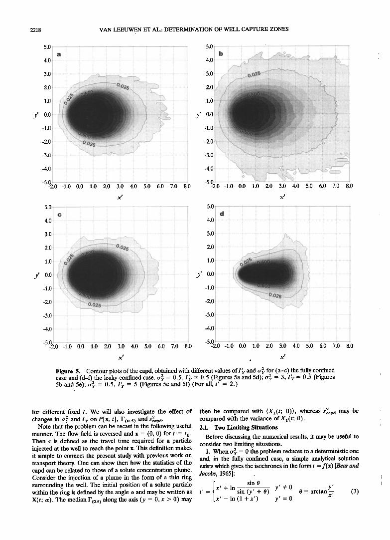
Figure 5. (continued)

where x', y', t' are the following dimensionless parameters

2 wqo 2 wqo 2 wqo 2 x' = .... t' = --t (4) QX, y-Qy, nQ

where qo = •'oJ[ L T-•] is the Darcy background flow velocity, •'o[L T-•] is T o per unit aquifer thickness, and n is effective porosity. For ease of comparison with (3), the dimensionless parameters in (4), together with a dimensionless integral scale I• = (2Iywqo)/Q, will be used in the sequel of the paper.

No analytical solution for the leaky-confined case is avail- able, but t' = f(x') may be determined through pathline tracing in a groundwater flow model. Figure 3 shows contour plots of t' -- f(x') for both aquifer models. It can be seen that

recharge reduces the size of the isochrones and the catchment is no longer infinite in the upstream direction.

2. When I• --• m the problem is that of a homogeneous aquifer with random transmissivity. For the fully confined case, the problem can be solved analytically and the capd can be described by the equation derived in the appendix:

•+• (ln •'* - In Ca) e[x', t']: • _ 2 erf oryx/• (5) where •'* is the transmissivity associated with the isochrone which goes through location x' at time t'. It can be calculated using (3) and (4). The evaluation of the plus-or-minus sign depends on the location relative to the well, as described in the appendix. In the leaky-confined case, an analytical solution is less straightforward, but a solution may be obtained numerically.

Figure 4 shows contour plots of P[x', t'] for both the fully confined and the leaky-confined case. In the fully confined case, the location of the capture zone is dependent on •' through the equation q o = TJ, so a change in T results in a linear change in q o as J is kept constant through the constant head boundary conditions. The shape of the capd can be understood by considering the upper and lower limits of •r. When T is large, q o is large and the capture zone is elongated in the upstream direction. When T is small, q o is small and the capture zone has a more circular shape. The shape of the capd in the leaky-confined case can be explained in a similar way, by considering the upper and lower limits of T.

2.2. Numerical Approach

Numerical estimates of P[x', t'] are obtained through Monte Carlo (MC) simulations, each comprising a total of 1000 realizations. For each MC realization, a realization of T is generated and assigned to the grid cells of the center part of the domain (-5 < x' < 11, -8 < y' < 8) (see Figure 1). Outside the center part, the geometric mean of the realization is used. Equation (1) is solved numerically using a standard block-centered finite difference approximation and forward particle tracking is applied to ideal tracer particles uniformly distributed over the area of interest (-2 < x' < 8, -5 < y' < 5). In order to obtain a good reproduction of the correlation structure, the grid size in the center part is chosen as Ax' = 0.1 for all simulations, resulting in a minimal ratio of I•/Ax' = 5, which gives a good reproduction of the correlation structure for all I• tested. The area outside the center part consists of four rows of cells with grid sizes of Ax' X 10 •, Ax' X 10 2, Ax' X 10 3, and Ax' respectively. This positions the boundaries sufficiently far from the well as to minimise the influence of boundary conditions on the random • and V fields. A more detailed discussion of issues regarding grid dis- cretization and boundary conditions in a very similar numerical setup was given by Franzetti and Guadagnini [1996].

3. Results and Discussion

In several Monte Carlo simulations different combinations

of cr• and I• have been tested: cr• = 0.1, 0.5, 1, 2, 3 and I• = 0.5, 1, 3, 5, 8, 16, 32, 64, 128, 256, 1024, c•. Two values of or} and I• were chosen as a reference; cr• = 0.5 and I• = 0.5. When either of these parameters was changed, the other was kept at its reference value. In each analysis, the capds for t' = 0.5, 1, 2, 3.5, 5 were determined.

Figure 5 shows contour plots of P[x', t' ] for different values

222O VAN LEEUWEN ET AL.: DETERMINATION OF WELL CAPTURE ZONES

l• b ] t' = 0.5 + ' '•'J•+• '+;• ' x +

[ i • • =2.o• 0.8 I •+ • • , =3.5 = 0.8

I f+ 0.6 0.6

0.4 0.4

-2 0 2 4 6 8 - ;2 -1 0 1 2 x' y'

s t' =0.5 = = =1.0

0.8 0.8 ß . = •.o =3.5

0.6 0.6

0.4 0.4

o.• oa

-2 0 2 4 6 8 -3 -2 -1 0 1 2 3

x' y'

Figure 6. Graphs of the capd along the x' axis and the y' axis for (a, b) the fully confined case and (c, d) the leaky-confined case. The solid lines in Figures 6a and 6c represent theoretical cumulative normal distributions. (For all, I• = 0.5 and rr2v = 0.5.)

of rr2v, for both aquifer models, and for different values of I•. It can be seen how uncertainty in T(x') results in uncertainty in the boundaries of the capture zone and how an increase in rr2v results in an expansion of the zone of uncertainty. The influence of I• is hardly noticeable in the fully confined case for the I• = 0.5 andI• = 5 shown here, but the insensitivity was also found for larger integral scales. In the leaky-confined case, an increase in I• results in an expansion of the zone of uncertainty.

Despite the high number of MC iterations, the contour lines for F(o) and FO) are very irregular, whereas the contour lines for F(o.s ) are smoother. The phenomenon is enhanced by an increase in rr2v. The cause lies in the low number of realisations that give rise to probabilities close to P = 0 or P = 1. This is a numerical artefact preserved by the contour plotting program which does not smooth the lines but plots them exactly at the prescribed levels. However, this does not have a significant effect on the main statistics of the capd.

3.1. Normality of F(x' > O, y' = O)

Figure 6 shows plots of P[x', t'] along the x' axis (y' = O) and the y' axis (x' = 0) for different times t', obtained with the reference values of rr2v and I•. The curves in Figure 6 closely resemble a cumulative normal distribution for all t' tested, which suggests that F(x' > 0, y' = 0) is normally distributed. Indeed, the capd along the axis (x' > 0, y' = O) is precisely the cumulative density function (cdf) of F (x' > 0,

y' = 0). In both the fully confined and the leaky-confined case, the distributions depart from normality when rr2v or I• increase. The analogy with transport is useful here, as several authors have found that for uniform flow the particle trajectories pdf is practically normal for sufficiently small rr•. any- where or for large time for any rr2v [e.g., Dagan and Fiori, 1997; Bellin et al., 1992]. Note that the analogy only holds where the mean flow is uniform, that is, where the particles are not too close to the well. The normality can be explained by the central limit theorem (CLT) as follows. The total particle travel dis- tance to the well can be viewed as the sum of rn travel distances

AX in the grid cells visited by a particle. As rn is very large, and the random variables AX have common probability distributions and are uncorrelated beyond a few times the integral scale, it follows from the CLT that the sum •;m AX tends to normality.

2

3.2. Influence of t' and o•r on Scapd A clear difference between the fully confined case and the

leaky-confined case is the behaviour of the capd's in time (see Figure 6). In the fully confined case, the curves do not just move along the axes, but the uncertainty increases too. This is due to the fact that the released particles travel longer and encounter more heterogeneity as the capture zone expands with time. The same behavior is seen in solute dispersion where the ensemble longitudinal variance with respect to the expected plume centroid is found to increase with the travel


time [e.g., Bellin et al., 1992; Tompkins et al., 1994]. The ob- a 1 servation is augmented by Figure 7a, which shows that the uncertainty 2 2 ($capd/O'y on the vertical axis) increases as the capd 0.8 expands in time (F(0.s)/I•-on the horizontal axis). It also shows that the gradients of the graphs increase with F(0.s)/I•-. A comparison with transport may be useful to understand the 0.6 increasing gradient. The ratio F(0.s)/I •. may be compared with a, the parameter Ut/Ir in uniform flow (U is the mean velocity). 0.4 It was shown by Dagan [1988] that for the ratios used here of F(0.s)/I •. < 10, the equivalent dispersion coefficient is far from its "Fickian" limit and increases with Ut/Ir. 0.2

In the leaky-confined case, the uncertainty increases initially, but when the capd reaches the water mount at x' • 4.5 its 0 expansion is inhibited and the uncertainty decreases again. Figure 7b illustrates this for tr} = 0.1 and tr} = 0.5. For tr• > 0.5, the uncertainty keeps increasing, probably because b 1 the location of the water mount becomes more variable as tr} increases.

2 0.8 An important observation about the influence of tr} on s capd can be made in Figure 7a. The coincidence of the curves for tr} = 0.1 and tr} = 0.5 shows that in the fully confined case 0.6 2 is linear in tr} for these values of tr}.. This is significant Scap d I•

because it implies that 2 easily be predicted from rr•. In Scapd can 0.4 the leaky confined case, Figure 7b suggests that for F(0.s)/I•- •< 6, 2 is linear in tr} for all tr• tested. S capd

•'",, I'y = 0.5 o ",,, I'y --> oo ...........

2 3 4 5 6

X'

b 0.8

0.7

0.6

,.•;• 0.5 " 0.4

½•L 0.:3 0.2

0.1

0.2

I'y = 32 o I'y = 1024 ß

1 2 3 4 5 6

2.5 x' ! i i i •

2 Figure 8. Graphs of the capd along the axis (x' > 0, y' - {;y =0.1 -- 0.5 x 0) for (a) the fully confined case and (b) the leaky confined

2 1.0 case. The solid lines represent theoretical cumulative normal 2.0 distributions. (For both, rr} = 0.5' t' = 2.) 2t.0 '

1.5

1 3.3. Influence of I•. on Sc,,va t 2

In the fully confined case, the influence of I y on Scapd was 0.5 found to be negligible for the rr} = 0.5 tested and for integral

scales of up to many times the length of the centre part. This 0 ............ is illustrated in Figure 8a which shows how little the capd's for

0 2 4 6 8 10

F(0.5 ) / I'y

Cry =0.1 = 0.5 = 1.0 = 2.0 = 3.0

0 ' i i i , i 0 1 2 3 4 5

F(0.5 ) / I'y

Figure 7. Graphs of the ratio 2 2 S capd/O'y as a function of F (0 I•. along the axis (x' > O, y' = 0) for (a) the fully confi•ed case and (b) the leaky-confined case. (For both, I•. = 0.5.)

I' = 0.5 and I•. --> o• differ along the axis (x' > 0 y' = O) Y , ß

This insensitivity is also observed in solute transport modelling. It was shown (e.g., by Dagan [1988]) that for small Ut/Ir the "macrodispersion" grows linearly with time and it does not depend on I•. However, for large tr• there should be depen- dence on I•.; otherwise, a large I•. approximation would always work. It is also important to emphasize that for larger t', not investigated, the impact of I•. should be felt at any

In the leaky-confined case, I•. has a distinct influence on the capd, as is illustrated in Figure 8b, which shows that when increases from I•. = 0.5 to I•. = 5, the capd expands, but when I•. further increases the capd shrinks again. In order to understand the cause of this behavior it is important to first discuss the sensitivity of the capd to T(x'). It was found that, in the confined case, the transmissivity within the reference capture zone ((x', y' ) • ( - 1..3, - 2..2)) influences the capture zone the most. In the leaky-confined case, the transmissivity in a large, wedge-shaped region in the vicinity and downstream of the capture zone is also important for the shape of the capture zone. When I•. increases, a larger area of T may have a value that is significantly different from the mean; if this area covers

2222 VAN LEEUWEN ET AL.' DETERMINATION OF WELL CAPTURE ZONES

............................ linear superposition of three mean velocity fields: (1) a velocity 1 ................. 2' 1 ' o¾ = 0. + field with a spatially constant mean, given by To/; (2) a veloc- = 0.5 x ity field with a spatially varying mean, resulting from the well of 0.8 = 1.0 ß

= 2.0 [] constant Q, and with a Teq changing from T H at the well to T o far from the well IDagan, 1982; Indelman and Abramovich, 1989;

0.6 Sdnchez-Idla, 1997]; (3) in the leaky-confined case, an additional velocity field with a spatially varying mean, resulting from the

0.4 uniformly distributed recharge R, must be added. It can be associated with a req equal to T o (this was numerically verified).

The total mean velocity field and the Teq that can be asso- 0.2 ciated with it will be complex. Along the axis (x' > O, y' = 0),

Teq will vary between T H at the well and T o far from the well. 1

0 As r H = r o exp (-3 tr2v) decreases with an increasing tr2v, so 0 1 2 3 4 5 6 7 8 does Teq along (x' > O, y' = 0), and F(o.s) will shrink.

.. r • x cs} = 0.1 + An interesting question is whether an equivalent transmis- 1 sivity Teq can be defined for which the capture zone coincides with F(o.s ). For a Teq as a function of x, this question is not easy

= 0.5 x to answer, but for a homogeneous Teq the question can be 0.8 = 1.0 • answered as follows. When o-2• changes, the isoline F(o.s ) ex- = 2.0

= 3.0 - pands or shrinks while its shape remains relatively unchanged. 0.6 When a homogeneous T changes, the corresponding isochrone

changes distinctly. Hence no homogeneous Teq can be found

0.4 N for which the capture zone coincides with F(o.5 ). 0.2 4. Summary and Conclusions

Well capture zones are usually estimated using analytical or

0 ' • • numerical models based on assumptions of homogeneous 0 1 2 3 4 5 6 7 8

X'

Figure 9. Graphs of the capd along the axis (x' > O, y' = 0) for (a) the fully confined case and (b) the leaky confined 6 case. The solid lines represent theoretical cumulative normal distributions. (For both, I• = 0.5 and t' = 2.) 5

part of the sensitive region, it influences the flow of recharge heavily, which in turn affects the capture zone. When I• further increases beyond I• • 5, the T values in the sensitive region will show little spatial variation and as a result the capture zone becomes less variable.

3.4. Behavior of F(o.5 ) Of particular interest is the location and behavior of the

median capture zone F(o.s ). The median capture zone is relevant for field applications as it is easily understood and it may serve as a criterion for the selection of an effective parameter.

Figure 9 shows graphs of the capd along the axis (x' > O, y' = 0) for different values of o-2•. An interesting feature in the figures is the movement of F(o.s)(x' > 0, y' = 0) toward the well with an increasing o-2•. The behavior is shown here along the axis (x' > O, y' = 0), but it is also observed for

2 increases. A further other directions that F(o.s ) shrinks as o-y analysis is made in Figure 10, which plots F(o.s ) as a function of t' for different o-2•. In Figure 10, the solid line represents F(o.s ) for the deterministic case with T o . It can be seen that the curves for different o-2• deviate more from this line when o-2• increases, indicating that F(o.s ) shrinks as o-2• increases. Obvi- ously, the deviation decreases when I• increases and it will be zero for/' --• • y ß

The phenomenon of a shrinking F(o:s) with an increasing •2 v may be explained using the concept of equivalent transmissivity Teq. The mean velocity field, which gives rise to F(o.s ), is a

i i i

1 2 3 4 5

b 6

= O. 1 .......... - 13.5 - 1.0

= 2.0 ......... = 3.0 .......... •-- -•• ................ 4

./•ff.-" .•. ......... _ ..... ..1 .............................

,?¾.--. .......

1 2 3 4 5

Figure 10. Graphs of F(o.5 ) as a function of t', along the axis (x' > 0, y' = 0) for (a) the confined case and (b) the leaky confined case. The full line pertains to the deterministic capture zone obtained with T o. (For both, I9 = 0.5.)


transmissivity T. However, aquifers can exhibit a considerable degree of heterogeneity at different scales. When heterogeneity of T is accounted for through a stochastic approach, capture zones can be defined in terms of probability and all locations in the domain are assigned a probability P[x, t] of being part of the capture zone.

In the work presented here, the effects of the statistical parameters of transmissivity variation (rr2v and Iy) on the capture zone probability distribution (capd) have been investigated for both a fully confined and a leaky-confined aquifer model. A connection is made with previous work on transport theory, and the statistical parameters of the capd are compared with those of a solute concentration plume.

The capd is found to be cumulative normal distributed for 2 and I • in both aquifer models. In the fully sufficiently small try

confined case, its behavior in time is similar to that of a dis- persing solute plume, in the sense that the spread of the capd

2 is 2 increases with time. In the fully confined case, $capd S capd found to be largely dependent on rr2v. In the leaky confined

2

case, Scapd also depends on I•. In both cases, the location of the median stochastic capture zone F(o.s) moves slightly toward the well as rr2v increases, a phenomenon that can be explained using the concept of equivalent transmissivity. When I• goes to infinity, T becomes a univariate random variable and the capd can be derived analytically in a straightforward manner.

The authors are currently investigating the influence of conditional simulation on the capd by using T fields conditioned on •b and T values.

Appendix A: Random Homogeneous Transmissivity

In this appendix, the capd P[x', t'] is derived for a case where the transmissivity of a fully confined aquifer is considered to be homogeneous, though random. The natural loga-

_

rithm of the homogeneous transmissivity Y = In T is assumed to be normally distributed with mean/xv = (ln •') - In •'G and variance rr2v. The cumulative distribution of •' is given by

F-•(•'•) = P(•' -< •'•) = 5 1 + erf (6) O'y

Objective of this derivation is P[x', t'], given the probability distribution of •'. From (3) and (4) it follows that the location of the capture zone is dependent on T through the equation q o - TJ, and it can be stated that the probability that a particle released at location x' will be captured by the well within time t' is equal to the probability that T is greater or smaller (depending on the position relative to the well) than •'*, where •'* is the transmissivity associated with the capture zone which goes through location x' at time t'. The probability P associated with location x' can then be written as

P = P(•'-> •'*) = 1 - F3(•'*)

or (depending on the position relative to the well)

P = P(T _< •*) - F3(•*)

(7)

(8)

In 7'* - In 7'G.) • + • erf . e = •_ • rrvx/-• (9) For given location and time, T* can be calculated by using (3) and (4).

Acknowledgments. The authors wish to thank Gedeon Dagan for his invaluable advice during the research and for his thorough review of drafts of the paper. The authors wish to thank the anonymous reviewers for their constructive comments.

References

Bair, E. S., C. M. Safreed, and E. A. Stasny, A Monte Carlo-based approach for determining traveltime-related capture zones of wells using convex hulls as confidence regions, Ground Water, 29, 849- 855, 1991.

Bear, J., and M. Jacobs, On the movement of water bodies injected into aquifers, J. Hydrol., 3, 37-57, 1965.

Bellin, A., P. Saladin, and A. Rinaldo, Simulation of dispersion in heterogeneous porous formations: Statistics, first-order theories, con- vergence of computations, Water Resour. Res., 28(9), 2211-2227, 1992.

Bhatt, K., Uncertainty in wellhead protection area delineation due to uncertainty in aquifer parameter values, J. Hydrol., 149, 1-8, 1993.

Dagan, G., Stochastic modelling of groundwater flow by unconditional and conditional probabilities, 1, Conditional simulation and the di- rect problem, Water Resour. Res., 18, 813-833, 1982.

Dagan, G., Time-dependent macrodispersion for solute transport in anisotropic heterogeneous aquifers, Water Resour. Res., 24, 1491- 1500, 1988.

Dagan, G., and A. Fiori, The influence of pore-scale dispersion on concentration statistical moments in transport through heterogeneous aquifers, Water Resour. Res., 33(7), 1595-1605, 1997.

Delhomme, J.P., Spatial variability and uncertainty in groundwater flow parameters: A geostatistical approach, Water Resour. Res., 15, 269 -280, 1979.

Evers, S., and D. N. Lerner, How uncertain is our estimate of a wellhead protection zone, Ground Water, 36, 49-57, 1998.

Franzetti, S., and A. Guadagnini, Probabilistic estimation of well catchments in heterogeneous aquifers, J. Hydrol., 174, 149-171, 1996.

G6mez-Hernfindez, J. J., Geostatistics and hydrology: An overview, JEC-61 Proc., 1,457-466, 1996.

Indelman, P., and B. Abramovich, Nonlocal properties of nonuniform averaged flows in heterogeneous media, Water Resour. Res., 30, 3385-3393, 1989.

Kinzelbach, W., M. Marburger, and W.-H. Chiang, Determination of groundwater catchment areas in two and three spatial dimensions, J. Hydrol., 134, 221-246, 1992.

Kinzelbach, W., S. Vassolo, and G.-M. Li, Determination of capture zones of wells by Monte Carlo simulation, Proceedings of the Mod- elCARE 96 Conference, IAHS Publ., no. 237, 1996.

Lerner, D. N., Well catchments and time-of-travel zones in aquifers with recharge, Water Resour. Res., 28(10), 2621-2628, 1992.

Sfinchez-Vila, X., Radially convergent flow in heterogeneous porous media, Water Resour. Res., 33(7), 1633-1641, 1997.

Tompkins, J. A., K. C. Gan, H. S. Wheater, and F. Hirano, Prediction of solute dispersion in heterogeneous porous media: Effects of er- godicity and hydraulic conductivity discretisation, J. Hydrol., 159, 105-123, 1994.

Uffink, G. J. M., Analysis of dispersion by the random walk method, Ph.D. thesis, Delft Univ. of Technol., Delft, Netherlands, 1990.

Van der Hoek, C. J., Contamination of a well in a uniform background flow, Stochastic Hydrol. Hydraul., 6, 191-208, 1992.

Van Herwaarden, O. A., and J. Grasman, Dispersive groundwater flow and pollution, Math. Models Meth. Appl. Sci., 1, 61-81, 1991.

Van Kooten, J. J. A., Advective-dispersive contaminant transport to- wards a pumping well, Ph.D. thesis, Landbouwuniversiteit Wagenin- gen, Wageningen, Netherlands, 1996.

Varljen, M.D., and J. M. Shafer, Assessment of uncertainty in time- related capture zones using conditional simulation of hydraulic conductivity, Ground Water, 29, 737-748, 1991.

A. P. Butler and J. A. Tompkins, Department of Civil Engineering, Imperial College of Science, Technology and Medicine, Imperial Col- lege Road, London SW7 2BU, England, UK.

C. B. M. te Stroet, Faculty of Civil Engineering, Delft University of Technology, Stevinweg 1, 2628 CN Delft, Netherlands.

M. van Leeuwen, Imperial College of Science, Technology and Med- icine, Imperial College Road, London SW7 2BU, England, UK.

(Received December 1, 1997; revised April 17, 1998; accepted May 8, 1998.)

Stochastic determination of well capture zones

Documents

Transcript of Stochastic determination of well capture zones