Forest--savanna transition zones - Biogeosciences

BGD11, 4591–4636, 2014

Forest–savannatransition zones

E. M. Veenendaal et al.

Title Page

Abstract Introduction

Conclusions References

Tables Figures

J I

J I

Back Close

Full Screen / Esc

Printer-friendly Version

Interactive Discussion

Discussion

Paper

|D

iscussionP

aper|

Discussion

Paper

|D

iscussionP

aper|

Biogeosciences Discuss., 11, 4591–4636, 2014www.biogeosciences-discuss.net/11/4591/2014/doi:10.5194/bgd-11-4591-2014© Author(s) 2014. CC Attribution 3.0 License.

Open A

ccess

BiogeosciencesDiscussions

This discussion paper is/has been under review for the journal Biogeosciences (BG).Please refer to the corresponding final paper in BG if available.

Structural, physiognomic andaboveground biomass variation insavanna-forest transition zones on threecontinents. How different areco-occurring savanna and forestformations?E. M. Veenendaal1, M. Torello-Raventos2, T. R. Feldpausch3, T. F. Domingues4,F. Gerard5, F. Schrodt3, G. Saiz2,25, C. A. Quesada3,6, G. Djagbletey7, A. Ford8,J. Kemp9, B. S. Marimon10, B. H. Marimon-Junior10, E. Lenza10, J. A. Ratter11,L. Maracahipes10, D. Sasaki12, B. Sonké13, L. Zapfack13, D. Villarroel14,M. Schwarz15, F. Yoko Ishida6,16, M. Gilpin3, G. B. Nardoto17, K. Affum-Baffoe18,L. Arroyo14, K. Bloomfield3, G. Ceca1, H. Compaore19, K. Davies2, A. Diallo20,N. M. Fyllas3, J. Gignoux21, F. Hien20, M. Johnson3, E. Mougin22, P. Hiernaux22,T. Killeen14,23, D. Metcalfe8, H. S. Miranda17, M. Steininger24, K. Sykora1,M. I. Bird2, J. Grace4, S. Lewis3,26, O. L. Phillips3, and J. Lloyd16,27

4591

http://www.biogeosciences-discuss.net

http://www.biogeosciences-discuss.net/11/4591/2014/bgd-11-4591-2014-print.pdf

http://www.biogeosciences-discuss.net/11/4591/2014/bgd-11-4591-2014-discussion.html

http://creativecommons.org/licenses/by/3.0/

BGD11, 4591–4636, 2014



Title Page



Tables Figures

J I

J I

Back Close

Full Screen / Esc



Discussion

Paper

|D

iscussionP

aper|

Discussion

Paper

|D

iscussionP

aper|

1Centre for Ecosystem Studies, University of Wageningen, 6700 AA, the Netherlands2School of Earth and Environmental Science, James Cook University, Cairns, Qld, Australia3Earth and Biosphere Institute, School of Geography, University of Leeds, UK4School of Geosciences, University of Edinburgh, Scotland, UK5Centre for Ecology & Hydrology, Wallingford, UK6Instituto Nacional de Pesquisas da Amazonia, Manaus, Brazil7Forest Research Institute of Ghana, Kumasi, Ghana8CSIRO Ecosystem Sciences Tropical Forest Research Centre, Atherton Qld, Australia9Australian Tropical Forest Research Institute, Cairns, Australia10Universidade do Estado de Mato Grosso, Nova Xavantina, MT, Brazil11Royal Botanic Garden, Edinburgh, Scotland, UK12Fundação Ecológica Cristalino, Alta Floresta, Brazil13Department of Biology, University of Yaoundé Cameroon14Museo Noel Kempff Mercado, Santa Cruz, Bolivia15Fieldwork Assistance, Jena, Germany16School of Marine and Tropical Biology, James Cook University, Cairns, Qld, Australia17Universidade de Brasilia, DF, Brazil18Resource Management Support Centre, Forestry Commission of Ghana, Kumasi, Ghana19Institut de l’Environnement et de Recherches Agricoles, Ouagadougou, Burkina Faso20Centre National des Semences Forestières, Ouagadougou, Burkina Faso21Ecole Normale Supérieure, Paris Cedex 05, France22Géosciences Environnement Toulouse, Observatoire Midi-Pyrénées, Toulouse, France23World Wildlife Fund, Washington DC, USA24Conservation International, Washington DC, USA25Karlsruhe Institute of Technology, Institute of Meteorology and Climate Research,Garmisch-Partenkirchen, Germany26Department of Geography, University College London, UK27Department of Life Sciences, Imperial College London, Silwood Park Campus, BuckhurstRoad, Ascot, Berkshire SL5 7PY, UK

4592





BGD11, 4591–4636, 2014



Title Page



Tables Figures

J I

J I

Back Close

Full Screen / Esc



Discussion

Paper

|D

iscussionP

aper|

Discussion

Paper

|D

iscussionP

aper|

Received: 12 December 2013 – Accepted: 10 February 2014 – Published: 24 March 2014

Correspondence to: J. Lloyd ([email protected])

Published by Copernicus Publications on behalf of the European Geosciences Union.

4593





BGD11, 4591–4636, 2014



Title Page



Tables Figures

J I

J I

Back Close

Full Screen / Esc



Discussion

Paper

|D

iscussionP

aper|

Discussion

Paper

|D

iscussionP

aper|

Abstract

Through interpretations of remote sensing data and/or theoretical propositions, theidea that forest and savanna represent “alternative stable states” is gaining increas-ing acceptance. Filling an observational gap, we present detailed stratified floristic andstructural analyses for forest and savanna stands mostly located within zones of tran-5

sition (where both vegetation types occur in close proximity) in Africa, South Americaand Australia. Woody plant leaf area index variation was related in a similar way totree canopy cover for both savanna and forest with substantial overlap between thetwo vegetation types. As total woody plant canopy cover increased, so did the contri-bution of middle and lower strata of woody vegetation to this total. Herbaceous layer10

cover also declined as woody cover increased. This pattern of understorey grasses andherbs being progressively replaced by shrubs as canopy closure occurs was found forboth savanna and forests and on all continents. Thus, once subordinate woody canopylayers are taken into account, a less marked transition in woody plant cover acrossthe savanna-forest species discontinuum is observed compared to that implied when15

trees of a basal diameter > 0.1 m are considered in isolation. This is especially thecase for shrub-dominated savannas and in taller savannas approaching canopy clo-sure. An increased contribution of forest species to the total subordinate cover is alsoobserved as savanna stand canopy closure occurs. Despite similarities in canopy covercharacteristics, woody vegetation in Africa and Australia attained greater heights and20

stored a greater concentration of above ground biomass than in South America. Up tothree times as much aboveground biomass is stored in forests compared to savannasunder equivalent climatic conditions. Savanna/forest transition zones were also foundto typically occur at higher precipitation regimes for South America than for Africa.Nevertheless, coexistence was found to be confined to a well-defined edaphic/climate25

envelope consistent across all three continents with both soil and climate playing a roleas the key determinants of the relative location of forest and savanna. Taken togetherthese observations do not lend support the notion of alternate stable states mediated

4594





BGD11, 4591–4636, 2014



Title Page



Tables Figures

J I

J I

Back Close

Full Screen / Esc



Discussion

Paper

|D

iscussionP

aper|

Discussion

Paper

|D

iscussionP

aper|

through fire-feedbacks as the prime force shaping the distribution of the two dominantvegetation types of the tropical lands.

1 Introduction

In general terms, “savannas” may be defined as woody vegetation formations typeshaving a fractional axylale (herbaceous) ground cover of at least 0.1; but also with5

a woody species composition quite distinct from “forests”; the latter also typically(though not always) with axylales absent (Torello-Raventos et al., 2013). Together for-est and savanna dominate the tropical vegetated regions covering 0.15 to 0.2 of theearth’s surface (Walter and Mueller-Dombois, 1971).

At a broad scale it has long been recognized that the distributions of these two10

biomes are principally governed by precipitation and its seasonality (Schimper, 1903).Nevertheless, it is sometimes possible to find these different vegetation formation typesin climatic zones where they are not usually occurring. For example, stands dominatedby species usually associated with forest vegetation formation types (“forest outliers”)may be found in Australia at mean annual precipitations (PA) of < 1.0 ma−1 in both Aus-15

tralia (Fensham, 1995) and South America (Killeen et al., 2006). Conversely, savannasare often seen on sandy soils under precipitation regimes usually associated with forest(PA > 2.0 ma−1) with such “savanna inliers” having been reported for South America,Australia and Africa (Hopkins, 1992; Lloyd et al., 2008; Torello-Raventos et al., 2013).

There are also discrete regions where the two biomes intercept – often referred to as20

“ecotones” or “Zones of (Ecological) Tension” (ZOT) – where both forest and savannaexist as discrete “patches” under similar climatic conditions. Although the influence ofsoil structure in shaping vegetation distributions within such ZOT has long been recog-nised (Cochrane, 1989; Ratter, 1992; Thompson et al., 1992; Hoffmann et al., 2009;Lehmann et al., 2011; Saiz et al., 2012), the observation that the artificial exclusion of25

fire from savanna areas within ZOT is followed by invasion of forest species has led tothe idea that forest and savanna stands may represent alternate stable states modu-

4595





BGD11, 4591–4636, 2014



Title Page



Tables Figures

J I

J I

Back Close

Full Screen / Esc



Discussion

Paper

|D

iscussionP

aper|

Discussion

Paper

|D

iscussionP

aper|

lated by fire-mediated feedbacks (Warman and Moles, 2009; Hoffmann et al., 2012a;Murphy and Bowman, 2012). Here the regular recurrence of fire in savanna systemsis considered to prevent these vegetation formations from becoming dominated by firesensitive forest species, with grasses and savanna trees characterised by adaptationsto a pyrogenically susceptible environment dominating (Gignoux et al., 2009; Hoffmann5

et al., 2012a; Murphy and Bowman, 2012). The observation that the exclusion of fireover prolonged periods often leads to transition of mesic savanna to forest is also seenas strong evidence for such feedbacks; see for example Hopkins and Jenkin (1962),Louppe et al. (1995), Swaine et al. (1992) and Geiger et al. (2011).

The notion of fire-mediated bistability has gained increasing acceptance through10

analysis of a global tree canopy cover data set (MOD44B; Hansen et al. (2002). A num-ber of studies have interpreted the observation of a lack of canopy cover around 0.6range (fractional cover) in this data set to provide planetary scale evidence of alterna-tive states with forest and savanna considered to exist above or below this threshold(Hirota et al., 2011; Staver et al., 2011a, b; Murphy and Bowman, 2012). Fire medi-15

ated feedbacks also form the basis of several models of tropical vegetation structureboth across the ZOT and within savanna systems (Van Langevelde et al., 2003; Staveret al., 2011a; Higgins and Scheiter, 2012) with conceptual origins lying in theoreticalframeworks of non-linear ecosystem population dynamics (May, 2001).

Hanan et al. (2013) have, however, recently pointed out that gaps in the distribution20

of the global vegetation cover data set may be the result of statistical procedures of cali-bration rather than low frequency occurrences of crown cover classes in the real world.Alternative explanations for the existence of observed tropical cover distribution pat-terns such a plant water demand (Bertram and Dewar, 2013) and herbivory (Pachzeltet al., 2013) have also been used in modelling studies to explain woody cover patterns25

not solely dependent on fire mediated feedbacks.Moreover, direct ground based observational evidence for forest-savanna discontinu-

ities and the existence of alternative stable states does not seem to have been activelysought. Nor has the structural and/or floristic (dis)similarity in structure of forests and

4596





BGD11, 4591–4636, 2014



Title Page



Tables Figures

J I

J I

Back Close

Full Screen / Esc



Discussion

Paper

|D

iscussionP

aper|

Discussion

Paper

|D

iscussionP

aper|

savannas in the transition been studied across continents in any sort of systematicmanner. We do know, however, that fire adapted woody species in vegetation typesusually defined as “savannas”, can attain forest-like woody canopy covers under cer-tain circumstances (Torello Raventos et al., 2013).

In this paper we attempt to fill this obvious data gap by providing detailed ground-5

based observational information on vegetation structure changes across the forest-savanna boundary. An emphasis is placed on the evaluation of all layers of the canopy,particularly the lower shrub and grass/herb (“axylale”) layers: these being particularlyimportant in the categorisation of the different tropical vegetation formations (Torello-Raventos et al., 2013), even though often excluded in definition and analysis of tropical10

forest structure. Our detailed field-based data thus include woody vegetation layersbelow 5 m and trees with diameter < 0.1 m. Indeed, these layers sometimes repre-sent a substantial component of both forest and savanna total woody cover and withsome savannas even dominated by these shorter woody vegetation types (Eiten, 1972;Haase and Beck, 1989; Gentry, 1995; Killeen et al., 1998; Oberle et al., 2009; Torello-15

Raventos et al., 2013).Our analysis utilises a global data set of newly established sample plots – mostly

located in ZOT – but also including specifically selected savanna inliers and forest out-liers as well as low precipitation savanna formations, with a delineation of these into for-est, woodland or savanna through a consistent set of rules designed to define tropical20

vegetation formation types globally (Torello Raventos et al., 2013). To our knowledgeour present analysis of structure of the plots used by Torrello Raventos et al. (2013)represents the first attempt to describe changes across ZOT on a field data basis andat a global scale. As well as describing structural differences, we also provide somefirst estimates of biomass differences for forest and savanna stands growing in close25

proximity with data coming from Australia, South America and Africa and with the an-ticipation that such data will be of considerable importance for global land-use changecarbon emission estimates (Malhi, 2010; Gloor et al., 2012; Houghton, 2012). Specificquestions addressed include:

4597





BGD11, 4591–4636, 2014



Title Page



Tables Figures

J I

J I

Back Close

Full Screen / Esc



Discussion

Paper

|D

iscussionP

aper|

Discussion

Paper

|D

iscussionP

aper|

1. Is there a really a marked discontinuity in dominant strata canopy cover distri-butions for tropical woody vegetation formation types as suggested by remotesensing products? And if so, is this associated with an abrupt transition from (i)vegetation formation types characterised by an obvious axylale layer and domi-nated by fire-adapted woody species (savannas) to (ii) contrasting closed forma-5

tions characterised by a very different woody species composition and with bothaxylales and fire virtually absent (forests)?

2. Does any such apparent marked continuity in woody plant cover continue to existonce variations all strata are taken into account? Specifically, around the pointof upper-strata canopy closure, is there a replacement of axylales by shrubs and10

small trees not included in most ground-based inventories and – most likely – alsonot detected by remote sensing products?

3. Do forest vs. savanna trees differ in their allometry? And if so, along with differ-ences in woody plant density – especially in the subordinate layers, how is thistranslated into differences in stand level biomass?15

4. Given the obvious influence of soils as key modulators of tropical vegetation struc-ture, to what extent might edaphic factors provide an explanation for both savannaand forest sometimes being found under apparently identical conditions? And ifthe soil effect is considerable, is an invocation of “alternative stable states” thennecessary for an understanding of the otherwise enigmatic distribution patterns20

of forest and savanna vegetation formation types across the tropical lands.

2 Materials and methods

With an objective of quantifying what factors define changes in vegetation structureand physiognomy across savanna-forest boundaries in so called Zones of Tension(ZOT), measurements of forest and savanna vegetation structure were made in ZOTs25

4598





BGD11, 4591–4636, 2014



Title Page



Tables Figures

J I

J I

Back Close

Full Screen / Esc



Discussion

Paper

|D

iscussionP

aper|

Discussion

Paper

|D

iscussionP

aper|

located in Australia, Africa and South America. Sites had been selected with a viewto maximising differences in climate and soils to allow an analysis of global applica-bility. The criteria of plot selection and establishment are detailed in Torello-Raventoset al. (2013). Drier savanna and forest plots were also examined in Australia, Boliviaand West Africa and with higher precipitation forest and savanna sites also studied5

in Brazil and Australia. A map showing all plot locations is given in Fig. 2 of Torello-Raventos et al. (2013) with a list of all plots studied, their location, vegetation formationtype, basic climatology and soil type also provided here (see Table S1 in Appendix A ofSupplement). Nomenclature of the various vegetation types follows Torello-Raventoset al. (2013) and in what follows all that is not referred to as some form of “Forest” is,10

by definition, considered part of the “Savanna Domain”. This includes all “grassland”,“savanna” and “woodland” types.

In terms of natural and human-mediated disturbances, some sites were fire-protected and with domestic animal grazing specifically excluded, but some others,especially in West Africa, farm animals were observed grazing in or nearby the sample15

plots. For all plots, there were no barriers placed to the grazing of vegetation by thenatural fauna. Table A1 of Torello-Raventos et al. (2013) gives details of plot histories(in terms of those previously or newly established), plot protection status and perceivedanthropogenic influences (grazing and fire protection or promotion).

2.1 Study sites20

Measurements were made from July 2006 to March 2009 in five field campaigns, eachover a period of ca. two months with as many plots as possible sampled within the allo-cated time and summarized as follows: West Africa (Ghana, Burkina Faso and Mali: 14plots; August to October 2006), Bolivia (11 plots; February to May 2007) Cameroon (8plots; November to December 2007), Brazil (17 plots; April to June 2008) and Australia25

(11 plots; February to April 2009). All sampling campaigns had been timed to coincidewith the end of the wet season and associated expected maximum plant physiologicalactivity and standing herbaceous biomass.

4599





BGD11, 4591–4636, 2014



Title Page



Tables Figures

J I

J I

Back Close

Full Screen / Esc



Discussion

Paper

|D

iscussionP

aper|

Discussion

Paper

|D

iscussionP

aper|

2.2 Tree and shrub canopy area index

Defining a canopy area index (C) as the sum of individual tree canopy projected area(including the skylight transmitted component) divided by the ground area as detailedin Torello-Raventos et al. (2013), C was estimated separately for three woody stratawithin each plot viz. for the upper (U), mid-stratum (M), and subordinate (S) layers as5

defined on the basis of with a stem diameter at breast height (1.3 m) D, and individualtree height (H). Data used here is as presented in Torello-Raventos et al. (2013), withprecise definitions of CU, CM and CS given in their Table 1. In short, the upper stratumwas considered to consist of all woody elements D > 0.1 m; the middle stratum allwoody elements with H > 1.5 m and 25 mm< D < 0.1 m and the lower stratum all other10

woody plant present (viz. less than 1.5 m high and/or D < 25 mm).For some analyses presented here the woody canopy cover component was

also divided into trees and shrubs, these being segregated as in Torello-Raventoset al. (2013). In brief, shrubs are defined as woody species with either a single stem(bole) of length at least 1.5 m, but with height less than 3 m, or a woody species with15

a stem length prior to branching of less than 1.5 m (also being less than 5 m height).The associated canopy area indices are designated as Ct and CSh and are formallydefined in Table 1 of Torello-Raventos et al. (2013).

Also considered separately here is a division of the woody vegetation according toheight, with the total woody plant canopy cover (all trees and shrubs taller than 1.5 m;20

CW) and seedling canopy cover (all trees and shrubs less than 1.5 m tall; CSe), againas defined in Table 1 of Torello-Raventos et al. (2013).

2.3 Fractional canopy covers

Assuming a random distribution of trees and/or shrubs, the crown cover; viz. the frac-tion of ground covered by crowns (including within-crown light gaps) referred to here25

as the fractional crown cover (ς) can be estimated for any combination of layers (Z) as

4600





BGD11, 4591–4636, 2014



Title Page



Tables Figures

J I

J I

Back Close

Full Screen / Esc



Discussion

Paper

|D

iscussionP

aper|

Discussion

Paper

|D

iscussionP

aper|

ςZ = 1−exp(−∑n

i=1Ci

), (1a)

where n is the number of layers. For example, for Z =W = U +M then n = 2 and

ςW = 1−exp(−CU −CM) . (1b)

Likewise for a single layer or vegetation form (e.g. shrubs) then5

ςSh = 1−exp(−CSh) . (1c)

Savanna vegetation may, however, be clumped and so we tested for complete spa-tial randomness (CSR) using a G function (Bivand et al., 2008) via the R spatstatpackage (Baddeley and Turner, 2005). The G function measures the distribution of dis-tances from an arbitrary event to its nearest event and comparisons of the theoretical10

expectation for CSR against that actually observed. There were only minor indicationsof clumping for those plots tested plots suggesting little if any underestimation of frac-tional covers using Eq. (1) (see Fig. S1 in Appendix B of Supplement).

Estimates of various ς so estimated are used extensively throughout this paper (andwith subscripts always as above) and here we note that estimates of fractional crown15

cover are not numerically or conceptually the same as those often presented for (frac-tional) woody canopy cover which – in remote sensing studies – is defined as “the por-tion of the skylight orthogonal to the surface which is intercepted by trees” (e.g. Hansenet al., 2002). Defining then α as the proportion of light intercepted on average by thetree crowns, and noting that canopy cover as so defined above is essentially equiva-20

lent to the fractional foliage cover or projective foliar cover of the stratum in question,ζ (Lloyd et al., 2008) it then follows that ζ = ας where α is the average proportion ofskylight passing through each tree.

Estimates of the fractional canopy cover of grasses and herbs in the ground layer(referred to here as “axylales”) are as in Torello-Raventos et al. (2013). In brief, the axy-25

lale fractional cover (ζa) was visually recorded along a series of transects with a typicalsampling intensity of 110×1.0 m2 quadrants per 1 ha plot.

4601





BGD11, 4591–4636, 2014



Title Page



Tables Figures

J I

J I

Back Close

Full Screen / Esc



Discussion

Paper

|D

iscussionP

aper|

Discussion

Paper

|D

iscussionP

aper|

2.4 Canopy height

Upper stratum tree heights (H) were estimated as described in Feldpausch et al. (2011)and Torello-Raventos et al. (2013). In short, site specific allometric equations weredeveloped to calculate 0.95 quantile and average woody plant heights for the upperstratum (D ≥ 0.10 m), these being denoted as H∗and 〈H〉U respectively.5

2.5 Stand-level leaf area index

Leaf area index of trees and shrubs taller than 1.5 m (L) was assessed using hemi-spherical photography. True-colour images were taken under diffuse light conditions(mostly sunrise and sunset) with a Nikon Coolpix 8800VR camera and Nikon FisheyeLens FC-E9 set at aperture 8.0 with a 2 step underexposure (Zhang et al., 2005). At10

most sites 10 to 25 images were taken at the centre of 25m×25m grid cells but for a fewsites with a very sparse woody cover, hemispheric images were taken from randomlyselected trees. This is because of a potentially problematic determination of L from gridhemispherical images in open vegetation (L . 1.5) as detailed by Ryu et al. (2010).

Images were analysed with the Gap light Analyser software Version 2 (Frazer et al.,15

1999) and in applying the technique two or more observers independently determinedimage specific threshold and contrast settings to reduce observer error. For each im-age, L was calculated from an integration over the zenith angles 0–75◦ after trunkand/or branch elements had been removed through manual editing. If images con-tained individual trees with non-overlapping crowns, fraction canopy cover in the image20

was also measured for each image by blackening total canopy area and determiningcanopy openness. Canopy-level L was then determined by dividing image L by imagecanopy fraction and L for plots where only images of individual trees were taken wasthen determined by multiplying the average individual tree estimates of L by the CW.Comparison of results of this calculation with L determined from grid cell images (if25

sites had images with non-overlapping crowns) gave comparable results particularly ifL < 1.0.

4602





BGD11, 4591–4636, 2014



Title Page



Tables Figures

J I

J I

Back Close

Full Screen / Esc



Discussion

Paper

|D

iscussionP

aper|

Discussion

Paper

|D

iscussionP

aper|

Estimates for end of season L for the axylale layer were determined from clippingstanding biomass (by drying to constant weight) in five to ten randomly selected 1 m2

plots. Leaf area of these samples was determined by scanning the fresh surface ofa subsample of the clipping before determination of specific leaf area.

2.6 Shrub and seedling dominance indices5

To quantify the relative dominance of shrubs in the ground layer relative to herbs andgrasses (axylales), we defined a “shrub dominance index” (χ1) as

χ1 =ςSh − ζa

ςSh + ζa, (2a)

where (as defined above) ςSh is the shrub crown projected cover and ζa is the axylalefractional cover. A second metric which quantifies competition between herbaceous10

and woody elements of the subordinate layer, a “seedling dominance index”, χ2, wasalso defined, viz.

χ2 =ςSe − ζa

ςSe + ζa, (2b)

where ςSe is the crown projected cover of all tree and shrub seedlings (as definedabove). The two indices (which can both potentially vary from −1 to +1) differ in that χ115

quantified the relative dominance of shrubs over axylales in the understorey (but ignor-ing any tree seedlings or tree saplings) whereas χ2 provides a measure of the relativeabundance of both tree and shrub seedlings relative to herbaceous cover extent.

2.7 Tree, shrub and liana biomass

2.7.1 Forests20

For all forest plots sensu Torello-Raventos et al. (2013) we applied a global equationfor predicting above ground biomass (B) from diameter at breast height (D) and tree

4603





BGD11, 4591–4636, 2014



Title Page



Tables Figures

J I

J I

Back Close

Full Screen / Esc



Discussion

Paper

|D

iscussionP

aper|

Discussion

Paper

|D

iscussionP

aper|

height (H) and density (ρ) using the “dry forest” equation of Chave et al. (2005) forall trees of D ≥ 25 mm (see Eq. S1 in Table S2 of Supplement Appendix C). Wooddensity values were obtained from Zanne et al. (2009) for Africa and South Americaand Ilic et al. (2000) for Australia. Unknown species densities are calculated usingthe mean values at closest taxon. For forest shrubs we developed our own generic5

equations for predicting B from basal area (AB) or crown diameter (DC) these beingbased on destructive measurements of 63 randomly selected individuals of the speciesAcacia tenuifolia, Croton argyroglossus, Tetrapterys racemulosa and two unidentifiedAcacia species harvested at the Tucavaca stunted forest and shrub-rich woodland sitein Bolivia (TUC-01 and TUC-02). The resulting parameterisation (see Eqs. S2 and S3 in10

Table S2 of Supplement Appendix C) gave rise to similar predictions to another derivedindependently for Indian understorey forest shrubs (Singh and Singh, 1991) suggestinga general applicability. For lianas we applied an equation from Schnitzer et al. (2006)and for palms the equation of de Castilho et al. (2006) both these parameterisationspredicting B from D (see Eqs. S4 and S5 in Table S2 of Supplement Appendix C)15

2.7.2 Savannas

For taller savanna trees in the African humid savannas of Burkina Faso, Cameroon andGhana (H > 10 m) we applied a generic allometric relationship for predicting B from Dand H , originally developed for miombo woodland trees (Malimbwi et al., 1994). Thisparameterisation (see Eq. S6 in Table S2 of Supplement Appendix C), tested for African20

savanna trees using unpublished data from Ivory Coast (Menaut, 1971), was confirmedas a good predictor for large trees (H > 10 m) but with a tendency to underestimate Bfor medium to smaller sized trees. For the more humid West African and Cameroonsavanna plots we therefore developed new equations for all trees of D > 25 mm andH < 10 m using the Menaut (1971) data set (see Eqs. S7 and S8 in Table S2 of Supple-25

ment Appendix C). For trees in the Sahelian savanna plots (HOM-01 and HOM-02) weused a parameterisation from Henry et al. (2011) using D as the predictor variable (seeEq. S13 in Table S2 of Supplement Appendix C) with the biomass parameterisations

4604





BGD11, 4591–4636, 2014



Title Page



Tables Figures

J I

J I

Back Close

Full Screen / Esc



Discussion

Paper

|D

iscussionP

aper|

Discussion

Paper

|D

iscussionP

aper|

for trees in the Guinean savannas BDA-01 and BDA-02 (Alexandre and Kaïré, 2001)also as given in Henry et al. (2011) with B derived from basal area (AB) measurements(see Eq. S14 in Table S2 of Supplement Appendix C). For shrubs at these drier siteswe used an equation from Skarpe (1990) with B estimated from crown area (AC) mea-surements (see Eq. S10 in Table S2 of Supplement Appendix C). For the subligneous5

fire resprouter shrub Cochlospermum planchonii (dominant in the Burkina Faso plotsDAN-01 and DAN-02) a separate equation was developed (see Eq. S9 in Table S2 ofSupplement Appendix C) with B calibrated against AC. For shrubs and trees in SouthAmerican cerrados we used an equation taken from Ribeiro et al. (2011) with B derivedfrom D, H and ρ (see Eq. S11 in Table S2 of Supplement Appendix C). Biomass of Aus-10

tralian trees and shrubs with D > 25 mm were estimated following Williams et al. (2005)with B derived from D and H (see Eq. S12 in Table S2 of Supplement Appendix C).

2.8 Climate

As in Torello-Raventos et al. (2013) we also estimated an index of plant water supplyin relation to evaporative demand, W , this being calculated as (Berry and Roderick,15

2002):

W = PA −Qs/(ρλ) (3)

where PA is mean annual precipitation rate, Qs is mean annual global solar radiation,ρ is the density of liquid water and λ is the latent heat of evaporation for H2O. Temper-ature and precipitation climatologies for all sites were obtained from the interpolated20

dataset from WorldClim dataset (see http://www.worldclim.org/) with mean annual so-lar radiation data obtained from NASA’s Langley Atmospheric Sciences Data CenterDistributed Active Center (DAAC) assimilated from daily records (1983 to 2005).

4605





http://www.worldclim.org/

BGD11, 4591–4636, 2014



Title Page



Tables Figures

J I

J I

Back Close

Full Screen / Esc



Discussion

Paper

|D

iscussionP

aper|

Discussion

Paper

|D

iscussionP

aper|

2.9 Soil cation status

Soil sampling and exchangeable cation determination methods are as described indetail in Quesada et al. (2010) and Quesada et al. (2011) and are thus only brieflysummarised here. In short, exchangeable aluminium, calcium, magnesium, potassiumand sodium viz. [Al]E, [Ca]E, [Mg]E, [K]E and [Na]E, were determined by the silver-5

thiourea method (Pleysier and Juo, 1980) with a simple measure of soil fertility definedhere, this being the “total major nutrient cations”, N+:

N+ = [Ca]E + [Mg]E + [K]E, (4)

with all cation concentrations expressed as meq+ kg−1 and integrated across the top0.3 m of soil depth.10

2.10 Statistical analysis

All analyses used the R statistical platform (R-Development-Core-Team, 2012). Mixedeffects models (Figs. 1 and 2) were developed using the mgcv and/or nlme packages(Wood, 2006; Pinheiro et al., 2012) allowing for heterogeneity in variances consideredin model fits using varClasses functions. Breakpoint regression analyses (Fig. 3)15

were with the segmented package (Muggeo, 2008); robust (rank-based) linear regres-sion analyses (Figs. 4–7) used the high breakpoint (HBR) option of wwest (Terpstraand McKean, 2005) and standard major axis regression (Fig. 9) was undertaken usingsmatr (Warton et al., 2012).

3 Results20

3.1 Leaf vs. canopy area index

The relationship between woody vegetation leaf area index estimates from hemispher-ical photographs (L) and woody plant canopy area index (CW) values obtained from

4606





BGD11, 4591–4636, 2014



Title Page



Tables Figures

J I

J I

Back Close

Full Screen / Esc



Discussion

Paper

|D

iscussionP

aper|

Discussion

Paper

|D

iscussionP

aper|

ground-based inventories is shown in Fig. 1. Here, as in most subsequent diagrams,sites have first been grouped into vegetation domain viz. savanna and forest; thesebeing differentiated on the basis of both floristics and structure (Marimon et al., 2006;Torello-Raventos et al., 2013). Both vegetation formation types are also further cate-gorised into three structural groups and with continents identified by colour. In brief,5

for the forests, the prefix “stunted” applies to those forests with a mean canopy height(upper stratum) of less than 12 m and “tall forests” have an upper stratum 0.95 quantileheight of more than 36 m. For the savanna domain, “shrub savannas” have a meancanopy height of less than 6 m (also with a canopy area index between 0.3 and 0.7)with “tall savannas” having a mean upper stratum canopy height greater than 12 m.10

Figure 1 suggests a uniform but non-linear relationship across vegetation types andcontinents, tending towards an asymptote at CW ' 2 (at which L ' 2.7). Below this pointthe ratio L/CW is reasonably constant indicating a reasonably constant leaf area den-sity (leaf area per unit projected canopy area; `D) of around 1.25, declining to less than1.0 at high L. Thus under conditions permitting only limited foliage development varia-15

tions in L are a direct consequence of variations in CW (with a more or less constant`D). But at higher CW there is a compensatory reduction in `D. Most importantly, Fig. 1shows that, although the relationship between L and CW is non-linear, CW providesa reasonable proxy for stand-level L that is broadly consistent across both vegetationtype and continent.20

3.2 Variations in canopy structure

Changes in fractional crown cover (ς) as CW increases are shown for the upper (U),middle (M) and subordinate (S) woody strata in Fig. 2a–c. This shows ςU saturatingbeyond CW ' 2, and with both ςM and ςS accounting for most of the increase in CWbeyond that (left side panels). Overall, there is little to suggest systematic differences25

between continents and, although overlap is limited, little to suggest any systematicdifference between forest and savanna. Figure 2a also shows an apparent gap in thedata around 0.55 ≤ ςU ≤ 0.65 for the upper stratum but with both forest and savanna

4607





BGD11, 4591–4636, 2014



Title Page



Tables Figures

J I

J I

Back Close

Full Screen / Esc



Discussion

Paper

|D

iscussionP

aper|

Discussion

Paper

|D

iscussionP

aper|

stands occurring above and below this break at around CW ' 1.5. By contrast, no sim-ilar discontinuity is observed for either ςM or ςS.

The same data is also shown in Fig. 2d and Fig. 2e but in this case divided intotrees (t) and shrubs (Sh). As CW increases ςt shows a saturating function similar toςU though with much less variability (though with two Australian forests occurring at5

unusually low rainfalls as clear outliers). The shrub fractional cover is clearly morevariable (Fig. 2e). At least in part this can be attributed to the presence of shrub domi-nated savannas at some of the lowest CW (these occurring on all three continents andfor clarity enclosed by the dotted-line polygon in Fig. 2e). And so the line shown hasbeen parameterised excluding these shrub-dominated sites so as to give an indication10

of how ςU varies with CW just for those savanna and forest formations with a distinctupper-stratum dominated by trees. This suggests a rapid increase in ςSh at CW ' 1,peaking around CW = 1.5 and maintained around ςSh at higher CW, at least for theforests within the ZOT as examined here. This increase in ςSh at CW ' 1 is observedfirst in tree-dominated savannas and stunted forests and it is only at CW ≥ 2 where the15

data is dominated by forest sites that ςSh tends to level out at a values of about 0.2.Figure 2f shows axylale fractional cover (ζa) to decline with increasing CW, first reach-

ing a minimum at CW ' 2 for both forest and savanna formation types. There is a rea-sonably strong relationship between ζa and axylale leaf area index (see Fig. S6 inAppendix D of Supplement) and so taken in conjunction with Fig. 2e, it can be con-20

cluded that as canopy closure occurs beyond CW ' 1 that the herbaceous layer (gen-erally dominated by C4 grasses in these ecosystems) declines, being replaced by anincreasingly dominant shrub layer. Importantly, this change in dominance is not associ-ated with a transition from savanna to forest, but is rather first observed in the woodiersavanna formation types.25

The consequences of any attempt to define tropical vegetation formations solely onthe basis of changes in upper stratum cover can be seen in Fig. 3 where the estimatedstand level crown cover is plotted against that of the upper stratum only. Here theshaded area between the fitted segmented regression line (Muggeo, 2008) and the

4608





BGD11, 4591–4636, 2014



Title Page



Tables Figures

J I

J I

Back Close

Full Screen / Esc



Discussion

Paper

|D

iscussionP

aper|

Discussion

Paper

|D

iscussionP

aper|

1 : 1 relationship shows the average woody cover overlooked by an “upper stratumonly” approach. Differences are greatest for ςU . 0.2 and 0.5 . ςU . 0.7: these beingassociated in the first instance with the presence of shrub-dominated savannas and inthe second instance with the higher relative dominance of shrub cover for vegetationcharacterised by 1 ≥ CW ≥ 2.5

3.3 Shrub and seedling dominance

The relative dominance of shrubs within the understorey in relation to axylale coveras affected by the upper-canopy cover is illustrated through a plotting of the shrub-dominance index (χ1: Eq. 2a) as a function of ςU in Fig. 4a. This shows χ1 to in-crease with increasing ςU both as savanna tree density increases and across the sa-10

vanna/forest transition. There are, however, distinct outliers as detected by the robustregression fitting technique, these being (long-grassed) savanna woodlands in Africaand tall savanna woodlands in Australia. When the seedling dominance index (χ2) is ap-plied (i.e. including tree seedlings, but excluding any shrubs taller than 1.5 m) then mostof the Australian tall savanna woodlands then fall into line (Fig. 4b) but with the long-15

grassed African savanna woodlands still identified as clear outliers. Thus, althoughthere are exceptions, there is a clear tendency for grasses and herbs to be replaced byseedlings and shrubs in the lower strata as canopy closure occurs higher up. This isseen first in woodier savannas (beyond ςU ' 0.3) extending then to the higher leaf areaforest vegetation formation types.20

3.4 Species composition of understorey

The presence of forest and savanna species in the middle and subordinate layersof savanna vegetation formation types plots is examined as a function of total frac-tional cover (this consisting mainly though not exclusively of savanna tree species)in Fig. 5a. This shows that associated with the upper canopy closure within savanna25

vegetation formation types beyond ςU ' 0.4 is a marked increase in the abundance of

4609





BGD11, 4591–4636, 2014



Title Page



Tables Figures

J I

J I

Back Close

Full Screen / Esc



Discussion

Paper

|D

iscussionP

aper|

Discussion

Paper

|D

iscussionP

aper|

forest species. On the other hand, there is no relationship between ςU and the cover ofsubordinate savanna tree and shrub species for these same stands (Fig. 5b).

3.5 Crown-cover/height allometry

Upper stratum quantile height (H∗) is examined as a function of the associated uppercanopy crown cover (ςU) in Fig. 6. This illustrates, for the South American savannas in5

particular, that there is relatively little variation in H∗ across a wide range of intermediateςU. At any given ςU it can be seen that H∗ is lower for South American savanna and/orforest than for Africa or Australia. There is also rapid increase in H∗ associated withthe transition from savanna to forest in South America that is more gradual on theother continents, especially once the stunted forests associated with unusually low10

precipitation (see Table S1 in Appendix 1 of Supplement) are taken into account.

3.6 Biomass/height allometry

The relationship between crown cover and biomass of the upper stratum (BU: D ≥0.1 m) – this being the only layer usually studied for estimates of forest biomass (e.g.,Feldpausch et al., 2012) – is shown in Fig. 7a. Here we find a strong inverse recip-15

rocal relationship and, although there is a rapid increase in BU for ςU > 0.8 (includinga few savanna plots) there is also considerable variation in BU beyond this point withdifferences of over 300 tha−1 possible at any given ςU > 0.8. A generally more con-sistent relationship is observed when biomass and crown canopy cover are examinedat the whole stand level (Fig. 7b) and with some overlap between savanna and forest20

observed in both cases. The higher biomass of the tall savanna types is also clearlydemonstrated by this diagram which also shows that, even at a ςU of only 0.5, someAustralian tall savanna formations can have a biomass approaching that of much highercrown cover South American and African forest formations.

4610





BGD11, 4591–4636, 2014



Title Page



Tables Figures

J I

J I

Back Close

Full Screen / Esc



Discussion

Paper

|D

iscussionP

aper|

Discussion

Paper

|D

iscussionP

aper|

3.7 Forest-savanna biomass differences

Figure 8 plots the biomass of all forest and savanna plots (excluding seedlings) asa function of the mean annual water availability, W , as calculated in Eq. (3). For eachcontinent, forest and savanna are shown separately and with plots located within ZOTshown by the shaded area (ZOT here being defined as regions occurring at the inter-5

section of major savanna/forest areas and with neither vegetation domain type clearlydominating at the scale of 10 km or less). Biomass estimates (B̂) for each plot are alsoshown separately for the upper and middle strata and for lianas and with additionalforest B̂ (upper stratum only) coming from Feldpausch et al. (2012) indicated by anasterisk. Apart from showing that the ZOT investigated occur at different W for different10

continents, the presence of stunted forests in areas significantly drier than the studiedZOT is illustrated, as is the occasional presence of savanna at low W . The most sub-stantial increase in biomass associated with a transition from savanna to forest is forthe South American ZOT (this being markedly less than for the sites sampled in Aus-tralia and Africa). There is also an important contribution of the middle stratum (trees15

and shrubs with D < 25 mm) to the total biomass of plots within the ZOT in some cases;and for the South American savannas in particular.

3.8 Inter-continental differences in the location of the forest-savanna boundary

The location of all sampled plots in terms of both W and soil cation nutrient status (N+;Eq. 4) is shown in Fig. 9 where with the N+∩W environmental space encompassed by20

ZOT (as identified in Fig. 8) shown through the shaded ellipse and with the fitted SMAregression line through these data points also shown. This shows that, not only is thepresence of the ZOT within South America at a more negative W associated with soilsof a lower exchangeable base cation status, but also that variations in the locations ofindividual plots within ZOT on each continent are also explicable in terms of the same25

N+; W relationship. Generally speaking, forests are found above the fitted line andsavanna formation types below. Savannas were, however, found at higher W for both

4611





BGD11, 4591–4636, 2014



Title Page



Tables Figures

J I

J I

Back Close

Full Screen / Esc



Discussion

Paper

|D

iscussionP

aper|

Discussion

Paper

|D

iscussionP

aper|

South America and Australia, these being associated with low N+. On the other hand,the stunted forests of both South America and Australia exist at relatively high N+ (andreasonably negative W ). Also of note is a lack of observations where W is stronglynegative and N+ also low.

The general notion that the location of forest-savanna transition zones may differ5

between continents is examined further in Fig. 10, where the frequency of occurrenceof savanna vegetation formation types in terms of PA is shown for all of Africa and SouthAmerica binned into 0.2 m PA classes (original data from the vegetation map basedstudy of Lloyd et al. (2008) undertaken at 1◦×1◦ resolution). Here, observations to theright of the frequency diagrams are mostly forest-type vegetation types and those on10

the left arid vegetation type formations. This confirms a clear difference between thetwo continents in terms of savanna distribution in relation to rainfall. Specifically, themaximum frequency of savanna occurrence occurring at a PA at least 0.2 m greater forSouth America than is the case for Africa. It was not, unfortunately, possible to includeAustralia in such an analysis due to the very limited area of tropical forest present.15

4 Discussion

The idea that forest and savanna present fire mediated alternate stable states hasrecently been being supported by analyses of bi- or tri- model distributions of treecanopy cover in a remotely sensed global tree cover dataset (Hirota et al., 2011; Staveret al., 2011b; Murphy and Bowman, 2012) with this notion having been underwritten by20

models also simulating such dichotomies (Van Langevelde et al., 2003; Staver et al.,2011a; Higgins and Scheiter, 2012). This has led to the general view that such alter-native stable states can exist under the same environmental conditions now becomingwidespread – see for example Warman and Moles (2009) and Hoffmann et al. (2012a).However Hanan et al. (2013) have pointed that gaps in the distribution patterns in the25

global tree cover data set may be caused by statistical procedure rather than repre-

4612





BGD11, 4591–4636, 2014



Title Page



Tables Figures

J I

J I

Back Close

Full Screen / Esc



Discussion

Paper

|D

iscussionP

aper|

Discussion

Paper

|D

iscussionP

aper|

senting true abundance differences. Unequivocal evidence supporting the notion ofalternative stable states should therefore be sought elsewhere.

Here we have reported an as complete as possible set of observations of structuralchanges across savanna and forest formations across ZOT on three continents. Ourexpectation was that, should alternative stable states driven by fire mediated feedbacks5

exist, then associated with that should be abrupt disjunctions in vegetation structure ob-servable across forest/savanna boundaries. Also, as argued previously by Warman andMoles (2009) and Murphy and Bowman (2012) it would also not be expected that theour studied zones of transition would be found to be located in some sort of consistentlycommon climate/soil environmental space.10

4.1 Disjunction vs. continua in the forest-savanna transition

In terms of disjunction of vegetation structure, Figs. 1 and 2 show much more a contin-uum, particularly if all layers of vegetation are taken into account. Specifically it wouldseem that, around the point that canopy closure occurs, that the shrub layer of bothforest and savanna becomes increasingly important (Fig. 2e); effectively replacing the15

grass layer in both woodland and open forest systems (Figs. 2f and 4). Confoundingcomparison with remote sensing products is, however, also the observation that many(shrub dominated) savannas can have a considerable canopy cover but with almost allof this contributed by trees < 5 m tall. Such low stature vegetation was apparently notincluded in the calibration of the global vegetation cover data set Hansen et al. (2003)20

and is presumably less accurately quantified as a result. This calls for caution whenusing such in silico datasets as a proxy for real world ecosystem level woody covermeasurements and the relative distribution of forest and savanna formations in zonesof transition.

We do, of course, acknowledge that the transitional vegetation formations described25

in our study do not present a spatially explicit frequency distribution of all savanna andforest formations present across the planet. They are, however, representative of thecommonly found formations in our study areas as they were specifically selected for this

4613





BGD11, 4591–4636, 2014



Title Page



Tables Figures

J I

J I

Back Close

Full Screen / Esc



Discussion

Paper

|D

iscussionP

aper|

Discussion

Paper

|D

iscussionP

aper|

purpose (Torello-Raventos et al., 2013). We do therefore not expect the analysis of thedifferences in structural layers as savanna transforms to forest to be fundamentally dif-ferent in other sites. Most formations studied by us – with the exception of the MDJ-05transitional forest plot in Central Africa - specifically selected as being in active transi-tion (Mitchard et al., 2009) and NXV-02 in Brazil (Franczak et al., 2011) – can therefore5

be assumed on the basis of history and stand age to reflect the recent climate, soil andland management activities. Although soil organic matter 13C/12C ratios (G. Saiz andTROBIT Consortium, unpublished data) do suggest that some forest plots in Cameroonmay have had savanna vegetation in a fairly recent (centennial timescale) past – seeTable S1 in Appendix A in Supplement as well as Torello-Raventos et al. (2013).10

4.2 The importance of the shrub layer

The observed increase in understorey wood plant density around the stage of full up-per canopy closure is at the expense of the axylale cover and may be a consequenceof the relative inefficiency of the C4 photosynthetic pathway typical of tropical grassesin shaded environments – as is also suggested by the axylale species persisting in15

dense savanna and forest formations at relatively low abundances actually being of theC3 photosynthetic mode (Torello-Raventos et al., 2013). In this context we also notethat Laubenfels (1975) working in North America and limiting his observations to “veg-etation cover showing a minimum of disturbance, particularly by chopping, by heavygrazing and by fire” noted a natural discontinuity between “woodland” and “forest” in20

terms of their upper canopy cover (the forest being “continuous” and the woodland“rarely more than 40 %”). This transition was accompanied by substantial differences inunderstorey structure (changing from a dominance of grasses to that of shade adaptedunderstorey shrubs) analogous to those described here for the savanna/forest transfor-mation. Effectively then, be it in the temperate zone or in the tropics, a new understorey25

environment is created around the stage that climatic and edaphic conditions combineto allow full upper-canopy closure to first occur. In both cases the resulting shadedunderstorey environment is very different to the high insolation and high evaporative

4614





BGD11, 4591–4636, 2014



Title Page



Tables Figures

J I

J I

Back Close

Full Screen / Esc



Discussion

Paper

|D

iscussionP

aper|

Discussion

Paper

|D

iscussionP

aper|

demand ground layer of the more open vegetation formation types. In the tropics thisthen favours relatively high canopy cover shade adapted C3 shrubs and – to a lesserextent – C3 grasses. Put another way, as a result of a “new niche creation” at or aroundCU = 1 it turns out that once conditions are suitably favourable for upper canopy closureto be achieved, then a rapid increase in total stand-level woody plant cover ensues5

with a “filling up” of this newly created shaded understorey environment by suitablyadapted woody species. Thus, when considering all woody canopy layers togetherthere is probably very little difference in the climatic/edaphic conditions necessary tosupport a stand of CW = 2 as opposed to CW = 1. And with fire-mediated feedbacksnot necessary to account for this phenomenon. Figures 1 and 2 also suggest that be-10

yond CW & 2 the upper-canopy strata become increasingly more dominant and withshade adapted shrubs expected eventually outcompeted by taller shade adapted treespecies and a preponderance of regenerating seedlings representing species of allstrata. Though interestingly the extent to which specialist shrubs can persist beneaththe denser canopies of the moister tropical forests seems to vary from continent to15

continent (LaFrankie et al., 2006).

4.3 Species traits and stand structure

We also found evidence of the presence of forest species in the subordinate layersof some plots within ZOT but with savanna species dominating the upper stratum(Fig. 5a). This increase of the proportion of forest species with an increase in canopy20

closure for savanna formations in ZOT, could be taken to suggest that fire suppressionthrough a dense savanna tree upper-canopy reducing herbaceous fuel loads (Fig. 2f)serves to promote the likelihood of survival of forest species. For this suggestion someempirical evidence exists (Hennenberg et al., 2006; Geiger et al., 2011). Alternatively,the increased abundance of understorey forest species relative to their savanna coun-25

terparts in such environments may simply be due to their typically greater shade tol-erance (Hoffmann et al., 2012a, b) through the “niche creation” mechanism discussedabove.

4615





BGD11, 4591–4636, 2014



Title Page



Tables Figures

J I

J I

Back Close

Full Screen / Esc



Discussion

Paper

|D

iscussionP

aper|

Discussion

Paper

|D

iscussionP

aper|

Although not always explicitly stated, theoretical models of fire mediated feedbacksassume implicitly that stand structure and tree functional traits are correlated. For ex-ample, fire is argued to persist in savanna formation types through the persistenceof flammable grasses which in turn require a relatively open canopy to be of suffi-cient biomass for fires to be able to spread (Hennenberg et al., 2006; Hoffmann et al.,5

2012a). Necessarily associated with this are woody species with typical fire-adaptedtraits such as a relatively thick bark and a high re-sprouting ability as well as a high lightrequirement for growth (Ratnam et al., 2011; Hoffmann et al., 2012b). Our field dataon vegetation formations in the ZOT show, however, that the supposed trait/canopystructure association is not obligatory. With some woodland formations dominated by10

species more usually associated with pyranogenic environments attaining forest likestructures. Though sometimes also with an appreciable abundance of forest species insubordinate layers. (Fig. 5). Our findings thus underline the importance of understand-ing canopy cover closure differences in response to varying climatic drivers or CO2increases (Higgins and Scheiter, 2012) as well as in association with the often cited15

explanation of fire reduction being the cause of the rapid expansion of forest species inthe ZOT savanna woodlands of Central Africa, Australia (Mitchard et al., 2009; Bowmanet al., 2010) or Brazil (Marimon et al., 2006).

4.4 Above-ground biomass differences

Forest vegetation formations generally showed a much higher aboveground biomass20

than savanna formations (Fig. 8), albeit with a smaller belowground trend in the oppo-site direction likely (Lloyd et al., 2009). The transition of forest to savanna therefore haslarge implications for carbon stocks in above ground vegetation. As reported before inthis study woody biomass increases rapidly with canopy closure beyond a fractionalcrown cover of 0.6 (Fig. 7). Within any particular region, B for ZOT savanna vegeta-25

tion formation types (sensu lato) are generally much less than for forests (Fig. 8) butglobally speaking the variation in B for both forest and savanna formation types withinZOT is large: with tall woodlands in Australia having a biomass similar to forests within

4616





BGD11, 4591–4636, 2014



Title Page



Tables Figures

J I

J I

Back Close

Full Screen / Esc



Discussion

Paper

|D

iscussionP

aper|

Discussion

Paper

|D

iscussionP

aper|

South American ZOT. For both forest and savanna, the lower woody strata may con-tribute significantly to the total biomass (up to 20 %) this being particularly important forthe South American plots. This may be of consequence not only for the accurate es-timation of carbon losses associated with the extensive removal of such vegetation inthe ZOT’s for economic development but also in assessing changes in biomass asso-5

ciated with climate change induced shifts in vegetation distribution (Malhi et al., 2009).A better understanding of the savanna type replacing the forest vegetation is neededfor such accurate predictions.

Continental differences were also observable with biomass and canopy height gen-erally lower in South American plots compared to Africa and Australia. The tendency10

for South American trees to be shorter for a given D (Fig. 6) has also been observed intropical forest allometric studies (Feldpausch et al., 2011). One possibility to accountfor this may be the extremely low cation status of many Amazonian forest and savannasoils (Cochrane, 1989; Quesada et al., 2010; Quesada et al., 2011). The notion that nu-trients limit the development of forest has been previously put forward through a simple15

analysis of total ecosystem nutrient stocks but with the overall evidence for this notioncurrently considered equivocal at best (Bond, 2010).

4.5 Soils and the distribution of forest vs. savanna

Biome distribution and ZOT locations differ between continents when considered inrelation to climatic variables, in particular precipitation (Lloyd et al., 2008; Lehmann20

et al., 2011). Combining soil information on total base nutrient cations (N+) and W inFig. 9 shows, however, that the ZOT globally occurs across a consistent climate/soilspace continuum with savannas generally in drier and forest in wetter environmentsthan the ZOT. Although savannas may vary greatly in biomass in the ZOT, the merefact that this climate/soil space exists argues against the overriding importance of fire25

mediated feedbacks as the main driver of forest savanna transitions.Of course, according to some rationales the evidence of Fig. 10 that savanna-forest

ecotones exist at different PA for different continents could also be presented as some4617





BGD11, 4591–4636, 2014



Title Page



Tables Figures

J I

J I

Back Close

Full Screen / Esc



Discussion

Paper

|D

iscussionP

aper|

Discussion

Paper

|D

iscussionP

aper|

sort of evidence for a fire-mediated feedbacks (Murphy and Bowman, 2012). Never-theless, fires actually much more common in the savanna regions of Africa than SouthAmerica (Giglio et al., 2013) – the opposite of what would expect should a greater in-tensity and/or frequency of fires be associated with ZOT occurring at higher PA thanwould otherwise be the case. More likely is as indicated by Fig. 9: that these intercon-5

tinental differences may be more related to differences in soil fertility as has also beensuggested by Lehmann et al. (2011). An ordination study of Lloyd et al. (2009) similarlyshowed soil cation status to be a key determinant of vegetation formation type distribu-tions across tropical South America. Such conclusions are, of course, not necessarilyat odds with the notion that the frequency and magnitude of fire occurrences – both10

natural and anthropogenic – can substantially affect savanna vegetation structure. Noris it at odds with the regular and persistent anthropogenic use of fire to maintain land-scapes that would otherwise support forest vegetation formation types in a more opensavanna-type state.

Supplementary material related to this article is available online at15

http://www.biogeosciences-discuss.net/11/4591/2014/bgd-11-4591-2014-supplement.pdf.

Acknowledgements. This work was funded by the UK Natural Environment Research Councilthrough a TROBIT Consortium grant administered by the University of Leeds. S.L.L. was fundedby a Royal Society University Research Fellowship and E.M.V received additional funding from20

the EU funded Geocarbon project (nr. 283080). Part of the work in Mato Grosso, Brazil, wasfunded by PROCAD/CAPES and we also acknowledge the support and assistance of CSIR-Forestry Research Institute of Ghana (CSIR-FORIG) and Resource Management Support Cen-tre of the Ghana Forestry Commission (FC-RMSC). WCS-Cameroon and J. Sonké providedlogistical assistance in Cameroon and Annette den Holander provided fieldwork assistance in25

both Bolivia and Cameroon. Shiela Lloyd assisted with manuscript and figure preparation.

4618





http://www.biogeosciences-discuss.net/11/4591/2014/bgd-11-4591-2014-supplement.pdf



BGD11, 4591–4636, 2014



Title Page



Tables Figures

J I

J I

Back Close

Full Screen / Esc



Discussion

Paper

|D

iscussionP

aper|

Discussion

Paper

|D

iscussionP

aper|

References

Alexandre, D.-Y. and Kaïré, M.: Les productions des jachères africaines à climat soudanien(Boiset produits divers), in: La Jachère en Afrique Tropicale, edited by: Ch. Floret, R. P.,John Libbey, Paris, 169–199, 2001.

Baddeley, A. and Turner, R.: Spatstat: an R package for analyzing spatial point patterns, J. Stat.5

Softw., 12, 1–42, 2005.Berry, S. L. and Roderick, M. L.: Estimating mixtures of leaf functional types using continental-

scale satellite and climatic data, Global Ecol. Biogeogr., 11, 23–39, 2002.Bertram, J. and Dewar, R. C.: Statistical patterns in tropical tree cover explained by the different

water demand of individual trees and grasses, Ecology, 94, 2138–2144, doi:10.1890/13-10

0379.1, 2013.Bivand, R. S., Pebesma, E. J., and Rubio, V. G.: Applied Spatial Data: Analysis with R, Springer,

2008.Bond, W.: Do nutrient-poor soils inhibit development of forests? A nutrient stock analysis, Plant

Soil, 334, 47–60, doi:10.1007/s11104-010-0440-0, 2010.15

Bowman, D. M., Murphy, B. P., and Banfai, D. S.: Has global environmental change causedmonsoon rainforests to expand in the Australian monsoon tropics?, Landscape Ecol., 25,1247–1260, 2010.

Chave, J., Andalo, C., Brown, S., Cairns, M. A., Chambers, J. Q., Eamus, D., Folster, H., Fro-mard, F., Higuchi, N., Kira, T., Lescure, J. P., Nelson, B. W., Ogawa, H., Puig, H., Riera, B.,20

and Yamakura, T.: Tree allometry and improved estimation of carbon stocks and balance intropical forests, Oecologia, 145, 87–99, doi:10.1007/s00442-005-0100-x, 2005.

Cochrane, T. T.: Chemical properties of native savanna and forest soils in central Brazil, SoilSci. Soc. Am. J., 53, 139–141, 1989.

de Castilho, C. V., Magnusson, W. E., de Araújo, R. N. O., Luizao, R. C., Luizao, F. J., Lima, A. P.,25

and Higuchi, N.: Variation in aboveground tree live biomass in a central Amazonian Forest:effects of soil and topography, Forest Ecol. Manag., 234, 85–96, 2006.

Eiten, G.: The Cerrado vegetation of Brazil, Bot. Rev., 38, 201–341, 1972.Feldpausch, T. R., Banin, L., Phillips, O. L., Baker, T. R., Lewis, S. L., Quesada, C. A., Affum-

Baffoe, K., Arets, E. J. M. M., Berry, N. J., Bird, M., Brondizio, E. S., de Camargo, P.,30

Chave, J., Djagbletey, G., Domingues, T. F., Drescher, M., Fearnside, P. M., França, M. B.,Fyllas, N. M., Lopez-Gonzalez, G., Hladik, A., Higuchi, N., Hunter, M. O., Iida, Y., Salim, K. A.,

4619





http://dx.doi.org/10.1890/13-0379.1

http://dx.doi.org/10.1890/13-0379.1

http://dx.doi.org/10.1890/13-0379.1

http://dx.doi.org/10.1007/s11104-010-0440-0

http://dx.doi.org/10.1007/s00442-005-0100-x

BGD11, 4591–4636, 2014



Title Page



Tables Figures

J I

J I

Back Close

Full Screen / Esc



Discussion

Paper

|D

iscussionP

aper|

Discussion

Paper

|D

iscussionP

aper|

Kassim, A. R., Keller, M., Kemp, J., King, D. A., Lovett, J. C., Marimon, B. S., Marimon-Junior, B. H., Lenza, E., Marshall, A. R., Metcalfe, D. J., Mitchard, E. T. A., Moran, E. F., Nel-son, B. W., Nilus, R., Nogueira, E. M., Palace, M., Patiño, S., Peh, K. S.-H., Raventos, M. T.,Reitsma, J. M., Saiz, G., Schrodt, F., Sonké, B., Taedoumg, H. E., Tan, S., White, L., Wöll, H.,and Lloyd, J.: Height-diameter allometry of tropical forest trees, Biogeosciences, 8, 1081–5

1106, doi:10.5194/bg-8-1081-2011, 2011.Fensham, R. J.: Floristics and environmental relations of inland dry rainforest in north Queens-

land, Australia, J. Biogeogr., 22, 1047–1063, 1995.Franczak, D. D., Marimon, B. S., Marimon-Junior, B. H., Mews, H. A., Maracahipes, L., and de

Oliveira, E. A.: Mudanças na estrutura de um cerradão em um período de seis anos, na tran-10

sição Cerrado-Floresta Amazônica, Mato Grosso, Brasil, Rodriguésia-Instituto de PesquisasJardim Botânico do Rio de Janeiro, 62, 2011.

Geiger, E. L., Gotsch, S. G., Damasco, G., Haridasan, M., Franco, A. C., and Hoffmann, W. A.:Distinct roles of savanna and forest tree species in regeneration under fire suppressionin a Brazilian savanna, J. Veg. Sci., 22, 312–321, doi:10.1111/j.1654-1103.2011.01252.x,15

2011.Gentry, A. H.: Diversity and floristic composition of neotropical dry forests, in: Seasonally Dry

Tropical Forests, edited by: Bullock, S., Mooney, H. A., and Medina, E., Cambridge UniversityPress, 146–194, 1995.

Giglio, L., Randerson, J. T., and Werf, G. R.: Analysis of daily, monthly, and annual burned20

area using the fourth-generation global fire emissions database (GFED4), J. Geophys. Res.-Biogeo., 118, 317–328, 2013.

Gignoux, J., Lahoreau, G., Julliard, R., and Barot, S.: Establishment and early persistence oftree seedlings in an annually burned savanna, J. Ecol., 97, 484–495, 2009.

Gloor, M., Gatti, L., Brienen, R., Feldpausch, T. R., Phillips, O. L., Miller, J., Ometto, J. P.,25

Rocha, H., Baker, T., de Jong, B., Houghton, R. A., Malhi, Y., Aragão, L. E. O. C., Guyot, J.-L.,Zhao, K., Jackson, R., Peylin, P., Sitch, S., Poulter, B., Lomas, M., Zaehle, S., Huntingford, C.,Levy, P., and Lloyd, J.: The carbon balance of South America: a review of the status, decadaltrends and main determinants, Biogeosciences, 9, 5407–5430, doi:10.5194/bg-9-5407-2012,2012.30

Haase, R. and Beck, G.: Structure and composition of savanna vegetation in northern Bolivia:a preliminary report, Brittonia, 41, 80–100, doi:10.2307/2807594, 1989.

4620





http://dx.doi.org/10.5194/bg-8-1081-2011

http://dx.doi.org/10.1111/j.1654-1103.2011.01252.x

http://dx.doi.org/10.5194/bg-9-5407-2012

http://dx.doi.org/10.2307/2807594

BGD11, 4591–4636, 2014



Title Page



Tables Figures

J I

J I

Back Close

Full Screen / Esc



Discussion

Paper

|D

iscussionP

aper|

Discussion

Paper

|D

iscussionP

aper|

Hanan, N. P., Tredennick, A. T., Prihodko, L., Bucini, G., and Dohn, J.: Analysis of stable statesin global savannas: is the CART pulling the horse?, Global Ecol. Biogeogr., 23, 259–263,2013.

Hansen, M. C., DeFries, R. S., Townshend, J. R. G., Marufu, L., and Sohlberg, R.: Developmentof a MODIS tree cover validation data set for Western Province, Zambia, Remote Sens.5

Environ., 83, 320–335, 2002.Hansen, M. C., DeFries, R. S., Townshend, J. R. G., Carroll, M., Dimiceli, C., and

Sohlberg, R. A.: Global percent tree cover at a spatial resolution of 500 meters: firstresults of the MODIS vegetation continuous fields algorithm, Earth Interact., 7, 1–15,doi:10.1175/1087-3562(2003)007<0001:GPTCAA>2.0.CO;2, 2003.10

Hennenberg, K. J., Fischer, F., Kouadio, K., Goetze, D., Orthmann, B., Linsenmair, K. E.,Jeltsch, F., and Porembski, S.: Phytomass and fire occurrence along forest–savanna tran-sects in the Comoé National Park, Ivory Coast, J. Trop. Ecol., 22, 303–311, 2006.

Henry, M., Picard, N., Trotta, C., Manlay, R. J., Valentini, R., Bernoux, M., and Saint-André, L.:Estimating Tree Biomass of Sub-Saharan African Forests: a Review of Available Allometric15

Equations, Finnish Society of Forest Science, 2011.Higgins, S. I. and Scheiter, S.: Atmospheric CO2 forces abrupt vegetation shifts locally, but not

globally, Nature, 488, 209–212, 2012.Hirota, M., Holmgren, M., Van Nes, E. H., and Scheffer, M.: Global resilience of tropical forest

and savanna to critical transitions, Science, 334, 232–235, doi:10.1126/science.1210657,20

2011.Hoffmann, W. A., Adasme, R., Haridasan, M., T. de Carvalho, M., Geiger, E. L., Pereira, M. A. B.,

Gotsch, S. G., and Franco, A. C.: Tree topkill, not mortality, governs the dynamics ofsavanna–forest boundaries under frequent fire in central Brazil, Ecology, 90, 1326–1337,doi:10.1890/08-0741.1, 2009.25

Hoffmann, W. A., Geiger, E. L., Gotsch, S. G., Rossatto, D. R., Silva, L. C., Lau, O. L., Hari-dasan, M., and Franco, A. C.: Ecological thresholds at the savanna-forest boundary: howplant traits, resources and fire govern the distribution of tropical biomes, Ecol. Lett., 15, 759–768, 2012a.

Hoffmann, W. A., Jaconis, S. Y., McKinley, K. L., Geiger, E. L., Gotsch, S. G., and Franco, A. C.:30

Fuels or microclimate? Understanding the drivers of fire feedbacks at savanna–forest bound-aries, Austral Ecol., 37, 634–643, doi:10.1111/j.1442-9993.2011.02324.x, 2012b.

4621





http://dx.doi.org/10.1175/1087-3562(2003)007%3C0001:GPTCAA%3E2.0.CO;2

http://dx.doi.org/10.1126/science.1210657

http://dx.doi.org/10.1890/08-0741.1

http://dx.doi.org/10.1111/j.1442-9993.2011.02324.x

BGD11, 4591–4636, 2014



Title Page



Tables Figures

J I

J I

Back Close

Full Screen / Esc



Discussion

Paper

|D

iscussionP

aper|

Discussion

Paper

|D

iscussionP

aper|

Hopkins, B.: Ecological processes at the forest-savanna boundary, in: Nature and Dynamicsof Forest-Savanna Boundaries, edited by: Furley, P., Proctor, J., and Ratter, J. A., Chapmanand Hall, London, 21–34, 1992.

Hopkins, B. and Jenkin, R. N.: Vegetation of the Olokemeji Forest Reserve, Nigeria: I. Generalfeatures of the reserve and the research sites, J. Ecol., 50, 559–598, doi:10.2307/2257471,5

1962.Houghton, R.: Carbon emissions and the drivers of deforestation and forest degradation in the

tropics, Current Opinion in Environmental Sustainability, 4, 597–603, 2012.Ilic, J., Boland, D., McDonald, M., Downes, G., and Blakemore, P.: Wood density phase 1 –

state of knowledge, Technical Report No. 18, National Carbon Accounting System, Canberra,10

2000.Killeen, T. J., Jardim, A., Mamani, F., and Rojas, N.: Diversity, composition and structure of

a tropical semideciduous forest in the Chiquitania region of Santa Cruz, Bolivia, J. Trop.Ecol., 14, 803–827, 1998.

Killeen, T. J., Chavez, E., Peña-Claros, M., Toledo, M., Arroyo, L., Caballero, J., Correa, L.,15

Guillén, R., Quevedo, R., and Saldias, M.: The Chiquitano dry forest, the transition betweenhumid and dry forest in eastern lowland Bolivia, in: Neotropical Savannas and SeasonallyDry Forests: Plant Diversity, Biogeography, and Conservation, edited by: Pennington, R. T.,Lewis, G. P., and Ratter, J. A., CRC Press, Boca Rato, 213–233, 2006.

LaFrankie, J. V., Ashton, P. S., Chuyong, G. B., Co, L., Condit, R., Davies, S. J., Foster, R.,20

Hubbell, S. P., Kenfack, D., and Lagunzad, D.: Contrasting structure and composition of theunderstorey in species-rich tropical rain forests, Ecology, 87, 2298–2305, 2006.

Laubenfels, D. D.: Mapping the World’s Vegetation. Regionalization of Formations and Flora,Syracuse University Press, Syracuse, New York, 1975.

Lehmann, C. E. R., Archibald, S. A., Hoffmann, W. A., and Bond, W. J.: Deciphering25

the distribution of the savanna biome, New Phytol., 191, 197–209, doi:10.1111/j.1469-8137.2011.03689.x, 2011.

Lloyd, J., Bird, M. I., Vellen, L., Miranda, A. C., Veenendaal, E. M., Djagbletey, G., Mi-randa, H. S., Cook, G., and Farquhar, G. D.: Contributions of woody and herbaceous vege-tation to tropical savanna ecosystem productivity: a quasi-global estimate, Tree Physiol., 28,30

451–468, doi:10.1093/treephys/28.3.451, 2008.Lloyd, J., Goulden, M., Ometto, J. P., Fyllas, N. M., Quesada, C. A., and Patino, S.: Eco-

physiology of forest and savanna vegetation, in: Amazonia and Climate Change, edited by:

4622





http://dx.doi.org/10.2307/2257471

http://dx.doi.org/10.1111/j.1469-8137.2011.03689.x

http://dx.doi.org/10.1111/j.1469-8137.2011.03689.x

http://dx.doi.org/10.1111/j.1469-8137.2011.03689.x

http://dx.doi.org/10.1093/treephys/28.3.451

BGD11, 4591–4636, 2014



Title Page



Tables Figures

J I

J I

Back Close

Full Screen / Esc



Discussion

Paper

|D

iscussionP

aper|

Discussion

Paper

|D

iscussionP

aper|

Keller, M., Gash, J., and Silva Dias, P., American Geophysical Union, Washington DC, 463–484, 2009.

Louppe, D., Oattara, N., and Coulibaly, A.: The effects of brush fires on vegetation: theAubréville fire plots after 60 years, Commonwealth Forestry Review 74, 288–292, 1995.

Malhi, Y.: The carbon balance of tropical forest regions, 1990–2005, Current Opinion in Envi-5

ronmental Sustainability, 2, 237–244, 2010.Malhi, Y., Aragão, L. E., Galbraith, D., Huntingford, C., Fisher, R., Zelazowski, P., Sitch, S.,

McSweeney, C., and Meir, P.: Exploring the likelihood and mechanism of a climate-change-induced dieback of the Amazon rainforest, P. Natl. Acad. Sci. USA, 106, 20610–20615, 2009.

Malimbwi, R., Solberg, B., and Luoga, E.: Estimation of biomass and volume in miombo wood-10

land at Kitulangalo Forest Reserve, Tanzania, J. Trop. For. Sci., 7, 230–242, 1994.Marimon, B., de Slima, E., Duarte, T., Chieregatto, L., and Ratter, J.: Observations on the

vegetation of northeastern Mato Grosso, Brazil. IV. An analysis of the Cerrado-AmazonianForest ecotone, Edin. J. Bot., 63, 323–341, 2006.

May, R. M.: Stability and Complexity in Model Ecosystems, Princeton University Press, 2001.15

Menaut, J.-C.: Etude de Quelques Peuplements Ligneux d’une Savane Guineenne de Corted’Ivoire, Faculte des Sciences de Paris, Paris, France, 1971.

Mitchard, E., Saatchi, S., Gerard, F., Lewis, S., and Meir, P.: Measuring woody encroachmentalong a forest-savanna boundary in Central Africa, Earth Interact., 13, 1–29, 2009.

Muggeo, V.: Segmented: an R package to fit regression models with broken-line relationships,20

R News, 8, 20–25, 2008.Murphy, B. P. and Bowman, D. M.: What controls the distribution of tropical forest and savanna?,

Ecol. Lett., 15, 748–758, 2012.Oberle, B., Grace, J. B., and Chase, J. M.: Beneath the veil: plant growth form influences the

strength of species richness–productivity relationships in forests, Global Ecol. Biogeogr., 18,25

416–425, 2009.Pachzelt, A., Rammig, A., Higgins, S., and Hickler, T.: Coupling a physiological grazer popu-

lation model with a generalized model for vegetation dynamics, Ecol. Model., 263, 92–102,2013.

Pleysier, J. L. and Juo, A. S. R.: A single-extraction method using silver-thiourea for measuring30

exchangeable cations and effective CEC in soils with variable charges, Soil Sci., 129, 205–211, 1980.

4623





BGD11, 4591–4636, 2014



Title Page



Tables Figures

J I

J I

Back Close

Full Screen / Esc



Discussion

Paper

|D

iscussionP

aper|

Discussion

Paper

|D

iscussionP

aper|

Quesada, C. A., Lloyd, J., Schwarz, M., Patiño, S., Baker, T. R., Czimczik, C., Fyllas, N. M.,Martinelli, L., Nardoto, G. B., Schmerler, J., Santos, A. J. B., Hodnett, M. G., Herrera, R.,Luizão, F. J., Arneth, A., Lloyd, G., Dezzeo, N., Hilke, I., Kuhlmann, I., Raessler, M.,Brand, W. A., Geilmann, H., Moraes Filho, J. O., Carvalho, F. P., Araujo Filho, R. N.,Chaves, J. E., Cruz Junior, O. F., Pimentel, T. P., and Paiva, R.: Variations in chemical and5

physical properties of Amazon forest soils in relation to their genesis, Biogeosciences, 7,1515–1541, doi:10.5194/bg-7-1515-2010, 2010.

Quesada, C. A., Lloyd, J., Anderson, L. O., Fyllas, N. M., Schwarz, M., and Czimczik, C. I.: Soilsof Amazonia with particular reference to the RAINFOR sites, Biogeosciences, 8, 1415–1440,doi:10.5194/bg-8-1415-2011, 2011.10

R: A language and environment for statistical computing, available at: http://www.R-project.org/,2012.

Ratnam, J., Bond, W. J., Fensham, R. J., Hoffmann, W. A., Archibald, S., Lehmann, C. E.,Anderson, M. T., Higgins, S. I., and Sankaran, M.: When is a “forest”a savanna, and whydoes it matter?, Global Ecol. Biogeogr., 20, 653–660, 2011.15

Ratter, J.: Transition between cerrado and forest vegetation in Brazil, in: Nature and Dynamicsof Forest-Savanna Boundaries, edited by: Furley, P., Proctor, J., and Ratter, J. A., Chapmanand Hall, London, 417–430, 1992.

Ribeiro, S. C., Fehrmann, L., Soares, C. P. B., Jacovine, L. A. G., Kleinn, C., and de OliveiraGaspar, R.: Above-and belowground biomass in a Brazilian Cerrado, Forest Ecol. Manag.,20

262, 491–499, 2011.Ryu, Y., Sonnentag, O., Nilson, T., Vargas, R., Kobayashi, H., Wenk, R., and Baldocchi, D. D.:

How to quantify tree leaf area index in an open savanna ecosystem: a multi-instrument andmulti-model approach, Agr. Forest Meteorol., 150, 63–76, 2010.

Saiz, G., Bird, M. I., Domingues, T. F., Schrodt, F., Schwarz, M., Feldpausch, T. R., Veenen-25

daal, E. M., Djagbletey, G., Hien, F., Compaore, H., Diallo, A., and Lloyd, J.: Variation in soilcarbon stocks and their determinants across a precipitation gradient in West Africa, Glob.Change Biol., 18, 1670–1683, doi:10.1111/j.1365-2486.2012.02657.x, 2012.

Schimper, A. F. W.: Plant Geography upon a Physiological Basis (translated from the Germanby Fisher, W. R.), Clarendon Press, Oxford, 1903.30

Schnitzer, S. A., DeWalt, S. J., and Chave, J.: Censusing and measuring lianas: a quantitativecomparison of the common methods, Biotropia, 38, 581–591, 2006.

4624





http://dx.doi.org/10.5194/bg-7-1515-2010

http://dx.doi.org/10.5194/bg-8-1415-2011

http://www.R-project.org/

http://dx.doi.org/10.1111/j.1365-2486.2012.02657.x

BGD11, 4591–4636, 2014



Title Page



Tables Figures

J I

J I

Back Close

Full Screen / Esc



Discussion

Paper

|D

iscussionP

aper|

Discussion

Paper

|D

iscussionP

aper|

Singh, L. and Singh, J.: Species structure, dry matter dynamics and carbon flux of a dry tropicalforest in India, Ann. Bot.-London, 68, 263–273, 1991.

Skarpe, C.: Shrub layer dynamics under different herbivore densities in an arid savanna,Botswana, J. Appl. Ecol., 873–885, 1990.

Staver, A. C., Archibald, S., and Levin, S.: Tree cover in sub-Saharan Africa: rainfall and5

fire constrain forest and savanna as alternative stable states, Ecology, 92, 1063–1072,doi:10.1890/10-1684.1, 2011a.

Staver, A. C., Archibald, S., and Levin, S. A.: The global extent and determinants of savanna andforest as alternative biome states, Science, 334, 230–232, doi:10.1126/science.1210465,2011b.10

Swaine, M. D., Hawthorne, W. D., and Orgle, T. K.: The effects of fire exclusion on savannavegetation at Kpong, Ghana, Biotropia, 24, 166–172, doi:10.2307/2388670, 1992.

Terpstra, J. T. and McKean, J. W.: Rank-based analysis of linear models using R, J. Stat. Softw.,available at http://www.jstatsoft.org/v14/i07, 2005.

Thompson, J., Viana, J., Proctor, J., and Ratter, J.: Contrasting forest-savanna boundaries on15

Maraca Island, Roraima, Brazil, in: Nature and Dynamics of Forest-Savanna Boundaries,edited by: Furley, P., Proctor, J., and Ratter, J. A., Chapman and Hall, London, 367–391,1992.

Torello-Raventos, M., Feldpausch, T., Veenendaal, E., Schrodt, F., Saiz, G., Domingues, T. F.,Djagbletey, G., Ford, A., Kemp, J., Marimon, B. S., Marimon Junior, B. H., Lenza, E., Rat-20

ter, J. A., Maracahipes, L., Sasaki, D., Sonké, B., Zapfack, L., Taedoumg, H., Villarroel, D.,Schwarz, M., Quesada, C. A., Ishida, F. Y., Nardoto, G. B., Affum-Baffoe, K., Arroyo, L., Bow-man, D. M. J. S., Compaore, H., Davies, K., Diallo, A., Fyllas, N. M., Gilpin, M., Hien, F., John-son, M., Killeen, T. J., Metcalfe, D., Miranda, H. S., Steininger, M., Thomson, J., Sykora, K.,Mougin, E., Hiernaux, P., Bird, M. I., Grace, J., Lewis, S. L., Phillips, O. L., and Lloyd, J.: On25

the delineation of tropical vegetation types with an emphasis on forest/savanna transitions,Plant Ecol. Divers., 6, 101–137, doi:10.1080/17550874.2012.762812, 2013.

Van Langevelde, F., Van De Vijver, C. A., Kumar, L., Van De Koppel, J., De Ridder, N., VanAndel, J., Skidmore, A. K., Hearne, J. W., Stroosnijder, L., and Bond, W. J.: Effects of fire andherbivory on the stability of savanna ecosystems, Ecology, 84, 337–350, 2003.30

Walter, H. and Mueller-Dombois, D.: Ecology of Tropical and Subtropical Vegetation, Oliver &Boyd, Edinburgh, UK, 1971.

4625





http://dx.doi.org/10.1890/10-1684.1

http://dx.doi.org/10.1126/science.1210465

http://dx.doi.org/10.2307/2388670

http://www.jstatsoft.org/v14/i07

http://dx.doi.org/10.1080/17550874.2012.762812

BGD11, 4591–4636, 2014



Title Page



Tables Figures

J I

J I

Back Close

Full Screen / Esc



Discussion

Paper

|D

iscussionP

aper|

Discussion

Paper

|D

iscussionP

aper|

Warman, L. and Moles, A. T.: Alternative stable states in Australia’s Wet Tropics: a theoreticalframework for the field data and a field-case for the theory, Landscape Ecol., 24, 1–13, 2009.

Warton, D. I., Duursma, R. A., Falster, D. S., and Taskinen, S.: SMATR 3-an R package for es-timation and inference about allometric lines, Macquarie University Research Online, 2012.

Williams, R. J., Zerihun, A., Montagu, K. D., Hoffman, M., Hutley, L. B., and Chen, X.: Allometry5

for estimating aboveground tree biomass in tropical and subtropical eucalypt woodlands:towards general predictive equations, Aust. J. Bot., 53, 607–619, 2005.

Wood, S. N.: Generalized Additive Models: an Introduction with R, Chapman & Hall, 2006.Zhang, Y., Chen, J. M., and Miller, J. R.: Determining digital hemispherical photograph exposure

for leaf area index estimation, Agr. Forest Meteorol., 133, 166–181, 2005.10

4626





BGD11, 4591–4636, 2014



Title Page



Tables Figures

J I

J I

Back Close

Full Screen / Esc



Discussion

Paper

|D

iscussionP

aper|

Discussion

Paper

|D

iscussionP

aper|

Fig. 1. Relationship between woody plant canopy area index (CW) and leaf area index (L)Symbols; (

32

Fig. 1. Relationship between woody plant canopy area index (CW) and leaf area index (L)

Symbols; (◬) grassland and grassland savanna; (⊖) shrub rich savanna formation types; (○)

savanna and woodland formation types; (⦶) tall woodlands; (⊟) stunted forests; (□) forest; ◫

tall forest. Vegetation nomenclature follows Torello-Raventos et al. (2013). Blue symbols, Africa;

Green symbols, South America; Red symbols, Australia. The fitted line represents a quadratically

penalised generalised general linear model fit with the variance modelled as an exponential

function of CW.

Lea

far

eain

dex

(mm

2-2

)

0 1 2 3 4

Canopy area index (m2 m )-2

0

1

2

3

4

) grassland and grassland savanna; (

32







function of CW.

Lea

far

eain

dex

(mm

2-2

)

0 1 2 3 4


0

1

2

3

4

) shrub rich savanna formation types; (

32







function of CW.

Lea

far

eain

dex

(mm

2-2

)

0 1 2 3 4


0

1

2

3

4

)savanna and woodland formation types; (

32







function of CW.

Lea

far

eain

dex

(mm

2-2

)

0 1 2 3 4


0

1

2

3

4

) tall woodlands; (

32







function of CW.

Lea

far

eain

dex

(mm

2-2

)

0 1 2 3 4


0

1

2

3

4

) stunted forests; (

32







function of CW.

Lea

far

eain

dex

(mm

2-2

)

0 1 2 3 4


0

1

2

3

4

) forest; (

32







function of CW.

Lea

far

eain

dex

(mm

2-2

)

0 1 2 3 4


0

1

2

3

4

)tall forest. Vegetation nomenclature follows Torello-Raventos et al. (2013). Blue symbols, Africa;Green symbols, South America; Red symbols, Australia. The fitted line represents a quadrati-cally penalised generalised general linear model fit with the variance modelled as an exponen-tial function of CW.

4627





BGD11, 4591–4636, 2014



Title Page



Tables Figures

J I

J I

Back Close

Full Screen / Esc



Discussion

Paper

|D

iscussionP

aper|

Discussion

Paper

|D

iscussionP

aper|

Fig. 2. Relationship between various measures of canopy structure and woody plant canopyarea index. The three left hand side panels separate the woody vegetation forms accordingto stratum viz. upper, middle and subordinate; the three right hand panels separate accordingto physiognomic form viz. trees, shrubs and axylales (=herbs and grasses). (a) Upper stra-tum=all trees with D > 0.1 m; (b) middle stratum=all trees and shrubs (25mm < D < 0.1 mand H > 1.5 m); (c) subordinate stratum=all tree and shrub species (H > 1.5 m); (d) all treespecies (including seedlings); (e) all shrub species (including seedlings) and (f) non-woodyplants (axylales). Symbols as in Fig. 1. The fitted lines represent a quadratically penalised gen-eralised general linear model fit which for (d) and (e) excludes the shrubby savannas (enclosedin the dotted-lined polygon in (e): see also text).

4628





BGD11, 4591–4636, 2014



Title Page



Tables Figures

J I

J I

Back Close

Full Screen / Esc



Discussion

Paper

|D

iscussionP

aper|

Discussion

Paper

|D

iscussionP

aper|

Fig. 3. Fractional cover of all woody layers combined (including seedlings) vs. the fractionalcover of the upper stratum only (ζU; all trees with D > 0.1 m). The upper (disjointed) line rep-resents the result from a segmented regression fit to the data (r2 = 0.84) with the bottom linerepresenting the 1 : 1 relationship. The hatched area therefore shows the average differencebetween the two estimates for which the area is greatest at ζU . 0.25 and 0.55 . ζU . 0.80.Symbols as in Fig. 1

4629





BGD11, 4591–4636, 2014



Title Page



Tables Figures

J I

J I

Back Close

Full Screen / Esc



Discussion

Paper

|D

iscussionP

aper|

Discussion

Paper

|D

iscussionP

aper|

Fig. 4. Relationships between upper stratum woody plant canopy dominance and measures ofshrub/seedling competition in the lower layers. (a) Relationship between a shrub dominanceindex (χ1: Eq. 3a) and the total fractional cover of all tree species with a height (H) > 1.5 m; (b)a measure of (tree+ shrub) seedling dominance (χ2: Eq. 3b) and the total woody crown cover(H > 1.5 m). Symbols as in Fig. 1. The fitted line comes from the application of a linear robust(high breakpoint) regression fit to the data

4630





BGD11, 4591–4636, 2014



Title Page



Tables Figures

J I

J I

Back Close

Full Screen / Esc



Discussion

Paper

|D

iscussionP

aper|

Discussion

Paper

|D

iscussionP

aper|

Fig. 5. Dependence upon upper stratum woody plant crown cover in plots for charac-terised as savanna vegetation formation types and geographically located in the ZOT of(a) [middle+ subordinate] forest-species canopy area index and (b) savanna species [mid-dle+ subordinate] layer canopy area index. Symbols as in Fig. 1. Note the different scalesfor the y-axes.

4631





BGD11, 4591–4636, 2014



Title Page



Tables Figures

J I

J I

Back Close

Full Screen / Esc



Discussion

Paper

|D

iscussionP

aper|

Discussion

Paper

|D

iscussionP

aper|

Fig. 6. Relationship between the upper stratum 0.95 quantile height and total woody plantcrown cover (H > 1.5 m. Symbols as in Fig. 1. The lines show results of rank based linearmodel regression fits for which South America (green line) is significantly different to Africa andAustralia (which in turn do not differ from each other: purple line).

4632





BGD11, 4591–4636, 2014



Title Page



Tables Figures

J I

J I

Back Close

Full Screen / Esc



Discussion

Paper

|D

iscussionP

aper|

Discussion

Paper

|D

iscussionP

aper|

Fig. 7. Relationship between (a) biomass and fractional crown cover for the upper canopystratum only, and (b) biomass and fractional cover for all trees and shrubs taller than 1.5 m.Fitted curves represent a simple reciprocal relationship (viz. 1/y = a+b/x) and have beenfitted using a rank based linear model regression. Symbols as in Fig. 1.

4633





BGD11, 4591–4636, 2014



Title Page



Tables Figures

J I

J I

Back Close

Full Screen / Esc



Discussion

Paper

|D

iscussionP

aper|

Discussion

Paper

|D

iscussionP

aper|

Fig. 8. Variations in estimates of biomass of forest and savanna across the three continentsstudies divided into the upper canopy stratum (diameter at breast height, D > 0.1 m), middlecanopy stratum (0.1 m< D < 25 mm) and lianas plotted as a function of mean annual wateravailability, W (Eq. 3). For each continent, the approximate location of the main studied for-est/savanna transition zone(s) are indicated by grey shading. For South America, extra sites atlow W (upper stratum only) have also been included and these are indicated by an asterisk.

4634





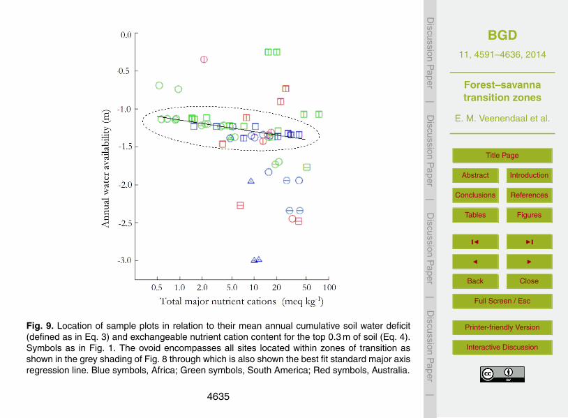
BGD11, 4591–4636, 2014



Title Page



Tables Figures

J I

J I

Back Close

Full Screen / Esc



Discussion

Paper

|D

iscussionP

aper|

Discussion

Paper

|D

iscussionP

aper|

Fig. 9. Location of sample plots in relation to their mean annual cumulative soil water deficit(defined as in Eq. 3) and exchangeable nutrient cation content for the top 0.3 m of soil (Eq. 4).Symbols as in Fig. 1. The ovoid encompasses all sites located within zones of transition asshown in the grey shading of Fig. 8 through which is also shown the best fit standard major axisregression line. Blue symbols, Africa; Green symbols, South America; Red symbols, Australia.

4635





BGD11, 4591–4636, 2014



Title Page



Tables Figures

J I

J I

Back Close

Full Screen / Esc



Discussion

Paper

|D

iscussionP

aper|

Discussion

Paper

|D

iscussionP

aper|

Fig. 10. Distribution of savanna vegetation formation types (including grasslands) in Africa andSouth America in relation to mean annual precipitation. Original data from Lloyd et al. (2008).

4636





Forest--savanna transition zones - Biogeosciences

Documents

Transcript of Forest--savanna transition zones - Biogeosciences